Raman spectroscopy of graphene trilayers with different stacking orders 

Paul V. Klimov University of New Mexico 

Summer 2009 Columbia University NSEC REU Student 

Graphene multilayers have received significant theoretical and experimental attention in recent years. Raman  scattering  has  become  a  particularly  useful  way  to  study  these  materials,  allowing  one  to determine the number of monolayers, strains within them, their level of doping, and the concentration of defects. However, one thing that Raman spectroscopy has not yet been used to study is the stacking configuration  of  graphene  in multilayers.  In  this  paper,  we  investigate  the  shape  of  the  2D  Raman mode in ABA and ABC stacked graphene trilayers. It was found that the 2D mode is asymmetric in ABC regions and symmetric in ABA regions. Additionally, we use Raman scanning to find a quantifier that allows  us  to map  ABA  and  ABC  stacking  domains.  Using  statistical  analysis,  we  find  that  the most effective quantifiers are the line width of the 2D mode and the spectrally integrated residual between the recorded Raman spectrum and  the ABC mode. While other parameters  that we considered vary between  the  different  stacking  regions  also,  the  changes  in  them  are  insignificant  compared  to  the measurement uncertainty.  

 

Graphene  is  a  one  atom‐thick  sheet  of  sp2‐hybridized carbon  atoms,  arranged  in  a  hexagonal  lattice.  The material  has  been  of  great  theoretical  interest  since  the mid  1900s  [1],  mainly  due  to  its  interesting  charge transport properties.  Theoretical studies have shown that the dispersion  relationship  for  graphene  is  conical  at  low energies,  implying  that  electrons  in  the  material’s  lattice have  a  zero  effective  mass.  In  particular,  graphene’s conduction‐band  electrons  behave  like  relativistic particles,  whose  behavior  is  governed  by  the  Dirac equation [2]. Interestingly, it was theorized by Landau that a  2‐dimensional  crystal  like  graphene  would  be thermodynamically unstable [3].  Therefore, it was thought that  that  the  production  of  the  material  would  be impossible.  However,  the  successful  production  of graphene was accomplished in 2004, by Andre Geim et. al. [4].    It  has  since  been  theorized  that  corrugations  and ripples  on  the  atomic  scale  might  be  responsible  for  the thermodynamic stabilization of graphene sheets [5].  

Since  the  initial  production  of  graphene  in  2004,  many applications  have  been  realized  for  both monolayers  and bilayers.  The driving force behind monolayer applications is  graphene’s  high  intrinsic  carrier  mobility  at  room temperature  [6].  This  has made  the material  favorable  in many  potential  technological  devices  including  nano‐ribbon  field  effect  transistors  (GNRFETs)  [7]  and  radio‐frequency  (RF)  transistors  [1].  The  number  of  potential applications  involving bilayer graphene  is also quite high. This is a result of the materials interesting band‐structure, which  arises  from  electronic  interactions  between graphene layers.  In particular, it was found that an electric field, applied perpendicular to the bilayer, can open a band gap [8,9]. This makes bilayers useful in gated devices, such as FETs, which are ubiquitous in modern microelectronics.  

While  graphene  monolayers  and  bilayers  have  been studied quite thoroughly, trilayers have not received much experimental  attention.  The main  complexity  in  studying them arises from the fact that there are two stable stacking orders:  ABA  and  ABC.  Although  the  difference  between these  stacking  configurations  is  quite  subtle,  theoretical studies  predict  that  they  have  completely  different  band structures, at  low energies. These studies show that ABA‐stacked trilayers are semi‐metals, with finite band overlap, while ABC‐stacked trilayers are zero‐gap semi conductors [10].  For  consistent  results  in  future  studies,  it  is important for one to be able to distinguish between these stacking  orders.  Therefore,  to  provide  this  groundwork, we must find a method for the effective characterization of trilayers.  

To  date,  several  characterization  techniques  have  been prominent  in  monolayer  and  multilayer  studies.  Atomic force  microscopy  (AFM)  has  been  used  to  study  the number  of  layers  in  few‐layer  samples,  along  with  their morphology. Although this technique is useful, it has been cited  as  unreliable  [11].    Another  method,  which  also allows  us  to  determine  the  number  of  layers,  is transmission  electron  microscopy  (TEM).  While  TEM  is more  reliable  than  AFM,  it  requires  the  sample  to  be suspended,  which  is  often  impractical.  The  presence  of optical  transitions  in  the  infrared  (IR)  range  for multilayers  offers  us  a  useful  new way  to  study  them.  IR spectroscopy  allows  us  to  probe  the  electronic  band structure, which gives us access to a wealth of information that cannot be determined  from either AFM or TEM data.  Recent theoretical studies have shown that high‐energy IR (NIR) measurements can be used to determine the number of  layers  in  a  multilayer,  and  lower‐energy  IR  (MIR) measurements  can  be  used  to  determine  the  stacking 

 

 

order  [12].  While  IR  is  more  reliable  and  practical  than TEM  and  AFM,  as  well  as  more  informative,  it  is  not available in most research laboratories. Raman scattering, on  the  other  hand,  has  not  been met with  the  difficulties described  above.  The method  is  reliable,  practical,  and  is available  in  most  research  laboratories.  Therefore,  it  is most  beneficial  for  us  to  study  the  Raman  spectrum  of graphene trilayers, in attempt to find ways to characterize as many physical features as possible. 

To date, the Raman spectrum of graphene, and multilayers, has been used to characterize many physical features. The intensity of the D mode has allowed one to determine the quality of a sample [13]. The shape of the 2D overtone has been  used  to  determine  the  number  of  layers  in  a multilayer [13]. The width of the G mode has allowed us to study the level of doping of a sample [14]. And finally, the shifts of the 2D and G modes, along with the width of the G mode,  have  allowed  one  to  study  the  strain  on  a  sample [15]. Although  this  information  tells us  a  lot,  there  is  still more to be inferred. To date, there is no clear consensus on the shape of the 2D mode in trilayer graphene. This mode is shown to have asymmetric features in some studies [16‐18],  and  symmetric  features  in  others  [19‐21].  In  this study, we aim to resolve this inconsistency by considering the  stacking  order  of  trilayer  graphene.  Additionally,  we look  for  a  quantifier  that  allows  us  to  map  stacking domains from Raman scanning measurements. 

II. Experimental and Analytical Methods 

Graphene  multilayer  samples  were  produced  by  the method of mechanical exfoliation of kish graphite [23]. Our substrate  was  Si  coated  with  300nm  SiO2.    Samples  of reasonable  shape  and  size  were  found  with  an  optical microscope. 

Raman spectroscopy was performed using a 532nm  laser as the excitation source, with an 1800 slit/cm grating, and a resulting spectral resolution of ~0.6cm‐1. The integration time  per  spectrum  was  set  at  8  minutes.  Infrared spectroscopy  was  performed  on  a  micro‐FTIR  apparatus with  a  Globar  source  and  a  HgCdTe  detector  in Brookhaven National Laboratory. 2D Raman mapping was performed using 514.5nm linearly polarized light from an Argon  laser.   Raman spatial maps were  taken with a  spot size  of  roughly  500nm,  a  step  size  of  500nm,  and  a resolution  of  8cm‐1.    The  integration  time was  fixed  at  5 seconds.  

Within  the  Results  and  Discussion,  we  refer  to  several parameters.  The  central  frequency  (<ω>)  is  given  by  the statistical  relationship  in Eq. 1., where ω  is  the  frequency and I(ω) is the Raman intensity at that frequency.  

     

€

ω =ω ⋅ I(ω) ⋅ dω∫I(ω) ⋅ dω∫

                                  (1)                                  

An  asymmetry  parameter  was  calculated  by  integrating each half of  the 2D mode and  then  taking  their  ratio. The mathematical formulation of this procedure is given in Eq. (2). Here ωL and ωR are the frequencies at which the mode reaches  15%  of  its  maximum  intensity.  IL  and  IR  are  the values of the left and right integrals.  

€

IRIL

=I(ω) ⋅ dω(ωL +ω R )

2

ω R∫

I(ω) ⋅ dωωL

(ωL +ω R )2∫

,ωR >ωL                  (2) 

A  so‐called  residual  parameter  (η)  was  also  calculated. This  was  done  by  subtracting  the  spectrum  of  the  ABC stacked  2D  mode  (IABC(ω))  from  the  measured  spectra (I(ω)), and then integrating the resulting spectrum over ω (see  Eq.  3).  The  ABC  stacked  2D mode will  be  discussed within the Results and Discussion section. 

 

€

η = IABC (ω) − I(ω)∫ dω                          (3) 

The  line width  (Γ) was  calculated  as  the width  of  the  2D mode at ¾ of maximum  intensity.  Statistical  analysis was performed in MATLAB using a mixture of original code and built in functions (see Appendix A5 for complete code). 

III. Results and Discussion 

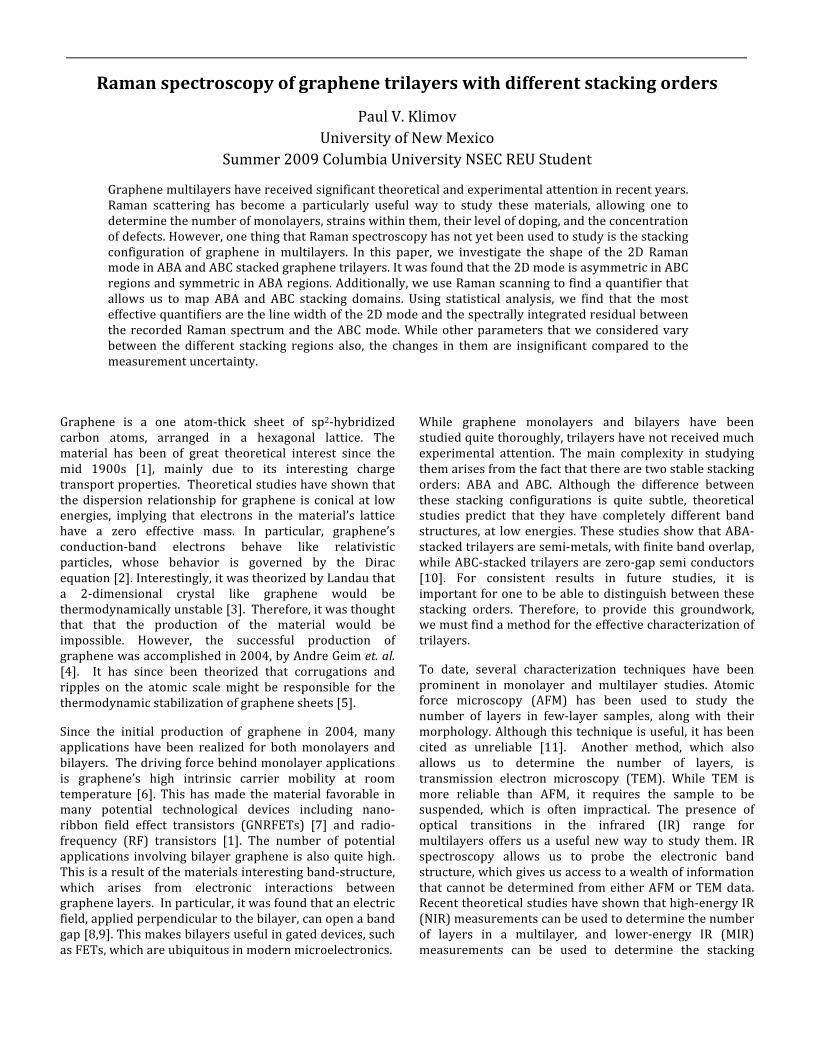
In  a  recent  study,  it  was  found  that  the  transmission plateau  in  the  NIR  spectrum  of  multilayers  is  quantized with  respect  to  layer  number  [12].  This  results  from  the hyperbolic  bands  that  make  up  multilayer’s  band structures. In NIR energy ranges, the bands run parallel to one  another,  along  their  respective  asymptotes. 

FIG. 1.  (a)‐(b) Band structures of ABC and ABA stacked trilayers [10]. (c) The  IR spectra of monolayers, bilayers, and  trilayers with ABA and ABC stacking  geometry.  The NIR  tails  of  the  teal  and  red  curves  tell  us  that both curves are representative of  trilayers. The MIR transmission peaks tell us the stacking type.  

 

 

Qualitatively, this situation is analogous to having multiple monolayers with  linear  bands.  Furthermore,  in  a  trilayer such  an  arrangement  will  result  in  roughly  triple  the absorption  of  a  monolayer.  After  finding  trilayers  in  this way,  we  looked  to  the  lower  energy  transmission spectrum. In accord with the literature, we found only two distinctly  different  MIR  transmission  patterns,  with converging tails in the NIR range. Theoretical studies have shown  that  ABA  and  ABC  stacked  trilayers  are  the  most energetically  favorable  [23].    To  determine  which spectrum  corresponds  to  which  stacking  geometry,  we studied  the  trilayer  band  structure.  It  turns  out  that  two strong  MIR  absorption  features  are  possible  with  ABC geometry  and  only  one with  ABA  geometry.    Indeed  one class of spectra had one transmission peak while the other had two transmission peaks, making it feasible to make the distinction. These results are summarized in Fig. 1. 

A  sample  was  found  with  both  stacking  orders,  and  the locations  of  these  domains  were  determined  by performing  multiple  IR  measurements.  Raman measurements were then taken within each domain, so as to determine the shapes of the 2D modes in ABA and ABC stacked  regions  (see  Fig.  2,  where we  have  the  averaged several spectra from ABA and ABC regions). Although both curves in the figure display some oscillatory noise, they are clearly distinct. The ABC domain produces an asymmetric 2D mode, with a pronounced peak, while the ABA domain produces  a  more  symmetric  mode  with  a  broad  peak. Additionally  it  appears  that  the  ABC mode  is  wider  than the  ABA  mode  by  several  wavenumbers.    As  already mentioned,  curves  similar  to  those  presented  here  have appeared in the literature. However, they have never been presented  simultaneously,  and  there  has  not  been  any inquiry as to what physical features are responsible for the variation  in  their shapes. From the combination of our  IR and  Raman  data,  it  becomes  clear  that  these  two  shapes are  the  signatures  of  ABA  and  ABC  stacking  geometries. After  clarifying  this  fact,  it was our goal  to quantify  these 

shape differences, and to map stacking domains. 

To  facilitate  this  study,  we  acquire  Raman  spectra  while raster‐scanning the sample along a 46 by 110 grid. Several quantities were calculated at each pixel and plotted in the form  of  colormaps  (each  pixel  corresponds  to  a  single spectrum). Each quantity attempts to capture the apparent difference between the 2D mode in ABA and ABC domains in  a  different  way.  First,  we  calculated  the  central frequency of the mode, by applying Eq. (1). (see Fig. 3(b)). The  leftward  asymmetry  of  the  ABC  mode  should  cause this to register a lower central frequency than a symmetric mode.  Then,  we  calculated  the  asymmetry  parameter,  as given by Eq.  (2).    In symmetric modes,  such as  those  that arise  in  ABA  regions,  this  quantity  should  be  close  to  1. However,  in  asymmetric  regions,  such  as  those with ABC 

FIG. 2. Raman spectra of graphene trilayers with ABA and ABC stacking geometries.    Stacking  geometry was  confirmed with  IR measurements. The ABC produced mode is asymmetric and has a greater width than the ABA mode. The ABA produced mode  is more symmetric with a smooth peak.  

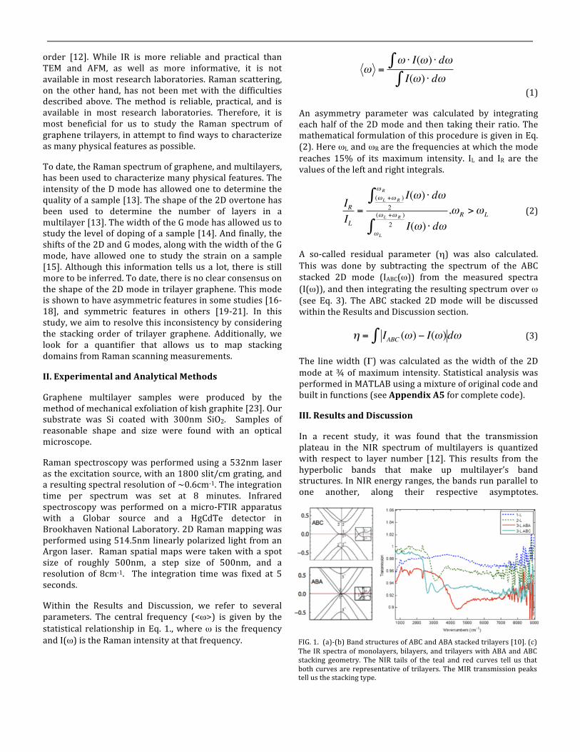
FIG.  3.  (a)  optical  photograph of  our  trilayer  sample. The  scale bar  represents 10um.  (b) The  central  frequency of  the 2D mode.  (c) The  ratio of  the integrated  intensities  of  the  left  hand  side  of  the mode  to  the  right  hand  side  (d)  The  residual  at  each  point.  (e)  The  line width  of  the mode  at ¾ maximum. In these figures, prominently in (c) and (d), we see a sharp boundary, which is representative of stacking. The physical explanation for the gradually  varying  features  in  (b)  has  not  yet  been  devised.    The  Blue  squares  represent  areas where  data was  sampled  for  statistical  analysis.  The stacking in these blue regions was also confirmed by IR spectroscopy.  

(a)  (b)  (c)  (d)  (e) 

 

 

stacking,  this ratio should be noticeably smaller  than one. These  results  are  plotted  in  Fig.  3(c).    Next,  the  residual parameter  was  calculated,  as  given  by  Eq.  (3)  (see  Fig. 3(d)). Asymmetric modes will return a small value for this parameter  while  symmetric  modes  will  return  a  large value.  Finally,  to  account  for  the  apparent  broadening  in the ABC mode, we calculated the  line width (denoted Γ2D. see Fig. 3(b)).  

In the obtained maps, we immediately notice the presence of  several  domains  (see  Fig.  3(b)‐(e)).  Note  that  the vertical  line  on  the  right‐hand  side  of  the  sample  is  a structural  artifact  and  can  be  seen  in  the  optical photograph  in  Fig.  3(a).  In  these  maps  we  clearly  see  a homogeneous ABC region at the center of the trilayer that separates two smaller ABA domains at the top and bottom parts  of  the  sample.  Indeed  these  are  the  same  regions where  IR  and  Raman  measurements  were  taken,  and where  we  have  confirmed  the  presence  of  different stacking domains.  Therefore,  it  appears  that  the  carefully chosen parameters are effective. However, we also notice that  some  parameters  are  better  than  others  in  this mapping.  In  particular,  we  see  a  lot  of  noise  in  Fig.  3(e), and gradually varying features, that are not representative of stacking, in Fig. 3(a).  

For  further  quantitative  analysis,  we  have  carefully examined  12x12  regions  within  homogeneous  ABA  and ABC  domains  (these  grids  are  indicated  by  the  blue squares  in  Fig.  3(b)‐(e)).  Histograms  representing  the distributions of  the  studied parameters,  for  each  stacking domain,  are  plotted  in  Fig.  4.    Each  distribution  was assumed normal and was fit with a Gaussian. See Table 1 in  Appendix  A4  for  the  mathematical  parameters  that describe these Gaussians. The purpose of  this step was to determine  the  amount  of  overlap  between  the distributions.    Each  Gaussian  was  integrated  from  their point  of  intersection,  and  the  lower  limit  was  denoted  ε, with  subscripts  indicating  the  quantifier.    This  procedure returned  the  following  values:  ε<ω> ~  .61,  εIR/IL~  .71,  εη ~ .88,  and  εΓ  ~  .89.  Note  that  an  ε  of  .5  means  that  both 

Gaussians overlap  completely,  and an ε  of  .84 means  that the  Gaussians  overlap  at  the  point  where  one  of  them attains its first standard deviation.  

Based  on  this  analysis,  the most  accurate  quantifiers  are the residual parameter and the line width of the 2D mode. It  is  surprising  that  ε  is  so  close  to  .5,  for  the  central frequency and the asymmetry parameter. This could be the result  of  noise  due  to  low  integration  times  or  the  wide spectral resolution of 8cm‐1.   

It  is  important  to  mention  that  homogeneously  stacked samples  are  quite  rare.  In  fact,  six  out  of  six  scanned samples  contained  both  ABA  and  ABC  domains. Additionally,  we  note  that  the  sample  analyzed  in  this paper  is  quite  exquisite,  in  that  the  stacking  domains  are quite  large  and  have  nice,  rectangular  shapes.  Other samples  that  we  studied  had  many  small  domains  with complex  profiles. We must  also  note  that  not  all  stacking domains  could  be  resolved.  The  laser  spot  in  our  Raman setup was 500nm  in diameter, which  is much  larger  than the length of a single hexagonal carbon ring. Furthermore, it  a  possibility  that  small  stacking  domains  are  not displayed  in  our  maps.  This  finding  should  be  a  concern (though hopefully not a deterrent) in future studies.  

One  important  issue  is  the  mechanism  for  formation  of different  stacking  domains.  It  is  rather  unlikely  that  they arose  in  the  process  of  cleaving  graphite  during mechanical  exfoliation.    Qualitatively,  we  must  consider the  strength  of  the  van  der  Waal  interactions  that  hold graphene  layers  together  in  graphite.  While  these  forces are  not  strong  enough  to  prevent  easy  peeling  of  layers, they  are  much  stronger  in  the  direction  along  the  layer. Therefore,  this  would  likely  resist  the  layer‐shifting processes  that  would  presumably  form  these  domains. Instead,  it  is more  likely  that  three‐dimensional  domains were  present  in  the  bulk  graphite  before  exfoliation,  and that  in  cleaving  graphene  layers, we  are  simply  exposing cross‐sections of these domains.  

FIG. 4. Histograms and corresponding Gaussians for (a) the central  frequency, (b) ratio of the integrated intensities of the right and left halves, (c) the residual parameter and (d) the line width of the 2D mode in ABA and ABC stacked domains. From these data, it is clear that the best way to map stacking domains  is with the  line width, whose histograms experience the  least overlap. The amount of overlap in the other quantifiers  is too significant to tell different stacking regions apart, with good confidence. See Table 1 in the Appendix for a summary of data presented here. 

 

(a)  (b)  (c)  (d) 

 

 

Now  we  must  ask  how  homogeneous  trilayers  might  be formed.  It  is  possible  that  methods  that  involve  the assembly  of  individual  carbon  atoms  into  sheets  could produce  homogeneous  trilayers.  These  alternative synthetic  routes  are  actually  topics  of  intense  research right  now,  with  prominent  methods  involving  chemical vapor  deposition  (CVD)  [24]  and  epitaxial  growth  [25]. However,  if  such  methods  could  produce  homogeneous trilayers, it would be yet another task to discover a way to control  stacking orders. Another possible way of  creating homogeneous  sheets  might  involve  the  heating  of inhomogeneous  samples.  Molecular  vibrations  due  to thermal excitation might force atoms to break out of their initial stacking order, and then into a homogeneous order upon cooling. Now that we have established methods that can  be  used  to  map  stacking  domains,  it  would  be interesting  to  implement  them  on  samples  produced  and treated in the ways described above. 

Conclusion 

In this study it was found that the shape of the 2D mode in the  Raman  spectra  of  graphene  trilayers  is  dependent upon  the  stacking  geometry  of  graphene  layers.  ABC stacked  samples  show  an  asymmetric  mode,  while  ABA stacked  samples  produce  a  more  symmetric  mode.    By quantifying these shapes and using Raman imaging, it was possible for us to map stacking domains. A new parameter (ε)  was  introduced  to measure  the  amount  of  overlap  in our  quantities  of  interest  within  ABA  and  ABC  stacking domains.    By  using  this  parameter,  it was  found  that  the most  accurate  way  to  map  stacking  domains  is  with residual  parameter  (see  Eq.  (3))  and  the  line width.  In  a future  study,  it  would  be  very  interesting  to  perform Raman  scanning  with  a  spectral  window  around  the  D mode. It is likely that we could observe this mode in areas of stacking discontinuity, which could also prove useful in the mapping of stacking domains.  

While we have  found a way  to map stacking domains, we have  not  formulated  a  theoretical  explanation  for  why there  is  a  difference  in  the  2D  mode  of  ABA  and  ABC stacked trilayers. In addition, we have not fully understood the origin of more subtle features, such as the gradual red shifts that are present in the map representing the central frequency.  Although  these  might  be  due  to  doping  or strains,  rigorous  quantitative  analysis  has  not  been performed (see Appendix A2 for further discussion).  

Future  work  should  extend  our  findings  to  higher  order multilayers. Although it was not presented here, we found that the 2D mode in tetralayers and hexalayers also takes on  different  shapes  in  different  stacking  regions  (see Appendix  A3).    While  it  may  seem  that  studying  higher order  multilayers  would  become  more  complicated,  this might  not  actually  be  the  case.  After  considering  mirror symmetries  within  the  crystal,  along  with  geometrically equivalent  orders,  the  number  of  energetically  favorable 

stacking configurations declines tremendously. In fact, it is believed  that  there  are  only  two  energetically  favorable tetralayers as well. Therfore, Raman might be effective for the  characterization  and mapping  of  stacking  domains  in higher order multilayers as well.  

Acknowledgements 

I would  like  to  thank Dr. Tony Heniz, Chun Hung Lui, and Zhiqiang  Li  for  hosting me  as  their  summer  student  and introducing  me  to  cutting  edge  developments  in  the fascinating  area  of  the  physics  of  graphene.  In  addition,  I would like to thank the NSF and NSEC for hosting this REU program at Columbia University.  

References   [1] R. F. Service. Carbon Sheets an Atom Thick Give Rise to Graphene Dreams. Science 324, 875 (2009). [2]  A.  K.  Geim.  Graphene:  Status  and  Prospects.  Science 324, 1530 (2009). [3]  A.K.  Geim  and K.  S.  Novoselov.  The  Rise  of  Graphene. Nat. Mater. 6, 183 (2007). [4] K. S. Novoselov, et al. Electric Field  in Atomically Thin Carbon Films. Science 306, 666 (2004). [5]  A.  Fasolino,  J.  H.  Los,  and  M.  I.  Katsnelson.  Intrinsic Ripples in Graphene. Nat. Mater. 6, 858 (2007). [6] S. V. Morozov, et al. Giant Intrinsic Carrier Mobilities in Graphene  and  its  Bilayer.  Phys.  Rev.  Lett.  100,  016602 (2008). [7]  K.  Alam,  Semicond.  Transport  and  performance  of  a zero‐Schottky  barrier  and  doped  contacts  graphene nanoribbon transistors. Sci. Technol. 24, 015007 (2009). [8] K. F. Mak, C.H. Lui, J. Shan, and T.F. Heinz. Observation of an Electric‐Field‐Induced Band Gap in Bilayer Graphene by  Infrared  Spectroscopy.  Phys.  Rev.  Lett.  102,  256405 (2009). [9] Y.  Zhang, et al. Direct observation of  a widely  tunable bandgap in bilayer graphene. Nature 459, 820 (2009). [10] M. F. Craciun. Trilayer graphene is a semimetal with a gate‐tunable band overlap. Nat. Nano. 4, 383 (2009). [11]  A.  C.  Ferrari,  J.  C.  Meyer,  and  V.  Scardaci.  Raman Spectrum  of  Graphene  and  Graphene  Layers.  Phys.  Rev. Lett. 97, 187401 (2006). [12] K. F. Mak, et al. The electronic structure of Few‐Layer Graphene: Probing the Evolution from a 2‐Dimensional to a 3‐Dimensional Material. Not yet published. (2009). [13]  A.  C.  Ferrari.  Raman  spectroscopy  of  graphene  and graphite: Disorder,  electron‐phonon  coupling,  doping  and nonadiabatic effects. Solid State Commun. 143, 47 (2007). [14] A. Das, et al. Nat. Nano. Monitoring dopants by Raman scattering  in  an  electrochemically  top‐gated  graphene transistor. 3, 210 (2008).  [15] M. Huang, et al. Phonon softening and crystallographic orientation  of  strained  graphene  studied  by  Raman spectroscopy. Proc. Natl. Acad. Sci. USA. 106, 7304 (2009). 

 

 

[16]  Z.  H.  Ni,  et  al.  Nano  Lett.  Graphene  Thickness Determination  Using  Reflection  and  Contrast Spectroscopy. 7, 2758 (2007). [17] L. M. Malard, D. L. Mafra, and S. K. Doom. Resonance Raman  scattering  in  graphene:  Probing  phonons  and electrons. Solid State Commun. 149, 1136 (2009). [18] L. M. Malard, et al. Raman Spectroscopy in Graphene. Phys. Rev. Lett. 473, 51 (2009). [19]  Z.  Ni,  et  al.  Raman  spectroscopy  and  imaging  of graphene. Nano Res. 1, 273 (2008). [20] D. Graf, et al. Spatially Resolved Raman Spectroscopy of  Single‐  and  Few‐Layer  Graphene.  Nano  Lett.  7,  238 (2007). 

[21] D.  S.  Lee, et al. Raman Spectra of Epitaxial Graphene on  SiC  and  of  Epitaxial  Graphene  Transferred  to  SiO2. 8, 4320 (2008).  [22]  K.  S.  Novoselov,  et  al.  Two‐dimentional  atomic crystals. Proc. Natl. Acad. Sci. USA. 102, 10451 (2005). [23]  M.  Aoki  and  H.  Amawashi.  Dependence  of  band structures on stacking and field in layered graphene. Solid State Commun. 142, 123 (2007). [24]  A.  N.  Obraztsov.  Chemical  vapor  deposition:  Making graphene on a large scale. Nat. Nano. 4, 212 (2009).  [25] J. Hass et al. The growth and morphology of epitaxial multilayer graphene.  J. Phys. Condens. Matter 20, 323202 (2008).  

 

Appendix 

A1. G Mode Analysis  

In  addition  to  studying  the 2D mode, we briefly  studied the G mode. Because  the  shape  looked  indistinguishable in  ABA  and  ABC  domains,  we  only  computed  the  line width and the frequency of the mode. Although statistical analysis was not performed, we made several qualitative observations based on the colormaps presented in Fig. 5. From Fig.  5(a),  it  appears  that  the width  of  the G mode might be useful in determining different stacking orders. However,  the  frequency  does  not  appear  to  be  a  useful parameter for this purpose, as ABC and ABA domains are essentially indistinguishable (see Fig. 5(b)).  

A2. Moderate features in the colormaps  

In Fig. 3(b), we see the presence of a moderately varying feature.  This  is  most  easily  seen  in  the  angled,  north‐eastern region of  the sample, within the ABA domain.  In attempt to find an explanation for this feature, we briefly consider  the  effects  of  doping  and  strain on  the Raman spectrum. 

Studies  in  the  literature  show  that doping  causes  the G mode to stiffen, while leaving the shape of the 2D mode unchanged.  Therefore,  the  ratio  of  the  integrated intensities  of  the  two modes  is  a  good  indicator  of  the doping  level.  This  calculation  was  performed  with  the result plotted in Fig. 6. Note that the horizontal lines are representative of instrumental malfunction. Irrespective of  these  artifacts,  however, we  do  not  see  any  features that resemble the one mentioned above. 

Given that the 2D mode appears red‐shifted in Fig. 3(c), it  is  natural  for  us  to  consider  strain  on  the  sample. Studies  show  that  strain  will  cause  the  red  shifting  of both  the 2D and G modes and will cause  the G mode to split.   While we do see a red shifting of  the 2D mode  in this region (Fig. 3(c)), the G mode does not appear to be 

FIG. 5. (a) linewidth of the G mode and (b) frequency of the G mode, as determined by center of the Lorentzian function used to fit it.  The horizontal lines in (a) are attributed to instrumental noise. 

FIG.  6.  Ratio  of  the  integrated  intensities  of  the  2D  mode  to  the  G mode.   The horizontal  lines may be attributed to  instrumental noise.  We do not  see  the  gradually  varying  feature  in  Fig.  3(b),  suggesting that  doping  might  not  be  responsible  for  it.  A  color  bar  is  not presented, as accurate numerical analysis here is not possible due to apparent laser intensity fluctuations. 

 

 

 

shifted (see Fig. 5(b)). In addition, the line width of the G mode does not appear to be wider in that region (see Fig. 5(a)).  

From  this  short,  qualitative,  analysis,  it  seems  that  neither  strain  nor  doping  are  responsible  for  the  gradually  varying feature seen Fig. 3(b). However, without a rigorous quantitative study, we cannot make any conclusions.  This would be an interesting topic for future studies. 

A3. Raman scattering on tetralayers and hexalayers 

Raman scattering was also performed on various stacking domains in tetralayers and hexalayers (See Fig. 6). The resulting data implies that the 2D mode in higher order multilayer samples is also dependent upon the stacking geometry. And in fact, it appears that it is affected even more than in trilayer samples.  

 

 

A4. Tables  

 

TABLE 1. After  spectral  data was  obtained, we determined  the width  at ¾ max  (Γ),  the  residual  parameter  (η),  the  central  frequency (<ω>),  and  the  asymmetry  parameter  (IL/IR).  Histograms were  then made  for  these  quantities,  and  a  Gaussian was  used  to  fit  them, assuming normal distributions. The mean (µ), the standard deviation (σ), the point of intersection of the Gaussians (χ), and the integral from the point of intersection, to infinity, were calculated.  

Q  ΓABA  ΓABC  η ABA  η ABC  <ωABA>  <ω ABC>  IL/IR ABA  IL/IR ABC 

µ  39.3cm‐1  43.6 cm‐1  3.46 (a.u.)  2.02 (a.u.)  2701.2cm‐

1  2700.8cm‐1  .86(a.u.)  .79(a.u.) 

σ  1.4 cm‐1  1.8 cm‐1  .49 (a.u.)  .64 (a.u.)  .55cm‐1  .48cm‐1  .06(a.u.)  .06(a.u.) 

χ  41.3 cm‐1  2.78(a.u.)  2701.1cm‐1  .82(a.u.) 

€

G(Q)dQχ

±∞

∫G(Q)dQ

−∞

+∞

∫

 .93  .89  .92  .88  .61  .72  .74  .71 

FIG. 6. 2D mode in differently stacked (a) tetralayers and in (b) hexalayers. The horizontal axis represents wavenumbers (cm‐1) and the vertical axis  the  intensity  (a.u.). Differences  in  stacking orders were determined by  infrared spectroscopy. However, we do not claim a specific stacking order, as the number of possible configurations is quite large. There is a clear difference in the shapes of the modes indicating that Raman might prove to be a useful tool in the characterization of these materials. 

   

 

 

 

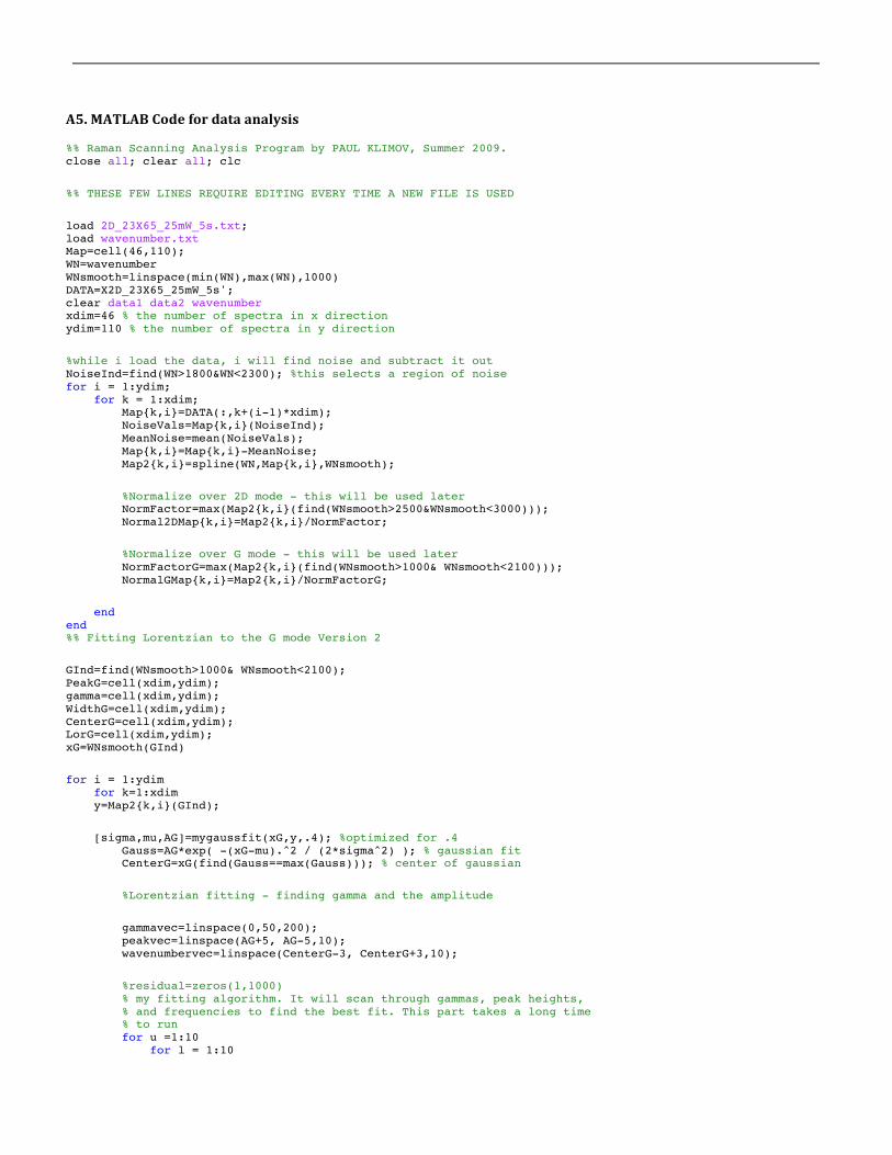
A5. MATLAB Code for data analysis 

%% Raman Scanning Analysis Program by PAUL KLIMOV, Summer 2009. close all; clear all; clc %% THESE FEW LINES REQUIRE EDITING EVERY TIME A NEW FILE IS USED load 2D_23X65_25mW_5s.txt; load wavenumber.txt Map=cell(46,110); WN=wavenumber WNsmooth=linspace(min(WN),max(WN),1000) DATA=X2D_23X65_25mW_5s'; clear data1 data2 wavenumber xdim=46 % the number of spectra in x direction ydim=110 % the number of spectra in y direction %while i load the data, i will find noise and subtract it out NoiseInd=find(WN>1800&WN<2300); %this selects a region of noise for i = 1:ydim; for k = 1:xdim; Map{k,i}=DATA(:,k+(i-1)*xdim); NoiseVals=Map{k,i}(NoiseInd); MeanNoise=mean(NoiseVals); Map{k,i}=Map{k,i}-MeanNoise; Map2{k,i}=spline(WN,Map{k,i},WNsmooth); %Normalize over 2D mode - this will be used later NormFactor=max(Map2{k,i}(find(WNsmooth>2500&WNsmooth<3000))); Normal2DMap{k,i}=Map2{k,i}/NormFactor; %Normalize over G mode - this will be used later NormFactorG=max(Map2{k,i}(find(WNsmooth>1000& WNsmooth<2100))); NormalGMap{k,i}=Map2{k,i}/NormFactorG; end end %% Fitting Lorentzian to the G mode Version 2 GInd=find(WNsmooth>1000& WNsmooth<2100); PeakG=cell(xdim,ydim); gamma=cell(xdim,ydim); WidthG=cell(xdim,ydim); CenterG=cell(xdim,ydim); LorG=cell(xdim,ydim); xG=WNsmooth(GInd) for i = 1:ydim for k=1:xdim y=Map2{k,i}(GInd); [sigma,mu,AG]=mygaussfit(xG,y,.4); %optimized for .4 Gauss=AG*exp( -(xG-mu).^2 / (2*sigma^2) ); % gaussian fit CenterG=xG(find(Gauss==max(Gauss))); % center of gaussian %Lorentzian fitting - finding gamma and the amplitude gammavec=linspace(0,50,200); peakvec=linspace(AG+5, AG-5,10); wavenumbervec=linspace(CenterG-3, CenterG+3,10); %residual=zeros(1,1000) % my fitting algorithm. It will scan through gammas, peak heights, % and frequencies to find the best fit. This part takes a long time % to run for u =1:10 for l = 1:10

 

 

for j = 1:200 testPeakG=peakvec(l); testgamma=gammavec(j); testwn=wavenumbervec(u); testLor=testPeakG*testgamma^2./((xG-testwn).^2+testgamma^2); residual(j,u,l)=sum(abs(y-testLor)); % residuals in a 3 dim matrix end end end %next line will find the minima of the 3 dimensional residual %matrix and then from the indicies, my program will determine the %corresponding gamma, frequency, and peak height. [minj,minu,minl]=ind2sub(size(residual),find(residual==min(min(min(residual))))); gammaG{k,i}=gammavec(minj); %HWHM of Lorentzian PeakG{k,i}=peakvec(minl); %Peak intensity of Lorentzian wnG{k,i}=wavenumbervec(minu); %frequency of Lorentzian % The following lines look for errors and get rid of them without % crashing the program. They look for empty matricies, or matricies % with more than one element, which can result from spectra with % only noise. if sum(size(gammaG{k,i}))>2 gammaG{k,i}=0; PeakG{k,i}=0; wnG{k,i}=0; errormatG{k,i}=1; end if sum(size(gammaG{k,i}))==0 gammaG{k,i}=0; PeakG{k,i}=0; wnG{k,i}=0; errormatG{k,i}=1; end FWHMGaussG(k,i)=2.3548*sigma; %The gaussian FWHM. This is not used anymore LorG{k,i}=PeakG{k,i}*gammaG{k,i}^2./((xG-wnG{k,i}).^2+gammaG{k,i}^2); %the lorentzian fit WidthG{k,i}=gammaG{k,i}; %HWHM of lorentzian i end end 'done' %tells you when the program has finished running. %It can take over 30 numbers depending on the resolution %% run this to clear some unimportant variables and free up memory clear residual testLor testwn testgamma testPeakG gammavec peakvec wavenumbervec clear NoiseVals MeanNoise DATA Map %% run this if you want to save out data to the current directory. You %% Might want to add to these names to be more specific! save WidthG2 WidthG save LorG2 LorG save PeakG2 PeakG save gammaG2 gammaG save wnG2 wnG %% Run this if you want to load data from the current directory %% If you changed names earlier, make sure to change these variables load WidthG WidthG load LorG LorG load PeakG PeakG load gammaG gammaG load wnG wnG %% Fitting Lorentzian to the 2D mode. Same code as for G mode. TwoDInd=find(WNsmooth>2550&WNsmooth<2850); %fit the 2D mode with a lorentzian PeakTwoD=cell(xdim,ydim); gamma=cell(xdim,ydim); WidthTwoD=cell(xdim,ydim); FWHMGaussTwoD=cell(xdim,ydim); CenterTwoD=cell(xdim,ydim); Lor2D=cell(xdim,ydim) x2D=WNsmooth(TwoDInd)

 

 

for i = 1:ydim for k=1:xdim y=Map2{k,i}(TwoDInd); [sigma,mu,A2D]=mygaussfit(x2D,y,.4); %optimized for .4 Gauss=A2D*exp( -(x2D-mu).^2 / (2*sigma^2) ); Center2D=x2D(find(Gauss==max(Gauss))); %Lorentzian fitting - finding gamma and the amplitude gammavec=linspace(0,50,200); peakvec=linspace(A2D+5, A2D-5,10); wavenumbervec=linspace(Center2D-3, Center2D+3,10); %residual=zeros(1,1000) for u =1:10 for l = 1:10 for j = 1:200 testPeak2D=peakvec(l); testgamma=gammavec(j); testwn=wavenumbervec(u); testLor=testPeak2D*testgamma^2./((x2D-testwn).^2+testgamma^2); residual(j,u,l)=sum(abs(y-testLor)); end end end [minj,minu,minl]=ind2sub(size(residual),find(residual==min(min(min(residual))))); gamma2D{k,i}=gammavec(minj); Peak2D{k,i}=peakvec(minl); wn2D{k,i}=wavenumbervec(minu); if sum(size(gamma2D{k,i}))>2 gamma2D{k,i}=0; Peak2D{k,i}=0; wn2D{k,i}=0; errormat2D{k,i}=1; end if sum(size(gamma2D{k,i}))==0 gamma2D{k,i}=0; Peak2D{k,i}=0; wn2D{k,i}=0; errormat2D{k,i}=1; end FWHMGaussG(k,i)=2.3548*sigma; Lor2D{k,i}=Peak2D{k,i}*gamma2D{k,i}^2./((x2D-wn2D{k,i}).^2+gamma2D{k,i}^2); Width2D{k,i}=gamma2D{k,i}; i end end 'done' %% Run this to save out 2D mode information save Width2D_2 Width2D save Lor2D_2 Lor2D save Peak2D_2 Peak2D save gamma2D_2 gamma2D save wn2D_2 wn2D %% Run this to load 2D mode information load Width2D_2 Width2D load Lor2D_2 Lor2D load Peak2D_2 Peak2D load gamma2D_2 gamma2D load wn2D_2 wn2D %% Run this to clear out some memory clear A2D DATA Gauss MeanNoise NoiseInd NoiseVals NormFactor NormFactorG clear testLor sigma residual peakvec testPeak2D testgamma testwn wavenumbervec %% Integrated intensity Gmode. Gintegrationind=find(WNsmooth>1570&WNsmooth<1610); %finds region of integration TwoDintegrationind=find(WNsmooth>2620&WNsmooth<2780); %finds region of integration for i = 1:ydim

 

 

for k=1:xdim IntegratedG(k,i)=sum(abs((Map2{k,i}(Gintegrationind)))); Integrated2D(k,i)=sum(abs(Map2{k,i}(TwoDintegrationind))); Integrated2DNorm(k,i)=sum((Normal2DMap{k,i}(TwoDintegrationind))); end end Ratio2DtoG=Integrated2D./IntegratedG; % The integrated intensities ratio %% Save Integrated Intensity data save IntegratedG IntegratedG save Integrated2D Integrated2D save Ratio2DtoG Ratio2DtoG %% Moments calculations WN2DcmInd=find(WNsmooth>2670&WNsmooth<2737) for i = 1:ydim for k = 1:xdim Intensitysum(k,i)=sum(Normal2DMap{k,i}(WN2DcmInd)); %first moment WNcm(k,i)=sum((WNsmooth(WN2DcmInd)).*Normal2DMap{k,i}(WN2DcmInd))/Intensitysum(k,i); end end climWNcm=[2700 2705] imagesc(WNcm,climWNcm) colorbar; axis equal tight title('first moment 2D') set(gcf,'color',[1,1,1]); colormap hot %the following plot gives random plots so you can see the region of %integration % figure % for p = 1:9 % subplot(3,3,p) % plot(WNsmooth(WN2DcmInd),... % Normal2DMap{floor(100*rand(1)+1),floor(40*rand(1)+1)}(WN2DcmInd)) % axis([2670,2737,0,1]) % end %% Save Moments save WNcm WNcm %% Plots %% %% %% %% Gmode Plots subplot(1,2,1) climwidth=[6.4 8]; imagesc(cell2mat(WidthG)',climwidth) colormap hot colorbar ylabel(texlabel('Gamma_G (cm^-^1)')) set(gcf,'color',[1,1,1]); axis equal tight set(gca,'YTickLabel',[]); set(gca,'XTickLabel',[]); %these next loops get rid of 'broken' data points, so we can plot the G %frequencies for i = 1:ydim for k = 1:xdim if length(find(LorG{k,i}==max(LorG{k,i})))>1 shiftG(k,i)=0 continue end shiftG(k,i)=wnG{find(LorG{k,i}==max(LorG{k,i}))}; end end subplot(1,2,2) climshiftG= [1590.2641 1590.2641] imagesc(shiftG',climshiftG) colorbar;set(gcf,'color',[1,1,1])

 

 

colormap hot; axis equal tight ylabel(texlabel('omega_G (cm^-^1)')) set(gca,'YTickLabel',[]); set(gca,'XTickLabel',[]); figure climintensity=[1475 1760]; imagesc(cell2mat(PeakG),climintensity) colorbar title('G Mode Intensity') set(gcf,'color',[1,1,1]) colormap hot %2D to G integrated intensity figure subplot(3,1,1) climratio=[1,1.76]*10^4 imagesc(IntegratedG,climratio) colorbar;title('IG');colormap hot;set(gcf,'color',[1,1,1]) subplot(3,1,2) climratio=[2,5]*10^4 imagesc(Integrated2D,climratio) colorbar;title('I2D');colormap hot;set(gcf,'color',[1,1,1]) subplot(3,1,3) climratio=[2,4] imagesc(Integrated2D./IntegratedG,climratio) colorbar;title('I2D/IG');colormap hot;set(gcf,'color',[1,1,1]) %% 2D mode plots figure climswidthD = [ 24 29 ] imagesc(cell2mat(Width2D),climswidthD) title('2D Mode Lorentzian Peak Width') colorbar; colormap hot; axis equal tight set(gcf,'color',[1,1,1]) figure climscenterD=[2690 2705] imagesc(cell2mat(wn2D),climscenterD) title('2D Mode Peak Center') colorbar; colormap hot; axis equal tight set(gcf,'color',[1,1,1]) %% Widths at different heights for 2D mode and one G. This measures the %% spectra directly, not the Lorentzians corresponding to the data TwoDInd=find(WNsmooth>2550&WNsmooth<2850); GInd2=find(WNsmooth>1570&WNsmooth<1620); for i = 1:ydim for k = 1:xdim fiftyInd=find(Normal2DMap{k,i}(TwoDInd)>.5); seventyfiveInd=find(Normal2DMap{k,i}(TwoDInd)>.75); %eightyInd=find(Normal2DMap{k,i}(TwoDInd)>.80); seventyfiveIndG=find(NormalGMap{k,i}(GInd2)>.5); if isempty(seventyfiveInd)==1 errorind(k,i)=1 continue end if isempty(fiftyInd)==1 errorind(k,i)=1 continue end % if isempty(eightyInd)==1 % errorind(k,i)=1 % continue % end if isempty(seventyfiveIndG)==1 errorindG(k,i)=1 continue end

 

 

fiftywidth(k,i)=abs(WNsmooth(min(fiftyInd))-WNsmooth(max(fiftyInd))); seventyfivewidth(k,i)=abs(WNsmooth(min(seventyfiveInd))-WNsmooth(max(seventyfiveInd))); % eightywidth(k,i)=abs(WNsmooth(min(eightyInd))-WNsmooth(max(eightyInd))); seventyfivewidthG(k,i)=abs(WNsmooth(min(seventyfiveIndG))-WNsmooth(max(seventyfiveIndG))); end end fiftywidth(find(errorind==1))=100 seventyfivewidth(find(errorind==1))=100 eightywidth(find(errorind==1))=100 figure climsfifty=[50 77] imagesc(fiftywidth,climsfifty) title('fifty width') colorbar axis equal tight set(gcf,'color',[1,1,1]) colormap hot % subplot(3,2,2) % plot(6:1:35, fiftywidth(7,6:end)) % axis tight figure climsseventyfive=[34 49] imagesc(seventyfivewidth,climsseventyfive) title('seventy five width') colorbar axis equal tight; colormap hot set(gcf,'color',[1,1,1]) figure hist(seventyfivewidth);axis([0 100 0 80]) % % % % subplot(3,2,4) % % plot(6:1:35, seventyfivewidth(7,6:end)) % % axis tight % % figure % climsseighty=[10 40] % imagesc(eightywidth,climsseighty) % title('eighty width') % colorbar % axis equal tight % set(gcf,'color',[1,1,1]) % colormap winter % % subplot(3,2,6) % % plot(6:1:35, eightywidth(7,6:end)) % % axis tight % % figure % climsseventyfiveG=[8 19] imagesc(seventyfivewidthG,climsseventyfiveG) title('fifty width G') colorbar axis equal tight set(gcf,'color',[1,1,1]) colormap hot %% Final Plots subplot(2,3,1) WNcm(30:34,32)=0% these types of changes are here to draw a square where data was taken WNcm(30:34,36)=0% in the later part of the program WNcm(34,32:36)=0 WNcm(30,32:36)=0 WNcm(34:38,43)=0 WNcm(34:38,47)=0 WNcm(34,43:47)=0

 

 

WNcm(38,43:47)=0 imagesc(WNcm,[2700,2706]) colorbar set(gcf,'color',[1,1,1]); colormap hot ylabel(texlabel('Omega_2_D (cm^-^1)')) set(gca,'YTickLabel',[]) set(gca,'XTickLabel',[]) subplot(2,3,2) WidthGPlot=cell2mat(WidthG) WidthGPlot(30:34,32)=0 WidthGPlot(30:34,36)=0 WidthGPlot(34,32:36)=0 WidthGPlot(30,32:36)=0 WidthGPlot(34:38,43)=0 WidthGPlot(34:38,47)=0 WidthGPlot(34,43:47)=0 WidthGPlot(38,43:47)=0 climwidth=[6.8 8.5]; imagesc(WidthGPlot,climwidth) colormap hot colorbar set(gcf,'color',[1,1,1]) ylabel(texlabel('Gamma_G (cm^-^1)')) set(gca,'YTickLabel',[]) set(gca,'XTickLabel',[]) wnGPlot=cell2mat(wnG) wnGPlot(30:34,32)=0 wnGPlot(30:34,36)=0 wnGPlot(34,32:36)=0 wnGPlot(30,32:36)=0 wnGPlot(34:38,43)=0 wnGPlot(34:38,47)=0 wnGPlot(34,43:47)=0 wnGPlot(38,43:47)=0 subplot(2,3,3) climcenter=[1587 1593]; imagesc(wnGPlot,climcenter) colorbar set(gcf,'color',[1,1,1]) colormap hot ylabel(texlabel('omega_G (cm^-^1)')) set(gca,'YTickLabel',[]) set(gca,'XTickLabel',[]) subplot(2,3,4) Width2DPlot=cell2mat(Width2D) Width2DPlot(30:34,32)=0 Width2DPlot(30:34,36)=0 Width2DPlot(34,32:36)=0 Width2DPlot(30,32:36)=0 Width2DPlot(34:38,43)=0 Width2DPlot(34:38,47)=0 Width2DPlot(34,43:47)=0 Width2DPlot(38,43:47)=0 climswidthD = [ 24 30 ] imagesc(Width2DPlot,climswidthD) colorbar; colormap hot set(gcf,'color',[1,1,1]) ylabel(texlabel('Gamma_2_D (cm^-^1)')) set(gca,'YTickLabel',[]) set(gca,'XTickLabel',[]) subplot(2,3,5)

 

 

wn2DPlot=cell2mat(wn2D) wn2DPlot(30:34,32)=0 wn2DPlot(30:34,36)=0 wn2DPlot(34,32:36)=0 wn2DPlot(30,32:36)=0 wn2DPlot(34:38,43)=0 wn2DPlot(34:38,47)=0 wn2DPlot(34,43:47)=0 wn2DPlot(38,43:47)=0 climscenterD=[2693 2710] imagesc(wn2DPlot,climscenterD) colorbar; colormap hot set(gcf,'color',[1,1,1]) ylabel(texlabel('omega_2_D (cm^-^1)')) set(gca,'YTickLabel',[]) set(gca,'XTickLabel',[]) subplot(2,3,6) climratio=[2,3.1] imagesc(Integrated2D./IntegratedG,climratio) colorbar;ylabel('I_2_D/I_G (a.u.)');colormap hot;set(gcf,'color',[1,1,1]) set(gca,'YTickLabel',[]) set(gca,'XTickLabel',[]) %% Calculation of variations of intensity. to determine magnitude of %% effect. The grid is shown in the figures above. DeltaMoment=mean(mean([WNcm(15:20,20:25)- WNcm(20:25,50:55)])) PercentMoment=mean(mean(DeltaMoment./WNcm(30:34,32:36)*100)) DeltaWidthG=mean(mean([cell2mat(WidthG(30:34,32:36))-cell2mat(WidthG(34:38,43:47))])) PercentWidthG=mean(mean([cell2mat(WidthG(30:34,32:36))-cell2mat(WidthG(34:38,43:47))]./cell2mat(WidthG(30:34,32:36))*100)) DeltafreqG=mean(mean([cell2mat(wnG(29:33,32:36))-cell2mat(wnG(34:38,43:47))])) PercentfreqG=mean(mean([cell2mat(wnG(29:33,32:36))-cell2mat(wnG(34:38,43:47))]/cell2mat(wnG(29:33,32:36))*100)) DeltaWidth2D=mean(mean([cell2mat(Width2D(30:34,32:36))-cell2mat(Width2D(34:38,43:47))])) PercentWidth2D=mean(mean([cell2mat(Width2D(30:34,32:36))-cell2mat(Width2D(34:38,43:47))]./cell2mat(Width2D(30:34,32:36))*100)) Deltafreq2D=mean(mean([cell2mat(wn2D(30:34,32:36))-cell2mat(wn2D(34:38,43:47))])) Percentfreq2D=mean(mean([cell2mat(wn2D(30:34,32:36))-cell2mat(wn2D(34:38,43:47))]./cell2mat(wn2D(30:34,32:36))*100)) %% The 2D and G mode averaged in the same regions as shown in the figures %% above. %Normal2DMap % ABAG=zeros(1,1000) ABA2D=zeros(1,1000) % % ABCG=zeros(1,1000) ABC2D=zeros(1,1000) %LorABAG=zeros(1,408) %LorABCG=zeros(1,408) %LorABA2D=zeros(1,141) %LorABC2D=zeros(1,141) for i = 1:5 for j = 1:10 % ABA stuff % tempspec=NormalGMap{30+(i-1),32+j-1}; %these are the ABA indicies % ABAG = ABAG + tempspec; tempspec=Normal2DMap{11+(i-1),18+j-1}; ABA2D= ABA2D + tempspec; % tempspec=LorG{30+(i-1),32+j-1}; % LorABAG=LorABAG+tempspec % tempspec=Lor2D{30+(i-1),32+j-1}; % LorABA2D=LorABA2D+tempspec

 

 

% % ABC stuff % tempspec=NormalGMap{34+(i-1),43+j-1}; % ABCG = ABCG + tempspec; tempspec=Normal2DMap{15+(i-1),60+j-1}; ABC2D= ABC2D + tempspec; % tempspec=LorG{34+(i-1),43+j-1}; % LorABCG=LorABCG+tempspec % tempspec=Lor2D{34+(i-1),43+j-1}; % LorABC2D=LorABC2D+tempspec end end % ABAG=ABAG/max(ABAG); % ABCG=ABCG/max(ABCG); ABA2D=ABA2D/max(ABA2D); ABC2D=ABC2D/max(ABC2D); % LorABCG=LorABCG/max(LorABCG); % LorABAG=LorABAG/max(LorABAG); % LorABC2D=LorABC2D/max(LorABC2D); % LorABA2D=LorABA2D/max(LorABA2D); % subplot(1,4,1) % plot(WNsmooth,ABAG,WNsmooth,ABCG,'m','linewidth',2);axis([1560,1620,0,1]);legend('ABA','ABC') % set(gca,'YTickLabel',[]);xlabel('cm^-^1') % subplot(1,4,2); % plot(xG,LorABAG,xG,LorABCG,'m','linewidth',2);axis([1560,1620,0,1]); % set(gca,'YTickLabel',[]);xlabel('cm^-^1') % subplot(1,4,3); plot(WNsmooth,ABA2D,WNsmooth,ABC2D,'m','linewidth',2);axis([2600,2800,0,1]); set(gca,'YTickLabel',[]);xlabel('cm^-^1'); legend('ABA','ABC') % plot(x2D,LorABA2D,x2D,LorABC2D,'m','linewidth',2);axis([2600,2800,0,1]); % set(gcf,'color',[1,1,1]);set(gca,'YTickLabel',[]);xlabel('cm^-^1') % % Now, load the Lorentzians %% Statistical analysis for width AWidth=reshape(seventyfivewidth(10:22,15:27),[prod(size(seventyfivewidth(10:22,15:27))) 1]) BWidth=reshape(seventyfivewidth(10:22,53:65),[prod(size(seventyfivewidth(10:22,15:27))) 1]) XWidth=linspace(20,60,140) [HAWidth,XAWidth]=hist(AWidth,11) [HBWidth,XBWidth]=hist(BWidth,19) XAWidth(1)-XAWidth(2) XBWidth(1)-XBWidth(2) YAWidth=88*sqrt(1/2/pi/std(AWidth)^2)*exp(-((XWidth-mean(AWidth)).^2)/(2*std(AWidth)^2)) histfit(AWidth,11); hold on plot(XWidth,YAWidth,XAWidth,HAWidth,'o'); hold off YBWidth=88*sqrt(1/2/pi/std(BWidth)^2)*exp(-((XWidth-mean(BWidth)).^2)/(2*std(BWidth)^2)) histfit(BWidth,19); hold on plot(XWidth,YBWidth,XBWidth,HBWidth,'o'); hold off NormAWidth=YAWidth/sum(YAWidth) NormBWidth=YBWidth/sum(YBWidth)

 

 

plot(XWidth,YAWidth,XWidth,YBWidth) plot(XWidth,NormAWidth,XWidth,NormBWidth) ABA.widthmean=mean(AWidth) ABA.widthstd=std(AWidth) ABA.widthintersect=41.3376 ABA.widthintegral=sum(NormAWidth(find(XWidth>ABA.widthintersect))) ABC.widthmean=mean(BWidth) ABC.widthstd=std(BWidth) ABC.widthintegral=sum(NormBWidth(find(XWidth<ABA.widthintersect))) %% histograms in the grid for first moment AMom=reshape(WNcm(10:22,15:27),[prod(size(WNcm(10:22,15:27))) 1]) BMom=reshape(WNcm(10:22,53:65),[prod(size(WNcm(10:22,15:27))) 1]) XMom=linspace(2690,2710,400) [HAMom,XAMom]=hist(AMom,13); [HBMom,XBMom]=hist(BMom,10); XAMom(1)-XAMom(2) XBMom(1)-XBMom(2) YAMom=37*sqrt(1/2/pi/std(AMom)^2)*exp(-((XMom-mean(AMom)).^2)/(2*std(AMom)^2)) histfit(AMom,13); hold on plot(XMom,YAMom,XAMom,HAMom,'o'); hold off YBMom=36*sqrt(1/2/pi/std(BMom)^2)*exp(-((XMom-mean(BMom)).^2)/(2*std(BMom)^2)) histfit(BMom,10); hold on plot(XMom,YBMom,XBMom,HBMom,'o'); hold off NormAMom=YAMom/sum(YAMom) NormBMom=YBMom/sum(YBMom) plot(XMom,YAMom,XMom,YBMom) plot(XMom,NormAMom,XMom,NormBMom) ABA.mommean=mean(AMom) ABA.momstd=std(AMom) ABA.momintersect=2701.0637 % this has to be entered manually ABA.momintegral=sum(NormAMom(find(XMom>ABA.momintersect))) ABC.mommean=mean(BMom) ABC.momstd=std(BMom) ABC.momintegral=sum(NormBMom(find(XMom<ABA.momintersect))) %% AFreq=reshape(cell2mat(wn2D(10:22,15:27)),[prod(size(cell2mat(wn2D(10:22,15:27)))) 1]) BFreq=reshape(cell2mat(wn2D(10:22,53:65)),[prod(size(cell2mat(wn2D(10:22,15:27)))) 1]) XFreq=linspace(2690,2710,400) [HAFreq,XAFreq]=hist(AFreq,15); [HBFreq,XBFreq]=hist(BFreq,11); XAFreq(1)-XAFreq(2) XBFreq(1)-XBFreq(2) YAFreq=89*sqrt(1/2/pi/std(AFreq)^2)*exp(-((XFreq-mean(AFreq)).^2)/(2*std(AFreq)^2)) histfit(AFreq,15); hold on plot(XFreq,YAFreq,XAFreq,HAFreq,'o'); hold off

 

 

YBFreq=89*sqrt(1/2/pi/std(BFreq)^2)*exp(-((XFreq-mean(BFreq)).^2)/(2*std(BFreq)^2)) histfit(BFreq,11); hold on plot(XFreq,YBFreq,XBFreq,HBFreq,'o'); hold off NormAFreq=YAFreq/sum(YAFreq) NormBFreq=YBFreq/sum(YBFreq) plot(XFreq,YAFreq,XFreq,YBFreq) plot(XFreq,NormAFreq,XFreq,NormBFreq) ABA.freqmean=mean(AFreq) ABA.freqstd=std(AFreq) ABA.freqintersect=2696.1463 % this has to be entered manually ABA.freqintegral=sum(NormAFreq(find(XFreq>ABA.freqintersect))) ABC.freqmean=mean(BFreq) ABC.freqstd=std(BFreq) ABC.freqintegral=sum(NormBFreq(find(XFreq<ABA.freqintersect))) %% Final Histogram plots subplot(1,4,4) plot(XWidth,YAWidth,'b',XWidth,YBWidth,'m',XAWidth,HAWidth,'bo',... XBWidth,HBWidth,'mo','linewidth',3) ylabel('counts') xlabel(texlabel('Gamma_2_D (cm^-^1)')) subplot(1,4,1) plot(XMom,YAMom,'b',XMom,YBMom,'m',XAMom,HAMom,'bo',... XBMom,HBMom,'mo','linewidth',3) legend('ABA','ABC') xlabel(texlabel('<omega_2_D> (cm^-^1)')) subplot(1,4,2) plot(XRat,YARat,'b',XRat,YBRat,'m',XARat,HARat,'bo',... XBRat,HBRat,'mo','linewidth',3) xlabel(texlabel('I_R/I_L (a.u.)')) set(gcf,'color',[1,1,1]) subplot(1,4,3) plot(XSum,YASum,'b',XSum,YBSum,'m',XASum,HASum,'bo',... XBSum,HBSum,'mo','linewidth',3) xlabel(texlabel('eta (a.u.)')) set(gcf,'color',[1,1,1]) %% Multiple gaussian fits for i = 1:ydim; for k = 1:xdim; Data=Normal2DMap{k,i}; Data=Data(TwoDInd); [u,sig,t,iter]=fit_mix_gaussian(Data',2); U{k,i}=u; SIG{k,i}=sig; DIST(k,i)=abs(u(1)-u(2)); i end end %% imagesc(DIST',[.4,.52]);axis equal tight; colorbar %% Integrating two halves for i = 1:ydim; for k=1:xdim Data=Normal2DMap{k,i}(TwoDInd); newindicies=find(Data>.15); newdata=Data(newindicies);

 

 

centerindex=round(length(newindicies)/2); LeftInt=sum(newdata(1:centerindex-3)); if sum(size(newdata))==1 continue end RightInt=sum(newdata(centerindex+3:end)); Ratio(k,i)=LeftInt/RightInt; end end imagesc(Ratio',[.5,1]); colorbar; axis equal tight; colormap hot %% histograms in the grid for Ratio ARat=reshape(Ratio(10:22,15:27),[prod(size(Ratio(10:22,15:27))) 1]); BRat=reshape(Ratio(10:22,53:65),[prod(size(Ratio(10:22,15:27))) 1]); XRat=linspace(0,2,400); [HARat,XARat]=hist(ARat,10); [HBRat,XBRat]=hist(BRat,11); XARat(1)-XARat(2) XBRat(1)-XBRat(2) YARat=4.9*sqrt(1/2/pi/std(ARat)^2)*exp(-((XRat-mean(ARat)).^2)/(2*std(ARat)^2)) histfit(ARat,10); hold on plot(XRat,YARat,XARat,HARat,'o'); hold off YBRat=5.1*sqrt(1/2/pi/std(BRat)^2)*exp(-((XRat-mean(BRat)).^2)/(2*std(BRat)^2)) histfit(BRat,11); hold on plot(XRat,YBRat,XBRat,HBRat,'o'); hold off NormARat=YARat/sum(YARat) NormBRat=YBRat/sum(YBRat) plot(XRat,YARat,XRat,YBRat) plot(XRat,NormARat,XRat,NormBRat) ABA.ratmean=mean(ARat) ABA.ratstd=std(ARat) ABA.ratintersect=2.78 % this has to be entered manually ABA.ratintegral=sum(NormARat(find(XRat>ABA.ratintersect))) ABC.ratmean=mean(BRat) ABC.ratstd=std(BRat) ABC.ratintegral=sum(NormBRat(find(XRat<ABA.ratintersect))) %% histograms in the grid for SUM ASum=reshape(SUMDAT(10:22,15:27),[prod(size(SUMDAT(10:22,15:27))) 1]); BSum=reshape(SUMDAT(10:22,53:65),[prod(size(SUMDAT(10:22,15:27))) 1]); XSum=linspace(0,5,400); [HASum,XASum]=hist(ASum,10); [HBSum,XBSum]=hist(BSum,10); XASum(1)-XASum(2) XBSum(1)-XBSum(2) YASum=54*sqrt(1/2/pi/std(ASum)^2)*exp(-((XSum-mean(ASum)).^2)/(2*std(ASum)^2)) histfit(ASum,10); hold on plot(XSum,YASum,XASum,HASum,'o'); hold off YBSum=52*sqrt(1/2/pi/std(BSum)^2)*exp(-((XSum-mean(BSum)).^2)/(2*std(BSum)^2))

 

 

histfit(BSum,10); hold on plot(XSum,YBSum,XBSum,HBSum,'o'); hold off NormASum=YASum/sum(YASum) NormBSum=YBSum/sum(YBSum) plot(XSum,YASum,XSum,YBSum) plot(XSum,NormASum,XSum,NormBSum) ABA.summean=mean(ASum) ABA.sumstd=std(ASum) ABA.sumintersect=2.78 % this has to be entered manually ABA.sumintegral=sum(NormASum(find(XSum>ABA.sumintersect))) ABC.summean=mean(BSum) ABC.sumstd=std(BSum) ABC.sumintegral=sum(NormBSum(find(XSum<ABA.sumintersect))) %% Divide everything by the smooth 2D Mode smooth2Dmode=Normal2DMap{15,51}(TwoDInd) for i = 1:ydim; for k=1:xdim Data=Normal2DMap{k,i}(TwoDInd); Ratio(k,i)=sum(abs(Data-smooth2Dmode)); end end imagesc(SUMDAT,[0,8]);colorbar; colormap hot %% plot(WNsmooth(TwoDInd),Normal2DMap{15,51}(TwoDInd)) %% Plots for long strip 2 subplot(1,4,4) climsseventyfive=[34 49] imagesc(seventyfivewidth',climsseventyfive) colorbar; colormap hot; axis equal tight set(gcf,'color',[1,1,1]);set(gca,'YTickLabel',[]); set(gca,'XTickLabel',[]); ylabel(texlabel('Gamma_2D (cm^-^1)')) %set(gca,'YTickLabel',[]);xlabel('cm^-^1') subplot(1,4,3) imagesc(SUMDAT',[0,8]); axis equal tight colorbar; colormap hot; set(gcf,'color',[1,1,1]);set(gca,'YTickLabel',[]); set(gca,'XTickLabel',[]); ylabel(texlabel('eta (a.u.)')) subplot(1,4,1) climWNcm=[2700 2705] imagesc(WNcm',climWNcm) colorbar; axis equal tight ylabel(texlabel('<omega_2D> (cm^-^1)')) set(gcf,'color',[1,1,1]); colormap hot;set(gca,'YTickLabel',[]); set(gca,'XTickLabel',[]); subplot(1,4,2) imagesc(Ratio',[.5,1]); colorbar; axis equal tight; colormap hot ylabel(texlabel('I_R/I_L (a.u.)')) set(gcf,'color',[1,1,1]); colormap hot;set(gca,'YTickLabel',[]); set(gca,'XTickLabel',[]);