1

Advancements in mm-wave On-Wafer Measurements:A Commercial Multi-Line TRL Calibration

Author: Leonard Hayden

Presenter: Gavin Fisher

The title of this section is “A Commercial Multi-Line TRL Calibration”

2

2

Outline

Motivation

On-Wafer vs. Off-Wafer Standards & Calibration

TRL / ML TRL Calibration Overview

Multi-Line TRL Implementation in WinCal XE

Example Results

We will start with a brief discussion of the motivation of this work and then discuss the idea of ‘on-wafer’ vs. ‘off-wafer’ standards and calibration. We will then take a quick look at the nuts and bolts of the TRL calibration and how it is implemented in WinCal XE. A quick example comparison of automated multi-line TRL with traditional methods will be followed by a brief conclusion.

3

3

Motivation

NIST Multi-Line TRL

• Established reference calibration

• Minimal knowledge of standards

needed

• Limited software support from NIST

(HP Basic, Labview)

WinCal XE Implementation

• Supported application with broad

array of calibration and

measurement tools

• Fully automated calibration using

automated probe positioners

• Broad selection of supported VNAs

The NIST multi-line TRL algorithm has become established as a reference calibration method. Its primary value is the need for minimal knowledge of the electrical behavior of the standards. It is provided from NIST as an HP Basic or Labview application.

WinCal is a supported commercial application with a broad array of additional calibration methods and measurement tools. Fully automated calibration is supported, including for TRL when using automated probe positioners. A broad selection of modern VNAs is supported.

4

4

On-Wafer vs Off-Wafer Calibration

On-wafer calibration

• Custom standards on the wafer

• Identical launch for DUT and Standards

• Need simple standards and cal requiring

minimal knowns- E.g., known loads usually hard,

transmission lines often easy

Off-wafer calibration

• Commercial impedance standard substrate- Process supporting precision standards (e.g., trimmed loads)

• Launch differences absorbed as additional uncertainty…- Pad layout and/or substrate dielectric differences

(delay error often dominates)

• …or corrected by intrinsic device de-embedding method- Limited at high freq or when precision phase is needed (T-lines)

TRL is particularly of value for on-wafer calibration. In on-wafer calibration the standards are fabricated on the same ‘wafer’ as the DUT. Note that the term ‘wafer’ can really mean any substrate, not just a semiconductor in wafer form.

The standards are created with the identical launch as the DUT with the same metal pad pattern and substrate dielectric.

The standards need to be very simple so that they can be created using the process used for the DUT. Transmission line standards require only metal patterns making them particularly well suited for on-wafer calibration.

Off-wafer calibration is the name used to describe the use of a separate impedance standard substrate with standards. This cal substrate is usually created in a process optimized for making precision standards – typically on a very low-loss Alumina substrate with precisely trimmed load resistors.

Launch differences between the cal substrate and the DUT result in additional measurement uncertainty. In the most benign cases this error results in only a delay error (reference plane location). This is often adequate for circuit measurement where the return loss, gain, and relative delay (flatness) of the circuit are of greatest concern. In device measurement (such as a transistor on a semiconducter wafer) the goal will be to get the intrinsic device without pads. The de-embedding steps needed to remove the parasitic pad behavior also serves to remove the launch difference associated with using off-wafer standards. These methods often used lumped element models for the parasitics and become less effective at higher frequencies. Measurement oftransmission line structures where the absolute phase is of great interest would also be significantly effected by launch differences.

5

5

What is TRL Calibration?

What is calibration?

• A long story, but the idea is to characterize the non-ideal

VNA + cables + probes system by measuring known and partly

known standards

What about TRL?

• With TRL the standards are:- Thru (short transmission line)

- Reflect (unknown but equal reflect on both ports, sign known)

- Line (transmission line with electrical length ~20-160 degrees)

• Lines cannot be 0 or 180 degrees long (or near there) since the

electrical behavior is not distinguishable from the Thru

• Multiple lines are required, each covers a subset frequency range- Data discontinuities occur at band edges

• Resulting S-parameter measurements are referenced to the

unknown (and sometimes complex) characteristic impedance of

the lines

Reflect

Thru

Lines

Reflect

Thru

Lines

The basic calibration concept is probably familiar to this audience so I simply remind that the goal is to characterize the non-ideal VNA and fixturing using known and partly known standards so that a measurement may be corrected to a specific corrected reference plane.

TRL calibration uses transmission lines – a short Thru and a longer Line –along with an unknown reflection that is equal at both ports. The Line structure cannot be too short or near 180 degrees of electrical length since at these locations it can be inadequately distinguished from the Thru’s electrical behavior. So to cover a wide frequency range a number of lines are required with each covering an appropriate frequency band.

In VNA based TRL the measured DUT S-parameters are normalized to the (often) unknown characteristic impedance of the lines.

6

6

How does TRL work?

Start with switch-corrected measurement data

so that we have an 8-term error model

Error boxes A and B represent all errors associated with ports 1 and 2

• A & B are transmission

scattering parameters (T-parameters)

• Reference plane is the center of the thru thru is identity

A B

BABTAM T ⋅=⋅⋅=

−

∆−⋅=

1

1

22

11

21

A

AA

AS

SS

SA AAAAA SSSSS

21122211⋅−⋅=∆

TRL is an advanced calibration using the 8-term error model created by switch-correcting all measurement data. The error boxes A and B represent all of the errors of the system down to the center of the Thru line, the initial measurement reference plane. By using the transmission scattering parameter representation of A and B we find that the measured T matrix is given by the matrix product of A and B.

7

7

Transmission Line Equations

Line impedance is reference impedance

Transmission is line loss and delay

• γ = propagation constant

In T-parameters:

Key equation:

Q = ALA-1 is called a similarity transform of Q

• L is a diagonal matrix with elements known as

eigenvalues pii of Q

• A is a matrix made up of columns that are

eigenvectors vi of Q (direction, any magnitude)

lLL eSS ∆⋅−== γ

2112

02211 == LLSS

=

∆⋅−

∆⋅+

l

l

e

eL

γ

γ

0

0 BLAM L ⋅⋅=

111

11)()(

−−−

−−

⋅⋅=⋅⋅⋅⋅=

⋅⋅⋅⋅=⋅≡

ALAABBLA

BABLAMMQ TL

0|| =⋅− IpQ ii

[ ] 0=⋅⋅− iii vIpQ

L B

02211 == LLSS

lLLeSS

∆⋅−== γ2112

=

∆⋅−

∆⋅+

l

l

e

eL

γ

γ

0

0 BLAM L ⋅⋅=

A

The line standard is inherently matched since its impedance is the reference impedance of the error box S-parameters. The line transmission behavior is set by the propagation constant and physical length resulting in a diagonal T-matrix. The Line measurement is simply the matrix product of A, L, and B.

The key to TRL is to formulate the matrix Q which is the product of the line and the inverse of the thru measurement (as T-parameters). This reduces to the A-L-A inverse form. This form is called a similarity transform of Q allowing the diagonal matrix L to be found from the eigenvalues of Q (by finding the roots of this determinant equation) and A is known to be composed of vectors of direction given by the eigenvalues of Q (using the roots of the matrix-vector product equation for each eigenvalue).

8

8

TRL Details

Propagation constant given directly by the eigenvalues

The eigenvectors give columns of A to multiplicative constants, ai

B-1 is likewise known to these same constants

A measurement of a DUT is given by:

So correction is obtained from:

• a1 drops out of the equation

• We only need to know a2/a1

• Finding a2/a1 comes from equal reflects, but we won’t go into this...

[ ]1

12

21

1a

aavvA ⋅

⋅=

( ) [ ] [ ]1

12

21

1111

aaa

vvMAMB TT ⋅

⋅⋅=⋅=

−−−

BDUTAM DUT ⋅⋅=

11 −− ⋅⋅= BMADUT DUT

DUT BBA

The line propagation constant is given directly by the eigenvalues (which will be handy later for moving the reference plane).

The eigenvectors give the columns of A to multiplicative constants a1 and a2. By using this form we will find when we go to correct a DUT measurement that the a1 constant drops out entirely leaving only one complex unknown (the a2/a1 ratio) to fully determine the correction equation. This term is determined using the equal reflects measurement, but time is too short to go into this…

9

9

Example TRL Measurement: Load

0

45

90

135

180

225

270

315

0.1 0.2

0.1 GHz

67.0 GHz

Scale=0.3

-40

-35

-30

-25

-20

-15

-10

-5

0

0 10 20 30 40 50 60 70

11-23-2004 16:57:04

[dB

]

[GHz]

Band Breaks

Complex Zo at low frequencies

Mismatch from 50 ΩΩΩΩ

S-Parameters referenced to line impedance, not 50 ΩΩΩΩ

When measuring a low-inductance load after a TRL calibration we see a poor-match at low-frequency and band breaks at higher frequency. This is the behavior one sees with conventional TRL such as is found in most VNAs.

10

10

Characteristic Impedance TRL

From per-unit-length resistance, inductance, conductance, and capacitance (r, l, g, c)

( ) ( )cjgljr ωωγ +⋅+=

( )( )cjg

ljrZo

ω

ω

+

+=

freq⋅⋅= πω 2

c

l

oZhighfreq

→→

L R

G C… …

!complexcj

ljr

oZlowfreq

=+

→→

ω

ω

Some people mistakenly refer to this low-frequency behavior as caused by skin-effect. This is not the case. Instead the resistance and conductance of a line is swamped by the inductive reactance and capacitive susceptanceresulting in a real Zo at high frequencies. But at low frequencies this doesn’t occur. For the low substrate loss case where g0, the line Zo is complex in the frequency range where r is equal to or greater than the omega-L inductive reactance.

11

11

What is Multi-line TRL?

Uses all lines at all frequencies

• not banded

Optimally weights data from line pairs according to how

distinguishable they are

• 90 degree differences maximally weighted

• 0 or 180 degree differences minimally weighted

No data discontinuities due to band breaks

Provides the ability to:

• Position the reference plane locations to a specific physical offset distance

from the center of the thru

• Renormalize the reference impedance to 50 ohms

Multi-line TRL was developed by Roger Marks, a distinguished NIST/ARFTG/IEEE alum. The data from all lines is used at each frequency eliminating banding. A weighted averaging process is used that maximally weights when the lines are electrically 90 degrees different and most distinguishable, and minimally weighted at 0 or 180 degrees where they are least distinguishable. The continuously varying weighting eliminates the abrupt band breaks of conventional TRL which uses only a single line pair at each frequency but must change lines to cover broad bands.

Additionally, the NIST multi-line TRL implementation allows relocation of the reference places to specific physical offsets from the center of the thru and the renormalization of the measurement reference impedance to a specific value like 50 ohms.

12

12

Characteristic Impedance ML TRL

When g << ωωωωc Zo = γγγγ/(jωωωωc)

• True for low-loss lines on Alumina, SiO2, GaAs, Quartz…- And the capacitance, c, is constant with frequency, c(f) = cdc

• Not true for Silicon, Polyimide, Epoxy…

With known Zo, the S-parameters may be renormalized to 50 ohms

( )( ) ( )cjgcjg

ljrZo

ω

γ

ω

ω

+=

+

+=

L R

G0 C… …

When the substrate loss is low then knowledge of the frequency independent capacitance per-unit-length at a single frequency (such as dc) allows full determination of the line characteristic impedance. [See the Dylan Williams bibliography on the NIST web site for many references covering the more complex general cases for lossy substrates).

13

13

Characteristic Impedance Correction

With known Zo, the S-parameters may be renormalized to 50 ohms

50 Ohm Load S-Parameter

Normalized to Complex Line Zo Normalized to 50 Ohms

The WinCal XE implementation of TRL includes a number of options for handling the reference transmission line impedance.

1. Treat the Zo of the reference line as unknown, leaving the DUT S-parameter normalizing impedance that of the line. In this case the Zo and system impedance are set to 1 indicating the normalization. This is how VNA front panel TRL calibrations normally work. The resultant S-parameters can have a complex reference impedance (particularly at low frequencies) resulting in non-intuitive behavior demanding careful use.

2. Treat the line as having a constant, real Zo that is known and entered. The line impedance may differ from the target system impedance (often 50 ohms). This is most useful when the data is for frequencies where the line behavior is dominated by the distributed inductive reactance and capacitive susceptance resulting in a real Zo. This is a good choice for a narrow band or measurements only at higher frequencies.

3. Treat the line as having a known, frequency-dependent complex Zo. The Zo is provided in the form of a reflection coefficient (in an S1P file) with a real (typically 50 ohm) normalizing impedance. This approach is very general compatible with even the most complex means of determining the line Zo (even simulation).

4. The line Zo is determined using the small G and constant C assumption and an entered value of C (per-unit-length). This method is suited for low-loss dielectrics such as Alumina, GaAs, etc. If a known DC resistance load is available one can start with an estimated C value and observe the impact when applying the correction to the load. If the load R is incorrect the C estimate is adjusted until the correct load resistance is found.

14

14

WinCal MLTRL Implementation

TRL calibration standards are defined by physical dimensions

The Location Manager tool provides a way to conveniently record a set of device locations including moves with probe position changes

Since the most useful use of TRL and ML-TRL calibration is with custom on-wafer standards, WinCal makes it convenient to describe the calibration standards from physical dimensions and locations. Automated moves are facilitated by the location manager tool. The location manager provides a way to record and move to any user artifacts, including repositioning the probes (when an automated probe positioner is available). These moves may be defined as relative to a single reference location. This makes it easy to realign for a new sample since one finds the reference location and optionally a second to provide a software angle correction. Simple calibration routines insure that the stage and positioner move axes are aligned to the DUT.

15

15

WinCal Calibration Measurement Plan

Moves to any location manager recorded location

Measure in an automated sequence or one-at-a-time

Additional measurement for:

• Pre-cal repeatability test

• Post-cal validation measurement comparison

• Post-cal monitoring reference

The WinCal measurement plan is very flexible for selecting locations and stepping through the calibration. With programmable positioners a fully automated, one-button MLTRL on-wafer calibration becomes very practical. Manual TRL with repeated repositioning of the probe positioner is error-probe and subject to small probe positional errors, significantly degrading the speed and accuracy.

16

16

Default MLTRL Calibration Report

Calibration report format is defined by customizable template

The calibration report provides several views of useful information about the standards. The template is easily customized if other or additional displays are desired.

17

17

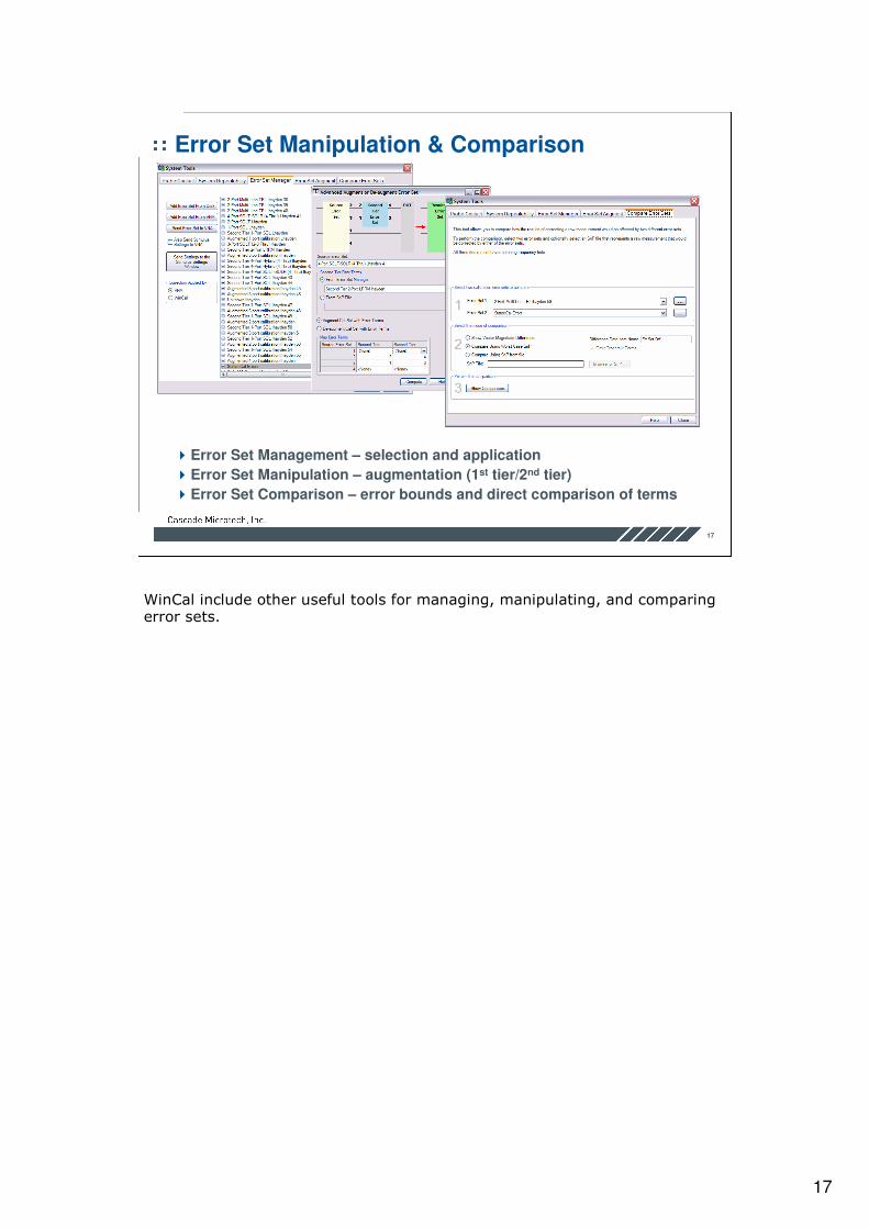
Error Set Manipulation & Comparison

Error Set Management – selection and application

Error Set Manipulation – augmentation (1st tier/2nd tier)

Error Set Comparison – error bounds and direct comparison of terms

WinCal include other useful tools for managing, manipulating, and comparing error sets.

18

18

Example: Comparison Study

Agilent 8364A PNA0.2-40 GHz, 200pts, 100Hz IF BW

Cascade Microtech Summit

12861B probe station200mm wafer chuck

Aux chuck for off-wafer stds

MS-1 programmable positioner

Infinity i40A-GSG-150 RF Probes

101-190C Imp. Standard Substrate

Reference Automated MLTRL

• One-button Cal! = Fast

• Very repeatable

SOLT Inaccuracy

• Ref Plane error?

SOLT

Manual MLTRL

Auto MLTRL

<2 minutesAuto MLTRL

>10 minutesManual MLTRL

1.25 minutesSOLT

TimeCal Method

A quick study compared the SOLT calibration with the manual and automated multi-line TRL calibrations.

19

19

Conclusion

A commercial implementation of Multi-Line TRL is now available

Programmable probe positioning enables automated

‘one-button’ MLTRL calibration

Automated MLTRL is quick and very repeatable

0.005<2Auto MLTRL

0.06>10Manual MLTRL

>0.11.25SOLT

Error Bound (@40GHz)Time (minutes)Cal Method

>5x Faster >12x Repeatability

Improvement