Policy Research Working Paper 9428

Raising College Access and Completion

How Much Can Free College Help?

Maria Marta Ferreyra Carlos Garriga

Juan David Martin Angelica Maria Sanchez Diaz

Latin America and the Caribbean RegionOffice of the Chief EconomistOctober 2020

Pub

lic D

iscl

osur

e A

utho

rized

Pub

lic D

iscl

osur

e A

utho

rized

Pub

lic D

iscl

osur

e A

utho

rized

Pub

lic D

iscl

osur

e A

utho

rized

Produced by the Research Support Team

Abstract

The Policy Research Working Paper Series disseminates the findings of work in progress to encourage the exchange of ideas about development issues. An objective of the series is to get the findings out quickly, even if the presentations are less than fully polished. The papers carry the names of the authors and should be cited accordingly. The findings, interpretations, and conclusions expressed in this paper are entirely those of the authors. They do not necessarily represent the views of the International Bank for Reconstruction and Development/World Bank and its affiliated organizations, or those of the Executive Directors of the World Bank or the governments they represent.

Policy Research Working Paper 9428

Free college proposals have become increasingly popular in many countries, yet cross-country evidence indicates that higher college subsidies raise enrollment but not graduation rates. To capture the evidence and evaluate proposals, this paper develops and estimates a dynamic model of college enrollment, performance, and graduation. A central piece of the model, student effort, has a direct effect on class completion and an indirect effect mitigating the risk of

performing poorly or dropping out. The model is estimated using rich student-level data from Colombia, and multiple free college programs are simulated. Among them, universal free college expands enrollment the most but does not affect graduation rates, thereby helping explain the evidence. Per-formance-based free college, in contrast, raises graduation rates yet has a smaller enrollment impact.

This paper is a product of the Office of the Chief Economist, Latin America and the Caribbean Region. It is part of a larger effort by the World Bank to provide open access to its research and make a contribution to development policy discussions around the world. Policy Research Working Papers are also posted on the Web at http://www.worldbank.org/prwp. The authors may be contacted at mferreyra@worldbank.org.

Raising College Access and Completion:How Much Can Free College Help? ∗

Maria Marta FerreyraThe World Bank

Carlos GarrigaFederal Reserve Bank of St. Louis

Juan David Martin-OcampoBanco de la Republica Colombia

Angelica Maria Sanchez DiazGeorgetown University

Keywords: Higher Education, free college, financial aid. JEL codes: E24, I21

∗We thank Kartik Athreya, Raquel Bernal, Adriana Camacho, Stephanie Cellini, Doug Harris, OksanaLeukhina, CJ Libassi, Alexander Ludwig, Fabio Sanchez, James Thomas, and Susan Vroman for useful commentsand suggestions. We thank Andrea Franco and Nicolas Torres for excellent research assistance. We benefitedfrom seminars at The World Bank, the St. Louis Fed, the DC Economics of Education Working Group, andUniversitat Autonoma de Barcelona, and by sessions at AEFP 2018, SED 2018, NASMES 2019, and LACEA2018. Ferreyra acknowledges financial support from The World Bank. The views expressed herein do notnecessarily reflect those of The World Bank, the Federal Reserve Bank of St. Louis, the Federal Reserve System,or of Banco de la Republica Colombia. Email contacts: mferreyra@worldbank.org, carlos.garriga@stls.frb.org,jmartioc@banrep.gov.co, amsanchez456@gmail.com. Corresponding author: Carlos Garriga, Research Division,Federal Reserve Bank of St. Louis, P.O. Box 442, St. Louis, MO 63166-0442. Phone: (314) 444-7412, Fax:(314) 444-8731, Email: carlos.garriga@stls.frb.org.

1 Introduction

In modern economies, higher education is crucial to the formation of skilled human capital. Notonly can higher education raise a country’s productivity; it can also lower income inequality.By subsidizing access to higher education, policymakers can contribute to these two roles. Thequestion, of course, is how large a subsidy they should provide. Advocates of free college arguethat policymakers should provide a full subsidy, resulting in zero tuition for students. Whilefree college has existed for years in a number of countries,1 free college proposals have sproutedrecently in other countries, including the United States, Chile, and Colombia.

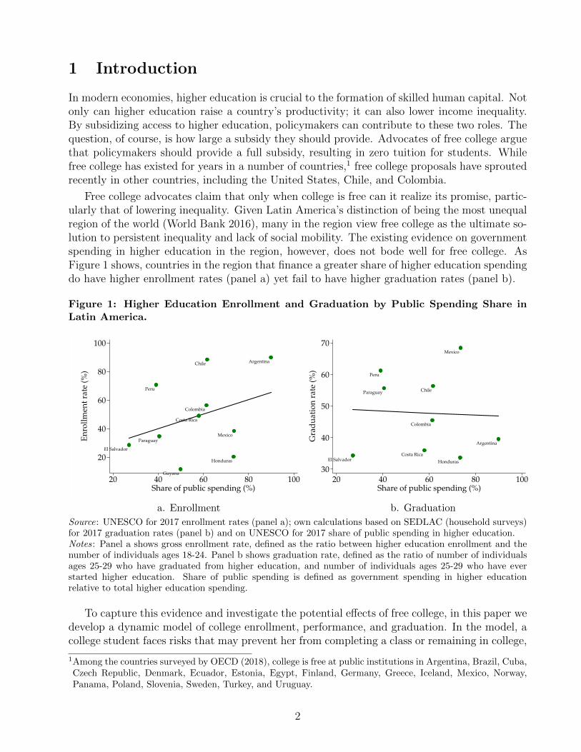
Free college advocates claim that only when college is free can it realize its promise, partic-ularly that of lowering inequality. Given Latin America’s distinction of being the most unequalregion of the world (World Bank 2016), many in the region view free college as the ultimate so-lution to persistent inequality and lack of social mobility. The existing evidence on governmentspending in higher education in the region, however, does not bode well for free college. AsFigure 1 shows, countries in the region that finance a greater share of higher education spendingdo have higher enrollment rates (panel a) yet fail to have higher graduation rates (panel b).

Figure 1: Higher Education Enrollment and Graduation by Public Spending Share inLatin America.

ArgentinaChile

Colombia

Costa Rica

El Salvador

Guyana

Honduras

MexicoParaguay

Peru

20

40

60

80

100

En

roll

men

t ra

te (

%)

20 40 60 80 100Share of public spending (%)

Argentina

Chile

Colombia

Costa RicaEl Salvador Honduras

Mexico

Paraguay

Peru

30

40

50

60

70

Gra

du

atio

n r

ate

(%)

20 40 60 80 100Share of public spending (%)

a. Enrollment b. Graduation

Source: UNESCO for 2017 enrollment rates (panel a); own calculations based on SEDLAC (household surveys)for 2017 graduation rates (panel b) and on UNESCO for 2017 share of public spending in higher education.Notes: Panel a shows gross enrollment rate, defined as the ratio between higher education enrollment and thenumber of individuals ages 18-24. Panel b shows graduation rate, defined as the ratio of number of individualsages 25-29 who have graduated from higher education, and number of individuals ages 25-29 who have everstarted higher education. Share of public spending is defined as government spending in higher educationrelative to total higher education spending.

To capture this evidence and investigate the potential effects of free college, in this paper wedevelop a dynamic model of college enrollment, performance, and graduation. In the model, acollege student faces risks that may prevent her from completing a class or remaining in college,

1Among the countries surveyed by OECD (2018), college is free at public institutions in Argentina, Brazil, Cuba,Czech Republic, Denmark, Ecuador, Estonia, Egypt, Finland, Germany, Greece, Iceland, Mexico, Norway,Panama, Poland, Slovenia, Sweden, Turkey, and Uruguay.

2

and which she can mitigate through effort. We estimate the model with unique administrativedata on the universe of higher education students in Colombia—a country highly representativeof Latin America—and use the parameter estimates to simulate free college programs whichdiffer in eligibility requirements. We study whether free college affects students’ risk and effort,and perform a simple cost-benefit analysis of free college.

Understanding the trade-offs in free college is critical, particularly in developing economies.In Latin America, higher education enrollment rates rose from 23 to 52 percent between 2000and 2017. Since only 14 percent of the working age population has completed higher education,Mincerian returns are high—104 percent on average relative to a high school diploma (Ferreyraet al 2017). Although such high returns should attract many individuals to higher education,liquidity constraints severely limit access, as countries subsidize public but not private highereducation and often lack credit markets. College subsidies are therefore a promising avenue tobroader access. While students in several of these countries have recently taken to the streetsin demand of full subsidies, the feasibility of free college has been called into question by thesecountries’ low growth and tight fiscal constraints in recent years—conditions, of course, thathave been seriously aggravated by the COVID-19 pandemic.

Even if free college were implemented, the cross-country evidence presented above suggeststhat it might not raise the stock of skilled human capital. One possible explanation is that freecollege might attract academically weak students, yet another is that it might discourage studenteffort. Free college raises consumption during college, therefore enhancing the attractivenessof being a college student (the “college experience”) and potentially unleashing three effectson effort. First is the loss-of-urgency effect, whereby the student wishes to enjoy the enhancedcollege experience and loses the urgency to graduate. Second is the substitution effect, wherebythe enhanced consumption compensates for greater effort. Third is the risk effect, as the effortchanges induced by the other two effects affect not only current but also future performanceand graduation prospects. If a strong loss of urgency prevails for many students, graduationrates will not rise and may even fall.

Because of its key role in free college’s success, student effort is a fundamental piece in ourstudy. In the model, heterogeneous high school graduates decide whether to enroll in college.Their labor market wage depends on their final educational attainment. To graduate, a studentmust complete a set number of classes in a given time. Each year she chooses the number ofclasses she expects to complete (henceforth, her target), which determines the effort she willmake. The number of classes completed by the student in a year depends on her ability, effort,and a performance shock which depends on her cumulative performance. At the end of the yearshe receives another shock, also dependent on cumulative performance, which may force her todrop out. Effort, then, has a direct effect on class completion and an indirect effect mitigatingthe risk of performing poorly or dropping out.

Our model captures indivisibilities that limit policy impact. To affect class completion, apolicy must induce a non-marginal effort change to complete at least one additional class. And,to affect graduation rates, the policy must induce a large enough effort increase to complete allthe required classes. These effort changes may be simply too costly for some students.

Estimated with Simulated Method of Moments, our model captures the main features ofthe data. In Colombia’s high school class of 2005, a staggering 70 percent of students comefrom low-income families and only 32.3 percent of students enroll in college within five years.Among those who attend college, only 46 percent graduate—mostly late. Student ability plays

3

a large role in year 1-survival but a lesser role in subsequent performance. The speed at whichstudents accumulate the completed classes required for graduation (henceforth, “cumulativeperformance” or “cumulative classes completed”) is highly persistent. As a result, early per-formance is a strong predictor of final outcomes.

According to our estimates, effort has a much greater impact than ability on the productionof classes completed. If effort were not modeled, ability’s role would be two or three timeslarger. The model would not fit the variation in classes completed and college outcomes amongstudents and over time, thereby affecting policy design particularly for students with lowerincome or ability. The model would also favor college subsidies promoting (positive) selectionof high-ability students rather than incentivizing effort—based on an attribute outside students’control rather than on a choice that they can control.

We simulate multiple free college programs with different eligibility requirements: 1) univer-sal (all students), 2) need-based (low-income students), 3) ability-based (high-ability students),and 4) performance-based (all students eligible in the first year; eligibility conditional on pastcumulative performance in subsequent years). We also simulate a need-based version of (3) and(4). In each counterfactual we distinguish between existing students (who enroll in the baselineand the counterfactual) and new students (who do not enroll in the baseline but enroll in thecounterfactual) to assess the impact of free college on graduation.

In our simulations, free college programs expand enrollment. Relative to the baseline,the largest expansion is for universal free college (85 percent), followed by need-based andperformance-based free college (72 and 66 percent, respectively). On average, new students areof lower income and ability than existing students except under ability-based programs, whichinduce positive selection of new students.

In contrast with these large enrollment rate effects, overall graduation rate effects aremodest—between -3 and 6 percent relative to the baseline. New students pull down the overallgraduation rate except under ability-based free college, in which case they pull it up. For ex-isting students graduation rates change little except under performance-based programs, whichraise them between 8 and 14 percent. By making free college contingent on performance, theseprograms eliminate the loss-of-urgency effect and induce greater effort. Our results providea theoretical justification for the financial aid literature in the U.S., which finds—as we do—positive and large enrollment effects, small or null graduation effects, and larger graduationeffects for performance-based than unconditional financial aid.2

Aggregate free college effects mask great heterogeneity across students. Consider, for in-stance, universal free college. Enrollment effects are largest for low- and middle-income stu-dents, and for mid-ability students. Hence, universal free college subsidizes many students whoalready enroll in the baseline and do not need the subsidy. Graduation rate effects also varyamong students. Graduation rates fall for high-ability or high-income students, who experi-ence a strong loss of urgency, but rise for low-ability or low-income students, who experience astrong substitution effect. In contrast, performance-based free college induces greater effort onthe part of all students and leads them all to higher graduation rates.

Behind the graduation rate success from performance-based free college is the greater riskfacing students. We develop a measure of anticipated risk and find that, as expected, anticipatedrisk falls when students exert greater effort or accumulate more classes completed. In the

2For recent reviews of this vast literature, see Avery et al (2019) and Dynarski and Scott-Clayton (2013).

4

early years, performance-based free college raises risk relative to the baseline and to universalfree college because it makes the level of college consumption contingent on performance. Byresponding to greater risk with greater effort, students attain better outcomes. Providingstudents with partial—rather than full—insurance therefore leads to better outcomes.

Using a framework that controls for institutional and potentially differences among coun-tries, our free college simulations rationalize the patterns in Figure 1. Greater college fundingsubstantially raises enrollment rates when many high school graduates face severe financialconstraints—as is the case in Latin America—but does not raise graduation rates unless it isperformance-based, which is not the case in Latin America. And, even if performance-basedprograms were more widespread, they would have little effect on graduation rates due to theindivisibilities discussed above: free college fails to induce in many students the large effortincrease needed to complete all graduation requirements. This is reminiscent of Oreopoulosand Petronijevic (2019), who find that even when students realize that more effort is needed toimprove outcomes, they adjust by lowering expectations rather than increasing effort.

For a policymaker committed to improving college access by providing free college to allor some students, we conduct a simple cost-benefit analysis to inform the choice among oursimulated programs. They all raise the per-graduate cost relative to the baseline—if anything,because fewer students pay for college. For a policymaker seeking to raise the fraction of highschool graduates that finish college while limiting costs, the best option is performance-based oreven need-based free college—but not universal free college. Since the per-graduate cost is quitehigh in every scenario—ranging from one (baseline) to 2.5 (universal free college) times the percapita GDP—free college should be considered with great care given current fiscal constraints.

Between 2014 and 2018, Colombia enacted a tuition subsidy program, Ser Pilo Paga (”Be-ing diligent pays off”), providing performance-based free college to low-income, high-abilitystudents. Its enrollment effects are quantitatively similar to our predictions (Londono et al2020); no data is yet available to study its graduation effects. The program has been recentlyreplaced by a similar one, Generacion E, which costs less. The current clamor in Latin Ameri-can countries, however, is not for this type of programs but rather for unconditional, universalprograms—which, as explained, are not the most efficient use of public funds.

By construction, our counterfactuals assume the most favorable scenario for free college.We assume that colleges have no capacity constraints; that the average and marginal cost ofeducating new and existing students are the same; and that free college does not crowd outparental transfers to children in college. We do not model taxation (which might be required topay for free college programs), and assume that the wage of college graduates relative to highschool graduates (henceforth, the college premium) does not fall with more college graduates.3

Relaxing any of these assumptions would lead to even less favorable free college outcomes.

The rest of the paper is organized as follows. Section 2 describes related literature, and Sec-tion 3 describes data sources and institutional environment. Section 4 presents stylized factsfrom the data. Section 5 presents the model, and Section 6 discusses its empirical implemen-tation. Section 7 describes estimation strategy and results. Section 8 presents the free collegecounterfactuals, including analyses of anticipated risk, fiscal costs, and potential labor marketgeneral equilibrium effects. Section 9 concludes.

3In Section 8.8 we investigate potential general equilibrium effects from the greater supply of college graduates.Since we find them to be small even in the medium run, we abstract away from them in our analysis.

5

2 Related Literature

Our paper relates to a large literature estimating sequential schooling models under uncertainty,with seminal contributions by Keane and Wolpin (2001), Eckstein and Wolpin (1998), andKeane (2002). This literature models college enrollment, performance, and college outcomes,and uncovers structural parameters based on students’ observed choices during college. Inone strand of this literature, researchers model students as acquiring information (learning)throughout college—regarding, for instance, their ability and preferences for college or specificmajors, and their expected labor market performance. This literature includes Arcidiacono(2004), Arcidiacono et al (2016), Ozdagli and Trachter (2011), Stinebrickner and Stinebrickner(2014), and Trachter (2015). As in these papers, students in our model adjust their expectedgraduation probability based on classes completed and choose effort accordingly.

The idea that higher education is risky is not new (Levhari and Weiss 1974, Altonji 1993,Akyol and Athreya 2005), but the recent availability of college transcript data in the U.S. hashelped estimate the role of risk in students’ performance. These data reveal substantial andpersistent heterogeneity in students’ credit accumulation rates, which are strongly related tograduation probability. According to Hendricks and Leukhina (2017, 2018), based on theircredit accumulation rates more than 50 percent of college entrants should be able to forecastwhether they are at least 80 percent likely to graduate. According to Stange (2012), the largeuncertainty faced by students makes them place a high value on the ability to drop out at anypoint rather than pre-commit to completing all graduation requirements. Our paper is similarto these in the use of administrative data to track students’ performance, but different in thatthe risk associated to class completion or college continuity is not fully exogenous as in thesepapers but depends on an endogenous variable—student effort.

While the literature has placed much attention on the role of ability in performance andcollege outcomes, a growing line of research highlights the role of effort. Zamarro, Hitt, andMendez (2019) use data from the Program for International Student Assessment (PISA) toshow that different effort measures explain about a third of observed cross-country test scorevariation. Stinebrickner and Stinebrickner (2004) rely on time use surveys to estimate the effectsof study time on grades. Ariely et al (2009) show that using incentives can help the averagestudent improve her test performance, though the effect is limited on high-ability students.Beneito et al (2018) provide evidence that the tuition increase implemented by Spanish collegesin 2012 boosted student effort. Ahn et al (2019) model effort in response to grading policies.We contribute to this line of research by explicitly modeling the role of effort and embeddingit in a dynamic setting, where it affects class accumulation and risk mitigation.

In an efficient and equitable world, college enrollment would depend on student ability ratherthan parental resources (Cameron and Heckman 1998 and 1999, Carneiro and Heckman 2002).In Colombia, as in other countries, parental resources matter greatly to college enrollmenteven controlling for ability. This provides strong evidence for credit constraints limiting collegeaccess, as discussed in a large literature. Lochner and Monge-Naranjo (2011) develop a modelthat helps explain the rising importance of family income for college attendance in the U.S.even in the presence of credit. Solis (2017) finds that relaxing credit constraints in Chilehad a positive impact on enrollment and college years completed, particularly for low-incomestudents. Parental resources and background, however, may be of limited importance. Hai andHeckman (2017) show that equalizing initial ability has larger effects on college outcomes and

6

inequality than equalizing parental background. The importance of credit access falls whenstudents can supply work to pay for college (Garriga and Keightley 2007). Although Colombiais a large developing economy, the market for student loans is very limited, covering only 7percent of students in 2003 (ICETEX 2010). Lack of family resources, limited opportunitiesto work during college, and missing credit markets for student loans are clear impediments tocollege access in countries such as Colombia.

In those countries, tuition subsidies may therefore expand college access. Our paper com-plements the literature on Chile’s recent free college policies (Bucarey 2018) and England’s freecollege elimination (Murphy et al 2019). It also joins in the vast literature of college financialaid in the U.S. (cited in Section 8.5), including the recent literature on free community collegeand the so-called “Promise” programs implemented in multiple U.S. states.

3 Data and institutional environment

In this section we describe our data sources, Colombia’s higher education environment, and ourstudy cohorts. Appendix A.1 contains further details.

Our data consists of student- and program-level information drawn from three administra-tive datasets: Saber 11, SPADIES, and SNIES. The Saber 11 dataset contains students’ testscores at the national mandatory high school exit exam (also named Saber 11) as well as self-reported socio-economic information. Saber 11 is a standardized test that measures a student’spreparedness for higher education—reflecting not only her innate ability but also her primaryand secondary education quality. We use it as a measure of student ability, broadly understoodas academic readiness for higher education. Family income is reported in brackets defined rel-ative to the monthly legal minimum wage (MW), which is equal to 381,000 Colombian pesos(COP) in 2005 (US$ 1 = 2,321 COP in 2005).

SPADIES tracks every higher education student. For each semester, it records the numberof classes attempted and passed by the student, as well as her graduation or dropout date. Itdoes not record the specific classes attempted, number of attempts per class, or class grades.SNIES contains program-level information, including institution, field, and tuition. We focuson bachelor’s programs, which capture approximately 80 percent of the country’s total highereducation enrollment. Enrollment is quite evenly split between public and private institutions;public institutions are heavily subsidized and charge a considerably lower tuition than privateinstitutions.

To analyze college enrollment, we focus on the 2005 high school cohort. We calculate decilesand quintiles of their ability distribution; in what follows, deciles and quintiles always refer tothis distribution. For consistency with the model, we classify students into “student types”defined by combinations of student ability quintiles and family income brackets. Appendixtable A1 shows the distribution of student types in this cohort. While a remarkable 70 percentof high school graduates come from the lowest two income brackets, less than 5 percent comefrom the top one. Not surprisingly, income and ability and strongly and positively correlated.

For our analysis of final outcomes and academic progression we focus on students fromthe 2006 college entry cohort that enroll in five-year bachelor’s programs within five years offinishing high school. Since every program requires a different number of classes for graduation,we normalize the requirement to 100 classes for every program to facilitate exposition.We assume

7

that students are required to complete the same number of classes (20) every year. We use theterm “classes completed” (or “performance”) to denote the number of classes completed in agiven year. We use “cumulative classes completed” (or “cumulative performance”) in a givenyear as the total number of classes completed over all years up to (and including) that one. Astudent is on track for on-time graduation when she has completed her on-track requirements,equal to accumulating 20, 40, 60, 80, and 100 classes by the end of years 1 through 5 respectively.

It is useful to classify students into tiers based on their cumulative performance relative tothe corresponding year’s on-track requirement. Tiers 1 through 4 correspond to students whocomplete the following percentage of the on-track requirements for the year: 95 percent or morefor tier 1, (85, 95] percent for tier 2, (65, 85] percent for tier 3, and 65 percent or less for tier4.4(See Appendix Table A2 for further details on tier classification). Importantly, a studentcan change tiers over time—catching up to a higher tier or falling behind to a lower one.

4 Stylized Facts

The data has distinctive features that our model seeks to capture. We describe them below.

Fact 1: Students of higher income or ability are more likely to enroll in college.Although the overall enrollment rate is 32 percent,5 enrollment rates vary widely among studenttypes (see Table 1), and rise with income and ability. On average, the enrollment gap betweenthe highest and lowest income brackets is equal to 55 percentage points (pp)—similar to the50-pp gap between the highest and lowest ability. Free college may therefore have ample roomto raise enrollment.

Table 1: Enrollment Rates by Income and Ability.

Income Ability quintileBracket 1 2 3 4 5 Total

5+ MW 32.85 44.14 58.87 69.23 83.85 73.383-5 MW 28.71 39.75 48.41 62.99 79.24 62.032-3 MW 20.34 28.72 36.96 48.03 67.88 43.501-2 MW 13.94 18.36 23.85 33.84 54.22 28.05<1 MW 9.05 12.67 17.20 26.56 43.93 17.67

Total 13.43 19.15 26.20 38.93 63.74 32.29

Source: Calculations based on SPADIES and Saber 11 for 2005 high school graduates.Notes: Each cell reports percent of high school graduates from a given income bracket and ability quintilewho enrolled in a bachelor’s program between 2006 and 2010. Income reported in brackets; MW = monthlyminimum wage. Ability reported in quintiles of standardized Saber 11 scores; quintile 1 is the lowest.

Fact 2: Dropout rates are high, particularly for low-ability students in year 1.

4To exemplify, consider a student who accumulates 16, 35, 42, 50, and 60 classes by the end of years 1 through5 respectively. This amounts to 80 (=16/20), 88 (=35/40), 70, 62.5, and 60 percent of the correspondingon-track requirements. Thus, the student falls in tiers 3, 2, 3, 4, and 4 in years 1 through 5 respectively.

5For comparison, in the US the enrollment rate of individuals ages 16-24 who finished high school in 2005 andstarted college right away (rather than within five years) is 44.6% (Source: Digest of Education Statistics).

8

Only 45.7 percent of students from our entry cohort graduate—15.1 percent graduates on time(in five years) and 30.6 percent graduates late (in 6-8 years).6 Dropout rates are far from uniformover time. As Figure 2 shows, over a quarter of college students (half of all dropouts) leavein the first year, and the first two years account for about 70 percent of all dropouts. Similarto enrollment rates, dropout rates vary widely across student types (Table 2). Conditional onincome, higher ability students have lower dropout rates; on average, the dropout rate gapbetween the highest and lowest ability quintiles is equal to 25 pp. In contrast, dropout ratesdo not vary much by income—suggesting that free college might affect enrollment more thandropout decisions.

Final college outcomes vary substantially by ability. High-ability students are more likelyto graduate, whether on time or late (Figure 3), whereas low-ability students are more likelyto drop out, particularly in year 1. After year 1, dropout rates vary little across abilities.

Figure 2: Dropout Timing.

0

10

20

30

40

50

60

Per

cen

t

1 2 3 4 5 6 7 8College year

% relative to entry cohort

% relative to all dropouts

Source: Calculations based on SPADIES, for studentsfrom the 2006 entry cohort (first semester).Notes: The blue line shows percent of students whodrop out in a given college year. The red line shows,among all dropouts, percent of those who drop out ina given college year.

Figure 3: College Outcomes by Ability.

0

10

20

30

40

50

Per

cen

t

1 2 3 4 5Ability quintile

Dropout 1st year Dropout 2nd year

On−time graduate Late graduate

Dropout after 2nd year

Source: Calculations based on SPADIES. Studentsbelong to the 2006 entry cohort (first semester).Notes: For each quintile, the graph shows the percentof students who attained each outcome. Percents addto 100 by quintile.

Fact 3: Cumulative performance varies more within than across abilities.Figure 4’s panel a shows average number of classes completed by ability quintile in year 1. Thethick black line depicts average over all students, whereas the color lines depict averages amongthe students with the following final outcomes: on-time graduation, late graduation, dropoutin year 1, and dropout later. On average, high-ability students complete more classes than low-ability students in year 1. However, the figure also shows a pattern repeated every year: averageclasses completed varies little across abilities—overall and conditional on outcomes—but variesgreatly within abilities. For a given ability, on-time graduates complete more classes than lategraduates, who complete more than dropouts. In other words, number of classes completed—as

6For comparison, in the U.S. 59.2 percent of students from the 2006 cohort graduated within six years—39percent on time (in four years), and 20.2 percent late ˙Source: Digest of Education Statistics.

9

Table 2: Dropout Rates by Income and Ability.

Ability quintile1 2 3 4 5 Total

5+ MW 81.36 65.83 61.48 52.13 39.04 44.733-5 MW 74.23 69.44 62.21 57.86 43.77 51.332-3 MW 68.54 67.58 63.73 57.68 46.53 55.091-2 MW 71.59 66.64 62.21 57.66 50.56 57.82<1 MW 69.04 67.95 61.34 55.94 50.30 58.71

Total 70.99 67.44 62.37 56.96 45.84 54.36

Source: Calculations based on SPADIES for students from the 2006 entry cohort (first semester).Notes: Each cell reports percent of students from a given income bracket and ability quintile who dropout of their bachelor’s program. A student is classified as a dropout if she does not graduate within eightyears. Income is reported in brackets; MW = monthly minimum wage. Ability is reported in quintiles ofstandardized Saber 11 scores. Quintile 1 is the lowest.

early as in year 1— is a powerful predictor of final outcomes. This point is further illustratedin panel b, which classifies students into tiers by the end of year 1. Consistent with panel a, itshows the strong predictive power of early performance—as explained by the next stylized fact.

Figure 4: First-year Classes Completed and College Outcomes.

9

11

13

15

17

19

21

23

Av

g. n

um

ber

of

clas

ses

com

ple

ted

1 2 3 4 5Ability quintile

On−time graduate Late graduate

Dropout after 1st year Dropout 1st year

All students

0

15

30

45

60

Per

cen

t

Tier 1 Tier 2 Tier 3 Tier 4

On−time graduate Late graduate

Dropout 1st year Dropout 2nd year

Dropout after 2nd year

a. First-year classes completed b. College outcomes by first-yearby college outcome tier of classes completed

Source: Calculations based on SPADIES for students from the 2006 entry cohort (first semester).Notes: In panel a, each color represents a college outcome. The green line, for instance, shows average numberof classes completed by the end of year 1 by students of a given ability quintile who went on to graduate on time.The thick black line does the same for all students regardless of college outcome. In panel b, the graph showsthe percent of students from a given performance tier by the end of year 1 that attain each college outcome.For the first year, tier 1 corresponds to 19+ classes completed; tier 2 to [17, 19); tier 3 to [13, 17); and tier 4 to[0, 13).

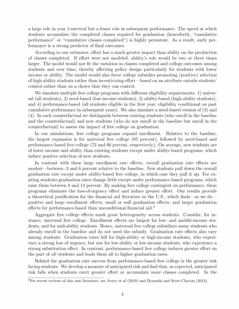
Fact 4: Cumulative performance is highly persistent over time.To investigate whether a student’s performance changes over time, Figure 5 depicts a student’sprobability of attaining each of four following outcomes—same-tier persistence, dropout, catchup, and fall behind—by the end of a year conditional on her previous year’s performance tier.7

7For example, a student who finished first year in tier 2 has second-year probabilities of persistence, dropout,

10

Figure 5: Tiers of Cumulative Classes Completed: Transitions Throughout College.

0

10

20

30

40

50

60

70

80

90

100P

erc

en

t

2 3 4 5

Year

Tier 1

Tier 2

Tier 3

Tier 4

a. Persistence

0

10

20

30

40

50

60

70

80

90

100

Pe

rce

nt

2 3 4 5Year

Tier 1

Tier 2

Tier 3

Tier 4

b. Dropout

0

10

20

30

40

50

60

70

80

90

100

Pe

rce

nt

2 3 4 5Year

Tier 2 to tier 1

Tier 3 to tier 1&2

Tier 4 to tier 1,2&3

c. Catch−up

0

10

20

30

40

50

60

70

80

90

100

Pe

rce

nt

2 3 4 5Year

Tier 1 to tier 2,3&4

Tier 2 to tier 3&4

Tier 3 to tier 4

d. Fall behind

Source: Calculations based on SPADIES for the 2006 entry cohort (first semester).Notes: Each panel shows the probability that a student who ended the previous year in a given tier experiencesthe following outcomes in the current year: persist in the tier (panel a), drop out (panel b), catch up (rise) toa higher tier (panel c), or fall behind to a lower tier (panel d). For a given year and tier, probabilities add upto 100 across panels. For example, a student who finished year 1 in tier 3 is depicted in green. In year 2, she is35, 23, 18, and 24 percent likely to persist in tier 3, drop out, catch up to tiers 1 or 2, and fall behind to tier 4respectively.

Same-tier persistence rises over time (panel a), in part because dropout rates fall over time(panel b). Although low-performing students are more likely than others to drop out, studentsfrom all tiers face a non-zero dropout probability. Some students move across tiers by catchingup or falling behind (panels c and d). Higher-performing students are more likely to catch upand less likely to fall behind than others, yet all students face a non-zero probability of fallingbehind. Despite transitions among tiers, the most likely outcome for a student in tier 1, 2, or3 is to remain in it the following year.

Reaching year 5 does not guarantee graduation, but cumulative performance up to thatpoint is strongly related to final outcomes. As Figure 7 shows, most students in the top threetiers graduate but most bottom-tier students do not. Further, most top-tier students graduateon time.

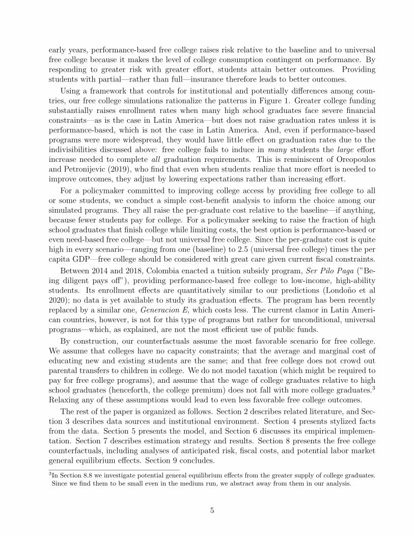
Fact 5: Within abilities, cumulative performance becomes more concentratedover time.As low-performing students drop out over time, the distribution of cumulative performancebecomes more concentrated at the top tiers. Panel a of Figure 6 shows the distribution acrossperformance tiers at the end of year 1 by ability quintile. High-ability students are the mostlikely to belong to the top tier while low-ability students are the most likely to belong to thebottom tier. Nonetheless, performance varies greatly within ability quintiles, and a sizable

catch up, and fall behind equal to 29, 14, 20, and 39 respectively. Beginning in year 5, students can ”transition”into graduation as well.

11

fraction of students from every quintile is concentrated in the middle tiers. Because of this“thick middle,” cumulative performance varies little, on average, across abilities. A similarpicture holds for year 5 (panel b), although by then all the performance distributions aremore concentrated in the top three tiers. Further, the performance distribution for low-abilitystudents is more dispersed than that of high-ability students in both years.

Figure 6: Tiers of Cumulative Classes Completed, by Ability.

0

10

20

30

40

50

60

Per

cen

t

1 2 3 4 5

Ability quintile

Tier 1 Tier 2&3 Tier 4

0

10

20

30

40

50

60

Per

cen

t

1 2 3 4 5

Ability quintile

Tier 1 Tier 2&3 Tier 4

a. Year 1 b. Year 5Source: Calculations based on SPADIES for students from the 2006 entry cohort (first semester).Notes: For students of a given ability who start year 1, panel a shows their classification into tiers of cumulativeclasses completed by the end of year 1. Panel b does the same for students beginning year 5.

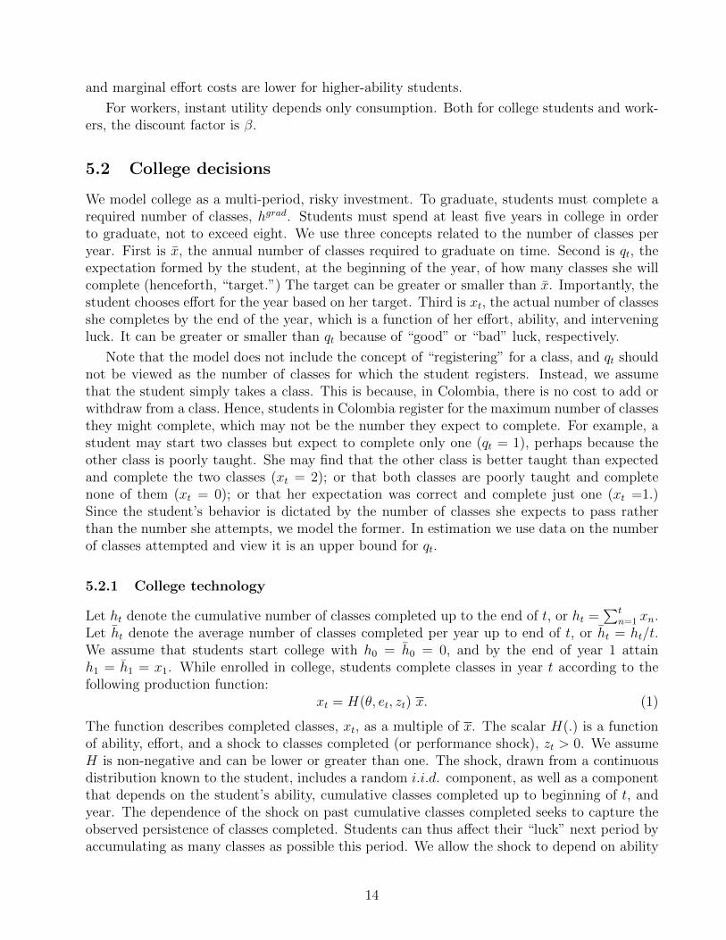
Fact 6: Higher-ability students attempt a higher number of classes.Although a student cannot fully control her performance, she can control the number of classesshe attempts (registers for) in a given year. While she may not pass all the classes attempted,the number of attempts is informative of her intended effort. As Figure 8 shows, on average stu-dents attempt fewer than the 20 required classes. In addition, on average high-ability studentsattempt more classes than low-ability students. We will return to these facts when discussingidentification of our empirical model.

Taking stock. The data shows that students of higher income or ability are more likelyto enroll in college. Conditional on enrolling, lower ability students are much more likely todrop out, particularly in year 1. Through this channel, ability serves a strong predictor ofgraduation. Ability, however, is not a strong predictor of cumulative performance. Althoughcumulative performance varies little, on average, across abilities, it varies greatly within abilities.Further, cumulative performance is highly persistent over time—students who start on trackare more likely to remain on track, less likely to fall behind, and more likely to catch up shouldthey fall behind. As a result, cumulative performance is highly predictive of final outcomes.Nonetheless, even on-track students face the risk of falling behind or dropping out. Our modelseeks to capture these data features.

12

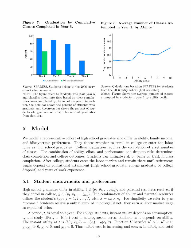
Figure 7: Graduation by CumulativeClasses Completed in Year 5.

0

20

40

60

80

100

Per

cen

t

Tier 1 Tier 2 Tier 3 Tier 4

Graduation rate On−time graduation rate

Source: SPADIES. Students belong to the 2006 entrycohort (first semester).Notes: The figure refers to students who start year 5and classifies them into tiers based on their cumula-tive classes completed by the end of the year. For eachtier, the blue bar shows the percent of students whograduate, and the green bar shows the percent of stu-dents who graduate on time, relative to all graduatesfrom that tier.

Figure 8: Average Number of Classes At-tempted in Year 1, by Ability.

17

17.5

18

18.5

19

19.5

20

Av

g. n

um

ber

of

clas

ses

tak

en

1 2 3 4 5 6 7 8 9 10Ability decile

Source: Calculations based on SPADIES for studentsfrom the 2006 entry cohort (first semester).Notes: Figure shows the average number of classesattempted by students in year 1 by ability decile.

5 Model

We model a representative cohort of high school graduates who differ in ability, family income,and idiosyncratic preferences. They choose whether to enroll in college or enter the laborforce as high school graduates. College graduation requires the completion of a set numberof classes. The combination of ability, effort, and performance and dropout risks determinesclass completion and college outcomes. Students can mitigate risk by being on track in classcompletion. After college, students enter the labor market and remain there until retirement;wages depend on educational attainment (high school graduate, college graduate, or collegedropout) and years of work experience.

5.1 Student endowments and preferences

High school graduates differ in ability, θ ∈ {θ1, θ2, . . . , θnθ}, and parental resources received ifthey enroll in college, y ∈ {y1, y2, . . . , yny}. The combination of ability and parental resourcesdefines the student’s type j = 1, 2, . . . , J , with J = nθ × ny. For simplicity we refer to y as“income.” Students receive y only if enrolled in college; if not, they earn a labor market wageas explained below.

A period, t, is equal to a year. For college students, instant utility depends on consumption,c, and study effort, e. Effort cost is heterogeneous across students as it depends on ability.The instant utility at t is U(ct, et, θ) = u(ct) − g(et, θ). Function U satisfies u′ > 0, u′′ < 0,g1, g11 > 0, g2 < 0, and g12 < 0. Thus, effort cost is increasing and convex in effort, and total

13

and marginal effort costs are lower for higher-ability students.

For workers, instant utility depends only consumption. Both for college students and work-ers, the discount factor is β.

5.2 College decisions

We model college as a multi-period, risky investment. To graduate, students must complete arequired number of classes, hgrad. Students must spend at least five years in college in orderto graduate, not to exceed eight. We use three concepts related to the number of classes peryear. First is x, the annual number of classes required to graduate on time. Second is qt, theexpectation formed by the student, at the beginning of the year, of how many classes she willcomplete (henceforth, “target.”) The target can be greater or smaller than x. Importantly, thestudent chooses effort for the year based on her target. Third is xt, the actual number of classesshe completes by the end of the year, which is a function of her effort, ability, and interveningluck. It can be greater or smaller than qt because of “good” or “bad” luck, respectively.

Note that the model does not include the concept of “registering” for a class, and qt shouldnot be viewed as the number of classes for which the student registers. Instead, we assumethat the student simply takes a class. This is because, in Colombia, there is no cost to add orwithdraw from a class. Hence, students in Colombia register for the maximum number of classesthey might complete, which may not be the number they expect to complete. For example, astudent may start two classes but expect to complete only one (qt = 1), perhaps because theother class is poorly taught. She may find that the other class is better taught than expectedand complete the two classes (xt = 2); or that both classes are poorly taught and completenone of them (xt = 0); or that her expectation was correct and complete just one (xt =1.)Since the student’s behavior is dictated by the number of classes she expects to pass ratherthan the number she attempts, we model the former. In estimation we use data on the numberof classes attempted and view it is an upper bound for qt.

5.2.1 College technology

Let ht denote the cumulative number of classes completed up to the end of t, or ht =∑t

n=1 xn.Let ht denote the average number of classes completed per year up to end of t, or ht = ht/t.We assume that students start college with h0 = h0 = 0, and by the end of year 1 attainh1 = h1 = x1. While enrolled in college, students complete classes in year t according to thefollowing production function:

xt = H(θ, et, zt) x. (1)

The function describes completed classes, xt, as a multiple of x. The scalar H(.) is a functionof ability, effort, and a shock to classes completed (or performance shock), zt > 0. We assumeH is non-negative and can be lower or greater than one. The shock, drawn from a continuousdistribution known to the student, includes a random i.i.d. component, as well as a componentthat depends on the student’s ability, cumulative classes completed up to beginning of t, andyear. The dependence of the shock on past cumulative classes completed seeks to capture theobserved persistence of classes completed. Students can thus affect their “luck” next period byaccumulating as many classes as possible this period. We allow the shock to depend on ability

14

to reflect that ability may be correlated with other elements, not modeled, that systematicallyaffect “luck.”8

If the student knew zt when choosing her effort, then choosing et would be equivalent tochoosing classes completed, xt. Since, as explained below, the student chooses et before zt isrealized, choosing effort is equivalent to choosing a target, qt, where qt = E(xt). Thus,

qt = E[H(zt, θ, et)] x. (2)

Assuming that H(·) is linear on zt so that it can be expressed as H(zt, θ, et) = ztH(θ, et), targetand effort are functions of E(zt):

qt = E(zt)H(θ, et) x and et = H−1e [θ, qt/(E(zt) x)]. (3)

Meanwhile, the actual number of classes completed, xt, is a function of the effort chosen giventhe target, and of the realized zt. Cumulative classes completed by the end of the year, ht, is

ht = ht−1 + xt. (4)

Finally, we assume that the production function in (1) is such that, when the student supplieszero effort, she completes zero classes: H(zt, θ, 0) = 0. For every student type, there alwaysexists a level of effort, et, that allows her to complete x, or H(zt, θ, et) = 1. Also, students canexert high effort to compensate for low ability or expected “bad luck”.

5.2.2 The student’s optimization problem

The student faces a sequential problem. We differentiate between the pre-graduation years(when she cannot yet graduate) and the graduation years (when she is eligible to graduate).We divide each year into two sub-periods. In the first sub-period, the student chooses her targetnumber of classes and hence effort. At the end of the first sub-period she receives the shock tothe number of classes completed, which determines her actual (as opposed to target) number ofclasses completed. In the second sub-period, she graduates if she has accumulated the requirednumber of classes; otherwise she draws a shock that determines whether she will remain incollege next year or drop out (“dropout shock”). Thus, as long as she has not completed hergraduation requirements, the student draws two shocks per year—one to classes completed inthe year and another to college continuity. The two shocks are endogenous in the sense thatthey depend on cumulative performance, which depends on effort. In a given year, a collegestudent’s state vector is (t, ht−1, θ, y). Appendix Figure B1 summarizes the timing of eventsand decisions, described in detail below.

Pre-Graduation Years (t = 1,...,4). During these years, students have not yet accu-mulated the required number of classes for graduation, or ht < hgrad. In year 1, students startwith zero cumulative classes completed, h0 = 0, and are heterogenous only in their type. Sincestudents of a given type may vary in their first-year completed classes h1 (depending, as we will

8For example, lower ability students may choose less selective programs than others, or may have lower levels ofthe non-cognitive skills necessary to succeed in college. In the first case, E(z) would be higher for lower-abilitystudents than for higher-ability ones; in the second case, it would be lower. In our estimation we let the dataidentify the sign of the relationship between E(z) and θ.

15

see below, on their z1 shock), from year 2 onward students are heterogenous not only in theirtype but also in their cumulative classes completed at the beginning of the year, ht−1.

In each of these years, at the beginning of the first sub-period the student chooses et (andhence qt) before zt is realized. As in (2), the chosen target is a function of the E(zt). At the endof the first sub-period zt is realized and determines the number of cumulative classes completed,ht ≥ ht−1. In the second sub-period the student receives her dropout shock, ddropt = {0, 1},which determines whether she will remain in college next year or drop out, respectively. Theprobability that this shock leads her to drop out is a function of her cumulative classes completedafter the realization of zt, that is ht, as well as her type and the year:

Pr(ddropt = 1 | zt) = pd(t, ht, θ, y). (5)

We assume that, by the end of t, if the student has accumulated less than a pre-specified numberof classes for the year, hdropt , she must drop out: pd(t, ht < hdropt , θ, y) = 1. If, in contrast, shecompletes x classes each year and is on track for on-time graduation, her dropout probabilityis very low: pd(t, ht, θ, y) ≈ 0. In general, pd is decreasing in ht. Importantly, the student canlower pd by exerting effort, which raises ht.

If the student drops out, she will receive the market wage of a college dropout from the fol-lowing year onward; the value of dropping out is V drop(t+1).Meanwhile, the value of remainingin college is V coll(t+ 1, ht, θ, y).

Graduation Years (t = 5,...,7). These years are different from the previous ones in thatcollege students become eligible to graduate. Those who have fulfilled graduation requirements,ht ≥ hgrad, will graduate and enter the labor market, whose value is V grad(t + 1). For them,additional classes beyond hgrad yield zero marginal benefits. Remaining students draw thedropout shock to determine college continuity the following year.

Terminal year (t = 8). This is the last year that a student is allowed in college. At theend of it, only two outcomes are possible: the student graduates if h8 ≥ hgrad, or drops outotherwise. Continuation values are equal to V grad(9) and V drop(9) respectively.

We can now present the student’s dynamic optimization problem from the first subperiod ofeach college year:

V coll(t, ht−1, θ, y) = maxet

{U(ct, et, θ) + βEz

[1{t≥5}Pr

(ht ≥ hgrad

)V grad(t+ 1) +

Pr(ht < hgrad

) [pd(t, ht, θ, y)V drop(t+ 1) +

(1− pd(t, ht, θ, y)

)V coll(t+ 1, ht, θ, y)

] ]},

(6)

s.t. ct = y − T (t, ht−1, θ, y)

ht = ht−1 + xt

xt = H(zt, θ, et)x

ct > 0.

16

Here, the argument of Ez[·] is the continuation value function. Variable T (·) is tuition, constantregardless of the target, qt.

9 To accommodate our counterfactuals, we write T (·) in general formso that it can vary by year, cumulative classes completed, ability, or income. In our baselineit varies only by y (see Section 6.2.1 below). For low-income students tuition might exceedincome, which would violate the ct > 0 constraint and make enrollment unfeasible. Note thesevere credit constraint: students cannot borrow to pay for tuition nor can they save.10 Thepolicy function is the sequence of optimal efforts, e∗(t, ht, θ, y), that solve the dynamic problemdefined in (6).

5.3 Workers

An individual can join the labor force after graduating from high school or college, or afterdropping out from college.11 The worker’s optimization problem, written in recursive form, is

V m(t) = maxct{u(ct) + βV m(t+ 1)}, (7)

s.t. ct = wmt ,

where V m(t) is the value function of a worker with educational attainmentm = {hs, grad, drop},denoting high school graduate, college graduate, and college dropout respectively. The worker’swage, wmt , is specific to educational attainment and varies with t to allow for returns to expe-rience.

5.4 Enrollment decision

To decide whether or not to enroll in college, a high school graduate compares the expectedpayoff of two choices—going to college, or joining the labor force as a high school graduate.The enrollment decision is a discrete choice problem, where the payoff associated to each optionis the sum of three components. The first component is the expected value of going to college,V coll(t = 1, h0 = 0, θ, y) or of entering the labor force as a high school graduate, V hs. The secondcomponent is a type-specific preference for college enrollment, ξj = ξ(θj, yj), which capturestype-related unobserved factors (i.e., parental education) that affect enrollment. We normalizethe unobserved preference for joining the labor force as a high school graduate to zero for alltypes. The third component is an idiosyncratic choice-specific shock for each individual, εhs andεcoll, corresponding to working as a high school graduate or enrolling in college, respectively.Thus, all individuals face the same V hs and individuals of a given type face the same V coll andξj, yet individuals within and across types differ in their idiosyncratic shocks. We assume that

9This is in keeping with the Colombian context, where tuition is fixed regardless of the number of classes taken.10We do not model student’s decision to work during college because our administrative data does not record this

information. Further, data from Colombia’s National Survey of Time Use (ENUT ) reveals that high-incomecollege students are more likely to work during college than their lower-income counterparts, suggesting thatthe primary motivation to work is not necessarily to pay for college (details available upon request). For amodel of student workers, see Garriga and Keightley (2007).

11We assume that workers consume all their earnings and do not have access to credit markets, which is anaccurate representation of developing economies. Since wages rise with experience and workers discount thefuture at the interest rate, they have no incentives to save.

17

εhs and εcoll are iid and distributed Type I Extreme Value with a scaling factor of σε. Theindividual chooses to attend college if

V coll(1, 0, θj, yj) + ξj + σεεcoll

Value of going to college

≥ V hs + σεεhs

Value of working as a high school graduate(8)

As a result, the probability of college enrollment for an individual of type j is

P coll(θj, yj) =exp{(V coll(1, 0, θj, yj) + ξj)/σε}

exp{(V coll(1, 0, θj, yj) + ξj)/σε}+ exp{V hs/σε}, (9)

Its complement, P hs(θ, y) = 1−P coll(θ, y), is the probability of joining the labor force as a highschool graduate.

6 Empirical implementation

In this section we describe the parameterization and computational version of the model. Wealso describe the algorithm to compute model predicted values for a given parameter point.

6.1 Functional forms

In the model, t = 1 corresponds to age 18. Retirement age is 65, or t = 48. Regardless of hereducational attainment or when she joined the labor force, the individual accrues returns toexperience (or becomes ”experienced”) from age 35 (t = 28) onward.

The utility of college students is given by

U (c, e, θ) =(c+ c)1−ρ − 1

1− ρ− µ eγ

(1 + θ)k. (10)

where the need to meet the minimum consumption level, c, might limit low-income students’ability to enroll in college. To prevent this, we set c equal to one million COP.12 The utility ofworkers is given by

u(c) =c1−ρ − 1

1− ρ. (11)

We set β = 0.04, which is consistent with an implicit discount rate of 4 percent, and assumeσε = 1.

The production function to complete classes has constant returns to scale in ability andeffort:

xt = H(zt, θ, et)x = zt(θαe1−α

t )x, (12)

where α ∈ (0, 1) is the elasticity of classes completed with respect to ability. Consistent withthe model, we set x = 20 classes. We set the minimum number of classes required to graduate,

12Our chosen value for c guarantees that, in our computational models, all students attain positive consumptionif they enroll in college. We can think of c as the minimum consumption guaranteed to college studentsthrough student subsidies, such as those for food and transportation in Colombia.

18

hgrad, equal to 98.13

The functional form for the zt shock is as follows:

zt = exp{− exp{−(κ0 + κ1d1 + κhht−1 + κθθ + (σ + σ1d1 + σθθ)νt)}}, (13)

where ht−1 is a measure of past cumulative number of classes completed, with ht−1 = ln(ht−1)for every t > 1, and h0 = 0 for t = 1.The terms associated with d1 allow the shock distributionto differ in year 1, when d1 = 1. The shock also depends on an iid component, νt, drawn fromthe uniform distribution U(0, 1). The functional form in (13) ensures that zt ∈ (0, 1) for anycombination of parameter values and for all h, θ ∈ R. Importantly, all the parameters in (13)affect the mean and variance of zt. In Section 7.3 below we discuss the effect of ht−1 and κθ onthis mean and variance at our specific parameter estimates.

We parameterize the probability of dropping out as

pd(t, ht, θ, y) =exp{δ(t, θ, y) + πht}

1 + exp{δ(t, θ, y) + πht}, (14)

where δ(t, θ, y) is a year-, ability- and income- specific fixed effect, and ht measures cumulativeperformance over all periods, including the current one. Evaluating pd(t, ht, θ, y) at π = 0 yieldsthe “exogenous dropout probability”—the dropout probability for students of a given type ina given year if they had accumulated no classes. It is “exogenous” because it is independentof effort. For example, low-income, low-ability students may have a high exogenous dropoutprobability in year 1—perhaps due to lack of parental guidance to navigate college—yet a lowerone in subsequent years.

The model’s full parameter vector is Θ = (Θ, ξ, δ), where

Θ = (ρ, µ, γ, k, α, κ0, κy1 , κh, κθ, σ, σy1 , σθ, π) (15)

is the vector of parameters common across individuals. Vector ξJ×1 contains type-specific unob-served preferences for college, ξj (see (9)) and δ(J∗8)×1 contains exogenous dropout probabilityfixed effects, δ(t, θj, yj), for the J types and 8 years (see (14)).

6.2 Computational representation

6.2.1 Student types

To build the empirical distribution of ability and income for school graduates, Φ(y, θ), we startfrom Appendix Table A1, which classifies 2005 high school graduates by ability quintile andincome bracket. We refine this table to work with ability deciles rather than quintiles, for a totalof fifty student types. To construct values for θ, we start from the distribution of standardizedSaber 11 test scores and normalize them between 0 and 1.14 Our θ values are the 5th, 15th,...95th percentiles from the normalized scores. We calculate the y value corresponding to each

13We set this requirement to 98 rather than 100 because we observe students who graduate with slightly fewerthan 100 classes, perhaps due to measurement error.

14Let sts denote the standardized test score. The normalized sts is thus equal to (sts−min(sts))/(max(sts)−min(sts)).

19

income bracket as the bracket’s average annual per capita income, computed from Colombia’shousehold survey data (SEDLAC). Lacking student-level data on tuition expenses, we estimatethe tuition paid by students of a given y as the average annual tuition paid by students from thecorresponding income bracket at public institutions, calculated from SNIES and SPADIES.15

Appendix Table A3 shows the resulting income and tuition by family income bracket. In-come varies greatly across income brackets but tuition varies less. Although public institutionsprovide income-based tuition discounts, the highest income individuals do not pay proportion-ally to their income: their per capita income is about twenty times as large as that of thelowest-income individuals, yet their tuition is only 2.5 times as large.

6.2.2 Workers

We use household surveys to compute the average wages earned by individuals with differenteducational attainment and experience in 2005. For workers aged 18-65, the average wage ofa college graduate, a college dropout with at least one year of complete college, and a collegedropout with less than one year of complete college is 160, 58, and 28 percent higher than theaverage wage of a high school graduate respectively (see Appendix Table A4).16 Among college(high school) graduates, the average wage of experienced workers is 35 (29) percent higherthan the average wage of inexperienced workers. Consistent with the data, we assume that thereturns to experience of college dropouts are the same as those of high school graduates.

6.3 Computing predicted values

Since the model does not have a closed-form solution, we use a numerical algorithm to solvestudents’ dynamic optimization problem for a given value of Θ. Appendix C provides a fulldescription of the algorithm. The estimation of δ and ξ is nested within the model solution fora given of value of Θ, in the spirit of Berry, Levinsohn and Pakes (1995).

In anticipation of next section, a couple of remarks are in order. First, our model solutionperfectly replicates observed enrollment rates by type by construction. Hence, enrollment ratesare not a moment to match in the estimation. Second, our model solution attempts to replicateobserved dropout rates at the (year, ability quintile, income) level, but only does it with mixedsuccess (see Appendix C.3 for further details). Thus, dropout rates are a moment to match.

7 Estimation

In this section we describe the estimation strategy and identification. We also present parameterestimates, describe the model’s fit, and address the role of effort given our estimates.

15We use tuition at public institutions because there is always a public institution that the student can attend.Modelling the choice of college type (public or private) is beyond the scope of this paper.

16This creates, in effect, four college attainments: high school, college, some college (one year), some college(two or more years). The two “some college” categories correspond to college dropouts. We work with tworather than one dropout category because their wages are quite different and can hence affect dropout timing.

20

7.1 Estimation Strategy

We estimate the model parameters using Simulated Method of Moments (SMM). Our estimationsearches for the value of Θ whose predicted moments, M(Θ), best match the observed ones,M. The moments we match are listed in Table 3. They reflect the patterns of dropout, collegeoutcomes, classes completed, persistence, and targets discussed in Section 4. Matching these585 moments enables us to estimate our 13 parameters.

Table 3: Moments Matched in Estimation.

Number ofData aspect Moments Moments

Dropout rates Dropout rate by year. 8Dropout rate by ability quintile and income. 25Dropout rate by ability decile. 10

College outcomes College outcomes by ability quintile. 25Fraction of students that graduate by year (years 5-8). 4

Cumulative classescompleted

Average number of cumulative classes completed byyear, ability quintile, and college outcome.

140

Average number of cumulative classes completed byyear and ability decile (years 1-5).

50

Distribution of students into tiers of cumulative classescompleted, by year.

24

Distribution of students into tiers of cumulative classes 75completed, by ability quintile and year (years 1-5).

Transition probabilities Pr(tier Y in t+ 1|tier X in t) for years 1-7. 112

Pr(ddropt = 1|tier X in t) for years 1-8. 32

Target number of classes Average target number of classes by ability decile andyear.

80

Total 585

Source: Own estimation.Notes: Moments per year are computed for years 1-8 unless otherwise specified. Tiers are 1-4, based oncumulative classes completed. For “College outcomes,” outcomes include on-time graduate, late graduate,drop out first year, drop out second year, drop out after second year. In “Cumulative classes completed,”which are calculated by year, outcomes include on-time graduate (until year 5), late graduate, drop outthis year, drop out later (until year 7); “this year” and “later” refer to the year under consideration. In“Transition probabilities”, t refers to year; tiers X and Y are 1,...,4. Observed data for target number ofclasses is average number of classes attempted by the corresponding students.

Formally, our SMM parameter estimates solve the following problem:

arg minΘ

(M(Θ)−M)′W−1(M(Θ)−M), (16)

where Θ is a 13×1 vector of parameters, M and M are 585×1 vectors of sample and predictedmoments, respectively, and W is a diagonal weighting matrix whose diagonal contains thestandard error of the sample moments. We compute numerically the predicted values, M, forevery value of Θ as explained in Appendix C.

21

7.2 Identification

A critical challenge is identifying the role of ability, effort, and performance shocks in theproduction of classes completed. Below we provide intuition for identification by describingeach parameter’s role in the model, and Section 7.5 below complements this discussion.

Effort. If effort had no role in the number of classes completed (α = 1), or if it were costless(µ = 0), then all students would take the required number of classes per year. The fact thatstudents take, on average, a lower number of classes than required (see Section 4) indicatesthat effort does have a role in classes completed and helps identify µ. An increase in µ leadsto lower targets, effort, and number of classes completed. An increase in µ also leads to lowercollege enrollment—particularly for low-income students, who have lower consumption thanothers to compensate for effort. The speed of accumulation of classes completed, as well as thetransitions among tiers over time, helps identify γ. A high γ penalizes high effort levels andmakes it costly to catch up. The fact that higher ability students take more classes, on average,than their lower-ability counterparts indicates that their effort cost is lower and identifies k. Anincrease in k raises the variance of average target, effort, and classes completed across abilities.

Performance shock. Despite the low variation of average classes completed across abilities,number of classes completed varies widely within abilities. Conditional on ability, effort variesby income. This explains some, but not all, of the within-ability variation of classes completed.The remainder of this variation, then, is explained by the performance shock, z. Since θ isbetween 0 and 1, we restrict z to be in this range as well. This helps us pin down the scale foreffort. An increase in κ0 makes shocks more favorable to all students, thus raising the numberof classes completed and lowering dropout rates across the board. Parameter κ1 is an interceptshifter that makes the scale of z comparable across years. An increase in κθ makes the expectedshock relatively more favorable for high-ability students and raises the dispersion in averageclasses completed and college outcomes across abilities. Parameter σ is identified by the overallvariation of classes completed conditional on ability, whereas σθ is identified by the greatervariation of classes completed among lower ability students. The higher overall variation ofclasses completed in year 1 relative to other years identifies σ1. After year 1, κh is identified bythe persistence of students in their performance tiers.

Ability. Given the role of effort and performance shocks in the production of classescompleted, the variation of average classes completed across abilities identifies α. This variationrises with an increase in α.

Other parameters. An increase in ρ raises the aversion to consumption variations overtime and decreases the propensity to college enrollment. It also lowers the speed of classaccumulation and increases time-to-degree. Finally, the sensitivity of dropout rates with respectto current classes completed, conditional on student income and ability, identifies π.

A sufficient condition for local identification is full rank for the matrix of first derivativesof the moments’ predicted values with respect to the parameter vector when evaluated at thetrue parameter point. Evaluated at our parameter estimates, this matrix has full column rankin our sample.

7.3 Parameter Estimates

We now turn to our parameter estimates, shown in Table 4.

22

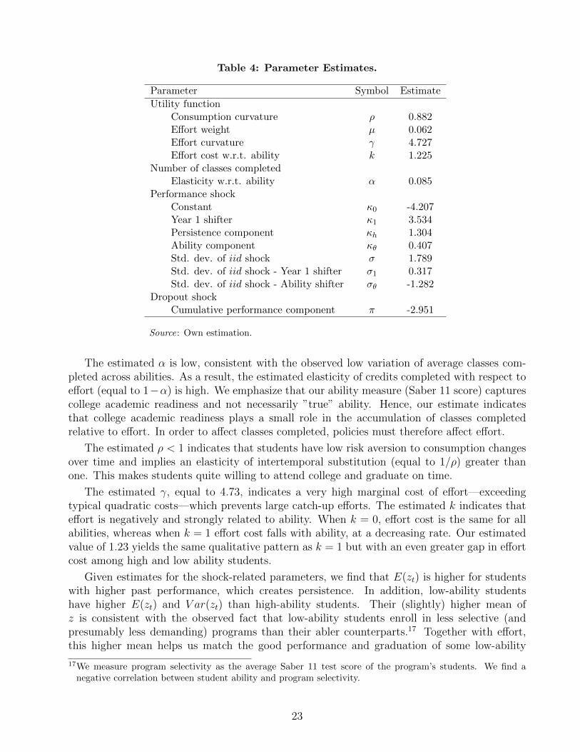
Table 4: Parameter Estimates.

Parameter Symbol Estimate

Utility functionConsumption curvature ρ 0.882Effort weight µ 0.062Effort curvature γ 4.727Effort cost w.r.t. ability k 1.225

Number of classes completedElasticity w.r.t. ability α 0.085

Performance shockConstant κ0 -4.207Year 1 shifter κ1 3.534Persistence component κh 1.304Ability component κθ 0.407Std. dev. of iid shock σ 1.789Std. dev. of iid shock - Year 1 shifter σ1 0.317Std. dev. of iid shock - Ability shifter σθ -1.282

Dropout shockCumulative performance component π -2.951

Source: Own estimation.

The estimated α is low, consistent with the observed low variation of average classes com-pleted across abilities. As a result, the estimated elasticity of credits completed with respect toeffort (equal to 1−α) is high. We emphasize that our ability measure (Saber 11 score) capturescollege academic readiness and not necessarily ”true” ability. Hence, our estimate indicatesthat college academic readiness plays a small role in the accumulation of classes completedrelative to effort. In order to affect classes completed, policies must therefore affect effort.

The estimated ρ < 1 indicates that students have low risk aversion to consumption changesover time and implies an elasticity of intertemporal substitution (equal to 1/ρ) greater thanone. This makes students quite willing to attend college and graduate on time.

The estimated γ, equal to 4.73, indicates a very high marginal cost of effort—exceedingtypical quadratic costs—which prevents large catch-up efforts. The estimated k indicates thateffort is negatively and strongly related to ability. When k = 0, effort cost is the same for allabilities, whereas when k = 1 effort cost falls with ability, at a decreasing rate. Our estimatedvalue of 1.23 yields the same qualitative pattern as k = 1 but with an even greater gap in effortcost among high and low ability students.

Given estimates for the shock-related parameters, we find that E(zt) is higher for studentswith higher past performance, which creates persistence. In addition, low-ability studentshave higher E(zt) and V ar(zt) than high-ability students. Their (slightly) higher mean ofz is consistent with the observed fact that low-ability students enroll in less selective (andpresumably less demanding) programs than their abler counterparts.17 Together with effort,this higher mean helps us match the good performance and graduation of some low-ability

17We measure program selectivity as the average Saber 11 test score of the program’s students. We find anegative correlation between student ability and program selectivity.

23

students. The more dispersed shock for lower-ability students, in turn, helps us match theirhigher variance of classes completed.

To examine the relative impact of past performance and ability on z given our estimates,consider students A and B. Student A is more able than B, with ∆θ = θA−θB = 0.22. This is alarge ability difference, equal to the difference between the 55th and the 5th ability percentile, orbetween the 95th and the 75th percentile. Assume that, at the beginning of t, A has completedone more class than B. Because A is abler than B, her E(zt) should be lower than B’s, yetbecause she has completed more classes, her E(zt) should be higher. Based on our estimates,just having completed that additional class gives her the same E(zt) as B’s, even though B ismuch less able. In other words, E(zt) is more sensitive to ht−1 than to θ. This makes z highlypersistent and more dependent on something the student can control—her performance—thanon ability, which she cannot control.

Finally, the estimated π indicates that an additional class completed by the end of the year,on average, decreases the probability of dropping out by about 5 pp. Since pd(·) has a logisticfunctional form, this marginal effect is stronger for students with intermediate values of thedropout probability rather than values close to zero or one.

Our full set of parameter estimates includes the dropout probability fixed effects in (14),δ(t, θ, y). To illustrate the relative magnitude of π and δ(t, θ, y), consider the average num-ber of additional classes that a student from the second ability quintile (“Q2 student”) mustcomplete to attain the same dropout probability as a student from the top ability quintile(“Q5 student”). In year 1, she must complete more than 4 additional classes—20 percent ofthe annual requirements—reflecting a high exogenous dropout probability. In year 5 she onlyneeds one additional class completed, as the Q2 students reaching year 5 are approximatelyon par with Q5 students. The important point is that, early on, low-ability students face ahigh exogenous dropout probability, which they can only counter through high initial effort orfavorable performance shocks.

7.4 Goodness of fit

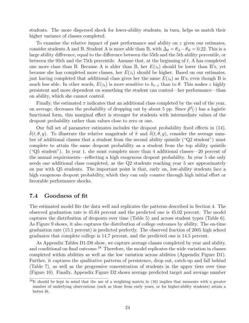
The estimated model fits the data well and replicates the patterns described in Section 4. Theobserved graduation rate is 45.64 percent and the predicted one is 45.02 percent. The modelcaptures the distribution of dropouts over time (Table 5) and across student types (Table 6).As Figure 9 shows, it also captures the distribution of college outcomes by ability. The on-timegraduation rate (15.1 percent) is predicted perfectly. The observed fraction of 2005 high schoolgraduates that complete college is 14.7 percent, and the predicted one is 14.5 percent.

As Appendix Tables D1-D8 show, we capture average classes completed by year and ability,and conditional on final outcome.18 Therefore, the model replicates the wide variation in classescompleted within abilities as well as the low variation across abilities (Appendix Figure D1).Further, it captures the qualitative patterns of persistence, drop out, catch-up and fall behind(Table 7), as well as the progressive concentration of students in the upper tiers over time(Figure 10). Finally, Appendix Figure D2 shows average predicted target and average number

18It should be kept in mind that the use of a weighting matrix in (16) implies that moments with a greaternumber of underlying observations (such as those from early years, or for higher-ability students) attain abetter fit.

24

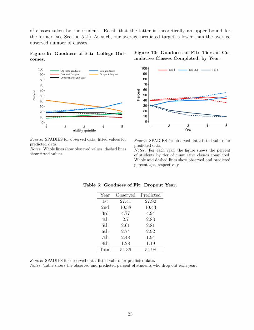
of classes taken by the student. Recall that the latter is theoretically an upper bound forthe former (see Section 5.2.) As such, our average predicted target is lower than the averageobserved number of classes.

Figure 9: Goodness of Fit: College Out-comes.

0

10

20

30

40

50

60

70

80

90

100

Per

cen

t

1 2 3 4 5Ability quintile

On−time graduate Late graduate

Dropout 2nd year Dropout 1st year

Dropout after 2nd year

Source: SPADIES for observed data; fitted values forpredicted data.Notes: Whole lines show observed values; dashed linesshow fitted values.

Figure 10: Goodness of Fit: Tiers of Cu-mulative Classes Completed, by Year.

0

10

20

30

40

50

60

70

80

90

100

Pe

rce

nt

1 2 3 4 5

Year

Tier 1 Tier 2&3 Tier 4

Source: SPADIES for observed data; fitted values forpredicted data.Notes: For each year, the figure shows the percentof students by tier of cumulative classes completed.Whole and dashed lines show observed and predictedpercentages, respectively.

Table 5: Goodness of Fit: Dropout Year.

Year Observed Predicted1st 27.41 27.922nd 10.38 10.433rd 4.77 4.944th 2.7 2.835th 2.61 2.816th 2.74 2.927th 2.48 1.948th 1.28 1.19

Total 54.36 54.98

Source: SPADIES for observed data; fitted values for predicted data.Notes: Table shows the observed and predicted percent of students who drop out each year.

25

Table 6: Goodness of Fit: Dropout Rates by Income and Ability.

Ability quintilesIncome Observed values Predicted valuesBracket 1 2 3 4 5 Total 1 2 3 4 5 Total

5+ MW 81.4 65.8 61.5 52.1 39.1 44.7 84.4 67.8 63.4 51.9 40.7 46.73-5 MW 74.2 69.4 62.2 57.9 43.8 51.3 81.6 68.3 62.2 57.3 44.4 52.52-3 MW 68.5 67.6 63.7 57.7 46.5 55.1 70.8 67.5 61.9 60.1 44.4 55.61-2 MW 71.6 66.6 62.2 57.7 50.6 57.8 69.9 66.5 60.9 56.2 46.9 56.7<1 MW 69.0 67.9 61.3 55.9 50.3 58.7 69.6 66.3 58.6 53.7 46.2 57.5

Total 71.0 67.4 62.4 60.0 45.8 54.4 71.3 66.9 61.0 56.6 44.8 55.0

Source: Source: SPADIES for observed data; fitted values for predicted data.Notes: Values are expressed in percentages (%). Income is reported in brackets; MW = monthly minimumwage. Ability is reported in quintiles of standardized Saber 11 scores. Quintile 1 is the lowest.

Table 7: Goodness of Fit: Transitions Among Tiers of Cumulative Classes Completed.

Observed values Predicted valuesYear 2 Year 3 Year 4 Year 5 Year 2 Year 3 Year 4 Year 5

PersistenceTier 1 64.33 79.78 86.98 79.89 63.70 75.80 75.10 74.30Tier 2 28.67 39.23 51.47 57.76 22.80 38.40 53.70 60.10Tier 3 34.94 49.44 60.94 69.04 35.10 59.20 71.20 78.80Tier 4 29.67 45.75 57.87 58.59 37.10 42.50 60.70 76.00

Dropout rateTier 1 12.16 4.03 1.75 0.71 11.60 4.20 3.00 2.20Tier 2 14.43 6.50 3.25 1.52 16.20 6.40 4.60 3.00Tier 3 23.02 12.30 7.29 4.02 25.10 9.20 7.00 5.20Tier 4 54.23 41.95 28.24 24.24 55.20 50.70 35.20 21.40

Prob. of Catch upTier 3 to Tiers 1 & 2 18.10 20.42 20.61 19.63 26.60 20.30 13.10 9.40Tier 4 to Tiers 1 & 2 4.26 0.55 0.22 0.14 0.82 0.00 0.00 0.00

Prob. of Fall behindTier 1 to Tiers 3 & 4 11.01 5.41 2.54 1.66 4.30 1.20 0.30 0.00Tier 2 to Tiers 3 & 4 36.8 28.77 17.70 18.40 26.00 25.60 22.80 24.40

Source: SPADIES for observed data; model simulations for predicted data.Notes: Values are expressed in percentages (%).

7.5 The Role of Effort

Since our estimates show that class completion is much more responsive to effort than ability,we now examine the role of effort.

7.5.1 Average effort over time.

We begin by looking at average student effort by year (Figure 11). On average, effort is relativelyhigh in years 1 and 4. In year 1, students work hard to complete classes and mitigate dropout

26

risk, which is highest that year. In year 4, they work hard in order to graduate. After year 5,average effort falls as the remaining students have few classes left.

Figure 11: Predicted Average Effort by Year.

.2

.4

.6

.8

1

Av

erag

e ef

fort

1 2 3 4 5 6 7 8College year

Source: Model baseline predictions.Notes: The figure shows average student effort by year in the simulated baseline. Individual efforts are normal-ized by the 95th percentile of the year’s effort distribution.

7.5.2 What if the model did not include effort?

In order to highlight the role of effort, we re-estimate the model eliminating effort as an inputin the production function. We do this by normalizing effort to a scaling constant. In this“exogenous effort” model, the student does not choose effort and thereby has no control overher performance. We run two variants of the exogenous effort model. In the first (“exogenoushomogeneous effort”) we set the scaling constant to the same value for all students and years,equal to the overall effort average in the baseline. In the second (“exogeneous heterogeneouseffort”) we set the constant for a given (student type, year) equal to the baseline average effortfor that (student type, year). The first variant is similar to models that do not include effortat all (see Section 2). The second variant is akin to adding (student type, year) fixed effects tomodels without effort.

Appendix Table E1 compares parameter estimates and objective function values for ourmodel and the exogenous effort models. When effort is exogenous, not surprisingly hetero-geneous effort fits the data better than homogeneous effort. However, both exogenous effortmodels fit the data much worse than our model (the objective function rises by a factor of 5to 8). In other words, the omission of effort cannot be solved by merely adding (student type,year) fixed effects to a model without effort.

Removing effort from performance places greater weight on ability and shocks. The elasticityof performance with respect to ability, α, becomes 2.5 or 3 times larger. Since higher abilitystudents have lower effort cost and exert more effort, other things equal, the exogenous effortmodel attributes to ability an effect that is actually mediated through effort. The implied E(z)rises steeply with ability, thereby amplifying ability’s role, and z becomes more dispersed in anattempt to match within-ability performance variation (see Appendix Figure E1). Interestingly,the risk aversion parameter, ρ, becomes twice as large to reflect that students, who can no longermitigate risk through effort, behave as if they were more risk averse.

27

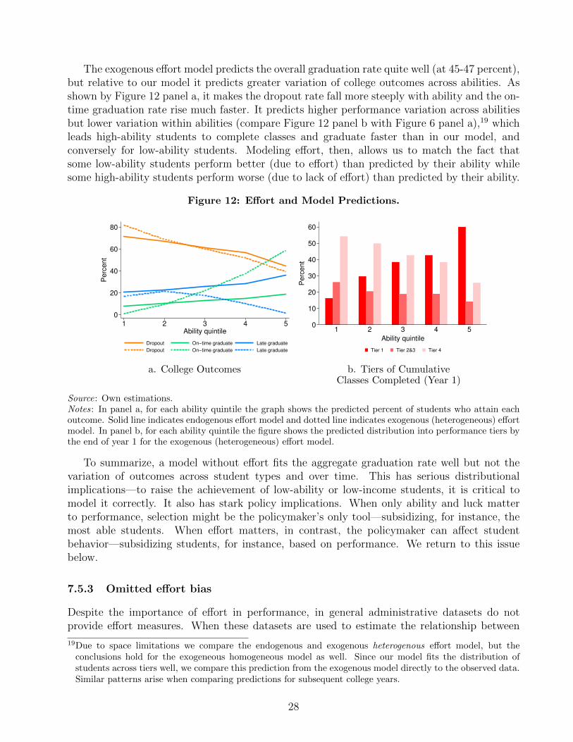
The exogenous effort model predicts the overall graduation rate quite well (at 45-47 percent),but relative to our model it predicts greater variation of college outcomes across abilities. Asshown by Figure 12 panel a, it makes the dropout rate fall more steeply with ability and the on-time graduation rate rise much faster. It predicts higher performance variation across abilitiesbut lower variation within abilities (compare Figure 12 panel b with Figure 6 panel a),19 whichleads high-ability students to complete classes and graduate faster than in our model, andconversely for low-ability students. Modeling effort, then, allows us to match the fact thatsome low-ability students perform better (due to effort) than predicted by their ability whilesome high-ability students perform worse (due to lack of effort) than predicted by their ability.

Figure 12: Effort and Model Predictions.

0

20

40

60

80

Pe

rce

nt

1 2 3 4 5Ability quintile

Dropout On−time graduate Late graduate

Dropout On−time graduate Late graduate

0

10

20

30

40

50

60

Pe

rce

nt

1 2 3 4 5

Ability quintile

Tier 1 Tier 2&3 Tier 4

a. College Outcomes b. Tiers of CumulativeClasses Completed (Year 1)

Source: Own estimations.Notes: In panel a, for each ability quintile the graph shows the predicted percent of students who attain eachoutcome. Solid line indicates endogenous effort model and dotted line indicates exogenous (heterogeneous) effortmodel. In panel b, for each ability quintile the figure shows the predicted distribution into performance tiers bythe end of year 1 for the exogenous (heterogeneous) effort model.

To summarize, a model without effort fits the aggregate graduation rate well but not thevariation of outcomes across student types and over time. This has serious distributionalimplications—to raise the achievement of low-ability or low-income students, it is critical tomodel it correctly. It also has stark policy implications. When only ability and luck matterto performance, selection might be the policymaker’s only tool—subsidizing, for instance, themost able students. When effort matters, in contrast, the policymaker can affect studentbehavior—subsidizing students, for instance, based on performance. We return to this issuebelow.

7.5.3 Omitted effort bias

Despite the importance of effort in performance, in general administrative datasets do notprovide effort measures. When these datasets are used to estimate the relationship between

19Due to space limitations we compare the endogenous and exogenous heterogenous effort model, but theconclusions hold for the exogeneous homogeneous model as well. Since our model fits the distribution ofstudents across tiers well, we compare this prediction from the exogenous model directly to the observed data.Similar patterns arise when comparing predictions for subsequent college years.

28

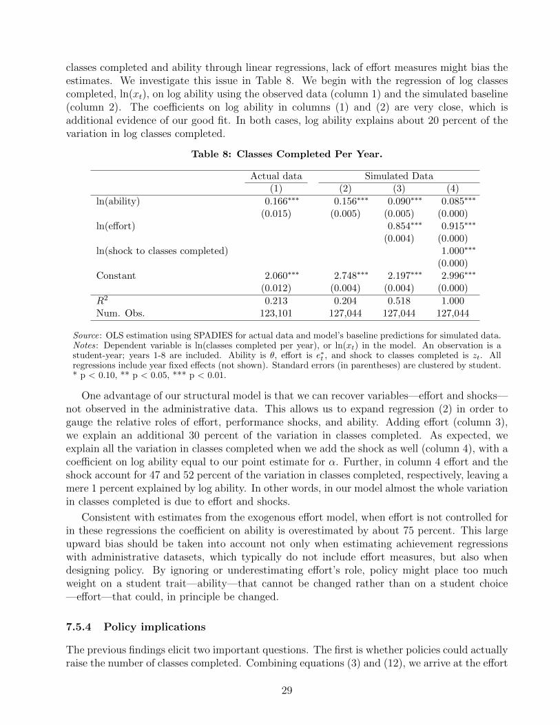
classes completed and ability through linear regressions, lack of effort measures might bias theestimates. We investigate this issue in Table 8. We begin with the regression of log classescompleted, ln(xt), on log ability using the observed data (column 1) and the simulated baseline(column 2). The coefficients on log ability in columns (1) and (2) are very close, which isadditional evidence of our good fit. In both cases, log ability explains about 20 percent of thevariation in log classes completed.

Table 8: Classes Completed Per Year.

Actual data Simulated Data(1) (2) (3) (4)

ln(ability) 0.166∗∗∗ 0.156∗∗∗ 0.090∗∗∗ 0.085∗∗∗

(0.015) (0.005) (0.005) (0.000)ln(effort) 0.854∗∗∗ 0.915∗∗∗

(0.004) (0.000)ln(shock to classes completed) 1.000∗∗∗

(0.000)Constant 2.060∗∗∗ 2.748∗∗∗ 2.197∗∗∗ 2.996∗∗∗

(0.012) (0.004) (0.004) (0.000)

R2 0.213 0.204 0.518 1.000Num. Obs. 123,101 127,044 127,044 127,044

Source: OLS estimation using SPADIES for actual data and model’s baseline predictions for simulated data.Notes: Dependent variable is ln(classes completed per year), or ln(xt) in the model. An observation is astudent-year; years 1-8 are included. Ability is θ, effort is e∗t , and shock to classes completed is zt. Allregressions include year fixed effects (not shown). Standard errors (in parentheses) are clustered by student.* p < 0.10, ** p < 0.05, *** p < 0.01.

One advantage of our structural model is that we can recover variables—effort and shocks—not observed in the administrative data. This allows us to expand regression (2) in order togauge the relative roles of effort, performance shocks, and ability. Adding effort (column 3),we explain an additional 30 percent of the variation in classes completed. As expected, weexplain all the variation in classes completed when we add the shock as well (column 4), with acoefficient on log ability equal to our point estimate for α. Further, in column 4 effort and theshock account for 47 and 52 percent of the variation in classes completed, respectively, leaving amere 1 percent explained by log ability. In other words, in our model almost the whole variationin classes completed is due to effort and shocks.

Consistent with estimates from the exogenous effort model, when effort is not controlled forin these regressions the coefficient on ability is overestimated by about 75 percent. This largeupward bias should be taken into account not only when estimating achievement regressionswith administrative datasets, which typically do not include effort measures, but also whendesigning policy. By ignoring or underestimating effort’s role, policy might place too muchweight on a student trait—ability—that cannot be changed rather than on a student choice—effort—that could, in principle be changed.

7.5.4 Policy implications

The previous findings elicit two important questions. The first is whether policies could actuallyraise the number of classes completed. Combining equations (3) and (12), we arrive at the effort

29

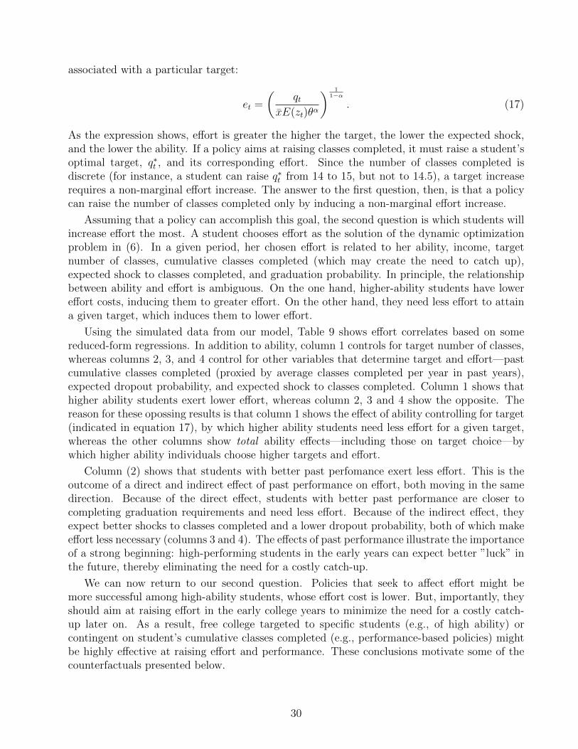
associated with a particular target:

et =

(qt

xE(zt)θα

) 11−α

. (17)

As the expression shows, effort is greater the higher the target, the lower the expected shock,and the lower the ability. If a policy aims at raising classes completed, it must raise a student’soptimal target, q∗t , and its corresponding effort. Since the number of classes completed isdiscrete (for instance, a student can raise q∗t from 14 to 15, but not to 14.5), a target increaserequires a non-marginal effort increase. The answer to the first question, then, is that a policycan raise the number of classes completed only by inducing a non-marginal effort increase.

Assuming that a policy can accomplish this goal, the second question is which students willincrease effort the most. A student chooses effort as the solution of the dynamic optimizationproblem in (6). In a given period, her chosen effort is related to her ability, income, targetnumber of classes, cumulative classes completed (which may create the need to catch up),expected shock to classes completed, and graduation probability. In principle, the relationshipbetween ability and effort is ambiguous. On the one hand, higher-ability students have lowereffort costs, inducing them to greater effort. On the other hand, they need less effort to attaina given target, which induces them to lower effort.

Using the simulated data from our model, Table 9 shows effort correlates based on somereduced-form regressions. In addition to ability, column 1 controls for target number of classes,whereas columns 2, 3, and 4 control for other variables that determine target and effort—pastcumulative classes completed (proxied by average classes completed per year in past years),expected dropout probability, and expected shock to classes completed. Column 1 shows thathigher ability students exert lower effort, whereas column 2, 3 and 4 show the opposite. Thereason for these opossing results is that column 1 shows the effect of ability controlling for target(indicated in equation 17), by which higher ability students need less effort for a given target,whereas the other columns show total ability effects—including those on target choice—bywhich higher ability individuals choose higher targets and effort.

Column (2) shows that students with better past perfomance exert less effort. This is theoutcome of a direct and indirect effect of past performance on effort, both moving in the samedirection. Because of the direct effect, students with better past performance are closer tocompleting graduation requirements and need less effort. Because of the indirect effect, theyexpect better shocks to classes completed and a lower dropout probability, both of which makeeffort less necessary (columns 3 and 4). The effects of past performance illustrate the importanceof a strong beginning: high-performing students in the early years can expect better ”luck” inthe future, thereby eliminating the need for a costly catch-up.

We can now return to our second question. Policies that seek to affect effort might bemore successful among high-ability students, whose effort cost is lower. But, importantly, theyshould aim at raising effort in the early college years to minimize the need for a costly catch-up later on. As a result, free college targeted to specific students (e.g., of high ability) orcontingent on student’s cumulative classes completed (e.g., performance-based policies) mightbe highly effective at raising effort and performance. These conclusions motivate some of thecounterfactuals presented below.

30

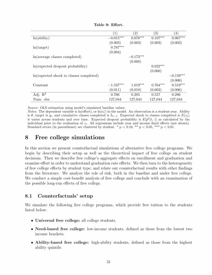
Table 9: Effort.

(1) (2) (3) (4)

ln(ability) −0.015∗∗∗ 0.076∗∗∗ 0.107∗∗∗ 0.067∗∗∗

(0.003) (0.003) (0.003) (0.003)ln(target) 0.787∗∗∗

(0.004)ln(average classes completed) −0.173∗∗∗

(0.008)ln(expected dropout probability) 0.022∗∗∗

(0.000)ln(expected shock to classes completed) −0.159∗∗∗

(0.006)Constant −1.537∗∗∗ 1.019∗∗∗ 0.764∗∗∗ 0.519∗∗∗

(0.011) (0.018) (0.003) (0.006)

Adj. R2 0.766 0.285 0.557 0.286Num. obs. 127,044 127,044 127,044 127,044

Source: OLS estimation using model’s simulated baseline values.Notes: The dependent variable is ln(effort), or ln(e∗t ) in the model. An observation is a student-year. Abilityis θ, target is qt, and cumulative classes completed is ht−1. Expected shock to classes completed is E[zt];it varies across students and over time. Expected dropout probability is E[pd(t, ·)] as calculated by theindividual prior to the realization of zt. All regressions include year and income fixed effects (not shown).Standard errors (in parentheses) are clustered by student. * p < 0.10, ** p < 0.05, *** p < 0.01.

8 Free college simulations

In this section we present counterfactual simulations of alternative free college programs. Webegin by describing their setup as well as the theoretical impact of free college on studentdecisions. Then we describe free college’s aggregate effects on enrollment and graduation andexamine effort in order to understand graduation rate effects. We then turn to the heterogeneityof free college effects by student type, and relate our counterfactual results with other findingsfrom the literature. We analyze the role of risk, both in the baseline and under free college.We conduct a simple cost-benefit analysis of free college and conclude with an examination ofthe possible long-run effects of free college.

8.1 Counterfactuals’ setup

We simulate the following free college programs, which provide free tuition to the studentslisted below:

• Universal free college: all college students.

• Need-based free college: low-income students, defined as those from the lowest twoincome brackets.

• Ability-based free college: high-ability students, defined as those from the highestability quintile.

31

• Ability- and need-based free college: students who are both low income and highability—students from the lowest two income brackets and the highest ability quintile.

• Performance-based free college: all students in year 1 but only high-performingstudents afterwards. In a given year, a high-performing student is one who finished theprevious year in tiers 1 or 2 based on her cumulative performance. Note that a studentmay be high-performing in one year but not in another.

• Performance- and need-based free college: all low-income students (from the lowesttwo income brackets) in year 1 but only students who are both low-income and high-performing afterwards.

Note that, by design, performance-based programs create a risk for the student, as the zerotuition is not guaranteed but conditional on performance. In contrast, the other free collegeprograms guarantee zero tuition regardless of performance.

As we analyze these counterfactuals, it is convenient to distinguish between two groups ofstudents—existing and new. For a given counterfactual, we define existing students as thosewho start college both in the baseline and counterfactual. In contrast, new students do notstart college in the baseline but they do in the counterfactual.

Three important assumptions hold in our counterfactuals. First, we assume a perfectlyelastic higher education supply, whereby institutions can adjust capacity as needed in order toabsorb additional students at a constant marginal cost, and tuition does not rise in responseto greater demand. If there were capacity constraints, institutions would need to ration freecollege. Second, we assume that parents continue to transfer the same y to their childrenin college even when college becomes free. In other words, public college funding does notcrowd out private funding at all. If, in contrast, parents reduce their transfers one-for-one (fullcrowd-out), free college has no effects and is similar to the baseline. More generally, crowdingout of any degree is analogous to a reduction in the tuition subsidy.20 Third, we assume thatthe average cost of educating new and existing students is the same. This does not hold,for instance, when new students are more costly because they need additional services suchas remedial education, in which case a government with fixed resources can only fund fewerstudents. Since these assumptions provide the most favorable setting possible for free college,the results presented below are best viewed as an upper bound on free college effects.

8.2 Free college and student choices

Free college affects students on the extensive and intensive margins. On the extensive mar-gin it raises college entry by adding new students, thereby affecting student body’s size andcomposition. On the intensive margin it has the following effects on student effort:

1. Loss-of-urgency effect. By raising consumption during college, free college enhancesthe ”college experience,” as it raises the value of being a student relative to joining thelabor force and makes the student less eager to leave college. Other things equal, this effect

20There is a large literature endogenizing parental transfers as a function of education cost and labor marketreturns. See, for instance, Keane and Wolpin (2001), Restuccia and Urrutia (2004), and Abbot et al (2013).

32

lowers effort. This higher the college consumption relative to the after-college expectedconsumption, the stronger this effect.

2. Substitution effect. Since free college raises consumption while in college, it allowsstudents to exert more effort without losing utility—in other words, it compensates forgreater effort with higher consumption. Other things equal, this effect raises effort. Thegreater the effort cost or the lower the baseline consumption, the greater this effect.

3. Risk effect. The performance and dropout shocks, zt and ddropt respectively, depend onthe number of cumulative classes completed, which in turn depends on effort. To theextent that free college raises (lowers) effort, it also lowers (raises) risk. Further, thelonger (shorter) a student spends in college, the greater (lower) her exposure to risks. Astudent with a strong loss-of-urgency effect and a weak substitution effect, for example,is subject to a strong and negative risk effect.

At the extensive margin free college affects enrollment rates. At the intensive margin itaffects graduation rates, which rise or fall depending on the net effort effect. Importantly,performance-based programs have a net positive effect on effort: by making tuition contingenton performance, they eliminate the loss-of-urgency effect and incentivize effort.

8.3 Aggregate Outcomes

8.3.1 Enrollment and graduation

Table 10 shows the aggregate effects of free college programs on enrollment and college outcomes.The magnitude of enrollment effects is related to the percent of high school students eligiblefor free college—equal to 100 for universal and performance-based free college, 71 percent forneed-based and performance- and need-based free college, and only 20 percent for ability-basedfree college. All programs raise enrollment relative to the baseline. Universal free collegedelivers the largest enrollment increase (28 pp), followed by need-based free college (23 pp)and performance-based free college (21.3 pp). In contrast, ability-based free college (whetherneed-based or not) has the smallest effect on enrollment rates (3 or 4 pp).

New students account for almost half of the student body under universal free college butjust about 10 percent under ability-based free college. The fraction of low-income studentsrises in all programs, particularly the need-based ones. The fraction of high-ability studentsrises with ability-based programs because these induce a positive selection of new students. Incontrast, the other programs induce negative selection of new students.

While four out of six programs raise enrollment rates by more than 15 pp, no policy affectsgraduation rate by more than 4 pp—and some programs actually lower it. Aggregate graduationeffects are small yet mask considerable differences between existing and new students. Thegraduation rate of existing students remains almost constant in all counterfactuals except forperformance-based programs, which raise it by 4 to 6 pp. As for new students, their graduationrate is higher (by about 10 pp) than that of existing students under ability-based programs butis lower otherwise. Similar patterns hold for on-time graduation rate. Free college, therefore,can raise overall graduation and on-time graduation rates by inducing ability-based positiveselection or by incentivizing effort—but will hardly raise them otherwise.

33

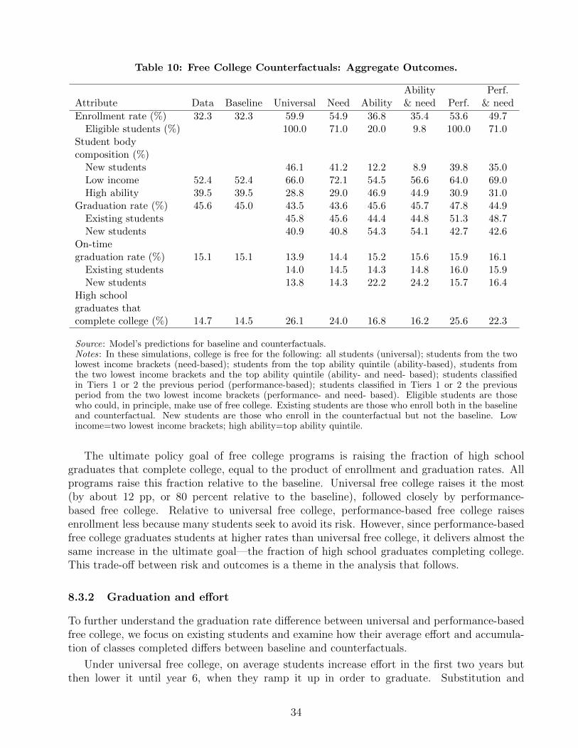
Table 10: Free College Counterfactuals: Aggregate Outcomes.

Ability Perf.Attribute Data Baseline Universal Need Ability & need Perf. & need

Enrollment rate (%) 32.3 32.3 59.9 54.9 36.8 35.4 53.6 49.7Eligible students (%) 100.0 71.0 20.0 9.8 100.0 71.0

Student bodycomposition (%)

New students 46.1 41.2 12.2 8.9 39.8 35.0Low income 52.4 52.4 66.0 72.1 54.5 56.6 64.0 69.0High ability 39.5 39.5 28.8 29.0 46.9 44.9 30.9 31.0

Graduation rate (%) 45.6 45.0 43.5 43.6 45.6 45.7 47.8 44.9Existing students 45.8 45.6 44.4 44.8 51.3 48.7New students 40.9 40.8 54.3 54.1 42.7 42.6

On-timegraduation rate (%) 15.1 15.1 13.9 14.4 15.2 15.6 15.9 16.1

Existing students 14.0 14.5 14.3 14.8 16.0 15.9New students 13.8 14.3 22.2 24.2 15.7 16.4

High schoolgraduates thatcomplete college (%) 14.7 14.5 26.1 24.0 16.8 16.2 25.6 22.3

Source: Model’s predictions for baseline and counterfactuals.Notes: In these simulations, college is free for the following: all students (universal); students from the twolowest income brackets (need-based); students from the top ability quintile (ability-based), students fromthe two lowest income brackets and the top ability quintile (ability- and need- based); students classifiedin Tiers 1 or 2 the previous period (performance-based); students classified in Tiers 1 or 2 the previousperiod from the two lowest income brackets (performance- and need- based). Eligible students are thosewho could, in principle, make use of free college. Existing students are those who enroll both in the baselineand counterfactual. New students are those who enroll in the counterfactual but not the baseline. Lowincome=two lowest income brackets; high ability=top ability quintile.

The ultimate policy goal of free college programs is raising the fraction of high schoolgraduates that complete college, equal to the product of enrollment and graduation rates. Allprograms raise this fraction relative to the baseline. Universal free college raises it the most(by about 12 pp, or 80 percent relative to the baseline), followed closely by performance-based free college. Relative to universal free college, performance-based free college raisesenrollment less because many students seek to avoid its risk. However, since performance-basedfree college graduates students at higher rates than universal free college, it delivers almost thesame increase in the ultimate goal—the fraction of high school graduates completing college.This trade-off between risk and outcomes is a theme in the analysis that follows.

8.3.2 Graduation and effort

To further understand the graduation rate difference between universal and performance-basedfree college, we focus on existing students and examine how their average effort and accumula-tion of classes completed differs between baseline and counterfactuals.

Under universal free college, on average students increase effort in the first two years butthen lower it until year 6, when they ramp it up in order to graduate. Substitution and

34

risk effects prevail in years 1 and 2, leading students to work harder (Figure 13 panel a) andaccumulate more classes (panel b) than in the baseline. Nonetheless, this greater accumulationof classes, together with the loss-of-urgency effect, leads students to work less and accumulatefewer classes than in the baseline in years 3-5. To compensate for their slower pace and graduate,students raise effort in years 6-8. Thus, students conduct an intertemporal re-allocation of effortwhich, on average, delivers almost the same graduation rate as the baseline yet a lower on-time-graduation rate.

Figure 13: Free college: Changes in effort and cumulative classes completed

−.04

−.02

0

.02

.04

Ch

ang

e in

eff

ort

1 2 3 4 5 6 7 8Year

Universal free college Performance−base free college

−1

−.5

0

.5

1

Ch

ang

e in

nu

mb

er o

f cu

mu

l.cl

asse

s co

mp

lete

d1 2 3 4 5 6 7 8

Year

Universal free college Performance−base free college

a. Change in effort w.r.t. to baseline b. Change in number of cumulative classes

Source: Model’s simulations.Notes: For existing students in the counterfactuals, panel a shows average effort in the corresponding counter-factual minus average effort in the baseline. Panel b does the same for average number of cumulative classescompleted.

In contrast, under performance-based free college students frontload effort. Absent the loss-of-urgency effect, the substitution and risk effect produce greater effort than in the baseline inyears 1-3. Since students accumulate more classes than in the baseline in those years, they canwork less later while still accumulating more classes than in the baseline. These effort changesimply not just an intertemporal reallocation of effort but also a net effort increase that raisesboth graduation and on-time graduation rates relative to the baseline.

8.4 Outcomes by student type

The aggregate outcomes shown above mask great heterogeneity among student types. For apolicymaker interested in promoting enrollment or graduation for specific students, this het-erogeneity is critical. To analyze it more easily, we aggregate our fifty student types intonine income- and ability-based groups. Income groups include high, middle and low-income—corresponding to the top, two middle, and two bottom income brackets respectively. Abilitygroups include high, middle, and low-ability—corresponding to the top, two middle, and twobottom ability quintiles respectively.

35

8.4.1 Enrollment

Table 11 shows enrollment rate by student group in the baseline (panel a) and enrollment rateincrease relative to the baseline under universal and performance-based free college (panels band c, respectively). We focus on these two counterfactuals because the remaining four arespecial cases of these. For example, the “low income” row of panel b displays the effects ofneed-based free college, while the “high ability” column displays the effects of ability-based freecollege.

Table 11: Free College Counterfactuals: Enrollment Effects.

a. Baseline b. Universal c. Performance-BasedEnrollment Rate Free College: Change Free College: Change

AbilityIncome High Mid Low High Mid Low High Mid Low

High 83.8 65.5 39.3 7.1 11.4 12.0 5.8 9.0 9.2Mid 73.1 47.4 27.3 15.0 21.1 18.3 12.5 16.8 13.9Low 51.4 26.0 13.6 32.2 36.5 27.8 27.1 28.5 20.1

Source: Model’s predictions for baseline and counterfactuals.Notes: For each student type, panel a shows predicted enrollment rate (%) in the baseline; panel b shows theenrollment rate difference (pp) between universal free college and baseline; and panel c shows the enrollmentrate difference (pp) between performance-based free college and baseline.

Both free college programs raise enrollment rates for all student groups. Under universalfree college, the greatest effects are for low- and middle-income students, who are most budget-constrained in the baseline. Their greater responsiveness justifies need-based free college asopposed to universal free college, which provides a subsidy to many students who do not needit. In terms of ability, effects are not greatest for high-ability students. Ability-based freecollege, therefore, cannot be justified based on enrollment considerations, but rather on thegrounds that it raises overall graduation rate through new students’ positive selection andlowers the income-based enrollment gap among high-ability students.

As for performance-based free college, its enrollment effects are qualitatively similar tothose of universal free college, albeit smaller. Effects are similar because performance-basedfree collegeprovides free college to all students in year 1, but smaller because some potentialstudents do not enroll to avoid the effort necessary to remain in tiers 1 or 2 in subsequent years.

These enrollment results are consistent with the small free college program run in Colombiabetween 2014 and 2018, Ser Pilo Paga (”being diligent pays off.”) This was an ability-, need-,and performance-based program that offered free tuition to high-ability, low-income studentsfor the theoretical duration of their program; students who dropped out were required to paythe tuition back. Among the eligible population, the program raised college enrollment ratesby 32 pp (Londono et al 2020), in line with the 27-32 pp increase depicted in Table 11 (panelsb and c) for these students.

36

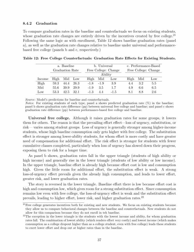
8.4.2 Graduation

To compare graduation rates in the baseline and counterfactuals we focus on existing students,whose graduation rate changes are entirely driven by the incentives created by free college.21

Following the same logic as with enrollment, Table 12 shows baseline graduation rates (panela), as well as the graduation rate changes relative to baseline under universal and performance-based free college (panels b and c, respectively.)

Table 12: Free College Counterfactuals: Graduation Rate Effects for Existing Students.

a. Baseline b. Universal c. Performance-BasedGraduation Rate Free College: Change Free College: Change

AbilityIncome High Mid Low High Mid Low High Mid Low

High 59.3 44.4 26.3 -1.8 -1.9 3.9 4.4 3.2 5.5Mid 55.6 39.9 29.9 -1.9 3.5 1.7 4.9 6.6 6.5Low 53.3 42.5 32.1 -1.3 4.4 -1.5 8.1 8.8 2.6

Source: Model’s predictions for baseline and counterfactuals.Notes: For existing students of each type, panel a shows predicted graduation rate (%) in the baseline;panel b shows graduation rate difference (pp) between universal free college and baseline; and panel c showsgraduation rate difference (pp) between performance-based free college and baseline.

Universal free college. Although it raises graduation rates for some groups, it lowersthem for others. The reason is that the prevailing effort effect—loss of urgency, substitution, orrisk— varies among student groups. Loss of urgency is generally stronger among higher-incomestudents, whose high baseline consumption only gets higher with free college. The substitutioneffect is stronger among lower-ability students, for whom effort is more costly and have greaterneed of compensation for additional effort. The risk effect is stronger for students with fewercumulative classes completed, particularly when loss of urgency has slowed down their progress,exposing them to risk for a longer time.

As panel b shows, graduation rates fall in the upper triangle (students of high ability orhigh income) and generally rise in the lower triangle (students of low ability or low income).In the upper triangle, baseline effort is already high because effort cost is low and consumptionhigh. Given the little room for additional effort, the substitution effect is weak. A strongloss-of-urgency effect prevails given the already high consumption, and leads to lower effort,greater risk, and lower graduation rates.

The story is reversed in the lower triangle. Baseline effort there is low because effort cost ishigh and consumption low, which gives room for a strong substitution effect. Since consumptionremains low even with free college, the loss-of-urgency effect is weak and the substitution effectprevails, leading to higher effort, lower risk, and higher graduation rates.22

21Free college generates incentives both for existing and new students. We focus on existing students becausethey allow us to compare behavioral changes between the baseline and counterfactuals. New students do notallow for this comparison because they do not enroll in teh baseline.

22The exception in the lower triangle is the students with the lowest income and ability, for whom graduationrates fall. The combination of lowest ability (which renders effort very costly) and lowest income (which makesconsumption as a college dropout higher than as a college student, even with free college) leads these studentsto exert lower effort and drop out at higher rates than in the baseline.

37

Performance-based free college. In contrast to universal free college, performance-based free college raises graduation rates for all student groups because it eliminates the loss-of-urgency effect. Substitution effect leads to greater effort and therefore less risk. In theaggregate, performance-based free college raises the graduation rate of existing students from45 to 51.3 percent (see Table 10), which is the greatest graduation rate increase for existingstudents among all programs considered here. Even new students attain a higher graduationrate under performance-based than universal free college (42.7 v. 40.9 percent).

Back to the policymaker’s goal of raising the fraction of high school graduates who completecollege, Table 13 shows this fraction in the baseline (panel a) as well as the differences withrespect to it under universal and performance-based free college (panels b and c, respectively.)Relative to the baseline, both programs raise this fraction for every student group. Performance-based free college is at least as effective as universal free college for every student group exceptlow-income students of middle or low ability, for whom the difficulty of meeting performancerequirements acts as an enrollment deterrent. In other words, a combination of unconditionalfree college for those students and performance-based free college for others could meet thepolicymaker’s goal not only in the aggregate but also by student group.

Table 13: Free College Counterfactuals: Percent of High School Graduates That Com-plete College.

a. BaselinePercent of High b. Universal c. Performance-Based

School Graduates Free College: Change Free College: ChangeAbility

Income High Mid Low High Mid Low High Mid Low

High 49.7 29.1 10.3 2.9 3.1 5.1 7.1 5.9 5.3Mid 40.7 18.9 8.2 6.7 10.1 6.4 10.7 10.1 6.4Low 27.4 11.0 4.4 16.7 17.5 8.5 19.1 15.5 7.0

Source: Model’s predictions for baseline and counterfactuals.Notes: For existing students of each type, panel a shows the percent of high school graduates that graduatefrom college; panel b shows difference (pp) in this variable between universal free college and baseline; andpanel c shows difference (pp) in this variable between performance-based free college and baseline.

8.5 Discussion

We can now return to the cross-country evidence depicted in Figure 1, which shows that, in LatinAmerica, government funding for college has a large, positive relationship with enrollment ratesbut a weak (actually negative) relationship with graduation rates. The evidence is consistentwith our counterfactuals, as these predict a greater impact of free college on enrollment thangraduation rates. The graduation rate evidence is also consistent with the financial aid regimesprevailing in those countries, where universal or need-based aid is most common, ability-basedaid is rare, and performance-based aid is almost non-existing (Ferreyra et al 2017). Indeed, forthe most common regimes in Latin America our counterfactuals predict a (slight) decline ingraduation rate (see Table 12), consistent with Figure 1.

Our findings are also consistent with the literature on U.S. higher education financial aid,

38

which has generally found positive enrollment and graduation effects.23 In recent years, severalstates have implemented a variety of financial aid programs based on ability and/or need,24 aswell as “Promise” programs, which provide free tuition to eligible students for local communitycolleges or state four-year institutions.25 Overall, these programs have had positive effects onenrollment and graduation. Also consistent with our counterfactuals, the literature has foundgreater effects of financial aid on enrollment than on graduation (the latter being in the modestrange of 0 to 6 or 7 pp)26 and greater effects for performance-based than unconditional aid(Dynarski and Scott-Clayton 2013).

Even though performance-based free college raises graduation rates the most in our simu-lations, it still delivers a relatively small graduation rate increase (approximately 10 percent ofthe baseline graduation rate). This begs the question of why free college (or financial aid, ingeneral) fails to substantially raise graduation rates.

The answer emerging from our model is that free college fails to induce in many students alarge, non-marginal effort increase. As Table 9 shows, students who need to catch up exert moreeffort. Particularly when the student has fallen far behind, catching up is difficult (Section 4),which limits the effectiveness of performance incentives. This suggests that additional supportsfor class completion—particularly in year 1—may be needed, including remedial education,advising, and tutoring.27 Indeed, in their study of possible policies to raise graduation rates inthe U.S., Avery et al (2019) conclude that need-based free college combined with institutionalfunding for these supports might be the most cost-effective policy. A cautionary tale, however,comes from Oreopoulos and Petronijevic (2019), who find that these supports help studentsrealize the need for greater effort but have little effect on college continuity or graduation. Thereason is that students respond not by raising effort but by expecting less of themselves.

Moreover, our counterfactuals have assumed some highly favorable—perhaps unrealistic—conditions, as discussed before. One of them is no capacity constraints in higher education.Free college, however, would likely run into capacity constraints and force institutions to rationaccess. Bucarey (2018) explores the potential effects of free college (gratuidad) in Chile, where itwas introduced in 2016 for the bottom 60 percent of the income distribution. Data prior to 2016shows that when low-income students are given additional financial aid, institutions respondby becoming more selective, thereby leading to a lower share of low-income students. Using hisstructural model, Bucarey (2018) predicts that capacity-constrained institutions would follow asimilar strategy under free college. We have also implicitly assumed that college quality remainsthe same after college becomes free. This may not happen if the policymaker reimburses collegesfor less than the per-student average cost. Indeed, Murphy et al (2019) provide evidence that

23See, for instance, Bettinger (2004), Dynarski (2003), Hoxby and Turner (2013) and the references therein, aswell as the surveys by Avery et al (2019), Deming and Dynarski (2009), Dynarski and Scott-Clayton (2013),Long (2008), Page and Scott-Clayton (2016).

24See Bettinger et al (2019), Castleman and Long (2016), Cornwell et al (2006), Dynarski (2000, 2004, 2008),Scott-Clayton (2011), Scott-Clayton and Zafar (2016), and the references therein.

25These programs vary across states in terms of eligible institutions (community colleges v. four-year institu-tions) and students. See, for instance, Carruthers et al (2018), Dynarski et al (2018), Gurantz (2020).

26For recent, well-identified studies, see Bettinger et al (2019), Denning (2017), Mayer et al (2015), and Scott-Clayton (2011).

27In the context of our model, these policies would amount to changing parameters from the distribution of z inorder to reach higher E(z) and lower V (z). Clotfelter et al (2018), Evans et al (2017), Scrivener et al (2015)and Sommo et al (2018) document positive effects of these supports on graduation rates.

39

higher education quality in England was lower when college was free because institutions werenot receiving full funding. It might not happen either if the cost of educating new students ishigher than that of existing students—for instance, because they need additional services.

8.6 Free college and anticipated risk

The typical rationale for free college is that students face financial constraints which preventthem from undertaking an investment with positive net present value. Our work, however,highlights another important, novel rationale: college students face risks. They are uncertainabout their performance and chances to remain enrolled due to shocks during college thatmight be particularly important in developing economies. Some students, then, might notattend college in order to avoid these risks—in which case free college might provide insuranceand induce more students to enroll.

In this section we investigate whether free college mitigates risk. Free college affects riskthrough two channels. First, it raises the value of remaining in college relative to droppingout by raising consumption during college and enhancing the ”college experience.” Second, itaffects effort through the loss-of-urgency, substitution, and risk effects. Effort changes affectthe number of current classes completed which, in turn, affect the future shocks to classescompleted and the dropout probability.

These consumption and effort changes are distinctive of our setting. In an economy withcredit, consumption is closely related to lifetime income—as in standard Ben-Porath models.Since free college would not substantially alter lifetime income in that economy, consumptionchanges would be small. But in Colombia, where credit constraints are severe, consumptionchanges could be quite large. As for effort changes, these are not present in models withexogenous risk, unrelated to effort (e.g. Hendricks and Leukhina 2017). Our model, in contrast,views effort as the direct tool used by students to mitigate risk.

The consumption and effort changes in our model affect the distribution of the value of col-lege, V coll(t, ht−1, θ, y), defined in (6). Whereas V coll(t, ht−1, θ, y) is calculated for the student’soptimal effort, e∗t , while taking expectation over zt, we now define the college payoff from anygiven effort and realization of zt:

V coll(t, ht−1, θ, y; zt, et) = U(ct, et, θ) + β

[1{t≥5}Pr

(ht−1 +H(zt, θ, et) x ≥ hgrad

)V grad(t+ 1)+

Pr(ht−1 +H(zt, θ, et) x < hgrad

) (pd(t, ht−1 +H(zt, θ, et) x, θ, y)V drop(t+ 1)+

(1− pd(t, ht−1 +H(zt, θ, et) x, θ, y)

)V coll(t+ 1, ht−1 +H(zt, θ, et) x, θ, y)

)].

(18)

From here, it follows that Ez[Vcoll(t, ht−1, θ, y; zt, e

∗t )] = V coll(t, ht−1, θ, y).

Our proposed measure of anticipated risk for student i, at the beginning of period t underscenario p (baseline or counterfactual) is the coefficient of variation of her college payoffs:

CV pit =

√Varz

[V coll(t, hit−1, θ, y; zit, e∗it) | p

]Ez

[V coll(t, hit−1, θ, y; zit, e∗it) | p

] , (19)

40

where the right-hand side is the ratio between the standard deviation and expected value ofcollege payoffs, calculated for the student’s optimal effort, e∗it, chosen under scenario p. Givene∗it, the randomness in V coll(·) comes from the performance and dropout shocks, z and ddrop

respectively, which are associated with cumulative classes completed and therefore effort. Notethat anticipated risk varies across students and programs, and over time.

Does effort lower anticipated risk? To investigate this matter, in principle we might think ofusing our simulated baseline data to regress anticipated risk on (optimal) effort, controlling forcumulative past performance. However, this regression would suffer from endogeneity becauseoptimal effort would appear in both sides of the regression. Since e∗it is a function of the statevariables, t, hit−1, θi, and yi, we instrument for effort using the state variables (see AppendixTable F1), and run the second-stage regression reported in Table 14. This regression indicatesthat, in our baseline model, effort indeed lowers anticipated risk. The elasticity of anticipatedrisk with respect to effort is negative and large at -2.34. Student effort is therefore highlyeffective at mitigating performance and dropout risk.

Table 14: Anticipated Risk.

Dependent variableln(Anticipated risk)

ln(effort) −2.340∗∗∗

(0.089)ln(average classes completed) −1.767∗∗∗

(0.043)Constant −0.772∗∗∗

(0.068)

Num. obs. 116,761

Source: 2SLS estimation using model’s simulated baseline values.Notes: The dependent variable is ln(anticipated risk), or ln(CVit) for the baseline. An observation is astudent-year. Included students are “existing” in both counterfactuals; upper 5% tail of risk has beentrimmed. Effort is e∗it, instrumented with by classes completed, as well as year, income, and ability fixed

effects. ln(average classes completed) is hit−1, as defined in the model. The regression includes year fixedeffects (not shown). Standard errors (in parentheses) are clustered by student. * p < 0.10, ** p < 0.05, ***p < 0.01.

Having established that effort indeed mitigates risk, the next question is whether free collegeraises or lowers risk relative to the baseline. Figure 14 shows average anticipated risk in thebaseline and under universal and performance-based free college. To facilitate comparisons, wefocus on the set of students who start college in all three scenarios and discuss average effects.

In the three scenarios, average anticipated risk is U-shaped with respect to time. In year 1,it is high for two reasons. The first is student body composition, which includes a large shareof students with a high exogenous dropout probability. The second is that every student isuncertain about her future performance, and her exogenous dropout probability is highest inyear 1. In years 2 through 5, anticipated risk falls as many high-risk students drop out whilethe remaining students settle on a performance path. For the students that remain after year6, anticipated risk rises because they face the risk of not graduating.

Relative to the baseline, free college raises Ez[Vcoll(·)] by raising consumption while in college

and, in some cases, effort (see Figure 13 a). Free college also raises Varz[Vcoll(·)] at least in year

41

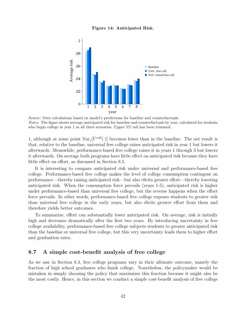
Figure 14: Anticipated Risk.

0

.02

.04

.06

.08

.1

Av

erag

e ri

sk

1 2 3 4 5 6 7 8

year

Baseline

Univ. free coll.

Perf.−based free coll.

Source: Own calculations based on model’s predictions for baseline and counterfactuals.Notes: The figure shows average anticipated risk for baseline and counterfactuals by year, calculated for studentswho begin college in year 1 in all three scenarios. Upper 5% tail has been trimmed.

1, although at some point Varz[Vcoll(·)] becomes lower than in the baseline. The net result is

that, relative to the baseline, universal free college raises anticipated risk in year 1 but lowers itafterwards. Meanwhile, performance-based free college raises it in years 1 through 3 but lowersit afterwards. On average both programs have little effect on anticipated risk because they havelittle effect on effort, as discussed in Section 8.5.

It is interesting to compare anticipated risk under universal and performance-based freecollege. Performance-based free college makes the level of college consumption contingent onperformance—thereby raising anticipated risk—but also elicits greater effort—thereby loweringanticipated risk. When the consumption force prevails (years 1-5), anticipated risk is higherunder performance-based than universal free college, but the reverse happens when the effortforce prevails. In other words, performance-based free college exposes students to greater riskthan universal free college in the early years, but also elicits greater effort from them andtherefore yields better outcomes.

To summarize, effort can substantially lower anticipated risk. On average, risk is initiallyhigh and decreases dramatically after the first two years. By introducing uncertainty in freecollege availability, performance-based free college subjects students to greater anticipated riskthan the baseline or universal free college, but this very uncertainty leads them to higher effortand graduation rates.

8.7 A simple cost-benefit analysis of free college

As we saw in Section 8.4, free college programs vary in their ultimate outcome, namely thefraction of high school graduates who finish college. Nonetheless, the policymaker would bemistaken in simply choosing the policy that maximizes this fraction because it might also bethe most costly. Hence, in this section we conduct a simple cost-benefit analysis of free college

42

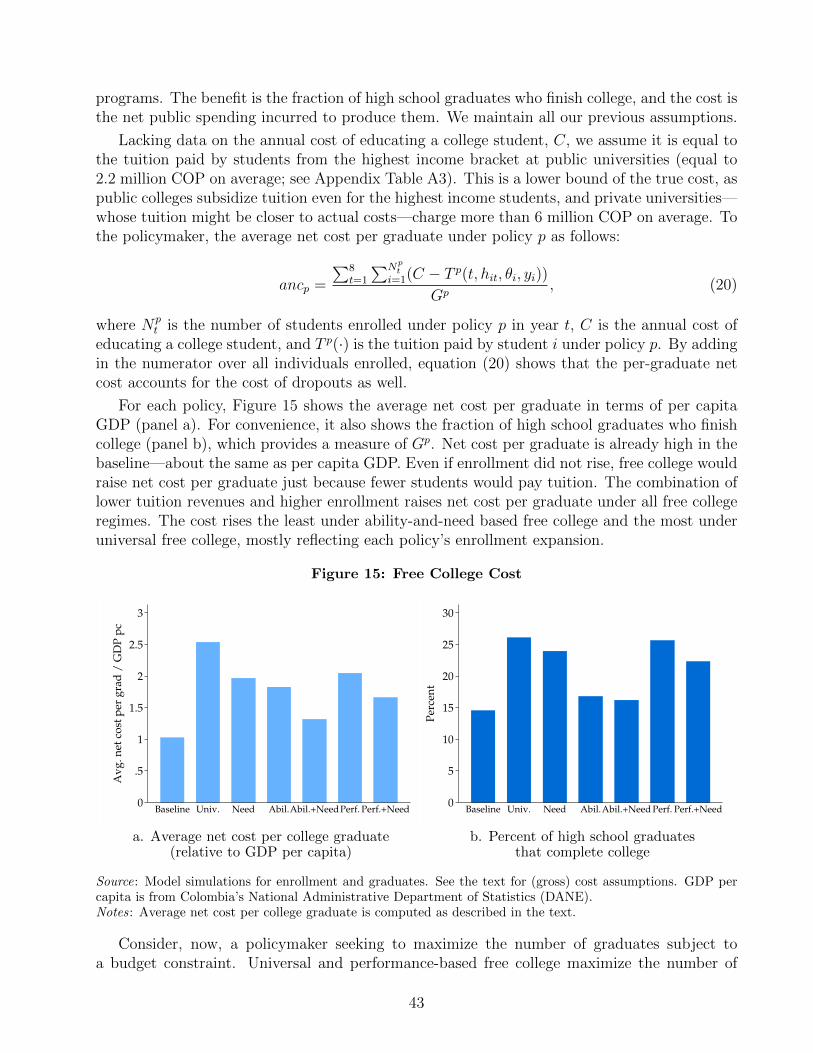
programs. The benefit is the fraction of high school graduates who finish college, and the cost isthe net public spending incurred to produce them. We maintain all our previous assumptions.

Lacking data on the annual cost of educating a college student, C, we assume it is equal tothe tuition paid by students from the highest income bracket at public universities (equal to2.2 million COP on average; see Appendix Table A3). This is a lower bound of the true cost, aspublic colleges subsidize tuition even for the highest income students, and private universities—whose tuition might be closer to actual costs—charge more than 6 million COP on average. Tothe policymaker, the average net cost per graduate under policy p as follows:

ancp =

∑8t=1

∑Npt

i=1(C − T p(t, hit, θi, yi))Gp

, (20)

where Npt is the number of students enrolled under policy p in year t, C is the annual cost of

educating a college student, and T p(·) is the tuition paid by student i under policy p. By addingin the numerator over all individuals enrolled, equation (20) shows that the per-graduate netcost accounts for the cost of dropouts as well.

For each policy, Figure 15 shows the average net cost per graduate in terms of per capitaGDP (panel a). For convenience, it also shows the fraction of high school graduates who finishcollege (panel b), which provides a measure of Gp. Net cost per graduate is already high in thebaseline—about the same as per capita GDP. Even if enrollment did not rise, free college wouldraise net cost per graduate just because fewer students would pay tuition. The combination oflower tuition revenues and higher enrollment raises net cost per graduate under all free collegeregimes. The cost rises the least under ability-and-need based free college and the most underuniversal free college, mostly reflecting each policy’s enrollment expansion.

Figure 15: Free College Cost

0

.5

1

1.5

2

2.5

3

Av

g. n

et c

ost

per

gra

d /

GD

P p

c

Baseline Univ. Need Abil.Abil.+NeedPerf. Perf.+Need0

5

10

15

20

25

30

Percen

t

Baseline Univ. Need Abil.Abil.+Need Perf. Perf.+Need

a. Average net cost per college graduate b. Percent of high school graduates(relative to GDP per capita) that complete college

Source: Model simulations for enrollment and graduates. See the text for (gross) cost assumptions. GDP percapita is from Colombia’s National Administrative Department of Statistics (DANE).Notes: Average net cost per college graduate is computed as described in the text.

Consider, now, a policymaker seeking to maximize the number of graduates subject toa budget constraint. Universal and performance-based free college maximize the number of

43

graduates, yet performance-based free college does it at a lower per-graduate cost. This isbecause the incentives embedded in performance-based free college produce fewer dropouts andgraduate students faster than universal free college. By adopting performance-based ratherthan universal free college, the policymaker would save no less than 40 percent of per capitaGDP per graduate.

Nonetheless, the policymaker might be reluctant to adopt performance-based free college,perhaps for political considerations. Indeed, students throughout Latin America have beenclamoring for unconditional, universal free college (gratuidad). As Figure 15 shows, universalfree college raises the number of graduates only slightly more than need-based free college yetcosts an additional 50 percent of per capita GDP per graduate. The reason is that universalfree college provides a transfer to medium- and high-income students who would attend collegeanyway. If choosing between unconditional programs, then need-based is preferable to universalfree college.

One caveat is in order. College dropouts seem to acquire some human capital during collegegiven their wage premium relative to high school graduates. This may motivate the policymakerto raise enrollment regardless of graduation. The question, then, is whether starting but notcompleting a bachelor’s program is the most efficient way of acquiring post-secondary humancapital. A short-cycle program, lasting two or three years, might be more cost-effective.28

Subsidizing these programs—in the spirit of subsidies to community college students in theU.S.—might therefore be preferable.

8.8 Long-run effects

We have assumed that, despite the greater supply of college graduates due to free college, thecollege premium does not change. However, the college premium might actually fall, therebyreducing the incentives to attend college. In addition, free college might be funded with taxes,further depressing after-tax wages for college graduates. In other words, free college might un-leash general equilibrium effects that could undermine some of the free college effects previouslydescribed (Heckman et al 1998).

To analyze the equilibrium relationship between college premium and number of collegegraduates, we postulate a production function following Katz and Murphy (1992), Heckman etal (1998), and Card and Lemieux (2001). Ignoring for the moment the connection between capi-

tal and technology, consider a CES production function, F (Nht , N

gt ) =

(Aht (N

ht )λ + Agt (N

gt )λ) 1λ ,

that combines high school and college graduates, whose amounts are Nht and N g

t respectively,to produce aggregate output. In this function, Aht and Agt are efficiency parameters, andω = 1/(1 − λ) is the elasticity of substitution between college and high school graduates.In a competitive labor market, the college premium is equal to

wgtwht

=AgtAht

(N gt

Nht

)λ−1

, (21)

where wgt and wht are the wages of college and high school graduates, respectively. Taking logs

28Ferreyra et al (2021) shows that students in short-cycle programs graduate at higher rates than those inbachelor’s programs, and that their graduates obtain better labor market outcomes than dropouts frombachelor’s programs.

44

on both sides and defining a time difference (4) yields an expression commonly used to studychanges in wage inequality:

4 ln

(wgtwht

)= 4 ln

(AgtAht

)− 1

ω4 ln

(N gt

Nht

). (22)

In this equation, changes in relative wages depend on two components. The first is technicalchanges in the relative productivity of the two labor inputs. Skill-biased technical change, or

4 ln(AgtAht

) > 0, increases the college premium. The second is changes in relative supply, adjusted

by the elasticity of substitution. An increase in the supply of college graduates lowers the collegepremium by an amount inversely related to ω. Over time, the evolution of the college premiumdepends on the relative strength of these two opposite forces.

To investigate the extent to which the increased supply of college graduates might depressthe college premium, we focus on universal free college, which increases supply the most andprovides an upper bound to the potential college premium decline. We examine short- and long-run effects. For the latter, we assume that universal free college becomes a permanent policybeginning with our 2006 cohort, and simulate the evolution of the share of college graduates(relative to all workers in the economy) and the college premium. We assume no skill-biasedtechnical change and therefore estimate an upper bound to the college premium decline.

The critical parameter for this exercise is ω, which we estimate as 3.2 for Colombia.29 Usingthis estimate, the left and right panel of Figure 16 show the evolution of the share of collegeeducated workers and the college premium, respectively. The former rises over time as young,more educated cohorts replace older, less educated ones. The replacement is complete aroundthe year 2045, when the economy reaches steady state.

Figure 16: Free College and and the College Premium

20

25

30

35

40

45

Percen

t

2015 2020 2025 2030 2035 2040 2045 2050

Year

.5

1

1.5

2

2.5

3

Co

lleg

e p

rem

ium

2015 2020 2025 2030 2035 2040 2045 2050Year

ω = 3.2ω = 2.5ω = 1.4ω = 1.2

a. Share College in Labor Force b.College Premium

Source: Own calculations based on estimates.Notes: Panel a shows predicted share of college graduates in the labor force, calculated as the share of workers(of all ages) with a college degree relative to all workers (all ages and educational attainment) in the economy.Panel b shows predicted college premium, calculated as the ratio between wage for college graduates and wagefor high school graduates.

29There is a large number of estimates for this parameter in the literature. For example, Katz and Murphy(1992) estimate it to be 1.4 for the U.S. for the period 1963-1987, but the low range of estimates also include0.5. Card and Lemieux (2001) estimate it for the United States (1959 to 1996) and the United Kingdom(1974-1996) and find estimates between 2 and 2.5. Following Card and Lemieux (2001), we estimate theproduction function parameters using Colombia’s household surveys (SEDLAC) for 2001-12. Due to datalimitations, college graduates include those from 2- and 4-year programs.

45

As in our model, the 2006 entry cohort starts to graduate in 2010. In 2006, the initialshare of college graduates in the workforce equals 27 percent.30 Universal free college raisesthis share for a particular cohort by 12 pp, to a long-run value of 39 percent (panel a). In theshort-run the college premium falls relatively little (panel b) because the increase in collegegraduates from the first few cohorts is small relative to the stock of college-educated workers,which includes individuals from 35 to 40 cohorts. Over time, the continuous inflow of a greaternumber of college graduates produces a larger college premium impact—but still small, givenour estimated ω, and unlikely to dissuade many high school graduates from college enrollment.As a robustness check, panel b depicts the implied college premium path for several ω estimatesfor developed economies.31 The college premium declines more for these values, yet even thegreatest decline -down to 1.70- still leaves the economy with a substantial college premium,comparable to that in the U.S. Skill-biased technical change, of course, would lead to an evensmaller decline for any value of ω.

In sum, both the short- and long-run college premium decline induced by free college wouldlikely be small in Colombia. As a result, abstracting away from the general equilibrium impli-cations of free college is not likely to bias our predictions substantially. College, thus, wouldremain a worthy investment even if free college produced more college graduates.32

9 Conclusions

In this paper we have developed and estimated a dynamic model of college enrollment, perfor-mance, and graduation. A central piece of the model, student effort, has a direct effect on thecompletion of classes and an indirect effect mitigating risks on class completion or college persis-tence. We have estimated the model using rich administrative data from Colombia. Accordingto our estimates, effort has a much greater impact than ability on class completion. Failing tomodel effort as an input to class completion leads to overestimating the role of ability by twoor three times, and to favoring policies that promote positive selection of new students insteadof effort. We have used our parameter estimates to simulate multiple free college programs.According to our simulations, universal free college expands enrollment the most but has thehighest per-graduate cost and does not raise graduation rates. Performance-based free college,in contrast, delivers a slightly lower enrollment expansion but has a greater graduation rateand a lower per-graduate cost. Performance-based free college faces students with greater risksthan the current baseline or universal free college; precisely for this reason it elicits greater

30Notice that the initial share of 27 percent is higher than the initial fraction of high school graduates that finishcollege, equal to 14.5 in the baseline. The reason is that 27 percent includes graduates from all bachelor’sprograms (rather than only five-year programs) as well as graduates from two-year programs. This is becausethe college premium is calculated for all higher education graduates, based on data that does not distinguishbetween graduates from bachelor’s and two-year programs.

31We use the point estimates of 1.4 from Katz and Murphy (1992) and Heckman et al (1998), 2.5 from Cardand Lemieux (2001), and include lower value of 1.2. For each ω value, the intercept has been adjusted togenerate the same college premium for the year 2012.

32These results are consistent with Garriga and Keightley (2007), who conduct a similar analysis for the U.S. ina model that endogenizes the college premium, government budget constraint, after-tax earnings, and laborsupply decisions. They show that tuition subsidies have small effects on the college premium even whenaccounting for taxes. Their results are partly due to the limited effects of the policy on graduation rates, andto the high elasticity of substitution between college and high school graduates.

46

effort and graduation rates.

For existing students, free college has little impact on effort and graduation rates, even whenit is performance-based. This suggests that additional, complementary policies might be needed.Given the high persistence of performance, improving first-year performance and retention iscritical. Supports such as tutoring, remedial education, mentoring, and advising might behelpful, particularly for the most disadvantaged students. Further, most college programs inLatin America start with classes specific to the major and rarely include general educationrequirements that transfer easily across majors. As a result, changing majors typically impliesstarting from scratch, which leads many students to abandon higher education. Shorteningbachelor’s programs (which last five or six years) and connecting them with the labor marketmight raise effort and graduation rates as well.

Finally, there might be an additional reason why free college fails to elicit large effort changes:particularly for low-income students, free college might not be enough. For them, the effortnecessary to complete college might require not only free tuition but also an additional, gen-erous stipend for living expenses. In countries with limited fiscal resources, providing thisadditional stipend might require lowering the existing college subsidies for affluent students—aredistribution that, while politically costly, would nonetheless enhance equity and efficiency.

References

[1] Abbot, B., Gallipoli, G., Meghir, C., & Violante, G. (2013). Education decisions and inter-generational transfers in equilibrium (Working Paper). New York: New York University.

[2] Ahn, T., Arcidiacono, P., Hopson, A., & Thomas, J. R. (2019). Equilibrium grade inflationwith implications for female interest in stem majors. NBER Working Paper No. w26556.

[3] Akyol, A. & Athreya, K. (2005). Risky higher education and subsidies. Journal of EconomicDynamics and Control, 29(6), pp. 979-1023.

[4] Altonji, J. (1993). The demand for and return to education when education outcomes areuncertain. Journal of Labor Economics, 11(1), pp. 48-83.

[5] Arcidiacono, P. (2004). Ability sorting and the returns to college major. Journal of Econo-metrics, 121(1-2), pp.343-375

[6] Arcidiacono, P., E. Aucejo, A. Maurel, & T. Ransom (2016). College attrition and thedynamics of information revelation. NBER Working Paper No. 22325.

[7] Ariely, D., U. Gneezy, G. Loewenstein, & N. Mazar (2009). Large stakes and big Mistakes.Review of Economic Studies, 76(2), pp. 451-469.

[8] Avery, C., Howell, J., Pender, M., & Sacerdote, B. (2019). Policies and payoffs to addressingAmerica’s college graduation deficit. In BPEA Conference Draft, Fall.

[9] Beneito, P., J. Bosca & J. Ferri (2018). Tuition fees and student effort at university.Economics of Education Review, 64(C), pp. 114-128.

[10] Berry, S., J. Levinsohn, A. Pakes (1995). Automobile prices in market equilibrium, Econo-metrica, pp: 841–890

[11] Bettinger, E. (2004). How financial aid affects persistence. In College choices: The eco-nomics of where to go, when to go, and how to pay for it (pp. 207-238). University ofChicago Press.

[12] Bettinger, E., Gurantz, O., Kawano, L., Sacerdote, B., & Stevens, M. (2019). The long-

47

run impacts of financial aid: Evidence from California’s Cal Grant. American EconomicJournal: Economic Policy, 11(1), 64-94.

[13] Bucarey, A. (2018). Who pays for college? Crowding out on campus. Working Paper,Massachusetts Institute of Technology.

[14] Cameron S.V. & Heckman, J. J. (1998). Life cycle schooling and dynamic selection bias:Models and evidence for five cohorts of American males. The Journal of Political Economy,106(2), pp. 262-333.

[15] Cameron S.V. & Heckman, J. J. (1999).The dynamics of educational attainment for blacks,hispanics and whites (Working Paper 7249). Cambridge, MA: National Bureau of EconomicResearch.

[16] Card, D. & Lemieux, T. (2001). Can falling supply explain the rising return to college foryounger men? A cohort-based analysis (Working Paper 7655). Cambridge, MA: NationalBureau of Economic Research.

[17] Carneiro, P. & Heckman, J. J. (2002). The Evidence on Credit Constraints in Post-Secondary Schooling. The Economic Journal, 112(482), pp. 705-734.

[18] Carruthers, C. K., Fox, W. F., & Jepsen, C. (2018). Promise kept? Free community collegeand attainment in Tennessee. Working Paper.

[19] Castleman, B. L., & Long, B. T. (2016). Looking beyond enrollment: The causal effectof need-based grants on college access, persistence, and graduation. Journal of Labor Eco-nomics, 34(4), pp. 1023-1073.

[20] Clotfelter, C. T., Hemelt, S. W., & Ladd, H. F. (2018). Multifaceted aid for low-incomestudents and college outcomes: Evidence from North Carolina. Economic Inquiry, 56(1),pp. 278-303.

[21] Cornwell, C., Mustard, D. B., & Sridhar, D. J. (2006). The enrollment effects of merit-based financial aid: Evidence from Georgia’s HOPE program. Journal of Labor Economics,24(4), pp. 761-786.

[22] Deming, D., & Dynarski, S. (2009). Into college, out of poverty? Policies to increase thepostsecondary attainment of the poor. NBER Working Paper, 15387.

[23] Deming, D., & Walters, C. (2017). The impacts of price and spending subsidies on USpost-secondary attainment. NBER Working Paper, 23736.

[24] Dynarski, S. (2000). Hope for whom? Financial aid for the middle class and its impact oncollege attendance (No. w7756). National Bureau of Economic Research.

[25] Dynarski, S. M. (2003). Does aid matter? Measuring the effect of student aid on collegeattendance and completion. American Economic Review, 93(1), pp. 279-288.

[26] Dynarski, S. (2004). The new merit aid. In College choices: The economics of where to go,when to go, and how to pay for it (pp. 63-100). University of Chicago Press.

[27] Dynarski, S. (2008). Building the stock of college-educated labor. Journal of human re-sources, 43(3), pp. 576-610.

[28] Dynarski, S., & Scott-Clayton, J. (2013). Financial aid policy: Lessons from research (No.w18710). National Bureau of Economic Research.

[29] Dynarski, S., Libassi, C. J., Michelmore, K., & Owen, S. (2018). Closing the gap: Theeffect of a targeted, tuition-free promise on college choices of high-achieving, low-incomestudents (No. w25349). National Bureau of Economic Research.

[30] Eckstein, Z., & Wolpin, K. I. (1998). Youth employment and academic performance inhigh school. CEPR Discussion Paper Series No. 1861

[31] Evans, W. N., Kearney, M. S., Perry, B. C., & Sullivan, J. X. (2017). Increasing community

48

college completion rates among low-income students: Evidence from a randomized con-trolled trial evaluation of a case management intervention (No. w24150). National Bureauof Economic Research.

[32] Ferreyra, M., Dinarte, L., Urzua, S., & Bassi, M. (2021). The fast track to new skills:short-cycle higher education programs in Latin America and the Caribbean. The WorldBank.

[33] Ferreyra, M., Avitabile, C., Botero Alvarez, J., Haimovich Paz, F., & Urzua, S. (2017). Ata crossroads: higher education in Latin America and the Caribbean. The World Bank.

[34] Garriga, C. & M.P. Keightley (2007). A general equilibrium theory of college with educationsubsidies, in-school labor supply, and borrowing constraints. Federal Reserve Bank of St.Louis Working Paper 2007-051A.

[35] Gurantz, O. (2020). What does free community college buy? Early impacts from theOregon Promise. Journal of Policy Analysis and Management, 39(1), pp. 11-35.

[36] Hai, R., & J.J. Heckman (2017). Inequality in human capital and endogenous credit con-straints. NBER Working Paper No. 22999.

[37] Heckman, J. J., Lochner, L. & Taber, C. (1998). General equilibrium treatment effects: Astudy of tuition policy. The American Economic Review, 88(2), pp. 381-386.

[38] Hendricks, L. & Leukhina, O. (2017). How risky is college investment? Review of EconomicDynamics, 26, pp. 140-163.

[39] Hendricks, L., & Leukhina, O. (2018). The return to college: selection and dropout risk.International Economic Review, 59(3), pp. 1077-1102.

[40] Hoxby, C., & Turner, S. (2013). Expanding college opportunities for high-achieving, lowincome students. Stanford Institute for Economic Policy Research Discussion Paper, 12,014.

[41] ICETEX (2010). Informe de gestion 2003-2010. Instituto Colombiano de Credito Educativoy Estudios Tecnicos en el Exterior (ICETEX).

[42] Katz, L. F., & Murphy, K. M. (1992). Changes in relative wages, 1963-1987: supply anddemand factors. The Quarterly Journal of Economics, 107(1), pp. 35-78.

[43] Keane, M. P. & Wolpin, K. I. (2001). The effect of parental transfers and borrowingconstraints on educational attainment. International Economic Review, 42(4), pp. 1051-1103.

[44] Keane, M. P. (2002). Financial aid, borrowing constraints, and college attendance: Evi-dence from structural estimates. The American Economic Review, 92(2), pp. 293-297.

[45] Levhari, D. & Weiss, Y (1974). The effect of risk on the investment in human capital. TheAmerican Economic Review, 64(6), pp. 950-963.

[46] Lochner, L.J. & A. Monge-Naranjo (2011). The nature of credit constraints and humancapital. American Economic Review, 101(6), pp. 2487-2529.

[47] Londono, J., Rodriguez, C., & Sanchez, F. (2020). Upstream and downstream impactsof college merit-based financial aid for low-income students: Ser Pilo Paga in Colombia.American Economic Journal: Economic Policy, 12(2), pp. 193-227.

[48] Long, B. T. (2008). What is known about the impact of financial aid? Implications forpolicy. An NCPR Working Paper. National Center for Post-secondary Research.

[49] Mayer, A., Patel, R., Rudd, T., & Ratledge, A. (2015). Designing scholarships to improvecollege success: Final report on the Performance-based scholarship demonstration. NewYork: MDRC.

[50] Murphy, R., S. Clayton, & G. Wyness (2019). The end of free college in England: Im-

49

plications for quality, enrollment, and equity. Economics of Education Review, 71, pp.7-22.

[51] OECD (2018). Education at a glance 2018: OECD indicators. Organisation for EconomicCo-operation and Development.

[52] Page, L. C., & Scott-Clayton, J. (2016). Improving college access in the United States:Barriers and policy responses. Economics of Education Review, 51, 4-22.

[53] Oreopoulos, P. & U. Petronijevic (2019). The remarkable unresponsiveness of college stu-dents to nudging and what we can learn from it. NBER Working Paper No. 26059.

[54] Ozdagli, A. K., & Trachter, N. (2011). On the distribution of college dropouts: Householdwealth and uninsurable idiosyncratic risk. Working Papers No. 11-8.

[55] Restuccia, D. & Urrutia, C. (2004). Intergenerational persistence of earnings: The role ofearly and college education. American Economic Review, 94(5), pp. 1354-1378.

[56] Scott-Clayton, J. (2011). On money and motivation a quasi-experimental analysis of finan-cial incentives for college achievement. Journal of Human resources, 46(3), pp. 614-646.

[57] Scott-Clayton, J., & Zafar, B. (2016). Financial aid, debt management, and socioeconomicoutcomes: Post-college effects of merit-based aid. Working Paper 22574, National Bureauof Economic Research.

[58] Scrivener, S., Weiss, M. J., Ratledge, A., Rudd, T., Sommo, C., & Fresques, H. (2015).Doubling graduation rates: Three-year effects of CUNY’s Accelerated Study in AssociatePrograms (ASAP) for developmental education students. New York: MDRC.

[59] Solis, A. (2017). Credit access and college enrollment. Journal of Political Economy,125(2), pp. 562-622.

[60] Sommo, C., Cullinan, D., Manno, M., Blake, S., & Alonzo, E. (2018). Doubling graduationrates in a new state: Two-year findings from the ASAP Ohio demonstration. New York:MDRC, Policy Brief.

[61] Stange, K.M. (2012). An empirical investigation of the option value of college enrollment.American Economic Journal: Applied Economics 4 (1), pp. 49-84

[62] Stinebrickner, R. & T. R. Stinebrickner (2004). Time-Use and college outcomes. Journalof Econometrics, 121(1-2), pp 243-269.

[63] Stinebrickner, R. & T. R. Stinebrickner (2014). Academic performance and college dropout:Using longitudinal expectations data to estimate a learning model. Journal of Labor Eco-nomics, 32(3), pp. 601 - 644.

[64] Trachter, N. (2015). Stepping stone and option value in a model of post-secondary educa-tion. Quantitative Economics, 6(1), pp. 223-256.

[65] World Bank (2016). Poverty and shared prosperity 2016: Taking on inequality. World BankPublications.

[66] Zamarro, G., C. Hitt, & I. Mendez (2019). When students don’t care: Reexamining inter-national differences in achievement and student Effort. Journal of Human Capital, 13(2),pp. 519-552.

50

For Online Publication: Appendices

Appendix

A Data

A.1 Students and programs

In Colombia, 80 percent of higher education students attend bachelor’s programs (lasting fourto six years), while the remaining 20 percent attends two- or three-year programs (akin to asso-ciate’s degree programs in the U.S). When finishing high school, students take the mandatorySaber 11 test–a standardized test that covers multiple academic fields and measures students’academic readiness for higher education. We average field scores and standardize the averageby semester-year.

To study dropout and academic progression, it is customary in the literature to focus onstudents from the same college entry cohort who study programs of the same duration. Weuse the 2006 college entry cohort of students who pursue five-year programs. These students,however, may have finished high school at different times. This is because, in Colombia, only10 percent of high school graduates enroll in college right away but about a third do it within afive-year window. Using this window therefore provides a more accurate enrollment rate. Sincethe composition of high school cohorts is similar during the 2000-2005 period, we view the 2005cohort of high school graduates as representative of the previous cohorts and use it to studyenrollment.

Strictly speaking, the 2005 high school cohort is the group of approximately 415,000 studentsages 15-22 who took Saber 11 in 2005. Since students typically take Saber 11 the year theygraduate from high school, we can safely view this cohort as the set of high school graduatesfrom 2005. We classify a student as having enrolled in college if she did so between 2006 and2010.

The 2006 college entry cohort of students pursuing five-year programs includes 27,344 stu-dents. Five-year programs capture about three-quarters of enrollment in bachelor’s programs.Dropout rates and academic progression correspond to the student’s first program in highereducation. Some students drop out in the first semester of a given year. Since a period inour model is a school year (rather than a semester), for those students we impute a num-ber of classes completed in their dropout year equal to twice the observed number for theirlast semester. This imputation is reasonable because, in their dropout year, second-semesterdropouts complete approximately twice as many classes, on average, as first-semester dropouts.

Since we do not observe the number of classes required by each program in order to graduate,we proxy for it with the average number of classes completed by the program’s graduates. Wethen normalize the total number of classes required by a program to 100. This allows us todescribe academic progress in terms of the cumulative number of classes completed. This is, ofcourse, equivalent to describing academic progress in terms of the percent of cumulative classescompleted relative to the required classes. For example, if a program’s graduation requirementis 50 classes, completing 10 classes is equivalent to completing 20 percent of the program–in ournormalization, equivalent to completing 20 classes. Lacking data on how many classes students

51

are supposed to complete per year, we assume the requirement is the same number of classes(20) by year. This assumption is plausible because we observe that students who graduate ontime complete classes at a rather uniform pace.

A.2 Tables

Table A1: Family income and Ability Distribution of High School Graduates.

Income Ability quintileBracket 1 2 3 4 5 Total

5+ MW 0.21 0.31 0.48 0.90 3.15 5.053-5 MW 0.88 1.08 1.37 1.94 3.43 8.692-3 MW 2.72 2.94 3.30 3.69 3.95 16.601-2 MW 8.47 8.99 9.16 8.69 6.64 41.95<1 MW 7.95 6.89 5.80 4.58 2.49 27.71

Total 20.23 20.21 20.11 19.80 19.65 100.00Source: Calculations based on Saber 11. The distribution refers to 415,269 high school graduates from 2005.Notes: Family income is reported in brackets; MW = monthly minimum wage. Ability is reported in quintilesof standardized Saber 11 scores. Quintile 1 is the lowest.

Table A2: Tiers: Lower Bound by Year.

Tier Year 1 Year 2 Year 3 Year 4 Year 5

Tier 1 19 38 57 76 95Tier 2 17 34 51 68 85Tier 3 13 26 39 52 65Tier 4 0 0 0 0 0

Recommended cumulative classes 20 40 60 80 100

Source: Own classification.Notes: This table shows the lower bound for each tier, by year, expressed in number of cumulative classescompleted. For a given year, tiers are defined by the percent of the cumulative number of classes completedby the student up to that year. Tier 1: 95 percent or more; Tier 2: (85, 95] percent; Tier 3: (65, 85]percent; Tier 4: 65 percent or less. For example, in year 2 the lower bounds (expressed in cumulative classescompleted) are as follows: 38 classes = 0.95× 40 for Tier 1; 34 classes = 0.85× 40 for Tier 2; and 26 classes= 0.65× 40 for Tier 3.

52

Table A3: Income and Tuition.

Income Avg. Per-Capita Avg. Per-CapitaBracket Household Income Tuition

5+ MW $ 21,027,690 $ 2,195,9723-5 MW $ 9,191,642 $ 1,826,3862-3 MW $ 5,337,010 $ 1,177,5431-2 MW $ 2,952,288 $ 978,690<1 MW $ 1,119,633 $ 855,493

Source: Calculations based on Saber 11 and SEDLAC (household surveys) for per-capita income; Ministryof Education of Colombia and SPADIES for tuition.Notes: Since Saber 11 provides income brackets rather than actual income, we use SEDLAC (householdsurveys) data household income and size data to calculate average per-capita income for households in agiven bracket. To calculate average tuition by bracket, we average over the tuitions paid by students in thebracket at public institutions. Income is reported in brackets; MW = monthly minimum wage.

Table A4: Average hourly wage by age bracket and educational attainment.

Age bracket18-60 18-22 23-35 36-60

College graduates 6,308 3,636 5,305 7,171HS graduates 2,424 1,845 2,213 2,864College dropouts; completed 1 year or less 3,091 2,349 2,897 3,619College dropouts, completed 2 years or more 3,824 2,459 3,340 4,451

Source: Household surveys for Colombia (SEDLAC); year 2005.Notes: Wages are expressed in Colombian pesos (COP) of 2005. Calculations include males and femaleswho work. Attainment reflects an individual’s highest completed level of schooling.

53

B Model timeline

The figure below summarizes the timing of events and student decisions:

Figure B1: Summary of Timing of Events and Individuals’ Decisions

EnrollmentDecision(t = 0)

{College

Labor force

College(t = 1:4)

State i. Choice ii. Classes iii. Accumulated iv. Dropout v. Payoffs

(t, ht−1, θ, y) et classes Completed shock ddropt V drop(t+ 1)

shock zt completed ht V coll(t+ 1, ht, θ, y)

College(t = 5:7)

State i. Choice ii. Classes iii. Accumulated iv. Dropout v. Payoffs

(t, ht−1, θ, y) et completed classes shock ddropt V drop(t+ 1)

shock zt completed ht V coll(t+ 1, ht, θ, y)

V grad(t+ 1)

College(t = 8)

State i. Choice ii. Classes iii. Accumulated iv. Dropout v. Payoffs

(8, h7, θ, y) e8 completed classes shock ddrop8 V drop(9)

shock z8 completed h8 V grad(9)

54

C Computation and Estimation

In this appendix we first summarize the computational solution of the model, and then providedetail on its main steps.

C.1 Solving the model: a summary

Recall that the state vector is (t, ht−1, θ, y).We discretize the state space for a total of 40,400points. We simulate N = 100,000 high school graduates from the empirical distribution ofability and income, Φ(θ, y).33 From a given student type, a fraction of the simulated highschool graduates receives a college enrollment shock equal to 1 and enrolls in college (thusbecoming the ”simulated college students”); the fraction is equal to the type’s observed collegeenrollment rate (see Appendix C).34

To compute the model’s predictions for a given value of Θ, the algorithm proceeds as follows:

1. For each point in the state space, use backward induction to solve for the sequenceof optimal efforts (i.e., the policy function) and the value function, e∗(t, ht−1, θ, y) andV coll(t, ht−1, θ, y) respectively.

2. For each simulated college student, and for every year she is enrolled, combine her optimaleffort with the corresponding νt shock to determine the year’s classes completed andprobability of dropping out, pd(t, ht, θ, y). Draw the binary dropout shock; the shock isequal to 1 with probability pd(t, ht, θ, y).

3. Based on step 2, aggregate the simulated dropout decisions to obtain a predicted dropoutrate for each of the 400 (t, θ, y)-combinations.

4. Find the vector δ that minimizes the distance between the predicted and observed dropoutrate for each (t, θ, y)-combination, using the contraction mapping algorithm described inAppendix C.3.

5. By comparing the value of going and not going to college for each type, V coll(1, 0, θ, y)and V hs, respectively, find the type-specific college enrollment shock, ξj, that renders thetype indifferent between going and not going to college. Further details are provided inAppendix C.4.

Solving steps 1-5 of the dynamic optimization problem for 100, 000 simulated high schoolgraduates and 40, 400 states takes approximately 8 minutes in a 1.4 GHz Intel Core i5 processor.Since the model does not have a closed-form solution, in estimation the problem must be solvedanew for each value of Θ. Note that the estimation of δ and ξ is nested within the modelsolution for a given of value of Θ, in the spirit of Berry et al (1995), as described in AppendixC.3.

33For each simulated high school graduate, we draw one i.i.d. shock per possible year, {νit}8t=1. For a givensimulated high school graduate, these shocks are the same for parameter vector values, and at baseline andcounterfactuals.

34In the free-college counterfactuals, the fraction of enrolled students is given by equation ((9)), where the valueof college changes in response to free college.

55

C.2 Further details on solving the model

The solution of the dynamic problem and computation of predicted outcomes for a given valueof Θ involve three steps: calculating the value of working by educational attainment, solvingfor the policy and value functions, and simulating college students.

Calculating the value of working by educational attainment Since we solve the stu-dent’s dynamic programming problem by backward induction, we begin by calculating the finalvalue of the individuals’ finite horizon problem. We calculate the value of future discountedpayoffs of working as a college graduate, high school graduate, college dropout with one yearof college, and college dropout with two or more years of college. In the timing of the model,t = 1 when the individual is 18 years old, and either starts college or joins the labor force as ahigh school graduate. The value of working as a high school graduate since t = 1 onward is

V hs =L∑t=1

βt−1u(whst ), (23)

where whst is the average wage for a high school graduate in year t, and L is retirement age(65 years old, or L = 48). For this and the other educational attainments, we allow the wageto vary over time to incorporate returns to experience (which accrue after age 35, that is fort > 17). Similarly, the value of working as a college dropout who has completed n years ofcollege is

V drop(n+ 1) =L∑

t=n+1

βt−n−1u(wdropt ), (24)

where wdropt is the wage an individual who dropped out of college receives in year t. Finally,the value of working as a college graduate who took n years to graduate is:

V grad(n+ 1) =L∑

t=n+1

βt−n−1u(wgradt ), (25)

Solving for the policy and value functions Since the state, (t, ht−1, θ, y), has four di-mensions, we build two-four dimensional grids - one for the policy function, e∗(t, ht−1, θ, y),which contains the optimal effort choice for each state, and another for the optimal payoffs,V coll(t, ht−1, θ, y) associated with e∗(t, ht−1, θ, y). The grid includes 8 points (years) for t, 101points for h (to represent 0, 1, 2, . . . , 100 credits completed), ten points (ability deciles) for θ,and five points for y for a total of 40,400 points. Each ability decile is represented by its median.In other words, θ takes on values corresponding to the 5th, 15th, .... 95th percentile of theability distribution.

We use backward induction to solve the Bellman equation for each period. Starting fromthe last year of college, t = 8, when students must either graduate or drop out, the Bellmanequation is:

V coll(8, h7, θ, y) = U(c8, e8, θ) +βEz

[Pr(h8 ≥ hgrad

)V grad(9) + Pr

(h8 < hgrad

)V drop(9)

]. (26)

56

By choosing e8 to maximize V coll for every state, (8, h7, θ, y), we find both the policy functionand the value function, e∗(8, h7, θ, y) and V coll(8, h7, θ, y).

Moving backwards to t = 7, we proceed analogously

V coll(7, h6, θ, y) = U(c7, e7, θ) + βEz

[Pr(h7 ≥ hgrad

)V grad(8)+

Pr(h7 < hgrad

) (pd(7, h7, θ, y)V drop(8)+

(1− pd(7, h7, θ, y)

)V coll(8, h7, θ, y)

)],

(27)

where all outcomes V grad(8), V drop(8) and V grad(8, ·) are already known. We continue this proce-dure for t = 6, . . . , 1 in order to complete the calculation of e∗(t, ht−1, θ, y) and V coll(t, ht−1, θ, y)for all possible states.

We use the resulting policy function, e∗(t, ht−1, θ, y), whenever we need to compute a stu-dent’s optimal effort during estimation or counterfactuals. In addition, we use the resultingvalue function at t = 1, that is, V coll(1, 0, θ, y), to calculate the value of enrolling in college,which is to be compared with the value of joining the workforce as a high school graduate, V hs,following equation (8).

Simulating college students We simulate N = 100,000 high school graduates. We makedraws from the joint distribution of ability of parental transfers of high school graduates in 2005,Φ (θj, yj) . Recall that a student type j is given by a (θj, yj) combination. We have J = 50 types.

For each type, let P coll(θj, yj), equal to the actual, observed share of individuals of that typethat enrolls in college. Note that P coll(θj, yj) varies across types, as illustrated by AppendixTable A1. Consider individual i who belongs to type j. For each simulated individual, wedraw a binary variable, denri , to determine whether the student goes to college or not. Morespecifically,

denri =

{1, i goes to college, with probability P coll(θj, yj)

0, i does not goes to college, with probability 1− P coll(θj, yj)(28)

Simulated students who receive denri = 1 are those who enroll in college. In other words, theproportion of simulated students of a given type who receive denri = 1 is the same as theproportion of actual students of that type who enroll in college.35 For students who do notenroll in college, the value function is V hs. For those who enroll in college, we simulate classescompleted and dropout shocks as described below.

For t = 1, we use the policy function e∗(1, 0, θj, yj) corresponding to every student type j.Since all students start at t = 1 with zero accumulated credits, h0 = 0, the policy functionassigns the same effort to all students of a given type, j. Then, we draw the iid shock νi1 foreach student; this, in turn, yields a value for the zi1 shock. The combination of the student’sability, effort, and zi1 shock yields the number of completed credits, hi1. Because of the z shock,

35For a large number of simulations such as ours, this is asymptotically equivalent to simply assigning denri = 1to a fraction of simulated students from a given type equal to the type’s observed enrollment rate.

57

individuals of a given type attain different values of h by the end of the first period.

For student i, we use the realized hit to establish whether the student drops out before thesecond period. The student receives a draw of the binary variable ddropit ; if the draw is equal to1, she drops out. The probability of ddropit = 1 is a function of student type, year, and averageperformance up to (and including) the corresponding year:

ddropit =

{1, i drops out of college, with probability pd(t, hit, θj, yj)

0, i continues in college, with probability 1− pd(t, hit, θj, yj)(29)

where pd is defined as in (14). The binary variable dgradit indicates whether a student graduates;the graduation requirement is hgrad = 98.Whenever t ≥ 5 and hit ≥ hgrad, we set dgradit = 1 andddropit = 0. In other words, a student in year 5 or beyond who has completed at least 98 creditsis no longer subject to the risk of dropping out, and automatically graduates. In addition,a student who reaches t = 8 without having completed at least 98 classes cannot graduate(dgradit = 0) and must drop out (ddropit = 1).

The final outcome of the simulation is a “dataset” with N = 100,000 simulated high schoolgraduates, some of whom enroll in college. For those who enroll, we obtain their numberof classes completed by year, final outcome (graduation or drop out), along with the periodin which they either drop out or graduate. This dataset mimics our observed student-leveladministrative data.

C.3 Estimation of fixed effects in the dropout probability

We now describe the estimation of the time- and type-specific fixed effects that enter in thedropout probability, δ(t, θ, y). This estimation is nested within the estimation Θ,as it must takeplace for every possible value of Θ.

From the simulation of college students described above, we compute the predicted dropoutrates by year, ability quintile, and income. This is the predicted fraction of students of type jwho drop out in every t, or pdropjt = fd(δ(t, θ, y); Θ). We compare these predicted rates with the

observed ones, denoted by pdropjt , and compute a measure of distance between them.

For each pair of predicted and observed dropout rates, we calculate the fixed effects δ(t, θ, y)that minimize this distance. We do so through an iterative contraction mapping, in the spirit ofBerry et al (1995). While Berry et al (1995) uses a contraction mapping to find the unobservedproduct characteristics that make predicted market shares for each product equal to theirobserved counterparts, we search for the time- and type-fixed effects that make observed dropoutrates as close as possible to their observed counterparts for each period and student type.

Formally, we use a contraction mapping algorithm to find the vector δ = [δ(t, θ, y)]J(8)×1

that fulfills the following condition:

‖fd(δ; Θ)− pdrop‖ ≤ εd, (30)

where εd is our chosen tolerance level. Below are the algorithm steps; recall that they areconditional on a given parameter point, Θ:

1. Define an initial guess for the fixed effects vector, δ(0).

58

2. Solve the dynamic optimization problem (see Appendix C.)

3. With the resultant panel data of simulated outcomes, compute the predicted vector ofdrop out rates fd(δ(0); Θ) = pdrop.

4. Using the observed drop out rates, compute the components of the updated fixed effectsvector, δ(1), as follows:

δ(1)(t, θj, yj) = ln

(pdropjt

fd(δ(0)(t, θj, yj); Θ)

). (31)

5. Using δ(1) as the new initial guess, repeat steps 1 through 4 until condition (30) is satisfiedor a predetermined maximum number iterations is reached.

The algorithm may not be able to meet (30) due to non-convexities in the model. Forinstance, in t = 8, dropping out in the model is a deterministic function of the number ofcredits completed, whereas in the data we observe some individuals graduate without havingcompleted all credits (due, perhaps, to measurement errors in number of classes completed.)Another non-convexity arises because, in the Berymodel, the student must meet a minimumnumber of cumulative credits per period, hdropt . If she does not complete them, she must dropout. In the data, in contrast, some students remain enrolled even though they do not meet thatrequirement.

C.4 Recovering type-specific preferences for college enrollment

Recall that ξj = ξ(θj, yj) is the type-specific unobserved preference shock for enrolling in college.For a given value of Θ, we recover it as follows. From the computation of equilibrium algorithmdescribed above, we compute the value function, V coll(·), for every state (t, ht, θ, y), which allowsus to compare the value of going to college, V coll(1, 0, θj, yj), with the value of working as a highschool graduate, V hs. Thus, the value of ξj is such that the predicted probability of enrollingto college is equal to the observed one. Under the assumption that σε = 1 (see Section 6.1), wesolve for ξj in equation (9):

ξj = ln

(P coll(θj, yj)

1− P coll(θj, yj)

)− (V coll(1, 0, θj, yj)− V hs). (32)

During counterfactuals, we hold these shocks at their baseline values, since they are prefer-ence parameters.

59

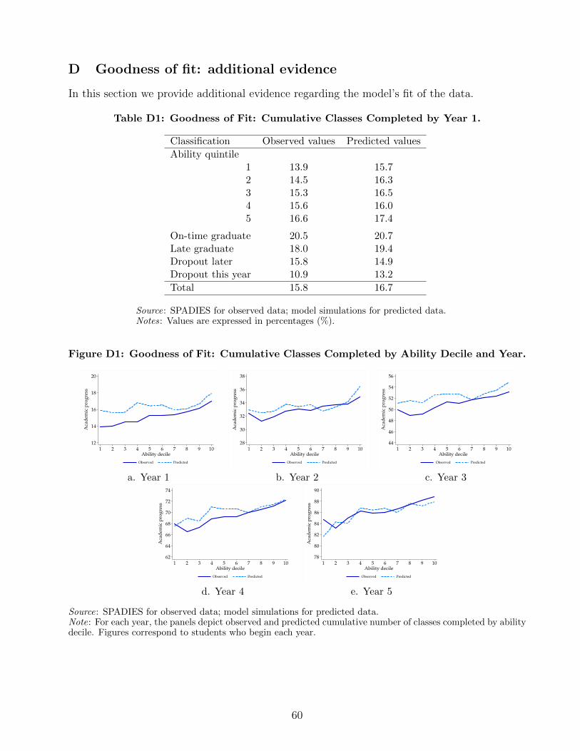
D Goodness of fit: additional evidence

In this section we provide additional evidence regarding the model’s fit of the data.

Table D1: Goodness of Fit: Cumulative Classes Completed by Year 1.

Classification Observed values Predicted values

Ability quintile1 13.9 15.72 14.5 16.33 15.3 16.54 15.6 16.05 16.6 17.4

On-time graduate 20.5 20.7Late graduate 18.0 19.4Dropout later 15.8 14.9Dropout this year 10.9 13.2

Total 15.8 16.7

Source: SPADIES for observed data; model simulations for predicted data.Notes: Values are expressed in percentages (%).

Figure D1: Goodness of Fit: Cumulative Classes Completed by Ability Decile and Year.

12

14

16

18

20

Aca

dem

ic p

rog

ress

1 2 3 4 5 6 7 8 9 10Ability decile

Observed Predicted

28

30

32

34

36

38

Aca

dem

ic p

rog

ress

1 2 3 4 5 6 7 8 9 10Ability decile

Observed Predicted

44

46

48

50

52

54

56

Aca

dem

ic p

rog

ress

1 2 3 4 5 6 7 8 9 10Ability decile

Observed Predicted

a. Year 1 b. Year 2 c. Year 3

62

64

66

68

70

72

74

Aca

dem

ic p

rog

ress

1 2 3 4 5 6 7 8 9 10Ability decile

Observed Predicted

78

80

82

84

86

88

90

Aca

dem

ic p

rog

ress

1 2 3 4 5 6 7 8 9 10Ability decile

Observed Predicted

d. Year 4 e. Year 5

Source: SPADIES for observed data; model simulations for predicted data.Note: For each year, the panels depict observed and predicted cumulative number of classes completed by abilitydecile. Figures correspond to students who begin each year.

60

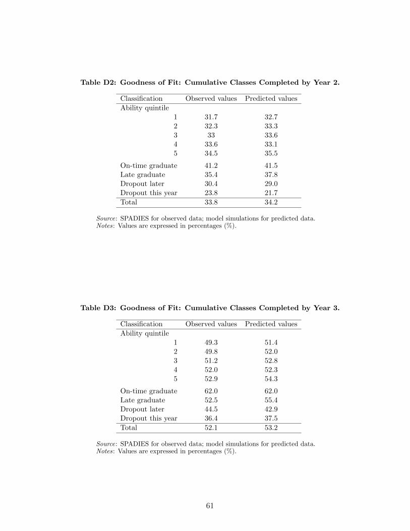
Table D2: Goodness of Fit: Cumulative Classes Completed by Year 2.

Classification Observed values Predicted values

Ability quintile1 31.7 32.72 32.3 33.33 33 33.64 33.6 33.15 34.5 35.5

On-time graduate 41.2 41.5Late graduate 35.4 37.8Dropout later 30.4 29.0Dropout this year 23.8 21.7

Total 33.8 34.2

Source: SPADIES for observed data; model simulations for predicted data.Notes: Values are expressed in percentages (%).

Table D3: Goodness of Fit: Cumulative Classes Completed by Year 3.

Classification Observed values Predicted values

Ability quintile1 49.3 51.42 49.8 52.03 51.2 52.84 52.0 52.35 52.9 54.3

On-time graduate 62.0 62.0Late graduate 52.5 55.4Dropout later 44.5 42.9Dropout this year 36.4 37.5

Total 52.1 53.2

Source: SPADIES for observed data; model simulations for predicted data.Notes: Values are expressed in percentages (%).

61

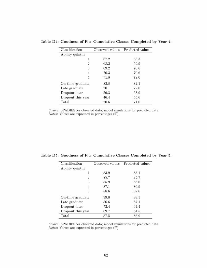
Table D4: Goodness of Fit: Cumulative Classes Completed by Year 4.

Classification Observed values Predicted values

Ability quintile1 67.2 68.32 68.2 69.93 69.2 70.64 70.3 70.65 71.8 72.0

On-time graduate 82.8 82.1Late graduate 70.1 72.0Dropout later 59.3 53.9Dropout this year 46.4 55.6

Total 70.6 71.0

Source: SPADIES for observed data; model simulations for predicted data.Notes: Values are expressed in percentages (%).

Table D5: Goodness of Fit: Cumulative Classes Completed by Year 5.

Classification Observed values Predicted values

Ability quintile1 83.9 83.12 85.7 85.73 85.9 86.64 87.1 86.95 88.6 87.6

On-time graduate 99.0 99.5Late graduate 86.6 87.1Dropout later 72.4 64.4Dropout this year 69.7 64.5

Total 87.5 86.9

Source: SPADIES for observed data; model simulations for predicted data.Notes: Values are expressed in percentages (%).

62

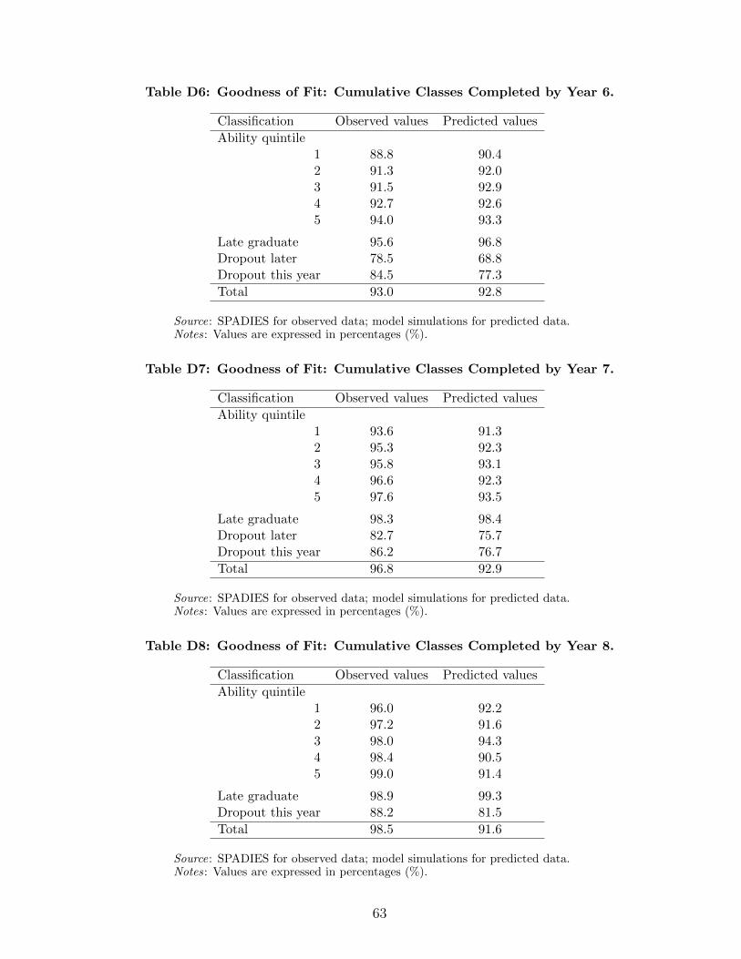
Table D6: Goodness of Fit: Cumulative Classes Completed by Year 6.

Classification Observed values Predicted values

Ability quintile1 88.8 90.42 91.3 92.03 91.5 92.94 92.7 92.65 94.0 93.3

Late graduate 95.6 96.8Dropout later 78.5 68.8Dropout this year 84.5 77.3

Total 93.0 92.8

Source: SPADIES for observed data; model simulations for predicted data.Notes: Values are expressed in percentages (%).

Table D7: Goodness of Fit: Cumulative Classes Completed by Year 7.

Classification Observed values Predicted values

Ability quintile1 93.6 91.32 95.3 92.33 95.8 93.14 96.6 92.35 97.6 93.5

Late graduate 98.3 98.4Dropout later 82.7 75.7Dropout this year 86.2 76.7

Total 96.8 92.9

Source: SPADIES for observed data; model simulations for predicted data.Notes: Values are expressed in percentages (%).

Table D8: Goodness of Fit: Cumulative Classes Completed by Year 8.

Classification Observed values Predicted values

Ability quintile1 96.0 92.22 97.2 91.63 98.0 94.34 98.4 90.55 99.0 91.4

Late graduate 98.9 99.3Dropout this year 88.2 81.5

Total 98.5 91.6

Source: SPADIES for observed data; model simulations for predicted data.Notes: Values are expressed in percentages (%).

63

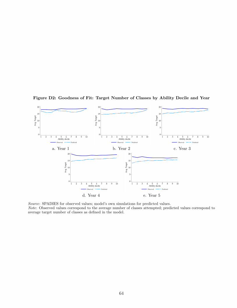
Figure D2: Goodness of Fit: Target Number of Classes by Ability Decile and Year

0

5

10

15

20

Av

g. T

arg

et

1 2 3 4 5 6 7 8 9 10Ability decile

Observed Predicted

0

5

10

15

20

Av

g. T

arg

et

1 2 3 4 5 6 7 8 9 10Ability decile

Observed Predicted

0

5

10

15

20

Av

g. T

arg

et

1 2 3 4 5 6 7 8 9 10Ability decile

Observed Predicted

a. Year 1 b. Year 2 c. Year 3

0

5

10

15

20

Av

g. T

arg

et

1 2 3 4 5 6 7 8 9 10Ability decile

Observed Predicted

0

5

10

15

20

Av

g. T

arg

et

1 2 3 4 5 6 7 8 9 10Ability decile

Observed Predicted

d. Year 4 e. Year 5

Source: SPADIES for observed values; model’s own simulations for predicted values.Note: Observed values correspond to the average number of classes attempted; predicted values correspond toaverage target number of classes as defined in the model.

64

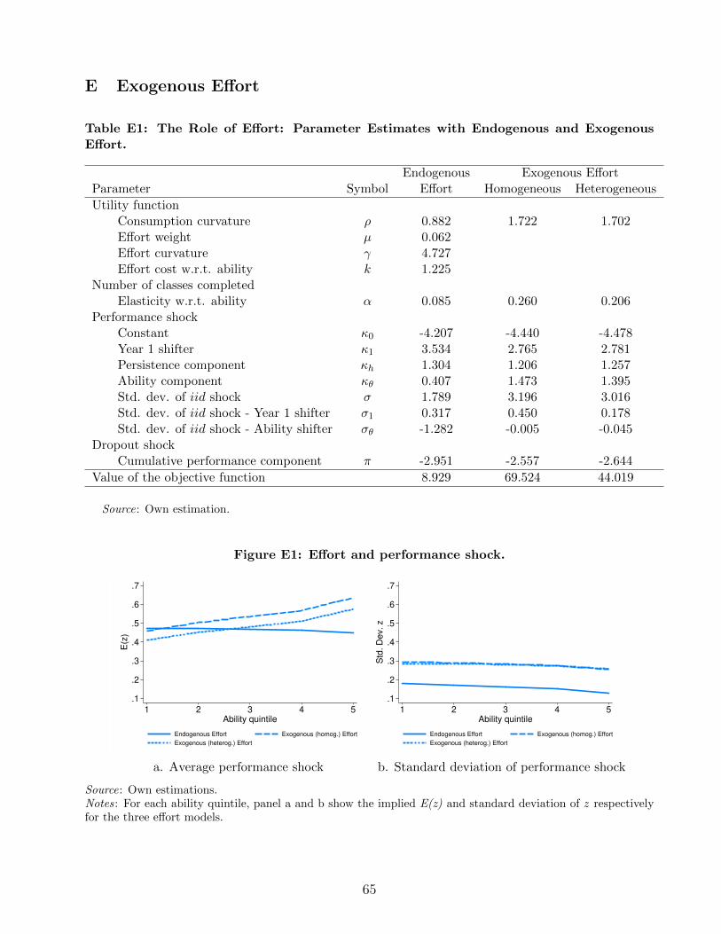
E Exogenous Effort

Table E1: The Role of Effort: Parameter Estimates with Endogenous and ExogenousEffort.

Endogenous Exogenous EffortParameter Symbol Effort Homogeneous Heterogeneous

Utility functionConsumption curvature ρ 0.882 1.722 1.702Effort weight µ 0.062Effort curvature γ 4.727Effort cost w.r.t. ability k 1.225

Number of classes completedElasticity w.r.t. ability α 0.085 0.260 0.206

Performance shockConstant κ0 -4.207 -4.440 -4.478Year 1 shifter κ1 3.534 2.765 2.781Persistence component κh 1.304 1.206 1.257Ability component κθ 0.407 1.473 1.395Std. dev. of iid shock σ 1.789 3.196 3.016Std. dev. of iid shock - Year 1 shifter σ1 0.317 0.450 0.178Std. dev. of iid shock - Ability shifter σθ -1.282 -0.005 -0.045

Dropout shockCumulative performance component π -2.951 -2.557 -2.644

Value of the objective function 8.929 69.524 44.019

Source: Own estimation.

Figure E1: Effort and performance shock.

.1

.2

.3

.4

.5

.6

.7

E(z

)

1 2 3 4 5Ability quintile

Endogenous Effort Exogenous (homog.) Effort

Exogenous (heterog.) Effort

.1

.2

.3

.4

.5

.6

.7

Std

. D

ev.

z

1 2 3 4 5Ability quintile

Endogenous Effort Exogenous (homog.) Effort

Exogenous (heterog.) Effort

a. Average performance shock b. Standard deviation of performance shock

Source: Own estimations.Notes: For each ability quintile, panel a and b show the implied E(z) and standard deviation of z respectivelyfor the three effort models.

65

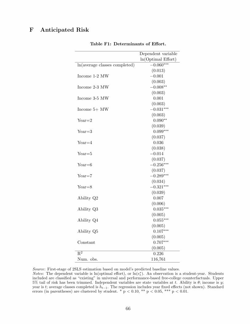
F Anticipated Risk

Table F1: Determinants of Effort.

Dependent variableln(Optimal Effort)

ln(average classes completed) −0.060∗∗∗

(0.013)Income 1-2 MW −0.001

(0.003)Income 2-3 MW −0.008∗∗

(0.003)Income 3-5 MW 0.001

(0.003)Income 5+ MW −0.031∗∗∗

(0.003)Year=2 0.090∗∗

(0.039)Year=3 0.099∗∗∗

(0.037)Year=4 0.036

(0.038)Year=5 −0.014

(0.037)Year=6 −0.256∗∗∗

(0.037)Year=7 −0.289∗∗∗

(0.034)Year=8 −0.321∗∗∗

(0.039)Ability Q2 0.007

(0.006)Ability Q3 0.035∗∗∗

(0.005)Ability Q4 0.055∗∗∗

(0.005)Ability Q5 0.107∗∗∗

(0.005)Constant 0.707∗∗∗

(0.005)

R2 0.226Num. obs. 116,761

Source: First-stage of 2SLS estimation based on model’s predicted baseline values.Notes: The dependent variable is ln(optimal effort), or ln(e∗t ). An observation is a student-year. Studentsincluded are classified as “existing” in universal and performance-based free-college counterfactuals. Upper5% tail of risk has been trimmed. Independent variables are state variables at t. Ability is θ; income is y;year is t; average classes completed is ht−1. The regression includes year fixed effects (not shown). Standarderrors (in parentheses) are clustered by student. * p < 0.10, ** p < 0.05, *** p < 0.01.

66