Rafiki: Machine Learning as an Analytics Service System

Wei Wang†, Sheng Wang†, Jinyang Gao†, Meihui Zhang�Gang Chen‡, Teck Khim Ng†, Beng Chin Ooi†

†National University of Singapore�Beijing Institute of Technology ‡Zhejiang University

†{wangwei, jinyang.gao, wangsh, ngtk, ooibc}@comp.nus.edu.sg�meihui zhang@bit.edu.cn, ‡ cg@zju.edu.cn

ABSTRACTBig data analytics is gaining massive momentum in the last fewyears. Applying machine learning models to big data has becomean implicit requirement or an expectation for most analysis tasks,especially on high-stakes applications.Typical applications includesentiment analysis against reviews for analyzing on-line products,image classification in food logging applications for monitoringuser’s daily intake and stock movement prediction. Extending tra-ditional database systems to support the above analysis is intriguingbut challenging. First, it is almost impossible to implement all ma-chine learning models in the database engines. Second, expertiseknowledge is required to optimize the training and inference proce-dures in terms of efficiency and effectiveness, which imposes heavyburden on the system users. In this paper, we develop and presenta system, called Rafiki, to provide the training and inference ser-vice of machine learning models, and facilitate complex analyticson top of cloud data storage systems. Rafiki provides distributedhyper-parameter tuning for the training service, and online ensem-ble modeling for the inference service which trades off betweenlatency and accuracy. Experimental results confirm the efficiency,effectiveness, scalability and usability of Rafiki.

1. INTRODUCTIONData analysis plays an important role in extracting valuable in-

sights from a huge amount of data. Database systems have beentraditionally used for storing and analyzing structured data, spatial-temporal data, graph data, etc. Other data, such as multimedia data(e.g., images and free text), and domain specific data (e.g, medicaldata and sensor data), are being generated at fast speed and con-stitutes a significant portion of the Big Data [35]. It is beneficialto analyze these data for database applications [36]. For instance,inferring the quality of a product from the review column in thesales database would help to explain the sales numbers; Analyz-ing food images from the food logging application can extract thefood preference of people from different ages. However, the aboveanalysis requires machine learning models, especially deep learn-ing [17] models, for sentiment analysis [4] to classify the review aspositive or negative, and image classification [15] to recognize the

food type from images. Figure 1 shows a pipeline of data analysis,where database systems have been widely used for the first 3 stagesand machine learning is good at the 4th stage.

Big Data 大数据

• 3Vs: Volume, Velocity and Variety 高容量，速度快，多样性

– Variety implies integrating and analyzing data

– It is necessary to develop end-to-end solutions that scale, are easy

to use, and minimize human effort

Acquisition

Extraction/

Cleaning/

Annotation

IntegrationAnalysis/

Modeling

Interpretation/

Visualization

Figure 1: Data analytic pipeline.

One approach to integrating the machine learning techniques intodatabase applications is to preprocess the data off-line and add theprediction results into a new column, e.g. a column for the foodtype. However, such off-line preprocessing has two-folds of restric-tion. First, it requires the developers to have expertise knowledgeand experience of training machine learning models. Second, thequeries cannot involve attributes of the object, e.g. the ingredientsof food, if they are not predicted in the preprocessing step. In addi-tion, it would waste a lot of time to do the prediction for all the rowsif queries only read the food type column of few rows, e.g. due to afiltering on other columns. Another approach is to carry out the pre-diction on-line as user-defined functions (UDFs) in the SQL query.However, it is challenging to implement all machine learning mod-els in UDFs by database users [23], for machine learning modelsvary a lot in terms of theory and implementation. It is also difficultto optimize the prediction accuracy in the database engine.

A better solution is to call the corresponding cloud machine learn-ing service e.g. APIs, in the UDFs for each prediction (or analysis)task. Cloud service is economical, elastic and easy to use. Withthe resurgence of AI, cloud providers like Amazon (AWS), Googleand Microsoft (Azure) have built machine learning services on theircloud platforms. There are two types of cloud services. The firstone is to provide an API for each specific task, e.g. image classifi-cation and sentiment analysis. Such APIs are available on AmazonAWS1 and Google cloud platform2. The disadvantage is that theaccuracy could be low since the models are trained by Amazonand Google with their data, which is likely to be different from theusers’ data. The second type of service overcomes this issue byproviding the training service, where users can upload their owndatasets to conduct training. This service is available on AmazonAWS and Microsoft Azure. However, only a limited number of ma-chine learning models are supported [37]. For example, only sim-

1https://aws.amazon.com/machine-learning/2https://cloud.google.com/products/machine-learning/

1

ple logistic regression or linear regression models3 are supportedby Amazon. Deep learning models such as convolutional neuralnetworks (ConvNets) and recurrent neural networks (RNN) are notincluded.

As a machine learning cloud service, it not only needs to covera wide range of models, including deep learning models, but alsoprovide an easy-to-use, efficient and effective service for users with-out much machine learning knowledge and experience, e.g. databaseusers. Considering that different models may result in differentperformance in terms of efficiency (e.g. latency) and effectiveness(e.g. accuracy), the cloud service has to select the proper modelsfor a given task. Moreover, most machine learning models and thetraining algorithms come with a set of hyper-parameters or knobs,e.g. number of layers and size of each layer in a neural network.Some hyper-parameters are vital for the convergence of the trainingalgorithm and the final model performance, e.g. the learning rateof the stochastic gradient descent (SGD) algorithm. Manual hyper-parameter tuning requires rich experience and is tedious. Randomsearch and Bayesian optimization are two popular automatic tun-ing approaches. However, both are costly as they have to train themodel till convergence, which may take hundreds of hours. A dis-tributed tuning platform is desirable. Besides training, inference4

also matters as it directly affects the user experience. Machinelearning products often ensemble multiple models and average theresults to boost the prediction performance. However, ensemblemodeling incurs a larger latency (i.e. response time) compared withusing a single prediction model. Therefore, there is a trade-off be-tween accuracy and latency.

There have been studies on these challenges for providing ma-chine learning as a service. mlbench [37] compares the cloud ser-vice of Amazon and Azure over a set of binary classification tasks.Ease.ml [18] builds a training platform with model selection aim-ing at optimizing the resource utilization. Google Vizier [9] is adistributed hyper-parameter tuning platform that provides tuningservice for other systems. Clipper [5] focuses on the inference byproposing a general framework and specific optimization for effi-ciency and accuracy.

In this paper, we present a system, called Rafiki, to provideboth the training and inference services for machine learning mod-els. With Rafiki, (database) users are exempted from managing thehardware resource, constructing the (deep learning) models, tun-ing the hyper-parameters, optimizing the prediction accuracy andspeed. Instead, they simply upload their datasets and configure theservice to conduct training and then deploy the model for infer-ence. As a cloud service system [1, 6], Rafiki manages the hard-ware resources, failure recovery, etc. It comes with a set of built-in(deep learning) models for popular tasks such as image and textprocessing. In addition, we make the following contributions tomake Rafiki easy-to-use, efficient and effective.

1. We propose a unified system architecture for both the train-ing and the inference services. We observe that the two ser-vices share some common components such as a parameterserver for model parameter storage, and distributed comput-ing environment for distributed hyper-parameter tuning andparallel inference. By sharing the same underlying storage,communication protocols and computation resource, we im-plicitly avoid some technical debts [25]. Moreover, by com-

3https://docs.aws.amazon.com/machine-learning/latest/dg/learning-algorithm.html4We use the term deployment, inference and serving interchange-ably.

bining the two services together, Rafiki enables instant modeldeployment after training.

2. For the training service, we first propose a general frame-work for distributed hyper-parameter tuning, which is ex-tensible for popular hyper-parameter tuning algorithms in-cluding random search and Bayesian optimization. In addi-tion, we propose a collaborative tuning scheme specificallyfor deep learning models, which uses the model parametersfrom the current top performing training trials to initializenew trials.

3. For the inference service, we propose a scheduling algorithmbased on reinforcement learning to optimize the overall ac-curacy and reduce latency. Both algorithms are adaptive tothe changes of the request arrival rate.

4. We conduct micro-benchmark experiments to evaluate theperformance of our proposed algorithms.

In the reminder of this paper, we give the system architecturein Section 3. Section 4 describes the training service and the dis-tributed hyper-parameter tuning algorithm. The deployment ser-vice and optimization techniques are introduced in Section 5. Sec-tion 6 describes the system implementation. We explain the ex-perimental study in Section 7 and then introduce related works inSection 2.

2. RELATED WORKRafiki is a SaaS that provides analytics services based on ma-

chine learning. Optimization techniques are proposed for both thetraining (i.e. distributed hyper-parameter tuning) and the inferencestage (i.e. accuracy and latency optimization). In this section, wereview related work on SaaS, hyper-parameter tuning, inference op-timization, and reinforcement learning which is adopted by Rafikifor inference optimization.

2.1 Software as a ServiceCloud computing has changed the way of IT operation in many

companies by providing infrastructure as a service (IaaS), platformas a service (PaaS) and software as a service (SaaS). With IaaS,users and companies can use remote physical or virtual machinesinstead of establishing their own data center. Based on user require-ments, IaaS can scale up the compute resources quickly. PaaS, e.g.,Microsoft Azure, provides development toolkit and running envi-ronment, which can be adjusted automatically based on businessdemand. SaaS, including database as a service[1, 6], installs soft-ware on cloud computing platforms and provides application ser-vices, which simplifies software maintenance. The ‘pay as you go’pricing model is convenient and economic for (small) companiesand research labs.

Recently, machine learning (especially deep learning) has gaina lot of interest due to its outstanding performance in analytic andpredictive tasks. There are two primary steps to apply machinelearning for an application, namely training and inference. Cloudproviders, like Amazon AWS, Microsoft Azure and Google Cloud,have already included some services for the two steps. However,their training services have limited support for deep learning mod-els, and their inference services cannot be customized for customers’data (see the explanation in Section 1). There are also researchpapers towards efficient resource allocation for training [18] andefficient inference [5] on the cloud. Rafiki differs from the exist-ing cloud services on both the service types and the optimizationtechniques. Firstly, Rafiki allows users to train machine learning

2

(including deep learning) models on their own data, and then de-ploy them for inference. Secondly, Rafiki has special optimizationfor the training and inference service, compared with the existingapproaches as explained in the following two subsections.

2.2 Hyper-parameter TuningTo train a machine learning model for an application, we need to

decide many hyper-parameters related to the model structure, opti-mization algorithm and data preprocessing operations. All hyper-parameter tuning algorithms work by empirical trials. Randomsearch [3] randomly selects the value of each hyper-parameter andthen try it. It has shown to be more efficient than grid search thatenumerates all possible hyper-parameter combinations. Bayesianoptimization [28] assumes the optimization function (hyper-parametersas the input and the inference performance as the output) followsGaussian process. It samples the next point in the hyper-parameterspace based on existing trials (according to an acquisition function).Reinforcement learning has recently been applied to tune the archi-tecture related hyper-parameters [38]. Google Vizier [9] provideshyper-parameter tuning service on the cloud. Rafiki provides dis-tributed hyper-parameter tuning service, which is compatible withall the above mentioned hyper-parameter tuning algorithms. In ad-dition, it supports collaborative tuning that shares model parame-ters across trials. Our experiments confirm the effectiveness of thecollaborative tuning scheme.

2.3 Inference OptimizationTo improve the inference accuracy, ensemble modeling that trains

and deploys multiple models is widely applied. For real-time in-ference, latency is another critical metric of the inference service.NoScope [14] proposes specific inference optimization for videoquerying. Clipper [5] studies multiple optimization techniques toimprove the throughput (via batch size) and reduce latency (viacaching). It also proposes to do model selection for ensemble mod-eling using multi-armed bandit algorithms. Compared with Clip-per, Rafiki provides both training and inference services, whereasClipper focuses only on the inference service. Also, Clipper op-timizes the throughput, latency and accuracy separately, whereasRafiki models them together to find the optimal model selection andbatch size. TensorFlow serving [2] and TFX [21] provide inferenceservice for models trained using Tensorflow. Rafiki and Clipper areboth implementation agnostic. They communicate with the trainingand inference programs in Docker containers via RPC.

2.4 Reinforcement LearningIn reinforcement learning (RL)[31], each time an agent takes one

action, it enters the next state. The environment returns a rewardbased on the action and the states. The learning objective is tomaximize the aggregated rewards. RL algorithms decide the ac-tion to take based on the current state and experience gained fromprevious trials (exploration). Policy gradient based RL algorithmsmaximize the expected reward by taking actions following a policyfunction πθ(at|st) over n steps (Equation 1), where ς representsa trajectory of n (action at, state st, reward Rt) tuples, and γ is adecaying factor. The expectation is taken over all possible trajec-tories. πθ is usually implemented using a multi-layer perceptronmodel (θ represents the parameters) that takes the state vector asinput and generates the action (a scalar value for continuous actionor a Softmax output for discrete actions). Equation 1 is optimizedusing stochastic gradient ascent methods. Equation 3 is used as a‘surrogate’ function for the objective as its gradient is easy to com-pute via automatic differentiation.

J(θ) = Eς∼πθ(ς)[

n∑t=0

γtRt], (1)

OθJ(θ) = Eς∼πθ(ς)[

n∑t=0

Oθ log πθ(at|st)T∑t=0

γtRt] (2)

J(θ) = Eς∼πθ(ς)[

T∑t=0

log πθ(at|st)n∑t=0

γtRt] (3)

Many approaches have been proposed to improve the policy gra-dient by reducing the variance of the rewards, including actor-criticmodel [20] which subtracts the reward Rt by a baseline V (st).V (st) is an estimation of the reward, which is also approximatedusing a neural network like the policy function. Then Rt in theabove equations becomesRt−V (st). Yuxi [19] has done a surveyof deep reinforcement learning, including the actor-critic modelused in this paper.

3. SYSTEM OVERVIEWIn this section, we present the system architecture of Rafiki and

illustrate its usability with some use cases.To use Rafiki, users simply configure the training or inference

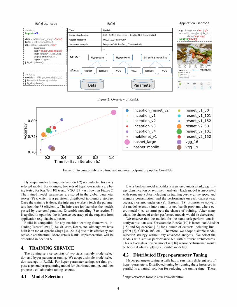
jobs through either RESTFul APIs or Python SDK. In Figure 2(left column), we show one image classification example using thePython SDK. The training code consists of 4 lines. The first lineloads the images from a folder into Rafiki’s distributed data stor-age (HDFS), where all images from the same subfolder are labeledwith the subfolder name, i.e. food name. The second line createsa configuration object representing hyper-parameter tuning options(see Section 4.2 for details). The third line creates the training jobby passing the data, the options and the input/output shapes (a tupleor a list of tuples). The input-output shapes are used for model cus-tomization. For example, ConvNets usually accept input images ofa fixed shape, i.e. the input shape, and adapt the final output layerto generate the same number of outputs as the output shape, whichcould be the total number of classes or bounding-box shape. Thelast line submits the job through RESTFul APIs to Rafiki for exe-cution. It returns a job ID as a handle for job monitoring. Once thetraining finishes, we can deploy the models instantly as shown ininfer.py. It gets the model instances, each of which consists of themodel name and the parameter names for retrieving the parametervalues from Rafiki’s parameter server. It then uses the second lineto create the inference job with the given models. After the modelis deployed by line 3, application users can submit their requeststo this job for prediction as shown by the code in query.py. Ap-plications like a mobile App can send RESTFul requests to do thequery.

For each training job, Rafiki selects the corresponding built-inmodels based on the task type. The table in Figure 2 lists somebuilt-in tasks and the models. With the proliferation of machinelearning, we are able to find open source implementations for al-most every model. Figure 3 compares the memory footprint, ac-curacy and inference speed of some open source ConvNets5. 5Groups of ConvNets are compared, including Inception ConvNets [32],MobileNet [12], NASNets [38], ResNets [10] and VGGs [27]. Theaccuracy is measured based on the top-1 prediction of images fromthe validation dataset of ImageNet. The inference time and mem-ory footprint is averaged over 50 iterations, each with 50 images(i.e. batch size=50).

5https://github.com/tensorflow/models/tree/master/research/slim/

3

Data

Hyper-tune Hyper-tune Ensemble modelling

ResNet

Parameter

Task Models

Image classification VGG, ResNet, Squeezenet, XceptionNet, InceptionNet

Object detection YOLO, SSD, FasterRCNN

Sentiment analysis TemporalCNN, FastText, CharacterRNN

… …

ResNet ResNetVGG VGG VGG

Master

Worker

Rafiki user code Rafiki Application user code

# train.py

import rafiki

data = rafiki.import_images('food/')

hyper = rafiki.HyperConf()

job = rafiki.Train(name='train’,

data=data,

task="ImageClassification",

input_shape=(3,256,256),

output_shape=(120,),

hyper = hyper)

job_id = job.run()

# infer.py

models = rafiki.get_models(job_id)

job = rafiki.Inference(models)

job_id = job.run()

img = Image.load('test.jpg')

ret = rafiki.query(job=job_id,

data={'img':img})

print(ret['label'])

ret[‘label’]

Figure 2: Overview of Rafiki.

0.2 0.4 0.6 0.8 1.0Time for Each Iteration (s)

0.70

0.75

0.80

Accu

racy

inception_resnet_v2inception_v1inception_v2inception_v3inception_v4mobilenet_v1nasnet_largenasnet_mobile

resnet_v1_50resnet_v1_101resnet_v1_152resnet_v2_50resnet_v2_101resnet_v2_152vgg_16vgg_19

Figure 3: Accuracy, inference time and memory footprint of popular ConvNets.

Hyper-parameter tuning (See Section 4.2) is conducted for everyselected model. For example, two sets of hyper-parameters are be-ing tested for ResNet [10] (resp. VGG [27]) as shown in Figure 2.The trained model parameters are stored in the global parameterserver (PS), which is a persistent distributed in-memory storage.Once the training is done, the inference workers fetch the parame-ters from the PS efficiently. The inference job launches the modelspassed by user configuration. Ensemble modeling (See section 5)is applied to optimize the inference accuracy of the requests fromapplication (e.g. database) users.

Rafiki is compatible for any machine learning framework, in-cluding TensorFlow [2], Scikit-learn, Kears, etc., although we havebuilt it on top of Apache Singa [34, 22, 33] due to its efficiency andscalable architecture. More details Rafiki implementation will bedescribed in Section 6.

4. TRAINING SERVICEThe training service consists of two steps, namely model selec-

tion and hyper-parameter tuning. We adopt a simple model selec-tion strategy in Rafiki. For hyper-parameter tuning, we first pro-pose a general programming model for distributed tuning, and thenpropose a collaborative tuning scheme.

4.1 Model Selection

Every built-in model in Rafiki is registered under a task, e.g. im-age classification or sentiment analysis. Each model is associatedwith some meta data including its training cost, e.g. the speed andmemory consumption, and the performance on each dataset (e.g.accuracy or area-under-curve). Ease.ml [18] proposes to convertthe model selection into a multi-armed bandit problem, where ev-ery model (i.e. an arm) gets the chance of training. After manytrials, the chance of under-performed models would be decreased.

We observe that the models for the same task perform consis-tently across datasets. For example, ResNet[10] is better than AlexNet[15] and SqueezeNet [13] for a bunch of datasets including Ima-geNet [7], CIFAR-106, etc.. Therefore, we adopt a simple modelselection strategy without any advanced analysis. We select themodels with similar performance but with different architectures.This is to create a diverse model set [16] whose performance wouldbe boosted when applying ensemble modeling.

4.2 Distributed Hyper-parameter TuningHyper-parameter tuning usually has to run many different sets of

hyper-parameters. Distributed tuning by running these instances inparallel is a natural solution for reducing the tuning time. There

6https://www.cs.toronto.edu/ kriz/cifar.html

4

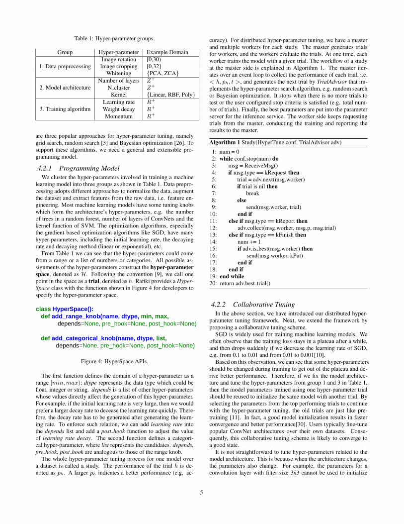
Table 1: Hyper-parameter groups.

Group Hyper-parameter Example Domain

1. Data preprocessingImage rotation [0,30)Image cropping [0,32]

Whitening {PCA, ZCA}

2. Model architectureNumber of layers Z+

N cluster Z+

Kernel {Linear, RBF, Poly}

3. Training algorithmLearning rate R+

Weight decay R+

Momentum R+

are three popular approaches for hyper-parameter tuning, namelygrid search, random search [3] and Bayesian optimization [26]. Tosupport these algorithms, we need a general and extensible pro-gramming model.

4.2.1 Programming ModelWe cluster the hyper-parameters involved in training a machine

learning model into three groups as shown in Table 1. Data prepro-cessing adopts different approaches to normalize the data, augmentthe dataset and extract features from the raw data, i.e. feature en-gineering. Most machine learning models have some tuning knobswhich form the architecture’s hyper-parameters, e.g. the numberof trees in a random forest, number of layers of ConvNets and thekernel function of SVM. The optimization algorithms, especiallythe gradient based optimization algorithms like SGD, have manyhyper-parameters, including the initial learning rate, the decayingrate and decaying method (linear or exponential), etc.

From Table 1 we can see that the hyper-parameters could comefrom a range or a list of numbers or categories. All possible as-signments of the hyper-parameters construct the hyper-parameterspace, denoted as H. Following the convention [9], we call onepoint in the space as a trial, denoted as h. Rafiki provides a Hyper-Space class with the functions shown in Figure 4 for developers tospecify the hyper-parameter space.

import rafiki

data = rafiki.import_images('food/')

hyper = rafiki.HyperConf()

job = rafiki.Train(name='train’,

data=data,

task="ImageClassification",

input_shape=(3,256,256),

output_shape=(120,),

hyper = hyper)

job_id = job.run()

models = rafiki.get_models(job_id)

job = rafiki.Inference(models)

job_id = job.run()

img = Image.load('test.jpg')

ret = rafiki.query(job=job_id, data={'img':img})

print(ret['label'])

class HyperSpace():

def add_range_knob(name, dtype, min, max,

depends=None, pre_hook=None, post_hook=None)

def add_categorical_knob(name, dtype, list,

depends=None, pre_hook=None, post_hook=None)

Figure 4: HyperSpace APIs.

The first function defines the domain of a hyper-parameter as arange [min,max); dtype represents the data type which could befloat, integer or string. depends is a list of other hyper-parameterswhose values directly affect the generation of this hyper-parameter.For example, if the initial learning rate is very large, then we wouldprefer a larger decay rate to decease the learning rate quickly. There-fore, the decay rate has to be generated after generating the learn-ing rate. To enforce such relation, we can add learning rate intothe depends list and add a post hook function to adjust the valueof learning rate decay. The second function defines a categori-cal hyper-parameter, where list represents the candidates. depends,pre hook, post hook are analogous to those of the range knob.

The whole hyper-parameter tuning process for one model overa dataset is called a study. The performance of the trial h is de-noted as ph. A larger ph indicates a better performance (e.g. ac-

curacy). For distributed hyper-parameter tuning, we have a masterand multiple workers for each study. The master generates trialsfor workers, and the workers evaluate the trials. At one time, eachworker trains the model with a given trial. The workflow of a studyat the master side is explained in Algorithm 1. The master iter-ates over an event loop to collect the performance of each trial, i.e.< h, ph, t >, and generates the next trial by TrialAdvisor that im-plements the hyper-parameter search algorithm, e.g. random searchor Bayesian optimization. It stops when there is no more trials totest or the user configured stop criteria is satisfied (e.g. total num-ber of trials). Finally, the best parameters are put into the parameterserver for the inference service. The worker side keeps requestingtrials from the master, conducting the training and reporting theresults to the master.

Algorithm 1 Study(HyperTune conf, TrialAdvisor adv)

1: num = 02: while conf.stop(num) do3: msg = ReceiveMsg()4: if msg.type == kRequest then5: trial = adv.next(msg.worker)6: if trial is nil then7: break8: else9: send(msg.worker, trial)

10: end if11: else if msg.type == kReport then12: adv.collect(msg.worker, msg.p, msg.trial)13: else if msg.type == kFinish then14: num += 115: if adv.is best(msg.worker) then16: send(msg.worker, kPut)17: end if18: end if19: end while20: return adv.best trial()

4.2.2 Collaborative TuningIn the above section, we have introduced our distributed hyper-

parameter tuning framework. Next, we extend the framework byproposing a collaborative tuning scheme.

SGD is widely used for training machine learning models. Weoften observe that the training loss stays in a plateau after a while,and then drops suddenly if we decrease the learning rate of SGD,e.g. from 0.1 to 0.01 and from 0.01 to 0.001[10].

Based on this observation, we can see that some hyper-parametersshould be changed during training to get out of the plateau and de-rive better performance. Therefore, if we fix the model architec-ture and tune the hyper-parameters from group 1 and 3 in Table 1,then the model parameters trained using one hyper-parameter trialshould be reused to initialize the same model with another trial. Byselecting the parameters from the top performing trials to continuewith the hyper-parameter tuning, the old trials are just like pre-training [11]. In fact, a good model initialization results in fasterconvergence and better performance[30]. Users typically fine-tunepopular ConvNet architectures over their own datasets. Conse-quently, this collaborative tuning scheme is likely to converge toa good state.

It is not straightforward to tune hyper-parameters related to themodel architecture. This is because when the architecture changes,the parameters also change. For example, the parameters for aconvolution layer with filter size 3x3 cannot be used to initialize

5

the convolution layer of another ConvNet whose filter size is 5x5.However, during architecture tuning, there are many architecturesavailable. It is likely that some architectures share the same config-urations of one convolution layer. For instance, if ConvNet a’s 3rdconvolution layer and ConvNet b’s 3rd layer have the same convo-lution setting, then we can use the parametersW from ConvNet a’s3rd layer to initialize ConvNet b’s 3rd layer. We just store allW s ina parameter server and fetch the shape matched W to initialize thelayers in new trials (ConvNets). If the performance of the new trailis better than the older one, we overwrite the W in the parameterserver with the new values.

A

B

C

𝛼 = 1

𝛼 = 0.1

𝛼 = 0.01

𝛼 = 0.1

𝛼 = 0.01

𝛼 = 0.1

Figure 5: A collaborative tuning example.

The whole process is illustrated in Figure 5, where 3 workersare running trials to tune the hyper-parameters (e.g. the learningrate) of the same model. After a while, the performance of workerA stops increasing. The training stops automatically according toearly stopping criteria, e.g the training loss is not decreasing for5 consecutive epochs. Early stopping is widely used for trainingmachine learning models7. The new trial on worker A uses the pa-rameters from the current best worker, which is B. The work doneby B serves as the pre-training for the new trial on A. Similarly,when C enters the plateau, the master instructs it to start a newtrial on C using the parameters from A, whose model has the bestperformance at that point in time.

The control flow for this collaborative tuning scheme is describedin Algorithm 2. It is similar to Algorithm 1 except that the masterinstructs the worker to save the model parameters into a global pa-rameter server (Line 9) if the model’s performance is significantlylarger than the current best performance (Line 8). The performancedifference, i.e. conf.delta is a configuration parameter in Hyper-Conf, which is set according to the user’s expectation about theperformance of the model. For example, for MNIST image classi-fication, an improvement of 0.1% is very large as the current bestperformance is above 99%. For CIFAR-10 image classification, wemay set the delta to be 0.5% as the best accuracy is about 97.4%[8],which means that there is a bigger improvement space.

We notice that bad parameter initialization degrades the perfor-mance in our experiments. This is very serious for random search.Because the checkpoint from one trial with poor accuracy wouldaffect the next trials as the model parameters are initialized into apoor state. To resolve this problem, a α-greedy strategy is intro-duced in our implementation, which initializes the model param-eters either by random initialization or from a pre-trained modelcheckpoint file. A threshold α represents the probability of choos-ing random initialization and (1-α) represents the probability of us-ing pre-trained checkpoint files. α decreases gradually to decreasethe chance of random initialization, i.e. increasing the chance ofCoStudy. This α-greedy strategy is widely used in reinforcementlearning to balance the exploration and exploitation.

5. INFERENCE SERVICE7https://keras.io/callbacks/#earlystopping

Algorithm 2 CoStudy(HyperTune conf, TrialAdvisor adv)

1: num = 0, best p = 02: while conf.stop(num) do3: msg = ReceiveMsg()4: if msg.type == kRequest then5: ... . // same as Algorithm 16: else if msg.type == kReport then7: adv.collect(msg.worker, msg.p, msg.trial)8: if msg.p - best p > conf.delta then9: send(msg.worker, kPut)

10: best p = msg.p11: else if adv.early stopping(msg.worker, conf) then12: send(msg.worker, kStop)13: end if14: else if msg.type == kFinish then15: num += 116: end if17: end while18: return adv.best trial()

Inference service provides real-time request serving by deploy-ing the trained model. Other services, like database services, sim-ply optimize the throughput with the constraint on latency, which isset manually as a service level objective (SLO), denoted as τ , e.g.τ = 0.1 seconds. For machine learning services, accuracy becomesan important optimization objective. The accuracy refers to a widerange of performance measurements, e.g. negative error, precision,recall, F1, area under curve, etc. A larger value (accuracy) indicatesbetter performance. If we set latency as a hard constraint as shownin Equation 4, overdue requests would get ‘time out’ responses.Typically, a delayed response is better than an error of ‘time out’for the end-users. Hence, we process the requests in the queue se-quentially following FIFO (first-in-first-out). The objective is tomaximize the accuracy and minimize the exceeding time accord-ing to τ . However, typically, there is a trade-off between accuracyand latency. For example, ensemble modeling with more modelsincreases both the accuracy and the latency. We shall optimize themodel selection for ensemble modeling in Section 5.2. Before that,we discuss a simpler case with a single inference model. Table 2summarizes the notations used in this section.

maxAccuracy(S) (4)subject to ∀s ∈ S, l(s) < τ

5.1 Single Inference ModelWhen there is only one single model deployed for an application,

the accuracy of the inference service is fixed from the system’s per-spective. Therefore, the optimization objective is reduced to mini-mizing the exceeding time, which is formalized in Equation 5.

min

∑s∈Smax(0, l(s)− τ)

|S| (5)

The latency l(s) of a request includes the waiting time in thequeue w(s), and the inference time which depends on the modelcomplexity, hardware efficiency (i.e. FLOPS) and the batch size.The batch size decides the number of requests to be processed to-gether. Modern processing units, like CPU and GPU, exploit dataparallelism techniques (e.g. SIMD) to improve the throughput andreduce the computation cost. Hence, a large batch size is necessary

6

Table 2: Notations.

Name DefinitionS request listM model listτ latency requirementb ∈ B one batch size from a candidate listqk the k−th oldest requests in the queueq:k is the oldest k requestsqk: is the latest |Q| − k requestsc(b) inference time for batch size bc(m, b) inference time for model m and batch size bw(s) waiting time for a request s in the queuel(s) latency (waiting + inference time) of a requestβ balancing factor between accuracy and latencyv binary vector for model selectionR() reward function over a set of requests

to saturate the parallelism capacity. Once the model is deployedon a cloud platform, the model complexity and hardware efficiencyare fixed. Therefore, Rafiki tunes the batch size to optimize thelatency.

To construct a large batch, e.g. with b requests, we have to delaythe processing until all b requests arrive, which may incur a largelatency for the old requests if the request arrival rate is low. The op-timal batch size is thus influenced by SLO τ , the queue status (e.g.the waiting time), and the request arrival rate which varies alongtime. Since the inference time of two similar batch sizes varies lit-tle, e.g. b=8 and b=9, a candidate batch size list should includevalues that have significant difference with each other w.r.t the in-ference time, e.g. B = {16, 32, 48, 64, ...}. The largest batch sizeis determined by the system (GPU) memory. c(b), the latency ofprocessing a batch of b requests b ∈ B, is determined by the hard-ware resource (e.g. GPU memory), and the model’s complexity.Figure 3 shows the inference time, memory footprint and accuracyof popular ConvNets trained on ImageNet.

Algorithm 3 shows a greedy solution for this problem. It al-ways applies the largest batch size possible. If the queue length(i.e. number of requests in the queue) is larger than the largestbatch size b = max(B), then the oldest b requests are processedin one batch. Otherwise, it waits until the oldest request (q0) isabout to overdue as checked by Line 8. b is the largest batch sizein B that is smaller or equal to the queue length (Line 8). δ is aback-off constant, which is equivalent to reducing the batch sizein Additive-Increase-Multiplicative-Decrease scheme (AIMD)[5],e.g. δ = 0.1τ .

Algorithm 3 Inference(Queue q, Model m)

1: while True do2: b = maxB3: if len(q) >= b then4: m.infer(q0:b)5: deque(q0:b)6: else7: b = max{b ∈ B, b <= len(q)}8: if c(b) + w(q0) + δ >= τ then9: m.infer(q0:b)

10: deque(q0:b)11: end if12: end if13: end while

5.2 Multiple Inference Models

Single Model Two Models Three Models Four ModelsEnsemble Method

0.75

0.76

0.77

0.78

0.79

0.80

0.81

0.82

0.83

Accu

racy

resnet_v2_101inception_v3inception_v4inception_resnet_v2

Figure 6: Accuracy of ensemble modeling with different models.

Ensemble modeling is an effective and popular approach to im-prove the inference accuracy. To give an example, we comparethe performance of different ensemble of 4 ConvNets as shown inFigure 6. Majority voting is applied to aggregate the predictions.The accuracy is evaluated over the validation dataset of ImageNet.Generally with more models, the accuracy is better. The exceptionis that the ensemble of resnet v2 101 and inception v3, which isnot as good as the single best model, i.e. inception resnet v2. Infact, the prediction of the ensemble modeling is the same as incep-tion v3 because when there is a tie, the prediction from the modelwith the best accuracy is selected as the final prediction.

Parallel ensemble modeling by running one model per node (orGPU) is a straight-forward way to scale the system and improve thethroughput. However, the latency could be high due to stragglers.For example, as shown in Figure 3, the node running nasnet largewould be very slow although its accuracy is high. In addition, en-semble modeling is also costly in terms of throughput when com-pared with serving different requests on different nodes (i.e. noensemble). We can see that there is a trade-off between latency(throughput) and accuracy, which is controlled by the model selec-tion. If the requests arrive slowly, we simply run all models foreach batch to get the best accuracy. However, when the requestarrival rate is high, like in Section 5.1, we have to select differentmodels for different requests to increase the throughput and reducethe latency. In addition, the model selection for the current batchalso affects the next batch. For example, if we use all models for abatch, the next batch has to wait until at least one model finishes.

To solve Equation 4, we have to balance the accuracy and latencyto get a single optimization objective. We move the latency terminto the objective as shown in Equation 6. It maximizes a rewardfunctionR related to the prediction accuracy and penalizes overduerequests. β balances the accuracy and the latency in the objective.If the ground truth of each request is not available for evaluatingthe accuracy, which is the normal case, we have to find a surrogateaccuracy.

maxR(S)− βR({s ∈ S, l(s) > τ}) (6)

Like the analysis for single inference model, we need to considerthe batch size selection as well. It is difficult to design an optimalpolicy for this complex decision making problem, which decidesboth the model selection and batch size selection. In this paper,

7

we propose to optimize Equation 6 using reinforcement learning(RL). RL optimizes an objective over a long term by trying differentactions and entering the corresponding states to collect rewards.By setting the reward as Equation 6 and defining the actions tobe model selection and batch selection, we can apply RL for ouroptimization problem.

RL has three core concepts, namely, the action, reward and state.Once these three concepts are defined, we can apply existing RL al-gorithms to do optimization. We define the three concepts w.r.t ouroptimization problem as follows. First, the state space consists of :a) the queue status represented by the waiting time of each requestin the queue. The waiting time of all requests form a feature vec-tor. To generate a fixed length feature vector, we pad with 0 for theshorter queues and truncate the longer queues. b) the model statusrepresented by a vector including the inference time for differentmodels with different batch sizes, i.e. c(m, b),m ∈M, b ∈ B, andthe left time to finish the existing requests dispatched to it. The twofeature vectors are concatenated into a state feature vector, whichis the input to the RL model for generating the action. Second, theaction decides the batch size b and model selection represented bya binary vector v of length |M | (1 for selected; 0 for unselected).The action space size is thus (2|M|− 1) ∗ |B|. We exclude the casewhere v = 0, i.e. none of the models are selected. Third, followingEquation 6, the reward for one batch of requests without groundtruth labels is defined in Equation 7, a(M [v]) is the accuracy ofthe selected models (ensemble modeling). In this paper, we use theaccuracy evaluated on a validation dataset as the surrogate accu-racy. In the experiment, we use the ImageNet’s validation datasetto evaluate the accuracy of different ensemble combinations for im-age classification. The results are shown in Figure 6. The rewardshown in Equation 7 considers the accuracy, the latency (indirectlyrepresented by the number of overdue requests) and the number ofrequests.

a(M [v]) ∗ (b− β|{s ∈ batch|l(s) > τ}|) (7)

With the state, action and reward well defined, we apply theactor-critic algorithm [24] to optimize the overall reward by learn-ing a good policy for selecting the models and batch size.

6. SYSTEM IMPLEMENTATIONIn this section, we introduce the implementation details of Rafiki,

including the cluster management, data and parameter storage, andfailure recovery.

6.1 Cluster Management

Manager

Master

Data

Worker Worker

Parameter

Master

Data

Worker Worker

Parameter

Train()Inference()

Node A

Node CNode B

Figure 7: Rafiki cluster topology.

Rafiki uses Kubernetes to manage the Docker containers, whichrun the masters, workers, data servers and parameter servers asshown in Figure 7. Docker container is widely used for applica-tion deployment, which bundles the application code (e.g. training

and inference code) and libraries (e.g. Keras) to avoid tedious en-vironment setup. New models, hyper-parameter tuning algorithms,and ensemble modeling approaches are deployed as new Dockercontainers. On each physical node, there could be multiple mastersand workers for different jobs, including both training and infer-ence jobs. These jobs are started by the Rafiki manager, whichaccepts job submissions from users (See Figure 2). Once a jobis launched, users communicate with its master directly to get thetraining progress or submit query requests. Rafiki prefers to locatethe master and workers for the same job in the same physical nodeto avoid network communication overhead.

6.2 Data and Parameter StorageDeep learning models are typically trained over large datasets

that would consume a lot of space if stored in CPU memory. There-fore, Rafiki uses HDFS for data storage, where the ‘data nodes’ arealso docker containers. Users upload their datasets into the HDFSvia Rafiki utility functions, e.g. rafiki.import images (see Fig-ure 2). The training dataset is downloaded to a local directory be-fore training, via rafiki.download() by passing the dataset name.

For model parameters, Rafiki has its own distributed parameterserver. The parameter server is designed with special optimiza-tion for hyper-parameter training and inference. In particular, thehyper-parameters will be cached in memory if they are accessedfrequently, e.g. when Rafiki is doing hyper-parameter training.Otherwise, they are stored in HDFS. The parameters trained forthe same model but different datasets can be shared as long as theprivacy setting is public. It has been shown that training warm-upby using the parameters pre-trained on other datasets speeds up thetraining [21].

6.3 Failure RecoveryFor both the hyper-parameter training and inference services, the

workers are stateless. Hence, Rafiki manager can easily recoverthese nodes by running a new docker container and registering itinto the training or inference master. However, for the masters, theyhave state information. For example, the master for the training ser-vice records the current best hyper-parameter trial. The master forthe inference service has the state, action and reward for reinforce-ment learning. Rafiki checkpoints these (small) state informationof masters for fast failure recovery.

7. EXPERIMENTAL STUDYIn this section we evaluate the scalability, efficiency and effec-

tiveness of Rafiki for hyper-parameter tuning and inference ser-vice optimization respectively. The experiments are conducted onthree machines, each with 3 Nvidia GTX 1080Ti GPUs, 1 IntelE5-1650v4 CPU and 64GB memory.

7.1 Evaluation of Hyper-parameter TuningTask and Dataset We test Rafiki’s distributed hyper-parameter

tuning service by running it to tune the hyper-parameters of deepConvNets over CIFAR-10 for image classification. CIFAR-10 is apopular benchmark dataset with RGB images from 10 categories.Each category has 5000 training images (including 1000 validationimages) and 1000 test images. All images are of size 32x32. Thereis a standard sequence of preprocessing steps for CIFAR-10, whichsubtracts the mean and divides the standard deviation from eachchannel computed on the training images, pads each image with4 pixels of zeros on each side to obtain a 40x40 pixel image, ran-domly crops a 32x32 patch, and then flips (horizontal direction) theimage randomly with probability 0.5.

8

0 100 200Trial Index

20

40

60

80Va

lidat

ion

Accu

racy

Without CoStudy

0 100 200Trial Index

With CoStudy

(a)

25 50 75Validation Accuracy

0

50

100

Num

ber o

f Tria

ls Without CoStudyWith CoStudy

(b)

0 100 200Total Training Epochs

20

40

60

80

Valid

atio

n Ac

cura

cy

Wihtout CoStudyWith CoStudy

(c)

Figure 8: Hyper-parameter tuning based on random search.

0 50 100Trial Index

20

40

60

80

Valid

atio

n Ac

cura

cy

Without CoStudy

0 50 100Trial Index

With CoStudy

(a)

25 50 75Validation Accuracy

0

25

50

75

100

Num

ber o

f Tria

ls Without CoStudyWith CoStudy

(b)

0 50 100Total Training Epochs

40

60

80

Valid

atio

n Ac

cura

cy

Without CoStudyWith CoStudy

(c)

Figure 9: Hyper-parameter tuning based on Bayesian optimization.

7.1.1 Tuning Optimization Hyper-parametersWe fix the ConvNet architecture to be the same as shown in Table

5 of [29], which has 8 convolution layers. The hyper-parameters tobe tuned are from the optimization algorithm, including momen-tum, learning rate, weight decay coefficients, dropout rates, andstandard deviations of the Gaussian distribution for weight initial-ization. We run each trial with early stopping, which terminates thetraining when the validation loss stops decreasing.

We compare the naıve distributed tuning algorithm, i.e. Study(Algorithm 1) and the collaborative tuning algorithm. i.e. CoS-tudy (Algorithm 2) with different TrialAdvisor algorithms. Figure 8shows the comparison using random search [3] for TrialAdvisor. Inparticular, each point in Figure 8a stands for one trial. We can seethat the top area for CoStudy is denser than that for Study. In otherwords, CoStudy is more likely to get better performance. This isconfirmed in Figure 8b, which shows that CoStudy has more trialswith high accuracy (i.e. accuracy>50%) than Study, and has fewertrials with low accuracy (i.e., accuracy≤50%). Figure 8c illustratesthe tuning progress of the two approaches, where each point on theline represents the best performance among all trials conducted sofar. The x-axis is the total number of training epochs8, which corre-sponds to the tuning time (=total number of epochs times the timeper epoch). We can observe that CoStudy is faster than Study andachieves better accuracy than Study. Notice that the validation ac-curacy is very high (>91%). Therefore, a small difference (1%)indicates significant improvement.

Figure 9 compares Study and CoStudy using Gaussian processbased Bayesian Optimization (BO)9 for TrialAdvisor. ComparingFigure 9a and Figure 8a, we can see there are more points in thetop area of BO figures. In other words, BO is better than random

8training the model by scanning the dataset once is called oneepoch.9https://github.com/scikit-optimize

searchwhich has been observed in other papers [28]. In Figure 9a,CoStudy has a few more points in the right bottom area than CoS-tudy. After doing an in-depth inspection, we found that those pointswere trials initialized randomly instead of from pre-trained models.For Study, it always uses random initialization, hence the BO algo-rithm has a fixed prior about the initialization method. However,for CoStuy, its initialization is from pre-trained models for mosttime. These random initialization trials change the prior and thusget biased estimation about the Gaussian process, which leads topoor accuracy. Since we are decaying α to reduce the chance ofrandom initialization, there are fewer and fewer points in the rightbottom area. Overall, CoStudy achieves better accuracy as shownin Figure 9b and Figure 9c.

We study the scalability of Rafiki by varying the number of work-ers. Figure 11 compares the 3 jobs running over 1, 2, 4 and 8 GPUsrespectively. Each point on the curves in the figure represents thebest validation performance among all trials that have been testedso far. The x-axis is the wall clock time. We can see that with moreGPUs, the tuning becomes faster. It scales almost linearly.

7.2 Evaluation of Inference OptimizationWe use image classification as the application to test the opti-

mization techniques introduced in Section 5. The inference modelsare ConvNets trained over the ImageNet [15] benchmark dataset.ImageNet is a popular image classification benchmark with manyopen-source ConvNets trained on it (Figure 3). It has 1.2 millionRGB training images and 50,000 validation images.

Our environment simulator randomly samples images from thevalidation dataset as requests. The number of requests is deter-mined as follows. First, to simulate the scenario with very higharriving rate and very low arriving rate, we set the arriving ratebased on the maximum throughput ru and minimum throughputrl. Specifically, the maximum throughput is the sum of all models’throughput, which is achieved when all models run asynchronously

9

0 250 500 750 1000 1250 1500Time (seconds)

0

100

200

300

400

Requ

ests

/sec

ond

RL Greedy Request Rate

Figure 10: Single inference model with the arriving rate defined based on the maximum throughput.

1 2 4 8Number of Workers

0

500

1000

1500

Wal

l Tim

e (M

inut

es)

(a)

0 250 500 750 1000Wall Time (Minutes)

80

85

90

95

Valid

atio

n Ac

cura

cy

1 Worker2 Workers4 Workers8 Workers

(b)

Figure 11: Scalability test of distributed hyper-parameter tuning.

T/2T/4

rm

t

0.1T 0.1T

Figure 12: Sine function for controlling the request arriving rate.

to process different batches of requests. In contrast, when all mod-els run synchronously, the slowest model’s throughput is just theminimum throughput. Second, we use a sine function and theextreme throughput values to define the request arriving rate, i.e.r = γsin(t) + b. The slope γ and intercept b are derived bysolving Equation 8 and 9, where T is the cycle period which isconfigured to be 500 × τ in our experiments. The first equationis to make sure that more requests than ru (or rl) are generatedfor 20% of each cycle period (Figure 12, T × 20% = 0.2T ). Inthis way, we are simulating the real-life environment where thereare overwhelming requests coming at times. The second equa-tion is to make sure that the highest arriving rate is not too large,otherwise the request queue would be filled up very quickly andnew requests have to be dropped. Finally, a small random noiseis applied over r to prevent the RL algorithm from rememberingthe sine function. To conclude, the number of new requests isδ × (γsin(t) + b)× (1 + φ), φ ∼ N (0, 0.1)), where δ is the timespan between the last invocation of the simulator and the currenttime.

k × sin(T/2− 0.2× 2T/2) + b = ru or rl (8)k × sin(T/2) + b = 1.1× ru or rl (9)

7.2.1 Single Inference ModelWe use inception v3 trained over ImageNet as the single infer-

ence model. Besides the greedy algorithm (Algorithm 3), we alsorun the RL algorithm from Section 5.2 to decide the batch size. Thestate is the same as that in Section 5.2 except that the model relatedstatus is removed.

The batch size list is B = {16, 32, 48, 64}. The maximumthroughput is max b/c(b) = 64/0.23 = 272 images/second andthe minimum throughput is min b/c(b) = 16/0.07 = 228. We setτ = c(64) × 2 = 0.56s. Figure 10 compares the RL algorithmand the greedy algorithm with the arriving rate defined based onthe maximum throughput ru. We can see that after a few iterations,RL performs similarly as the greedy algorithm when the requestarriving rate r is high. When r is low, RL performs better thanthe greedy algorithm. This is because there are a few requests leftwhen the queue length does not equal to any batch size in Line 7of Algorithm 3. These left requests are likely to overdue becausethe new requests are coming slowly to form a new batch. Figure 13compares the RL algorithm and the greedy algorithm with the ar-riving rate defined based on the minimum throughput rl. We cansee that RL performs better than the greedy algorithm when the ar-riving rate is either high or low. Overall, since the arriving rate issmaller than that in Figure 10, there are fewer overdue requests.

7.2.2 Multiple Inference ModelsIn the following experiments, we select inception v3, inception v4

and inception resnet v2 to construct the model list M . The maxi-mum throughput and minimum throughput are 572 requests/secondand 128 requests/second respectively. The experimental results areplotted in Figure 14, Figure 15 and Figure 16. The legend text‘Overdue’ represents for the number of overdue requests per sec-ond, and ‘Arriving’ stands for the request arriving rate.

We compare our RL algorithm with two baseline algorithms re-spectively. For each baseline, we use the greedy algorithm to findthe batch size. They differ in the model selection strategy. The firstbaseline runs all models synchronously for each batch of requests.Correspondingly, the requests are generated using the rate based onrl. From Figure 14a and Figure 14b, we can see that the greedyalgorithm has the fixed accuracy, whereas the RL algorithm’s ac-curacy is high (resp. low) when the rate is low (resp. high). In

10

0 250 500 750 1000 1250 1500Time (seconds)

0

50

100

150

200

250

300

Requ

ests

/sec

ond

RL Greedy Request Rate

Figure 13: Single inference model with the arriving rate defined based on the minimum throughput.

0 500 1000Time (seconds)

0.78

0.80

0.82

0.84

Accu

racy

25

50

75

100

125

150

Requ

ests

/sec

ond

(a) Greedy algorithm.

23000 23500 24000Time (seconds)

0.802

0.804

0.806

0.808

0.810

Accu

racy

25

50

75

100

125

150

Requ

ests

/sec

ond

(b) RL algorithm.

0 500 1000Time (seconds)

0

50

100

150

200

Requ

ests

/sec

ond

OverdueArriving

(c) Greedy algorithm.

23000 23500 24000Time (seconds)

0

50

100

150

200

Requ

ests

/sec

ond

OverdueArriving

(d) RL algorithm.

Figure 14: Multiple model inference with the arriving rate defined based on the minimum throughput.

0 500 1000Time (seconds)

0.76

0.78

0.80

0.82

0.84

Accu

racy

100

200

300

400

500

600

Requ

ests

/sec

ond

(a) Greedy algorithm.

13500 14000 14500Time (seconds)

0.76

0.78

0.80

0.82

0.84

Accu

racy

100

200

300

400

500

600

Requ

ests

/sec

ond

(b) RL algorithm.

0 500 1000Time (seconds)

0

200

400

600

800

1000

Requ

ests

/sec

ond

OverdueArriving

(c) Greedy algorithm.

13500 14000 14500Time (seconds)

0

200

400

600

800

1000

Requ

ests

/sec

ond

OverdueArriving

(d) RL algorithm.

Figure 15: Multiple model inference with the arriving rate defined based on the maximum throughput.

0 2000 4000 6000Time (seconds)

0.800

0.805

0.810

Accu

racy

25

50

75

100

125

150

Requ

ests

/sec

ond

(a) β = 0.

0 2000 4000 6000Time (seconds)

0.795

0.800

0.805

0.810

Accu

racy

25

50

75

100

125

150

Requ

ests

/sec

ond

(b) β = 1.

0 2000 4000 6000Time (seconds)

0

50

100

150

200

Requ

ests

/sec

ond

OverdueArriving

(c) β = 0.

0 2000 4000 6000Time (seconds)

0

50

100

150

200

Requ

ests

/sec

ond

OverdueArriving

(d) β = 1.

Figure 16: Comparison of the effect of different β for the RL algorithm.

fact, the synchronous algorithm always uses all models to do en-semble modelling, whereas the RL algorithm uses fewer models todo ensemble modeling when the arriving rate is high. Since therequest arriving rate is very low, the baseline is able to handle al-most all requests. Similar to Figure 13, some overdue requests inFigure 14c are due to the mismatch of the queue size and the batch

size in Algorithm 3.The second baseline runs all models asynchronously, one model

per batch of requests. In other words, there is no ensemble mod-eling. Correspondingly, the requests are generated using the ratebased on ru. We can see that RL has better accuracy (Figure 15aand 15b) and fewer overdue requests (Figure 15c and 15d) than the

11

baseline. Moreover, it is adaptive to the request arriving rate. Whenthe rate is high, it uses fewer models to serve the same batch to im-prove the throughput and reduce the overdue requests. When therate is low, it uses more models to serve the same batch to improvethe accuracy.

We also compare the effect of different β, namely β = 0 andβ = 1 in the reward function, i.e. Equation 7. Figure 16 showsthe results with the requests generated based on rl. We can seethat when β is smaller, the accuracy (Figure 16a) is higher. This isbecause the reward function focus more on the accuracy part. Con-sequently, there are many overdue requests as shown in Figure 16c.In contrast, when β = 1, the reward function tries to avoid overduerequests by reducing the number of models for ensemble. There-fore, the accuracy and the number of overdue requests are smaller(Figure 16b and Figure 16d).

8. CASE STUDY ON USABILITYcurl -i -F=@image.jpg http://<ip of rafiki>:<app port>/api

CREATE TABLE foodlog ( user_id integer, age integer NOT NULL, location text NOT NULL, time text NOT NULL, image_path text NOT NULL, PRIMARY KEY (user_id, time) );

SELECT UDF_FOOD_NAME(image_path) as food_name, count(*) FROM foodlog WHERE age > 30 GROUP BY food_name;

Figure 17: SQL for table creation.

In this section, we detail how Rafiki can help a database expertuse deep learning services easily in an existing application. Wepresent a scenario for analyzing the food preference of users of afood logging application as shown in Figure 2. This applicationkeeps a log for the food that the user eats by storing the time, loca-tion and photo of each meal. For simplicity, we assume that all datais stored in one table created in Figure 17. Each row in the tablecontains information about a meal. The image path is a file pathfor an image. This image contains the picture of the food, howeverthere is no direct way to query the information (e.g., name) of thefood image. Using Rafiki, the database developer collaborates witha deep learning expert who develops and trains an image recog-nition model for the food images. This trained model is sharedin Rafiki and provides recognition services to database users as ablack box via Web APIs. Figure 18 displays the web interface ofRafiki.

Figure 18: Rafiki web interface.

Deep Learning Expert The deep learning expert prepares thetraining (train.py) and serving (serve.py) scripts for a deep learningmodel [10] using Apache SINGA 10.

10http://singa.apache.org/

Database User After uploading the training dataset, i.e. a set offood image and label pairs, into the Rafiki, the database user startsthe training job. Once the training is finished, the user deploys thetrained model for a serving job. Afterwards, he exploits the deeplearning service to get the food name by sending a request to Rafikivia an user-defined function (UDF). The food name() function callsthe Web API of the serving application in Rafiki. In particular,the function is executed only on the images of the rows that sat-isfy the condition (age is greater than 30). Consequently, it savesmuch time. Batch processing is supported at the Rafiki side to im-prove the efficiency. Furthermore, when the model is modified orre-trained in Rafiki, there is no change to the SQL query at thedatabase user’s side.

curl -i -F=@image.jpg http://<ip of rafiki>:<app port>/api

CREATE TABLE foodlog ( user_id integer, age integer NOT NULL, location text NOT NULL, time text NOT NULL, image_path text NOT NULL, PRIMARY KEY (user_id, time) );

SELECT UDF_FOOD_NAME(image_path) as food_name, count(*) FROM foodlog WHERE age > 30 GROUP BY food_name;

select food_name(image_path) as name, count(*) from foodlog where age > 52 group by name;

This service can also serve requests from mobile Apps as demon-strated in Figure 2. We have created a food logging App whichsends requests to Rafiki for food image prediction.

9. CONCLUSIONSComplex analytics has become an inherent and expected func-

tionality to be supported by big data systems. However, it is widelyrecognized that machine learning models are not easy to build andtrain, and they are sensitive to data distributions and characteris-tics. It is therefore important to reduce the pain points of imple-menting and tuning of dataset specific models, as a step towardsmaking AI more usable. In this paper, we present Rafiki to providethe training and inference service of machine learning models, andfacilitate complex analytics on top of cloud data storage systems.Rafiki supports effective distributed hyper-parameter tuning for thetraining service, and online ensemble modeling for the inferenceservice that is amenable to the trade off between latency and accu-racy. The system is evaluated with various benchmarks to illustrateits efficiency, effectiveness and scalability. We also conducted acase study that demonstrates how the system enables a databasedeveloper to use deep learning services easily.

10. REFERENCES[1] Providing database as a service. In Proceedings of the 18th

International Conference on Data Engineering, ICDE ’02,pages 29–, Washington, DC, USA, 2002. IEEE ComputerSociety.

[2] M. Abadi, P. Barham, J. Chen, Z. Chen, A. Davis, J. Dean,M. Devin, S. Ghemawat, G. Irving, M. Isard, M. Kudlur,J. Levenberg, R. Monga, S. Moore, D. G. Murray, B. Steiner,P. Tucker, V. Vasudevan, P. Warden, M. Wicke, Y. Yu, andX. Zheng. Tensorflow: A system for large-scale machinelearning. In 12th USENIX Symposium on Operating SystemsDesign and Implementation (OSDI 16), pages 265–283, GA,2016. USENIX Association.

[3] J. Bergstra and Y. Bengio. Random search forhyper-parameter optimization. J. Mach. Learn. Res.,13:281–305, Feb. 2012.

[4] R. Collobert, J. Weston, L. Bottou, M. Karlen,K. Kavukcuoglu, and P. P. Kuksa. Natural languageprocessing (almost) from scratch. CoRR, abs/1103.0398,2011.

12

[5] D. Crankshaw, X. Wang, G. Zhou, M. J. Franklin, J. E.Gonzalez, and I. Stoica. Clipper: A low-latency onlineprediction serving system. In 14th USENIX Symposium onNetworked Systems Design and Implementation (NSDI 17),pages 613–627, Boston, MA, 2017. USENIX Association.

[6] C. Curino, E. Philip Charles Jones, R. Popa, N. Malviya,E. Wu, S. Madden, H. Balakrishnan, and N. Zeldovich.Relational cloud: A database-as-a-service for the cloud, 042011.

[7] J. Deng, W. Dong, R. Socher, L.-J. Li, K. Li, and L. Fei-Fei.ImageNet: A Large-Scale Hierarchical Image Database. InCVPR09, 2009.

[8] T. Devries and G. W. Taylor. Improved regularization ofconvolutional neural networks with cutout. CoRR,abs/1708.04552, 2017.

[9] D. Golovin, B. Solnik, S. Moitra, G. Kochanski, J. E. Karro,and D. Sculley, editors. Google Vizier: A Service forBlack-Box Optimization, 2017.

[10] K. He, X. Zhang, S. Ren, and J. Sun. Deep residual learningfor image recognition. CoRR, abs/1512.03385, 2015.

[11] G. E. Hinton, S. Osindero, and Y.-W. Teh. A fast learningalgorithm for deep belief nets. Neural Comput.,18(7):1527–1554, July 2006.

[12] A. G. Howard, M. Zhu, B. Chen, D. Kalenichenko, W. Wang,T. Weyand, M. Andreetto, and H. Adam. Mobilenets:Efficient convolutional neural networks for mobile visionapplications. CoRR, abs/1704.04861, 2017.

[13] F. N. Iandola, M. W. Moskewicz, K. Ashraf, S. Han, W. J.Dally, and K. Keutzer. Squeezenet: Alexnet-level accuracywith 50x fewer parameters and <1mb model size. CoRR,abs/1602.07360, 2016.

[14] D. Kang, J. Emmons, F. Abuzaid, P. Bailis, and M. Zaharia.Noscope: Optimizing neural network queries over video atscale. Proc. VLDB Endow., 10(11):1586–1597, Aug. 2017.

[15] A. Krizhevsky, I. Sutskever, and G. E. Hinton. Imagenetclassification with deep convolutional neural networks. InNIPS, pages 1106–1114, 2012.

[16] L. I. Kuncheva and C. J. Whitaker. Measures of diversity inclassifier ensembles and their relationship with the ensembleaccuracy. Mach. Learn., 51(2):181–207, May 2003.

[17] Y. LeCun, Y. Bengio, and G. Hinton. Deep learning. Nature,521(7553):436–444, 2015.

[18] T. Li, J. Zhong, J. Liu, W. Wu, and C. Zhang. Ease.ml:Towards multi-tenant resource sharing for machine learningworkloads. arXiv:1708.07308, 2017.

[19] Y. Li. Deep reinforcement learning: An overview. CoRR,abs/1701.07274, 2017.

[20] V. Mnih, A. Puigdomenech Badia, M. Mirza, A. Graves, T. P.Lillicrap, T. Harley, D. Silver, and K. Kavukcuoglu.Asynchronous Methods for Deep Reinforcement Learning.ArXiv e-prints, Feb. 2016.

[21] A. N. Modi, C. Y. Koo, C. Y. Foo, C. Mewald, D. M. Baylor,E. Breck, H.-T. Cheng, J. Wilkiewicz, L. Koc, L. Lew, M. A.Zinkevich, M. Wicke, M. Ispir, N. Polyzotis, N. Fiedel, S. E.Haykal, S. Whang, S. Roy, S. Ramesh, V. Jain, X. Zhang,and Z. Haque. Tfx: A tensorflow-based production-scalemachine learning platform. In KDD 2017, 2017.

[22] B. C. Ooi, K. Tan, S. Wang, W. Wang, Q. Cai, G. Chen,J. Gao, Z. Luo, A. K. H. Tung, Y. Wang, Z. Xie, M. Zhang,and K. Zheng. SINGA: A distributed deep learning platform.In ACM Multimedia, pages 685–688, 2015.

[23] C. Re, D. Agrawal, M. Balazinska, M. I. Cafarella, M. I.Jordan, T. Kraska, and R. Ramakrishnan. Machine learningand databases: The sound of things to come or a cacophonyof hype? In SIGMOD, pages 283–284, 2015.

[24] J. Schulman, F. Wolski, P. Dhariwal, A. Radford, andO. Klimov. Proximal policy optimization algorithms. CoRR,abs/1707.06347, 2017.

[25] D. Sculley, G. Holt, D. Golovin, E. Davydov, T. Phillips,D. Ebner, V. Chaudhary, and M. Young. Machine learning:The high interest credit card of technical debt. In SE4ML:Software Engineering for Machine Learning (NIPS 2014Workshop), 2014.

[26] B. Shahriari, K. Swersky, Z. Wang, R. P. Adams, andN. de Freitas. Taking the human out of the loop: A review ofbayesian optimization. Proceedings of the IEEE,104(1):148–175, Jan 2016.

[27] K. Simonyan and A. Zisserman. Very deep convolutionalnetworks for large-scale image recognition. CoRR,abs/1409.1556, 2014.

[28] J. Snoek, H. Larochelle, and R. P. Adams. Practical BayesianOptimization of Machine Learning Algorithms. ArXive-prints, June 2012.

[29] J. Snoek, O. Rippel, K. Swersky, R. Kiros, N. Satish,N. Sundaram, M. M. A. Patwary, Prabhat, and R. P. Adams.Scalable Bayesian Optimization Using Deep NeuralNetworks. ArXiv e-prints, Feb. 2015.

[30] I. Sutskever, J. Martens, G. Dahl, and G. Hinton. On theimportance of initialization and momentum in deep learning.In Proceedings of the 30th International Conference onInternational Conference on Machine Learning - Volume 28,ICML’13, pages III–1139–III–1147. JMLR.org, 2013.

[31] R. S. Sutton and A. G. Barto. Introduction to ReinforcementLearning. MIT Press, Cambridge, MA, USA, 1st edition,1998.

[32] C. Szegedy, W. Liu, Y. Jia, P. Sermanet, S. Reed,D. Anguelov, D. Erhan, V. Vanhoucke, and A. Rabinovich.Going deeper with convolutions. CoRR, abs/1409.4842,2014.

[33] W. Wang, G. Chen, H. Chen, T. T. A. Dinh, J. Gao, B. C.Ooi, K.-L. Tan, and S. Wang. Deep learning at scale and atease. Transactions on Multimedia ComputingCommunications and Applications, 12(4s), 2016.

[34] W. Wang, G. Chen, T. T. A. Dinh, J. Gao, B. C. Ooi, K. Tan,and S. Wang. SINGA: putting deep learning in the hands ofmultimedia users. In ACM Multimedia, pages 25–34, 2015.

[35] W. Wang, X. Yang, B. C. Ooi, D. Zhang, and Y. Zhuang.Effective deep learning-based multi-modal retrieval. TheVLDB Journal, pages 1–23, 2015.

[36] W. Wang, M. Zhang, G. Chen, H. Jagadish, B. C. Ooi, andK.-L. Tan. Database meets deep learning: Challenges andopportunities. ACM SIGMOD Record, 45(2):17–22, 2016.

[37] H. Zhang, L. Zeng, W. Wu, and C. Zhang. How good aremachine learning clouds for binary classification with goodfeatures? CoRR, abs/1707.09562, 2017.

[38] B. Zoph and Q. V. Le. Neural architecture search withreinforcement learning. CoRR, abs/1611.01578, 2016.

13