Embed Size (px)
Citation preview

PB, 2 9 3 9 9 4 ,{~,, *~;"' ~ DOT" HS-803 828
~RAFFIC SAFETY DEMONSTRATION PROGRAM MODELING SYSTEM
VOLUME Ii,: ~System Manual N. A. David S. I. Gass
R. H. Cronin R. E. Denny
SRI International 333 Ravenswood Avenue
Menlo Park, California 94025
Contract No. DOT HS-6-01401 Contract Amt. $49,967
Z
IATES 0 T
, . _ . /
i
iv') It)
February 1979 FINAL REPORT
This document is available to the U.S. Public through the National Technical Informat ion Service,
" Springfield, Virginia 22161
Prepared For
UoS. DEPARTMENT OF TRANSPORTATION National Highway Traffic Safety Administration
Washington, D.C. 20590
If you have issues viewing or accessing this file contact us at NCJRS.gov.

. . - i ̧ . , •
J
PREPARED FOR THE DEPARTMENT OF TRANSPORTATION, NATIONAL HIGHWAY TRAFEIC
SAFETY ADMINISTRATION UNDER CONTRACT NO. DOT-HS-6-01401. THE OPINIONS, FINDINGS, AND cONCLUSIONS EXPRESSED IN THIS PUBLICATION ARE THOSE OF THE AUTHORS AND NOT NECESSARILY THOSE OF THE NATIONAL HIGHWAY TRAFFIC SAFETY
ADMINISTRATION.

:ID "
|. Re~ort No. 2, Government Acce$gion NO.
1 DOT-HS-803 828 i .
"~ . Title and Subtitle
Traffic SafetyDemonstration Program Modeling System Volume II System Manual
7. A ~ o r t g)
N. A. David, S. I. Gass, R; H. Cronin, R. E. Denny 9.
SRI International 333 Ravenswood Avenue Menlo Park, California 94025
12. ~On,oring Agency N ~ e ond Addroes
U. S. Department of Transporta,tion National Highway Traffic Safety Administration
Washington, D.C 2O59O N C J R S 15. Supplementary Notes
*:f JAN 5 1981
Technical ~epor~ Docume,tation PagQ
3. Recipient 's Eotolog No.
S. Report Dote '
June 1977 6. Perform*ng Organization Code
135 8. Performing Organization Report No.
5520 Final Report
10. Work Un i tNo. (TRAIS)
i | . Contract or Grant No.
DOT-HS~6-01401 13. Type o| Report end Period Covered
Final ReP~r t 6/14/76-6/30/77
14. ~poneor, ng Agoncy L.eoa
16. Ab0traCl
The Traffic Safety Demonstr System (DEMON) is an interactive computer model for use in the analysis of individual NHTSA demon- stration projects. OngoSng projects are currently being analyzed using this system, and new or alternative concepts may also be modeled. Volume I of this report is a technical summary of the modeling system. Volume II of this report documents the DEMON system access, and mathematical assumptions made. Volume III documents a specialized model of the use of Citizens Band radio by highway patrol. Appendices are given in Volume IV.
This volume describes the DEMON operating system. Pre-set or newly derived data files are called by DEMON to study new options of varying the target groups being studied, increasing or decreasingcosts and workload associated with sequences of countermeasures. Recidivism estimates are made so that statistical analysis of proposed project impact may be conducted. DEMON computes sample sizes obtained and, alternatively, those required to assess impact within desired confidence bounds. The system is highly inter- active and was designed for a noncomputer-oriented user;
11. Keywo,do DEMON, Computer Modeling, DWI,
Alcohol, Enforcement, Demonstration Projects, Citizens Band Radio, Probation Driver Licensing, Motorcycle Licensing, Young Problem Drivers
18. Distribution Statement
Document is available to the public through the National Technical Informai tion Service, Springfield, VA 22161
|9" $ecv'~tV C|esslf" (°f ~i° '°Pe't~ I 20" Security C|°eoif" (el thi s P o g ° ) U N C L A S S I FlED UNCLAS S !FIED [ 21" N°" °tPa°es I 22" P r i c ° _ iii
Fo~ ~T F |7~.7 (6°72) Reproduction of form and completed page is authorized
i r

~ETROC CONVERSION FACTORS
A ~ r e s l ~ Co¢~enio~ to ~ot~i¢ E2oe~o¢os
vca ~ i~i~d?, by To Fiad
LENGTH
i J=
Vd m,
m z
t t z
Z
&T
m
tack le * 2.S ¢~0m~te~s tern 30 t i m ,n~e~.~s
m i l l e ! .G 5dom~levs
ARE~
oquem~ ~ch~s 6 .S
~ fom 0,O9
square v4~ls 0.8
. S~Fum~ moles 2.6"
ecms 0.4
~ASS l u ~ t )
m m ~ s 29
s l~ r t toads' 0.9 ( 2 ~ 0 USl
VOLU~E
S(pK~q~ C ~ t nn~lC~S
tquam m=~ws 9qu¢~, mpl~r s
h~ct.l~Os
h t ~ C ~ S tcl~n~s
, . . ; : . .
II o~
c Cd
qts . gag
I ;eml~a~s S m i l l i h t ~ s U I ~ S 15 "-- mo lhh te ts fhl~[~ ot~ces 30 m l l h h l e r S
CUpS 0,~4 l i l t s p,~18 - 0.47 I , l ~ s
qua~s 0.9S - fvte¢5 p,~IIoIlS ) . 0 t,tl~rS
. ~kd)¢c leer 0.03 CuboC met,-~s
cubic ~a~ls O.~S cub*c nmlers
TEBPiiRATURE (esoct)
S~c~c~
cm
4m
¢m ,1
m z m 2 km z
Ira
" 9
I
m l
m l
mo ~
I
I
I
I
m )
m )
*--: - - ' - - e4
" : ~ . . . . .
= - - . .:: . . . . .
; - - . . . . . : m
. • * - - : . :.:.. . . . . .
- - . : . :
~ : ~ -
,~ _ . : /_=.--_ " -~,
App¢osi~t~ Cec~ors/ecm ho~ (~Oeric ~oo'~oros
Wbeo You K~o: r~olti¢~ by T 9 Pi~
LEHGTH
~ t l ~ O.O~ ~
cm ¢ ~ S ~ s 0.4 m ~ s m
m m~41,cs 3 . 3 ( ~ t 4 f l
m m~te~r~ 1.1 vm~h ?d
cm 2
ha
e*
-- ,.g
• -* . _ =
~ m l
- I
m ~
~_- : .~ . . . . . m )
"'C
- _ _ : ~ , , ~
' ' ~ F ~ I I S "n' 9 ( 0 ~ C ~ I l a b s 1 * . i c
temp~atu~e subSractia 9 l~ltp~retlRP.
321
. - . . , . . ' •
A~ED~
ocpac~ ~ r s 0.1G ~
squi re b,l~5~tmrs 0.4 ~ 8 . e ~hms
h ~ C ~ e s (10,000 m 2) 2.s
~ASS q n ~ t )
O.O'J6 o=~=os
tmm~s t l ~ be) 1.1 ~ tc~s
VOLUME
a~l l iGtcrs 0.03 ~ mcnc~e
l o s 2.1 5 t ~ s 1 .GS q~m~e
hteos O.~qS 9altoas c u b , ¢ m e t e r s 3 S c u t ~ c ~
cuh~c mev~rs 1,3 Cub*C yards
TEMPEflATURE (e~ct)
COIsms 9 /5 I1he~ • F~=cs~mt tamq~wo~ro add 32) " u ~ 8 1 = ~
o F
° F 3 2 9 0 - G E l 2
_.o.. o . , j .o: . , o ' ° L ' " ,oo - , o ! - ~ o ~ ' 1~o ' o ; . o o i
uC ' 39 ° ¢
m m
m~
~ 2
* F
. . . . . . . . o . . . . . . . . . . . . . . . . . . . • . . . . . . . . . . . . . . . . . . . • . . . . . . . . . . . . . . . . . . . . . . . . . . . . • e • : • • 0

•0
,/
CONTENTS
II
III
PURPOSE OF THE MODEL . . . . . . . . . . .....
Ao
Bo
NHTSA Requirements . . . . . . . . . . . . . . . . . . . •
Modeling Technique Selected . . . . . . . . . . • •
MODELING TECHNIQUE . . . . . . . . . . . . . . . . . . . .
A. Preprocessing Routine to Determine Increased Target
Group Arrests ..... . . . . . . . . . . •
1
i 2
7
i. Assumptions . . . . . . . . . . . . . . . . . . . . 7
2. Deterrence Concept . . . . . . . . . . . • i0
3. Arrest Concept ..... • . . . . . . . . . . . 14
4. Computation of Crashes ~ . . . . . . . . . . . . . . . 15
5. Cost Effectiveness . . . . . . . . . . . . . . . 17
Bo Modeling Demonstration Projects . . . . . . . . . . . 17
io Flow Calculations . . . . . . . . . . • . . . . . 17
2. Countermeasure Stage Types . . . . . . . . . . . . 19
3. Stage Linkage. • . . . . . . . . ~ • • ........ 39
4. Input Data . . . . . . . . . . . . . . . . . . . 41
Postprocessing Routine to Evaluate Impact . . . . . 42
,
2. 3. 4, 5. 6.
Notation . . . . . . . . . . . . . . . . . . . . 44
Hypothesis Testing . . . . . . . . . . . . . . . 46
Size and Power . . . . . . . . . . . . . . . . . 47
Statistical Tests . . . . . . . . . . . . . . . . . . 49
Computation of •Test Power . . . . . . . . . . . . 49
Computation of Sample Size. . . . . . . . . . . 51
Co
INTERACTIVE SYSTEM . . . . . . . . . . . . . . . . . . . .
System Access . . . . . . . . . . . . . . . . . . .
Enforcement . . . . . . . . . . . . . . . . . . . .
AD
B.
IQ
2.
3o 4.
5. 6.
53
53 55
55 56 57
57
58
58
Population Parameters . . . . . . . . . . . . . .
Deterrence Parameters . . . . . . . . . . . . . .
Accident Rate Parameters ..... o . • • • •
Enforcement Parameters . . . . . . . . . . . . .
Cost Parameters . . . . . . . . . . . . . . . .
Enforcement Output . . . . . . . . . . . . . . . .
iii

IV
C. Treatment Programs .
io
2.
3.
4.
5.
o
7.
8.
Retrieving Data Files . . . . . . . . . . .
Groupings . . . . . . . . . . . . . . . . . .
Changing the Test Case . . . . . . . . .
Operations Output . . . . . . . . . . . . . . .
Statistical Testing on Recidivism or Test
Score Data . . . . . . . . . . . . . . .
Saving Interactively Created Test Cases ....
Copy and Rerun Options . . . . . . . . . . . .
Logoff Procedure . . . . . . . . . . . . . . .
DATA FILE CONSTRUCTION . . . . . . . . . . . . . . .
A o
B. C.
Entering+a New Project File . . . . . . . . . . . .
Modification of an Existing Data File . . . . . . . .
DataFiles and Format . . . . . . . . . . . . .
59
59
61
62
77
86
92
92
94
95
96
97
99
Figure i
Figure 2
LIST OF FIGURES
D~MONSTRATIONPROJECT . . . . . . .
DEMON STAGE ~(PES . . . . . . . . . . . . . . .
+5 +20
Table i
Table 2
LIST OF TABLES
AVERAGE NUMBER OF DRIVERS IN A CATEGORY BY PHASE
DATA FILE FORMAT . . . . . . . . . . . . . . .
16 lO0
b-
O + +
O
iv
-+ • ,+
..... ++;++; i~/+: ® - +!

I PURPOSE OF THE MODEL
This project had as its basic objective the development of an inter-
active computer model that could be used to estimate the operati0nal char,
aeteristics and impact of a proposedNational Highway Traffic Safety Ad-
ministration (NHTSA) demonstration project. The model was to be used prior
to project implementation and then to update the estimation, as the project
planning and operational phases proceed. As an aid to planningand manage-
ment, the analyst should be able to Vary the proposed project's assumptions
and data and t0 compare results in terms of cost, workloads and other
factors. Project sample size requirements, and impact measures such as
crash reduction, reduction in recidivism, or improvement in test scores,
should also be able to be evaluated.
Volume I of this report is a general summary of the model concept with
an example application. This volume, Volume II, is a detailed manual giving
mathematical rationale and computer instructions° If the reader's interest is
to determine whether or not the model would be applicable to a problem, the
authors suggest that Volume I be read° If the reader is interested in
mathematical assumptions, Section II of this volume should be read. If
the user has interest in using the model, without great attention to techni-
cal details, the authors suggest reading Volume I~ then proceeding directly
to Section III of this volume.
A. NHTSA Requirement s
The NHTSA's Office of Driver & Pedestrian Programs (ODPP) has responsi-
bility for the implementation and management of countermeasure demonstration
programs. Elements of these demonstration programs consist of combinations
of enforcement, adjudication, screening, rehabilitation, and public inf0rma -
tion and education countermeasureSo Each year ODPP conceives and funds
specialized traffic safety demonstration projects to be implemented at the
1

state and local community level. Each project consists of a countermeasure
or a group of countermeasures which, hopefully, will have impact on some
Ultimate Criterion measure such as fatal or injury crashes.
The purpose of this study was to develop a computer modeling capa-
bility so that the elements of demonstration project planning and design
could be expedited and made more comprehensive. This modeling capability
could be[used to examine possible alternatives under assumed or known
parameter settings. The modeling system requirements were that it be:
® Developed on a modular •basis for each countermeasure area associated with traffic safety programs.
• Able to generate workload performance and cost data at each countermeasure modeof the system.
• Capable of bypassing countermeasures modules if not included•in the demonstration project.
• Sensitive to variation within a configuration strategy as well asbetween alternative strategies.
Capable of simulating real time processing through the systemconsldering program impact and recycling of clients through the countermeasure modes.
• Capable of generating estimates of recidivism and •measure ultimate project impact over the demonstration period.
The modeling system was to be designed for non-computer oriented users
such as traffic safety planners and was to be utilized from a remote terminal
operation, in an interactive, conversational mode,
B. Modeling Technique Selected
The computer model developed by SRI to meet these needs is named
DEMON for Traffic Safety DEMONstration Model and was derived in part from
the JUSSIM simulation developed at Carnegie Mellon Institute. I DEMON has
Described in the report entitled, "JUSSiM: An Interactive Computer Program for:Analysls of Criminal Justice Systems," by J. Belkin, A. Blumstein and W. G l a s s , . C a r n e g i e - M e l l o n U n i v e r s i t y , Urban S y s t e m s I n s t i t u t e , ' P i t t s S u r g h ~ : .. Pa . ( J u i y 1 9 7 4 ) .
1
i . - ..i : - y • .. /
-i

0
0
Q
been used to evaluate current NHTSA demonstration projects and future
projects yet in the conceptual stages. The interactive capability is de-
signed so as to put a minimum burden on the user in terms of operating know s
how and data input requirements. The user can readily perform sensitivity
studies by making rapid repetitive runs for the range of data under evalua-
tion.
In sum, the main analytical uses of the computer model are as follows:
O
~O
O
O
To provide basic project structures for the user to evaluate or modify, or to permit the user to develop a new structure.
To evaluate a project in terms of the number of individuals (by control, experimental and other designated groupings) that are processed through each node of the project's flow network representation.
To compare alternative results of a project as a function of variations in the input data (e.g., costs, length of project, worker availabilities, etc.) and project assumptions (e.go, effectiveness of treatment programs, recidivism rates, etc.).
To perform statistical testing with respect to the measured differences between the control and experimental groups.
To determine sample size and other changes (e.g., rate of persons arrested) required to produce the desired project results.
To develop cost-effectiveness comparisons for a range of possible project operational plans.
O To update the procedures as actual data are available.
,J Although NHTSA demonstration projects encompass a diverse range Of
activities (enforcement, probation, court, education, etc.), the structure
and purposes of most projects are quite similar. From a modeling point of
view~ the form is that of a network flow model consisting of branches and
nodes. Individuals are moved from one node, or stage, to another along
connecting branches based on given transition probabilities and timing
requirements. The model enables the planner to separate and stratify
3
i

control and experimental groups, to compare res~11tant Costs, and to deter-
mine samPlesizes required for evaluation of treatments. Initialization of
a computer run requires statements by the user as to how the general popu-
lation is to be grouped and tracked based on assignment to treatment groupS,
anddemographicand personal characteristics.
A project flow structure of the type that can be analyzed by the model
This type of stage by stage flow structure is is illustrated in Figure i.
typical of most NHTSA demonstration projects.
In thisproject, the individuals selected for study are licensed
drivers who have been arrested for DWI and were not acquitted; After a
presentence investSgation to determine whether an individual is a problem
drinker, an individual is randomly assigned to queue for admittance to one
of three treatment moda~lities or assigned directly to a control group.
Individuals who do not violate the terms of their treatment modalities are
monitored for recidivism, in this case, repeat DWI o~fenses.
For another application, the number of stages and project structure
will vary from this one. The numbering on stages denotes the order of the
structure and the letters for the stages denote the type of activity. Data
files already prepared for the user for several projects contain both the
structure and the stage parameters and are given in Volume IV of this report.
Using a prepared data file, changes to the data may be made interactively.
One NHTSA project, A Citizens Band Radio project, differs markedly from this
network structure and is discussed separately in Volume III of this report.
.I
0
0
O
Q
O

~e i
I 1
21 22~
NON-PROB DRINKERSI RANDOM I 5 ASSIG:MENT I
l TOTAL POPULATION
( LICENSED DRIVERS ]
WHO DRINK
OWl ARREST'S
J
t CONVICTED & O|VERTED OFFENDERS J
PRE.,,SENTENCE INVESTIGATION A
'
5 PROBATION
Figure 1
V ROB. DRINKERS RANDOM 6 ASSIGNMENT K


II MODELING TECHNIQUE
The DEMON model can be most simply described as an expected Value,
network flow model° •Target groups may be studied and derived. Once target
groups are generated, individuals enter into a system consisting of various
stages of group allocation and treatment. Flow from various treatment and
Control groups is used to calculate recidivism behavior that follows•these
activities. Statistical tests are made to determine treatment effects on
future offenses.
In this section of the report, first a preprocessing routine for de-
riving a target group is discussed, then the method of modeling a demonstra-
tion project on that target group and finally a postprocessing routine for
evaluating the project's effects.
A. Preprocessin$ Routine to Determine Increased Target Group Arrests
Since many NHTSA projects involve task force arrest patrols, and since
many target group flow rates are arrest rates, it may be difficult to plan
a project based on an existing arrest rate; the actual demonstration project
rate may be higher at first, and eventually lower. For this reason an
enforcement routine was added to provide the user with a preliminary assess-
ment of possible arrest and deterrence effects. The routine is described
below.
i. Assumptions
In the enforcement routine, two areas of a jurisdiction • having
similar characteristics, called Area A and Area B, are selected. A
task force of officers is first assigned to Area A to increase DWI
surveillance and apprehension. This effort is assumed to be supplemented
by an intensive public information campaign. This is Phase I. For Phase
II, the task force moves to Area B, repeating the procedure for the same
I

length of time. K control period is also calculated for a time equlva"
lent to Phase I (also equivalent to Phase II) to determine effects with
n o p r o g r a m .
Further assumption~•for the routine are as follows. First, each
area, A or B, has four categories of indlvlduals--non-drlnkers (do not ever
drink and drlve), deterred d1:inkers (do not drink and drive because of the
program) ~, drinking drivers who are• arrested by the task force,•anddrlnking
drivers who are not arrested:by the task force. Each •such category Hasi•a
crash rate. People may move from category to category during the project!~
For example, a drinking driver may become a deterred drinker and alnon -~
arrest drinking driver may eventually be arrested. Themode!c0unts crashes
by category, i.e,, the crashes Which people had while they were in a partlcu-
far categorY are counted. This calculation is made•according to category
crash rates and the number of indlvldualsln a category over time,
In Area A, P~ase I, all categories are possible since the task
force unit is in this area. In•Phase II, Area A task force arrest Care ~
gory is excluded because the task force is in Area B. In Area A, Phase II,
deterred drinkers remain due to Phase I task force effects and the public
information campaign. Phase II is continued for the same time period as
that for Phase I. In•the control for Area A, there are no deterred drinkers
Or task force arrests since no program effects are assumed. The control
• period has• equal length to that of each Phase. ~ • •• •
Area B, Plmse I has allbut task force arrests, with the deter-•
rence group attributable to public information only. In Phase iI, Area B, •
task force arrests are• then added. The control is similar tO that for
Area A--no program effects for•an equal time period. i
8
"i ~ ~ ~ ' ~/ .
. .~ .
• • . " -. :
Q °
@
O
O
5
V.

.
• ' j.
. • .
~,
In order to discuss the calculations involved we first list the
input data"
o General, Input Data:
h = number of task force units (dimensionless)
I = rate drinking drivers can be observed (people/hour) = booking rate (people/hour)
w = hours per work week per task force unit (hours/week) c = cost of one task force unit for one hour (S/hour) T = total project operation time, Phase I plus Phase II (weeks)
o Area Specific Input Data
Area A Area B
- Deterrence Data:
x a = maximum percent deter-
renee with public infor- mation a n d t a s k f o r c e enforcement, reached at t x
a
= maximum percent deter-
rence with public infor- mation and task force enforcement, reached at t
t = time x is obtained t x a a
= time ~ is obtained
Ya = maximum percent deter- Yb fence with public infor- mation only, reached at
t y a
= maximum percent deter- rence with public infor- mation only, reached at t Yb
ty = time y is obtained a
ty b time Yb is obtained
- Population Data:
L^ = no. of licensed drivers
in Area A
L B = nOo of licensed drivers in Area B
d A = proportion of drinking drivers
d B = proportion of drinking drivers

Area A Area B
Crash Rate Data (accidents/person/year)
AND = Crash rates for non- BND = Crash rates for non- drinkers drinkers
A~ = Crash rates for deterred B D = Crash rates for deterred drinkers drinkers
ANA = Crash rate~ drinker, no arrest
A A = Crash rated drinkerp arrested
BNA = Crash rated drinker, no arrest
B A = Crash rate D drinkerD arrested
The enfOrcement routine has two important concepts: deterrence
and arrest. The deterrence concept is that individuals are affected
according to exponential distributions (learning curves.) for public
information alone and in combination with increased arrest. The arrest
concept draws from queuing theory methods of examining a large customer
population (drinking drivers) with a limited queue length (number of
task force units).
2. Deterrence Concept
The concept deals with the change over time of the probability of
deterring the drinking driver. We assume that a deterrence effect is
specified by I) a time at which maximum deterrence is reached, t; 2) the
maximum proportion of the drinking/driver population which can be deterred,
x; and 3) a relationship
x~ l-e
where ~ is such that a probability distribution is defined, i.e.s
Prob (deterred by time t) = i - e -~t , ~ > 0 .
The user supplies t and x, and ~ is computed. This enables a probability
of deterrence to be defined for any time after program commencement.
We assume that in Area A, Phase I, a public information effort
plus arrest visibility results in a probability of deterrence curve,
increasing with time, up to some maximum value. In Phase II, Area A,
i0
i

Q
the curve works in reverse~ decreasing with time, exactly as it had
increased~ but never decreasing below the public information only
deterrence curve atany point in time° For Area B, Phase I, a public
information only curve is followed and at the outset of Phase II increases
from its current position upa public information and arrest visibility curve
There are many situations to consider depending on whether or not
a maximum deterrence proportion is reached before the phase is completed.
The assumption that maximum deterrence time is always less than • the •time
period of a phase was made to simplify computations, and has given no
problems to users to date.
We are given as input T = time period of Phase I plus Phase II and (XaD t x )p (Ya' t ), (x b, t ! (Yh' tyb)°
a Ya x b ~.~
During Phase I the rate of deterrence in Area A is given by
f (t) = a
-~ t for t < t I - e a x a
× for t < t < T a x -- --2
a
In Area B the rate of deterrence is
I -[~b t for t < t ].- e Yb
fb(t) = for t < t < T Yb Yb -- -- 2
We have assumed t X a
the length of a phase. so t h a t
and t to be both less than or equal to T Yb ~ '
The functions fa(t) and fb(t) are continuous
= I- e a fa = x Xa a
and
It b) -Bbt Yb
fb = i- e Y = Yb
ii

Thum~ we can solve for the unknown qualities ~a and B b
In ( i - x a)
(~a t x
a
and
BID -- _
I n ( i - yb) t Yb
- In Phase ,II we assume that when the enforcement effort in Area A stopsp the rate Of deterrence falls gradually from x a to y_~ while in Area B the rate of deterrence rises with increased enforcement from Yb
to X b according to
-c~ (t - t +21 I a x a i - e
fa (t) = T Ya 2 + tx a
T T ~< t < ~+ t x - t a XYa
- t < t < T xy a --
O
O
O
fb(t) =
I T + t bl 7~b "" ~ xy
1 - e
x b
T T ~< t <~+t - t
x b xY b
T - t < t < T + txb XY b -- _
where
(I b = --
in (i - x b)
t x b
in (i - ya ) t x a
t xy a i n (! - x a)
Bbty b
t ~b ×Yb
12
/:k
.~I- 7 ~
• . . • .
"~./'~,, i",

D • " •
O
O.
O
O • !
fa(t) and fb(t) are shown graphically below for the case
= x b , t = t ' Ya Yb t = t x b ' Xa Ya Yb x a
100% ] X = w , (t) / ' a ~ -- f fb<t)
t)
/f~(t)f~(t) !
Y.a = Yb ~ / " " '
/
~ I I. . 1 I txy a t t TI2 (Tl2+t x -t~ T
Ya Xa .a a
li II [} (T/2+t [I -t ) t t t xYb Yb Xb Y a xY a
This graph assumes the same deterrence effects.in Areas A and Bo The model can account for differences in deterrence for the two areas.
The tlme-average proportion of people deterred in each area during 'each'phase. is then given by
For Area A0 Phase I:
T/2 x 1 = ~ fa(t) dt = ~ Xa a a
0
For Area AD Phase II: T
/ = T ~ X a XYa (x - ya) 2 t - t a PA(ll)= --2 f (t) dt T a' " ~a
T/2
+ y a
13
x xY a a

• • i ~ , • ' . • ' L
• .. For Area~B,•Phase I: •
. , . PB(1)., = 2 dt = T I b
. ' 0
~" .deterred, discussed ifi Section C.
For Area Bj Phase II:
pB,(II ) 2 /f 2 {tED " (Xb " YD)" = ~ b(t) dt =g - t xY b O- b
• T/2
These results are! then used to compute the number of: individuals
i
B b +Yb i. " Y i; . . . . .
+Xb ( 2 - ' tx b 4-/txY "
/.
3 Arrest Concept
Another feature of the enforcement routine is the arrest concept.
The computation of arrest rate is based on a fixed •queue length model which
turns away (does not arrest) • all customers (drinking drivers) who arrive
when thequeue length is at its maximum (all task force units are making
an arrest). The assumptions for this model are that drinking drivers
could be apprehended by the task force at a rate of %, if the task force
was merely observing~ rather than apprehending° This rate is assumed to
be the same in Areas A and B. It is also assumed to be considerably
less than the actuai numbers Of drinking drivers and thus no program
effects are considered to be so great as to reduce the task force's
ability to obtain arrests. We assume that there are h task force units
and each unit holds only one driver for booking, Thus a queue length
for booking is only h individuals and officers are occupied until th e
individual is booked. The booking is central and only one driver may be
booked at a timel The "service rate" or booking capability is ~ drivers
per hour. After the driver is admitted~ the task force may arrest another
driver (the queue is not busy).
•o
Q
O
For these assumptions and assuming Poisson drinking driver obser-~
vation rate and exponential serviced the arrest rate ~AR (weekly) can
be shown to he:
14
: . ' ' •

Q/
and the number arrested during each phase,
where w is the hours/work week/task force unit and T/2 is the number of. weeks-of operation for each phase. The task force hours for each
phase are given by
whT W = - -
2-
and the costs are C = cW
where c is the hourly cost of a task force unit in operation.
4. Computation of Crashes
Using the deterrence model we have PA(1), PAIl), PB(1), PB(II),
the time-average proportion of deterred drivers for each area and each
phase° Multiplying this by the proportion of drivers who drink in each area,
dA and dB, yields the average proportion of the driving population in each
deterred drinker group. Further multiplication by the number of licensed
drivers, L A and LBp yields the average number of deterred drivers;
Using the arrest model, the average number of drivers in the task
force arrest category is NAR/2 where NAR is the number Of arrests in a phase
Table 1 shows the number of drivers by category and by phase.
Finally, for each category the number of drivers is multiplied by
the crash rate p4r driver in that category° The crash rate is input by
year, so a factor is included to yield the number of crashes for the
relevant time period (Phase I = Phase II = Control) in each categ0ry~
Phase I VSo Phase II vs. Control. 15

Table i
AVERAGE NI~BER OF DRI~ERS IN A CATEGORY BY PHASE
Area :
Non-drinkers
Deterred Drinkers
Task Force Arrest
No Task Force Arrest
-Phase I
-. B
L A (l'd A)
LAdAPA (I)
NAN/2 EAR
LAd A (I-P A (I)) - --~--
Phase II
A B
Control
A
LB (l-d B ) LA (l,dA)~ LB(I-d B ) LA (l-d A )
LBdBPB(I ) LAdAPA (Ii) LBdBPB (II) 0
0 0 NAR/2 0
N~R LAdA LBdB(I-PB(1)) LAdA(I'PA(II)) LBdB(1-PB(II)~- --i'-
LB(I-d B)
0
0
LBd B
2 •
I
• • O

c
5, Cost. ffectzven~ss
For arrest, a cost of task force-operation was computed~ Next,
the number of crashes in each area, each phase, is summed and a societal
cost of a crash (input) is applied to determine the cost of crashes in each
area~ in each phase. The cost savings of reduced crashes are determlned
by subtracting the Phase I, Area A crash cost and task force cost from the
Area A control° The computation for Phase II, Area B is the same. For
Phase II 0 Area A and Phase I, Area B, there are no task force costs, but
differences in crash costs are computed. Total savings for the task force
activity are then Computed°
B. Mode!.ing Demonstration Project°
The model assumes that individuals enter stage i at a parameterized
rate° The process is assumed to be in steady state D admitting individuals
to treatment for a period equivalent to the project operational time° The
process 5ranches out of stages and individuals encounter delays as they flow
through the system of stages and are collected in exit stages for tracking.
Each stageoperates as an entity D independent of other stages, responding
to the incoming flow in various ways. From the standpoint of an individual
flowing through the systems the functional relationships involve stage
linkages and time is calculated through these linkages. A project's counter-
measure sequence of stages shares a common as well as an individual account-
ing of costs~ workloads, and time.
I. FIOW Calculations
The computation of number of individuals in each s.tage at any
time, number of indlviduals passing through each stage at any time, and
delays for an individual are computed simuitaneousiy. The number of individuals delayed in stage i at any time, Li, is just
L i .= I i D i
17

• . • .~. • •
,, } "
where llis the flow rate of individuals into the stage and D i is the delay
time associated with the stage. The number of individuals who have passed
through each stage by time T (project operational time) is calculated in
sequence according to possible flow paths, starting with stage number l.
The number oflindividuais• Who have passed through stage l,by time T, Ni(T) ,
is, givenby: " .. . . . . 4
NI(T) = l I T-IID I, •
O
i,e.~ the number that entered stage i during T minus the number who are
delayed there. The program proceeds to the stage or stages following stage i.
For illustratlon~ suppose that stages 2 and 3 follow Stage 1 with appropriate
branching probabilities Pl,2 and Pl~3' where Pij is the probability
of going from stage i to stage j. Then the program computes the number
of people delayed in stages 2 and 3 respectively~ as:
L 2 = I!PI~2D 2 = 12 D 2
i=2 and 3 are then computed as:
L 3 = 11p 1,3D3 = 13 D 3
The number of individuals, NI(T) , who have passed through stages
N 2 ( T ) " N I . ( T ) Pl,2-L2
N3(T) .~" NI(T ) Pl,3-L3
• • .. •
• •k
These computations are repeated for the stages which follow stages 2 and 3~
and so on until all the stages are accounted for.
The process •ends in a number of exit stages. Every •stage except
exit stages has branching probabilitles pl j out Of the stage. Individuals in
intermediate stages who•do not reach an exit stage by the completion Of the
project operational £ime are counted as "trapped" since they cannot:fully
complete treatment. For individuals entering exit recidivism stages prior
18 • ., • "•,
• ~ i ~ ~i~i ~: ~:
- . . ,

0
0
to this time, tracking is begun immediately and is completedafter a
specified period, called the tracking time.
2. Countermeasu;e ' Stage TXP99
The countermeasure stages described below can be selected for use
in the model, representing group allocations for treatment, actual treat-'
ment, and evaluation of treatment. These stages are highly specialized ,
as they were developed from specific test projects. The stages currently
in use are shown on Figure 2. However, the model is quite general in that
new stage types may be added, if desired. For each stage, the following
is computed:
I. 2. 3b
4. 5°
Number of individuals~:who}3~ave completed the stage Cost of processing these individuals through the stage Workload required to process these individuals Time spent by an individual in a stage Number of individuals waiting to complete a stage.
The following variables are used in computations for one or more
stage types. The subscript x for each variable denotes the type of stage
in which• the variable is used:
Definitions
Cx(T) D X
L X
Nx(T)
= Cost accrued in Stage Type x by time To
i = Delay per individual in Stage Type Xo
= Number of individuals in Stage Type x at any time.
= Number of individuals who have completed Stage Type x by time T.
w x (T) = Work accrued in Stage Typex by time To
a t x
a v X
c x
= Actual time spent by an individUal in treatment or processing in Stage Type x.
= Worker availability in Stage Type x.
= Cost rate for one worker in Stage Type Xo
19

FO
Type
A
' • g
C
D •
E. .
F
G
H
. • . ~ • •
Description TyPe
Multiserver queue with service J
. . . E
.K "
• L
Multiserver queue without service
M
Batch queue N
O
Several D or E-type queues P combined
Several A-type queues . Q combined
R
Description
.Pass through•
Delay/Treatment
Several K-type treatments combined
Intermittent Treatment
Several M-type treatments combined
Figure 2 DEMON STAGE TYPES
Type
S
T
U
V
W
X
Y
.Z
Description
: Recidivism exit after t rea tmen
[ ]
Recidivism exit during treat- ment
Exit °nly
. - - . ~ i • -
0 0 t
: 0 • • • • • • ®

0
.
0
fx
gx
it x
•k X
x
it x
= Fees paid by an individual in Stage Type x.
= Number of individuals in a group~ sharing treat-
ment in Stage Type Xo
=Time interval between possible assignment of
groups in Stage Type x~
= Number of workers in Stage Type xo
= Polsson arrival rate at Stage Type Xo
= Length of time required for completion of treat- men£ or processing of an individual in Stage Type x.
PYxn (t)
qYxn(~)
ryxn (w)
= Probability of n y-type offenses in Stage Type x during time t, without considering treatment.
= Probability~6f ~$y-type offenses in Stage Type x
during time u D during treatment.
= Probability of n y-type offenses in Stage Type x
during time wD after treatment°
tY x
uY x
wY x
W X
= Input time for PYxn
= Input time for qYxn
= Input time for rYxn
= Workload or number of groups one worker can lead simultaneously in the next stage to meet queues for
Stage Type x.
Next each stage type is discussed in detail.
ao Stage Type A (Multi-server Queue with Service)
Type A represents a general queuing stage with multiple (or
single) servers (workers). Several workers are available to process indivi-
duals, one at a time. Each worker has a common exponential service rate°
Individuals queue until they can be processed by a worker,
21

!
The variables required for computation are as follows'
®
at a
= Actual time spent by an individual in treatment or processing in Stage Type A ( = expected service time = 1/service rate).
av = Worker availability in Stage Type A (portion of a a Workers time devoted to stage's effort).
k = Number of workers in Stage Type A. a
c = Cost rate for one worker in Stage Type A. a
For a Poisson arrival rate at a Stage Type A of la, the expected delay in queue, Qa ~ is:
• K a
at a
Qa . . . . / k , a.v \ 2 , a a_
% a. . l
where
P0 =
n=0
-I k " ~ k " --a (X a_t ) al at a -v a I (%a a!; )n + a . - - ~ |
~ks"'., \ i ka!~K- X 4 ]
and the expected time spent in the stage Or total delay, Da, is the expected delay in queue plus the expected time in service,
D =Q +at . a a a
The expected number of individuals in a Stage Type A at any time is La, where
L =% D . a a a
These equations are common in queuing theory applications.
Let Ma(T) be the number of individuals who entered Stage Type A during time T, the project operational time. Then, Na(T) , the number of individuals who passed through and completed the Stage Type A in time T, is just
N (T) = M (T) - L . a a a
22 j_
0
0
0

J
i i ~
This becomes the '~" value for the next stage. If the Stage Type A is the first stage, then Ma(T) = %T where % is the Poisson arrival rate at stage i° If the Stage Type A is the last stage before an exit stage which computes recidivism, Na(T) is the number of individuals who have completed a treatment sequence and may be tracked for pur-
poses of program evaluation.
The work accrued in time T in the Stage Type A, WA(T), is
computed as ,
W (T) = N (T) at a a a
and the cost accrued, Ca(T), is
Ca(T ) = Wa(r) c a •
The quantities D a, La' Na(T)' Ca(T) computed for Stage
Type A have similar quantities computed for all stage types.
Stage Type A can have a queue overload, when %a > k oav a a
o
at a
DEMON stops computation at this point and provides a queue overload
message, allowing the user to change the flow to the stage, number
of workers, worker availability or service time so that
k av % < a a . a
at a
The user is cautioned that a change in flow will reduce the flow in all other
stages, including stage i, so as to maintain the ratio of branching proba-
bilitieso If the input flow for stage i is desired to be maintained, one
option is to reduce the branching probability ~o the overloaded stage°
This, of course, increases the number flowing to other stages and could
result in new overloads.
b. Stage Type D (Multi-server Queue Without Service)
This stage type has the same properties as the Stage Type A
except that the service time is not accounted for in this stage, i.e., D d = Qd •
23

All other equatlons are the same. The stage following this one must be a
treatment stage (K-N) which has an at d value equal to that used for the D-type.
The purpose for this stage is to allow an individual to queueuntil a
worker has the time available for treatment, but to spread actual treatment
sparsely over an extended period of time in the next stage. The notion is
that the worker would not accept an individual in a treatment program unless
he can see the total time for treatment ahead.
c. Stage Type E (Batch Queue Without Service)
O
O
O
Type E is a batch queue stage which might be useful if indi-
Viduals are accepted for treatment in batchesD and if waiting time is sig-
nlficant. In this case, one worker must have several individuals (a batch)
in Order to begin processing. This is a queue only stage and no service
or treatment times are counted. This type of stage is, then, naturally
followed~by a treatment stage.
O
O
This queue is not derived from exponential service time as
are Stage Types A and D~ but takes several variables into account and computes
an approximate (fixed) time delay. The variables are:
it e
= Time interval between possible assignment of groups in Stage Type E (if it = one week, then workers meet weekly to decide ~f a new group can be assembled).
it = Length of time required for completion of treatment e on p r o c e s s i n g in the nex t s t a g e .
ge = Number of individuals in a group sharing treatment or processing in the next stage.
k = Number Of workers in the next stage to meet queues e
for Stage Type E.
W e
= Workload or number of groups one worker can lead simultaneously in the next stage to meet queues for Stage Type E.
Notice that there are no wage or other cost data for this type of stage
since it is merely a queuing function.
O
~ 24

i
The computation proceeds as follows. A maximum of
k w ge e e
it /it e e
individuals could start each time of assignment (each it )o e
So if
% it > ke We ge
e e lte/it e
the work force is not sufficient to handle the arrivals and DEMON stops
c o m p u t i n g and g i v e s a queue o v e r l o a d , T h i s can be ove rcome by c h a n g e s i n
the parameters so that
k % it < w ge e e e e
If the user elects to decrease the flow, % , or reallocate branching proba- e
bilities the same reservations are expressed as for Stage Type A--all system
flows become altered.
Next, whether more or less than one group is likely to arrive
during the assignment period, ite, is determined. Let I be the number of
assignment intervals required • to assemble a group. Then select a positive
integer I such that
it > ge > (I-I) % it . I h e e - e e
Let J be the number of complete groups expected to arrive during an assign-
ment interval° Select a positive integer J such that
it > J ge (J + i) ge > I h e e - "
If I >i then J=l and if I=ip J > i.
25

At the end of the Ith'ite interval, J groups of size ge can be•assigned. If r individuals remain from the time when the last assign-
~ - . . . i : ment Was made, then roughly J ge individuals arrived between r
- " " . %e ire - . m
time units before the last assignment and J ge r time units after the
/ %e ite
last assignment. J ge individuals are assumed to be assigned. The average waiting time for these individuals to be assigned is then
+(li% Jg"- 1 e + ~ ite ,
2
where the •first term is th~time between arrival and acceptance for assignment~ and the second term is the time from acceptance to the first •group meeting, i! f it •is assumed that the average r is gJ2, then
*)ge 1 D e = I it e +~ it
e e
Also,
Le = %e De
Ne(T) = Me(T)
We(T) = 0
C e ( T ) = 0
- L e
The variables it, g, and k must have the same values in this
stage as for the following stage, where treatment is actually rendered.
26
..... -? .....
d. Stage Type G (Combined Qqeues Without Service)
Type G is a special stage type which applies to a queue for
tr~tment when it is required that individuals complete two or more
simultaneous queues, of types D or E, to enter a multiple treatment stage.
Elsewhere in the model flow, the D and E type s must appear separately
if used unless a dummy stage D or E is declared (See m below for Dummy
Stages). The Stage Types L and N, described below, are combined treatment
Stage Types to one of which a Stage Type G must always flow.
The only input variable~or a Stage Type G are the stage
numbers for singular queues. This designation will direct the model to the
appropriate stages.
For n composites, the workloads, costs and delays for a G
stage are computed as follows:
Dg = max (Dglp Dg2, ..., Dgn)
Lg = max (Lgl, Lg2, ..., Lgn)
N (T) = M (T) - L g g g
W (T) : 0 g
c (T) = 0 g
No changes of parameters for the G Stage may be made independent of those
for the corresponding D or E stages. A change in a D or E stage automatically
changes the G stage.
27

. . ' i ~ . • ~ • . ,
For the same flow, a Stage Type G will overload if any of the
components o v e r l o a d . While the a c t u a l component s tages share parameter s w i t h
the G, a G may overload without the others overloading or vice versa. This
is because the actual flow of the G Stage depends on the branching probabiii-
t i e s , thus Gmay have. a d i f f e r e n t input f l o w . Parameter c h a n g e s t o acCommo-
date the overload stage (D, E or G) will be made in the other stage(s)
which did not overload. If this dependence is not desired, a dt~my stage
Should be used.
e. Stage Type 11 (Combined queues with Service)
O
e
This stage operates in a manner similar to Stage Type G,
except that it is a combination of any number (say, n) of A queues in the flow
or A dummies, rather than D and E. The inclusion of treatment in this stage
is shown by the equations:
D h = max (Dhl, Dh2, "''' Dhn )
= max (Lhl, Lh2, ..., Lhn )
NN(T) = ~(T)-L n
Wh(T) = Nh(T) [at h + ath2 + ... + at h ] 1 n
Ch(T) = Nh(T) [athl Chl + ath2 Ch2 + "'" + athn Chn ]
f. Stage Type J (Pass-Throush)
Type J is a pass'through stage with no time delays and with
no costs or work expended. It is primarily used as a branch only stage for
delineation of the population totally out of control of the project. No:data
are input.
J
28 r

. . . . . . r
The computations are as follows:
D n = 0
Ln=O
Nn(T) = Mn(T)
Wn(T) =0
Cn(T) = 0
go Sta~Be Type K (Fixed Time Delay With Holdin$)
Type K represents any process which takes Place with a fixed
time delay; i.e., an individual remains in the stage for a constant length
Of time, independent of the number-o~ individuals or the number of workers.
The variables required for computation are as follows:
atk = Actual time spent by an individual in treatment or processing in Stage Type K
it k = Length of time required for completion of treatment or processing of an individual in Stage Type K
gk = Number of individuals in a group, sharing treat- ment in Stage Type K
c k = Cost rate for one worker in Stage Type K
fk = Fees paid by an individual in Stage Type K.
In this stage, it is assumed that an individual is delayed by itk, regard-
less of queue problems, worker availability, etc., and that at some time
during it k he receives the workerVs attention for a time atk, attention
which is shared among gk individuals°
29

The computations for this stage are straightforward:
D k = it k
Lk = %k Dk
' Nk(T ) = ~(r)•" L k
Wk(T) = Nk(T ) (~k)
[ ] atk - fk Ck(T) = Nk(T) Ck gk
If individuals receive treatment alone, set gk=l. If groups
are to be considered, and general queuing or waiting for a group to be
assembled may be a problem, the user may precede this stage by a Stage
Type E, batch queue.
O
h. Stage Type L (Simultaneous Fixed Time Delays With ~olding)
Type L can be used in conjunction with a Stage Type G or it
can be used alone. The L stage represents two or more simultaneous K type
treatment stages.
The input data for a Stage Type L are the stage numbers of
the n K stages. Computations are made as follows:
D£ = max (D/I , D£2,...,DZn )
L 1 = max (L/I , L/2,...,L/ ) n
N~(T) = M l(T)-L~t I at/ at£
Wl(T) N£(T) f ~i + ~2 +...÷ / n 1
"~li g/2 g/n
' ~ /at l ~ / a t / C/(T) NI(T) Icl I - ' 11 + c I I - 2
I ,..
at l +...+ e I n n~)

changes in the L stage are made only through the G stages and changing a
non-dummy G stage makes the identiaal change to the L°
i° Stage Type M (Fixed Time Delay Without Hold ins)
Type M is a stage with zero residence time for the indiVi-
dual but costs and workloads are accrued. It is used only to represent
treatment in cases where the subject is considered to be capable of re-
Peating while undergoing treatment. Treatment is for a fixed time period.
Generally, the individual passes on to an exit recidivism stage while still
being treated by the workers in the Stage Type M.
The variables required for computation are as follows:
it = Length of time~:~'ired for Completion of treatment m
o r p r o c e s s i n g o f an i n d i v i d u a l i n S t a g e T y p e M°
at = Actual time spent by an individual in treatment or m
processing in Stage Type M.
C m
gm
= Cost rate for one worker in Stage Type Mo
= Number of individuals in a group, sharing treatment in Stage Type M.
f = Fees paid by an individual in Stage Type Mo m
The reader will notice that the input data are identical to
that for a Stage Type K, but the computations are different:
D - - 0 m
L = 0 m
Nm(T) = M (T) m
W (T) = N m(T)~atml m
Group treatment is also used as in K.
31

One useful application of a Stage Type M is for a type of
treatment where the individual has been assigned to a program for an ex-
tended period of time but only meets with the worker a few times during
the time period. The Stage Type M counts the actual time spent with the
Worker while the individual•is free to repeat a violation in the next stage.
The time that the individual is in treatment is considered in •recidivism •
behavior. This compares to a Stage Type K where an individual maynot re-
peatduring treatment. ~
*j. Stage Type N (Simultaneous Fixed Time Delays Without Holding)
Type N can be used in conjunction with a Stage Type G or it
can be •used alone. The N stage represents two or more simultaneous M type
treatment stages.• •
n M stages.
The input data for a Stage Type N are the stage numbers of the
Computations are made as follows:
O
O
D = 0 n
Ln= 0
N n(T) = M n(T)~ "' ]
! atn~ " atn2 • at Wn(T) = N (T) + +..+ nnJ • n -- --
Lgnl gn 2 gn n J
n [c atn2 . atnl + c +..+ c C n(T) = N (r) nl n2
L gn I gn 2
- f - f •- n 1 n 2
at n n n
n gn n
"'"- fnnl~ " / -"
Changes in the N stage s are made only through the M stages •and changing a non-
dummy M stage makes the identical change to the M. • •
I
32 v,
• . • ,.,,. "
. ... .. . • ...,, ,.
• " • ,, ,
J
0
•••
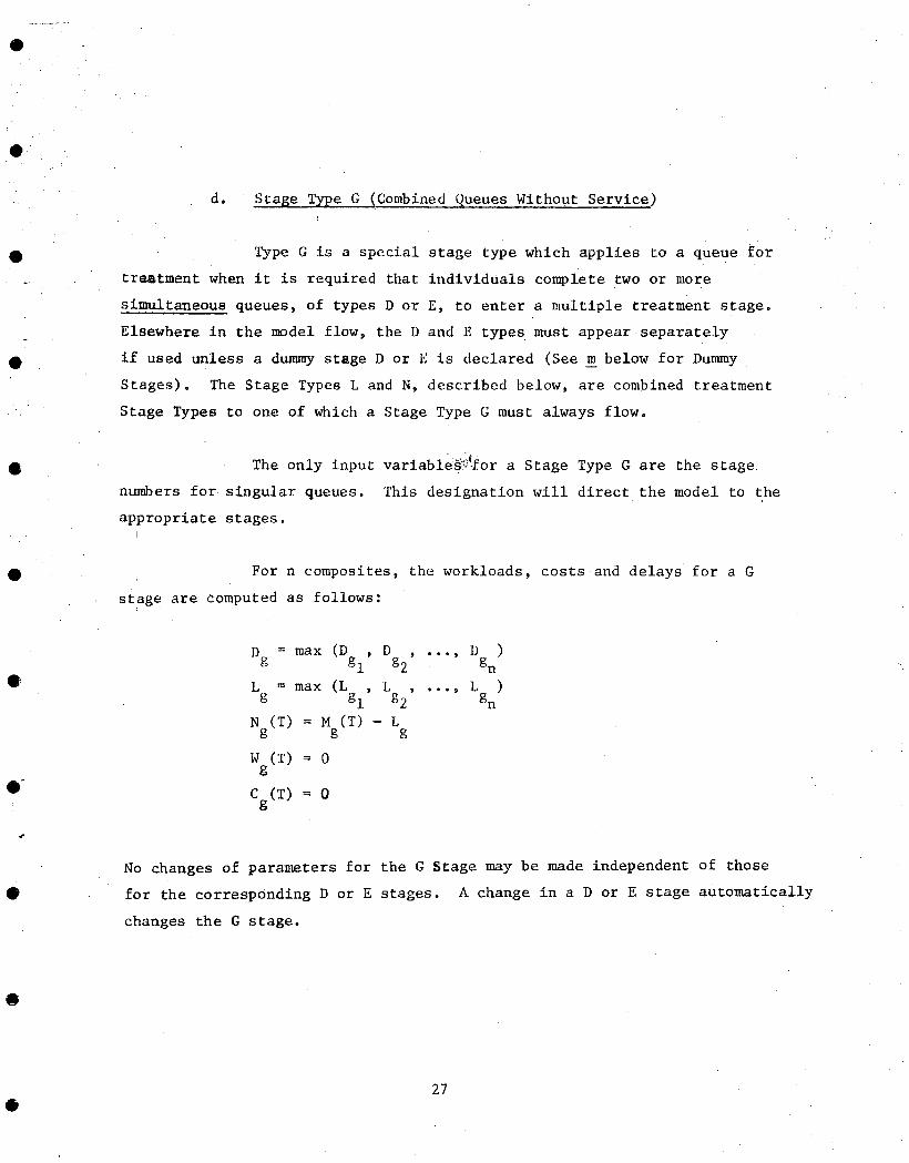
k. Stage Ty~es S and V (Reqidivism)
Types S and V are recidivism stages, final stages through
which an individual flows no further. Every allocation/treatment or control
group enters this type of stage or another exit stage, Type Z. The differ- •
ence between a type S and a ~ype V is that the type V allows recidivism
during treatment; S does not.
Two measures of program impact can be analyzed within the
DEMON structure: the number of future offenses and test score improvement.
The number of future offenses is assumed to be a function of the time
since treatment, while pre- and post-treatment test score differences are
not a function of time. The offense recidivism function assumes an increas-
ing probability of committing an obS,e!~ed offense as the time since an
individual underwent treatment increases. The measurement of any test
score improvement is done by comparing the results of a test that is ad-
ministered before and after treatment.
In DEMON, three types of offense recidivism and one type of
test score improvement may be modeled simultaneously and analyzed separately.
It is emphasized that the recidivism probabilities and test score changes
are assumed known based on the expected impact of the project under analysis.
These data can be treated as parameters , and sensitivity studies• on how the
program impact varies as •the parameters are arranged can be accomplished
readily by DEMON.
o Offense Recidivism
It is assumed that the time between successive violations are
distributed exponentially, fi(x) = n i e-nix, where fi(x) is the density function for the time between the (l - l)st and the i th offense. Thus, we have the mean parameter , for the time to the
H I i , for the time from the first to the second vio- first violation, -- rl 2
lation, etc. For this assumption, the probabilities Pn(t), n = 0, i, 2, ... are the probabilities of having n offenses in time t. We ex- amine the probabilities of 0, i, 2, 3, 4, 5 or more offenses in time t for the model:
33

Po(t) =/f(xl)~ 1
I xl>- I
Pl (t) =/f(x I) f(x 2) dx I dx 2 I x2>-- t - x I,
XlSt
0
0
0
P2(t) =/f(x I) f(x 2) f(x 3) dx I dx 2 dx 3
{ x3>_t- x I - x 2,
x2_< t - x I,
Xl.< t }
P3(t) =/f(x I) f(x 2) f(x 3) f(x 4) dx I dx 2 dx 3 dx 4
~- '~{ x4>_ t - x I - x 2 - x 3,
x 3 < t - x I - x 2,
x2_< t - x I
Xl-<~t }
P4(t) =ff(x I) f(x 2) f(x 3) f(x4) f(x 5) dx I dx 2 dx 3 dx 4
{ x5>__t - x I - x 2 - x 3 - x 4,
x4_<t - x I - x 2 - x 3,
x3_< t - x I - x 2,
x2<_ t - x I,
Xl< t}
P5(t) = 1 - Po(t) - Pl (t) - P2 (t) P3 (t) - P4 (t)"
@
0
34

• For a.type v, two sets of parameters may be used for a type of offense studied, •one set of recidivism probabilities while still under a •program, and another set after completion of the program. In this situation we let
Pn(t) =• probability of n violations by time t, considering treatment
qn(t) -- probability of n violations during treatment by time t, t<_ t I
r (t) = probability of n violations after treatment by time n
t, t >tl,
where t I is the length of treatment and q and r follow the same distribution as p. Below, p is derived using q and r°
By properties of the exponential distribution, we have
p~(t) = Ii 0 (t) , t~tl
0 (tl) r0 (t-tl)' t>tl
Pl(t) = ql(t~ , t< t I
q0(tl) r I (t, tl) + ql(tl) r 0 (t-tl), t>t I
P2(t) = l q2(t) t< t 1
q0(tl ) r2 (t-tl) + ql (tl) rl (t-tl) + q2 (tl) r0 (t-tl)'t >tl
or, in general we have
Pn(t) =
qn (t)
n
i = O
, t_<t I.
qi(tl) rn_i(t-tl) , t>t I
for n = O, i, 2, 3, 4, and
4
Ps(t ) = i=0 4
-~Pn (t)
i=O
, t_<t I
, t>t I
35

O
Fo~ a:Stage Type S (no recidivism during treatment), the data input for
offense type y are a time, ty s and a set of probabilities ~Ysn~tYs), n=o,
..., 4). Then pysn(tYs) is computed. For a Stage Type V (recidivism
possible while in treatment), the data for offense type y is a time UYv, set {qyvn(UYv), n=o, ..., 4}, a time, wy v, and a set (rYvn(WYv), n=o,
...4), and the whole set {pyvn(UYv + WYv), n=o, -.., 4) is computed,
O
• Probability Conversion
While the input probabilities must correspond to the input times, they need not reflect the actual treatment or tracking time. The user may input probability data for whatever time interval is ueed by the data source. The recidivism routines in DEMON will convert to actual treatment and track-
ing times for output.
Given an input time and input probabilities, first DEMON converts the input data to exponential parameters. For a Stage Type S, the time t and probabilities {pysn(t)) are converted to the exponential parameters H I, ~2, etc. For a Sta e T e V, the time u and probabilities [qY.m(u)~ are converted
g YP .L. w to during treatment parameters and time w and probabilities ~y_( ~ are con- verted to after treatment parameters. Now, the input data haveV~een converted to time-independent parameters. These parameters may then be used to compute
equations for~PYvn(t)} , as shown above, for any t.
As the actual solution for the integrals is lengthy and the conversion routine is complicated, a simplifying assumption was made on the parameters; i.e., the parameters for the second and further offenses for a given type
of violation are the same,
~I = nl; nn = n2' n~2.
With this simplifying assumption for offense recidivism, only the first two probabilities are required to solve for the exponential parameters. Only the probabilit~y equations need be replaced in DEMON if another re-
cidivism submodel would ever be desired. L ,
• Test Score Improvements
An optional input is to allow the recidivism routines to make calcu- lations of test score improvement. The input are probabilities of improve" ment in tests taken before and after treatment. The categories are:
(i) More than 25% better; (2) 20% to 25% better; (3) 15% to 20% better;
36

O
1 (5) (6>
10% to 20% better; 5% to 10% better; and, Noimprov~neht.
These input correspond to P0(t), Pl(t), P2(t), P3(t), P4(t) a~d P5(t) respectively for the offense recidivism. The individuals ta~ing these tests are presumed to be placed into one of the sixcategories in each exit stage. No calculations using the exponential distribution are made, as no time factor is included. The input probabilities are used directly for final calculations.
Number of Recidivists
Each data file has up to four types of recidivism categories--DWl Arrests, Crashes, Violations or Test Score Improvements. Probabilities for each correspond to a common time. If a type is not used in a data file, this type may not be studied with that data file. The probabilities of recidivating during the tracking time are computed by DEMON or, in the case of test scores, taken directly, and~ar,e:multiplied by the number of indivi- duals who entered the exit stage during the project operational time. These give the number of individuals who had 0, i, 2, 3, 4, 5 or more repeat offenses. These calculations are used for statistical testing.
O pro~ect Accountin 8
For a Stage Type S the individual is delayed for the project tracking time, S. In this stage all who have completed treatment or control stages enter the exit stage and are finally "captured" as Ns(T)o The computations are as follows:
D = S (tracking time) S
L =0 S
Ns(T) = Ms(T )
Ws(T) = Ns(T) [ats]
Cs(T) = Ws(T)Cs
The calculations for a Stage Type V are exactly the same.
37

i. Stage Ty2e Z (Dropout Exit)
Type Z is a stage representing an exit from the system under.
study. This is used to represent individuals who violate the rules, are.
diverted from or do not qualify for a particular type of treatment and are
not tracked. There are no delays, work or costs associated with this stage;
it simply counts individuals. The computations are as foll0ws:
D h = 0
Lh= 0
N h(T) = M h(T)
Wh¢ ) ° o
%Cr) .= o.
The costs and work required for treatment of these individuals are counted
in previous stages; costs and work in the previous stages are counted as if
the individual completed treatment.
Interactive changes are made as for a Stage Type Sand both
setsof time-dependent probabilities may be changed' independent of one
another. After the computations resulting in one set of probabilities the
D , Lv, Nv(t), Wv(T) and C (T) computations are the same as for a Stage Type S V V
m. Dummy Stages
The previously mentioned combined stages--G, H, L or N have
the property of only being able to be changed by changing one or all of ~the
component stages--types D, E, A, K or M. This property is useful for demon-
stration projects because of balancing treatments. Occasionally one wishes
to add a treatment, combined with others which is not represented elsewhere in
the flow. This is accomplished by declaring a dum~y stage which can be a
D, E, A, K or M and is denoted by a stage number greater than 80. A dummy
stage is not in the flow but is called by a combined stage, which is in
the flow.
38

!
• ••• Another use is to allow an experiment to be designed to be
• • unbalanced, unbalanced in the sense of having a stage in a combined modality
• that has the same structure as one represented elsewhere alone, but can be
changed within the combined modality, independent of its separate counter-
part. An extra dummy stage may be kept separate if one wishes to introduce
• i this variation.
3. Stase Linkage
Summarizing the above stage descriptions, certain linkage rules
are given as follows:
Stage Sequence--Exit stages cannot be followedby other stages;•treatment and queuing stages must be followed by other stages. Permissible order is given below
- Stage Types A, H, J, K, L - may be followed by any
stage other than Stage Type V
- Stage Types D, E, G - may only be followed by Stage
Types K, L, M or N
- Stage Types M, N - may only be followed by Stage
Types V or Z
- Stage Types S, V, Z - may not be followed°
A data file which violates one of these requirements will
not be accepted by DEMON.
O
Treatment Time--The treatment time variable, atx, in queues • without service (Stage Types D or E) should have an inPut• value which coincides with that of the treatment time variable in the next stage. The treatment time variable for M or N stages will be used for calculations of during treatment recidivism in the next stage, if the next stage
is a recidivism Stage Type S.
Combined Stages--Stage Types G, H, L and N are combined stages and take variable valuesfrom other stages.
39

O
below.
Other model features which involve stage linkage are described
B
Svstem Flows--In the model, every stage has flow into it. Of particular importance is the system flow to stage number i, the flow to the total system. This is the only data file flow input. Flow to all Other stages are computed based on this initial flow and input branching ratios. A change in flow to one stage will affect others, and changes in flow to all stages are made immediately upon change of one stage and according to the branching ratios allocated. For any stage changed, then, the flow will be increased or decreased in other stages to maintain the ratios.
Branching Ratios--All stages except exit Stage Types S, V and Z have branching ratios, i.e., probabilities of transfer to succeeding stages. Two or more stages may not branch to the same stage and branching is from a lower numbered stage to a higher one. For a data file already made, new branches may not be added but probabilities may be changed. A branch may be eliminated by assigning a probability value of zero. If the user wishes to add.or delete a stage, it is best to make a new data file. If input branching probabilities do not sum to one, the program normalizes input accordingly, so that resultant probabilities of bramching out of a stage sum to one.
Groupings--Data files may be prepared which use the grouPing feature of the model. Using this feature, the system flows are partitioned into various groups. Each group has its own flow that sums to the total flow for that stage. Each cate- gory has its own set of branching ratios at each stage and the flow is split accordingly, but costs and types of stages are identical and workers are shared among the groups. No differences in recidivism can be identified by groups. The primary use for this feature is to assign varying probabi!ities of being identified, e.g., as a problem drinker or as a treat- ment dropout according to the demographic grouping.
Queues--Every queueing stage has certain parameters which determine the speed of service and number of individuals Who can be handled. If the flow rate into a queue is too large i.e., if the queue will increase indefinitely ~ DEMON will stop proCessing and indicate to the user that a parameter change is necessary.
40

!
.
o Target Group Generator--The user is given the option to de- lineate'the total population of an area into a target group (e.g•o9 DWI arrests shown on Figure i)° These delineation stages are unnun~eredand precede stage i. If the last stage in the target group generator, i.e., the stage that feeds directly into stage 1 does not indicate enough individuals to be obtained for project evaluation, DEMON will not continue This shortage will occur if the system flow rate to stage 1 times •the project operational time T is greater than the number of remaining in the population in the last stage in thetarget group generator.
Speciflc data items required to define a flow are listed below:
e Total population, subpopulation delineation to reach the target group, stage i generator.
o Time unit used for all•d~t~a variables (e.g., work day, work week, Work month).
o Numerical ordering of stages, stage names and Stage Type identification.
• Project operational time.
• Tracking time.
Branching ratios, groupings and identification of succeeding stages (non-exit stages only).
O Other input by stage:
Types A & D
Type E
-io Actual treatment (service) time (at or atl)
Q 2o Number of workers (k or k=) 3. Workers wages (c or c=) 4. Worker:availability (av~ or av d)
-I. 2. 3. 4. 5.
Number of individuals pe r group (ge) Number of workers (k) Number of groups per~worker (w) Time interval between assignments (ite) Length of treatment (ire)
41

C,
Types K & M
Type G, H, L, N
Types S & V
Types J & Z
--i. 2. 3.
4. 5.
-i. -n.
Actual treatment (service) time (at~ or at m) Number of individmals per group (gkL'org m) Workers' wages (c k or Cm ) Length of treatment (it k or it m) Fees paid per individuaI (fk 0r fm )
Stage numbers of n component stages
-i. Actual treatment (tracking) time (at or at )
V 2. Wor~ers wages (c or c v) 3. Identification o~ types of recidivism
used and times and probabilities.
No further input.
Post~rooessing Routine to Evaluate Impact
Statistical routines were added to DEMON to aid in analyzing, in a
statistical sense, any project impact implied by the recidivism and test
score calculations. ~ ~is commonly involves a question of sample size, and
for a Demonstration Project, the sample size is a major determiner of cost.
The cost Of processing the model derived sample size is a standard DEMON
output. The question is, "Does the given project sample size meet statis-
tical criteria--i.e., allow us to make statements Of statistical significance
concerning the results of the recidivism and test score computations?" More
precisely, "Can a reduction in recidivism be detected when a relatively
small portion of the sample can be expected to repeat violations in a typical
1-2 year tracking period?" Sample size requirements tend to be large in
this type of situation.
A typical situation involves experimental and control groups. Both
groups' traffic records are monitored for a fixed length of time to deter-
m~ne future traffic accidents, future drunk driving arrests, etc. The
objective is to measure differences in future behavior with respect to each
such offense, experimental versus control. Thus, for one type of offense,
data might appear as follows:
42

Number Offenses of a Certain T~pe
0
i:
2
3
4
5 o r m o r e
Total
.Experimental
X 0
X 1
X 2
X 3
X 4
X 5
X
Control
V
x0 I
x 1 'V
x 2 !
X 3
X 4 I
X 5
x
where Xi = number of individuals in the experimental group who had i
offenses of a certain type•during the fixed time of traffic record •
monitoring and similarly, X~ for controls.
• k
The interest is to determfne whether or not there are differences
in the number of offenses which result from individuals in each group--
~hat is, whether the mean number of offenses in the experimental group
is lower than the mean of the control group, e.g., the experimental
mean is less than 80 percent of the control mean. Similarly, a test that
the proportion (rather than the mean) in the no offense category is
increased is of value.
In studying test scores, the test • score improvement-->25%, 20-25%~
15-20%, 10-15%, 5-i0%j 5%--is examined instead of 0, i, 2, 3, 4, 5 or
more offenses, testing for differences in percent mmprovement or for
difference in maximum improvement (>25%).
43

. Notation
The following definitions are made:
For Experimental Group
x i j
M
i i xij
= Number of individuals having i offenses of type j
= Number of individuals tested
= Mean number of j type offenses*
= m Xj = True mean number of J type offenses (input parameter, not to be calculated)
oJ M
8j = E Xej
2 i i 2 _ ~2 Sj = ~ ~ Xij j
i - 1
= Proportion of non-offenders
= True proportion of non-offenders (input parameter, not to be calculated)
= Sample variance for the number of offenses
5 or more is assigned 5, with little anticipated loss of accuracy.
For test scores, Xij is the number of individuals in each category
i X. is the mean percent test score reduction and v ~j~ is the P 3 proportion
of those who had maximum improvement of~25%, for J the "test score offense."
The proportion is still computed as Xoj/M. For this case, the mean is
computed differently:
(.25 Xoj + .20 XIj + .15 X2j + .i0 X3j + .05 X4j + 0 X5j)/M.
44

Q
• 7
Q For the Control Group.
X ! l j
N t
M'
N -- i x i :
i=l
~' = EX 3 3
X |o =Xo~
o3 M
O~ = E Xoj
= Number of individuals having i
offenses of type j
= Maximum number of offenses
= Number of individuals tested
= Mean number of j type offenses*
= True mean number of j type offenses (input paramete~ not to be calculated)
= Proportion of non-offenders
= True proportion of non-offenders (input parameterln0t to be calculated)
N '$2'= 1 ~ i 2 -- 2 3 M Xij - Xj
i=l
= Sample variance for the number of
offenses
General
1 - ~
z(w)
= Test size (level of significance), i.e,, P {rej H[H~ = =
- Test power, i.eo, P {rej Hlalt} = i- B will depend on the particular alternative.
= The W percentile of a standard normal, i°eo,
z (w)
I - -- - ! - - e "t212 _ ® ¢ ' ~ ' -
i19~
dt = W
45

2 ,; Bypoghesls Testling
In the following it is assumed that all testing, power deter-
mination, and sample sizing will be done separately for each offense
type J. The primary hypotheses are
H I ~ 8j = 8~ (Proportion Hypothesis)
or
H 2 : Uj = ~' (Mean Hypothesis) J
The primary interest for demonstration projects is in one-slded tests.
However, several variations of the primary hypotheses and associated
alternatives may be investigated, such as
< 8 vs 8j> 0j 3
Note that for these variations of H 1 (also H 2) and alternatives,
the test ~ statistic remains the same. DEMON only prints the value of
the appropriate statistic. The user can then choose a critical level,
test variation, and only a simple table (Normal) look up is required.
The procedure then is to compute, for H 1 type hypotheses
Z I
X' oJ - xoj
(i- Xo/- Xoj ( l - Xo ) o3 -_ +
M' M
and for H 2 type hypotheses
Z 2
+i_ M'
Both Z 1 and Z 2 are assumed Normal for M, M'>_50. Note that the
numerators are set up for a one-sided test to the left; i.e., negative
values for both Z l, Z 2 indicate an improvement in the experimental group.
46

3. ,size and Power
For discussion purposes consider the H 2 type hypotheses. Suppose
that an e level test is required, and that it is one-sided. The samples
are collected so that M, M', etCo are known° From the preceding section
P {rejecting H2IH 2 }
I - } P ~ - x! _1 <_ z(c , ) =
M'
' andboth To find the power 1 - B for an alternative where ~j # ~j
are specified, theexpresslon is .~..¢~ J
P {reJ H 2 ]yj. y$, B # B~ }= • J 3
P ~ -x~
• ~/..S~.~ S'2 + J--
M w
s z ( a ) , ~ # ~ ' . ~j, ~j, j J
I, -.~) xj-x~- % . . . . . _ ~ _ _<
I I 1 , 2 " ,2 S S
M "I" M'
z (~) ("j - v.j)
~M ~ S'2 _D__ + M'
P I _h~ 1 z _< z (~) -
s~4 s~ 2 ._9__ + M'
= 1-8
47

All terms on the right of the inequality above are known, so that the
probaSillty 1 8 can be read directly from the normal density tables.
an assumption was made that S~ - and $42 are true variances. This But~
assUmption is routinely made for sample sizes of 30 or more, and in this
case, when M, M'>I00 the resulting error can be ignored.
From the above equation the relatively simple exgression
= z (i- =) + z (I- S)
iS derived which is the final form required. If all terms on the left
side are given and ~ is specified, a table look up only is required
(or calculation) for Z (l - ~ and then the power may be computed directly.
To find the required sample size for a given power, set M = a M'
(where a is the ratio of the experimental to control group size and is
given by the user) in order to have an equation with only one unknown,
and solve the last equation for sample size.
For H I type hypotheses, the procedure is exactly the same,
oStaining
0'. - 0 . _ J 3 _
, . . - ,
= Z(l- =) + z (! - S)
The above derivations are based on a one-slded test. A~two-sided test
approach follows almost trlvally by doubling ~ and taking absolute
values of the left sides of the two equations above.
I 48

O • • / <• •
O
4. Statlstlcal•Tests
The user will first specify the offense type to be analyzed.
Then~ the hypothesis to be tested is selected, either H 1 or H2o Next,
t~ere are three questions to be answered:
i° Is the observed difference significant;• i.ei, what is found in a test of the selected hypothesis?
2. What is the power of the test for a specified alternative?
3. What sample size would be required to achieve a given (input specified) test power?
• To meet these objectives the following routine was derived.
First the values .-.
{ } - - S 2 (experimental) Xij ,M~Xj,Xoj~ J
I 1 -- ~ -- I X' ' ij ~ M'~ Xj ~Xoj ~S 3 (control)
are computed and output • for the users information. Next, according to
whether H 1 or H 2 is selectedp Z 1 or Z 2 (equations cited in B above) are
provided°
5. Comjputation of Test Power
To determine the test power for a specified alternative using
hypothesis type HI, the user specified values for
- The test level
• m
Oj - (Theoretical) expected value of Xoj
0j (Theoretical) expected value of X'. 03
and the equation cited in C above is solved for 1 - B, providing test
power as output.
49

Similarlyp to determine the test power for a specified alternative
under a type H2~ the followlng five parameters must be input specified:
- The~test level
pj - (Theoretical) expected value of X--j
2 Oj - (Theoretical) variance in the experimental group
p~ - (TheoreEical) expected value of X. J
O~ 2L (Theoretical) variance in the control group 3
and the equation cited in C above is solved to provide test power.
For example, for H2, one-slded, to find the power i - ~ given the
following input:
' = 5 : . 05 ~ J
2 : 3 o ! = 50 PJ a
2 ~ j = 50 M' = 100
M = 100
the computation
3 - 5
50 + io---6
z(.95) + z(z - 8)
2 = 1.65 + Z(I - ~)
• 35 = z(1 - B)
is made and the power determined
1 - ~ ~ .6368.
50

6. _C_omput.atlon_ of Sample. _Size
To determine sample size required for a specified alternative,
the user will specify
- The test level
8j - (Theoretical) expected value of XLj
8~ - (Theoretical) expected value Of x'. o3
1,8 - The desired test power L
a - Ratio desired, (Experimental Group Size)/(Control I ~. Group Size)
For H 2 type h y p o t h e s e s :
- The test level ;
~j - (Theoretical) expected Value of X--~
[
2 o. - (Theoretical) variance in the experimental =roun 3
~ - (Theoretical) expected value of X! J
~;2 _(Theoretical) variance in the control group
i-~ - The desired test power
a - Ratio desired, (Experimental Group Size)/(Contr01 Group Size).
r
Then H 1 and H 2 a r e so lved f o r M, and M' i s then o b t a i n e d by Solv ing
M' = aM. M is then the required sample size for the experimental group
and M w for control to detect differences in proportions (HI) or means
(H 2) to the extent specified by the theoretical values input~ !
w = 5 then the postulated reduction For example, if ~j = 3 and ~j i
is 2 offenses per person or 40 percent. The M, M' computed would be
the samples required to detect the 40 percent reduction for a given power.
51

0
( . .
0

Ill INTEI~ACT [VE SYSTEM
The model use is dependent on the data/files. A data file contains
the structure and all•parameters pertaining to a given project. The user
may use one of the files provided (see Volume IV)or createi~a new one (see !
Section IV of this volume). The file used is referred to as the base case
fileo For purposes of analysis, the user creates a test case by making
interactive changes to the base case. Then, comparisons, base to test may :
be made. Further, if desired, the test case may be saved as a new permanent
base case for future use.
i
• Only two routines are moderately "base case independent"--the pre-
processing enforcement routine and•the post-processing statistical testing
routine. For these, data may be input or evaluated which aye contradictory
or extraneous to the base case data file material.
test case material may, of course, also be used.
is base case•dependent. •
J Base case or current
The main modeling • routine
t
As mentioned previously, one project involving Citizens Band Radio
is a totally separate routine and, while it operates under the same inter-
active system as the flow models, it is not discussed inthis volume.
The following sections serve as a user's guide, describing the series
of steps that a user must take to access DEMON, input data and produce out-
put.
A. System Access
First, the user checks the terminal settings. They should be 30CPS,
Half Duplex, On-Line, Terminal-On. Next, the proper NIH computer telephone
number for the terminal in use is dialed. An entire list of telephone
numbers is given in the front of the NIH Computer Users' Guide, but an
53

abbreviation of system TSO numbers is:
(301) 654-8610 (301) 654-8514 (301) 652-6451
for Trl~'s for IBM 2741's for 1200 Baud
The user should hear a high-pitched tone when the connection has been
established, at which time the phone is placed into the acoustic coupler.
Thecarrier light shouldgo on. The user hits two carriage returns to get
the attention of the computer, which replies:
'ENTER LOGON'.
The user responds:
' logon accoun/>->Lni tia Is~ termir~ l-id/box-number '
After sending system messages, TSO will send its herald,
' READY' o
Any time the user sees this herald, it means that TSO is waiting for a
command. The command to initiate the program execution procedure is
'ex demon2'
O
Users having difficulty with the above procedures should call the NIH PAL
Unit at (301) 496-5525 for assistance.
First the user will be given an option to use the Citizens Band Radio
simulation model, then to compute increased enforcement effects, and then to
analyze a treatment program.
The first option, to use the Citizens Band simulation model, is documented
in Volume llI.
54
I

O
B. Enforcement
In the DWI Enforcement (:omputations, two areas of a jurisdiction having
similar characteristics, called Area A and Area B, are selected° A task
force of officers is first assigned to Area A to increase DWI surveillance
and. apprehensiono This effort is supplemented by an intensive public
~information campaign° The task force then moves to Area B, •repeating •
the procedure° Each activity, Phase I (in Area A), Phase II (in Area B)
is conducted for the same length of time.
:; l l If the user does not want to use the Citizen Band Radio model
'and does want .to compute enforcement effects, the answer is "N" for No on
the former and. "Y" for Yes on the latter° Having indicated "Y" to enforce-
mentD five cat'egories of 27 parameters are first identified. ,j:; • _
i : 'i
ID9 '•,'.qLl-MqH] • T] ,.i-:= T~4~ ,T:ITI?F~~7 f:qHD ='qDIU !.:I~'ILIL.~TI~H ~'I.DI-mL ~" I
. "f" , o
[i:-"l "f'O'.l ',lC'l"/T T ~ ,-:_r'lr"ll:::'llT~ I"-.I ,-:r- '~'cl-:E[i E H c r ' 3 ~ . ' l r ' : E M = H T I E r : - ~ ' ~ ' . T ~ 7
I
~]'~.". . . :T, 27' r:"Hq'c-1~4CTE~'~" W I : i ' T =.:~ ~ : r : - 'EC : ] c ' ]E [ I .
1 • ~'O~"UL q T I rJN, 3'. D-~ T ~- ~'~'_~ H,TI E .'7,. ~C.L'; I rl.r~ N T F..' ~.i 1 F -:
. Population Parameters
There are four •parameters in the first category of Populatlono
.. i
55
"7
+./ . •

MHr~T IS : T N E t I L I M B E P ~ O P LIr:Erq3:ED DreIVEE"_',: I N qr,.'ECt :~?
;.;ooo .MH~T 13: T~4E P~'Dr-'DF,.'TI,rlr4 FIF- t. ICENSED D~.'I',/E=.''.,.: IN c. T~IT D.=.!}HK ~riD DPIVE?
:'5 h~HRT I ; THE NUtIBEP OF LIC:EN'-..:ED D4'IVEP.S IN R~'E~ £:?
6 ~:: r.i 0 O . . .
I,IH#iT I."..' THE PP.OPO~.'TI-rlN ~ r L I,_":EH'SED DRIVERS IN £: THRT [Ir~lN~::" RND DRIVE?"
. 5
To input the number desired after each question, wait for ...~ input the
number and hit the carriage return which will signal the computer that input
is complete. There are built in checks for data limits, and error messages
will appear if ~he input data is incorrect. For example, the proportion
Eust be between 0 and ! for the questions above°
2. Deterrence Parameters
There are eight parameters in the second category of Deterrence.
2 ; DETERRENCE P F ~ M E T E ~
tJ'-l~T I~ THE MAXIMUM =)~,rJ~DQTION O E THE r~OPUL~ITIQM IN a~:E~l FI WHICH CAN BE DETERr~ED WITH ET4Eor~.':EMEMT FIND ]t4EO~'M~TIOM C~IM~FIIL~N.~: ~IMD ~IT klH~IT TIME (IM I,IEEKS~ MILL THI:~ MqXIMU~ DEIER~EIICE .qCCUR?
~clH~l |~; THE MA'~.IMLIM ~oPrJ~'TIO~I r j r THE DEI~ULATIEPI l!~ fl~EA B '~I~IICH CRhl BE ~ DETEI~ED WITH Er~cO~CEMEI~IT ~l la ]f4cO~'M~TII]M CAM~r~I6t, I~ ~l~lD l~T *~H~T TIME ( I M '~EEK~', WILL THI~.: M~IX1MLIM DETEP~ENCE OCCUr'?
• i5,5_~"
MH~T I ; T~E M~".tlM~ M Pe~o~¢'Tlrlr,l 0 c THE P~ULCITInN ~M ~II;'E~ ~I ~,IHICH ,.':-~N BE D E T E ~ F D ~,l|Tl.I Dt4LY ,at4 I~I;CI~M~TIO,~ C~,4~IG~t qMD ,:IT ~,~H~IT TIME ( I N ~EEI(~) MILL THI~ M~'KIMLIM DETEr~eEFI".:E [}1~1:31~?
• O'.:t, 7~3.
'aH-~T--l~ THE 'M~'r<i'4LIM #r~rjoor.'Tlgt4 rj¢ THE ~J#LIL~TIhN IM ~'leEr-I B I~IHICHCClN BE [JETF~tQED ~,IlTH Ot4LY cI~4 I~lrOCtM~ITION r.:gMP~Ir~I ~FI[~ FIT hIHClT TIME (IM ~4EEK~.) *dILL THl~ M~"KIMUM DETE{'~'E~IC:E rJCC *Q?
,) '3 , '7 '~1.
56

• ..
. L" L,
J
These parameters are input in series, separated by a comma. Specific units
requlred will be indicated. For example, the time units above must be in
weeks°
3. Accident RatsParameters
.
The~e are eight pm~ameters in the third categorY of Accident Rates.
3 . Iq,>-IDE,. tT ~,r-ITE v'c.I~.'q,qETEP-:
='!.EQ-:~ I"t'-'LIT TNc ~'FJLLOqlIr-.I,S 4 .A,-:r:IDENI" c'ATE-, c'.'3=' Cl?Eq q : | . ,:t,-:.':IToEt;I~: " E P ? 3 ' 4 [ ~ A ? r:U? H_q;~-D='ItI~:'-/P,- ? . q r r l D E , ~ T 3 : ~F~'~r3~'~ , ~ q s' or3? r~ETEOOE.I~ Dc'IH,:-_EP. 3: . -:. ,~,':,-:T3E'IT?":'EP'-..O"~","'-.-q~' ~-~' ~~O '4-9'-'--TEc'c'ED r-~'- i"~:EP:: :.,IITH ' i g q~'PE~'T3:
• °
. , ' ; 7 , . . ~ , . ~ , 1 . . : . ' ~ , • ' ) 1 .
:'LE~3:F Ir-4mlT TWE c~'..L[I',ITN":, 4 q,Z:L-'.Ir_~Er4T ~'-qTEZ..: c~]R qC'.EA B: I . "~:L'-:I.']E t*T-.''pFK'':-':qN'''Eqc'' r:"O~' Mq'N-Dc'It'Ik'E~"-" ?. qq,-:iT~=.~.iI-:.v.,-_p:.91..,,.,~qc. '-'~c~ D'--.TEP~'ED 9~'Ir l ~:~~'~ 3. ~4?,-:lqEtiT-:...PFF..,-:.Fl,.i.'.,.'Fq~, ~Do H.7]'4-r~r-TE.~'pEri rJ~':Ir'4~zEF<£ ! , I ITH ".1'3 cI~'RE3:T~: '4, r~.](:IOEP.4T.]:,¢.Eq.T:Dr.4,"HEq~,' ~.q~: H3"4-~ETEP~'ED T.+~:I~4L::.E~'% '.,IITH q~:REST'.:
9";',, I 59, 1 • 22-", . 9 4
Enforcement Parameters
There are five parameters in the fourth category of Enforcement.
4. .r.- N= f]~'CEM= NT ~ ;It.' q"l E T E ~' "..-:
I,.INqT "IT.: TN~ , - ' JpP~r.4T NLIt,I~',~ ' D c Tq~>K =Oq"2:E uMIT".:"?
• o
:-.:
~..q,,I ,"4e4r.4y rlPlNF.'.'lr4,.~ Dq'IVEP'3: PE~. ' NUt.~.' ,-:~rt T H E IF4":-:K pr lp . , -E OE".:E~",.'E'7
] ,:j
; , I ~ T 1~: TNE F.:O..?.'.IH'S ~ATE (q~'C'E'.'.:TEE'_~: "E~'. N O . I m : , 7
. 7
HD+,.I rq~t.+y N,.q. I="-" P=~' ~IE~+:' DOE'S: E~,.'.:N TF~ .--. !.-.[ ';: 'r]P-E I D~'+("?
16
MN,ZlT I "-..: THE PRCI.IE'_':T ,.']PEPQTIrJ,.'"I~L T I M E Ir-.I I..tEE~f";.: <~O~.? ¢'Nq"-._-.E5: I c-tr'ID 1 ] " , 7
t :3 0
57

'-, . -, -.- ,
: •
,, , •
5. Cost Parameters
There are two cost parameters to be specified.
5. ,1: O _T-" T P' A ~' r4 !4 E T E R ~
t,l,-l~T i':.'.: TLIE E:3:TIt'I~:TED ,-:.q-!T TO S:,~,::IET'Y' P'E~ q,:]iI ')ENT?'
15000 '
:MH,~T ]"_:.: TNE HrJ~]~.'L'y' C:O..::T OP THE T~I".-:K =E]g:CE LIDIIT".,
i
After all 27 parameters have been initially identified, the user
is given the option to change any.of the parameters. I •
I'IB ~/rll.iI I,I¢4NT TO -'HtaN';= . . . . . . . . . . . . AN'Y' ..rlF TME PAP~MPT~ ' : : ' ; '
,.#,
PA~F4MF TF_ P T'v'F'E :'z..:: I. PrlF') !I A T l Elr-I ,?. DE1 F. P~'FNC:E 3. Rc:r: I DFNT P~TF"..' 4, ENP-[IPC:FMFNT "5. r: rl ..-.: T ~:
ENTER bF~IPFD F'ADRMFTFP T"/F'F
4P
If the user had wanted to change a :parameter, he would have
entered a parameter type number from i to 5. A list of th e current Parameter
values would.~E displayed and he would, be requested to enter the new de-
sired value. An asterisk (*) indicates that no change is desired.
.
quested:
Enforcement Output
The enforcement output is given when no further changes are re-
58

>
/
H ~
@
EM~O~CEMEMT OUTPUT
P H A ~ E F'H~•~E 2 R B" R B
NUMBER DETE~ED 3397 1443 2934 4419 NO. TA~.FO~CE q ~ . ~09~ - . . . . - - - ~009 TS;~ FO~'CE HO~.l~'~ I | 5 5 0 ° 0 . . . . . . . . | 1 5 ~ 0 . 0
T A ~ ~O~¢E C:O~T~ 507360. '00 . . . . . 207'3~0.00 NOND~ 1 ~E~ C~:HFS 9:3~ 6 9'916 3~I 8 3:316 DETI D~f4KER CRA~HE~ 9469 ~474 ~894 451~ DPN~CN,~ NO A~&. C~A'~H 575| 5 63466 60529 55054 TS~k' ~O~CF AR R C~8~H 8~0 . . . . 9~0
CONTROL
3~16 ___~
66519.
TOTAL CRA';HE~ '~ 65317 68756 67239 64505 70329 ~O.~T ~ g V I N ~ 74~7~64(I° 295949'92. 46350000. 91697635° TOTSL. ~V|N,3~ = $ 236615264,
Theltable. shows project performance (number of people deterred,
number of arr4sts D, costs, crashes~ etCo) for each of the two areas, Area A
and Area Bp during Phase 1 and Phase 2, and compares these with a Control r
(no increased.enforcement in Area A,o~.~).
Nex(, the user may specify a rerun code to either continue to
work with the ienforcement routlne9 to analyze a program, or end the computer
session.
B
381&
6651'9
?0959
C°
'RERUN CODE~ ~ E : I =tCHqN';E E4~DRC:EMEMT ~A~METER~
i
=;AN~LYZE.A TREATMENT P~OG~AM CA~['IA,3E RETURN = EM9 P~O,3~AM
[
Treatment Programs
i. Retrieving Data Files
DEMON relies on a previously created data file to describe the
demonstration projects° To remain flexiSle~ the data file is not associated
with the program at the time the program files are being a11ocated. Rather~
59

:theuser is prompted interac=ively to enter the file name Of the data
file robe examined. In thi~ way, the user may, at one session, analyze
any number of ~ifferent projc~ct data files by DEMON.
There are two dlff#rent types of data files used for DEMON: a
Readable Data!Flle and a Binary Data File. A Readable Data File has the
advantageof ~elng readable by both manana machine, but the disadvantages
are that it is slower, thus more costly, and It is a Valid format for a
base Case only. A test case which is read in must be in the Binary Data
A File format, test case which is derived interactively from the base
case has no such requirement, of course. The advantages of the Binary
Data Flle format are that it is a •valid format for both the base and test
case and it •is a faster and thus less expensive form of input/output; !
however, it i s not readableby man. I
At ~he beginning of execution, the user and DEMON have the fol-
lowing conver@ation: , -
i
EX DEM~M~ I
,JEL OME i
I
DO ~D'J ,,IA~T TO 'J~E T~4E CITI~EN~ BqtlD RqDI~ ~IMULqTIDN MODEL? , ee I , . ,
N •i
DO VOLI bl~'IT TO CD'4~UTE I~C:e~R~D EMcO~CEMEMT EFFECTS?
.-. t
YQU M~'¢ tlg',l qttqL'f~E ~ T~ERTME,tT D~OG~M FHTE~ B~:~ 9q~:~ ~IL•E'HqME O@DBq. DqTq
DEMON will search for the data flle named PROBA.DATA , associate
it with logical unit i, ~ and read in the data as the base case (see;Appendlx
A, Volume III for PROBA.DATA project flow diagram and data files; See also •
Figure i). All files reside on disk pack FILE16. The most common errors
that can occur in thls allocation are as foll0ws:
"e
O
60

E r r o r C o d e Exploration
10
1 2 ¸
I
320 I
20 I I
r i
File in Use°
File Not Found° Check spelling of filename or residence on FILEI6o
Bad Data Set Name. Too many or invalid characters in data set name.
Another file iscurrently associated with this logical unit number°
For a more co, fete llst, the user is directed to NIH documentation.
I
After the base case has been initialized by reading in the data
file, D~ON a~ks
DD 'fD'J '~IG~T TD ~E~I TE2T 'I:~:E =~DH ~ = I L E ?
I
I A tNO w response would cause the test case to be initialized identical to
the base case. A 'YES' response would cause DEMON to prompt the user for
a file name of a file previously saved interactively. Thus, the file would P
have to be a Binary Data File that is compatible with the base case speci-
fied~ and must also reside on FILEI6o By a compatible data file, it is
meant that the file must have the same number of population groups and
stages, the same flowpaths~ and same stage types. The branching ratios and
stage data may be different.
The input data file is closed and released immediately after having
been read, thus freeing logical unit 1 for future input or output assign~
ments.
2. Groupings
A data file may contain more than one demographic grouping of the
target population. If such is the case, the user is asked if he wishes to
61

, ' , , ,
• ;~,. ,,. i:i .~ • .
i
see the groupings. This listing is a good reference for fu'ture possible
changes of branching ratios and system flow~which are.group dependent.
Following is an example of such a listing: '
I L,r..1 I','E'III ',l~rIT To ~:EI[ -,.~'8,.IP~.:;
Y i l
~'O1,.I="~: PI'IP THT~ ;:'lie A~'E.* : . I !4~, [ : , I 4 -1 " . - : , LOM-MTDDLr "RO," IOI:~Ep.I,HTG~ ~:r:HO.rJL . . . . . . . . ° . .
2 M~LF, 14-19~oLOM-MIDDLF ~:O,T:IOFr:Dt4,CrJLLE,3E+ . . . .
3 ' MA!. E, 1 4 - 1 .~, M 1 DT'L E"I.IPPFI~ "~DI-: I .rJEr.:~t, H I I.~,l-I '_<:r.:H~_ 4 I MAI. E • 1 4 - 1 ~:~, M TTIDL .E-f IF'~'EI~ ".::L'IC l I]F. C.Or4, C...rJLLEGE+ 5 I N;l!. I : , 1 '9-~ '5, L OM-MT D[ILE ~r],-:l .rl. ECrJMo ~ l ,;~1 i:CHgrJL & I.M~IL E, | 9 - 2 . ~,, L riNI-M | [ iDLE ~.:~C l OEc:.rlH, r:OLL EGE+ 7 ' Mill. E , I c~_?~,, t4I DIlL E-I.tPc'.IE, r~ . ".,:rjr.: I [1Er .riM, H I GH ' ~.~C:HElrlL .9. I M¢.II ~ , 19-~5, Ml DDL F-I F'.PF~ ~:.rIC|E]E,.~I3N.,-:OL/E,3C+ 9 I~,=~:.E, 1 4 - 1 ? o L D ' d - M I . [ , D L E ,?.O.~IOECOr4,HIGH ;CHDOL
I 0 .~EMFIL F , t 4 - l ~ , LEII,I-M l DT=L E :~.~rJC: l OEC:O.~I • COLLEGE+ I I . I :EMAI.E, 1 4 - I ~ . , M ] D D L E - = I C ' P E ~ " [<O,: ]DEErI~I ,HIGH .~r.'HOriL 1~ !~IEM~!.E, I 4 - 1 9 o M T D D ! . E - , I ~ p E ~ ~..OC:IOECO~I,C~LLEGE.+ | 9 I FEMAL E, 19- ,~5 • I OI,I-M l DDLE .%0010ECrI!4, H IGH .~ .P.HEJOL 14 !FF. M A L E , I 9 - , ~ 5 , LOM-MTDDLF ~OCIoEcr I .~ , r :OLLEGE+ 15 ~F='M~ILE, IW-~5,MT[wDLF-UmpER ~:DcIrJEcrjH,HIGH S.-.HrjrjL 16 iFEMALF, 19-?5,MIrDLF-U~pF~ .~.rjr.;TOECOM, COLLE~E+
1
I
" - i i .
These groups can not be changed Interactlvely in a test case.
i
3. Changing the Test case . .
, , the test case data ;may be altered before producing output
and performing statistical analysis. The possible alterations of the test •
case have been grouped into • nine Categories called Data Types. The inter-
active sequence for each Data Type •proceeds as follows. At the first ]'evel
of program interaction , DEMON asks the user whether the current test data
set is to be changed or to be displayed for viewing. A 'yes' reply would
cause the program to enter the appropriate Data Type alteratio n routine,
which would lead to further questioning. A 'no' reply • would cause the
@
@
. • , •
62
• .?"
>
• . ...
/ '
, . .

...., .... . . . . . .
program to proceed to the first level of interaction for the next Data
Type. The Data Types are ordered as follows:
I. Target Group Generator 2. System Flows 3. Branching Ratios 4. ICosts
: 5. Time Intervals 6. Worklogds 7. .Recidivism 8. 'Tracking 9. I ProJect Life
I
I
The above sequence applies for zhe first time a user analyzes a particular
base and test ~ icase. After the first analysis has been completed, and if
a rerun code of 1 is entered, the Data Types are merely listed and the
user is asked to specify the number of the Data Type to be displayed or changed.
As long as analysis continues of the base and test case files, the most
recent change# are maintained in the test case.
a. Data Type i - Specification of Target Group Generator
r
X~e Target Group Generator is a visual representation de-
lineating thelflow of population arriving at the project target group.
When enterlng*data type i, the user is first given the option to view the
Target Group Generator° It is output* with the test case data, thus re- J
flecting any changes that might be made.
D.q "¢_rIu ,,I~,,~T TO ,::HAr'4,_~E or~ ~EE Tt4E TqP,3ET GR:'rIuP GE,~E~',FITO~ DATA?
Y
Note: All DEMON output is screen sized to 26 lines for CRT viewing. This means after each continuous output of 26 lines, DEMON output will stop until the user prompts with a carriage return.
63

TFtE:GET GRFILIP GEI".tERFITDR
- TOI '~L POPULATIIIr- . I - ,
@, 0 R Fo ra ro - - . . .
w
N rl N D P I . . . . . .:,.ER.-..
2 E: 0 0 0 0
[aR I '.,'E P :'-:: I
' .:-'-:28 0 0 0
m
w
w
. : - DRI',/R.S I.:IHD DF.:IttK -
- 2 4 8 0 0 0 -.
A ~;S TF] I PIERS:
8 0 0 0 0
m . I I
m
I N i I I A T E E:EAL T I N E
F' F'O L-: E'S :-: I N G
- , : ,
m
64
i :

O ~ . . "
The user is next asked if he wishes to change the target .
group generator data. If he' answers "yes", Target Group Generator data
codes, based on the data just displayed, are listed and the user may+make
changes by indicating the code number and the respective change in numeri-
cal value•
D3 '¢~U M~f lT Ta CHqf l , ;E T M E ' T ~ G E T GROU p GEMERRTOR D@T~? . o + l '
Tq~..~ET '.~;'.~I'.IP ' ;-- ' tqFg~TO& [ I ; ITq '-:ODES:: | • T'3TqI.. ~_rlDt L @T T g; t . ; r i :~000 _~ '1 q N il ~ l V F = 5: ~ ~ 9 0 0 rj .~ D ~ l './E ~'.~ 3.~'~, 0 0 0 .~ alP, :'.,: T'q I NE r,"~: ':~ O :." 0 ';! 5 I l l ' iVY. ' . ; ,,l;.lrJ .'['I~'TNI." .349,)i.'10
E~TE~' DF~: IRED B@T~ ":ODE t t , . l ~ S ~
5
ENTEm ,':N~'4'SE l~4 ~4LI'dE=:!,."~L '4~LLIE • I
~ T E ~ [F~ : I~ 'ED D~T~ CODE ~U~E:E{' + i
O
The asterisk i(*) indicates that no further data codes are of intere+st at
this time.
After the user has indicated that no additional changes in
data are desired in all nine phases, the program then checks the data
feasibilities for changes in the Target Group Generator. if a shortage
exists, an error message is displayed.
T':F':'"~'.':T ,;~'."ill: ' (;:H~r~';-tT.FI{;' r lqT,~ l ; : H ' ]T r~"I='~T'IE:LI:: . : , I ]T~ ~.:'I"3:TE~I :I...;O~,I
~3,99~I ~' ~::I."T.E "i-4'."1'1, [, ~:F '%='L".~TEI;' Tq;.l '1 5 1 4 " . "..:T'.:TEhl =L O',l TD ~T~'.~E 1 I~: ~ , ='E~. '~1~;_~:. ~'~,'[}.I.--.CT ['l'='=l::'"~Tl~r4¢'l!. T ]~ I c T.': I ~ G . ~,.Ik"':..,.
L ~ ; T .::T.'4,~F ~= T ~ , ; E T '3~'0'.1° '3Ert-c~'~T'~ "~'~ .rl,~|'./~"*..: I, l~g [I@]~L'. = -'9(11"1
65

' j •
- . ' -
• , • ,
In this example, the change made in the target group generator data has • . . .
• created a shortage, The population size as indicated by the target group
generator is tOO smali to meet system flow requirements. (2000 < 33 x i56).
The user is not allowed to • proceed until a change in data has
been made to correct the situation. The opportunity to change the data to
correct the shortage is provided:
1. P.H~t4,~g .~ '2EE D ~ T ~ 2 . ~.._=AD I H ~ /F•ST Cq~.:_ = =~.0~4 ~ P i L E • 3. ~Eqr, l,.l ,4_c1,1 E:c4~:E .~'.:= _'l=' U'..:E '::E: Dr< EM~rJ~,'EHEHT MrJI~*EL.~
, EtqTE~' ~'ErcUN CDDE
I
D~IT~4 TYF>E. c r j r j E ' . ; - : . I . TC~c'.,SET GRrJU~ ,3EHER.~TrJ~ ' 2 , ~ Y ~ T E M F! O,dS: ~ . E:~'At4,::H I r,l,3 r ~ q T 1 CI i,' • ,
4 . C:O~T~ 'B, T ! rqF. ! HT_=r;'V~L .~,. ~,IO~K L O~q~ 7 . REC:I I,I V I <~!¢ ca. TRFICKIH~ " 9 . ~.~.r'J.IE CT LICE
@
One of three changes may be made:
i.
.
.
The target group generator population may•be increased to meet the required group size
(at least 5148).
The system flow rate may be reduced (12 persons/week
or less). •
The project • operational time may be reduced
(60 weeks or less).
66 • . . • [

O
@
One of these changes is shown below:
Target Group Generator adjustment:
E'ITER DE~I~'E[~ DqTA TY='E 'q'_I"IBE~ • t
DgTQ TYPE I -";F'ECICICATI-qrl O= T Q~"3ET G~O'.IP '3EHE~ATOR
DO YOU '.IgNT Ig _~EE THE Tqg'.~ET G~O,I=' GE~E~:qTOR?
tl
T'=I~'GET ,.g~EILI" ,3ENEG:gTO~ Dc~T~I '.':DDES:
g P, S: T g I ~'1 u- !~' $ "-: 0 0 ') 0 5 D~'I',/~S: ',lqg D~'I"I~.,..~. '.::. " o q o
E' ITE~' DES:IK'E'[I l l g T g CZrjDE ~'I'~'.II"~E:~
5
'"E'.'4TE.~ c..'H':-It'I'.~E "T4 ~l MEc;:IC:~L ' 4qLUE
~20rJ
_rf'tTE~' _TI.I~'I~II~E[I l ' l qTq ,~rJD=_ NLI~'I't~EI~'I
0
="4T.== ' TIE'.,:I~'Erl l l g T q TY='E N'.I~I~:E~ '
b. Data Type 2 - Specification of Rate of Sjstem Flow
To change or see the rate of system flow, the user is asked
to 'ENTER STAGE NUMBER ~ INPUT TYPE CODE'. There are two possible input
type codes: Vl' and '2'. A 'i' indicates that the user will input an
absolute value and a '2' indicates that a relative or percentile value will
be input. A typical input format would be '5, i', indicating stage number
5 and input type code I. If working with a file containing more than one
67

i
/
demographic grouping, t~e user will be asked to indicate a group number
for each Stage number glven~ In response the user is given the current flow
rate per standard time unit,i stage number, stage name and group number, if
applicable. Cha~es to the data can then be made, by providing a new flow
rate (input code l) or apercentage increase (or decrease) of the existing
flow rate (input code 2). If the flow rate is changed for any Stage other i
than number l, new flow rates are assigned to all stages. Therefore, the
user should exercise caution with Data Type 2.
Follow~ng is an example using the file TYOUNG.DATA which
uses the groups feature (see Appendix C, Volume III for TYOUNG.DATA project
flow diagram and data files)
DO YI3=! MAHT TO CHHN~F OR' .~EF. THE Tr-.trvGET ~R'OU D GENEI~C.ITOR" DFtTFI?
- * o
N
~.q Yn l l ,=IRPIT TO CHRH~F O~' ~<EE THE R'RTE nit ~Y~:TEH F'LOkI'~:?
BFITi:I T'¢PF ? - *;PECllEIr.:RTIOPI rl~" R'RTE OF ¢~Y~TEPI FLOtd~
FNTER ~TnG. ¢ HUM'RER'.IHPUT TYPE CODE , .,
AB~OLi lTF F'LOI,I~: FOR ~TRGE 15 - MM7 PIP
EPITER GROUP HLIH]~ER
14 ' CURRENT FLOM OF ~ . 6 PER 14K$. FOR ~TRGE I 5 PIPIT PIP
" FPITER CHRPIGE • - ,
°
ENTER ~TRGE PILIPI.~ER, IPIPUT TYPE CODE . . e
, e
. • , -
~OR GROUP 14
In this phase, as in other phases, when the user has completed
changes for a glven stageor only wishes to view the data, an asterisk is
entered. If there is no further interest in the Data Type, an asterisk is
entered again.
i
/
68
'i . :
' ~,~' ~ i: • . "
®
0

C. Data Type 3 - Specification of Branchin~ Ratios
When entering this phase, the user is asked to input a stage
number for data to be displayed or changed. As in Data Type 2, if working
with a file containing more than one population group, the user will be
asked for a group number for each stage number indicated. The name of the
stage~ the names of the stages to which it flows and the associated branch-
ing ratios are printed for the user's information. The user is then asked
to 'ENTL~ CHANGE.' If no changes to that stage are desired, an asterisk v*',
is the correct response, leaving the data as they were. If a change is
desired, the new numerical values are interactively input~ The inputs are
probabilities, reading from top to bottom on the user information output.
All probabilities are input, in the same order, whether changed or not.
Actually, any numbers may be inpu~ bu~ if the probabilities of branch-
ing do not add to one, the program will normalize the input values according
to the ratios of data input, so that they sum to one.
Follo~ing is an example, again using the file TYOUNG.DATA with
g r o u p s ,
DI'J YrJLI WI{::INT Tn CH~H6E fIR ~EE BRFINCHIPIG RFITJ'I3S?
I IRT~ TYPE ~ - ~ P E C I F I C A T I O N DF B R A N C H I f f G R A T I O S
EFITF.• ~TFIKE FII.IMBEI~
ENTER 61~'Ol.Ip NI.IM~EI;,
.~TFtGE ] 5 - MM7 NP FOR GRrlLIP 12 GI;'BI.IP I t I . IM]~ ' 1 .P.U~'~'E.NT R~TIO~ F~[? .~.T~GE 15 MM7 NP POrTEnT T NP 1. O0 EHTER C.H~NGES • •
o
~r~E
69

The user will then be asked again to 'ENTER STAGE NUMBER'
and the procedure is repeatqd. When no further changes to Data Type 2
are desired, the user response to the request for a stage number is an
asterisk• Next, changes to another data type may be made.
d. Data Type 4 -. Specification of Costs
After indicating a desire to change or see costs, the user
is again asked to 'ENTER STAGE NUMBER.' Only certain stage types (A, D,
M, K, S, V) have cost information associated with them. If the user
enters a Stage number of an inappropriate stage type, DEMON answers
'PARAMETERS UNACCEPTABLE FOR THIS MODIFICATION' and asks for another
stage number, '~TER STAGE NUMBER'. When an acceptable stage number is
given, the current wages for the standard time unit associated with that
stage are prlnted. Any changes in the data are then requested. Next the
current fees per person for the stage are given (Stage Types K and M only)
and any changes are requested.
played•
For S and V type stages, a tracking cost per person is dis-
D3. ' , '3J ,i-~'~f TD ."Hc~'~:.~E D;~ ~EF ,'..q.~TS ?
Y
.Dgl~ T'I='E 4 - -'.,'='FCI~IC~TI0'4 D = CO.RTS
_="4TE~', ST~'.~F F4LI:',I~:EG'
!, C,J.~cEr~T ,,I~,'4FS .=D~ $:T~';- = [MTE~ N=o,I ~,I~GES
CU~eEMT =EF~ ' : 'Be .~T~IGE ENTE.~ MFIJ ¢'.=E~ • •
ENTER ST~I~- c MLIMB~R
@
15 SCHB3L ~
1 5 SCHOqtl NP
qRE '~ 2'.~9. O0 ='ER '~.KS.
This is an M stage In PROBA.DATA.
70

eo Data Type 5 Specification of Time Intervals
The first rec.uest made of the user is again to enter a stage
nu~ero The only acceptable stage types in this phase are A, D, E, K, M, S,
and V° Other stage types requested will result in the message Shown above
as in Data•Type 4o When an A or D type stage type is indicated by the User's
stage number~ DEMON will print the current time spent with worker. When a i
K or M stage type is indicated, DEMON will output both current time spent ••
with worker and current time spent in the stage. When an E stage type is
indicated, the current time between group assignments and the current time
spent with worker are displayed. For S or V type stages, a tracking time •
per person is displayed. Changes may be made for each item, separately°
DD YDLI ,~IAriT TO C:HQ!~,~F.~R ~EE TIME IMTERVqL~? a •
-,,.~
D~TFi TYPE 5 - _~:PE,-:IPlL-:.BTIDt~ flP TIME IMTERV~L-~
ENTFP..'_~TQGE N'.IMBEQ a o
5
C~LI~EDIT TIME ~PENT I" i STC~'.~E I~ I . 000 g~Ce.o ~'hITEP CH~r~,.~E e o
0
C:LI~'PFtiT TIME ~.PENT I,IITH I,ID~ER IS O. 005 v.,.IK.~. FtiTE"Q. ,.'.H~N,]E o o
O.
• ENTER '.~TFI,)E Htt~4BE~ > • •
.@
This is a K stage in PROBA.DATAo
71

@
f. Data Type 6 - Specification of Workload Data
The first request of the user is to enter a stage number.
The acceptable stage types for this phase are A, D, E, K, and M. Other
stage types will result in an unacceptable stage message. If an A or D
stage type is indicated, current number of servers and worker availability
are printed. If a K or M stage type is indicated, DEMON outputs the Current
number of individuals per group. If an E stage type is indicated, both
current number of groups per worker and current number of servers are pre,
sented. As in other Data Types, the user is glven a chan~e to make changes
in each data item.
@
."~fq T'lO£ G - ~..EC|CI'-':.~T|~} ~'I '.~= 'IO~'KLOq~.I PR~'R~ETER~
-'11.=.= ;.T,.~,~= ~,I!.IH~_¢'K, ..
" 1 ~ ' T i t T ' 4 ' l . l ~ F l ~ !~ll ~ I ~ I i . . , I ' , ' ID : . I , e4L~ : P E ! ~ G~'rJIJP r o l l . ' ~,T,.=IG=__ 2 0 - p l i ' r J l i q T l O r , I P | ~ .
. o
@
, ° e
This is an M type stage in PROBA.DATA.
g. Data Type 7 - S~ecification of Recidivism Parameters
The user is asked for a stage number. The only acceptable
stage types in this phase are S and V. Other stage types will result in
an unacceptable stage message. Stage type S has associated with it up to
4 se~s of 5 recidivism probabilities (not associated with treatment)while
stage type V has twice as many--those for during treatment and those for
after treatment. The sets of probabilities are: crash recidivism pr0b a-
bllities, DWI recidivism probabilities, violation recidivism probabilities,
and probabilities of test score improvement.
°°o 72

/
When a user has indicated a stage number
a series of questions are asked:
(a V in PROBA,DATA) ,
N'l ¢0:.1 hI;4HT TrJ CH::+HSE t]l;' ~V.'.V ~ 'ECIDIVISH ¢'~'~IHETER.~? ,~,"
~,.-'IT-.'I TyC'r" 7 . ~ O ~ C l C l C : q i l ~ q 9= C:DHpO~IEMT,-t q= ~ECIDIVITM
TJ.'] '/~l.I M~.t,,IT Trl C1.~,.4.:+= rF.. --EE C¢'":I-I-t + ( ' - " I D I ' I I ~ " I ='P,'r]F::.IgILITIE:"T' :." ~+l'C"~Ft'lt ,D'I~IN"~ tr, r.=~lMFHt TIME |'~: 4 . 0 0 bl~:~,. ?'J I : ' ! ' i 3 ~O~'=ITM~MT c~.gc:gl::lLITtC::-,: 0 . 9 3 7 ? 0 . 0 0 3 3 O. O90J ~T} '¢3'J '+~'+IT T~ CHg%SF TH ~ T I M E ; |+ .
D.'3 yg,.i W.-~,4T T~ CWq"I,~E THE Pq'L' I I~ABILITIE~?
";.'J:'r~ENT .a=TE@ T~'E~THEt,IT TIME I~ 1 9 0 . O0 Id~(.~+ q":TE c' T~E@T~ENT P~gE:~I: : ILITIEoSI, : 9.'.:lOG! 0.03.R0 0.0_~73 D"J YOU U~MT t.g CHA,~,;E THF"TI~M'E"~
;," D~ YEIU ~ -~T T~] CN~I ,~ " THE ~'.~.D~.RTLITIE~?
."I~I YI3'J ',I,:IMT TO CH~MGF D{P ;EE D',II RECIDIVI'~M PI~OB,aBILITIES? ,,-.. Y "CU~EMT DLI~INIG T~E~TMF!,IT TIME I$ 4 . 0 0 Wk~:. DUR'IMG TR'EATMENT. -pDBr~BII. I T I E T - 0. 9961 O. 003:B 0. 0 0 0 - ~ I Iri YOU WClNT T{] CHAH,.';E THE TIME?
bf'J YOU ~,IqHT T~] C+4=IHGE THE Pr,'OB~BI,I. ITIE¢?
~dCU~r~EeIT ~CTFR' T~'F'taTHEHT TIME I~ 1 9 0 . 0 0 ~IK$.. ;IP'I'ER TR'E~ITHEt,IT ~'~OF:~BILITIES~ 0 . 0 ~ 9 7 0.04~7 0.0 '370 DO YOU M~INT TO CH~GE THE TIME"#
.~"
lID YOU ~ARt4T TO CHmMGE THE I: ' i~OBP~BILITIE~?
II~ YrJLI I.I~I~4T TO Ct4FIhI~F ~c, ~'E'.E TEST ~COC~E DClT~? : ¢ ' "
THE TF'~T ¢CI]~'E IMPPOVEMEHT PPI'JBF~BILITIE~ FIRE: ~5 "/. - ft. 070 ,~n% - O. lOfl
• 1 5 "¢ . - n . l ~ n ln '¢ - rl. lS f l 5 "~. - ft. ~?0
ENTER' ¢ IVE flEW P~DF:r~BILITIE~:
o
FHTF.R .~.TRGE MIIM~EI~
¢>
0 . 0 0 0 0 O. Oa09
0.)161 0.0976
o . o o ~ o . o o o o
0 .9237 9 . 0 1 ~ 1
7 3

. . ~ ' . .
,. : . , • .
In each case, if a positive ~esponse is given, the current time and Probabilities
a r e p r i n t e d and t h e u s e r i s ~!iven~ a chance to make changes i n e a c h , . T h e
interactive portion will only indicate the probability sets which the data
file utilizes; e.g., if the d!ata file only has DWI arrest recidivism data,
Only the third question woul~ be asked.
When a user h~s indicated a stage number of stage type V,
the user will be given time and probabilities for both durlng and after
treatment. Since a stage of type S does not have treatment associated
with it, 0nly one set of time and probabilities will be printed.
h. Data Type 8 m S~eciflcation of Demonstration Trackinz
There is one ~,tem of information presented in this phase:
tracking time. l~is data ty;!e does not apply to any particular stages but
to the overall model. The user is asked iN turn if the tracking time is
to be Viewed and/or changed. If there is a positive response, the current
values are displayed and then the user may make any desiredchange.
. . . .
• ~.gr] ?.rj~j !,I,:I..IT T.rl ,': ~.I q '1..q .c .fl;. ".':~E THE T~' :4C:I<I t IG ~Qr, :Qt lZTEI~,- : • o
Y
D.=ITq T Y r , ~ S - ~,Efz . Tc] , - :qT l . . rJ ,1 r j c T~.q,c:L..,ITIG ~ 'Q~FIr IETE~'
'.':.!.1;'~.'.£'~'IT TD. QC:L.':.'Itl;~ T l rMF I'.-: 104.0.999 'xlk:~. .=~"lT=r, ' ~IEI,I T~:,I,'.'v. I,',IG T ' l r , l_= • o
This means that for PROBA.DATA, individuals are tracked for 104 weeks (2 years).
@
i. Data Type 9 - Specification of ~roject Operational Time
This phase also applies to the overall model and allows the
user to change or see the project operational time• The Current vaiueis
shown first and the user is asked to make any changes.
74 '".F"

e ¸
D~ y~]ij ',I~NT ~0 ']'~qr~GE O~ ~:EE T~. = ='~'OJE'I:T OPE~QTID~QL T~ME? • o
~DqTQ TYPE ~. -S:='E;TFI,:'qT]EI,~ 0 c P~O.IECT O='E~'QI'I~NqL TIME
~.I~,~'EttT ¢'c, rJ.l~;,]T OpE~.qTTrJ~tQL TIME [ ~ I 5 6 . 0 0 ~;K~:.
o,o
o
This means that for PROBA.DATA, individuals are admitted to treatment for
156 weeks (3 years).
J. Summary of l~teractive Input
In summary~ ~ request of any data type sends the program into
the particular phase which ~resents the current test case data to the user;
The user is then allowed to change the test case if desired. In each phase,
checks are built into the px¢ogram to validate responses and if invalid,
error messages aresupplied (i.e., incorrect stage types, exceeding for"
matted data limits, etc.). As a general rule, an asterisk (*) response indi-
cates that the user does not want to see any more of the data associated
with a particular question or phase, and DEMON then proceeds to the next
item in the analysis--another item of data, another stage, another data type
or, finally, output.
For the first analysis, the user is required to respond to
all questions in sequence pertaining to desire to change or see data of
each type. A final question is 'DO YOU WANT TO CHANGE OR SEE ANY DATA? v
This allows the user to return to any of the questions for further modifi-
cation or to check existing data before output. If 'yes', the datatypes are
listed and the user selecta them in any sequence.
75

? ; ., •
" D O 'YOU t,l~qrtT T g , :H;qrt ,3S ~ ' ~.:.r-.E A N Y l~CtTCt; ' Tm u
' l ' " i " "
r, qTq T"f='E '~..q~t'3 i
." 4 . C: .rl .'.: T 3: =,. T I h1~ INTCI~,'v,C~L'-:
7 . =' ¢'-" I rl I ';/I ; ,.i .-:. T~.,ct<:~< I ~4,3' 9. PP-r'J-I~C:T L I ~E
, • ;: . •
/
UPOn completiqn of new changes, DEMON •proceeds to the •output
phase if the test case data result in a feasible set Of results. Thls may . • • .
not be the case, for example~ if a queue overload condition is encountered.
When this occurs, a corresponding message is displayed.
,o
~UELIF O V E R L O A d - - P A R A M E T E R CHRMGE MECE~SRRY ~TRGE 12 - 0 GT P ARRIVRE RRTE 6,399
~. IM~ER OF GROLIP~ HANDLED ~ I M U L T R N E O U ~ L Y |.000 NUMBER OF INDIVIDURL~ PER GROU o 5
LEHGTH OF TRERTMENT 9 NUMBER OF SERVER~ 10
OOJEt..IE OVEI~LI ' IRD--PA¢'AMETER CHANGE I, I E C E ~ F I R Y .~TFIGE t ~ - ra PRO GT P R R R I V R L RRTE 6 , 3 9 9
I, IO.IMBF. I~ OF GR[ILIP.~ HFthlDLED _~IMLILTRNEDU~.LY 1 , 0 0 0 HtlMBEI~ OF I H D I V I D L l t a L S PER 61~OLIP 5
LENGTH OF TRERTMEI'tT 9 HUMBER OF .~ERVER~ I 0
I;'E PUN COl'IE~: |. CHRH,:;F 017 ~E'E DRTR ?..,; RFRD I14 R TF~:T CA~E FROM FI FILE :~, RFAD I N NEW P, Fr;F.. r.;FI~E n.~ Lr"_<E C B OR ENFORCEMEI' IT: .MODELS
:KAI?PIFIGE RFTLIR~t = END PRLIGRt:tM ' :
E I ITEP. I?FI;,.!.IFI COnE . . -. . '
76
! .

The user is rlot allowed to proceed with the output portion
of the program until the overload condition is corrected (in stages 12 and 13
in this example). The para~leters provided are those which will affect a
change according to the equations given in Section II for the particular •
queue type. •
4. Operations Output
When all desired data changes have been made and the new values
are acceptable the output options are:
i. Incrementing of the project operational time 2. Stage-by-Stage Table 3. Sulm~ary Table 4. Caseload Diagram ~
Note that the output is on a screen size of 26•lineso After each
continuous output of 26 lines, output will stop until the user prompts the
terminal with a carriage return.
a° Incrementing th 9 Project Operational Time
For a test case, tile user will be permitted to time incre-
ment data up to the project operational time. No more than seven time
increments are allowed and increments can be any length, as long as all
increments sum to less titan the project operational time. All increments
must be in the standard time unit specified for the particular data file
in use (e.g., weeks). Below is a sample run showing the table output for
this feature°
77

0
~[~g Yg'.l W~IHT TO IHC:~EME~4T THe PPOJECT O~E~CtTIq~IAL TIME?
c'~'O).ccT .r'lC'.c~'ATl~'t~( TIME IS 15G.0~ ',1~'~,
q.q,,I M.~"4Y TIM.C" |H":C'EHE~IT~. [~C] yr'j,j ',,I~"~T Tr'J U-'E?
S;PE'CI rY TIH ,c- IH'.'~I;'EHC~'IT ~ . 1 IH M~5:,
LlO yrJU MA"4T Tr'J ~c.~ THE .r'JL~TOLIT ~ , ' THI~ IHC¢'_CMEHT ?
HErE I.~ T~4~ .~'JTC>UT cD~ I,tCREME~4T Hrj. 1 qF 5 0 . 0 0 ~IK~,
@
CTRSE
STA~E 1 D~l A ~ E ~ T ~
STAG~ ACQUIT
~TRGE 3 CONY OR D!
STFI~E 4 CO~DUCT o$ I
CTAGE 5 ~ ; S I ~ N D ~P
~TA~E A¢¢TSN D P
T~R9 ~ANC ~P
~TA~E e ~Q ~CH NP
STAFF 9 O ~ 0 ;CA H D
STqG~ 10 ¢ ~R0 ND
~TA~E 1.1 T~AD ~A'4C D
OQDBqT[~H TABLE FOR INCREMENT HO. 1
OF PROJECT DDERRTIDHAL TIME
INDIV IDU~L~ THRU STq~E
1650
214
1436
1412
692
5 0 . 0 0 ~ ¢ .
~K$. UKS. OF ~PEMT BY
~ R K C O S T INDIVID'~AL
o. 0 0 . 0 0 . 0
0. o 0 . 0 0 . 0
0 . 0 0 . 0 0 . 0
141 ,32 33991 .766 0 . 9 1
3 . 4 6 5 1 g . 2 5 0 1 . 0 0
69_ =
141
150
1"~o
! 7 2
141
3 . 4 6 510 . 250
1.7 '5 - :>1910 .605
0 , 0 0 . 0
0 . 0 0 . 0
~ 5 . 3 5 6=03. 910
14. OQ -3= '10 .~03
I . O0
9 . 0 0
6 . 2 9
6 . 2 9
0 . 1 2
9 . 0 0
HU~BER IH STAGE
0
0
0
23
14
14
33
>-3-
2 3
1
33
78

/ ,
;Tq~E I ~ 9 ST o
~T~;= l 3
~T~SE I~
9 ° R g o
~Tq'~E 15 ~ C ~ O 3 L ~P
3 T ~ E I ~ P~D ~CH H=
eTUdE t 7
~T~GE I ~ G~OU~ T~ P
PeO GT 0
P ~ O B ~ T I ~ ~
gT~G£ 21 RECID T~ H~
STAGE ~ RECID ~CH HP
~T~GE 23 VIOL ~CH Ha
~T~GE 24 ~ECID PRS H~
~ T ~ E 25 VIOL PR$ H=
;T~SE ~6 RECID P~ Ho
0 ~T~GE ~7 VIOL mR H D
• ECIP 9T
~ T ~ E 30 VIO~ GT ~
~TGG~ 31 ~ECID P~GT o
V i ~ L ~ , ~ T
~ T q ~ 33
~ T,::i ~, _ ~ 34 VI3L oQ
16~
1 "~;?
172
la.;O
172
' I 7 2
141
I,,)3
0
113
9
9
14i
17
0 . 0
0 . 0
5 1 . 7 5
2 . 0 0
2 4 . 4 4
3.~. :JO
~ . 3 0
5 4 . 5 9
5 1 . 6 0
1 9 5 7 . 0 7
0 . 0
I . g 6
0 . 0
2 . 1 3
0 . 0
I . ~ 3
I . g 9
0 . 0
I . g ' P
0 . 0
2 . 0 2
0 . 9
79
0 . 0
0 . 0
1 ~ 4 t ~ . 337
-~I. 1o:'
- 3 ~ 4 . 9 0 ' 9
0 . 0
5 0 4 0 . 0 0 o
4352 . 5 9 9
0 . 0
4 5 . 705
464~.A. 791
0 . 0
4 ~ . 4 2 7
0 . 0
0 . 0
4 5 . 7 O 5
4 7 . ~ 1 3
9 . 0
47 . J1~
0 . 0
5 0 . 4 5 ~
0 . 0
3 . 1 1
3 . 1 1
0 . 1 3
O.O
g . O
0 . 0
0 . 0
0 . 0
0 . 0
1 04 . O0
1 04 . O0
0 . 0
1 0 4 . O0
0 . 0
104 . O0
0 . 0
lOa,. O0
104 . O0
0 . 0
I 04.. O0
0 . 0
1 0 4 . O0
0 . 0
11
I1
9
0
0
9"
0
0
0
0
0
0
0
0
O,
0
0
0
0
0
9
o

b .
:?
;OECiCY TIN. = I~I'3~'EME~IT ME]. 2 IN W<';.
,'.. !
~ ] yf'J'.l hI~INT "~O ~'.,_ THE ri~.llPi.IT PO~ THI~; INCREMENT?
~ECIeY TINE INC~EI'IENT N~. ~ IN MK~.
DO YOU M=INT TO ~!£E THF OUTPUT cO~' THI~ IMC~EMENT?
Stage-by-Stage Table
. . •
If the user wants to see the Stage-by-Stage Table, the table
is output, showing the following ~nformation for each stage comparing
the base and test cases: number of individuals who havepassed through
each stage, work expended, ~0sts accrued, time spent by an indlvidual in
the stage and number trapped in t~e stage at the~end of the project opera-
tlonai tlme. Since thls output is quite lengthy~ the user is given an
option to dlscontlnue the output after the first four stages. Following ls
an example (PROBA.DATA) of the Stage-by-Stage Table where the project opera-
tlonal time has been increased from 156 weeks to 208 weeks.
~ DO YOU .t.al~l',lT TO :%:EE sTRGE I B.Y - ~ T R 6 E • OI-I:.T.PU T", T,R, BL E ?': . ,,,~i,~. " ~ " - . " . ~ : . : L . . " ' . " : . . . . . ' ; ~ A : i ~
~ T R G F
S T R 6 E .| DId| R P R E ~ T ~
~TAGE 2 RCOU|T
F'POBATION STAGE BY ~TRGE OUTPUT TABLE
~ T A G E E L E M E M T B A ; E TEST;
5 t 4~ 6 8 6 4 0 . 0 0 . 0 0 . 0 0 . 0 0 . .0 0 . . 0 -
0 0
IHD|VI.DURLS THPU STAGE hlk'S. OF hlOl~'k" FDP STAGE CO~T FOP-ABOVE IdORK I,IK.~. S:PEMT ~3Y I H D I V I D U A L NI.IMBEP IN ~TR|;E
l t ' ID|VIDURI.~ THPLI ~TFIGE blk'R. DF I,IEIPI~ FDR ~TRGE cnS:T FEIR RBnVE IdDPK I~KS. ~PEHT BY Ih IDIVIDURL NUMBER IN .~TRGE
669 0.0 0 .0 0 ;0
0
892 0 . 0 0 ;0 0 .0
0
O ~0 . CHRN6E
33 . :33 0 . ' 0 0 .0 0.0 0 .0
" 33.33"
0.0,.:-- O. O: O . 0 .0.' .0 "
80

e
~TAGE 3 CDMV BR D I
~TAGE 4 CDMDUCT P S i
I f t D I V | D U R L S THRLI ~TAGE . I,IK~. OF blDl;'K FOR STAGE
CO~T FOR RBElVE I~IEIRK I,~K~. SPEMT BY INDIVIDUAL MIJMBER IN .:gTIaGE
~'MDIVIDLIRL~ THI?U STAGE I,IKS. ElF I,IBRK FOR STAGE CElST FOI~ RBOVE hlORK
IIIK:~. ~PEMT B'¢ I M D I V I D U R L MUMBER IM :STF~GE
DFJ YOU hlAMT TO .'S:EE THE RES:T OF THI.'S: TABLE?. • =
Y
STAGE 5 RSSIGI,I 9 HP
STAGE 6 l a ~ I G H D P
.'3:TAGE 7 TR'AD SAt,I,:: MF'
:'..:TAGE O ~:C:H I'-+C,
IMDTVIDURL.~ THPLI ~TAGE I,Ik~. OF I,IORK FOR 3:TRGE COS:T FOP. ABOVE MOPk"
• I , ;~ : . SPENT BY IHlqlVIDI.IAL NUMBER IN .~TAGE
] MTI 1 ',' 1 DUAL S THRI_I :;;TGIGE ,,,::::.:. ElF r.:D:'?T FOP ABO',,,,'E I,IO~t~ :''c~:~-~'̀ ~:-;~ MI.:S:. SPENT B'¢ INDIVIDLtAL HUMBEP IM ~TI:~GE
1MD l V ] DI.IAL ~: "rHel.i .~:TAGE hlF.~:. [IF I,llZIl;'t::: FOP .RTRGE r:.O~:T FOI;' ABOVE I,ID~'K hlk'~. :5:PENT B'( ] t ' I D ] Y I D U A L HUMBEP. 11'4 $:TAGE
l NO1V ] rll.IRt ~: THPt.I ~:TA,SE hlK:"..:. ElF I,IPl~'~( Fil l ; ' ~:TFIGE I::EI;T FOP ABOVE I,IEIF,'K I,IKS. ".<F'EMT BY IMDI ' . / IDLIFIL NUt'IF:EI;' I M :~:TAGE
3TAGE 9
0 PRO :T.CH NP
I M D T V I I , I.IAL$ THI;'I.I :STAGE
hlti:::. OF I,IEll;'K FEll;' S:TAGE F:D":T Fffll;' ABOVE hlOl;'k hlL:'{:. -:PFHT BY I M b I Y I D U A L H, II',I;:FP IN ~:TAAF
"~Tm,;F I o 0 F'F?rl LIP
'...:TAF;E 1 1 TPAD :;:Art,T: P
I : t D I V T D ' . t q l - : TH;:'II ;:T.q,;E !,IK T.:. .rlF ',lSl;'k Fnl; ' ~:TAF~E I::O-:T F['}D RE:Ot,'F. I,IEIr4k MK"..:. ; F ' E NT =.:Y l ND 1 'v' ! DI_IRL I',IUrqRFR l t t S T A G E ..
• TNDT'...'TDI.IAL .~:: THI;'I.I - :T~': ,E h l k ' : . ElF hl[]~'K' FOl;' :;:T~GE r.:DST FOR" ABOVE hlEll;'K hit(':'...:. SPENT BY INDI , . / IDUFIL rlf.lt'qF:E~. I r,l ~:TR,;P,
4479 0 . 0 0 ° 0 0 . 0
0
4455 445.54
106929.94
0 . 9 1 23
2213 1 1 . 0 7
1659.75 1 . 0 0
1 4
2213 11.07
1659.75 1.00
]4
521 6.51
-80761.75 9i 00
32
531 0 . 0 0 . 0 6 . 2 9
2 9
5,'91
0 . 0 0 . 0 6 . 2 ' 9
55": ":E~. 91
19:9'77.57 ' ) . 1 7
. i .
5 ~ . 1 0 - 7 ::': 2 1 . :-: 1
9.00 .4>'
5 9 7 2 0 . 0 0, ,0 0 o 0
0
5 9 4 9 5 9 4 . 8 3
1 4 2 7 6 0 . O0
O.Sl 2 3
2 9 6 0 1 4 . 8 0
2219.25 " 1 ° 0 0
14
2 9 6 0 1 4 . 8 0
22i9.25 1 . 0 0
14
708 .°,.84
- I 09699.44 9.00
-:>-.
717 O. 0 0.0 6.29
23
717
0. 0 • 0. 0 6 . 2 ' 9
::':-i
7 3 9 1 1 0 . 9 0
2 6 6 1 5 . 7 ~ 0.17
I
7 OL:: 70.70
-I 0719.50 9.00
_:: 3'
3 3 . 3 3 0 . 0 . "
. 0 . 0 0 , , 0 .
0 ° 0
3 3 . ~ l 3 3 . 5 1 33.51
0.0 0.0
33.-73 33.71 33.71 0.0 0.0
33.73 33.71 33.71 0.0 0.0
35. o.-'~ 35i 70 35. 83 0.0 0.0
35.16 0.0 0.0 0.0 0.0
35. 16
0.0 0.0 0.0 O. 0
39.76 33. "6 93.76 O. 0 O. r,
35. L::2 .":5.70 37.. 05 0.0 0.0
81

. . . . '<
O ~T P
• STAGE. I S O PAD GT P
STAGE 14 0 PRO P
3:TRRE 15 SC:HOEIL liP
STAGE 16 F'I~'O Sr.:H NP
i STA,~F 17 iP~'B£:AT I OH llF'
! i
I
T.. T A:~F IN '~I~'OIIF' TH F'
STAI;F 1 9 F'P.rl GT F '
3TAGE ~'n P~'OJ::AT l Of 4 P
S:TAGF ,E'I ~EC:ID TS: t4P
-z."
TMD] V I DUAl :".,: "FHf;'LI STA,SE I,IKS, rl!:. ILIORR"tFDP. :STAGE COS:T FOR. RP,[]yE hlrlp.l<: , MK$., ~PEt"IT P""T' I N D I V I D U A L MIJM~.EI;t IN :S:TF~GE
IM. ' t IV IDI . IRLS THOU :S:TRGE hlF.':'.~. OF i,IDP.K FDP. S:TAGE . r.:D;:T FO~' A[-:O'./E I.,IOp.k:
hlK:.<. ~PEr,IT BY I M D I V | D L I A L NLII4BEI;' IM 3:T!:~GE.
1.1"I~]VI [;I.IFIL.~.: THRU 3TAGE I,iK~:. ElF I,I~]P.K. FOR ~TRGE r:OS:T FO~ R~:OVE I,IO~t:. t,IK:~. S P E N T BY I M D I V I D L I A L MI.IM~,ER IN 3:TRGE
. .
IMDI',]l DI.IAL 7.'.: THRLI ~TAGE I,IkS. OF: I.,IEII;'I(" FrlR STAGE C03:T FOR A~:OVE hl[l~'K h!t,".~.. ~PENT 'FrY I M D I V l D U A L HUMBER . !hi STAGE
-IHDIVIDI.iAI.:'S.-: TH~I;I 'S:TRGE " I,IF."3:. ElF I,iDE,'K FOP. ~TAGE CD:'.,:T FDI~' A~['J'./E !,10~'1<.'
I *" h K.:.. %..:PF..MT ~..'q l t4D l " / I DURL HI.IMBEd' IN STARVE
ll~[ lVl DLIAL:~: TH~.'I.I :-.,:TRGE I;IK"_... ['iF I,I~I~'K ~ FOP. xTRGE
r.:o¢. . T FOP.. ABOVE t,IOP.K 1,1~. :~:PEI'rI" BY I H D I V I D L I R L NVlHBE~ IN STAGE
IH'.al°,.,'InllAl S: THP.LI S:TRGE t,ll.'.".':... OF ;,19~'k FD~ 5'TAGF.. crJ•::T FOP. ABEI'.,,'E l,lOIqK hlt<.?:. S:F'FHT ~:"f' ]MD] ' , : ' I DUFIL HI.IMI~:F..I~ IH :STAGE:
]M'D];.,'1DI.iAI.:..7.. THP'I_I :;:TRGE t,lL 7.. OF" M ~ ' k FEIR S:TRGE r.:gST FE1P. RE:9',,,'E t,tO~'K hlk"...:. -F'.C!4T 'P.'{ .tH,'.lT'v'l'Tt'.lgL
r.II.IM£:ER 1 rl ~.TAGE
i r,tT.i T'.;' l DLI~I. % TMt~'IJ -TAGE .I,I~S:. r]F t,lrJP...t< FI']F;' STAGE ,':,r'J"T.:T FrJI;' ~BO'.,,'E hl['].,.F-:~: l,lb'."S:. S:PEHT B"," I N D I V I D U A L Mt.IMI-.:F.'.Ft I1"+ :".,:TAGE
I t ID IVTDI . IALS: THP.I.I S:TA,.~E hlF,":'.'4. DF hlOp.|:: FOR STAGE E:ISS:T FOR AF.:~VE l,IOp.k b.IK:'S...:. $:PEI4T F:Y ] M D I V | D U A L tt[IMI::ER 1 M -S:TA,SE
82 •
54 , 0 . 0 0 . 0 3.11
11
542 0 . 0 0. r.!,.
3.11 II
553 1 6 5 . 8 7
3 9 5 0 8 , 7 0 0 , 1 2
0 . .
531 6.75
-14033.31 0.0
0
531 86.25
-14065.59 0 . 0
0
553 ~ . :30
0 . 0 O. 0
0
542 2 0 . 4 0
16 :319 .99 0 . 0
0
5 4 2 1 S2.9-'-,'
16264 . :31 (I. t.'l
0
55_-: 165.60
0 , I:1
0 . 0 0
• 5--, i 6 . 7 7
1E ,9 .34 1 ,."4. O0
. 0
72 'I:" .0.0
• O. 0
• 3 . 1 1 11
7219 0 . 0 0 ,0"
3 . ! 1 11
7 4 0 221, 85
5 3 2 4 4 . 9 ~ . 0 . 1 2
0
. 717 9.00
- 1 9 0 0 1 . 7 7 0 . 0
0
717 1 1 6 . 5 8
-19010.89 0 . 0
0
739 1 0 . $ 5
0 . 0 0 . 0
0
729 c7.30
21840.00
0
• 72'9 245.96
21.:363. ~..':"~ 0 . 0
0
74A 221 ,:7 n
O n 0.0
0
7 0 :~ 9.20
: £ 2 9 . 9 9 104.0~,
0
-• , .
. , , . '
~4.42: , 0 . 0 0.0 0. .0
0 . 0
34.4~ 0.0 0.0
O. O. O. 0
33.75 33.75 3:3.75 0;0 0.0
35.16 33.33 35, 40
0.0
0.0
35. t6
16 35, ! 6 o : o
0 . 0
33, 76 3 3 , 89 0 . 0 O = 0 0 . 0
. 34 . : 42 3 3 . 3 2 3 3 . 8 2
0 . . 0 0 . 0
3 4 . 4 2 4:. 42
':.14.42 ' 0 . 0
0. n
3 . . 75 • :33. :3:3
o . 0 0,.0
0.,.0.
55...sz • -;,S c, "~
. "':'
0.0 . .
o. 0:. " "
@

i I
, l l ,
I I
STAGE 2~ °
RECID SCH NP
S T A G E 2 3 : VIOL ~:CH HP
STAGF 24 RECID PR:'.,: NP
STAGF 25 VIOL PR~ NF'
STAGE 26 PECID PR MP
STAOE ~7 V I O L PR N P
gTR~E 28 RECID TS P
ST~GE P9 I~ECID &T P
STRGF 30 VIOL GT P
I N h l V I D U A L g yHI~'U STAGE
WK:~:, OF bIDPK FOP STAGE COST FOR ABOVE WORK MK',:. ",:PENT BY INDIVIDUAL HUMBER IN STFIGE
INDIVIDUALS THRU STAGE WKS. OF WORK FOE' STAGE COST FB6' ABOVE WORK I,It."S. SPENT B'r' I N D I V I [ £ 1 A L NUMBER IN STAGE
INDIVIDUALS THRU STAGE I.IKS. OF hlDRK FOP ~TAGE CO:..-:T FOR ABOVE I, IORI< I,IKS. SPFNT BY IMDIVIDUFtL NUMBER IN STA'SE
INDIV IDUALS THPU '-:TAGE WK:~.. Dr wO,~'K FD~' -.:TAGE COST FOR REt i rE WOP~ IJKS. SPENT BY IMDIVIDU@L NUMBER IM STA~E ;"
IND IV IDUALS TH='U .-:TAGE hlKS. OF WORK FOP STAGE F:OI:T FOR ABOVE t, IORK
I.IKS. SPENT BY IMDIVIDURL HUMBER IN STAGE
IMDIVIDUAI .S THRU STAGE I,Ik'S. [Jg WORK FB~ STAGE COST FOP. ABOVE I,IOF~k" WKS. SPENT BY ' I N D I V I D U A L NUMBER IN STAGE
INDIV ID IJALS THRU STAGE IJKS:. OF WORK FOR STAGE COST FOR ABOVE WORK hlKS. "_,:PENT BY INDIVIDUAL NUMBER IN 5:TAf~E
INDIVIDUAL:~' THRU STAGE WKS. OF WORK FOR STAGE CO:".']" FOR ABOVE I.IOPK WKS. SPENT BY IM]'II'/IrIUAL NUMBER IH :'.,:TAGE
IND IV IDUALS THRU STAGE h&"S. OF MOF.'K FOP STAGE COST FOP ABOVE WORK WKS. SPENT. BY INDIVIDUAL NUMBER IN STAGE
504
6555.09 163877.31
1 04. O0 ' 0
27 o.-o
0 . 0 O
• 5 0 4 6 . 5 6
163. :E8 1 04. O0
0
27 0,0 0 . 0 0 . 0
0
525 6.:93
170.65
I 04. O0 0
2 8 0 . 0 0 . 0 0 . 0
0
551 6.77
169.34 1 04. O0
0
48,_0, 6 . 3 4
!5'~.. 5s 1 04. O0
0
54 0.0 0.0 0.0
0
682
8:B59° 79 221494.81
. 1 0 4 . 0 0 0
36 0.0 0.0 0.0
0
6:?.2 8.86
221.50 104. O0
0
36 0 . 0 0 . 0 0 . 0
0
702 9.13
228.27
I 04. O0 0
3? O.O 0 . 0 0 ° 0 '
0
709. 9.~/0
22'9.99 I04. O0
0
656 8.53
213.17 I 04, O0
0
73 0.0 0.0 0.0
0
35.. 16
35.:16 35. !6
ii.O 0 . 0
35. ~. 0,0 0.0 0 .0 0.0
s5. i6 35.16 35.16 0 .0 0°0
n.16 0.0 9 . 0 r.,,n 0 . 0
S S . 7 6 33.76 39.76
0 , [ I 0.6
/
33.?6 0.0 0.0 0.0 0.0
35,E:2 35.S2 35.8-" O,O
0,0
34.42 34.42 34.42 0.0 0.0
Z4.4s 0 . 0 O. 0 0 , 0 0 . 0
8 3

~:TRGE ~:1 I H D T V I D f l A L ~ : THl::.il 3:TAGE 4,'3.'-,' 6 5 6 • 3 4 , 4 . : ' RECI I1 PR6T P I,II<'S:. [!1" I,IrJRF: FOR.' '~:.[FIGE 6 . 3 4 8.5:?.: 3 .4 .4,£
CO:;T FOP.. A ~ l ' , / E I, lO~4:: 15:~.5::': ~ 1 3 . 1 . ? ' 3 4 . 4 £ I,IKS. S:PEI4T . PY |P4[I] 'v ' | [ l l . IFIL 1 0 4 . I:11"1 1 04+ [1[I " L"I,. 0 r41JMRFR I N :.'.:'[AGE 0 0 0 . 0
~TRC~E. ~ I N D l V 1 DUAL 5: THi~'I_I :~:TAGE 5 4 7~.: 3 4 , 4 , £ V I O L PI;4.~T P I,Ik'~:. OF" hlEIl~'}.': FIl l ; ' ~:TAGE O. rl r~. +.'1 r~. 0
r.:rJ~T F O P A . . . . . . . t, u v ~ hlOp,k O. I'l 0 I:1 [ I . I.'1 I,It.":~. ~:F'EI"IT F.;'f T I4D IV I I I I . iAL O. 0 O.r.+ 0,, 0 NI.IM~:EI;' .l H :'-..:TFIGE 0 ;:~ O. 0
STA~SE :'~'.-: ! I" l [! l ; / | [ILIF~L ".." .THt;'U - T R G E 49:3 6 6 6 3 3 . 7 5 PECI [3 PI~' P I , IKS. DF t,IOI:'K F D~' ~:TAGE 6 . 4 7 : 3 . 6 5 3 3 , 7 5
:CEI"..:T Ft7~' AE;.q.',,,'E I,l~.~::. 161 .,'c--' ~16. "41 ~:':. T5 ldKS:. SPENT ~Y IN l : | I ' . / ] DUAL 1 0 4 . r.' l 1 0 4 . O0 l'l. ,."1
• r . J I . M + E R 1'I'4 ] : T . ' : I , ~ F 0 0 O. L+
I T A G F "::4 | t41"II',/1 DUAL ':_. THe41 " ;TA~E 5 5 7 4 3 3.7". VIOl_ PI;, p, hit: ,',:. |'IF hll3~'t: F[.], c;' -:TFtGE O. 0 O. rj ,). 0
,'~rl~T ~n+, A~.n..',E ,,in~.k n. n 0.0 o. 0 I,Ik'~.,. S:F'EHT F:'/ I rE I I ' , / IDUAI_ 0 . 0 r.l..rt O,U- r-IUM~FI~' 1 I4 ~:TA~_F-" 0 0 O. 0
c . Summary Table
The next output is the "Summary Output Table". For this output,
the total system time delay for an individual, and costs/workloads accrued
to treat all individuals (i.e., those reaching an exit stage during the pro-
ject operational time) are computed, by exit stage. Overall system parameters
and total project cost are also output. Both base and test case values
are computed and percentage comparisons are made.
Following is an example of the Summary Table.
PI~'O BAT I OH ~IJMMAR'f OUTPUT TA~:LE
PRO.IEr.:T OF'PRATII3r4AL T I M E I Z~ 1 5 6 . rJO lilK".3:, t:A.--:E AHD 20',7. Oq I,IK:'!~. T E ~ T fi:Y:~TEM FI. EI!,I ~'FtTE |.':: _:':':o ¢ rl F'EI;' hike:. PA~.:E FIr'lTI 33 . O0 PEI;' Mk'~. TE~.:T TRAr.:k IPIf3 T TME I S ] r14. 0[ i hll<"~. [:A~.:E ArID 1 0 4 . O0 !.~IK:~.. TE:"=.:T
~P,DLIP r lF OF
PE DPL E WORK c r lST
"~TAr;E ? - T Y P E Z BA'S.,:E 6 6 9 O. 0 O. O ACOUI T TEST 8 9 ? O. O O. 0
84
WKS. :~PENT BY
. ! l iD IM X:DURI
o..o 0.0
• + . +

~IFt,.~E S:I - T Y P E ii; ~: R ~ E R E C I D TS: MP TEST
~ S T A G E 2 2 - T Y P E V BASE PEC: ID SC:H NP TEST
%:TAISE P 3 - T Y P E Z BASE V I O L .~C:H ME' TEST
S T A G E 2 4 - T Y P E V IRR:SE P E C I D PPS HP TES:T
S T A G E 25 - T Y P E 7." BASE ~ V I O L PPS: MP T E ~ T
ST@~E 26 - T"¢PF V BA~E PFCID PP hip I ' EST
STAGE 2 7 - TYPE Z PF~:'.,:E V I B L P R NP TEST
~TAGE 28 - T Y P E ' S ~:A:~E ~'EC:ID T:5: P TEST
S T R ~ E ~q - T Y P E V I~RSE R E C I D I~T P TES:T
3:TAGE 'l~O - TYPE Z BAS:E V I O L GT P TFST
STAGE ~1 - T Y P F './l P, ASF PFCID PPt.gT F' ' TE:-_,:T
STFt.~E 3 ? - TYPE Z ]~ASE
V I O L PPGT P TEST
';TFIE-~E :S" I~ -- TYPF. V BA~:E PEr . : ID F'R P l E S T
":T@GF ~ 4 - TYPF ~ T:A-IF ' , / IOL F'P P TE- ;T
o<> T 0 T A I. :S: oo l::q~:E TF'T
5E'I 708
504 68~'
27 36
504 6,82
L . . ,
36
5 ~ 5 7 02
o~
37
521 7 r :-:
48::.: 656
54 73
:?, ,'3
656
54
73
4 '~ 'S
74
< '-
8:~. I'] 0 [ l ~ l ~ I [
6614.54 8 9 4 0 . I n
_ c-.-i.
4 • ~-,7""?
1 4 1 . 4 4 1 9 1 , 17
7 . 1{ ' 9 . 6 0
2 1 9 . 4 7 2 9 3 . 5 S
1 1 . 1 0 14 .8 :3
1 1 3 . 5 9 154.27
7 5 . 8 : 3 1 02. Oil
7.79 10.35
222.26 299.76
23.99
3~'.. 25
957. I 0 477. 7 0
.-::_:. ::.,, ,-~
5 1 . : ' :5
- 6 7 6 ' 9 5 . 8 7 - 9 1 9 4 1 . 9 7
1 7 7 4 2 0 . 7 5 2 3 9 7 9 0 • 1 2
7 5 7 . 0 3 9 7 3 . 9 7
-7118• 53 -971.16
- 46 • 44 -62.77
32068.92 42896.5:-:
1678.86 2245.70
5249.50 7 1 2 9 . 6 2
26875.20 :36128 • 63
:3021.85 396' , : . 72
26873.5.'~ :-:612--~ • 57
2 9 6 8 . 3 3
3 9 9 0 . 0 5
4 8 3135. 754 64~09.46
5349. E'9 7 1 5 4 . 7 9
~'62107,; 131 -:5P 02:-:. 06
1l i4o81 1 , 1 4 , 8 1
1 1 2 . 1 0 112• 10
8.10 8.10
112.10 112.10
8.10 8.10
1 05.99 1 [15.99
I. 99 1 . 9 9
114 . . 81 1 1 4 . 8 1
1 08.93 1 0:::. 9 3
4.93 4 . 9 3
1 0 9 . 9 3
4 . 9 9
4 . 9 3
1 0 5 . 9 4 1 0 5 . 9 4
1 . 9 4 1. '94
d. Caseload Diagram
The next output allows the user to see a visual representa-
tJon of the caseload for any of the treatment stages (stage types A, K,
and M).
85

• i
[,.9 :,:B~t ,,J~I"IT T~ C:Br'I~H.ITE ".:QTE.LOqI:.~: =rj~: qr.r.,.' r]= THE T~:EFITr:IEt '4T "_::TQC~E!.:I • • •
~LENT~' T:..TqGE Ni M~.=~,
|
!
|
,:: ~ ) - ,
I I
q e
n
: •q ~. E_FJqT It I q ,S~'~ ' , l
'~ l ~'3 E : ::_' ,:1 ='RrjE:':tT I rjr.,i ~,
:¢'.~",".."~",:"~".<".~".:"..:".'vv,.'vv..',,¢v'<. q= 57". 00 ' I,:"~'. , , ° , , . .
'~ "<: E:= 1 5 ~ . . On 'd ~~' '.< :< C:= :',:t_~. 0 0 , I~ : :S .
' "< '< [ ' = 1'~:4 ':<. .,.<.
% . . , '-<:
,%
::< '¢.
v . . ~
':~ . - '~:
g g l
q P, i: - T l ~'IE
~,:E Y :
=1 = T | ' 4 E ' , IHEt ' I "4q".!~1'4'.1~'| C:r-4".:ELBqD l" . : ~ : E R C ~ E D ~; = T I M E t,l~4F,-4 r4q'.<lr4,.,¢ '::@~:ELBq[., ~:E'S!HS T rl = q L L 9=F C: = T Tt'I~ ', lqE"t T~'=@ThlEttT ]IS C!9"I='EETED I I = ~@~:I '4 ' .1 '4 c I g ' . . . E L D q n
{~: t,! T E R :S: T ~:'S 5 t:~!.!M B E R . . . . .
This table shows the caseload for the probation workers in Stage 20, PROBA.
DATA with two workers.
5.
of recidivism and•test score inputs.
• Statistical Testing on Recidivism or Test Score Data
This routine may be used to analyze project impact on the basis
86

Each data file used as a base case has up to four types of re-
cidivism categories--DWl Arrests, Crashes, Violations or Test Score improve-
mentso
The user is first asked for a recidivism type to be used in testing
[1~ Yri ' l ',I~'4T "l'rl c'~c'l:r'~"r'l ~T~IT|'~I:TI ' IqL TETT[- F.t'4 It;'~.,'.:I[ol'¢l'.,z~ r3=' TE$:T ~ 9 ~ ' E DC~Tg?
Dr} yOI'l IJC4'4T T r} TE3:T =_rlr;, r.'==l~WE~, Ac'C'E~T~., v|rOLCtTI] ' t" . , : , O =' TEZ.<T $CU~E$?
The objective of this testing is to measure differences in future
behavior with respect to each such offense, experimental versus control.
Thus, the user is next •asked to input the stage number(s) for the experi- i !fiA
mental and control groups.
/.<'
• I ~ T THE ~'.ITr>'jT ~Tr4'SE ~I~I'4T~E~; cOc' THE E'~,¢'E~:IMENTg~- ,.~tQ,.ie
L I ~ T THE OIJTDUT STF~GE NIJMBE~'~. ~'[11;' THE C~IT~'~JL G~'3LID
If more than one stage number is used, ioe., if one wanted a
composite control or experimental group, they are separated by commas and
input on one line.
The following data are displayed (from PROBA.DATA) o
L4~'E cI4r-'F THF ~'IC.".:IDI'./I~:M D q T ~
~,I~. D= ~'EIr).='LE hIITH E'MPEr~'Ii"IEt'IT~ '-
r4~J , - :~ '~. : :ME ~: 4 " I "
• 1 "--: =' ~ " H '~ 0
? C:~ 'q ' : :ME~: 1 4 I
9 C:l;!c-I ~.:H~"~ .:
c : r J , ' 4 T ~ : g L
470
":' "l
1 5
9 ,
87

. . . . ,
q.
"i i
i~ C ~,q.:..: ~IE?I
5+ ~.:~q 7:4:i~: <~,,I"4 c :.ir ?c
"-'~'Dc,,].~.,TTUN g=. ,:4.q~.,IEl!--L-.r:-r.4D.=~:.: -:q'~='!LF ','qF-: I ~4'7:.:
• !
4
. 5 0 4 O. 1944 O. "~ '34'-3 O. 4 ::_:,E' 0
., /" ,, , •
4
S 5 ~ 1
ro. :P. 0,.-' 3 , .
O; 90"_-'1 l
0'. 5 7 . : _ ' q
I ,
The user next has the choice of testing the proportion of non-
offenders or the mean number of offenders. :
r •
D9 'r'DU t,l~"(T TU TE~:T H' , ; 'C 'DTH~)I3 I ( : ' q ' D : ' ~ O T l ] r t ~ = '40Ng==ErHDERS: 9~' ~: ( " q ~ t l r'tU'q~:F~' 9 = ~==Er IS=~: :, ? , ~ .
• I
The Z statistic for hypothesis 1 is displayed
¢
..'/
71 = - ' ) . I:~.-:-,
• T h e user next has three additional options: to determine test
power required, to determine sample size required, or to change •the sample
size.
a. Test Power
The user is asked to specify two items: test • level and pro-
portion of non-offenders (for hypothesis i) for the experimental and control
group. For hypothesis 2, the user would be asked to specify the mean. This
input is followed with the tes£ power.
[1['i '¢D'I Id6.'4T TB CALCLILATE T E S T POMEI~?
~ P E C T F Y THF T F ~ T L E ' V ~ ' L . . .
88
!

0 ! ,
t P F C | ~ ' f THF F~PFCTED P~O~D~TIDN DF Hg~ ~PFEHDF&S FD~ THF FXPF&IMFNTRL GgOt.lP V~LLDMF~ BY THF ~RME VDR THE COHT~OL ~ H P . . . .
" ~ 0 4 ~ . ~ 0 2 !
THE TF~T P~IJ=~ ,, O . ~ T n
These values for proportions (or means for the other hypothesis) may be
read from the previous table showing recidivism data, to determine the
power of that test or for revised values that the user feels are more
realistic than the ones shown. The sample size, though, is fixe( as the
value shown on the table.
b. s= ie Size
0
To derive sample size the user must specify four items:
the desired test level, proportion (f01=ihypothesis 2, the mean) of offenders
for the experimental and control groups, the desired test power, and the
ratio of the control group size to the experimental group size. If values
for the proportion and ratio are taken from the recidivism table, this sample
size is the one required to obtain desired confidence with the data being
considered.
.)"
:~:':>~.Ci¢'f T~4':: T.C::T I ~ ' , / E ~ . . . . .
';L'6:CI=Y TWF~ E<C'ECT~'D og'r'J~'.r]g'T|rJ~',4 PJ~" rl"~H 'r'J~-~'ci'l[iEg.~ crj¢. TH~ E"<c:'c~'|HE',IT~t ,.:,¢q,.I=. ~r'Je LC],.dE[I ~'f THE $':1"1E =r'jq. THE CO~lTq'r'J~ ~g;~J¢>. . .
'~r-,c'C|C Y TL4E TF~'T Dr]MEt;'.. .
~='E'I:I~CY THE ~'qTlrJ O ~ i~lTC~'~i.. ,~.rj,ji:. S IZE TrJ E'<~'EC'IHE~ITCIL ,3r<CIU => ~ I Z E . . .
i"
The necessary sample sizes for the experimental and control groups are
displayed.
THE EXoE~IM~.~T<a_ ~ U D S I T E = t 4 ~ 9 7 7
89

Since this sample size is very large, the user would probably attempt to
reduce it by having proportions which are less close, numerically or by
changing the stage used to comprise the experimental group. This sample size
derivation can then be done again, since the user is next given the option
ofperforming further statistical tests with the same data or different
data,
DD YOU JJ~HT I0 c'EI~',:O~'.M ~:UreTHE~ STATIST|Cr~L TE'~TS !JITH THE D~TCl YOU q!.~E~DY HqVE...
G I I
DrJ YOU Mq~';T TO ~E~'~OeM ~_:T~TI~.'TICQL TEST~. SdITH r'lE_~d DQTi:t?
I,I
c. Changing the Sample Size
The user may now choose to change the flows so that some
desired sample size for either the experimental or the control group
is obtalned.
DO YOUJ 'J~MT TO ~ H ' ~ E T~E ~ M ~ L E SIZE fOR EITHER THE E ~ E R I M E N T q L OR THE COnTrOL ~RO'JD?
ENTE~ EITMED ~ P E ~ I M E N T q L O~ CONTROL
The present sample size is displayed and the user is asked to
imput a new sample size.
OLD SqM~LE SIZE = 504.
ErITEG! t'.IEW ~qMC>LE ".~]ZE I~0~ L~OIJP • m
Next, the ratio change is computed and applied to the system
flows for all stages. Data compatibility checks are made. If an overload
situation has been created by the change in system flow, a message ±S dis-
played.
90

0
.'~ 9,,
Q
i
situation.
I'IE.~:I~'FD -."~tlp)..E ~.:IZF IS: 550.
¢,QTlr'J C~4q'4'3 =. l~. 1.091
O".IELIF OVE~'LOQ.')--PQr<QMETE ~, '~;HA'I'3E '4E::E~'~q~"( ' s:T,:I'3E 4 - cr]~trJUr:T ~''.:I q';;~;'.l%,'~L RqTE
• tt~ I,'1~ L-O . ~ ; . .c~,V~.~,; - r . ICTUqL T~,EqTME~tT T!;M.E
~drjr<.KERS: ~l',/c't ! Let B l L ! TY
$1.3~0 3
0,100 1 o 0 0 0
Ncbl '~qM~LE SIZE CQ'I'I.nT cJE G".:c:r'j~rl-rlQTED BY o~'E'S:EtIT =LO'~I
I
The user must then make a change to correct, the overi0ad
D ° T I D H S ~0~ CHQ,t,;ES:
I~. TIME I.HTERVqLS
5. $QM~L.E S I Z E
In this example, the us&r has adjusted the sample size tO accommodate
the system flow.
n
E~ITEP _rI~T]D~I MUMSE~ o •
E~TE@ EITNEP E~PE~'IMENTRL OP COr~TROL E
..I~.E = 5 5 0 . OLD SFIM°LE ~ "~
ErtTEr~ ,IE41 SQM='LE ~ I Z E Erj~.~ G ~ r I , J p
~504.
DESIq 'FD e..QM~,LE SIZE I.~ 5 0 4 .
' r~qT|O 'I:HQHGE T~ CI ,gtG
91

Dg''(~'J M~,IT T~ CNq~'4%F T~E ~qM=LE ~IZE ~OR EITNE~ TME E'<~EQIME~TqS' OR ~ T ~ C O a T , O + . GQOUP?
if the user indicates he does not want to make any fUrther
sample size changes, he now has the option Of saving the test case he has
createdinteractively.
6. Saving Interactively Created Test Cases
O
O
Interactive conversation in the program allows the user to per-
manently save an interactively created test case. Options are as follows:
Dr) ',,.q,.l ,,h~t,iT Tr] ~qVC ~ Bt~q~"i De'Tel ~ILE =~:.OM THE TE.~JT CSI~E?
I [ * " ] ",'.rl. '. l , , i , : l ' . I T T ~ .- - - . . . . .
L
Q
Q
If the user had responded "yes" to either or both of these ques-
tions, he would have been requested to specify a name for the file. (See
Section IV for conventions of naming a data file.) These saved data files
will then be available for reading in as either a base or test case at
any future session.
It is important to note that NIH storage charges will be made
for these permanently catalogued data files. When theuser no longer has
use for any of these data files, they may be purged from the system with
the TSO command.
'scratch (data fl~e name)'
7. Copy and Rerun Options
Q
Q
O
The user will next be asked to input a copy code.
92
. +

O
I ' . / , y
O,
COPY coDF.~.: O o FlrJ COPY 1. COPY ~A~:!- ,_':A~F O~4T..rl TE~T C:A~E ~.., £:OPY TEST C:A3F. OrITO BF~3'.E CF~:E
ENTEI~ CDPY cnr, E
0
The Copy Code is used to switch base and test case files. The
user specifies a Copy Code prior to the Rerun code which is requested next:
I~E~UN r DDEE: I . ¢H~t~,;F OF~ .t~E DFIT~ ~. r.,F~D IN ~ TF~:T CFI3:E =PI3M ¢t ~TLE 3. ~EAI' IH H,-I,I BR~F C:R-~E 0~ U~E CB nR EM~DRCEMEPIT MODELS
CARRIAGE RF. TL~N = END PROGRAM
Any changes made by the Copy Code will already be in effect when the Rerun
Code is used; i.e., the base and/or test case will be the ones whichhave
been copied.
For example, answering with Rerun Code of '3' will completely
restart execution by asking for a new base case such as YOUNGoDATA, another
type of project:
?. .=.'EAD IH A TE.'..:T ,':c~3:_~ =~OM Fi FILE 3. PEEl[, Ir~ ~EU .=:Q3:E CF~"..E OP U~.E ,.':9 DR EI'I=OQC:EMEtIT MODELS
Et'ITE~' R.'EPLN COr~F.
,~=LCOt,t=. T.rl DF,~"~
l'o~ YOU i,l~4T Tg I.I~:E T!'~b- ,-TTIZE~r-: ~;~r.llt ~,qDICI ]:IMUL~TION M~DEL'- ""
FIO y rJll ',l~e-,tT T'.'I ,-'C}MC'IIT~" I~.IL--c.,~:F'D =t'Ic, ~'c'cMr'~.IT ~'~~r.'r~.? • •
"i
y-l'.l h1'~l'y' "VIM q,.1ql.'.(~= ~ T='C~TME~'.IT o='Or~:'~r.l
93

O
whereas a Rerun Code of '0' or 'i' leaves the base and test case as they
are and allows further analysis. Rerun Code '2' allows the user to read
in a • new test case previously saved on a file. D
8. Logoff Procedure
To get a listing of time and charges, the user should request
RFA~Y LDGDFF CHARGE ~PU T|MF ELAPSED IIMFi |~O COUHT REGIOH-=
'logoff'
After charges are given the phone is removed from the coupler and the ter-
minal set to off. The user may elect to simply disconnect the phone without
requesting charges.
The user is directed to the publication, "370 Time Sharing Option
Command Reference Manual," distributed by the Computer Center Branch, Division
of Computer Research and Technology, National Institutes Of Health, Bethesda~
Maryland 20014, for a description of the commands available to the TSO
user.
94
i/
r

I IV DATA FILE CONSTRUCTION
As previously discussed, many changes to the prepared DEMON files may
be made interactivelyo If the user would like to prepare a totally new
project data file, it can belconstructed Outside of DEMON by the methods
described in the next section of this report. Tbe user is advised to Pre-
pare a stage-by-stage flow diagram such as those shown in the Appendices
and to examine data input for stage-to-stage cohesiveness prior to setting
up a file.
Existing files may also be permanently modified.
for primarily these reasons: ~
This would be done
i. To correct errors in a new project file; 2. To change a stage type° 3o To add another type of recidivism. 4. To add or remove a countermeasure stage.
Other modifications are most easily made by interactive changes on a test
case derived from a base case. A special feature of the program allows the
user to save for future use a permanent copy of a test case created inter-
actively. This is especially appropriate for making major data changes to ~
an existing file.
To create a completely new file with a new flow, the user must enter
TSO outside Of DEMON° The TSO Reference Manual contains a complete de-
scription of all commands used. (See Section IV-A for discussion of system
access.)
The following procedure is used to enter a new data file:
O
Dial NIH computer number for the terminal used. Depending on terminal, settings are as follows: online, 30CPS half- duplex, terminal on. When a high-pitched tone is heard on the phone, indicating that the computer is ready, place
95

A.
phone in cradle (carrier light should go on) and hit two carriage returns. Computer will request LOGON:
'ENTER LOGON'
'logon account-ini~ia~/terminal-ID/Box-Number'
If LOGON is acceptable, the computer answers, requesting 'KE~WORD?'
If LOGON is not acceptable, either account is in use, or TSO is not active.
Type a 3,1etter KEYWORD:
' ~ORD? xxx '
Computer answers, indicating 'LOGON IN PROGRESS'.
When computer answers 'READY', type in the following command-- 'terminal linesizei(80)'--required for DEMON files.
Computer answers 'READY'.
These LOGON commands and procedures are required to either create a file or modify one. Further procedures differ after the second'READY'
Entering a New Project File
To enter a new data file in the system, select a first data file
name using six or fewer letters and type the following command:
'edit f~6£ data f~e ~e. data • new nonum'
The letters in script are assigned to each new data file as unique identi-
fication. The computer answers 'INPUT'. Now, proceed with data file
input. Data file format is given in Section C.
Two carriage returns in sequence will indicate termination of input,
after which the computer answers 'EDIT'. This tells the user that this
file may be modified before saving it. (See Section B for edit commands
and procedures). Once editing is completed or if'no editing seems to be
required, the user can save the file. To save the file type the command,
'save' and the computer answers, 'SAVED'.
96

j
O
o
To get out of the edit mode, type the following command, 'end'. The
computer answers 'READY'. A temporary file has been created and the user
may either return to DEMON to use it on a short-term basis or Create a
permanent fileo
To transfer a file from a temporary storage file to a permanent file
location, the user selects a second data file name and types the following
command :
'copy f i r s t data f i l e name. data second data f i l e name. data vol(filel6) nonum'
The name of both files may be no longer than six characters and the
o n l y o t h e r r e s t r i c t i o n i s t h a t t h e f i r s t ~ f i l e name m u s t d i f f e r f r o m t h e I
s e c o n d . A p e r m a n e n t d a t a f i l e has , n o w . : b e e n c r e a t e d a n d t h e c o m p u t e r a n s w e r s
' READY'.
If no further work is desired, the next step is to LOGOFF, which is
accomplished by typing the command, 'logoff' The computer answers with
cost and time information and automatically disconnects°
• p •
o
After the 'READY', the user may elect to do other things such as list
the newly created file. This is accomplished by following 'READY'• with
~llst second data rifle name.data'
and the data file will be listed. The user may also enter DEMON and use
this new file by appropriate calling of the program (see Section IV).
Another new project file may also be created following 'READ____~Y'°
I
B. Modification of an Existing Data File
The following procedure is used to •modify an existing data file. The•
same LOGON procedure as for entering a new file is used° The next step
is to provide an edit command:
'edit data f/~e name.data'.
• 97

i iii ~
/ . . . . . .
The~ computer answers With a Short description of the file:
• , " 'DATA SET do~ta f/fle n6un¢. DATA NOTLINE NUMBERED~ USING NONUM'
and then 'EDIT.i A typical LOGON to edit mode sequence is shown below for a
datafile name PROBA.DATA:
v ENTER LOGON' ." b
, l o g o n . a c c o u n t - i ~ t ~ / t ~ m i n a l ID/box numbs' •
' KEYWORD? ' ' xxx'
WLOGON IN PROGRESS AT daZz t ££me'
'TSO LINE 184'
'READY'
' terminal llneslze (80) '
'edit proba, data'
'DATA SET PROBA.DATA NOT LINE NUMB ERED~ USING NONUM'
t E D I T " '
/
E
Several commands are useful in scanning a data file and >ointing to a
particular llne in the code which you wish to edit:
'top'--To get to the top of the data file.
'bottom'--To get to the bottom of the data file.
'Down'--Moves down one line of text. (The command 'down 2' moves down 2 lines.)
up'~Moves up one llne of text. moves up 2 lines).
(The command 'up 2'
'find'--To search a file for a particular wording, etc. (e.g., 'find *stage 21''). After the word find is used an asterisk delimiter is used to indicate the beginning of information being looked for, The delimite~ is followed by the Wording beingsea~ched for, and that in turn is followed by the end delimiter.
98

i
O
m
•0
O •
O
• L
Using these commands the usher can reach the desired line of code. After
each such co~and, the line of code to which the user is pointing is dis-
played~ SO that changes may be made. Some change commands are:
'delete'--Deletes the line of text where you are pointing.
'change'--To change a designated pointed string of characters to another string of characters (e.g., Wchange "21"22''). In this example the string of characters 21, set off by asterisk delimiters, is being changed to the string of characters 22.
'insert'--This command is used to insert additional lines following the pointed line. Type the command 'insert' and the computer will answer 'INPUT', then begin inputting data. As many lines as desired may be input. End of input is indicated by hitting the carriage ret~h twice in sequence. The Computer wlll answer with 'EDIT' and the user may continue to make other changes.
At any time in the edit mode the complete listing of the current data
file values may be viewed by making the command 'list'. When all editing is
accomplished, type the following command to save the changes: 'save'. The
computer will answer 'SAVED'. To get out of the edit mode, type 'end'.
The computer will answer 'READY' and the user may proceed to enter DEMON
or LOGOFF.
k
C. Data Files and Format
Examples of data files are given in Volume IV. Data files representing
demonstration models currently being used are named PROBAoDATA (Probation),
PSA.DATA (PROBA.DATA with different stage data), YOUNG.DATA (Young Problem
Drivers), TYOUNGoDATA (YOUNG DATA with groupings),~ MOTOR,DATA(Motorcycle
Licensing), DRVR.DATA (Driver Licensing), OFFEND.DATA (Offender Treatment),
and SPC.DATA (Secondary Schools)° These files are available to be used with
DEMON.
If the user wishes to create a new file, the format shown on Table 2
Should be used.
99

Table 2
DATA FILEFORMAT
Card Type Number or Order of Lines on Terminal
o 3 O--
Definition
a) READ: These 4 letters must appear in ist 4 columns of card i. b) Free-read: The rest of the card is free-read and thus available
for further identification of the da~a file (e.g., name of file and date).
Name of File: This is a 16-character ~-~ ~ I ~.e =~~e~d. The name of ~ file shouldbe centered in the first 16 columns for printout on target group generator and tables.
Target Group Generator: (number of cards varies from file to file). There must be an odd number of cards to accommodate the flow diagram output. Data are printed as follows:
f # ! I I
, Card i ', -1 Card 2 '
I I
' Card 3 1 . . . . . . . . . : Card 4 , i i i l
i
, Card k i
I
/ Initiate ) Real Time
, Processing \ /
Format Restrict ions
A4, cci-4 free-read, cc 5-80
J.^A .... 1 1,"
® • • • ® • • q) • • •

O, • •
0
Card Type Number or Order of Lines on Terminal
4
O~, r • • • •
T a b l e 2 ( c o n t i ' d ) . . . . . . . . . . . . . . . . . . . . . .
o
Definition
Each card consists of the following two •parts: a) Title of Information: ist 16 characters of each card gives the
name or title of information presented (e.g., TOTAL POPULATION) b) Numerical Value of Information: The next 8 characters represent
the numerical value of previously given Title Information and is right justified (e.g., 690000)
4 asterisks in the first 4 columns of the card immediately follow the end Of information for Target Group Generator. This signals the end of this information.
Number of groupings: A real number, the number of groupings, fol- lowed by a blank may appear anywhere on the card. The card is free- read. After the blank, the card is available •.for comment.
Group Names: If more than one group has been indicated in card 5, DEMON will expect a listing of the group names (one name per card and number of groups indicated in card 5). This is a alphanumeric field with a maximum of 72 characters.
a) Project Operational Time: Real number, right-justified in the ist 5 columns, followed by blank--the time during which indivi- duals are entered into system. Units are the standard time unit.
b) Standard Time Unit: (any reference to time within thesystem is expected to be in this time unit). This is a 4-character alpha field in cc7-10. Only possible inputs are: HRS,, DAYS, WKS., MOS., YRS. " "
Format Restrictions
4A4, C¢I-16
18, cc17-24 Right justified
****, cci-4
F2.0 followed by hlank, free-read
18A4
FSo0, cci-5 right-justified, followed by blank in CC6o
A4, cc7-i0

O
Card Type Number or Order of Lines on Terminal
I0
a)
Table 2 (cont'd)
Definition
Demonstration Trackin$ Time: (in standardtimeunit, free-read). This is a real number, the time during which individuals' records are tracked, or followup is made. It is free-read and separated from next item of information on this card by a comma.
b) Demonstration Trackin$ Cost: Real ($) followed by blank. After blank, comments may be put on the card.
4 asterisks in cci-4
4 asterisks in cci-4
Cards 11-16 are repeated for each stage; The order of the input assumes the stage number, that is, the first stage input is stage i, the second, stage 2, and so forth.
ii a) b) c)
d)
Name of Stase: This is a 12-character alpha field in cci,12. Blank in cc13. Type of Stase: Single alpha character in cc14. The only accepta- ble stage'types are Ap D, E, G~ H, J, K, L~ M~ N, S, V, or Z Free-reid: Restof card is free-read and a~ailable for comment (particularly useful for listing stage numbers, e.g., Stage i).
Format Restrictions
Real, free-read followed by comma
Real, free-read followed by blank
****,cci-4
****,cci-4
3A4, cci-12 cc-13 Kl,ccl4
Free
@ • • 0 ° @ @ @ @ ° ~ 0 @ @

• • • Ob • • • • O O ~̧
O Lo
Card Type Number or Order of Lines on Terminal
12
Table 2 (cont'd) ......
Definition
Stage Parameters (all are reals separated by commas, and, when applica- ble, in standard time unit). Parameters for each stage type are as follows:
Stage Type
A D E G H J K L M N
S V Z
Parameters
at, k, c, av at, k, c, av k, g, it, it, w sg, sg, sg, sg, sg sh, sh, sh, sh, sh none (card 12 omitted) at, g, c, it, f sl, sl, sl, sl, sl at, g, c, it, f sn, sn, sn, sn, sn c, at,t,~p(t)} , ~ts~ • .
c , at, u ~q(u)} , v , Jr(v)}, none (card 12 omitted)
Codes for parameters are:
at = actual treatment time (when worker is with person or group--in standard time unit)
av = worker's availability c = worker's wages f = fees paid/person g = number persons/group
it = time interval between assignments k = number of workers
it = length of treatment
{p(t)~ = a set of 15 offense recidivism probabilities~ These probabilities are for the time unit t. For Stage
Type S, only i set of 15 probabilities are needed (accepts 80 cc of information). The numbers in par- entheses on the table below indicate order in which recidivism probabilities will be expected.
Forma t
Restrictions
Real s, sep ara ted by commas

Card Type Number or Order of Lines on Terminal
i
Table 2 (cont'd)
Definition
Codes continued: } "
Type of Offense
Crashes DWI Arrests Violations
Number of Offenses in time t prob 0 i 2 3 4
(i) (2) (3) (4) (5) (6) (7) (8) (9) ( lO)
(11) (12) ( 1 3 ) (14) (15)
Zero probabilities are input for 0, i, 2, 3, 4 offenses if a particular type of offense is not applicable (e.g., crashes are not of interest)
{q(u) } = a set Of 15 probabilities. This second set is only used with a stage Type V for during treatment proba- bilities.
{r(v)} = a second set of 15 probabilities, placed on a separate card (unit record) and, as with the first set of proba- bilities, is preceded on the same card by the time unit v. These are the after treatment probabilities for a Stage Type V.
S = Stage numbers, used with stage type G, to a maxim,,m nf 5 g stages. They indicate the D- o r E, type queues combined by the
G-type stage. Sh = Stage numbers, used with stage type H, to a maximum of 5
stages. They indicate the A-type queues combined by the H-type stage.
~s£ Stage numbers, used with stage type L, to a maximum of 5 Stages. They indicate the K-type stages combined by the L-type stage.
s = Stage numbers -, used with stage type N, to a maximum of 5 n stages. They indicate the M-type stages combined by the
N-type stage
Format Restrictions
O 0 .0 e - • • ® • O ®

0 O I
0
Card Type Number or Order of Lines on Terminal
Table 2 (cont ' d)
Definition Fo V~II~ t
Kestrictions
Codes continued:
t = time unit used with Stage Type S and is the time period (in standard time units) for which the recidivism probabilities are given.
u = time unit used with Stage Type V and is the time period for which the during treatment recidivism probabilities are given.
v = time unit used with Stage Type V and is the time period for which the after treatment recidivism probabilities are given.
ts = test scores: a set of 5 probabil~ties on a separate card (unit record)--third card for St~e V, second for Stage S. Test scores represent the probabilities of doing a certain percent better on the post-test than on the pre-test. are expected in the following sequence:
(i) probability of doing 25% better;
(2) probability of doing 20% better; (3) probability of doing 15% better; (4) probability of doing i0% better; (5) probability of doing 5% better.
If there are no test scores involved in a particular data file, there must be instead an input card which states "NO TEST SCORES" in cci-14.
inputs
w = workload or number of groups per worker.

o
Card T)~pe Number or Order of Lines on Termiha i
Card 13-15 are re- peated f0r each flowpath of a Single stage.
13
14
15
Table 2 (cont'd)
Definition
r
ZJ rma t Kestrictio~is
Flowpath Name Name of stage to which this stage flows This is a 12- character'alpha field in columns 1-12. ~e rest of the card, cc13-80 is free-read. If it isan exit stage, the name is EXIT.
3A4, c c i-12, CC±J--D~
free-read
Destination Stase Number: Input is Stage number of stage indicated ~ ~L~=~_ ~=~ flowpath name of card type 13. For a stage name EXIT, zero is the starting in
ccl stage number.
Branchin$ Ratio: (real number). If stage 0nly flows to one other stage, Real n~er, branching ratio is 1.00. If stage flows to more than one stage, all 8Y9.0 flowpaths' branching ratios for one stage must add up to i.00. If there are more than one gr~ouping, there must be one branching ratio for each group, input inorder of the group numbers and not separated by commas. The number of ratios for each stage must correspond to
the number of groupings on Card 5.
Cards,13-i5 are re- peated for each flowpath Of a single stage.
16
Cards 11-16 are re- :peated for each ~ stage.
A sin$1e asterisk in cc 1 indicates the end of the stage's flowpaths. *, c i
0 O " • • • • ' O. O

card Type Number
or Order of Lines on Terminal
17
18 J
19
20
Cards 19 and 20 are repeated for each
dummy stage.
.21
o O
23
Table I (cont'd)
Definition
4 asterisks in cc 1-4 indicates the end of all stage input.
Dummy Stases: Tilis card indicates tile number of dunmly stages in the file (maxim~ of i0). Only stage types A, D, E, K, or H are acceptable.
The next 2 cards are omitted if there are no dummy stages.
a. Name of Stage b. Blank c. Type of Stage
Stage Parameters (see card 12 for correct format).
4 asterisks indicates end of du~!y s~ag~ ~.
Reference Stage Number for which arrival rate is given in next card.
Arrival Rate: People per standard time unit for reference stage I.
(Real number starting in cc i). If there are more than one group- ing there must be one arrival rate for each group. The number of groups must correspond to Card 5 and format is the same as card 15.
Format Restrictions
****, cc i-4
12, cc 1-2 right-justified
3A4, cc !-12 cc13 AI, cci4
Reals, separatea by
COZI~aS
cc i-4
integer -' ~: starting in ~^
~eal number
starting in
cc I, 8F9.9