Embed Size (px)
Citation preview

Radiometric Modeling of Mechanical Draft Cooling Towersto Assist in the Extraction of their Absolute Temperature
from Remote Thermal Imagery
by
Matthew Montanaro
B.S. Physics, Rochester Institute of Technology, 2005
A dissertation submitted in partial fulfillment of the
requirements for the degree of Doctor of Philosophy
in the Chester F. Carlson Center for Imaging Science
Rochester Institute of Technology
May 2009
Signature of the Author
Accepted byCoordinator, Ph.D. Degree Program Date

CHESTER F. CARLSON CENTER FOR IMAGING SCIENCE
ROCHESTER INSTITUTE OF TECHNOLOGY
ROCHESTER, NEW YORK
CERTIFICATE OF APPROVAL
Ph.D. DEGREE DISSERTATION
The Ph.D. Degree Dissertation of Matthew Montanarohas been examined and approved by the
dissertation committee as satisfactory for thedissertation required for the
Ph.D. degree in Imaging Science
Dr. Carl Salvaggio, Dissertation Advisor Date
Dr. Alfred J. Garrett
Dr. David W. Messinger
Dr. Edward C. Hensel

DISSERTATION RELEASE PERMISSION
ROCHESTER INSTITUTE OF TECHNOLOGY
CHESTER F. CARLSON CENTER FOR IMAGING SCIENCE
Title of Dissertation:
Radiometric Modeling of Mechanical Draft Cooling Towers
to Assist in the Extraction of their Absolute Temperature
from Remote Thermal Imagery
I, Matthew Montanaro, hereby grant permission to Wallace Memorial Library of
R.I.T. to reproduce my thesis in whole or in part. Any reproduction will not be for
commercial use or profit.
Signature Date


Radiometric Modeling of Mechanical Draft Cooling Towersto Assist in the Extraction of their Absolute Temperature
from Remote Thermal Imagery
by
Matthew Montanaro
Submitted to theChester F. Carlson Center for Imaging Science
in partial fulfillment of the requirementsfor the Doctor of Philosophy Degree
at the Rochester Institute of Technology
Abstract
Determination of the internal temperature of a mechanical draft cooling tower (MDCT)
from remotely-sensed thermal imagery is important for many applications that provide
input to energy-related process models. The problem of determining the temperature of
an MDCT is unique due to the geometry of the tower and due to the exhausted water
vapor plume. The radiance leaving the tower is dependent on the optical and thermal
properties of the tower materials (i.e., emissivity, BRDF, temperature, etc.) as well as the
internal geometry of the tower. The tower radiance is then propagated through the ex-
haust plume and through the atmosphere to arrive at the sensor. The expelled effluent
from the tower consists of a warm plume with a higher water vapor concentration than
the ambient atmosphere. Given that a thermal image has been atmospherically compen-
sated, the remaining sources of error in extracted tower temperature due to the exhausted
plume and the tower geometry must be accounted for. A temperature correction factor
due to these error sources is derived through the use of three-dimensional radiometric
modeling. A range of values for each important parameter are modeled to create a target
space (i.e., look-up table) that predicts the internal MDCT temperature for every combina-
tion of parameter values. The look-up table provides data for the creation of a fast-running
parameterized model. This model, along with user knowledge of the scene, provides a
means to convert the image-derived apparent temperature into the estimated absolute
temperature of an MDCT.
I

II

”Be patient, for the world is broad and wide”
III

IV

In Memoria di Mio Nonno,
Giuseppe Bonomo
V

VI

Acknowledgements
Issac Newton famously said “If I have seen further it is only by standing on the shoul-
ders of giants.” This statement captures the reality of my time at RIT. I would not have
completed this degree if it were not for the continuous support of many people. I am
extremely grateful to my advisor, Carl Salvaggio, for his guidance, patience, trust, and
faith in me. I appreciate him taking me on as a student and for his constant support and
encouragement. Al Garrett of the Savannah River National Laboratory (SNRL) sponsored
the MDCT project on which this dissertation is based. His guidance and encouragement
is very appreciated. Dave Messinger was always available for help and to guide me in
the right direction. Ed Hensel graciously agreed to be on my committee. His suggestions
were very helpful during the process. I would also like to acknowledge the U.S. Depart-
ment of Energy for their sponsorship under contract number DE-AC09-96SR18500.
In addition to the committee members, there have been many others who have lent their
help and expertise over the past few years. Joel Kastner and Zoran Ninkov, who along
with Carl Salvaggio, encouraged me to pursue a graduate degree at the Center for Imag-
ing Science (CIS). Jim Bollinger of the SRNL was very helpful in providing data sets that
I requested. His guidance and encouragement is much appreciated. The entire MDCT
staff at the SRNL obtained and provided data on the imaging and ground measurement
campaign. Niek Sanders and Adam Goodenough have spent countless hours writing and
debugging DIRSIG code that was used in this dissertation. Paul Lee and David Pogorzala
took the time to give me a crash course in using DIRSIG when I first started my degree.
Guy Ward and Peter Falise provided surplus MDCT construction materials. Christina
Kucerak and Kyle Foster measured and recorded the spectral emissivities of the MDCT
materials. Mike Metzler, Carol May, and Doug Ratay were very helpful in deciphering the
NEFDS. Gail Anderson shared her MODTRAN expertise and answered many questions
even when she was on vacation. Frank Padula shared his atmospheric and meteorolog-
ical expertise. Steve LaLonde, Shawn Higbee, and Melissa Rura shared their expertise
in multivariate statistics. Paul Mezzanini, Ryan Lewis, and Gurcharan Khanna kept the
RIT Research Computing cluster running. Paul was always available to answer my many
emails to him no matter what time it was. Jim Bodie maintained the CIS servers and work-
stations on which much of the calculations in this dissertation were performed on. I am
thankful to the DIRS staff and students and to the RIT staff for all their help throughout
my years at DIRS and at RIT.
VII

I am indebted to Scott Brown for sharing his endless knowledge and expertise on the
wide range of subjects that have come up in our conversations. I greatly appreciate his
guidance and support. Mike Richardson, “my agent,” always looked out for me and was
very encouraging and supportative. John Schott, “the Godfather,” was always there for
advice and help although I am still afraid to look him in the eye for fear of turning to
stone. I am grateful for the opportunity and privilege to have worked with him. Cindy
Schultz, my “work mom,” has been a source of constant support throughout my time in
graduate school. She kept me in line everyday and always laughed when I passed by her
office on my many laps around the building. Aaron Gerace and Prudhvi Gurram started
the program with me four years ago and have accompanied me on many of those laps.
Over the years they have not only been a huge help but have also been a constant source
of reason to scare off the clowns.
I have many friends outside of RIT who always ask me how my work is going and who
always encourage me to continue. I am very thankful of my close friends who have been
the quiet keepers of my sanity.
Lastly, I am very grateful of my parents, Nicola and Romea Montanaro, and of my broth-
ers, Andrew, Christopher, and Patrick. I am very fortunate to have a family that has
always been supportative in all of my endeavours. My parents, along with my grandpar-
ents, Antonio, Antonietta, Giuseppe, and Luisa, immigrated to the United States leaving
their homes in the hillside towns of Italy. They have made many sacrifices to provide their
children with a new world of opportunities. This degree is for them as much as it is for me.
Thank you to all of you,
Matt Montanaro
Rochester, New York
May 2009
VIII

Contents
Abstract I
Table of Contents IX
List of Figures XV
List of Tables XXI
Nomenclature XXV
Acronyms XXVII
1 Introduction 1
2 Objectives 3
2.1 Cooling Tower Basics . . . . . . . . . . . . . . . . . . . . . . . . . . . . . . . . 3
2.2 Mechanical Draft Cooling Tower Anatomy . . . . . . . . . . . . . . . . . . . 5
2.3 MDCT Thermal Imagery . . . . . . . . . . . . . . . . . . . . . . . . . . . . . . 5
2.4 Analysis . . . . . . . . . . . . . . . . . . . . . . . . . . . . . . . . . . . . . . . 12
2.5 Preliminary Variables . . . . . . . . . . . . . . . . . . . . . . . . . . . . . . . . 13
2.6 Summary . . . . . . . . . . . . . . . . . . . . . . . . . . . . . . . . . . . . . . . 14
3 Theory 15
3.1 Self-Emitted Radiance . . . . . . . . . . . . . . . . . . . . . . . . . . . . . . . 15
3.1.1 Blackbody Radiation . . . . . . . . . . . . . . . . . . . . . . . . . . . . 15
3.1.2 Directional Emissivity . . . . . . . . . . . . . . . . . . . . . . . . . . . 16
3.2 Reflected Radiance . . . . . . . . . . . . . . . . . . . . . . . . . . . . . . . . . 17
3.2.1 Bidirectional Reflectance Distribution Function . . . . . . . . . . . . . 17
3.2.1.1 BRDF models . . . . . . . . . . . . . . . . . . . . . . . . . . . 18
3.2.1.1.1 Lambertian Model . . . . . . . . . . . . . . . . . . . 18
3.2.1.1.2 Ward Model . . . . . . . . . . . . . . . . . . . . . . 18
3.2.1.1.3 Torrance-Sparrow and Priest-Germer Models . . . 19
3.2.1.1.4 Beard-Maxwell Model and the NEFDS . . . . . . . 20
3.2.1.1.5 Shell Target Model . . . . . . . . . . . . . . . . . . 20
IX
3.2.2 Directional Hemispherical Reflectance . . . . . . . . . . . . . . . . . . 20
3.3 Conservation of Energy . . . . . . . . . . . . . . . . . . . . . . . . . . . . . . 21
3.4 Energy Paths Reaching a Sensor . . . . . . . . . . . . . . . . . . . . . . . . . . 22
3.4.1 Material Radiance . . . . . . . . . . . . . . . . . . . . . . . . . . . . . 22
3.4.2 Atmospheric Effects . . . . . . . . . . . . . . . . . . . . . . . . . . . . 22
3.4.2.1 Atmospheric Transmission . . . . . . . . . . . . . . . . . . . 23
3.4.2.1.1 Absorption . . . . . . . . . . . . . . . . . . . . . . . 23
3.4.2.1.2 Scattering . . . . . . . . . . . . . . . . . . . . . . . . 24
3.4.2.1.3 Total Transmission . . . . . . . . . . . . . . . . . . 26
3.4.2.2 Atmospheric Emission . . . . . . . . . . . . . . . . . . . . . 26
3.4.3 Governing Equation . . . . . . . . . . . . . . . . . . . . . . . . . . . . 27
3.5 Imaging System . . . . . . . . . . . . . . . . . . . . . . . . . . . . . . . . . . . 28
3.5.1 Collection . . . . . . . . . . . . . . . . . . . . . . . . . . . . . . . . . . 28
3.5.2 Detection . . . . . . . . . . . . . . . . . . . . . . . . . . . . . . . . . . . 30
3.5.2.1 Spatial Sampling . . . . . . . . . . . . . . . . . . . . . . . . . 31
3.5.2.2 Temporal Sampling . . . . . . . . . . . . . . . . . . . . . . . 31
3.5.2.3 Spectral Sampling . . . . . . . . . . . . . . . . . . . . . . . . 31
3.5.2.3.1 Band Effective Values . . . . . . . . . . . . . . . . . 32
3.5.2.4 Noise . . . . . . . . . . . . . . . . . . . . . . . . . . . . . . . 32
3.5.3 Calibration . . . . . . . . . . . . . . . . . . . . . . . . . . . . . . . . . . 33
3.6 Apparent Temperature . . . . . . . . . . . . . . . . . . . . . . . . . . . . . . . 33
3.6.1 Planck Formula Inversion . . . . . . . . . . . . . . . . . . . . . . . . . 34
3.6.2 Temperature-Radiance Look-Up Table . . . . . . . . . . . . . . . . . . 34
4 Background 37
4.1 Modeling Tools . . . . . . . . . . . . . . . . . . . . . . . . . . . . . . . . . . . 37
4.1.1 MODTRAN . . . . . . . . . . . . . . . . . . . . . . . . . . . . . . . . . 37
4.1.2 DIRSIG . . . . . . . . . . . . . . . . . . . . . . . . . . . . . . . . . . . . 39
4.2 Temperature Retrieval Methods . . . . . . . . . . . . . . . . . . . . . . . . . . 40
4.2.1 Atmospheric Compensation . . . . . . . . . . . . . . . . . . . . . . . . 40
4.2.1.1 Ground Truth . . . . . . . . . . . . . . . . . . . . . . . . . . 40
4.2.1.2 Single-Channel Method . . . . . . . . . . . . . . . . . . . . . 41
4.2.1.3 Multi-Channel Method . . . . . . . . . . . . . . . . . . . . . 42
4.2.1.4 Multi-Angle Method . . . . . . . . . . . . . . . . . . . . . . 43
4.2.1.5 MTI Sea Surface Temperature Retrieval . . . . . . . . . . . . 44
4.2.1.6 AAC Algorithm . . . . . . . . . . . . . . . . . . . . . . . . . 45
X
4.2.1.7 ISAC Algorithm . . . . . . . . . . . . . . . . . . . . . . . . . 46
4.2.1.8 Physics-Based Modeling . . . . . . . . . . . . . . . . . . . . 46
4.2.2 Temperature/Emissivity Separation . . . . . . . . . . . . . . . . . . . 47
4.2.2.1 Reference Channel Method . . . . . . . . . . . . . . . . . . . 48
4.2.2.2 Normalizied Emissivity Method . . . . . . . . . . . . . . . . 48
4.2.2.3 Temperature/Emissivity Separation Algorithm . . . . . . . 48
4.2.2.4 ARTEMISS Algorithm . . . . . . . . . . . . . . . . . . . . . . 50
4.2.3 Temperature Retrieval Summary . . . . . . . . . . . . . . . . . . . . . 50
5 Methodology 51
5.1 Tower Leaving Radiance . . . . . . . . . . . . . . . . . . . . . . . . . . . . . . 51
5.1.1 Spectral Measurements of MDCT Materials . . . . . . . . . . . . . . . 54
5.1.2 BRDF of NEFDS Materials . . . . . . . . . . . . . . . . . . . . . . . . . 56
5.1.3 DIRSIG Model of Closed and Open Cavities . . . . . . . . . . . . . . 58
5.1.4 Effective Emissivity of Drift Eliminators . . . . . . . . . . . . . . . . . 61
5.1.5 MDCT DIRSIG Rendering with BRDF Materials . . . . . . . . . . . . 65
5.1.6 MDCT Fan Blade Motion . . . . . . . . . . . . . . . . . . . . . . . . . 68
5.1.7 Atmospheric Downwelled Radiance . . . . . . . . . . . . . . . . . . . 72
5.1.8 Tower Leaving Radiance Summary . . . . . . . . . . . . . . . . . . . 74
5.2 sensor-reaching Radiance . . . . . . . . . . . . . . . . . . . . . . . . . . . . . 75
5.2.1 MODTRAN Simulation of Air Column . . . . . . . . . . . . . . . . . 76
5.2.2 MODTRAN Simulation of MDCT Exhaust Plume . . . . . . . . . . . 82
5.2.3 Sensitivity of Plume Gradient . . . . . . . . . . . . . . . . . . . . . . . 86
5.2.4 sensor-reaching Radiance Summary . . . . . . . . . . . . . . . . . . . 88
5.3 Approach . . . . . . . . . . . . . . . . . . . . . . . . . . . . . . . . . . . . . . . 89
5.3.1 Overview . . . . . . . . . . . . . . . . . . . . . . . . . . . . . . . . . . 90
5.3.2 Physics Model . . . . . . . . . . . . . . . . . . . . . . . . . . . . . . . . 90
5.3.2.1 Tower Leaving Radiance with DIRSIG . . . . . . . . . . . . 90
5.3.2.1.1 DIRSIG Parameters . . . . . . . . . . . . . . . . . . 92
5.3.2.2 Plume Leaving Radiance with MODTRAN . . . . . . . . . 93
5.3.2.2.1 MODTRAN Parameters . . . . . . . . . . . . . . . 94
5.3.2.3 Physics Model Summary . . . . . . . . . . . . . . . . . . . . 94
5.3.3 Sensor Model . . . . . . . . . . . . . . . . . . . . . . . . . . . . . . . . 95
5.3.3.1 Region of Interest - Mixed vs. Cavity . . . . . . . . . . . . . 96
5.3.4 Target Space Look-Up Table . . . . . . . . . . . . . . . . . . . . . . . . 97
5.3.5 Parameterized Model . . . . . . . . . . . . . . . . . . . . . . . . . . . 97
XI
5.4 Methodology Summary . . . . . . . . . . . . . . . . . . . . . . . . . . . . . . 98
6 Results 99
6.1 Physics Model Generation . . . . . . . . . . . . . . . . . . . . . . . . . . . . . 99
6.2 Sensor Model and LUT Generation . . . . . . . . . . . . . . . . . . . . . . . . 100
6.2.1 Ideal Sensor . . . . . . . . . . . . . . . . . . . . . . . . . . . . . . . . . 101
6.2.2 SC 2000 Inframetrics Sensor . . . . . . . . . . . . . . . . . . . . . . . . 103
6.2.2.1 SC 2000 Random Dataset . . . . . . . . . . . . . . . . . . . . 104
6.3 SRNL Data Set . . . . . . . . . . . . . . . . . . . . . . . . . . . . . . . . . . . . 106
6.3.1 Understanding the SRNL Data Set . . . . . . . . . . . . . . . . . . . . 107
6.3.2 Atmospheric Compensation . . . . . . . . . . . . . . . . . . . . . . . . 108
6.3.3 Actual Temperature Errors . . . . . . . . . . . . . . . . . . . . . . . . 112
6.3.4 Predicted Temperature Errors . . . . . . . . . . . . . . . . . . . . . . . 114
6.3.5 Comparison of Atmospheric Uncertainties . . . . . . . . . . . . . . . 123
6.3.6 Comparison of Sensor Spectral Response . . . . . . . . . . . . . . . . 128
6.3.7 Validity of Parameterized Model . . . . . . . . . . . . . . . . . . . . . 133
6.3.8 Look-up Table Interpolation . . . . . . . . . . . . . . . . . . . . . . . . 135
6.4 Results Summary . . . . . . . . . . . . . . . . . . . . . . . . . . . . . . . . . . 140
7 Summary and Conclusions 141
7.1 Recommendations . . . . . . . . . . . . . . . . . . . . . . . . . . . . . . . . . 143
A Derivation of the Planck Blackbody Radiation Equation 145
A.1 Statistical Physics . . . . . . . . . . . . . . . . . . . . . . . . . . . . . . . . . . 145
A.2 Planck Distribution . . . . . . . . . . . . . . . . . . . . . . . . . . . . . . . . . 146
A.3 Total Energy of the States . . . . . . . . . . . . . . . . . . . . . . . . . . . . . . 147
A.4 Planck Spectral Energy Density . . . . . . . . . . . . . . . . . . . . . . . . . . 149
A.5 Blackbody Spectral Exitance . . . . . . . . . . . . . . . . . . . . . . . . . . . . 149
A.6 Blackbody Spectral Radiance . . . . . . . . . . . . . . . . . . . . . . . . . . . 151
A.7 Total Blackbody Radiated Power . . . . . . . . . . . . . . . . . . . . . . . . . 151
A.8 Wavelength of Maximum Emission . . . . . . . . . . . . . . . . . . . . . . . . 152
B Multiple Regression Analysis 155
B.1 Least-Squares Regression . . . . . . . . . . . . . . . . . . . . . . . . . . . . . 155
B.2 Analysis of Variance . . . . . . . . . . . . . . . . . . . . . . . . . . . . . . . . 156
B.2.1 Sum of Squares . . . . . . . . . . . . . . . . . . . . . . . . . . . . . . . 156
B.2.2 Mean Squares . . . . . . . . . . . . . . . . . . . . . . . . . . . . . . . . 157
XII
B.2.3 Coefficient of Multiple Determination . . . . . . . . . . . . . . . . . . 157
B.2.4 F-Test . . . . . . . . . . . . . . . . . . . . . . . . . . . . . . . . . . . . . 158
B.3 Aptness of the Fitted Model . . . . . . . . . . . . . . . . . . . . . . . . . . . . 158
B.3.1 Standardized Residuals vs. Fitted Responses . . . . . . . . . . . . . . 159
B.3.2 Normal Probability Plot of Standardized Residuals . . . . . . . . . . 159
C Propagation of Uncertainties 161
C.1 Analytical Method . . . . . . . . . . . . . . . . . . . . . . . . . . . . . . . . . 161
C.2 Empirical Method . . . . . . . . . . . . . . . . . . . . . . . . . . . . . . . . . . 162
D Calculation of Effective Sky Temperature 163
E Estimation of Plume Path Length 165
F Precipitable Water in an Air Column 169
Bibliography 171
XIII

XIV

List of Figures
1.1 Electromagnetic Spectrum . . . . . . . . . . . . . . . . . . . . . . . . . . . . . 1
2.1 Mechanical draft cooling towers at the Savannah River Site. . . . . . . . . . 3
2.2 Schematic drawing of a counter-flow MDCT . . . . . . . . . . . . . . . . . . 4
2.3 Location of ground-truth measurements taken by SRNL . . . . . . . . . . . . 6
2.4 SRNL 20may04D14 thermal image with mixed and cavity ROIs . . . . . . . 8
2.5 SRNL 20may04e02 thermal image with mixed and cavity ROIs . . . . . . . . 9
2.6 SRNL 20may04e04 thermal image with mixed and cavity ROIs . . . . . . . . 10
2.7 SRNL 20jun05G09 thermal image with mixed and cavity ROIs . . . . . . . . 11
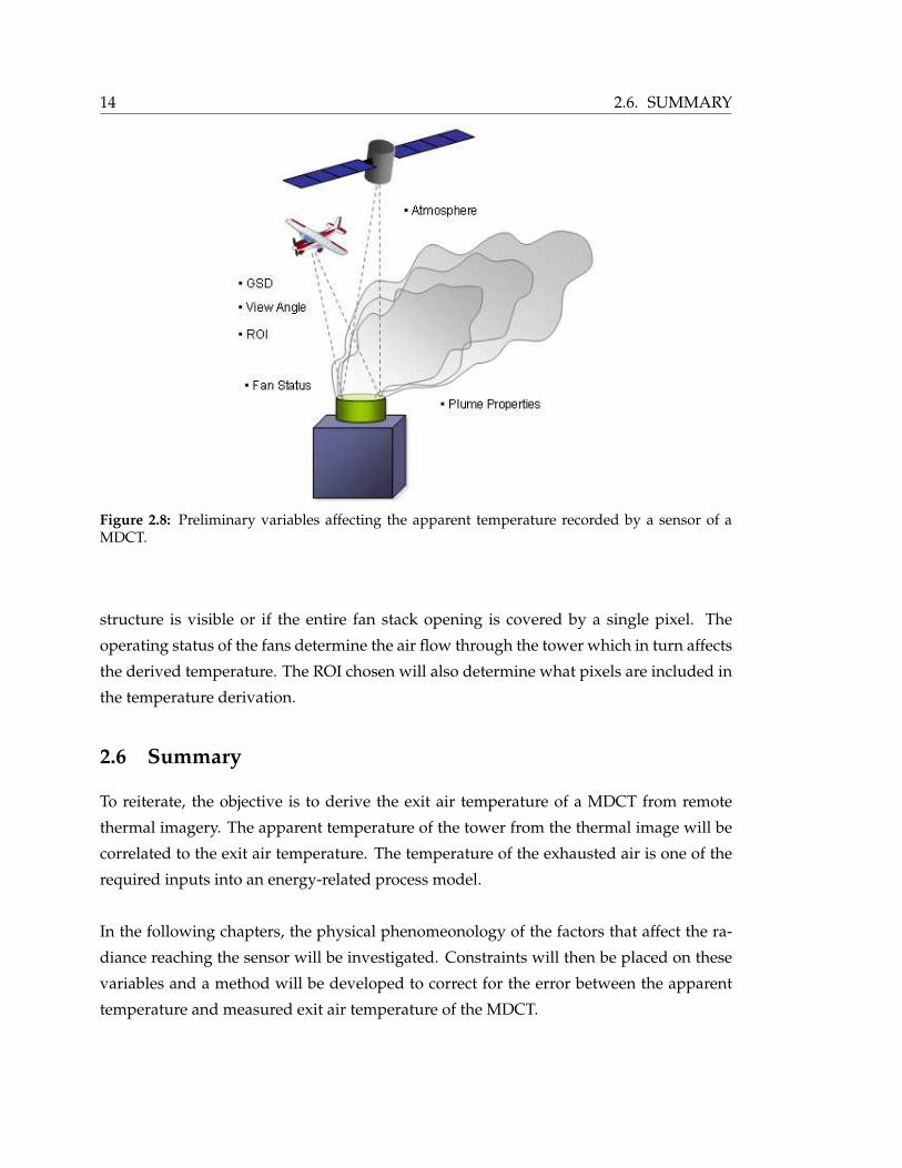
2.8 Preliminary variables affecting the apparent temperature recorded by a
sensor of a MDCT. . . . . . . . . . . . . . . . . . . . . . . . . . . . . . . . . . . 14
3.1 Planck curves for a 5800 Kelvin and 300 Kelvin blackbody. . . . . . . . . . . 17
3.2 Ward diffuse and specular BRDF models. . . . . . . . . . . . . . . . . . . . . 19
3.3 Atmospheric scattering as a function of particle radius and incident radia-
tion wavelength. . . . . . . . . . . . . . . . . . . . . . . . . . . . . . . . . . . . 25
3.4 Atmospheric spectral transmission along a vertical space-to-ground path
generated from a MODTRAN mid-latitude summer atmosphere. . . . . . . 26
3.5 Illustration of atmospheric emission as the sum of the emissions from each
homogeneous layer. . . . . . . . . . . . . . . . . . . . . . . . . . . . . . . . . . 27
3.6 Illustration of the blurring effect and sampling as radiance from a point
source passes through an imaging system. . . . . . . . . . . . . . . . . . . . . 29
3.7 Airy disc pattern representing the PSF of a diffraction-limited circular aper-
ture system. . . . . . . . . . . . . . . . . . . . . . . . . . . . . . . . . . . . . . 30
4.1 Multispectral Thermal Imager (MTI) band locations . . . . . . . . . . . . . . 44
5.1 Diagram of a single photon path for an exposed object and a cavity object. . 52
5.2 Drift eliminator emissivity spectra of two separate physical locations on the
material measured with a SOC-400 instrument. . . . . . . . . . . . . . . . . . 54
5.3 Metal plate emissivity spectra of two separate physical locations on the ma-
terial measured with a SOC-400 instrument. . . . . . . . . . . . . . . . . . . . 54
XV

5.4 Wood support emissivity spectra of two separate physical locations on the
material measured with a SOC-400 instrument. . . . . . . . . . . . . . . . . . 55
5.5 Plastic disc emissivity spectra of two separate physical locations on the ma-
terial measured with a SOC-400 instrument. . . . . . . . . . . . . . . . . . . . 55
5.6 NEFDS BRDF of weathered galvanized bare steel (NEF #0525UUUSTLa)
measured at an illumination angle of 20°. . . . . . . . . . . . . . . . . . . . . 56
5.7 NEFDS BRDF of mildly weathered plastic tarp (NEF #1019UUUFABa) mea-
sured at an illumination angle of 20°. . . . . . . . . . . . . . . . . . . . . . . . 56
5.8 NEFDS BRDF of weathered bare construction lumber (NEF #0404UUU-
WOD) measured at an illumination angle of 20°. . . . . . . . . . . . . . . . . 57
5.9 NEFDS BRDF of weathered paint on insulation panel (NEF #0887UUUPNT)
measured at an illumination angle of 20°. . . . . . . . . . . . . . . . . . . . . 57
5.10 DIRSIG simulation layout of a closed box and an open well . . . . . . . . . . 58
5.11 Results of the closed box DIRSIG simulation. . . . . . . . . . . . . . . . . . . 59
5.12 Results of the open well DIRSIG simulation. . . . . . . . . . . . . . . . . . . 59
5.13 Comparison between a photograph of MDCT drift eliminators and a CAD
drawing of the drift eliminators. . . . . . . . . . . . . . . . . . . . . . . . . . 62
5.14 Ward BRDF models used in the drift eliminator effective emissivity simu-
lation. . . . . . . . . . . . . . . . . . . . . . . . . . . . . . . . . . . . . . . . . . 63
5.15 CAD drawing of a counter-flow MDCT exterior view and interior view . . . 65
5.16 DIRSIG MDCT radiance images rendered with a diffuse Ward BRDF model
and a specular Ward BRDF model. . . . . . . . . . . . . . . . . . . . . . . . . 66
5.17 Apparent temperature profiles across the fan stack opening of the MDCT
for the diffuse Ward BRDF image and the specular Ward BRDF image. . . . 67
5.18 DIRSIG rendering of an MDCT looking into the fan stack opening with a
one-pixel-wide ring drawn. . . . . . . . . . . . . . . . . . . . . . . . . . . . . 68
5.19 Square-wave signal representing the fan blade and cavity radiances at each
pixel location in the ring at different times. . . . . . . . . . . . . . . . . . . . 69
5.20 DIRSIG rendering of an MDCT with a stationary fan and a blurred render-
ing representing a rotating fan. . . . . . . . . . . . . . . . . . . . . . . . . . . 70
5.21 Temperature error from a 300 K object as a function of emissivity and MOD-
TRAN standard atmospheric profile. . . . . . . . . . . . . . . . . . . . . . . . 73
5.22 Illustration of the radiance from the tower passes through the exhaust plume
to reach the sensor. . . . . . . . . . . . . . . . . . . . . . . . . . . . . . . . . . 75
5.23 Atmospheric column representing the plume layer and the ambient atmo-
sphere modeled in MODTRAN. . . . . . . . . . . . . . . . . . . . . . . . . . . 76
XVI
5.24 Schematic of the atmospheric layers assigned in MODTRAN. The first seg-
ment represents the exhaust plume while the second segment represents
the rest of the air column. Standard atmospheric conditions are assigned to
every layer except for those in the first segment where the air temperature
and dew point temperature are varied. . . . . . . . . . . . . . . . . . . . . . . 78
5.25 Results of the MODTRAN plume mid-latitude summer simulation show-
ing the temperature error between the material blackbody temperature and
the sensor derived apparent temperature. . . . . . . . . . . . . . . . . . . . . 79
5.26 Results of the MODTRAN plume sub-arctic winter simulation showing the
temperature error between the material blackbody temperature and the
sensor derived apparent temperature. . . . . . . . . . . . . . . . . . . . . . . 80
5.27 Results of the MODTRAN plume-only mid-latitude summer simulation
showing the temperature error between the material blackbody tempera-
ture and the sensor derived apparent temperature. . . . . . . . . . . . . . . . 83
5.28 Results of the MODTRAN plume-only sub-arctic winter simulation show-
ing the temperature error between the material blackbody temperature and
the sensor derived apparent temperature. . . . . . . . . . . . . . . . . . . . . 84
5.29 Three plume gradient functions modeled in MODTRAN. . . . . . . . . . . . 87
5.30 Illustration of the procedure to predict the MDCT temperature error. . . . . 89
5.31 Ward BRDF model assigned to the facets in the DIRSIG CAD model. . . . . 91
5.32 Illustration of atmospheric layers in MODTRAN used to model the mois-
ture gradient in the plume. . . . . . . . . . . . . . . . . . . . . . . . . . . . . . 93
5.33 High resolution DIRSIG image along with the mixed ROI and cavity-only
ROI drawn for sensor angle of 0°. . . . . . . . . . . . . . . . . . . . . . . . . . 96
6.1 SRNL data set LWIR images. . . . . . . . . . . . . . . . . . . . . . . . . . . . 106
6.2 Interpolated atmospheric profiles used in MODTRAN to correct the SRNL
images. . . . . . . . . . . . . . . . . . . . . . . . . . . . . . . . . . . . . . . . . 109
6.3 Radiosonde station locations shown relative to SRS. . . . . . . . . . . . . . . 110
6.4 The actual and the predicted temperature error with uncertainty ranges
for the 20may04D14 image. ROI, atmosphere, and sensor uncertainty is
included in the error bars. . . . . . . . . . . . . . . . . . . . . . . . . . . . . . 117
6.5 The actual and the predicted temperature error with uncertainty ranges
for the 20may04E02 image. ROI, atmosphere, and sensor uncertainty is
included in the error bars. . . . . . . . . . . . . . . . . . . . . . . . . . . . . . 118
XVII
6.6 The actual and the predicted temperature error with uncertainty ranges
for the 20may04E04 image. ROI, atmosphere, and sensor uncertainty is
included in the error bars. . . . . . . . . . . . . . . . . . . . . . . . . . . . . . 119
6.7 The actual and the predicted temperature error with uncertainty ranges
for the 20jun05G09 image. ROI, atmosphere, and sensor uncertainty is in-
cluded in the error bars. . . . . . . . . . . . . . . . . . . . . . . . . . . . . . . 120
6.8 The actual and the predicted temperature error with uncertainty ranges
for the 20may04D14 image. The uncertainty ranges are for an atmospheric
uncertainty of 0.1 K (top), 1.1 K (middle), and 2.2 K (bottom). . . . . . . . . . 124
6.9 The actual and the predicted temperature error with uncertainty ranges
for the 20may04E02 image. The uncertainty ranges are for an atmospheric
uncertainty of 0.1 K (top), 1.1 K (middle), and 2.2 K (bottom). . . . . . . . . . 125
6.10 The actual and the predicted temperature error with uncertainty ranges
for the 20may04E04 image. The uncertainty ranges are for an atmospheric
uncertainty of 0.1 K (top), 1.1 K (middle), and 2.2 K (bottom). . . . . . . . . . 126
6.11 The actual and the predicted temperature error with uncertainty ranges
for the 20jun05G09 image. The uncertainty ranges are for an atmospheric
uncertainty of 0.1 K (top), 1.1 K (middle), and 2.2 K (bottom). . . . . . . . . . 127
6.12 Comparison of an ideal, flat, unit spectral response and a realistic microbolome-
ter spectral response in the longwave infrared region. . . . . . . . . . . . . . 128
6.13 The actual and the predicted temperature error with uncertainty ranges for
the 20may04D14 image using the microbolometer spectral response. . . . . 129
6.14 The actual and the predicted temperature error with uncertainty ranges for
the 20may04E02 image using the microbolometer spectral response. . . . . . 130
6.15 The actual and the predicted temperature error with uncertainty ranges for
the 20may04E04 image using the microbolometer spectral response. . . . . . 131
6.16 The actual and the predicted temperature error with uncertainty ranges for
the 20jun05G09 image using the microbolometer spectral response. . . . . . 132
6.17 Diagonistic plots indicating a lack-of-fit of the multiple linear regression
model to the 20may04D14 mixed ROI LUT data. . . . . . . . . . . . . . . . . 133
6.18 The actual temperature errors and the predicted temperature errors based
on a LUT nearest neighbor interpolation with uncertainty ranges for the
20may04D14 image. . . . . . . . . . . . . . . . . . . . . . . . . . . . . . . . . . 136
6.19 The actual temperature errors and the predicted temperature errors based
on a LUT nearest neighbor interpolation with uncertainty ranges for the
20may04E02 image. . . . . . . . . . . . . . . . . . . . . . . . . . . . . . . . . . 137
XVIII
6.20 The actual temperature errors and the predicted temperature errors based
on a LUT nearest neighbor interpolation with uncertainty ranges for the
20may04E04 image. . . . . . . . . . . . . . . . . . . . . . . . . . . . . . . . . . 138
6.21 The actual temperature errors and the predicted temperature errors based
on a LUT nearest neighbor interpolation with uncertainty ranges for the
20jun05G09 image. . . . . . . . . . . . . . . . . . . . . . . . . . . . . . . . . . 139
A.1 Photons escaping a blackbody cavity from a thin shell inside the cavity . . . 149
A.2 Spectral radiance for a blackbody at a temperature of 300 Kelvin . . . . . . . 154
E.1 Comparison of the six atmospheric stability classes using the associated
ambient temperature gradients in reference to dry and wet adiabatic lapse
rates. . . . . . . . . . . . . . . . . . . . . . . . . . . . . . . . . . . . . . . . . . 167
E.2 Gaussian plume model rendered in Matlab. The solid line represents the
sensor line-of-sight. The exit air velocity is set to 10 m/s, stack height is 9
m, stack radius is 2 m, wind speed is 0.75 m/s, and the atmospheric stability
is slightly unstable. The estimated path length through this plume is 6 m. . 168
XIX

XX
List of Tables
1 Radiometric Terms . . . . . . . . . . . . . . . . . . . . . . . . . . . . . . . . . XXV
2 Acronyms . . . . . . . . . . . . . . . . . . . . . . . . . . . . . . . . . . . . . . XXVII
2.1 SRNL 20may04D14 image ROI statistics. . . . . . . . . . . . . . . . . . . . . . 8
2.2 SRNL 20may04D14 ground measured temperatures compared to the mean
ROI temperatures. . . . . . . . . . . . . . . . . . . . . . . . . . . . . . . . . . . 8
2.3 SRNL 20may04D14 ground measurements collected at 02:06 EDT on 20
May 2004. . . . . . . . . . . . . . . . . . . . . . . . . . . . . . . . . . . . . . . 8
2.4 SRNL 20may04e02 image ROI statistics. . . . . . . . . . . . . . . . . . . . . . 9
2.5 SRNL 20may04e02 ground measured temperatures compared to the mean
ROI temperatures. . . . . . . . . . . . . . . . . . . . . . . . . . . . . . . . . . . 9
2.6 SRNL 20may04e02 ground measurements collected at 02:06 EDT on 20 May
2004. . . . . . . . . . . . . . . . . . . . . . . . . . . . . . . . . . . . . . . . . . 9
2.7 SRNL 20may04e04 image ROI statistics . . . . . . . . . . . . . . . . . . . . . 10
2.8 SRNL 20may04e04 ground measured temperatures compared to the mean
ROI temperatures. . . . . . . . . . . . . . . . . . . . . . . . . . . . . . . . . . . 10
2.9 SRNL 20may04e04 ground measurements collected at 02:06 EDT on 20 May
2004. . . . . . . . . . . . . . . . . . . . . . . . . . . . . . . . . . . . . . . . . . 10
2.10 SRNL 20jun05G09 image ROI statistics. . . . . . . . . . . . . . . . . . . . . . 11
2.11 SRNL 20jun05G09 ground measured temperatures compared to the mean
ROI temperatures. . . . . . . . . . . . . . . . . . . . . . . . . . . . . . . . . . . 11
2.12 SRNL 20jun05G09 ground measurements collected at 22:17 EDT on 20 June
2005. . . . . . . . . . . . . . . . . . . . . . . . . . . . . . . . . . . . . . . . . . 11
5.1 Results of the DIRSIG drift eliminator effective emissivity simulations. . . . 64
5.2 Effective sky apparent temperatures for the standard MODTRAN atmo-
spheres. . . . . . . . . . . . . . . . . . . . . . . . . . . . . . . . . . . . . . . . . 73
5.3 Parameter values for the MODTRAN plume simulations. . . . . . . . . . . . 78
5.4 Parameter values for the plume-only MODTRAN simulations. . . . . . . . . 82
5.5 Apparent temperature errors for three plume gradient functions and for
three plume lengths. . . . . . . . . . . . . . . . . . . . . . . . . . . . . . . . . 87
6.1 MDCT physics model parameters and associated modeling tools. . . . . . . 99
XXI

6.2 MDCT parameter values used for the target-space LUT. . . . . . . . . . . . . 100
6.3 Regression model parameter labels. . . . . . . . . . . . . . . . . . . . . . . . 101
6.4 MDCT random parameter values . . . . . . . . . . . . . . . . . . . . . . . . . 105
6.5 Radiosonde station information for the radiosonde profiles used to atmo-
spherically compensate the SRNL images. . . . . . . . . . . . . . . . . . . . . 108
6.6 Original and the atmospherically-corrected image ROI temperatures for the
SRNL 20may04D14 image. . . . . . . . . . . . . . . . . . . . . . . . . . . . . . 111
6.7 Original and the atmospherically-corrected image ROI temperatures for the
SRNL 20may04E02 image. . . . . . . . . . . . . . . . . . . . . . . . . . . . . . 111
6.8 Original and the atmospherically-corrected image ROI temperatures for the
SRNL 20may04E04 image. . . . . . . . . . . . . . . . . . . . . . . . . . . . . . 111
6.9 Original and the atmospherically-corrected image ROI temperatures for the
SRNL 20jun05G09 image. . . . . . . . . . . . . . . . . . . . . . . . . . . . . . 111
6.10 Temperature uncertainties in the measured ground, ROI, sensor, and atmo-
spheric variables . . . . . . . . . . . . . . . . . . . . . . . . . . . . . . . . . . 112
6.11 Temperature errors between the atmospherically-corrected mean ROI tem-
perature and the measured ground-truth exit air temperature for the SRNL
20may04D14 image. . . . . . . . . . . . . . . . . . . . . . . . . . . . . . . . . . 113
6.12 Temperature errors between the atmospherically-corrected mean ROI tem-
perature and the measured ground-truth exit air temperature for the SRNL
20may04E02 image. . . . . . . . . . . . . . . . . . . . . . . . . . . . . . . . . . 113
6.13 Temperature errors between the atmospherically-corrected mean ROI tem-
perature and the measured ground-truth exit air temperature for the SRNL
20may04E04 image. . . . . . . . . . . . . . . . . . . . . . . . . . . . . . . . . . 113
6.14 Temperature errors between the atmospherically-corrected mean ROI tem-
perature and the measured ground-truth exit air temperature for the SRNL
20jun05G09 image. . . . . . . . . . . . . . . . . . . . . . . . . . . . . . . . . . 113
6.15 Estimates of the sensor view zenith angle along with uncertainties. The
angles were estimated by measuring the vertical and horizontal pixel di-
ameters of the fan stack opening of each image. . . . . . . . . . . . . . . . . . 115
6.16 Predictor estimates and uncertainties used in the 20may04D14 parameter-
ized regression model . . . . . . . . . . . . . . . . . . . . . . . . . . . . . . . 117
6.17 Comparison of the actual and predicted temperature errors for the 20may04D14
image. ROI, atmosphere, and sensor uncertainty is included. . . . . . . . . . 117
6.18 Predictor estimates and uncertainties used in the 20may04E02 parameter-
ized regression model . . . . . . . . . . . . . . . . . . . . . . . . . . . . . . . 118
XXII

6.19 Comparison of the actual and predicted temperature errors for the 20may04E02
image. ROI, atmosphere, and sensor uncertainty is included. . . . . . . . . . 118
6.20 Predictor estimates and uncertainties used in the 20may04E04 parameter-
ized regression model . . . . . . . . . . . . . . . . . . . . . . . . . . . . . . . 119
6.21 Comparison of the actual and predicted temperature errors for the 20may04E04
image. ROI, atmosphere, and sensor uncertainty is included. . . . . . . . . . 119
6.22 Predictor estimates and uncertainties used in the 20jun05G09 parameter-
ized regression model . . . . . . . . . . . . . . . . . . . . . . . . . . . . . . . 120
6.23 Comparison of the actual and predicted temperature errors for the 20jun05G09
image. ROI, atmosphere, and sensor uncertainty is included. . . . . . . . . . 120
6.24 Predictor estimates and uncertainties used in the 20may04D14 parameter-
ized regression model . . . . . . . . . . . . . . . . . . . . . . . . . . . . . . . 129
6.25 Comparison of the actual and predicted temperature errors for the 20may04D14
image using the microbolometer spectral response. . . . . . . . . . . . . . . 129
6.26 Predictor estimates and uncertainties used in the 20may04E02 parameter-
ized regression model . . . . . . . . . . . . . . . . . . . . . . . . . . . . . . . 130
6.27 Comparison of the actual and predicted temperature errors for the 20may04E02
image using the microbolometer spectral response. . . . . . . . . . . . . . . 130
6.28 Predictor estimates and uncertainties used in the 20may04E04 parameter-
ized regression model . . . . . . . . . . . . . . . . . . . . . . . . . . . . . . . 131
6.29 Comparison of the actual and predicted temperature errors for the 20may04E04
image using the microbolometer spectral response. . . . . . . . . . . . . . . 131
6.30 Predictor estimates and uncertainties used in the 20jun05G09 parameter-
ized regression model . . . . . . . . . . . . . . . . . . . . . . . . . . . . . . . 132
6.31 Comparison of the actual and predicted temperature errors for the 20jun05G09
image using the microbolometer spectral response. . . . . . . . . . . . . . . 132
6.32 Predictor estimates used in the 20may04D14 LUT nearest neighbor interpo-
lation. . . . . . . . . . . . . . . . . . . . . . . . . . . . . . . . . . . . . . . . . . 136
6.33 Comparison of the actual temperature errors and the predicted tempera-
ture errors based on a LUT nearest neighbor interpolation for the 20may04D14
image. . . . . . . . . . . . . . . . . . . . . . . . . . . . . . . . . . . . . . . . . 136
6.34 Predictor estimates used in the 20may04E02 LUT nearest neighbor interpo-
lation. . . . . . . . . . . . . . . . . . . . . . . . . . . . . . . . . . . . . . . . . . 137
6.35 Comparison of the actual temperature errors and the predicted tempera-
ture errors based on a LUT nearest neighbor interpolation for the 20may04E02
image. . . . . . . . . . . . . . . . . . . . . . . . . . . . . . . . . . . . . . . . . 137
XXIII

6.36 Predictor estimates used in the 20may04E04 LUT nearest neighbor interpo-
lation. . . . . . . . . . . . . . . . . . . . . . . . . . . . . . . . . . . . . . . . . . 138
6.37 Comparison of the actual temperature errors and the predicted tempera-
ture errors based on a LUT nearest neighbor interpolation for the 20may04E04
image. . . . . . . . . . . . . . . . . . . . . . . . . . . . . . . . . . . . . . . . . 138
6.38 Predictor estimates used in the 20jun05G09 LUT nearest neighbor interpo-
lation. . . . . . . . . . . . . . . . . . . . . . . . . . . . . . . . . . . . . . . . . . 139
6.39 Comparison of the actual temperature errors and the predicted tempera-
ture errors based on a LUT nearest neighbor interpolation for the 20jun05G09
image. . . . . . . . . . . . . . . . . . . . . . . . . . . . . . . . . . . . . . . . . 139
E.1 Constants used in the calculation of the vertical and crosswind dispersion
coefficients for the Gaussian plume model in an urban environment. . . . . 166
E.2 Description of the six atmospheric stability classes and the associated am-
bient temperature gradients. . . . . . . . . . . . . . . . . . . . . . . . . . . . . 166
XXIV
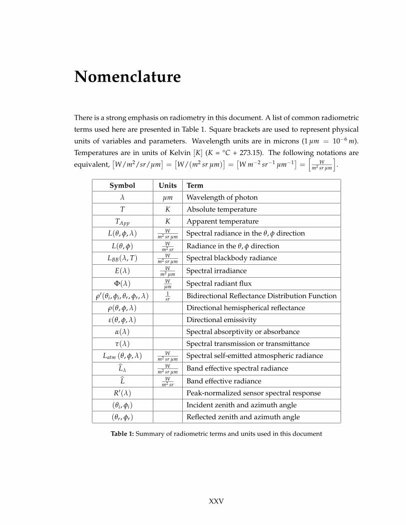
Nomenclature
There is a strong emphasis on radiometry in this document. A list of common radiometric
terms used here are presented in Table 1. Square brackets are used to represent physical
units of variables and parameters. Wavelength units are in microns (1 µm = 10−6 m).
Temperatures are in units of Kelvin [K] (K = °C + 273.15). The following notations are
equivalent,[W/m2/sr/µm
]=
[W/(m2 sr µm)
]=
[W m−2 sr−1 µm−1] =
[W
m2 sr µm
].
Symbol Units Term
λ µm Wavelength of photon
T K Absolute temperature
TApp K Apparent temperature
L(θ, φ, λ) Wm2 sr µm Spectral radiance in the θ, φ direction
L(θ, φ) Wm2 sr Radiance in the θ, φ direction
LBB(λ, T) Wm2 sr µm Spectral blackbody radiance
E(λ) Wm2 µm Spectral irradiance
Φ(λ) Wµm Spectral radiant flux
ρ′(θi, φi, θr, φr, λ) 1sr Bidirectional Reflectance Distribution Function
ρ(θ, φ, λ) Directional hemispherical reflectance
ε(θ, φ, λ) Directional emissivity
α(λ) Spectral absorptivity or absorbance
τ(λ) Spectral transmission or transmittance
Latm (θ, φ, λ) Wm2 sr µm Spectral self-emitted atmospheric radiance
LλW
m2 sr µm Band effective spectral radiance
L Wm2 sr Band effective radiance
R′(λ) Peak-normalized sensor spectral response
(θi, φi) Incident zenith and azimuth angle
(θr, φr) Reflected zenith and azimuth angle
Table 1: Summary of radiometric terms and units used in this document
XXV

XXVI
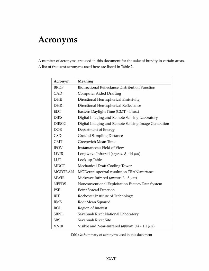
Acronyms
A number of acronyms are used in this document for the sake of brevity in certain areas.
A list of frequent acronyms used here are listed in Table 2.
Acronym Meaning
BRDF Bidirectional Reflectance Distribution Function
CAD Computer Aided Drafting
DHE Directional Hemispherical Emissivity
DHR Directional Hemispherical Reflectance
EDT Eastern Daylight Time (GMT - 4 hrs.)
DIRS Digital Imaging and Remote Sensing Laboratory
DIRSIG Digital Imaging and Remote Sensing Image Generation
DOE Department of Energy
GSD Ground Sampling Distance
GMT Greenwich Mean Time
IFOV Instantaneous Field of View
LWIR Longwave Infrared (approx. 8 - 14 µm)
LUT Look-up Table
MDCT Mechanical Draft Cooling Tower
MODTRAN MODerate spectral resolution TRANsmittance
MWIR Midwave Infrared (approx. 3 - 5 µm)
NEFDS Nonconventional Exploitation Factors Data System
PSF Point Spread Function
RIT Rochester Institute of Technology
RMS Root Mean Squared
ROI Region of Interest
SRNL Savannah River National Laboratory
SRS Savannah River Site
VNIR Visible and Near-Infrared (approx. 0.4 - 1.1 µm)
Table 2: Summary of acronyms used in this document
XXVII

XXVIII

Chapter 1
Introduction
If we knew what it was we were doing, it would not be called research, would it?
- Albert Einstein
The derivation of the absolute temperature of a material surface from remote thermal im-
agery is a complex process. Remote thermal imaging is necessary when it is impossible
or impractical to obtain a direct temperature measurement of a material surface. Only
photons that have been thermally emitted from the surface carry information about the
temperature of that surface. However, this self-emitted signal from the surface is not the
only signal entering a sensor. Signals from other background objects will enter the field
of view of the sensor and will be detected. Furthermore, the temperature signal from the
surface of interest will be altered by the optical properties of the surface and by its envi-
ronment. Separating out these unwanted signals and effects is a painstaking process.
Figure 1.1: Electromagnetic radiation spectrum
The topic of remote sensing involves analyzing the signals, or photons, that are collected
by a sensor. A photon contains a certain amount of energy depending on its wavelength.
For a beam of photons, the rate at which its energy is propagating is known as the radiant
flux, Φ, in units of energy per unit time, or Watts [1]. It is often convenient to express the
energy flux that originates from a surface and into a particular direction. The radiometric
term known as radiance, L, describes the flux per unit projected area per unit solid an-
1
2 Introduction
gle [1]. The radiance when measured per wavelength has units of Watts per square meter
per steradian per micron,[W/m2/sr/µm
].
Although remote sensing may encompass the entire electromagnetic spectrum, only the
infrared region will be utilized here. From the ultraviolet to the short-wave infrared (ap-
proximately 0.1 - 2 µm), there will be several orders of magnitude more flux from the sun
than from self-emission of objects at the Earth ambient temperature of 300 K. This spectral
range is referred to as the reflective region and thermal or self-emitted flux is ignored. At
longwave infrared (LWIR) wavelengths (approximately 8 - 14 µm), there are several or-
ders of magnitude more flux from self-emission than from reflected solar flux. This region
is referred to as the thermal region [1]. The self-emitted radiation from objects at the ambi-
ent Earth temperature makes this spectral region ideal for determining the temperature of
such objects. For this reason, the discussion and analysis in this document will be limited
to this spectral region.
This document will present a detailed description of the problem, introduce the physics of
thermal radiometry, provide an overview of previous approaches to remote temperature
retrieval, propose a methodology to obtain the MDCT temperature from a remote thermal
image, and reveal the results and conclusions of the research.

Chapter 2
Objectives
Knowledge of the absolute temperature of a surface is useful for a wide range of appli-
cations ranging from environmental to industrial to security. The objective of this project
is to estimate the temperature of the air exiting a mechanical draft cooling tower (MDCT)
through the use of remote thermal imagery. Knowledge of the temperature of the cool-
ing towers is necessary for input into process models that yield information about the
industrial processes that the cooling towers service. A visible and thermal image of such
cooling towers is displayed in Figure 2.1.
A camera sensitive to the LWIR spectral region is used to observe the cooling tower. Each
pixel in the resulting thermal image is converted into an apparent temperature, or image-
derived temperature. The apparent temperature of pixels inside the fan stack of the tower is to
be correlated to the exit air temperature.
(a) Visible color image (b) LWIR image
Figure 2.1: Mechanical draft cooling towers at the Savannah River Site.
2.1 Cooling Tower Basics
Industrial plants generate substantial amounts of excess heat. Water is a popular medium
used to transport excess heat from an industrial process. Waste heat is absorbed by wa-
ter having a cooler temperature than the process. This warm water must now either be
discharged into a body of water, or cooled and recycled. In the latter method, a cooling
3

4 2.1. COOLING TOWER BASICS
Figure 2.2: Schematic drawing of a counter-flow MDCT (Burger 1995 [2]).
tower is a standard option to recycle the water. In the cooling tower, the waste heat from
the water is rejected into the atmosphere and the cooled water is recirculated through the
system [2]. There are various types of cooling towers but all function on the same physics.
The basic principle governing the cooling of the water is evaporative cooling and the
exchange of sensible heat. Water exposed to cooling air streams will release heat and
evaporate. The penalty is the loss of water which is discharged into the atmosphere as
hot moist water vapor. When the water is warmer than the ambient air, the air cools the
water. Air gets warmer as it gains sensible heat of the water and the water is cooled as
sensible heat is transferred to the air. The evaporative effect of the release of latent heat
of vaporization also cools the water. Approximately 75% of the cooling is latent heat and
25% is due to sensible heat transfer [2].
Air becomes heated and saturated as it passes through the cooling tower. Atmospheric
cooling is limited by the ambient wet bulb temperature. Wet bulb is determined from a
psychrometric chart as the intersection of the ambient dry bulb temperature and the dew
point temperature. Therefore, the wet bulb temperature is always between the dry bulb
and dew point temperatures. Wet bulb is an indication of the evaporative potential of the
atmosphere. The water cannot be cooled to a lower temperature than the wet bulb [2].

2.2. MECHANICAL DRAFT COOLING TOWER ANATOMY 5
2.2 Mechanical Draft Cooling Tower Anatomy
The counter-flow variety of MDCT is presented here in detail since this type is widely
used in industry and at the Savannah River Site (SRS). A schematic drawing of a counter-
flow tower is shown in Figure 2.2. Water that has been heated through an industrial
process is pumped to the top of the cooling tower. A water distribution system turns the
heavy stream of water into light droplets as preparation to being cooled by the air stream.
The water is sprayed onto a baffle material, called fill, that provides large water surface
areas to facilitate heat transfer. Air enters the tower from below and contacts the water
falling through the fill. The cooled water is collected at the base of the tower in a basin
to be recirculated to the industrial plant. Moisture-laden air rises through the distribu-
tion plumbing and is exhausted out the stack of the tower. The flowing air will pick up
mist and droplets and will carry them with the air flow out of the tower. Material known
as drift eliminators is placed between the water distribution system and the tower stack
to minimize the dispersal of entrained water droplets into the surrounding atmosphere.
Drift eliminators are a series of baffles which cause air to gently change direction at least
three times thereby obtaining greater surface contact to release water droplets [2]. A fan
is situated in the stack to induce air flow through the tower. It is the presence of this fan
that gives the MDCT its name.
The towers exist in one of three states. Water on, fans on refers to water flowing through
the tower and the fan is operating to force air through the tower. Water on, fans off refers to
water flowing through the tower but the fan is inactive. This is a so called “natural draft”
mode in which air exits the fan stack opening through natural convection. The final state
is water off, fans off in which the tower is not operating.
2.3 MDCT Thermal Imagery
The Savannah River National Laboratory (SRNL) recorded thermal imagery of the cool-
ing towers at the Savannah River Site in the late spring of 2004 and 2005. The images
were captured with an Inframetrics SC 2000 microbolometer thermal camera having a 7.6
- 13.5 µm spectral range, an instantaneous field of view (IFOV) of 1.4 milliradians, and
a sensitivity of less than 0.1 K. The sensor was flying on board a helicopter at altitudes
between 350 and 2000 feet (106.7 and 610 meters) above the ground. The output image is
converted directly into a brightness, or apparent, temperature by the sensor.

6 2.3. MDCT THERMAL IMAGERY
Figure 2.3: Location of ground-truth measurements taken by SRNL [2] [3].
Thermal images of the H-area and F-Area cooling units at SRS are presented in the fol-
lowing figures. Regions of interest (ROIs) were drawn for each tower and statistics across
these regions were determined. The ROIs were first drawn to include the entire fan stack
opening of the tower. This first set of ROIs simulate low spatial resolution imagery in
which the ground sample distance (GSD) of the sensor is large enough to encompass the
fan stack opening of the tower. A second set of ROIs were drawn in such a manner that
avoided visible obstructions such as fan blades and internal support structures. Ground-
truth measurements were taken nearly simultaneous with the airborne imagery. The ex-
haust air temperature exiting the cooling tower is Tex. The exhaust is either forced out of
the fan stack when fans are operating or it is expelled by natural convection when fans
are off. This temperature was measured with a HOBO temperature sensor mounted on
a metal pipe positioned about 0.5 meters inside the edge of the shroud by the motor that
drives the fan. The corresponding dew point temperature of the exhaust air is Tdex and
was measured by the same HOBO in the same place. The temperature of the hot water
coming into the tower is Tin while Tout is the average temperature of the cooled water
collected in the basin at the base of the towers. The ambient air temperature Tamb, dew
point temperature Tdamb, and pressure P were taken approximately two meters above the
ground and five meters from the base of the towers [3]. Simultaneous wind speed and
direction data is also available for each image. The wind measurements were obtained at
heights of 4 meters and 60 meters.

2.3. MDCT THERMAL IMAGERY 7
Each data set presented here includes the original image with the ROIs overlaid. Brighter
pixels represent higher apparent temperatures while darker pixels represent lower appar-
ent temperatures. Each image has two sets of ROIs: one in which the ROI was drawn
over the entire fan stack opening of the tower (ROI·1) and another in which the fans and
other structures were avoided (ROI·2). A table of ROI statistics is included for each set of
ROIs and another table contains the coincident measured ground data. All temperatures
are displayed in Kelvin. The operating status of each tower in the image is also given
along with a comparison of the ground measured exit air temperature and the mean ROI
temperatures from the image. Ground temperature, pressure, and wind measurements
are presented in the ground measurements table. The images were all collected at night
and span observation altitudes of 350 to 2000 feet (106.7 to 610 meters).
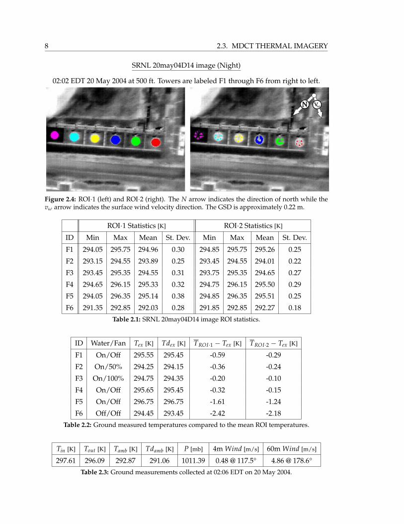
8 2.3. MDCT THERMAL IMAGERY
SRNL 20may04D14 image (Night)
02:02 EDT 20 May 2004 at 500 ft. Towers are labeled F1 through F6 from right to left.
Figure 2.4: ROI·1 (left) and ROI·2 (right). The N arrow indicates the direction of north while thevω arrow indicates the surface wind velocity direction. The GSD is approximately 0.22 m.
ROI·1 Statistics [K] ROI·2 Statistics [K]
ID Min Max Mean St. Dev. Min Max Mean St. Dev.
F1 294.05 295.75 294.96 0.30 294.85 295.75 295.26 0.25
F2 293.15 294.55 293.89 0.25 293.45 294.55 294.01 0.22
F3 293.45 295.35 294.55 0.31 293.75 295.35 294.65 0.27
F4 294.65 296.15 295.33 0.32 294.75 296.15 295.50 0.29
F5 294.05 296.35 295.14 0.38 294.85 296.35 295.51 0.25
F6 291.35 292.85 292.03 0.28 291.85 292.85 292.27 0.18
Table 2.1: SRNL 20may04D14 image ROI statistics.
ID Water/Fan Tex [K] Tdex [K] TROI·1 − Tex [K] TROI·2 − Tex [K]
F1 On/Off 295.55 295.45 -0.59 -0.29
F2 On/50% 294.25 294.15 -0.36 -0.24
F3 On/100% 294.75 294.35 -0.20 -0.10
F4 On/Off 295.65 295.45 -0.32 -0.15
F5 On/Off 296.75 296.75 -1.61 -1.24
F6 Off/Off 294.45 293.45 -2.42 -2.18
Table 2.2: Ground measured temperatures compared to the mean ROI temperatures.
Tin [K] Tout [K] Tamb [K] Tdamb [K] P [mb] 4m Wind [m/s] 60m Wind [m/s]
297.61 296.09 292.87 291.06 1011.39 0.48 @ 117.5° 4.86 @ 178.6°
Table 2.3: Ground measurements collected at 02:06 EDT on 20 May 2004.
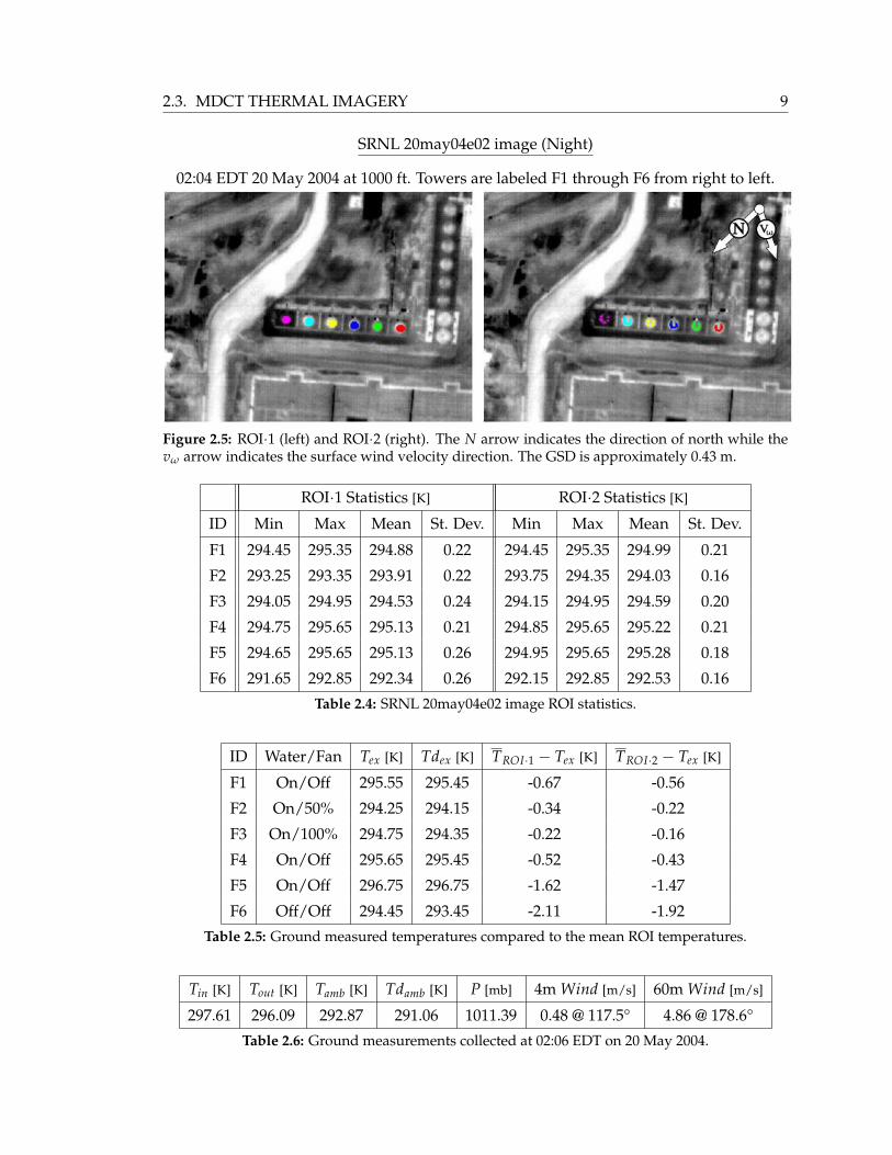
2.3. MDCT THERMAL IMAGERY 9
SRNL 20may04e02 image (Night)
02:04 EDT 20 May 2004 at 1000 ft. Towers are labeled F1 through F6 from right to left.
Figure 2.5: ROI·1 (left) and ROI·2 (right). The N arrow indicates the direction of north while thevω arrow indicates the surface wind velocity direction. The GSD is approximately 0.43 m.
ROI·1 Statistics [K] ROI·2 Statistics [K]
ID Min Max Mean St. Dev. Min Max Mean St. Dev.
F1 294.45 295.35 294.88 0.22 294.45 295.35 294.99 0.21
F2 293.25 293.35 293.91 0.22 293.75 294.35 294.03 0.16
F3 294.05 294.95 294.53 0.24 294.15 294.95 294.59 0.20
F4 294.75 295.65 295.13 0.21 294.85 295.65 295.22 0.21
F5 294.65 295.65 295.13 0.26 294.95 295.65 295.28 0.18
F6 291.65 292.85 292.34 0.26 292.15 292.85 292.53 0.16
Table 2.4: SRNL 20may04e02 image ROI statistics.
ID Water/Fan Tex [K] Tdex [K] TROI·1 − Tex [K] TROI·2 − Tex [K]
F1 On/Off 295.55 295.45 -0.67 -0.56
F2 On/50% 294.25 294.15 -0.34 -0.22
F3 On/100% 294.75 294.35 -0.22 -0.16
F4 On/Off 295.65 295.45 -0.52 -0.43
F5 On/Off 296.75 296.75 -1.62 -1.47
F6 Off/Off 294.45 293.45 -2.11 -1.92
Table 2.5: Ground measured temperatures compared to the mean ROI temperatures.
Tin [K] Tout [K] Tamb [K] Tdamb [K] P [mb] 4m Wind [m/s] 60m Wind [m/s]
297.61 296.09 292.87 291.06 1011.39 0.48 @ 117.5° 4.86 @ 178.6°
Table 2.6: Ground measurements collected at 02:06 EDT on 20 May 2004.

10 2.3. MDCT THERMAL IMAGERY
SRNL 20may04e04 image (Night)
02:07 EDT 20 May 2004 at 2000 ft. Towers are labeled F1 through F6 from right to left.
Figure 2.6: ROI·1 (left) and ROI·2 (right). The N arrow indicates the direction of north while thevω arrow indicates the surface wind velocity direction. The GSD is approximately 0.85 m.
ROI·1 Statistics [K] ROI·2 Statistics [K]
ID Min Max Mean St. Dev. Min Max Mean St. Dev.
F1 294.65 295.05 294.82 0.14 294.65 295.05 294.83 0.14
F2 293.75 294.15 293.88 0.12 293.35 294.15 293.81 0.22
F3 293.85 294.45 294.22 0.17 293.55 294.75 294.24 0.29
F4 294.65 295.05 294.84 0.14 293.75 295.05 294.63 0.40
F5 294.45 294.85 294.68 0.14 294.45 294.85 294.70 0.11
F6 292.25 292.85 292.58 0.19 292.55 292.85 292.65 0.11
Table 2.7: SRNL 20may04e04 image ROI statistics
ID Water/Fan Tex [K] Tdex [K] TROI·1 − Tex [K] TROI·2 − Tex [K]
F1 On/Off 295.55 295.45 -0.73 -0.72
F2 On/50% 294.25 294.15 -0.37 -0.44
F3 On/100% 294.75 294.35 -0.53 -0.51
F4 On/Off 295.65 295.45 -0.81 -1.02
F5 On/Off 296.75 296.75 -2.08 -2.05
F6 Off/Off 294.45 293.45 -1.87 -1.80
Table 2.8: Ground measured temperatures compared to the mean ROI temperatures.
Tin [K] Tout [K] Tamb [K] Tdamb [K] P [mb] 4m Wind [m/s] 60m Wind [m/s]
297.61 296.09 292.87 291.06 1011.39 0.48 @ 117.5° 4.86 @ 178.6°
Table 2.9: Ground measurements collected at 02:06 EDT on 20 May 2004.
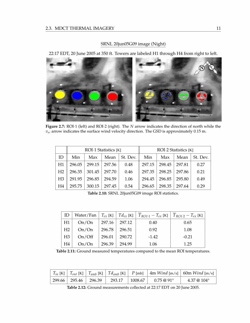
2.3. MDCT THERMAL IMAGERY 11
SRNL 20jun05G09 image (Night)
22:17 EDT, 20 June 2005 at 350 ft. Towers are labeled H1 through H4 from right to left.
Figure 2.7: ROI·1 (left) and ROI·2 (right). The N arrow indicates the direction of north while thevω arrow indicates the surface wind velocity direction. The GSD is approximately 0.15 m.
ROI·1 Statistics [K] ROI·2 Statistics [K]
ID Min Max Mean St. Dev. Min Max Mean St. Dev.
H1 296.05 299.15 297.56 0.48 297.15 298.45 297.81 0.27
H2 296.35 301.45 297.70 0.46 297.35 298.25 297.86 0.21
H3 291.95 296.85 294.59 1.06 294.45 296.85 295.80 0.49
H4 295.75 300.15 297.45 0.54 296.65 298.35 297.64 0.29
Table 2.10: SRNL 20jun05G09 image ROI statistics.
ID Water/Fan Tex [K] Tdex [K] TROI·1 − Tex [K] TROI·2 − Tex [K]
H1 On/On 297.16 297.12 0.40 0.65
H2 On/On 296.78 296.51 0.92 1.08
H3 On/Off 296.01 290.72 -1.42 -0.21
H4 On/On 296.39 294.99 1.06 1.25
Table 2.11: Ground measured temperatures compared to the mean ROI temperatures.
Tin [K] Tout [K] Tamb [K] Tdamb [K] P [mb] 4m Wind [m/s] 60m Wind [m/s]
299.66 295.46 296.39 293.17 1008.67 0.75 @ 91° 4.37 @ 104°
Table 2.12: Ground measurements collected at 22:17 EDT on 20 June 2005.

12 2.4. ANALYSIS
2.4 Analysis
The data presented in Figures 2.4 through 2.7 are representative of images obtained at
night, at various collection altitudes, for various tower operating conditions, and for
different view angles. The mean ROI temperatures, TROI·1 and TROI·2, and the ground-
measured exit air temperature, Tex, are not equal. This difference must be accounted for.
Several statements can be made about the data presented here.
For the nadir images (Figures 2.4 to 2.6), the temperature errors are all less than zero which
means that the mean ROI temperature is less than the measured exit air temperature. This
is expected since factors such as the emissivity, atmospheric effects, and blurring would
tend to cause the apparent temperature to be less than the absolute temperature.
The magnitude of the temperature errors, |∆T|, is smaller in the fans on case than in the
fans off case for all altitudes. The spinning fan forces the air inside the tower cavity out
of the tower stack. Therefore the interior and exterior air are closer to being the same
temperature. On the other hand, in the fans off case air is expelled from the tower through
natural convection. As a consequence, the air exiting the tower stack is at a slightly lower
temperature since it cools as it expands and rises. The |∆T| is therefore larger for the fans
off case than in the fans on case.
The magnitude of the temperature errors are smaller for ROI·2 than for ROI·1 for alti-
tudes of 500 feet (152.5 m) and 1000 feet (305.0 m). This is expected because when the
fan blades are avoided, as in ROI·2, the ROI contains pixels from the interior of the tower
only. When the ROI does not avoid the fan blades, as in ROI·1, the ROI contains pixels
from both the interior and exterior (fan blades) of the tower. The exterior pixels will have
a lower apparent temperature since they will reflect a lower radiance from the sky and
will be at a lower absolute temperature because of radiative cooling at night. Also, the
ROI·1 and ROI·2 temperatures are roughly the same at an observation altitude of 2000
feet (610.0 m). The optical blur of the pixels at this higher altitude cause ROI·2 to behave
as ROI·1 and therefore the apparent temperatures are roughly equal.
Lastly, |∆T| increases for both ROIs as the observation altitude increases. This decrease
in apparent temperature with increasing altitude is caused by the increase in atmospheric
path.
2.5. PRELIMINARY VARIABLES 13
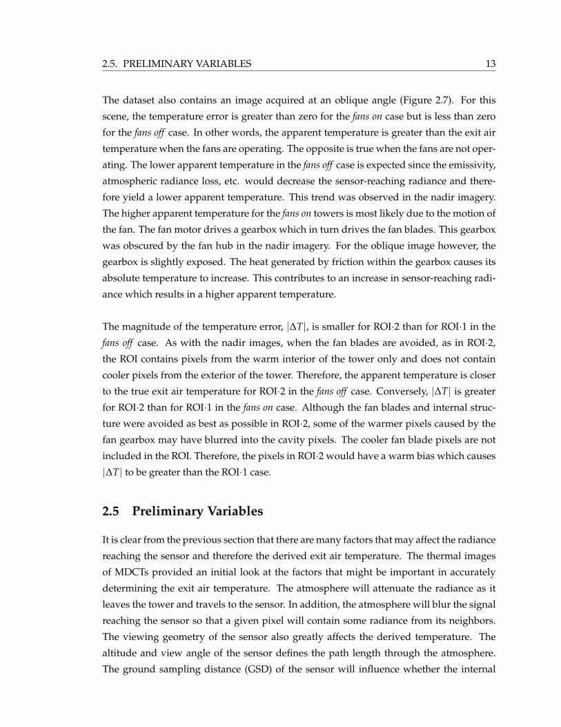
The dataset also contains an image acquired at an oblique angle (Figure 2.7). For this
scene, the temperature error is greater than zero for the fans on case but is less than zero
for the fans off case. In other words, the apparent temperature is greater than the exit air
temperature when the fans are operating. The opposite is true when the fans are not oper-
ating. The lower apparent temperature in the fans off case is expected since the emissivity,
atmospheric radiance loss, etc. would decrease the sensor-reaching radiance and there-
fore yield a lower apparent temperature. This trend was observed in the nadir imagery.
The higher apparent temperature for the fans on towers is most likely due to the motion of
the fan. The fan motor drives a gearbox which in turn drives the fan blades. This gearbox
was obscured by the fan hub in the nadir imagery. For the oblique image however, the
gearbox is slightly exposed. The heat generated by friction within the gearbox causes its
absolute temperature to increase. This contributes to an increase in sensor-reaching radi-
ance which results in a higher apparent temperature.
The magnitude of the temperature error, |∆T|, is smaller for ROI·2 than for ROI·1 in the
fans off case. As with the nadir images, when the fan blades are avoided, as in ROI·2,
the ROI contains pixels from the warm interior of the tower only and does not contain
cooler pixels from the exterior of the tower. Therefore, the apparent temperature is closer
to the true exit air temperature for ROI·2 in the fans off case. Conversely, |∆T| is greater
for ROI·2 than for ROI·1 in the fans on case. Although the fan blades and internal struc-
ture were avoided as best as possible in ROI·2, some of the warmer pixels caused by the
fan gearbox may have blurred into the cavity pixels. The cooler fan blade pixels are not
included in the ROI. Therefore, the pixels in ROI·2 would have a warm bias which causes
|∆T| to be greater than the ROI·1 case.
2.5 Preliminary Variables
It is clear from the previous section that there are many factors that may affect the radiance
reaching the sensor and therefore the derived exit air temperature. The thermal images
of MDCTs provided an initial look at the factors that might be important in accurately
determining the exit air temperature. The atmosphere will attenuate the radiance as it
leaves the tower and travels to the sensor. In addition, the atmosphere will blur the signal
reaching the sensor so that a given pixel will contain some radiance from its neighbors.
The viewing geometry of the sensor also greatly affects the derived temperature. The
altitude and view angle of the sensor defines the path length through the atmosphere.
The ground sampling distance (GSD) of the sensor will influence whether the internal
14 2.6. SUMMARY
Figure 2.8: Preliminary variables affecting the apparent temperature recorded by a sensor of aMDCT.
structure is visible or if the entire fan stack opening is covered by a single pixel. The
operating status of the fans determine the air flow through the tower which in turn affects
the derived temperature. The ROI chosen will also determine what pixels are included in
the temperature derivation.
2.6 Summary
To reiterate, the objective is to derive the exit air temperature of a MDCT from remote
thermal imagery. The apparent temperature of the tower from the thermal image will be
correlated to the exit air temperature. The temperature of the exhausted air is one of the
required inputs into an energy-related process model.
In the following chapters, the physical phenomeonology of the factors that affect the ra-
diance reaching the sensor will be investigated. Constraints will then be placed on these
variables and a method will be developed to correct for the error between the apparent
temperature and measured exit air temperature of the MDCT.
Chapter 3
Theory
Remote sensing involves the gathering of information about a target of interest by ana-
lyzing the radiant energy emanating from that target. The energy detected by a sensor,
however, is a collection of light from many sources traveling various paths to reach the
sensor. Many of these paths are unrelated to the target of interest and the paths directly
between the target and sensor are modified by the radiometric environment. The factors
affecting the signal entering the sensor cannot be easily separated and therefore must be
modeled or estimated in order to extract the desired information about the target of inter-
est. An overview of temperature extraction from remote thermal imagery is presented in
this chapter.
3.1 Self-Emitted Radiance
The amount of thermal energy contained in a material is represented by its absolute tem-
perature, T, expressed in units of Kelvin. All materials have an absolute temperature
above zero since all materials interact with their environment through the laws of ther-
modynamics. A material having an absolute temperature, T, will continuously radiate
and absorb energy in order to reach thermal equilibrium with its environment.
3.1.1 Blackbody Radiation
An idealized surface in which all electromagnetic radiation is completely absorbed at all
wavelengths and then re-radiated is known as a blackbody. These surfaces have the prop-
erty that their absorptivity is unity while their reflectivity is zero. Max Planck derived
an expression for the spectral radiance of a blackbody in 1901 (See Appendix A) [4]. The
Planck blackbody radiation equation describes the spectral distribution of the emitted energy
of a blackbody at temperature, T, into a solid angle above the blackbody surface. Planck’s
law is defined as
LBB(λ, T) =2hc2
λ51
e hc/λkT − 1
[W
m2 sr µm
], (3.1)
15

16 3.1. SELF-EMITTED RADIANCE
where:
h Planck constant 6.6256 · 10−34 [J · s]
c speed of light in vacuum 2.9979 · 108 [m/s]
k Boltzmann constant 1.3807 · 10−23 [J/K]
λ wavelength of emission [µm]
T absolute temperature [K].
The Planck equation is dependent on both the temperature of the object and on the wave-
length of emission. The units of the variables and constants in equation (3.1) must be
handled with care in order to arrive at the desired dimensions of[W/m2/sr/µm
].
The relationship between the wavelength of peak emission of a blackbody and its tem-
perature is Wien’s displacement law stated as
λpeak =2897.768 [µm K]
T[µm] . (3.2)
The sun is approximately a blackbody at a temperature of 5800 Kelvin having a peak emis-
sion in the visible region (approximately 0.5 µm). The average temperature of the Earth
is about 300 Kelvin with a peak emission in the longwave infrared region (approximately
10 µm). Most terrestrial emissive remote sensing is done in the longwave infrared since
most objects on the Earth are near 300 Kelvin. The Planck distribution for blackbodies of
different temperatures are shown in Figure 3.1.
3.1.2 Directional Emissivity
Ideal blackbodies do not exist in nature. Real objects are not perfect emitters and will
therefore emit less radiance than a blackbody. The spectral emissivity, ε(λ), is a measure
of the effectiveness of an object as a radiator. The emissivity of a material at wavelength
λ and temperature T is defined as the ratio of the radiation emitted by the material at
that wavelength to the radiation emitted by a blackbody at the same temperature and
wavelength [5]. For Lambertian surfaces, the emitted radiance is distributed equally into
the hemisphere above the surface. The self-emission for Lambertian surfaces is defined as
L(λ, T) = ε(λ)LBB(λ, T)[
Wm2 sr µm
]. (3.3)
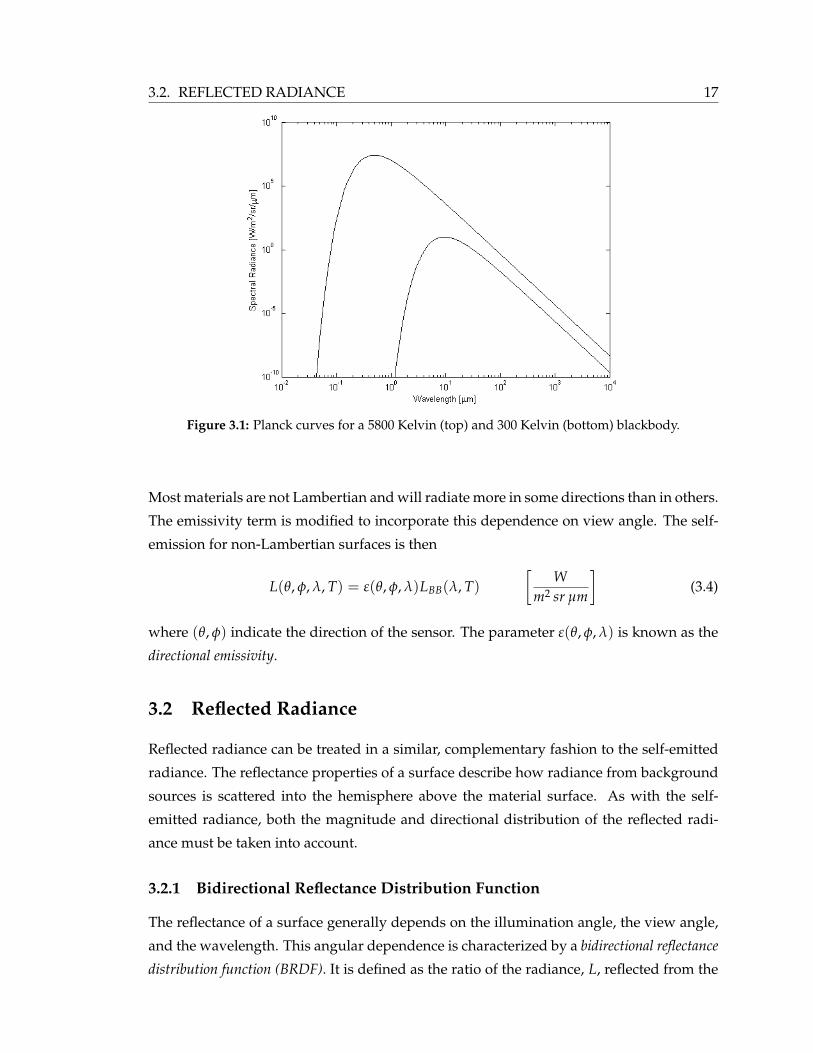
3.2. REFLECTED RADIANCE 17
Figure 3.1: Planck curves for a 5800 Kelvin (top) and 300 Kelvin (bottom) blackbody.
Most materials are not Lambertian and will radiate more in some directions than in others.
The emissivity term is modified to incorporate this dependence on view angle. The self-
emission for non-Lambertian surfaces is then
L(θ, φ, λ, T) = ε(θ, φ, λ)LBB(λ, T)[
Wm2 sr µm
](3.4)
where (θ, φ) indicate the direction of the sensor. The parameter ε(θ, φ, λ) is known as the
directional emissivity.
3.2 Reflected Radiance
Reflected radiance can be treated in a similar, complementary fashion to the self-emitted
radiance. The reflectance properties of a surface describe how radiance from background
sources is scattered into the hemisphere above the material surface. As with the self-
emitted radiance, both the magnitude and directional distribution of the reflected radi-
ance must be taken into account.
3.2.1 Bidirectional Reflectance Distribution Function
The reflectance of a surface generally depends on the illumination angle, the view angle,
and the wavelength. This angular dependence is characterized by a bidirectional reflectance
distribution function (BRDF). It is defined as the ratio of the radiance, L, reflected from the

18 3.2. REFLECTED RADIANCE
surface into the direction (θr, φr) to the irradiance, E, incident on the surface from direction
(θi, φi) [1] and is written as
ρ′(θi, φi, θr, φr, λ) =L(θr, φr, λ)E(θi, φi, λ)
[1sr
]. (3.5)
The BRDF describes the distribution of reflected radiance into the hemisphere from a
given source geometry. It can be thought of as a probability distribution function for
the reflected radiance in any direction [1].
3.2.1.1 BRDF models
The BRDF is a function of all combinations of the incident and reflected angles as well as
wavelength. The large number of angles and wavelengths needed to fully describe the
directional distribution makes measuring a BRDF a tedious process. As a result, models
have been introduced that approximate a true BRDF with only a hand full of adjustable
parameters. These parameters control the shape of the BRDF so that any range of a spec-
ular to a diffuse BRDF can be modeled.
3.2.1.1.1 Lambertian Model Probably the simplest BRDF model is the Lambertian model.
A Lambertian, or diffuse, surface is one that reflects equally in all directions [1]. The model
is written as
ρ′(θi, φi, θr, φr) =ρ
π
[1sr
], (3.6)
where ρ is the reflectance of the material. This model is often used for quick calculations
when a “directional” BRDF is not necessary.
3.2.1.1.2 Ward Model The BRDF model described by Ward [6] adds a specular compo-
nent to the Lambertian model. It is a mathematical model designed to approximate a true
physical BRDF. The objective was to fit measured isotropic and anisotropic reflectance
data with a simplistic formula with intuitively meaningful parameters. For an isotropic
surface, the slope only varies in one dimension and is based on a Gaussian distribution.
The BRDF of this case is modeled as
ρ′(θi, φi, θr, φr) =ρd
π+
ρs√cos θi cos θr
e− tan2 α/σ2
4πσ2
[1sr
], (3.7)
where ρd is the diffuse reflectance, ρs is the specular reflectance, σ is the root-mean-square
(RMS) of the surface slope (similar to surface roughness), and α is the angle between the

3.2. REFLECTED RADIANCE 19
(a) ρd = 0.4, ρs = 0.0, σ = 0.13, θi = 45 (b) ρd = 0.0, ρs = 0.07, σ = 0.13, θi = 45
Figure 3.2: Ward BRDF model: diffuse (left) and specular (right). The thin line on the right handside in the figures indicates the incident ray.
surface normal~n and vector~n′ that bisects the incident and reflected rays. Ward notes that
the reflectance values in equation (3.7) may have a spectral dependence and may vary as
a function of angle so long as the sum of ρd and ρs is less than unity. The normalization
factor is valid as long as σ is not much greater than 0.2. A proper normalization is nec-
essary to ensure physically meaningful results [6]. The α and φ angles are determined by
the geometry of the incident and reflected rays. The user is only responsible for providing
estimates of ρd, ρs, and σ. A small value of σ corresponds to a narrow specular lobe, while
a large value corresponds to a wide lobe. The Ward BRDF model is appealing due to its
simplicity. However, the model and its input parameters are not based on any physical
measurements. Figure 3.2 illustrates two Ward reflectance functions.
3.2.1.1.3 Torrance-Sparrow and Priest-Germer Models Torrance and Sparrow devel-
oped a BRDF model based on the microfacet theory [7]. A rough surface is modeled as a
collection of tiny facets. The slopes of these microfacets are assumed to be randomly ori-
ented according to a probability distribution. Each microfacet acts as a specular reflector
that obeys the law of reflection so that reflection occurs in the plane of incidence and the
reflected angle equals the incident angle. The reflectance of the microfacet is calculated
from the Fresnel equations. Torrance and Sparrow also account for the effect of shadow-
ing and masking of a facet by adjacent facets. See reference [7] for a complete description
of the Torrance-Sparrow BRDF model.
Priest and Germer extended the Torrance-Sparrow model to provide a polarized bidirec-
tional reflectance function [8]. The Priest-Germer model itself only provides the specular

20 3.2. REFLECTED RADIANCE
component of the BRDF. It assumes that the polarized reflectance is due to specular re-
flection while the diffuse reflection is unpolarized. Like the Torrance-Sparrow model, the
Priest-Germer model is based on the assumption that the rough surface of the material is
a collection of tiny, specular, and randomly oriented microfacets. Refer to reference [8] for
details of the Priest-Germer BRDF model.
3.2.1.1.4 Beard-Maxwell Model and the NEFDS The Beard-Maxwell model is also
based on the microfacet theory in which reflection occurs at the first surface but adds
a volumetric component in which scattering occurs beneath the surface [5] [9]. The model
requires seven input parameters that adjust the scatter from the first surface and from
beneath the surface. The number of free parameters in this model is large compared to
the previously mentioned BRDF models. These parameters are based on actual measured
data for real materials which allow the model to more accurately describe a BRDF. The
Beard-Maxwell model serves as the basis for the Nonconventional Exploitation Factors
Data System (NEFDS) [5]. The NEF database contains measured input parameters for
several hundred materials. The Beard-Maxwell model along with NEF materials provide
a powerful way to generate reflectance models from a few measured parameters for sev-
eral hundred materials.
3.2.1.1.5 Shell Target Model Shell generalized the previously mentioned BRDF mod-
els in his Ph.D. dissertation in 2005 [10]. Shell decomposes these models into a general
form to allow for polarization of the model based on the polarized Priest-Germer model.
Shell splits the BRDF model into a specular and a volumetric component. The specular
component results from specular scattering from the front surface via the Fresnel equa-
tions. The volumetric component results from subsurface scattering and is assumed to be
completely depolarizing.
3.2.2 Directional Hemispherical Reflectance
The ratio of the total power reflected into the entire hemisphere by a surface to the power
incident on the surface from a specified direction is the directional hemispherical reflectance
(DHR). It is the integral of the BRDF over the entire hemisphere above a surface for a fixed
incident angle. The directional hemispherical reflectance is
ρ(θi, φi, λ) =∫
2πρ′(θi, φi, θr, φr, λ) cos(θr)dωr, (3.8)
3.3. CONSERVATION OF ENERGY 21
where the integral is taken over all solid angles, dωr, of the hemisphere. The DHR is a
unitless quantity whose range of values are 0 ≤ ρ ≤ 1. The DHR is also defined through
the reciprocal relation as the ratio of the radiance reflected by a surface into direction
(θr, φr) to the radiance uniformly incident on the surface from the entire hemisphere. The
two definitions are equivalent so that ρ(θi, φi, λ) = ρ(θr, φr, λ). If a material is isotropic,
then the azimuthal dependence in equation (3.8) can be ignored,
ρ(θi, φi, λ) = ρ(θ, λ). (3.9)
Furthermore, if the angular dependence is ignored altogether, then the familiar reflectance
of a material is ρ(λ).
3.3 Conservation of Energy
When radiance is incident on an object, it may be absorbed, reflected, or transmitted.
These phenomena are represented by the unitless quantities of absorptivity α(λ), reflec-
tivity ρ(λ), and transmittance τ(λ), respectively [1]. The conservation of energy requires
that these quantities sum to unity so that all the incident radiance is accounted for:
α(λ) + ρ(λ) + τ(λ) = 1. (3.10)
Kirchhoff’s work in thermal radiation led to the conclusion that energy being absorbed
at a particular wavelength must be equal to the energy emitted at that same wavelength
for an object in thermal equilibrium. Therefore, the absorptivity is equal to the emissivity
α(λ) = ε(λ) [11]. For an opaque object where transmission is zero, Kirchhoff’s law is
ε(λ) + ρ(λ) = 1. (3.11)
This relation can be generalized so that the angular dependence of the emissivity and
reflectivity manifests itself,
ε(θ, φ, λ) + ρ(θ, φ, λ) = 1. (3.12)
The quantities ε(θ, φ, λ) and ρ(θ, φ, λ) are the previously defined directional emissivity
and directional hemispherical reflectance from Sections 3.1.2 and 3.2.2.

22 3.4. ENERGY PATHS REACHING A SENSOR
3.4 Energy Paths Reaching a Sensor
The radiance incident on a sensor has many components. These components come from
a variety of sources and depend on the material optical properties and on the radiometric
properties of the surrounding scene. Photons will be traced from the major energy paths
entering the sensor to produce a generic equation describing the radiance at the sensor.
3.4.1 Material Radiance
In thermal remote sensing, information about the temperature of the target is of interest.
This temperature information is carried by the self-emitted radiance term. It is a function
of the Planck equation modified by the object’s directional emissivity (see Section 3.1).
Given that the emissivity is less than unity and through Kirchoff’s relation, real material
surfaces will also reflect radiance from the surround. The reflected background compo-
nent is due to the self-emission from background sources due to the temperature of these
sources. The reflected component depends on the BRDF of the material surface (see Sec-
tion 3.2). The radiance leaving the surface of an object headed toward the sensor is written
as
L(θ, φ, λ) = ε(θ, φ, λ)LBB(λ, T) +∫
2πLbkgd(θi, φi, λ) ρ′(θi, φi, θ, φ, λ) cos(θi)dωi, (3.13)
where the units are[W/m2/sr/µm
]. In the reflected term, the background radiance inci-
dent from direction (θi, φi) is weighted by the BRDF and solid angle in that direction and
the integral is evaluated over the hemisphere above the surface. The emissive term is the
familiar self-emission from equation (3.4). The angles (θ, φ) indicate the direction of the
sensor. Note that the background radiance is a generic term representing all the surround-
ing radiation sources. These sources may include the sun, the sky, other objects, etc. For
a uniform background, Lbkgd is independent of direction and is a constant of integration.
The resulting integral is simply the directional hemispherical reflectance from equation
(3.8) so the surface-leaving radiance reduces to
L(θ, φ, λ) = ε(θ, φ, λ)LBB(λ, T) + ρ(θ, φ, λ)Lbkgd(λ)[
Wm2 sr µm
]. (3.14)
3.4.2 Atmospheric Effects
The radiance leaving the material surface must then propagate through the atmosphere to
reach the sensor. The atmosphere may considerably modify this radiance along the line of
sight to the sensor. The constituent gases and aerosols attenuate the signal by absorption

3.4. ENERGY PATHS REACHING A SENSOR 23
and scattering out of photons. This phenomenon is captured by the atmospheric trans-
mission parameter, τ(λ). The atmospheric constituents also have a finite temperature and
will emit their own self-emitted radiance in all directions, thereby adding to the apparent
material radiance [5]. This radiance from the atmosphere may be reflected off the target,
thereby contributing to the background radiance, Lbkgd, or may enter the sensor directly.
3.4.2.1 Atmospheric Transmission
Atmospheric transmission refers to the loss of photons by a volume of atmosphere. It
encompasses both the absorption and scattering out of photons.
3.4.2.1.1 Absorption Absorption refers to the removal of photons by a material through
the conversion of electromagnetic energy to some other form of energy, usually thermal. It
occurs when the energy (wavelength) of the incoming photon is sufficient to cause a rota-
tional, vibrational, or electronic energy transition in a molecule present in the atmosphere.
The molecule absorbs the photon and makes a quantum jump to a higher energy state.
The molecule will quickly lose this excess energy through collisions with other molecules
and return to its original energy state. The photon energies (wavelengths) that will be
absorbed by a molecule depend on the transition energies between states of that molecule
[11]. The amount of absorption by atmospheric gases is dependent on the quanitity of the
gas and on its temperature and pressure [5]. These discrete energy absorptions manifest
themselves as discrete lines in the absorption spectrum of a gas. However, interactions
between the gas molecules will cause perturbations in their energy states which results
in broadening of the absorption lines. When the broadened lines are close to each other,
they combine to form a continuum of absorption [1]. A typical gas absorption spectrum
will therefore exhibit both discrete (molecular) and continuum absorption features. Major
absorbers in Earth’s atmosphere in the LWIR are O3, CO2, and H2O.
The amount of absorption of a propagating beam of radiation in a given path length
depends on the effective size and density of absorbing particles. The absorption cross
section, Cα(λ), is a measure of the effectiveness of a particle as an absorber to a particular
wavelength of radiation. The fractional amount of flux that is absorbed per unit length is
defined as
βα(λ) = m Cα(λ)[
1m
](3.15)
where m is the number of particles per unit volume and βα(λ) is known as the absorption
coefficient. It is the fractional amount of flux lost to absorption per unit length [1].

24 3.4. ENERGY PATHS REACHING A SENSOR
For a horizontal layer of gas of infinitesimally small thickness, dz, the fractional amount
of absorption through the layer is
dα(λ) =dΦ(λ)Φ(λ)
= −βα(λ) sec θ dz (3.16)
where θ is the zenith angle through the layer, Φ is the incident flux entering the layer and
dΦ is the flux lost to absorption in the layer. Integrating both sides and taking the antilog
yields the transmission,
τα(θ, φ, λ) = e−
z2∫z1
βα(λ) sec θ dz
(3.17)
where the integral is performed over the starting and ending altitudes of the path. If there
is more than one constituent gas in the layer, then the absorption coefficient is the sum of
the absorption coefficients of the constituent gases.
3.4.2.1.2 Scattering Transmission losses are also the result of photons being scattered
out of the propagating beam. The transmission loss due to scattering can be written simi-
lar to the transmission loss due to absorption as
τs(θ, φ, λ) = e−
z2∫z1
βs(λ) sec θ dz
(3.18)
where βs(λ) is the scattering coefficient. The scattering coefficient is a function of the index
of refraction of the scattering particles. It can also be expressed as a function of a size
parameter a = 2πr/λ which is a measure of the size of particles in comparision to the
wavelength of radiation [12].
A complete theory on the scattering of electromagnetic radiation involves developing so-
lutions to the Maxwell equations. In a given volume of air, a variety of particle shapes
and sizes are present [12]. For the idealized case of spherical particles, Gustav Mie de-
veloped a complete analytical solution to Maxwell’s equations. The Mie solution, com-
monly referred to as Mie scattering, is valid for all possible size parameters, a. The angular
distribution of the scattered radiation varies greatly depending on the particle size and
wavelength of radiation. In general, however, forward scattering dominates over back
scattering. Mie scattering also depends weakly on wavelength and becomes independent
of it when the particle size exceeds the wavelength [11].
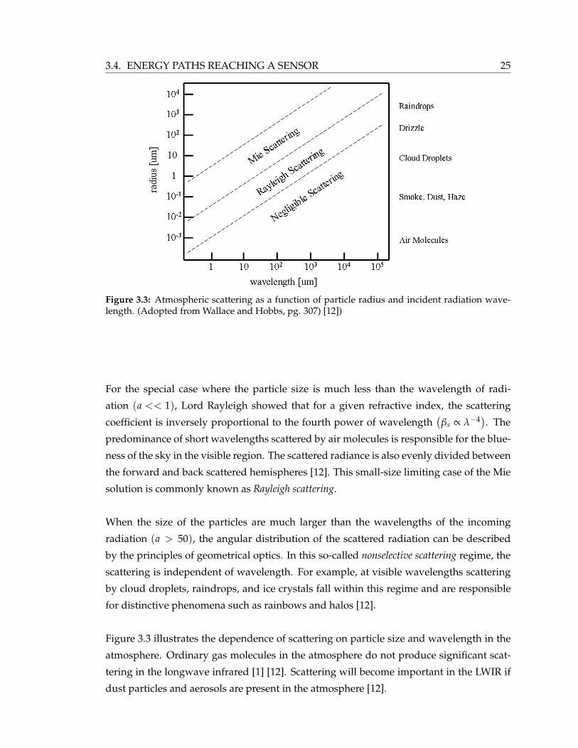
3.4. ENERGY PATHS REACHING A SENSOR 25
Figure 3.3: Atmospheric scattering as a function of particle radius and incident radiation wave-length. (Adopted from Wallace and Hobbs, pg. 307) [12])
For the special case where the particle size is much less than the wavelength of radi-
ation (a << 1), Lord Rayleigh showed that for a given refractive index, the scattering
coefficient is inversely proportional to the fourth power of wavelength(
βs ∝ λ−4). The
predominance of short wavelengths scattered by air molecules is responsible for the blue-
ness of the sky in the visible region. The scattered radiance is also evenly divided between
the forward and back scattered hemispheres [12]. This small-size limiting case of the Mie
solution is commonly known as Rayleigh scattering.
When the size of the particles are much larger than the wavelengths of the incoming
radiation (a > 50), the angular distribution of the scattered radiation can be described
by the principles of geometrical optics. In this so-called nonselective scattering regime, the
scattering is independent of wavelength. For example, at visible wavelengths scattering
by cloud droplets, raindrops, and ice crystals fall within this regime and are responsible
for distinctive phenomena such as rainbows and halos [12].
Figure 3.3 illustrates the dependence of scattering on particle size and wavelength in the
atmosphere. Ordinary gas molecules in the atmosphere do not produce significant scat-
tering in the longwave infrared [1] [12]. Scattering will become important in the LWIR if
dust particles and aerosols are present in the atmosphere [12].

26 3.4. ENERGY PATHS REACHING A SENSOR
Figure 3.4: Atmospheric spectral transmission along a vertical space-to-ground path generatedfrom a MODTRAN mid-latitude summer atmosphere[13].
3.4.2.1.3 Total Transmission The transmission due to absorption and scattering effects
can be combined to describe the total transmission by
τ(θ, φ, λ) = e−
z2∫z1
βext(λ) sec θ dz
(3.19)
where βext(λ) is known as the extinction coefficient and is the sum of the absorption and
scattering coefficients. The total spectral atmospheric transmission is visualized in Fig-
ure 3.4.
3.4.2.2 Atmospheric Emission
The constituents of the atmosphere have a finite temperature and will therefore be a
source of energy [1]. To calculate this radiance, the continuously varying atmosphere is
approximated as a set of homogeneous layers as in Figure 3.5. Each layer has an effective
transmission, ∆τi, along the line of sight of the sensor defined by the angles (θ, φ). Since
scattering is negligible in the LWIR, the effective emissivity of the ith layer is ∆ε i = 1−∆τi
[1]. The self-emitted radiance of the ith layer is the blackbody radiance, LBB(Ti), due to
its temperature, modified by the effective emissivity of that layer and the product of the
effective transmissions of the (i− 1) layers. If the number of layers in direction (θ, φ) is N,

3.4. ENERGY PATHS REACHING A SENSOR 27
Figure 3.5: Self-emitted atmospheric radiance into the (θ, φ) direction is the sum of the self-emittedradiance from each homogeneous atmospheric layer (Adopted from Schott 1997, pg 109 [1]).
then the atmospheric radiance is
Latm (θ, φ, λ) =N
∑i=1
LBB (λ, Ti) [1− ∆τi( θ, φ, λ)]i−1
∏j=1
∆τj(θ, φ, λ)[
Wm2 sr µm
]. (3.20)
The atmospheric radiance that is emitted towards the target material is known as the
emissive downwelled radiance, Ld(θ, φ, λ). This may contribute to the background radi-
ance that is reflected from the target material (see Section 3.4.1). The atmospheric thermal
energy that is emitted towards the sensor is known as the emissive upwelled radiance,
Lu(θ, φ, λ). The upwelled radiance and the reflected downwelled radiance add to the tar-
get material’s signal as recorded by the sensor [1].
3.4.3 Governing Equation
Combining all these radiometric effects into a single equation, the total spectral radiance
reaching the sensor is then
L(θ, φ, λ) = (3.21)[ε(θ, φ, λ)LBB(λ, T) +
∫
2πLbkgd(θi, φi, λ) ρ′(θi, φi, θ, φ, λ) cos(θi)dωi
]τ(θ, φ, λ)
+Lu(θ, φ, λ),

28 3.5. IMAGING SYSTEM
in units of[W/m2/sr/µm
]and where (θ, φ) indicate the direction of the sensor. This is
the governing equation for radiance reaching the sensor. For uniform backgrounds, the re-
flected component in equation (3.21) reduces to the DHR multiplied by the background
radiance.
From equation (3.21) it is clear that the radiance from the target itself is substantially mod-
ified on its way to the sensor. The directional emissivity, BRDF, background radiances,
atmospheric transmission and upwelled radiances all work to alter the blackbody radi-
ance from the target. This makes deriving the temperature of the target rather difficult.
Each of the mentioned variables must be modeled or estimated in order to reconstruct the
original blackbody radiance. Uncertainities in these parameters will lead to uncertainity
in the derived temperature.
3.5 Imaging System
The combined spectral radiance from all the energy paths, L(θ, φ, λ), is then incident on
the sensor, or imaging system. In the general sense, an imaging system is a series of pro-
cesses in which the incoming spectral radiances are represented as an image. The spectral
radiances from all points visible to the sensor are collected, sampled, and measured to
produce a quantifiable signal. The imaging system can be divided into several steps serv-
ing a specific task. Each step in this process unavoidably degrades the incoming signal so
that the final image cannot be a perfect representation of the original signal.
3.5.1 Collection
The radiance incident on the sensor must first be collected. This operation is performed by
the optical elements of the sensor. The radiance entering the aperture is focused onto the
focal plane. Ideally, radiance from a point entering the aperture (i.e., a point on the object
plane) would be perfectly focused onto a point on the focal plane (image plane). However,
for a diffraction-limited system, radiance from a point source on the object plane will be
spread out over a finite area on the focal plane [11]. In other words, even a perfect point
source (mathematically represented by a delta function [14]) will be blurred by the optical
system. Figure 3.6 demonstrates this effect.
The image produced by a point source is called the point-spread function (PSF). For a
shift-invariant linear system, the output signal (image) is the summation of spatially dis-
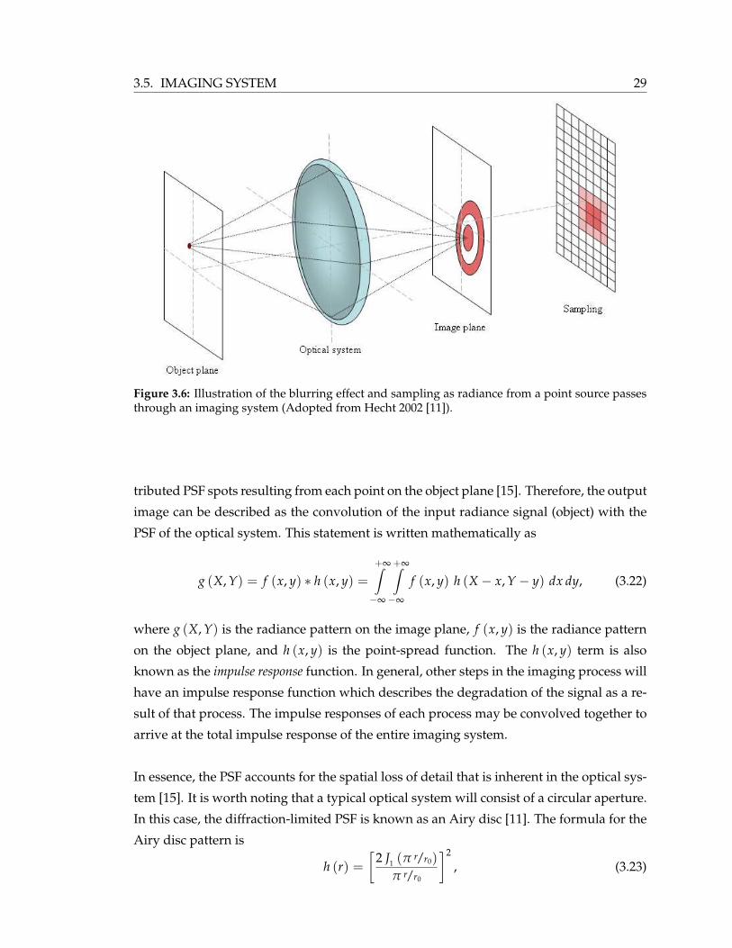
3.5. IMAGING SYSTEM 29
Figure 3.6: Illustration of the blurring effect and sampling as radiance from a point source passesthrough an imaging system (Adopted from Hecht 2002 [11]).
tributed PSF spots resulting from each point on the object plane [15]. Therefore, the output
image can be described as the convolution of the input radiance signal (object) with the
PSF of the optical system. This statement is written mathematically as
g (X, Y) = f (x, y) ∗ h (x, y) =+∞∫
−∞
+∞∫
−∞
f (x, y) h (X− x, Y− y) dx dy, (3.22)
where g (X, Y) is the radiance pattern on the image plane, f (x, y) is the radiance pattern
on the object plane, and h (x, y) is the point-spread function. The h (x, y) term is also
known as the impulse response function. In general, other steps in the imaging process will
have an impulse response function which describes the degradation of the signal as a re-
sult of that process. The impulse responses of each process may be convolved together to
arrive at the total impulse response of the entire imaging system.
In essence, the PSF accounts for the spatial loss of detail that is inherent in the optical sys-
tem [15]. It is worth noting that a typical optical system will consist of a circular aperture.
In this case, the diffraction-limited PSF is known as an Airy disc [11]. The formula for the
Airy disc pattern is
h (r) =[
2 J1 (π r/r0)π r/r0
]2
, (3.23)

30 3.5. IMAGING SYSTEM
Figure 3.7: Airy disc pattern representing the PSF of a diffraction-limited circular aperture system.
where J1() is the first-order Bessel function of the first kind [15], r is the radial distance
from the center of the Airy disc on the image plane, and r0 is the radial distance from the
center of the disc to the first minimum (see Figure 3.7). The Bessel function is written as
J1(r) =1π
π∫
0
cos (t− r sin(t)) dt. (3.24)
The constant r0 is computed by
r0 =1.22 λ f
a[µm], (3.25)
where a is the diameter of the circular aperture, f is the focal length, and λ is the wave-
length of the radiation.
3.5.2 Detection
The optical system focuses the sensor reaching radiance onto the focal plane. Detectors
located on the focal plane then convert this radiance into a quantifiable signal. For electro-
optical systems, the detector converts the incident flux on it into an electronic signal. This
is accomplished when a photon is absorbed by the detector material and induces a charge
in the material. The accumulated charge is then read out as an electronic signal. A typical
sensor might consist of a two-dimensional array of detector elements called pixels. Each
pixel acts as a tiny detector that absorbs the incident photons and stores the accumulated

3.5. IMAGING SYSTEM 31
charge. The two-dimensional array therefore allows the spatial distribution of the inci-
dent flux to be recorded as an image. As with the collection process, the detector process
further degrades the incoming radiance signal.
3.5.2.1 Spatial Sampling
The incoming flux is sampled and quantizied by the detector in order to convert that flux
into a digital form. Each pixel spans a finite area such that photons that are absorbed in
this area contribute to the signal in that pixel. Therefore, the incident photon flux is es-
sentially integrated over the physical dimensions of the pixel resulting in a loss of spatial
information within the pixel. The physical dimensions of the pixels influence the ground
sampling distance (GSD) of the sensor. The GSD corresponds to the projection of the pixel
size onto the ground. The GSD can be calculated from basic geometry and knowledge of
the focal length, pixel size, and distance to the target (ground).
As mentioned previously, each step in the imaging process might have an impulse re-
sponse associated with it. The impulse response associated with the loss of spatial de-
tail in the sampling process could be described by a two-dimensional RECT function,
h(x, y) = RECT(
xpx
, ypy
), where px and py are the x and y pixel dimensions. In some
circumstances, the GSD may be defined as the full-width at half-maximum amplitude of
the total system impulse response projected onto the ground [1]. See Gaskill (1978) [14]
for detailed information about impulse response functions.
3.5.2.2 Temporal Sampling
The detector material is only exposed to the incident flux for a finite time. The interval
of time in which the detector is allowed to absorb photons is known as the integration
time. It is typically controlled with a mechanical shutter or through electronic means. The
integration time represents the temporal averaging of the incident photon flux over the
finite time interval which results in a loss of temporal information.
3.5.2.3 Spectral Sampling
In addition to spatial and temporal sampling, the detector also performs spectral sampling
of the incident photon flux. The detector is only sensitive to a certain range of wavelengths
known as the bandpass. The sensitivity of the detector to each wavelength is represented
by the spectral response function, R(λ). It is defined as the signal output, S, per unit
32 3.5. IMAGING SYSTEM
incident flux, Φi(λ) at a particular wavelength. The detector material is carefully chosen
such that photons of the desired wavelength are absorbed with relatively high efficiency.
A detector designed for LWIR photons would consist of Mercury Cadmium Telluride
(HgCdTe) semiconductor material, for example, which has a high response in the 8 - 14 µm
region.
The incident flux on the detector is weighted by the response function and integrated
over all wavelengths (essentially the bandpass of the sensor) to produce an output signal.
Mathematically, this detector signal relative to the spectral response of the sensor is stated
as
S =∫
Φi(λ) R(λ) dλ. (3.26)
The signal is typically expressed in units of Amperes or Volts depending on the detector.
3.5.2.3.1 Band Effective Values
In general, the term ”band effective” value is often used to describe the effective value of
a spectral parameter in the sensor band of interest. For a generic spectral parameter, ϕ(λ),
its band effective value is written as
ϕ =∫
ϕ(λ) R′(λ) dλ. (3.27)
The hat () indicates a band effective value and R′(λ) is the spectral response function of
the detector normalized by its maximum value.
The band effective value may be expressed “per wavelength” by normalizing equation
(3.27) by the sensor response,
ϕλ =∫
ϕ(λ) R′(λ) dλ∫R′(λ) dλ
. (3.28)
3.5.2.4 Noise
Another degradation of the signal as it passes through the imaging system will be the
addition of noise. Noise corresponds to random variations in the output signal level even
when the detector is exposed to a uniform flux. These random fluctuations are due to such
factors as thermal variation in the detector and the random occurence of photon events.
Noise is usually characterized as the root mean square (RMS) variation about the mean
signal.
3.6. APPARENT TEMPERATURE 33
For thermal imaging, it may be useful to express the concept of noise in terms of detectable
temperature [1]. The noise equivalent change in temperature (NE∆T) is a measure of the
change in temperature of a blackbody at the front of the sensor that would produce a
change in the sensor output equal to the sensor’s noise level [1].
3.5.3 Calibration
The result of the imaging process is a temporally-averaged, and a spatially- and spectrally-
integrated signal for each pixel. This signal is then read out by the sensor electronics. The
amplitude of the output signal is quantitized into discrete digital values. The resulting
digital image consists of a spatial distribution of recorded digital count values.
Sensors are usually calibrated so that the digital count values can be converted into a
sensor-reaching radiance. This calibration may be performed in a laboratory in which ra-
diance from a known source is recorded by the sensor. A calibration curve is constructed
by altering the source radiance and recording the resulting output signal from the sensor.
The digital image may now be presented as a distribution of radiance values in which
each pixel contains the spatially, temporally, and spectrally degraded radiance for that
pixel location. These radiance values are essentially the output sensor digital count val-
ues projected back to the front of the sensor. This effective radiance is denoted here as L.
3.6 Apparent Temperature
In the previous sections, the energy paths reaching a sensor were examined. The effective
radiance recorded by the sensor, L, is usually expressed in terms of an apparent tempera-
ture (also called brightness temperature in the literature). The apparent temperature is the
equivalent temperature of a spatially homogeneous and temporally constant blackbody
that will produce the same sensor effective radiance when cascaded with the spectral re-
sponse of the sensor [16]. This is written mathematically as
L =∫ ∞
0LBB(λ, Tapp) R′(λ) dλ
[W
m2 sr
]. (3.29)
It is important to note that the temperature derived from the integrated sensor radiance
is an “apparent” temperature since the Planck function predicts radiances from a perfect
blackbody in a perfect transmitting, non-scattering, non-absorbing media. Real-world
objects with emissivities less than unity radiate less than a blackbody at the same tem-
perature. Furthermore, the radiance reaching the sensor is not solely from the target of

34 3.6. APPARENT TEMPERATURE
interest, but rather from a variety of energy paths as described in Section 3.4.
3.6.1 Planck Formula Inversion
Given the integrated radiance as measured by the sensor for a particular band L, the
apparent temperature of the blackbody, Tapp, can be estimated by inverting the Planck
equation,
Tapp =hcλk
[ln
(2hc2 Ψ
L λ5+ 1
)]−1
[K], (3.30)
where λ is the effective wavelength in the band (see Section 3.5.2.3.1), Ψ is the integral of
the sensor response function in the spectral band, and L is the integrated radiance in the
band in[W/m2/sr
]. Note that by equation (3.28), Lλ = L/Ψ.
This method is attractive due to its simplicity, however, it overlooks the spectral nature
of the signal. The Planck formula produces a spectral radiance for a given temperature
and wavelength. Since the sensor output is an integrated radiance and not a spectral ra-
diance, the radiance used in equation (3.30) should be deconvolved to separate out the
sensor’s spectral response and the spectral blackbody radiance. This is a very difficult
task and therefore the integrated radiance and the effective wavelength are used instead.
As an example, the DIRSIG tool (see Section 4.1.2) was used to simulate the radiance from
a blackbody plate as recorded by a LWIR sensor. The blackbody had a temperature of
300 K and the sensor had a perfect response from 8 to 14 µm with a wavelength spacing
of 0.001 µm. There was no intervening atmosphere in the simulation. The integrated radi-
ance reported by the sensor was 54.9410[W/m2/sr
]. The resulting apparent temperature
is 297.0071 K. This difference from the actual temperature of 300 K is due to the use of the
effective wavelength in the Planck function. The spectral aspect of the Planck function
was not taken into account.
3.6.2 Temperature-Radiance Look-Up Table
To incorporate the spectral nature of the blackbody radiance and the spectral response
of the sensor, a look-up table (LUT) can be generated to convert the sensor’s integrated
radiance into an apparent temperature. Sospedra et al. (1998) notes that this is the most
accurate way to perform the band radiance to temperature conversion [17].
The Planck equation is evaluated at the sensor wavelengths and weighted by the sensor
response and finally integrated to produce an integrated effective radiance via equation
3.6. APPARENT TEMPERATURE 35
(3.29) for a range of temperatures. The temperature range should be wide enough to cover
the suspected range of temperatures for the objects in the scene. The temperature resolu-
tion should also be very high (temperatures were calculated in 0.001 K increments for this
project). Note that the sensor response function is taken into account so the LUT is only
valid for that particular sensor. It must be regenerated for other sensors with different
responses. The LUT now provides a relationship between the integrated sensor radiance
and the blackbody temperature.
The integrated radiance from the sensor is then compared to the radiances in the LUT and
a temperature is chosen through an interpolation scheme. For example, a nearest neighbor
interpolation would select the temperature whose associated integrated radiance in the
table had the smallest absolute difference with the sensor’s reported integrated radiance.
For the same DIRSIG simulation in Section 3.6.1, an integrated LWIR sensor radiance of
54.9410[W/m2/sr
]yields an apparent temperature of 299.9970 K using the LUT method.

36 3.6. APPARENT TEMPERATURE
Chapter 4
Background
In the last chapter, the interaction between the self-emitted signal from a target and its ra-
diometric environment was discussed. The self-emitted radiance from the target, carrying
the desired information about the target’s temperature, is heavily modified before it is fi-
nally recorded by the sensor. The objective of temperature retrieval from remote thermal
imagery is to account for the discrepancy between the at-sensor apparent temperature
and the absolute temperature of the target as accurately as possible. There are several
tools and methods used to extract the absolute temperature from the radiance recorded
by the sensor. There is currently no single approach that is widely accepted and used
by the thermal remote sensing community [1]. Therefore, a number of different methods
exist that are useful for a particular type of problem. An overview of common methods is
presented in this chapter.
4.1 Modeling Tools
It is clear from the previous chapter that the signal from a target material is significantly
altered before being recorded by the sensor. The terms in the governing equation may be
modeled in order to back out the original target signal. There are several tools available
to model radiometric phenomena and radiation propagation. The two major tools used
in this project are MODTRAN and DIRSIG.
4.1.1 MODTRAN
The MODerate spectral resolution TRANsmittance tool is an atmospheric radiative trans-
fer code [18]. It was developed by the Air Force Research Laboratory (AFRL) and Spectral
Sciences, Inc (SSI). MODTRAN models the atmosphere as a series of stacked homoge-
neous layers. The pressure and temperature of each layer is provided by several preset at-
mospheric profiles or by user-supplied radiosonde data. The concentration of permanent
gases can be estimated from the radiosonde or from the generic preset profiles. MOD-
TRAN contains six predefined atmospheres that can be supplemented with radiosonde
37
38 4.1. MODELING TOOLS
data if available. The user may also specify meteorological conditions such as visibility,
season, air mass type, etc. to estimate the size and distribution of aerosols [1]. MODTRAN
will provide the spectral absorption, transmission, emission and scattering characteristics
of the atmosphere based on the given input data for a spectral range of 0 to 50,000 cm−1
[19]. It is based on the lower spectral resolution LOWTRAN 7 code. MODTRAN 4 incor-
porates all the LOWTRAN 7 options but also improves the spectral resolution to 2 cm−1
[18].
As previously mentioned, MODTRAN divides the atmosphere into homogeneous layers
as illustrated in Figure 3.5. The transmission between the sensor and target is calculated
from equations (3.15) and (3.19). The transmission is expressed as
τ(θ, λ) = ∏i
e−∑
kmikCik(λ) sec θ zi
(4.1)
where again mik and Cik(λ) are the number density and extinction cross-section of the kth
atmospheric constituent in the ith layer, respectively. The thickness of the layer is zi and
the zenith view angle is θ. The summation in the exponent is taken over all the constituent
gases and the total transmission is the product of the transmissions of the individual lay-
ers. MODTRAN derives the number densities from the atmospheric profile data and de-
rives extinction cross-sections from database values of the atmospheric constituents [1].
The emission of the atmosphere is calculated similar to equation (3.20) rewritten here as
Latm (θ, λ) =N
∑i=1
LBB (λ, Ti) [1− ∆τi( θ, λ)]i−1
∏j=1
∆τj(θ, λ)[
Wm2 sr µm
]. (4.2)
where Ti and ∆τi are the temperature and transmission of the ith layer, respectively. Note
that the transmission and self-emitted atmospheric radiance are independent of the az-
imuth angle since the atmosphere is modeled as a series of homogeneous layers.
MODTRAN can be manipulated to estimate the atmospheric parameters in the governing
equation (Section 3.4.3). The total spectral transmission and upwelling radiance are pro-
vided in the MODTRAN output. The downwelling radiance can be calculated through
equation (4.2) for various look angles. MODTRAN can also provide the spectral trans-
missions of the individual gas species and aerosols in the path. The aerosol models in
MODTRAN are defined by regions that contain typical aerosol sources. The sources are
4.1. MODELING TOOLS 39
representative of rural, urban, desert and maritime environments [20]. The predefined at-
mospheric profiles are characteristic of tropical, mid-latitude, and arctic atmospheres for
summer and winter seasons [20].
4.1.2 DIRSIG
The Digital Imaging and Remote Sensing Image Generation (DIRSIG) tool was developed
by the Digital Imaging and Remote Sensing (DIRS) Laboratory at the Rochester Institute
of Technology (RIT) [21]. It is a synthetic image generation application that produces sim-
ulated visible through thermal imagery. DIRSIG utilizes ray tracing and first principle
physics, chemistry, and mathematical theories to accurately reproduce the radiometry of
a scene [22]. The simulated images are generated through the integration of first prin-
ciple based sub-models. These sub-models include BRDF predictions, facet temperature
prediction, sensor models, and atmospheric models, among others. The modeled compo-
nents are combined spectrally to create a simulated integrated radiance image of the scene
for the given sensor and viewing geometry. DIRSIG also has the capability to model po-
larimetric, RADAR, and LIDAR imaging systems.
A DIRSIG scene consists of full three-dimensional facetized object geometries usually
created with a CAD software package. A material’s physical and optical properties are
assigned to each facet. These properties may be obtained through field and laboratory
measurements or from material databases. A temperature prediction model estimates the
temperature of every facet in the scene based on material thermodynamic and optical
properties, illumination history, and local weather history. The atmospheric model uses
the MODTRAN radiative transfer code. DIRSIG creates a MODTRAN look-up table for a
series of atmospheric paths of interest. An accurate estimate of the atmospheric transmis-
sion, upwelling and downwelling radiances is therefore possible. The geometric sensor
model allows the user to simulate broadband, multispectral, and hyperspectral sensors in
a variety of geometries such as framing arrays, line scanners, etc. [22].
DIRSIG is a powerful tool for the remote sensing community [22]. The synthetic data pro-
duced by the model is useful for a range of applications. These application areas range
from algorithm training and testing to instrument prototyping.

40 4.2. TEMPERATURE RETRIEVAL METHODS
4.2 Temperature Retrieval Methods
The ultimate goal in thermal remote sensing is to obtain the absolute temperature of a
material surface. The atmospheric and emissivity effects must be isolated and accounted
for in order to arrive at the “pure” blackbody signal from the target material.
4.2.1 Atmospheric Compensation
The term atmospheric compensation refers to the removal of atmospheric effects in an image.
Specifically, these effects are the atmospheric transmission and upwelling radiance from
equation (3.21). The sensor-reaching radiance is atmospherically corrected to arrive at the
surface-leaving radiance. Since the emissivity and other surface effects are not accounted
for, the surface-leaving radiance will yield only the apparent surface temperature and not
the absolute surface temperature.
4.2.1.1 Ground Truth
Probably the most straightforward method of atmospheric compensation is to perform
surface measurements of objects in the scene coincident with the time of image acquisi-
tion [1]. These “ground truth” collects are measurements of the absolute temperatures
of fully resolved targets with known emissivities in the scene. Recall that the radiance
reaching a sensor from a surface after passing through the atmosphere is
Lsensor =[ε LBB(T) + (1− ε) Ld
]τ + Lu
[W
m2 sr
]. (4.3)
If the calibration targets are blackbodies (ε = 1), then the downwelling term in equa-
tion (4.3) is zero. By taking temperature measurements of blackbody objects in the scene
having a range of temperatures, a linear regression can be performed to yield the band
effective transmission and upwelling radiances from the slope and intercept of the regres-
sion for the given scene atmosphere. Once the atmospheric terms are known, a calibration
curve now exists that relates the sensor effective radiance to the surface-leaving effective
radiance. This can then be converted into an apparent temperature of the surface.
This method may also work for non-blackbody targets if the emissivity is known. In
this case, the downwelling sky radiance must also be known. It can be measured with
a radiometer in the scene that collects and integrates the radiance over the same pass
band as the sensor [1]. The downwelling radiance may also be approximated through an
4.2. TEMPERATURE RETRIEVAL METHODS 41
atmospheric modeling tool such as MODTRAN.
4.2.1.2 Single-Channel Method
The absolute temperature of the target may be obtained from radiance measurements in
a single IR channel which have been corrected for atmospheric effects [23]. A radiative
transfer model is used to derive the atmospheric terms in equation (3.21). This method
assumes knowledge of the bidirectional reflectance characteristics of the target material.
The MODTRAN tool is commonly used to model the state of the atmosphere and numer-
ically calculate the spectral transmission and upwelling and downwelling radiances for
the given image acquistion time and location. The horizontal and vertical distribution of
temperature and water vapor must be accurately known for input into the radiative trans-
fer model. Atmospheric profiles may be obtained from satellite sounding instruments,
numerical weather prediction models, and radiosondes. Since profile data is discrete in
time and space, the data must be spatially and temporally interpolated for the target of
interest. Once the atmospheric terms are accounted for, the kinetic temperature of the tar-
get can be determined given that its BRDF and geometry are known [23].
For the given spectral channel, the surface radiance can be computed from the sensor
radiance and the MODTRAN calculated transmission and upwelling radiance as
Lsur f =Lsensor − Lu
τ
[W
m2 sr
](4.4)
where each of the parameters are band effective values [1]. The surface radiance can then
be converted into an apparent surface temperature (see Section 3.6).
An alternative approach is to make use of a LUT to relate the apparent surface tempera-
ture to an effective sensor radiance in the channel of interest. The method is similar to the
one presented in Section 3.6.2. For a given temperature, the spectral blackbody radiance
is calculated from the Planck equation. This radiance is then multiplied by wavelength
by the spectral transmission and then added to the spectral upwelled radiance generated
from MODTRAN. Finally, this spectral radiance is multiplied with the sensor response
and integrated to arrive at a band effective radiance for the given blackbody temperature.
This is written mathematically as
L =∫
[LBB(λ, T) τ(λ) + Lu(λ)] R′(λ) dλ
[W
m2 sr
]. (4.5)
42 4.2. TEMPERATURE RETRIEVAL METHODS
A LUT is created that relates a range of blackbody temperatures to a range of effective
radiances. The surface apparent temperature is therefore the temperature from the LUT
whose radiance is the closest match to the actual effective radiance recorded by the sensor.
The single channel method was successfully used by Qin et al. (2001) to retrieve desert
land surface temperatures using the Landsat TM thermal band [24]. The authors used in
situ atmospheric profile data that was coincident with the satellite pass to compensate for
the atmosphere. The resulting temperature errors were approximately 1.1 K.
4.2.1.3 Multi-Channel Method
The multi-channel method uses differential absorption in several spectral channels to
eliminate atmospheric effects. The split-window technique makes use of two channels
within one atmospheric window [23]. The target’s temperature is usually taken as a linear
or quadratic function of the apparent temperatures in the two channels [25]. The coeffi-
cients of these temperature retrieval algorithms are usually determined by a regression
of the apparent temperature measured by the sensor with coincident in situ surface tem-
perature measurements. The regression analysis can also be performed on synthetic data
generated from a large sample of atmospheric profiles using a radiative transfer model.
There are numerous split-window algorithms depending on the specific sensor and ap-
plication [23]. Schott (1997) describes a general split-window technique in which the ap-
parent surface temperature can be derived from the apparent temperature in two spectral
bands as
Tsur f =Ti − b Tj
1− b[K], (4.6)
where Ti and Tj are the apparent temperatures in the two bands and b = βext,i/βext,j, the
ratio of the effective extinction coefficients in the two channels [1]. The extinction coeffi-
cients can be computed through the use of radiation propagation models [1].
Prata (1993) developed a dual-channel method to retrieve land surface temperatures [26].
This approach uses the brightness temperatures in the two channels along with an esti-
mate of the atmospheric transmission, the downwelling radiance, and the surface emis-
sivity in each channel. Prata’s method yielded land surface temperatures to within± 1.5 K
for flat terrain with uniform surface composition in relatively dry atmospheres [26].
The split-window technique has been used successfully on data from the Advanced Very
4.2. TEMPERATURE RETRIEVAL METHODS 43
High Resolution Radiometer (AVHRR) instrument on the NOAA polar-orbiting satellites
[27]. The instrument uses three bands for sea surface temperature retrieval at 3.7 µm
(band 3), 11 µm (band 4), and 12 µm (band 5). The non-linear algorithm uses two bands
for daytime temperature retrieval and three bands for nighttime temperature retrieval.
The coefficients of these algorithms are calculated by matching a set of AVHRR data with
buoy observations. A global dataset is assembled of AVHRR data and coincident tem-
perature measurements from buoys. This dataset contains a global range of sea surface
temperatures and atmospheric moisture content. A regression analysis is then performed
on this dataset to calculate coefficients for the split-window algorithms. A validation of
these algorithms by Li et al. (2001) indicate a small temperature bias of 0.08 °C to 0.14 °C
with a standard deviation of 0.50 °C or less [27].
4.2.1.4 Multi-Angle Method
The multi-angle approach takes advantage of the differential absorption arising from the
difference in path length when a target is viewed from two different angles [23]. The same
target is viewed from a small zenith angle (usually at nadir) and then near-simultaneously
from a high zenith angle. The ATSR instrument aboard the ERS-1 satellite uses a nadir
view and a forward-looking 55° view, for example. The atmospheric transmission and
upwelling radiance are approximated from the differing radiances resulting from the dif-
ferent view angles. This method assumes a spatially uniform air column. It also strictly
requires that one view path be significantly longer than the other [23]. The angular vari-
ation of the target’s emissivity is assumed to be negligible. However, to reduce errors in
the derived apparant surface temperature, angular emissivity effects should be taken into
account if known.
Schott (1997) provides an overview of the procedure for this method [1]. Assuming that
the targets in the scene are Lambertian, the relationship between the observed radiance at
nadir, L(θ = 0), and at some other angle, L(θ = θ′), is given as
L(θ = θ′) =[
τ(θ′)τ(0)
]L(θ = 0) +
[Lu(θ′)− τ(θ′)
τ(0)Lu(0)
](4.7)
If several Lambertian targets are imaged, then a linear regression may be performed in
which the first bracketed term in equation (4.7) is the slope, m, and the second bracketed
term is the intercept, b. For clear atmospheres, the effective transmission and upwelled

44 4.2. TEMPERATURE RETRIEVAL METHODS
Figure 4.1: Multispectral Thermal Imager (MTI) band locations (Szymanski and Weber 2005 [28]).
radiance for nadir-viewing can be derived from the slope and intercept by
τ(0) = m1/(sec θ′)−1 (4.8)
Lu(0) =b
sec θ′ −m.
4.2.1.5 MTI Sea Surface Temperature Retrieval
The Multispectral Thermal Imager (MTI) is a Department of Energy (DOE) mission to
demonstrate technology and algorithms for industrial and environmental remote sensing
research [28]. The MTI sensor contains 15 spectral bands between 0.4 and 11 µm which
include two bands in the MWIR (bands J and K) and three bands in the LWIR (bands L,
M, and N) (See Figure 4.1). The visible and infrared bands have a GSD of 5 m and 20
m, respectively. Borel et al. (1999) developed a method to use the thermal bands on MTI
to retrieve sea surface temperatures [29]. The method is based on linear combinations of
the brightness temperatures in the MTI bands J, K, L, M, and N for night time imaging.
It also relies on two view angles of a body of water at nadir and at 60°. First an atmo-
spheric database (LUT) is created using a radiative transfer code such as MODTRAN. The
database contains the atmospheric transmission, upwelling, and downwelling radiances
for a wide range atmospheric conditions as seen in the five MTI bands at the two view
angles. Next, from the atmospheric database, the top-of-atmosphere (TOA) radiance is
computed for a given water emissivity and temperature. A TOA database is created from
4.2. TEMPERATURE RETRIEVAL METHODS 45
the atmospheric database and a range of water temperatures. Finally, a linear regression
model is fit to this database. The sea surface temperature is then a linear combination
of the brightness temperatures in the five bands [29]. Preliminary post-launch validation
of this algorithm was performed by Clodius et al. (2002) using available ocean and lake
buoy data [30]. The results indicated that the algorithm was able to retrieve sea surface
temperatures to within approximately ± 3 K.
4.2.1.6 AAC Algorithm
The autonomous atmospheric compensation (AAC) algorithm was designed to compen-
sate for atmospheric effects in high resolution, hyperspectral thermal infrared imagery [31].
In particular, atmospheric compensation of natural land surface image data is of interest.
It was developed out of the desire to have an atmospheric correction technique using only
data from the image.
This method attempts to separate atmospheric effects from temperature/emissivity ef-
fects by assuming the image data obey certain conditions. The first condition is that the
atmospheric parameters vary significantly less than the land surface parameters. The vari-
ability of atmospheric parameters occur on larger spatial scales compared to land surface
parameters. The local atmosphere is therefore generally homogeneous. The high vari-
ability of the land surface is ensured if the sensor has high spatial resolution. The second
assumption of this method is the at-surface spectral radiances are significantly smoother
than the atmospheric spectral absorption and emission. This assumption depends on the
spectral resolution of the sensor and the spectral emissivity of the surface. A high emissiv-
ity surface is ideal so that the reflected downwelling sky radiance is small. Therefore, the
algorithm may not be directly applied to scenes with low-emissivity man-made surfaces.
The water absorption band at 11.73 µm is used to estimate the atmospheric profile. If
the two conditions previously mentioned hold, then the variability at this wavelength is
predominately the result of atmospheric effects. A strong absorption channel at 11.73 µm
and an adjacent, weak absorption channel are used to calculate a transmission index and
an upwelled radiance index. These indices, along with a radiative transfer code, are used
to derive the spectral transmission and upwelled radiance.
Gu et al. (2000) show that the accuracy of the AAC algorithm in retrieving surface ap-
parent temperatures is comparable to the accuracy of algorithms based on radiosonde

46 4.2. TEMPERATURE RETRIEVAL METHODS
measurements [31]. The algorithm also does not have the temporal and spatial limita-
tions of radiosonde measurements. The authors note too that it is possible to automate
the process since the algorithm is driven by the image data alone.
4.2.1.7 ISAC Algorithm
The in-scene atmospheric compensation (ISAC) method attempts to correct for the at-
mosphere to recover the apparent surface temperature for hyperspectral imagery [32].
The algorithm assumes that the atmosphere is homogeneous over the entire scene. It
depends on the natural occurrences of blackbodies in the scene, such as vegetation and
water. For each pixel, the sensor radiance in each channel, L(λi), is converted into an
apparent temperature. The channel with the highest apparent temperature for the given
pixel is denoted as λm. The channel with the most occurrences (pixels) of λm is chosen as
the reference channel, λre f . For each channel λi, the blackbody radiance from the appar-
ent temperature in that channel is calculated for only the pixels where λm = λi. A scatter
plot of L(λi) versus L′BB(λi) is constructed for each channel. Pixels for which ε(λ) ≈ 1
(blackbodies) are represented by points near the top edge of the scatter plot. The slope of
a line fit through these points represents the effective spectral transmission, τ′(λi), while
the vertical intercept is the effective spectral upwelling radiance, L′u(λi) in the channel.
These effective values may not be physical. For example, the slope may be greater than
one. Estimated quantitative values can be obtained by scaling these effective values to
true atmospheric conditions. This can be done by creating an independent estimate of
the spectral transmission and upwelled radiance at the reference channel using an atmo-
spheric model such as MODTRAN. The effective values are then scaled to the modeled
values at the reference channel. The effective transmission and upwelled radiance values
may also be scaled by taking advantage of the water vapor absorption band at 11.7µm. A
detailed procedure for this method is presented in Young et al. (2002) [32].
4.2.1.8 Physics-Based Modeling
The atmospheric compensation methods discussed thus far remove atmospheric effects
by converting the sensor-reaching radiance into a surface-leaving radiance. This is ac-
complished using in-scene or auxiliary information about the state of the atmosphere.
Another approach is to take advantage of physics-based models to anticipate the radi-
ance reaching the sensor from a target for a variety of atmospheric conditions. These
anticipated sensor radiances form a target space of possible sensor radiances from a fixed
surface leaving target radiance.

4.2. TEMPERATURE RETRIEVAL METHODS 47
The invariant method proposed by Healey and Slater (1999) uses a physical model for
the sensor-reaching radiance along with MODTRAN to generate a target space of spectral
radiance vectors [33]. Healey and Slater used their method to perform target detection at
visible and near-infrared (VNIR) wavelengths. The sensor reaching radiance is calculated
by a physics-based governing equation similar to equation (3.21) except with the emissiv-
ity replaced with the VNIR spectral reflectance. Only the spectral reflectance contains any
information about the target. The other parameters in the radiative transfer equation de-
scribe the atmospheric effects. For a known target spectrum, the atmospheric parameters
are varied in MODTRAN to generate a multitude of spectral sensor-reaching radiances.
Healey and Slater produced 17,920 physical estimates of how a given target signature
might appear to a sensor [33]. An image pixel containing the target of interest is then
compared to the spectra in the target space. The target space is essentially a look-up table
relating the atmospheric parameters to the sensor radiance from the target. The closest
estimate of the atmospheric parameters in the scene correspond to the closest match of
the given pixel spectrum to the spectra in the target space.
Borel developed a physics-based algorithm for temperature retrieval using the MTI instru-
ment [29]. This approach uses a radiative transfer model such as MODTRAN to model
the atmospheric column. The water vapor column density and the effective water va-
por temperature is varied in the model and for each combination of these two parameter
values, an estimate of the water surface temperature in the MTI bands is produced. The
water vapor density and temperature combination that produced the most consistent wa-
ter surface temperature over the region of interest is selected as the best atmosphere. It
is then used to retrieve the water surface temperature for the whole image. Clodius et al.
notes that the combination of bands L, M, and N produced consistently good results [30].
4.2.2 Temperature/Emissivity Separation
Atmospheric compensation allows for the recovery of the surface-leaving radiance. This
radiance must now be deconvolved in order to extract the absolute temperature of the
surface. If there is a priori knowledge of the surface emissivity and BRDF, then the abso-
lute temperature can be calculated from equation (3.21). However, if the emissivity is un-
known, then it is not possible to obtain the surface temperature from a passive radiometer
alone [23]. Given a sensor with N channels, there are always N + 1 unknowns: an emis-
sivity value for each of the N channels plus the absolute temperature of the surface. This
yields an infinite number of solutions to the corresponding system of equations. There-

48 4.2. TEMPERATURE RETRIEVAL METHODS
fore, an assumption is usually made to constrain the extra degree of freedom. There are
several temperature/emissivity separation techniques that rely on different assumptions.
All of the following techniques assume that the image has already been atmospherically
compensated.
4.2.2.1 Reference Channel Method
The reference channel method is based on the assumption that a pixel will have a con-
stant emissivity at some spectral channel [34]. If the emissivity in this reference channel
is known then the temperature in the channel can be calculated using the methods in Sec-
tion 3.6. This temperature is then used along with equations (3.1) and (3.3) to calculate the
emissivity in the other channels. The drawback of this method is the requirement for a pri-
ori knowledge of the material’s emissivity at some wavelength. However, this is possible
if laboratory measurements of the material exist. Kealy and Hook (1993) demonstrated
the use of the reference channel method on data from the Thermal Infrared Multispectral
Scanner (TIMS) instrument for land surface studies [34]. The authors used channel 6 with
an emissivity of 0.95 since it represents an average emissivity value for silicate rocks in
channel 6 (11.655 µm).
4.2.2.2 Normalizied Emissivity Method
The normalized emissivity method (NEM) is similar to the reference channel method ex-
cept that it assumes a constant emissivity in every channel [34]. The apparent temperature
is calculated for each channel using the assumed emissivity value. The highest channel
temperature is designated as the temperature of the pixel. Now that the temperature of
the material is defined, the emissivity of every channel can be calculated. Kealy and Hook
(1993) note that an emissivity of 0.96 is often used for land surface studies since it repre-
sents an average of likely values for geologic surfaces [34].
4.2.2.3 Temperature/Emissivity Separation Algorithm
The Temperature/Emissivity Separation (TES) algorithm was developed for the Advanced
Spaceborne Thermal Emission and Reflection Radiometer (ASTER) sensor [35]. ASTER
has five bands in the LWIR to estimate land surface temperatures and emissivity spec-
tra with a noise equivalent temperature (NE∆T) of <0.3 K. The sensor data must first
be atmospherically compensated to arrive at the surface-leaving radiance for each pixel.
The algorithm also requires the downwelling radiance in the scene. The ASTER standard
product AST09 provides the necessary surface-leaving and downwelling radiances [36].

4.2. TEMPERATURE RETRIEVAL METHODS 49
The TES algorithm uses several modules to arrive at the temperature and emissivity spec-
tra of the surface. The first module is the NEM module which assumes a maximum emis-
sivity. Using this emissivity and the provided downwelling radiance, the surface-emitted
radiance is estimated from the surface-leaving radiance as
Lsel f (λ) = Lsur f (λ)− [1− ε(λ)] Ld(λ)[
Wm2 sr µm
], (4.9)
where Lsur f is the atmospherically-corrected surface-leaving radiance in the channel, and
Lsel f is the estimated self-emitted radiance. The assumed maximum emissivity is used for
the value of ε. As with the normalized emissivity method, the apparent temperature is
calculated in each band and the estimated surface temperature is taken as the maximum
apparent temperature over all bands. This NEM temperature is then used to calculate the
emissivity in each channel. The self-emitted term from equation (4.9) is then re-calculated
using the NEM channel emissivities. This process is repeated until the change in the esti-
mated self-emitted radiance is less than a defined threshold [36].
Next, the NEM emissivities are scaled by the Ratio module. The relative emissivity, β(λ),
is found by divding each NEM emissivity by its average for the channel. Finally, the
relative emissivities are scaled to absolute emissivities by the maximum-minimum rela-
tive emissivity difference (MMD) module. An empirical relationship predicts the min-
imum emissivity from the maximum-minimum relative emissivity difference, MMD =
β(λ)|max − β(λ)|min. The minimum emissivity/MMD relationship was established using
laboratory and field spectra of naturally occurring materials. This process is described in
Gillespie et al. (1998) and the result is written here as
εmin = 0.994− 0.687× MMD0.737. (4.10)
The absolute emissivities are then calculated by
ε(λ) = β(λ)[
εmin
β(λ)|min
]. (4.11)
The surface temperature must be recalculated from these new emissivities and from the
atmospherically corrected radiances. These TES temperature and emissivity values com-
prise the ASTER Standard Products [35]. Gillespie et al. (1998) demonstrate that the TES
algorithm was able to recover the surface temperature and emissivity to within 1.5 K and
0.015, respectively, for an ASTER test data set [35].

50 4.2. TEMPERATURE RETRIEVAL METHODS
4.2.2.4 ARTEMISS Algorithm
The Automatic Retrieval of Temperature and Emissivity using Spectral Smoothness (ARTE-
MISS) is a temperature/emissivity method developed by Borel (2003) [37]. It is based on
the observation that in the thermal infrared region, the spectra of solids are smoother than
the spectra of gases. First, an atmospheric LUT of transmission, upwelling, and down-
welling radiance is created for a range of atmospheric conditions. The ISAC algorithm
is used to narrow down the number of atmospheres in the LUT to a handful of candi-
date atmospheres. Next, the spectral emissivity is estimated. Given knowledge of the
atmosphere, the surface temperature can be estimated by
Test = L−1BB
[λ0,
Li − Lu − (1− ε0) Ld τ
ε0 τ
], (4.12)
where ε0 is an assumed emissivity of 0.95, λ0 is a channel where the atmosphere is highly
transmissive, and Li is the measured radiance in the channel. The estimated surface tem-
perature is used to calculate an estimated spectral emissivity by
ε =Li − Lu − Ld τ
[LBB(λ, Test − Ld] τ. (4.13)
This emissivity spectrum will show some atmospheric line features. The smoothness of
the spectrum is measured by the standard deviation of the spectral emissivity and the lo-
cal 3-point average emissivity. Low standard deviation values indicate smoother spectra.
The transmission, upwelling, and downwelling radiance from each candidate atmosphere
from the ISAC algorithm are used in equations 4.12 and 4.13. The atmospheric case with
the smallest smoothness is found for every pixel. The atmosphere that occurs the most
often is selected as the best atmosphere. Now that an atmosphere has been chosen, the es-
timated emissivity can be smoothed by adding an offset to the estimated surface temper-
ature Test. A range of temperature offsets is applied until a minimum standard deviation
is found. The result is an accurate estimate of the surface emissivity and temperature.
4.2.3 Temperature Retrieval Summary
Each of the temperature retrieval techniques just presented is useful for a particular set of
scene and sensor characteristics. The modeling tools presented in Section 4.1 are intended
to aid the temperature retrieval process. The methods and modeling tools will now be
adapted to derive the temperature of a mechanical draft cooling tower.
Chapter 5
Methodology
Derivation of the exit air temperature of a mechanical draft cooling tower (MDCT) is a
complex radiometric problem. The ultimate goal is to reconstruct the blackbody radiance
of the tower from a thermal image in order to solve for the absolute temperature. The
problem is unique due to the cavity properties of the tower and due to the presence of an
exhausted water vapor plume. This chapter explores the role that these factors have on
the apparent temperature of the MDCT. A detailed methodology is developed that will
provide a correction factor to convert the image-derived apparent temperature into the
exit air temperature of the MDCT.
5.1 Tower Leaving Radiance
Recall from equation (3.13) that the radiance leaving the surface of an object consists of
a self-emitted term and a reflected background term. Equation (3.13), representing the
tower-leaving radiance, is rewritten here as
Ltower(θ, φ, λ) = ε(θ, φ, λ)LBB(λ, T) +∫
2πLbkgd(θi, φi, λ) ρ′(θi, φi, θ, φ, λ) cos(θi)dωi, (5.1)
where again the units are[W/m2/sr/µm
]and (θ, φ) indicate the direction of the sensor.
From this equation, it is apparent that the tower-leaving radiance will be affected by the
background radiance and by the optical properties of the tower. The background radiance
will depend on the geometry of the tower and on the reflected downwelling radiance from
the interior elements of the tower. The optical properties consist of the BRDF and direc-
tional emissivity of the tower materials.
The geometry of an MDCT introduces an added complexity when determining the tower-
leaving radiance. For an exposed, level surface the reflected background Lbkgd(θi, φi, λ) is
the reflected downwelled radiance from the (θi, φi) direction. The downwelling radiance
is the self-emitted radiance from the skydome. However, for a cavernous object such as an
MDCT, the background radiance is a collection of the self-emitted and reflected energies
51
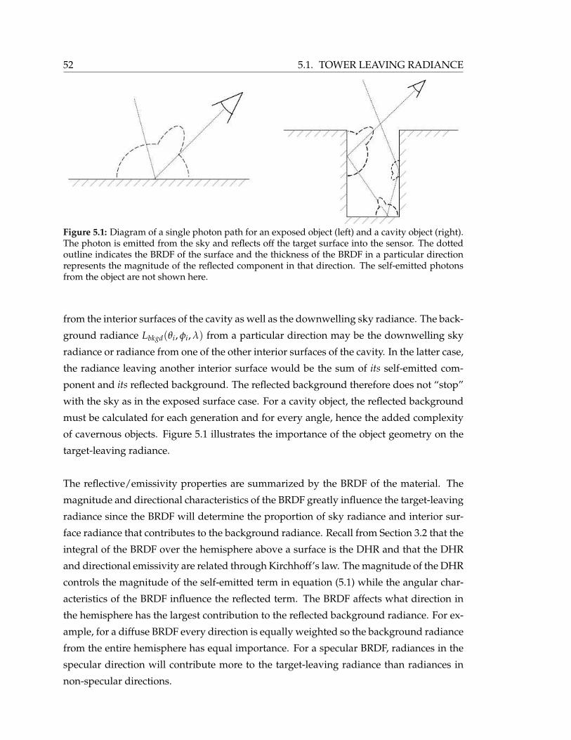
52 5.1. TOWER LEAVING RADIANCE
Figure 5.1: Diagram of a single photon path for an exposed object (left) and a cavity object (right).The photon is emitted from the sky and reflects off the target surface into the sensor. The dottedoutline indicates the BRDF of the surface and the thickness of the BRDF in a particular directionrepresents the magnitude of the reflected component in that direction. The self-emitted photonsfrom the object are not shown here.
from the interior surfaces of the cavity as well as the downwelling sky radiance. The back-
ground radiance Lbkgd(θi, φi, λ) from a particular direction may be the downwelling sky
radiance or radiance from one of the other interior surfaces of the cavity. In the latter case,
the radiance leaving another interior surface would be the sum of its self-emitted com-
ponent and its reflected background. The reflected background therefore does not “stop”
with the sky as in the exposed surface case. For a cavity object, the reflected background
must be calculated for each generation and for every angle, hence the added complexity
of cavernous objects. Figure 5.1 illustrates the importance of the object geometry on the
target-leaving radiance.
The reflective/emissivity properties are summarized by the BRDF of the material. The
magnitude and directional characteristics of the BRDF greatly influence the target-leaving
radiance since the BRDF will determine the proportion of sky radiance and interior sur-
face radiance that contributes to the background radiance. Recall from Section 3.2 that the
integral of the BRDF over the hemisphere above a surface is the DHR and that the DHR
and directional emissivity are related through Kirchhoff’s law. The magnitude of the DHR
controls the magnitude of the self-emitted term in equation (5.1) while the angular char-
acteristics of the BRDF influence the reflected term. The BRDF affects what direction in
the hemisphere has the largest contribution to the reflected background radiance. For ex-
ample, for a diffuse BRDF every direction is equally weighted so the background radiance
from the entire hemisphere has equal importance. For a specular BRDF, radiances in the
specular direction will contribute more to the target-leaving radiance than radiances in
non-specular directions.

5.1. TOWER LEAVING RADIANCE 53
Since an MDCT is a large cavity, the tower-leaving radiance might reduce to the black-
body radiance of the interior tower surfaces under certain conditions.
Emissivity: Relatively low DHR values of the tower materials in the thermal infrared
would translate to high emissivities. This would cause the self-emissive term in equa-
tion (5.1) to dominate the tower-leaving radiance. The tower-leaving radiance would
therefore approach the blackbody radiance if the actual emissivities were sufficiently high.
BRDF: The shape of the BRDF of the tower materials would greatly influence the reflected
radiance within the tower. For a sensor placed above the tower and targeted at an interior
surface through the fan stack opening, a specular BRDF would allow more radiance from
within the tower to be reflected back to the sensor.
Bounces: As with a perfect blackbody cavity, the radiance exiting the cavity approaches
the blackbody radiance as the number of internal reflections within the cavity increase.
The magnitude and shape of the BRDF and also the number of reflections within the
tower are therefore free parameters that affect the radiance leaving the tower. In the fol-
lowing sections, constraints are placed on these parameters through measurements and
modeling of the physical phenomena.

54 5.1. TOWER LEAVING RADIANCE
5.1.1 Spectral Measurements of MDCT Materials
Spectral reflectance measurements were taken of several MDCT construction materials
obtained from the Johnston Equipment Company in Rochester, New York. The reflectance
spectrum from approximately 2 to 25 µm was measured with a SOC-400 instrument. The
device illuminates the sample with an infrared beam at a 20° angle to the surface nor-
mal of the sample and measures the total directional reflectance of the sample [38]. The
reflectance measurements have been converted to an emissivity spectrum through Kirch-
hoff’s law. In each figure, a photograph of the material is shown at left and the emissivity
spectrum is shown at right. There are two emissivity curves for each material which were
measured from two different points on the material. This was meant to show any varia-
tion in emissivity for the material.
(a) Photograph of Sample (b) Emissivity Spectrum
Figure 5.2: Drift eliminator emissivity spectra of two separate physical locations on the material.
(a) Photograph of Sample (b) Emissivity Spectrum
Figure 5.3: Metal plate emissivity spectra of two separate physical locations on the material.

5.1. TOWER LEAVING RADIANCE 55
(a) Photograph of Sample (b) Emissivity Spectrum
Figure 5.4: Wood support emissivity spectra of two separate physical locations on the material.
(a) Photograph of Sample (b) Emissivity Spectrum
Figure 5.5: Plastic disc emissivity spectra of two separate physical locations on the material.
The spectra shown here cover a wide range of construction materials encompassing metal,
plastic, wood, and vinyl. The MWIR and LWIR spectra of the materials exhibit emissivity
values above 0.75 for all the sample points of measure in the 3-5 µm and 8-14 µm bands.
These results demonstrate that, in general, typical cooling tower materials will have rela-
tively high emissivities (low DHR) in the midwave and longwave infrared regions.

56 5.1. TOWER LEAVING RADIANCE
5.1.2 BRDF of NEFDS Materials
Materials similar to those in Section 5.1.1 were found in the NEF database. Recall from
Section 3.2.1.1.4 that the NEFDS is a collection of BRDF model parameters for several
hundred different materials. The materials selected represent metal, wood, plastic, and
insulation and all have a DHE of at least 0.93. The BRDF of each material at 3.5 µm and at
10.0 µm at an incident illumination angle of 20° are plotted in Figures 5.6 - 5.9.
(a) BRDF at 3.5 µm (MWIR) (DHE = 0.9512) (b) BRDF at 10.0µm (LWIR) (DHE = 0.9533)
Figure 5.6: NEFDS BRDF of weathered galvanized bare steel (NEF #0525UUUSTLa) measured atan illumination angle of 20°.
(a) BRDF at 3.5 µm (MWIR) (DHE = 0.9978) (b) BRDF at 10.0µm (LWIR) (DHE = 0.9589)
Figure 5.7: NEFDS BRDF of mildly weathered plastic tarp (NEF #1019UUUFABa) measured at anillumination angle of 20°.

5.1. TOWER LEAVING RADIANCE 57
(a) BRDF at 3.5 µm (MWIR) (DHE = 0.9431) (b) BRDF at 10.0µm (LWIR) (DHE = 0.9375)
Figure 5.8: NEFDS BRDF of weathered bare construction lumber (NEF #0404UUUWOD) mea-sured at an illumination angle of 20°.
(a) BRDF at 3.5 µm (MWIR) (DHE = 0.9510) (b) BRDF at 10.0µm (LWIR) (DHE = 0.9335)
Figure 5.9: NEFDS BRDF of weathered paint on insulation panel (NEF #0887UUUPNT) measuredat an illumination angle of 20°.
The BRDF plots indicate that typical MDCT construction materials are relatively specular
in the MWIR and LWIR. In addition, these selected materials also have high emissivity (at
least 0.93) at these wavelengths as consistent with Section 5.1.1.

58 5.1. TOWER LEAVING RADIANCE
5.1.3 DIRSIG Model of Closed and Open Cavities
The geometry of an object will have an important influence on its apparent temperature.
A three-dimensional cavity was modeled in DIRSIG to study the relationship between
the number of internal reflections resulting from the cavity geometry and the reflectance
characteristics of the internal surfaces on the apparent temperature of the cavity. Both a
closed cavity and an open cavity were studied.
(a) Closed box layout (b) Open well layout
Figure 5.10: DIRSIG cavity simulation layouts (not to scale)
The first simulation consisted of a sealed six-facet box. A broadband 8 - 14 µm sensor with
a unit spectral response was placed inside the box and targeted at one of the interior faces
at a 45° angle (Figure 5.10(a)). The total number of reflections that a photon is allowed to
make before being recorded by the sensor can be set manually in DIRSIG. Several runs
were performed with a diffuse (no specular component) Ward BRDF and then with a
specular (no diffuse component) Ward BRDF in which the number of internal reflections
were increased incrementally. The BRDF shapes used in the simulations were shown in
Figure 3.2. The model parameters were carefully chosen so that that DHR values were
0.05, 0.15, and 0.25 for the diffuse and specular models. These DHR values correspond
to emissivity values of 0.95, 0.85, and 0.75, respectively, through equation (3.12). The box
facets were also assigned a temperature of 306 K. The radiance recorded by the sensor
is an integrated radiance between 8 and 14 µm. This radiance is then converted into an
apparent temperature. For both the diffuse and specular BRDF models and for each DHR
value, trends in the apparent temperature as a function of the number of internal bounces
were investigated.
The second scenario consisted of an open, deep well. A broadband 8 - 14 µm sensor with a

5.1. TOWER LEAVING RADIANCE 59
unit spectral response was placed outside the well and targeted at one of the interior faces
at a 45° angle (Figure 5.10(b)). Several runs were performed with a diffuse (no specular
component) Ward BRDF and then with a specular (no diffuse component) Ward BRDF in
which the number of internal reflections were increased incrementally. As before, DHR
values of 0.05, 0.15, and 0.25 were chosen for the diffuse and specular models. The well
facets were assigned a temperature of 306 K while the atmosphere was a spectrally flat
240 K source with a transmission of unity. Again, the integrated radiance recorded by the
sensor was converted into an apparent temperature. For both the diffuse and specular
BRDF models and for each DHR value, trends in the apparent temperature as a function
of the number of internal bounces were investigated.
(a) Diffuse Ward BRDF (b) Specular Ward BRDF
Figure 5.11: Results of the closed box simulation. Actual temperature is 306 K (indicated by arrow)
(a) Diffuse Ward BRDF (b) Specular Ward BRDF
Figure 5.12: Results of the open well simulation. Actual temperature is 306 K (indicated by arrow)
60 5.1. TOWER LEAVING RADIANCE
The results of the sealed box and open well simulations are shown in Figures 5.11 and
5.12, respectively. The DIRSIG output is an integrated 8 - 14 µm radiance image. The av-
erage radiance of 100 pixels was converted to an apparent temperature using a radiance-
to-temperature look-up table. The apparent temperature for up to six internal reflections
are shown for each DHR value on the same plot.
Theoretically, the apparent temperature should increase and approach a final apparent
temperature as the number of bounces increases. The radiance reaching a sensor is the
self-emitted radiance of the target facet, modified by its emissivity, plus the reflected back-
ground radiances written as
Lsensor = εLtarget + ρLbackground. (5.2)
The BRDF of the target facet will affect which direction in the hemisphere has the largest
contribution to the reflected background radiance. For example, for a diffuse BRDF, every
direction is equally weighted so the background radiance from the entire hemisphere has
equal importance. For a specular BRDF, radiances in the specular direction will contribute
more to the sensor-reaching radiance than radiances in non-specular directions. For the
sealed box, since the background radiances are always just the other facets of the box (at
the same temperature) the shape of the BRDF should not matter so the apparent temper-
ature should approach the actual assigned blackbody temperature of 306 K. This can be
seen in Figure 5.11. However, in the open well case, the background consists both of the
other well facets and also the much colder sky. A specular BRDF would cause the sensor
to see more of the warmer well than the colder sky, so the apparent temperature should
still approach the actual blackbody temperature of 306 K as it does in Figure 5.12(b). On
the other hand, a diffuse BRDF would cause the sensor to see both the other well facets
and the sky. The apparent temperature in this last case will therefore be a weighted aver-
age of the cold sky and the warm well temperature as seen in Figure 5.12(a).
In addition, the DHR of the BRDF will affect how quickly the apparent temperature ap-
proaches its asymptote. A lower DHR value will result in a higher emissivity by equa-
tion (3.12). A higher emissivity will cause the apparent temperature to approach its
asymptote more quickly since a higher emissivity indicates an object has a higher effi-
ciency as a radiator. In other words, a high-emissivity object behaves more like a black-
body and the dependence on the number of internal reflections is diminished. This trend
is evident in all of the plots shown in Figures 5.11 and 5.12.

5.1. TOWER LEAVING RADIANCE 61
The results of this study confirm that a cavity will behave as a blackbody radiator if there
have been a sufficient number of internal reflections. The sealed box scenario demon-
strated that the apparent temperature approaches the actual blackbody temperature after
approximately one, two, and three reflections for DHR values of 0.05, 0.15, and 0.25, re-
spectively. This scenario also confirmed that the shape of the facet BRDF does not matter
since the sensor will always see one of the box facets. The open well scenario demon-
strated that the shape of the facet BRDF is important when there are multiple background
sources at disparate temperatures. A diffuse BRDF will cause more radiometric mixing
between the warm well radiance and the cold sky radiance, resulting in a lower apparent
temperature than the blackbody temperature of the well. A specular BRDF on the other
hand will cause more of the warm well radiance to reach the sensor, producing a result
similar to the sealed box simulation. Again, the DHR will determine how quickly the ap-
parent temperature approaches its asymptotic temperature.
For an MDCT, the open well, diffuse case represents the worst-case scenario in terms of
the internal geometry and material properties. If the internal tower materials are perfectly
diffuse and have sufficiently high emissivities in the longwave infrared, then the apparent
temperature will be within one or two Kelvin of the actual blackbody temperature if there
has been approximately three internal reflections.
5.1.4 Effective Emissivity of Drift Eliminators
The primary interior component of a counter-flow MDCT that is visible to an overhead
sensor is the drift eliminators. This material has a complex geometry that must be care-
fully modeled in order to determine its contribution to the radiance leaving the tower. An
investigation was performed to determine if the geometry and optical properties of the
drift eliminators would cause them to behave as a blackbody. If the effective emissivity
is indeed unity, then the complex drift eliminators could be replaced with a simple black-
body plate in the radiometry models, allowing for much more rapid simulations to be
used in the development of the parametric model for temperature error prediction.
As suggested by Figure 2.2, an overhead sensor targeted at the fan stack opening will
probably not be able to see past the drift eliminator layer. Therefore, the drift eliminators
are the last surface seen by the sensor which makes them very important since they are
the closest surface to the hot cooling water.

62 5.1. TOWER LEAVING RADIANCE
(a) (b)
Figure 5.13: Photograph of the drift eliminators (a) and the CAD drawing reproduction (b).
The drift eliminators have a complex cavity geometry. As mentioned in Section 2.1, they
are designed to change the direction of the air stream multiple times. In order to model
their radiometry, a detailed representation of the drift eliminators must be produced. A
high fidelity geometric model contains a very large number of facets and may greatly af-
fect the execution speed of the simulations. A close-up photograph and a carefully drawn
CAD model of the drift eliminator are shown in Figure 5.13.
Spectral reflectance measurements were taken of a drift eliminator sample as shown in
Figure 5.2. The spectral emissivity plots demonstrate that the drift eliminators have a
relatively high emissivity in the longwave infrared. The average emissivity of all the
measured spectra from the sample in the 8 to 14 µm range is 0.941.
The BRDF of the drift eliminator material also demands careful attention. The sample
material appears to be plastic or vinyl. Although a direct BRDF measurement of this
sample is not available, the BRDF of a similar material can be found in the Nonconven-
tional Exploitation Factors Data System (NEFDS). Two such materials were found: mildly
weathered plastic tarp (NEF 1019UUUFABa) and weathered paint on insulation panel
(NEF 0887UUUPNT). The BRDF of each material at a wavelength of 10 µm was shown in
Figures 5.7 and 5.9. The BRDF for both of these materials is very specular in the longwave
infrared. Since the drift eliminator material is similar to these materials, the drift elimina-
tors could be considered fairly specular in the LWIR.
The study in Section 5.1.3 investigated the apparent temperature and effective emissivity
of an open cavity for multiple internal reflections. That study concluded that an open
cavity with high emissivity and a specular BRDF would have an effective emissivity of
unity if photons underwent at least three internal reflections before exiting the cavity.

5.1. TOWER LEAVING RADIANCE 63
The DIRSIG simulations conducted in that study are now adapted to the drift eliminators
specifically. A detailed CAD drawing of the drift eliminators as shown in Figure 5.13(b)
was created. The Ward BRDF model was used to represent the BRDF of the drift elimina-
tor material. The spectral measurements of the sample indicated an average emissivity of
0.941 in the longwave infrared. The Ward model was adjusted to provide several BRDFs
having a directional emissivity of 0.941 measured at 20° to the surface normal. Since drift
eliminators are designed to allow air to change direction three times, photons were al-
lowed to make a maximum of three bounces in the simulation. A broadband 8 - 14 µm
sensor was placed approximately 150 meters above the drift eliminators. The entire drift
eliminator was assigned a temperature of 306 K. A flat blackbody plate having a tem-
perature of 276 K was placed under the drift eliminator to provide a low temperature
background source. The atmosphere was a spectrally flat 240 K source with a transmis-
sion of unity. The apparent temperature of the drift eliminator was determined from the
at-sensor radiance.
The shape of the BRDF and the sensor zenith view angle were varied in these simulations.
Ward BRDF models included one diffuse-only BRDF and four specular-only BRDFs. The
specular BRDFs had lobes exhibiting various widths as shown in Figure 5.14(b) - 5.14(e).
The drift eliminators were viewed from zenith angles of 0, 10, and 20 degrees.
The results of these various simulations are listed in Table 5.1. The drift eliminators were
assigned a temperature of 306 K. The table shows the apparent temperature recorded by
the sensor as a function of the sensor view angle and the shape of the BRDF. Recall that
for all the BRDF shapes, the directional emissivity was fixed at 0.941.
The data indicates that the apparent temperature increases and approaches the absolute
(a) (b) (c) (d) (e)
Figure 5.14: Ward BRDF shapes used in the DIRSIG simulations. Diffuse (a), specular, σ = 0.35 (b),specular, σ = 0.22 (c), specular, σ = 0.15 (d), and specular, σ = 0.03 (e).
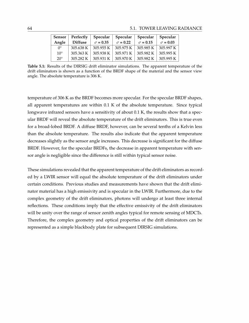
64 5.1. TOWER LEAVING RADIANCE
Sensor Perfectly Specular Specular Specular SpecularAngle Diffuse σ = 0.35 σ = 0.22 σ = 0.15 σ = 0.03
0° 305.638 K 305.955 K 305.975 K 305.985 K 305.997 K10° 305.363 K 305.938 K 305.971 K 305.982 K 305.995 K20° 305.282 K 305.931 K 305.970 K 305.982 K 305.995 K
Table 5.1: Results of the DIRSIG drift eliminator simulations. The apparent temperature of thedrift eliminators is shown as a function of the BRDF shape of the material and the sensor viewangle. The absolute temperature is 306 K.
temperature of 306 K as the BRDF becomes more specular. For the specular BRDF shapes,
all apparent temperatures are within 0.1 K of the absolute temperature. Since typical
longwave infrared sensors have a sensitivity of about 0.1 K, the results show that a spec-
ular BRDF will reveal the absolute temperature of the drift eliminators. This is true even
for a broad-lobed BRDF. A diffuse BRDF, however, can be several tenths of a Kelvin less
than the absolute temperature. The results also indicate that the apparent temperature
decreases slightly as the sensor angle increases. This decrease is significant for the diffuse
BRDF. However, for the specular BRDFs, the decrease in apparent temperature with sen-
sor angle is negligible since the difference is still within typical sensor noise.
These simulations revealed that the apparent temperature of the drift eliminators as record-
ed by a LWIR sensor will equal the absolute temperature of the drift eliminators under
certain conditions. Previous studies and measurements have shown that the drift elimi-
nator material has a high emissivity and is specular in the LWIR. Furthermore, due to the
complex geometry of the drift eliminators, photons will undergo at least three internal
reflections. These conditions imply that the effective emissivity of the drift eliminators
will be unity over the range of sensor zenith angles typical for remote sensing of MDCTs.
Therefore, the complex geometry and optical properties of the drift eliminators can be
represented as a simple blackbody plate for subsequent DIRSIG simulations.

5.1. TOWER LEAVING RADIANCE 65
Figure 5.15: CAD drawing of a counter-flow MDCT exterior view (left) and interior view (right).
5.1.5 MDCT DIRSIG Rendering with BRDF Materials
The DIRSIG modeling tool was used to investigate the apparent temperature of an MDCT
model. The DIRSIG rendering was generated by assigning basic thermal properties to a
geometric model of a tower. The geometrically detailed three-dimensional CAD draw-
ing was intended to mimic a counter-flow tower similar to the F-area and H-area units at
the Savannah River Site (SRS). The geometry of the drawing was based on measurements
taken at SRS and on schematics obtained from SPX Cooling Technologies [39]. A high
fidelity geometric model is necessary to reproduce the geometry for multiple reflections
within the cooling tower.
Recall that a sensor targeted at the fan stack opening will not be able to see past the drift
eliminator layer. Therefore, the geometry above the drift eliminators was carefully re-
produced, as it would have the greatest influence on the observed radiance. Structures
located below the drift eliminators were only approximated or deleted altogether. De-
tailed views of the CAD drawing are shown in Figure 5.15.
For the DIRSIG model, each facet of the CAD drawing was assigned a temperature of
306 K. In the first scenario, a diffuse Ward BRDF (no specular component) was assigned
to every facet. The model parameters were adjusted to produce a DHR of 0.15. In the sec-
ond scenario, a specular Ward BRDF (no diffuse component) was assigned to every facet.
The approximate shapes of the Ward models used were shown in Figure 3.2.
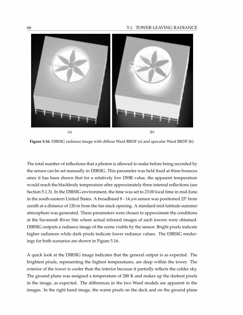
66 5.1. TOWER LEAVING RADIANCE
(a) (b)
Figure 5.16: DIRSIG radiance image with diffuse Ward BRDF (a) and specular Ward BRDF (b).
The total number of reflections that a photon is allowed to make before being recorded by
the sensor can be set manually in DIRSIG. This parameter was held fixed at three bounces
since it has been shown that for a relatively low DHR value, the apparent temperature
would reach the blackbody temperature after approximately three internal reflections (see
Section 5.1.3). In the DIRSIG environment, the time was set to 23:00 local time in mid-June
in the south-eastern United States. A broadband 8 - 14 µm sensor was positioned 25° from
zenith at a distance of 120 m from the fan stack opening. A standard mid-latitude summer
atmosphere was generated. These parameters were chosen to approximate the conditions
at the Savannah River Site where actual infrared images of such towers were obtained.
DIRSIG outputs a radiance image of the scene visible by the sensor. Bright pixels indicate
higher radiances while dark pixels indicate lower radiance values. The DIRSIG render-
ings for both scenarios are shown in Figure 5.16.
A quick look at the DIRSIG image indicates that the general output is as expected. The
brightest pixels, representing the highest temperatures, are deep within the tower. The
exterior of the tower is cooler than the interior because it partially reflects the colder sky.
The ground plane was assigned a temperature of 288 K and makes up the darkest pixels
in the image, as expected. The differences in the two Ward models are apparent in the
images. In the right hand image, the warm pixels on the deck and on the ground plane
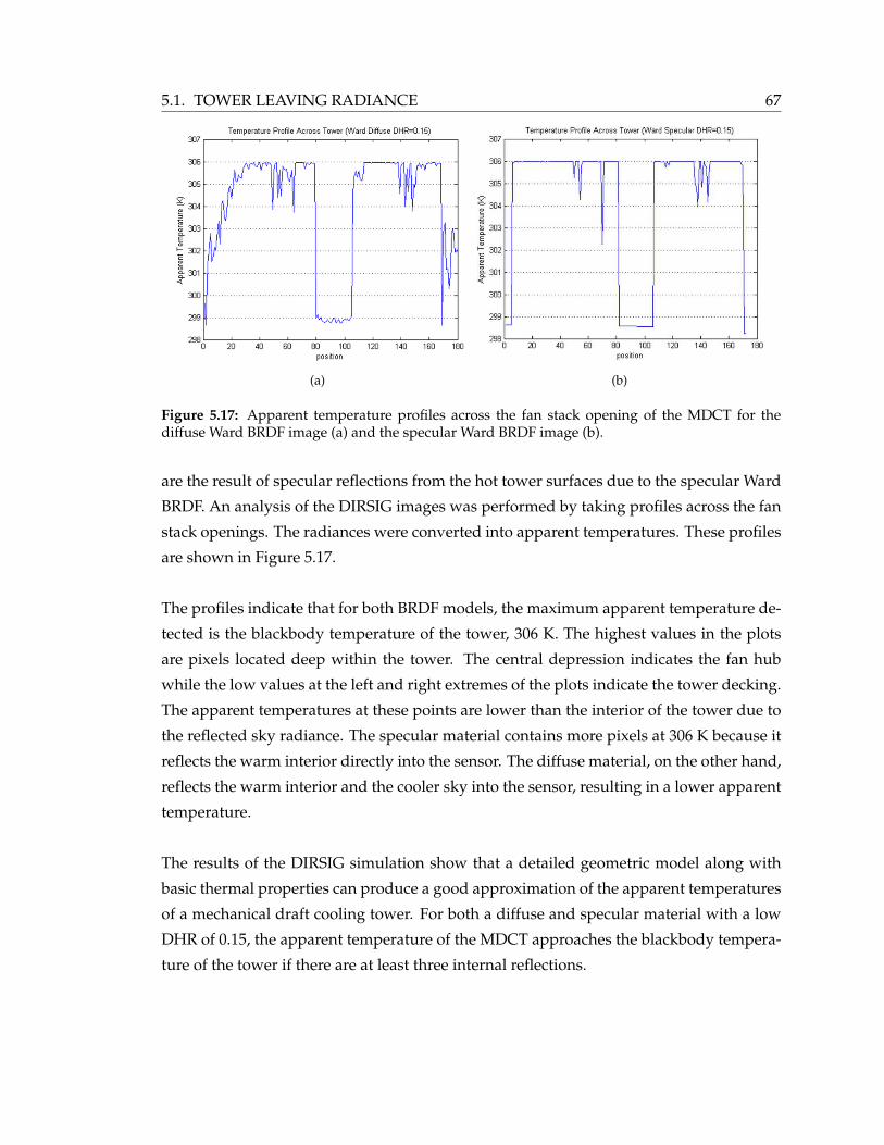
5.1. TOWER LEAVING RADIANCE 67
(a) (b)
Figure 5.17: Apparent temperature profiles across the fan stack opening of the MDCT for thediffuse Ward BRDF image (a) and the specular Ward BRDF image (b).
are the result of specular reflections from the hot tower surfaces due to the specular Ward
BRDF. An analysis of the DIRSIG images was performed by taking profiles across the fan
stack openings. The radiances were converted into apparent temperatures. These profiles
are shown in Figure 5.17.
The profiles indicate that for both BRDF models, the maximum apparent temperature de-
tected is the blackbody temperature of the tower, 306 K. The highest values in the plots
are pixels located deep within the tower. The central depression indicates the fan hub
while the low values at the left and right extremes of the plots indicate the tower decking.
The apparent temperatures at these points are lower than the interior of the tower due to
the reflected sky radiance. The specular material contains more pixels at 306 K because it
reflects the warm interior directly into the sensor. The diffuse material, on the other hand,
reflects the warm interior and the cooler sky into the sensor, resulting in a lower apparent
temperature.
The results of the DIRSIG simulation show that a detailed geometric model along with
basic thermal properties can produce a good approximation of the apparent temperatures
of a mechanical draft cooling tower. For both a diffuse and specular material with a low
DHR of 0.15, the apparent temperature of the MDCT approaches the blackbody tempera-
ture of the tower if there are at least three internal reflections.

68 5.1. TOWER LEAVING RADIANCE
Figure 5.18: DIRSIG rendering of an MDCT with a one-pixel-wide ring drawn.
5.1.6 MDCT Fan Blade Motion
A methodology is needed to model the spinning fan blades of an MDCT. Recall from
Section 2.2 that an MDCT may operate in two states. In the fans off case, hot water is
flowing through the tower and the warm, moist air exits the tower stack through natural
convection. The fan blades are motionless so the fan blades and tower cavity can be dis-
tinguished in an image from an overhead sensor of fine enough spatial resolution. In the
fans on case, the fan in the stack rotates to force the warm, moist air out of the fan stack
opening. The spinning fan blades will appear blurred in an image from an overhead sen-
sor assuming a significant temporal integration time. The effect of the spinning fan blades
on the tower-leaving radiance was investigated.
The first study conducted was to determine if the radiance from the tower opening de-
pends on the fan speed and/or on the integration time of the sensor. Consider the image
of the tower opening in Figure 5.18. At any radius r, a ring may be drawn that is one
pixel in thickness. In the fans off case, the pixels in this ring can be distinguished as “fan”
pixels or “cavity” pixels. In the fans on case, however, the fan and cavity pixels in this
ring cannot be distinguished due to the blurring effect caused by the rotating fans and
due to the integration time of the sensor. To model the fans on case, a square-wave sig-
nal was generated in Matlab. The signal has a value of one to represent cavity pixels

5.1. TOWER LEAVING RADIANCE 69
Figure 5.19: Square-wave signal representing the fan blade and cavity radiances at each pixellocation in the ring at different times.
and a value of zero to represent fan pixels. To give the simulation some physical mean-
ing, the fan pixels were given a blackbody radiance at 10 µm for a temperature of 280 K
(L = 7.0286 [W/m2/sr/µm]) while the cavity pixels were given a blackbody radiance at
10 µm for a temperature of 300 K (L = 9.9240 [W/m2/sr/µm]).
The signal was modified so that for each iteration, the signal would shift by v pixels.
The variable v represents the speed of the signal (i.e., the linear speed of the fan blades
at the given radius). One iteration represents one unit of time (e.g., one second). The ra-
diance value is observed at each pixel location on the signal and for every iteration. The
number of iterations (the number of seconds) represents the integration time of the sensor.
For each pixel location, the radiance was summed for the time interval and then normal-
ized by the total integration time. In other words, for a particular pixel, the “shutter”
was opened for the specified integration time so that the time-averaged signal could be
collected. This simulation is illustrated in Figure 5.19.
The result is a vector of radiance values that represent the time-averaged radiances of a
square-wave passing through each pixel location. These integrated radiance values differ
for each pixel location and will depend on the speed of the signal and on the integration
time. The mean value of the radiances is always constant regardless of the signal speed
or the integration time. The reason for this observation is that, for the entire sampling

70 5.1. TOWER LEAVING RADIANCE
(a) (b)
Figure 5.20: DIRSIG rendering of an MDCT with a stationary fan (a) and a blurred renderingrepresenting a rotating fan (b).
ring (vector) in Figure 5.18, there are always the same number of fan pixels and the same
number of cavity pixels. Therefore, the average value of the vector remains constant.
The conclusion of this investigation was that the average radiance in a ring at radius r
was the same for a stationary fan blade as it was for a spinning fan blade. Based on this
information, the next study seeks to determine if the spinning fan blade can be modeled
using the stationary fan model. In other words, is it possible to represent the fans on case
from the fans off model?
As mentioned previously, the rotating fan blade will blur the radiances in each ring drawn
in the fan stack opening. The average value in each ring is constant. For every ring, the
pixel values in the ring were replaced with the average pixel value of the ring. This ring
averaging represents the blur caused by the rotating fan. Figure 5.20 illustrates a station-
ary fan image and a motion-blurred spinning fan image.
The images in Figure 5.20 show the apparent temperature of each pixel (bright pixels are
hot). In a fans on case, the user would have to take an average value over the entire open-
ing since the fan and cavity pixels cannot be distinguished. Therefore, a region of interest
(ROI) was drawn over the entire opening for the fans off and the fans on image and the av-
erage value was computed. The average value for both the fans off and the fans on image
is 294.57 K.
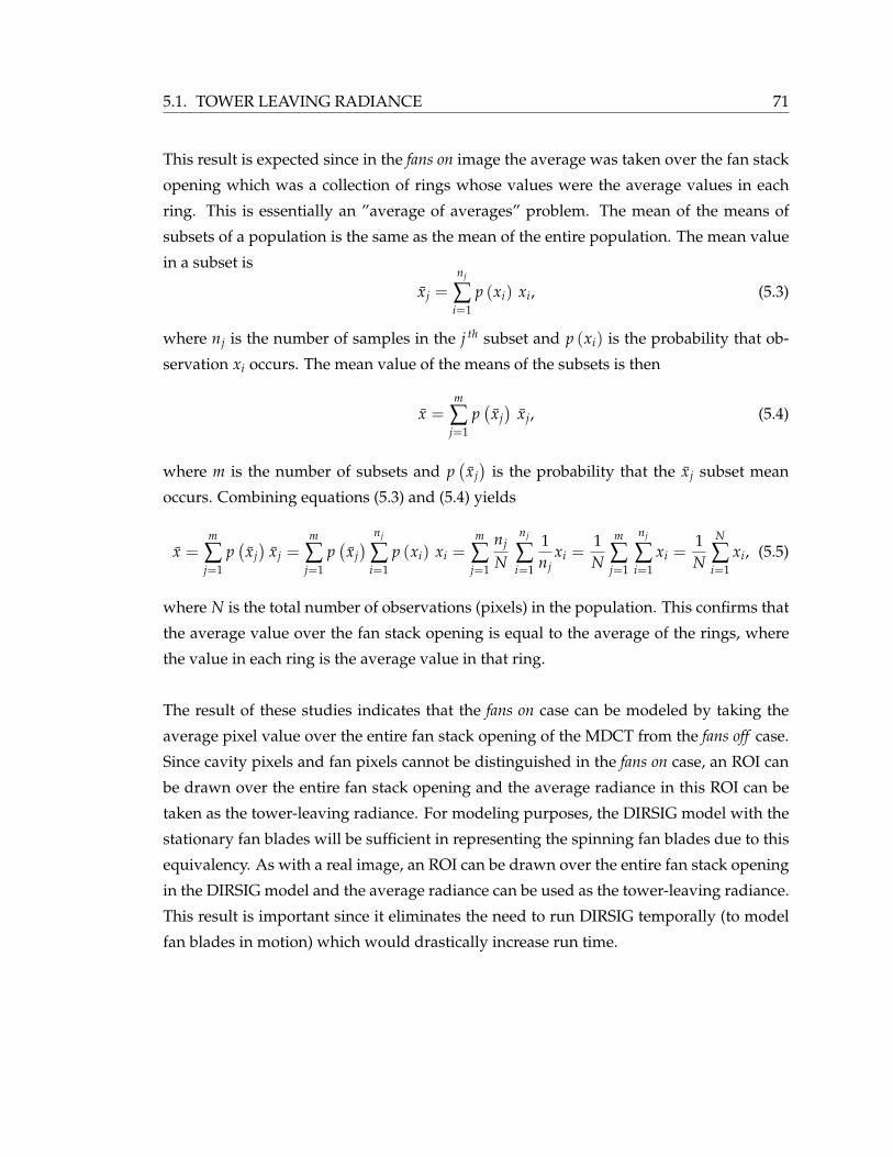
5.1. TOWER LEAVING RADIANCE 71
This result is expected since in the fans on image the average was taken over the fan stack
opening which was a collection of rings whose values were the average values in each
ring. This is essentially an ”average of averages” problem. The mean of the means of
subsets of a population is the same as the mean of the entire population. The mean value
in a subset is
xj =nj
∑i=1
p (xi) xi, (5.3)
where nj is the number of samples in the j th subset and p (xi) is the probability that ob-
servation xi occurs. The mean value of the means of the subsets is then
x =m
∑j=1
p(
xj)
xj, (5.4)
where m is the number of subsets and p(xj
)is the probability that the xj subset mean
occurs. Combining equations (5.3) and (5.4) yields
x =m
∑j=1
p(xj
)xj =
m
∑j=1
p(
xj) nj
∑i=1
p (xi) xi =m
∑j=1
nj
N
nj
∑i=1
1nj
xi =1N
m
∑j=1
nj
∑i=1
xi =1N
N
∑i=1
xi, (5.5)
where N is the total number of observations (pixels) in the population. This confirms that
the average value over the fan stack opening is equal to the average of the rings, where
the value in each ring is the average value in that ring.
The result of these studies indicates that the fans on case can be modeled by taking the
average pixel value over the entire fan stack opening of the MDCT from the fans off case.
Since cavity pixels and fan pixels cannot be distinguished in the fans on case, an ROI can
be drawn over the entire fan stack opening and the average radiance in this ROI can be
taken as the tower-leaving radiance. For modeling purposes, the DIRSIG model with the
stationary fan blades will be sufficient in representing the spinning fan blades due to this
equivalency. As with a real image, an ROI can be drawn over the entire fan stack opening
in the DIRSIG model and the average radiance can be used as the tower-leaving radiance.
This result is important since it eliminates the need to run DIRSIG temporally (to model
fan blades in motion) which would drastically increase run time.

72 5.1. TOWER LEAVING RADIANCE
5.1.7 Atmospheric Downwelled Radiance
The previous sections investigated the behavior of the self-emitted radiance of the MDCT.
The reflected component of the tower-leaving radiance must also be considered. An anal-
ysis was performed to determine how sensitive the derived apparent temperature is to
changes in the atmospheric downwelling radiance. The MODTRAN atmospheric model-
ing tool was used to aid this analysis. The total sky downwelling radiances in the long-
wave infrared spectral region for the six MODTRAN standard atmospheres were com-
puted. These spectral radiances were used in the reflected term of the governing radiom-
etry equation. The influence of each atmosphere on the radiance reaching the sensor was
investigated.
The reflected radiance component consists of the sky downwelling radiance modified by
the reflectance of the object. By Kirchhoff’s law, the sum of the reflectivity and the emis-
sivity of an opaque object is unity. For a diffuse object, the reflectance is the same for every
view angle. The surface-leaving radiance from equation (3.14) is then
Lsur f (λ) = ε(λ) LBB(λ, T) + [1− ε(λ)] Ld(λ), (5.6)
where Ld(λ) is the downwelling sky spectral radiance and is assumed to be uniform. The
spectral response of the sensor is then applied to the surface-leaving spectral radiance to
arrive at an integrated radiance value for the passband of the sensor. This band radiance
is converted into an apparent temperature. A temperature error metric is defined as the
difference between the apparent temperature at the sensor and the actual temperature of
the object.
The six MODTRAN standard atmospheres used in this study were tropical, mid-latitude
summer, mid-latitude winter, sub-arctic summer, sub-arctic winter, and 1976 U.S. stan-
dard [13]. These atmospheric profiles were processed in the DIRSIG utility called make adb [22].
The utility samples the hemispheric sky dome at discrete angles and for each sample di-
rection, the path radiance is computed from MODTRAN. A table is built of the zenith and
azimuth angle of the sample and the spectral downwelling radiance from the sample. The
sky is sampled from 7.5 to 82.5 degrees on 15 degree intervals in the zenith direction and
from 0 to 330 degrees on 30 degree intervals in the azimuth direction. This results in six
zenith samples and twelve azimuth samples which yield 72 total sky samples. The sam-
ples are then integrated over the hemisphere to arrive at the diffuse spectral downwelling
radiance [22].
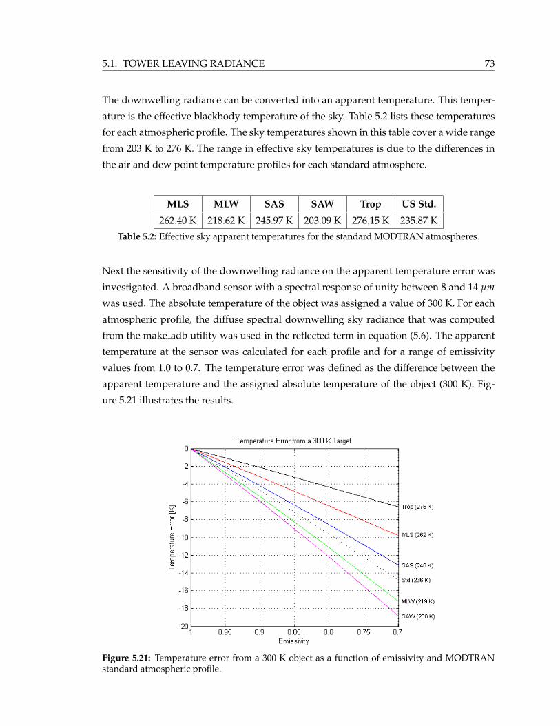
5.1. TOWER LEAVING RADIANCE 73
The downwelling radiance can be converted into an apparent temperature. This temper-
ature is the effective blackbody temperature of the sky. Table 5.2 lists these temperatures
for each atmospheric profile. The sky temperatures shown in this table cover a wide range
from 203 K to 276 K. The range in effective sky temperatures is due to the differences in
the air and dew point temperature profiles for each standard atmosphere.
MLS MLW SAS SAW Trop US Std.
262.40 K 218.62 K 245.97 K 203.09 K 276.15 K 235.87 K
Table 5.2: Effective sky apparent temperatures for the standard MODTRAN atmospheres.
Next the sensitivity of the downwelling radiance on the apparent temperature error was
investigated. A broadband sensor with a spectral response of unity between 8 and 14 µm
was used. The absolute temperature of the object was assigned a value of 300 K. For each
atmospheric profile, the diffuse spectral downwelling sky radiance that was computed
from the make adb utility was used in the reflected term in equation (5.6). The apparent
temperature at the sensor was calculated for each profile and for a range of emissivity
values from 1.0 to 0.7. The temperature error was defined as the difference between the
apparent temperature and the assigned absolute temperature of the object (300 K). Fig-
ure 5.21 illustrates the results.
Figure 5.21: Temperature error from a 300 K object as a function of emissivity and MODTRANstandard atmospheric profile.
74 5.1. TOWER LEAVING RADIANCE
The magnitude of the temperature errors increase as the emissivity decreases. This is due
to a decrease of the self-emitted radiance component as the emissivity decreases resulting
in more of the colder sky radiance being included in the sensor-reaching radiance. The
temperature errors also increase as the apparent sky temperature decreases. The sky tem-
peratures are less than the object temperature of 300 K for all the atmospheric profiles.
Therefore, if a “colder” radiance is reflected to the sensor, the apparent temperature at the
sensor will be colder as well, resulting in a higher temperature error.
This study demonstrated that the atmospheric downwelling radiance may have a sig-
nificant effect on the derived temperature error. Knowledge of the atmospheric profile is
important to accurately determine the temperature of a remotely-sensed object.
5.1.8 Tower Leaving Radiance Summary
The radiance leaving the tower consists of both self-emitted radiance and also reflected
downwelled radiance. Typical MDCT construction materials have relatively high emissiv-
ities at longwave infrared wavelengths (Section 5.1.1). Therefore, the self-emissive term
in equation (5.1) will be dominant. Emissivities of 0.80 and 0.90 translate into DHR values
of 0.20 and 0.10, respectively. These DHR values are still significant so the reflected terms
cannot be ignored. an MDCT can be represented as an open well. If the tower materials
are relatively specular for longwave infrared wavelengths, as indicated by Section 5.1.2,
then background radiance reflected to an airborne sensor will be dominated by the self-
emitted radiances from the other interior surfaces of the tower. Finally, given the above
constraints, the radiance leaving the tower will be the blackbody radiance of the tower
materials if there has been at least three internal reflections. Given the complex internal
geometry of an MDCT, there is a high probability a photon will undergo at least three re-
flections before exiting the tower. Therefore, pixels from deep within the tower cavity will
have an effective emissivity of unity. On the other hand, pixels from ”shallow” regions of
the tower will have an effective emissivity less than unity.

5.2. SENSOR-REACHING RADIANCE 75
Figure 5.22: Radiance from the tower passes through the exhaust plume to reach the sensor.
5.2 sensor-reaching Radiance
Radiance leaving the tower cavity must now propagate through the intervening column
of air between the tower and the sensor. Recall from Section 3.4.2 that the atmosphere
will both attenuate and exaggerate the signal through transmission losses and additive
upwelling radiance. The radiance reaching the front of the sensor after passing through
the air column is
Lsensor(θ, φ, λ) = τ(θ, φ, λ) Ltower(θ, φ, λ) + Lu(θ, φ, λ)[
Wm2 sr µm
]. (5.7)
For a mechanical draft cooling tower, the target-to-sensor air column not only consists
of the ambient atmosphere, but will also include a localized water vapor plume directly
above the tower. The additional water vapor introduced by this plume will contribute an
additional error in the derived apparent temperature. Figure 5.22 demonstrates radiance
from the tower passing through the exhaust plume to reach the sensor. The air column
can be divided into two segments. The first segement falls within the exhaust plume of
the tower. The second segment is the free atmosphere not influenced by the plume.
The exhaust plume from an MDCT would introduce water vapor at an elevated temper-
ature into the volume immediately above the tower. Radiance emitted within the tower
must pass through this plume to reach an airborne sensor. Transmission values of less
than unity will decrease the radiance at the sensor resulting in an apparent temperature
that is lower than the actual material temperature. Conversely, the upwelled radiance
will increase the radiance at the sensor resulting in an apparent temperature that is higher

76 5.2. SENSOR-REACHING RADIANCE
Figure 5.23: Atmospheric column representing the plume layer and the ambient atmosphere mod-eled in MODTRAN.
than the actual material temperature. These two effects compete with each other so that
the apparent temperature at the sensor may be higher or lower than the actual temper-
ature depending on the atmospheric conditions. The atmospheric conditions must be
carefully modeled in order to correct for errors in the derived temperature.
The first segment of the air column would contain a higher water vapor concentration
than the second segment (in most cases). The free parameters of the plume are the air
temperature, the water vapor concentration, and the height. The ambient atmospheric
conditions (second segment) will also affect the transmission and upwelled radiance sep-
arately.
5.2.1 MODTRAN Simulation of Air Column
The MODTRAN radiative transfer model was used to simulate how the water vapor con-
centration affects the target-to-sensor transmission and upwelled radiance in the atmo-
sphere at longwave infrared wavelengths. The dew point depression and air temperature
were chosen as measures of the water vapor concentration in the column due to their feasi-
bility of measurement in situ. The air column was divided into two layers in MODTRAN.
The first layer extends from the ground to a height of z meters to represent the exhausted
plume. The second layer extends from the terminating point of the first layer up to an
observation altitude of 100 meters. The second layer was assigned standard atmospheric
conditions. The first layer was also assigned standard conditions for all parameters except
the air temperature and the dew point depression which were varied to simulate various
temperatures and water vapor concentrations. Figure 5.23 illustrates this layout.
Several MODTRAN runs were conducted under a variety of conditions. The air temper-
5.2. SENSOR-REACHING RADIANCE 77
ature in the first layer was varied in increments of 5 K from 280 K to 310 K. For each
temperature, dew point depressions of 0, 2, 5, 10, and 20 K were used. The dew point
depression is the difference between the air temperature and the dew point temperature.
A dew point depression close to zero indicates near saturated air while a large depres-
sion indicates dryer air. The observation altitude was held fixed at 100 m. The thickness
of the first layer, z, was set to values of 1, 5, 10, and 20 m representing various plume
thicknesses under a variety of ambient wind conditions (i.e., lower wind speed indicates
a more vertical plume and a thicker layer). The above parameters were run for standard
mid-latitude summer conditions and then repeated for sub-arctic winter conditions rep-
resenting relatively wet and dry ambient atmospheres, respectively. The target material
was a perfect blackbody. Several runs were performed with blackbody targets of 302 K,
306 K, and 310 K. MODTRAN4v3r1 was run in solar/thermal radiance mode between 8
and 14 µm at a resolution of 0.3 µm with an 8-stream discrete ordinate multiple scattering
algorithm [40].
The intent of the MODTRAN simulation was to model an air column containing a high
water vapor concentration layer within a column of standard water vapor conditions. The
transition between this lower layer and the standard atmosphere is marked by a dramatic
gradient in the water vapor profile. In a user-defined atmosphere, MODTRAN allows
the user to specify the height, pressure, temperature and dew point of the atmospheric
layer at each altitude. These supplied values are used at the exact heights specified. How-
ever, MODTRAN’s interpolation scheme is inadequate for such large gradients across
large, relatively broad altitude ranges [41]. Therefore, in order to realize the strength of
this gradient, several thinner (one meter thick) layers were inserted between the standard
layers of the upper atmosphere and the user-defined, high humidity conditions of the
lowest layer. These extra layers provided the necessary buffer to allow a sharp fall off in
temperature and dew point depression between the first and second layers. Figure 5.24
demonstrates the layers set in MODTRAN.
The variables for the MODTRAN simulations were the height of the plume segment, the
air temperature and dew point depression in the plume, and the ambient atmospheric
conditions. Table 5.3 summarizes the values used in the simulation. A MODTRAN run
was performed for every combination of the variables. The model output contains spec-
tral values of the transmission (TRANS) and upwelled radiance (PATH THERMAL) be-
tween wavelengths of 8 and 14 µm. These spectral values were used to calculate the
radiance reaching a sensor from several blackbody targets through equation (5.7). The

78 5.2. SENSOR-REACHING RADIANCE
Figure 5.24: Schematic of the atmospheric layers assigned in MODTRAN. The first segment repre-sents the exhaust plume while the second segment represents the rest of the air column. Standardatmospheric conditions are assigned to every layer except for those in the first segment where theair temperature and dew point temperature are varied (not to scale).
material radiance was taken as the spectral blackbody radiance from the Planck equation.
Temperatures of 302 K, 306 K, and 310 K were used for the targets. The spectral radi-
ance at the sensor from equation (5.7) was integrated between 8 and 14 µm to arrive at
an integrated radiance at the sensor. The sensor had a flat, unit spectral response func-
tion between 8 and 14 µm and a zero response outside that region. The integrated sensor
radiance was converted to an apparent temperature. Finally, the temperature error was
defined as the difference between the blackbody temperature used in the Planck equation
and the apparent temperature derived from the integrated sensor radiance. The results
are shown in Figures 5.25 and 5.26.
Blackbody Plume Plume Air Plume Dew Pt. AmbientTemp. [K] Height [m] Temp. [K] Depression [K] Conditions
302 1 280 0 mid-latitude summer306 5 285 2 sub-arctic winter310 10 290 5
20 295 10300 20305310
Table 5.3: Parameter values for the MODTRAN plume simulations.
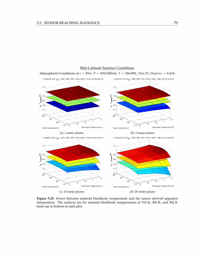
5.2. SENSOR-REACHING RADIANCE 79
Mid-Latitude Summer ConditionsAtmospheric Conditions at z = 25m: P = 1010.065mb, T = 294.09K, Dew Pt. Depress. = 4.41K
(a) 1 meter plume (b) 5 meter plume
(c) 10 meter plume (d) 20 meter plume
Figure 5.25: Errors between material blackbody temperature and the sensor derived apparenttemperature. The surfaces are for material blackbody temperatures of 310 K, 306 K, and 302 Kfrom top to bottom in each plot.
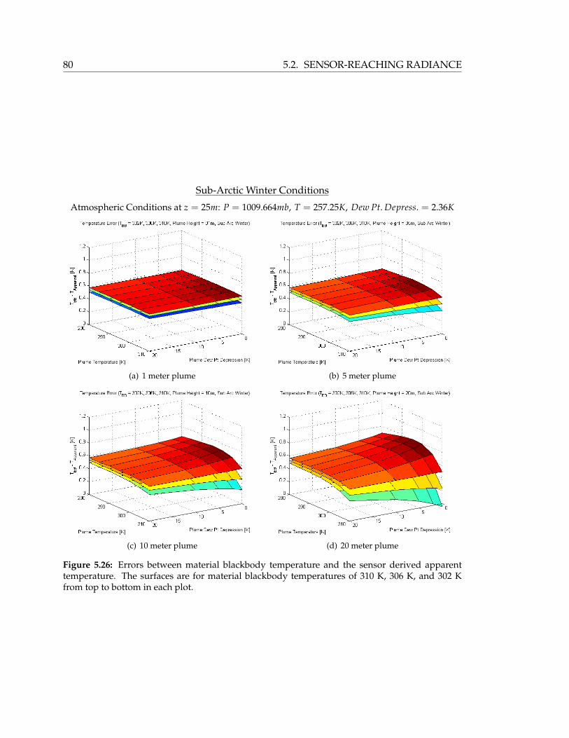
80 5.2. SENSOR-REACHING RADIANCE
Sub-Arctic Winter Conditions
Atmospheric Conditions at z = 25m: P = 1009.664mb, T = 257.25K, Dew Pt. Depress. = 2.36K
(a) 1 meter plume (b) 5 meter plume
(c) 10 meter plume (d) 20 meter plume
Figure 5.26: Errors between material blackbody temperature and the sensor derived apparenttemperature. The surfaces are for material blackbody temperatures of 310 K, 306 K, and 302 Kfrom top to bottom in each plot.
5.2. SENSOR-REACHING RADIANCE 81
Several trends are apparent in the plots. By visual inspection, the material blackbody
temperature has the greatest influence on the temperature error, followed by the ambient
atmospheric conditions, and then the plume. In general, the target blackbody temperature
and the ambient atmospheric conditions affect the overall magnitude of the temperature
errors (magnitude of the surfaces in Figures 5.25 and 5.26) and the plume influences the
shape of the surface.
The material kinetic temperature influences the temperature errors. A greater kinetic tem-
perature for the material results in a higher temperature error. The reason for this trend
is apparent from equation (5.7). The temperature error is proportional to the difference
between the material blackbody radiance and the sensor-reaching radiance such that,
Terror ∝ LBB − Lsensor (5.8)
∝ LBB − (τ LBB + Lu)
∝ (1− τ) LBB − Lu.
A higher blackbody temperature, LBB, would result in a higher radiance. Although the
transmission does not change as the blackbody temperature changes, the result of the
blackbody radiance multiplied by the transmission is greater for high target temperatures
than for low temperatures. The first term is larger for a higher blackbody radiance than
for a lower blackbody radiance. The sensor radiance will therefore also be higher as will
the resulting temperature errors.
The effect of the plume becomes apparent as the plume thickness increases, thus increas-
ing the integrated water vapor along the path. There is a competing effect of transmission
losses and additive upwelled radiance. The temperature error seems to peak for a plume
temperature of 295 K to 300 K at a dew point depression of 0 K (saturated). The mini-
mum temperature error occurs for the highest set plume temperature of 310 K and a dew
point depression of 0 K. The range of temperature errors increase as the plume thickness
increases.
Finally the overall temperature errors are greater under mid-latitude summer conditions
than for sub-arctic winter conditions. A mid-latitude summer atmosphere is warmer and
contains a greater amount of water vapor which leads to a decreased transmission and
increased upwelled radiance. However, the transmission loss has a greater effect than the
upwelled radiance in this case which results in increased temperature errors. Conversely,
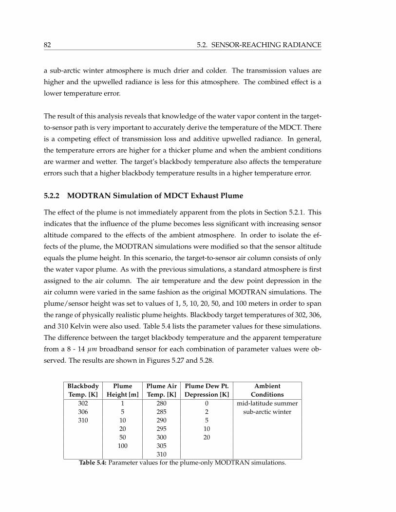
82 5.2. SENSOR-REACHING RADIANCE
a sub-arctic winter atmosphere is much drier and colder. The transmission values are
higher and the upwelled radiance is less for this atmosphere. The combined effect is a
lower temperature error.
The result of this analysis reveals that knowledge of the water vapor content in the target-
to-sensor path is very important to accurately derive the temperature of the MDCT. There
is a competing effect of transmission loss and additive upwelled radiance. In general,
the temperature errors are higher for a thicker plume and when the ambient conditions
are warmer and wetter. The target’s blackbody temperature also affects the temperature
errors such that a higher blackbody temperature results in a higher temperature error.
5.2.2 MODTRAN Simulation of MDCT Exhaust Plume
The effect of the plume is not immediately apparent from the plots in Section 5.2.1. This
indicates that the influence of the plume becomes less significant with increasing sensor
altitude compared to the effects of the ambient atmosphere. In order to isolate the ef-
fects of the plume, the MODTRAN simulations were modified so that the sensor altitude
equals the plume height. In this scenario, the target-to-sensor air column consists of only
the water vapor plume. As with the previous simulations, a standard atmosphere is first
assigned to the air column. The air temperature and the dew point depression in the
air column were varied in the same fashion as the original MODTRAN simulations. The
plume/sensor height was set to values of 1, 5, 10, 20, 50, and 100 meters in order to span
the range of physically realistic plume heights. Blackbody target temperatures of 302, 306,
and 310 Kelvin were also used. Table 5.4 lists the parameter values for these simulations.
The difference between the target blackbody temperature and the apparent temperature
from a 8 - 14 µm broadband sensor for each combination of parameter values were ob-
served. The results are shown in Figures 5.27 and 5.28.
Blackbody Plume Plume Air Plume Dew Pt. AmbientTemp. [K] Height [m] Temp. [K] Depression [K] Conditions
302 1 280 0 mid-latitude summer306 5 285 2 sub-arctic winter310 10 290 5
20 295 1050 300 20
100 305310
Table 5.4: Parameter values for the plume-only MODTRAN simulations.
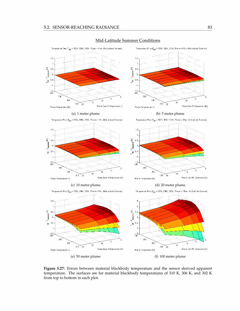
5.2. SENSOR-REACHING RADIANCE 83
Mid-Latitude Summer Conditions
(a) 1 meter plume (b) 5 meter plume
(c) 10 meter plume (d) 20 meter plume
(e) 50 meter plume (f) 100 meter plume
Figure 5.27: Errors between material blackbody temperature and the sensor derived apparenttemperature. The surfaces are for material blackbody temperatures of 310 K, 306 K, and 302 Kfrom top to bottom in each plot.

84 5.2. SENSOR-REACHING RADIANCE
Sub-Arctic Winter Conditions
(a) 1 meter plume (b) 5 meter plume
(c) 10 meter plume (d) 20 meter plume
(e) 50 meter plume (f) 100 meter plume
Figure 5.28: Errors between material blackbody temperature and the sensor derived apparenttemperature. The surfaces are for material blackbody temperatures of 310 K, 306 K, and 302 Kfrom top to bottom in each plot.

5.2. SENSOR-REACHING RADIANCE 85
The effect of the plume is apparent in that it affects the shape of the plot. There is a
competing effect of transmission losses and additive upwelled radiance. The largest tem-
perature errors occur for a plume temperature of 290 K to 295 K and for a temperature
of 310 K with a dew point depression of 0 K (saturated). The absolute magnitude of the
errors increase as the plume height increases. The maximum temperature errors intro-
duced by plumes with heights of 1, 5, 10, 20, 50, and 100 meters are approximately±0.03,
±0.1, ±0.2, ±0.4, ±0.8, and ±1.4 Kelvin, respectively. The blackbody target temperature
along with the plume air temperature and dew point depression determine whether the
additional temperature error introduced by the plume is less than or greater than zero.
Finally, the ambient atmospheric conditions appear to have an insignificant effect on the
temperature errors.
To provide a context for the error introduced by the plume, it is compared to a typical
residual error after a standard atmospheric compensation method. For example, Qin et
al. (2001) used the Landsat TM thermal band to retrieve desert land surface tempera-
tures [24]. The authors used in situ atmospheric profile data that was coincident with the
satellite pass to compensate for the atmosphere. The resulting temperature errors were
approximately 1.1 K. When in situ atmospheric data is not available, a multi-channel ap-
proach can be used. Using such a dual-channel method, the algorithm presented by Prata
(1993) yielded land surface temperatures to within ±1.5 K for flat terrain with uniform
surface composition in relatively dry atmospheres [26]. These temperature errors are sev-
eral times the temperature errors introduced from plumes with heights of zero to 20 me-
ters. However, 50 and 100 meter high plumes will introduce errors roughly the same as
the residual errors of the atmospheric compensation methods mentioned. The temper-
ature error caused by the plume can also be compared to the temperature error due to
uncertainties in the surface emissivity. Dash et al. (2002) points out that for mid-latitude
vegetated areas, for example, an emissivity error of ±0.025 results in a land surface tem-
perature error of ±2 K when a single channel is used [23].
From these studies, it appears that the temperature error introduced by plumes with
heights less than about 20 meters is roughly an order of magnitude less than the mag-
nitude of the residual errors from the aforementioned atmospheric compensation tech-
niques and sensitivity of surface emissivity. The additional temperature errors caused by
the plume will become significant as the plume height reaches approximately 50 meters
and greater.
86 5.2. SENSOR-REACHING RADIANCE
5.2.3 Sensitivity of Plume Gradient
In an MDCT, the air mass inside the tower between the drift eliminators and the fan stack
opening is assumed to be at a homogeneous temperature. The initial air temperature
of the plume in the tower throat is therefore assumed to be at the same temperature as
the internal air. Since the tower operates through evaporative processes, the initial dew
point depression of the plume is assumed to be very close to zero. As the plume rises
and travels downwind, it will diffuse within the ambient air. The plume air temperature
will gradually cool and the moisture content will decrease. Therefore, there will be a tem-
perature and moisture gradient along the line-of-sight of the sensor through the plume.
The gradient in the plume is of interest since it may affect the derived apparent tempera-
ture of the cooling tower. A perfect atmospheric compensation is assumed to have been
performed on the image. This compensation essentially removes the atmospheric effect
along the line-of-sight path from the sensor down to the edge of the plume. This ”edge”
of the plume is not well defined since the diffusion of the plume is a gradual process. The
edge will be dependant on the functional form of the gradient in the plume.
To investigate this ”edge” problem further, several gradients were modeled using the
MODTRAN software. The purpose of this study was to determine the effect of various
plume air temperature and dew point temperature gradients. A user-defined atmospheric
profile was created in MODTRAN. The air temperature and dew point temperature at the
first level (ground) was set to 295.0 K. A sensor covering the 8 to 14 µm spectral range
was placed at an altitude of 20 meters. This altitude represents the ”top” of the plume.
In other words, in a real scene, it is assumed that an atmospheric compensation has been
performed that removes the atmospheric effect from the sensor to the ”top” of the plume
(the ”top” being 20 meters in this case). The temperature gradient in the intervening
levels determines how the air temperature and dew point temperature changes from the
initial temperature at the surface to the ambient temperature and dew point at the ”top”
of the plume. For this study, the ambient air temperature was 290 K and the ambient
dew point temperature was 285 K. Three different gradients were investigated. The first
profile followed a Gaussian function in which the maximum value of the Gaussian is the
initial temperature. The temperature gradually decreases to the ambient temperature as
the height increases. The standard deviation of the Gaussian was 10 meters. The top of
the plume (20 meters) is defined as two standard deviations. The second profile was a
Step function in which the temperature remained constant at the initial temperature up to
a height of 10 meters, and then dropped suddenly to the ambient temperature for heights

5.2. SENSOR-REACHING RADIANCE 87
(a) (b)
Figure 5.29: Linear, Step, and Gaussian temperature gradients modeled in MODTRAN. Air tem-perature (a) and dew point temperature (b). The sensor altitude is marked at 20 meters..
greater than 10 meters. The last profile was a linear gradient in which the temperature
decreased linearly from the initial temperature at zero meters to the ambient temperature
at 20 meters. Figure 5.29 illustrates the three gradients used in the simulation.
For each profile, the spectral transmission and spectral upwelled radiance was computed
in MODTRAN. Recall that the initial temperature of the plume equals the internal tem-
perature of the MDCT. The tower cavity is modeled as a blackbody with a temperature
of 295 K. The sensor-reaching radiance is computed through equation (5.7). The spectral
radiance was then multiplied with the spectral response of the sensor to arrive at an in-
tegrated radiance value. For this analysis, a broadband sensor with a spectral response
of unity between 8 and 14 µm was used. This band radiance is converted into an ap-
parent temperature. A temperature error metric is defined as the difference between the
apparent temperature at the sensor and the internal temperature (also the initial plume
temperature) of 295 K.
The resulting temperature errors for the Gaussian, step, and linear gradients are shown in
Table 5.5. Plume lengths of 20, 50, and 100 meters were simulated. These results indicate
Plume Length Gaussian Step Linear20 m -0.0269 K -0.0245 K -0.0317 K50 m -0.0637 K -0.0607 K -0.0744 K
100 m -0.1162 K -0.1121 K -0.1350 K
Table 5.5: Apparent temperature errors for three plume gradient functions and for three plumelengths.

88 5.2. SENSOR-REACHING RADIANCE
that the error which occurs is independent of gradient type. The Gaussian gradient, how-
ever, is believed to be more representative of actual plume scenarios.
The conclusion of this study is that the effect of the MDCT exhaust plume will be mod-
eled using the MODTRAN software. The initial air temperature of the plume will be
equal to the selected internal temperature of the tower. The initial dew point depression
of the plume will be zero to indicate a saturated water vapor plume. The air temperature
and dew point temperature gradient will follow a Gaussian function in which the plume
length is defined as two standard deviations from the tower opening. The air temper-
ature of the plume will approach the ambient air temperature as the distance from the
tower throat increases. Similarly, the dew point temperature will approach the ambient
dew point temperature as the distance from the opening increases. The plume parameters
that will be varied in the MDCT target space are the initial plume temperature (the inter-
nal MDCT temperature), the plume length, the ambient air temperature, and the ambient
dew point temperature.
5.2.4 sensor-reaching Radiance Summary
The atmosphere greatly affects the derived temperature at the sensor. For an MDCT, the
target-to-sensor air column consists of an additional water vapor plume. The air temper-
ature, moisture content, and path length through the plume are all parameters that in-
fluence the transmission and upwelling radiance of the plume. The ambient atmosphere
also influences the signal at the sensor for the reasons discussed in Section 3.4.2. The at-
mospheric effects become more apparent as the observation altitude increases. Accurate
atmospheric compensation of the recorded signal is key to determine the temperature of
an MDCT. In general, for a moderately sized plume of approximately 10 to 20 meters in
height, the temperature error introduced by the plume is smaller than the residual error
from standard atmospheric compensation techniques (see Section 4.2.1).
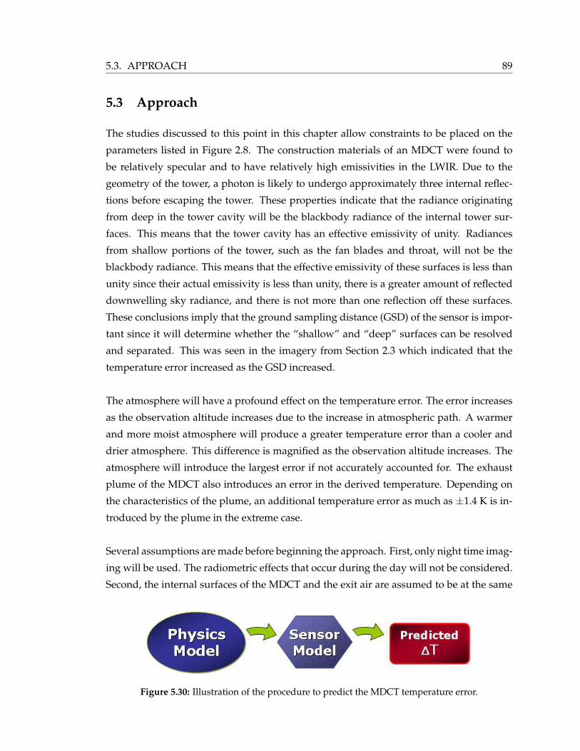
5.3. APPROACH 89
5.3 Approach
The studies discussed to this point in this chapter allow constraints to be placed on the
parameters listed in Figure 2.8. The construction materials of an MDCT were found to
be relatively specular and to have relatively high emissivities in the LWIR. Due to the
geometry of the tower, a photon is likely to undergo approximately three internal reflec-
tions before escaping the tower. These properties indicate that the radiance originating
from deep in the tower cavity will be the blackbody radiance of the internal tower sur-
faces. This means that the tower cavity has an effective emissivity of unity. Radiances
from shallow portions of the tower, such as the fan blades and throat, will not be the
blackbody radiance. This means that the effective emissivity of these surfaces is less than
unity since their actual emissivity is less than unity, there is a greater amount of reflected
downwelling sky radiance, and there is not more than one reflection off these surfaces.
These conclusions imply that the ground sampling distance (GSD) of the sensor is impor-
tant since it will determine whether the “shallow” and “deep” surfaces can be resolved
and separated. This was seen in the imagery from Section 2.3 which indicated that the
temperature error increased as the GSD increased.
The atmosphere will have a profound effect on the temperature error. The error increases
as the observation altitude increases due to the increase in atmospheric path. A warmer
and more moist atmosphere will produce a greater temperature error than a cooler and
drier atmosphere. This difference is magnified as the observation altitude increases. The
atmosphere will introduce the largest error if not accurately accounted for. The exhaust
plume of the MDCT also introduces an error in the derived temperature. Depending on
the characteristics of the plume, an additional temperature error as much as ±1.4 K is in-
troduced by the plume in the extreme case.
Several assumptions are made before beginning the approach. First, only night time imag-
ing will be used. The radiometric effects that occur during the day will not be considered.
Second, the internal surfaces of the MDCT and the exit air are assumed to be at the same
Figure 5.30: Illustration of the procedure to predict the MDCT temperature error.
90 5.3. APPROACH
temperature. The exit air is also assumed to be nearly saturated. Lastly, an atmospheric
compensation is assumed to have been performed on the images. Therefore, the effects of
the atmospheric column (other than the exhausted vapor plume) are not considered.
5.3.1 Overview
A camera sensitive to the LWIR spectral region (approximately 8 - 14 µm) is used to ob-
serve the cooling tower. Each pixel in the resulting thermal image is converted into an
apparent temperature, or image-derived temperature. The apparent temperature of pix-
els inside the fan stack opening of the tower is to be correlated to the exit air temperature.
To do so, a 3-D physics model of the radiation transfer is necessary to accurately derive the
exhaust air temperature from the thermal image. A sensor model is necessary to derive
the apparent temperature of the MDCT from the simulated image for a particular sensor.
Finally, a target space is constructed to predict the apparent temperature of the MDCT
for a range of model parameters. This target space information will allow a temperature
correction factor to be assembled that will be applied to the thermal image to produce an
accurate MDCT temperature.
5.3.2 Physics Model
Based on the studies performed in Sections 5.1 and 5.2, a methodology is developed to
accurately model the radiance field from the MDCT, through the exhausted plume, and
into the sensor. The DIRSIG software developed at RIT and the MODTRAN software
developed by the AFRL are used to model the internal and propagated radiometry of the
MDCT. The parameters used in these simulations are listed here along with a detailed
description of how they will be modeled. Eventually, every combination of parameter
values will be used to create a target space (look-up table) that will predict the at-sensor
radiance and therefore the necessary temperature correction factor.
5.3.2.1 Tower Leaving Radiance with DIRSIG
The tower-leaving radiance is modeled using DIRSIG. This radiance includes the self-
emitted radiance and any reflected radiance from the tower surfaces. The simulation is
based on a CAD drawing of an MDCT. Given the results from Section 5.1, a highly de-
tailed CAD model does not appear to be necessary to reproduce the exact radiometry
inside the tower. Instead, a simplified drawing derived from that shown in Figure 5.15
will be used. The diagonal internal support structure, water distribution system, and fill
was deleted. The exterior surfaces (i.e., the siding and decking) were drawn as plain facets
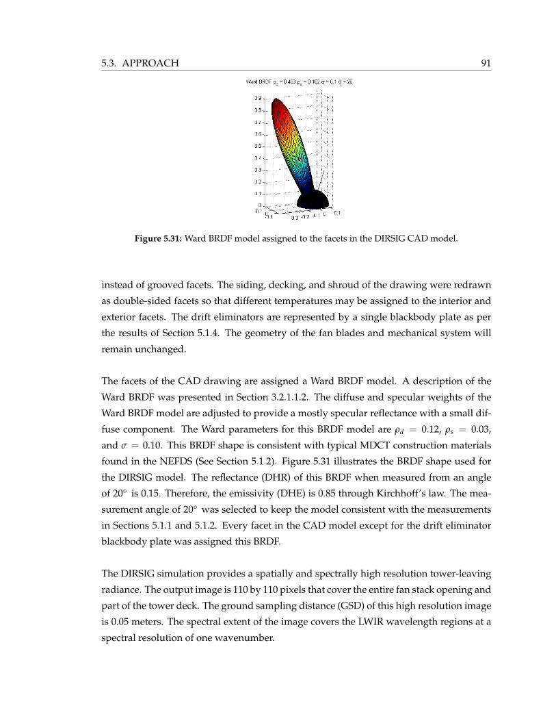
5.3. APPROACH 91
Figure 5.31: Ward BRDF model assigned to the facets in the DIRSIG CAD model.
instead of grooved facets. The siding, decking, and shroud of the drawing were redrawn
as double-sided facets so that different temperatures may be assigned to the interior and
exterior facets. The drift eliminators are represented by a single blackbody plate as per
the results of Section 5.1.4. The geometry of the fan blades and mechanical system will
remain unchanged.
The facets of the CAD drawing are assigned a Ward BRDF model. A description of the
Ward BRDF was presented in Section 3.2.1.1.2. The diffuse and specular weights of the
Ward BRDF model are adjusted to provide a mostly specular reflectance with a small dif-
fuse component. The Ward parameters for this BRDF model are ρd = 0.12, ρs = 0.03,
and σ = 0.10. This BRDF shape is consistent with typical MDCT construction materials
found in the NEFDS (See Section 5.1.2). Figure 5.31 illustrates the BRDF shape used for
the DIRSIG model. The reflectance (DHR) of this BRDF when measured from an angle
of 20° is 0.15. Therefore, the emissivity (DHE) is 0.85 through Kirchhoff’s law. The mea-
surement angle of 20° was selected to keep the model consistent with the measurements
in Sections 5.1.1 and 5.1.2. Every facet in the CAD model except for the drift eliminator
blackbody plate was assigned this BRDF.
The DIRSIG simulation provides a spatially and spectrally high resolution tower-leaving
radiance. The output image is 110 by 110 pixels that cover the entire fan stack opening and
part of the tower deck. The ground sampling distance (GSD) of this high resolution image
is 0.05 meters. The spectral extent of the image covers the LWIR wavelength regions at a
spectral resolution of one wavenumber.
92 5.3. APPROACH
5.3.2.1.1 DIRSIG Parameters
The list of DIRSIG parameters that will be varied are presented here along with a descrip-
tion of each.
MDCT Internal Temperature is the temperature assigned to the internal facets of the
MDCT DIRSIG model. These internal facets include the interior faces of the deck-
ing and siding, the drift eliminator plate, the internal tower support structures, the
fan support structure, and the fan mechanical structures. This internal temperature
is important since it is the desired temperature to be retrieved from the remotely-
sensed image.
MDCT External Temperature is the temperature assigned to the exterior facets of the
MDCT DIRSIG model. These external facets include the exterior faces of the decking
and siding, the fan stack shroud (cowling), and the fan blades. The important exter-
nal facets for the physics model are the fan blades and the shroud since these objects
are in the line-of-sight between the sensor and the tower cavity. The MDCT external
temperature is set to be less than or equal to the assigned MDCT internal tempera-
ture (assuming night time imaging only). From the MDCT experimental collection
performed at SRS in the spring of 2004 and 2005, the external apparent tempera-
tures appear to be between 0 and 4 Kelvin less than the internal temperature for the
nighttime scenes (see Section 2.3).
Fan Blade Emissivity can be adjusted by altering the Ward BRDF model parameters
for the fan blade facets. The fan blade emissivity parameter is used to scale the magni-
tude of the BRDF assigned to the fan blades. To do so, a reference Ward BRDF is set
in which the diffuse and specular weights were chosen to produce the desired BRDF
shape of a mostly specular lobe with a small diffuse component (ρd = 0.0408 and ρs
= 0.0102). The integral of this BRDF shape yields a DHR of 0.05 for a measurement
angle of 20°. To scale the magnitude of this BRDF while maintaining its shape, the
diffuse and specular weights are adjusted by
[ρd , ρs] =1− ε f an
0.05[0.0408 , 0.0102] . (5.9)
Effective Sky Temperature is the apparent temperature of the sky computed from the
integrated downwelling sky radiance. This is the equivalent blackbody tempera-
ture of the sky. It can be computed from a known atmospheric temperature and
moisture profile (sounding). The profile is used as input into MODTRAN and the

5.3. APPROACH 93
Figure 5.32: Illustration of atmospheric layers in MODTRAN used to model the moisture gradientin the plume.
path radiance from sample points covering the entire sky hemisphere is computed.
The downwelling radiance from the computed samples is integrated over the entire
sky hemisphere and converted into an apparent temperature. The effective sky tem-
perature is used by DIRSIG to compute the thermal downwelling radiance from the
sky. This downwelling radiance is necessary since it reflects off the tower facets and
therefore becomes a component of the tower-leaving radiance. A utility is provided
that calculates the effective sky temperature given an atmospheric sonde profile (See
Appendix D).
Sensor Zenith Angle is the view angle of the sensor measured relative to a nadir (down-
looking) viewing position of the MDCT. The radiance leaving the tower has an an-
gular distribution. The view angle is important since it determines what features of
the tower, such as the tower cavity and shroud side, are visible by the sensor and
may therefore be included in the interior radiance field due to optical, mechanical,
and atmospheric blurring.
5.3.2.2 Plume Leaving Radiance with MODTRAN
The tower-leaving radiance produced by DIRSIG must now propagate through the ex-
hausted water vapor plume to reach the sensor. The MODTRAN software is used to
model the plume. A standard atmosphere is used as the base atmosphere to be modified.
A plume layer is then defined that extends from the ground to a height, z. The surface
temperature in this profile is assigned the same value that was used for the MDCT inter-
nal temperature in the DIRSIG model since the assumption is made that the interior MDCT
surfaces and the exit air are at the same temperature. Similarly, the surface dew point
94 5.3. APPROACH
depression is set to zero since the assumption is made that the exit air is nearly saturated.
The sensor is placed at the height of the plume layer (z) so that the atmospheric effect of
the plume is isolated. Figure 5.32 illustrates this layout.
A temperature and moisture gradient established in the atmospheric profile follows a
Gaussian function decay. The temperature approaches the ambient air temperature as
the height increases. Similarly, the dew point temperature approaches the ambient dew
point temperature as the height increases. The height of the plume is defined as the two
standard deviations distance of the Gaussian (2σ) as per the results of Section 5.2.3. The
MODTRAN simulation provides spectral atmospheric transmission and spectral atmo-
spheric path radiance curves for the same spectral range as the DIRSIG simulation.
5.3.2.2.1 MODTRAN Parameters
The list of MODTRAN parameters that will be varied are presented here along with a
description of each.
Ambient Air Temperature is the temperature of the ambient air measured at the sur-
face. This value will be the final temperature the plume approaches.
Ambient Dew Point Temperature is the dew point temperature of the ambient air mea-
sured at the surface. This value will be the final dew point temperature of the plume.
Water Vapor Plume Path Length is the effective length of the line-of-site path through
the plume. This parameter is estimated by the user based on knowledge of the
sensor view angle, air flow through the tower, and wind speed and direction. The
plume path length is modeled as the height of the plume layer (z) in the MODTRAN
user-defined atmosphere. A utility has been produced to estimate the plume path
length if a more sophisticated plume model is not available (See Appendix E).
5.3.2.3 Physics Model Summary
Each spectral pixel in the DIRSIG tower-leaving radiance image is multiplied by wave-
length with the spectral transmission data and then added by wavelength to the spectral
path radiance from MODTRAN. The result of the DIRSIG and MODTRAN simulations
is a sensor-reaching radiance that is spatially and spectrally high resolution. Note that it
is assumed that an atmospheric compensation has been performed on the image that re-
moved the effect of the air column from the sensor to the ground. The remaining sources
of error to account for are due to the effects of the tower geometry and of the exhausted
5.3. APPROACH 95
plume. Therefore, the result of the DIRSIG and MODTRAN run is essentially a ”top of
plume” radiance.
5.3.3 Sensor Model
The high spatial and spectral resolution image generated by the physics model represents
the radiance reaching the sensor. The sensor will degrade and record the incident radiance
as described in Section 3.5. The sensor model accepts sensor specifications from the user
and applies those specifications to the high resolution physics model radiance image. An
algorithm was written in the Matlab programming environment that processes the high
resolution image according to the sensor information provided by the user. Specifically,
the spectral response, the GSD, and the radius of the system point spread function are
necessary.
The sensor spectral response consists of a vector of wavelengths and a corresponding
vector of response weights for a particular spectral band. The algorithm first spectrally
samples the radiance images with the supplied spectral response. The spectral response
function is resampled to the wavelengths used in the radiance image. The response func-
tion and the high resolution image radiance are then multiplied together by wavelength
for every pixel and integrated over all wavelengths to arrive at a band integrated image.
This new image now consists of a single band but is still spatially high resolution (110 by
110 pixels).
Next, a system point spread function (PSF) (modeled as an Airy disc) whose radius was
provided by the user is applied to the image thereby blurring it. The user-supplied radius
is in units of microns. If the user does not wish to apply a PSF, the radius should be set
to zero. An image of an Airy disc with the proper radius is created that has the same di-
mensions as the radiance image. To make the computations easier, the Fourier transform
of the Airy image and of the radiance image were taken. The transformed images were
multiplied together and then the inverse Fourier transform was taken. The result of the
PSF application is a blurred image that still consists of 110 by 110 pixels.
Finally, the image must be down-sampled such that the final image has the user required
GSD. The GSD of the high resolution radiance image is 0.05 meters. The user-supplied
GSD is rounded to the nearest 0.05 meters so that the final GSD is an integer multiple of
the original GSD to make the computations easier. The image is then divided into blocks
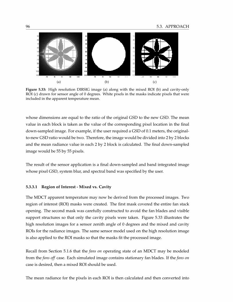
96 5.3. APPROACH
(a) (b) (c)
Figure 5.33: High resolution DIRSIG image (a) along with the mixed ROI (b) and cavity-onlyROI (c) drawn for sensor angle of 0 degrees. White pixels in the masks indicate pixels that wereincluded in the apparent temperature mean.
whose dimensions are equal to the ratio of the original GSD to the new GSD. The mean
value in each block is taken as the value of the corresponding pixel location in the final
down-sampled image. For example, if the user required a GSD of 0.1 meters, the original-
to-new GSD ratio would be two. Therefore, the image would be divided into 2 by 2 blocks
and the mean radiance value in each 2 by 2 block is calculated. The final down-sampled
image would be 55 by 55 pixels.
The result of the sensor application is a final down-sampled and band integrated image
whose pixel GSD, system blur, and spectral band was specified by the user.
5.3.3.1 Region of Interest - Mixed vs. Cavity
The MDCT apparent temperature may now be derived from the processed images. Two
region of interest (ROI) masks were created. The first mask covered the entire fan stack
opening. The second mask was carefully constructed to avoid the fan blades and visible
support structures so that only the cavity pixels were taken. Figure 5.33 illustrates the
high resolution images for a sensor zenith angle of 0 degrees and the mixed and cavity
ROIs for the radiance images. The same sensor model used on the high resolution image
is also applied to the ROI masks so that the masks fit the processed image.
Recall from Section 5.1.6 that the fans on operating state of an MDCT may be modeled
from the fans off case. Each simulated image contains stationary fan blades. If the fans on
case is desired, then a mixed ROI should be used.
The mean radiance for the pixels in each ROI is then calculated and then converted into
5.3. APPROACH 97
an apparent temperature. The predicted temperature error was defined as the difference be-
tween the predicted apparent temperature (i.e., mean ROI apparent temperature) and the
assigned MDCT internal temperature. The temperature errors were calculated for both the
mixed ROI and the cavity-only ROI.
5.3.4 Target Space Look-Up Table
The physics model and the sensor model generate a single simulated thermal image for a
given set of parameter values and for a given sensor. The result is a predicted temperature
error (temperature correction) for the set of parameter values. To be useful for an image
analyst, a temperature correction must be known for any scene. Since the values of each
of the eight parameters will probably not be known exactly, the physics model may be run
many times with various parameter values. The resulting list of temperature correction
factors for each combination of parameter values is known as a target space. This concept
is similar to the target space used by Healey and Slater [33] and Ientilucci and Schott [42]
for target detection (See Section 4.2.1.8). The target space is essentially a look-up table
(LUT) that lists the predicted image-derived apparent temperature for a specific sensor
for each combination of parameter values.
5.3.5 Parameterized Model
Multiple regression analysis may be performed on the LUT of temperature corrections
(Appendix B). A multiple linear regression equation may be fit to the dataset to arrive
at a single multi-parameter equation that predicts the temperature error given a set of
parameter values. A multiple linear regression model has the form [43],
yi = β0 + βi,1 xi,1 + βi,2 xi,2 + ... + βi,p−1 xi,p−1 + ε i (5.10)
where the β variables are the model-fit coefficients. A relationship between the response
variable (the temperature error) and the predictor variables (the target-space parameters)
is desired. Since the first target-space parameter, MDCT internal temperature, is the ulti-
mate variable that is to be determined, it is not included in the regression model. The
model predictors are therefore the other seven parameters.
The least-squares regression equation may be expressed in matrix form as
Y = X β + ε. (5.11)
98 5.4. METHODOLOGY SUMMARY
The estimated fit coefficients, b, are found by
b =(X′ X
)−1 X′ Y. (5.12)
Therefore, the predicted temperature error, Y, is
Y = X b. (5.13)
5.4 Methodology Summary
The problem of determining the exit air temperature of an MDCT is unique due to the
geometry of the tower and due to the exhausted water vapor plume. These two factors
represent the remaining sources of error in the extracted tower temperature that must be
accounted for given that the image has been atmospherically compensated. The stud-
ies presented in this chapter investigated the sensitivity of these factors and placed con-
straints on the variables affecting the derived temperature estimation. The results of those
investigations allowed a methodology to be developed to estimate the temperature cor-
rection factor that must be applied to a thermal image to remove the effects of the tower
geometry and the exhausted plume. The result should be a more accurate estimate of the
MDCT exit air temperature.

Chapter 6
Results
The methodology developed in the previous chapter may now be implimented in order
to achieve the ultimate goal of deriving a temperature correction factor for an MDCT
thermal image. The process yields a LUT of predicted correction factors for each set of
model parameters. A parameterized model is then fit to this data set. The parameterized
model is tested with simulated data and then applied to the SRNL data set to test its utility
with actual image data.
6.1 Physics Model Generation
All eight target space parameters described in Sections 5.3.2.1.1 and 5.3.2.2.1 were varied
in this study. The physics model consists of the DIRSIG and MODTRAN simulation tools.
The model parameters are listed in Table 6.1 for reference.
Parameter Modeling ToolMDCT Internal Temperature DIRSIGMDCT External Temperature DIRSIGFan Blade Emissivity DIRSIGEffective Sky Temperature DIRSIGSensor Zenith Angle DIRSIGAmbient Air Temperature MODTRANAmbient Dew Point Temperature MODTRANPlume Path Length MODTRAN
Table 6.1: MDCT physics model parameters and associated modeling tools.
UNIX scripts were written to easily change these parameter values in the DIRSIG and
MODTRAN models. The values for each parameter were chosen to cover the possible
range of values for the datasets presented in Section 2.3. These values are summarized in
Table 6.2.
The DIRSIG simulation was set at midnight local time. There was no atmospheric trans-
mission loss or path radiance. Therefore, the DIRSIG simulation represents the tower-
99
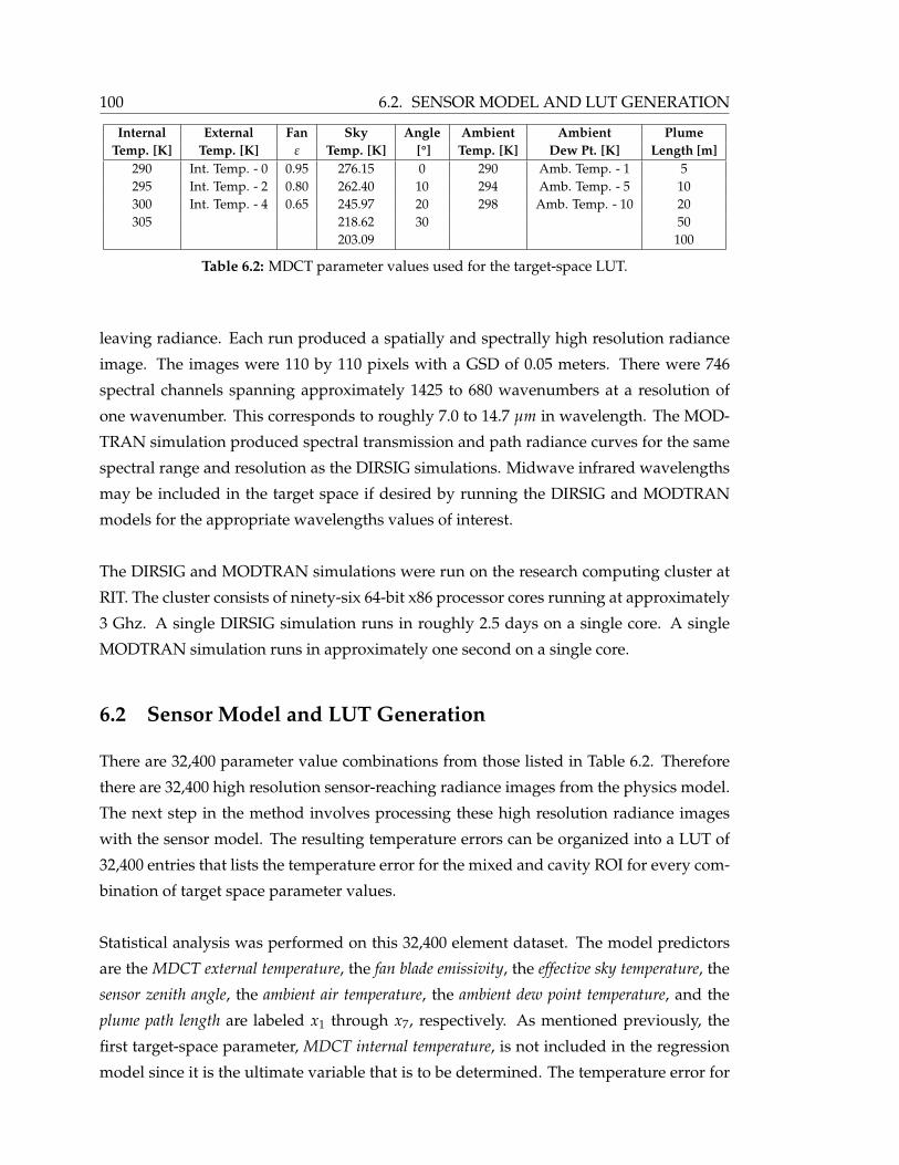
100 6.2. SENSOR MODEL AND LUT GENERATION
Internal External Fan Sky Angle Ambient Ambient PlumeTemp. [K] Temp. [K] ε Temp. [K] [°] Temp. [K] Dew Pt. [K] Length [m]
290 Int. Temp. - 0 0.95 276.15 0 290 Amb. Temp. - 1 5295 Int. Temp. - 2 0.80 262.40 10 294 Amb. Temp. - 5 10300 Int. Temp. - 4 0.65 245.97 20 298 Amb. Temp. - 10 20305 218.62 30 50
203.09 100
Table 6.2: MDCT parameter values used for the target-space LUT.
leaving radiance. Each run produced a spatially and spectrally high resolution radiance
image. The images were 110 by 110 pixels with a GSD of 0.05 meters. There were 746
spectral channels spanning approximately 1425 to 680 wavenumbers at a resolution of
one wavenumber. This corresponds to roughly 7.0 to 14.7 µm in wavelength. The MOD-
TRAN simulation produced spectral transmission and path radiance curves for the same
spectral range and resolution as the DIRSIG simulations. Midwave infrared wavelengths
may be included in the target space if desired by running the DIRSIG and MODTRAN
models for the appropriate wavelengths values of interest.
The DIRSIG and MODTRAN simulations were run on the research computing cluster at
RIT. The cluster consists of ninety-six 64-bit x86 processor cores running at approximately
3 Ghz. A single DIRSIG simulation runs in roughly 2.5 days on a single core. A single
MODTRAN simulation runs in approximately one second on a single core.
6.2 Sensor Model and LUT Generation
There are 32,400 parameter value combinations from those listed in Table 6.2. Therefore
there are 32,400 high resolution sensor-reaching radiance images from the physics model.
The next step in the method involves processing these high resolution radiance images
with the sensor model. The resulting temperature errors can be organized into a LUT of
32,400 entries that lists the temperature error for the mixed and cavity ROI for every com-
bination of target space parameter values.
Statistical analysis was performed on this 32,400 element dataset. The model predictors
are the MDCT external temperature, the fan blade emissivity, the effective sky temperature, the
sensor zenith angle, the ambient air temperature, the ambient dew point temperature, and the
plume path length are labeled x1 through x7, respectively. As mentioned previously, the
first target-space parameter, MDCT internal temperature, is not included in the regression
model since it is the ultimate variable that is to be determined. The temperature error for
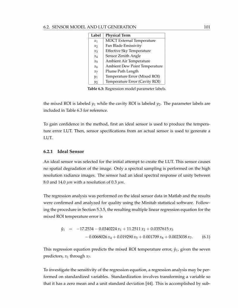
6.2. SENSOR MODEL AND LUT GENERATION 101
Label Physical Termx1 MDCT External Temperaturex2 Fan Blade Emissivityx3 Effective Sky Temperaturex4 Sensor Zenith Anglex5 Ambient Air Temperaturex6 Ambient Dew Point Temperaturex7 Plume Path Lengthy1 Temperature Error (Mixed ROI)y2 Temperature Error (Cavity ROI)
Table 6.3: Regression model parameter labels.
the mixed ROI is labeled y1 while the cavity ROI is labeled y2. The parameter labels are
included in Table 6.3 for reference.
To gain confidence in the method, first an ideal sensor is used to produce the tempera-
ture error LUT. Then, sensor specifications from an actual sensor is used to generate a
LUT.
6.2.1 Ideal Sensor
An ideal sensor was selected for the initial attempt to create the LUT. This sensor causes
no spatial degradation of the image. Only a spectral sampling is performed on the high
resolution radiance images. The sensor had an ideal spectral response of unity between
8.0 and 14.0 µm with a resolution of 0.3 µm.
The regression analysis was performed on the ideal sensor data in Matlab and the results
were confirmed and analyzed for quality using the Minitab statistical software. Follow-
ing the procedure in Section 5.3.5, the resulting multiple linear regression equation for the
mixed ROI temperature error is
y1 = −17.2534− 0.0340224 x1 + 11.2511 x2 + 0.0357615 x3
− 0.0068026 x4 + 0.019290 x5 + 0.001709 x6 + 0.0023038 x7. (6.1)
This regression equation predicts the mixed ROI temperature error, y1, given the seven
predictors, x1 through x7.
To investigate the sensitivity of the regression equation, a regression analysis may be per-
formed on standardized variables. Standardization involves transforming a variable so
that it has a zero mean and a unit standard deviation [44]. This is accomplished by sub-
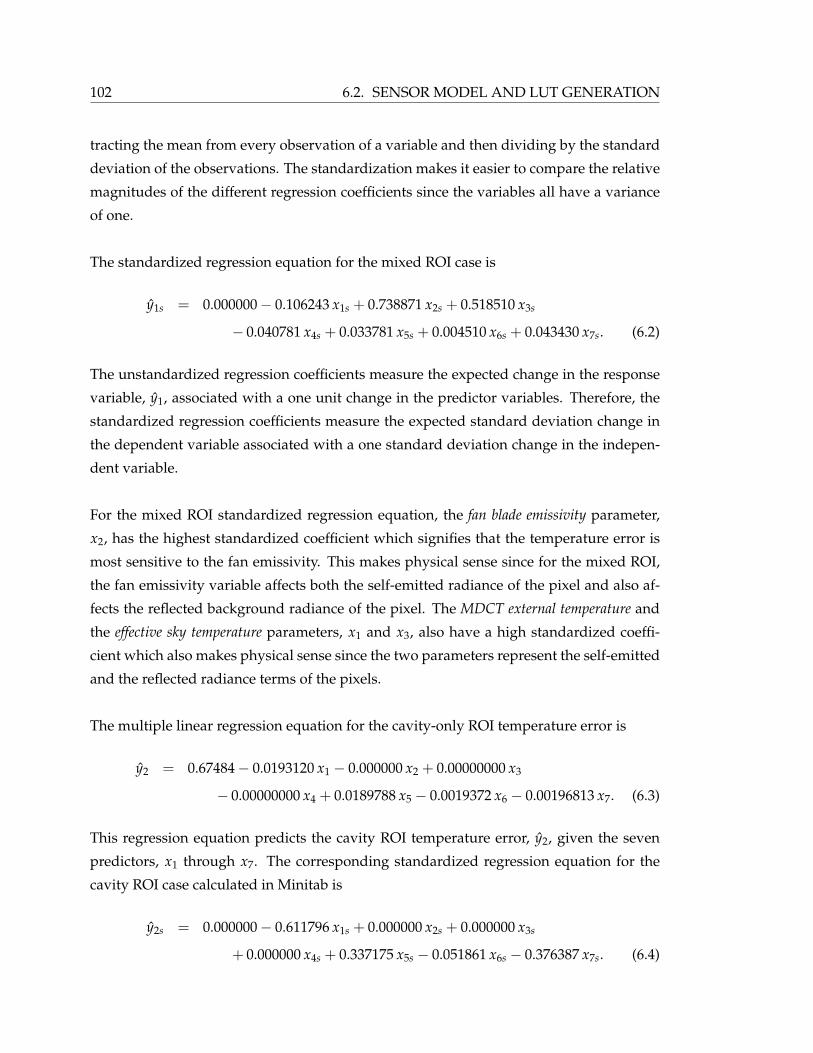
102 6.2. SENSOR MODEL AND LUT GENERATION
tracting the mean from every observation of a variable and then dividing by the standard
deviation of the observations. The standardization makes it easier to compare the relative
magnitudes of the different regression coefficients since the variables all have a variance
of one.
The standardized regression equation for the mixed ROI case is
y1s = 0.000000− 0.106243 x1s + 0.738871 x2s + 0.518510 x3s
− 0.040781 x4s + 0.033781 x5s + 0.004510 x6s + 0.043430 x7s. (6.2)
The unstandardized regression coefficients measure the expected change in the response
variable, y1, associated with a one unit change in the predictor variables. Therefore, the
standardized regression coefficients measure the expected standard deviation change in
the dependent variable associated with a one standard deviation change in the indepen-
dent variable.
For the mixed ROI standardized regression equation, the fan blade emissivity parameter,
x2, has the highest standardized coefficient which signifies that the temperature error is
most sensitive to the fan emissivity. This makes physical sense since for the mixed ROI,
the fan emissivity variable affects both the self-emitted radiance of the pixel and also af-
fects the reflected background radiance of the pixel. The MDCT external temperature and
the effective sky temperature parameters, x1 and x3, also have a high standardized coeffi-
cient which also makes physical sense since the two parameters represent the self-emitted
and the reflected radiance terms of the pixels.
The multiple linear regression equation for the cavity-only ROI temperature error is
y2 = 0.67484− 0.0193120 x1 − 0.000000 x2 + 0.00000000 x3
− 0.00000000 x4 + 0.0189788 x5 − 0.0019372 x6 − 0.00196813 x7. (6.3)
This regression equation predicts the cavity ROI temperature error, y2, given the seven
predictors, x1 through x7. The corresponding standardized regression equation for the
cavity ROI case calculated in Minitab is
y2s = 0.000000− 0.611796 x1s + 0.000000 x2s + 0.000000 x3s
+ 0.000000 x4s + 0.337175 x5s − 0.051861 x6s − 0.376387 x7s. (6.4)

6.2. SENSOR MODEL AND LUT GENERATION 103
For this case, the highest coefficient occurs for the MDCT external temperature parameter.
Caution must be taken in interpreting this result. Recall that only a spectral integration
was performed on the high resolution images. There was no spatial blurring of the images
for this study. Unlike for the mixed ROI case, the cavity ROI does not include any pixels
from the fan. Therefore, the only influence on the temperature error for the cavity pixel
should be due to the plume. The DIRSIG parameters should have coefficients of zero, as
the fan blade emissivity, the effective sky temperature, and the sensor zenith angle do. The non-
zero coefficient occurs due to the relationship between the MDCT internal temperature and
the MDCT external temperature. Recall from Table 6.2 that the MDCT external temperature
is always less than or equal to the MDCT internal temperature. The non-zero coefficients
on the MODTRAN parameters, however, agree with the physical understanding that the
plume should be the only influential parameter over the temperature errors in the cavity
ROI case.
Finally, the 32,400 observations for each parameter were used as input into the unstan-
dardized regression equations. The root-mean-square (RMS) of the residuals was com-
puted. For the mixed ROI regression equation, the RMS error was 0.767 K. The RMS error
for the cavity ROI regression equation was 0.115 K. These RMS values represent an initial
estimate of the error in the temperature correction factor.
6.2.2 SC 2000 Inframetrics Sensor
Now that the methodology has been established, the LUT may be generated for an ac-
tual sensor, the SC 2000 Inframetrics thermal camera. Recall from Section 2.3 that the SC
2000 was used to obtain LWIR imagery of several MDCT units at SRS. The camera is an
un-cooled microbolometer having a 7.6 - 13.5 µm spectral range, an instantaneous field
of view (IFOV) of 1.4 milliradians, an accuracy of ± 2 K, and a sensitivity of 0.1 K. The
sensor altitude was between 350 and 2000 feet (106.7 and 610 meters) above the ground
for the imagery presented in Section 2.3. For this study, the GSD was set to 0.22 m which
corresponds to a sensor altitude of 500 feet (Figure 2.4)
The regression equation for the mixed ROI case is
y1 = −17.5651− 0.0340 x1 + 10.7236 x2 + 0.0350 x3
− 0.0083 x4 + 0.0223 x5 + 0.0016 x6 + 0.0021 x7. (6.5)

104 6.2. SENSOR MODEL AND LUT GENERATION
This regression has a calculated RMS error of 0.785 K. Notice that the RMS error is slightly
higher in this case than in the ideal sensor case due to the spatial blurring that occurred
with this sensor. The standardized regression for the mixed ROI case is calculated as
y1s = 0.0000− 0.1090 x1s + 0.7236 x2s + 0.5208 x3s
− 0.0509 x4s + 0.0402 x5s + 0.0044 x6s + 0.0407 x7. (6.6)
As in the ideal sensor case, the fan blade emissivity appears to have the most impact on the
predicted temperature error since its standardized coefficient has the highest value.
The regression equation for the cavity ROI case for the SC 2000 is
y2 = −6.3753− 0.0268 x1 + 4.0693 x2 + 0.0136 x3
− 0.0054 x4 + 0.0220 x5 − 0.0006 x6 − 0.0004 x7. (6.7)
The RMS error for this regression is 0.355 K. This RMS is similarly higher than in the ideal
sensor case since spatial blurring occurs. The corresponding standardized form of this
equation is
y2s = 0.0000− 0.2117 x1s + 0.6769 x2s + 0.4983 x3s
− 0.0826 x4s + 0.0976 x5s − 0.0040 x6s − 0.0171 x7. (6.8)
Unlike the ideal sensor case, the DIRSIG coefficients for the SC 2000 LUT are non-zero.
This is due to the spatial blurring that occurs with the SC 2000 sensor and blurring due
to the atmosphere. The spatial blurring causes radiance from non-cavity pixels to be in-
cluded in the cavity-only pixels and therefore alters the temperature estimate for these
pixels.
6.2.2.1 SC 2000 Random Dataset
A set of 1944 random physics model runs were generated and processed using the SC
2000 sensor parameters. Each parameter value was randomly chosen from the range of
the values of that parameter in the LUT (Table 6.2). The 1944 point random dataset was
used with the regression equations for the SC 2000 sensor and the RMS errors between the
actual temperature error for each random run and the predicted error from the regression
were calculated. The parameter values used in the random dataset are listed in Table 6.4.
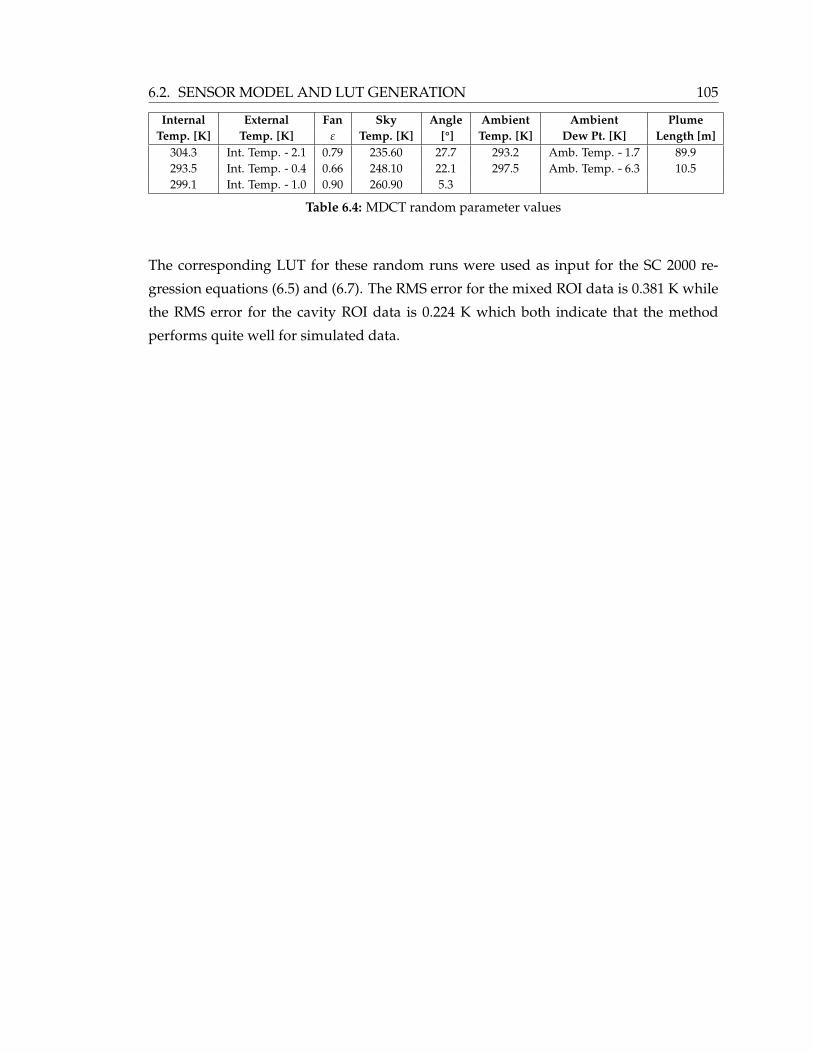
6.2. SENSOR MODEL AND LUT GENERATION 105
Internal External Fan Sky Angle Ambient Ambient PlumeTemp. [K] Temp. [K] ε Temp. [K] [°] Temp. [K] Dew Pt. [K] Length [m]
304.3 Int. Temp. - 2.1 0.79 235.60 27.7 293.2 Amb. Temp. - 1.7 89.9293.5 Int. Temp. - 0.4 0.66 248.10 22.1 297.5 Amb. Temp. - 6.3 10.5299.1 Int. Temp. - 1.0 0.90 260.90 5.3
Table 6.4: MDCT random parameter values
The corresponding LUT for these random runs were used as input for the SC 2000 re-
gression equations (6.5) and (6.7). The RMS error for the mixed ROI data is 0.381 K while
the RMS error for the cavity ROI data is 0.224 K which both indicate that the method
performs quite well for simulated data.

106 6.3. SRNL DATA SET
6.3 SRNL Data Set
The parameterized model can now be used to derive temperature corrections for the
SRNL imagery from Section 2.3. There are several issues with the data that must be ad-
dressed before proceeding. Once these issues are understood, the images may be cor-
rected using the parameterized model to obtain the desired exit air temperature of the
MDCTs. The images in the data set are shown in Figure 6.1 for reference.
(a) 20may04D14 (b) 20may04E02
(c) 20may04E04 (d) 20jun05G09
Figure 6.1: SRNL data set LWIR images.

6.3. SRNL DATA SET 107
6.3.1 Understanding the SRNL Data Set
The images and associated ground measurements in Section 2.3 have many unknown
variables that must be examined. These variables include aspects of the ground measure-
ments, the atmosphere, and the sensor.
First, the collection of simultaneous ground truth measurements is a very difficult task
in general. Recall from Section 2.3 that a temperature measurement was obtained of the
air exiting the fan stack. The measurement was made about two feet inside the edge of
the fan stack shroud for each tower. The exit air temperature is the desired temperature
that is to be determined from the thermal image. This measurement represents the only
ground truth of the desired target. Ideally, several measurements of the exit air tempera-
ture would have been obtained at several places in the fan stack opening to determine any
spatial variation to the exit air temperature. The uncertainty in the ground temperature
measurement can be estimated as ± 0.4 K. This is based on measured accuracies for simi-
lar temperature measurement technologies. In addition, one of the predictor variables of
the parameterized model is the MDCT external temperature. This is the temperature of the
surrounding deck material. No ground-truth temperature measurements are available for
the decking.
Another non-characterized aspect of the ground measurements is the atmospheric state.
A meteorological station recorded ambient air temperature, dew point temperature, and
wind velocity data approximately five meters away from the tower units. These environ-
mental conditions recorded at this location are not exactly the same as those directly next
to the towers. Ideally, several measurements would be obtained around the direct perime-
ter of the towers. Wind measurements would be taken directly at the fan stack opening to
infer the exact direction of the exhausted plume. A more significant problem is the lack of
atmospheric profile information. Such information is necessary to correct the images for
the atmospheric effects of path transmission and path radiance.
In addition to environmental variables, there are uncertainties in the sensor used to col-
lect the images. As mentioned previously, the SRNL images were obtained with a SC 2000
Inframetrics camera. The detector size and field of view are known fairly well so that the
GSD can be calculated accurately. However, the exact spectral response of the camera is
unknown. Information from the manufacturer lists the spectral response as between 7.6
and 13.5 µm. Since the exact response in this wavelength region is not available, an as-

108 6.3. SRNL DATA SET
sumption is made that the response is unity between 7.6 and 13.5 µm and is zero outside
this region. Furthermore, the images are in terms of apparent temperature at the sensor.
Ideally, the image would have been kept in terms of radiance at the sensor to eliminate
any errors associated with converting radiance to temperature. The manufacturer reports
a temperature accuracy of± 2 K and a thermal sensitivity of 0.1 K. The thermal sensitivity
is the precision level of the camera (i.e., image temperatures are reported to one decimal
place). The accuracy value is a measure of the sensor noise. The value of ± 2 K can be
interpreted as the three standard deviation value (3σ) for a random normal distribution
of noise. Therefore, the uncertainty in the camera measurement is ± 0.66 K.
6.3.2 Atmospheric Compensation
Most of the factors discussed in the previous section are already set and cannot be changed.
The atmospheric compensation issue, however, is managable to a certain extent. Although
a true atmospheric sounding at the time of image acquisition is not available, the atmo-
spheric profile can be interpolated from nearby radiosonde stations. These radiosonde
profiles must be spatially and temporally interpolated to estimate the profile at SRS at the
time of image aquisition. The five surrounding radiosonde locations are listed in Table 6.5.
Each radiosonde profile contains measurements of the atmospheric pressure, air temper-
ature, and dew point temperature at various pressure levels. The measurement altitude is
calculated from the atmospheric pressure through the hydrostatic equation and the ideal
gas equation [12]. The radiosonde measurements are not taken at regular altitude inter-
vals. Therefore, each radiosonde profile is first interpolated to regular altitude intervals.
Next, a temporal interpolation is performed. Each radiosonde location contains a pro-
file before and after the time of image acquisition. A linear interpolation is performed to
calculate the atmospheric profile for each of the five locations for the time of image acqui-
sition. The next step is a spatial interpolation. A weighted average of the five radiosonde
station profile is taken to calculate the atmospheric profile at SRS. The weights are based
Station ID Location Latitude/Longitude/Altitude Distance to SRS72206 Jacksonville, FL 30.50°/ -81.70°/ 9.0 m 308.74 km72208 Charleston, SC 32.92°/ -80.02°/ 15.0 m 157.82 km72214 Tallahassee, FL 30.45°/ -84.30°/ 53.0 m 401.52 km72215 Peach Tree City, GA 33.35°/ -84.57°/244.0 m 271.15 km72317 Greensboro, NC 36.07°/ -79.95°/ 270.0 m 345.52 km
Table 6.5: Radiosonde station information for the radiosonde profiles used to atmosphericallycompensate the SRNL images.

6.3. SRNL DATA SET 109
(a) 20 May 2004 at 06:00 GMT (b) 21 June 2005 at 02:30 GMT
Figure 6.2: Interpolated atmospheric profiles used in MODTRAN to correct the SRNL images.These profiles are linearly interpolated both spatially and temporally from five radiosonde stationsnear SRS.
on the distance of each station to SRS as listed in Table 6.5. Finally, a surface correction
is performed on the temporally and spatially interpolated profile for SRS. A meteorolog-
ical station recorded the ambient air temperature and ambient dew point for the scenes
in Section 2.3. The atmospheric pressure, air temperature, and dew point temperature
of the surface level for the interpolated profile is replaced with the actual measurements
obtained from the SRS meteorological station. The interpolated profiles for the SRS scenes
are shown in Figure 6.2.
The spectral transmission and path radiance of this interpolated profile is then calculated
in MODTRAN. Following the method in Section 4.2.1.2, the blackbody radiance is calcu-
lated for a given temperature and multiplied by wavelength by the spectral transmission
and then added to the spectral path radiance. This sensor-reaching radiance is then multi-
plied and integrated with the spectral response function of the sensor to arrive at an inte-
grated band radiance which is expressed as an apparent temperature. A LUT is generated
that relates a range of possible surface blackbody temperatures to at-sensor apparent tem-
peratures. The apparent temperature at the sensor can then be converted to an apparent
temperature at the surface through the LUT. Note that the surface apparent temperature
does not take into account any emissivity effects.
This procedure was applied to the SRNL images from Section 2.3. The mean temperature
for both the mixed ROI and the cavity-only ROI was corrected for atmospheric effects.
An ROI drawn on the decking of each tower was also corrected to remove these atmo-
spheric effects. This deck ROI temperature will be used in the regression model since an
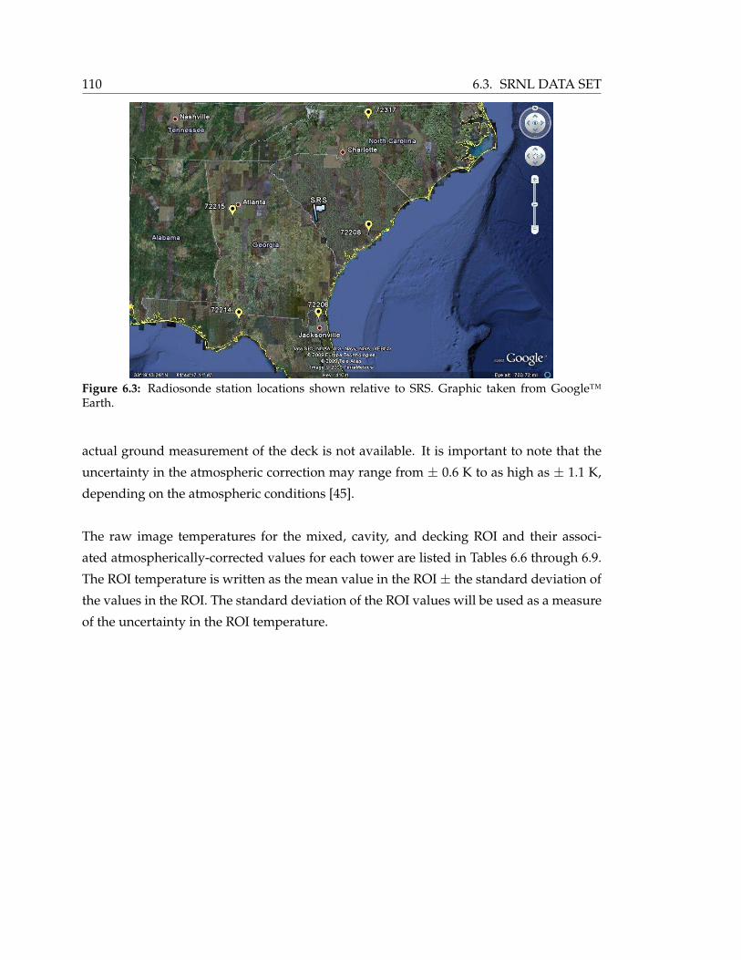
110 6.3. SRNL DATA SET
Figure 6.3: Radiosonde station locations shown relative to SRS. Graphic taken from Google™Earth.
actual ground measurement of the deck is not available. It is important to note that the
uncertainty in the atmospheric correction may range from ± 0.6 K to as high as ± 1.1 K,
depending on the atmospheric conditions [45].
The raw image temperatures for the mixed, cavity, and decking ROI and their associ-
ated atmospherically-corrected values for each tower are listed in Tables 6.6 through 6.9.
The ROI temperature is written as the mean value in the ROI ± the standard deviation of
the values in the ROI. The standard deviation of the ROI values will be used as a measure
of the uncertainty in the ROI temperature.

6.3. SRNL DATA SET 111
Image ROI Temperature [K] Atm-Corrected ROI Temperature [K]ID Mixed Cavity Decking Mixed Cavity DeckingF1 294.96 ± 0.30 295.26 ± 0.25 293.23 ± 0.29 295.04 ± 0.33 295.38 ± 0.28 293.11 ± 0.32F2 293.89 ± 0.25 294.01 ± 0.22 292.62 ± 0.21 293.84 ± 0.28 293.98 ± 0.25 292.42 ± 0.23F3 294.55 ± 0.31 294.65 ± 0.27 292.66 ± 0.31 294.58 ± 0.35 294.69 ± 0.30 292.46 ± 0.34F4 295.33 ± 0.32 295.50 ± 0.29 292.99 ± 0.28 295.46 ± 0.36 295.65 ± 0.33 292.83 ± 0.32F5 295.14 ± 0.38 295.51 ± 0.25 293.12 ± 0.33 295.24 ± 0.42 295.66 ± 0.28 292.98 ± 0.36F6 292.03 ± 0.28 292.27 ± 0.18 291.46 ± 0.23 291.75 ± 0.31 292.02 ± 0.20 291.12 ± 0.26
Table 6.6: Original and the atmospherically-corrected image ROI temperatures for the SRNL20may04D14 image.
Image ROI Temperature [K] Atm-Corrected ROI Temperature [K]ID Mixed Cavity Decking Mixed Cavity DeckingF1 294.88 ± 0.22 294.99 ± 0.21 293.32 ± 0.34 294.99 ± 0.27 295.12 ± 0.26 293.11 ± 0.41F2 293.91 ± 0.22 294.03 ± 0.16 292.79 ± 0.22 293.82 ± 0.27 293.97 ± 0.20 292.34 ± 0.27F3 294.53 ± 0.24 294.59 ± 0.20 292.68 ± 0.26 294.58 ± 0.29 294.65 ± 0.24 292.34 ± 0.32F4 295.13 ± 0.21 295.22 ± 0.21 293.03 ± 0.24 295.30 ± 0.26 295.41 ± 0.25 292.76 ± 0.33F5 295.13 ± 0.26 295.28 ± 0.18 293.18 ± 0.25 295.29 ± 0.31 295.48 ± 0.22 292.95 ± 0.31F6 292.34 ± 0.26 292.53 ± 0.16 291.86 ± 0.13 291.93 ± 0.32 292.16 ± 0.19 291.35 ± 0.16
Table 6.7: Original and the atmospherically-corrected image ROI temperatures for the SRNL20may04E02 image.
Image ROI Temperature [K] Atm-Corrected ROI Temperature [K]ID Mixed Cavity Decking Mixed Cavity DeckingF1 294.82 ± 0.14 294.83 ± 0.14 293.38 ± 0.23 295.07 ± 0.19 295.09 ± 0.18 293.18 ± 0.31F2 293.88 ± 0.12 293.81 ± 0.22 293.05 ± 0.13 293.84 ± 0.16 293.75 ± 0.28 292.74 ± 0.17F3 294.22 ± 0.17 294.24 ± 0.29 293.13 ± 0.20 294.28 ± 0.22 294.32 ± 0.38 292.84 ± 0.27F4 294.84 ± 0.14 294.63 ± 0.40 293.39 ± 0.27 295.11 ± 0.18 294.83 ± 0.53 293.19 ± 0.36F5 294.68 ± 0.14 294.70 ± 0.11 293.34 ± 0.26 294.89 ± 0.18 294.92 ± 0.14 293.13 ± 0.35F6 292.58 ± 0.19 292.65 ± 0.11 292.28 ± 0.13 292.13 ± 0.25 292.21 ± 0.15 291.72 ± 0.18
Table 6.8: Original and the atmospherically-corrected image ROI temperatures for the SRNL20may04E04 image.
Image ROI Temperature [K] Atm-Corrected ROI Temperature [K]ID Mixed Cavity Decking Mixed Cavity DeckingH1 297.56 ± 0.48 297.81 ± 0.27 293.88 ± 0.41 297.32 ± 0.53 298.00 ± 0.29 293.68 ± 0.46H2 297.70 ± 0.46 297.86 ± 0.21 293.86 ± 0.69 297.88 ± 0.50 298.06 ± 0.23 293.65 ± 0.76H3 294.59 ± 1.06 295.80 ± 0.49 292.37 ± 0.20 294.45 ± 1.17 295.79 ± 0.54 292.01 ± 0.22H4 297.45 ± 0.54 297.64 ± 0.29 293.70 ± 0.44 297.60 ± 0.60 297.81 ± 0.31 293.48 ± 0.49
Table 6.9: Original and the atmospherically-corrected image ROI temperatures for the SRNL20jun05G09 image.

112 6.3. SRNL DATA SET
6.3.3 Actual Temperature Errors
The actual temperature error between the image-derived temperature and the measured
ground-truth can now be re-calculated for the atmospherically compensated images. The
exit air temperature, Tex, of the towers is the desired temperature to be retrieved. The
temperature error is defined as the difference between the image mean ROI temperature
and the recorded exit air temperature. The uncertainty in the temperature error can be
calculated from uncertainties in the ROI temperature, the sensor measurement, the atmo-
spheric compensation, and the measured exit air temperature. The uncertainties in all
these factors are listed in Table 6.10.
Variable UncertaintyGround measurement ± 0.4 KROI temperature ± (ROI St. Dev.) KSensor measurement ± 0.66 KAtmospheric compensation ± 0.6 K - ± 1.1 K
Table 6.10: Temperature uncertainties in the measured ground, ROI, sensor, and atmospheric vari-ables
The square of the uncertainty in the temperature error can be found by summing the
squares of the uncertainties in the exit air measurements, the ROI temperatures, the atmo-
spheric compensation, and the sensor measurement assuming that each term is indepen-
dent. This can be written as
δT2error = δT2
ROI + δT2atm + δT2
sensor + δT2ex. (6.9)
This method of calculating the uncertainty in the temperature error is described in Ap-
pendix C.
The actual temperature errors and their associated uncertainties for each operating tower
in each image are listed in Tables 6.11 through 6.14. All of the uncertainties from Table 6.10
where taken into account. The operating towers are those in which water is flowing (i.e.,
water on, fans on or water on, fans off ).
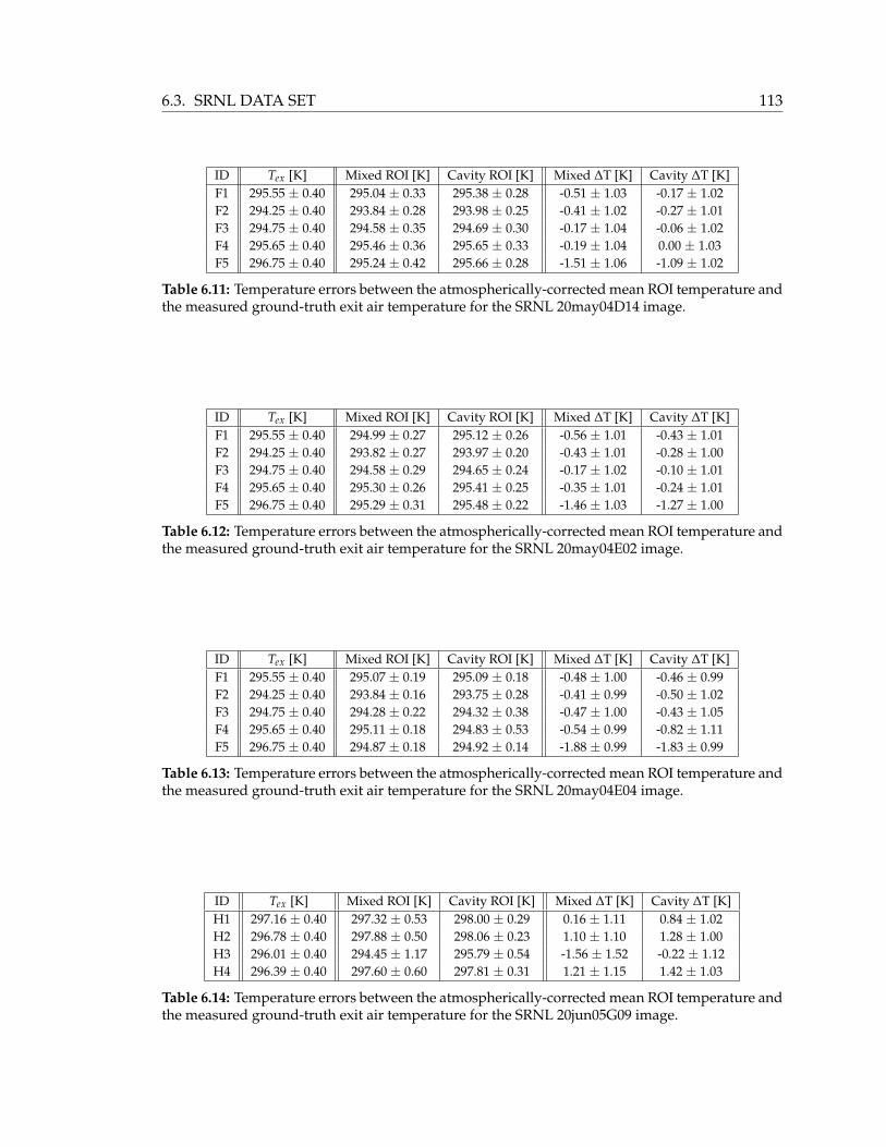
6.3. SRNL DATA SET 113
ID Tex [K] Mixed ROI [K] Cavity ROI [K] Mixed ∆T [K] Cavity ∆T [K]F1 295.55 ± 0.40 295.04 ± 0.33 295.38 ± 0.28 -0.51 ± 1.03 -0.17 ± 1.02F2 294.25 ± 0.40 293.84 ± 0.28 293.98 ± 0.25 -0.41 ± 1.02 -0.27 ± 1.01F3 294.75 ± 0.40 294.58 ± 0.35 294.69 ± 0.30 -0.17 ± 1.04 -0.06 ± 1.02F4 295.65 ± 0.40 295.46 ± 0.36 295.65 ± 0.33 -0.19 ± 1.04 0.00 ± 1.03F5 296.75 ± 0.40 295.24 ± 0.42 295.66 ± 0.28 -1.51 ± 1.06 -1.09 ± 1.02
Table 6.11: Temperature errors between the atmospherically-corrected mean ROI temperature andthe measured ground-truth exit air temperature for the SRNL 20may04D14 image.
ID Tex [K] Mixed ROI [K] Cavity ROI [K] Mixed ∆T [K] Cavity ∆T [K]F1 295.55 ± 0.40 294.99 ± 0.27 295.12 ± 0.26 -0.56 ± 1.01 -0.43 ± 1.01F2 294.25 ± 0.40 293.82 ± 0.27 293.97 ± 0.20 -0.43 ± 1.01 -0.28 ± 1.00F3 294.75 ± 0.40 294.58 ± 0.29 294.65 ± 0.24 -0.17 ± 1.02 -0.10 ± 1.01F4 295.65 ± 0.40 295.30 ± 0.26 295.41 ± 0.25 -0.35 ± 1.01 -0.24 ± 1.01F5 296.75 ± 0.40 295.29 ± 0.31 295.48 ± 0.22 -1.46 ± 1.03 -1.27 ± 1.00
Table 6.12: Temperature errors between the atmospherically-corrected mean ROI temperature andthe measured ground-truth exit air temperature for the SRNL 20may04E02 image.
ID Tex [K] Mixed ROI [K] Cavity ROI [K] Mixed ∆T [K] Cavity ∆T [K]F1 295.55 ± 0.40 295.07 ± 0.19 295.09 ± 0.18 -0.48 ± 1.00 -0.46 ± 0.99F2 294.25 ± 0.40 293.84 ± 0.16 293.75 ± 0.28 -0.41 ± 0.99 -0.50 ± 1.02F3 294.75 ± 0.40 294.28 ± 0.22 294.32 ± 0.38 -0.47 ± 1.00 -0.43 ± 1.05F4 295.65 ± 0.40 295.11 ± 0.18 294.83 ± 0.53 -0.54 ± 0.99 -0.82 ± 1.11F5 296.75 ± 0.40 294.87 ± 0.18 294.92 ± 0.14 -1.88 ± 0.99 -1.83 ± 0.99
Table 6.13: Temperature errors between the atmospherically-corrected mean ROI temperature andthe measured ground-truth exit air temperature for the SRNL 20may04E04 image.
ID Tex [K] Mixed ROI [K] Cavity ROI [K] Mixed ∆T [K] Cavity ∆T [K]H1 297.16 ± 0.40 297.32 ± 0.53 298.00 ± 0.29 0.16 ± 1.11 0.84 ± 1.02H2 296.78 ± 0.40 297.88 ± 0.50 298.06 ± 0.23 1.10 ± 1.10 1.28 ± 1.00H3 296.01 ± 0.40 294.45 ± 1.17 295.79 ± 0.54 -1.56 ± 1.52 -0.22 ± 1.12H4 296.39 ± 0.40 297.60 ± 0.60 297.81 ± 0.31 1.21 ± 1.15 1.42 ± 1.03
Table 6.14: Temperature errors between the atmospherically-corrected mean ROI temperature andthe measured ground-truth exit air temperature for the SRNL 20jun05G09 image.

114 6.3. SRNL DATA SET
6.3.4 Predicted Temperature Errors
The SRNL data will serve as a test of the methodology developed in Chapter 5. The
physics model data presented in Section 6.1 must be processed using the SC 2000 sensor
model with the appropriate GSD. A LUT is generated for GSD values of 0.22 m, 0.43 m,
0.85 m, and 0.15 m which correspond to the 20may04D14, 20may04E02, 20may04E04, and
20jun05G09 images, respectively. Next, a multiple linear regression model for the mixed
ROI case and one for the cavity-only ROI case were fit to each LUT. The associated RMS
error was calculated for each regression model.
Now that a parameterized regression equation has been found, the values of the predictor
variables must be estimated. Recall from Section 6.2 that the seven predictor parameters
are the MDCT external temperature (x1), the fan blade emissivity (x2), the effective sky temper-
ature (x3), the sensor zenith angle (x4), the ambient air temperature (x5), the ambient dew point
temperature (x6), and the plume path length (x7). The response variable y1 is the predicted
temperature error for the mixed ROI case. The response variable y2 is the predicted tem-
perature error for the cavity-only ROI case.
Each predictor parameter value and uncertainty must be estimated:
MDCT external temperature (x1) is the temperature of the decking. The deck ROI tem-
perature from Tables 6.6 through 6.9 will be used as the estimate of this predictor. The
deck ROI temperature does not take into account emissivity effects. If an emissivity of
0.95 is assumed for the decking material then the actual temperature of the deck would
be roughly 3 K higher than the deck ROI temperature. Therefore, the uncertainty in this
predictor estimate will be set to ± 3 K. (If the emissivity was underestimated as 0.90, then
the uncertainty would increase to ± 7 K.)
Fan blade emissivity (x2) is estimated to be 0.90. This value is based on the observation
that most materials in the LWIR have relatively high emissivities. The uncertainty is set
as ± 0.04 which is intended to cover the expected conditions of the fan blade material.
Effective sky temperature (x3) can be computed from the interpolated atmospheric profile
from Section 6.3.2. The DIRSIG make adb utility calculates the total hemispherical spec-
tral downwelling radiance from the profile data (Appendix D). This radiance is then in-
tegrated with the SC 2000 spectral response and converted into an apparent temperature.
6.3. SRNL DATA SET 115
The uncertainty in the sky temperature is taken as the approximate difference between
the interpolated profile sky temperature and the MODTRAN standard tropical profile
sky temperature (276 K). The uncertainty is ± 9 K for the nadir images and ± 12 K for the
oblique image.
Sensor zenith angle (x4) is estimated from the image. The apparent diameter of the fan
stack opening in the horizontal and vertical image directions are compared and an ap-
proximate view angle is computed by
θzenith = cos−1(
Dv
Dh
), (6.10)
where Dv and Dh are the diameter of the fan stack opening in the vertical and horizontal
image directions, respectively, in terms of the number of pixels. The uncertainty in this
measurement is found by adding and subtracting one pixel from the vertical and horizon-
tal diameters and recalculating the angle. Half of the range bounded by these two angles
is taken as the uncertainty. For example, for the D14 image, the vertical and horizontal
diameters were found to be 22 and 22 pixels, respectively. One pixel is subtracted from
the vertical diameter and one pixel is added to the horizontal diameter to yield 21 and
23, respectively. This yields an angle of 24°. The estimated view angle is then taken as
0° ± 12°. The estimated angles and the uncertainties for each image are listed in Table
6.15.
Image 20may04D14 20may04E02 20may04E04 20jun05G09Angle 0°± 12° 0°± 17° 0°± 22° 29°± 6°
Table 6.15: Estimates of the sensor view zenith angle along with uncertainties. The angles wereestimated by measuring the vertical and horizontal pixel diameters of the fan stack opening ofeach image.
Ambient air temperature (x5) is an actual measured ground value. The uncertainty is± 0.4 K
for the HOBO temperature sensor measurement error.
Ambient dew point temperature (x6) is an actual measured ground value. The uncertainty is
approximately ± 2 K for the HOBO temperature sensor measurement error.
Plume path length (x7) is estimated via the utility in Appendix E. The utility takes into
account the environmental information from the scene and the sensor geometry to cal-
culate an approximate path length through the plume. The calculations are based on a
116 6.3. SRNL DATA SET
Gaussian plume model. The uncertainty in the plume path length is between 1 m and 5 m
for the conditions found in the SRNL data set.
Once estimates of the predictor parameters are set, the predicted temperature error for the
mixed and cavity ROIs can be calculated from the regression equations. The uncertainty
in the predicted temperature is found from the uncertainties of each predictor parameter
using the methods in Appendix C. The uncertainty was calculated by equation (C.5) and
the result was verified empirically using a set of 100,000 trials to numerically determine
the uncertainty (see Section C.2). Note that the RMS error of the regression equation is
included in the uncertainty in the predicted temperature. The regression RMS error is a
measure of the fit of the regression model to the LUT data.
The data tables in the following pages present the regression equations for the mixed
and cavity ROI and the estimates and uncertainties for each parameter value used in the
regression. The resulting predicted temperature errors are compared to the actual tem-
perature errors presented in the previous section. Finally, a plot is shown of the actual
and predicted temperature errors along with the associated uncertainties for each tower.

6.3. SRNL DATA SET 117
SRNL 20may04D14 image02:02 EDT 20 May 2004 at 500 ft (152.5 m) with a GSD of 0.22 m.
(Parameterized Model Prediction)
Mixed ROI: (RMS error = 0.79 K)
y1 = −17.5651− 0.0340 x1 + 10.7236 x2 + 0.0350 x3 − 0.0083 x4 + 0.0223 x5 + 0.0016 x6 + 0.0021 x7
Cavity ROI: (RMS error = 0.36 K)
y2 = −6.3753− 0.0268 x1 + 4.0693 x2 + 0.0136 x3 − 0.0054 x4 + 0.0220 x5 − 0.0006 x6 − 0.0004 x7
ID x1 [K] x2 [ ] x3 [K] x4 [°] x5 [K] x6 [K] x7 [m]F1 293.11 ± 3.00 0.90 ± 0.04 267 ± 9 0 ± 12 292.87 ± 0.40 291.06 ± 2.00 3 ± 1F2 292.42 ± 3.00 0.90 ± 0.04 267 ± 9 0 ± 12 292.87 ± 0.40 291.06 ± 2.00 15 ± 5F3 292.46 ± 3.00 0.90 ± 0.04 267 ± 9 0 ± 12 292.87 ± 0.40 291.06 ± 2.00 20 ± 5F4 292.83 ± 3.00 0.90 ± 0.04 267 ± 9 0 ± 12 292.87 ± 0.40 291.06 ± 2.00 3 ± 1F5 292.98 ± 3.00 0.90 ± 0.04 267 ± 9 0 ± 12 292.87 ± 0.40 291.06 ± 2.00 3 ± 1
Table 6.16: Predictor estimates used in the 20may04D14 parameterized regression model.
Mixed ROI Cavity ROIID Image ∆T [K] Predicted ∆T [K] Image ∆T [K] Predicted ∆T [K]F1 -0.51 ± 1.03 -1.52 ± 0.96 -0.17 ± 1.02 -0.66 ± 0.42F2 -0.41 ± 1.02 -1.47 ± 0.96 -0.27 ± 1.01 -0.65 ± 0.42F3 -0.17 ± 1.04 -1.46 ± 0.96 -0.06 ± 1.02 -0.65 ± 0.42F4 -0.19 ± 1.04 -1.51 ± 0.96 0.00 ± 1.03 -0.66 ± 0.42F5 -1.51 ± 1.06 -1.51 ± 0.96 -1.09 ± 1.02 -0.66 ± 0.42
Table 6.17: Comparison of the actual and predicted temperature errors for the 20may04D14 image.ROI, atmosphere, and sensor uncertainty is included.
(a) Mixed ROI (b) Cavity ROI
Figure 6.4: The actual and the predicted temperature error with uncertainty ranges for the20may04D14 image. ROI, atmosphere, and sensor uncertainty is included in the error bars.
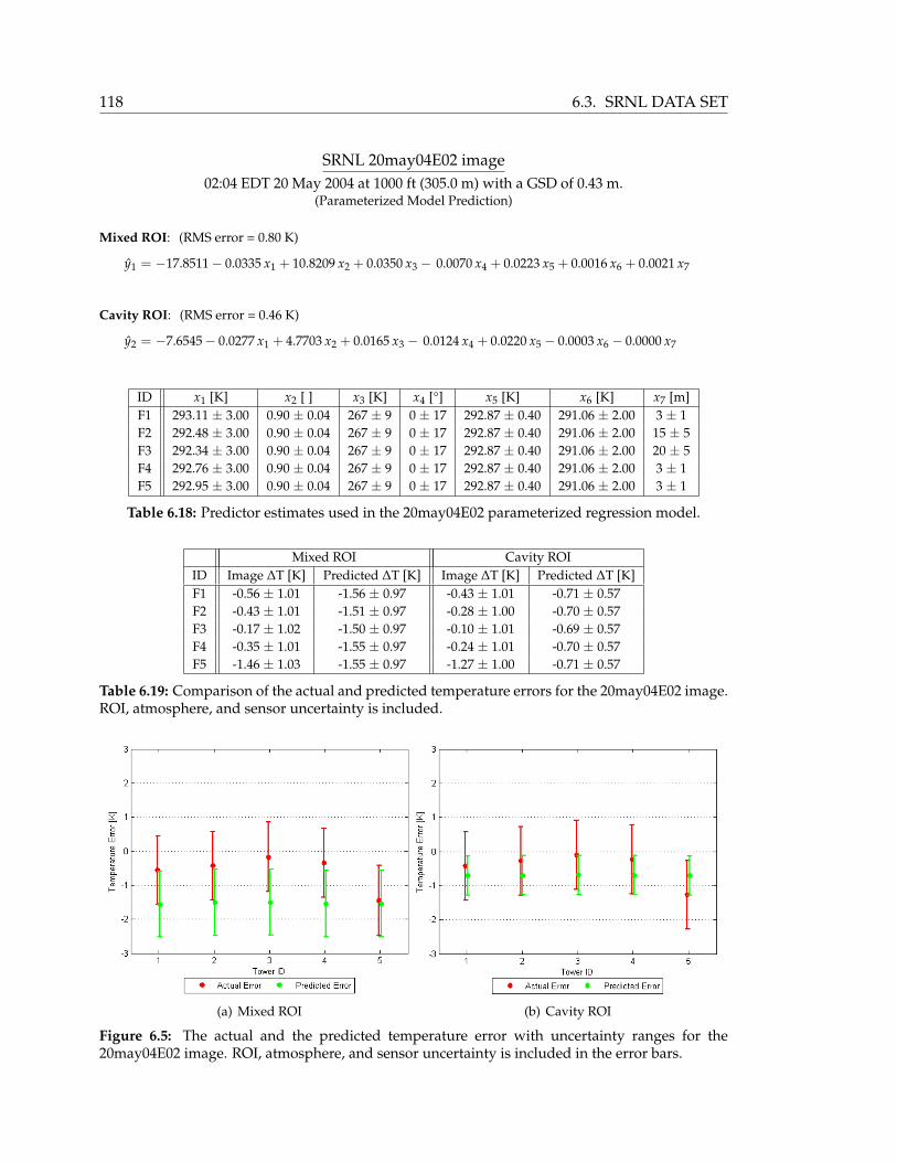
118 6.3. SRNL DATA SET
SRNL 20may04E02 image02:04 EDT 20 May 2004 at 1000 ft (305.0 m) with a GSD of 0.43 m.
(Parameterized Model Prediction)
Mixed ROI: (RMS error = 0.80 K)
y1 = −17.8511− 0.0335 x1 + 10.8209 x2 + 0.0350 x3 − 0.0070 x4 + 0.0223 x5 + 0.0016 x6 + 0.0021 x7
Cavity ROI: (RMS error = 0.46 K)
y2 = −7.6545− 0.0277 x1 + 4.7703 x2 + 0.0165 x3 − 0.0124 x4 + 0.0220 x5 − 0.0003 x6 − 0.0000 x7
ID x1 [K] x2 [ ] x3 [K] x4 [°] x5 [K] x6 [K] x7 [m]F1 293.11 ± 3.00 0.90 ± 0.04 267 ± 9 0 ± 17 292.87 ± 0.40 291.06 ± 2.00 3 ± 1F2 292.48 ± 3.00 0.90 ± 0.04 267 ± 9 0 ± 17 292.87 ± 0.40 291.06 ± 2.00 15 ± 5F3 292.34 ± 3.00 0.90 ± 0.04 267 ± 9 0 ± 17 292.87 ± 0.40 291.06 ± 2.00 20 ± 5F4 292.76 ± 3.00 0.90 ± 0.04 267 ± 9 0 ± 17 292.87 ± 0.40 291.06 ± 2.00 3 ± 1F5 292.95 ± 3.00 0.90 ± 0.04 267 ± 9 0 ± 17 292.87 ± 0.40 291.06 ± 2.00 3 ± 1
Table 6.18: Predictor estimates used in the 20may04E02 parameterized regression model.
Mixed ROI Cavity ROIID Image ∆T [K] Predicted ∆T [K] Image ∆T [K] Predicted ∆T [K]F1 -0.56 ± 1.01 -1.56 ± 0.97 -0.43 ± 1.01 -0.71 ± 0.57F2 -0.43 ± 1.01 -1.51 ± 0.97 -0.28 ± 1.00 -0.70 ± 0.57F3 -0.17 ± 1.02 -1.50 ± 0.97 -0.10 ± 1.01 -0.69 ± 0.57F4 -0.35 ± 1.01 -1.55 ± 0.97 -0.24 ± 1.01 -0.70 ± 0.57F5 -1.46 ± 1.03 -1.55 ± 0.97 -1.27 ± 1.00 -0.71 ± 0.57
Table 6.19: Comparison of the actual and predicted temperature errors for the 20may04E02 image.ROI, atmosphere, and sensor uncertainty is included.
(a) Mixed ROI (b) Cavity ROI
Figure 6.5: The actual and the predicted temperature error with uncertainty ranges for the20may04E02 image. ROI, atmosphere, and sensor uncertainty is included in the error bars.
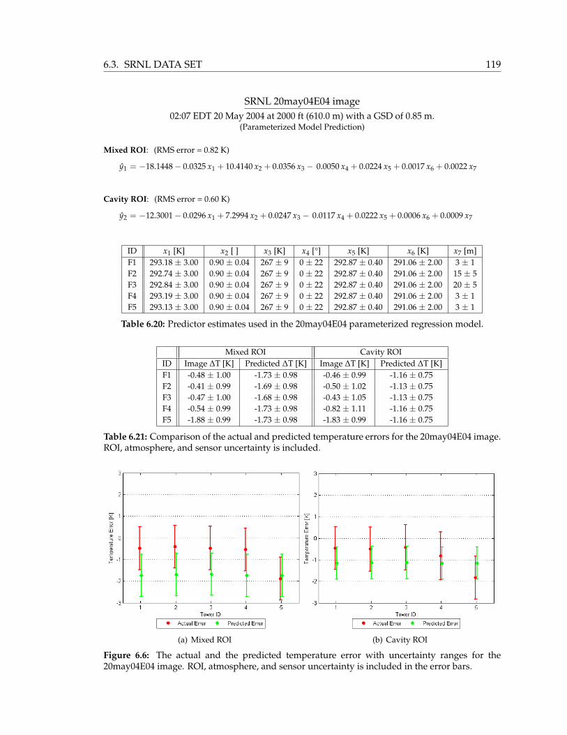
6.3. SRNL DATA SET 119
SRNL 20may04E04 image02:07 EDT 20 May 2004 at 2000 ft (610.0 m) with a GSD of 0.85 m.
(Parameterized Model Prediction)
Mixed ROI: (RMS error = 0.82 K)
y1 = −18.1448− 0.0325 x1 + 10.4140 x2 + 0.0356 x3 − 0.0050 x4 + 0.0224 x5 + 0.0017 x6 + 0.0022 x7
Cavity ROI: (RMS error = 0.60 K)
y2 = −12.3001− 0.0296 x1 + 7.2994 x2 + 0.0247 x3 − 0.0117 x4 + 0.0222 x5 + 0.0006 x6 + 0.0009 x7
ID x1 [K] x2 [ ] x3 [K] x4 [°] x5 [K] x6 [K] x7 [m]F1 293.18 ± 3.00 0.90 ± 0.04 267 ± 9 0 ± 22 292.87 ± 0.40 291.06 ± 2.00 3 ± 1F2 292.74 ± 3.00 0.90 ± 0.04 267 ± 9 0 ± 22 292.87 ± 0.40 291.06 ± 2.00 15 ± 5F3 292.84 ± 3.00 0.90 ± 0.04 267 ± 9 0 ± 22 292.87 ± 0.40 291.06 ± 2.00 20 ± 5F4 293.19 ± 3.00 0.90 ± 0.04 267 ± 9 0 ± 22 292.87 ± 0.40 291.06 ± 2.00 3 ± 1F5 293.13 ± 3.00 0.90 ± 0.04 267 ± 9 0 ± 22 292.87 ± 0.40 291.06 ± 2.00 3 ± 1
Table 6.20: Predictor estimates used in the 20may04E04 parameterized regression model.
Mixed ROI Cavity ROIID Image ∆T [K] Predicted ∆T [K] Image ∆T [K] Predicted ∆T [K]F1 -0.48 ± 1.00 -1.73 ± 0.98 -0.46 ± 0.99 -1.16 ± 0.75F2 -0.41 ± 0.99 -1.69 ± 0.98 -0.50 ± 1.02 -1.13 ± 0.75F3 -0.47 ± 1.00 -1.68 ± 0.98 -0.43 ± 1.05 -1.13 ± 0.75F4 -0.54 ± 0.99 -1.73 ± 0.98 -0.82 ± 1.11 -1.16 ± 0.75F5 -1.88 ± 0.99 -1.73 ± 0.98 -1.83 ± 0.99 -1.16 ± 0.75
Table 6.21: Comparison of the actual and predicted temperature errors for the 20may04E04 image.ROI, atmosphere, and sensor uncertainty is included.
(a) Mixed ROI (b) Cavity ROI
Figure 6.6: The actual and the predicted temperature error with uncertainty ranges for the20may04E04 image. ROI, atmosphere, and sensor uncertainty is included in the error bars.

120 6.3. SRNL DATA SET
SRNL 20jun05G09 image22:17 EDT, 20 June 2005 at 350 ft (106.7 m) with a GSD of 0.15 m.
(Parameterized Model Prediction)
Mixed ROI: (RMS error = 0.78 K)
y1 = −17.5961− 0.0340 x1 + 10.7930 x2 + 0.0349 x3 − 0.0075 x4 + 0.0223 x5 + 0.0016 x6 + 0.0021 x7
Cavity ROI: (RMS error = 0.35 K)
y2 = −6.3769− 0.0273 x1 + 4.1551 x2 + 0.0138 x3 − 0.0049 x4 + 0.0220 x5 − 0.0006 x6 − 0.0003 x7
ID x1 [K] x2 [ ] x3 [K] x4 [°] x5 [K] x6 [K] x7 [m]H1 293.68 ± 3.00 0.90 ± 0.04 264 ± 12 29 ± 6 296.39 ± 0.40 293.17 ± 2.00 8 ± 3H2 293.65 ± 3.00 0.90 ± 0.04 264 ± 12 29 ± 6 296.39 ± 0.40 293.17 ± 2.00 8 ± 3H3 292.01 ± 3.00 0.90 ± 0.04 264 ± 12 29 ± 6 296.39 ± 0.40 293.17 ± 2.00 4 ± 1H4 293.48 ± 3.00 0.90 ± 0.04 264 ± 12 29 ± 6 296.39 ± 0.40 293.17 ± 2.00 8 ± 3
Table 6.22: Predictor estimates used in the 20jun05G09 parameterized regression model.
Mixed ROI Cavity ROIID Image ∆T [K] Predicted ∆T [K] Image ∆T [K] Predicted ∆T [K]H1 0.16 ± 1.11 -1.76 ± 1.00 0.84 ± 1.02 -0.79 ± 0.43H2 1.10 ± 1.10 -1.76 ± 1.00 1.28 ± 1.00 -0.79 ± 0.43H3 -1.56 ± 1.52 -1.71 ± 1.00 -0.22 ± 1.12 -0.75 ± 0.43H4 1.21 ± 1.15 -1.76 ± 1.00 1.42 ± 1.03 -0.79 ± 0.43
Table 6.23: Comparison of the actual and predicted temperature errors for the 20jun05G09 image.ROI, atmosphere, and sensor uncertainty is included.
(a) Mixed ROI (b) Cavity ROI
Figure 6.7: The actual and the predicted temperature error with uncertainty ranges for the20jun05G09 image. ROI, atmosphere, and sensor uncertainty is included in the error bars.
6.3. SRNL DATA SET 121
The comparison of the actual temperature error and the predicted temperature error is
presented in Figures 6.4 to 6.7. Several statements can be made about the data.
In general, the predicted errors are less than zero for both the mixed and cavity ROIs.
The magnitude of the predicted errors are greater than the magnitude of the actual errors
for the nadir images (20may04D14, 20may04E02, 20may04E04). The uncertainty ranges
overlap for the mixed and cavity ROIs for all the nadir images. Compared to the actual er-
rors, the predicted temperature errors were within± 1.3 K for the mixed ROIs and within
± 0.7 K for the cavity ROIs.
For the oblique image (20jun05G09), the actual errors vary more from tower to tower
than in the nadir images. The uncertainty ranges overlap for two of the four towers for
the mixed ROI and overlap for only one tower for the cavity ROI. The predicted temper-
ature errors differed from the actual errors by as much as ± 3 K for the mixed and cavity
ROIs. However, the predicted temperature error was within ± 0.5 K for the H3 tower for
both ROIs.
These results can be attributed to several factors. First, the the SRNL data set issues dis-
cussed in Section 6.3.1 will influence the actual temperature errors. Although uncertain-
ties were assigned to the ground measurements based on expected errors in the tempera-
ture sensors, this does not take into account the prospect that the recorded measurement
was not the actual measurement desired. The exit air temperature measurement, for ex-
ample, may not have been the true exit air temperature since the measurement could have
been altered by the ambient conditions. The uncertainties are due to the physical process
of temperature measurement and are not due to statistical sampling of the temperature.
In addition, estimates were made for the uncertainty in the atmospheric compensation
and in the sensor measurement. Ideally, these uncertainties would have been understood
in detail.
These results may also be attributed to the modeling process. Imperfect information was
used in parameterized model. The exact MDCT external temperature had to be estimated
from the images. The value for the fan blade emissivity was estimated based on similar,
but not exact, materials. The effective sky temperature was estimated from the interpolated
atmospheric profile used to atmospherically correct the images. The sensor view angle was
estimated from the images. Actual sensor orientation data could be used in practice to
obtain the value for the view angle. The ambient air temperature and ambient dew point
122 6.3. SRNL DATA SET
temperature measurements were subject to the uncertainties described previously. Finally,
the plume path length was roughly estimated using a Gaussian plume model. This model
yields a time-averaged estimate of the plume path length and is not sensitive to instan-
taneous changes in the environment around the MDCT. The regression model fit to each
sensor LUT was also not a perfect fit to the data. The RMS errors for the regression fits
indicated that the parameterized model itself may introduce errors of up to 0.82 K and
0.60 K for the mixed and cavity ROIs, respectively.
Although this demonstration produced mixed results, it did work very well for the nadir
images which lends confidence in the use of this methodology and parameterized model
for real data sets. The connection between the performance of the parameterized model
and the properties of the MDCT units is arbitrary, however. As an example, for the nadir
images the parameterized model for the F5 tower performed the best for the mixed ROI.
There is nothing unique about this tower. Recall from Section 2.3 that the F1, F4, and F5
units were operating as water on, fans off while the F2 and F3 units were water on, fans on.
The fan status does not appear to be an indication of model performance since there was
no correlation between fan status and model performance for the other units. Similarly
for the oblique image, the parameterized model performed the best for the H3 tower. This
unit was also operating in the water on, fans off model while the other units were operat-
ing in the water on, fans on mode. In this particular case, it appears that the parameterized
model was more accurate for the fans off unit than for the fans on unit. However, no con-
clusion can be drawn from this observation since it is not consistent with the nadir images.
The poorer performance of the parameterized model predictions for the oblique image
might be due to several factors that were not accounted for in the physics model. The
oblique viewing geometry means that the emissivity will be different from the nadir
viewing geometry due to directional emissivity effects. For external pixels this means
that these facets will have a higher reflectance thereby increasing the amount of reflected
background radiance. Although the directional emissivity is accounted for in the physics
model, the temperature error might be more sensitive to background radiances. The sky
was modeled as a uniform radiator. In reality, the skydome radiance will be a function of
zenith and azimuth angle depending on the weather conditions. These factors combine
to have an increased effect on the sensor-reaching radiance in the oblique case than in the
nadir case. Given the physical processes discussed and investigated in Chapters 3 and 5
(i.e., emissivity, atmospheric tranmission and path radiance, etc.), the actual temperature
errors should be less than zero given the atmospheric information provided. The actual
6.3. SRNL DATA SET 123
errors for the oblique image are greater than zero for three of the towers. This suggests
that there were errors in the ground-truth measurements or that the physics model did
not account for a physical attribute in the scene. For example, an assumption is made
that the internal surfaces of the MDCT are the same temperature as the exit air. If this is
not true, the measured exit air temperature would be lower than the internal temperature
given that the ambient temperature was also less than the internal temperature. In addi-
tion, the increased temperature of the gear box associated with the fan mechanical system
was not modeled. The high temperature of the gear box for the fans on towers might have
contributed to the higher apparent temperatures for those towers.
6.3.5 Comparison of Atmospheric Uncertainties
The data presented in Section 6.3.4 included uncertainty ranges that incorporated the sus-
pected errors due to the ROI measurement, the atmospheric compensation, and the sen-
sor measurement along with the uncertainty in the ground measurement (Table 6.10). The
total uncertainty for the temperature error was found through equation (6.9). The uncer-
tainties in the ROI temperature and the sensor measurement is fixed for a given sensor.
The atmospheric compensation error, however, is dependent on how well atmospheric
effects can be removed. This is dependent on knowledge of the atmospheric state. The
atmospheric uncertainty was set to ± 0.6 K in Figures 6.4 - 6.7 but this uncertainty in the
atmospheric compensation may vary considerable. To demonstrate the effect of this un-
certainty, the atmospheric uncertainty was varied between ± 0.1 K, ± 1.1 K, and ± 2.2. K
and the corresponding total uncertainty in the image temperature error was calculated for
each image. The results are shown in Figures 6.8 - 6.11.
The plots demonstrate the influence of the atmospheric uncertainty on the overall process.
As expected, the overall uncertainty increases as the atmospheric uncertainty increases.
The overall uncertainty ranges between ± 1.0 K to ± 2.5 K over the atmospheric uncer-
tainty range of ± 0.1 K to ± 2.2 K. This study demonstrates the importance of accurate
atmospheric compensation.

124 6.3. SRNL DATA SET
SRNL 20may04D14 image
(a) Atmospheric Uncertainty = 0.1 K (Mixed) (b) Atmospheric Uncertainty = 0.1 K (Cavity)
(c) Atmospheric Uncertainty = 1.1 K (Mixed) (d) Atmospheric Uncertainty = 1.1 K (Cavity)
(e) Atmospheric Uncertainty = 2.2 K (Mixed) (f) Atmospheric Uncertainty = 2.2 K (Cavity)
Figure 6.8: The actual and the predicted temperature error with uncertainty ranges for the20may04D14 image. The uncertainty ranges are for an atmospheric uncertainty of 0.1 K (top),1.1 K (middle), and 2.2 K (bottom).

6.3. SRNL DATA SET 125
SRNL 20may04E02 image
(a) Atmospheric Uncertainty = 0.1 K (Mixed) (b) Atmospheric Uncertainty = 0.1 K (Cavity)
(c) Atmospheric Uncertainty = 1.1 K (Mixed) (d) Atmospheric Uncertainty = 1.1 K (Cavity)
(e) Atmospheric Uncertainty = 2.2 K (Mixed) (f) Atmospheric Uncertainty = 2.2 K (Cavity)
Figure 6.9: The actual and the predicted temperature error with uncertainty ranges for the20may04E02 image. The uncertainty ranges are for an atmospheric uncertainty of 0.1 K (top),1.1 K (middle), and 2.2 K (bottom).
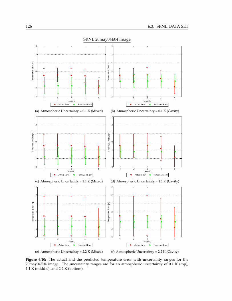
126 6.3. SRNL DATA SET
SRNL 20may04E04 image
(a) Atmospheric Uncertainty = 0.1 K (Mixed) (b) Atmospheric Uncertainty = 0.1 K (Cavity)
(c) Atmospheric Uncertainty = 1.1 K (Mixed) (d) Atmospheric Uncertainty = 1.1 K (Cavity)
(e) Atmospheric Uncertainty = 2.2 K (Mixed) (f) Atmospheric Uncertainty = 2.2 K (Cavity)
Figure 6.10: The actual and the predicted temperature error with uncertainty ranges for the20may04E04 image. The uncertainty ranges are for an atmospheric uncertainty of 0.1 K (top),1.1 K (middle), and 2.2 K (bottom).
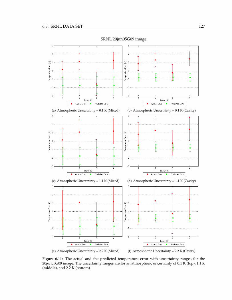
6.3. SRNL DATA SET 127
SRNL 20jun05G09 image
(a) Atmospheric Uncertainty = 0.1 K (Mixed) (b) Atmospheric Uncertainty = 0.1 K (Cavity)
(c) Atmospheric Uncertainty = 1.1 K (Mixed) (d) Atmospheric Uncertainty = 1.1 K (Cavity)
(e) Atmospheric Uncertainty = 2.2 K (Mixed) (f) Atmospheric Uncertainty = 2.2 K (Cavity)
Figure 6.11: The actual and the predicted temperature error with uncertainty ranges for the20jun05G09 image. The uncertainty ranges are for an atmospheric uncertainty of 0.1 K (top), 1.1 K(middle), and 2.2 K (bottom).

128 6.3. SRNL DATA SET
6.3.6 Comparison of Sensor Spectral Response
The sensor model used to generate the target space LUT for the SRNL data set required
the spectral response function of the SC 2000 Inframetrics sensor. Recall from Section 6.3.1
that since the exact spectral response was not known, it was approximated by using a flat,
unit response between 7.6 and 13.5 µm and zero otherwise.
To investigate the influence of the sensor spectral response function on the predicted tem-
perature error, a realistic spectral response was used in the sensor model to compare the
predicted temperature errors to the errors predicted using the flat response. The Long-
wave Infrared Camera (LIR) described by Taguchi et al. (2007) [46] is a microbolometer
array with a LWIR filter to get the desired spectral range of 8 - 12 µm. The design of this
sensor is similar to the SC 2000 sensor. Therefore, the spectral response curve of the LIR
was modified so that the full spectral width at half its maximum value fell between 7.6 and
13.5 µm while maintaining the same spectral shape. A comparison of this microbolometer
spectral response and the flat spectral response is shown in Figure 6.12.
The microbolometer response function is then used in the sensor model in the genera-
tion of the LUT of each image. A regression model is fit to the LUT and the predicted
temperature errors are compared to the actual temperature errors. The results are shown
in Figures 6.13 through 6.16.
(a) Ideal, flat, unit spectral response (b) Realistic microbolometer spectral response
Figure 6.12: Comparison of an ideal, flat, unit spectral response and a realistic microbolometerspectral response in the longwave infrared region.
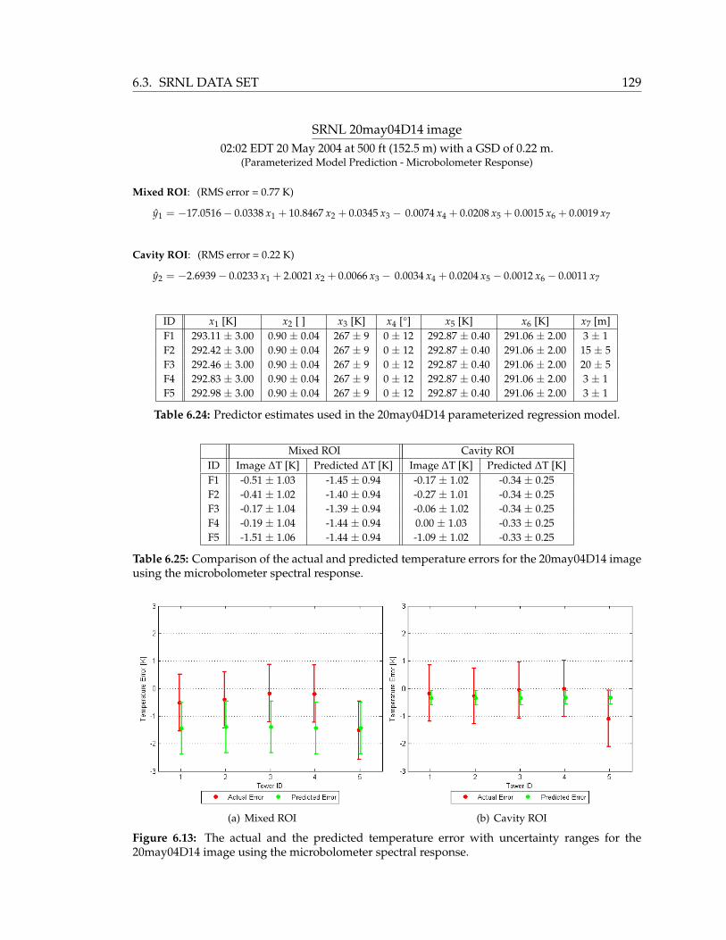
6.3. SRNL DATA SET 129
SRNL 20may04D14 image02:02 EDT 20 May 2004 at 500 ft (152.5 m) with a GSD of 0.22 m.
(Parameterized Model Prediction - Microbolometer Response)
Mixed ROI: (RMS error = 0.77 K)
y1 = −17.0516− 0.0338 x1 + 10.8467 x2 + 0.0345 x3 − 0.0074 x4 + 0.0208 x5 + 0.0015 x6 + 0.0019 x7
Cavity ROI: (RMS error = 0.22 K)
y2 = −2.6939− 0.0233 x1 + 2.0021 x2 + 0.0066 x3 − 0.0034 x4 + 0.0204 x5 − 0.0012 x6 − 0.0011 x7
ID x1 [K] x2 [ ] x3 [K] x4 [°] x5 [K] x6 [K] x7 [m]F1 293.11 ± 3.00 0.90 ± 0.04 267 ± 9 0 ± 12 292.87 ± 0.40 291.06 ± 2.00 3 ± 1F2 292.42 ± 3.00 0.90 ± 0.04 267 ± 9 0 ± 12 292.87 ± 0.40 291.06 ± 2.00 15 ± 5F3 292.46 ± 3.00 0.90 ± 0.04 267 ± 9 0 ± 12 292.87 ± 0.40 291.06 ± 2.00 20 ± 5F4 292.83 ± 3.00 0.90 ± 0.04 267 ± 9 0 ± 12 292.87 ± 0.40 291.06 ± 2.00 3 ± 1F5 292.98 ± 3.00 0.90 ± 0.04 267 ± 9 0 ± 12 292.87 ± 0.40 291.06 ± 2.00 3 ± 1
Table 6.24: Predictor estimates used in the 20may04D14 parameterized regression model.
Mixed ROI Cavity ROIID Image ∆T [K] Predicted ∆T [K] Image ∆T [K] Predicted ∆T [K]F1 -0.51 ± 1.03 -1.45 ± 0.94 -0.17 ± 1.02 -0.34 ± 0.25F2 -0.41 ± 1.02 -1.40 ± 0.94 -0.27 ± 1.01 -0.34 ± 0.25F3 -0.17 ± 1.04 -1.39 ± 0.94 -0.06 ± 1.02 -0.34 ± 0.25F4 -0.19 ± 1.04 -1.44 ± 0.94 0.00 ± 1.03 -0.33 ± 0.25F5 -1.51 ± 1.06 -1.44 ± 0.94 -1.09 ± 1.02 -0.33 ± 0.25
Table 6.25: Comparison of the actual and predicted temperature errors for the 20may04D14 imageusing the microbolometer spectral response.
(a) Mixed ROI (b) Cavity ROI
Figure 6.13: The actual and the predicted temperature error with uncertainty ranges for the20may04D14 image using the microbolometer spectral response.

130 6.3. SRNL DATA SET
SRNL 20may04E02 image02:04 EDT 20 May 2004 at 1000 ft (305.0 m) with a GSD of 0.43 m.
(Parameterized Model Prediction - Microbolometer Response)
Mixed ROI: (RMS error = 0.77 K)
y1 = −17.3534− 0.0338 x1 + 10.8467 x2 + 0.0345 x3 − 0.0074 x4 + 0.0208 x5 + 0.0015 x6 + 0.0019 x7
Cavity ROI: (RMS error = 0.22 K)
y2 = −2.6939− 0.0233 x1 + 2.0021 x2 + 0.0066 x3 − 0.0034 x4 + 0.0204 x5 − 0.0012 x6 − 0.0011 x7
ID x1 [K] x2 [ ] x3 [K] x4 [°] x5 [K] x6 [K] x7 [m]F1 293.11 ± 3.00 0.90 ± 0.04 267 ± 9 0 ± 17 292.87 ± 0.40 291.06 ± 2.00 3 ± 1F2 292.48 ± 3.00 0.90 ± 0.04 267 ± 9 0 ± 17 292.87 ± 0.40 291.06 ± 2.00 15 ± 5F3 292.34 ± 3.00 0.90 ± 0.04 267 ± 9 0 ± 17 292.87 ± 0.40 291.06 ± 2.00 20 ± 5F4 292.76 ± 3.00 0.90 ± 0.04 267 ± 9 0 ± 17 292.87 ± 0.40 291.06 ± 2.00 3 ± 1F5 292.95 ± 3.00 0.90 ± 0.04 267 ± 9 0 ± 17 292.87 ± 0.40 291.06 ± 2.00 3 ± 1
Table 6.26: Predictor estimates used in the 20may04E02 parameterized regression model.
Mixed ROI Cavity ROIID Image ∆T [K] Predicted ∆T [K] Image ∆T [K] Predicted ∆T [K]F1 -0.56 ± 1.01 -1.51 ± 0.96 -0.43 ± 1.01 -0.55 ± 0.49F2 -0.43 ± 1.01 -1.47 ± 0.96 -0.28 ± 1.00 -0.53 ± 0.49F3 -0.17 ± 1.02 -1.46 ± 0.96 -0.10 ± 1.01 -0.53 ± 0.49F4 -0.35 ± 1.01 -1.50 ± 0.96 -0.24 ± 1.01 -0.54 ± 0.49F5 -1.46 ± 1.03 -1.51 ± 0.96 -1.27 ± 1.00 -0.54 ± 0.49
Table 6.27: Comparison of the actual and predicted temperature errors for the 20may04E02 imageusing the microbolometer spectral response.
(a) Mixed ROI (b) Cavity ROI
Figure 6.14: The actual and the predicted temperature error with uncertainty ranges for the20may04E02 image using the microbolometer spectral response.

6.3. SRNL DATA SET 131
SRNL 20may04E04 image02:07 EDT 20 May 2004 at 2000 ft (610.0 m) with a GSD of 0.85 m.
(Parameterized Model Prediction - Microbolometer Response)
Mixed ROI: (RMS error = 0.81 K)
y1 = −17.4717− 0.0327 x1 + 10.4363 x2 + 0.0352 x3 − 0.0048 x4 + 0.0208 x5 + 0.0016 x6 + 0.0020 x7
Cavity ROI: (RMS error = 0.56 K)
y2 = −11.3297− 0.0283 x1 + 6.9223 x2 + 0.0232 x3 − 0.0147 x4 + 0.0207 x5 + 0.0004 x6 + 0.0007 x7
ID x1 [K] x2 [ ] x3 [K] x4 [°] x5 [K] x6 [K] x7 [m]F1 293.18 ± 3.00 0.90 ± 0.04 267 ± 9 0 ± 22 292.87 ± 0.40 291.06 ± 2.00 3 ± 1F2 292.74 ± 3.00 0.90 ± 0.04 267 ± 9 0 ± 22 292.87 ± 0.40 291.06 ± 2.00 15 ± 5F3 292.84 ± 3.00 0.90 ± 0.04 267 ± 9 0 ± 22 292.87 ± 0.40 291.06 ± 2.00 20 ± 5F4 293.19 ± 3.00 0.90 ± 0.04 267 ± 9 0 ± 22 292.87 ± 0.40 291.06 ± 2.00 3 ± 1F5 293.13 ± 3.00 0.90 ± 0.04 267 ± 9 0 ± 22 292.87 ± 0.40 291.06 ± 2.00 3 ± 1
Table 6.28: Predictor estimates used in the 20may04E04 parameterized regression model.
Mixed ROI Cavity ROIID Image ∆T [K] Predicted ∆T [K] Image ∆T [K] Predicted ∆T [K]F1 -0.48 ± 1.00 -1.69 ± 0.97 -0.46 ± 0.99 -1.05 ± 0.74F2 -0.41 ± 0.99 -1.65 ± 0.97 -0.50 ± 1.02 -1.02 ± 0.74F3 -0.47 ± 1.00 -1.64 ± 0.97 -0.43 ± 1.05 -1.02 ± 0.74F4 -0.54 ± 0.99 -1.69 ± 0.97 -0.82 ± 1.11 -1.05 ± 0.74F5 -1.88 ± 0.99 -1.68 ± 0.97 -1.83 ± 0.99 -1.04 ± 0.74
Table 6.29: Comparison of the actual and predicted temperature errors for the 20may04E04 imageusing the microbolometer spectral response.
(a) Mixed ROI (b) Cavity ROI
Figure 6.15: The actual and the predicted temperature error with uncertainty ranges for the20may04E04 image using the microbolometer spectral response.
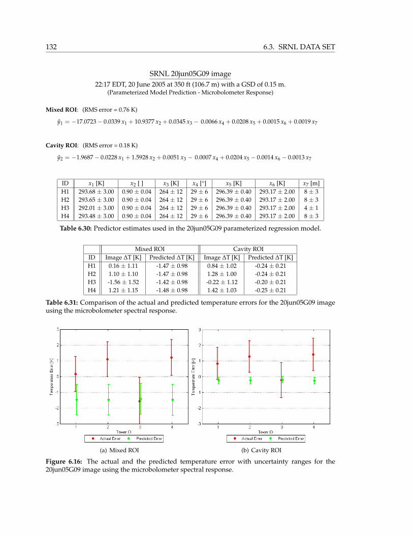
132 6.3. SRNL DATA SET
SRNL 20jun05G09 image22:17 EDT, 20 June 2005 at 350 ft (106.7 m) with a GSD of 0.15 m.
(Parameterized Model Prediction - Microbolometer Response)
Mixed ROI: (RMS error = 0.76 K)
y1 = −17.0723− 0.0339 x1 + 10.9377 x2 + 0.0345 x3 − 0.0066 x4 + 0.0208 x5 + 0.0015 x6 + 0.0019 x7
Cavity ROI: (RMS error = 0.18 K)
y2 = −1.9687− 0.0228 x1 + 1.5928 x2 + 0.0051 x3 − 0.0007 x4 + 0.0204 x5 − 0.0014 x6 − 0.0013 x7
ID x1 [K] x2 [ ] x3 [K] x4 [°] x5 [K] x6 [K] x7 [m]H1 293.68 ± 3.00 0.90 ± 0.04 264 ± 12 29 ± 6 296.39 ± 0.40 293.17 ± 2.00 8 ± 3H2 293.65 ± 3.00 0.90 ± 0.04 264 ± 12 29 ± 6 296.39 ± 0.40 293.17 ± 2.00 8 ± 3H3 292.01 ± 3.00 0.90 ± 0.04 264 ± 12 29 ± 6 296.39 ± 0.40 293.17 ± 2.00 4 ± 1H4 293.48 ± 3.00 0.90 ± 0.04 264 ± 12 29 ± 6 296.39 ± 0.40 293.17 ± 2.00 8 ± 3
Table 6.30: Predictor estimates used in the 20jun05G09 parameterized regression model.
Mixed ROI Cavity ROIID Image ∆T [K] Predicted ∆T [K] Image ∆T [K] Predicted ∆T [K]H1 0.16 ± 1.11 -1.47 ± 0.98 0.84 ± 1.02 -0.24 ± 0.21H2 1.10 ± 1.10 -1.47 ± 0.98 1.28 ± 1.00 -0.24 ± 0.21H3 -1.56 ± 1.52 -1.42 ± 0.98 -0.22 ± 1.12 -0.20 ± 0.21H4 1.21 ± 1.15 -1.48 ± 0.98 1.42 ± 1.03 -0.25 ± 0.21
Table 6.31: Comparison of the actual and predicted temperature errors for the 20jun05G09 imageusing the microbolometer spectral response.
(a) Mixed ROI (b) Cavity ROI
Figure 6.16: The actual and the predicted temperature error with uncertainty ranges for the20jun05G09 image using the microbolometer spectral response.

6.3. SRNL DATA SET 133
The data presented in Figures 6.13 through 6.16 indicate that the spectral response func-
tion of the sensor does have a noticeable impact on the predicted temperature errors. The
predicted errors are closer to the actual errors for both ROIs for the nadir images. The
cavity ROI case shows the largest improvement in the prediction model performance. For
the oblique image, the predicted errors moved slightly closer to the actual errors. There
is a slight improvement in performance in that the uncertainty ranges now overlap for
two of the four towers for the cavity ROI as opposed to just one of the towers for the flat
spectral response.
6.3.7 Validity of Parameterized Model
The validity of the parameterized model may be checked to determine if the multiple lin-
ear regression model is a good fit to the LUT data. The tests described in Section B.3 were
applied to the 20may04D14 data set with the flat spectral response and the mixed ROI to
determine if the parameterized model adequately fit the LUT data.
A plot of the standardized residuals versus the fitted responses (predicted temperature
errors) is shown in Figure 6.17(a). The data points in this plot should not display any
distinct pattern if the regression model was a good fit to the data. Instead, the data points
clearly resemble an overall parabolic pattern. This is a visual indication that the regres-
sion model is not a good fit to the LUT data.
(a) Residual Plot (b) Normal Probability Plot
Figure 6.17: Diagonistic plots indicating a lack-of-fit of the multiple linear regression model to the20may04D14 mixed ROI LUT data.

134 6.3. SRNL DATA SET
To get a quantitative understanding of possible lack-of-fit of the regression model, a nor-
mal probability plot of the standardized residuals was created (Figure 6.17(b)). The data
points should lie on a straight line if the regression model was a good fit to the data.
However, the data points exhibit curvature at extreme values. The Ryan-Joiner statistic
computed in Minitab yielded a value of 0.9970. The critical value for the Ryan-Joiner test
at α = 0.05 is greater than 0.9984 [47]. Since the test statistic is below the critical value, the
assumption of normality is invalid and therefore the regression model exhibits a lack-of-fit
to the LUT data [48].
6.3. SRNL DATA SET 135
6.3.8 Look-up Table Interpolation
The analysis in Section 6.3.7 indicated that the multiple linear regression model did not
adequately fit the LUT data. Although the parameterized model suffered from lack-of-fit,
the errors introduced by the model were taken into account when predicting the temper-
ature errors. The regression equations had an associated RMS error that described how
well the regression model fit the look-up table data and these errors were incorporated
into the uncertainties reported for the predicted temperature errors. In order to elim-
inated the error introduced by the regression, the predicted temperature error may be
determined from the look-up table data directly without the use of a regression model.
The predicted temperature error is selected from the LUT through a nearest neighbor
interpolation using all of the seven predictor parameters. The effectiveness of this LUT
search method depends on the sampling resolution of the LUT. A more densely populated
LUT should yield a better temperature error prediction.
For each of the SRNL images, the MDCT temperature errors were predicted using the
LUT method. The estimated uncertainties in the predicted temperature errors were found
from 1944 random physics model runs that were spanned by the LUT. The predicted tem-
perature error for each random run using the LUT nearest neighbor interpolation method
was compared to the actual temperature error of the random run. The RMS of all 1944
temperature error residuals was taken as the uncertainty for the LUT method. The results
are shown in Figures 6.18 through 6.21.
The predicted temperature errors are similar to the predicted errors from the regression
model. For nadir images, the LUT method and the parameterized model predicted tem-
perature errors to within approximately 0.1 K of each other. The estimated uncertainty
ranges are approximately one-third to one-half as much as the regression model uncer-
tainties. The uncertainties associated with the LUT table are due to the coarse sampling of
the LUT data. These results indicated that the LUT nearest neighbor interpolation method
does not show a significant improvement over the parameterized model.

136 6.3. SRNL DATA SET
SRNL 20may04D14 image02:02 EDT 20 May 2004 at 500 ft (152.5 m) with a GSD of 0.22 m.
(LUT Nearest Neighbor Interpolation)
ID x1 [K] x2 [ ] x3 [K] x4 [°] x5 [K] x6 [K] x7 [m]F1 293.11 0.90 267 0 292.87 291.06 3F2 292.42 0.90 267 0 292.87 291.06 15F3 292.46 0.90 267 0 292.87 291.06 20F4 292.83 0.90 267 0 292.87 291.06 3F5 292.98 0.90 267 0 292.87 291.06 3
Table 6.32: Predictor estimates used in the 20may04D14 LUT nearest neighbor interpolation.
Mixed ROI Cavity ROIID Image ∆T [K] Predicted ∆T [K] Image ∆T [K] Predicted ∆T [K]F1 -0.51 ± 1.03 -1.56 ± 0.36 -0.17 ± 1.02 -0.69 ± 0.14F2 -0.41 ± 1.02 -1.54 ± 0.36 -0.27 ± 1.01 -0.69 ± 0.14F3 -0.17 ± 1.04 -1.53 ± 0.36 -0.06 ± 1.02 -0.69 ± 0.14F4 -0.19 ± 1.04 -1.56 ± 0.36 0.00 ± 1.03 -0.69 ± 0.14F5 -1.51 ± 1.06 -1.56 ± 0.36 -1.09 ± 1.02 -0.69 ± 0.14
Table 6.33: Comparison of the actual temperature errors and the predicted temperature errorsbased on a LUT nearest neighbor interpolation for the 20may04D14 image.
(a) Mixed ROI (b) Cavity ROI
Figure 6.18: The actual temperature errors and the predicted temperature errors based on a LUTnearest neighbor interpolation with uncertainty ranges for the 20may04D14 image.

6.3. SRNL DATA SET 137
SRNL 20may04E02 image02:04 EDT 20 May 2004 at 1000 ft (305.0 m) with a GSD of 0.43 m.
(LUT Nearest Neighbor Interpolation)
ID x1 [K] x2 [ ] x3 [K] x4 [°] x5 [K] x6 [K] x7 [m]F1 293.11 0.90 267 0 292.87 291.06 3F2 292.48 0.90 267 0 292.87 291.06 15F3 292.34 0.90 267 0 292.87 291.06 20F4 292.76 0.90 267 0 292.87 291.06 3F5 292.95 0.90 267 0 292.87 291.06 3
Table 6.34: Predictor estimates used in the 20may04E02 LUT nearest neighbor interpolation.
Mixed ROI Cavity ROIID Image ∆T [K] Predicted ∆T [K] Image ∆T [K] Predicted ∆T [K]F1 -0.56 ± 1.01 -1.59 ± 0.37 -0.43 ± 1.01 -0.89 ± 0.24F2 -0.43 ± 1.01 -1.58 ± 0.37 -0.28 ± 1.00 -0.88 ± 0.24F3 -0.17 ± 1.02 -1.57 ± 0.37 -0.10 ± 1.01 -0.88 ± 0.24F4 -0.35 ± 1.01 -1.59 ± 0.37 -0.24 ± 1.01 -0.89 ± 0.24F5 -1.46 ± 1.03 -1.59 ± 0.37 -1.27 ± 1.00 -0.89 ± 0.24
Table 6.35: Comparison of the actual temperature errors and the predicted temperature errorsbased on a LUT nearest neighbor interpolation for the 20may04E02 image.
(a) Mixed ROI (b) Cavity ROI
Figure 6.19: The actual temperature errors and the predicted temperature errors based on a LUTnearest neighbor interpolation with uncertainty ranges for the 20may04E02 image.

138 6.3. SRNL DATA SET
SRNL 20may04E04 image02:07 EDT 20 May 2004 at 2000 ft (610.0 m) with a GSD of 0.85 m.
(LUT Nearest Neighbor Interpolation)
ID x1 [K] x2 [ ] x3 [K] x4 [°] x5 [K] x6 [K] x7 [m]F1 293.18 0.90 267 0 292.87 291.06 3F2 292.74 0.90 267 0 292.87 291.06 15F3 292.84 0.90 267 0 292.87 291.06 20F4 293.19 0.90 267 0 292.87 291.06 3F5 293.13 0.90 267 0 292.87 291.06 3
Table 6.36: Predictor estimates used in the 20may04E04 LUT nearest neighbor interpolation.
Mixed ROI Cavity ROIID Image ∆T [K] Predicted ∆T [K] Image ∆T [K] Predicted ∆T [K]F1 -0.48 ± 1.00 -1.74 ± 0.38 -0.46 ± 0.99 -1.31 ± 0.25F2 -0.41 ± 0.99 -1.72 ± 0.38 -0.50 ± 1.02 -1.30 ± 0.25F3 -0.47 ± 1.00 -1.71 ± 0.38 -0.43 ± 1.05 -1.29 ± 0.25F4 -0.54 ± 0.99 -1.74 ± 0.38 -0.82 ± 1.11 -1.31 ± 0.25F5 -1.88 ± 0.99 -1.74 ± 0.38 -1.83 ± 0.99 -1.31 ± 0.25
Table 6.37: Comparison of the actual temperature errors and the predicted temperature errorsbased on a LUT nearest neighbor interpolation for the 20may04E04 image.
(a) Mixed ROI (b) Cavity ROI
Figure 6.20: The actual temperature errors and the predicted temperature errors based on a LUTnearest neighbor interpolation with uncertainty ranges for the 20may04E04 image.

6.3. SRNL DATA SET 139
SRNL 20jun05G09 image22:17 EDT, 20 June 2005 at 350 ft (106.7 m) with a GSD of 0.15 m.
(LUT Nearest Neighbor Interpolation)
ID x1 [K] x2 [ ] x3 [K] x4 [°] x5 [K] x6 [K] x7 [m]H1 293.68 0.90 264 29 296.39 293.17 8H2 293.65 0.90 264 29 296.39 293.17 8H3 292.01 0.90 264 29 296.39 293.17 4H4 293.48 0.90 264 29 296.39 293.17 8
Table 6.38: Predictor estimates used in the 20jun05G09 LUT nearest neighbor interpolation.
Mixed ROI Cavity ROIID Image ∆T [K] Predicted ∆T [K] Image ∆T [K] Predicted ∆T [K]H1 0.16 ± 1.11 -1.71 ± 0.36 0.84 ± 1.02 -0.74 ± 0.16H2 1.10 ± 1.10 -1.71 ± 0.36 1.28 ± 1.00 -0.74 ± 0.16H3 -1.56 ± 1.52 -1.73 ± 0.36 -0.22 ± 1.12 -0.76 ± 0.16H4 1.21 ± 1.15 -1.71 ± 0.36 1.42 ± 1.03 -0.74 ± 0.16
Table 6.39: Comparison of the actual temperature errors and the predicted temperature errorsbased on a LUT nearest neighbor interpolation for the 20jun05G09 image.
(a) Mixed ROI (b) Cavity ROI
Figure 6.21: The actual temperature errors and the predicted temperature errors based on a LUTnearest neighbor interpolation with uncertainty ranges for the 20jun05G09 image.

140 6.4. RESULTS SUMMARY
6.4 Results Summary
The methodology developed in Chapter 5 was used to generate a parameterized model
to predict the temperature error of an MDCT from a thermal image. The physics model
parameter values were chosen to cover the range of expected values in the SRNL data set.
A parameterized model was generated for the SC 2000 sensor. It was first tested against a
simulated data set with 1944 data points. The parameterized model performed well with
this random data set producing RMS errors of less than 0.4 K. The model was then used
to predict the temperature errors found in the SRNL data set. After taking into account
uncertainties in the ground-truth measurements, image ROI temperature, atmospheric
compensation, and sensor accuracy, the predicted temperature errors could be compared
to the actual temperature errors. The results show that the parameterized model was able
to predict the temperature error of the MDCTs to within 1.3 K and 0.7 K of the actual tem-
perature errors for the nadir images for the mixed and cavity ROIs, respectively. For the
oblique image, the predicted temperature errors were within 3 K of the actual tempera-
ture errors but were as good as 0.5 K in one case. The actual temperature errors are greatly
influenced by the amount of error in the atmospheric compensation. The sensitivity of the
spectral response of the sensor was also investigated. Using a realistic spectral response
function for a microbolometer instead of an ideal flat response, the predicted temperature
errors were similar to the previous results for the nadir images. For the oblique image
however, the predicted temperature errors with the realistic spectral response improved
to within 2.7 K and 1.7 K for the mixed and cavity ROI, respectively. Finally, the predicted
temperature errors could also be determined from the LUT data directly through the use
of a nearest neighbor interpolation scheme. The resulting predicted temperature errors
were similar to those determined from the parameterized regression model. To avoid in-
troducing additional errors due to any lack-of-fit of the parameterized model, the use of
the LUT directly to determine the temperature correction factor is recommended.

Chapter 7
Summary and Conclusions
Before I came here I was confused about this subject. Having listened to your lecture I am still
confused, but on a higher level.
- Enrico Fermi
Determining the internal temperature of a mechanical draft cooling tower from remotely-
sensed thermal imagery is important for many applications that provide input to energy-
related process models. Data taken of MDCT units at SRS by the Savannah River National
Lab indicated a difference between the measured ground-truth temperature of the cooling
towers and the derived apparent temperature from the thermal images. The temperature
error was defined as the difference between the apparent temperature of the MDCT in the
thermal image and the ground-truth temperature. The objective of this research was to
estimate the temperature of the air exiting an MDCT by correlating the temperature of the
exit air to the apparent temperature of pixels inside the fan stack of the tower in a thermal
image.
The derivation of the absolute temperature of a material surface from remote imagery is a
complex process in general. The imaging chain approach was followed from the emission
of thermal photons of a material, through their interaction with the radiometric environ-
ment, their collection and detection by a sensor, and finally the production of a thermal
image. Many methods and tools exist to convert the at-sensor apparent temperature into
the absolute temperature of the target material. Each of these methods is specific to a
certain set of circumstances. The problem of determining the temperature of an MDCT is
unique due to the geometry of the tower and due to the exhausted water vapor plume.
Given the existing methods of temperature retrieval and the uniqueness of this problem,
a methodology was developed to predict the temperature correction needed to determine
the exit air temperature of an MDCT from a thermal image.
141
142 Summary and Conclusions
The methodology is based on physically modeling the three-dimensional radiometric en-
vironment of an MDCT. Studies were performed on the sensitivity of specific aspects of
the radiance leaving the fan stack opening of the tower and on the radiance propagating
through the exhausted plume. These studies allowed constraints to be placed on sev-
eral variables in order to assist the creation of the physical model. Conclusions of these
studies showed that pixels within the cavity of an MDCT have a unit effective emissiv-
ity while pixels from shallow surfaces of an MDCT have an effective emissivity less than
unity. Results of the plume studies show that the contribution of the exhausted plume to
the temperature error was less than the expected residual error from typical atmospheric
compensation techniques.
The approach constructed to predict the MDCT temperature error begins with the phys-
ical model. The physics model was used to simulate and predict the radiance reaching
the sensor from the MDCT. It consisted of 32,400 parameter value combinations to cover
the range of suspected values in the SRNL data set. These runs were processed with an
ideal LWIR sensor that consisted of a unit spectral response between 8 - 14 µm and no
spatial blurring. A multiple linear regression model was fit to this sensor data set. The
RMS error of the regression model was 0.77 K and 0.12 K for the mixed ROI and cavity
ROI, respectively.
A sensor model based on specifications from an actual sensor was then used to process
the physics model data set. The Inframetrics SC 2000 IR camera was used to collect ther-
mal imagery of MDCT units at SRS. Next, 1944 random physics model data points were
produced such that the parameter values were emcompassed by the range of values in
the physics data set. The random data points were tested with the SC 2000 regression
equation. The corresponding RMS values for the mixed ROI and cavity ROI were 0.38 K
and 0.22 K, respectively, which indicates a good temperature error prediction by the re-
gression model.
The ultimate test of the regression model was to use it with actual image data. The SRNL
data set was first atmospherically compensated using an interpolated radiosonde profile.
The actual temperature error is the difference between the ground-truth measurement
and the image mean ROI temperature. Uncertainties in the ground measurement, ROI
temperature, atmospheric compensation, and sensor temperature measurement were all
incorporated to produce an overall temperature error uncertainty. The uncertainty in the
atmospheric compensation was found to have a significant impact on the uncertainty in
7.1. RECOMMENDATIONS 143
temperature error. The parameterized regression model was then used to predict the tem-
perature error for the MDCTs in each SRNL image. Values for the seven predictor pa-
rameters of the parameterized model were estimated based on actual measurements or
on models of the processes occurring in the scene. The uncertainties in the estimates of
each predictor value were incorporated into the uncertainty in the overall predicted tem-
perature error. The predicted temperature errors were compared to the actual measured
temperature errors in each SRNL image. For some units, the parameterized model was
able to predict the error to within less than 0.5 K. Overall, the parameterized model pre-
dictions for the nadir images were within 1.3 K and 0.7 K for the mixed and cavity ROIs,
respectively. For the oblique image, the parameterized model predictions were within 3 K
of the actual temperature errors. The MDCT temperature errors were also determined
from the LUT data directly through the use of a nearest neighbor interpolation scheme.
The LUT method produced similar results to that of the parameterized model method.
Lastly, the spectral response of the sensor was found to have an important influence on
the predicted temperature errors. Using a realistic spectral response function, the temper-
ature error prediction showed improved results.
The exit air temperature of a mechanical draft cooling tower can be derived from a remotely-
sensed thermal image. The parameterized model produced excellent results with a sim-
ulated data set. The model had very good success with the actual SRNL images with a
nadir viewing geometry. The performance was less than ideal for the SRNL image with
an oblique viewing geometry.
7.1 Recommendations
To rigoriously test the methodology, another ground-truth measurement collect is recom-
mended. Atmospheric profile and MDCT measurements should be made as accurately as
possible. This would include the use of a radiosonde launched at the time of image acqui-
sition to obtain an accurate atmospheric temperature and humidity profile. Also, multi-
ple temperature measurements of the target from different temperature sensors is highly
desirable. These targets would include the exit air temperature of the MDCT at multi-
ple heights in and above the fan stack opening, the decking temperature, the fan blade
temperature, the interior fan stack temperature, the drift eliminator temperature, and the
ambient temperature and dew point from multiple points around the MDCT perimeter.
Emissivity measurements of the fan blades, fan stack shroud, and decking should also
be obtained. A thermally stable LWIR camera with a well-known spectral response and

144 7.1. RECOMMENDATIONS
noise characteristics is also recommended to reduce errors in the data collection. The
camera should be mounted on a stable platform with accurately measured orientation
information. The result of this project emphasized the need for accurate ground truth
measurements, atmospheric state knowledge, and sensor design information.
Appendix A
Derivation of the Planck Blackbody
Radiation Equation
A blackbody is an object that absorbs all electromagnetic radiation that falls onto it. No
light is transmitted through it or reflected off it. Black bodies emit only thermal radiation
and the amount is directly related to their temperature. A small opening into a large
cavity is considered a blackbody. Any light entering the hole would have to reflect off the
walls of the cavity multiple times before it escapes. If the cavity is heated, the spectrum of
the hole’s radiation will be continuous and will not depend on the material in the cavity.
This derivation is adopted from Schroeder (2000) [49].
A.1 Statistical Physics
The key concept in statistical mechanics is the probability of finding a system in a par-
ticular microstate when that system is in thermal equilibrium with its environment. The
system can be almost anything but here a single particle will be considered as the system
of interest. The microstates are the energy levels the particle may exist in. If the parti-
cle was completely isolated from the rest of universe then its energy would be fixed and
all the microstates associated with that energy would be equally probable. For a particle
constantly interacting with its environment, it may still be found in any microstate but
some states will be more likely than others depending on the energy of the microstate.
The probability of microstate s occuring is
P(s) =1Z
e−ε(s)/kT, (A.1)
where ε(s) is the energy of the microstate, T is the absolute temperature of the system,
and k is Boltzmann’s constant (k = 1.38 · 10−23 J/K). The normalization factor, Z, is found
145

146 A.2. PLANCK DISTRIBUTION
by realizing that the total probability of finding the system in some state is unity so
1 = ∑s
P(s) = ∑s
1Z
e−ε(s)/kT =1Z ∑
se−ε(s)/kT. (A.2)
Solving for Z therefore gives
Z = ∑s
e−ε(s)/kT. (A.3)
The quantity Z is known as the partition function and the quantity e−ε(s)/kT is known as
the Boltzmann factor. The partition function essentially counts how many microstates are
accessible to the system. It does not depend on any particular state, s, but does depend
on the temperature, T. In words, equation (A.1) gives the probability that the particle will
have energy, ε(s), given a temperature, T (probability that the particle will be in state s
given temperature, T).
The average value of the particle energies, ε, at a particular temperature is the sum of
the energy of a microstate multiplied by the probability of that state occuring:
ε = ∑s
ε (s) P(s) =1Z ∑
sε (s) e−ε(s)/kT (A.4)
The average energy can be rewritten by letting β = 1/kT and writing the term inside the
summation as a partial derivative:
ε =1Z ∑
sε e−βε = − 1
Z ∑s
∂
∂βe−βε = − 1
Z∂
∂β
(∑
se−βε
)= − 1
Z∂Z∂β
(A.5)
A.2 Planck Distribution
The basic quantum of electromagnetic radiation is known as a photon. Photons have both
particle-like properties such as momentum, and wave-like properties such as frequency.
The energy of a single photon depends only on its frequency:
ε = hν (A.6)
where ν is the frequency and h is Planck’s constant (h = 6.626 · 10−34 J s).
Radiation trapped inside a box can be thought of as a combination of standing wave pat-
terns. Each standing wave acts as a harmonic oscillator with frequency, ν. Planck made

A.3. TOTAL ENERGY OF THE STATES 147
the assertion that each oscillator could take on only certain energy values. The allowed
energy states for a quantum oscillator are
εn = (n + 1/2)hν = 1/2hν + nhν, f or n = 0, 1, 2, ... (A.7)
Considering only the energy with respect to the ground state, the allowed energy levels
are
εn = nhν = nε, f or n = 0, 1, 2, ... (A.8)
The partition function for a single oscillator is then
Z = 1 + e−hν/kT + e−2hν/kT + e−3hν/kT + ... =1
1− e−hν/kT, (A.9)
where the geometric series,
11− q
= 1 + q + q2 + q3 + ..., (A.10)
was used with q = e−hν/kT to arrive at the result in equation (A.9). The average energy of
the photons is calculated from equation (A.5) as
ε =ε
e ε/kT − 1=
h ν
e h ν/kT − 1. (A.11)
This equation is known as the Planck distribution and gives the average energy of the
photons at temperature, T.
A.3 Total Energy of the States
For a photon in a box, its wavefunction must vanish at the walls. In a one-dimensional
box of length L, the allowed wavelengths of the photon are
λ =2 Ln
f or n = 1, 2, 3, ... (A.12)
The energy of a photon is given as
ε = p c =hcn2L
(A.13)
where de Boglie’s relation, p = h/λ, was used to write the momentum of the photon in
terms of its wavelength. In three dimensions the momentum becomes a vector and the

148 A.3. TOTAL ENERGY OF THE STATES
energy is the speed of light times the magnitude of the vector:
ε = c√
p2x + p2
y + p2z =
hc2L
√n2
x + n2y + n2
z =hcn2L
(A.14)
where n is now the magnitude of the~n vector.
The total energy in all states is the sum of the average energy of the states,
U = 2 ∑nx
∑ny
∑nz
ε = 2 ∑nx
∑ny
∑nz
ε
e ε/kT − 1= 2 ∑
nx
∑ny
∑nz
hcn2L
1e hcn/2LkT − 1
, (A.15)
where the factor of two is needed to account for the two polarization states of the photon
since both polarization states have the same energy (same frequency). Equations (A.11)
and (A.14) were used to express the total energy in terms of n. Since the number of terms
is so large, the expression in the sum can be considered continuous. The summations can
then be written as integrals. The integration is performed in spherical coordinates over a
volume, dV, in n-space as
U =∫ ∞
n=0
∫ π/2
θ=0
∫ π/2
φ=0
hcnL
1e hcn/2LkT − 1
n2 sin θ dθ dφ dn, (A.16)
where dV = n2 sin θ dθ dφ dn. The angular limits of the θ and φ integrals are necessary to
take the volume of 1/8 of a sphere in n-space in order to count only the positive values of
n. Evaluating the angular integrals in equation (A.16) reduces the equation to
U =∫ ∞
n=0
hcL
π
2n3
e hcn/2LkT − 1dn. (A.17)
The total energy can be expressed in terms of the photon energy using equation (A.14) to
change variables which results in
U =∫ ∞
0
8πL3
h3c3ε 3
e ε/kT − 1dε. (A.18)
The volume of the box containing the photons is V = L3. The total energy per unit volume
can then be expressed asUV
=∫ ∞
0
8π
h3c3ε 3
e ε/kT − 1dε. (A.19)

A.4. PLANCK SPECTRAL ENERGY DENSITY 149
A.4 Planck Spectral Energy Density
The integrand in equation (A.19) is known as the energy density per unit photon energy,
u(ε) =8π
h3c3ε 3
e ε/kT − 1. (A.20)
This is the Planck equation for the energy density of the photons.
Changing units in equation (A.19) from energy to frequency through the relation, ε = hν
yields
u(ν) =8πhν3
c31
e hν/kT − 1. (A.21)
Changing units in equation (A.19) from energy to wavelength through the relation, ε =hc/λ yields
u(λ) =8πhc
λ51
e hc/λkT − 1. (A.22)
A.5 Blackbody Spectral Exitance
The energy density derived in the last section is the energy of the photons in the box per
unit volume. Suppose a small hole is cut in the box so photons are allowed to escape. The
photons that escape out the hole during time interval dt are from a hemispherical shell of
radius R inside the box. The thickness of the shell is c · dt. The photons in the shell that
escape are those that were traveling towards the hole.
Figure A.1: Photons escaping the cavity from a thin shell inside the cavity [49]
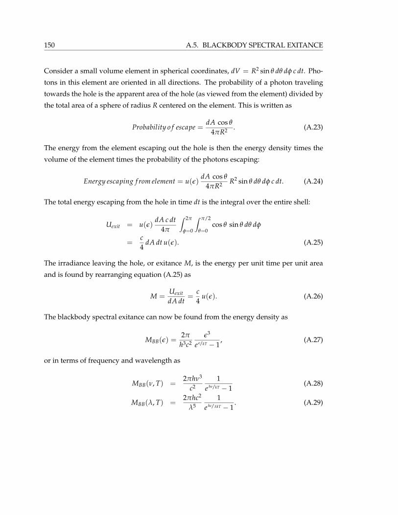
150 A.5. BLACKBODY SPECTRAL EXITANCE
Consider a small volume element in spherical coordinates, dV = R2 sin θ dθ dφ c dt. Pho-
tons in this element are oriented in all directions. The probability of a photon traveling
towards the hole is the apparent area of the hole (as viewed from the element) divided by
the total area of a sphere of radius R centered on the element. This is written as
Probability o f escape =dA cos θ
4πR2 . (A.23)
The energy from the element escaping out the hole is then the energy density times the
volume of the element times the probability of the photons escaping:
Energy escaping f rom element = u(ε)dA cos θ
4πR2 R2 sin θ dθ dφ c dt. (A.24)
The total energy escaping from the hole in time dt is the integral over the entire shell:
Uexit = u(ε)dA c dt
4π
∫ 2π
φ=0
∫ π/2
θ=0cos θ sin θ dθ dφ
=c4
dA dt u(ε). (A.25)
The irradiance leaving the hole, or exitance M, is the energy per unit time per unit area
and is found by rearranging equation (A.25) as
M =Uexit
dA dt=
c4
u(ε). (A.26)
The blackbody spectral exitance can now be found from the energy density as
MBB(ε) =2π
h3c2ε3
e ε/kT − 1, (A.27)
or in terms of frequency and wavelength as
MBB(ν, T) =2πhν3
c21
e hν/kT − 1(A.28)
MBB(λ, T) =2πhc2
λ51
e hc/λkT − 1. (A.29)

A.6. BLACKBODY SPECTRAL RADIANCE 151
A.6 Blackbody Spectral Radiance
The radiance, L, is the energy per unit time per unit area emitted per unit solid angle. The
relationship between the radiance and the exitance of a material is defined as
dM = L cos θdΩ = L cos θ sin θ dθ dφ. (A.30)
The total exitance into the hemisphere above the blackbody is found by integrating both
sides over the entire hemisphere:
M =∫ 2π
φ=0
∫ π/2
θ=0L cos θ sin θ dθ dφ. (A.31)
A blackbody is a Lambertian radiator by definition so the radiance, L, does not depend
on angle and may be considered a constant of integration. The result of the integration
over the hemisphere is π. The relation between the radiance and exitance of a blackbody
is then
L =Mπ
. (A.32)
The spectral radiance of a blackbody is finally
LBB(ε, T) =2
h3c2ε3
e ε/kT − 1, (A.33)
or in terms of frequency and wavelength as
LBB(ν, T) =2 h ν3
c21
e hν/kT − 1(A.34)
LBB(λ, T) =2 h c2
λ51
e hc/λkT − 1. (A.35)
A.7 Total Blackbody Radiated Power
The total radiated power of a blackbody can be found by integrating the Planck equa-
tion over all wavelengths. Equation (A.29) gives the radiant flux per unit area per unit
wavelength and is rewritten here as
ΦdA dλ
=2πhc2
λ51
e hc/λkT − 1. (A.36)
152 A.8. WAVELENGTH OF MAXIMUM EMISSION
The total power is found by rearranging the equation and integrating over all wavelengths
as
Φ = dA∞∫
0
2πhc2
λ51
e hc/λkT − 1dλ. (A.37)
Substituting x = hc/λkT yields
Φ = dA2πk4T4
h3c2
∞∫
0
x3
ex − 1dx. (A.38)
The integral over x evaluates to π4/15. Substituting this value yields
Φ = dA2π5k4
15h3c2 T4. (A.39)
Grouping the constants and representing the differential area as the radiating surface area,
A, the total radiated power of a blackbody of a given area is
Φ = A σ T4. (A.40)
The constant σ equals 5.6704 · 10−8 [J/s/m2/K4] and is known as the Stefan-Boltzmann
constant. Equation (A.40) is usually referred to as the Stefan-Boltzmann Law.
A.8 Wavelength of Maximum Emission
The Planck spectrum is a well-behaved function with a single maximum as indicated in
Figure A.2. The wavelength corresponding to the maximum emission can be found by
differentiating equation (A.29) and equating it to zero:
∂L∂λ
=2hc2
ehc/λkT − 1
[− 5
λ6
]+
2hc2
λ5
[ehc/λkT
(ehc/λkT − 1)2hckT
1λ2
]= 0. (A.41)
Rearranging equation (A.41) yields
hcλkT
· 11− ehc/λkT
− 5 = 0. (A.42)
Let x = hc/λkT and substitute to yield
x1− ex − 5 = 0. (A.43)
A.8. WAVELENGTH OF MAXIMUM EMISSION 153
The solution to equation (A.43) is x = 4.96511423. Solving for λ yields
λ =hc
xkT. (A.44)
Evaluating the constants yields a relationship between the wavelength associated with
the maximum radiance of a blackbody and the temperature of the blackbody:
λpeak =2897.768 [µm K]
T[µm] . (A.45)
This relationship is referred to as Wien’s displacement law.

154 A.8. WAVELENGTH OF MAXIMUM EMISSION
Figure A.2: Spectral radiance for a blackbody at a temperature of 300 Kelvin

Appendix B
Multiple Regression Analysis
Multiple regression analysis seeks to find a relationship between two or more quantita-
tive variables so that one variable can be predicted from the others [43]. The variable
to be predicted is known as the response (dependent variable) while the other variables
are called predictors (independent variables). Since a perfect relationship between the
response and the predictors may not exist, it is desirable to minimize the differences be-
tween the predicted values and the actual measured values of the responses. A brief
overview of finding a statistical relationship between a dependent variable and multiple
independent variables along with ways to test the fit of the model to the data is presented
in this chapter.
B.1 Least-Squares Regression
An actual data set may contain a set of independent variables that were varied so that a de-
pendent variable could be observed and measured. For the ith observation, the dependent
variable is denoted as Yi and the independent variables are denoted as xi,1, xi,2, ... xi,p−1
where p− 1 is the number of independent variables.
A linear model can be fit to this data in the form
Yi = β0 + βi,1 xi,1 + βi,2 xi,2 + ... + βi,p−1 xi,p−1 + ε i, (B.1)
where ε i is the error term between the predicted response and the actual response. The
error is a random variable and it expected to have a normal distribution with a zero
mean [48]. Note that each predictor may be a power or product of other predictors (i.e.,
x3 = x1 x2). Equation (B.1) can be expressed in matrix notation as
Y = Xβ + ε, (B.2)
155

156 B.2. ANALYSIS OF VARIANCE
where the matrices are
Y(nx1)
=
Y1
Y2
...
Yn
, X(nxp)
=
1 x11 x12 . . . x1,p−1
1 x21 x22 . . . x2,p−1
......
......
1 xn1 xn2 . . . xn,p−1
, β(px1)
=
β0
β1
...
βp−1
, ε(nx1)
=
ε1
ε2
...
εn
.
Let b represent the vector of estimated regression coefficients so that the fitted (estimated)
response values, Y, are represented by
Y = X b. (B.3)
The difference between the observed values and the fitted values is known as the residuals
(e = Y− Y). Least-squares regression attempts to choose b in order to minimize the sum of
the square residuals e’e. The least-squares regression coefficients are calculated by
b =(X′X
)−1 X′ Y. (B.4)
B.2 Analysis of Variance
The analysis of variance is based on sums of squares and on degrees of freedom associated
with the response, Y [43]. There are several metrics that must be defined.
B.2.1 Sum of Squares
Error Sum of Squares (SSE) is a measure of the variation of the observations around the
regression model:
SSE = ∑(Yi − Yi
)2 = e′e = Y′Y− b′X′Y (B.5)
The SSE is the sum of the squared residuals and SSE = 0 if the regression model predicted
all the observations perfectly.
Regression Sum of Squares (SSR) is the sum of the square deviations between the pre-
dicted responses and the mean observed response:
SSE = ∑(Yi − Y
)2 = b′X′Y− n Y2 (B.6)

B.2. ANALYSIS OF VARIANCE 157
For least-squares regression, the mean of the fitted values equals the mean of the observed
responses.
Total Sum of Squares (SSTO) is the sum of the deviations between each response vari-
able, Yi, and the mean response:
SSTO = ∑ (Yi − Y)2 = Y′Y− n Y2 (B.7)
If SSTO = 0, then all observations are the same. The total sum of squares is related to the
square error and square regression by
SSTO = SSE + SSR. (B.8)
B.2.2 Mean Squares
A sum of squares divided by its associated degree of freedom is called a mean square [43].
Regression Mean Square (MSR) is the SSR divided by its degrees of freedom:
MSR =SSRp− 1
. (B.9)
Error Mean Square (MSE) is the SSE divided by its degrees of freedom:
MSE =SSE
n− p. (B.10)
Recall from equation (B.1) that there are p coefficients and p − 1 independent variables.
Note that the degrees of freedom of the SSTO is the sum of the degrees of freedom of the
SSR and SSE: (p− 1) + (n− p) = n− 1.
B.2.3 Coefficient of Multiple Determination
The coefficient of multiple determination is used as a goodness of fit of a regression
model [44]. The coefficient is defined as
R2 =SSR
SSTO= 1− SSE
SSTO. (B.11)
The value of R2 lies between 0 and 1. Higher values of R2 correspond to smaller devia-
tions (a better fit) between the predicted and observed response values.

158 B.3. APTNESS OF THE FITTED MODEL
The coefficient of determination is often adjusted to take into account the number of ob-
servations and the number of degrees of freedom [43]. The adjusted coefficient is then
defined as,
R2a = 1− (n− 1)
(n− p)SSE
SSTO. (B.12)
B.2.4 F-Test
It may be useful to test whether there is a statistically significant relation between a depen-
dent variable, Y, and a set of independent variables, xk. In terms of regression variables, it
is possible to simultaneously test whether all βk = 0 or alternatively whether at least one
βk 6= 0. This statement is written as
H0 : β1 = β2 = ... = βp−1 = 0
H1 : at least one βk 6= 0.
If all βk = 0, then the response function reduces to Y = β0. Therefore, the predicted
value of the response is the same for all xk values and there is no regression relationship
between the response and the independent variables [50]. The test statistic for this case is
denoted F∗ and is defined as
F∗ =MSRMSE
. (B.13)
The decision as to whether to include a variable in the regression equation or not is defined
by,
H0 : F∗ ≤ F (1− α; p− 1, n− p)
H1 : F∗ > F (1− α; p− 1, n− p) ,
where F( ) is the F distribution and (1− α)100 is the percentile of the F distribution. F dis-
tribution tables are included in many statistics textbooks.
B.3 Aptness of the Fitted Model
Once a model has been fit to the data, it is important to check the fit of the model to de-
termine if the model is appropriate for the given data. A common way to check the fit
of a model is through the use of residual diagnostic plots [48]. For these plots, standard-
ized residuals are used. Standardization involves subtracting the mean value from each
residual and then dividing by the standard deviation.
B.3. APTNESS OF THE FITTED MODEL 159
B.3.1 Standardized Residuals vs. Fitted Responses
A plot of the standardized residuals, e∗, versus the fitted responses, y, provides a visual
diagnostic of the fit of the model. The data points in this plot should be randomly dis-
tributed about zero, usually with the standardized residuals falling mostly between ± 2.
A good model fit is indicated by the lack of any distinct patterns in the plot [48].
B.3.2 Normal Probability Plot of Standardized Residuals
A normal probability plot of the standardized residuals investigates the assumption that
the residuals from a least squares regression model should be normally distributed [48].
If the data points come from a normal distribution, they will fall on an approximately
straight line which indicates a good model fit. If the data points come from some alterna-
tive distribution, the plot will exhibit some degree of curvature which would indicate a
poor model fit.
A Ryan-Joiner test may be performed on the normal probability data to determine if the
points fall sufficiently on a line. The Ryan-Joiner statistic is essentially a correlation coeffi-
cient of the data points in the normal probability plot. If the Ryan-Joiner statistic is below
the critical value, the null hypothesis of a normal distribution is rejected and therefore the
model is not a good fit to the data [47]. A Ryan-Joiner test may be computed in statis-
tical analysis software such as Minitab. Some critical values for the Ryan-Joiner test are
included in reference [47].

160 B.3. APTNESS OF THE FITTED MODEL
Appendix C
Propagation of Uncertainties
The uncertainty in a response can be calculated from the uncertainties of each predictor.
An analytical solution can be derived from random variable statistics. An empirical so-
lution can be found by observing the calculated responses of a large number of predictor
distribution values. Both of these methods are based on a weighted sum of random vari-
ables to yield a response variable. Let y be a weighted sum of p random variables, xi, so
that
y = α0 + α1 x1 + α2 x2 + ... + αp xp = α0 +p
∑i=1
αi xi, (C.1)
where the αi are real weighting constants [51].
C.1 Analytical Method
The uncertainty in the response may be derived analytically from equation (C.1). The
expected value (mean) of the response, y, is written as
E [y] = E
[α0 +
p
∑i=1
αi xi
]= E [α0] + E
[p
∑i=1
αi xi
]= α0 +
p
∑i=1
αi E [xi] . (C.2)
The interpretation of equation (C.2) is that the mean value of a weighted sum of random
variables is the weighted sum of the mean values of the random variables. The difference
between the response and the expected value of the response (residual) is written as
y− E [y] =
(α0 +
p
∑i=1
αi xi
)−
(α0 +
p
∑i=1
αi E [xi]
)
=p
∑i=1
αi xi −p
∑i=1
αi E [xi] =p
∑i=1
αi (xi − E [xi]) . (C.3)
161

162 C.2. EMPIRICAL METHOD
The variance in the response, σ2y , is the expected value of the square of the residual in y
written as
σ2y = E
[(y− E [y])2
]= E
[(p
∑i=1
αi (xi − E [xi])
)·(
p
∑i=1
αi (xi − E [xi])
)]
=p
∑i=1
p
∑j=1
αi αj E[(xi − E [xi]) ·
(xj − E
[xj
])]=
p
∑i=1
p
∑j=1
αi αj Cij, (C.4)
where Cij is the covariance between xi and xj.
For the case where the random variables are uncorrelated such that Cij = σ2xi
for i = j
and Cij = 0 for i 6= j, the variance in the response becomes
σ2y =
p
∑i=1
α2i σ2
xi. (C.5)
Equation (C.5) means that the variance of a weighted sum of uncorrelated random vari-
ables is the weighted sum of the variances of the random variables.
C.2 Empirical Method
The uncertainty in the response may also be found empirically from equation (C.1). For
each random variable, a random value is selected based on a Gaussian distribution. The
mean of the Gaussian is equal to the expected value of that random variable while the
standard deviation is equal to the uncertainty value. A large number of trials (N À p) of
each random variable is generated and then used in equation (C.1) to calculate the asso-
ciated responses. The mean of these responses equals the expected value of the response
and the standard deviation of the responses is equal to the uncertainty in the response.
Appendix D
Calculation of Effective Sky
Temperature
The effective temperature of the sky dome in a given spectral band of a sensor can be com-
puted from the DIRSIG make adb utility. The utility uses a user-provided atmospheric
profile in the form of a MODTRAN input data file (tape5) to calculate the hemispherically-
integrated, spectral downwelling radiance. This radiance can then be spectrally sampled
by a user-provided sensor spectral response and converted into an apparent temperature.
A MODTRAN input file (tape5) is supplied by the user. The file contains the atmospheric
profile information (i.e., altitude, pressure, temperature, humidity, etc.) derived from ei-
ther one of the standard MODTRAN atmospheres or as a custom atmosphere created by
the user. The purpose of the make adb utility is to create an atmospheric database for
scenes modeled in the DIRSIG environment. The database contains the spectral transmis-
sions and path radiances for the viewing angles of the sensor. It also calculates the spatial
distribution of the atmospheric downwelling radiance. To do so, the make adb utility di-
vides the sky hemisphere into discrete samples known as quads. The elevation direction
is divided into six angles and the azimuth direction is divided into twelve angles. This
results in 72 quads covering the hemisphere that are 15° tall in the elevation direction
and 30° wide in the azimuth direction. For each point in the center of these quads, the
path radiance is computed from MODTRAN using the profile specified by the user and
auxiliary scene information (i.e., time of day, location, etc.). In other words, the sensor is
placed on the ground and targeted at the center of one of the quads. MODTRAN is run
for this geometry and the thermal path radiance is recorded for that direction (quad). A
table is built of the zenith and azimuth angle of the sample and the spectral path radiance
from the sample. Therefore, the table contains spectral radiances for a total of 72 samples
in the hemisphere which represent the spectral downwelling radiances for each of the 72
directions (quads). Finally, these 72 spectral radiances are spatially integrated to produce
163

164 Calculation of Effective Sky Temperature
a diffuse spectral downwelling radiance. The spatial integration is written as
Ld(λ) =∫
2πL(θ, φ, λ) cos θ dΩ =
2π∫
φ=0
π2∫
θ=0
L(θ, φ, λ) cos θ sin θ dθ dφ
[W
m2 sr µm
]. (D.1)
This diffuse downwelling spectral radiance is then sampled by the sensor’s spectral re-
sponse function and integrated to arrive at the integrated band radiance. This is written
as
L =∫
Ld(λ) R′(λ) dλ
[W
m2 sr
]. (D.2)
This integrated band radiance is then converted into an apparent temperature using the
methods described in Section 3.6. The apparent temperature is known as the effective sky
temperature in the given sensor spectral band.

Appendix E
Estimation of Plume Path Length
The plume length is the line-of-sight path length through the plume between the sen-
sor and the tower throat. To assist the user in estimating the plume length, a simple
plume model is considered. The estimated plume length is based on a Gaussian, contin-
uous point-source plume model [52]. In this model, the centerline of the plume at any
downrange distance, x, is calculated from knowledge of the wind speed, exhaust velocity,
plume temperature and ambient temperature. The plume concentration at any point can
also be calculated. The shape of the plume resembles a cone in which diffusion occurs
only in the vertical and crosswind directions (z and y directions, respectively). The plume
disperses in the vertical and crosswind directions according to a Gaussian distribution
with dispersion coefficients σz and σy.
The plume is assumed to be a continuous point-source. The downwind direction is la-
beled x and the dispersion of the plume gas occurs only in the crosswind and vertical
directions (y and z directions, respectively). The plume therefore has the appearance of
a cone with the vertex as the source of emission. This model also assumes that the hori-
zontal wind speed is constant and the mean wind direction is constant. The height of the
plume source is He.
The centerline of the plume at a downwind distance x is calculated as
∆h = 1.6 F1/3 x2/3 u−1 [m], (E.1)
where ∆h is the change in centerline height relative to the height of the emission source, F
is the buoyancy flux parameter, x is the downwind distance in meters, and u is the wind
speed in meters per second. The buoyancy parameter characterizes the buoyancy of the
stack exit gas and can be written as
F = g vs r2 Ts − Ta
Ts
[m4
s3
], (E.2)
165
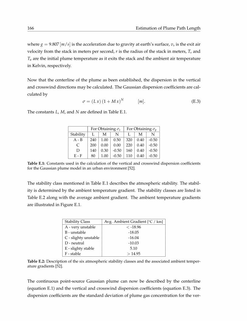
166 Estimation of Plume Path Length
where g = 9.807 [m/s] is the acceleration due to gravity at earth’s surface, vs is the exit air
velocity from the stack in meters per second, r is the radius of the stack in meters, Ts and
Ta are the initial plume temperature as it exits the stack and the ambient air temperature
in Kelvin, respectively.
Now that the centerline of the plume as been established, the dispersion in the vertical
and crosswind directions may be calculated. The Gaussian dispersion coefficients are cal-
culated by
σ = (L x) (1 + M x)N [m]. (E.3)
The constants L, M, and N are defined in Table E.1.
For Obtaining σz For Obtaining σy
Stability L M N L M NA - B 240 1.00 0.50 320 0.40 -0.50
C 200 0.00 0.00 220 0.40 -0.50D 140 0.30 -0.50 160 0.40 -0.50
E - F 80 1.00 -0.50 110 0.40 -0.50
Table E.1: Constants used in the calculation of the vertical and crosswind dispersion coefficientsfor the Gaussian plume model in an urban environment [52].
The stability class mentioned in Table E.1 describes the atmospheric stability. The stabil-
ity is determined by the ambient temperature gradient. The stability classes are listed in
Table E.2 along with the average ambient gradient. The ambient temperature gradients
are illustrated in Figure E.1.
Stability Class Avg. Ambient Gradient [°C / km]A - very unstable < -18.96B - unstable -18.05C - slighty unstable -16.04D - neutral -10.03E - slighty stable 5.10F - stable > 14.95
Table E.2: Description of the six atmospheric stability classes and the associated ambient temper-ature gradients [52].
The continuous point-source Gaussian plume can now be described by the centerline
(equation E.1) and the vertical and crosswind dispersion coefficients (equation E.3). The
dispersion coefficients are the standard deviation of plume gas concentration for the ver-

Estimation of Plume Path Length 167
Figure E.1: Comparison of the six atmospheric stability classes using the associated ambient tem-perature gradients in reference to the dry and wet adiabatic lapse rates [52].
tical and crosswind Gaussian profiles.
The path length through the plume between the fan stack opening and the sensor can
be estimated with the Gaussian model and with knowledge of the sensor viewing geom-
etry. The point-source model is modified so that the entire area of the fan stack aperture is
the source of emission. First, the coordinates of the centerline trajectory of the plume are
computed through equation E.1. For each point along the centerline trajectory, a sphere is
drawn whose radius in the vertical and crosswind directions equals the sum of the radius
of the stack opening and twice the vertical and crosswind dispersion coefficients, r + 2σz
and r + 2σy, respectively. The radius in the downwind direction x is taken as r + 2σy. In
other words, the “edge” of the plume is a distance of two standard deviations from the
centerline of the plume in the z and y directions plus the radius of the stack opening. This
concept is illustrated from a Matlab rendering in Figure E.2.
The sensor viewing vector is determined from the distance to the stack opening and the
sensor zenith and azimuth viewing angles. This vector originates at the center of the
stack opening and points in the direction of the sensor. The points on this vector that are
within two standard deviations of the plume centerline are considered points contained
within the plume. The length of the vector containing these enclosed points equals the
path length through the plume.
The necessary user inputs for this model are the stack height [m], the stack radius [m],

168 Estimation of Plume Path Length
Figure E.2: Gaussian plume model rendered in Matlab. The solid line represents the sensor line-of-sight. The exit air velocity is set to 10 m/s, stack height is 9 m, stack radius is 2 m, wind speedis 0.75 m/s, and the atmospheric stability is slightly unstable. The estimated path length throughthis plume is 6 m.
the approximate stack gas and ambient air temperatures [K], the wind speed [m/s], the
vertical exit gas speed [m/s], and the sensor zenith and azimuth direction angles [o] (the
azimuth angle is measured from the downwind direction, x).

Appendix F
Precipitable Water in an Air Column
The atmospheric precipitable water is defined as the total atmospheric water vapor con-
tained in a vertical column of unit cross-sectional area extending between any two speci-
fied levels [53]. This concept is commonly expressed in terms of the height to which that
water would stand if completely condensed and collected in a vessel of the same unit
cross section. The precipitable water, W, can be expressed mathematically as
W =1g
p2∫
p1
w(p) dp [mm], (F.1)
where p is the atmospheric pressure in Pascals (Pa = N/m2), g is the acceleration due to
gravity at the earth’s surface (g = 9.807 m/s2), and w(p) is the water vapor mixing ratio.
The integral is computed between two pressure levels, p1 and p2. The result has units of
millimeters which represents the height of the precipitable water in the air column. The
mixing ratio is defined from the pressure and vapor pressure as
w(p) = 0.622e
p− e, (F.2)
where e is the water vapor pressure expressed in the same units as the pressure, p (usually
in [mb] or [Pa]). The vapor pressure can be calculated from the dew point temperature [K]
at a given pressure as
e = 0.01 · exp[1.391499− 0.048640239 Td + (0.41764768 · 10−4) T2
d
− (0.14452093 · 10−7) T3d + 6.5459673 log e (Td)− 5800.2206
1Td
][mb]. (F.3)
Finally, the dew point can be calculated from the relative humidity [%] and the dry-bulb
temperature [K] as
Td =243.5 ·
[log e
( RH100
)+ 17.67 (T−273.15)
243.5+(T−273.15)
]
17.67−[log e
( RH100
)+ 17.67 (T−273.15)
243.5+(T−273.15)
] + 273.15 [K]. (F.4)
169

170 Precipitable Water in an Air Column
Equations (F.3) and (F.4) were obtained from http://cires.colorado.edu/∼voemel/vp.pro.

Bibliography
[1] J. R. Schott, Remote Sensing: The Image Chain Approach, Oxford University Press, New
York, NY, 1997.
[2] R. Burger, Cooling Tower Technology: Maintenance, Upgrading and Rebuilding, The Fair-
mont Pres, Inc., Lilburn, GA, third ed., 1995.
[3] A. Garrett, “Email correspondence.” October 2006.
[4] M. Planck, “On the law of distribution of energy in the normal spectrum,” in Annalen
der Physik, 4, p. 553, 1901.
[5] “Nonconventional Exploitation Factors (NEF) Modeling,” Tech. Rep. v9.5,
April 2005.
[6] G. J. Ward, “Measuring and modeling anisotropic reflection,” in Computer Graphics,
pp. 265–272, July 1992.
[7] K. E. Torrance and E. M. Sparrow, “Theory of off-specular reflection from roughened
surfaces,” in Journal of the Optical Society of America, 57(9), pp. 1105–1114, September
1967.
[8] R. G. Priest and T. A. Germer, “Polarimetric BRDF in the microfacet model: Theory
and measurements,” in Proceedings of the 2000 Meeting of the Military Sensing Symposia
Specialty Group on Passive Sensors, 1, pp. 169–181, 2002.
[9] J. R. Maxwell, J. Beard, S. Weiner, D. Ladd, and S. Ladd, “Bidirectional reflectance
model validation and utilization,” Tech. Rep. AFAL-TR-73-303, Environmental Re-
search Institute of Michigan, Ann Arbor, MI, October 1973.
[10] J. R. Shell, Polarimetric Remote Sensing in the Visible to Near Infrared. PhD thesis,
Rochester Institute of Technology, 54 Lomb Memorial Drive, Rochester NY 14623,
2005.
[11] E. Hecht, Optics, Addison-Wesley Publishing Company, Reading, Massachusetts,
second ed., 1990.
[12] J. M. Wallace and P. V. Hobbs, Atmospheric Science An Introductory Survey, Academic
Press, New York, 1977.
171
172 BIBLIOGRAPHY
[13] Air Force Research Laboratory, Hanscom AFB, MA, MODTRAN User’s Manual, ver-
sions 3.7 and 4.0 ed., 1998.
[14] J. D. Gaskill, Linear System, Fourier Transforms, and Optics, John Wiley & Sons, Inc.,
New York, NY, 1978.
[15] K. R. Castleman, Digital Image Processing, Prentice Hall, Inc., Upper Saddle River, NJ,
1996.
[16] F. Becker and Z.-L. Li, “Towards a local split window method over land surfaces,” in
Groupement Scientifique de Teledetection Spatial, pp. 369–393, Laboratoire des Sciences
de l’Image et de la Teledetection, 1989.
[17] F. Sospedra, V. Caselles, and E. Valor, “Effective wavenumber for thermal infrared
bands - application to Landsat-TM,” in International Journal of Remote Sensing, 19(11),
pp. 2105–2117, 1998.
[18] A. Berk, L. S. Bernstein, and D. C. Robertson, “MODTRAN: A moderate resolution
model for LOWTRAN 7,” Tech. Rep. GL-TR-89-0122, Spectral Sciences, Inc., Burling-
ton, MA, April 1989.
[19] Air Force Geophysics Laboratory, Hanscom AFB, MA, User’s Guide to LOWTRAN 7,
afgl-tr-88-0177 ed., August 1988.
[20] S. Carr, “The aerosol models in MODTRAN: Incorporating selected measurements
from northern australia,” Tech. Rep. AR-013-545, Defence Science and Technology
Organisation, Commonwealth of Australia, December 2005.
[21] J. R. Schott, S. D. Brown, R. V. Raqueno, H. N. Gross, and G. Robinson, “An ad-
vanced synthetic image generation model and its application to multi/hyperspectral
algorithm development,” in Canadian Journal of Remote Sensing, 25(2), pp. 99–111,
1999.
[22] Digital Imaging and Remote Sensing Laboratory, Rochester, NY, The DIRSIG User’s
Manual, February 2006.
[23] P. Dash, F. M. Gottsche, F. S. Olesen, and H. Fischer, “Land surface temperature
and emissivity estimation from passive sensor data: Theory and practice - current
trends,” in International Journal of Remote Sensing, 23(13), pp. 2563–2594, 2002.
BIBLIOGRAPHY 173
[24] Z. Qin, A. Karnieli, and P. Berliner, “A mono-window algorithm for retrieving land
surface temperature from Landsat TM data and its application to the israel-egypt
border region,” in International Journal of Remote Sensing, 22(18), pp. 3719–3746, 2001.
[25] K. Mathew, C. M. Nagarani, and A. S. Kirankumar, “Split-window and multi-angle
methods of sea surface temperature determination: An analysis,” in International
Journal of Remote Sensing, 22(16), pp. 3237–3251, 2001.
[26] A. J. Prata, “Land surface temperatures derived from the advanced very high res-
olution radiometer and the along-track scanning radiometer: Theory,” in Journal of
Geophysical Research, 98(D9), pp. 16689–16702, 1993.
[27] X. Li, W. Pichel, E. Maturi, P. Clemente-Colon, and J. Sapper, “Deriving the oper-
ational nonlinear multichannel sea surface temperature algorithm coefficients for
NOAA-14 AVHRR/3,” in International Journal of Remote Sensing, 22(4), pp. 699–704,
2001.
[28] J. J. Szymanski and P. G. Weber, “Multispectral thermal imager: Mission and appli-
cations overview,” in IEEE Transactions on Geoscience and Remote Sensing, 43, pp. 1943
– 1949, IEEE, September 2005.
[29] C. C. Borel, W. B. Clodius, A. B. Davis, B. W. Smith, J. J. Szymanski, J. Theiler, P. V.
Villeneuve, and P. G. Weber, “MTI core science retrieval algorithms,” in Imaging Spec-
trometry V, 3753, pp. 403 – 415, SPIE, (Denver), July 1999.
[30] W. B. Clodius, C. Borel, L. Balick1, and S. J. Hook, “Validation of the MTI water sur-
face temperature retrieval algorithms,” in Geoscience and Remote Sensing Symposium,
1, pp. 30 – 32, IEEE International, June 2002.
[31] D. Gu, A. R. Gillespie, A. B. Kahle, and F. D. Palluconi, “Autonomous atmospheric
compensation (AAC) of high resolution hyperspectral thermal infrared remote-
sensing imagery,” in IEEE Transactions on Geoscience and Remote Sensing, 38(6),
pp. 2557–2570, IEEE, 2000.
[32] S. J. Young, R. Johnson, and J. A. Hackwell, “An in-scene method for atmospheric
compensation of thermal hyperspectral data,” in Journal of Geophysical Research,
107(D24), p. 4774, 2002.
[33] G. Healey and D. Slater, “Models and methods for automated material identifica-
tion in hyperspectral imagery aquired under unknown illumination and atmospheric
174 BIBLIOGRAPHY
conditions,” in IEEE Transactions on Geoscience and Remote Sensing, 37(6), pp. 2706–
2717, IEEE, 1999.
[34] P. S. Kealy and S. J. Hook, “Separating temperature and emissivity in thermal in-
frared multispectral scanner data: Implications for recovering land surface temper-
atures,” in IEEE Transactions on Geoscience and Remote Sensing, 31(6), pp. 1155–1164,
IEEE, 1993.
[35] A. Gillespie, S. Rokugawa, T. Matsunaga, J. S. Cothern, S. Hook, and A. B. Kahle, “A
temperature and emissivity separation algorithm for advanced spaceborne thermal
emission and reflection radiometer (ASTER) images,” in IEEE Transactions on Geo-
science and Remote Sensing, 36(4), pp. 1113–1126, IEEE, 1998.
[36] M. Boonmee, Land Surface Temperature and Emissivity Retrieval from Thermal Infrared
Hyperspectral Imagery. PhD thesis, Rochester Institute of Technology, 54 Lomb Memo-
rial Drive, Rochester NY 14623, 2007.
[37] C. C. Borel, “ARTEMISS - an algorithm to retrieve temperature and emissivity from
hyper-spectral thermal image data,” Tech. Rep. LA-UR-027907, Los Alamos National
Laboratory, Tampa, Florida, March - April 2003.
[38] R. Kaiser and L. Smith, SOC-400T Field Use Protocol. DIRS Laboratory, Rochester
Institute of Technology, 0.3 ed., July 2004.
[39] SPX Cooling Technologies, Inc., Overland Park, KS, http://spxcooling.com/en/.
[40] K. Stamnes, S.-C. Tsay, W. Wiscombe, and K. Jayaweera, “Numerically stable algo-
rithm for discrete-ordinate-method radiative transfer in multiple scattering and emit-
ting layered media,” in Applied Optics, pp. 2502–2509, No. 12, Vol. 27, June 1988.
[41] G. Anderson, “Email correspondence.” August 2007.
[42] E. J. Ientilucci and J. R. Schott, “Physics based target detection using a hybrid al-
gorithm with an infeasibility metric,” in IEEE International Conference on Acoustics,
Speech, and Signal Processing (ICASSP), pp. 1193–1196, IEEE ICASSP Vol. 5, (Toulouse,
France), May 2006.
[43] J. Neter and W. Wasserman, Applied Linear Statistical Models: regression, analysis of
variance, and experimental designs, Richard D. Irwin, Inc., Homewood, Illinois, 1974.
BIBLIOGRAPHY 175
[44] R. L.Mason, R. F. Gunst, and J. L. Hess, Statistical Design and Analysis of Experiments
with Applications to Engineering and Science, John Wiley & Sons, Inc., New York, NY,
1989.
[45] F. P. Padula, “Historic thermal calibration of Landsat 5 TM through an improved
physics based approach,” Master’s thesis, Rochester Institute of Technology, 54 Lomb
Memorial Drive, Rochester NY 14623, November 2008.
[46] M. Taguchi, T. Fukuhara, T. Imamura, M. Nakamura, N. Iwagami, M. Ueno,
M. Suzuki, G. Hashimoto, and K. Mitsuyama, “Longwave infrared camera onboard
the venus climate orbiter,” in Advances in Space Research, 40, p. 861868, COSPAR,
Elsevier Ltd., May 2007.
[47] J. Thomas A. Ryan and B. L. Joiner, “Normal probability plots and tests for normal-
ity,” tech. rep., The Pennsylvania State University, Statistics Department, 1976.
[48] J. L. Devore, Probability and Statistics for Engineering and the Sciences, Duxbury Thom-
son Learning, Pacific Grove, CA, fifth ed., 2000.
[49] D. V. Schroeder, Introduction to Thermal Physics, Addison Wesley Longman, New
York, NY, 2000.
[50] J. Neter, W. Wasserman, and G. A. Whitmore, Applied Statistics, Allyn and Bacon, Inc.,
Boston, MA, second ed., 1982.
[51] J. Peyton Z. Peebles, Probability, Random Variables and Random Signal Principles,
McGraw-Hill Science/Engineering/Math, 4 ed., July 2000.
[52] M. R. Beychok, Fundamentals of Stack Gas Dispersion, Irvine, CA, third ed., 1994.
[53] “Glossary of meteorology.” http://amsglossary.allenpress.com/glossary/,
March 2009. Search string: Precipitable Water.


![WP91 Lucia Montanaro Kosovo State Building Conundrum 3dic[1]](https://img.dokumen.tips/doc/110x75/577d27671a28ab4e1ea3d6e5/wp91-lucia-montanaro-kosovo-state-building-conundrum-3dic1.jpg)