Embed Size (px)
Citation preview

Radio Search for Extraterrestrial IntelligenceSETI is fun !
Society of Amateur Radio Astronomers
Annual Conference
Aug. 4-8, 2019
Green Bank Observatory, West Virginia
Presented by Skip CrillyEducation & Public OutreachVolunteer Science AmbassadorGreen Bank Observatory West Virginia Rev. July 30, 2019
Geographically-spaced Synchronized Signal Detection System
Abstract
Radio Frequency Interference (RFI) is a confounding problem in radio SETI, as false positives are introduced into receiver signals. Various methods exist to attempt to excise suspected RFI, with a possibility that true positives are rejected, and that un-excised RFI remain as false positives. Uncertain far side-lobe antenna patterns add to the uncertainty. To ameliorate the RFI problem, a system having geographically-spaced simultaneous and synchronized pulse reception has been implemented. A radio telescope at the Green Bank Observatory in Green Bank, West Virginia has been combined with a radio telescope of the Deep Space Exploration Society, near Haswell, Colorado to implement a spatial filter having a thrice-Moon-distance transmitter rejection. Approximately 135 hours of simultaneous synchronized pulse observations have been captured from November 2017 through February 2019 and another 45 hours captured in April 2019. This presentation describes the problem, observation system, observed results and proposedhypotheses to be subjected to attempts at refutation and relative inference, through further experimentation, and RFI and ETI transmitter signal model development.
1
12:35
Radio SETI usually uses very large radio telescopes
Green Bank TelescopeGreen Bank Observatory West Virginia
Radio Frequency Interference (RFI)
RFI is a very difficult problem !
Problem for SETI:
The Fermi Paradox: Where are the extraterrestrials?Leads to the question: Are ETI signals over-suspected to be RFI?
satellites
aircraft
reflections
towers
devices
clock radios
SETI data flow @ UC BerkeleyDepartment of Astronomy
monitor in UCB Campbell Hall lobby
100 meters
Pluto planet flag
(where I volunteer work part-time)
Fig. 1
Problem
Radio SETI has been plagued by an increasingly difficult problem – Radio Frequency Interference (RFI). As communication systems and computing devices have modernized, human-caused electromagnetic emissions and speculated extraterrestrial-caused radio communication signals have become difficult to differentiate.
Antenna pointing direction is typically used to identify celestial transmitting sources. Issues arise: 1. In a terrestrial, airborne and satellite RFI environment, antenna pattern sidelobeschange as antenna pointing is changed; highly sensitive telescopes can yield false positives, given the uncertainty of off-beam RFI and antenna patterns. 2. Multi-pixel feeds aid in directional differentiation, yet do not entirely solve the problem of multipath local RFI entering the sidelobes of the feed elements, resulting in outlying false positives. 3. Long term monitoring of identified candidate pointing directions requires time-consuming and careful follow-up, especially in the presence of sporadic RFI, and intermittent ETI transmissions.
2
Machine-based learning of human-sourced signals, and local RFI source identification, can help ameliorate the problem, through RFI excision. However, one is left with a quandary: How does one differentiate between a modern human communication system (RFI) and a typical celestial communication system (ETI), both designed to operate under a common Shannon’s Law scenario?
Energy-efficient communication signals are speculated to be transmitted by celestial intentional transmitters, as high information transfer and low transmitter cost are apparent goals. Communication signals contributing to these goals are expected to span large radio frequency bandwidths, contain narrow bandwidth elements for detectability, and in their high capacity and bandwidth, and low energy limit, be indistinguishable from random noise. Modern communication systems transmit different information to closely spaced receive antennas, in systems using multiple transmit and/or receive antennas. Increased channel capacity results.
If energy-efficient and high capacity communications signals are, in the limit, indistinguishable from random noise, and multiple receive antennas receive different parts of a single transmitted information stream, how can a communicative and gregarious ETI make itself known? Relatively easily identifiable signals seem to be required, leading to the ideas proposed in this paper.
2
view
Green Bank Observatory 40ft, WV180.0 degree Azimuth 44.0 degrees Elevation-7.6 degrees Declination
Deep Space Exploration Society60ft, Haswell, CO
149.6 degrees Azimuth39.2 degrees Elevation-7.6 degrees Declination
~parallel celestial radio-wave photons
+676.49 Hz Doppler shiftat 1420 MHZ
Image Ref. NASA
0 Hz Doppler Earth rotation shift
N
S
+-1.23 Hz Δ Doppler @ +-0.5° parallel rays
+-15 Hz Doppler@ +-0.5° GBO 40@ center pointingHaswell DSES 60 ft
RFI filter: reject ≈<720,000 miles
Signal
An experimentunderway,to try to reduce theeffect of RFI:
Use two telescopes each in low RFI areas,spaced far apart,
search for simultaneous pulsed signals in 3.73 Hz bins, measured on closeDoppler-corrected frequencies, in
≈12 million channels 1405-1448 MHz.
1,257 miles telescope spacing
and GPS synchronizedfrequency and time
Fig. 2
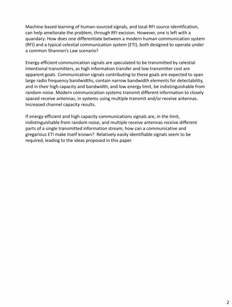
Idea to help solve the RFI problem (Fig. 2)Receiver spatial filtering may be assumed by the transmitter, leading to a method to make a transmitter known to a receiver, by intermittently transmitting spatial-simultaneous and time-simultaneous narrow bandwidth pulses, within an otherwise efficient and high capacity information stream. Additional characteristics of received signals, correlated to these simultaneous pulses, should ideally make the overall event likelihood low in noise and RFI, and support an ETI or very distant RFI transmitter hypothesis.
Receiver antennas (Fig. 2) may be distantly spaced to search for simultaneous pulses of hypothetical celestial origin. For example, a 1,257 mile receive antenna spacing provides a 720,000 mile spatial filter, to counter local and near-space RFI. The spatial filtering distance is considerably farther than the distance to the two antennas’ -3 dB beam overlap point, because Doppler shift within the antennas’ beamwidth gives space-based-RFI signals a frequency difference potentially greater than an FFT bin size. For example, there is a +-15 Hz difference in Doppler-induced frequency shift for signals arriving across the Green Bank Forty Foot Telescope’s -3 dB beamwidth, e.g. when the two electromagnetic signal rays and antenna spacing baseline form a triangle, and therefore indicate signals from close-in space transmitters.
3

A -7.6° declination was chosen for four reasons: 1. declinations close to the celestial equator produce the highest number of unique antenna pointing directions when transit scanning and 2. increase volumetric search space, 3. the declination is below the Clarke Belt at typical latitudes, and 4. anomalous pulses were apparent at the -7.6° declination during a few years of transit scanning observation using radio telescopes in New Hampshire.
Receiver bandwidth selectionThe choice of a 3.73 Hz FFT bin bandwidth and 1405 to 1448 MHz results from the processing tradeoffs of on-the-fly narrowband pulse signal detection and storage using an SNR threshold. A celestial transmitter may transmit with different occupied bandwidths and pulse durations, to increase channel capacity. Signals that are guessed to be intended for ease of detectability likely have various pulse durations, to avoid a receiver-transmitter un-matched filter scenario. The 3.73 Hz bin bandwidth may be considered to be a matched filter to one set of potentially transmitted identification pulses.
The 1405 to 1448 MHz spectrum is chosen because it is a somewhat well-RFI-protected wide band of spectrum. Contiguous frequency coverage is prioritized in signal processing, over contiguous time, due to the need to identify CW and narrow bandwidth, potentially drifting RFI sources within the chosen band. The pulse detection system operates at one-quarter duty cycle, at four second triggered intervals.
In observations starting in April 2019, we have used improved receiver systems with a range of approximately 1395 MHz to 1456 MHz and a one-third duty cycle. The following paragraphs describe the pre-April 2019 and the April 2019 processing systems.
Signal Processing
Signal processing was changed in the observations of April 2019. The following paragraph describes the pre-April 2019, with April 2019 changes in the next paragraph.
Four 0.27 s duration contiguous time uniform windows are each 2^25 point FFT-filtered and applied to a per-bin SNR threshold. A dwell time between measurements is required to allow GPS-sync’d time triggering of the two telescopes’ intermediate frequency analog-to-digital converters. Local oscillator frequency is synchronized using OCXOs at each site, each locked to a GPS signal. SNR thresholds are two-fold, at 11.2 dB per FFT bin and 12.0 dB 4x0.27s contiguous time average SNR, to reduce noise-induced false positives. Intentionally transmitted signals are expected to often partially straddle adjacent and/or alternate time windows, thus allowing the 12.0 dB threshold to select and store these pulses and partially reject noise-induced pulses. The spectral Noise values in SNR is measured in each 256 bin segment of the FFT output, averaged over four time samples. ADC sampling is at 125 MSPS. Polarization is circular at Haswell and linear at Green Bank,
3

resulting in a 3 dB maximum polarization match-to-mismatch, given random Poincare-Sphere transmitted polarization and site-differential Faraday rotation. Raw time domain data is not stored. The two telescopes’ software systems do not communicate with each other, to avoid near-simultaneous software-event induced corruption of data.
In observations starting in April 2019, improved receiver systems have duty cycle increased from one-fourth to one-third. ADC sampling is at 62.5 MSPS. SNR thresholds have been decreased to 11.0 dB per FFT bin and 11.8 dB composite one second SNR. Cycle time is three seconds, compared to four seconds in pre-April 2019 observations.
3
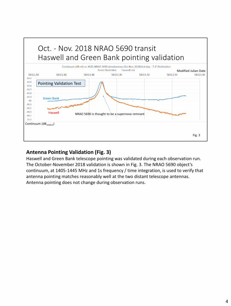
Oct. - Nov. 2018 NRAO 5690 transit Haswell and Green Bank pointing validation
Pointing Validation Test
Haswell
Green Bank
NRAO 5690 is thought to be a supernova remnant
Continuum (dBrelative)
Modified Julian Date
Fig. 3
Antenna Pointing Validation (Fig. 3)Haswell and Green Bank telescope pointing was validated during each observation run. The October-November 2018 validation is shown in Fig. 3. The NRAO 5690 object’s continuum, at 1405-1445 MHz and 1s frequency / time integration, is used to verify that antenna pointing matches reasonably well at the two distant telescope antennas. Antenna pointing does not change during observation runs.
4

Surveyed sky coverage RA (hrs) vs MJD
24 RA(hrs)
MJD
Nov 2017
April 2019
135 hours180 hours
at -7.6° declination
April 2018
Aug 2018
Nov 2018
Feb 2019
Fig. 4
Sky coverage during simultaneous Green Bank and Haswell observations (Fig. 4) Fig. 4 is a plot of Right Ascension coverage at -7.6°declination, during the 180 hours of simultaneous two telescope observation. Several of the analyses in this paper describe events observed during the first 135 hours, while other analyses cover the full 180 hour observations.
5
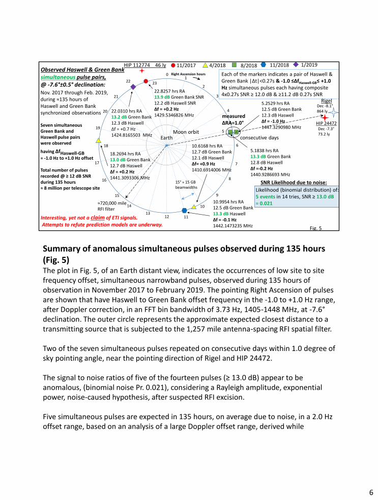
Observed Haswell & Green Banksimultaneous pulse pairs, @ -7.6°±0.5° declination:Nov. 2017 through Feb. 2019,during ≈135 hours of Haswell and Green Bank synchronized observations
Seven simultaneousGreen Bank and Haswell pulse pairs were observed
having ΔfHaswell-GB= -1.0 Hz to +1.0 Hz offset
Total number of pulsesrecorded @ ≥ 12 dB SNRduring 135 hours ≈ 8 million per telescope site
≈720,000 mileRFI filter
2
1
3
6
4
7
8
5
17
16
15
14
1312 11
10
9
19
20
21
18
2322
0
11/2017 8/2018 11/2018
measured ΔRA=1.0°
Right Ascension hours
EarthMoon orbit
15° ≈ 15 GB beamwidths
Dec -8.1°864 ly
Interesting, yet not a claim of ETI signals.Attempts to refute prediction models are underway.
Each of the markers indicates a pair of Haswell & Green Bank |Δt|<0.27s & -1.0 ≤ΔfHaswell-GB≤ +1.0 Hz simultaneous pulses each having composite 4x0.27s SNR ≥ 12.0 dB & ≥11.2 dB 0.27s SNR
Rigel
22.8257 hrs RA13.9 dB Green Bank SNR 12.2 dB Haswell SNRΔf = +0.2 Hz1429.5346826 MHz
5.2529 hrs RA12.5 dB Green Bank12.3 dB HaswellΔf = -1.0 Hz 1447.3290980 MHz
5.1838 hrs RA13.3 dB Green Bank12.8 dB HaswellΔf =-0.2 Hz1440.9286693 MHz
10.9954 hrs RA12.5 dB Green Bank 13.3 dB HaswellΔf = -0.1 Hz1442.1473235 MHz
4/2018
18.2694 hrs RA13.0 dB Green Bank12.7 dB HaswellΔf = +0.2 Hz1441.3093306 MHz
SNR Likelihood due to noise:
22.0310 hrs RA13.2 dB Green Bank12.3 dB HaswellΔf = +0.7 Hz1424.8165503 MHz
1/2019
10.6168 hrs RA12.7 dB Green Bank12.1 dB HaswellΔf= +0.9 Hz1410.6914006 MHz
Likelihood (binomial distribution) of:5 events in 14 tries, SNR ≥ 13.0 dB= 0.021
consecutive days
Fig. 5
HIP 24472Dec -7.3°73.2 ly
HIP 112774 46 ly
Summary of anomalous simultaneous pulses observed during 135 hours (Fig. 5)The plot in Fig. 5, of an Earth distant view, indicates the occurrences of low site to site frequency offset, simultaneous narrowband pulses, observed during 135 hours of observation in November 2017 to February 2019. The pointing Right Ascension of pulses are shown that have Haswell to Green Bank offset frequency in the -1.0 to +1.0 Hz range, after Doppler correction, in an FFT bin bandwidth of 3.73 Hz, 1405-1448 MHz, at -7.6°declination. The outer circle represents the approximate expected closest distance to a transmitting source that is subjected to the 1,257 mile antenna-spacing RFI spatial filter.
Two of the seven simultaneous pulses repeated on consecutive days within 1.0 degree of sky pointing angle, near the pointing direction of Rigel and HIP 24472.
The signal to noise ratios of five of the fourteen pulses (≥ 13.0 dB) appear to be anomalous, (binomial noise Pr. 0.021), considering a Rayleigh amplitude, exponential power, noise-caused hypothesis, after suspected RFI excision.
Five simultaneous pulses are expected in 135 hours, on average due to noise, in a 2.0 Hz offset range, based on an analysis of a large Doppler offset range, derived while
6

assuming that almost all simultaneous pulses in a larger Doppler offset range are due to noise. Therefore, it is thought at least some of the seven simultaneous pulses observed are likely due to noise.
The repetition of a transmitting signal, observed at a single celestial pointing direction, is unexpected from a near-space transmitter, as the transmitter is affected by the Sun-Earth-Moon gravity wells and needs thrust to retain close to the same celestial pointing direction during the period of a day. Such a celestial-station-keeping thrusting system would not naturally be expected in a human-built transmitter. RFI modeling is underway to quantify this idea.
The anomalous 13.9 dB SNR, 0.2 Hz offset, simultaneous pulse at RA 22.8257 hours corresponds to a pointing direction estimated towards HIP 112774 on 11/25/2017. Numerous simultaneous, associated and other pulse events observed in this pointing direction, during five days of transits, are described in a presentation given at the SARA 2018 Annual Conference in Green Bank.
6

Probability = 1 – Poisson Cumulative in |Δf| ≤ 0.2 Hz; 4 events observed(≤3 events, 1.0 expected)
= 0.0037 Likelihood of >3 pulse
events observed in noise
± 0.2 Hz range
Noise Expectation of Δf density1.06 simultaneous pulses(SNR pairs) are expected in 135 hrs, in a 0.4 Hz range, due to noise;4 SNR pairs were observed
SNR(dB)
Δf (Hz)
SNR and Poisson pulse Likelihoods due to noise in 135 hours
Likelihood due to
noise ≈ 4.1 x 10⁻⁵
combined high SNR and |Δf| ≤ 0.2 Hz
Estimated parallel ray Δf instrumentation residual error ≈ +-1 Hz
Binomial distribution Likelihood of 4 events of SNR ≥13.0 dB in 8 tries
= 0.011 Likelihood in noise
Δf with Doppler Δf = 676.49 Hz0 Hz
Fig. 6
Anomalous population of simultaneous pulses in |Δf| ≤ 0.2 Hz (Fig. 6)An anomalous population of four simultaneous pulses, within the set of seven simultaneous pulses, exhibited frequency offsets in a 0.4 Hz range, from -0.2 Hz to +0.2 Hz, with moderately high SNR (two un-correlated factor Pr. 4.1x10⁻⁵).
This anomalous population may have its effect size analyzed for significance, using Cohen’s d.
7

MeanN of d = 0.99
Cohen’s d Effect SizeGuidelines1.2 Huge0.8 Large0.5 Medium
Δf Hz
Cohen’s d
d = (MeanSNRPop. 1 – MeanSNRPop. n ) / std. dev. SNR N
Population 1
Population n
Population n
Simultaneous Haswell & Green Bank Δf = 0 Hz after Doppler correction
Simultaneous pulses convey little informationWhere is the transmitted information?In pulses “associated” with simultaneous pulses?
0 is expected if low effect size
Fig. 7
135 hours data
Cohen’s d analysis of anomalous simultaneous pulse population (Fig. 7)Cohen’s d may be used to compare the effect size of various populations of data. The SNRs of the anomalous ±0.2 Hz range population are compared to the same-size populations at other Doppler offsets, over the -600 to +2000 Hz Δf range. The guideline of the computed Cohen’s d indicates that the effect size of the selected anomalous ±0.2 Hz population, around zero Doppler offset, is midway between “large” and “huge”.
Negative values of Cohen’s d are expected if one or more high SNR outliers are present in the overall set of simultaneous pulse data, at a value of ∆f. Grouping of these negative values at a particular ∆f can occur due to the relatively small sample size (eight) of the selected and comparative populations (Pop. 1 and Pop. n), i.e. data within ±0.2 Hz of the chosen ∆f, combined with the negative-going effect of the high SNR outlier. Other than this speculation about the presence of high SNR outliers due to unexcised and suspected RFI, or communication pulses, in the data, it is not known what might be causing the negative values.
A problem arises with simultaneous pulses in a communication systemIf simultaneous pulses are present in a communication system, to provide detectability, the receiver might expect to observe additional close-time and/or close-frequency
8

pulses that contain information. Intermittent simultaneous pulses, surmised to be for identification, are concise, and similar at spaced receiver locations, and therefore do not appear to carry a great amount of information. Other signals appear to be needed in a transmitter signal to increase channel capacity. To address this issue, hypothetical additional pulses potentially carry information and are referred to as “associated” pulses.
It is not necessary that associated transmitted pulses be present at multiple receiver locations, as a transmitter antenna system may use spatial filtering to increase channel capacity. If signal detectability has been achieved, in time and pointing direction, further transmitted signals are expected to not be simultaneously present, and may be readily received at high channel capacity. This concept is discussed further in hypothesis development.
8

Likelihood of close-spaced tones due to noise
RF Frequency+12 dB
Received Signal Detectability in noise = function of transmitted frequency tone spacing in Hz
Signal to Noise Ratioof same time pulses
Δf > 0 Hz
Median spacing: Δ f50% ; i.e. 50% of Δf < Δf50% , due to noise
𝐿𝑖𝑘𝑒𝑙𝑖ℎ𝑜𝑜𝑑 = 1 − 𝑒− ln 2 Τ∆𝑓 ∆𝑓50%
𝐿𝑖𝑘𝑒𝑙𝑖ℎ𝑜𝑜𝑑 ≈ ln 2 Τ∆𝑓 ∆𝑓50% if Τ∆𝑓 ∆𝑓50%≪ 1
Nth event1st event
𝐿𝑖𝑘𝑒𝑙𝑖ℎ𝑜𝑜𝑑 𝑤𝑖𝑡ℎ𝑖𝑛 𝑁 𝑒𝑣𝑒𝑛𝑡 𝑠𝑡𝑟𝑒𝑎𝑚 ≈ 𝑁 ln 2 Τ∆𝑓 ∆𝑓50% if 𝑁 Τ∆𝑓 ∆𝑓50%≪ 1 Fig. 8
Likelihood of close-frequency spaced tones due to noise (Fig. 8)Figure 8 describes a method of calculating the likelihood of close frequency spaced tones in Additive White Gaussian Noise (AGWN), assuming Poisson statistics apply. The measurement of low probability pulse pairs, given a noise cause, or, alternatively, readily identifiable received communication signals, compels the calculation.
Pulses that are observed at one telescope, temporally and spatially correlated with a multi-telescope simultaneous pulse, are referred to as Associated pulses.
Poisson events occur randomly with a Uniform Distribution within a given interval. The number of events expected in the given interval then follows the Poisson Distribution, having a rate parameter. The spacing between events in a Poisson process follows an Exponential Distribution. This property results due to the proportionality between the expected rate of event occurrence and the expected quantity of events. A derivation yields the ln 2 = 0.693 factor in the exponent. At low event spacings, the relationship may be simplified to be minus the exponent. The likelihood of a single close-spaced event observed within a stream of multiple events is estimated to be the product of the individual Poisson event likelihood and the number of event pairs within the stream.
9

This estimate is useful when calculating the likelihood that a noise model might explain pulses that otherwise might be explained as identification signals in a transmitted signal, an RFI mechanism, equipment faults, natural signals and other models subjected to inference attempts.
9
Offset
time RF Freq. cSNR
Tone
spacing
Event
Likelihood
Event
Likelihood
within offset
time
-8.25 s 1427.1206200 MHz 12.739 dB 607.2 Hz 0.000216 0.0330
-4.50 s 1429.6278708 MHz 12.596 dB 339.0 Hz 0.000120 0.0128
-0.50 s 1429.7780670 MHz 12.681 dB 5971.6 Hz 0.002120 0.1039
-0.25 s 1439.3661335 MHz 12.451 dB 2700.8 Hz 0.000959 0.0240
4.25 s 1430.8780819 MHz 12.682 dB 11153.5 Hz 0.003960 0.2416
8.00 s 1447.7421694 MHz 12 dB 2794.0 Hz 0.000992 0.1121
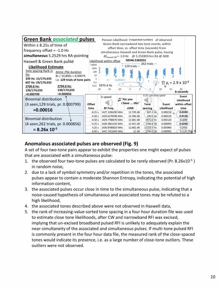
Green Bank associated pulses Within ± 8.25s of time offrequency offset = -1.0 Hz simultaneous 5.2529 hrs RA-pointing
Haswell & Green Bank pulse
Δ seconds
58346.5382031
(≈expected number)
Tone spacing Rank in file339 Hz: 15/174,033607 Hz: 29/174,0332700.8 Hz:139/174,033 =0.000799
Δtime /file duration8s / 10,800s = 0.00074i.e. 129 trials of tone pairs
Binomial distribution(3 seen,129 trials, pr. 0.000799)
=0.00016
Likelihood Estimate
Binomial distribution(4 seen,262 trials, pr. 0.000856)
= 8.26x 10⁻⁵
129 trials
2794.0 Hz:149/174,033 =0.000856
262 trials
outliers
Likelihood within offset
0.25 s per tone speed ¼ speed
ΔfHaswell-GB = -1.0 Hz
Fig. 9
∏ pi = 2.9 x 10⁻⁸
65975.4 Hz
“For you I have ... this”
♫
Anomalous associated pulses are observed (Fig. 9)A set of four two-tone pairs appear to exhibit the properties one might expect of pulses that are associated with a simultaneous pulse: 1. the observed four two-tone pulses are calculated to be rarely observed (Pr. 8.26x10⁻⁵ )
in random noise, 2. due to a lack of symbol symmetry and/or repetition in the tones, the associated
pulses appear to contain a moderate Shannon Entropy, indicating the potential of high information content,
3. the associated pulses occur close in time to the simultaneous pulse, indicating that a noise-caused hypothesis of simultaneous and associated tones may be refuted to a high likelihood,
4. the associated tones described above were not observed in Haswell data,5. the rank of increasing-value-sorted tone spacing in a four hour duration file was used
to estimate close tone likelihoods, after CW and narrowband RFI was excised, implying that un-excised broadband pulsed RFI is unlikely to adequately explain the near-simultaneity of the associated and simultaneous pulses. If multi-tone pulsed RFI is commonly present in the four hour data file, the measured rank of the close-spaced tones would indicate its presence, i.e. as a large number of close-tone outliers. These outliers were not observed.
10

A relationship between highly anomalous associated pulses and one of the two near-Rigel-pointing simultaneous pulses (described in Fig. 5) appears evident. Simultaneous ±1.0 Hz offset pulses occur randomly due to noise, on average, at approximately twenty-seven hour intervals, (97,200 seconds) while a highly unlikely multi-tone event (Pr. 8.26 x 10⁻⁵ in seventeen seconds) occurred at Green Bank, i.e. within ±8.25 s of the simultaneous Haswell-Green Bank pulse. The simultaneous and associated events appear to be time-correlated.
The four close-tone pairs’ noise likelihood of 8.26 x 10⁻⁵ is calculated using the binomial distribution and a common event probability, based on the noise-likelihood of the 2794.0 Hz tone spacing. The expected composite multi-tone likelihood value is significantly lower than the calculated composite likelihood, due to the unlikely presence of the closer tone spacing pairs, at 607.2 and 339.0 Hz, given the probability as the 2794.0 Hz tone pair.During system validation, a comparison of post-RFI-excision tone spacing likelihood, in sky data, to the calculated probability of noise-induced Poisson close tone spacing, has been examined, with close match of sky noise to theory. Evidence of time-correlated two-tone bursting signals does not appear within the files examined for such anomalies, except for the anomalies described near RA 5.25, and anomalies expected due to a noise model.
Further analysis is required, and potential equipment issues and assumptions need to be questioned, as a multi-tone transmit-receive mechanism using simultaneous and associated pulses appears to be present in the observed data, implying a powerful signal identification and RFI amelioration mechanism might exist.
10
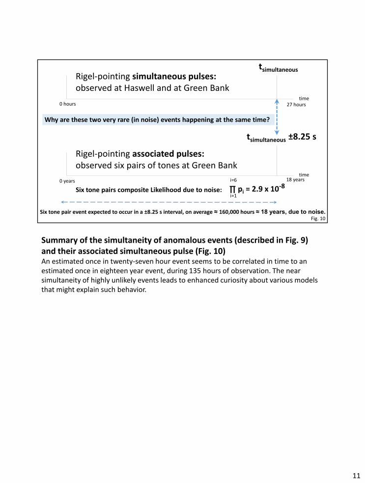
Rigel-pointing simultaneous pulses: observed at Haswell and at Green Bank
Rigel-pointing associated pulses:observed six pairs of tones at Green Bank
∏ pi = 2.9 x 10⁻⁸Six tone pairs composite Likelihood due to noise:
i=1
i=6
Six tone pair event expected to occur in a ±8.25 s interval, on average ≈ 160,000 hours ≈ 18 years, due to noise.
Why are these two very rare (in noise) events happening at the same time?
time
time
Fig. 10
tsimultaneous
tsimultaneous ±8.25 s
0 hours
0 years
27 hours
18 years
Summary of the simultaneity of anomalous events (described in Fig. 9) and their associated simultaneous pulse (Fig. 10)An estimated once in twenty-seven hour event seems to be correlated in time to an estimated once in eighteen year event, during 135 hours of observation. The near simultaneity of highly unlikely events leads to enhanced curiosity about various models that might explain such behavior.
11

MJD IRIG Frequency MHz >12dB SNR dB Δf FFT bins ln(2)Δf/Δf50
58346.53820310 1407.4044988 12.16 1987630 1.7144
58346.53820310 1407.7067725 12.183 81141 0.0700
58346.53820310 1407.9347268 12.854 61191 0.0528
58346.53820310 1420.4539560 13.213 690637 0.5957
58346.53820310 1420.5810294 12.674 34111 0.0294
58346.53820310 1423.8617770 12.038 880669 0.7596
58346.53820310 1424.1481364 12.278 76869 0.0663
58346.53820310 1432.5168036 12.361 343015 0.2959
58346.53820310 1432.9764746 12.651 123392 0.1064
58346.53820310 1440.8468805 12.045 1339655 1.1555
58346.53820310 1441.0708897 12.265 60132 0.0519
58346.53820310 1447.3290980 12.495 86917Spacing low due 1447.005
MHz RFI
Fig. 11
Rigel-pointing low frequency spaced pulses observed at Green Bank @ Δt = 0.0 seconds relative to time of simultaneous Green Bank & Haswell ΔfHaswell-GB = -1.0 Hz pulse
Poisson Likelihood of a tone spacing event in noise
Simultaneous Haswell&Green Bank pulse, expected due to noise at average 27 hour intervals
Number seen (in 20 tries)
Event Probability BinomDist
1 0.0294 0.33352 0.0519 0.19613 0.0528 0.06674 0.0663 0.03125 0.0700 0.01266 0.1064 0.0116
Composite likelihood
BinomDist(6,20, @ Pr. 0.0468) = 0.0002082
Average Pr.
Average once in 15 year event due to noise, if seen at time of simultaneous pulse
Additional anomalous pulses observed at Green Bank (Fig. 11)A set of additional anomalous pulses were observed at Green Bank at the same time as one of the Rigel-pointing simultaneous pulses, i.e. the simultaneous pulse correspondingto RA 5.2529 having other associated pulses described in Fig. 9 and Fig. 10.
Twelve anomalous tones were observed at Green Bank at the time of the RA 5.2529 simultaneous pulse at Green Bank and Haswell, among a set of twenty pulses, including the simultaneous pulse. An average probability of the close spaced pair events may be estimated to be 0.0468, yielding a likelihood of observing a similarly anomalous combination of pairs, at approximately two events in ten thousand simultaneous pulse event trials, itself a 27 hour average time interval event, given a noise cause.
12
Green Bank associated pulses re: RA 5.1838 hr (ΔfHaswell-GB = -0.2 Hz) at time of simultaneous pulse i.e. @ MJD 58345.53806130
Offset
Time RF Freq. cSNR
Tone
Spacing Event Likelihood
Event
Likelihood
within offset
frequency
0 s 1408.0909692 MHz 12.766 dB 2171903 8090969.2 Hz 2.493405525
0 s 1409.3006417 MHz 12.106 dB 324719 1209672.5 Hz 0.372786514
0 s 1409.7767003 MHz 12.217 dB 127791 476058.6 Hz 0.14670765
0 s 1410.0691803 MHz 12.941 dB 78512 292480.0 Hz 0.090133977
0 s 1410.3755482 MHz 13.642 dB 82240 306367.9 Hz 0.094413825 0.003745399
0 s 1414.4826546 MHz 12.381 dB 1102493 4107106.5 Hz 1.265692868
0 s 1420.6385441 MHz 12.673 dB 1652459 6155889.5 Hz 1.897069253
0 s 1421.4794949 MHz 12.301 dB 225741 840950.8 Hz 0.259156996
0 s 1424.5024636 MHz 13.375 dB 811472 3022968.8 Hz 0.931592603
0 s 1426.5113376 MHz 12.346 dB 539253 2008874.0 Hz 0.61907756
0 s 1428.0339979 MHz 12.014 dB 408736 1522660.3 Hz 0.469240385
0 s 1430.7576656 MHz 12.078 dB 731129 2723667.8 Hz 0.839356587
0 s 1432.9897180 MHz 12.592 dB 599162 2232052.4 Hz 0.687854771
0 s 1440.9286693 MHz 13.293 dB 2131096 7938951.3 Hz 2.446557946
0 s 1445.0470410 MHz 12.769 dB 1105517 4118371.8 Hz 1.269164505
0 s 1447.0053740 MHz 18.865 dB 525686 1958333.0 Hz 0.603502264
Simultaneous pulse
FFT Δbins
13.642 dB rank 2,001/151,517Pr. (noise) ≈ 0.013
Noise-caused
product multiplied by 3 because the four pulsescould have been here
continuous CW RFI
typical tone spacingdue tonoise
atypical
Fig. 12
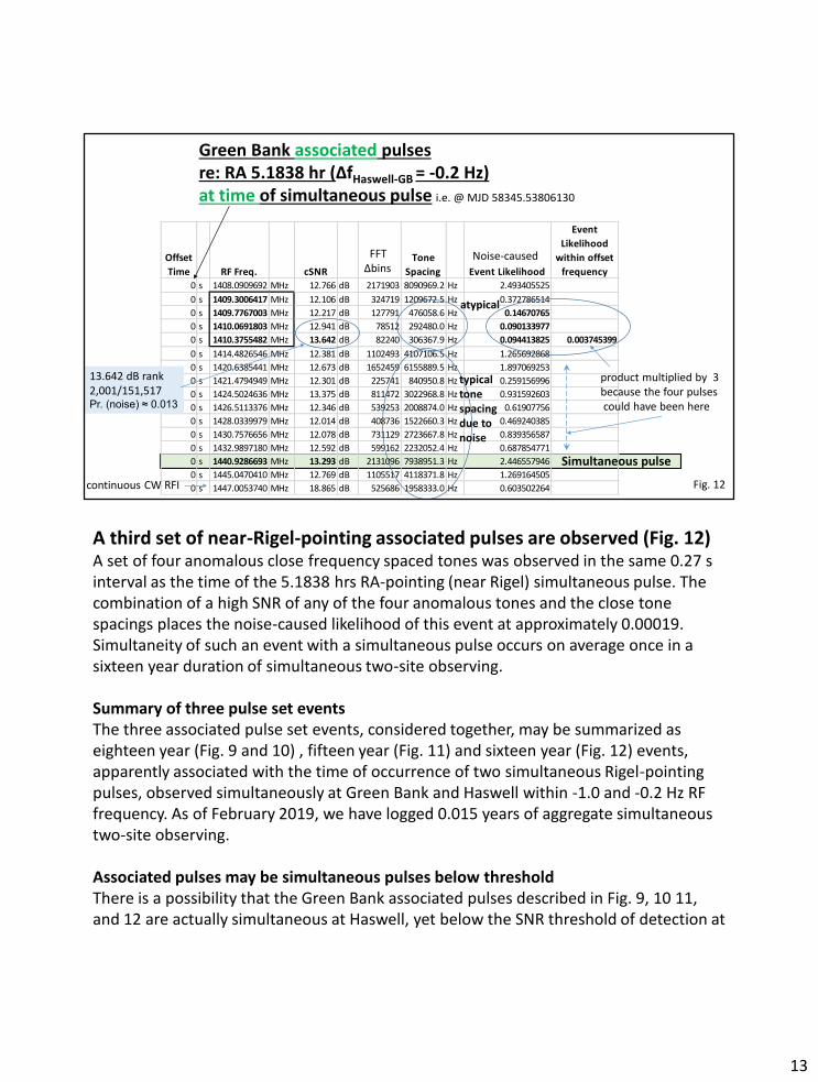
A third set of near-Rigel-pointing associated pulses are observed (Fig. 12)A set of four anomalous close frequency spaced tones was observed in the same 0.27 s interval as the time of the 5.1838 hrs RA-pointing (near Rigel) simultaneous pulse. The combination of a high SNR of any of the four anomalous tones and the close tone spacings places the noise-caused likelihood of this event at approximately 0.00019. Simultaneity of such an event with a simultaneous pulse occurs on average once in a sixteen year duration of simultaneous two-site observing.
Summary of three pulse set eventsThe three associated pulse set events, considered together, may be summarized as eighteen year (Fig. 9 and 10) , fifteen year (Fig. 11) and sixteen year (Fig. 12) events, apparently associated with the time of occurrence of two simultaneous Rigel-pointing pulses, observed simultaneously at Green Bank and Haswell within -1.0 and -0.2 Hz RF frequency. As of February 2019, we have logged 0.015 years of aggregate simultaneous two-site observing.
Associated pulses may be simultaneous pulses below thresholdThere is a possibility that the Green Bank associated pulses described in Fig. 9, 10 11, and 12 are actually simultaneous at Haswell, yet below the SNR threshold of detection at
13
Haswell. Six two-tone pairs at RA 5.2529 hrs (Fig. 9), twelve pulses described in Fig. 11, and the quad pulse set at 5.1838 hrs (Fig. 12), i.e. twenty-eight anomalous pulses, do not appear in data captured at the Haswell receive site. The absence of observation at Haswell leads to a thought that associated pulses may not be intentionally transmitted as simultaneous pulses to both telescope sites.
There is a possibility that polarization mismatch, bin straddling, and/or pointing differences account for the apparent scarcity of simultaneous pulses, given the high number of anomalous pulses. This is an idea that is under investigation.
Rician statistical modeling of simultaneous and associated pulses, considering RFI, SNR and polarization, is expected to refute, or support, simultaneous and associated pulses’ hypotheses.
13

1.1 58575.91094040 1395.0271226 11.198 2.136 6.514 -1.616 12.854 -5.8 5.2706305
1.2 58575.91094040 1395.0278081 11.156 -1.193 2.368 -7.062 11.913 -5.8 5.2706305
φ.site MJD pre-Doppler Freq. (MHz) SNR1 (dB) SNR2 SNR3 SNR4 comp.SNR Δfreq(Hz) RA (hrs)
April 2, 2019 simultaneous pulse ΔfHaswell-GB =-5.8 Hzat Green Bank and Haswell (a third simultaneous pulse)
Fig. 13
≈Rigel & HIP 24472pointing ∆f = -5.8 Hz
Green Bank
Haswell
Are there pulses associated with these simultaneous pulse elements?
130 simultaneous pulse pairs were observed in April 2019 with measured |∆f| < 7500 Hzhaving a target RA 5.181 to 5.271 hours. ----------------------------------------------------------------------------------------
Likelihood of target RA, April 2019, simultaneous pulse measuring |∆f| < 5.8 Hz = 0.101
7th highest SNR GB pulse, of 130 GB pulsesNoise Likelihood of SNR and Δf: 0.0108, GB and Haswell
April 2, 2019 Observations (Fig. 13)A simultaneous pulse was observed on April 2, 2019 while pointing approximately at the Right Ascension of Rigel. This “third” approximate Rigel pointing simultaneous pulse has an estimated likelihood of occurring, assuming measured sky data adheres to a Gaussian noise model, during an RA sweep through the target pointing direction, in April 2019 observations, of 0.101. The higher than expected SNR of the Green Bank pulse reduces the likelihood of the pulse due to a Gaussian noise model, having Raleigh amplitude statistics, to 0.0054 for Green Bank pulses and 0.0108 considering both Haswell and Green Bank pulses. The Gaussian noise model is unlikely to explain this third pulse. The April, 2019 simultaneous pulse is moderately rare in noise, when considered in isolation. Non-isolated considerations, including associated pulses occurring during the same time sample window, are discussed further in this paper.
The Rigel direction was scanned a total of eight times during the full Nov. 2017 through April 2019 observations, twice each in 8/2018, 11/2018, 1/2019 and 4/2019. SNR thresholds were lowered by 0.2 dB in April 2019 observations, resulting in a higher number of April 2019 simultaneous pulses in the data, all else equal.
Estimate of likelihood of simultaneous pulses given RFI and ETI models depends on
14

assumptions about signal transmitter duty cycle.
The difference in Haswell and Green Bank measured RF frequency is -5.8 Hz, a significantly higher magnitude offset than expected, given average residual frequency noise, and modeled pointing direction Doppler offsets. Normally, such a result would be rejected from further consideration. However, there are several partial unknowns in the experimental system, as the system tests multiple models each within multiple hypotheses:
1. It is not quantifiably known how a variation in received GPS satellite constellations, and/or geometric quality, might induce a rare and momentary shift in short term GPS-locked OCXO frequency,
2. Observations, Shannon’s Law and speculation contributes to the idea that a high channel capacity communication system need not transmit geographically spaced simultaneous pulses on exactly the same frequency,
3. Doppler offset of near-Earth space-based RFI may be present, assuming that the signal’s propagation directions fall within the two antennas’ approximate beamwidths, and
4. The anomalous pulses may be due to noise.
The pre-Doppler frequency values in the table are data produced by the pulse capture systems before site-differential sample clock offset and Doppler-induced corrections were included in post-processing software.
A non-noise model statistical significance of this third pulse depends on a presence of associated pulses, analyzed in the next section.
14

1.2 58575.9109404 1394.9009582 11.529 8.117 -1.751 -1.677 13.298
1.2 58575.9109404 1395.0278081 11.156 -1.193 2.368 -7.062 11.913 0.1268499 0.0316212161.2 58575.9109404 1396.6646299 11.091 -1.646 8.634 2.105 13.189 1.6368218 0.408027881.2 58575.9109404 1403.4137458 11.207 -10.281 3.196 0.117 11.871 6.7491159 1.6824234961.2 58575.9109404 1404.4054814 11.695 3.882 1.769 -3.296 12.724 0.9917356 0.2472204211.2 58575.9109404 1408.4641740 11.476 3.004 -6.675 5.158 12.111 4.0586926 1.011753227
1.2 58575.9109404 1409.0221480 11.589 -9.047 1.739 -9.307 12.051 0.557974 0.13909208
1.2 58575.9109404 1409.0238094 11.22 3.22 2.8 -3.656 12.367 0.0016614 0.0004141551.2 58575.9109404 1409.7591966 11.29 -10.556 2.792 0.899 11.889 0.7353872 0.1833177441.2 58575.9109404 1412.1208034 11.715 -9.866 -5.46 -6.127 11.827 2.3616068 0.5887027021.2 58575.9109404 1413.2985801 12.11 3.605 -5.157 -12.411 12.754 1.1777767 0.2935968541.2 58575.9109404 1419.7278462 11.628 -4.934 2.339 0.025 12.196 6.4292661 1.6026911541.2 58575.9109404 1421.7308640 11.533 2.574 -4.1 -8.726 12.156 2.0030178 0.49931343
1.2 58575.9109404 1430.0492100 11.74 -2.296 -4.96 -1.149 11.997 8.318346 2.073602078
1.2 58575.9109404 1430.2444264 11.03 3.543 4.841 1.717 12.55 0.1952164 0.0486636571.2 58575.9109404 1431.0416237 11.271 -6.717 3.898 0.261 12.06 0.7971973 0.1987258021.2 58575.9109404 1434.5924102 11.303 3.04 -14.67 4.732 11.916 3.5507865 0.885142102
1.2 58575.9109404 1438.1721981 11.165 3.989 -4.802 -4.68 12.018 3.5797879 0.892371588
1.2 58575.9109404 1438.4109333 11.442 -13.092 4.305 -4.807 12.222 0.2387352 0.0595120481.2 58575.9109404 1442.1725713 11.365 1.765 1.113 -7.247 12.171 3.761638 0.9377032861.2 58575.9109404 1446.8812451 11.661 -7.393 1.338 -1.665 12.096 4.7086738 1.1737809151.2 58575.9109404 1448.4182924 11.899 -1.178 0.731 -2.724 12.413 1.5370473 0.3831560361.2 58575.9109404 1449.0795128 11.504 -6.434 1.454 -1.014 11.976 0.6612204 0.1648294021.2 58575.9109404 1453.0215815 11.442 5.684 5.692 -0.593 13.294 3.9420687 0.9826811541.2 58575.9109404 1454.5479186 11.077 5.61 -1.271 -2.309 12.355 1.5263371 0.380486191
Haswell associated pulses at the time of the RA 5.2706305 simultaneous ( Δf = -5.8 Hz) pulseφ.site MJD pre-Doppler Freq. (MHz) SNR1 (dB) SNR2 SNR3 SNR4 comp.SNR Δfreq(MHz) Poisson Likelihood
Fig. 14
Δf Haswell-GB = 1.9194 kHz
April 2, 2019 Simultaneous and Associated Pulses Observed at Haswell (Fig. 14)Haswell associated pulses are evident at the time of the simultaneous pulse. One of the associated pulses, seen at both sites, is a pulse offset in frequency between Haswell and Green Bank at 1.9194 kHz, significantly less than the approximate 2 MHz expected value.
A set of associated pulses are observed in the Haswell data. A highly unlikely, in noise, 0.000414 likelihood close frequency spaced pair is observed. Its binomial distribution likelihood in seven tries is 0.0029.
The presence of a second simultaneous pulse with low offset, 1.9194 kHz, at the same time as the -5.8 Hz offset simultaneous pulse, seems unexpected in a noise model. Rare Poisson events occurring between two telescope sites are expected to have a likelihood at approximately the same likelihood as such events at one telescope site. This expectation may be gleaned by randomly splitting Poisson events into two Poisson event streams, each having double the Δf(50%), calculating the likelihood within one of the two streams, then multiplying by two to account for the halving of the number of points within each stream.
15
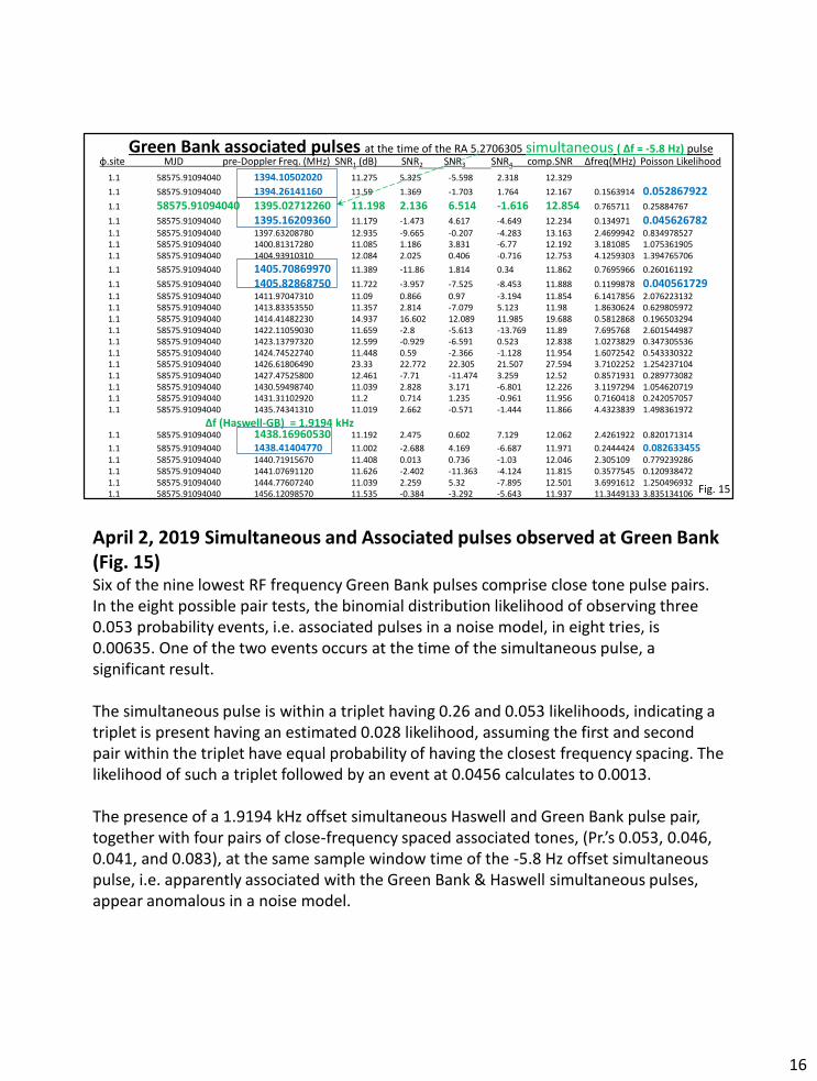
Fig. 15
1.1 58575.91094040 1394.10502020 11.275 5.325 -5.598 2.318 12.329
1.1 58575.91094040 1394.26141160 11.59 1.369 -1.703 1.764 12.167 0.1563914 0.0528679221.1 58575.91094040 1395.02712260 11.198 2.136 6.514 -1.616 12.854 0.765711 0.25884767
1.1 58575.91094040 1395.16209360 11.179 -1.473 4.617 -4.649 12.234 0.134971 0.0456267821.1 58575.91094040 1397.63208780 12.935 -9.665 -0.207 -4.283 13.163 2.4699942 0.8349785271.1 58575.91094040 1400.81317280 11.085 1.186 3.831 -6.77 12.192 3.181085 1.0753619051.1 58575.91094040 1404.93910310 12.084 2.025 0.406 -0.716 12.753 4.1259303 1.394765706
1.1 58575.91094040 1405.70869970 11.389 -11.86 1.814 0.34 11.862 0.7695966 0.260161192
1.1 58575.91094040 1405.82868750 11.722 -3.957 -7.525 -8.453 11.888 0.1199878 0.0405617291.1 58575.91094040 1411.97047310 11.09 0.866 0.97 -3.194 11.854 6.1417856 2.0762231321.1 58575.91094040 1413.83353550 11.357 2.814 -7.079 5.123 11.98 1.8630624 0.6298059721.1 58575.91094040 1414.41482230 14.937 16.602 12.089 11.985 19.688 0.5812868 0.1965032941.1 58575.91094040 1422.11059030 11.659 -2.8 -5.613 -13.769 11.89 7.695768 2.6015449871.1 58575.91094040 1423.13797320 12.599 -0.929 -6.591 0.523 12.838 1.0273829 0.3473055361.1 58575.91094040 1424.74522740 11.448 0.59 -2.366 -1.128 11.954 1.6072542 0.5433303221.1 58575.91094040 1426.61806490 23.33 22.772 22.305 21.507 27.594 3.7102252 1.2542371041.1 58575.91094040 1427.47525800 12.461 -7.71 -11.474 3.259 12.52 0.8571931 0.2897730821.1 58575.91094040 1430.59498740 11.039 2.828 3.171 -6.801 12.226 3.1197294 1.0546207191.1 58575.91094040 1431.31102920 11.2 0.714 1.235 -0.961 11.956 0.7160418 0.2420570571.1 58575.91094040 1435.74341310 11.019 2.662 -0.571 -1.444 11.866 4.4323839 1.498361972
1.1 58575.91094040 1438.16960530 11.192 2.475 0.602 7.129 12.062 2.4261922 0.820171314
1.1 58575.91094040 1438.41404770 11.002 -2.688 4.169 -6.687 11.971 0.2444424 0.0826334551.1 58575.91094040 1440.71915670 11.408 0.013 0.736 -1.03 12.046 2.305109 0.7792392861.1 58575.91094040 1441.07691120 11.626 -2.402 -11.363 -4.124 11.815 0.3577545 0.1209384721.1 58575.91094040 1444.77607240 11.039 2.259 5.32 -7.895 12.501 3.6991612 1.2504969321.1 58575.91094040 1456.12098570 11.535 -0.384 -3.292 -5.643 11.937 11.3449133 3.835134106
φ.site MJD pre-Doppler Freq. (MHz) SNR1 (dB) SNR2 SNR3 SNR4 comp.SNR Δfreq(MHz) Poisson LikelihoodGreen Bank associated pulses at the time of the RA 5.2706305 simultaneous ( Δf = -5.8 Hz) pulse
Δf (Haswell-GB) = 1.9194 kHz
April 2, 2019 Simultaneous and Associated pulses observed at Green Bank (Fig. 15)Six of the nine lowest RF frequency Green Bank pulses comprise close tone pulse pairs. In the eight possible pair tests, the binomial distribution likelihood of observing three 0.053 probability events, i.e. associated pulses in a noise model, in eight tries, is 0.00635. One of the two events occurs at the time of the simultaneous pulse, a significant result.
The simultaneous pulse is within a triplet having 0.26 and 0.053 likelihoods, indicating a triplet is present having an estimated 0.028 likelihood, assuming the first and second pair within the triplet have equal probability of having the closest frequency spacing. The likelihood of such a triplet followed by an event at 0.0456 calculates to 0.0013.
The presence of a 1.9194 kHz offset simultaneous Haswell and Green Bank pulse pair, together with four pairs of close-frequency spaced associated tones, (Pr.’s 0.053, 0.046, 0.041, and 0.083), at the same sample window time of the -5.8 Hz offset simultaneous pulse, i.e. apparently associated with the Green Bank & Haswell simultaneous pulses, appear anomalous in a noise model.
16

The associated pulses observed at Green Bank and Haswell, observed at the same time as the simultaneous pulse, appear to not be explained well using a noise model.
Short bursts of broadband random noise are not expected to generally contain close-frequency-spaced high SNR narrowband signals. High occupied bandwidth communication signals, of human design, containing high SNR narrowband identification signals, is a possible RFI model to explore.
16
5
10
15
20
25
30
1390 1400 1410 1420 1430 1440 1450 1460
10
11
12
13
14
15
1390 1400 1410 1420 1430 1440 1450 1460
11
12
13
14
1408.4 1408.6 1408.8 1409 1409.2 1409.4 1409.6 1409.8 Fig. 16
ΔfHaswell-Haswell = 1.6614 kHz zoom
ΔfHaswell-GB = -5.8 Hz ΔfHaswell-GB = 1.9194 kHzΔfHaswell-GB = -3.7878 kHz
Green Bank
Haswell
Haswellzoomed
suspected RFI due to persistence
zoom
April 2, 2019 simultaneous and associated pulses Rigel & HIP 24472 pointing
SNR dB
RF Freq.MHz
zoom
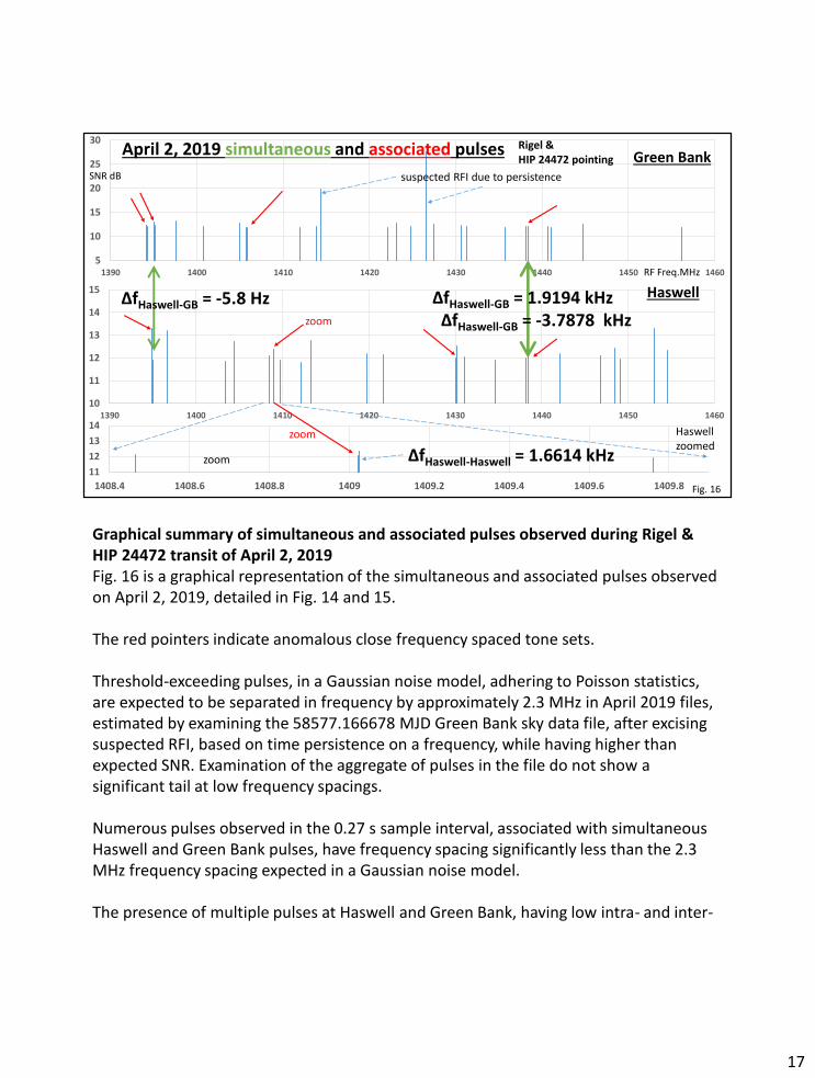
Graphical summary of simultaneous and associated pulses observed during Rigel & HIP 24472 transit of April 2, 2019 Fig. 16 is a graphical representation of the simultaneous and associated pulses observed on April 2, 2019, detailed in Fig. 14 and 15.
The red pointers indicate anomalous close frequency spaced tone sets.
Threshold-exceeding pulses, in a Gaussian noise model, adhering to Poisson statistics, are expected to be separated in frequency by approximately 2.3 MHz in April 2019 files, estimated by examining the 58577.166678 MJD Green Bank sky data file, after excising suspected RFI, based on time persistence on a frequency, while having higher than expected SNR. Examination of the aggregate of pulses in the file do not show a significant tail at low frequency spacings.
Numerous pulses observed in the 0.27 s sample interval, associated with simultaneous Haswell and Green Bank pulses, have frequency spacing significantly less than the 2.3 MHz frequency spacing expected in a Gaussian noise model.
The presence of multiple pulses at Haswell and Green Bank, having low intra- and inter-
17

telescope frequency offset, appears anomalous.
The observations, contrary to predictions, compel additional observations, analysis and tests of various signal models and potential equipment issues.
17

Fig. 16a
58575.9109404 simultaneous pulse
In a subsequent section in this paper, Pulsed and other Additive White Gaussian Noise source models, an analysis of short noise bursts is presented to try to explain a potential signal source model that produces close-spaced frequencies.
Fig. 16a and Fig. 16b are plots of the number of Green Bank and Haswell SNR threshold crossings near and around the time of the April 2 simultaneous Green Bank and Haswell pulse. If a broadband short duration (< 4x0.27 s) noise pulse is present at the receiver, the pulse is expected to produce an excess number of SNR Threshold crossings. The excess number was not observed. The simultaneous pulse occurred at a time of a relative reduction in the number of SNR Threshold crossings.
18

Fig. 16b
58575.9109404 simultaneous pulse
19
Haswell – Green Bank pulse ∆RF frequency (Hz) vs. Right Ascension (hrs)± 4000 Hz ± 500 Hz ± 50 Hz ± 10 Hz
180 hour data 11/2017 - 4/2019 all SNRs
≈Rigel pointing
April 2, 2019
Green Bank – 3 dB beamwidth 1.1° meas.Haswell – 3 dB beamwidth 0.8° meas.
August 16, 2018
August 15, 2018
≈HIP 24472 pointing
Fig. 17
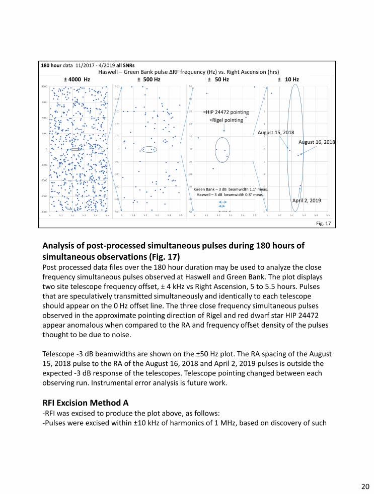
Analysis of post-processed simultaneous pulses during 180 hours of simultaneous observations (Fig. 17)Post processed data files over the 180 hour duration may be used to analyze the close frequency simultaneous pulses observed at Haswell and Green Bank. The plot displays two site telescope frequency offset, ± 4 kHz vs Right Ascension, 5 to 5.5 hours. Pulses that are speculatively transmitted simultaneously and identically to each telescope should appear on the 0 Hz offset line. The three close frequency simultaneous pulses observed in the approximate pointing direction of Rigel and red dwarf star HIP 24472 appear anomalous when compared to the RA and frequency offset density of the pulses thought to be due to noise.
Telescope -3 dB beamwidths are shown on the ±50 Hz plot. The RA spacing of the August 15, 2018 pulse to the RA of the August 16, 2018 and April 2, 2019 pulses is outside the expected -3 dB response of the telescopes. Telescope pointing changed between each observing run. Instrumental error analysis is future work.
RFI Excision Method A-RFI was excised to produce the plot above, as follows:-Pulses were excised within ±10 kHz of harmonics of 1 MHz, based on discovery of such
20
suspected RFI having SNR threshold crossings, persistent outside a point source antenna beamwidth response.-Suspected RFI in the range of 1447 MHz ± 100 kHz was excised.-Pulses that had a four contiguous sample minimum SNR in a one second interval of 0 dB were excised. The receiver bandwidth is matched to a pulse having a 0.27 second duration. Longer pulses, with >0 dB SNR over one second, are assumed to be continuous RFI. It is possible that true positives are excised, and possible that false positives appear as they may be related to excised RFI. -Method A does not excise RFI at frequencies close to the 1425.0 MHz LO, used in April 2019 simultaneous observations. Prior to April 2019, the local oscillator was 1400.0 MHz.
Follow-up of suspected excised RFI, compared to observed simultaneous pulses at multiple telescopes and repeated pointing directions, is future work.
20
∆f Hz
RA(hrs)-0.2 Hz Haswell and Green Bank
-1.0 Hz Green Bank
-5.8 Hz Green Bank+180.6 Hz
Haswell and Green Bank
+596.2 Hz Haswell and Green Bank
+1265.2 Hz Haswell and Green Bank
+1269.7 Hz Haswell
-1733.4 Hz Haswell and Green Bank
+248.6 Hz Haswell and Green Bank
Likelihood analysisNumber of pulses observed in ∆f of ±5.8 Hz = 4;∆f total range = 4000 Hz;Pr. pulse in ±5.8 Hz = 11.6/4000 = 0.0029;--------------------------------------
Binomial Distribution:4 seen in 59 tries =
2.74 x 10⁻⁵
-----------------------------Likelihood analysisNumber of pulses observed in ∆f of ±1.0 Hz = 3;∆f total range = 4000 Hz;Pr. pulse in ±1.0 Hz = 2/4000 = 0.0005;--------------------------------------
Binomial Distribution:3 seen in 59 tries =
3.95 x 10⁻⁶Fig. 18
Simultaneous data filtered to SNR >12.49 dB
1000 HzΔf range
1.3° sky angle
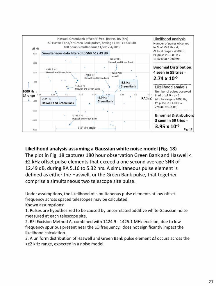
Likelihood analysis assuming a Gaussian white noise model (Fig. 18) The plot in Fig. 18 captures 180 hour observation Green Bank and Haswell < ±2 kHz offset pulse elements that exceed a one second average SNR of 12.49 dB, during RA 5.16 to 5.32 hrs. A simultaneous pulse element is defined as either the Haswell, or the Green Bank pulse, that together comprise a simultaneous two telescope site pulse.
Under assumptions, the likelihood of simultaneous pulse elements at low offset frequency across spaced telescopes may be calculated. Known assumptions:1. Pulses are hypothesized to be caused by uncorrelated additive white Gaussian noise measured at each telescope site.2. RFI Excision Method A, combined with 1424.9 - 1425.1 MHz excision, due to low frequency spurious present near the LO frequency, does not significantly impact the likelihood calculation.3. A uniform distribution of Haswell and Green Bank pulse element ∆f occurs across the <±2 kHz range, expected in a noise model.
21
4. The receiver systems and calculation methods do not contain errors, or induce anomalies, to affect likelihood calculations significantly.
Likelihood calculates to 2.74 x 10⁻⁵ given the four simultaneous pulse elements observed within ±5.8 Hz and calculates to 3.95 x 10⁻⁶ given the three pulse elements observed within ±1.0 Hz.
Some of the pulse elements captured in the plot did not exceed the 12.49 dB SNR threshold at both Haswell and Green Bank, while some did. Those pulses that exceeded the SNR threshold at both sites are indicated by the larger datapoint marker. Three points, a Green Bank Haswell pair and a Haswell pulse, near 1270 Hz offset, are shown with the smaller datapoint marker so that the otherwise larger Green Bank Haswell pair marker does not obscure the Haswell pulse marker.
The likelihood of observing pulse elements in the plot should normally be multiplied by the number of possible pointing directions in the data, approximately 360, to estimate the likelihood of seeing the anomalous points in any pointing direction, assuming that no prior knowledge uniquely identifies the 5.25 hour RA for interest. Assuming 360 -7.6°declination pointing directions, the all-RA estimate yields 0.0099 and 0.0014 likelihood for the four and three elevated SNR pulse sets, respectively. The values may be multiplied by 0.67 if a 5.18 to 5.28 hours RA range is used to assume 240 possible pointing directions, in lieu of 360 pointing directions.
Alternatively, one of the two -0.2 Hz offset elevated SNR pulses, Green Bank or Haswell, may be considered as an identifier of an approximate 5.18 hour RA pointing direction of interest. Using this prior, the modified estimate yields 0.00067 and 0.00042 likelihood of observing, in noise, three and two additional elevated SNR pulse sets, respectively, using binomial calculations.
A telescope-site-uncorrelated continuous noise hypothesis, having an Additive White Gaussian Noise model, adhering to Poisson process, exponential frequency spacing and Rayleigh amplitude statistics, appears to be refuted, given the observations, spectral and spatial signal analysis, priors and assumptions. Other noise and signal models and equipment issues are among candidate hypotheses.
Pulsed and other Additive White Gaussian Noise source modelsA burst of terrestrial or extraterrestrial broadband noise, during a 0.27 s sample interval, is a candidate hypothesis to explain the anomalous Haswell and Green Bank pulses, compelling an analysis of potential signal reception models. Signal reception has three contributing aspects: source spectra, propagation impairments, and receiver response.
Source spectra: A broadband pulsed noise source is similar to a broadband continuous noise source when a discrete time interval of the continuous source and pulsed source
21
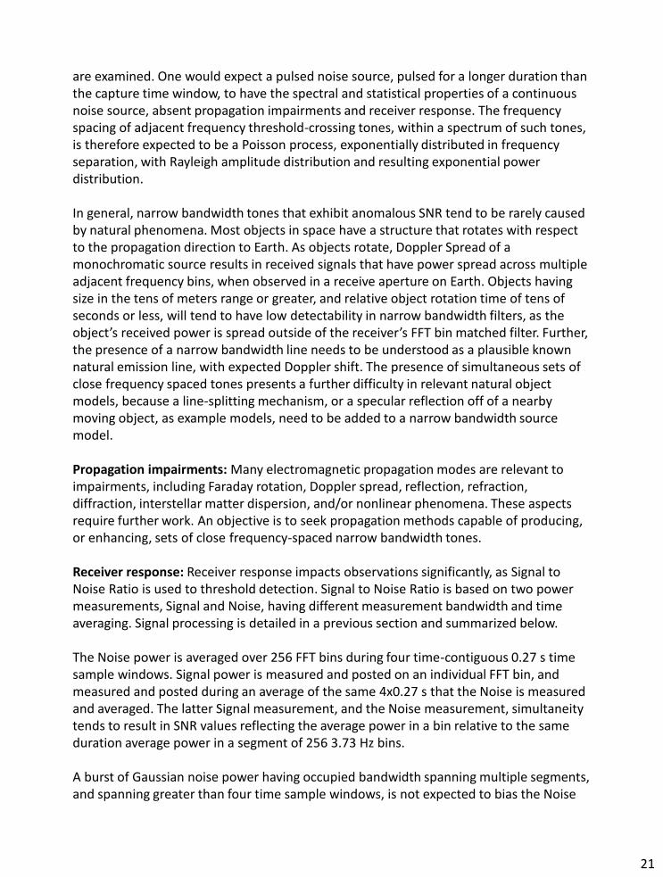
are examined. One would expect a pulsed noise source, pulsed for a longer duration than the capture time window, to have the spectral and statistical properties of a continuous noise source, absent propagation impairments and receiver response. The frequency spacing of adjacent frequency threshold-crossing tones, within a spectrum of such tones, is therefore expected to be a Poisson process, exponentially distributed in frequency separation, with Rayleigh amplitude distribution and resulting exponential power distribution.
In general, narrow bandwidth tones that exhibit anomalous SNR tend to be rarely caused by natural phenomena. Most objects in space have a structure that rotates with respect to the propagation direction to Earth. As objects rotate, Doppler Spread of a monochromatic source results in received signals that have power spread across multiple adjacent frequency bins, when observed in a receive aperture on Earth. Objects having size in the tens of meters range or greater, and relative object rotation time of tens of seconds or less, will tend to have low detectability in narrow bandwidth filters, as the object’s received power is spread outside of the receiver’s FFT bin matched filter. Further, the presence of a narrow bandwidth line needs to be understood as a plausible known natural emission line, with expected Doppler shift. The presence of simultaneous sets of close frequency spaced tones presents a further difficulty in relevant natural object models, because a line-splitting mechanism, or a specular reflection off of a nearby moving object, as example models, need to be added to a narrow bandwidth source model.
Propagation impairments: Many electromagnetic propagation modes are relevant to impairments, including Faraday rotation, Doppler spread, reflection, refraction, diffraction, interstellar matter dispersion, and/or nonlinear phenomena. These aspects require further work. An objective is to seek propagation methods capable of producing, or enhancing, sets of close frequency-spaced narrow bandwidth tones.
Receiver response: Receiver response impacts observations significantly, as Signal to Noise Ratio is used to threshold detection. Signal to Noise Ratio is based on two power measurements, Signal and Noise, having different measurement bandwidth and time averaging. Signal processing is detailed in a previous section and summarized below.
The Noise power is averaged over 256 FFT bins during four time-contiguous 0.27 s time sample windows. Signal power is measured and posted on an individual FFT bin, and measured and posted during an average of the same 4x0.27 s that the Noise is measured and averaged. The latter Signal measurement, and the Noise measurement, simultaneity tends to result in SNR values reflecting the average power in a bin relative to the same duration average power in a segment of 256 3.73 Hz bins.
A burst of Gaussian noise power having occupied bandwidth spanning multiple segments, and spanning greater than four time sample windows, is not expected to bias the Noise
21

power measurement that affects the likelihood that a burst-associated threshold crossing will occur. In general, one would expect that the spectral properties of the source will be reflected in the SNR measurement output. In summary, anomalous close frequency spaced tones are not expected in such a broadband pulsed noise source, due to the SNR calculation method in receiver response. Simulated noise sources applied to the receiver software confirm this expectation.
Short pulsed noise sources are expected to produce a different result. If the noise pulse is shorter than 4x0.27 s, the 4x0.27 s averaged Noise measurement will be expected to be lower than the 0.27 s average noise during the noise pulse, producing an expected excess of SNR threshold crossings during the 0.27 s the noise pulse is active. An increased absolute number of SNR threshold crossings are expected, together with a resulting increase in the absolute number close-frequency-spaced tones. These expectations have been confirmed with a simulated pulsed noise source applied to the receiver software.
Fig. 16a and Fig. 16b indicate that an excess number of SNR thresholds did not occur at the time of the April 2 simultaneous pulse, at either Haswell or Green Bank, implying that a shorter than 4x0.27s noise pulse was not present, and is not likely to explain the close spaced tones observed at the time of the simultaneous pulse, described in Fig. 14, 15, and 16. The close spaced tones appear to indicate discrete signals, not part of a broadband pulse of energy. It appears to be intentional that one of the low spaced tone sets would be -5.8 Hz offset in frequency at Haswell and Green Bank. This close an offset is not expected, as there are only several apparent anomalous close spaced tones available at each site, Green Bank and Haswell, during the sample window, to contribute to a close tone offset between sites. (Fig. 16). The -5.8 Hz offset therefore seems to be intentionally placed, possibly as an indicator of some sort.
Analysis and/or simulations of other aspects of receiver response, including spurious signals, quantization noise, limiting and other distortion response due to in-band and out-of-band RFI, are further work items.
21

Red dwarf star HIP 24472 is 73.23 light years distant, 0.28° off beam center on April 2, 2019 @ MJD 58575.91094 @ Green Bank
HIP 24472
Rigel
Fig. 19
Stellarium plot of the sky during the April 2, 2019 -5.8Hz offset simultaneous Green Bank and Haswell pulse (Fig. 19)The MJD and declination of the anomalous observations may be used to examine the Green Bank Forty Foot telescope pointing direction during the time of the April 2, 2019 simultaneous pulse. HIP 24472 is a red dwarf star at 73.23 light years distance and is near the telescope’s central pointing direction.
22
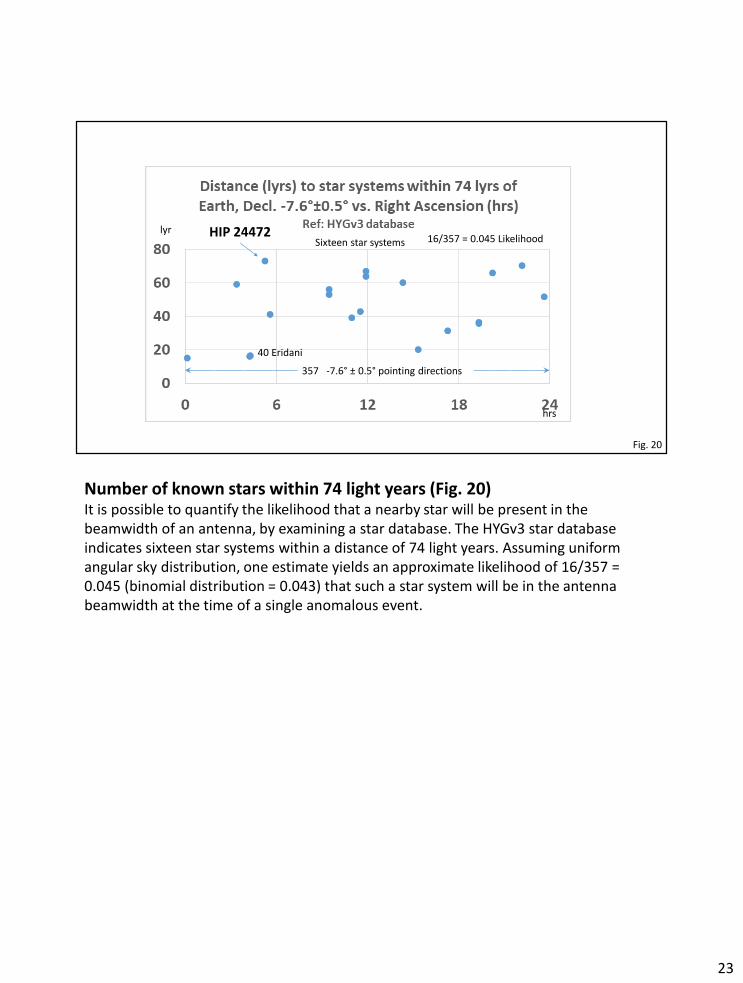
Fig. 20
HIP 24472
357 -7.6° ± 0.5° pointing directions
hrs
lyr
40 Eridani
Sixteen star systems 16/357 = 0.045 Likelihood
Number of known stars within 74 light years (Fig. 20)It is possible to quantify the likelihood that a nearby star will be present in the beamwidth of an antenna, by examining a star database. The HYGv3 star database indicates sixteen star systems within a distance of 74 light years. Assuming uniform angular sky distribution, one estimate yields an approximate likelihood of 16/357 = 0.045 (binomial distribution = 0.043) that such a star system will be in the antenna beamwidth at the time of a single anomalous event.
23

Bayesian Candidate-Model Inference
Pr 𝑴𝒐𝒅𝒆𝒍 𝒎 "𝑒𝑥𝑝𝑙𝑎𝑖𝑛𝑠" 𝑔𝑖𝑣𝑒𝑛 𝑫𝒂𝒕𝒂= Pr 𝑫𝒂𝒕𝒂 "explained", 𝑔𝑖𝑣𝑒𝑛 𝑴𝒐𝒅𝒆𝒍 𝒎
xPr(𝑀𝑜𝑑𝑒𝑙 𝑚 𝑏𝑒𝑙𝑖𝑒𝑓)
Pr(𝐷𝑎𝑡𝑎 𝑣𝑎𝑙𝑖𝑑)
Candidate-Models are selectively a null hypothesis and the alternate hypotheses
Given the Data and Model, solve this 3 factor equation, for each Model m:
Assume that Pr(Data Valid) ≈ 1 i.e. that Anomalous Data (“outliers” on the tail) are being
observed. If Pr(Data Valid) << 1, then all known Models will appear to explain the Data.
Model Prior Belief ValuesPr. N ≈ 1 except “outliers”
Pr. R ≈ increasing to 1- ?
Pr. E ≈ increasing to 1- ?
Pr. U ≈ decreasing to 0+?
This Pr() is a Likelihood Function,developed for each Model m
Candidate models Probability prior beliefs (Model m) Explanation
A. Model Noise + telescopes Probability Model N belief ≈ 1- i.e. good confidence e.g. a “good” null hypothesis. Does receiver noise and quiet sky explain data?
B. Model RFI + telescopes Probability Model R belief ≈ 1- to 0+ depending on RFI knowledge Does RFI into spaced antennas explain data?
C. Model ETI + telescopes Probability Model E belief ≈ 0+ to 1- over time Do the Drake Equation, Shannon’s Law & observations explain data?
D. Models Unknown Probability Model U belief ≈ 1- to 0+ over time Unknown-caused – Where are the “gotchas”?Natural objects having low Doppler Spread?
Model Likelihood FunctionsN: Rayleigh & Poisson statsR: Find & model RFIE: More observationsU: Find “gotchas”
Fig. 21
Anomalous data compels the analysis of multiple hypotheses (Fig. 21)Bayesian Inference may be used to compare hypotheses, given that each Model, related to its hypothesis, may explain observed Data, to a varying degree. Observed Data is considered to include simultaneous pulses, pulses apparently associated in frequency and time with simultaneous pulses, and other associated pulses.
As observational work progresses, model development and follow-up observations may provide a refutation of various hypotheses. For example, the noise hypothesis has a high Model belief, based on our knowledge of communication systems. However, the noise hypothesis produces a Model having an apparent low probability in explaining observed anomalous Data. If the anomalous Data is considered valid, the three factor Bayesian Inference then yields a low probability that the Noise Model explains the observed Data.
Bayesian Inference may be used to quantify the common understanding that “absence of evidence is not the same as evidence of absence”, as the former idea is based on limited experimental data, while the latter is based on models, data and inference, in an attempt to refute a hypothesis to a given statistical significance.
Various receiver antenna spacing may be implemented. It is expected that multi-
24
telescope observation of the same associated pulses should occur at close telescope spacing, if transmitted signals are celestially transmitted. The noise hypothesis may then be refuted to a statistical likelihood. Close antenna spacing, however, increases the probability that an RFI hypothesis, and its particular RFI Models, will explain the observed Data. Close antenna spacing and large antenna spacing may then be used together to selectively refute various hypotheses, to statistical significance.
An important effort in hypothesis development is to imagine models within each category of hypothesis. For example, a satellite-based RFI hypothesis includes reflective, intentional and unintentional transmission models.
Simultaneous narrow band pulse detection SETI systems provide a vehicle to refute RFI hypotheses, because the RFI models that include distant spaced telescopes, naturally filter RFI signals from the observed Data.
24
…
Unexpected observations compel multiple hypotheses,leading to experiments to try to refute the hypotheses.
Summary of one working hypothesis: “Associated” pulses are associated with “simultaneous” pulses
Telescope-similar, i.e. simultaneous pulses, are predicted at low noise-likelihood (full detectability pulses).
Telescope-different, i.e. associated pulses, are predicted at low noise-likelihood (partial information pulses).
What is guessed to be causing these pulses? Idea: ETI may be politely transmitting high information capacity, i.e. almost-noise-like,
spatially encoded signals to Earth to compel human cooperation, readily indicating ETI transmission motive: clearly indicate the cooperation directive in the first signals detected.
8.3x10⁻¹¹ radians angle subtended angle
7.1x10⁻¹³ radians between nulls of beams
1420 MHz 1 AU radius phased array
Example guessed ETI transmitter: 16.3 light years distant 40 Eridani, the home triple star system of Vulcan, ref: Star Trek.
≈100 beams in one dimension, ≈16,000 information beams to Earth
Transmit many beams of different information to all locations on Earth. Design signals that are easy to detect, yet no small set of antennas can decode to information.
Fig. 22
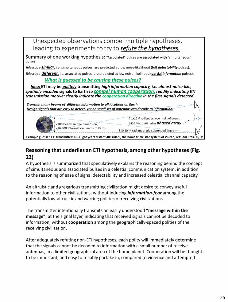
Reasoning that underlies an ETI hypothesis, among other hypotheses (Fig. 22)A hypothesis is summarized that speculatively explains the reasoning behind the concept of simultaneous and associated pulses in a celestial communication system, in addition to the reasoning of ease of signal detectability and increased celestial channel capacity.
An altruistic and gregarious transmitting civilization might desire to convey useful information to other civilizations, without inducing information-fear among the potentially low-altruistic and warring polities of receiving civilizations.
The transmitter intentionally transmits an easily understood “message within the message”, at the signal layer, indicating that received signals cannot be decoded to information, without cooperation among the geographically-spaced polities of the receiving civilization.
After adequately refuting non-ETI hypotheses, each polity will immediately determine that the signals cannot be decoded to information with a small number of receive antennas, in a limited geographical area of the home planet. Cooperation will be thought to be important, and easy to reliably partake in, compared to violence and attempted
25

domination by one polity. Information-fear is ameliorated as the “message in a message” is gleaned similarly by humans in all receiving polities: “Learn how to live together and cooperate with each other peacefully. You will learn more than you would otherwise.”
The idea that a polity’s controlled land and resources establish the power of a polity, becomes insignificant in light of the power of a planetary civilization cooperating among all polities to gain information about the universe. Civilizations that learn to cooperate on their home planet will be able to benefit from information provided by advanced celestial civilizations. Civilizations that do not cooperate among polities on their home planet will be left without useful information they may likely need to survive.
An example of a simultaneous and associated pulse transmitter model A distant intentional transmitter might expect a receiver entity, in control of a number of geographically spaced, single polarization receivers, to wish to ascertain the likelihood that received signals originate from a hypothetical geographically-multiplexed multi-frequency transmitter system. The receiver entity will be expected by the transmitter entity to develop a transmitter model that emulates the expected transmitter, and to compare received data to the data expected from the particular transmitter model.
As an example of a receiver-entity’s guessed transmitter model, a transmitter entity might hypothetically transmit tones that have equal polarization and power level across the overall target receiver area, e.g. a planet. The transmitted tones’ frequencies may be set geographically differently across the planet. A small number of the geographically-spaced tones might be assumed to be on the same, or very close frequencies, across the overall target receive area, to imply to the receiver entity that a single transmitter source exists, while ameliorating multi-source RFI, at the expense of a small reduction in overall channel capacity to the planet. Tones may be transmitted in close frequency spaced doublets, triplets, etc. to enhance their detectability at low SNR.
Given this transmitter model, if the total number of received tones, i.e. tones exceeding an SNR threshold, are measured to be approximately equal at each receiver site, the receiver entity might guess, given the prior assumptions, that the transmit-to-receive polarization mismatches are approximately equal at each receiver site. In general, statistics of the number of tones that cross SNR threshold at each site may be used to calculate the likelihood that a geographically-multiplexed transmitter model might explain the measured data, i.e. be refuted, or not, to statistical significance by the received data. For example, if a large number of tones exceed SNR threshold at one receiver site, while few tones exceed SNR threshold at a second receiver site, a receiver entity will likely suspect that polarization mismatch differences at the two receiver sites explain the measured results, given that all else is reasonably identical at the receiver sites.
As always, such a chosen transmitter model might explain the received data, while not
25

implying that the data is best explained by the particular model, absent Bayesian Inference.
Quantification and modeling of the expected parameters of simultaneous and associated pulses is underway, to aid in the refinement of further experimental procedures and refutation of various hypotheses, to statistical significance.
25

…
8.3x10⁻¹¹ radians angle subtended angle
7.1x10⁻¹¹ radians between nulls of beams
1420 MHz .01 AU radius close-spaced phased array
Example guessed ETI transmitter: 16.3 light years distant 40 Eridani, HIP 19849
≈1 beam in one dimension, ≈1 information beam to Earth
Fig. 22a
Celestial Channel Capacity depends on transmitter antenna spacing
8.3x10⁻¹¹ radians angle subtended angle
7.1x10⁻¹³ radians between nulls of beams
1420 MHz 1 AU radius wide-spaced phased array ≈100 beams in one dimension, ≈16,000 information beams to Earth
radio frequency
radio frequency
many narrow beams
single wide beam
Normalized total received energy = 16,000
Normalized total received energy = 1
Celestial Channel Capacity depends on transmitter antenna element spacing (Fig. 22a)
We are able to compare two celestial transmitter scenarios. In one system, a phased array has elements spanned out to one astronomical unit (AU), to produce many low area separate receive spots on a distant planet. In a second system, the same antenna elements are brought together by a factor of 100, for example, to produce a single wide beam that covers a distant planet with a single receive spot.
Celestial channel capacity may be estimated by the number of possible messages that may be encoded in a set of received signals. In the graphical example in Fig. 22a, each of the set of close spaced tones may encode one of 220 = 1048576 messages if the ratio of the tones’ frequency resolution to maximum occupied bandwidth is equal to approximately 220 . This represents a channel message rate of 20 bits per symbol. A few additional
26
bits may be added due to the presence of the second tone in a tone set, and third tone, etc. The Shannon channel capacity is an upper bound on the maximum possible channel message rate in a signal to noise ratio and bandwidth limited system, given that the noise is Additive White Gaussian Noise (AWGN), and the message is encoded for a long duration. The transmitter is assumed to produce a transmission rate of detectable signals at the receiver, less than the channel capacity. For example, close frequency-spaced tone sets may be transmitted, unlikely to occur in AWGN.
In the following system comparisons, as assumption is made that the signal to noise ratios of the tone sets, in the example received signal, measure at the signal to noise ratio of a given Shannon channel capacity, e.g. 20 bits. This is not strictly true, as message rate and Shannon Capacity are not equal, yet the assumption allows channel capacity comparisons to be made between systems having differing antenna characteristics, e.g. differing transmitted energy levels. For example, if the transmitted energy level of one of two otherwise identical system, when doubled to provide an increase of received SNR from one to two, results in the Shannon Capacity increased by log2(3)/log2(2) , as predicted by Shannon’s Capacity Theorem.
Phasing of the coherent energy applied to each transmitter element allows the total transmit energy to produce one or more beams of propagating plane waves, resulting in one or more spots of energy on a distant receiver region. Transmit antenna elements are assumed to be randomly spaced to reduce grating lobes to a negligible level. Wide element spaced phased arrays do transmit energy in spurious lobes that, when summed, can be a significant portion of the total transmit energy. In aggregate, the spurious sideband energy is comparable to the energy in the grating lobes. Parseval’s Theorem applied to the propagation angle and aperture illumination (an approximate Fourier pair) can be used to quantify this.
Conservation of energy dictates that the total energy impinging onto all of the transmitter‘s illuminated spots on the distant planet and surrounding region is equal to the total transmitter energy, i.e. the total energy applied to all of the transmitter antenna elements.
As the transmitter antenna element spacing is increased, the coherently
26

summed E-Field at the intended receive aperture remains almost constant, i.e. at the center of a synthesized beam. The total energy in the receiver spot decreases as the spot size decreases, while the energy in a fixed aperture remains constant. The two spectral plots in Fig. 22b show this behavior. Four beams, separately synthesized to create four spots, converge to a single beam and receive spot, as transmit antenna element spacing is decreased.
At first glance, it appears that the information transferred from the transmitter to the planet is independent of transmitter element spacing. Close examination indicates that the information transferred is increased as the transmitter element spacing is increased. In the single beam scenario, a single set of composite tones are transferred. The information content of this signal may be computed by considering the number of possible symbols that may be transmitted. In the multi-beam scenario, the tone sets can be transmitted in different combinations of the four beams. There are 24 =16 different signals that may be created in the multi-beam system. The multi-beam signal therefore transfers at least four additional information bits, compared to the single beam scenario, all else equal, for example, with equal energy of the transmitter signals in the single and multi-beam scenarios.
The addition of several bits to a message that contains twenty bits understates the potential channel capacity gain due to the orthogonality of receive and transmit channels. Modern communication systems utilize multiple transmit and received antennas, to multiply the potential channel capacity between transmitter and receiver entities. Each identical orthogonal channel has the capability of providing a channel capacity at the Shannon Capacity Limit of the orthogonal channel. The rank of the transmitter to receiver antenna element transmission matrix is a measure of this channel orthogonality. In a rich scattering limit, a set of M transmit elements and N receive antenna elements can achieve an overall channel capacity multiple equal to the Min(M,N). The transmission matrix rank may be increased through scattering, or beam synthesis.
Synthesized beams in a phased array achieves a similar Min(M,N) multiplicative limit, depending on transmitter sidelobe energy and received signal to noise ratio. In the example above, using close-spaced readily
26
detectable tone pairs, the channel capacity of the distant-spaced antenna system may be 16,000 times the channel capacity of the close-spaced antenna system. To produce this multiplicative increase in channel capacity, the total transmitted energy needs to be increased by 16,000 times. Increased transmitter energy, by itself, increases the Shannon capacity of a single transmit to receive channel by a factor of log2(16,000) = 13.96 , far less than the factor of 16,000 capacity gain possible using multiple orthogonal transmit to receive antenna beams.
A potential issue is self-interference caused by the sidelobes of the transmit phased array. At 16,000 beams, it is likely that the combined sidelobes of one beam can raise the interference level in pointing directions corresponding to other beams. This problem may be ameliorated by using sparsely filled spectrum. Orthogonality of frequency is a powerful interference reduction mechanism, albeit limited by the available bandwidth of the transmitter and receiver systems. When frequency orthogonality is used by itself to increase channel capacity, the risk of interference increases, unless narrow transmit beam-widths are utilized.
It is expected that readily identifiable signals may be transmitted at higher energy levels than signals used to maximize capacity through utilization of bandwidth.
Orthogonal transmitter beams, pointing to a celestial destination is a natural way to greatly increase celestial channel capacity. Given technological limitations, it seems likely that such systems would be implemented by civilizations having a human level of communication system maturity.
26
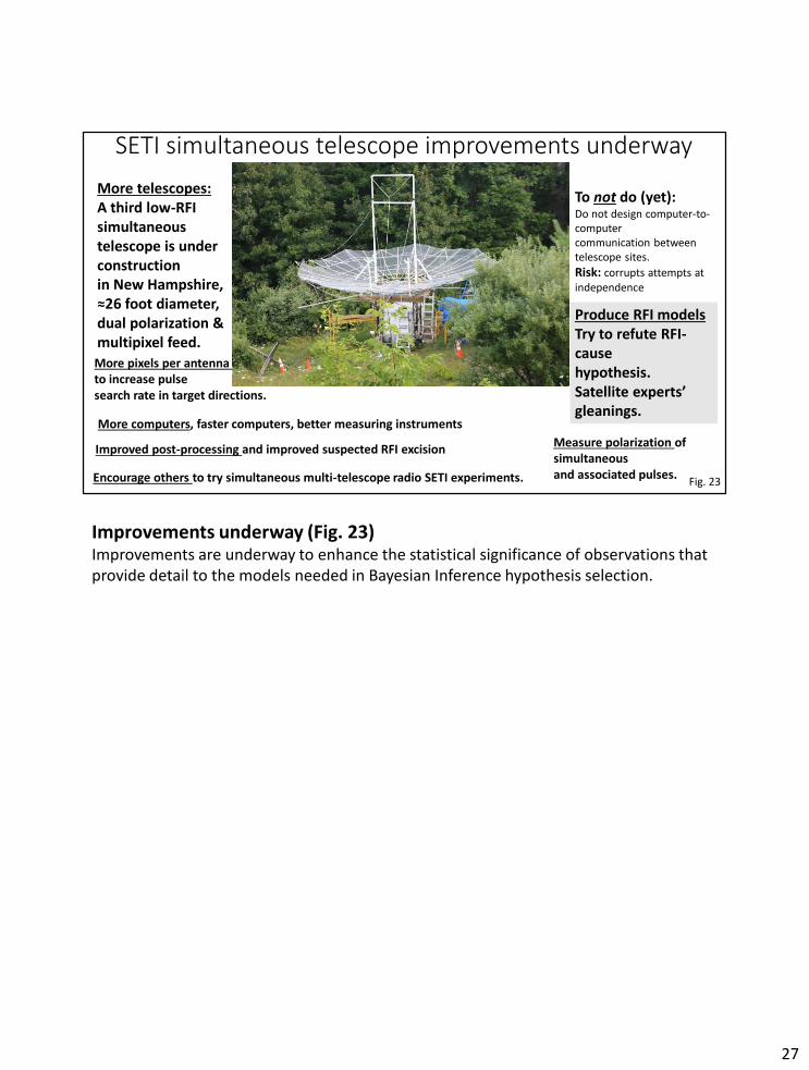
SETI simultaneous telescope improvements underway
More telescopes:A third low-RFI simultaneous telescope is under constructionin New Hampshire,≈26 foot diameter,dual polarization & multipixel feed.
More computers, faster computers, better measuring instruments
Measure polarization of simultaneous and associated pulses.
More pixels per antenna to increase pulse search rate in target directions.
Encourage others to try simultaneous multi-telescope radio SETI experiments.
To not do (yet):Do not design computer-to-computer communication between telescope sites.
Risk: corrupts attempts at independence
Improved post-processing and improved suspected RFI excision
Produce RFI models Try to refute RFI-cause hypothesis. Satellite experts’ gleanings.
Fig. 23
Improvements underway (Fig. 23)Improvements are underway to enhance the statistical significance of observations that provide detail to the models needed in Bayesian Inference hypothesis selection.
27

Thank You !!
Questions?
Thank youSteve Plock Deep Space Exploration Society teamGreen Bank Observatory teamfamily and friends
28