Embed Size (px)
Citation preview
UNIVERSITY OF SOUTHERN QUEENSLAND
RADIAL-BASIS-FUNCTION
CALCULATIONS OF HEAT AND VISCOUS
FLOWS IN MULTIPLY-CONNECTED
DOMAINS
A dissertation submitted by
LE CAO KHOA
B.Eng.(Hon.), Ho Chi Minh City University of Technology, VietNam, 2003
M.Eng.(Hon.), Ho Chi Minh City University of Technology, VietNam, 2005
For the award of the degree of
Doctor of Philosophy
February 2011

Dedication
To my family.

Certification of Dissertation
I certify that the idea, experimental work, results and analyses, software and
conclusions reported in this dissertation are entirely my own effort, except where
otherwise acknowledged. I also certify that the work is original and has not been
previously submitted for any other award.
KHOA LE-CAO, Candidate Date
ENDORSEMENT
A/Prof. NAM MAI-DUY, Principal supervisor Date
Prof. THANH TRAN-CONG, Co-supervisor Date
Dr. CANH-DUNG TRAN, External supervisor (CSIRO) Date

Acknowledgments
I would like to express my deepest gratitude to A/Prof. Nam Mai-Duy and
Prof. Thanh Tran-Cong, my principal supervisors, not only for their invalu-
able guidance throughout my research but also for their philosophical attitude
which has inspired my research interest. Undoubtedly, without their continuing
support and encouragement this thesis would not have been completed.
In addition, I wish to express my sincere thanks to Dr. Canh-Dung Tran for
acting his role as external supervisor, and to Prof. David Buttsworth and Ms.
Juanita Ryan for their kind supports.
I gratefully acknowledge the financial support provided by the University of
Southern Queensland (USQ) and the Commonwealth Scientific and Industrial
Research Organisation (CSIRO), including a USQ Research Excellence scholar-
ship, a Faculty of Engineering and Surveying (FoES) scholarship supplement, a
Computational Engineering and Science Research Centre (CESRC) scholarship
supplement, and a CSIRO Future Manufacturing Flagship Top Up scholarship.
Finally, I would like to dedicate this work to my parents. I am greatly indebted
to my family for much unconditional support, understanding and love over the
years and for endlessly encouraging me in academic pursuits.
Notes to Readers
To facilitate the reading of this thesis, a number of files are included on the
attached CD to provide animation of some numerical results in this thesis. The
contents of the CD include:
1. thesis.pdf: An electronic version of this thesis;
2. Chapter3-Circular-Circular-Annuli-velocity.wmv: An animation showing
the evolution of velocity field of the buoyancy flow in a concentric circular-
circular annulus using a Cartesian grid 36 × 36 (Pr = 0.71, Ra = 104)
(Section 3.4.3, Chapter 3);
3. Chapter3-Square-Circular-Annuli-velocity.wmv: An animation showing the
evolution of velocity field of the buoyancy flow in a concentric square-
circular annulus using a Cartesian grid 36 × 36 (Pr = 0.71, Ra = 105)
(Section 3.4.4, Chapter 3);
4. Chapter4-Rotating-cylinder.wmv: An animation showing the evolution of
the flow between a rotating circular cylinder and a fixed square cylinder
using a Cartesian grid 26× 26 (Section 4.5.1, Chapter 4).

Abstract
This PhD research project is concerned with the development of accurate and ef-
ficient numerical methods, which are based on one-dimensional integrated radial
basis function networks (1D-IRBFNs), point collocation and Cartesian grids,
for the numerical simulation of heat and viscous flows in multiply-connected
domains, and their applications to the numerical prediction of the material
properties of suspensions (i.e. particulate fluids). In the proposed techniques,
the employment of 1D-IRBFNs, where the RBFN approximations on each grid
line are constructed through integration, provides a powerful means of repre-
senting the field variables, while the use of Cartesian grids and point collocation
provides an efficient way to discretise the governing equations defined on com-
plicated domains.
Firstly, 1D-IRBFN-based methods are developed for the simulation of heat
transfer problems governed by Poisson equations in multiply-connected do-
mains. Derivative boundary conditions are imposed in an exact manner with
the help of the integration constants. Secondly, 1D-IRBFN based methods are
further developed for the discretisation of the stream-function - vorticity for-
mulation and the stream-function formulation governing the motion of a New-
tonian fluid in multiply-connected domains. For the stream-function - vorticity
formulation, a novel formula for obtaining a computational vorticity bound-
ary condition on a curved boundary is proposed and successfully verified. For
the stream-function formulation, double boundary conditions are implemented

Abstract v
without the need to use external points or to reduce the number of interior
nodes for collocating the governing equations. Processes of implementing cross
derivatives and deriving the stream-function values on separate boundaries are
presented in detail. Thirdly, for a more efficient discretisation, 1D-IRBFNs are
incorporated into the domain embedding technique. The multiply-connected
domain is transformed into a simply-connected domain, which is more suitable
for problems with several unconnected interior moving boundaries. Finally, 1D-
IRBFN-based methods are applied to predict the bulk properties of particulate
suspensions under simple shear conditions.
All simulated results using Cartesian grids of relatively coarse density agree well
with other numerical results available in the literature, which indicates that the
proposed discretisation schemes are useful numerical techniques for the analysis
of heat and viscous flows in multiply-connected domains.

Papers Resulting from the
Research
Journal Papers
1. N. Mai-Duy, K. Le-Cao and T. Tran-Cong (2008) A Cartesian grid tech-
nique based on one-dimensional integrated radial basis function networks
for natural convection in concentric annuli, International Journal for Nu-
merical Methods in Fluids, 57, p. 1709–1730.
2. K. Le-Cao, N. Mai Duy and T. Tran-Cong (2009) An effective integrated-
RBFN Cartesian-grid discretisation to the stream function-vorticity-temperature
formulation in non-rectangular domains, Numerical Heat Transfer, Part
B, 55, p. 480–502.
3. K. Le-Cao, N. Mai-Duy, C.-D. Tran and T. Tran-Cong (2010) Numer-
ical study of stream-function formulation governing flows in multiply-
connected domains by integrated RBFs and Cartesian grids, Computer
& Fluids Journal, 44(1), p. 32–42.
4. K. Le-Cao, N. Mai-Duy, C.-D. Tran and T. Tran-Cong (2010) Towards
the analysis of shear suspension flows using radial basis functions, CMES:
Computer Modeling in Engineering & Sciences, 67(3), p. 265–294.

Published Papers Resulting from the Research vii
Conference Papers
1. K. Le-Cao, N. Mai-Duy and T. Tran-Cong (2007) Radial basis function
calculations of buoyancy-driven flow in concentric and eccentric annuli. In
P. Jacobs, T. McIntyre, M. Cleary, D. Buttsworth, D. Mee, R. Clements,
R. Morgan and C. Lemckert (eds). The 16th Australasian Fluid Mechanics
Conference, Gold Coast, QLD, Australia, 3-7 December. Proceedings of
The 16th Australasian Fluid Mechanics Conference (CD), p. 659–666.
The University of Queensland (ISBN 978-1-864998-94-8).
2. K. Le-Cao, C.-D. Tran, N. Mai-Duy and T. Tran-Cong (2009) Direct
simulation of two-dimensional particulate shear flows using radial basis
functions. In R.P. Jagadeeshan, W. Li, A. Jabbarzadeh, H. See, R. Tanner
(Scientific Committee). The 5th Australian-Korean Rheology Conference,
Sydney, NSW, Australia, 1-4/Nov/2009. Abstract Book, p. 19.
3. K. Le-Cao, N. Mai-Duy, C.-D. Tran and T. Tran-Cong (2010) A new
integrated-RBF-based domain-embedding scheme for solving fluid flow
problems. In N. Khalili, S. Valliappan, Q. Li and A. Russell (eds). The
9th World Congress on Computational Mechanics and 4th Asian Pacific
Congress on Computational Mechanics (WCCM/APCOM 2010), Sydney,
Australia, 19-23/Jul/2010. IOP Conference Series: Materials Science and
Engineering, Vol. 10, Paper No. 012021, 10 pages. IOP Publishing (ISSN
1757-899X (Online) and ISSN 1757-8981 (Print)).
4. K. Le-Cao, N. Mai-Duy, C.-D. Tran and T. Tran-Cong (2010) Integrated-
RBF calculations for direct simulation of shear suspension flows. Inter-
national Conference on Computational & Experimental Engineering and
Sciences(ICCES MM’10), Busan, South Korea, 17-21/Aug/2010. IC-
CES journal. Tech Science Press (ISSN: 1933-2815 (online)) (accepted,
30/Nov/2010)
5. D. Ho-Minh, K. Le-Cao, N. Mai-Duy and T. Tran-Cong (2010) Simulation

Published Papers Resulting from the Research viii
of fluid flows at high Reynolds numbers using radial basis function net-
works. In G.D. Mallinson and J.E. Cater (eds). 17th Australasian Fluid
Mechanics Conference, Auckland, New Zealand, 5-9/Dec/2010. Proceed-
ings of 17th Australasian Fluid Mechanics Conference, Paper No 139, 4
pages. The University of Auckland (ISBN: 978-0-86869-129-9).

Contents
Dedication ii
Certification of Dissertation i
Acknowledgments ii
Notes to Readers iii
Abstract iv
Published Papers Resulting from the Research vi
Acronyms & Abbreviations xv
List of Tables xvi
List of Figures xx
Chapter 1 Introduction 1

Contents x
1.1 Governing equations and Discretisation methods . . . . . . . . . 2
1.1.1 Governing equations . . . . . . . . . . . . . . . . . . . . 2
1.1.2 Discretisation methods . . . . . . . . . . . . . . . . . . . 5
1.1.3 Nonlinear solvers . . . . . . . . . . . . . . . . . . . . . . 8
1.2 Viscous flows in multiply-connected domains . . . . . . . . . . . 9
1.2.1 Problem description . . . . . . . . . . . . . . . . . . . . 9
1.2.2 Numerical simulations . . . . . . . . . . . . . . . . . . . 11
1.3 Motivation . . . . . . . . . . . . . . . . . . . . . . . . . . . . . . 13
1.4 Outline of the Dissertation . . . . . . . . . . . . . . . . . . . . . 14
Chapter 2 1D-integrated-RBFN calculation of heat transfer in
multiply-connected domains 17
2.1 Review of RBFN-based methods . . . . . . . . . . . . . . . . . . 18
2.1.1 Conventional direct/differential approach . . . . . . . . . 19
2.1.2 Indirect/Integral approach . . . . . . . . . . . . . . . . . 22
2.2 One-dimensional IRBFN method for heat transfer in multiply-
connected domains . . . . . . . . . . . . . . . . . . . . . . . . . 24
2.2.1 Mathematical formulations . . . . . . . . . . . . . . . . . 26
2.2.2 Numerical examples . . . . . . . . . . . . . . . . . . . . 30
2.3 Concluding remarks . . . . . . . . . . . . . . . . . . . . . . . . . 40
Contents xi
Chapter 3 1D-integrated-RBFN discretisation of stream-function
- vorticity (ψ − ω) formulation in multiply-connected domains 42
3.1 Introduction . . . . . . . . . . . . . . . . . . . . . . . . . . . . . 43
3.2 Governing equations . . . . . . . . . . . . . . . . . . . . . . . . 45
3.3 The present technique . . . . . . . . . . . . . . . . . . . . . . . 47
3.3.1 1D-IRBFN discretisation . . . . . . . . . . . . . . . . . . 47
3.3.2 A new formula for computing vorticity boundary conditions 51
3.3.3 Numerical implementation of vorticity boundary conditions 54
3.3.4 Solution procedure . . . . . . . . . . . . . . . . . . . . . 56
3.4 Numerical examples . . . . . . . . . . . . . . . . . . . . . . . . . 58
3.4.1 Example 1: Circular shape domain . . . . . . . . . . . . 59
3.4.2 Example 2: Multiply-connected domain . . . . . . . . . . 62
3.4.3 Example 3: Concentric annulus between two circular cylin-
ders . . . . . . . . . . . . . . . . . . . . . . . . . . . . . 64
3.4.4 Example 4: Concentric annulus between a square outer
cylinder and a circular inner cylinder . . . . . . . . . . . 72
3.5 Concluding remarks . . . . . . . . . . . . . . . . . . . . . . . . . 74
Chapter 4 1D-integrated-RBFN discretisation of stream-function
(ψ) formulation in multiply-connected domains 78
4.1 Introduction . . . . . . . . . . . . . . . . . . . . . . . . . . . . . 79

Contents xii
4.2 Governing equations . . . . . . . . . . . . . . . . . . . . . . . . 81
4.3 Brief review of 1D-integrated RBFNs . . . . . . . . . . . . . . . 83
4.3.1 1D-IRBFN-4 . . . . . . . . . . . . . . . . . . . . . . . . 83
4.3.2 1D-IRBFN-2 . . . . . . . . . . . . . . . . . . . . . . . . 84
4.4 Proposed numerical procedure . . . . . . . . . . . . . . . . . . . 84
4.4.1 Boundary values for stream function . . . . . . . . . . . 85
4.4.2 Cross derivatives . . . . . . . . . . . . . . . . . . . . . . 87
4.4.3 1D-IRBFN expressions . . . . . . . . . . . . . . . . . . . 89
4.4.4 Solution Procedure . . . . . . . . . . . . . . . . . . . . . 94
4.5 Numerical results . . . . . . . . . . . . . . . . . . . . . . . . . . 95
4.5.1 Example 1: Steady flow between a rotating circular cylin-
der and a fixed square cylinder . . . . . . . . . . . . . . 97
4.5.2 Example 2: Natural convection in an eccentric annulus
between two circular cylinders . . . . . . . . . . . . . . . 100
4.5.3 Example 3: Natural convection in eccentric annuli be-
tween a square outer and a circular inner cylinder . . . . 112
4.6 Concluding Remarks . . . . . . . . . . . . . . . . . . . . . . . . 117
Chapter 5 1D-integrated-RBFN-based domain embedding tech-
nique 119
5.1 Introduction . . . . . . . . . . . . . . . . . . . . . . . . . . . . . 120

Contents xiii
5.2 Proposed domain-embedding technique . . . . . . . . . . . . . . 121
5.2.1 1D-IRBFN discretisation for extended domain . . . . . . 123
5.2.2 Imposition of the boundary conditions on the inner bound-
aries . . . . . . . . . . . . . . . . . . . . . . . . . . . . . 126
5.3 Numerical examples . . . . . . . . . . . . . . . . . . . . . . . . . 129
5.4 Concluding remarks . . . . . . . . . . . . . . . . . . . . . . . . . 139
Chapter 6 1D-integrated-RBFN calculation of particulate sus-
pension flows 142
6.1 Introduction . . . . . . . . . . . . . . . . . . . . . . . . . . . . . 143
6.2 Governing equations and sliding frames concept . . . . . . . . . 145
6.2.1 Governing equations . . . . . . . . . . . . . . . . . . . . 145
6.2.2 Sliding bi-periodic frames concept . . . . . . . . . . . . . 149
6.3 Proposed numerical procedure . . . . . . . . . . . . . . . . . . . 150
6.3.1 1D-IRBFNs . . . . . . . . . . . . . . . . . . . . . . . . . 152
6.3.2 Sliding bi-periodic boundary conditions . . . . . . . . . . 155
6.3.3 Boundary conditions on the particles’ boundaries . . . . 157
6.4 Numerical examples . . . . . . . . . . . . . . . . . . . . . . . . . 161
6.4.1 Example 1: Sliding bi-periodic boundary conditions . . . 161
6.4.2 Example 2: A rotating circular cylinder . . . . . . . . . . 165

Contents xiv
6.4.3 Example 3: Shear suspension flow . . . . . . . . . . . . . 168
6.5 Concluding remarks . . . . . . . . . . . . . . . . . . . . . . . . . 181
Chapter 7 Conclusion 182
7.1 Research contributions . . . . . . . . . . . . . . . . . . . . . . . 183
7.2 Suggested work . . . . . . . . . . . . . . . . . . . . . . . . . . . 185

Acronyms & Abbreviations
1D-IRBFN One-Dimensional Indirect/Integrated Radial Basis Function Network
BEM Boundary Element Method
CFD Computational Fluid Dynamics
DNS Direct Numerical Simulations
DRBFN Direct/Differentiated Radial Basis Function Network
FDM Finite Difference Method
FEM Finite Element Method
FVM Finite Volume Method
IRBFN Indirect/Integrated Radial Basis Function Network
MQ MultiQuadric
ODE Ordinary Differential Equation
PDE Partial Differential Equation
SVD Singular Value Decomposition

List of Tables
2.1 Example 1 (boundary value problem - Dirichlet boundary condi-
tion - Case 1): Condition numbers of the IRBFN system matrix. 33
2.2 Example 2 (boundary value problem - Dirichlet and Neumann
boundary conditions): Overall accuracy of the solution T by the
present technique. Condition numbers of the IRBFN system ma-
trix are also included. . . . . . . . . . . . . . . . . . . . . . . . . 37
2.3 Example 3 (initial-value problem): Relative L2 errors of the so-
lution (grid of 32× 32). It is noted that a(b) represents a× 10b. 39
2.4 Example 3 (initial-value problem): Relative L2 errors of the so-
lution (grid of 52× 52). It is noted that a(b) represents a× 10b. 40
3.1 Example 1( circular shape domain): Errors by 1D-IRBFN-2s
(Scheme 1) and 1D-IRBFN-4s (Scheme 2) in the computation
of second derivatives of ψ at the boundary points. It is noted
that a(b) represents a× 10b. . . . . . . . . . . . . . . . . . . . . 62

List of Tables xvii
3.2 Example 1 (circular shape domain): Overall accuracy of the solu-
tion ψ by the present technique employed with two different com-
putational vorticity boundary schemes, namely Scheme 1 (1D-
IRBFN-2s) and Scheme 2 (1D-IRBFN-4s). Condition numbers
of the IRBFN system matrix are also included. It is noted that
h is the spacing (grid size) and a(b) represents a× 10b. . . . . . 63
3.3 Example 2 (multiply-connected domain): Condition numbers of
the system matrix and relative L2 errors of the solution. It is
noted that h is the spacing (grid size) and a(b) represents a× 10b. 64
3.4 Example 3 (circular - circular cylinders): Condition numbers of
the 1D-IRBFN system matrix by the two formulations. . . . . . 67
3.5 Example 3 (circular - circular cylinders): Comparison of the av-
erage equivalent conductivity on the inner and outer cylinders,
keqi and keqo, between the present IRBFN technique using a grid
of 52× 52 and some other techniques for Ra in the range of 102
to 7× 10⁴. KG stands for Kuehn and Goldstein . . . . . . . . . 69
3.6 Example 4 (square-circular cylinders): Comparison of the aver-
age Nusselt number on the outer and inner cylinders, Nuo and
Nui, for Ra from 104 to 106 between the present technique (grid
52× 52) and some other techniques. . . . . . . . . . . . . . . . . 73
4.1 Example 1 (rotating cylinder): Comparison of the stream-function
values at the inner cylinder, ψw, for Re from 1 to 1000 between
the present technique (grid of 52× 52) and finite difference tech-
nique. . . . . . . . . . . . . . . . . . . . . . . . . . . . . . . . . 98
4.2 Condition numbers of the RBFN matrices associated with the
harmonic and biharmonic operators. . . . . . . . . . . . . . . . 104

List of Tables xviii
4.3 Example 2 (symmetric flow, concentric circular-circular annuli):
Convergence of keq with grid refinement for the flow at Ra = 102. 104
4.4 Example 2 (symmetric flow, concentric circular-circular annuli):
Convergence of keq with grid refinement for the flow at Ra = 103. 105
4.5 Example 2 (symmetric flow, concentric circular-circular annuli):
Convergence of keq with grid refinement for the flow at Ra = 3×103.105
4.6 Example 2 (symmetric flow, concentric circular-circular annuli):
Convergence of keq with grid refinement for the flow at Ra = 6×103.106
4.7 Example 2 (symmetric flow, concentric circular-circular annuli):
Convergence of keq with grid refinement for the flow at Ra = 104. 106
4.8 Example 2 (symmetric flow, concentric circular-circular annuli):
Convergence of keq with grid refinement for the flow at Ra = 5×104.107
4.9 Example 2 (symmetric flow, concentric circular-circular annuli):
Convergence of keq with grid refinement for the flow at Ra = 7×104.107
4.10 Example 2 (symmetric flow, eccentric circular-circular annuli):
Comparison of the maximum stream-function values, ψmax, for
two special cases ϕ = −900, 900 between the present technique
and DQM technique. . . . . . . . . . . . . . . . . . . . . . . . . 109
4.11 Example 2 (unsymmetrical flow, eccentric circular-circular an-
nuli): Comparison of the stream-function values at the inner
cylinders, ψw, for ε = 0.25, 0.5, 0.75, 0.95 and ϕ = −450, 00, 450between the present, DQM and DFD techniques. . . . . . . . . . 109

List of Tables xix
4.12 Example 3 (symmetric flow, eccentric square-circular annuli):
Comparison of the maximum stream-function values, ψmax, for
special cases ϕ = −900, 900 between the present technique and
MQ-DQ technique. . . . . . . . . . . . . . . . . . . . . . . . . . 113
4.13 Example 3 (concentric square-circular annuli): Comparison of
the average Nusselt number on the outer and inner cylinders, Nuo
and Nui, for Ra from 104 to 106 between the present technique
(grid of 62× 62) and some other techniques. . . . . . . . . . . . 113
4.14 Example 3 (unsymmetrical flow, eccentric square-circular an-
nuli): Comparison of the maximum stream-function values, ψmax,
for ε = 0.25, 0.5, 0.75, 0.95 and ϕ = −450, 00, 450 between
the present technique and MQ-DQ technique. . . . . . . . . . . 114
5.1 Example 1 (boundary-value problem - Case 1): Errors of the
solution and condition numbers of the system matrix. . . . . . . 133
5.2 Example 3 (initial-value problem): Errors of f with k = 2 and
k = 3 by Scheme 1 and Scheme 2 using grid of 40 × 40. It is
noted that a(b) represents a× 10b. . . . . . . . . . . . . . . . . . 140
6.1 Example 1 (sliding bi-periodic boundary conditions): Errors of
the solution and condition numbers of the system matrix denoted
by Cond(A). It is noted that h is the spacing (grid size). . . . . 163
6.2 Example 2 (rotating cylinder): Comparison of the stream-function
value at the inner cylinder, ψwall, between the present technique
(grid of 36×36) and finite difference technique for several values
of Re. . . . . . . . . . . . . . . . . . . . . . . . . . . . . . . . . 167

List of Figures
1.1 A typical multiply-connected domain . . . . . . . . . . . . . . . 9
1.2 A typical boundary fitted mesh . . . . . . . . . . . . . . . . . . 11
1.3 A typical domain embedding mesh . . . . . . . . . . . . . . . . 12
2.1 Differential (left) and Integral (right) approaches . . . . . . . . . 22
2.2 1D-IRBFN discretisation and a typical grid line. Points on the
grid line consist of interior nodal points xi () and boundary
points xbi (2). . . . . . . . . . . . . . . . . . . . . . . . . . . . . 25
2.3 Example 1 (boundary value problem - Dirichlet boundary con-
dition): Domain of interest and its typical discretisation. Two
holes are of circular shapes with the same radius 0.2. The coor-
dinates of the hole centres are (−0.4, 0.3) and (0.2;−0.3). It is
noted that the nodes outside the domain are removed. . . . . . . 32
2.4 Example 1 (boundary value problem - Dirichlet boundary condi-
tion - Case 1): Profile of the approximate solution using a grid
of 42× 42. . . . . . . . . . . . . . . . . . . . . . . . . . . . . . 34

List of Figures xxi
2.5 Example 1 (boundary value problem - Dirichlet boundary condi-
tion - Case 1): Convergence behaviour of the approximate solu-
tion with grid refinement. . . . . . . . . . . . . . . . . . . . . . 35
2.6 Example 1 (boundary value problem - Dirichlet boundary con-
dition - Case 2): A contour plot of T by the 1D-IRBFN method
using a grid of 42× 42 (top) and FEM (bottom). . . . . . . . . 36
2.7 Example 2 (boundary value problem - Dirichlet and Neumann
boundary conditions): Domain of interest and its typical dis-
cretisation. It is noted that the nodes outside the domain are
removed. . . . . . . . . . . . . . . . . . . . . . . . . . . . . . . . 38
2.8 Example 2 (boundary value problem - Dirichlet and Neumann
boundary conditions): Approximate solution using a grid of 42×42. This plot contains 21 contour lines whose levels vary linearly
from the minimum to maximum values . . . . . . . . . . . . . . 39
2.9 Example 3 (initial-value problem): 1D-IRBFN solution for four
values of k at t = 1 using a grid of 32× 32. . . . . . . . . . . . . 41
3.1 Points on a grid line consist of interior points xi () and boundary
points xbi (2). . . . . . . . . . . . . . . . . . . . . . . . . . . . . 48
3.2 A curved boundary. . . . . . . . . . . . . . . . . . . . . . . . . 52
3.3 Example 1: Domain of interest and its typical discretisation. It
is noted that the nodes outside the domain are removed. . . . . 60
3.4 Example 1 (circular shape domain): Exact solution. It is noted
that the exact solution is plotted over the square covering the
problem domain. . . . . . . . . . . . . . . . . . . . . . . . . . . 61

List of Figures xxii
3.5 Example 2: Multiply-connected domain and its typical discreti-
sation. It is noted that the nodes outside the domain are removed. 65
3.6 Example 2 (multiply-connected domain): Exact solution. It is
noted that the exact solution is plotted over the square covering
the problem domain. . . . . . . . . . . . . . . . . . . . . . . . . 66
3.7 Computational domains and discretisations: Annulus between
two circular cylinders (a) and annulus between inner circular
cylinder and outer square cylinder (b). . . . . . . . . . . . . . . 67
3.8 Example 3 (circular-circular cylinders): Convergence of the tem-
perature (left) and stream-function (right) fields with respect to
grid refinement for the flow at Ra = 104. . . . . . . . . . . . . . 70
3.9 Example 3 (circular-circular cylinders): Convergence of the tem-
perature (left) and stream-function (right) fields with respect to
grid refinement for the flow at Ra = 7× 10⁴. . . . . . . . . . . . 71
3.10 Example 4 (square-circular cylinders): Iterative convergence. Time
steps used are 0.002 for Ra = 104, 0.005 for Ra = 5× 10⁴, and
0.008 for Ra = 105, 5×10⁵, 106. The values of CM become less
than 10−12 when the numbers of iterations reach 10925, 9740,
8609, 15017, and 17938 for Ra = 104, 5× 10⁴, 105, 5× 10⁵, 106,respectively. Using the last point on the curves as a positional in-
dicator, from left to right the curves correspond to Ra = 104, 5×10⁴, 105, 5× 10⁵, 106. . . . . . . . . . . . . . . . . . . . . . . . . 75
3.11 Example 4 (square-circular cylinders): Convergence of the tem-
perature (left) and stream-function (right) fields with respect to
grid refinement for the flow at Ra = 5× 10⁵. . . . . . . . . . . . 76

List of Figures xxiii
3.12 Example 4 (square-circular cylinders): Convergence of the tem-
perature (left) and stream-function (right) fields with respect to
grid refinement for the flow at Ra = 106. . . . . . . . . . . . . . 77
4.1 A curved boundary. . . . . . . . . . . . . . . . . . . . . . . . . 88
4.2 Points on a grid line consist of interior points xi () and boundary
points xbi (2). . . . . . . . . . . . . . . . . . . . . . . . . . . . . 89
4.3 Example 1 (rotating cylinder): geometry (top) and discretisation
(bottom). . . . . . . . . . . . . . . . . . . . . . . . . . . . . . . 96
4.4 Example 1 (rotating cylinder, R=0.25, L=1): Velocity field (left)
and vorticity field (right) for the flow at Re = 1 and Re = 700. . 99
4.5 Example 2 (eccentric circular-circular annulus): geometry. . . . 100
4.6 Schematic spatial discretisations for an annulus between two cir-
cular cylinders (a) and an annulus between inner circular and
outer square cylinders (b). . . . . . . . . . . . . . . . . . . . . . 101
4.7 Example 2 (circular-circular annulus): 61 × 61, decoupled ap-
proach, iterative convergence. Time steps used are 0.5 for Ra =
102, 103, 3 × 10³, 0.1 for Ra = 6 × 10³, 104, and 0.05 for
Ra = 5 × 10⁴, 7 × 10⁴. The values of CM become less than
10−12 when the numbers of iterations reach 58, 154, 224, 1276,
1541, 5711 and 5867 for Ra = 102, 103, 3× 10³, 6× 10³, 104, 5×10⁴, 7× 10⁴, respectively. Using the last point on the curves as
a positional indicator, from left to right the curves correspond to
Ra = 102, 103, 3× 10³, 6× 10³, 104, 5× 10⁴, 7× 10⁴ . . . . . . 103
4.8 Example 2 (concentric circular-circular annulus): Local equiva-
lent conductivities for Ra = 103 by 1D-IRBFN and FDM. . . . . 108

List of Figures xxiv
4.9 Example 2 (concentric circular-circular annulus): Local equiva-
lent conductivities for Ra = 5× 104 by 1D-IRBFN and FDM. . 108
4.10 Example 2 (concentric circular-circular annulus): Contour plots
of temperature (left) and stream function (right) for four different
Rayleigh numbers using a grid of 51× 51. Each plot contains 21
contour lines whose levels vary linearly from the minimum to
maximum values. . . . . . . . . . . . . . . . . . . . . . . . . . . 110
4.11 Example 2 (eccentric circular-circular annuli): Contour plots for
the temperature (left) and stream-function (right) fields for sev-
eral values of eccentricity ε and angular directions ϕ for the flow
at Ra = 1×10⁴. Each plot contains 21 contour lines whose levels
vary linearly from the minimum to maximum values. . . . . . . 111
4.12 Example 3 (eccentric square-circular domain): geometry. . . . . 112
4.13 Example 3 (concentric square-circular annulus): Contour plots of
temperature (left) and stream function (right) for four different
Rayleigh numbers using a grid of 61 × 61. Each plot contains
21 contour lines whose levels vary linearly from the minimum to
maximum values. . . . . . . . . . . . . . . . . . . . . . . . . . . 115
4.14 Example 3 (eccentric square-circular annulus): the effects of time-
step length on convergence behaviour. . . . . . . . . . . . . . . 117
4.15 Example 3 (eccentric square-circular annuli): The temperature
(left) and stream-function (right) fields for several values of ec-
centricity ε and angular direction ϕ for the flow at Ra = 3×10⁵.
Each plot contains 21 contour lines whose levels vary linearly
from the minimum to maximum values. . . . . . . . . . . . . . . 118

List of Figures xxv
5.1 A multiply-connected domain. Its extension is a rectangular do-
main that is represented by a Cartesian discretisation. . . . . . . 122
5.2 Points on a grid line consist of interior points xi () and boundary
points xbi (2). . . . . . . . . . . . . . . . . . . . . . . . . . . . . 127
5.3 Example 1 (boundary-value problem): Domain of interest and a
typical discretisation . . . . . . . . . . . . . . . . . . . . . . . . 131
5.4 Example 1 (boundary-value problem - Case 1): A plot of the
approximate solution using a grid of 42× 42 . . . . . . . . . . . 132
5.5 Example 1 (boundary-value problem - Case 2): A contour plot
of fr by the 1D-IRBFN method using grid of 40 × 40 (top) and
FEM (bottom). . . . . . . . . . . . . . . . . . . . . . . . . . . . 134
5.6 Example 2 (boundary value problem): Discretisation by the present
1D-IRBFN method (top) and FEM (bottom) . . . . . . . . . . . 135
5.7 Example 2 (boundary value problem): A contour plot of fr by
the present 1D-IRBFN method using grid of 80 × 80 (top) and
FEM (bottom) . . . . . . . . . . . . . . . . . . . . . . . . . . . 137
5.8 Example 3 (initial-value problem): Domain of interest and a typ-
ical discretisation . . . . . . . . . . . . . . . . . . . . . . . . . . 138
5.9 Example 3 (initial-value problem): Plots of the approximate so-
lution for two values of k using a grid of 40× 40. . . . . . . . . 141
6.1 A particle-fluid system . . . . . . . . . . . . . . . . . . . . . . . 143
6.2 Shear bi-periodic frames. . . . . . . . . . . . . . . . . . . . . . . 147
6.3 A reference frame and its typical Cartesian-grid discretisation. 151

List of Figures xxvi
6.4 Nodal points on a grid line consisting of interior points xi () andboundary points xbi (2). . . . . . . . . . . . . . . . . . . . . . . 151
6.5 A curved boundary of the particle: arclength, and unit normal
and tangential vectors. . . . . . . . . . . . . . . . . . . . . . . 158
6.6 Example 1 (sliding bi-periodic boundary conditions): Contour
plots of the approximate and exact solutions at different time
values. The two plots are indistinguishable. . . . . . . . . . . . . 164
6.7 Example 2 (rotating cylinder): geometry. . . . . . . . . . . . . . 165
6.8 Example 2 (rotating cylinder): Velocity vector field (left) and
vorticity field (right) for the flow at Re = 100, 200 and 500. . . . 166
6.9 Example 3 (shear suspension): A reference frame (top) and its
discretisation (bottom). . . . . . . . . . . . . . . . . . . . . . . . 169
6.10 Example 3 (shear suspension): Problem description with two
instances during a period of shearing. . . . . . . . . . . . . . . . 172
6.11 Example 3 (shear suspension): Profile of the angular velocity
over the period K. . . . . . . . . . . . . . . . . . . . . . . . . . 173
6.12 Example 3 (shear suspension): Streamlines and iso-vorticity lines
at the shear time of 0 and 0.3. . . . . . . . . . . . . . . . . . . . 175
6.13 Example 3 (shear suspension): Variations of the bulk shear stresses
over the period K. . . . . . . . . . . . . . . . . . . . . . . . . . 178
6.14 Example 3 (shear suspension): Variations of the bulk normal
stress difference over the period K. . . . . . . . . . . . . . . . . 179

List of Figures xxvii
6.15 Example 3 (shear suspension): Computed bulk viscosity. Ana-
lytic results for the dilute case are also included. . . . . . . . . . 180

Chapter 1
Introduction
This chapter starts with an overview of the Navier-Stokes equations and con-
ventional numerical methods. A review of the numerical study of viscous flows
in multiply connected domains and the motivation for the present study are
then presented. Finally, the structure of the dissertation is outlined.

1.1 Governing equations and Discretisation methods 2
1.1 Governing equations and Discretisation meth-
ods
1.1.1 Governing equations
Computational Fluid Dynamics (CFD) is concerned with the numerical study
of the motion of a fluid. The laws of mass and momentum conservation for an
incompressible fluid lead to
∇ · u = 0, (1.1)
ρfDu
Dt= ρf f +∇ · σ, (1.2)
where u is the velocity vector, ρf the fluid density, f the body force vector
per unit mass (e.g. gravitational acceleration), σ the total stress tensor, and
D[.]/Dt the material derivative defined as
D[·]Dt
=∂[·]∂t
+ (u ·∇)[·]. (1.3)
For an incompressible fluid, e.g. Oldroyd-B, the stress tensor can be decomposed
into
σ = −p1 + 2η1D+ τ p, (1.4)
where p is the hydrodynamic pressure, 1 the unit tensor, η1 the solvent viscosity,
D the strain rate tensor
D =1
2[∇u+ (∇u)T ]; (1.5)

1.1 Governing equations and Discretisation methods 3
and τ p the polymer-contributed stress tensor
λ(Dτ p
Dt−∇uT · τ p − τ p ·∇u) + τ p = 2η2D. (1.6)
In (1.6), λ is the relaxation time and η2 the polymer-contributed viscosity.
When λ = 0, the Oldroyd-B model reduces to the Newtonian model with the
viscosity η being η = η1 + η2.
In this research project, we consider the motion of a Newtonian fluid (λ = 0) in
two dimensions. The stress-tensor equation (1.4) simply becomes functions of
the velocity and pressure variables and one can write the governing equations
(Navier-Stokes) in the following dimensionless forms.
Velocity and pressure (u− p) formulation
∂u
∂x+∂v
∂y= 0, (1.7)
∂u
∂t+ u
∂u
∂x+ v
∂u
∂y= −∂p
∂x+
1
Re
(∂2u
∂x2+∂2u
∂y2
), (1.8)
∂v
∂t+ u
∂v
∂x+ v
∂v
∂y= −∂p
∂y+
1
Re
(∂2v
∂x2+∂2v
∂y2
), (1.9)
where u and v are the velocity components, p the dynamic pressure, and Re the
Reynolds number defined as Re = UL/ν in which ν is the kinematic viscosity,
L a characteristic length, and U a characteristic velocity.
The velocities and pressure are regarded as the primitive variables. Since there
is no transport equation for the pressure in (1.7)-(1.9), velocity equations (1.8)-
(1.9) need be solved iteratively towards the satisfaction of the continuity condi-
tion (1.7). Several implementations were reported, including the semi-implicit
method for pressure-linked equations (SIMPLE) (e.g. Patankar and Spalding,
1972), the pressure-implicit with splitting of operators (PISO)(e.g. Issa, 1986)

1.1 Governing equations and Discretisation methods 4
and the fractional step (FS) method (e.g. Le and Moin, 1991).
Stream-function and vorticity (ψ − ω) formulation
By introducing two new variables, namely the stream function (ψ) and the
vorticity (ω),
u =∂ψ
∂y, v = −∂ψ
∂x,
ω =∂u
∂y− ∂v
∂x, (1.10)
the primitive variable form, (1.7)-(1.9), reduces to
∂2ψ
∂x2+∂2ψ
∂y2= ω, (1.11)
∂ω
∂t+∂ψ
∂y
∂ω
∂x− ∂ψ
∂x
∂ω
∂y=
1
Re
(∂2ω
∂x2+∂2ω
∂y2
). (1.12)
In comparison with the u − p formulation, the continuity equation is satisfied
automatically and the number of the field equations is reduced to two.
The given velocity boundary conditions can be transformed into two boundary
conditions on the stream function and its normal derivative
ψ = γ,∂ψ
∂n= ξ,
where n is the direction normal to the boundary, and γ and ξ prescribed func-
tions. It can be seen that boundary conditions are over-prescribed for (1.11)
and under-prescribed for (1.12). In practice, the boundary condition on ψ is
used for solving (1.11), while the boundary condition on ∂ψ/∂n is employed to
derive a computational vorticity boundary condition for solving (1.12).

1.1 Governing equations and Discretisation methods 5
Stream-function (ψ) formulation
This formulation is obtained by substituting (1.11) into (1.12)
∂
∂t
(∂2ψ
∂x2+∂2ψ
∂y2
)+∂ψ
∂y
(∂3ψ
∂x3+
∂3ψ
∂x∂y2
)− ∂ψ
∂x
(∂3ψ
∂x2∂y+∂3ψ
∂y3
)=
1
Re
(∂4ψ
∂x4+ 2
∂4ψ
∂x2∂y2+∂4ψ
∂y4
). (1.13)
The number of the field equations is further reduced to one. As a result, the
dimension of the set of resultant algebraic equations is only one half of that
by the ψ − ω formulation and only one third of that by the primitive variable
formulation. Solutions to the ψ formulation generally converge faster than
those to the ψ − ω formulation. However, its numerical difficulties lie in the
approximation of higher-order derivatives including cross/mixed ones, and the
treatment of double boundary conditions.
It is noted that the advantages of the ψ−ω formulation and the ψ formulation,
which are mentioned above, are restricted to two-dimensional (2D) problems
only.
1.1.2 Discretisation methods
Principal techniques for the discretisation of (1.7)-(1.9), (1.11)-(1.12) and (1.13)
can be classified into two groups, namely high-order and low-order.
Low-order discretisation methods, which are widely based on constant and linear
interpolants, include finite difference methods (FDMs) (e.g. Harlow and Welch,
1965; Lewis, 1979; Sugiyama et al., 2011), finite element methods (FEMs) (e.g.
Hu, 1996; Sammouda et al., 1999; Glowinski, 2008), finite volume methods
(FVMs) (e.g. Demirdzic and Peric, 1990; Udaykumar et al., 2001), and bound-
ary element methods (BEMs) (e.g. Kitagawa et al., 1988; Tran-Cong and Phan-
Thien, 1989; Beskos, 1997). Each method has some advantages over the others

1.1 Governing equations and Discretisation methods 6
in certain classes of problems. In FDMs, the computational domain needs be
a rectangular one that is usually represented by a uniform grid. In the case of
irregular domains, there might be exist suitable coordinate transformations to
achieve a rectangular computational domain and the governing equations are
then transformed into new forms that are usually more complicated. Deriva-
tive terms in the governing equations are simply replaced with equivalent ap-
proximate finite-difference expressions based on truncated Taylor series. The
methods have been applied to solve fluid mechanics problems (e.g. Lewis, 1979;
Noye and Tan, 1989; Prasad et al., 2011). However, because of their domain-
shape restrictions and large truncation errors, FDMs still have their limitations
in dealing with practical problems. In contrast, FEMs, FVMs, and BEMs,
which involve some sorts of integration, are capable of handling irregular ge-
ometries directly. In FEMs and FVMs, the problem domain is divided into a
finite number of non-overlapping small sub-domains identified as elements or
control volumes, i.e. a mesh. The field variables are sought in the form of
piecewise continuous polynomials defined over elements. For fluid mechanics
problems, FVMs are seen to be more attractive than FEMs. In BEMs, the
governing equations are converted into equivalent boundary integral equations.
The methods may require the discretisation on the boundaries (lines/surfaces)
of the domain only. FVMs, FEMs, and BEMs have achieved a lot of success in
solving engineering and science problems (Hortmann et al., 1990; Feng et al.,
1994a,b; Manzari, 1999; Sahin and Wilson, 2007; etc.). However, the task of
generating a mesh is still difficult, especially for 3D problems or even for 2D
problems with complex geometries. In addition, a very dense mesh is generally
needed to deal with flows with fine structure in practice (Peyret, 2002).
High-order discretisation methods include spectral methods (e.g. Fornberg,
1998; Peyret, 2002), differential quadrature methods (e.g. Shu and Richards,
1992; Bert and Malik, 1996), and radial basis function network (RBFN) based
methods (e.g. Kansa, 1990a; Power and Barraco, 2002; Power et al., 2007;
Sarler, 2005, 2009; Sarler et al., 2010; Divo and Kassab, 2007, 2008; Kosec and

1.1 Governing equations and Discretisation methods 7
Sarler, 2008a,b; Mai-Duy and Tran-Cong, 2001a). These methods are capable
of providing accurate simulations for highly nonlinear problems such as buoy-
ancy flows with very thin boundary layers using relatively coarse grids/meshes.
In spectral methods, the computational domain also needs be a rectangular one
that is represented by a non-uniform grid. The field variables are sought in the
form of truncated Fourier series for periodic problems and Chebyshev polynomi-
als for non-periodic problems (Peyret, 2002). Spectral solutions to problems in
fluid dynamics were given in, for instance, (Ghosh et al., 1993; Paik et al., 1994;
Peyret, 2002). In RBFN-based methods, the computational domains can be of
complex geometries. A network of radial basis functions is used as an inter-
polant to represent the solution field over a set of data sites that are randomly
or uniformly distributed. In order to avoid the problem of reduced conver-
gence rates caused by differentiation, the integral collocation formulation was
proposed in (Mai-Duy and Tran-Cong, 2001a). For the integral formulation,
highest-order derivatives of the field variable in the partial differential equation
(PDE) are decomposed into RBFNs and these RBFNs are then integrated to
obtain expressions for its lower-order derivatives and the variable itself (inte-
grated RBFNs (IRBFN)). In (Mai-Duy and Tran-Cong, 2007), IRBFNs were
employed on each grid line (1D-IRBFNs) to solve second-order elliptic PDEs.
The 1D-IRBFN approximations at a grid node involve only points that lie on the
grid lines intersecting at that point rather than the whole set of nodes, leading
to a significant improvement in the matrix condition and computational effort.
RBFN-based methods are further described in Chapter 2. High-order methods
are capable of producing a solution that can converge at a high rate with re-
spect to grid/mesh refinement. However, their matrix is not as sparse as those
generated by low-order methods.

1.1 Governing equations and Discretisation methods 8
1.1.3 Nonlinear solvers
The discretisation of (1.7)-(1.9), (1.11)-(1.12) and (1.13) leads to a set of non-
linear algebraic equations because of the presence of the advection/convection
terms. In the present project, we only consider the steady state of flows. There
are two basic approaches to handle this nonlinearity, namely a steady-state so-
lution approach and a time marching approach (Roache, 1998). Each approach
has its own particular strengths.
A steady-state solution approach
All time derivative terms in the transport equations are dropped out. Two
iterative techniques, namely the Picard iteration (Layton and Lenferink, 1995)
and the Newton iteration (Lan, 1994), are widely employed. The former is
known to be simpler but converge slower than the latter. It is noted that, in
the context of Newton iteration, the trust region dogleg techniques (Conn et al.,
2000) are capable of handling the cases where the starting point is far from the
solution and the Jacobian matrix is close to singular.
A time marching approach
Time derivative terms are widely discretised by means of finite difference. The
diffusion and advection terms can be treated implicitly or explicitly. In practice,
first-order accurate finite-difference schemes are usually employed to handle the
variation of the solution with time. At time t = 0, one needs to guess the
initial values of the field variables, e.g. using a lower-Re solution. In the case
of Re = 0, the initial solution can simply be set to zeros. The solution will then
be updated until a steady state is reached.

1.2 Viscous flows in multiply-connected domains 9
1.2 Viscous flows in multiply-connected domains
1.2.1 Problem description
In this thesis, we consider viscous flows in multiply-connected domains. Figure
1.1 shows a typical domain, Π, of rectangular shape with sides Γ1,Γ2,Γ3,Γ4and several holes of circular shape. Let Hi and ∂Hi be the region of the ith hole
and its boundary, respectively, where i = 1, · · · , N in which N is the number
of holes. Flows in multiply-connected domains occur in many applications from
Figure 1.1: A typical multiply-connected domain
industry to biology, such as thermal conductivity for porous materials, natural
convection, cooling system, particulate suspension, transport of red blood cells
in a vessel, etc. Numerical simulation of such flows faces a lot of numerical diffi-
culties, particularly for the task of generating a mesh (Maury, 2001). Problems
to be studied in the project include natural convection flows and particulate

1.2 Viscous flows in multiply-connected domains 10
flows.
Natural convection is of great interest in many fields of science and engineering
such as meteorology, nuclear reactors and solar energy systems. The problem
has been extensively studied by both experimental and numerical simulations.
The latter was conducted with a variety of numerical techniques such as finite-
difference methods (FDMs) (e.g. Kuehn and Goldstein, 1976; de Vahl Davis,
1983), finite-element methods (FEMs) (e.g. Manzari, 1999; Sammouda et al.,
1999), finite-volume methods (FVMs) (e.g. Glakpe et al., 1986; Kaminski and
Prakash, 1986), boundary-element methods (BEMs) (e.g. Kitagawa et al., 1988;
Hribersek and Skerget, 1999), RBFN-based methods (e.g. Sarler et al., 2004;
Divo and Kassab, 2008; Kosec and Sarler, 2008b; Ho-Minh et al., 2009; Mai-
Duy and Tran-Cong, 2001b; Mai-Duy et al., 2008) and spectral techniques (e.g.
LeQuere, 1991; Shu, 1999).
Particulate suspensions, which involve transport of rigid particles suspended in
a fluid medium, occur in many industrial processes such as slurries, colloids and
fluidised beds. There is a need for the numerical prediction of the macroscopic
rheological properties of these multiphase materials from their microstructure
parameters. Various numerical schemes have been proposed, including Stoke-
sian Dynamics and direct numerical simulations. Examples of direct approaches
include the Arbitrary Lagrangian-Eulerian (ALE) moving mesh technique (e.g.
Hu et al., 1992; Feng et al., 1994a,b; Hu et al., 2001), the fictitious domain
method, in which no-slip boundary conditions were enforced using a distributed
Lagrange multiplier (DLM) (e.g. Glowinski et al., 1998; Wan and Turek, 2007;
Yu and Shao, 2007; D’Avino et al., 2008), and the lattice Boltzmann method,
where the governing equations are derived from microscopic models and meso-
scopic kinetic equations, (e.g. Ladd, 1994; Aidun and Lu, 1995; Aidun et al.,
1998).

1.2 Viscous flows in multiply-connected domains 11
1.2.2 Numerical simulations
Discretisation techniques for multiply-connected domain problems can be broadly
classified into two categories. The first one is based on the boundary fitted mesh
approach, where only the original domain is considered and several nodes lie
on the boundary of the domain (Figure 1.2). The second one is based on the
domain embedding approach, where the original domain is converted into a
simply-connected domain that is then represented by a fixed regular grid/mesh
(Figure 1.3).
Figure 1.2: A typical boundary fitted mesh
Boundary fitted methods
For this category, unstructured meshes/grids are usually used (Figure 1.2). It
can be seen that one can use a body fitted mesh to represent a geometrically

1.2 Viscous flows in multiply-connected domains 12
complex surface accurately. Moreover, an unstructured finite element mesh can
be locally refined in particular regions in order to capture further details of
the solution fields. In the case of moving boundary, a distorted mesh needs be
regenerated and the flow field is then projected onto a new mesh. Such a task
is a sophisticated work. Further details can be found in, e.g., (Hu et al., 1992;
Feng et al., 1994a).
Figure 1.3: A typical domain embedding mesh
Domain embedding methods
For this category, regular meshes/grids can be used (Figure 1.3). Since the com-
putational domain is simply-connected, one can use fixed meshes and efficient
solution methods (e.g. fast direct solvers for elliptic problems on rectangular
domains). These are particularly helpful for the handling of moving boundary
problems. However, the implementation of boundary conditions on the holes

1.3 Motivation 13
is conducted in an approximate manner, making the solution less accurate.
Further details can be found in (Glowinski et al., 1998; Wan and Turek, 2006).
1.3 Motivation
It has generally been accepted that currently-used discrete schemes for solving
PDEs defined in multiply-connected domains still face a lot of numerical chal-
lenges. For finite-element-based methods (e.g. FEMs and FVMs), the task of
generating a finite-element mesh is complicated and time consuming. On the
other hand, for certain grid-based methods (e.g. FDMs and pseudo-spectral
methods), difficulties lie in the way to find suitable coordinate transformations.
This research project is mainly concerned with the development of accurate
and efficient discretisation schemes for the simulation of heat and fluid flows in
multiply-connected domains. Our objectives include the overcoming of draw-
backs associated with other methods as described above.
A high level of accuracy is achieved by means of the following main components.
• High-order RBFNs are employed to represent the field variables in the
governing equations. The order of accuracy of conventional low-order
polynomials is estimated as O(hα), where α is a finite small number and
h the mesh size. RBFNs can offer O(hγ), where the value of γ is dependent
on the smoothness of the solution. For problems having smooth solutions,
γ is known to be much greater than α.
• The integral collocation formulation is utilised to construct the RBFN
approximations. For conventional approximation schemes, the approxi-
mation order for a kth derivative is reduced to O(hγ−k). It is expected
that the use of integration in IRBFNs can avoid such a reduction.
• The constants of integration arising from the construction of the RBFN

1.4 Outline of the Dissertation 14
approximations are exploited to impose derivative boundary conditions
through the process of conversion of the RBF coefficient space into the
physical space. Since the conversion matrix is not over-determined, deriva-
tive boundary conditions are incorporated into the RBFN approximations
in an exact manner.
A high level of efficiency is achieved by means of the following main components.
• Point collocation is employed to discretise the governing equations. No
integrations are involved in the process of transforming the PDEs into sets
of algebraic equations.
• Cartesian grids are used to represent the problem domain. It is clear that
generating a Cartesian grid is much simpler and easier than generating a
finite-element mesh. This benefit is particularly important for the present
problems.
• One-dimensional (1D) IRBFNs rather than 2D-IRBFNs are employed to
simulate 2D problems in order to achieve some degree of local approxima-
tion. The 1D-IRBFN approximations at a nodal point involve nodes on
the two associated grid lines only.
• One-dimensional IRBFNs are also introduced into the domain embedding
approach towards the handling of moving boundary problems.
1.4 Outline of the Dissertation
The dissertation has seven chapters including this chapter (Introduction); each
chapter is presented in a self-explanatory way. The outline of the remaining
chapters is as follows.

1.4 Outline of the Dissertation 15
• Chapter 2 gives a brief review of RBFNs including IRBFNs and a de-
scription of a new 1D-IRBFN collocation method for solving heat transfer
problems governed by Poisson equation in multiply-connected domains.
The problem domain is simply discretised by a Cartesian grid. Special
attention is given to the handling of Neumann boundary conditions. The
proposed method is validated through some test problems with exact so-
lutions.
• Chapter 3 describes a new 1D-IRBFN collocation method for the dis-
cretisation of the stream-function - vorticity - temperature (ψ -ω - T )
formulation in multiply-connected domains. Special attention is given
to the derivation of computational vorticity boundary conditions for a
Cartesian grid. Examples used to validate the proposed method include
the buoyancy flows in concentric annuli.
• Chapter 4 describes a new 1D-IRBFN collocation method for the dis-
cretisation of the stream-function - temperature (ψ - T ) formulation in
multiply-connected domains. Special attention is given to the handling of
higher-order derivatives, double boundary conditions and unknown values
of the stream function on the inner boundaries. Examples used to vali-
date the proposed method include the buoyancy flows in concentric and
eccentric annuli and the viscous flows between a fixed outer cylinder and
a rotating inner cylinder.
• Chapter 5 describes a new 1D-IRBFN-based domain embedding method
for the solution of Poisson equation in multiply-connected domains. Spe-
cial attention is given to the handling of boundary conditions on the hole
boundaries. The proposed method is validated through several linear
boundary-value and initial-value problems.
• Chapter 6 presents a practical application of the proposed 1D-IRBFN
collocation method for numerical prediction of the bulk properties of par-
ticulate suspensions under shear conditions. Special attention is given

1.4 Outline of the Dissertation 16
to the reduction of a very large original domain to a reference compu-
tational domain and the implementation of sliding bi-periodic boundary
conditions. Results obtained are compared well with those based on finite
elements in the literature.
• Chapter 7 gives the closure of the present research and suggests some
possible future research developments.

Chapter 2
1D-integrated-RBFN calculation
of heat transfer in
multiply-connected domains
This chapter consists of two parts. The first gives a brief overview of RBFN-
based methods. The second describes a new technique based on Cartesian grids
and one-dimension (1D) IRBFNs for solving heat problems governed by Poisson
equations in multiply-connected domains. Important features of the proposed
method include: (i) Constructing the approximations through integration; (ii)
Employing a Cartesian grid to discretise the problem domain; and (iii) Using in-
tegrated RBFN approximations in one dimension to represent the approximate
solution. These features result in an efficient numerical scheme as (i) the pre-
processing is simple; (ii) the associated matrices have condition numbers that
are much lower than those yielded through conventional RBFN techniques; and
(iii) the reduction of convergence rate caused by differentiation is avoided. Both
Dirichlet and Neumann-type boundary conditions are considered. Several test
boundary-value and initial-value problems, some of which have exact solutions,
are employed to validate the method.

2.1 Review of RBFN-based methods 18
2.1 Review of RBFN-based methods
RBFNs have become one of the main fields of research in numerical analysis
(Haykin, 1998). They have the property of universal approximation, i.e. an
arbitrary continuous function can be approximated to a prescribed degree of
accuracy by increasing the number of nodes (Poggio and Girosi, 1990; Park
and Sandberg, 1991, 1993). It is noted that some RBFN schemes can offer
an exponential rate of convergence (Madych and Nelson, 1988). RBFNs have
emerged as a powerful tool for the representation of a function and the solution
of an ODE/PDE.
A network of RBFs allows one to convert a nonlinear function representing a
physical field in a low-dimensional space (e.g. 1D, 2D and 3D) into a weighted
linear combination of RBFs in a very high-dimensional space. It can be math-
ematically described as
y(x) ≈ f(x) =m∑
i=1
wigi(x), (2.1)
where y is the exact function, f the approximate function, x the position vector,
m the number of RBFs, gi(x)mi=1 the set of RBFs, and wimi=1 the set of
weights to be found. Common types of RBF include
- the multiquadric function:
gi(x) =√
‖ x− ci ‖2 +a2i , (2.2)
- the inverse multiquadric function:
gi(x) =1√
‖ x− ci ‖2 +a2i, (2.3)

2.1 Review of RBFN-based methods 19
- the Gaussian function:
gi(x) = exp
(‖ x− ci ‖2a2i
), (2.4)
where ci and ai are the centre and the width of the ith basis function, respec-
tively.
For a large class of RBFs including (2.2)-(2.4), the interpolation matrices de-
rived from (2.1) and a set of distinct data points are proven to be invertible
for some ai > 0 (Micchelli’s theorem (Micchelli, 1986)). Moreover, according
to the Cover theorem (Haykin, 1998), the higher the dimension of the hidden
space (i.e. the number of RBFs used), the more accurate the approximation
will be, indicating the property of “mesh convergence” of RBFNs. These im-
portant theorems can be seen to provide the basis for the design of RBFNs for
the solution of ODEs/PDEs.
2.1.1 Conventional direct/differential approach
The application of RBFNs for solving PDEs was first reported by Kansa (1990b),
where the RBF construction is based on differentiation (direct/differential ap-
proach). In this approach, the field variable is first decomposed into RBFs
using (2.1) and all relevant derivatives of the field variable are subsequently ob-
tained by differentiating (2.1). RBFN-based collocation methods are extremely
easy to implement and capable of achieving a high degree of accuracy using
relatively low numbers of nodal points. Furthermore, they require only a set
of unstructured discrete points to support the approximation, which naturally
offers the advantage of being meshless (Fasshauer, 2007). In this sense, RBFN-
based methods are more suitable for dealing with problems defined on complex
geometries. RBFN-based methods have been developed and applied to solve
different types of differential problems encountered in applied mathematics,
science and engineering (e.g. Zerroukat et al., 1998; Sarler et al., 2004; Sarler,

2.1 Review of RBFN-based methods 20
2005; Sarler et al., 2006; Sarler, 2009; Sarler et al., 2010; Divo and Kassab,
2005, 2006, 2007, 2008; Vertnik and Sarler, 2006; Vertnik et al., 2006; Yun-Xin
and Yong-Ji, 2006; Kosec and Sarler, 2008a,b, 2009; Bernal and Kindelan, 2007;
Siraj-ul-Islam et al., 2008; Zahab et al., 2009; Chen et al., 2010; Roque et al.,
2010). Numerical experience has indicated that the accuracy of an RBFN so-
lution is strongly influenced by the shape parameter ai. Unfortunately, there
is still a lack of mathematical theories for specifying the optimal values of this
free parameter. Moreover, the resultant RBFN matrix is fully populated and
its condition number grows rapidly with increasing number of nodes. It was
reported in (Li and Hon, 2004) that the system matrix becomes unsolvable
when the total number of collocation points are over 1000. Direct applications
of RBFNs for large-scale problems can thus be seen to be limited. Several at-
tempts to circumvent these difficulties/limitations have been proposed in the
literatures. They include the use of preconditioning, compactly supported RBF,
domain decomposition and local approximation.
Works concerning the development of a pre-conditioner for RBFN collocation
methods include (Beatson et al., 1999; Ling and Kansa, 2005; Brown et al.,
2005; Mai-Duy and Tran-Cong, 2010). A badly conditioned linear system can
be replaced with a new system that is in much better condition. It can work
well for various values of the shape parameter and a large number of nodes.
Another way to improve the matrix condition number is to employ a class of
positive definite and compactly supported RBFs proposed by Wendland (1995,
1998).
RBFNs were also combined with domain decomposition (e.g. Li and Chen,
2003; Li and Hon, 2004; Divo and Kassab, 2006; Chinchapatnam et al., 2007;
Power et al., 2007). A domain of interest is divided into a set of subdomains,
leading to a series of coupled smaller subproblems. These subproblems can
be solved separately, which are suitable for parallel computing. Li and Chen
(2003) employed RBFN collocation methods in conjunction with domain de-

2.1 Review of RBFN-based methods 21
composition for solving convection-diffusion problems at high Peclet numbers.
Li and Hon (2004) presented both overlapping and nonoverlapping domain de-
composition methods coupled with the meshless RBF method. Divo and Kassab
(2006) developed a domain decomposition RBF method for viscous incompress-
ible fluid flow problems. Chinchapatnam et al. (2007) proposed a numerical
procedure, based on RBFNs and Schwarz domain decomposition technique, to
solve time-dependent problems. Power et al. (2007) studied the influence of
the non-overlapping domain decomposition technique on the symmetric RBFN
collocation method.
Several researchers developed local RBFN methods, where only a small sub-
region, namely the influence domain, is considered for the construction of the
RBFN approximations at a nodal point. It is noted that the influence domain
is usually employed with circular/rectangular shape. Local methods lead to a
sparse and better-conditioned system matrix. Wu and Liu (2003) proposed a lo-
cal radial point interpolation method for incompressible flows. Shu et al. (2003)
incorporated local RBFNs into the differential quadrature method to simulate
incompressible flows. Sarler and Vertnik (2006) localised RBF approximations
using a set of overlapping subregions. Vertnik and Sarler (2006) developed
a meshless local RBFN collocation method for convective-diffusive solid-liquid
phase change problems. Divo and Kassab (2007) presented a localised RBFN
meshless method for coupled viscous fluid flow and convective heat transfer
problems. Chinchapatnam et al. (2009) proposed a mesh-free computational
method based on radial basis functions in a finite difference mode (RBF-FD). Li
et al. (2011) improved localised RBFN expansions using Hardy multiquadrics
for the desired unknowns. Skouras et al. (2011) coupled local multiquadrics
RBFNs with moving least square (MLS).

2.1 Review of RBFN-based methods 22
Function f(x)
g(x)
g(x)
dg(x)dx
∫g(x)dx
Derivative df(x)dx
Figure 2.1: Differential (left) and Integral (right) approaches
2.1.2 Indirect/Integral approach
Indirect/integrated RBFNs (IRBFNs) were proposed in (Mai-Duy and Tran-
Cong, 2001a). In the integral approach, the highest derivatives in a given PDE
are first decomposed into RBFs using (2.1), and lower derivatives and the field
variable itself are then obtained by integrating (2.1). Figure 2.1 shows a com-
parison of the ways in which DRBFNs and IRBFNs are constructed. The use of
integration, instead of conventional differentiation, to construct the RBFN ap-
proximations allows one (i) to avoid the reduction in convergence rate caused by
differentiation; and (ii) to make a numerical solution more stable. The constants

2.1 Review of RBFN-based methods 23
of integration in IRBFNs have been found extremely useful in the solution of
ODEs/PDEs in several ways: (i) to provide a proper way of implementing Neu-
mann and multiple boundary conditions (Mai-Duy and Tran-Cong, 2007); (ii)
to describe irregular boundaries on a Cartesian grid accurately (Mai-Duy et al.,
2008); and (iii) to improve the continuity order of the approximate solution
across the subdomain interfaces (Mai-Duy and Tran-Cong, 2008). Numerical
results have shown that the integral approach performs better than the differen-
tial approach for both function approximation (Mai-Duy and Tran-Cong, 2003)
and solution of ODEs/PDEs (Mai-Duy, 2004). For simplicity, consider an uni-
variate function f(x). The integral approach can be mathematically described
as
dpf(x)
dxp=
m∑
i=1
wigi(x) =m∑
i=1
wiI(p)i (x), (2.5)
dp−1f(x)
dxp−1=
m∑
i=1
wiI(p−1)i (x) + c1, (2.6)
dp−2f(x)
dxp−2=
m∑
i=1
wiI(p−2)i (x) + c1x+ c2, (2.7)
· · · · · · · · · · · · · · ·df(x)
dx=
m∑
i=1
wiI(1)i (x) + c1
xp−2
(p− 2)!+ c2
xp−3
(p− 3)!+ · · ·+ cp−2x+ cp−1,
(2.8)
f(x) =m∑
i=1
wiI(0)i (x) + c1
xp−1
(p− 1)!+ c2
xp−2
(p− 2)!+ · · ·+ cp−1x+ cp,
(2.9)
where I(p−1)i (x) =
∫I(p)i (x)dx, I
(p−2)i (x) =
∫I(p−1)i (x)dx, · · · , I(0)i (x) =
∫I(1)i (x)dx,
and c1, c2, · · · , cp are the constants of integration. In this thesis, the IRBFN
approximation scheme is said to be of pth-order, denoted by IRBFN-p, if the
pth-order derivative is taken as the starting point.

2.2 One-dimensional IRBFN method for heat transfer in multiply-connecteddomains 24
2.2 One-dimensional IRBFN method for heat
transfer in multiply-connected domains
The objective of discretisation techniques is to reduce the PDEs to sets of alge-
braic equations. To do so, the problem domain needs be discretised into a set of
finite elements, a Cartesian grid or a set of unstructured points. Among these
typical types of domain discretisation, generating a Cartesian grid is seen to be
a straightforward task, and hence the computational cost associated with mesh
generation is much less than that associated with FEMs. Cartesian grid meth-
ods have a long history. Examples of Cartesian grid methods include FDMs
and pseudospectral methods. Applications of FDMs and pseudospectral meth-
ods to problems defined on non-rectangular domains are not straightforward.
One usually needs to use coordinate transformations to convert the problem
domain into a rectangular one. In recent years, there has been a great in-
terest in the development of Cartesian-grid-based techniques for dealing with
geometrically-complicated domains without the need for coordinate transforma-
tions; their applications have become widespread (e.g. Calhoun, 2002; Marella
et al., 2005; Ito et al., 2009; Sarler, 2009; Shinn et al., 2009; Udaykumar et al.,
2009; Erhart et al., 2010; Liao et al., 2010; Sugiyama et al., 2011).
Inspired by attractive features of Cartesian grid and IRBFNs, we extend 1D-
IRBFNs proposed in (Mai-Duy and Tran-Cong, 2007; Mai-Duy et al., 2008)
to handle differential problems with more complicated geometries. Consider
a multiply-connected domain as shown in Figure 2.2. The problem domain is
embedded in a Cartesian grid. Grid points outside the domain (external points)
together with internal points that fall very close - within a small distance - to the
boundary are removed. The remaining grid points are taken to be the interior
nodes. The boundary nodes are points that are generated by the intersection of
the grid lines with the boundaries. IRBFNs are employed to represent the field
variable on each line of the grid separately (1D-IRBFNs). The construction of

2.2 One-dimensional IRBFN method for heat transfer in multiply-connecteddomains 25
the 1D-IRBFN approximations for a grid node thus involves only nodal points
that lie on lines intersecting at that point and parallel to the coordinate axes,
rather than the whole set of nodes. The inversion is now conducted for a series
of small matrices (each grid line) rather than for a large single matrix (whole
domain). This use of 1D-IRBFNs thus leads to a considerable reduction of
computational cost in constructing the system matrix over conventional RBFN
methods. The meshfree property (i.e. no underlying structured topologies
required) of 1D-IRBFNs is exploited to handle irregular boundaries, where the
boundary nodes do not generally coincide with grid nodes.
Figure 2.2: 1D-IRBFN discretisation and a typical grid line. Points on the gridline consist of interior nodal points xi () and boundary points xbi (2).

2.2 One-dimensional IRBFN method for heat transfer in multiply-connecteddomains 26
2.2.1 Mathematical formulations
Heat transfer equations usually involve the following term
L2(T ) =∂2T
∂x2+∂2T
∂y2, (2.10)
where L2 is the Laplace operator and T the temperature. As presented earlier,
an IRBFN-p scheme permits the approximation of a function and its derivatives
of orders up to p. One can employ IRBFN-2 here to represent T . Consider a
typical grid line as shown Figure 2.2. On this grid line, the following expressions
are obtained by using (2.5)-(2.9) with p = 2
∂2T (x)
∂x2=
m∑
i=1
wigi(x) =m∑
i=1
wiI(2)i (x), (2.11)
∂T (x)
∂x=
m∑
i=1
wiI(1)i (x) + c1, (2.12)
T (x) =
m∑
i=1
wiI(0)i (x) + c1x+ c2, (2.13)
where m is the number of RBFs on the grid line. It has generally been accepted
that, among RBFs, the multiquadric (MQ) scheme tends to result in the most
accurate approximation (Franke, 1982). The present technique implements the
MQ function whose form is
I(2)i (x) =
√(x− ci)2 + a2i , (2.14)
I(1)i (x) =
(x− ci)
2A+
a2i2B, (2.15)
I(0)i (x) =
(−a2i3
+(x− ci)
2
6
)A+
a2i (x− ci)
2B, (2.16)
where ci and ai are the centre and the width of the ith MQ, respectively; A =√
(x− ci)2 + a2i ; and B = ln((x− ci) +
√(x− ci)2 + a2i
). A set of collocation
points ximi=1 is chosen to be a set of centres cimi=1. Such a set is comprised of
two subsets. The first subset consists of the interior nodal points (xiqi=1) that

2.2 One-dimensional IRBFN method for heat transfer in multiply-connecteddomains 27
are also the grid nodes (regular nodes). The values of the field variable at the
interior points are unknown. The second subset is formed from the boundary
nodes (xbi2i=1) that do not generally coincide with the grid nodes (irregular
nodes).
Dirichlet boundary conditions
Assume that T is given at xb1 and xb2. Unlike the finite-difference and spectral
approximation schemes, 1D-IRBFNs have the capability to handle unstructured
nodes with high accuracy and thus to deal with irregular boundary in a direct
manner.
Evaluation of (2.13) at a set of collocation points results in
T
Tb
= C w, (2.17)
where
T = (T1, T2, · · · , Tq)T ,
Tb = (Tb1, Tb2)T ,
w = (w1, w2, · · · , wm, c1, c2)T ,
C =
I(0)1 (x1) · · · I
(0)m (x1) x1 1
I(0)1 (x2) · · · I
(0)m (x2) x2 1
.... . .
......
...
I(0)1 (xq) · · · I
(0)m (xq) xq 1
I(0)1 (xb1) · · · I
(0)m (xb1) xb1 1
I(0)1 (xb2) · · · I
(0)m (xb2) xb2 1
,
and m = q + 2.
The obtained system (2.17) for the unknown vector of network weights w can

2.2 One-dimensional IRBFN method for heat transfer in multiply-connecteddomains 28
be solved using the singular value decomposition (SVD) technique
w = C−1
T
Tb
, (2.18)
where C−1 is the pseudo-inverse of C.
Taking (2.18) into account, the values of the first and second derivatives of T
at the interior points are computed by (2.12)
∂T1∂x
∂T2∂x...
∂Tq∂x
=
I(1)1 (x1) · · · I
(1)m (x1) 1 0
I(1)1 (x2) · · · I
(1)m (x2) 1 0
.... . .
......
...
I(1)1 (xq) · · · I
(1)m (xq) 1 0
C−1
T
Tb
, (2.19)
and (2.11)
∂2T1∂x2
∂2T2∂x2
...
∂2Tq∂x2
=
I(2)1 (x1) · · · I
(2)m (x1) 0 0
I(2)1 (x2) · · · I
(2)m (x2) 0 0
.... . .
......
...
I(2)1 (xq) · · · I
(2)m (xq) 0 0
C−1
T
Tb
, (2.20)
or in compact forms
∂T
∂x= D1xT + k1x, (2.21)
and
∂2T
∂x2= D2xT + k2x, (2.22)
where the matrices D1x and D2x consist of all but the last two columns of the
product of two matrices on the right-hand side of (2.19) and (2.20), and k1x and
k2x are obtained by multiplying the vector Tb with these last two columns. It is
noted that k1x and k2x are the vectors of known quantities related to boundary

2.2 One-dimensional IRBFN method for heat transfer in multiply-connecteddomains 29
conditions.
Dirichlet and Neumann boundary conditions
It is known that RBFN results for Dirichlet and Neumann problems are gener-
ally less accurate than those for Dirichlet problems. To alleviate this problem,
several techniques have been proposed. Examples include (i) a properly selected
weight method, which is based on the observation of unbalanced errors between
domain, Neumann boundary, and Dirichlet boundary least-squares terms (Hu
et al., 2004); (ii) a stabilised RBF collocation scheme for Neumann type bound-
ary value problems (Libre et al., 2008); and (iii) a modified equilibrium on line
method to impose Neumann boundary conditions (Sadeghirad and Kani, 2009).
In this research, Neumann boundary conditions are presently incorporated into
the 1D-IRBFN approximations with the help of integration constants through
the process of converting the network-weight space into the physical space.
Assume that ∂T/∂x and T are given at xb1 and xb2, respectively (Figure 2.2).
The process of conversion above, i.e. (2.17)-(2.18), is modified as follows.
T
Tb1
Tb2∂Tb1∂x
=
C
B
w
c1
c2
, (2.23)
w
c1
c2
=
C
B
−1
T
Tb1
Tb2∂Tb1∂x
, (2.24)
where
B =[I(1)1 (xb1) · · · I
(1)m (xb1) 1 0
].
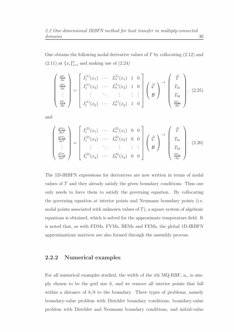
2.2 One-dimensional IRBFN method for heat transfer in multiply-connecteddomains 30
One obtains the following nodal derivative values of T by collocating (2.12) and
(2.11) at xiqi=1 and making use of (2.24)
∂T1∂x
∂T2∂x...
∂Tq∂x
=
I(1)1 (x1) · · · I
(1)m (x1) 1 0
I(1)1 (x2) · · · I
(1)m (x2) 1 0
.... . .
......
...
I(1)1 (xq) · · · I
(1)m (xq) 1 0
C
B
−1
T
Tb1
Tb2∂Tb1∂x
, (2.25)
and
∂2T1∂x2
∂2T2∂x2
...
∂2Tq∂x2
=
I(2)1 (x1) · · · I
(2)m (x1) 0 0
I(2)1 (x2) · · · I
(2)m (x2) 0 0
.... . .
......
...
I(2)1 (xq) · · · I
(2)m (xq) 0 0
C
B
−1
T
Tb1
Tb2∂Tb1∂x
. (2.26)
The 1D-IRBFN expressions for derivatives are now written in terms of nodal
values of T and they already satisfy the given boundary conditions. Thus one
only needs to force them to satisfy the governing equation. By collocating
the governing equation at interior points and Neumann boundary points (i.e.
nodal points associated with unknown values of T ), a square system of algebraic
equations is obtained, which is solved for the approximate temperature field. It
is noted that, as with FDMs, FVMs, BEMs and FEMs, the global 1D-IRBFN
approximations matrices are also formed through the assembly process.
2.2.2 Numerical examples
For all numerical examples studied, the width of the ith MQ-RBF, ai, is sim-
ply chosen to be the grid size h, and we remove all interior points that fall
within a distance of h/8 to the boundary. Three types of problems, namely
boundary-value problem with Dirichlet boundary conditions, boundary-value
problem with Dirichlet and Neumann boundary conditions, and initial-value

2.2 One-dimensional IRBFN method for heat transfer in multiply-connecteddomains 31
problem with Dirichlet boundary conditions are considered.
The solution accuracy is measured by means of the discrete relative L2 norm of
the error defined as
Ne =
√∑Mi=1(T
ei − Ti)2√∑M
i=1(Tei )
2
, (2.27)
where M is the number of unknown nodal values of T , and T e and T denote
the exact and approximate solutions, respectively. Another important measure
is the convergence rate α of the solution with respect to grid refinement
Ne(h) ≈ γhα = O(hα), (2.28)
in which α and γ are exponential model’s parameters. Given a set of ob-
servations, these parameters can be found by the general linear least squares
technique.
Example 1 - A boundary value problem (Dirichlet)
The present technique is first verified through the solution of a test problem
governed by
∂2T
∂x2+∂2T
∂y2= b(x, y), (2.29)
on a multiply-connected domain and subject to Dirichlet boundary conditions.
The problem domain chosen and its typical discretisation are shown in Figure
2.3. Two particular driving functions are considered.
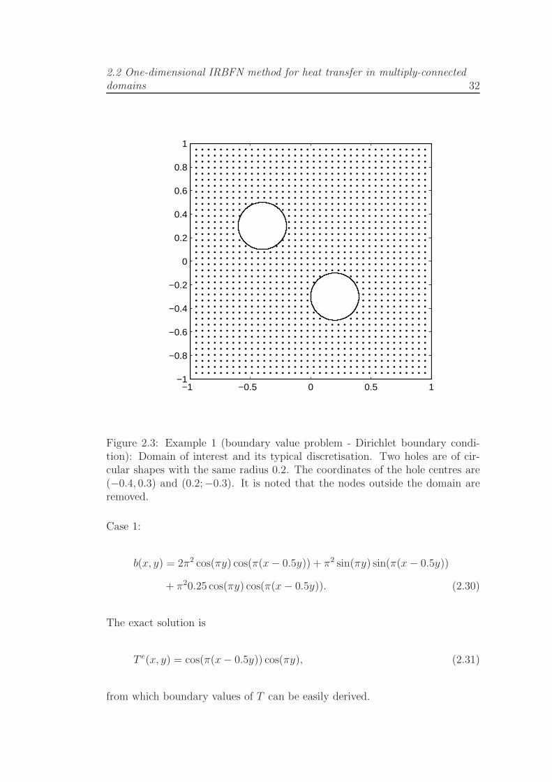
2.2 One-dimensional IRBFN method for heat transfer in multiply-connecteddomains 32
−1 −0.5 0 0.5 1−1
−0.8
−0.6
−0.4
−0.2
0
0.2
0.4
0.6
0.8
1
Figure 2.3: Example 1 (boundary value problem - Dirichlet boundary condi-tion): Domain of interest and its typical discretisation. Two holes are of cir-cular shapes with the same radius 0.2. The coordinates of the hole centres are(−0.4, 0.3) and (0.2;−0.3). It is noted that the nodes outside the domain areremoved.
Case 1:
b(x, y) = 2π2 cos(πy) cos(π(x− 0.5y)) + π2 sin(πy) sin(π(x− 0.5y))
+ π20.25 cos(πy) cos(π(x− 0.5y)). (2.30)
The exact solution is
T e(x, y) = cos(π(x− 0.5y)) cos(πy), (2.31)
from which boundary values of T can be easily derived.

2.2 One-dimensional IRBFN method for heat transfer in multiply-connecteddomains 33
Case 2:
b(x, y) = 0. (2.32)
Analytic solution to this case is not available. The boundary conditions are set
to one at the outer square boundary and to zero at the inner boundaries.
For Case 1, a number of uniform grids, (12 × 12, 22 × 22, ..., 102 × 102), are
considered. Table 2.1 presents the matrix condition (denoted by cond(A)). It
can be seen that condition numbers of the present matrix are relatively low (e.g.
6.5× 10³ with grid 102× 102). Figure 2.4 shows the profile of the approximate
solution. Figure 2.5 displays the behaviour of Ne against h, where the 1D-
IRBFN solution converges apparently as O(h3.28).
Table 2.1: Example 1 (boundary value problem - Dirichlet boundary condition- Case 1): Condition numbers of the IRBFN system matrix.
Grid cond(A)12× 12 4.4× 101
22× 22 2.0× 10²
32× 32 5.5× 10²
42× 42 1.2× 10³
52× 52 1.7× 10³
62× 62 2.0× 10³
72× 72 3.3× 10³
82× 82 4.5× 10³
92× 92 5.2× 10³
102× 102 6.5× 10³
For Case 2, we present a visual comparison of the distribution of T between
the present technique and FEM (Figure 2.6). It is noted that the FEM result
is obtained using the PDE Toolbox in MATLAB. It can be seen that the two
solutions have similar behaviours.

2.2 One-dimensional IRBFN method for heat transfer in multiply-connecteddomains 34
−1−0.5
00.5
1
−1
−0.5
0
0.5
1
−1
−0.5
0
0.5
1
Figure 2.4: Example 1 (boundary value problem - Dirichlet boundary condition- Case 1): Profile of the approximate solution using a grid of 42× 42.
Example 2 - A boundary value problem (Dirichlet and Neumann)
The driving function is taken as
b(x, y) = −cos(√x2 + y2)
(x2 + y2)
(1
x2+
1
y2
)+
sin(√x2 + y2)
(x2 + y2)3/2y2
(1
x2+
1
y2
)
− 2sin(
√x2 + y2)√x2 + y2
(2.33)
and the domain of interest is the region lying between a square of 1 × 1 and
a circle of radius 1/8 which are both centered at the origin (Figure 2.7). The

2.2 One-dimensional IRBFN method for heat transfer in multiply-connecteddomains 35
−3.5 −3 −2.5 −2 −1.5 −1−14
−13
−12
−11
−10
−9
−8
−7
−6
−5
log(h)
log(Ne)
Figure 2.5: Example 1 (boundary value problem - Dirichlet boundary condi-tion - Case 1): Convergence behaviour of the approximate solution with gridrefinement.
exact solution for this problem can be verified to be
T e(x, y) = cos(√x2 + y2). (2.34)
from which Dirichlet boundary conditions on the inner circular boundary and
Neumann boundary conditions on the outer square boundary can be derived
analytically.
A number of grids, namely (12 × 12, 22× 22, · · · , 102 × 102), are employed to
study the convergence behaviour of the solution. Results concerning the error
Ne and condition numbers of the system matrix are given in Table 2.2. It can
be seen that the 1D-IRBFN solution is very accurate even at coarse grids (e.g.
Ne = 2.25× 10⁻⁴ using a grid of 12× 12) and condition numbers of the system

2.2 One-dimensional IRBFN method for heat transfer in multiply-connecteddomains 36
Figure 2.6: Example 1 (boundary value problem - Dirichlet boundary condition- Case 2): A contour plot of T by the 1D-IRBFN method using a grid of 42×42(top) and FEM (bottom).

2.2 One-dimensional IRBFN method for heat transfer in multiply-connecteddomains 37
matrix is relatively low (e.g. 3.1× 10⁴ for a grid of 102× 102). A contour plot
of T is shown in Figure 2.8
Table 2.2: Example 2 (boundary value problem - Dirichlet and Neumann bound-ary conditions): Overall accuracy of the solution T by the present technique.Condition numbers of the IRBFN system matrix are also included.
Grid Ne(T ) cond(A)12× 12 2.2529× 10⁻⁴ 4.7× 10²
22× 22 7.9877× 10⁻⁵ 1.4× 10³
32× 32 3.9202× 10⁻⁵ 3.0× 10³
42× 42 2.3111× 10⁻⁵ 5.2× 10³
52× 52 1.5405× 10⁻⁵ 1.3× 10⁴
62× 62 1.1084× 10⁻⁵ 1.8× 10⁴
72× 72 8.2404× 10⁻⁶ 1.6× 10⁴
82× 82 6.3450× 10⁻⁶ 2.0× 10⁴
92× 92 5.0574× 10⁻⁶ 4.4× 10⁴
102× 102 4.1250× 10⁻⁶ 3.1× 10⁴
Example 3 - An initial-value problem
Consider the following PDE
∂T
∂t−
(∂2T
∂x2+∂2T
∂y2
)= (1 + 2π2k2t) sin(kπx) sin(kπy), (2.35)
where k is a given number. We choose the domain to be the same as that in
Example 1 (i.e. Figure 2.3). The exact solution is given by
T e(x, y, t) = sin(kπx) sin(kπy)t, (2.36)
from which the initial solution and Dirichlet boundary conditions are derived
analytically.
The time derivative term in (2.35) is simply discretised using a first-order finite-
difference scheme. It is noted that the system matrix, which is generated from

2.2 One-dimensional IRBFN method for heat transfer in multiply-connecteddomains 38
−0.5 0 0.5−0.5
−0.4
−0.3
−0.2
−0.1
0
0.1
0.2
0.3
0.4
0.5
R = 0.125
L = 1
Figure 2.7: Example 2 (boundary value problem - Dirichlet and Neumannboundary conditions): Domain of interest and its typical discretisation. It isnoted that the nodes outside the domain are removed.
the Laplacian and the time derivative term in (2.35), stays the same during the
iterative process.
The spatial discretisation is based on Cartesian grids of 32 × 32 and 52 × 52.
Results concerning Ne for four values of k , namely 1, 2, 3, 4, using a time step
of 0.1 are listed in Table 2.3 and Table 2.4 for grids of 32 × 32 and 52 × 52,
respectively. Condition numbers of the system matrix are 5.5 × 10² for a grid
of 32 × 32 and 1.6 × 10² for 52× 52. Plots for T at t = 1 are shown in Figure
2.9. It can be seen that the behaviour of the solution T grows complex quickly
with increasing value of k and the present scheme is able to capture accurately
a very complex function at k = 4 using a relatively low number of nodes (about
900 nodes).

2.2 One-dimensional IRBFN method for heat transfer in multiply-connecteddomains 39
Figure 2.8: Example 2 (boundary value problem - Dirichlet and Neumannboundary conditions): Approximate solution using a grid of 42 × 42. Thisplot contains 21 contour lines whose levels vary linearly from the minimum tomaximum values
Table 2.3: Example 3 (initial-value problem): Relative L2 errors of the solution(grid of 32× 32). It is noted that a(b) represents a× 10b.
t k = 1 k = 2 k = 3 k = 40.1 6.1616(-5) 3.4048(-4) 8.7540(-4) 1.8977(-3)0.2 6.6472(-5) 3.5274(-4) 8.9339(-4) 1.9259(-3)0.3 6.8883(-5) 3.5777(-4) 9.0031(-4) 1.9368(-3)0.4 7.0252(-5) 3.6040(-4) 9.0388(-4) 1.9425(-3)0.5 7.1114(-5) 3.6200(-4) 9.0606(-4) 1.9460(-3)0.6 7.1701(-5) 3.6308(-4) 9.0752(-4) 1.9483(-3)0.7 7.2124(-5) 3.6385(-4) 9.0857(-4) 1.9500(-3)0.8 7.2442(-5) 3.6443(-4) 9.0935(-4) 1.9513(-3)0.9 7.2691(-5) 3.6488(-4) 9.0997(-4) 1.9522(-3)1.0 7.2890(-5) 3.6524(-4) 9.1046(-4) 1.9530(-3)

2.3 Concluding remarks 40
Table 2.4: Example 3 (initial-value problem): Relative L2 errors of the solution(grid of 52× 52). It is noted that a(b) represents a× 10b.
t k = 1 k = 2 k = 3 k = 40.1 2.7378(-5) 1.5101(-4) 3.9744(-4) 8.5594(-4)0.2 2.9372(-5) 1.5589(-4) 4.0499(-4) 8.6748(-4)0.3 3.0365(-5) 1.5789(-4) 4.0789(-4) 8.7195(-4)0.4 3.0932(-5) 1.5893(-4) 4.0938(-4) 8.7428(-4)0.5 3.1291(-5) 1.5957(-4) 4.1029(-4) 8.7571(-4)0.6 3.1536(-5) 1.5999(-4) 4.1089(-4) 8.7667(-4)0.7 3.1714(-5) 1.6030(-4) 4.1133(-4) 8.7736(-4)0.8 3.1847(-5) 1.6053(-4) 4.1165(-4) 8.7788(-4)0.9 3.1952(-5) 1.6071(-4) 4.1191(-4) 8.7828(-4)1.0 3.2036(-5) 1.6085(-4) 4.1211(-4) 8.7861(-4)
2.3 Concluding remarks
In this chapter, we give a brief review of RBFNs and then present 1D-IRBFN
calculations of heat problems governed by Poisson equation on irregular multiply-
connected domains. Numerical examples show that (i) accurate results are ob-
tained using relatively coarse grids; and (ii) condition numbers of the system
matrix are relatively low. In the following chapters, 1D-IRBFNs are further
developed for the simulation of fluid-flow problems.

2.3 Concluding remarks 41
k = 1 k = 2
−1−0.5
00.5
1
−1
−0.5
0
0.5
1−1
−0.5
0
0.5
1
−1−0.5
00.5
1
−1
−0.5
0
0.5
1−1
−0.5
0
0.5
1
k = 3 k = 4
−1−0.5
00.5
1
−1
−0.5
0
0.5
1−1
−0.5
0
0.5
1
−1−0.5
00.5
1
−1
−0.5
0
0.5
1−1
−0.5
0
0.5
1
Figure 2.9: Example 3 (initial-value problem): 1D-IRBFN solution for fourvalues of k at t = 1 using a grid of 32× 32.

Chapter 3
1D-integrated-RBFN
discretisation of stream-function
- vorticity (ψ − ω) formulation in
multiply-connected domains
This chapter presents a new numerical collocation procedure, based on Carte-
sian grids and one-dimensional integrated radial-basis-function networks (1D-
IRBFNs), for the simulation of natural convection defined in two-dimensional
multiply-connected domains and governed by the stream-function - vorticity -
temperature (ψ−ω−T ) formulation. Special emphasis is placed on the handling
of vorticity values at boundary points that do not coincide with grid nodes. A
suitable formula for computing vorticity boundary conditions, which is based on
the approximations with respect to one coordinate direction only, is proposed.
Normal derivative boundary conditions for the stream function are forced to be
satisfied identically. Several test problems, including natural convection in an
annulus between square and circular cylinders, are considered to investigate the
accuracy of the proposed technique.
3.1 Introduction 43
3.1 Introduction
Natural convection, where the motion of a fluid is caused by the combination
of density variations and gravity, can be governed by the coupling of the mo-
mentum (velocity field) and energy (temperature field) equations within the
Boussinesq approximation. In the momentum equation, the fluid is assumed
to have a constant density except for the generation of buoyancy forces and in
the energy equation, one neglects the viscous dissipation and compressibility ef-
fects. The governing equations can be written in different dependent variables,
including the velocity - pressure - temperature (u − p − T ), stream-function -
vorticity - temperature (ψ−ω−T ), and stream-function - temperature (ψ−T )formulations. Each formulation has some strengths and weaknesses from a com-
putational point of view.
With the introduction of the stream-function variable, the pressure variable
does not have to be considered, resulting in an easy implementation. However,
several issues arise, to which special attention should be paid. For example, in
the ψ − T approach, one has to cope with fourth-order derivatives and double
boundary conditions. Fourth-order systems are known to have higher matrix
condition numbers than second-order systems. Errors for approximating higher-
order derivatives are generally larger. In the implementation of double bound-
ary conditions, special treatments are required because of two values given at a
boundary point. For the ψ−ω−T formulation, one has to derive computational
boundary conditions for the vorticity transport equation. The boundary vortic-
ity values are defined through the Poisson equation, which needs to be solved
discretely on the boundaries. The ψ − ω − T approach requires the approxi-
mations for derivatives of order up to 2 (instead of 4), leading to a significant
improvement in the matrix condition number over the ψ − T approach. This
feature is very attractive in dealing with flows with a fine structure as a large
number of nodes is usually required for an accurate simulation.

3.1 Introduction 44
Numerical solutions to these formulations can be achieved by means of dis-
cretisation, followed by solutions of the resultant algebraic equations. Results
have been reported using different numerical techniques such as FDMs, FEMs,
FVMs, BEMs, meshless methods and spectral methods (e.g. Kuehn and Gold-
stein, 1976); Manzari, 1999; Glakpe et al., 1986; Hribersek and Skerget, 1999;
Sarler et al., 2004; Sarler, 2005; Kosec and Sarler, 2008a; Shu, 1999). These
methods are based on a finite-element mesh, a finite-volume mesh, a Carte-
sian grid or a set of unstructured points. When dealing with non-rectangular
domains, conventional FDMs and pseudospectral techniques require coordinate
transformations to convert the physical domains into rectangular ones (e.g.
Moukalled and Acharya, 1996; Shu and Zhu, 2002). The relationships between
the physical and computational coordinates are given by a set of algebraic equa-
tions or a set of PDEs, depending on the level of complexity of the geometry.
These transformation processes are, in general, complicated. It is very desirable
that one is able to retain the PDEs in their original form (i.e. in terms of x and
y coordinates) and then solve them on a Cartesian grid. Such a numerical solu-
tion procedure can be very economical. The use of Cartesian grids for solving
problems defined on irregular domains has received much increased attention in
recent decades.
It has been recognised that RBFN-based methods are easy to implement and
capable of achieving a high level of accuracy using a relatively-small number of
nodes. These approximators can work well with gridded and scattered points.
RBFN solutions to fluid flow problems can be found in Ding et al., 2006; Divo
and Kassab, 2006, 2007, 2008; Kosec and Sarler, 2008a,b; Orsini et al., 2009;
Sarler et al., 2004; Sarler, 2005, 2009; Zahab et al., 2009; Erhart et al. (2010).
One can construct the RBFN approximations through differentiation or inte-
gration. Since integration is a smoothing operator, the latter has higher ap-
proximation power than the former in the handling of derivative functions (e.g.
Mai-Duy and Tran-Cong, 2003; Mai-Duy et al., 2008; Mai-Duy and Tanner,
2005).

3.2 Governing equations 45
This chapter reports a Cartesian-grid-based collocation technique incorporating
1D-IRBFNs on grid lines for the simulation of natural convection in multiply-
connected domains. The technique combines strengths of the three approaches,
namely 1D-IRBFNs (high-order accuracy), Cartesian grids (easy preprocessing)
and the ψ−ω−T formulation (low-order system). It should be emphasised that
conventional RBFN methods lead to fully-populated matrices that tend to be-
come ill-conditioned quickly with increasing numbers of RBFs. Instead of using
conventional schemes, 1D-IRBFN approximation schemes (Mai-Duy and Tran-
Cong, 2007) are utilised in the present work. We take the governing equations in
the ψ−ω−T formulation. A new formula for deriving computational vorticity
boundary conditions on a Cartesian grid is developed. First derivatives of the
stream function along the boundaries are incorporated into computational vor-
ticity boundary values by means of integration constants. The present IRBFN
approximations are constructed to satisfy all boundary conditions identically.
The matrix condition number is significantly improved over that produced by
the ψ− T formulation. Since there are no coordinate transformations required,
the present technique works in a similar fashion for all domain shapes. Results
obtained are compared well with available numerical data in literature.
The remainder of the chapter is organised as follows. Section 3.2 gives a brief
review of the governing equations. In Section 3.3, the proposed technique is de-
scribed. Emphasis is placed on the development of a novel formula for handling
vorticity boundary conditions at irregular boundary points. Numerical results
are presented in Section 3.4. Section 3.5 concludes the chapter.
3.2 Governing equations
The ψ − ω − T formulation is used here. The non-dimensional basic equations
for natural convection under the Boussinesq approximation in the Cartesian
3.2 Governing equations 46
x− y coordinate system can be written as (e.g. Ostrach, 1988)
∂2ψ
∂x2+∂2ψ
∂y2= ω, (3.1)
∂ω
∂t+ u
∂ω
∂x+ v
∂ω
∂y=
√Pr
Ra
(∂2ω
∂x2+∂2ω
∂y2
)− ∂T
∂x, (3.2)
∂T
∂t+ u
∂T
∂x+ v
∂T
∂y=
1√RaPr
(∂2T
∂x2+∂2T
∂y2
), (3.3)
where ψ is the stream function, ω the vorticity, T the temperature, t the time, u
and v the velocity components, and Pr and Ra the Prandtl and Rayleigh num-
bers defined as Pr = ν/α and Ra = βg∆TL3/αν, in which ν is the kinematic
viscosity, α the thermal diffusivity, β the thermal expansion coefficient and g
the gravity, respectively. In this dimensionless scheme, L, ∆T (temperature
difference), U =√gLβ∆T and (L/U), are taken as scale factors for length,
temperature, velocity and time, respectively. Here, the velocity scale is chosen
in such a way that the buoyancy and inertial forces are balanced (e.g. Ostrach,
1988).
The velocity components are defined in terms of the stream function as
u =∂ψ
∂y, v = −∂ψ
∂x.
The given velocity boundary conditions can be transformed into two boundary
conditions on the stream function and its normal derivative
ψ = γ,∂ψ
∂n= ξ,
where n is the direction normal to the boundary, and γ and ξ prescribed func-
tions. In the case of fixed concentric cylinders, non-slip boundary conditions
usually lead to γ = 0 and ξ = 0.

3.3 The present technique 47
3.3 The present technique
The fluid domain is simply embedded in a Cartesian grid. Grid nodes outside
the domain are removed from the computations. Boundary points are generated
by the intersection of the grid lines and the boundaries of the domain. It can
be seen that boundary conditions are over-prescribed for the stream-function
equation (3.1) and under-prescribed for the vorticity equation (3.2). Normal
derivative boundary conditions for the stream function are utilised to derive
boundary conditions for the vorticity. For natural-convection problems em-
ployed in this study, boundary conditions for the energy equation (3.3) are the
temperature values. Consequently, the three governing equations are all subject
to Dirichlet boundary conditions. On a grid line, 1D-IRBFNs are employed to
represent the stream function, vorticity and temperature variables.
3.3.1 1D-IRBFN discretisation
All PDEs in the present governing equations are of second order. Consider an
x−grid line. Making use of (2.5)-(2.9) with p = 2, second-order derivative of
the field variable f along a grid line can be decomposed into RBFs
∂2f(x)
∂x2=
m∑
i=1
wigi(x) =
m∑
i=1
wiI(2)i (x), (3.4)
where m is the number of RBFs, gi(x)mi=1 ≡I(2)i (x)
mi=1
the set of RBFs,
wimi=1 the set of weights to be found and f represents ψ, ω and T . Approximate
expressions for first-order derivative and the field variable are then obtained

3.3 The present technique 48
through integration
∂f(x)
∂x=
m∑
i=1
wiI(1)i (x) + c1, (3.5)
f(x) =
m∑
i=1
wiI(0)i (x) + c1x+ c2, (3.6)
where I(1)i (x) =
∫I(2)i (x)dx and I
(0)i (x) =
∫I(1)i (x)dx. As shown in Figure
x1 x2 xq
xb1 xb2
Figure 3.1: Points on a grid line consist of interior points xi () and boundarypoints xbi (2).
3.1, a grid line contains two sets of points. The first set consists of q interior
points that are also the grid nodes (regular nodes). The function values at the
interior points (xiqi=1) are unknown. The second set is formed with the two
boundary nodes that do not generally coincide with the grid nodes (irregular
nodes). At the boundary nodes (xb1 and xb2), the function values are given
(Dirichlet boundary conditions). The boundary conditions are incorporated into
the IRBFN approximations through the process of conversion of the network-
weight space into the physical space. Collocating (3.6) at the nodal points
yields
f
fb
= I(0)
[2]
w
c1
c2
, (3.7)

3.3 The present technique 49
where
f = (f(x1), f(x2), · · · , f(xq))T ,
fb = (f(xb1), f(xb2))T ,
w = (w1, w2, · · · , wm)T ,
I(0)[2] =
I(0)1 (x1) I
(0)2 (x1) · · · I
(0)m (x1) x1 1
I(0)1 (x2) I
(0)2 (x2) · · · I
(0)m (x2) x2 1
......
. . ....
......
I(0)1 (xq) I
(0)2 (xq) · · · I
(0)m (xq) xq 1
I(0)1 (xb1) I
(0)2 (xb1) · · · I
(0)m (xb1) xb1 1
I(0)1 (xb2) I
(0)2 (xb2) · · · I
(0)m (xb2) xb2 1
,
m = q + 2 and the subscript [2] indicates that the integral formulation starts
with second-order derivatives. Solving (3.7) for the coefficient vector including
the two integration constants results in
w
c1
c2
=
(I(0)[2]
)−1
f
fb
, (3.8)
where(I(0)[2]
)−1
is the generalised inverse of I(0)[2] .
The values of the first and second derivatives of f with respect to x at the
interior points are thus computed in terms of nodal variable values
∂f(x1)∂x
∂f(x2)∂x...
∂f(xq)∂x
= I(1)[2]
(I(0)[2]
)−1
f
fb
, (3.9)

3.3 The present technique 50
and
∂2f(x1)∂x2
∂2f(x2)∂x2
...
∂2f(xq)∂x2
= I(2)[2]
(I(0)[2]
)−1
f
fb
, (3.10)
where
I(1)[2] =
I(1)1 (x1) I
(1)2 (x1) · · · I
(1)m (x1) 1 0
I(1)1 (x2) I
(1)2 (x2) · · · I
(1)m (x2) 1 0
......
. . ....
......
I(1)1 (xq) I
(1)2 (xq) · · · I
(1)m (xq) 1 0
,
and
I(2)[2] =
g1(x1) g2(x1) · · · gm(x1) 0 0
g1(x2) g2(x2) · · · gm(x2) 0 0...
.... . .
......
...
g1(xq) g2(xq) · · · gm(xq) 0 0
.
Expressions (3.9) and (3.10) can be rewritten in compact form
∂f
∂x= D1xf + k1x, (3.11)
and
∂2f
∂x2= D2xf + k2x, (3.12)
where D1x and D2x are the first- and second-order differentiation matrices in
the physical space, and k1x and k2x are the known vectors whose components
are functions of given boundary conditions.
In the same manner, one can obtain the IRBFN expressions for ∂f/∂y and

3.3 The present technique 51
∂2f/∂y2 at the interior points along a vertical grid line.
As with FDMs, FVMs, BEMs and FEMs, the IRBFN approximations will be
gathered together to form the global matrices for the discretisation of the PDE.
3.3.2 A new formula for computing vorticity boundary
conditions
The values of the vorticity on the boundaries can be computed via
ωb =∂2ψb∂x2
+∂2ψb∂y2
, (3.13)
where the subscript b is used to indicate the boundary quantities. The handling
of ωb thus involves the evaluation of second-order derivatives of the stream
function in both x and y directions.
For regular boundary points (also grid nodes), one can apply (3.13) directly. The
x− and y−grid lines passing through those points can be used for computing
∂2ψb/∂x2 and ∂2ψb/∂y
2, respectively. However, in general, the boundary points
do not coincide with the grid nodes and hence they lie on either x− or y−grid
lines. Information about ψ is thus given explicitly in one coordinate direction
only. A great challenge here is how to compute second derivatives of ψ in (3.13)
with respect to the direction without a grid line. A new formula to overcome
this difficulty is proposed as follows.
Consider a curved boundary, along which the values for ψ and ∂ψ/∂n are pre-
scribed (Figure 3.2). It can be seen that the values of ∂ψ/∂x and ∂ψ/∂y on
the boundary can then be obtained in a straightforward manner. Let s be the
arc length of the boundary. By introducing an interpolating scheme (e.g. 1D-
IRBFNs), one is able to derive derivatives of ∂ψ/∂x and ∂ψ/∂y with respect to
s such as ∂2ψ/∂x∂s and ∂2ψ/∂y∂s.

3.3 The present technique 52
Figure 3.2: A curved boundary.
A tangential derivative of a function f at a boundary point can be computed
using the following formula
∂f
∂s=∂f
∂xtx +
∂f
∂yty, (3.14)
where tx and ty are the two x and y components of the unit vector t tangential
to the curve (tx = ∂x/∂s and ty = ∂y/∂s).
Replacing f with ∂ψb/∂x, one has
∂2ψb∂x∂s
=∂2ψb∂x2
tx +∂2ψb∂x∂y
ty, (3.15)
or
∂2ψb∂x∂y
=1
ty
(∂2ψb∂x∂s
− ∂2ψb∂x2
tx
), (3.16)
where ∂2ψb/∂x∂s is considered as a known quantity.
Similarly, taking f as ∂ψb/∂y results in
∂2ψb∂x∂y
=1
tx
(∂2ψb∂y∂s
− ∂2ψb∂y2
ty
), (3.17)

3.3 The present technique 53
where ∂2ψb/∂y∂s is a known value.
From (3.16) and (3.17), one can derive the relationship between ∂2ψ/∂x2 and
∂2ψ/∂y2 at a boundary point
1
ty
(∂2ψb∂x∂s
− ∂2ψb∂x2
tx
)=
1
tx
(∂2ψb∂y∂s
− ∂2ψb∂y2
ty
). (3.18)
Consider an x−grid line. The interpolating scheme employed along this line
does not facilitate the computation of second-order derivative of ψ with respect
to the y coordinate. However, such a derivative at a boundary point can be
found by using (3.18)
∂2ψb∂y2
=
(txty
)2∂2ψb∂x2
+ qy, (3.19)
where qy is a known quantity defined by
qy = −txt2y
∂2ψb∂x∂s
+1
ty
∂2ψb∂y∂s
. (3.20)
By substituting (3.19) into (3.13), a boundary condition for the vorticity at a
boundary point on a horizontal grid line will be computed by
ωb =
[1 +
(txty
)2]∂2ψb∂x2
+ qy, (3.21)
where only the approximations in the x direction are needed.
In the same manner, on a vertical grid line, a boundary condition for the vor-
ticity at a boundary point will be computed by
ωb =
[1 +
(tytx
)2]∂2ψb∂y2
+ qx, (3.22)

3.3 The present technique 54
where qx is a known quantity defined by
qx = − tyt2x
∂2ψb∂y∂s
+1
tx
∂2ψb∂x∂s
. (3.23)
The boundary conditions for the vorticity are thus written in terms of second
derivative of the stream function with respect to x or y only.
3.3.3 Numerical implementation of vorticity boundary
conditions
As mentioned earlier, normal derivative boundary conditions for the stream
function are used for solving the vorticity transport equation. As a result, the
values of ∂ψ/∂x and ∂ψ/∂y at the boundary points have to be incorporated
into (3.21) and (3.22), respectively.
It is well known that the computational vorticity boundary conditions strongly
affect the performance of a numerical discretisation scheme. To evaluate the
values of a second-order derivative using integrated RBFs only, the 1D-IRBFN
scheme of at least second order needs be employed. As shown in (Mai-Duy and
Tanner, 2005), higher-order IRBFNs can give more accurate results. In this
study, we attempt to employ 1D-IRBFNs of order 2 (Scheme 1) and 4 (Scheme
2), in which second and fourth derivatives of ψ are respectively decomposed
into RBFs, to evaluate ∂2ψ/∂x2 and ∂2ψ/∂y2 in (3.21) and (3.22). A distin-
guishing feature here is that derivative boundary values, ∂ψ/∂x and ∂ψ/∂y,
are incorporated into the IRBFN approximations by means of the constants of
integration.
Along an x−grid line, the process of conversion of the network-weight space

3.3 The present technique 55
into the physical space can be described as follows.
B
w
c
=
ψ
ψb∂ψb
∂x
, (3.24)
where c is a vector of integration constants, w and ψ are defined as before,
ψb = (ψ(xb1), ψ(xb2))T ,
∂ψb∂x
=
(∂ψ(xb1)
∂x,∂ψ(xb2)
∂x
)T
,
and
B =
B1
B2
,
in which
B1 = I(0)[2] ,
B2 =
I
(1)1 (xb1) I
(1)2 (xb1) · · · I
(1)m (xb1) 1 0
I(1)1 (xb2) I
(1)2 (xb2) · · · I
(1)m (xb2) 1 0
,
for Scheme 1, and
B1 = I(0)[4] =
I(0)1 (x1) I
(0)2 (x1) · · · I
(0)m (x1) x31/6 x21/2 x1 1
I(0)1 (x2) I
(0)2 (x2) · · · I
(0)m (x2) x32/6 x22/2 x2 1
......
. . ....
......
......
I(0)1 (xm) I
(0)2 (xm) · · · I
(0)m (xm) x3m/6 x2m/2 xm 1
,
B2 =
I
(1)1 (xb1) I
(1)2 (xb1) · · · I
(1)m (xb1) x2b1/2 xb1 1 0
I(1)1 (xb2) I
(1)2 (xb2) · · · I
(1)m (xb2) x2b2/2 xb2 1 0
,
for Scheme 2, where I(4)i (x) = gi(x), I
(3)i (x) =
∫I(4)i (x), · · · , I(0)i (x) =
∫I(1)i (x).
Taking (3.24) into account, second derivatives of ψ at the two boundary points

3.3 The present technique 56
can be expressed in terms of the values of ψ at every point on the grid line and
the values of ∂ψ/∂x at the two boundary points
∂2ψb∂x2
= DB−1
ψ
ψb∂ψb
∂x
, (3.25)
where
D =
g1(xb1) g2(xb1) · · · gm(xb1) 0 0
g1(xb2) g2(xb2) · · · gm(xb2) 0 0
for Scheme 1, and
D =
I
(2)1 (xb1) I
(2)2 (xb1) · · · I
(2)m (xb1) xb1 1 0 0
I(2)1 (xb2) I
(2)2 (xb2) · · · I
(2)m (xb2) xb2 1 0 0
for Scheme 2.
It should be emphasised that the IRBFN approximation for ∂2ψ/∂x2 satisfies
normal derivative of ψ at the two boundary points identically. Substituting
(3.25) into (3.21), one is able to obtain the boundary conditions for the vorticity
equation.
The process of computing the values of the vorticity at the two boundary points
on a vertical line is similar to that on a horizontal line.
3.3.4 Solution procedure
The three governing equations must be solved simultaneously to find the values
of the temperature, vorticity and stream function at the discrete points within
the domain. In this chapter, a time marching approach is adopted and at each
time step, to minimise the memory requirement, the three equations are solved

3.3 The present technique 57
in a sequential manner. The solution procedure involves the following main
steps.
1. Guess the distributions of T, ω and ψ.
2. Discretise the governing equations in time using a first-order accurate
finite-difference scheme, where the diffusive and convective terms are treated
implicitly and explicitly, respectively.
3. Discretise the governing equations in space using 1D-IRBFNs. Since the
differentiation matrices are the same for all variables, the construction
process only needs to be carried out for one variable. The system matrices,
which involve the IRBFN approximations for the Laplacian operator in
the governing equations, stay the same during the iterative process. All
equations are subject to Dirichlet boundary conditions.
4. Solve the energy equation (3.3) for T .
5. Derive computational boundary conditions for ω.
6. Solve the vorticity equation (3.1) for ω.
7. Solve the stream-function equation (3.2) for ψ.
8. Check to see whether the solution has reached a steady state using the
following convergence measure (CM)
CM =
√∑nip
i=1
(ψ
(k)i − ψ
(k−1)i
)2
√∑nip
i=1
(ψ
(k)i
)2< ǫ, (3.26)
where nip is the number of interior points, k the time level and ǫ the
tolerance (in this study, ǫ is taken to be 10−12).
9. If it is not satisfied, advance time step and repeat from step 4. Otherwise,
stop the computation and output the results.

3.4 Numerical examples 58
3.4 Numerical examples
The first two examples, for which analytic solutions are available, are used to
verify the vorticity boundary formula and its numerical implementations on
both simply- and multiply-connected domains. In the last two examples, the
proposed technique is applied for the simulation of natural convection in the
region between two concentric cylinders. The thermal boundary conditions are
prescribed as T = 0 and T = 1 along the stationary outer and inner walls,
respectively.
The present technique implements the multiquadric (MQ) basis function whose
form is
gi(x) =√(x− ci)2 + a2i , (3.27)
where ci and ai are the centre and the width of the ith MQ function.
For all numerical examples presented in this chapter, the problem domain is
discretised with a uniform Cartesian grid. The width of the ith MQ-RBF, ai,
is simply chosen to be the grid spacing h (grid size), and the interior points
that fall very close to the boundary (within a distance of h/8) are removed
from the set of nodal points. In the first two examples, the accuracy of an
approximation scheme is measured by means of the discrete relative L2 norm
of the error defined as
Ne =
√∑Mi=1(f
ei − fi)2√∑M
i=1(fei )
2
, (3.28)
where M is the number of unknown nodal values of f , and f e and f are the
exact and approximate solutions, respectively. Another important measure is
the convergence rate α of the solution with respect to the refinement of spatial

3.4 Numerical examples 59
discretisation
Ne(h) ≈ γhα = O(hα), (3.29)
in which α and γ are exponential model’s parameters. Given a set of ob-
servations, these parameters can be found by the general linear least squares
technique.
3.4.1 Example 1: Circular shape domain
The present technique is first verified through the solution of the following test
problem governed by
∂2ψ
∂x2+∂2ψ
∂y2= ω, (3.30)
∂2ω
∂x2+∂2ω
∂y2= b(x, y), (3.31)
on a unit circular domain with the boundary conditions in terms of ψ and
∂ψ/∂n. The exact solution of this problem is taken as
ψe = cos(√x2 + y2), (3.32)
from which the driving function b(x, y) and the boundary conditions can be
derived analytically. The problem domain and its typical discretisation are
shown in Figure 3.3, while the exact solution is shown in Figure 3.4. It can be
seen that the two components of the unit vector t tangential to the boundary
of the present domain are simply computed by
tx =−y√x2 + y2
, (3.33)
ty =x√
x2 + y2. (3.34)

3.4 Numerical examples 60
−1 −0.8 −0.6 −0.4 −0.2 0 0.2 0.4 0.6 0.8 1−1
−0.8
−0.6
−0.4
−0.2
0
0.2
0.4
0.6
0.8
1
Figure 3.3: Example 1: Domain of interest and its typical discretisation. It isnoted that the nodes outside the domain are removed.
Expressions for the vorticity at the boundary nodes on the x− and y−grid lines
thus reduce to
ωb =
[1 +
(yx
)2]∂2ψb∂x2
+ qy, (3.35)
ωb =
[1 +
(x
y
)2]∂2ψb∂y2
+ qx, (3.36)
each of which only requires the approximation of second-order derivative of ψ
with respect to one coordinate direction. Both Scheme 1 and Scheme 2 are
employed to compute the above expressions.
Two investigations are conducted here: (i) the accuracy of Scheme 1 and Scheme
2 for approximating ∂2ψ/∂x2 in (3.35); and (ii) the accuracy of the RBF solution
to the PDEs.

3.4 Numerical examples 61
−1−0.5
00.5
1
−1
−0.5
0
0.5
10
0.2
0.4
0.6
0.8
1
Figure 3.4: Example 1 (circular shape domain): Exact solution. It is noted thatthe exact solution is plotted over the square covering the problem domain.
For the former, calculations are carried out for various grids from 5×5 to 90×90.
Results of Ne obtained by the two different order interpolating schemes are
displayed in Table 3.1, which shows that Scheme 2 gives much more accurate
results than Scheme 1. Scheme 2 is thus recommended for use in practice.
For the latter, a number of grids, namely (12×12, 22×22, · · · , 62×62), are em-
ployed to study the convergence behaviour of the solution. Results concerning
the condition number of the system matrix, denoted by cond(A), and the error
Ne are given in Table 3.2. The present technique produces system matrices with
relatively-low condition numbers. For example, the matrix condition number is
only 6.0× 10³ for a grid of 62× 62. It can be seen that the choice of Scheme 1
(1D-IRBFN-2s) and Scheme 2 (1D-IRBFN-4s) for computing ωb in (3.35) and
(3.36) has a profound influence on the overall accuracy of the IRBFN solution.

3.4 Numerical examples 62
Table 3.1: Example 1( circular shape domain): Errors by 1D-IRBFN-2s (Scheme1) and 1D-IRBFN-4s (Scheme 2) in the computation of second derivatives of ψat the boundary points. It is noted that a(b) represents a× 10b.
Grid NeScheme 1 Scheme 2
5× 5 3.5(-2) 4(-3)10× 10 3.7(-2) 5.3(-4)30× 30 6.8(-2) 1.1(-4)50× 50 9.6(-2) 9.5(-5)70× 70 6.9(-2) 1.9(-5)90× 90 7.3(-2) 1.3(-5)
The fourth-order boundary scheme outperforms the second-order one regarding
both accuracy and convergence rate. The recommended scheme 2 yields a fast
rate of convergence, Ne of O(h3.1), in comparison with that of Scheme 1, Ne of
O(h1.8).
3.4.2 Example 2: Multiply-connected domain
This test problem is also governed by the two coupled equations (3.30) and
(3.31) with Dirichlet boundary conditions, ψ and ∂ψ/∂n. The driving function
is taken as
b(x, y) = 256(π2 − 1)2 [sin(4πx) cosh(4y) + cos(4πx) sinh(4y)] , (3.37)
and the domain of interest is the region lying between a circle of radius 1/2 and
a square of dimensions 1/2× 1/2 which are both centered at the origin (Figure
3.5). The exact solution for this problem is
ψe = sin(4πx) cosh(4y)− cos(4πx) sinh(4y). (3.38)

3.4 Numerical examples 63
Table 3.2: Example 1 (circular shape domain): Overall accuracy of the so-lution ψ by the present technique employed with two different computationalvorticity boundary schemes, namely Scheme 1 (1D-IRBFN-2s) and Scheme 2(1D-IRBFN-4s). Condition numbers of the IRBFN system matrix are also in-cluded. It is noted that h is the spacing (grid size) and a(b) represents a× 10b.
Grid Ne(ψ) cond(A)Scheme 1 Scheme 2
12× 12 1.5(-3) 6.5(-5) 8.9(1)22× 22 9.4(-4) 1.1(-5) 3.6(2)32× 32 7.4(-4) 3.9(-6) 8.0(2)42× 42 6.4(-4) 1.4(-6) 2.4(3)52× 52 6.4(-4) 6.4(-7) 3.3(3)62× 62 4.5(-4) 3.1(-7) 6.0(3)
O(h1.8) O(h3.1)
The variation of (3.38) over the extended square domain is plotted in Figure
3.6. A number of uniform grids, (10× 10, 20× 20, ..., 50× 50), are considered.
Since inner boundaries are parallel to the x and y axes, one can use the original
formula for deriving a computational vorticity boundary condition. The stream-
function equation can be rewritten as
ωb =∂2ψb∂n2
+∂2ψb∂t2
, (3.39)
where ∂2ψb/∂t2 is a known quantity derived from the boundary conditions for ψ,
and ∂2ψb/∂n2 can be evaluated using a grid line passing through that point. On
the outer boundary, the handling of ωb is similar to that in the previous example.
For brevity, only the recommended scheme (i.e. Scheme 2) for computing ωb is
employed here. Results concerning Ne(ψ) are given in Table 3.3, from which one
can also make remarks that are similar to those in the case of simply-connected
domains. It can be seen that the present matrix condition numbers are relatively
low and the approximate solution converges fast to the exact solution with Ne
of O(h3.78).

3.4 Numerical examples 64
Table 3.3: Example 2 (multiply-connected domain): Condition numbers of thesystem matrix and relative L2 errors of the solution. It is noted that h is thespacing (grid size) and a(b) represents a× 10b.
Grid Ne cond(A)10× 10 2.6(−2) 1.2(1)20× 20 9.4(−4) 4.5(1)30× 30 2.0(−4) 1.0(2)40× 40 8.5(−5) 1.8(2)44× 44 6.0(−5) 2.5(2)50× 50 4.2(−5) 2.9(2)
O(h3.78)
3.4.3 Example 3: Concentric annulus between two cir-
cular cylinders
The present method is now applied to the simulation of buoyancy-driven flow in
an annulus between two concentric cylinders which are separated by a distance
L, the inner cylinder heated (T = 1) and the outer cylinder cooled (T = 0)
(Figure 3.7a). A comprehensive review of this problem can be found in (Kuehn
and Goldstein, 1976). Most cases have been reported with Pr = 0.7 and L/Di =
0.8, in whichDi is the diameter of the inner cylinder. To these conditions, results
by Kuehn and Goldstein (1976) using FDM for Ra = 102 to Ra = 7 × 10⁴ are
often cited in the literature for comparison purposes. Later on, Shu (1999), who
employed a differential quadrature method (DQM), has provided very accurate
solutions for the values of Ra in the range of 102 to 5 × 10⁴. It is noted that
those works required a computational domain be rectangular.
The three governing equations (3.1), (3.2), (3.3) are presently solved with re-
spect to Cartesian coordinates (Figure 3.7a). Numerical simulations are also
conducted for Pr = 0.7 and L/Di = 0.8 . Like in the case of Kuehn and
Goldstein (1976), the values of the Rayleigh number varies from Ra = 102 to
Ra = 7 × 10⁴, which is broader than those reported in (Shu, 1999). Several

3.4 Numerical examples 65
−0.5 −0.4 −0.3 −0.2 −0.1 0 0.1 0.2 0.3 0.4 0.5−0.5
−0.4
−0.3
−0.2
−0.1
0
0.1
0.2
0.3
0.4
0.5
Figure 3.5: Example 2: Multiply-connected domain and its typical discretisa-tion. It is noted that the nodes outside the domain are removed.
grids, namely (12× 12, 22× 22, · · · , 52× 52), are employed.
The stream function and its normal derivative are set to zero along the inner
and outer cylinders. Expressions (3.35) and (3.36) derived in Example 1 are
applicable here to compute the values of the vorticity on the cylinder walls.
Since the boundary values for ∂ψ/∂x and ∂ψ/∂y are simply zeros, the terms qx
and qy vanish. The values for the vorticity at the boundary nodes on the x−and y−grid lines can thus be computed by
ωb = [1 + (y
x)2]∂2ψb∂x2
, (3.40)
ωb = [1 + (x
y)2]∂2ψb∂y2
, (3.41)
respectively. As mentioned earlier, Neumann boundary conditions for the stream

3.4 Numerical examples 66
−0.5
0
0.5
−0.5
0
0.5−6
−4
−2
0
2
4
6
Figure 3.6: Example 2 (multiply-connected domain): Exact solution. It is notedthat the exact solution is plotted over the square covering the problem domain.
function, ∂ψ/∂x = 0 and ∂ψ/∂x = 0, are presently incorporated into the com-
putational vorticity boundary conditions via integration constants and they are
satisfied identically. Table 3.4 indicates a significant improvement in the ma-
trix condition number of the present formulation over the ψ − T formulation
reported in (Mai-Duy et al., 2008). The former yields the matrix condition
number several orders of magnitude lower than the latter. This feature is very
attractive in the context of RBFN techniques. One is thus able to use a larger
number of nodes with the present approach in the RBFN simulation of fluid
flow problems.
Both accuracy and grid convergence of the present technique are investigated.
The solution accuracy is assessed through the average equivalent conductivity

3.4 Numerical examples 67
(a) (b)
Figure 3.7: Computational domains and discretisations: Annulus between twocircular cylinders (a) and annulus between inner circular cylinder and outersquare cylinder (b).
Table 3.4: Example 3 (circular - circular cylinders): Condition numbers of the1D-IRBFN system matrix by the two formulations.
Grid cond(A)ψ − ω − T ψ − T
12× 12 1.7× 101 8.4× 101
22× 22 9.1× 101 1.6× 10³
32× 32 2.4× 10² 6.9× 10³
42× 42 6.7× 10² 1.0× 10⁵
52× 52 9.3× 10² 2.1× 10⁵
62× 62 1.7× 10³ 1.2× 10⁶
defined as e.g. (Kuehn and Goldstein, 1976; Shu, 1999)
keq =− ln(Do/Di)
2π
∮∂T
∂nds, (3.42)
in which Do and Di are the diameters of the outer cylinder and the inner
cylinder, respectively. Results concerning keq together with those of Kuehn and
Goldstein (1976) and of Shu (1999) for Ra = 102, 103, 3× 10³, 6× 10³, 104, 5×10⁴, 7 × 10⁴ are presented in Table 3.5. It can be seen that there is a good
agreement between these numerical solutions.

3.4 Numerical examples 68
Figures 3.8 and 3.9 show the convergence of the stream function and temper-
ature fields with respect to grid refinement for Ra = 104 and Ra = 7 × 10⁴,
respectively. It can be seen that the present technique is able to capture com-
plex structures of the stream function and temperature fields even at coarse
grids, and those patterns are improved in quality (smoothness) with increasing
grid-densities. At a grid of 42 × 42 for Ra = 104 and a grid of 52 × 52 for
Ra = 7× 10⁴, the plots look reasonable when compared with those reported in
(Kuehn and Goldstein, 1976; Shu, 1999).

3.4 Numerical examples 69
Table 3.5: Example 3 (circular - circular cylinders): Comparison of the averageequivalent conductivity on the inner and outer cylinders, keqi and keqo, betweenthe present IRBFN technique using a grid of 52×52 and some other techniquesfor Ra in the range of 102 to 7× 10⁴. KG stands for Kuehn and Goldstein
Ra 102 103 3× 10³ 6× 10³ 104 5× 10⁴ 7× 10⁴
keqiPresent Method 1.000 1.083 1.396 1.709 1.975 2.962 3.207
FDM(KG, 1976) 1.000 1.081 1.404 1.736 2.010 3.024 3.308
DQM(Shu, 1999) 1.001 1.082 1.397 1.715 1.979 2.958
keqoPresent Method 0.999 1.080 1.393 1.712 1.970 2.942 3.246
FDM(KG, 1976) 1.002 1.084 1.402 1.735 2.005 2.973 3.226
DQM(Shu, 1999) 1.001 1.082 1.397 1.715 1.979 2.958

3.4 Numerical examples 70
22× 22
32× 32
42× 42
Figure 3.8: Example 3 (circular-circular cylinders): Convergence of the temper-ature (left) and stream-function (right) fields with respect to grid refinementfor the flow at Ra = 104.

3.4 Numerical examples 71
32× 32
42× 42
52× 52
Figure 3.9: Example 3 (circular-circular cylinders): Convergence of the temper-ature (left) and stream-function (right) fields with respect to grid refinementfor the flow at Ra = 7× 10⁴.

3.4 Numerical examples 72
3.4.4 Example 4: Concentric annulus between a square
outer cylinder and a circular inner cylinder
For this example, natural convection between a heated inner circular cylinder
and a cooled square enclosure is considered (Figure 3.7b). It is noted that the
transformation of this domain into a rectangular one in other methods where it
is required is much more complicated than that in the previous problem.
An aspect ratio of H/Di = 2.5 (H : the side length of the outer square and Di:
the diameter of the inner circle), Pr = 0.71 and Ra = 104, 5 × 10⁴, 105, 5 ×10⁵, 106 are employed here to investigate the accuracy of the technique.
An attractive feature here is that the present technique does not require any
coordinate transformations. The problem domain is simply represented by a
Cartesian grid (Figure 3.7b). Numerical results are obtained for three uniform
grids of 32× 32, 42× 42, and 52× 52.
For Ra = 104, the solution is started from rest to simulate the flow. For higher
values of Ra, the initial solution is taken as the solution obtained at the nearest
lower Ra. Figure 3.10 presents the behaviour of the convergence measure CM
against the number of time steps. It can be seen that the decrease in CM
is rather monotonic. As expected, the simulation of high-Ra flows requires a
larger number of iterations.
The obtained results are presented in Table 3.6, and Figures 3.11 and 3.12.
Table 3.6 is concerned with the accuracy of the solution. Following the work of
Moukalled and Acharya (1996), the local heat transfer coefficient is defined as
h = −k∂T∂n
, (3.43)
where k is the thermal conductivity. The average Nusselt number (the ratio
of the temperature gradient at the wall to a reference temperature gradient) is

3.4 Numerical examples 73
Table 3.6: Example 4 (square-circular cylinders): Comparison of the averageNusselt number on the outer and inner cylinders, Nuo and Nui, for Ra from 104
to 106 between the present technique (grid 52× 52) and some other techniques.
Ra 104 5× 10⁴ 105 5× 10⁵ 106
NuoPresent Method 3.22 4.04 4.89 7.43 8.70
DQM (Shu and Zhu, 2002) 3.24 4.86 8.90FVM (Moukalled and Acharya, 1996) 3.33 5.08 9.37
NuiPresent Method 3.21 4.04 4.89 7.51 8.85
DQM (Shu and Zhu, 2002) 3.24 4.86 8.90FVM (Moukalled and Acharya, 1996) 3.33 5.08 9.37
computed by
Nu =h
k, (3.44)
where h = −∮
∂T∂nds. Since the computational domain in (Moukalled and
Acharya, 1996) is taken as one-half of the physical domain, the values of Nu
in the present work (Table 3.6) are divided by 2 for comparison purposes. The
present results agree well with those in (Moukalled and Acharya, 1996) and
(Shu and Zhu, 2002).
Figures 3.11 and 3.12 display streamlines and isotherms versus grid densities
for Ra = 5×10⁵ and Ra = 106, which show a very fast convergence of all fields.
The qualitative behaviour of these fields and those in (Shu and Zhu, 2002) is
similar.

3.5 Concluding remarks 74
3.5 Concluding remarks
In this chapter, a new numerical discretisation scheme for the ψ−ω−T formu-
lation using Cartesian grids and 1D-IRBFNs is reported. Attractive features
of the proposed technique include (i) the preprocessing is simple; and (ii) the
boundary conditions for the vorticity are implemented in a new and effective
manner. Numerical results show that (i) the matrix condition number is sig-
nificantly improved over the ψ − T formulation; and (ii) accurate results are
obtained using a relatively-coarse grid.

3.5 Concluding remarks 75
0 2000 4000 6000 8000 10000 12000 14000 16000 18000−14
−12
−10
−8
−6
−4
−2
0
Number of iterations
log(Ne)
Figure 3.10: Example 4 (square-circular cylinders): Iterative convergence. Timesteps used are 0.002 for Ra = 104, 0.005 for Ra = 5× 10⁴, and 0.008 forRa = 105, 5 × 10⁵, 106. The values of CM become less than 10−12 whenthe numbers of iterations reach 10925, 9740, 8609, 15017, and 17938 for Ra =104, 5× 10⁴, 105, 5× 10⁵, 106, respectively. Using the last point on the curvesas a positional indicator, from left to right the curves correspond to Ra =104, 5× 10⁴, 105, 5× 10⁵, 106.

3.5 Concluding remarks 76
32× 32
42× 42
52× 52
Figure 3.11: Example 4 (square-circular cylinders): Convergence of the temper-ature (left) and stream-function (right) fields with respect to grid refinementfor the flow at Ra = 5× 10⁵.

3.5 Concluding remarks 77
32× 32
42× 42
52× 52
Figure 3.12: Example 4 (square-circular cylinders): Convergence of the temper-ature (left) and stream-function (right) fields with respect to grid refinementfor the flow at Ra = 106.

Chapter 4
1D-integrated-RBFN
discretisation of stream-function
(ψ) formulation in
multiply-connected domains
This chapter describes a new numerical procedure, based on point collocation,
integrated multiquadric functions and Cartesian grids, for the discretisation
of the stream-function formulation for flows of a Newtonian fluid in multiply-
connected domains. Three particular issues, namely (i) the derivation of the
stream-function values on separate boundaries; (ii) the implementation of cross
derivatives in irregular regions; and (iii) the treatment of double boundary
conditions, are studied in the context of Cartesian grids and approximants based
on integrated multiquadric functions in one dimension. Several test problems,
i.e. steady flows between a rotating circular cylinder and a fixed square cylinder
and also between eccentric cylinders maintained at different temperatures, are
investigated. Results obtained are compared well with numerical data available
in the literature.

4.1 Introduction 79
4.1 Introduction
The motion of a Newtonian fluid is governed by the Navier-Stokes equations
which can be written in terms of different dependent variables, including the
velocity - pressure (u− p) formulation, the stream-function - vorticity (ψ − ω)
formulation and the stream-function (ψ) formulation. The u− p formulation is
able to work for two- and three-dimension flows in a similar manner. One main
concern is that there are no explicit transport equation and boundary conditions
for the pressure variable. The resultant algebraic system could be solved itera-
tively where the pressure value is corrected using the continuity equation. For
two-dimensional (2D) problems, by introducing the stream-function variable,
one can eliminate the pressure and reduce the number of unknowns, i.e. from
three ( for the u− p formulation) to two (the ψ − ω formulation) and only one
(the ψ formulation). However, the last two formulations have some drawbacks.
Special attention should be given to the handling of the vorticity boundary
condition for the ψ − ω formulation and the double boundary conditions as
well as high-order derivatives including the cross ones for the ψ formulation.
Furthermore, the pressure field needs be computed after solving the governing
equations, which is generally regarded as a complicated process. In the case
of multiply-connected domains, an added difficulty is that the stream-function
variable generally has different values, which are unknown, on separate bound-
aries.
The governing differential equations can be transformed into sets of algebraic
equations by means of discretisation. To support the approximations, the prob-
lem domain needs be represented by a set of finite elements, a Cartesian grid or
a collection of discrete points. For problems with complicated geometries such
as flows in multiply-connected domains, it has been recognised that the task of
dividing the spatial domain into a number of finite elements can be the most
time-consuming part of the solution process. Generating a Cartesian grid or a
set of discrete points is clearly much more economical.

4.1 Introduction 80
In recent years, RBFNs have been developed to solve different types of differ-
ential problems encountered in applied mathematics, science and engineering.
Details can be found in (Divo and Kassab, 2005, 2006, 2007, 2008; Kosec and
Sarler, 2008a,b, 2009; Sarler et al., 2004; Sarler, 2005; Sarler et al., 2010; Wu and
Liu, 2003; Siraj-ul-Islam et al., 2010; Yao et al., 2011). As shown in (Driscoll
and Fornberg, 2002; Schaback, 2005; Wright and Fornberg, 2006), there is a re-
lation between the RBFN collocation method and the finite difference method
(FDM). For 1D approximations, the standard RBF interpolant converges to
the Lagrange interpolating polynomial as the RBF width goes to infinity, which
means that all classical FD formulas can be recovered by the limiting RBF in-
terpolant. In the case of two and higher dimensions, the situation is not clear
due to the fact that multivariate polynomial interpolations are not well-posed.
In (Le-Cao et al., 2009; Mai-Duy et al., 2008; Mai-Duy and Tran-Cong, 2001b,
2003, 2007), the RBFN approximations are constructed using integration (inte-
grated RBFNs (IRBFNs)) rather than the usual differentiation. This approach
has the ability to overcome the problem of reduced convergence rates caused by
differentiation and to provide effective ways to implement derivative boundary
conditions. IRBFNs have been developed for the simulation of flows in simply-
connected domains governed by the ψ formulation and the ψ − ω formulation
(e.g. Mai-Duy and Tran-Cong, 2001b) as well as natural convection governed
by the ψ−ω formulation in a region between concentric cylinders (symmetrical
flows) (e.g. Le-Cao et al., 2009).
This chapter is concerned with the simulation of unsymmetrical flows of a New-
tonian fluid in multiply-connected domains using the ψ formulation, Cartesian
grids and 1D-IRBFNs. Unlike the symmetrical case, the stream-function vari-
able has different values on separate boundaries. These values can be found
using the single-value condition for the pressure, whose implementations are
known to be difficult (e.g. Peyret, 2002). Further difficulties include the imple-
mentation of cross derivatives in regions bounded by irregular surfaces as the
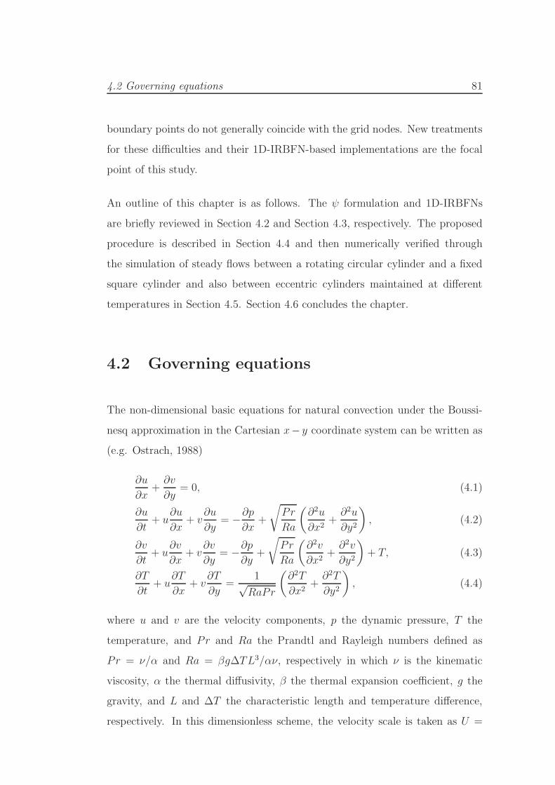
4.2 Governing equations 81
boundary points do not generally coincide with the grid nodes. New treatments
for these difficulties and their 1D-IRBFN-based implementations are the focal
point of this study.
An outline of this chapter is as follows. The ψ formulation and 1D-IRBFNs
are briefly reviewed in Section 4.2 and Section 4.3, respectively. The proposed
procedure is described in Section 4.4 and then numerically verified through
the simulation of steady flows between a rotating circular cylinder and a fixed
square cylinder and also between eccentric cylinders maintained at different
temperatures in Section 4.5. Section 4.6 concludes the chapter.
4.2 Governing equations
The non-dimensional basic equations for natural convection under the Boussi-
nesq approximation in the Cartesian x− y coordinate system can be written as
(e.g. Ostrach, 1988)
∂u
∂x+∂v
∂y= 0, (4.1)
∂u
∂t+ u
∂u
∂x+ v
∂u
∂y= −∂p
∂x+
√Pr
Ra
(∂2u
∂x2+∂2u
∂y2
), (4.2)
∂v
∂t+ u
∂v
∂x+ v
∂v
∂y= −∂p
∂y+
√Pr
Ra
(∂2v
∂x2+∂2v
∂y2
)+ T, (4.3)
∂T
∂t+ u
∂T
∂x+ v
∂T
∂y=
1√RaPr
(∂2T
∂x2+∂2T
∂y2
), (4.4)
where u and v are the velocity components, p the dynamic pressure, T the
temperature, and Pr and Ra the Prandtl and Rayleigh numbers defined as
Pr = ν/α and Ra = βg∆TL3/αν, respectively in which ν is the kinematic
viscosity, α the thermal diffusivity, β the thermal expansion coefficient, g the
gravity, and L and ∆T the characteristic length and temperature difference,
respectively. In this dimensionless scheme, the velocity scale is taken as U =

4.2 Governing equations 82
√gLβ∆T for the purpose of balancing the buoyancy and inertial forces.
By writing the velocity components in terms of a stream function ψ defined as
u =∂ψ
∂y, (4.5)
v = −∂ψ∂x
. (4.6)
the continuity equation is satisfied identically and the momentum equations
reduce to
∂
∂t
(∂2ψ
∂x2+∂2ψ
∂y2
)+∂ψ
∂y
(∂3ψ
∂x3+
∂3ψ
∂x∂y2
)− ∂ψ
∂x
(∂3ψ
∂x2∂y+∂3ψ
∂y3
)
=
√Pr
Ra
(∂4ψ
∂x4+ 2
∂4ψ
∂x2∂y2+∂4ψ
∂y4
)− ∂T
∂x, (4.7)
Using the equivalent stream-function formulation, the set of four equations
(4.1)-(4.4) reduces to a set of two equations: (4.4) and (4.7).
For iso-thermal flows, the non-dimensional basic equations reduce to
∂
∂t
(∂2ψ
∂x2+∂2ψ
∂y2
)+∂ψ
∂y
(∂3ψ
∂x3+
∂3ψ
∂x∂y2
)− ∂ψ
∂x
(∂3ψ
∂x2∂y+∂3ψ
∂y3
)=
1
Re
(∂4ψ
∂x4+ 2
∂4ψ
∂x2∂y2+∂4ψ
∂y4
), (4.8)
where Re is the Reynolds number defined as Re = UL/ν.
The given velocity boundary conditions for u and v can be transformed into
two boundary conditions on the stream function and its normal derivative
ψ = γ, (4.9)
∂ψ
∂n= ξ, (4.10)
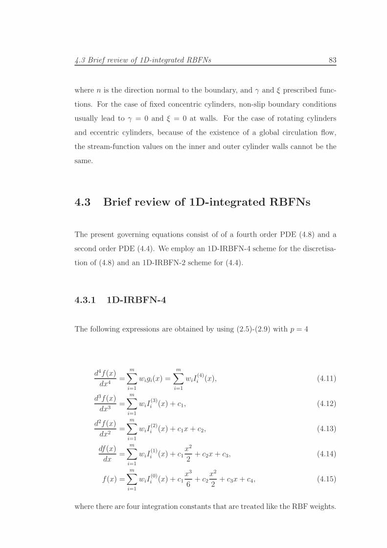
4.3 Brief review of 1D-integrated RBFNs 83
where n is the direction normal to the boundary, and γ and ξ prescribed func-
tions. For the case of fixed concentric cylinders, non-slip boundary conditions
usually lead to γ = 0 and ξ = 0 at walls. For the case of rotating cylinders
and eccentric cylinders, because of the existence of a global circulation flow,
the stream-function values on the inner and outer cylinder walls cannot be the
same.
4.3 Brief review of 1D-integrated RBFNs
The present governing equations consist of of a fourth order PDE (4.8) and a
second order PDE (4.4). We employ an 1D-IRBFN-4 scheme for the discretisa-
tion of (4.8) and an 1D-IRBFN-2 scheme for (4.4).
4.3.1 1D-IRBFN-4
The following expressions are obtained by using (2.5)-(2.9) with p = 4
d4f(x)
dx4=
m∑
i=1
wigi(x) =m∑
i=1
wiI(4)i (x), (4.11)
d3f(x)
dx3=
m∑
i=1
wiI(3)i (x) + c1, (4.12)
d2f(x)
dx2=
m∑
i=1
wiI(2)i (x) + c1x+ c2, (4.13)
df(x)
dx=
m∑
i=1
wiI(1)i (x) + c1
x2
2+ c2x+ c3, (4.14)
f(x) =
m∑
i=1
wiI(0)i (x) + c1
x3
6+ c2
x2
2+ c3x+ c4, (4.15)
where there are four integration constants that are treated like the RBF weights.

4.4 Proposed numerical procedure 84
4.3.2 1D-IRBFN-2
The following expressions are obtained by using (2.5)-(2.9) with p = 2
d2f(x)
dx2=
m∑
i=1
wiI(2)i (x), (4.16)
df(x)
dx=
m∑
i=1
wiI(1)i (x) + c1, (4.17)
f(x) =m∑
i=1
wiI(0)i (x) + c1x+ c2, (4.18)
where there are two integration constants that are treated like the RBF weights.
Both 1D-IRBFN-4 and 1D-IRBFN-2 implement the multiquadric (MQ) func-
tion whose form is
gi(x) =√(x− ci)2 + a2i , (4.19)
where ci and ai are, respectively, the centre and the width of the ith MQ basis
function.
4.4 Proposed numerical procedure
Calculations for unsymmetrical flows in multiply-connected domains are carried
out on Cartesian grids. Grid nodes inside the domain of interest are taken to
be interior nodes. Boundary points are generated by the intersection of the grid
lines and boundaries. Boundary nodes are thus comprised of two sets of points.
The first set is generated by the x−grid lines; the other by the y−grid lines.
1D-IRBFNs of orders 4 (i.e. equations (4.11)-(4.15)) and 2 (i.e. equations
(4.16)-(4.18)) are employed on the grid lines to represent the stream-function
and temperature variables, respectively. The governing differential equations,

4.4 Proposed numerical procedure 85
which involve high-order and cross derivatives, are discretised by means of point
collocation. Emphasis is placed on the following issues: (i) the implementation
of cross derivatives in irregular regions; (ii) the derivation of the stream-function
values on separate boundaries; and (iii) the treatment of double boundary con-
ditions. Formulas are derived in terms of Cartesian coordinates and they are
implemented with 1D-IRBFNs.
It is noted that conventional RBFN methods are global and lead to full pop-
ulated matrices. Unlike conventional methods, at a grid node, the proposed
method only uses RBF centres on the two associated grid lines rather than the
whole set of RBF centres to construct the approximations at that point. The
present method thus possesses some local approximation properties. In compar-
ison with conventional RBFN methods, relatively-large numbers of nodes can
be employed here. However, the resultant system matrix is still not as sparse
as those produced by finite-difference methods. The present technique needs
be combined with domain decompositions for handling large-scale engineering
problems.
4.4.1 Boundary values for stream function
Since there is no flow in the direction normal to a solid boundary, the stream
function is constant at a wall. The stream-function variable has different values
on different walls. The value of ψ on the outer wall is simply set to zero,
while the values of ψ on inner walls are considered as unknowns. Consider
an inner wall. The associated unknown there cannot be determined from the
governing equation; an independent equation/integral condition is needed. To
find the value of ψ on the wall, Lewis (1979) suggested using the condition
that the pressure is a single-valued function of position. This condition can be

4.4 Proposed numerical procedure 86
mathematically described as
∮
Γ
∂p
∂sds =
∮
Γ
∇p · d~s = 0, (4.20)
where p is the pressure, s the arc length, ds the length of an infinitesimal part
of the boundary Γ. It should be pointed out that Γ can be any closed path. In
the present work, the inner cylinder boundary is taken to be Γ . The pressure
gradient ∇p can be obtained from the momentum equations. The reader is
referred to, for example, (Lewis, 1979; Shu et al., 2002; Shu and Wu, 2002) for
further details. In the Cartesian coordinate system, equation (4.20) becomes
∮∂p
∂xdx+
∮∂p
∂ydy = 0. (4.21)
From the primitive variable formulation, we have
∂p
∂x=
1
Re
(∂2u
∂x2+∂2u
∂y2
)−
(u∂u
∂x+ v
∂u
∂y
), (4.22)
∂p
∂y=
1
Re
(∂2v
∂x2+∂2v
∂y2
)−
(u∂v
∂x+ v
∂v
∂y
). (4.23)
Substituting (4.22) and (4.23) into (4.21) and then making use of (4.5) and (4.6)
lead to
∮∂3ψ
∂x2∂ydx+
∮∂3ψ
∂y3dx−Re
∮∂ψ
∂y
∂2ψ
∂x∂ydx+Re
∮∂ψ
∂x
∂2ψ
∂y2dx−
∮∂3ψ
∂x3dy −
∮∂3ψ
∂y2∂xdy +Re
∮∂ψ
∂y
∂2ψ
∂x2dy − Re
∮∂ψ
∂x
∂2ψ
∂y∂xdy = 0.
(4.24)
In the case of a fixed cylinder, the convection term vanishes on its wall. Equation
(4.24) thus reduces to
∮∂3ψ
∂x2∂ydx+
∮∂3ψ
∂y3dx−
∮∂3ψ
∂x3dy −
∮∂3ψ
∂y2∂xdy = 0. (4.25)

4.4 Proposed numerical procedure 87
By expressing integrals in (4.24)/(4.25) in terms of the values of ψ at the interior
points, the resultant equation can be used as an extra equation to determine
the value of ψ on the wall.
4.4.2 Cross derivatives
In the present formulations, the governing equations and the single-valued pres-
sure condition involve cross derivatives, namely ∂4ψ/∂2x∂2y, ∂3ψ/∂2x∂y, and
∂3ψ/∂x∂y2. As mentioned earlier, the IRBFN approximations are constructed
on the grid lines. It is necessary to transform the computation of these mixed
derivatives to that of pure derivatives. This can be achieved through the fol-
lowing relations
∂4ψ
∂x2∂y2=
1
2
[∂2
∂x2
(∂2ψ
∂y2
)+
∂2
∂y2
(∂2ψ
∂x2
)], (4.26)
∂3ψ
∂x2∂y=
∂2
∂x2
(∂ψ
∂y
), (4.27)
∂3ψ
∂x∂y2=
∂2
∂y2
(∂ψ
∂x
). (4.28)
In (4.26)-(4.28), there are two terms, namely ∂2 (∂2ψ/∂y2) /∂x2 and ∂2 (∂ψ/∂y) /∂x2,
to be evaluated on the x−grid lines and two terms, namely ∂2 (∂2ψ/∂x2) /∂y2
and ∂2 (∂ψ/∂x) /∂y2, to be evaluated on the y−grid lines.
Consider an x−grid line. To carry out the approximation of ∂2 (∂2ψ/∂y2) /∂x2
and ∂2 (∂ψ/∂y) /∂x2, the values of ∂2ψ/∂y2 and ∂ψ/∂y at the interior and
boundary nodes on the x−grid line are assumed to be given (i.e. they are
known values or can be expressed in terms of the nodal values of ψ). For nodal
interior points, these values can be obtained straightforwardly by using the
approximations on the vertical grid lines. For the boundary points, the value of
∂ψ/∂y is known as it can be easily computed from the given boundary conditions
ψ and ∂ψ/∂n, while one does not generally know the value of ∂2ψ/∂y2. For
the latter, there are two possible cases. If the boundary point is also a grid
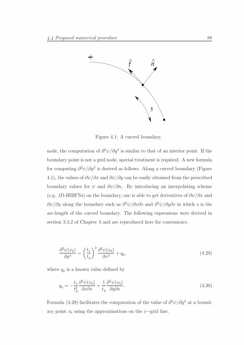
4.4 Proposed numerical procedure 88
Figure 4.1: A curved boundary.
node, the computation of ∂2ψ/∂y2 is similar to that of an interior point. If the
boundary point is not a grid node, special treatment is required. A new formula
for computing ∂2ψ/∂y2 is derived as follows. Along a curved boundary (Figure
4.1), the values of ∂ψ/∂x and ∂ψ/∂y can be easily obtained from the prescribed
boundary values for ψ and ∂ψ/∂n. By introducing an interpolating scheme
(e.g. 1D-IRBFNs) on the boundary, one is able to get derivatives of ∂ψ/∂x and
∂ψ/∂y along the boundary such as ∂2ψ/∂x∂s and ∂2ψ/∂y∂s in which s is the
arc-length of the curved boundary. The following expressions were derived in
section 3.3.2 of Chapter 3 and are reproduced here for convenience.
∂2ψ(xb)
∂y2=
(txty
)2∂2ψ(xb)
∂x2+ qy, (4.29)
where qy is a known value defined by
qy = −txt2y
∂2ψ(xb)
∂x∂s+
1
ty
∂2ψ(xb)
∂y∂s. (4.30)
Formula (4.29) facilitates the computation of the value of ∂2ψ/∂y2 at a bound-
ary point xb using the approximations on the x−grid line.

4.4 Proposed numerical procedure 89
Consider a y−grid line. In the same manner, the value of ∂2ψ/∂x2 at a boundary
point yb can be computed by
∂2ψ(yb)
∂x2=
(tytx
)2∂2ψ(yb)
∂y2+ qx, (4.31)
where qx is a known value defined by
qx = − tyt2x
∂2ψ(yb)
∂y∂s+
1
tx
∂2ψ(yb)
∂x∂s. (4.32)
It can be seen that, given a Cartesian grid, expressions (4.29) and (4.31) allow
the approximations of mixed derivatives in regions bounded by irregular surfaces
to be expressed in terms of the nodal values of ψ and the boundary conditions.
4.4.3 1D-IRBFN expressions
1D-IRBFN expressions on the x− and y−grid lines have similar forms. In the
following, the process of deriving 1D-IRBFN expressions for the stream-function
variable and its derivatives on the x−grid lines is presented in detail.
Pure derivatives
x1 x2 xq
xb1 xb2
Figure 4.2: Points on a grid line consist of interior points xi () and boundarypoints xbi (2).
Along an x−grid line (Figure 4.2), the set of RBF centres consists of the inte-
rior points xiqi=1 and the two boundary points xbi2i=1. The stream-function
variable is approximated using 1D-IRBFN-4s (equations (4.11)-(4.15) and f is
replaced with ψ). At a boundary point xb, there are double boundary condi-

4.4 Proposed numerical procedure 90
tions, ψ(xb) and ∂ψ(xb)/∂x. Unlike conventional differentiated RBFNs, there
are four integration constants in the 1D-IRBFN formulation. These extra co-
efficients allows for the addition of some extra equations to the process of con-
version of the coefficient space into the physical space. The extra equations
are utilised here to implement derivative boundary conditions. The conversion
system is thus formed by not only collocating (4.15) at xiqi=1 and xbi2i=1 but
also collocating (4.14) at xbi2i=1
ψ
ψb∂ψb
∂x
= C w, (4.33)
where
ψ = (ψ(x1), ψ(x2), · · · , ψ(xq))T ,
ψb = (ψ(xb1), ψ(xb2))T ,
∂ψb∂x
=
(∂ψ(xb1)
∂x,∂ψ(xb2)
∂x
)T
,
C =
I(0)1 (x1) · · · I
(0)m (x1) x31/6 x21/2 x1 1
I(0)1 (x2) · · · I
(0)m (x2) x32/6 x22/2 x2 1
.... . .
......
......
...
I(0)1 (xq) · · · I
(0)m (xq) x3q/6 x2q/2 xq 1
I(0)1 (xb1) · · · I
(0)m (xb1) x3b1/6 x2b1/2 xb1 1
I(0)1 (xb2) · · · I
(0)m (xb2) x3b2/6 x2b2/2 xb2 1
I(1)1 (xb1) · · · I
(1)m (xb1) x2b1/2 xb1 1 0
I(1)1 (xb2) · · · I
(1)m (xb2) x2b2/2 xb2 1 0
,
w = (w1, w2, · · · , wm, c1, c2, c3, c4)T ,
and m = q + 2. The values of the lth-order derivative (l = 1, 2, 3, 4) of ψ at

4.4 Proposed numerical procedure 91
the interior points on the grid line are evaluated as
∂lψ
∂xl= I(l)
[4] C−1
ψ
ψb∂ψb
∂x
, (4.34)
where
I(4)[4] =
I(4)1 (x1) · · · I
(4)m (x1) 0 0 0 0
I(4)1 (x2) · · · I
(4)m (x2) 0 0 0 0
.... . .
......
......
...
I(4)1 (xq) · · · I
(4)m (xq) 0 0 0 0
,
I(3)[4] =
I(3)1 (x1) · · · I
(3)m (x1) 1 0 0 0
I(3)1 (x2) · · · I
(3)m (x2) 1 0 0 0
.... . .
......
......
...
I(3)1 (xq) · · · I
(3)m (xq) 1 0 0 0
,
I(2)[4] =
I(2)1 (x1) · · · I
(2)m (x1) x1 1 0 0
I(2)1 (x2) · · · I
(2)m (x2) x2 1 0 0
.... . .
......
......
...
I(2)1 (xq) · · · I
(2)m (xq) xq 1 0 0
,
and
I(1)[4] =
I(1)1 (x1) · · · I
(1)m (x1) x21/2 x1 1 0
I(1)1 (x2) · · · I
(1)m (x2) x22/2 x2 1 0
.... . .
......
......
...
I(1)1 (xq) · · · I
(1)m (xq) x2q/2 xq 1 0
.

4.4 Proposed numerical procedure 92
Expressions (4.34) can be rewritten in compact form
∂lψ
∂xl= Dlxψ + klx, (4.35)
where Dlx are the differentiation matrices in the physical space, and klx the
vectors whose components are functions of boundary conditions. It is noted
that, for the grid lines which cross over the inner cylinder, only the values of ψ
on the outer cylinder are given.
Similarly, 1D-IRBFN expressions for pure derivatives on the y−grid lines take
the following forms
∂lψ
∂yl= Dlyψ + kly, (4.36)
where l = 1, 2, 3, 4.
The temperature variable is represented by 1D-IRBFN-2s, i.e. equations (4.16)-
(4.18), where f is replaced with T . It is noted that the present energy equation
(4.4) is subject to the Dirichlet boundary condition only. The process of deriving
1D-IRBFNs for T is similar to that for ψ, except that no extra equations are
employed in the process of conversion (4.33).
Mixed derivatives
On an x−grid line, it can be seen from (4.26)-(4.28) that relevant mixed deriva-
tive to be evaluated here are ∂2 (∂ψ/∂y) /∂x2 and ∂2 (∂2ψ/∂y2) /∂x2. Approxi-
mate expressions for ∂ψ/∂y and ∂2ψ/∂y2 can be obtained at the interior points
using (4.36) with l = 1, 2. At the boundary points, the values of ∂ψ/∂y
are given, while the values of ∂2ψ/∂y2 can be computed using (4.29) in which

4.4 Proposed numerical procedure 93
∂2ψ/∂x2 is evaluated using the nodal values of ψ on the x−grid line
∂2ψ(xb)
∂x2=
[I(2)1 (xb) · · · I(2)m (xb) xb 1 0 0
]C−1
ψ
ψb∂ψb
∂x
, (4.37)
where xb is a boundary point and ψ, ∂ψb/∂x, w and C are defined as before.
Let g represent ∂2ψ/∂y2 and ∂ψ/∂y. The remaining task is to form an 1D-
IRBFN expression for ∂2g/∂x2. This process is similar to that for the stream
function which is described in Section 4.4.3, except that there are no extra
equations representing derivative boundary values in (4.33).
Single-valued pressure equation
As shown in (4.24)/(4.25), this pressure condition involves pure and mixed
derivatives on the wall.
Using 1D-IRBFN expressions which are derived above, one can express deriva-
tives in (4.24)/(4.25) in terms of the nodal values of ψ. For example, the
integrand of the third term in (4.25) can be written as
∂3ψ(xb)
∂x3=
[I(3)1 (xb) · · · I(3)m (xb) 1 0 0 0
]C−1
ψ
ψb∂ψb
∂x
, (4.38)
where xb is the boundary point on the inner wall and ψ, ∂ψb/∂x, w and C are
defined as before. The vector ψb in (4.38) contains the value of the stream
function on the inner cylinder, i.e. ψ(xb), that is an unknown to be found.
All associated integrals in (4.24)/(4.25) are then evaluated using the Gauss
quadrature scheme.

4.4 Proposed numerical procedure 94
The pressure condition leads to a relation where the value of ψ on the inner wall
is expressed as a linear combination of the values of ψ at the interior points.
4.4.4 Solution Procedure
The set of algebraic equations resulting from the discretisation of the stream-
function formulation is nonlinear because of the presence of the convective
terms. There are two approaches widely used to handle this nonlinearity. In
the first approach, all time derivative terms are dropped out and nonlinear
solvers such as Newton iterations can be applied. In the second approach, the
solution is obtained by means of time marching. Each approach has some ad-
vantages over the other for certain problems. In this study, fluid flow problems
are considered and the second approach is applied.
1. Guess initial values of T, ψ and their spatial derivatives at time t = 0.
2. Discretise the governing equations in time using a first-order accurate
finite-difference scheme, where the diffusive and convective terms are treated
implicitly and explicitly, respectively.
3. Discretise the governing equations in space using 1D-IRBFN schemes,
Solve the energy equation (4.4) for T , and
Solve the momentum equation (4.7) for ψ.
The two equations are solved separately in order to keep matrix sizes to
a minimum.
4. Check to see whether the solution has reached a steady state
CM =
√∑nip
i=1
(ψ
(k)i − ψ
(k−1)i
)2
√∑nip
i=1
(ψ
(k)i
)2< ǫ, (4.39)
where k is the time level and ǫ is the prescribed tolerance.

4.5 Numerical results 95
5. If it is not satisfied, advance time step and repeat from step 2. Otherwise,
stop the computation and output the results.
4.5 Numerical results
The present method is verified through the simulation of steady iso-thermal
flows between a rotating circular cylinder and a fixed square cylinder, and steady
buoyancy-driven flows in eccentric annuli with a wide range of the eccentricity
parameter. The computed solution at the nearest lower value of Re/Ra is
taken to be the initial solution. Internal grid points that fall very close–within
a distance of h/8–to the boundary are removed.
It is well known that RBFN-based schemes suffer from the so-called uncer-
tainty or trade-off principle. As the value of the RBF-width/shape-parameter
increases, the approximation error reduces while the condition number of the
system matrix grows. Unfortunately, there is still a lack of theory to determine
the optimal value for the RBF width. The RBF width is usually chosen by trial
and error or some other ad-hoc means. In this study, the grid size h is taken to
be the MQ-RBF width.
For conventional FDMs and pseudo-spectral techniques, coordinate transfor-
mations are required to convert non-rectangular domains into rectangular ones
(Shu et al., 2002; Moukalled and Acharya, 1996). The relationships between
the physical and computational coordinates are given by a set of algebraic equa-
tions or a set of partial differential equations (PDEs), depending on the level
of complexity of the geometry. Such transformation processes are, in general,
complicated. The proposed technique can work with irregular domains in a di-
rect manner, i.e. without the need for using coordinate transformations. How-
ever, the proposed technique is restricted to structured uniform or non-uniform
Cartesian grids.

4.5 Numerical results 96
Figure 4.3: Example 1 (rotating cylinder): geometry (top) and discretisation(bottom).

4.5 Numerical results 97
4.5.1 Example 1: Steady flow between a rotating circular
cylinder and a fixed square cylinder
This test problem is employed for the investigation of accuracy of the proposed
technique in computing the value of the stream function on the inner cylinder.
The flow geometry and discretisation are shown in Figure 4.3. The inner cylin-
der rotates at a unit angular velocity. The stream function on the outer wall
is set to zero. Formula (4.24) is utilised to determine the value of the stream
function on the inner wall, denoted by ψw. This flow is governed by (4.8) and
subject to the boundary conditions
ψ =∂ψ
∂x=∂ψ
∂y= 0,
on the outer cylinder and
ψ = ψw,∂ψ
∂x= −x, ∂ψ
∂y= −y,
on the inner cylinder. The flow is simulated with R = 0.25 and L = 0.55, 1.0using a uniform grid of 52×52. Several values of the Reynolds number, namely
1, 100, 500, 700 and 1000, are considered. Results concerning ψw obtained
by the proposed technique and the finite-difference technique (Lewis, 1979) are
presented in Table 4.1, showing a satisfactory agreement. Plots for the velocity
and vorticity fields for the case of L = 1 and R = 0.25 at Re = 1, 700 are
given in Figure 4.4.

4.5 Numerical results 98
Table 4.1: Example 1 (rotating cylinder): Comparison of the stream-functionvalues at the inner cylinder, ψw, for Re from 1 to 1000 between the presenttechnique (grid of 52× 52) and finite difference technique.
Re 1 100 500 1000(R,L) (0.25, 0.55)
ψwPresent method 0.0581 0.0582 0.0586 0.0596
FDM (Lewis, 1979) 0.0625 0.0626 0.0621 0.0600(R,L) (0.25, 1)
ψwPresent method 0.4622 0.4617 0.4500 0.4264
FDM (Lewis, 1979) 0.4656 0.4577 0.4465 0.4375

4.5 Numerical results 99
Re = 1
Re = 700
Figure 4.4: Example 1 (rotating cylinder, R=0.25, L=1): Velocity field (left)and vorticity field (right) for the flow at Re = 1 and Re = 700.

4.5 Numerical results 100
4.5.2 Example 2: Natural convection in an eccentric an-
nulus between two circular cylinders
Natural convection is governed by the coupling of the momentum equation
(velocity field) (4.7) and energy equation (temperature field) (4.4). Solutions to
natural convection have been reported using various discretisation techniques
such as FDMs (e.g. Kuehn and Goldstein, 1976; de Vahl Davis, 1983), FEMs
(e.g. Manzari, 1999; Sammouda et al., 1999), FVMs (e.g. Glakpe et al., 1986;
Kaminski and Prakash, 1986), BEMs (e.g. Kitagawa et al., 1988; Hribersek and
Skerget, 1999), spectral methods (e.g. Shu, 1999; Shu et al., 2002; Shu and Wu,
2002) and meshless methods (e.g. Divo and Kassab, 2008; Sarler et al., 2004;
Sarler, 2005).
Figure 4.5: Example 2 (eccentric circular-circular annulus): geometry.

4.5 Numerical results 101
(a)
(b)
Figure 4.6: Schematic spatial discretisations for an annulus between two circularcylinders (a) and an annulus between inner circular and outer square cylinders(b).

4.5 Numerical results 102
Consider buoyancy-driven flows of a Newtonian fluid between two cylinders
whose centres are separated by a distance ε (Figure 4.5). As shown in Figure
4.5, the flow geometry is defined by the following geometrical parameters: the
eccentricity ε, angular position ϕ, the diameter of the outer cylinder Do and the
diameter of the inner cylinder Di. In the present work, the numerical results
are reported with Pr = 0.71 and Do/Di = 2.6. A typical discretisation is shown
on Figure 4.6a, where no coordinate transformations are employed.
The inner and outer cylinders are heated (T = 1) and cooled (T = 0), re-
spectively. The stream-function value at the outer cylinder is set to zero. The
stream-function value at the inner cylinder is a part of the solution and can be
determined by the single-valued pressure condition (4.25). The normal deriva-
tives of the stream function are set to zero at both walls.
Both trust region and time marching techniques are applied here to solve the
nonlinear equation set. For the trust region technique, it takes about 5 to 10
iterations to get a converged solution. For the time marching technique, much
more iterations are required as shown in Figure 4.7. However, a single iteration
of the decoupled approach consumes much less CPU time than that of the
coupled approach. Overall, the decoupled approach is more efficient than the
coupled approach. For example, in the case of simulating the flow at Ra = 104
using a grid of 41 × 41, the decoupled approach is about 9.2 times faster than
the coupled approach.

4.5 Numerical results 103
0 1000 2000 3000 4000 5000 600010
−14
10−12
10−10
10−8
10−6
10−4
10−2
100
Number of iterations
CM
Figure 4.7: Example 2 (circular-circular annulus): 61×61, decoupled approach,iterative convergence. Time steps used are 0.5 for Ra = 102, 103, 3× 10³, 0.1for Ra = 6×10³, 104, and 0.05 for Ra = 5×10⁴, 7×10⁴. The values of CMbecome less than 10−12 when the numbers of iterations reach 58, 154, 224, 1276,1541, 5711 and 5867 for Ra = 102, 103, 3 × 10³, 6 × 10³, 104, 5× 10⁴, 7× 10⁴,respectively. Using the last point on the curves as a positional indicator, fromleft to right the curves correspond to Ra = 102, 103, 3 × 10³, 6 × 10³, 104, 5 ×10⁴, 7× 10⁴

4.5 Numerical results 104
Table 4.2: Condition numbers of the RBFN matrices associated with the har-monic and biharmonic operators.
Grid cond(L2T ) cond(L4ψ)11× 11 1.3× 101 7.4× 101
21× 21 1.2× 10² 5.0× 10³
31× 31 3.3× 10² 3.3× 10⁴
41× 41 5.1× 10² 7.9× 10⁴
51× 51 7.5× 10² 1.6× 10⁵
61× 61 1.0× 10³ 3.2× 10⁵
The condition numbers of the system matrix associated with the energy equa-
tion (4.4) and momentum equation (4.7) are reported in Table 4.2.
One typical quantity associated with this type of flow is the average equivalent
conductivity denoted by keq. This quantity is defined as (e.g. Kuehn and
Goldstein, 1976)
keq =− ln(Do/Di)
2π
∮∂T
∂nds (4.40)
Table 4.3: Example 2 (symmetric flow, concentric circular-circular annuli): Con-vergence of keq with grid refinement for the flow at Ra = 102.
Grid Outer cylinder, keqo Inner cylinder, keqi11× 11 0.969 0.97221× 21 0.994 0.98931× 31 0.997 0.99741× 41 0.999 0.999
FDM (Kuehn and Goldstein, 1976) 1.002 1.000DQM (Shu, 1999) 1.001 1.001
The present method is first tested with the case of symmetrical flows, where the
exact value of ψ at the inner wall is known (i.e. ψw = 0 for the present case).
Three uniform grids of 41×41, 51×51 and 61×61 are employed to represent the

4.5 Numerical results 105
Table 4.4: Example 2 (symmetric flow, concentric circular-circular annuli): Con-vergence of keq with grid refinement for the flow at Ra = 103.
Grid Outer cylinder, keqo Inner cylinder, keqi11× 11 1.133 1.04621× 21 1.072 1.06931× 31 1.078 1.07741× 41 1.080 1.07951× 51 1.081 1.080
FDM (Kuehn and Goldstein, 1976) 1.084 1.081DQM (Shu, 1999) 1.082 1.082
Table 4.5: Example 2 (symmetric flow, concentric circular-circular annuli): Con-vergence of keq with grid refinement for the flow at Ra = 3× 10³.
Grid Outer cylinder, keqo Inner cylinder, keqi11× 11 1.745 1.20021× 21 1.365 1.37831× 31 1.387 1.38641× 41 1.391 1.39051× 51 1.393 1.393
FDM (Kuehn and Goldstein, 1976) 1.402 1.404DQM (Shu, 1999) 1.397 1.397
flow field. For concentric cylinders, results concerning keq together with those of
(Kuehn and Goldstein, 1976) and of (Shu, 1999) for various Rayleigh numbers
from 102 to 7×10⁴ are presented in Tables 4.3-4.9. It can be seen that there is a
good agreement between these numerical solutions. For each Rayleigh number,
the convergence of the average equivalent conductivity with grid refinement is
fast, e.g. the solution keqo for the last two Rayleigh numbers (i.e. Ra = 104
and Ra = 5 × 10⁴) converges as O(h2.71) and O(h3.36) in which h is the grid
spacing (errors are computed relative to the spectral results). Variations of the
local equivalent conductivity on the inner and outer cylinder surfaces using a
grid of 51 × 51 for Ra = 103 and Ra = 5 × 10⁴ are shown in Figures 4.8 and

4.5 Numerical results 106
Table 4.6: Example 2 (symmetric flow, concentric circular-circular annuli): Con-vergence of keq with grid refinement for the flow at Ra = 6× 10³.
Grid Outer cylinder, keqo Inner cylinder, keqi31× 31 1.698 1.70241× 41 1.704 1.70551× 51 1.709 1.70961× 61 1.711 1.711
FDM (Kuehn and Goldstein, 1976) 1.735 1.736DQM (Shu, 1999) 1.715 1.715
Table 4.7: Example 2 (symmetric flow, concentric circular-circular annuli): Con-vergence of keq with grid refinement for the flow at Ra = 104.
Grid Outer cylinder, keqo Inner cylinder, keqi41× 41 1.961 1.96751× 51 1.969 1.97161× 61 1.973 1.973
FDM (Kuehn and Goldstein, 1976) 2.005 2.010DQM (Shu, 1999) 1.979 1.979
4.9, respectively. It can be seen that they are compared well with those of
(Kuehn and Goldstein, 1976). The present solutions converge well and are in
close agreement with the other solutions. It can be seen that the IRBFN results
are more agreeable to the DQ ones than the FD results. Figure 4.10 shows the
streamlines and isotherms of the flow for Ra = 103, 6 × 10³, 5 × 10⁴, 7 × 10⁴using a grid of 51 × 51. Each plot contains 21 contour lines whose levels vary
linearly from the minimum to maximum values. The plots look reasonable in
comparison with those of the FD and DQ methods. For eccentric cylinders (i.e.
the centres of inner and outer cylinders lie on the vertical symmetrical axis),
results obtained show that the value of ψw is less than 10−6, which is close to
zero. Table 4.10 compares the maximum value of ψ for Ra = 104 between the
proposed method and the DQM (Shu, 1999). Good agreement is achieved.

4.5 Numerical results 107
Table 4.8: Example 2 (symmetric flow, concentric circular-circular annuli): Con-vergence of keq with grid refinement for the flow at Ra = 5× 10⁴.
Grid Outer cylinder, keqo Inner cylinder, keqi41× 41 3.089 3.04551× 51 2.936 2.94661× 61 2.922 2.941
FDM (Kuehn and Goldstein, 1976) 2.973 3.024DQM (Shu, 1999) 2.958 2.958
Table 4.9: Example 2 (symmetric flow, concentric circular-circular annuli): Con-vergence of keq with grid refinement for the flow at Ra = 7× 10⁴.
Grid Outer cylinder, keqo Inner cylinder, keqi41× 41 3.465 3.25451× 51 3.241 3.18761× 61 3.167 3.174FDM
(Kuehn and Goldstein, 1976) 3.226 3.308
For the case of unsymmetrical flows, the value of ψ at the inner wall has non-zero
value that varies with the location of the inner cylinder. Different amounts of
eccentricity (ε), namely 0.25, 0.5, 0.75, 0.95, and angular direction ϕ, namely
−450, 00, 450, are employed. In Table 4.11, the values of ψ at the inner walls
are presented and agree satisfactorily with those conducted by the DQM (Shu
et al., 2002) and the domain free discretisation method (DFD) (Shu and Wu,
2002). Figure 4.11 shows the streamlines and isotherms of the flow at Ra =
104 using a grid of 61 × 61, where several values of eccentricity and angular
directions are employed. Each plot contains 21 contour lines whose levels vary
linearly from the minimum to maximum values. All plots look reasonable when
compared with those of the DQM (Shu et al., 2002).

4.5 Numerical results 108
0 20 40 60 80 100 120 140 160 1800.4
0.6
0.8
1
1.2
1.4
1.6
1.8
2
IRBFN, Inner cylinderFDMIRBFN, Outer cylinderFDM
θ (degree)
keq
Figure 4.8: Example 2 (concentric circular-circular annulus): Local equivalentconductivities for Ra = 103 by 1D-IRBFN and FDM.
0 20 40 60 80 100 120 140 160 1800
2
4
6
8
10
12
IRBFN, Inner cylinderFDMIRBFN, Outer cylinderFDM
θ (degree)
keq
Figure 4.9: Example 2 (concentric circular-circular annulus): Local equivalentconductivities for Ra = 5× 104 by 1D-IRBFN and FDM.

4.5 Numerical results 109
Table 4.10: Example 2 (symmetric flow, eccentric circular-circular annuli):Comparison of the maximum stream-function values, ψmax, for two special casesϕ = −900, 900 between the present technique and DQM technique.
ε 0.25 0.5 0.75 0.95ϕ −900
ψmaxPresent method 22.19 20.72 18.50 15.71
DQM (Shu et al., 2002) 22.16 20.62 18.32 15.50ϕ 900
ψmaxPresent method 11.26 9.64 8.25 7.28
DQM (Shu et al., 2002) 11.13 9.55 8.12 7.17
Table 4.11: Example 2 (unsymmetrical flow, eccentric circular-circular annuli):Comparison of the stream-function values at the inner cylinders, ψw, for ε =0.25, 0.5, 0.75, 0.95 and ϕ = −450, 00, 450 between the present, DQM andDFD techniques.
ε 0.25 0.5 0.75 0.95ϕ 450
ψwPresent method 0.52 1.25 1.01 0.01
DQM (Shu et al., 2002) 0.52 1.31 1.07 0.03DFD (Shu and Wu, 2002) 0.54 1.29 1.09 0.03
ϕ 00
ψwPresent method 0.60 1.28 1.18 0.01
DQM (Shu et al., 2002) 0.72 1.15 1.30 0.06DFD (Shu and Wu, 2002) 0.72 1.10 1.26 0.06
ϕ −450
ψwPresent method 0.48 0.80 1.05 0.6
DQM (Shu et al., 2002) 0.51 0.92 0.99 0.08DFD (Shu and Wu, 2002) 0.51 0.77 0.77 0.04

4.5 Numerical results 110
Ra = 103
Ra = 6× 10³
Ra = 5× 10⁴
Ra = 7× 10⁴
Figure 4.10: Example 2 (concentric circular-circular annulus): Contour plotsof temperature (left) and stream function (right) for four different Rayleighnumbers using a grid of 51 × 51. Each plot contains 21 contour lines whoselevels vary linearly from the minimum to maximum values.

4.5 Numerical results 111
ε = 0.25, ϕ = 450
ε = 0.5, ϕ = 00
ε = 0.75, ϕ = −450
ε = 0.95, ϕ = 00
Figure 4.11: Example 2 (eccentric circular-circular annuli): Contour plots forthe temperature (left) and stream-function (right) fields for several values ofeccentricity ε and angular directions ϕ for the flow at Ra = 1 × 10⁴. Eachplot contains 21 contour lines whose levels vary linearly from the minimum tomaximum values.

4.5 Numerical results 112
4.5.3 Example 3: Natural convection in eccentric annuli
between a square outer and a circular inner cylin-
der
Figure 4.12: Example 3 (eccentric square-circular domain): geometry.
In this example, natural convection between a heated inner circular cylinder
and a cooled square enclosure (Figure 4.12) is considered. An aspect ratio of
L/2R = 2.6 (L: the side length of the outer square and R: the radius of the
inner circle), Pr = 0.71 and Ra = 3× 10⁵ are used.
The problem domain is simply replaced with a Cartesian grid (Figure 4.6b),
where no coordinate transformations are employed.
For the concentric case, the obtained results are presented in the forms of
streamlines and isotherms (Figure 4.13). In Figure 4.13, each plot contains
21 contour lines whose levels vary linearly from the minimum to maximum val-

4.5 Numerical results 113
Table 4.12: Example 3 (symmetric flow, eccentric square-circular annuli):Comparison of the maximum stream-function values, ψmax, for special casesϕ = −900, 900 between the present technique and MQ-DQ technique.
ε 0.25 0.5 0.75 0.95ϕ −900
ψmaxPresent method 18.63 21.30 23.47 24.48
MQ-DQ (Ding et al., 2005) 18.64 21.29 23.52ϕ 900
ψmaxPresent method 12.37 11.36 10.10 9.289
MQ-DQ (Ding et al., 2005) 12.39 11.38 10.09
ues. For special cases of eccentric square-circular annuli, where the centre of the
inner cylinder lies on the vertical symmetrical axis of the outer square cylinder,
the values of ψmax are given in Table 4.12. It can be seen that the present
results are in very good agreement with those of Ding et al., 2005.
Table 4.13: Example 3 (concentric square-circular annuli): Comparison of theaverage Nusselt number on the outer and inner cylinders, Nuo and Nui, for Rafrom 104 to 106 between the present technique (grid of 62× 62) and some othertechniques.
Ra 104 5× 10⁴ 105 5× 10⁵ 106
NuoPresent method 3.22 4.04 4.89 7.43 8.70
MQ-DQ (Ding et al., 2005) 3.24 4.86 8.90FVM (Moukalled and Acharya, 1996) 3.33 5.08 9.37
NuiPresent method 3.21 4.04 4.89 7.51 8.85
MQ-DQ (Ding et al., 2005) 3.24 4.86 8.90FVM (Moukalled and Acharya, 1996) 3.33 5.08 9.37
Following the work of Moukalled and Acharya (Moukalled and Acharya, 1996),

4.5 Numerical results 114
Table 4.14: Example 3 (unsymmetrical flow, eccentric square-circular an-nuli): Comparison of the maximum stream-function values, ψmax, for ε =0.25, 0.5, 0.75, 0.95 and ϕ = −450, 00, 450 between the present techniqueand MQ-DQ technique.
ε 0.25 0.5 0.75 0.95ϕ 450
ψmaxPresent method 15.31 14.23 13.52 12.91
MQ-DQ (Ding et al., 2005) 15.32 14.35 13.61 12.98ϕ 00
ψmaxPresent method 17.00 16.99 16.87 17.18
MQ-DQ (Ding et al., 2005) 17.00 16.97 16.84ϕ −450
ψmaxPresent method 18.50 20.09 21.02 21.61
MQ-DQ (Ding et al., 2005) 18.50 20.03 21.01 21.68
the local heat transfer coefficient is defined as
θ = −k∂T∂n
, (4.41)
where k is the thermal conductivity. The average Nusselt number (the ratio
of the temperature gradient at the wall to a reference temperature gradient) is
computed by
Nu =θ
k, (4.42)
where θ = −∮
∂T∂nds. Since the computational domain in (Moukalled and
Acharya, 1996) is taken as one-half of the physical domain, the values of Nu in
the present work (Table 4.13) are divided by 2 for comparison purposes. The
present results agree well with those in (Moukalled and Acharya, 1996) and
(Ding et al., 2005).

4.5 Numerical results 115
Ra = 5× 10⁴
Ra = 105
Ra = 5× 10⁵
Ra = 106
Figure 4.13: Example 3 (concentric square-circular annulus): Contour plotsof temperature (left) and stream function (right) for four different Rayleighnumbers using a grid of 61 × 61. Each plot contains 21 contour lines whoselevels vary linearly from the minimum to maximum values.

4.5 Numerical results 116
Similar to Example 2, the eccentricity values used are ε = 0.25, 0.5, 0.75, 0.95and the angular positions are ϕ = −450, 00, 450. The value of ψ along the
inner wall is considered as an unknown and the values of ψ along the outer
boundary can be taken to be zero. Calculations are performed on a uniform
Cartesian grid of 62 × 62. In Table 4.14, the maximum values of the stream
function are presented and compared very well with those obtained by Ding
et al. (2005).
In Figure 4.14, the effects of time step on convergence behaviour of the proposed
technique are investigated for the case of Ra = 1×10⁵ using a grid of 53×53. It
can be seen that the present technique can work with a wide range of values of
time step. As expected, convergence is faster but less stable when the length of
time step increases. In relation to CPU times, the present technique consumes
0.013715 (s) per iteration for a grid of 33 × 33, 0.0599 for 49 × 49 and 0.0807
for 53× 53 (Intel Core 2 6300-1.86 Ghz). Figures 4.15 displays streamline and
isotherm fields for several positions of the inner cylinder for Ra = 3× 10⁵. The
qualitative behaviours of these fields and those in (Ding et al., 2005) are similar.
For all values of the Reynolds/Rayleigh number employed in these examples,
it is observed that the solution evolves in a stable manner with relatively-large
time steps. As a result, the use of special treatments for the convection term
such as the upwind scheme is not necessary here.

4.6 Concluding Remarks 117
0 20 40 60 80 1000
0.02
0.04
0.06
0.08
0.1
0.12
dt=0.05dt=0.1dt=0.5dt=1
CM
Number of time steps
Figure 4.14: Example 3 (eccentric square-circular annulus): the effects of time-step length on convergence behaviour.
4.6 Concluding Remarks
In this chapter, flows in multiply-connected domains are studied using the
stream-function formulation, one-dimensional integrated RBFN approximations
and Cartesian grids. Formulas for handling mixed derivatives in irregular re-
gions and boundary conditions for the stream-function variable are derived un-
der the Cartesian framework, and they are implemented effectively with 1D-
IRBFNs. Attractive features of the proposed technique include (i) simple pre-
processing; and (ii) the ability to retain the PDEs in their Cartesian forms, and
thus to work in a similar fashion for different shapes of annuli. Various solutions
are reported to demonstrate the capabilities of the proposed technique.

4.6 Concluding Remarks 118
ε = 0.25, ϕ = −450
ε = 0.5, ϕ = 00
ε = 0.75, ϕ = 450
ε = 0.95, ϕ = 900
Figure 4.15: Example 3 (eccentric square-circular annuli): The temperature(left) and stream-function (right) fields for several values of eccentricity ε andangular direction ϕ for the flow at Ra = 3×10⁵. Each plot contains 21 contourlines whose levels vary linearly from the minimum to maximum values.

Chapter 5
1D-integrated-RBFN-based
domain embedding technique
This chapter presents a new domain embedding numerical technique for solving
PDEs in multiply-connected domains. The problem domain is converted into a
simply-connected domain that is then discretised using a Cartesian grid. The
field variable in a given PDE is assumed to vary over interior holes according
to appropriate analytic functions that are constructed to satisfy the boundary
conditions. Point collocation and 1D-IRBFNs are applied to discretise the PDE
in a resultant simple domain. Several linear boundary-value and initial-value
problems, some of which have exact solutions, are considered to validate the
proposed technique.

5.1 Introduction 120
5.1 Introduction
There are two general approaches of handling geometrically-complex multiply-
connected domains in solving PDEs, namely boundary fitted and domain em-
bedding. The former was considered in the previous three chapters, while the
latter is studied in the context of 1D-IRBFNs in this chapter.
The use of the domain embedding approach for solving differential problems
defined on irregular domains has received much increased attention in recent
years (e.g. Glowinski et al., 1994; Maury, 2001; Parvizian et al., 2007; Husain
et al., 2009; Mai-Duy et al., 2009; Buffat and Penven, 2010). The concept of
domain embedding or fictitious domain is known to provide an efficient way
to handle complex geometries. The basic idea of domain-embedding/fictitious-
domain based methods is to extend the problem defined on a geometrically-
complex domain to that on a larger, but simpler shaped domain. However,
special attention is paid to the imposition of given boundary conditions in order
to match the solution on the extended domain with that on the original domain.
The extended domain allows the use of a regular grid/mesh, and one can thus
employ fast direct solvers for the resultant algebraic system. In the case of
multiply-connected domains with moving interior holes, the mesh/grid may
remain fixed. As a result, the discrete system matrix may be formed once and
stay unchanged through the computation process.
Domain-embedding-based methods have been very successful in solving compli-
cated engineering problems. Glowinski et al. (1994, 1998) presented a family
of fictitious-domain techniques which are based on the explicit use of Lagrange
multipliers defined on the actual boundary and associated with the boundary
conditions for Dirichlet elliptic problems. Since then, Lagrange multiplier/fictitious-
domain methods have become increasingly popular. They were applied success-
fully to simulate practical problems including fluid/rigid-body interactions (e.g.
Patankar et al., 2000), fluid/flexible-body interactions (e.g. Yu, 2005), and par-

5.2 Proposed domain-embedding technique 121
ticulate suspension flows (e.g. Wan and Turek, 2006). Parvizian et al. (2007)
proposed a finite cell method with h− and p− extension for embedded domain
problems in solid mechanics. Duster et al. (2008) extended the finite cell method
to 3D problems of linear elasticity. Maury (2001) introduced a fat boundary
method (FBM) for solving PDEs in a domain with holes. Bertoluzza et al.
(2005) gave some numerical results on a semi-discrete FBM in the framework
of a FE discretisation. Vos et al. (2008) combined the classic fictitious domain
method and FBM to form an implicit FBM.
This chapter reports a new domain-embedding-based technique for the solution
of PDEs in multiply-connected domains. The proposed technique combines
strengths of the three approaches, namely 1D-IRBFNs (high-order approxima-
tor), Cartesian grids (simple preprocessing) and fictitious domains (complex
geometry). Unlike other domain-embedding-based techniques, the variations
of the field variable over interior holes are presently represented by appropri-
ate analytic functions that are constructed to satisfy the boundary conditions.
Results obtained are compared well with analytic and other numerical solutions.
The remainder of this chapter is organised as follows. In Section 5.2, the pro-
posed method is presented for the solution of elliptic and parabolic equations.
Emphasis is placed on the construction of analytic functions representing the
solution over fictitious regions. Details for 1D-IRBFN discretisations of PDEs
in extended (rectangular) domains are also included. Numerical results are
presented in Section 5.3. Section 5.4 concludes the chapter.
5.2 Proposed domain-embedding technique
Consider a multiply-connected domain such as the one shown in Figure 5.1. This
physical domain is embedded in a rectangular domain that is used for compu-
tation. The computational domain thus involves two kinds of subregion: the

5.2 Proposed domain-embedding technique 122
first made up of the holes (fictitious) and the second by the multiply-connected
domain (real). One thus needs to ensure that all boundary conditions on the
boundaries of the inner holes are taken into account.
Let ff and fr represent the solution f in the holes and in the real domain,
respectively. We assume that (i) the function f is at least C0-continuous (i.e.
ff = fr) across the interfaces between the real domain and fictitious regions; and
(ii) the solution in the holes can be represented by suitable analytic functions.
Figure 5.1: A multiply-connected domain. Its extension is a rectangular domainthat is represented by a Cartesian discretisation.
Cartesian grids are employed to represent the extended/computational domain
and IRBFNs are then utilised to approximate the field variable f on each grid
line. In the following, details are presented for two main parts, namely (i)
1D-IRBFN discretisation for the PDE in a rectangular domain (i.e. extended
domain); and (ii) imposition of boundary conditions on the interfaces between
the real domain and fictitious regions.

5.2 Proposed domain-embedding technique 123
5.2.1 1D-IRBFN discretisation for extended domain
All PDEs in the present chapter are of second order. Consider an x−grid line.
Making use of (2.5)-(2.9) with p = 2, second-order derivative of the field variable
f along a grid line can be decomposed into RBFs
∂2f(x)
∂x2=
m∑
i=1
wigi(x) =
m∑
i=1
wiI(2)i (x), (5.1)
where m is the number of RBFs, gi(x)mi=1 ≡I(2)i (x)
mi=1
the set of RBFs,
wimi=1 the set of weights to be found. Approximate expressions for the first-
order derivative and the field variable are then obtained through integration
∂f(x)
∂x=
m∑
i=1
wiI(1)i (x) + c1, (5.2)
f(x) =m∑
i=1
wiI(0)i (x) + c1x+ c2, (5.3)
where I(1)i (x) =
∫I(2)i (x)dx, I
(0)i (x) =
∫I(1)i (x)dx and c1, c2 are the constants
of integration.
Collocating (5.3) at the nodal points yields
f = I(0)
w
c1
c2
, (5.4)

5.2 Proposed domain-embedding technique 124
where
f = (f(x1), f(x2), · · · , f(xm))T ,
w = (w1, w2, · · · , wm)T ,
I(0) =
I(0)1 (x1) I
(0)2 (x1) · · · I
(0)m (x1) x1 1
I(0)1 (x2) I
(0)2 (x2) · · · I
(0)m (x2) x2 1
......
. . ....
......
I(0)1 (xm) I
(0)2 (xm) · · · I
(0)m (xm) xm 1
.
Solving (5.4) for the coefficient vector including the two integration constants
results in
w
c1
c2
=
(I(0)
)−1
f , (5.5)
where(I(0)
)−1
is the generalised inverse of I(0). The values of the first and
second derivatives of f with respect to x at the nodal points are thus computed
in terms of nodal variable values
∂f
∂x= I(1)
(I(0)
)−1
f = D1xf , (5.6)
and
∂2f
∂x2= I(2)
(I(0)
)−1
f = D2xf , (5.7)

5.2 Proposed domain-embedding technique 125
where
∂f
∂x=
(∂f(x1)
∂x,∂f(x2)
∂x, · · · , ∂f(xm)
∂x
)T
,
∂2f
∂x2=
(∂2f(x1)
∂x2,∂2f(x2)
∂x2, · · · , ∂
2f(xm)
∂x2
)T
,
I(1) =
I(1)1 (x1) I
(1)2 (x1) · · · I
(1)m (x1) 1 0
I(1)1 (x2) I
(1)2 (x2) · · · I
(1)m (x2) 1 0
......
. . ....
......
I(1)1 (xm) I
(1)2 (xm) · · · I
(1)m (xm) 1 0
,
I(2) =
g1(x1) g2(x1) · · · gm(x1) 0 0
g1(x2) g2(x2) · · · gm(x2) 0 0...
.... . .
......
...
g1(xm) g2(xm) · · · gm(xm) 0 0
,
and D1x, D2x are the first- and second-order differentiation matrices in the
physical space.
In the same manner, one can obtain the IRBFN expressions for ∂f/∂y and
∂2f/∂y2 along a vertical line.
The 1D-IRBFN approximations of derivatives at a grid point are expressed in
terms of the nodal values of f along the grid lines that go through that point.
As with finite-difference and finite-element techniques, one will gather these
approximations together to form the global matrices. This task is relatively
simple since the grid used here is regular. For example, in the case of the
Laplacian, the corresponding global matrix can be generated by means of tensor

5.2 Proposed domain-embedding technique 126
products
A = D2x ⊗ 1+ 1⊗ D2y, (5.8)
where 1 is the identity matrix of dimension of m×m. In (5.8), the grid nodes
are numbered from left to right and from bottom to top. The next task is
to impose the boundary conditions. It is straightforward to implement the
boundary conditions on the outer boundary. However, special treatments are
required when imposing the boundary conditions on the inner boundaries as
the grid nodes do not generally lie on these boundaries.
5.2.2 Imposition of the boundary conditions on the inner
boundaries
Two types of equations, namely elliptic and parabolic, with Dirichlet boundary
conditions are considered. Using 1D-IRBFNs and point collocation, the PDE
reduces to a set of algebraic equations that can be written in the following form
Af = b, (5.9)
where A is the system matrix, f the vector consisting of nodal values of f over
the whole 2D computational domain and b the known vector generated by the
driving function.
This system can be rearranged for unknown values of f in the real domain as
A(idr, idr)f(idr) = b(idr)− A(idr, idb)f(idb)− A(idr, idf)f(idf), (5.10)
where idr, idb and idf are the sets whose elements are the indices of nodes in the
real domain, on the outer boundary and in the fictitious regions, respectively.
We assume that the solution in inner holes is known and can be described

5.2 Proposed domain-embedding technique 127
by polynomials of third order in one dimension. The construction of these
polynomials is presented in detail for a typical case: an x−grid line that crosses
several inner holes as shown in Figure 5.2.
xb1 = x1 xb2 = xm
x(h1)b1
x(h1)b2 x
(h2)b1 x
(h2)b2
Hole 1 Hole 2
Figure 5.2: Points on a grid line consist of interior points xi () and boundarypoints xbi (2).
Let x(hi)b1 and x
(hi)b2 (i = (1, 2)) be the coordinates of the boundary points of the
ith hole on the x−grid line (Figure 5.2). We seek a function ff(x) over the
interval x(hi)b1 ≤ x ≤ x
(hi)b2 in the form
f(hi)f (x) = ax3 + bx2 + cx+ d, (5.11)
where a, b, c, d are unknown values. Two schemes for determining these coef-
ficients, namely Scheme 1 and Scheme 2, are proposed.
Scheme 1: This scheme is based on function values only. The coefficients in

5.2 Proposed domain-embedding technique 128
(5.11) can be found through
a
b
c
d
= P−1
fb1
f(hi)b1
f(hi)b2
fb2
, (5.12)
where fb1 = f(x1), fb2 = f(xm), f(hi)b1 = f
(x(hi)b1
), f
(hi)b2 = f
(x(hi)b2
), and
P =
x3b1 x2b1 xb1 1(x(hi)b1
)3 (x(hi)b1
)2
x(hi)b1 1
(x(hi)b2
)3 (x(hi)b2
)2
x(hi)b2 1
x3b2 x2b2 xb2 1
.
The values of f(hi)f at the interior nodes xi are thus computed by
f(hi)f (xi) = [x3i x2i xi 1]P−1
fb1
f(hi)b1
f(hi)b2
fb2
, (5.13)
where x(hi)b1 < xi < x
(hi)b2 . It can be seen that there are two values of f
(hi)f at a
grid point located within the ith hole: one associated with the x−grid line (i.e.
(5.13)) and one with the y−grid line. The nodal value of f(hi)f at a fictitious
point is thus taken in an average sense.
By substituting nodal values of ff within holes into (5.10) and then replacing the
boundary conditions with given values, the right hand side of (5.13) becomes
known. One can now apply linear algebra to solve the system (5.10) for the
nodal values of fr.
Scheme 2: This scheme is based on not only function values but also derivative

5.3 Numerical examples 129
values. The coefficients in (5.11) can be found through
a
b
c
d
= P−1
f(hi)b1
f(hi)b2
∂f(hi)b1
∂x
∂f(hi)b2
∂x
, (5.14)
where ∂f(hi)b1 /∂x = ∂f
(x(hi)b1
)/∂x, ∂f
(hi)b2 /∂x = ∂f
(x(hi)b2
)/∂x, and
P =
(x(hi)b1
)3 (x(hi)b1
)2
x(hi)b1 1
(x(hi)b2
)3 (x(hi)b2
)2
x(hi)b2 1
3(x(hi)b1
)2
2x(hi)b1 1 0
3(x(hi)b2
)2
2x(hi)b2 1 0
.
It is noted that Scheme 2 uses local data only, i.e. the values of f and ∂f/∂x
at x(hi)b1 and at x
(hi)b2 , to construct the polynomials. Derivative values need be
obtained in advance and how to compute these values will be discussed in next
section. The remaining steps of the solution procedure are similar to those for
Scheme 1.
5.3 Numerical examples
For all examples in this chapter, 1D-IRBFNs are implemented with the mul-
tiquadric (MQ) function. A grid size is taken to be the MQ width. Both
boundary-value and initial-value problems are considered to validate the present
technique.
The solution accuracy is measured by means of the discrete relative L2 norm of

5.3 Numerical examples 130
the error defined as
Ne =
√∑nip
i=1(fei − fi)2√∑nip
i=1(fei )
2, (5.15)
where nip is the number of interior points in the physical domain, and f e and
f are the exact and approximate solutions, respectively.
The convergence rate of the solution with respect to grid refinement is measured
by α in
Ne(h) ≈ γhα = O(hα), (5.16)
in which α and γ are exponential model’s parameters and h the average nodal
spacing. Given a set of observations, these parameters can be found by the
general linear least squares technique.
Example 1 - A boundary-value problem
This problem is governed by Poisson equation
∂2f
∂x2+∂2f
∂y2= b(x, y), (5.17)
where b(x, y) is a given function. A domain of interest is a square region,
[−0.5, 0.5] × [−0.5, 0.5], with a circular hole of radius R = 0.2 and its centre
located at position (−0.2,−0.2). This physical domain is embedded in a square
computational one that can be conveniently represented by a uniform Cartesian
grid (Figure 5.3).
Two particular driving functions are considered.

5.3 Numerical examples 131
−0.6 −0.4 −0.2 0 0.2 0.4 0.6−0.5
−0.4
−0.3
−0.2
−0.1
0
0.1
0.2
0.3
0.4
0.5
Figure 5.3: Example 1 (boundary-value problem): Domain of interest and atypical discretisation
Case 1:
b(x, y) = −8π2(sin(3πx) cosh(πy)− cos(3πx) sinh(πy)). (5.18)
The exact solution to this case is available
f e(x, y) = sin(3πx) cosh(πy)− cos(3πx) sinh(πy), (5.19)
from which Dirichlet boundary conditions can be derived analytically.
Case 2:
b(x, y) = 0. (5.20)
Analytic solution to this case is not available. On the outer and inner bound-
aries, f = 1 and f = 0 are prescribed, respectively.

5.3 Numerical examples 132
For Case 1, Scheme 1 is employed to construct the fictitious solution over the
hole. Results of the matrix condition number and the solution accuracy are pre-
sented in Table 5.1. In terms of stability, the proposed method yields relatively
low condition numbers (e.g. about 1.0 × 10³ for a grid of 66 × 66). In terms
of accuracy, errors obtained are relatively small, varying from 2.09× 10⁻² (grid
of 22× 22) to 3.73× 10⁻³ (grid of 66× 66). Figure 5.4 displays the computed
solution using a grid of 42× 42. It can be seen that the present scheme is able
to capture a complex function.
−0.5 0 0.5−0.5
00.5
−4
−3
−2
−1
0
1
2
3
4
Figure 5.4: Example 1 (boundary-value problem - Case 1): A plot of the ap-proximate solution using a grid of 42× 42
For Case 2, Scheme 2 is employed. As mentioned earlier, one needs to have
the values of ∂f/∂x at x(hi)b1 and at x
(hi)b2 in advance. An iterative procedure is
employed here for this purpose. At the beginning, these derivative values are
set to zero. Through (5.14), a function ff is obtained. By substituting nodal
values of ff into (5.10), one is able to acquire the solution fr. These ff and fr
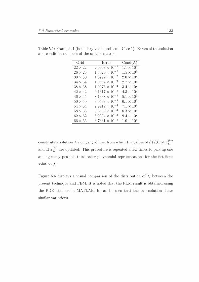
5.3 Numerical examples 133
Table 5.1: Example 1 (boundary-value problem - Case 1): Errors of the solutionand condition numbers of the system matrix.
Grid Error Cond(A)22× 22 2.0903× 10⁻² 1.1× 10²
26× 26 1.3029× 10⁻² 1.5× 10²
30× 30 1.0792× 10⁻² 2.0× 10²
34× 34 1.0584× 10⁻² 2.7× 10²
38× 38 1.0076× 10⁻² 3.4× 10²
42× 42 9.1317× 10⁻³ 4.3× 10²
46× 46 8.1338× 10⁻³ 5.1× 10²
50× 50 8.0598× 10⁻³ 6.1× 10²
54× 54 7.9912× 10⁻³ 7.1× 10²
58× 58 5.6866× 10⁻³ 8.3× 10²
62× 62 6.9334× 10⁻³ 9.4× 10²
66× 66 3.7331× 10⁻³ 1.0× 10³
constitute a solution f along a grid line, from which the values of ∂f/∂x at x(hi)b1
and at x(hi)b2 are updated. This procedure is repeated a few times to pick up one
among many possible third-order polynomial representations for the fictitious
solution ff .
Figure 5.5 displays a visual comparison of the distribution of fr between the
present technique and FEM. It is noted that the FEM result is obtained using
the PDE Toolbox in MATLAB. It can be seen that the two solutions have
similar variations.

5.3 Numerical examples 134
Figure 5.5: Example 1 (boundary-value problem - Case 2): A contour plot offr by the 1D-IRBFN method using grid of 40× 40 (top) and FEM (bottom).

5.3 Numerical examples 135
−1 −0.5 0 0.5 1−1
−0.8
−0.6
−0.4
−0.2
0
0.2
0.4
0.6
0.8
1
Figure 5.6: Example 2 (boundary value problem): Discretisation by the present1D-IRBFN method (top) and FEM (bottom)

5.3 Numerical examples 136
Example 2 - A boundary value problem
This problem is governed by Poisson equation with the driving function b(x, y) =
−1 and homogeneous Dirichlet boundary conditions. The domain of interest is
a unit square with 10 holes of radius 0.1. This example provides a good means of
testing the capability of the proposed technique in dealing with geometrically-
complex-domain problems. It is noted that multi-hole domains occur in many
practical modelling situations such as thermal conductivity for composite ma-
terials, fluid flow in porous medium and particulate flows.
In Figure 5.6, a typical discretisation of the present technique and that of FEM
are shown. The pre-processing for the present technique is much more eco-
nomical than that for FEM. Since there is no exact solution available here, we
present a visual comparison of the distribution of fr between the present tech-
nique (Scheme 1, grid of 80 × 80) and FEM (Figure 5.7). It is noted that the
FEM result is obtained using the PDE Toolbox in MATLAB. It can be seen
that the two solutions have similar behaviours.

5.3 Numerical examples 137
Figure 5.7: Example 2 (boundary value problem): A contour plot of fr by thepresent 1D-IRBFN method using grid of 80× 80 (top) and FEM (bottom)

5.3 Numerical examples 138
−0.6 −0.4 −0.2 0 0.2 0.4 0.6−0.5
−0.4
−0.3
−0.2
−0.1
0
0.1
0.2
0.3
0.4
0.5
Figure 5.8: Example 3 (initial-value problem): Domain of interest and a typicaldiscretisation
Example 3 - An initial-value problem
This problem is governed by the following parabolic PDE
∂f
∂t−
(∂2f
∂x2+∂2f
∂y2
)= (1 + 2π2k2t) sin(kπx) sin(kπy), (5.21)
where k is a given number. The problem domain is the region lying between a
square of 1× 1 and a circle of radius 0.2 which are both centered at the origin
(Figure 5.8). The exact solution is given by
f e(x, y, t) = sin(kπx) sin(kπy)t, (5.22)
from which the initial solution and Dirichlet boundary conditions are derived
analytically.
The spatial discretisation is carried out using a Cartesian grid of 40× 40. Both
Scheme 1 and Scheme 2 for calculating the function ff in (5.10) are employed.

5.4 Concluding remarks 139
For the latter, the values of ∂f/∂x at x(hi)b1 and at x
(hi)b2 are simply taken from
the previous time level. Results of Ne for k = 2 and k = 3 using a time step of
0.1 are presented in Table 5.2, which shows that Scheme 2 gives more accurate
results than Scheme 1. Scheme 2 is thus recommended for use in practice. It is
noted that the matrix condition number is only 3.8× 10² for a grid of 40× 40.
Plots for f with two values of k at t = 1 are shown in Figure 5.9.
5.4 Concluding remarks
In this chapter, Cartesian grids and 1D-IRBFNs are incorporated into the do-
main embedding framework to solve elliptic and parabolic equations of sec-
ond order on multiply-connected domains. The preprocessing is simple as the
multiply-connected domain is converted into a rectangular one. We employ
polynomials of third order to represent the fictitious solution within holes. Two
schemes to construct polynomials are proposed. The first is based on func-
tion values while the second relies on both function and derivative values. The
system matrix is expressed in terms of the values of the field variable at grid
nodes only. The technique is validated successfully through several boundary-
value and initial-value problems. Numerical results indicate that the inclusion
of derivative values in constructing the polynomials leads to an improvement in
accuracy. In comparison with the 1D-IRBFN-based boundary fitted method,
the 1D-IRBFN-based domain embedding method is seen to be less accurate, but
appears to be more convenient for solving multiply-connected domain problems
with many moving inner holes.

5.4 Concluding remarks 140
Table 5.2: Example 3 (initial-value problem): Errors of f with k = 2 and k = 3by Scheme 1 and Scheme 2 using grid of 40×40. It is noted that a(b) representsa× 10b.
k = 2 k = 3Time Scheme 1 Scheme 2 Scheme 1 Scheme 20.2 1.4690(-3) 8.1363e(-3) 1.1299(-2) 3.9580e(-3)0.4 1.4858(-3) 4.0864e(-3) 1.1435(-2) 3.9580e(-3)0.6 1.4915(-3) 2.7144e(-3) 1.1481(-2) 2.5376e(-3)0.8 1.4943(-3) 2.0333e(-3) 1.1504(-2) 1.8324e(-3)1.0 1.4961(-3) 1.6249e(-3) 1.1518(-2) 1.4103e(-3)1.2 1.4972(-3) 1.3527e(-3) 1.1528(-2) 1.1297e(-3)1.4 1.4980(-3) 1.1583e(-3) 1.1534(-2) 9.2994e(-4)1.6 1.4986(-3) 1.0125e(-3) 1.1539(-2) 7.8087e(-4)1.8 1.4991(-3) 8.9925e(-4) 1.1543(-2) 6.6565e(-4)2.0 1.4995(-3) 8.0867e(-4) 1.1546(-2) 5.7421e(-4)2.2 1.4998(-3) 7.3460e(-4) 1.1549(-2) 5.0016e(-4)2.4 1.5001(-3) 6.7292e(-4) 1.1551(-2) 4.3925e(-4)2.6 1.5003(-3) 6.2077e(-4) 1.1553(-2) 3.8855e(-4)2.8 1.5005(-3) 5.7610e(-4) 1.1554(-2) 3.4597e(-4)3.0 1.5007(-3) 5.3742e(-4) 1.1555(-2) 3.1000e(-4)3.2 1.5008(-3) 5.0361e(-4) 1.1557(-2) 2.7951e(-4)3.4 1.5009(-3) 4.7381e(-4) 1.1558(-2) 2.5366e(-4)3.6 1.5010(-3) 4.4735e(-4) 1.1559(-2) 2.3178e(-4)3.8 1.5011(-3) 4.2370e(-4) 1.1559(-2) 2.1335e(-4)4.0 1.5012(-3) 4.0244e(-4) 1.1560(-2) 1.9795e(-4)

5.4 Concluding remarks 141
k=2
−0.5
0
0.5
−0.5
0
0.5−4
−2
0
2
4
k=3
−0.5
0
0.5
−0.5
0
0.5−5
0
5
Figure 5.9: Example 3 (initial-value problem): Plots of the approximate solutionfor two values of k using a grid of 40× 40.

Chapter 6
1D-integrated-RBFN calculation
of particulate suspension flows
In this chapter, 1D-IRBFN methods are applied for the numerical prediction of
bulk properties of particulate suspensions under simple shear conditions. The
suspending fluid is Newtonian and the suspended particles are rigid. Results
obtained are compared well with those based on finite elements in the literature.

6.1 Introduction 143
6.1 Introduction
Figure 6.1: A particle-fluid system
Particulate suspensions, which involve transport of rigid particles suspended in
a fluid medium, occur in many industrial processes such as slurries, colloids,
fluidised beds, etc. Due to their great structural and physical variety, the use
of experiments to determine the macroscopic rheological properties of these
multiphase materials was seen to be impractical (Phan-Thien and Kim, 1994).
However, it may be possible to employ numerical simulations to predict the
bulk properties of multiphase materials. Various numerical models have been
proposed. Among them are direct numerical simulations (DNSs) which have
received a great deal of attention. In DNSs, the fundamental equations for par-
ticles (Newton-Euler equation) and a fluid (Navier-Stokes equation) are solved
in a direct and fully-coupled manner. Two main advantages of DNSs are that
(i) they can handle particles of different shapes and sizes as well as any type
of fluid; and (ii) hydrodynamic forces and moments can be calculated directly

6.1 Introduction 144
from the fluid flow. Difficulties faced by DNSs include (i) a very large number
of particles is typically required for a proper simulation; and (ii) the fluid do-
main is of very complex shape due to the presence of particles and the change
of their positions with time. Based on the fluid-phase solver employed, DNSs
can be classified into two categories. In the first category, a mesh follows the
movement of the particles, i.e. a moving mesh is used. Methods based on the
Arbitrary Lagrangian-Eulerian (ALE) moving mesh approach proposed by Hu
et al. (1992) are widely used, (e.g. Hu, 1995; Huang et al., 1997; Huang et al.,
1998). In the second category, a mesh covers the whole domain and is indepen-
dent of the position of particles, i.e. a fixed mesh is used. Methods based on
the fictitious domain approach proposed by Glowinski et al. (1998) are widely
employed, (e.g. Hwang et al., 2004; Patankar et al., 2000; Singh et al., 2000).
Hwang et al. (2004) incorporated sliding bi-periodic frames, introduced by Lees
and Edwards (1972) for molecular dynamics, into the simulation of particulate
flows. This concept allows the modelling of suspension systems with infinite
numbers of particles to be conducted through a small number of particles in a
representative reference sliding frame. The computational fluid domain is thus
small with bi-periodic conditions on the frame and no-slip conditions on the
surfaces of the particles.
In recent years, RBFN-based methods, which are extremely easy to implement
and capable of achieving a high level of accuracy using a relatively-small number
of nodes, have been successfully applied to solve complex problems encountered
in engineering, (e.g. Sarler et al., 2004; Sarler, 2005; Sarler et al., 2010; Gerace
et al., 2009; Kosec and Sarler, 2008a,b; Orsini et al., 2009; Divo and Kassab,
2005, 2006, 2007, 2008; Pepper and Sarler, 2005; Zahab et al., 2009; Yao et al.,
2011 and the references therein). In this chapter, we report a new numerical
method based on 1D integrated RBFNs and point collocation in the context
of boundary fitted Cartesian grids and sliding bi-periodic frames for the direct
simulation of flows of Newtonian-based particulate systems.

6.2 Governing equations and sliding frames concept 145
The remainder of the chapter is organised as follows. Section 6.2 gives a brief
review of the governing equations and the concept of sliding frames. In Sec-
tion 6.3, the proposed numerical procedure is described. Numerical results are
presented in Section 6.4. Section 6.5 concludes the chapter.
6.2 Governing equations and sliding frames con-
cept
6.2.1 Governing equations
Let Π be the entire computational domain, including the interior regions occu-
pied by the particles. Let Pi(t) and ∂Pi(t) be the region and its boundary of the
ith particle of time t, where i = (1, 2, · · · , N) and N is the number of particles
(Figure 6.1).
Fluid motion: The laws of mass and momentum conservation for an incom-
pressible fluid lead to
∇ · u = 0, (6.1)
ρfDu
Dt= ∇ · σ, (6.2)
where u is the velocity vector, ρf the density of the fluid, σ the total stress
tensor, and D[.]/Dt the material derivative defined as
D[.]
Dt=∂[.]
∂t+ (u ·∇)[.]. (6.3)

6.2 Governing equations and sliding frames concept 146
For a Newtonian fluid, the total stress tensor is given by
σ = −pI + 2ηD, (6.4)
where p is the hydrodynamic pressure, I the unit tensor, η the viscosity, and D
the strain rate tensor defined as
D =1
2[∇u+ (∇u)T ]. (6.5)
In the case of 2D problems, the ψ − ω formulation has been widely employed
because of its simplicity. The governing equations (6.1), (6.2) and (6.4) can be
rewritten as follows.
∂2ψ
∂x2+∂2ψ
∂y2= ω, (6.6)
∂ω
∂t+ u
∂ω
∂x+ v
∂ω
∂y=
1
Re
(∂2ω
∂x2+∂2ω
∂y2
), (6.7)
where ψ is the stream function, ω the vorticity, Re the Reynolds number, and
u and v the components of u, which are defined in terms of the stream function
as
u =∂ψ
∂y, v = −∂ψ
∂x.
The given velocity boundary conditions can be transformed into two boundary
conditions on the stream function and its normal derivative
ψ = γ,∂ψ
∂n= ξ,
where n is the direction normal to the boundary, and γ and ξ prescribed func-
tions.

6.2 Governing equations and sliding frames concept 147
Figure 6.2: Shear bi-periodic frames.
6.2 Governing equations and sliding frames concept 148
Particle motion: Consider an ith particle. The motion of the particle can be
described by the Newton-Euler equations
MidUi
dt= Fi, (6.8)
IidΩi
dt= Ti, (6.9)
whereMi, Ii,Ui andΩi are the mass, inertia tensor, translational velocity vector
of the mass centre and angular velocity vector of the ith particle, respectively,
and Fi and Ti the force and torque vectors acting on the ith particle.
The force and torque vectors can be computed from the fluid flow as
Fi =
∮
∂Pi(t)
σ · nds, (6.10)
Ti =
∮
∂Pi(t)
r× (σ · n) ds, (6.11)
where r is the position vector, n the outward unit vector normal to the boundary
∂Pi and ds the length of an infinitesimal part of ∂Pi.
Non-slip boundary conditions on the interface between the fluid and the ith
particle are given by
u = Ui +Ωi × r, (6.12)
where
Ui =dXi
dt,
Ωi =dΘi
dt,
in which Xi is the position vector of the mass center and Θi the orientation of

6.2 Governing equations and sliding frames concept 149
the ith particle. In terms of the stream function, (6.12) becomes
∂ψ
∂y= Ui − Ωiy (6.13)
∂ψ
∂x= −Vi − Ωix, (6.14)
where Ui and Vi are the two components of U and Ωi the magnitude of Ωi.
6.2.2 Sliding bi-periodic frames concept
Consider a particulate flow of very large domain under simple shear conditions
in the x direction. One possible way to make such a large problem tractable is to
simplify it using the concept of sliding bi-periodic frames. The problem domain
can be divided into a set of identical sliding frames of width L and height H
(Figure 6.2). Each frame translates along the shear direction at its own average
velocity. Rows of frames slide relatively to one another by an amount ∆ = γHt,
where γ is the given shear rate, H height of the frame and t shear time (Hwang
et al., 2004).
Because frames have similar solutions, only one frame is considered. If particles
in a frame are ignored, it can be seen that the velocity profile is linear
u = u0 + γy, (6.15)
v = 0, (6.16)
where the origin of the x− y coordinate system is located at the centre of the
frame; u0 the translation velocity of the frame and −H/2 ≤ y ≤ H/2. With
the presence of particles, one has
u = u+ u0 + γy, (6.17)
v = v, (6.18)

6.3 Proposed numerical procedure 150
where u and v are the perturbations from the linear profile.
Since the solution is continuous across sliding frames, the following bi-periodic
boundary conditions for the velocity u and the traction τ can be applied to
each frame
u(−L/2, y, t) = u(L/2, y, t), −H/2 ≤ y ≤ H/2, (6.19)
τ (−L/2, y, t) = τ (L/2, y, t), −H/2 ≤ y ≤ H/2, (6.20)
for the two vertical faces, and
u(x,−H/2, t) = u(x+ γHt,H/2, t) + (γH, 0)T , −L/2 ≤ x ≤ L/2,
(6.21)
τ (x,−H/2, t) = τ (x+ γHt,H/2, t), −L/2 ≤ x ≤ L/2,
(6.22)
for the two horizontal faces.
6.3 Proposed numerical procedure
In this chapter, we propose a numerical procedure based on IRBFNs and slid-
ing frames for the simulation of particulate suspensions under simple shear
conditions. The fluid domain in a reference frame is simply discretised using a
Cartesian grid nx×ny . Let Γ1,Γ2,Γ3 and Γ4 be the sides of the reference frame
(Figure 6.3). IRBFNs are employed on each grid line to represent the field
variables ψ and ω (one-dimensional IRBFNs). Sliding bi-periodic boundary
conditions are presently implemented by means of point collocation rather than
the Lagrange multipliers used in (Hwang et al., 2004). The proposed procedure
combines strengths of three approaches, namely IRBFNs (high-order accuracy),
Cartesian grids (easy preprocessing) and the sliding bi-periodic frames concept

6.3 Proposed numerical procedure 151
(infinite number of particles). To our best knowledge, this is a first attempt to
use RBFs for the analysis of shear particulate flows. In the following, details are
presented for the three constituent components of the proposed procedure. 1D-
IRBFNs are first described. Sliding bi-periodic boundary conditions are then
expressed in terms of the stream function and implemented with IRBFs and
point collocation. Finally, suitable formulas and their IRBFN implementation
are presented for computing the boundary values on the particles.
Γ1
Γ2
Γ3
Γ4
Figure 6.3: A reference frame and its typical Cartesian-grid discretisation.
x1 x2 xq
xb1 xb2
Figure 6.4: Nodal points on a grid line consisting of interior points xi () andboundary points xbi (2).

6.3 Proposed numerical procedure 152
6.3.1 1D-IRBFNs
Consider a grid line that can be bounded by two faces of the frame, the bound-
aries of two particles, or the boundary of the particle and the frame. Assume a
grid line in the x direction and let f be the field variable. IRBFNs are employed
to approximate f . The construction procedure is as follows.
Second-order derivative of f along a grid line can be decomposed into RBFs
∂2f(x)
∂x2=
m∑
i=1
wigi(x) =m∑
i=1
wiI(2)i (x), (6.23)
where m is the number of RBFs, gi(x)mi=1 ≡I(2)i (x)
mi=1
the set of RBFs,
wimi=1 the set of weights to be found and f represents ψ and ω. Approximate
expressions for the first-order derivative and the field variable are then obtained
through integration
∂f(x)
∂x=
m∑
i=1
wiI(1)i (x) + c1, (6.24)
f(x) =
m∑
i=1
wiI(0)i (x) + c1x+ c2, (6.25)
where I(1)i (x) =
∫I(2)i (x)dx and I
(0)i (x) =
∫I(1)i (x)dx. In this study, IRBFNs
are implemented with the multiquadric (MQ) function and one thus has
I(2)i (x) =
√(x− ci)2 + a2i , (6.26)
I(1)i (x) =
(x− ci)
2A+
a2i2B, (6.27)
I(0)i (x) =
(−a2i3
+(x− ci)
2
6
)A+
a2i (x− ci)
2B, (6.28)
where ci and ai are the centre and the width of the ith MQ, respectively, A =√
(x− ci)2 + a2i , and B = ln((x− ci) +
√(x− ci)2 + a2i
). The grid size h is
chosen as the RBF width ai. The set of collocation points ximi=1 is taken to
be the same as the set of centres cimi=1.

6.3 Proposed numerical procedure 153
As shown in Figure 6.4, a grid line contains two sets of nodal points. The first
set consists of q interior points that are also the grid nodes (regular nodes). The
function values at the interior points (xiqi=1) are unknown. The second set
consists of the two nodes xb1 and xb2 which are generated by the intersection of
the grid line and the boundaries.
Collocating (6.25) at the nodal points yields
f
f(xb1)
f(xb2)
= I(0)
w
c1
c2
, (6.29)
where
f = (f(x1), f(x2), · · · , f(xq))T ,
w = (w1, w2, · · · , wm)T ,
I(0) =
I(0)1 (x1) I
(0)2 (x1) · · · I
(0)m (x1) x1 1
I(0)1 (x2) I
(0)2 (x2) · · · I
(0)m (x2) x2 1
......
. . ....
......
I(0)1 (xq) I
(0)2 (xq) · · · I
(0)m (xq) xq 1
I(0)1 (xb1) I
(0)2 (xb1) · · · I
(0)m (xb1) xb1 1
I(0)1 (xb2) I
(0)2 (xb2) · · · I
(0)m (xb2) xb2 1
,
m = q + 2.
Solving (6.29) for the coefficient vector, including the two integration constants,
results in
w
c1
c2
=
(I(0)
)−1
f
f(xb1)
f(xb2)
, (6.30)
where(I(0)
)−1
is the generalised inverse of I(0).

6.3 Proposed numerical procedure 154
Making use of (6.30), the values of the first and second derivatives of f at the
interior points are computed in terms of nodal variable values
∂f(x1)∂x
∂f(x2)∂x...
∂f(xq)∂x
= I(1)(I(0)
)−1
f
f(xb1)
f(xb2)
, (6.31)
and
∂2f(x1)∂x2
∂2f(x2)∂x2
...
∂2f(xq)∂x2
= I(2)(I(0)
)−1
f
f(xb1)
f(xb2)
, (6.32)
where
I(1) =
I(1)1 (x1) I
(1)2 (x1) · · · I
(1)m (x1) 1 0
I(1)1 (x2) I
(1)2 (x2) · · · I
(1)m (x2) 1 0
......
. . ....
......
I(1)1 (xq) I
(1)2 (xq) · · · I
(1)m (xq) 1 0
,
and
I(2) =
g1(x1) g2(x1) · · · gm(x1) 0 0
g1(x2) g2(x2) · · · gm(x2) 0 0...
.... . .
......
...
g1(xq) g2(xq) · · · gm(xq) 0 0
.
It can be seen from (6.31) and (6.32) that Dirichlet conditions at xb1 and xb2
are incorporated into the IRBFN approximations. Depending on how a grid
line is bounded, the boundary points xb1 and xb2 have particular locations. For
example, one has (xb1 ∈ Γ2 and xb2 ∈ Γ4) if a grid line is bounded by the two
vertical faces of the frame, and (xb1 ∈ Γ2 and xb2 ∈ ∂Pi) if the bounding surfaces

6.3 Proposed numerical procedure 155
are the left face and the ith particle boundary.
In the same manner, one can obtain the IRBFN expressions for a y−grid line.
6.3.2 Sliding bi-periodic boundary conditions
The continuity of the stream function and the vorticity across two adjacent
sliding frames leads to the following periodic boundary conditions (Anderson
et al., 2006)
ψ(−L/2, y, t) = ψ(L/2, y, t), −H/2 ≤ y ≤ H/2, (6.33)
∂ψ
∂x(−L/2, y, t) = ∂ψ
∂x(L/2, y, t), −H/2 ≤ y ≤ H/2, (6.34)
ω(−L/2, y, t) = ω(L/2, y, t), −H/2 ≤ y ≤ H/2, (6.35)
∂ω
∂x(−L/2, y, t) = ∂ω
∂x(L/2, y, t), −H/2 ≤ y ≤ H/2, (6.36)
for the two vertical faces and
ψ(x,−H/2, t) = ψ(x+ γHt,H/2, t), −L/2 ≤ x ≤ L/2, (6.37)
∂ψ
∂y(x,−H/2, t) = ∂ψ
∂y(x+ γHt,H/2, t) + γH, −L/2 ≤ x ≤ L/2,
(6.38)
ω(x,−H/2, t) = ω(x+ γHt,H/2, t), −L/2 ≤ x ≤ L/2, (6.39)
∂ω
∂y(x,−H/2, t) = ∂ω
∂y(x+ γHt,H/2, t), −L/2 ≤ x ≤ L/2, (6.40)
for the two horizontal faces.
Consider the stream function ψ. The values of ψ are unknown not only at the
interior points (xi, yj) with 2 ≤ i ≤ nx − 1 and 2 ≤ j ≤ ny − 1 but also at the
boundary points of the reference frame (−L/2, yj), (L/2, yj), (xi,−H/2) and
(xi, H/2) with 1 ≤ j ≤ ny and 2 ≤ i ≤ nx − 1. There are 2ny + 2(nx − 2)
unknowns for the latter, leading to nip + 2ny + 2(nx − 2) unknowns in total,

6.3 Proposed numerical procedure 156
where nip is the number of interior points. Apart from collocating the governing
equation for ψ at the interior points, one also needs to generate 2ny + 2(nx −2) extra equations which can be achieved by using the bi-periodic boundary
conditions (6.33), (6.34), (6.37) and (6.38). Details are as follows.
ψ(−L/2, yj)− ψ(L/2, yj) = 0, 1 ≤ j ≤ ny, (6.41)
∂ψ
∂x(−L/2, yj)−
∂ψ
∂x(L/2, yj) = 0, 1 ≤ j ≤ ny, (6.42)
ψ(xi,−H/2)− ψ(xi + γHt,H/2) = 0, 2 ≤ i ≤ nx − 1, (6.43)
∂ψ
∂y(xi,−H/2)−
∂ψ
∂y(xi + γHt,H/2)− γH = 0, 2 ≤ i ≤ nx − 1, (6.44)
where the time variable t is left out for the sake of simplicity.
In (6.41)-(6.44), one needs to express ∂ψ(L/2, yj)/∂x, ∂ψ(−L/2, yj)/∂x, ∂ψ(xi,−H/2)/∂y,ψ(xi + γHt,H/2) and ∂ψ(xi + γHt,H/2)/∂y in terms of nodal values of ψ.
For ∂ψ(±L/2, yj)/∂x, the following IRBFN expressions are obtained by collo-
cating (6.24) at x = ±L/2 and then making use of (6.30)
∂ψ
∂x(L/2, yj) = [I
(1)1 (L/2), · · · , I(1)m (L/2), 1, 0]
(I(0)
)−1
ψ
ψ(xb1, yj)
ψ(L/2, yj)
,
(6.45)
∂ψ
∂x(−L/2, yj) = [I
(1)1 (−L/2), · · · , I(1)m (−L/2), 1, 0]
(I(0)
)−1
ψ
ψ(−L/2, yj)ψ(xb2, yj)
.
(6.46)
Similarly, one can obtain
∂ψ
∂y(xi,−H/2) = [I
(1)1 (−H/2), · · · , I(1)m (−H/2), 1, 0]
(I(0)
)−1
ψ
ψ(xi,−H/2)ψ(xi, yb2)
.

6.3 Proposed numerical procedure 157
(6.47)
For ψ(xi + γHt,H/2), collocating (6.25) at xi + γHt and then making use of
(6.30) lead to
ψ(x, H/2) = [I(0)1 (xi), · · · , I(0)m (xi), xi, 1]
(I(0)
)−1
ψ
ψ(−L/2, H/2)ψ(L/2, H/2)
, (6.48)
where xi = xi+ γHt. The process of deriving the IRBFN expression for ∂ψ(xi+
γHt,H/2)/∂y is similar to that for ψ(xi + γHt,H/2).
Sliding bi-periodic boundary conditions for the vorticity are also obtained in a
similar fashion.
6.3.3 Boundary conditions on the particles’ boundaries
Boundary conditions for the stream function
The values of the stream function ψ on the boundary of each particle Pi are
constant due to no-slip condition at the particle surface. Particles have their
own boundary values of ψ which are unknown. To find these unknowns, Lewis
(1979) suggested using the condition that the pressure is a single-valued function
on the boundary of a particle. This condition can be mathematically described
as
∮
∂Pi
∂p
∂sds =
∮
∂Pi
∇p · d~s = 0, (6.49)

6.3 Proposed numerical procedure 158
where p is the pressure and s the arc length. In the Cartesian coordinate system,
(6.49) becomes
∮∂p
∂xdx+
∮∂p
∂ydy = 0. (6.50)
The pressure gradient ∇p can be obtained from the momentum equations in
the primitive variable form. By replacing u = ∂ψ/∂y and v = −∂ψ/∂x, onecan express the components of ∇p in terms of the stream function and its
derivatives.
Boundary conditions for the vorticity
Figure 6.5: A curved boundary of the particle: arclength, and unit normal andtangential vectors.
The values of the vorticity on ∂Pi can be computed via
ω =∂2ψ
∂x2+∂2ψ
∂y2, x ∈ ∂Pi. (6.51)
The handling of (6.51) thus involves the evaluation of second-order derivatives
of the stream function in both x and y directions. Unfortunately, the boundary
points on ∂Pi do not generally coincide with the grid nodes and hence they lie

6.3 Proposed numerical procedure 159
on either x− or y−grid lines. In (Le-Cao et al., 2009), the following formulae
were proposed
ω =
[1 +
(txty
)2]∂2ψ
∂x2− txt2y
∂2ψ
∂x∂s+
1
ty
∂2ψ
∂y∂s, x ∈ ∂Pi, (6.52)
for the x−grid lines, and
ω =
[1 +
(tytx
)2]∂2ψ
∂y2− tyt2x
∂2ψ
∂y∂s+
1
tx
∂2ψ
∂x∂s, x ∈ ∂Pi, (6.53)
for the y−grid lines. In (6.52) and (6.53), tx and ty are the x and y components
of the unit tangential vector and ∂(.)/∂s represents the derivative of (.) on ∂Pi
which is known (Figure 6.5). The boundary conditions for the vorticity are thus
written in terms of the second derivative of ψ with respect to x or y only.
In the case that the ith particle is of circular shape of radius Ri and rotates
about the centre of the reference frame at the angular velocity Ωi. Expressions
for computing tx, ty, ∂2ψ/∂x∂s and ∂2ψ/∂y∂s become
tx =−y√x2 + y2
, (6.54)
ty =x√
x2 + y2, (6.55)
∂2ψ
∂x∂s=
1
RiΩiy, (6.56)
∂2ψ
∂y∂s= − 1
RiΩix. (6.57)
Substitution of (6.54)-(6.57) into (6.52) and (6.53) yields
ω =
[1 +
(yx
)2]∂2ψ
∂x2+
[(yx
)2
− 1
]Ωi, x ∈ ∂Pi, (6.58)
ω =
[1 +
(x
y
)2]∂2ψ
∂y2+
[(x
y
)2
− 1
]Ωi, x ∈ ∂Pi. (6.59)
The IRBFN implementation of (6.50) is straightforward, while special treat-

6.3 Proposed numerical procedure 160
ments are required in handling (6.52)-(6.53) and (6.58)-(6.59). For the latter,
normal derivative boundary conditions for the stream function, i.e. ∂ψ/∂n,
need be incorporated into expressions (6.52), (6.53), (6.58) and (6.59). Since
ψ and ∂ψ/∂n are known from the previous iteration, one can easily obtain the
values of ∂ψ/∂x and ∂ψ/∂y on ∂Pi. The proposed procedure imposes ∂ψ/∂n,
i.e. ∂ψ/∂x and ∂ψ/∂y, using the constants of integration. On an x−grid line,
one needs to incorporate ∂ψ/∂x into ∂2ψ/∂x2, while on a y−grid line, ∂ψ/∂y
is incorporated into ∂2ψ/∂y2. Because these two processes are similar, details
are given here for an x−grid line only, e.g. the one with xb1 ∈ Γ2 and xb2 ∈ ∂Pi.
The system for the conversion of the RBF space into the physical space (6.29)
now takes the form
ψ
ψ(xb1)
ψ(xb2)
∂ψ∂x(xb2)
=
I(0)
B
w
c1
c2
, (6.60)
where the conversion matrix is of dimensions (m+ 1)× (m+ 2) and
B =[I(1)1 (xb2), I
(1)2 (xb2), · · · , I(1)m (xb2), 1, 0
].
Using (6.60), one obtains the following from (6.23) (in which f ≡ ψ and x ≡ xb2)
∂2ψ
∂x2(xb2) = [g1(xb2), g2(xb2), · · · , gm(xb2), 0, 0]
I(0)
B
−1
ψ
ψ(xb1)
ψ(xb2)
∂ψ∂x(xb2)
.
(6.61)
Since the conversion matrix in (6.60) is not over-determined, the IRBFN approx-
imation for ∂2ψ(xb2)/∂x2 satisfies ∂ψ/∂x at x = xb2 identically. This imposition
shows a clear advantage of IRBFNs over the usual differentiated approximations.

6.4 Numerical examples 161
Substituting (6.61) into (6.52), one is able to obtain the boundary conditions
on ∂Pi for the vorticity equation. It is noted that given ∂ψ/∂x and ∂ψ/∂y on
∂Pi, the terms ∂2ψ/∂x∂s and ∂2ψ/∂y∂s in (6.52) and (6.53) are known.
6.4 Numerical examples
In this section, the proposed procedure is validated through three examples. The
first example examines the performance of the present technique in the imple-
mentation of sliding bi-periodic boundary conditions of the frame. The second
example investigates the accuracy of the present technique in the handling of
boundary conditions that are similar to those on the particles’ boundaries. In
the third example, the proposed method is applied to simulate a shear flow of
a Newtonian-based particulate system, which is modelled by one particle sus-
pended in a sliding rectangular frame. For all numerical examples, the problem
domain is discretised using a uniform Cartesian grid. The interior points that
fall very close to the curved/irregular boundary (within a distance of h/8, h -
the grid size) are removed from the set of nodal points.
6.4.1 Example 1: Sliding bi-periodic boundary condi-
tions
In this example, the 1D-IRBFN implementation of shear bi-periodic boundary
conditions is validated. The test problem is governed by
∂2ψ
∂x2+∂2ψ
∂y2= b(x, y). (6.62)
The domain of interest is the region lying between a circle of radius 1/2 and a
square of dimensions 2 × 2 which are both centered at the origin. The exact

6.4 Numerical examples 162
solution is
ψ(x, y) = sin(π(x− γyt)) sin(πy), (6.63)
from which the driving function b(x, y) in (6.62) and the Dirichlet boundary
conditions on the hole can be easily derived. The value of γ is set to 1. This
problem is taken from (Anderson et al., 2006).
The accuracy of an approximation scheme is measured by means of the discrete
relative L2 norm of the error defined as
Ne =
√∑Mi=1(ψ
ei − ψi)2√∑M
i=1(ψei )
2
, (6.64)
where M is the number of unknown nodal values of ψ, and ψe and ψ are the
exact and approximate solutions, respectively. Another important measure is
the convergence rate α of the solution with respect to grid refinement
Ne(h) ≈ γhα = O(hα), (6.65)
in which α and γ are exponential model’s parameters. Given a set of ob-
servations, these parameters can be found by the general linear least squares
technique.

6.4 Numerical examples 163
Table 6.1: Example 1 (sliding bi-periodic boundary conditions): Errors of thesolution and condition numbers of the system matrix denoted by Cond(A). Itis noted that h is the spacing (grid size).
Grid Ne Cond(A)12× 12 3.1078× 10⁻³ 1.6× 10³
22× 22 4.9660× 10⁻⁴ 5.1× 10³
32× 32 1.5234× 10⁻⁴ 1.8× 10⁴
42× 42 6.6599× 10⁻⁵ 2.2× 10⁴
52× 52 3.6510× 10⁻⁵ 5.2× 10⁴
62× 62 1.9881× 10⁻⁵ 5.9× 10⁴
O(h2.94)

6.4 Numerical examples 164
t = 0 t = 0.25
−1 −0.5 0 0.5 1−1
−0.8
−0.6
−0.4
−0.2
0
0.2
0.4
0.6
0.8
1
−1 −0.5 0 0.5 1−1
−0.8
−0.6
−0.4
−0.2
0
0.2
0.4
0.6
0.8
1
t = 0.5 t = 0.6
−1 −0.5 0 0.5 1−1
−0.8
−0.6
−0.4
−0.2
0
0.2
0.4
0.6
0.8
1
−1 −0.5 0 0.5 1−1
−0.8
−0.6
−0.4
−0.2
0
0.2
0.4
0.6
0.8
1
t = 0.75 t = 1
−1 −0.5 0 0.5 1−1
−0.8
−0.6
−0.4
−0.2
0
0.2
0.4
0.6
0.8
1
−1 −0.5 0 0.5 1−1
−0.8
−0.6
−0.4
−0.2
0
0.2
0.4
0.6
0.8
1
Figure 6.6: Example 1 (sliding bi-periodic boundary conditions): Contour plotsof the approximate and exact solutions at different time values. The two plotsare indistinguishable.

6.4 Numerical examples 165
Figure 6.7: Example 2 (rotating cylinder): geometry.
A number of grids, namely (12 × 12, 22 × 22, · · · , 62 × 62), are employed for
the convergence study. Results concerning the condition number of the system
matrix, denoted by cond(A), and the error Ne at t = 0 are listed in Table
6.1. It can be seen that the present system matrix has relatively-low condition
numbers and the solution converges fast at the rate of 2.94.
Contour plots for ψ at several values of the shear time t, namely (0, 0.5, 0.75, 1),
using a grid of 42×42 are shown in Figure 6.6. Exact solutions are also included.
The two solutions are indistinguishable.
6.4.2 Example 2: A rotating circular cylinder

6.4 Numerical examples 166
Re = 100
Re = 200
Re = 500
Figure 6.8: Example 2 (rotating cylinder): Velocity vector field (left) and vor-ticity field (right) for the flow at Re = 100, 200 and 500.

6.4 Numerical examples 167
Table 6.2: Example 2 (rotating cylinder): Comparison of the stream-functionvalue at the inner cylinder, ψwall, between the present technique (grid of 36×36)and finite difference technique for several values of Re.
Re 100 200 500ψwall
Present 0.4637 0.4632 0.4550(Lewis, 1979) 0.4577 0.4539 0.4465
In this test problem, the 1D-IRBFN implementation of boundary conditions of
particles is validated through the simulation of the flow of a Newtonian fluid
shown in Figure 6.7. The inner cylinder rotates at a unit angular velocity while
the outer cylinder is stationary. The value of ψ on the outer wall is simply set
to zero, while the value of ψ on the inner wall is considered as an unknown,
denoted by ψwall. The flow is governed by (6.6) and (6.7) and subject to the
boundary conditions
ψ =∂ψ
∂x=∂ψ
∂y= 0,
on the outer cylinder and
ψ = ψwall,∂ψ
∂x= −x, ∂ψ
∂y= −y,
on the inner cylinder. Using (6.58) and (6.59) with Ω = 1, the vorticity bound-
ary conditions on the rotating cylinder can be computed by
ω =
[1 +
(yx
)2]∂2ψ
∂x2+
[(yx
)2
− 1
],
ω =
[1 +
(x
y
)2]∂2ψ
∂y2+
[(x
y
)2
− 1
].
The value of ψwall is found using the single-valued pressure condition as dis-
cussed earlier.

6.4 Numerical examples 168
The flow is simulated with R = 0.25 and L = 1.0 using a uniform grid of
36 × 36. Several values of the Reynolds number, namely (100, 200, 500), are
considered. Results concerning ψwall obtained by the proposed technique and
the finite-difference technique (Lewis, 1979) are presented in Table 6.2, showing
a good agreement. Plots for the velocity vector and vorticity fields for the case
of Re = 100, 200, 500 are given in Figure 6.8.
6.4.3 Example 3: Shear suspension flow
In this example, a single particle of radius R is suspended freely at the center of
the reference sliding bi-periodic frame of dimensions 1× 1. The fluid domain is
the region lying between the particle and the frame boundary (Figure 6.9). The
fluid is Newtonian and moves under a shear rate γ = 1. This configuration can
represent the system of an infinite number of particles as described in Figure
6.10. It can be seen that the initial configuration is reproduced after the time
period K = 1/γ. The inertia of the particle and fluid are ignored. This problem
was studied using the fictitious-domain/finite-element method in (Hwang et al.,
2004). The governing equations for the motion of a fluid thus reduce to
∂2ψ
∂x2+∂2ψ
∂y2= ω, (6.66)
∂2ω
∂x2+∂2ω
∂y2= 0. (6.67)

6.4 Numerical examples 169
Figure 6.9: Example 3 (shear suspension): A reference frame (top) and itsdiscretisation (bottom).

6.4 Numerical examples 170
The boundary conditions for the frame are bi-periodic and determined through
(6.33)-(6.40), while the boundary conditions for the particle are computed using
(6.50), (6.58) and (6.59). However, as only one particle is considered, the value
of ψ on ∂P is simply set to 0. The stress tensor can be written in terms of the
stream function and pressure as
σ =
(−p+ 2 ∂2ψ
∂x∂y
) (∂2ψ∂y2
− ∂2ψ∂x2
)(∂2ψ∂y2
− ∂2ψ∂x2
) (−p + 2 ∂2ψ
∂x∂y
) . (6.68)
Conventionally, the interacting hydrodynamic force and moment are first calcu-
lated from the fluid flow, and the movement of the particle is then determined
from these force and moment using the Newton-Euler equations. Because the
inertia of the particle is neglected and there is no external force acting on the
particle, the hydrodynamic force and torque are zero (force free and torque
free). It can be seen that the particle rotates about the frame centre at the
angular velocity Ω and does not translate relative to the frame, i.e. U = 0 and
V = 0. One thus only needs to use the torque-free condition to determine the
value of Ω
T =
∫
∂P
r× (σ · n) ds = 0. (6.69)
The reader is referred to (Hwang et al., 2004) for further details. Substitution
of (6.68) into (6.69) yields
∮(x2 − y2)
(∂2ψ
∂y2− ∂2ψ
∂x2
)ds = 0. (6.70)
In this study, a new way of obtaining Ω is proposed. On the particle boundary
(Figure 6.5), one can have
∂f
∂s=∂f
∂xtx +
∂f
∂yty, (6.71)
where f is a generic function, and s, tx and ty are defined as before. By replacing

6.4 Numerical examples 171
f = ∂ψ/∂x, (6.71) becomes
∂2ψ
∂s∂x=∂2ψ
∂x2tx +
∂2ψ
∂y∂xty. (6.72)
Since U = 0 and V = 0, (6.13) and (6.14) reduce to
∂ψ
∂y= −Ωy, (6.73)
∂ψ
∂x= −Ωx. (6.74)
Substituting (6.73) and (6.74) into (6.72) and making use of tx = −y/R and
ty = x/R give
Ω = −∂2ψ
∂x2. (6.75)
Similarly, by replacing f = ∂ψ/∂y, one has
Ω = −∂2ψ
∂y2. (6.76)
These conditions (6.75) and (6.76) can be used as an alternative to (6.70). In
practice, (6.75) and (6.76) are applied to the boundary points of the particle
on the x− and y−grid lines, respectively, from which the angular velocity is
derived in an average sense.

6.4 Numerical examples 172
(a) t = 0
(b) t = K/2
Figure 6.10: Example 3 (shear suspension): Problem description with two in-stances during a period of shearing.

6.4 Numerical examples 173
0 0.1 0.2 0.3 0.4 0.5 0.6 0.7 0.8 0.9 1−0.52
−0.5
−0.48
−0.46
−0.44
−0.42
−0.4
R=0.15R=0.25R=0.35R=0.38R=0.42
Shear time
Angu
larvelocity
Figure 6.11: Example 3 (shear suspension): Profile of the angular velocity overthe period K.

6.4 Numerical examples 174
For each shear interval, the solution procedure is as follows.
1. Guess the distribution of ω and ψ.
2. Discretise (6.66) and (6.67) using 1D-IRBFNs. The two system matrices
arising from the discretisation of the Laplace operator are identical and
remain unchanged during the iterative process.
3. Impose the sliding bi-periodic boundary conditions for ψ and ω on the
frame.
4. Derive computational boundary conditions for ω on ∂P .
5. Solve (6.66) for ω and (6.67) for ψ.
6. Compute Ω from (6.75) and (6.76).
7. Check the following convergence measure
CM =
√∑nip
i=1
(ψ
(k)i − ψ
(k−1)i
)2
√∑nip
i=1
(ψ
(k)i
)2< ǫ,
where nip is the number of interior points, k the current iteration and ǫ
the tolerance. In this study, ǫ is taken to be 10−12.
8. If not, relax the field solution
ψ(k)i = αψ
(k)i + (1− α)ψ
(k−1)i ,
where α is a given number (0 < α < 1), and repeat from step 4. Otherwise,
stop the computation and save the results.
The particle’s radius R is considered in the range of 0.15 to 0.42. Simulations
are carried out using Cartesian grids whose densities vary from 50×50 to 72×72.
Denser grids are used for larger values of R.

6.4 Numerical examples 175
t = 0
t = 0.3
Figure 6.12: Example 3 (shear suspension): Streamlines and iso-vorticity linesat the shear time of 0 and 0.3.

6.4 Numerical examples 176
Figure 6.11 shows the variation of Ω with respect to the shear time for several
values of R over the period K. It can be seen that the profile of Ω is symmetric
about the vertical line t = K/2. The largest value of Ω occurs when the frames
line up in the vertical direction (Figure 6.10a). Furthermore, the fluctuation of
Ω is an increasing function of R, indicating stronger hydrodynamic interaction
between particles at shorter range. In Figure 6.12, the distribution of ψ and
ω over a reference frame are multiplied to produce the ψ and ω fields on the
original large domain, where the sliding bi-periodic boundary conditions are
clearly observed.
Prediction of the bulk material properties
Following the work of Hwang et al. (2004), the bulk stress can be computed by
〈σ〉 = 1
A
∫
Γ
xτ Tds, (6.77)
where Γ = Γ1 ∩ Γ2 ∩ Γ3 ∩ Γ4 and A is the area of the frame domain, x the
position vector and τ the traction vector. In terms of ψ, (6.77) takes the form
〈σxy〉 =1
A
∫
Γ
ytxds =
∫
Γ1
(∂2ψ
∂y2− ∂2ψ
∂x2
)dy, (6.78)
〈σxx〉 =1
A
∫
Γ
xtxds =
∫
Γ2
(−p + ∂2ψ
∂x∂y
)dy +
∫
Γ3
x
(∂2ψ
∂y2− ∂2ψ
∂x2
)dx
−∫
Γ1
x
(∂2ψ
∂y2− ∂2ψ
∂x2
)dx, (6.79)
〈σyy〉 =1
A
∫
Γ
ytyds =1
2
∫
Γ3
(−p + ∂2ψ
∂x∂y
)dx− 1
2
∫
Γ1
(−p + ∂2ψ
∂x∂y
)dx,
(6.80)
where the pressure on Γ2 and Γ1 are computed using
p =
∫
Γ2
∂p
∂ydy = −
∫
Γ2
(∂3ψ
∂x3+
∂3ψ
∂y2∂x
)dy,
p =
∫
Γ1
∂p
∂xdx =
∫
Γ1
(∂3ψ
∂y3+
∂3ψ
∂x2∂y
)dx,

6.4 Numerical examples 177
and the pressure on Γ3 is derived from the pressure on Γ1 and the sliding periodic
condition.
Results for the bulk shear stress 〈σxy〉 and the normal stress difference 〈σxx−σyy〉are plotted in Figure 6.13 and 6.14. When the distance from a given particle in
a sliding layer to the nearest particle in an adjacent layer is maximum (Figure
6.10b), the bulk shear stress becomes maximum and the bulk normal stress
difference becomes minimum. Both the bulk shear and normal stress difference
become larger when the particle radius increases and they oscillate with the
period K.
The bulk shear viscosity can be obtained by taking the time average of the bulk
shear stress over the period K (Hwang et al., 2004),
〈η〉η
=1
K
∫ K
0
〈σxy〉dt. (6.81)
In Figure 6.15, 〈η〉/η is plotted against the solid area fraction φ (φ = πR2). In
the case of dilute suspensions with circular disks, the bulk shear viscosity can
be computed by 〈η〉 = (1 + 2φ)η (Hwang et al., 2004). The dilute suspension
results are also plotted in Figure 6.15. It can be seen that the present model
produces larger values of 〈η〉/η than the dilute model. This looks reasonable as
the present simulations take the interaction between the particles into account
and the dilute result is only valid for small φ.
The observations presented above are similar to those reported in (Hwang et al.,
2004). Since the finite-element results were presented in graph, we are not able
to reproduce them here. However, numerical results by the two techniques
appear to be of comparable values, judging from the graphical presentations.

6.4 Numerical examples 178
0 0.1 0.2 0.3 0.4 0.5 0.6 0.7 0.8 0.9 11
1.5
2
2.5
3
3.5
4
R=0.15R=0.25R=0.35R=0.38R=0.42
Shear time
〈σxy〉
Figure 6.13: Example 3 (shear suspension): Variations of the bulk shear stressesover the period K.

6.4 Numerical examples 179
0 0.1 0.2 0.3 0.4 0.5 0.6 0.7 0.8 0.9 1−2.5
−2
−1.5
−1
−0.5
0
0.5
1
1.5
2
2.5
R=0.15R=0.25R=0.35R=0.38R=0.42
Shear time
〈σxx−σyy〉
Figure 6.14: Example 3 (shear suspension): Variations of the bulk normal stressdifference over the period K.

6.4 Numerical examples 180
0 0.1 0.2 0.3 0.4 0.5 0.6 0.7 0.81
1.5
2
2.5
3
3.5
4
4.5
Analytic (Dilute)Numerical
Solid area fraction
〈η〉/η
Figure 6.15: Example 3 (shear suspension): Computed bulk viscosity. Analyticresults for the dilute case are also included.

6.5 Concluding remarks 181
6.5 Concluding remarks
In this chapter, a new computational procedure based on 1D-IRBFNs is devel-
oped for the simulation of 2D particulate flows under simple shear conditions.
Sliding bi-periodic frames are applied to reduce the large domain to a small
one. For the fluid component, the governing equations are taken in the stream-
function - vorticity formulation and the multiply-connected domain is simply
discretised using a Cartesian grid. For the particle component, a new efficient
way, based on direct point-wise calculations rather than line/surface integrals,
is proposed to compute the angular velocity. Three examples concerning sliding
bi-periodic conditions, particle-like boundary conditions and shear particulate
suspensions modelled by one particle in each frame are simulated successfully.
The presently predicted bulk properties are in good agreement with those by
the fictitious-domain/finite-element method.

Chapter 7
Conclusion
This chapter concludes the thesis. We will briefly summarise research contribu-
tions of the project and also present some suggestions for improvement.

7.1 Research contributions 183
7.1 Research contributions
The outcome of the present research project is the successful development of
accurate and efficient numerical methods based on Cartesian grids and 1D-
IRBFNs for the simulation of heat and viscous flows defined on two-dimensional
multiply-connected domains. Significant applications of the proposed methods
include the simulation of natural convection flows and the prediction of mate-
rial properties of particulate flows. Research works in this project are briefly
outlined below.
Development of 1D-IRBFNs for solving heat transfer problems in
multiply-connected domains
This research work has been presented in Chapter 2. A multiply-connected
domain is simply discretised by a Cartesian grid, in which all boundaries are
represented by sets of points that are generated by the intersections between the
grid lines and the boundaries. We employ IRBFNs in one dimension on each
grid line to approximate the field variable and point collocation to discretise
the governing equation. Advantages of the proposed method include (i) very
economical preprocessing (Cartesian grids for multiply-connected domains); (ii)
high order of accuracy (RBFNs); (iii) avoidance of the reduction in convergence
rate caused by differentiation (integral formulation); (iv) accurate imposition of
Neumann boundary conditions (integration constants); and (v) achievement of
some degree of local approximation (IRBFNs in one dimension). The proposed
method is validated successfully through the solution of second-order elliptic and
parabolic equations. Numerical results show that high rates of convergence with
respect to grid refinement are obtained and condition numbers of the system
matrix are relatively low, e.g. in the range of O(101) to O(103) for grids with
densities of 12× 12 to 62× 62, respectively.
Development of 1D-IRBFNs for discretising the stream-function -

7.1 Research contributions 184
vorticity (ψ − ω) formulation in multiply-connected domains
This research work has been presented in Chapter 3. The Navier-Stokes equa-
tions are employed in the ψ − ω formulation. We devise a new formula to
compute a boundary condition for ω on an irregular boundary. It should be
emphasised that the boundary vorticity formula requires information about ψ
on one grid line only. The accuracy of the proposed technique is demonstrated
through several linear and non-linear problems, including natural convection in
annuli between circular-circular and square-circular cylinders. Results obtained
by the present 1D-IRBFN technique are compared well with numerical data
available in the literature.
Development of 1D-IRBFNs for discretising the stream-function (ψ)
formulation in multiply-connected domains
This research work has been presented in Chapter 4. The Navier-Stokes equa-
tions are employed in the ψ formulation. We employ 1D-IRBFNs of order 4 and
utilise the integral constants to incorporate double boundary conditions into the
approximations. Formulas for computing mixed derivatives in irregular regions
using 1D-IRBFNs are derived in the Cartesian system. We use the condition
that the pressure is a single-valued function of position to find the values of ψ
at inner boundaries. To verify the proposed technique, simulations of buoyancy
flows in several annuli of various shapes are carried out. High Rayleigh-number
solutions are achieved and they are in good agreement with previously published
numerical data.
Incorporation of 1D-IRBFNs into the domain embedding framework
This research work has been presented in Chapter 5. The multiply-connected
domain is now transformed into a simply-connected one. Solutions over interior
holes are assumed to be represented by third-order polynomials. These poly-
nomials are constructed to satisfy the boundary conditions. Several boundary-

7.2 Suggested work 185
value and initial-value problems are considered. Preliminary results indicate
that this method is more suitable for the handling of problems with moving
interior holes.
Application of 1D-IRBFNs for the prediction of material properties
This research work has been presented in Chapter 6, which seems to be a first
RBFN report on the prediction of macro properties of particulate suspensions.
The concept of sliding bi-periodic frames is adopted. We impose sliding bi-
periodic boundary conditions in the collocation form and use a direct point-wise
way to calculate the angular velocity of a rigid particle in a reference frame.
Bulk properties are predicted numerically and they agree well with those by the
finite-element method.
7.2 Suggested work
The following works are suggested for possible further developments
• The 1D-IRBFN discretisation methods lead to matrices that are not as
sparse as those yielded through FDMs and FVMs. To improve the sparse-
ness of the matrix, one possible way is to introduce domain decompositions
into the methods.
• The 1D-IRBFN boundary fitted methods are presently developed for the
simulation of 2D fluid flows governed by the ψ − ω and ψ formulations.
Extension of the methods to the discretisation of the velocity - pressure
(u− p) or velocity - vorticity (u−ω) formulations is possible. Such u− p
and u− ω formulations are known to suit 3D problems.
• The 1D-IRBFN domain embedding techniques are seen to be more effi-
cient in solving multiply-connected domain problems with moving inte-
rior boundaries (e.g. particulate suspensions). More accurate imposition

7.2 Suggested work 186
of the inner boundary conditions can be achieved by using T-splines and
infinitely smooth functions over fictitious subregions.
• 1D-IRBFNs are presently formulated for the direct simulation of particu-
late shear flows modelled by one particle in a reference frame. Extension
of this formulation to a more sophisticated model, i.e. two or more parti-
cles in a reference frame, is possible. In this case, one needs to pay extra
attention to deal with collision among rigid particles.

References
Aidun, C. K. and Lu, Y. (1995). Lattice Boltzmann simulation of solid particles
suspended in fluid, Journal of Statistical Physics 81(1-2): 49–61.
Aidun, C. K., Lu, Y. and Ding, E. (1998). Direct analysis of particulate sus-
pensions with inertia using the discrete Boltzmann equation, Journal of Fluid
Mechanics 373: 287–311.
Anderson, P. D., Keestra, B. J. and Hulsen, M. A. (2006). On the stream
function-vorticity formulation in sliding bi-period frames: Application to bulk
behavior for polymer blends, Journal of Computational Physics 212: 268–287.
Beatson, R. K., Cherrie, J. B. and Mouat, C. T. (1999). Fast fitting of radial ba-
sis functions: Methods based on preconditioned GMRES iteration, Advances
in Computational Mathematics 11(2-3): 253–270.
Bernal, F. and Kindelan, M. (2007). RBF meshless modeling of non-Newtonian
Hele-Shaw flow, Engineering Analysis with Boundary Elements 31(10): 863–
874.
Bert, C. W. and Malik, M. (1996). Differential quadrature method in compu-
tational mechanics: A review, Applied Mechanics Reviews 49(1): 1–27.
Bertoluzza, S., Ismail, M. and Maury, B. (2005). The Fat Boundary Method:
Semi-Discrete Scheme and Some Numerical Experiments, Vol. 40 of Lecture
Notes in Computational Science and Engineering, Springer Berlin Heidelberg.

REFERENCES 188
Beskos, D. E. (1997). Boundary element methods in dynamic analysis: Part II
(1986-1996), Applied Mechanics Reviews 50(3): 149–197.
Brown, D., Ling, L., Kansa, E. J. and Levesley, J. (2005). On approximate car-
dinal preconditioning methods for solving PDEs with radial basis functions,
Engineering Analysis with Boundary Elements 29(4): 343–353.
Buffat, M. and Penven, L. L. (2010). A spectral fictitious domain method with
internal forcing for solving elliptic PDEs, Journal of Computational Physics
In Press: –.
Calhoun, D. (2002). A Cartesian grid method for solving the two-dimensional
streamfunction-vorticity equations in irregular regions, Journal of Computa-
tional Physics 176(2): 231–275.
Chen, W., Ye, L. and Sun, H. (2010). Fractional diffusion equations by the
Kansa method, Computers and Mathematics with Applications 59(5): 1614–
1620.
Chinchapatnam, P., Djidjeli, K. and Nair, P. (2007). Domain decomposition
for time-dependent problems using radial based meshless methods, Numerical
Methods for Partial Differential Equations 23: 38–59.
Chinchapatnam, P., Djidjeli, K., Nair, P. and Tan, M. (2009). A compact RBF-
FD based meshless method for the incompressible Navier-Stokes equations,
Proceedings of the Institution of Mechanical Engineers Part M: Journal of
Engineering for the Maritime Environment 223(3): 275–290.
Conn, A. R., Gould, N. I. M. and Toint, P. L. (2000). Trust-Region Methods
(MPS-SIAM Series on Optimization), Society for Industrial Mathematics.
D’Avino, G., Maffettone, P. L., Hulsen, M. A. and Peters, G. W. M. (2008). Nu-
merical simulation of planar elongational flow of concentrated rigid particle
suspensions in a viscoelastic fluid, Journal of Non-Newtonian Fluid Mechan-
ics 150: 65–79.

REFERENCES 189
de Vahl Davis, G. (1983). Natural convection of air in a square cavity: a bench
mark numerical solution, International Journal for Numerical Methods in
Fluids 3: 249–264.
Demirdzic, I. and Peric, M. (1990). Finite volume method for prediction of fluid
flow in arbitrarily shaped domains with moving boundaries, International
Journal for Numerical Methods in Fluids 10(7): 771–790.
Ding, H., Shu, C., Yeo, K. S. and Lu, Z. L. (2005). Simulation of natural
convection in eccentric annuli between a square outer cylinder and a circular
inner cylinder using local MQ-DQ method, Numerical Heat Transfer, Part
A: Applications 47(3): 291–313.
Ding, H., Shu, C., Yeo, K. and Xu, D. (2006). Numerical computation of
three-dimensional incompressible viscous flows in the primitive variable form
by local multiquadric differential quadrature method, Computer Methods in
Applied Mechanics and Engineering 195(7-8): 516–533.
Divo, E. and Kassab, A. (2008). Localized meshless modeling of natural-
convective viscous flows, Numerical Heat Transfer, Part B: Fundamentals
53(6): 487–509.
Divo, E. and Kassab, A. J. (2005). A meshless method for conjugate heat
transfer problems, Engineering Analysis with Boundary Elements 29(2): 136
– 149.
Divo, E. and Kassab, A. J. (2006). Iterative domain decomposition meshless
method modeling of incompressible viscous flows and conjugate heat transfer,
Engineering Analysis with Boundary Elements 30(6): 465–478.
Divo, E. and Kassab, A. J. (2007). An efficient localized radial basis function
meshless method for fluid flow and conjugate heat transfer, Journal of Heat
Transfer 129(2): 124–136.

REFERENCES 190
Driscoll, T. A. and Fornberg, B. (2002). Interpolation in the limit of increasingly
flat radial basis functions, Computers and Mathematics with Applications
43: 413–422.
Duster, A., Parvizian, J., Yang, Z. and Rank, E. (2008). The finite cell method
for three-dimensional problems of solid mechanics, Computer Methods in Ap-
plied Mechanics and Engineering 197(45-48): 3768 – 3782.
Erhart, K. J., Gerace, S. A., Divo, E. A. and Kassab, A. J. (2010). An RBF
interpolated generalized finite difference meshless method for compressible
turbulent flows, ASME International Mechanical Engineering Congress and
Exposition, Proceedings, Vol. 9, pp. 571–581.
Fasshauer, G. (2007). Meshfree Approximation Methods with Matlab, Interdis-
ciplinary Mathematical Sciences, World Scientific Publishers.
Feng, J., Hu, H. H. and Joseph, D. D. (1994a). Direct simulation of initial
value problems for the motion of solid bodies in a Newtonian fluid. Part
1:Sedimentation, Journal of Fluid Mechanics 261: 95–134.
Feng, J., Hu, H. H. and Joseph, D. D. (1994b). Direct simulation of initial value
problems for the motion of solid bodies in a Newtonian fluid. Part 2: Couette
and Poiseuille flows, Journal of Fluid Mechanics 277: 271–301.
Fornberg, B. (1998). A Practical Guide to Pseudospectral Methods, Cambridge
University Press.
Franke, R. (1982). Scattered data interpolation: Tests of some method, Math-
ematics of Computation 38: 181–200.
Gerace, S., Erhart, K., Divo, E. and Kassab, A. (2009). Local and virtual RBF
meshless method for high-speed flows, WIT Transactions on Modelling and
Simulation 49: 83–94.

REFERENCES 191
Ghosh, S., Hossain, M. and Matthaeus, W. H. (1993). The application of spec-
tral methods in simulating compressible fluid and magnetofluid turbulence,
Computer Physics Communications 74(1): 18–40.
Glakpe, E. K., Watkins, C. B. and Cannon, J. N. (1986). Constant heat flux
solutions for natural convection between concentric and eccentric horizontal
cylinders, Numerical Heat Transfer: Part B: Fundamentals 10: 279–295.
Glowinski, R. (2008). Lectures on Numerical Methods for Non-Linear Varia-
tional Problems, Springer.
Glowinski, R., Pan, T. W. and Periaux, J. (1998). Distributed Lagrange mul-
tiplier methods for incompressible viscous flow around moving rigid bodies,
Computer Methods in Applied Mechanics and Engineering 151(1-2): 181–194.
Glowinski, R., Pan, T.-W. and Priaux, J. (1994). A fictitious domain method
for external incompressible viscous flow modeled by Navier-Stokes equations.,
Computer Methods in Applied Mechanics and Engineering 112: 133–148.
Harlow, F. H. and Welch, J. E. (1965). Numerical calculation of time-dependent
viscous incompressible flow of fluid with free surface, Physics of Fluids
8(12): 2182–2189.
Haykin, S. (1998). Neural networks: a comprehensive foundation, Prentice Hall.
Ho-Minh, D., Mai-Duy, N. and Tran-Cong, T. (2009). A Galerkin-RBF ap-
proach for the streamfunction-vorticity-temperature formulation of natural
convection in 2D enclosured domains, CMES: Computer Modeling in Engi-
neering & Sciences 44(3): 219–248.
Hortmann, M., Peric, M. and Scheuerer, G. (1990). Finite volume multigrid
prediction of laminar natural convection. Bench-mark solutions, International
Journal for Numerical Methods in Fluids 11(2): 189–207.
Hribersek, M. and Skerget, L. (1999). Fast boundary-domain integral algorithm

REFERENCES 192
for the computation of incompressible fluid flow problems, International Jour-
nal for Numerical Methods in Fluids 31: 891–907.
Hu, H. H. (1995). Motion of a circular cylinder in a viscous liquid between
parallel plates, Theoretical and Computational Fluid Dynamics 7: 441–455.
Hu, H. H. (1996). Direct simulation of flows of solid-liquid mixtures, Interna-
tional Journal of Multiphase Flow 22(2): 335–352.
Hu, H. H., Joseph, D. D. and Crochet, M. J. (1992). Direct simulation of fluid
particle motions, Theoretical and Computational Fluid Dynamics 3: 285–306.
Hu, H. H., Patankar, N. A. and Zhu, M. Y. (2001). Direct numerical simula-
tions of fluid-solid systems using the arbitrary Lagrangian-Eulerian technique,
Journal of Computational Physics 169(2): 427–462.
Hu, H. Y., Chen, J. S. and Hu, W. (2004). Weighted radial basis collocation
method for boundary value problems, International Journal for Numerical
Methods in Engineering 69(13): 2736–2757.
Huang, P. Y., Feng, J., Hu, H. H. and Joseph, D. D. (1997). Direct simulation
of the motion of solid particles in Couette and Poiseuille flows of viscoelastic
fluids, Journal of Fluid Mechanics 343: 73–94.
Huang, P. Y., Hu, H. H. and Joseph, D. D. (1998). Direct simulation of the sedi-
mentation of elliptic particles in Oldroyd-B fluids, Journal of Fluid Mechanics
362: 297–325.
Husain, S., Floryan, J. and Szumbarski, J. (2009). Over-determined formulation
of the immersed boundary conditions method, Computer Methods in Applied
Mechanics and Engineering 199(1-4): 94 – 112.
Hwang, W. R., Hulsen, M. A. and Meijer, H. E. H. (2004). Direct simulation of
particle suspensions in sliding bi-periodic frames, Journal of Computational
Physics 194: 742–772.

REFERENCES 193
Issa, R. I. (1986). Solution of the implicitly discretised fluid flow equations by
operator-splitting, Journal of Computational Physics 62: 40–65.
Ito, K., Lai, M. C. and Li, Z. (2009). A well-conditioned augmented system for
solving Navier-Stokes equations in irregular domains, Journal of Computa-
tional Physics 228(7): 2616–2628.
Kaminski, D. A. and Prakash, C. (1986). Conjugate natural convection in a
square enclosure: Effect of conduction in one of the vertical walls, Interna-
tional Journal for Heat and Mass Transfer 29(12): 1979–1988.
Kansa, E. J. (1990a). Multiquadrics- A scattered data approximation scheme
with applications to computational fluid-dynamics-I. surface approximations
and partial derivative estimates, Computers and Mathematics with Applica-
tions 19(8/9): 127–145.
Kansa, E. J. (1990b). Multiquadrics- A scattered data approximation scheme
with applications to computational fluid-dynamics-II. solutions to parabolic,
hyperbolic and elliptic partial differential equations, Computers and Mathe-
matics with Applications 19(8/9): 147–161.
Kitagawa, K., Wrobel, L. C., Brebbia, C. A. and Tanaka, M. (1988). A boundary
element formulation for natural convection problems, International Journal
for Numerical Methods in Fluids 8: 139–149.
Kosec, G. and Sarler, B. (2008a). Local RBF collocation method for Darcy
flow, CMES: Computer Modeling in Engineering & Sciences 25(3): 197–207.
Kosec, G. and Sarler, B. (2008b). Solution of thermo-fluid problems by col-
location with local pressure correction, International Journal of Numerical
Methods for Heat & Fluid Flow 18(7/8): 868–882.
Kosec, G. and Sarler, B. (2009). Solution of phase change problems by colloca-
tion with local pressure correction, CMES: Computer Modeling in Engineer-
ing & Sciences 47(2): 191–216.

REFERENCES 194
Kuehn, T. and Goldstein, R. (1976). An experimental and theoretical study
of natural convection in the annulus between horizontal concentric cylinders,
Journal of Fluids Mechanics 74(4): 695–719.
Ladd, A. J. C. (1994). Numerical simulations of particulate suspensions via a
discretized Boltzmann equation. I. Theoretical foundation, Journal of Fluid
Mechanics 271: 285–309.
Lan, C. W. (1994). Newton’s method for solving heat transfer, fluid flow and in-
terface shapes in a floating molten zone, International Journal for Numerical
Methods in Fluids 19(1): 41–65.
Layton, W. and Lenferink, W. (1995). Two-level Picard and modified Picard
methods for the Navier-Stokes equations, Applied Mathematics and Compu-
tation 69(2-3): 263–274.
Le-Cao, K., Mai-Duy, N. and Tran-Cong, T. (2009). An effective integrated-
RBFN Cartesian-grid discretization for the stream function-vorticity-
temperature formulation in nonrectangular domains, Numerical Heat Trans-
fer, Part B: Fundamentals 55(6): 480–502.
Le, H. and Moin, P. (1991). An improvement of fractional step methods for the
incompressible Navier-Stokes equations, Journal of Computational Physics
92(2): 369–379.
Lees, A. W. and Edwards, S. F. (1972). The computer study of transport
processes under extreme conditions, Journal of Physics C: Solid State Physics
5(15): 1921.
LeQuere, P. (1991). Accurate solutions to the square thermally driven cavity
at high Rayleigh number, Computers & Fluids 20(1): 29–41.
Lewis, E. (1979). Steady flow between a rotating circular cylinder and fixed
square cylinder, Journal of Fluid Mechanics 95: 497–513.

REFERENCES 195
Li, J. and Chen, C. S. (2003). Some observations on unsymmetric radial basis
function collocation methods for convection-diffusion problems, International
Journal for Numerical Methods in Engineering 57(8): 1085–1094.
Li, J. and Hon, Y. (2004). Domain decomposition for radial basis meshless
methods, Numerical Methods for Partial Differential Equations 20: 450–462.
Li, K., Huang, Q., Wang, J. and Lin, L. (2011). An improved localized radial
basis function meshless method for computational aeroacoustics, Engineering
Analysis with Boundary Elements 35(1): 47 – 55.
Liao, C. C., Chang, Y. W., Lin, C. A. and McDonough, J. M. (2010). Simu-
lating flows with moving rigid boundary using immersed-boundary method,
Computers & Fluids 39(1): 152–167.
Libre, N. A., Emdadi, A., Rahimian, E. K. M. and Shekarchi, M. (2008). A sta-
bilized RBF collocation scheme for Neumann type boundary value problems,
CMES: Computer Modeling in Engineering & Sciences 24(1): 61–80.
Ling, L. and Kansa, E. (2005). A least-squares preconditioner for radial ba-
sis functions collocation methods, Advances in Computational Mathematics
23(1-2): 31–54.
Madych, W. R. and Nelson, S. A. (1988). Multivariate interpolation and con-
ditionally positive definite functions, Approximation Theory and its Applica-
tions 4: 77–89.
Mai-Duy, N. (2004). Indirect RBFN method with scattered points for numerical
solution of PDEs., CMES: Computer Modeling in Engineering & Sciences
6(2): 209–226.
Mai-Duy, N., Le-Cao, K. and Tran-Cong, T. (2008). A Cartesian grid tech-
nique based on one-dimensional integrated radial basis function networks for
natural convection in conccentric annuli, International Journal for Numerical
Methods in fluids 57: 1709–1730.

REFERENCES 196
Mai-Duy, N., See, H. and Tran-Cong, T. (2009). A spectral collocation tech-
nique based on integrated Chebyshev polynomials for biharmonic problems
in irregular domains, Applied Mathematical Modelling 33(1): 284 – 299.
Mai-Duy, N. and Tanner, R. I. (2005). Solving high order partial differential
equations with indirect radial basis function networks, International Journal
for Numerical Methods in Engineering 63: 1636–1654.
Mai-Duy, N. and Tran-Cong, T. (2001a). Numerical solution of differential
equations using multiquadric radial basic function networks, Neural Networks
14: 185–199.
Mai-Duy, N. and Tran-Cong, T. (2001b). Numerical solution of Navier-Stokes
equations using multiquadric radial basis function networks, International
Journal for Numerical Methods in Fluids 37(1): 65–86.
Mai-Duy, N. and Tran-Cong, T. (2003). Approximation of function and its
derivatives using radial basis function networks, Applied Mathematical Mod-
eling 27: 197–220.
Mai-Duy, N. and Tran-Cong, T. (2007). A Cartesian-grid collocation method
based on radial-basis-function networks for solving PDEs in irregular do-
mains, Numerical Methods for Partial Differential Equations 23(5): 1192–
1210.
Mai-Duy, N. and Tran-Cong, T. (2008). A multidomain integrated-radial-basis-
function collocation method for elliptic problems, Numerical Methods for Par-
tial Differential Equations 24(5): 1301–1320.
Mai-Duy, N. and Tran-Cong, T. (2010). A simple and effective preconditioner
for integrated-rbf-based cartesian-grid schemes, International Conference on
Computational & Experimental Engineering and Sciences 14(2): 51–56.
Manzari, M. T. (1999). An explicit finite element algorithm for convection heat
transfer problems, International Journal of Numerical Methods for Heat and
Fluid Flow 9(8): 860–877.

REFERENCES 197
Marella, S., Krishnan, S., Liu, H. and Udaykumar, H. S. (2005). Sharp interface
Cartesian grid method I: An easily implemented technique for 3D moving
boundary computations, Journal of Computational Physics 210(1): 1–31.
Maury, B. (2001). A fat boundary method for the Poisson problem in a domain
with holes, Journal of Scientific Computing 16(3): 319–339.
Micchelli, C. A. (1986). Interpolation of scattered data: Distance matrices
and conditionally positive definite functions, Constructive Approximation
2(1): 11–22.
Moukalled, F. and Acharya, S. (1996). Natural convection in the annulus be-
tween concentric horizontal circular and square cylinders, Journal of Ther-
mophysics and Heat Transfer 10(3): 524–531.
Noye, B. J. and Tan, H. H. (1989). Finite difference methods for solving the
two-dimensional advection-diffusion equation, International Journal for Nu-
merical Methods in Fluids 9(1): 75–98.
Orsini, P., Power, H., Lees, M. and Morvan, H. (2009). A control volume radial
basis function techniques for the numerical simulation of saturated flows in
semi-confined aquifer, Transport in Porous Media 79(2): 171–196.
Ostrach, S. (1988). Natural convection in enclosures, Journal of Heat Transfer
110: 1175–1190.
Paik, S., Nguyen, H. D. and Chung, J. N. (1994). A spectral method for un-
steady flow and heat transfer past a spherical droplet: primitive variable for-
mulation, International Journal of Computational Fluid Dynamics, 3(3): 171
– 192.
Park, J. and Sandberg, I. W. (1991). Universal approximation using radial basis
function networks, Neural Computation 3(2): 246–257.
Park, J. and Sandberg, I. W. (1993). Approximation and radial basis function
networks, Neural Computation 5: 305–316.

REFERENCES 198
Parvizian, J., Duster, A. and Rank, E. (2007). Finite cell method h - and p
-extension for embedded domain problems in solid mechanics, Computational
Mechanics 41: 121–133.
Patankar, N. A., Singh, P., Joseph, D. D., Glowinski, R. and Pan, T. W.
(2000). A new formulation of the distributed Lagrange multiplier/ fictitious
domain method for particulate flows, International Journal Multiphase Flow
26: 1509–1524.
Patankar, S. V. and Spalding, D. B. (1972). A calculation procedure for heat,
mass and momentum transfer in three-dimensional parabolic flows, Interna-
tional Journal of Heat and Mass Transfer 15: 1787–1806.
Pepper, D. W. and Sarler, B. (2005). Application of meshless methods for
thermal analysis, Strojniski Vestnik/Journal of Mechanical Engineering 51(7-
8): 476–483.
Peyret, R. (2002). Spectral Methods for Incompressible Viscous Flow, Vol. 148
of Applied Mathematical Sciences, New York Springer-Verlag.
Phan-Thien, N. and Kim, S. (1994). Microstructures in Elastic media principles
and computational methods, Oxford University Press.
Poggio, T. and Girosi, F. (1990). Networks for approximation and learning,
Proceedings of the IEEE 78: 1481–1497.
Power, H. and Barraco, V. (2002). A comparison analysis between unsymmetric
and symmetric radial basis function collocation methods for the numerical
solution of partial differential equations, Computers and Mathematics with
Applications 43(3-5): 551–583.
Power, H., Hernandez, A. and Rocca, A. L. (2007). Non-overlapping domain de-
composition scheme for the symmetric radial basis function meshless approach
with double collocation at the sub-domain interfaces, WIT Transactions on
Modelling and Simulation 44: 13–22.

REFERENCES 199
Prasad, V. R., Reddy, N. B., Muthucumaraswamy, R. and Vasu, B. (2011).
Finite difference analysis of radiative free convection flow past an impulsively
started vertical plate with variable heat and mass flux, Journal of Applied
Fluid Mechanics 4(1): 59–68.
Roache, P. J. (1998). Fundamentals of Computational Fluid Dynamics, Hermosa
Publishers.
Roque, C. M. C., Ferreira, A. J. M. and Jorge, R. M. N. (2010). An optimized
shape parameter radial basis function formulation for composite and sandwich
plates using higher order formulations, Journal of Sandwich Structures and
Materials 12(3): 279–306.
Sadeghirad, A. and Kani, I. M. (2009). Modified equilibrium on line method for
imposition of Neumann boundary conditions in meshless collocation methods,
Communications in Numerical Methods in Engineering 25(2): 147–171.
Sahin, M. and Wilson, H. J. (2007). A semi-staggered dilation-free finite volume
method for the numerical solution of viscoelastic fluid flows on all-hexahedral
elements, Journal of Non-Newtonian Fluid Mechanics 147(1-2): 79–91.
Sammouda, H., Belghith, A. and Surry, C. (1999). Finite element simulation
of transient natural convection of low-Prandtl-number fluids in heated cav-
ity, International Journal of Numerical Methods for Heat and Fluid Flow
9(5): 612–624.
Sarler, B. (2005). A radial basis function collocation approach in computa-
tional fluid dynamics, CMES: Computer Modeling in Engineering & Sciences
7(2): 185–194.
Sarler, B. (2009). Solution of potential flow problems by the modified method
of fundamental solutions: Formulations with the single layer and the double
layer fundamental solutions, Engineering Analysis with Boundary Elements
33(12): 1374–1382.

REFERENCES 200
Sarler, B., Jelic, N., Kovacevic, I., Lakner, M. and Perko, J. (2006). Axisymmet-
ric multiquadrics, Engineering Analysis with Boundary Elements 30(2): 137
– 142.
Sarler, B., Kosec, G., Lorbicka, A. and Vertnik, R. (2010). A meshless approach
in solution of multiscale solidification modeling, Materials Science Forum
649: 211–216.
Sarler, B., Perko, J. and Chen, C. S. (2004). Radial basis function collocation
method solution of natural convection in porous media, International Journal
of Numerical Methods for Heat and Fluid Flow 14(2): 187–212.
Sarler, B. and Vertnik, R. (2006). Meshfree explicit local radial basis function
collocation method for diffusion problems, Computers and Mathematics with
Applications 51(8 SPEC. ISS.): 1269–1282.
Schaback, R. (2005). Multivariate interpolation by polynomials and radial basis
functions, Constructive Approximation 21: 293–317.
Shinn, A., Goodwin, M. and Vanka, S. (2009). Immersed boundary computa-
tions of shear- and buoyancy-driven flows in complex enclosures, International
Journal of Heat and Mass Transfer 52(17-18): 4082 – 4089.
Shu, C. (1999). Application of differential quadrature method to simulate nat-
ural convection in a concentric annulus, International Journal for Numerical
Methods in Fluids 30: 977–993.
Shu, C., Ding, H. and Yeo, K. (2003). Local radial basis funcion-based differen-
tial quadrature method and its application to solve two-dimensional incom-
pressible Navier-Stokes equations, Computer Methods in Applied Mechanics
and Engineering 192(7-8): 941–954.
Shu, C. and Richards, B. E. (1992). Application of generalized differential
quadrature to solve two-dimensional incompressible Navier-Stokes equations,
International Journal for Numerical Methods in Fluids 15(7): 791–798.

REFERENCES 201
Shu, C. and Wu, Y. L. (2002). Domain-free discretization method for dou-
bly connected domain and its application to simulate natural convection in
eccentric annuli, Computer Methods in Applied Mechanics and Engineering
191(17-18): 1827–1841.
Shu, C., Yao, Q., Yeo, K. S. and Zhu, Y. D. (2002). Numerical analysis of flow
and thermal fields in arbitrary eccentric annulus by differential quadrature
method, Journal of Heat and Mass Transfer 38: 597–608.
Shu, C. and Zhu, Y. D. (2002). Efficient computation of natural convection in
a concentric annulus between an outer square cylinder and an inner circular
cylinder, International Journal for Numerical Methods in Fluids 38: 429–445.
Singh, P., Joseph, D. D., Hesla, T. I., Glowinski, R. and Pan, T. W. (2000).
A distributed Lagrange multiplier/fictitious domain method for viscoelastic
particulate flows, Journal of Non-Newtonian Fluid Mechanics 91: 165–188.
Siraj-ul-Islam, Aziz, I. and Sarler, B. (2010). The numerical solution of
second-order boundary-value problems by collocation method with the Haar
wavelets, Mathematical and Computer Modelling 52(9-10): 1577 – 1590.
Siraj-ul-Islam, Khattak, A. J. and Tirmizi, I. A. (2008). A meshfree method
for numerical solution of KdV equation, Engineering Analysis with Boundary
Elements 32(10): 849–855.
Skouras, E., Bourantas, G., Loukopoulos, V. and Nikiforidis, G. (2011). Truly
meshless localized type techniques for the steady-state heat conduction prob-
lems for isotropic and functionally graded materials, Engineering Analysis
with Boundary Elements 35(3): 452 – 464.
Sugiyama, K., Ii, S., Takeuchi, S., Takagi, S. and Matsumoto, Y. (2011). A
full Eulerian finite difference approach for solving fluid-structure coupling
problems, Journal of Computational Physics 230(3): 596–627.

REFERENCES 202
Tran-Cong, T. and Phan-Thien, N. (1989). Stokes problems of multiparti-
cle systems: A numerical method for arbitrary flows, Physics of Fluids A
1(3): 453–461.
Udaykumar, H. S., Krishnan, S. and Marella, S. V. (2009). Adaptively refined,
parallelised sharp interface Cartesian grid method for three-dimensional mov-
ing boundary problems, International Journal of Computational Fluid Dy-
namics 23(1): 1–24.
Udaykumar, H. S., Mittal, R., Rampunggoon, P. and Khanna, A. (2001). A
sharp interface Cartesian grid method for simulating flows with complex mov-
ing boundaries, Journal of Computational Physics 174(1): 345 – 380.
Vertnik, R. and Sarler, B. (2006). Meshless local radial basis function collocation
method for convective-diffusive solid-liquid phase change problems, Interna-
tional Journal of Numerical Methods for Heat and Fluid Flow 16(5): 617–640.
Vertnik, R., Zaloznik, M. and Sarler, B. (2006). Solution of transient direct-chill
aluminium billet casting problem with simultaneous material and interphase
moving boundaries by a meshless method, Engineering Analysis with Bound-
ary Elements 30(10): 847–855.
Vos, P., van Loon, R. and Sherwin, S. (2008). A comparison of fictitious do-
main methods appropriate for spectral/hp element discretisations, Computer
Methods in Applied Mechanics and Engineering 197(25-28): 2275 – 2289.
Wan, D. and Turek, S. (2006). Direct numerical simulation of particulate flow
via multigrid FEM techniques and the fictitious boundary method, Interna-
tional Journal of Numerical Method Fluids 51: 531–566.
Wan, D. and Turek, S. (2007). Fictitious boundary and moving mesh methods
for the numerical simulation of rigid particulate flows, Journal of Computa-
tional Physics 222(1): 28–56.

REFERENCES 203
Wendland, H. (1995). Piecewise polynomial, positive definite and compactly
supported radial functions of minimal degree, Advances in Computational
Mathematics 4(1): 389–396.
Wendland, H. (1998). Error estimates for interpolation by compactly supported
radial basis functions of minimal degree, Journal of Approximation Theory
93(2): 258 – 272.
Wright, G. B. and Fornberg, B. (2006). Scattered node compact finite difference-
type formulas generated from radial basis functions, Journal of Computa-
tional Physics 212: 99–123.
Wu, Y. L. and Liu, G. R. (2003). A meshfree formulation of local radial point
interpolation method (LRPIM) for incompressible flow simulation, Compu-
tational Mechanics 30(5-6): 355–365.
Yao, G., Sarler, B. and Chen, C. (2011). A comparison of three explicit lo-
cal meshless methods using radial basis functions, Engineering Analysis with
Boundary Elements 35(3): 600 – 609.
Yu, Z. A. (2005). DLM/FD method for fluid / flexible-body interactions, Jour-
nal of Computational Physics 207: 1–27.
Yu, Z. and Shao, X. (2007). A direct-forcing fictitious domain method for
particulate flows, Journal of Computational Physics 227(1): 292–314.
Yun-Xin, Z. and Yong-Ji, T. (2006). Meshless schemes for unsteady Navier-
Stokes equations in vorticity formulation using radial basis functions, Journal
of Computational and Applied Mathematics 192(2): 328–338.
Zahab, Z. E., Divo, E. and Kassab, A. (2009). A localized collocation meshless
method (LCMM) for incompressible flows CFD modeling with applications
to transient hemodynamics, Engineering Analysis with Boundary Elements
33(8-9): 1045 – 1061.

REFERENCES 204
Zerroukat, M., Power, H. and Chen, C. (1998). A numerical method for heat
transfer problems using collocation and radial basis functions, International
Journal for Numerical Methods in Engineering 42: 1263–1728.