Embed Size (px)
Citation preview

R E A L
Regional Economics Applications Laboratory
www.real.illinois.edu
Regional Economics Applications Laboratory
65-67 Mumford Hall
1301 West Gregory Drive
Urbana, IL, 61801
Phone: (217) 333- 4740
The Regional Economics Applications Laboratory (REAL) is a unit in the University of Illinois
focusing on the development and use of analytical models for urban and regional economic development.
The purpose of the Discussion Papers is to circulate intermediate and final results of this research among
readers within and outside REAL. The opinions and conclusions expressed in the papers are those of the
authors and do not necessarily represent those of the University of Illinois. All requests and comments
should be directed to Sandy Dall’erba, Director.
Comparing the economic impact of natural disasters generated
by different input-output models. An application to the 2007
Chehalis River Flood (WA)
Andre F. T. Avelino and Sandy Dall’erba
REAL 18-T-1
May, 2018

1
Comparing the economic impact of natural disasters generated by
different input-output models. An application to the 2007 Chehalis
River Flood (WA)
Andre Fernandes Tomon Avelino
Regional Economics Applications Laboratory and Department of Agricultural and Consumer
Economics, University of Illinois, Urbana, IL
Sandy Dall’erba
Regional Economics Applications Laboratory and Department of Agricultural and Consumer
Economics, University of Illinois, Urbana, IL
Abstract: Due to the concentration of assets in disaster-prone zones, changes in risk landscape
and in the intensity of natural events, property losses have increased considerably in recent
decades. While measuring these stock damages is common practice in the literature, the assessment
of the economic ripple effects due to business interruption is still limited and available estimates
tend to vary significantly across models. Given the myriad of proposed input-output models in the
disaster literature, this paper reviews the most used methodologies (the traditional Leontief model,
Cochrane’s rebalancing algorithm, the sequential interindustry model, the dynamic inoperability
input-output model and its inventory counterpart) and compares the total losses they generate. We
also highlight the nuances of the input-output framework that have been overlooked by applied
researchers. As a common benchmark, we analyze the first and higher-order flow effects of the
Chehalis river flood that took place in Washington State in 2007. In order to quantify the direct
damages, we rely on fine-scale water depth-grids from the U.S. Army Corps of Engineers and the
widely used HAZUS software. The results indicate a difference of 69% to 115% in the estimation
of total losses across models, hence a careful model selection based on the characteristics of the
disaster, of the affected region(s) and on the knowledge of the inoperability and intersectoral
interdependency is needed. Such efforts will help us understand the level of vulnerability of our
economic systems and be better prepared for future events.
Keywords: Flood, Economic Impact, Input-Output Analysis

2
1. INTRODUCTION
Major disaster databases (Emergency Events Database (EM-DAT), Natural Hazards
Assessment Network (NATHAN), Spatial Hazard Events and Losses Database for the United
States (SHELDUS)) tend to compile only stock losses, i.e. damages to physical or human capital,
as these are routinely collected and reported in the aftermath of a disaster(1). In the case of floods,
the National Weather Service is required to provide monetary estimates of damages for all such
events in the US, with special attention to property damages(2). They are measured by determining
the amount of physical destruction and the associated repair costs. Estimation is performed via
engineering models (traditionally damage-depth functions for floods) and the results can be
validated through actual post-event assessment from public (local governments) and/or private
(insurance companies) entities. Given their availability and the simplicity of the estimation, stock
losses are widely used in hazard mitigation planning, especially in cost-benefit analyses. However,
they offer only an incomplete picture of the economic impacts by not portraying the business
interruptions they induce either locally or in their trade partners.
Conversely, flow losses provide a more comprehensive view as they account for the direct
loss in production due to capital damages (first-order effects according to Rose(3)) and for
spillovers to non-affected industries and regions (higher-order effects). These ripple effects can be
significant if major industrial chains are disrupted or infrastructure is compromised. For instance,
the 1993 Midwest flood halted freight in the Mississippi River, highways and rail lines along the
inundated areas leading to $2 billion in losses. Damaged crops in Iowa caused flow losses of $3.6
billion in the state(4). More recently, physical damage from the 2012 Hurricane Sandy caused direct
and indirect losses totaling $1.2 billion in New Jersey due to a plunge in tourism spending(5).

3
In the disaster literature, detailed data on flow losses are limited and usually incomplete, as
a comprehensive survey would entail tracking businesses inside and outside the affected area for
an extensive time length. Most studies on business recovery are geographically constrained to the
affected region and qualitative. In addition, few of them provide a long-term assessment that
extends beyond the reconstruction phase. Exceptions are Tierney(6) on the impact of the Northridge
earthquake in the Greater Los Angeles area and Green et al.(7) on the 2007 Chehalis flood in Lewis
County which is part of our study area.
Due to these issues, several economic models have been proposed to assess flow losses.
Most of them are rooted in the Input-Output (IO) framework that models linkages and feedbacks
between the productive sectors of an economy. However, a lack of consensus on a preferred model
has led to an increasing number of alternative specifications with varying results(8). In order to
exemplify the model selection dilemma a practitioner has to face as well as the difference in the
various models’ capacity to assess sectorial vulnerability and overall losses, which can lead to
dramatically distinct disaster relief efforts, we focus on the same event – the 2007 Chehalis flood
in Washington State – but under the lens of the five most applied IO models in the literature. They
are the traditional Leontief model(4), Cochrane’s rebalancing algorithm(9), the sequential
interindustry model(10), the dynamic inoperability IO model(11) and its inventory counterpart(12).
Moreover, we highlight some common theoretical misconceptions in the application of these
models when translating stock damages into flow impacts.
In order to investigate these issues, the next section offers a review of the above models.
Section 3 describes the benchmark event and the bridge between physical damages and the IO
framework. Section 4 discusses and compares the results of each model, and section 5 concludes
and offers some recommendations for future disaster analysis studies.

4
2. METHODOLOGY
A non-exhaustive literature review of the methodologies used for flow loss estimation is
available in Okuyama(13) and Przyluski and Hallegatte(14). Among those, IO, computable general
equilibrium (CGE) and econometric models comprise the most used frameworks in the field. The
strength of an econometric approach derives from estimations based on historical data. They
provide a statistical base for forecasting, but time-series usually convey limited information on
future disasters due to their infrequency and idiosyncrasy. Furthermore, their large majority
overlooks interregional effects. As a result, the estimated marginal effects are not generalizable
and most models represent partial equilibrium only(15). CGE models, on the other hand, provide a
more comprehensive view of total flow impacts as they capture production chain linkages across
various industries and regions as well as the flow of income across industries, factors and
institutions. They provide a greater degree of flexibility when modeling supply-demand co-
movements, such as allowing non-linear specifications, substitution effects and behavioral
responses(16). Their weakness derives from large data requirements and the technical knowledge
needed to build the model. Greenberg et al.(15) highlight that the source of many behavioral
parameters is usually questionable. When the lack of regional data makes their estimation at the
local level unfeasible, they are regularly “borrowed” from national or international studies, which
may lead to biases. Oosterhaven(17) adds that it is a challenge to separate short-run input
substitution, which is fairly minimal, with more flexible long-run substitution effects.

5
Furthermore, optimizing behavior assumptions coupled with input substitutability lead these
models to underestimate impacts according to Przyluski and Hallegatte(14) and Meyer et al.(18).
Despite a more restricted focus on productive activities and rigidity in terms of inputs
substitution and prices, the IO framework offers several advantages. It captures the economic
linkages between industries and regions, hence allowing to quantify the spread of disruptions in
production chains. It also has the benefit of portability in that the same methodology can be applied
to structurally different regions and the results can be compared. Its relatively lower data
requirement in comparison to CGE models or survey analysis allows for easy deployability, and
forecast capacity as simulations on future events or diverse set of constraints can be performed.
Regarding the disaster literature, IO also permits an easy integration with external models (e.g.
engineering models) and a more accurate portrait of the industrial short-run behavior after
disruptions, when rigidities restrict substitution effects(17).
Among the various IO specifications applied in the literature, the traditional Leontief
demand-driven model is one of the simplest and most popular (see Miller and Blair(19), for a
detailed explanation). It assumes linear production functions with perfectly complementary inputs
that are portrayed in the direct input requirement table 𝑨. Total output is a function of the
interdependencies among industries presented in the Leontief inverse matrix (𝑰 – 𝑨)−1 and the
final demand to be supplied in the period (𝒇). Impact analysis is performed by estimating the
Leontief inverse, changing the demand vector to reflect conditions post-disaster (�̅�∗) and pre-
multiplying it by the original Leontief inverse to obtain the post-disaster output 𝒙∗ (Eq. 1).
𝒙∗(𝑡) = (𝑰 − 𝑨)−1�̅�∗(𝑡) (1)

6
Total flow losses per period are easily retrieved by subtracting the pre-disaster output from
the post-disaster output. This is the approach used by Changnon(4) to assess the flow impacts of
the 1993 Midwest flood and by WSDOT(20) in estimating the total economic impact of the I-5 and
I-90 highways closures during the 2007 Chehalis flood.
In the traditional Leontief model, it is assumed that production is simultaneous and
contained in each time period, i.e., all the output necessary to attend a given final demand is
produced within the time interval without any lag. Moreover, there are no trade constraints nor
supply constraints for production. The model is demand-driven so that supply constraints are
captured through demand reductions by applying the corresponding capacity constraint (𝛾𝑖) to 𝒇
(Eq. 2).
𝑓�̅�∗(𝑡) = (1 − 𝛾𝑖(𝑡))𝑓𝑖 ∀𝑖, 𝑡 (2)
This simplified model has severe issues in modeling disruptive events. By assuming
constant local input requirement coefficients throughout the aftermath of the disaster, it cannot
incorporate input substitution effects due to local supply constraints. The static nature of the model
combined with the assumption of production simultaneity limits the scope of the analysis by
restricting disruptive leakages within and between production chains and through time. Safety
inventories, that traditionally smooth volatile periods, are also not accounted for in the model.
Therefore, the recovery process portrayed is negatively biased (i.e. it underestimates losses) as,
despite demand changes, the rest of the economy is constant from the pre-disaster scenario.
In order to incorporate supply constraints explicitly in the demand-driven model,
Cochrane(9) and Oosterhaven and Bouwmeester(21) propose a rebalancing of the post-disaster IO

7
table. The latter relies on an interregional IO (IRIO) table to recalculate the flows inside and
outside the affected region. Given the post-disaster output and trade constraints, a nonlinear
programming model that minimizes information gains recalculates the economic flows to support
the post-disaster final demand. The implementation of this methodology, however, requires an
IRIO table that is usually not readily available to the researcher. As input substitution can only
occur with exogenous foreign sectors, the case of a single region requires additional assumptions
on trade flexibility. A simpler single-region rebalancing algorithm was introduced by Cochrane(9).
It is the one used by HAZUS (HAZard US), a standardized hazard risk assessment tool created by
the Federal Emergency Management Agency (FEMA) and widely used in mitigation planning and
cost-benefit analysis. The iterative routine checks for excess supply/demand, existing flexibility in
inventories and trade, and reallocates production accordingly (Fig. 1).
<< INSERT FIGURE 1 HERE >>
The rebalanced IO table reflects the new steady-state of the economy at each time period.
If one assumes no trade constraints nor inventories, the rebalancing algorithm can be directly
implemented in the Leontief model by pre-multiplying the input requirement table by a matrix of
post-disaster remaining capacity (𝑰 − 𝚪(t)), where 𝚪(t) is a diagonal matrix with 𝛾𝑖(𝑡) as the non-
zero elements (Eq. 3).
𝒙∗(𝑡) = (𝑰 − (𝑰 − 𝚪(t))𝑨)−1�̅�∗(𝑡) (3)

8
This model overcomes the supply-demand incompatibility of the Leontief model, relaxing
the previous assumption of constant economic structure and mitigating its bias. Nonetheless, all
constraints are exogenously imposed and new production restrictions cannot arise endogenously.
Moreover, the static nature of these models still implicitly assumes that the effects of the disruption
are contained within the set time interval, as if production was not a continuum. The amount of
bias is related to the length of the model’s time interval as shorter periods ignore larger
intertemporal disruptive “leakages” to future production.
As highlighted by Cole(22) and Romanoff and Levine(23), the idea of an instantaneous
production process is unrealistic, as contractual obligations and production delays can linger in the
economic system for several months, thus influencing output inter-temporally. A dynamic
approach is therefore needed to accurately assess the total impact of a disaster. One of the first
works attempting to incorporate dynamics in disruptive events is the time-lagged model proposed
by Cole(22,24) and applied to industrial plants closure. Its core assumption is that the spread of
income shocks in the economy suffers different levels of inertia (lags) at various points of the
supply/demand chain that the instantaneous model ignores. However, Cole advocates for the
endogeneization of all flows in the IO table, which makes the model theoretically inconsistent, not
solvable and led to criticism by Jackson et al.(25), Jackson and Madden(26) and Oosterhaven (27).
An alternative dynamic formulation is the Sequential Interindustry Model (SIM). Proposed
by Romanoff and Levine(23) and based on the series expansion of the Leontief inverse, it introduces
production timing in the IO framework. While developed before Cole’s model, it was applied to
disaster contexts much later(10). In the SIM, industries are classified according to three production
schedules: anticipatory, just-in-time or responsive. The former type is related to sectors that
produce before orders are placed. They anticipate the demand as their production process is lengthy
9
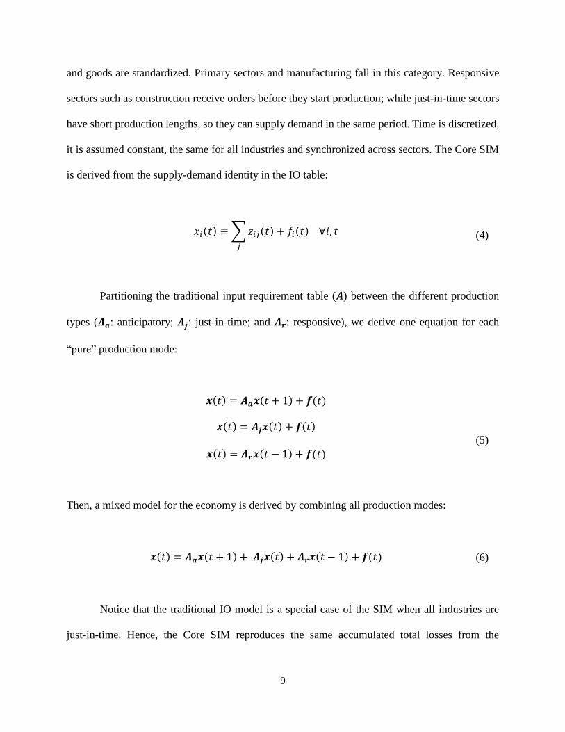
and goods are standardized. Primary sectors and manufacturing fall in this category. Responsive
sectors such as construction receive orders before they start production; while just-in-time sectors
have short production lengths, so they can supply demand in the same period. Time is discretized,
it is assumed constant, the same for all industries and synchronized across sectors. The Core SIM
is derived from the supply-demand identity in the IO table:
𝑥𝑖(𝑡) ≡∑𝑧𝑖𝑗(𝑡)
𝑗
+ 𝑓𝑖(𝑡) ∀𝑖, 𝑡 (4)
Partitioning the traditional input requirement table (𝑨) between the different production
types (𝑨𝒂: anticipatory; 𝑨𝒋: just-in-time; and 𝑨𝒓: responsive), we derive one equation for each
“pure” production mode:
𝒙(𝑡) = 𝑨𝒂𝒙(𝑡 + 1) + 𝒇(𝑡)
𝒙(𝑡) = 𝑨𝒋𝒙(𝑡) + 𝒇(𝑡)
𝒙(𝑡) = 𝑨𝒓𝒙(𝑡 − 1) + 𝒇(𝑡)
(5)
Then, a mixed model for the economy is derived by combining all production modes:
𝒙(𝑡) = 𝑨𝒂𝒙(𝑡 + 1) + 𝑨𝒋𝒙(𝑡) + 𝑨𝒓𝒙(𝑡 − 1) + 𝒇(𝑡) (6)
Notice that the traditional IO model is a special case of the SIM when all industries are
just-in-time. Hence, the Core SIM reproduces the same accumulated total losses from the

10
traditional Leontief model but spreads them through time. However, it relies on a set of strong
assumptions such as perfect foresight of demand and perfect knowledge of interindustrial
requirements(28), of changes in the economic structure and perfect sectoral adaptability to the
disruption (no inventories). Romanoff and Levine(29,30) have remedied some of these issues by
including inventories, post-disaster technology changes and delivery delays, but their
implementation is not straightforward(10). In addition, the system’s inoperability in the SIM is inter-
temporal only to the extent that intra-temporal impacts are carried over via production lags.
On the other hand, the Dynamic Inoperability Input-Output Model (DIIM) proposed by
Lian and Haimes(11) aims at introducing a framework that bridges intra-temporal and inter-
temporal inoperability. The DIIM is the dynamic version of the Inoperability Input-Output
Model(31,32) that we do not cover in this review given that it offers no methodological advances
compared to the traditional IO model(17,33).
DIIM is based on the classic Leontief Dynamic model which assumes that current output
accounts for both the production required to attend current demand and any required capital to
attend production in the next period via the capital formation matrix 𝑩 (Eq. 7).
𝒙(𝑡) = 𝑨𝒙(𝑡) + 𝒇(𝑡) + 𝑩[𝒙(𝑡 + 1) − 𝒙(𝑡)] (7)
While the Leontief’s model is a growth model, the DIIM models a recovery process where
the economy moves back to the pre-disaster steady-state. Hence, the capital formation matrix is
replaced by a resilience matrix 𝑲 = �̂� that represents the speed at which the pre- vs. post-disaster
production gap closes (Eq. 8).

11
𝐵=−�̂�−1
⇒ 𝒙(𝑡) = 𝑨𝒙(𝑡) + 𝒇(𝑡) − 𝑲−1[𝒙(𝑡 + 1) − 𝒙(𝑡)]
⟺ 𝒙(𝑡 + 1) = 𝒙(𝑡) + 𝑲 [𝑨𝒙(𝑡) + 𝒇(𝑡) − 𝒙(𝑡)]
(8)
Taking 𝑡 = 0 as the first period post-disaster and 𝑡 = 𝑇𝑖 the time industry 𝑖 takes to recover
to a target (minimal) level of inoperability 𝑞𝑖, the interdependency recovery rate 𝑘𝑖 is defined as:
𝑘𝑖 =ln (𝑞𝑖(0)
𝑞𝑖(𝑇𝑖)⁄ )
𝑇𝑖(1 − 𝑎𝑖𝑖)
(9)
Notice that Eq. 9 defines an exponential recovery path. Moreover, the leakage of
inoperability among industries and their inertia in the system depends on the size of 𝑲. The larger
is 𝑲, the faster is the recovery. In their original exposition, all matrices are normalized with the
pre-disaster total output levels: 𝒒(𝑡) = [�̂�−1(𝒙 − 𝒙∗(𝑡))], 𝒄∗(𝑡) = [�̂�−1(𝒇 − �̅�∗(𝑡))] and 𝐀∗ =
[�̂�−1𝑨�̂�], which yields the model:
𝒒(𝑡 + 1) = 𝒒(𝑡) + �̂� [𝐀∗𝒒(𝑡) + 𝒄∗(𝑡) − 𝒒(𝑡)] (10)
The connection between intra-temporal and inter-temporal inoperability is embedded in
Eq. 10 where an increase in current inoperability creates contemporaneous supply constraints that
also influence the next period, hence accounting for both effects. One could criticize the DIIM for
assuming all industries operate in anticipatory mode and use the previous period’s final demand
and production imbalance as the expected output level. Moreover, an ad-hoc proportional rationing
rule is implicitly assumed to redistribute reduced output, there are no trade constraints and

12
inventories are not available to mitigate inoperability. With regards to the latter issue, Barker and
Santos(12) extended the DIIM to include finished goods inventories (𝐼𝐹) which magnitude defines
a sector-specific inoperability 𝑝 distinct from the overall inoperability 𝑞. As such, they introduce
a sector-specific recovery coefficient (𝑙𝑖) similar to 𝑘𝑖 in Eq. 9 that informs the speed of recovery
from a physical inoperability (Eq. 11).
𝑙𝑖 =ln (𝑝𝑖(0)
𝑝𝑖(𝑇𝑖)⁄ )
𝑇𝑖
(11)
Different functional forms could be applied to the recovery function, but Barker and
Santos(12) use the following:
𝑝𝑖(𝑡) = 𝑒−𝑙𝑖𝑡𝑝𝑖(0) (12)
Initial overall inoperability conditions 𝑞𝑖(0) are determined by the available finished
goods inventory in the aftermath of the event (𝑰𝑭(0)) and by supply constraints (sector-specific
inoperability post-disaster 𝑝𝑖(0)):
𝑞𝑖(0) = {
01 − 𝐼𝑖
𝐹(0) 𝑝𝑖(0)𝑥𝑖(0)⁄
𝑝𝑖(0)
𝑖𝑓 𝐼𝑖𝐹(0) ≥ 𝑝𝑖(0)𝑥𝑖(0)
𝑖𝑓 0 < 𝐼𝑖𝐹(0) < 𝑝𝑖(0)𝑥𝑖(0)
𝑖𝑓 𝐼𝑖𝐹(0) = 0
(13)
Hence, the evolution of each industry in the system depends on the remaining inventories
in relation to the output constraints (Eq. 14). If inventories are numerous enough to supplant the

13
lost output, then a sector’s inoperability will depend solely on its own previous inoperability and
on the one of the other sectors (condition 1). In case some inventory remains, but it is not enough
to fully overcome the new production constraints, then the level of inoperability is mitigated
proportionally (condition 2). If the inventories become depleted in the next period but are still
positive in the current period, an additional supply constraint appears in the system, hence
increasing the overall inoperability (condition 3). Finally, if there are no contemporaneous
inventories, we revert back to the traditional DIIM model (condition 4). Any remaining inventories
are updated at the end of each time step.
𝑞𝑖(𝑡 + 1)
=
{
𝑞𝑖(𝑡) + 𝑘𝑖 [𝑐𝑖
∗(𝑡) − 𝑞𝑖(𝑡) +∑ 𝑎𝑖𝑗∗ 𝑞𝑗(𝑡)
𝑛
𝑗=1] 𝑖𝑓 𝐼𝑖
𝐹(𝑡 + 1) ≥ 𝑝𝑖(𝑡 + 1)𝑥𝑖(𝑡 + 1)
max {
𝑝𝑖(𝑡 + 1) − 𝐼𝑖𝐹(𝑡 + 1) 𝑥𝑖(𝑡 + 1)⁄
𝑞𝑖(𝑡) + 𝑘𝑖 [𝑐𝑖∗(𝑡) − 𝑞𝑖(𝑡) +∑ 𝑎𝑖𝑗
∗ 𝑞𝑗(𝑡)𝑛
𝑗=1]𝑖𝑓 0 < 𝐼𝑖
𝐹(𝑡 + 1) < 𝑝𝑖(𝑡 + 1)𝑥𝑖(𝑡 + 1)
max {
𝑝𝑖(𝑡 + 1)
𝑞𝑖(𝑡) + 𝑘𝑖 [𝑐𝑖∗(𝑡) − 𝑞𝑖(𝑡) +∑ 𝑎𝑖𝑗
∗ 𝑞𝑗(𝑡)𝑛
𝑗=1] 𝑖𝑓 𝐼𝑖
𝐹(𝑡 + 1) = 0, 𝐼𝑖𝐹(𝑡) > 0
𝑞𝑖(𝑡) + 𝑘𝑖 [𝑐𝑖∗(𝑡) − 𝑞𝑖(𝑡) +∑ 𝑎𝑖𝑗
∗ 𝑞𝑗(𝑡)𝑛
𝑗=1] 𝑖𝑓 𝐼𝑖
𝐹(𝑡 + 1) = 0, 𝐼𝑖𝐹(𝑡) = 0
(14)
Although the approach above assesses the impact of pre-disaster inventories of finished
goods, it does not explain their formation nor accounts for the presence of material and supply
inventories. Furthermore, the model lacks different production modes and trade constraints. It still
assumes that the external sectors can absorb local imbalances by providing more imports and
purchasing excess production. As the latter is unlikely in real situations, overproduction can further
decrease local production due to additions to inventories.
14
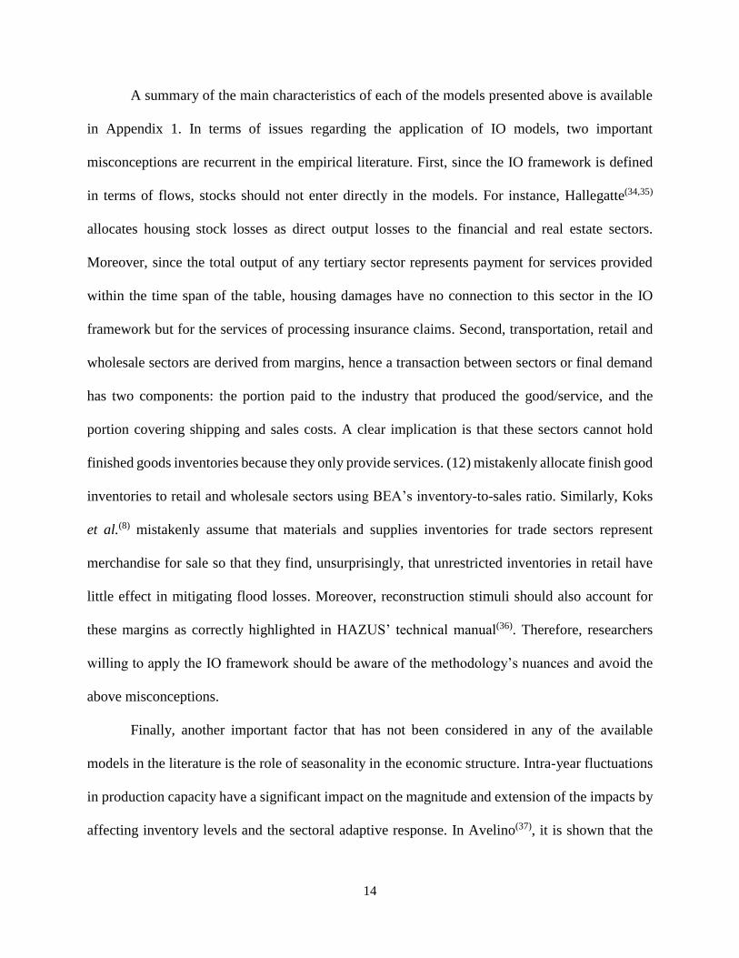
A summary of the main characteristics of each of the models presented above is available
in Appendix 1. In terms of issues regarding the application of IO models, two important
misconceptions are recurrent in the empirical literature. First, since the IO framework is defined
in terms of flows, stocks should not enter directly in the models. For instance, Hallegatte(34,35)
allocates housing stock losses as direct output losses to the financial and real estate sectors.
Moreover, since the total output of any tertiary sector represents payment for services provided
within the time span of the table, housing damages have no connection to this sector in the IO
framework but for the services of processing insurance claims. Second, transportation, retail and
wholesale sectors are derived from margins, hence a transaction between sectors or final demand
has two components: the portion paid to the industry that produced the good/service, and the
portion covering shipping and sales costs. A clear implication is that these sectors cannot hold
finished goods inventories because they only provide services. (12) mistakenly allocate finish good
inventories to retail and wholesale sectors using BEA’s inventory-to-sales ratio. Similarly, Koks
et al.(8) mistakenly assume that materials and supplies inventories for trade sectors represent
merchandise for sale so that they find, unsurprisingly, that unrestricted inventories in retail have
little effect in mitigating flood losses. Moreover, reconstruction stimuli should also account for
these margins as correctly highlighted in HAZUS’ technical manual(36). Therefore, researchers
willing to apply the IO framework should be aware of the methodology’s nuances and avoid the
above misconceptions.
Finally, another important factor that has not been considered in any of the available
models in the literature is the role of seasonality in the economic structure. Intra-year fluctuations
in production capacity have a significant impact on the magnitude and extension of the impacts by
affecting inventory levels and the sectoral adaptive response. In Avelino(37), it is shown that the

15
bias in output multipliers from using an annual table instead of quarterly tables is up to 6% in
either direction.
3. CASE STUDY: THE 2007 CHEHALIS FLOOD
In order to compare the results of the five IO methodologies listed above, we will rely on
the same benchmark event: the 2007 Chehalis Flood in the state of Washington. Over December
1-4 2007 a system of storms formed by an atmospheric river hit the U.S. West Coast and led to a
record-breaking 14 inches of precipitation at the Willapa Hills which feed the main stems of both
the Chehalis and the South Fork rivers. The surrounding areas experienced an additional 3-8 inches
of rain. This event led to landslides, failed levees, overtopped dikes(38) and floods in western
Washington and Oregon. Traditionally, this region experiences an average precipitation of 7-13
inches for the entire October to March period(38). Most of the damage was concentrated alongside
the Chehalis River Basin, southwest Washington. The flood extent is shown in Fig. 2 below.
<< INSERT FIGURE 2 HERE >>
The counties of Grays Harbor, Thurston and Lewis were the most affected and were
declared major disaster areas on December 8, 2007. Around 75,000 customers lost power and
several roads became impassable(7). The cities of Centralia and Chehalis, both in Lewis County,
sustained the most damage with 25% and 33% of their respective area inundated. It affected more
than half of the commercial land-use and 32% of the industrial zones in the Centralia-Chehalis
Urban Growth Area. The direct building damage in the county was assessed at $166 million. In

16
addition, around 10,702 acres of the 22,919 acres of agricultural land in western Lewis County
were flooded at an estimated reseeding cost of between $188-$490 million(39).
Damage to Interstate 5, the main corridor connecting Portland to Seattle, led to its closure
to all traffic for 4 days. Flow losses estimates were calculated using a combination of business
surveys and traditional IO analysis via IMPLAN (see section 3 of WSDOT(20) for a full discussion).
Besides the $5 million in physical damage, WSDOT(20) estimates that $47 million in economic
activity, $2.4 million in state tax revenue and $14.6 million in personal income were lost due to
this event.
However, when it comes to flow losses due to building damages, only a qualitative survey
on local businesses was conducted(7). The study in Centralia and Chehalis comprising flooded and
non-flooded businesses revealed that more than 80% of them had below average sales two weeks
after the event and a third after two months. The main disruption channels reported were a loss of
accessibility by road and a temporary absence of employees. Sales plunged due to flood-affected
households and a smaller discretionary spending from non-impacted individuals. Nonetheless,
businesses related to redistribution and recovery efforts showed above average sales in the survey.
Overall, 31% of the local businesses expected to fully recover in a year and 20% in more than two
years(7).
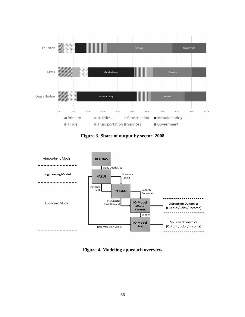
The tri-county region impacted by the 2007 Chehalis flood has contrasting characteristics.
While Grays Harbor and Lewis counties are more primary based economies with a significant
commercial logging sector, Thurston County is a service based economy and is part of the Seattle-
metro area. Economic data for 2008 indicates that, in terms of total output and employment,
Thurston is the largest and the most diversified economy among the three (Fig. 3). Lewis and
Grays Harbor have similar sized economies with a combined output that is a third of Thurston’s.
17
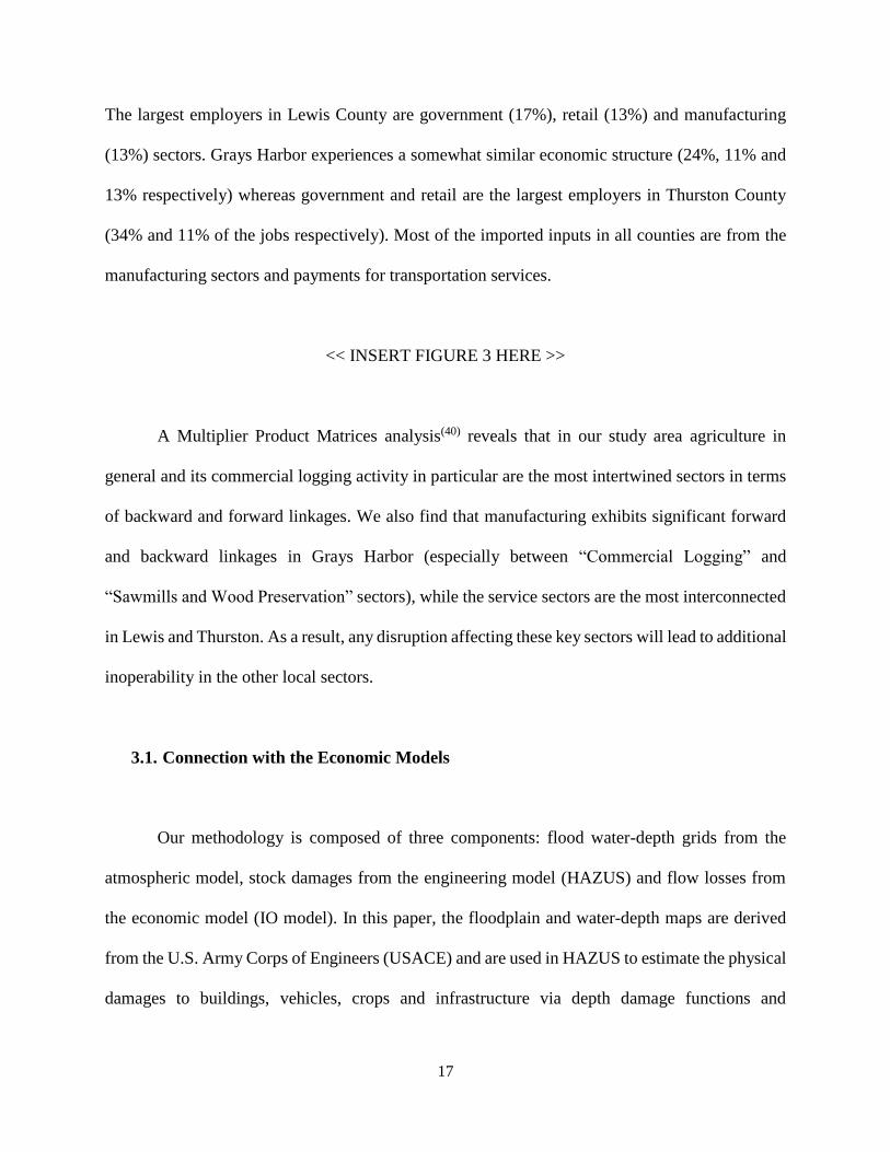
The largest employers in Lewis County are government (17%), retail (13%) and manufacturing
(13%) sectors. Grays Harbor experiences a somewhat similar economic structure (24%, 11% and
13% respectively) whereas government and retail are the largest employers in Thurston County
(34% and 11% of the jobs respectively). Most of the imported inputs in all counties are from the
manufacturing sectors and payments for transportation services.
<< INSERT FIGURE 3 HERE >>
A Multiplier Product Matrices analysis(40) reveals that in our study area agriculture in
general and its commercial logging activity in particular are the most intertwined sectors in terms
of backward and forward linkages. We also find that manufacturing exhibits significant forward
and backward linkages in Grays Harbor (especially between “Commercial Logging” and
“Sawmills and Wood Preservation” sectors), while the service sectors are the most interconnected
in Lewis and Thurston. As a result, any disruption affecting these key sectors will lead to additional
inoperability in the other local sectors.
3.1. Connection with the Economic Models
Our methodology is composed of three components: flood water-depth grids from the
atmospheric model, stock damages from the engineering model (HAZUS) and flow losses from
the economic model (IO model). In this paper, the floodplain and water-depth maps are derived
from the U.S. Army Corps of Engineers (USACE) and are used in HAZUS to estimate the physical
damages to buildings, vehicles, crops and infrastructure via depth damage functions and

18
reconstruction timing. Both first and higher-order effects are then estimated using the range of IO
models described above. Total flow losses in terms of output, income and jobs are calculated. The
relationship between all these components is shown in Fig. 4.
<< INSERT FIGURE 4 HERE >>
This study relies on a fine scale estimate of floodplain and water-depth maps derived from
the 2007 event. Observed data collected by the USACE from gauges along several river branches
in the Chehalis basin were used in HEC-RAS to generate a water-depth map for the area(41). The
engineering model (HAZUS) uses this water-depth grid to determine the total stock losses in each
affected county. It has been the most widely applied model in the literature evaluating economic
losses and performing cost-benefit analysis as it offers a balanced trade-off between modeling
capability and required technical engineering knowledge(42).
HAZUS determines the percentage of damaged square footage by occupancy class at the
census block level. Then, capital stock damages are measured in terms of repair costs, inventory,
content, crop losses and vehicle replacement costs. Transportation infrastructure damage is only
evaluated in terms of impacted bridges, so a comprehensive assessment of transportation
disruption is lacking. The software provides estimates of first-order flow losses in business
interruptions and rental income based on average sales data for the occupancy class. We detract
from the latter and estimate both first and higher-order flow losses using the county’s IO table to
have more accurate results.
Natural disasters create constraints to production, thus leading to negative economic
impacts. However, the reconstruction efforts that follow stimulate the local economy. Capacity

19
constraints 𝚪(t) are determined by assuming a homogeneous productivity per square foot for each
industry in a specific county and that industries operate at full capacity before the disaster. Using
information on crop losses, on damaged squared footage from the General Building Stock (GBS)
as well as information about the economic sectors these buildings belong to (HAZUS occupancy
class classification is matched to NAICS classification), we set the capacity constraints based on
the pre-disaster total output by industry (Fig. 5). When it comes to agriculture’s output, it is reduced
proportionally to the share of crop and livestock output in the county. Livestock losses are not
considered independently as they are not reported by HAZUS.
<< INSERT FIGURE 5 HERE >>
The reconstruction demand 𝑹(𝑡) is determined by repair costs to the GBS, to the lifelines
and the replacement of building content and vehicles. While the first two generate construction
stimuli, the last two support demand in manufacturing. Given the reduced size of the affected
counties, all the reconstruction stimuli are allocated outside the area. Following the HAZUS
methodology, we assume that manufacturing orders include a margin to be split 20%-80% between
transportation and wholesale (Fig. 6).
<< INSERT FIGURE 6 HERE >>
The total square footage per industry before the disaster (𝑠𝑖𝑇), the damaged square footage
(𝑠𝑖𝐷) and the timing of the disruption are used to determine the capacity constraints and the reduced
local final demand in the economic model. We also assume that recovery is proportionally
20
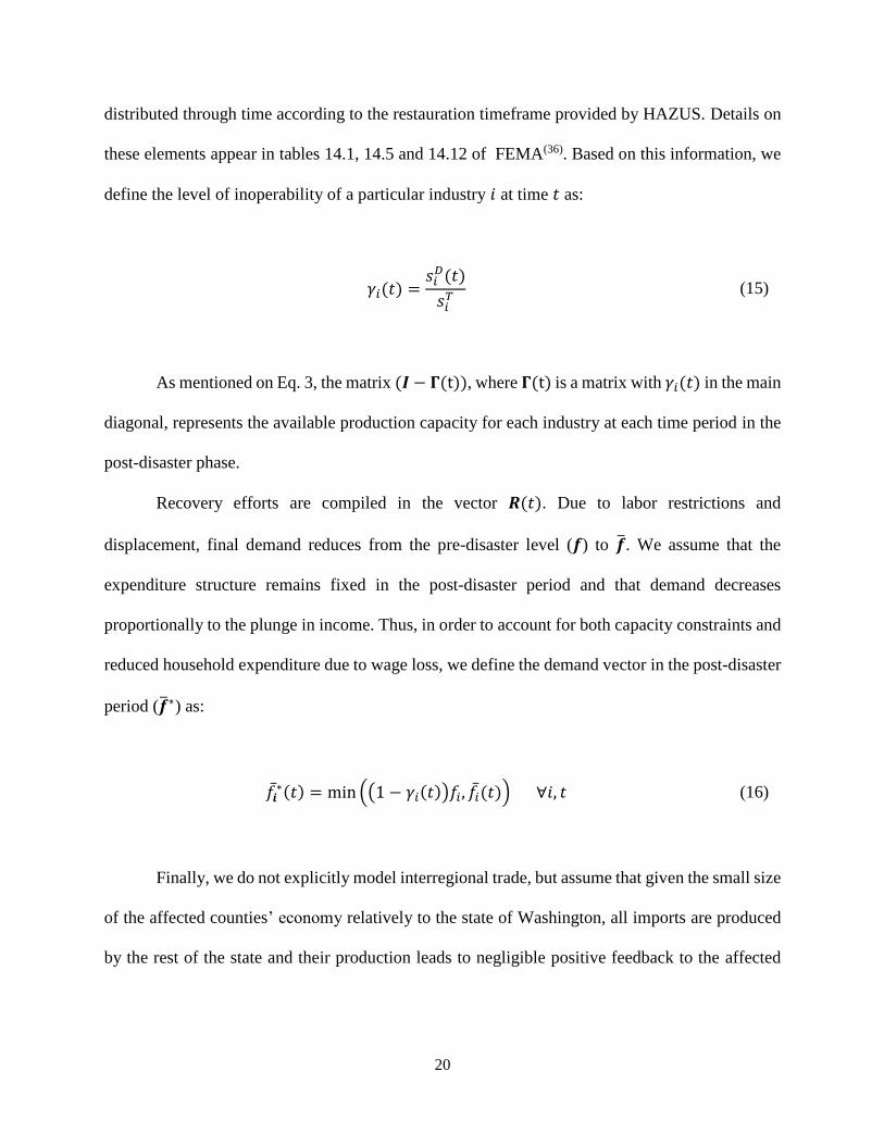
distributed through time according to the restauration timeframe provided by HAZUS. Details on
these elements appear in tables 14.1, 14.5 and 14.12 of FEMA(36). Based on this information, we
define the level of inoperability of a particular industry 𝑖 at time 𝑡 as:
𝛾𝑖(𝑡) =𝑠𝑖𝐷(𝑡)
𝑠𝑖𝑇 (15)
As mentioned on Eq. 3, the matrix (𝑰 − 𝚪(t)), where 𝚪(t) is a matrix with 𝛾𝑖(𝑡) in the main
diagonal, represents the available production capacity for each industry at each time period in the
post-disaster phase.
Recovery efforts are compiled in the vector 𝑹(𝑡). Due to labor restrictions and
displacement, final demand reduces from the pre-disaster level (𝒇) to �̅�. We assume that the
expenditure structure remains fixed in the post-disaster period and that demand decreases
proportionally to the plunge in income. Thus, in order to account for both capacity constraints and
reduced household expenditure due to wage loss, we define the demand vector in the post-disaster
period (�̅�∗) as:
𝑓�̅�∗(𝑡) = min ((1 − 𝛾𝑖(𝑡))𝑓𝑖, 𝑓�̅�(𝑡)) ∀𝑖, 𝑡 (16)
Finally, we do not explicitly model interregional trade, but assume that given the small size
of the affected counties’ economy relatively to the state of Washington, all imports are produced
by the rest of the state and their production leads to negligible positive feedback to the affected
21
counties. Notice that the assumption of fixed prices holds here due to the small size of the affected
region.
Direct losses are estimated in HAZUS-MH version 3.0 using the default dasymetric
datasets and assuming a warning time of 48h. It implies a 35% loss reduction in building damage
according to the embedded Day Curve. No reduction in vehicle damage is assumed as no reliable
source of information is available. As the software informs both day and night losses for vehicles,
we follow the flood timing reported in NOAA(43) and select day losses for Grays Harbor and
Thurston and night losses for Lewis County.
We use the 2008 IO tables extracted from IMPLAN at a 16 sectors aggregation level. The
sectors are presented in Table I alongside the assumptions used in the SIM and DIIM models. This
level of aggregation was chosen to minimize incompatibilities when bridging HAZUS’ occupancy
class classification and NAICS classification used by IMPLAN as shown in Appendix 2.
<< INSERT TABLE I HERE >>
The inventory data for the DIIM are based on the December 2007 inventory-to-sales ratio
for manufacturing reported by the Federal Reserve Bank of St. Louis(44), as suggested in Barker
and Santos(12). This not-seasonally-adjusted ratio is 1.23 for the period under study. It is
homogeneously applied to all counties. Data for wholesale and retail are not considered as these
sectors’ activities are recorded as margins, so they cannot hold finished goods inventories
(although they can hold “materials and supplies” and “work-in-progress” inventories, which data
are not available).

22
3.2. Stock Damages Estimates via HAZUS
Physical damages are estimated at $680 million. As expected, the largest impact is in Lewis
County. A breakdown of damages is provided in Table II. The only available counterfactual for
direct losses is from Lewis County(39) where the total building losses (structure + inventory) were
assessed at $166.2 million. Our HAZUS-based estimates lead to a figure of $150.9 million. This
difference can be explained, in part, by the fact that our model estimates the total number of
damaged structures at 439 when 957 of them were actually reported(39). Five fire stations were
affected during the flood, at a total repair cost of $6 million(39); however, HAZUS does not report
any impact.
<< INSERT TABLE II HERE >>
When it comes to the estimated square footage of damage per industry, most of the affected
area is concentrated in Lewis County, followed by Grays Harbor and then Thurston (see Fig. 7).
Agriculture, construction and health services are the main impacted industries, the latter being
almost exclusively located in Lewis. In Grays Harbor and Thurston, agriculture is the main
affected sector. These results appear in figures 8-10 below.
<< INSERT FIGURE 7 HERE >>
<< INSERT FIGURE 8 HERE >>

23
<< INSERT FIGURE 9 HERE >>
<< INSERT FIGURE 10 HERE >>
4. RESULTS AND DISCUSSION
Considering the disruption timing set by default in HAZUS, we estimate a total direct
output loss of $26.3 million over 25 months. First-order effects are the same across models. Health
services, agriculture and manufacturing are the most affected sectors. Given the economic
structure of the counties, Lewis has the most losses in the service sectors and Thurston the most
losses in government activities (Fig. 7). Such loss of output translates into a $10.5 million decrease
in direct labor income (Fig. 11).
<< INSERT FIGURE 11 HERE >>
Next, we use the five specifications described in Section 2 to estimate higher-order effects.
The full results by model, county and sector are available in Appendix 3. It is clear that in all
counties the accumulated losses are in-between the lower bound given by the Leontief model and
the upper bound calculated by the DIIM (Fig. 12, 13 and 14). This difference varies from 69% to
115% in Thurston and Grays Harbor respectively depending on which sectors are the most affected
in each county and on their local linkages (Appendix 4). The results make it also obvious that, due
to the truncation of intertemporal effects, static models suffer from a negative bias.

24
<< INSERT FIGURE 12 HERE >>
<< INSERT FIGURE 13 HERE >>
<< INSERT FIGURE 14 HERE >>
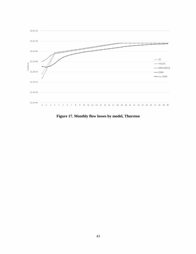
When it comes to monthly losses by county (Fig. 15, 16 and 17), Cochrane’s model
consistently shows the highest production plunges in the initial post-disaster periods when the
economic structure is the most impaired. This highlights the importance of accounting for both
capacity constraints and their implication to local interdependence. As the economy rebounds and
returns towards its original steady state, Cochrane’s model approaches the traditional IO model
estimates.
Moreover, as the Leontief and Cochrane models are static, the initial inoperability does not
spread inter-temporally, so there is a large loss in the first post-disaster months that fades quickly.
The SIM distributes losses in time due to perfect foresight, so the efficient output path begins pre-
disaster and involves lower reductions in output. While we are aware that an event like the one
studied here cannot be expected, it is important to recall that the SIM is originally designed for
positive shocks. The DIIM creates an inertial inoperability effect that extends the length of the
disruption. The exponential recovery assumption determines the shape of the curve.
In the case of Grays Harbor, the primary sector is the one sustaining the most stock
damages (2.7%) and also the one with most backward and forward linkages in the local economy.
As a result, the inoperability it generates spreads significantly to other sectors. This reflects in the

25
37% difference between Leontief’s and Cochrane’s estimates (the largest difference of all
counties). It now becomes clear that if highly interdependent sectors are affected and the economic
structure is kept fixed, the bias is exacerbated. Besides agriculture and construction, government,
manufacturing and professional services are indirectly affected. Notice also that by considering
manufacturing inventories in the model, the total losses calculated by the inventory DIIM (noted
Inv-DIIM) can be mitigated by 5.6%.
<< INSERT FIGURE 15 HERE >>
Lewis County is the most affected county with major damages to the health sector (4.6%),
construction (2.8%) and agriculture (2.5%). Due to the high amount of direct losses, almost all of
its sectors suffer some indirect negative impact, although the low interdependence of the affected
sectors leads them to experience the largest losses. As such, health services are estimated to have
lost between $12.2-19.3 million, while losses in manufacturing and agriculture sum up to $2.0-4.1
million and $1.2-3.0 million respectively. Contrary to Grays Harbor, the difference in accumulated
losses generated by the Leontief and the Cochrane models is significantly lower (only 8%) as their
local linkages are reduced. Recovery is slower due to a long reconstruction time in the health sector
while most other sectors rebound within 6 months.
<< INSERT FIGURE 16 HERE >>
Despite a similar pattern of damages in Thurston and Grays Harbor whereby agriculture
and construction sustain the most stock reductions, total flow losses in Thurston are significantly

26
different due to differences in the economic structure. The agricultural sector is not integrated in
the local economy as in Grays Harbor since Thurston is mainly service based and manufacturing
inventories do not attenuate flow losses. As a result, the DIIM and the Inventory DIIM yield the
same estimates. Moreover, the inoperability does not spread as much as in Grays Harbor County,
so the flow losses are concentrated in the agriculture and construction sectors only (compare Fig.
17 with 15).
<< INSERT FIGURE 17 HERE >>
In summary, we compile the estimates for stock damages, flow losses and recovery time
for each county. Thurston is the fastest county to recover with an overall negative impact of $4
million. Conversely, Lewis’ $37 million losses spread throughout 2.5 years until full recovery
(Table III). Notice the significant variation in high-order effects between lower and upper bound
estimates.
<< INSERT TABLE III HERE >>
When it comes to the positive economic impacts from reconstruction, we find that the rest
of Washington receives a direct stimulus of $680 million. It leads to a total impact of $957 million
in that area. A comprehensive net effect on who bears the costs of reconstruction or on the
investment/expenditure decisions it leads to is out of the scope of this paper. If we assume that all
of the aid is external and that the regional economies return to their pre-disaster steady-state, the
27
total net effect for the state as a whole is positive: it is composed of a $52 million loss in the
affected counties and of a $ 905 million gain in the rest of Washington.
5. CONCLUSIONS
Although stock damages are well understood, flow impacts taking place in the post-disaster
period tend to be overlooked(8,18). As a result, mitigation strategies for future events are myopically
applied to the affected economies only as if they had no spatial and temporal linkages. This partial
account of impacts ignores the interconnectivity of modern production chains and may lead to
significant negative effects to non-affected regions.
The disaster literature has several models to assess flow losses and most of them are rooted
in the IO framework. However, there exist no consensus on a preferred methodology. Therefore,
researchers are often faced with a model selection issue based on the characteristics of the disaster,
of the affected region(s) and on their assumptions on the mechanics of the local economy.
In this paper, we use fine-scale characteristics of a single event, the 2007 Chehalis flood
(WA), to calculate the flow losses that are generated by the five most commonly used models in
the disaster literature. The results highlight their bias under different economic structures, level of
industrial interdependency in affected sectors and amount of inoperability. We find that for each
county the accumulated losses are in-between the lower bound given by the Leontief model and
the upper bound calculated by the DIIM. This difference varies from 69% to 115% in Thurston
and Grays Harbor respectively depending on which sectors are the most affected and on their local
linkages. Static formulations (traditional IO and HAZUS) underestimate the losses by ignoring the

28
presence of intertemporal externalities. They truncate the inoperability impacts at each time period,
which leads to a significant bias in the event of large disruptions as the recovery period is deemed
shorter than it actually is. Moreover, modeling changes in the sectoral interdependencies between
the pre- and post-disaster period is paramount when industries with strong backward and forward
linkages are impacted. Finally, we show that the role of inventories depends on the external
dependency of the affected sectors, so that estimates for mainly tertiary-based regions may not
change significantly whether inventories are modeled or not.
We also highlight that most of the common theoretical inconsistencies in the disaster
literature derive from issues in integrating stock damages into a framework developed for flow
analysis. Stocks should be introduced as primary inputs constraints (capital, labor, land) to analyze
losses and later be converted into reconstruction stimuli via repair information to assess positive
impacts. Furthermore, transportation and trade sectors are recorded as margins; hence IO
practitioners should not consider that they hold finished goods inventories. Beyond these points of
caution, we believe that the IO framework is still rich of opportunities for further methodological
developments. For instance, efforts focusing on integrating both input and output inventories into
a single framework and on developing a dynamic rebalancing of the local industrial linkages after
a disruption are certainly needed. In addition, the role of the time of the event, of the seasonality
in the economic structure and its implication on sectoral interdependency, inventories and
resilience have been largely ignored in the literature. A solution for the former issue is to rely on
intra-year IO tables that better reflect the industrial relationships at the time of the disaster. As
shown by Avelino(37), highly seasonal sectors such as agriculture and services exhibit significantly
different linkages across quarters, which are not captured using annual tables.

29
While the additional complexity of such extensions seems to conflict with the short timing
emergency and disaster relief efforts have to work under, the more accurate and detailed analysis
they generate informs us better of the current vulnerability of our economic systems and allow us
to adapt more suitably to future events(13).
30
REFERENCES
1. Gall M, Borden KA, Cutter SL. When do losses count? Bull Am Meteorol Soc.
2009;90(6):799–809.
2. NOAA. Storm data preparation. National Weather Service Instruction 10-1605. 2007;97.
Available from: http://www.nws.noaa.gov/directives/sym/pd01016005curr.pdf
3. Rose A. Economic principles, issues, and research priorities in hazard loss estimation. In:
Okuyama Y, Chang SE, editors. Modeling of spatial economic impacts of natural hazards.
1st ed. Springer; 2004. p. 13–36.
4. Changnon SD. The Great Flood of 1993: Causes, Impacts, and Responses. Westview
Press; 1996.
5. USDC. Economic Impact of Hurricane Sandy: Potential Economic Activity Lost and
Gained in New Jersey and New York [Internet]. 2013. Available from:
www.esa.doc.gov/sites/default/files/sandyfinal101713.pdf
6. Tierney KJ. Business Impacts of the Northridge Earthquake. J Contingencies Cris Manag.
1997;5(2):87–97.
7. Green R, Miles S, Gulacsik G, Levy J. Business Recovery Related to High-Frequency
Natural Hazard Events. 2008.
8. Koks EE, Bočkarjova M, de Moel H, Aerts JCJH. Integrated direct and indirect flood risk
modeling: Development and sensitivity analysis. Risk Anal. 2015;35(5):882–900.
9. Cochrane H. Economic Impacts of a Midwestern Earthquake. Q Publ NCEER.
1997;11(1):1–20.
10. Okuyama Y, Hewings GJD, Sonis M. Measuring Economic Impacts of Disasters:

31
Interregional Input-Output Analysis Using Sequential Interindustry Model. In: Okuyama
Y, Chang SE, editors. Modeling of spatial economic impacts of natural hazards. Springer;
2004.
11. Lian C, Haimes YY. Managing the risk of terrorism to interdependent infrastructure
systems through the dynamic inoperability input–output model. Syst Eng. 2006
Jan;9(3):241–58.
12. Barker K, Santos JR. Measuring the efficacy of inventory with a dynamic inputoutput
model. Int J Prod Econ. 2010;126(1):130–43.
13. Okuyama Y. Economic Modeling for Disaster Impact Analysis: Past, Present, and Future.
Econ Syst Res. 2007;19(2):115–24.
14. Przyluski V, Hallegatte S. Indirect Costs of Natural Hazards [Internet]. SMASH- CIRED;
2011. Report No.: WP2 Final Report. Available from: http://conhaz.org/CONHAZ
REPORT WP02_2_FINAL.pdf
15. Greenberg MR, Lahr M, Mantell N. Understanding the economic costs and benefits of
catastrophes and their aftermath: A review and suggestions for the U.S. federal
government. Risk Anal. 2007;27(1):83–96.
16. Okuyama Y, Santos JR. Disaster Impact and Input–Output Analysis. Econ Syst Res.
2014;26(1):1–12.
17. Oosterhaven J. On the Doubtful Usability of the Inoperability IO Model. 2015. Report
No.: 15008–EEF.
18. Meyer V, Becker N, Markantonis V, Schwarze R, Van Den Bergh JCJM, Bouwer LM, et
al. Review article: Assessing the costs of natural hazards-state of the art and knowledge
gaps. Nat Hazards Earth Syst Sci. 2013;13(5):1351–73.

32
19. Miller RE, Blair P. Input-Output Analysis: Foundations and Extensions. Second. 2009.
20. WSDOT. Storm-Related Closures of I-5 and I-90: Freight Transportation Economic
Impact Assessment Report Winter 2007-2008. 2008.
21. Oosterhaven J, Bouwmeester MC. A new approach to modeling the impact of disruptive
events. J Reg Sci. 2016;0(0):1–13.
22. Cole S. Expenditure Lags in Impact Analysis. Reg Stud. 1989;23(2):105–16.
23. Romanoff E, Levine SH. Interregional Sequential Interindustry Model: A preliminary
analysis of regional growth and decline in a two region case. Northeast Reg Sci Rev.
1977;7:87–101.
24. Cole S. The Delayed Impacts of Plant Closures in a Reformulated Leontief Model. Pap
Reg Sci Assoc. 1988;65(1):135–49.
25. Jackson RW, Madden M, Bowman HA. Closure in Cole’s Reformulated Leontief Model.
Pap Reg Sci. 1997;76(1):21–8.
26. Jackson RW, Madden M. Closing the case on closure in Cole’s model. Pap Reg Sci.
1999;78(4):423–7.
27. Oosterhaven J. Lessons from the debate on Cole’s model closure. Pap Reg Sci.
2000;79(2):233–42.
28. Mules TJ. Some simulations with a sequential input-output model. Vol. 51, Papers of the
Regional Science Association. 1983. p. 197–204.
29. Romanoff E, Levine SH. Capacity Limitations, Inventory and Time-Phased Production in
the Sequential Interindustry Model. Pap Reg Sci Assoc. 1986;59:73–91.
30. Romanoff E, Levine SH. Technical Change in Production Processes of the Sequential
Interindustry Model. Metroeconomica. 1990;41(1):1–18.
33
31. Santos J. Interdependency analysis: Extensions to demand reduction inoperability input-
output modeling and portfolio selection. University of Virginia; 2003.
32. Santos JR, Haimes YY. Modeling the demand reduction input-output (I-O) inoperability
due to terrorism of interconnected infrastructures. Risk Anal. 2004;24(6):1437–51.
33. Dietzenbacher E, Miller RE. Reflections on the Inoperability Input–Output Model. Econ
Syst Res. 2015;25(4):478–86.
34. Hallegatte S. An adaptive regional input-output model and its application to the
assessment of the economic cost of Katrina. Risk Anal. 2008;28(3):779–99.
35. Hallegatte S. Modeling the role of inventories and heterogeneity in the assessment of the
economic costs of natural disasters. Risk Anal. 2014;34(1):152–67.
36. FEMA. Multi-hazard loss estimation methodology, flood model, HAZUS, technical
manual [Internet]. Department of Homeland Security, Emergency Preparedness and
Response Directorate, FEMA, Mitigation Division, Washington, D.C. 2015. Available
from: http://www.fema.gov/media-library-data/20130726-1820-25045-
8292/hzmh2_1_fl_tm.pdf
37. Avelino AFT. Disaggregating Input-Output Tables in Time: the Temporal Input-Output
Framework. 2016.
38. CRBFA. Chehalis River Basin Comprehensive Flood Hazard Management Plan [Internet].
2010. Available from: http://lewiscountywa.gov/attachment/3009/ JuneFloodPlan 6.10.pdf
39. Lewis County. Lewis County 2007 Flood Disaster Recovery Strategy [Internet]. 2009.
Available from: https://www.ezview.wa.gov/Portals/_1492/images/default/April 2009
Lewis Co Recovery Strategy.pdf
40. Sonis M, Hewings GJD. Sonis and Hewings (1999) Economic Landscapes MPM

34
Analysis.pdf. Hitotsubashi J Econ. 1999;40(1):59–74.
41. USACE. HEC-RAS River Analysis System: User’s Manual. Davis; 2016.
42. Banks JC, Camp J V., Abkowitz MD. Adaptation planning for floods: a review of
available tools. Nat Hazards. 2014 Jan 28;70(2):1327–37.
43. NOAA. Pacific Northwest Storms of December 1-3 , 2007. 2008.
44. Federal Reserve Bank of St. Louis. Manufacturers: Inventories to Sales Ratio [Internet].
2016. Available from: https://research.stlouisfed.org/fred2

35
Figure 1. Cochrane’s rebalance scheme(9)
Figure 2. Flood-depth grid for the Chehalis Basin
36
Figure 3. Share of output by sector, 2008
Figure 4. Modeling approach overview

37
Figure 5. Bridge HAZUS-IO for Capacity Constraints
Figure 6. Bridge HAZUS-IO for Reconstruction Stimuli

38
Figure 7. Initial inoperability by county
Figure 8. Sectoral inoperability by month, Grays Harbor County

39
Figure 9. Sectoral inoperability by month, Lewis County
Figure 10. Sectoral inoperability by month, Thurston County

40
Figure 11. First-Order Effects: direct labor income loss due to business disruptions
Figure 12. Accumulated flow losses by model, Grays Harbor

41
Figure 13. Accumulated flow losses by model, Lewis
Figure 14. Accumulated flow losses by model, Thurston

42
Figure 15. Monthly flow losses by model, Grays Harbor
Figure 16. Monthly flow losses by model, Lewis
43
Figure 17. Monthly flow losses by model, Thurston

44
Table I. Input-output table disaggregation and assumptions
IO Sectors Production Mode Hold Inventories
11 Ag, Forestry, Fish & Hunting Anticipatory (3 months) Yes
21 Mining Anticipatory (3 months) Yes
22 Utilities Just-in-Time No
23 Construction Responsive (1 month) Yes
31-33 Manufacturing Anticipatory (1 month) Yes
42 Wholesale Trade Just-in-Time No
44-45 Retail Trade Just-in-Time No
48-49 Transportation & Warehousing Just-in-Time No
51-53 Information, Finance and Real Estate Just-in-Time No
54-56 Professional, Mgmt. and Adm. Just-in-Time No
61 Educational Services Just-in-Time No
62 Health & Social Services Just-in-Time No
71 Arts-Entertainment & Recreation Just-in-Time No
72 Accommodation & Food Services Just-in-Time No
81 Other Services Just-in-Time No
92 Government & non-NAICs Just-in-Time No
Table II. Direct Physical Damage by County, in 2008 Thousand dollars
Grays Harbor Lewis Thurston
Agriculture
Crops $ - $ - $ -
Building Stock
Capital Stock Losses
Building Loss $ 71,449 $ 142,845 $ 22,282
Contents Loss $ 52,366 $ 192,622 $ 23,731
Inventory Loss $ 977 $ 8,079 $ 357
Vehicles
$ 18,413 $ 46,452 $ 9,601
Infrastructure
Transportation $ - $ - $ -
Utilities $ 26,719 $ 31,567 $ 20,040
Essential Facilities
Fire Station $ - $ - $ -
Police Station $ - $ - $ -
Hospitals $ - $ - $ -
Schools $ 7,412 $ 4,657 $ -
Total Physical Damage
$ 177,336 $ 426,221 $ 76,011

45
Table III. Summary of Results, Lower and Upper Bounds
Grays Harbor Lewis Thurston
Stock Damages $ 177.34 $ 426.22 $ 76.01
Flow Losses $ 3.86 - $ 7.84 $ 24.38 - $ 39.03 $ 2.95 - $ 4.97
First-Order 95% - 47% 84% - 53% 73% - 43%
Higher-Order 5% - 53% 16% - 47% 27% - 57%
Full Output Recovery* 10 months 30 months 3 months
*Below 1% inoperability

46
Appendix 1 – Main features of alternative input-output methodologies
IO HAZUS SIM DIIM Inv-DIIM
Type static static dynamic dynamic dynamic
Causality demand-driven demand-driven demand-driven demand-driven demand-driven
Constraints demand
demand
supply
trade
demand demand demand
supply
Inventories no no no no yes
Production simultaneous simultaneous time dependent simultaneous time dependent
Market Clearing Implicit implicit implicit implicit implicit
Prices constant constant constant constant constant
Behavior perfect foresight perfect foresight perfect foresight perfect foresight perfect foresight

47
Appendix 2 – Bridge between IO disaggregation and HAZUS occupancy
classes
IO Sectors HAZUS Occupancy Classes
11 Ag, Forestry, Fish & Hunting AGR1
21 Mining -
22 Utilities -
23 Construction IND6
31-33 Manufacturing IND1, IND2, IND3, IND4, IND5
42 Wholesale Trade COM2
44-45 Retail Trade COM1
48-49 Transportation & Warehousing -
51-53 Information, Finance and Real Estate COM5
54-56 Professional, Management and Administrative COM4
61 Educational Services EDU1, EDU2
62 Health & Social Services RES6, COM6, COM7
71 Arts-Entertainment & Recreation COM8, COM9
72 Accommodation & Food Services RES4
81 Other Services COM3, COM10, REL1
92 Government & non-NAICs GOV1, GOV2

48
Appendix 3 – Comparison of total losses by sector and by county, 2008 constant dollars
Note: we use Cochrane’s rebalancing algorithm as the base for the SIM.
IO HAZUS SIM DIIM Inv-DIIM IO HAZUS SIM DIIM Inv-DIIM IO HAZUS SIM DIIM Inv-DIIM
11 Ag, Forestry, Fish & Hunting (0.98)$ (1.79)$ (1.81)$ (2.92)$ (2.90)$ (1.18)$ (1.77)$ (2.14)$ (3.01)$ (2.92)$ (0.36)$ (0.46)$ (0.47)$ (0.90)$ (0.90)$
21 Mining (0.00)$ (0.00)$ (0.00)$ (0.00)$ (0.00)$ (0.02)$ (0.02)$ (0.21)$ (0.04)$ (0.03)$ (0.00)$ (0.00)$ (0.00)$ (0.00)$ (0.00)$
22 Utilities (0.00)$ (0.00)$ (0.00)$ (0.00)$ (0.00)$ (0.39)$ (0.40)$ (0.61)$ (0.52)$ (0.49)$ (0.02)$ (0.02)$ (0.02)$ (0.02)$ (0.02)$
23 Construction (0.47)$ (0.53)$ (0.56)$ (1.17)$ (1.17)$ (1.07)$ (1.16)$ (1.50)$ (2.59)$ (2.59)$ (0.20)$ (0.21)$ (0.27)$ (0.48)$ (0.48)$
31-33 Manufacturing (0.44)$ (0.52)$ (0.69)$ (0.97)$ (0.57)$ (2.00)$ (2.08)$ (3.80)$ (4.11)$ (2.10)$ (0.03)$ (0.03)$ (0.12)$ (0.04)$ (0.04)$
42 Wholesale Trade (0.09)$ (0.17)$ (0.17)$ (0.22)$ (0.20)$ (0.35)$ (0.46)$ (0.44)$ (0.62)$ (0.57)$ (0.21)$ (0.27)$ (0.27)$ (0.38)$ (0.38)$
44-45 Retail trade (0.16)$ (0.17)$ (0.09)$ (0.21)$ (0.21)$ (1.74)$ (1.84)$ (1.83)$ (2.92)$ (2.91)$ (0.15)$ (0.16)$ (0.11)$ (0.20)$ (0.20)$
48-49 Transportation & Warehousing (0.03)$ (0.04)$ (0.05)$ (0.05)$ (0.05)$ (0.19)$ (0.20)$ (0.48)$ (0.28)$ (0.26)$ (0.02)$ (0.02)$ (0.03)$ (0.02)$ (0.02)$
51-53 Information, Finance and Real Estate (0.35)$ (0.41)$ (0.26)$ (0.50)$ (0.50)$ (2.43)$ (2.52)$ (1.81)$ (3.11)$ (3.07)$ (0.42)$ (0.44)$ (0.34)$ (0.50)$ (0.50)$
54-56 Professional, Management and Administrative (0.21)$ (0.47)$ (0.47)$ (0.51)$ (0.51)$ (1.12)$ (1.84)$ (1.88)$ (2.25)$ (2.21)$ (0.22)$ (0.38)$ (0.37)$ (0.43)$ (0.43)$
61 Educational svcs (0.01)$ (0.01)$ (0.01)$ (0.01)$ (0.01)$ (0.06)$ (0.07)$ (0.03)$ (0.07)$ (0.07)$ (0.02)$ (0.02)$ (0.02)$ (0.03)$ (0.03)$
62 Health & social services (0.16)$ (0.16)$ (0.05)$ (0.16)$ (0.16)$ (12.19)$ (12.32)$ (12.32)$ (19.31)$ (19.31)$ (0.20)$ (0.20)$ (0.13)$ (0.20)$ (0.20)$
71 Arts- entertainment & recreation (0.02)$ (0.02)$ (0.01)$ (0.03)$ (0.03)$ (0.18)$ (0.20)$ (0.19)$ (0.30)$ (0.30)$ (0.02)$ (0.02)$ (0.01)$ (0.02)$ (0.02)$
72 Accomodation & food services (0.06)$ (0.07)$ (0.05)$ (0.08)$ (0.07)$ (0.41)$ (0.42)$ (0.35)$ (0.48)$ (0.47)$ (0.06)$ (0.06)$ (0.06)$ (0.07)$ (0.07)$
81 Other services (0.06)$ (0.07)$ (0.07)$ (0.10)$ (0.10)$ (0.81)$ (0.89)$ (0.90)$ (1.38)$ (1.37)$ (0.03)$ (0.04)$ (0.05)$ (0.04)$ (0.04)$
92 Government & non NAICs (0.79)$ (0.87)$ (0.86)$ (1.35)$ (1.35)$ (0.25)$ (0.27)$ (1.01)$ (0.36)$ (0.36)$ (0.98)$ (1.02)$ (1.02)$ (1.64)$ (1.64)$
(3.86)$ (5.30)$ (5.16)$ (8.30)$ (7.84)$ (24.38)$ (26.45)$ (29.52)$ (41.34)$ (39.03)$ (2.95)$ (3.34)$ (3.29)$ (4.97)$ (4.97)$
Lewis County Thurston CountyGrays Harbor County

49
Appendix 4 – Comparison of total losses by sector and county