3 ABUNDANCE AND FRACTIONATION OF STABLE ISOTOPES

In classical chemistry isotopes of an element are regarded as having equal chemical properties. In reality variations in isotopic abundances occur far exceeding measuring precision. This phenomenon is the subject of this section.

3.1 ISOTOPE RATIOS AND CONCENTRATIONS Before we can give a more quantitative description of isotope effects, we must define isotope abundances more carefully. Isotope (abundance) ratios are defined by the expression

isotopeabundant of abundance

isotope rare of abundanceR � (3.1)

The ratio carries a superscript before the ratio symbol R, which refers to the isotope under consideration. For instance:

]OC[]OOC[)CO(R

]CO[]CO[

)CO(R2

16

1618

218

212

213

213

��

(3.2)

)OH[]OH[

)OH(R]OH[]HOH[)OH(R 16

2

182

218

21

12

22

��

We should clearly distinguish between an isotope ratio and an isotope concentration. For CO2 for instance, the latter is defined by:

R1

R]CO[]CO[

]CO[]CO[]CO[

13

13

2

213

212

213

213

�

��

�

(3.3a)

Especially if the rare isotope concentration is very large, as in the case of labeled compounds, the rare isotope concentration is often given in atom %. This is then related to the isotope ratio

by: R = (atom %/100) / [1 � (atom %/100)] (3.3b)

3.2 ISOTOPE FRACTIONATION

According to classical chemistry, the chemical characteristics of isotopes, or rather of molecules that contain different isotopes of the same element (such as 13CO2 and 12CO2) are

31

Chapter 3

equal. To a large extent this is true. However, if a measurement is sufficiently accurate -and this is the case with the modern mass spectrometers (Chapter 11)- we observe tiny differences in chemical as well as physical behaviour of so-called isotopic molecules or isotopic compounds. The phenomenon that these isotopic differences exist is called isotope fractionation. (Some authors refer to this phenomenon as isotope discrimination; however, we see no reason to deviate from the original expression). This can occur as a change in isotopic composition by the transition of a compound from one state to another (liquid water to water vapour) or into another compound (carbon dioxide into plant organic carbon), or it can manifest itself as a difference in isotopic composition between two compounds in chemical equilibrium (dissolved bicarbonate and carbon dioxide) or in physical equilibrium (liquid water and water vapour). Throughout this volume examples of all these phenomena will be discussed.

The differences in physical and chemical properties of isotopic compounds (i.e. chemical compounds consisting of molecules containing different isotopes of the same element) are brought about by mass differences of the atomic nuclei. The consequences of these mass differences are two-fold:

1) The heavier isotopic molecules have a lower mobility. The kinetic energy of a molecule is solely determined by temperature: kT = ½mv2 (k = Boltzmann constant, T = absolute temperature, m= molecular mass, v = average molecular velocity). Therefore, molecules have the same ½mv2, regardless of their isotope content. This means that the molecules with larger m necessarily have a smaller v. Some practical consequences are:

a) heavier molecules have a lower diffusion velocity;

b) the collision frequency with other molecules - the primary condition for chemical reaction - is smaller for heavier molecules; this is one of the reasons why, as a rule, lighter molecules react faster.

2) The heavier molecules generally have higher binding energies. The chemical bond between two molecules (in a liquid or a crystal for instance, or between two atoms in a molecule) can be represented by the following simple model. Two particles exhibit competing forces on each other. The one force is repulsive and rapidly increases with decreasing distance (~ 1/r13). The other is attractive and increases less rapidly with decreasing distance (in ionic crystals (~ 1/r2, between uncharged particles ~ 1/r7). As a result of these forces the two particles will be located at a certain distance from each other. In Fig.3.1 the potential energies corresponding to each force and to the resulting net force are drawn schematically. If one particle is located at the origin of the co-ordinate system, the other will be in the energy well. Escape from the well is possible only, if it obtains sufficient kinetic energy to overcome the net attractive force. This energy is called the binding energy of the particle. A simple example is the heat of evaporation.

32

Stable Isotope Fractionation

-4000

-2000

2000

4000

1,5 2 2,5 3 5

T

T0

potential energy

attraction ( �r�6)

repulsion ( +r�12 )

EB

3,5 4 4,5distance between particles

00

EB'

Fig.3.1 Schematic representation of the potential energy distribution caused by the repulsive and attractive forces between two particles, in this case between oppositely charged ions. The resulting potential is well-shaped (solid line). The one particle is situated at the origin (r = 0). The second particle is situated in the well. The small horizontal lines in the well are the energy levels of the system, the thin and heavy lines referring to the light and the heavy isotopic particle, respectively. The arrows indicate the respective binding energies at the zero temperature T0 and a higher temperature T, respectively. At higher temperatures the difference between the binding energies for the isotopic particles is smaller, resulting in a smaller isotope effect.

Although the particle is in the energy well, it is not at the bottom of the well, even at the zero point of the absolute temperature scale (-273.15oC). All particles have three modes of motion: translation, i.e. displacement of the molecule as a whole, vibrations of the atoms in the molecule with respect to each other, and rotations of the molecule around certain molecular axes. In the energy well representation: the particle is not at the bottom of the well, but at a certain (energy) level above the zero energy. In Fig. 3.1 an energy level is indicated by a horizontal line. The higher the temperature of the substance, the higher energy level will be occupied by the particle.

The energy required to leave the well - i.e. to become separated from the other particle - is indicated as the binding energy EB, whereas EB' is the binding energy for the rare (heavy) particle. The energy of a certain particle at a certain temperature depends on its mass. The

33

Chapter 3

heavier isotopic particle is situated deeper in the energy well than the lighter (heavy line in Fig.3.1) and, therefore, escapes less easily: the heavier isotopic particle (atom or molecule) generally has a higher binding energy: EB' > EB (Fig.3.2: normal case).

Examples of this phenomenon are:

1) 1H218O and 1H2H16O have lower vapour pressures than 1H2

16O; they also evaporate less easily and

2) in most chemical reactions the light isotopic species reacts faster than the heavy. For example Ca12CO3 dissolves faster in an acid solution than does Ca13CO3.

In an isotope equilibrium between two chemical compounds the heavy isotope is generally concentrated in the compound which has the largest molecular weight.

The depth of the energy well may also depend on the particle masses in a more complicated manner. Under certain conditions with poly-atomic molecules the potential energy well is deeper for the light than for the heavy isotopic molecule. Due principally to this phenomenon the binding energy of the heavy molecule can be smaller. Because the isotope effects discussed above generally result in lower vapour pressure for the isotopically heavy species (normal isotope effect), this effect is referred to as the inverse isotope effect (Fig.3.2). Practical examples of the inverse isotope effect are the higher vapour pressure of 13CO2 in the liquid phase as well as the lower solubility of 13CO2 in water than of 12CO2, both at room temperature (Vogel et al., 1970).

At high temperatures the differences between binding energies of isotopic molecules becomes smaller, resulting in smaller -an ultimately disappearing- isotope effects (Fig.3.1).

3.3 KINETIC AND EQUILIBRIUM ISOTOPE FRACTIONATION

The process of isotope fractionation is mathematically described by comparing the isotope ratios of the two compounds in chemical equilibrium (A � B) or of the compounds before and after a physical or chemical transition process (A � B). The isotope fractionation factor is then defined as the ratio of the two isotope ratios:

A

BA/BA R

R)A(R)B(R)B( ����� (3.4)

which expresses the isotope ratio in the phase or compound B relative to that in A.

If we are dealing with changes in isotopic composition, for instance C is oxidised to CO2, the carbon isotope fractionation refers the "new" 13R(CO2) value to the "old" 13R(C), in other words 13� = 13R(CO2)/13R(C).

34

Stable Isotope Fractionation

Fig.3.2 Schematic representation of the normal (left) and the inverse (right) isotope effect. For some interactions the potential energy well for the heavy particle (heavy line) is less deep than for the light particle (thin line). Depending on the specific interaction the binding energy for the isotopically heavy particle can be larger (left-hand side: normal effect) or smaller (right-hand side: inverse effect) than for the light particle.

In general isotope effects are small: � � 1. Therefore, the deviation of � from 1 is widely used rather than the fractionation factor. This quantity, to which we refer as the fractionation, is defined by:

1RR

1A

BA/BA/B ������ (�103 ‰) (3.5)

� represents the enrichment (� > 0) or the depletion (� < 0) of the rare isotope in B with respect to A. The symbols �B/A and �B/A are equivalent to �A(B) and �A(B). In the one-way process (A � B) � is the change in isotopic composition, in other words: the new isotopic composition compared to the old.

Because � is a small number, it is generally given in ‰ (per mill, equivalent to 10�3). Note that we do not define � in ‰, as many authors claim they do. (In fact they do not, as they always add the ‰ symbol). An � value of, for instance, 5‰ is equal to 0.005. The consequence is that in mathematical equations it is incorrect to use �/103 instead of merely �. The student is to be reminded that � is a small number; in equations one may numerically write, for instance, " �25‰ " instead of " �25/103 ".

35

-500

0

500

6-500

0

500

2 3

EB' EBEB' EB

2 3 4 54 5 6normal effect inverse effect

Chapter 3

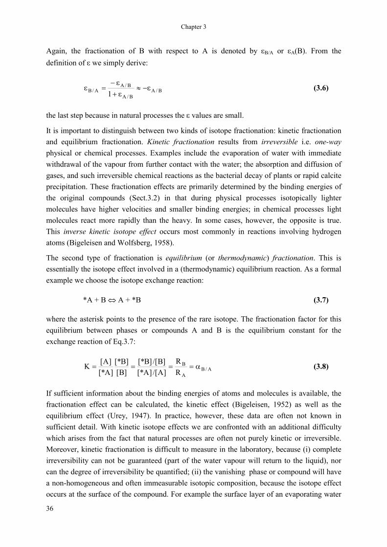
Again, the fractionation of B with respect to A is denoted by �B/A or �A(B). From the definition of � we simply derive:

B/AB/A

B/AA/B 1

���

��

��

�� (3.6)

the last step because in natural processes the � values are small.

It is important to distinguish between two kinds of isotope fractionation: kinetic fractionation and equilibrium fractionation. Kinetic fractionation results from irreversible i.e. one-way physical or chemical processes. Examples include the evaporation of water with immediate withdrawal of the vapour from further contact with the water; the absorption and diffusion of gases, and such irreversible chemical reactions as the bacterial decay of plants or rapid calcite precipitation. These fractionation effects are primarily determined by the binding energies of the original compounds (Sect.3.2) in that during physical processes isotopically lighter molecules have higher velocities and smaller binding energies; in chemical processes light molecules react more rapidly than the heavy. In some cases, however, the opposite is true. This inverse kinetic isotope effect occurs most commonly in reactions involving hydrogen atoms (Bigeleisen and Wolfsberg, 1958).

The second type of fractionation is equilibrium (or thermodynamic) fractionation. This is essentially the isotope effect involved in a (thermodynamic) equilibrium reaction. As a formal example we choose the isotope exchange reaction:

*A + B � A + *B (3.7)

where the asterisk points to the presence of the rare isotope. The fractionation factor for this equilibrium between phases or compounds A and B is the equilibrium constant for the exchange reaction of Eq.3.7:

A/BA

B

RR

]A/[]A[*]B/[]B[*

]B[]B[*

]A[*]A[K ����� (3.8)

If sufficient information about the binding energies of atoms and molecules is available, the fractionation effect can be calculated, the kinetic effect (Bigeleisen, 1952) as well as the equilibrium effect (Urey, 1947). In practice, however, these data are often not known in sufficient detail. With kinetic isotope effects we are confronted with an additional difficulty which arises from the fact that natural processes are often not purely kinetic or irreversible. Moreover, kinetic fractionation is difficult to measure in the laboratory, because (i) complete irreversibility can not be guaranteed (part of the water vapour will return to the liquid), nor can the degree of irreversibility be quantified; (ii) the vanishing phase or compound will have a non-homogeneous and often immeasurable isotopic composition, because the isotope effect occurs at the surface of the compound. For example the surface layer of an evaporating water

36

Stable Isotope Fractionation

mass may become enriched in 18O and 2H if the mixing within the water mass is not rapid enough to keep its content homogeneous throughout.

Isotope fractionation processes in nature which are not purely kinetic (i.e. one-way processes) will be referred to as non-equilibrium fractionations. An example is the evaporation of ocean or fresh surface water bodies: the evaporation is not a one-way process (certainly water vapour condenses), neither an equilibrium process as there is a net evaporation.

Equilibrium fractionation, on the other hand, can be determined by laboratory experiments and in several cases reasonable agreement has been shown between experimental data and thermodynamic calculations.

The general condition for the establishment of isotopic equilibrium between two compounds is the existence of an isotope exchange mechanism. This can be a reversible chemical equilibrium such as:

H216O + C18O16O � H2C18O16O2 � H2

18O + C16O2 (3.9a)

or such a reversible physical process as evaporation/condensation:

H216O(vapour) + H2

18O(liquid) � H218O(vapour) + H2

16O(liquid) (3.9b)

The reaction rates of exchange processes and, consequently, the periods of time required to reach isotopic equilibrium, vary greatly. For instance, the exchange of H2O � CO2 proceeds on a scale of minutes to hours at room temperature, while that of H2O � SO2- requires millennia.

The fractionation resulting from kinetic isotope effects generally exceeds that from equilibrium processes. Moreover, in a kinetic process the compound formed may be depleted in the rare isotope while it is enriched in the equivalent equilibrium process. This can be understood by comparing the fractionation factor in a reversible equilibrium with the kinetic fractionation factors involved in the two opposed single reactions. As an example we take the carbonic acid equilibrium of Eq.3.9a:

��

��� 322 HCOHOHCO

For the single reactions

��

��� 312

2212 COHHOHCO

and

��

��� 313

2213 COHHOHCO

37

Chapter 3

the reaction rates are, respectively:

(3.10) ]CO[krand]CO[kr 2131313

2121212

��

where 12k and 13k are the reaction rate constants. The isotope ratio of the bicarbonate formed (�HCO3

-) is:

)CO(R]CO[k]CO[k

rr)HCO(R 2

13k

21212

21313

12

13

313

����� (3.11)

where �k is the kinetic fractionation factor for this reaction. Conversely, for:

OHCOCOHH 2212

312

�����

and

OHCOCOHH 2213

313

�����

the reaction rates are

(3.12) ]COH['k'rand]COH['k'r 3131313

3121212 ��

��

The carbon dioxide formed (�CO2) has an isotope ratio

)HCO(R]COH['k]COH['k

'r'r)CO(R 3

13'k

31212

31313

12

13

213 �

�

�

����� (3.13)

At isotopic equilibrium the isotope effects balance, in other words:

(3.14) )CO(R)HCO(R 213

313

����

so that combining Eqs.3.11 and 3.13 results in:

e3

132

123

122

13

313

213

k

k

]COH][CO[]COH][CO[

)HCO(R)CO(R'

����

�

�

�

�

�

(3.15)

which shows that the isotopic equilibrium fractionation �e is equivalent to the equilibrium constant of the isotope exchange reaction:

(3.16) 213

312

212

313 COCOHCOCOH ���

�

38

Stable Isotope Fractionation

Most �k and �k' values are less than 1 by more than one per cent. Differences between their ratios are less - in the order of several per mill. Later we will see that rapid evaporation of water might cause the water vapour to be about twice as depleted in 18O as the vapour in equilibrium with the water. The reason for this is, that H2

16O is favoured also in the condensation process.

From Eq.3.15 it is obvious that, while �k for a certain phase transition is smaller than 1, �e might be larger than 1. An example is to be found in the system: dissolved/gaseous CO2: the 13C content of CO2 rapidly withdrawn from an aqueous CO2 solution is smaller than that of the dissolved CO2 (i.e. 12C moves faster: �k1), while under equilibrium conditions the gaseous CO2 contains relatively more 13C (�e1; inverse isotope effect, Sect.3.2).

3.4 THEORETICAL BACKGROUND OF EQUILIBRIUM FRACTIONATION

In this section we will present a discussion of the origin of isotope effects, in particular the mass-dependent isotope fractionation, based on some principles from thermodynamics and statistical mechanics. The treatment here will not be exhaustive and so, for full details, the reader is referred to textbooks on these subjects. A basic discussion has been given by Broecker and Oversby (1971) and Richet et al. (1977).

A basic principle of quantum physics is that the energy of the particle can take only certain discrete values. This is true for any kind of motion. These discrete energy values were already mentioned in Sect.3.2, where we discussed the position of a particle at a certain time at a certain level in the energy well (Figs.3.1 and 3.2).

A basic principle of statistical mechanics states that the chance that a particle is at a certain energy level �r is:

q

epkT/r

r

��

�

where k is the Boltzmann constant and T the absolute temperature of the compound. The value of q, the partition function, is determined by the requirement that the sum of all chances

equals unity:

� ��

�0rr 1p

so that:

(3.17) ���

�

��

0r

kT/req

39

Chapter 3

The partition function is thus the summing up of the population of all energy levels of a certain system and so determines the energy state of the system. It is an important quantity, because thermodynamic considerations show that equilibrium conditions can be expressed as a ratio of partition functions.

Consider again the isotope exchange reaction of Eq.3.7:

*A + B � A + *B

where A and B denote two different compounds (for instance, CO2 and HCO3�) or two phases

of the same compound (for instance, liquid H2O and water vapour), and the asterisk refers to the presence of a rare isotope in the molecule (13C, 18O, 2H, etc.). In the definition of the fractionation factor -i.e. the equilibrium constant- the concentration or rather the activities are now represented by the partition functions:

AA

BB

BA

BAA q/q*

q/q*qq*q*q

K)B( ���� (3.18)

We must now evaluate the various partition functions.

In Sect.3.2 the three modes of motion were mentioned, translation, rotation and vibration. The total partition function of a system of one compound or one phase is related to the partition functions of the different motions by:

q = qtransqrotqvibr (3.19)

Each partition function results from intramolecular (internal) motions, such as vibrations of atoms with respect to each other, and rotations of the molecule around molecular axes, and intermolecular (external) motions, such as vibrations and rotations of molecules with respect to each other, in a crystal lattice, for instance. Most systems are too complicated to allow an exact calculation of the partition functions. The only simple systems are ideal mono-atomic or di-atomic gases. The translations are not hindered by neighbouring atoms or molecules and intermolecular vibrations and rotations do not exist, so that only the internal components of the partition functions have to be calculated. In order to point out the mass dependence of fractionation factors and to illustrate the influence of temperature on fractionation, we will briefly mention the various partition functions.

Translation of a molecule as a whole has the partition function:

VhmkT2q

2/3

2trans ��

���

� �� (3.20)

40

Stable Isotope Fractionation

(V = volume in which the molecules are free to move, m is the mass of the molecule, h Planck's constant). In a gas the translational contribution to the partition function ratio then is (M = molar weight):

2/32/3

trans MM*

mm*

qq*

��

���

���

�

���

����

�

����

� (3.21)

which is temperature independent.

The partition function for internal rotational motion of a diatomic molecule is:

2

20

2

rot shkTr8

q��

� (3.22)

where ro is the equilibrium distance between the two atoms and µ is the reduced mass of the molecule = m1m2/(m1 + m2); the energy of rotation is equal to that of a system where µ rotates around the centre of mass instead of m1 and m2 around each other. We should further remember that µr0

2 is the moment of inertia of a rotating mass, and that s = 1, unless the molecule consists of two equal atoms in which case s = 2. In a gas the rotational contribution to the partition function ratio thus is:

s*

sM*

Mmm**

qq*

1

1

rot

���

����

����

� (3.23)

where *m1 is the rare isotope of atom m1. This ratio also is independent of temperature.

The vibrational partition function is:

kT/h

kT2/h

vibr e1eq

�

��

�

� (3.24)

where � is the frequency of vibration of the two atoms with respect to each other. The frequency is generally known from experimental spectroscopic data. The temperature dependence of the fractionation effect can be shown to be caused primarily by the temperature dependence of the vibration.

The mass dependence of the vibration frequency of the harmonic oscillator is given by:

2/1

'k21

���

����

���

(3.25)

where again µ is the reduced mass of the molecule and k' is the force constant. In a first order approximation k' is not altered by an isotope substitution in the molecule, and so:

41

Chapter 3

2/1

**

���

����

���

� (3.26)

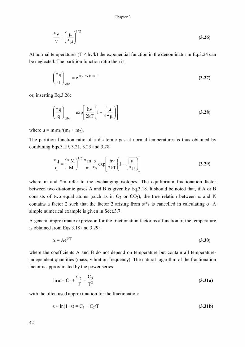
At normal temperatures (T < hv/k) the exponential function in the denominator in Eq.3.24 can be neglected. The partition function ratio then is:

� � kT2/*h

vibr

eqq*

�������

����

� (3.27)

or, inserting Eq.3.26:

���

�

���

����

�

�

��

����

�

�

*1

kT2hexp

qq*

vibr

(3.28)

where µ = m1m2/(m1 + m2).

The partition function ratio of a di-atomic gas at normal temperatures is thus obtained by combining Eqs.3.19, 3.21, 3.23 and 3.28:

���

�

���

����

�

�

��

��

�

��*

1kT2hexp

s*s

mm*

MM*

qq* 2/1

(3.29)

where m and *m refer to the exchanging isotopes. The equilibrium fractionation factor between two di-atomic gases A and B is given by Eq.3.18. It should be noted that, if A or B consists of two equal atoms (such as in O2 or CO2), the true relation between � and K contains a factor 2 such that the factor 2 arising from s/*s is cancelled in calculating �. A simple numerical example is given in Sect.3.7.

A general approximate expression for the fractionation factor as a function of the temperature is obtained from Eqs.3.18 and 3.29:

� = AeB/T (3.30)

where the coefficients A and B do not depend on temperature but contain all temperature-independent quantities (mass, vibration frequency). The natural logarithm of the fractionation factor is approximated by the power series:

232

1 TC

+T

C+C=αln (3.31a)

with the often used approximation for the fractionation:

� � ln(1+�) = C1 + C2/T (3.31b)

42

Stable Isotope Fractionation

It can further be shown, that at very high temperatures the vibrational contribution to the fractionation balances the product of the translational and rotational factors, so that finally at very high temperatures � = 1, and thus, isotope effects disappear at sufficiently high temperatures.

From the foregoing we can draw the following conclusions:

1) In a kinetic (one-way or irreversible) process the phase or compound formed is depleted in the heavy isotope with respect to the original phase or compound (�k < 1); theoretical predictions about the degree of fractionation can only be qualitative (fast evaporating water is depleted in 18O relative to the water itself)

2) In an isotopic equilibrium (reversible) process it can not with certainty be predicted whether the one phase or compound is enriched or depleted in the heavy isotope. However, the dense phase (liquid rather than vapour) or the compound having the largest molecular mass (CaCO3 versus CO2) usually contains the highest abundance of the heavy isotope

3) Under equilibrium conditions and provided sufficient spectroscopic data on the binding energies are available, �e may be calculated; measurements on �e of various isotope equilibria will be reported in chapter 6

4) As a rule fractionation decreases with increasing temperature; in Chapter 6 this is shown, for instance, for the exchange equilibria of CO2 � H2O and H2Oliquid � H2Ovapour. At very high temperatures the isotopic differences between the compounds disappear.

3.5 FRACTIONATION BY DIFFUSION As was mentioned in Sect.3.2 isotope fractionation might occur because of the different mobilities of isotopic molecules. An example in nature is the diffusion of CO2 or H2O through air.

According to Fick's law the net flux of gas, F, through a unit surface area is:

dxdCDF �� (3.32)

where dC/dx is the concentration gradient in the direction of diffusion and D is the diffusion constant. The latter is proportional to the temperature and to 1/�m, where m is the molecular mass. This proportionality results from the fact that all molecules in a gas (mixture) have equal temperature and thus equal average ½mv2. The average velocity of the molecules and, thus, their mobilities are inversely proportional to �m.

If the diffusion process of interest involves the movement of gas A through gas B, however, m has to be replaced by the reduced mass:

43

Chapter 3

BA

BA

mmmm�

�� (3.33)

(see textbooks on the kinetic theory of gases).

The above equations hold for the abundant as well as for the rare isotope. The resulting fractionation is then given by the ratio of the diffusion coefficient for the two isotopic species. Furthermore, the molecular masses can be replaced by the molar weights M in numerator and denominator:

BA

BA

BA

BA

MMMM

MM*MM*

DD*

�

�

�

�

��� (3.34)

In the example of water vapour diffusing through air, the resulting fractionation factor for oxygen is (MB of air is taken to be 29, MA = 18, *MA = 20):

969.029182918

29202920 2/1

18 ���

���

�

�

�� (3.35)

By diffusion through air water vapour thus will become depleted in 18O (in agreement with the rules given at the end of Sect.3.4) by 31 ‰: 18� = �31 ‰.

The 13C fractionation factor for diffusion of CO2 through air is:

9956.029442944

29452945 2/1

13 ���

���

�

�

�� (3.36)

in other words 13� = �4.4 ‰, a depletion of 4.4 ‰.

3.6 RELATION BETWEEN ATOMIC AND MOLECULAR ISOTOPE RATIOS

We want to have a closer look at the meaning of the isotope ratio in the context of the abundance of rare isotopes of an element in poly-atomic molecules, containing at least two atoms of this element. The isotope ratio is the chance that the abundant isotope has been replaced by the rare isotope. To be more specific, we define the atomic isotope ratio (Ratom) as the abundance of all rare isotopic atoms in the compound divided by the abundance of all abundant isotopic atoms. For the sake of clarity, we select a simple example, the isotopes of hydrogen in water:

........]HOH[]HOH[2]HOH[2]HOH[2

.........]HOH[2]HOH[]HOH[]HOH[R 1161118111711161

2162118211721162

atom2

����

����

� (3.37)

44

Stable Isotope Fractionation

The "second-order" abundances, such as for instance 2H218O in the nominator and 1H2H18O in

the denominator, have been neglected. In this context the molecular isotope ratio (Rmol) is defined as the abundance of the rare isotope of a specific element in a specific type of molecule divided by the abundance of the abundant isotope. In our example of deuterium in water:

]HOH[2

]HOH[=R 1161

1162

mol2 (3.38)

The realistic value of this definition refers, for instance, to the measurement of isotope ratios by laser spectrometry (see Sect.10.2.1.2), where the light absorption is compared of two isotopic molecules, only differing in one isotope, contrary to mass spectrometry (Kerstel et al., 1999; priv.comm.).

Eq.3.37 can be rewritten as:

.......

]HOH[2]HOH[

+]HOH[]HOH[

+]HOH[]HOH[

+1

.......]HOH[]HOH[2

+]HOH[]HOH[

+]HOH[]HOH[

+1

]HOH[2]HOH[

=R

1161

2161

1161

1181

1161

1171

1162

2162

1162

1182

1162

1172

1161

1162

atom2 (3.39)

The first factor on the right in Eq.3.39 is the molecular isotope ratio. To a very good approximation the molecular isotope ratios in the second factor may be replaced by the atomic isotope ratios:

mol2

21817

21817

mol2

atom2 R

.......RRR1

.......RRR1RR �

����

����

�� (3.40)

This result means that to a first-order approximation the atomic isotope ratio is equal to a molecular isotope ratio. Although it was shown for one specific molecule, the reasoning is equally valid for the other molecules in Eq.3.39. Also for more complicated molecules the demonstration of the proof is analogous.

The approximations made are indicated as "first-order". However, if we use values the approximation is even better, because almost equal approximations occur in the R values of the nominator as well as the denominator of Eq.3.40 (cf. Sect.4.3.1).

3.7 RELATION BETWEEN FRACTIONATIONS FOR THREE ISOTOPIC MOLECULES

For some isotope studies, it is of interest to know the relation between the fractionations for more than two isotopic molecules. For instance, water contains three different isotopic molecules as far as oxygen is concerned: H2

16O, H217O and H2

18O; carbon dioxide consists of 12CO2, 13CO2 as well 14CO2. The question now is, whether there is a theoretical relation

45

Chapter 3

between the 17O and 18O fractionation with respect to 16O (for instance, during evaporation) and between the 13C and 14C fractionation with respect to 12C (for instance, during the uptake of CO2 by plants).

Generally the fractionation for the heaviest isotope is taken twice as large as that for the less heavy isotope:

� � � �2171821314 and ������ (3.41)

while

� � ���������������13213132131414 21)(2111

so that for the CO2 uptake by plants as well as the isotope exchange between CO2 and water, respectively:

(3.42) ������17181314 2and2

The approximation that these fractionations differ by a factor of 2 originates from the relation between the molecular masses as presented in Eqs. 3.21 and 3.23. For the heaviest isotope m+2� is a function of (M+2)/M, while m+1� is a similar function of (M + 1)/M.

Having discussed the theoretical background of isotope effects in the preceding sections, we are able to make an approximation of the exponent � in the general relation:

���

����

����

�

�

��

�

�

�

�

B/A1m

B/A2m

B1m

A1m

B2m

A2m

lnln

orRR

RR (3.43)

where m = 12 for carbon or 16 for oxygen. The fractionations by diffusion are easily calculated. For the diffusion of water vapour through air Eqs.3.35 and 3.43 result in:

ln 18� / ln 17� = 1.93

whereas according to Eqs.3.36 and 3.43 for the diffusion of CO2 through air:

ln 14� / ln 13� = 1.96

In terms of fractionation this comes to:

18� � 1.93 17� and 14� � 1.96 13�

46

Stable Isotope Fractionation

Calculating the exponent � for fractionation effects in general is quite elaborate. The relatively simple case for the CO � O2 isotopic equilibrium may serve as an example (cf. Broecker and Oversby, 1971). The isotope exchange reactions are:

18O16O + 12C16O � 16O2 + 12C18O

and

17O16O + 12C16O � 16O2 + 12C17O

Inserting the proper mass numbers and the vibration frequencies: �(12C16O) = 6.50 x 1013/s and �(16O16O) = 4.74 x 1013/s in Eqs.3.18 and 3.29, the � values at 20oC are:

023363.1OinO/OCOinO/O

21618

1618

2O/CO18

���

and

012245.1OinO/OCOinO/O

21617

1617

2O/CO17

���

so that:

90.1ln/ln 2O/CO17

2O/CO18

���

(h = 6.626 * 10-34 Js; k = 1.38 * 10-23 J/K).

Applying the equations to poly-atomic molecules can only result in approximate � values. However, calculations on the exchange equilibria such as CO � CO2 and CO2 � CH4 result in:

ln m+2� / ln m+1� � 1.9 (3.44)

rather than in � = 2 (Skaron and Wolfsberg, 1980).

In one case an experimental determination of the relation between 17O and 18O has been possible. A series of natural water samples was electrolytically converted into oxygen which was then analysed mass spectrometrically. The resulting relation between the 17 and 18 values was reported as (Meijer and Li, 1998):

(3.45) )005.08935.1(1718 )1(1 ������

Despite this, in many routine cases, where the obtainable precision is limited or irrelevant, we may still use the relation:

47

Chapter 3

� �21m2m1m2m and2ln/ln ���������� (3.46)

or:

(3.47) ����� 1m2m 2

at least with a precision of 10%. In this respect, we will continue to apply the factor of 2 in the relation between the 13C/12C and 14C/12C isotope ratios for natural processes:

14� = 2 13�

as originally used by Craig (1954). The precision of a 14C analysis is not sufficient to allow an experimental verification of the relation of Eq.3.42 between the fractionations for 13C and 14C containing molecules.

On the other hand, Eq.3.44 is to be applied if the fractionations involved are large and the measurements sufficiently accurate.

48