Embed Size (px)
Citation preview

. . . . . .
ROBOTICS: ADVANCED CONCEPTS & ANALYSISMODULE 5 - VELOCITY AND STATIC ANALYSIS OF MANIPULATORS
Ashitava Ghosal1
1Department of Mechanical Engineering&
Centre for Product Design and ManufactureIndian Institute of ScienceBangalore 560 012, India
Email: [email protected]
NPTEL, 2010
ASHITAVA GHOSAL (IISC) ROBOTICS: ADVANCED CONCEPTS & ANALYSIS NPTEL, 2010 1 / 98

. . . . . .
.. .1 CONTENTS
.. .2 LECTURE 1IntroductionLinear and Angular Velocity of Links
.. .3 LECTURE 2Serial Manipulator Jacobian Matrix
.. .4 LECTURE 3Parallel Manipulator Jacobian Matrix
.. .5 LECTURE 4Singularities in Serial and Parallel Manipulators
.. .6 LECTURE 5Statics of Serial and Parallel Manipulators
.. .7 MODULE 5 – ADDITIONAL MATERIALProblems, References and Suggested Reading
ASHITAVA GHOSAL (IISC) ROBOTICS: ADVANCED CONCEPTS & ANALYSIS NPTEL, 2010 2 / 98

. . . . . .
OUTLINE.. .1 CONTENTS
.. .2 LECTURE 1IntroductionLinear and Angular Velocity of Links
.. .3 LECTURE 2Serial Manipulator Jacobian Matrix
.. .4 LECTURE 3Parallel Manipulator Jacobian Matrix
.. .5 LECTURE 4Singularities in Serial and Parallel Manipulators
.. .6 LECTURE 5Statics of Serial and Parallel Manipulators
.. .7 MODULE 5 – ADDITIONAL MATERIALProblems, References and Suggested Reading
ASHITAVA GHOSAL (IISC) ROBOTICS: ADVANCED CONCEPTS & ANALYSIS NPTEL, 2010 3 / 98

. . . . . .
INTRODUCTIONREVIEW
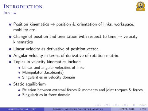
Position kinematics → position & orientation of links, workspace,mobility etc.Change of position and orientation with respect to time → velocitykinematicsLinear velocity as derivative of position vector.Angular velocity in terms of derivative of rotation matrix.Topics in velocity kinematics include
Linear and angular velocities of linksManipulator Jacobian(s)Singularities in velocity domain
Static equilibriumRelation between external forces & moments and joint torques & forces.Singularities in force domain
ASHITAVA GHOSAL (IISC) ROBOTICS: ADVANCED CONCEPTS & ANALYSIS NPTEL, 2010 4 / 98

. . . . . .
INTRODUCTIONREVIEW
Position kinematics → position & orientation of links, workspace,mobility etc.Change of position and orientation with respect to time → velocitykinematicsLinear velocity as derivative of position vector.Angular velocity in terms of derivative of rotation matrix.Topics in velocity kinematics include
Linear and angular velocities of linksManipulator Jacobian(s)Singularities in velocity domain
Static equilibriumRelation between external forces & moments and joint torques & forces.Singularities in force domain
ASHITAVA GHOSAL (IISC) ROBOTICS: ADVANCED CONCEPTS & ANALYSIS NPTEL, 2010 4 / 98

. . . . . .
OUTLINE.. .1 CONTENTS
.. .2 LECTURE 1IntroductionLinear and Angular Velocity of Links
.. .3 LECTURE 2Serial Manipulator Jacobian Matrix
.. .4 LECTURE 3Parallel Manipulator Jacobian Matrix
.. .5 LECTURE 4Singularities in Serial and Parallel Manipulators
.. .6 LECTURE 5Statics of Serial and Parallel Manipulators
.. .7 MODULE 5 – ADDITIONAL MATERIALProblems, References and Suggested Reading
ASHITAVA GHOSAL (IISC) ROBOTICS: ADVANCED CONCEPTS & ANALYSIS NPTEL, 2010 5 / 98

. . . . . .
LINEAR AND ANGULAR VELOCITY OF RIGID BODYLINEAR VELOCITY OF RIGID BODY
The linear velocity of Oi with respect to 0 is defined as
0VOi∆=
ddt
0Oi (t) = lim∆t→0
0Oi (t +∆t)−0 Oi (t)∆t
(1)
X
Y
Z
Oi
Oi
i(t)i(t + ∆t)
0Oi(t + ∆t)
0Oi(t)
Rigid body at t
Rigid body att + ∆t
0
Figure 1: Linear velocity of a rigid body
‘0’ denote the coordinate system0 where the limit is taken.The linear velocity vector can bedescribed in j as
j (0VOi
)= j
0[R]0VOi (2)
Two different coordinate systeminvolved: where differentiationdone, and where described!
ASHITAVA GHOSAL (IISC) ROBOTICS: ADVANCED CONCEPTS & ANALYSIS NPTEL, 2010 6 / 98

. . . . . .
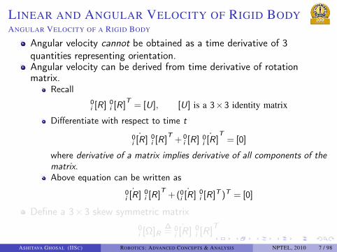
LINEAR AND ANGULAR VELOCITY OF RIGID BODYANGULAR VELOCITY OF A RIGID BODY
Angular velocity cannot be obtained as a time derivative of 3quantities representing orientation.Angular velocity can be derived from time derivative of rotationmatrix.
Recall0i [R] 0
i [R]T= [U], [U] is a 3×3 identity matrix
Differentiate with respect to time t
˙0i [R] 0
i [R]T+ 0
i [R] ˙0i [R]
T= [0]
where derivative of a matrix implies derivative of all components of thematrix.Above equation can be written as
˙0i [R] 0
i [R]T+( ˙0
i [R] 0i [R]T )T = [0]
Define a 3×3 skew symmetric matrix0i [Ω]R
∆= ˙0
i [R] 0i [R]
T
ASHITAVA GHOSAL (IISC) ROBOTICS: ADVANCED CONCEPTS & ANALYSIS NPTEL, 2010 7 / 98
. . . . . .
LINEAR AND ANGULAR VELOCITY OF RIGID BODYANGULAR VELOCITY OF A RIGID BODY
Angular velocity cannot be obtained as a time derivative of 3quantities representing orientation.Angular velocity can be derived from time derivative of rotationmatrix.
Recall0i [R] 0
i [R]T= [U], [U] is a 3×3 identity matrix
Differentiate with respect to time t
˙0i [R] 0
i [R]T+ 0
i [R] ˙0i [R]
T= [0]
where derivative of a matrix implies derivative of all components of thematrix.Above equation can be written as
˙0i [R] 0
i [R]T+( ˙0
i [R] 0i [R]T )T = [0]
Define a 3×3 skew symmetric matrix0i [Ω]R
∆= ˙0
i [R] 0i [R]
T
ASHITAVA GHOSAL (IISC) ROBOTICS: ADVANCED CONCEPTS & ANALYSIS NPTEL, 2010 7 / 98

. . . . . .
LINEAR AND ANGULAR VELOCITY OF RIGID BODYANGULAR VELOCITY OF RIGID BODY – SKEW SYMMETRIC MATRIX
Skew-symmetric matrix in detail
0i [Ω]R =
0 −ωsz ωs
yωs
z 0 −ωsx
−ωsy ωs
x 0
(3)
The product of Oi [Ω]R and a vector (px ,py ,pz)
T ∈ ℜ3 is across-product
0i [Ω]R(px ,py ,pz)
T =
ωsypz − ωs
zpyωs
zpx − ωsxpz
ωsxpy − ωs
ypx
= 0ω is ×0 p (4)
0i [Ω]R called angular velocity matrix0ω i
s called angular velocity vector of i with respect to 0.In contrast to linear velocity, angular velocity vector is not astraightforward differentiation!
ASHITAVA GHOSAL (IISC) ROBOTICS: ADVANCED CONCEPTS & ANALYSIS NPTEL, 2010 8 / 98

. . . . . .
LINEAR AND ANGULAR VELOCITY OF RIGID BODYANGULAR VELOCITY OF RIGID BODY – IN TERMS OF EULER ANGLES
Angular velocity in terms of Z-Y-Z Euler angles.Recall for α , β and γ as the Z-Y-Z Euler angles
AB [R] =
cαcβ cγ − sαsγ −cαcβ sγ − sαcγ cαsβsαcβ cγ + cαsγ −sαcβ sγ + cαcγ sαsβ
−sβ cγ sβ sγ cβ
(5)
Obtain ˙AB [R] A
B [R]T
The X, Y and Z components of the angular velocity vector
ωxs = γ cosα sinβ − β sinα
ωys = γ sinα sinβ + β cosα (6)
ωzs = γ cosβ + α
ASHITAVA GHOSAL (IISC) ROBOTICS: ADVANCED CONCEPTS & ANALYSIS NPTEL, 2010 9 / 98

. . . . . .
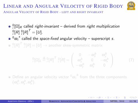
LINEAR AND ANGULAR VELOCITY OF RIGID BODYANGULAR VELOCITY OF RIGID BODY - LEFT AND RIGHT INVARIANT
0i [Ω]R called right-invariant – derived from right multiplication0i [R] 0
i [R]T= [U].
0ω is called the space-fixed angular velocity – superscript s.
0i [R]
T 0i [R] = [U] → another skew-symmetric matrix
0i [Ω]L
∆= 0
i [R]T ˙0
i [R] =
0 −ωbz ωb
yωb
z 0 −ωbx
−ωby ωb
x 0
(7)
Define an angular velocity vector 0ω ib from the three components
(ωbx ,ωb
y ,ωbz ).
ASHITAVA GHOSAL (IISC) ROBOTICS: ADVANCED CONCEPTS & ANALYSIS NPTEL, 2010 10 / 98
. . . . . .
LINEAR AND ANGULAR VELOCITY OF RIGID BODYANGULAR VELOCITY OF RIGID BODY - LEFT AND RIGHT INVARIANT
0i [Ω]R called right-invariant – derived from right multiplication0i [R] 0
i [R]T= [U].
0ω is called the space-fixed angular velocity – superscript s.
0i [R]
T 0i [R] = [U] → another skew-symmetric matrix
0i [Ω]L
∆= 0
i [R]T ˙0
i [R] =
0 −ωbz ωb
yωb
z 0 −ωbx
−ωby ωb
x 0
(7)
Define an angular velocity vector 0ω ib from the three components
(ωbx ,ωb
y ,ωbz ).
ASHITAVA GHOSAL (IISC) ROBOTICS: ADVANCED CONCEPTS & ANALYSIS NPTEL, 2010 10 / 98

. . . . . .
LINEAR AND ANGULAR VELOCITY OF RIGID BODYANGULAR VELOCITY OF RIGID BODY – LEFT INVARIANT
For the Z-Y-Z rotation the three components are
ωxb = −α cosγ sinβ + β sinγ
ωyb = α sinβ sinγ + β cosγ (8)
ωzb = α cosβ + γ
0i [Ω]L called left-invariant angular velocity matrix.0ω i
b called body-fixed angular velocity vector of i with respect to0 – superscript b.The two skew-symmetric matrices are related like two tensors
0i [Ω]R = 0
i [R] 0i [Ω]L
0i [R]
T (9)
The two angular velocities are related as
0ω is= 0
i [R]0ω ib (10)
ASHITAVA GHOSAL (IISC) ROBOTICS: ADVANCED CONCEPTS & ANALYSIS NPTEL, 2010 11 / 98

. . . . . .
LINEAR AND ANGULAR VELOCITY OF RIGID BODYANGULAR VELOCITY OF RIGID BODY (CONTD.)
Z Rigid Body
at t
Rigid Body at
t + ∆t
Oi
0
X
Y
ip
it+∆t
it
Figure 2: Angular velocity of a rigid body
More on two forms of angularvelocity matrix and vectors.Pure rotation – 0Oi (t) and0Oi (t +∆t) are coincident andonly the elements of the rotationmatrix i
0[R] change with time.Point P located by ip, and fixedin i
ASHITAVA GHOSAL (IISC) ROBOTICS: ADVANCED CONCEPTS & ANALYSIS NPTEL, 2010 12 / 98

. . . . . .
LINEAR AND ANGULAR VELOCITY OF RIGID BODYANGULAR VELOCITY OF RIGID BODY (CONTD.)
Location of P in 00p = 0
i [R]ip
and since P is fixed in i
˙0p ∆=
0Vp = ˙0
i [R] ip
and since 0i [R]
−1= 0
i [R]T ,
0Vp = ˙0i [R] 0
i [R]T 0p
= 0i [Ω]R
0p= 0ω i
s ×0 p (11)
The coordinate system i does not appear except in denoting thatrigid body i is being considered.Space-fixed angular velocity vector is said to be independent of thechoice of the body coordinate system.
ASHITAVA GHOSAL (IISC) ROBOTICS: ADVANCED CONCEPTS & ANALYSIS NPTEL, 2010 13 / 98

. . . . . .
LINEAR AND ANGULAR VELOCITY OF RIGID BODYANGULAR VELOCITY OF RIGID BODY (CONTD.)
Using relation between 0i [Ω]R and 0
i [Ω]L
0Vp = 0i [R] 0
i [Ω]L0i [R]
T 0p= 0
i [R]0i [Ω]Lip
and get0i [R]
−1 0Vp = 0i [Ω]L
ip
which yieldsiVp = 0
i [Ω]Lip = 0ω i
b ×i p (12)
Again except for denoting the reference coordinate system, thecoordinate system 0 does not appear!Body-fixed angular velocity vector is said to be independent of thechoice of the fixed coordinate system.Unless explicitly stated, space-fixed angular velocity vector derivedfrom ˙0
i [R] 0i [R]
T is normally used.
ASHITAVA GHOSAL (IISC) ROBOTICS: ADVANCED CONCEPTS & ANALYSIS NPTEL, 2010 14 / 98

. . . . . .
LINEAR AND ANGULAR VELOCITY OF LINKSANGULAR VELOCITY IN SERIAL MANIPULATOR – ROTARY (R) JOINT
For two links connected by a rotary (R) joint (see Module 2, Lecture 2)
0i [R] = 0
i−1[R] i−1i [R(k,θi )]
The time derivative operation
˙0i [R] 0
i [R]T=
ddt
(0i−1[R] i−1i [R(k,θi )]) (i−1
i [R(k,θi )]T 0
i−1[R]T )
Rewrite above equation as
0i [Ω]R = 0
i−1[Ω]R + 0i−1[R] (i−1
i [R(k,θi )]i−1i [R(k,θi )]
T ) 0i−1[R]T
To simplify, use the result
i−1i [R(k,θi )] = e(
i−1i [K ]θi )
i−1i [K ] is the skew-symmetric form of the rotation axis vector k andθi is the rotation at the rotary joint (see Module 2, Lecture 2).
ASHITAVA GHOSAL (IISC) ROBOTICS: ADVANCED CONCEPTS & ANALYSIS NPTEL, 2010 15 / 98
. . . . . .
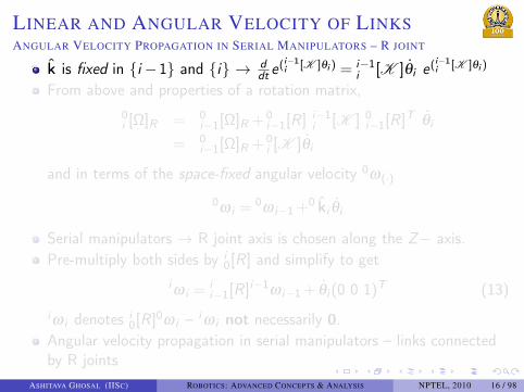
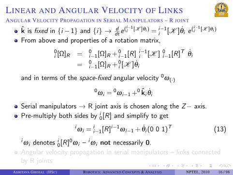
LINEAR AND ANGULAR VELOCITY OF LINKSANGULAR VELOCITY PROPAGATION IN SERIAL MANIPULATORS – R JOINT
k is fixed in i −1 and i → ddt e
(i−1i [K ]θi ) = i−1
i [K ]θi e(i−1i [K ]θi )
From above and properties of a rotation matrix,0i [Ω]R = 0
i−1[Ω]R + 0i−1[R] i−1
i [K ] 0i−1[R]T θi
= 0i−1[Ω]R + 0
i [K ]θi
and in terms of the space-fixed angular velocity 0ω(·)
0ω i =0ω i−1+
0 ki θi
Serial manipulators → R joint axis is chosen along the Z− axis.Pre-multiply both sides by i
0[R] and simplify to getiω i =
ii−1[R]i−1ω i−1+ θi (0 0 1)T (13)
iω i denotes i0[R]0ω i – iω i not necessarily 0.
Angular velocity propagation in serial manipulators – links connectedby R joints
ASHITAVA GHOSAL (IISC) ROBOTICS: ADVANCED CONCEPTS & ANALYSIS NPTEL, 2010 16 / 98

. . . . . .
LINEAR AND ANGULAR VELOCITY OF LINKSANGULAR VELOCITY PROPAGATION IN SERIAL MANIPULATORS – R JOINT
k is fixed in i −1 and i → ddt e
(i−1i [K ]θi ) = i−1
i [K ]θi e(i−1i [K ]θi )
From above and properties of a rotation matrix,0i [Ω]R = 0
i−1[Ω]R + 0i−1[R] i−1
i [K ] 0i−1[R]T θi
= 0i−1[Ω]R + 0
i [K ]θi
and in terms of the space-fixed angular velocity 0ω(·)
0ω i =0ω i−1+
0 ki θi
Serial manipulators → R joint axis is chosen along the Z− axis.Pre-multiply both sides by i
0[R] and simplify to getiω i =
ii−1[R]i−1ω i−1+ θi (0 0 1)T (13)
iω i denotes i0[R]0ω i – iω i not necessarily 0.
Angular velocity propagation in serial manipulators – links connectedby R joints
ASHITAVA GHOSAL (IISC) ROBOTICS: ADVANCED CONCEPTS & ANALYSIS NPTEL, 2010 16 / 98

. . . . . .
LINEAR AND ANGULAR VELOCITY OF LINKSLINEAR VELOCITY PROPAGATION IN SERIAL MANIPULATOR – R JOINT
For two consecutive links in a serial manipulator (see Module 2,Lecture 2)
0Oi =0 Oi−1+
0i−1[R]i−1Oi
Taking derivatives on both sides
0VOi =0 VOi−1 +
0 ω i−1× 0i−1[R]i−1Oi
Simplify and rewrite above as
iVi =ii−1[R](i−1Vi−1+
i−1 ω i−1×i−1 Oi ) (14)
Note: iVi and i−1Vi−1 denote i0[R]0Vi and i−1
0 [R]0Vi−1, respectively.They are not necessarily 0!Linear velocity vector propagation in links of a serial manipulator –Rotary joint.
ASHITAVA GHOSAL (IISC) ROBOTICS: ADVANCED CONCEPTS & ANALYSIS NPTEL, 2010 17 / 98

. . . . . .
LINEAR AND ANGULAR VELOCITY OF LINKSVELOCITY PROPAGATION – PRISMATIC JOINTS
Two links connected by a prismatic (P) joint (see Module 2, Lecture 2)Prismatic joint allows relative translation between 1− i and i →angular velocity is sameRelative translation is along Z− axis → di (0 0 1)T
Velocity propagation for P joint
Angular velocityiω i =
ii−1[R]i−1ω i−1 (15)
Linear velocityiVi =
ii−1[R](i−1Vi−1+
i−1 ω i−1×i−1 Oi )+ di (0 0 1)T (16)
where ii−1[R]i−1ω i
∆= iω i and i
i−1[R]i−1Vi∆= iVi .
ASHITAVA GHOSAL (IISC) ROBOTICS: ADVANCED CONCEPTS & ANALYSIS NPTEL, 2010 18 / 98

. . . . . .
LINEAR AND ANGULAR VELOCITY OF LINKSVELOCITY PROPAGATION – PLANAR 3R MANIPULATOR
2
3
YTool
X0
Y0
Link 1
0
1
Y1
O2
l1
O1
θ2
l2
l3
Link 3
O3
X2
Link 2
X3, XTool
Toolθ3
Y3
Y2 X1
θ1
Figure 3: The planar 3R manipulator – revisited
All joint axis are parallel andcoming out of page.0 is fixed →
0ω0 = 00V0 = 0
Links connected by rotary (R)joint → Equations (13) and (14)give velocities of all links.
ASHITAVA GHOSAL (IISC) ROBOTICS: ADVANCED CONCEPTS & ANALYSIS NPTEL, 2010 19 / 98

. . . . . .
LINEAR AND ANGULAR VELOCITY OF LINKSVELOCITY PROPAGATION – PLANAR 3R MANIPULATOR (CONTD.)
For i=11ω1 = (0 0 θ1)
T
1V1 = 0
For i=22ω2 = (0 0 θ1+ θ2)
T
2V2 =
c2 s2 0−s2 c2 00 0 1
0l1θ10
=
l1s2θ1
l1c2θ10
For i=3
3ω3 = (0 0 θ1+ θ2+ θ3)T
3V3 =
(l1s23+ l2s3)θ1+ l2s3θ2
(l1c23+ l2c3)θ1+ l2c3θ20
ASHITAVA GHOSAL (IISC) ROBOTICS: ADVANCED CONCEPTS & ANALYSIS NPTEL, 2010 20 / 98
. . . . . .
LINEAR AND ANGULAR VELOCITY OF LINKSVELOCITY PROPAGATION – PLANAR 3R MANIPULATOR (CONTD.)
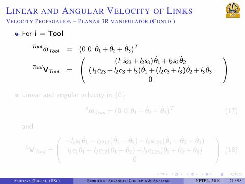
For i = Tool
ToolωTool = (0 0 θ1+ θ2+ θ3)T
ToolVTool =
(l1s23+ l2s3)θ1+ l2s3θ2
(l1c23+ l2c3+ l3)θ1+(l2c3+ l3)θ2+ l3θ30
Linear and angular velocity in 0
0ωTool = (0 0 θ1+ θ2+ θ3)T (17)
and
0VTool =
−l1s1θ1− l2s12(θ1+ θ2)− l3s123(θ1+ θ2+ θ3)
l1c1θ1+ l2c12(θ1+ θ2)+ l3c123(θ1+ θ2+ θ3)0
(18)
ASHITAVA GHOSAL (IISC) ROBOTICS: ADVANCED CONCEPTS & ANALYSIS NPTEL, 2010 21 / 98

. . . . . .
LINEAR AND ANGULAR VELOCITY OF LINKSVELOCITY PROPAGATION – PLANAR 3R MANIPULATOR (CONTD.)
For i = Tool
ToolωTool = (0 0 θ1+ θ2+ θ3)T
ToolVTool =
(l1s23+ l2s3)θ1+ l2s3θ2
(l1c23+ l2c3+ l3)θ1+(l2c3+ l3)θ2+ l3θ30
Linear and angular velocity in 0
0ωTool = (0 0 θ1+ θ2+ θ3)T (17)
and
0VTool =
−l1s1θ1− l2s12(θ1+ θ2)− l3s123(θ1+ θ2+ θ3)
l1c1θ1+ l2c12(θ1+ θ2)+ l3c123(θ1+ θ2+ θ3)0
(18)
ASHITAVA GHOSAL (IISC) ROBOTICS: ADVANCED CONCEPTS & ANALYSIS NPTEL, 2010 21 / 98

. . . . . .
OUTLINE.. .1 CONTENTS
.. .2 LECTURE 1IntroductionLinear and Angular Velocity of Links
.. .3 LECTURE 2Serial Manipulator Jacobian Matrix
.. .4 LECTURE 3Parallel Manipulator Jacobian Matrix
.. .5 LECTURE 4Singularities in Serial and Parallel Manipulators
.. .6 LECTURE 5Statics of Serial and Parallel Manipulators
.. .7 MODULE 5 – ADDITIONAL MATERIALProblems, References and Suggested Reading
ASHITAVA GHOSAL (IISC) ROBOTICS: ADVANCED CONCEPTS & ANALYSIS NPTEL, 2010 22 / 98

. . . . . .
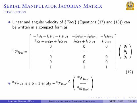
SERIAL MANIPULATOR JACOBIAN MATRIXINTRODUCTION
Linear and angular velocity of Tool (Equations (17) and (18)) canbe written in a compact form as
0VTool =
−l1s1− l2s12− l3s123 −l2s12− l3s123 −l3s123l1c1+ l2c12+ l3c123 l2c12+ l3c123 l3c123
0 0 0−− −− −−0 0 00 0 01 1 1
θ1
θ2
θ3
(19)
0VTool is a 6×1 entity – 0VTool∆=
0VTool−−
0ωTool
ASHITAVA GHOSAL (IISC) ROBOTICS: ADVANCED CONCEPTS & ANALYSIS NPTEL, 2010 23 / 98
. . . . . .
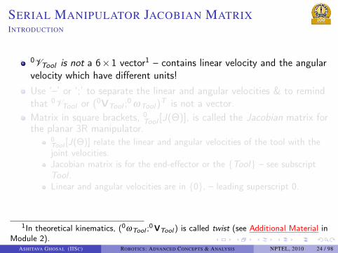
SERIAL MANIPULATOR JACOBIAN MATRIXINTRODUCTION
0VTool is not a 6×1 vector1 – contains linear velocity and the angularvelocity which have different units!Use ‘–’ or ‘;’ to separate the linear and angular velocities & to remindthat 0VTool or (0VTool ;
0 ωTool )T is not a vector.
Matrix in square brackets, 0Tool [J(Θ)], is called the Jacobian matrix for
the planar 3R manipulator.0Tool [J(Θ)] relate the linear and angular velocities of the tool with thejoint velocities.Jacobian matrix is for the end-effector or the Tool – see subscriptTool .Linear and angular velocities are in 0, – leading superscript 0.
1In theoretical kinematics, (0ωTool ;0 VTool ) is called twist (see Additional Material in
Module 2).ASHITAVA GHOSAL (IISC) ROBOTICS: ADVANCED CONCEPTS & ANALYSIS NPTEL, 2010 24 / 98

. . . . . .
SERIAL MANIPULATOR JACOBIAN MATRIXPROPERTIES OF JACOBIAN MATRIX
0Tool [J(Θ)] is not a proper matrix.
The first and the last three rows represent linear and angular velocity,Elements of the first three rows have units of length,Elements of last three rows have no units.
Similar to 0VTool , top and bottom halves of a Jacobian matrix areseparated by ‘–’.Many matrix operations makes no sense – the condition number2 ofthis matrix changes with the choice of length units.0Tool [J(Θ)] is best thought of as a map 0
Tool [J(Θ)] : Θ→0 VTool
2The condition number of a matrix is the ratio of the absolute value of the largest tothe smallest eigenvalues.
ASHITAVA GHOSAL (IISC) ROBOTICS: ADVANCED CONCEPTS & ANALYSIS NPTEL, 2010 25 / 98
. . . . . .
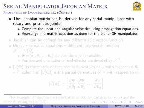
SERIAL MANIPULATOR JACOBIAN MATRIXPROPERTIES OF JACOBIAN MATRIX (CONTD.)
The Jacobian matrix can be derived for any serial manipulator withrotary and prismatic joints.
Compute the linear and angular velocities using propagation equationsRearrange in a matrix equation as done for the planar 3R manipulator.
Jacobian can be defined for any differentiable vector function.Direct kinematics equations – differentiable vector functionX =Ψ(Θ)
Θ= (θ1,θ2, . . . ,θn) denotes the n joint variablesPosition and orientation of end-effector are denoted by X 3.
[J(Θ)] is the matrix of first partial derivatives of Ψ with respect to θi– i th column of [J(Θ)] is the partial derivatives of Ψ with respect to θi .
[J(Θ)] =
[∂Ψ∂θ1
∂Ψ∂θ2
. . .∂Ψ∂θn
]3For example, X denotes the three Cartesian position variables (x , y , z) and the
three Euler angles (α, β ,γ).ASHITAVA GHOSAL (IISC) ROBOTICS: ADVANCED CONCEPTS & ANALYSIS NPTEL, 2010 26 / 98

. . . . . .
SERIAL MANIPULATOR JACOBIAN MATRIXPROPERTIES OF JACOBIAN MATRIX (CONTD.)
The Jacobian matrix can be derived for any serial manipulator withrotary and prismatic joints.
Compute the linear and angular velocities using propagation equationsRearrange in a matrix equation as done for the planar 3R manipulator.
Jacobian can be defined for any differentiable vector function.Direct kinematics equations – differentiable vector functionX =Ψ(Θ)
Θ= (θ1,θ2, . . . ,θn) denotes the n joint variablesPosition and orientation of end-effector are denoted by X 3.
[J(Θ)] is the matrix of first partial derivatives of Ψ with respect to θi– i th column of [J(Θ)] is the partial derivatives of Ψ with respect to θi .
[J(Θ)] =
[∂Ψ∂θ1
∂Ψ∂θ2
. . .∂Ψ∂θn
]3For example, X denotes the three Cartesian position variables (x , y , z) and the
three Euler angles (α, β ,γ).ASHITAVA GHOSAL (IISC) ROBOTICS: ADVANCED CONCEPTS & ANALYSIS NPTEL, 2010 26 / 98
. . . . . .
SERIAL MANIPULATOR JACOBIAN MATRIXPROPERTIES OF JACOBIAN MATRIX (CONTD.)
0Tool [J(Θ)] very important in velocity kinematics of serial manipulators.The elements of the Jacobian matrix are non-linear functions of thejoint variables Θ.
Manipulator in motion → 0Tool [J(Θ)] is time varying.
At instant with Θ known, 0Tool [J(Θ)] relates linear and angular
velocities to joint rates.The relationship is linear!
The Jacobian matrix can be obtained for any link – most often forend-effector.The Jacobian matrix is always with respect to a coordinate system –where the linear and angular velocities are obtained.Most often Jacobian matrix is with respect to fixed 0.Jacobian matrix can be written in any coordinate system usingrotation matrices.
ASHITAVA GHOSAL (IISC) ROBOTICS: ADVANCED CONCEPTS & ANALYSIS NPTEL, 2010 27 / 98
. . . . . .
SERIAL MANIPULATOR JACOBIAN MATRIXPROPERTIES OF JACOBIAN MATRIX (CONTD.)
The Jacobian matrix is m×n – m is dimension of the motion space4
and n is the number of actuated joints.If 0
Tool [J(Θ)] is square, i.e., m = n, and if the determinantdet(0Tool [J(Θ)]) = 0, then
Θ = 0Tool [J(Θ)]
−1 0VTool (20)
Above relationship gives joint velocities required for a desired linearand angular velocities of Tool.Direct velocity kinematics – 0VTool =
0Tool [J(Θ)]Θ
Inverse velocity kinematics – Θ = 0Tool [J(Θ)]
−1 0VTool
4Same as λ in the definition of DOF in Module 3, Lecture 1 – m = 6 for ℜ3 andm = 3 for plane.
ASHITAVA GHOSAL (IISC) ROBOTICS: ADVANCED CONCEPTS & ANALYSIS NPTEL, 2010 28 / 98

. . . . . .
SERIAL MANIPULATOR JACOBIAN MATRIXGEOMETRIC INTERPRETATION OF JACOBIAN MATRIX
X2
(x, y)
X0
Y0
Link 1
0
O2
l1
O1
θ2
l2
Link 2
X1
θ1
Figure 4: A planar 2R manipulator
Consider a planar 2R manipulator shownin in figure 4.The linear velocity V of the end-effector(point (x ,y)) is
V ∆=
(xy
)=
[−l1s1− l2s12 −l2s12l1c1+ l2c12 l2c12
](θ1
θ2
)where θ1, θ2 are the two joint rates.The matrix inside square brackets is theJacobian matrix in 0.
ASHITAVA GHOSAL (IISC) ROBOTICS: ADVANCED CONCEPTS & ANALYSIS NPTEL, 2010 29 / 98

. . . . . .
SERIAL MANIPULATOR JACOBIAN MATRIXGEOMETRIC INTERPRETATION OF JACOBIAN MATRIX
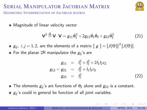
Magnitude of linear velocity vector
V2 ∆= V ·V = g11θ2
1 +2g12θ1θ2+g22θ22 (21)
gij , i , j = 1,2, are the elements of a matrix [ g ] = [J(Θ)]T [J(Θ)].For the planar 2R manipulator the gij ’s are
g11 = l21 + l22 +2l1l2c2
g12 = g21 = l22 + l1l2c2
g22 = l22 (22)
The elements gij ’s are functions of θ2 alone and g22 is a constant.gij ’s could in general be function of all joint variables.
ASHITAVA GHOSAL (IISC) ROBOTICS: ADVANCED CONCEPTS & ANALYSIS NPTEL, 2010 30 / 98

. . . . . .
SERIAL MANIPULATOR JACOBIAN MATRIXGEOMETRIC INTERPRETATION OF JACOBIAN MATRIX
Magnitude of linear velocity vector
V2 ∆= V ·V = g11θ2
1 +2g12θ1θ2+g22θ22 (21)
gij , i , j = 1,2, are the elements of a matrix [ g ] = [J(Θ)]T [J(Θ)].For the planar 2R manipulator the gij ’s are
g11 = l21 + l22 +2l1l2c2
g12 = g21 = l22 + l1l2c2
g22 = l22 (22)
The elements gij ’s are functions of θ2 alone and g22 is a constant.gij ’s could in general be function of all joint variables.
ASHITAVA GHOSAL (IISC) ROBOTICS: ADVANCED CONCEPTS & ANALYSIS NPTEL, 2010 30 / 98

. . . . . .
SERIAL MANIPULATOR JACOBIAN MATRIXGEOMETRIC INTERPRETATION OF JACOBIAN MATRIX
Maximum and minimum V2 subject to constraint θ21 + θ2
2 = 15
Solve ∂V∗2/∂ θi = 0, i = 1,2, where
V∗2 = g11θ21 +2g12θ1θ2+g22θ2
2 −λ (θ11 + θ2
2 −1)
Partial differentiation reduces to an eigenvalue problem
[ g ]Θ−λ Θ = 0 (23)
The eigenvalues are
λ1,2 = (1/2)(g11+g22)± [(g11+g22)2−4(g11g22−g2
12)]1/2
5Without any constraint V ∈ ℜ2 and fills up ℜ2. The constraint θ21 + θ2
2 = 1 issimilar to the unit speed constraint in differential geometry of space curves.
ASHITAVA GHOSAL (IISC) ROBOTICS: ADVANCED CONCEPTS & ANALYSIS NPTEL, 2010 31 / 98

. . . . . .
SERIAL MANIPULATOR JACOBIAN MATRIXGEOMETRIC INTERPRETATION OF JACOBIAN MATRIX (CONTD.)
[ g ] real, symmetric and positive definite → eigenvalues are alwaysreal and positive.For λ1 > λ2,
|V|max =√
λ1, |V|min =√
λ2
For square Jacobian matrix, eigenvalues of [J(Θ)] are√
λ1 and√
λ2(see Strang 1976).Maximum and minimum |V| for 2R manipulator –
√λ1 and
√λ2.
If θ21 + θ2
2 = k2 is used → maximum and minimum |V| are scaled by k .
ASHITAVA GHOSAL (IISC) ROBOTICS: ADVANCED CONCEPTS & ANALYSIS NPTEL, 2010 32 / 98

. . . . . .
SERIAL MANIPULATOR JACOBIAN MATRIXGEOMETRIC INTERPRETATION OF JACOBIAN MATRIX (CONTD.)
From V = [J(Θ)]Θ,[J]TV = [ g ]Θ
and for non-singular [ g ],
VT ([J][ g ]−1)([J][ g ]−1)TV = ΘTΘ
For a planar 2R manipulator, ([J][ g ]−1)([J][ g ]−1)T is symmetricand of rank 2.Hence for Θ
TΘ = 1, (x , y)T ([J][ g ]−1)([J][ g ]−1)T (x , y) = 1.
xT [A]x = 1, with [A] symmetric and non-singular, describes an ellipse.The tip of the linear velocity vector traces an ellipse and thesemi-major and semi-minor axes of the ellipse are
√λ1 and
√λ2,
respectively.
For ΘTΘ = k2, size of ellipse is scaled by k , but shape of ellipse does
not change with k .
ASHITAVA GHOSAL (IISC) ROBOTICS: ADVANCED CONCEPTS & ANALYSIS NPTEL, 2010 33 / 98

. . . . . .
SERIAL MANIPULATOR JACOBIAN MATRIXGEOMETRIC INTERPRETATION OF JACOBIAN MATRIX (CONTD.)
Eigenvalues of [ g ] are onlyfunctions of θ2 → shape and sizeof ellipse will change with θ2.Can plot ellipses at all points inthe workspaceRecall: workspace of a planar 2Ris the area between two circlesof radii l1+ l2 and l1− l2.Ellipse independent of θ1 → Allellipses at a chosen radius (inthe annular region) are same!
(x, y)
X0
Y0
Link 1
0
O2
l1
O1
θ2
l2
θ1
Link 2
Figure 5: Velocity ellipse for a planar 2Rmanipulator
ASHITAVA GHOSAL (IISC) ROBOTICS: ADVANCED CONCEPTS & ANALYSIS NPTEL, 2010 34 / 98

. . . . . .
SERIAL MANIPULATOR JACOBIAN MATRIXGEOMETRIC INTERPRETATION OF JACOBIAN MATRIX (CONTD.)
The shape of the velocity ellipse indicates which directions are ‘easier’to move for given joint rates|V| is larger along major axis → Easier to move along major axis.Less easier to move along the minor axis.Ellipse reduces to a circle → equally easy to move in all directions.All points in the workspace, where the ellipse is a circle, are calledisotropic (see Salisbury 1982)
ASHITAVA GHOSAL (IISC) ROBOTICS: ADVANCED CONCEPTS & ANALYSIS NPTEL, 2010 35 / 98

. . . . . .
SERIAL MANIPULATOR JACOBIAN MATRIXGEOMETRIC INTERPRETATION OF JACOBIAN MATRIX (CONTD.)
Isotropic configuration – eigenvalues of [J(Θ)] (or [ g ]) are equal.For planar 2R, eigenvalues equal only if
g11 = g22 and g12 = 0
From the expressions of gij ’s above conditions imply that
l21 +2l1l2c2 = 0 and l22 + l1l2c2 = 0
and this is only possible if
l1 =√
2l2 and c2 =− 1√2
A planar 2R manipulator can posses isotropic configurations only if thelink lengths have a ratio of
√2, and θ2 = 135.
Since θ1 ∈ [0,2π], all the isotropic configurations lie on a circle.Degenerate form of velocity ellipse → singular configuration (seeLecture 4).
ASHITAVA GHOSAL (IISC) ROBOTICS: ADVANCED CONCEPTS & ANALYSIS NPTEL, 2010 36 / 98

. . . . . .
SERIAL MANIPULATOR JACOBIAN MATRIXGEOMETRIC INTERPRETATION OF JACOBIAN MATRIX (CONTD.)
Spatial motion & 2 degree-of-freedom → Velocity vector on tangentplane to a surface → Velocity ellipse.Spatial motion & 3 degree-of-freedom → Velocity vector lies in ℜ3 →Velocity ellipsoid.Same ideas can be extended to angular velocity vector.Extension to 6×6 Jacobian matrix – more complicated since not aproper matrix (see Ghosal and Ravani (1998), Bandyopadhyay andGhosal (2004b) and references in them)
Need to use notions of screws and twists (see Hunt 1976).Velocity ellipse → Cylindroid & Two screw systemVelocity ellipsoid → Hyperboloid & Three screw system.
Extension to parallel manipulators using parallel manipulator Jacobian.
ASHITAVA GHOSAL (IISC) ROBOTICS: ADVANCED CONCEPTS & ANALYSIS NPTEL, 2010 37 / 98

. . . . . .
SERIAL MANIPULATOR JACOBIAN MATRIXRESOLUTION OF REDUNDANCY AT VELOCITY LEVEL
For square Jacobian → matrix can be inverted to obtain joint rates.Redundant systems (see Module 3, Lecture 3) Jacobian matrix is notsquare → number of joint variables more than 6 (for ℜ3) or more than3 (for ℜ2).Jacobian matrix cannot be inverted to obtain joint rates given linearand angular velocity of end-effector.Use of pseudo-inverse (Strang 1976) to resolve redundancy –pseudo-inverse of m×n (n > m) matrix [J(Θ)]
[J(Θ)]# = [J(Θ)]T ([J(Θ)][J(Θ)]T )−1
ASHITAVA GHOSAL (IISC) ROBOTICS: ADVANCED CONCEPTS & ANALYSIS NPTEL, 2010 38 / 98

. . . . . .
SERIAL MANIPULATOR JACOBIAN MATRIXRESOLUTION OF REDUNDANCY AT VELOCITY LEVEL
Some properties of pseudo-inverseDimension of [J(Θ)]# is n×m – not square!Left inverse → [J(Θ)][J(Θ)]# = [U] – [U] is an identity matrix.Not a right inverse [J(Θ)]#[J(Θ)] = [U]General solution to 0VTool =
0Tool [J(Θ)]Θ is
Θ = [J(Θ)]#0VTool +([U]− [J(Θ)]#[J(Θ)])W
([U]− [J(Θ)]#[J(Θ)])W lies in the null-space of [J(Θ)].The pseudo-inverse solution, without the null-space term, minimisesΘ
TΘ.
The null-space term used to avoid obstacles, joint limits and tomaximise manipulability index det([[J(Θ)][J(Θ)]T ]1/2)(see Nakamura1991).Disadvantages
Local numerical scheme – cannot obtain global or analytical results.Velocity level and not a position and orientation level scheme forresolution of redundancy.
ASHITAVA GHOSAL (IISC) ROBOTICS: ADVANCED CONCEPTS & ANALYSIS NPTEL, 2010 39 / 98
. . . . . .
OUTLINE.. .1 CONTENTS
.. .2 LECTURE 1IntroductionLinear and Angular Velocity of Links
.. .3 LECTURE 2Serial Manipulator Jacobian Matrix
.. .4 LECTURE 3Parallel Manipulator Jacobian Matrix
.. .5 LECTURE 4Singularities in Serial and Parallel Manipulators
.. .6 LECTURE 5Statics of Serial and Parallel Manipulators
.. .7 MODULE 5 – ADDITIONAL MATERIALProblems, References and Suggested Reading
ASHITAVA GHOSAL (IISC) ROBOTICS: ADVANCED CONCEPTS & ANALYSIS NPTEL, 2010 40 / 98

. . . . . .
PARALLEL MANIPULATOR JACOBIAN MATRIXINTRODUCTION
Parallel manipulator – actuated and passive joints – q = (θ ,ϕ)T
Loop-closure constraint equations do not contain all joint variables.No natural choice of end-effector Tool → no velocity propagationPlatform type parallel manipulator – position of centroid & orientationof platform Tool is of interest.Linear and angular velocity of centroid and Tool
0ωTool =ddt
(0Tool [R]) 0Tool [R]
T=0
Tool [Jω (q)] q
0VTool =13( ˙0p1+ ˙0p2+ ˙0p3) =
0Tool [JV(q)] q (24)
0Tool [Jω (q)], 0
Tool [JV(q)] – Jacobian for linear, angular velocities.q – time derivatives of configuration variables q.
ASHITAVA GHOSAL (IISC) ROBOTICS: ADVANCED CONCEPTS & ANALYSIS NPTEL, 2010 41 / 98

. . . . . .
PARALLEL MANIPULATOR JACOBIAN MATRIXELIMINATION OF PASSIVE JOINT RATES
Linear and angular velocity function of all q and q.Only the actuated joints θi , i = 1,2, ...,n are specified.The m passive ϕi ’s can be obtained from direct kinematicsNeed expression for ϕi and obtain linear and angular velocities in termsof only θi ’s.Derived from the m loop-closure or constraint equations.
ASHITAVA GHOSAL (IISC) ROBOTICS: ADVANCED CONCEPTS & ANALYSIS NPTEL, 2010 42 / 98
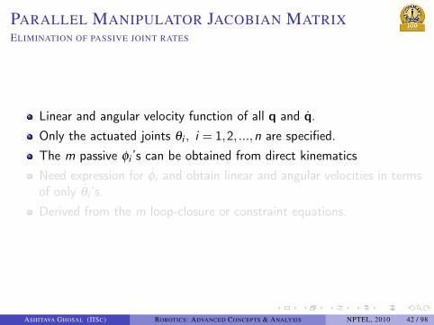

. . . . . .
PARALLEL MANIPULATOR JACOBIAN MATRIXELIMINATION OF PASSIVE JOINT RATES
For m passive variables, m constraint equationsηi (q1, ...,qn+m) = 0, i = 1, ...,m or in a vector form
η(q) = η(θ ,ϕ) = 0 (25)
Differentiate equation (25) with respect to t, and rearrange
[K (q)]θ +[K ∗(q)]ϕ = 0 (26)
Columns of the m×n matrix [K (q)] are the partial derivatives of η(q)with respect to the actuated variables θi , i = 1, ...,n,Columns of m×m matrix [K ∗(q)] are the partial derivatives of η(q)with respect to the passive variables ϕi , i = 1, ...,m.
[K ∗(q)] is always an m×m square matrix.[K (q)] and [K ∗(q)] are functions q = (θ ,ϕ) ∈ ℜn+m.
ASHITAVA GHOSAL (IISC) ROBOTICS: ADVANCED CONCEPTS & ANALYSIS NPTEL, 2010 43 / 98

. . . . . .
PARALLEL MANIPULATOR JACOBIAN MATRIXELIMINATION OF PASSIVE JOINT RATES (CONTD.)
If det([K ∗]) = 0,ϕ =−[K ∗]−1[K ]θ (27)
The angular and linear velocity can partitioned as
0ωTool = [Jω ]θ +[J∗ω ]ϕ , 0VTool = [JV]θ +[J∗
V]ϕ
Substitute ϕ to get
0ωTool = ([Jω ]− [J∗ω ][K ∗]−1[K ])θ0VTool = ([JV ]− [J∗
V ][K∗]−1[K ])θ
Define equivalent [Jω ]eq and [JV]eq
[JV]eq∆= [JV]− [J∗
V][K∗]−1[K ] (28)
[Jω ]eq∆= [Jω ]− [J∗
ω ][K ∗]−1[K ] (29)
ASHITAVA GHOSAL (IISC) ROBOTICS: ADVANCED CONCEPTS & ANALYSIS NPTEL, 2010 44 / 98

. . . . . .
PARALLEL MANIPULATOR JACOBIAN MATRIXELIMINATION OF PASSIVE JOINT RATES (CONTD.)
If det([K ∗]) = 0,ϕ =−[K ∗]−1[K ]θ (27)
The angular and linear velocity can partitioned as
0ωTool = [Jω ]θ +[J∗ω ]ϕ , 0VTool = [JV]θ +[J∗
V]ϕ
Substitute ϕ to get
0ωTool = ([Jω ]− [J∗ω ][K ∗]−1[K ])θ0VTool = ([JV ]− [J∗
V ][K∗]−1[K ])θ
Define equivalent [Jω ]eq and [JV]eq
[JV]eq∆= [JV]− [J∗
V][K∗]−1[K ] (28)
[Jω ]eq∆= [Jω ]− [J∗ω ][K ∗]−1[K ] (29)
ASHITAVA GHOSAL (IISC) ROBOTICS: ADVANCED CONCEPTS & ANALYSIS NPTEL, 2010 44 / 98

. . . . . .
PARALLEL MANIPULATOR JACOBIAN MATRIXELIMINATION OF PASSIVE JOINT RATES (CONTD.)
If det([K ∗]) = 0,ϕ =−[K ∗]−1[K ]θ (27)
The angular and linear velocity can partitioned as
0ωTool = [Jω ]θ +[J∗ω ]ϕ , 0VTool = [JV]θ +[J∗V]ϕ
Substitute ϕ to get
0ωTool = ([Jω ]− [J∗ω ][K ∗]−1[K ])θ
0VTool = ([JV ]− [J∗V ][K
∗]−1[K ])θ
Define equivalent [Jω ]eq and [JV]eq
[JV]eq∆= [JV]− [J∗
V][K∗]−1[K ] (28)
[Jω ]eq∆= [Jω ]− [J∗ω ][K ∗]−1[K ] (29)
ASHITAVA GHOSAL (IISC) ROBOTICS: ADVANCED CONCEPTS & ANALYSIS NPTEL, 2010 44 / 98

. . . . . .
PARALLEL MANIPULATOR JACOBIAN MATRIXEQUIVALENT JACOBIAN MATRIX IN PARALLEL MANIPULATORS
Using [JV]eq and [Jω ]eq
0VTool∆=
0VTool−−
0ωTool
= 0Tool [Jeq]θ (30)
The 6×n matrix, 0Tool [Jeq], consists of 3×n rows from [JV]eq and
3×n rows from [Jω ]eq.
The matrix 0Tool [Jeq] is the Jacobian matrix for parallel manipulators.
At a known q, equation (30) relate actuated joint rates θ to the linearand angular velocity of chosen end-effector Tool.
ASHITAVA GHOSAL (IISC) ROBOTICS: ADVANCED CONCEPTS & ANALYSIS NPTEL, 2010 45 / 98

. . . . . .
PARALLEL MANIPULATOR JACOBIAN MATRIXEQUIVALENT JACOBIAN MATRIX IN PARALLEL MANIPULATORS
The matrix 0Tool [JV]eq can be used define a [ gV ]eq for parallel
manipulators.
[ gV ]eq = ([JV]− [JV∗][K ∗]−1[K ])T ([JV]− [JV
∗][K ∗]−1[K ]) (31)
[ gV ]eq is symmetric and positive definite.Similar to a serial manipulator, the tip of the linear velocity vector lieson an ellipse or an ellipsoid.Much more complicated than in serial manipulators![ gω ]eq defined using [Jω ]eq → angular velocity ellipse or ellipsoid.The above geometrical description is valid if det [K ∗] = 0.
ASHITAVA GHOSAL (IISC) ROBOTICS: ADVANCED CONCEPTS & ANALYSIS NPTEL, 2010 46 / 98
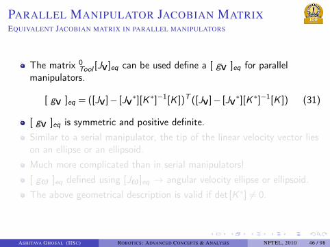
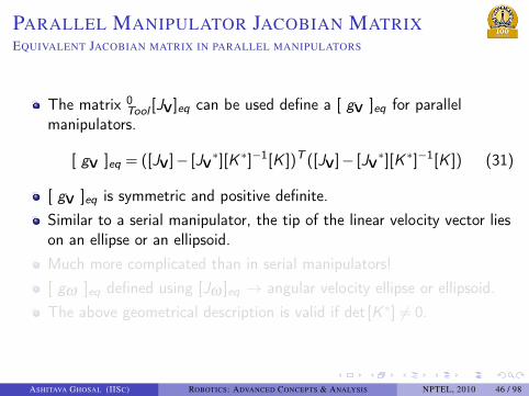

. . . . . .
PARALLEL MANIPULATOR JACOBIAN MATRIXEXAMPLE – PLANAR 4-BAR MECHANISM
Constraint equation of a four-bar (see Module 4, Lecture 1)
η1(q)∆= l1 cosθ1+ l2 cos(θ1+ϕ2)− l0− l3 cosϕ1 = 0
η2(q)∆= l1 sinθ1+ l2 sin(θ1+ϕ2)− l3 sinϕ1 = 0
θ1 is the actuated joint variable and (ϕ1,ϕ2) are the passive jointvariables.Derivative of constraint equations with respect to time t gives(
−l1 sinθ1− l2 sin(θ1+ϕ2)l1 cosθ1+ l2 cos(θ1+ϕ2)
)θ1+(
l3 sinϕ1 −l2 sin(θ1+ϕ2)−l3 cosϕ1 l2 cos(θ1+ϕ2)
)(ϕ1
ϕ2
)= 0
ASHITAVA GHOSAL (IISC) ROBOTICS: ADVANCED CONCEPTS & ANALYSIS NPTEL, 2010 47 / 98

. . . . . .
PARALLEL MANIPULATOR JACOBIAN MATRIXEXAMPLE – PLANAR 4-BAR MECHANISM
[K ] and [K ∗] matrices for the planar 4-bar are
[K ] =
(−l1 sinθ1− l2 sin(θ1+ϕ2)l1 cosθ1+ l2 cos(θ1+ϕ2)
)
[K ∗] =
[l3 sinϕ1 −l2 sin(θ1+ϕ2)−l3 cosϕ1 l2 cos(θ1+ϕ2)
]The matrix [K ∗] is a square 2×2 matrix.[K ] and [K ∗] matrices are functions of the actuated and passivevariables.Fairly simple to calculate for planar 4-bar.Multi- degree-of-freedom spatial mechanisms → use symbolic algebrasoftware such as MAPLE.
ASHITAVA GHOSAL (IISC) ROBOTICS: ADVANCED CONCEPTS & ANALYSIS NPTEL, 2010 48 / 98

. . . . . .
PARALLEL MANIPULATOR JACOBIAN MATRIXEXAMPLE – 3-RPS PARALLEL MANIPULATOR
For the 3-RPS manipulator, loop-closure equations are
η1(q) = 3−3a2+ l21 + l22 + l1l2c1c2−2l1l2s1s2−3l1c1−3l2c2 = 0η2(q) = 3−3a2+ l22 + l23 + l2l3c2c3−2l2l3s2s3−3l2c2−3l3c3 = 0η3(q) = 3−3a2+ l23 + l21 + l3l1c3c1−2l3l1s3s1−3l3c3−3l1c1 = 0
Perform the derivative of ηi (q), i = 1,2,3, with respect to time andrearrange to obtain [K ] and [K ∗]
[K ] involves derivative with respect to the actuated variables l
2l1 −3c1 + l2c1c2 −2l2s1s2 2l2 −3c2 + l1c1c2 −2l1s1s2 00 2l2 −3c2 + l3c2c3 −2l3s2s3 2l3 −3c3 + l2c2c3 −2l2s2s3
2l1 −3c1 + l3c1c3 −2l3s1s3 0 2l3 −3c3 + l1c1c3 −2l1s1s3
ASHITAVA GHOSAL (IISC) ROBOTICS: ADVANCED CONCEPTS & ANALYSIS NPTEL, 2010 49 / 98

. . . . . .
PARALLEL MANIPULATOR JACOBIAN MATRIXEXAMPLE – 3-RPS PARALLEL MANIPULATOR (CONTD.)
[K ∗] involves derivative with respect to passive joint variables, θ
3l1s1 − l1l2s1c2 −2l1l2c1s2 3l2s2 − l1l2c1s2 −2l1l2s1c2 00 3l2s2 − l2l3s2c3 −2l2l3c2s3 3l3s3 − l2l3c2s3 −2l2l3s2c3
3l1s1 − l1l3s1c3 −2l1l3c1s3 0 3l3s3 − l1l3c1s3 −2l1l3s1c3
For the centroid, [JV] and [JV∗], are
[JV] = (1/3)
−c1 (1/2)c2 (1/2)c3
0 (−√
3/2)c2 (√
3/2)c3s1 s2 s3
and
[JV∗] = (1/3)
l1s1 −(1/2)l2s2 (−1/2)l3s30 (
√3/2)l2s2 (−
√3/2)l3s3
l1c1 l2c2 l3c3
ASHITAVA GHOSAL (IISC) ROBOTICS: ADVANCED CONCEPTS & ANALYSIS NPTEL, 2010 50 / 98

. . . . . .
PARALLEL MANIPULATOR JACOBIAN MATRIXEXAMPLE – 3-RPS PARALLEL MANIPULATOR (CONTD.)
To obtain [Jω ] and [Jω ∗], compute ddt (
BaseTop [R]) Base
Top [R]T and then
rearrange.Expressions are too large – for l1 = 2/3, l2 = 3/5, l3 = 3/4 andcorresponding θ1 = 0.7593, θ2 = 0.2851, θ3 = 0.8028 radians,
[Jω ] =
−1.4147 1.3103 1.69290.2092 0.7130 0.8537−1.3628 −0.1286 0.6743
, [Jω ∗] =
0.6682 0.8774 −0.3316−1.6372 0.4175 0.16721.4206 0.0226 0.1321
Expressions for [JV]eq and [Jω ]eq are more harder to obtain – [K ∗]−1
is needed. For above numerical values
[JV]eq =
−0.2313 0.5372 0.01140.0722 −0.6758 0.19511.1765 −1.6830 0.9223
, [Jω ]eq =
2.1409 −6.4331 0.46650.0072 −4.1216 1.60480.1565 0.4570 −0.3285
ASHITAVA GHOSAL (IISC) ROBOTICS: ADVANCED CONCEPTS & ANALYSIS NPTEL, 2010 51 / 98
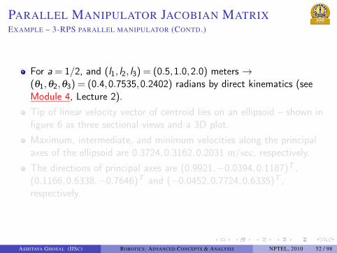
. . . . . .
PARALLEL MANIPULATOR JACOBIAN MATRIXEXAMPLE – 3-RPS PARALLEL MANIPULATOR (CONTD.)
For a = 1/2, and (l1, l2, l3) = (0.5,1.0,2.0) meters →(θ1,θ2,θ3) = (0.4,0.7535,0.2402) radians by direct kinematics (seeModule 4, Lecture 2).Tip of linear velocity vector of centroid lies on an ellipsoid – shown infigure 6 as three sectional views and a 3D plot.Maximum, intermediate, and minimum velocities along the principalaxes of the ellipsoid are 0.3724,0.3162,0.2031 m/sec, respectively.The directions of principal axes are (0.9921,−0.0394,0.1187)T ,(0.1166,0.6338,−0.7646)T and (−0.0452,0.7724,0.6335)T ,respectively.
ASHITAVA GHOSAL (IISC) ROBOTICS: ADVANCED CONCEPTS & ANALYSIS NPTEL, 2010 52 / 98

. . . . . .
PARALLEL MANIPULATOR JACOBIAN MATRIXEXAMPLE – 3-RPS PARALLEL MANIPULATOR (CONTD.)
−0.4 −0.2 0 0.2 0.4−0.4
−0.2
0
0.2
0.4
Vx
Vy
−0.4 −0.2 0 0.2 0.4−0.4
−0.2
0
0.2
0.4
Vx
Vz
−0.4 −0.2 0 0.2 0.4−0.4
−0.2
0
0.2
0.4
Vy
Vz
−0.50
0.5
−0.5
0
0.5−0.5
0
0.5
VxVy
Vz
Figure 6: Velocity ellipsoid at a non-singular point
ASHITAVA GHOSAL (IISC) ROBOTICS: ADVANCED CONCEPTS & ANALYSIS NPTEL, 2010 53 / 98

. . . . . .
OUTLINE.. .1 CONTENTS
.. .2 LECTURE 1IntroductionLinear and Angular Velocity of Links
.. .3 LECTURE 2Serial Manipulator Jacobian Matrix
.. .4 LECTURE 3Parallel Manipulator Jacobian Matrix
.. .5 LECTURE 4Singularities in Serial and Parallel Manipulators
.. .6 LECTURE 5Statics of Serial and Parallel Manipulators
.. .7 MODULE 5 – ADDITIONAL MATERIALProblems, References and Suggested Reading
ASHITAVA GHOSAL (IISC) ROBOTICS: ADVANCED CONCEPTS & ANALYSIS NPTEL, 2010 54 / 98

. . . . . .
SINGULARITIES IN SERIAL AND PARALLEL
MANIPULATORSSERIAL MANIPULATORS – REVIEW
Direct velocity kinematics0VTool =
0Tool [J(Θ)]Θ
For known Θ and Θ, linear and angular velocity of end-effectorobtained from above equation.0VTool always exists
Inverse velocity kinematics
Θ = 0Tool [J(Θ)]
−1 0VTool
Joint rates can be obtained when Jacobian matrix is square, anddet(0Tool [J(Θ)]) = 0
det(0Tool [J(Θ)]) = 0 → Loss of rank of 0Tool [J(Θ)] → Singular
configuration.At singular configuration, Θ cannot be obtained for given linear andangular velocity.
ASHITAVA GHOSAL (IISC) ROBOTICS: ADVANCED CONCEPTS & ANALYSIS NPTEL, 2010 55 / 98

. . . . . .
SINGULARITIES IN SERIAL AND PARALLEL
MANIPULATORSSERIAL MANIPULATORS – SINGULARITY IN PLANAR 2R MANIPULATOR
For a planar 2R manipulator(xy
)=
[−l1s1− l2s12 −l2s12l1c1+ l2c12 l2c12
](θ1
θ2
)The Jacobian matrix is
0Tool [J(Θ)] =
[−l1s1− l2s12 −l2s12l1c1+ l2c12 l2c12
]det(0Tool [J(Θ)]) = 0 → sinθ2 = 0.This implies θ2 = 0,π → the second link is stretched completely orfolded on top of first link.
ASHITAVA GHOSAL (IISC) ROBOTICS: ADVANCED CONCEPTS & ANALYSIS NPTEL, 2010 56 / 98

. . . . . .
SINGULARITIES IN SERIAL AND PARALLEL
MANIPULATORSSERIAL MANIPULATORS – SINGULARITY IN PLANAR 2R MANIPULATOR
radius = l1 − l2
radius = l1 + l2Possible directions
of velocity
vector
X0
Y0
Link 1
0
O2
O1
Link 2
l2
l1
θ1
Figure 7: Singular configurations for a planar2R manipulator
Planar 2R manipulator forθ2 = 0,π.End-effector can only moveperpendicular to the line O1−O2connecting the two rotary joints.The end-effector cannot have avelocity component along thesecond link.Instantaneous loss (only at thisconfiguration) of one degree offreedom.
ASHITAVA GHOSAL (IISC) ROBOTICS: ADVANCED CONCEPTS & ANALYSIS NPTEL, 2010 57 / 98

. . . . . .
SINGULARITIES IN SERIAL AND PARALLEL
MANIPULATORSSERIAL MANIPULATORS – SINGULARITY IN PLANAR 2R MANIPULATOR
At θ2 = 0,π, the velocity ellipse degenerates to a line – along thepossible direction of motion as shown in figure 7.For the 2R planar example, the Jacobian matrix can be inverted easily,and (
θ1
θ2
)=
1l1l2s2
(l2c12 l2s12
−l1c1− l2c12 −l1s1− l2s12
)(xy
)sinθ2 is in the denominator and as θ2 → 0 or π, (θ1, θ2)
T → ∞.Knowledge of singularity is important – when det(0Tool [J(Θ)]) is closeto zero, joint velocities tend to become large and cause problems forthe servo controller of the robot.Singularities occurs in all serial manipulator and not only in planar 2RPlanar 2R singularity only at workspace boundaries – in othermanipulators can happen elsewhere also!
ASHITAVA GHOSAL (IISC) ROBOTICS: ADVANCED CONCEPTS & ANALYSIS NPTEL, 2010 58 / 98

. . . . . .
SINGULARITIES IN SERIAL AND PARALLEL
MANIPULATORSPARALLEL MANIPULATORS – REVIEW
In parallel manipulators, equivalent Jacobian need to be used.For parallel manipulators, the linear and angular velocity Jacobians are
[JV]eq∆= [JV]− [J∗
V][K∗]−1[K ]
[Jω ]eq∆= [Jω ]− [J∗
ω ][K ∗]−1[K ]
Equivalent Jacobian
0Tool [J]eq =
[JV]eq−−
[Jω ]eq
det(0Tool [Jeq]) = 0 → End-effector looses one or more degrees offreedom → actuated joint rates Θ→ ∞.Similar to serial manipulators – at singularity velocity ellipse orellipsoid degenerates.
ASHITAVA GHOSAL (IISC) ROBOTICS: ADVANCED CONCEPTS & ANALYSIS NPTEL, 2010 59 / 98

. . . . . .
SINGULARITIES IN SERIAL AND PARALLEL
MANIPULATORSPARALLEL MANIPULATORS – REVIEW
In parallel manipulators, equivalent Jacobian need to be used.For parallel manipulators, the linear and angular velocity Jacobians are
[JV]eq∆= [JV]− [J∗
V][K∗]−1[K ]
[Jω ]eq∆= [Jω ]− [J∗ω ][K ∗]−1[K ]
Equivalent Jacobian
0Tool [J]eq =
[JV]eq−−
[Jω ]eq
det(0Tool [Jeq]) = 0 → End-effector looses one or more degrees offreedom → actuated joint rates Θ→ ∞.Similar to serial manipulators – at singularity velocity ellipse orellipsoid degenerates.
ASHITAVA GHOSAL (IISC) ROBOTICS: ADVANCED CONCEPTS & ANALYSIS NPTEL, 2010 59 / 98
. . . . . .
SINGULARITIES IN SERIAL AND PARALLEL
MANIPULATORSPARALLEL MANIPULATORS – GAIN SINGULARITY
In addition to loss singularity, second kind of singularity in parallelmanipulators.θ = 0 → Actuated joints locked → mechanism becomes a structure.Equation [K (q)]θ +[K ∗(q)]ϕ = 0 becomes
[K ∗(q)]ϕ = 0
From linear algebra, above equation can have a non-zero solution ϕ ∗
when det([K ∗]) = 0.ϕ ∗
is the eigenvector corresponding to the zero eigenvalue of [K ∗].
ASHITAVA GHOSAL (IISC) ROBOTICS: ADVANCED CONCEPTS & ANALYSIS NPTEL, 2010 60 / 98

. . . . . .
SINGULARITIES IN SERIAL AND PARALLEL
MANIPULATORSPARALLEL MANIPULATORS – GAIN SINGULARITY
For a non-zero ϕ ∗, and θ = 0,
0ωTool = [Jω ∗]ϕ ∗
0VTool = [JV∗]ϕ ∗
Even with actuators locked the linear and angular velocity arenon-zero.The end-effector of the parallel manipulator can instantaneously gainone or more degrees of freedom.Termed as gain singularity.
ASHITAVA GHOSAL (IISC) ROBOTICS: ADVANCED CONCEPTS & ANALYSIS NPTEL, 2010 61 / 98

. . . . . .
SINGULARITIES IN SERIAL AND PARALLEL
MANIPULATORSPARALLEL MANIPULATORS – GAIN SINGULARITY (CONTD.)
Geometric picture: Non-singular configuration.At non-singular configurations, θ = 0 → ϕ = 0 → 0VTool = 0.At a non-singular position velocity ellipsoid is of zero size.
Geometric picture: Gain singularity configuration.Loss of rank of [K ∗].If rank is (m−1) → there exists non zero eigenvector ϕ1 for the zeroeigenvalue of [K ∗]C1ϕ also an eigenvector with C1 a scaling constant.For θ = 0
0VTool = C1[JV∗]ϕ1
There can be motion along [JV∗]ϕ1 !
The zero velocity ellipsoid ‘grows’ into a line.
ASHITAVA GHOSAL (IISC) ROBOTICS: ADVANCED CONCEPTS & ANALYSIS NPTEL, 2010 62 / 98
. . . . . .
SINGULARITIES IN SERIAL AND PARALLEL
MANIPULATORSPARALLEL MANIPULATORS – GAIN SINGULARITY (CONTD.)
If rank of matrix [K ∗] is (m−2), then
0VTool = C1[JV∗]ϕ1+C2[JV
∗]ϕ2
ϕ1, ϕ2 are eigenvectors from the two zero eigenvalues of [K ∗].C1, C2 are the two scaling constants.
For C 21 +C 2
2 = 1, tip of velocity vector traces an ellipse6.If rank of [K ∗] is (m−3), then tip of velocity vector will lie on anellipsoid.If rank is less than (m−3) and only 0VTool is of interest → similar toa redundant serial manipulator.
6C1 and C2 are similar to θ1 and θ2 and C21 +C2
2 = 1 is similar to the constraintθ21 + θ2
2 = 1 used in the planar 2R example. Using same reasoning as in 2R case, the tipof 0VTool for a parallel manipulator lies on an ellipse.
ASHITAVA GHOSAL (IISC) ROBOTICS: ADVANCED CONCEPTS & ANALYSIS NPTEL, 2010 63 / 98
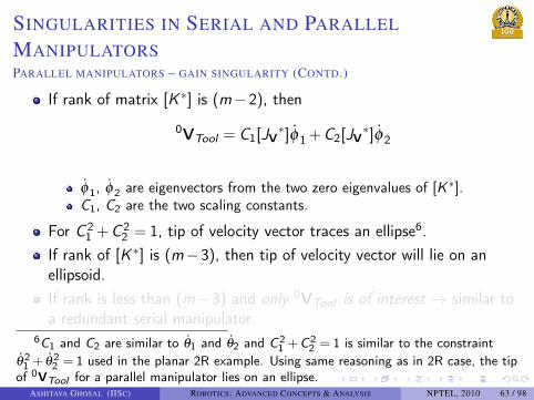

. . . . . .
SINGULARITIES IN SERIAL AND PARALLEL
MANIPULATORSPARALLEL MANIPULATORS – GAIN SINGULARITY
Gain singularity occurs in all parallel and hybrid manipulators.In fully-parallel six- degree-of-freedom manipulator (end-effectordirectly connected to base by one actuated joint – Stewart-Goughplatform) only gain singularity possible (Hunt, 1991).In six- degree-of-freedom hybrid parallel manipulator (example six-degree-of-freedom three-fingered hand, see Module 2, Lecture 3 andModule 4, Lecture 2) both loss and gain singularity possible.Gain singularity is related to capability of resisting external force ormoments (see Lecture 5).Large amount of literature on singularity analysis of parallelmanipulators (see, for example, Hunt 1986, Litvin et. al 1990, Merlet1991, Gosselin and Angeles 1990, Zlatanov 1995, Park and Kim 1999).Singularity analysis & uses of singularity analysis is an active topic ofresearch (see Bandyopadhyay and Ghosal 2009, Ranganath et al.2004)
ASHITAVA GHOSAL (IISC) ROBOTICS: ADVANCED CONCEPTS & ANALYSIS NPTEL, 2010 64 / 98

. . . . . .
SINGULARITIES IN SERIAL AND PARALLEL
MANIPULATORS
Special link lengths and geometry → gain over finite range of motion.Passive link can show instantaneous and finite dwell.
l0
L
YL
XL
YR
XR
R
OL
OR
θ2
l4
Link 4
l3
Link 3
θ1
l2
Link 2
O2
O3
Link 1
l1
Figure 8: Finite motion at gain singularity
Link 2 and Link 3 can rotatefrom 0 to 2π with θ1 and θ2locked (see Bandyopadhyayand Ghosal (2004a) fordetails).
ASHITAVA GHOSAL (IISC) ROBOTICS: ADVANCED CONCEPTS & ANALYSIS NPTEL, 2010 65 / 98

. . . . . .
SINGULARITIES IN SERIAL AND PARALLEL
MANIPULATORSSINGULARITIES IN PARALLEL MANIPULATORS – EXAMPLES
l0
L
φ1
YL
XL
YR
R
O2
OL, O1
O3
φ2
XR
OR
Link 1l1
θ1
Link 2
Link 3
l3
l2
Figure 9: Singular configuration for a planar four-barmechanism
det([K ∗]) = 0 givesl2l3 sin(θ1+ϕ2−ϕ1) = 0⇒ θ1+ϕ2−ϕ1 = nπ →ϕ3 = 2πLink 2 and 3 are parallel.Instantaneous gain: θ1locked, point O2 is fixed→ Link 2 and Link 3along a straight line →O3 can haveinstantaneous velocityalong the commontangent.
ASHITAVA GHOSAL (IISC) ROBOTICS: ADVANCED CONCEPTS & ANALYSIS NPTEL, 2010 66 / 98

. . . . . .
SINGULARITIES IN SERIAL AND PARALLEL
MANIPULATORSSINGULARITIES IN PARALLEL MANIPULATORS – EXAMPLES
Example – The 3-RPS parallel manipulator (see Basu and Ghosal, 1997For the 3-RPS parallel manipulator,
det([JV]eq) = 0 → linear velocity ellipsoid described by the centroid ofthe top platform degenerates to an ellipse7
For (l1, l2, l3) = (0.5,1.0,1.9710) meters and(θ1,θ2,θ3) = (1.1691,0.4781,0.2355) radians → det([JV]eq) = 0.
The linear velocity ellipse at this configuration is shown in sectionaland a 3D view in figure 10.Not a contradiction to result by Hunt (1991)
The 3-RPS parallel manipulator is not six- degree-of-freedommanipulator,Only the linear velocity vector of the centroid is considered.
7See Ghosal and Ravani (2001) for more details.ASHITAVA GHOSAL (IISC) ROBOTICS: ADVANCED CONCEPTS & ANALYSIS NPTEL, 2010 67 / 98

. . . . . .
SINGULARITIES IN SERIAL AND PARALLEL
MANIPULATORSSINGULARITIES IN PARALLEL MANIPULATORS – EXAMPLES
Example – The 3-RPS parallel manipulator
−2 −1 0 1 2−2
−1
0
1
2
Vx
Vy
−2 −1 0 1 2−2
−1
0
1
2
Vx
Vz
−2 −1 0 1 2−2
−1
0
1
2
Vy
Vz
−20
2
−2
0
2−2
0
2
VxVy
Vz
Figure 10: Linear velocity ellipse at a loss singular point
ASHITAVA GHOSAL (IISC) ROBOTICS: ADVANCED CONCEPTS & ANALYSIS NPTEL, 2010 68 / 98

. . . . . .
SINGULARITIES IN SERIAL AND PARALLEL
MANIPULATORSSINGULARITIES IN PARALLEL MANIPULATORS – EXAMPLES
Example – 3-RPS parallel manipulatorGain one or more degrees-of-freedom when det([K ∗]) = 0 i.e.,
det([K ∗]) =
(3l1s1− l1l2s1c2−2l1l2c1s2)× (3l2s2− l2l3s2c3−2l2l3c2s3)×(3l3s3− l1l3c1s3−2l1l3s1c3)
+(3l1s1− l1l3s1c3−2l1l3c1s3)× (3l2s2− l1l2c1s2−2l1l2s1c2)×(3l3s3− l2l3c2s3−2l2l3s2c3) = 0
det([K ∗]) = 0 is a function of all (θ ,ϕ)det([K ∗]) = 0 and three loop-closure equations → four equations in sixvariables → a 2D surface.Difficult to eliminate (see Module 3, Lecture 4) and get analyticalexpression.
ASHITAVA GHOSAL (IISC) ROBOTICS: ADVANCED CONCEPTS & ANALYSIS NPTEL, 2010 69 / 98

. . . . . .
SINGULARITIES IN SERIAL AND PARALLEL
MANIPULATORSSINGULARITIES IN PARALLEL MANIPULATORS – EXAMPLES
Example – 3-RPS parallel manipulatorFor (l1, l2, l3) = (0.575,0.483,0.544), and(θ1,θ2,θ3) = (−0.3441,−0.0138,0.2320) radians, det[K ∗]≈ 0.The eigenvalues of [K ∗] are approximately −0.5565, 0 and 0.4509.The three corresponding eigenvectors are(−0.8098,0.3571,−0.4656)T , (−0.3109,−0.8743,−0.3727)T and(−0.0877,−0.4781,−0.8739)T .Gained velocity of centroid is
0VTool =
−0.064700.1804
θ1+
0.0011−0.00190.1610
θ2+
−0.0208−0.03610.1763
θ3
where (θ1, θ2, θ3)T = α × (−0.3109,−0.8743,−0.3727)T with α
arbitrary.ASHITAVA GHOSAL (IISC) ROBOTICS: ADVANCED CONCEPTS & ANALYSIS NPTEL, 2010 70 / 98

. . . . . .
SINGULARITIES IN SERIAL AND PARALLEL
MANIPULATORSSINGULARITIES IN PARALLEL MANIPULATORS – EXAMPLES
Example – 3-RPS parallel manipulator
−0.1 −0.05 0 0.05 0.1−0.05
0
0.05
Vx
Vy
−0.1 −0.05 0 0.05 0.1−1
−0.5
0
0.5
1
Vx
Vz
−0.05 0 0.05−1
−0.5
0
0.5
1
Vy
Vz
−0.10
0.1
−0.05
0
0.05−1
0
1
VxVy
Vz
Figure 11: Velocity at a gain singular point
ASHITAVA GHOSAL (IISC) ROBOTICS: ADVANCED CONCEPTS & ANALYSIS NPTEL, 2010 71 / 98

. . . . . .
SINGULARITIES IN SERIAL AND PARALLEL
MANIPULATORSSINGULARITIES IN PARALLEL MANIPULATORS – EXAMPLES
Example – 3-RPS parallel manipulatorAt (l1, l2, l3) = (1.9363,2.9998,1.9363) metersCorresponding (θ1,θ2,θ3) = (1.3096,0.9817,1.3096) radians,det[K ∗]≈ 0 → eigenvalues are approximately 0, 0, 3.9680.At this configuration, gain of two degrees of freedom.The singularities corresponding to gain of two degrees of freedom lieon a curve in ℜ3 → difficult to get analytical expression.
ASHITAVA GHOSAL (IISC) ROBOTICS: ADVANCED CONCEPTS & ANALYSIS NPTEL, 2010 72 / 98

. . . . . .
SINGULARITIES IN SERIAL AND PARALLEL
MANIPULATORSSINGULARITIES IN PARALLEL MANIPULATORS – EXAMPLES
Example – 3-RPS parallel manipulator
−0.4 −0.2 0 0.2 0.4−1.5
−1
−0.5
0
0.5
1
1.5
Vx
Vy
−0.4 −0.2 0 0.2 0.4−1
−0.5
0
0.5
1
Vx
Vz
−2 −1 0 1 2−1
−0.5
0
0.5
1
Vy
Vz
−0.50
0.5
−2
0
2−1
0
1
VxVy
Vz
Figure 12: Velocity ellipse at a gain singular point
ASHITAVA GHOSAL (IISC) ROBOTICS: ADVANCED CONCEPTS & ANALYSIS NPTEL, 2010 73 / 98

. . . . . .
OUTLINE.. .1 CONTENTS
.. .2 LECTURE 1IntroductionLinear and Angular Velocity of Links
.. .3 LECTURE 2Serial Manipulator Jacobian Matrix
.. .4 LECTURE 3Parallel Manipulator Jacobian Matrix
.. .5 LECTURE 4Singularities in Serial and Parallel Manipulators
.. .6 LECTURE 5Statics of Serial and Parallel Manipulators
.. .7 MODULE 5 – ADDITIONAL MATERIALProblems, References and Suggested Reading
ASHITAVA GHOSAL (IISC) ROBOTICS: ADVANCED CONCEPTS & ANALYSIS NPTEL, 2010 74 / 98

. . . . . .
STATICS OF SERIAL AND PARALLEL MANIPULATORSSERIAL MANIPULATORS – REVIEW
Joints of a serial manipulator are locked → the manipulator becomes astructure.Forces and moments acting at joints when manipulator structure issubjected to external forces and moments.External forces and moments on end-effector if pushing some object orcarrying a payload.Useful to know joint forces or torques which can maintain the staticequilibrium.Use free-body diagram.
ASHITAVA GHOSAL (IISC) ROBOTICS: ADVANCED CONCEPTS & ANALYSIS NPTEL, 2010 75 / 98

. . . . . .
STATICS OF SERIAL AND PARALLEL MANIPULATORSSERIAL MANIPULATORS – STATICS
i
Zi
Xi
Yi Link i
Oi
Oi+1
iOi+1
i + 1 Zi+1
Xi+1
Yi+1
fi
ni
ni+1 fi+1
Figure 13: Free-body diagram of a link
Two intermediate rotary (R)joints and a link of amanipulator.fi and ni denote the forces andmoments exerted on link i bylink i −1.
ASHITAVA GHOSAL (IISC) ROBOTICS: ADVANCED CONCEPTS & ANALYSIS NPTEL, 2010 76 / 98

. . . . . .
STATICS OF SERIAL AND PARALLEL MANIPULATORSSERIAL MANIPULATORS – STATICS (CONTD.)
For static equilibrium of i, ΣF = 0
i fi −i fi+1 = 0
fi+1 is the force on link i +1 exerted by link i → Force on link iexerted by link i +1 will be equal and of opposite sign.The leading superscript i signifies that the vectors are described in i.
For static equilibrium of i, ΣM = 0
ini −i ni+1−i Oi+1×i fi+1 = 0
iOi+1 is the vector from Oi to Oi+1.Negative sign due to same reason as for forces.
ASHITAVA GHOSAL (IISC) ROBOTICS: ADVANCED CONCEPTS & ANALYSIS NPTEL, 2010 77 / 98

. . . . . .
STATICS OF SERIAL AND PARALLEL MANIPULATORSSERIAL MANIPULATORS – STATICS (CONTD.)
Equilibrium equations can be written asi fi = i
i+1[R] i+1fi+1ini = i
i+1[R] i+1ni+1+i Oi+1×i fi (32)
Inward Recursion for forces and moments on each link.Forces and moments at the end-effector: n+1fn+1 =
n+1 nn+1 = 0 if notin contact with environment.n+1fn+1, n+1nn+1 known otherwise.Recursively compute i fi , ini for i : n → 1 using equation (32).
Joint can only apply force or moment along Z− axis – all othercomponents resisted by structure/bearings.Torque required at joint i to maintain equilibrium
τi = ini ·i Zi (joint i is rotary (R))τi = i fi ·i Zi (joint i is prismatic (P)) (33)
ASHITAVA GHOSAL (IISC) ROBOTICS: ADVANCED CONCEPTS & ANALYSIS NPTEL, 2010 78 / 98

. . . . . .
STATICS OF SERIAL AND PARALLEL MANIPULATORSSERIAL MANIPULATORS – EXAMPLE 3R PLANAR MANIPULATOR
3R planar manipulator applying force
0fTool = (fx , fy , 0)T0nTool = (0, 0, nz)
T
In Tool coordinate system f ′xf ′y0
=
c123 s123 0−s123 c123 0
0 0 1
fxfy0
and (0, 0, n′z)T = (0, 0, nz)
T
YTool
f
n
τ1
τ2
τ3
X0
Y0
Link 1
0
O2
O1
θ2
O3
X2Toolθ3
X1
θ1
Link 3
lf3
Link 2l2
l1
X3, XTool
Figure 14: A 3R manipulatorapplying force and moment
ASHITAVA GHOSAL (IISC) ROBOTICS: ADVANCED CONCEPTS & ANALYSIS NPTEL, 2010 79 / 98

. . . . . .
STATICS OF SERIAL AND PARALLEL MANIPULATORSSERIAL MANIPULATORS – EXAMPLE 3R PLANAR MANIPULATOR
i=3
3f3 = (f ′x , f ′y , 0)T
3n3 = (0, 0, n′z + l3f ′y )T
i=2
2f2 = (c3f ′x − s3f ′y , s3f ′x + c3f ′y , 0)T
2n2 = (0, 0, n′z + l2(s3f ′x + c3f ′y )+ l3f ′y )T
i=1
1f1 = (c23f ′x − s23f ′y , s23f ′x + c23f ′y , 0)T
1n1 = (0, 0, n′z + l1(s23f ′x + c23f ′y )+ l2(s3f ′x + c3f ′y )+ l3f ′y )T
ASHITAVA GHOSAL (IISC) ROBOTICS: ADVANCED CONCEPTS & ANALYSIS NPTEL, 2010 80 / 98

. . . . . .
STATICS OF SERIAL AND PARALLEL MANIPULATORSSERIAL MANIPULATORS – EXAMPLE 3R PLANAR MANIPULATOR
Finally, the joint torques required to maintain equilibrium
τ1 =1 n1 ·1 Z1 = n′z + f ′x(l1s23+ l2s3)+ f ′y (l1c23+ l2c3+ l3)
τ2 =2 n2 ·2 Z2 = n′z + f ′x l2s3+ f ′y (l2c3+ l3)
τ3 =3 n3 ·3 Z3 = n′z + f ′y l3
Above equations can be re-arranged as
τ =
−l1s1− l2s12− l3s123 l1c1+ l2c12+ l3c123 0 0 0 1−l2s12− l3s123 l2c12+ l3c123 0 0 0 1
−l2s123 l3c123 0 0 0 1
fxfy000nz
(34)
ASHITAVA GHOSAL (IISC) ROBOTICS: ADVANCED CONCEPTS & ANALYSIS NPTEL, 2010 81 / 98

. . . . . .
STATICS OF SERIAL AND PARALLEL MANIPULATORSSERIAL MANIPULATORS – FORCE TRANSFORMATION MATRIX
Term in the square bracket is the transpose of the Jacobian matrix(see equation (19)).As in velocities, denote forces and moments acting on the end-effectorby
0FTool∆=
0fTool−−
0nTool
= (fx fy fz ; nx ny nz)T (35)
Note: 0FTool is not a 6×1 vector since forces and moments havedifferent units.0FTool is called a wrench in theoretical kinematics, and a wrench canbe thought of as screw with a magnitude which has units of force.
ASHITAVA GHOSAL (IISC) ROBOTICS: ADVANCED CONCEPTS & ANALYSIS NPTEL, 2010 82 / 98

. . . . . .
STATICS OF SERIAL AND PARALLEL MANIPULATORSSERIAL MANIPULATORS – FORCE TRANSFORMATION MATRIX
Consider an infinitesimal Cartesian displacement of the end effector0δX Tool
8 and the virtual work done by 0FTool
Equating virtual work done by external force/moment and at joints
0FTool ·0 δX Tool∆=
0fTool ·δx+0 nTool ·δθ = τ ·δΘ
Using the definition of Jacobian (0δX Tool =0Tool [J(Θ)]δΘ),
0FTool · 0Tool [J(Θ)]δΘ= τ ·δΘ
The above equations hold true for all δΘ, hence
τ = 0Tool [J(Θ)]
T 0FTool (36)
Not surprising transpose of Jacobian appears in statics!!8The quantity 0δX Tool is not a 6×1 vector and it is like a twist. The infinitesimal
change in position and orientation could be (δx;δθ)T .ASHITAVA GHOSAL (IISC) ROBOTICS: ADVANCED CONCEPTS & ANALYSIS NPTEL, 2010 83 / 98

. . . . . .
STATICS OF SERIAL AND PARALLEL MANIPULATORSPARALLEL MANIPULATORS – STATICS
For serial manipulators τ = 0Tool [J(Θ)]
T 0FTool
Principle of virtual work equally applicable – for parallel manipulator
τ = 0Tool [Jeq]
T 0FTool
Tool is a chosen end-effector.0Tool [Jeq] is the equivalent Jacobian – function of q, andτ is the vector of forces or torques applied at the actuated joints only.
Difficult to compute 0Tool [Jeq] since computation of [K ∗]−1 (see
Lecture 3).Inverse problem: Obtaining forces/moments applied by Tool
0FTool =0Tool [J(q)eq]
−T τ
Inverse of Jacobian even more difficult!! Simpler approach forGough-Stewart platform.
ASHITAVA GHOSAL (IISC) ROBOTICS: ADVANCED CONCEPTS & ANALYSIS NPTEL, 2010 84 / 98

. . . . . .
STATICS OF SERIAL AND PARALLEL MANIPULATORSPARALLEL MANIPULATORS – STATICS
P0
B0
P0pi
B0bi
X
Y
Z
P Joint
S Joint
U Joint
B0t
li
Bi
Pi
Figure 15: A leg of a Stewart-Gough platform– revisited
The vector along the leg, B0Si ,
B0Si =B0P0[R]P0pi +
B0 t−B0 bi
Unit vector along leg B0si =B0Si
li
ASHITAVA GHOSAL (IISC) ROBOTICS: ADVANCED CONCEPTS & ANALYSIS NPTEL, 2010 85 / 98

. . . . . .
STATICS OF SERIAL AND PARALLEL MANIPULATORSPARALLEL MANIPULATORS – STATICS
The force exerted by actuated prismatic joint is f B0i si .
The moment of the force (about the origin B0) fi (B0bi ×B0 si ).Denoting external force and moment by 0FTool ,
B0FTool∆=
B0FTool−−−
B0MTool
=
∑6i=1
B0si fi−−−
∑6i=1(
B0bi ×B0 si )fi
where B0FTool , B0MTool are the 3×1 force and moment vectors actingon Tool.In matrix form B0FTool =
B0Tool [ H ]f
ASHITAVA GHOSAL (IISC) ROBOTICS: ADVANCED CONCEPTS & ANALYSIS NPTEL, 2010 86 / 98

. . . . . .
STATICS OF SERIAL AND PARALLEL MANIPULATORSPARALLEL MANIPULATORS – FORCE TRANSFORMATION MATRIX
The force transformation matrix B0Tool [ H ]
B0Tool [ H ] =
B0s1B0s2 ... B0s6
−−− −−− −−− −−−(B0b1×B0 s1) (B0b2×B0 s2) ... (B0b6×B0 s6)
(37)
f = (f1, f2, ..., f6)T is the vector of forces applied at the prismatic joints.Like the manipulator Jacobian matrix, B0
Tool [ H ] is not a proper matrixin the linear algebra sense.B0Tool [ H ] = 0
Tool [J(q)eq]−T but 0
Tool [ H ] is much simpler to compute!Easily extended to any fully parallel manipulator – there are n columns.
ASHITAVA GHOSAL (IISC) ROBOTICS: ADVANCED CONCEPTS & ANALYSIS NPTEL, 2010 87 / 98
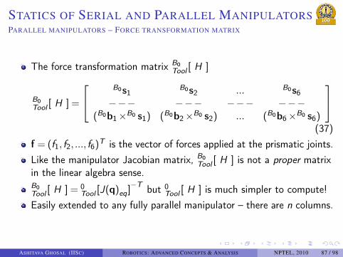

. . . . . .
STATICS OF SERIAL AND PARALLEL MANIPULATORSPARALLEL MANIPULATORS – SINGULARITY IN FORCE DOMAIN
Direct force analysis: Obtain external force/moment given leg forces
B0FTool =B0Tool [ H ]f
Inverse force analysis: Obtain leg forces given external force/moment
f = B0Tool [ H ]
−1B0FTool
If det([ H ]) = 0, then inverse problem cannot be solved → Forcesingularity.As det([ H ])→ 0, f → ∞ – any external force/moment along certaindirection cannot be resisted by the parallel manipulator9.
9In velocity singularity, no joint rates can cause motion along certain (singular)directions.
ASHITAVA GHOSAL (IISC) ROBOTICS: ADVANCED CONCEPTS & ANALYSIS NPTEL, 2010 88 / 98

. . . . . .
STATICS OF SERIAL AND PARALLEL MANIPULATORSPARALLEL MANIPULATORS – SINGULARITY IN FORCE DOMAIN
Force singularity can be visualised using degeneracy of force ellipsoid.In a Stewart-Gough platform, external force F is given by
F = [HF]f =[
s1 s2 s3 s4 s5 s6]f
|F|2 is FTF = fT [gF]f where [gF] = [HF]T [HF].
The maximum, intermediate and minimum values of FTF subject to aconstraint of the form fT f = 1 are the eigenvalues of [gF].Since the rank of [gF] is 3, the tip of the force vector F lies on anellipsoid in ℜ3.
ASHITAVA GHOSAL (IISC) ROBOTICS: ADVANCED CONCEPTS & ANALYSIS NPTEL, 2010 89 / 98

. . . . . .
STATICS OF SERIAL AND PARALLEL MANIPULATORSPARALLEL MANIPULATORS – SINGULARITY IN FORCE DOMAIN
rank([gF]) = 2 → force ellipsoid shrinks to an ellipse and the Stewartplatform manipulator cannot apply a force normal to the plane of theellipse.rank([gF]) = 1,0, the Stewart platform cannot apply any force in aplane or cannot apply any external force, respectively.Example:
Stewart-Gough platform with fixed base and moving platform as regularhexagons of same size.Consider the configuration of all legs parallel to the vertical.[ H ] matrix is given by
[H] =
0 0 0 0 0 00 0 0 0 0 01 1 1 1 1 1
b1y b2y b3y b4y b5y b6y−b1x −b2x −b3x −b4x −b5x −b6x
0 0 0 0 0 0
ASHITAVA GHOSAL (IISC) ROBOTICS: ADVANCED CONCEPTS & ANALYSIS NPTEL, 2010 90 / 98

. . . . . .
STATICS OF SERIAL AND PARALLEL MANIPULATORSPARALLEL MANIPULATORS – SINGULARITY IN FORCE DOMAIN
Three rows of ([ H ]) are zero and the Stewart-Gough platform is in asingular configuration → [gF] has rank 1.Tip of the force vector F can only lie along a line and only the verticalexternal force can be resisted.The Stewart-Gough platform, in this configuration, has singularityalong Fx and Fy .Similar analysis can be done for M → Any Mz cannot be resisted inthis configuration.Above analysis used by Ranganath et al. 2004 to design sensitive 6components force-torque sensors (see Module 10, Lecture 2).
ASHITAVA GHOSAL (IISC) ROBOTICS: ADVANCED CONCEPTS & ANALYSIS NPTEL, 2010 91 / 98

. . . . . .
STATICS OF SERIAL AND PARALLEL MANIPULATORSRELATION BETWEEN GAIN SINGULARITY AND FORCE SINGULARITY
If det([ K ∗ ]) = 0 → parallel manipulator gains one (or more) degreeof freedom instantaneously.If det([ H ]) = 0 parallel manipulator cannot resist forces/moments inone (or more) directions at that configuration.Relationship between two?Illustrated using simple planar 4-bar mechanism!
ASHITAVA GHOSAL (IISC) ROBOTICS: ADVANCED CONCEPTS & ANALYSIS NPTEL, 2010 92 / 98
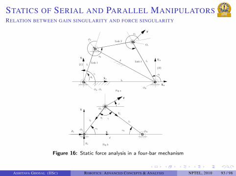
. . . . . .
STATICS OF SERIAL AND PARALLEL MANIPULATORSRELATION BETWEEN GAIN SINGULARITY AND FORCE SINGULARITY
l0
L
φ2
φ1
YL
XL
YR
XR
R
φ3
O2
O3
OL, O1
d
d
l2
O2OR
Fig a
F
α1α2
O3
β
Y
X
Fig b
OR
τ1
R1
R2
T1
T2
l3
F
γ
Link 1l1
l3
Link 2
Link 3
θ1
Figure 16: Static force analysis in a four-bar mechanism
ASHITAVA GHOSAL (IISC) ROBOTICS: ADVANCED CONCEPTS & ANALYSIS NPTEL, 2010 93 / 98

. . . . . .
STATICS OF SERIAL AND PARALLEL MANIPULATORSRELATION BETWEEN GAIN SINGULARITY AND FORCE SINGULARITY
With θ1 locked → point O2 is fixed.For a given θ1, l0 and l1, the length d opposite to θ1 is known.Draw the planar truss structure determined by Link 2, Link 3 and thenow fixed side O2−OR . Angles α1 and α2 can be computed in termsof θ1, ϕ1 and ϕ2.Consider a force F = Fx ,Fy , acting at an angle β at point O3.Denote axial forces along the links O2−O3 and O3−OR of the planartruss by T1 and T2, respectively.
ASHITAVA GHOSAL (IISC) ROBOTICS: ADVANCED CONCEPTS & ANALYSIS NPTEL, 2010 94 / 98

. . . . . .
STATICS OF SERIAL AND PARALLEL MANIPULATORSRELATION BETWEEN GAIN SINGULARITY AND FORCE SINGULARITY
By using a free-body diagram(FxFy
)=
[cosα1 −cosα2sinα1 sinα2
](T1T2
)T1 and T2 are(
T1T2
)=
1sin(α1+α2)
[sinα2 cosα2−sinα1 cosα1
](FxFy
)
ASHITAVA GHOSAL (IISC) ROBOTICS: ADVANCED CONCEPTS & ANALYSIS NPTEL, 2010 95 / 98

. . . . . .
STATICS OF SERIAL AND PARALLEL MANIPULATORSRELATION BETWEEN GAIN SINGULARITY AND FORCE SINGULARITY
From T1 obtain reactions R1 and R2 at the joint O2(R1R2
)=
1sin(α1+α2)
[cosα1 sinα2 cosα1 cosα2sinα1 sinα2 sinα1 cosα2
](FxFy
)Torque required in joint 1, τ1, to keep the four-bar mechanism inequilibrium τ1 = R1l1s1−R2l1c1
det([ H ]) = 0 if sin(α1+α2) = 0 or γ is π radians → ϕ3 2π → Link 2and Link 3 are aligned.Gain singularity condition same as force singularity condition!Gain singularity → Instantaneous velocity perpendicular to line alongLink 2 and Link 3 (singular direction).Force singularity → Any force along singular direction gives rise toinfinite R1 and R2 and infinite τ1 is required to maintain staticequilibrium.
ASHITAVA GHOSAL (IISC) ROBOTICS: ADVANCED CONCEPTS & ANALYSIS NPTEL, 2010 96 / 98

. . . . . .
OUTLINE.. .1 CONTENTS
.. .2 LECTURE 1IntroductionLinear and Angular Velocity of Links
.. .3 LECTURE 2Serial Manipulator Jacobian Matrix
.. .4 LECTURE 3Parallel Manipulator Jacobian Matrix
.. .5 LECTURE 4Singularities in Serial and Parallel Manipulators
.. .6 LECTURE 5Statics of Serial and Parallel Manipulators
.. .7 MODULE 5 – ADDITIONAL MATERIALProblems, References and Suggested Reading
ASHITAVA GHOSAL (IISC) ROBOTICS: ADVANCED CONCEPTS & ANALYSIS NPTEL, 2010 97 / 98

. . . . . .
MODULE 5 – ADDITIONAL MATERIAL
Exercise ProblemsReferences & Suggested Reading
ASHITAVA GHOSAL (IISC) ROBOTICS: ADVANCED CONCEPTS & ANALYSIS NPTEL, 2010 98 / 98