Quiz-5 EE628 Advanced Circuit Design Fall 2014 EED-SEN UMT

Feb 26, 2015

1. (5 points)

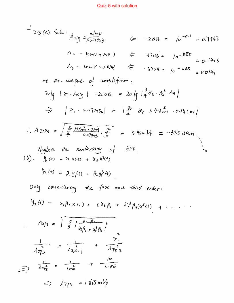
Quiz-5 with solution

2. Explain the difference between cross modulation and intermodulation while studying non-linearity effects in RF systems. Explain what will happen at the output in the following figure? (5 points)

3. What is Gain Compression? (5 points)

Quiz-5 with solution

4. Suppose cos 2 cos 2 . What will be in the following figure? (5 points)

5. Draw the output spectrum for 3rd order intermodulation when2 . ( 5 points)

Quiz-5 with solution

6. Suppose an interferer contains phase modulation but not amplitude modulation. Does cross modulation occur in this case? ( 5 points)

Quiz-5 with solution

7.

Quiz-5 with solution

324 13 RF Receivers

Fig. 13.6 Output signallevel against input signallevel and the 1 dBcompression point

which is solved as

b0 =Ib

2+

Imax

4+

Imin

4= 17.5μA,

b1 =Imax

2− Imin

2= 975μA,

b2 =− Ib

2+

Imax

4+

Imin

4= 7.5μA.

By definition, we write

D2 =b2

b1× 100% = 0.77,

T HD =√

D22 +D2

3 +D24 · · ·=

√D2

2 = D2 = 0.77%

because with only three measurements we can solve for up to the second order term in (13.4). If moredetailed measurement was done, for instance with five measured points that would add amplitudes atVin(±1/2), then we would have ω t = π/3 and ω t = 2π/3 corresponding angles as well, which wouldenable us to calculate b0, b1, b2, b3, and b4 constants.

13.2.1.1 Gain Compression

A common property of most amplifier circuits is that as the input signal power level increases, atfirst the output signal level increases proportionally. That is, for low-power signals, the output–inputrelationship is linear Pout =APin, where A is the gain that is calculated as the A= dPout/dPin derivative.However, eventually, the output signal level is limited by the circuit’s power supply level or thereduced biasing current of its active devices. In other words, the small signal linearity relationshipdoes not hold for large input signal levels.

We define the 1 dB compression point as the input signal power level Sin(−1dB) which correspondsto the gain A(−1dB) for which the output signal level is 1 dB lower relative to the linear model (seeFig. 13.6, noting that the plot is in log–log scale).

The 1 dB compression point is determined both analytically and experimentally. Let us take anonlinear system described by (13.4) and try to find the 1 dB compression point. The first term in(13.4) is the DC term, hence its derivative is zero and it is not part of the gain equation. The secondterm describes the output signal of the input x(t) = Acosω t, hence we write the equations for the

Quiz-5 with solution

13.2 Nonlinear Effects 325

linear gain function (i.e., if all nonlinear terms in (13.3) are ignored) and the nonlinear gain function as

|Vout| ≈ a1B cosω t,

|V ′out| ≈

(a1B+

3a3B3

4

)cosω t,

∴∣∣∣∣V′out

Vout

∣∣∣∣=(

1+3a3 B2

4a1

),

where the ratio V ′out/Vout is the apparent gain between the linear and the nonlinear functions. Clearly,

if a3/a1 < 0 and∣∣∣ 3a3 B2

4a1

∣∣∣< 1 then there is compression in the gain. After conversion into the dB scale,2

we write an expression for the apparent gain as

20 logV ′out− 20logVout = 20log

(1+

3a3 B2

4a1

),

−1dB = 20 log

(1+

3a3 B2

4a1

),

10−1/20 − 1 =3a3 B2

4a1,

∴

B(−1dB) =

√0.145

∣∣∣∣a1

a3

∣∣∣∣, (13.7)

where the input signal level Sin(−1dB) was introduced in dB, therefore

Sin(−1dB) = 20log [B(−1dB)] dB. (13.8)

Interestingly enough, (13.7) shows that the 1 dB compression point of the first harmonic is, througha3, intimately connected to the third harmonic of the input signal. We formalize this connection in thefollowing sections.

13.2.2 Inter-Modulation

As opposed to harmonic distortion, which is caused by self-mixing of one input signal and wherethe higher-order harmonics in (13.4) are relatively easy to suppress by LP filtering, intermodulationinvolves two input tones with close frequencies ωa and ωb. Consequently, in case of any nonlinearitythe output spectrum must contains various harmonics of the fundamental tones, however, it alsocontains tones that are not harmonics of the input frequencies.

2Keep in mind that loga/b = loga− logb.

Quiz-5 with solution

326 13 RF Receivers

Fig. 13.7 Part of theintermodulation frequencyspectrum showing thethird-order terms 2ωa ±ωbclose to the fundamentaltones

Let us assume the input signal is the sum of x(t) = B1 cosωa t +B2 cosωb t; then (13.3) becomes

y(t) = a1 (B1 cosωa t +B2 cosωb t)

+ a2 (B1 cosωa t +B2 cosωb t)2

+ a3 (B1 cosωa t +B2 cosωb t)3 + · · · , (13.9)

which, after expanding and collecting the frequency terms, yields the following terms

y(t) =a2(B2

1 +B22)

2(DC term)

+

(a1B1 +

34

a3B31 +

32

a3B1B22

)cosωa t (fundamental terms)

+

(a1B2 +

34

a3B32 +

32

a3B2B21

)cosωb t

+a2

2

(B2

1 cos2ωa t +B22 cos2ωb t

)(second-order terms)

+ a2B1B2 [cos(ωa +ωb)t + cos |ωa −ωb|t]+

a3

4

(B3

1 cos3ωa t +B32 cos3ωb t

)(third-order terms)

+3a3

4

{B2

1B2 [cos(2ωa +ωb)t + cos(2ωa −ωb)t]

+B1B22 [cos(2ωb +ωa)t + cos(2ωb −ωa)t]

}, (13.10)

which shows that the output spectrum contains the two fundamental tones, ωa, ωb, the second-orderterms, 2ωa, 2ωb, |ωa±ωb|, and the third-order terms 3ωa, 3ωb, 2ωa±ωb, 2ωb±ωa. It is of particularinterest that we found third-order tones such as 2ωa ±ωb that are not harmonics of the fundamentaltones. The problem is that if the two input tones are close to each other, i.e., ωa ≈ωb, then 2ωa−ωb ≈2ωa −ωa ≈ ωa! That is, there are cases in the frequency spectrum when the third-order terms are tooclose to the fundamental tones, Fig. 13.7 and cannot easily be filtered out.

Frequency spectrum analysis (13.10) comes in handy for the “two-tone test” that uses two slightlydifferent tones with the same small amplitude B1 = B2 = B, which means that the higher harmonicsare negligible and (13.10) simplifies to

Quiz-5 with solution

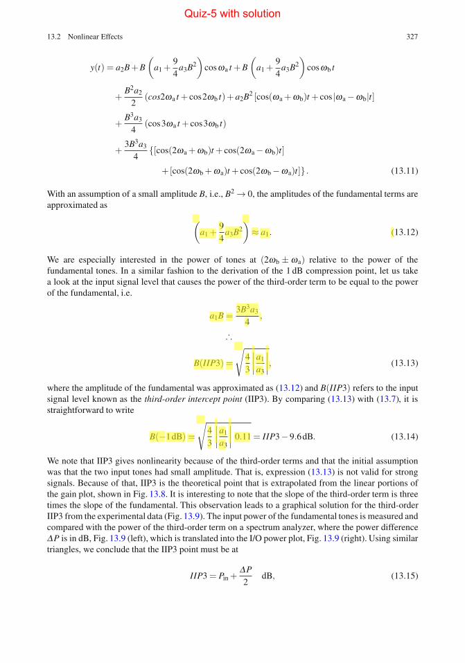
13.2 Nonlinear Effects 327

y(t) = a2B+B

(a1 +

94

a3B2)

cosωa t +B

(a1 +

94

a3B2)

cosωb t

+B2a2

2(cos2ωa t + cos2ωb t)+ a2B2 [cos(ωa +ωb)t + cos|ωa −ωb|t]

+B3a3

4(cos3ωa t + cos3ωb t)

+3B3a3

4{[cos(2ωa +ωb)t + cos(2ωa −ωb)t]

+[cos(2ωb +ωa)t + cos(2ωb −ωa)t]} . (13.11)

With an assumption of a small amplitude B, i.e., B2 → 0, the amplitudes of the fundamental terms areapproximated as

(a1 +

94

a3B2)≈ a1. (13.12)

We are especially interested in the power of tones at (2ωb ± ωa) relative to the power of thefundamental tones. In a similar fashion to the derivation of the 1 dB compression point, let us takea look at the input signal level that causes the power of the third-order term to be equal to the powerof the fundamental, i.e.

a1B =3B3a3

4,

∴

B(IIP3) =

√43

∣∣∣∣a1

a3

∣∣∣∣, (13.13)

where the amplitude of the fundamental was approximated as (13.12) and B(IIP3) refers to the inputsignal level known as the third-order intercept point (IIP3). By comparing (13.13) with (13.7), it isstraightforward to write

B(−1dB) =

√43

∣∣∣∣a1

a3

∣∣∣∣ 0.11 = IIP3−9.6dB. (13.14)

We note that IIP3 gives nonlinearity because of the third-order terms and that the initial assumptionwas that the two input tones had small amplitude. That is, expression (13.13) is not valid for strongsignals. Because of that, IIP3 is the theoretical point that is extrapolated from the linear portions ofthe gain plot, shown in Fig. 13.8. It is interesting to note that the slope of the third-order term is threetimes the slope of the fundamental. This observation leads to a graphical solution for the third-orderIIP3 from the experimental data (Fig. 13.9). The input power of the fundamental tones is measured andcompared with the power of the third-order term on a spectrum analyzer, where the power differenceΔP is in dB, Fig. 13.9 (left), which is translated into the I/O power plot, Fig. 13.9 (right). Using similartriangles, we conclude that the IIP3 point must be at

IIP3 = Pin +ΔP2

dB, (13.15)

Quiz-5 with solution

328 13 RF Receivers

Fig. 13.8 Third-orderintercept pointextrapolation

Fig. 13.9 Graphicalsolution for third-orderintercept point

which is a practical way of estimating the IIP3 by measurement. In this analysis, we have ignoredany effects of the second-order terms. They have less influence in narrowband systems relative to thethird-order terms, however in the case of low IF or direct conversion systems, the second-order termscome very close to the baseband signal. If not taken care of, they may even “overwrite” the desiredtone. More detailed study of intermodulation terms is beyond the scope of this book.

13.2.3 Cross-Modulation

There are two important cases of cross-modulation that we need to become familiar with. In the firstscenario, two signals arrive at the antenna, one much stronger than the other. The problem is that thedesired signal is the “weak” one. As an illustration, imagine using a cell phone in a crowded bus withanother cell phone user very close by. The signal leaving the neighbouring cell phone is very strong,but unfortunately it is not for you. The one that you are trying to hear is already at the end of itsjourney and is very weak, barely dumping its leftover energy into the antenna. Unfortunately for you,the other user is doing the same and your signal may be “blocked” or “jammed”.

Let us take a closer look at the case from the mathematical perspective. The incoming signal

x(t) = B1 cosωa t +B2 cosωb t; B2 � B1 (13.16)

is processed by a nonlinear circuit whose gain equation is given by (13.2), which, after substitution of(13.16), becomes

y(t) ≈(

a1B1 +34

a3B31 +

32

a3B1B22

)cosωa t + · · · ,

(B2 � B1)

≈(

1+32

a3

a1B2

2

)a1B1 cosωa t + · · · , (13.17)

Quiz-5 with solution

13.2 Nonlinear Effects 329

Fig. 13.10 Stronginterference and weaksignal in the same band

where, we focus only on the first fundamental term of the desired tone at ωa. Most circuits arecompressive, therefore a3/a1 < 0, which leads to the conclusion that, under the right circumstancesand large amplitude B2 of the blocking signal, the amplitude of the desired signal ωa may be reducedto zero, i.e.

0 =

(1− 3

2

∣∣∣∣a3

a1

∣∣∣∣B22

)∴ B2 =

√23

∣∣∣∣a1

a3

∣∣∣∣. (13.18)

Modern RF equipment is expected to correctly decode the desired signal in presence of an interferingsignal that may be 60–70 dB stronger.

In the second scenario (see Fig. 13.10), the receiving antenna is exposed to two signals, the desiredone at frequency ωa and a strong AM signal, i.e.

x(t) = B1 cosωa t +B2(1+mcosωb t)cosωc t. (13.19)

Using the same approach again, we focus only on the main harmonic of the desired signal, i.e.

y(t)≈[

a1B1 +32

a3B1B22

(1+

m2

2+

m2

2cos2ωb t +2mcosωb t

)]cosωa t + · · ·

= f (ωb,2ωb)cosωa t (13.20)

in other words, the receiving signal is modulated by the AM signal, which is superimposed onthe original message. Depending on the exact circumstances, the desired signal may be completelyblocked by the strong AM signal.

13.2.4 Image Frequency

The main limitation of a TRF receiver, its limited selectivity over a wide range of receivingfrequencies, was a strong motivation for development of heterodyne receiver topology. Even though itis much more complicated than the simple TRF receiver structure, advances in IC technology enablevery sophisticated heterodyne and super-heterodyne receivers to be manufactured as a sub-circuitof even more complex communication integrated systems. Indeed, it is a standard expectation formodern equipment to have one or more integrated RF transceivers included for a fractional increasein the overall cost.

Quiz-5 with solution

Sec. 2.2. Effects of Nonlinearity 21

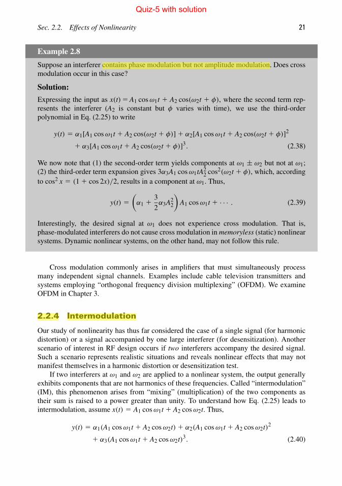
Example 2.8

Suppose an interferer contains phase modulation but not amplitude modulation. Does cross

modulation occur in this case?

Solution:

Expressing the input as x(t) 5 A1 cos ω1t 1 A2 cos(ω2t 1 φ), where the second term rep-

resents the interferer (A2 is constant but φ varies with time), we use the third-order

polynomial in Eq. (2.25) to write

y(t) 5 α1[A1 cos ω1t 1 A2 cos(ω2t 1 φ)] 1 α2[A1 cos ω1t 1 A2 cos(ω2t 1 φ)]2

1 α3[A1 cos ω1t 1 A2 cos(ω2t 1 φ)]3. (2.38)

We now note that (1) the second-order term yields components at ω1 ± ω2 but not at ω1;

(2) the third-order term expansion gives 3α3A1 cos ω1tA22 cos2(ω2t 1 φ), which, according

to cos2 x 5 (1 1 cos 2x)/2, results in a component at ω1. Thus,

y(t) 5

(

α1 13

2α3A2

2

)

A1 cos ω1t 1 · · · . (2.39)

Interestingly, the desired signal at ω1 does not experience cross modulation. That is,

phase-modulated interferers do not cause cross modulation in memoryless (static) nonlinear

systems. Dynamic nonlinear systems, on the other hand, may not follow this rule.

Cross modulation commonly arises in amplifiers that must simultaneously process

many independent signal channels. Examples include cable television transmitters and

systems employing “orthogonal frequency division multiplexing” (OFDM). We examine

OFDM in Chapter 3.

2.2.4 Intermodulation

Our study of nonlinearity has thus far considered the case of a single signal (for harmonic

distortion) or a signal accompanied by one large interferer (for desensitization). Another

scenario of interest in RF design occurs if two interferers accompany the desired signal.

Such a scenario represents realistic situations and reveals nonlinear effects that may not

manifest themselves in a harmonic distortion or desensitization test.

If two interferers at ω1 and ω2 are applied to a nonlinear system, the output generally

exhibits components that are not harmonics of these frequencies. Called “intermodulation”

(IM), this phenomenon arises from “mixing” (multiplication) of the two components as

their sum is raised to a power greater than unity. To understand how Eq. (2.25) leads to

intermodulation, assume x(t) 5 A1 cos ω1t 1 A2 cos ω2t. Thus,

y(t) 5 α1(A1 cos ω1t 1 A2 cos ω2t) 1 α2(A1 cos ω1t 1 A2 cos ω2t)2

1 α3(A1 cos ω1t 1 A2 cos ω2t)3. (2.40)

Quiz-5 with solution

22 Chap. 2. Basic Concepts in RF Design

Expanding the right-hand side and discarding the dc terms, harmonics, and components at

ω1 ± ω2, we obtain the following “intermodulation products”:

ω 5 2ω1 ± ω2 :3α3A2

1A2

4cos(2ω1 1 ω2)t 1

3α3A21A2

4cos(2ω1 2 ω2)t (2.41)

ω 5 2ω2 ± ω1 :3α3A1A2

2

4cos(2ω2 1 ω1)t 1

3α3A1A22

4cos(2ω2 2 ω1)t (2.42)

and these fundamental components:

ω 5 ω1, ω2 :

(

α1A1 13

4α3A3

1 13

2α3A1A2

2

)

cos ω1t

1

(

α1A2 13

4α3A3

2 13

2α3A2A2

1

)

cos ω2t (2.43)

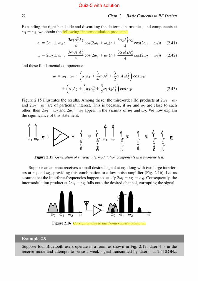
Figure 2.15 illustrates the results. Among these, the third-order IM products at 2ω1 2 ω2

and 2ω2 2 ω1 are of particular interest. This is because, if ω1 and ω2 are close to each

other, then 2ω1 2 ω2 and 2ω2 2 ω1 appear in the vicinity of ω1 and ω2. We now explain

the significance of this statement.

ω21ω ω

1ω

−ω

2

1ω

−ω

22

1ω ω

2

−ω

2ω

21 2

ωω

1+ 1

ωω

22

+

ωω

2+

21 ω

Figure 2.15 Generation of various intermodulation components in a two-tone test.

Suppose an antenna receives a small desired signal at ω0 along with two large interfer-

ers at ω1 and ω2, providing this combination to a low-noise amplifier (Fig. 2.16). Let us

assume that the interferer frequencies happen to satisfy 2ω1 2 ω2 5 ω0. Consequently, the

intermodulation product at 2ω1 2 ω2 falls onto the desired channel, corrupting the signal.

1ω ω

2 ω ω0

LNA

1ω ω

2 ω ω0

Figure 2.16 Corruption due to third-order intermodulation.

Example 2.9

Suppose four Bluetooth users operate in a room as shown in Fig. 2.17. User 4 is in the

receive mode and attempts to sense a weak signal transmitted by User 1 at 2.410 GHz.

Quiz-5 with solution

Quiz-5 with solution

Quiz-5 with solution

18 Chap. 2. Basic Concepts in RF Design

To calculate the input 1-dB compression point, we equate the compressed gain, α1 1

(3α3/4)A2in,1dB, to 1 dB less than the ideal gain, α1:

20 log

∣

∣

∣

∣

α1 13

4α3A2

in,1dB

∣

∣

∣

∣

5 20 log |α1| 2 1 dB. (2.33)

It follows that

Ain,1dB 5

√

0.145

∣

∣

∣

∣

α1

α3

∣

∣

∣

∣

. (2.34)

Note that Eq. (2.34) gives the peak value (rather than the peak-to-peak value) of the input.

Also denoted by P1dB, the 1-dB compression point is typically in the range of 220 to

225 dBm (63.2 to 35.6 mVpp in 50-� system) at the input of RF receivers. We use the

notations A1dB and P1dB interchangeably in this book. Whether they refer to the input or

the output will be clear from the context or specified explicitly. While gain compression by

1 dB seems arbitrary, the 1-dB compression point represents a 10% reduction in the gain

and is widely used to characterize RF circuits and systems.

Why does compression matter? After all, it appears that if a signal is so large as to

reduce the gain of a receiver, then it must lie well above the receiver noise and be easily

detectable. In fact, for some modulation schemes, this statement holds and compression of

the receiver would seem benign. For example, as illustrated in Fig. 2.11(a), a frequency-

modulated signal carries no information in its amplitude and hence tolerates compression

(i.e., amplitude limiting). On the other hand, modulation schemes that contain information

in the amplitude are distorted by compression [Fig. 2.11(b)]. This issue manifests itself in

both receivers and transmitters.

Another adverse effect arising from compression occurs if a large interferer accom-

panies the received signal [Fig. 2.12(a)]. In the time domain, the small desired signal is

superimposed on the large interferer. Consequently, the receiver gain is reduced by the

large excursions produced by the interferer even though the desired signal itself is small

(a)

(b)

Frequency Modulation

Amplitude Modulation

Figure 2.11 Effect of compressive nonlinearity on (a) FM and (b) AM waveforms.