Queuing modelsBasic definitions, assumptions, and identitiesOperational laws Little’s law

Queuing networks and Jackson’s theoremThe importance of think timeNon-linear results as saturation approachesWarningsReferences

What problem are we solving?Describe a system’s mean

ThroughputResponse timeCapacity

PredictChanges in these quantities when system characteristics change

See Stallings, Figure 1

Stallings, Figure 1

One queue

arrivals departures

waiting serving

= a job

Server

See Stallings, Figure 2

Stallings, Figure 2, Table 2

Basic assumptionsOne kind of jobInter-arrival times are independent of system stateService times are independent of system stateNo jobs lost because of buffer overflowStability: λ < 1 / TsIn a network, no parallel processing of a given job visit ratios are independent of system state

Queuing definitionsA / S / m / B / K / SDA = Inter-arrival time distributionS = Service time distributionm = Number of serversB = Number of buffers (system capacity)K = Population sizeSD = service disciplineUsually specify just the first three: M/M/1

Usual assumptionsA is often the Exponential distributionS is often Exponential or constantB is often infinite (all the buffer space you need)K is often infiniteSD is often FCFS (first come, first served)

Exponential distributionAlso known as “memoryless”Expected time to the next arrival is always the same, regardless of previous arrivalsWhen the interarrival times are independent, identically-distributed, and the distribution is exponential, the arrival process is called a “Poisson” process

Poisson processesPopular because they are tractable to analyzeYou can merge several Poisson streams and get a Poisson streamYou can split a Poisson stream and get Poisson streamsPoisson arrivals to a single queue with exponential service times => departures are Poisson with same rateSame is true of departures from a M/M/m queue

Basic formulas: Stallings, Table 3b

AssumptionsPoisson arrivalsNo dispatching preference based on service timesFIFO dispatchingNo items discarded from queue

Basic multi-server formulas

Expected response timeFor a single M/M/1 queue, expected residence (response) time is 1/(μ-λ), where μ is the server’s maximum output rate

(1/Ts) λ is the mean arrival rate

Example: Disk can process 100 accesses/sec Access requests arrive at 20/sec Expected response time is 1/(100-20) =

0.0125 sec/access

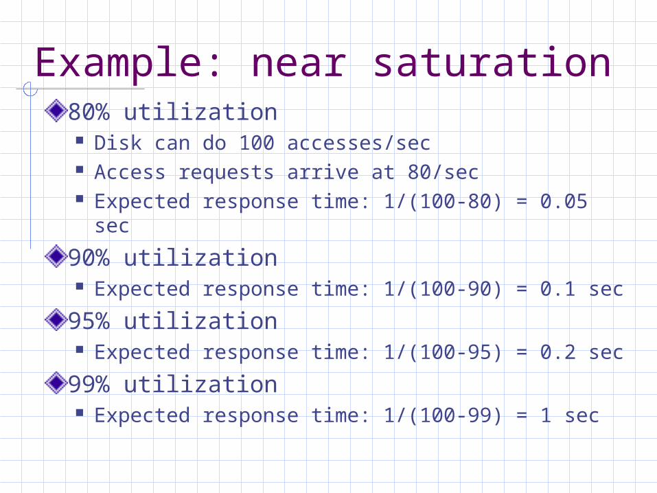
Example: near saturation80% utilization Disk can do 100 accesses/sec Access requests arrive at 80/sec Expected response time: 1/(100-80) = 0.05 sec

90% utilization Expected response time: 1/(100-90) = 0.1 sec

95% utilization Expected response time: 1/(100-95) = 0.2 sec

99% utilization Expected response time: 1/(100-99) = 1 sec

Nearing saturation (M/M/1)

0

0.2

0.4

0.6

0.8

1

1.2

utilization (%)

exp

ecte

d r

esp

onse

tim

e (s

ec)

response

Operational law

Little’s Lawr = λ Tr

Example: Tr = 0.3 sec average residence in the system λ = 10 transactions / sec r = 3 average transactions in the system

Queuing network

Queue 1 Queue 2

Queue 3

Jackson’s theoremAssuming

Each node in the network provides an independent servicePoisson arrivalsOnce served at a node, an item goes immediately to another node, or out of the system

ThenEach node is an independent queuing systemEach node’s input is PoissonMean delays at each node may be added to compute system delays

Queuing network example

ServletHistory

data

Orderdata

Tr = 50 msec Tr = 60 msec

Tr = 80 msec

λ = 12 jobs/sec

P = 0.4

P = 0.6

Average system residence time = 0.4 * (50+60) + 0.6 * (50+80)(Jackson’s theorem) = 122 msec

Average jobs in system = 12 * 0.122 = 1.464(Little’s Law)

An example in a spreadsheet

Think time

“think time” between

transactions

request a transaction

Think time can have a huge effect onthe arrival rate for a system.

Main ReferenceQueuing Analysis, William Stallings

Cached copy on the resource page:http://cs.franklin.edu/~swartoud/650/QueuingAnalysis.pdf