Embed Size (px)
Citation preview

Overview
Description of Queueing Processes
The Single Server Markovian Queue
Multi Server Markovian Queues
2 / 63

Description of Queueing Processes
3 / 63

Queueing Theory
A queueing system consists of:
arrivals
wait service
departure
• Arrival process
• Waiting regime
• Service process
• Departure process
4 / 63

Examples
• Customers waiting to pay at the supermarket
• Patients at a medical clinic waiting to see a doctor
• Passengers waiting at the bus stop
• Aeroplanes circling an airport waiting to land
• Parts on a production line waiting for further processing
5 / 63

Arrival Process
The arrival process can be:
• Deterministic:
time0 1 2 3
• Random:
timeT1 T2 T3 T4
Here T1,T2,T3, . . . are random interarrival times.
6 / 63

Arrival Process
• Batched:
timeT1 T2 T3 T4
N1
N2N3
N4
The batch sizes Ni and interarrival times Ti can bedeterministic or random.
• Typed arrivals: arrivals can be of different types, requiringdifferent types of service.
We consider random arrivals on this course.
7 / 63

Waiting Regime
The waiting regime typically consists of a buffer size. This is justthe maximum number of people/units that can wait in the queueto be served. People/units that arrive when the buffer is full areeither lost to the system, or come back later.
8 / 63

Service Process
The service process typically consists of:
• Service times: can be deterministic, random, batched and/ordepend on the type of customer. They can also depend on thequeue size.
• Number of servers
• The service discipline:▶ FIFO: First In First Oout▶ LIFO: Last In First Oout▶ SIRO: Service In Random Order
9 / 63

Departure Process
This is the outcome of the arrival, waiting and service processes.
10 / 63

Examples
• Customer waiting to pay at the supermarket. Randomarrivals. Multiple servers with random service times, numbermay depend on queue size. May have typed customers suchas “8 items of less” or “pay by cash”,
• Patients at a medical clinic waiting to see a doctor.Deterministic arrivals (appointment times). Random servicetimes.
• Passengers waiting at the bus stop. Random arrivals. Randomservice times with batched service.
• Aeroplanes circling an airport waiting to land. Randomarrivals. Deterministic service times (approximately every 2minutes at Heathrow).
11 / 63

Aims of queueing analysis
12 / 63

Aims of queueing analysis
In general we want to know things like:
• Average time a customer is in the system
• Average queue length
• Utilisation of servers (proportion of time busy)
These are examples of performance measures for the system. Wemay be designing or trying to improve a queueing system. Wewould like to be able to gauge the effect of:
• A change in arrival rate
• A change in service time
• A change in the number of servers
• A change in the service regime
13 / 63

Approaches to queueing analysis
There are a variety of approaches to the study of queueingsystems:
• Real World: real-world systems provide the best information,but are expensive to experiment with.
• Simulation: simulation allows cheap analysis of the effects ofchange to a system and is the only practical way to deal withvery complex queueing systems.
• Theory: theoretical analysis is only possible for relativelysimple systems, but provides unrivalled insight into whyqueues behave as they do,
This course takes the theoretical approach to queueing.
14 / 63

Example
Suppose 3 customers arrive one just after the other with servicerequirements (in units of time):
10, 20, 30
In a FIFO regime the average time in the system will be:
10 + 30 + 60
3=
100
3
In a LIFO regime the average time in the system will be:
30 + 50 + 60
3=
140
3
15 / 63
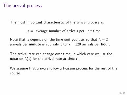
The arrival process
The most important characteristic of the arrival process is:
λ = average number of arrivals per unit time
Note that λ depends on the time unit you use, so that λ = 2arrivals per minute is equivalent to λ = 120 arrivals per hour.
The arrival rate can change over time, in which case we use thenotation λ(t) for the arrival rate at time t.
We assume that arrivals follow a Poisson process for the rest of thecourse.
16 / 63

The arrival process
If an arrival process is a Poisson process, the number of arrivalsoccurring within any interval of time of length t, follows a Poissondistribution with parameter λt.
The probability that there are n arrivals in a time interval of lengtht is equal to:
p(n) =(λt)ne−λt
n!for n = 0, 1, 2, . . .
and is independent of the number of units currently in the systemor the history of arrivals prior to the start of the interval.
The average number of arrivals in an interval of length t is λt andthe variance is also equal to λt (properties of the Poissondistribution).
17 / 63

Infinitesimal Arrival Rate
Consider a short interval of length γt and let N(t, t + γt) be thenumber of arrivals between t and t + γt. From the expression forthe Poisson distribution:
P(N(t, t+γt) = 1) = (λγt)e−λγt = (λγt)
(1− λγt +
(λγt)2
2− . . .
)where we have expanded e−λγt in a Taylor series. As γt → 0,(γt)2 and higher order terms become negligible and:
P(N(t, t + γt) = 1) ≈ λγt
P(N(t, t + γt) = 0) ≈ 1− λγt
P(N(t, t + γt) > 1) ≈ 0
18 / 63

Inter-Arrival Times
For a poisson process, the time between events (arrivals) mustfollow a negative exponential distribution.
To show this, assume we start observing a Poisson processimmediately after an event (arrival) and say this occurred at time0. The probability that we have no events at time t is:
P(N(0, t) = 0) = e−λt
but this is equal to the probability that the time between twosuccessive events (arrivals) is greater than t. Writing X as thetime between two successive event (arrivals), this means that:
P(X > t) = e−λt
P(X ≤ t) = 1− e−λt
19 / 63

Inter-Arrival Times
We know that P(X ≤ t) = F (t), where F (t) is the cumulativedensity function (cdf) of the distribution of time between events.The probability density function (pdf) is given by
f (t) = dF (t)dt
f (t) = λe−λt
but this is the pdf of a negative exponential distribution. Thus,inter arrival times ∼ NegExp(λ).
20 / 63

The memoryless property
The most important property of the negative exponentialdistribution is the memoryless property. This says that if you havea NegExp(λ) inter arrival time, and have already waited time t forthe next arrival, then the time remaining until the next arrival stillhave NegExp(λ) distribution.
i.e. the amount of time you have waited tells you nothing abouthow long you still have to wait.
The exponential distribution is the only continuous distributionwith this property. It can be used to describe e.g. the arrival oftelephone calls at an exchange, the arrival of customer at a store. . .
21 / 63

The memoryless property
The memoryless property is equivalent to the conditionalprobability statement:
P(Ti > s + t | Ti > s) = P(Ti > t)
The proof is a straight forward application of the definition ofconditional probability, and the fact that P(Ti > t) = e−λt :
P(Ti > s + t | Ti > s) = P( Ti>s |Ti>s+t )P( Ti<s+t )P(Ti>s)
= P(Ti>s+t)P(Ti>s)
= e−λ(s+t)
e−λs = e−λt = P(Ti > t)
22 / 63

Memoryless property paradox
Consider the following argument. Suppose we have a Poissonprocess of rate λ, and we turn up at some random time t toobserve it. On average, we will arrive half way between twoarrivals. Thus the expected time until the next arrival will be halfthe expected time between any two arrivals, that is 1
2λ .
But the memoryless property tells us that the time from ourappearance to the next arrival should still be NegExp(λ), withmean 1
λ : a contradiction!
23 / 63

Memoryless property paradox
Of course there is a flaw in the previous argument.
If we turn up at a random time, then we are more likely to turn upbetween two widely spaced arrivals than between two closelyspaced arrival. Thus, the inter arrival period we turn up in will onaverage be larger than the norm, and so its expected length will belarger than the norm (in fact, exactly twice the norm)
24 / 63

Merging and thinning
The poisson process has many useful properties. Two of theseconcern merging and thinning.
time0 1 2 3
+
time0 1 2 3
=
time0 3 5 71 2 4 6
25 / 63
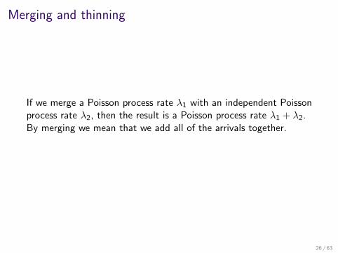
Merging and thinning
If we merge a Poisson process rate λ1 with an independent Poissonprocess rate λ2, then the result is a Poisson process rate λ1 + λ2.By merging we mean that we add all of the arrivals together.
26 / 63

Merging and thinning
We thin a process by selecting arrivals at random. For example wecould toss a coin for each arrival: heads we keep it, tails it isdiscarded.
time0 1 2 3
H T H H
time0 1 2
27 / 63

Merging and thinning
We thin a process by selecting arrivals at random. For example wecould toss a coin for each arrival: heads we keep it, tails it isdiscarded.
time0 1 2 3
H T H H
time0 1 2
27 / 63

Merging and thinning
If we start with a Poisson process rate λ, and the probability ofkeeping an arrival is p, then the results is a Poisson process ratepλ.
(A proof of these results is not part of the course)
28 / 63

The service process
Most simple queueing models assume that that service times havea negative exponential distribution with parameter µ, so that thepdf is written as:
f (t) = µe−µt
where 1µ is the average length of a service.
If this is true, the service process is also a Poisson process andservice times will also obey the memoryless property. For example,if you arrive at a cash desk and find the server busy and the serviceprocess is a Poisson process, the expected time until the servicefinishes serving will be independent of how long the current servicehas been in progress.
29 / 63

The service process
What is the expected waiting time of a unit that joins the queueand finds n unites ahead of it(n − 1 in the queue and 1 beingserved)?
Total expected time = n × 1µ = n
µ
Variance = n × 1µ2 = n
µ2
Standard deviation =√nµ
The distribution of the waiting times is the convolution of nnegative exponential distributions. I.e. a gamma distribution withparameters (n, µ):
f (t) =µtn−1e−µt
(n − 1)!, t ≥ 0
30 / 63

Classification of queues
There is a classification scheme for commonly encountered queues(originally devised by David Kendall). A general queue is denoted:
A/B/m/n
where we make the following assumptions:
1. Inter-arrival times are independent and give by somedistribution A.
2. Service times are independent and given by some distributionB.
3. There are m servers.
4. There is a buffer of size n.
31 / 63

Standard notation for distributions
There is also some standard notation for the possible types ofdistribution A and B:
• M the exponential distribution (Markovian)
• D deterministic
• Ek the Erlang distribution with k stages
• Hk the hyper-exponential with k channels
• G a general distribution
32 / 63

The M/M/1 queue
33 / 63

The M/M/1 queue
The M/M/1 queue has Markov arrival and service processes, oneserver and infinite waiting spaces. We can describe how a queueingsystem works using a transition diagram. The transition diagramfor the M/M/1 queue is given below:
λ
µ
0 1 2 3
λ λ
µ µ
...
We study queues as continuous Markov chains.
34 / 63

Stability of queues
Recall:
λ
µ
0 1 2 3
λ λ
µ µ
...
This has rate matrix:−λ λ 0 0 0 . . .µ −(λ+ µ) λ 0 0 . . .0 µ −(λ+ µ) λ 0 . . ....
......
......
. . .
35 / 63

Steady state of a single server queue
Consider a single server queue with infinite buffer, arrival rate λand service rate µ, as shown on the previous slide.
Using the transition diagram on the previous slide, and balancingthe probability flows into and out of states, the steady-stateequations for this model are:
π0λ = π1µ
π1(λ+ µ) = π0λ+ π2µ
π2(λ+ µ) = π1λ+ π3µ
...
πi (λ+ µ) = πi−1λ+ πi+1µ
We solve these iteratively.
36 / 63

Steady state of a single server queue
The first equation gives:
π1 =λ
µπ0
Substituting this into the second equation gives:
π2 =λ+ µ
µ
λ
µπ0 −
λ
µπ0 =
(λ
µ
)2
π0
Similarly, the third equation gives: π3 =(λµ
)3π0. We postulate:
πi =
(λ
µ
)i
π0
this will be proved using an inductive process.
37 / 63

Proof by induction
We assume that πi =(λµ
)iπ0 is true for all i ≤ n and show that
this implies that it must also hold for the (n+1)th term. We know:
πi (λ+ µ) = πi−1λ+ πi+1µ
but πi =(λµ
)iπ0 and πi−1 =
(λµ
)i−1π0, thus:
πi+1 =λ
µπi =
(λ
µ
)i+1
π0
as required. We have shown that if the result is true for πi andπi−1, it is true for πi+1. We have also shown that it is true for π0and π1, therefore it must be true for all πi .
38 / 63

Steady state of a single server queue
To find π0, we use the additional equation∑∞
i=0 πi = 1:
∞∑i=0
πi =∞∑i=0
(λ
µ
)i
π0 =π0
1− λµ
= 1
thus, π0 = 1− λµ and so πi =
(1− λ
µ
)(λµ
)i.
Note: this proof only holds for λµ < 1 as otherwise
∑∞i=0
(λµ
)idoes not converge. If λ ≥ µ then the sum is infinite and there isno solution to the steady state equations. In this case the queue isunstable: its length grows indefinitely. (If λ ≥ µ then customersare arriving faster than the server can deal with them.)
39 / 63

Steady state of a single server queue
The traffic intensity is given by ρ = λµ . The M/M/1 queue is
stable if and only if ρ < 1.
For a stable queue, we can use the steady state distribution todescribe the behaviour of the queue:
• The proportion of time the server is busy is 1− π0 = ρ. Theproportion of time the system is idle is π0.
• The average number of units in the system is:
Lc =∑∞
i=1 iπi = (1− ρ)ρ∑∞
i=1 iρi−1
= (1− ρ)ρ 1(1−ρ)2
= ρ(1−ρ)
40 / 63

Steady state of a single server queue
• The average number of units in the queue is:
Lq =∑∞
i=1(i − 1)πi =∑∞
i=1 iπi −∑∞
i=1 πi
= Lc − (1− π0)
= ρ2
(1−ρ)
41 / 63

Steady state of a single server queue
• The average time in the queue Wq (assuming FIFO) is theaverage number of units in the system when the new unitarrives (Lc), multipled by the average time for one unit to be
served(
1µ
). Therefore:
Wq =ρ
µ(1− ρ)
42 / 63

Steady state of a single server queue
• The average time spent in the system Wc (assuming FIFO) isthe average spent in the queue (Wq) plus the average time ittakes to service one unit. Therefore:
Wc = Wq +1µ
= 1µ(1−ρ)
(note that we have used the memoryless property to tell us thatwhen you arrive, the service time remaining for the personcurrently being served is still NegExp(λ))
43 / 63

Little’s queueing formulae
For any G/G/m/n queue take:
λ = arrivals per unit time
Lc = mean number in system Wc = mean time in system
Lq = mean number in queue Wq = mean time in queue
Ls = mean number in service Ws = mean time in service
then provided the queue has a long-term steady state:
Lc = λWc
Lq = λWq
Ls = λWs
Note that the units match: λ is measured in customer/time, L ismeasured in customers and W is measured in time.
44 / 63

Little’s queueing formulae
For any M/M/1 queue:
Lc = ρ1−ρ Wc = 1
µ(1−ρ)
Lq = ρ2
1−ρ Wq = ρµ(1−ρ)
Ls = ρ Ws =1µ
45 / 63

Multi-server queues
46 / 63

Multi-server queues
The M/M/2 queue.Suppose we have arrivals at rate λ, and two servers who each serveat rate µ. The operational difference between two servers rate µeach, and a single server rate 2µ, is that if there is only one personin the system then only one server is active at rate µ.
λ
µ
0 1 2 3
λ λ
2µ 2µ
...
47 / 63

Multi-server queues
The steady state equations are
π0λ = π1µ
π1(λ+ µ) = π0λ+ π22µ
π2(λ+ 2µ) = π1λ+ π32µ
...
πi (λ+ 2µ) = πi−1λ+ πi+12µ
Solving these iteratively we obtain:
πi =λi
2i−1µiπ0 for all i ≥ 1
48 / 63
Multi-server queues
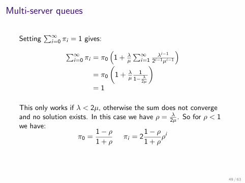
Setting∑∞
i=0 πi = 1 gives:∑∞i=0 πi = π0
(1 + λ
µ
∑∞i=1
λi−1
2i−1µi−1
)= π0
(1 + λ
µ1
1− λ2µ
)= 1
This only works if λ < 2µ, otherwise the sum does not convergeand no solution exists. In this case we have ρ = λ
2µ . So for ρ < 1we have:
π0 =1− ρ
1 + ρπi = 2
1− ρ
1 + ρρi
49 / 63

Multi-server queues
We have arrivals at a rate λ and k servers who each serve at a rateµ.
λ
µ
0 1 2 3
λ λ
2µ 3µ
...
λ
kµ
k-1 k k+1
λ
kµ
...
50 / 63

Multi-server queues
The steady state equations are
π0λ = π1µ
π1(λ+ µ) = π0λ+ π22µ
π2(λ+ 2µ) = π1λ+ π33µ
...
πk(λ+ kµ) = πk−1λ+ πk+1kµ
...
πi (λ+ kµ) = πi−1λ+ πi+1kµ for i > k
51 / 63

Multi-server queues
Solving these iteratively we obtain:
πi =
(
λµ
)i
i! π0 for i < k(λµ
)i
k!k i−k π0 for i ≥ k
We now set∑∞
i=0 πi = 1 to give:
1 =
k−1∑i=0
(λµ
)ii !
+∞∑i=k
(λµ
)ik!k i−k
π0
52 / 63

Multi-server queues
Consider the second term in the sum:
∞∑i=k
(λµ
)ik!k i−k
=1
k!
∞∑i=k
(λµ
)ik i−k
Let j = i − k , then:
1k!
∑∞i=k
(λµ
)i
k i−k = 1k!
∑∞j=0
(λµ
)j+k
k j
=
(λµ
)k
k!
∑∞j=0
(λµ
)j
k j
=
(λµ
)k
k!
∑∞j=0
(λkµ
)j=
(λµ
)k
k!(1− λ
kµ
)
53 / 63

Multi-server queues
Thus:
π0 =1(∑k−1
i=0
(λµ
)i
i! +
(λµ
)k
k!(1−
(λkµ
)))
54 / 63

Multi-server queuesThe probability an arrival will have to wait for service is theprobability that all servers are busy:
P(wait for service) =∞∑i=k
πi =
(λµ
)kk!(1−
(λkµ
))π0The expected number of servers busy is:
E (channels busy) =k−1∑i=1
iπi + k∞∑i=k
πi =λ
µ
The expected number in the queue is:
Lq =∞∑
i=k+1
(i − k)πi =
(λµ
)k+1π0
kk!(1− λ
kµ
)255 / 63

Multi-server queues
The expected number in the system is the expected number in thequeue plus the expected number in service:
Lc = Lq +λ
µ
We can use Little’s formula to find the expected time in thesystem Wc and the queue Wq:
Wc = Lcλ
Wq =Lqλ
56 / 63
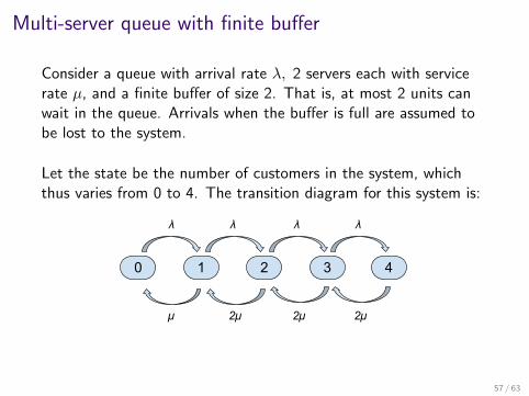
Multi-server queue with finite buffer
Consider a queue with arrival rate λ, 2 servers each with servicerate µ, and a finite buffer of size 2. That is, at most 2 units canwait in the queue. Arrivals when the buffer is full are assumed tobe lost to the system.
Let the state be the number of customers in the system, whichthus varies from 0 to 4. The transition diagram for this system is:
λ
µ
0 1 2 3
λ λ
2µ 2µ
4
λ
2µ
57 / 63
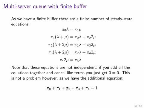
Multi-server queue with finite buffer
As we have a finite buffer there are a finite number of steady-stateequations:
π0λ = π1µ
π1(λ+ µ) = π0λ+ π22µ
π2(λ+ 2µ) = π1λ+ π32µ
π3(λ+ 2µ) = π2λ+ π42µ
π42µ = π3λ
Note that these equations are not independent: if you add all theequations together and cancel like terms you just get 0 = 0. Thisis not a problem however, as we have the additional equation:
π0 + π1 + π2 + π3 + π4 = 1
58 / 63

Multi-server queue with finite buffer
Putting ρ = λ2µ , the solution to this system is:
π0 =1−ρ
1+ρ−2ρ5
πi = 2ρiπ0 for i ≥ 1
Note, in this case the steady-state equations have a solution evenif ρ ≥ 1. This is possible because the finite buffer prevents thelength of the queue heading off to infinity.
Exercise: use the steady state distribution to calculate the serverutility, average number in the system and average time spentwaiting. What happens as ρ → ∞.
59 / 63

Machine interference model
Consider a shop floor with m machines and a single operator,whose job is to reset/repair machines when they jam or breakdown. Suppose that each machine breaks down at a rate λ(average time between breakdowns is 1
λ), and that the operatorrepairs machines at rate µ (average time to repair a machine is 1
µ).
mλ
µ
0 1 2
(m-1)λ (m-2)λ
µ µ
m
λ
µ
...
60 / 63

Machine interference model
The steady state equations:
π0mλ = π1µ
π1((m − 1)λ+ µ) = π0mλ+ π2µ
...
πm−1(λ+ µ) = πm−22λ+ πmµ
πmµ = πm−1λ
The solution to these equations is:
πi =m!
(m − i)!
(λ
µ
)i
π0
61 / 63

General Birth-Death Process
All of the examples we have seen so far can be viewed as examplesof a birth-death process. If we let the state i correspond to the sizeof population, then a transition i → i + 1 corresponds to a birth,and a transition i → i − 1 corresponds to a death. (Note that weallow transitions from 0 → 1, which correspond to immigrationfrom a separate population.)
A general birth death process allows the birth rate and death rateto depend on the current state, i.e. we jump from i → i + 1 atrate λi , and from i → i − 1 at rate µi . The transition diagram is:
λ0
µ1
0 1 2 3
λ1 λ2
µ2 µ3
...
λi
µk
i k j
λk
µj
...
62 / 63

General Birth-Death ProcessThe steady state equations are:
π0λ0 = π1µ1
π1(λ1 + µ1) = π0λ0 + π2µ2
...
πi (λi + µi ) = πi−1λi−1 + πi+1µi+1
The solution to these equations is, for i ≥ 1:
πi =λ0λ1 . . . λi−1
µ1µ2 . . . µiπ0
Thus, a steady-state distribution exists provided:
∞∑i=1
λ0λ1 . . . λi−1
µ1µ2 . . . µi< ∞
63 / 63