Questions in genomic selection,

some answers and some history of

single-step

Ignacy Misztal

University of Georgia

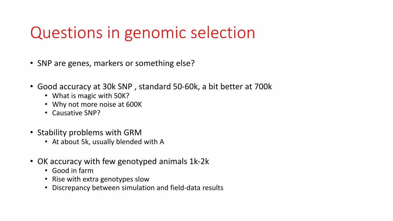
Questions in genomic selection

• SNP are genes, markers or something else?

• Good accuracy at 30k SNP , standard 50-60k, a bit better at 700k • What is magic with 50K?• Why not more noise at 600K• Causative SNP?

• Stability problems with GRM• At about 5k, usually blended with A

• OK accuracy with few genotyped animals 1k-2k• Good in farm• Rise with extra genotypes slow• Discrepancy between simulation and field-data results

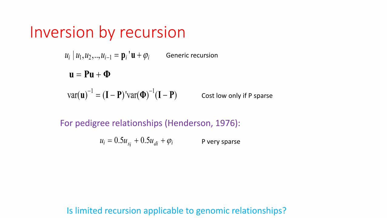
Inversion by recursion

u Pu Φ

1 2 1| , ,.., 'i i i iu u u u p u

1 1var( ) ( ) 'var( ) ( )

u I P Φ I P

Generic recursion

Cost low only if P sparse

P very sparse0.5 0.5i is diiu u u

For pedigree relationships (Henderson, 1976):

Is limited recursion applicable to genomic relationships?

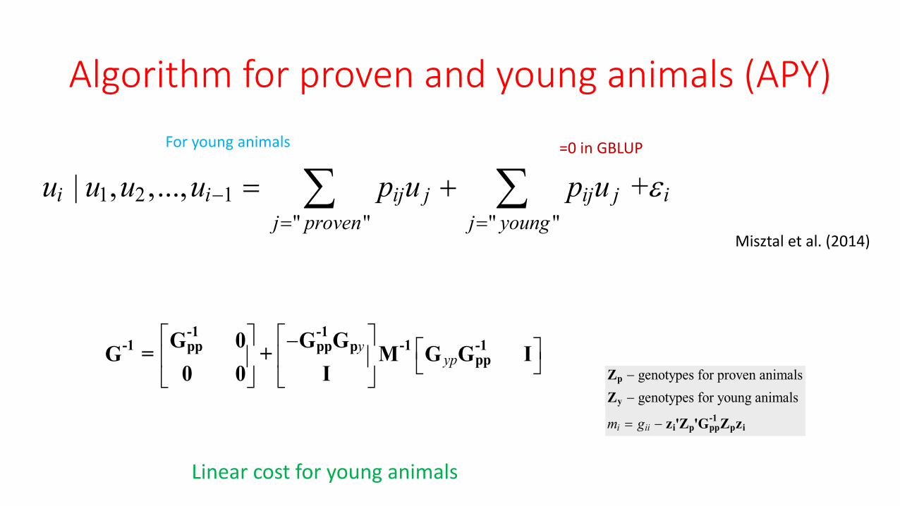
Algorithm for proven and young animals (APY)

1 2 1

" " " "

| , ,..., + i i ij j ij j i

j proven j young

u u u u p u p u

=0 in GBLUPFor young animals

yyp

-1 -1-1 -1 -1pp pp p

pp

G 0 G GG = + M G G I

0 0 I genotypes for proven animals

genotypes for young animals

i iim g

p

y

-1i p pp p i

Z

Z

z 'Z 'G Z z

Linear cost for young animals

Misztal et al. (2014)

Tests with Holsteins (Fragomeni et al., 2015)

G needed G-1

APY inverse

Regular inverse

Correlations of GEBV with regular inverse

23k bullsas core

17k cows as core

> 0.99

> 0.99

20k random animals as core

> 0.99

Impact of recursion size in Holsteins and chicken

Holstein

broiler

15,0003000

Corr(GEBV, GEBV APY)

Number of randomly-chosen animals in recursion

Theory of junctions

…………

Heterogenetic and homogenic tracts in genome (Stam, 1980)

Called independent chromosome segments Me (Goddard et al., 2009; Daetwyler et al., 2010)

E(Me)=4NeL (Stam, 1980)Ne – effective population sizeL –length of genome in Morgans

Need 12 Me SNPs to detect 90% of junctions (MacLeod et al., 2005)

Haplotype blocks = Independent chromosome segments

• E(Me) = 4NeL Stam (1980)

• Ne – Effective population size

• L – Length of genome in Morgans

2NeL Hayes et al. (2009)

• Me 2NeL/[log(NeL)] Goddard et al. (2011)

Many more Brard and Ricard (2015)

Cuppen (2005)

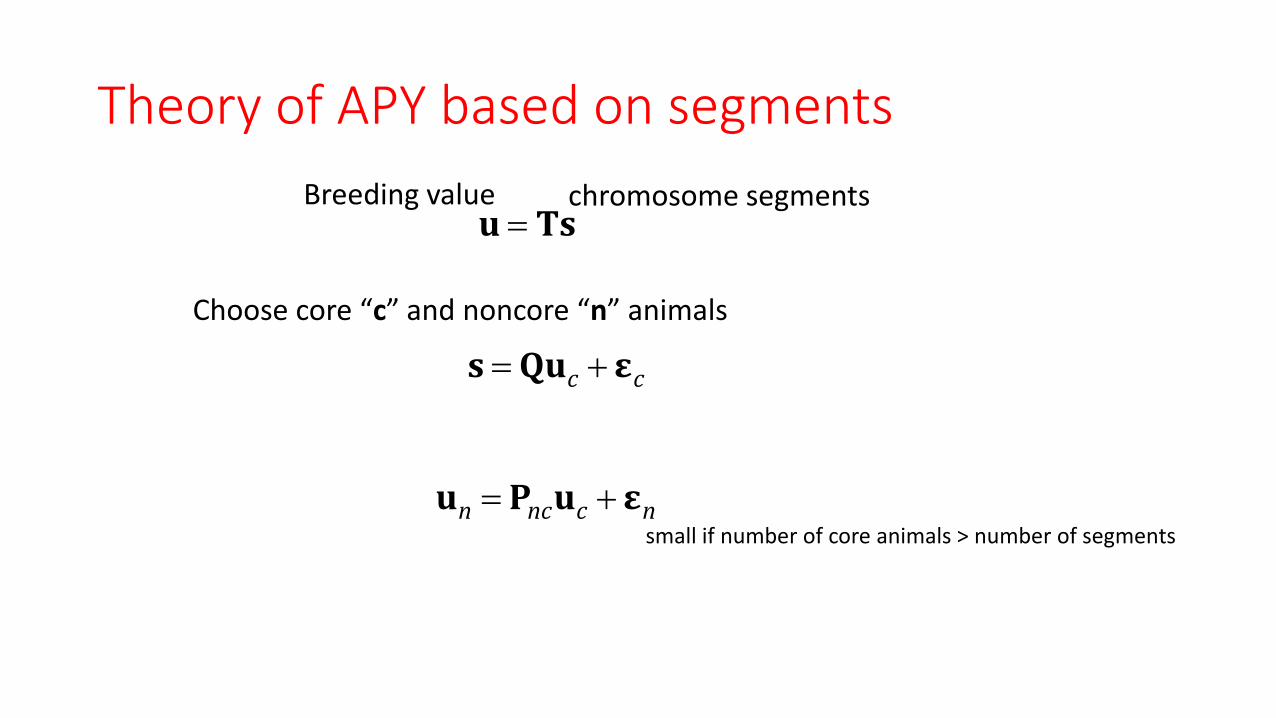
Choose core “c” and noncore “n” animals

n nc c nu P u ε

u Tschromosome segments

c cs Qu ε

Theory of APY based on segments

Breeding value

small if number of core animals > number of segments

c cu u

c c

ncn n

I 0u u

P Iu ε

0cncc

nc nn

I 0 I PG 0G

P I 0 IM

11

1

cccn

ncnn

I 0G 0I PG

P I0 M0 I

1nc nc ccP G G

, nn , i,1: 1 ,1: 1{ ' }i i i i idiag g M p g 1

Choose core “c” and noncore “n” animals

n nc c nu P u

The inverse

Unknown matrices from conditional expectation

BV of noncore animals linear function of core animals

Matrix notation

Var(u)

Misztal&Legarra&Aguilar (2014)

's s sG = U D U' = U D U

U – eigenvalues

D – eigenvectors

Eigenvalues sum to 100%

What % is useful, 95%? 98% 99%, 99.999%?

Finding dimensionalities by eigenvalues

2 NeL

NeL

4 NeL

99%

98%

95%

90%

True accuracies as function of number of eigenvalues corresponding to given explained variance in G

Ne=200

Ne=20

Approximate number of animals / segments NeL 2NeL 4NeL

Accuracies maximized by 98% “information in G, 95% almost as goodLast 2% of information in G noise

Pocrnic et al., 2016a

Number of eigenvalues in G to explain given fraction of variability

HolsteinJerseyAngus

PigsChicken

Reliabilities – Jerseys (75k animals)

Milk

Protein

Fat

3300 6100 11,500 assumed dimensionality≈NeL ≈2NeL ≈4 NeL

(number of core animals)

100% = full inverse lower accuracy

Pocrnic et al., 2016b

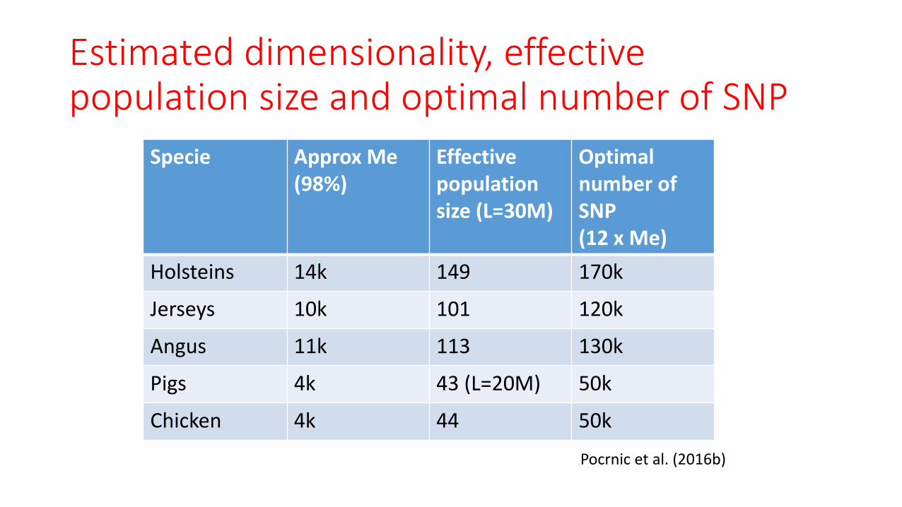
Estimated dimensionality, effective population size and optimal number of SNP

Specie Approx Me(98%)

Effective population size (L=30M)

Optimal number of SNP(12 x Me)

Holsteins 14k 149 170k

Jerseys 10k 101 120k

Angus 11k 113 130k

Pigs 4k 43 (L=20M) 50k

Chicken 4k 44 50k

Pocrnic et al. (2016b)

Side effects of reduced dimensionality

• Number of segments• 800k in humans

• 5-15k in animals

• Impact on SNP selection and GWAS

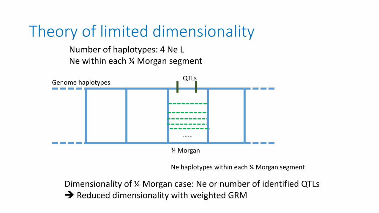
Theory of limited dimensionality

……

Number of haplotypes: 4 Ne LNe within each ¼ Morgan segment

¼ Morgan

Ne haplotypes within each ¼ Morgan segment

QTLsGenome haplotypes

Dimensionality of ¼ Morgan case: Ne or number of identified QTLs Reduced dimensionality with weighted GRM

Eigenvalue profile

10% should be 300

segments

0.43

0.57

0.660.69 0.69 0.69

0.47

0.6

0.76

0.850.88 0.89

0.3

0.4

0.5

0.6

0.7

0.8

0.9

1

30 40 50 60 70 80 90 100

Acc

ura

cy

% of explained variance

Accuracies with largest eigenvalues only

6k animals with own records

6k bulls with 50 daughters

Eigenvalues 25 120 400 1400 2000 3000

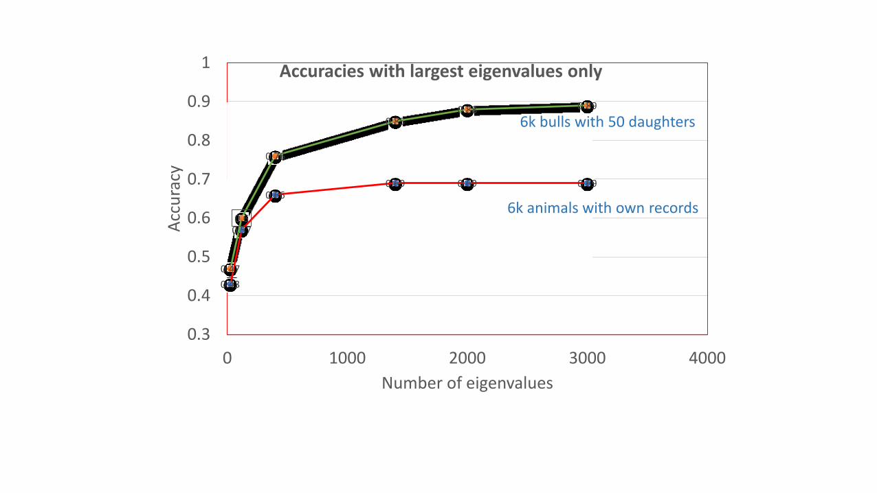
0.43

0.57

0.660.69 0.69 0.69

0.47

0.6

0.76

0.850.88 0.89

0.3

0.4

0.5

0.6

0.7

0.8

0.9

1

0 1000 2000 3000 4000

Acc

ura

cy

Number of eigenvalues

Accuracies with largest eigenvalues only

6k animals with own records

6k bulls with 50 daughters

0.47

0.6

0.76

0.850.88 0.89

0.34

0.71

0.840.87 0.88

0.3

0.4

0.5

0.6

0.7

0.8

0.9

1

0 1000 2000 3000 4000

Acc

ura

cy

Number of eigenvalues

Largest eigenvalues or core animals in APY

APY

Eigenvalues

Which core animals in APY?

Bradford et al. (2017)

Simulated populations (QMSim; Sargolzaei and Schenkel, 2009) Ne = 40 #genotyped animals = 50,000

Core animals: Random gen 6 || gen 7 || gen8 || gen9 || gen 10 (y) Random all generations Incomplete pedigree Genotypes in gen 9 and 10 imputed with 98% accuracy

Which core animals in APY?

0

0.1

0.2

0.3

0.4

0.5

0.6

0.7

0.8

0.9

1

98% 95% 90%

Co

rrel

atio

n (

GEB

V, T

BV

)

Percent of variation explained in G

Accuracy

Gen 6 Gen 7 Gen 8 Gen 9 Gen 10 Random

G-1

Bradford et al. (2016)

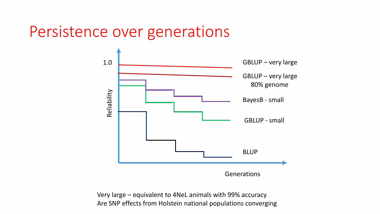
Persistence over generations

Generations

Rel

iab

ility

1.0

BLUP

GBLUP - small

BayesB - small

GBLUP – very large

GBLUP – very large80% genome

Very large – equivalent to 4NeL animals with 99% accuracyAre SNP effects from Holstein national populations converging

Multitrait ssGBLUP: Is SNP selection important? Causative SNPs?

• SNP selection/weighting (BayesB, etc.) • Large impact with few genotypes

• Little or no impact with many

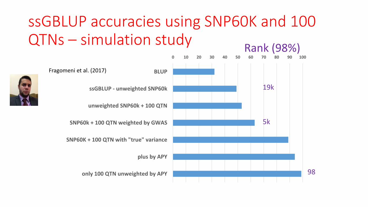
ssGBLUP accuracies using SNP60K and 100 QTNs – simulation study

0 10 20 30 40 50 60 70 80 90 100

BLUP

ssGBLUP - unweighted SNP60k

unweighted SNP60k + 100 QTN

SNP60k + 100 QTN weighted by GWAS

SNP60K + 100 QTN with "true" variance

plus by APY

only 100 QTN unweighted by APY

Fragomeni et al. (2017)

Rank (98%)

19k

5k

98

QTL

Accuracy and distance from markers to QTL

Fragomeni et al. (2017)

Nothing can be more fatal to progress than a

too confident reliance on mathematical

symbols; for the student is only too apt to take

the easier course, and consider the formula not

the fact as the physical reality.”

Kelvin

Group and sponsors

Yutaka

Masuda

Shogo

Tsuruta

Daniela

Lourenco

Breno

Fragomeni

Ignacio

Aguilar

Andres

Legarra

Ivan

Pocrnic

Heather

Bradford

Development of the combined matrix

-1 -1

12 22 22 21

22

IA A 0 A A 0H = A + G - A I I

I0 I 0 I

Initial (Misztal et al., 2009)

1-ungenotyped animals

2-genotyped animals22

0 0H=A+

0 G-A

1 1

1 1

22

0 0H =A +

0 G -A

Comprehensive (Legarra ,2009)

Inverse of Comprehensive (Aguilar et al., 2010)

Christensen and Lund, 2010Boemcke et al., 2010

Implementation at UGA

• Module genomic in BLUPF90 package (Aguilar et al. 2011)

• Option SNP_File xxx in RENUMF90

• Lots of options with defaults

• Creation of G-1: minutes for 10k

genotypes, hours for 50k genotypes

Prediction in 2004 DD2009

R2 (%) Inflation (%)

Parent Avg 24 31

Multistep

(VanRaden)+16 16

Single-step

Regular +17 31

Refined +17 4

Predictions for US final scores in Holsteins (Aguilar et

al., 2010)

1 1

22G -A

1 1

221.5G -0.6A

• US Holsteins (10 million animals)

• 18 traits

• Almost 50,000 genotypes of bulls and cows

• 2 days computing

Multitrait national genomic evaluation for type (Tsuruta et al., 2010)

Genomic evaluations of broiler chicken (Chen et al., 2010)

• 180k broiler chicken

• 3 k genotyped with SNP60k chip

• 3 methods– BLUP- full data

– BayesA – genotyped subset

– Single step – subset and full data set

Trait Accuracy*100

BLUPBayesA

Subset

Single-step

Subset

Single-step

Full

Body

Weight56 +4 +11 +12

Breast

Meat35 +1 +0 +6

Leg Score 29 -20 -23 +7

Accuracies for broiler chickens

Next cycle of selection

Body

Weight38 +13 +22 =

Breast Meat39 +10 +26 +29

Leg Score 28 -21 +6 =

Multiple trait

BayesA – days of computing + errors

Single-step –2 minutes

-0.06

-0.04

-0.02

0

0.02

0.04

0.06

0.08

(2.5)

(2.0)

(1.5)

(1.0)

(0.5)

-

0.5

200601 200701 200801 200901 201001 201101 201201 201301 201401 201501 201601

Birth weight

(kg/pig) (relative to '13-'15 avg)

Total born

(pigs/sow/yr) (relative to '13-'15 avg)

Birth year / month

Trend: genetic improvement in birth weight and total born(PIC Genetic Nucleus)

Total Born Birth Weight

1. Relationship based genomic selectionSource: PIC L02, L03 pure lines (Camborough)

Introduction of RBGS1

Introduction of RBGS1

-0.06

-0.04

-0.02

0

0.02

0.04

0.06

0.08

(2.5)

(2.0)

(1.5)

(1.0)

(0.5)

-

0.5

200601 200701 200801 200901 201001 201101 201201 201301 201401 201501 201601

Birth weight

(kg/pig) (relative to '13-'15 avg)

Total born

(pigs/sow/yr) (relative to '13-'15 avg)

Birth year / month

Trend: genetic improvement in birth weight and total born(PIC Genetic Nucleus)

Total Born Birth Weight

1. Relationship based genomic selectionSource: PIC L02, L03 pure lines (Camborough)

Introduction of RBGS1

Introduction of RBGS1

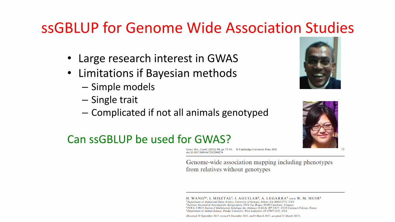
• Large research interest in GWAS• Limitations if Bayesian methods

– Simple models– Single trait– Complicated if not all animals genotyped

Can ssGBLUP be used for GWAS?

ssGBLUP for Genome Wide Association Studies

Three Methods for GWAS – chicken

ssGBLUPIterations on SNP (it5)

Classical GWAS

BayesB

Can large QTL exist despite selection?

• Genetics and genomics of mortality in US Holsteins

• (Tokuhisa et al, 2014; Tsuruta et al., 2014)

• 6M records, SNP50k genotypes of 35k bulls

Milk – first parity

Mortality – first parity

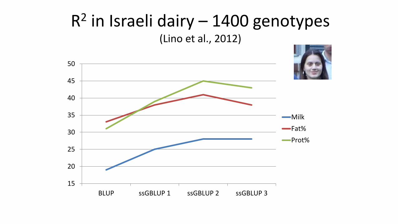
R2 in Israeli dairy – 1400 genotypes(Lino et al., 2012)

15

20

25

30

35

40

45

50

BLUP ssGBLUP 1 ssGBLUP 2 ssGBLUP 3

Milk

Fat%

Prot%

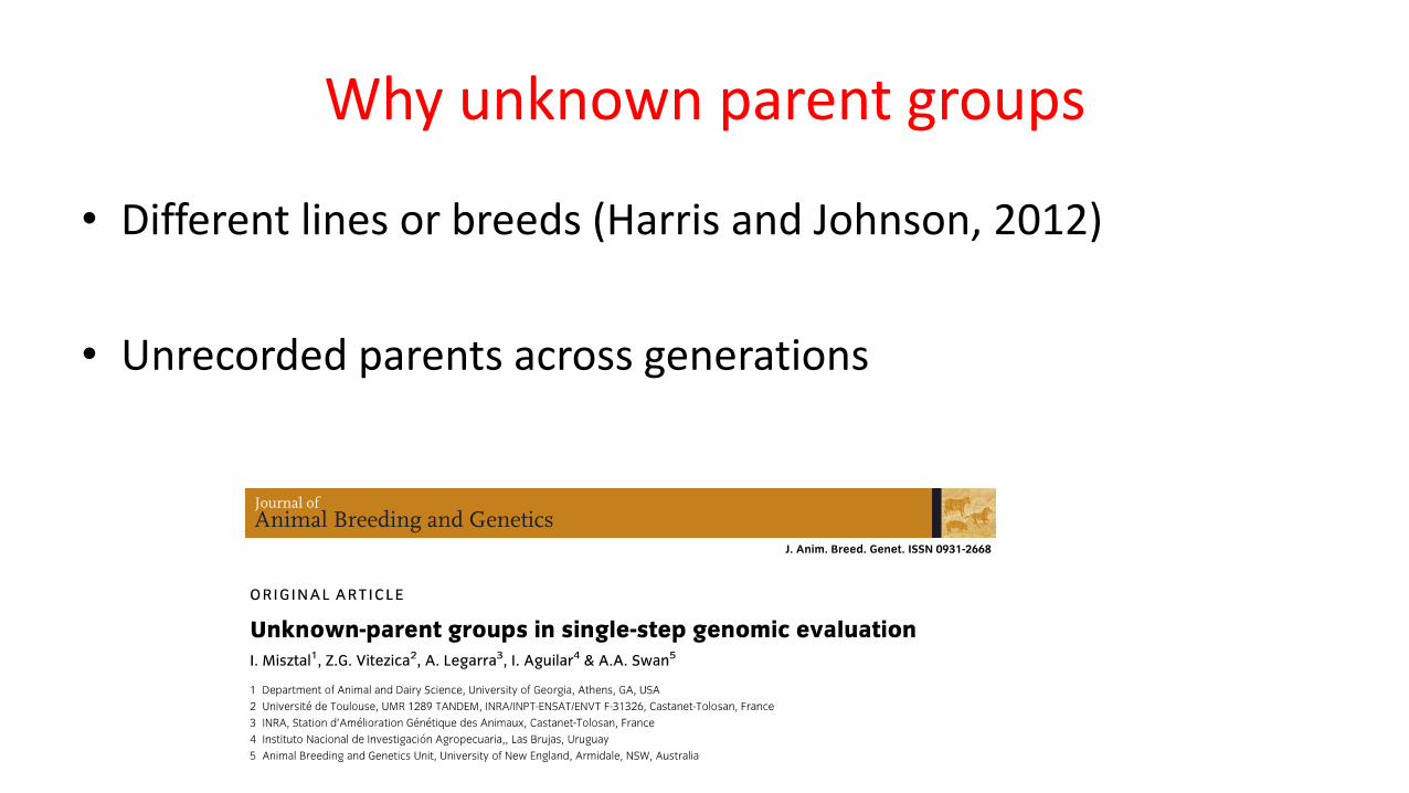
Why unknown parent groups

• Different lines or breeds (Harris and Johnson, 2012)

• Unrecorded parents across generations

Pedigree depth for young animals

1950 1960 1970 1980 1990 2000 2010

g1 g5 g11 g18 g24 g31

Pedigree length and convergence

H-1= A

-1+

0 0

0 G-1 -A22

-1

é

ë

êê

ù

û

úú

G-1 - A22

-1Good convergence and genotyped animals biased down

G-1 - A22

-1Bad convergence and genotyped animals biased up

G-1 -A22,1

-1 - Bad convergence and genotypedanimals biased down and up

A22,2

-1 - A22,3

-1

Long medium shortpedigrees

Big A22 makes H less PD,Reduces convergence rate

Cut pedigree and data?

1950 1960 1970 1980 1990 2000 2010

g1 g5 g11 g18 g24 g31

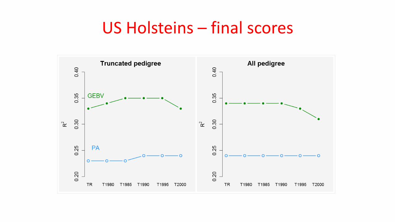
US Holsteins – final scores

Realized broiler accuracies with male, female or both genotypes – Trait A

0

0.1

0.2

0.3

0.4

0.5

0.6

0.7

0.8

Male EPD Female EPD

196,000 birds with phenotype~13,000 genotypes

(Lourenco et al., submitted)

BLUP

Male

Fem

M+F

BLUP Male

Fem

M+F

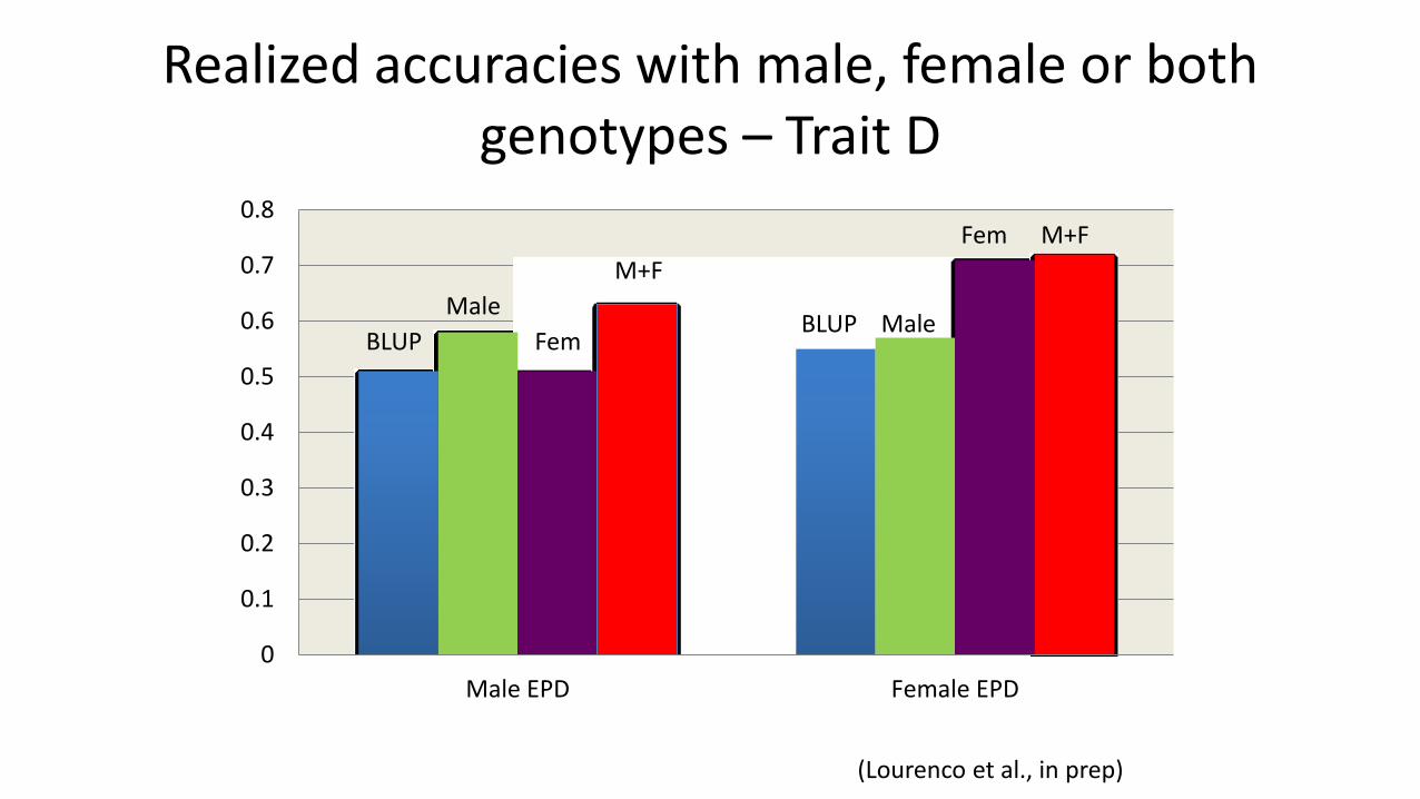
Realized accuracies with male, female or both genotypes – Trait D

0

0.1

0.2

0.3

0.4

0.5

0.6

0.7

0.8

Male EPD Female EPD

(Lourenco et al., in prep)

BLUP

Male

Fem

M+F

BLUP Male

Fem M+F

Why realized accuracies differ by sex?

parents

Bigger selection pressure on females

Selection graph for GEBV; possibly more differential selection EBV from BLUP

Why realized accuracies differ by traits for similar h2

h2=0.25 h2=0.22

Decomposition of GEBV in Single-step

GEBV = w1CD+w2PA+w3PC +w4DGV +w5PI

Z 'MZ +aA-1 +0 0

0 G-1 - A22-1

é

ë

êê

ù

û

úú

ì

íï

îï

ü

ýï

þïu = Z 'My

CD – contemporary deviationPA – Parent averagePC – Progeny Contribution

DGV – direct genomic valuePI – Parental Index

w1 =1å

No genotype, no extra accuracy

GEBV for young animals

GEBV = w2PA+w4DGV +w5PI

GEBV = DGV

GEBV = PAIf no genotype

If genotype via SNP only

Complete

Little improvement with genomics if animal not genotyped

New studies

• Unbiased evaluations of US Holstein with > 2 M genotypes of varying quality

• Helping Interbull survive• Unbiased pseudo-observations for bulls• GBLUP MACE

• Crossbreeding evaluation without reduction of accuracy

• Resilience and genomic selection

Programming/methodology

• Better approximations of accuracy

• Better GWAS

• GUI?

Applied studies

• Pigs• Mortality, survival, changing correlations

• Chickens• Sexual dimorphism,…

• Dairy

• Beef• Altitude, GxE

• Fish

• Heat stress

• GxE

• Resilience

• Theory

Production (high h2)

Raw fitness (low h2)

Management

Realized fitness

Genomic selectionTrends

Is UGA a good place to come?

• Good place for Science

• Improving South

• Politics small at universities

• Funding available

• Interesting projects

• Data from biggest animal institutions across species

Asch (1951) experiments

A, B or C?