Querying RDF Data Using A Multigraph-based Approach

Vijay IngalalliLIRMM, IRSTEA

Montpellier, Francevijay@lirmm.fr

Dino IencoIRSTEA

Montpellier, Francedino.ienco@irstea.fr

Pascal PonceletLIRMM

Montpellier, Francepascal.poncelet@lirmm.fr

Serena VillataCNRS, I3S Laboratory

Sophia Antipolis, Francevillata@i3s.unice.fr

ABSTRACTRDF is a standard for the conceptual description of knowl-edge, and SPARQL is the query language conceived to queryRDF data. The RDF data is cherished and exploited byvarious domains such as life sciences, Semantic Web, socialnetwork, etc. Further, its integration at Web-scale compelsRDF management engines to deal with complex queries interms of both size and structure. In this paper, we proposeAMbER (Attributed Multigraph Based Engine for RDFquerying), a novel RDF query engine specifically designedto optimize the computation of complex queries. AMbERleverages subgraph matching techniques and extends themto tackle the SPARQL query problem. First of all RDFdata is represented as a multigraph, and then novel index-ing structures are established to efficiently access the in-formation from the multigraph. Finally a SPARQL queryis represented as a multigraph, and the SPARQL queryingproblem is reduced to the subgraph homomorphism prob-lem. AMbER exploits structural properties of the querymultigraph as well as the proposed indexes, in order to tacklethe problem of subgraph homomorphism. The performanceof AMbER, in comparison with state-of-the-art systems, hasbeen extensively evaluated over several RDF benchmarks.The advantages of employing AMbER for complex SPARQLqueries have been experimentally validated.

1. INTRODUCTIONIn the recent years, structured knowledge represented in

the form of RDF data has been increasingly adopted to im-prove the robustness and the performances of a wide rangeof applications with various purposes. Popular examples areprovided by Google, that exploits the so called knowledgegraph to enhance its search results with semantic informa-tion gathered from a wide variety of sources, or by Facebook,that implements the so called entity graph to empower itssearch engine and provide further information extracted, for

c©2016, Copyright is with the authors. Published in Proc. 19th Inter-national Conference on Extending Database Technology (EDBT), March15-18, 2016 - Bordeaux, France: ISBN 978-3-89318-070-7, on OpenPro-ceedings.org. Distribution of this paper is permitted under the terms of theCreative Commons license CC-by-nc-nd 4.0

instance by Wikipedia. Another example is supplied by re-cent question-answering systems [4, 15] that automaticallytranslate natural language questions in SPARQL queries andsuccessively retrieve answers considering the available infor-mation in the different Linked Open Data sources. In allthese examples, complex queries (in terms of size and struc-ture) are generated to ensure the retrieval of all the requiredinformation. Thus, as the use of large knowledge bases, thatare commonly stored as RDF triplets, is becoming a com-mon way to ameliorate a wide range of applications, efficientquerying of RDF data sources using SPARQL is becomingcrucial for modern information retrieval systems.

All these different scenarios pose new challenges to theRDF query engines for two vital reasons: firstly, the au-tomatically generated queries cannot be bounded in theirstructural complexity and size (e.g., the DBPEDIA SPARQLBenchmark [12] contains some queries having more than 50triplets [1]); secondly, the queries generated by retrieval sys-tems (or by any other applications) need to be efficientlyanswered in a reasonable amount of time. Modern RDFdata management, such as x-RDF-3X [13] and Virtuoso [7],are designed to address the scalability of SPARQL queriesbut they still have problems to answer big and structurallycomplex SPARQL queries [2]. Our experiments with stateof-the-art systems demonstrate that they fail to efficientlymanage such kind of queries (Table 1).

Systems AMbER gStore Virtuoso x-RDF-3X

Time (sec) 1.56 11.96 20.45 >60

Table 1: Average Time (seconds) for a sample of 200 com-plex queries on DBPEDIA. Each query has 50 triplets.

In order to tackle these issues, in this paper, we introduceAMbER (Attributed Multigraph Based Engine for RDFquerying), which is a graph-based RDF engine that involvestwo steps: an offline stage where RDF data is transformedinto multigraph and indexed, and an online step where an ef-ficient approach to answer SPARQL query is proposed. Firstof all RDF data is represented as a multigraph where sub-jects/objects constitute vertices and multiple edges (predi-cates) can appear between the same pair of vertices. Then,new indexing structures are conceived to efficiently accessRDF multigraph information. Finally, by representing theSPARQL queries also as multigraphs, the query answering

Series ISSN: 2367-2005 245 10.5441/002/edbt.2016.24

Prefixes: x= http://dbpedia.org/resource/ ; y=http://dbpedia.org/ontology/

Subject Predicate Object

x:London y:isPartOf x:England

x:England y:hasCapital x:London

x:Christophar_Nolan y:wasBornIn x:London

x:Christophar_Nolan y:LivedIn x:England

x:Christophar_Nolan y:isPartOf x:Dark_Knight_Trilogy

x:London y:hasStadium x:WembleyStadium

x:WembleyStadium y:hasCapacityOf “90000”

x:Amy_Winehouse y:wasBornIn x:London

x:Amy_Winehouse y:diedIn x:London

x:Amy_Winehouse y:wasPartOf x:Music_Band

x:Music_Band y:hasName “MCA_Band”

x:Music_Band y:FoundedIn “1994”

x:Music_Band y:wasFormedIn X:London

x:Amy_Winehouse y:livedIn x:United States

x:Amy_Winehouse y:wasMarriedTo x:Blake Fielder-Civil

x:Blake Fielder-Civil y:livedIn x:United States

(a) RDF tripleset

“MCA_Band”“1934”

hasCapitalisPartOf

hasStadium

wasMarriedTowasPartOf

wasBornIn

diedIn

foundedIn wasFormedIn

hasA

Name

“90000”

hasCapacityOf

livedIn

BlakeFielder-Civil

United States

WembleyStadium

Amy_Winehouse

London

England

Music_Band

Christopher_Nolan

wasBornIn

livedIn

livedIn

Dark_Knight_TrilogyisPartOf

(b) Graph representation of RDF data

{-}

{-}{-, a1, a

2}

{-}{-,a

0}

{-}

{-}

t1t

0 t2

{t4, t

5}t

6

t7

t8V

0

V2

V1

V3

V4

V5

V6

{-}

V7

t5

t3

t3

{-} V8

t0

t3

(c) Equivalent multigraph G

Figure 1: (a) RDF data in n-triple format; (b) graph representation (c) attributed multigraph G

task can be reduced to the problem of subgraph homo-morphism. To deal with this problem, AMbER employsan efficient approach that exploits structural properties ofthe multigraph query as well as the indices previously builton the multigraph structure. Experimental evaluation overpopular RDF benchmarks show the quality in terms of timeperformances and robustness of our proposal.

In this paper, we focus only on the SELECT/WHERE clauseof the SPARQL language1, that constitutes the most impor-tant operation of any RDF query engines. It is out of thescope of this work to consider operators like FILTER, UNIONand GROUP BY or manage RDF update. Such operations canbe addressed in future as extensions of the current work.

The paper is organized as follows. Section 2 introducesthe basic notions about RDF and SPARQL language. InSection 3 AMbER is presented. Section 4 describes theindexing strategy while Section 5 presents the query pro-cessing. Related works are discussed in Section 6. Section 7provides the experimental evaluation. Section 8 concludes.

2. BACKGROUND AND PRELIMINARIESIn this section we provide basic definitions on the interplay

between RDF and its multigraph representation. Later, weexplain how the task of answering SPARQL queries can bereduced to multigraph homomorphism problem.

2.1 RDF DataAs per the W3C standards 2, RDF data is represented

as a set of triples <S,P,O>, as shown in Figure 1a, whereeach triple <s, p, o> consists of three components: a subject,a predicate and an object. Further, each component of theRDF triple can be of any two forms; an IRI (International-ized Resource Identifier) or a literal. For brevity, an IRI isusually written along with a prefix (e.g., <http://dbpedia.

1http://www.w3.org/TR/sparql11-overview/2http://www.w3.org/TR/2014/REC-rdf11-concepts-20140225/

org/resource/isPartOf> is written as ‘x:isPartOf’), whereasa literal is always written with double quotes (e.g., “90000”).While a subject s and a predicate p are always an IRI, anobject o is either an IRI or a literal.

RDF data can also be represented as a directed graphwhere, given a triple <s, p, o>, the subject s and the objecto can be treated as vertices and the predicate p forms adirected edge from s to o, as depicted in Figure 1b. Further,to underline the difference between an IRI and a literal, weuse standard rectangles and arc for the former while we usebeveled corner and edge (no arrows) for the latter.

2.1.1 Data Multigraph RepresentationMotivated by the graph representation of RDF data (Fig-

ure 1b), we take a step further by transforming it to a datamultigraph G, as shown in Figure 1c.

Let us consider an RDF triple <s, p, o> from the RDFtripleset <S,P,O>. Now to transform the RDF triplesetinto data multigraph G, we set four protocols: we alwaystreat the subject s as a vertex; a predicate p is always treatedas an edge; we treat the object o as a vertex only if it is anIRI (e.g., vertex v2 corresponds to object ‘x:London’); whenthe object is a literal, we combine the object o and the cor-responding predicate p to form a tuple <p, o> and assign itas an attribute to the subject s (e.g., <‘y:hasCapacityOf’,“90000”> is assigned to vertex v4). Every vertex is assigneda null value {-} in the attribute set. However, to realize thisin the realms of graph management techniques, we main-tain three different dictionaries, whose elements are a pairof ‘key’ and ‘value’, and a mapping function that links them.The three dictionaries depicted in Table 2 are: a vertex dic-tionary (Table 2a), an edge-type dictionary (Table 2b) andan attribute dictionary (Table 2c). In all the three dictio-naries, an RDF entity represented by a ‘key’ is mapped to acorresponding ‘value’, which can be a vertex/edge/attributeidentifier. Thus by using the mapping functions -Mv,Me,andMa for vertex, edge-type and attribute mapping respec-tively, we obtain a directed, vertex attributed data multi-

246

graph G (Figure 1c), which is formally defined as follows.

Definition 1. Directed, Vertex Attributed Multigraph.A directed, vertex attributed multigraph G is defined as a4-tuple (V,E, LV , LE) where V is a set of vertices, E ⊆V ×V is a set of directed edges with (v, v′) 6= (v′, v), LV is alabelling function that assigns a subset of vertex attributes Ato the set of vertices V , and LE is a labelling function thatassigns a subset of edge-types T to the edge set E.

To summarise, an RDF tripleset is transformed into a datamultigraph G, whose elements are obtained by using themapping functions as already discussed. Thus, the set of ver-tices V = {v0, . . . , vm} is the set of mapped subject/objectIRI, and the labelling function LV assigns a set of vertex at-tributes A = {-, a0, . . . , an} (mapped tuple of predicate andobject-literal) to the vertex set V . The set of directed edgesE is a set of pair of vertices (v, v′) that are linked by a pred-icate, and the labelling function LE assigns the set of edgetypes T = {t0, . . . , tp} (mapped predicates) to these set ofedges. The edge set E maintains the topological structure ofthe RDF data. Further, mapping of object-literals and thecorresponding predicates as a set of vertex attributes, resultsin a compact representation of the multigraph. For exam-ple (in Fig. 1c), all the object-literals and the correspondingpredicates are reduced to a set of vertex attributes.

2.2 SPARQL QueryA SPARQL query usually contains a set of triple patterns,

much like RDF triples, except that any of the subject, pred-icate and object may be a variable, whose bindings are tobe found in the RDF data 3. In the current work, we ad-dress the SPARQL queries with ‘SELECT/WHERE’ option,where the predicate is always instantiated as an IRI (Fig-ure 2a). The SELECT clause identifies the variables to appearin the query results while the WHERE clause provides triplepatterns to match against the RDF data.

2.2.1 Query Multigraph RepresentationIn any valid SPARQL query (as in Figure 2a), every triplet

has at least one unknown variable ?X, whose bindings are tobe found in the RDF data. It should now be easy to observethat a SPARQL query can be represented in the form ofa graph as in Figure 2b, which in turn is transformed intoquery multigraph Q (as in Figure 2c).

In the query multigraph representation, each unknownvariable ?Xi is mapped to a vertex ui that forms the ver-tex set U component of the query multigraph Q (e.g., ?X6

is mapped to u6). Since a predicate is always instantiatedas an IRI, we use the edge-type dictionary in Table 2b, tomap the predicate to an edge-type identifier ti ∈ T (e.g.,‘isMarriedTo’ is mapped as t8). When an object oi is a lit-eral, we use the attribute dictionary (Table 2c), to find theattribute identifier ai for the predicate-object tuple <pi, oi>(e.g., {a0} forms the attribute for vertex u4). Further, whena subject or an object is an IRI, which is a not a variable, weuse the vertex dictionary (2a), to map it to an IRI -vertexuirii (e.g., ‘x:United States’ is mapped to uiri

0 ) and maintaina set of IRI vertices R. Since this vertex is not a variableand a real vertex of the query, we portray it differently by ashaded square shaped vertex. When a query vertex ui does

3http://www.w3.org/TR/2008/REC-rdf-sparql-query-20080115/

s/o Mv(s/o)x:Music Band v0

x:Amy Winehouse v1

x:London v2

x:England v3

x:WembleyStadium v4

x:United States v5

x:Blake Fielder-Civil v6

x:Christopher Nolan v7x:Dark Knight Trilogy v8

(a) Vertex Dictionary

p Me(p)y:isPartOf t0

y:hasCapital t1y:hasStadium t2

y:livedIn t3y:diedIn t4

y:wasBornIn t5y:wasFormedIn t6y:wasPartOf t7

y:wasMarriedTo t8

(b) Edge-type Dictionary

<p, o> Ma(<p, o>)<y:hasCapacityOf, “90000”> a0

<y:wasFoundedIn, “1994”> a1

<y:hasName, “MCA Band”> a2

(c) Attribute Dictionary

Table 2: Dictionary look-up tables for vertices, edge-typesand vertex attributes

not have any vertex attributes associated with it (e.g., u0,u1, u2, u3, u6), a null attribute {-} is assigned to it. Onthe other hand, an IRI -vertex uiri

i ∈ R does not have anyattributes. Thus, a SPARQL query is transformed into aquery multigraph Q.

In this work, we always use the notation V for the set ofvertices of G, and U for the set of vertices of Q. Conse-quently, a data vertex v ∈ V , and a query vertex u ∈ U .Also, an incoming edge to a vertex is positive (default), andan outgoing edge from a vertex is labelled negative (‘-’).

2.3 SPARQL Querying by AdoptingMultigraph Homomorphism

As we recall, the problem of SPARQL querying is ad-dressed by finding the solutions to the unknown variables?X, that can be bound with the RDF data entities, so thatthe relations (predicates) provided in the SPARQL queryare respected. In this work, to harness the transformeddata multigraph G and the query multigraph Q, we reducethe problem of SPARQL querying to a sub-multigraph ho-momorphism problem. The RDF data is transformed intodata multigraph G and the SPARQL query is transformedinto query multigraph Q. Let us now recall that findingSPARQL answers in the RDF data is equivalent to findingall the sub-multigraphs of Q in G that are homomorphic.Thus, let us now formally introduce homomorphism for avertex attributed, directed multigraph.

Definition 2. Sub-multigraph Homomorphism. Givena query multigraph Q = (U,EQ, LU , L

QE) and a data multi-

graph G = (V,E, LV , LE), the sub-multigraph homomor-phism from Q to G is a surjective function ψ : U → Vsuch that:

1. ∀u ∈ U,LU (u) ⊆ LV (ψ(u))

2. ∀(um, un) ∈ EQ, ∃ (ψ(um), ψ(un)) ∈ E, where (um, un)

is a directed edge, and LQE(um, un) ⊆ LE(ψ(um), ψ(un)).

Thus, by finding all the sub-multigraphs in G that arehomomorphic to Q, we enumerate all possible homomorphicembeddings of Q in G. These embeddings contain the solu-tion for each of the query vertex that is an unknown variable.Thus, by using the inverse mapping function M−1

v (vi) (in-troduced already), we find the bindings for the SPARQL

247

SELECT ?X0 ?X1 ?X2 ?X3 ?X4 ?X5 ?X6 WHERE { ?X0 y:livedIn ?X1 .?X1 y:isPartOf ?X2 . ?X2 y:hasCapital ?X1 . ?X1 y:hasStadium ?X4 .?X3 y:wasBornIn ?X1 .?X3 y:diedIn ?X1 .?X3 y:isMarriedTo ?X6 .?X3 y:wasPartOf ?X5 .?X5 y:wasFormedIn ?X1 .?X4 y:hasCapacity “90000” .?X5 y:hasName “MCA_Band” .?X5 y:foundedIn “1934” . ?X3 y:livedIn x:United States . }

(a) SPARQL Query

“MCA_Band”“1934”

hasCapital

isPartOf

hasStadium

isMarriedTowasPartOf

wasBornIn

diedIn

foundedIn wasFormedIn

hasA

Name

“90000”

hasCapacityOf

X:United_States

livedIn

wasBornIn

?X6

?X1

?X2

?X3?X5

?X0

?X4

(b) Graph representation of SPARQL

{-}

{-}{a1, a

2}

{-}

{-}

t1

t0

t2

{t4, t

5}t

6

t7

t8

U3

U5

U1

U2 U

4

U6

{a0}

{-}

U0

t5

U0

iri

t3

(c) Equivalent Multigraph Q

Figure 2: (a) SPARQL query representation; (b) graph representation (c) attributed multigraph Q

query. The decision problem of subgraph homomorphismis NP-complete. This standard subgraph homomorphismproblem can be seen as a particular case of sub-multigraphhomomorphism, where both the labelling functions LE andLQ

E always return the same subset of edge-types for all theedges in both Q and G. Thus the problem of sub-multigraphhomomorphism is at least as hard as subgraph homomor-phism. Further, the subgraph homomorphism problem is ageneric scenario of subgraph isomorphism problem where,the injectivity constraints are slackened [11].

3. AMBER: A SPARQL QUERYING ENGINEWe now present an overview of our proposal - AMbER

(Attributed Mulitgraph Based Engine for RDF querying).AMbER contains two different stages: (i) an offline stageduring which, RDF data is transformed into multigraph Gand then a set of index structures I is constructed that cap-tures the necessary information contained in G; (ii) an onlinestage during which, a SPARQL query is transformed into amultigraph Q, and then by exploiting the subgraph match-ing techniques along with the already built index structuresI, the homomorphic matches of Q in G are obtained.

Given a multigraph representation Q of a SPARQL query,AMbER decomposes the query vertices U into a set of corevertices Uc and satellite vertices Us. Intuitively, a vertexu ∈ U is a core vertex, if the degree of the vertex is morethan one; on the other hand, a vertex u with degree one is asatellite vertex. For example, in Figure 2c, Uc = {u1, u3, u5}and Us = {u0, u2, u4, u6}. Once decomposed, we run thesub-multigraph matching procedure on the query structurespanned only by the core vertices. However, during the pro-cedure, we also process the satellite vertices (if available)that are connected to a core vertex that is being processed.For example, while processing the core vertex u1 , we alsoprocess the set of satellite vertices {u0, u2, u4} connected toit; whereas, the core vertex u5 has no satellite vertices tobe processed. In this way, as the matching proceeds, theentire structure of the query mulitgraph Q is processed tofind the homomorphic embeddings in G. The set of indexingstructures I are extensively used during the process of sub-multigraph matching. The homomorphic embeddings arefinally translated back to the RDF entities using the inversemapping function M−1

v as discussed in Section 2.

4. INDEX CONSTRUCTIONGiven a data multigraph G, we build the following three

different indices: (i) an inverted list A for storing the setof data vertex for each attribute in ai ∈ A (ii) a trie indexstructure S to store features of all the data vertices V (iii)a set of trie index structures N to store the neighbourhoodinformation of each data vertex v ∈ V . For brevity of rep-resentation, we ensemble all the three index structures intoI := {A,S,N}.

During the query matching procedure (the online step),we access these indexing structures to obtain the candidatesolutions for a query vertex u. Formally, for a query vertexu, the candidate solutions are a set of data vertices Cu ={v|v ∈ V } obtained by accessing A or S or N , denoted asCAu , CSu and CNu respectively.

4.1 Attribute IndexThe set of vertex attributes is given by A = {a0, . . . , an}

(Section 2), where a data vertex v ∈ V might have a subsetof A assigned to it. We now build the vertex attribute indexA by creating an inverted list where a particular attributeai has the list of all the data vertices in which it appears.

Given a query vertex u with a set of vertex attributesu.A ⊆ A, for each attribute ai ∈ u.A, we access the indexstructure A to fetch a set of data vertices that have ai. Thenwe find a common set of data vertices that have the entireattribute set u.A. For example, considering the query vertexu5 (Fig. 2c), it has an attribute set {a1, a2}. The candidatesolutions for u5 are obtained by finding all the common datavertices, in A, between a1 and a2, resulting in CAu5

= {v0}.

4.2 Vertex Signature IndexThe index S captures the edge type information from the

data vertices. For a lucid understanding of this indexingschema we formally introduce the notion of vertex signaturethat is defined for a vertex v ∈ V , which encapsulates theedge information associated with it.

Definition 3. Vertex signature. For a vertex v ∈ V ,the vertex signature σv is a multiset containing all the di-rected multi-edges that are incident on v, where a multi-edgebetween v and a neighbouring vertex v′ is represented bya set that corresponds to the edge types. Formally, σv =⋃

v′∈N(v) LE(v, v′) where N(v) is the set of neighbourhoodvertices of v, and ∪ is the union operator for multiset.

248

Data vertex Signature Synopsesv σv f+

1 f+2 f+

3 f+4 f−1 f−2 f−3 f−4

v0 {{−t6}, {t7}} 1 1 -7 7 1 1 -6 6v1 {{−t3}, {−t7}, {−t8}, {−t4,−t5}} 0 0 0 0 2 5 -3 8v2 {{−t0}, {t1}, {−t2}, {t5}, {t6}, {t4, t5}} 2 4 -1 6 1 2 0 2v3 {{t0}, {t3}, {−t1}} 1 2 0 3 1 1 -1 1v4 {{t2}} 1 1 -2 2 0 0 0 0v5 {{t3}, {t3}} 1 1 -3 3 0 0 0 0v6 {{t8}, {−t3}} 1 1 -8 8 1 1 -3 3v7 {{−t0}, {−t3}, {−t5}} 0 0 0 0 1 3 0 5v8 {{t0}} 1 1 0 0 0 0 0 0

Table 3: Vertex signatures and the corresponding synopses for the vertices in the data multigraph G (Figure 1c)

The index S is constructed by tailoring the informationsupplied by the vertex signature of each vertex in G. To ex-tract some interesting features, let us observe the vertex sig-nature σv2 as supplied in Table 3. To begin with, we can rep-resent the vertex signature σv2 separately for the incomingand outgoing multi-edges as σ+

v2 = {{t1}, {t5}, {t6}, {t4, t5}}and σ−v2 = {{−t0}{−t2}} respectively. Now we observe thatσ+v2 has four distinct multi-edges and σ−v2 has two distinct

multi-edges. Now, lets think that we want find candidatesolutions for a query vertex u. The data vertex v2 can be amatch for u only if the signature of u has at most four in-coming (‘+’) edges and at most two outgoing (‘-’) edges; elsev2 can not be a match for u. Thus, more such features (e.g.,maximum cardinality of a set in the vertex signature) can beproposed to filter out irrelevant candidate vertices. Thus, foreach vertex v, we propose to extract a set of features by ex-ploiting the corresponding vertex signature. These featuresconstitute a synopses, which is a surrogate representationthat approximately captures the vertex signature informa-tion.

The synopsis of a vertex v contains a set of features F ,whose values are computed from the vertex signature σv. Inthis background, we propose four distinct features: f1 - themaximum cardinality of a set in the vertex signature; f2 -the number of unique dimensions in the vertex signature;f3 - the minimum index value of the edge type; f4 - themaximum index value of the edge type. For f3 and f4, theindex values of edge type are nothing but the position of thesequenced alphabet. These four basic features are replicatedseparately for outgoing (negative) and incoming (positive)edges, as seen in Table 3. Thus for the vertex v2, we obtainf+1 = 2, f+

2 = 4, f+3 = −1 and f+

4 = 7 for the incomingedge set and f−1 = 1, f−2 = 2, f−3 = 0 and f−4 = 2 for theoutgoing edge set. Synopses for the entire vertex set V forthe data multigraph G are depicted in Table 3.

Once the synopses are computed for all data vertices, anR-tree is constructed to store all the synopses. This R-treeconstitutes the vertex signature index S. A synopsis with|F | fields forms a leaf in the R-tree.

When a set of possible candidate solutions are to be ob-tained for a query vertex u, we create a vertex signatureσu in order to compute the synopsis, and then obtain thepossible solutions from the R-tree structure.

The general idea of using an R-tree is as follows. Asynopsis F of a data vertex spans an axes-parallel rectan-gle in an |F |-dimensional space, where the maximum co-ordinates of the rectangle are the values of the synopses

fields (f1, . . . , f|F |), and the minimum co-ordinates are theorigin of the rectangle (filled with zero values). For example,a data vertex represented by a synopses with two featuresF (v) = [2, 3] spans a rectangle in a 2-dimensional space inthe interval range ([0, 2], [0, 3]). Now, if we consider synopsesof two query vertices, F (u1) = [1, 3] and F (u2) = [1, 4], weobserve that the rectangle spanned by F (u1) is wholly con-tained in the rectangle spanned by F (v) but F (u2) is notwholly contained in F (v). Thus, u1 is a candidate matchwhile u2 is not.

Lemma 1. Querying the vertex signature index S con-structed with synopses, guarantees to output at least the en-tire set of candidate solutions.

Proof. Consider the field f±1 in the synopses that rep-resents the maximum cardinality of the neighbourhood sig-nature. Let σu be the signature of the query vertex u and{σv1 , . . . , σvn} be the set of signatures on the data vertices.By using f1 we need to show that CSu has at least all thevalid candidate matches. Since we are looking for a supersetof query vertex signature, and we are checking the conditionf±1 (u) ≤ f±1 (vi), where vi ∈ V , a vertex vi is pruned if itdoes not match the inequality criterion since, it can neverbe an eligible candidate. This analogy can be extended tothe entire synopses, since it can be applied disjunctively.

Formally, the candidates solutions for a vertex u can bewritten as CSu = {v|∀i∈[1,...,|F |]f±i (u) ≤ f±i (v)}, where theconstraints are met for all the |F |-dimensions. Since weapply the same inequality constraint to all the fields, wenegate the fields that refer to the minimal index value of theedge type (f+

3 and f−3 ) so that the rectangular containmentproblem still holds good. Further to respect the rectangularcontainment, we populate the synopses fields with ‘0’ val-ues, in case, the signature does not have either positive ornegative edges in it, as seen for v1, v3, v4, v5 and v7.

For example, if we want to compute the possible candi-dates for a query vertex u0 in Figure 2c, whose signature isσu0 = {−t5}, we compute the synopsis which is [0 0 0 0 11 5 5]. Now we look for all those vertices that subsume thissynopsis in the R-tree, whose elements are depicted in Ta-ble 3, which gives us the candidate solutions CSu0

= {v1, v7},thus pruning the rest of the vertices.

The S index helps to prune the vertices that do not re-spect the edge type constraints. This is crucial since thispruning is performed for the initial query vertex, and hencemany candidates are cast away, thereby avoiding unneces-sary recursion during the matching procedure. For example,

249

for the initial query vertex u0, whose candidate solutions are{v1, v7}, the recursion branch is run only on these two start-ing vertices instead of the entire vertex set V .

4.3 Vertex Neighbourhood IndexThe vertex neighbourhood index N captures the topologi-

cal structure of the data multigraph G. The index N com-prises of 1-neighbourhood trees built for each data vertexv ∈ V . Since G is a directed multigraph, and each vertexv ∈ V can have both the incoming and outgoing edges, weconstruct two separate index structures N+ and N− for in-coming and outgoing edges respectively, that constitute thestructure N .

To understand the index structure, let us consider the datavertex v2 from Figure 1c, shown separately in Figure 3a. Forthis vertex v2, we collect all the neighbourhood information(vertices and multi-edges), and represent this information bya tree structure, built separately for incoming (‘+’) and out-going (‘-’) edges. Thus, the tree representation of a vertex vcontains the neighbourhood vertices and the correspondingmulti-edges, as shown in Figure 3b, where the vertices of thetree structure are represented by the edge types.

{-}

{-}{-, a1, a

2}

{-}

{-, a0}

t1

t0

t2

{t4, t

5}t

6

V0

V2

V1

V3 V

4

{-}

V7

t5

(a) Neighbourhood struc-ture of v2

t0

Root V2

+

t1

t2

t4

t5

t6

Root V2

--

{V3} {V

1} {V

1,V

7} {V

0} {V

3} {V

4}

N+ N--

(b) OTIL structure for v2

Figure 3: Building Neighbourhood Index for data vertex v2

In order to construct an efficient tree structure, we takeinspiration from [14] to propose the structure - Ordered Triewith Inverted List (OTIL). To construct the OTIL index asshown in Figure 3b, we insert each ordered multi-edge thatis incident on v at the root of the trie. Consider a datavertex vi, with a set of n neighbourhood vertices N(vi).Now, for every pair of incoming edge (vi, N

j(vi)), wherej ∈ {1, . . . , n}, there exists a multi-edge {ti, . . . , tj}, whichis inserted into the OTIL structure N+. Similarly for everypair of outgoing edge (N j(vi), vi), there exists a multi-edge{tm, . . . , tn}, which is inserted into the OTIL structure N−maintaining two OTIL structures that constitute N . Eachmulti-edge is ordered (w.r.t. increasing edge type indexes),before inserting into the respective OTIL structure, and theorder is universally maintained for all data vertices. Further,for every edge type ti, we maintain a list that contains allthe neighbourhood vertices N+(vi)/N

−(vi), that have theedge type ti incident on them.

To understand the utility of N , let us consider an illus-trative example. Considering the query multigraph Q inFigure 2c, let as assume that we want to find the matchesfor the query vertices u1 and u0 in order. Thus, for the ini-tial vertex u1, let us say, we have found the set of candidatesolutions which is {v2}. Now, to find the candidate solutionsfor the next query vertex u0, it is important to maintain thestructure spanned by the query vertices, and this is wherethe indexing structure N is accessed. Thus to retain thestructure of the query multigraph (in this case, the struc-

{-}

{-}{a1, a

2}

{-}

{-}

t1

t0

t2

{t4, t

5}t

6

t7

t8

U3

U5

U1

U2

U4

U6

{a0}

{-}

U0

t5

(a) Query graph Q highlightedwith satellite vertices

{-}

{-}{a1, a

2}

{t4, t

5}t

6

t7

U3

U5

U1

(b) Query graph spannedby core vertices

Figure 4: Decomposing the query multigraph into core andsatellite vertices

ture between u1 and u0), we have to find the data verticesthat are in the neighbourhood of already matched vertex v2(a match for vertex u1), that has the same structure (edgetypes) between u1 and u0 in the query graph. Thus to fetchall the data vertices that have the edge type t5, which isdirected towards v2 and hence ‘+’, we access the neighbour-hood index trie N+ for vertex v2, as shown in Figure 3.This gives us a set of candidate solutions CNu0

= {v1, v7}. Itis easy to observe that, by maintaining two separate index-ing structures N+ and N−, for both incoming and outgoingedges, we can reduce the time to fetch the candidate solu-tions.

Thus, in a generic scenario, given an already matched datavertex v, the edge direction ‘+’ or ‘-’, and the set of edgetypes T ′ ⊆ T , the index N will find a set of neighbourhooddata vertices {v′|(v′, v) ∈ E ∧ T ′ ⊆ LE(v′, v)} if the edgedirection is ‘+’ (incoming), while N returns {v′|(v, v′) ∈E ∧ T ′ ⊆ LE(v, v′)} if the edge direction is ‘-’ (outgoing).

5. QUERY MATCHING PROCEDUREIn order to follow the working of the proposed query match-

ing procedure, we formalize the notion of core and satellitevertices. Given a query graph Q, we decompose the set ofquery vertices U into a set of core vertices Uc and a set ofsatellite vertices Us. Formally, when the degree of the querygraph ∆(Q) > 1, Uc = {u|u ∈ U ∧ deg(u) > 1}; however,when ∆(Q) = 1, i.e, when the query graph is either a vertexor a multiedge, we choose one query vertex at random as acore vertex, and hence |Uc|= 1. The remaining vertices areclassified as satellite vertices, whose degree is always 1. For-mally, Us = {U \ Uc}, where for every u ∈ Us, deg(u) = 1.The decomposition for the query multigraph Q is depictedin Figure 4, where the satellite vertices are separated (ver-tices under the shaded region in Fig. 4a), in order to obtainthe query graph that is spanned only by the core vertices(Fig. 4b).

The proposed AMbER-Algo (Algorithm 3) performs re-cursive sub-multigraph matching procedure only on the querystructure spanned by Uc as seen in Figure 4b. Since the en-tire set of satellite vertices Us is connected to the querystructure spanned by the core vertices, AMbER-Algo pro-cesses the satellite vertices while performing sub-multigraphmatching on the set of core vertices. Thus during the re-cursion, if the current core vertex has satellite vertices con-nected to it, the algorithm retrieves directly a list of possiblematching for such satellite vertices and it includes them in

250

the current partial solution. Each time the algorithm exe-cutes a recursion branch with a solution, the solution notonly contains a data vertex match vc for each query vertexbelonging to Uc, but also a set of matched data vertices Vs

for each query vertex belonging to Us. Each time a solu-tion is found, we can generate not only one, but a set ofembeddings through the Cartesian product of the matchedelements in the solution.

Since finding SPARQL solutions is equivalent to findinghomomorphic embeddings of the query multigraph, the ho-momorphic matching allows different query vertices to bematched with the same data vertices. Recall that there isno injectivity constraint in sub-multigraph homomorphismas opposed to sub-multigraph isomorphism [11]. Thus dur-ing the recursive matching procedure, we do not have tocheck if the potential data vertex has already been matchedwith previously matched query vertices. This is an advan-tage when we are processing satellite vertices: we can findmatches for each satellite vertex independently without thenecessity to check for a repeated data vertex.

Before getting into the details of the AMbER-Algo, wefirst explain how a set of candidate solutions is obtainedwhen there is information associated only with the vertices.Then we explain how a set of candidate solutions is obtainedwhen we encounter the satellite vertices.

5.1 Vertex Level ProcessingTo understand the generic query processing, it is necessary

to understand the matching process at vertex level. When-ever a query vertex u ∈ U is being processed, we need tocheck if u has a set of attributes A associated with it or anyIRI s are connected to it (recall Section 2.2).

Algorithm 1: ProcessVertex(u,Q,A,N )

1 if u.A 6= ∅ then

2 CAu = QueryAttIndex(A, u.A)

3 if u.R 6= ∅ then

4 CIu =

⋂uirii

∈u.R( QueryNeighIndex(N , LQ

E(u, uirii ), uiri

i ) )

5 CandAttu = CAu ∩ CI

u /* Find common candidates */6 return CandAttu

To process an arbitrary query vertex, we propose a proce-dure ProcessVertex, depicted in Algorithm 1. This algo-rithm is invoked only when a vertex u has at least, either aset of vertex attributes or any IRI associated with it. TheProcessVertex procedure returns a set of data verticesCandAttu, which are matchable with u; in case CandAttuis empty, then the query vertex u has no matches in V .

As seen in Lines 1-2, when a query vertex u has a setof vertex attributes i.e., u.A 6= ∅, we obtain the candidatesolutions CA

u by invoking QueryAttIndex procedure, thataccesses the index A as explained in Section 4.1. For exam-ple, the query vertex u5 with vertex attributes {a1, a2}, canonly be matched with the data vertex v0; thus CA

u5= {v0}.

When a query vertex u has IRI s associated with it, i.e.,u.R 6= ∅ (Lines 3-4), we find the candidate solutions CI

u byinvoking the QueryNeighIndex procedure. As we recallfrom Section 2.2, a vertex u is connected to an IRI vertexuirii through a multi-edge LQ

E(u, uirii ). An IRI vertex uiri

i

always has only one data vertex v, that can match. Thus,the candidate solutions CI

u are obtained by invoking theQueryNeighIndex procedure, that fetches all the neigh-

{-}

{-}

t1

t0

t2

U4{a

0}{-}U

0

t5

U1

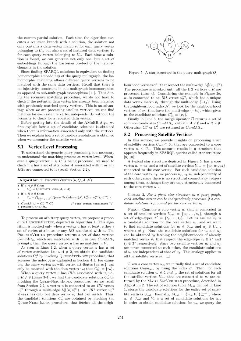
U2

Figure 5: A star structure in the query multigraph Q

bourhood vertices of v that respect the multi-edge LQE(u, uiri

i ).The procedure is invoked until all the IRI vertices u.R areprocessed (Line 4). Considering the example in Figure 2c,u3 is connected to an IRI -vertex uiri

0 , which has a uniquedata vertex match v5, through the multi-edge {−t3}. Usingthe neighbourhood index N , we look for the neighbourhoodvertices of v5, that have the multi-edge {−t3}, which givesus the candidate solutions CI

u3= {v1}.

Finally in Line 5, the merge operator ∩ returns a set ofcommon candidates CandAttu, only if u.A 6= ∅ and u.R 6= ∅.Otherwise, CA

u or CIu are returned as CandAttu.

5.2 Processing Satellite VerticesIn this section, we provide insights on processing a set

of satellite vertices Usat ⊆ Us that are connected to a corevertex uc ∈ Uc. This scenario results in a structure thatappears frequently in SPARQL queries called star structure[8, 10].

A typical star structure depicted in Figure 5, has a corevertex uc = u1, and a set of satellite vertices Usat = {u0, u2, u4}connected to the core vertex. For each candidate solutionof the core vertex u1, we process u0, u2, u4 independently ofeach other, since there is no structural connectivity (edges)among them, although they are only structurally connectedto the core vertex u1.

Lemma 2. For a given star structure in a query graph,each satellite vertex can be independently processed if a can-didate solution is provided for the core vertex uc.

Proof. Consider a core vertex uc that is connected toa set of satellite vertices Usat = {u0, . . . , us}, through aset of edge-types T ′ = {t0, . . . , ts}. Let us assume vc isa candidate solution for the core vertex uc, and we wantto find candidate solutions for ui ∈ Usat and uj ∈ Usat,where i 6= j. Now, the candidate solutions for ui and uj

can be obtained by fetching the neighbourhoods of alreadymatched vertex vc that respect the edge-type ti ∈ T ′ andtj ∈ T ′ respectively. Since two satellite vertices ui and uj

are never connected to each other, the candidate solutionsof ui are independent of that of uj . This analogy applies toall the satellite vertices.

Given a core vertex uc, we initially find a set of candidatesolutions Canduc , by using the index S. Then, for eachcandidate solution vc ∈ Canduc , the set of solutions for allthe satellite vertices Usat that are connected to uc are re-turned by the MatchSatVertices procedure, described inAlgorithm 2. The set of solution tuple Msat defined in Line1, stores the candidate solutions for the entire set of satel-

lite vertices Usat. Formally, Msat = {[us, Vs]}|Usat|s=1 , where

us ∈ Usat and Vs is a set of candidate solutions for us.In order to obtain candidate solutions for us, we query the

251

Algorithm 2: MatchSatVertices(A,N , Q, Usat, vc)

1 Set: Msat = ∅, where Msat = {[us, Vs]}|Usat|s=1

2 for all us ∈ Usat do

3 Candus = QueryNeighIndex(N , LQE(uc, us), vc)

4 Candus = Candus ∩ ProcessVertex(us, Q,A,N )5 if Candus 6= ∅ then6 Msat = Msat ∪ (us, Candus ) /* Satellite solutions */

7 else8 return Msat := 0 /* No solutions possible */

9 return Msat /* Matches for satellite vertices */

neighbourhood index N (Line 3); the QueryNeighIndexfunction obtains all the neighbourhood vertices of alreadymatched vc, that also considers the multi-edge in the querymultigraph LQ

E(uc, us). As every query vertex us ∈ Usat

is processed, the solution set Msat that contains candidatesolutions grows until all the satellite vertices have been pro-cessed (Lines 2-8).

In Line 4, the set of candidate solutions Candus are re-fined by invoking Algorithm 1 (VertexProcessing). Afterthe refinement, if there are finite candidate solutions, we up-date the solution Msat; else, we terminate the procedure asthere can be no matches for a given matched vertex vc. TheMatchSatVertices procedure performs two tasks: firstly,it checks if the candidate vertex vc ∈ Candus is a validmatchable vertex and secondly, it obtains the solutions forall the satellite vertices.

5.3 Arbitrary Query ProcessingAlgorithm 3 shows the generic procedure we develop to

process arbitrary queries.Recall that for an arbitrary query Q, we define two dif-

ferent types of vertexes: a set of core vertices Uc and a setof satellite vertices Us. The QueryDecompose procedurein Line 1 of Algorithm 3, performs this decomposition bysplitting the query vertices U into Uc and Us, as observedin Figure 4.

To process arbitrary query multigraphs, we perform recur-sive sub-mulitgraph matching procedure on the set of corevertices Uc ⊆ U ; during the recursion, satellite vertexes con-nected to a specific core vertex are processed too. Since therecursion is performed on the set of core vertices, we proposea few heuristics for ordering the query vertices.

Ordering of the query vertices forms one of the vital stepsfor subgraph matching algorithms [11]. In any subgraphmatching algorithm, the embeddings of a query subgraphare obtained by exploring the solution space spanned by thedata graph. But since the solution space itself can growexponentially in size, we are compelled to use intelligentstrategies to traverse the solution space. In order to achievethis, we propose a heuristic procedure VertexOrdering(Line 2, Algorithm 3) that employs two ranking functions.

The first ranking function r1 relies on the number of satel-lite vertices connected to the core vertex, and the query ver-tices are ordered with the decreasing rank value. Formally,r1(u) = |Usat|, where Usat = {us|us ∈ Us ∧ (u, us) ∈ E(Q)}.A vertex with more satellite vertices connected to it, is richin structure and hence it would probably yield fewer can-didate solutions to be processed under recursion. Thus, inFigure 4, u1 is chosen as an initial vertex. The second rank-ing function r2 relies on the number of incident edges ona query vertex. Formally, r2(u) =

∑mj=1 |σ(u)j |, where u

has m multiedges and |σ(u)j | captures the number of edgetypes in the jth multiedge. Again, Uord

c contains the orderedvertices with the decreasing rank value r2. Further, whenthere are no satellite vertices in the query Q, this rankingfunction gets the priority. Despite the usage of any rank-ing function, the query vertices in Uord

c , when accessed insequence, should be structurally connected to the previousset of vertices. If two vertices tie up with the same rank,the rank with lesser priority determines which vertex wins.Thus, for the example in Figure 4, the set of ordered corevertices is Uord

c = {u1, u3, u5}.

Algorithm 3: AMbER-Algo (I, Q)

1 QueryDecompose: Split U into Uc and Us

2 Uordc = VertexOrdering(Q,Uc)

3 uinit = u|u ∈ Uordc

4 CandInit = QuerySynIndex(uinit, S)5 CandInit = CandInit ∩ ProcessVertex(uinit, Q,A,N )

6 Fetch: Usatinit = {u|u ∈ Us ∧ (uinit, u) ∈ E(Q)}

7 Set: Emb = ∅8 for vinit ∈ CandInit do9 Set: M = ∅,Ms = ∅,Mc = ∅

10 if Usatinit 6= ∅ then

11 Msat = MatchSatVertices(A,N , Q, Usatinit, vinit)

12 if Msat 6= ∅ then13 for [us, Vs] ∈ Msat do14 Update: Ms = Ms ∪ [us, Vs]

15 Update: Mc = Mc ∪ [uinit, vinit]

16 Emb = Emb ∪ HomomorphicMatch(M, I, Q, Uordc )

17 else18 Update: Mc = Mc ∪ (uinit, vinit)

19 Emb = Emb ∪ HomomorphicMatch(M, I, Q, Uordc )

20 return Emb /* Homomorphic embeddings of query multigraph */

The first vertex in the set Uordc is chosen as the initial ver-

tex uinit (Line 3), and subsequent query vertices are chosenin sequence. The candidate solutions for the initial queryvertex CandInit are returned by QuerySynIndex proce-dure (Line 4), that are constrained by the structural prop-erties (neighbourhood structure) of uinit. By querying theindex S for initial query vertex uinit, we obtain the can-didate solutions CandInit ∈ V that match the structure(multiedge types) associated with uinit. Although some can-didates in CandInit may be invalid, all valid candidates arepresent in CandInit, as deduced in Lemma 1. Further, Pro-cessVertex procedure is invoked to obtain the candidatessolutions according to vertex attributes and IRI informa-tion, and then only the common candidates are retained.

Before getting into the algorithmic details, we explain howthe solutions are handled and how we process each queryvertex. We define M as a set of tuples, whose ith tuple isrepresented as Mi = [mc,Ms], where mc is a solution pairfor a core vertex, and Ms is a set of solution pairs for theset of satellite vertices that are connected to the core vertex.Formally mc = (uc, vc), where uc is the core vertex and vcis the corresponding matched vertex; Ms is a set of solutionpairs, whose jth element is a solution pair (us, Vs), whereus is a satellite vertex and Vs is a set of matched vertices.In addition, we maintain a set Mc whose elements are thesolution pairs for all the core vertices. Thus during eachrecursion branch, the size of M grows until it reaches thequery size |U |; once |M |= |U |, homomorphic matches areobtained.

For all the candidate solutions of initial vertex CandInit,

252

we perform recursion to obtain homomorphic embeddings(lines 8-19). Before getting into recursion, for each initialmatch vinit ∈ CandInit, if it has satellite vertices connectedto it, we invoke the MatchSatVertices procedure (Lines10-11). This step not only finds solution matches for satellitevertices, if there are, but also checks if vinit is a valid can-didate vertex. If the returned solution set Msat is empty,then vinit is not a valid candidate and hence we continuewith the next vinit ∈ CandInit; else, we update the set ofsolution pairs Ms for satellite vertices and the solution pairMc for the core vertex (Lines 12-15) and invoke Homomor-phicMatch procedure (Lines 17). On the other hand, ifthere are no satellite vertices connected to uinit, we updatethe core vertex solution set Mc and invoke Homomorphic-Match procedure (Lines 18-19).

Algorithm 4: HomomorphicMatch(M, I, Q, Uordc )

1 if |M |= |U | then2 return GenEmb(M)

3 Emb = ∅4 Fetch: unxt = u|u ∈ Uord

c5 Nq = {uc|uc ∈ Mc} ∩ adj(unxt)6 Ng = {vc|vc ∈ Mc ∧ (uc, vc) ∈ Mc}, where uc ∈ Nq

7 Candunxt =⋂|Nq|

n=1 (QueryNeighIndex(N , LQE(un, unxt), vn))

8 Candunxt = Candunxt∩ ProcessVertex(unxt, Q,A,N )9 for each vnxt ∈ Candunxt do

10 Fetch: Usatnxt = {u|u ∈ Vs ∧ (unxt, u) ∈ E(Q)}

11 if Usatnxt 6= ∅ then

12 Msat = MatchSatVertices(A,N , Q, Usatnxt, vnxt)

13 if Msat 6= ∅ then14 for every [us, V s] ∈ Msat do15 Update: Ms = Ms ∪ [us, V s]

16 Update: Mc = Mc ∪ (unxt, vnxt)

17 Emb = Emb ∪ HomomorphicMatch(M, I, Q, Uordc )

18 else19 Update: Mc = Mc ∪ (unxt, vnxt)

20 Emb = Emb ∪ HomomorphicMatch(M, I, Q, Uordc )

21 return Emb

In the HomomorphicMatch procedure (Algorithm 4),we fetch the next query vertex from the set of ordered corevertices Uord

c (Line 4). Then we collect the neighbourhoodvertices of already matched core query vertices and the cor-responding matched data vertices (Lines 5-6). As we recall,the set Mc maintains the solution pair mc = (uc, vc) of eachmatched core query vertex. The set Nq collects the alreadymatched core vertices uc ∈ Mc that are also in the neigh-bourhood of unxt, whose matches have to be found. Fur-ther, Ng contains the corresponding matched query verticesvc ∈ Mc. As the recursion proceeds, we find those match-able data vertices of unxt that are in the neighbourhood ofall the matched vertices v ∈ Ng, so that the query structureis maintained. In Line 7, for each un ∈ Nq and the corre-sponding vn ∈ Ng, we query the neighbourhood index N ,to obtain the candidate solutions Candunxt , that are in theneighbourhood of already matched data vertex vn and havethe multiedge LQ

E(un, unxt), obtained from the query multi-graph Q. Finally (line 7), the set of candidates solutions thatare common for every un ∈ Nq are retained in Candunxt .

Further, the candidate solutions are refined with the helpof ProcessVertex procedure (Line 8). Now, for each of thevalid candidate solution vnxt ∈ Candunxt , we recursively callthe HomomorphicMatch procedure. When the next queryvertex unxt has no satellite vertices attached to it, we update

the core vertex solution set Mc and call the recursion pro-cedure (Lines 19-20). But when unxt has satellite verticesattached to it, we obtain the candidate matches for all thesatellite vertices by invoking the MatchSatVertices pro-cedure (Lines 11-12); if there are matches, we update boththe satellite vertex solution Ms and the core vertex solutionMc, and invoke the recursion procedure (Line 17).

Once all the query vertices have been matched for thecurrent recursion step, the solution set M contains the so-lutions for both core and satellite vertices. Thus when allthe query vertices have been matched, we invoke the Gen-Emb function (Line 2) which returns the set of embeddings,that are updated in Emb. The GenEmb function treatsthe solution vertex vc of each core vertex as a singletonand performs Cartesian product among all the core vertexsingletons and satellite vertex sets. Formally, Embpart =

{v1c}× . . .×{v|Uc|c }×V 1

s × . . .×V|Us|c . Thus, the partial set

of embeddings Embpart is added to the final result Emb.

6. RELATED WORKThe proliferation of semantic web technologies has influ-

enced the popularity of RDF as a standard to representand share knowledge bases. In order to efficiently answerSPARQL queries, many stores and API inspired by rela-tional model were proposed [7, 3, 13, 5]. x-RDF-3X [13],inspired by modern RDBMS, represent RDF triples as a bigthree-attribute table. The RDF query processing is boostedusing an exhaustive indexing schema coupled with statisticsover the data. Also Virtuoso[7] heavily exploits RDBMSmechanism in order to answer SPARQL queries. Virtuosois a column-store based systems that employs sorted multi-column column-wise compressed projections. Also these sys-tems build table indexing using standard B-trees. Jena[5] supplies API for manipulating RDF graphs. Jena ex-ploits multiple-property tables that permit multiple viewsof graphs and vertices which can be used simultaneously.

Recently, the database community has started to inves-tigate RDF stores based on graph data management tech-niques [6, 16, 11]. The work in [6] addresses the problem ofsupporting property graphs as RDF, since majority of thegraph databases are based on property graph model. Theauthors introduce a property graph to RDF transformationscheme and propose three models to address the challengeof representing the key/value properties of property graphedges in RDF. gStore [16] applies graph pattern match-ing techniques using filter-and-refinement strategy to answerSPARQL queries. It employs an indexing schema, namedVS∗-tree, to concisely represent the RDF graph. Once theindex is built, it is used to find promising subgraphs thatmatch the query. Finally, exact subgraphs are enumeratedin the refinement step. Turbo Hom++ [11] is an adapta-tion of a state of the art subgraph isomorphism algorithm(TurboISO[9]) to the problem of SPARQL queries. Exploit-ing the standard graph isomorphism problem, the authorsrelax the injectivity constraint to handle the graph homo-morphism, which is the RDF pattern matching semantics.

Unlike our approach, TurboHom++ does not index theRDF graph, while gStore concisely represents RDF datathrough VS∗-tree. Another difference between AMbER andthe other graph stores is that our approach explicitly man-ages the multigraph induced by the SPARQL queries whileno clear discussion is supplied for the other tools.

253

7. EXPERIMENTAL ANALYSISIn this section, we perform extensive experiments on the

three RDF benchmarks. We evaluate the time performanceand the robustness of AMbER w.r.t. state-of-the-art com-petitors by varying the size, and the structure of the SPARQLqueries. Experiments are carried out on a 64-bit Intel Corei7-4900MQ @ 2.80GHz, with 32GB memory, running LinuxOS - Ubuntu 14.04 LTS. AMbER is implemented in C++.

7.1 Experimental SetupWe compare AMbER with the four standard RDF en-

gines: Virtuoso-7.1 [7], x-RDF-3X [13], Apache Jena [5] andgStore [16]. For all the competitors we employ the sourcecode available on the web site or obtained by the authors.Another recent work TurboHOM++ [11] has been excludedsince it is not publicly available.

For the experimental analysis we use three RDF datasets- DBPEDIA, YAGO and LUBM. DBPEDIA constitutes themost important knowledge base for the Semantic Web com-munity. Most of the data available in this dataset comesfrom the Wikipedia Infobox. YAGO is a real world datasetbuilt from factual information coming from Wikipedia andWordNet semantic network. LUBM provides a standardRDF benchmark to test the overall behaviour of engines.Using the data generator we create LUBM100 where thenumber represents the scaling factor.

Dataset # Triples # Vertices # Edges # Edge types

DBPEDIA 33 071 359 4 983 349 14 992 982 676YAGO 35 543 536 3 160 832 10 683 425 44LUBM100 13 824 437 2 179 780 8 952 366 13

Table 4: Benchmark Statistics

The data characteristics are summarized in Table 4. Wecan observe that the benchmarks have different character-istics in terms of number of vertices, number of edges, andnumber of distinct predicates. For instance, DBPEDIA hasmore diversity in terms of predicates (∼700) while LUBM100contains only 13 different predicates.

The time required to build the multigraph database aswell as to construct the indexes are reported in Table 5.We can note that the database building time and the cor-responding size are proportional to the number of triples.Regarding the indexing structures, we can underline thatboth building time and size are proportional to the numberof edges. For instance, DBPEDIA has the biggest numberof edges (∼15M) and, consequently, AMbER employs moretime and space to build and store its data structure.

Dataset Database Index I

Building Time Size Building Time Size

DBPEDIA 307 1300 45.18 1573YAGO 379 2400 29.1 1322LUBM100 67 497 18.4 1057

Table 5: Offline stage: Database and Index Constructiontime (in seconds) and memory usage (in Mbytes)

7.2 Workload GenerationIn order to test the scalability and the robustness of the

different RDF engines, we generate the query workloads con-sidering a similar setting as in [8, 1, 9]. We generate thequery workload from the respective RDF datasets, whichare available as RDF tripleset. In specific, we generate twotypes of query sets: a star-shaped and a complex-shapedquery set; further, both query sets are generated for varyingsizes (say k) ranging from 10 to 50 triplets, in steps of 10.

To generate star-shaped or complex-shaped queries of sizek, we pick an initial-entity at random from the RDF data.Now to generate star queries, we check if the initial-entityis present in at least k triples in the entire benchmark, toverify if the initial-entity has k neighbours. If so, we choosethose k triples at random; thus the initial entity forms thecentral vertex of the star structure and the rest of the en-tities form the remaining star structure, connected by therespective predicates. To generate complex-shaped queriesof size k, we navigate in the neighbourhood of the initial-entity through the predicate links until we reach size k. Inboth query types, we inject some object literals as well asconstant IRI s; rest of the IRI s (subjects or objects) aretreated as variables. However, this strategy could choosesome very unselective queries [8]. In order to address thisissue, we set a maximum time constraint of 60 seconds foreach query. If the query is not answered in time, it is notconsidered for the final average (similar procedure is usuallyemployed for graph query matching [9] and RDF workloadevaluation [1]). We report the average query time and, also,the percentage of unanswered queries (considering the giventime constraint) to study the robustness of the approaches.

7.3 Comparison with RDF EnginesIn this section we report and discuss the results obtained

by the different RDF engines. For each combination of querytype and benchmark we report two plots by varying thequery size: the average time and the corresponding percent-age of unanswered queries for the given time constraint. Weremind that the average time per approach is computed onlyon the set of queries that were answered.

The experimental results for DBPEDIA are depicted inFigure 6 and Figure 7. The time performance (averagedover 200 queries) for Star-Shaped queries (Fig. 6a), affirmthat AMbER clearly outperforms all the competitors. Fur-ther the robustness of each approach, evaluated in termsof percentage of unanswered queries within the stipulatedtime, is shown in Figure 6b. For the given time constraint,x-RDF-3X and Jena are unable to output results for size 20and 30 onwards respectively. Although Virtuoso and gStoreoutput results until query size 50, their time performanceis still poor. However, as the query size increases, the per-centage of unanswered queries for both Virtuoso and gStorekeeps on increasing from ∼0% to 65% and ∼45% to 95%respectively. On the other hand AMbER answers >98%of the queries, even for queries of size 50, establishing itsrobustness.

Analyzing the results for Complex-Shaped queries (Fig.7), we underline that AMbER still outperforms all the com-petitors for all sizes. In Figure 7a, we observe that x-RDF-3X and Jena are the slowest engines; Virtuoso and gStoreperform better than them but nowhere close to AMbER.We further observe that x-RDF-3X and Jena are the leastrobust as they don’t output results for size 30 onwards (Fig. 7b);

254

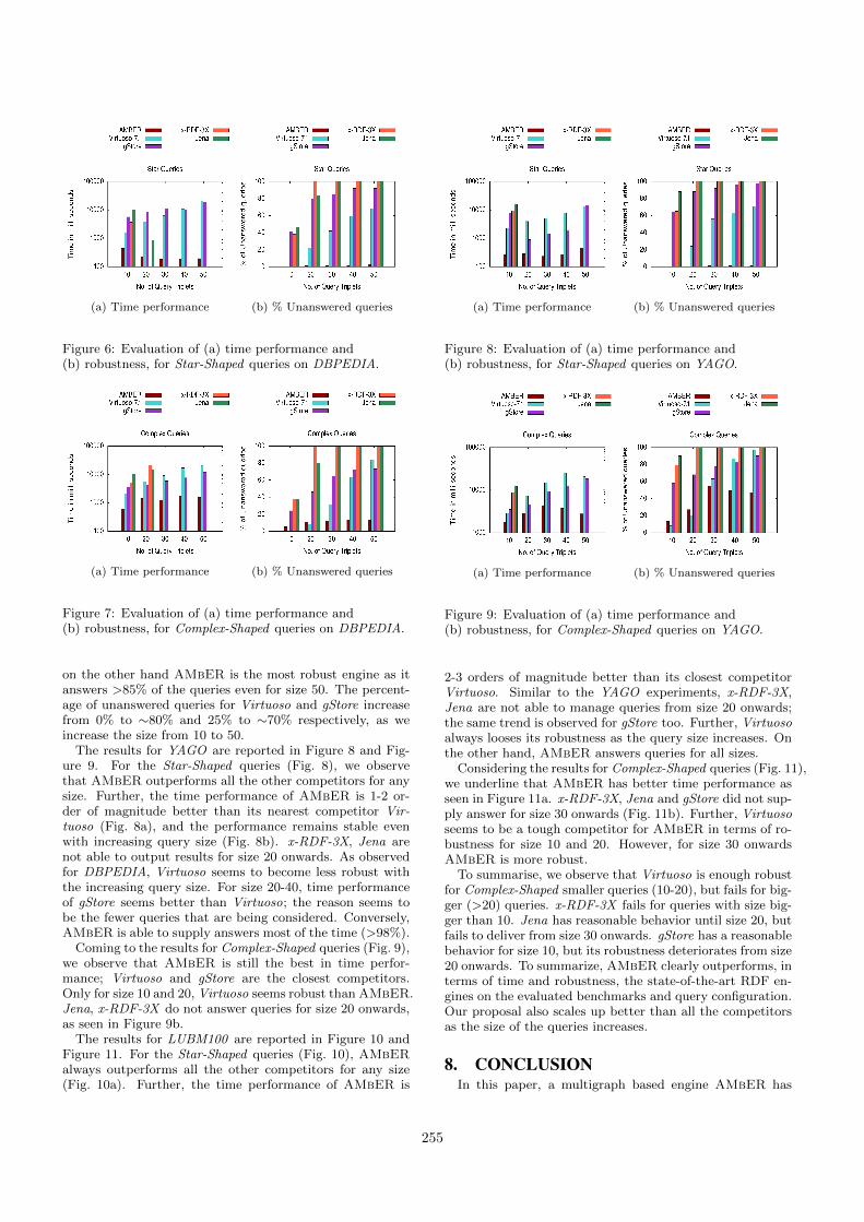
(a) Time performance (b) % Unanswered queries

Figure 6: Evaluation of (a) time performance and(b) robustness, for Star-Shaped queries on DBPEDIA.

(a) Time performance (b) % Unanswered queries

Figure 7: Evaluation of (a) time performance and(b) robustness, for Complex-Shaped queries on DBPEDIA.

on the other hand AMbER is the most robust engine as itanswers >85% of the queries even for size 50. The percent-age of unanswered queries for Virtuoso and gStore increasefrom 0% to ∼80% and 25% to ∼70% respectively, as weincrease the size from 10 to 50.

The results for YAGO are reported in Figure 8 and Fig-ure 9. For the Star-Shaped queries (Fig. 8), we observethat AMbER outperforms all the other competitors for anysize. Further, the time performance of AMbER is 1-2 or-der of magnitude better than its nearest competitor Vir-tuoso (Fig. 8a), and the performance remains stable evenwith increasing query size (Fig. 8b). x-RDF-3X, Jena arenot able to output results for size 20 onwards. As observedfor DBPEDIA, Virtuoso seems to become less robust withthe increasing query size. For size 20-40, time performanceof gStore seems better than Virtuoso; the reason seems tobe the fewer queries that are being considered. Conversely,AMbER is able to supply answers most of the time (>98%).

Coming to the results for Complex-Shaped queries (Fig. 9),we observe that AMbER is still the best in time perfor-mance; Virtuoso and gStore are the closest competitors.Only for size 10 and 20, Virtuoso seems robust than AMbER.Jena, x-RDF-3X do not answer queries for size 20 onwards,as seen in Figure 9b.

The results for LUBM100 are reported in Figure 10 andFigure 11. For the Star-Shaped queries (Fig. 10), AMbERalways outperforms all the other competitors for any size(Fig. 10a). Further, the time performance of AMbER is

(a) Time performance (b) % Unanswered queries

Figure 8: Evaluation of (a) time performance and(b) robustness, for Star-Shaped queries on YAGO.

(a) Time performance (b) % Unanswered queries

Figure 9: Evaluation of (a) time performance and(b) robustness, for Complex-Shaped queries on YAGO.

2-3 orders of magnitude better than its closest competitorVirtuoso. Similar to the YAGO experiments, x-RDF-3X,Jena are not able to manage queries from size 20 onwards;the same trend is observed for gStore too. Further, Virtuosoalways looses its robustness as the query size increases. Onthe other hand, AMbER answers queries for all sizes.

Considering the results for Complex-Shaped queries (Fig. 11),we underline that AMbER has better time performance asseen in Figure 11a. x-RDF-3X, Jena and gStore did not sup-ply answer for size 30 onwards (Fig. 11b). Further, Virtuososeems to be a tough competitor for AMbER in terms of ro-bustness for size 10 and 20. However, for size 30 onwardsAMbER is more robust.

To summarise, we observe that Virtuoso is enough robustfor Complex-Shaped smaller queries (10-20), but fails for big-ger (>20) queries. x-RDF-3X fails for queries with size big-ger than 10. Jena has reasonable behavior until size 20, butfails to deliver from size 30 onwards. gStore has a reasonablebehavior for size 10, but its robustness deteriorates from size20 onwards. To summarize, AMbER clearly outperforms, interms of time and robustness, the state-of-the-art RDF en-gines on the evaluated benchmarks and query configuration.Our proposal also scales up better than all the competitorsas the size of the queries increases.

8. CONCLUSIONIn this paper, a multigraph based engine AMbER has

255

(a) Time performance (b) % Unanswered queries

Figure 10: Evaluation of (a) time performance and(b) robustness, for Star-Shaped queries on LUBM100.

(a) Time performance (b) % Unanswered queries

Figure 11: Evaluation of (a) time performance and(b) robustness, for Complex-Shaped queries on LUBM100.

been proposed in order to answer complex SPARQL queriesover RDF data. The multigraph representation has be-stowed us with two advantages: on one hand, it enablesus to construct efficient indexing structures, that amelioratethe time performance of AMbER; on the other hand, thegraph representation itself motivates us to exploit the valu-able work done until now in the graph data managementfield. Thus, AMbER meticulously exploits the indexingstructures to address the problem of sub-multigraph homo-morphism, which in turn yields the solutions for SPARQLqueries. The proposed engine AMbER has been extensivelytested on three well established RDF benchmarks. As a re-sult, AMbER stands out w.r.t. the state-of-the-art RDFmanagement systems considering both the robustness re-garding the percentage of answered queries and the time per-formance. As a future work, we plan to extend AMbER byincorporating other SPARQL operations and, successively,study and develop a parallel processing version of our pro-posal to scale up over huge RDF data.

9. ACKNOWLEDGMENTSThis work has been funded by Labex NUMEV (NUMEV,

ANR-10-LABX-20).

10. REFERENCES[1] G. Aluc, O. Hartig, M. T. Ozsu, and K. Daudjee.

Diversified stress testing of RDF data management

systems. In ISWC, pages 197–212, 2014.

[2] G. Aluc, M. T. Ozsu, and K. Daudjee. Workloadmatters: Why RDF databases need a new design.PVLDB, 7(10):837–840, 2014.

[3] J. Broekstra, A. Kampman, and F. van Harmelen.Sesame: A generic architecture for storing andquerying RDF and RDF schema. In ISWC, pages54–68, 2002.

[4] E. Cabrio, J. Cojan, A. P. Aprosio, B. Magnini,A. Lavelli, and F. Gandon. Qakis: an open domain QAsystem based on relational patterns. In ISWC, 2012.

[5] J J. Carroll, I. Dickinson, C. Dollin, D. Reynolds,A. Seaborne, and K. Wilkinson. Jena: implementingthe semantic web recommendations. In WWW, pages74–83, 2004.

[6] Souripriya Das, Jagannathan Srinivasan, MatthewPerry, Eugene Inseok Chong, and Jayanta Banerjee. Atale of two graphs: Property graphs as rdf in oracle. InEDBT, pages 762–773, 2014.

[7] O. Erling. Virtuoso, a hybrid rdbms/graph columnstore. IEEE Data Eng. Bull., 35(1):3–8, 2012.

[8] A. Gubichev and T. Neumann. Exploiting the querystructure for efficient join ordering in sparql queries.In EDBT, pages 439–450, 2014.

[9] W.-S. Han, J. Lee, and J.-H. Lee. Turboiso: towardsultrafast and robust subgraph isomorphism search inlarge graph databases. In SIGMOD, pages 337–348,2013.

[10] J. Huang, D. J Abadi, and K. Ren. Scalable sparqlquerying of large rdf graphs. PVLDB,4(11):1123–1134, 2011.

[11] J. Kim, H. Shin, W.-S. Han, S. Hong, and H. Chafi.Taming subgraph isomorphism for RDF queryprocessing. PVLDB, 8(11):1238–1249, 2015.

[12] M. Morsey, J. Lehmann, S. Auer, and A.C.N. Ngomo.Dbpedia sparql benchmark performance assessmentwith real queries on real data. In ISWC, pages454–469, 2011.

[13] T. Neumann and G. Weikum. x-rdf-3x: Fast querying,high update rates, and consistency for RDF databases.PVLDB, 3(1):256–263, 2010.

[14] M. Terrovitis, S. Passas, P. Vassiliadis, and T. Sellis.A combination of trie-trees and inverted files for theindexing of set-valued attributes. In CIKM, pages728–737. ACM, 2006.

[15] L. Zou, R. Huang, H. Wang, J. Xu Yu, W. He, andD. Zhao. Natural language question answering overRDF: a graph data driven approach. In SIGMODConference, pages 313–324, 2014.

[16] L. Zou, M. T. Ozsu, L. Chen, X. Shen, R. Huang, andD. Zhao. gstore: a graph-based SPARQL queryengine. VLDB J., 23(4):565–590, 2014.

256