Quench dynamics of the 2d XY model

This article has been downloaded from IOPscience. Please scroll down to see the full text article.

J. Stat. Mech. (2011) P02032

(http://iopscience.iop.org/1742-5468/2011/02/P02032)

Download details:

IP Address: 131.91.169.193

The article was downloaded on 24/08/2013 at 08:45

Please note that terms and conditions apply.

View the table of contents for this issue, or go to the journal homepage for more

Home Search Collections Journals About Contact us My IOPscience

J.Stat.M

ech.(2011)

P02032

ournal of Statistical Mechanics:J Theory and Experiment

Quench dynamics of the 2d XY model

Asja Jelic1 and Leticia F Cugliandolo2

1 Universite Paris-Sud, Laboratoire de Physique Theorique, CNRS UMR 8627,Batiment 210, Orsay F-91405, France2 Universite Pierre et Marie Curie—Paris 6, Laboratoire de Physique Theoriqueet Hautes Energies, CNRS UMR 7589, 4, Place Jussieu, Tour 13, 5eme etage,75252 Paris Cedex 05, FranceE-mail: asja@lpthe.jussieu.fr and leticia@lpthe.jussieu.fr

Received 3 December 2010Accepted 27 January 2011Published 18 February 2011

Online at stacks.iop.org/JSTAT/2011/P02032doi:10.1088/1742-5468/2011/02/P02032

Abstract. We investigate the out of equilibrium dynamics of the two-dimensional XY model when cooled across the Berezinskii–Kosterlitz–Thouless(BKT) phase transition using different protocols. We focus on the evolution ofthe growing correlation length and the density of topological defects (vortices).By using Monte Carlo simulations we first determine the time and temperaturedependence of the growing correlation length after an infinitely rapid quenchfrom above the transition temperature to the quasi-long-range order region. Thefunctional form is consistent with a logarithmic correction to the diffusive law andit serves to validate dynamic scaling in this problem. This analysis clarifies thedifferent dynamic roles played by bound and free vortices. We then revisit theKibble–Zurek mechanism in thermal phase transitions in which the disorderedstate is plagued with topological defects. We provide a theory of quenchingrate dependence in systems with the BKT-type transition that goes beyondthe equilibrium scaling arguments. Finally, we discuss the implications of ourresults for a host of physical systems with vortex excitations, including planarferromagnets and liquid crystals.

Keywords: classical phase transitions (theory), coarsening processes (theory),slow dynamics and ageing (theory)

ArXiv ePrint: 1012.0417

c©2011 IOP Publishing Ltd and SISSA 1742-5468/11/P02032+26$33.00

J.Stat.M

ech.(2011)

P02032

Quench dynamics of the 2d XY model

Contents

1. Introduction 2

2. Model and method 42.1. The 2d XY model . . . . . . . . . . . . . . . . . . . . . . . . . . . . . . . 42.2. Dynamics . . . . . . . . . . . . . . . . . . . . . . . . . . . . . . . . . . . . 4

2.2.1. Monte Carlo dynamics. . . . . . . . . . . . . . . . . . . . . . . . . . 52.2.2. Time-dependent Ginzburg–Landau equation. . . . . . . . . . . . . . 6

3. The BKT equilibrium phase transition 6

4. Relaxation after a quench 74.1. Analytic prediction for the growing length . . . . . . . . . . . . . . . . . . 74.2. Numerical measurements of the growing length . . . . . . . . . . . . . . . . 9

4.2.1. Temperature dependence. . . . . . . . . . . . . . . . . . . . . . . . 104.3. Spatial structure . . . . . . . . . . . . . . . . . . . . . . . . . . . . . . . . 114.4. Pair distribution function . . . . . . . . . . . . . . . . . . . . . . . . . . . 12

5. Dynamics after a slow cooling 155.1. Snapshots . . . . . . . . . . . . . . . . . . . . . . . . . . . . . . . . . . . . 155.2. Equilibrium–out of equilibrium crossover . . . . . . . . . . . . . . . . . . . 185.3. Numerical estimate of the crossover length . . . . . . . . . . . . . . . . . . 205.4. Out of equilibrium evolution . . . . . . . . . . . . . . . . . . . . . . . . . . 205.5. Numerical measurements of vortex density . . . . . . . . . . . . . . . . . . 21

6. Conclusions 23

Acknowledgments 24

References 24

1. Introduction

The out of equilibrium dynamics of systems with continuous symmetries annealed orquenched from the symmetric to the symmetry broken phase is a subject of study indifferent branches of physics. Liquid crystals quenched across a phase transition intotheir ordered phase present a large variety of topological defects that diffuse, interactand eventually annihilate [1]. Vector ferromagnets cooled across their Curie temperatureare other condensed matter examples with a variety of dynamic topological defects [2].Cosmology provides a set of interesting models in which similar dynamics occur [3].Moreover, the decay of vortex density in freely decaying turbulence has also been ofinterest [4]. In all these areas, there is considerable interest in the dynamics of defectsonce the phase transition has been crossed.

Of special interest is the planar time-dependent Ginzburg–Landau model with SO(2)symmetry or its lattice counterpart, the 2d XY model. A static phase transition occurs ata finite critical temperature, TKT, between a high-T disordered paramagnet and a low-Tferromagnetic phase with quasi-long-range order. When the model is quenched from the

doi:10.1088/1742-5468/2011/02/P02032 2

J.Stat.M

ech.(2011)

P02032

Quench dynamics of the 2d XY model

high to the low temperature phase the continuous symmetry of the disordered phase isbroken to that of the ordered phase. In these systems the defects are singular vortices thatcarry topological charge and have logarithmic interactions [5]–[7]. In the high-T phase freevortices proliferate while in the low-T phase vortices bind in pairs. Physical realizations aretwo-dimensional planar ferromagnets [2], superconducting films [8], Josephson-junctionarrays [9], especially tailored nematic liquid crystals [10], toy models for two-dimensionalturbulence [4], and others (see [11]). The exponential singularity may also describe thecritical properties of superfluid helium films [12].

Phase ordering kinetics following an infinitely rapid quench through a thermal criticalpoint have been extensively studied in the statistical physics literature [13]. In condensedmatter applications the time spent close to the critical point, when the dynamics iscontrolled by the critical point, is typically much shorter than the time spent far fromit, when the dynamic mechanism is different and, therefore, the infinitely fast quenchapproximation is justified. A few studies where cooling rate dependences have been takeninto account are [14]–[17]. The study of cooling rate dependences in defect dynamics is, incontrast, central in cosmology. The goal in this case is to estimate the density of defects,ρ, left over in the universe after it went through a number of potential (second order)phase transitions. The importance lies on the fact that, initially, these were thought toact as seeds for matter clustering. This scenario seems to be excluded by observationdata now but, still, the interest in predicting the density of topological defects remainsdue to other possible effects of these objects [18]. In the late 1980s Zurek derived aquantitative prediction for ρ that is based on critical scaling in the disordered phaseclose to a second order phase transition. The proposal is based upon the hypothesiswhereby the defect dynamics should be negligible below the transition. In consequence,ρ is assumed to remain fixed to the value it takes at the control parameter at which thesystem falls out of equilibrium in the disordered phase. In his articles Zurek proposed tocheck these predictions in condensed matter systems with the same symmetry propertiesas the cosmological models [19]. A vast experimental [20, 21] and numerical [22] activityfollowed, with variable results summarized in [23].

The fact that the annihilation of defects can be neglected in the out of equilibriumregime was questioned in [24]. In this paper, a scaling argument that includes themechanism of defect annihilation in the low temperature phase for systems with secondorder phase transitions and dissipative dynamics was proposed. A scaling of the density ofdefects with cooling rate and time spent in the out of equilibrium evolution was derived.The predictions were checked numerically with Monte Carlo dynamics of the 2d Isingmodel, a paradigmatic system with discrete symmetry breaking. Similar ideas about theimportance of the dynamics below the transition were stressed in [25].

The treatment of all cases mentioned in the previous paragraph is classical.Recently, pushed by the advent of powerful experimental techniques in cold atomsystems, the extension of the Kibble–Zurek mechanism to quantum isolated systems wasdeveloped [26]–[28]. These claims have been critically revisited in [29, 30], as reviewedin [31].

In this paper we examine the density of vortices left over after going through theBerezinskii–Kosterlitz–Thouless classical phase transition [5, 6] with a finite speed. Werevisit the Kibble–Zurek mechanism and we provide a theory of quenching rate dependencein systems with continuous symmetry and the BKT-type of ‘infinite order’ phase transition

doi:10.1088/1742-5468/2011/02/P02032 3

J.Stat.M

ech.(2011)

P02032

Quench dynamics of the 2d XY model

that goes beyond the equilibrium scaling arguments. We test it with a Monte Carlonumerical study of the 2d XY model on a square lattice. We work in the canonicalsetting, in the sense that the system is coupled to an equilibrium environment thatallows for energy dissipation. As a control parameter driving the phase transition weuse the temperature of the heat bath. For concreteness we use linear cooling procedures,characterized by a single parameter, the cooling rate. A previous numerical study of thisproblem with a different method that ignores the effects of free vortices appeared in [32].We shall discuss the results in this paper and compare them with ours in the body of thiswork.

The organization of the paper is the following. In section 2 we recall the definitionsof the 2d XY model and the time-dependent Ginzburg–Landau equation and we presentthe Monte Carlo method used. In section 3 we briefly review the BKT scenario. Section 4is devoted to the analysis of infinitely rapid quenches. In section 5 we present our resultson annealing procedures. Finally, in section 6 we give our conclusions. Readers interestedjust in the slow cooling results can jump over sections 2–4 and go directly to section 5.

2. Model and method

In this section we recall the definition of the 2d XY model and we describe the MonteCarlo method that we use in our simulations of the lattice model. We also explain thecorresponding time-dependent Ginzburg–Landau stochastic equation.

2.1. The 2d XY model

The two-dimensional XY model is defined by the Hamiltonian

H = −J∑

〈i,j〉�si · �sj, (1)

with ferromagnetic exchange coupling, J > 0. The spins are classical variables constrainedto lie on a plane. Here �s2

i = 1, and the sum runs over nearest neighbors on a squarelattice of linear size L. It is convenient to use a parametrization in which the spin vectoris represented by the angle it forms with a chosen axis, �si = eiθi; with it the Hamiltonianbecomes

H = −J∑

〈i,j〉cos(θi − θj). (2)

Above the critical temperature TKT, unbound positively and negatively charged vorticesare present and the system is disordered. Below TKT vortex–antivortex pairs bind andthe system is critical in a sense that we shall make more precise below. The criticaltemperature is found to be kBTKT � 0.89J [6]. We measure T in units of J/kB in thefollowing.

2.2. Dynamics

Stochastic dynamics, mimicking the coupling of the classical spins to a thermal bath, canbe accounted for in different ways. In this section we define the Monte Carlo procedureused in our simulations. We focus on non-conserved order parameter dynamics (model A)

doi:10.1088/1742-5468/2011/02/P02032 4

J.Stat.M

ech.(2011)

P02032

Quench dynamics of the 2d XY model

in which the magnetization is not conserved. We also briefly recall the time-dependentGinzburg–Landau approach.

2.2.1. Monte Carlo dynamics. We performed a Monte Carlo study of the 2d XY modelon a square lattice of linear size L with periodic boundary conditions. The Monte Carloalgorithm consists in updating the angular variable θi associated to a randomly chosensite i to a new value θ′i randomly chosen in the interval [−π, π], with probabilityp = min{1, e−βΔE}, where ΔE is the energy variation between the two configurations.Equilibrium data are for relatively small system sizes, L = 16–50, while out of equilibriumones are for larger samples, L = 100–400. We briefly discuss finite size effects whenpresenting the simulation data. The results are an average of 5–10 000 independent runseach (depending on the quantity calculated) and one unit of time is an attempted moveof every spin.

In infinitely rapid quenches from infinite temperature we took a fully random initialcondition in which a random number θi in the interval [−π, π] is associated to site i. Weexplain the implementation of more sophisticated cooling procedures in section 5.

The focus of our study is the evolution of the number of vortices. We determine itnumerically with two types of measurements. On the one hand dynamic scaling impliesthat the density of vortices, ρv, should depend on the typical growing length, ξ, asρv � ξ−2. We shall use several determinations of ξ that include the exponential decayof the two-point correlation function, C[ξc(t, T ), t] = const., and the second moment of

C(r, t), that is defined as follows [33]. From the total magnetization �M(t) =∑

i �si(t) andthe magnetic susceptibility

χ(t) =1

L2�M2(t), (3)

the second moment correlation length on a lattice of size L2 is defined by

ξ22(t) =

1

(2 sin(π/L))2

(χ(t)

F (t)− 1

), (4)

where

F (t) =1

L2

∑

ij

〈�si(t) · �sj(t)〉 cos(2π(jx − ix)). (5)

In addition, we determine the number of vortices Nv directly from the configuration ofthe system by counting the plaquettes with non-zero vorticity. The vorticity is determinedas the integer winding number n, so that the phase difference θij ≡ θi − θj around theplaquette is equal to

∑θij = 2πn. The number of vortices Nv is then obtained as the

number of plaquettes around which the phase θi rotates through ±2π, taking care thatthe phase difference θij is restricted to the interval [−π, π], as are the phases θi. Thedensity of vortices is then ρv = Nv/L

2.In the figures we will not report the statistical errors because they are very small for

the quantities we consider (smaller than the dot dimensions in the various plots). Forexample, for the largest system size (L = 400) for which the fluctuations are larger, thevariance of the number of vortices is at most 3–4%.

doi:10.1088/1742-5468/2011/02/P02032 5

J.Stat.M

ech.(2011)

P02032

Quench dynamics of the 2d XY model

2.2.2. Time-dependent Ginzburg–Landau equation. A field theory version of this problem,better suited for analytic calculations, is given by the time-dependent Ginzburg–Landauequation that determines the stochastic evolution of the coarse-grained two-component

field �φ:

∂�φ(�r, t)

∂t= −Γ

δH

δ�φ(�r, t), (6)

with Γ the kinetic coefficient. The ‘free energy’ is

H =

∫d2r

[ρs

2(�∇�φ(�r))2 +

u

4(φ2(�r) − 1)2

], (7)

with ρs the stiffness coefficient or elastic constant and u > 0 the strength of thenonlinearity that drives the vector field to take unit modulus. Noise can be added toequation (6) in the form of an additional stochastic term in its right-hand-side withGaussian statistics and, typically, delta-correlated, 〈ζa(�r, t)ζb(�r

′, t′)〉 = 2kBTΓδabδ(�r −�r′)δ(t − t′), with a, b = 1, 2. The analytic predictions on the time-dependent growinglength to be discussed in section 4.1 have been obtained using this approach [34, 35].

3. The BKT equilibrium phase transition

We summarize the static properties of the 2d XY model as figured out by Berezinskii [5]and Kosterlitz and Thouless [6] (the BKT picture).

In the thermodynamic limit 2d XY models display no conventional long-rangeorder (the magnetization vanishes at all temperatures due to spin-wave excitations) buttopological order below a critical temperature TKT. The physics is dominated by two typesof excitations: harmonic spin waves and vortices. The former are responsible for destroyingconventional long-range order while the latter are responsible for the phase transition.The Berezinskii–Kosterlitz–Thouless (BKT) phase transition at TKT is characterized by achange in the behavior of the equilibrium spatial correlation function C(r) = 〈�si�sj〉||�ri−�rj |=r

where the angular brackets denote an average over the equilibrium measure. The high-Tphase is disordered, the correlation decays exponentially,

C(r) � e−r/ξeq , (8)

and there is a finite density of free vortices. Close to and above TKT the correlation lengthdiverges exponentially,

ξeq � aξebξ [(T−TKT)/TKT]−ν

, (9)

with ν = 1/2 and bξ a non-universal constant that typically takes a value of order one(on a square lattice bξ ∼ 1.5) [5, 6]. Thermodynamic quantities are smooth across thetransition. The low-T phase has quasi-long-range order,

C(r) � r−d+2−η(T ) = r−η(T ) ; (10)

it is critical in the sense that the equilibrium correlation length diverges, ξeq → ∞, andit is characterized by the T -dependent exponent η(T ) [6] that decreases upon decreasingtemperature from η(TKT) = 1/4 to η(T → 0) = T/(2πJ). Bound vortex–antivortex pairspopulate the low temperature ordered phase coexisting with spin waves. The transition is

doi:10.1088/1742-5468/2011/02/P02032 6

J.Stat.M

ech.(2011)

P02032

Quench dynamics of the 2d XY model

interpreted by using an analogy of the 2D XY model with the Coulomb gas where chargesplay the role of vortices. In fact, the Coulomb gas has a low temperature dielectric phasewith charges bound into dipoles, and a high temperature plasma or conducting phase withfree charges [5, 6]. In short, at TKT pairs dissociate.

The BKT singularity yields the best fit to data generated with large-scale MonteCarlo simulations and short time dynamics. The data tend to confirm the analyticalvalues of the exponents ν and η(T ) and the critical temperature was estimated to beTKT � 0.89 [36]–[40]. In finite size systems the effective transition temperature behavesas TKT + O(ln−2 L) [41]. Monte Carlo values of the correlation length ξeq(T ) obtainedwith lattices with linear size L = 512 are ξeq(1.25) � 3.8, ξeq(1.04) � 18.7, andξeq(0.98) � 70 [37]. We shall discuss our own data, obtained with much smaller systemsizes, in figure 11.

4. Relaxation after a quench

The nonequilibrium behavior of the 2d XY model following an instantaneous quench belowTKT has been studied theoretically as well as experimentally3 [10, 42]. In this section werecall the time dependence of the growing correlation length. We go beyond this by anow well-established aspect of the dynamics with a careful analysis of the temperaturedependence that will be of use in the rest of the paper. We present a detailed analysis ofthe vortex–antivortex time-dependent structure.

4.1. Analytic prediction for the growing length

In this section we prepare the system in a given initial condition and at t = 0 we letit evolve with the new parameter. At all T ≤ TKT a system prepared in an out ofequilibrium initial state approaches equilibrium through a coarsening process in whichlocal—critical—equilibrium is established over a length scale ξ(t, T ). The space–timecorrelation C(r, t) = 〈�si(t)�sj(t)〉||�ri−�rj |=r is governed by the scaling form

C(r, t) � r−η(T )f

(r

ξ(t, T )

). (11)

η(T ) is the static critical exponent. The scaling function depends on the initial conditions.We focus on high temperature, disordered ones. Here f(0) = 1 so that the equilibriumresult (10) is recovered for all a � r � ξ(t, T ), a being a microscopic cut-off length, and,in particular, in the infinite long time limit in which ξ(t, T ) → ∞. In the opposite limitr � ξ(t, T ) the system remains disordered, as in the initial condition, and this is ensuredby an f(x) that rapidly falls off for x � 1.

The relaxation of an out of equilibrium state is due to two processes: the dynamicsof Goldstone modes and the annihilation and pairing of vortices. One can tune theimportance of the vortex contribution by choosing the initial condition. For example, acompletely ordered configuration is free of vortices while a high temperature configurationhas a finite density of free vortices. After taking a fully ordered initial condition to

3 It is common in the field to claim that the times at which the measurements are made are much longer thanthe cooling times, in such a way that the cooling procedure can be ignored. This is true in some systems but notin others, and the experiments have to be analyzed in consequence.

doi:10.1088/1742-5468/2011/02/P02032 7

J.Stat.M

ech.(2011)

P02032

Quench dynamics of the 2d XY model

0 < T < TKT, no free vortices are generated by thermal fluctuations and the systemorders in the new conditions by growing a length ξ(t, T ) ∝ [λ0(T )t]1/2 [43, 44]. Instead,the relaxation of an initial condition with free vortices in the critical low temperaturephase is far more interesting. Whether dynamic scaling holds and, in the affirmative,what the time-dependent growth law is was a subject of debate for some time. Thefollowing scenario is well established now.

The numerical integration of the zero temperature Ginzburg–Landau equation usingfully random initial conditions (with, on average, a density of vortices of 1/3) firstsuggested a power law for ξ(t, T ) with a small but measurable deviation from the diffusivelaw t1/2 [45, 46]. This regime was considered to be a transient fully determined by thevortex annihilation dynamics. Yurke et al [34] and Bray et al [35] built upon these resultsand gave an argument for

ξ(t, T ) �{

λ(T )t

ln[t/t0(T )]

}1/z

z = 2 (12)

in quenches from equilibrium at T ≥ TKT to T = 0, see below. For the sake ofcompleteness, we wrote this expression inserting the dynamic exponents z (= 2 in thiscase). The extension to finite working T was worked out in [47]. This law was confirmedby extensive zero temperature numerical simulations in [48, 49]. The parameter λ(T )and the microscopic cut-off t0(T ) are non-universal in the sense that they depend on theprocedure used to measure ξ.

Let us briefly reproduce here the argument that leads to (12) and extend it later toinfer the relaxation time. Within the Ginzburg–Landau model (6), a field configuration,

describing a single free vortex �φ = �r/r, has an energy Ev = πρs ln(L/a), where L and aare the system size and microscopic cut-off (e.g., the lattice spacing). In the many-vortexsituation, where ξ(t) represents the typical spacing between vortices and antivortices, onecan derive the following expression for the typical speed of a vortex [34, 47], meaning thevelocity with which it approaches its partner antivortex:

dξ(t)

dt� ρsΓ

ξ(t) ln[ξ(t)/a](13)

from the zero temperature time-dependent Ginzburg–Landau equation (6). The solutionis equation (12) with t0 � a2/ρsΓ. We assume, following [47], that this equation holdsat finite T , and even above TKT where, though, the growing length saturates to theequilibrium correlation length at sufficiently long times. Matching the growing lengthwith the equilibrium law by dξ/dt|ξeq � ξeq/τeq above TKT one finds

τeq � ξzeq ln(ξeq/a). (14)

An exponential divergence of τeq with the distance to criticality is recovered by substitutingξeq with the expression in (9):

τeq � aτ ebξz[(T−TKT)/TKT]−ν

(T − TKT

TKT

)−ν

. (15)

The same behavior is estimated in [50] with a different argument.

doi:10.1088/1742-5468/2011/02/P02032 8

J.Stat.M

ech.(2011)

P02032

Quench dynamics of the 2d XY model

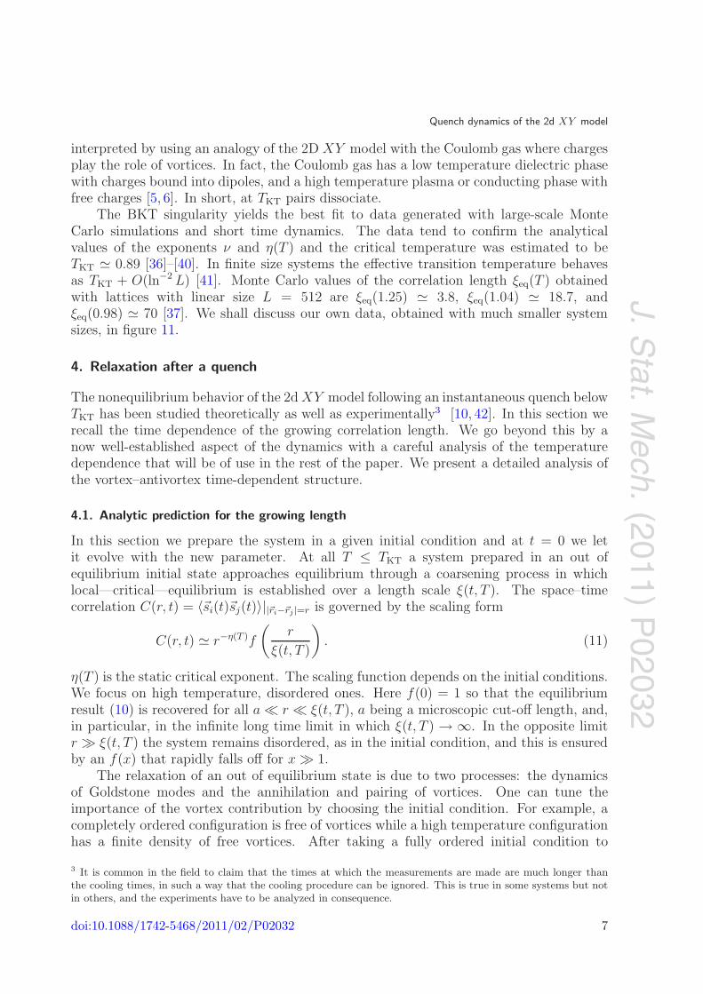
Figure 1. Space–time correlation after an infinitely rapid quench from a fullyrandom initial condition into the low temperature phase. (a) Bare data for C(r, t)at different times t after a quench to T = 0.5 that are given in the key. The insetshows the scaling plot rη(T )C against r/ξc(t, T ) using ξc(t, T ) computed fromC[ξc(t, T ), t] = 0.3. (b) ξc(t, T ) against t for instantaneous quenches to differenttemperatures.

4.2. Numerical measurements of the growing length

Although different determinations of the growing length should converge asymptoticallyto the same and unique law, some are more convenient than others at finite times.Comparison of different prescriptions (from scaling of the space–time correlation, thedensity of topological defects, and the structure factor) was discussed in [48, 49]. Werevisit this issue with the purpose of clarifying the different roles played by bound andfree vortices and establishing the temperature dependence of the correlation length.

In figure 1 we extract the growing length ξ(t, T ) from the decay of the space–time correlation. In the left panel we show the bare data, and we confirm that Csatisfies dynamic scaling by using the value of ξc(t, T ) inferred from the conditionC[ξc(t, T ), t] = 0.3. In the right panel we compare the time dependence of ξc(t, T ) tothe power law t1/2 and we see the expected slower growth at sufficiently long times. Thesmall deviations due to the logarithmic correction will be studied in more detail in figure 2.

Next we analyze the growing length as extracted from the density of vortices. Inthe fully random, infinite temperature limit, ρv � 0.3. In equilibrium at 2TKT wefound a value slightly smaller than 0.2 in agreement with data shown in [37]. Afterthe infinitely rapid quench the very high density of free vortices present in the initial hightemperature condition decreases. Two processes contribute to the re-organization of thevortex configuration. On the one hand over-abundant defects annihilate. On the otherhand vortices and antivortices bind to approach the non-vanishing equilibrium density ofpairs, ρeq � e−2μ/T with μ � 3.77 [37], that is an increasing function of T .

According to dynamic scaling, during the out of equilibrium relaxation the densityof defects in the ordered phase should decrease as ρv(t, T ) � 1/ξ2

v(t, T ), which usingequation (12) is equivalent to ρv(t, T ) ln ρv(t, T ) � t−1 [34]. In figure 2 we show ourdata for all vortices in two ways: in the left panel we plot ρv(t) as a function of t forseveral values of T ; in the right panel Nv(t) lnNv(t) as a function of t where Nv is thenumber of vortices selecting the case T = 0.4. After one MC step the density is very

doi:10.1088/1742-5468/2011/02/P02032 9

J.Stat.M

ech.(2011)

P02032

Quench dynamics of the 2d XY model

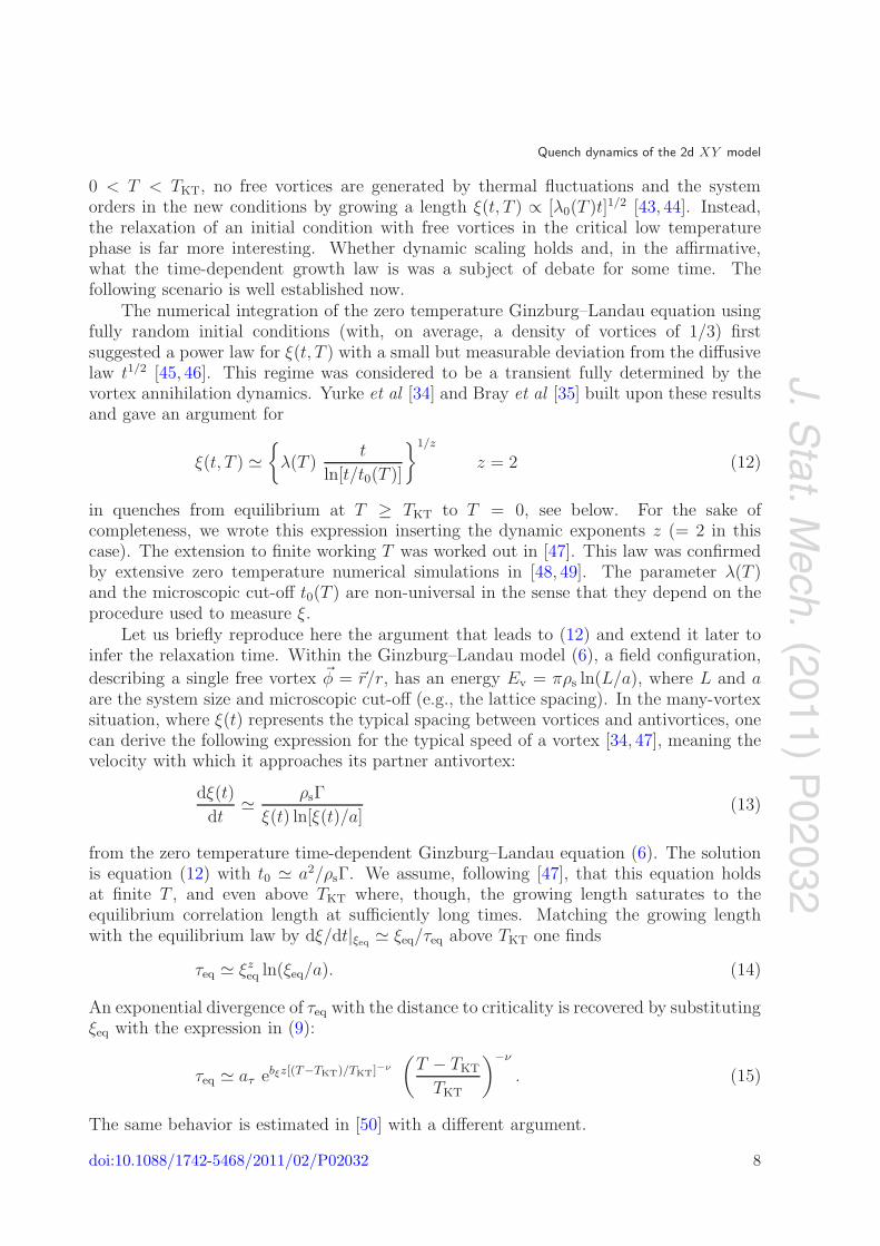
Figure 2. Time dependence of the total density of vortices, ρv(t, T ) ≡Nv(t, T )/L2, after an infinitely rapid quench from T0 → ∞ to 0 ≤ T ≤ TKT givenin the key. The data are shown in the form ρv(t) versus t in (a) and Nv ln Nv

versus t at a relatively low T in (b). The former display the deviation from the‘diffusive’ t−1 law. The latter confirms the expected logarithmic correction to apower law decay. The T dependence and, especially, the saturation observed athigh T are discussed in the text.

close to the initial value ρv(T → ∞) � 0.3 but it subsequently monotonically decreasesin time in all cases. As already stressed by Yurke et al [34], who solved numerically thetime-dependent Ginzburg–Landau equation with noise, the second presentation gives a

much better description of data for T<∼ 0.4, confirming the growth law (12). However,

at T close to TKT the number of vortices gets close to the equilibrium value, for exampleρeq � 10−4 at T = 0.8, and the crossover to equilibrium dynamics is reached within thesimulation times. This is accompanied by the generation of many short-lived vortex–antivortex pairs, similar to what was observed in [34], and the data deviate from theexpected scaling. The failure of scaling of the space–time correlation when ξv is used wasalso mentioned in [48, 49].

A more precise determination of the growing length at temperatures close to TKT

should be given by the evolution of the density of free vortices only, ρfv. The identification

of free vortices involves, however, some ambiguity. We used a simple-minded form thatconsists in counting as free all vortices and antivortices that do not have a neighbor ofopposite vorticity at Euclidean distance r ≤ rc. By varying the parameter rc from 1 to2 we found that the second choice gives very good results, shown in figure 3 in the formN f

v ln N fv against t for T = 0.4, 0.6, 0.8. (In [53] rc is chosen to be equal to ξ(t, T ).)

Consistently, ξfv � ξv at sufficiently low temperatures (say, T ≤ 0.4) but the two depart at

higher temperatures, with the former yielding the correct out of equilibrium correlationlength and being the one that ensures dynamic scaling.

4.2.1. Temperature dependence. The T dependence in λ and t0 in equation (12) has notbeen fully established yet. The assumption that at finite temperature the dynamics onscales that are shorter than ξ(t, T ) should be described, in the limit of large ξ(t, T ),by renormalized spin-wave theory [35, 47] suggests λ(T ) = ρs(T )Γ(T ) and t0(T ) =a2/[ρs(T )Γ(T )] at all T ≤ TKT. a is the lattice spacing or microscopic cut-off, ρs

the renormalized spin-wave stiffness and Γ the renormalized kinetic coefficient in the

doi:10.1088/1742-5468/2011/02/P02032 10

J.Stat.M

ech.(2011)

P02032

Quench dynamics of the 2d XY model

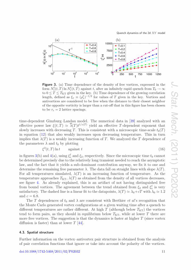
Figure 3. (a) Time dependence of the density of free vortices, expressed in theform N f

v(t, T ) ln N fv(t, T ) against t, after an infinitely rapid quench from T0 → ∞

to 0 ≤ T ≤ TKT given in the key. (b) Time dependence of the growing correlationlength, defined as ξv ≡ (ρf

v)−1/2 for values of T given in the key. Vortices andantivortices are considered to be free when the distance to their closest neighborof the opposite vorticity is larger than a cut-off that in this figure has been chosento be rc = 2 lattice spacings.

time-dependent Ginzburg–Landau model. The numerical data in [39] analyzed with aneffective power law ξ(t, T ) � λ(T )t1/z(T ) yield an effective T -dependent exponent thatslowly increases with decreasing T . This is consistent with a microscopic time-scale t0(T )in equation (12) that also weakly increases upon decreasing temperature. This in turnimplies that λ(T ) is a weakly increasing function of T . We analyzed the T dependence ofthe parameters λ and t0 by plotting

ξ2(t, T ) ln t against t (16)

in figures 3(b) and 4(a), using ξfv and ξ2, respectively. Since the microscopic time t0 cannot

be determined precisely due to the relatively long transient needed to reach the asymptoticlaw, and the fact that it yields a sub-dominant contribution anyway, we fix it to one anddetermine the remaining free parameter λ. The data fall on straight lines with slope λ(T ).For all temperatures simulated, λ(T ) is an increasing function of temperature. As thetemperature approaches TKT, λ(T ) as obtained from the density of all vortices decreases,see figure 4. As already explained, this is an artifact of not having distinguished freefrom bound vortices. The agreement between the trend obtained from ξ2 and ξf

v is verysatisfactory. The dashed line is a linear fit to the datapoints, λ(T ) � λ0+cT with λ0 � 1.2and c = 6.8.

The T dependences of t0 and λ are consistent with Berthier et al ’s recognition thatthe Monte Carlo generated vortex configurations at a given waiting time after a quench todifferent temperatures are rather different. At high T (although below TKT) the vorticestend to form pairs, as they should in equilibrium below TKT, while at lower T there aremore free vortices. The suggestion is that the dynamics is faster at higher T (since vortexdiffusion is faster) than at lower T [44].

4.3. Spatial structure

Further information on the vortex–antivortex pair structure is obtained from the analysisof pair correlation functions that ignore or take into account the polarity of the vortices.

doi:10.1088/1742-5468/2011/02/P02032 11

J.Stat.M

ech.(2011)

P02032

Quench dynamics of the 2d XY model

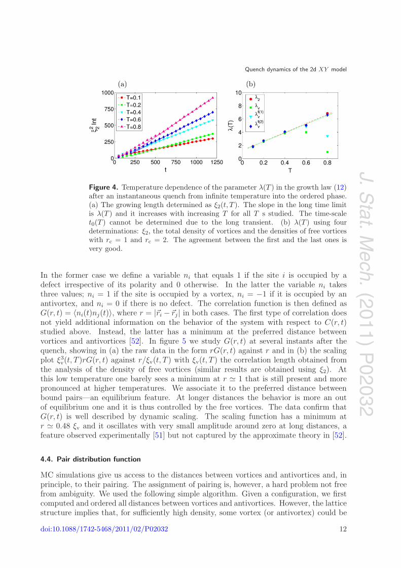
Figure 4. Temperature dependence of the parameter λ(T ) in the growth law (12)after an instantaneous quench from infinite temperature into the ordered phase.(a) The growing length determined as ξ2(t, T ). The slope in the long time limitis λ(T ) and it increases with increasing T for all T s studied. The time-scalet0(T ) cannot be determined due to the long transient. (b) λ(T ) using fourdeterminations: ξ2, the total density of vortices and the densities of free vorticeswith rc = 1 and rc = 2. The agreement between the first and the last ones isvery good.

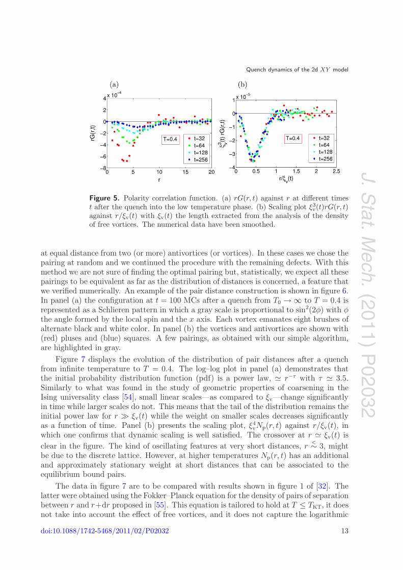
In the former case we define a variable ni that equals 1 if the site i is occupied by adefect irrespective of its polarity and 0 otherwise. In the latter the variable ni takesthree values; ni = 1 if the site is occupied by a vortex, ni = −1 if it is occupied by anantivortex, and ni = 0 if there is no defect. The correlation function is then defined asG(r, t) = 〈ni(t)nj(t)〉, where r = |�ri − �rj| in both cases. The first type of correlation doesnot yield additional information on the behavior of the system with respect to C(r, t)studied above. Instead, the latter has a minimum at the preferred distance betweenvortices and antivortices [52]. In figure 5 we study G(r, t) at several instants after thequench, showing in (a) the raw data in the form rG(r, t) against r and in (b) the scalingplot ξ3

v(t, T )rG(r, t) against r/ξv(t, T ) with ξv(t, T ) the correlation length obtained fromthe analysis of the density of free vortices (similar results are obtained using ξ2). Atthis low temperature one barely sees a minimum at r � 1 that is still present and morepronounced at higher temperatures. We associate it to the preferred distance betweenbound pairs—an equilibrium feature. At longer distances the behavior is more an outof equilibrium one and it is thus controlled by the free vortices. The data confirm thatG(r, t) is well described by dynamic scaling. The scaling function has a minimum atr � 0.48 ξv and it oscillates with very small amplitude around zero at long distances, afeature observed experimentally [51] but not captured by the approximate theory in [52].

4.4. Pair distribution function

MC simulations give us access to the distances between vortices and antivortices and, inprinciple, to their pairing. The assignment of pairing is, however, a hard problem not freefrom ambiguity. We used the following simple algorithm. Given a configuration, we firstcomputed and ordered all distances between vortices and antivortices. However, the latticestructure implies that, for sufficiently high density, some vortex (or antivortex) could be

doi:10.1088/1742-5468/2011/02/P02032 12

J.Stat.M

ech.(2011)

P02032

Quench dynamics of the 2d XY model

Figure 5. Polarity correlation function. (a) rG(r, t) against r at different timest after the quench into the low temperature phase. (b) Scaling plot ξ3

v(t)rG(r, t)against r/ξv(t) with ξv(t) the length extracted from the analysis of the densityof free vortices. The numerical data have been smoothed.

at equal distance from two (or more) antivortices (or vortices). In these cases we chose thepairing at random and we continued the procedure with the remaining defects. With thismethod we are not sure of finding the optimal pairing but, statistically, we expect all thesepairings to be equivalent as far as the distribution of distances is concerned, a feature thatwe verified numerically. An example of the pair distance construction is shown in figure 6.In panel (a) the configuration at t = 100 MCs after a quench from T0 → ∞ to T = 0.4 isrepresented as a Schlieren pattern in which a gray scale is proportional to sin2(2φ) with φthe angle formed by the local spin and the x axis. Each vortex emanates eight brushes ofalternate black and white color. In panel (b) the vortices and antivortices are shown with(red) pluses and (blue) squares. A few pairings, as obtained with our simple algorithm,are highlighted in gray.

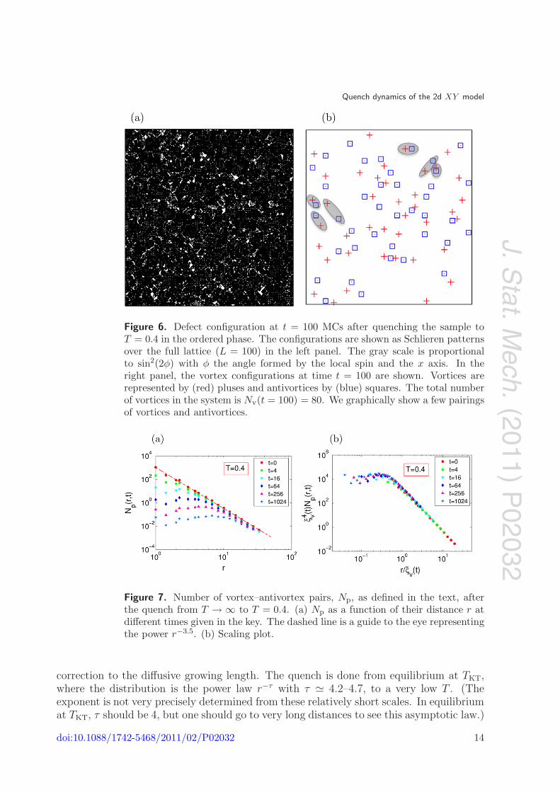
Figure 7 displays the evolution of the distribution of pair distances after a quenchfrom infinite temperature to T = 0.4. The log–log plot in panel (a) demonstrates thatthe initial probability distribution function (pdf) is a power law, � r−τ with τ � 3.5.Similarly to what was found in the study of geometric properties of coarsening in theIsing universality class [54], small linear scales—as compared to ξv—change significantlyin time while larger scales do not. This means that the tail of the distribution remains theinitial power law for r � ξv(t) while the weight on smaller scales decreases significantlyas a function of time. Panel (b) presents the scaling plot, ξ4

vNp(r, t) against r/ξv(t), inwhich one confirms that dynamic scaling is well satisfied. The crossover at r � ξv(t) is

clear in the figure. The kind of oscillating features at very short distances, r<∼ 3, might

be due to the discrete lattice. However, at higher temperatures Np(r, t) has an additionaland approximately stationary weight at short distances that can be associated to theequilibrium bound pairs.

The data in figure 7 are to be compared with results shown in figure 1 of [32]. Thelatter were obtained using the Fokker–Planck equation for the density of pairs of separationbetween r and r+dr proposed in [55]. This equation is tailored to hold at T ≤ TKT, it doesnot take into account the effect of free vortices, and it does not capture the logarithmic

doi:10.1088/1742-5468/2011/02/P02032 13

J.Stat.M

ech.(2011)

P02032

Quench dynamics of the 2d XY model

Figure 6. Defect configuration at t = 100 MCs after quenching the sample toT = 0.4 in the ordered phase. The configurations are shown as Schlieren patternsover the full lattice (L = 100) in the left panel. The gray scale is proportionalto sin2(2φ) with φ the angle formed by the local spin and the x axis. In theright panel, the vortex configurations at time t = 100 are shown. Vortices arerepresented by (red) pluses and antivortices by (blue) squares. The total numberof vortices in the system is Nv(t = 100) = 80. We graphically show a few pairingsof vortices and antivortices.

Figure 7. Number of vortex–antivortex pairs, Np, as defined in the text, afterthe quench from T → ∞ to T = 0.4. (a) Np as a function of their distance r atdifferent times given in the key. The dashed line is a guide to the eye representingthe power r−3.5. (b) Scaling plot.

correction to the diffusive growing length. The quench is done from equilibrium at TKT,where the distribution is the power law r−τ with τ � 4.2–4.7, to a very low T . (Theexponent is not very precisely determined from these relatively short scales. In equilibriumat TKT, τ should be 4, but one should go to very long distances to see this asymptotic law.)

doi:10.1088/1742-5468/2011/02/P02032 14

J.Stat.M

ech.(2011)

P02032

Quench dynamics of the 2d XY model

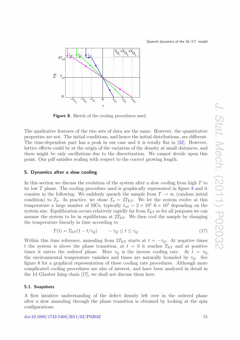
Figure 8. Sketch of the cooling procedures used.

The qualitative features of the two sets of data are the same. However, the quantitativeproperties are not. The initial conditions, and hence the initial distributions, are different.The time-dependent part has a peak in our case and it is totally flat in [32]. However,lattice effects could be at the origin of the variation of the density at small distances, andthese might be only oscillations due to the discretization. We cannot decide upon thispoint. Our pdf satisfies scaling with respect to the correct growing length.

5. Dynamics after a slow cooling

In this section we discuss the evolution of the system after a slow cooling from high T toits low T phase. The cooling procedure used is graphically represented in figure 8 and itconsists in the following. We suddenly quench the sample from T → ∞ (random initialcondition) to T0. In practice, we chose T0 = 2TKT. We let the system evolve at thistemperature a large number of MCs, typically trel = 2 × 105–6 × 105 depending on thesystem size. Equilibration occurs relatively rapidly far from TKT so for all purposes we canassume the system to be in equilibrium at 2TKT. We then cool the sample by changingthe temperature linearly in time according to

T (t) = TKT(1 − t/τQ) − τQ ≤ t ≤ τQ. (17)

Within this time reference, annealing from 2TKT starts at t = −τQ. At negative timest the system is above the phase transition, at t = 0 it reaches TKT and at positivetimes it enters the ordered phase. Here τQ is the inverse cooling rate. At t = τQ

the environmental temperature vanishes and times are naturally bounded by τQ. Seefigure 8 for a graphical representation of these cooling rate procedures. Although morecomplicated cooling procedures are also of interest, and have been analyzed in detail inthe 1d Glauber Ising chain [17], we shall not discuss them here.

5.1. Snapshots

A first intuitive understanding of the defect density left over in the ordered phaseafter a slow annealing through the phase transition is obtained by looking at the spinconfigurations.

doi:10.1088/1742-5468/2011/02/P02032 15

J.Stat.M

ech.(2011)

P02032

Quench dynamics of the 2d XY model

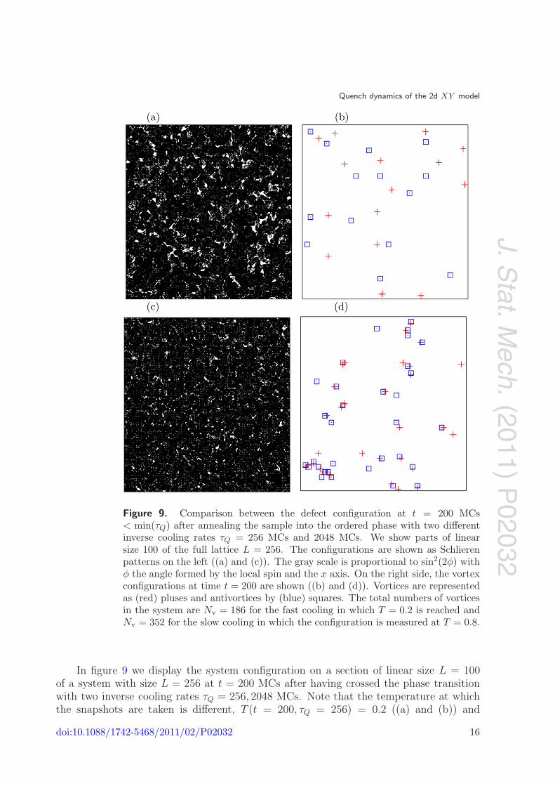
Figure 9. Comparison between the defect configuration at t = 200 MCs< min(τQ) after annealing the sample into the ordered phase with two differentinverse cooling rates τQ = 256 MCs and 2048 MCs. We show parts of linearsize 100 of the full lattice L = 256. The configurations are shown as Schlierenpatterns on the left ((a) and (c)). The gray scale is proportional to sin2(2φ) withφ the angle formed by the local spin and the x axis. On the right side, the vortexconfigurations at time t = 200 are shown ((b) and (d)). Vortices are representedas (red) pluses and antivortices by (blue) squares. The total numbers of vorticesin the system are Nv = 186 for the fast cooling in which T = 0.2 is reached andNv = 352 for the slow cooling in which the configuration is measured at T = 0.8.

In figure 9 we display the system configuration on a section of linear size L = 100of a system with size L = 256 at t = 200 MCs after having crossed the phase transitionwith two inverse cooling rates τQ = 256, 2048 MCs. Note that the temperature at whichthe snapshots are taken is different, T (t = 200, τQ = 256) = 0.2 ((a) and (b)) and

doi:10.1088/1742-5468/2011/02/P02032 16

J.Stat.M

ech.(2011)

P02032

Quench dynamics of the 2d XY model

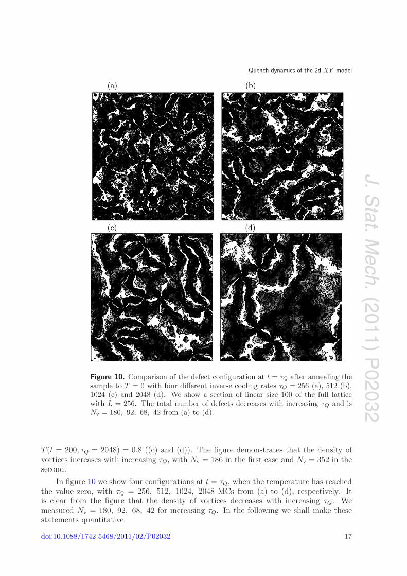
Figure 10. Comparison of the defect configuration at t = τQ after annealing thesample to T = 0 with four different inverse cooling rates τQ = 256 (a), 512 (b),1024 (c) and 2048 (d). We show a section of linear size 100 of the full latticewith L = 256. The total number of defects decreases with increasing τQ and isNv = 180, 92, 68, 42 from (a) to (d).

T (t = 200, τQ = 2048) = 0.8 ((c) and (d)). The figure demonstrates that the density ofvortices increases with increasing τQ, with Nv = 186 in the first case and Nv = 352 in thesecond.

In figure 10 we show four configurations at t = τQ, when the temperature has reachedthe value zero, with τQ = 256, 512, 1024, 2048 MCs from (a) to (d), respectively. Itis clear from the figure that the density of vortices decreases with increasing τQ. Wemeasured Nv = 180, 92, 68, 42 for increasing τQ. In the following we shall make thesestatements quantitative.

doi:10.1088/1742-5468/2011/02/P02032 17

J.Stat.M

ech.(2011)

P02032

Quench dynamics of the 2d XY model

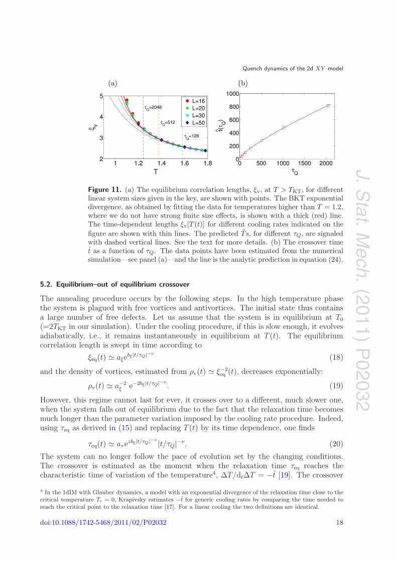
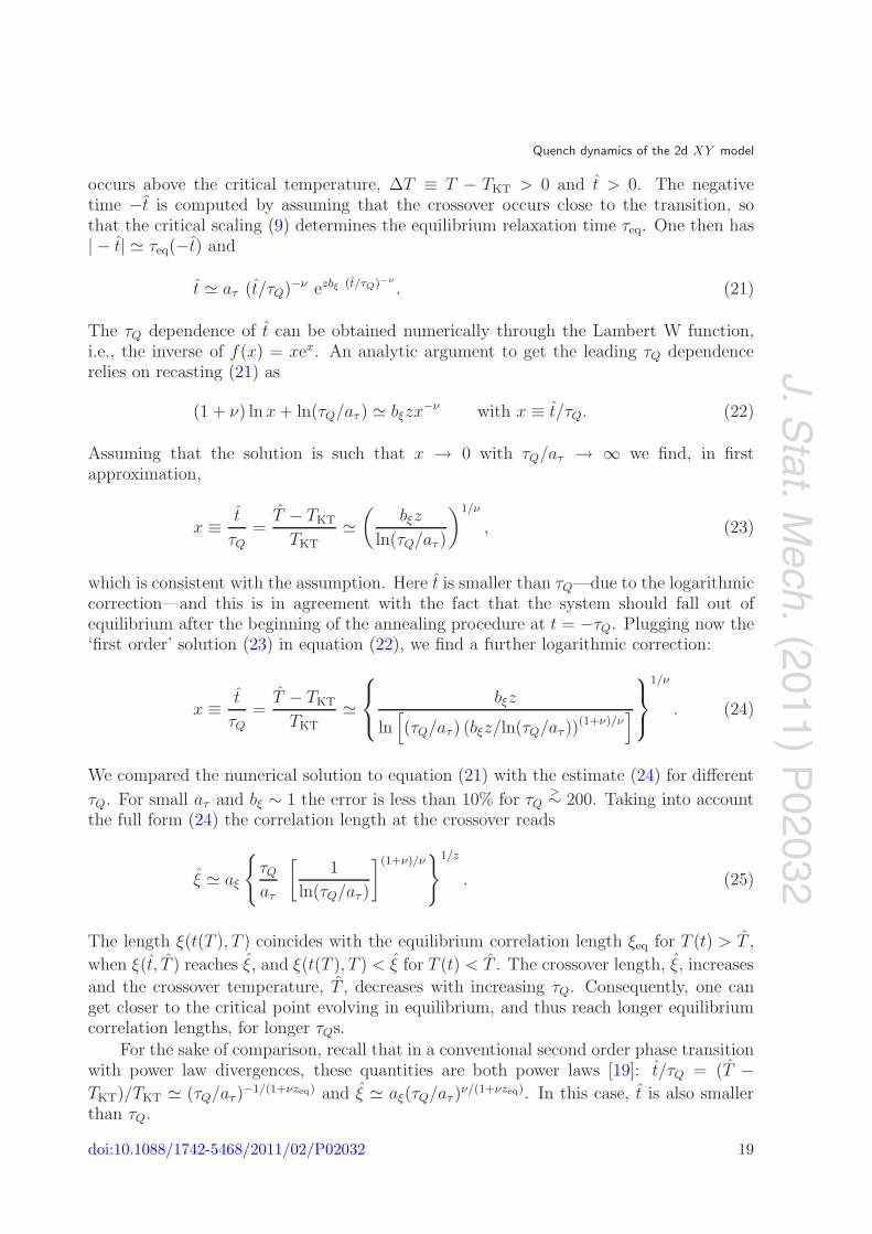
Figure 11. (a) The equilibrium correlation lengths, ξv, at T > TKT, for differentlinear system sizes given in the key, are shown with points. The BKT exponentialdivergence, as obtained by fitting the data for temperatures higher than T = 1.2,where we do not have strong finite size effects, is shown with a thick (red) line.The time-dependent lengths ξv[T (t)] for different cooling rates indicated on thefigure are shown with thin lines. The predicted T s, for different τQ, are signaledwith dashed vertical lines. See the text for more details. (b) The crossover timet as a function of τQ. The data points have been estimated from the numericalsimulation—see panel (a)—and the line is the analytic prediction in equation (24).

5.2. Equilibrium–out of equilibrium crossover

The annealing procedure occurs by the following steps. In the high temperature phasethe system is plagued with free vortices and antivortices. The initial state thus containsa large number of free defects. Let us assume that the system is in equilibrium at T0

(=2TKT in our simulation). Under the cooling procedure, if this is slow enough, it evolvesadiabatically, i.e., it remains instantaneously in equilibrium at T (t). The equilibriumcorrelation length is swept in time according to

ξeq(t) � aξebξ |t/τQ|−ν

(18)

and the density of vortices, estimated from ρv(t) � ξ−2eq (t), decreases exponentially:

ρv(t) � a−2ξ e−2bξ |t/τQ|−ν

. (19)

However, this regime cannot last for ever, it crosses over to a different, much slower one,when the system falls out of equilibrium due to the fact that the relaxation time becomesmuch longer than the parameter variation imposed by the cooling rate procedure. Indeed,using τeq as derived in (15) and replacing T (t) by its time dependence, one finds

τeq(t) � aτezbξ|t/τQ|−ν |t/τQ|−ν. (20)

The system can no longer follow the pace of evolution set by the changing conditions.The crossover is estimated as the moment when the relaxation time τeq reaches thecharacteristic time of variation of the temperature4, ΔT/dtΔT = −t [19]. The crossover

4 In the 1dIM with Glauber dynamics, a model with an exponential divergence of the relaxation time close to thecritical temperature Tc = 0, Krapivsky estimates −t for generic cooling rates by comparing the time needed toreach the critical point to the relaxation time [17]. For a linear cooling the two definitions are identical.

doi:10.1088/1742-5468/2011/02/P02032 18

J.Stat.M

ech.(2011)

P02032

Quench dynamics of the 2d XY model

occurs above the critical temperature, ΔT ≡ T − TKT > 0 and t > 0. The negativetime −t is computed by assuming that the crossover occurs close to the transition, sothat the critical scaling (9) determines the equilibrium relaxation time τeq. One then has| − t| � τeq(−t) and

t � aτ (t/τQ)−ν ezbξ (t/τQ)−ν

. (21)

The τQ dependence of t can be obtained numerically through the Lambert W function,i.e., the inverse of f(x) = xex. An analytic argument to get the leading τQ dependencerelies on recasting (21) as

(1 + ν) ln x + ln(τQ/aτ ) � bξzx−ν with x ≡ t/τQ. (22)

Assuming that the solution is such that x → 0 with τQ/aτ → ∞ we find, in firstapproximation,

x ≡ t

τQ

=T − TKT

TKT

�(

bξz

ln(τQ/aτ )

)1/ν

, (23)

which is consistent with the assumption. Here t is smaller than τQ—due to the logarithmiccorrection—and this is in agreement with the fact that the system should fall out ofequilibrium after the beginning of the annealing procedure at t = −τQ. Plugging now the‘first order’ solution (23) in equation (22), we find a further logarithmic correction:

x ≡ t

τQ

=T − TKT

TKT

�⎧⎨

⎩bξz

ln[(τQ/aτ ) (bξz/ln(τQ/aτ ))

(1+ν)/ν]

⎫⎬

⎭

1/ν

. (24)

We compared the numerical solution to equation (21) with the estimate (24) for different

τQ. For small aτ and bξ ∼ 1 the error is less than 10% for τQ>∼ 200. Taking into account

the full form (24) the correlation length at the crossover reads

ξ � aξ

{τQ

aτ

[1

ln(τQ/aτ )

](1+ν)/ν}1/z

. (25)

The length ξ(t(T ), T ) coincides with the equilibrium correlation length ξeq for T (t) > T ,

when ξ(t, T ) reaches ξ, and ξ(t(T ), T ) < ξ for T (t) < T . The crossover length, ξ, increases

and the crossover temperature, T , decreases with increasing τQ. Consequently, one canget closer to the critical point evolving in equilibrium, and thus reach longer equilibriumcorrelation lengths, for longer τQs.

For the sake of comparison, recall that in a conventional second order phase transitionwith power law divergences, these quantities are both power laws [19]: t/τQ = (T −TKT)/TKT � (τQ/aτ )

−1/(1+νzeq) and ξ � aξ(τQ/aτ )ν/(1+νzeq). In this case, t is also smaller

than τQ.

doi:10.1088/1742-5468/2011/02/P02032 19

J.Stat.M

ech.(2011)

P02032

Quench dynamics of the 2d XY model

5.3. Numerical estimate of the crossover length

In order to put the prediction for ξ to the test we compared the equilibrium and growinglength extracted from the numerical data. We calculated the equilibrium values usingsystems with small linear sizes, L = 16, 20, 30, 50, that we allowed to equilibrate. In

figure 11(a) we display equilibrium data for ξv ∝ ρ−1/2v with points. The data for T ≥ 1.2

do not show finite size effects and are in agreement with the ones in [37] (obtained usingmuch larger samples, L = 512) while at lower T the spread of data is severe and themaximum values found for L = 50 are way below the values estimated in [37]. The BKTexponential divergence is reported in the figure with a solid line. The dynamic data forξv[T (t)] obtained by using different cooling rates, τQ = 128, 512, 2048 MCs, are shown

with thin lines in both panels. Finally, the T -values at which the dynamic data shoulddiverge from the static ones are signaled with dashed vertical lines. They are obtainedfrom the numerical solution of equation (21) by using the bξ stemming from the fit of theBKT exponential divergence. The parameter aτ is, on the other hand, determined in sucha way that the resulting T -values give a good estimate of the divergence of the dynamicdata from the static ones.

In figure 11(b) the numerically determined t data are compared with the analyticestimate (24). The agreement between the Monte Carlo data and the analytic estimateis very good within our numerical accuracy.

5.4. Out of equilibrium evolution

At time −t close to criticality, the system falls out of equilibrium but it continues to evolvefurther, from T = T (−t) > TKT to T (τQ) = 0 following the out of equilibrium criticaldynamics rules. In the case of a finite rate quench, the total time spent in a criticalregion includes time t, which the system spent above TKT after falling out of equilibrium.That is to say, the total time evolving with critical dynamics is Δt = t + t. Then, wepropose to match the equilibrium relaxation above T with the critical one below T withthe asymptotic scaling of the growing length

ξ(t) =

⎧⎪⎨

⎪⎩

ξeq[T (t)] t < −t(τQ)

ξ +

{λ[T (t)]

Δt

ln(Δt/t0[T (t)])

}1/z

≡ ξlowT (t) t > −t(τQ).(26)

Note that we assumed that the T -variation of the parameters λ and t0 should be sufficientlyslow so that we can simply replace their time-dependent values in the growth lawafter a quench. We shall further fix t0 = 1 as in the quenching case. At Δt = 0,T (t) = T (−t) = T , ξeq(t) = ξ, and these formulæ match.

Let us confront the order of magnitude of the two terms in the second line ofequation (26) for times of the order of the inverse cooling rate, t � τQ. Using equation (25),

the first term is ξ � [τQ/(ln τQ)(1+ν)/ν ]1/z . Since t is much smaller than τQ, in the long τQ

limit Δt � τQ. The λ prefactor is a function of T and hence of t but it should be boundedby the finite and non-vanishing limiting values in figure 4. Therefore, apart from the finiteprefactor originating in λ, the second term is of the order � [τQ/ ln τQ]1/z . Using ν = 1/2,one concludes that the second term, describing the out of equilibrium dynamics belowT , dominates in the large τQ limit. (The same occurs in the conventional second order

doi:10.1088/1742-5468/2011/02/P02032 20

J.Stat.M

ech.(2011)

P02032

Quench dynamics of the 2d XY model

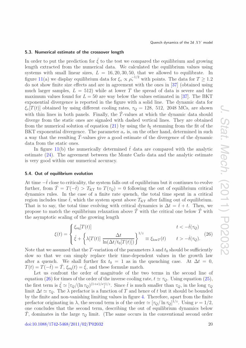
Figure 12. Growing correlation length ξv(t) during annealing from 2TKT to T = 0with different cooling rates τQ. (a) Bare data for seven cooling rates given in thekey. (b) Rescaling with the proposed asymptotic form (26) for t > −t(τQ).

phase transitions although the mechanism is different [24].) This fact can be observed inpanel (a) of figure 12 where the growing ξv under annealing with seven cooling rates givenin the key is shown as a function of the time-varying temperature.

In figure 12 we present data for the dynamic growing length for different coolingrates. Panel (a) displays the bare data for seven inverse cooling rates τQ given in the key.Panel (b) is a scaling plot that tests the hypothesis in equation (26) in the low temperatureregion during the annealing process. We use the values of the parameter λ[T (t)] obtainedfrom the linear fit of data for the quench in figure 4. Before rescaling, the correlationlength ξv(t) grows with time, i.e., with decrease of temperature, in such a way that at agiven T , the value of ξv increases with τQ (see panel (a)). After rescaling with the proposedasymptotic form (26) for t > −t(τQ), the values of ξ fall on top of each other. Perfectagreement with the analytic prediction would be the flat master curve ξv(t)/ξlowT (t) ≡1. The master curve deviates from this prediction but the range of variation isrelatively small, varying from about 1 to 1.6. We ascribe this mismatch to potentialnonlinear corrections to λ[T (t)] and small variations in t0[T (t)] that we have not takeninto account.

5.5. Numerical measurements of vortex density

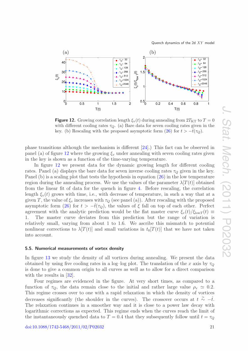
In figure 13 we study the density of all vortices during annealing. We present the dataobtained by using five cooling rates in a log–log plot. The translation of the x axis by τQ

is done to give a common origin to all curves as well as to allow for a direct comparisonwith the results in [32].

Four regimes are evidenced in the figure. At very short times, as compared to afunction of τQ, the data remain close to the initial and rather large value ρv � 0.2.This regime crosses over to one with a rapid relaxation in which the density of vortices

decreases significantly (the shoulder in the curves). The crossover occurs at t>∼ −t.

The relaxation continues in a smoother way and it is close to a power law decay withlogarithmic corrections as expected. This regime ends when the curves reach the limit ofthe instantaneously quenched data to T = 0.4 that they subsequently follow until t = τQ

doi:10.1088/1742-5468/2011/02/P02032 21

J.Stat.M

ech.(2011)

P02032

Quench dynamics of the 2d XY model

Figure 13. Time dependence of the total number of vortices after annealing toT = 0 with different inverse cooling rates τQ given in the key. The data are shownwith points in the form Nv ln Nv as a function of t + τQ. The (red) line plots thenumber of vortices after an infinitely rapid quench to T = 0.4 ≤ TKT.

and T = 0. In our setting the density of defects increases with increasing τQ at fixedt + τQ.

The qualitative features of our data are very close to those obtained by Chu andWilliams [32] for a quench or annealing from equilibrium at TKT to below the criticalpoint. As already said, their method is to solve numerically the Fokker–Planck equationfor vortex-pair dynamics in conjunction with the Kosterlitz–Thouless recursion relationsderived in [55]. This approach can only be used for initial conditions at and below TKT

and does not include the effect of free vortices. In consequence, the scalings found areconsistent with power laws without logarithmic corrections.

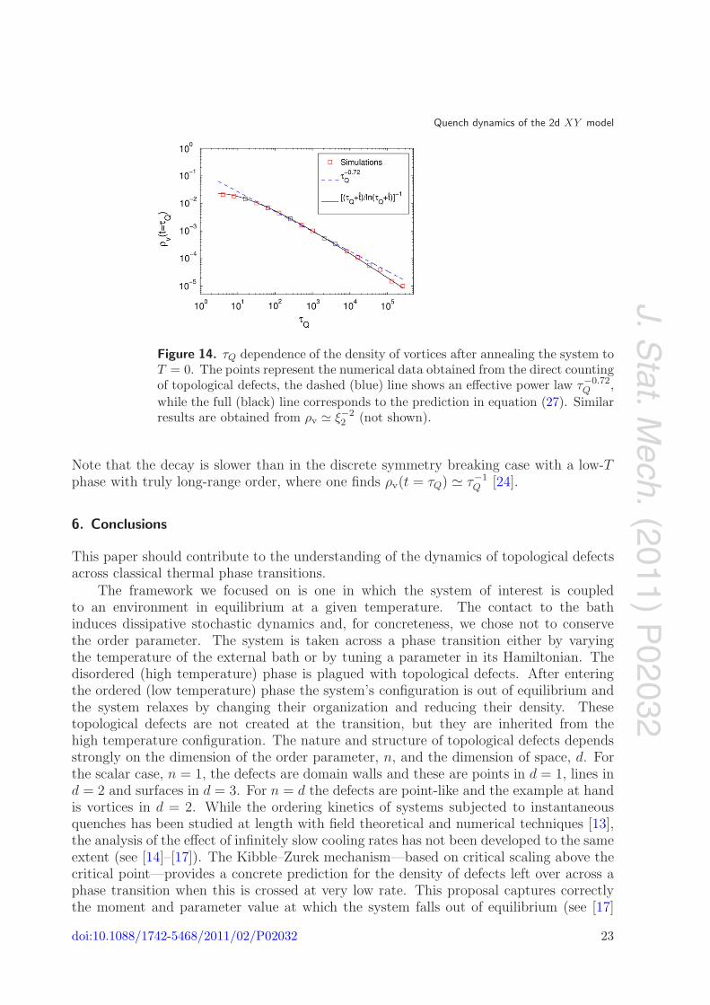
Finally, we extracted the remanent number of vortices at the end of the coolingprocedure, t = τQ and T = 0, and we plot it as a function of τQ in figure 14. The datacorrespond to the direct counting of (free) defects. The total number of defects varies fromabout 104 to 10. On the analytic side, the scaling assumption in equation (26) suggests

ρv(τQ) � τ−1Q +

{λ[T (τQ)]

Δt(τQ)

ln(Δt(τQ)/t0[T (τQ)])

}−1

= τ−1Q +

{λ

(τQ + t)

ln[(τQ + t)/t0]

}−1

�{

λ(τQ + t)

ln[(τQ + t)/t0]

}−1

, (27)

where λ and t0 in the last expression are the zero temperature values. We compared theabove assumption with the numerical data in figure 14 by using the values of t obtainednumerically in section 5.3 and we found good agreement within our numerical accuracy.The fact that the data points bend at short τQ is well captured by the addition of t in thenumerator. This term becomes negligible for longer τQ. At intermediate values of τQ thedecay can be easily confused with an effective power law, τ−0.72

Q , shown in the figure witha dashed (blue) line. For longer values of τQ the data confirm the logarithmic correction.

doi:10.1088/1742-5468/2011/02/P02032 22

J.Stat.M

ech.(2011)

P02032

Quench dynamics of the 2d XY model

Figure 14. τQ dependence of the density of vortices after annealing the system toT = 0. The points represent the numerical data obtained from the direct countingof topological defects, the dashed (blue) line shows an effective power law τ−0.72

Q ,while the full (black) line corresponds to the prediction in equation (27). Similarresults are obtained from ρv � ξ−2

2 (not shown).

Note that the decay is slower than in the discrete symmetry breaking case with a low-Tphase with truly long-range order, where one finds ρv(t = τQ) � τ−1

Q [24].

6. Conclusions

This paper should contribute to the understanding of the dynamics of topological defectsacross classical thermal phase transitions.

The framework we focused on is one in which the system of interest is coupledto an environment in equilibrium at a given temperature. The contact to the bathinduces dissipative stochastic dynamics and, for concreteness, we chose not to conservethe order parameter. The system is taken across a phase transition either by varyingthe temperature of the external bath or by tuning a parameter in its Hamiltonian. Thedisordered (high temperature) phase is plagued with topological defects. After enteringthe ordered (low temperature) phase the system’s configuration is out of equilibrium andthe system relaxes by changing their organization and reducing their density. Thesetopological defects are not created at the transition, but they are inherited from thehigh temperature configuration. The nature and structure of topological defects dependsstrongly on the dimension of the order parameter, n, and the dimension of space, d. Forthe scalar case, n = 1, the defects are domain walls and these are points in d = 1, lines ind = 2 and surfaces in d = 3. For n = d the defects are point-like and the example at handis vortices in d = 2. While the ordering kinetics of systems subjected to instantaneousquenches has been studied at length with field theoretical and numerical techniques [13],the analysis of the effect of infinitely slow cooling rates has not been developed to the sameextent (see [14]–[17]). The Kibble–Zurek mechanism—based on critical scaling above thecritical point—provides a concrete prediction for the density of defects left over across aphase transition when this is crossed at very low rate. This proposal captures correctlythe moment and parameter value at which the system falls out of equilibrium (see [17]

doi:10.1088/1742-5468/2011/02/P02032 23

J.Stat.M

ech.(2011)P

02032

Quench dynamics of the 2d XY model

for a very detailed calculation in the 1d Glauber Ising chain) but neglects, incorrectlyin dissipative thermal phase transitions, the relaxation dynamics in the ordered phase.In [24] the case of a second order phase transition with discrete spontaneously brokensymmetry was discussed. In this paper we studied a different type of transition, the BKTone in the 2d XY model.

To summarize our results, we first analyzed in more detail than previously done theout of equilibrium relaxation of a 2d XY model infinitely rapidly quenched from T0 → ∞to T < TKT. Using MC simulations we confirmed the functional form of the growthlaw ξ(T, t) � [λ(T )t/ ln t/t0]

1/2 derived in [34, 35] and we determined its temperaturedependence numerically. Although the log-correction has a theoretical foundation, thislaw has been frequently confused with an effective power law, especially in the field offreely decaying 2d turbulence as modeled with a Ginzburg–Landau approach [46]. Wealso analyzed the evolution of the structural properties such as the distribution of pairdistances or the polarity correlation function in the course of time and we found thatthey all satisfy dynamic scaling with respect to the same growing length. Importantlyenough, we demonstrated that the out of equilibrium dynamic properties are determinedby the density of free vortices in the low-T phase, as opposed to the density of all vorticesthat includes the equilibrium contribution of bound pairs. This fact is the reason forthe failure of dynamic scaling when the length determined from the decay of the totaldensity of vortices was used [48, 49]. Next, we studied cooling rate dependences; weproposed a scaling form for the growing length under these circumstances, and we checkedit numerically. We found that the density of free topological defects not only depends onthe cooling rate used but also on the time spent in the low temperature phase, wherevortices and antivortices tend to bind or annihilate. In particular, the density of vorticesat t � τQ is ρv � [τQ/ ln τQ]−1 for very long τQ. In short, the dynamics in the criticallow-T phase of the 2d XY model is crucial to determine the density of topological defects.

Acknowledgments

This research was financially supported by ANR-BLAN-0346 (FAMOUS), in part by theNational Science Foundation under Grant No. NSF PHY05-51164, and in part by theSwiss National Science Foundation (SNSF). We acknowledge very useful discussions withG Biroli, P Calabrese, D Domınguez, G Lozano, R Rivers, A Sicilia, and G Williams.

References

[1] Pargellis A N, Green S and Yurke B, 1991 Phys. Rev. B 43 3699Dierking I, 2003 Textures of Liquid Crystals (Weinheim: Wiley–VCH)

[2] Kawabat C and Bishop A R, 1986 Solid State Commun. 60 167Elmers H-J, Hauschild J, Liu G H and Gradmann U, 1996 J. Appl. Phys. 79 4984Elmers H-J, Hauschild J, Liu G H and Gradmann U, 1994 Ultrathin Magnetic Structures

ed J A C Bland and B Heinrich (Berlin: Springer)Elmers H-J, Hauschild J, Liu G H and Gradmann U, 1995 Int. J. Mod. Phys. B 9 3115

[3] Vilenkin A and Shellard E P S, 2000 Cosmic Strings and Other Topological Defects 2nd edn (Cambridge:Cambridge University Press)

[4] Tabeling P, 2002 Phys. Rep. 362 1[5] Berezinskii V L, 1970 Zh. Eksp. Teor. Fiz. 59 907

Berezinskii V L, 1971 Sov. Phys.—JETP 32 493 (translation)[6] Kosterlitz J M and Thouless D J, 1973 J. Phys. C: Solid State Phys. 6 1181

Kosterlitz J M, 1974 J. Phys. C: Solid State Phys. 7 1046

doi:10.1088/1742-5468/2011/02/P02032 24

J.Stat.M

ech.(2011)P

02032

Quench dynamics of the 2d XY model

[7] Chaikin P M and Lubensky T C, 1995 Principles of Condensed Matter Physics (Cambridge: CambridgeUniversity Press)

[8] Bishop D J and Reppy J D, 1980 Phys. Rev. B 22 5171[9] Beasley M R, 1979 Phys. Rev. Lett. 41 1165

Hebard A F and Fiory A T, 1980 Phys. Rev. Lett. 44 291[10] Pargellis A N, Green S and Yurke B, 1994 Phys. Rev. E 49 4250[11] Taroni A, Bramwell S T and Holdsworth P C W, 2008 J. Phys.: Condens. Matter 20 275233[12] Karimov Y S and Novikov Y N, 1974 Zh. Eksp. Teor. Fiz. Pis’ma Red. 19 268

Karimov Y S and Novikov Y N, 1974 Sov. Phys.—JETP Lett. 19 159Bishop D J and Reppy J D, 1978 Phys. Rev. Lett. 40 1727

[13] Bray A J, 1994 Adv. Phys. 43 357Puri S, 2004 Phase Transit. 77 407Cugliandolo L F, 2010 Physica A 389 4360

[14] Cornell S, Kaski K and Stinchcombe R, 1992 Phys. Rev. B 45 2725Suzuki S, 2009 J. Stat. Mech. P03032

[15] Huse D A and Fisher D S, 1986 Phys. Rev. Lett. 57 2203[16] Yoshino H, Hukushima K and Takayama H, 2002 Phys. Rev. B 66 064431[17] Krapivsky P, 2010 J. Stat. Mech. P02014[18] Kibble T W B, 1976 J. Phys. A: Math. Gen. 9 1387[19] Zurek W H, 1985 Nature 317 505

Zurek W H, 1996 Phys. Rep. 276 177[20] Ruutu V M H, Eltsov V B, Gill A J, Kibble T W B, Krusius M, Makhlin Y G, Placais B, Volovik G E and

Xu W, 1996 Nature 382 334Bauerle C, Bunkov Y M, Fisher S N, Godfrin H and Pickett G R, 1996 Nature 382 332The Grenoble cosmological experiment: the Kibble–Zurek scenario in superfluid 3He, Bauerle C,

Bunkov Yu M, Fisher S and Godfrin H, 1999 Topological Defects and the Non-Equilibrium Dynamcis ofSymmetry Breaking Phase Transitions vol 549, ed Y M Bunkov and H Godfrin (Dordrecht: KluwerAcademic)

[21] Karra G and Rivers R J, 1998 Phys. Rev. Lett. 81 3707Rivers R J, 2000 Phys. Rev. Lett. 84 1248

[22] Laguna P and Zurek W H, 1997 Phys. Rev. Lett. 78 2519Laguna P and Zurek W H, 1998 Phys. Rev. D 58 5021Yates A and Zurek W H, 1998 Phys. Rev. Lett. 80 5477Antunes N D, Bettencourt L M A and Zurek W H, 1999 Phys. Rev. Lett. 82 2824

[23] Kibble T W B, 2007 Phys. Today 60 47[24] Biroli G, Cugliandolo L F and Sicilia A, 2010 Phys. Rev. E 81 050101[25] Antunes N D, Gandra P and Rivers R J, 2006 Phys. Rev. D 73 125003[26] Zurek W H, Dorner U and Zoller P, 2005 Phys. Rev. Lett. 95 105701[27] Polkovnikov A, 2005 Phys. Rev. B 72 161201[28] Dziarmaga J, 2005 Phys. Rev. Lett. 95 245701

Dziarmaga J, 2010 Adv. Phys. 59 1063[29] Caneva T, Fazio R and Santoro G E, 2007 Phys. Rev. B 76 144427

Pellegrini F, Montangero S, Santoro G E and Fazio R, 2008 Phys. Rev. B 77 140404Canovi E, Rossini D, Fazio R and Santoro G E, 2009 J. Stat. Mech. P03038

[30] Divakaran U, Mukherjee V, Dutta A and Sen D, 2009 J. Stat. Mech. P02007Mondal S, Sengupta K and Sen D, 2009 Phys. Rev. B 79 045128

[31] Polkovnikov A, Sengupta K, Silva A and Vengalattore M, 2010 arXiv:1007.5331[32] Chu H-C and Williams G A, 2001 Phys. Rev. Lett. 86 2585[33] Hasenbusch M, 2005 J. Phys. A: Math. Gen. 38 5869

Hasenbusch M, Pelissetto A and Vicari E, 2005 J. Stat. Mech. P12002[34] Yurke B, Pargellis A N, Kovacs T and Huse D A, 1993 Phys. Rev. E 47 1525[35] Bray A J and Rutenberg A D, 1994 Phys. Rev. E 49 R27

Rutenberg A D and Bray A J, 1995 Phys. Rev. E 51 5499[36] Wolff U, 1989 Nucl. Phys. B 322 759[37] Gupta R and Baillie C F, 1992 Phys. Rev. B 45 2883[38] Luo H J and Zheng B, 1997 Mod. Phys. Lett. B 11 615

Zheng B, Schulz M and Trimper S, 1999 Phys. Rev. E 59 R1351[39] Luo H J, Schulz M, Schulke L, Trimper S and Zheng B, 1998 Phys. Lett. A 250 383

doi:10.1088/1742-5468/2011/02/P02032 25

J.Stat.M

ech.(2011)

P02032

Quench dynamics of the 2d XY model

[40] Ozeki Y, Ogawa K and Ito N, 2003 Phys. Rev. E 67 026702[41] Bramwell S T and Holdsworth P C W, 1993 J. Phys.: Condens. Matter 5 L53

Bramwell S T and Holdsworth P C W, 1994 Phys. Rev. B 49 8811[42] Nagaya T, Hotta H, Orihara H and Ishibashi Y, 1992 J. Phys. Soc. Japan 61 3511

Nagaya T, Orihara H and Ishibashi Y, 1995 J. Phys. Soc. Japan 64 78[43] Cugliandolo L F, Kurchan J and Parisi G, 1994 J. Phys. I 4 1641[44] Berthier L, Holdsworth P W C and Sellitto M, 2001 J. Phys. A: Math. Gen. 34 1805[45] Mondello M and Goldenfeld N, 1990 Phys. Rev. A 42 5865[46] Huber G and Alstrom P, 1993 Physica A 195 448[47] Bray A J, Briant A J and Jervis D K, 2000 Phys. Rev. Lett. 84 1503

Bray A J, 2000 Phys. Rev. E 62 103[48] Rojas F and Rutenberg A D, 1999 Phys. Rev. E 60 212[49] Lee J-R, Lee S J and Kim B, 1995 Phys. Rev. E 52 1550[50] Jonsson A and Minnhagen P, 1997 Phys. Rev. B 55 9035[51] Golubchik D, Polturak E and Koren G, 2010 Phys. Rev. Lett. 104 247002[52] Liu F and Mazenko G F, 1992 Phys. Rev. B 46 5963[53] Dimitrov D A and Wysin G M, 1998 J. Phys.: Condens. Matter 10 7453[54] Arenzon J J, Bray A J, Cugliandolo L F and Sicilia A, 2007 Phys. Rev. Lett. 98 145701

Sicilia A, Arenzon J J, Bray A J and Cugliandolo L F, 2007 Phys. Rev. E 76 061116Sicilia A, Sarrazin Y, Arenzon J J, Bray A J and Cugliandolo L F, 2009 Phys. Rev. E 80 031121

[55] Ambegaokar V, Halperin B I, Nelson D R and Siggia E D, 1980 Phys. Rev. B 21 1806

doi:10.1088/1742-5468/2011/02/P02032 26