Quasar Quartet Embedded in Giant NebulaReveals Rare Massive Structure in Distant Universe

Joseph F. Hennawi1,∗, J. Xavier Prochaska2,Sebastiano Cantalupo2,3,Fabrizio Arrigoni-Battaia1

1Max-Planck-Institut fur Astronomie, Konigstuhl, Germany2University of California Observatories-Lick Observatory, UC Santa Cruz, CA

3ETH Zurich, Institute of Astronomy, Zurich, Switzerland

∗To whom correspondence should be addressed; E-mail: joe@mpia.de

All galaxies once passed through a hyper-luminous quasar phase powered byaccretion onto a supermassive black hole. But because these episodes are brief,quasars are rare objects typically separated by cosmological distances. In asurvey for Lyman-α emission at redshift z ≈ 2, we discovered a physical as-sociation of four quasars embedded in a giant nebula. Located within a sub-stantial overdensity of galaxies, this system is likely the progenitor of a massivegalaxy cluster. The chance probability of finding a quadruple-quasar is esti-mated to be∼ 10−7, implying a physical connection between Lyman-α nebulaeand the locations of rare protoclusters. Our findings imply that the most mas-sive structures in the distant Universe have a tremendous supply (' 1011 solarmasses) of cool dense (volume density ' 1 cm−3) gas, in conflict with currentcosmological simulations.

Cosmologists do not fully understand the origin of supermassive black holes (SMBHs) at thecenters of galaxies, and how they relate to the evolution of the underlying dark matter, whichforms the backbone for structure in the Universe. In the current paradigm, SMBHs grew inevery massive galaxy during a luminous quasar phase, making distant quasars the progenitorsof the dormant SMBHs found at the centers of nearby galaxies. Tight correlations between themasses of these local SMBHs and both their host galaxy (1) and dark matter halo masses (2)support this picture, further suggesting that the most luminous quasars at high-redshift shouldreside in the most massive galaxies. It has also been proposed that quasar activity is triggeredby the frequent mergers that are a generic consequence of hierarchical structure formation (3,4).Indeed, an excess in the number of small-separation binary quasars (5, 6), as well as the mere

1

arX

iv:1

505.

0378

6v1

[as

tro-

ph.G

A]

14

May

201

5

existence of a handful of quasar triples (7,8), support this hypothesis. If quasars are triggered bymergers, then they should preferentially occur in rare peaks of the density field, where massivegalaxies are abundant and the frequency of mergers is highest (9).

Following these arguments, one might expect that at the peak of their activity z ∼ 2 − 3,quasars should act as signposts for protoclusters, the progenitors of local galaxy clusters andthe most massive structures at that epoch. However, quasar clustering measurements (10, 11)indicate that quasar environments at z ∼ 2 − 3 are not extreme: these quasars are hosted bydark matter halos with masses Mhalo ∼ 1012.5 M� (where M� is the mass of the Sun), toosmall to be the progenitors of local clusters (12). But the relationship between quasar activityand protoclusters remains unclear, owing to the extreme challenge of identifying the latter athigh-redshift. Indeed, the total comoving volume of even the largest surveys for distant galaxiesat z ∼ 2− 3 is only ∼ 107 Mpc3, which would barely contain a single rich cluster locally.

Protoclusters have been discovered around a rare-population of active galactic nuclei (AGN)powering large-scale radio jets, known as high-redshift radio galaxies (HzRGs) (13). TheHzRGs routinely exhibit giant∼ 100 kpc nebulae of luminous Lyα emissionLLyα ∼ 1044 erg s−1.Nebulae of comparable size and luminosity have also been observed in a distinct population ofobjects known as ‘Lyα blobs’ (LABs) (14, 15). The LABs are also frequently associated withAGN activity (16–18), although lacking powerful radio jets, and appear to reside in overdense,protocluster environments (15, 19, 20). Thus among the handful of protoclusters (21) known,most appear to share two common characteristics: the presence of an active SMBH and a giantLyα nebula.

We have recently completed a spectroscopic search for extended Lyα emission around asample of 29 luminous quasars at z ∼ 2, each the foreground (f/g) member of a projectedquasar pair (22). Analysis of spectra from the background (b/g) members in such pairs revealsthat quasars exhibit frequent absorption from a cool, metal-enriched, and often optically thickmedium on scales of tens to hundreds kpc (22–28). The UV radiation emitted by the luminousf/g quasar can, like a flashlight, illuminate this nearby neutral hydrogen, and power a large-scaleLyα-emission nebula, motivating our search. By construction, our survey selects for exactlythe two criteria which seem to strongly correlate with protoclusters: an active SMBH and thepresence of a large-scale Lyα emission nebula.

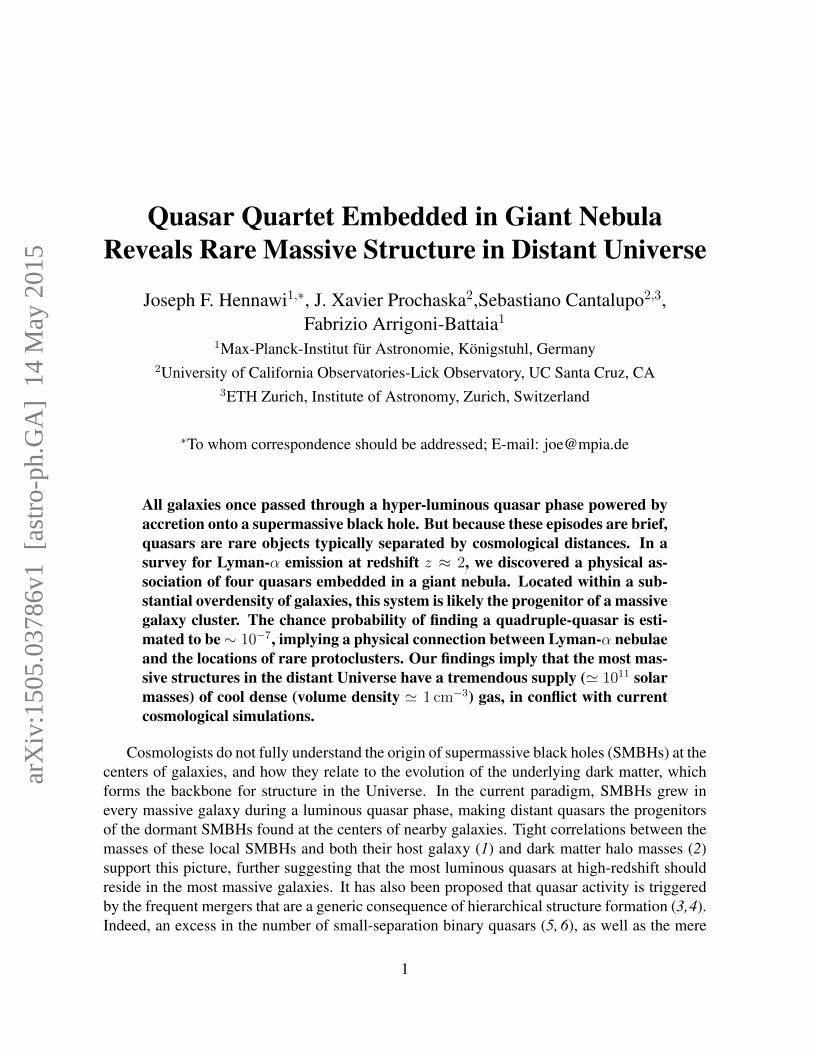
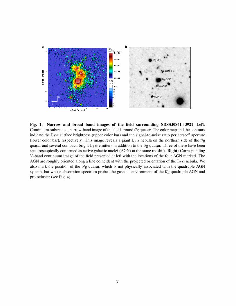
Of the 29 quasars surveyed, only SDSSJ0841+3921 exhibited extended large-scale (& 50 kpc)Lyα emission above our characteristic sensitivity limit of 6 × 10−18 erg s−1 cm−2 arcsec−2 (2σ).We designed a custom narrow-band filter tuned to the wavelength of Lyα at the f/g quasar red-shift z = 2.0412 (λcenter = 3700A, FWHMλ = 33A), and imaged the field with the Keck/LRISimaging spectrometer for 3hrs on UT 12 November 2012. The combined and processed imagesreveal Lyα emission from a giant filamentary structure centered on the f/g quasar and extendingcontinuously towards the b/g quasar (see Fig. 1). This nebulosity has an end-to-end size of 37′′

corresponding to 310 kpc and a total line luminosity LLyα = 2.1 × 1044 erg s−1, making it oneof the largest and brightest nebula ever discovered.

The giant nebula is only one of the exceptional properties of SDSSJ 0841+3921. Ourimages reveal three relatively compact candidate Lyα emitting sources with faint continuum

2

magnitudes V ' 23 − 24, embedded in the Lyα filament and roughly aligned with its majoraxis. Follow-up spectroscopy reveals that the sources labeled AGN1, AGN2, and AGN3 arethree AGN at the same redshift as the f/g quasar (see right panel of Fig. 1and (29)), making thissystem the only quadruple AGN known. Adopting recent measurements of small-scale quasarclustering (30), we estimate that the probability of finding three AGN around a quasar withsuch small separations is ∼ 10−7 (31). Why then did we discover this rare coincidence of AGNin a survey of just 29 quasars? Did the giant nebula mark the location of a protocluster withdramatically enhanced AGN activity?

To test this hypothesis, we constructed a catalog of Lyα-emitting galaxies (LAEs), andcomputed the cumulative overdensity profile of LAEs around SDSSJ0841+3921, relative tothe background number expected based on the LAE luminosity function (32) (see Fig. 2). Toperform a quantitative comparison to other giant Lyα nebulae, many of which are known tocoincide with protoclusters, we measured the giant nebulae-LAE cross-correlation function fora sample of eight systems – six HzRGs and two LABs – for which published data was availablein the literature (33). In Fig. 2, we compare the overdensity profile around SDSSJ0841+3921 tothis giant nebulae-LAE correlation function. On average, the environment of HzRGs and LABshosting giant Lyα nebulae (red line) is much richer than that of radio-quiet quasars (10) (blueline), confirming that they indeed reside in protoclusters. Furthermore, the clustering of LAEsaround SDSSJ0841+3921 has a steeper overdensity profile, and exceeds the average protoclus-ter by a factor of & 20 for R < 200 kpc and by ∼ 3 on scales of R ' 1 Mpc. In addition tothe overdensity of four AGN, the high number of LAEs surrounding SDSSJ0841+3921 makeit one of the most overdense protoclusters known at z ∼ 2− 3.

The combined presence of several bright AGN, the Lyα emission nebula, and the b/g absorp-tion spectrum, provide an unprecedented opportunity to study the morphology and kinematicsof the protocluster via multiple tracers, and we find evidence for extreme motions (34). Specif-ically, AGN1 is offset from the precisely determined systemic redshift (35) of the f/g quasar by+1300± 400 km s−1. This large velocity offset cannot be explained by Hubble expansion – theminiscule probability of finding a quadruple quasar in the absence of clustering P ∼ 10−13 (31)and the physical association between the AGN and giant nebula demand that the four AGNreside in a real collapsed structure – and thus provides an unambiguous evidence for extremegravitational motions. In addition, our slit spectra of the giant Lyα nebula reveal extreme kine-matics of diffuse gas (Fig. 3), extending over a velocity range of −800 to +2500 km s−1 fromsystemic. Furthermore, there is no evidence for double-peaked velocity profiles characteristicof resonantly-trapped Lyα, which could generate large velocity widths in the absence of corre-spondingly large gas motions. Absorption line kinematics of the metal-enriched gas, measuredfrom the b/g quasar spectrum at impact parameter of R⊥ = 176 kpc (Fig. 4), show strong ab-sorption at ≈ +650 km s−1 with a significant tail to velocities as large as ' 1000 km s−1. It isof course possible that the extreme gas kinematics, traced by Lyα emission and metal-line ab-sorption, are not gravitational but rather arise from violent large-scale outflows powered by themultiple AGN. While we cannot completely rule out this possibility, the large velocity offset of+1300 km s−1 between the f/g quasar and the emission redshift of AGN1 can only result from

3

gravity.One can only speculate about the origin of the dramatic enhancement of AGN in the

SDSSJ0841+3921 protocluster. Perhaps the duty cycle for AGN activity is much longer in pro-toclusters, because of frequent dissipative interactions (5,6), or an abundant supply of cold gas.A much larger number of massive galaxies could also be the culprit, as AGN are known to tracemassive halos at z ∼ 2. Although SDSSJ0841+3921 is the only example of a quadruple AGNwith such small separations, previously studied protoclusters around HzRGs and LABs, alsooccasionally harbor multiple AGN (13,36). Regardless, our discovery of a quadruple AGN andprotocluster from a sample of only 29 quasars suggests a link between giant Lyα nebulae, AGNactivity, and protoclusters – similar to past work on HzRGs and LABs – with the exception thatSDSSJ 0841+3921 was selected from a sample of normal radio-quiet quasars. From our surveyand other work (37), we estimate that ' 10% of quasars exhibit comparable giant Lyα nebulae.Although clustering measurements imply that the majority of z ∼ 2 quasars reside in moderateoverdensities (10–12), we speculate that this same 10% trace much more massive protoclus-ters. SDSSJ0841+3921 clearly supports this hypothesis, as does another quasar-protoclusterassociation (10, 38), around which a giant Lyα nebula was recently discovered (39, 40).

Given our current theoretical picture of galaxy formation in massive halos, an associationbetween giant Lyα nebulae and protoclusters is completely unexpected. The large Lyα lumi-nosities of these nebulae imply a substantial mass (∼ 1011M�) of cool (T ∼ 104 K) gas (41),whereas cosmological hydrodynamical simulations indicate that already by z ∼ 2− 3, baryonsin the massive progenitors (Mhalo & 1013M�) of present-day clusters are dominated by a hotshock-heated plasma T ∼ 107 K (42, 43). These hot halos are believed to evolve into the X-rayemitting intra-cluster medium observed in clusters, for which absorption-line studies indicatenegligible . 1% cool gas fractions (44). Clues about the nature of this apparent discrepancycome from our absorption line studies of the massive ' 1012.5 M� halos hosting z ∼ 2 − 3quasars. This work reveals substantial reservoirs of cool gas & 1010 M� (22–28), manifest asa high covering factor ' 50% of optically thick absorption, several times larger than predictedby hydrodynamical simulations (42,43). This conflict most likely indicates that current simula-tions fail to capture essential aspects of the hydrodynamics in massive halos at z ∼ 2 (27, 42),perhaps failing to resolve the formation of clumpy structure in cool gas (41).

If illuminated by the quasar, these large cool gas reservoirs in the quasar circumgalacticmedium (CGM) will emit fluorescent Lyα photons, and we argue that this effect powers the neb-ula in SDSSJ0841+3921 (45). But according to this logic, nearly every quasar in the Universeshould be surrounded by a giant Lyα nebulae with size comparable to its CGM (∼ 200 kpc).Why then are these giant nebulae not routinely observed?

This apparent contradiction can be resolved as follows. If this cool CGM gas is illumi-nated and highly ionized, it will fluoresce in the Lyα line with a surface brightness scalingas SBLyα ∝ NHnH, where NH is the column density of cool gas clouds which populate thequasar halo, and nH is the number density of hydrogen atoms inside these clouds. Note the totalcool gas mass of the halos scales as Mcool ∝ R2NH, where R is the radius of the halo (45).Given our best estimate for the properties of the CGM around typical quasars (nH ∼ 0.01 cm−3

4

and NH ∼ 1020 cm−2 or Mcool ' 1011M�) (22, 26, 27), we expect these nebulae to be ex-tremely faint SBLyα ∼ 10−19 erg s−1 cm−2 arcsec−2, and beyond the sensitivity of current in-struments (22). One comes to a similar conclusion based on a full radiative transfer calculationthrough a simulated dark-matter halo with mass Mhalo ≈ 1012.5M� (41). Thus the factor of∼ 100 times larger surface brightness observed in the SDSSJ0841+3921 and other protoclusternebulae, arises from either a higher nH, NH (and hence higher Mcool), or both. The cool gasproperties required to produce the SDSSJ0841+3921 nebula can be directly compared to thosededuced from an absorption line analysis of the b/g quasar spectrum (46).

The b/g quasar sightline pierces through SDSSJ0841+3921 at an impact parameter ofR⊥ =176 kpc, giving rise to the absorption spectrum shown in Fig. 4. Photoionization modeling ofthese data constrains the total hydrogen column density to be log10NH = 20.4 ± 0.4 (45),implying a substantial mass of cool gas 1.0 × 1011M� < Mcool < 6.5 × 1011M� withinr = 250 kpc. Assuming that the Lyα emitting gas has the same column density as the gasabsorbing the b/g sightline, reproducing the large fluorescent Lyα surface brightness requiresthat this gas be distributed in compact rcloud ∼ 40 pc clouds at densities characteristic of theinterstellar medium nH ' 2 cm−3, but on ∼ 100 kpc scales in the protocluster.

Clues to the origin of these dense clumps of cool gas comes from their high enrichment level,which we have determined from our absorption line analysis (46) to be greater than 1/10th ofthe solar value. At first glance, this suggests that strong tidal interactions due to merger activityor outflows due to powerful AGN feedback are responsible for dispersing dense cool gas in theprotocluster. However, the large cool gas mass ∼ 1011 M� and high velocities ∼ 1000 km s−1,imply an extremely large kinetic luminosity Lwind ∼ 1044.6 for an AGN powered wind, makingthe feedback scenario implausible (25). An even more compelling argument against a merger orfeedback origin comes from the extremely small cloud sizes rcloud ∼ 40 pc implied by our mea-surements. Such small clouds moving supersonically∼ 1000 km s−1 through the hot T ∼ 107 Kshock-heated plasma predicted to permeate the protocluster, will be disrupted by hydrodynamicinstabilities in ∼ 5 × 106 yr, and can thus only be transported ∼ 5 kpc (47). These short dis-ruption timescales instead favor a scenario where cool dense clouds are formed in situ, perhapsvia cooling and fragmentation instabilities, but are short-lived. The higher gas densities mightnaturally arise if hot plasma in the incipient intra-cluster medium pressure confines the clouds,compressing them to high densities (48, 49). Emission line nebulae from cool dense gas hasalso been observed at the centers of present-day cooling flow clusters (50, 51), albeit on muchsmaller scales . 50 kpc. The giant Lyα nebulae in z ∼ 2− 3 protoclusters might be manifesta-tions of the same phenomenon, but with much larger sizes and luminosities, reflecting differentphysical conditions at high-redshift.

The large reservoir of cool dense gas in the protocluster SDSSJ0841+3921 , as well asthose implied by the giant nebulae in other protoclusters, appear to be at odds with our currenttheoretical picture of how clusters form. This is likely symptomatic of the same problem of toomuch cool gas in massive halos already highlighted for the quasar CGM (27, 42, 43). Progresswill require more cosmological simulations of massive halos M & 1013 M� at z ∼ 2, as wellas idealized higher-resolution studies. In parallel, a survey for extended Lyα emission around

5

∼ 100 quasars would uncover a sample of ∼ 10 giant Lyα nebulae likely coincident withprotoclusters, possibly also hosting multiple AGN, and enabling continued exploration of therelationship between AGN, cool gas, and cluster progenitors.

6

AGN 1!

AGN 2!

AGN 3!

f/g QSO!

b/g QSO!

SBLyα"(erg s-1 cm-2 arcsec-2)"

S/N"(arcsec-2)"

a! b!

N

E

Fig. 1: Narrow and broad band images of the field surrounding SDSSJ0841+3921 Left:Continuum-subtracted, narrow-band image of the field around f/g quasar. The color map and the contoursindicate the Lyα surface brightness (upper color bar) and the signal-to-noise ratio per arcsec2 aperture(lower color bar), respectively. This image reveals a giant Lyα nebula on the northern side of the f/gquasar and several compact, bright Lyα emitters in addition to the f/g quasar. Three of these have beenspectroscopically confirmed as active galactic nuclei (AGN) at the same redshift. Right: CorrespondingV -band continuum image of the field presented at left with the locations of the four AGN marked. TheAGN are roughly oriented along a line coincident with the projected orientation of the Lyα nebula. Wealso mark the position of the b/g quasar, which is not physically associated with the quadruple AGNsystem, but whose absorption spectrum probes the gaseous environment of the f/g quadruple AGN andprotocluster (see Fig. 4).

7

100 1000R (pkpc)

1

10

100

1000

δ(<

R)

1

10

100

1000

0.1 1.0R (cMpc/h)

Fig. 2: Characterization of the protocluster environment around SDSSJ0841+3921 . Thedata points indicate the cumulative overdensity profile of LAEs δ(< R) as a function of impact parameterR from the f/g quasar in SDSSJ0841+3921 , with Poisson error bars. The red curve shows the predictedoverdensity profile, based on our measurement of the giant nebulae-LAE cross-correlation function de-termined from a sample of eight systems – six HzRGs and two LABs – for which published data wasavailable in the literature. Assuming a power-law form for the cross-correlation ξcross = (r/r0)−γ , wemeasure the correlation length r0 = 29.3± 4.9h−1 Mpc, for a fixed value of γ = 1.5. The gray shadedregion indicates the 1σ error on our measurements based on a bootstrap analysis, where both r0 andγ are allowed to vary. The solid blue line indicates the overdensity of Lyman break galaxies (LBGs)around radio-quiet quasars based on recent measurements (10), with the dotted blue lines the 1σ erroron this measurement. On average, the environment of HzRGs and LABs hosting giant Lyα nebulae ismuch richer than that of radio-quiet quasars (10), confirming that they indeed reside in protoclusters.SDSSJ0841+3921 exhibits a dramatic excess of LAEs compared to the expected overdensities aroundradio-quiet quasars (blue curve). Its overdensity even exceeds the average protocluster (red curve) by afactor of & 20 for R < 200 kpc decreasing to an excess of ∼ 3 on scales of R ' 1 Mpc, and exhibits amuch steeper profile.

8

Slit 2!

Slit 3!

Slit 1!

10“!88 kpc!

Slit 2! Slit 3!

b!

c! d!

Flux!

Flux! Flux!

a!Slit 1!

Slit 2! Slit 3!

AGN2

AGN1

f/g QSO

b/g QSO

AGN1

AGN2

f/g QSO

f/g QSO

AGN1

b/g QSO b/g QSO

NB image!

Fig. 3: Lyα spectroscopy of the giant nebula and its associated AGN. Upper Left: Thespectroscopic slit locations (white rectangles) for three different slit orientations are overlayed on thenarrow band image of the giant nebula. The locations of the f/g quasar (brightest source), b/g quasar,AGN1, and AGN2 are also indicated. Two-dimensional spectra for Slit1 (Upper Right), Slit2 (LowerLeft), and Slit3 (Lower Right) are shown in the accompanying panels. In the upper right and lowerleft panels, spatial coordinates refer to the relative offset along the slit with respect to the f/g quasar.Spectra of AGN1 are present both in Slit 1 (upper right) and Slit 3 (lower right) at spatial offsets 75kpcand 25kpc, respectively, while the Lyα spectrum of AGN2 is located at a spatial offset −60 kpc in Slit 1(upper right). The b/g quasar spectra are located in both Slit 2 (lower left) and Slit 3 (lower right) at thesame spatial offset of 176 kpc. The spectroscopic observations demonstrate the extreme kinematics ofthe system: AGN1 has a velocity of +1300±400 km s−1 relative to the f/g quasar and the Lyα emissionin the nebula exhibits motions ranging from −800km s−1 (at ≈ 100 kpc offset in Slit 3, lower right) to+2500km s−1 (at ≈ 100 kpc in Slit 1, upper right). A 3× 3 pixel boxcar smoothing, which corresponds120 km s−1× 0.8′′, has been applied to the spectra. In each two-dimensional spectrum, the zero velocitycorresponds to the systemic redshift of the f/g quasar. The color bars indicate the flux levels in units oferg s−1 cm−2 arcsec−2 A−1. 9

0.0

0.2

0.4

0.6

0.8

1.0

HI LyαKeck/LRISb

0.0

0.2

0.4

0.6

0.8

1.0

CII 1334Keck/LRISb

−1000 0 1000 2000Relative Velocity (km s−1)

0.0

0.2

0.4

0.6

0.8

1.0

CIV 1548BOSS

0.0

0.2

0.4

0.6

0.8

1.0

SiII 1304Keck/LRISb

0.0

0.2

0.4

0.6

0.8

1.0

SiIII 1206Keck/LRISb

−1000 0 1000 2000Relative Velocity (km s−1)

0.0

0.2

0.4

0.6

0.8

1.0

SiIV 1393Keck/LRISb

Nor

mal

ized

Flu

x

Fig. 4: Absorption line spectrum of cool gas in SDSSJ0841+3921 . Spectrum of the absorbinggas detected in the b/g quasar sightline at an impact parameter of 176 kpc from the f/g quasar. Thegas shows strong H I and low-ionization state metal absorption, offset by ≈ 650km s−1 from the f/gquasar’s systemic redshift. The CII absorption in particular exhibits a significant tail to velocities aslarge as ' 1000 km s−1, providing evidence for extreme gas kinematics. We modeled the strong HILyα absorption with a Voigt profile (blue curve with grey band indicating uncertainty) and estimate acolumn density logNHI = 19.2 ± 0.3. The strong low and intermediate ion absorption (SiII, CII, SiIII)and correspondingly weak high-ion absorption (CIV, SiIV) indicate that the gas is not highly ionized,and our photoionization modeling (45) implies log10 xHI = −1.2 ± 0.3 or log10NH = 20.4 ± 0.4. Weestimate a conservative lower-limit on the gas metallicity to be 1/10 of the solar value.

10

AcknowledgmentsWe thank the staff of the W.M. Keck Observatory for their support during the installation andtesting of our custom-built narrow-band filter. We are grateful to B. Venemans and M. Prescottfor providing us with catalogs of LAE positions around giant nebulae in electronic format.We also thank the members of the ENIGMA group (http://www.mpia-hd.mpg.de/ENIGMA/)at the Max Planck Institute for Astronomy (MPIA) for helpful discussions. JFH acknowledgesgenerous support from the Alexander von Humboldt foundation in the context of the Sofja Ko-valevskaja Award. The Humboldt foundation is funded by the German Federal Ministry forEducation and Research. J.X.P. acknowledge support from the National Science Foundation(NSF) grant AST-1010004. The data presented here were obtained at the W.M. Keck Observa-tory, which is operated as a scientific partnership among the California Institute of Technology,the University of California and NASA. The Observatory was made possible by the financialsupport of the W.M. Keck Foundation. We acknowledge the cultural role that the summit ofMauna Kea has within the indigenous Hawaiian community. We are most fortunate to have theopportunity to conduct observations from this mountain. The data reported in this paper areavailable through the Keck Observatory Archive (KOA).

Supplementary Online Materialwww.sciencemag.orgMaterials and MethodsSOM TextFigs. S1 to S10Tables S1 to S6References (52-133)

11

Supplementary Online Material

This PDF file includesMaterials and MethodsSOM TextFigs. S1 to S10Tables S1 to S6References (52-133)

1 Optical Observations

1.1 Discovery SpectraThe source SDSSJ084158.47+392121.0 (f/g quasar) was targeted as a quasar by the Sloan Digi-tal Sky Survey (SDSS) through their color-selection algorithms and observed spectroscopicallyin the standard survey (52). It has a cataloged emission redshift of z = 2.046. Our analysis ofthe SDSS imaging data revealed a second, neighboring source at SDSSJ084159.26+392140.0(b/g quasar) with colors characteristic of a z ∼ 2 quasar, characterizing this system as a can-didate quasar pair. In the course of our ongoing spectroscopic campaign to discover closequasar pairs at z > 2 (6, 53), we confirmed this source to have z = 2.214 implying a pro-jected quasar pair with a physical separation of R⊥ = 176 kpc at the f/g quasar redshift.SDSSJ084159.26+392140.0 was also observed by the SDSS-III survey in the Baryonic Oscil-lating Spectroscopic Survey campaign at a spectral resolution ofR ≈ 2000 and with wavelengthcoverage λ ≈ 3600− 10, 000A (54).

On UT 2007 Jan 18, we observed the quasar pair with the Low Resolution Imaging Spec-trograph (LRIS) (55). These data were taken to study the intergalactic medium probed by thequasar pair, to examine the HI gas associated with the circumgalactic medium of the f/g quasar,and to search for fluorescent emission associated with the f/g quasar. The latter analyses ofthese data have been presented in previous works (22, 26–28). Summarizing the observations,we used LRIS in multi-slit mode with a custom designed slitmask which allowed placementof one slit on the known quasars and other slits on additional quasar candidates in the field.Specifically, a slit was placed at the position angle PA=25.8◦ between the f/g and b/g quasars,allowing them to be observed simultaneously. LRIS is a double spectrograph with two armsgiving simultaneous coverage of the near-UV and optical. We used the D460 dichroic with the1200 lines mm−1 grism blazed at 3400 A on the blue side, resulting in wavelength coverageof ≈ 3250 − 4300 A. The dispersion of this grism is 0.50 A per pixel and our 1′′ slits give aresolution with full width at half maximum (FWHM) FWHM' 160km s−1. On the red side weused the R1200/5000 (covering≈ 4700−6000A) and R300/5000 (covering≈ 4700−10, 000A)gratings having a FWHM of ≈ 100km s−1 and ≈ 400km s−1 respectively.

1

The science frames were complemented by a series of calibration images: arc lamp, domeflat, twilight sky, and standard star spectra with the same instrument configurations. All of theseexposures were reduced using the LowRedux (http://www.ucolick.org/∼xavier/LowRedux/)pipeline which bias subtracts and flat fields the images, corrects for non-uniform illumination,derives a wavelength solution, performs sky subtraction, optimally extracts the sources, andfluxes the resultant spectra. The 1D spectra are corrected for instrument flexure and shifted to aheliocentric, vacuum-corrected system.

Using custom software, we also coadded the 2D spectral images to search for diffuse Lyαemission surrounding the f/g quasar (22). This software enables us to model and subtract thespectral PSF of sources in the 2D spectra. Extended Lyα emission will be manifest as residualflux in our 2D sky-and-PSF-subtracted images which is inconsistent with being noise. To vi-sually assess the statistical significance of any putative emission feature, we define a χ imageχsky+PSF = (DATA − SKY − OBJECTS)/σ. If our model is an accurate description of thedata, the distribution of pixel values in the χsky+PSF should be a Gaussian with unit variance.The middle row of the images in Fig. S1 shows this quantity for SDSSJ 0841+3921 for eachslit orientation. The lower row of these images shows χsky = (DATA − SKY)/σ. The upperrow shows a smoothed version of the middle row, helpful for identifying extended emission.Specifically, the smoothed images are given by χsmth = CONVOL[DATA−SKY−OBJECTS]√

CONVOL2[σ2], where

the CONVOL operation denotes smoothing of the stacked images with a symmetric Gaus-sian kernel (same spatial and spectral widths) with FWHM=235 km s−1 (dispersion σsmth =100 km s−1), which is 5.7 pixels, or 1.4 times the spectral resolution element, and correspondsto FWHM = 1.5′′ spatially. The operation CONVOL2 represents convolution with the squareof the smoothing kernel. With this definition of χsmth the distribution of the pixel values in thesmoothed image will still obey Gaussian statistics, although they are of course correlated, andhence not independent.

Sky and object PSF-subtracted χ-maps for all of the slit-orientations that we used to char-acterize extended emission in SDSSJ 0841+3921 are shown in Fig. S1. Fig. 3 of the Main text,shows just the smoothed sky-subtracted images with a color-map chosen to accentuate the faintextended emission and a slightly different smoothing, namely a 3 × 3 pixel boxcar smoothing,which corresponds 120 km s−1 × 0.8′′. The χ-maps in Fig. S1 enable the reader to objectivelyassess the statistical significance of all emission features in the unsmoothed data. Note that inall of these maps, only the PSF model of the f/g and b/g quasars have been subtracted, whereasneither AGN1 nor AGN2 were removed from the other slit-orientations (see Fig. 1 in main text).Following the calibration procedure described in (22), we deduce the following spectroscopicsurface brightness limits (1σ) for the Lyα line at the f/g quasar redshift z = 2.0412: Slit1,SB1σ = 2.2 × 10−18 erg s−1 cm−2 arcsec−2; Slit2, SB1σ = 2.3 × 10−18 erg s−1 cm−2 arcsec−2;and Slit3, SB1σ = 4.8 × 10−18 erg s−1 cm−2 arcsec−2, where these SBs are computed in win-dows of 700 km s−1× 1.0′′, which corresponds to an aperture of 700 km s−1× 1.0 arcsec2 on thesky because we always used a 1.0′′ slit. The depth that we attain in our Lyα spectroscopy is com-parable to that achieved by our narrow-band imaging SB1σ = 1.7 × 10−18 erg s−1 cm−2 arcsec−2

(see next section).

2

The original observation from the Quasars Probing Quasars (QPQ) (22) survey correspondsto slit-orientation Slit2 (see Fig. S1 and Fig. 3 in main text). Our initial visual inspectionof the Lyα emission map revealed a bridge of Lyα emission along the slit connecting thequasar pair. Although the SB varies with position, this structure has a characteristic SBLyα '10−17 erg s−1 cm−2 arcsec−2 and is detected at ' 4 − 5σ at location R⊥ ' +100 kpc betweenthe two quasars. The emission extends along the slit from −80 kpc below the f/g quasar to+150 kpc between the two quasars, and possibly to +250 kpc. With an end-to-end size of∼ 250 kpc, this represented one of the largest Lyα emission nebula ever detected, and thusmotivated the additional imaging and spectroscopic observations, which are the focus of thismanuscript.

1.2 Narrow Band ImagingWe purchased a custom-designed narrow-band (NB) filter from Andover Corporation, sizedto fit within the grism holder of the Keck/LRISb camera. The filter was tuned to λcenter =3700A, and designed with a narrow band-pass FWHMλ = 33A to minimize sky backgroundwhile maintaining throughput. On UT 12 November 2012, we imaged the ∼ 5′ × 7′ field-of-view surrounding SDSSJ0841+3921 , offset to place the quasar pair on the CCD with highestquantum efficiency. We observed for a total of 3.2 hours in a series of dithered, 1280s exposures.Conditions were clear with sub-arcsecond atmospheric seeing. In parallel, we obtained 3hrs ofbroad-band V images with the LRISr camera. The instrument was configured with the D460dichroic and the detectors of the blue camera were binned 2x2 to minimize read noise.

The images were reduced using standard routines within the IRAF reduction software pack-age. This includes bias subtraction, flat fielding and an illumination correction. A combinationof twilight sky flats and unregistered science frames were used to produce flat-field images andillumination corrections in each band. The individual frames were sequentially registered to theSDSS-DR7 catalog using the SExtractor (56) and SCAMP (57) packages. The RMS uncertaintyin the astrometry of our registered images is approximately 0.2′′. Finally, the corrected framesfrom each band were average-combined using the SWarp package (58).

We calibrated the photometry of our images as follows. At the beginning and end of thenight, we observed two spectrophotometric stars (G191b2b and Feige34) with the NB filterunder clear conditions. Neither star has significant spectral features in the relevant wavelengthrange covered by our NB filter. For the broad-band images, we observed the standard starfield PG0231+051. To compute the zero-point for the narrow-band images, we compared themeasured count rates of Feige34 and G191b2b with the expected fluxes estimated by convolvingthe standard star spectra (resolution of 1A) (59) with the normalized filter transmission curve.We calculate an average, zero-point magnitude of 23.58 mag, with a few percent differencebetween the two stars. With this calibration, we deduce that the 1σ limiting surface brightnessof our combined NB images is SB1σ = 1.7 × 10−18 erg s−1 cm−2 arcsec−2 for a 1.0 arcsec2

aperture.For the broad-band images, we compared the number of counts per second of the five stars in

3

the PG0231+051-field with their tabulated V -band magnitudes (60). The derived zero-point forthe five stars are consistent to within a few percent and we adopt the average value: VZP = 28.07.Because the Feige34 and the PG0231+051 fields were observed with an airmass (AM≈ 1.2)similar to our science field, we did not correct the individual images before combination. Weestimate that the correction would be on the order of few percent. The 1σ limiting point sourcemagnitude for our combined broad band images is V = XX .

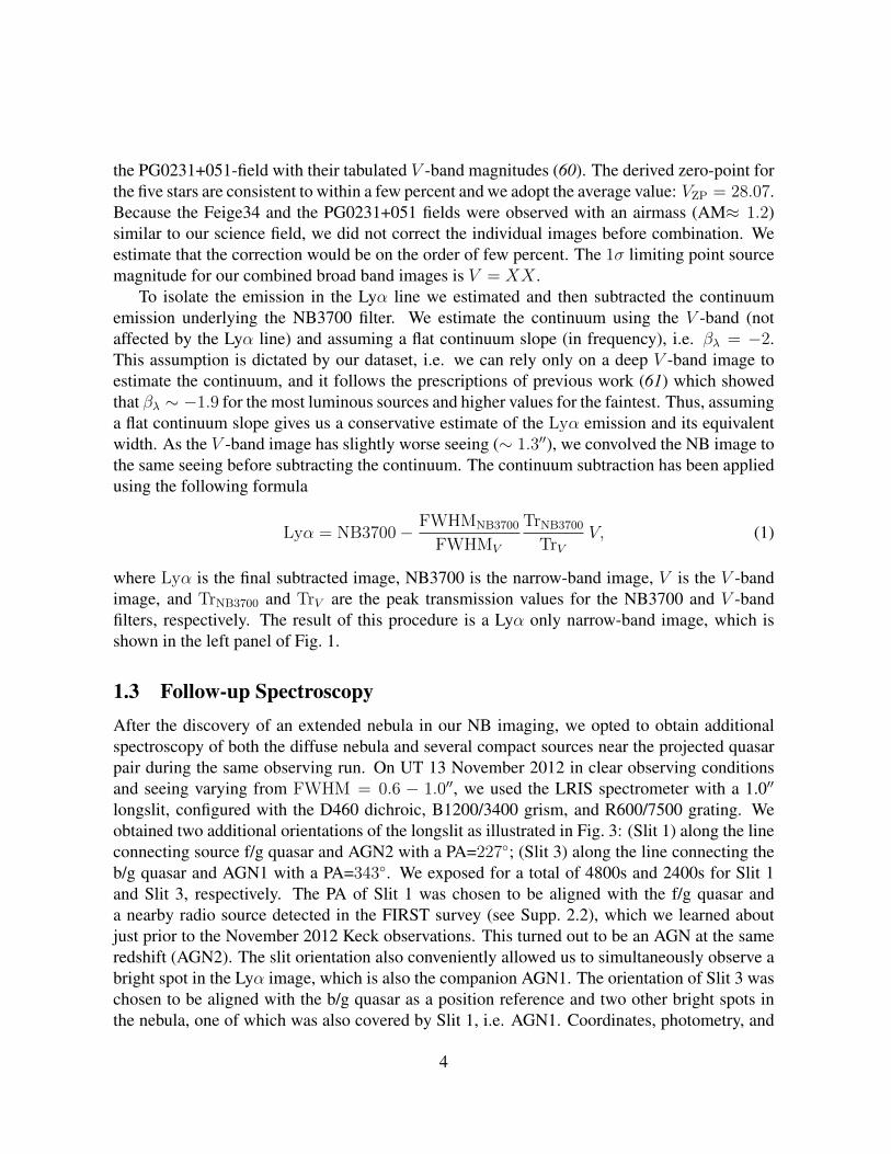
To isolate the emission in the Lyα line we estimated and then subtracted the continuumemission underlying the NB3700 filter. We estimate the continuum using the V -band (notaffected by the Lyα line) and assuming a flat continuum slope (in frequency), i.e. βλ = −2.This assumption is dictated by our dataset, i.e. we can rely only on a deep V -band image toestimate the continuum, and it follows the prescriptions of previous work (61) which showedthat βλ ∼ −1.9 for the most luminous sources and higher values for the faintest. Thus, assuminga flat continuum slope gives us a conservative estimate of the Lyα emission and its equivalentwidth. As the V -band image has slightly worse seeing (∼ 1.3′′), we convolved the NB image tothe same seeing before subtracting the continuum. The continuum subtraction has been appliedusing the following formula

Lyα = NB3700− FWHMNB3700

FWHMV

TrNB3700

TrVV, (1)

where Lyα is the final subtracted image, NB3700 is the narrow-band image, V is the V -bandimage, and TrNB3700 and TrV are the peak transmission values for the NB3700 and V -bandfilters, respectively. The result of this procedure is a Lyα only narrow-band image, which isshown in the left panel of Fig. 1.

1.3 Follow-up SpectroscopyAfter the discovery of an extended nebula in our NB imaging, we opted to obtain additionalspectroscopy of both the diffuse nebula and several compact sources near the projected quasarpair during the same observing run. On UT 13 November 2012 in clear observing conditionsand seeing varying from FWHM = 0.6 − 1.0′′, we used the LRIS spectrometer with a 1.0′′

longslit, configured with the D460 dichroic, B1200/3400 grism, and R600/7500 grating. Weobtained two additional orientations of the longslit as illustrated in Fig. 3: (Slit 1) along the lineconnecting source f/g quasar and AGN2 with a PA=227◦; (Slit 3) along the line connecting theb/g quasar and AGN1 with a PA=343◦. We exposed for a total of 4800s and 2400s for Slit 1and Slit 3, respectively. The PA of Slit 1 was chosen to be aligned with the f/g quasar anda nearby radio source detected in the FIRST survey (see Supp. 2.2), which we learned aboutjust prior to the November 2012 Keck observations. This turned out to be an AGN at the sameredshift (AGN2). The slit orientation also conveniently allowed us to simultaneously observe abright spot in the Lyα image, which is also the companion AGN1. The orientation of Slit 3 waschosen to be aligned with the b/g quasar as a position reference and two other bright spots inthe nebula, one of which was also covered by Slit 1, i.e. AGN1. Coordinates, photometry, and

4

other information about these targets are listed in Table S1. Corresponding calibration frameswere obtained and these data were reduced with the same procedures described above. The slitorientation of our original January 2007 spectroscopy is also indicated in Fig. 3 as Slit 2, whichsimultaneously observed the f/g and b/g quasars at PA=25.8◦ for an exposure time of 1800s (butin better conditions).

Our Lyα image (left panel of Fig. 1) reveals several compact Lyα-emitting sources (LAEs)with rest-frameWLyα > 20A in the vicinity of the f/g quasar, which are hence very likely to be atthe same redshift. On UT 2012 Dec 14, we targeted two of these LAEs with the DEIMOS spec-trometer (62) on the Keck II telescope in partly cloudy conditions. Specifically, we employedthe 1.0′′ long-slit mask oriented to cover the object labeled AGN3 in Fig. 1 (see also Table S1),and another LAE which we designate as Target1 at RA=08:41:58.8, DEC= +39:21:57.4,which lies off of the image in Fig. 3. The instrument was configured with the 600ZD grat-ing tilted to a central wavelength of 7200A which provides coverage from ≈ 4600 − 9800Awith a spectral resolution FWHM≈ 235km s−1. We took two exposures totaling 4500s. Thesedata were reduced and extracted with the SPEC2D pipeline (63, 64) and fluxed using a spec-trum of the spectrophotometric standard star Feige 34 taken that (non-photometric) night withthe same instrument configuration. Note that given the limited blue sensitivity of DEIMOS,these spectra did not cover the Lyα emission line at ' 3700A. Owing to its faint continuummagnitude (V = 25.2 mag) the spectrum of Target1 was inconclusive, although its large Lyαequivalent width WLyα = 97A suggests it is a real LAE. A setup covering Lyα is likely neces-sary to spectroscopically confirm this source. The object AGN3 is an AGN at the same redshiftas the f/g quasar, as described in the next section.

2 Discovery of Four AGNOur follow-up spectroscopy reveals three additional AGN within θ < 18′′ or R⊥ < 150 kpcof the f/g quasar, with very similar redshifts. These objects are labeled as AGN1-3 in Fig. 3,and their optical spectra are shown in Fig. S2. Relevant information for all five of the AGNassociated with the nebula, namely the f/g quasar, the three AGN discovered at the same redshift,and the b/g quasar are provided in Table S1.

Motivated by the discovery of these AGN, we force-photometered the SDSS and WISEsurvey images at the coordinates of each AGN, measured from our deep Keck images. Thiswas performed using a custom algorithm (65), which simultaneously models the input sourcesat their respective locations, as well as all other nearby sources detected in the SDSS surveyimaging. This modeling fully accounts for the potentially overlapping PSFs of the sources(a significant issue for WISE given its FWHM≈ 6′′ PSF), and thus effectively de-blends thephotometry. It also utilizes data from multiple visits, thus effectively co-adding all epochs andimproving the effective depth over that in the published catalogs. Table S2 shows photometryfor the five AGN. There we list the SDSS ugriz and WISE W1,W2,W3,W4 measurementsdetermined from our forced photometry procedure, measurements or limits on the Peak 20cm

5

radio flux F20cm from the FIRST survey, the LRIS V -band photometry, the Lyα line-flux, andthe rest-frame Lyα equivalent width.

2.1 AGN1: An Obscured Type-2 QuasarThe object AGN1 is embedded in a bright ridge of the nebular Lyα emission, as shown in ourLyα image and the 2D spectrum (Fig. 3). Our LRIS spectra have relatively low continuumsignal-to-noise S/N ∼ 1 − 2 ratio, consistent with the faint continuum magnitude of AGN1:V = 23.95 ± 0.07. Nevertheless, we detect strong emission in several lines: He IIIλ1640,C III]λ1908, C II]λ2328, and a tentative detection of C IVλ1549, along with bright Lyα, whichour narrow-band imaging indicated should be strong. The FWHM, line flux, and rest-frameequivalent widths (EWs) of these lines are listed in Table S3. The presence of emission inseveral high-ionization UV lines (i.e. He II and C IV) characteristic of AGN, clearly indicatesthat this source is powered by a hard-ionizing spectrum, rather than star-formation. Althoughhigh-ionization lines like C IV, He II, and C III] can be formed in starbursts, stellar winds, thephotospheres of massive stars, and the interstellar medium, the spectra of star-forming galaxiestypically exhibit much smaller rest-frame EWs (. 2A) (66) in these lines than observed in ourspectra. Several independent lines of argument suggest that this object is actually a luminous butobscured quasar, also referred to as a Type-2 quasar, as we elaborate on below. From the weakHe IIλ1640 line, we measure z = 2.05476 which is≈ 300km s−1 lower than the estimates fromLyα, and C III]λ1908. We estimate an uncertainty in this redshift of 400km s−1, which arisesboth because of line-centroiding error, and possible systematic uncertainty about the degree towhich a high-ionization line like He IIλ1640 traces the systemic frame for a Type-2 AGN.

According to unified models of AGN (67, 68), orientation is the primary determining fac-tor governing the ultraviolet/optical appearance of an AGN. In this context, vantage pointswhich are not extincted by the obscuring torus observe a spatially unresolved power-law ul-traviolet and optical continuum believed to emerge from the SMBH accretion disk, and broadhigh-ionization emission lines (FWHM' 5000 − 20, 000km s−1) from photoionized gas inthe so called broad line region at distances ∼ 1 pc from the SMBH. However, all vantagepoints, observe narrow emission lines from the spatially extended (∼ 100pc − 10 kpc) nar-row (FWHM' 500 − 1500km s−1) line region. When the line-of-sight to the central engine isblocked by a dusty obscuring torus, only the narrow line region is seen. AGN lacking broademission lines, but which nevertheless exhibit narrow high-ionization lines are classified asType-2 systems, while those with broad-line emission are classified as Type-1. Alternatives tothe AGN unification viewing angle picture argue instead that Type-1s and Type-2s representdifferent phases of quasar evolution (69), with all quasars passing through an obscured phasebefore outflows expel the obscuring material.

Characteristics of Type-2 quasars at other wavelengths are a hardened X-ray spectrum, re-sulting from photoelectric absorption of soft X-rays presumably from the same obscuring torusextincting the broad-line region, and strong mid-IR (λ ∼ 10µm) emission, which representsultraviolet/optical energy emitted from the disk, but absorbed, reprocessed, and re-emitted

6

isotropically by the torus. In a subset of radio-loud systems, synchrotron radiation, believedto be emitted isotropically from scales much larger than the torus, is also observed.

Luminous high-redshift radio-loud Type-2 quasars have been studied for decades (see thereview by (70)) but their radio-quiet counterparts have been much harder to identify. Over thepast decade, significant progress has been made in identifying sizable samples of low-redshift(z . 1) radio-quiet Type-2s from mid-IR (71,72), X-ray (73), and optical narrow-line emission(74). However, to date the vast majority of these Type-2s are at z < 1, and there are stillonly handfuls of bonafied Type-2 quasars known at z ∼ 2 (75) with bolometric luminositiescomparable to the typical SDSS/BOSS Type-1 quasar, Lbol & 1046 erg s−1

The three lines of argument that we use to establish that AGN1 is a Type-2 quasar are 1) thenarrow velocity width of its emission lines 2) the line ratios in its spectrum, and 3) its extremelyred optical-to-mid-IR colors.

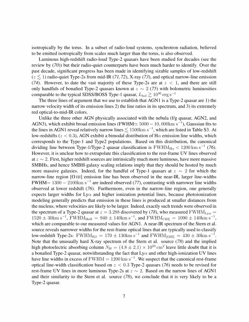
Unlike the three other AGN physically associated with the nebula (f/g quasar, AGN2, andAGN3), which exhibit broad emission lines (FWHM' 5000− 10, 000km s−1), Gaussian fits tothe lines in AGN1 reveal relatively narrow lines . 1500km s−1, which are listed in Table S3. Atlow-redshifts (z < 0.3), AGN exhibit a bimodal distribution of Hα emission line widths, whichcorresponds to the Type-1 and Type2 populations. Based on this distribution, the canonicaldividing line between Type-1/Type-2 quasar classification is FWHMHα < 1200 km s−1 (76).However, it is unclear how to extrapolate this classification to the rest-frame UV lines observedat z ∼ 2. First, higher redshift sources are intrinsically much more luminous, have more massiveSMBHs, and hence SMBH-galaxy scaling relations imply that they should be hosted by muchmore massive galaxies. Indeed, for the handful of Type-1 quasars at z ∼ 2 for which thenarrow-line region [O III] emission line has been observed in the near-IR, larger line-widthsFWHM= 1300− 2100km s−1 are indeed observed (77), contrasting with narrower line widthsobserved at lower redshift (76). Furthermore, even in the narrow-line region, one generallyexpects larger widths for Lyα and higher ionization potential lines, because photoionizationmodeling generally predicts that emission in these lines is produced at smaller distances fromthe nucleus, where velocities are likely to be larger. Indeed, exactly such trends were observed inthe spectrum of a Type-2 quasar at z = 3.288 discovered by (78), who measured FWHMLyα =1520 ± 30km s−1, FWHMHeII = 940 ± 140km s−1, and FWHMCIII] = 1090 ± 140km s−1,which are comparable to our measured values for AGN1. A near-IR spectrum of the Stern et al.source reveals narrower widths for the rest-frame optical lines that are typically used to classifylow-redshift Type-2s: FWHMHβ = 170 ± 130km s−1 and FWHM[OIII] = 430 ± 30km s−1.Note that the unusually hard X-ray spectrum of the Stern et al. source (78) and the impliedhigh photoelectric absorbing column NH = (4.8 ± 2.1) × 1023 cm2 leave little doubt that it isa bonafied Type-2 quasar, notwithstanding the fact that Lyα and other high-ionization UV lineshave line widths in excess of FWHM = 1200 km s−1. We suspect that the canonical rest-frameoptical line-width classification based on z < 0.3 Type-2 quasars (76) needs to be revised forrest-frame UV lines in more luminous Type-2s at z ∼ 2. Based on the narrow lines of AGN1and their similarity to the Stern et al. source (78), we conclude that it is very likely to be aType-2 quasar.

7

Table S3 presents measurements of the line fluxes and measurements or limits on rest-frameequivalent width for the characteristic AGN lines covered by our spectrum. Based on theseline flux measurements, Fig. S3 shows the line-ratios of AGN1 in the C IV/He II vs C IV/C III]plane (left) as well as the C III]/He II vs C III]/C II] plane (right). These are the standard lineratios conventionally discussed in studies that use photoionization modeling to diagnose thephysical conditions in the narrow-line region (79), although we note that the ratios C III]/He II

vs C III]/C II] are not typically plotted against each other. In Fig. S3, we compare the lineratios of AGN1 to other Type-2 AGN compiled from the literature. Specifically, the circles areindividual measurements of HzRGs (black) from the compilation of (80), and narrow-line X-raysources (cyan) and Seyfert-2s (blue) from the compilation of (81). In addition, triangles indicatemeasurements from the composite spectra of HzRGs (orange) from (70), the composite Type-2AGN spectra (purple) from (82), who split their population into two samples above and belowLyα EW of 63A, and a composite spectrum of mid-IR selected Type-2 AGN (green) from (83).Finally, the stars represent measurements of these line ratios from composite spectra of Type-1quasars, based on the analysis of (magenta) (84), (red-magenta) (85), and (blue-magenta) (86).

We caution that determination of robust emission line fluxes for Type-1 quasars is extremelychallenging. Generally the broad emission lines, non-trivial emission line shapes, and the factthat many of the lines of interest are severely blended, makes the separation of the spectruminto line and continuum rather ambiguous. To minimize the impact of noise and variationsamong quasars, one typically analyzes extremely high signal-to-noise ratio composite spectra,which also average down quasar-to-quasar variation (84–86). But nevertheless, the resultingline fluxes and hence line flux ratios are dependent on the method adopted (see (85)) section4.1 for a detailed discussion). These issues are particularly acute for the lines that we consider:He IIλ1640 is heavily blended with the red wing of C IV λ1549 and O III]λ1663, Al IIλ1670,and a broad Fe II complex, C III]λ1909 is severely blended with Al IIλ 1857 and Si IIIλ1892,and C II]λ2326 is blended with a broad Fe II complex. These ambiguities are reflected in thelarge variation in the line ratios determined from Type-1 quasar composites in Fig. S3 (stars)by different studies. Despite these challenges, Fig. S3 clearly illustrates that the line-ratios forAGN1 are consistent with the Type-2/Seyfert-2 locus, and differ rather significantly from theType-1 line ratios, notwithstanding the somewhat divergent measurements for the latter. Wethus conclude based on the emission line ratios of AGN1 that it is very likely to be a Type-2AGN.

Many studies utilizing WISE data have shown that at bright magnitudes W2 ' 15 mag,the WISE W1 −W2 color efficiently selects AGN at z ∼ 1 − 3, including obscured objects(87–89). This results from the rising roughly power law shape of AGN SEDs in the mid-IR (90,91), and the fact that stellar contamination is low, because the WISE W1 and W2 bandscover the Rayleigh-Jeans tail of emission from Galactic stars, resulting in much bluer colorswhich cleanly separate from redder AGN. At fainter magnitudes W2 ' 17, contaminationincreases because of optically faint, high-redshift elliptical and Sbc galaxies, which tend to alsohave very red W1 − W2 colors. In addition, obscured AGN are also expected to have veryred optical to mid-IR colors, if the mid-IR traces reprocessed dust emission from a heavily

8

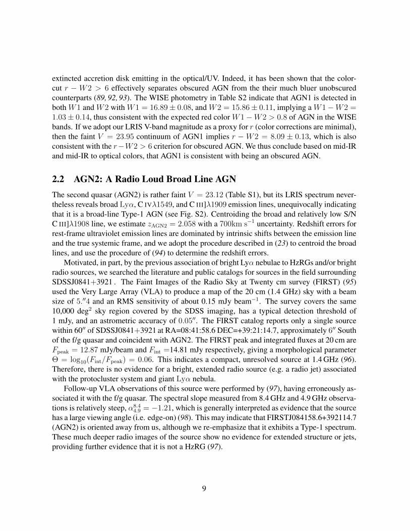
extincted accretion disk emitting in the optical/UV. Indeed, it has been shown that the color-cut r − W2 > 6 effectively separates obscured AGN from the their much bluer unobscuredcounterparts (89, 92, 93). The WISE photometry in Table S2 indicate that AGN1 is detected inboth W1 and W2 with W1 = 16.89± 0.08, and W2 = 15.86± 0.11, implying a W1−W2 =1.03± 0.14, thus consistent with the expected red color W1−W2 > 0.8 of AGN in the WISEbands. If we adopt our LRIS V-band magnitude as a proxy for r (color corrections are minimal),then the faint V = 23.95 continuum of AGN1 implies r −W2 = 8.09 ± 0.13, which is alsoconsistent with the r−W2 > 6 criterion for obscured AGN. We thus conclude based on mid-IRand mid-IR to optical colors, that AGN1 is consistent with being an obscured AGN.

2.2 AGN2: A Radio Loud Broad Line AGNThe second quasar (AGN2) is rather faint V = 23.12 (Table S1), but its LRIS spectrum never-theless reveals broad Lyα, C IVλ1549, and C III]λ1909 emission lines, unequivocally indicatingthat it is a broad-line Type-1 AGN (see Fig. S2). Centroiding the broad and relatively low S/NC III]λ1908 line, we estimate zAGN2 = 2.058 with a 700km s−1 uncertainty. Redshift errors forrest-frame ultraviolet emission lines are dominated by intrinsic shifts between the emission lineand the true systemic frame, and we adopt the procedure described in (23) to centroid the broadlines, and use the procedure of (94) to determine the redshift errors.

Motivated, in part, by the previous association of bright Lyα nebulae to HzRGs and/or brightradio sources, we searched the literature and public catalogs for sources in the field surroundingSDSSJ0841+3921 . The Faint Images of the Radio Sky at Twenty cm survey (FIRST) (95)used the Very Large Array (VLA) to produce a map of the 20 cm (1.4 GHz) sky with a beamsize of 5.′′4 and an RMS sensitivity of about 0.15 mJy beam−1. The survey covers the same10,000 deg2 sky region covered by the SDSS imaging, has a typical detection threshold of1 mJy, and an astrometric accuracy of 0.05′′. The FIRST catalog reports only a single sourcewithin 60′′ of SDSSJ0841+3921 at RA=08:41:58.6 DEC=+39:21:14.7, approximately 6′′ Southof the f/g quasar and coincident with AGN2. The FIRST peak and integrated fluxes at 20 cm areFpeak = 12.87 mJy/beam and Fint =14.81 mJy respectively, giving a morphological parameterΘ = log10(Fint/Fpeak) = 0.06. This indicates a compact, unresolved source at 1.4 GHz (96).Therefore, there is no evidence for a bright, extended radio source (e.g. a radio jet) associatedwith the protocluster system and giant Lyα nebula.

Follow-up VLA observations of this source were performed by (97), having erroneously as-sociated it with the f/g quasar. The spectral slope measured from 8.4 GHz and 4.9 GHz observa-tions is relatively steep, α8.4

4.9 = −1.21, which is generally interpreted as evidence that the sourcehas a large viewing angle (i.e. edge-on) (98). This may indicate that FIRSTJ084158.6+392114.7(AGN2) is oriented away from us, although we re-emphasize that it exhibits a Type-1 spectrum.These much deeper radio images of the source show no evidence for extended structure or jets,providing further evidence that it is not a HzRG (97).

9

2.3 AGN3: A Faint Broad Line AGNSimilar to AGN2, the source AGN3 is also faint V = 23.09 but exhibits broad emission-lines ofC IVλ 1549, C III]λ 1908, and Mg IIλ 2798 (see Fig. S2). Unfortunately Lyα was not covered byour DEIMOS spectrum, but the source has a large rest-frame equivalent width (WLyα = 35A)indicative of strong emission. Based on the broad lines, we also classify this source as a broad-line (Type-1) AGN. We determine a redshift of zAGN3 = 2.050 from the C III]λ1908 line with a700km s−1 uncertainty.

3 Probability of Finding a Quadruple QuasarThe probability dP of detecting three quasars around a single known quasar (here the f/g quasar)can be written as

dP = n3QSOdV2dV3dV4 [1

+ ξ(r12) + · · · (6 permutations)+ ζ(r12, r23, r31) + · · · (4 permutations)+ ξ(r12)ξ(r34) + ... (3 permutations)+ η(r1, r2, r3, r4) ]

(2)

where nQSO is the number density of quasars, dVi is the infinitesimal volume element centeredon the location ~ri of the ith quasar, rij is the distance between the ith and jth quasar, and ξ, ζ ,and η are the two-point, three-point, and four-point correlation functions, respectively (99).

The total probability P of finding a quadruple quasar system within a maximum radius rmax

is the integral∫dP over the three volume elements dVi, for all possible configurations of the ~ri.

Our goal in what follows is to obtain an order of magnitude estimate for this total probability.First note that on the small scales of interest to us (here r . 200 kpc), many of the terms in

eqn. (2) can be neglected. For the higher order correlation functions ζ and η, a scaling of theform ζ ∝ ξ2 and η ∝ ξ3 is often assumed. This arises from the fact that for Gaussian initialconditions and a scale-free initial power spectrum, this scaling is obeyed to second order inEulerian perturbation theory (100). However, this scaling is not valid for the highly non-linearsmall-scales of interest to us here. On these small scales, we follow the halo model approach(101), and write the higher order functions as a sum of terms representing contributions fromthe multiple possible halos. For example the four-point function can be written as the sum

η = η1h + η2h + η3h + η4h, (3)

resulting from contributions from one to four halos. As we are concerned with scales com-parable to the virial radius of the dark matter halo hosting, i.e. the f/g quasar r . 200 kpc,the one halo term, which quantifies the four-point correlations when all four points lie in thesame dark matter halo, will dominate (101). It is easier to calculate this one-halo term of thefour-point function η1h in Fourier space, where one instead works with the one halo term of thetrispectrum T 1h, and it can be shown that T 1h scales as the Fourier transform of the dark matter

10

halo density profile to the fourth power T 1h ∝ ρ4DM. This scaling holds likewise for η. Thus for

quasar 4-point correlations on small-scales, the halo model indicates that we expect η ∝ ρ4QSO,

where ρQSO is the density profile of quasars in the dark matter halos which host them.By a similar line of argument, the small-scale two- and three-point functions scale as ξ ∝

ρ2QSO and ζ ∝ ρ3

QSO, respectively. Or alternatively, ζ ∝ ξ3/2 and η ∝ ξ2. On the proper scalesof interest to us here r . 200 kpc (rcom = 600kpc, comoving), ξ � 1 and thus the termsdominating eqn. (2) are the three permutations of terms like ξ(r12)ξ(r34), and η, which are allof comparable order ξ2.

Thus in order to compute the total probability of finding three quasars around a knownquasar, we must integrate the four dominant terms in eqn. (2), over all possible configurationsof the ~ri, which can be realized within a spherical volume, whose radius is set by the largestseparation in the quadruple quasar rmax. These integrals all have a common form and order-of-magnitude. For example the first three terms involving pairs of correlation functions can bewritten

n3QSO

(∫ rmax

0

ξ(r)4πr2dr

)(∫ξ(r34)dV3dV4

)∼ n3

QSO

(∫ rmax

0

ξ(r)4πr2dr

)2

V, (4)

where V = 4π/3r3max. Thus the final expression for an order-of-magnitude estimate of the

probability is

P ∼ 4n3QSO

(∫ rmax

0

ξ(r)4πr2dr

)2

V , (5)

where the factor of four accounts for the four similar dominant terms of order ∼ ξ2 in eqn. (2).To calculate nQSO, we use the quasar luminosity function of (102) assuming an apparent

magnitude limit V < 24. This limit is highly conservative, as even AGN2 and AGN3 haveV = 23.1 mag. Although the Type-2 AGN1 has V = 24, its nucleus is obscured from ourperspective, and this magnitude represents host-galaxy emission or a small-fraction ∼ 5% ofscattered nuclear emission. The corresponding nuclear V -band emission of this AGN is likelyto be much brighter than V = 24 given that its Lyα flux, coming from the narrow-line region, isso strong, i.e. larger than that of AGN2. To account for the fact that our luminosity function onlyincludes unobscured AGN, we divide it by a factor (1−fobs), where fobs is the obscured fractionof AGN. We adopt an obscured fraction of fobs = 0.5 consistent with recent determinations(103, 104). Altogether, we estimate that the comoving number density of faint AGN is nQSO =3.8× 10−5 cMpc−3.

We assume that all four AGN reside in a physical structure with physical size rmax. This isa good assumption, given that: the projected separations of the AGN are small, they reside in alarger-scale overdensity of Lyα emitters, the f/g quasar, AGN1, and AGN2 are all embedded inthe giant Lyα nebula, and the morphology of the nebular emission around the AGN suggests aphysical association. Moreover, although we argue here that the probability of finding a quadru-ple AGN is very small, it would be much smaller if the AGN had larger line-of-sight separations,in which case one cannot invoke as large of an enhancement due to clustering. Taking the f/g

11

quasar location as the origin, the largest angular separation measured in the quadruple quasar isthat of AGN3 with θ = 18′′, corresponding to to a transverse separation r⊥ = 150 kpc. We thuschoose rmax = 250 kpc, such that the the spherical comoving volume we consider correspondsto V = 1.9 cMpc3. The probability of finding the three AGN around the f/g quasar at random,i.e. in the absence of clustering, is extremely small Pran = (nQSOV )3 = 3.4× 10−13.

The small-scale two-point correlation function of quasars was first computed by (6), andlater extended to even smaller scales ∼ 5 kpc by the gravitational lensing search of (30), whofound that a power law form ξ = (r/r0)−γ with γ = −2 and r0 = 5.4± 0.3h−1 cMpc providesa good fit to the data over a large range of scales. Plugging these numbers into eqn. (5), wefinally arrive at a probability of P = 6.9× 10−8, justifying our order of magnitude estimate ofP ∼ 1× 10−7.

4 Giant Nebulae-LAE Clustering Analysis

4.1 Constructing the LAE CatalogWe created an LAE catalog from our images of SDSSJ0841+3921 using SExtractor (105) indual-mode, using the NB image as the reference image. In order to minimize spurious detectionwe varied the parameters DETECT MINAREA (minimum detection area) andDETECT THRESH (relative detection threshold) creating a large number of LAE candidatecatalogs. We verify the number of spurious detections for each catalog running SExtractor onthe “negative” NB image obtained by multiplying the NB image by −1. The ratio between thenumber of sources detected in the NB image and the sum of sources detected in both the NBand “negative” image define a “reliability” criterion. We selected DETECT MINAREA equalto 8 pixels and DETECT THRESH equal to 1.8σ corresponding to a ”reliability” of 94%. Weused the same parameters to obtain a catalog of sources for the V -band image. In order to selectLAE candidates, we estimated the NB − V color from SExtractor isophotal magnitudes andapplied a color-cut corresponding to a Lyα rest-frame equivalent width of WLyα > 20A whichis the standard threshold used in the literature. In particular, we assumed a flat continuum slopein frequency to convert the V-band magnitude to a continuum flux at the Lyα wavelength. Forthe objects in the catalog without broad-band detection (i.e., with S/N< 3), we determine alower limit on the EW following (61). Finally, we inspected each object by eye and removedfour spurious sources that were lying in proximity to a bright star.

The final clean catalog consisted of 61 LAE candidates above a Lyα flux of limit of 5.4×10−18

erg s−1 cm−2, over our 6′×7.8′ imaging field-of-view, and the redshift range z = 2.030−2.057spanned by the narrow-band filter. We estimated that our catalog is 50% (90%) complete abovea flux limit of F50 = 6.7× 10−18 erg s−1 cm−2 (F90 = 7.4× 10−18 erg s−1 cm−2). This catalogof LAEs is presented in Table S4. In the following clustering analysis, we consider only thosesources with rest-frame WLyα > 20A and a luminosity log10 LLyα > 42.1 which at z = 2.04corresponds to a flux limit of 4.0 × 10−17 erg s−1 cm−2. Given that this flux level is a factor

12

of five higher than the 90% completeness flux limit of our catalog, we are certain that we arecomplete to such sources. The f/g quasar lies at a distance of 2.08′ from the edge of our imag-ing field, and for simplicity, our clustering analysis considers only the 10 sources within thisradius which corresponds to a comoving impact parameter of 2.2h−1 cMpc. Of these, 3/10 arethe spectroscopically confirmed AGN1-3. The sources included in our clustering analysis aredenoted by an asterisk in Table S4.

4.2 Clustering Analysis of HzRGs and LABsWe now describe how we used a compilation of LAEs around HzRGs and LABs to estimatethe giant nebulae-LAE cross correlation function. The vast majority of z ∼ 2− 3 protoclustersin the literature have been identified and studied via overdensities of LAEs over comparablefields of view 6′ × 7.8′ as our LRIS observations. For the HzRGs, we used a catalog of LAEpositions around HzRGs from the survey of (13). Specifically, we focus on six HzRGs fromthe Venemans et al. study in the redshift range z = 2.06 − 3.13, which are approximatelyco-eval with SDSSJ0841+3921 at z = 2.0412. In addition to the six HzRGs from Venemanset al. (13), we also include two LABs at z ∼ 2 − 3 from the literature whose environmentshave been surveyed for LAEs. Nestor et al. (106) conducted a narrow band imaging surveyof the well known SSA22 protocluster field at z = 3.10. Their Keck/LRIS observations werecentered on LAB1, whereas LAB2, the other known LAB in this field, resides at the edge oftheir imaging field. For this reason we only consider the overdensity around LAB1. Prescott etal. (19) conducted an intermediate-band imaging survey for LAEs around an LAB at z = 2.66(LABd05) discovered by Dey et al. (16), finding a significant overdensity, and argued that theLAB resides in a protocluster. The eight objects used in our clustering analysis are listed inTable S5.

Given that the Venemans et al. sample (13) is the largest compilation of LAEs aroundHzRGs, and that, to our knowlege, the two LABs we consider are the only ones whose envi-ronments have been characterized using LAEs to a depth comparable to our observations, thissample of eight HzRGs/LABs is the only dataset currently avaailable for conducting our clus-tering analysis and we believe that they comprise a fairly representative sample. Venemans etal. applied standard HzRG selection criteria to define their sample, and they published resultsfor all HzRGs, not just those that hosted dramatic overdensities. Although LAB1 and LABd05are larger and brighter than more typical LABs, they are comparable in size and luminosity tothe HzRGs and to SDSSJ0841+3921, making for a fair comparison. One cause for concern isthat the distribution of LAEs around the LABs were published specifically because these twosystems resided in overdensities, and thus there may be a publication bias against LABs resid-ing in lower density environments. Given that LABS only comprise a fourth of our clusteringsample, we do not believe that this significantly biases our results, but repeating our clusteringanalysis for a larger and more uniformly selected sample of LABs would clearly be desirable.

Note that the HzRG MRC 1138−2262 included in our analysis is the famous Spider WebGalaxy protocluster, which has been the subject of extensive multi-wavelength follow-up, and

13

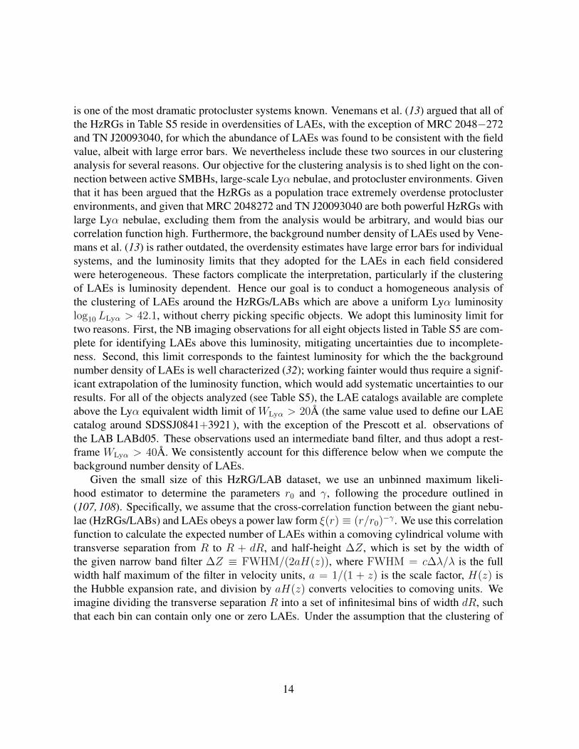
is one of the most dramatic protocluster systems known. Venemans et al. (13) argued that all ofthe HzRGs in Table S5 reside in overdensities of LAEs, with the exception of MRC 2048−272and TN J20093040, for which the abundance of LAEs was found to be consistent with the fieldvalue, albeit with large error bars. We nevertheless include these two sources in our clusteringanalysis for several reasons. Our objective for the clustering analysis is to shed light on the con-nection between active SMBHs, large-scale Lyα nebulae, and protocluster environments. Giventhat it has been argued that the HzRGs as a population trace extremely overdense protoclusterenvironments, and given that MRC 2048272 and TN J20093040 are both powerful HzRGs withlarge Lyα nebulae, excluding them from the analysis would be arbitrary, and would bias ourcorrelation function high. Furthermore, the background number density of LAEs used by Vene-mans et al. (13) is rather outdated, the overdensity estimates have large error bars for individualsystems, and the luminosity limits that they adopted for the LAEs in each field consideredwere heterogeneous. These factors complicate the interpretation, particularly if the clusteringof LAEs is luminosity dependent. Hence our goal is to conduct a homogeneous analysis ofthe clustering of LAEs around the HzRGs/LABs which are above a uniform Lyα luminositylog10 LLyα > 42.1, without cherry picking specific objects. We adopt this luminosity limit fortwo reasons. First, the NB imaging observations for all eight objects listed in Table S5 are com-plete for identifying LAEs above this luminosity, mitigating uncertainties due to incomplete-ness. Second, this limit corresponds to the faintest luminosity for which the the backgroundnumber density of LAEs is well characterized (32); working fainter would thus require a signif-icant extrapolation of the luminosity function, which would add systematic uncertainties to ourresults. For all of the objects analyzed (see Table S5), the LAE catalogs available are completeabove the Lyα equivalent width limit of WLyα > 20A (the same value used to define our LAEcatalog around SDSSJ0841+3921 ), with the exception of the Prescott et al. observations ofthe LAB LABd05. These observations used an intermediate band filter, and thus adopt a rest-frame WLyα > 40A. We consistently account for this difference below when we compute thebackground number density of LAEs.

Given the small size of this HzRG/LAB dataset, we use an unbinned maximum likeli-hood estimator to determine the parameters r0 and γ, following the procedure outlined in(107, 108). Specifically, we assume that the cross-correlation function between the giant nebu-lae (HzRGs/LABs) and LAEs obeys a power law form ξ(r) ≡ (r/r0)−γ . We use this correlationfunction to calculate the expected number of LAEs within a comoving cylindrical volume withtransverse separation from R to R + dR, and half-height ∆Z, which is set by the width ofthe given narrow band filter ∆Z ≡ FWHM/(2aH(z)), where FWHM = c∆λ/λ is the fullwidth half maximum of the filter in velocity units, a = 1/(1 + z) is the scale factor, H(z) isthe Hubble expansion rate, and division by aH(z) converts velocities to comoving units. Weimagine dividing the transverse separation R into a set of infinitesimal bins of width dR, suchthat each bin can contain only one or zero LAEs. Under the assumption that the clustering of

14

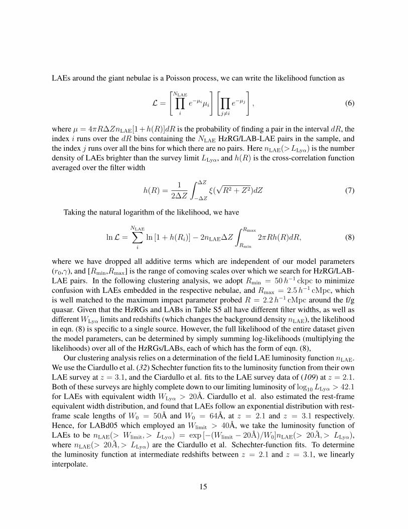
LAEs around the giant nebulae is a Poisson process, we can write the likelihood function as

L =

[NLAE∏i

e−µiµi

][∏j 6=i

e−µj

], (6)

where µ = 4πR∆ZnLAE[1 +h(R)]dR is the probability of finding a pair in the interval dR, theindex i runs over the dR bins containing the NLAE HzRG/LAB-LAE pairs in the sample, andthe index j runs over all the bins for which there are no pairs. Here nLAE(>LLyα) is the numberdensity of LAEs brighter than the survey limit LLyα, and h(R) is the cross-correlation functionaveraged over the filter width

h(R) =1

2∆Z

∫ ∆Z

−∆Z

ξ(√R2 + Z2)dZ (7)

Taking the natural logarithm of the likelihood, we have

lnL =

NLAE∑i

ln [1 + h(Ri)]− 2nLAE∆Z

∫ Rmax

Rmin

2πRh(R)dR, (8)

where we have dropped all additive terms which are independent of our model parameters(r0,γ), and [Rmin,Rmax] is the range of comoving scales over which we search for HzRG/LAB-LAE pairs. In the following clustering analysis, we adopt Rmin = 50h−1 ckpc to minimizeconfusion with LAEs embedded in the respective nebulae, and Rmax = 2.5h−1 cMpc, whichis well matched to the maximum impact parameter probed R = 2.2h−1 cMpc around the f/gquasar. Given that the HzRGs and LABs in Table S5 all have different filter widths, as well asdifferentWLyα limits and redshifts (which changes the background density nLAE), the likelihoodin eqn. (8) is specific to a single source. However, the full likelihood of the entire dataset giventhe model parameters, can be determined by simply summing log-likelihoods (multiplying thelikelihoods) over all of the HzRGs/LABs, each of which has the form of eqn. (8),

Our clustering analysis relies on a determination of the field LAE luminosity function nLAE.We use the Ciardullo et al. (32) Schechter function fits to the luminosity function from their ownLAE survey at z = 3.1, and the Ciardullo et al. fits to the LAE survey data of (109) at z = 2.1.Both of these surveys are highly complete down to our limiting luminosity of log10 LLyα > 42.1for LAEs with equivalent width WLyα > 20A. Ciardullo et al. also estimated the rest-frameequivalent width distribution, and found that LAEs follow an exponential distribution with rest-frame scale lengths of W0 = 50A and W0 = 64A, at z = 2.1 and z = 3.1 respectively.Hence, for LABd05 which employed an Wlimit > 40A, we take the luminosity function ofLAEs to be nLAE(> Wlimit, > LLyα) = exp [−(Wlimit − 20A)/W0]nLAE(> 20A, > LLyα),where nLAE(> 20A, > LLyα) are the Ciardullo et al. Schechter-function fits. To determinethe luminosity function at intermediate redshifts between z = 2.1 and z = 3.1, we linearlyinterpolate.

15

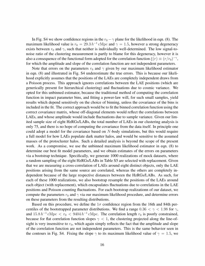
In Fig. S4 we show confidence regions in the r0−γ plane for the likelihood in eqn. (8). Themaximum likelihood value is r0 = 29.3h−1 cMpc and γ = 1.5, however a strong degeneracyexists between r0 and γ, such that neither is individually well-determined. The low signal-to-noise ratio of the clustering measurement is partly to blame for this degeneracy, however it isalso a consequence of the functional form adopted for the correlation function ξ(r) ≡ (r/r0)−γ ,for which the amplitude and slope of the correlation function are not independent parameters.

Note that errors on the parameters r0 and γ given by our maximum likelihood estimatorin eqn. (8) and illustrated in Fig. S4 underestimate the true errors. This is because our likeli-hood explicitly assumes that the positions of the LAEs are completely independent draws froma Poisson process. This approach ignores correlations between the LAE positions (which aregenerically present for hierarchical clustering) and fluctuations due to cosmic variance. Weopted for this unbinned estimator, because the traditional method of computing the correlationfunction in impact parameter bins, and fitting a power-law will, for such small samples, yieldresults which depend sensitively on the choice of binning, unless the covariance of the bins isincluded in the fit. The correct approach would be to fit the binned correlation function using thecorrect covariance matrix, whose off-diagonal elements would reflect the correlations betweenLAEs, and whose amplitude would include fluctuations due to sample variance. Given our lim-ited sample size of eight HzRGs/LABs, the total number of LAEs in our clustering analysis isonly 75, and there is no hope of computing the covariance from the data itself. In principle onecould adopt a model for the covariance based on N -body simulations, but this would requirea full model for how LAEs populate dark matter halos, and would be sensitive to the assumedmasses of the protocluster halos. Such a detailed analysis is beyond the scope of the presentwork. As a compromise, we use the unbinned maximum likelihood estimator in eqn. (8) todetermine our best fit model parameters, and we obtain estimates of the errors on parametersvia a bootstrap technique. Specifically, we generate 1000 realizations of mock datasets, wherea random sampling of the eight HzRGs/LABs in Table S5 are selected with replacement. Giventhat we are measuring a cross-correlation of LAEs around eight distinct objects, only the LAEpositions arising from the same source are correlated, whereas the others are completely in-dependent because of the large respective distances between the HzRGs/LABs. As such, foreach of these 1000 realizations, we also bootstrap resample the positions of the LAEs aroundeach object (with replacement), which encapsulates fluctuations due to correlations in the LAEpositions and Poisson counting fluctuations. For each bootstrap realizationn of our dataset, wecompute the parameters r0 and γ via our maximum likelihood procedure, and determine errorson these parameters from the resulting distributions.

Based on this procedure, we define the 1σ confidence region from the 16th and 84th per-centiles of the bootstrapped parameter distributions. We find a range 0.36 < γ < 1.98 for γ,and 15.8h−1 cMpc < r0 < 9404h−1 cMpc. The correlation length r0 is poorly constrained,because for flat correlation function slopes γ < 1, the clustering projected along the line-of-sight is very insensitive to r0, which again simply reflects the fact that the amplitude and slopeof the correlation function are not independent parameters. This is the same behavior seen inthe contours in Fig. S4. Fixing the slope γ to its maximum likelihood value of γ = 1.5, we

16

determine a 1σ confidence region for the cross-correlation length of r0 = 29.3± 4.9h−1 cMpc.Although we do not fit the binned correlation function to determine model parameters, it is

instructive to compute a binned correlation function to visualize the data, our model fits, andthe errors on these fits. As such, we define a dimensionless correlation function as

χ(Ri, Ri+1) ≡∑Nproto

j 〈PG〉ij∑Nproto

ij 〈PR〉ij− 1, (9)

where 〈PG〉ij is the number of real HzRG/LAB-LAE pairs in the impact parameter bin [Ri, Ri+1]around the jth object. The quantity 〈PR〉ij = nLAE(zj, > Wlimit,j)Vij is the expected randomnumber of pairs, which is simply the product of the background number density of LAEs, nLAE,and the cylindrical volume, Vij , defined by the bin [Ri, Ri+1] and the half-height ∆Zj of the NBfilter used to survey the jth object. We compute errors on the binned correlation function viaan analogous bootstrap method, whereby χ(Ri, Ri+1) is recomputed from 1000 bootstrap re-samplings of the sample of eight HzRGs/LABs while simultaneously bootstrap resampling theLAE separations from each object.

In Fig. S5, we show the binned correlation function calculated via this procedure, with 1σerror bars, determined by taking the 16th and 84th percentiles of the distribution of χ(Ri, Ri+1)resulting from the bootstrap samples. For any value of the model parameters r0 and γ, we cancompute the predicted value of χ(Ri, Ri+1) by evaluating the integrals

〈PG〉ij = nLAE(zj, > Wlimit,j)Vij

∫ ∆Zj

−∆Zj

∫ Ri+1

Ri

[1 + ξ(√R2 + Z2)]2πRdRdZ, (10)

and then evaluating the sum in eqn. (9). The uncertainty on the predicted clustering level,arising from the uncertainty on our model parameters, can thus be determined by evaluating the16th to 84th percentile confidence region of the predicted χ(Ri, Ri+1), using the distribution ofr0 and γ from the bootstrap resampling of our model fits. The resulting 1σ uncertainty on thepredicted correlation function is shown as the gray shaded region in Fig. S5, with the maximumlikelihood value r0 = 29.3 h−1 cMpc and γ = 1.5 shown by the red curve. We see that ourmaximum likelihood model fit and bootstrap errors are consistent with the binned correlationfunction estimates and their respective errors.

Given the results of the clustering analysis described in this sub-section, we generate Fig. 2of the main text as follows. Using our catalog of LAEs around the f/g quasar with log10 LLyα >42.1 (Table S4), and the LAE luminosity function prediction for the background number densitynLAE, we can compute the cumulative overdensity profile δ(< R) ≡ 1 + ξ(Rmin, R) = 〈PG〉/〈PR〉. The overdensity profile predicted by our maximum likelihood determination of r0 andγ for the giant nebulae-LAE correlation function are determined by evaluating eqn. (10). Thisis shown as the red curve in Fig. 2. Similarly we can determine the 1σ error on the predictedδ(< R) by evaluating it for all of our bootstrap samples of r0 and γ and taking the 16th-84thpercentile region of the resulting δ(< R) distribution. This region is shown as the shaded greyarea in Fig. 2. For comparison we show the expected overdensity (projected over our NB filter)

17

of Lyman break galaxies (LBGs) around radio-quiet quasars, based on the recent measurementsof quasar-LBG clustering at z ' 2.7 by Trainor et al. (10), who found a cross-correlationlength of r0 = 7.3 ± 1.3h−1 cMpc, assuming a fixed slope of γ = 1.5, similar to the best-fitslope deduced for our giant nebulae-LAE correlation. The blue dotted lines indicate the 1σerror quoted by Trainor et al. (10) on the cross-correlation length with the slope held fixed.Comparing to the Trainor et al. (10) measurements may seem questionable, given that: a) thisis the cross-correlation with LBGs, whereas the clustering analysis in Fig. 2 is concerned withLAEs; b) the quasars studied by Trainor et al. were hyper-luminous. However, both of thesedifferences are likely to produce small effects on the cross-correlation strength because a) theclustering of LAEs and LBGs are comparable at z ∼ 2.7, and, assuming hierarchical clustering,the cross-correlation strength is only sensitive to the square-root of any differences in clusteringstrength; and b) the Trainor et al. (10) results are consistent, within the errors, with the quasar-LBG cross-correlation results of (110), who studied much fainter quasars. Indeed, both (110)and Trainor et al. (10) argue that the clustering of LBGs around quasars is independent ofluminosity, assuaging concerns about comparing to hyper-luminous quasar clustering.

5 Near-IR Observations: The Systemic Redshift of the f/gQuasar

Quasar redshifts determined from the rest-frame ultraviolet emission lines (redshifted into theoptical at z ∼ 2) can differ by up to one thousand kilometers per second from the systemicframe, because of the complex motions of material in the broad line regions of quasars (94,111).To achieve higher precision, one may analyze spectra of the narrow [O III] emission lines emerg-ing from the narrow-line region, but at z ∼ 2, this requires near-IR spectroscopy. On UT 2007April 24, we obtained a near-IR spectrum of the f/g quasar (and also the b/g quasar) with theNear InfraRed Imager and Spectrometer (NIRI) on the Gemini North telescope. These datawere reduced and calibrated with the LowRedux package, which performs wavelength calibra-tion using the atmospheric sky lines recorded in each spectrum. With the chosen configuration,the spectra span 1.40− 1.94µm in the H-band.

Fig. S6 presents the NIRI spectra, fluxed with telluric standard stars taken that night. Eachquasar shows the detection of strong [O III] emission and modest Hβ emission. The [O III]λ5007lines were centroided using a flux-weighted line-centering algorithm with pixel values weightedby a Gaussian kernel, and this algorithm was iterated until the line center converged to withina specified tolerance (see (25) for more details). A small offset of 27km s−1 was also addedto the redshifts determined in this manner to account for average blueshift of the [O III]λ5007from systemic (111). We measured wavelength centroids of λobs = 1.5231 ± 0.0001µm and1.6095 ± 0.00006µm for the f/g and b/g quasars, respectively. This gives systemic redshiftszfg = 2.0412 for the f/g quasar and 2.2138 for the b/g quasar. We estimate an uncertainty inthis redshift of 50 km s−1 based on error in our wavelength calibration, line centering, and theestimated uncertainty when one uses [O III] to assess the systemic redshift of a quasar (111).

18

6 KinematicsIn the Main text, we described the complex kinematic motions of the quadruple AGN systemand nebula as measured with slit spectroscopy (optical and near-IR; Figs. 3,S6) and absorption-line spectroscopy of a b/g quasar (Fig. 4). The AGN exhibit line-of-sight velocity differencesof at least δv = 1300km s−1, requiring extreme gravitational motions. Note that these largevelocities cannot be explained by Hubble expansion. The miniscule probability of finding aquadruple quasar system in the absence of clustering P ∼ 10−13 (see Supp. 3), and the physicalassociation between the AGN and giant nebula, demand that the four AGN reside in a realcollapsed structure, and thus the relative motions of the AGN must result from gravitationalmotions in a collapsed structure.

The velocities of the nebular Lyα emission are also extreme, exhibiting line-of-sight veloc-ities relative to the systemic redshift of f/g quasar ranging from δv = −800 to +2500 km s−1.These also trace the gravitational potential of the protocluster but may be influenced by otherphysical processes (e.g. kinematic or radiative feedback from the AGN). Finally, the absorp-tion line kinematics of cool metal-enriched gas in the protocluster halo, measured from the b/gquasar spectrum, show strong absorption at ≈ +650 km s−1 with a significant tail to velocitiesas large as ' 1000 km s−1.

We further emphasize two aspects here. First, although the nebular emission exhibits large,relative velocity offsets, the internal motions are relatively quiescent and generally unresolvedat the Keck/LRIS spectral resolution (FWHM ≈ 160km s−1). There is no evidence for the“double-peaked” emission characteristic of resonantly trapped Lyα. This implies that the gaswithin the nebula has modest opacity to Lyα photons and that the observed radiation is notpredominantly scattered photons. These data also indicate that the gas motions are not strictlyrandom, but are rather organized into coherent flows, i.e. the velocity offsets observed greatlyexceed the measured velocity dispersions. Similar coherent motions have been previously ob-served in giant Lyα nebulae in HzRGs (112–115) and LABs (116).

Second, consider the gas kinematics along the single Slit 2 (Figs. 3and S1). This slit coversthe nebula from near the f/g quasar, where one observes a negligible velocity offset (δv ≈0km s−1), to the b/g quasar at ≈ 200 kpc separation. As one travels along the slit, the velocityoffset increases to ' +500km s−1 as one approaches the b/g quasar, where the absorption-linespectrum shows a velocity offset of δv ≈ +650km s−1 (Fig. 4). Altogether, the gas alongSlit 2 exhibits a velocity gradient of at least 500km s−1 across 200 kpc (projected). These dataestablish the presence of large-scale, high-velocity flows of cool gas within this protoclusterhalo.

19

7 Estimates for the Abundance of Giant LyαNebulae AroundQuasars

The protocluster SDSSJ0841+3921 was discovered because of its large-scale Lyα emissionproperties, and was selected from a well-defined survey for extended Lyα emission around 29quasars (22). We can use the statistics of this survey to estimate the prevalence of giant Lyαnebulae around quasars. Insofar as there appears to be a physical connection between giant Lyαnebulae and protoclusters, this also provides insight into the prevalence of protoclusters aroundquasars. We also present an estimate for the frequency of occurrence of giant Lyα nebulae froman independent narrow-band imaging survey of quasars conducted by our group, and also dis-cuss the results of similar narrow-band imaging surveys performed by others. Although muchpast work has been dedicated to characterizing Lyα nebulae around radio-loud quasar sam-ples (117), it is only recently that sensitive observations have been undertaken to characterizethe abundance of nebulae around predominantly radio-quiet quasars.

Our slit-spectroscopic observations allow us to estimate the effective covering factor of ex-tended Lyα emission around the typical quasars (Lbol ∼ 1046 erg s−1) we surveyed. Follow-ing the discussion in § 4.3 of (22; see Fig. 4 of that paper), large ∼ 70 kpc scale nebulaecan be detected down to 2 × SB1σ, where SB1σ are the 1σ surface brightness limits quotedin Table 1 of (22). In that sample a nebula of comparable brightness to SDSSJ 0841+3921SBLyα ' 10−17 erg s−1 cm−2 arcsec−2 could have been detected at > 2σ significance in 23/29cases (see Table 1 of (22)). Based on this, we can crudely determine the covering factor ofsuch filamentary emission as being the ratio of the area of the filament covered by our origi-nal slit observation of SDSSJ 0841+3921 (Slit2 in Figs. 3and S1), to the total area surveyed atsensitivity sufficient to detect a SBLyα > 10−17 erg s−1 cm−2 arcsec−2 nebula.

We consider an annular region around a z = 2 quasar with an inner radius of R⊥,min =50 kpc (5.8′′) and outer radius of R⊥,max = 150 kpc (17.3′′). The inner radius is chosen to ex-clude the small-scale fuzz atR⊥ < 50 kpc, which is detected in a large fraction of quasars (22),from the larger scale filamentary emission. The outer radius corresponds to the maximum extentof the (high significance) emission detected in our discovery spectrum of SDSSJ 0841+3921(see Slit2 in Fig. 3panel c, and the middle column of Fig. S1), and is about the virial radius ofthe dark matter halos Mvir = 1012.5 M� at z = 2 which host quasars (11). We also observea drop-off in the covering factor of optically thick absorbers at R⊥ ' 200 kpc, comparableto this R⊥,max (27). We assume the filamentary emission in the discovery spectrum extendsfrom +50 kpc to +150 kpc at positive slit position, and −50 to −80 kpc at negative slit po-sitions, corresponding to an area of 15 sq. arcsec given our 1′′ slit (1130 kpc2). The total areais equal to the NQSO = 23 quasars observed to sufficient depth, times the 23 sq. arcsec area(1740 kpc2) for which our slit intersects the annular region, implying a total area of 530 sq.arcsec (39922 kpc2) surveyed. For reference, the total annular area around a single quasar is834 sq. arcsec (62832 kpc2), so the effective area of our survey is 64% of the area around asingle quasar. Hence we deduce a covering factor of filamentary emission of fC,fil = 0.028.

Thus taken in aggregate, we find that only ' 3% of the area between R⊥ = 50 − 150 kpc

20

around quasars is covered by Lyα emission with SBLyα > 10−17 erg s−1 cm−2 arcsec−2 , whichcan be compared to the much larger covering factor of 31% above this level, measured foremission over the same area from our NB image of SDSSJ0841+3921 (see Fig. 1a). The ag-gregate and individual covering factors can be commensurated if the majority of quasars donot exhibit large-scale Lyα nebulae above SBLyα > 10−17 erg s−1 cm−2 arcsec−2, but a smallfraction ' 10% have bright nebulae covering a large area, as in SDSSJ0841+3921 , and theproduct of this ∼ 10% frequency and ∼ 31% covering factor set the aggregate ∼ 3% effectivecovering factor for the entire population. This argument is consistent with our intuition that,given the random orientation of the slit, we could probably only have identified the asymmetricextended emission around SDSSJ0841+3921 for ∼ 50% of the possible slit orientations, andgiven that 23 objects were surveyed to the required depth, this again suggests that ∼ 10% ofquasars exhibit giant nebulae.

An independent estimate for the frequency of giant Lyα nebulae around quasars can also bedetermined from a narrow band imaging survey conducted by our group. As part of a continuingprogram to search for fluorescent Lyα emission powered by luminous z ∼ 2 quasars, to date wehave obtained deep narrow band imaging of a sample of 26 objects. These survey observationsare analogous to the narrow-band imaging of SDSSJ 0841+3921 discussed in Supp. 1.2, in thatthey use custom designed narrow-band filters, however the targets constitute an independentsample of quasars, which are not part of the QPQ survey of (22). These observations have beenconducted on multiple telescopes, which we briefly summarize. For the present purposes wedefine a giant Lyα nebula to be extended emission on a scale > 50 kpc from the quasar withaverage SBLyα > 10−17 erg s−1 cm−2 arcsec−2.

The quasar HE0109−3518 at z = 2.41 was observed with the Very Large Telescope/ -FOcalReducer Spectrograph (VLT-FORS) using a custom designed narrow band filter (λcenter =4145A, FWHMλ = 40A) for a total exposure time of about 20 hours, achieving a sensitiv-ity limit (1σ) of SBLyα = 8 × 10−19 erg s−1 cm−2 arcsec−2 (61). No extended Lyα nebulawas discovered. We have imaged a total of eight quasars with the Keck LRIS imaging spec-trometer, of which three were observed with a filter centered on Lyα redshifted to z = 2.279(λcenter = 3986A, FWHMλ = 30A), and five with one centered at z = 2.190 (λcenter = 3878A,FWHMλ = 30A). The exposure times for the LRIS observations vary from 2 to 10 hours, re-sulting in sensitivity limits (1σ) ranging from SBLyα = 1.2 × 10−18 erg s−1 cm−2 arcsec−2 to5 × 10−19. These VLT/FORS and Keck/LRIS observations specifically targeted hyper-luminousquasars V . 17, with the goal of understanding fluorescent Lyα emission from dark-galaxies(61) and the quasar CGM (41), and led to the discovery of a giant Lyα nebula around thequasar UM287 at z = 2.28. Nebulae were not detected around any of the other quasarssurveyed. Finally, using a custom filter centered on Lyα at z = 2.253 (λcenter = 3955A,FWHMλ = 30A), we have observed a total of 17 quasars using the Gemini Multi ObjectSpectrograph (GMOS) on the telescope Gemini South. For the GMOS observations, a subsetof 3 quasars were observed with longer integrations, typically 5 hours and achieving a depthof (1σ) SBLyα = 1.5 × 10−18 erg s−1 cm−2 arcsec−2; whereas the other 14 quasars were ob-served in a fast survey mode with typical exposure times of about 2 hours and depth SBLyα =

21

3 − 4 × 10−18 erg s−1 cm−2 arcsec−2. Although the instruments used and depths achievedare heterogeneous, all of the aforementioned observations reached sufficient depth to detectLyα nebulae with SBLyα > 10−17 erg s−1 cm−2 arcsec−2. Taking all of these observations to-gether, we have observed a total of 26 quasars and detected a single giant Lyα nebula aroundUM287 (41), implying that 1/26 = 0.04 of quasars host giant Lyα nebulae. Adopting the1σ confidence interval appropriate for the Poisson distribution in the small number regime, wededuce that the frequency of occurrence of giant nebulae is in the range 3− 9%.

Finally, an independent narrow band imaging survey of quasars at z ∼ 2.7 is being car-ried out as part of the Keck Baryonic Structure Survey (KBSS), and the first results on thedistribution of LAEs around quasars were recently published by Trainor et al. (118). Basedon these narrow band imaging observations, (39) published the discovery and additional ob-servations of a giant Lyα nebula around the quasar HS1549+19 with properties comparable tothat around SDSSJ0841+3921 . Trainor et al. quote a typical narrow-band imaging depth ofmNB(3σ) ∼ 26.7 for point sources, resulting from 5-7hr integrations on Keck LRIS using filterswith FWHM∼ 80A. This corresponds to a (1σ) SBLyα ' 1.5 × 10−18 erg s−1 cm−2 arcsec−2,which although shallower than our own Keck LRIS survey (owing to their wider filters), itis nevertheless sufficient to detect giant nebulae with SBLyα > 10−17 erg s−1 cm−2 arcsec−2.There are 8 objects observed in the Trainor et al. sample, but it is unknown to us whether ad-ditional Lyα nebulae are present, besides that around HS1549+19. As such, one can place alower limit on the frequency of giant Lyα nebulae to be 1/8 = 0.125, or a 1σ Poisson confidenceinterval of 10− 29%.

To summarize, three independent surveys indicate that the frequency of occurrence of giantLyα nebulae around quasars is consistent with being ' 10%, although there are still limitationsdue to relatively small samples, heterogeneity of the datasets, and the differences in the searchtechniques (narrow-band imaging versus spectroscopy).

8 The Environments of Other Quasars with Giant Lyα Neb-ulae and the Impact of Lyα Fluorescence

Although quasar clustering indicates that the majority of z ∼ 2 quasars reside in moderateoverdensities, we speculate that∼ 10% trace much more massive structures, and it is this subsetwhich also exhibits giant Lyα nebulae. SDSSJ0841+3921 clearly supports this interpretation,but there are indeed other examples.

Of course, we also have NB imaging data for UM287, the quasar at z = 2.27 with a gi-ant Lyα nebula recently discovered by our group (41). However, because UM287 is a hyper-luminous quasar, we cannot characterize its environment via the number counts of LAEs as wehave for SDSSJ0841+3921 . The reason for this is that distribution of LAEs on Mpc scalesfrom hyper-luminous quasars is likely to be dramatically enhanced by Lyα fluorescence (61),and it is not straightforward to disentangle the fluorescence and clustering enhancements. Forexample, consider the hyper-luminous quasar HE0109−3518, the proto-typical case for Lyα

22

fluorescence by dark-galaxies studied by (61). The number of LAEs within R < 4h−1 cMpcof HE0109−3518 is ∼ 8.5 times larger than the cosmic background number expected from theLAE luminosity function, whereas the quasar-LBG correlation function (a reasonable proxy forthe quasar-LAE clustering) averaged over the volume probed by these narrow-band observa-tions would only predict an enhancement of ∼ 1.5. One comes to similar conclusions about thenumber of LAEs discovered around the hyper-luminous quasars in the KBSS sample of (118).Progress on understanding the environment of UM287, and its relationship to the giant Lyαnebulae, will require a sample of galaxies selected via broad-band photometry (i.e. LBG selec-tion), to avoid contamination from fluorescence. Nevertheless, while fluorescence precludes asimple interpretation of LAE clustering around UM287, we note that, intriguingly, follow-upobservations also revealed a faint V ' 22 companion quasar, indicating an overdensity of AGNsimilar to SDSSJ0841+3921 .

Note however that enhanced LAE clustering around SDSSJ0841+3921 due to Lyα fluores-cence is expected to be negligible, because brightest quasar in the system, namely the f/g quasarwith V = 19.8 is an order of magnitude fainter than the hyper-luminous quasars which exhibitthis fluorescence effect. Radiative transfer simulations of Lyα fluorescence around quasars (61)supports this conclusion. Furthermore, the four AGN in SDSSJ0841+3921 clearly constitute adramatic overdensity of AGN, and there is no way for Lyα fluorescence to enhance AGN clus-tering. Note that the other three AGN do not significantly enhance the ionizing luminosity andhence cannot boost the fluorescence signal. The fainter Type-1 AGN AGN2 and AGN3 haveV ' 23 (see Table S2), and thus contribute negligibly to the total ionizing photon productioncompared to the f/g quasar. Although we do not detect the continuum from the accretion diskof the Type-2 AGN AGN1, it is detected in the WISE bands W1 and W2 (see Table S2). Atz ' 2 these bands probe rest-frame ∼ 1µm, which are likely still dominated by emission fromthe reddest part of the accretion disk. The fact that AGN1 is > 1 magnitude fainter than the f/gquasar indicates that its UV ionizing continuum (although obscured from our perespective) isvery unlikely to be brighter than that of the f/g quasar.

The KBSS quasar HS1549+19 at z = 2.85, which has been narrow band imaged by Trainoret al. (118), harbors a giant Lyα nebula (39) with SB and properties comparable to that aroundSDSSJ0841+3921 . Extensive imaging and spectroscopy of HS1549+19 has demonstratedthat it is clearly a dramatic protocluster, with a Mpc-scale overdensity of Lyman break galaxies(LBGs) a factor of ∼ 3.5 times larger than that around typical quasars (10, 38). Although thisquasar is hyper-luminous, Lyα fluorescence is not an issue because the protocluster overdensityis based on the clustering of broad-band selected LBGs, and not LAEs.

Finally, one may have concerns that the dramatic enhancements of LAEs around HzRGsand LABs, quantified by our clustering analysis in Supp. 4 and shown in Figs. 2 and S5, couldbe partly due to Lyα fluorescence. This is a valid concern, because there is compelling evidencethat the HzRGs are obscured quasars (119), and their ionizing photons, although obscured fromour perspective, surely shine in other directions, and are likely to power their giant Lyα nebu-lae. Similar considerations hold for LABs, although a direct association with obscured AGN hasbeen more challenging to establish (18,120–123). However, we think that it is unlikely that flu-

23

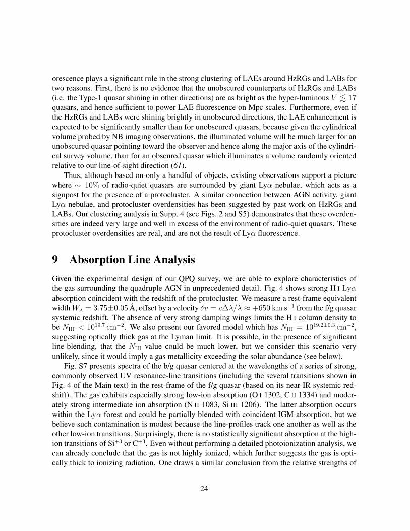
orescence plays a significant role in the strong clustering of LAEs around HzRGs and LABs fortwo reasons. First, there is no evidence that the unobscured counterparts of HzRGs and LABs(i.e. the Type-1 quasar shining in other directions) are as bright as the hyper-luminous V . 17quasars, and hence sufficient to power LAE fluorescence on Mpc scales. Furthermore, even ifthe HzRGs and LABs were shining brightly in unobscured directions, the LAE enhancement isexpected to be significantly smaller than for unobscured quasars, because given the cylindricalvolume probed by NB imaging observations, the illuminated volume will be much larger for anunobscured quasar pointing toward the observer and hence along the major axis of the cylindri-cal survey volume, than for an obscured quasar which illuminates a volume randomly orientedrelative to our line-of-sight direction (61).

Thus, although based on only a handful of objects, existing observations support a picturewhere ∼ 10% of radio-quiet quasars are surrounded by giant Lyα nebulae, which acts as asignpost for the presence of a protocluster. A similar connection between AGN activity, giantLyα nebulae, and protocluster overdensities has been suggested by past work on HzRGs andLABs. Our clustering analysis in Supp. 4 (see Figs. 2 and S5) demonstrates that these overden-sities are indeed very large and well in excess of the environment of radio-quiet quasars. Theseprotocluster overdensities are real, and are not the result of Lyα fluorescence.

9 Absorption Line AnalysisGiven the experimental design of our QPQ survey, we are able to explore characteristics ofthe gas surrounding the quadruple AGN in unprecedented detail. Fig. 4 shows strong H I Lyαabsorption coincident with the redshift of the protocluster. We measure a rest-frame equivalentwidthWλ = 3.75±0.05 A, offset by a velocity δv = c∆λ/λ ≈ +650 km s−1 from the f/g quasarsystemic redshift. The absence of very strong damping wings limits the H I column density tobe NHI < 1019.7 cm−2. We also present our favored model which has NHI = 1019.2±0.3 cm−2,suggesting optically thick gas at the Lyman limit. It is possible, in the presence of significantline-blending, that the NHI value could be much lower, but we consider this scenario veryunlikely, since it would imply a gas metallicity exceeding the solar abundance (see below).

Fig. S7 presents spectra of the b/g quasar centered at the wavelengths of a series of strong,commonly observed UV resonance-line transitions (including the several transitions shown inFig. 4 of the Main text) in the rest-frame of the f/g quasar (based on its near-IR systemic red-shift). The gas exhibits especially strong low-ion absorption (O I 1302, C II 1334) and moder-ately strong intermediate ion absorption (N II 1083, Si III 1206). The latter absorption occurswithin the Lyα forest and could be partially blended with coincident IGM absorption, but webelieve such contamination is modest because the line-profiles track one another as well as theother low-ion transitions. Surprisingly, there is no statistically significant absorption at the high-ion transitions of Si+3 or C+3. Even without performing a detailed photoionization analysis, wecan already conclude that the gas is not highly ionized, which further suggests the gas is opti-cally thick to ionizing radiation. One draws a similar conclusion from the relative strengths of

24

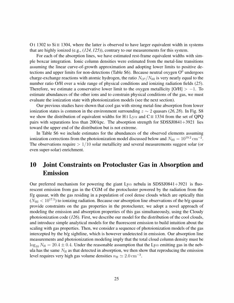
O I 1302 to Si II 1304, where the latter is observed to have larger equivalent width in systemsthat are highly ionized (e.g., (124, 125)), contrary to our measurements for this system.

For each of the absorption lines, we have estimated rest-frame equivalent widths with sim-ple boxcar integration. Ionic column densities were estimated from the metal-line transitionsassuming the linear curve-of-growth approximation and adopting lower limits to positive de-tections and upper limits for non-detections (Table S6). Because neutral oxygen O0 undergoescharge-exchange reactions with atomic hydrogen, the ratio NO0/NHI is very nearly equal to thenumber ratio O/H over a wide range of physical conditions and ionizing radiation fields (25).Therefore, we estimate a conservative lower limit to the oxygen metallicity [O/H] > −1. Toestimate abundances of the other ions and to constrain physical conditions of the gas, we mustevaluate the ionization state with photoionization models (see the next section).

Our previous studies have shown that cool gas with strong metal-line absorption from lowerionization states is common in the environment surrounding z ∼ 2 quasars (26, 28). In Fig. S8we show the distribution of equivalent widths for H I Lyα and C II 1334 from the set of QPQpairs with separations less than 200 kpc. The absorption strength for SDSSJ0841+3921 liestoward the upper end of the distribution but is not extreme.

In Table S6 we include estimates for the abundances of the observed elements assumingionization corrections from the photoionization model discussed below and NHI = 1019.2 cm−2.The observations require > 1/10 solar metallicity and several measurements suggest solar (oreven super-solar) enrichment.

10 Joint Constraints on Protocluster Gas in Absorption andEmission

Our preferred mechanism for powering the giant Lyα nebula in SDSSJ0841+3921 is fluo-rescent emission from gas in the CGM of the protocluster powered by the radiation from thef/g quasar, with the gas residing in a population of cool dense clouds which are optically thin(NHI < 1017.5) to ionizing radiation. Because our absorption line observations of the b/g quasarprovide constraints on the gas properties in the protocluster, we adopt a novel approach ofmodeling the emission and absorption properties of this gas simultaneously, using the Cloudyphotoionization code (126). First, we describe our model for the distribution of the cool clouds,and introduce simple analytical models for the fluorescent emission to build intuition about thescaling with gas properties. Then, we consider a sequence of photoionization models of the gasintercepted by the b/g sightline, which is however undetected in emission. Our absorption linemeasurements and photoionization modeling imply that the total cloud column density must belog10NH = 20.4± 0.4. Under the reasonable assumption that the Lyα emitting gas in the neb-ula has the same NH as that detected in absorption, we then show that reproducing the emissionlevel requires very high gas volume densities nH ' 2.0 cm−3.

25

10.1 Cool Cloud Model and Emission EstimatesWe consider an idealized model whereby the gas in the protocluster halo resides in a popula-tion of cool T ∼ 104 K spherical gas clouds, which have a single uniform hydrogen volumedensity nH and hydrogen column density NH. The clouds are uniformly distributed throughouta spherical halo of radius R, and their aggregate covering factor, defined to be an average overthe sphere, is fC. Four parameters (R,nH,NH, fC) completely describe the distribution of thegas (see (22) for further details), for example the total cool gas mass can be written

Mc = 3.3 × 1011

(R

250 kpc

)2(NH

1020.5 cm−2

)(fC

0.5

)M� (11)

We now consider fluorescent Lyα emission from this population of cool gas clouds poweredby a bright central quasar. There are two regimes where simple expressions can be obtained forthe resulting emission, namely when the gas clouds are either optically thin NHI < 1017.5 cm−2

or optically thick NHI > 1017.5 cm−2 to Lyman continuum photons. For the optically thin case,the gas clouds are highly ionized, and the average Lyα SB from the halo will be

SBLyα = 1.2× 10−17

(1 + z

3.0

)−4(fC

0.5

)( nH

1.0 cm−3

)( NH

1020.5 cm−2

)erg s−1 cm−2 arcsec−2.

(12)Note that because the gas is already highly-ionized, the SB is independent of the luminosity ofthe central ionizing source provided that it is bright enough to maintain the gas as optically thin.

If the clouds are optically thick to ionizing radiation, they will no longer emit Lyα propor-tional to the volume that they occupy because of self-shielding effects. Instead, a thin highlyionized skin will develop around each cloud, and nearly all recombinations and resulting Lyαphotons will originate in this skin. The cloud will then behave like a ‘mirror’, converting a frac-tion ηthick = 0.66 of the ionizing photons it intercepts into Lyα photons (127). In this regime,it can be shown (see (22)) that the fluorescent SB, averaged over the halos is

SBLyα =ηthickhνLyα

4π(1 + z)4fCΦ(R/

√3) (13)

= 8.8× 10−17

(1 + z

3.0

)−4(fC

0.5

)(R

100 kpc

)−2

×(

LνLL

1030.5 erg s−1 Hz−1

)erg s−1 cm−2 arcsec−2,

where hνLyα is the energy of a Lyα photon and Φ (phot s−1 cm−2) is the ionizing photon numberflux

Φ =

∫ ∞νLL

Fνhνdν =

1

4πr2

∫ ∞νLL

Lνhνdν. (14)

To obtain the second equality in eqn (13), we assume that the quasar spectral energy distribu-tion obeys the power-law form Lν = LνLL

(ν/νLL)αUV , blueward of νLL and adopt a slope of

26

αUV = −1.7 consistent with the measurements of (128). The quasar ionizing luminosity is thenparameterized by LνLL

, the specific luminosity at the Lyman edge. As we describe in detail be-low, we estimate that f/g quasar has log10 LνLL

= 30.5, which is the value adopted in eqn. (13).In the optically thick regime, we see that the SB now depends on the luminosity of the quasar,as well as on the covering factor fC, but is independent of the gas properties (i.e. nHandNH).

The smooth morphology of the emission in the Lyα nebula implies a covering factor offC & 0.5. Even if the emitting clouds have angular sizes much smaller than the PSF of ourNB imaging, the morphology of the nebular emission would appear much more clumpy forlower covering factors. We have explicitly verified this by generating simulated images ofmock Lyα emission distributions with the required SB and a range of covering factors fC,and then convolving them with our NB-imaging PSF (129). In what follows we will alwaysassume a covering factor of fC = 0.5 for both the gas we detect in emission, as well as thatdetected in absorption. This value is well motivated: a) for the emission it is based on thesmooth morphology of the nebula; b) for the absorption it is approximately the covering factorof optically thick absorbers on R . 200 kpc scales in the quasar CGM (27).

The average SB of the giant Lyα nebula at R ' 100 kpc is SBLyα = 1.3× 10−17

erg s−1 cm−2 arcsec−2, which we compute via the emission from the area within our 2σ SBcontour which intersects the the annulus R = [75, 125] kpc. This is several times lower than theexpectation from eqn. (13) for the optically thick regime. Thus our simple analytical scalingrelations already appear to favor a situation where the clouds are optically thin. We return tothis comparison below using photoionization models.

10.2 Details of Cloudy ModelingThe expressions in eqns. (12) and (13) provide reasonable estimates for the fluorescent SB, butthey neglect other sources of Lyα emission such as collisional excitation (i.e. cooling radiation),and pumped or ‘scattered’ Lyα photons arising from the diffuse continuum produced by the gasitsel. Note that we do not attempt to model scattering of Lyα photons produced by central f/gquasar itself. Radiative transfer simulations of radiation from a hyper-luminous quasar througha simulated gas distribution (41), have shown that the contribution of scattered Lyα line photonsfrom the quasar do not contribute significantly to the Lyα surface brightness of the nebula.Given that this calculation was for a hyper-luminous quasar a factor of∼ 10 times brighter thanthe f/g quasar, scattered line photons from the quasar are expected to contribute negligibly tothe nebular emission., and they also do not treat the temperature dependence of the emission.To fully account for these effects, we construct photoionization models for a slab of gas beingilluminated by a quasar using the Cloudy software package (126). Cloudy predicts the emergentspectrum from the gas, allowing us to compute its SB, which we then dilute by the coveringfactor fC = 0.5.

We model the quasar spectral-energy distribution (SED) using a composite quasar spectrumwhich has been corrected for IGM absorption (128). This IGM corrected composite is importantbecause it allows us to relate the g-band magnitude of the f/g quasar to the specific luminosity

27

at the Lyman limit LνLL. For energies greater than one Rydberg, we assume a power law form

Lν = LνLL(ν/νLL)αUV and adopt a slope of αUV = −1.7, consistent with the measurements

of (128). We determine the normalization LνLLby integrating the Lusso et al. (128) composite

spectrum against the SDSS filter curve, and choosing the amplitude to give the correct g-bandmagnitude of the f/g quasar (see Table S2), which gives a value of log10 LνLL

= 30.5. Weextend this UV power law to an energy of 30 Rydberg, at which point a slightly different powerlaw is chosen α = −1.65, such that we obtain the correct value for the specific luminosity at2 keV Lν(2 keV) implied by measurements of αOX, defined to be Lν(2 keV)/Lν(2500 A) ≡(ν2 keV/ν

2500 A)αOX . We adopt the value αOX = −1.5 measured by (130) for SDSS quasars

of comparable luminosities. An X-ray slope of αX = −1, which is flat in νfν is adoptedin the interval of 2-100 kev, and above 100 keV, we adopt a hard X-ray slope of αHX = −2.For the rest-frame optical to mid-IR part of the SED, we splice together the composite spectraof (128), (84), and (131). These assumptions about the SED are essentially the standard onesused in photoionization modeling of AGN (e.g. (132)). We also include the contribution fromthe radiation field of the ambient UV background radiation field using the spectrum of (133),but it is completely sub-dominant relative to the f/g quasar at the distances that we consider.

These Cloudy models require as an input the ionizing photon number flux Φ(r) (seeeqn. (14)) at the surface of the cloud. Because this varies with radius as r−2, in principle mod-eling the halo emission would require integrating over a distinct photoionization model at eachradius. For simplicity, we restrict attention to just a few radii. For our model of the opticallythick absorber, we set r = 250 kpc, which we believe is the likely location of the absorbinggas for several reasons. First, the nebula itself has an end-to-end size of ' 500 kpc roughlycentered on the f/g quasar, such that r = 250 kpc is a reasonable radius for the absorber giventhe measured impact parameter R⊥ = 176 kpc of the b/g quasar sightline. Second, given thisimpact parameter, the characteristic velocity separation of the absorbing gas from systematicvmax = 600 kms−1 implied by the metal-line absorption (see Fig. S7), we can compute the con-ditional probability distribution P (< r|R⊥, vmax) that the distance between the quasar and theabsorber is less than r, which is determined by the quasar-LLS correlation function which wehave measured (24, 27). For the problem at hand, we find that P (< r|R⊥, vmax) = 0.43 forr = 250 kpc, again indicating that this is a reasonable distance (see a similar discussion in § 4.1of (25)). According to eqn. (13), the SB arising from such optically thick gas scales with Φ,and hence will decrease as r−2. For the gas producing the Lyα emission, we model three radiir = [50, 100, 250] kpc. We will argue that the emitting gas in the nebula is optically thin, and inthis regime the SB is independent of Φ (see eqn. (12)). Thus considering a few radii to describethe emission is a reasonable approximation provided the gas remains optically thin at the radiiin question.

The Cloudy model of the cool cloud is completely specified by the value of Φ, the SEDshape, the metallicity of the gas Z, the hydrogen volume density nH, and a ‘stopping criterion’,which sets the total column density of the cloud. Because we assume the f/g quasar and UVBare the only sources of ionizing photons, Φ and the SED shapes are fixed. For the metallicity,we adopt a value of log(Z/Z�) = −0.5 consistent with our lower-limit (log(Z/Z�) > −1) on

28

the metallicity of the optically thick absorber detected in the b/g quasar sightline (see Supp. 9).We have confirmed that the results discussed below are insensitive to the assumed gas metal-licity. We have also verified that our results are insensitive to the exact value of the UV slopeα = −1.7, within the 1σ error measured by Lusso et al. α = −1.7 ± 0.6. Our models thusconstitute a one-dimensional sequence parameterized by the volume density of the clouds nH.Photoionization models are known to be self-similar in the ionization parameter U = Φ/nHc,which is the ratio of the number density of ionizing photons to hydrogen atoms. Since Φ hasbeen fixed, our sequence of models is thus also a sequence in U , spanning the relevant range ofionization conditions. Our stopping criterion depends on what is known about the gas that weare attempting to model, which we elaborate on next.

10.3 Photoionization Model of the Absorbing GasHere we compare photoionization models to the properties of the optically thick absorber inthe spectrum of the b/g quasar, lying at at an impact parameter of R⊥ = 176 kpc from the f/gquasar. We follow the standard approach (25) and focus our analysis on multiple ionizationstates of individual elements to avoid uncertainties related to intrinsic abundances. Specifically,our column density measurements in Table S6 yield the following limits on ionic ratios:C+/C3+ > 0.8, Si+/ Si3+ > 1.3, and Si+/Si2+ < 0.7. In addition, we measured the neutralcolumn density to be NHI = 1019.2 cm−2, which we use as the stopping criterion of the Cloudymodel. In other words, Cloudy will continue to add slabs of material until this neutral columnis reached, guaranteeing that we satisfy this constraint. Finally, we do not detect Lyα emissionfrom the vicinity of the background sightline, allowing us to set an upper limit of SBLyα < 5.1×10−18 erg s−1 cm−2 arcsec−2 from the cool gas. This SB limit was computed via simulationswhereby a fake circular source with radius of 3′′ was placed at the location of the b/g quasar.This exercise showed that only sources with SBLyα > 3 × SB1σ would be clearly detectable,where SB1σ = 1.7×10−18 erg s−1 cm−2 arcsec−2 is our 1σ SB limit for 1.0 sq. arcsec apertures.Note that the individual clouds intercepted by our sightline may have extremely small sizes∼ 10 pc making it impossible to angularly resolve emission from a single cloud. However, wehave argued that these clouds have a large covering factor of fC = 0.5 such that we would beable to detect their aggregate emission near the location of the b/g sightline (see Fig. 1 in (22)for more details).

Our sequence of photoionization models is compared to the observational constraints inFig. S9. The three different ionic ratios considered paint a consistent picture for the ioniza-tion state, and we constrain the ionization parameter to be log10 U = −2.7 ± 0.3, where weconservatively include an error of 0.3 dex to account for both statistical and systematic uncer-tainties in the photoionization modeling. Accordingly, the neutral fraction is constrained to belog10 xHI = −1.2 ± 0.3, and the total hydrogen column log10NH = 20.4 ± 0.4, where the er-ror on NH includes the quadrature sum of modeling uncertainty in the neutral fraction, and theuncertainty in our measurement of NHI (see Supp. 9). Plugging this determination of the totalhydrogen column density into eqn. (11) we obtain a total cool gas mass ofMc = 2.4 × 1011M�

29

within a spherical halo R = 250 kpc, or the range 1.0 × 1011M� < Mc < 6.5 × 1011M� im-plied by the 1σ measurement and modeling error on NH. Note that given the self-similarity ofthe photoionization models with ionization parameter U , these results are essentially indepen-dent of the value of Φ that we have assumed in our models, and hence the distance of the gasfrom the quasar. Lastly, we have calculated the ionization corrections to the ionic column den-sities measured for the absorbing gas and provide limits on the elemental abundances impliedby each metal absorption line measurement in Table S6.

According to the photoionization models, if indeed the absorbing gas lies at a distancer = 250 kpc and is illuminated by the f/g quasar, the Lyα emission would be SBLyα '3 − 4 × 10−18 erg s−1 cm−2 arcsec−2, which lies just below our detection limit SBLyα = 5.1 ×10−18 erg s−1 cm−2 arcsec−2, and is hence consistent with our non-detection of extended emis-sion near the b/g quasar sightline. Indeed, because the gas is optically thick, and essentiallyabsorbs all ionizing photons that impinge on it, the SBLyα is nearly independent of the volumedensity, and as expected from eqn. (13), depends primarily on Φ and our assumed covering fac-tor fC = 0.5. The weak dependence on nH arises because, at the lowest ionization parametersand hence highest neutral fractions, as much as ∼ 20% of the Lyα is produced by collisionalexcitation (green curve labeled collisions in Fig. S9). This is because collisional excitation ofneutral hydrogen requires a large neutral fraction, and it is also exponentially sensitive to tem-perature. The low nH . 10−2 cm3 and high ionization parameter log10 U & −1 models arehighly ionized xHI . 10−3, and have higher temperatures T & 17, 000 K, both of which tendto suppress collisional excitation. As a result of the very weak dependence of SBLyα on nH inthe optically thick regime, our non-detection of emission does not allow us to put interestingconstraints on the volume density nH for the absorbing gas.

Note that the fact that our photoionization model predicts Lyα emission from the absorbinggas just below our detection limit results from our assumed distance of r = 250 kpc, sincefor optically thick gas SBLyα ∝ φ ∝ r−2 (see eqn. 13). Had we assumed a distance equalto the impact parameter R⊥ = 176 kpc the predicted emission would be a factor of two higherSBLyα ∼ 10−17 erg s−1 cm−2 arcsec−2, and hence detectable. As such it is informative to brieflydiscuss all possible scenarios that would result in a non-detection of Lyα from the absorbinggas. These are: 1) the gas is illuminated by the f/g quasar, but it lies at a distance r & 250 kpcsuch that its fluorescent Lyα emisssion is below our detection threshold; 2) the gas is illuminatedby the quasar and is at a distance comparable to the impact parameter, but the covering factor ofoptically thick gas is much lower than we have assumed fC = 0.5; 3) the absorbing gas is notilluminated by the f/g quasar but is instead shadowed, perhaps because from its vantage point thequasar is extincted by the same obscuring medium invoked in AGN unification models (67,68).

Unfortuately, our current observations cannot distinguish between these three scenarios,however we favor scenario 1), that the gas lies at a distance ' 250 kpc from the quasar, asshown in Fig. S9. While it is possible that the covering factor of optically thick gas is indeedlower than the fC = 0.5 that we have assumed, we consider this unlikely for two reasons.First, this would be in conflict with the statistical properties of optically thick absorption for theaggregate population of quasars (27). Although, SDSSJ0841+3921 is atypical given that it is

30

a protocluster and hosts a giant nebula, we already argued that the smooth morphology of thegiant nebula also argues for a high covering factor fC & 0.5 of the emitting gas, to prevent theemission from appearing too clumpy. Under the reasonable assumption that the absorbing andemitting gas have the same origin, one expects their covering factors to be comparable.

At first glance, the possibility that the absorbing gas is shadowed from the quasar radiationseems quite plausible. Indeed, we have previously argued in the QPQ series that the anisotropicclustering of LLSs around quasars implies that the optically thick gas in the quasar CGM isoften shadowed (22–24). However, we robustly determine the ionization parameter of the ab-sorbing gas to be log10 U = −2.7 ± 0.3. If obscuration shadows the gas from the quasar, thenthe radiation field would be expected to be the UV background, which given our ionizationparameter, would then imply a gas density nH ∼ 10−3 cm−3. In the next section, we will seethat the detection of bright Lyα emission implies that the density of the emitting gas is threeorders of magnitude higher nH ∼ 1 cm−3. As indicated in the middle panel of Fig. S9, if thegas is illuminated by the quasar at a distance r = 250 kpc, then gas density implied by our ion-ization parameter is then nH ' 0.7 cm−3, which is then consistent with the value deduced frommodeling the emission. Thus again invoking the very reasonable assumption that the absorbingand emitting gas have the same origin, the fact that we infer a comparable nH for the absorb-ing gas as required for the emitting gas, seems to favor a scenario where the absorbing gas isilluminated by the f/g quasar, but lies at a distance r & 250 kpc, such that the fluorescent Lyαis below our threshold. Future deeper Lyα observations could test this hypothesis if they canreach SBLyα ' 10−18 erg s−1 cm−2 arcsec−2 levels, such that one could then detect emissionfrom the absorbing gas out to a distance as far as r ' 500 kpc.

10.4 Photoionization Model of the Emitting GasHere we consider photoionization models for the emitting gas under the assumption that it hasa comparable column density NH to the gas we detect in absorption. In modeling the emissionwe consider gas at r = 100 kpc which is the characteristic scale of the emission nebula. Weassume that the total hydrogen column density does not vary strongly between these distances.This hypothesis is supported by a photoionization modeling study of a large sample of quasarCGM absorbers, which indicates that on average the total column density NH varies weakly (ifat all) with impact parameter on such scales. We run the same Cloudy photoionization modelsas described previously, but with the modification that the stopping criterion is now chosen tobe that the total hydrogen column NH = 1020.4 cm−2, deduced in the previous section.

In Fig. S10 we show the results of our sequence of photoionization models for the Lyαemitting gas. The black curve illustrates the dependence of SBLyα on volume density nH forour fiducial choice of the radiation field intensity, where the gas lies at a distance of r = 100 kpc.The upper x-axis indicates the corresponding ionization parameter U at this distance. The redand blue curves are for stronger and weaker radiation fields, corresponding to r = 50 kpcand r = 250 kpc, respectively. For low values of nH the gas remains optically thin NHI .1017.5 cm−2, and the SBLyα exhibits a nearly linear dependence on the volume density nH and

31

is nearly independent of the ionizing radiation intensity, as predicted by eqn. (12). The gasbecomes self-shielding and optically thick once NHI & 1017.5 cm−2, at which point the SBLyα

plateaus at a single value depending only on Φ (since we have fixed the covering factor fC =0.5) and hence on distance r, as predicted by eqn. (13).

These models clearly indicate that, given the column density of cool material NH = 1020.4

cm−2, the volume density must be nH ' 2.0 cm−3, in order to reproduce the observed averageemission level at 100 kpc of SBLyα = 1.3 × 10−17 erg s−1 cm−2 arcsec−2 (indicated by thehorizontal dashed line in Fig. S10). Provided that the emitting gas is optically thinNHI . 1017.5,this conclusion is essentially indepdenent of the radiation field and hence the assumed distanceof the gas from the f/g quasar. In this regard, the relatively flat radial SBLyα profile observed forthe giant nebula is readily explained. It naturally arises because order of magnitude variationsin the radiation field, corresponding to gas at distances ranging from r = 50−200 kpc, producenearly the same level of Lyα emission, provided that NH does not vary significantly across thenebula, as we have assumed.

A corollary of our absorption-line constraint on NH ' 1020.4 cm−2 and our emission con-straint on nH ' 2.0 cm−3 is that the implied absorption path length through the cool clouds islcloud ≡ NH/nH ∼ 40 pc, implying that the emitting gas is distributed in extremely compactdense clouds.

32

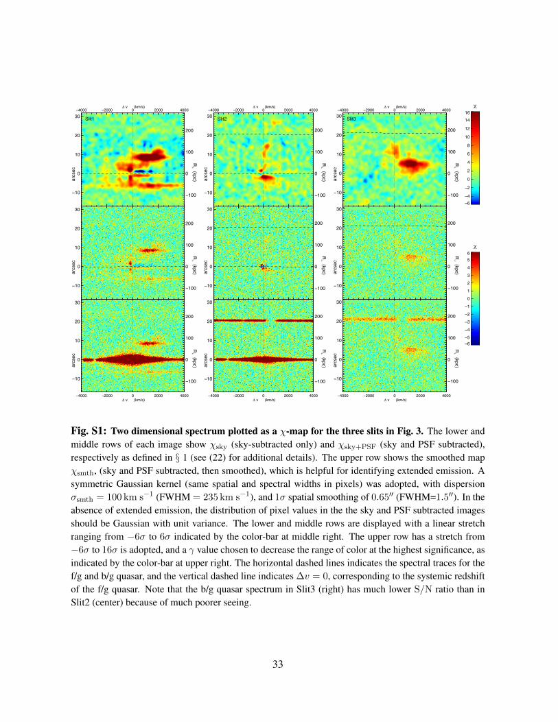
−6−4

−2

0

2

4

6

8

10

12

1416

χ

−6−5

−4

−3

−2

−1

0

1

2

3

4

56

χ

−10

0

10

20

30

∆ v (km/s)

−4000 −2000 0 2000 4000 ∆ v (km/s)

−100

0

100

200

−10

0

10

20

30

∆ v (km/s)

−100

0

100

200

Slit2

−10

0

10

20

30−4000 −2000 0 2000 4000

∆ v (km/s)

−100

0

100

200

arcs

ecar

csec

arcs

ec

R⊥ (kpc)

R⊥ (kpc)

R⊥ (kpc)

−10

0

10

20

30

∆ v (km/s)

−4000 −2000 0 2000 4000 ∆ v (km/s)

−100

0

100

200

−10

0

10

20

30

∆ v (km/s)

−100

0

100

200

Slit3

−10

0

10

20

30−4000 −2000 0 2000 4000

∆ v (km/s)

−100

0

100

200

arcs

ecar

csec

arcs

ec

R⊥ (kpc)

R⊥ (kpc)

R⊥ (kpc)

−10

0

10

20

30

∆ v (km/s)

−4000 −2000 0 2000 4000 ∆ v (km/s)

−100

0

100

200

−10

0

10

20

30

∆ v (km/s)

−100

0

100

200

Slit1

−10

0

10

20

30−4000 −2000 0 2000 4000

∆ v (km/s)

−100

0

100

200

arcs

ecar

csec

arcs

ec

R⊥ (kpc)

R⊥ (kpc)

R⊥ (kpc)

Fig. S1: Two dimensional spectrum plotted as a χ-map for the three slits in Fig. 3. The lower andmiddle rows of each image show χsky (sky-subtracted only) and χsky+PSF (sky and PSF subtracted),respectively as defined in § 1 (see (22) for additional details). The upper row shows the smoothed mapχsmth, (sky and PSF subtracted, then smoothed), which is helpful for identifying extended emission. Asymmetric Gaussian kernel (same spatial and spectral widths in pixels) was adopted, with dispersionσsmth = 100 km s−1 (FWHM = 235 km s−1), and 1σ spatial smoothing of 0.65′′ (FWHM=1.5′′). In theabsence of extended emission, the distribution of pixel values in the the sky and PSF subtracted imagesshould be Gaussian with unit variance. The lower and middle rows are displayed with a linear stretchranging from −6σ to 6σ indicated by the color-bar at middle right. The upper row has a stretch from−6σ to 16σ is adopted, and a γ value chosen to decrease the range of color at the highest significance, asindicated by the color-bar at upper right. The horizontal dashed lines indicates the spectral traces for thef/g and b/g quasar, and the vertical dashed line indicates ∆v = 0, corresponding to the systemic redshiftof the f/g quasar. Note that the b/g quasar spectrum in Slit3 (right) has much lower S/N ratio than inSlit2 (center) because of much poorer seeing.

33

0

50

100f/g QSO Ly_ C IVSi IV C III]He II C II]

0.0

0.2

0.4 AGN1 Ly_ C IV C III]He II C II]

0

1

AGN2 Ly_ C IV C III]He II C II]

4000 5000 6000 7000h (Å)

0.0

0.1

0.2 AGN3C IV C III]He II C II]

f h (1

0−17

erg

/s/c

m2 /Å

)

Fig. S2: Optical spectra of the four AGN at the same redshift. From top to bottom: f/g quasar,AGN1, AGN2, and AGN3. The gaps in the coverage of the spectra of AGN1 and AGN2 are due to theLRIS configuration chosen to cover both Lyα, C IV, and He II. The spectrum of AGN3 does not coverthe Lyα line due to the limited blue sensitivity of DEIMOS. Note the different scale on the y-axis tobetter show the different emission lines, which are marked with vertical dotted lines and labeled.

34

10−1 100 101

CIV/CIII

10−1

100

101

102CIV/HeII

10−1 100 101 102

CIII]/CII]

10−1

100

101

102

CIII]/H

eII

Fig. S3: Comparison of the Line-ratios of AGN1 to other Type-2 AGN. The line-ratios of AGN1(red square) are compared to other Type-2 AGN compiled from the literature in the C IV/He II vs C IV/

C III] plane (left) as well as the C III]/He II vs C III]/C II] plane (right). The circles are individual mea-surements of HzRGs (black) from the compilation of (80), and narrow-line X-ray sources (cyan) andSeyfert-2s (blue) from the compilation of (81). Triangles indicate measurements from the compositespectra of HzRGs (orange) from (70), the composite Type-2 AGN spectra (purple) from (82), who splittheir population into two samples above and below Lyα EW of 63A, and a composite spectrum of mid-IRselected Type-2 AGN (green) from (83). The stars represent measurements from composite spectra ofType-1 quasars, based on the analysis of (magenta) (84), (red-magenta) (85), and (blue-magenta) (86).The line-ratios for AGN1 lie in the locus of points spanned by other Type-2 objects in the literature.

35

20 40 60 80 100r0 (h

−1 Mpc)

0.0

0.5

1.0

1.5

2.0

2.5

3.0

γ

Fig. S4: Confidence regions on correlation function parameters from maximum likeklihood clus-tering analysis. The 1 ,2 , and 3σ confidence regions are illustrated by the black, blue, and red contours,respectively. The maximum likelihood value is r0 = 29.3h−1 Mpc and γ = 1.5, which is indicatedby the white cross. Due to the low signal-to-noise ratio of the clustering measurement, and the formadopted for the correlation function ξ(r) ≡ (r/r0)−γ (such that amplitude and slope are not indepen-dent parameters), a strong degeneracy exists between r0 and γ, such that neither is individually welldetermined.

36

0.1 1.0R (Mpc/h)

1

10

100

χ(R

)

1

10

100

Fig. S5: Binned correlation function of LAEs around HzRGs and LABs. The dimensionless corre-lation function χ defined by eqn. (9) is indicated by the data points, with 1σ error bars, determined bytaking the 16th and 84th percentiles of the distribution of χ resulting from our bootstrap procedure. Thesolid red line indicates the best-fit protocluster-LAE cross correlation function (r0 = 29.3h−1 Mpc andγ = 1.5) determined by our unbinned maximum likelihood procedure. The gray shaded region indicatesthe 1σ error on our cross-correlation function fit, implied by the erorrs on the parameters r0 and γ. Thisregion is determined by evaluating χ for each sample of the boostrap error distributions of r0 and γ, andtaking the 16th to 84th percentile confidence region of χ. Our best fit correlation function (red line), andits quoted errors (gray shaded) clearly provides an acceptable representation of the binned data pointsand their respective errors.

37

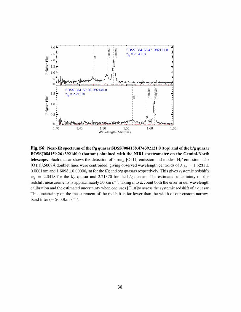
0.0

0.5

1.0

1.5

2.0

2.5

3.0R

elat

ive

Flux

SDSSJ084158.47+392121.0zfg = 2.04118

Hβ

[OII

I] 4

960

[OII

I] 5

008

1.40 1.45 1.50 1.55 1.60 1.65Wavelength (Microns)

0.0

0.5

1.0

1.5

Rel

ativ

e Fl

ux

SDSSJ084159.26+392140.0zbg = 2.21370

Hβ

[OII

I] 4

960

[OII

I] 5

008

Fig. S6: Near-IR spectrum of the f/g quasar SDSSJ084158.47+392121.0 (top) and of the b/g quasarBOSSJ084159.26+392140.0 (bottom) obtained with the NIRI spectrometer on the Gemini-Northtelescope. Each quasar shows the detection of strong [O III] emission and modest Hβ emission. The[O III]λ5008A doublet lines were centroided, giving observed wavelength centroids of λobs = 1.5231±0.0001µm and 1.6095±0.00006µm for the f/g and b/g quasars respectively. This gives systemic redshiftszfg = 2.0418 for the f/g quasar and 2.21370 for the b/g quasar. The estimated uncertainty on thisredshift measurements is approximately 50 km s−1, taking into account both the error in our wavelengthcalibration and the estimated uncertainty when one uses [O III]to assess the systemic redshift of a quasar.This uncertainty on the measurement of the redshift is far lower than the width of our custom narrow-band filter (∼ 2600km s−1).

38

0.00.2

0.4

0.6

0.8

1.0

HI LyαKeck/LRISb

0.00.2

0.4

0.6

0.8

1.0

OI 1302Keck/LRISb

0.00.2

0.4

0.6

0.8

1.0

SiII 1304Keck/LRISb

−1000−500 0 500 1000 1500 2000Relative Velocity (km s−1)

0.00.2

0.4

0.6

0.8

1.0

CII 1334Keck/LRISb

0.00.2

0.4

0.6

0.8

1.0

NII 1083Keck/LRISb

0.00.2

0.4

0.6

0.8

1.0

SiIII 1206Keck/LRISb

0.00.2

0.4

0.6

0.8

1.0

SiIV 1393Keck/LRISb

−1000−500 0 500 1000 1500 2000Relative Velocity (km s−1)

0.00.2

0.4

0.6

0.8

1.0

CIV 1548BOSS

Nor

mal

ized

Flu

x

Fig. S7: One-dimensional spectra of the b/g quasar centered at the wavelengths of a series ofcommonly observed UV-line transitions in the rest frame of the f/g quasar. The gas exhibits espe-cially strong low-ion absorption (O Iλ1302, Si IIλ1304, C IIλ1334) and moderately strong intermediateion absorption (N IIλ1083, Si IIIλ1206). The latter absorption occurs within the Lyα forest and could bepartially blended with coincident IGM absorption, but such contamination should be modest given thatthe line-profiles track one another and also the low-ion transitions. In contrast, there is no statisticallysignificant absorption corresponding to the Si IVλ1393 and C IVλ1548 transitions indicating the gas isnot highly ionized. See Table S6 for a summary of the properties of these metal absorption lines.

39

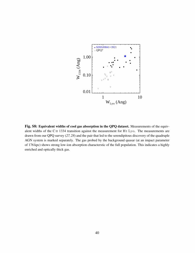
1 10WLyα (Ang)

0.01

0.10

1.00

W13

34 (

Ang

)

SDSSJ0841+3921QPQ7

Fig. S8: Equivalent widths of cool gas absorption in the QPQ dataset. Measurements of the equiv-alent widths of the C II 1334 transition against the measurement for H I Lyα. The measurements aredrawn from our QPQ survey (27,28) and the pair that led to the serendipitous discovery of the quadrupleAGN system is marked separately. The gas probed by the background quasar (at an impact parameterof 176 kpc) shows strong low-ion absorption characterstic of the full population. This indicates a highlyenriched and optically thick gas.

40

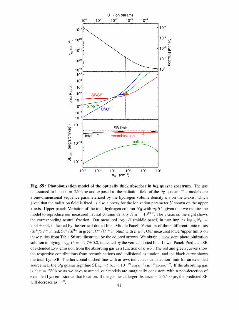
1019

1020

1021

1022

1023

NH (

cm−

2 )

100 10−1 10−2 10−3 10−4

100

10−1

10−2

10−3

10−4

10−410−3

10−2

10−1

100

101

102

103Io

nic

Rat

io

C+/C3+Si+/Si3+

Si+/Si2+

10−3 10−2 10−1 100 101 102

nH (cm−3)

10−19

10−18

10−17

SB

Lyα

(erg

/s/c

m2 /s

q′′ )

SB limit

total recombination

collisions

Neutral F

raction

U (ion param)

Fig. S9: Photoionization model of the optically thick absorber in b/g quasar spectrum. The gasis assumed to be at r = 250 kpc and exposed to the radiation field of the f/g quasar. The models area one-dimensional sequence parameterized by the hydrogen volume density nH on the x-axis, whichgiven that the radiation field is fixed, is also a proxy for the ionization parameter U shown on the upperx-axis. Upper panel: Variation of the total hydrogen column NH with nH/U , given that we require themodel to reproduce our measured neutral column density NHI = 1019.2. The y-axis on the right showsthe corresponding neutral fraction. Our measured log10 U (middle panel) in turn implies log10NH =

20.4 ± 0.4, indicated by the vertical dotted line. Middle Panel: Variation of three different ionic ratios(Si+/Si2+ in red; Si+/Si3+ in green; C+/C3+ in blue) with nH/U . Our measured lower/upper limits onthese ratios from Table S6 are illustrated by the colored arrows. We obtain a consistent photoioinizationsolution implying log10 U = −2.7±0.3, indicated by the vertical dotted line. Lower Panel: Predicted SBof extended Lyα emission from the absorbing gas as a function of nH/U . The red and green curves showthe respective contributions from recombinations and collisional excitation, and the black curve showsthe total Lyα SB. The horizontal dashed line with arrows indicates our detection limit for an extendedsource near the b/g quasar sightline SBLyα < 5.1 × 10−18 erg s−1 cm−2 arcsec−2. If the absorbing gasis at r = 250 kpc as we have assumed, our models are marginally consistent with a non-detection ofextended Lyα emission at that location. If the gas lies at larger distances r > 250 kpc, the predicted SBwill decreaes as r−2.

41

1014

1015

1016

1017

1018

1019

1020

NH

I (cm

−2 )

100 10−1 10−2 10−3 10−4

10−6

10−5

10−4

10−3

10−2

10−1

100

10−3 10−2 10−1 100 101 102

nH (cm−3)

10−22

10−21

10−20

10−19

10−18

10−17

10−16

SB

Lyα

(erg

/s/c

m2 /s

q′′ )

SBLyα @ 100 kpc

100 kpc

250 kpc 50 kpc

Neutral F

raction

U (ion param @ r = 100 kpc)

Fig. S10: Photoionization model of the Lyα emitting nebular gas. The models assume a total hy-drogen column density NH = 1020.4 cm−2, deduced from our photoionization modeling of the opticallythick absorber in the b/g sightline (see Fig. S9and § 10.3). The gas is assumed to be exposed to theradiation field of the f/g quasar at distances of r = 50, 100, and 250 kpc, indicated by the red, black,and blue curves, respectively. The models are parameterized by the hydrogen volume density nH onthe x-axis. The ionization parameter U corresponding to the gas at r = 100 kpc (black curves) is de-noted on the upper x-axis. Upper panel: Variation of the neutral hydrogen column NHI with nH. They-axis on the right shows the corresponding neutral fraction. Lower panel: Variation of the Lyα SBwith nH. For low nH the gas remains optically thin NHI . 1017.5 cm−2, and the SB SBLyα varieslinearly with nH and is nearly independent of the ionizing radiation intensity. At higher nH the gasbegins self-shielding NHI & 1017.5 cm−2, and the SB plateaus at a single value depending only on Φ

and hence on distance r. The models indicate that a value of nH ' 2.0 cm−3, indicated by the ver-tical dotted line, is required in order to reproduce the observed average emission level at 100 kpc ofSBLyα = 1.3× 10−17 erg s−1 cm−2 arcsec−2, indicated by the horizontal dashed line in Fig. S10. Thisconclusion is essentially independent of the radiation field and hence the assumed distance of the gasfrom the f/g quasar.

42

Name RA DEC z σz θ R⊥(km s−1) (′′) (kpc)

f/g QSO 08 41 58.47 +39 21 21.0 2.0412 50 — —AGN1 08 41 58.24 +39 21 29.1 2.055 400 8.6 71AGN2 08 41 58.66 +39 21 14.7 2.058 700 6.6 55AGN3 08 41 59.10 +39 21 04.6 2.050 700 18.0 150b/g QSO 08 41 59.25 +39 21 40.0 2.2138 50 21.1 176

Table S1: AGN properties. The coordinates, redshift z, redshift error σz , angular θ and transverse separa-tion R⊥ from the f/g quasar are listed for the four AGN in the protocluster, as well as the b/g quasar.

43

Nam

eu

±σu

g±σg

r±σr

i±σi

z±σz

W1±σW

1W

2±σW

2W

3±σW

3W

4±σW

4F20cm

V±σV

fLyα

WLyα

f/g

QSO

19.7

6±0.

0219

.75±

0.01

19.5

8±0.

0119

.27±

0.01

19.1

9±0.

0315

.85±

0.03

14.6

5±0.

0410

.79±

0.07

8.33±

0.36

<1.

0219

.76±

0.03

1709

.072

.6A

GN

1>

23.1

124

.04±

0.31

>23

.74

>23

.24

>21

.86

16.8

9±0.

0815

.86±

0.11

>12

.58

>8.

36<

1.02

23.9

5±0.

0721

0.1

110.

8A

GN

2>

23.1

1>

24.3

4>

23.4

0>

22.9

3>

21.8

618

.19±

0.26

>17

.10

>12

.58

>8.

3512

.87

23.1

2±0.

0641

.137

.0A

GN

3>

23.1

122

.71±

0.09

22.7

3±0.

1622

.18±

0.15

>21

.86

>18

.52

>17

.12

>12

.58

>8.

36<

1.02

23.0

9±0.

0639

.834

.7b/

gQ

SO20

.00±

0.02

19.3

9±0.

0019

.71±

0.01

19.3

9±0.

0119

.39±

0.04

16.4

0±0.

0515

.76±

0.10

12.0

0±0.

21>

8.36

<1.

0219

.96±

0.03

-7.0

-6.2

Tabl

eS2

:A

GN

phot

omet

ry.

SDSS

optic

al(ugriz

)an

dW

ISE

mid

-IR

(W1−

4)

mag

nitu

des

are

dete

rmin

edfr

omfo

rced

phot

omet

ryof

the

corr

espo

ndin

gim

ages

.SD

SSan

dL

RIS

mag

nitu

des

are

onth

eA

Bsc

ale,

whe

reas

WIS

Em

agni

tude

sar

ein

the

Veg

asy

stem

.For

mea

sure

men

tsw

ithS/N<

3w

equ

ote

low

erlim

itson

the

mag

nitu

des.

Peak

20cm

radi

oflu

xF20cm

(mJy

)ar

elis

ted

for

obje

cts

with

am

atch

inth

eso

urce

cata

log

from

the

VL

A/F

IRST

surv

ey(B

ecke

ret

al.

1995

).Fo

rob

ject

sw

ithou

tFI

RST

mat

ches

we

list

the

5σup

per

limit

base

don

the

sky-

rms

cove

rage

map

s.W

eal

solis

tKec

kL

RISV

band

mag

nitu

des,

Lyα

line

fluxe

sf L

yα

(10−

17

erg

s−1

cm−2),

and

rest

-fra

me

Lyα

equi

vale

ntw

idth

(A).

44

Line FWHM Flux Wλ

(km s−1) (10−17 erg s−1 cm−2) (A)Lyα............ 1575± 36 76.5± 1.5 > 118.2NV............. — −0.4± 1.4 —CIV............ — 1.3± 0.8 —HeII........... 1154± 276 2.4± 0.4 > 15.8CIII].......... 1434± 171 2.6± 0.3 22.6± 2.2CII]........... — 1.0± 0.2 11.2± 2.6

Table S3: Emision line measurements for the Type-2 quasar AGN1. Line fluxes were measured from theone-dimensional spectrum of the AGN, and errors determined from the 1σ noise vector. For lines de-tected at S/N > 3, rest-frame equivalent widths Wλ are computed. If the continuum lies above the 1σnoise vector these are listed as values, otherwise we quote lower limits. The FWHM for emission linesfor which our discovery spectra had sufficient S/N for a measurement (Lyα, He II, and C III]) are alsolisted.

45

Tag RA DEC fLyα fλ WLyα R⊥(10−17 ergs−1cm−2) (10−19 ergs−1cm−2A−1) (A) (kpc)

f/g QSO 08:41:58.470 +39:21:20.97 1708.76 774.23 72.61 0AGN2* 08:41:58.685 +39:21:15.00 41.13 36.57 36.98 50

* 08:41:57.982 +39:21:25.88 12.07 2.04 195.0 5808:41:58.872 +39:21:14.45 4.14 3.38 40.28 62

AGN1* 08:41:58.238 +39:21:28.87 210.08 62.35 110.80 6508:41:57.535 +39:21:17.72 1.33 0.41 106.14 88

* 08:41:58.543 +39:21:34.03 21.45 14.42 48.91 102* 08:41:58.262 +39:21:37.57 14.07 3.97 116.50 130

AGN3* 08:41:59.107 +39:21:04.67 39.81 37.76 34.67 139* 08:41:58.286 +39:21:39.20 4.33 0.95 148.98 143

08:41:58.238 +39:20:57.05 3.42 5.10 22.06 18708:41:59.035 +39:21:46.27 1.72 1.09 52.02 20308:41:57.019 +39:21:48.45 1.13 0.46 80.45 251

Target1* 08:41:58.824 +39:21:57.42 17.22 5.86 96.66 28508:41:59.762 +39:21:55.52 0.69 0.14 157.38 29308:41:55.754 +39:21:46.27 0.86 0.99 28.70 31408:41:54.958 +39:21:14.99 1.30 0.49 87.57 32108:41:56.198 +39:21:55.51 0.78 0.82 31.32 33808:41:53.926 +39:21:33.75 0.72 0.52 45.52 42208:41:54.982 +39:20:41.54 0.85 0.65 43.33 44008:41:59.038 +39:20:20.88 1.63 2.77 19.42 47008:41:59.225 +39:20:21.16 0.85 1.10 25.30 47008:41:56.762 +39:20:19.79 0.54 0.89 20.02 50008:42:02.412 +39:20:30.94 0.93 1.49 20.44 52708:41:57.794 +39:20:11.63 1.12 1.56 23.56 543

* 08:41:52.003 +39:21:14.16 5.31 3.44 50.73 58608:41:52.142 +39:21:48.16 1.21 0.82 48.76 60908:41:55.778 +39:20:03.75 0.63 0.63 33.07 64808:42:02.225 +39:20:09.46 0.96 0.30 105.43 65108:42:02.412 +39:20:06.74 0.99 0.98 32.99 678

* 08:41:52.802 +39:20:21.41 7.38 3.22 75.25 69008:42:05.930 +39:22:09.65 0.82 1.34 20.01 77208:41:58.027 +39:23:01.05 0.66 0.80 27.08 77908:41:52.099 +39:20:11.62 1.86 1.28 47.73 78808:41:51.722 +39:20:16.51 0.74 0.19 126.03 78908:42:07.313 +39:21:23.42 0.56 0.91 20.07 79808:41:49.610 +39:21:22.58 0.55 0.85 21.21 80008:42:05.486 +39:22:24.88 0.59 0.65 29.80 80508:41:51.209 +39:20:17.33 0.68 0.30 75.60 82108:41:51.701 +39:20:08.90 0.62 0.68 30.16 82908:41:59.340 +39:23:07.04 0.61 0.80 25.07 82908:42:07.829 +39:21:32.66 0.92 1.10 27.59 84908:41:51.701 +39:20:01.01 0.92 1.33 22.82 87208:41:50.482 +39:20:10.25 0.67 0.66 33.42 90708:41:51.067 +39:20:02.09 0.96 0.11 282.90 90708:41:54.461 +39:23:11.92 0.91 0.97 30.68 93608:41:49.982 +39:22:30.30 0.66 0.85 25.42 93708:42:08.441 +39:22:05.84 1.71 1.33 42.09 96408:42:07.826 +39:20:09.72 0.73 0.69 34.54 101008:42:10.267 +39:21:13.89 0.70 0.60 38.54 106508:41:51.482 +39:23:15.72 0.62 0.92 22.36 109308:42:10.759 +39:21:24.49 0.66 0.25 87.20 110908:42:10.010 +39:22:10.45 2.21 0.27 268.26 111008:42:12.590 +39:21:39.16 2.09 1.83 37.44 128108:42:13.382 +39:20:05.34 11.69 4.20 91.60 146808:42:11.702 +39:23:13.80 1.11 0.73 49.85 148108:42:12.840 +39:19:12.32 0.82 0.62 43.35 163808:42:03.629 +39:17:19.50 2.27 1.16 64.47 193508:41:52.363 +39:17:15.40 1.35 1.44 30.75 198808:42:03.677 +39:17:02.64 1.22 0.65 61.92 206408:42:12.223 +39:16:41.66 2.61 2.83 30.30 2502

Table S4: Properties of the candidate LAEs around the f/g quasar. Here fLyα is the Lyα line flux in 10−17

erg s−1 cm−2, fλ is the flux density in the continuum in units of 10−19 erg s−1 cm−2 A−1 estimated from theV -band, WLyα is the rest-frame Lyα equivalent width, andR⊥ the proper projected distance from the f/g quasar inkpc. LAEs are selected using the procedure described in § 4.1, namely they are required to have WLyα > 20A andfLyα > 5.4× 10−18 erg s−1. Objects which were used to measure the overdensity profile around the f/g quasar inFig. 2 are denoted by a ∗ in the column Tag, where the name of the source is also indicated. These sources had tosatisfy a brighter flux limit, namely fLyα > 4.0× 10−17 erg s−1 cm−2, and lie within 2.08′ of the f/g quasar.

46

Name Type RA DEC z Filter FWHM (A) EWlimit (A) ReferenceMRC 2048−272 HzRG 20 51 03.5 −27 03 04.1 2.06 73 20 1MRC 1138−262 HzRG 11 40 48.2 −26 29 09.5 2.16 65 20 1LABd05 LAB 14 34 11.0 +33 17 32.6 2.66 201 40 2MRC 0052241 HzRG 00 54 29.8 −23 51 31.1 2.86 66 20 1MRC 0943−242 HzRG 09 45 32.7 −24 28 49.7 2.92 68 20 1LAB1 LAB 22 17 26.0 +00 12 37.7 3.10 80 20 3MRC 0316−257 HzRG 03 18 12.0 −25 35 10.8 3.13 59 20 1TN J2009−3040 HzRG 20 09 48.1 −30 40 07.4 3.16 59 20 1

Table S5: Properties of objects analyzed in our protocluster-LAE correlation analysis. The nature of thesource (HzRG or LAB), coordinates, redshift z, the FWHM of the NB filter used (A), the limiting EWof the LAE search (Wlimit), and the reference for the observations are indicated. References used are:(1) Venemans et al. 2007 (13); (2) Prescott et al. 2008 (19); (3) Nestor et al. 2011 (106).

47

Ion λ log f vint Wλ logN [X/H](A) (km s−1) (mA)

H 11215.6701 −0.3805 [−225, 1449] 3750.0± 50.0 19.2± 0.3

C 21334.5323 −0.8935 [355, 1315] 1110.5± 34.7 > 14.7 > −1.19

C 41548.1949 −0.7194 [355, 1315] < 331.5 < 13.9 < 0.721550.7700 −1.0213 [355, 1315] < 340.4 < 14.2 < 1.03

N 21083.9900 −0.9867 [480, 850] 216.3± 31.8 > 14.3 > −1.00

O 11302.1685 −1.3110 [355, 985] 672.9± 14.0 > 15.0 > −0.95

Al 21670.7874 0.2742 [355, 1315] 335.0± 110.0 > 12.9 > −0.97

Si 21304.3702 −1.0269 [431, 1315] 259.3± 17.5 > 14.3 > −0.81

Si 31206.5000 0.2201 [355, 1315] 951.0± 43.6 > 13.6 > −0.80

Si 41393.7550 −0.2774 [355, 1315] < 96.2 < 13.0 < −0.271402.7700 −0.5817 [355, 1315] < 93.7 < 13.3 < 0.02

Table S6: Absorption line measurements. The columns indicate the Ion, rest wavelength λ, oscillatorstrength log f , velocity interval vint used for the calculation of the rest equivalent widths, rest-equivalentwidth Wλ, ionic column density N , and elemental abundances [X/H] implied by each metal absorptionline measurement. The column densities N reported assume the linear curve-of-growth approximation.The metal abundances [X/H] are computed using ionization corrections from our favored Cloudy modelpresented in Section S10, and are reported according to the standard convention of logarithmic relativeto Solar (i.e. 0 = solar abundance).

48

References and Notes1. J. Magorrian, et al., AJ 115, 2285 (1998).

2. L. Ferrarese, ApJ 578, 90 (2002).

3. J. N. Bahcall, S. Kirhakos, D. H. Saxe, D. P. Schneider, ApJ 479, 642 (1997).

4. M. G. Haehnelt, M. J. Rees, MNRAS 263, 168 (1993).

5. S. Djorgovski, The Space Distribution of Quasars, D. Crampton, ed. (1991), vol. 21 of Astronomical Societyof the Pacific Conference Series, pp. 349–353.

6. J. F. Hennawi, et al., AJ 131, 1 (2006).

7. S. G. Djorgovski, et al., ApJL 662, L1 (2007).

8. E. P. Farina, C. Montuori, R. Decarli, M. Fumagalli, MNRAS 431, 1019 (2013).

9. C. Lacey, S. Cole, MNRAS 262, 627 (1993).

10. R. F. Trainor, C. C. Steidel, ApJ 752, 39 (2012).

11. M. White, et al., MNRAS 424, 933 (2012).

12. N. Fanidakis, A. V. Maccio, C. M. Baugh, C. G. Lacey, C. S. Frenk, MNRAS 436, 315 (2013).

13. B. P. Venemans, et al., A & A 461, 823 (2007).

14. P. J. Francis, et al., ApJ 457, 490 (1996).

15. C. C. Steidel, et al., ApJ 532, 170 (2000).

16. A. Dey, et al., ApJ 629, 654 (2005).

17. R. A. Overzier, et al., ApJ 771, 89 (2013).

18. M. K. M. Prescott, I. Momcheva, G. B. Brammer, J. P. U. Fynbo, P. Møller, ArXiv e-prints (2015).

19. M. K. M. Prescott, N. Kashikawa, A. Dey, Y. Matsuda, ApJL 678, L77 (2008).

20. Y. Yang, A. Zabludoff, C. Tremonti, D. Eisenstein, R. Dave, ApJ 693, 1579 (2009).

21. Y.-K. Chiang, R. Overzier, K. Gebhardt, ApJ 779, 127 (2013).

22. J. F. Hennawi, J. X. Prochaska, ApJ 766, 58 (2013).

23. J. F. Hennawi, et al., ApJ 651, 61 (2006).

24. J. F. Hennawi, J. X. Prochaska, ApJ 655, 735 (2007).

25. J. X. Prochaska, J. F. Hennawi, ApJ 690, 1558 (2009).

26. J. X. Prochaska, J. F. Hennawi, R. A. Simcoe, ApJL 762, L19 (2013).

27. J. X. Prochaska, et al., ApJ 776, 136 (2013).

28. J. X. Prochaska, M. W. Lau, J. F. Hennawi, ApJ 796, 140 (2014).

29. See further information in supplementary online material § S2 on Science Online.

30. I. Kayo, M. Oguri, MNRAS 424, 1363 (2012).

31. See further information in supplementary online material § S3 on Science Online.

32. R. Ciardullo, et al., ApJ 744, 110 (2012).

49

33. See further information in supplementary online material § S4 on Science Online.

34. See further information in supplementary online material § S6 on Science Online.

35. See further information in supplementary online material § S5 on Science Online.

36. B. D. Lehmer, et al., ApJ 691, 687 (2009).

37. See further information in supplementary online material § S7 on Science Online.

38. R. E. Mostardi, et al., ApJ 779, 65 (2013).

39. D. C. Martin, et al., ApJ 786, 106 (2014).

40. See further information in supplementary online material § S8 on Science Online.

41. S. Cantalupo, F. Arrigoni-Battaia, J. X. Prochaska, J. F. Hennawi, P. Madau, Nature 506, 63 (2014).

42. M. Fumagalli, et al., ApJ 780, 74 (2014).

43. C.-A. Faucher-Giguere, et al., ArXiv e-prints (2014).

44. S. Lopez, et al., ApJ 679, 1144 (2008).

45. See further information in supplementary online material § S9 on Science Online.

46. See further information in supplementary online material § S10 on Science Online.

47. N. H. M. Crighton, et al., ArXiv e-prints (2014).

48. A. H. Maller, J. S. Bullock, MNRAS 355, 694 (2004).

49. H. J. Mo, J. Miralda-Escude, ApJ 469, 589 (1996).

50. T. M. Heckman, S. A. Baum, W. J. M. van Breugel, P. McCarthy, ApJ 338, 48 (1989).

51. M. McDonald, S. Veilleux, D. S. N. Rupke, R. Mushotzky, ApJ 721, 1262 (2010).

52. K. N. Abazajian, et al., ApJS 182, 543 (2009).

53. J. F. Hennawi, et al., ApJ 719, 1672 (2010).

54. C. P. Ahn, et al., ApJS 203, 21 (2012).

55. J. B. Oke, et al., PASP 107, 375 (1995).

56. E. Bertin, S. Arnouts, A&AS 117, 393 (1996).

57. E. Bertin, Astronomical Data Analysis Software and Systems XV , C. Gabriel, C. Arviset, D. Ponz, S. Enrique,eds. (2006), vol. 351 of Astronomical Society of the Pacific Conference Series, p. 112.

58. E. Bertin, et al., Astronomical Data Analysis Software and Systems XI, D. A. Bohlender, D. Durand, T. H.Handley, eds. (2002), vol. 281 of Astronomical Society of the Pacific Conference Series, p. 228.

59. J. B. Oke, AJ 99, 1621 (1990).

60. A. U. Landolt, AJ 104, 372 (1992).

61. S. Cantalupo, S. J. Lilly, M. G. Haehnelt, MNRAS 425, 1992 (2012).

62. S. M. Faber, et al., Instrument Design and Performance for Optical/Infrared Ground-based Telescopes,M. Iye, A. F. M. Moorwood, eds. (2003), vol. 4841 of Society of Photo-Optical Instrumentation Engineers(SPIE) Conference Series, pp. 1657–1669.

63. J. A. Newman, et al., ApJS 208, 5 (2013).

50

64. M. C. Cooper, J. A. Newman, M. Davis, D. P. Finkbeiner, B. F. Gerke, spec2d: DEEP2 DEIMOS SpectralPipeline, Astrophysics Source Code Library (2012).

65. D. Lang, D. W. Hogg, D. J. Schlegel, ArXiv e-prints (2014).

66. A. E. Shapley, C. C. Steidel, M. Pettini, K. L. Adelberger, ApJ 588, 65 (2003).

67. R. Antonucci, ARAA 31, 473 (1993).

68. C. M. Urry, P. Padovani, PASP 107, 803 (1995).

69. D. B. Sanders, et al., ApJ 325, 74 (1988).

70. P. J. McCarthy, ARAA 31, 639 (1993).

71. M. Lacy, et al., ApJS 154, 166 (2004).

72. D. Stern, et al., ApJ 631, 163 (2005).

73. W. N. Brandt, G. Hasinger, ARAA 43, 827 (2005).

74. N. L. Zakamska, et al., AJ 126, 2125 (2003).

75. M. Brusa, et al., ApJ 716, 348 (2010).

76. L. Hao, et al., AJ 129, 1783 (2005).

77. M. Kim, et al., ApJL 768, L9 (2013).

78. D. Stern, et al., ApJ 568, 71 (2002).

79. B. A. Groves, M. A. Dopita, R. S. Sutherland, ApJS 153, 75 (2004).

80. C. De Breuck, H. Rottgering, G. Miley, W. van Breugel, P. Best, A & A 362, 519 (2000).

81. T. Nagao, R. Maiolino, A. Marconi, A & A 447, 863 (2006).

82. K. N. Hainline, A. E. Shapley, J. E. Greene, C. C. Steidel, ApJ 733, 31 (2011).

83. M. Lacy, et al., ApJS 208, 24 (2013).

84. D. E. Vanden Berk, et al., AJ 122, 549 (2001).

85. T. Nagao, A. Marconi, R. Maiolino, A & A 447, 157 (2006).

86. W. Zheng, G. A. Kriss, R. C. Telfer, J. P. Grimes, A. F. Davidsen, ApJ 475, 469 (1997).

87. D. Stern, et al., ApJ 753, 30 (2012).

88. R. J. Assef, et al., ApJ 772, 26 (2013).

89. L. Yan, et al., AJ 145, 55 (2013).

90. M. Polletta, et al., ApJ 663, 81 (2007).

91. R. J. Assef, et al., ApJ 713, 970 (2010).

92. R. C. Hickox, et al., ApJ 671, 1365 (2007).

93. R. C. Hickox, et al., ApJ 731, 117 (2011).

94. Y. Shen, et al., AJ 133, 2222 (2007).

95. R. H. Becker, R. L. White, D. J. Helfand, ApJ 450, 559 (1995).

96. F. M. Montenegro-Montes, et al., MNRAS 388, 1853 (2008).

51

97. M. A. DiPompeo, M. S. Brotherton, C. De Breuck, S. Laurent-Muehleisen, ApJ 743, 71 (2011).

98. S. Fine, M. J. Jarvis, T. Mauch, MNRAS 412, 213 (2011).

99. P. J. E. Peebles, The large-scale structure of the universe (Princeton University Press, 1980).

100. J. N. Fry, ApJ 279, 499 (1984).

101. A. Cooray, R. Sheth, Physics Reports 372, 1 (2002).

102. P. F. Hopkins, G. T. Richards, L. Hernquist, ApJ 654, 731 (2007).

103. R. Reyes, et al., AJ 136, 2373 (2008).

104. E. Lusso, et al., ApJ 777, 86 (2013).

105. E. Bertin, S. Arnouts, Astronomy and Astrophysics Supplement 117, 393 (1996).

106. D. B. Nestor, A. E. Shapley, C. C. Steidel, B. Siana, ApJ 736, 18 (2011).

107. R. A. C. Croft, G. B. Dalton, G. Efstathiou, W. J. Sutherland, S. J. Maddox, MNRAS 291, 305 (1997).

108. Y. Shen, et al., ApJ 719, 1693 (2010).

109. L. Guaita, et al., ApJ 733, 114 (2011).

110. K. L. Adelberger, C. C. Steidel, ApJL 627, L1 (2005).

111. G. T. Richards, et al., AJ 124, 1 (2002).

112. R. van Ojik, et al., A & A 313, 25 (1996).

113. M. Villar-Martın, et al., MNRAS 346, 273 (2003).

114. M. Villar-Martın, New A Rev. 51, 194 (2007).

115. A. Humphrey, et al., MNRAS 375, 705 (2007).

116. M. K. M. Prescott, C. L. Martin, A. Dey, ApJ 799, 62 (2015).

117. T. M. Heckman, G. K. Miley, M. D. Lehnert, W. van Breugel, ApJ 370, 78 (1991).

118. R. Trainor, C. C. Steidel, ApJL 775, L3 (2013).

119. G. Miley, C. De Breuck, A&A Rev. 15, 67 (2008).

120. K. K. Nilsson, J. P. U. Fynbo, P. Møller, J. Sommer-Larsen, C. Ledoux, A & A 452, L23 (2006).

121. D. J. B. Smith, M. J. Jarvis, MNRAS 378, L49 (2007).

122. T. M. A. Webb, et al., ApJ 692, 1561 (2009).

123. J. W. Colbert, et al., ApJ 728, 59 (2011).

124. J. X. Prochaska, H.-W. Chen, A. M. Wolfe, M. Dessauges-Zavadsky, J. S. Bloom, ApJ 672, 59 (2008).

125. G. E. Prochter, J. X. Prochaska, J. M. O’Meara, S. Burles, R. A. Bernstein, ApJ 708, 1221 (2010).

126. G. J. Ferland, et al., PASP 110, 761 (1998).

127. A. Gould, D. H. Weinberg, ApJ 468, 462 (1996).

128. E. Lusso, et al., ArXiv e-prints (2015).

129. F. Arrigoni Battaia, et al., ArXiv e-prints (2014).

130. I. V. Strateva, W. N. Brandt, D. P. Schneider, D. G. Vanden Berk, C. Vignali, AJ 130, 387 (2005).

131. G. T. Richards, et al., ApJS 166, 470 (2006).

132. A. Baskin, A. Laor, J. Stern, MNRAS 438, 604 (2014).

133. F. Haardt, P. Madau, ApJ 746, 125 (2012).

52