Quarterly Report forJuly - September 2000

Stanford Geothermal ProgramDE-FG07-99ID13763

2

i

Table of Contents

1. MEASUREMENTS OF STEAM-WATER RELATIVE PERMEABILITY 1

1.1 BACKGROUND 1

1.2 EXPERIMENTAL PROCEDURE 1

1.3 FUTURE RESEARCH 2

2. STEAM-WATER CAPILLARY PRESSURE 3

2.1 SUMMARY 3

2.2 INTRODUCTION 3

2.3 THEORY 3

2.4 EXPERIMENTS 7

2.5 RESULTS 9

2.6 CONCLUSIONS 13

2.7 FUTURE WORK 13

3. WATER INJECTION 14

3.1 SUMMARY 14

3.2 INTRODUCTION 14

3.3 MATHEMATICS 14

3.4 EXPERIMENTS 15

3.5 RESULTS 17

3.6 CONCLUSIONS 24

3.7 FUTURE WORK 24

4. INFERRING RESERVOIR CONNECTIVITY BY WAVELET ANALYSIS OFPRODUCTION DATA 25

4.1 BACKGROUND 25

4.2 METHODOLOGY 25

4.3 CONTINUING WORK 26

ii

5 EXPERIMENTAL INVESTIGATION OF STEAM AND WATER RELATIVEPERMEABILITY ON SMOOTH WALLED FRACTURE 31

5.1 BACKGROUND 31

5.2 EXPERIMENTAL APPARATUS AND MEASUREMENT TECHNIQUES 32

5.2 PARTIAL RESULTS AND DISCUSSION 35

5.3 FUTURE WORK 36

6. REFERENCES 39

1

1. MEASUREMENTS OF STEAM-WATER RELATIVE PERMEABILITY This research project is being conducted by Research Assistant Peter O’Connor andProfessor Roland Horne. The aim is to measure relative permeability relations for steamand water flowing simultaneously in rock and to examine the effects of temperature, flowrate, and rock type. In the first stage, the experiments will attempt to reproduce resultsobtained in a previous experiment (Mahiya, 1999), but holding the experimental pressureas close as possible to a constant value.

1.1 BACKGROUND

An X-ray CT technique has been used in recent years to measure the distribution of steamand water saturation in rocks to obtain steam-water relative permeability curves (Satik,1998, Mahiya, 1999).

The current experiment is attempting to maintain a constant pressure, to avoidcomplications of the slip factor. As the experiment will be constantly at an inlet gaugepressure of 15 psi, it will necessarily be at a constant 120ºC at the inlet in order to havetwo-phase flow throughout, with the rest of the core being at the saturation temperaturefor the pressure at that point. Our expectation is an identical pressure profile andtemperature profile for every step of the process.

1.2 EXPERIMENTAL PROCEDURE

A Berea sandstone was drained, flushed with nitrogen, then subjected to a vacuum. Adry X-ray scan was made to obtain CTdry. The next step was to saturate the core withwater and scan to obtain CTwet; however, the CT scanner failed at this point and this stepwill have to be repeated. From these scans, a porosity distribution will be obtained,expected to yield an average value of 24.7%. In the next step, hot liquid water is flowedthrough to obtain CThw, which is necessary to calculate experimental saturations. Thenext steps are the actual flow-through experiments. The core will be under a pressuregradient of approximately 15 psi across the 41-cm length. First, the core is saturated withsteam. Steam flow rate will be gradually lowered in 10% increments, to implement animbibition process whereby the wetting phase (water) displaces the nonwetting phase(steam). A flexible heat guard ensures negligible overall heat loss for a near-adiabaticprocess. The flexible heat guard control mechanism was re-designed this year. At eachstep, the system will reach a steady state and will then be subject to CT scan to measuresaturation. Steam flow rate will be reduced to 0%, then increased. This second sequencewill be a drainage sequence.

At every stage, pressure, temperature and heat fluxes from the core are to be measured.Calculated relative permeability to steam and water are then plotted against the saturationmeasurements. The major suggested change from the previous experiment is to performthe imbibition step first. Performing the imbibition step first allows determination of themaximum pressure. This pressure can be maintained by increasing flow rates if

2

necessary.

In the spring quarter, we worked to determine the correct flow rates and power inputs toensure a pressure differential of 15 psi and a temperature at the inlet of slightly over 120ºC for the steam, and slightly under 120º C for the hot water. In this procedure, wedetermined several pairs of flow rates for water and steam, at different ratios, to result insteady-state flow with a pressure differential of 15 psi. This process also determined thecorresponding voltage and current settings for the hot water and steam heaters and for theflexible heater. All that is unknown is the saturation; once the CT scanner is available, itshould be a simple matter to determine the saturation. However, the core was damagedthrough excessive heat in the process, and we are currently awaiting replacement parts.

1.3 FUTURE RESEARCH

Future research will involve repeating the experiment at different pressure gradients andtemperatures. The next experiment will probably occur at approximately half the currentpressure gradient. In each case, the experiment will maintain a uniform pressure gradientfor the range of saturations.

Also under consideration are other possible methods of measuring saturation, either byweighing the core or using acoustic sounding to determine saturation. While not asprecise as the CT scanner, these methods have the advantage of producing averagesaturation readings extremely quickly.

Basic calculations show that a water-saturated core at 120º C would weigh 0.2 kg morethan a steam-saturated core. Such a difference is great enough to allow for measurementof the whole range of saturations; however, it would require the assumption of uniformsaturation throughout the core. The presence of a steam front would not be detected bysimply weighing the core.

Acoustic sounding would use the travel time for a sound wave signal to determine thesaturation of the core. Several sensors could be placed, to determine saturations at manylocations simultaneously. Saturation-sound speed relations could be calculatedtheoretically using the Gassman relations or could be calibrated using the CT scanner.More research will be necessary on the effects of geometry on the method; it may be thata rectangular core would be better suited to this method.

3

2. STEAM-WATER CAPILLARY PRESSURE This research project is being conducted by Research Associate Kewen Li and ProfessorRoland Horne. In this study the imbibition steam-water capillary pressures weremeasured by using an X-ray CT technique and compared to the imbibition air-watercapillary pressures in the same ceramic core sample. The final objective of this project isto develop new techniques of measuring and calculating steam-water capillary pressure ingeothermal systems.

2.1 SUMMARY

Steam-water flow exists in all two-phase geothermal reservoirs. Steam-water capillarypressure plays important role in controlling fluid distribution, well productivity, andultimate reserves. However, it is very difficult to measure steam-water capillary pressure.Are there any differences between steam- and air-water capillary pressures? If not, wecould represent steam-water flow by air-water flow, which would be a major advantagesince air-water capillary pressure can be measured easily. To this end, we conductedspontaneous water imbibition experiments using the same core sample saturated first withsteam and then a second time with air. The imbibition steam- and air-water capillarypressures in the core sample were measured using an X-ray CT technique. The resultswere compared, and it was found that there are significant differences between steam-and air-water capillary pressures. The imbibition steam-water capillary pressure was lessthan the air-water capillary pressure.

2.2 INTRODUCTION

Li and Horne (2000a) described a method to measure and calculate steam-water capillarypressure due to the experimental evidence of significant differences between steam- andair-water flow shown by Horne et al. (2000). However, there have been no investigationsshowing the direct comparison between steam-water capillary pressure and air-watercapillary pressure in the same core sample. In order to identify the differences betweenthe two, we conducted spontaneous water imbibition (cocurrent) experiments into thesame core sample saturated with steam and with air. The core sample was positionedvertically. The steam- and air-water capillary pressures were calculated using therelationship between height and water saturation measured by the X-ray CT method afterthe equilibrium between gravity and capillary pressure had been reached.

2.3 THEORY

In this study, the basic theory behind the measurement of steam- and air-water capillarypressures is the balance between gravity and capillary pressure as a function of height ina core sample positioned vertically. Steam-water or air-water capillary pressure is equalto the gravity force once the spontaneous water imbibition into the core sample has beencompleted. The equation is expressed as follows:

ghPci ρ∆= (2.1)

4

where Pci is steam-water or air-water capillary pressure; ∆ρ is the density differencebetween water and steam or air; g is gravity constant and h the height. The watersaturation in the core at h was measured by using an X-ray CT method. Water saturationis calculated as follows:

)()(

)()(exp

TCTTCT

TCTTCTS

drywet

dryw −

−= (2.2)

where CTwet(T), CTdry(T) are CT numbers of the core when it is fully saturated by waterand air respectively; CTexp(T) is the CT number of the rock when it is partially saturatedby steam, all at the same temperature T.

Porosity is usually computed using the following expression:

)()(

)()(

TCTTCT

TCTTCT

airwater

drywet

−−

=φ (2.3)

where CTwater and CTair are the CT numbers of water and air respectively. However, theceramic core sample used in this study had a hollow center, as shown in Figure 2.1.Hence we used a modified equation to calculate the porosity of the core sample with thisparticular shape once we know the CT values of the whole area with a radius of ro.

ri

ro

Figure 2.1: Cross-section of the ceramic core sample.

The CT values, CTwet(T) and CTdry(T), of the whole area with a radius of ro can bemeasured. The porosity calculated using Eq. 2.3 is the mean porosity φm in that area,including the hole. The mean porosity is expressed as follows:

)()()()(

TCTTCT

TCTTCT

airwater

drym

wetm

m

−−=φ (2.4)

5

where )(TCT wetm and )(TCT m

dry are the average CT values of the whole area with a

radius of ro when the sample is saturated with water and air, respectively. If we know theCT values of the rock part, then the porosity can be calculated using the followingequation:

)()()()(

TCTTCT

TCTTCT

airwater

dryo

weto

−−=φ (2.5)

where )(TCT weto and )(TCT o

dry are the average CT values of the annular area between

ro and ri (see Figure 2.1) when the sample is saturated with water and air, respectively.

We can measure )(TCT wetm and )(TCT m

dry easily. Therefore, the question is how to

calculate )(TCT weto and )(TCT o

dry from the measured values of )(TCT wetm and

)(TCT mdry . To this end, it is necessary to look into the fundamentals of the X-ray CT

method. The linear absorption coefficient of X-ray through a uniform object is equal to:

ρµµ m= (2.6)

where µ and µm are the linear absorption coefficient and mass absorption coefficient; ρ isthe density of the object. For a nonuniform object composed of n components, thefollowing equation applies:

∑==

n

iiiV

1µµ (2.7)

where µi and Vi are the linear absorption coefficient and the volumetric fraction ofcomponent i.

The CT value is defined as follows:

w

wCTµ

µµ −=1000 (2.8)

where µw is the linear absorption coefficient of pure water. The CT value of water shouldbe equal to zero according to Eq. 2.8 but the actual measurements may shift from zerodue to the calibration error or other reasons. The absorption of X-ray in air is very small,so the CT value of air should be around –1000. The measured value of CTair in this studywas –1005.

6

According to Eqs. 2.7 and 2.8, the CT value of a nonuniform object can be calculated asfollows:

∑==

n

iiiVCTCT

1(2.9)

where CTi is the CT value of component i.

The object shown in Figure 2.1 can be considered as two parts: the hole and the annularsolid. According to Eq. 2.9, the following expressions apply:

m

hhwet

m

rowet

mwet A

ACT

A

ACTCT += (2.10)

where wethCT is the CT value of the hole when the core sample is saturated with water.

Ar, Ah and Am are the areas of the annular part between ro and ri, the hole and the wholeobject (see Figure 2.1).

m

hhdry

m

rodry

mdry A

ACT

A

ACTCT += (2.11)

here dryhCT is the CT value of the hole when the core sample is saturated with air or

steam. In our experiment, no water existed in the hole when the core sample was

saturated with water. Therefore, dryhCT is equal to wet

hCT in this case. Using Eqs. 2.10and 2.11, we can obtain:

)()( mdry

mwet

r

modry

owet CTCT

A

ACTCT −=− (2.12)

Substituting Eq. 2.12 into Eq. 2.5:

airwater

mdry

mwet

r

m

CTCT

CTCT

A

A

−−

=φ (2.13)

Substituting Eq. 2.4 into Eq. 2.13:

mr

m

A

A φφ = (2.14)

7

Eq. 2.14 can also be expressed as follows:

mio

o

rr

r φφ22

2

−= (2.15)

The inner radius ri and the outer radius ro are known. Therefore, the porosity of the coresample as shown in Figure 2.1 can be calculated using Eq. 2.15 once the average porosityis measured.

Using a similar procedure, we were able to prove that the water saturation in the annularpart, Sw, is equal to the average water saturation, Swm, in the whole area. Therefore, wecould calculate water saturation in the core sample using Eq. 2.2 with all the CT valuesfrom the whole object.

2.4 EXPERIMENTS

Rock and Fluids. Distilled water was used as the liquid phase in this study; the specificgravity and viscosity were 1.0 and 1.0 cp at 20oC. Steam and air were used as the gasphase; the surface tension of water/air at 20oC was 72.75 dynes/cm. The values of thesurface tension at high temperatures were calculated from the steam property softwarefrom Techware Engineering Applications, Inc. It was assumed, as usual, that there wereno differences between the surface tension of water/air and that of water/steam. Theceramic sample was provided by Refractron Technologies Corp. and had a porosity of39.19%, a length of 25.0 cm, an inner diameter of 4.275 cm, and an outer diameter of6.287 cm. We did not measure the permeability of the core sample yet due to its specialshape but the permeability was estimated to be more than 10 darcy.

X-ray CT Scanner. Distribution of water saturation in the core sample was measuredalong the height using a PickerTM Synerview X-ray CT scanner (Model 1200 SX) with1200 fixed detectors. The voxel dimension was 0.5 mm by 0.5 mm by 5 mm, the tubecurrent used was 50 mA, and the energy level of the radiation was 140 keV. Theacquisition time of one image was about 3 seconds while the processing time was around40 seconds.

Experimental Apparatus. A schematic of the apparatus is shown in Figure 2.2. The coresystem was assembled in an aluminum cylinder wrapped in a heating belt; thetemperature in the cylinder was controlled using an Autotune Temperature Controller(manufactured by OMEGA, Model CN6071A) by turning the heating belt on and offautomatically. The temperatures at both the top (in steam or air) and the bottom (in water)of the core were measured during the experiment. A simulation test was conducted beforethe entire system was assembled in the CT scanner in order to obtain uniform temperaturedistribution along the core. We wanted to have the temperature at the top, T1, equal tothat at the bottom, T2 (See Figure 2.2). This was realized by adjusting the spacingbetween two strips of the heating belt wrapped outside the aluminum cylinder.

8

P

T1

T2

Water Pump

Scale

WaterCT Scanner

Vacuum

Cold Trap

Dry Ice

Core

TemperatureController

Heating Belt

Figure 2.2: Schematic of the apparatus of measuring steam- and air-water capillarypressure.

The vacuum pump (Welch Technology, Inc., Model 8915) was used to remove the air inthe core sample and in the aluminum cylinder. The cold trap with dry ice was employedto protect the steam from entering the vacuum pump in order to extend its life and reducethe frequency of replacing the pump oil. Water in the aluminum cylinder was deliveredby the water pump (Dynamax, Model SD-200), manufactured by RAININ InstrumentCo., and the amount was measured by the scale (Mettler, Model PE 1600) with anaccuracy of 0.01g and a range from 0 to 1600g. Comparing the volume of the spaceunder the bottom of the core, which was known, we could judge whether the watercontacted the bottom of the core sample or not. This judgement was aided by the CTscanning near the bottom. We kept scanning from time to time and could know where thewater level was by checking the CT values in the annular space.

Procedure. The core sample was dried by heating to a temperature of 105oC until theweight did not vary during 8 hours or more. We conducted the spontaneous waterimbibition into the air-saturated and upward-positioned core sample using the procedureof Li and Horne (2000b) at room temperature. An X-ray CT scan was made at eachcentimeter along the sample before and after the water imbibition. Then the core wasdried again and saturated with water. Another X-ray CT scan was made after thesaturation to obtain the values of CTwet. We calculated the air-water capillary pressure inthe core sample using these measurements.

The core sample was dried one more time and was assembled in the aluminum cylinder(see Figure 2.2). One X-ray CT scan was made to obtain the values of CTdry since thesemay be affected by the presence of the aluminum cylinder. After that, the temperature ofthe core system was increased to about 98oC. We scanned the core to obtain the values ofCTdry at 98oC about 10 hours later after the core was kept at this temperature. The mainpurpose of waiting 10 hours was to obtain a uniform temperature distribution. The corewas evacuated to 60 minitorr for about 4 hours to remove the air in the core after the hotscan. A certain amount of water was then introduced into the bottom of the aluminumcylinder using the water pump. The core then became saturated with steam. Water startedto imbibe into the steam-saturated core once the bottom of the sample was brought into

9

contact with the water surface that was raised by injection using the water pump. In orderto monitor the distribution of water saturation in the core sample, we scanned the corefrom time to time until the imbibition of water was completed. Finally, the sample wasdried again and the last X-ray CT scan was made after completely resaturating withwater. The CT values measured under different states were used to calculate the porosityby Eqs. 2.4 and 2.15. Also calculated was the distribution of the water saturation as afunction of height using Eq. 2.1. We obtained the steam-water capillary pressure fromthese data.

2.5 RESULTS

We conducted spontaneous water imbibition into both steam- and air-saturated coresample to compute steam- and air-water capillary pressures. Figure 2.3 shows the CTvalues of the whole area with a radius of ro (see Figure 2.1) when the core was dry andsaturated with water.

0

50

100

150

200

250

300

350

400

0 5 10 15 20 25 30Distance from Bottom (cm)

CT

Val

ue

CTDry

CTWet

Figure 2.3: Distribution of CT value in the core sample.

The porosity of the core sample was calculated using Eqs. 2.4 and 2.15, as shown inFigure 2.4. The porosity distribution along the height of this ceramic core sample wasvery homogeneous and its average value was 39.61%. The porosity measured using thesaturation method was 39.19%, close to the value of 39.61% obtained from the X-ray CTmethod. The average porosity calculated using Eq. 2.3 (including the hole) is also shownin Figure 2.4; as expected, it is much smaller than those values of the actual porosity.

10

Distance from Bottom (cm)

0

10

20

30

40

50

60

0 5 10 15 20 25 30

Poro

sity

(%

)

Core porosity

Average porosity

Figure 2.4: Porosity distribution of the core sample.

Using the image manipulation tools provided in the X-ray CT machine, we couldmeasure the CT value of a local area of any size in the CT image. We measured the CTvalues of four circular areas (top, bottom, left, and right sides) in the annular part of thecore sample between ro and ri at different states. Then we calculated the mean values ofthe CT numbers from the four different areas for each state (dry, wet, and after waterimbibition). The calculated results of the core sample before and after the spontaneouswater imbibition, including those when the core was saturated completely with water, areshown in Figure 2.5. Obviously, the values of CTdry and CTwet shown in Figure 2.5 aredifferent from those in Figure 2.3. This is because the calculated CT numbers using thismethod are the real CT values of the core instead of those (in Figure 2.3) including theempty hole in the center. With the CT values shown in Figure 2.5, we also calculated theporosity of the core sample by using Eq. 2.3 directly instead of Eq. 2.15. The averageporosity calculated using the data shown in Figure 2.5 is also 39.61%, the same as that inFigure 2.4. This confirms the validity of calculating porosity using Eq. 2.15. The methodof measuring average CT values as shown in Figure 2.5 is much more time-consumingthan measuring those shown in Figure 2.3. Therefore, for all the rest of calculation, weonly measured the CT values for the whole area with a radius of ro (see Figure 2.1).

11

0

400

800

1200

1600

2000

0 5 10 15 20 25 30

Distance from Bottom (cm)

CT

Val

ue

CTDryCTWetCTObj

Figure 2.5: CT distribution before and after water imbibition in the air-saturated core(including those for complete saturation with water).

Using the data in Figure 2.5, the air-water capillary pressure of the core sample at atemperature of 21oC was calculated and is plotted in Figure 2.6.

0

5

10

15

20

25

30

0 20 40 60 80 100Water Saturation (%)

Cap

illa

ry P

ress

ure

(cm

) 21oC98oC

Figure 2.6: Air-water capillary pressure curves.

Steam-water capillary pressure was measured at a temperature of 98oC and a pressurelower than the atmosphere pressure. Therefore we needed to scale the air-water capillarypressure data at 21oC to 98oC in order to compare steam- and air-water capillary pressurecurves in the same core sample. Assuming that there is no effect of temperature on thewettability or contact angle of the fluid-rock system, the air-water capillary pressure at atemperature of T2 can be calculated from that at a temperature of T1 using the followingequation (Li and Horne, 2000c):

12

)()( 1

1

22w

Tc

T

Tw

Tc SPSP

σσ

= (2.16)

where )(1w

Tc SP and )(2

wTc SP are the air-water capillary pressure at the same water

saturation of Sw but at different temperatures of T1 and T2. The air-water capillarypressure at a temperature of 98oC calculated using Eq. 2.16 is shown in Figure 2.6.

We measured the distribution of the water saturation along the height from time to timeafter starting the spontaneous water imbibition into the steam-saturated core sample. Therelationships between the height and the water saturation at different time of waterimbibition are demonstrated in Figure 2.7. It can be seen that the water imbibitionstopped at about 24 hours. This implies that the capillary and gravity forces were inequilibrium by this time. The steam-water capillary pressure could be calculatedaccording to the force balance (considering the height as the capillary pressure).

0

5

10

15

20

25

0 20 40 60 80 100Water Saturation (%)

Hei

ght f

rom

Bot

tom

(cm

) 1.5 hr24 hr40 hr72 hr

Figure 2.7: Distribution of water saturation in the core at different time at a temperatureof 98oC.

The calculated steam-water capillary pressure at 98oC is plotted in Figure 2.8. Air-watercapillary pressure scaled previously to the same temperature is also shown in Figure 2.8for comparison. The experimental results demonstrate that steam-water capillary pressurein the ceramic core is less than the air-water capillary pressure at the same watersaturation. The differences between the two are significant. However, there are almost nodifferences between the residual steam saturation and the residual air saturation as shownin Figure 2.8. Horne et al. (2000) observed that the residual steam saturation was lessthan the residual nitrogen saturation in Berea sandstone with a permeability of about1400 md, which was much lower than the permeability of the ceramic core in this study.We may need more research on this issue.

13

0

5

10

15

20

25

0 20 40 60 80 100Water Saturation (%)

Cap

illa

ry P

ress

ure

(cm

H2o

)

Air-Water Steam-Water

Figure 2.8: Comparison of steam- and air-water capillary pressure curves at atemperature of 98oC.

Few reports could be found regarding the comparison between steam- and air-watercapillary pressures. In order to confirm the phenomenon we observed in Figure 2.8, weare planning to conduct water drainage tests in the same core but under differentconditions (steam- and air-saturated). In doing this we will obtain drainage steam- andair-water capillary pressures.

2.6 CONCLUSIONS

Based on the present work, the following conclusions may be drawn:1. A direct method of measuring steam-water capillary pressure in geothermal systems

has been developed based on an X-ray CT technique.2. Imbibition steam-water capillary pressure in the ceramic core sample studied is less

than the imbibition air-water capillary pressure at the same water saturation. Thedifferences between the two are significant.

3. The experimental results in this study show that we may not be able to infer steam-water flow measurements simply using air-water experiments.

2.7 FUTURE WORK

The next step is to measure the drainage steam- and air-water capillary pressures usingthe same rock sample in order to identify the differences between them.

14

3. WATER INJECTION This research project is being conducted by Research Associate Kewen Li, Huda Nassori,and Professor Roland Horne. Water injection has been investigated at different porepressures and temperatures. The objective of this project is to study the effects oftemperature and pressure on the in-situ water saturation and the end-point relativepermeability in a core sample.

3.1 SUMMARY

Water injection has been proved a successful engineering technique in geothermalreservoirs, such as The Geysers, as a means to maintain reservoir pressure and sustainwell productivity. However, many questions related to water injection into geothermalreservoirs still remain unclear. For example, how does the in-situ water saturation changewith reservoir pressure and temperature? How does the reservoir pressure influence wellproductivity? To answer these questions, we studied the effects of temperature andpressure on the in-situ water saturation in a core sample using an apparatus developed forthis work. The in-situ water saturation decreases very rapidly once the saturation pressureis reached. When the mean pressure in the core sample decreases further, the in-situ watersaturation decreases sharply again to almost zero at a pressure much less than thesaturation pressure. Also investigated were the effects of pressure on well productivityindex. We found that well productivity first increased with the increase of mean reservoirpressure within a certain range but then decreased. The well productivity reached amaximum value at a pressure close to the saturation pressure. Using the same apparatus,we also measured the end-point steam relative permeabilities.

3.2 INTRODUCTION

In order to answer the questions related to water injection, it is necessary to measure fluidsaturation in the expriements. However, it is difficult to measure steam or watersaturation in a geothermal core sample due to the significant mass transfer and phasetransformation between steam and water phases. In the past, we have measured the steamor water saturation and their distribution using an X-ray CT technique. This method isaccurate and fast but it is complicated, expensive, and sometimes not available because ofmaintenance of the instrument or other nontechnical reasons. Therefore, we developed analternative method and designed an apparatus to infer the average steam or watersaturation by weight measurements. Using this approach we were able to measure theaverage in-situ water saturation and the end-point relative permeability. We also studiedthe effects of temperature and pressure on the in-situ water saturation.

3.3 MATHEMATICS

Although we did not measure water saturation using the X-ray CT technique, we did usethe CT approach to measure the porosity distribution of the core sample. Another purposein using the X-ray CT machine was to determine whether the core sample and the coreholder had any fractures since the core system, including the core sample and holder, hadbeen used before at high temperatures.

15

Porosity is computed using the following expression:

)()(

)()(

TCTTCT

TCTTCT

airwater

drywet

−−

=φ (3.1)

where CTwet(T), CTdry(T) are CT numbers of the rock when it is fully saturated by waterand air at a temperature of T, respectively; CTwater(T) and CTair(T) are the CT numbers ofwater and air at a temperature of T.

Productivity index is calculated as follows:

p

qPI

∆= (3.2)

here PI is the productivity index; q is the production at the outlet of the core sample and∆p the differential pressure across the core sample.

3.4 EXPERIMENTS

Rock and Fluids. Distilled water was injected into the core as the liquid phase; thespecific gravity and viscosity were 1.0 and 1.0 cp at 20oC. The surface tension ofwater/steam at 20oC is 72.75 dynes/cm. The values of the surface tension at hightemperatures were calculated from the steam property software bought from TechwareEngineering Applications, Inc. A Berea sandstone sample fired at high temperature wasused; its permeability and porosity were 1440 md and 25.0%; the length and diameterwere 43.2 cm and 5.08 cm, respectively.

Experimental Apparatus. A schematic of the apparatus is shown in Figure 3.1. Thesteam generator was a heater with a power of 500 W. The power required to generatesteam was calculated roughly according to the flow rate of water injection and thetemperatures of water and steam. To ensure that the injected cold water was evaporatedfully to steam, a coil of stainless steel tubing with a length of about 2 m was installedbetween the steam generator and the inlet of the core in the oven. A thermocouple wasinstalled in the water injection line close to the inlet of the core sample in order tomeasure the temperature (T1) of the fluid injected into the core. Another thermocouplewas installed to measure the temperature (T2) in the oven but around the core system. Theflow parameters were not measured until T1 was equal to T2. The balance (ModelBP6100) in Figure 3.1 was manufactured by Sartorius Corporations and used to monitorthe water saturation in the core sample; this balance has an accuracy of 0.1g and a rangefrom 0 to 6100 g.

16

∆p

Scale

wCore

Steam Generator

Water Pump

w

Air Bath

Stea

m Wat

er

Heat Exchanger

P. Regulator

T1

T2

Figure 3.1: Schematic of the apparatus.

The pump (Model III) used to inject distilled water was manufactured by ConstaMetric;the minimum flow rate is 0.1 ml/min with an accuracy of 1%. This pump is a constant-rate pump; its flow rate was calibrated before the experiment. The calibration was doneby using a stop watch and a Mettler balance (Model PE 1600) with an accuracy of 0.01gand a range from 0 to 1600 g. The flow rate of this pump at room temperature is shown inFigure 3.2. The measured flow rates were consistent with those specified on the pump.

0

2

4

6

8

0 2 4 6 8

Q set (ml/min)

Q m

easu

re (

ml/

min

)

Pump ConstaMetric

Figure 3.2: Calibration of flow rate for the water pump.

The flow rate of steam can be calculated using the water injection rate and the density ofsteam at the temperature and pressure measured during the experiment.

17

Procedure. The core sample was dried by heating to a temperature of 105oC until theweight did not vary during eight hours or more. The porosity and its distribution weremeasured using the X-ray CT method after the core system was cooled. The core samplewas then saturated with distilled water and the core system was assembled in theapparatus shown in Figure 3.1. The absolute permeabilities were measured at differentflow rates and different pore pressures. The purpose was to confirm that the core wascompletely saturated with water and to detect any other abnormal phenomena. Forexample, if there were significant amount of air in the core sample, the permeabilitymight change with the flow rates. Following that, the temperature in the oven was raisedto 110oC while the pressure at the outlet of the core sample was increased to 35 psia,(which is above the saturation pressure at this temperature) using the back pressureregulator installed outside the oven. We measured the permeability at a temperature of110oC 24 hours later to make sure that the permeability was equal to that measured at lowtemperature. After that, the pressure at the outlet was decreased gradually to atmosphericpressure while the temperature was kept constant and the water was injected continuouslyinto the core. This was the first drainage process at variable mean pressure. The firstimbibition process was conducted by increasing the pressure at the outlet. The change ofthe reading from the balance and the differential pressure across the core sample wererecorded during both the drainage and the imbibition processes. Using a similarprocedure, we conducted a second drainage test by varying the system temperature tostudy the effect of temperature on the in-situ water saturation.

3.5 RESULTS

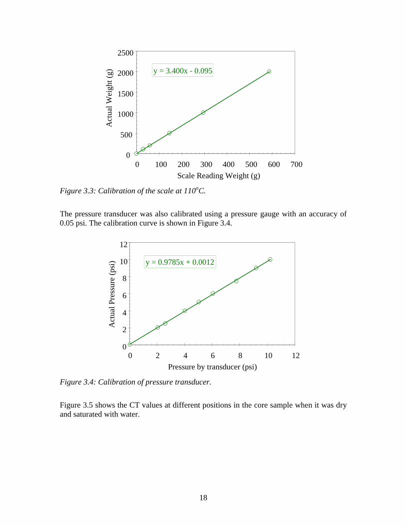
The core system did not sit on the scale directly. Therefore the weight variation recordedby the scale was not that of the actual core system but was related to it linearly. To findthe relationship between the weight measured by the scale and that of the core system, weused standard known weights to substitute the core system. We could obtain the readingrecorded by the scale for different weights. The relationship between the two is shown inFigure 3.3. The weight of the core system can be calculated from the reading of the scaleusing the relationship as follows:

095.04.3 −= scalecore WW (3.3)

where Wcore and Wscale are the weight of the core and the reading of the scale,respectively.

We found that the relationship represented by Eq. 3.3 was somewhat temperature-dependent. So the scale was calibrated at both room temperature and high temperature.The relationship in Eq. 3.3 represents the calibration at a temperature of 110oC. Most ofthe experiments were conducted at this temperature.

18

y = 3.400x - 0.095

0

500

1000

1500

2000

2500

0 100 200 300 400 500 600 700

Scale Reading Weight (g)

Act

ual W

eigh

t (g)

Figure 3.3: Calibration of the scale at 110oC.

The pressure transducer was also calibrated using a pressure gauge with an accuracy of0.05 psi. The calibration curve is shown in Figure 3.4.

y = 0.9785x + 0.0012

0

2

4

6

8

10

12

0 2 4 6 8 10 12

Pressure by transducer (psi)

Act

ual P

ress

ure

(psi

)

Figure 3.4: Calibration of pressure transducer.

Figure 3.5 shows the CT values at different positions in the core sample when it was dryand saturated with water.

19

600

800

1000

1200

1400

1600

0 10 20 30 40 50

Distance from the Bottom (cm)

CT

Val

ue

Wet CT Dry CT

Figure 3.5: CT distribution before and after water saturation.

Using the data in Figure 3.5, the porosity and its distribution of the core sample werecalculated with Eq. 3.1 and are plotted in Figure 3.6. The average porosity measuredusing the X-ray CT technique was about 24.75%; the porosity measured using the wet vs.dry weight method was about 25.0%. The two values of the porosity using differentmethods are in good agreement. We did not see any visible fractures in the core sample inthe CT images.

0.0

0.1

0.2

0.3

0.4

0.5

0 10 20 30 40 50Distance from the Bottom (cm)

Por

osity

(Fr

acti

on)

Figure 3.6: Porosity and its distribution of the core sample.

After the core was saturated with water, the permeability was measured at different flowrates with and without back pressure applied. The results are shown in Figure 3.7. Thevariation of permeability at different flow rates was negligible. The fact that the

20

permeability was almost constant at different flow rates and different mean pore pressuredemonstrated that the core sample was completely saturated with water.

1.0

1.2

1.4

1.6

1.8

2.0

0 2 4 6 8 10 12

Water Injection Rate (ml/min)

Abs

olut

e Pe

rmea

bili

ty (

Dar

cy)

with back pressure (20 psi)without back pressure

Figure 3.7: Permeability of the core at different flow rates and mean pressures.

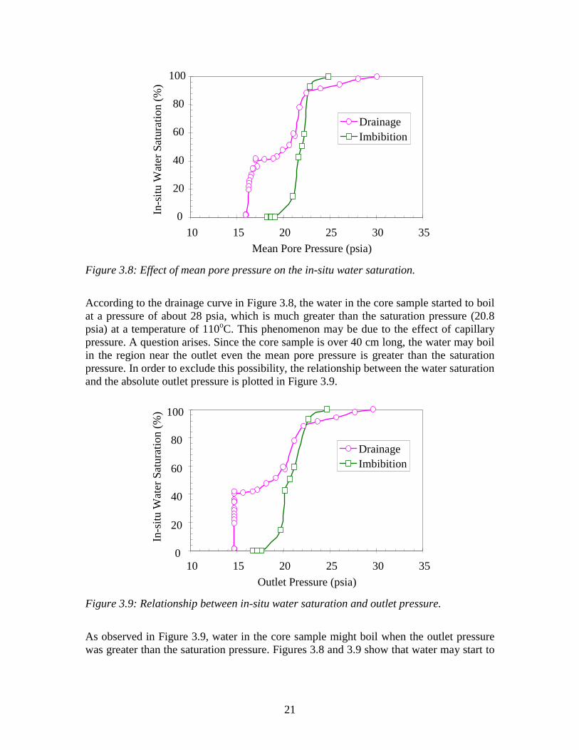
The temperature of the core system was raised to 110oC while the outlet pressure waskept at 35 psia and the water injection rate was kept at 0.5 ml/min. Then the pressure atthe outlet of the core sample was decreased step by step. The in-situ water saturation inthe core sample was calculated using the data from the scale with calibration relationshipof Eq. 3.2. The computed results are shown in Figure 3.8. The mean pore pressure in thecore sample was calculated using the outlet pressure and the differential pressure acrossthe core. The in-situ water saturation decreases with the decrease of the mean porepressure and drops very sharply close to the saturation pressure at this temperature, whichis 20.8 psia. Interestingly, the water saturation did not drop to zero, but to about 40percent. This may be due to the effect of adsorption. When the mean pore pressuredecreases further, the in-situ water saturation decreases abruptly again, to almost zero.The core dried out. The drainage curve of in-situ water saturation vs. mean pore pressureis characteristic of a two-step decrease (see Figure 3.8). Following the drainage process,we increased the mean pore pressure gradually while the injection rate of water was keptat the same value, 0.5 ml/minute. Figure 3.8 shows that the in-situ water saturationincreases with the increase of the mean pore pressure and increases sharply close to thesaturation pressure. However, we did not observe the second step as in the drainageprocess. There was only one sharp increase of the water saturation.

21

0

20

40

60

80

100

10 15 20 25 30 35

Mean Pore Pressure (psia)

In-s

itu

Wat

er S

atur

atio

n (%

)

DrainageImbibition

Figure 3.8: Effect of mean pore pressure on the in-situ water saturation.

According to the drainage curve in Figure 3.8, the water in the core sample started to boilat a pressure of about 28 psia, which is much greater than the saturation pressure (20.8psia) at a temperature of 110oC. This phenomenon may be due to the effect of capillarypressure. A question arises. Since the core sample is over 40 cm long, the water may boilin the region near the outlet even the mean pore pressure is greater than the saturationpressure. In order to exclude this possibility, the relationship between the water saturationand the absolute outlet pressure is plotted in Figure 3.9.

0

20

40

60

80

100

10 15 20 25 30 35

Outlet Pressure (psia)

In-s

itu

Wat

er S

atur

atio

n (%

)

DrainageImbibition

Figure 3.9: Relationship between in-situ water saturation and outlet pressure.

As observed in Figure 3.9, water in the core sample might boil when the outlet pressurewas greater than the saturation pressure. Figures 3.8 and 3.9 show that water may start to

22

boil at a pressure much greater than the saturation pressure (20.8 psia in this experiment)in water-wet porous media. If the core were steam-wet, this would not happen.

After the imbibition, we decreased the temperature of the core system to about 94oC inorder to study the effect of temperature on the water saturation. The temperature was thenraised gradually while the injection rate of water was kept at 0.5 ml/minute. The meanpore pressure was not constant during this process. The experimental data are shown inFigure 3.10. The water saturation decreased with the increase of temperature. There was asharp drop of the water saturation at around 109oC.

0

20

40

60

80

100

90 95 100 105 110 115 120

Temperature (oC)

In-s

itu

Wat

er S

atur

atio

n (%

)

Figure 3.10: Effect of temperature on the in-situ water saturation.

The water injection rate influences the water saturation -- the higher the differentialpressure, the greater the mean pore pressure. The experimental results are plotted inFigure 3.11. We can see that the in-situ water saturation increases with the increase ofwater injection rate.

Using the experimental data from the first drainage process (see Figure 3.8), wecalculated the steam relative permeabilities at the water saturations under 40%. It wasassumed that the water phase was immobile at these values of water saturation. Thecalculated results are shown in Figure 3.12.

23

20

30

40

50

60

0.2 0.4 0.6 0.8 1.0 1.2

Injection Rate (ml/min)

In-s

itu

Wat

er S

atur

atio

n (%

)

Figure 3.11: Effect of water injection rate on the in-situ water saturation.

0.0

0.2

0.4

0.6

0.8

1.0

0 20 40 60 80 100

In-situ Water Saturation (%)

Stea

m R

elat

ive

Per

mea

bili

ty (

frac

)

Figure 3.12: Steam relative permeabilities at a temperature of 110oC.

The experimental data in Figure 3.8 were also used to calculate the productivity indexrepresented by Eq. 3.2. The results are shown in Figure 3.13. The productivity index, inthe unit of kg/Mpa.hr, increases with the increase of mean pore pressure and reaches amaximum value at a pressure close to the saturation pressure in both drainage andimbibition.

24

0

3

6

9

12

15

0 5 10 15 20 25 30 35

Mean Reservoir Pressure (psia)

Prod

uctiv

ity I

ndex

(kg

/Mpa

.hr)

DrainageImbibition

Figure 3.13: Effect of mean pressure on the productivity index.

It would be interesting to calculate the productivity index using the unit of liter/Mpa.hr.However, there is a difficulty to obtain the fraction of steam or water in the two-phaseflow region so this calculation was not done.

3.6 CONCLUSIONS

Based on the present work, the following conclusions may be drawn:

1. An experimental method to model the water injection into geothermal systems and tomeasure end-point steam relative permeabilities has been developed.

2. The in-situ water saturation is dependent on the mean pore pressure and changes verysharply at a pressure close to the saturation pressure during both drainage andimbibition.

3. The in-situ water saturation increases with the increase of water injection rate andwith the decrease of temperature.

4. The productivity index, in the unit of kg/Mpa.hr, increases with the increase of meanpore pressure and reaches a maximum value at a pressure close to the saturationpressure in both drainage and imbibition.

5. Water may boil at a pressure greater than the saturation pressure in water-wet porousmedia due to the effect of capillary pressure.

3.7 FUTURE WORK

We may conduct a similar experimental study using geothermal rocks.

25

4. INFERRING RESERVOIR CONNECTIVITY BY WAVELET ANALYSIS OF PRODUCTION DATA This project is being conducted by Research Assistant Brian A. Arcedera and Prof.Roland Horne. The objective is to determine reservoir connectivity by applying waveletanalysis to data gathered in day-to-day operations. Use of this technique would establishthe degree of connectivity between wells without doing additional tests and datagathering.

4.1 BACKGROUND

In 1998, Sullera used wavelet analysis and multiple regression techniques to inferinjection returns by analyzing injection rates and chloride concentrations. The studyindicated that wavelet analysis could isolate short-term signal variations which could becorrelated from one well to another. The results of Sullera’s study were verifiedsuccessfully against tracer test data and qualitative field observations.

Sullera’s study, however, only yielded successful results in one set of field data. Otherdata sets analyzed did not have sufficient data points for meaningful statisticalcorrelations. The frequency of chloride data further hindered the approach by limiting theanalysis to the use of monthly data. Data with monthly frequency may not be suitable forthis analysis because they would not capture the short-term variations in the signal.

This project was conceived as an extension of Sullera’s study. The study addresses theproblems of lack of data and low sampling frequency by analyzing production data (e.g.total rate, steam rate, brine rate, wellhead pressure, enthalpy). Production data is alreadygathered on a regular basis for normal operating records so no additional tests or datagathering needs to be done.

4.2 METHODOLOGY

The analysis required in the study can be broken into four main steps: preprocessing,wavelet analysis, cross-correlation analysis, and multiple regression analysis.

The preprocessing step rearranges the data from different sources into a uniform formatfor subsequent analysis. Each data set from a unique source goes through a customtranslation that extracts the pertinent information and writes it into a new file. Thisuniform data format is essential in the automation of the succeeding filtration andanalysis steps. The formatted data is then filtered to remove nonnumeric entries andinterpolated linearly to produce data signals over a uniform time interval. Safeguards inthe interpolation macro prevent interpolation over long periods of missing data. In thesecases, the data signal is truncated to include only the longest relevant time period.

The processed data signal is separated into a general approximation and a series of signalfluctuations through wavelet decomposition. Wavelet analysis separates the data intosmall sections and fits a predetermined wavelet function to each subgroup. Each level ofwavelet decomposition handles a different section length thus capturing signal variations

26

at different time scales. Wavelet analysis is done using the Haar wavelet (a waveletsimilar to a square wave) since it best captures the fluctuations expected from the on/offvariations in surface conditions. This decomposition is applied until the approximationcurve becomes smooth.

The different detail signals obtained in the wavelet analysis from different wells areanalyzed in groups to determine correlations between them. Different types of productiondata are paired and analyzed in turn (e.g. injection rate – production enthalpy, or injectionrate – production wellhead pressure). For each pair of data type, cross-correlation is donefor each detail level between wells to determine any signal lag so that the data can beadjusted accordingly.

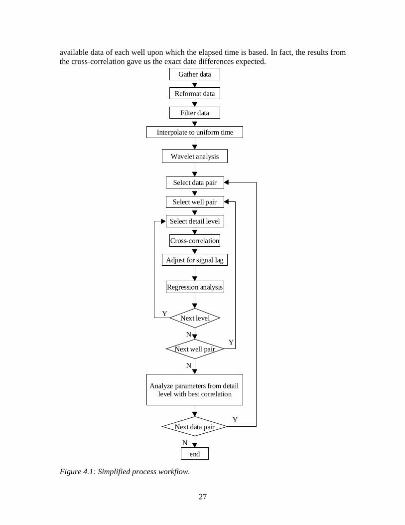
The adjusted signals can be analyzed through multiple regression to determine the effectsof one data signal on another. For each pair of wells being analyzed, the different detaillevels will be compared and the regression coefficients noted. The detail level with thebest meaningful correlation will be analyzed further. The regression parameters obtainedat the best detail level will be compared to other well pairs to infer relative connectivitystrengths between them. Figure 4.1 illustrates the process workflow.

4.3 CONTINUING WORK

The wavelet analysis was applied initially to a group of relatively isolated injection wells.Injection wells were chosen to test the analysis procedure because of the availability ofdaily injection data. By comparison, production data from the Tiwi geothermal field isrecorded in intervals of five to nine days, which would require further data preparation.Another reason for choosing the group of injection wells was to determine if surfaceconnectivity effects through pipelines could be isolated from reservoir connectivityeffects.

Three injection wells were processed through the wavelet decomposition procedure:Nag-08, Nag-70, and Nag-71. Figure 4.2 shows the decomposition of the injection ratedata for Nag-70. The figure shows the original signal, s, followed by the approximation,a8, and the different detail levels, dn, all plotted against the number of days elapsed sinceFebruary 1, 1990. The wavelet analysis separates the general trend (shown in a8 as adeclining injection rate for this particular well), and gives us the detail signals indicatingfluctuations over different time intervals. These fluctuations are what we hope tocorrelate between wells and ultimately use to determine reservoir connectivity.

The date of data acquisition was masked by indexing the data by the number of dayselapsed since the date of the first available data for that well. This was done to provide aone-dimensional data set that could be manipulated more easily through wavelet analysis.The signal offset for the three injector wells was determined as a check on the cross-correlation function that is used to determine lag time. Since a common injection networksupplies the injectors, it is expected that there will be no lag time. The signal offsetprovided by the cross-correlation should then give us the date difference between the first

27

available data of each well upon which the elapsed time is based. In fact, the results fromthe cross-correlation gave us the exact date differences expected.

Gather data

Reformat data

Filter data

Interpolate to uniform time

Wavelet analysis

Select data pair

Select well pair

Select detail level

Cross-correlation

Adjust for signal lag

Regression analysis

Next level

Next well pair

Analyze parameters from detail level with best correlation

Next data pair

Y

NY

N

N

Y

end

Figure 4.1: Simplified process workflow.

28

Figure 4.2: Wavelet decomposition of Nag-70 daily injection data. Note: x-axisrepresents number of days since 1 February 1990.

Figure 4.3 compares the injection rate from the three injectors. The wells are all tied-in toone injection network and, as expected, exhibit strong data correlation resulting fromtheir surface connections. This surface connectivity might be isolated from the signalthrough wavelet decomposition. Figure 4.4 compares the details signal (d1) of the threewells over a data frequency of one day. Visual inspection of the plots leads us to assumethat this detail level captures the data correlation. A comparison of the details signal fromthe three wells over a data frequency of 1 month (d6) is shown in Figure 4.5. Visualinspection of the plots at this frequency seems to show a better correlation between thelatter two wells – Nag-70 and Nag-71. However, statistical tools will still be used tobetter evaluate the correlation.

29

0 500 1000 1500 2000 2500 3000 3500 4000 45000

100

200

300

400

500

0 500 1000 1500 2000 2500 3000 3500 4000 45000

100

200

300

400

500

0 500 1000 1500 2000 2500 3000 3500 4000 45000

100

200

300

400

500

Figure 4.3: Injection rate (x1000 lbs/hr) plotted against number of days elapsed sinceMarch 26, 1989 (from top to bottom: Nag-08, Nag-70, and Nag-71).

0 500 1000 1500 2000 2500 3000 3500 4000 4500-200

-100

0

100

200

0 500 1000 1500 2000 2500 3000 3500 4000 4500-200

-100

0

100

200

0 500 1000 1500 2000 2500 3000 3500 4000 4500-200

-100

0

100

200

Figure 4.4: Detail level 1 (daily frequency) of injection rate (x1000 lbs/hr) plottedagainst number of days elapsed since March 26, 1989 (from top to bottom:Nag-08, Nag-70, and Nag-71).

30

0 500 1000 1500 2000 2500 3000 3500 4000-100

-50

0

50

100

0 500 1000 1500 2000 2500 3000 3500 4000 4500-100

-50

0

50

100

0 500 1000 1500 2000 2500 3000 3500 4000 4500-100

-50

0

50

100

Figure 4.5: Detail level 6 (~monthly frequency) of injection rate (x1000 lbs/hr) plottedagainst number of days elapsed since March 26, 1989 (from top to bottom:Nag-08, Nag-70, and Nag-71).

Analysis of the three injection wells illustrates that our procedures for using waveletanalysis to decompose the production data into an approximation and a series of detaillevels at different frequencies can be applied properly. The next step in our analysis willbe to use statistical tools to interpret reservoir connectivity from the detail signals. Basicstatistical tools can be used to determine quantitatively which of the signals in Figure 4.5are really more closely correlated.

After the initial testing of our procedures, production and injection data will be analyzed.In particular, we will be looking at data from the Tiwi and MakBan geothermal fields inthe Philippines. The first data pairs analyzed will be injection rate against productionwellhead pressure, and injection rate against production enthalpy. It is hoped thatanalyzing these data pairs will provide information on injection returns in these specificfields. In particular, information on the effects of injection returns in the form of pressuresupport as well as effects on reservoir enthalpy may prove useful.

31

5. EXPERIMENTAL INVESTIGATION OF STEAM AND WATER RELATIVE PERMEABILITY ON SMOOTH WALLED FRACTURE This project is being conducted by Research Assistant Gracel P. Diomampo, ResearchAssociate Kewen Li and Prof. Roland Horne. The goal is to gain better understanding ofsteam-water flow through fractured media and determine the behavior of relativepermeability in fractures.

5.1 BACKGROUND

Geothermal reservoirs are complex systems of porous and fractured rocks. Completeunderstanding of geothermal fluid flow requires knowledge of flow in both types ofrocks. Many studies have been done to investigate steam and water flow through porousrocks, however fewer studies have examined multiphase flow in fractures. Only a fewpublished data are available most of which have been done for air-water or for water-oilsystems. Earliest is Romm’s (1966) experiment with kerosene and water flow through anartificial parallel-plate fracture lined with strips of polyethylene or waxed paper. Rommfound a linear relationship between permeability and saturation, Sw= krw, Snw = krnw suchthat krw+krnw = 1. Pan et al. (1996) performed a similar experiment with an oil-watersystem but arrived at conflicting results -- significant phase interference was observedsuch that krw + krnw <1. Both studies, however, concluded that residual saturations arezero and that a discontinuous phase can flow as discrete units along with the other phase.

In an attempt to develop a relationship between fracture relative permeability and voidspace geometry, Pruess and Tsang (1990) conducted numerical simulation for flowthrough rough-walled fractures. Their study showed the sum of the relativepermeabilities to be less than 1, residual saturation of the nonwetting phase to be large,and phase interference to be greatly dependent on the presence or absence of spatialcorrelation of aperture in the direction of flow. Persoff et al. (1991) performedexperiments on gas and water flow through rough-walled fractures using transparent castsof natural fractured rocks. The experiments showed strong phase interference similar tothat seen in the flow in porous media. The data of Persoff (1991) and Persoff and Pruess(1995) for flow through rough-walled fractures were compared in Horne et al. (2000), asshown in Figure 5.1.

Presently, the mechanism of flow and the characteristic behavior of relative permeabilityin fractures are still undetermined. As yet unresolved are issues such as whether adiscontinuous phase can travel as discrete units carried along by another phase or will betrapped as a residual saturation as in porous media. The question of phase interference isstill unanswered, i.e. whether the curve of relative permeability vs. saturation is an X-curve, Corey curve, or some other function. The main objective of this study is tocontribute to the resolution of these issues. Experiments using air-water flow throughsmooth-walled fractures will be done first with the aim of establishing a reliablemethodology for flow characterization and permeability calculation. Then theseexperiments will be repeated with steam-water flow; and with rough-walled fractures.

32

0.001

0.01

0.1

1

0.001 0.01 0.1 1krl

k rg

Persoff and Pruess (1995) Expt CPersoff and Pruess (1995) Expt DPersoff et al. (1991) CoreyLinear (X-curves)

Figure 5.1: Some measurements of air-water relative permeabilities in rough-walledfractures (graph from Horne et al. (2000))

5.2 EXPERIMENTAL APPARATUS AND MEASUREMENT TECHNIQUES

The smooth-walled fracture apparatus consisted of a 183 cm by 31 cm horizontal glassplate on top of an aluminum plate. The aperture between the glass and aluminum plateswas dictated by 0.2-mm thick shims inserted between them. The shims were placedalong the boundaries and in three columns along the flow area. It should be noted thatthe shims placed as columns along the plate did not divide the plate into separate flowsections. This was deduced upon observing cross flow along the shims.

The sides of the plates were sealed together with silicone adhesive. Even with theadhesive, the inlet head had to be kept below 15 cm to avoid leakage. This constraintpresented a maximum limit in the flow rates approximately 2 cc/sec for water and 9cc/sec for nitrogen.

Horizontal slits at the ends of the metal plate served as entry and exit points for the fluids.There were two available canals for input of gas and liquid. The options to injectnitrogen and water as separate streams or as mixed fluid in a single stream were tried. Itwas found that mixing the gas and water prior to input caused no significant improvementin fluid distribution. Thus, the gas and water streams were injected separately forsimplicity, ease of flow rate control, and inlet pressure reading.

Gas flow was controlled through a flow regulator. A meter pump controlled the rate ofliquid injection. Dye was dissolved in the injection reservoir for better phaseidentification. Figure 5.2 shows a schematic diagram of this configuration.

33

N2

Gas regulator

Meter pumpDyed waterreservoir

transducertransducer

computer

Digital camera

Glass plate

Aluminum plateWatercollectionbin

Figure 5.2: Experimental set-up for air and water flow through smooth walled fractures.

watergas

Figure 5.3: Sample camera image for two-phase run.

34

Low capacity transducers measured the gas and liquid inlet pressures separately. Thesetransducers were attached to a Labview program designed to record data at user-specifiedtime intervals. The water rate was read from the pump meter and gas rate from theregulator. Saturation was computed by measuring the area that each phase occupied. Thiswas done by taking digital photographs of a constant area of the plate at a particular gasand water rate. The area was around 3 ft. long and was chosen far enough from the endsof the plates to avoid end effects. Figure 5.3 shows a sample photo from a two-phase run.The photographs were processed in a Matlab program. The program uses quadraticdiscriminant analysis to group the pixels of the photograph into three groups: the waterphase, gas phase, and the shim. The grouping was based on color differences. Saturationwas calculated as total pixels of liquid group over the sum of the gas and liquid group.Figure 5.4 is a comparison of the gray-scale image produce by the program and theoriginal photograph from the digital camera. The accuracy of the program in calculatingthe saturation can be confirmed from the similarity in details of the gray-scale image tothe true image. From the figure, it can be said that the program has reasonable accuracy.

20 40 60 80 100 120

50

100

150

200

250

300

Saturation = 0.5987

Figure 5.4: Comparison of gray-scale image produced by the Matlab program to actualphoto taken by digital camera.

Pan et al. (1996) also used this technique for measurement of saturation. This studynoted that the sources of error in this technique were the quality of the photographs andthe water film adsorbed on the surfaces of the plates with the latter being of minimaleffect. Good quality photographs are the ones with clear distinction between the gas and

35

liquid phases. The use of dyed liquid enhanced visualization of phase boundaries andproduced better quality photographs.

5.3 PARTIAL RESULTS AND DISCUSSION

Preliminary experiments were done with qgas/qliq values of 1, 5, 10, 20 and single-phaseruns at residual saturation. There were some important observations:

In these ratios of qgas/qliq, the water and gas phase traveled along the plate as separatechannels. These separate flow paths changed with time and position. This is illustratedin the series of images in Figure 5.5, which were taken at constant gas and liquid rate.This observation implies that at these ratio, phases move individually and not as “movingislands” or “globules” of the discontinuous phase carried along by the other phase. It alsosuggests that there is no local steady-state saturation.

Run4 at 20:54:01 Run4 at 20:54:37 Run4 at 20:55:10

Figure 5.5: Images at constant gas and liquid rate in short time intervals to illustratechanges in the gas and liquid flow paths.

These fast changes in flow paths were accompanied by pressure fluctuations. When thegas established enough energy to break through the water flow path, there was acorresponding increase in inlet gas pressure and decrease in water line pressure. Thesame was true when the water phase breaches through gas channels. This fluctuationcaused difficulty in registering the current pressure.

Residual saturations obtained were very low. Residual water saturation Swr was around0.02 -0.06. Similarly, residual steam saturation Sgr was around 0.04-0.06. This indicatesthat there is negligible trapping in this smooth-walled fracture.

Pan et al. (1996) discussed two approaches in data analysis: the porous medium approachwhere Darcy’s law is used and the homogeneous single-phase approach where the system

36

is treated as a single-phase pipe flow. Because of the observations in the experiments, itseemed appropriate to treat the data using porous medium approach.

Darcy’s law was used to obtained the single-phase and two-phase liquid permeability:

)( oi

il pp

Lqk

−= µ

(5.1)

subscripts ‘o’ stands for outlet and ‘i’ for inlet, µ the viscosity, p as pressure, L for lengthof the plate and q as Darcy flow velocity from

bw

Qq o

o = (5.2)

where Q is the volumetric rate, b the aperture and w as the width of the plate.

The relative permeability is then calculated by taking the ratio of the two-phase kl withthe single-phase kl.

The gas permeability was calculated using the equation from Scheidegger (Scheidegger,1974):

222

oi

oog pp

pLqk

−= µ (5.3)

Similarly, taking the ratio of the two-phase kg with single-phase run gives the relativepermeability.

The complete list of calculated relative permeability values, their correspondingsaturation range is shown in Table 5.1. Figures 5.6 and 5.7 show plots of these dataalong with the X-curves. The data are clustered over a small saturation range and lie farfrom the X-curves.

5.4 FUTURE WORK

Further experiments with nitrogen-water system will be done at higher orders of variationof qgas/qliq. This will be to obtain wider saturation range in the relative permeabilitycurves. To investigate the flow mechanism further, a digital video camera will be used torecord the flow. A voltmeter has been attached to the transducer and its pressure readingwill be recorded visually along with the flow. Snapshots will be taken from the videorecording. These snapshots will be analyzed to observe the periodic snap-off andreconnection of flow channels, pressure fluctuations and accompanying changes insaturation.

The experiment will also be performed with sand or glass beads in between the glass andaluminum plate to simulate flow through rough-walled fractures.

Simultaneous with these nitrogen-water experiments, design of a similar apparatus forsteam-water system is under study. The challenges encountered in the design include:

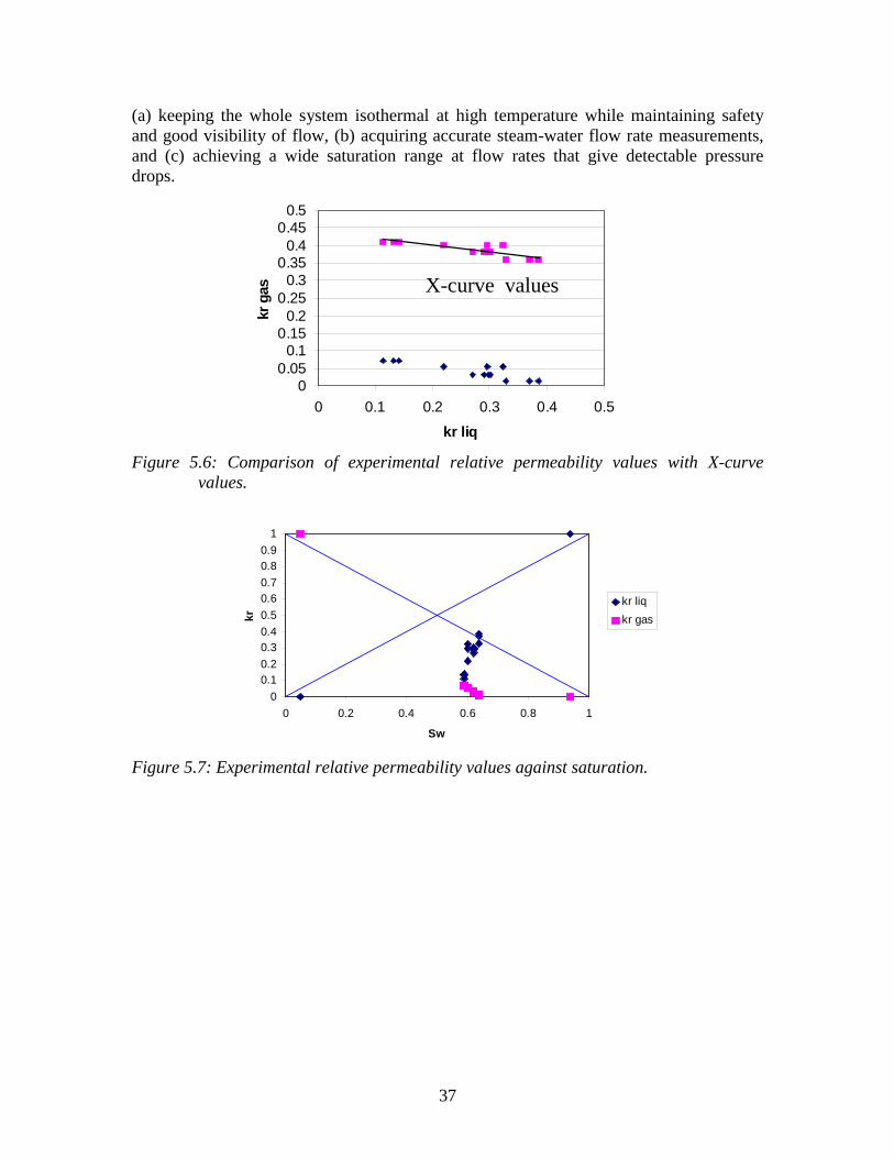
37

(a) keeping the whole system isothermal at high temperature while maintaining safetyand good visibility of flow, (b) acquiring accurate steam-water flow rate measurements,and (c) achieving a wide saturation range at flow rates that give detectable pressuredrops.

00.05

0.10.15

0.20.25

0.30.35

0.40.45

0.5

0 0.1 0.2 0.3 0.4 0.5

kr liq

kr g

as X-curve values

Figure 5.6: Comparison of experimental relative permeability values with X-curvevalues.

0

0.10.2

0.30.4

0.5

0.60.7

0.80.9

1

0 0.2 0.4 0.6 0.8 1

Sw

kr

kr liq

kr gas

Figure 5.7: Experimental relative permeability values against saturation.

38

Table 5.1: Calculated relative permeability values.

run # Qg Gas Head krg Qw Water Head krl(cc/min) (cm H2O) (cc/min) (cm H2O)

1 74 12.5 0.013 35.16 11.5 0.3851 74 12.5 0.013 33.77 11.5 0.3701 74 12.5 0.013 29.97 11.5 0.3282 172 13 0.030 26.51 11.5 0.2912 172 13 0.030 27.45 11.5 0.3012 172 13 0.030 27.19 11.5 0.2983 172 13 0.030 24.71 11.5 0.2713 332 13.7 0.055 26.98 11.5 0.2963 332 13.7 0.055 29.51 11.5 0.3233 332 13.7 0.055 20.04 11.5 0.2204 407 12.8 0.072 12.36 11.0 0.1424 407 12.8 0.072 9.92 11.0 0.1144 407 12.8 0.072 11.52 11.0 0.132

39

6. REFERENCES Hanselman, D. and Littlefield, B. Mastering Matlab 5 A Comprehensive Tutorial andReference, Prentice-Hall, Inc.,New Jersey, 1998.

Horne, R.N., Satik, C., Mahiya, G., Li, K., Ambusso, W., Tovar, R., Wang, C., andNassori, H.: “Steam-Water Relative Permeability,” Proc. of the World GeothermalCongress 2000, Kyushu-Tohoku, Japan, May 28-June 10, 2000.

Li, K. and Horne, R.N. (2000a): “Steam-Water Capillary Pressure,” SPE 63224,presented at the 2000 SPE Annual Technical Conference and Exhibition, October 1-4,2000, Dallas, TX, USA.

Li, K. and Horne, R.N. (2000b): “Characterization of Spontaneous Water Imbibition intoGas-Saturated Rocks,” SPE 62552, presented at the 2000 SPE/AAPG Western RegionalMeeting, Long Beach, California, 19–23 June 2000.

Li, K. and Horne, R.N. (2000c): “Steam-Water Capillary Pressure in GeothermalSystems,” presented at the 25th Stanford Workshop on Geothermal ReservoirEngineering, January 24-26, 2000, Stanford University, Stanford, CA 94043, USA.

Mahiya, G.F.: Experimental Measurement of Steam-Water Relative Permeability, MSreport, Stanford University, Stanford, Calif., 1999.

Pan, X., Wong, R.C., and Maini, B.B.: “Steady State Two-Phase Flow in a SmoothParallel Fracture”, presented at the 47th Annual Technical Meeting of the PetroleumSociety in Calgary, Alberta, Canada, June 10-12, 1996.

Persoff, P., and Pruess, K.: “Two-Phase Flow Visualization and Relative PermeabilityMeasurement in Transparent Replicas of Rough-Walled Fractures”, Proceedings, 16th

Workshop on Geothermal Reservoir Engineering, Stanford University, Stanford, CA, Jan.23-25, 1991, pp 203-210.

Pruess, K., and Tsang, Y. W.: “On Two-Phase Relative Permeability and CapillaryPressure of Rough-Walled Rock Fractures”, Water Resources Research 26 (9), (1990), pp1915-1926.

Satik, C.: "A Study of Steam-Water Relative Permeability", paper SPE46209 presentedat the SPE Western Regional Meeting, 10-13 May 1998, Bakersfield, California.

Scheidegger, A.E. The Physics of Flow Through Porous Media, 3rd ed., University ofToronto, Toronto. 1974.

Sullera, M.M., and Horne, R.N.: “Inferring Injection Returns from Chloride MonitoringData”, to appear in Geothermics, 2000.