Quarry Evolution in the Nova Olinda Region, Ceará, Brazil Lizzy McKinnon GIS and GPS Applications, Fall 2016

ABSTRACT

Quarry growth in the Nova Olinda region is rapid and poorly understood. This study aims to

quantify changes in quarry areas due to active quarrying and quarry abandonment/revegetation

using Google Earth satellite imagery from 2008 to 2016. Quarries in the region have almost

tripled in area over the past eight years, with nearly one square kilometer of new quarry growth.

1

INTRODUCTION

The Araripe Basin (AB) is located in the northeast of Brazil between the states of Ceará and

Pernambuco (Fig. 1). This study focuses on an area of 39 km2 in the Araripe Geopark near

Nova Olinda (Fig. 2). The Crato and Ipubi Formations of the Araripe Basin are heavily quarried

in the Nova Olinda region. The Crato Formation is a laminated limestone deposit that is used for

construction and decorative purposes and the Ipubi Formation is a massive gypsum deposit

used primarily for the production of concrete. This study aims to estimate the change in area of

quarries in the Nova Olinda region from 2008 to 2016. Changes include growth due to active

quarrying and creation of rubbish piles and shrinkage from reclamation by vegetation after

quarry abandonment, both of which are active processes in the region. This question will be

addressed using ArcMap to map quarries visible in current and historical satellite imagery from

Google Earth.

Figure 1. Location of Araripe Basin on the South American continent. Topographic map of AB created

using 1-arc second SRTM data. Study area is indicated by the black box on the northern margin of the

plateau.

2

Figure 2. 2016 Google Earth satellite imagery of study region. Yellow box indicates the location of the

quarry shown in Figures 5 & 6.

DATA COLLECTION AND PREPROCESSING

All data was stored in a personal geodatabase file that was created before data collection. Georeferenced high resolution images for regions of the study area that had visible quarries during the year of interest were generated using the Image Overlay tool in Google Earth (Fig. 3).

3

Figure 3. Image overlay tool in Google Earth.

The years 2008 and 2016 were chosen for study because they both had reliable, high

resolution satellite imagery available in the study area. These Image Overlays were saved as

KML files and converted using the KML to Layer file in ArcCatalog with the “include Ground

Overlay” box checked (Fig. 4). Two raster catalogs were created within the database to hold the

satellite images. After conversion, the Ground Overlay rasters were added to their respective

raster catalogs by dragging and dropping them in ArcCatalog. Twelve images were processed

for quarried areas in 2016 and eleven were processed for quarried areas in 2008.

Figure 4. KML to Layer tool in ArcCatalog. Ground Overlay box must be checked as it contains the

georeferenced raster.

4

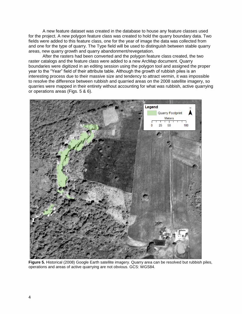
A new feature dataset was created in the database to house any feature classes used for the project. A new polygon feature class was created to hold the quarry boundary data. Two fields were added to this feature class, one for the year of image the data was collected from and one for the type of quarry. The Type field will be used to distinguish between stable quarry areas, new quarry growth and quarry abandonment/revegetation. After the rasters had been converted and the polygon feature class created, the two raster catalogs and the feature class were added to a new ArcMap document. Quarry boundaries were digitized in an editing session using the polygon tool and assigned the proper year to the “Year” field of their attribute table. Although the growth of rubbish piles is an interesting process due to their massive size and tendency to attract vermin, it was impossible to resolve the difference between rubbish and quarried areas on the 2008 satellite imagery, so quarries were mapped in their entirety without accounting for what was rubbish, active quarrying or operations areas (Figs. 5 & 6).

Figure 5. Historical (2008) Google Earth satellite imagery. Quarry area can be resolved but rubbish piles, operations and areas of active quarrying are not obvious. GCS: WGS84.

5

Figure 6. Google Earth 2016 satellite imagery of the same area as Figure 5. Areas of active quarrying, operations and rubbish piles are easily resolved. For simplicity, all of these units were mapped together as a 2016 quarry footprint. GCS: WGS84.

ARCGIS PROCESSING

After data collection and processing, the polygon data needed to be converted to raster

data to calculate the overlap between polygons. The data was selected by year and exported as

two new feature classes, one for 2008 and one for 2016. These new feature classes were

converted to rasters using the Feature to Raster tool with an output cell size of

1.65365131999806E-06 to ensure smoothness along quarry edges (Figs. 7, 8 & 9).

6

Figure 7. Feature to Raster tool in ArcMap. The small cell size is crucial to ensure smoothness along

quarry boundaries.

Figure 8. Raster of

2008 quarry

footprints (R1) over

2016 Google Earth

satellite imagery.

7

Figure 9. Raster of

2016 quarry

footprints (R2) over

2016 Google Earth

satellite imagery.

The Raster Calculator tool was used to create a new raster that showed the intersection

between these two rasters (Fig. 10). This intersection area represents quarry areas that have

been stable over the past eight years (Fig. 11).

Figure 10. Raster calculator tool in

ArcMap with expression used to

generate the intersection raster.

This raster contains values where

the 2008 (R1) and 2016 (R2)

satellite imagery overlap.

8

Figure 11. Raster of

the intersection

between R1 and R2.

These are the areas

of quarries that have

remained stable over

the past eight years.

Anything outside of this area on the 2016 raster represents new quarry growth. Anything

outside of this area on the 2008 raster represents reclamation of quarries by vegetation/quarry

abandonment. In order to properly calculate these areas, it was necessary to return to working

with feature classes, so the intersection raster was converted to a polygon feature class using the

Raster to Polygon tool.

There were now three independent polygons to work with, one from each raster. These

three features were combined using the Merge tool (Fig. 12). This resulted in a polygon with eight

fields. A ninth field was added for the calculation of area of the feature. All areas of intersection

were recorded as <null> for the “Year” field. These values were selected from the attribute table

and the Clip function was used from the editing toolbar to remove this area from the 2008 and

2016 polygons to prevent errors in area calculations. In the attribute table, the Calculate Geometry

function was used to fill in the new Area field for each object. The area calculation was completed

in square meters. This calculation was also performed on an Area field created for the individual

2008 and 2016 feature classes as well to understand the total area of these quarries during each

year. Three attribute tables were exported in dBase format: one for the 2008 feature class, one

for the 2016 feature class and one for the feature class that contained the data for 2008, 2016

and their intersection.

9

Figure 12. Final

map of quarry

footprint polygons

showing stable,

abandoned and

newly quarried

areas.

RESULTS

In 2008, quarries in the study region comprised an area of 411,211 m2. In 2016, quarries

in the study region comprised an area of 1,207,526 m2, meaning that quarried areas in the

region nearly tripled in size over this eight-year period. Not all of this was new quarry growth.

From 2008 to 2016, 227,752 m2 of quarry remained stable. 183,459 m2 of quarries were

abandoned and reclaimed by vegetation. Quarry growth over this period was impressive, with

979,774 m2 of new quarries added over eight years. Values for quarry growth are summarized

in the following table:

Year Total Area (m2)

2008 411,211

2016 1,207,526

Category Stable 227,752

New 979,774

Abandoned 183,459

10

Future work is necessary to understand how much of this growth was the result of

quarrying and how much was the result of rubbish pile accumulations. In many quarries, rubbish

piles cover large areas, especially when they accumulate on hillslopes like in the Três Irmãoes

quarry, the largest quarry in the region. Hopefully this will lend insight into vegetation loss due to

rubbish pile accumulation and prompt better management of rejected material from these quarry

sites.

DATA SOURCES

Source: "Nova Olinda Region, 2016." 7° 7'52.85"S and 39°42'56.80"W. Google Earth. November 28, 2016. July 20, 2016. Source: "Nova Olinda Region, 2008." 7° 7'52.85"S and 39°42'56.80"W. Google Earth. November 28, 2016. December 24, 2008.