PHYSICAL REVIEW A 93, 013413 (2016)

Quantum optimal control of photoelectron spectra and angular distributions

R. Esteban Goetz,1 Antonia Karamatskou,2,3 Robin Santra,2,3 and Christiane P. Koch1,*

1Theoretische Physik, Universitat Kassel, Heinrich-Plett-Straße 40, D-34132 Kassel, Germany2Center for Free-Electron Laser Science, DESY, Luruper Chaussee 149, D-22716 Hamburg, Germany

3Department of Physics, Universitat Hamburg, Jungiusstraße 9, D-20355 Hamburg, Germany(Received 2 November 2015; published 14 January 2016)

Photoelectron spectra and photoelectron angular distributions obtained in photoionization reveal importantinformation on, e.g., charge transfer or hole coherence in the parent ion. Here we show that optimal control of theunderlying quantum dynamics can be used to enhance desired features in the photoelectron spectra and angulardistributions. To this end, we combine Krotov’s method for optimal control theory with the time-dependentconfiguration interaction singles formalism and a splitting approach to calculate photoelectron spectra andangular distributions. The optimization target can account for specific desired properties in the photoelectronangular distribution alone, in the photoelectron spectrum, or in both. We demonstrate the method for hydrogenand then apply it to argon under strong XUV radiation, maximizing the difference of emission into the upper andlower hemispheres, in order to realize directed electron emission in the XUV regime.

DOI: 10.1103/PhysRevA.93.013413

I. INTRODUCTION

Photoelectron spectroscopy is a powerful tool for studyingphotoionization in atoms, molecules, and solids [1–6]. With theadvent of new light sources, photoelectron spectroscopy usingintense, short pulses has become available, revealing importantinformation about electron dynamics and time-dependentphenomena [7–10]. In particular, it allows for characterizingthe light-matter interaction of increasingly complex systems[1,3,5]. Photoelectron spectra (PES) and photoelectron angulardistributions (PAD) contain fingerprints not only of theinteraction of the electrons with the electromagnetic fieldsbut also of their interaction and their correlations with eachother [11]. PAD in particular can be used to uncover electroninteractions and correlations [12,13].

Tailoring the pulsed electric field in its amplitude, phase, orpolarization allows us to control the coupled electron-nucleardynamics, with corresponding signatures in the photoelectronspectrum [14–18]. While it is natural to ask how the electrondynamics is reflected in the experimental observables—PESand PAD [14–18], it may also be interesting to see whetherone can control or manipulate directly these observablesby tailoring the excitation pulse. Moreover, one may beinterested in certain features such as directed electron emissionwithout analyzing all the details of the time evolution. This isparticularly true for complex systems where it may not beeasy to trace the full dynamics all the way to the spectrum.The question that we ask here is how to find an external fieldthat steers the dynamics such that the resulting photoelectrondistribution fulfills certain prescribed properties. Importantly,the final state of the dynamics does not need to be known. Thedesired features may be reflected in the angle-integrated PES,the energy-integrated PAD, or both.

To answer this question, we employ optimal control theory(OCT), using Krotov’s monotonically convergent method [19]and adapting it to the specific task of realizing photoelectrondistributions with prescribed features. The photoelectron

*christiane.koch@uni-kassel.de

distributions are calculated within the time-dependent config-uration interaction singles scheme (TDCIS) [20], employingthe splitting method for extracting the spectral componentsfrom the outgoing wave packet [21,22]. While OCT has beenutilized to study the quantum control of electron dynamicsbefore, in the framework of TDCIS [23] as well as the mul-ticonfigurational time-dependent Hartree-Fock (MCTDHF)method [24] or time-dependent density functional theory(TDDFT) [25,26], the PES and PAD have not been tackledas control targets before. In fact, most previous studies didnot even account for the presence of the ionization continuum.A proper representation of the ionization continuum becomesunavoidable [27–31], however, when investigating the inter-action with XUV light where a single photon is sufficient toionize [32], and it is indispensable for the full description ofphotoionization experiments.

To demonstrate the versatility of our approach, we applyit to two different control problems: (i) We prescribe the fullthree-dimensional photoelectron distribution and search fora field that produces, at least approximately, a given angle-integrated PES and energy-integrated PAD. Such a detailedcontrol objective is rather demanding and corresponds to adifficult control problem. (ii) We seek to maximize the relativenumber of photoelectrons emitted into the upper as opposed tothe lower hemisphere, assuming that the polarization axis ofthe light pulse runs through the poles of the two hemispheres.This implies a condition on the PAD alone, leaving completefreedom to the energy dependence. The corresponding controlobjective leaves considerable freedom to the optimizationalgorithm and the control problem becomes much simpler.Maximizing the relative number of photoelectrons emitted intothe upper as opposed to the lower hemisphere correspondsto a maximization of the PAD’s asymmetry. Asymmetricphotoelectron distributions arising in strong-field ionizationwere studied previously for near-infrared few-cycle pulseswhere the effect was attributed to the carrier envelope phase[33,34]. Here we pose the question whether it is possible toachieve asymmetry in the PAD for multiphoton ionizationin the XUV regime and we seek to determine the shapedpulse that steers the electrons into one hemisphere. To ensure

2469-9926/2016/93(1)/013413(17) 013413-1 ©2016 American Physical Society

GOETZ, KARAMATSKOU, SANTRA, AND KOCH PHYSICAL REVIEW A 93, 013413 (2016)

experimental feasibility of the optimized pulses, we introducespectral as well as amplitude constraints. We test our controltoolbox for hydrogen and argon atoms, corresponding toa single channel and three active channels, respectively.These comparatively simple examples allow for a completediscussion of our optimization approach, while keeping thenumerical effort at an acceptable level.

The remainder of this paper is organized as follows.Section II briefly reviews the methodology for describingthe electron dynamics, with Sec. II A devoted to the TDCISmethod, and Sec. II B presenting the wave function splittingapproach. Optimal control theory for photoelectron distri-butions is developed in Sec. III. Specifically, we introducethe optimization functionals to prescribe a certain PES plusPAD and to generate directed photoelectron emission inSec. III A. The corresponding optimization algorithms arepresented in Sec. III B, emphasizing the combination of OCTwith the wave-function splitting method. For the additionalfunctionality of restricting the spectral bandwidth of the fieldin the optimization, the reader is referred to Appendix A. Ournumerical results are presented in Sec. IV to VI, demonstrating,for hydrogen, the prescription of the PES and PAD in Sec. IVand the minimization of photoelectron emission into the lowerhemisphere in Sec. V. Maximization of the relative number ofphotoelectrons emitted into the upper hemisphere is discussedfor both hydrogen and argon in Sec. VI. Finally, Sec. VIIconcludes.

II. THEORY

In the following, we briefly review, following Refs. [20,21],the theoretical framework for describing the electron dynamicsand the interaction with strong electric fields.

A. First-principles calculation of the N-particlewave function: TDCIS

Our method for calculating the outgoing electron wavepacket is based on the TDCIS scheme [20,35]. The time-dependent Schrodinger equation of the full N -electron system,

i∂

∂t|�(t)〉 = H (t)|�(t)〉, (1)

is solved numerically using the Lanczos-Arnoldi propagator[36,37]. To this end, the N -electron wave function is expandedin the one-particle–one-hole basis:

|�(t)〉 = α0(t)|�0〉 +∑i,a

αai (t)

∣∣�ai

⟩, (2)

where the index i denotes an initially occupied orbital, a standsfor a virtual orbital to which the particle can be excited, and|�0〉 symbolizes the Hartree-Fock ground state. The full time-dependent Hamiltonian has the form

H (t) = H0 + H1 + p · A(t), (3)

where H0 = T + Vnuc + VMF − EHF contains the kinetic en-ergy T , the nuclear potential Vnuc, the potential at themean-field level VMF, and the Hartree-Fock energy EHF.H1 = 1

|r12| − VMF describes the Coulomb interactions beyondthe mean-field level, and p · A(t) is the light-matter interaction

within the velocity form in the dipole approximation, assuminglinear polarization.

The TDCIS approach is a multichannel method, i.e., allionization channels that lead to a single excitation of thesystem are included in the calculation. Since only states withtotal spin S = 0 are considered, only spin singlets occur andwe denote the occupied orbitals by |φi〉. As introduced inRef. [38], for each ionization channel all single excitationsfrom the occupied orbital |φi〉 may be collected in one “channelwave function”:

|ϕi(t)〉 =∑

a

αai (t)|φa〉, (4)

where the summation runs over all virtual orbitals, labeled witha, which is a multi-index [20]. These channel wave functionsallow us to calculate all quantities in a channel-resolvedmanner [21,22]. In the actual implementation, the orbitals inEq. (4) are expressed as a product of radial and angular parts[20,21],

φa(r) = una

�a(r)

rY �a

ma(ϑr,ϕr ), (5)

where Y lm denote the spherical harmonics and un

l (r) is theradial part of the wave function which is represented on apseudospectral spatial grid [20].

B. The wave-function splitting method

The PES and PAD are calculated using the splittingmethod [39] which was implemented within the TDCISscheme [21,22]. Briefly, in this propagation approach the wavefunction is split into an inner and an outer part using a smoothradial splitting function,

S = [1 + e−(r−rc)/]−1, (6)

where the parameter controls how steep the slope of thefunction is and rc is the splitting radius. The channel wavefunctions (4) are used to calculate the spectral components ina channel-resolved manner by projecting the outer part ontoVolkov states, |pV 〉 = (2π )−3/2eip·r. To this end, each channelwave function is split into an inner and an outer part at everysplitting time tj ,

|ϕi(tj )〉 = |ϕi,in(tj )〉 + |ϕi,out(tj )〉, (7a)

where

|ϕi,in(tj )〉 = (1 − S)|ϕi(tj )〉 (7b)

and

|ϕi,out(tj )〉 = S|ϕi(tj )〉. (7c)

At each splitting time, the inner part, |ϕi,in(tj )〉, is repre-sented in the CIS basis and further propagated with the fullHamiltonian (3), whereas the outer part is stored and propa-gated analytically to large times with the Volkov Hamiltonian,

HV (τ ) = 12 [p + A(τ )]2. (8)

In this way, the outer part of the wave function can be analyzedseparately in order to obtain information on the photoelectron.Furthermore, since the outgoing part of the wave function is

013413-2

QUANTUM OPTIMAL CONTROL OF PHOTOELECTRON . . . PHYSICAL REVIEW A 93, 013413 (2016)

absorbed efficiently at the splitting times, large box sizes areavoided in the inner region.

The spectral coefficient ϕi(p,T ; tj ) for a given channel i,originating from splitting time tj and evaluated at the finaltime t = T , is obtained as a function of the momentum vectorp [21],

ϕi,out(p,T ; tj ) =∫

d3p′〈p V |UV (T ,tj )|p ′V 〉〈p ′V |ϕi,out(tj )〉

= 2

πe−iϑV (p)

∑a

(−i)la βai (tj )Y la

ma(�p)

×∫ ∞

0dr ru

na

la(r)jla (pr), (9)

where ϑV (p) denotes the Volkov phase, given by

ϑV (p) = 1

2

∫ T

tj

dτ [p + A(τ )]2, (10)

the sum runs over the virtual orbitals, βai (tj ) is the overlap of

the outer part with the virtual orbital,

βai (tj ) = 〈φa|ϕi,out(tj )〉, (11)

and jl(x) is the lth Bessel function. UV (t2,t1) =exp [−i

∫ t2t1

HV (τ )dτ ] is the evolution operator associated withthe Volkov Hamiltonian (8) and T is a sufficiently long time soall parts of the wave function that are of interest have reachedthe outer region and are included in the PES. The contributionsfrom all splitting times must be added up coherently to formthe total spectral coefficient for the channel i,

ϕi,out(p,T ) =∑tj

ϕi,out(p,T ; tj ). (12)

Finally, incoherent summation over all possible ionizationchannels yields the total spectrum [21],

d2σ (p)

dp d�= |ϕout(p,T )|2 =

∑i

|ϕi,out(p,T )|2. (13)

The energy-integrated PAD is given by integrating over energyor, equivalently, momentum,

dσ

d�=

∫ ∞

0

d2σ (p)

dpd�p2dp. (14a)

Analogously, the angle-integrated PES is obtained uponintegration over the solid angle,

dσ

dE= p

∫ 2π

0

∫ π

0

d2σ (p)

dpd�sin θdθdφ (14b)

with p = √2E. The optimizations considered below are based

on these measurable quantities.

III. OPTIMAL CONTROL THEORY

A. Optimization problem

Our goal is to find a vector potential, or control, A(t), thatsteers the system from the ground state |�(t = 0)〉 = |�0〉,defined in Eq. (2), to an unknown final state |�(T )〉 whosePES and/or PAD display certain desired features. Such an

optimization target is expressed mathematically as a final timefunctional JT [ϕout,ϕ

†out] [19]. We consider two different final

time optimization functionals in the following.As a first example, we seek to prescribe the angle-integrated

PES and energy-integrated PAD together. The correspondingfinal time cost functional is defined as

J(1)T [ϕout(T ),ϕ†

out(T )] = λ1

∫[σ (p,T ) − σ0(p)]2 d3p, (15)

where σ (p,T ) = d2σ (p)/dp d� denotes the actual photoelec-tron distribution, cf. Eq. (13), σ0(p) stands for the targetdistribution, and λ1 is a weight that stresses the importanceof J

(1)T [ϕout,ϕ

†out] compared to additional terms in the total

optimization functional. The goal is thus to minimize thesquared Euclidean distance between the actual and the desiredphotoelectron distributions.

Alternatively, we would like to control the difference inthe number of electrons emitted into the lower and upperhemispheres. This can be expressed via the following final-time functional:

J(2)T [ϕout(T ),ϕ†

out(T )]

= λ(−)2

∫ π

π/2sin θ dθ

∫ +∞

0|ϕout(p,T )|2p2 dp

+ λ(+)2

∫ π/2

0sin θ dθ

∫ +∞

0|ϕout(p,T )|2p2 dp

+ λtot2

∫ π

0sin θ dθ

∫ +∞

0|ϕout(p,T )|2p2 dp, (16)

where the first and second terms correspond to the probabilityof the photoelectron being emitted into the lower and upperhemispheres, whereas the third term is the total ionizationprobability; λ

(−)2 , λ

(+)2 , and λtot

2 are weights. The factor of2π resulting from integration over the azimuthal angle hasbeen absorbed into the weights. Directed emission can beachieved in several ways—one can suppress the emission ofthe photoelectron into the lower hemisphere, without imposingany specific constraint on the number of electrons emittedinto the upper hemisphere. This is achieved by choosingλ

(+)2 = λtot

2 = 0 and λ(−)2 > 0. Alternatively, one can maximize

the difference in the number of electrons emitted into theupper and lower hemispheres. To this end, the relative weightsneed to be chosen such that λ

(−)2 > 0 and λ

(+)2 < 0. If λtot

2 = 0,the optimization seeks to increase the absolute difference inthe number of electrons emitted into the upper and lowerhemispheres. Close to an optimum, this may result in a strongincrease in the overall ionization probability, accompaniedby a very small increase in the difference, since only thecomplete functional is required to converge monotonically, andnot each of its parts. This undesired behavior can be avoidedby maximizing the relative instead of the absolute differenceof electrons emitted into the upper and lower hemispheres.It requires λtot

2 > 0, i.e., minimization of the total ionizationprobability in addition to maximizing the difference. Notethat λtot

2 could also be absorbed into the weights for the

013413-3

GOETZ, KARAMATSKOU, SANTRA, AND KOCH PHYSICAL REVIEW A 93, 013413 (2016)

hemispheres,

J(2)T [ϕout(T ),ϕ†

out(T )]

= +λ(−)eff

∫ π

π/2sin θ dθ

∫ +∞

0|ϕout(p,T )|2p2 dp

+ λ(+)eff

∫ π/2

0sin θ dθ

∫ +∞

0|ϕout(p,T )|2p2 dp, (17)

where λ(+)eff = −|λ(+)

2 | + |λtot2 | and λ

(−)eff = |λ(−)

2 | + |λtot2 | are

effective weights. Since λ(+)eff < 0 and λ

(−)eff > 0 in order to max-

imize (minimize) emission into the upper (lower) hemisphere,the weights need to fulfill the condition |λ(+)

2 | > |λtot2 |.

The complete functional to be minimized,

J = JT [ϕout(T ),ϕ†out(T )] + C[A] , (18)

also includes constraints C[A] to ensure that the controlremains finite or has a limited spectral bandwidth. Theconstraints may be written for the electric field E(t) associatedwith the vector potential A(t), even though the minimizationproblem is expressed in terms of A(t) and the dynamics isgenerated by H [A], cf. Eq. (3). The relation between the vectorpotential A(t) and the electric field E(t) is given by

A(t) = −∫ t

t0

E(τ ) dτ, (19)

with A(to) = 0. Without loss of generality, we can write

C[A] = Ca[A] + Cω[A] + Ce[A], (20)

where the independent terms in the right-hand side of Eq. (20)are defined below.

The first property that the optimized electric field mustfulfill is that its integral over time vanishes, i.e.,∫ T

t0

E(t) dt = 0, (21)

which implies, according to Eq. (19), A(T ) = A(t0) = 0.Therefore, we choose initial guess fields with A(T ) = A(t0) =0 and utilize

Ca[A] = λa

∫s−1(t)[A(t) − Aref(t)]

2 dt (22)

with s(T ) = 0 to ensure that Eq. (21) is fulfilled. In Eq. (22),Aref(t) and s(t) refer to a reference vector potential and a shapefunction, respectively, and λa � 0 is a weight that stressesthe importance of Ca[A] compared to all other terms in thecomplete functional, Eq. (18). The shape function, s(t), can beused to guarantee that the control is smoothly switched on andoff at the initial and final times.

A second important property of the optimized field is alimited spectral bandwidth. Typically, optimization withoutspectral constraints leads to pulses with unnecessarily broadspectra which would be very hard or impossible to produceexperimentally. To restrict the bandwidth of the electric field,E(t), we construct a constraint Cω[A] in frequency domain,

Cω[A] = λω

∫γ (ω)|E(ω)|2 dω

= λω

∫γ (ω)ω2|A(ω)|2 dω, (23)

with E(ω) being the Fourier transform of the field,

E(ω) =∫

E(t) e−iωt dt. (24)

Constraints of the form of Eq. (23) were previously discussedin Refs. [40,41]: The kernel γ (w) plays a role similarlyto the inverse shape function s−1(t) in Eq. (22), that is, ittakes large values at all undesired frequencies. Additionally,we assume that the symmetry requirement γ (ω) = γ (−ω) isfulfilled; see Appendix A for details.

Finally, in view of experimental feasibility, we would alsolike to limit the amplitude of the electric field to reasonablevalues. To this end, we construct a constraint that penalizeschanges in the first time derivative of A(t). In fact, sinceE(t) = −A(t), large values in the derivative of the vectorpotential translate into large amplitudes of the correspondingelectric field E(t). To avoid this, we adopt here a modifiedregularization condition [42] for A(t), defining

Ce[A] = λe

∫s−1(t)|E(t)|2 dt

= λe

∫s−1(t)|A(t)|2 dt. (25)

Ce[A] plays the role of a penalty functional [42], ensuringthe regularity of A(t), and, as a consequence, penalizing largevalues on the electric field amplitude E(t). The choice of thesame s−1(t) in both Eq. (22) and Eq. (25) will simplify theoptimization algorithm as shown below.

B. Krotov’s method combined with wave function splitting

Krotov’s method for quantum optimal control providesa recipe to construct monotonically convergent optimizationalgorithms, depending on the target functional and additionalconstraints, the type of equation of motion, and the power of thecontrol in the light-matter interaction [19]. The optimizationalgorithm consists of a set of coupled equations for the updateof the control, the forward propagation of the state, and thebackward propagation of the so-called costate. This set ofequations needs to be solved iteratively. The final-time targetfunctional (or, more precisely, its functional derivative withrespect to the propagated state, evaluated at the final time,which reflects the extremum condition on the optimizationfunctional [43]) determines the “initial” condition, at finaltime, for the backward propagation of the costate [19].Additional constraints which depend on the control such asthose in Eq. (20) show up in the update equation for the control[19,41]. The challenge when combining Krotov’s methodwith the wave-function splitting approach is due to the factthat splitting in the forward propagation of the state implies“glueing” in the backward propagation of the costate. Here wepresent an extension of the optimization algorithm obtainedwith Krotov’s method that takes the splitting procedure intoaccount.

013413-4

QUANTUM OPTIMAL CONTROL OF PHOTOELECTRON . . . PHYSICAL REVIEW A 93, 013413 (2016)

Evaluating the prescription given in Refs. [19,41], we findfor the update equation, with k labeling the iteration step,

A(k+1)(t) = A(k)(t) + I (k+1)(t)

− λω

λa

s(t)A(k+1) � h(t) + λe

λa

A(k+1)(t), (26a)

with λω = √2πλω. A(k+1) � h(t) denotes the convolution of

A(k+1) and h(t),

A(k+1) � h(t) =∫

A(k+1)(τ ) h(t − τ ) dτ (26b)

with h(t) the inverse Fourier transform of h(ω) = ω2γ (ω). Thesecond term in Eq. (26a) is given by

I (k+1)(t) = s(t)

λa

Im

{⟨χ (k)(t)

∣∣∣∣∣∂H

∂A

∣∣∣∣∣�(k+1)(t)

⟩}

= s(t)

λa

Im{〈χ (k)(t)|p|�(k+1)(t)〉}, (26c)

where |�(k+1)(t)〉 and |χ (k)(t)〉 denote the forward propagatedstate and backward propagated costate at iterations k + 1 and k,respectively. The derivation of Eq. (26) is detailed in AppendixA. In order to evaluate Eq. (26), the costate obtained at theprevious iteration, |χ (k)(t)〉, using the old control, A(k)(t), mustbe known. Its equation of motion is found to be [19]

i∂

∂t|χ (t)〉 = H (t)|χ (t)〉 . (27a)

Just as |�(t)〉 is decomposed into channels wave functions, cf.Eqs. (2) and (4), so is the costate. The “initial” condition at thefinal time T is written separately for each channel,

|χi,out(T )〉 = −∂JT [ϕi,out(T ),ϕ†i,out(T )]

∂〈ϕi,out(T )| . (27b)

Evaluation of Eq. (27b) requires knowledge of the outer partof each channel wave function, |ϕi,out(T )〉, which is obtained byforward propagation of the initial state, including the splittingprocedure. In what follows, U (t ′,τ ; A(t)) denotes the evolutionoperator that propagates a given state from time t = τ tot = t ′ under the control A(t). We distinguish the time evolutionoperators for the inner part, UF (t ′,τ ; A(t)), generated by thefull Hamiltonian, Eq. (3), and for the outer part, UV (t ′,τ ; A(t)),generated by the Volkov Hamiltonian, Eq. (8). For everychannel, the total wave function is given by∣∣ϕ(k+1)

i (t)⟩ = ∣∣ϕ(k+1)

i,in (t)⟩ + ∣∣ϕ(k+1)

i,out (t)⟩, (28)

which is valid for arbitrary times t � t1 with t1 the first splittingtime. The second term in Eq. (28) reads

∣∣ϕ(k+1)i,out (t)

⟩ =�t/t1�∑j=1

∣∣ϕ(k+1)i,out (t ; tj )

⟩

=�t/t1�∑j=1

UV (t,tj ; A(k+1))∣∣ϕ(k+1)

i,out (tj )⟩

(29)

with �x� = max{m ∈ Z,m � x}. Equation (29) accounts forthe fact that for t � t2, all outer parts |ϕ(k+1)

i,out (t ; tj )〉 that origi-nate at splitting times tj � t must be summed up coherently.

Propagation of all |ϕ(k+1)i,out (t ; tj )〉 and continued splitting of

|ϕ(k+1)i,in (t)〉 eventually yields the state at final time, |ϕ(k+1)

i (T )〉.Its outer part is given by

∣∣ϕ(k+1)i,out (T )

⟩ =N∑

j=1

∣∣ϕ(k+1)i,out (T ; tj )

⟩, (30)

where N denotes the number of splitting times utilized duringpropagation, and the last splitting time tN is chosen such thattN � T . The best compromise between size of the spatial grid,time step, and duration between two consecutive splitting timesis discussed in Ref. [21].

Equation (27b) can now be evaluated: Since our final timefunctionals all involve the product ϕout(p,T ) · ϕ∗

out(p,T ) =σ (p,T ), Eq. (27b) can be written, at the kth iteration of theoptimization, as

χ(k)i,out(p,T ) = μ(p) ϕ

(k)i,out(p,T ), (31a)

where μ(p) is a function that depends on the target functionalunder consideration. It becomes

μ(k)1 (p) = −2λ1[σ (k)(p,T ) − σ0(p)] (31b)

for J(1)T given in Eq. (15) and

μ2(p) = λ−2 1ϑ− (θ ) + λ+

2 1ϑ+(θ ) (31c)

for J(2)T given in Eq. (16).

The intervals ϑ− = [π/2,π ] and ϑ+ = [0,π/2] denote thelower and upper hemispheres, respectively, and 1ϑ± (θ ) is thecharacteristic function on a given interval,

1ϑ±(θ ) ={

1 if θ ∈ ϑ±0 if θ /∈ ϑ±

with θ ∈ [0,π ] the polar angle with respect to the polarizationaxis. According to Eqs. (1) and (27a), or, more precisely, sincewe do not consider intermediate-time constraints that dependon the state of the system [19], |�(t)〉 and its costate |χ (t)〉 obeythe same equation of motion. For that reason, it is convenientto define inner and outer parts of |χ (t)〉, analogously to theforward propagated state,∣∣χ (k)

i (t)⟩ = ∣∣χ (k)

i,in(t)⟩ + ∣∣χ (k)

i,out(t)⟩

(32a)

with

∣∣χ (k)i,out(T )

⟩ =N∑

j=1

∣∣χ (k)i,out(T ; tj )

⟩. (32b)

Equation (32b) implies that also |χ (k)i,out(T )〉 is obtained by

coherently summing up the contributions from all splittingtimes.

Conversely, the outer part of the costate originating at thesplitting time tj and evaluated at the same time is given by

χ(k)i,out(p,tj ; tj ) = μ(p)ϕ(k)

i,out(p,tj ; tj ). (33)

The next step is to construct the total costate at an arbitrarytime t , |χ (k)

i (t)〉, required in Eq. (26), from all |χ (k)i,out(tj ; tj )〉

using Eq. (33). This is achieved by backward propagationand “glueing” inner and outer parts, as opposite to “splitting”

013413-5

GOETZ, KARAMATSKOU, SANTRA, AND KOCH PHYSICAL REVIEW A 93, 013413 (2016)

during the forward propagation. However, when reconstruct-ing the costate by backward propagation, care should betaken to not to perform the “glue” procedure twice or more,at a given splitting time. The backward propagation of thecostate is explicitly explained in what follows: Since atthe final time, T , the total costate is given by a coherentsuperposition of all outer parts originating at the splittingtimes, tj , cf. Eq. (32b), it suffices to store all |ϕ(k)

i,out(tj ; tj )〉and apply Eq. (33) to evaluate |χ (k)

i,out(tj ; tj )〉. We recall that

|χ (k)i,out(tj ; tj )〉, respectively |φ(k)

i,out(tj ; tj )〉, denote the outer partborn exclusively at t = tj and evaluated at the same splittingtime. Once all outer parts of the costate are evaluated at everysplitting time using Eq. (33), |χ (k)

i (t)〉 is obtained for all timest by backward propagation and “glueing,” with the additionalcare of not “glueing” twice or more. In detail, |χ (k)

i,out(tN ; tN )〉is propagated backwards from tN to tN−1 using the full CISHamiltonian, H , cf. Eq. (3). The resulting wave function att = tN−1 is |χ (k)

i,in(tN−1)〉. The outer part born exclusively atthe splitting time t = tN−1 is obtained using Eq. (33), andthe “composite” wave function |χ (k)

i (tN−1)〉 is obtained by“glueing” |χ (k)

i,in(tN−1)〉 and |χ (k)i,out(tN−1; tN−1)〉,∣∣χ (k)

i (tN−1)⟩ = ∣∣χ (k)

i,in(tN−1)⟩ + ∣∣χ (k)

i,out(tN−1; tN−1)⟩.

The procedure is now repeated: the composite costate|χ (k)

i (tN−1)〉 is propagated backwards from t = tN−1 to t =tN−2 using the full CIS Hamiltonian, resulting in |χ (k)

i,in(tN−2)〉,and “glueing” yields the composite wave function at t = tN−2,∣∣χ (k)

i (tN−2)⟩ = ∣∣χ (k)

i,in(tN−2)⟩ + ∣∣χ (k)

i,out(tN−2; tN−2)⟩,

with |χ (k)i,out(tN−2,tN−2)〉 given by Eq. (33), and so on and so

forth for all splitting times tj , until t = t0, where t0 refers tothe initial time. During the backward propagation, as describedabove, the resulting costate is stored in CIS basis. It gives byconstruction, at an arbitrary time t , the first term in Eq. (32a).The second term in Eq. (32a) involving the outer parts “born” atthe splitting times t = tj and evaluated at t > tj is merely givenby forward propagating analytically all |χi,out(tj ; tj )〉 usingthe Volkov Hamiltonian and summing them up coherentlyaccording to Eq. (29). This allows us to calculate the “total”costate wave function at an arbitrary time t , analogouslyto |ϕi(t)〉. Finally, Eqs. (32a) and (28) allow for evaluatingKrotov’s update equation for the control, Eq. (26), where theiteration label just indicates whether the guess, A(0)(t), the old,A(k)(t), or the new control, A(k+1)(t), enter the propagationof |χi(t)〉 and |ϕi(t)〉, respectively. A difficulty in solving theupdate equation for the control is given by the fact that Eq. (26)is implicit in A(k+1)(t). Strategies to overcome this obstacledepend on the additional constraints.

C. Additional constraints

Implicitness of Eq. (26) in A(k+1)(t) for λω = λe = 0 caneasily be circumvented by a zeroth-order solution, employingtwo shifted time grids, one for the states, which are evaluatedat nt , and another one for the control, which is evaluated at(n + 1/2)t [43]. However, for λω �= 0, Eq. (26) correspondsto a second-order Fredholm equation with inhomogeneityI (k+1)(t) [41]. Numerical solution is possible using, for

example, the method of degenerate kernels [41]. To this end,the inhomogeneity I (k+1)(t), which depends on |ϕ(k+1)(t)〉and thus on A(k+1)(t), is first approximated to zeroth orderby solving Eq. (26) with λω = 0, that is, without frequencyconstraints, and the resulting approximation I

(k+1)0 (t) is then

used to solve the Fredholm equation. While an iterative proce-dure to improve the approximation of I (k+1)(t) is conceivable,the zeroth-order approximation was found to be sufficient inRefs. [40,41]. Here we adopt a slightly different procedure,in the sense that the Fredholm equation is not solved intime domain but in frequency domain. This allows us totreat the cases λω �= 0 and λe �= 0 on the same footing. Itis made possible by assuming that s(t) in Eqs. (22) and(25) rises and falls off very quickly at the beginning andend of the optimization time interval. This judicious choiceof s(t) together with the fact that the Fourier transform of aconvolution of two functions in time domain, as encountered inEq. (26), is the product of the functions in frequency domain,allows to approximate∣∣∣∣∫

s(t)�(k+1)(t) e−iωtdt − S0

∫�(k+1)(t) e−iωtdt

∣∣∣∣ � ε, (34)

where ε is a small, positive number and �(k+1)(t) is defined as

�(k+1)(t) = A(k+1) � h(t). (35)

A possible choice for s(t) to fulfill the condition (34) is

s(t) = e−β((t−tc)/2σ )2n

, (36)

where σ refers to the duration of the pulse centered at t = tc. IfEq. (34) is satisfied, we can easily take the Fourier transformof both sides of Eq. (26a) to get

A(k+1)(ω) = A(k)(ω) + I (k+1)(ω)

1 + λω

λa

ω2γ (ω) + λe

λa

ω2

(37a)

with A(k+1)(t) = ∫A(k+1)(ω) e+iωt dω/

√2π . Note that

Eq. (37a) becomes exact if s(t) is constant. ApproximatingI (k+1)(ω) by its zeroth-order solution analogously to Ref. [41],Eq. (37a) can be expressed as

A(k+1)(ω) = G(ω) A(k+1)0 (ω), (37b)

where A(k+1)0 (ω) is the zeroth-order solution of the updated

control, found by solving Eq. (26) with λω = λe = 0,

A(k+1)0 (ω) = A(k)(ω) + I

(k+1)0 (ω), (37c)

and G(ω) is a transfer function given by

G(ω) =[

1 + λω

λa

ω2γ (ω) + λe

λa

ω2

]−1

. (37d)

D. Summary of the algorithm

The complete implementation of the optimization withinthe time-splitting framework of the TDCIS method is summa-rized as follows:

(1) Choose an initial guess for the vector potential,A(k=0)(t).

013413-6

QUANTUM OPTIMAL CONTROL OF PHOTOELECTRON . . . PHYSICAL REVIEW A 93, 013413 (2016)

(2) Forward propagation of the state:(a) Propagate |�(k=0)(t = 0)〉, cf. Eq. (2), from t = 0

until the first splitting time, t = t1, in the CIS basis. We labelthe projection of the propagated state onto the channel wavefunctions defined in Eq. (4) by i = 1,2, . . . , while i = 0 isreserved for the projection onto the Hartree-Fock groundstate.

(b) At t = t1, apply the splitting function defined inEq. (6) to obtain |ϕ(k)

i,in(t1)〉 and |ϕ(k)i,out(t1; t1)〉. Store the

outer part in the CIS representation, before transforming|ϕ(k)

i,out(t1; t1)〉 to the Volkov representation.

(c) Propagate |ϕ(k)i,in(t1)〉 using H and |ϕ(k)

i,out(t1; t1)〉 usingHV from t = t1 to the next splitting time, t = t2.

(d) At t = t2, apply the splitting function to |ϕ(k)i,in(t2)〉,

again store the resulting outer part in CIS representation,and transform |ϕ(k)

i,out(t2; t2)〉 to the Volkov representation.

(e) Propagate |ϕ(k)i,in(t2)〉 using H and |ϕ(k)

i,out(t2)〉 =|ϕ(k)

i,out(t2; t1)〉 + |ϕ(k)i,out(t2; t2)〉 using HV from t = t2 to the

next splitting time t = t3.(f) Repeat steps (2d) and (2e) for all remaining splitting

times tj up to tN .(g) Propagate for each channel wave function,

|ϕ(k)i,out(tN )〉 = ∑tN

tj =t1|ϕ(k)

i,out(tN ; tj )〉 from the last splitting

time, t = tN , to the final time, t = T , to obtain |ϕ(k)i,out(T )〉

and evaluate the target functional JT .(h) Calculate χ

(k)i,out(p,T ) according to Eq. (31a).

(3) Backward propagation of the costate:(a) Calculate μ(p,T ) according to Eq. (31b) or (31c).(b) Calculate |χ (k)

i,out(tN ; tN )〉 from Eq. (33) and prop-agate it backwards using H from t = tN to the previoussplitting time tN−1. The resulting state is |χ (k)

i,in(tN−1)〉.(c) At t = tN−1, calculate |χ (k)

i,out(tN−1; tN−1)〉 from

Eq. (33) and “glue” to obtain |χ (k)i (tN−1)〉 = |χ (k)

k,in(tN−1)〉 +|χ (k)

i,out(tN−1; tN−1)〉. This procedure is performed in the CISbasis for each channel wave function.

(d) Propagate |χ (k)i (tN−1)〉 from t = tN−1 to tN−2 using

H to obtain |χ (k)i,in(tN−2)〉.

(e) Repeat steps (3c) and (3d) for all remaining splittingtimes and propagate backward up to t = 0. During thebackward propagation, the resulting wave function is storedin the CIS basis. As previously detailed, this procedureallows for performing the “glueing” procedure only onceat every splitting time. It gives rise to the first term inEq. (32a). The second term involving the evaluation of theouter part (coherent summation) at any arbitrary time t isobtained upon application Eq. (29) to each of the individualcontribution |χi,out(tj ; tj )〉 for all splitting times.(4) Forward propagation and update of control:

(1) Determine the zeroth-order approximation of thenew control at times (n + 1/2)t , A(k+1)

0 (n + 1/2t), fromEq. (26), using the states at times nt , i.e., the costateobtained in step (3), |χ (k)

i (nt)〉 and |ϕ(k+1)i (nt)〉 obtained

with the control A(k+1)((n − 1/2)t).(2) If λω �= 0 or λe �= 0, then solve Eq. (37b) to obtain

A(k+1)(ω), using the approximated A(k+1)0 (t), and Fourier

transform A(k+1)(ω) to time domain.

(5) Increase k by 1 and repeat steps (3) and (4) untilconvergence of JT is reached.

At this point, we stress that the parameters chosen forthe momentum grid require particular attention for the op-timization algorithm to work. This is due to the transformationfrom the CIS representation to the Volkov basis (CIS–to–p

transformation) at each splitting time, as discussed in Sec. II B.During the backward propagation, correspondingly, the inversetransformation is required, i.e., the p-to-CIS transformation.The CIS-to-p transformation of the outer part is evaluatedusing Eq. (9); the inverse of this transformation is straight-forwardly derived. Since the dynamics is reversible, forwardpropagation (involving wave function splitting and the CIS-to-p transformation) needs to give identical results to backwardpropagation (involving wave function “glueing” and the p-to-CIS transformation). This can and needs to be used to checkthe numerical accuracy of the CIS-to-p transformation and itsinverse: Since the inverse transformation involves integrationover p, a significant error is introduced if the sampling of themomentum grid is insufficient. Consequently, transformingthe outer part from the CIS representation to the Volkov basisand then back may not yield exactly the same wave function.While for each p-to-CIS transformation the error may berelatively small, it accumulates as the optimization proceedsiteratively according to Eq. (26). It results in optimized pulseswith nonphysical and undesirable “jumps” at those splittingtimes where the accuracy of the p-to-CIS transformation isinsufficient and destroys the monotonic convergence of theoptimization algorithm. The jumps disappear when the numberof the momentum grid points is increased and pmax is adjusted.

Therefore, a naive solution to this problem would be toconsiderably enlarge the number of momentum grid points.However, this will significantly increase the numerical effortof the optimization, i.e., evaluation of the inner productin the right-hand side of Eq. (26c). The inner productnot only involves calculation of the overlap of the innerpart in the CIS representation and the outer part in theVolkov basis but also requires evaluation of the mixed terms,〈χ (k)

i,in(t)|pz|ϕ(k+1)i,out (t)〉 and 〈χ (k)

i,out(t)|pz|ϕ(k+1)i,in (t)〉, and thus one

CIS-to-p transformation and integration over two—perhapseven three—degrees of freedom at every time t for eachchannel i and in every iteration step k + 1. Therefore, findingthe best balance between efficiency and accuracy in thep-to-CIS transformation is essential for the proper functioningand feasibility of the optimization calculations. Also, reducingthe total size of the radial coordinate while simultaneouslyincreasing the number of splitting times translates into amore important number of evaluations of the inner productdefined in Eq. (26c) in momentum representation. Below, westate explicitly the momentum grid parameters utilized in oursimulations which allowed for a good compromise betweenefficiency and accuracy.

IV. APPLICATION I: PRESCRIBING THE COMPLETEPHOTOELECTRON DISTRIBUTION

We consider, as a first example, the optimization ofthe complete photoelectron distribution, cf. Eq. (15), for ahydrogen atom. The wave packet is represented, accordingto Eq. (2), in terms of the ground state |�0〉 and excitations

013413-7

GOETZ, KARAMATSKOU, SANTRA, AND KOCH PHYSICAL REVIEW A 93, 013413 (2016)

0 10 20 30 40 50energy (eV)

0

0.01

0.02

0.03

0.04

0.05

0.06

PE

S

targetguess

0 π/8 π/4 3π/8 π/2 5π/8 3π/4 7π/8 πangle

0

0.01

0.02

0.03

0.04

PA

D

50150450724

(a)

(b)iteration:

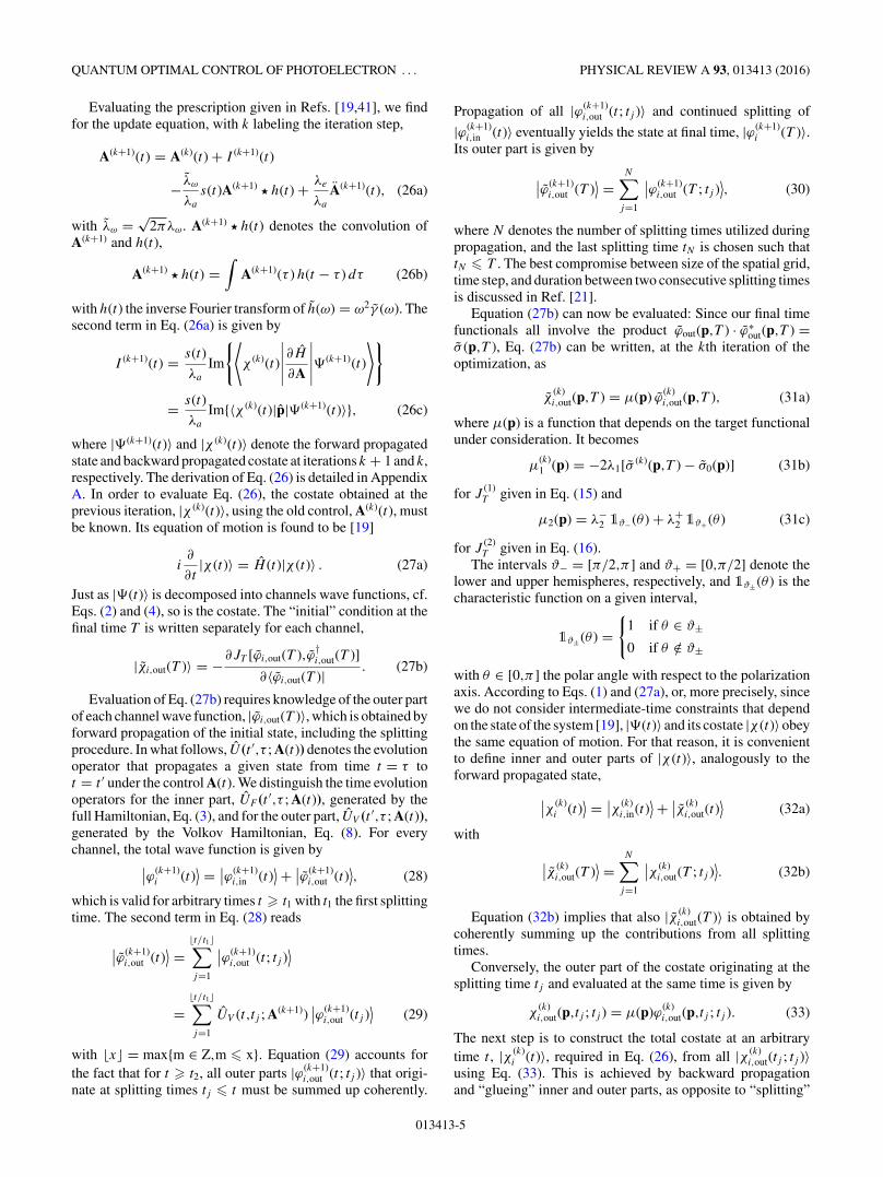
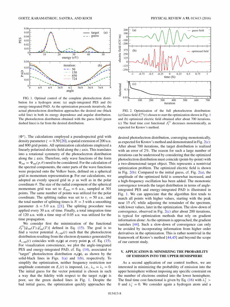
FIG. 1. Optimal control of the complete photoelectron distri-bution for a hydrogen atom: (a) angle-integrated PES and (b)energy-integrated PAD. As the optimization proceeds iteratively, theactual photoelectron distribution approaches the desired one (blacksolid line) in both its energy dependence and angular distribution.The photoelectron distribution obtained with the guess field (greendashed lines) is far from the desired distribution.

|�a〉. The calculations employed a pseudospectral grid withdensity parameter ζ = 0.50 [20], a spatial extension of 200 a.u.and 800 grid points. All optimization calculations employed alinearly polarized electric field along the z axis. This translatesinto a rotational symmetry of the photoelectron distributionalong the z axis. Therefore, only wave functions of the form�out = �out(p,θ ) need to be considered. For the calculation ofthe spectral components, the outer parts of the wave functionswere projected onto the Volkov basis, defined on a sphericalgrid in momentum representation p. For our calculations, weadopted an evenly spaced grid in p as well as in the polarcoordinate θ . The size of the radial component of the sphericalmomentum grid was set to Emax = 6 a.u., sampled at 301points. The same number of points was utilized for the polarcoordinate. The splitting radius was set to rc = 50 a.u., andthe total number of splitting times is N = 3 with a smoothingparameter = 5.0 a.u. [21]. The splitting procedure wasapplied every 30 a.u. of time. Finally, a total integration timeof 120 a.u. with a time step of 0.05 a.u. was utilized for thetime propagation.

We consider first the minimization of the functionalJ

(1)T [ϕout(T ),ϕ†

out(T )] defined in Eq. (15). The goal is tofind a vector potential Az,opt(t) such that the photoelectrondistribution resulting from the electron dynamics generated byAz,opt(t) coincides with σ0(p) at every point p, cf. Eq. (15).For visualization convenience, we plot the angle-integratedPES and energy-integrated PAD, cf. Eq. (14), associated to“target” photoelectron distribution σ0(p), as shown by thesolid-black lines in Figs. 1(a) and 1(b), respectively. Tosimplify the optimization, neither frequency restriction noramplitude constraint on Ez(t) is imposed, i.e., λω = λe = 0.The initial guess for the vector potential is chosen in sucha way that the fidelity with respect to the target σ0(p) ispoor, see the green dashed lines in Fig. 1. Despite thebad initial guess, the optimization quickly approaches the

-200-100

0100200

elec

tric

fie

ld (

GV

/m)

guess field

-1 -0.75 -0.5 -0.25 0 0.25 0.5 0.75 1time (fs)

-250

-125

0125

250

375 optimized field

0 100 200 300 400 500 600 700iteration

0.01

0.1

1

func

tion

al

(a)

(b)

(c)

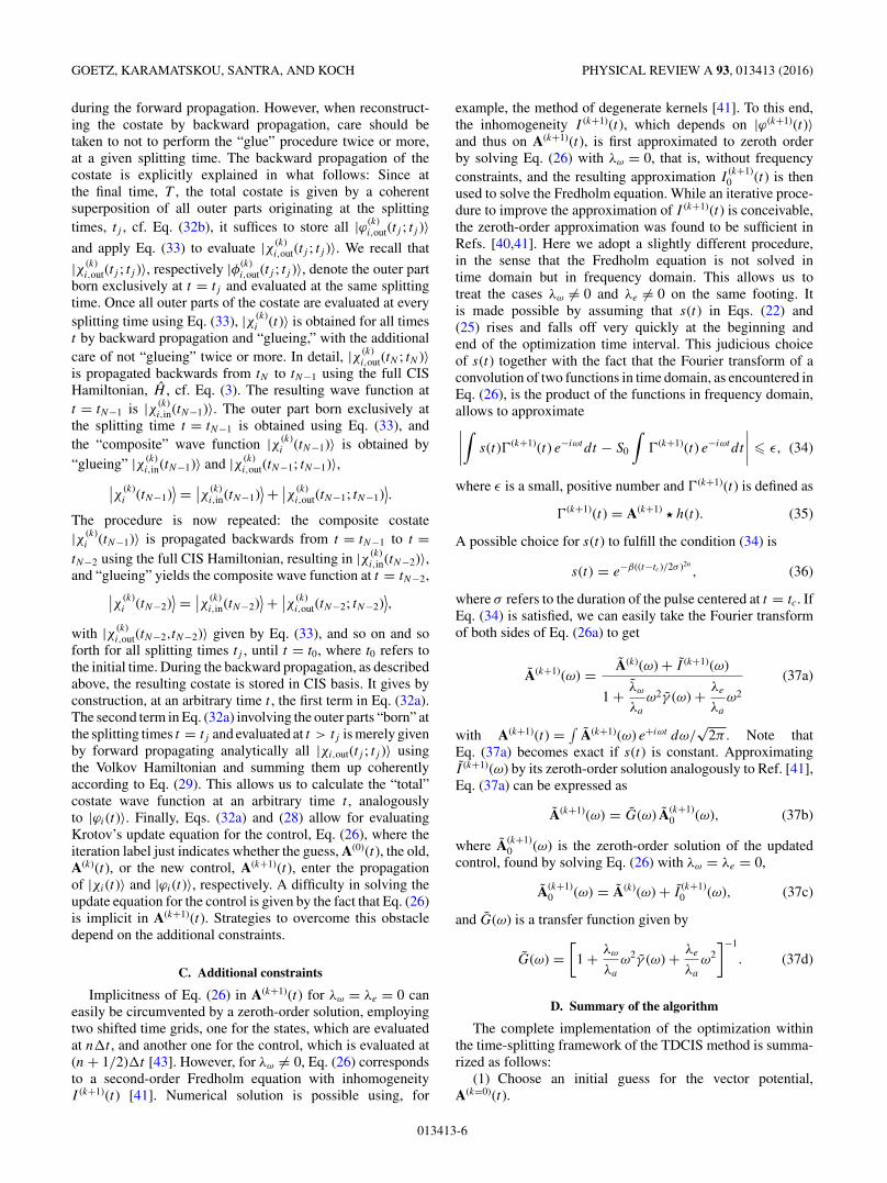
FIG. 2. Optimization of the full photoelectron distribution:(a) Guess field E(0)

z (t) chosen to start the optimization shown in Fig. 1and (b) optimized electric field obtained after about 700 iterations.(c) The final time cost functional J

(1)T decreases monotonically, as

expected for Krotov’s method.

desired photoelectron distribution, converging monotonically,as expected for Krotov’s method and demonstrated in Fig. 2(c):After about 700 iterations, the target distribution is realizedwith an error of 2%. The reason for such a large number ofiterations can be understood by considering that the optimizedphotoelectron distribution must coincide (point-by-point) witha two-dimensional target object. This represents a nontrivialoptimization problem. The optimized electric field is shownin Fig. 2(b): Compared to the initial guess, cf. Fig. 2(a), theamplitude of the optimized field is somewhat increased, anda high-frequency oscillation has been added. The monotonicconvergence towards the target distribution in terms of angle-integrated PES and energy-integrated PAD is illustrated inFig. 1. We can appreciate that the algorithm first tends tomatch all points with higher values, starting with the peaknear 15 eV, while adjusting the remainder of the spectrum,with lower values, later in the optimization. The slow-down ofconvergence, observed in Fig. 2(c) after about 200 iterations,is typical for optimization methods that rely on gradientinformation alone: As the optimum is approached, the gradientvanishes [44]. Such a slow-down of convergence can onlybe avoided by incorporating information from higher orderderivatives in the optimization. This is rather nontrivial in theframework of Krotov’s method [44,45] and beyond the scopeof our current study.

V. APPLICATION II: MINIMIZING THE PROBABILITYOF EMISSION INTO THE UPPER HEMISPHERE

As a second application of our control toolbox, we areinterested in minimizing the probability of emission into theupper hemisphere without imposing any specific constraint onthe number of electrons emitted into the lower hemisphere.The final time cost functional is given by Eq. (16) with λ+

2 >

0 and λ−2 = 0. We consider again a hydrogen atom and a

013413-8

QUANTUM OPTIMAL CONTROL OF PHOTOELECTRON . . . PHYSICAL REVIEW A 93, 013413 (2016)

0 π/8 π/4 3π/8 π/2 5π/8 3π/4 7π/8 πangle

0.0

2.5×10-3

5.0×10-3

7.5×10-3

1.0×10-2

1.2×10-2

1.5×10-2

PA

D

guess104060100

iteration:

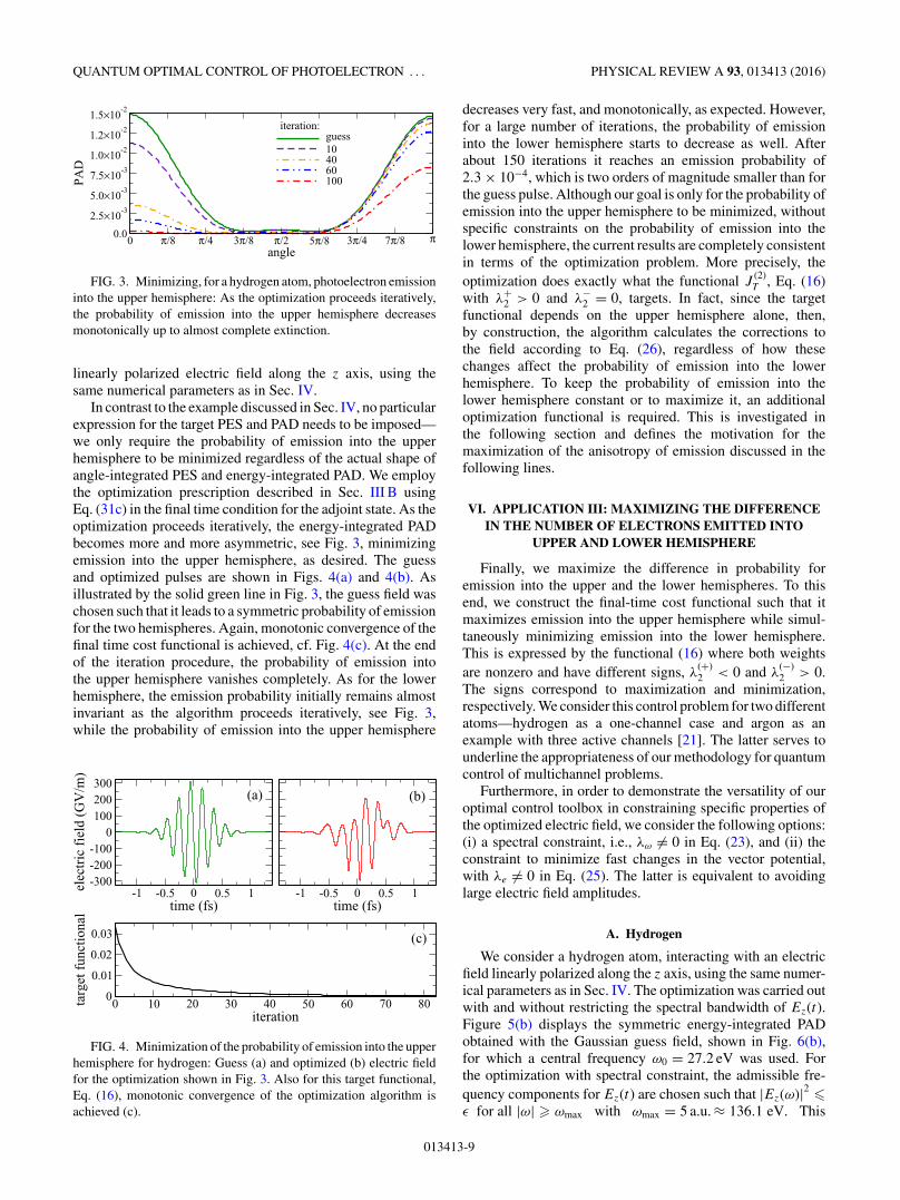
FIG. 3. Minimizing, for a hydrogen atom, photoelectron emissioninto the upper hemisphere: As the optimization proceeds iteratively,the probability of emission into the upper hemisphere decreasesmonotonically up to almost complete extinction.

linearly polarized electric field along the z axis, using thesame numerical parameters as in Sec. IV.

In contrast to the example discussed in Sec. IV, no particularexpression for the target PES and PAD needs to be imposed—we only require the probability of emission into the upperhemisphere to be minimized regardless of the actual shape ofangle-integrated PES and energy-integrated PAD. We employthe optimization prescription described in Sec. III B usingEq. (31c) in the final time condition for the adjoint state. As theoptimization proceeds iteratively, the energy-integrated PADbecomes more and more asymmetric, see Fig. 3, minimizingemission into the upper hemisphere, as desired. The guessand optimized pulses are shown in Figs. 4(a) and 4(b). Asillustrated by the solid green line in Fig. 3, the guess field waschosen such that it leads to a symmetric probability of emissionfor the two hemispheres. Again, monotonic convergence of thefinal time cost functional is achieved, cf. Fig. 4(c). At the endof the iteration procedure, the probability of emission intothe upper hemisphere vanishes completely. As for the lowerhemisphere, the emission probability initially remains almostinvariant as the algorithm proceeds iteratively, see Fig. 3,while the probability of emission into the upper hemisphere

-1 -0.5 0 0.5 1time (fs)

-300-200-100

0100200300

elec

tric

fie

ld (

GV

/m)

-1 -0.5 0 0.5 1time (fs)

0 10 20 30 40 50 60 70 80iteration

0

0.01

0.02

0.03

targ

et f

unct

iona

l

(a) (b)

(c)

FIG. 4. Minimization of the probability of emission into the upperhemisphere for hydrogen: Guess (a) and optimized (b) electric fieldfor the optimization shown in Fig. 3. Also for this target functional,Eq. (16), monotonic convergence of the optimization algorithm isachieved (c).

decreases very fast, and monotonically, as expected. However,for a large number of iterations, the probability of emissioninto the lower hemisphere starts to decrease as well. Afterabout 150 iterations it reaches an emission probability of2.3 × 10−4, which is two orders of magnitude smaller than forthe guess pulse. Although our goal is only for the probability ofemission into the upper hemisphere to be minimized, withoutspecific constraints on the probability of emission into thelower hemisphere, the current results are completely consistentin terms of the optimization problem. More precisely, theoptimization does exactly what the functional J

(2)T , Eq. (16)

with λ+2 > 0 and λ−

2 = 0, targets. In fact, since the targetfunctional depends on the upper hemisphere alone, then,by construction, the algorithm calculates the corrections tothe field according to Eq. (26), regardless of how thesechanges affect the probability of emission into the lowerhemisphere. To keep the probability of emission into thelower hemisphere constant or to maximize it, an additionaloptimization functional is required. This is investigated inthe following section and defines the motivation for themaximization of the anisotropy of emission discussed in thefollowing lines.

VI. APPLICATION III: MAXIMIZING THE DIFFERENCEIN THE NUMBER OF ELECTRONS EMITTED INTO

UPPER AND LOWER HEMISPHERE

Finally, we maximize the difference in probability foremission into the upper and the lower hemispheres. To thisend, we construct the final-time cost functional such that itmaximizes emission into the upper hemisphere while simul-taneously minimizing emission into the lower hemisphere.This is expressed by the functional (16) where both weightsare nonzero and have different signs, λ

(+)2 < 0 and λ

(−)2 > 0.

The signs correspond to maximization and minimization,respectively. We consider this control problem for two differentatoms—hydrogen as a one-channel case and argon as anexample with three active channels [21]. The latter serves tounderline the appropriateness of our methodology for quantumcontrol of multichannel problems.

Furthermore, in order to demonstrate the versatility of ouroptimal control toolbox in constraining specific properties ofthe optimized electric field, we consider the following options:(i) a spectral constraint, i.e., λω �= 0 in Eq. (23), and (ii) theconstraint to minimize fast changes in the vector potential,with λe �= 0 in Eq. (25). The latter is equivalent to avoidinglarge electric field amplitudes.

A. Hydrogen

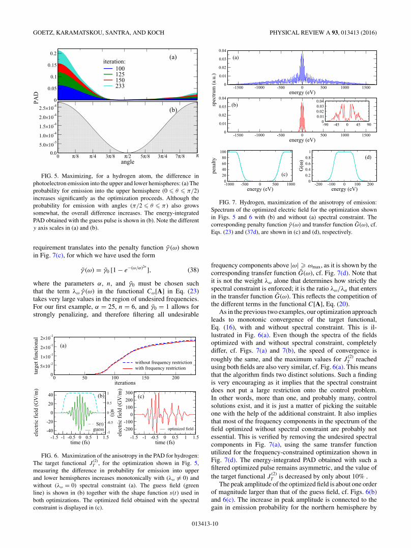
We consider a hydrogen atom, interacting with an electricfield linearly polarized along the z axis, using the same numer-ical parameters as in Sec. IV. The optimization was carried outwith and without restricting the spectral bandwidth of Ez(t).Figure 5(b) displays the symmetric energy-integrated PADobtained with the Gaussian guess field, shown in Fig. 6(b),for which a central frequency ω0 = 27.2 eV was used. Forthe optimization with spectral constraint, the admissible fre-quency components for Ez(t) are chosen such that |Ez(ω)|2 �ε for all |ω| � ωmax with ωmax = 5 a.u. ≈ 136.1 eV. This

013413-9

GOETZ, KARAMATSKOU, SANTRA, AND KOCH PHYSICAL REVIEW A 93, 013413 (2016)

0

0.05

0.1

0.15

0.2

100125150233

0 π/8 π/4 3π/8 π/2 5π/8 3π/4 7π/8 πangle

0.05.0×10-51.0×10-41.5×10-42.0×10-42.5×10-4

PAD

(a)

(b)

iteration:

FIG. 5. Maximizing, for a hydrogen atom, the difference inphotoelectron emission into the upper and lower hemispheres: (a) Theprobability for emission into the upper hemisphere (0 � θ � π/2)increases significantly as the optimization proceeds. Although theprobability for emission with angles (π/2 � θ � π ) also growssomewhat, the overall difference increases. The energy-integratedPAD obtained with the guess pulse is shown in (b). Note the differenty axis scales in (a) and (b).

requirement translates into the penalty function γ (ω) shownin Fig. 7(c), for which we have used the form

γ (ω) = γ0 [1 − e−(ω/α)2n

], (38)

where the parameters α, n, and γ0 must be chosen suchthat the term λω γ (ω) in the functional Cω[A] in Eq. (23)takes very large values in the region of undesired frequencies.For our first example, α = 25, n = 6, and γ0 = 1 allows forstrongly penalizing, and therefore filtering all undesirable

0 50 100 150 200iterations

0

5×10-2

1×10-1

2×10-1

2×10-1

targ

et f

unct

iona

l

without frequency restrictionwith frequency restriction

-1.5 -1 -0.5 0 0.5 1 1.5time (fs)

-40

-20

0

20

40

elec

tric

fie

ld (

GV

/m)

guess

-1.5 -1 -0.5 0 0.5 1 1.5time (fs)

-200

-100

0

100

200

300

elec

tric

fie

ld (

GV

/m)

optimized field-1

-0.5

0

0.5

1

s(t)

S(t)

(a)

(b) (c)

FIG. 6. Maximization of the anisotropy in the PAD for hydrogen:The target functional J

(2)T , for the optimization shown in Fig. 5,

measuring the difference in probability for emission into upperand lower hemispheres increases monotonically with (λω �= 0) andwithout (λω = 0) spectral constraint (a). The guess field (greenline) is shown in (b) together with the shape function s(t) used inboth optimizations. The optimized field obtained with the spectralconstraint is displayed in (c).

-1500 -1000 -500 0 500 1000 1500energy (eV)

0

0.01

0.02

0.03

0.04

spec

trum

(a.

u.)

-1500 -1000 -500 0 500 1000 1500energy (eV)

0

0.01

0.02

0.03

0.04

-1000 -500 0 500 1000energy (eV)

0

20

40

60

80

100

pena

lty

-200 -100 0 100 200energy (eV)

0

0.2

0.4

0.6

0.8

1

G(ω

)

-90 -45 0 45 900

0.010.020.030.04

(a)

(b)

(c)

(d)

FIG. 7. Hydrogen, maximization of the anisotropy of emission:Spectrum of the optimized electric field for the optimization shownin Figs. 5 and 6 with (b) and without (a) spectral constraint. Thecorresponding penalty function γ (ω) and transfer function G(ω), cf.Eqs. (23) and (37d), are shown in (c) and (d), respectively.

frequency components above |ω| � ωmax, as it is shown by thecorresponding transfer function G(ω), cf. Fig. 7(d). Note thatit is not the weight λω alone that determines how strictly thespectral constraint is enforced; it is the ratio λω/λa that entersin the transfer function G(ω). This reflects the competition ofthe different terms in the functional C[A], Eq. (20).

As in the previous two examples, our optimization approachleads to monotonic convergence of the target functional,Eq. (16), with and without spectral constraint. This is il-lustrated in Fig. 6(a). Even though the spectra of the fieldsoptimized with and without spectral constraint, completelydiffer, cf. Figs. 7(a) and 7(b), the speed of convergence isroughly the same, and the maximum values for J

(2)T reached

using both fields are also very similar, cf. Fig. 6(a). This meansthat the algorithm finds two distinct solutions. Such a findingis very encouraging as it implies that the spectral constraintdoes not put a large restriction onto the control problem.In other words, more than one, and probably many, controlsolutions exist, and it is just a matter of picking the suitableone with the help of the additional constraint. It also impliesthat most of the frequency components in the spectrum of thefield optimized without spectral constraint are probably notessential. This is verified by removing the undesired spectralcomponents in Fig. 7(a), using the same transfer functionutilized for the frequency-constrained optimization shown inFig. 7(d). The energy-integrated PAD obtained with such afiltered optimized pulse remains asymmetric, and the value ofthe target functional J

(2)T is decreased by only about 10% .

The peak amplitude of the optimized field is about one orderof magnitude larger than that of the guess field, cf. Figs. 6(b)and 6(c). The increase in peak amplitude is connected to thegain in emission probability for the northern hemisphere by

013413-10

QUANTUM OPTIMAL CONTROL OF PHOTOELECTRON . . . PHYSICAL REVIEW A 93, 013413 (2016)

-1.2 -0.8 -0.4 0 0.4 0.8 1.2time (fs)

-800-400

0400800

12001600

elec

tric

fie

ld (

GV

/m)

without frequency restrictionwith frequency restriction

0 π/4 π/2 3π/4 πangle

0

0.05

0.1

0.15

0.2

PA

D

0 50 100 150 200iteration

0

0.05

0.1

0.15

0.2

0.25pr

obab

ilit

y o

f em

issi

on

(a)

(b) (c)

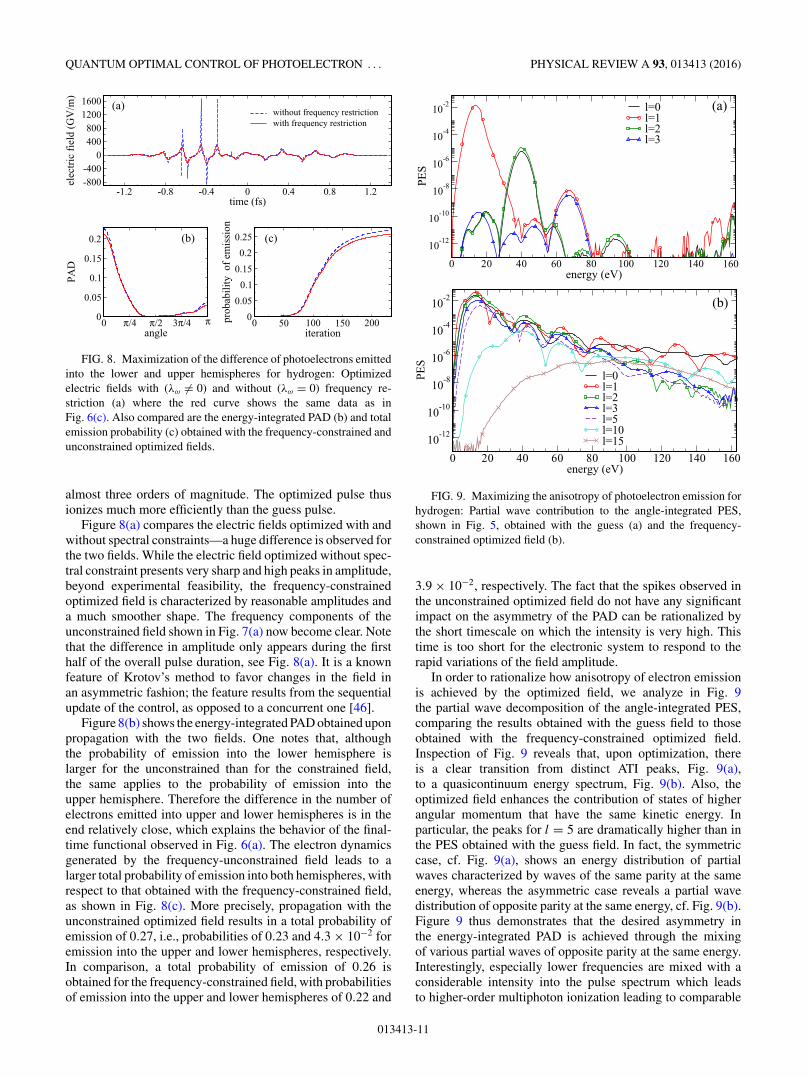
FIG. 8. Maximization of the difference of photoelectrons emittedinto the lower and upper hemispheres for hydrogen: Optimizedelectric fields with (λω �= 0) and without (λω = 0) frequency re-striction (a) where the red curve shows the same data as inFig. 6(c). Also compared are the energy-integrated PAD (b) and totalemission probability (c) obtained with the frequency-constrained andunconstrained optimized fields.

almost three orders of magnitude. The optimized pulse thusionizes much more efficiently than the guess pulse.

Figure 8(a) compares the electric fields optimized with andwithout spectral constraints—a huge difference is observed forthe two fields. While the electric field optimized without spec-tral constraint presents very sharp and high peaks in amplitude,beyond experimental feasibility, the frequency-constrainedoptimized field is characterized by reasonable amplitudes anda much smoother shape. The frequency components of theunconstrained field shown in Fig. 7(a) now become clear. Notethat the difference in amplitude only appears during the firsthalf of the overall pulse duration, see Fig. 8(a). It is a knownfeature of Krotov’s method to favor changes in the field inan asymmetric fashion; the feature results from the sequentialupdate of the control, as opposed to a concurrent one [46].

Figure 8(b) shows the energy-integrated PAD obtained uponpropagation with the two fields. One notes that, althoughthe probability of emission into the lower hemisphere islarger for the unconstrained than for the constrained field,the same applies to the probability of emission into theupper hemisphere. Therefore the difference in the number ofelectrons emitted into upper and lower hemispheres is in theend relatively close, which explains the behavior of the final-time functional observed in Fig. 6(a). The electron dynamicsgenerated by the frequency-unconstrained field leads to alarger total probability of emission into both hemispheres, withrespect to that obtained with the frequency-constrained field,as shown in Fig. 8(c). More precisely, propagation with theunconstrained optimized field results in a total probability ofemission of 0.27, i.e., probabilities of 0.23 and 4.3 × 10−2 foremission into the upper and lower hemispheres, respectively.In comparison, a total probability of emission of 0.26 isobtained for the frequency-constrained field, with probabilitiesof emission into the upper and lower hemispheres of 0.22 and

0 20 40 60 80 100 120 140 160energy (eV)

10-12

10-10

10-8

10-6

10-4

10-2

PE

S

l=0l=1l=2l=3

(a)

0 20 40 60 80 100 120 140 160energy (eV)

10-12

10-10

10-8

10-6

10-4

10-2

PE

S

l=0l=1l=2l=3l=5l=10l=15

(b)

FIG. 9. Maximizing the anisotropy of photoelectron emission forhydrogen: Partial wave contribution to the angle-integrated PES,shown in Fig. 5, obtained with the guess (a) and the frequency-constrained optimized field (b).

3.9 × 10−2, respectively. The fact that the spikes observed inthe unconstrained optimized field do not have any significantimpact on the asymmetry of the PAD can be rationalized bythe short timescale on which the intensity is very high. Thistime is too short for the electronic system to respond to therapid variations of the field amplitude.

In order to rationalize how anisotropy of electron emissionis achieved by the optimized field, we analyze in Fig. 9the partial wave decomposition of the angle-integrated PES,comparing the results obtained with the guess field to thoseobtained with the frequency-constrained optimized field.Inspection of Fig. 9 reveals that, upon optimization, thereis a clear transition from distinct ATI peaks, Fig. 9(a),to a quasicontinuum energy spectrum, Fig. 9(b). Also, theoptimized field enhances the contribution of states of higherangular momentum that have the same kinetic energy. Inparticular, the peaks for l = 5 are dramatically higher than inthe PES obtained with the guess field. In fact, the symmetriccase, cf. Fig. 9(a), shows an energy distribution of partialwaves characterized by waves of the same parity at the sameenergy, whereas the asymmetric case reveals a partial wavedistribution of opposite parity at the same energy, cf. Fig. 9(b).Figure 9 thus demonstrates that the desired asymmetry inthe energy-integrated PAD is achieved through the mixingof various partial waves of opposite parity at the same energy.Interestingly, especially lower frequencies are mixed with aconsiderable intensity into the pulse spectrum which leadsto higher-order multiphoton ionization leading to comparable

013413-11

GOETZ, KARAMATSKOU, SANTRA, AND KOCH PHYSICAL REVIEW A 93, 013413 (2016)

-1.5 -1 -0.5 0 0.5 1 1.5time (fs)

-60

-45

-30

-15

0

15

30

45

Ele

ctri

c fi

eld

(GV

/m) Guess field

Optimized field

-50 -25 0 25 50energy (eV)

0

0.005

0.01

spec

trum

(a.

u.)

0 π/8 π/4 3π/8 π/2 5π/8 3π/4 7π/8 πangle

0

0.001

0.002

0.003

0.004

0.005

PA

D

(a)

(c) (b)

FIG. 10. Maximizing the anisotropy of photoelectron emissionfor hydrogen: Optimization results obtained when simultaneouslyconstraining the maximal amplitude and frequency components ofthe electric field for the weights |λ(−)

eff | = 2|λ(+)eff | with |λ(+)

eff | = 1.Guess and optimized electric fields are shown in panel (a) andtheir spectra in panel (b). A perfectly anisotropy of photoelectronemission is obtained with the optimized field, as demonstrated in thephotoelectron angular distribution shown in panel (c).

final energies in the PES. Thus, more angular momentum statesare mixed.

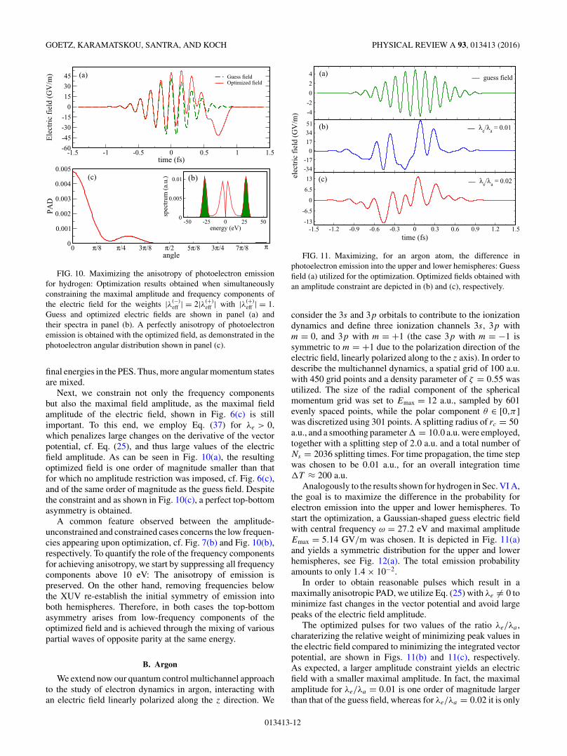
Next, we constrain not only the frequency componentsbut also the maximal field amplitude, as the maximal fieldamplitude of the electric field, shown in Fig. 6(c) is stillimportant. To this end, we employ Eq. (37) for λe > 0,which penalizes large changes on the derivative of the vectorpotential, cf. Eq. (25), and thus large values of the electricfield amplitude. As can be seen in Fig. 10(a), the resultingoptimized field is one order of magnitude smaller than thatfor which no amplitude restriction was imposed, cf. Fig. 6(c),and of the same order of magnitude as the guess field. Despitethe constraint and as shown in Fig. 10(c), a perfect top-bottomasymmetry is obtained.

A common feature observed between the amplitude-unconstrained and constrained cases concerns the low frequen-cies appearing upon optimization, cf. Fig. 7(b) and Fig. 10(b),respectively. To quantify the role of the frequency componentsfor achieving anisotropy, we start by suppressing all frequencycomponents above 10 eV: The anisotropy of emission ispreserved. On the other hand, removing frequencies belowthe XUV re-establish the initial symmetry of emission intoboth hemispheres. Therefore, in both cases the top-bottomasymmetry arises from low-frequency components of theoptimized field and is achieved through the mixing of variouspartial waves of opposite parity at the same energy.

B. Argon

We extend now our quantum control multichannel approachto the study of electron dynamics in argon, interacting withan electric field linearly polarized along the z direction. We

-4

-2

0

2

4guess field

-34

-17

0

17

34

51

elec

tric

fie

ld (

GV

/m)

λe/λ

a = 0.01

-1.5 -1.2 -0.9 -0.6 -0.3 0 0.3 0.6 0.9 1.2 1.5time (fs)

-13

-6.5

0

6.5

13 λe/λ

a = 0.02

(a)

(b)

(c)

FIG. 11. Maximizing, for an argon atom, the difference inphotoelectron emission into the upper and lower hemispheres: Guessfield (a) utilized for the optimization. Optimized fields obtained withan amplitude constraint are depicted in (b) and (c), respectively.

consider the 3s and 3p orbitals to contribute to the ionizationdynamics and define three ionization channels 3s, 3p withm = 0, and 3p with m = +1 (the case 3p with m = −1 issymmetric to m = +1 due to the polarization direction of theelectric field, linearly polarized along to the z axis). In order todescribe the multichannel dynamics, a spatial grid of 100 a.u.with 450 grid points and a density parameter of ζ = 0.55 wasutilized. The size of the radial component of the sphericalmomentum grid was set to Emax = 12 a.u., sampled by 601evenly spaced points, while the polar component θ ∈ [0,π ]was discretized using 301 points. A splitting radius of rc = 50a.u., and a smoothing parameter = 10.0 a.u. were employed,together with a splitting step of 2.0 a.u. and a total number ofNs = 2036 splitting times. For time propagation, the time stepwas chosen to be 0.01 a.u., for an overall integration timeT ≈ 200 a.u.

Analogously to the results shown for hydrogen in Sec. VI A,the goal is to maximize the difference in the probability forelectron emission into the upper and lower hemispheres. Tostart the optimization, a Gaussian-shaped guess electric fieldwith central frequency ω = 27.2 eV and maximal amplitudeEmax = 5.14 GV/m was chosen. It is depicted in Fig. 11(a)and yields a symmetric distribution for the upper and lowerhemispheres, see Fig. 12(a). The total emission probabilityamounts to only 1.4 × 10−2.

In order to obtain reasonable pulses which result in amaximally anisotropic PAD, we utilize Eq. (25) with λe �= 0 tominimize fast changes in the vector potential and avoid largepeaks of the electric field amplitude.

The optimized pulses for two values of the ratio λe/λa ,charaterizing the relative weight of minimizing peak values inthe electric field compared to minimizing the integrated vectorpotential, are shown in Figs. 11(b) and 11(c), respectively.As expected, a larger amplitude constraint yields an electricfield with a smaller maximal amplitude. In fact, the maximalamplitude for λe/λa = 0.01 is one order of magnitude largerthan that of the guess field, whereas for λe/λa = 0.02 it is only

013413-12

QUANTUM OPTIMAL CONTROL OF PHOTOELECTRON . . . PHYSICAL REVIEW A 93, 013413 (2016)

0.0005

0.001

0.0015

guess field

0.004

0.008

0.012

0.016

0.02

PA

D

λe/λ

a = 0.01

0 π/4 π/2 3π/4 ππ/8 3π/8 5π/8 7π/8

angle

0.0004

0.0008

0.0012

0.0016

0.002

0.0024λ

e/λ

a = 0.02

(a)

(b)

(c)

FIG. 12. Maximization of the top-bottom asymmetry in argon:Energy-integrated PAD obtained with the guess pulse (a) andamplitude-constrained cases with |λ(−)

eff | = 2|λ(+)eff | and |λ(+)

eff | = 1 in(b) and (c), respectively. Note the different scales for the probabilityof emission.

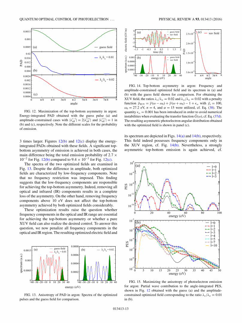
3 times larger. Figures 12(b) and 12(c) display the energy-integrated PADs obtained with these fields. A significant top-bottom asymmetry of emission is achieved in both cases, themain difference being the total emission probability of 2.7 ×10−2 for Fig. 12(b) compared to 9.4 × 10−3 for Fig. 12(c).

The spectra of the two optimized fields are examined inFig. 13. Despite the difference in amplitude, both optimizedfields are characterized by low-frequency components. Notethat no frequency restriction was imposed. This findingsuggests that the low-frequency components are responsiblefor achieving the top-bottom asymmetry. Indeed, removing alloptical and infrared (IR) components results in a completeloss of the asymmetry. On the other hand, removing frequencycomponents above 10 eV does not affect the top-bottomasymmetry achieved by both optimized fields considerably.

These optimization results raise the question whetherfrequency components in the optical and IR range are essentialfor achieving the top-bottom asymmetry or whether a pureXUV field can also realize the desired control. To answer thisquestion, we now penalize all frequency components in theoptical and IR region. The resulting optimized electric field and

-40 -30 -20 -10 0 10 20 30 40

energy (eV)

0

0.0005

0.001

0.0015

spec

trum

(a.

u.)

guess fieldλ

e/λ

a = 0.01

-40 -30 -20 -10 0 10 20 30 400

0.0002

0.0004

0.0006

0.0008λ

e/λ

a = 0.02(a) (b)

FIG. 13. Anisotropy of PAD in argon: Spectra of the optimizedpulses and the guess field for comparison.

-1.5 -1 -0.5 0 0.5 1 1.5 2time (fs)

-6

-3

0

3

6

elec

tric

fie

ld (

GV

/m)

guess fieldxuv field

0 π/4 π/2 3π/4 πangle

5.0×10-6

1.0×10-5

1.5×10-5

2.0×10-5

2.5×10-5

PA

D

xuv field

-40 -30 -20 -10 0 10 20 30 40energy (eV)

0

0.0003

0.0005

0.0008

0.001

spec

trum

(a.

u.)

guess fieldxuv field

(a)

(b)

(c)

FIG. 14. Top-bottom asymmetry in argon: Frequency andamplitude-constrained optimized field and its spectrum in (a) and(b) with the guess field shown for comparison. For obtaining theXUV field, the ratios λe/λa = 0.02 and λω/λa = 0.02 with a penaltyfunction γXUV = γ (ω − ω0) + γ (ω + ω0) − 1 + εω with γo = 100,ω0 = 27.2 eV, n = 4, and α = 15 were utilized, cf. Eq. (38). Thequantity εω = 0.001 has been introduced in order to avoid numericalinstabilities when evaluating the transfer function G(ω), cf. Eq. (37d).The resulting asymmetric photoelectron angular distribution obtainedwith the optimized field is shown in panel (c).

its spectrum are depicted in Figs. 14(a) and 14(b), respectively.This field indeed possesses frequency components only inthe XUV region, cf. Fig. 14(b). Nevertheless, a stronglyasymmetric top-bottom emission is again achieved, cf.

0 20 40 60 80 100energy (eV)

10-16

10-12

10-8

10-4

100

PE

S

l=0l=1l=2l=3

(a)

0 5 10 15 20 25 30 35 40 45 50energy (eV)

10-7

10-6

10-5

10-4

10-3

10-2

PE

S

l=0l=1l=2l=3l=4l=5l=7l=10

(b)

FIG. 15. Maximizing the anisotropy of photoelectron emissionfor argon: Partial wave contribution to the angle-integrated PES,shown in Fig. 12 obtained with the guess (a) and the amplitude-constrained optimized field corresponding to the ratio λe/λa = 0.01in (b).

013413-13

GOETZ, KARAMATSKOU, SANTRA, AND KOCH PHYSICAL REVIEW A 93, 013413 (2016)

0 5 10 15 20 25 30 35 40 45 50energy (eV)

10-10

10-9

10-8

10-7

10-6

10-5

10-4

10-3

PE

S

l=0l=1l=2l=3l=4l=5l=7l=10

(a)

0 5 10 15 20 25 30 35 40 45 50energy (eV)

10-14

10-12

10-10

10-8

10-6

10-4

PE

S

l=0l=1l=2l=3l=4l=5

(b)

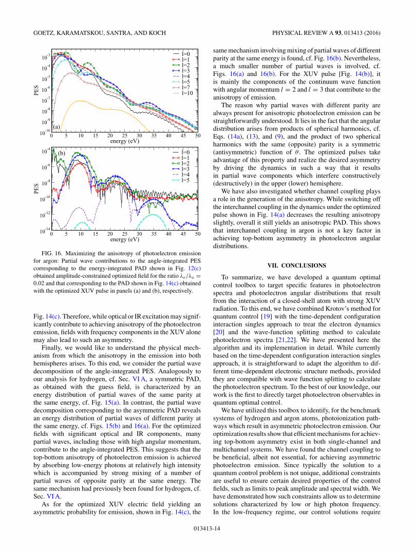
FIG. 16. Maximizing the anisotropy of photoelectron emissionfor argon: Partial wave contributions to the angle-integrated PEScorresponding to the energy-integrated PAD shown in Fig. 12(c)obtained amplitude-constrained optimized field for the ratio λe/λa =0.02 and that corresponding to the PAD shown in Fig. 14(c) obtainedwith the optimized XUV pulse in panels (a) and (b), respectively.

Fig. 14(c). Therefore, while optical or IR excitation may signif-icantly contribute to achieving anisotropy of the photoelectronemission, fields with frequency components in the XUV alonemay also lead to such an asymmetry.

Finally, we would like to understand the physical mech-anism from which the anisotropy in the emission into bothhemispheres arises. To this end, we consider the partial wavedecomposition of the angle-integrated PES. Analogously toour analysis for hydrogen, cf. Sec. VI A, a symmetric PAD,as obtained with the guess field, is characterized by anenergy distribution of partial waves of the same parity atthe same energy, cf. Fig. 15(a). In contrast, the partial wavedecomposition corresponding to the asymmetric PAD revealsan energy distribution of partial waves of different parity atthe same energy, cf. Figs. 15(b) and 16(a). For the optimizedfields with significant optical and IR components, manypartial waves, including those with high angular momentum,contribute to the angle-integrated PES. This suggests that thetop-bottom anisotropy of photoelectron emission is achievedby absorbing low-energy photons at relatively high intensitywhich is accompanied by strong mixing of a number ofpartial waves of opposite parity at the same energy. Thesame mechanism had previously been found for hydrogen, cf.Sec. VI A.

As for the optimized XUV electric field yielding anasymmetric probability for emission, shown in Fig. 14(c), the

same mechanism involving mixing of partial waves of differentparity at the same energy is found, cf. Fig. 16(b). Nevertheless,a much smaller number of partial waves is involved, cf.Figs. 16(a) and 16(b). For the XUV pulse [Fig. 14(b)], itis mainly the components of the continuum wave functionwith angular momentum l = 2 and l = 3 that contribute to theanisotropy of emission.

The reason why partial waves with different parity arealways present for anisotropic photoelectron emission can bestraightforwardly understood. It lies in the fact that the angulardistribution arises from products of spherical harmonics, cf.Eqs. (14a), (13), and (9), and the product of two sphericalharmonics with the same (opposite) parity is a symmetric(antisymmetric) function of θ . The optimized pulses takeadvantage of this property and realize the desired asymmetryby driving the dynamics in such a way that it resultsin partial wave components which interfere constructively(destructively) in the upper (lower) hemisphere.

We have also investigated whether channel coupling playsa role in the generation of the anisotropy. While switching offthe interchannel coupling in the dynamics under the optimizedpulse shown in Fig. 14(a) decreases the resulting anisotropyslightly, overall it still yields an anisotropic PAD. This showsthat interchannel coupling in argon is not a key factor inachieving top-bottom asymmetry in photoelectron angulardistributions.

VII. CONCLUSIONS

To summarize, we have developed a quantum optimalcontrol toolbox to target specific features in photoelectronspectra and photoelectron angular distributions that resultfrom the interaction of a closed-shell atom with strong XUVradiation. To this end, we have combined Krotov’s method forquantum control [19] with the time-dependent configurationinteraction singles approach to treat the electron dynamics[20] and the wave-function splitting method to calculatephotoelectron spectra [21,22]. We have presented here thealgorithm and its implementation in detail. While currentlybased on the time-dependent configuration interaction singlesapproach, it is straightforward to adapt the algorithm to dif-ferent time-dependent electronic structure methods, providedthey are compatible with wave function splitting to calculatethe photoelectron spectrum. To the best of our knowledge, ourwork is the first to directly target photoelectron observables inquantum optimal control.

We have utilized this toolbox to identify, for the benchmarksystems of hydrogen and argon atoms, photoionization path-ways which result in asymmetric photoelectron emission. Ouroptimization results show that efficient mechanisms for achiev-ing top-bottom asymmetry exist in both single-channel andmultichannel systems. We have found the channel coupling tobe beneficial, albeit not essential, for achieving asymmetricphotoelectron emission. Since typically the solution to aquantum control problem is not unique, additional constraintsare useful to ensure certain desired properties of the controlfields, such as limits to peak amplitude and spectral width. Wehave demonstrated how such constraints allow us to determinesolutions characterized by low or high photon frequency.In the low-frequency regime, our control solutions require

013413-14

QUANTUM OPTIMAL CONTROL OF PHOTOELECTRON . . . PHYSICAL REVIEW A 93, 013413 (2016)

relatively high intensities. Correspondingly, the anisotropy ofthe photoelectron emission is realized by strong mixing ofmany partial waves. In contrast, for pure XUV pulses, wehave found low to moderate peak amplitudes to be sufficientfor asymmetric photoelectron emission. In both cases, wehave identified the top-bottom asymmetry to originate frommixing, in the photoelectron wave function, various partialwaves of opposite parity at the same energy. The correspondingconstructive (destructive) interference pattern in the upper(lower) hemisphere yields the desired asymmetry of photo-electron emission. Whereas many partial waves contributefor control fields characterized by low photon energy andhigh intensity, interference of two partial waves is found tobe sufficient in the pure XUV regime. In all our examples,we have found surprisingly simple shapes of the optimizedelectric fields. In the case of hydrogen, tailored electric fieldsto achieve asymmetric photoelectron emission have beendiscussed before and we can compare our results to thoseof Refs. [34,47]. Our work differs from these studies in thatwe avoid a parametrization of the field and allow for completefreedom in the change the electric field, whereas Refs. [34,47]considered only the carrier-envelope phase, intensity, andduration of the pulse as control knobs. The additional freedomof quantum optimal control theory is important, in particularwhen more complex systems are considered.

The set of applications that we have presented here is farfrom being exhaustive, and our current work opens manyperspectives for both photoionization studies and quantumoptimal control theory. On the one hand, we have shownhow to develop optimization functionals that target directly anexperimentally measurable quantity obtained from continuumwave functions. On the other hand, since our approach isgeneral, it can straightforwardly be applied to more complexexamples. In this respect it is desirable to lift the restrictionto closed-shell systems. This would pave the way to studyingthe role of electron correlation in maximizing certain featuresin the photoelectron spectrum. Similarly, allowing for circularor elliptic polarization of the electric field, one could envi-sion, for example, maximizing signatures of chirality in thephotoelectron angular distributions. This requires, however,substantial further development on the level of the time-dependent electronic structure theory.

ACKNOWLEDGMENTS

Financial support by the State Hessen Initiative for the De-velopment of Scientific and Economic Excellence (LOEWE)within the focus project Electron Dynamic of Chiral Systems(ELCH) and the Deutsche Forschungsgemeinschaft underGrant No. SFB 925/A5 is gratefully acknowledged.

APPENDIX: FREQUENCY AND AMPLITUDERESTRICTION

In the following, we present the derivation of Krotov’supdate equation for the control, Eq. (26a), using the approx-imation for s(t) previously described. This allows for a morecompact expression for Krotov’s equation for the specificconstraints on the field used in this work. It is obtainedfollowing Ref. [19]: We seek to minimize the complete

functional, Eq. (18). In order to evaluate the extremumcondition, we start by evaluating the functional derivative ofthe penalty functional with respect to the changes in the controlfield A(t) in Eq. (22),

δCa[A]

δA(t)= 2λas

−1(t)[A(t) − Aref(t)]. (A1)

Next we evaluate the functional derivative of Eq. (23).Abbreviating ω2γ (ω) by h(ω) in Eq. (23), the functionalderivative reads

δCω[A]

δA(t)= λω

∫A�(ω)

δA(ω)

δA(t)h(ω) dω

+ λω

∫A(ω)

δA�(ω)

δA(t)h(ω) dω. (A2)

Using the fact that A(ω) is the Fourier transform of A(t),

A(ω) =∫

A(t)e−iωt dt,

the functional derivative becomes

δA(ω)

δA(t ′)= e−iωt ′ ,

such that

δCω[A]

δA(t)= λω

∫A�(ω)e−iωt h(ω) dω

+ λω

∫A(ω)e+iωt h(ω) dω .

This can be rewritten as

δCω[A]

δA(t)= λω

∫A�(−ω)e+iωt h(−ω) dω

+ λω

∫A(ω)e+iωt h(ω) dω. (A3)

Since the control A(t) is a real function of time, A�(−ω) =A(ω). Moreover, by construction h(ω) = h(−ω). Therefore,Eq. (A3) becomes

δCω[A]

δA(t)= 2λω

∫A(ω)e+iωt h(ω) dω

= 2λω

∫A(ω)eiωtdω

∫h(τ )e−iωτ dτ

= 2λω

∫h(τ )dτ

∫A(ω)e+iω(t−τ )dω

= 2λω

∫h(τ )A(t − τ )dτ = 2λωA � h(t), (A4)

with λω = √2πλω, and h(t) = ∫

h(ω) exp (+iωt) dω/√

2π

and where f � g(t) refers to the convolution product of f

and g.We now calculate the functional derivative of the constraint

penalizing large values of A(t), Eq. (25). Assuming vanishingboundary conditions for A(t), we find, upon integration byparts,

δCe[A]

δA(t)= −2λes

−1(t)A(t). (A5)

013413-15

GOETZ, KARAMATSKOU, SANTRA, AND KOCH PHYSICAL REVIEW A 93, 013413 (2016)

Using Eqs. (A1), (A4), and (A5), the extremum condition withrespect to a variation in the control becomes

0 = λa s−1(t)[A(t) − Aref(t)] − λe s−1(t)A(t)

+ λω A � h(t) − Im

{⟨χ (t)

∣∣∣∣∣∂H

A

∣∣∣∣∣�(t)

⟩}.

where the last term has been previously introduced in Eq. (26).It can be straightforwardly derived from variational princi-ples, i.e., the Euler-Lagrange equation, or in the context ofPontriagin’s maximum-minimum principle or in the contextof Krotov’s optimization method, cf. Refs. [19,41]. It stressesthe dynamics to which the forward propagated state is subject.Solving for A(t) gives us the update rule for the optimizedpulse,

A(t) = Aref(t) + s(t)

λa

Im

{⟨χ (t)

∣∣∣∣∣∂H

A

∣∣∣∣∣�(t)

⟩}

− λω

λa

s(t)A � h(t) + λe

λ aA(t), (A6)

i.e., we retrieve Eq. (26a). Using the property

∫A(t) e−iω t dt = −ω2 A(ω),

together with Eq. (36) for s(t), it is straightforward to writeKrotov’s equation in frequency domain. To this end, we merelytake the Fourier transform of Eq. (A6) and utilize the well-known property that the Fourier transform of a convolution oftwo functions in time domain is the product of the functionsin frequency domain. We thus find

A(k+1)(ω) ≈ A(k)(ω) + I (k+1)(ω)

− λω

λa

A(k+1)(ω)h(ω) − ω2 λe

λa

A(k+1)(ω),

(A7)

which yields Eq. (37a).

[1] S. Hufner, Photoelectron Spectroscopy, Principles and Applica-tions, 3rd ed. (Springer, Berlin, 2003).

[2] M. Meyer, D. Cubaynes, V. Richardson, J. T. Costello, P.Radcliffe, W. B. Li, S. Dusterer, S. Fritzsche, A. Mihelic,K. G. Papamihail et al., Phys. Rev. Lett. 104, 213001 (2010).

[3] F. Fabre, P. Agostini, G. Petite, and M. Clement, J. Phys. B 14,L677 (1981).

[4] U. Becker and D. A. Shirley, VUV and Soft X-Ray Photoioniza-tion, 3rd ed. (Springer, Berlin, 1996).

[5] G. Wu, P. Hockett, and A. Stolow, Phys. Chem. Chem. Phys.13, 18447 (2011).

[6] C. I. Blaga, F. Catoire, P. Colosimo, G. G. Paulus, H. G.Muller, P. Agostini, and L. DiMauro, Nat. Phys. 5, 335(2009).

[7] F. Krausz and M. Ivanov, Rev. Mod. Phys. 81, 163 (2009).[8] H. Wabnitz, L. Bittner, A. R. B. de Castro, R. Dohrmann, P.

Gurtler, T. Laarmann, W. Laasch, J. Schulz, A. Swiderski, K.von Haeften et al., Nat. Phys. 420, 482 (2002).

[9] P. Corkum and F. Krausz, Nat. Phys. 3, 381 (2007).[10] E. P. Kanter, B. Krassig, Y. Li, A. M. March, P. Ho, N. Rohringer,

R. Santra, S. H. Southworth, L. F. DiMauro, G. Doumy et al.,Phys. Rev. Lett. 107, 233001 (2011).

[11] W. H. E. Schwarz, J. Electron Spectrosc. Relat. Phenom. 21,257 (1980).

[12] P. Duinker, Rev. Mod. Phys. 54, 325 (1982).[13] K. L. Reid, Annu. Rev. Phys. Chem. 54, 397 (2003).[14] C. Meier and V. Engel, Phys. Rev. Lett. 73, 3207 (1994).[15] Z. Shen and V. Engel, Chem. Phys. Lett. 358, 344 (2002).[16] M. Wollenhaupt, V. Engel, and T. Baumert, Annu. Rev. Phys.

Chem. 56, 25 (2005).[17] S. Grafe, M. Erdmann, and V. Engel, Phys. Rev. A 72, 013404

(2005).[18] H. Braun, T. Bayer, C. Sarpe, R. Siemering, R. de Vivie-Riedle,

T. Baumert, and M. Wollenhaupt, J. Phys. B 47, 124015 (2014).[19] D. M. Reich, M. Ndong, and C. P. Koch, J. Chem. Phys. 136,

104103 (2012).

[20] L. Greenman, P. J. Ho, S. Pabst, E. Kamarchik, D. A. Mazziotti,and R. Santra, Phys. Rev. A 82, 023406 (2010).

[21] A. Karamatskou, S. Pabst, Y.-J. Chen, and R. Santra, Phys. Rev.A 89, 033415 (2014).

[22] A. Karamatskou, S. Pabst, Y.-J. Chen, and R. Santra, Phys. Rev.A 91, 069907(E) (2015).

[23] T. Klamroth, J. Chem. Phys. 124, 144310 (2006).[24] M. Mundt and D. J. Tannor, New J. Phys. 11, 105038 (2009).[25] A. Castro, J. Werschnik, and E. K. U. Gross, Phys. Rev. Lett.

109, 153603 (2012).[26] M. Hellgren, E. Rasanen, and E. K. U. Gross, Phys. Rev. A 88,

013414 (2013).[27] C. W. McCurdy and T. N. Rescigno, Phys. Rev. A 56, R4369

(1997).[28] F. Martın, J. Phys. B 32, R197 (1999).[29] T. N. Rescigno and C. W. McCurdy, Phys. Rev. A 62, 032706

(2000).[30] H. Bachau, E. Cormier, P. Decleva, J. E. Hansen, and F. Martın,

Rep. Prog. Phys. 64, 1815 (2001).[31] C. W. McCurdy and F. Martın, J. Phys. B 37, 917 (2004).[32] L. Greenman, C. P. Koch, and K. B. Whaley, Phys. Rev. A 92,

013407 (2015).[33] T. Rathje, A. M. Sayler, S. Zeng, P. Wustelt, H. Figger, B. D.

Esry, and G. G. Paulus, Phys. Rev. Lett. 111, 093002 (2013).[34] N. I. Shvetsov-Shilovski, E. Rasanen, G. G. Paulus, and L. B.

Madsen, Phys. Rev. A 89, 043431 (2014).[35] S. Pabst, L. Greenman, A. Karamatskou, Y.-J. Chen, A.

Sytcheva, O. Geffert, and R. Santra, XCID program package formultichannel ionization dynamics, DESY, Hamburg, Germany,2015, Rev. 1855.

[36] C. Leforestier, R. Bisseling, C. Cerjan, M. Feit, R. Friesner, A.Guldberg, A. Hammerich, G. Jolicard, W. Karrlein, H.-D. Meyeret al., J. Comput. Phys. 94, 59 (1991).

[37] R. Kosloff, Annu. Rev. Phys. Chem. 45, 145 (1994).[38] N. Rohringer, A. Gordon, and R. Santra, Phys. Rev. A 74,

043420 (2006).

013413-16

QUANTUM OPTIMAL CONTROL OF PHOTOELECTRON . . . PHYSICAL REVIEW A 93, 013413 (2016)

[39] X. M. Tong, K. Hino, and N. Toshima, Phys. Rev. A 74, 031405(2006).

[40] J. P. Palao, D. M. Reich, and C. P. Koch, Phys. Rev. A 88, 053409(2013).

[41] D. M. Reich, J. P. Palao, and C. P. Koch, J. Mod. Opt. 61, 822(2014).

[42] U. Hohenester, P. K. Rekdal, A. Borzı, and J. Schmiedmayer,Phys. Rev. A 75, 023602 (2007).

[43] J. P. Palao and R. Kosloff, Phys. Rev. A 68, 062308 (2003).

[44] R. Eitan, M. Mundt, and D. J. Tannor, Phys. Rev. A 83, 053426(2011).

[45] G. Jager, D. M. Reich, M. H. Goerz, C. P. Koch,and U. Hohenester, Phys. Rev. A 90, 033628(2014).

[46] S. G. Schirmer and P. de Fouquieres, New J. Phys. 13, 073029(2009).

[47] S. Chelkowski, A. D. Bandrauk, and A. Apolonski, Phys. Rev.A 70, 013815 (2004).

013413-17