Quantum optics in superconducting circuitspublications.lib.chalmers.se/records/fulltext/249423/249423.pdf · Quantum optics in superconducting circuits Generating, engineering and

THESIS FOR THE DEGREE OF DOCTOR OF PHILOSOPHY

Quantum optics in superconducting circuits

Generating, engineering and detecting microwave photons

SANKAR RAMAN SATHYAMOORTHY

Department of Microtechnology and Nanoscience (MC2)

Applied Quantum Physics Laboratory

CHALMERS UNIVERSITY OF TECHNOLOGY

Göteborg, Sweden 2017

Quantum optics in superconducting circuitsGenerating, engineering and detecting microwave photonsSANKAR RAMAN SATHYAMOORTHYISBN 978-91-7597-589-4

c© SANKAR RAMAN SATHYAMOORTHY, 2017

Doktorsavhandlingar vid Chalmers tekniska högskolaNy serie nr. 4270ISSN 0346-718X

Technical Report MC2-362ISSN 1652-0769

Applied Quantum Physics LaboratoryDepartment of Microtechnology and Nanoscience (MC2)Chalmers University of TechnologySE-412 96 GöteborgSwedenTelephone: +46 (0)31-772 1000

Cover:Schematic setup of an all-optical quantum processor at microwave frequencies.The insets show the proposals discussed in the thesis for the different components.

Printed by Chalmers ReproserviceGöteborg, Sweden 2017

Quantum optics in superconducting circuitsGenerating, engineering and detecting microwave photonsThesis for the degree of Doctor of Philosophy

SANKAR RAMAN SATHYAMOORTHY

Department of Microtechnology and Nanoscience (MC2)Applied Quantum Physics LaboratoryChalmers University of Technology

ABSTRACT

Quantum optics in superconducting circuits, known as circuit QED, studiesthe interaction of photons at microwave frequencies with artificial atoms madeof Josephson junctions. Although quite young, remarkable progress has beenmade in this field over the past decade, especially given the interest in buildinga quantum computer using superconducting circuits. In this thesis based onthe appended papers, we look at generation, engineering and detection of mi-crowave photons using superconducting circuits. We do this by taking advantageof the strong coupling, on-chip tunability and huge nonlinearity available insuperconducting circuits.

First, we present the strong photon-photon interaction measured experimentally,as shown in the giant cross-Kerr effect. In this work, conditional phase shift ofabout 20 degrees per photon was measured between two coherent fields at singlephoton level. Given this strong interaction, we propose and analyze a cascadedsetup based on the cross-Kerr effect to detect itinerant microwave photons, a longoutstanding problem with only recent experimental realizations. We show that anondestructive detection of microwave photons is possible with few cascadedtransmons. The on-chip tunability of Superconducting Quantum InterferenceDevice (SQUID) is exploited to create a tunable superconducting resonator inthe next presented experimental work. Finally, we show that by placing theatom at the end of a transmission line, microwave photons can be generatedefficiently and on-demand. We also present a setup that can generate the photonsin arbitrary wave packets.

Keywords: Quantum optics, superconducting circuits, circuit QED, single photonsource, single photon detector, cross-Kerr effect.

iii

ACKNOWLEDGEMENTS

A PhD program seems to be both long and short at the same time. I would liketo thank all those who helped to keep up the spirits during the long times andprovided ample support when time was short.

First of all, I would like to thank my supervisor Göran Johansson, for providingme with an opportunity to work in this interesting area of circuit QED. I amalso thankful for all the time you spend teaching physics and being open todiscussing any other topic such as career choices. I am especially grateful for allthe quick support that you provide in dealing with administrative issues such asvisa applications, which at times become more stressful than not having results.I should also thank Anton and Lars for providing ample guidance during theinitial years of my PhD.

I am very grateful for all the discussions and support we get from our experi-mental colleagues in the Quantum Device Physics lab. I thank our collaborators(currently) at other universities, Ben Baragiola, Josh Combes, Bixuan Fan, Io-ChunHoi, Mathieu Pierre, Tom Stace and Chris Wilson for all their fruitful contribu-tions. I would also like to thank Irfan Siddiqi and his group, for hosting me atUC Berkeley and making it a memorable experience.

To everyone at Applied Quantum Physics Laboratory, thank you for making thisa fun place to work. I enjoy all our discussions on physics, different cultures,languages and food. Thanks to all for the Friday fika. And those who make suresomeone brings fika, good job!

Thanks to Göran, Fernando, Joel and Bala for all the comments on the thesis.

Last but not least, thanks to my parents and all my friends for their love andsupport. Thank you Mananyaa for working tirelessly to increase the entropy ofour house. Thank you Aruna for trying to restore equilibrium every now andthen.

Thanks to Stack Overflow for having answers to abstruse questions in LaTeX.Thank you coffee machine for showing the light on dark days.

v

LIST OF PUBLICATIONS

This thesis consists of an extended summary based on the following appendedpapers:

I. Giant Cross–Kerr Effect for Propagating Microwaves Induced by an Ar-tificial Atom,I.-C. Hoi, A. F. Kockum, T. Palomaki, T. M. Stace, B. Fan, L. Tornberg, S. R.Sathyamoorthy, G. Johansson, P. Delsing, and C. M. Wilson,Physical Review Letters 111, 053601 (2013).

II. Quantum Nondemolition Detection of a Propagating Microwave Pho-ton,S. R. Sathyamoorthy, L. Tornberg, A. F. Kockum, B. Q. Baragiola, J. Combes,C. M. Wilson, T. M. Stace, and G. Johansson,Physical Review Letters 112, 093601 (2014).

III. Storage and on-demand release of microwaves using superconductingresonators with tunable coupling,M. Pierre, I.-M. Svensson, S. Raman Sathyamoorthy, G. Johansson, and P.Delsing,Applied Physics Letters 104, 232604 (2014).

IV. Detecting itinerant single microwave photons,S. R. Sathyamoorthy, T. M. Stace, and G. Johansson,Comptes Rendus Physique 17, 756-765 (2016).

V. Simple, robust, and on-demand generation of single and correlated pho-tons,S. R. Sathyamoorthy, A. Bengtsson, S. Bens, M. Simoen, P. Delsing, and G.Johansson,Physical Review A 93, 063823 (2016).

VI. Microwave field oscillation and swapping in coupled superconductingresonators,M. Pierre, S. R. Sathyamoorthy, I.-M. Svensson, G. Johansson, and P. Delsing,In review (2017).

vii

CONTENTS

Abstract iii

Acknowledgements v

List of publications vii

Contents ix

1 Introduction 11.1 Photon sources . . . . . . . . . . . . . . . . . . . . . . . . . . . . . . . 31.2 Storage and retrieval of photons . . . . . . . . . . . . . . . . . . . . . 41.3 Photon-photon interaction . . . . . . . . . . . . . . . . . . . . . . . . . 51.4 Single photon detection . . . . . . . . . . . . . . . . . . . . . . . . . . 61.5 Structure of the thesis . . . . . . . . . . . . . . . . . . . . . . . . . . . . 8

2 Superconducting quantum circuits 112.1 Circuits as quantum systems . . . . . . . . . . . . . . . . . . . . . . . 112.2 Single Cooper pair box . . . . . . . . . . . . . . . . . . . . . . . . . . . 172.3 Transmission line . . . . . . . . . . . . . . . . . . . . . . . . . . . . . . 192.4 Rounding up . . . . . . . . . . . . . . . . . . . . . . . . . . . . . . . . . 23

3 Open quantum systems 253.1 Master equation . . . . . . . . . . . . . . . . . . . . . . . . . . . . . . . 263.2 Input and Output . . . . . . . . . . . . . . . . . . . . . . . . . . . . . . 333.3 Coherence functions . . . . . . . . . . . . . . . . . . . . . . . . . . . . 363.4 Master equation for Fock state input . . . . . . . . . . . . . . . . . . . 38

4 Measurement 434.1 Photon detection . . . . . . . . . . . . . . . . . . . . . . . . . . . . . . 474.2 Homodyne detection . . . . . . . . . . . . . . . . . . . . . . . . . . . . 504.3 Quantum Nondemolition (QND) measurements . . . . . . . . . . . . 53

5 Connecting quantum systems 575.1 (S, L, H) formalism . . . . . . . . . . . . . . . . . . . . . . . . . . . . . 605.2 Cascaded quantum systems . . . . . . . . . . . . . . . . . . . . . . . . 625.3 Coupled quantum systems . . . . . . . . . . . . . . . . . . . . . . . . . 655.4 Feedback . . . . . . . . . . . . . . . . . . . . . . . . . . . . . . . . . . . 69

ix

6 Overview of the articles 736.1 Cross-Kerr Effect for propagating microwaves . . . . . . . . . . . . . 736.2 Quantum nondemolition detection of a propagating microwave photon 756.3 Coupled superconducting resonators . . . . . . . . . . . . . . . . . . . 776.4 Generating single photons on demand . . . . . . . . . . . . . . . . . . 79

7 Summary 83

References 85

x

List of Figures

1.1 A possible implementation of a quantum internet. . . . . . . . . . 4

2.1 Schematic setup of a circuit QED experiment. . . . . . . . . . . . . 122.2 Circuit diagram of an LC oscillator . . . . . . . . . . . . . . . . . . 132.3 Circuit diagrams of a Josephson junction and a dc-SQUID. . . . . 152.4 Circuit diagram of a single Cooper Pair Box (SCB) and a transmon. 172.5 First three eigenenergies for a SCB for EJ/EC = 0.2, 2.0 and 20.0 . 192.6 Circuit diagram of a transmission line. . . . . . . . . . . . . . . . . 202.7 Circuit diagram for a λ/4 resonator. . . . . . . . . . . . . . . . . . 222.8 Circuit diagram for a λ/2 resonator. . . . . . . . . . . . . . . . . . 23

3.1 Scattering of a Fock state on a qubit. . . . . . . . . . . . . . . . . . 40

4.1 Probability of excitation Pexc of a qubit under direct photon detec-tion, with the qubit initially in the excited state. . . . . . . . . . . . 49

4.2 Probability of excitation Pexc of a qubit under direct photon detec-tion, with the qubit initially in the plus state. . . . . . . . . . . . . 50

4.3 A schematic setup of homodyne detection. . . . . . . . . . . . . . 514.4 Probability of excitation Pexc of a qubit under homodyne detection,

with the qubit initially in the plus state. . . . . . . . . . . . . . . . 524.5 Homodyne current j for a qubit initially in the plus state. . . . . . 53

5.1 A schematic setup of two qubits cascaded. . . . . . . . . . . . . . . 585.2 The (S, L, H) products . . . . . . . . . . . . . . . . . . . . . . . . . 605.3 Two cascaded qubits driven by a cavity output. . . . . . . . . . . . 645.4 A schematic setup of two transmon qubits separated by a distance. 655.5 Reflection and transmission coefficient for two coupled qubits as a

function of input field amplitude. . . . . . . . . . . . . . . . . . . . 675.6 Reflection and transmission coefficient for two coupled qubits as a

function of detuning. . . . . . . . . . . . . . . . . . . . . . . . . . . 675.7 Schematic of a two level system in front of a mirror. . . . . . . . . 69

xi

5.8 Reflection coefficient for a qubit in front of a mirror. . . . . . . . . 70

6.1 Schematic of setup proposed in paper II for microwave photondetection. . . . . . . . . . . . . . . . . . . . . . . . . . . . . . . . . . 75

6.2 Schematic setup for coupled cavities considered in papers III and VI. 776.3 Schematic setups proposed in paper V to generate single photons 80

xii

“In the beginning there was nothing.God said, ‘Let there be light!’ And there was light.There was still nothing, but you could see it a whole lot better.”

Attributed to Ellen DeGeneres

1Introduction

The birth of quantum theory at the beginning of the 20th century revolutionizedour understanding of the universe and along with Einstein’s theory of relativityform the basis of our modern view on how nature works. This development ofquantum mechanics now referred to as the “first quantum revolution", led to bothfundamental scientific progress and several important applications. Currently,there is a huge drive to develop technologies based on quantum principlessuch as superposition and entanglement. This activity, termed as the "secondquantum revolution" or quantum 2.0, is expected to have significant impactin computing, communications and metrology among others [1]. Research inthis regard is driven by several countries and regions around the world withsignificant participation from industry.

While one may envision building these quantum devices top-down, a preferredapproach has been to start from the mastery of individual quantum systems andbuild up. This can also be seen as pragmatic as the complexity of a quantumsystem grows exponentially with size and one would like to understand/controlsmaller setups before scaling up. During the initial development of quantummechanics, control of individual quantum systems was only possible in gedankenexperiments. However, with significant progress over the past several decades we

2 Introduction

can now routinely address single quantum systems in labs around the world. Fortheir pioneering work in this direction, Serge Haroche and David Wineland wereawarded the Nobel Prize in Physics in 2012. Wineland’s group traps individualions using electric fields in ultrahigh vacuum and probes them with laser light[2]. Haroche’s group takes the opposite approach, where the field at microwavefrequency is trapped in a cavity and is studied by sending highly excited atomscalled Rydberg atoms through the cavity [2].

The above experiments of Wineland and Haroche fall under the broad topic ofquantum optics, where one studies the interaction between light and matter at thefundamental level. Specifically, the approach used in Haroche’s experiments fallsunder the field called cavity quantum electrodynamics (cavity QED), where light-matter interactions are studied inside a cavity [3, 4]. While tremendous progresshas been made in using both ions and natural atoms to build quantum devices[5], alternate approaches using solid state systems have also been developedrecently. These include systems such as quantum dots, NV centers in diamondand superconducting circuits, each of which have their own pros and cons [6].

In this thesis, we will focus on superconducting circuits which has recentlyemerged as a promising candidate in the race to build quantum devices [7, 8]. Inthese devices, artificial atoms made of superconducting circuits replace real atomsand they interact with microwave photons routed through one-dimensionalwaveguides. Analogous to cavity QED, this area of research is known as cir-cuit QED. As these setups are made on chip using standard microfabricationtechniques, they offer a number of advantages such as tunability, scalability andmechanical stability over the traditional laser-real atom case. Due to the con-finement of the field to one dimension, these systems also show large couplingbetween the field and the artificial atom [9]. Such advantages have enableda plethora of experiments covering a wide range of areas such as microwavequantum optics [10], quantum information processing [7, 11, 12] and relativisticquantum mechanics [13].

In quantum information processing with superconducting circuits, one usuallythinks of the artificial atoms as the quantum bits (qubits). The microwave photonsare then used to manipulate and transfer information between the qubits. Onecan take an alternate viewpoint, where the information is always in the photons(referred to as flying qubits), and the atoms are used as photonic devices that op-erate on these qubits. As photons have low decoherence and can be transmittedover distance, using them as qubits is advantageous. Indeed, several proposalsexist for quantum information processing using photons [14–16] including thosespecific to superconducting circuits [17, 18]. For such photonic quantum appli-

1.1 Photon sources 3

cations, one has to be able to generate photons on demand, manipulate them,store and retrieve them from a memory and finally detect them. In this thesis,based on the appended papers, we look at some of the solutions for achievingthe above goals at microwave frequencies.

1.1 Photon sources

Photons were hypothesised by Planck as quantum packets of energy to calculatethe spectrum of blackbody radiation [19]. In one of his seminal papers of 1905,Einstein used the concept of these quanta to explain the photoelectric effect [20].This effect was already observed in the photomultiplier tubes, which we canconsider as a precursor to single photon detectors. The first sources of singlephotons were realized in the 1970s using cascaded emission [21].

Current photon sources can be broadly put into two categories, probabilistic anddeterministic [22]. The probabilistic sources include those based on parametricdown-conversion and four-wave mixing. In these sources, photons from a strongpump field are converted to signal and idler photons. While this conversion pro-cess is stochastic, the emitted photon pairs are correlated such that the detectionof an idler photon heralds the presence of a signal photon.

Deterministic photon sources are based on either single atomic or ensembleemitters. In a single atomic source, when a photon is needed, the atom is excitedusing an external drive. The atomic decay to the ground state leads to theemission of a single photon. As the atom decays in all available modes, usuallyone embeds the atom in a cavity to improve collection efficiency. In ensemblesources, instead of using a single atomic level, collective excitation of all theatoms in the ensemble is used to generate the desired photons.

Current research in single photon sources is pushed by applications in quantumcomputation and in quantum communication which include quantum key distri-bution and quantum repeaters [22, 23]. Other applications in combination withsingle photon detectors include random number generation [24].

Microwave photons have been generated using superconducting qubits coupledto transmission line resonators [25–27], including in shaped photon wave packets[28, 29]. While the use of resonators provide better collection efficiency, they alsolimit the bandwidth of operation. To generate photons at different frequencies,one needs tune both the qubit and cavity frequencies with good control. A cavityfree setup for generating microwave photons using two transmission lines was

4 Introduction

Stationaryqubit

Flyingqubit

Tunablecoupling

QNDphotondetector

Figure 1.1: A possible implementation of a quantum internet inspired by a figure from[32]. The stationary qubits are used to process quantum information which is then sentout as photons (flying qubits). A QND photon detector detects the incoming photon and"opens or closes" a cavity to efficiently capture the incoming signal.

proposed in [30] and was experimentally realized in [31]. In paper V, we showhow to generate single photons efficiently using an atom in front of a mirror.

An ideal single photon source generates indistinguishable photons on demand,with a fast repetition rate [22]. That is, the source would produce a single photonwith 100% probability and have 0% probability for all other photon number states.Calculating or measuring these probabilities provides a way to determine theefficiency of the proposed setup. In paper V, we calculate these probabilities fromcorrelation functions, which are described in chapter IV.

1.2 Storage and retrieval of photons

The setup presented in paper V and other similar schemes, can in principlegenerate any arbitrary superposition of 0 and 1 photons. This would be a formof photonic qubit that can be written as α |0〉+ β |1〉, where α and β are complexnumbers with |α|2 + |β|2 = 1. An on-demand generation of such photonic qubitscould have applications in quantum communication. Assume for instance thatAlice generates one such qubit and sends it to Bob. Bob then has to catch thequbit and process the information. This would form a simple transaction over aquantum network (Fig. 1.1).

The quantum internet, a distributed quantum network, is one of the long termgoals of quantum information and quantum communication [32]. In this setup,analogous to the "classical internet", individual quantum nodes are connected via

1.3 Photon-photon interaction 5

quantum channels for performing distributed quantum computing and commu-nication. The individual nodes where the processing of information takes placeare ideally made of atoms (artificial or real), while the quantum information iscommunicated using photons, playing the role of flying qubits. As one couldimagine, a quantum memory that would store the incoming photon and retrieveit for later processing becomes an essential part of this setup. Proposals for setupsthat would "catch and release" [33] photons on demand exist based on atomicensembles [34] and superconducting circuits [28, 35]. In papers III and VI, welook at one such proposal in circuit QED, where a coherent field is stored andretrieved from a tunable cavity. Apart from the use as a quantum memory, suchtunable cavities can potentially be also used for generating single photon wavepackets of arbitrary shapes [28, 29].

1.3 Photon-photon interaction

While photons are carriers of electromagnetic interaction, they rarely interactwith each other in vacuum. While this property makes them great carriers ofinformation, it also makes it harder to manipulate them. Effective photon-photoninteractions can however be engineered using non-linear materials. One sucheffective interaction is the so called Kerr effect, which is the change in refractiveindex of a material due to an applied electric field. While a dc field can be thesource of the Kerr effect, we are more interested in the ac or optical Kerr effect,where an intense beam of light changes the refractive index of the medium. Thetotal refractive index of such a medium as seen by the intense control field isgiven as [36]

n(c) = n(c)0 + n(c)

2 I(c), (1.1)

where n(c)0 is the normal (low intensity) refractive index and I(c) is the intensity

of the incoming control field. n2 is referred to as the second order refractiveindex or the non-linear Kerr index. It can be shown that this non-linear effectcomes from the third order susceptibility χ(3) of the medium [36]. The changeof refractive index gives rise to an intensity dependent non-linear phase shiftto the field over and above the one due to just n0. This is usually referred toas self-phase modulation (SPM). We are interested in cross-phase modulation(XPM), which is the phase shift experienced by a weak probe field due to thischange caused by an intense field. Assuming that the probe is weak enough tonot induce non-linearity on its own, the refractive index seen by the weaker probe

6 Introduction

field is given by [36, 37]n(p) = n(p)

0 + n(p)2 I(c). (1.2)

This is similar to the previous case, with the non-linear term depending on theintensity of the strong field. This leads to modulation of the phase of the weakerfield and is also known as the cross-Kerr effect.

Traditionally, such cross-Kerr interactions are mediated using nonlinear mediumsuch as crystals, which are several wavelengths long and are composed of a hugenumber of atoms. Other setups where the Kerr nonlinearity was demonstratedinclude cold atoms using an EIT (electromagnetically induced transparency)scheme [38]. Whether such an interaction can be mediated by just a single atomis the question addressed in paper I. In this experimental work, two coherentfields, control and probe, are scattered off a superconducting artificial atom, thetransmon. The conditional phase shift in the probe field due to the presence ofthe control field is measured and shown to be much higher than those obtainedin the optical regime using setups such as crystal fibers [39]. Hence the title, giantcross-Kerr effect. However, it has to be noted that a single atom can only processone excitation per lifetime of the transition. So the phase change doesn’t increaseas one continuously increases the intensity of the control field as in the abovediscussion. The giant phase shift shown in paper I occurs when both the controland probe field are in the single photon regime. This is the most interestingregime for quantum optics and quantum information processing. The effectcould however be further improved by cascading several of these atoms [40].

Kerr non-linearities have previously been used in several proposals for quantuminformation processing to make quantum gates [41–44]. There have been severalstudies in the literature discussing the feasibility of implementing a controlledphase gate using cross-Kerr nonlinearity [45, 46], with recent results suggestingthat it is indeed possible [47]. Cross-Kerr nonlinearities have also been proposedas a way to nondestructively detect photons [37, 48–50]. We turn to this particularproblem in the next subsection.

1.4 Single photon detection

Now that we have looked at generating, storing and engineering photons, letus turn our attention to detecting a single photon. Due to research and devel-opment over the past several decades, single photon detectors based on manydifferent technologies exist in the optical regime [22, 51], and are even availablecommercially. Current research in this field continues to push the efficiency of

1.4 Single photon detection 7

these detectors. Apart from quantum information processing and quantum com-munications, such single photon detectors have applications in biology, medicine,remote sensing and ranging, spectroscopy and metrology to name a few [22, 24].

Detecting a propagating single photon at microwave frequency has howeverbeen particularly challenging. This can be attributed to the fact that the energyof microwave photons are 4 to 5 orders of magnitude lower than that of opticalphotons. Over the past few years, several novel proposals have been put forthto address this problem [52–58] (also paper II) including a few experimentaldemonstrations [59–61]. A pedagogical review of some of these proposals ispresented in paper IV. A itinerant single microwave photon detector has beenrealized recently [62] with an impedence matched lambda system. Given thepopularity of superconducting circuits as a platform for quantum informationprocessing, single microwave photon detectors would add significant flexibilityto the toolbox. Apart from other applications similar to those in the optical regime,microwave photon detectors could also be useful in the search of dark matter [63,64].

1.4.1 Quantum nondemolition detection

Traditional photon detectors such as photodiodes, are destructive. Typically theyabsorb the photon and convert it into an electrical signal, which is then measured(possibly after amplification). Such schemes complicate the use of photons ascarriers of quantum information. For example, if the information is stored in thepolarization of the photon, the detection of the photon destroys this information.A nondestructive kind of detector would allow us to process the photons, afterwe detect their presence (as in Fig. 1.1 for example).

Measurement back-action, the change in the state of the system due to measure-ment, is an inherent property of quantum mechanics. Along with the Heisen-berg’s uncertainty principle, this leads to limitations in repeated measurementsas follows [37]. Consider two non-commuting operators of a system, such asposition x and momentum p. The uncertainty principle states that the values ofthese two operators cannot be simultaneously established to arbitrary precision,the lower bound in their uncertainity being ∆x∆p = 1

2 h. Any precise measure-ment of x, leads to a large uncertainity in p. If the system evolution depends onmomentum, a second measurement of x even after a short time interval couldlead to a different result [65].

Quantum nondemolition (QND) measurements were introduced in the 1970s

8 Introduction

to circumvent the above restrictions imposed by the uncertainty principle [65–70], by using clever measurement schemes such that the uncertainity in the con-jugate variable does not lead to disturbance of the measured quantity. Theseschemes were first devised to measure mechanical oscillators that would de-tect gravitational-waves, with the aim of repeating the measurements withoutperturbing the oscillators. The ideas were however well suited for the field ofquantum optics, leading to the successful implementations of QND measure-ments of photon flux in the optical regime [37]. These schemes have since thenbeen extended to microwave quantum optics, initially in cavity QED [71] andnow in circuit QED [59, 72–75].

The cross-phase modulation (XPM) offered by a Kerr medium leads us to onesuch scheme of nondestructive photon detection [37, 48–50]. Instead of havingan intense field changing the refractive index of the medium and causing a phaseshift in the probe field, we would like a single photon to have such an effect.Then, by measuring the phase shift of the probe, one might infer the presence ofthe single photon. The single photon survives this process, making the schemenondestructive. Given that the setup in paper I shows a giant cross-Kerr phaseshift in the single photon regime, we explore if it could be used as a photondetector. We then propose a scheme using this effect in paper II and show that itovercomes the noise arising from vacuum fluctuations.

1.5 Structure of the thesis

In the next few chapters, we will briefly review the ingredients that form thebasis of the appended papers. We start in chapter 2 and look at the quantummechanical description of superconducting circuits. We will focus on how toderive the Hamiltonian of a superconducting artificial atom, the single Cooperpair box, leading towards a discussion of the transmon qubit. We will also lookat transmission lines and transmission line resonators. As all of the appendedpapers are either experiments in circuit QED or theoretical proposals primarilyaimed at experiments in circuit QED, this chapter provides a background to thephysical setups used.

In chapter 3, we abstract away the physical setups used and look at the evolutionof a generic quantum system coupled to an environment. We will review thederivation of the master equation that describes the evolution of such an opensystem. We will also look at the input-output formalism which describes how tocalculate the scattered field from the atom. We will use these relations to calculate

1.5 Structure of the thesis 9

the amplitudes and correlation functions of the output field. The theoreticalpart of all of the appended papers rely on the above master equations and theinput-output formalism.

In chapter 4, we focus on the evolution of a quantum system under measurement.We look at the stochastic master equations describing the evolution under directphotodetection and homodyne detection. We will also add a few commentson QND measurements. Stochastic master equations are used in paper II tocharacterize and calculate the efficiency of the proposed microwave photondetector.

In chapter 5, we move beyond the domain of single quantum systems and lookat composite setups that consists of cascaded/stacked quantum subsystems. Welook at the (S,L,H) formalism that makes it easier to derive the master equation forsuch a composite system and apply it to a few example problems. The (S, L, H)formalism is used in paper II to derive the master equation of a chain of cascadedthree level atoms. This formalism can also be used to get the master equation foran atom in front of a mirror [76], a setup that is used in paper V.

We will briefly discuss and highlight the salient points from the attached papersin chapter 6 and conclude with a summary in chapter 7.

"Resistance is futile."

The BorgStar Trek: The Next Generation

2Superconducting quantum circuits

The field of circuit QED is concerned with the study of light matter interactionusing superconducting circuits. As already mentioned in the previous chapter,these systems are now also prime candidates for implementing quantum tech-nologies. As this thesis falls under the domain of circuit QED, we will brieflylook into the same in this chapter. Our main goal will be to understand how thesemacroscopic circuits can be described using quantum mechanics.

2.1 Circuits as quantum systems

While initially envisioned for mechanical systems, it has been known for a longtime that electrical circuits can also be analyzed using the Lagrangian formalism[78]. In such an analysis, one chooses either charge or flux (defined below) asa generalized coordinate to calculate the energies stored in the different circuitelements, resulting in a Lagrangian of the total circuit. This, then allows us toextend the canonical quantization procedure to electrical circuits as described inreferences [79–81].

12 Superconducting quantum circuits

Frommicrowave

source

Toamplifiers

anddetectors

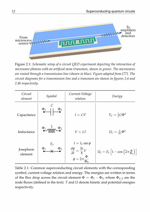
Figure 2.1: Schematic setup of a circuit QED experiment depicting the interaction ofmicrowave photons with an artificial atom (transmon, shown in green). The microwavesare routed through a transmission line (shown in blue). Figure adapted from [77]. Thecircuit diagrams for a transmission line and a transmon are shown in figures 2.6 and2.4b respectively.

Circuitelement

SymbolCurrent-Voltage

relationEnergy

Capacitance

CΦ1 Φ2

I = CV TC = 12 CΦ2

Inductance

LΦ1 Φ2V = LI UL = 1

2L Φ2

Josephsonelement

EJ

Φ1 Φ2

I = IC sin φ

dφ

dt=

2eh

V

φ = 2πΦΦ0

UJ = EJ

[1− cos

(2π Φ

Φ0

)]

Table 2.1: Common superconducting circuit elements with the correspondingsymbol, current-voltage relation and energy. The energies are written in termsof the flux drop across the circuit element Φ = Φ1 − Φ2, where Φ1/2 are thenode fluxes (defined in the text). T and U denote kinetic and potential energiesrespectively.

2.1 Circuits as quantum systems 13

C L

Φ

Figure 2.2: Circuit diagram of an LC oscillator, with thebottom node grounded. Φ is the flux associated with the topnode.

For superconducting circuits, it is advantageous to work with node fluxes as thegeneralized coordinates (due to Josephson junctions). These are defined as thetime integral of the voltages as

Φn =∫ t

−∞Vn(t′)dt′, (2.1)

where Vn is the voltage at node n. Using the current-voltage relationships, we cancalculate the energies stored in the element at time t as E(t) =

∫ t−∞ V(t′)I(t′)dt′.

We list the energies of common superconducting circuit elements in table 2.1using flux as the generalized coordinate. Analogous to classical mechanics, wedenote energies that are function of the coordinate Φ itself as potential energiesU, while the ones that are function of the velocity Φ as kinetic energies T.

Using the energies of the different components, we can write down the La-grangian of an arbitrary circuit. The simplest of such a combination is the LCoscillator (see Fig. 2.2), where we have grounded the lower node. The Lagrangianof the circuit is

L = TC −UL =12

CΦ2 − 12L

Φ2. (2.2)

From the Lagrangian, we can derive the Hamiltonian using the Legendre trans-formation. In order to do this, we need the momentum conjugate to the flux Φgiven by

q =∂L

∂Φ= CΦ, (2.3)

which has the units of charge and in this case, corresponds to the charge on thecapacitor. Now the Hamiltonian is given by,

H = qΦ−L

=q2

2C+

Φ2

2L, (2.4)

which is analogous to the Hamiltonian of a harmonic oscillator of the formp2

2m + 12 mω2x, with m = C and ω =

√1/LC. So far we have considered everything


classically. To get to the quantum description, we now promote q and Φ tooperators satisfying the commutation relation,

[Φ, q] = ih, (2.5)

where we have for the first and last time explicitly included the hats to identifythe operators. We can then define the ladder operators a and a† as

Φ =

√h

2Cω(a + a†), (2.6)

q = −i

√hCω

2(a− a†), (2.7)

which satisfy the commutation relation [a, a†] = 1. In terms of these operators,the Hamiltonian can be rewritten as

H = hω

(a†a +

12

). (2.8)

The striking feature of the harmonic potential (U ∝ x2) is its equidistant energyspectrum, which means we cannot address individual energy transitions like forinstance in a Coulomb potential (U ∝ 1/x). Thus to mimic real atoms, we haveto include a non-linearity in our circuit that would provide anharmonicity tothe spectrum. In superconducting circuits, this is naturally given by Josephsonjunctions.

The Josephson junction is a device made of two superconductors separated by asmall tunnel barrier. It is modelled as a capacitor CJ in parallel to a Josephsonelement characterized by its energy EJ (circuit diagram shown in Fig. 2.3a). Suchjunctions follow the DC and AC Josephson effects [82, 83] given by the relations

I(t) = IC sin φ(t), (2.9)dφ

dt=

2eh

V(t), (2.10)

where φ is the phase difference between the order parameters of the two super-conductors. The phase difference is related to the flux drop across the junction asφ = 2πΦ/Φ0 = 2π(Φ1 −Φ2)/Φ0, where Φ0 = h/2e is the flux quantum. IC isthe critical current, i.e. the maximum supercurrent that the junction can conduct.

Combining Eq. (2.9) and Eq. (2.10), we can write (suppressing the time argumentfor clarity)

I =(

2π

Φ0Ic cos φ

)V ≡ 1

LJV (2.11)

2.1 Circuits as quantum systems 15

J = EJ CJ

(a)

⊗

Φext

EJ,1

CJ,1

EJ,2

CJ,2

(b)

Figure 2.3: Circuit diagrams of (a) a Josephson junction and (b) a dc-SQUID. TheJosephson junction is characterized by its Josephson energy EJ and capacitance CJ . Thedc-SQUID consists of a superconducting loop interrupted by two Josephson junctions.An external flux through the loop Φext can be used to tune the effective Josephson energyof the SQUID.

which shows that the Josephson junction acts as a nonlinear inductor with in-ductance LJ =

(Φ02π

)1

Ic cos φ . Thus in the flux basis, the Josephson junction gives apotential energy contribution to the Lagrangian as

UJ =∫ t

−∞I(t′)V(t′)dt′ =

h2e

IC

∫ t

−∞sin φ(t′)

dφ

dt′dt′ = EJ(1− cos φ), (2.12)

where we have defined the Josephson energy EJ = h2e IC. This is indeed an

anharmonic potential that can be exploited to make artificial atoms. The abovepotential energy corresponds to that of the pure Josephson element. Addingthe kinetic energy from the capacitance of the junction CJ , we can write theLagrangian of the Josephson junction as

L =12

CJΦ2 + EJ cos(

2π

Φ0Φ)

, (2.13)

where we have dropped the constant term.

Placing the Josephson junctions in a loop to make a superconducting quantuminterference device (SQUID), offers additional on-chip tunability. In this thesis,we will focus only on what is called a dc-SQUID, which is made of two Josephsonjunctions in parallel (see Fig. 2.3b). By using an external coil, one can now threada flux Φext through the loop containing the Josephson junctions. We will see howthis allows us to realize an effective Josephson junction with a tunable Josephsonenergy in the following.

The condition that the superconducting order parameter must be single valued,leads to fluxoid quantization [83] which can be written in the case of the SQUID


as [84, 85]

Φ1 −Φ2 + Φext + Φind = nΦ0 (2.14)

where Φind is the flux induced by the circulating current in the loop and n isan integer. We will consider a small loop whose inductance is much smallerthan the inductance of the Josephson junctions and neglect this term. The fluxdrops across the Josephson junctions are related to the phase difference acrossthe junctions as before i.e. Φ1/2 = Φ0

2π φ1/2. Without any loss of generality, we takethe number of flux quanta in the loop to be 0. With this constraint, we can define

Φ1 = Φ− 12

Φext, (2.15)

Φ2 = Φ +12

Φext. (2.16)

Considering also that the Josephson junctions are identical with CJ,1 = CJ,2 =CJ/2 and EJ,1 = EJ,2 = EJ/2, the Lagrangian of the SQUID becomes

L =12

CJ,1Φ21 +

12

CJ,2Φ22 + EJ,1 cos

(2π

Φ0Φ1

)+ EJ,2 cos

(2π

Φ0Φ2

)(2.17)

=12

CJΦ2 + EJ(Φext) cos(

2π

Φ0Φ)

, (2.18)

where EJ(Φext) = EJ cos(

πΦextΦ0

). To obtain the above expressions, we have also

neglected the terms that only depends on Φext. Comparing with Eq. (2.13), wesee that the Lagrangian of the SQUID is analogous to that of a Josephson junctionwhose Josephson energy EJ(Φext) can be tuned using an external flux. As wealready saw, the Josephson element acts like a nonlinear inductor with inductance

LJ =(

Φ02π

)21

EJ cos φ . By replacing the Josephson junction with a SQUID, we cantune this inductance using Φext.

The tunability provided by a SQUID had been exploited in several experiments incircuit QED to either change the frequency of the artificial atoms [76] or to changethe boundary conditions of a field [13]. In papers III and VI, we use a SQUID totune the resonant frequency of the coupling cavity. We also take advantage ofthe tunability of the SQUID in paper V, where we propose generation of singlephotons in arbitrary wave packets by either changing the qubit frequency or bychanging the boundary condition.

2.2 Single Cooper pair box 17

Cg

EJ CJ

+−Vg

ΦJ

(a)

Cg

CS

+−VgJ1 J2

(b)

Figure 2.4: Circuit diagram of (a) single Cooper pair box (SCB) and (b) transmon, acapacitively shunted Cooper pair box. We have also replaced the Josephson junction in (b)with a SQUID to make the transmon’s frequency tunable.

2.2 Single Cooper pair box

Now that we have looked at the description of some of the basic elements ofsuperconducting circuits, let us proceed to describe how to engineer an artificialatom. In this thesis, we primarily focus on the transmon qubit [86], which is avariant of the single Cooper pair box (SCB) [87–89]. The SCB consists of a smallisland made of superconducting metal (such as aluminium) that is connectedto a bigger metallic plate (reservoir of Cooper pairs) via a Josephson junction.The island is also capacitively coupled to a gate voltage Vg, through which thetunneling of Cooper pairs to or from the island can be controlled. Fig. 2.4a showsthe circuit diagram of a SCB. From this we can write the Lagrangian of the circuitas

L =12

CJΦ2J +

12

Cg(ΦJ + Vg)2 + EJ cos

(2π

ΦJ

Φ0

), (2.19)

where ΦJ = (Φ0/2π)φ is once again the flux connected to the phase difference φacross the Josephson junction. The conjugate momentum,

qJ =∂L

∂ΦJ= CJΦJ + Cg(ΦJ + Vg) = 2en, (2.20)


where n is the number of Cooper pairs on the island. Using the Legendre trans-formation, we get the SCB Hamiltonian as

H = 4EC(n− ng)2 − EJ cos

(2π

ΦJ

Φ0

), (2.21)

where EC ≡ e2/2(Cg + CJ) is the charging energy of the island and ng = CgVg/2eis the number of Cooper pairs induced by the gate. We can then follow thequantization procedure and promote n and ΦJ to be operators that satisfy thecommutation relation [90],

[exp(

i2πΦJ

Φ0

), n] = − exp

(i2π

ΦJ

Φ0

). (2.22)

Using this commutation relation, we can show that

e±i2πΦJΦ0 |n〉 = |n± 1〉 , (2.23)

where |n〉 represents the charge basis which are the eigenstates of the numberoperator such that n |n〉 = n |n〉. We can then write the Hamiltonian in the chargebasis, by using the completeness relation (i.e. ∑n |n〉〈 n| = 1) and by expandingthe cosine term as sum of two exponentials as

H = ∑n

4EC(n− ng)

2 |n〉〈 n| − 12

EJ

(|n + 1〉〈 n|+ |n− 1〉〈 n|

). (2.24)

By diagonalizing the above Hamiltonian we can plot the energy levels of the SCBas a function of ng for different values of the parameters EC and EJ . The firstthree energy levels are shown in Fig. 2.5 for different values of these parameters.We see that at low ratios of EJ/EC, the transition energies between the levelsvary significantly as a function of the gate charge ng. Any fluctuations in ng (i.e.charge noise) leads to variations in transition frequencies that after averagingmanifests itself as dephasing. As can be seen from the figure, the wiggles inthe energy spectrum reduces as one increases the ratio of EJ/EC. However,this change has a negative side-effect in reducing the anharmonicity, which iscrucial to address individual transitions. Fortunately we can find values of EJ/ECwhere a useful trade-off between the charge noise and anharmonicity can beachieved. The value of EJ/EC can be modified by shunting the SCB with a largecapacitor. The capacitively shunted Cooper pair box is known as a transmon [86](schematically presented in Fig. 2.1). A simplified circuit diagram in shown inFig. 2.4b. The insensitivity of transmons to charge noise has made them a popularsuperconducting qubit for implementing quantum information processing [8].

2.3 Transmission line 19

E n/

E 01(

n g=

0)

−1 −0.5 0 0.5 10

0.5

1

1.5

2

2.5

ng

(a) EJ/EC = 0.2

−1 −0.5 0 0.5 10

0.5

1

1.5

2

2.5

ng

(b) EJ/EC = 2.0

−1 −0.5 0 0.5 10

0.5

1

1.5

2

2.5

ng

(c) EJ/EC = 20.0

Figure 2.5: First three eigen-energies for a SCB normalized to the energy difference E01

at ng = 0. As seen in the figures, increasing the value of EJ/EC reduces the wiggles inthe energy spectrum but also reduces the anharmonicity.

We note that, there are several other types of superconducting qubits proposedand experimentally realized [88, 91–96]. In this thesis, we will consider only thetransmon and hence we will not go into the details of the rest of the qubits.

2.3 Transmission line

As mentioned previously, in circuit QED one studies the interaction of mi-crowaves with superconducting artificial atoms such as the transmon. The mi-crowaves are routed through a transmission line to which we turn our attentionnow. Microwave transmission lines consist of a central conductor separated by adielectric to the ground plane (Fig. 2.1). They can be modeled as coupled LC os-cillators as shown in Fig. 2.6, where C0 and L0 are the capacitance and inductanceper unit length of the transmission line. By discretizing the transmission line witha small length ∆x and using the node fluxes as the generalized coordinates wecan write the Lagrangian of the transmission line as

L = ∑n

12

C0∆xΦ2n −

12(Φn −Φn−1)

2

L0∆x. (2.25)


∆xL0 Φn−1

· · · ∆xC0

∆xL0 Φn

∆xC0

∆xL0 Φn+1

∆xC0

∆xL0

· · ·

Figure 2.6: Circuit diagram of an infinite transmission line. C0 and L0 are the capaci-tance and inductance per unit length of the line. The fluxes in blue are the generalizedcoordinates.

The conjugate momenta,

qn =∂L

∂Φn= C0∆xΦn, (2.26)

is the charge at node n. With this, we can write down the Hamiltonian as

H = ∑n

12

q2n

C0∆x+

12(Φn −Φn−1)

2

L0∆x, (2.27)

which in the continuous limit gives,

H =12

∫ [q(x, t)2

C0+

1L0

(∂Φ(x, t)

∂x

)2]

dx. (2.28)

We now promote q(x, t) and Φ(x, t) as the quantum mechanical field operatorsobeying the equal time commutation relations [q(x, t), q(x′, t)] = [Φ(x, t), Φ(x′, t)] =0 and [Φ(x, t), q(x′, t)] = iδ(x− x′). The flux field Φ(x, t) satisfies the masslessKlein-Gordon equation

∂2Φ(x, t)∂t2 − v2 ∂2Φ(x, t)

∂x2 = 0, (2.29)

where v = 1/√

L0C0 is the propagation velocity. A general solution of the aboveequation

Φ(x, t) = ΦL(kx + ωt) + ΦR(−kx + ωt) (2.30)

2.3 Transmission line 21

consists of left and right moving parts, which can be expanded as [79, 97]

ΦR(−kx + ωt) =

√hZ0

4π

∫ ∞

0

dω√ω

(aR(ω)e−i(−kx+ωt) + h.c.

), (2.31)

ΦL(kx + ωt) =

√hZ0

4π

∫ ∞

0

dω√ω

(aL(ω)e−i(kx+ωt) + h.c.

), (2.32)

where k = ω/v and Z0 =√

L0/C0 is the characteristic impedance of the trans-mission line. The annihilation (a) and creation (a†) operators in the above ex-pansion satisfy the commutation relation [aα(ω), a†

α′(ω′)] = δ(ω−ω′)δαα′ where

α = L/R.

The Klein-Gordon field can also be expanded in terms of the wave vector k insteadof the frequency as above. Using such an expansion, the Hamiltonian of the fieldcan be shown to be of the form [85, 98]

H =∫ ∞

−∞dk hωk

(a†

k ak +12[ak, a†

k ]

)(2.33)

where ωk = v|k|. The above Hamiltonian is that of a continuum of harmonicoscillators whose modes are defined by k, with their creation and annihilation op-erators satisfying the commutation relation [ak, a†

k′ ] = δ(k− k′). The transmissionline acts as a bath or environment to the artificial atoms and we will model suchan environment as a collection of harmonic oscillators in the following chapters.

2.3.1 Resonators

So far we have considered an infinite transmission line that supports propagatingphotons. We could also make cavities or resonators that support standing modes.This can be achieved by terminating a segment of transmission line either witha short to ground or an open circuit. Depending on the choice made, we getdifferent boundary conditions resulting in different types of resonators. If boththe ends of the resonator are either open (i.e.) connected to a capacitor or shortedto ground, we have a λ/2 resonator. If one end of the resonator is open and theother is grounded, we get a λ/4 resonators. Figures 2.7 and 2.8 show the circuitdiagram of quarter and half wavelength resonators along with their first twomodes. The boundary conditions restrict our spectrum from continuous mode todiscrete multimode. The Hamiltonian becomes

H = ∑m

hωm

(a†(ωm)a(ωm) +

12

), (2.34)


∆xL0 Φ1 ΦN−2

∆xC0

∆xL0 ΦN−1

∆xC0

∆xL0 ΦN

∆xC0

Cc

0 0.1 0.2 0.3 0.4 0.5 0.6 0.7 0.8 0.9 1−1−0.5

00.5

1

x/d

Φ/

Φm

ax

Figure 2.7: Circuit diagram for a λ/4 resonator grounded at x = 0. Shown below thecircuit are the first two modes with normalized amplitude along the length of the cavity d.

where ωm = mπv/d for λ/2 resonators and ωm = (m − 12 )πv/d for λ/4 res-

onators with m ∈ 1, 2, 3.... v = 1/√

L0C0 is the velocity of photons in thetransmission line and d is the length of the cavity. Most often, we are only inter-ested in the fundamental mode with m = 1. In this case, we get back to a singlemode picture, with the Hamiltonian similar to that of an LC oscillator

H = hω

(a†a +

12

), (2.35)

where ω is the fundamental frequency.

Resonators or cavities play an important role in the study of quantum optics,where several experimets use atoms interacting with cavity fields and the sub-field is known as cavity QED [4]. In circuit QED too resonators are routinely used,especially for reading out qubits. In paper III and VI, we look at experimentalrealizations of a tunable cavity. The effective cavity is made of two cavities, oneof them is a λ/4 resonator called the storage cavity and the other one, called thecoupling cavity is a λ/2 resonator. The λ/2 resonator has a SQUID in its center.By tuning the flux through the SQUID loop, we can tune the frequency that thecavity supports [99, 100]. It is then shown that this scheme is effectively the sameas tuning the coupling of the storage cavity to the external transmission line.Such cavities with tunable coupling can be used to generate photon pulses with

2.4 Rounding up 23

CLc

Φ−N∆xL0 Φ−1

∆xC0

∆xL0 Φ0

∆xC0

∆xL0 Φ1∆xL0 ΦN

∆xC0

CRc

0 0.1 0.2 0.3 0.4 0.5 0.6 0.7 0.8 0.9 1−1−0.5

00.5

1

x/d

Φ/

Φm

ax

Figure 2.8: Circuit diagram for a λ/2 resonator. Shown below the circuit are the firsttwo modes with normalized amplitude along the length of the cavity d.

different wave packets [28, 29] and to catch incoming photons of known shapes[35]. Such a tunable cavity is used in paper II as a model source of single photonsenveloped in wave packets that are either Gaussian or exponentially decaying orrising.

2.4 Rounding up

Now that we have seen that using superconducting circuits, we can create artifi-cial atoms, waveguides and resonators, it is time to motivate why not just usereal atoms and optical light. While nature is rich and bountiful, it is also limitedin a certain sense. Although natural atoms or ions are readily available, theyhave preset properties that are not widely tunable. With the advent of micro-fabrication methods and nanotechnology, there has been significant progress intweaking these "God given" restrictions. Artificial atoms such as transmons builtfrom bottom-up, give us access to different parameter regimes with wider in-situtunability that are not readily available in nature. Also by confining photons toone dimension like in a transmission line we can more easily reach the strong-coupling regime which is difficult to attain in 3D space [9, 101, 102]. Apart fromthe traditional quantum optics related problems, these setups have been recently


used to probe for relativistic effects such as the dynamical Casimir effect [13]which is in principle impossible to attain in traditional setups with real mirrors.The downside of superconducting circuits is of course the need of cryogenics. Itis also very difficult to get two superconducting qubits with exactly the sameparameters. Apart from these, we also have to convert microwave photons tooptical photons if we need to transmit quantum information across a network.However, the potential advantages seem to outweigh the drawbacks and circuitQED has emerged as one of the front runners for the implementation of quantuminformation processing [7, 8].

The wheels on the bus go round and round,Round and round,Round and round,

Round and round ...

Popular children’s song that doesn’t stop playing (earworm)

3Open quantum systems

In the last chapter, we looked at how superconducting circuits with Josephsonjunctions can be used as qubits. These artificial atoms are manipulated by routingmicrowave photons through a transmission line to which the atoms are coupled.The transmission line which can be modeled as a collection of harmonic oscillatorsacts as an environment for the atom. We would now like to describe how suchan atom coupled to an environment evolves in time. While we are specificallyinterested in circuit QED setups, the formalism that we will use applies to ageneral quantum system. These are the master equations and we will review thesame in this chapter.

An isolated quantum system evolves according to the Schrödinger equation [103]

ih∂

∂t|ψ〉 = H |ψ〉 , (3.1)

where the system is described by a state vector |ψ〉 that evolves under the Hamil-tonian H. The dimensions are taken care of by h, a fundamental constant thatwe will set to 1 henceforth. While the Schrödinger equation was in itself a break-through of sorts, not all quantum mechanical systems can be described by a statevector. A more general formalism that allows for both pure and mixed states is

26 Open quantum systems

using the density matrix ρ ≡ ∑i pi |ψi〉〈ψi|, where pi is the probability for thesystem to be in state |ψi〉. From Eq. (3.1) and its conjugate bra version, we canderive the quantum Liouville or the von Neumann equation [104]

ρ = −i[H, ρ]. (3.2)

Both of these equations of motion are valid for isolated or closed systems, whichmeans we have to take into account enough degrees of freedom (if not the wholeuniverse) in order to use them. However, as we are interested in only a certainpart of the universe that is under observation (viz. the system such as the artificialatom) and do not care about the rest (viz. the environment), we would like toget an equation of motion for the system alone. We do this by tracing out theenvironment’s degrees of freedom from the Liouville equation. This leads us tothe master equation, which describes the evolution of an open quantum system.The master equation is derived in many references including [104, 105]. We willreview this derivation in the next section based on these references.

3.1 Master equation

We start with the Liouville equation rewritten as

ρtot = −i[Htot, ρtot] (3.3)

with the HamiltonianHtot = Hsys + Hbath + Hint, (3.4)

where we have identified the internal Hamiltonian of the system Hsys, the bath(environment) Hbath and their interaction Hint. The interaction Hamiltonian givesthe effect of the bath on the system and vice versa. It is helpful to go to theinteraction picture by using the unitary transformation U(t) = expi(Hsys +Hbath)t. With this transformation, Eq. (3.3) becomes,

ρI(t) = −i[Hint(t), ρI(t)], (3.5)

where we have defined Hint(t) = U(t)HintU†(t) and ρI(t) = U(t)ρtot(t)U†(t).By iterating the above equation (i.e by substituting the solution back into theright hand side of the equation), we get

ρI(t) = −i[Hint(t), ρI(0)]−[

Hint(t),∫ t

0[Hint(t′), ρI(t′)]dt′

]. (3.6)

3.1 Master equation 27

The equations are exact up to this point. We now make some assumptions andapproximations to simplify the derivation. First, we assume that the bath isvery large and that the coupling between the system and the bath is weak. Thismeans that the interaction between the system and the bath does not significantlyaffect the bath density matrix (Born approximation). By starting with an initialcondition ρtot(0) = ρsys(0)⊗ ρbath, the weak coupling assumption then leads usto

ρtot(t) ≈ ρsys(t)⊗ ρbath (3.7)

where the system density matrix that we are after, ρsys(t) = Trbathρtot(t). Byinserting this condition and tracing over the bath degrees of freedom in Eq. (3.6),we have

ρIsys(t) = −

∫ t

0dt′ Trbath

[Hint(t), [Hint(t′), ρI

sys(t′)⊗ ρbath]

](3.8)

where we have also assumed TrbathHint(t)ρI(0) = 0.

To proceed further, we will consider the interaction Hamiltonian to be of theform A(t)B(t), where A and B are the system and bath operators respectively.In the case of atoms coupled to the electromagnetic field, this is usually givenby the dipole approximation which takes the form i ∑(σij + σji)(b†

k − bk), i.e.the product of the lowering+raising operators of the atom with the creation-annihilation operators of the bath. Such an interaction gives us terms such asTrbathB(t)B(t′)ρbath in the above equation. These are nothing but the correlationfunctions of the bath which decay over a typical correlation time, say τbath. Ourprevious assumptions of the bath having a large number of degrees of freedomand the weak coupling means that τbath is much smaller compared to the timescales at which the system in the interaction picture evolves (say, τsys). This letsus to make the following approximations :

. Markov approximation: Take ρ(t′) → ρ(t), as the system would not haveevolved much in the time scales dictated by τbath.

. Substituting t′ → t− s, we can extend the upper limit for the time difference sto ∞. This is also justified by the fact that τbath τsys and hence the integrandanyways goes to zero for any time s τbath.

With these, we have a Markovian master equation,

ρIsys(t) = −

∫ ∞

0ds Trbath

[Hint(t), [Hint(t− s), ρI

sys(t)⊗ ρbath]]

. (3.9)

The above equation is valid for general systems subject to the approximationswe have made (together known as the Born-Markov approximations). We are


however interested in the quantum optical master equation. In this case, theenvironment is the electromagnetic field which can be modeled as a collection ofharmonic oscillators similar to that of the transmission line in superconductingcircuits. This implies, we can write the Hamiltonians as

Hbath = ∑k

ωkb†k bk (3.10)

andHint = A⊗ B = A† ⊗ B†, (3.11)

where A and B are the Hermitian system and bath operators, which in theinteraction picture become AI(t) and BI(t). With this interaction Hamiltonian inEq. (3.9), we get

ρIsys(t) =

∫ ∞

0ds 〈BI(t)BI(t− s)〉

AI(t− s)ρI

sys(t)AI(t)− AI(t)AI(t− s)ρIsys(t)

+ 〈BI(t− s)BI(t)〉

AI(t)ρIsys(t)AI(t− s)− ρI

sys(t)AI(t− s)AI(t)

,

(3.12)

where 〈BI(t)BI(t′)〉 ≡ TrbathBI(t)BI(t′)ρbath. The time evolution of the systemoperators can be written explicitly by expanding the operators in the energyeigenbasis of the system Hamiltonian as

AI(t) = ∑m,n

eiωmt |m〉〈m| A |n〉〈 n| e−iωnt = ∑m,n

Amn |m〉〈 n| eiωmnt ≡ ∑m,n

Amneiωmnt,

(3.13)where Hsys |m〉 = ωm |m〉 and ωmn = ωm − ωn. We have also defined the tildeoperators Amn = Amn |m〉〈 n| to keep the notations simple in the followingequations. With this form of the system operators, one can get the master equationas

ρIsys(t) = ∑

m,n∑

m′,n′Γmnei(ωm′n′−ωmn)t

A†

mnρIsys(t)Am′n′ − Am′n′ A†

mnρIsys(t)

+ h.c.,

(3.14)where we have defined

Γmn =∫ ∞

0ds 〈BI(t)BI(t− s)〉 eiωmns. (3.15)

Assuming the bath to be in its stationary state with [Hbath, ρbath] = 0, we can showthat the bath correlators 〈BI(t)BI(t− s)〉 depend only on the time difference sand not on the time t itself [104] . Thus, we have

Γmn =∫ ∞

0ds 〈BI(s)BI(0)〉 eiωmns. (3.16)


Now we come to the next set of approximations, that is either called the secularapproximation [106] or the rotating wave approximation [104, 105]. In this, wediscard the fast rotating terms in the sum (i.e.) all the terms except those thathave ωmn −ωm′n′ = 0, as they average out to zero on the time scales that we areinterested in. In our case, this condition can be met for two cases: either m = m′

and n = n′ or m = n and m′ = n′. Keeping only these terms, we get,

ρIsys(t) = ∑

m,nΓmn

A†

mnρIsys(t)Amn − Amn A†

mnρIsys(t)

+ ∑m,n

Γmm

A†

mmρIsys(t)Ann − Ann A†

mmρIsys(t)

+ h.c. (3.17)

Substituting Γmn = 12 γmn + iSmn and noting that Γmm is independent of the energy

levels (as ωmm = 0), we get

ρIsys(t) = ∑

mn

(γmn

(A†

mnρIsys(t)Amn −

12

Amn A†

mn, ρIsys(t)

)

− iSmn

[Amn A†

mn, ρIsys(t)

]

+ γmm

(A†

mmρIsys(t)Ann −

12

Ann A†

mm, ρIsys(t)

)

− iSmm

[Ann A†

mm, ρIsys(t)

]). (3.18)

The above can be written more succinctly by defining a Hamiltonian

HLS ≡∑mn

(Smn Amn A†mn + Smm Ann A†

mm)

= ∑mn

Smn|Amn|2 |m〉〈m|+ ∑m

Smm|Amm|2 |m〉〈m| (3.19)

and a dissipation super-operator

DρIsys(t) ≡ ∑

mnγmn

(A†

mnρIsys(t)Amn −

12

Amn A†

mn, ρIsys(t)

)

+ ∑mn

γmm

(A†

mmρIsys(t)Ann −

12

Ann A†

mm, ρIsys(t)

). (3.20)

The master equation then becomes

ρIsys(t) = −i[HLS, ρI

sys(t)] +DρIsys(t). (3.21)


The Hamiltonian HLS leads to a renormalization of the system eigenfrequenciesand is usually referred to as Lamb shift. As it commutes with Hsys, it can beadded to the same but it is usually neglected as it only leads to a small shift ofeigenenergies. Going back to the system’s frame from the interaction picture, weget

ρsys(t) = −i[Hsys, ρsys(t)] +Dρsys(t), (3.22)

where the first term is the same as that from the Liouville equation for the systemalone. The second term leads to an irreversible decay of the initial state of thesystem and hence the name dissipator. By explicitly writing the frequenciesinvolved in the γ terms, we see that

γmn = Γmn + Γ∗mn =∫ ∞

−∞

⟨B†

I (s)BI(0)⟩

eiωmns (3.23)

andγmm =

∫ ∞

−∞

⟨B†

I (s)BI(0)⟩

ei0s (3.24)

are nothing but the power spectral density of the bath at the frequencies ωmn and0 respectively (Wiener-Khinchin theorem) [107].

It is instructive to look at the master equation for a two-level system (2LS) in athermal bath as this is the most relevant case for this thesis. As the name suggests,we have only two levels which we label the ground state |0〉 ≡ (1 0)T and theexcited state |1〉 ≡ (0 1)T. If this is an atomic system such as a transmon, thehigher transitions are neglected assuming they are well separated in frequencyfrom the lower transition and also assuming that we will not drive the systemstrongly as that would lead to excitation of the higher levels. Thus we havean effective two-level system which can be mapped to a spin-1

2 particle in amagnetic field and we can write our system operators using the Pauli matrices.The system Hamiltonian Hsys = −∆

2 σz, where ∆ = ω1 − ω0 is the transitionfrequency between the ground and excited state. The interaction Hamiltoniancan be written as

Hint(t) = iAI(t)∑k

gk

[bk(t)− b†

k (t)]

, (3.25)

where gk is the coupling between the kth mode of the bath and the system. For athermal bath in equilibrium at temperature T, we have the average number ofphotons in mode k as (Planck distribution)

N(ωk) =1

exp(βωk)− 1(3.26)


where β = 1/kBT. With this we have,⟨

B†I (s)BI(0)

⟩= ∑

kg2

k

(N(ωk)eiωks +

[1 + N(ωk)

]e−iωks

). (3.27)

Going to the continuum limit by replacing ∑k in the above with∫

dω J(ω), whereJ(ω) is the density of states, it can be shown that

γmn = 2Real[Γmn] = γ0

1 + N(ωmn) for ωmn > 0N(ωmn) for ωmn < 0

(3.28)

where γ0 = 2π J(|ωmn|)g(|ωmn|)2 is the rate of spontaneous decay. To get to theabove result, we have used the formula

∫ ∞

0dseiωs = πδ(ω)− iP 1

ω, (3.29)

where P is the Cauchy principal value.

The coupling of the bath to the system can be categorized into longitudinal (alongthe direction of quantization) and transverse (perpendicular to the direction ofquantization). They lead to different kinds of decoherence of the system as wewill see below.

• Transverse coupling

Assuming the coupling of the bath to the qubit is along the x-direction, we havethe system part of the interaction Hamiltonian as AI(t) = σx(t) = σ+ei∆t +σ−e−i∆t where σ− = |0〉〈 1| and σ+ = σ†

−. This means only the off-diagonalelements are non-zero and we have Amn = (1− δmn) |m〉〈 n| where m, n ∈0, 1. Combining this along with Eq. (3.20) and Eq. (3.28), we get

Dρ = γ0(N + 1)(

σ−ρσ+ −12σ+σ−, ρ

)+ γ0N

(σ+ρσ− −

12σ−σ+, ρ

),

(3.30)where N ≡ N(ωmn), the average number of thermal photons in the bath withfrequency equal to the transition frequency ωmn = ∆. At T = 0, we have nothermal photons in the bath on average i.e. N = 0 and this further reduces thedissipator to a form that we write as

D[√

Γσ−]

ρ ≡ Γ(

σ−ρσ+ −12σ+σ−, ρ

). (3.31)

The dissipators that we will use in the following sections and in the appendedpapers are of this kind, as we will assume to work at 0 K. We have changed


the notation of the relaxation rates to Γ = γ0 to be consistent with the attachedpapers.

• Longitudinal coupling

For the coupling along the quantization axis, we have AI(t) = σz(t) =|0〉〈 0| eiω00t − |1〉〈 1| eiω11t, where ω00 = ω11 = 0. We now only have the diag-onal terms in the dissipator with Amn = (−1)mδmn |m〉〈 n| where m, n ∈ 0, 1.Defining the pure dephasing rates 2Γφ = γ00 + γ11, we once again rewrite thedissipator in the form

D[√

Γφ

2σz

]ρ =

Γφ

2

(σzρσz −

12σzσz, ρ

)

=Γφ

2(σzρσz − ρ) . (3.32)

In general the master equation of the two level system coupled to a thermal bathat 0 K can be written as,

ρ = −i[−∆2

σz, ρ] +D [L] ρ +D[Lφ

]ρ, (3.33)

where we have defined the so called Lindblad operators L =√

Γσ− and Lφ =√Γφ

2 σz. The first term on the RHS gives a Liouvillian evolution of the systemunder its own Hamiltonian. The second term leads not only to the decay of excitedstate population (relaxation) but also to decay of the off-diagonal elements of thedensity matrix (dephasing). The third term affects only the off-diagonal elements(and hence the rate is called pure dephasing). We can see this from the solutionof the above master equation which starting from a density matrix ρ(0) at t = 0,is given as

ρ(t) =(

1− ρ11(0)e−Γt ρ01(0)ei∆te−γt

ρ10(0)e−i∆te−γt ρ11(0)e−Γt

), (3.34)

where γ = Γ/2 + Γφ is called the total decoherence rate. At this point we notethat in the appended papers, we use a shorthand notation for the master equationby defining a Liouvillian superoperator L such that

ρ = Lρ. (3.35)

3.2 Input and Output 33

3.2 Input and Output

The master equation presented in the previous section describes the evolution ofan open quantum system such as a transmon coupled to a transmission line. Tolearn about the properties of the transmon or to manipulate the qubit, we scattermicrowave photons on it and measure the output radiation. Alternatively, wemight also be interested in the effect of the transmon on the microwave photons.For all of these reasons, we use the input-output theory that gives the relationshipbetween the incoming and the scattered field. We will review the derivation ofthis relation based on the reference [108].

We once again begin with the total Hamiltonian of our system coupled to a bathas

H = Hsys + Hbath + Hint (3.36)

Hbath =∫ ∞

0dωωb†

ωbω (3.37)

Hint = i∫ ∞

0dωg(ω)

(b†

ωa− a†bω

)(3.38)

where a is a system operator and g(ω) is the coupling strength between thebath and the system. The bath operators obey the usual commutation relation[bω, b†

ω′ ] = δ(ω −ω′). The interaction Hamiltonian is written after the rotatingwave approximation (RWA), which is valid in the weak coupling regimes thatwe consider. As a next step, we extend the lower limits in the integrals of Hbathand Hint to −∞. This approximation is valid if the operators a are off-diagonalin the eigenbasis of Hsys and evolve as a(t) = a exp(iωst). Then the terms in theintegrals that are far off-resonance from ωs are negligibly small. In this thesis,we assume that we have interactions of the above type. For example, for a qubitcoupled to a transmission line with Hsys = − 1

2 ωqbσz, we consider only the dipolecoupling to the transmission line. This means the interaction term involves onlythe off-diagonal σx = σ− + σ+ operator as mentioned in the previous section. Wealso assume that the coupling is slowly varying around the system frequency ωs.This lets us to approximate g(ω) =

√Γ/2π.

With these we have the Hamiltonians as

Hbath =∫ ∞

−∞dωωb†

ωbω, (3.39)

Hint = i

√Γ

2π

∫ ∞

−∞dω(

b†ωa− a†bω

). (3.40)


Using these Hamiltonians, we can write down the Heisenberg’s equations ofmotion

bω = −iωbω +

√Γ

2πa, (3.41)

X = i[Hsys, X]−√

Γ2π

∫ ∞

−∞dω(

b†ω[a, X]− [a†, X]bω

), (3.42)

where X is an arbitrary system operator. Solving Eq. (3.41) with initial conditionat t0 < t, we get

bω(t) = e−iω(t−t0)bω(t0) +

√Γ

2π

∫ t

t0

dt′eiω(t′−t)a(t′), (3.43)

where bω(t0) is the state of the field at t0. Substituting the solution in Eq. (3.42)and defining

bin(t) =1√2π

∫ ∞

−∞dωe−iω(t−t0)bω(t0) (3.44)

we get

X(t) = i[Hsys, X(t)]−(√

Γb†in(t) +

Γ2

a†(t))[a(t), X(t)]

+

(√Γbin(t) +

Γ2

a(t))[a†(t), X(t)]. (3.45)

The above equation is known as the quantum Langevin equation. We inter-pret bin(t) as the input field that interacts with our system at time t. From thecommutation relation of the bath operators, we see that [bin(t), b†

in(t′)] = δ(t− t′).

Solving Eq. (3.41) with a final condition at a later time t1 > t, we get

bω(t) = e−iω(t−t1)bω(t1)−√

Γ2π

∫ t1

tdt′eiω(t′−t)a(t′), (3.46)

where bω(t1) is the state of the field at t1. Defining the output field as

bout(t) =1√2π

∫ ∞

−∞dωe−iω(t−t1)bω(t1) (3.47)

and substituting the above solution in Eq. (3.42), we get

X(t) = i[Hsys, X(t)]−(√

Γb†out(t)−

Γ2

a†(t))[a(t), X(t)]

+

(√Γbout(t)−

Γ2

a(t))[a†(t), X(t)]. (3.48)

3.2 Input and Output 35

We interpret bout(t) as the output field that leaves the system at time t. ComparingEq. (3.45) and Eq. (3.48), we have

bout(t) = bin(t) +√

Γa(t), (3.49)

which gives us the relation between the input and output. By solving the systemdynamics for a(t) and by specifying an input field, we can calculate the outputfield. For a qubit that is driven by a coherent field, we can write the coherentoutput field as

αout(t) = αin(t) +√

Γ 〈σ−(t)〉 , (3.50)

where αin/out(t) = 〈bin/out(t)〉 is the complex amplitude of the coherent in-put/output fields and 〈σ−(t)〉 = Tr[σ−ρsys(t)]. In this case, we have assumedthat the atom is connected to the bath or environment through a single port. Thissituation corresponds to having an atom in front of a mirror. In superconductingcircuits, this means we have an artificial atom at the end of a semi-infinite trans-mission line. The above input-output relations can be extended to the situationwhere we have a system coupled to an open 1-D transmission line as

bLout(t) = bL

in(t) +

√Γ2

a(t), (3.51)

bRout(t) = bR

in(t) +

√Γ2

a(t), (3.52)

where bL/Rin/out are the left and right moving input/output fields. We have kept the

total decay rate of the system at Γ. Driving a two-level atom only from the leftwith a coherent field of amplitude αin, now gives the coherent outputs as

αLout(t) = αin(t) +

√Γ2〈σ−(t)〉 , (3.53)

αRout(t) =

√Γ2〈σ−(t)〉 . (3.54)

In this case, αLout(t) is the transmitted field and αR

out(t) is the reflected field. Mostoften, we are interested in the steady-state or the stationary outputs. In this case,one can drop the time arguments in the above equations and the atomic termbecomes 〈σ−〉ss = Tr[σ−ρss], where ρss is the steady state solution of the masterequation. In such a situation, we can define the reflection and transmissioncoefficients as r = αR

out/αin and t = αLout/αin = 1 + r.


3.3 Coherence functions

As the input-output relations give us the total output field, we can also calculatecoherence functions of the output field. Also known as correlation functions, theytell us about the statistics of the outcoming radiation.

The first order correlation function of the output field is defined as

G(1)(t1, t2) =⟨

b†out(t1)bout(t2)

⟩, (3.55)

which is usually given normalized as

g(1)(t1, t2) =

⟨b†

out(t1)bout(t2)⟩

√⟨b†

out(t1)bout(t1)⟩ ⟨

b†out(t2)bout(t2)

⟩ . (3.56)

In the case of stationary fields, the above correlation depends only on the timedifference t1 − t2 = τ as

g(1)(τ) =⟨b†

out(t)bout(t + τ)⟩

⟨b†

out(t)bout(t)⟩ . (3.57)

These correlation functions can be calculated using [105]⟨

b†out(t1)bout(t2)

⟩= Tr

[b†

outP(t1, t2)

boutρ(t2)]

for t1 > t2, (3.58)⟨

b†out(t1)bout(t2)

⟩= Tr

[boutP(t2, t1)

ρ(t2)b†

out]

for t2 > t1, (3.59)

where the propagator P(t, t′) evolves everything on its right from time t′ to t.As we require this to be true for the density matrix as well, we have ρ(t) =P(t, t′)ρ(t′). Differentiating this with respect to t, and using the master equationρ(t) = L(t)ρ(t), we end up with a differential equation for the propagatorP(t, t′) = L(t)P(t, t′) with the initial condition P(t′, t′) = 1 [30]. From thesolution of this differential equation, we can calculate the correlation function asabove.

The first order correlation function is an amplitude-amplitude correlation func-tion and can be measured using a Mach–Zehnder interferometer [109]. Thenormalized first order correlation, also known as degree of first order coherence,has values such that 0 ≤ |g(1)(t1, t2)| ≤ 1. The value of 1 corresponds to a fullyfirst-order coherent light and the value 0 means that the radiation is incoherent.Both quantum and classical fields satisfy these limits.

3.3 Coherence functions 37

A more interesting quantity is the second order correlation function, which isan intensity-intensity correlation that is measured using a Hanbury Brown andTwiss interferometer [109]. It is defined as

G(2)(t1, t2) =⟨

b†out(t2)b†

out(t1)bout(t1)bout(t2)⟩

, (3.60)

and is normalized as

g(2)(t1, t2) =

⟨b†

out(t2)b†out(t1)bout(t1)bout(t2)

⟩⟨b†

out(t1)bout(t1)⟩ ⟨

b†out(t2)bout(t2)

⟩ . (3.61)

In the case of stationary fields, the above correlation once again depends only onthe time difference t1 − t2 = τ as

g(2)(τ) =⟨b†

out(t)b†out(t + τ)bout(t + τ)bout(t)

⟩⟨b†

out(t)bout(t)⟩2 . (3.62)

The numerator can be calculated as [105],⟨

b†out(t2)b†

out(t1)bout(t1)bout(t2)⟩= Tr

[b†

outboutP(t1, t2)

boutρ(t2)b†out]

. (3.63)

The second order correlation function is used to determine if the radiationis "nonclassical". Using a classical theory, the lower limit for g(2)(0) is 1 andg(2)(τ) ≤ g(2)(0). However, in the quantum version both of these conditionscan be violated and we can have 0 ≤ g(2)(0) ≤ 1. Any output radiation thatleads to g(2)(0) < 1 is said to have sub-Poissonian statistics and radiations withg(2)(τ) > g(2)(0) are called antibunched [110].

The g(2)(τ) can be thought of as the conditional probability for detecting a photonat time τ if a photon was detected at time t. The output field from an ideal singlephoton source has g(2)(0) = 0. However g(2)(0) = 0 alone may not be a fullmeasure of the efficiency of a single photon source as it only means that there areno more than 1 photon at the same time in the output. Consider for example aqubit coupled to an open transmission line driven by a coherent field αin from theleft. The reflected field (as in Eq. (3.54) but without the average) has g(2)(0) = 0.However, as shown in [30], the probability to have a single photon in the reflectedfield by exciting the qubit with a π-pulse has a maximum of 50%. This is becausethe qubit can equally radiate in the left and right moving fields and does thiswith 50 % probability. Thus, to calculate the full efficiency of the source we haveto calculate the probability distribution for the number of photons in the outputfield, which can be done also using the correlation functions.


Moving from the first and second order coherence functions, we define a generalmth order correlation function as

G(m)(t1, t2, ..., tm) =⟨

b†out(t1)b†

out(t2)...b†out(tm)bout(tm)...bout(t2)bout(t1)

⟩

= Tr

[boutP(tm, tm−1)

...P(t3, t2)

boutP(t2, t1)

boutρ(t1)b†

out

b†out

...

b†out

],

(3.64)

where the propagators act on the braces immediately on their right. From the mth

order correlation function, we can calculate photon m-tiples and the probabilityto have m photons in the output as outlined in reference [30].

3.4 Master equation for Fock state input

As mentioned in the introduction, recent progress in quantum optics and quan-tum information depend on manipulation of single photons. Such a single photonstate in a continuous mode is given by [109]

∣∣1ξ

⟩=∫

dωξ(ω)b†(ω) |0〉 , (3.65)

where ξ(ω) is the spectral density function (SDF) or the wave packet in frequencyspace. The Fourier transform of the SDF gives a wave packet in the time domainξ(t), which satisfies the normalization condition

∫dt|ξ(t)|2 = 1. We can then

define a photon wave packet creation operator

a†ξ =

∫dtξ(t)a†(t) (3.66)

such that∣∣1ξ

⟩= a†

ξ |0〉. Any arbitrary number state∣∣Nξ

⟩can be created by

applying the operator N times on the vacuum state and taking care of the nor-malization.

We would like to describe the evolution of a system driven by such a singlephoton Fock state. The absorption of the single photon by the system leavesthe field in an entirely different state as opposed to the case for a coherent field.As the single photon starts interacting with the system, it also gets entangledwith the same. Unlike in the derivation of the master equation, one has to keeptrack of all of the system-field correlations [111]. To address this issue, one cantake two approaches. In the first one, we can include the source of the photons

3.4 Master equation for Fock state input 39

(usually a cavity) in our picture, and use the Markovian master equations. Theother approach is to derive master equations explicitly considering Fock stateinputs. The second approach previously calculated by different authors forspecific scenarios [112–114], was unified and extended to a general situationin reference [115]. We will briefly describe the formalism here and refer to theoriginal paper for more details.

Consider a system interacting with a input field in state∣∣Nξ

⟩. As before, we

assume that initially at time t = 0, the system and the field are uncorrelated andcan be represented as a product state

ρ(0) = ρsys ⊗∣∣Nξ

⟩ ⟨Nξ

∣∣ . (3.67)

The evolution of the system is then given by the time evolution of the asymmetricreduced density matrices defined as

ρm,n(t) ≡ Trfield

[U(t)(ρsys ⊗

∣∣mξ

⟩ ⟨nξ

∣∣)U†(t)], (3.68)

where m, n label the Fock subspaces that run from 0 to N. The time evolutionof the total state is given by the unitary operator U(t). The master equation forthese reduced density matrices is then shown to be

ρm,n = −i[H, ρm,n] +D [L] ρm,n +√

mξ(t)[ρm−1,n, L†] +√

nξ∗(t)[L, ρm,n−1],(3.69)

with the initial condition ρm,n(0) = ρsys(0)δmn. The first term in the aboveequation gives the evolution of the system under the Hamiltonian H. The secondterm leads to dissipation due to the presence of the environment. These two termsare very similar to that of the master equation derived in the previous sections.The last two terms describe the coupling of the single photon to the systemand contribute whenever ξ(t) 6= 0 (i.e.) when the N-photon wave packet startsinteracting with the system. As can be seen from the equation, these couplingterms however involve the reduced density matrix of lower-levels. Thus wehave to solve a (thankfully finite) set of (N + 1)2 master equations, that coupledownwards from ρN,N to ρ0,0. Using the fact that the total density matrix has tobe Hermitian, which leads us to the conclusion ρn,m = ρ†

m,n, we can reduce thenumber of equations to be solved to 1

2 (N + 1)(N + 2).

It is also interesting to look at the output field quantities - the mean photon fluxand the integrated photon flux. Here too we get a system of coupled equations.The mean photon flux is given by

fout(t) = Em,n[L†L] +√

mξ∗(t)Em−1,n[L] +√

nξ(t)Em,n−1[L†] +√

mn|ξ(t)|2,(3.70)


0 10 20 300

0.2

0.4

0.6

0.8

1

Γqbt

ξ(t)

(a)

0 10 20 300

0.5

1

1.5

2

Γqbt

Ftr

(t)

Γph = 0.25Γqb

Γph = Γqb

Γph = 2Γqb

(b)

Figure 3.1: (a) Gaussian wave packets of different width given by Γph. (b) Integratedphoton flux (Ftr) in the transmitted field for these different wave packets.

where Em,n[O] ≡ Tr[ρ†m,nO]. The integrated flux output till time t is F(t) =∫ t

0 fout(t′)dt′.

3.4.1 Example: Scattering of a two photon wave packet on a two levelsystem

As an example, let us consider scattering a two photon state on a two level systemcoupled to an open transmission line. The Fock state is enclosed in a Gaussianwave packet given by

ξ(t) =

(Γ2

ph

2π

)1/4

exp

(−

Γ2ph(t− Tph)

2

4

), (3.71)

where Γph is the width of the wave packet and Tph is the time of arrival of thepeak of the wave packet at the two level system. The Fock state master equationsin this case are

ρm,n = − i[−∆2

σz, ρm,n] + ΓqbD [σ−] ρm,n

+√

m

√Γqb

2ξ(t)[ρm−1,n, σ+] +

√n

√Γqb

2ξ(t)[σ−, ρm,n−1], (3.72)

3.4 Master equation for Fock state input 41

where ∆ is the energy difference between the ground and excited state of thequbit, Γqb is the coupling rate of the qubit to the transmission line. The indicesm, n ∈ 0, 1, 2. We numerically solve these coupled equation for three differentwidths of the wave packet and show the result in Fig. 3.1. The first panel showsthe input photon wave packets with Tph = 15. The second panel shows theintegrated flux in the transmitted field. As can be seen from the figure, a widerpulse in time is mostly reflected by the qubit. As the wave packets becomesharper in time, they become broader in frequency and are not close to resonanceof the transition. Also as the pulse contains more than 1 photon, the qubit getssaturated quickly. So we see most of the field getting transmitted.

(possibly written between 4th to 1st BCE [116])

In everything of every kind whatsoever,Wisdom perceives Truth in that thing.

Thirukkural - 355(English Translation - Himalayan Academy [117])

4Measurement

In the previous chapter, we studied the evolution of a quantum system in thepresence of an environment. In this regard, we started from a unitary evolutiongiven by the quantum Liouville equation. A quantum system can also undergo adifferent kind of evolution - the one under measurement. Consider a quantumstate |ψ〉, say that of a quantum harmonic oscillator. We would like to measurethe number of excitations in the oscillator. As per the postulates of quantummechanics, such an observable is represented by a Hermitian operator, say N,with eigenstates |n〉 which form a complete orthonormal basis in the systemHilbert space 1. In this basis, we can expand |ψ〉 to ∑n cn |n〉, where cn = 〈n|ψ〉.As introduced in the elementary quantum mechanics courses, the effect of a mea-surement is to "collapse" the above state into an eigenstate of the correspondingmeasurement operator, N in our example. Suppose the measurement result isn, then the state after measurement is |ψ′〉 = |n〉 = 1

cn|n〉〈n|ψ〉. Starting with

a density matrix ρ, which can now also include mixed states, the state after themeasurement is

ρ′ =ΠnρΠn

Tr (ΠnρΠn), (4.1)

1We assume a non-degenerate spectrum for simplicity.

44 Measurement

where Πn = |n〉〈 n| is known as the projection operator. The above collapsemodel is known as the von Neumann projection postulate [104]. We note that theprojectors obey Π†

n′Πn = δnn′Πn and ∑n Π†nΠn = 1.

As introduced above, measurements cause instantaneous non-unitary evolutionof the system. In experiments however, measurements take time during which thesystem can also evolve according to some unitary dynamics. In some cases, forexample to do feedback, a continuous monitoring of the system is required. Wewould also like to have the back action of the measurement on the system as smallas possible. All of this is possible by coupling a second quantum system, calledprobe to our original system of interest and then performing a measurement onthe probe [118]. In circuit QED and other setups, the state of a qubit is read byscattering photons on the qubit and then measuring the photons, which act as theprobe system. The aim of paper II is to build a photon detector, i.e to measure thestate of the control field to see if it contains either 0 or 1 photon. To achieve this,we use a coherent field as a probe and measure the scattered field continuouslyusing a homodyne detector. The interaction between the control and probe fieldsis mediated by a three-level atom. For this, we require a description of continuousmeasurement of probe quantum systems. We will look at this problem in thischapter.

Before starting with the full development of master equations under measure-ment, we will look at a simple example to explain a few salient points. Let ustake a qubit in state |ψ〉 = α |0〉+ β |1〉 as our system, with |α|2 + |β|2 = 1. Thesimplest probe is another qubit which we initialize in the state |0〉. The systemand probe now evolve by some unitary dynamics. We take as an example theunitary operator [119],

UCNOT(θ) = exp(−iθUCNOT) = cos θ 1− i sin θ UCNOT (4.2)

where UCNOT = |0〉〈 0| ⊗ 1 + |1〉〈 1| ⊗ σx. UCNOT is the CNOT gate that flips thestate of the probe qubit if the system qubit is in state |1〉. After the interaction, wehave the total state of the system and probe as

|ψ〉tot = cos θ (α |00〉+ β |10〉)− i sin θ (α |00〉+ β |11〉) . (4.3)

Having θ = π/2, gives a fully entangled state (neglecting the global phase)|ψ〉tot = α |00〉+ β |11〉. In such a case, measuring the probe (in the σz basis) as |0〉or |1〉 fully projects the system to the corresponding state. Such a measurement isthen termed as a "strong" measurement and we have full information about thestate of the system after measurement. Instead let us suppose θ 1. Expanding

45

the state in Eq. (4.3) for small θ, we have

|ψ〉tot ≈1√

1 + θ2[α(1− iθ) |00〉+ β |10〉 − iθβ |11〉] . (4.4)

Measuring the probe in the σz basis now give the following outcomes. If wemeasure the probe to be in state |0〉, the system is in state

∣∣ψ′⟩

0 =α(1− iθ) |0〉+ β |1〉√|α(1− iθ)|2 + |β|2

. (4.5)

This measurement result occurs with probability p0 = (|α(1− iθ)|2 + |β|2)/(1 +θ2) (close to 1). Instead if we measure the probe to be in state |1〉, the system is instate

∣∣ψ′⟩

1 = |1〉 . (4.6)

The above result occurs with probability p1 = |β|2θ2/(1 + θ2). Thus in this casewe see that, while most of the time there is very little information gained aboutthe system (i.e. when we measure the probe to be in state |0〉), every now andthen there is a "jump" with a small probability during which the system collapsesto state |1〉.Instead if we choose to measure the probe in the σx basis, we get the followingstates for the system qubit

∣∣ψ′⟩+= α |0〉+ β |1〉 (4.7)

∣∣ψ′⟩− = α |0〉+ βe2iφ |1〉 , φ = arctan(θ) (4.8)

for the measurement results +/−, which occur with equal probabilities. Thismeasurement however does not give any information about the state of thesystem, but gives a phase kick to the system depending on the results. Theabove kind of measurements where the information gain about the system andcorresponding backaction is small are known as weak measurements [119]. In theabove examples, θ can be thought of as the parameter that quantifies the strengthof the measurement. It could be a function of parameters such as the strengthof the coupling between the system and the probe and the time period duringwhich the system and the probe were coupled.

Moving from these examples, let us proceed to describe these indirect measure-ments in general, following references [104] and [120]. Consider that we wouldlike to measure a quantum system in the state ρsys. We couple a probe in the

46 Measurement

initial state |ψ〉 to the system and let them evolve under a unitary U for time t.The total state at time t is

ρtot(t) = U(t)(ρsys(0)⊗ |ψ〉〈ψ|

)U†(t), (4.9)

where ρsys(0) is the initial state of the system and we use the shorthand U(t) forU(t, 0). We then perform a projective measurement on the probe. Assume thatwe find that the probe is in state |i〉. The system is then in the state

ρsys,i(t) =1pi〈 i|U(t)

(ρsys(0)⊗ |ψ〉p 〈ψ|p

)U†(t) |i〉

≡ 1pi

Ωi(t)ρsys(0)Ω†i (t) (4.10)

where we have defined the measurement operators Ωi(t) = 〈 i|U(t) |ψ〉 andthe probabilities pi =

⟨Ω†

i (t)Ωi(t)⟩= Tr[Ωi(t)ρsys(0)Ω†

i (t)]. As opposed toprojection operators, we can see from the definition that Ω†

i Ωj 6= δijΩi. However,we still have ∑i Ω†

i Ωi = 1, which ensures that the probabilities sum to 1. If weignore the measurement results, we get the unconditional system state [118]

ρucsys = ∑

iΩi(t)ρsys(0)Ω†

i (t) (4.11)

which is usually a mixed state. This state would be the same as the one obeyingthe unconditional master equations similar to those described in the previouschapter. Thus, we have a connection between open quantum systems and mea-surement.

Our aim now is to get a differential equation for the state of the system while wecontinuously measure the probe. This can be derived using Eq. (4.10) for shorttime scales dt as

ρsys,i(t + dt) =1pi

Ωi(dt)ρsys(t)Ω†i (dt). (4.12)

Due to the probabilistic nature of the measurement (and the corresponding backaction), this differential equation will be stochastic in nature. As one can imagine,the equations also depend on the type of measurement that is performed. In themicrowave domain, and thus also in the appended papers, the measurement ofchoice and necessity is the homodyne detection. A homodyne detector is usuallymodeled using two photodetectors as will be shown in the following section(Fig. 4.3). Thus, we will start with the problem of getting a stochastic masterequation for a system under photodetection and then proceed to homodynedetection. In either of these cases we will only outline the derivation and referthe reader to other sources for detailed calculations.

4.1 Photon detection 47

4.1 Photon detection

Let us start with a physical model similar to those considered in the previouschapter - a qubit coupled to a bath of harmonic oscillators. We then followreferences [104, 120] to derive a stochastic master equation. The Hamiltonian ofthe total system is

H = Hsys + Hbath + Hint, (4.13)

where we have

Hsys =12

ωqbσz, (4.14)

Hbath = ∑k

ωkb†k bk, (4.15)

Hint = ∑k

gk

(bk + b†

k

)σx + Hdrive, (4.16)

where gk is the coupling strength of the qubit to the mode k. The HamiltonianHdrive contains other qubit only terms such as a Rabi drive of the form ΩRσx.Going to the rotating frame with R = exp

(i ∑k ωkb†

k bkt− 12 iωqbσzt

), we have

the total Hamiltonian after neglecting the fast rotating terms (rotating waveapproximation) as

H = σ+B(t) + σ−B†(t) + Hdrive, (4.17)

where we have defined B(t) = ∑k gkbke−i(ωk−ωqb)t for brevity. Considering smalltime step dt, the unitary operator to second order is

U(dt) ≡ U(t + dt, t) ≈ 1− i∫ t+dt

tdt1H(t1)−

∫ t+dt

tdt1

∫ t1

tdt2H(t1)H(t2).

(4.18)Measuring the bath in the Fock basis gives the following measurement operators

Ω0(dt) = 〈 0|U(t + dt, t) |0〉 = 1− iHdrivedt− g0σ+σ− (4.19)Ω1,k(dt) = 〈 1k|U(t + dt, t) |0〉 = fkσ− (4.20)

with the corresponding probabilities pi = 〈Ω†i Ωi〉. The operator Ω1,k corresponds

to measuring a photon in mode k while Ω0 corresponds to the measurementresult of not detecting any photon in any of the modes k. The parameters fk andg0 are the integrals defined as

g0 =∫ t+dt

tdt1

∫ t1

tdt2 ∑

kg2

ke−i(ωk−ωqb)(t1−t2), (4.21)

fk = −i∫ t+dt

tdt1gkei(ωk−ωqb)t1 . (4.22)

48 Measurement

From ρ1,k(t + dt, t) = Ω1,kρ(t)Ω†1,k/

⟨Ω1,kΩ†

1,k

⟩, we see that the normalized con-

ditioned state for photon detection doesn’t depend on fk. Thus we can treatdetection in any mode k as equivalent for the dynamics of the system. A photondetection in any mode k happens with the probability, p1 = ∑k

⟨Ω1,kΩ†

1,k

⟩=

∑k | fk|2〈σ+σ−〉. Furthermore, it can be shown that ∑k | fk|2 = Γdt and g0 = 12 Γdt,

where Γ is the decay rate of the qubit [104, 120]. Using all of these, the qubit statesconditioned on the measurement results can be written as

ρ0(t + dt) =1p0

Ω0ρ(t)Ω†0

=1p0

(ρ(t)− i[Hdrive, ρ(t)]dt− 1

2Γσ+σ−, ρ(t)dt

)

= ρ(t)− i[Hdrive, ρ(t)]dt− 12

Γσ+σ−, ρ(t)dt + Γ〈σ+σ−〉ρ(t)dt,

(4.23)

ρ1(t + dt) =1p1

Ω1ρ(t)Ω†1

=σ−ρ(t)σ+〈σ+σ−〉

, (4.24)

where we have only kept the terms to first order in dt. The above equations canbe combined into a single master equation by defining a measurement recordN(t) that counts the number of photons detected over time. The correspondingincrement dN(t) = N(t + dt)− N(t) has the properties dN2(t) = dN(t) (i.e. wedetect only 0 or 1 photons in the time interval dt) and E[dN(t)] = Γ〈σ+σ−〉dt,where E[·] is the classical average. With this the evolution of the qubit can bewritten as

dρ = −i[Hdrive, ρ]dt− 12

Γσ+σ−, ρdt + Γ〈σ+σ−〉ρdt +(

σ−ρσ+〈σ+σ−〉

− ρ

)dN(t).

(4.25)

This is the stochastic master equation (SME) that we were after. The solution ofthe above equation is called a quantum trajectory, which gives the path taken bythe system under measurement [118]. Averaging over several trajectories (ideallyinfinitely many) gives back the evolution described by the unconditional masterequation similar to the ones discussed in the previous chapter. In deriving theabove SME, we assumed that all the photons in the bath were detected. In case of

4.1 Photon detection 49

Probability of excitation Pexc(t)

0 2 4 60

0.2

0.4

0.6

0.8

1

Γt

(a) n = 1

0 2 4 60

0.2

0.4

0.6

0.8

1

Γt

(b) n = 10

0 2 4 60

0.2

0.4

0.6

0.8

1

Γt

(c) n = 100

Figure 4.1: Probability of excitation Pexc of a qubit under direct photon detection as afunction of time, for n trajectories. The qubit is initially in the excited state. The solidred lines are the averages over n trajectories En[Pexc]. The dashed lines correspond to theaverage evolution from the unconditional master equation. We see from the individualtrajectories (orange traces) that the qubit stays in the excited state until a jump takes it tothe ground state.

inefficient detection, the SME is modified to be [118]

dρ = −i[Hdrive, ρ]dt− 12

ηΓσ+σ−, ρdt + ηΓ〈σ+σ−〉ρdt + (1− η)ΓD [σ−] ρdt

+

(σ−ρσ+〈σ+σ−〉

− ρ

)dN(t) (4.26)

with E[dN(t)] = ηΓ〈σ+σ−〉dt and 0 ≤ η ≤ 1 is the detection efficiency. In figures4.1 and 4.2, we show simulation results based on the above SME for a qubitinitially in state |1〉 and state 1√

2(|0〉+ |1〉). The simulations were performed

using QuTip [121]. While the unconditional dynamics look similar in both thecases (exponential decay), we can see qualitative differences in the individualtrajectories. In the case where we know that the atom is in the excited state with100% probability, a change in the quantum state does not happen unless there isa photodetection. However, if we have a superposition of |0〉 and |1〉 and don’tdetect a photon for a long time, this would imply that the qubit was more likelyto have been in the ground state. Thus, not detecting a photon is also a signaland the state of the qubit is updated based on this measurement result [122].

50 Measurement


0 2 4 60

0.2

0.4

0.6

Γt

(a) n = 1

0 2 4 60

0.2

0.4

0.6

Γt

(b) n = 10

0 2 4 60

0.2

0.4

0.6

Γt

(c) n = 100

Figure 4.2: Probability of excitation Pexc of a qubit under direct photon detection as afunction of time, for n trajectories.. The qubit is initially in an equal superposition ofground and excited state. The solid red lines are the averages over n trajectories En[Pexc].The dashed lines are the average evolution from the unconditional master equation. Wesee from the individual trajectories (orange traces) that even in the absence of any jumpthe state of the qubit decays.

4.2 Homodyne detection

Now that we have looked at the evolution of a qubit under photon detection, letus move towards homodyne detection. A schematic setup for the same is shownin Fig. 4.3. In this setup, the output field from the system, a is mixed with a strongcoherent field β (in mode b) from a local oscillator (LO) using a beam splitter. Wewill consider a 50:50 beam splitter (balanced homodyne detection) including aπ/2 phase shift for the reflected field. The output fields from such a beam splitteris given by (

cd

)=

1√2

(1 ii 1

)(ab

). (4.27)

Detectors D1 and D2, measure the photocurrent in the fields output from thebeam splitter, c and d. The difference in the measured photocurrents gives thehomodyne current j(t).

As in the previous section, we start with the Hamiltonian in the rotating frame

4.2 Homodyne detection 51

ain a cSystem

LO

b

d

D1

D2 j(t)−

Figure 4.3: A schematic setup of homodyne detection. We are interested in measuringthe output from the system, a. This field is mixed with a very (ideally infinitely) strongcoherent field β from the local oscillator at a beam splitter. The output fields from the beamsplitter are measured by the photodetectors D1 and D2. The difference in the measuredphotocurrents gives the homodyne current j(t).

that now includes the local oscillator field as

H = σ−A†(t) + σ+A(t) + βB†(t) + β∗B(t) + Hdrive, (4.28)

where we have defined A(t) = ∑k gkake−i(ωk−ωqb)t and B(t) = ∑k gkbke−i(ωk−ωqb)t

similar to previous section. From the second order perturbation theory, we canwrite the unitary operator U(t + dt, t) also as before.

The detectors D1 and D2 lead to three measurement outcomes - no photon de-tected (corresponding to Ω0) and a single photon detected in either of the detector(corresponding to Ω1,c/d). The detectors measure modes c and d which are linearcombinations of the modes a and b according to the beam splitter equation above.Defining two measurement records N1/2(t) for the two detectors along with theircorresponding increments, one can arrive at an SME for the evolution of the qubitstate. Taking the limit |β| → ∞, the SME for homodyne detection can be shownto be of the form [118, 120]

dρ = −i[Hdrive, ρ]dt + ΓD [σ−] ρdt +√

ηΓM [σ−] ρ dW(t), (4.29)

where dW(t) is a Wiener increment with E[dW(t)] = 0 and E[dW(t)2] = dt. Themeasurement super-operatorM [c] ρ ≡ (eiφcρ + e−iφρc†)−

⟨eiφc + e−iφc†⟩ ρ and

0 ≤ η ≤ 1 is the measurement efficiency. In this limit, the homodyne currentbecomes

j(t)dt =√

ηΓ⟨

σ−e−iφ + σ+eiφ⟩

dt + dW(t). (4.30)

52 Measurement


0 2 4 60

0.2

0.4

0.6

0.8

1

Γt

(a) n = 1

0 2 4 60

0.2

0.4

0.6

0.8

1

Γt

(b) n = 10

0 2 4 60

0.2

0.4

0.6

0.8

1

Γt

(c) n = 100

Figure 4.4: Probability of excitation Pexc of a qubit under homodyne detection as afunction of time, for n trajectories. The qubit is initially in an equal superposition ofground and excited state. The solid red lines are the averages over n trajectories En[Pexc].The dashed lines are the average evolution from the unconditional master equation.Individual trajectories are in orange.

The phase angle φ defines the quadrature of measurement. In particular, for theabove case, φ = 0 (usually called the in-phase component) gives informationabout σx and φ = π/2 (known as the quadrature) is proportional to σy of thequbit. From the above properties of the Wiener increment we see that taking theclassical expectation value of the whole equation just gives us back the masterequation as expected.

To compare with the results from direct photon detection, we show the trajectoriesfrom homodyne detection in figures 4.4 and 4.5. The simulations were performedusing QuTip [121]. We take the qubit to be initially in an equal superposition of|0〉 and |1〉. There is no external driving of the qubit and we will also assume nopure dephasing. As compared to direct photon detection, we see no jumps inthe evolution and the state of the system follows a diffusive trajectory [123]. Wecould also see what the measurement record itself would look like by plotting thehomodyne current. The results are shown for in-phase measurement (φ = 0). So,we are just measuring the projection on the x-axis of the Bloch sphere as j(t)dt =√

Γ 〈σ− + σ+〉 dt + dW(t). As we can see from the figure, while the individualmeasurements just look like noise, a clear pattern emerges after averaging overseveral runs.

4.3 Quantum Nondemolition (QND) measurements 53

Homodyne current j(t)

0 2 4 6−10

0

10

Γt

(a) n = 1

0 2 4 6

−10

0

10

Γt

(b) n = 10

0 2 4 6−2

−1

0

1

2

Γt

(c) n = 100

Figure 4.5: Homodyne current j for n trajectories as a function of time. The qubit isinitially in an equal superposition of ground and excited state. The solid green lines arethe averages over n trajectories En[j]. The dashed lines are the average evolution from theunconditional master equation. Individual trajectories are in cyan, which we don’t showin (c) for clarity. We have taken φ = 0, which corresponds to measuring σx in this case.

In the absence of a photon detector at microwave frequencies, homodyne detec-tors have been the go-to measurement setup for superconducting circuits. Thesetup however is different from the above (due to the absence of photo-detectors)which is just a theoretical model. In circuit QED experiments, the signal to be mea-sured is mixed with a local oscillator signal and amplified using linear amplifiers.These amplified signals are then down-converted to a DC signal and measured asa voltage [124, 125]. Such detectors have been used in the experiments of papersI, III and VI. In paper II, we use homodyne detectors as part of the proposal to dosingle photon detection at microwave frequencies. Stochastic master equationssuch as the above one play an important role in the analysis of the proposedsetup.

4.3 Quantum Nondemolition (QND) measurements

Quantum measurements as introduced in the first quantum mechanics coursesand textbooks are not only ideal projective measurements, they are also idealQND measurements. Take the typical example of a Stern-Gerlach measurement.

54 Measurement

A stream of spin-12 particles is measured in one of the Pauli basis, say σz. The

measurement projects the spin into the state |↑〉 or |↓〉. If we then have a sec-ond measurement device also measuring the projection along the z-axis, themeasurement result is expected to be exactly same as the previous result (100%correlated). This is possible under the following considerations. The first is thatthe measurable does not change in between the two measurements. In otherwords, the observable (say A) being measured is a constant of motion underfree evolution i.e. [Hsys, A] = 0. The second assumption is that the interactionbetween the system and the measurement apparatus does not modify the ob-servable. If we once again consider that the measurement is done using a probesystem, this assumption implies that the interaction Hamiltonian between theprobe and system commutes with the observable i.e. [Hint, A] = 0. The abovecondition that the observable commutes with the total Hamiltonian is sufficientbut not necessary. A more general condition that is necessary and sufficient isto demand [A, U(t, 0)] |ψ〉 = 0, where the unitary operator U(t, 0) gives the totalevolution of the system and the probe which is in the initial state |ψ〉 [104].

Let us look at a typical system in quantum optics - a two level atom coupledto a single mode cavity. The dynamics of such a system after the rotating waveapproximation (RWA) is given by the Jaynes-Cummings Hamiltonian [126]

H =12

ωqbσz + ωcav

(a†a +

12

)+ g(aσ+ + a†σ−) (4.31)

where ωqb/cav is the frequency of the qubit/cavity and g is the coupling strengthbetween them. As we can see [H, σz] 6= 0 due to the form of the interactionHamiltonian. Thus if we perform a measurement in the σz eigenbasis of the qubit(to determine the excitation probability), a second measurement might not givethe same result. To use such a setup for qubit readouts, we have to choose theparameter regime where the energy exchange between the qubit and the cavity issuppressed. This is the dispersive limit with |∆| = |ωqb −ωcav| g. Choosingthis parameter regime and applying the unitary transformation

U = exp[ g

∆

(aσ+ − a†σ−

)](4.32)

we end up with the dispersive Hamiltonian

Hdisp ≈12(ωqb + χ)σz + ωcava†a + χσza†a (4.33)

where χ = g2/∆ and we have kept terms only up to second order in g/∆. Nowwe see that [Hdisp, σz] = 0 and we can have a QND measurement of the qubit

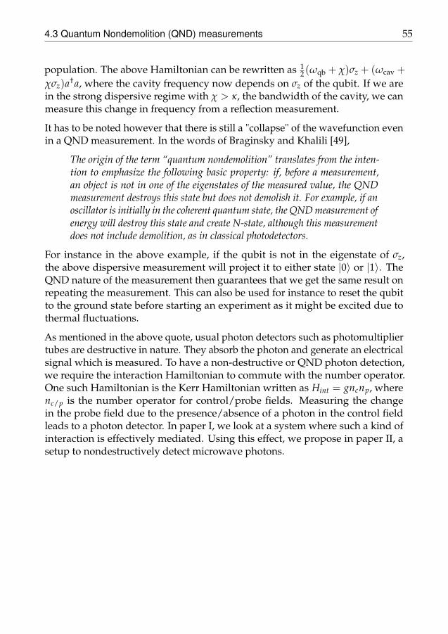
4.3 Quantum Nondemolition (QND) measurements 55

population. The above Hamiltonian can be rewritten as 12 (ωqb + χ)σz + (ωcav +

χσz)a†a, where the cavity frequency now depends on σz of the qubit. If we arein the strong dispersive regime with χ > κ, the bandwidth of the cavity, we canmeasure this change in frequency from a reflection measurement.

It has to be noted however that there is still a "collapse" of the wavefunction evenin a QND measurement. In the words of Braginsky and Khalili [49],

The origin of the term “quantum nondemolition” translates from the inten-tion to emphasize the following basic property: if, before a measurement,an object is not in one of the eigenstates of the measured value, the QNDmeasurement destroys this state but does not demolish it. For example, if anoscillator is initially in the coherent quantum state, the QND measurement ofenergy will destroy this state and create N-state, although this measurementdoes not include demolition, as in classical photodetectors.

For instance in the above example, if the qubit is not in the eigenstate of σz,the above dispersive measurement will project it to either state |0〉 or |1〉. TheQND nature of the measurement then guarantees that we get the same result onrepeating the measurement. This can also be used for instance to reset the qubitto the ground state before starting an experiment as it might be excited due tothermal fluctuations.

As mentioned in the above quote, usual photon detectors such as photomultipliertubes are destructive in nature. They absorb the photon and generate an electricalsignal which is measured. To have a non-destructive or QND photon detection,we require the interaction Hamiltonian to commute with the number operator.One such Hamiltonian is the Kerr Hamiltonian written as Hint = gncnp, wherenc/p is the number operator for control/probe fields. Measuring the changein the probe field due to the presence/absence of a photon in the control fieldleads to a photon detector. In paper I, we look at a system where such a kind ofinteraction is effectively mediated. Using this effect, we propose in paper II, asetup to nondestructively detect microwave photons.

I have yet to see any problem, however complicated, which,when you looked at it the right way, did not become still morecomplicated.

Attributed to Poul Anderson

5Connecting quantum systems

Over the past decade the coherence times of superconducting qubits have beenexponentially increasing [7], mimicking the well known Moore’s law. The "long"coherence times that is shown by current transmon qubits has placed them asa qubit of choice for building scalable quantum computers [8]. Many groupsaround the world are actively pushing towards setups with several transmontype qubits (for example see [127–131]). This implies that we need to developtools and formalisms to describe such complex quantum systems. Apart fromapplications in quantum computation, such formalisms would also be useful inother quantum devices where we have more than one quantum subsystem.

Let us start by looking at a typical example where the output of one quantumsystem becomes the input of the next system. Such a setup, known as a cascadedquantum system, was first looked at in references [132, 133]. While the masterequation is derived starting from a Hamiltonian in [132], we will here brieflyreview the approach taken in [105]. We look at an example setup shown inFig. 5.1, where we have two qubits connected to an unidirectional field. This canbe implemented in circuit QED by placing a transmon at the end of a transmissionline and by using circulators. As shown in the figure, the output field from qubit1 drives the qubit 2 after a time τ.

58 Connecting quantum systems

b(1)in (t− τ) b(1)out(t− τ) b(2)in (t) b(2)out(t)

Qubit 1 Qubit 2

Figure 5.1: A schematic setup of two qubits cascaded.

Writing out the input-output relation (Eq. (3.49)) for the qubits, we have

b(1)out(t) = b(1)in (t) + L(1)(t) (5.1)

b(2)out(t) = b(2)in (t) + L(2)(t) = b(1)in (t− τ) + L(1)(t− τ) + L(2)(t) (5.2)

where we have defined L(1/2) =√

Γ1/2σ(1/2)− . Considering two system operators

X1 and X2 belonging to qubits 1 and 2 respectively, we can write the quantumLangevin equations (Eq. (3.45))

Xi(t) = i[H(i)sys, Xi(t)]−

(√Γib

(i)in

†(t) +Γi

2σ(i)+ (t)

)[σ

(i)− (t), Xi(t)]

+

(√Γib

(i)in (t) +

Γi

2σ(i)− (t)

)[σ

(i)+ (t), Xi(t)], (5.3)

for i = 1, 2. Now considering an operator X belonging to either of the two qubits,we can combine the two equations above as

X(t) = i[Hsys, X(t)]−(√

Γ1b†in(t) +

Γ1

2σ(1)+ (t)

)[σ

(1)− (t), X(t)]

+

(√Γ1bin(t) +

Γ1

2σ(1)− (t)

)[σ

(1)+ (t), X(t)]

−(√

Γ2b†in(t− τ) +

√Γ1Γ2σ

(1)+ (t− τ) +

Γ2

2σ(2)+ (t)

)[σ

(2)− (t), X(t)]

+

(√Γ2bin(t− τ) +

√Γ1Γ2σ

(1)− (t− τ) +

Γ2

2σ(2)− (t)

)[σ

(2)+ (t), X(t)], (5.4)

where Hsys = H(1)sys + H(2)

sys. To get to the above result, we have used b(2)in (t) =

b(1)in (t− τ) + L(1)(t− τ) and have replaced b(1)in with just bin. The above equation

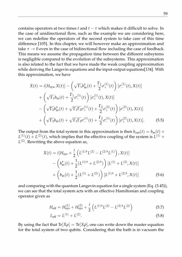
59

contains operators at two times t and t− τ which makes it difficult to solve. Inthe case of unidirectional flow, such as the example we are considering here,we can redefine the operators of the second system to take care of this timedifference [105]. In this chapter, we will however make an approximation andtake τ → 0 even in the case of bidirectional flow including the case of feedback.This means we assume the propagation time between the different subsytemsis negligible compared to the evolution of the subsystems. This approximationis also related to the fact that we have made the weak coupling approximationwhile deriving the Langevin equations and the input-output equations[134]. Withthis approximation, we have

X(t) = i[Hsys, X(t)]−(√

Γ1b†in(t) +

Γ1

2σ(1)+ (t)

)[σ

(1)− (t), X(t)]

+

(√Γ1bin(t) +

Γ1

2σ(1)− (t)

)[σ

(1)+ (t), X(t)]

−(√

Γ2b†in(t) +

√Γ1Γ2σ

(1)+ (t) +

Γ2

2σ(2)+ (t)

)[σ

(2)− (t), X(t)]

+

(√Γ2bin(t) +

√Γ1Γ2σ

(1)− (t) +

Γ2

2σ(1)− (t)

)[σ

(2)+ (t), X(t)]. (5.5)

The output from the total system in this approximation is then bout(t) = bin(t) +L(1)(t) + L(2)(t), which implies that the effective coupling of the system is L(1) +L(2). Rewriting the above equation as,

X(t) = i[Hsys +i2

(L(1)†L(2) − L(2)†L(1)

), X(t)]

−(

b†in(t) +

12(L(1)† + L(2)†)

)[L(1) + L(2), X(t)]

+

(bin(t) +

12(L(1) + L(2))

)[L(1)† + L(2)†, X(t)] (5.6)

and comparing with the quantum Langevin equation for a single system (Eq. (3.45)),we can see that the total system acts with an effective Hamiltonian and couplingoperator given as

Heff = H(1)sys + H(2)

sys +i2

(L(1)†L(2) − L(2)†L(2)

)(5.7)

Leff = L(1) + L(2). (5.8)

By using the fact that Tr[Xρ] = Tr[Xρ], one can write down the master equationfor the total system of two qubits. Considering that the bath is in vacuum the


(a) Cascade (b) Stack (c) Feedback

Figure 5.2: Connecting quantum systems - The series product, the concatenation productand the feedback.

master equation can be shown to be [132]

ρ = −i[Hsys, ρ] +D[

L(1)]

ρ +D[

L(2)]

ρ− [L(2)†, L(1)ρ]− [ρL(1)†, L(2)] (5.9)

which is the same asρ = −i[Heff, ρ] +D [Leff] ρ. (5.10)

While it is possible to extend the above method, one can imagine that it becomestedious if we have a complex network with many subsystems and several con-nections. A modular approach that makes the derivation of the master equationseasier has been proposed in [135, 136] and is known as the (S, L, H) formalism.We will look at an introduction to this formalism and apply it to a few systems ofinterest in this chapter. For more details, we refer to a recent review [134] thatprovides a good pedagogical overview and discusses the history and applicationsof the formalism.

5.1 (S, L, H) formalism

In this formalism, each subsystem is described by a triplet G ≡ (S, L, H), where Sis the scattering matrix, L is the vector of coupling operators of the subsystem andH is the Hamiltonian of the subsystem. Some examples of the (S, L, H) triplets aregiven in table 5.1. Once the triplets are identified for each of the subsystem, thetotal triplet for the composite system can be written using the following products(also see Fig. 5.2). The series product / of the triplets describes feeding the output

5.1 (S, L, H) formalism 61

System (S, L, H) triplet

50:50 beam splitter GBS =

(1√2

[1 ii 1

],

[00

], 0

)

Phase shifter Gφ =(eiφ, 0, 0

)

Qubit with one inputand output port (Atom

in front of a mirror)Gqb =

(1,√

Γσ−,− 12 ωqbσz

)

Qubit connected to anopen transmission line

Gqb =

(1,

[ √Γ/2σ−√Γ/2σ−

],− 1

2 ωqbσz

)

Table 5.1: Examples of some (S, L, H) triplets.

from one subsystem into another

G2 / G1 =

(S2S1, S2L1 + L2, H1 + H2 +

12i

(L†

2S2L1 − L†1S†

2 L2

)). (5.11)

The concatenation product is used for composing subsystems into a systemwith stacked channels

G2 G1 =

([S2 00 S1

],[

L2L1

], H2 + H1

). (5.12)

Lastly, we have feedback, written as [(S, L, H)]k→l = (S, L, H), where the outputfrom the kth port of the system is fed back as the input through the lth port of thesame system. The triplet is given by [137]

S = S[k,l] +

S1,l...

Sk−1,lSk+1,l

...Sn,l

(1− Sk,l)−1 (Sk,1 . . . Sk,l−1 Sk,l+1 . . . Sk,n

),


L = L[k]+

S1,l...

Sk−1,lSk+1,l

...Sn,l

(1− Sk,l)−1 Lk,

H = H +12i

((n

∑j=1

L†j Sj,l

)(1− Sk,l)

−1 Lk − h.c.

), (5.13)

where S[k,l] and L[k]are the original scattering matrix and coupling vector with

row k and column l removed.

Using the above defined products, we can write down the (S, L, H) triplet for thewhole system

Gtot =

Stot,

L1...

Ln

, Htot

, (5.14)

from which we can extract the corresponding master equation as

ρ = −i [Htot, ρ] +n

∑i=1D [Li] ρ, (5.15)

where the dissipation super-operator is given by D [c] ρ = cρc† − 12 c†cρ− 1

2 ρc†cas in previous chapters. The output from the ith channel is just given by Li. Atthis point, we once again note that the above rules work in the Markov limit andassume that the propagation time between the different subsystems is negligible[134]. Systems that involve appreciable time delays between subsystems and inthe feedback loop are considered using other approaches, for example [138, 139].

5.2 Cascaded quantum systems

As a first example, let us relook at the cascaded setup in Fig. 5.1. We will derivethe master equation now via the (S, L, H) formalism considering no input fields.The total (S, L, H) triplet in this case, assuming that no phase is gained by the

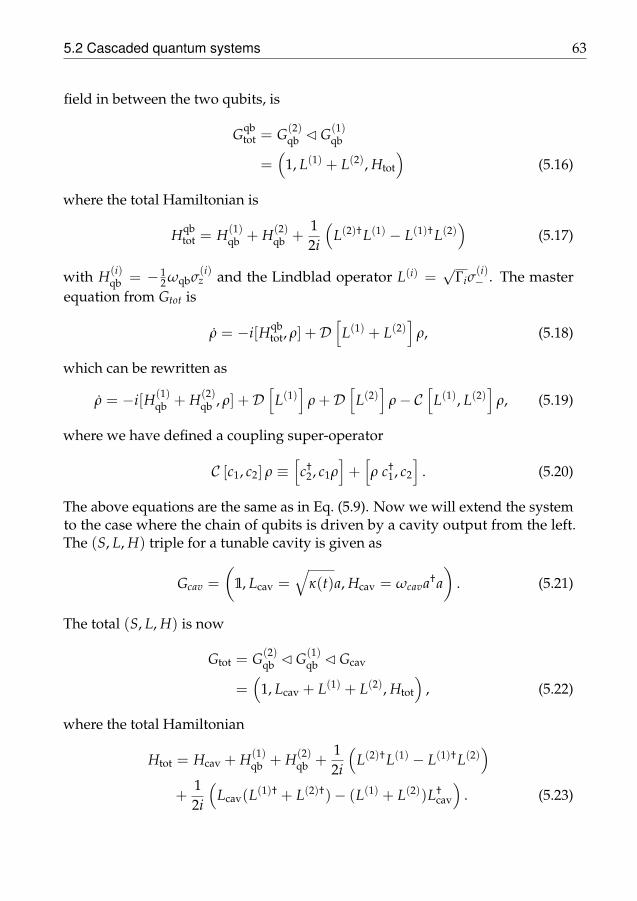
5.2 Cascaded quantum systems 63

field in between the two qubits, is

Gqbtot = G(2)

qb C G(1)qb

=(

1, L(1) + L(2), Htot

)(5.16)

where the total Hamiltonian is

Hqbtot = H(1)

qb + H(2)qb +

12i

(L(2)†L(1) − L(1)†L(2)

)(5.17)

with H(i)qb = − 1

2 ωqbσ(i)z and the Lindblad operator L(i) =

√Γiσ

(i)− . The master

equation from Gtot is

ρ = −i[Hqbtot, ρ] +D

[L(1) + L(2)

]ρ, (5.18)

which can be rewritten as

ρ = −i[H(1)qb + H(2)

qb , ρ] +D[

L(1)]

ρ +D[

L(2)]

ρ− C[

L(1), L(2)]

ρ, (5.19)

where we have defined a coupling super-operator

C [c1, c2] ρ ≡[c†

2, c1ρ]+[ρ c†

1, c2

]. (5.20)

The above equations are the same as in Eq. (5.9). Now we will extend the systemto the case where the chain of qubits is driven by a cavity output from the left.The (S, L, H) triple for a tunable cavity is given as

Gcav =

(1, Lcav =

√κ(t)a, Hcav = ωcava†a

). (5.21)

The total (S, L, H) is now

Gtot = G(2)qb C G(1)

qb C Gcav

=(

1, Lcav + L(1) + L(2), Htot

), (5.22)

where the total Hamiltonian

Htot = Hcav + H(1)qb + H(2)

qb +12i

(L(2)†L(1) − L(1)†L(2)

)

+12i

(Lcav(L(1)† + L(2)†)− (L(1) + L(2))L†

cav

). (5.23)


0 5 10 150

0.2

0.4

0.6

0.8

Γpht

P(1)exc

P(2)exc

ξ(t)

(a) ncav(0) = 1

0 5 10 150

0.2

0.4

0.6

0.8

Γpht

(b) ncav(0) = 2

0 5 10 150

0.2

0.4

0.6

0.8

Γpht

(c) ncav(0) = 1

Figure 5.3: Probability of excitation of two cascaded qubits driven by a cavity output.The initial cavity state contains (a) 1 photon, (b) 2 photons and (c) a coherent state withan average of 1 photon. The coupling rates are such that Γ1 = Γph and Γ2 = 2Γ1. Boththe qubits are on resonance with the incoming field. The photon shape ξ(t) is plotted forreference.

Writing the master equation from the above (S, L, H) triple and expanding thedissipator terms, we end up with

ρ = −i[Heff, ρ] +D [Lcav] ρ +D[

L(1)]

ρ +D[

L(2)]

ρ

− C[

L(1), L(2)]

ρ− C[

Lcav, L(1) + L(2)]

ρ, (5.24)

where Heff = Hcav + H(1)tr + H(2)

tr .

We will consider the cases where we start the cavity in a Fock state with one ortwo photons and a coherent state. We tune the coupling of the cavity such thatthe output photon is in a Gaussian wave packet (Eq. (3.71)) [114]. We numericallysolve the master equation and show the results in Fig. 5.3. The first two panels (a)and (b) show the probability of excitation of the two qubits when we start withncav = 1 and ncav = 2 Fock states in the cavity. For the ncav = 1 case, we see thatthe second qubit gets excited appreciably by the field that is coming from therelaxation of the first qubit as expected. In contrast, for the ncav = 2 case, both the

5.3 Coupled quantum systems 65

α α + L(1)eiφ

(α + L(1)) eiφ(α + L(1)) + L(2)Transmon 1

L(1) + eiφL(2) eiφL(2) L(2)

Transmon 2

φ

Figure 5.4: A schematic setup of two transmon qubits separated by a distance. We sendin a coherent signal of amplitude α from the left and look at the transmitted and reflectedpart.

qubits get excited almost simultaneously. This can be attributed to the saturationof the first qubit and so the rest of the field is transmitted to the second qubitwhich then gets excited. In the third panel (c), we see the excitation of the qubitswhen the cavity is loaded with a coherent field with average number of photonsncav = 1. As the coherent state has a Poisson distribution of photon numbers, wesee that the second qubit gets excited appreciably at the same time as the firstqubit, compared to the case with only a single photon in the cavity.

5.3 Coupled quantum systems

Now, let us look at the scenario where we have two transmons coupled to anopen transmission line. We consider only the two lowest levels of the transmonsi.e. essentially qubits. The distance between the two transmons is modeled as aphase gained by the field. However as mentioned before, we have assumed thatthe traveling time of the field between the two qubits is negligible, i.e. it is muchsmaller than the time of evolution of the system. The setup is driven from the leftby a coherent field of strength α. A schematic setup is shown in the Fig. 5.4.

As each transmon can both reflect and transmit the incoming fields, it is conve-nient to write the right going and left going parts of the equations separatelyand then stack them using the concatenation product. In this case, the (S, L, H)triplets of the individual transmons can be written as,

G(i)tr = G(i)

Ltr G(i)Rtr (5.25)

where

G(i)Rtr =

(1, L(i), H(i)

tr

),

G(i)Ltr =

(1, L(i), 0

), (5.26)


with L(i) =√

Γi/2 σ(i)− as before. The Hamiltonian of the individual transmons

in the frame rotating with the frequency of the incoming drive ωd is given byH(i)

tr = −(∆(i)/2) σ(i)z , where ∆(i) = ω

(i)01 − ωd is the detuning of the i-th qubit

and σz is the third Pauli matrix. The incoming signal in its own rotating frame isrepresented by the triplet

Gα = (1, α, 0) (5.27)

and the phase gained between the qubits by

Gφ =(

eiφ, 0, 0)

. (5.28)

With these, we can write the total triplet for the above setup using the series andconcatenation products as,

Gtot =(

G(2)Rtr C Gφ C G(1)

Rtr C Gα

)(

G(1)Ltr C Gφ C G(2)

Ltr

)

=

([eiφ 00 eiφ

],

[eiφ(

α + L(1))+ L(2)

L(1) + eiφL(2)

], Htot

)(5.29)

where

Htot = H(1)tr + H(2)

tr +12i

(L(1)†α− α∗L(1)

)+

12i

(eiφL(2)†α− e−iφα∗L(2)

)

+ sin φ(

L(1)†L(2) + L(2)†L(1))

. (5.30)

The first two terms in the above Hamiltonian are that of the bare qubits, whilethe next two give the interaction of the field with the qubits. The last term isusually referred to as exchange interaction that is mediated by virtual photons.The master equation can be written from the total (S, L, H) triplet as

ρ = −i[Htot, ρ] +D[eiφ(

α + L(1))+ L(2)

]ρ +D

[L(1) + eiφL(2)

]ρ. (5.31)

Such a master equation was also derived in [140] for N-atoms with M levels usinga different formalism. As a special case, they also look at two qubits separatedby an arbitrary distance. To compare our results with the above reference, werewrite the above master equation by expanding the dissipation super-operatorsas

ρ = −i[Heff, ρ] +2

∑i,j=1

Υi,j

(σ(i)− ρσ

(j)†− − 1

2

σ(j)†− σ

(i)− , ρ

), (5.32)

introducing the matrix

Υ ≡(

Γ1 cos φ√

Γ1Γ2cos φ

√Γ1Γ2 Γ2

)(5.33)

5.3 Coupled quantum systems 67

0 1 2 3 4 5 60

0.2

0.4

0.6

0.8

1

α

|r|

d = 0

d = λ/8

d = λ/4

Figure 5.5: Absolute value of the reflection coefficient for the setup in Fig. 5.4 for differentdistances between the qubits. Both the qubits are on resonance with the incoming coherentfield and also have the same coupling rates (Γ) to the transmission line.

−4 −2 0 2 40

0.2

0.4

0.6

0.8

1

∆/Γ

|r|2,|t|2

(a) d = 0

−4 −2 0 2 40

0.2

0.4

0.6

0.8

1

∆/Γ

(b) d = λ/8

−4 −2 0 2 40

0.2

0.4

0.6

0.8

1

∆/Γ

(c) d = λ/4

Figure 5.6: Reflection (solid lines) and transmission (dashed lines) coefficient as afunction of qubit detuning ∆(1) = ∆(2) = ∆ at low input power. Both the qubits havethe same coupling rates (Γ) to the transmission line. Plots (a) and (c) agree with theresults shown in [140] for the case of d = λ and d = 3λ/4 respectively.


and the effective Hamiltonian

Heff = H(1)tr + H(2)

tr −12i

(α∗L(1) − αL(1)†

)− 1

2i

(α∗e−iφL(2) − αeiφL(2)†

). (5.34)

The master equation can be written in diagonal form, by diagonalizing the Υmatrix. By this procedure, we get the coupling rate of the dressed states (labeledB and D following [140]) as

ΓB/D =Γ1 + Γ2

2± 1

2

√(Γ1)

2 + (Γ2)2 + 2 cos 2φ Γ1Γ2 (5.35)

and the dressed lowering operators given by

σµ− =

(Γµ − Γ2)σ(1)− + cos φ

√Γ1Γ2σ

(2)−√

(Γµ − Γ2)2 + Γ1Γ2 cos2 φ(5.36)

where µ = B/D. Using these, we can write the master equation as

ρ = −i[Heff, ρ] +D [LB] ρ +D [LD] ρ, (5.37)

where Lµ=B/D =√

Γµσµ−. From the steady state solution of the above equation,

we can get the coherently transmitted and reflected fields at steady state as

αtr =⟨

eiφ(

α + L(1))+ L(2)

⟩ss

, (5.38)

αref =⟨

L(1) + eiφL(2)⟩

ss. (5.39)

From these, the reflection (r = αref/α) and transmission coefficients (t = αtr/α)can be calculated. We plot |r| for three different values of distance between thequbits d = φλ/2π in Fig. 5.5. As can be seen from the figure, at low power(α 1) almost all of the field is reflected by the qubits. As the power is increased,the qubits get saturated and more and more of the incoming field gets transmitted.Thus the reflection coefficient goes to 0 at higher powers. We also plot the |r|2and |t|2 as a function of the detuning ∆ in Fig. 5.6 at low input power. In thisregime, we have fully coherent scattering with |r|2 + |t|2 = 1. We can comparethe results in subplots (a) and (c) to the results shown in [140] for the case ofd = λ and d = 3λ/4 respectively. We also show the results for an intermediatedistance of d = λ/8.

5.4 Feedback 69

Figure 5.7: Schematic of a two level system in front of a mirror.

5.4 Feedback

At the beginning of this chapter, we looked at the case of having qubits coupledunidirectionally. One key requirement in that case was to have only one input-output port. In superconducting circuits, we can achieve this by placing the qubit(transmon) at the end of a transmission line which can either be open or shortedto ground. This boundary condition acts as a mirror for the field. In this section,we explicitly look at the master equation for a two level system that is in front ofa mirror. A schematic is shown in Fig. 5.7, where the distance between the qubitand the mirror is once again modeled as a phase gained by the field. The fieldreflected from the mirror is fed back to the qubit and we can use the feedbackoperation of the (S, L, H) formalism to derive the master equation as in [76]. Inthis case, the triplet for the qubit-mirror without any drive is given by

G = (S, L, H) = [(Gφ I) / Gtr]1→2 (5.40)

where the triplets Gtr and Gφ are same as in Eq. (5.25) and Eq. (5.28) respectively.We have to concatenate an identity triple I = (1, 0, 0) to keep the dimensionsintact. Using the feedback rules given in Eq. (5.13), we get

S = eiφ, (5.41)

L = (1 + eiφ)L, (5.42)

H = Htr + sin φL†L, (5.43)

where Htr = −(ω0/2)σz and L =(√

γ/2)

σ−. With this triplet, we can nowinclude the drive which could be either a coherent state or a Fock state. In thisexample, we will assume a coherent input specified by a triplet Gα as in Eq. (5.27).The total triplet is then

Gtot = (S, L, H) / Gα (5.44)


0 1 2 3 4 50

0.2

0.4

0.6

0.8

1

α

|r| d = 0

d = λ/8

d = λ/4

Figure 5.8: Absolute value of the reflection coefficient |r| as a function of input fieldstrength for different distances between the qubit and the mirror. The qubit is on resonancewith the incoming field and the coupling rate γ = 1.

which gives the master equation

ρ = −i[Htot, ρ] +D[eiφα + (1 + eiφ)L

]ρ, (5.45)

where the Hamiltonian Htot = −(∆/2)σz + sin φL†L + 12i

(αL†(eiφ + 1)− h.c.

).

The Hamiltonian is in the the rotating frame of the incoming field with ∆ =ω0 −ωd. We can expand the dissipator and simplify the master equation to get

ρ = −i[Heff, ρ] + 2(1 + cos φ)D [L] ρ, (5.46)

where the effective Hamiltonian now is

Heff = −(∆/2)σz + sin φL†L− i(

αL†(eiφ + 1)− h.c.)

. (5.47)

For φ = 0, we see that the master equation can be rewritten as

ρ = −i[Htr − i(αL′† − L′α∗)] +D[L′]

ρ (5.48)

by defining L′ = 2L =√

2γσ− ≡√

Γσ−. Here we have defined a renormalizedcoupling rate Γ that is twice the original relaxation rate γ. This is the coupling ratethat is used in the previous sections and also in paper II. As an example, let us lookat the scattering property of this setup by calculating the reflection coefficients rfor different distances between the mirror and the qubit. The absolute value ofr = 〈αout〉 /α, where αout = eiφα + (1 + eiφ)L, is plotted in Fig. 5.8. Note that the

5.4 Feedback 71

phase φ is gained by the field over the entire trip between the qubit and the mirror(i.e. back and forth). We can convert this into distance in terms of wavelength ofthe field as d = φ λ

4π . As we have an open end, the field is maximum at the mirrorand the qubit couples maximally to the field at this point. At d = λ/4, the fieldgoes to zero and we do not see any effect of the qubit on the reflected field, asexpected. We get intermediate results for d = λ/8. Such an setup has also beentested experimentally recently (but with a slightly different boundary condition)and the results are presented in [76].

"You probably think this paper’s about you: narcissists’ perceptionsof their personality and reputation.",Carlson, E. N., Vazire, S. and Oltmanns, T. F. ,Journal of Personality and Social Psychology 101, 185–201 (2011).

Listed in Scientists’ Silly, Dark, and Sometimes Inappropriate Humor,Slate.com

6Overview of the articles

In this chapter, we provide a brief summary of the appended papers on which thethesis is based on. In particular, we will highlight the salient points of the articlesand show how the framework developed in the previous chapters is connectedto the work presented.

6.1 Cross-Kerr Effect for propagating microwaves

In paper I, we look at inducing photon-photon interaction at microwave frequen-cies for propagating photons. As discussed in the introduction, photons rarelyinteract with each other in vacuum and such interactions are usually engineeredusing a nonlinear material. In this experimental work, an effective photon-photoninteraction is mediated using the lowest three levels of an artificial atom, thesuperconducting transmon. Two coherent fields, control and probe, close toresonance with these two transition frequencies, are scattered off of the transmon.The interaction effectively induces a phase change in the probe field due to thepresence of the control field à la the cross-Kerr effect.

In the article, two setups are investigated. In one, the transmon is coupled to an

74 Overview of the articles

open transmission line and in another it is placed at the end of a semi-infinitetransmission line. The second setup corresponds to having an atom in front ofa mirror and has only one input-output port, thus reducing the loss of signal inthe reflected field. The output fields scattered from the transmons are measuredusing a homodyne detector.

The input-output relations are different for the two setups as we already saw inChapter 3. In the case of the transmon connected to an open transmission line,only the transmitted field is measured. Combining these two cases we can writethe average output in the steady-state for both the fields as [141]

α(c)out = α

(c)in +

√Γ01

kn

⟨σ01−⟩

ss, (6.1)

α(p)out = α

(p)in +

√Γ12

kn

⟨σ12−⟩

ss, (6.2)

where kn is the number of output channels i.e. kn = 1 for atom in front of a mirrorand kn = 2 for an atom in an open transmission line. The lowering operators aregiven by σ01

− = |0〉〈 1| and σ12− = |1〉〈 2|. The expectation values are calculated

by solving the master equation of the system as discussed in Chapter 3. TheHamiltonian of the three level system in the rotating frame of the two drivescan be written as Htr = −∆c |0〉〈 0| + ∆p |2〉〈 2|, where the detuning betweenthe transition frequencies and the drive frequencies are given as ∆c = ω10 −ωcand ∆p = ω21 − ωp. The coherent drives can be included in the Hamiltonianas Hdrive = −i

√Γ01/kn(αcσ01

−† − h.c.)− i

√Γ12/kn(αpσ12

−† − h.c.). With these, the

master equation without including dephasing can be written as

ρ = −i[Htr + Hdrive, ρ] + Γ01D[σ01−]

ρ + Γ12D[σ12−]

ρ. (6.3)

The setup in the experiment is slightly different, where the probe was close tothe resonance of the 0− 1 transition and the control was close to the resonanceof the 1− 2 transition. The above model however gives a more intuitive picture.In this case, starting with a transmon in the ground state, the probe is scatteredfrom the transmon only when the control field is on. Thus the phase shift in theabsence of control field is 0. As it is more straightforward to interpret, we will usethis model in the next section as well, where we look at photon detection using athree level atom.

From the measurement results, we see that an average conditional phase changeof 10 and 20 degrees is induced in the probe field using setup 1 and 2 respectively.The input signals are in the single photon range, i.e the average number of

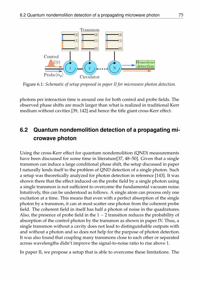
6.2 Quantum nondemolition detection of a propagating microwave photon 75

Figure 6.1: Schematic of setup proposed in paper II for microwave photon detection.

photons per interaction time is around one for both control and probe fields. Theobserved phase shifts are much larger than what is realized in traditional Kerrmedium without cavities [39, 142] and hence the title giant cross-Kerr effect.

6.2 Quantum nondemolition detection of a propagating mi-crowave photon

Using the cross-Kerr effect for quantum nondemolition (QND) measurementshave been discussed for some time in literature[37, 48–50]. Given that a singletransmon can induce a large conditional phase shift, the setup discussed in paperI naturally lends itself to the problem of QND detection of a single photon. Sucha setup was theoretically analyzed for photon detection in reference [143]. It wasshown there that the effect induced on the probe field by a single photon usinga single transmon is not sufficient to overcome the fundamental vacuum noise.Intuitively, this can be understood as follows. A single atom can process only oneexcitation at a time. This means that even with a perfect absorption of the singlephoton by a transmon, it can at most scatter one photon from the coherent probefield. The coherent field in itself has half a photon of noise in the quadratures.Also, the presence of probe field in the 1− 2 transition reduces the probability ofabsorption of the control photon by the transmon as shown in paper IV. Thus, asingle transmon without a cavity does not lead to distinguishable outputs withand without a photon and so does not help for the purpose of photon detection.It was also found that coupling many transmons close to each other or separatedacross wavelengths didn’t improve the signal-to-noise ratio to rise above 1.

In paper II, we propose a setup that is able to overcome these limitations. The


key ingredient is to couple the transmons unidirectionally i.e. to cascade themusing circulators as shown in Fig. 6.1. In such a setup, we can show that usingtwo coherent drives, similar to the previous section, the conditional phase changein the probe accumulates over several transmons [40]. In the article, we check theperformance of the setup for photon detection.

We take two different approaches to model the input single photon that is even-tually needed to be detected by our setup. In one, we consider a tunable cavity asthe source as in section 5.2. In the other approach, we use the Fock state formalismdiscussed in section 3.4. The control field that will contain the single photon ison resonance with the 0− 1 transition of all the transmons. This control fieldand a coherent probe field (on resonance with the 1− 2 transition) are scatteredon the chain of cascaded transmons. The output probe field is then measuredusing a homodyne detector as in the previous section. If the control field has aphoton at some time t, the effect on the probe field is seen from the measuredhomodyne current. We integrate the homodyne current over a time period T andthis integrated current becomes our signal. The single photon itself survives thismeasurement process, making the scheme non-destructive.

To evaluate the performance of the setup, we take two approaches. In one, wesolve the unconditional master equations and from the average dynamics calcu-late the signal-to-noise ratio (SNR). In another approach, we simulate quantumtrajectories using the stochastic master equation for homodyne detection, similarto the ones shown in section 4.2. From these, we get the histograms of the signalmeasured with and without a single photon in the control field. From the meanand variance of the histogram, we calculate the signal-to-noise ratio (SNR) of theproposed detector. From the simulation results, we also see that as we increasethe number of transmons, the signal distribution (histogram) does not remainGaussian in the case of having a single photon in the control field. To take thisinto account we define a better measure, detection fidelity. As shown in the article,we can overcome the noise (i.e. get a SNR above 1) and detect the presence of asingle photon with a 90% fidelity in certain parameter regimes.

Furthermore, we also consider imperfections such as dephasing of the transmons,power loss in circulators and imperfect homodyne detection. We conclude thatfor small imperfections the signal survives and we can still detect the photon.Comparing with experimentally available performance of these devices, it shouldbe possible (probably with some effort) to build such a device with currentlyavailable resources. The major difficulty comes from circulators which are bulkydevices that are off-chip. Apart from cooling down these bulky devices, we alsohave to worry about impedance matching the lines when we go on and off chips.

6.3 Coupled superconducting resonators 77

Figure 6.2: Schematic setup for coupled cavities considered in papers III and VI.

Our proposed scheme looks more attractive with the development of on-chipcirculators [144]. Chiral quantum optics might also be a solution for realizing theproposed setup [145]. Further to this work, reference [55] shows how to improvethe maximum signal that one can get from a single transmon by using a cavityfor the probe field and by using more sophisticated filtering techniques. Thesignal can be further improved by once again cascading these individual units(transmon+cavity).

The proposal in paper II is one of the many proposals[52–61, 146, 147] for solvingthe long standing problem of detecting single itinerant microwave photon. Inpaper IV, we review some of the above proposals, which can be broadly classifiedas destructive or nondestructive type of detectors. The destructive microwavephoton detectors are predominantly mapped as a Λ system. Such a Λ system canbe realized using a current biased Josephson junction with a suitable bias current.It was shown theorectically in reference [53] that a photon detection of 100% ispossible by one of these current biased junctions at the end of a transmissionline. A more recent proposal for photon detection uses impedence matched Λsystems implemented by driving a qubit coupled to a resonator [146, 147]. Sucha setup was also experimentally realized recently [62]. As these results werepublished quite close to the submission of paper IV, they are not reviewed in thesame. Apart from these destructive schemes, in paper IV, we mainly present apedagogical review of the nondestructive photon detector proposals based onPaper II and [55].

6.3 Coupled superconducting resonators

In one of the approaches of paper II, we consider a cavity with tunable couplingas a source of single photons. By tuning the coupling of the cavity, photon wavepackets of desirable shapes (a gaussian, for example) can be created [28, 29, 114].In paper III, we consider one such implementation of a tunable cavity that could


lead to the shaping of photon wave packets in the future. The tunable cavityin this case is made up of two cavities - a λ/4 resonator that acts as the storagecavity and a λ/2 resonator that acts as a coupling cavity. We have a SQUID atthe current anti-node of the coupling cavity i.e. at its middle (see Fig. 6.2). Bythreading flux through the SQUID loop, we can modify the total inductance ofthe resonator and hence its mode frequencies.

The device can be analyzed following the circuit model presented in chapter 2.For the coupling cavity alone, we can write down the Lagrangian and from it theEuler-Lagrange equation of motion for the flux. From an approximate solutionof this equation, we can find the resonant frequency of the coupling cavity as afunction of the flux through the SQUID [148, 149]. The analysis can be extendedby including the storage cavity and the coupling to the transmission line. Byconsidering only the two lowest modes of the coupling and storage cavities, weend up with two normal modes. As is well known in any such coupled oscillatorsystems, we can have either an under, over or critically damped system. Thisis characterized by the ratio of the coupling to the transmission line κ to thecoupling between the the cavities g.

The results presented in paper III can be understood as follows. The effectivecoupling of the storage cavity is via the coupling cavity, which acts like a barrierbetween the transmission line and the storage cavity. By bringing the couplingcavity on and off resonance with the storage cavity (similar to lowering andraising of a potential barrier), we can effectively tune the coupling of the storagecavity to the transmission line. In the sample discussed in the paper III, thecoupling can be tuned by three orders of magnitude. This is seen from thelifetime of the field stored in the cavity which is shown to vary from 14ns to18µs. Also by varying the detuning of the coupling cavity, it is shown that we canrelease the field in exponentially decaying wave packets of different widths. Theabove experiments were done when the cavity was filled with a coherent statethat has on average 80 photons. However, the results suggests that by loadingthe cavity with a single photon and by modulating the coupling, we should beable to get single photon wave packets of different shapes. As mentioned inthe introduction, such sources of single photons are of importance not only forquantum optics but also for quantum computing and communication.

In paper VI, a similar device but operating at a different parameter regime ispresented. In the device presented in paper III, the energy relaxation rate setby κ was larger than the energy exchange rate between the cavities. Thus, wecould understand the results as in the above paragraph. In paper VI however,the damping to the transmission line is much smaller than the energy exchange

6.4 Generating single photons on demand 79

rate between the cavities, which means there is significant energy oscillationbetween the cavities while there is also decay to the transmission line. Thisparameter scheme however allows us to demonstrate a different scheme forcatching and releasing microwave photons. In this case, we can start with thecoupling cavity completely decoupled from the storage cavity. The incomingsignal is then captured in the coupling cavity and then swapped into the storagecavity by bringing them both on resonance. The excitation can then be stored inthe resonator cavity and released either directly by tuning the coupling as in paperIII or by doing a swap back into the coupling cavity. This protocol thus allowsus to catch and release photons at a wide range of frequencies (correspondingto that of the tunable coupling cavity) and we are no longer restricted to thefrequency range of the storage cavity. We hope that such devices can play therole of photonic memories in the microwave domain. We once again note thatthis initial demonstration is with coherent fields and further work is needed toshow that the setup works for non-classical fields as well.

6.4 Generating single photons on demand

As the final topic, we look at generating single photons on demand. As mentionedin the introduction, several cavity based schemes for generating single microwavephotons exist [25–29]. However, the use of cavities limit the bandwidth of op-eration and requires full control of both the qubit and the cavity. A cavity freeapproach was theoretically studied in [30] and experimentally demonstratedin [31]. In this setup, an atom is asymmetrically coupled to two transmissionlines. The coupling of the atom to the control line is much weaker compared tothe emission line. A π pulse from the weakly coupled control line excites thequbit which then preferably emits in the emission line. However, as noted in [31],there is also a direct coupling between the transmission line which might leadto leakage of photons from the incoming π pulse into the emission line and oneneeds to separate these from the emission of the atom. Also, it might be difficultin such a setup to get the photons in desired wave packet shapes.

In paper V, we propose two different setups to generate single photons on de-mand. Both of these use atom in front a mirror, which is crucial for gettinghigh efficiency. As we already discussed in chapter 3, an excited atom in anopen transmission line emits a photon in the left and right moving modes withequal probability. By placing the atom in front of a mirror, we collect all theemission from the atom. However, the coherent pulse used to excite the atomalso comes out through the same port. Thus, we have to separate it from the


(a) (b)

Figure 6.3: Schematic setups to generate single photons (a) Using a beam splitter (b)Using tunable coupling.

atomic decay. We can see this from the input-output relation which is given asαout(t) = αin(t) +

√Γσ−(t), where Γ is the effective coupling rate of the qubit

to the transmission line. αin(t) is the input π-pulse. We propose two differentmethods to separate the atomic decay from αin(t).

In the first method (Fig. 6.3a), we use an unbalanced beam splitter with reflectioncoefficient r → 1. It can be shown that such a beam splitter can be used toimplement a displacement operator by using a strong coherent beam [150]. Weuse this to "undisplace" the coherent part of the output field and separate theatomic decay in one of the output channels. This can also be seen from the beamsplitter input-output relations as shown in the article.

To characterize the efficiency of this method, we calculate Pn, the probability ofhaving n photons in the output field (d(t) in Fig. 6.3a). This is done by calculatingthe mth order coherence function of the output (Eq. (3.64)). From the correlationfunction, we can calculate the photon m-tiples and the probabilities Pn [30]. Theprobability of having exactly one photon in the output becomes the measure ofefficiency of our setup. We show that using experimentally realizable values forthe beam splitter, a photon generation efficiency of 97% is straightforward toachieve.

In method two (Fig. 6.3b), we take advantage of the on-chip tunability of su-perconducting circuits as follows. The coupling between a transmon and thetransmission line depends on the value of voltage at the coupling point. Anopen boundary condition at the end of the transmission line (d = 0), imposes thecondition that the voltage is maximum at this point for all the allowed modes. Aqubit at d = 0 thus has a maximum coupling to the transmission line. The modestructure due to the boundary condition imposes a node at a distance d = λ/4for each of the mode. A qubit at this distance with the corresponding frequency

6.4 Generating single photons on demand 81

is completely decoupled from the transmission line. By changing the boundarycondition i.e. by moving the mirror, we can go from a qubit that is maximallycoupled to completely decoupled from the transmission line. A tunable boundarycondition with a SQUID at the end of the transmission line, thus leads to a tunablecoupling [151]. An alternative is to place the qubit at a finite distance from themirror and tune the frequency of the qubit, which also leads to tunable coupling[76]. As we discussed in the previous section, the advantage of such a tunablesystem is to shape the output photon in desirable wave packets.

The photon generation in the second method is as follows. We start with thequbit coupled to the transmission and tune the coupling to be very close to 0. Wesend a strong π-pulse and excite the qubit. At the end of the pulse, we tune thecoupling to 0. This can be done fast as we started at a very low coupling beforethe pulse. Now, a single excitation is trapped in the qubit which can be thenreleased as needed in a desirable wave packet by tuning the coupling accordingly.In this case, we once again calculate the photon generation efficiency as beforeand find that with current technologies it can reach above 97%.

Given that the above setups are quite simple, one can imagine extending itto generate either correlated or entangled photons. As all of the ingredientsrequired to test the proposals are readily available, we hope to see experimentalrealizations of the schemes presented in the near future.

Cuius rei demonstrationem mirabilem sane detexi hancmarginis exiguitas non caperet.

(I have discovered a truly remarkable proof of this theoremwhich this margin is too small to contain.)

Pierre de Fermat

7Summary

Linear optical quantum computing (LOQC) is an approach to develop a quantumcomputer primarily using linear elements such as beam splitters along withsingle photon sources and detectors. However, to perform universal quantumcomputing, some nonlinearity is required [15, 17]. Superconducting circuitshave the advantage of possessing a strong low loss nonlinearity that comes fromthe Josephson junction, which can enable development of all-optical quantumcomputing at microwave frequencies [17]. This however requires efficient singlephoton devices in the microwave regime, especially a single microwave photondetector, a first implementation of which has only been recently realized. In thisthesis, we look at our proposals for microwave single photon devices based onthe appended papers.

One of the main results of the thesis, is the proposal for a nondestructive detectorfor propagating single microwave photons as presented in paper II. The detec-tor is based on the large photon-photon interaction mediated by a three levelsuperconducting transmon, as shown in paper I. We also show how to efficientlygenerate single microwave photons on demand by using an atom in front of amirror in paper V. In paper III and VI, we present experimental results on coupledcavities which could serve the purpose of a photonic quantum memory. While

84 Summary

the proposals are primarily aimed at circuit QED setups, we believe they could beextended to other systems where atoms are strongly coupled to one-dimensionalwaveguides. These include superconducting qubits coupled to surface acousticwaves [152], quantum dots coupled to photonic waveguides [153] or surfaceplasmons [154].

References

[1] J. P. Dowling and G. J. Milburn. “Quantum technology: the second quan-tum revolution.” Philosophical transactions. Series A, Mathematical, physical,and engineering sciences 361, 1655–1674 (2003) [cit. on p. 1].

[2] Measuring and manipulating individual quantum systems - Scientific Back-ground on the Nobel Prize in Physics 2012. eprint: http://www.nobelprize.org/nobel_prizes/physics/laureates/2012/advanced-physicsprize2012.pdf. Last visited on 13 May 2017 [cit. on p. 2].

[3] S. Haroche and D. Kleppner. “Cavity Quantum Electrodynamics”. PhysicsToday 42, 24 (1989) [cit. on p. 2].

[4] H. Walther, B. T. H. Varcoe, B.-G. Englert, and T. Becker. “Cavity quantumelectrodynamics”. Reports on Progress in Physics 69, 1325 (2006) [cit. onpp. 2, 22].

[5] S. Debnath, N. M. Linke, C. Figgatt, K. A. Landsman, K. Wright, and C.Monroe. “Demonstration of a small programmable quantum computerwith atomic qubits”. Nature 536, 63–66 (2016) [cit. on p. 2].

[6] T. D. Ladd, F. Jelezko, R. Laflamme, Y. Nakamura, C. Monroe, and J. L.O’Brien. “Quantum computers.” Nature 464, 45–53 (2010) [cit. on p. 2].

[7] M. H. Devoret and R. J. Schoelkopf. “Superconducting Circuits for Quan-tum Information: An Outlook”. Science 339, 1169–1174 (2013) [cit. on pp. 2,24, 57].

[8] G. Wendin. “Quantum information processing with superconductingcircuits: a review” (2016). arXiv: 1610.02208 [cit. on pp. 2, 18, 24, 57].

http://dx.doi.org/10.1098/rsta.2003.1227


http://www.nobelprize.org/nobel_prizes/physics/laureates/2012/advanced-physicsprize2012.pdf



http://dx.doi.org/10.1063/1.881201

http://stacks.iop.org/0034-4885/69/i=5/a=R02


http://dx.doi.org/10.1038/nature18648



http://dx.doi.org/10.1126/science.1231930


http://arxiv.org/abs/1610.02208



86 References

[9] A. Wallraff, D. I. Schuster, A. Blais, L. Frunzio, R.-S. Huang, J. Majer, S.Kumar, S. M. Girvin, and R. J. Schoelkopf. “Strong coupling of a single pho-ton to a superconducting qubit using circuit quantum electrodynamics”.Nature 431, 162–167 (2004) [cit. on pp. 2, 23].

[10] J. Q. You and F. Nori. “Atomic physics and quantum optics using super-conducting circuits”. Nature 474, 589–597 (2011) [cit. on p. 2].

[11] J. Clarke and F. K. Wilhelm. “Superconducting quantum bits”. Nature 453,1031–1042 (2008) [cit. on p. 2].

[12] R. J. Schoelkopf and S. M. Girvin. “Wiring up quantum systems”. Nature451, 664–669 (2008) [cit. on p. 2].

[13] C. M. Wilson, G. Johansson, A. Pourkabirian, M. Simoen, J. R. Johansson,T. Duty, F. Nori, and P. Delsing. “Observation of the dynamical Casimireffect in a superconducting circuit”. Nature 479, 376–379 (2011) [cit. onpp. 2, 16, 24].

[14] E. Knill, R. Laflamme, and G. J. Milburn. “A scheme for efficient quantumcomputation with linear optics”. Nature 409, 46–52 (2001) [cit. on p. 2].

[15] P. Kok, W. J. Munro, K. Nemoto, T. C. Ralph, J. P. Dowling, and G. J. Mil-burn. “Linear optical quantum computing with photonic qubits”. Reviewsof Modern Physics 79, 135–174 (2007) [cit. on pp. 2, 83].

[16] S. Barz. “Quantum computing with photons: introduction to the circuitmodel, the one-way quantum computer, and the fundamental principlesof photonic experiments”. Journal of Physics B: Atomic, Molecular and OpticalPhysics 48, 083001 (2015) [cit. on p. 2].

[17] P. Adhikari, M. Hafezi, and J. M. Taylor. “Nonlinear optics quantumcomputing with circuit QED”. Physical Review Letters 110, 060503 (2013)[cit. on pp. 2, 83].

[18] R. J. Kokkoniemi, T. Ollikainen, R. E. Lake, S. Saarenpää, J. Kokkala, C.B. Dag, and M. Möttönen. “Quantum Gates for Propagating MicrowavePhotons” (2017). arXiv: 1703.02241 [cit. on p. 2].






http://dx.doi.org/10.1038/451664a

http://dx.doi.org/10.1038/nature10561 http://www.nature.com/nature/journal/v479/n7373/abs/nature10561.html\#supplementary-information

http://dx.doi.org/10.1038/nature10561 http://www.nature.com/nature/journal/v479/n7373/abs/nature10561.html\#supplementary-information

http://dx.doi.org/10.1038/35051009 http://www.nature.com/nature/journal/v409/n6816/suppinfo/409046a0\_S1.html

http://dx.doi.org/10.1038/35051009 http://www.nature.com/nature/journal/v409/n6816/suppinfo/409046a0\_S1.html

http://dx.doi.org/10.1103/RevModPhys.79.135

http://dx.doi.org/10.1088/0953-4075/48/8/083001

http://dx.doi.org/10.1088/0953-4075/48/8/083001

http://dx.doi.org/10.1088/0953-4075/48/8/083001

http://dx.doi.org/10.1103/PhysRevLett.110.060503


https://arxiv.org/abs/1703.02241

https://arxiv.org/abs/1703.02241


References 87

[19] M. Planck. “On the Theory of the Energy Distribution Law of the NormalSpectrum”. Verhandlungen der Deutschen Physikalischen Gesselschaft 2, 237–245 (1900) [cit. on p. 3].

[20] A. B. Arons and A. Einstein. “Concerning an Heuristic Point of ViewTowards the Emission and Transformation of Light; Einstein’s Proposal ofthe Photon Concept—a Translation of the Annalen der Physik Paper of1905”. American Journal of Physics 33, 367 (1965) [cit. on p. 3].

[21] A. Aspect and P. Grangier. “Chapter 10 - The First Single-Photon Sources”.Single-Photon Generation and Detection: Physics and Applications. Ed. by A.Migdall, S. V. Polyakov, J. Fan, and J. C. Bienfang. Vol. 45. ExperimentalMethods in the Physical Sciences. Academic Press, 2013, pp. 315–350 [cit.on p. 3].

[22] M. D. Eisaman, J. Fan, A. Migdall, and S. V. Polyakov. “Invited Review Ar-ticle: Single-photon sources and detectors”. Review of Scientific Instruments82, 071101 (2011) [cit. on pp. 3, 4, 6, 7].

[23] N. Sangouard and H. Zbinden. “What are single photons good for?”Journal of Modern Optics 59, 1458–1464 (2012) [cit. on p. 3].

[24] J. Bienfang, J. Fan, A. Migdall, and S. Polyakov. “Chapter 1 - Introduction”.Single-Photon Generation and Detection: Physics and Applications. Ed. by A.Migdall, S. V. Polyakov, J. Fan, and J. C. Bienfang. Vol. 45. 2013, pp. 1–24[cit. on pp. 3, 7].

[25] A. A. Houck, D. I. Schuster, J. M. Gambetta, J. A. Schreier, B. R. Johnson,J. M. Chow, L. Frunzio, J. Majer, M. H. Devoret, S. M. Girvin, and R. J.Schoelkopf. “Generating single microwave photons in a circuit”. Nature449, 328–331 (2007) [cit. on pp. 3, 79].

[26] M. Hofheinz, E. M. Weig, M. Ansmann, R. C. Bialczak, E. Lucero, M.Neeley, A. D. O’Connell, H. Wang, J. M. Martinis, and A. N. Cleland.“Generation of Fock states in a superconducting quantum circuit”. Nature454, 310–314 (2008) [cit. on pp. 3, 79].

http://dx.doi.org/10.1119/1.1971542

http://dx.doi.org/10.1119/1.1971542

http://dx.doi.org/10.1119/1.1971542

http://dx.doi.org/10.1119/1.1971542

http://dx.doi.org/http://doi.org/10.1016/B978-0-12-387695-9.00010-X

http://dx.doi.org/http://dx.doi.org/10.1063/1.3610677


http://dx.doi.org/10.1080/09500340.2012.687500

http://dx.doi.org/10.1016/B978-0-12-387695-9.00001-9



88 References

[27] D. Bozyigit, C. Lang, L. Steffen, J. M. Fink, C. Eichler, M. Baur, R. Bianchetti,P. J. Leek, S. Filipp, M. P. da Silva, A. Blais, and A. Wallraff. “Antibunchingof microwave-frequency photons observed in correlation measurementsusing linear detectors”. Nature Physics 7, 154–158 (2011) [cit. on pp. 3, 79].

[28] Y. Yin, Y. Chen, D. Sank, P. J. J. O’Malley, T. C. White, R. Barends, J. Kelly,E. Lucero, M. Mariantoni, A. Megrant, C. Neill, A. Vainsencher, J. Wenner,A. N. Korotkov, A. N. Cleland, and J. M. Martinis. “Catch and Releaseof Microwave Photon States”. Physical Review Letters 110, 107001 (2013)[cit. on pp. 3, 5, 23, 77, 79].

[29] M. Pechal, L. Huthmacher, C. Eichler, S. Zeytinoglu, A. A. Abdumalikov,S. Berger, A. Wallraff, and S. Filipp. “Microwave-Controlled Generationof Shaped Single Photons in Circuit Quantum Electrodynamics”. PhysicalReview X 4, 041010 (2014) [cit. on pp. 3, 5, 23, 77, 79].

[30] J. Lindkvist and G. Johansson. “Scattering of coherent pulses on a two-level system—single-photon generation”. New Journal of Physics 16, 055018(2014) [cit. on pp. 4, 36–38, 79, 80].

[31] Z. H. Peng, S. E. de Graaf, J. S. Tsai, and O. V. Astafiev. “Tuneable on-demand single-photon source in the microwave range”. Nature Communi-cations 7, 12588 (2016) [cit. on pp. 4, 79].

[32] H. J. Kimble. “The quantum internet”. Nature 453, 1023–1030 (2008) [cit. onp. 4].

[33] A. Browaeys. “Catch and Release of Photons”. Physics 6, 25 (2013) [cit. onp. 5].

[34] D. Maxwell, D. J. Szwer, D. Paredes-Barato, H. Busche, J. D. Pritchard,A. Gauguet, K. J. Weatherill, M. P. A. Jones, and C. S. Adams. “Storage andControl of Optical Photons Using Rydberg Polaritons”. Physical ReviewLetters 110, 103001 (2013) [cit. on p. 5].

[35] J. Wenner, Y. Yin, Y. Chen, R. Barends, B. Chiaro, E. Jeffrey, J. Kelly, A.Megrant, J. Y. Mutus, C. Neill, P. J. J. O’Malley, P. Roushan, D. Sank, A.Vainsencher, T. C. White, A. N. Korotkov, A. N. Cleland, and J. M. Martinis.

http://dx.doi.org/10.1038/nphys1845





http://dx.doi.org/10.1103/PhysRevX.4.041010


http://stacks.iop.org/1367-2630/16/i=5/a=055018

http://stacks.iop.org/1367-2630/16/i=5/a=055018

http://dx.doi.org/10.1038/ncomms12588

http://dx.doi.org/10.1038/ncomms12588

http://search.proquest.com/docview/204550705?accountid=10041

http://dx.doi.org/10.1103/Physics.6.25



References 89

“Catching Time-Reversed Microwave Coherent State Photons with 99.4%Absorption Efficiency”. Physical Review Letters 112, 210501 (2014) [cit. onpp. 5, 23].

[36] R. W. Boyd. Nonlinear Optics. Third Edition. Academic Press, 2008 [cit. onpp. 5, 6].

[37] P. Grangier, J. A. Levenson, and J.-P. Poizat. “Quantum non-demolitionmeasurements in optics”. Nature 396, 537–542 (1998) [cit. on pp. 6–8, 75].

[38] H. Kang and Y. Zhu. “Observation of large Kerr nonlinearity at low lightintensities.” Physical review letters 91, 093601 (2003) [cit. on p. 6].

[39] V. Venkataraman, K. Saha, and A. L. Gaeta. “Phase modulation at the few-photon level for weak-nonlinearity-based quantum computing”. NaturePhotonics 7, 138–141 (2013) [cit. on pp. 6, 75].

[40] S. R. Sathyamoorthy. “Quantum non-demolition detection of propagatingmicrowave photons”. Master’s thesis. Chalmers University of Technology,2012 [cit. on pp. 6, 76].

[41] G. J. Milburn. “Quantum optical Fredkin gate”. Physical Review Letters 62,2124–2127 (1989) [cit. on p. 6].

[42] I. L. Chuang and Y. Yamamoto. “Simple quantum computer”. PhysicalReview A 52, 3489–3496 (1995) [cit. on p. 6].

[43] G. D. Hutchinson and G. J. Milburn. “Nonlinear quantum optical com-puting via measurement”. Journal of Modern Optics 51, 1211–1222 (2004)[cit. on p. 6].

[44] T. C. Ralph, K. J. Resch, and A. Gilchrist. “Efficient Toffoli gates usingqudits”. Physical Review A 75, 022313 (2007) [cit. on p. 6].

[45] J. H. Shapiro. “Single-photon Kerr nonlinearities do not help quantumcomputation”. Physical Review A 73, 062305 (2006) [cit. on p. 6].



http://dx.doi.org/10.1038/25059

http://dx.doi.org/10.1038/25059



http://dx.doi.org/10.1038/nphoton.2012.283 http://www.nature.com/nphoton/journal/v7/n2/abs/nphoton.2012.283.html\#supplementary-information

http://dx.doi.org/10.1038/nphoton.2012.283 http://www.nature.com/nphoton/journal/v7/n2/abs/nphoton.2012.283.html\#supplementary-information


http://dx.doi.org/10.1103/PhysRevA.52.3489

http://dx.doi.org/10.1080/09500340310001643407

http://dx.doi.org/10.1080/09500340310001643407





90 References

[46] J. Gea-Banacloche. “Impossibility of large phase shifts via the giant Kerreffect with single-photon wave packets”. Physical Review A 81, 043823(2010) [cit. on p. 6].

[47] D. J. Brod and J. Combes. “Passive CPHASE Gate via Cross-Kerr Nonlin-earities”. Physical Review Letters 117, 080502 (2016) [cit. on p. 6].

[48] N. Imoto, H. H. A. Haus, and Y. Yamamoto. “Quantum nondemolitionmeasurement of the photon number via the optical Kerr effect”. PhysicalReview A 32, 2287–2292 (1985) [cit. on pp. 6, 8, 75].

[49] V. B. Braginsky and F. Y. Khalili. “Quantum nondemolition measurements:the route from toys to tools”. Reviews of Modern Physics 68, 1–11 (1996)[cit. on pp. 6, 8, 55, 75].

[50] W. J. Munro, K. Nemoto, R. G. Beausoleil, and T. P. Spiller. “High-efficiencyquantum-nondemolition single-photon-number-resolving detector”. Phys-ical Review A 71, 033819 (2005) [cit. on pp. 6, 8, 75].

[51] R. H. Hadfield. “Single-photon detectors for optical quantum informationapplications”. Nature Photonics 3, 696–705 (2009) [cit. on p. 6].

[52] G. Romero, J. J. García-Ripoll, and E. Solano. “Microwave Photon Detectorin Circuit QED”. Physical Review Letters 102, 173602 (2009) [cit. on pp. 7,77].

[53] B. Peropadre, G. Romero, G. Johansson, C. M. Wilson, E. Solano, and J. J.Garcia-Ripoll. “Approaching perfect microwave photodetection in circuitQED”. Physical Review A 84, 063834 (2011) [cit. on pp. 7, 77].

[54] L. Neumeier, M. Leib, and M. J. Hartmann. “Single-Photon Transistor inCircuit Quantum Electrodynamics”. Physical Review Letters 111, 063601(2013) [cit. on pp. 7, 77].

[55] B. Fan, G. Johansson, J. Combes, G. J. Milburn, and T. M. Stace. “Nonab-sorbing high-efficiency counter for itinerant microwave photons”. PhysicalReview B 90, 035132 (2014) [cit. on pp. 7, 77].







http://link.aps.org/doi/10.1103/RevModPhys.68.1

http://link.aps.org/doi/10.1103/RevModPhys.68.1



http://dx.doi.org/10.1038/nphoton.2009.230

http://dx.doi.org/10.1038/nphoton.2009.230



http://link.aps.org/doi/10.1103/PhysRevA.84.063834




http://dx.doi.org/10.1103/PhysRevB.90.035132


References 91

[56] O. Kyriienko and A. S. Sørensen. “Continuous-Wave Single-Photon Tran-sistor Based on a Superconducting Circuit”. Physical Review Letters 117,140503 (2016) [cit. on pp. 7, 77].

[57] A. Cridland, J. Lacy, J. Pinder, and J. Verdú. “Single Microwave PhotonDetection with a Trapped Electron”. Photonics 3, 59 (2016) [cit. on pp. 7,77].

[58] J. Leppäkangas, M. Marthaler, D. Hazra, S. Jebari, G. Johansson, andM. Hofheinz. “Multiplying microwave photons by inelastic Cooper-pairtunneling” (2016). arXiv: 1612.07098 [cit. on pp. 7, 77].

[59] B. R. Johnson, M. D. Reed, A. A. Houck, D. I. Schuster, L. S. Bishop, E.Ginossar, J. M. Gambetta, L. DiCarlo, L. Frunzio, S. M. Girvin, and R. J.Schoelkopf. “Quantum non-demolition detection of single microwavephotons in a circuit”. Nature Physics 6, 663–667 (2010) [cit. on pp. 7, 8, 77].

[60] Y.-F. Chen, D. Hover, S. Sendelbach, L. Maurer, S. T. Merkel, E. J. Pritchett,F. K. Wilhelm, and R. McDermott. “Microwave Photon Counter Based onJosephson Junctions”. Physical Review Letters 107, 217401 (2011) [cit. onpp. 7, 77].

[61] A. Narla, S. Shankar, M. Hatridge, Z. Leghtas, K. M. Sliwa, E. Zalys-Geller,S. O. Mundhada, W. Pfaff, L. Frunzio, R. J. Schoelkopf, and M. H. Devoret.“Robust concurrent remote entanglement between two superconductingqubits”. Physical Review X 6, 031036 (2016) [cit. on pp. 7, 77].

[62] K. Inomata, Z. Lin, K. Koshino, W. D. Oliver, J.-S. Tsai, T. Yamamoto, and Y.Nakamura. “Single microwave-photon detector using an artificial Λ-typethree-level system”. Nature Communications 7, 12303 (2016) [cit. on pp. 7,77].

[63] S. K. Lamoreaux, K. A. van Bibber, K. W. Lehnert, and G. Carosi. “Analysisof single-photon and linear amplifier detectors for microwave cavity darkmatter axion searches”. Physical Review D 88, 035020 (3 2013) [cit. on p. 7].



http://dx.doi.org/10.3390/photonics3040059

http://dx.doi.org/10.3390/photonics3040059




http://dx.doi.org/10.1038/nphys1710 http://www.nature.com/nphys/journal/v6/n9/abs/nphys1710.html\#supplementary-information

http://dx.doi.org/10.1038/nphys1710 http://www.nature.com/nphys/journal/v6/n9/abs/nphys1710.html\#supplementary-information





http://www.nature.com/doifinder/10.1038/ncomms12303

http://www.nature.com/doifinder/10.1038/ncomms12303

http://dx.doi.org/10.1103/PhysRevD.88.035020



92 References

[64] H. Zheng, M. Silveri, R. T. Brierley, S. M. Girvin, and K. W. Lehnert.“Accelerating dark-matter axion searches with quantum measurementtechnology” (2016). arXiv: 1607.02529 [cit. on p. 7].

[65] V. B. Braginsky, Y. I. Vorontsov, and K. S. Thorne. “Quantum nondemoli-tion measurements.” Science 209, 547–557 (1980) [cit. on pp. 7, 8].

[66] V. B. Braginskii and Y. I. Vorontsov. “Quantum-mechanical limitations inmacroscopic experiments and modern experimental technique”. SovietPhysics Uspekhi 17, 644 (1975) [cit. on p. 8].

[67] V. Braginskii, Y. I. Vorontsov, and F. Y. Khalili. “Quantum singularities ofa ponderomotive meter of electromagnetic energy”. Journal of Experimentaland Theoretical Physics 46, 705–706 (1977) [cit. on p. 8].

[68] K. S. Thorne, R. W. P. Drever, C. M. Caves, M. Zimmermann, and V. D.Sandberg. “Quantum nondemolition measurements of harmonic oscilla-tors.” Physical Review Letters 40, 667–671 (1978) [cit. on p. 8].

[69] W. G. Unruh. “Quantum nondemolition and gravity-wave detection.”Physical Review D 19, 2888–2896 (1979) [cit. on p. 8].

[70] C. M. Caves, K. S. Thorne, R. W. P. Drever, V. D. Sandberg, and M. Zim-mermann. “On the measurement of a weak classical force coupled to aquantum-mechanical oscillator. I. Issues of principles.” Reviews of ModernPhysics 52, 341–392 (1980) [cit. on p. 8].

[71] C. Guerlin, J. Bernu, S. Deléglise, C. Sayrin, S. Gleyzes, S. Kuhr, M. Brune,J.-M. Raimond, and S. Haroche. “Progressive field-state collapse and quan-tum non-demolition photon counting”. Nature 448, 889–893 (2007) [cit. onp. 8].

[72] F. Helmer, M. Mariantoni, E. Solano, and F. Marquardt. “Quantum nonde-molition photon detection in circuit QED and the quantum Zeno effect”.Physical Review A 79, 052115 (2009) [cit. on p. 8].






http://adsabs.harvard.edu/abs/1977JETP...46..705B

http://adsabs.harvard.edu/abs/1977JETP...46..705B










References 93

[73] L. Chirolli and G. Burkard. “Quantum nondemolition measurements of aqubit coupled to a harmonic oscillator”. Physical Review B 80, 184509 (2009)[cit. on p. 8].

[74] I. Diniz, E. Dumur, O. Buisson, and A. Auffèves. “Ultrafast quantumnondemolition measurements based on a diamond-shaped artificial atom”.Physical Review A 87, 033837 (2013) [cit. on p. 8].

[75] L. Sun, A. Petrenko, Z. Leghtas, B. Vlastakis, G. Kirchmair, K. M. Sliwa,A. Narla, M. Hatridge, S. Shankar, J. Blumoff, L. Frunzio, M. Mirrahimi,M. H. Devoret, and R. J. Schoelkopf. “Tracking photon jumps with re-peated quantum non-demolition parity measurements”. Nature 511, 444–448 (2014) [cit. on p. 8].

[76] I.-C. Hoi, A. F. Kockum, L. Tornberg, A. Pourkabirian, G. Johansson,P. Delsing, and C. M. Wilson. “Probing the quantum vacuum with anartificial atom in front of a mirror”. Nature Physics 11, 1045–1049 (2015)[cit. on pp. 9, 16, 69, 71, 81].

[77] A. A. Houck, H. E. Türeci, and J. Koch. “On-chip quantum simulationwith superconducting circuits”. Nature Physics 8, 292–299 (2012) [cit. onp. 12].

[78] D. A. Wells. “Application of the Lagrangian Equations to Electrical Cir-cuits”. Journal of Applied Physics 9, 312–320 (1938) [cit. on p. 11].

[79] B. Yurke and J. Denker. “Quantum network theory”. Physical Review A 29,1419 (1984) [cit. on pp. 11, 21].

[80] M. H. Devoret. “Quantum Fluctuations in Electrical Circuits”. Les Houches,Session LXIII (1995) [cit. on p. 11].

[81] U. Vool and M. H. Devoret. “Introduction to Quantum ElectromagneticCircuits” (2016). arXiv: 1610.03438 [cit. on p. 11].

[82] B. D. Josephson. “Possible new effects in superconductive tunnelling”.Physics Letters 1, 251 –253 (1962) [cit. on p. 14].





http://dx.doi.org/10.1038/nature13436 10.1038/nature13436

http://dx.doi.org/10.1038/nature13436 10.1038/nature13436

http://dx.doi.org/10.1038/nphys3484 10.1038/nphys3484 http://www.nature.com/nphys/journal/vaop/ncurrent/abs/nphys3484.html\#supplementary-information http://www.nature.com/nphys/journal/v11/n12/abs/nphys3484.html\

http://dx.doi.org/10.1038/nphys3484 10.1038/nphys3484 http://www.nature.com/nphys/journal/vaop/ncurrent/abs/nphys3484.html\#supplementary-information http://www.nature.com/nphys/journal/v11/n12/abs/nphys3484.html\



http://dx.doi.org/10.1063/1.1710422

http://dx.doi.org/10.1063/1.1710422

http://journals.aps.org/pra/abstract/10.1103/PhysRevA.29.1419

http://www.physique.usherb.ca/tremblay/cours/PHY-731/Quantum\_circuit\_theory-1.pdf




http://dx.doi.org/http://dx.doi.org/10.1016/0031-9163(62)91369-0

94 References

[83] M. Tinkham. Introduction to Superconductivity. Second edition. Dover Pub-lications, 2004 [cit. on pp. 14, 15].

[84] J. R. Johansson. “Quantum mechanics in superconducting circuits andnanomechanical devices”. PhD thesis. Chalmers University of Technology,2009 [cit. on p. 16].

[85] J. Lindkvist. “Quantum optics and relativistic motion with superconduct-ing circuits”. PhD thesis. Chalmers University of Technology, 2015 [cit. onpp. 16, 21].

[86] J. Koch, T. M. Yu, J. Gambetta, A. A. Houck, D. I. Schuster, J. Majer, A. Blais,M. H. Devoret, S. M. Girvin, and R. J. Schoelkopf. “Charge-insensitivequbit design derived from the Cooper pair box”. Physical Review A 76,042319 (2007) [cit. on pp. 17, 18].

[87] V. Bouchiat, D. Vion, P. Joyez, D. Esteve, and M. H. Devoret. “Quantumcoherence with a single Cooper pair”. Physica Scripta 1998, 165 (1998) [cit.on p. 17].

[88] Y. Makhlin, G. Scohn, and A. Shnirman. “Josephson-junction qubits withcontrolled couplings”. Nature 398, 305–307 (1999) [cit. on pp. 17, 19].

[89] Y. Nakamura, Y. A. Pashkin, and J. S. Tsai. “Coherent control of macro-scopic quantum states in a single-Cooper-pair box”. Nature 398, 786 (1999)[cit. on p. 17].

[90] L. S. Bishop. “Circuit Quantum Electrodynamics”. PhD thesis. Yale Uni-versity, 2010 [cit. on p. 18].

[91] J. M. Martinis, M. H. Devoret, and J. Clarke. “Energy-Level Quantizationin the Zero-Voltage State of a Current-Biased Josephson Junction”. PhysicalReview Letters 55, 1543–1546 (1985) [cit. on p. 19].

[92] J. E. Mooij, T. P. Orlando, L. Levitov, L. Tian, C. H. der Wal, and S. Lloyd.“Josephson persistent-current qubit”. Science 285, 1036–1039 (1999) [cit. onp. 19].



http://stacks.iop.org/1402-4896/1998/i=T76/a=024

http://stacks.iop.org/1402-4896/1998/i=T76/a=024

http://dx.doi.org/10.1038/18613

http://dx.doi.org/10.1038/18613

http://dx.doi.org/10.1038/19718

http://dx.doi.org/10.1038/19718



http://dx.doi.org/10.1126/science.285.5430.1036

References 95

[93] D. Vion, A. Aassime, A. Cottet, P. Joyez, H. Pothier, C. Urbina, D. Esteve,and M. H. Devoret. “Manipulating the Quantum State of an ElectricalCircuit”. Science 296, 886–889 (2002) [cit. on p. 19].

[94] A. Zazunov, V. S. Shumeiko, E. N. Bratus’, J. Lantz, and G. Wendin. “An-dreev Level Qubit”. Physical Review Letters 90, 087003 (2003) [cit. on p. 19].

[95] A. Kitaev. “Protected qubit based on a superconducting current mirror”(2006). arXiv: cond-mat/0609441 [cit. on p. 19].

[96] V. E. Manucharyan, J. Koch, L. I. Glazman, and M. H. Devoret. “Fluxonium:Single Cooper-Pair Circuit Free of Charge Offsets”. Science 326, 113–116(2009) [cit. on p. 19].

[97] B. Peropadre, J. Lindkvist, I.-C. Hoi, C. M. Wilson, J. J. Garcia-Ripoll,P. Delsing, and G. Johansson. “Scattering of coherent states on a singleartificial atom”. New Journal of Physics 15, 035009 (2013) [cit. on p. 21].

[98] M. E. Peskin and D. V. Schroeder. An Introduction to Quantum Field Theory.Westview Press, 1995 [cit. on p. 21].

[99] M. Sandberg, C. M. Wilson, F. Persson, T. Bauch, G. Johansson, V. Shumeiko,T. Duty, and P. Delsing. “Tuning the field in a microwave resonator fasterthan the photon lifetime”. Applied Physics Letters 92, 203501 (2008) [cit. onp. 22].

[100] A. Palacios-Laloy, F. Nguyen, F. Mallet, P. Bertet, D. Vion, and D. Esteve.“Tunable Resonators for Quantum Circuits”. Journal of Low TemperaturePhysics 151, 1034–1042 (2008) [cit. on p. 22].

[101] O. V. Astafiev, A. A. Abdumalikov Jr., A. M. Zagoskin, Y. A. Pashkin,Y. Nakamura, and J. S. Tsai. “Ultimate On-Chip Quantum Amplifier”.Physical Review Letters 104, 183603 (2010) [cit. on p. 23].

[102] I.-C. Hoi, C. M. Wilson, G. Johansson, T. Palomaki, B. Peropadre, andP. Delsing. “Demonstration of a Single-Photon Router in the MicrowaveRegime”. Physical Review Letters 107, 073601 (2011) [cit. on p. 23].





http://arxiv.org/abs/cond-mat/0609441




http://dx.doi.org/10.1088/1367-2630/15/3/035009

http://dx.doi.org/10.1088/1367-2630/15/3/035009

http://dx.doi.org/10.1063/1.2807734



http://dx.doi.org/10.1007/s10909-008-9774-x

http://link.aps.org/doi/10.1103/PhysRevLett.104.183603



96 References

[103] E. Schrödinger. “An Undulatory Theory of the Mechanics of Atoms andMolecules”. Physical Review 28, 1049–1070 (1926) [cit. on p. 25].

[104] H.-P. Breuer and F. Petruccione. The theory of open quantum systems. OxfordUniversity Press, 2006 [cit. on pp. 26, 28, 29, 44, 45, 47, 48, 54].

[105] C. W. Gardiner and P. Zoller. Quantum Noise. Springer, 2004 [cit. on pp. 26,29, 36, 37, 57, 59].

[106] I. Rau, G. Johansson, and A. Shnirman. “Cavity quantum electrodynam-ics in superconducting circuits: Susceptibility at elevated temperatures”.Physical Review B 70, 054521 (2004) [cit. on p. 29].

[107] A. A. Clerk, M. H. Devoret, S. M. Girvin, F. Marquardt, and R. J. Schoelkopf.“Introduction to quantum noise, measurement, and amplification”. Re-views of Modern Physics 82, 1155–1208 (2010) [cit. on p. 30].

[108] C. Gardiner and M. Collett. “Input and output in damped quantum sys-tems: Quantum stochastic differential equations and the master equation”.Physical Review A 31, 3761–3774 (1985) [cit. on p. 33].

[109] R. Loudon. The Quantum Theory of Light. Oxford University Press, 2000[cit. on pp. 36–38].

[110] M. J. Stevens. “Photon Statistics, Measurements, and Measurements Tools”.Single-Photon Generation and Detection: Physics and Applications. Ed. by A.Migdall, S. V. Polyakov, J. Fan, and J. C. Bienfang. Vol. 45. Elsevier Inc.,2013, pp. 25–68 [cit. on p. 37].

[111] B. Q. Baragiola. “Open systems dynamics for propagating quantum fields”.PhD thesis. The University of New Mexico, 2014 [cit. on p. 38].

[112] K. M. Gheri, K. Ellinger, T. Pellizzari, and P. Zoller. “Photon-Wavepacketsas Flying Quantum Bits”. Fortschritte der Physik 46, 401–415 (1998) [cit. onp. 39].

[113] J. E. Gough, M. R. James, and H. I. Nurdin. “Quantum master equationand filter for systems driven by fields in a single photon state”. Decision

http://dx.doi.org/10.1103/PhysRev.28.1049

http://dx.doi.org/10.1103/PhysRev.28.1049






http://dx.doi.org/10.1016/B978-0-12-387695-9.00002-0

http://dx.doi.org/10.1109/CDC.2011.6160675

http://dx.doi.org/10.1109/CDC.2011.6160675

References 97

and Control and European Control Conference (CDC-ECC), 2011 50th IEEEConference on. 2011, pp. 5570–5576 [cit. on p. 39].

[114] J. E. Gough, M. R. James, H. I. Nurdin, and J. Combes. “Quantum filteringfor systems driven by fields in single-photon states or superposition ofcoherent states”. Physical Review A 86, 043819 (2012) [cit. on pp. 39, 64, 77].

[115] B. Q. Baragiola, R. L. Cook, A. M. Branczyk, and J. Combes. “N-photonwave packets interacting with an arbitrary quantum system”. PhysicalReview A 86, 013811 (2012) [cit. on p. 39].

[116] Tirukkural on Wikipedia. https ://en .wikipedia .org/wiki/Tirukkural.Accessed: 2017-04-28 [cit. on p. 43].

[117] Tirukural translation. https : / / www. himalayanacademy. com / view /tirukural. Accessed: 2017-04-28 [cit. on p. 43].

[118] H. M. Wiseman and G. J. Milburn. Quantum Measurement and Control.Cambridge University Press, 2010 [cit. on pp. 44, 46, 48, 49, 51].

[119] T. A. Brun. “A simple model of quantum trajectories”. American Journal ofPhysics 70, 719–737 (2002) [cit. on pp. 44, 45].

[120] L. Tornberg. “Superconducting qubits - measurement , entanglement ,and noise”. PhD thesis. Chalmers University of Technology, 2009 [cit. onpp. 45, 47, 48, 51].

[121] J. R. Johansson, P. D. Nation, and F. Nori. “QuTiP 2: A Python frameworkfor the dynamics of open quantum systems”. Computer Physics Communi-cations 184, 1234–1240 (2013) [cit. on pp. 49, 52].

[122] H. Carmichael. An Open Systems Approach to Quantum Optics. SpringerBerlin Heidelberg, 2001 [cit. on p. 49].

[123] H. M. Wiseman and G. J. Milburn. “Interpretation of quantum jump anddiffusion processes illustrated on the Bloch sphere”. Physical Review A 47,1652–1666 (1993) [cit. on p. 52].






https://en.wikipedia.org/wiki/Tirukkural

https://www.himalayanacademy.com/view/tirukural

https://www.himalayanacademy.com/view/tirukural

https://books.google.se/books?id=ZNjvHaH8qA4C

http://dx.doi.org/10.1119/1.1475328

http://dx.doi.org/https://doi.org/10.1016/j.cpc.2012.11.019

http://dx.doi.org/https://doi.org/10.1016/j.cpc.2012.11.019



98 References

[124] M. Mariantoni, M. J. Storcz, F. K. Wilhelm, W. D. Oliver, A. Emmert,A. Marx, R. Gross, H. Christ, and E. Solano. “On-Chip Microwave FockStates and Quantum Homodyne Measurements” (2005). arXiv: cond -mat/0509737 [cit. on p. 53].

[125] M. P. da Silva, D. Bozyigit, A. Wallraff, and A. Blais. “Schemes for theobservation of photon correlation functions in circuit QED with lineardetectors”. Physical Review A 82, 043804 (2010) [cit. on p. 53].

[126] C. C. Gerry and P. L. Knight. Introductory Quantum Optics. CambridgeUniversity Press, 2008 [cit. on p. 54].

[127] A. D. Córcoles, E. Magesan, S. J. Srinivasan, A. W. Cross, M. Steffen,J. M. Gambetta, and J. M. Chow. “Demonstration of a quantum errordetection code using a square lattice of four superconducting qubits”.Nature Communications 6, 6979 (2015) [cit. on p. 57].

[128] R. Barends, J. Kelly, A. Megrant, A. Veitia, D. Sank, E. Jeffrey, T. C. White,J. Mutus, A. G. Fowler, B. Campbell, Y. Chen, Z. Chen, B. Chiaro, A.Dunsworth, C. Neill, P. O’Malley, P. Roushan, A. Vainsencher, J. Wenner,A. N. Korotkov, A. N. Cleland, and J. M. Martinis. “Superconductingquantum circuits at the surface code threshold for fault tolerance”. Nature508, 500–503 (2014) [cit. on p. 57].

[129] D. Ristè, S. Poletto, M.-Z. Huang, A. Bruno, V. Vesterinen, O.-P. Saira, andL. DiCarlo. “Detecting bit-flip errors in a logical qubit using stabilizermeasurements”. Nature Communications 6, 6983 (2015) [cit. on p. 57].

[130] J. Kelly, R. Barends, A. G. Fowler, A. Megrant, E. Jeffrey, T. C. White, D.Sank, J. Y. Mutus, B. Campbell, Y. Chen, Z. Chen, B. Chiaro, A. Dunsworth,I.-C. Hoi, C. Neill, P. J. J. O’Malley, C. Quintana, P. Roushan, A. Vainsencher,J. Wenner, A. N. Cleland, and J. M. Martinis. “State preservation by repet-itive error detection in a superconducting quantum circuit”. Nature 519,66–69 (2015) [cit. on p. 57].

[131] R. Barends, A. Shabani, L. Lamata, J. Kelly, A. Mezzacapo, U. L. Heras,R. Babbush, A. G. Fowler, B. Campbell, Y. Chen, Z. Chen, B. Chiaro, A.Dunsworth, E. Jeffrey, E. Lucero, A. Megrant, J. Y. Mutus, M. Neeley, C.








http://dx.doi.org/10.1038/ncomms7979 http://10.0.4.14/ncomms7979 https://www.nature.com/articles/ncomms7979\#supplementary-information


http://dx.doi.org/10.1038/nature13171 http://10.0.4.14/nature13171 http://www.nature.com/nature/journal/v508/n7497/abs/nature13171.html\#supplementary-information






References 99

Neill, P. J. J. O’Malley, C. Quintana, P. Roushan, D. Sank, A. Vainsencher,J. Wenner, T. C. White, E. Solano, H. Neven, and J. M. Martinis. “Digitizedadiabatic quantum computing with a superconducting circuit”. Nature534, 222–226 (2016) [cit. on p. 57].

[132] C. Gardiner. “Driving a quantum system with the output field from an-other driven quantum system”. Physical Review Letters 70, 2269–2272 (1993)[cit. on pp. 57, 60].

[133] H. Carmichael. “Quantum trajectory theory for cascaded open systems”.Physical Review Letters 70, 2273–2276 (1993) [cit. on p. 57].

[134] J. Combes, J. Kerckhoff, and M. Sarovar. “The SLH framework for mod-eling quantum input-output networks” (2016). arXiv: 1611.00375 [cit. onpp. 59, 60, 62].

[135] J. Gough and M. R. James. “Quantum Feedback Networks: Hamilto-nian Formulation”. Communications in Mathematical Physics 287, 1109–1132 (2009) [cit. on p. 60].

[136] J. Gough and M. R. James. “The Series Product and Its Application toQuantum Feedforward and Feedback Networks”. IEEE Transactions onAutomatic Control 54, 2530–2544 (2009) [cit. on p. 60].

[137] N. Tezak, A. Niederberger, D. S. Pavlichin, G. Sarma, and H. Mabuchi.“Specification of photonic circuits using quantum hardware descriptionlanguage”. Philosophical Transactions of the Royal Society of London A: Math-ematical, Physical and Engineering Sciences 370, 5270–5290 (2012) [cit. onp. 61].

[138] A. L. Grimsmo. “Time-Delayed Quantum Feedback Control”. PhysicalReview Letters 115, 060402 (2015) [cit. on p. 62].

[139] H. Pichler and P. Zoller. “Photonic Circuits with Time Delays and Quan-tum Feedback”. Physical Review Letters 116, 093601 (2016) [cit. on p. 62].

[140] K. Lalumière, B. C. Sanders, A. F. van Loo, A. Fedorov, A. Wallraff, andA. Blais. “Input-output theory for waveguide QED with an ensemble









http://dx.doi.org/10.1007/s00220-008-0698-8

http://dx.doi.org/10.1007/s00220-008-0698-8











100 References

of inhomogeneous atoms”. Physical Review A 88, 043806 (2013) [cit. onpp. 66–68].

[141] I.-C. Hoi. “Quantum Optics with Propagating Microwaves in Supercon-ducting Circuits”. PhD thesis. Chalmers University of Technology, 2009[cit. on p. 74].

[142] C. Perrella, P. Light, J. Anstie, F. Benabid, T. Stace, A. White, and A. Luiten.“High-efficiency cross-phase modulation in a gas-filled waveguide”. Phys-ical Review A 88, 013819 (2013) [cit. on p. 75].

[143] B. Fan, A. Kockum, J. Combes, G. Johansson, I.-c. Hoi, C. Wilson, P. Delsing,G. Milburn, and T. Stace. “Breakdown of the Cross-Kerr Scheme for PhotonCounting”. Physical Review Letters 110, 053601 (2013) [cit. on p. 75].

[144] A. C. Mahoney, J. I. Colless, S. J. Pauka, J. M. Hornibrook, J. D. Watson,G. C. Gardner, M. J. Manfra, A. C. Doherty, and D. J. Reilly. “On-ChipMicrowave Quantum Hall Circulator”. Physical Review X 7, 011007 (2017)[cit. on p. 77].

[145] P. Lodahl, S. Mahmoodian, S. Stobbe, A. Rauschenbeutel, P. Schneeweiss,J. Volz, H. Pichler, and P. Zoller. “Chiral quantum optics”. Nature 541,473–480 (2017) [cit. on p. 77].

[146] K. Koshino, K. Inomata, Z. Lin, Y. Nakamura, and T. Yamamoto. “Theoryof microwave single-photon detection using an impedance-matched Λsystem”. Physical Review A 91, 043805 (2015) [cit. on p. 77].

[147] K. Koshino, Z. Lin, K. Inomata, T. Yamamoto, and Y. Nakamura. “Dressed-state engineering for continuous detection of itinerant microwave pho-tons”. Physical Review A 93, 023824 (2016) [cit. on p. 77].

[148] M. Wallquist, V. S. Shumeiko, and G. Wendin. “Selective coupling ofsuperconducting charge qubits mediated by a tunable stripline cavity”.Physical Review B 74, 224506 (2006) [cit. on p. 78].


















References 101

[149] J. Bourassa, F. Beaudoin, J. M. Gambetta, and A. Blais. “Josephson junction-embedded transmission-line resonators: from Kerr medium to in-linetransmon”. Physical Review A 86, 013814 (2012) [cit. on p. 78].

[150] M. G. A. Paris. “Displacement operator by beam splitter”. Physics Letters,Section A: General, Atomic and Solid State Physics 217, 78–80 (1996) [cit. onp. 80].

[151] K. Koshino and Y. Nakamura. “Control of the radiative level shift andlinewidth of a superconducting artificial atom through a variable bound-ary condition”. New Journal of Physics 14, 043005 (2012) [cit. on p. 81].

[152] M. V. Gustafsson, T. Aref, A. F. Kockum, M. K. Ekström, G. Johansson, andP. Delsing. “Propagating phonons coupled to an artificial atom”. Science346, 207–211 (2014) [cit. on p. 84].

[153] P. Lodahl, S. Mahmoodian, and S. Stobbe. “Interfacing single photons andsingle quantum dots with photonic nanostructures”. Reviews of ModernPhysics 87, 347–400 (2015) [cit. on p. 84].

[154] M. S. Tame, K. R. McEnery, S. K. Özdemir, J. Lee, S. A. Maier, and M. S.Kim. “Quantum plasmonics”. Nature Physics 9, 329–340 (2013) [cit. onp. 84].




http://dx.doi.org/10.1016/0375-9601(96)00339-8

http://dx.doi.org/10.1088/1367-2630/14/4/043005

http://dx.doi.org/10.1088/1367-2630/14/4/043005

http://dx.doi.org/10.1088/1367-2630/14/4/043005





Documents

Quantum optics in superconducting circuitspublications.lib.chalmers.se/records/fulltext/249423/249423.pdf · Quantum optics in superconducting circuits Generating, engineering and