Embed Size (px)
Citation preview

Quantum Mechanics
Uwe-Jens WieseInstitute for Theoretical Physics
Albert Einstein Center for Fundamental PhysicsBern University
November 30, 2015

2
Preface
Learning quantum mechanics is probably the most exciting and, at the same time, themost disturbing experience in the education of a physicist. The development of quantumphysics is one of the greatest intellectual achievements of science in the twentieth century.It has opened the door to aspects of reality that are far beyond what we can access with theconcepts of classical physics. At atomic scales Nature is governed by the rules of quantumphysics. In the twenty-first century, about one hundred years after the beginnings of quan-tum mechanics, it remains the basis for research at the forefront of fundamental physics.Particle and nuclear physics, atomic and molecular physics, chemistry, condensed matterand mesoscopic physics, quantum optics, as well as astrophysics and modern cosmologyare all unthinkable without quantum physics. Understanding quantum mechanics is thusan indispensable prerequisite for contributing to these exciting fields of current research.
In contrast to classical physics which emerges from quantum physics at macroscopicscales, quantum physics is — as far as we know today — truly fundamental. Whileclassical physics fails at microscopic scales because it is just not applicable there, noexperiment has ever indicated a failure of quantum physics. On the contrary, numeroustheoretical predictions of quantum mechanics, which seem paradoxical from a classicalphysics point of view, have been verified experimentally in great detail. In contrast toclassical physics, quantum physics is not directly accessible to our everyday experience.Consequently, its theoretical description is more abstract than the one of classical physics.While classical physics is deterministic, quantum physics is probabilistic. As a result, someclassical concepts like the path of a particle or the distinguishability of elementary objectsbreak down at microscopic scales. After a century of research at the quantum level, eventhe interpretation and meaning of quantum mechanics remain partly unsettled issues. Itis a big effort and a great intellectual challenge for a physics student to go beyond theintuitive concepts of macroscopic classical physics and to understand the abstract quantumreality at microscopic scales. The rewards are plenty because understanding quantummechanics opens the door to a whole world of exciting phenomena ranging from the physicsof single elementary particles to atoms, molecules, laser light, Bose-Einstein condensates,strongly correlated electron systems including high-temperature superconductors, to thedense matter at the core of neutron stars, and the hot gas of electrons, photons, quarks,and other elementary particles that filled the early Universe.
These lectures address the curious student learning quantum mechanics at an early
3

4
stage, willing to enrich his or her mathematical tool box, eager to move on to the questionsthat drive current research. As an additional motivation, the lectures connect quantummechanics to some big questions that we may hope to answer during this century. Theauthor wants to encourage the student to face these problems, and think about them at adeep level. This should serve as a strong motivation to penetrate the subject of quantummechanics in a profound manner. Although quantum mechanics is already about one-hundred years old, it is one of the most promising tools that will allow us to push thefrontiers of present knowledge further into the unknown.
At the forefront of current research in fundamental physics a number of advancedconcepts are needed. These concepts include, for example, group theory, Abelian andnon-Abelian gauge fields, or topological considerations, which are usually not empha-sized much in the teaching of elementary quantum mechanics. In order to facilitate asmooth progression to quantum field theory and other more advanced topics, these lec-tures introduce these concepts already within quantum mechanics. For example, we willencounter non-Abelian gauge fields when studying the adiabatic approximation and thePauli equation, we will learn about the groups O(4) and SU(3) when investigating acci-dental symmetries of the hydrogen atom and the harmonic oscillator, and we will use thepermutation group SN when discussing the statistics of identical particles. The currenttext attempts to present a modern view of quantum physics. While still covering theclassical topics that can already be found in old books on the subject, we will focus ontopics of current interest including neutrino oscillations, the cosmic background radiation,the quark content of protons and neutrons, the Aharonov-Bohm effect, the quantum Halleffect, quantum spin systems and quantum computation, as well as on the Berry phase.
Modern physics is a rich and very diverse field. It covers all length scales from singleelementary particles to the entire cosmos, all time scales from the shortest laser pulse tothe age of the Universe, and all energy scales from the coldest Bose-Einstein condensate tothe extremely hot early Universe at the Planck scale. Necessarily, physicists specialize inone of the many exciting subfields, and it is sometimes difficult to see physics as a whole.Quantum mechanics is one of the uniting themes that allows us to address physics in itsentirety. These lectures want to underscore that physics is one entity, containing countlessexciting facets, all held together by mathematics, the universal language that Nature haschosen to express herself in. The fascination that results from this fact has driven theauthor in all of his work and also in writing these lecture notes.
Quantum mechanics is such an important subject that the student needs a sufficientamount of time to understand the material at a deep level. At Bern University and atMIT undergraduate quantum mechanics is taught in three semesters. This reflects a motto(well known at MIT) which the author has tried to follow in his teaching:
Victor Weisskopf: “It is better to uncover a little than to cover a lot.”
In physics as well as in mathematics a given theoretical framework can be understoodcompletely. Achieving complete command of a complex subject such as quantum mechan-ics needs time, but leaves us with a sense of empowerment and an urge to progress to more

5
advanced topics. Empowering the curious student and encouraging him or her to thinkabout Nature’s biggest puzzles at a deep level is a major goal of these lectures.

6
Contents
1 Introduction 13
1.1 Motivation . . . . . . . . . . . . . . . . . . . . . . . . . . . . . . . . . . . . 13
1.2 The Cube of Physics . . . . . . . . . . . . . . . . . . . . . . . . . . . . . . . 15
1.3 What is Quantum Mechanics? . . . . . . . . . . . . . . . . . . . . . . . . . . 16
2 Beyond Classical Physics 21
2.1 Photons — the Quanta of Light . . . . . . . . . . . . . . . . . . . . . . . . . 21
2.2 The Compton Effect . . . . . . . . . . . . . . . . . . . . . . . . . . . . . . . 22
2.3 The Photoelectric Effect . . . . . . . . . . . . . . . . . . . . . . . . . . . . . 23
2.4 Some Big Questions and the Cosmic Background Radiation . . . . . . . . . 24
2.5 Planck’s Formula for Black Body Radiation . . . . . . . . . . . . . . . . . . 28
2.6 Quantum States of Matter . . . . . . . . . . . . . . . . . . . . . . . . . . . . 31
2.7 The Double-Slit Experiment . . . . . . . . . . . . . . . . . . . . . . . . . . . 32
2.8 Estimating Simple Atoms . . . . . . . . . . . . . . . . . . . . . . . . . . . . 38
3 De Broglie Waves 43
3.1 Wave Packets . . . . . . . . . . . . . . . . . . . . . . . . . . . . . . . . . . . 43
3.2 Expectation Values . . . . . . . . . . . . . . . . . . . . . . . . . . . . . . . . 45
3.3 Coordinate and Momentum Space Representation of Operators . . . . . . . 46
3.4 Heisenberg’s Uncertainty Relation . . . . . . . . . . . . . . . . . . . . . . . 47
3.5 Dispersion Relations . . . . . . . . . . . . . . . . . . . . . . . . . . . . . . . 49
7

8 CONTENTS
3.6 Spreading of a Gaussian Wave Packet . . . . . . . . . . . . . . . . . . . . . 51
4 The Schrodinger Equation 53
4.1 From Wave Packets to the Schrodinger Equation . . . . . . . . . . . . . . . 53
4.2 Conservation of Probability . . . . . . . . . . . . . . . . . . . . . . . . . . . 55
4.3 The Time-Independent Schrodinger Equation . . . . . . . . . . . . . . . . . 56
5 Square-Well Potentials and Tunneling Effect 59
5.1 Continuity Equation in One Dimension . . . . . . . . . . . . . . . . . . . . 59
5.2 A Particle in a Box with Dirichlet Boundary Conditions . . . . . . . . . . . 60
5.3 The Tunneling Effect . . . . . . . . . . . . . . . . . . . . . . . . . . . . . . . 64
5.4 Semi-Classical Instanton Formula . . . . . . . . . . . . . . . . . . . . . . . . 66
5.5 Reflection at a Potential Step . . . . . . . . . . . . . . . . . . . . . . . . . . 67
5.6 Quantum Height Anxiety Paradox . . . . . . . . . . . . . . . . . . . . . . . 68
5.7 Free Particle on a Circle . . . . . . . . . . . . . . . . . . . . . . . . . . . . . 70
5.8 Free Particle on a Discretized Circle . . . . . . . . . . . . . . . . . . . . . . 71
6 Spin, Precession, and the Stern-Gerlach Experiment 73
6.1 Quantum Spin . . . . . . . . . . . . . . . . . . . . . . . . . . . . . . . . . . 73
6.2 Neutron Spin Precession in a Magnetic Field . . . . . . . . . . . . . . . . . 77
6.3 The Stern-Gerlach Experiment . . . . . . . . . . . . . . . . . . . . . . . . . 79
7 The Formal Structure of Quantum Mechanics 81
7.1 Wave Functions as Vectors in a Hilbert Space . . . . . . . . . . . . . . . . . 81
7.2 Observables as Hermitean Operators . . . . . . . . . . . . . . . . . . . . . . 82
7.3 Eigenvalues and Eigenvectors . . . . . . . . . . . . . . . . . . . . . . . . . . 83
7.4 Completeness . . . . . . . . . . . . . . . . . . . . . . . . . . . . . . . . . . . 84
7.5 Ideal Measurements . . . . . . . . . . . . . . . . . . . . . . . . . . . . . . . 85
7.6 Simultaneous Measurability and Commutators . . . . . . . . . . . . . . . . 87
CONTENTS 9
7.7 Commutation Relations of Coordinates, Momenta, and Angular Momenta . 89
7.8 Time Evolution . . . . . . . . . . . . . . . . . . . . . . . . . . . . . . . . . . 90
8 Contact Interactions in One Dimension 93
8.1 Parity . . . . . . . . . . . . . . . . . . . . . . . . . . . . . . . . . . . . . . . 93
8.2 A Simple Toy Model for “Atoms” and “Molecules” . . . . . . . . . . . . . . 94
8.3 Shift Symmetry and Periodic Potentials . . . . . . . . . . . . . . . . . . . . 98
8.4 A Simple Toy Model for an Electron in a Crystal . . . . . . . . . . . . . . . 99
9 The Harmonic Oscillator 103
9.1 Solution of the Schrodinger Equation . . . . . . . . . . . . . . . . . . . . . . 103
9.2 Operator Formalism . . . . . . . . . . . . . . . . . . . . . . . . . . . . . . . 104
9.3 Coherent States and the Classical Limit . . . . . . . . . . . . . . . . . . . . 107
9.4 The Harmonic Oscillator in Two Dimensions . . . . . . . . . . . . . . . . . 111
10 The Hydrogen Atom 115
10.1 Separation of the Center of Mass Motion . . . . . . . . . . . . . . . . . . . . 115
10.2 Angular Momentum . . . . . . . . . . . . . . . . . . . . . . . . . . . . . . . 117
10.3 Solution of the Radial Equation . . . . . . . . . . . . . . . . . . . . . . . . . 118
10.4 Relativistic Corrections . . . . . . . . . . . . . . . . . . . . . . . . . . . . . 120
11 EPR Paradox, Bell’s Inequality, and Schrodinger’s Cat 123
11.1 The Einstein-Podolsky-Rosen Paradox . . . . . . . . . . . . . . . . . . . . . 123
11.2 The Quantum Mechanics of Spin Correlations . . . . . . . . . . . . . . . . . 125
11.3 A Simple Hidden Variable Model . . . . . . . . . . . . . . . . . . . . . . . . 125
11.4 Bell’s Inequality . . . . . . . . . . . . . . . . . . . . . . . . . . . . . . . . . 126
11.5 Schrodinger’s Cat . . . . . . . . . . . . . . . . . . . . . . . . . . . . . . . . . 128
12 Abstract Formulation of Quantum Mechanics 131
10 CONTENTS
12.1 Dirac’s Bracket Notation . . . . . . . . . . . . . . . . . . . . . . . . . . . . . 131
12.2 Unitary Time-Evolution Operator . . . . . . . . . . . . . . . . . . . . . . . 136
12.3 Schrodinger versus Heisenberg Picture . . . . . . . . . . . . . . . . . . . . . 136
12.4 Time-dependent Hamilton Operators . . . . . . . . . . . . . . . . . . . . . . 137
12.5 Dirac’s Interaction picture . . . . . . . . . . . . . . . . . . . . . . . . . . . . 138
13 Quantum Mechanical Approximation Methods 141
13.1 The Variational Approach . . . . . . . . . . . . . . . . . . . . . . . . . . . . 141
13.2 Non-Degenerate Perturbation Theory to Low Orders . . . . . . . . . . . . . 143
13.3 Degenerate Perturbation Theory to First Order . . . . . . . . . . . . . . . . 146
13.4 The Hydrogen Atom in a Weak Electric Field . . . . . . . . . . . . . . . . . 147
13.5 Non-Degenerate Perturbation Theory to All Orders . . . . . . . . . . . . . . 149
13.6 Degenerate Perturbation Theory to All Orders . . . . . . . . . . . . . . . . 151
14 Charged Particle in an Electromagnetic Field 155
14.1 The Classical Electromagnetic Field . . . . . . . . . . . . . . . . . . . . . . 155
14.2 Classical Particle in an Electromagnetic Field . . . . . . . . . . . . . . . . . 157
14.3 Gauge Invariant Form of the Schrodinger Equation . . . . . . . . . . . . . . 159
14.4 Magnetic Flux Tubes and the Aharonov-Bohm Effect . . . . . . . . . . . . . 161
14.5 Flux Quantization for Monopoles and Superconductors . . . . . . . . . . . . 163
14.6 Charged Particle in a Constant Magnetic Field . . . . . . . . . . . . . . . . 165
14.7 The Quantum Hall Effect . . . . . . . . . . . . . . . . . . . . . . . . . . . . 166
14.8 The “Normal” Zeeman Effect . . . . . . . . . . . . . . . . . . . . . . . . . . 169
15 Coupling of Angular Momenta 171
15.1 Quantum Mechanical Angular Momentum . . . . . . . . . . . . . . . . . . . 171
15.2 Coupling of Spins . . . . . . . . . . . . . . . . . . . . . . . . . . . . . . . . . 174
15.3 Coupling of Orbital Angular Momentum and Spin . . . . . . . . . . . . . . 176

CONTENTS 11
16 Systems of Identical Particles 177
16.1 Bosons and Fermions . . . . . . . . . . . . . . . . . . . . . . . . . . . . . . . 177
16.2 The Pauli Principle . . . . . . . . . . . . . . . . . . . . . . . . . . . . . . . . 180
16.3 The Helium Atom . . . . . . . . . . . . . . . . . . . . . . . . . . . . . . . . 182
16.4 Perturbation Theory for the Helium Atom . . . . . . . . . . . . . . . . . . . 184
17 Quantum Mechanics of Elastic Scattering 187
17.1 Differential Cross Section and Scattering Amplitude . . . . . . . . . . . . . 187
17.2 Green Function for the Schrodinger Equation . . . . . . . . . . . . . . . . . 189
17.3 The Lippmann-Schwinger Equation . . . . . . . . . . . . . . . . . . . . . . . 190
17.4 Abstract Form of the Lippmann-Schwinger Equation . . . . . . . . . . . . . 190
18 The Adiabatic Berry Phase 193
18.1 Abelian Berry Phase of a Spin 12 in a Magnetic Field . . . . . . . . . . . . . 193
18.2 Non-Abelian Berry Phase . . . . . . . . . . . . . . . . . . . . . . . . . . . . 196
18.3 SO(3) Gauge Fields in Falling Cats . . . . . . . . . . . . . . . . . . . . . . . 197
18.4 Final Remarks . . . . . . . . . . . . . . . . . . . . . . . . . . . . . . . . . . 200
A Physical Units and Fundamental Constants 201
A.1 Units of Time . . . . . . . . . . . . . . . . . . . . . . . . . . . . . . . . . . . 201
A.2 Units of Length . . . . . . . . . . . . . . . . . . . . . . . . . . . . . . . . . . 202
A.3 Units of Mass . . . . . . . . . . . . . . . . . . . . . . . . . . . . . . . . . . . 202
A.4 Units of Energy . . . . . . . . . . . . . . . . . . . . . . . . . . . . . . . . . . 203
A.5 Natural Planck Units . . . . . . . . . . . . . . . . . . . . . . . . . . . . . . . 203
A.6 The Strength of Electromagnetism . . . . . . . . . . . . . . . . . . . . . . . 204
A.7 The Feebleness of Gravity . . . . . . . . . . . . . . . . . . . . . . . . . . . . 205
A.8 Units of Charge . . . . . . . . . . . . . . . . . . . . . . . . . . . . . . . . . . 206
A.9 Various Units in the MKS System . . . . . . . . . . . . . . . . . . . . . . . 206
12 CONTENTS
B Scalars, Vectors, and Tensors 209
B.1 Scalars and Vectors . . . . . . . . . . . . . . . . . . . . . . . . . . . . . . . . 209
B.2 Tensors and Einstein’s Summation Convention . . . . . . . . . . . . . . . . 210
B.3 Vector Cross Product and Levi-Civita Symbol . . . . . . . . . . . . . . . . . 211
C Vector Analysis and Integration Theorems 213
C.1 Fields . . . . . . . . . . . . . . . . . . . . . . . . . . . . . . . . . . . . . . . 213
C.2 Vector Analysis . . . . . . . . . . . . . . . . . . . . . . . . . . . . . . . . . . 214
C.3 Integration Theorems . . . . . . . . . . . . . . . . . . . . . . . . . . . . . . 215
D Differential Operators in Different Coordinates 217
D.1 Differential Operators in Spherical Coordinates . . . . . . . . . . . . . . . . 217
D.2 Differential Operators in Cylindrical Coordinates . . . . . . . . . . . . . . . 218
E Fourier Transform and Dirac δ-Function 219
E.1 From Fourier Series to Fourier Transform . . . . . . . . . . . . . . . . . . . 219
E.2 Properties of the δ-Function . . . . . . . . . . . . . . . . . . . . . . . . . . . 221
Chapter 1
Introduction
In the following, we will discuss how quantum mechanics is related to the rest of physicsand we will get a first impression what quantum mechanics might be.
1.1 Motivation
In our everyday life we experience a world which seems to be governed by the laws ofclassical physics. The mechanics of massive bodies is determined by Newton’s laws andthe dynamics of the electromagnetic field follows Maxwell’s equations. As we know, thesetwo theories — non-relativistic classical mechanics and classical electrodynamics — arenot consistent with one another. While Maxwell’s equations are invariant against Lorentztransformations, Newton’s laws are only Galilei invariant. As first realized by AlbertEinstein (1879 - 1955), this means that non-relativistic classical mechanics is incomplete.Once it is replaced by relativistic classical mechanics (special relativity) it becomes consis-tent with electromagnetism, which — as a theory for light — had relativity built in fromthe start. The fact that special relativity replaced non-relativistic classical mechanics doesnot mean that Sir Isaac Newton (1643 - 1727) was wrong. In fact, his theory emerges fromEinstein’s in the limit c → ∞, i.e. if light would travel with infinite speed. As far as oureveryday experience is concerned this is practically the case, and hence for these purposesNewton’s theory is sufficient. There is no need to convince a mechanical engineer to useEinstein’s theory because her airplanes are not designed to reach speeds anywhere nearthe speed of light
c = 2.99792456× 10⁸m sec−1. (1.1.1)
Still, as physicists we know that non-relativistic classical mechanics is not the whole storyand relativity (both special and general) has totally altered our way of thinking aboutspace and time. It is certainly a great challenge for a physics student to abstract from oureveryday experience of flat space and absolute time and to deal with Lorentz contraction,time dilation, or even curved space-time. At the end, it is Nature that forces us to doso, because experiments with objects moving almost with the speed of light are correctly
13

14 CHAPTER 1. INTRODUCTION
described by relativity, but not by Newton’s theory. The classical theories of special andgeneral relativity and of electromagnetism are perfectly consistent with one another.
At the beginning of the twentieth century some people thought that physics was aclosed subject. Around that time a young student — Werner Heisenberg (1901 - 1976,Nobel Prize in 1932) — was therefore advised to study mathematics instead of physics.He ignored this advice and got involved in the greatest scientific revolution that has evertaken place. Fortunately, he knew enough mathematics to formulate the rules of the newtheory — quantum mechanics.
In fact, it was obvious already at the end of the nineteenth century that classical physicswas headed for a crisis. The spectra of all kinds of substances consisted of discrete lines,indicating that atoms emit electromagnetic radiation at characteristic discrete frequencies.Classical physics offers no clue to why the frequency of the radiation is quantized. Infact, classically an electron orbiting around the atomic nucleus experiences a constantcentripetal acceleration and would hence constantly emit radiation. This should soonuse up all its energy and should lead to the electron collapsing into the atomic nucleus:classically atoms would be unstable.
The thermodynamics of light also was in bad shape. The classical Rayleigh-Jeans lawpredicts that the total energy radiated by a black body should be infinite. It required thegenius of Max Planck (1858 - 1947, Nobel prize for the year 1918) to solve this complicatedproblem by postulating that matter emits light of frequency ν only in discrete energy unitsE = hν. Interestingly, it took a young man like Einstein to take this idea really seriously,and conclude that light actually consists of quanta — so-called photons. Not for relativitybut for the explanation of the photoelectric effect he received the Nobel prize in 1921.Planck’s constant
h = 6.6205× 10⁻³⁴kg m2sec−1 (1.1.2)
is a fundamental constant of Nature. It plays a similar role in quantum physics as cplays in relativity theory. In particular, it sets the scale at which the predictions ofquantum mechanics differ significantly from those of classical physics. Again, the existenceof quantum mechanics does not mean that classical mechanics is wrong. It is, however,incomplete and should not be applied to the microscopic quantum world. In fact, classicalmechanics is entirely contained within quantum mechanics as the limit h→ 0, just like itis the c→∞ limit of special relativity.
Similarly, classical electrodynamics and special relativity can be extended to quantumelectrodynamics — a so-called quantum field theory — by “switching on” h. Other inter-actions like the weak and strong nuclear forces are also described by quantum field theorieswhich form the so-called standard model of particle physics. Hence, one might think thatat the beginning of the twenty-first century, physics finally is complete. However, the forceof gravity that is classically described by general relativity has thus far resisted quantiza-tion. In other words, again our theories don’t quite fit together when we apply them toextreme conditions under which quantum effects of gravity become important. Ironically,
1.2. THE CUBE OF PHYSICS 15
today everything fits together only if we put Newton’s gravitational constant
G = 6.6720× 10⁻¹¹kg−1m3sec−2 (1.1.3)
to zero. The “simplest” interaction — gravity — which got physics started, is now causingtrouble. This is good news because it gives us something to think about for this century.In fact, there are promising ideas how to quantize gravity by using, for example, stringtheories which might be a consistent way of letting G 6= 0, c 6= ∞ and h 6= 0 all at thesame time.
1.2 The Cube of Physics
In order to orient ourselves further in the space of physics theories let us consider what onemight call the “cube of physics”. Quantum mechanics — the subject of this text — hasits well-deserved place in the space of all theories. Theory space can be spanned by threeaxes labeled with the three most fundamental constants of Nature: Newton’s gravitationalconstant G, the velocity of light c (which would deserve the name Einstein’s constant),and Planck’s quantum h. Actually, it is most convenient to label the three axes by G,1/c, and h. For a long time it was not known that light travels at a finite speed or thatthere is quantum mechanics. In particular, Newton’s classical mechanics corresponds toc =∞ ⇒ 1/c = 0 and h = 0, i.e. it is non-relativistic and non-quantum, and it thus takesplace along the G-axis. If we also ignore gravity and put G = 0 we are at the origin oftheory space doing Newton’s classical mechanics but only with non-gravitational forces. Ofcourse, Newton realized that in Nature G 6= 0, but he couldn’t take into account 1/c 6= 0 orh 6= 0. James Clerk Maxwell (1831 - 1879) and the other pioneers of electrodynamics hadc built into their theory as a fundamental constant, and Einstein realized that Newton’sclassical mechanics needs to be modified to the theory of special relativity in order to takeinto account that 1/c 6= 0. This opened a new dimension in theory space which extendsNewton’s line of classical mechanics to the plane of relativistic theories. When we takethe limit c → ∞ ⇒ 1/c → 0, special relativity reduces to Newton’s non-relativisticclassical mechanics. Once special relativity was discovered, it became clear that theremust be a theory that takes into account 1/c 6= 0 and G 6= 0 at the same time. Afteryears of hard work, Einstein was able to construct this theory — general relativity —which is a relativistic theory of gravity. The G-1/c-plane contains classical (i.e. non-quantum) relativistic and non-relativistic physics. Classical electrodynamics fits togethernaturally with general relativity, and thus relativistic classical physics forms a completelyconsistent system. Still, this is not sufficient because it does not describe Nature correctlyat microscopic scales.
A third dimension in theory space was discovered by Planck who started quantummechanics and introduced the fundamental action quantum h. When we put h = 0, quan-tum physics reduces to classical physics. Again, the existence of quantum mechanics doesnot mean that classical mechanics is wrong. It is, however, incomplete and should notbe applied to the microscopic quantum world. Classical mechanics is contained within
16 CHAPTER 1. INTRODUCTION
quantum mechanics as the limit h → 0. Quantum mechanics was first constructed non-relativistically (i.e. by putting 1/c = 0). When we allow h 6= 0 as well as 1/c 6= 0 (butput G = 0) we are doing relativistic quantum physics. This is where the quantum versionof classical electrodynamics — quantum electrodynamics (QED) — is located in theoryspace. Also the entire standard model of elementary particle physics which includes QEDas well as its analog for the strong force — quantum chromodynamics (QCD) — is locatedthere. Today we know that there must be a consistent physical theory that allows G 6= 0,1/c 6= 0, and h 6= 0 all at the same time. Although string theory is a promising candidate,a generally accepted theory of relativistic quantum gravity has not yet been found. Indeed,this is one of the big questions for this century:
What is the correct theory of quantum gravity?
Obviously, this question directly involves quantum physics. If we want to be able tothink about it, we must understand quantum mechanics.
1.3 What is Quantum Mechanics?
Before one can get involved in an enterprise such as quantum gravity, we must go backabout one hundred years and understand what got people like Planck and Heisenbergexcited in those days. Even more than understanding relativity, this is a tremendouschallenge for a physics student because it requires to leave our everyday experience behind,and be ready to think in completely new categories. Like for Heisenberg, this will only bepossible if we equip ourselves with some mathematical tools (like matrices, eigenvalues,eigenvectors, and partial differential equations). The rewards are plenty because this willopen the door to the quantum world of atoms, molecules, atomic nuclei, and elementaryparticles, with phenomena that are totally different from anything in our macroscopiceveryday experience.
Learning quantum mechanics can be a truly disturbing — but exciting — experiencebecause the concept of quantum reality differs from the one of classical physics. Classicalphysics is deterministic: given some initial conditions for position and velocity of a particle,classical mechanics makes definite predictions for the trajectory of the particle. In practicethe predictive power of classical mechanics may be limited because we never know theinitial conditions with absolute precision. This is especially important for chaotic systems.Still, the classical concept of reality implies that the initial conditions could, at least inprinciple, be determined exactly. In the microscopic quantum world this is not possible,even in principle. In fact, Heisenberg’s uncertainty principle,
∆x∆p ≥ h
4π, (1.3.1)
states that position x and momentum p of a particle cannot be determined simultaneouslywith unlimited precision. If the position is measured absolutely precisely (∆x = 0) themomentum will be completely uncertain (∆p = ∞) and vice versa. At best we can

1.3. WHAT IS QUANTUM MECHANICS? 17
achieve ∆x∆p = h/4π. In quantum reality position and momentum cannot be determinedsimultaneously. This immediately implies that the concept of a classical particle trajectorydoes not make sense at the quantum level. After all, the trajectory just specifies x and psimultaneously as functions of time.
As Heisenberg’s uncertainty principle indicates, quantum mechanics is not determin-istic. In fact, measurements on identically prepared systems generally lead to differentresults. For example, a sample of identical uranium atoms shows different behavior ofindividual atoms. Some decay right in front of us, others may wait for years to decay, andwe have no way of predicting when a particular atom will dissolve. Still, statistically wecan predict how many atoms will decay on average during a certain period of time. In fact,quantum mechanics only makes predictions of statistical nature and does not say what anindividual particle “will do next”. It only predicts the probability for a particular resultof a measurement. Hence, only when we prepare identical experiments and repeat themover and over again, we can determine the statistical distribution of the results and thustest the predictions of quantum mechanics. The quantum concept of reality implies thata particle has no definite position or momentum before we measure it. During the mea-surement process the particle “throws the dice” and “chooses” its position from a givenstatistical distribution. According to the standard Copenhagen interpretation of quantummechanics a definite position of a particle is not part of quantum reality. Hence, it is nota failure of quantum mechanics that it does not predict it.
Starting with Einstein, some physicists have not been happy with the quantum con-cept of reality. (Einstein: “God does not play dice.”) Since the quantum concept ofreality contradicts our classical everyday experience one can construct various kinds of“paradoxes” involving half-dead animals like Schrodinger’s cat. At the end they are alldue to our difficulties to abstract from our usual concept of classical reality, and they getresolved when we accept the different concept of quantum reality. Some people includingEinstein, who had a hard time to accept this, have suggested alternative theories, e.g.involving so-called hidden variables. This is equivalent to Nature telling every uraniumatom deterministically when to decay, but such that it is indistinguishable from a statis-tical distribution. Remarkably, any experiment that has been performed until today iscorrectly described by quantum mechanics and the Copenhagen interpretation, even if itmay contradict our classical concept of reality.
While it is amusing to think about Schrodinger’s cat, one can do so in a meaningfulmanner only when one understands the basics of quantum mechanics. This requires somemathematical formalism. In fact, a beginner will lack intuition for the phenomena inthe quantum world and it is the formalism that will help us to reach correct conclusions.Fortunately, we do not need a whole new mathematics to do quantum physics. An essentialfeature of quantum mechanics is that it only predicts probabilities. For example, insteadof predicting where a particle is (not an element of quantum reality), it predicts theprobability density with which it can be found at a particular position. In effect, theparticle’s position is uncertain and in some sense the particle is therefore smeared out. Inthis respect, it behaves like a wave (which also exists simultaneously in different regions ofspace). In fact, in quantum mechanics the probability density to find a particle at position

18 CHAPTER 1. INTRODUCTION
x at time t is given by the absolute square of its wave function Ψ(x, t) which is in generalcomplex-valued.
The simplest formulation of non-relativistic quantum mechanics is the wave mechanicswhich Erwin Schrodinger (1887 - 1961, Nobel prize in 1933) developed in 1926. It is basedon the Schrodinger equation
i~∂Ψ(x, t)
∂t= − ~2
2M
∂2Ψ(x, t)
∂x2+ V (x)Ψ(x, t). (1.3.2)
Here ~ = h/2π = 1.055× 10⁻²⁷erg sec and M is the mass of a particle moving under theinfluence of a potential V (x). The Schrodinger equation is a partial differential equation(just like Maxwell’s equations or other wave equations) that describes the time evolutionof the wave function. In fact, it is the quantum analog of Newton’s equation. Sincethe Schrodinger equation is a differential equation, to a large extent the mathematics ofquantum mechanics is that of differential equations.
A more abstract formulation of quantum mechanics is due to Paul Adrien MauriceDirac (1902 - 1984, Nobel prize shared with Schrodinger in 1933). He would write theSchrodinger equation as
i~∂|Ψ(t)〉∂t
= H|Ψ(t)〉. (1.3.3)
Here |Ψ(t)〉 is a state vector (which is equivalent to Schrodinger’s wave function) in anabstract Hilbert space (a vector space with infinitely many dimensions). The object
H =p2
2M+ V (1.3.4)
is the so-called Hamilton operator describing kinetic and potential energy of the particle.The Hamilton operator can be viewed as a matrix (with infinitely many rows and columns)in the Hilbert space. Also the momentum p is an operator which can be represented as
p =~i
∂
∂x, (1.3.5)
and can again be viewed as a matrix in Hilbert space. It was Heisenberg who first formu-lated quantum mechanics as matrix mechanics. Then the various observables (like positionx and momentum p) are represented by matrices which not necessarily commute with eachother. For example, in quantum mechanics one finds
px− xp =~i. (1.3.6)
This is the origin of Heisenberg’s uncertainty relation. Two observables cannot be mea-sured simultaneously with arbitrary precision when the corresponding matrices (opera-tors) do not commute. In the classical limit ~ → 0 we recover px = xp, such that wecan then determine position and momentum simultaneously with arbitrary precision. Fortime-independent problems the Schrodinger equation reduces to
H|Ψ〉 = E|Ψ〉, (1.3.7)

1.3. WHAT IS QUANTUM MECHANICS? 19
which can be viewed as the eigenvalue equation of the Hamilton operator matrix H. The(sometimes quantized) energy E is a (sometimes discrete) eigenvalue and the state vector|Ψ〉 is the corresponding eigenvector. In the early days of quantum physics there were a lotof arguments whether Heisenberg’s or Schodinger’s formulation was correct. These endedwhen Schrodinger showed that both formulations are equivalent. Yet another equivalentformulation of quantum mechanics was developed later by Richard Feynman (1918 - 1988,Nobel prize in 1965). His path integral method is applicable to non-relativistic quantummechanics, but it shows its real strength only for relativistic quantum field theories.
We may now have a vague idea what quantum mechanics might be, but it will takea while before we fully understand the Schrodinger equation. However, it is time nowto switch to a more quantitative approach to the problem. Hopefully you are ready toexplore the exciting territory of the microscopic quantum world. Please, leave behindyour concept of classical reality and grab your mathematical tool kit. It will help you tounderstand an environment in which reality is probabilistic and where cats can be halfalive and half dead.

20 CHAPTER 1. INTRODUCTION

Chapter 2
Beyond Classical Physics
In this chapter we will familiarize ourselves with some phenomena of the quantum worldthat played a crucial role in the historical development of quantum mechanics. Just likethe early pioneers of quantum mechanics, we do not yet have the entire formalism ofquantum mechanics at our disposal. Hence, some of our arguments will necessarily stillbe semi-classical. Only in chapter 3 we will begin to develop the formalism of quantummechanics in a systematic manner. A reader less interested in the historical beginnings ofquantum mechanics, who wants to immediately progress to the development of the modernformalism, may skip this chapter and move on directly to chapter 3.
2.1 Photons — the Quanta of Light
Historically the first theoretical formula of quantum physics was Planck’s law for blackbody radiation. For example, the cosmic background radiation — a remnant of the bigbang — is of the black body type. Planck was able to explain the energy distribution ofblack body radiation by assuming that light of frequency ν and thus of angular frequencyω = 2πν is absorbed and emitted by matter only in discrete amounts of energy
E = hν = ~ω. (2.1.1)
Nowadays, we would associate Planck’s radiation formula with a rather advanced field ofquantum physics. Strictly speaking, it belongs to the quantum statistical mechanics ofthe electromagnetic field, i.e. it is part of quantum field theory — clearly a subject forgraduate courses. It is amazing that theoretical quantum physics started with such anadvanced topic. Still, we will try to understand Planck’s radiation formula later in thischapter.
Einstein took Planck’s idea more seriously than Planck himself and concluded thatlight indeed consists of quanta of energy E = ~ω which he called photons. In this way hewas able to explain the photoelectric effect, which will be discussed below. According to
21

22 CHAPTER 2. BEYOND CLASSICAL PHYSICS
Maxwell’s equations an electromagnetic wave of wave vector ~k has angular frequency
ω = |~k|c. (2.1.2)
Recall that the wave length is given by λ = 2π/|~k| such that λ = c/ν. From specialrelativity we know that a massless particle such as a photon with momentum ~p has energy
E = |~p|c. (2.1.3)
Combining eqs.(2.1.1), (2.1.2), and (2.1.3) suggests that the momentum of a photon in anelectromagnetic wave of wave vector ~k is given by
~p = ~~k. (2.1.4)
The Compton effect results from an elastic collision of electron and photon in which bothenergy and momentum are conserved. The Compton effect, to be discussed below, is cor-rectly described when one uses the above quantum mechanical formula for the momentumof a photon.
It is common to refer to photons as particles, e.g. because they can collide with electronsalmost like billiard balls. Then one may get confused because light can behave both likewaves or like particles. Books about quantum physics are full of remarks about particle-wave duality and about how one picture may be more appropriate than the other dependingon the phenomenon in question. The resulting confusion is entirely due to the fact thatour common language is often inappropriate to describe the quantum world. At the endthe appropriate language is mathematics whose answers are always unique. For example,when we refer to the photon as a particle, we may think of it like a classical billiard ball.This is appropriate only as far as its energy and momentum are concerned. A classicalbilliard ball also has a definite position in space. Due to Heisenberg’s uncertainty relationthis is not the case for a photon of definite momentum. When we say that the photon is aparticle we should hence not think of a classical billiard ball. Then what do we mean by aparticle as opposed to a wave? Our common language distinguishes between the two, butin the mathematical language of quantum physics both are the same thing. It is a factthat quantum theory works with wave equations and objects never have simultaneously awell defined position and momentum. In this sense we are always dealing with waves. Inour common language we sometimes like to call these objects particles as well. If you findthis confusing, just don’t worry about it. It has nothing to do with the real issue. Letmathematics be our guide in the quantum world: in quantum reality there is no distinctionbetween particles and waves.
2.2 The Compton Effect
In the Compton effect we consider the elastic collision of a photon and an electron. In1922 Arthur Holly Compton (1892 — 1962, Nobel prize in 1927) performed his originalexperiment with electrons bound in the atoms of a metallic foil. The foil was experi-mentally essential but it complicates the theoretical issue and we thus ignore it in our

2.3. THE PHOTOELECTRIC EFFECT 23
discussion. The main lesson to be learned here is that a photon in an electromagneticwave of angular frequency ω and wave vector ~k carries energy E = ~ω and momentum~p = ~~k, and can exchange energy and momentum by colliding with other particles likeelectrons. When the energy of the photon changes in the collision, the frequency of thecorresponding electromagnetic wave changes accordingly.
Let us consider an electron at rest. Then its energy is
Ee = Mc2, (2.2.1)
where M = 8.29×10⁻⁷erg/c2 is its rest mass and its momentum is ~pe = 0. Now we collidethe electron with a photon of energy Ep = ~ω and momentum ~pp = ~~k. Of course, we
then have ω = |~k|c. After the collision the electron will no longer be at rest, but will pickup a momentum ~pe
′. Then its energy will be given by
E′e =√
(Mc2)2 + |~pe ′|2c2. (2.2.2)
Also energy and momentum of the photon will change during the collision. The energyafter the collision will be E′p = ~ω′ and the momentum will be ~pp
′ = ~~k′. The scatteringangle θ of the photon is hence given by
cos θ =~k · ~k′
|~k||~k′|. (2.2.3)
Using energy and momentum conservation one can show that
1
ω′− 1
ω=
~Mc2
(1− cos θ). (2.2.4)
This means that the frequency of the scattered photon changes depending on the scatteringangle. This is clearly a quantum effect, which disappears in the classical limit ~→ 0.
Let us consider two extreme cases for the photon scattering angle: θ = 0 and θ = π.For θ = 0 the photon travels forward undisturbed, also leaving the electron unaffected.Then cos θ = 1 and hence ω′ = ω. In this case the photon does not change its frequency.For θ = π the photon reverses its direction and changes its frequency to
ω′ =ω
1 + 2~ω/Mc2< ω. (2.2.5)
The photon’s frequency — and hence its energy — is smaller than before the collisionbecause it has transferred energy to the electron.
2.3 The Photoelectric Effect
In 1886 Heinrich Hertz (1857 — 1894) discovered that light shining on a metal surfacemay knock out electrons from the metal. The crucial observation is that light of too small

24 CHAPTER 2. BEYOND CLASSICAL PHYSICS
frequency cannot knock out any electrons even if it is arbitrarily intense. Once a minimalfrequency is exceeded, the number of electrons knocked out of the metal is proportional tothe intensity of the light. The kinetic energy of the knocked out electrons was measured torise linearly with the difference between the applied frequency and the minimal frequency.All these observations have a natural explanation in quantum physics, but cannot beunderstood using classical concepts.
Einstein explained the photoelectric effect as follows. Electrons are bound withinthe metal and it requires a minimal work W to knock out an electron from the metal’ssurface. Any excess energy will show up as kinetic energy of the knocked out electron. Theenergy necessary to knock out an electron is provided by a single photon in the incomingelectromagnetic wave. Photons with frequencies below the minimum value simply do nothave enough energy. Also it is extremely unlikely that many photons of small energy can“collaborate” and combine their energies to knock out an electron. Instead, an electronis usually hit by one photon at a time and none of them is sufficiently energetic to knockout an electron. As we have learned before, such a photon has energy E = ~ω where ω isthe angular frequency of the light wave. Only when ω exceeds a minimal frequency
ω0 =W
~, (2.3.1)
an electron can actually be knocked out. The excess energy shows up as kinetic energy
T = ~ω −W = ~(ω − ω0) (2.3.2)
of the knocked out electron. This is exactly what was observed experimentally.
2.4 Some Big Questions and the Cosmic Background Radi-ation
In this section we address some big questions of current research that arise in the context ofthe cosmic microwave background radiation. A reader only interested in a straightforwardintroduction to quantum mechanics may skip this section and move on directly to section2.5.
A system of photons in thermal equilibrium has been with us from the beginning ofour Universe. Immediately after the big bang the energy density — and hence the temper-ature — was extremely high and all kinds of elementary particles (among them photons,electrons, and their anti-particles — positrons — as well as neutrinos and anti-neutrinos)have existed as an extremely hot gas filling all of space. These particles interacted witheach other, e.g., via Compton scattering. As the Universe expanded, the temperaturedecreased and electrons and positrons annihilated into a vast number of photons. A verysmall fraction of the electrons (actually all the ones in the Universe today) exceeded thenumber of positrons and thus survived annihilation. At this time — a few seconds af-ter the big bang — no atom had ever been formed. As a consequence, there were no
2.4. SOME BIG QUESTIONS AND THE COSMIC BACKGROUND RADIATION 25
characteristic colors of selected spectral lines. This is what we mean when we talk aboutthe cosmic photons as black body radiation. About 380’000 years after the big bang theUniverse had expanded and cooled so much that electrons and atomic nuclei could settledown to form neutral atoms. At that time the Universe became transparent. The photonsthat emerged from the mass extinction of electrons and positrons were left alone and arestill floating through our Universe today. However, during the past 13.7 × 10⁹ years theUniverse has expanded further and the cosmic photon gas has cooled down accordingly.Today the temperature of the cosmic background radiation is 2.735 K (degrees Kelvinabove absolute zero temperature).
The investigation of the cosmic microwave background radiation is related to severalbig questions which can be addressed only if we master quantum mechanics. First of all,one may ask why some particles (like protons, neutrons, and electrons) survived the massextinction of matter and anti-matter that gave rise to the cosmic background radiation.The tiny surplus of matter is essential for our own existence, because it provides all ordi-nary matter (consisting of atoms and thus of protons, neutrons, and electrons) that existsin the Universe today. Protons and neutrons belong to a class of elementary particlesknown as baryons, while anti-protons and anti-neutrons are anti-baryons. Without anasymmetry between baryons and anti-baryons we would have no matter in the Universetoday, just cosmic background radiation. Hence, one of the big questions that we mayhope to answer in the future is:
What is the origin of the baryon asymmetry?
There are already some very interesting ideas concerning this question related to cos-mic phase transitions, neutrino physics, or grand unified theories (GUT) that extend thestandard model of elementary particle physics to very high energies almost at the Planckscale. Whatever the solution of the baryon puzzle may be, it will certainly involve quantumphysics.
There are other big questions related to the cosmic background radiation. Already in1933, applying the virial theorem to galaxy clusters, the astronomer Fritz Zwicky (1898— 1974) predicted that galaxies must contain large amounts of non-luminous, so-calleddark matter. The presence of dark matter can also be inferred from measurements ofthe rotation speed of stars around the center of distant galaxies. One candidate for darkmatter are the so-called MACHOS — massive compact halo objects consisting of ordinarymatter made of atoms. For example, the huge planet Jupiter, which is nevertheless notsufficiently massive to ignite nuclear fusion in its core, and which is thus non-luminous,falls in this category. Numerical simulations of the formation of large scale structures inthe Universe suggest that besides MACHOS there must also be other more exotic forms ofdark matter. A detailed study of the tiny angle-dependent temperature variations in thecosmic background radiation, measured by the Wilkinson Microwave Anisotropy Probe(WMAP) satellite, indicates that about 20 percent of the energy of the Universe indeedresides in an exotic form of dark matter, while only about 5 percent is in the form ofordinary matter consisting of atoms. Naturally, one of the big questions today is:

26 CHAPTER 2. BEYOND CLASSICAL PHYSICS
What is the nature of the exotic dark matter?
At present, the most prominent candidates are so-called WIMPs — weakly interactingmassive particles. For example, the minimal supersymmetric (SUSY) extension of thestandard model of particle physics (the so-called MSSM) postulates the existence of heavypartners for all of the existing elementary particles. The lightest of these SUSY partners— the lightest supersymmetric particle (also known as the LSP) — is a promising WIMPcandidate. The large hadron collider (LHC) at CERN in Geneva is the first particle ac-celerator that can reach energies high enough to perhaps produce WIMPs or other SUSYparticles. At LHC one already found the so-called Higgs particle which is predicted bythe standard model but had not been produced in earlier experiments at lower energies.It goes without saying that the standard model as well as its extensions all rely on quan-tum physics. If we want to understand the outcome of the exciting LHC experiments, wecertainly need a solid background in quantum mechanics.
Since 1923, when Edwin Hubble (1889 - 1953) observed that the light from distantgalaxies is red-shifted, we know that the Universe is expanding. Until the end of thetwentieth century, it was believed that the expansion is decelerating due to the gravita-tional attraction between the galaxies. In such a scenario, the Universe might re-collapseand finally end in a big crunch. In 1998 two international collaborations, the supernovacosmology project and the high-z supernova search team, have reported observations ofsupernova explosions in very distant galaxies which revealed that the expansion of theUniverse is actually accelerating. What is counteracting the gravitational pull that shouldslow down the expansion? The same detailed analysis of the temperature variations inthe cosmic background radiation has also answered that question: about 75 percent ofthe energy of the Universe is not of material origin, but is uniformly spread out through“empty” space. This vacuum energy is also known as dark energy, a cosmological constant,or in a more dynamical variant as so-called quintessence. The many names just reflect ourignorance about this major fraction of the energy of our Universe. Indeed, another bigquestion is:
What is the nature of the vacuum energy?
Originally, the cosmological constant had been introduced by Einstein as an additionalparameter of general relativity besides Newton’s constant. By tuning the cosmologicalconstant to a specific value, Einstein was able to describe a static Universe. When helearned about Hubble’s discovery of the expanding Universe, he supposedly called theintroduction of the cosmological constant his “biggest blunder”. Today we know thatan extremely tiny, but non-zero, cosmological constant is needed to explain the observedaccelerated expansion of the Universe. This leads us to yet another big question — thecosmological constant problem:
Why is the cosmological constant so incredibly small, but still non-zero?

2.4. SOME BIG QUESTIONS AND THE COSMIC BACKGROUND RADIATION 27
This may be one of the hardest problems in physics today. Perhaps it can be answeredonly after the correct theory of quantum gravity has been found. A currently popular at-tempt of an explanation uses the anthropic principle. If the cosmological constant wouldbe much bigger, the Universe would accelerate very strongly. Then everything would bepulled apart so quickly that no complex structures such as galaxies, solar systems, or intel-ligent life-forms could ever develop. In other words, life is possible only in a Universe witha tiny value of the vacuum energy. If one accepts the anthropic principle, but does notwant to subscribe to “theories” of intelligent design, one may assume that our Universeis part of a much bigger Multiverse. Most regions in the Multiverse would have a largevalue of the vacuum energy and would thus not be inhabitable. The author would prefernot to subscribe to this way of thinking. Instead, he hopes that perhaps some very cleverreader of this text will eventually find a natural explanation for the cosmological constantproblem in the one Universe we will always be confined to.
It is amazing that the temperature of the cosmic background radiation is to a veryhigh degree of precision the same, no matter what corner of the Universe the cosmicphotons come from. How can very distant regions that seem causally disconnected havethermalized at the same temperature? This puzzle was first explained by Alan Guth fromMIT using the idea of the inflationary Universe: an exponential expansion of the veryearly Universe, let us say at about 10−30 seconds after the big bang, would imply thatour entire observable Universe had been in causal contact very early on. The idea of anearly epoch of inflationary exponential expansion would also solve at least three other bigquestions. While dimensional analysis suggests that the natural life-time of a randomlycreated Universe is about the Planck time, tPlanck =
√G~/c5 = 5.3904 × 10−44sec, our
Universe has reached the respectable age of about 13.7 billion years. Hence the questionarises:
Why is the Universe so old?
Again, one could invoke the anthropic principle and argue that we can only live in aUniverse that exists sufficiently long to allow intelligent life-forms to develop. Guth hasanother explanation: inflation would naturally lead to a Universe that can become veryold. General relativity allows space to be curved. However, observation indicates that ourUniverse is flat. Remarkably, the next big question that the idea of inflation can answer is:
Why is space flat?
And yet another big question potentially solved by inflation is:
Why are there no magnetic monopoles?
The grand unified extensions of the standard model of elementary particles (GUT the-ories) predict the production of magnetically charged particles at about 10−34 secondsafter the big bang. However, despite numerous intensive searches, no magnetic monopolehas ever been found. If there was an epoch of inflation after monopoles were produced,
28 CHAPTER 2. BEYOND CLASSICAL PHYSICS
they would get extremely diluted by the exponential inflationary expansion of the Uni-verse. This would explain why no monopoles are to be found today. Apparently, inflationis a very powerful idea which may solve several big questions about our Universe. However,it still remains to be seen whether Nature has actually made use of this idea. Obviously,we must ask:
Was there an early inflationary epoch?
Remarkably, the tiny temperature variations in the cosmic background radiation seemto indicate that this was indeed the case. If inflation is indeed established as a fact, itleads to the next big question:
What could be the cause of inflation?
Obviously, there is a lot to think about in this century. We see over and over againthat we can address some of the biggest questions that drive current research only witha solid basis in quantum physics. This should be motivation enough to once again stepabout one hundred years back, and understand in detail what quantum mechanics is allabout.
2.5 Planck’s Formula for Black Body Radiation
Now that we have familiarized ourselves with the properties of photons, we may turn totheir thermodynamics. Thermodynamics deals with systems of many particles that arein thermal equilibrium with each other and with a thermal bath. The energies of theindividual states are statistically distributed, following a Boltzmann distribution for agiven temperature T . The thermal statistical fluctuations are of a different nature thanthose related to quantum uncertainty. Thermal fluctuations are present also at the classicallevel. Following the classical concept of reality, it is possible, at least in principle, to treata system with a large number of particles deterministically. In practice, it is, however,much more appropriate to use a classical statistical description. In the thermodynamicsof photons, i.e. in quantum statistical mechanics, we deal with thermal and quantumfluctuations at the same time.
How does one measure the temperature of a system of photons? The temperatureis defined via the Boltzmann distribution, in our case by the intensity of radiation witha certain frequency. Hence, by measuring the photon spectrum one can determine thetemperature. This is exactly what the Wilkinson Microwave Anisotropy Probe (WMAP)satellite has been doing when it measured the temperature distribution of the cosmicmicrowave background radiation, which was generated immediately after the big bang bythe annihilation of electrons and their anti-particles — the positrons. Equipped with theidea of Planck, let us now derive this spectrum theoretically. For simplicity we replacethe Universe by a large box of spatial size L× L× L with periodic boundary conditions.

2.5. PLANCK’S FORMULA FOR BLACK BODY RADIATION 29
This is just a technical trick that will allow us to simplify the calculation. At the endwe will let L → ∞. The calculation proceeds in three steps. First, we work classicallyand classify all possible modes of the electromagnetic field in the box. Then we switch toquantum physics and populate these modes with light quanta (photons). Finally, we applyquantum statistical mechanics by summing over all quantum states using the Boltzmanndistribution.
What are the modes of the electromagnetic field in an L3 periodic box? First of all,we can classify them by their wave vector ~k which is now restricted to discrete values
~k =2π
L~m, mi ∈ Z. (2.5.1)
The frequency of this mode is given by
ω = |~k|c. (2.5.2)
Each of the modes can exist in two polarization states.
Now we turn to quantum mechanics and populate the classical modes with photons.As we have learned, a mode of frequency ω can host photons of energy
E(~k) = ~ω = ~|~k|c (2.5.3)
only. Photons are so-called bosons. This means that an arbitrary number of them canoccupy a single mode of the electromagnetic field. Electrons and neutrinos, for example,behave very differently. They are so-called fermions, i.e. at most one of them can occupya single mode. All elementary particles we know are either fermions or bosons. We cancompletely classify a quantum state of the electromagnetic field by specifying the numberof photons n(~k) ∈ 0, 1, 2, ... occupying each mode (characterized by wave vector ~k andpolarization, which we suppress in our notation). It is important to note that it does notmatter “which photon” occupies which mode. Individual photons are indistinguishablefrom each other, they are like perfect twins. Hence specifying their number per modedetermines their state completely.
Now that we have classified all quantum states of the electromagnetic field by speci-fying the photon occupation numbers for each mode, we can turn to quantum statisticalmechanics. We must then evaluate the so-called partition function (a normalization factorfor the probability) by summing over all states. Since the different modes are completelyindependent of one another, the total partition function
Z =∏~k
Z(~k)2 (2.5.4)
factorizes into partition functions Z(~k) for each individual mode. The square of Z(~k) arisesbecause each wave vector ~k is associated with two polarization states. Let us consider thesingle-mode partition function
Z(~k) =
∞∑n(~k)=0
exp(−n(~k)E(~k)/kBT
)=
∞∑n(~k)=0
exp(−βn(~k)~|~k|c
). (2.5.5)

30 CHAPTER 2. BEYOND CLASSICAL PHYSICS
The state of each mode is weighed by its Boltzmann factor exp(−n(~k)E(~k)/kBT ) whichis determined by its total energy of photons n(~k)E(~k) occupying the mode and by thetemperature T . The Boltzmann constant kB = 1.38×10⁻¹⁶erg/K arises purely for dimen-sional reasons. Had we decided to measure temperature in energy units, there would beno need for Boltzmann’s constant. We have also introduced
β = 1/kBT. (2.5.6)
Now we make use of the well-known summation formula for a geometric series
∞∑n=0
xn =1
1− x. (2.5.7)
Using x = exp(−β~|~k|c) we obtain the partition function corresponding to the so-calledBose-Einstein statistics
Z(~k) =1
1− exp(−β~|~k|c). (2.5.8)
We are interested in the statistical average of the energy in a particular mode, which isgiven by
〈n(~k)E(~k)〉 =1
Z(~k)
∞∑n(~k)=0
n(~k)E(~k) exp(−βn(~k)E(~k)
)
= − 1
Z(~k)
∂Z(~k)
∂β= −∂ logZ(~k)
∂β=
~|~k|cexp(β~|~k|c)− 1
. (2.5.9)
Finally, we are interested in the average total energy as a sum over all modes
〈E〉 = 2∑~k
〈n(~k)E(~k)〉 → 2
(L
2π
)3 ∫d3k 〈n(~k)E(~k)〉. (2.5.10)
Here a factor 2 arises due to the two polarization states. In the last step we have performedthe infinite volume limit L→∞. Then the sum over discrete modes turns into an integral.It is no surprise that our result grows in proportion to the volume L3. We should simplyconsider the energy density u = 〈E〉/L3. We now perform the angular integration andalso replace |~k| = ω/c to obtain
u =1
π2c3
∫ ∞0
dω~ω3
exp(β~ω)− 1. (2.5.11)
Before we do the integral we read off the energy density per frequency unit for modes ofa given angular frequency ω
du(ω)
dω=
1
π2c3
~ω3
exp(~ω/kBT )− 1. (2.5.12)
This is Planck’s formula that was at the origin of quantum mechanics. If you have followedthe above arguments: congratulations, you have just mastered a calculation in quantumfield theory!
2.6. QUANTUM STATES OF MATTER 31
Since we have worked hard to produce this important result, let us discuss it in somedetail. Let us first consider the classical limit ~ → 0. Then we obtain the classicalRayleigh-Jeans law
du(ω)
dω=ω2kBT
π2c3. (2.5.13)
Integrating this over all frequencies gives a divergent result from the high frequency endof the spectrum. This is the so-called ultraviolet Jeans catastrophe. The classical ther-modynamics of the electromagnetic field gives an unphysical result. Now we go back toPlanck’s quantum result and perform the integral over all frequencies ω. This gives theStefan-Boltzmann law
u =π2k4
BT4
15~3c3, (2.5.14)
which is not only finite, but also agrees with experiment. Again, in the classical limitthe result would be divergent. It is interesting that for high temperatures and for lowfrequencies, i.e. for kBT ~ω, Planck’s formula also reduces to the classical result.Quantum effects become import only in the low-temperature or high-frequency regimes.
Now we can understand how WMAP measures the temperature of the cosmic back-ground radiation. The energy density is measured for various frequencies and is thencompared with Planck’s formula which leads to a high precision determination of T . TheWMAP data tell us a lot about how our Universe began. In fact, the early history ofthe Universe is encoded in the photons left over from the big bang. Sometimes one mustunderstand the very small before one can understand the very large.
2.6 Quantum States of Matter
As we have seen, at the quantum level the energy of a light wave is carried by photonswhich sometimes behave like particles. Similarly, in the quantum world objects thatwe like to think about as particles may also behave like waves. Typical properties ofclassical electromagnetic waves are diffraction and interference. Similar experiments canalso be performed with electrons, neutrons, or atoms. Quantum mechanically they allshow typical wave behavior as, e.g., observed in the experiments by Davisson and Germerin 1927. A famous experiment that illustrates the diffraction of matter waves is the double-slit experiment, in analogy to Young’s experiment using light waves. De Broglie (1892 —1987, Nobel prize in 1929) was first to suggest that not only photons but any particle ofmomentum ~p has a wave vector ~k associated with it. Just as for photons, he postulatedthat also for massive particles
~p = ~~k. (2.6.1)
The de Broglie wave length of a particle is hence given by
λ =2π
|~k|=
h
|~p|. (2.6.2)
32 CHAPTER 2. BEYOND CLASSICAL PHYSICS
When one wants to detect the wave properties of matter experimentally, one must workwith structures of the size of the wave length. In the classical limit h→ 0 the wave lengthgoes to zero. Then even on the smallest scales one would not detect any wave property.However, in the real world h 6= 0 and wave properties are indeed observed.
Another manifestation of quantum mechanics in the material world are the discretespectra of atoms and molecules. They arise from transitions between quantized energylevels of the electrons surrounding the atomic nucleus. The Schrodinger equation predictsthe existence of discrete energy values. For example, in the hydrogen atom (consisting ofan electron and a much heavier proton that acts as the atomic nucleus) the allowed energyvalues in the discrete spectrum are given by
En = − Me4
2~2n2, n ∈ 1, 2, 3, ..., (2.6.3)
where M and e are mass and charge of the electron. When an atom is in an excited statewith n′ > 1 it can emit a photon and thus jump into a lower lying state with n < n′. Theenergy difference between the two states shows up as the energy (and hence the frequency)of the emitted photon, i.e.
En′ − En =Me4
2~2
(1
n2− 1
n′2
)= ~ω. (2.6.4)
This simple observation led Niels Bohr (1885 — 1962, Nobel prize in 1922) to a basicunderstanding of atomic spectra. His model of the atom was ultimately replaced by theSchrodinger equation, but it played an important role in the early days of quantum physics.
2.7 The Double-Slit Experiment
Double-slit experiments where originally performed with electromagnetic waves. The in-terference patterns resulting from light passing through the slits in a screen reflect the waveproperties of electromagnetic radiation. They also confirm that electromagnetic waves canbe linearly superimposed. The fact that Maxwell’s equations are linear in the electromag-netic field are a mathematical manifestation of the superposition principle. The double slitexperiment has also been used to illustrate the wave properties of matter. Again, inter-ference patterns emerge that point to a superposition principle for matter waves. Indeed,Schrodinger’s wave equation is linear in the quantum mechanical wave function. Exper-imentally it is much harder to perform double-slit experiments with matter waves thanwith light waves in the visible range of the spectrum. This is because the wave length ofmatter waves is usually a lot shorter. Hence, the slits that cause the diffraction patternmust be much more closely spaced than in experiments with light waves. Still, experimentswith electron beams, for example, have been performed and they clearly demonstrate thewave properties of matter.
Let us first discuss the double-slit experiment for light waves that was originally per-formed by Thomas Young at the beginning of the nineteenth century. We consider a plane
2.7. THE DOUBLE-SLIT EXPERIMENT 33
electromagnetic wave propagating in the x-direction with wave number k and angular fre-quency ω = kc. The wave falls on an opaque planar screen oriented in the y-z-plane withtwo holes located at x = z = 0 and y1 = 0, y2 = d. Geometrical optics would predict thatonly two rays of light will make it through the slits, and the screen creates a sharp shadowbehind it. This prediction is correct only when the wave length of the light is very smallcompared to the size of the holes in the screen. Here we are interested in the opposite limitof very small holes compared to the wave length. Then the predictions of geometrical op-tics fail completely and only Maxwell’s equations predict the correct behavior. For matterwaves the analog of geometrical optics is classical physics. Once the wave properties ofmatter become important, only the Schrodinger equation yields correct results. For lightwaves each of the two holes in the screen acts like an antenna that radiates a circularwave. Let us restrict ourselves to the x-y-plane. Then the electric field of an antenna isgiven by
~E(r, t) =A
rsin(ωt− kr)~ez, (2.7.1)
where r is the distance from the antenna. Also we have assumed polarization in the z-direction. For an observer at large distance, the two antennae corresponding to the twoholes have, to a first approximation, the same distance r. However, this approximationis not good enough for our purposes. Because we are interested in interference effects,we must be able to detect differences in the lengths of the optical paths of the order of awavelength. Still, for an observer in the far zone we can assume that all incoming lightrays are practically parallel. The difference between the path lengths of the circular wavesemanating from the two holes is d sinϕ where ϕ is the angle between the x-axis and thedirection of observation behind the screen. When d sinϕ = λm is an integer multiple of thewavelength the two waves arrive at the observer in phase and we obtain a large intensity.To see this analytically, we add up the two contributions to the total electric field
~E(r, ϕ, t) = ~E1(r1, t) + ~E2(r2, t)
=A
r1sin(ωt− kr1)~ez +
A
r2sin(ωt− kr2)~ez
=A
rIm[exp i(ωt− kr) + exp i(ωt− kr + δ)]~ez. (2.7.2)
Here we have used r = r1 ≈ r2 in the amplitude of the waves. In the phase we need to bemore precise. There we have used
r2 = r − d sinϕ, (2.7.3)
and we have introduced the phase shift
δ = kd sinϕ. (2.7.4)
The complex notation is not really necessary but it simplifies the calculation. We nowwrite
~E(r, ϕ, t) =A
rImexp[i(ωt− kr + δ/2)][exp(−iδ/2) + exp(iδ/2)]~ez
=A
rsin(ωt− kr + δ/2) 2 cos(δ/2)~ez. (2.7.5)
34 CHAPTER 2. BEYOND CLASSICAL PHYSICS
We are interested in the time averaged intensity of the field. Hence, we square ~E, averageover t, and obtain the intensity
I(ϕ) = 4I0 cos2(δ/2). (2.7.6)
Here I0 is the ϕ-independent intensity in the presence of just a single hole. What is theintensity observed at the angle ϕ = 0? Naively, one might expect 2I0, but the value isindeed 4I0. Furthermore, what happens at the angles ϕ for which d sinϕ = λm? In thatcase
δ = kd sinϕ = kλm = 2πm. (2.7.7)
The intensity is 2π-periodic in δ and hence the intensity is again 4I0. For these particularangles both waves are in phase, thus yielding a large intensity. The minima of the intensity,on the other hand, correspond to δ = π.
Let us now turn to the diffraction and interference of matter waves. We can thinkof a beam of electrons incident on the same screen as before. We prepare an ensembleof electrons with momentum px in the x-direction and with py = pz = 0. As we willunderstand later, this state is described by a quantum mechanical wave function which isagain a plane wave. We will detect the diffracted electrons with a second detection screena distance l behind the screen with the two holes and parallel to it. We are interestedin the probability to find electrons in certain positions at the detection screen at x = l.Again, we limit ourselves to z = 0 and ask about the probability as a function of y.
As for any problem in quantum mechanics, one can answer this question by solvingthe Schrodinger equation. Since we have not yet discussed the Schrodinger equation insufficient detail, we will proceed differently. In fact, we will make a detour to so-calledpath integrals — a very interesting formulation of quantum mechanics that was discoveredby Richard Feynman (1918 — 1988, Nobel prize in 1965). He noted that classical andquantum physics are more closely related than one might think based on the Schrodingerequation. In particular, Feynman realized that quantum physics is governed by the actionof the corresponding classical problem. Let us introduce the action in the context of aparticle of mass M moving under the influence of a potential V (x) in one dimension. Theaction is a number associated with any possible path x(t) connecting a point x(0) at theinitial time t = 0 to a point x(T ) at a final time T . The path need not be the one thata classical particle will actually follow according to Newton’s equation. Even a path thatcannot be realized classically has an action associated with it. The action is defined as
S[x(t)] =
∫ T
0dt
[M
2
(dx(t)
dt
)2
− V (x(t))
], (2.7.8)
i.e. one simply integrates the difference of kinetic and potential energy over time. Theaction has a quite remarkable property. It is minimal (or at least extremal) for the classicalpath — the one that the particle takes following Newton’s equation. All other (classicallynot realized) paths have a larger action than the actual classical path. This can beunderstood most easily when we discretize time into N small steps of size ε such that
2.7. THE DOUBLE-SLIT EXPERIMENT 35
Nε = T and tn = nε. At the end we will let N → ∞ and ε → 0 such that T remainsfixed. The discretized version of the action takes the form
S[x(t)] =
N−1∑n=0
ε
[M
2
(x(tn+1)− x(tn)
ε
)2
− V (x(tn))
]. (2.7.9)
Note that we have also replaced the derivative dx(t)/dt by its discretized variant — acorresponding quotient of differences. Let us now find the path that minimizes the actionsimply by varying S[x(t)] with respect to all x(tn). We then obtain
dS[x(t)]
dx(tn)= ε
[−Mx(tn+1)− x(tn)
ε2+M
x(tn)− x(tn−1)
ε2− dV (x(tn))
dx(tn)
]= 0. (2.7.10)
We know that the gradient of the potential determines the force, i.e.
−dV (x)
dx= F (x), (2.7.11)
such that the above equation takes the form
Mx(tn+1)− 2x(tn) + x(tn−1)
ε2= F (x(tn)). (2.7.12)
The term on the left-hand side is a discretized second derivative. Taking the limit ε→ 0we obtain
Md2x(t)
dt2= F (x(t)). (2.7.13)
This is exactly Newton’s equation that determines the classical path. Hence, we haveshown that the classical path is a minimum (more generally an extremum) of the action.In fact, in modern formulations of classical mechanics the action plays a central role.
Feynman discovered that the action also governs quantum mechanics. In fact, he founda new path integral formulation of quantum mechanics that is equivalent to Heisenberg’sand Schrodinger’s formulations, and that is often used in quantum field theories. Inquantum mechanics, on the other hand, solving the Schrodinger equation is usually easierthan doing the path integral. Therefore, we will soon concentrate on Schrodinger’s method.Still, to describe the diffraction of matter waves, the path integral is very well suited.Quantum mechanically we should not think of a particle tracing out a classical path.This follows already from Heisenberg’s uncertainty relation which tells us that positionand momentum of a particle are not simultaneously measurable with arbitrary precision.Feynman realized that the concept of a particle’s path can still be useful when one wantsto determine the probability for finding a particle (which started at time t = 0 at position~x = 0) at a final time t = T in a new position ~x(T ). More precisely we are interestedin the transition probability amplitude Ψ(~x(T )) — a complex number closely relatedto the quantum mechanical wave function — whose absolute value |Ψ(~x(T ))|2 defines aprobability density, i.e. |Ψ(~x(T ))|2d3x is the probability to find the particle at time Tin a volume element d3x around the position ~x(T ). Recall that we have assumed thatthe particle started initially at time t = 0 at position ~x = 0. Feynman’s idea was that

36 CHAPTER 2. BEYOND CLASSICAL PHYSICS
Ψ(~x(T )) receives contributions from all possible paths that connect ~x = 0 with ~x(T ),not just from the classical path that minimizes the action. The Feynman path integralrepresents Ψ(~x(T )) as an integral over all paths
Ψ(~x(T )) =
∫D~x(t) exp
(i
~S[~x(t)]
). (2.7.14)
The essential observation is that the action S[x(t)] of a path x(t) determines its contri-bution to the total path integral. Defining precisely what we mean by the above pathintegral expression, and finally performing the path integral, goes beyond the scope ofthis chapter. What we will need for the calculation of electron diffraction is just the pathintegral for a free particle. In that case one finds
Ψ(~x(T )) = A exp
(i
~S[~xc(t)]
). (2.7.15)
Here ~xc(t) is the classical path — the one determined by Newton’s equation. Hence, fora free particle the whole path integral is proportional to the contribution of the classicalpath. The proportionality factor A is of no concern for us here.
What is the action of the classical path of a free particle moving from ~x = 0 at timet = 0 to ~x(T ) at time t = T? Newton’s equation tells us that a free particle moves alonga straight line, and hence the classical path is
~xc(t) =~x(T )
Tt. (2.7.16)
The derivatived~xc(t)
dt=~x(T )
T, (2.7.17)
is just the constant velocity. The action of the classical path is thus given by
S[~xc(t)] =
∫ T
0dt
M
2
|~x(T )|2
T 2=M |~x(T )|2
2T, (2.7.18)
and Feynman’s transition probability amplitude takes the form
Ψ(~x(T )) = A exp
(iM |~x(T )|2
2~T
). (2.7.19)
The amplitude depends on the distance squared |~x(T )|2 that the particle traveled duringthe time T .
Now we are ready to calculate the probability distribution of electrons at the detectionscreen. Compared to the previous calculation for light waves, here it is more convenientto shift the positions of the two holes in the screen from 0 and d to ±d/2. An electrondetected at a position y may have originated either from the hole at y1 = d/2 or from thehole at y2 = −d/2, and we don’t know through which hole it came. In the first case it hastraveled a distance squared |~x(T )|2 = l2 + (y − d/2)2, and in the second case the distance

2.7. THE DOUBLE-SLIT EXPERIMENT 37
squared is |~x(T )|2 = l2 + (y+ d/2)2. Feynman’s path integral method requires to add thecontributions of the two paths such that the total transition probability amplitude is
Ψ(y) = A exp
(iM [l2 + (y − d/2)2]
2~T
)+A exp
(iM [l2 + (y + d/2)2]
2~T
)= A exp
(iM [l2 + y2 + d2/4]
2~T
)[exp
(iMyd
2~T
)+ exp
(− iMyd
2~T
)]= A exp
(iM [l2 + y2 + d2/4]
2~T
)2 cos
(Myd
2~T
). (2.7.20)
To obtain the probability density we take the absolute value squared
ρ(y) = |Ψ(y)|2 = 4|A|2 cos2
(Myd
2~T
)= 4ρ0 cos2
(Myd
2~T
). (2.7.21)
Here ρ0 is the y-independent probability density that one finds in an experiment with justa single hole.
The above result is very similar to the one for diffraction of light waves. In particular,again we find the cos2(δ/2) distribution if we identify
δ =Myd
~T. (2.7.22)
In the case of light waves we hadδ = kd sinϕ. (2.7.23)
In the present case we have y = l tanϕ ≈ l sinϕ for small ϕ, such that we can identify
k =Ml
~T. (2.7.24)
Here l/T is the distance that the electron traveled in the x-direction divided by the timeT . Multiplying this velocity by the mass we obtain the momentum component in thex-direction
px =Ml
T. (2.7.25)
Hence, we finally identifypx = ~k. (2.7.26)
In other words, the diffraction pattern of electrons of momentum px is the same as theone of light waves with wave number k = px/~. Then it is natural to associate this wavenumber also with the electrons. The corresponding wave length
λ =2π
k=
2π~px
=h
px, (2.7.27)
is the so-called de Broglie wave length of a particle of momentum px. It is remarkable thatwe obtain the same relation as for photons. Generalizing to three dimensions we henceassociate with any particle of momentum ~p a wave with wave number vector ~k such that
~p = ~~k. (2.7.28)

38 CHAPTER 2. BEYOND CLASSICAL PHYSICS
It is important to note that the above double slit experiment can be performed withone individual particle at a time. In particular, it should be stressed that the observedinterference patterns do not result from multi-particle interactions. Of course, a singleelectron that passes through a double slit just leaves a single black spot somewhere at thedetection screen. Only after the experiment has been repeated with many individual elec-trons (one after the other) the collection of numerous black spots reveals the interferencepattern. In a double slit experiment, it is essential that we did not determine throughwhich slit the particle (a photon or an electron) actually went. In fact, we added contribu-tions from both “alternatives”, and only that gave rise to the interference pattern. Oncewe would figure out through which slit the particle went (for example, by putting a smalldetector) the interference pattern would disappear. This is a consequence of Heisenberg’suncertainty relation. At the quantum level the influence that a measuring device has onthe observed phenomenon can in general not be made arbitrarily small. A small detec-tor, for example, that determines through which slit the particle went would unavoidablychange the particle’s momentum, which then wipes out the interference pattern.
2.8 Estimating Simple Atoms
A series of experiments by Ernest Rutherford (1871 — 1937, Nobel prize in chemistry in1908) and his collaborators in 1911 revealed that atoms consisting of negatively chargedelectrons and a positively charged atomic nucleus have the positive charge concentratedin a tiny region compared to the size of the atom. Consequently, as far as atomic physicsis concerned, the atomic nucleus can essentially be considered point-like. Of course, theatomic nucleus itself consists of protons and neutrons, which in turn consist of quarksand gluons, but this is physics at much smaller length scales. In contrast to the positivecharge, the negative charge of the electrons is distributed over the whole volume of theatom, i.e. over a region with a radius of about 10−10 m. The electron itself has no internalstructure, at least as far as we know today. Hence, the distribution of negative charge overthe atom is entirely due to the fact that electrons move inside the atom. The forces thatgovern the electron dynamics are of electromagnetic origin. The Coulomb force attractsthe negatively charged electron to the positively charged atomic nucleus. As opposed tothe charge, the mass of an atom is almost entirely concentrated in the nucleus, simplybecause protons and neutrons have masses roughly a factor 2000 bigger than the electronmass. The above picture of the atom that emerged from various experiments is inconsistentwith classical physics. In fact, an electron that surrounds an atomic nucleus is constantlyaccelerated and should hence constantly emit electromagnetic radiation. This should leadto a fast energy loss, causing the electron to spiral into the nucleus. After this collapsethe classical atom would not be bigger than the nucleus itself.
Based on the experimental observations of Rutherford, Bohr constructed a model ofthe atom that eliminated the classical collapse problem by postulating that electrons canmove around the nucleus in certain discrete stable orbits without emitting electromagneticradiation. These discrete orbits were singled out by certain quantization conditions. The
2.8. ESTIMATING SIMPLE ATOMS 39
energies of the discrete orbits are then also quantized. Atoms can absorb or emit electro-magnetic radiation by undergoing transitions between the various quantized energy levels.The energy difference between the levels is then turned into the energy of a photon, andhence manifests itself in the characteristic spectral lines that are observed experimentally.In this way Bohr was able to describe the spectra of various atoms. Although in the earlydays of quantum mechanics Bohr’s model of the atom played an important role, from amodern perspective Bohr’s quantization method is considered to be semi-classical, or ifone wants semi-quantum. A full quantum description of the atom emerged only when onewas able to derive atomic spectra from the Schrodinger equation.
It will take us until the end of the second semester of this course to solve the Schrodingerequation for the simplest atom — the hydrogen atom consisting of a single electron and aproton that plays the role of the atomic nucleus. Hence, we will now use Bohr’s quantiza-tion method to get at least a first estimate of simple atoms. Let us consider hydrogen-likeatoms with just a single electron of charge −e, but with Z protons in the atomic nucleusand hence with nuclear charge Ze. The Coulomb potential exerted on the electron is thengiven by
V (r) = −Ze2
r, (2.8.1)
where r is the distance of the electron from the atomic nucleus. Since the nucleus is somuch heavier than the electron we can assume that it remains at rest in the center ofmass frame of the whole atom. Further, let us assume that the electron moves aroundthe nucleus classically in a circular orbit of radius r with angular frequency ω. Then itsacceleration is given by a = ω2r, and thus Newton’s equation tells us that
Mω2r = Ma = F (r) =Ze2
r2. (2.8.2)
Let us now use Feynman’s path integral again. We have learned that a particle thatstarted at ~x = 0 at t = 0 has a transition probability amplitude Ψ(~x(T )) for arriving at alater time T at the new position ~x(T ). This amplitude is given by a path integral, and fora free particle the amplitude is proportional to the contribution of the classical path, i.e.
Ψ(~x(T )) = A exp
(i
~S[~xc(t)]
). (2.8.3)
An electron that is bound inside an atom is obviously not free. Therefore the aboveequation can only be approximately correct. In fact, the assumption of the dominanceof the classical path implies a semi-classical approximation. The motion of the electronon its circular orbit is periodic with period T = 2π/ω. Hence, Feynman’s transitionamplitude for a complete period, with the particle returning to its initial position, will beapproximately given by the action corresponding to the periodic path. As we will learnlater, the phase of the quantum mechanical wave function of a stationary state with energyE changes by exp(−iET/~) during the time T . Consistency with Feynman’s transitionamplitude therefore requires
exp
(i
~S[~xc(t)]
)= exp
(− i~ET
), (2.8.4)
40 CHAPTER 2. BEYOND CLASSICAL PHYSICS
and hence
S[~xc(t)] + ET = 2πn~. (2.8.5)
Here n ∈ 1, 2, 3, .... This is the so-called Bohr-Sommerfeld quantization condition forstationary states with energy E.
Let us use the Bohr-Sommerfeld quantization condition to estimate the energies ofstationary states of hydrogen-like atoms. First, we need to compute the action of theperiodic circular path of the electron. For this path the kinetic energy is given by 1
2Mω2r2
and the potential energy is −Ze2/r, which are both time-independent for a circular path.The action for a complete period — as the time integral of the difference between kineticand potential energy — is then given by
S[~xc(t)] = T
(1
2Mω2r2 +
Ze2
r
). (2.8.6)
The total energy, on the other hand, is
E =1
2Mω2r2 − Ze2
r. (2.8.7)
Hence, the quantization condition takes the form
S[~xc(t)]/T + E = Mω2r2 = 2πn~/T = n~ω, (2.8.8)
and therefore
Lz = Mωr2 = n~. (2.8.9)
This is nothing but the angular momentum, more precisely its component Lz perpendicularto the plane of the circular path, which is hence quantized in integer multiples of ~. Usingthis together with eq.(2.8.2) one obtains
r =n2~2
Ze2M=
n2~ZαMc
. (2.8.10)
Here we have introduced the fine-structure constant
α =e2
~c≈ 1
137.04, (2.8.11)
which characterizes the strength of the electromagnetic interaction. One notices that theradius of the electronic orbit grows in proportion to the quantum number n squared. Theorbit of smallest radius corresponds to n = 1. In the hydrogen atom, i.e. for Z = 1, thisorbit has a radius
r =~
αMc≈ 5.3× 10⁻⁹cm. (2.8.12)
This so-called Bohr radius sets the scale for the typical size of atoms. We also note thatthe radius of the smallest orbit is proportional to 1/Z. Thus in heavy atoms electrons cancome closer to the atomic nucleus, simply because there is a stronger Coulomb force due
2.8. ESTIMATING SIMPLE ATOMS 41
to the larger number of protons in the nucleus. Using eq.(2.8.7) together with eq.(2.8.2)and eq.(2.8.10) one obtains
E = −MZ2e4
2n2~2= −Mc2(Zα)2
2n2. (2.8.13)
These are the correct quantized energy values of the hydrogen spectrum. Although ourcalculation was only semi-classical, we got the full quantum answer — the same that oneobtains from Schrodinger’s equation. This is a peculiarity of the hydrogen atom and willin general not be the case. The state of lowest energy of the hydrogen atom — its so-calledground state — corresponds to n = 1. If we want to ionize the hydrogen atom out of itsground state, i.e. if we want to strip off the electron from the proton, we thus need toinvest the energy
E =Me4
2~2=Mc2α2
2≈ 13.6eV. (2.8.14)
Similarly, if we want to raise the energy of the hydrogen atom from its ground state withn = 1 to its first excited state with n = 2 we must provide the energy difference
E = E2 − E1 =Mc2α2
2
(1− 1
4
)≈ 10.2eV. (2.8.15)
A hydrogen atom in its first excited state will, after a while, emit a photon and return toits ground state. The energy of the emitted photon is then given by the above expression,and hence its angular frequency is
ω =E
~=
3Mc2α2
8~. (2.8.16)
The corresponding wave length then is
λ =2πc
ω=
16π~3α2Mc
≈ 1.2× 10⁻⁵cm, (2.8.17)
which is indeed observed in the ultraviolet part of the hydrogen spectrum.

42 CHAPTER 2. BEYOND CLASSICAL PHYSICS
Chapter 3
De Broglie Waves
In chapter 2 we have seen that — at the quantum level — light, which is classically de-scribed by Maxwell’s wave equations, also displays particle features. On the other hand,matter, which is classically described as particles, shows wave behavior at the small scalesof the quantum world. In fact, in quantum physics we should think of particle and waveas the same thing. In particular, the classical particle picture of an object with definiteposition and momentum always breaks down at very short distances. Schrodinger’s for-mulation of quantum mechanics uses the wave function Ψ(x, t) to describe the probabilityamplitude to find a particle at position x at time t. The Schrodinger equation is thewave equation for Ψ(x, t). In this chapter we discuss the quantum description of freenon-relativistic particles by de Broglie waves.
3.1 Wave Packets
We have seen that quantum mechanically particles with momentum p = ~k behave likewaves with wave number k. The corresponding wave function given by
Ψ(x) = A exp(ikx), (3.1.1)
describes a particle with definite momentum. When we form the probability density wefind
ρ(x) = |Ψ(x)|2 = |A|2, (3.1.2)
which is independent of the position x. Hence, all positions are equally probable and it iscompletely uncertain where the particle is. This is consistent with Heisenberg’s uncertaintyrelation. To describe a particle that is localized in a particular region of space, one needsto go beyond a simple plane wave. In general one can superimpose plane waves withdifferent k values to construct a wave packet
Ψ(x) =1
2π
∫ ∞−∞
dk Ψ(k) exp(ikx). (3.1.3)
43
44 CHAPTER 3. DE BROGLIE WAVES
Here Ψ(k) is the amplitude of the plane wave with wave number k. The above equationdescribes a Fourier transformation and Ψ(k) is called the Fourier transform of the wavefunction Ψ(x). Note that Ψ(k) and Ψ(x) are two different functions. They are denoted bythe same letter Ψ just because they are closely related via the Fourier transform which isfurther discussed in appendix E.
As we have learned, |Ψ(x)|2 is the probability density to find the particle at positionx. Consequently, |Ψ(x)|2dx is the probability to find it in an interval dx around the pointx. The integral ∫ ∞
−∞dx |Ψ(x)|2 = 1 (3.1.4)
therefore is the probability to find the particle somewhere in space. This total probabilityshould be normalized to one. The normalization condition for Ψ(x) implies a normalizationcondition for Ψ(k) which can be derived by inserting eq.(3.1.3) into eq.(3.1.4) such that∫ ∞
−∞dx
1
2π
∫ ∞−∞
dk Ψ(k)∗ exp(−ikx)1
2π
∫ ∞−∞
dk′ Ψ(k′) exp(ik′x) =
1
2π
∫ ∞−∞
dk
∫ ∞−∞
dk′ Ψ(k)∗Ψ(k′)1
2π
∫ ∞−∞
dx exp(i(k′ − k)x) =
1
2π
∫ ∞−∞
dk
∫ ∞−∞
dk′ Ψ(k)∗Ψ(k′)δ(k′ − k) =
1
2π
∫ ∞−∞
dk Ψ(k)∗Ψ(k). (3.1.5)
Here we have identified the Dirac δ-function
δ(k′ − k) =1
2π
∫ ∞−∞
dx exp(i(k′ − k)x), (3.1.6)
which is further discussed in appendix E, and we have used∫ ∞−∞
dk′ f(k′)δ(k′ − k) = f(k). (3.1.7)
For the normalization condition in momentum space we hence obtain
1
2π
∫ ∞−∞
dk |Ψ(k)|2 = 1. (3.1.8)
It is important that the wave function in momentum space is properly normalized to 1only if the integral of |Ψ(k)|2 is divided by 2π. Hence,
ρ(~k) =1
2π|Ψ(k)|2, (3.1.9)
is the probability density to find the particle at wave number k (or equivalently withmomentum p = ~k). It is important to realize that unlike Ψ(k) which is the Fouriertransform of Ψ(x), ρ(k) is not the Fourier transform of ρ(x).
3.2. EXPECTATION VALUES 45
3.2 Expectation Values
Since |Ψ(x)|2dx is the probability to find the particle in an interval dx around the positionx we can compute the expectation value of the position, i.e. the average over a largenumber of position measurements, as
〈x〉 =
∫ ∞−∞
dx x|Ψ(x)|2. (3.2.1)
Similarly we obtain
〈x2〉 =
∫ ∞−∞
dx x2|Ψ(x)|2. (3.2.2)
The variance ∆x of the position is given by
(∆x)2 = 〈(x− 〈x〉)2〉 = 〈x2 − 2x〈x〉+ 〈x〉2〉= 〈x2〉 − 2〈x〉〈x〉+ 〈x〉2 = 〈x2〉 − 〈x〉2. (3.2.3)
Similarly, one defines expectation values of momenta (or k values) as
〈k〉 =1
2π
∫ ∞−∞
dk k|Ψ(k)|2, 〈k2〉 =1
2π
∫ ∞−∞
dk k2|Ψ(k)|2, (3.2.4)
and (up to a factor of ~) the variance of the momentum is given by
∆k =√〈k2〉 − 〈k〉2. (3.2.5)
One can also derive 〈k〉 directly from Ψ(x). This follows from∫ ∞−∞
dx Ψ(x)∗(−i∂x)Ψ(x) =∫ ∞−∞
dx1
2π
∫ ∞−∞
dk Ψ(k)∗ exp(−ikx)(−i∂x)1
2π
∫ ∞−∞
dk′ Ψ(k′) exp(ik′x) =∫ ∞−∞
dx1
2π
∫ ∞−∞
dk Ψ(k)∗ exp(−ikx)1
2π
∫ ∞−∞
dk′ Ψ(k′)k′ exp(ik′x) =
1
2π
∫ ∞−∞
dk
∫ ∞−∞
dk′ Ψ(k)∗Ψ(k′)k′1
2π
∫ ∞−∞
dx exp(i(k′ − k)x) =
1
2π
∫ ∞−∞
dk
∫ ∞−∞
dk′ Ψ(k)∗Ψ(k′)k′δ(k′ − k)
1
2π
∫ ∞−∞
dk k|Ψ(k)|2 = 〈k〉. (3.2.6)
Here ∂x is the derivative with respect to x. Similarly, one finds∫ ∞−∞
dx Ψ(x)∗(−i∂x)2Ψ(x) = 〈k2〉. (3.2.7)

46 CHAPTER 3. DE BROGLIE WAVES
3.3 Coordinate and Momentum Space Representation ofOperators
In quantum mechanics observables like x and k are generally described by operators, and−i∂x is the operator that represents k in coordinate space. Similarly, the operator i∂krepresents x in momentum space.
In three dimensions, the operator that represents the momentum vector acting on acoordinate space wave function Ψ(~x) is given by
~p = −i~(∂x, ∂y, ∂z) = −i~~∇. (3.3.1)
In momentum space, on the other hand, the operator ~p = ~~k acts on a wave function Ψ(~k)simply by multiplication, i.e.
~pΨ(~k) = ~~kΨ(~k). (3.3.2)
Similarly, the operator that represents the position vector ~x of the particle, acts on a wavefunction Ψ(~x) by a simple multiplication ~xΨ(~x), while it acts on a momentum space wavefunction Ψ(~k) by differentiation, i.e.
~x = i(∂kx , ∂ky , ∂kz) = i~∇k, (3.3.3)
such that
~xΨ(~k) = i~∇kΨ(~k). (3.3.4)
The kinetic energy of a free non-relativistic particle of mass M is given by
T =~p 2
2M. (3.3.5)
The corresponding operator that acts on a position space wave function Ψ(~x) is hencegiven by
T =~p 2
2M=
1
2M(−i~~∇)2 = − ~2
2M(∂2x + ∂2
y + ∂2z ) = − ~2
2M∆, (3.3.6)
where ∆ is the Laplace operator, such that
TΨ(~x) = − ~2
2M∆Ψ(~x). (3.3.7)
In momentum space, on the other hand, the kinetic energy operator acts again simply bymultiplication
TΨ(~k) =~p 2
2MΨ(~k) =
~2~k 2
2MΨ(~k). (3.3.8)
These results are summarized in table 3.3.

3.4. HEISENBERG’S UNCERTAINTY RELATION 47
Object coordinate space momentum space
wave function in 1-d Ψ(x) Ψ(k)
particle coordinate in 1-d x i∂kmomentum operator in 1-d −i~∂x p = ~k
wave function in 3-d Ψ(~x) Ψ(~k)
particle coordinate in 3-d ~x i~∇k = i(∂kx , ∂ky , ∂kz)
momentum operator in 3-d −i~~∇ = −i~(∂x, ∂y, ∂z) ~p = ~~kkinetic energy operator in 3-d − ~2
2M∆ = − ~22M (∂2
x + ∂2y + ∂2
z ) T = ~2~k 2
2M
Table 3.1: Representations of operators acting in coordinate and in momentum space.
3.4 Heisenberg’s Uncertainty Relation
We are now in a position to state the Heisenberg uncertainty relation. It takes the form
∆x∆k ≥ 1
2, (3.4.1)
or equivalently ∆x∆p ≥ ~2 . Gaussian wave packets have a minimal uncertainty product,
i.e. for them ∆x∆k = 12 . The corresponding wave function takes the form
Ψ(x) = A exp
(− x2
2a2
), (3.4.2)
where A = 1/√a√π follows from the normalization condition. For a Gaussian wave packet
one finds 〈x〉 = 0 and 〈x2〉 = a2
2 such that ∆x = a√2. Performing the Fourier transform to
momentum space one finds
Ψ(k) = B exp
(−a
2k2
2
), (3.4.3)
where B =√
2a√π again follows from the normalization condition. In momentum space
we find 〈k〉 = 0 and 〈k2〉 = 12a2
such that ∆k = 1√2a
. Hence, for a Gaussian wave packet
indeed ∆x∆k = 12 .
Let us now prove Heisenberg’s relation for general wave packets. For that purpose weconstruct the function
Φ(x) = ∂xΨ(x) + αxΨ(x) + βΨ(x). (3.4.4)
Here we choose α to be real, while β may be complex. The idea of the proof is to evaluatethe integral
I =
∫ ∞−∞
dx |Φ|2 ≥ 0, (3.4.5)
which is positive by construction, and then vary α and β to find the minimum value of this
48 CHAPTER 3. DE BROGLIE WAVES
integral. The resulting relation will turn out to be Heisenberg’s inequality. One obtains
I =
∫ ∞−∞
dx (∂xΨ∗ + αxΨ∗ + β∗Ψ∗)(∂xΨ + αxΨ + βΨ)
=
∫ ∞−∞
dx (∂xΨ∗∂xΨ + ∂xΨ∗αxΨ + ∂xΨ∗βΨ + αxΨ∗∂xΨ
+ αxΨ∗αxΨ + αxΨ∗βΨ + β∗Ψ∗∂xΨ + β∗Ψ∗αxΨ + β∗Ψ∗βΨ)
=
∫ ∞−∞
dx (−Ψ∗∂2xΨ− α|Ψ|2 −Ψ∗αx∂xΨ−Ψ∗β∂xΨ + αxΨ∗∂xΨ
+ α2x2|Ψ|2 + αβx|Ψ|2 + β∗Ψ∗∂xΨ + αβ∗x|Ψ|2 + |β|2|Ψ|2)
= 〈k2〉 − α+ 2βi〈k〉+ α2〈x2〉+ 2αβr〈x〉+ β2r + β2
i . (3.4.6)
Here β = βr + iβi. Now we search for the minimum of the integral
dI
dα= −1 + 2α〈x2〉+ 2βr〈x〉 = 0,
dI
dβr= 2α〈x〉+ 2βr = 0,
dI
dβi= 2〈k〉+ 2βi = 0. (3.4.7)
These equations imply
α =1
2(∆x)2, βr = − 〈x〉
2(∆x)2, βi = −〈k〉. (3.4.8)
Inserting this back into eq.(3.4.6) yields
I = (∆k)2 − 1
4(∆x)2≥ 0, (3.4.9)
and hence
∆x∆k ≥ 1
2. (3.4.10)
From the above derivation it follows that Heisenberg’s inequality can be saturated, i.e.∆x∆k = 1
2 can be reached, only if Φ = 0. For the Gaussian wave packet
Ψ(x) = A exp
(− x2
2a2
), (3.4.11)
we had 〈x〉 = 0, 〈k〉 = 0 and ∆x = a√2. Hence, in that case α = 1
a2and βr = βi = 0 and
indeed
Φ(x) = ∂xΨ(x) + αxΨ(x) + βΨ(x) = − x
a2Ψ(x) +
x
a2Ψ(x) = 0. (3.4.12)

3.5. DISPERSION RELATIONS 49
3.5 Dispersion Relations
Classically, the electromagnetic field is described by Maxwell’s wave equations which areconsistent with special relativity. As a consequence, an electromagnetic plane wave invacuum with space-time dependence exp(i(~k · ~x− ωt)) obeys the dispersion relation
ω = |~k|c. (3.5.1)
Using the quantum physics relations
E = ~ω, ~p = ~~k, (3.5.2)
for photons, this is indeed equivalent to the relativistic energy-momentum relation
E = |~p|c (3.5.3)
for massless particles. For massive particles with rest mass M the corresponding relationtakes the form
EM =√
(Mc2)2 + (~pc)2. (3.5.4)
Here we will restrict ourselves to the non-relativistic limit of small momenta or largemasses, such that
EM = Mc2 +~p 2
2M. (3.5.5)
The rest energy Mc2 represents a constant (momentum-independent) energy shift, whichin non-relativistic physics is usually absorbed in a redefinition of the energy, and hence
E = EM −Mc2 =~p 2
2M. (3.5.6)
De Broglie was first to postulate the general validity of eq.(3.5.2) not just for photonsbut for any free massive particle as well. This immediately implies that for a free non-relativistic particle the dispersion relation reads
ω =~p 2
2M~=
~~k 2
2M. (3.5.7)
Indeed, in Schrodinger’s wave mechanics a free particle with momentum ~p is described bythe wave function
Ψ(~x, t) = A exp
(i
(~k · ~x− ~~k 2
2Mt
)). (3.5.8)
The time evolution of a 3-dimensional wave packet is then determined by
Ψ(~x, t) =1
(2π)3
∫d3k Ψ(~k) exp
(i
(~k · ~x− ~~k 2
2Mt
))
=1
(2π)3
∫d3k Ψ(~k, t) exp(i~k · ~x). (3.5.9)

50 CHAPTER 3. DE BROGLIE WAVES
The time-dependent momentum space wave function takes the form
Ψ(~k, t) = Ψ(~k) exp
(−i~
~k 2
2Mt
). (3.5.10)
In particular, the probability density in momentum space
ρ(~k, t) =1
(2π)3|Ψ(~k, t)|2 =
1
(2π)3|Ψ(~k)|2, (3.5.11)
is time-independent. This is typical for the propagation of a free particle. Its momentumis a conserved quantity, and therefore the probability distribution of momenta also doesnot change with time. The position of the particle, on the other hand, is obviouslynot conserved, since it is moving with a certain velocity. Let us now calculate the timeevolution of a 1-dimensional wave function in coordinate space, first approximately for awave packet that has a narrow distribution Ψ(k) in momentum space centered around awave number k0. In that case we can approximate the dispersion relation by
ω(k) = ω(k0) +dω
dk(k0)(k − k0) +O((k − k0)2). (3.5.12)
Neglecting quadratic and higher order terms, we find
Ψ(x, t) =1
2π
∫ ∞−∞
dk Ψ(k) exp(i(kx− ω(k)t))
=1
2π
∫ ∞−∞
dk Ψ(k) exp
(i
(kx−
(ω(k0) +
dω
dk(k0)(k − k0)
)t
))=
1
2π
∫ ∞−∞
dk Ψ(k) exp
(ik
(x− dω
dk(k0)t
))× exp
(−i(ω(k0)− dω
dk(k0)k0
)t
)= Ψ(x− dω
dk(k0)t, 0) exp
(−i(ω(k0)− dω
dk(k0)k0
)t
). (3.5.13)
Up to a phase factor, the wave function is just the one at time t = 0 shifted in space bydωdk (k0)t, i.e. the wave packet is moving with the so-called group velocity
vg =dω
dk(k0) =
~k0
M, (3.5.14)
which indeed is the velocity of a non-relativistic particle with momentum ~k0. Still, itis important to note that the above calculation is only approximate because we haveneglected quadratic terms in the dispersion relation. As a consequence, the wave packettraveled undistorted like an electromagnetic wave in vacuum. Once the quadratic terms areincluded, the wave packet will also change its shape because the different wave numbercomponents travel with different velocities. This is similar to an electromagnetic wavetraveling in a medium. Unfortunately, the spreading of a quantum mechanical wave packetis difficult to work out for a general wave packet. Therefore we restrict ourselves toGaussian wave packets in the following.
3.6. SPREADING OF A GAUSSIAN WAVE PACKET 51
3.6 Spreading of a Gaussian Wave Packet
Let us consider a properly normalized 1-dimensional Gaussian wave packet
Ψ(k) =
√2a√π exp
(−a
2(k − k0)2
2
), (3.6.1)
centered around k0 in momentum space. The corresponding wave function in coordinatespace is given by
Ψ(x, t) =1
2π
∫ ∞−∞
dk
√2a√π exp
(−a
2(k − k0)2
2
)exp
(i
(kx− ~k2
2Mt
))=
1
2π
∫ ∞−∞
dk
√2a√π exp
(−a
2k2
2
)× exp
(i
((k + k0)x− ~(k + k0)2
2Mt
))=
1
2π
∫ ∞−∞
dk
√2a√π exp
(−(a2 + i
~tM
)k2
2
)exp
(ik
(x− ~k0
Mt
))× exp
(i
(k0x−
~k20
2Mt
)). (3.6.2)
At this point we use a result obtained before
1
2π
∫ ∞−∞
dk
√2a√π exp
(−a
2k2
2
)exp(ikx) =
1√a√π
exp
(− x2
2a2
). (3.6.3)
We can therefore read off
Ψ(x, t) =
√a
a′2√π
exp
(− x′2
2a′2
)exp
(i
(k0x−
~k20
2Mt
)), (3.6.4)
where x′ = x− ~k0t/M , i.e. the particle moves with velocity v = ~k0/M and
a′2 = a2 + i~tM⇒ 1
a′2=
a2 − i~t/Ma4 + (~t/M)2
. (3.6.5)
Inserting this in the previous result and squaring the wave function we obtain the proba-bility density
ρ(x, t) = |Ψ(x, t)|2 =a√
a4 + (~t/M)2√π
exp
(−(x− ~k0t/M)2a2
a4 + (~t/M)2
). (3.6.6)
The width of the wave packet in coordinate space increases with time according to
a(t) =
√a2 +
(~tMa
)2
. (3.6.7)

52 CHAPTER 3. DE BROGLIE WAVES
At t = 0 we have a(t) = a and at very large times we have a(t) = ~t/Ma. The speedof spreading of the wave packet is ~/Ma, i.e. a packet that was very localized initially(had a small a) will spread very quickly. This is understandable because a spatiallylocalized wave packet (with a small ∆x = a√
2) necessarily has a large spread ∆k = 1
a√
2in
momentum space. Hence, the various wave number contributions to the packet travel withvery different speeds and consequently the wave packet quickly spreads out in coordinatespace. One should not think of the spread ∆x as the size of the quantum mechanicalparticle. Indeed, we have assumed the particle to be point-like. The increasing spread∆x(t) = a(t)√
2simply tells us that with time we know less and less about where the particle
is. This is simply because it has traveled with an uncertain velocity that is picked fromthe assumed Gaussian probability distribution.

Chapter 4
The Schrodinger Equation
In this chapter we introduce the Schrodinger equation as the fundamental dynamicalequation of quantum mechanics. While we will motivate the Schrodinger equation basedon the dispersion relation of de Broglie waves, it can presently not be derived from amore fundamental physical theory. Even our most fundamental theory — the standardmodel of particle physics — which is a relativistic quantum field theory is governed by acorresponding (functional) Schrodinger equation.
4.1 From Wave Packets to the Schrodinger Equation
In chapter 3 we have learned how to deal with wave functions describing free non-relativisticparticles. In particular, those are entirely determined by an initial distribution Ψ(~k) inmomentum space. The time evolution of the wave function in 3-dimensional coordinatespace is then given by
Ψ(~x, t) =1
(2π)3
∫d3k Ψ(~k) exp
(i
(~k · ~x− ~|~k|2
2Mt
)). (4.1.1)
Writing
Ψ(~x, t) =1
(2π)3
∫d3k Ψ(~k, t) exp(i~k · ~x), (4.1.2)
we can thus identify
Ψ(~k, t) = Ψ(~k) exp
(−i~|
~k|2
2Mt
), (4.1.3)
53

54 CHAPTER 4. THE SCHRODINGER EQUATION
such that |Ψ(~k, t)|2 = |Ψ(~k)|2 is time-independent. Let us investigate the space- andtime-dependence of Ψ(~x, t) by taking the corresponding derivatives
i~∂tΨ(~x, t) =1
(2π)3
∫d3k Ψ(~k)
~2|~k|2
2Mexp
(i
(~k · ~x− ~|~k|2
2Mt
)),
∆Ψ(~x, t) =1
(2π)3
∫d3k Ψ(~k)(i~k)2 exp
(i
(~k · ~x− ~|~k|2
2Mt
)). (4.1.4)
Here ∆ = ∂2x + ∂2
y + ∂2z is the Laplacian. One thus obtains
i~∂tΨ(~x, t) = − ~2
2M∆Ψ(~x, t), (4.1.5)
which is indeed the Schrodinger equation for a free particle. By our construction it is clearthat the Schrodinger equation resulted just from the non-relativistic dispersion relationE = |~p|2/2M . Indeed
−~2∆ = (−i~~∇)2 = ~p 2, (4.1.6)
is nothing but the square of the momentum operator
~p = −i~~∇ = −i~(∂x, ∂y, ∂z). (4.1.7)
It is now straightforward to include interactions of the particle with an external potentialV (~x). The total energy of the classical problem then receives contributions from the kineticand the potential energy
E =|~p|2
2M+ V (~x). (4.1.8)
Hence, we should include V (~x) also in the Schrodinger equation
i~∂tΨ(~x, t) = − ~2
2M∆Ψ(~x, t) + V (~x)Ψ(~x, t). (4.1.9)
In fact, this is the equation that Schrodinger wrote down originally. In quantum mechanicsthe total energy is represented by the operator
H =~p 2
2M+ V (~x) = − ~2
2M∆ + V (~x), (4.1.10)
which is known as the Hamilton operator or Hamiltonian. The kinetic part of the Hamil-tonian acts on the wave function by taking its second derivative. The potential part, onthe other hand, just multiplies the wave function with V (~x). The Schrodinger equation isthe wave equation for the quantum mechanical wave function, i.e. it determines the timeevolution of Ψ(~x, t) once we specify an initial distribution Ψ(~x, 0). Hence, Schrodinger’sequation plays the same role in quantum mechanics that Maxwell’s wave equations playin electrodynamics.
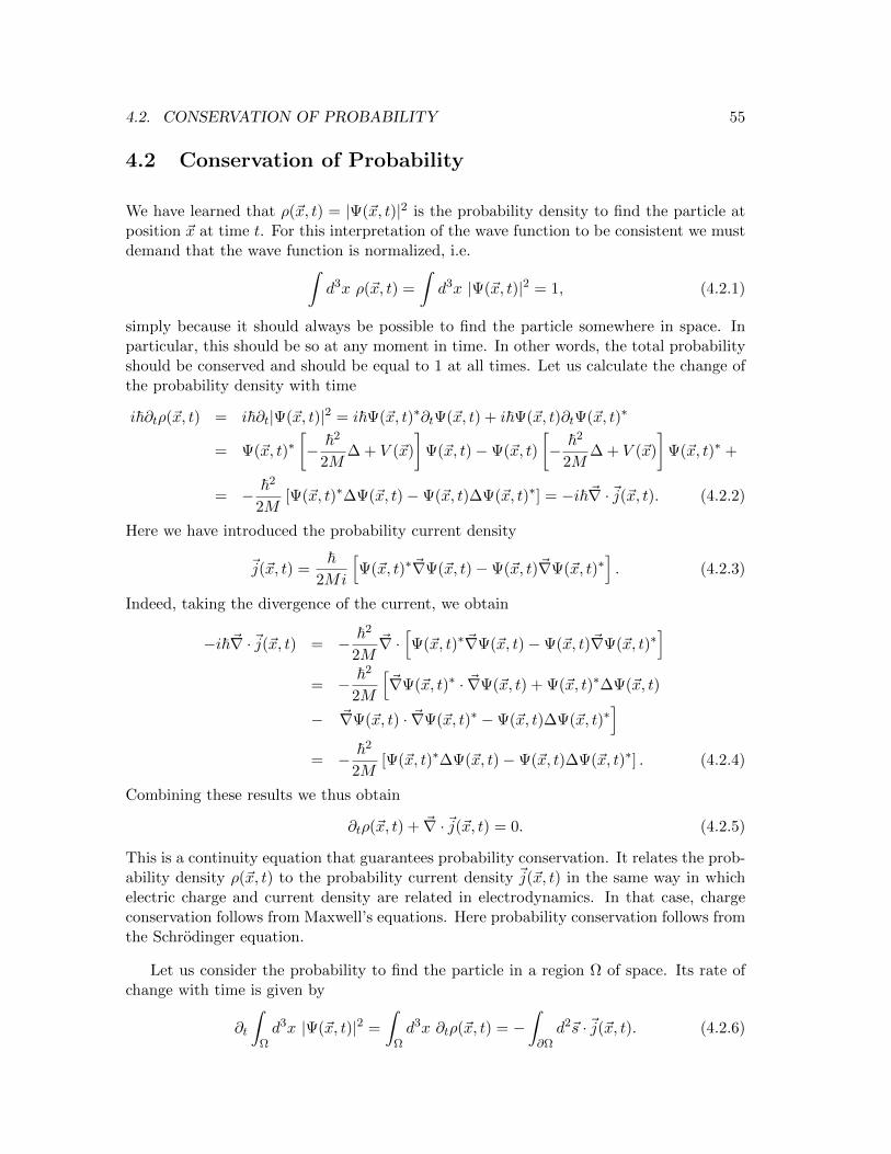
4.2. CONSERVATION OF PROBABILITY 55
4.2 Conservation of Probability
We have learned that ρ(~x, t) = |Ψ(~x, t)|2 is the probability density to find the particle atposition ~x at time t. For this interpretation of the wave function to be consistent we mustdemand that the wave function is normalized, i.e.∫
d3x ρ(~x, t) =
∫d3x |Ψ(~x, t)|2 = 1, (4.2.1)
simply because it should always be possible to find the particle somewhere in space. Inparticular, this should be so at any moment in time. In other words, the total probabilityshould be conserved and should be equal to 1 at all times. Let us calculate the change ofthe probability density with time
i~∂tρ(~x, t) = i~∂t|Ψ(~x, t)|2 = i~Ψ(~x, t)∗∂tΨ(~x, t) + i~Ψ(~x, t)∂tΨ(~x, t)∗
= Ψ(~x, t)∗[− ~2
2M∆ + V (~x)
]Ψ(~x, t)−Ψ(~x, t)
[− ~2
2M∆ + V (~x)
]Ψ(~x, t)∗ +
= − ~2
2M[Ψ(~x, t)∗∆Ψ(~x, t)−Ψ(~x, t)∆Ψ(~x, t)∗] = −i~~∇ ·~j(~x, t). (4.2.2)
Here we have introduced the probability current density
~j(~x, t) =~
2Mi
[Ψ(~x, t)∗~∇Ψ(~x, t)−Ψ(~x, t)~∇Ψ(~x, t)∗
]. (4.2.3)
Indeed, taking the divergence of the current, we obtain
−i~~∇ ·~j(~x, t) = − ~2
2M~∇ ·[Ψ(~x, t)∗~∇Ψ(~x, t)−Ψ(~x, t)~∇Ψ(~x, t)∗
]= − ~2
2M
[~∇Ψ(~x, t)∗ · ~∇Ψ(~x, t) + Ψ(~x, t)∗∆Ψ(~x, t)
− ~∇Ψ(~x, t) · ~∇Ψ(~x, t)∗ −Ψ(~x, t)∆Ψ(~x, t)∗]
= − ~2
2M[Ψ(~x, t)∗∆Ψ(~x, t)−Ψ(~x, t)∆Ψ(~x, t)∗] . (4.2.4)
Combining these results we thus obtain
∂tρ(~x, t) + ~∇ ·~j(~x, t) = 0. (4.2.5)
This is a continuity equation that guarantees probability conservation. It relates the prob-ability density ρ(~x, t) to the probability current density ~j(~x, t) in the same way in whichelectric charge and current density are related in electrodynamics. In that case, chargeconservation follows from Maxwell’s equations. Here probability conservation follows fromthe Schrodinger equation.
Let us consider the probability to find the particle in a region Ω of space. Its rate ofchange with time is given by
∂t
∫Ωd3x |Ψ(~x, t)|2 =
∫Ωd3x ∂tρ(~x, t) = −
∫∂Ωd2~s ·~j(~x, t). (4.2.6)

56 CHAPTER 4. THE SCHRODINGER EQUATION
Here we have used the Gauss law. The continuity equation tells us that the probabilityto find the particle in a region Ω can change only if there is a probability current flowingthrough the boundary ∂Ω of that region. Assuming that the probability current density~j(~x, t) vanishes at spatial infinity immediately implies that the total probability remainsconstant.
4.3 The Time-Independent Schrodinger Equation
We have seen that the Schrodinger equation governs the time evolution of the quantummechanical wave function. In many cases, however, one is interested in stationary solutionsof the Schrodinger equation, for example, in the stationary states of an atom. Also it turnsout that once one has found all stationary solutions of the Schrodinger equation, one canuse them to construct the general time-dependent solution. In a stationary state theprobability density ρ(~x, t) = |Ψ(~x, t)|2 = |Ψ(~x)|2 is time-independent. This does not meanthat Ψ(~x, t) is time-independent. In fact, it may still have a time-dependent phase. Hencewe make the ansatz
Ψ(~x, t) = Ψ(~x) exp(iϕ(t)). (4.3.1)
Inserting this in the Schrodinger equation implies
−~∂tϕ(t)Ψ(~x) exp(iϕ(t)) =
[− ~2
2M∆ + V (~x)
]Ψ(~x) exp(iϕ(t)). (4.3.2)
Dividing this equation by exp(iϕ(t)) one finds that the right-hand side becomes time-independent. Hence, the left-hand side should also be time-independent and thus
−~∂tϕ(t) = E, (4.3.3)
where E is a constant. Integrating this equation one obtains
ϕ(t) = −1
~Et, (4.3.4)
and thus
Ψ(~x, t) = Ψ(~x) exp
(− i~Et
). (4.3.5)
The remaining equation for the time-independent wave function Ψ(~x) takes the form[− ~2
2M∆ + V (~x)
]Ψ(~x) = EΨ(~x). (4.3.6)
This is the so-called time-independent Schrodinger equation. Identifying the Hamiltonoperator
H = − ~2
2M∆ + V (~x), (4.3.7)
we can also write it asHΨ(~x) = EΨ(~x). (4.3.8)

4.3. THE TIME-INDEPENDENT SCHRODINGER EQUATION 57
As we will soon understand, this can be viewed as an eigenvalue problem for the operatorH with the eigenvalue E and the eigenvector Ψ(~x). We can now calculate the expectationvalue of the Hamiltonian (the operator that describes the total energy). Using the time-independent Schrodinger equation we find∫
d3x Ψ(~x, t)∗HΨ(~x, t) =
∫d3x Ψ(~x)∗HΨ(~x) =
∫d3x E|Ψ(~x)|2 = E. (4.3.9)
This clarifies the meaning of the constant E. It is nothing but the total energy.

58 CHAPTER 4. THE SCHRODINGER EQUATION

Chapter 5
Square-Well Potentials andTunneling Effect
We now know enough quantum mechanics to go ahead and start applying it to physicalproblems. Doing quantum mechanics essentially means solving the Schrodinger equa-tion. As we will see in chapter 7, for time-independent Hamilton operators the gen-eral solution of the time-dependent Schrodinger equation follows from those of the time-independent Schrodinger equation. Hence, in this chapter we will concentrate on thetime-independent equation. For a general potential it may be difficult to solve the time-independent Schrodinger equation. In fact, in general one will not be able to find ananalytic solution, and hence one must then use some approximate numerical method.Still, there are a number of potentials for which the Schrodinger equation can be solvedanalytically, among them several examples in one dimension. Obviously, it is simpler towork in one than in three dimensions. This is the main reason for studying 1-dimensionalproblems in this chapter. We will learn techniques to solve the Schrodinger equation thatwill be useful also in two and three spatial dimensions. In this chapter we will solvethe 1-dimensional time-independent Schrodinger equation with square-well potentials. Inparticular, we will investigate a genuine quantum phenomenon — the so-called tunnelingeffect — which is classically forbidden, but allowed at the quantum level. We will alsoencounter a paradoxical quantum reflection problem, which we denote as the “quantumheight anxiety paradox”, and finally we will study a free particle moving on a circle.
5.1 Continuity Equation in One Dimension
As we have seen, quantum mechanical probability conservation is encoded in the continuityequation (4.2.5). In one spatial dimension the continuity equation takes the form
∂tρ(x, t) + ∂xj(x, t) = 0, (5.1.1)
59

60 CHAPTER 5. SQUARE-WELL POTENTIALS AND TUNNELING EFFECT
with the probability density ρ(x, t) = |Ψ(x, t)|2 and the probability current density
j(x, t) =~
2Mi[Ψ(x, t)∗∂xΨ(x, t)−Ψ(x, t)∂xΨ(x, t)∗] . (5.1.2)
As we learned from eq.(4.3.5), stationary solutions of the time-dependent Schrodingerequation with energy E take the factorized form
Ψ(x, t) = Ψ(x) exp
(− i~Et
), (5.1.3)
such that
ρ(x, t) = |Ψ(x)|2 = ρ(x) ⇒ ∂tρ(x, t) = ∂tρ(x) = 0. (5.1.4)
Furthermore,
j(x, t) =~
2Mi[Ψ(x)∗∂xΨ(x)−Ψ(x)∂xΨ(x)∗] = j(x), (5.1.5)
such that the continuity equation (5.1.1) reduces to
∂tρ(x, t) + ∂xj(x, t) = ∂xj(x) = 0 ⇒ j(x) = j. (5.1.6)
Hence, the probability current is, in fact, a constant j independent of x. States that arelocalized and thus do not extend to spatial infinity have Ψ(±∞) = 0, such that for themj = 0.
5.2 A Particle in a Box with Dirichlet Boundary Conditions
One of the simplest problems in quantum mechanics concerns a particle in a 1-dimensionalbox with perfectly reflecting walls. We can realize this situation by switching on a potentialthat is infinite everywhere outside an interval [0, a], and zero inside this interval. Theinfinite potential energy implies that the particle cannot exist outside the box, and henceΨ(x) = 0 for x /∈ [0, a]. Consequently, the constant probability current density j = 0 alsovanishes everywhere. This is consistent with the fact that the particle is indeed localizedinside the finite interval [0, a].
The most general boundary conditions that are consistent with the vanishing proba-bility current density are the so-called mixed or Robin boundary conditions
γ(0)Ψ(0) + ∂xΨ(0) = 0, γ(a)Ψ(a) + ∂xΨ(a) = 0, (5.2.1)
with γ(0), γ(a) ∈ R. Indeed, the probability current density at x = 0 then takes the form
j(0) =~
2Mi[Ψ(0)∗∂xΨ(0)−Ψ(0)∂xΨ(0)∗]
=~
2Mi[−Ψ(0)∗γΨ(0) + Ψ(0)γ(0)∗Ψ(0)∗] = 0. (5.2.2)
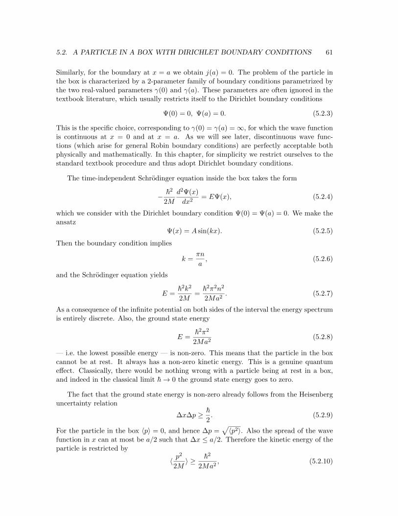
5.2. A PARTICLE IN A BOX WITH DIRICHLET BOUNDARY CONDITIONS 61
Similarly, for the boundary at x = a we obtain j(a) = 0. The problem of the particle inthe box is characterized by a 2-parameter family of boundary conditions parametrized bythe two real-valued parameters γ(0) and γ(a). These parameters are often ignored in thetextbook literature, which usually restricts itself to the Dirichlet boundary conditions
Ψ(0) = 0, Ψ(a) = 0. (5.2.3)
This is the specific choice, corresponding to γ(0) = γ(a) =∞, for which the wave functionis continuous at x = 0 and at x = a. As we will see later, discontinuous wave func-tions (which arise for general Robin boundary conditions) are perfectly acceptable bothphysically and mathematically. In this chapter, for simplicity we restrict ourselves to thestandard textbook procedure and thus adopt Dirichlet boundary conditions.
The time-independent Schrodinger equation inside the box takes the form
− ~2
2M
d2Ψ(x)
dx2= EΨ(x), (5.2.4)
which we consider with the Dirichlet boundary condition Ψ(0) = Ψ(a) = 0. We make theansatz
Ψ(x) = A sin(kx). (5.2.5)
Then the boundary condition implies
k =πn
a, (5.2.6)
and the Schrodinger equation yields
E =~2k2
2M=
~2π2n2
2Ma2. (5.2.7)
As a consequence of the infinite potential on both sides of the interval the energy spectrumis entirely discrete. Also, the ground state energy
E =~2π2
2Ma2(5.2.8)
— i.e. the lowest possible energy — is non-zero. This means that the particle in the boxcannot be at rest. It always has a non-zero kinetic energy. This is a genuine quantumeffect. Classically, there would be nothing wrong with a particle being at rest in a box,and indeed in the classical limit ~→ 0 the ground state energy goes to zero.
The fact that the ground state energy is non-zero already follows from the Heisenberguncertainty relation
∆x∆p ≥ ~2. (5.2.9)
For the particle in the box 〈p〉 = 0, and hence ∆p =√〈p2〉. Also the spread of the wave
function in x can at most be a/2 such that ∆x ≤ a/2. Therefore the kinetic energy of theparticle is restricted by
〈 p2
2M〉 ≥ ~2
2Ma2, (5.2.10)
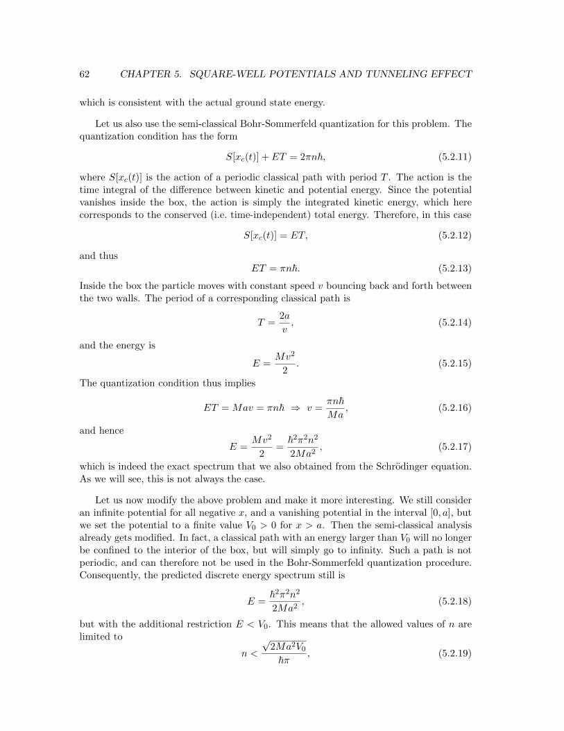
62 CHAPTER 5. SQUARE-WELL POTENTIALS AND TUNNELING EFFECT
which is consistent with the actual ground state energy.
Let us also use the semi-classical Bohr-Sommerfeld quantization for this problem. Thequantization condition has the form
S[xc(t)] + ET = 2πn~, (5.2.11)
where S[xc(t)] is the action of a periodic classical path with period T . The action is thetime integral of the difference between kinetic and potential energy. Since the potentialvanishes inside the box, the action is simply the integrated kinetic energy, which herecorresponds to the conserved (i.e. time-independent) total energy. Therefore, in this case
S[xc(t)] = ET, (5.2.12)
and thusET = πn~. (5.2.13)
Inside the box the particle moves with constant speed v bouncing back and forth betweenthe two walls. The period of a corresponding classical path is
T =2a
v, (5.2.14)
and the energy is
E =Mv2
2. (5.2.15)
The quantization condition thus implies
ET = Mav = πn~ ⇒ v =πn~Ma
, (5.2.16)
and hence
E =Mv2
2=
~2π2n2
2Ma2, (5.2.17)
which is indeed the exact spectrum that we also obtained from the Schrodinger equation.As we will see, this is not always the case.
Let us now modify the above problem and make it more interesting. We still consideran infinite potential for all negative x, and a vanishing potential in the interval [0, a], butwe set the potential to a finite value V0 > 0 for x > a. Then the semi-classical analysisalready gets modified. In fact, a classical path with an energy larger than V0 will no longerbe confined to the interior of the box, but will simply go to infinity. Such a path is notperiodic, and can therefore not be used in the Bohr-Sommerfeld quantization procedure.Consequently, the predicted discrete energy spectrum still is
E =~2π2n2
2Ma2, (5.2.18)
but with the additional restriction E < V0. This means that the allowed values of n arelimited to
n <
√2Ma2V0
~π, (5.2.19)

5.2. A PARTICLE IN A BOX WITH DIRICHLET BOUNDARY CONDITIONS 63
and only a finite set of discrete energy values exists.
Let us see what the Schrodinger equation implies for the modified problem. First, let usagain assume that E < V0. Again using Dirichlet boundary conditions, the wave functionmust still vanish at x = 0. However, it can now extend into the classically forbidden regionx > a. In that region the Schrodinger equation takes the form
− ~2
2M
d2Ψ(x)
dx2+ V0Ψ(x) = EΨ(x), (5.2.20)
such thatd2Ψ(x)
dx2=
2M(V0 − E)
~2Ψ(x). (5.2.21)
We make the ansatzΨ(x) = B exp(−κx), (5.2.22)
and obtain
κ = ±√
2M(V0 − E)
~. (5.2.23)
Only the positive solution is physical because it corresponds to an exponentially decayingnormalizable wave function. The other solution is exponentially rising, and thus notnormalizable. Inside the box the solution of the Schrodinger equation still takes the form
Ψ(x) = A sin(kx), (5.2.24)
but now the wave function need not vanish at x = a. Later we will discuss the mostgeneral boundary condition that can be imposed in case of a finite potential step. In thischapter, we again restrict ourselves to the standard textbook procedure by demandingthat both the wave function and its first derivative are continuous at x = a. This implies
A sin(ka) = B exp(−κa), Ak cos(ka) = −Bκ exp(−κa), (5.2.25)
and thusκ = −k cot(ka). (5.2.26)
We can also use the relations for k and κ and obtain
k2 + κ2 =2ME
~2+
2M(V0 − E)
~2=
2MV0
~2. (5.2.27)
This equation describes a circle of radius√
2MV0/~ in the k-κ-plane, which suggests agraphical method to solve for the energy spectrum. In fact, plotting κ = −k cot(ka) aswell as the circle yields the quantized energies as the intersections of the two curves. Thecondition for at least n intersections to exist is
√2MV0
~>π
a
(n− 1
2
). (5.2.28)
For n = 1 this implies
V0 >~2π2
8Ma2. (5.2.29)
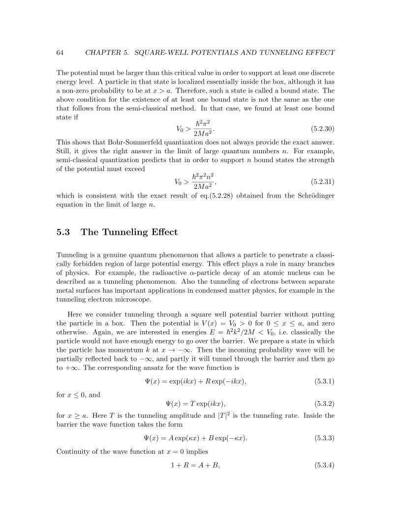
64 CHAPTER 5. SQUARE-WELL POTENTIALS AND TUNNELING EFFECT
The potential must be larger than this critical value in order to support at least one discreteenergy level. A particle in that state is localized essentially inside the box, although it hasa non-zero probability to be at x > a. Therefore, such a state is called a bound state. Theabove condition for the existence of at least one bound state is not the same as the onethat follows from the semi-classical method. In that case, we found at least one boundstate if
V0 >~2π2
2Ma2. (5.2.30)
This shows that Bohr-Sommerfeld quantization does not always provide the exact answer.Still, it gives the right answer in the limit of large quantum numbers n. For example,semi-classical quantization predicts that in order to support n bound states the strengthof the potential must exceed
V0 >~2π2n2
2Ma2, (5.2.31)
which is consistent with the exact result of eq.(5.2.28) obtained from the Schrodingerequation in the limit of large n.
5.3 The Tunneling Effect
Tunneling is a genuine quantum phenomenon that allows a particle to penetrate a classi-cally forbidden region of large potential energy. This effect plays a role in many branchesof physics. For example, the radioactive α-particle decay of an atomic nucleus can bedescribed as a tunneling phenomenon. Also the tunneling of electrons between separatemetal surfaces has important applications in condensed matter physics, for example in thetunneling electron microscope.
Here we consider tunneling through a square well potential barrier without puttingthe particle in a box. Then the potential is V (x) = V0 > 0 for 0 ≤ x ≤ a, and zerootherwise. Again, we are interested in energies E = ~2k2/2M < V0, i.e. classically theparticle would not have enough energy to go over the barrier. We prepare a state in whichthe particle has momentum k at x → −∞. Then the incoming probability wave will bepartially reflected back to −∞, and partly it will tunnel through the barrier and then goto +∞. The corresponding ansatz for the wave function is
Ψ(x) = exp(ikx) +R exp(−ikx), (5.3.1)
for x ≤ 0, andΨ(x) = T exp(ikx), (5.3.2)
for x ≥ a. Here T is the tunneling amplitude and |T |2 is the tunneling rate. Inside thebarrier the wave function takes the form
Ψ(x) = A exp(κx) +B exp(−κx). (5.3.3)
Continuity of the wave function at x = 0 implies
1 +R = A+B, (5.3.4)
5.3. THE TUNNELING EFFECT 65
and continuity of its derivative yields
ik(1−R) = κ(A−B), (5.3.5)
which implies
2A = 1 +R+ik
κ(1−R), 2B = 1 +R− ik
κ(1−R). (5.3.6)
Similarly, at x = a we obtain
T exp(ika) = A exp(κa) +B exp(−κa), (5.3.7)
as well as
ikT exp(ika) = Aκ exp(κa)−Bκ exp(−κa), (5.3.8)
and thus
T exp(ika)
(1 +
ik
κ
)= 2A exp(κa) =
[1 +
ik
κ+R
(1− ik
κ
)]exp(κa),
T exp(ika)
(1− ik
κ
)= 2B exp(−κa) =
[1− ik
κ+R
(1 +
ik
κ
)]exp(−κa).
Eliminating R from these equations we obtain
T exp(ika)
[(1 +
ik
κ
)2
exp(−κa)−(
1− ik
κ
)2
exp(κa)
]=
(1 +
ik
κ
)2
−(
1− ik
κ
)2
,
(5.3.9)which results in
T = exp(−ika)2ikκ
(k2 − κ2) sinh(κa) + 2ikκ cosh(κa). (5.3.10)
The tunneling rate then takes the form
|T |2 =4k2κ2
(k2 + κ2)2 sinh2(κa) + 4k2κ2. (5.3.11)
In the limit of a large barrier (κa→∞) the tunneling rate is exponentially suppressed
|T |2 =16k2κ2
(k2 + κ2)2exp(−2κa). (5.3.12)
The most important term is the exponential suppression factor. The prefactor representsa small corrections to this leading effect, and hence we can write approximately
|T |2 ≈ exp(−2κa) = exp
(−2a
√2M
~2[V0 − E]
). (5.3.13)

66 CHAPTER 5. SQUARE-WELL POTENTIALS AND TUNNELING EFFECT
5.4 Semi-Classical Instanton Formula
In practical applications tunneling barriers in general do not have square well shapes.Therefore, let us now turn to tunneling through an arbitrary potential barrier. Thenwe will, in general, not be able to solve the Schrodinger equation exactly. Still, we canperform a semi-classical approximation (similar to Bohr-Sommerfeld quantization) and ob-tain a closed expression for the tunneling rate. Of course, in contrast to Bohr-Sommerfeldquantization, for a tunneling process no corresponding classical path exists, simply becausetunneling is forbidden at the classical level. Still, as we will see, classical mechanics atpurely imaginary “time” will provide us with a tunneling path. The concept of imaginaryor so-called Euclidean time plays an important role in the modern treatment of quantumfield theories, which simplifies the mathematics of path integrals. Also here imaginarytime is just a mathematical trick to derive an expression for the tunneling rate in a simplemanner. We should keep in mind that in real time there is no classical path that describesthe tunneling process. Let us write the tunneling amplitude as
T = exp
(i
~(S[x(t)] + EtT )
). (5.4.1)
This expression follows from Feynman’s path integral in the same way as Bohr-Sommerfeldquantization. In that case the action was to be evaluated for a classical path xc(t) withperiod T . Here a tunneling path x(t) occurs instead, and the period T is replaced bythe tunneling time tT . Note again that in this calculation T represents the tunnelingamplitude and not a time period. How is the tunneling path determined? Let us justconsider energy conservation, and then let mathematics be our guide
E =M
2
(dx(t)
dt
)2
+ V (x(t)). (5.4.2)
This classical equation has no physically meaningful solution because now E < V (x(t)),and hence formally the kinetic energy would be negative. Mathematically we can makesense of
M
2
(dx(t)
dt
)2
= E − V (x(t)) < 0, (5.4.3)
if we replace real time t by imaginary “time” it. Then the above equation takes the form
−M2
(dx(t)
d(it)
)2
= E − V (x(t)) < 0, (5.4.4)
which is perfectly consistent. The effect of using imaginary time is the same as changingE − V (x(t)), which is negative, into V (x(t))−E. Hence, the tunneling path in imaginarytime would be the classical path in an inverted potential. Next we write
S[x(t)] + EtT =
∫ tT
0dt
[M
2
(dx(t)
dt
)2
− V (x(t)) + E
]=
∫ tT
0dt 2[E − V (x(t)]. (5.4.5)

5.5. REFLECTION AT A POTENTIAL STEP 67
Here we have just used the energy conservation equation from above. Next we turn theintegral over t into an integral over x between the classical turning points x(0) and x(tT )at which V (x) = E. Then
S[x(t)] + EtT =
∫ x(tT )
x(0)dx
1
dx(t)/dt2[E − V (x(t)]. (5.4.6)
Using
dx(t)
dt=
√2
M[E − V (x(t))] = i
√2
M[V (x(t))− E], (5.4.7)
we thus obtain
T = exp
(i
~(S[x(t)] + EtT )
)= exp
(−1
~
∫ x(tT )
x(0)dx√
2M [V (x)− E]
). (5.4.8)
For the square well potential from before the classical turning points are x(0) = 0 andx(tT ) = a. Hence, the tunneling rate then takes the form
|T |2 = exp(−2
~
∫ x(tT )
x(0)dx√
2M [V (x)− E]) = exp
(−2a
~√
2M [V0 − E]
), (5.4.9)
in complete agreement with our previous approximate result eq.(5.3.13).
5.5 Reflection at a Potential Step
We have seen that quantum mechanics differs from classical mechanics because a quantumparticle can tunnel through a classically forbidden region. A similar non-classical behavioroccurs when a particle is reflected from a potential step. Let us consider a potential whichis zero for x ≤ 0, and constant and repulsive for x ≥ 0, i.e. V (x) = V0 > 0. Let usconsider energies E > V0 that are sufficient to step over the barrier classically. Thenclassically a particle that is coming from −∞ would just slow down at x = 0 and continueto move to +∞ with a reduced kinetic energy. Classically there would be no reflectionin this situation. Still, quantum mechanically there is a probability for the particle tobe reflected despite the fact that it has enough energy to continue to +∞. We make thefollowing ansatz for the wave function at x ≤ 0
Ψ(x) = exp(ikx) +R exp(−ikx), (5.5.1)
while for x ≥ 0 we writeΨ(x) = T exp(iqx). (5.5.2)
We have not included a wave exp(−iqx) at x ≥ 0 because we are describing an experimentin which the particle is coming in only from the left. The energy is given by
E =~2k2
2M=
~2q2
2M+ V0. (5.5.3)

68 CHAPTER 5. SQUARE-WELL POTENTIALS AND TUNNELING EFFECT
Next we impose continuity conditions for both the wave function and its first derivative
1 +R = T, ik(1−R) = iqT ⇒ 1−R =q
kT. (5.5.4)
Solving these equations yields
T =2k
k + q, R =
k − qk + q
. (5.5.5)
The reflection rate |R|2 vanishes only when k = q. This happens either if the potentialvanishes (V0 = 0) or if the energy goes to infinity. Otherwise, there is a non-zero probabilityfor the particle to be reflected back to −∞.
Let us look at the above problem from the point of view of probability conservation.For time-independent 1-dimensional problems the continuity equation reduces to
∂xj(x) = 0 ⇒ j(x) = j, (5.5.6)
i.e. the current
j(x) =~
2iM[Ψ(x)∗∂xΨ(x)−Ψ(x)∂xΨ(x)∗] , (5.5.7)
should then be a constant j (independent of x). Let us calculate the current for theproblem from before. First, we consider x ≤ 0 and we obtain
j(x) =~k2M[exp(−ikx) +R∗ exp(ikx)][exp(ikx)−R exp(−ikx)]
− [exp(ikx) +R exp(−ikx)][− exp(−ikx) +R∗ exp(ikx)]
=~kM
(1− |R|2). (5.5.8)
For x ≥ 0, on the other hand, we find
j(x) =~q
2M[T ∗ exp(−ikx)T exp(ikx)− T exp(ikx)T ∗ exp(−ikx)] =
~qM|T |2. (5.5.9)
Indeed, both currents are independent of x. In addition, they are equal (as they should)because
k(1− |R|2) = k
[1−
(k − qk + q
)2]
=4k2q
(k + q)2= q|T |2. (5.5.10)
5.6 Quantum Height Anxiety Paradox
We have seen that quantum mechanically particles behave differently than in classicalphysics. For example, a classical billiard ball will never tunnel through a region of potentialenergy higher than its total energy, and it will never get reflected from a region of potentialenergy lower than its total energy. Let us go back to the problem with the potential stepfrom before. However, now we want the particle to step down in energy, in other words,

5.6. QUANTUM HEIGHT ANXIETY PARADOX 69
now V0 < 0. Certainly, a classical billiard ball incident from −∞ would enter the regionof decreased potential energy, thereby increasing its kinetic energy, and would then moveto +∞. In particular, it would not be reflected back to −∞. Let us see what happensquantum mechanically. In the previous calculation with the potential step we have neverused the fact that V0 > 0. Therefore our result is equally valid for V0 < 0. Hence, again
T =2k
k + q, R =
k − qk + q
. (5.6.1)
Let us take the limit of a very deep potential step (V0 → −∞). Then q →∞ and thus
T → 0, R→ −1, (5.6.2)
such that the transmission rate is zero and the reflection rate is |R|2 = 1. This is theexact opposite of what happens classically. The quantum particle stops at the top of thepotential step and turns back, instead of entering the region of very low potential energy,as a classical particle would certainly do. One may want to call this the “quantum heightanxiety paradox” because the quantum particle steps back into the region of high potentialenergy, while a classical billiard ball would happily jump down the cliff. It is obvious thatsomething is wrong in this discussion. Quantum mechanics may give different results thanclassical physics, but the results should not differ as much as in this paradox. In particular,in the classical limit ~ → 0 quantum mechanics should give the same result as classicalmechanics. This is certainly not the case in this paradox. In fact, our result for R doesnot even depend on ~. Hence, taking the classical limit does not change the answer: theparticle would still turn around instead of going forward.
The above paradox gets resolved when we consider a potential that interpolates moresmoothly between the regions of large and small potential energies. As we will see, theabrupt step function change in the potential is responsible for the paradox, and we shouldhence be careful in general when we use square well potentials. Still, they are the simplestpotentials for which the Schrodinger equation can be solved in closed form, and theytherefore are quite useful for learning quantum mechanics. To understand why the stepfunction is special, let us smear out the step over some length scale a by writing thepotential as
V (x) = V0f(x/a), (5.6.3)
where f is a smooth function that interpolates between f(−∞) = 0 and f(+∞) = −1,which in the limit a → 0 approaches the step function. The Schrodinger equation withthe smooth potential takes the form
− ~2
2M
d2Ψ(x)
dx2+ V0f(x/a)Ψ(x) = EΨ(x). (5.6.4)
Dividing the equation by V0 and introducing the dimensionless variable
y =√
2MV0/~2x, (5.6.5)
one obtains
−d2Ψ(y)
dy2+ f(y/
√2Ma2V0/~2)Ψ(y) =
E
V0Ψ(y). (5.6.6)
70 CHAPTER 5. SQUARE-WELL POTENTIALS AND TUNNELING EFFECT
This rescaled form of the Schrodinger equation shows that the reflection rate |R|2 onlydepends on E/V0 and on the combination 2Ma2V0/~2. In particular, now the limit V0 →∞ is equivalent to the classical limit ~ → 0 as well as to the limit a → ∞ of a verywide potential step. This is exactly what one would expect. The paradox arises onlyin the case of a true step function which has a = 0. Only then ~ disappears from therescaled equations, and we do not get a meaningful result in the classical limit. In fact,an arbitrarily small amount of smearing of the potential step is sufficient to eliminate theparadox.
5.7 Free Particle on a Circle
Let us apply the time-independent Schrodinger equation to a simple problem — a particleof mass M moving on a circle of radius R. The position of the particle can then becharacterized by an angle ϕ and we can identify x = Rϕ. The Hamilton operator hencetakes the form
H = − ~2
2M∂2x = − ~2
2MR2∂2ϕ = −~2
2I∂2ϕ. (5.7.1)
Here we have introduced I = MR2 — the moment of inertia of the quantum mechanicalrotor represented by the particle. We can now write the time-independent Schrodingerequation as
−~2
2I∂2ϕΨ(ϕ) = EΨ(ϕ). (5.7.2)
Since the particle is moving on a circle, the angles ϕ = 0 and ϕ = 2π correspond to thesame point. Hence, we must impose periodic boundary conditions for the wave function,i.e.
Ψ(ϕ+ 2π) = Ψ(ϕ). (5.7.3)
Now we make the ansatz
Ψ(ϕ) = A exp(imϕ). (5.7.4)
Periodicity of the wave function implies that m ∈ Z. Inserting the ansatz in the time-independent Schrodinger equation yields
E =~2
2Im2, (5.7.5)
i.e. only a discrete set of energies is allowed for stationary states. Also it is interestingthat the two states with quantum numbers m and −m have the same energy — theyare degenerate with each other. What is the probability density to find the particle at aparticular angle ϕ when it is in the stationary state with quantum number m? We simplysquare the wave function and find
|Ψ(ϕ)|2 = |A exp(imϕ)|2 = |A|2. (5.7.6)
5.8. FREE PARTICLE ON A DISCRETIZED CIRCLE 71
This is independent of the angle ϕ and hence independent of the position on the circle.This result is plausible because no point on the circle is singled out, the particle appearseverywhere with the same probability. Properly normalizing the wave function, we obtain∫ 2π
0dϕ |Ψ(ϕ)|2 = 2π|A|2 = 1 ⇒ A =
1√2π. (5.7.7)
The quantum number m is related to the angular momentum of the particle. Theoperator for the linear momentum is px = −i~∂x. Using x = Rϕ we identify
pϕ = − i~R∂ϕ. (5.7.8)
For circular motion the angular momentum is given by L = Rpϕ. Hence, the quantummechanical angular momentum operator is identified as
L = −i~∂ϕ. (5.7.9)
When we operate with L on the wave function with quantum number m we find
LΨ(ϕ) = −i~∂ϕA exp(imϕ) = m~Ψ(ϕ). (5.7.10)
We see that Ψ(ϕ) is an eigenvector of the angular momentum operator with eigenvaluem~, i.e. in quantum mechanics also angular momentum is quantized.
5.8 Free Particle on a Discretized Circle
In order to understand better why the time-independent Schrodinger equation correspondsto an eigenvalue problem, let us now discuss the dynamics of a free particle on a discretizedcircle. We allow the particle to sit only at the discrete angles
ϕn = nδϕ =2πn
N, δϕ =
2π
N, (5.8.1)
where N is some positive integer. In the limit N →∞ we recover the case of the continuouscircle that we discussed before. With only discrete points available, the particle is nowhopping from one point to a neighboring point. The wave function then also has valuesonly at the discrete angles ϕn, i.e. Ψ(ϕ)→ Ψ(ϕn). The Hamilton operator that contains asecond derivative with respect to the angle ϕ cannot be applied to such a discretized wavefunction. Consequently, the second derivative — and hence the Hamiltonian — must bediscretized as well. A discretized second derivative takes the form
∆ϕΨ(ϕn) =Ψ(ϕn+1)− 2Ψ(ϕn) + Ψ(ϕn−1)
δϕ2. (5.8.2)
Thus we can write the discretized time-independent Schrodinger equation as
−~2
2I∆ϕΨ(ϕn) = −~2
2I
Ψ(ϕn+1)− 2Ψ(ϕn) + Ψ(ϕn−1)
δϕ2= EΨ(ϕn). (5.8.3)

72 CHAPTER 5. SQUARE-WELL POTENTIALS AND TUNNELING EFFECT
This equation can be expressed in matrix form as
~2
2Iδϕ2
2 −1 0 ... −1−1 2 −1 ... 00 −1 2 ... 0. . . .. . . .. . . .−1 0 0 ... 2
Ψ(ϕ1)Ψ(ϕ2)Ψ(ϕ3)...
Ψ(ϕN )
= E
Ψ(ϕ1)Ψ(ϕ2)Ψ(ϕ3)...
Ψ(ϕN )
. (5.8.4)
The entries −1 in the upper right and lower left corners of the matrix are due to periodicboundary conditions on the circle. We see that the Hamilton operator is represented byan N ×N matrix, while the wave function Ψ(ϕ) has turned into an N -component vector.In the continuum limit N → ∞ the dimension of the corresponding vector space goes toinfinity and the vector space turns into a so-called Hilbert space.
The above matrix equation only has trivial solutions Ψ(ϕn) = 0 for generic values ofE. This can be understood as follows. Let us write
HΨ = EΨ, (5.8.5)
as
H11 − E H12 H13 ... H1N
H21 H22 − E H23 ... H2N
H31 H32 H33 − E ... H3N
. . . .
. . . .
. . . .HN1 HN2 HN3 ... HNN − E
Ψ(ϕ1)Ψ(ϕ2)Ψ(ϕ3)...
Ψ(ϕN )
= 0. (5.8.6)
This equation implies that the columns of the matrix (H − E1) are linearly dependent.This is possible only if the determinant of the matrix is zero, i.e.
det(H − E1) =
N∑n=0
hnEn = 0. (5.8.7)
Here the coefficients hn depend on the matrix elements of H and define the characteristicpolynomial of H. For generic values of E the characteristic polynomial — and hencethe determinant of (H − E1) — does not vanish and hence the equation HΨ = EΨdoes not have a non-trivial solution. Only for special discrete values of E the abovedeterminant vanishes and non-trivial solutions exist. These eigenvalues are the zeros ofthe characteristic polynomial of H. The corresponding non-trivial solutions of the abovematrix problem are the eigenvectors.

Chapter 6
Spin, Precession, and theStern-Gerlach Experiment
Until now we have discussed how quantum physics manifests itself for point particles thatcan be described classically by their position and momentum. In this chapter, we willdiscuss quantum systems that have no classical counterpart, because they involve a fun-damental discrete degree of freedom, known as spin, which is of intrinsically quantumand thus of non-classical nature. Spin is an intrinsic quantum mechanical angular mo-mentum of elementary particles, which gives rise to a magnetic moment that can interactwith an external magnetic field. This results in spin precession and manifests itself in theStern-Gerlach experiment.
6.1 Quantum Spin
Elementary particles fall into two categories: bosons and fermions. As we already learnedin chapter 2, bosons and fermions obey different forms of quantum statistics: an arbitrarynumber of bosons but at most a single fermion can occupy the same quantum state. Besidesin their statistics, bosons and fermions also differ in their spin, which is a discrete quantumdegree of freedom, that plays the role of an intrinsic angular momentum. While bosonshave integer spin 0, 1, 2, . . . (in units of ~), fermions have half-integer spin 1
2 ,32 ,
52 , . . . .
In particular, all known truly elementary fermions including electrons, neutrinos, andquarks have spin 1
2 . Even composite objects like protons and neutrons, which consistof three quarks, have spin 1
2 , while some extremely short-lived elementary particles —known as ∆-isobars — which also consist of three quarks, have spin 3
2 . All currentlyknown truly fundamental bosons, namely photons, W- and Z-bosons, and gluons havespin 1. The Higgs particle, which plays a central role in the standard model of particlephysics, and has recently been detected at the LHC at CERN, has spin 0, but may not betruly fundamental. Finally, gravitons, the hypothetical quanta of the gravitational field,should have spin 2, but interact so weakly that there is little hope to detect them in the
73

74CHAPTER 6. SPIN, PRECESSION, AND THE STERN-GERLACH EXPERIMENT
foreseeable future. In this section, we limit ourselves to the simplest non-trivial spin 12
which is relevant for elementary fermions.
As we have learned already, we should not think of elementary particles as tiny billiardballs. This implies that one should not think of elementary particles with spin as tinyspinning tops. Such classical pictures do not help in the quantum world and often aremisleading. A correct way of thinking about spin is to view it as a discrete quantumdegree of freedom, which has no classical analog. While at the classical level an electronis described just by its position and momentum, at the quantum level a new degree offreedom — the electron’s spin — reveals itself. An electron can exist in two states: spinup (↑) and spin down (↓). However, as a quantum object, an electron can also exist in astate that is a superposition of spin up and spin down.
In this chapter, we concentrate entirely on the discrete spin degree of freedom ofan elementary particle, and we decouple the classical degrees of freedom, such as thecontinuous particle coordinate ~x. Discussing spin and position independently is completelyjustified in non-relativistic quantum mechanics, because the interactions between orbitalmotion and spin — the so-called spin-orbit couplings — are of relativistic nature. Indeedthe nature of the spin as an intrinsic angular momentum of elementary particles manifestsitself only through relativistic effects. For this reason, one sometimes reads that the spinitself is of relativistic origin. This is somewhat misleading because, first and foremost,spin is a most important quantum degree of freedom that has drastic implications evenin non-relativistic physics. However, it is true that relativity theory sheds an entirelynew light on spin, by revealing its nature as an intrinsic angular momentum. We willaddress these issues when we discuss the Pauli equation (which is an approximation tothe fully relativistic Dirac equation). In the context of relativistic quantum field theories,which goes far beyond the scope of this text, one can derive the spin-statistics theoremwhich shows that particles with Bose statistics necessarily have integer spin, while Fermistatistics is associated with half-integer spin. Here we treat spin from a non-relativisticpoint of view. Then it just describes a new quantum degree of freedom, not obviouslyrelated to angular momentum.
It is best to speak about spin in the appropriate language, which clearly is mathematics.Hence, let us now define mathematically what spin is. Until now, ignoring spin, wehave described the quantum state of an electron by a wave function Ψ(~x), which is aprobability amplitude depending on the continuous classical position degree of freedom ~xof the electron. Since electrons are fundamental fermions, they have an additional discretequantum degree of freedom — the spin s ∈ ↑, ↓. Hence, the quantum state of an electronis actually described by a 2-component wave function known as a Pauli spinor
Ψ(~x) =
(Ψ↑(~x)Ψ↓(~x)
). (6.1.1)
The component Ψs(~x) is the probability amplitude for finding the electron at the position~x with the spin s. Correspondingly, the correct normalization condition for a Pauli spinor

6.1. QUANTUM SPIN 75
is given by ∫d3x Ψ(~x)†Ψ(~x) =
∫d3x
(|Ψ↑(~x)|2 + |Ψ↓(~x)|2
)= 1. (6.1.2)
Here we have introduced the complex conjugated and transposed spinor
Ψ(~x)† = (Ψ↑(~x)∗,Ψ↓(~x)∗) . (6.1.3)
For example, the probability to find the electron anywhere in space with spin up is givenby
P↑ =
∫d3x|Ψ↑(~x)|2, (6.1.4)
while the probability to find it in a finite region Ω with spin down is
P↓(Ω) =
∫Ωd3x|Ψ↓(~x)|2. (6.1.5)
On the one hand, spin is an additional label s =↑, ↓ on the wave function of an electron.On the other hand, there is also a spin operator
~S = (Sx, Sy, Sz) =~2~σ =
~2
(σx, σy, σz), (6.1.6)
representing a vector of physical observables, whose components are the 2×2 Pauli matrices
σx =
(0 11 0
), σy =
(0 −ii 0
), σz =
(1 00 −1
). (6.1.7)
The Pauli matrices are invariant under transposition combined with complex conjugation.The spin operator acts on a Pauli spinor by matrix multiplication. The expectation valueof the spin operator in the state Ψ(~x) is given by
〈~S〉 =
∫d3x Ψ(~x)†~SΨ(~x). (6.1.8)
For example, the third component of the spin operator acts on a Pauli spinor as
SzΨ(~x) =~2
(1 00 −1
)(Ψ↑(~x)Ψ↓(~x)
)=
~2
(Ψ↑(~x)−Ψ↓(~x)
), (6.1.9)
such that
〈Sz〉 =~2
∫d3x
(|Ψ↑(~x)|2 − |Ψ↓(~x)|2
). (6.1.10)
Eigenstates of the operator Sz must obey Szχ(~x) = szχ(~x), where sz is the correspondingeigenvalue. This implies
Szχ(~x) =~2
(χ↑(~x)−χ↓(~x)
)= sz
(χ↑(~x)χ↓(~x)
). (6.1.11)
76CHAPTER 6. SPIN, PRECESSION, AND THE STERN-GERLACH EXPERIMENT
The two possible eigenvalues are sz = ±~/2 and the corresponding eigenstates are
χ+(~x) =
(χ↑(~x)
0
)= χ↑(~x)
(10
), χ−(~x) =
(0
χ↓(~x)
)= χ↓(~x)
(01
). (6.1.12)
Irrespective of the form of the spatial wave functions χ↑(~x) and χ↓(~x), the Pauli spinorsχ+(~x) and χ−(~x) are always eigenstates of Sz. The eigenstates of Sz are not simultaneouslyeigenstates of Sx or Sy, in particular,
Sx
(10
)=
~2
(0 11 0
)(10
)=
~2
(01
),
Sx
(01
)=
~2
(0 11 0
)(01
)=
~2
(10
),
Sy
(10
)=
~2
(0 −ii 0
)(10
)=
~2
(0i
),
Sy
(01
)=
~2
(0 −ii 0
)(01
)=
~2
(−i0
). (6.1.13)
This is due to the fact that the different components of the spin operator do not commutewith each other. We define the so-called commutator of two quantum mechanical operatorsA and B as
[A,B] = AB −BA. (6.1.14)
By straightforward matrix multiplication one then obtains
[Sx, Sy] =~2
4
(0 11 0
)(0 −ii 0
)−(
0 −ii 0
)(0 11 0
)= i
~2
2
(1 00 −1
)= i~Sz,
[Sy, Sz] =~2
4
(0 −ii 0
)(1 00 −1
)−(
1 00 −1
)(0 −ii 0
)= i
~2
2
(0 11 0
)= i~Sx,
[Sz, Sx] =~2
4
(1 00 −1
)(0 11 0
)−(
0 11 0
)(1 00 −1
)= i
~2
2
(0 −ii 0
)= i~Sy. (6.1.15)
Using the totally anti-symmetric Levi-Civita tensor, these relations can be summarized as
[Si, Sj ] = i~εijkSk. (6.1.16)
As we will see later, these are the same commutation relations as the ones of the quantummechanical orbital angular momentum operator. This is consistent with the fact that spinwill turn out to be an intrinsic (non-orbital) angular momentum of elementary particles.This aspect of spin is, however, only revealed through relativistic effects.
6.2. NEUTRON SPIN PRECESSION IN A MAGNETIC FIELD 77
6.2 Neutron Spin Precession in a Magnetic Field
In the same way as the momentum of a particle can be affected by external forces, the spinof a particle can be affected by an external magnetic field. Of course, via the Lorentz force,magnetic fields also affect the momentum of a charged particle. To simplify the situation,here we limit ourselves to neutral particles with spin. The neutron, which together withprotons forms atomic nuclei, indeed is a neutral particle with spin 1
2 . The Hamilton
operator that describes a non-relativistic neutron in a constant external magnetic field ~Bis given by
H =~p 2
2M− µ~B · ~S. (6.2.1)
Here µ is the magnetic moment of the neutron and ~S is the neutron’s spin vector. Themagnetic moment of the neutron is given by
µ = gne~
2M, (6.2.2)
where M is the neutron mass, e is the elementary unit of electric charge, and gn = −1.913is the so-called anomalous g-factor of the neutron. For truly elementary neutral particles,the relativistic Dirac theory predicts g = 0, while for charged particles it predicts g =2. The electron — which is a truly elementary fermion as far as we know today —indeed has ge = 2.002319304362. The tiny deviation from 2 arises mostly from QuantumElectrodynamics (QED), but also from other parts of the standard model of particlephysics. The anomalous magnetic moment of the electron is the most accurately measuredquantity in all of physics, with 13 digits accuracy. On the other hand, it is also veryaccurately described by the theory. The muon, an about 200 times heavier cousin of theelectron, is another elementary fermion which has gµ = 2.002331842. Again, this number istheoretically very well understood. By working out the theory to even higher accuracy, onehopes to eventually find some hints to potential new physics beyond the standard model.In contrast to the electron and the muon, the proton has gp = 2.793. The deviations ofgp from 2 and of gn from 0 indicate that proton and neutron are not truly elementaryobjects. Indeed, these particles are known to consist of quarks and gluons, which in turnare truly elementary as far as we can tell today.
Let us return to the neutron in a constant magnetic field, which we assume to pointin the z-direction, i.e. ~B = (0, 0, B), such that
H = T +HS = − ~2
2M∆− µBSz. (6.2.3)
The Hamilton operator of the neutron in a magnetic field is a sum of the kinetic energyT and the magnetic spin energy HS . In particular, due to our non-relativistic treatment,there is no coupling of the spin to the orbital motion. The wave function of an energyeigenstate then factorizes into an orbital and a spin contribution
χ+(~x) = exp
(i
~~p · ~x
)(10
), χ−(~x) = exp
(i
~~p · ~x
)(01
), (6.2.4)

78CHAPTER 6. SPIN, PRECESSION, AND THE STERN-GERLACH EXPERIMENT
with the corresponding energies
E± =~p 2
2M∓ µB~
2. (6.2.5)
Let us now ignore the kinetic energy and concentrate entirely on the spin Hamiltonian
HS = −µ~B · ~S = −µBSz. (6.2.6)
Next, we solve the time-dependent Schrodinger equation
i~∂tΨ(t) = HSΨ(t), (6.2.7)
for a spin that is initially described by the quantum state
Ψ(0) =
(Ψ↑(0)Ψ↓(0)
). (6.2.8)
The solution of the time-dependent Schrodinger equation is then given by
Ψ(t) =
(Ψ↑(0) exp
(− i
~E+t)
Ψ↓(0) exp(− i
~E−t) ) =
Ψ↑(0) exp(iµB2 t
)Ψ↓(0) exp
(−iµB2 t
) . (6.2.9)
We can now determine the expectation value of the spin operator as a function of time
〈~S〉(t)~
= Ψ(t)†~S
~Ψ(t)
=
(Ψ↑(0)∗ exp
(−iµB
2t
),Ψ↓(0)∗ exp
(iµB
2t
))~σ
2
Ψ↑(0) exp(iµB2 t
)Ψ↓(0) exp
(−iµB2 t
) = (Ψ↑(0)∗Ψ↓(0) exp(−iωt) + Ψ↓(0)∗Ψ↑(0) exp(iωt),
−iΨ↑(0)∗Ψ↓(0) exp(−iωt) + iΨ↓(0)∗Ψ↑(0) exp(iωt),|Ψ↑(0)|2 − |Ψ↓(0)|2
2)
= (<[Ψ↑(0)∗Ψ↓(0) exp(−iωt)],=[Ψ↑(0)∗Ψ↓(0) exp(−iωt)],|Ψ↑(0)|2 − |Ψ↓(0)|2
2).
(6.2.10)
The spin expectation value thus rotates around the magnetic field direction, i.e. the spinprecesses in the magnetic field, with the Larmor frequency
ω = µB = gneB
2M. (6.2.11)
Larmor precession is important, for example, in nuclear magnetic resonance (NMR) ap-plications.

6.3. THE STERN-GERLACH EXPERIMENT 79
6.3 The Stern-Gerlach Experiment
In 1922 Otto Stern and Walther Gerlach performed an experiment that reveals the spindegree of freedom. They sent a beam of silver atoms through an inhomogeneous magneticfield and observed a splitting of the beam into two components corresponding to spin upand spin down. Silver atoms contain many electrons. Most of them combine their orbitalangular momenta and spins to a total angular momentum zero, but the spin of one electronremains uncanceled and produces the effect. It was not immediately clear in 1922 thatStern and Gerlach had observed an effect of the electron’s spin. In 1924 Wolfgang Pauliintroduced a new discrete quantum degree of freedom in order to explain atomic spectra,which was identified as the electron’s spin by George Uhlenbeck and Samuel Goudsmit in1925.
Due to the inhomogeneity of the magnetic field, it is not so easy to compute theresults of the Stern-Gerlach experiment. To illustrate the main effect, we will thus makean oversimplified model. Actually, we will replace space by just two discrete points x1 andx2 with two different magnitudes of the magnetic field B1 and B2 in order to mimic theinhomogeneity. Let us assume that a spin 1
2 particle can hop between the two points witha hopping amplitude t, without changing its spin. The wave function and the Hamiltonoperator then take the form
Ψ =
Ψ1↑Ψ1↓Ψ2↑Ψ2↓
, H =
−µB1~
2 0 t 0
0 µB1~2 0 t
t 0 −µB2~2 0
0 t 0 µB2~2
. (6.3.1)
The problem decouples into two separate problems, one for spin up and one for spin down(Sz = ±~
2)
ΨSz =
(Ψ1Sz
Ψ2Sz
), HSz =
(−µB1Sz t
t −µB2Sz
). (6.3.2)
The time-independent Schrodinger equation then yields
HSzΨSz = ESzΨSz ⇒ ESz ,± = −µB1 +B2
2Sz ±
1
2
√µ2(B1 −B2)2S2
z + 4t2. (6.3.3)
In the ground state with energy ESz ,− the probabilities to find the particle in position x1
or x2 have the ratio
P2Sz
P1Sz
=1
t2
(µB1 −B2
2Sz ±
1
2
√µ2(B1 −B2)2S2
z + 4t2)2
. (6.3.4)
For a homogeneous magnetic field (B1 = B2) one obtains P1Sz = P2Sz , such that spinup and spin down are not spatially separated. For an inhomogeneous field, on the otherhand, since P2Sz/P1Sz depends on Sz, we see that up and down spin particles appear at x1
and x2 with different probabilities. This is exactly what is observed in the Stern-Gerlachexperiment.

80CHAPTER 6. SPIN, PRECESSION, AND THE STERN-GERLACH EXPERIMENT

Chapter 7
The Formal Structure of QuantumMechanics
In this chapter we investigate the mathematical structure of quantum mechanics. In par-ticular, we will understand that wave functions can be viewed as abstract vectors in aninfinite-dimensional vector space — the so-called Hilbert space. Physical observables arerepresented by Hermitean operators acting in the Hilbert space. The normalized eigenvec-tors of such an operator form a complete set of orthogonal basis states in the Hilbert space.Quantum mechanical measurements of a physical observable return one of the eigenvaluesof the corresponding Hermitean operator as a result of the measurement. Immediately af-ter the measurement, the physical system will find itself in the state corresponding to theeigenvector associated with the measured eigenvalue. Two different physical observablesare simultaneously measurable with absolute precision only if the corresponding operatorscommute with each other.
7.1 Wave Functions as Vectors in a Hilbert Space
As we have seen in the example of a free particle on a discretized circle with N points, thequantum mechanical wave function resembles an N -component vector, and the Hamiltonoperator takes the form of an N×N matrix. In the continuum limit N →∞ the dimensionof the corresponding vector space diverges, and we end up in a so-called Hilbert space.Let us consider the space of all normalizable wave functions Ψ(~x). We can consider themas vectors in the Hilbert space, i.e. we can add them up and multiply them with complexfactors such that, for example, λΨ(~x)+µΦ(~x) is also an element of the Hilbert space. Thescalar product of ordinary 3-component vectors 〈a|b〉 = ~a ·~b = a1b1 + a2b2 + a3b3 has ananalog in the Hilbert space. The scalar product of two wave functions is defined as
〈Φ|Ψ〉 =
∫d3x Φ(~x)∗Ψ(~x). (7.1.1)
81

82 CHAPTER 7. THE FORMAL STRUCTURE OF QUANTUM MECHANICS
For ordinary 3-component vectors the scalar product induces the norm ||a||2 = 〈a|a〉 =~a · ~a = a2
1 + a22 + a2
3 while for wave functions
||Ψ||2 = 〈Ψ|Ψ〉 =
∫d3x Ψ(~x)∗Ψ(~x) =
∫d3x |Ψ(~x)|2. (7.1.2)
The physical interpretation of the wave function as a probability amplitude implied thenormalization condition ||Ψ||2 = 1, i.e. physical wave functions are unit-vectors in theHilbert space. Two ordinary vectors are orthogonal when 〈a|b〉 = ~a ·~b = 0. Similarly, twowave functions are orthogonal when
〈Φ|Ψ〉 =
∫d3x Φ(~x)∗Ψ(~x) = 0. (7.1.3)
7.2 Observables as Hermitean Operators
In quantum mechanics physical observable quantities (so-called observables) are repre-sented by operators. For example, we have seen that the momentum is represented by thederivative operator (times −i~), while the energy is represented by the Hamilton operator.Also the angular momentum and other physical observables are represented by operators.As we have seen, we can think of these operators as matrices with infinitely many rowsand columns acting on the infinite dimensional vectors in the Hilbert space. A generaloperator A that acts on a wave function Ψ(~x) generates a new vector AΨ(~x) in the Hilbertspace. We can, for example, evaluate the scalar product of this vector with any other wavefunction Φ(~x) and obtain
〈Φ|AΨ〉 =
∫d3x Φ(~x)∗AΨ(~x). (7.2.1)
For example, the expectation value of an operator A is given by
〈A〉 = 〈Ψ|AΨ〉 =
∫d3x Ψ(~x)∗AΨ(~x). (7.2.2)
We also have seen that eigenvalue problems play a central role in quantum mechanics.For example, the time-independent Schrodinger equation is the eigenvalue problem of theHamilton operator. As we will soon learn, the eigenvalues of an operator are the onlypossible results of measurements of the corresponding physical observable. Since physicalobservables are real numbers, they are represented by operators with real eigenvalues.These operators are called Hermitean. To formally define Hermiticity we first need todefine the Hermitean conjugate (or adjoint) A† of a general (not necessarily Hermitean)operator A. The operator A† is defined such that
〈A†Φ|Ψ〉 = 〈Φ|AΨ〉, (7.2.3)
for all wave functions Φ(~x) and Ψ(~x). This means∫d3x (A†Φ(~x))∗Ψ(~x) =
∫d3x Φ(~x)∗AΨ(~x). (7.2.4)

7.3. EIGENVALUES AND EIGENVECTORS 83
An operator is called Hermitean ifA† = A, (7.2.5)
which means ∫d3x (AΦ(~x))∗Ψ(~x) =
∫d3x Φ(~x)∗AΨ(~x), (7.2.6)
for all Φ(~x) and Ψ(~x). In fact, physical observables are represented by operators that arenot only Hermitean but even self-adjoint. The subtle differences between Hermiticity andself-adjointness are rarely emphasized in the textbook literature. We will return to thisissue later.
For the momentum operator we have∫d3x (−i~~∇Φ(~x))∗Ψ(~x) =
∫d3x i~~∇Φ(~x)∗Ψ(~x)
=
∫d3x Φ(~x)∗(−i~~∇)Ψ(~x), (7.2.7)
which shows that it is indeed Hermitean. Here we have used partial integration. There areno boundary terms because a normalizable wave function necessarily vanishes at infinity.It is obvious that a Hermitean operator always has real expectation values because
〈A〉 = 〈Ψ|AΨ〉 = 〈A†Ψ|Ψ〉 = 〈AΨ|Ψ〉 =
∫d3x (AΨ(~x))∗Ψ(~x) = 〈A〉∗. (7.2.8)
7.3 Eigenvalues and Eigenvectors
Let us derive some facts about the eigenvalues and eigenvectors of Hermitean operators.We consider the eigenvalue problem of a Hermitean operator A
Aχn(~x) = anχn(~x). (7.3.1)
Here the an are the eigenvalues and the χn(~x) are the corresponding eigenvectors (some-times also called eigenfunctions). For example, A could be the Hamilton operator. Thenthe an would be the allowed energy values and χn(~x) would be the corresponding time-independent part of the wave function. Let us consider the scalar product
〈χm|Aχn〉 =
∫d3x χm(~x)∗Aχn(~x) = an
∫d3x χm(~x)∗χn(~x) = an〈χm|χn〉. (7.3.2)
On the other hand, because A is Hermitean, we also have
〈χm|Aχn〉 = 〈Aχm|χn〉 =
∫d3x (Aχm(~x))∗χn(~x) = a∗m〈χm|χn〉. (7.3.3)
Let us first consider the case m = n. Then comparing the above equations implies an = a∗n,i.e. the eigenvalues of a Hermitean operator are always real. Now consider the case m 6= nand use a∗m = am. Then
(an − am)〈χm|χn〉 = 0. (7.3.4)

84 CHAPTER 7. THE FORMAL STRUCTURE OF QUANTUM MECHANICS
Assuming that an 6= am (non-degenerate eigenvalues) this implies
〈χm|χn〉 = 0, (7.3.5)
i.e. the eigenvectors corresponding to two non-degenerate eigenvalues are orthogonal. Fordegenerate eigenvalues (i.e. for an = am) the corresponding eigenvectors are not alwaysautomatically orthogonal, but one can always find a set of orthogonal eigenvectors. Nor-malizing the eigenvectors one hence obtains the orthonormality relation
〈χm|χn〉 = δmn. (7.3.6)
7.4 Completeness
The eigenvectors of a Hermitean operator form an orthogonal basis of the Hilbert space.This basis is complete, i.e. every wave function in the Hilbert space can be written as alinear combination of eigenvectors
Ψ(~x) =∑n
cnχn(~x). (7.4.1)
The expansion coefficients are given by
cn = 〈χn|Ψ〉. (7.4.2)
An equivalent way to express the completeness of the eigenvectors is∑n
χn(~x)∗χn(~x′) = δ(~x− ~x′), (7.4.3)
whereδ(~x− ~x′) = δ(x1 − x′1)δ(x2 − x′2)δ(x3 − x′3) (7.4.4)
is the 3-dimensional Dirac δ-function. Indeed one then finds∑n
cnχn(~x) =∑n
〈χn|Ψ〉χn(~x) =∑n
∫d3x′ χn(~x′)∗Ψ(~x′)χn(~x)
=
∫d3x′ Ψ(~x′)δ(~x− ~x′) = Ψ(~x). (7.4.5)
The normalization condition for the wave function implies∫d3x |Ψ(~x)|2 =
∫d3x
(∑m
cmχm(~x)
)∗∑n
cnχn(~x)
=
∫d3x
∑m
c∗mχm(~x)∗∑n
cnχn(~x)
=∑m,n
c∗mcn〈χm|χn〉 =∑m,n
c∗mcnδmn =∑n
|cn|2 = 1. (7.4.6)

7.5. IDEAL MEASUREMENTS 85
Let us now consider the expectation value of a Hermitean operator A in the state describedby the above wave function Ψ(~x)
〈A〉 =
∫d3x Ψ(~x)∗AΨ(~x) =
∫d3x
(∑m
cmχm(~x)
)∗A∑n
cnχn(~x)
=
∫d3x
∑m
c∗mχm(~x)∗∑n
cnAχn(~x) =
∫d3x
∑m
c∗mχm(~x)∗∑n
cnanχn(~x)
=∑m,n
c∗mcnan〈χm|χn〉 =∑m,n
c∗mcnanδmn =∑n
|cn|2an. (7.4.7)
The expectation value of A gets contributions from each eigenvalue with the weight |cn|2which determines the contribution of the eigenvector χn(~x) to the wave function Ψ(~x).
7.5 Ideal Measurements
An important part of the formal structure of quantum mechanics concerns the interpre-tations of the various objects in the theory, as well as their relation with real physicalphenomena. Quantum mechanics makes predictions about the wave function, which con-tains information about probabilities. Such a prediction can be tested only by performingmany measurements of identically prepared systems, and averaging over the results. Theresult of a specific single measurement is not predicted by the theory, only the probabilityto find a certain result is. Still, of course every single measurement gives a definite an-swer. Although the outcome of a measurement is uncertain until it is actually performed,after the measurement we know exactly what has happened. In other words, by doing themeasurement we generally increase our knowledge about at least certain aspects of thequantum system. This has drastic consequences for the state of the system. In classicalphysics the influence of a measurement device on an observed phenomenon is assumed tobe arbitrarily small, at least in principle. In quantum physics, on the other hand, this isnot possible. A measurement always influences the state of the physical system after themeasurement. In a real measurement the interaction of the quantum system and the mea-suring device may be very complicated. Therefore we want to discuss ideal measurements,whose outcome is directly related to the objects in the theory that we have discussedbefore. Let us consider the following relations from before. First, we have an expansionof the physical state
Ψ(~x) =∑n
cnχn(~x), (7.5.1)
in terms of the eigenvectors χn(~x) of an operator A describing an observable that we wantto measure. The expansion coefficients are given by
cn = 〈χn|Ψ〉, (7.5.2)
and they are normalized by ∑n
|cn|2 = 1. (7.5.3)

86 CHAPTER 7. THE FORMAL STRUCTURE OF QUANTUM MECHANICS
The expectation value of our observable — i.e. the average over the results of a largenumber of measurements — is given by
〈A〉 =∑n
|cn|2an, (7.5.4)
where the an are the eigenvalues of the operator A. These equations suggest the followinginterpretation. The possible outcomes of a measurement of the observable A are just itseigenvalues an. The probability to find a particular an is given by |cn|2, which determinesthe contribution of the corresponding eigenvector χn(~x) to the wave function Ψ(~x) thatdescribes the state of the physical system. Note that the interpretation of the |cn|2 asprobabilities for the results of measurements is consistent because they are correctly nor-malized and indeed summing over all n with the appropriate probability gives the correctexpectation value 〈A〉.
It is important that the theory can be tested only by performing many measurementsof identically prepared systems. This implies that before each measurement we have torestart the system from the same initial conditions. We cannot simply perform a secondmeasurement of the same system that we have just measured before, because the firstmeasurement will have influenced the state of the system. In general the state of thesystem after the first measurement is not described by Ψ(~x) any longer. Then what is thestate after the measurement? Let us assume that the actual measurement of the observableA gave the result an (one of the eigenvalues of A). Then after the measurement we knowexactly that the system is in a state in which the observable A has the value an. What wasa possibility before the measurement, has been turned into reality by the measurementitself. We may say that our decision to perform the measurement has forced the quantumsystem to “make up its mind” and decide which an it wants to pick. The system “chooses”a value an from the allowed set of eigenvalues with the appropriate probability |cn|2. Oncethe value an has been measured the new state of the system is χn(~x). In this state theonly possible result of a measurement of A is indeed an. Would we decide to measureA again immediately after the first measurement, we would get the same result an withprobability 1. If we wait a while until we perform the second measurement, the systemevolves from the new initial state χn(~x) following the Schrodinger equation. In particular,it will no longer be in the state Ψ(~x). The possible results of a second measurement hencedepend on the outcome of the first measurement.
The above concept of an ideal measurement has led to many discussions, sometimesof philosophical nature. To define an ideal measurement we have made a clear cut be-tween the quantum system we are interested in and the measuring device. For example,the decision to perform the measurement has nothing to do with the quantum systemitself, and is not influenced by it in any way. The Schrodinger equation that governs thetime evolution of the quantum system does not know when we will decide to do the nextmeasurement. It only describes the system between measurements. When a measurementis performed the ordinary time evolution is interrupted and the wave function Ψ(~x) isreplaced by the eigenvector χn(~x) corresponding to the eigenvalue an that was obtainedin the actual measurement. In a real experiment it may not always be clear where oneshould make the cut between the quantum system and the observer of the phenomenon.

7.6. SIMULTANEOUS MEASURABILITY AND COMMUTATORS 87
In particular, should we not think of ourselves as part of a big quantum system — knownas the Universe? Then aren’t our “decisions” to perform a particular measurement justconsequences of solving the Schrodinger equation for the wave function of the Universe?If so, how should we interpret that wave function? After all, in the past our Universe hasbehaved in a specific way. Who has decided to make the “measurements” that forced theUniverse to “make up its mind” how to behave? These questions show that the aboveinterpretation of the formal structure of quantum mechanics does not allow us to think ofquantum mechanics as a theory of everything including the observer. Fortunately, whenwe observe concrete phenomena at microscopic scales it is not very important where wedraw the line between the quantum system and the observer or the measuring device. Onlywhen the microscopic physics has macroscopic consequences like in the thought experi-ments involving Schrodiger’s cat, which may be in a quantum mechanical superposition ofdead and alive, we are dragged into the above philosophical discussions. These discussionsare certainly interesting and often very disturbing, and they may even mean that quantummechanics is not the whole story when the physics of everything (the whole Universe) isconcerned. In any case, if we think that quantum mechanics is truly fundamental we mustaddress another big question:
What could possibly be the meaning of the wave function of the Universe?
From a practical point of view, however, the above assumptions about ideal measure-ments are not unreasonable, and the above interpretation of the formalism of quantummechanics has led to a correct description of all experiments performed at the microscopiclevel.
7.6 Simultaneous Measurability and Commutators
As we have learned earlier, in quantum mechanics position and momentum of a particlecannot be measured simultaneously with arbitrary precision. This follows already fromHeisenberg’s uncertainty relation. Now that we know more about measurements we canask which observables can be measured simultaneously with arbitrary precision. Accordingto our discussion of ideal measurements this would require that the operators describingthe two observables have the same set of eigenvectors. Then after a measurement of oneobservable that reduces the wave function to a definite eigenstate, a measurement of theother observable will also give a unique answer (not just a set of possible answers withvarious probabilities). The quantity that decides about simultaneous measurability of twoobservables is the so-called commutator of the corresponding Hermitean operators A andB
[A,B] = AB −BA. (7.6.1)
The two observables are simultaneously measurable with arbitrary precision if
[A,B] = 0, (7.6.2)

88 CHAPTER 7. THE FORMAL STRUCTURE OF QUANTUM MECHANICS
i.e. if the order in which the operators are applied does not matter. Let us prove that thisis indeed equivalent to A and B having the same set of eigenvectors. We assume that theeigenvectors are the same and write the two eigenvalue problems as
Aχn(~x) = anχn(~x), Bχn(~x) = bnχn(~x). (7.6.3)
Then indeed
[A,B]χn(~x) = (AB −BA)χn(~x) = Abnχn(~x)−Banχn(~x)
= (anbn − bnan)χn(~x) = 0. (7.6.4)
Now let us proceed in the other direction by assuming [A,B] = 0. Then we want to showthat A and B indeed have the same set of eigenvectors. First, we write very generally
Aχn(~x) = anχn(~x), Bφn(~x) = bnφn(~x). (7.6.5)
Then
BAφn(~x) = ABφn(~x) = bnAφn(~x), (7.6.6)
which implies that Aφn(~x) is an eigenvector of B with eigenvalue bn. Assuming non-degenerate eigenvalues this implies
Aφn(~x) = λφm(~x), (7.6.7)
i.e. up to a factor λ the vector Aφn(~x) is one of the φm(~x). Then λ is an eigenvalue of A— say an — and hence indeed
φm(~x) = χn(~x). (7.6.8)
Let us evaluate the commutator for position and momentum operators
[xi, pj ]Ψ(~x) = −i~(xi∂j − ∂jxi)Ψ(~x) = i~δijΨ(~x), (7.6.9)
such that
[xi, pj ] = i~δij . (7.6.10)
This is consistent with Heisenberg’s uncertainty relation. The commutator does not vanish,and hence position and momentum of a particle (or more precisely their components in thesame direction) cannot be measured simultaneously with arbitrary precision. Can energyand momentum always be measured simultaneously? To answer that question we evaluate
[~p,H]Ψ(~x) = [~p,~p 2
2M+ V (~x)]Ψ(~x) = −i~[~∇, V (~x)]Ψ(~x) = −i~(~∇V (~x))Ψ(~x), (7.6.11)
and we obtain
[~p,H] = −i~~∇V (~x) = i~~F (~x). (7.6.12)
Here ~F (~x) is the force acting on the particle. Only if the force vanishes — i.e. only fora free particle — energy and momentum can be simultaneously measured with arbitraryprecision.
7.7. COMMUTATION RELATIONS OF COORDINATES, MOMENTA, AND ANGULARMOMENTA89
7.7 Commutation Relations of Coordinates, Momenta, andAngular Momenta
Now that we understand the importance of commutation relations, let us work them outfor a number of important observables: the position ~x, the momentum ~p, and the angularmomentum ~L = ~x× ~p of a single particle. First of all, we note that the components of theposition operator commute with each other, i.e.
[xi, xj ] = 0, (7.7.1)
because they just act by multiplying a coordinate space wave function. Similarly, thecomponents of the momentum operator also commute with each other, i.e.
[pi, pj ] = −~2[∂i, ∂j ] = 0, (7.7.2)
because differentiation does not depend on the order either. However, as we saw already,the components of position and momentum do not necessarily commute
[xi, pj ] = [xi,−i~∂j ] = i~∂jxi = i~δij . (7.7.3)
Next, let us consider the commutation relations of components of the angular momen-tum vector
[Lx, Ly] = [ypz − zpy, zpx − xpz] = y[pz, x]px + x[z, pz]py
= i~(xpy − ypx) = i~Lz. (7.7.4)
Using cyclic permutations one also obtains [Ly, Lz] = i~Lx and [Lz, Lx] = i~Ly. Addingthe trivial relation [Li, Li] = 0, this can be summarized as
[Li, Lj ] = i~εijkLk. (7.7.5)
Here we sum over the repeated index k and we have used the totally antisymmetric Levi-Civita tensor εijk, which vanishes except for
ε123 = ε231 = ε312 = −ε132 = −ε213 = −ε321 = 1. (7.7.6)
Next we consider
[Lx, ~L2] = [Lx, L
2x + L2
y + L2z]
= Ly[Lx, Ly] + [Lx, Ly]Ly + Lz[Lx, Lz] + [Lx, Lz]Lz
= i~(LyLz + LzLy − LzLy − LyLz) = 0.
Similarly, for general Li we obtain
[Li, ~L2] = 0. (7.7.7)
Interestingly, although the components of the angular momentum vector do not commutewith each other, they do commute with ~L 2.

90 CHAPTER 7. THE FORMAL STRUCTURE OF QUANTUM MECHANICS
Let us also commute the components of the angular momentum with those of theposition vector
[Lx, x] = [ypz − zpy, x] = 0, [Lx, y] = [ypz − zpy, y] = i~z. (7.7.8)
Applying cyclic permutations, these relations can be summarized as
[Li, xj ] = i~εijkxk. (7.7.9)
Furthermore, one can show that
[Li, ~x2] = 0, [xi, ~L
2] = 0. (7.7.10)
Finally, let us also commute the components of momenta and angular momenta
[Lx, px] = [ypz − zpy, px] = 0, [Lx, py] = [ypz − zpy, py] = i~pz. (7.7.11)
These relations as well as their partners under cyclic permutations can be summarized as
[Li, pj ] = i~εijkpk. (7.7.12)
It is straightforward to convince oneself that
[Li, ~p2] = 0. (7.7.13)
Remarkably, all commutators of the components of ~x, ~p, and ~L result again in linearcombinations of ~x, ~p, and ~L. Mathematically speaking, this means that ~x, ~p, and ~L forma closed algebra whose “multiplication” rule is the commutator. Such algebras were firstdiscussed by the mathematician Marius Sophus Lie (1842-1899). The angular momentumoperators form a closed algebra by themselves which is characterized by the commutationrelations [Li, Lj ] = i~εijkLk. This algebra is known as the Lie algebra SU(2). It char-acterizes the rotation properties of a single particle moving in 3-dimensional space. Thenine components of the three vectors ~x, ~p, and ~L form what one might call the Galileanalgebra. It is characterized by the commutation relations listed above, and it describesthe rotation and translation properties of a non-relativistic particle. Symmetry algebrasplay a central role in modern physics. In particular, the Lie algebras SU(2) and SU(3)govern the fundamental weak and strong nuclear forces.
7.8 Time Evolution
As we have discussed before, a measurement has an effect on the time evolution of aquantum system. In fact, immediately after the measurement it is in the eigenstate of theobservable that corresponds to the eigenvalue that was actually measured. Between mea-surements the time evolution of a quantum system is determined by the time-dependentSchrodinger equation
i~∂tΨ(~x, t) = HΨ(~x, t). (7.8.1)
7.8. TIME EVOLUTION 91
We will now see that it is indeed sufficient to solve the time-independent Schrodingerequation
Hχn(~x) = Enχn(~x). (7.8.2)
The information about the time-dependence can be extracted from there. In the aboveequation the χn(~x) are eigenvectors of the Hamilton operator, i.e. wave functions of sta-tionary states, and the En are the corresponding energy eigenvalues. Since H is Hermitean,its eigenvectors form a complete basis of orthonormal vectors in the Hilbert space. Con-sequently, we can write the time-dependent wave function
Ψ(~x, t) =∑n
cn(t)χn(~x), (7.8.3)
as a linear combination of eigenvectors. Now, however, the coefficients cn(t) will be time-dependent. To figure out the time-dependence we plug the above expression into thetime-dependent Schrodinger equation and obtain
i~∑n
∂tcn(t)χn(~x) =∑n
cn(t)Hχn(~x) =∑n
cn(t)Enχn(~x). (7.8.4)
Since the eigenvectors are orthogonal to one another, we can identify their coefficients ina linear combination and conclude that
i~∂tcn(t) = cn(t)En. (7.8.5)
This implies
cn(t) = cn(0) exp
(− i~Ent
), (7.8.6)
and hence
Ψ(~x, t) =∑n
cn(0) exp
(− i~Ent
)χn(~x). (7.8.7)
Still, we need to determine cn(0). At t = 0 the above equation reads
Ψ(~x, 0) =∑n
cn(0)χn(~x), (7.8.8)
which impliescn(0) = 〈χn|Ψ(0)〉. (7.8.9)
In fact, solving the time-dependent Schrodinger equation requires to specify an initialcondition for the wave function. We have to pick Ψ(~x, 0) and then the Schrodinger equationdetermines Ψ(~x, t) for any later time t. All we have to do is to decompose the initial wavefunction into a linear combination of eigenvectors of the Hamilton operator, and then
Ψ(~x, t) =∑n
〈χn|Ψ(0)〉 exp
(− i~Ent
)χn(~x). (7.8.10)

92 CHAPTER 7. THE FORMAL STRUCTURE OF QUANTUM MECHANICS
Chapter 8
Contact Interactions in OneDimension
In this chapter we consider simple toy models for atoms, molecules, and electrons in acrystal. For simplicity we treat these systems in one instead of three dimensions. Inaddition, we replace the long-ranged electrostatic Coulomb potential by an ultra-short-ranged contact interaction described by a δ-function potential. We also discuss the physicalconsequences of the parity (i.e. reflection) and translation symmetries of these models.
8.1 Parity
Symmetries are always very important in a physical problem. In fact, using a symmetrywill often simplify the solution considerably. When we are dealing with potentials thatare reflection symmetric, i.e. when
V (−x) = V (x), (8.1.1)
the corresponding symmetry is called parity. The parity operator P acts on a wave functionas
PΨ(x) = Ψ(−x). (8.1.2)
For reflection symmetric potentials the parity operator commutes with the Hamilton op-erator because
[P,H]Ψ(x) = P
[− ~2
2M
d2Ψ(x)
dx2+ V (x)Ψ(x)
]−[− ~2
2M
d2
dx2+ V (x)
]Ψ(−x)
= − ~2
2M
d2Ψ(−x)
dx2+ V (−x)Ψ(−x)
+~2
2M
d2Ψ(−x)
dx2− V (x)Ψ(−x) = 0. (8.1.3)
93

94 CHAPTER 8. CONTACT INTERACTIONS IN ONE DIMENSION
Since [P,H] = 0 both P and H have the same eigenvectors. Let us consider the eigenvalueproblem for the parity operator
PΨ(x) = λΨ(x). (8.1.4)
Acting with the parity operator twice implies
P 2Ψ(x) = λ2Ψ(x). (8.1.5)
On the other handP 2Ψ(x) = PΨ(−x) = Ψ(x), (8.1.6)
such that λ = ±1, and thusPΨ(x) = ±Ψ(x). (8.1.7)
The eigenvectors with eigenvalue 1 are even functions
Ψ(−x) = Ψ(x), (8.1.8)
while the eigenvectors with eigenvalue −1 are odd
Ψ(−x) = −Ψ(x). (8.1.9)
Since the Hamilton operator has the same eigenvectors as P , we can assume that the wavefunctions of stationary states are either even or odd for reflection symmetric potentials.Making an appropriate ansatz for the wave function will simplify the solution of theSchrodinger equation. Of course, even without noticing the symmetry one will get thesame answer, but in a more complicated way. It is important to note that symmetryof the potential (V (−x) = V (x)) does not imply symmetry of the wave function in thesense of Ψ(−x) = Ψ(x). In fact, half of the solutions have Ψ(−x) = −Ψ(x). This isunderstandable because only |Ψ(x)|2 has the physical meaning of probability density, andin both cases |Ψ(−x)|2 = |Ψ(x)|2.
8.2 A Simple Toy Model for “Atoms” and “Molecules”
While real physics takes place in three dimensions, one dimensional models often shed somelight on the physical mechanisms responsible for a certain physical phenomenon. Here wediscuss a very simple 1-d model for atoms and molecules, that certainly oversimplifies thereal 3-d physics, but still captures some essential properties of chemical binding. Themodel uses so-called δ-function potentials, which are easy to handle analytically. Theδ-function potential models a positively charged ion that attracts a negatively chargedelectron, thus forming an electrically neutral atom. Of course, the interaction betweenreal ions and electrons is via the long-ranged Coulomb potential, not via an ultra short-ranged δ-function potential. In this respect the model is certainly unrealistic. Still, as wewill see, it has some truth in it.
Let us first write down the potential as
V (x) = −V0aδ(x). (8.2.1)
8.2. A SIMPLE TOY MODEL FOR “ATOMS” AND “MOLECULES” 95
Here V0 > 0 such that the potential is attractive. The parameter a has the dimensionof a length to compensate for the dimension of the δ-function. As a consequence, V0 hasthe dimension of an energy. The fact that the δ-function has the dimension of an inverselength already follows from its most important property∫ ∞
−∞dx f(x)δ(x) = f(0), (8.2.2)
which holds for any smooth function f(x). Let us now write the Schrodinger equationwith the above δ-function potential
− ~2
2M
d2Ψ(x)
dx2− V0aδ(x)Ψ(x) = EΨ(x). (8.2.3)
Integrating this equation over the interval [−ε, ε] and using∫ ε
−εdx f(x)δ(x) = f(0), (8.2.4)
yields
− ~2
2M
[dΨ(ε)
dx− dΨ(−ε)
dx
]= V0aΨ(0). (8.2.5)
Here we have also taken the limit ε→ 0. The above equation implies a discontinuity in thefirst derivative of the wave function, that is proportional to the strength of the potentialand to the value of the wave function at the location of the δ-function.
How can we solve the above Schrodinger equation? Because we are interested inbinding of model electrons to model ions we restrict ourselves to bound state solutionswith E < 0. For x 6= 0 the δ-function vanishes, and thus we are then dealing with a freeparticle Schrodinger equation. Its solutions with E < 0 are exponentially rising or falling.The rising solution is unphysical because it cannot be properly normalized and hence
Ψ(x) = A exp(−κ|x|), (8.2.6)
with
E = −~2κ2
2M. (8.2.7)
We have used parity symmetry to motivate the above ansatz. Then by construction thewave function is automatically continuous at x = 0. However, we still must impose theappropriate discontinuity of the derivative of the wave function. We find
− ~2
2M
[dΨ(ε)
dx− dΨ(−ε)
dx
]=
~2
2M2Aκ = V0aΨ(0) = V0aA ⇒ κ =
V0aM
~2, (8.2.8)
and hence
E = −V2
0 a2M
2~2. (8.2.9)
In our model this is the binding energy of an atom consisting of electron and ion (repre-sented by the δ-function potential). There are also solutions with positive energy, but weare not interested in them at the moment.

96 CHAPTER 8. CONTACT INTERACTIONS IN ONE DIMENSION
Instead, we now want to make a model for a pair of ions that share a single electron.It is important to note that we do not consider two electrons yet. Up to now we havealways dealt with the Schrodinger equation for a single particle, and we will continue todo so until we will talk about the hydrogen atom. We will see that the model electronthat is shared by two model ions induces an attractive interaction (chemical binding) oftwo atoms. Hence, we are now considering a pair of δ-functions at a distance R such that
V (x) = −V0a
[δ(x− R
2) + δ(x+
R
2)
]. (8.2.10)
Again, parity symmetry allows us to consider even and odd wave functions separately.Since we are interested in E < 0, and especially in the ground state, we first consider evenwave functions. We know that away from the points x = ±R/2 we are dealing with thefree particle Schrodinger equation. For |x| > R/2 normalizability again singles out theexponentially decaying solution, i.e. then
Ψ(x) = A exp(−κR|x|). (8.2.11)
In this case κR will depend on R. In particular, it will in general be different from the κof a single δ-function potential. Of course, then also the energy
E(R) = −~2κ2
R
2M, (8.2.12)
will be a function of the separation R. For |x| < R/2 normalizability does not imposeany restrictions, i.e. both exponentially rising and falling solutions are allowed. The evencombination of the two is a hyperbolic cosine, such that for |x| < R/2
Ψ(x) = B cosh(κRx). (8.2.13)
Note that κR has the same value as for |x| > R/2 because it is related to the energy justas before. To find the physical solution we first require continuity of the wave function atx = R/2. Parity symmetry then guarantees that the wave function is continuous also atx = −R/2. We demand
A exp(−κRR2
) = B cosh(κRR
2). (8.2.14)
Also we must impose the appropriate discontinuity of the derivative of the wave function
− ~2
2M
[dΨ(R/2 + ε)
dx− dΨ(R/2− ε)
dx
]=
~2
2M
[BκR sinh
(κRR
2
)+AκR exp
(−κRR
2
)]= V0aΨ(R/2) = V0aA exp
(−κRR
2
), (8.2.15)
and hence
B sinh
(κRR
2
)=
[2V0aM
~2κR− 1
]A exp
(−κRR
2
). (8.2.16)

8.2. A SIMPLE TOY MODEL FOR “ATOMS” AND “MOLECULES” 97
Combining the two conditions implies
tanh
(κRR
2
)=
2V0aM
~2κR− 1. (8.2.17)
Using a graphical method it is easy to see that this equation always has a solution. Fur-thermore, using tanhx ≤ 1 for x > 0 one obtains
2V0aM
~2κR− 1 ≤ 1 ⇒ κR ≥
V0aM
~2= κ, (8.2.18)
i.e. the value κR for two δ-functions at a distance R is always bigger than the value κ fora single δ-function. Hence
E(R) ≤ E, (8.2.19)
i.e. the energy of an electron in the field of two ions a distance R apart, is smaller thanthe binding energy of a single atom. In other words, it is energetically favorable for thetwo ions to share the electron. This is indeed the mechanism responsible for chemicalbinding. Of course, real molecules are more complicated than the one in our model, forexample, because the direct Coulomb interaction between the two ions leads to a repulsivecontribution as well. Although we have ignored this effect in our model, it still capturesan essential quantum aspect of chemistry. Sharing an electron, in other words delocalizingit and thus spreading its wave function over a larger region in space, allows a molecule tohave less energy than two separated atoms.
We have not yet discussed the parity odd solutions in the double δ-function potential.The appropriate ansatz is
Ψ(x) = ±A exp(−κRx), (8.2.20)
for |x| ≥ R/2 and
Ψ(x) = B sinh(κRx), (8.2.21)
for |x| ≤ R/2. The matching conditions then take the form
A exp
(−κRR
2
)= B sinh
(κRR
2
), (8.2.22)
and
B cosh
(κRR
2
)=
[2V0aM
~2κR− 1
]A exp
(−κRR
2
), (8.2.23)
such that now
tanh
(κRR
2
)=
(2V0aM
~2κR− 1
)−1
. (8.2.24)
Again, one can use a graphical method to solve this equation. A solution exists only if
R
2≥ ~2
2V0aM⇒ V0 ≥
~2
aMR. (8.2.25)
98 CHAPTER 8. CONTACT INTERACTIONS IN ONE DIMENSION
This condition is satisfied if the potential is strong enough, or if the two δ-functions areseparated by a large distance. For too weak potentials no bound state exists besides theground state. Again, we can use tanhx ≤ 1, such that now(
2V0aM
~2κR− 1
)−1
≤ 1 ⇒ κR ≤V0aM
~2= κ, (8.2.26)
i.e. in this energetically excited state the energy of the molecule is larger than that of twoseparated atoms. This is understandable because an odd wave function goes through zerobetween the ions, and consequently the electron is then more localized than in the case oftwo separated atoms. In chemistry this would correspond to an anti-binding orbital.
8.3 Shift Symmetry and Periodic Potentials
We have seen that parity considerations simplify calculations involving potentials with areflection symmetry. In crystals a periodic structure of ions generates a periodic potentialfor the electrons
V (x+ a) = V (x), (8.3.1)
which is symmetric under translations by multiples of the lattice spacing a. In the nextsection we will study a simple model for electrons in a crystal, and the shift symmetry willsimplify the solution of that model. The analog of the parity operator P in a translationinvariant problem is the shift operator
T = exp
(i
~pa
), (8.3.2)
where p is the momentum operator. The shift operator acts on a wave function as
TΨ(x) = Ψ(x+ a). (8.3.3)
Let us consider the commutator of the shift operator with the Hamilton operator
[T,H]Ψ(x) = T
[− ~2
2M
d2Ψ(x)
dx2+ V (x)Ψ(x)
]−[− ~2
2M
d2
dx2+ V (x)
]Ψ(x+ a)
= − ~2
2M
d2Ψ(x+ a)
dx2+ V (x+ a)Ψ(x+ a)
+~2
2M
d2Ψ(x+ a)
dx2− V (x)Ψ(x+ a) = 0. (8.3.4)
Since [T,H] = 0 both T and H have the same eigenvectors. The eigenvalue problem forthe shift operator takes the form
TΨ(x) = λΨ(x). (8.3.5)
The Hermitean conjugate of the shift operator is
T † = exp
(− i~pa
), (8.3.6)
8.4. A SIMPLE TOY MODEL FOR AN ELECTRON IN A CRYSTAL 99
which describes a shift backwards, i.e. T †Ψ(x) = Ψ(x− a). The eigenvalue problem of T †
takes the formT †Ψ(x) = λ∗Ψ(x), (8.3.7)
with the same λ and Ψ(x) as in the eigenvalue problem of T . Acting with T †T implies
T †TΨ(x) = T †λΨ(x) = λλ∗Ψ(x) = |λ|2Ψ(x). (8.3.8)
On the other handT †TΨ(x) = T †Ψ(x+ a) = Ψ(x), (8.3.9)
such that |λ|2 = 1 and henceλ = exp(iqa), (8.3.10)
is a phase factor. Here the phase was arbitrarily written as qa. One obtains
TΨ(x) = Ψ(x+ a) = exp(iqa)Ψ(x), (8.3.11)
i.e. the eigenvectors of T are periodic up to a phase factor. It is important to note thatΨ(x) itself is not periodic. Only the probability density is periodic, i.e.
|Ψ(x+ a)|2 = |Ψ(x)|2. (8.3.12)
8.4 A Simple Toy Model for an Electron in a Crystal
We have seen that a δ-function potential provides a simple model for an ion in an atomor molecule. The same model can also describe the ions in a crystal with lattice spacinga, which generate a periodic potential
V (x) = −V0a∑n∈Z
δ(x− na), (8.4.1)
for an electron. Let us look for positive energy solutions of the Schrodinger equation withthis potential. We make an ansatz for the wave function in each interval [na, (n + 1)a]separately. For x ∈ [na, (n+ 1)a] we write
Ψ(x) = An exp(ik(x− na)) +Bn exp(−ik(x− na)). (8.4.2)
The energy is then given by
E =~2k2
2M. (8.4.3)
By definition, for x ∈ [(n+ 1)a, (n+ 2)a] the wave function is given by
Ψ(x) = An+1 exp(ik(x− (n+ 1)a)) +Bn+1 exp(−ik(x− (n+ 1)a)). (8.4.4)
Therefore for x ∈ [na, (n+ 1)a] we have
Ψ(x+ a) = An+1 exp(ik(x− na)) +Bn+1 exp(−ik(x− na)). (8.4.5)

100 CHAPTER 8. CONTACT INTERACTIONS IN ONE DIMENSION
Since we are dealing with a periodic potential, the Hamilton operator commutes with theshift operator. Hence, the eigenvectors of H can simultaneously be chosen as eigenvectorsof T . As such they obey
Ψ(x+ a) = exp(iqa)Ψ(x). (8.4.6)
Comparing this with eq.(8.4.2) and eq.(8.4.5) yields
An+1 = exp(iqa)An, Bn+1 = exp(iqa)Bn. (8.4.7)
Next we impose continuity and discontinuity conditions for the wave function and its firstderivative. The continuity condition at x = (n+ 1)a takes the form
An+1 +Bn+1 = An exp(ika) +Bn exp(−ika) ⇒An[exp(iqa)− exp(ika)] +Bn[exp(iqa)− exp(−ika)] = 0. (8.4.8)
The discontinuity equation reads
− ~2
2M[ikAn+1 − ikBn+1 − ikAn exp(ika) + ikBn exp(−ika)]
= V0a[An exp(ika) +Bn exp(−ika)] ⇒
An
[exp(iqa)− exp(ika) +
2MV0a
~2ikexp(ika)
]+Bn
[− exp(iqa) + exp(−ika) +
2MV0a
~2ikexp(−ika)
]= 0. (8.4.9)
The two conditions can be summarized in matrix form( [eiqa − eika
] [eiqa − e−ika
][eiqa + eika
(2MV0a~2ik − 1
)] [−eiqa + e−ika
(2MV0a~2ik + 1
)] )( AnBn
)= 0. (8.4.10)
We can read this as an eigenvalue problem with eigenvalue zero. A non-zero solution forAn and Bn hence only exists if the above matrix has a zero eigenvalue. This is the caseonly if the determinant of the matrix vanishes, i.e. if
[exp(iqa)− exp(ika)]
[− exp(iqa) + exp(−ika)
(2MV0a
~2ik+ 1
)]− [exp(iqa)− exp(−ika)]
[exp(iqa) + exp(ika)
(2MV0a
~2ik− 1
)]= 4 exp(iqa)
[− cos(qa) + cos(ka)− MV0a
~2ksin(ka)
]= 0, (8.4.11)
and thus
cos(qa) = cos(ka)− MV0a
~2ksin(ka). (8.4.12)
A graphical method reveals that there are bands of allowed energies separated by forbiddenenergy regions. This follows when we plot the function cos(ka) − (MV0a/~2k) sin(ka)noticing that −1 ≤ cos(qa) ≤ 1. For example, when ka is slightly less than π we have

8.4. A SIMPLE TOY MODEL FOR AN ELECTRON IN A CRYSTAL 101
cos(ka) ≈ −1 and sin(ka) > 0 such that cos(ka)− (MV0a/~2k) sin(ka) < −1. In that caseno solution to the above equation exists, and the corresponding energy is forbidden.
This simple model sheds some light on what happens in real 3-d crystals. In fact, alsothere finite bands of allowed energy states exist. In a conductor the energy levels of anallowed band are not all occupied by electrons. Therefore an externally applied electricfield can raise the energy of the electrons by accelerating them within the crystal, thusinducing an electric current. In an insulator, on the other hand, an allowed energy band iscompletely filled. In that case the external field cannot increase the energy of the electronsunless it provides enough energy to lift them to the next allowed energy band. Hence asmall external field does not induce an electric current. A large field, however, may causethe insulator to break down, and become a conductor.

102 CHAPTER 8. CONTACT INTERACTIONS IN ONE DIMENSION
Chapter 9
The Harmonic Oscillator
9.1 Solution of the Schrodinger Equation
The harmonic oscillator plays an important role in many areas of physics. It describes smalloscillations of a physical system around an equilibrium configuration. For example, theions in a crystal oscillate around their equilibrium positions, and thus for small oscillationsrepresent a coupled system of harmonic oscillators. In quantum mechanics the energy ofsuch oscillations is quantized, and the corresponding quanta are called phonons. Phononsplay an important role, for example, in superconductors, because they provide a mecha-nism that binds electrons into Cooper pairs, which can undergo so-called Bose-Einsteincondensation and therefore carry electric current without resistance. Also photons — thequantized oscillations of the electromagnetic field — are directly related to harmonic os-cillators. In fact, one can view the electromagnetic field as a system of coupled oscillators,one for each space point. Here we consider the quantum mechanics of a single harmonicoscillator first in one dimension. A classical realization of this situation is, for example,a particle attached to a spring with spring constant k. The potential energy of such anoscillator is
V (x) =1
2kx2 =
1
2Mω2x2. (9.1.1)
Here ω is the angular frequency of the oscillator. Solving the Schrodinger equation
− ~2
2M
d2Ψ(x)
dx2+
1
2Mω2x2Ψ(x) = EΨ(x), (9.1.2)
for the harmonic oscillator is more complicated than for the potentials that we havepreviously discussed because now we are no longer just patching together solutions ofthe free particle Schrodinger equation in various regions. Let us divide the equation by~ω and use the rescaled dimensionless position variable
y = αx, α =
√Mω
~. (9.1.3)
103

104 CHAPTER 9. THE HARMONIC OSCILLATOR
Then the Schrodinger equation takes the form
−1
2
d2Ψ(y)
dy2+
1
2y2Ψ(y) = εΨ(y), (9.1.4)
where ε = E/~ω is a rescaled dimensionless energy variable. Let us make the followingansatz for the wave function
Ψ(y) = ϕ(y) exp
(−1
2y2
). (9.1.5)
Inserting this in the Schrodinger equation yields the following equation for ϕ(y)
−1
2
d2ϕ(y)
dy2+ y
dϕ(y)
dy=
(ε− 1
2
)ϕ(y). (9.1.6)
Since this problem has a parity symmetry, we look separately for even and odd solutions.The above equation has an even solution ϕ(y) = 1 with ε = 1/2. The corresponding wavefunction
Ψ0(x) = A exp
(−1
2α2x2
), (9.1.7)
with energy E = ~ω/2 represents the ground state of the harmonic oscillator. It should benoted that, unlike a classical oscillator, the quantum oscillator cannot have zero energy.In fact, this would imply that the particle is at rest at x = 0, which is in contradictionwith the Heisenberg uncertainty principle. Next we look for the first excited state, whichmust be odd, by putting ϕ(y) = y and we realize that this is a solution for ε = 3/2. Thissolution corresponds to the wave function
Ψ1(x) = Bαx exp
(−1
2α2x2
), (9.1.8)
with energy E = 3~ω/2. The second excited state is again even, and follows from theansatz ϕ(y) = y2 + c. Inserting this in the above equation one obtains ε = 5/2 andc = −1/2, such that
Ψ2(x) = C(2α2x2 − 1) exp
(−1
2α2x2
), (9.1.9)
with energy E = 5~ω/2. One can construct all higher excited states Ψn(x) by writingϕ(y) as a polynomial of degree n, and inserting it in the equation for ϕ(y). The resultingpolynomials are the so-called Hermite polynomials, and the resulting energy is
En = ~ω(n+
1
2
). (9.1.10)
9.2 Operator Formalism
An alternative and more elegant method to solve the harmonic oscillator problem uses anoperator formalism that we will now discuss. The Hamilton operator for the harmonic
9.2. OPERATOR FORMALISM 105
oscillator takes the formH
~ω= − 1
2α2
d2
dx2+
1
2α2x2. (9.2.1)
Let us introduce the operators
a =1√2
(αx+
1
α
d
dx
), a† =
1√2
(αx− 1
α
d
dx
), (9.2.2)
which are Hermitean conjugates of one another. Acting with them on a wave function oneobtains
a†aΨ(x) =1
2
(αx− 1
α
d
dx
)(αxΨ(x) +
1
α
dΨ(x)
dx
)= − 1
2α2
d2Ψ(x)
dx2+
1
2α2x2Ψ(x)− 1
2Ψ(x)
=
(H
~ω− 1
2
)Ψ(x), (9.2.3)
such thatH
~ω= a†a+
1
2. (9.2.4)
We can solve the eigenvalue problem of H very elegantly, just by working out variouscommutation relations. First of all
[a, a†]Ψ(x) = (aa† − a†a)Ψ(x)
=1
2
(αx+
1
α
d
dx
)(αxΨ(x)− 1
α
dΨ(x)
dx
)− 1
2
(αx− 1
α
d
dx
)(αxΨ(x) +
1
α
dΨ(x)
dx
)= Ψ(x), (9.2.5)
such that[a, a†] = 1. (9.2.6)
Also we need the commutation relations with the Hamilton operator
[H
~ω, a] = [a†a+
1
2, a] = [a†, a]a = −a,
[H
~ω, a†] = [a†a+
1
2, a†] = a†[a, a†] = a†. (9.2.7)
We will now prove that a† and a act as raising and lowering operators between the variouseigenstates of the harmonic oscillator. First, we act with a† on an eigenstate Ψn(x) andobtain a new state
Φ(x) = a†Ψn(x), (9.2.8)
which, as we will now show, is also an eigenstate of H. For this purpose we evaluate
H
~ωΦ(x) =
H
~ωa†Ψn(x) =
([H
~ω, a†] + a†
H
~ω
)Ψn(x)
= (εn + 1)a†Ψn(x) = (εn + 1)Φ(x). (9.2.9)
106 CHAPTER 9. THE HARMONIC OSCILLATOR
Thus, Φ(x) is an eigenstate of H with eigenvalue ~ω(εn + 1). This means it must beproportional to Ψn+1(x), i.e.
Φ(x) = λΨn+1(x). (9.2.10)
To determine the proportionality constant λ we compute the normalization of Φ(x) as
〈Φ|Φ〉 = 〈a†Ψn|a†Ψn〉 = 〈aa†Ψn|Ψn〉 = 〈(a†a+ 1)Ψn|Ψn〉 = n+ 1. (9.2.11)
On the other hand〈Φ|Φ〉 = |λ|2〈Ψn+1|Ψn+1〉 = |λ|2, (9.2.12)
such that λ =√n+ 1 and thus
a†Ψn(x) =√n+ 1Ψn+1(x). (9.2.13)
Iterating this equation one can construct the n-th excited state by acting with the raisingoperator a† on the ground state n times, i.e.
Ψn(x) =1√n!
(a†)nΨ0(x). (9.2.14)
Next we act with the lowering operator a on an eigenstate Ψn(x) and obtain
Φ(x) = aΨn(x), (9.2.15)
which again is an eigenstate of H because now
H
~ωΦ(x) =
H
~ωaΨn(x) =
([H
~ω, a] + a
H
~ω
)Ψn(x)
= (εn − 1)aΨn(x) = (εn − 1)Φ(x). (9.2.16)
Thus, Φ(x) is an eigenstate of H with eigenvalue ~ω(εn − 1), and hence it is proportionalto Ψn−1(x), i.e. now
Φ(x) = λΨn−1(x). (9.2.17)
The constant λ again follows from
〈Φ|Φ〉 = 〈aΨn|aΨn〉 = 〈a†aΨn|Ψn〉 = n, (9.2.18)
and〈Φ|Φ〉 = |λ|2〈Ψn−1|Ψn−1〉 = |λ|2, (9.2.19)
such that now λ =√n and
aΨn(x) =√nΨn−1(x). (9.2.20)
Indeed a acts as a lowering operator. When a acts on the ground state the above equationimplies
aΨ0(x) = 0, (9.2.21)
which is consistent because there is no eigenstate below the ground state. The operatora†a is called the number operator because
a†aΨn(x) = a†√nΨn−1(x) = nΨn(x), (9.2.22)
i.e. it measures the number of energy quanta in the state Ψn(x).
9.3. COHERENT STATES AND THE CLASSICAL LIMIT 107
9.3 Coherent States and the Classical Limit
Classically a harmonic oscillator changes its position and momentum periodically suchthat
x(t) = A cos(ωt), p(t) = Mdx(t)
dt= −MAω sin(ωt). (9.3.1)
The eigenstates of the quantum harmonic oscillator, on the other hand, have expectationvalues of x and p, which are zero independent of time. Hence, the question arises how theclassical oscillations can emerge from the quantum theory in the limit ~→ 0. Obviously,the states that resemble classical oscillatory behavior cannot be the energy eigenstates.Instead, we will discuss so-called coherent states, which are linear combinations of energyeigenstates, and which indeed have the expected behavior in the classical limit. Thecoherent states are eigenstates of the lowering operator a, i.e.
aΦλ(x) = λΦλ(x), (9.3.2)
For the eigenvalue λ we have the corresponding eigenstate Φλ(x). Since a is not a Her-mitean operator, the eigenvalue λ will in general be complex. Let us now construct thecoherent state as a linear combination of energy eigenstates
Φλ(x) =∑n
cn(λ)Ψn(x). (9.3.3)
The eigenvalue equation takes the form
aΦλ(x) =∑n
cn(λ)aΨn(x) =∑n
cn(λ)√nΨn−1(x) = λ
∑n
cn(λ)Ψn(x). (9.3.4)
Hence, we can read off a recursion relation
cn(λ) =λ√ncn−1(λ). (9.3.5)
Iterating the recursion relation we find
cn(λ) =λn√n!c0(λ). (9.3.6)
We still need to normalize the state Φλ(x). The normalization condition takes the form
〈Φλ|Φλ〉 =∑n
|cn(λ)|2 =∑n
|λ|2n
n!|c0(λ)|2 = exp(|λ|2)|c0(λ)|2 = 1, (9.3.7)
such that
cn(λ) =λn√n!
exp
(−1
2|λ|2). (9.3.8)
108 CHAPTER 9. THE HARMONIC OSCILLATOR
By construction it is clear that the coherent state is not an energy eigenstate. Still we cancompute the expectation value of the energy
〈Φλ|HΦλ〉 = 〈Φλ|~ω(a†a+
1
2
)∑n
cn(λ)Ψn〉 = ~ω∑n
(n+
1
2
)|cn(λ)|2
= ~ω∑n
(n+
1
2
)|λ|2n
n!exp(−|λ|2) = ~ω
(|λ|2 +
1
2
). (9.3.9)
We see explicitly that we are not in an energy eigenstate when we calculate the varianceof the energy
〈H2〉 = 〈Φλ|~2ω2
(a†a+
1
2
)2
Φλ〉 = ~2ω2〈Φλ|(a†aa†a+ a†a+
1
4
)Φλ〉
= ~2ω2〈Φλ|(a†([a, a†] + a†a)a+ a†a+
1
4
)Φλ〉
= ~2ω2〈Φλ|(
(a†)2a2 + 2a†a+1
4
)Φλ〉
= ~2ω2
(〈a2Φλ|a2Φλ〉+ 2〈aΦλ|aΦλ〉+
1
4
)= ~2ω2
(|λ|4 + 2|λ|2 +
1
4
), (9.3.10)
and thus
∆H =√〈H2〉 − 〈H〉2 = ~ω|λ|. (9.3.11)
Only for λ = 0 there is no fluctuation in the energy, and then indeed the coherent statereduces to the oscillator ground state, which of course has a sharp energy. Let us now

9.3. COHERENT STATES AND THE CLASSICAL LIMIT 109
consider the following position and momentum expectation values
〈x〉 = 〈Φλ|1√2α
[a+ a†]Φλ〉 =1√2α
[〈Φλ|aΦλ〉+ 〈aΦλ|Φλ〉]
=1√2α
[λ+ λ∗],
〈p〉 = 〈Φλ|α~√
2i[a− a†]Φλ〉 =
α~√2i
[〈Φλ|aΦλ〉 − 〈aΦλ|Φλ〉]
=α~√
2i[λ− λ∗],
〈x2〉 = 〈Φλ|1
2α2[a2 + aa† + a†a+ (a†)2]Φλ〉
=1
2α2〈Φλ|[a2 + 2a†a+ 1 + (a†)2]Φλ〉
=1
2α2[〈Φλ|a2Φλ〉+ 2〈aΦλ|aΦλ〉+ 〈Φλ|Φλ〉+ 〈a2Φλ|Φλ〉]
=1
2α2[λ2 + 2|λ|2 + 1 + λ∗2],
〈p2〉 = 〈Φλ| −α2~2
2[a2 − aa† − a†a+ (a†)2]Φλ〉
= −α2~2
2〈Φλ|[a2 − 2a†a− 1 + (a†)2]Φλ〉
= −α2~2
2[〈Φλ|a2Φλ〉 − 2〈aΦλ|aΦλ〉 − 〈Φλ|Φλ〉+ 〈a2Φλ|Φλ〉]
= −α2~2
2[λ2 − 2|λ|2 − 1 + λ∗2].
Thus, we obtain
(∆x)2 = 〈x2〉 − 〈x〉2 =1
2α2, (∆p)2 = 〈p2〉 − 〈p〉2 =
α2~2
2, (9.3.12)
such that
∆x∆p =~2, (9.3.13)
i.e. the coherent state saturates Heisenberg’s inequality. This is a first indication that thisstate is as classical as possible, it has a minimal uncertainty product. From the proofof the Heisenberg uncertainty relation of chapter 3 it follows that the inequality can besaturated for a state Ψ(x) only if
d
dxΨ(x) +
1
2(∆x)2xΨ(x)−
(〈x〉
2(∆x)2+i
~〈p〉)
Ψ(x) = 0. (9.3.14)
Inserting the above results for the coherent state this equation takes the form
d
dxΦλ(x) + α2xΦλ(x)−
√2αλΦλ(x) = 0. (9.3.15)

110 CHAPTER 9. THE HARMONIC OSCILLATOR
Using
a =1√2
(αx+
1
α
d
dx
), (9.3.16)
we indeed identify this as the eigenvalue equation for a.
As we learned earlier, a Gaussian wave packet saturates the Heisenberg uncertaintyrelation. As we now know, the same is true for an oscillator coherent state, and as we willsee next, the two are actually the same thing. In fact, let us consider a shifted Gaussianwave packet that also has an average momentum 〈p〉
Φ(x) = A exp
(−1
2α2(x− 〈x〉)2
)exp
(i
~〈p〉x
). (9.3.17)
Such a wave packet spreads during its time evolution if we are dealing with free particles.Here, however, we have a harmonic oscillator potential. As we will see later, the wavepacket then does not spread. Instead it oscillates back and forth without changing itsshape. Let us first convince ourselves that the above wave packet is indeed equal to oneof our coherent states. For that purpose we act on it with the lowering operator
aΦ(x) =1√2
(αx+
1
α
d
dx
)Φ(x)
=1√2
(αx− α(x− 〈x〉) +
i
α~〈p〉)
Φ(x)
=1√2
(α〈x〉+
i
α~〈p〉)
Φ(x) = λΦ(x). (9.3.18)
We see that the Gaussian wave packet Φ(x) is indeed an eigenstate of the lowering operator,and hence equal to the coherent state with eigenvalue
λ =1√2
(α〈x〉+
i
α~〈p〉). (9.3.19)
In order to understand that the Gaussian wave packet equivalent to the coherentstate does not spread, we now investigate its time evolution. We know that each energyeigenstate Ψn(x) simply picks up the phase exp(−iEnt/~) during its time evolution. Hencewe obtain
Φλ(x, t) =∑n
cn(λ)Ψn(x) exp
(− i~Ent
)=
∑n
λn√n!
exp
(−1
2|λ|2)
Ψn(x) exp
(−iω
(n+
1
2
)t
)= exp
(−iωt
2
)∑n
[λ exp(−iωt)]n√n!
exp
(−1
2|λ|2)
Ψn(x)
= exp
(−iωt
2
)Φλ(t)(x). (9.3.20)

9.4. THE HARMONIC OSCILLATOR IN TWO DIMENSIONS 111
We see that up to an irrelevant global phase exp(−iω2 t) the time evolution only manifestsitself in a time-dependent eigenvalue
λ(t) = λ exp(−iωt). (9.3.21)
In particular, a coherent state remains coherent, i.e. the corresponding Gaussian wavepacket does not change its shape (in coordinate space). However, it oscillates back andworth exactly like a classical harmonic oscillator. This become clear when we remind our-selves that the real part of λ is proportional to 〈x〉, while the imaginary part is proportionalto 〈p〉. Since λ(t) has a periodic behavior described by exp(−iωt), the same is true for itsreal and imaginary parts. Consequently, both average position and average momentum ofthe Gaussian wave packet change periodically, but its shape remains unchanged. This isas close as one can get to a quasi classical behavior of the quantum oscillator.
9.4 The Harmonic Oscillator in Two Dimensions
Let us now turn to the harmonic oscillator in more than one dimension. Here we considertwo dimensions, but it will become clear that we could go to three (and even higher)dimensions in exactly the same way. In two dimensions the harmonic oscillator potentialtakes the form
V (~r) = V (x, y) =1
2Mω2(x2 + y2). (9.4.1)
We see that the potential separates into an x-dependent and a y-dependent piece. This isa special property of the harmonic oscillator, which will allow us to reduce the harmonicoscillator problem in higher dimensions to the one dimensional problem. Alternatively wecan write the potential in polar coordinates
V (~r) = V (r, ϕ) =1
2Mω2r2, (9.4.2)
wherex = r cosϕ, y = r sinϕ. (9.4.3)
It is obvious that the problem is rotation invariant because the potential is ϕ-independent.This symmetry leads to the conservation of angular momentum, both classically and atthe quantum level. In quantum mechanics symmetries often lead to degeneracies in thespectrum. In fact, as we will see, the harmonic oscillator spectrum is highly degenerate inmore than one dimension. We can understand part of the degeneracy based on rotationalinvariance. However, there is more degeneracy in the harmonic oscillator spectrum thanone would expect based on rotation invariance. In fact, there are other less obvioussymmetries in the problem. These symmetries are sometimes called accidental because itwas for some time not well understood where the symmetry came from. Now we knowthat the symmetry reflects a special property of the harmonic oscillator force law. At theclassical level, the symmetry implies that all orbits in a harmonic oscillator potential areclosed curves in space. This is a very special property of the harmonic oscillator. In fact,a generic rotation invariant potential V (r) will not have closed classical orbits. Another
112 CHAPTER 9. THE HARMONIC OSCILLATOR
important problem with closed classical orbits is given by the Coulomb potential. In thatcase all bound classical orbits are closed, and indeed we will see later that the discretespectrum of the hydrogen atom again has more degeneracy than one would expect basedon rotation symmetry alone.
Let us first look at the classical solutions of the two dimensional harmonic oscillator.The most general solution of Newton’s equation is
x(t) = A cos(ωt), y(t) = B cos(ωt− ϕ0), (9.4.4)
which parameterizes an ellipse. After one period T = 2π/ω both x(t) and y(t) return totheir original positions and the classical orbit closes. In fact, the particle returns to itsoriginal position with its original momentum because
px(t) = −MAω sin(ωt), py(t) = −MBω sin(ωt− ϕ0), (9.4.5)
are also periodic functions. Consequently, the whole motion repeats itself after one period.Let us now consider the angular momentum
Lz = xpy − ypx = MABω[sin(ωt) cos(ωt− ϕ0)− cos(ωt) sin(ωt− ϕ0)]
= MABω sinϕ0, (9.4.6)
which is time-independent and thus conserved. We will see later that the conservation ofangular momentum also manifests itself in quantum mechanics.
We are now ready to solve the Schrodinger equation of the two dimensional harmonicoscillator. It takes the form
− ~2
2M∆Ψ(~r) + V (~r)Ψ(~r) = EΨ(~r), (9.4.7)
or equivalently in Cartesian coordinates
− ~2
2M
[∂2xΨ(x, y) + ∂2
yΨ(x, y)]
+1
2Mω2(x2 + y2)Ψ(x, y) = EΨ(x, y). (9.4.8)
Since the potential separates into an x-dependent and a y-dependent piece it is natural totry a separation of variables also for the wave function. This motivates the ansatz
Ψ(x, y) = φ(x)χ(y). (9.4.9)
Inserting this in the Schrodinger equation and dividing by χ(y) implies
− ~2
2M
[∂2xφ(x) +
φ(x)
χ(y)∂2yχ(y)
]+
1
2Mω2(x2 + y2)φ(x) = Eφ(x), (9.4.10)
or
− ~2
2M∂2xφ(x) +
1
2Mω2x2φ(x)− Eφ(x) =
~2
2M
φ(x)
χ(y)∂2yχ(y)− 1
2Mω2y2φ(x). (9.4.11)
9.4. THE HARMONIC OSCILLATOR IN TWO DIMENSIONS 113
The left hand side of this equation is y-independent, while the right-hand side seems tobe y-dependent. However, if the two sides are equal, also the right hand side must bey-independent. Calling the function on the left-hand side f(x) we can write
~2
2M
φ(x)
χ(y)∂2yχ(y)− 1
2Mω2y2φ(x) = −f(x), (9.4.12)
such that
− ~2
2M∂2yχ(y) +
1
2Mω2y2χ(y) =
f(x)
φ(x)χ(y), (9.4.13)
Now the left hand side is x-independent, and therefore the same must be true for the righthand side. This implies that
f(x)
φ(x)= Ey, (9.4.14)
is some constant. Then the above equation is just the Schrodinger equation of a onedimensional harmonic oscillator with energy Ey
− ~2
2M∂2yχ(y) +
1
2Mω2y2χ(y) = Eyχ(y). (9.4.15)
Inserting this back into the original Schrodinger equation we also obtain
− ~2
2M∂2xφ(x) +
1
2Mω2x2φ(x) = Exφ(x), (9.4.16)
withE = Ex + Ey. (9.4.17)
This shows that the two dimensional (and in fact any higher dimensional) harmonic os-cillator problem is equivalent to a set of one dimensional oscillator problems. This allowsus to write down the solutions of the two dimensional oscillator problem as
Ψ(x, y) = Ψnx(x)Ψny(y), (9.4.18)
where Ψnx(x) and Ψny(y) are eigenfunctions of one dimensional harmonic oscillators. Thecorresponding energy eigenvalue is
En = Ex + Ey = ~ω(nx + ny + 1) = ~ω(n+ 1). (9.4.19)
The n-th excited state is (n+1)-fold degenerate because there are n+1 ways of writing theinteger n as a sum of non-negative integers nx and ny. This high degeneracy is only partlydue to the rotational symmetry of the problem. The rest of the degeneracy is related tothe symmetry that ensures that all classical orbits of the oscillator are closed curves.

114 CHAPTER 9. THE HARMONIC OSCILLATOR

Chapter 10
The Hydrogen Atom
10.1 Separation of the Center of Mass Motion
The hydrogen atom is the simplest atom consisting of a single electron of charge −e anda proton of charge +e that represents the atomic nucleus. The two particles are boundtogether via the attractive Coulomb interaction. In the following we want to discussa slight generalization of the hydrogen problem. So-called hydrogen-like atoms consistagain of a single electron, but may have a more complicated atomic nucleus consistingof Z protons (and hence with charge +Ze) and A − Z neutrons. A neutron has almostthe same mass as a proton, and thus the mass of the atomic nucleus is then given byMA ≈ AMp, where Mp is the mass of the proton. As far as atomic physics is concerned wecan consider the nucleus as a single particle of mass MA and charge +Ze. Hence hydrogen-like atoms can be viewed as two-particle systems consisting of an electron and an atomicnucleus. So far we have only considered single particles moving under the influence ofan external potential. Now we are dealing with two particles influenced by their mutualCoulomb attraction. We do not consider any external forces in this case, which impliesthat the system is translation invariant. This invariance leads to the conservation of thetotal momentum. We can then go to the center of mass frame, and reduce the two-particleproblem formally to the problem of a single particle moving in an external potential.
The two-particle Schrodinger equation for hydrogen-like atoms takes the form[− ~2
2Me∆e −
~2
2MA∆A + V (~re − ~rA)
]Ψ(~re, ~rA) = EΨ(~re, ~rA), (10.1.1)
where Me is the electron mass, MA is the mass of the nucleus, and V (~r) is the Coulombpotential depending of the separation ~r = ~re − ~rA of the two particles. The Laplaceoperators ∆e and ∆A represent second derivatives with respect to the position of theelectron and the nucleus respectively. Although we now have a two-particle Schrodingerequation we still have a single wave function Ψ(~re, ~rA), which, however, now dependson the positions of both particles. Ψ(~re, ~rA) specifies the probability amplitude to find
115
116 CHAPTER 10. THE HYDROGEN ATOM
the electron at position ~re and simultaneously the nucleus at position ~rA. The propernormalization of the wave function therefore is∫
d3red3rA |Ψ(~re, ~rA)|2 = 1. (10.1.2)
Next we introduce the center of mass coordinate
~R =Me~re +MA~rAMe +MA
. (10.1.3)
The kinetic energy of the two particles can then be expressed as
− ~2
2Me∆e −
~2
2MA∆A = − ~2
2M∆R −
~2
2µ∆r, (10.1.4)
where M = Me +MA is the total mass, and
µ =MeMA
Me +MA(10.1.5)
is the so-called reduced mass. Since the atomic nucleus is several thousand times heavierthan an electron, the reduced mass is very close to the electron mass. The total Hamiltonoperator now takes the form
H = − ~2
2M∆R −
~2
2µ∆r + V (~r). (10.1.6)
The first term represents the kinetic energy of the center of mass motion and dependsonly on ~R. The second and third term represent kinetic and potential energy of therelative motion and depend only on ~r. This separation of the Hamilton operator suggestsa separation ansatz for the wave function
Ψ(~r, ~R) = ψ(~r)Φ(~R). (10.1.7)
Inserting this ansatz in the two-particle Schrodinger equation implies
− ~2
2M∆RΦ(~R) = ERΦ(~R), (10.1.8)
for the center of mass motion. This is the equation for a free particle of mass M . Itssolutions are plane waves
Φ(~R) = exp
(i
~~R · ~P
), (10.1.9)
characterized by the total momentum ~P . From now on we will go to the center of massframe in which ~P = 0. Then the energy of the center of mass motion ER = P 2/2M alsovanishes. The remaining equation for the relative motion takes the form
− ~2
2µ∆rψ(~r) + V (~r)ψ(~r) = Eψ(~r). (10.1.10)
Formally, this is the Schrodinger equation for a single particle of the reduced mass µinteracting with a potential V (~r). By separating the center of mass motion we havereduced the original two-particle problem to a single-particle problem.
10.2. ANGULAR MOMENTUM 117
10.2 Angular Momentum
Up to now we have not used the fact that the Coulomb potential only depends on thedistance between the electron and the atomic nucleus. The corresponding rotational in-variance implies that the angular momentum is a conserved quantity. This will allow us toalso separate the angular variables, and to reduce the problem further to a 1-dimensionalradial Schrodinger equation. In spherical coordinates r, θ and ϕ the Laplace operatortakes the form
∆r = ∂2r +
2
r∂r +
1
r2 sin θ∂θ(sin θ∂θ) +
1
r2 sin2 θ∂2ϕ. (10.2.1)
Using the definitions of the angular momentum operator ~L = ~r × ~p and the relativemomentum operator ~p = ~~∇r/i one can show that
~L2 = −~2
[1
sin θ∂θ(sin θ∂θ) +
1
sin2 θ∂2ϕ
], (10.2.2)
which implies
∆r = ∂2r +
2
r∂r −
~L2
~2r2. (10.2.3)
Therefore the Hamilton operator for the relative motion takes the form
H = − ~2
2µ
(∂2r +
2
r∂r
)+ Veff (r), (10.2.4)
where
Veff (r) = V (r) +~L2
2µr2(10.2.5)
is an effective potential consisting of the original Coulomb potential V (r) and a so-calledcentrifugal barrier, which corresponds to a repulsive potential for states with non-zeroangular momentum. Since the effective potential is rotation invariant (independent ofthe angles θ and ϕ) the above Hamilton operator commutes with the angular momentumoperator, i.e. [H, ~L] = 0. As we have seen earlier, the various components of the angularmomentum vector, however, do not commute with each other. Still, they all commutewith the angular momentum squared, i.e. [Li, ~L
2] = 0. We can now select Lz, ~L2 and
H as a set of mutually commuting operators. This means that we can diagonalize thesethree operators simultaneously. In particular, we can chose the eigenfunctions of H to besimultaneously eigenfunctions of Lz and ~L2. The eigenfunctions of Lz = −i~∂ϕ are simplyexp(imϕ) with m ∈ Z as we have already seen for a particle on a circle. The eigenvalue ofthis state is the z-component of angular momentum m~. The simultaneous eigenfunctionsof Lz and ~L2 are known as spherical harmonics Ylm(θ, ϕ). One can show that
~L2Ylm(θ, ϕ) = ~2l(l + 1)Ylm(θ, ϕ), LzYlm(θ, ϕ) = ~mYlm(θ, ϕ). (10.2.6)
118 CHAPTER 10. THE HYDROGEN ATOM
Here l ∈ Z and the possible values for m are given by m ∈ −l,−l+ 1, ..., l. The simplestspherical harmonics are given by
Y00(θ, ϕ) =1√4π,
Y10(θ, ϕ) =
√3
4πcos θ,
Y1±1(θ, ϕ) = ∓√
3
8πsin θ exp(±iϕ).
It is beyond the scope of this course to discuss angular momentum in more detail. Forthe moment we should accept the above result without a detailed proof. The proof is notdifficult, just time consuming. The states with angular momentum l = 0 are sometimesalso called s-states, states with l = 1 are called p-states, and states with l = 2 are so-calledd-states. The p-states are 3-fold, and the d-states are 5-fold degenerate because there are2l + 1 possible m-values for a given angular momentum l. Since the Hamilton operatorcommutes with the angular momentum vector, we can write its eigenfunctions as
ψ(~r) = R(r)Ylm(θ, ϕ). (10.2.7)
Inserting this in the Schrodinger equation for the relative motion implies[− ~2
2µ
(∂2r +
2
r∂r
)+ V (r) +
~2l(l + 1)
2µr2
]R(r) = ER(r). (10.2.8)
This is a 1-dimensional Schrodinger equation for the radial motion. Note, however, thatthe angular momentum l enters the equation via the centrifugal barrier term. Note alsothat the z-component m of the angular momentum does not appear in the equation. Thisagain shows that all states with angular momentum l are (2l+ 1)-fold degenerate becausethere are that many spherical harmonics Ylm(θ, ϕ) all with the same eigenvalue l(l + 1).
10.3 Solution of the Radial Equation
Having reduced the problem to a 1-dimensional radial Schrodinger equation, we are nowready to solve that equation. Up to this point we have only used the fact that the potentialV (r) is rotation invariant. From now on we will use the explicit Coulomb form
V (r) = −Ze2
r. (10.3.1)
First we introduce the dimensionless variable
ρ =
√8µ|E|~2
r. (10.3.2)
Then the radial equation takes the form[∂2ρ +
2
ρ∂ρ −
l(l + 1)
ρ2+λ
ρ− 1
4
]R(ρ) = 0, (10.3.3)
10.3. SOLUTION OF THE RADIAL EQUATION 119
where
λ =Ze2
~
õ
2|E|. (10.3.4)
First we consider the large distance limit ρ→∞. Then[∂2ρ −
1
4
]R(ρ) = 0, (10.3.5)
such that R(ρ) ∼ exp(−ρ/2). This motivates the following ansatz
R(ρ) = G(ρ) exp(−ρ/2). (10.3.6)
Inserting this ansatz in the above equation yields[∂2ρ +
(2
ρ− 1
)∂ρ −
l(l + 1)
ρ2+λ− 1
ρ
]G(ρ) = 0. (10.3.7)
At very small ρ we thus have[∂2ρ +
2
ρ∂ρ −
l(l + 1)
ρ2
]G(ρ) = 0, (10.3.8)
which is solved by G(ρ) ∼ ρl. Therefore we also explicitly separate off this short distancebehavior and write
G(ρ) = H(ρ)ρl. (10.3.9)
Inserting this in the above equation for G(ρ) we obtain[∂2ρ +
(2l + 2
ρ− 1
)∂ρ +
λ− 1− lρ
]H(ρ) = 0. (10.3.10)
We see that a constant H(ρ) = a0 solves the equation provided that λ = l + 1. Thecorresponding wave function has no radial node, and thus corresponds to the state oflowest energy for a given value of l. However, we can also make the ansatz H(ρ) = a0+a1ρ.Then (
2l + 2
ρ− 1
)a1 +
λ− 1− lρ
(a0 + a1ρ) = 0, (10.3.11)
such that λ = l+ 2 and (2l+ 2)a1 + a0 = 0. This solution has one zero of the radial wavefunction, and thus corresponds to the first excited state for a given value of l. Similarly,one can find solutions with nr zeros of the radial wave function. In that case
λ = nr + l + 1 = n ∈ Z. (10.3.12)
This implies for the quantized energy values
E = −Z2e4µ
2~2n2. (10.3.13)
Based on rotation invariance one would expect that a state with angular momentum l is(2l+1)-fold degenerate. However, we can realize a given n with various nr and hence with

120 CHAPTER 10. THE HYDROGEN ATOM
various l. For example, for the first excited states with n = 2 we can have nr = 0, l = 1 ornr = 1, l = 0. This means that an s-state and a p-state have the same energy (somethingone would not expect based on rotation invariance alone). The s-state is 1-fold degenerate,while the p-state is 3-fold degenerate, and hence the first excited state of hydrogen-likeatoms is in fact 4-fold degenerate. Generally, the state with quantum number n is n2-fold degenerate. This high degeneracy, which one would not expect based on rotationinvariance alone, is due to the fact that all bound classical orbits in the Coulomb potentialare closed curves (ellipses).
10.4 Relativistic Corrections
At this point we have reached our goal of understanding quantitatively the simplest atom— hydrogen. We have gained some insight in the quantum world, which is indeed consis-tent with experiments. Still, the non-relativistic 1/r potential problem does not exactlyrepresent the real hydrogen atom. There are small relativistic corrections, which we wantto mention at the end of the course. The Schrodinger equation provides a non-relativisticdescription, while we know that Nature is relativistic. The correct relativistic equationfor the electron is the so-called Dirac equation, which follows from the Hamilton operator
H = ~α · ~pc+ βMec2 + V (r). (10.4.1)
Here
~α =
(0 ~σ~σ 0
), β =
(I 00 −I
), (10.4.2)
are 4× 4 matrices with
I =
(1 00 1
), σx =
(0 11 0
), σy =
(0 −ii 0
), σz =
(1 00 −1
), (10.4.3)
as 2× 2 submatrices. The Dirac Hamilton operator acts on a 4-component wave function
Ψ(~r) =
Ψ1(~r)Ψ2(~r)Ψ3(~r)Ψ4(~r)
, (10.4.4)
a so-called Dirac spinor. The upper components Ψ1(~r) and Ψ2(~r) describe electrons, andthe lower components Ψ3(~r) and Ψ4(~r) describe positrons — the anti-particles of theelectron. The fact that we need a 2-component wave function to describe the electron isrelated to a property called spin, which represents the intrinsic angular momentum of theelectron, which is independent of its orbital motion. In fact, the above Pauli matrices ~σare related to the spin
~S =~2~σ. (10.4.5)
10.4. RELATIVISTIC CORRECTIONS 121
Indeed, it is straightforward to show that the components of ~S obey angular momentumcommutation relations. For example
[Sx, Sy] =~2
4(
(0 11 0
)(0 −ii 0
)−(
0 −ii 0
)(0 11 0
))
=~2
4
(2i 00 −2i
)= i~Sz. (10.4.6)
Also
~S2 =~2
4(
(0 11 0
)2
+
(0 −ii 0
)2
+
(1 00 −1
)2
) =3~2
4I. (10.4.7)
Writing this as s(s+ 1)~2 we identify s = 1/2, i.e. the Pauli matrices describe an angularmomentum 1/2 with z-components Sz = m~ and m = ±1/2. This additional intrinsicquantum number of the electron leads to a doubling of the whole hydrogen spectrum. Infact, each state that we have discussed previously can now occur with spin up (m = 1/2)and with spin down (m = −1/2). This effect survives even in the extreme non-relativisticlimit. Hence the degeneracy of hydrogen states with quantum number n is indeed 2n2.
Spin is not only an extra label on the electron. It also influences the dynamics viarelativistic effects. The most important of these is due to the so-called spin-orbit coupling.When one reduces the Dirac equation to the upper electron components one finds an extracontribution to the potential which has the form
Vso(r) =Ze2
2M2e c
2r3~S · ~L, (10.4.8)
involving the scalar product of spin and orbital angular momentum. The s-states areunaffected by this term because they have l = 0, but p-states are energetically shifted dueto the spin-orbit coupling. With the above term in the Hamilton operator, the orbitalangular momentum no longer commutes with the Hamiltonian. Still, the total angularmomentum
~J = ~S + ~L (10.4.9)
does commute with H reflecting the fact that the problem is still rotation invariant. Thetotal angular momentum ~J also obeys angular momentum commutation relations, andhence the eigenvalues of ~J2 are given by ~2j(j + 1). For a given value l of the orbitalangular momentum one can construct states with j = l ± 1/2. We can now write
~J2 = ~S2 + 2~S · ~L+ ~L2, (10.4.10)
such that
~S · ~L =~2
2
[j(j + 1)− l(l + 1)− 3
4
]. (10.4.11)
Consequently, the state with j = l+1/2 has ~S · ~L = ~2l/2 and is shifted to higher energies,while the state with j = l−1/2 has ~S ·~L = −~2(l+1)/2 such that its energy is lowered. Theactual spin-orbit energy shifts in the hydrogen atom are very small, but experimentallyclearly verified.
122 CHAPTER 10. THE HYDROGEN ATOM
One can solve the Dirac equation for hydrogen-like atoms just like we have solved theSchrodinger equation. The resulting energy spectrum is given by
E = Mec2
√√√√1 +α2[
n+√
(j + 1/2)2 − α2]2 . (10.4.12)
Here α = e2/~c is the fine-structure constant and again n ∈ Z. Even in this spectrumthere is more degeneracy than one would expect based on rotation invariance alone. Still,due to spin-orbit couplings the degeneracy is now greatly reduced compared to the non-relativistic calculation.
In the real hydrogen atom there are even more subtle effects that the above DiracHamilton operator does not contain. For example, the atomic nucleus also has a spin,which interacts with the spin of the electron. This gives rise to extremely small (but ob-servable) energy shifts known as the hyperfine structure of the hydrogen spectrum. Finally,a full quantum treatment of the hydrogen atom must also quantize the electromagneticfield that mediates the Coulomb interaction between electron and proton. Then we areentering the subject of Quantum Electrodynamics (QED) which is far beyond the scopeof this course. Still, it is worth mentioning that a tiny energy shift — the so-called Lambshift — is an observable consequence of QED in the hydrogen spectrum. Also this effectfinally lifts all the degeneracies that we cannot understand based on rotation invariancealone. In the real hydrogen atom with all its tiny relativistic corrections the classical orbitof an electron would finally no longer be closed.
Chapter 11
Einstein-Podolsky-Rosen Paradox,Bell’s Inequality, andSchrodinger’s Cat
In this chapter we investigate the foundations of quantum mechanics. In particular, wediscuss the Einstein-Podolsky-Rosen (EPR) paradox, we ask whether some hidden classicalvariables might underlie quantum physics, and we talk about Schrodinger’s famous cat.
11.1 The Einstein-Podolsky-Rosen Paradox
By now we have a solid knowledge of quantum mechanics. We have understood the formalstructure of the theory, the statistical interpretation of the wave function, and its relationto actual measurements. In particular, we have learned how to do quantum mechanicsby solving the Schrodinger equation for several systems of physical interest. Hopefully,we have gained some confidence in our ability to use quantum mechanics for describingconcrete physical phenomena, and perhaps we have also gained some intuition for whatquantum mechanics does. Although we have learned how quantum mechanics works, havewe understood what it really means? As Feynman once said: “I think I can safely saythat nobody understands quantum mechanics.” So, we should not feel too bad if we don’teither. In order to understand better what it is that is so hard to understand, we will nowdiscuss the Einstein-Podolsky-Rosen paradox.
Einstein was convinced that quantum mechanics cannot be the whole story. In par-ticular, the probabilistic nature of quantum reality was unacceptable for him. Of course,he had to acknowledge that quantum mechanics correctly describes Nature at microscopicscales, but he believed that it must be incomplete. Instead of assuming that there is noth-ing more to know about a quantum system than its wave function, he believed that thereare elements of reality that quantum mechanics simply does not “know” about. Following
123
124CHAPTER 11. EPR PARADOX, BELL’S INEQUALITY, AND SCHRODINGER’S CAT
Einstein, people have attempted to describe such elements of reality by so-called hiddenvariables. These attempts ended when Bell showed that local theories of hidden variablesare inconsistent with quantum mechanics.
In order to argue that quantum mechanics is incomplete, in 1935 Einstein, Podolsky,and Rosen discussed the following “paradox”. Consider the decay of a spinless particle,e.g. a neutral pion at rest, into two particles with spin 1/2, e.g. an electron and a positron.After the decay, the electron is moving in one direction, and, as a consequence of momen-tum conservation, the positron is moving in the opposite direction. Angular momentumconservation implies that the spin of the electron plus the spin of the positron add up tothe spin zero of the neutral pion. Hence, either the electron has spin up and the positronhas spin down, or the electron has spin down and the positron has spin up. The spin partof the wave function takes the form
|Ψ〉 =1√2
(| ↑↓〉 − | ↓↑〉). (11.1.1)
The total spin operator~S = ~Se + ~Sp, (11.1.2)
is the sum of the spin ~Se = ~2~σe of the electron and the spin ~Sp = ~
2~σp of the positron. Wehave
σe3| ↑↓〉 = | ↑↓〉, σp3| ↑↓〉 = −| ↑↓〉, σe3| ↓↑〉 = −| ↓↑〉, σp3| ↓↑〉 = | ↓↑〉, (11.1.3)
and hence
σ3|Ψ〉 = (σe3 + σp3)1√2
(| ↑↓〉 − | ↓↑〉) = 0, (11.1.4)
i.e. the total spin indeed vanishes.
Let us imagine that the electron travels a large distance until it reaches a detector thatmeasures its spin. Simultaneously, the positron travels a large distance in the oppositedirection until it reaches another detector that measures its spin. If the electron spin ismeasured to be up, the positron spin must be measured to be down, and vice versa. Exper-iments of this kind have actually been done, and indeed the measured spins always point inopposite directions. What did Einstein find paradoxical about this situation? Accordingto the standard interpretation of quantum mechanics, the outcome of the measurementof the electron spin is uncertain until it is actually being performed. In particular, bothspin up and spin down are equally probable. Only the measurement itself forces the elec-tron “to make up its mind” and choose one of the two results from the given statisticaldistribution. Once the electron spin has been measured, the result of the measurement ofthe positron spin is completely determined. However, the positron is by now so far awaythat no light signal can communicate the result of the measurement of the electron spinbefore the measurement of the positron spin is actually being performed. Still, the mea-sured positron spin is certainly opposite to the one of the electron. Einstein believed thatimmediately after the pion decay, the electron and positron are equipped with a hiddenvariable that determines whether they have spin up or down. Hence, before the electronspin is actually measured, the result of the measurement is already pre-determined by the

11.2. THE QUANTUM MECHANICS OF SPIN CORRELATIONS 125
hidden variable. In particular, in order to ensure that the positron has opposite spin, noaction needs to travel faster than light. Since the hidden variable is not part of quantummechanics, Einstein, Podolsky, and Rosen argued that quantum mechanics is incomplete.
11.2 The Quantum Mechanics of Spin Correlations
In 1964 Bell showed that local hidden variable theories are inconsistent with quantummechanics. Since the predictions of quantum mechanics are indeed in agreement withexperiment, this means that Nature is fundamentally non-local. No wonder that Einsteinfound that unacceptable. Still, there seems to be no way around this. In order to ap-preciate what Bell argued, we first need to understand what quantum mechanics has tosay about spin correlations. Bell suggested to consider measurements of the electron andpositron spins along different quantization axes defined by the unit-vectors ~a and ~b. Hethen considered the expectation value of the product of the two measured spin values
P (~a,~b) = 〈(~σe · ~a)(~σp ·~b)〉. (11.2.1)
Let us evaluate this expectation value for the state |Ψ〉 from above. First, we consider
〈σe3σp3〉 = −1. (11.2.2)
Similarly, one obtains〈σe1σp1〉 = 〈σe2σp2〉 = −1. (11.2.3)
Next, we consider
〈σe1σp3〉 = 〈12
(σe+ + σe−)σp3〉 = 0. (11.2.4)
These results can be summarized as
〈σeiσpj〉 = −δij , (11.2.5)
which impliesP (~a,~b) = −~a ·~b. (11.2.6)
In particular, if the two quantization axes are parallel (~a = ~b), the product of the twomeasured spins is always −1. If the axes are anti-parallel (~a = −~b), on the other hand,the product is 1.
11.3 A Simple Hidden Variable Model
We will now consider a simple concrete example of a hidden variable theory. As wewill see, this hidden variable model is inconsistent with the above results of quantummechanics, which in turn are consistent with experiment. Although the hidden variablemodel is hence ruled out by experiment, it may illustrate the general ideas behind hidden

126CHAPTER 11. EPR PARADOX, BELL’S INEQUALITY, AND SCHRODINGER’S CAT
variable theories. We consider a particular hidden variable model that is classical butstill probabilistic. It assumes that the quantum spins of the electron and the positron aredetermined by corresponding classical spin vectors ±~λ of unit length, which are a concreterealization of a hidden variable. We assume that in the moment of the decay the electronis endowed with a classical hidden spin variable ~λ which points in a random direction,while the positron is endowed with the classical spin −~λ. In this model, the measurementof the spin of the electron along the quantization axis ~a gives
se(~a,~λ) = sign(~a · ~λ) = ±1, (11.3.1)
while the measurement of the spin of the positron along the quantization axis ~b gives
sp(~b, ~λ) = −sign(~b · ~λ) = ±1. (11.3.2)
In other words, the quantum spin is +1 (in units of ~2) if the classical spin has an angle
less than π/2 with the quantization axis, and −1 otherwise. It is typical of a hiddenvariable theory that the measurement of the quantum spin ±1 does not reveal all detailsof the hidden variable — in this case the direction of the classical spin ~λ. In this sense,if the hidden variable theory were correct, there would be certain elements of reality thatquantum mechanics does not “know” about. Let us first consider two special cases: ~a and~b parallel or anti-parallel. For ~a = ~b, we have
se(~a,~λ) = −sp(~a,~λ) ⇒ P (~a,~a) = −1, (11.3.3)
and for ~a = −~bse(~a,~λ) = sp(−~a,~λ) ⇒ P (~a,−~a) = 1. (11.3.4)
At least these special cases are consistent with quantum mechanics and thus with experi-ment. It is easy to show that, for general ~a and ~b, our hidden variable model predicts
P (~a,~b) =2
πacos(~a ·~b)− 1. (11.3.5)
Obviously, this contradicts quantum mechanics and is thus inconsistent with experiment.As we will see in the next section, there is a general proof (using Bell’s inequality) whichshows that, not only this particular hidden variable model, but any local theory of hiddenvariables necessarily disagrees with quantum mechanics and thus with experiment.
11.4 Bell’s Inequality
Let us assume that there are some hidden variables λ that pre-determine the spins of theelectron and the positron in the moment they are created in the decay of the neutral pion.The result of the spin measurement of the electron, se(~a, λ) = ±1 (in units of ~
2), dependsonly on the quantization axis ~a and on the value of the hidden variables λ. Similarly, themeasured spin of the positron, sp(~a, λ) = ±1, depends on the quantization axis ~b and λ.

11.4. BELL’S INEQUALITY 127
If the quantization axes are chosen to be parallel (~a = ~b), it is an experimental fact thatthe results of the two measurements are perfectly anti-correlated, i.e.
se(~a, λ) = −sp(~a, λ). (11.4.1)
We want to assume that the hidden variables are distributed according to some arbitraryprobability distribution ρ(λ) ≥ 0 which is normalized as∫
dλ ρ(λ) = 1, (11.4.2)
so that
P (~a,~b) =
∫dλ ρ(λ)se(~a, λ)sp(~b, λ) = −
∫dλ ρ(λ)se(~a, λ)se(~b, λ). (11.4.3)
Next, we consider
P (~a,~c)− P (~a,~b) =
∫dλ ρ(λ)
[se(~a, λ)se(~b, λ)− se(~a, λ)se(~c, λ)
]=
∫dλ ρ(λ)
[1− se(~b, λ)se(~c, λ)
]se(~a, λ)se(~b, λ).
(11.4.4)
In the last step, we have used se(~b, λ)2 = 1. Since
se(~a, λ)se(~b, λ) = ±1, (11.4.5)
we haveρ(λ)
[1− se(~b, λ)se(~c, λ)
]≥ 0, (11.4.6)
and hence
|P (~a,~c)− P (~a,~b)| ≤∫dλ ρ(λ)
[1− se(~b, λ)se(~c, λ)
]|se(~a, λ)se(~b, λ)|
=
∫dλ ρ(λ)
[1− se(~b, λ)se(~c, λ)
]= 1 + P (~b,~c). (11.4.7)
This is Bells’ inequality.
It is remarkable that this result — derived for a general theory of local hidden variables— is actually inconsistent with the predictions of quantum mechanics. This is easy to see.Let us assume that the three quantization axes ~a, ~b, and ~c are in the xy-plane with a 90degrees angle between ~a and ~b, and with 45 degrees angles between ~a and ~c and between~b and ~c. Then
P (~a,~b) = 0, P (~a,~c) = P (~b,~c) = − 1√2, (11.4.8)
so that
|P (~a,~c)− P (~a,~b)| = 1√2> 1− 1√
2= 1 + P (~b,~c). (11.4.9)

128CHAPTER 11. EPR PARADOX, BELL’S INEQUALITY, AND SCHRODINGER’S CAT
Obviously, this violates Bell’s inequality. Consequently, the results of quantum mechanics(which are in excellent agreement with experiment) are inconsistent with any underlyingtheory of local hidden variables. Most physicists concluded from this results that hiddenvariables are simply not the correct idea. People who fell in love with hidden variableshad to admit that they cannot be local. Thus, in any case, Bell’s inequality tells us thatNature is fundamentally non-local at the quantum level.
Einstein was not amused by the “spooky action at a distance” that happens when thewave function collapses in the process of a measurement. Although no light signal couldpossibly communicate the result of the measurement of the electron spin, the measurementof the positron spin is always perfectly anti-correlated. Still, this apparent violation ofcausality is not as catastrophic as it may seem. In particular, the observer of the electronspin cannot use the “spooky” correlation to transmit information to the observer of thepositron with velocities faster than light. This is because she has no way to influence theresult of her spin measurement. After a long sequence of measurements, both observerssimply get a long list of results ±~/2 which are perfectly random. Only when they comparetheir lists at the end of the day, they realize that both lists are identical, up to an overallminus sign.
11.5 Schrodinger’s Cat
Let us also discuss the (in)famous experiment with Schrodinger’s cat. The cute animalis put in a box together with a container of cyanide, a hammer, a Geiger counter, anda single unstable atomic nucleus. The life-time of the nucleus is such that during onehour it decays with a probability of 50 percent. When this happens, the Geiger counterregisters the event, activates the hammer, which hits the container, releases the cyanide,and kills the cat. On the other hand, with the other 50 percent probability, nothinghappens. Before we open the box, we do not know whether the cat is dead or alive. Infact, quantum mechanically, the cat is in a quantum state
|Ψ〉 =1√2
(|dead〉+ |alive〉). (11.5.1)
Here we have again used Dirac’s bracket notation which will be explained in the nextsection. Of course, Dirac can also not help to make sense of |Ψ〉. A macroscopic objectlike a cat can hardly be in a linear superposition of dead and alive.
In any case, Schrodinger then puts us in the following situation. When we open thebox and look at the cat, we make the measurement that forces the cat to “make up itsmind” whether it wants to be dead or alive. In some sense, we kill the cat (with 50 percentprobability) by opening the box. The delicacy of quantum measurements becomes obviouswhen situations are driven to such extremes. Is it really us who decides the fate of thecat? Probably not. We can blame everything on the Geiger counter. Once it registers theradioactive decay, a classical event has happened and the fate of the cat is determined.When we open the box after one hour, the thing has long happened. However, this thought

11.5. SCHRODINGER’S CAT 129
experiment should still bother us. There may be something very deep about the quan-tum mechanical measurement process that we presently do not comprehend. This cannotstop us from doing quantum mechanics by using what we have learned to describe thephysics at microscopic scales. However, I invite you to remain curious and open aboutnew ideas, even if they may sound crazy at first. In this spirit, let us allow the big question:
Are there hidden degrees of freedom underlying quantum physics?

130CHAPTER 11. EPR PARADOX, BELL’S INEQUALITY, AND SCHRODINGER’S CAT
Chapter 12
Abstract Formulation of QuantumMechanics
12.1 Dirac’s Bracket Notation
In chapter 7 we have investigated the formal structure of quantum mechanics. In partic-ular, we found that wave functions can be viewed as unit-vectors in an abstract infinite-dimensional Hilbert space, and that physical observables are described by Hermitean op-erators acting on those vectors. The value of a wave function Ψ(x) at the point x can beviewed as a component of a vector with infinitely many components — one for each spacepoint. From ordinary vector algebra, we know that it is useful to describe vectors in abasis-free notation ~a instead of using the Cartesian coordinate representation (a1, a2, a3).For wave functions in the Hilbert space we have thus far used the position space repre-sentation Ψ(x) or the momentum space representation Ψ(k), and we will now proceed tothe basis-free abstract notation |Ψ〉 introduced by Dirac. In chapter 7 we have alreadywritten the scalar product of two wave functions Ψ(x) and Φ(x) as 〈Φ|Ψ〉. Dirac dissectsthis bracket expression into a “bra”-vector 〈Φ| and a “ket”-vector |Ψ〉. As in ordinaryvector algebra, Dirac’s basis-free notation is quite useful in many calculations in quantummechanics. It should be pointed out that we are not really learning anything new in thissection. We are just reformulating what we already know in a more compact notation.
Let us investigate the analogy with ordinary vector algebra in some detail. The scalarproduct of two ordinary vectors ~a = (a1, a2, a3) and ~b = (b1, b2, b3) takes the form
〈a|b〉 = ~a ·~b = a1b1 + a2b2 + a3b3, (12.1.1)
and the norm of a vector can be written as
||a||2 = 〈a|a〉 = ~a · ~a = a21 + a2
2 + a23. (12.1.2)
131

132 CHAPTER 12. ABSTRACT FORMULATION OF QUANTUM MECHANICS
Similarly, the scalar product of two wave functions takes the form
〈Φ|Ψ〉 =
∫dx Φ(x)∗Ψ(x), (12.1.3)
and the norm of a wave function is given by
||Ψ||2 = 〈Ψ|Ψ〉 =
∫dx Ψ(x)∗Ψ(x) =
∫dx |Ψ(x)|2. (12.1.4)
Introducing the ordinary unit-vectors ~i in the Cartesian i-direction one can write
ai = 〈i|a〉 =~i · ~a, (12.1.5)
i.e. the component ai of the basis-free abstract vector ~a in the Cartesian basis of unit-vector ~i is simply the projection onto those basis vectors. Similarly, one can introduceabstract vectors |x〉 as analogs of ~i in the quantum mechanical Hilbert space. The ket-vectors |x〉 are so-called position eigenstates. They describe the wave function of a particlecompletely localized at the point x. The usual wave function Ψ(x) is the analog of theCartesian component ai, and the abstract ket-vector |Ψ〉 is the analog of ~a. In analogy toeq.(12.1.5) one can now write
Ψ(x) = 〈x|Ψ〉, (12.1.6)
i.e. the ordinary wave function Ψ(x) is a component of the abstract state vector |Ψ〉 in thebasis of position eigenstates |x〉 and is again given by the projection 〈x|Ψ〉.
Obviously, the j-component of the Cartesian unit vectors ~i (in Cartesian coordinates)is given by
ij = ~j ·~i = 〈j|i〉 = δij . (12.1.7)
Similarly, the position eigenstates obey
〈x′|x〉 = δ(x− x′). (12.1.8)
Since the position x is a continuous variable, the Kronecker δ for the discrete indices iand j is replaced by a Dirac δ-function. Since the unit-vectors ~i form a complete basis oforthogonal vectors, one can write the 3× 3 unit-matrix as a sum of tensor products∑
i
ijik =∑i
δijδik = δjk = 1jk. (12.1.9)
In a basis-free notation one can write this equation as∑i
(~i⊗~i) = 1. (12.1.10)
Here the direct tensor product ⊗ turns two 3-component vectors into a 3 × 3 matrix. Inbasis-free notation the corresponding equation for position eigenstates in the Hilbert spacetakes the form ∫
dx |x〉〈x| = 1, (12.1.11)
12.1. DIRAC’S BRACKET NOTATION 133
where the sum over the discrete index i is replaced by an integral over the continuouscoordinate x. In the basis of position eigenstates the same equation reads∫
dx 〈x′|x〉〈x|x′′〉 =
∫dx δ(x− x′)δ(x− x′′) = δ(x′ − x′′) = 〈x′|1|x′′〉. (12.1.12)
Using the completeness relation eq.(12.1.11) we can write
|Ψ〉 = 1|Ψ〉 =
∫dx |x〉〈x|Ψ〉 =
∫dx Ψ(x)|x〉, (12.1.13)
i.e. the wave function Ψ(x) = 〈x|Ψ〉 is the component of an abstract state vector |Ψ〉 inthe complete orthonormal basis of position eigenstates |x〉. Multiplying this equation with〈x′| one consistently obtains
〈x′|Ψ〉 =
∫dx Ψ(x)〈x′|x〉 =
∫dx Ψ(x)δ(x− x′) = Ψ(x′). (12.1.14)
The two equations for ordinary vectors corresponding to eqs.(12.1.13,12.1.14) take theform
~a = 1~a =∑i
(~i⊗~i)~a =∑i
(~i · ~a)~i =∑i
ai~i, (12.1.15)
and~j · ~a =
∑i
ai~j ·~i =∑i
aiδij = aj . (12.1.16)
Just as the Cartesian basis of unit-vectors ~i is not the only basis in real space, thebasis of position eigenstates |x〉 is not the only basis in Hilbert space. In particular, themomentum eigenstates |k〉 (with p = ~k) also form an orthonormal complete basis. Inthis case we have
1
2π
∫dk |k〉〈k| = 1. (12.1.17)
Hence, we can also write
|Ψ〉 = 1|Ψ〉 =1
2π
∫dk |k〉〈k|Ψ〉. (12.1.18)
This raises the question how the object 〈k|Ψ〉 defined in the basis of momentum eigenstates|k〉 is related to the familiar wave function Ψ(x) = 〈x|Ψ〉 in the basis of position eigenstates|x〉. Expressed in the basis of position eigenstates, the momentum eigenstates take theform
〈x|k〉 = exp(ikx) = exp
(i
~px
), (12.1.19)
i.e. they are the familiar wave functions of free particles with momentum p = ~k. Hence,one obtains consistently
〈x|Ψ〉 = 〈x|1|Ψ〉 =1
2π
∫dk 〈x|k〉〈k|Ψ〉 =
1
2π
∫dk Ψ(k) exp(ikx) = Ψ(x). (12.1.20)
134 CHAPTER 12. ABSTRACT FORMULATION OF QUANTUM MECHANICS
We identify the object 〈k|Ψ〉 as the momentum space wave function Ψ(k) that we encoun-tered earlier as the Fourier transform of the position space wave function Ψ(x). Similarly,one obtains
〈k|x〉 = 〈x|k〉∗ = exp(−ikx). (12.1.21)
and thus
〈k|Ψ〉 = 〈k|1|Ψ〉 =
∫dx 〈k|x〉〈x|Ψ〉 =
∫dx Ψ(x) exp(−ikx) = Ψ(k). (12.1.22)
We are already familiar with Hermitean operators A representing physical observables.We are also familiar with the object
〈Φ|AΨ〉 =
∫dx Φ(x)∗AΨ(x). (12.1.23)
Now we consider the operator A in a basis-free notation and write
〈Φ|A|Ψ〉 = 〈Φ|1A|Ψ〉 =
∫dx 〈Φ|x〉〈x|A|Ψ〉 =
∫dx Φ(x)∗〈x|A|Ψ〉. (12.1.24)
Hence, we easily identify 〈x|A|Ψ〉 = AΨ(x).
As we have seen earlier, the eigenfunctions χn(x) that solve the eigenvalue problemAχn(x) = anχn(x) form a complete orthonormal basis in Hilbert space. In basis-freenotation this is expressed as
A|χn〉 = an|χn〉, (12.1.25)
with〈χm|χn〉 = δmn, (12.1.26)
and ∑n
|χn〉〈χn| = 1. (12.1.27)
An arbitrary state |Ψ〉 can be decomposed as
|Ψ〉 =∑n
cn|χn〉. (12.1.28)
Multiplying this equation with 〈χm| we obtain
〈χm|Ψ〉 =∑n
cn〈χm|χn〉 =∑n
cnδmn = cm. (12.1.29)
We now consider the eigenvalue problem of the Hamilton operator
H|χn〉 = En|χn〉, (12.1.30)
which is nothing but the time-independent Schrodinger equation. For example, the Hamil-ton operator for a single particle moving in a potential V (x)
H = T + V, (12.1.31)
12.1. DIRAC’S BRACKET NOTATION 135
separates into the kinetic energy operator T and the potential energy operator V. In abasis of coordinate eigenstates one has
〈x|T|χn〉 = − ~2
2M
d2χn(x)
dx2, (12.1.32)
as well as
〈x|V|x′〉 = V (x)δ(x− x′) ⇒ 〈x|V|χn〉 =
∫dx 〈x|V|x′〉〈x|χn〉 = V (x)χn(x), (12.1.33)
and hence
〈x|H|χn〉 = 〈x|T + V|χn〉 = − ~2
2M
d2χn(x)
dx2+ V (x)χn(x) = Enχn(x). (12.1.34)
In basis-free Dirac notation the time-dependent Schrodinger equation (with a Hamiltonianthat is time-independent) takes the form
i~∂t|Ψ(t)〉 = H|Ψ(t)〉. (12.1.35)
Expanding
|Ψ(t)〉 =∑n
cn(t)|χn〉, (12.1.36)
in the basis of stationary energy eigenstates |χn〉 one obtains
cn(t) = 〈χn|Ψ(t)〉. (12.1.37)
Thus, multiplying the time-dependent Schrodinger equation with 〈χn| one finds
i~∂tcn(t) = 〈χn|H|Ψ(t)〉 =∑m
〈χn|H|χm〉〈χm|Ψ(t)〉
=∑m
Emδmn〈χm|Ψ(t)〉 = Encn(t), (12.1.38)
which implies
cn(t) = cn(0) exp
(− i~Ent
), (12.1.39)
and hence
|Ψ(t)〉 =∑n
〈χn|Ψ(0)〉 exp
(− i~Ent
)|χn〉. (12.1.40)
It should be pointed out again that all results of this section have been derived in earlierchapters. We have just presented them in the more compact basis-free Dirac notation.
136 CHAPTER 12. ABSTRACT FORMULATION OF QUANTUM MECHANICS
12.2 Unitary Time-Evolution Operator
The time-dependent Schrodinger equation can be solved formally by writing
|Ψ(t)〉 = exp
[− i~H(t− t0)
]|Ψ(t0)〉, (12.2.1)
because then indeed
i~∂t|Ψ(t)〉 = H exp
[− i~H(t− t0)
]|Ψ(t0)〉 = H|Ψ(t)〉. (12.2.2)
The operator
U(t, t0) = exp
[− i~H(t− t0)
], (12.2.3)
is known as the time-evolution operator because it determines the time-evolution
|Ψ(t)〉 = U(t, t0)|Ψ(t0)〉, (12.2.4)
of the physical state |Ψ(t)〉 starting from an initial state |Ψ(t0)〉. The time-evolutionoperator is unitary, i.e.
U(t, t0)†U(t, t0) = U(t, t0)U(t, t0)† = 1. (12.2.5)
This property follows from the Hermiticity of the Hamiltonian because H† = H implies
U(t, t0)† = exp
[i
~H†(t− t0)
]= exp
[i
~H(t− t0)
]= U(t, t0)−1. (12.2.6)
Unitarity of the time-evolution operator guarantees conservation of probability because
〈Ψ(t)|Ψ(t)〉 = 〈Ψ(t0)|U(t, t0)†U(t, t0)|Ψ(t0)〉 = 〈Ψ(t0)|Ψ(t0)〉 = 1. (12.2.7)
12.3 Schrodinger versus Heisenberg Picture
S far we have formulated quantum mechanics in the way it was first done by Schro-dinger. In his approach the Hermitean operators that describe physical observables aretime-independent and the time-dependence of the wave function is obtained by solvingthe time-dependent Schrodinger equation. At the end, the results of measurements of anobservable quantity A are given as expectation values 〈Ψ(t)|A|Ψ(t)〉 which inherit theirtime-dependence from the wave function while the operator A itself is time-independent.
Heisenberg had a different (but equivalent) picture of quantum mechanics. He preferedto think of the wave function as being time-independent, i.e. |Ψ(t)〉 = |Ψ(0)〉 and attributethe time-dependence to the operators. In particular, a time-dependent Hermitean oper-ator A(t) in the Heisenberg picture is related to the time-independent operator A in theSchrodinger picture by a unitary transformation with the time-evolution operator
A(t) = U(t, t0)†AU(t, t0). (12.3.1)
12.4. TIME-DEPENDENT HAMILTON OPERATORS 137
In the Heisenberg picture, the result of a measurement is given by
〈Ψ(t0)|A(t)|Ψ(t0)〉 = 〈Ψ(t0)|U(t, t0)†AU(t, t0)|Ψ(t0)〉 = 〈Ψ(t)|A|Ψ(t)〉, (12.3.2)
which agrees with Schrodinger’s result. Since Heisenberg worked with time-dependent op-erators he needed an analog of the Schrodinger equation to describe the operator dynamics.One finds
∂tA(t) = ∂t[U(t, t0)†AU(t, t0)]
= ∂tU(t, t0)†AU(t, t0) + U(t, t0)†A∂tU(t, t0)
=i
~HU(t, t0)†AU(t, t0)− U(t, t0)†A
i
~HU(t, t0) =
i
~[H,A(t)]. (12.3.3)
This is the so-called Heisenberg equation of motion. It is physically completely equivalentto the Schrodinger equation. It should be noted that the Hamilton operator itself remainstime-independent in the Heisenberg picture, i.e.
H(t) = U(t, t0)†HU(t, t0) = H. (12.3.4)
This is a consequence of energy conservation.
It should be noted that the time-dependent operator A(t) in the Heisenberg picture isHermitean at all times if the time-independent operator in the Schrodinger picture A isHermitean, i.e.
A(t)† = [U(t, t0)†AU(t, t0)]† = U(t, t0)†A†U(t, t0) = U(t, t0)†AU(t, t0) = A(t). (12.3.5)
Furthermore, the commutation relations of two operators A(t) and B(t) are covariant undertime-evolution, i.e.
[A(t),B(t)] = [U(t, t0)†AU(t, t0),U(t, t0)†BU(t, t0)]
= U(t, t0)†[A,B]U(t, t0) = [A,B](t). (12.3.6)
12.4 Time-dependent Hamilton Operators
Until now, we have only considered closed systems with time-independent Hamilton op-erators. Interestingly, as a consequence of energy conservation, the Hamilton operatorremained time-independent even in the Heisenberg picture. For open quantum systemsthat are influenced by external forces, on the other hand, time-translation invariance isbroken and, consequently, energy is in general no longer conserved. In that case one hasa time-dependent Hamilton operator already in the Schrodinger picture. The Schrodingerequation then takes the form
i~∂t|Ψ(t)〉 = H(t)|Ψ(t)〉. (12.4.1)
Again, we introduce a time-evolution operator U(t, t0) that evolves the quantum state
|Ψ(t)〉 = U(t, t0)|Ψ(t0)〉, (12.4.2)

138 CHAPTER 12. ABSTRACT FORMULATION OF QUANTUM MECHANICS
from an initial time t0 to a later time t. Inserting eq.(12.4.2) into the Schrodinger equationone obtains
i~∂tU(t, t0) = H(t)U(t, t0). (12.4.3)
A formal integration of this equation yields
U(t, t0) = 1− i
~
∫ t
t0
dt1 H(t1)U(t1, t0). (12.4.4)
Iterating this equation one obtains
U(t, t0) = 1 +∞∑n=1
(− i~
)n∫ t
t0
dt1
∫ t1
t0
dt2...
∫ tn−1
t0
dtn H(t1)H(t2)...H(tn). (12.4.5)
In particular, for a time-independent Hamilton operator H one again obtains
U(t, t0) = 1 +∞∑n=1
(− i~
)n∫ t
t0
dt1
∫ t1
t0
dt1...
∫ tn−1
t0
dtn Hn
= 1 +∞∑n=1
(− i~
)n1
n!
∫ t
t0
dt1
∫ t
t0
dt2...
∫ t
t0
dtn Hn
= exp
[− i~H(t− t0)
]. (12.4.6)
Even for general time-dependent (Hermitean) Hamilton operators the time-evolution op-erator is unitary. Taking the Hermitean conjugate of eq.(12.4.3) one finds
−i~∂tU(t, t0)† = U(t, t0)†H(t). (12.4.7)
Thus, we have
i~∂t[U(t, t0)†U(t, t0)] = −U(t, t0)†H(t)U(t, t0) + U(t, t0)†H(t)U(t, t0) = 0, (12.4.8)
and, consequently,U(t, t0)†U(t, t0)) = U(t0, t0)†U(t0, t0)) = 1. (12.4.9)
12.5 Dirac’s Interaction picture
In the Schrodinger picture of quantum mechanics the time-dependence resides in the wavefunction and possibly in an explicitly time-dependent Hamiltonian. In the Heisenbergpicture, on the other hand, the time-dependence resides in the operators. Dirac introducedthe so-called interaction picture which is a hybrid of the Schrodinger and Heisenbergpictures and has time-dependence in both the wave function and the operators. TheDirac picture is useful when a closed system with time-independent Hamilton operator H0
is influenced by time-dependent external forces described by the interaction HamiltonianV(t) such that the total Hamilton operator
H(t) = H0 + V(t), (12.5.1)

12.5. DIRAC’S INTERACTION PICTURE 139
is indeed time-dependent. In this case, one may perform a unitary transformation withthe time-evolution operator
U0(t, t0) = exp[− i~H0(t− t0)], (12.5.2)
of the unperturbed closed system. This transformation turns the state |Ψ(t)〉 of theSchrodinger picture into the state
|ΨD(t)〉 = U0(t, t0)†|Ψ(t)〉, (12.5.3)
in Dirac’s interaction picture. Similarly, an operator A in the Schrodinger picture turnsinto the operator
AD(t) = U0(t, t0)†AU0(t, t0), (12.5.4)
in the Dirac picture. For example, one finds
H0D(t) = U0(t, t0)†H0U0(t, t0) = H0, VD(t) = U0(t, t0)†V(t)U0(t, t0). (12.5.5)
In the interaction picture the Schrodinger equation takes the form
i~∂t|ΨD(t)〉 = i~∂t[U0(t, t0)†|Ψ(t)〉]= −U0(t, t0)†H0|Ψ(t)〉+ U0(t, t0)†i~∂t|Ψ(t)〉= U0(t, t0)†(H(t)− H0)|Ψ(t)〉 = VD(t)|ΨD(t)〉, (12.5.6)
i.e. the equation of motion for the wave function is driven by the interaction VD(t). Simi-larly, in the Dirac picture the analog of the Heisenberg equation for the time-dependenceof operators takes the form
∂tAD(t) = ∂t[U0(t, t0)†AU0(t, t0)]
= U0(t, t0)†i
~H0AU0(t, t0)− U0(t, t0)†A
i
~H0U0(t, t0)
=i
~U0(t, t0)†[H0,A]U0(t, t0) =
i
~[H0D,AD(t)], (12.5.7)
i.e. the equation of motion for operators is driven by H0D. In the Dirac picture the time-evolution operator is defined by
|ΨD(t)〉 = UD(t, t0)|ΨD(t0)〉. (12.5.8)
It takes the form
UD(t, t0) = 1 +∞∑n=1
(− i~
)n∫ t
t0
dt1
∫ t1
t0
dt2...
∫ tn−1
t0
dtn VD(t1)VD(t2)...VD(tn). (12.5.9)
In the absence of time-dependent external forces, i.e. for V(t) = 0, the Dirac picturereduces to the Heisenberg picture.

140 CHAPTER 12. ABSTRACT FORMULATION OF QUANTUM MECHANICS
Chapter 13
Quantum MechanicalApproximation Methods
13.1 The Variational Approach
In many cases of physical interest it is impossible to find an analytic solution of theSchrodinger equation. Numerical methods are a powerful tool to find accurate approximatesolutions. A thorough discussion of numerical methods would deserve a whole course andwill not be attempted here. Instead, we will concentrate on approximate analytic methods.An interesting method is the variational approach. It is based on the observation that thetime-independent Schrodinger equation
Hχn(x) = Enχn(x), (13.1.1)
can be derived from a variational principle. The Schrodinger equation results when onevaries the wave function χn(x) such that
〈χn|H|χn〉 − En〈χn|χn〉 =
∫dx χn(x)∗(H − En)χn(x), (13.1.2)
is minimized. Here the energy En appears as a Lagrange multiplier that enforces theconstraint
〈χn|χn〉 =
∫dx χn(x)∗χn(x) = 1. (13.1.3)
It is not difficult to derive the Schrodinger equation from this variational principle. Forexample, using
H = − ~2
2M
d2
dx2+ V (x), (13.1.4)
141

142 CHAPTER 13. QUANTUM MECHANICAL APPROXIMATION METHODS
one can write
〈χn|(H− En)|χn〉 =∫dx [
~2
2M
dχn(x)∗
dx
dχn(x)
dx+ χn(x)∗(V (x)− En)χn(x)] =∫
dx L(χn(x),dχn(x)
dx). (13.1.5)
Here we have introduced the Lagrange density
L(χn,dχndx
) =~2
2M
dχn(x)∗
dx
dχn(x)
dx+ χn(x)∗(V (x)− En)χn(x). (13.1.6)
The Euler-Lagrange equation that results from the variational principle then takes theform
d
dx
δLδ(dχ∗n/dx)
− δLδχ∗n
=~2
2M
d2χn(x)
dx2− (V (x)− En)χn(x) = 0, (13.1.7)
which is indeed nothing but the Schrodinger equation. Varying the Lagrange density withrespect to χn(x) yields the same equation in complex conjugated form.
The variational approximation now proceeds as follows. When one cannot find theanalytic solution χ0(x) for a ground state wave function, one makes an ansatz for a trialfunction χ0(x) that depends on a number of variational parameters αi. Then one computes〈χ0|H|χ0〉 as well as 〈χ0|χ0〉 and one puts
d
dαi
〈χ0|H|χ0〉〈χ0|χ0〉
= 0. (13.1.8)
The resulting equations for the parameters αi determine the best approximate solutionχ0(x) given the chosen ansatz. The approximate ground state energy results as
E0 =〈χ0|H|χ0〉〈χ0|χ0〉
. (13.1.9)
The true ground state energy E0 is the absolute minimum of the right-hand side underarbitrary variations of χ0(x). Hence, E0 ≥ E0, i.e. the variational result for the groundstate energy is an upper limit on the true value.
Let us illustrate the variational method with an example — a modified 1-dimensionalharmonic oscillator problem with the potential
V (x) =1
2Mω2x2 + λx4. (13.1.10)
In the presence of the quartic term λx4 it is impossible to solve the Schrodinger equationanalytically. We now make the variational ansatz
χ0(x) = A exp
(−1
2α2x2
), (13.1.11)

13.2. NON-DEGENERATE PERTURBATION THEORY TO LOW ORDERS 143
for the ground state wave function. This particular ansatz depends on only one variationalparameter α. In this case, one finds
〈χ0|H|χ0〉 =|A|2√π
α
[~2α2
4M+Mω2
4α2+
3λ
4α4
],
〈χ0|χ0〉 =|A|2√π
α. (13.1.12)
Hence, the variation with respect to α takes the form
d
dα
〈χ0|H|χ0〉〈χ0|χ0〉
=~2α
2M− Mω2
2α3− 3λ
α5= 0. (13.1.13)
For λ = 0 this equation implies α2 = Mω/~ in agreement with our earlier results forthe harmonic oscillator. Using this optimized value for the variational parameter α oneobtains
E0 =〈χ0|H|χ0〉〈χ0|χ0〉
=~2α2
4M+Mω2
4α2=
~ω2, (13.1.14)
which is indeed the exact ground state energy of a harmonic oscillator. In general, onecannot expect to obtain the exact result from a variational calculation. However, for λ = 0our family of ansatz wave functions χ0(x) indeed contains the exact wave function. Hence,in this case the variational calculation gives the exact result.
For λ 6= 0 the equation for α can be written as
α6 − M2ω2α2
~2− 6λM
~2= 0. (13.1.15)
This cubic equation for α2 can still be solved in closed form, but the result is not verytransparent. Hence, we specialize on small values of λ and we write
α2 =Mω
~+ cλ+O(λ2), (13.1.16)
which implies c = 3/Mω2. The variational result for the ground state energy then becomes
E0 =〈χ0|H|χ0〉〈χ0|χ0〉
=~2α2
4M+Mω2
4α2+
3λ
4α4=
~ω2
+3λ~2
4M2ω2. (13.1.17)
13.2 Non-Degenerate Perturbation Theory to Low Orders
Perturbation theory is another powerful approximation method. It is applicable whena quantum system for which an analytic solution of the Schrodinger equation exists isinfluenced by a small additional perturbation. First, we consider time-independent per-turbations V and we write the total Hamilton operator as
H = H0 + λV, (13.2.1)

144 CHAPTER 13. QUANTUM MECHANICAL APPROXIMATION METHODS
where λ is a small parameter that controls the strength of the perturbation. The Hamil-tonian H0 is the one of the unperturbed system for which an analytic solution of thetime-independent Schrodinger equation
H0|χ(0)n 〉 = E(0)
n |χ(0)n 〉, (13.2.2)
is known. Here |χ(0)n 〉 and E
(0)n are the eigenstates and energy eigenvalues of the unper-
turbed system. The full time-independent Schrodinger equation (including the perturba-tion) takes the form
H|χn〉 = (H0 + λV)|χn〉 = En|χn〉. (13.2.3)
Now we expand the full solution as a superposition of unperturbed states
|χn〉 =∑m
cmn(λ)|χ(0)m 〉. (13.2.4)
The expansion coefficients are given by
cmn(λ) = 〈χ(0)m |χn〉. (13.2.5)
In perturbation theory these coefficients are expanded in a power series in the strengthparameter λ, i.e.
cmn(λ) =∞∑k=0
c(k)mnλ
k. (13.2.6)
Similarly, the energy eigenvalues of the perturbed problem are written as
En(λ) =∞∑k=0
E(k)n λk. (13.2.7)
First, we consider non-degenerate perturbation theory, i.e. we assume that the unperturbed
states |χ(0)n 〉 that we consider have distinct energy eigenvalues E
(0)n . In that case, the
perturbed state |χn〉 reduces to the unperturbed state |χ(0)n 〉 as the perturbation is switched
off, and hencecmn(0) = c(0)
mn = δmn. (13.2.8)
Let us consider non-degenerate perturbation theory up to second order in λ, such that
En = E(0)n + λE(1)
n + λ2E(2)n + ..., (13.2.9)
and|χn〉 = |χ(0)
n 〉+ λ∑m
c(1)mn|χ(0)
m 〉+ λ2∑m
c(2)mn|χ(0)
m 〉+ ... (13.2.10)
Inserting this into the Schrodinger equation one obtains
(H0 + λV)
[|χ(0)n 〉+ λ
∑m
c(1)mn|χ(0)
m 〉+ λ2∑m
c(2)mn|χ(0)
m 〉+ ...
]=(
E(0)n + λE(1)
n + λ2E(2)n + ...
)×[
|χ(0)n 〉+ λ
∑m
c(1)mn|χ(0)
m 〉+ λ2∑m
c(2)mn|χ(0)
m 〉+ ...
]. (13.2.11)
13.2. NON-DEGENERATE PERTURBATION THEORY TO LOW ORDERS 145
Let us consider this equation order by order in λ. To zeroth order we simply obtain theunperturbed Schrodinger equation
H0|χ(0)n 〉 = E(0)
n |χ(0)n 〉, (13.2.12)
while to first order in λ one obtains
H0
∑m
c(1)mn|χ(0)
m 〉+ V|χ(0)n 〉 = E(0)
n
∑m
c(1)mn|χ(0)
m 〉+ E(1)n |χ(0)
n 〉, (13.2.13)
which implies ∑m
c(1)mn(E(0)
m − E(0)n )|χ(0)
m 〉+ V|χ(0)n 〉 = E(1)
n |χ(0)n 〉. (13.2.14)
Projecting this equation on the state 〈χ(0)l | one obtains
c(1)ln (E
(0)l − E
(0)n ) + 〈χ(0)
l |V|χ(0)n 〉 = E(1)
n δln. (13.2.15)
Hence, putting l = n one obtains
E(1)n = 〈χ(0)
n |V|χ(0)n 〉, (13.2.16)
i.e. the leading order correction to the energy is given by the expectation value of the
perturbation V in the unperturbed state |χ(0)n 〉. Putting l 6= n and using the fact that the
energies are non-degenerate, i.e. E(0)l 6= E
(0)n , one also finds
c(1)ln =
〈χ(0)l |V|χ
(0)n 〉
E(0)n − E(0)
l
. (13.2.17)
It should be noted that the coefficient c(1)nn is not determined by this equation. In fact, it
is to some extent arbitrary. Through a choice of phase for the state |χn〉 one can always
make c(1)nn real. Then it can be determined from the normalization condition
〈χn|χn〉 =∑m
|cmn(λ)|2 = 1 + 2λcnn +O(λ2) = 1 ⇒ c(1)nn = 0. (13.2.18)
As an example, we consider again an anharmonic perturbation V (x) = λx4 to a 1-dimensional harmonic oscillator. The unperturbed ground state wave function is thengiven by
〈x|χ(0)0 〉 = A exp
(−1
2α2x2
), (13.2.19)
with α2 = Mω/~ and |A|2 = α/√π. We thus obtain
E(1)0 = 〈χ(0)
0 |V|χ(0)0 〉 =
∫dx λx4|A|2 exp(−α2x2) =
3λ~2
4M2ω2. (13.2.20)
This result happens to agree with the one of the previous variational calculation expandedto first order in λ. In general, one would not necessarily expect agreement between a
146 CHAPTER 13. QUANTUM MECHANICAL APPROXIMATION METHODS
variational and a perturbative calculation. The perturbative calculation is based on asystematic power series expansion in the strength λ of the perturbation. Hence, it givescorrect results order by order. The precision of a variational calculation, on the otherhand, depends on the choice of variational ansatz for the wave function. In our example,the variational ansatz contained the exact wave function of the unperturbed problem.Since that wave function alone determines the first order correction to the energy, in thisparticular case the variational calculation gives the correct result to first order in λ.
Next, we consider second order perturbation theory. The terms of second order in λin eq.(13.2.11) imply
H0
∑m
c(2)mn|χ(0)
m 〉+ V∑m
c(1)mn|χ(0)
m 〉 =
E(0)n
∑m
c(2)mn|χ(0)
m 〉+ E(1)n
∑m
c(1)mn|χ(0)
m 〉+ E(2)n |χ(0)
n 〉. (13.2.21)
Projecting this equation on the state 〈χ(0)n | one finds
E(2)n =
∑m
c(1)mn〈χ(0)
n |V|χ(0)m 〉 − E(1)
n c(1)nn
=∑m 6=n
c(1)mn〈χ(0)
n |V|χ(0)m 〉 =
∑m6=n
|〈χ(0)n |V|χ(0)
m 〉|2
E(0)n − E(0)
m
. (13.2.22)
It should be noted that E(2)0 for the ground state is always negative.
13.3 Degenerate Perturbation Theory to First Order
Until now we have assumed that the unperturbed level is not degenerate. Now we consider
the degenerate case, i.e. we assume that there are N states |χ(0)t 〉 (t ∈ 1, 2, ..., N) with the
same energy E(0)n . This degeneracy may be lifted partly or completely by the perturbation
V. As in the non-degenerate case we write
|χn〉 =∑m
cmn(λ)|χ(0)m 〉. (13.3.1)
Since the states |χ(0)t 〉 are now degenerate, any linear combination of them is also an energy
eigenstate. Consequently, in contrast to the non-degenerate case, one can no longer assume
that cmn(0) = c(0)mn = δmn. Instead, in the degenerate case one has
c(0)tn = Utn, (13.3.2)
for t, n ∈ 1, 2, ..., N. Here U is a unitary transformation that turns the arbitrarilychosen basis of unperturbed degenerate states into the basis of (not necessarily degenerate)perturbed states in the limit λ→ 0. Hence, to first order in λ we have
En = E(0)n + λE(1)
n + ..., (13.3.3)
13.4. THE HYDROGEN ATOM IN A WEAK ELECTRIC FIELD 147
and
|χn〉 =N∑t=1
|χ(0)t 〉Utn + λ
∑m
c(1)mn|χ(0)
m 〉+ ... (13.3.4)
Again, inserting into the Schrodinger equation one obtains
(H0 + λV)
[N∑t=1
|χ(0)t 〉Utn + λ
∑m
c(1)mn|χ(0)
m 〉+ ...
]=
(E(0)n + λE(1)
n + ...)
[N∑t=1
|χ(0)t 〉Utn + λ
∑m
c(1)mn|χ(0)
m 〉+ ...
]. (13.3.5)
To first order in λ one now obtains
H0
∑m
c(1)mn|χ(0)
m 〉+ VN∑t=1
|χ(0)n 〉Utn = E(0)
n
∑m
c(1)mn|χ(0)
m 〉+ E(1)n
N∑t=1
|χ(0)t 〉Utn, (13.3.6)
which implies
∑m
c(1)mn(E(0)
m − E(0)n )|χ(0)
m 〉+ VN∑t=1
|χ(0)t 〉Utn = E(1)
n
N∑t=1
|χ(0)t 〉Utn. (13.3.7)
Projecting on 〈χ(0)s | with s ∈ 1, 2, ..., N one obtains
N∑t=1
〈χ(0)s |V|χ
(0)t 〉Utn = E(1)
n Usn. (13.3.8)
Multiplying from the left by U †ls, summing over s, and using U †lsUsn = δln, one obtains
E(1)n δln =
N∑s,t=1
U †ls〈χ(0)s |V|χ
(0)t 〉Utn, (13.3.9)
i.e. to first order in λ, the perturbed energies E(1)n result from diagonalizing the per-
turbation V in the space of degenerate unperturbed states by the unitary transformationU .
13.4 The Hydrogen Atom in a Weak Electric Field
Let us apply perturbation theory to the problem of the hydrogen atom in a weak exter-nal electric field. We consider a homogeneous electric field Ez in the z-direction. Thecorresponding potential energy for an electron at the position ~r is then given by
V (~r) = eEzz. (13.4.1)

148 CHAPTER 13. QUANTUM MECHANICAL APPROXIMATION METHODS
The unperturbed Hamilton operator is the one of the hydrogen atom without the externalfield, i.e.
H0 = − ~2
2µ− Ze2
|~r|. (13.4.2)
The unperturbed energy spectrum of bound states is
E(0)n = −Z
2e4µ
2~2n2. (13.4.3)
The corresponding wave functions are
ψnlm(~r) = Rnl(r)Ylm(θ, ϕ), (13.4.4)
where Ylm(θ, ϕ) are the spherical harmonics. In particular, the ground state is a non-degenerate s-state with a spherically symmetric wave function
ψ100(~r) = R10(r)Y00(θ, ϕ) =1√4πR10(r). (13.4.5)
To first order in the perturbation, the shift of the ground state energy,
E(1)n = 〈ψ100|V|ψ100〉 =
eEz4π
∫d3r R10(r)2z =
eEz4π
∫d3r R10(r)2r cos θ = 0, (13.4.6)
vanishes. The first excited state of the unperturbed hydrogen atom is 4-fold degenerate.There are one s-state
ψ200(~r) = R20(r)Y00(θ, ϕ) =1√4πR20(r). (13.4.7)
and three p-states
ψ210(~r) = R20(r)Y10(θ, ϕ) =
√3
4πR20(r) cos θ,
ψ21±1(~r) = R20(r)Y1±1(θ, ϕ) = ∓√
3
8πR20(r) sin θ exp(±iϕ). (13.4.8)
We must now evaluate the perturbation in the space of degenerate unperturbed states.The perturbation V (~r) = eEzz is invariant against rotations around the z-axis. Conse-quently, the perturbed Hamiltonian still commutes with Lz (but no longer with Lx andLy). Thus, the perturbation cannot mix states with different m quantum numbers. Thefour degenerate states have m = ±1 for two of the p-states and m = 0 for the other p-stateand the s-state. Hence, only the m = 0 states can mix. The m = ±1 states are not evenshifted in their energies because
〈ψ21±1|V|ψ21±1〉 = 0. (13.4.9)
The energy shifts of the two m = 0 states are the eigenvalues of the matrix
V =
(〈ψ200|V|ψ200〉 〈ψ200|V|ψ210〉〈ψ210|V|ψ200〉 〈ψ210|V|ψ210〉
). (13.4.10)
13.5. NON-DEGENERATE PERTURBATION THEORY TO ALL ORDERS 149
Parity symmetry implies that the diagonal elements vanish
〈ψ200|V|ψ200〉 = 〈ψ210|V|ψ210〉 = 0. (13.4.11)
In addition, for the off-diagonal matrix elements one obtains
〈ψ200|V|ψ210〉 = 〈ψ210|V|ψ200〉 = −3~2EzZem
. (13.4.12)
Hence, the energy shifts of the two m = 0 states are
E(1) = ±3~2EzZeM
. (13.4.13)
13.5 Non-Degenerate Perturbation Theory to All Orders
In the next step we investigate non-degenerate perturbation theory to all orders. In thiscalculation we put λ = 1 and we thus write H = H0 + V. Let us consider the so-calledresolvent
R(z) =1
z − H, (13.5.1)
as well as its expectation value in the unperturbed state |χ(0)n 〉, i.e. the function
Rn(z) = 〈χ(0)n |
1
z − H|χ(0)n 〉. (13.5.2)
One pole of Rn(z) is located at the energy eigenvalue En of the perturbed HamiltonianH. We write
1
z − H=
1
z − H0(z − H + V)
1
z − H=
1
z − H0+
1
z − H0V
1
z − H. (13.5.3)
Iterating this equation one obtains
1
z − H=
1
z − H0
∞∑k=0
[V
1
z − H0
]k, (13.5.4)
which implies
Rn(z) =1
z − E(0)n
+1(
z − E(0)n
)2 〈χ(0)n |V
∞∑k=0
[1
z − H0V
]k|χ(0)n 〉
=1
z − E(0)n
+1(
z − E(0)n
)2 〈χ(0)n |V
∞∑k=0
[(
P0
z − E(0)n
+Q0
z − H0)V
]k|χ(0)n 〉
=1
z − E(0)n
+1(
z − E(0)n
)2 〈χ(0)n |A
∞∑k=0
[P0
z − E(0)n
A
]k|χ(0)n 〉. (13.5.5)
150 CHAPTER 13. QUANTUM MECHANICAL APPROXIMATION METHODS
Here we have introduced the projection operators
P0 = |χ(0)n 〉〈χ(0)
n |, Q0 = 1− P0, (13.5.6)
on the unperturbed state |χ(0)n 〉 and on the rest of the Hilbert space of unperturbed states.
We have also defined the operator
A = V∞∑k=0
[Q0
z − H0V
]k, (13.5.7)
which satisfies
A = V + VQ0
z − H0A. (13.5.8)
Similarly, the operator
B = V∞∑k=0
[(P0
z − E(0)n
+Q0
z − H0
)V
]k, (13.5.9)
obeys the equation
B = V + V
(P0
z − E(0)n
+Q0
z − H0
)B. (13.5.10)
The last equality in eq.(13.5.5), namely
B = A +∞∑k=0
[P0
z − H0A
]k, (13.5.11)
is equivalent to
B = A + AP0
z − H0B. (13.5.12)
This is indeed consistent because
B = V + V
(P0
z − E(0)n
+Q0
z − H0
)B
= A + VQ0
z − H0(B− A) + A
P0
z − H0B + (V − A)
P0
z − H0B
= B + VQ0
z − H0(B− A) + (V − A)
P0
z − H0B
. = B + VQ0
z − H0A
P0
z − H0B− V
Q0
z − H0A
P0
z − H0B = B. (13.5.13)
Next we introduce the function
An(z) = 〈χ(0)n |A|χ(0)
n 〉, (13.5.14)

13.6. DEGENERATE PERTURBATION THEORY TO ALL ORDERS 151
and we evaluate
〈χ(0)n |A
∞∑k=0
[P0
z − E(0)n
A
]k|χ(0)n 〉 = 〈χ(0)
n |A∞∑k=0
[|χ(0)n 〉〈χ(0)
n |z − E(0)
n
A
]k|χ(0)n 〉 =
An(z)∞∑k=0
(An(z)
z − E(0)n
)k=(z − E(0)
n
) An(z)
z − E(0)n −An(z)
. (13.5.15)
Inserting this in eq.(13.5.5) we finally obtain
Rn(z) =1
z − E(0)n
+1
z − E(0)n
An(z)
z − E(0)n −An(z)
=1
z − E(0)n −An(z)
. (13.5.16)
Hence, there is a pole in Rn(z) if z = E(0)n − An(z). The pole position determines the
perturbed energy En = z and hence
En − E(0)n = An(En) = 〈χ(0)
n |V∞∑k=0
[Q0
En − H0V
]k|χ(0)n 〉. (13.5.17)
This is an implicit equation for the perturbed energy En valid to all orders in the pertur-bation V. Expanding this equation to first order we obtain
En − E(0)n = E(1)
n = 〈χ(0)n |V|χ(0)
n 〉, (13.5.18)
in complete agreement with our previous result. To second order we find
En − E(0)n = E(1)
n + E(2)n = 〈χ(0)
n |V|χ(0)n 〉+ 〈χ(0)
n |VQ0
En − H0V|χ(0)
n 〉. (13.5.19)
To order V2 in the term Q0/(En−H0) the energy En must be replaced by E(0)n and hence
E(2)n = 〈χ(0)
n |VQ0
E(0)n − H0
V|χ(0)n 〉 = 〈χ(0)
n |V∑m 6=n
|χ(0)m 〉〈χ(0)
m |E
(0)n − E(0)
m
V|χ(0)n 〉
=∑m 6=n
|〈χ(0)n |V|χ(0)
m 〉|2
E(0)n − E(0)
m
, (13.5.20)
again in agreement with our previous result.
13.6 Degenerate Perturbation Theory to All Orders
Let us now consider degenerate perturbation theory to all orders. Again, we assume that
there are N states |χ(0)s 〉 (s ∈ 1, 2, ..., N) with the same energy E
(0)n . We introduce the
projection operators
P0 =N∑s=1
|χ(0)s 〉〈χ(0)
s |, Q0 = 1− P0, (13.6.1)

152 CHAPTER 13. QUANTUM MECHANICAL APPROXIMATION METHODS
on the space of degenerate unperturbed states and its complement in the Hilbert space.We now consider the N ×N matrix-function
Ast(z) = 〈χ(0)s |A|χ
(0)t 〉 = 〈χ(0)
s |V∞∑k=0
[Q0
z − H0V
]k|χ(0)t 〉, (13.6.2)
which we diagonalize by a unitary transformation
|φ(0)n 〉 =
N∑t=1
|χ(0)t 〉Utn, 〈φ
(0)l | =
N∑s=1
U †ls〈χ(0)s |, (13.6.3)
such that
〈φ(0)l |V
∞∑k=0
[Q0
z − H0V
]k|φ(0)n 〉 =
N∑s,t=1
U †lsAst(z)Utn = An(z)δln. (13.6.4)
It should be noted that the projector on the set of unitarily transformed unperturbed
states |φ(0)n 〉 is still given by
N∑n=1
|φ(0)n 〉〈φ(0)
n | =N∑
n,s,t=1
|χ(0)t 〉UtnU †ns〈χ(0)
s |
=N∑
s,t=1
|χ(0)t 〉δts〈χ(0)
s | =N∑s=1
|χ(0)s 〉〈χ(0)
s | = P0. (13.6.5)
At this stage we have reduced the degenerate case to the previously discussed non-degenerate case. In particular, the perturbed energy eigenvalues are solutions of theimplicit equation
En − E(0)n = An(En) = 〈φ(0)
n |V∞∑k=0
[Q0
En − H0V
]k|φ(0)n 〉. (13.6.6)
To first order in the perturbation V we obtain
En − E(0)n = E(1)
n = 〈φ(0)n |V|φ(0)
n 〉. (13.6.7)
To that order the perturbed wave functions are simply the states |φ(0)n 〉 (n ∈ 1, 2, ..., N)
in which the perturbation is diagonalized. It should be noted that the original degeneracyis often at least partially lifted by the perturbation. In particular, if the perturbationV has fewer symmetries than the unperturbed Hamiltonian H0 some degeneracies maydisappear in the presence of the perturbation.
Sometimes the states of an unperturbed Hamiltonian are almost — but not quite— degenerate. In this case of quasi-degeneracy one might think that non-degenerateperturbation theory would be appropriate. However, if the perturbation gives rise toenergy shifts that are comparable with or even larger than the splittings between the almost
13.6. DEGENERATE PERTURBATION THEORY TO ALL ORDERS 153
degenerate levels, one must use quasi-degenerate perturbation theory. Let us consider a
group of quasi-degenerate states |χ(0)s 〉 (s ∈ 1, 2, ..., N) with energies E
(0)s that are all
close to an energy E(0). In that case, it is useful to consider a modified unperturbedHamiltonian
H′0 = H0 +N∑t=1
(E(0) − E(0)
t
)|χ(0)t 〉〈χ
(0)t |, (13.6.8)
and a modified perturbation
V′ = V −N∑t=1
(E(0) − E(0)
t
)|χ(0)t 〉〈χ
(0)t |, (13.6.9)
such that the whole problem
H′0 + V′ = H0 + V, (13.6.10)
remains unchanged. By construction, the unperturbed quasi-degenerate eigenstates |χ(0)t 〉
of the original Hamiltonian are exactly degenerate eigenstates of modified unperturbedHamiltonian, i.e.
H′0|χ(0)s 〉 = H0|χ(0)
s 〉+N∑t=1
(E(0) − E(0)
t
)|χ(0)t 〉〈χ
(0)t |χ(0)
s 〉
= E(0)s |χ(0)
s 〉+(E(0) − E(0)
s
)|χ(0)s 〉 = E(0)|χ(0)
s 〉. (13.6.11)
At this stage one can use the formalism of degenerate perturbation theory. In particular,we consider the function
A′st(z) = 〈χ(0)s |V′
∞∑k=0
[Q0
z − H′0V′]k|χ(0)t 〉
= 〈χ(0)s |
(V −
N∑u=1
(E(0) − E(0)
u
)|χ(0)u 〉〈χ(0)
u |
)
×∞∑k=0
[Q0
z − H′0
(V −
N∑v=1
(E(0) − E(0)
v
)|χ(0)v 〉〈χ(0)
v |
)]k|χ(0)t 〉
= 〈χ(0)s |
(V −
N∑u=1
(E(0) − E(0)
u
)|χ(0)u 〉〈χ(0)
u |
) ∞∑k=0
[Q0
z − H′0V
]k|χ(0)t 〉
= 〈χ(0)s |V
∞∑k=0
[Q0
z − H′0V
]k|χ(0)t 〉
+(E(0)s − E(0)
)〈χ(0)s |
∞∑k=0
[Q0
z − H′0V
]k|χ(0)t 〉
= Ast(z) +(E(0)s − E(0)
)δst, (13.6.12)

154 CHAPTER 13. QUANTUM MECHANICAL APPROXIMATION METHODS
which we again diagonalize by a unitary transformation such that
N∑s,t=1
U †lsA′st(z)Utn = A′n(z)δln. (13.6.13)
Hence, the perturbed energy eigenvalues are now solutions of the implicit equation
En − E(0) = A′n(En). (13.6.14)

Chapter 14
Charged Particle in anElectromagnetic Field
14.1 The Classical Electromagnetic Field
In this chapter we will study the quantum mechanics of a charged particle (e.g. an electron)in a general classical external electromagnetic field. In principle, the electromagnetic fielditself should also be treated quantum mechanically. This is indeed possible and naturallyleads to quantum electrodynamics (QED). QED is a relativistic quantum field theory— a subject beyond the scope of this course. Here we will limit ourselves to classicalelectrodynamics. Hence, we will only treat the charged particle moving in the externalfield (but not the field itself) quantum mechanically.
In previous chapters we have investigated the quantum mechanics of a point particlewith coordinate ~x moving in an external potential V (~x). In particular, we have studiedthe motion of a non-relativistic electron with negative charge −e in the Coulomb field ofan atomic nucleus of positive charge Ze. In that case the potential energy is given by
V (~x) = −eΦ(~x) = −Ze2
r, (14.1.1)
where r = |~x|. The electrostatic potential
Φ(~x) =Ze
r, (14.1.2)
is related to the static electric field of the nucleus by
~E(~x) = −~∇Φ(~x) =Ze
r2~er, (14.1.3)
where ~er = ~x/|~x| is the unit-vector in the direction of ~x. The electric field of the atomicnucleus (and hence Φ(~x)) can be obtained as a solution of the first Maxwell equation
~∇ · ~E(~x, t) = 4πρ(~x, t), (14.1.4)
155
156 CHAPTER 14. CHARGED PARTICLE IN AN ELECTROMAGNETIC FIELD
with the point-like static charge density of the nucleus given by
ρ(~x, t) = Zeδ(~x). (14.1.5)
Here we want to investigate the quantum mechanical motion of a charged particle ina general classical external electromagnetic field. For this purpose, we remind ourselvesof Maxwell’s equations
~∇ · ~E(~x, t) = 4πρ(~x, t),
~∇× ~E(~x, t) +1
c∂t ~B(~x, t) = 0,
~∇ · ~B(~x, t) = 0,
~∇× ~B(~x, t)− 1
c∂t ~E(~x, t) =
4π
c~j(~x, t). (14.1.6)
Adding the time-derivative of the first and c times the divergence of the last equation oneobtains the continuity equation
∂tρ(~x, t) + ~∇ ·~j(~x, t) = 0, (14.1.7)
which guarantees charge conservation.
The electromagnetic fields ~E(~x, t) and ~B(~x, t) can be expressed in terms of scalar andvector potentials Φ(~x, t) and ~A(~x, t) as
~E(~x, t) = −~∇Φ(~x, t)− 1
c∂t ~A(~x, t),
~B(~x, t) = ~∇× ~A(~x, t). (14.1.8)
Then the homogeneous Maxwell equations
~∇× ~E(~x, t) +1
c∂t ~B(~x, t)
= −~∇× ~∇ · Φ(~x, t)− 1
c~∇× ∂t ~A(~x, t) +
1
c∂t~∇× ~A(~x, t) = 0,
~∇× ~B(~x, t) = ~∇ · ~∇× ~A(~x, t) = 0, (14.1.9)
are automatically satisfied. The inhomogeneous equations can be viewed as four equationsfor the four unknown functions Φ(~x, t) and ~A(~x, t).
All fundamental forces in Nature are described by gauge theories. This includes theelectromagnetic, weak, and strong forces and even gravity. Gauge theories have a highdegree of symmetry. In particular, their classical equations of motion (such as the Maxwellequations in the case of electrodynamics) are invariant against local space-time dependentgauge transformations. In electrodynamics a gauge transformation takes the form
Φ(~x, t)′ = Φ(~x, t) +1
c∂tϕ(~x, t),
~A(~x, t)′ = ~A(~x, t)− ~∇ϕ(~x, t). (14.1.10)
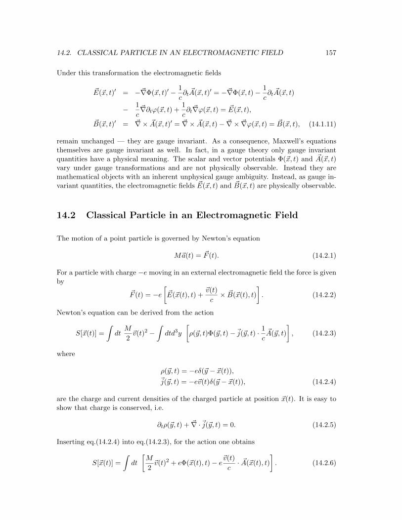
14.2. CLASSICAL PARTICLE IN AN ELECTROMAGNETIC FIELD 157
Under this transformation the electromagnetic fields
~E(~x, t)′ = −~∇Φ(~x, t)′ − 1
c∂t ~A(~x, t)′ = −~∇Φ(~x, t)− 1
c∂t ~A(~x, t)
− 1
c~∇∂tϕ(~x, t) +
1
c∂t~∇ϕ(~x, t) = ~E(~x, t),
~B(~x, t)′ = ~∇× ~A(~x, t)′ = ~∇× ~A(~x, t)− ~∇× ~∇ϕ(~x, t) = ~B(~x, t), (14.1.11)
remain unchanged — they are gauge invariant. As a consequence, Maxwell’s equationsthemselves are gauge invariant as well. In fact, in a gauge theory only gauge invariantquantities have a physical meaning. The scalar and vector potentials Φ(~x, t) and ~A(~x, t)vary under gauge transformations and are not physically observable. Instead they aremathematical objects with an inherent unphysical gauge ambiguity. Instead, as gauge in-variant quantities, the electromagnetic fields ~E(~x, t) and ~B(~x, t) are physically observable.
14.2 Classical Particle in an Electromagnetic Field
The motion of a point particle is governed by Newton’s equation
M~a(t) = ~F (t). (14.2.1)
For a particle with charge −e moving in an external electromagnetic field the force is givenby
~F (t) = −e[~E(~x(t), t) +
~v(t)
c× ~B(~x(t), t)
]. (14.2.2)
Newton’s equation can be derived from the action
S[~x(t)] =
∫dt
M
2~v(t)2 −
∫dtd3y
[ρ(~y, t)Φ(~y, t)−~j(~y, t) · 1
c~A(~y, t)
], (14.2.3)
where
ρ(~y, t) = −eδ(~y − ~x(t)),
~j(~y, t) = −e~v(t)δ(~y − ~x(t)), (14.2.4)
are the charge and current densities of the charged particle at position ~x(t). It is easy toshow that charge is conserved, i.e.
∂tρ(~y, t) + ~∇ ·~j(~y, t) = 0. (14.2.5)
Inserting eq.(14.2.4) into eq.(14.2.3), for the action one obtains
S[~x(t)] =
∫dt
[M
2~v(t)2 + eΦ(~x(t), t)− e~v(t)
c· ~A(~x(t), t)
]. (14.2.6)

158 CHAPTER 14. CHARGED PARTICLE IN AN ELECTROMAGNETIC FIELD
This action is indeed invariant under gauge transformations because∫dt
[Φ(~x(t), t)′ − ~v(t)
c· ~A(~x(t), t)′
]=∫
dt
[Φ(~x(t), t) +
1
c∂tϕ(~x(t), t)− ~v(t)
c· ( ~A(~x(t), t)− ~∇ϕ(~x(t), t))
]=∫
dt
[Φ(~x(t), t)− ~v(t)
c· ~A(~x(t), t) +
1
c
d
dtϕ(~x(t), t)
], (14.2.7)
and because the total derivative
d
dtϕ(~x(t), t) = ∂tϕ(~x(t), t) + ~v · ~∇ϕ(~x(t), t), (14.2.8)
integrates to zero as long as ϕ(~x(t), t) vanishes in the infinite past and future. Identifyingthe Lagrange function
L =M
2~v(t)2 + eΦ(~x(t), t)− e~v(t)
c· ~A(~x(t), t), (14.2.9)
it is straightforward to derive Newton’s equation as the Euler-Lagrange equation
d
dt
δL
δvi(t)− δL
δxi= 0. (14.2.10)
The theory can also be formulated in terms of a classical Hamilton function
H = ~p(t) · ~v(t)− L, (14.2.11)
where ~p is the momentum canonically conjugate to the coordinate ~x. One finds
M~v(t) = ~p(t) +e
c~A(~x(t), t), (14.2.12)
and thus one obtains
H =1
2M
[~p(t) +
e
c~A(~x(t), t)
]2− eΦ(~x(t), t). (14.2.13)
This is indeed consistent because
vi(t) =dxi(t)
dt=
∂H
∂pi(t)=
1
M
[pi(t) +
e
cAi(~x(t), t)
]. (14.2.14)
The other equation of motion is
dpi(t)
dt= − ∂H
∂xi(t)= − e
Mc
[pj(t) +
e
cAj(~x(t), t)
]∂iAj(~x(t), t) + e∂iΦ(~x(t), t). (14.2.15)
It is straightforward to show that these equations of motion are again equivalent to New-ton’s equation.

14.3. GAUGE INVARIANT FORM OF THE SCHRODINGER EQUATION 159
14.3 Gauge Invariant Form of the Schrodinger Equation
Remarkably, the gauge invariance of electrodynamics is intimately related to the phase am-biguity of the quantum mechanical wave function. As we have seen earlier, the Schrodingerequation
i~∂tΨ(~x, t) = − ~2
2M∆Ψ(~x, t) + V (~x)Ψ(~x, t), (14.3.1)
determines the wave function only up to a global phase ambiguity
Ψ(~x, t)′ = Ψ(~x, t) exp(iφ). (14.3.2)
Here φ is a constant, independent of space and time.
We now apply the gauge principle to the Schrodinger equation, i.e. we demand thatthe physics is invariant even under local transformations
Ψ(~x, t)′ = Ψ(~x, t) exp(iφ(~x, t)), (14.3.3)
with a space-time dependent phase φ(~x, t). Of course, if the wave function Ψ(~x, t) solvesthe original Schrodinger equation (14.3.1), the wave function Ψ(~x, t)′ of eq.(14.3.3) ingeneral does not. This is easy to see because
∂tΨ(~x, t)′ = [∂tΨ(~x, t) + iΨ(~x, t)∂tφ(~x, t)] exp(iφ(~x, t)), (14.3.4)
contains the second term on the right hand side that was not present in the originalSchrodinger equation. However, if the potential energy V (~x) is replaced by a scalar po-tential −eΦ(~x, t), the Schrodinger equation takes the form
i~DtΨ(~x, t) = − ~2
2M∆Ψ(~x, t), (14.3.5)
with the covariant derivative
DtΨ(~x, t) = ∂tΨ(~x, t)− i e~
Φ(~x, t)Ψ(~x, t). (14.3.6)
Using the gauge transformation property
Φ(~x, t)′ = Φ(~x, t) +1
c∂tϕ(~x, t), (14.3.7)
of the electromagnetic scalar potential, one obtains
DtΨ(~x, t)′ = ∂tΨ(~x, t)′ − i e~
Φ(~x, t)′Ψ(~x, t)′
= [∂tΨ(~x, t) + iΨ(~x, t)∂tφ(~x, t)] exp(iφ(~x, t))
− ie
~
[Φ(~x, t) +
1
c∂tϕ(~x, t)
]Ψ(~x, t) exp(iφ(~x, t))
= DtΨ(~x, t) exp(iφ(~x, t)), (14.3.8)

160 CHAPTER 14. CHARGED PARTICLE IN AN ELECTROMAGNETIC FIELD
provided that we identify
φ(~x, t) =e
~cϕ(~x, t). (14.3.9)
We also introduce a space-like covariant derivative
~DΨ(~x, t) = ~∇Ψ(~x, t) + ie
~c~A(~x, t)Ψ(~x, t), (14.3.10)
which also transforms as
~DΨ(~x, t)′ = ~∇Ψ(~x, t)′ + ie
~c~A(~x, t)′Ψ(~x, t)′
=[~∇Ψ(~x, t) + iΨ(~x, t)~∇φ(~x, t)
]exp(iφ(~x, t))
+ ie
~c
[~A(~x, t)− ~∇ϕ(~x, t)
]Ψ(~x, t) exp(iφ(~x, t))
= ~DΨ(~x, t) exp(iφ(~x, t)), (14.3.11)
under a gauge transformation. Using ~p = (~/i)~∇ one obtains
~i~D = ~p+
e
c~A(~x, t), (14.3.12)
which is the quantum version of M~v from eq.(14.2.12) that we encountered in the classicaltheory.
Finally, in the Schrodinger equation we replace ∆Ψ(~x, t) = ~∇ · ~∇Ψ(~x, t) with ~D ·~DΨ(~x, t) and we obtain
i~DtΨ(~x, t) = − ~2
2M~D · ~DΨ(~x, t). (14.3.13)
Inserting the explicit form of the covariant derivatives, the Schrodinger equation for acharged particle in an arbitrary external electromagnetic field takes the form
i~[∂t − i
e
~Φ(~x, t)
]Ψ(~x, t) = − ~2
2M
[~∇+ i
e
~c~A(~x, t)
]·[~∇+ i
e
~c~A(~x, t)
]Ψ(~x, t). (14.3.14)
This equation is invariant under gauge transformations of the form
Φ(~x, t)′ = Φ(~x, t) +1
c∂tϕ(~x, t),
~A(~x, t)′ = ~A(~x, t)− ~∇ϕ(~x, t),
Ψ(~x, t)′ = Ψ(~x, t) exp(ie
~cϕ(~x, t)
). (14.3.15)
Under this transformation, both sides of the Schrodinger equation change by a factorexp(i(e/~c)ϕ(~x, t)). Canceling this factor out, the equation remains invariant.
As usual, the wave function Ψ(~x, t) that solves the gauged Schrodinger equation(14.3.14) can be interpreted as the probability amplitude for finding the particle at position~x at time t. In particular, the probability density
ρ(~x, t) = |Ψ(~x, t)|2, (14.3.16)

14.4. MAGNETIC FLUX TUBES AND THE AHARONOV-BOHM EFFECT 161
is gauge invariant and hence physically meaningful. Again, probability conservation followsfrom a continuity equation
∂tρ(~x, t) + ~∇ ·~j(~x, t) = 0. (14.3.17)
However, in the presence of electromagnetic fields the usual probability current must bemodified by replacing ordinary with covariant derivatives such that now
~j(~x, t) =~
2Mi
[Ψ(~x, t)∗ ~DΨ(~x, t)− ( ~DΨ(~x, t))∗Ψ(~x, t)
]. (14.3.18)
14.4 Magnetic Flux Tubes and the Aharonov-Bohm Effect
Let us consider a charged particle moving in the electromagnetic field of an idealizedsolenoid. Such a solenoid generates magnetic flux inside it but has no outside magneticor electric field. Hence a classical particle moving outside the solenoid is not affected byit at all. We will see that this is not the case quantum mechanically. We consider aninfinitely thin and infinitely long solenoid oriented along the z-axis. The correspondingvector potential is given by
Ax(~x, t) = − Φ
2π
y
x2 + y2, Ay(~x, t) =
Φ
2π
x
x2 + y2, Az(~x, t) = 0, (14.4.1)
while the scalar potential Φ(~x, t) = 0 vanishes. The corresponding electric and magneticfields vanish. However, there is an infinitely thin tube of magnetic flux along the z-direction. The quantity Φ (which has nothing to do with the scalar potential Φ(~x, t)) isthe magnetic flux. This follows from∫
Sd~f · ~B(~x, t) =
∫Sd~f · ~∇× ~A(~x, t) =
∫∂Sd~l · ~A(~x, t) = Φ. (14.4.2)
Here S is any 2-d surface pinched by the z-axis and its boundary ∂S is a closed curvewinding around this axis. Hence, the magnetic field takes the form
Bx(~x, t) = By(~x, t) = 0, Bz(~x, t) = Φδ(x)δ(y), (14.4.3)
i.e. it vanishes everywhere except along the z-axis. Since both the electric and the magneticfield vanish outside the solenoid, a classical particle moving outside the solenoid is totallyunaffected by it and travels in a straight line with constant velocity. We will see that thisis not the case quantum mechanically.
To see this, we first consider a modified double slit experiment, similar to the onediscussed in chapter 2, section 2.7. Again, we consider a planar screen oriented in they-z-plane with two slits located at x = z = 0, the first at y1 = −d/2 and the second aty2 = d/2. We place a source of electrons at the point x = −l, y = z = 0 a distancel before the screen, and we detect an interference pattern at a parallel detection screena distance l behind the screen with the two slits. An electron detected at position y attime T may have passed through the slit at y1 = −d/2 or through the one at y2 = d/2,

162 CHAPTER 14. CHARGED PARTICLE IN AN ELECTROMAGNETIC FIELD
but we don’t know through which slit it went. In the first case it has traveled a totaldistance squared |~x(T )|2 = 2l2 + d2/4 + (y + d/2)2, while in the second case we have|~x(T )|2 = 2l2 + d2/4 + (y − d/2)2. Using Feynman’s path integral method, the totalprobability amplitude is a superposition of contributions from two paths
Ψ(y) = A exp
(iM(2l2 + d2/4 + (y − d/2)2)
2~T
)+ A exp
(iM(2l2 + d2/4 + (y + d/2)2)
2~T
)= A exp
(iM(2l2 + y2 + d2/2)
2~T
)[exp
(iMyd
2~T
)+ exp
(− iMyd
2~T
)]= A exp
(iM(2l2 + y2 + d2/2)
2~T
)2 cos
(Myd
2~T
). (14.4.4)
To obtain the probability density we take the absolute value squared
ρ(y) = |Ψ(y)|2 = 4|A|2 cos2
(Myd
2~T
)= 4ρ0 cos2
(Myd
2~T
). (14.4.5)
This is the typical interference pattern of a double slit experiment.
Now we modify the situation by adding the solenoid discussed before. It is orientedalong the z-axis within the screen, right between the two slits. As a result, electronspassing through the different slits pass the solenoid on different sides. Classically, thiswould make no difference because there is no electromagnetic field outside the solenoid.Quantum mechanically, however, there is an effect, as first suggested by Aharonov andBohm. The set-up with the two slits and the solenoid is known as an Aharonov-Bohmexperiment and its result is the Aharonov-Bohm effect. To investigate the Aharonov-Bohmeffect, we must include the electromagnetic contribution
Sem[~x(t)] =
∫dt
[eΦ(~x(t), t)− e~v(t)
c· ~A(~x(t), t)
]=
∫dt e
~v(t)
c· ~A(~x(t), t) =
e
c
∫C~dl · ~A(~x, t) (14.4.6)
to the action in the Feynman path integral. Here C is the path along which the particletravels. The relative phase between the two paths C1 and C2 contributing in the doubleslit experiment, that is generated by this term, is given by
1
~(Sem[~x1(t)]− Sem[~x2(t)]) =
e
~c
(∫C1
~dl · ~A(~x, t)−∫C2
~dl · ~A(~x, t)
)=
e
~c
∫C~dl · ~A(~x, t) =
eΦ
~c. (14.4.7)
Here C = C1 ∪ C2 is the closed curve obtained by combining the two paths C1 and C2. Byconstruction, this curve winds around the solenoid and hence the corresponding integral

14.5. FLUX QUANTIZATION FOR MONOPOLES AND SUPERCONDUCTORS 163
yields the magnetic flux ϕ. The resulting interference pattern of the modified double slitexperiment is now given by
ρ(y)′ = |Ψ(y)|2 = 4ρ0 cos2
(Myd
2~T+eΦ
2~c
). (14.4.8)
In other words, the presence of the magnetic flux Φ causes an observable effect in theinterference pattern. Interestingly, when the magnetic flux is quantized in integer units n,i.e. when
Φ = 2πn~ce, (14.4.9)
the solenoid becomes invisible to the electron and thus behaves classically.
14.5 Flux Quantization for Monopoles and Superconduc-tors
In 1931 Dirac investigated the quantum mechanics of magnetically charged particles —so-called magnetic monopoles. There is no experimental evidence for such particles, andMaxwell’s equation ~∇· ~B(~x, t) = 0 indeed says that magnetic monopoles do not exist. Still,there are some theories — the so-called grand unified extensions of the standard model ofparticle physics — that naturally contain magnetically charged particles. The magneticfield of a point-like magnetic charge (a so-called Dirac monopole) is determined from
~∇ · ~B(~x, t) = 4πgδ(~x), (14.5.1)
where g is the magnetic charge of the monopole. The resulting magnetic field is given by
~B(~x, t) =g
r2~er, (14.5.2)
and the corresponding magnetic flux through any surface S surrounding the monopole isgiven by
Φ =
∫Sd~f · ~B(~x, t) = 4πg. (14.5.3)
The magnetic field of a monopole can not be obtained from a vector potential as ~B(~x, t) =~∇ × ~A(~x, t). In order to still be able to work with a vector potential Dirac introduceda mathematical trick — the so-called Dirac string. A Dirac string is an infinitely thinsolenoid that emanates from the monopole and carries its magnetic flux g to infinity. Ofcourse, the Dirac string (being just a mathematical trick) must be physically invisible.This is the case if the magnetic charge g and thus the magnetic flux of the solenoid obeysthe Dirac quantization condition
g =Φ
4π=
~c2e⇒ eg =
~c2. (14.5.4)
The Dirac quantization condition implies that the units e and g of electric and magneticcharge are related. In particular, the existence of magnetic monopoles would immediately

164 CHAPTER 14. CHARGED PARTICLE IN AN ELECTROMAGNETIC FIELD
explain why electric charge is quantized. This is one reason why many physicists findgrand unified theories an attractive idea for going beyond the standard model of particlephysics. However, despite numerous experimental efforts, nobody has ever observed asingle magnetic charge. Grand unified theories predict that magnetic monopoles must haveexisted immediately after the big bang. Then, why don’t we see any of them today? Thisquestion has been answered by Alan Guth from MIT. In his scenario of the inflationaryuniverse with an exponential expansion early on magnetic monopoles get so much dilutedthat it would indeed be impossible to find any in the universe today.
In the presence of magnetic monopoles flux quantization would simply follow the Diracquantization condition. Interestingly, magnetic flux is also quantized inside superconduc-tors, despite the fact that no magnetic monopoles seem to exist in the universe. Supercon-ductivity is a very interesting effect that occurs in metals at very low temperatures. Belowa critical temperature, electric currents flow in a superconductor without any resistance.This effect is due to a pair formation of electrons. The so-called Cooper pairs (consist-ing of two electrons) are bosons and can thus undergo Bose-Einstein condensation. Theelectrons in the condensate of Cooper pairs are in a coherent quantum state that leadsto superconductivity. In order to form a Cooper pair, the electrons must overcome theirCoulomb repulsion. This is possible inside a crystal lattice because the quantized latticeoscillations — the phonons — mediate an attractive force between electrons. There areother interesting materials — the more recently discovered ceramic high-temperature su-perconductors — for which the mechanism of Cooper pair formation is not yet understood.Both the ordinary low-temperature superconductors and the more exotic high-temperaturesuperconductors show the so-called Meissner effect: magnetic fields are expelled from thesuperconductor. When a ring of non-superconducting metal is placed in an external mag-netic field, the magnetic flux permeates the material. When the ring is cooled down belowthe critical temperature it becomes superconducting and the magnetic flux is expelled.Some of the flux is expelled to the outside, some to the inside of the ring. It turns outthat the magnetic flux trapped inside the ring is quantized in units of
Φ = 2πn~c2e. (14.5.5)
Interestingly, the quantization is such that the trapped flux does not give rise to an observ-able Aharonov-Bohm phase for a Cooper pair of charge 2e moving around the ring. Thewave function of an electron (of charge e), on the other hand, would pick up a minus signwhen it moves around the ring. The flux quantization in superconductors is a dynamicaleffect. If the trapped magnetic flux would not be quantized, the Aharonov-Bohm effect forCooper pairs would destroy their coherence and hence the superconductivity. It is ener-getically favorable to maintain the superconducting state and have an invisible quantizedtrapped flux. It is irrelevant that the trapped flux is visible to unpaired electrons becausethose do not superconduct.
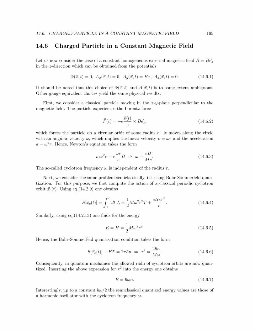
14.6. CHARGED PARTICLE IN A CONSTANT MAGNETIC FIELD 165
14.6 Charged Particle in a Constant Magnetic Field
Let us now consider the case of a constant homogeneous external magnetic field ~B = B~ezin the z-direction which can be obtained from the potentials
Φ(~x, t) = 0, Ax(~x, t) = 0, Ay(~x, t) = Bx, Az(~x, t) = 0. (14.6.1)
It should be noted that this choice of Φ(~x, t) and ~A(~x, t) is to some extent ambiguous.Other gauge equivalent choices yield the same physical results.
First, we consider a classical particle moving in the x-y-plane perpendicular to themagnetic field. The particle experiences the Lorentz force
~F (t) = −e~v(t)
c×B~ez, (14.6.2)
which forces the particle on a circular orbit of some radius r. It moves along the circlewith an angular velocity ω, which implies the linear velocity v = ωr and the accelerationa = ω2r. Hence, Newton’s equation takes the form
mω2r = eωr
cB ⇒ ω =
eB
Mc. (14.6.3)
The so-called cyclotron frequency ω is independent of the radius r.
Next, we consider the same problem semiclassically, i.e. using Bohr-Sommerfeld quan-tization. For this purpose, we first compute the action of a classical periodic cyclotronorbit ~xc(t). Using eq.(14.2.9) one obtains
S[~xc(t)] =
∫ T
0dt L =
1
2Mω2r2T +
eBπr2
c. (14.6.4)
Similarly, using eq.(14.2.13) one finds for the energy
E = H =1
2Mω2r2. (14.6.5)
Hence, the Bohr-Sommerfeld quantization condition takes the form
S[~xc(t)]− ET = 2π~n ⇒ r2 =2~nMω
. (14.6.6)
Consequently, in quantum mechanics the allowed radii of cyclotron orbits are now quan-tized. Inserting the above expression for r2 into the energy one obtains
E = ~ωn. (14.6.7)
Interestingly, up to a constant ~ω/2 the semiclassical quantized energy values are those ofa harmonic oscillator with the cyclotron frequency ω.

166 CHAPTER 14. CHARGED PARTICLE IN AN ELECTROMAGNETIC FIELD
Finally, we consider the problem fully quantum mechanically. The Schrodinger equa-tion (14.3.14) then takes the form
i~∂tΨ(~x, t) = − ~2
2M
[∂2x +
(∂y + i
eBx
~c
)(∂y + i
eBx
~c
)+ ∂2
z
]Ψ(~x, t)
= − ~2
2M
[∂2x + ∂2
y + 2ieBx
~c∂y −
(eBx
~c
)2
+ ∂2z
]Ψ(~x, t).
(14.6.8)
The corresponding time-independent Schrodinger equation takes the form
− ~2
2M
[∂2x + ∂2
y + 2ieBx
~c∂y −
(eBx
~c
)2
+ ∂2z
]Ψ(~x) = EΨ(~x). (14.6.9)
Again, we want to consider motion in the x-y-plane. We make the factorized ansatzΨ(~x) = ψ(x) exp(ipyy/~) (which implies pz = 0) and we obtain[
− ~2
2M∂2x +
1
2Mω2
(x+
pyMω
)2]ψ(x) = Eψ(x). (14.6.10)
Indeed, this is the equation of motion of a (shifted) harmonic oscillator. Hence, thequantum mechanical energy spectrum takes the form
E = ~ω(n+
1
2
). (14.6.11)
Interestingly, the energy of the charged particle is completely independent of the transversemomentum py. As a result, the energy levels — which are known as Landau levels — havean infinite degeneracy.
14.7 The Quantum Hall Effect
The quantum Hall effect is one of the most remarkable effects in condensed matter physicsin which quantum mechanics manifests itself on macroscopic scales. One distinguishesthree effects: the classical Hall effect discovered by the student Hall in 1879, the integerquantum Hall effect discovered by von Klitzing in 1980 (Nobel prize in 1985), and thefractional quantum Hall effect discovered by Tsui, Stormer and Gossard in 1982 andtheoretically explained by Laughlin (Nobel prize in 1998).
The basic experimental set-up is the same in the three cases. Some flat (quasi 2-dimensional) rectangular sample of size Lx × Ly (oriented in the x-y-plane) of some
conducting or semi-conducting material is placed in a strong magnetic field ~B = B~ezperpendicular to the sample. A current with density
~j = −ne~v, (14.7.1)

14.7. THE QUANTUM HALL EFFECT 167
is flowing through the sample in the y-direction, i.e. jy = −nev. Here n is the number ofelectrons per unit area which move with the velocity ~v = v~ey. The electrons moving inthe magnetic field experience the Lorentz force
~F = −e~vc× ~B. (14.7.2)
The resulting sideways motion of the electrons leads to an excess of negative charge onone edge of the sample which generates an electric field transverse to the current. Onethen observes a voltage drop along the transverse direction, the x-direction in this case.More electrons move to the edge of the sample until the resulting electric field
~E = −~vc× ~B, (14.7.3)
exactly compensates the Lorentz force. Hence, in equilibrium we have
~E =~j
nec× ~B. (14.7.4)
The resistivity tensor ρ is defined by
~E = ρ~j, (14.7.5)
such that we can identify
ρ =B
nec
(0 1−1 0
). (14.7.6)
The conductivity tensor σ is the matrix inverse of the resistivity tensor ρ and it is definedby
~j = σ ~E, (14.7.7)
such that
σ =nec
B
(0 −11 0
). (14.7.8)
Since both the resistivity and the conductivity tensor are purely off-diagonal the materialbehaves paradoxically. On the one hand, it looks insulating because σxx = 0, i.e. there isno current in the direction of the electric field. On the other hand, it looks like a perfectconductor because ρxx = 0. The Hall resistivity is given by
ρxy =B
nec. (14.7.9)
This is indeed the result of the classical Hall effect. The resistivity is linear in the magneticfield B and depends on the electron density n. The classical Hall effect can thus be usedto determine the electron density by measuring the Hall resistivity as well as the appliedmagnetic field.
Remarkably, at sufficiently low temperatures eq.(14.7.9) is not the correct result in realsamples. In fact, one observes deviations from the linear behavior in the form of quantum

168 CHAPTER 14. CHARGED PARTICLE IN AN ELECTROMAGNETIC FIELD
Hall plateaux, i.e. the Hall resistivity becomes independent of the magnetic field in regionsthat correspond to the quantized values
ρxy =h
νe2. (14.7.10)
Here h is Planck’s quantum, e is the electric charge, and ν is an integer. This so-calledinteger quantum Hall effect was first observed by von Klitzing and his collaborators. Later,quantum Hall plateaux were also observed at fractional values (e.g. at ν = 1/3, 2/5, 3/7)by Tsui, Stormer and Gossard. This is now known as the fractional quantum Hall effect.Very surprisingly, the value of the resistivity is independent of any microscopic details ofthe material, the purity of the sample, the precise value of the magnetic field, etc. In fact,the quantum Hall effect is now used to maintain the standard of resistance. At each of thequantum Hall plateaux the dissipative resistivity ρxx practically drops to zero (by about13 orders of magnitude).
In addition to the previous discussion of Landau levels we should now add the trans-verse electric field ~E = Ex~ex generated by the sideways moving electrons. The Schrodingerequation then takes the form[
− ~2
2M∂2x +
1
2Mω2
(x+
pyMω
)2+ eExx
]ψ(x) =[
− ~2
2M∂2x +
1
2Mω2
(x+
pyMω
+eExMω2
)2
− pyeExMω
− e2E2x
2Mω2
]ψ(x) = Eψ(x).
(14.7.11)
Again, this is the equation of motion of a shifted harmonic oscillator, now centered around
x0 = − pyMω
− eExMω2
. (14.7.12)
It is straightforward to construct the current density and to verify that eq.(14.7.3) is indeedsatisfied for the quantum mechanical solution.
Let us count the number of states in each of the Landau levels for a Hall sample ofsize Lx × Ly. For simplicity, we choose periodic boundary conditions in the y-direction,such that
py =2π~Ly
ny, (14.7.13)
with ny ∈ Z. Since the wave function must be located inside the Hall sample one musthave x0 ∈ [0, Lx]. The number N of ny values for which this is the case, and hence thedegeneracy of a given Landau level, is
N =MωLxLy
2π~=eBLxLy
2π~c. (14.7.14)
When ν Landau levels are completely occupied by Nν electrons, the number density (perunit area) of electrons is given by
n =Nν
LxLy=eBν
2π~c. (14.7.15)

14.8. THE “NORMAL” ZEEMAN EFFECT 169
Using eq.(14.7.9) one then finds
ρxy =B
nec=
h
νe2, (14.7.16)
i.e. the quantum Hall plateaux correspond to completely filled Landau levels. It is clearthat complete filling implies a very special situation for the electron system in the Hallsample. In particular, in that case there are no available low-lying energy levels into whichinteracting electrons could scatter, and thus dissipation is extremely suppressed. A fullunderstanding of the integer quantum Hall effect requires the incorporation of impurities inthe sample. In particular, it is non-trivial to understand the enormous precision with whicheq.(14.7.9) is realized despite numerous imperfections in actual materials. To understandthis goes beyond the scope of the present discussion.
In contrast to the integer quantum Hall effect, the fractional quantum Hall effect reliesheavily on electron-electron correlations. It is a complicated collective phenomenon inwhich electrons break up into quasiparticles with fractional charge and with with fractionalspin — so-called anyons. Again, the explanation of the fractional quantum Hall effect isbeyond the scope of this course.
14.8 The “Normal” Zeeman Effect
Let us briefly discuss the so-called “normal” Zeeman effect, which describes the shiftof energy levels of hydrogen-like atoms in a weak homogeneous external magnetic field~B = B~ez ignoring the effects of spin. When spin is included one speaks of the “anomalous”Zeeman effect. This is clearly a case of bad nomenclature because normally spin plays animportant role and the “anomalous” Zeeman effect is the more common phenomenon. Inthis case, it is natural to choose the so-called symmetric gauge
Ax(~x, t) = −By2, Ay(~x, t) =
Bx
2, Az(~x, t) = 0. (14.8.1)
Then to leading order in the magnetic field we have(px +
e
cAx
)2+(py +
e
cAy
)2= p2
x + p2y +
eB
c(xpy − ypx) +O(B2). (14.8.2)
Hence, the “normal” Zeeman effect results from the Hamilton operator
H = H0 +eBLz2µc
, (14.8.3)
where H0 is the unperturbed problem (at B = 0) and µ is the reduced mass of theelectron and the atomic nucleus. Due to the rotation invariance of the unperturbedproblem [H0, ~L] = 0. The external magnetic field explicitly breaks rotation invariance.Only the rotations around the z-axis remain a symmetry of the perturbed problem andhence [H,Lz] = 0. Since the unperturbed states of hydrogen-like atoms can be chosen as

170 CHAPTER 14. CHARGED PARTICLE IN AN ELECTROMAGNETIC FIELD
eigenstates of Lz with eigenvalue ~m, they remain eigenstates when the magnetic field isswitched on. However, the energy eigenvalue is now shifted to
E = E0 +eB~m
2µc. (14.8.4)
As a result, the (2l+1)-fold degeneracy of states with angular momentum quantum numberl is lifted.

Chapter 15
Coupling of Angular Momenta
15.1 Quantum Mechanical Angular Momentum
Angular momentum is a fundamental quantity that is conserved in any known physicalprocess. Angular momentum conservation is a consequence of the isotropy of space —the laws of Nature are invariant against spatial rotations. Of course, rotation invariancemay be broken explicitly under certain conditions, for example, in the presence of externalelectric or magnetic fields. In that case, the subsystem without the fields is not rotationinvariant. Still, the total system behaves in the same way when everything including thefields is spatially rotated. Angular momentum is a vector. In quantum mechanics itscomponents cannot be measured simultaneously because the corresponding operators donot commute. This has interesting consequences for the physical behavior of quantummechanical particles under spatial rotations.
Besides the orbital angular momentum ~L = ~r × ~p familiar from classical mechanics,quantum mechanical particles can carry an internal angular momentum known as spin.While orbital angular momentum is quantized in integer units, spin may be quantized ininteger or half-integer units. Interestingly, there is an intimate connection between spinand statistics: particles with half-integer spin obey Fermi-Dirac statistics and are thusfermions, while particles with integer spin obey Bose-Einstein statistics and are hencebosons. This connection between spin and statistics can be understood in the frameworkof relativistic quantum field theory — but not from quantum mechanics alone.
When particles carry both orbital angular momentum ~L and spin ~S, in general onlytheir total angular momentum ~J = ~L+ ~S is conserved. In that case, one is confronted withthe problem of coupling two angular momenta together. The same problem arises whenseveral particles add their angular momenta together to the conserved angular momentumof the total system. Performing the corresponding angular momentum “gymnastics” is animportant tool of the quantum mechanic. Although the subject is a bit formal, its under-standing is vital in atomic, molecular and particle physics, as well as in other branches of
171

172 CHAPTER 15. COUPLING OF ANGULAR MOMENTA
our field.
Let us consider the commutation relations of an arbitrary angular momentum ~J inquantum mechanics. Here ~J may be an orbital angular momentum, a spin, or any com-bination of these. For an orbital angular momentum ~L we have already derived thecommutation relation
[Li, Lj ] = i~εijkLk, (15.1.1)
from the definition ~L = ~r × ~p and from the fundamental commutation relation [xi, pj ] =i~δij . Now we postulate
[Ji, Jj ] = i~εijkJk, (15.1.2)
for any angular momentum in quantum mechanics. In particular, different components ofthe angular momentum vector do not commute with one another. However, all componentscommute with the magnitude ~J2 = J2
x+J2y+J2
z , i.e. [Ji, ~J2] = 0. As a consequence, one can
construct simultaneous eigenstates of the operator ~J2 and one component Ji. Usually onechooses Jz, i.e. the arbitrary quantization direction is then the z-direction. In general, thischoice does not imply a physical violation of rotation invariance. One could have chosenany other quantization axis without any effect on the physics. When rotation invarianceis already broken, for example, by the direction of an external electric or magnetic field,it is very convenient to choose the quantization axis along the same direction. As usual,we choose the z-direction as our quantization axis and we thus construct simultaneouseigenstates |j,m〉 of both ~J2 and Jz,
~J2|j,m〉 = ~2j(j + 1)|j,m〉, Jz|j,m〉 = ~m|j,m〉. (15.1.3)
It will turn out that both j and m are either integer or half-integer.
For convenience, we introduce the angular momentum raising and lowering operators
J± = Jx ± iJy. (15.1.4)
They obey the commutation relations
[J+, J−] = 2~Jz, [ ~J2, J±] = 0, [Jz, J±] = ±~J±. (15.1.5)
We haveJzJ±|j,m〉 = (J±Jz + [Jz, J±])|j,m〉 = ~(m± 1)J±|j,m〉, (15.1.6)
i.e. the state J±|j,m〉 is also an eigenstate of Jz and has the quantum number m ± 1.Similarly
~J2J±|j,m〉 = J± ~J2|j,m〉 = ~2j(j + 1)J±|j,m〉, (15.1.7)
i.e. J±|j,m〉 is still also an eigenstate of ~J2 with the unchanged quantum number j. Sincej determines the magnitude of the angular momentum vector, one expects that for fixed jthe m quantum number that measures the z-component of the angular momentum vectorshould be bounded from above and from below. On the other hand, for any state |j,m〉with quantum number m one can construct the states
J±|j,m〉 = Cj,m|j,m± 1〉, (15.1.8)
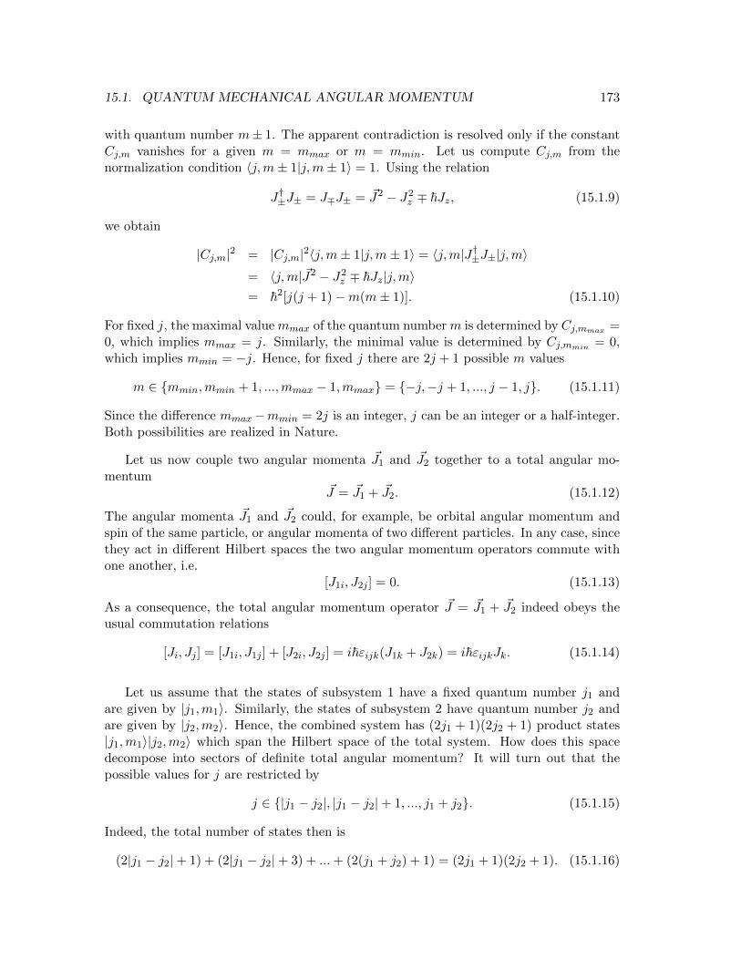
15.1. QUANTUM MECHANICAL ANGULAR MOMENTUM 173
with quantum number m± 1. The apparent contradiction is resolved only if the constantCj,m vanishes for a given m = mmax or m = mmin. Let us compute Cj,m from thenormalization condition 〈j,m± 1|j,m± 1〉 = 1. Using the relation
J†±J± = J∓J± = ~J2 − J2z ∓ ~Jz, (15.1.9)
we obtain
|Cj,m|2 = |Cj,m|2〈j,m± 1|j,m± 1〉 = 〈j,m|J†±J±|j,m〉= 〈j,m| ~J2 − J2
z ∓ ~Jz|j,m〉= ~2[j(j + 1)−m(m± 1)]. (15.1.10)
For fixed j, the maximal value mmax of the quantum number m is determined by Cj,mmax =0, which implies mmax = j. Similarly, the minimal value is determined by Cj,mmin = 0,which implies mmin = −j. Hence, for fixed j there are 2j + 1 possible m values
m ∈ mmin,mmin + 1, ...,mmax − 1,mmax = −j,−j + 1, ..., j − 1, j. (15.1.11)
Since the difference mmax−mmin = 2j is an integer, j can be an integer or a half-integer.Both possibilities are realized in Nature.
Let us now couple two angular momenta ~J1 and ~J2 together to a total angular mo-mentum
~J = ~J1 + ~J2. (15.1.12)
The angular momenta ~J1 and ~J2 could, for example, be orbital angular momentum andspin of the same particle, or angular momenta of two different particles. In any case, sincethey act in different Hilbert spaces the two angular momentum operators commute withone another, i.e.
[J1i, J2j ] = 0. (15.1.13)
As a consequence, the total angular momentum operator ~J = ~J1 + ~J2 indeed obeys theusual commutation relations
[Ji, Jj ] = [J1i, J1j ] + [J2i, J2j ] = i~εijk(J1k + J2k) = i~εijkJk. (15.1.14)
Let us assume that the states of subsystem 1 have a fixed quantum number j1 andare given by |j1,m1〉. Similarly, the states of subsystem 2 have quantum number j2 andare given by |j2,m2〉. Hence, the combined system has (2j1 + 1)(2j2 + 1) product states|j1,m1〉|j2,m2〉 which span the Hilbert space of the total system. How does this spacedecompose into sectors of definite total angular momentum? It will turn out that thepossible values for j are restricted by
j ∈ |j1 − j2|, |j1 − j2|+ 1, ..., j1 + j2. (15.1.15)
Indeed, the total number of states then is
(2|j1 − j2|+ 1) + (2|j1 − j2|+ 3) + ...+ (2(j1 + j2) + 1) = (2j1 + 1)(2j2 + 1). (15.1.16)
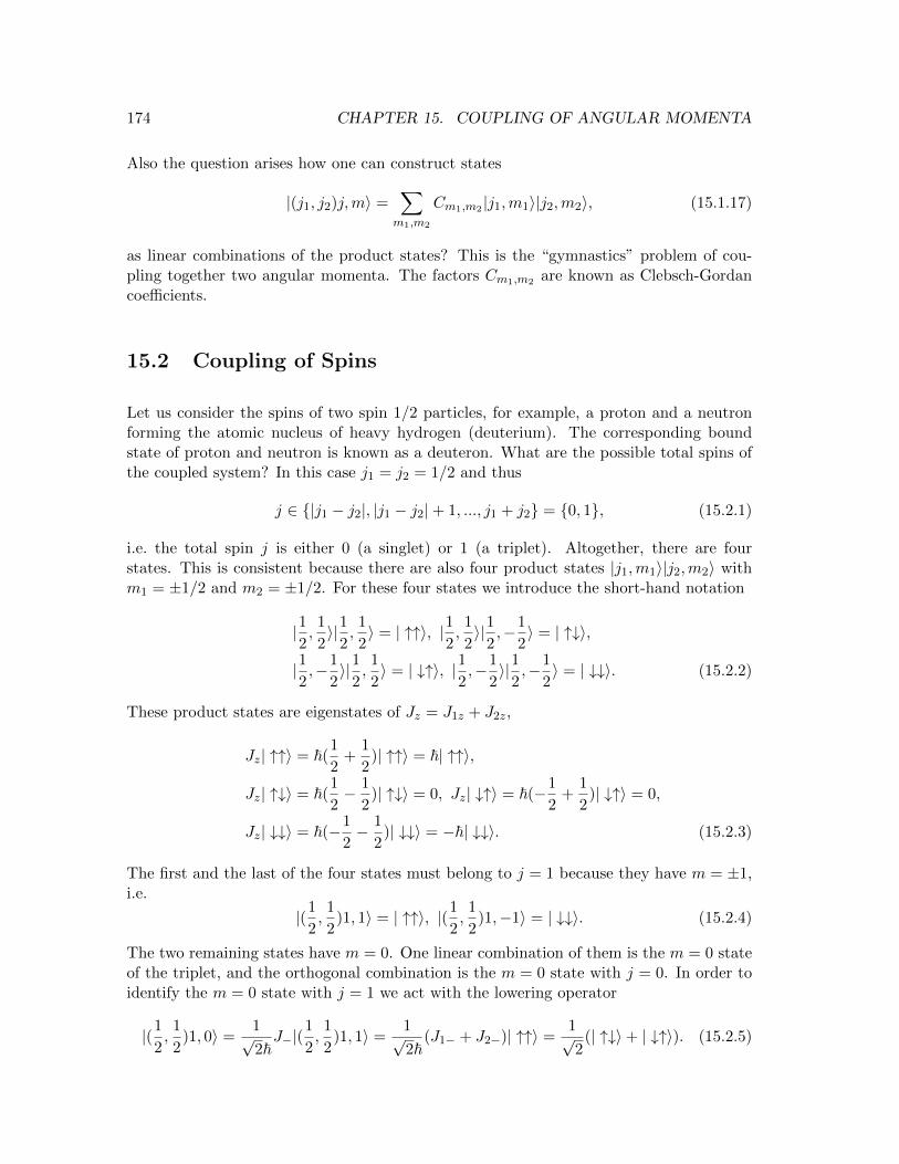
174 CHAPTER 15. COUPLING OF ANGULAR MOMENTA
Also the question arises how one can construct states
|(j1, j2)j,m〉 =∑m1,m2
Cm1,m2 |j1,m1〉|j2,m2〉, (15.1.17)
as linear combinations of the product states? This is the “gymnastics” problem of cou-pling together two angular momenta. The factors Cm1,m2 are known as Clebsch-Gordancoefficients.
15.2 Coupling of Spins
Let us consider the spins of two spin 1/2 particles, for example, a proton and a neutronforming the atomic nucleus of heavy hydrogen (deuterium). The corresponding boundstate of proton and neutron is known as a deuteron. What are the possible total spins ofthe coupled system? In this case j1 = j2 = 1/2 and thus
j ∈ |j1 − j2|, |j1 − j2|+ 1, ..., j1 + j2 = 0, 1, (15.2.1)
i.e. the total spin j is either 0 (a singlet) or 1 (a triplet). Altogether, there are fourstates. This is consistent because there are also four product states |j1,m1〉|j2,m2〉 withm1 = ±1/2 and m2 = ±1/2. For these four states we introduce the short-hand notation
|12,1
2〉|1
2,1
2〉 = | ↑↑〉, |1
2,1
2〉|1
2,−1
2〉 = | ↑↓〉,
|12,−1
2〉|1
2,1
2〉 = | ↓↑〉, |1
2,−1
2〉|1
2,−1
2〉 = | ↓↓〉. (15.2.2)
These product states are eigenstates of Jz = J1z + J2z,
Jz| ↑↑〉 = ~(1
2+
1
2)| ↑↑〉 = ~| ↑↑〉,
Jz| ↑↓〉 = ~(1
2− 1
2)| ↑↓〉 = 0, Jz| ↓↑〉 = ~(−1
2+
1
2)| ↓↑〉 = 0,
Jz| ↓↓〉 = ~(−1
2− 1
2)| ↓↓〉 = −~| ↓↓〉. (15.2.3)
The first and the last of the four states must belong to j = 1 because they have m = ±1,i.e.
|(1
2,1
2)1, 1〉 = | ↑↑〉, |(1
2,1
2)1,−1〉 = | ↓↓〉. (15.2.4)
The two remaining states have m = 0. One linear combination of them is the m = 0 stateof the triplet, and the orthogonal combination is the m = 0 state with j = 0. In order toidentify the m = 0 state with j = 1 we act with the lowering operator
|(1
2,1
2)1, 0〉 =
1√2~J−|(
1
2,1
2)1, 1〉 =
1√2~
(J1− + J2−)| ↑↑〉 =1√2
(| ↑↓〉+ | ↓↑〉). (15.2.5)

15.2. COUPLING OF SPINS 175
The orthogonal combination
|(1
2,1
2)0, 0〉 =
1√2
(| ↑↓〉 − | ↓↑〉), (15.2.6)
should hence be the state with j = 0. This can be checked explicitly, for example, byacting with the operator ~J+ = J1+ + J2+, i.e.
~J+|(1
2,1
2)0, 0〉 = (J1+ + J2+)
1√2
(| ↑↓〉 − | ↓↑〉) =~√2
(| ↑↑〉 − | ↑↑〉) = 0. (15.2.7)
Hence, according to the previous discussion the spin of the deuteron could be 0 or1. The proton and neutron that form the deuteron nucleus attract each other throughthe so-called strong interaction. This interaction is spin-dependent. There is a termproportional to − ~J1 · ~J2 (where ~J1 and ~J2 are the spin operators of proton and neutron)in the proton-neutron potential. One can write
~J2 = ( ~J1 + ~J2)2 = ~J21 + ~J2
2 + 2 ~J1 · ~J2, (15.2.8)
and hence
− ~J1 · ~J2 =1
2( ~J2
1 + ~J22 − ~J2). (15.2.9)
Since both the proton and the neutron have spin 1/2 we have
~J21 = ~J2
2 = ~2 1
2
(1
2+ 1
)=
3
4~2. (15.2.10)
In the spin singlet state we have ~J2 = 0 and hence
− ~J1 · ~J2|(1
2,1
2)0, 0〉 =
3
4~2|(1
2,1
2)0, 0〉. (15.2.11)
In the spin triplet state, on the other hand, ~J2 = 2~2 such that
− ~J1 · ~J2|(1
2,1
2)1,m〉 = −1
4~2|(1
2,1
2)1,m〉. (15.2.12)
In the triplet channel the proton-neutron interaction is attractive while in the singletchannel it is repulsive. As a consequence, the deuteron has spin 1, while in the spin 0channel there is no bound state.
The strong interaction is mediated by gluons, just as electromagnetic interactions aremediated by photons. The strong interaction analogs of electrons and positrons are quarksand anti-quarks — the basic building blocks of protons and neutrons. There are two u-quarks and one d-quark in each proton. A u-quark has electric charge 2/3 and a d-quarkhas −1/3. Hence, the charge of a proton is indeed 2× 2/3− 1/3 = 1. Similarly, a neutroncontains one u-quark and two d-quarks and thus has charge 2/3 − 2 × 1/3 = 0. Likeelectrons, quarks are fermions with spin 1/2. What is the possible total spin of a boundsystem of three quarks? As we learned before, two spin 1/2 particles can couple to a totalspin j = 0 or j = 1. When a third spin 1/2 particle is added to the j = 0 state, the totalspin is 1/2. If it is added to the j = 1 state the total spin can be either j − 1/2 = 1/2or j + 1/2 = 3/2. Again, the strong interactions between quarks are spin-dependent andthey favor the total spin 1/2 states corresponding to proton and neutron. The spin 3/2state also exists but is unstable. It is known in particle physics as the ∆-isobar.
176 CHAPTER 15. COUPLING OF ANGULAR MOMENTA
15.3 Coupling of Orbital Angular Momentum and Spin
Just as there are spin-dependent strong interactions between protons and neutrons or be-tween quarks, there are also spin-dependent electromagnetic interactions between electronsand protons. As we already discussed in the context of the relativistic Dirac equation,there are spin-orbit coupling terms proportional to
~L · ~S =1
2( ~J2 − ~L2 − ~S2) =
~2
2
(j(j + 1)− l(l + 1)− 3
4
). (15.3.1)
Let us consider the coupling of an orbital angular momentum l and a spin s = 1/2 of anelectron in more detail. In this case, there are 2(2l+ 1) product states |l,ml〉|s,ms〉. Thepossible values of the total angular momentum are
j ∈ |l − s|, l + s = l − 1
2, l +
1
2. (15.3.2)
Indeed, there are again
2
(l − 1
2
)+ 1 + 2
(l +
1
2
)+ 1 = 2(2l + 1) (15.3.3)
states. The direct product state
|(l, 1
2) l +
1
2, l +
1
2〉 = |l, l〉| ↑〉 (15.3.4)
has m = l + 1/2 and must thus have j = l + 1/2. We can construct the other states withj = l + 1/2 and with lower m-values by acting with J− = L− + S−. For example,
|(l, 1
2) l +
1
2, l − 1
2〉 =
1√2l + 1~
J−|l, l〉| ↑〉
=1√
2l + 1~(L− + S−)|l, l〉| ↑〉
=1√
2l + 1(|l, l〉| ↓〉+
√2l|l, l − 1〉| ↑〉). (15.3.5)
The orthogonal combination
|(l, 1
2) l − 1
2, l − 1
2〉 =
1√2l + 1
(√
2l|l, l〉| ↓〉 − |l, l − 1〉| ↑〉), (15.3.6)
has j = l − 1/2 and m = l − 1/2. Again, by acting with J− one can generate all otherstates with j = l − 1/2 and smaller m-values.
Chapter 16
Systems of Identical Particles
16.1 Bosons and Fermions
Identical elementary particles (like two photons or two electrons) are indistinguishable fromone another — they are like perfect twins. Ultimately, this is a consequence of quantumfield theory. Elementary particles are quantized excitations of fields that fill all of space.Since the properties of the field are the same everywhere in space, a particle created herehas exactly the same properties as a particle created somewhere else. In classical physicsone usually thinks about a particle in a different way. Starting from some initial positions,one can use Newton’s equation to predict the particles’ paths and one can always keeptrack of where a given particle came from. Classically, one can always distinguish twoparticles by referring to their initial positions. One can say: “This is the same particlethat originally came from the position ~x1”. It is classically distinguishable from anotherparticle that started from the position ~x2. However, photons or electrons are not classicalparticles. As elementary particles they must be treated quantum mechanically, and at thequantum level the concept of a classical path breaks down. In quantum mechanics it isimpossible to keep track of a particle by constantly watching it as it travels along a path.Instead a quantum system of N particles is described by a multi-particle wave functionΨ(~x1, ~x2, ..., ~xN ), where ~x1, ~x2, ..., ~xN are the positions of the particles. The absolutevalue |Ψ(~x1, ~x2, ..., ~xN )|2 determines the probability density for finding the particles at thepositions ~x1, ~x2, ..., ~xN . Consequently, the normalization condition takes the form∫
d3x1d3x2...d
3xN |Ψ(~x1, ~x2, ..., ~xN )|2 = 1. (16.1.1)
Similarly, the probability density for finding one of the particles at the position ~x1 whilethe other particles are in arbitrary positions is given by
ρ(~x1) =
∫d3x2...d
3xN |Ψ(~x1, ~x2, ..., ~xN )|2 = 1. (16.1.2)
As we said above, identical elementary particles are absolutely indistinguishable. Hence,when two identical particles are interchanged, this has no physically observable effects.
177
178 CHAPTER 16. SYSTEMS OF IDENTICAL PARTICLES
Let us denote the pair permutation operator of two identical particles by Pij . It acts ona wave function by interchanging the corresponding particle coordinates. For example,
P12Ψ(~x1, ~x2, ..., ~xN ) = Ψ(~x2, ~x1, ..., ~xN ). (16.1.3)
For identical particles the states Ψ(~x1, ~x2, ..., ~xN ) and its corresponding permutation part-ner Ψ(~x2, ~x1, ..., ~xN ) are physically equivalent. However, this does not imply that the twowave functions are the same. In fact, they may still differ by a complex phase which dropsout from physical observables.
The Hamilton operator of a system of non-relativistic identical particles can be writtenas
H = − ~2
2m
N∑i=1
∆i + V (~x1, ~x2, ..., ~xN ), (16.1.4)
Here m is the particle mass and ∆i is the Laplace operator that takes second derivativeswith respect to the coordinates of ~xi. It should be noted that the masses of all theparticles are the same — otherwise they would not be indistinguishable. The potentialenergy V (~x1, ~x2, ..., ~xN ) depends on the coordinates of all particles. For indistinguishableparticles the potential energy must be invariant against particle permutations Pij , forexample,
P12V (~x1, ~x2, ..., ~xN ) = V (~x2, ~x1, ..., ~xN ) = V (~x1, ~x2, ..., ~xN ). (16.1.5)
One obtains
P12HΨ(~x1, ~x2, ..., ~xN ) =
[− ~2
2M
N∑i=1
∆i + V (~x2, ~x1, ..., ~xN )
]Ψ(~x2, ~x1, ..., ~xN )
= HP12Ψ(~x1, ~x2, ..., ~xN ), (16.1.6)
and thus P12H = HP12. The same is true for all permutations and hence
[H,Pij ] = 0. (16.1.7)
This means that the eigenstates of H can be chosen such that they are simultaneouslyeigenstates of Pij . For example, an eigenstate of P12 obeys
P12Ψ(~x1, ~x2, ..., ~xN ) = λΨ(~x1, ~x2, ..., ~xN ), (16.1.8)
where λ is the corresponding eigenvalue. When we apply the permutation operator twicewe obtain
P 212Ψ(~x1, ~x2, ..., ~xN ) = P12Ψ(~x2, ~x1, ..., ~xN ) = Ψ(~x1, ~x2, ..., ~xN )
= λ2Ψ(~x1, ~x2, ..., ~xN ) ⇒ λ = ±1. (16.1.9)
It should be noted that, in general, different pair permutation operators do not commute.For example, for three particles the operators P12 and P23 do not commute. The combi-nations P312 = P12P23 and P231 = P23P12 correspond to two different cyclic permutations.
16.1. BOSONS AND FERMIONS 179
As a consequence, in general one cannot find simultaneous eigenstates to all permutationoperators Pij .
The permutations Pij form a finite group — the permutation group SN . Since dif-ferent permutations, in general, do not commute, the group SN is non-Abelian. In thisrespect it is like the group of spatial rotations in three dimensions, SO(3). However,unlike the permutation group SN , the rotation group SO(3) is continuous: there is aninfinite (continuous) number of rotations, but there is only a finite (discrete) number ofpermutations. Mathematically speaking, the angular momentum multiplets characterizedby j form (2j + 1)-dimensional irreducible representations of the group SO(3). Similarly,the irreducible representations of the group SN have different dimensions. There are twodifferent irreducible representations of the permutation group of two particles S2: the sym-metric and the anti-symmetric one, which are both 1-dimensional. In fact, all permutationgroups SN have two 1-dimensional representations: the totally symmetric and the totallyanti-symmetric one. However, for N ≥ 3 the permutation group SN also has irreduciblerepresentations of larger dimension. For example, besides the 1-dimensional symmetricand anti-symmetric representations the group S3 has a 2-dimensional irreducible repre-sentation of mixed symmetry.
The indistinguishability of elementary particles has profound consequences for theirwave function. For example, in a quantum state in which two particles are located atthe positions ~x1 and ~x2, it makes no sense to ask which particle is in which position.Hence, the distinct states |~x1〉|~x2〉 and |~x2〉|~x1〉 cannot be correct wave functions for sucha quantum state. Only if the two particles were distinguishable it would matter if theparticle of type 1 is at position ~x1 and the particle of type 2 is at position ~x2 (|~x1〉|~x2〉) orvice versa (|~x2〉|~x1〉). For indistinguishable particles there is only one state describing thetwo identical particles at the positions ~x1 and ~x2. Since the Hamiltonian commutes withthe permutation operator one can choose this state as a simultaneous eigenstate of H andP12. Since P12 has eigenvalues ±1, one can construct a symmetric state
|s〉 =1√2
(|~x1〉|~x2〉+ |~x2〉|~x1〉) , (16.1.10)
as well as an anti-symmetric state
|a〉 =1√2
(|~x1〉|~x2〉 − |~x2〉|~x1〉) . (16.1.11)
By construction, we have
P12|s〉 = |s〉, P12|a〉 = −|a〉. (16.1.12)
Four three identical particles one can again construct a totally symmetric state
|s〉 =1√6
(|~x1〉|~x2〉|~x3〉+ |~x2〉|~x1〉|~x3〉+ |~x2〉|~x3〉|~x1〉
+ |~x3〉|~x2〉|~x1〉+ |~x3〉|~x1〉|~x2〉+ |~x1〉|~x3〉|~x2〉) , (16.1.13)

180 CHAPTER 16. SYSTEMS OF IDENTICAL PARTICLES
as well as an anti-symmetric state
|a〉 =1√6
(|~x1〉|~x2〉|~x3〉 − |~x2〉|~x1〉|~x3〉+ |~x2〉|~x3〉|~x1〉
− |~x3〉|~x2〉|~x1〉+ |~x3〉|~x1〉|~x2〉 − |~x1〉|~x3〉|~x2〉) . (16.1.14)
For any pair permutation operator Pij we then have
Pij |s〉 = |s〉, Pij |a〉 = −|a〉. (16.1.15)
Besides the totally symmetric and anti-symmetric states, for three particles there are alsostates of mixed symmetry.
16.2 The Pauli Principle
Remarkably, there is an intimate relation between the statistics of particles (i.e. their prop-erties under permutations) and their spin. Bosons obeying Bose-Einstein statistics havea totally symmetric wave function and have integer spins. Fermions obeying Fermi-Diracstatistics, on the other hand, have a totally anti-symmetric wave function and have half-integer spin. This connection between spin and statistics is known as the Pauli principle.It cannot be derived within the theoretical framework of quantum mechanics alone. How-ever, it can be derived from quantum field theory in the form of the so-called spin-statisticstheorem.
First, we consider bosons with spin 0 whose spin wave function is trivial. The Pauliprinciple implies that their orbital wave function Ψ(~x1, ~x2, ..., ~xN ) must be totally sym-metric, i.e. for any pair permutation
PijΨ(~x1, ~x2, ..., ~xN ) = Ψ(~x1, ~x2, ..., ~xN ). (16.2.1)
For example, two (or three) spinless bosons located at the positions ~x1, ~x2 (and ~x3) aredescribed by the states |s〉 constructed above.
For particles with spin the situation is a bit more complicated. Let us now considerfermions with spin 1/2, whose spin wave function is non-trivial. The Pauli principledictates that the total wave function (orbital and spin) is anti-symmetric under particleexchange. This does not imply that the orbital or spin wave functions alone must beanti-symmetric. Two spin 1/2 particles can couple their spins to a total spin j = 0 orj = 1. The singlet state with spin 0 given by
|(1
2,1
2)0, 0〉 =
1√2
(| ↑↓〉 − | ↓↑〉), (16.2.2)
is anti-symmetric under the exchange of the two spins. In that case, in order to obtain atotally anti-symmetric wave function, the orbital wave function Ψ(~x1, ~x2) must be sym-metric, i.e. P12Ψ(~x1, ~x2) = Ψ(~x1, ~x2). On the other hand, the triplet states with spin j = 1

16.2. THE PAULI PRINCIPLE 181
given by
|(1
2,1
2)1, 1〉 = | ↑↑〉,
|(1
2,1
2)1, 0〉 =
1√2
(| ↑↓〉+ | ↓↑〉),
|(1
2,1
2)1,−1〉 = | ↓↓〉, (16.2.3)
are symmetric under spin exchange. Hence, in that case the orbital wave function mustbe anti-symmetric, i.e. P12Ψ(~x1, ~x2) = −Ψ(~x1, ~x2).
Let us now consider three identical spin 1/2 fermions, for example, three quarks insidea proton or neutron. As we have discussed before, the spins of three spin 1/2 particlescan couple to a total spin 1/2 or 3/2. For three quarks the coupling to a total spin 1/2 isenergetically favored by the spin-dependence of the strong interactions. In that case, thespin wave function is of mixed symmetry. Here we consider the simpler case of couplingto total spin 3/2 which leads to the unstable ∆-isobar. For example, if we combine threeu-quarks we obtain the ∆++ particle with electric charge 3 × 2/3 = 2. In this state thequark spins are coupled to a total spin j = 3/2. The corresponding 2j + 1 = 4 states
|(1
2,1
2,1
2)3
2,3
2〉 = | ↑↑↑〉,
|(1
2,1
2,1
2)3
2,1
2〉 =
1√3
(| ↑↑↓〉+ | ↑↓↑〉+ | ↓↑↑〉),
|(1
2,1
2,1
2)3
2,−1
2〉 =
1√3
(| ↓↓↑〉+ | ↓↑↓〉+ | ↑↓↓〉),
|(1
2,1
2,1
2)3
2,−3
2〉 = | ↓↓↓〉, (16.2.4)
are totally symmetric under spin exchange. It turns out that the orbital wave functionof the ∆-isobar is also totally symmetric. This seems to contradict the Pauli principle.The quarks are spin 1/2 fermions and still they seem to have a totally symmetric wavefunction. In order to resolve this puzzle a new quantum number for quarks was postulatedby Gell-Mann. Besides orbital quantum numbers and spin quarks also carry “color” —the generalized charge of the strong interactions. There are three different color statesof a quark, arbitrarily called red, green and blue. Indeed, the color wave function of thethree quarks inside a ∆-isobar (and also of a proton or neutron) is totally anti-symmetric
|a〉 =1√6
(|rgb〉 − |rbg〉+ |gbr〉 − |grb〉+ |brg〉 − |bgr〉). (16.2.5)
This state forms a 1-dimensional representation of the color gauge group SU(3) (a colorsinglet). In particular, the three quarks all have different colors. The strong interactionsare not only spin-dependent but, most important, color-dependent. In particular, quarksare always in a color-singlet state. This leads to one of the most important properties of thestrong interactions — the so-called quark confinement. Despite numerous experimentalefforts, no single quark has ever been observed. They are always confined together in color-singlet groups of three, forming protons, neutrons, ∆-isobars or other strongly interactingelementary particles.
182 CHAPTER 16. SYSTEMS OF IDENTICAL PARTICLES
16.3 The Helium Atom
The helium atom consists of three particles: the atomic nucleus and two electrons, in-teracting through their mutual Coulomb potentials. The Helium nucleus contains Z = 2protons and two neutrons and thus has electric charge Ze = 2e. The two negativelycharged electrons make the whole atom electrically neutral. The helium nucleus is about8000 times heavier than an electron and can thus, to a very good approximation, be treatedas fixed in space. The Hamiltonian then takes the form
H = H1 +H2 + V12. (16.3.1)
Here
Hi = − ~2
2M∆i −
Ze2
|~ri|(16.3.2)
is the Hamilton operator for electron i ∈ 1, 2 at position ~ri in the Coulomb field ofthe nucleus located at the origin. The Laplace operator ∆i entering the kinetic energy ofelectron i takes second derivatives with respect to the coordinates ~ri. The term
V12 =e2
|~r1 − ~r2|(16.3.3)
represents the Coulomb repulsion between the two electrons. The Hamilton operator Hdoes not contain any spin-dependent forces because we have neglected tiny relativisticeffects like the spin-orbit interaction. Still, as a consequence of the Pauli principle, we willfind that the spectrum depends on the spin.
The spins s = 1/2 of the two electrons can couple to a total spin S = 0 or S = 1. Thecorresponding spin states are anti-symmetric for S = 0, i.e.
|(1
2
1
2)0, 0〉 =
1√2
(| ↑↓〉 − | ↓↑〉), (16.3.4)
and symmetric for S = 1, i.e.
|(1
2
1
2)1, 1〉 = | ↑↑〉,
|(1
2
1
2)1, 0〉 =
1√2
(| ↑↓〉+ | ↓↑〉),
|(1
2
1
2)1,−1〉 = | ↓↓〉. (16.3.5)
The S = 0 states are referred to as para-, and the S = 1 states are referred to as ortho-helium. The total wave function of the two electrons is given by
|Ψ〉 = Ψ(~r1, ~r2)|(1
2
1
2)S, Sz〉. (16.3.6)
Here the orbital wave function Ψ(~r1, ~r2) solves the time-independent Schrodinger equation
HΨ(~r1, ~r2) = EΨ(~r1, ~r2). (16.3.7)
16.3. THE HELIUM ATOM 183
In addition, according to the Pauli principle, Ψ(~r1, ~r2) must be symmetric under theexchange of the coordinates ~r1 and ~r2 for para-helium (S = 0), and anti-symmetric forortho-helium (S = 1). Symmetric and anti-symmetric wave functions will in general havedifferent energies, such that a spin-dependent spectrum emerges although the Hamiltoniandoes not contain explicitly spin-dependent forces.
Solving the Schrodinger equation for the helium atom is much more difficult than forhydrogen and can, in fact, not be done in closed form. Instead, one can use numericalmethods, perturbation theory, or a variational approach. Here we perform an approximatecalculation treating V12 as a small perturbation. As a first step, we completely neglectthe Coulomb repulsion between the electrons and we put V12 = 0. Then the HamiltonianH = H1+H2 separates into two hydrogen-like problems. The corresponding single-particleSchrodinger equation
HiΨni,li,mi(~ri) = EniΨni,li,mi
(~ri) (16.3.8)
has been solved earlier. The energy eigenvalues for bound states are given by
En = −Z2e4M
2~2n2. (16.3.9)
The correctly normalized and (anti-)symmetrized two-particle orbital wave functionthen takes the form
Ψ(~r1, ~r2) =1√2
(Ψn1,l1,m1(~r1)Ψn2,l2,m2(~r2)±Ψn1,l1,m1(~r2)Ψn2,l2,m2(~r1)). (16.3.10)
The plus-sign corresponds to para-helium (spin state anti-symmetric, orbital wave functionsymmetric) and the minus-sign corresponds to ortho-helium (spin state symmetric, orbitalwave function anti-symmetric). Neglecting V12, the ground state has n1 = n2 = 1, l1 =l2 = 0 and thus m1 = m2 = 0. In that case, the anti-symmetric orbital wave function
Ψ(~r1, ~r2) =1√2
(Ψ1,0,0(~r1)Ψ1,0,0(~r2)−Ψ1,0,0(~r2)Ψ1,0,0(~r1)) , (16.3.11)
simply vanishes. Hence, the ground state is para-helium (a non-degenerate spin singlet)with the symmetric orbital wave function
Ψ(~r1, ~r2) =1√2
(Ψ1,0,0(~r1)Ψ1,0,0(~r2) + Ψ1,0,0(~r2)Ψ1,0,0(~r1))
=√
2Ψ1,0,0(~r1)Ψ1,0,0(~r2). (16.3.12)
This wave function seems to be incorrectly normalized to 2. However, the correct normal-ization condition for two identical electrons takes the form
1
2
∫d3r1d
3r2 |Ψ(~r1, ~r2)|2 = 1. (16.3.13)
The prefactor 1/2 arises due to the indistinguishability of the electrons. The value of theground state energy is given by E = 2E1, which is a factor 2Z2 = 8 larger than the ground

184 CHAPTER 16. SYSTEMS OF IDENTICAL PARTICLES
state energy of the hydrogen atom. Of course, we should keep in mind that we have notyet included the electron repulsion term V12. The first excited states still have n1 = 1,l1 = m1 = 0 (a 1s state), but now n2 = 2 and hence the total energy is E = E1 + E2.The possible values for the angular momentum are l2 = m2 = 0 (a 2s state) and l2 = 1,m2 = 0,±1 (one of three 2p states). In this case, both para- and ortho-helium states existwith the orbital wave functions
Ψ(~r1, ~r2) =1√2
(Ψ1,0,0(~r1)Ψ2,l,m(~r2)±Ψ1,0,0(~r2)Ψ2,l,m(~r1)) . (16.3.14)
Altogether there are 16 degenerate excited states: the four spin states combined with thefour possible choices for l2,m2.
16.4 Perturbation Theory for the Helium Atom
In the next step we will include the electron-electron Coulomb repulsion V12 using pertur-bation theory. First, we consider the correction ∆E to the ground state energy E = 2E1,which is given by
∆E = 〈Ψ|V12|Ψ〉 =
∫d3r1d
3r2e2
|~r1 − ~r2||Ψ1,0,0(~r1)|2|Ψ1,0,0(~r2)|2. (16.4.1)
From our study of the hydrogen atom, we know the ground state wave function
Ψ1,0,0(~r) =1√πa3
exp(−|~r|/a), (16.4.2)
where a = ~2/(Ze2M) is the Bohr radius. In the next step we write
|~r1 − ~r2| =√|~r1|2 + |~r2|2 − 2~r1 · ~r2 =
√r2
1 + r22 − 2r1r2 cos θ. (16.4.3)
Inserting this and performing all angular integrations except the one over the angle θbetween the vectors ~r1 and ~r2 one obtains
∆E =8π2e2
π2a6
∫dr1dr2dθ r
21r
22 sin θ
exp(−2r1/a) exp(−2r2/a)√r2
1 + r22 − 2r1r2 cos θ
. (16.4.4)
Substituting x = cos θ, dx = − sin θdθ one finds∫ π
0dθ sin θ
1√r2
1 + r22 − 2r1r2 cos θ
=
∫ 1
−1dx
1√r2
1 + r22 − 2r1r2x
=
− 1
r1r2
(√r2
1 + r22 − 2r1r2 −
√r2
1 + r22 + 2r1r2
)=
r1 + r2 − |r1 − r2|r1r2
=
2/r1 for r1 > r2
2/r2 for r2 > r1.(16.4.5)
16.4. PERTURBATION THEORY FOR THE HELIUM ATOM 185
Hence, we now obtain
∆E =16e2
a6
∫ ∞0
dr1 r1 exp(−2r1/a)
×[∫ r1
0dr2 r
22 exp(−2r2/a) + r1
∫ ∞r1
dr2 r2 exp(−2r2/a)
]=
5e2
8a=
5Ze4M
8~2. (16.4.6)

186 CHAPTER 16. SYSTEMS OF IDENTICAL PARTICLES

Chapter 17
Quantum Mechanics of ElasticScattering
In order to investigate the structure of molecules, atoms, atomic nuclei, or individual pro-tons, one must interact with these systems from outside. To study these fundamentalobjects, one can probe them with other elementary particles such as electrons, photons,or neutrinos. For this purpose, one performs scattering experiments. For example, bybombarding atoms with electrons Rutherford and his collaborators were able to demon-strate that the atomic nucleus is tiny compared to the entire atom. Similarly, electronscattering experiments have revealed that protons are not truly elementary but consistof quarks and gluons. In Rutherford’s experiments the atomic nucleus remained intactand in its ground state, i.e. the electrons were scattered elastically. The experiments thatrevealed the quark structure of the proton, on the other hand, were deeply inelastic. Insuch a scattering event the proton is broken up into numerous fragments. In this chapterwe consider the quantum mechanics of elastic scattering.
17.1 Differential Cross Section and Scattering Amplitude
Let us consider projectile particles (for example, electrons) moving along the z-directionwith constant momentum ~k = k~ez. They hit a heavy target (for example, an atom) thatis at rest. The target exerts a potential V (~x) (in our example the Coulomb potential) onthe projectile. Here we assume that the target is static and unaffected by the projectile(elastic scattering), and can be described entirely in terms of the scattering potential V (~x).In reality the target, of course, also suffers some recoil which we neglect here. It would beeasy to incorporate this by describing the collision in the center of mass frame.
The incoming projectile particles are described by an incident probability current den-sity j which measures the number of incident projectile particles per beam area and time.The projectile particles are then affected by the scattering potential and in general change
187
188 CHAPTER 17. QUANTUM MECHANICS OF ELASTIC SCATTERING
their direction of motion until they leave the interaction region and disappear to infinity.The scattering angles (θ, ϕ) describe the direction of the momentum of the projectile afterthe collision. When we place a detector covering an angle dΩ in that direction, we mea-sure the current dJ which counts the number of projectile particles per unit time. Thedifferential cross section is defined as
dσ(θ, ϕ)
dΩ=dJ
dΩ
1
Nj. (17.1.1)
Here N is the number of scattering centers (in this case atoms) in the target. The differen-tial cross section thus counts the number of projectiles scattered into the direction (θ, ϕ),normalized to the incident current and the number of scattering centers. Here we assumea dilute target. Then each projectile particle scatters only on a single target particle andthe current dJ is proportional to N . For multiple scattering events this would not be thecase. The theory allows us to derive the differential cross section dσ(θ, ϕ)/dΩ from thescattering potential V (~x). Experiments, on the other hand, directly measure dσ(θ, ϕ)/dΩand thus indirectly yield information on V (~x) and thus on the structure of the target. Onecan also define the total cross section
σ =
∫dΩ
dσ(θ, ϕ)
dΩ. (17.1.2)
We limit the discussion to scattering potentials that vanish at infinity. The energy ofthe incident projectile particles is then given by
E =~2k2
2M. (17.1.3)
We are looking for a stationary scattering wave function |Ψ(~k)〉 that solves the time-independent Schrodinger equation
H|Ψ(~k)〉 = E|Ψ(~k)〉. (17.1.4)
At asymptotic distances the wave function can be decomposed into the incident planewave exp(ikz) and a scattered wave, i.e.
〈~x|Ψ(~k)〉 ∼ A[exp(ikz) + f(θ, ϕ)
exp(ikr)
r
]. (17.1.5)
Here r = |~x| is the distance from the target. The factor exp(ikr)/r describes a radial wavewith an angular-dependent amplitude f(θ, ϕ) — the so-called scattering amplitude.
Let us now derive a relation between the scattering amplitude f(θ, ϕ) and the differ-ential cross section dσ(θ, ϕ)/dΩ. The total probability current density is given by
~j(~x) =~
2Mi
[〈Ψ(~k)|~x〉~∇〈~x|Ψ(~k)〉 − (~∇〈Ψ(~k)|~x〉)~∇〈~x|Ψ(~k)〉
]. (17.1.6)
For the incident plane wave A exp(ikz) one obtains
~jin(~x) =~kM|A|2~ez. (17.1.7)

17.2. GREEN FUNCTION FOR THE SCHRODINGER EQUATION 189
The probability current density of the scattered wave, on the other hand, is given by
~jout(~x) =~
2Mi|A|2
[f(θ, ϕ)∗
exp(−ikr)r
(~∇f(θ, ϕ)
exp(ikr)
r
)−
(~∇f(θ, ϕ)∗
exp(−ikr)r
)f(θ, ϕ)
exp(ikr)
r
]=
~kM|A|2|f(θ, ϕ)|2 1
r2+O
(1
r3
). (17.1.8)
Hence, we can identify the differential cross section as
dσ(θ, ϕ)
dΩ=dJ
dΩ
1
jN=|~jout|r2
|~jin|= |f(θ, ϕ)|2. (17.1.9)
This shows that the asymptotic form of the wave function determines the differential crosssection.
17.2 Green Function for the Schrodinger Equation
Let us consider the Schrodinger equation[− ~2
2M∆ + V (~x)
]〈~x|Ψ(~k)〉 = E〈~x|Ψ(~k)〉 (17.2.1)
for scattering states of positive energy E = ~2k2/2M . First, we replace the potential bya δ-function
V (~x) =~2
8Mπδ(~x), (17.2.2)
and we consider the following equation for the Green function G0(~x)
[∆ + k2]G0(~x) = −4πδ(~x). (17.2.3)
In momentum space this equation takes the form
G0(~k′) =4π
k′2 − k2. (17.2.4)
Here G0(~k′) is the Fourier transform of G0(~x), which is obtained by an inverse Fouriertransform
G0(~x) =1
(2π)3
∫d3k′ G(~k′) exp(i~k′ · ~x)
=1
π
∫ ∞0
dk′k′2
k′2 − k2
∫ 1
−1d cos θ exp(ik′|~x| cos θ)
=1
πi|~x|
∫ ∞−∞
dk′k′ exp(ik′|~x|)
(k′ − k)(k′ + k)=
exp(ik|~x|)|~x|
. (17.2.5)
In the last step we have closed the integration contour in the complex plane and we haveused the residue theorem.

190 CHAPTER 17. QUANTUM MECHANICS OF ELASTIC SCATTERING
17.3 The Lippmann-Schwinger Equation
The Schrodinger equation is equivalent to the Lippmann-Schwinger equation
〈~x|Ψ(~k)〉 = 〈~x|~k〉 − 1
4π
2M
~2
∫d3x′
exp(ik|~x− ~x′|)|~x− ~x′|
V (~x′)〈~x′|Ψ(~k)〉. (17.3.1)
Here 〈~x|~k〉 = A exp(i~k · ~x) is the incident plane wave. Acting with the Laplacian [∆ + k2]and using the defining property of the Green function we indeed obtain
~2
2M[∆ + k2]〈~x|Ψ(~k)〉 =
− 1
4π
∫d3x′ [∆ + k2]
exp(ik|~x− ~x′|)|~x− ~x′|
V (~x′)〈~x′|Ψ(~k)〉 =∫d3x′ δ(~x− ~x′)V (~x′)〈~x′|Ψ(~k)〉 = V (~x)〈~x|Ψ(~k)〉, (17.3.2)
which is nothing but the Schrodinger equation.
Let us consider the scattering wave function 〈~x|Ψ(~k)〉 at asymptotic distances ~x. Thewave vector pointing in the corresponding direction is then given by ~k′ = k~x/|~x| and wecan write
k|~x− ~x′| = k√x2 + x′2 − 2~x · ~x′ ≈ k|~x|
√1− 2~x · ~x′/|~x|2
≈ k|~x| − k~x · ~x′/|~x| = k|~x| − ~k′ · ~x′. (17.3.3)
At asymptotic distances the Lippmann-Schwinger equation thus takes the form
〈~x|Ψ(~k)〉 ≈ 〈~x|~k〉 − 1
4π
2M
~2
exp(ik|~x|)|~x|
∫d3x′ exp(i~k′ · ~x′)V (~x′)〈~x′|Ψ(~k)〉. (17.3.4)
Hence, we can identify the scattering amplitude as
f(~k′) = −2π2 2M
~2
∫d3x′ exp(i~k′ · ~x′)V (~x′)〈~x′|Ψ(~k)〉 = −2π2 2M
~2〈~k′|V |Ψ(~k)〉. (17.3.5)
17.4 Abstract Form of the Lippmann-Schwinger Equation
Let us now define a free propagator as
G0(E) =1
E − p2/2M, (17.4.1)
where p is the momentum operator. The corresponding matrix element
〈~x|G0(E)|~x′〉 = 〈~x| 1
E − p2/2M|~x′〉 =
∫d3k′ 〈~x|~k′〉2M
~2
1
k2 − k′2〈~k′|~x′〉
=1
(2π)3
2M
~2
∫d3k′
exp(i~k′ · (~x− ~x′)
)k2 − k′2
= G0(~x− ~x′),
(17.4.2)
17.4. ABSTRACT FORM OF THE LIPPMANN-SCHWINGER EQUATION 191
is just the Green function defined above. This allows us to write the Lippmann-Schwingerequation in the more abstract form
|Ψ(~k)〉 = |~k〉+G0(E)V |Ψ(~k)〉. (17.4.3)
Indeed, by left-multiplication with 〈~x| one obtains
〈~x|Ψ(~k)〉 = 〈~x|~k〉+ 〈~x|G0(E)V |Ψ(~k)〉
= 〈~x|~k〉+
∫d3x′ 〈~x|G0(E)|~x′〉〈~x′|V |Ψ(~k)〉
= 〈~x|~k〉+
∫d3x′ G0(~x− ~x′)V (~x′)〈~x′|Ψ(~k)〉. (17.4.4)
In the next step we define a full interacting propagator
G(E) =1
E −H=
1
E − p2/2M − V, (17.4.5)
and we write
G(E)−G0(E) =1
E − p2/2M − V− 1
E − p2/2M
=1
E − p2/2M − V(E − p2/2M)
1
E − p2/2M
− 1
E − p2/2M − V(E − p2/2M − V )
1
E − p2/2M
=1
E − p2/2M − VV
1
E − p2/2M= G(E)V G0(E). (17.4.6)
Then the abstract form of the Lippmann-Schwinger equation takes the form
|Ψ(~k)〉 = |~k〉+G0(E)V |Ψ(~k)〉= |~k〉+G(E)V |Ψ(~k)〉 −G(E)V G0(E)V |Ψ(~k)〉= |~k〉+G(E)V |Ψ(~k)〉 −G(E)V (|Ψ(~k)〉 − |~k〉)= |~k〉+G(E)V |~k〉. (17.4.7)
Indeed, multiplying this equation with E −H, we obtain
(E −H)Ψ(~k)〉 = (E −H)|~k〉+ V |~k〉 =
(E − p2
2M
)|~k〉 = 0, (17.4.8)
which is nothing but the Schrodinger equation.
Iterating the abstract form of the Lippmann-Schwinger equation one obtains
|Ψ(~k)〉 = |~k〉+G0(E)V |Ψ(~k)〉= |~k〉+G0(E)V |~k〉+G0(E)V G0(E)V |Ψ(~k)〉
=∞∑n=0
(G0(E)V )n|~k〉. (17.4.9)

192 CHAPTER 17. QUANTUM MECHANICS OF ELASTIC SCATTERING

Chapter 18
The Adiabatic Berry Phase
In this chapter we will consider quantum mechanical systems with a Hamiltonian thatdepends on some slowly varying external parameters, such that the system undergoesan adiabatic time evolution. In 1928 Born and Fock derived the adiabatic theorem inquantum mechanics. According to the theorem, a quantum system then evolves froman eigenstate of the initial Hamiltonian through the momentary eigenstates of the time-dependent Hamiltonian. When the Hamiltonian undergoes a periodic time evolution,the system ultimately returns to the initial eigenstate, at least up to a complex U(1)phase, known as the Berry phase which was noticed by Michael Berry in 1983. Whenthe eigenstate is n-fold degenerate, the Berry phase becomes a non-Abelian U(n) matrix.There is an abstract Abelian or non-Abelian Berry gauge field in the space of slowlyvarying external parameters, whose parallel transport along a closed path in parameterspace yields the Berry phase. Non-Abelian gauge fields even arise in the classical physicsof falling cats.
18.1 Abelian Berry Phase of a Spin 12 in a Magnetic Field
Let us consider a spin 12 in a time-dependent magnetic field ~B(t). The time-dependent
Hamiltonian then takes the form
H(t) = µ~B(t) · ~σ, (18.1.1)
where ~σ denotes the Pauli matrices, and µ is a magnetic moment.
The states of a spin 12 can be parameterized as
|~e〉 = a| ↑〉+ b| ↓〉, |a|2 + |b|2 = 1, (18.1.2)
193

194 CHAPTER 18. THE ADIABATIC BERRY PHASE
which gives rise to the projection operator
P (~e) = |~e〉〈~e| = (a| ↑〉+ b| ↓〉)(a∗〈↑ |+ b∗〈↓ |) =
(|a|2 a∗bb∗a |b|2
)=
1
2
(1 + e3 e1 − ie2
e1 + ie2 1− e3
)=
1
2(1 + ~e · ~σ), (18.1.3)
where we have identified
~e = 〈~e|~σ|~e〉 = (a∗b+ b∗a,−ia∗b+ ib∗a, |a|2 − |b|2). (18.1.4)
The vector ~e ∈ S2 associates a spin state with a point on the so-called Bloch sphere.Thereby we do not distinguish the state |~e〉 from states exp(iα)|~e〉 which differ only by anirrelevant phase, which cancels in the physical projection operator P (~e) = |~e〉〈~e|.
Identifying ~e(t) = ± ~B(t)/| ~B(t)| we obtain
H(t)|~e(t)〉〈~e(t)| = H(t)P (t) = µ~B(t) · ~σ1
2(1 + ~e · ~σ)
=µ
2~B(t) · ~σ +
µ
2~B(t) · ~e(t) =
µ
2~B(t) · ~σ ± µ
2| ~B(t)|
= ±µ| ~B(t)||~e(t)〉〈~e(t)|. (18.1.5)
Hence, the state |~e(t)〉 = | ± ~B(t)/| ~B(t)|〉 is a momentary eigenstate of the Hamiltonianwith eigenvalue ±µ| ~B(t)|.
Let us now consider the time-dependent Schrodinger equation
i∂t|Ψ(t)〉 = H(t)|Ψ(t)〉. (18.1.6)
For a slowly varying external magnetic field, the adiabatic theorem then suggests theansatz
|Ψ(t)〉 = exp
(∓i∫ t
0dt′ µ| ~B(t′)|
)exp(iγ±(t))|~e(t)〉, (18.1.7)
i.e. the system always remains in a momentary eigenstate |~e(t)〉, but it also accumulatesa phase. Inserting this ansatz in the time-dependent Schrodinger equation, we obtain
i∂t|Ψ(t)〉 =[±µ| ~B(t)| − ∂tγ±(t) + i∂t
]exp
(∓i∫ t
0dt′ µ| ~B(t′)|
)exp(iγ±(t))|~e(t)〉,
H(t)|Ψ(t)〉 = ±µ| ~B(t)| exp
(∓i∫ t
0dt′ µ| ~B(t′)|
)exp(iγ±(t))|~e(t)〉, (18.1.8)
such that|~e(t)〉∂tγ±(t) = i∂t|~e(t)〉. (18.1.9)
This equation can be satisfied only when the time-evolution is indeed adiabatic. In thatcase, one obtains
∂tγ±(t) = i〈~e(t)|∂t|~e(t)〉. (18.1.10)
18.1. ABELIAN BERRY PHASE OF A SPIN 12 IN A MAGNETIC FIELD 195
The Berry phase is defined for a cyclic variation of the external magnetic field withthe period T , for which ~B(t+ T ) = ~B(t),
γ±(T ) =
∫ T
0dt ∂tγ±(t) = i
∫ T
0dt 〈~e(t)|∂t|~e(t)〉. (18.1.11)
Since |~e(t)〉 depends on t only through ~B(t), we can write
|~e(t)〉 = |~e( ~B(t))〉 ⇒ ∂t|~e(t)〉 = ∂t ~B(t) · ~∇B|~e( ~B(t))〉, (18.1.12)
such that
γ±(T ) = i
∫ T
0dt ∂t ~B(t) · 〈~e( ~B(t))|~∇B|~e( ~B(t))〉 = i
∫Cd ~B · 〈~e( ~B)|~∇B|~e( ~B)〉. (18.1.13)
This shows that the Berry phase depends only on the curve C along which ~B(t) varieswith time, but not on the velocity of the variation, at least as long as it remains adiabatic.Consequently, the Berry phase is a purely geometric and not a dynamical object. Thissuggests to introduce an abstract vector potential, also known as the Berry connection,
~A( ~B) = i〈~e( ~B)|~∇B|~e( ~B)〉, (18.1.14)
which is real-valued despite the factor i. The Berry phase is then identified as a Wilsonloop of the abstract Abelian Berry gauge field. It should be pointed out that this gaugefield does not exist in coordinate space, but rather in the space of external parameters ofa quantum system, in this case, in the space of all possible external magnetic fields ~B.
Let us now make a different choice for the arbitrary phase of a momentary eigenstate
|~e( ~B)〉′ = exp(iα( ~B))|~e( ~B)〉. (18.1.15)
This implies an Abelian gauge transformation of the vector potential
~A( ~B)′ = ~A( ~B)− ~∇Bα( ~B). (18.1.16)
The Berry phase is gauge invariant, i.e.
γ±(T )′ =
∫Cd ~B · ~A( ~B)′ =
∫Cd ~B · [ ~A( ~B)− ~∇Bα( ~B)] = γ±(T ). (18.1.17)
Let us now associate an abstract Berry field strength with the Abelian vector potential
~F ( ~B) = ~∇B × ~A( ~B), (18.1.18)
which obviously is gauge invariant. Using Stoke’s theorem, the Berry phase can then beexpressed as
γ±(T ) =
∫Cd ~B · ~A( ~B) =
∫Sd~s · ~∇B × ~A( ~B) =
∫Sd~s · ~F ( ~B), (18.1.19)

196 CHAPTER 18. THE ADIABATIC BERRY PHASE
i.e. it represents the flux of the Berry field strength through a surface S bounded by theclosed curve C.
Let us evaluate the Berry gauge field for the spin 12 in an external magnetic field
~B = | ~B|(sin θ cosϕ, sin θ sinϕ, cos θ). (18.1.20)
For ~B = (0, 0, | ~B|) the ground state is given by |~e( ~B)〉 = | ↑〉. The ground state for ageneral orientation of ~B is obtained by a rotation
|~e( ~B)〉 = exp(iϕSz) exp(−iθSx)| ↑〉. (18.1.21)
Based on this, it is straightforward to work out
〈~e( ~B)|∂ϕ|~e( ~B)〉 =i
2cos θ, 〈~e( ~B)|∂θ|~e( ~B)〉 = 〈~e( ~B)|∂| ~B||~e( ~B)〉 = 0, (18.1.22)
such that one obtains
~A( ~B) = − cos θ
2| ~B| sin θ~eϕ. (18.1.23)
The corresponding field strength is the one of a “magnetic monopole” in parameter space
~F ( ~B) = ~∇B × ~A( ~B) = − 1
| ~B| sin θ∂θ
(cos θ
2| ~B|
)~eB =
1
2
~B
| ~B|3. (18.1.24)
18.2 Non-Abelian Berry Phase
Non-Abelian Berry phases arise when one considers the adiabatic evolution of a set of ndegenerate states, which remain degenerate while some external parameters are varied.After a slow periodic variation of the external parameters, the initial state may then notturn back to itself, but may turn into another member of the set of degenerate states.The Berry phase, which rotates the initial into the final state, then takes the form of anon-Abelian U(n) matrix.
As a concrete example, we consider a nuclear spin resonance experiment in which aprobe rotates in a magnetic field. In this case, the interaction of the spin ~S proceeds viathe nuclear quadrupole moment and is given by
H = ω( ~B(t) · ~S)2. (18.2.1)
When ~B = (0, 0, | ~B|), the energy eigenstates are |m〉 with m = −S,−S + 1, ..., S witheigenvalues Em = ω| ~B(t)|2m2. In particular, the states |m〉 and | − m〉 are degenerate.Again, we obtain the momentary eigenstates by a rotation
|m( ~B)〉 = exp(iϕSz) exp(−iθSx)|m( ~B)〉. (18.2.2)

18.3. SO(3) GAUGE FIELDS IN FALLING CATS 197
In this case, the Berry gauge field is non-Abelian
~A++( ~B) = i〈m( ~B)|~∇B|m( ~B)〉 = −m2
cos θ
| ~B| sin θ~eϕ,
~A−−( ~B) = i〈−m( ~B)|~∇B| −m( ~B)〉 =m
2
cos θ
| ~B| sin θ~eϕ,
~A+−( ~B) = i〈m( ~B)|~∇B| −m( ~B)〉, ~A−+( ~B) = i〈−m( ~B)|~∇B|m( ~B)〉. (18.2.3)
A straightforward calculation reveals that ~A+−( ~B) and ~A−+( ~B) vanish, unless m = ±12 .
In that case, one obtains
~A±∓( ~B) =1
2| ~B|
√S(S + 1) +
1
4(±i~eϕ + ~eθ) , (18.2.4)
such that the non-Abelian SU(2) Berry vector potential takes the form
~A( ~B) =1
2| ~B|
(√S(S + 1) +
1
4~eθσ1 +
√S(S + 1) +
1
4~eϕσ2 −
cos θ
sin θ~eϕσ3
). (18.2.5)
Under a unitary change U ∈ SU(2) of the two basis states
|m( ~B)〉′ = |n( ~B)〉U( ~B)†nm, (18.2.6)
the Berry gauge field transforms as one would expect for a non-Abelian gauge field
~A( ~B)′ = i′〈n( ~B)|~∇B|m( ~B)〉′ = iU( ~B)〈n( ~B)|~∇B|m( ~B)〉U( ~B)†
= U( ~B) ~A( ~B)U( ~B)† + iU( ~B)~∇BU( ~B)†. (18.2.7)
The corresponding non-Abelian field strength is then given by
~F ( ~B) = ~∇B × ~A( ~B) + i ~A( ~B)× ~A( ~B)
=~B
2| ~B|3σ3 +
1
2| ~B|2
[cos θ
sin θ
√S(S + 1) +
1
4~ezσ2 −
(S(S + 1) +
1
4
)~ezσ3
].
(18.2.8)
18.3 SO(3) Gauge Fields in Falling Cats
Cats have the ability to land on their feet, even if they are dropped head down from someheight. They twist their body and use their tail, such that their body undergoes a netrotation. Let us try to understand this phenomenon in mathematical terms. Somewhatsurprisingly, we will encounter a non-Abelian gauge field in the space of all shapes of thecat’s body, whose non-Abelian Berry phase gives the net rotation angle of the cat.
Let us discretize the cat by a set of point masses mi at positions ~xi, and let us imaginethat the cat has control over the shape of its body, by influencing the relative orientation
198 CHAPTER 18. THE ADIABATIC BERRY PHASE
of the point masses. While the cat is in free fall, it does not feel gravity, at least untilit hits the ground. During the fall, we can simply go to the accelerated center of massframe of the cat, and then describe the time-dependent shape of the cat in the absence ofgravity. The key to the understanding of this problem is angular momentum conservation.The angular momentum of the cat is simply given by
~L =∑i
mi~xi ×d~xidt. (18.3.1)
When the cat is originally released at rest, the angular momentum vanishes and will remain~L = 0 until the cat hits the ground, as a consequence of angular momentum conservation.
Let us now define a possible shape of the cat as a particular configuration of the points~xi, with configurations being identified if they differ just by an SO(3) spatial rotation.Any possible shape can be characterized by a reference configuration ~yi, which can thenbe realized in all possible orientations
~xi = O~yi, OTO = OOT = 1, detO = 1. (18.3.2)
Here O ∈ SO(3) is an orthogonal rotation matrix that rotates the reference configuration~yi into the general orientation ~xi, keeping the shape fixed. Let us now assume that, bycontrolling its body, the cat can send the point masses inside its body through any time-dependent sequence of shapes, defined by time-dependent reference configurations ~yi(t)that the cat can choose at will. The question then is how the reference configuration isrotated by a time-dependent orthogonal rotation O(t) into the actual position of the cat~xi(t). This simply follows from angular momentum conservation
~L =∑i
mi~xi(t)×d~xi(t)
dt
=∑i
miO(t)~yi(t)×d
dt[O(t)~yi(t)]
=∑i
miO(t)~yi(t)×[dO(t)
dt~yi(t) +O(t)
d~yi(t)
dt
]= 0, (18.3.3)
which thus implies
O(t)∑i
mi~yi(t)×O(t)TdO(t)
dt~yi(t) = −O(t)
∑i
mi~yi(t)×d~yi(t)
dt⇒
∑i
mi~yi(t)×O(t)TdO(t)
dt~yi(t) = −
∑i
mi~yi(t)×d~yi(t)
dt= − ~M(t), (18.3.4)
where ~M(t) is the non-conserved “angular momentum” of the reference configuration. Wenow introduce the anti-Hermitean non-Abelian SO(3) vector potential
A(t) = O(t)TdO(t)
dt= iAa(t)T a, T abc = −iεabc. (18.3.5)
18.3. SO(3) GAUGE FIELDS IN FALLING CATS 199
Expressed in components, eq.(18.3.4) takes the form∑i
miεabcybi (t)A
d(t)εdceyei (t) = −Ma(t) ⇒∑
i
mi[yei (t)y
ei (t)δab − yai (t)ybi (t)]A
b(t) = Ma(t). (18.3.6)
Introducing the moment of inertia tensor
Iab(t) =∑i
mi[yei (t)y
ei (t)δab − yai (t)ybi (t)], (18.3.7)
we finally obtainIab(t)A
b(t) = Ma(t) ⇒ ~A(t) = I(t)−1 ~M(t). (18.3.8)
Of course, the reference configuration ~yi for a given shape of the cat can be chosenarbitrarily. Let us investigate how the vector potential A(t) changes when the referenceconfiguration is rotated to a new configuration
~yi(t)′ = Ω(t)~yi(t), Ω ∈ SO(3). (18.3.9)
After such a rotation, the new transformation O′(t) that rotates ~yi(t)′ into ~xi(t), is given
by~xi(t) = O(t)′~yi(t)
′ = O(t)′Ω(t)~yi(t) → O(t)′ = O(t)Ω(t)T . (18.3.10)
The corresponding vector potential then takes the form
A(t)′ = O(t)′T dO(t)′
dt= Ω(t)O(t)T
(dO(t)
dtΩ(t)T +O(t)
dΩ(t)T
dt
)= Ω(t)
(A(t) +
d
dt
)Ω(t)T . (18.3.11)
Hence, the change of reference configuration for a given shape amounts to an SO(3) gaugetransformation. This is not surprising because the different shapes play the role of gaugeequivalence classes.
Finally, let us calculate the total rotation of the cat during a sequence of shape changesafter which the cat returns to its initial shape. Using
O(t)A(t) =dO(t)
dt, (18.3.12)
we obtain
O(T ) = P exp
(∫ T
0dt A(t)
), (18.3.13)
where P denotes path ordering. Hence, when the cat returns from its initial shape to thesame final shape after a time T , its net rotation can be computed as a closed Wilson loopin an SO(3) gauge field, very much like a non-Abelian Berry phase in quantum mechanics.Of course, all this does not explain why the cat is actually able to perform the difficulttask of landing on her feet. While it is unlikely that it has an SO(3) Wilson loop computerhard-wired in its brain, at least our brain is capable of describing the cat’s motion usingthe abstract mathematical concept of non-Abelian gauge fields.

200 CHAPTER 18. THE ADIABATIC BERRY PHASE
18.4 Final Remarks
One message of all this is that gauge fields may exist in many places. They arise naturallywhen we use redundant variables to describe Nature, be they fundamental quantum fieldsin the Standard Model of particle physics, ambiguous phases of quantum mechanical wavefunctions, or standard orientations of falling cats. From this point of view, gauge fieldsare clearly a human invention resulting from our choice of redundant variables. One mayspeculate whether Nature herself also uses redundancies in order to realize the phenomenathat we describe with gauge theories. I personally like to think that this may not bethe case. Trying to understand what Nature does (perhaps at the Planck scale) in orderto generate effective gauge theories at low energies is interesting and may perhaps evenreveal deep insights into the emergence of space-time at short distances. While all thisis highly speculative, there is no doubt that, endowed with great curiosity, theoreticalphysicists will continue to use their mathematical capabilities to push the boundaries ofcurrent knowledge further into the unknown. This course may be viewed as an invitationto participate in this most exciting and potentially quite satisfying enterprise.

Appendix A
Physical Units and FundamentalConstants
In this text we encounter several units. For example, when we discuss quantum mechan-ical problems that involve electrodynamics we use the so-called Gaussian system whichis natural from a theoretical physicist’s point of view. An alternative often preferred intechnical applications is the MKS system. In any case, units represent man-made con-ventions, influenced by the historical development of science. Interestingly, there are alsonatural units which express physical quantities in terms of fundamental constants of Na-ture: Newton’s gravitational constant G, the velocity of light c, and Planck’s quantum h.In this appendix, we consider the issue of physical units from a general point of view. Wealso address the strength of electromagnetism and the feebleness of gravity.
A.1 Units of Time
Time is measured by counting periodic phenomena. The most common periodic phe-nomenon in our everyday life is the day and, related to that, the year. Hence, it is nosurprise that the first precise clock used by humans was the solar system. In our lifespan, if we stay healthy, we circle around the sun about 80 times, every circle defining oneyear. During one year, we turn around the earth’s axis 365 times, every turn defining oneday. When we build, for example, a pendulum clock, it helps us to divide the day into24× 60× 60 = 86400 seconds. The second (about the duration of one heart beat) is per-haps the shortest time interval that people care about in their everyday life. However, asphysicists we do not stop there, because we need to be able to measure much shorter timeintervals, in particular, as we investigate physics of fundamental objects such as atoms orindividual elementary particles. Instead of using the solar system as a gigantic mechanicalclock, the most accurate modern clock is a tiny quantum mechanical analog of the solarsystem — an individual cesium atom. Instead of defining 1 sec as one turn around earth’saxis divided into 86400 parts, the modern definition of 1 sec corresponds to 9.192.631.770
201
202 APPENDIX A. PHYSICAL UNITS AND FUNDAMENTAL CONSTANTS
periods of a particular microwave transition of the cesium atom. The atomic cesium clockis very accurate and defines a reproducible standard of time. Unlike the solar system, thisstandard could in principle be established anywhere in the Universe. Cesium atoms arefundamental objects which work in the same way everywhere at all times.
A.2 Units of Length
The lengths we care about most in our everyday life are of the order of the size of ourbody. It is therefore not surprising that, in order to define a standard, some stick —defined to be 1 meter — was deposited near Paris a long time ago. Obviously, this isa completely arbitrary man-made unit. A physicist elsewhere in the Universe would notwant to subscribe to that convention. A trip to Paris just to measure a length would betoo inconvenient. How can we define a natural standard of length that would be easy toestablish anywhere at any time? For example, one could say that the size of our cesiumatom sets such a standard. However, this is not how this is handled. Einstein has taughtus that the velocity of light c in vacuum is an absolute constant of Nature, independentof the motion of an observer. Instead of referring to the stick in Paris, one now definesthe meter through c and the second as
c = 2.99792456× 10⁸m sec−1 ⇒ 1m = 3.333564097× 10⁻⁷c sec. (A.2.1)
In other words, the measurement of a distance is reduced to the measurement of the timeit takes a light signal to pass that distance. Since Einstein’s theory of relativity tells usthat light travels with the same speed everywhere at all times, we have thus established astandard of length that could easily be used by physicists anywhere in the Universe.
A.3 Units of Mass
Together with the meter stick, a certain amount of platinum-iridium alloy was depositednear Paris a long time ago. The corresponding mass was defined to be one kilogram.Obviously, this definition is as arbitrary as that of the meter. Since the original kilogramhas been moved around too often over the past 100 years or so, it has lost some weightand no longer satisfies modern requirements for a standard of mass. One might thinkthat it would be best to declare, for example, the mass of a single cesium atom as aneasily reproducible standard of mass. While this is true in principle, it is inconvenientin practical experimental situations. Accurately measuring the mass of a single atom ishighly non-trivial. Instead, it was decided to produce a more stable kilogram that willremain constant for the next 100 years or so. Maintaining a standard is important businessfor experimentalists, but a theorist doesn’t worry too much about the arbitrarily chosenamount of matter deposited near Paris.

A.4. UNITS OF ENERGY 203
A.4 Units of Energy
Energy is a quantity derived from time, length, and mass. For example, Einstein’s famousrelation E = Mc2 reminds us that energy has the dimension of mass× length2 × time−2.The relation also underscores that mass is a form of energy. In particular, in elementaryparticle physics it is often convenient to specify the rest energy Mc2 instead of the massM of a particle. For example, the mass of the proton is
Mp = 1.67266× 10⁻²⁷kg, (A.4.1)
which corresponds to the rest energy
Mpc2 = 0.940 GeV = 9.40× 10⁸eV. (A.4.2)
An electron Volt (eV) is the amount of energy that a charged particle with elementarycharge e (for example, a proton) picks up when it passes a potential difference of one Volt.
A.5 Natural Planck Units
Irrespective of practical considerations, it is interesting to think about standards that arenatural from a theoretical physicist’s point of view. There are three fundamental constantsof Nature that can help us in this respect. First, in order to establish a standard of length,we have already used the velocity of light c which plays a central role in the theory ofrelativity. Quantum mechanics provides us with another fundamental constant — Planck’saction quantum (divided by 2π)
~ =h
2π= 1.0546× 10⁻³⁴kg m2sec−1. (A.5.1)
A theoretical physicist is not terribly excited about knowing the value of ~ in units ofkilograms, meters, and seconds, because these are arbitrarily chosen man-made units.Instead, it would be natural to use ~ itself as a basic unit with the dimension of anaction, i.e. energy × time. A third dimensionful fundamental constant which suggestsitself through general relativity (or even just through Newtonian gravity) is Newton’sgravitational constant
G = 6.6720× 10⁻¹¹kg−1m3sec−2. (A.5.2)
Using c, ~, and G we can define natural units also known as Planck units. First there arethe Planck time
tPlanck =
√G~c5
= 5.3904× 10−44sec, (A.5.3)
and the Planck length
lPlanck =
√G~c3
= 1.6160× 10⁻³⁵m, (A.5.4)
204 APPENDIX A. PHYSICAL UNITS AND FUNDAMENTAL CONSTANTS
which represent the shortest times and distances relevant in physics. Today we are very farfrom exploring such short length- and time-scales experimentally. One may even expectthat our classical concepts of space and time will break down at the Planck scale. Onemay speculate that, at the Planck scale, space and time become discrete, and that lPlanckand tPlanck may represent the shortest elementary quantized units of space and time. Wecan also define the Planck mass
MPlanck =
√~cG
= 2.1768× 10⁻⁸kg, (A.5.5)
which is expected to be the highest mass scale relevant to elementary particle physics.
Planck units would not be very practical in our everyday life. For example, a heartbeat lasts about 1043tPlanck, the size of our body is about 1035lPlanck, and we weigh onthe order of 1010MPlanck. Still, these are the natural units that Nature suggests to usand it is interesting to ask why we exist at scales so far removed from the Planck scale.For example, we may ask why the Planck mass corresponds to about 10−8 kg. In somesense this is just a historical question. The amount of matter deposited near Paris todefine the kilogram obviously was an arbitrary man-made unit. However, if we assumethat the kilogram was chosen because it is a reasonable fraction of our own weight, ourquestion may be rephrased as a biological one: Why do intelligent creatures weigh about1010MPlanck? We can turn the question into a physics problem when we think aboutthe physical origin of mass. Indeed (up to tiny corrections) the mass of the matter thatsurrounds us is contained in atomic nuclei which consist of protons and neutrons withmasses
Mp = 1.67266× 10⁻²⁷kg = 7.6840× 10⁻²⁰MPlanck,
Mn = 1.67496× 10⁻²⁷kg = 7.6946× 10⁻²⁰MPlanck. (A.5.6)
Why are protons and neutrons so light compared to the Planck mass? This physics ques-tion has actually been understood at least qualitatively using the property of asymptoticfreedom of quantum chromodynamics (QCD) — the quantum field theory of quarks andgluons whose interaction energy explains the masses of protons and neutrons. The Nobelprize of the year 2004 was awarded to David Gross, David Politzer, and Frank Wilczekfor the understanding of asymptotic freedom.
A.6 The Strength of Electromagnetism
The strength of electromagnetic interactions is determined by the quantized charge unit e(the electric charge of a proton). In natural Planck units it gives rise to the experimentallydetermined fine-structure constant
α =e2
~c=
1
137.036. (A.6.1)
The strength of electromagnetism is determined by this pure number which is completelyindependent of any man-made conventions. It is a very interesting physics question to ask
A.7. THE FEEBLENESS OF GRAVITY 205
why α has this particular value. At the moment, physicists have no clue how to answerthis question. These days it is popular to refer to the anthropic principle. If α would bedifferent, all of atomic physics and thus all of chemistry would work differently, and lifeas we know it might be impossible. According to the anthropic principle, we can onlylive in an inhabitable part of a Multiverse (namely in our Universe) with a “life-friendly”value of α. In the author’s view the anthropic principle is a last resort which shouldonly be used when all other possible explanations have failed. Since we will always beconfined to our Universe and thus cannot check whether it is part of a bigger Multiverse,in practice we cannot falsify the anthropic argument. In this sense, it does not belong torigorous scientific thinking. This does not mean that one should not think that way, butit is everybody’s private business. The author prefers to remain optimistic. Instead ofreferring to the anthropic principle, he hopes that perhaps some day a particularly smartreader of this text may understand why α takes the above experimentally measured value.
A.7 The Feebleness of Gravity
In our everyday life we experience gravity as a rather strong force because the enormousmass of the earth exerts an attractive gravitational force. The force of gravity acts univer-sally on all massive objects. For example, two protons of mass Mp at a distance r exert agravitational force of magnitude
Fg =GM2
p
r2(A.7.1)
on each other. However, protons carry an electric charge e and thus they also exert arepulsive electrostatic Coulomb force
Fe =e2
r2(A.7.2)
on each other. Electromagnetic forces are less noticeable in our everyday life becauseprotons are usually contained inside the nucleus of electrically neutral atoms, i.e. theircharge e is screened by an equal and opposite charge −e of an electron in the electroncloud of the atom. Still, as a force between elementary particles, electromagnetism is muchstronger than gravity. The ratio of the electrostatic and gravitational forces between twoprotons is
FeFg
=e2
GM2p
= αM2
Planck
M2p
≈ 1036. (A.7.3)
Hence, as a fundamental force electromagnetism is very much stronger than gravity, justbecause the proton mass Mp is a lot smaller than the Planck mass. As we have seenbefore, this is a consequence of the property of asymptotic freedom of QCD. Indeed, ithas been pointed out by Wilczek that the feebleness of gravity is a somewhat unexpectedconsequence of this fundamental property of the theory of the strong interactions.

206 APPENDIX A. PHYSICAL UNITS AND FUNDAMENTAL CONSTANTS
A.8 Units of Charge
As we have seen, in Planck units the strength of electromagnetism is given by the fine-structure constant which is a dimensionless number independent of any man-made conven-tions. Obviously, the natural unit of charge that Nature suggests to us is the elementarycharge quantum e — the electric charge of a single proton. Of course, in experiments onmacroscopic scales one usually deals with an enormous number of elementary charges atthe same time. Just like using Planck units in everyday life is not very practical, measuringcharge in units of
e =
√~c
137.036= 1.5189× 10⁻¹⁴kg1/2m3/2sec−1 (A.8.1)
can also be inconvenient. For this purpose large amounts of charge have also been usedto define charge units. For example, one electrostatic unit is defined as
1esu = 2.0819× 10⁹e = 3.1622× 10⁻⁵kg1/2m3/2sec−1. (A.8.2)
This charge definition has the curious property that the Coulomb force
F =q1q2
r2(A.8.3)
between two electrostatic charge units at a distance of 1 centimeter is
1esu2
cm2= 10−5kg m sec−2 = 10−5N = 1dyn. (A.8.4)
Again, the origin of this charge unit is at best of historical interest and just representsanother man-made convention.
A.9 Various Units in the MKS System
An alternative to the Gaussian system is the MKS system that is often used in technicalapplications. Although it is natural and completely sufficient to assign the above dimensionto charge, in the MKS system charge is measured in a new independent unit called aCoulomb in honor of Charles-Augustin de Coulomb (1736 - 1806). In MKS units Coulomb’slaw for the force between two charges q1 and q2 at a distance r takes the form
F =1
4πε0
q1q2
r2. (A.9.1)
The only purpose of the quantity ε0 is to compensate the dimension of the charges. Forexample, in MKS units the elementary charge quantum corresponds to e′ with
e =e′√4πε0
. (A.9.2)
A.9. VARIOUS UNITS IN THE MKS SYSTEM 207
The Coulomb is then defined as
1Cb = 6.2414× 10¹⁸e′. (A.9.3)
Comparing with eq.(A.8.2) one obtains
1Cb = 10c√
4πε0 sec m−1esu. (A.9.4)
It so happens that most pioneers of electrodynamics have been honored by naming aunit after them. To honor Allessandro Volta (1845 - 1897) the unit for potential differenceis called a Volt and is defined as
1V = 1kg m2 sec−2Cb−1. (A.9.5)
To maintain the Volt standard one uses the Josephson effect related to the current flowingbetween two superconductors separated by a thin insulating layer — a so-called Josephsonjunction. The effect was predicted by Brian David Josephson in 1962, for which he receivedthe Nobel prize in 1973. A Josephson junction provides a very accurate standard forpotential differences in units of the fundamental magnetic flux quantum h/2e.
In honor of Andre-Marie Ampere (1775 - 1836), the unit of current is called an Amperewhich is defined as
1A = 1Cb sec−1. (A.9.6)
Using Ohm’s law, the standard of the Ampere is maintained using the standards of po-tential difference and resistance.
The unit of resistance is one Ohm in honor of Georg Simon Ohm (1789 - 1854) whodiscovered that the current I flowing through a conductor is proportional to the appliedvoltage U . The proportionality constant is the resistance R and Ohm’s law thus readsU = RI. Historically, the Ohm was defined at an international conference on electricityin 1881 as
1Ω = 1V A−1 = 1kg m2 sec−1Cb−2. (A.9.7)
Once this was decided, the question arose how to maintain the standard of resistance.In other words, which conductor has a resistance of 1 Ohm? At another internationalconference in 1908 people agreed that a good realization of a conductor with a resistanceof one Ohm are 14.4521 g of mercury in a column of length 1.063 m with constant cross-section at the temperature of melting ice. However, later it was realized that this was notcompletely consistent with the original definition of the Ohm. Today the standard of theOhm is maintained extremely accurately using an interesting quantum phenomenon — thequantum Hall effect — discovered by Klaus von Klitzing in 1980, for which he receivedthe Nobel prize in 1985. Von Klitzing observed that at extremely low temperatures theresistance of a planar conductor in a strong perpendicular magnetic field is quantized inunits of h/e2, where h is Planck’s quantum and e is the basic unit of electric charge.The quantum Hall effect provides us with an accurate and reproducible measurement ofresistance and is now used to maintain the standard of the Ohm by using the fact that
1Ω = 3.8740459× 10⁻⁵ h
e2. (A.9.8)

208 APPENDIX A. PHYSICAL UNITS AND FUNDAMENTAL CONSTANTS
In honor of Nikola Tesla (1856 - 1943), magnetic fields are measured in Tesla definedas
1T = 1kg sec−1Cb−1. (A.9.9)
The corresponding unit in the Gaussian system is 1 Gauss, honoring Carl Friedrich Gauss(1777 - 1855), with 104 Gauss corresponding to 1 Tesla.
Appendix B
Scalars, Vectors, and Tensors
In this appendix we remind ourselves of the concepts of scalars and vectors and we alsodiscuss general tensors. Then we introduce the Kronecker and Levi-Civita symbols as wellas Einstein’s summation convention.
B.1 Scalars and Vectors
Physical phenomena take place in space. Hence, their mathematical description naturallyinvolves space points
~x = (x1, x2, x3). (B.1.1)
Here x1, x2, and x3 are the Euclidean components of the 3-dimensional vector ~x. Thefact that ~x is a vector means that it behaves in a particular way under spatial rotations.In particular, in a rotated coordinate system, the components x1, x2, and x3 changeaccordingly. Let us consider a real 3 × 3 orthogonal rotation matrix O with determinant1. For an orthogonal matrix
OTO = OOT = 1, (B.1.2)
where T denotes transpose. Under such a spatial rotation the vector ~x transforms into
~x ′ = O~x. (B.1.3)
The scalar product of two vectors
~x · ~y = x1y1 + x2y2 + x3y3 (B.1.4)
is unaffected by the spatial rotation, i.e.
~x ′ · ~y ′ = ~xOTO~y = ~x1~y = ~x · ~y. (B.1.5)
Quantities that don’t change under spatial rotations are known as scalars (hence the name“scalar” product). The length of a vector is the square root of its scalar product with itself,
209

210 APPENDIX B. SCALARS, VECTORS, AND TENSORS
i.e.
|~x| =√~x · ~x =
√x2
1 + x22 + x2
3. (B.1.6)
Obviously, the length of a vector also is a scalar, i.e. it does not change under spatialrotations.
B.2 Tensors and Einstein’s Summation Convention
A tensor Ti1i2...in of rank n is an object with n indices which transforms appropriatelyunder spatial rotations, i.e.
T ′i1i2...in =3∑
j1=1
3∑j2=1
3∑jn=1
Oi1j1Oi2j2 ...OinjnTj1j2...jn . (B.2.1)
For example, vectors are tensors of rank one such that
T ′i =
3∑j=1
OijTj . (B.2.2)
This is nothing but ~T ′ = O~T expressed in component form. Similarly, scalars are tensorsof zero rank.
For example, general relativity involves a lot of tensors as well as numerous sums overrepeated indices. In order to save space, Einstein thus introduced an elegant summationconvention in which repeated indices are automatically summed over. In his notationeq.(B.2.1) takes the form
T ′i1i2...in = Oi1j1Oi2j2 ...OinjnTj1j2...jn . (B.2.3)
The sums over j1, j2, ..., jn need not be written explicitly. They are automatically impliedbecause j1, j2, ..., jn are repeated indices which each occur twice on the right-hand side.In Einstein’s notation the defining relation of a vector, eq.(B.2.2), simply takes the form
T ′i = OijTj . (B.2.4)
Similarly, the scalar product of two vectors, eq.(B.1.4), is rewritten as
~x · ~y =3∑i=1
xiyi = xiyi, (B.2.5)
while the norm of a vector is given by
|~x| =√xixi. (B.2.6)

B.3. VECTOR CROSS PRODUCT AND LEVI-CIVITA SYMBOL 211
It is convenient to introduce the Kronecker symbol δij which is 1 for i = j and 0 oth-erwise. The Kronecker symbol represents the unit-matrix. For example, using Einstein’ssummation convention the orthogonality condition eq.(B.1.2) takes the form
OijOTjk = OijOkj = δik. (B.2.7)
Again, the repeated index j is automatically summed over, thus leading to the multiplica-tion of the matrices O and OT . In three dimensions the trace of the unit-matrix is givenby
δii = 3. (B.2.8)
The definition of δij immediately implies
Tijδjk = Tik. (B.2.9)
Furthermore, the Kronecker symbol is invariant under spatial rotations, i.e.
δ′i1i2 = Oi1j1Oi2j2δj1j2 = Oi1j1Oi2j1 = δi1i2 (B.2.10)
B.3 Vector Cross Product and Levi-Civita Symbol
Two 3-dimensional vectors ~x and ~y can be combined to another vector ~z by forming thevector cross product
~z = ~x× ~y = (x1y2 − x2y1, x2y3 − x3y2, x3y1 − x1y3). (B.3.1)
The norm of the cross product results from
|~z|2 = (~x× ~y) · (~x× ~y) = |~x|2|~y|2 − (~x · ~y)2, (B.3.2)
while the double cross product of three vectors is given by
~x× (~y × ~z) = (~x · ~z)~y − (~x · ~y)~z. (B.3.3)
It is very useful to introduce the totally anti-symmetric Levi-Civita symbol εijk whosenon-zero elements are given by
ε123 = ε231 = ε312 = 1, ε321 = ε213 = ε132 = −1. (B.3.4)
All other elements are zero. The Levi-Civita symbol is anti-symmetric under pair permu-tations of its indices, e.g.
εjik = −εijk, (B.3.5)
while it is symmetric under cyclic permutations, i.e.
εkij = εijk. (B.3.6)

212 APPENDIX B. SCALARS, VECTORS, AND TENSORS
Using Einstein’s summation convention the vector cross product of eq.(B.3.1) cansimply be written as
zi = εijkxjyk. (B.3.7)
Just like the Kronecker symbol, the Levi-Civita symbol is invariant under spatial rotations,i.e.
ε′i1i2i3 = Oi1j1Oi2j2Oi3j3εj1j2j3 = εi1i2i3 , (B.3.8)
which holds because O has the determinant
detO =1
3!εi1i2i3εj1j2j3Oi1j1Oi2j2Oi3j3 = 1. (B.3.9)
There is a useful summation formula for the Levi-Civita symbol
εijkεilm = δjlδkm − δjmδkl. (B.3.10)
Using this relation it is easy to verify eq.(B.3.2) for the norm of a cross product
(~x× ~y) · (~x× ~y) = εijkxjykεilmxlym = (δjlδkm − δjmδkl)xjykxlym= xjxjykyk − xjyjxkyk= |~x|2|~y|2 − (~x · ~y)2, (B.3.11)
Similarly, eq.(B.3.3) for the double cross product results from
[~x× (~y × ~z)]i = εijkxj [~y × ~z]k = εijkxjεklmylzm
= (δilδjm − δimδjl)xjylzm = xjzjyi − xjyjzi= [(~x · ~z)~y − (~x · ~y)~z]i . (B.3.12)
It may not be obvious that ~z = ~x × ~y is indeed a vector. Obviously, it has threecomponents, but do they transform appropriately under spatial rotations? We need toshow that
~z ′ = ~x ′ × ~y ′ = O~x×O~y = O~z. (B.3.13)
Using eq.(B.3.8) we indeed find
zi = OTijz′j = Ojiεjklx
′ky′l = OjiεjklOkmxmOlnyn = εimnxmyn. (B.3.14)
Appendix C
Vector Analysis and IntegrationTheorems
Before we can study quantum mechanics we need to equip ourselves with some necessarymathematical tools including vector analysis and integration theorems. First, we willconsider scalar and vector fields as well as their derivatives. Then we will introduce thetheorems of Gauss and Stokes.
C.1 Fields
The concept of fields is central to many areas of physics, in particular, in electrodynamicsand all other field theories including general relativity and the standard model of elemen-tary particle physics. A field describes physical degrees of freedom attached to points ~xin space. The simplest example is a real-valued scalar field Φ(~x). Here Φ(~x) is a realnumber attached to each point ~x in space. In other words, Φ(~x) is a real-valued functionof the three spatial coordinates. In general, fields depend on both space and time. Forthe moment we limit ourselves to static (i.e. time-independent) fields. When we say thatΦ(~x) is a scalar field, we mean that its value is unaffected by a spatial rotation O, i.e.
Φ(~x ′)′ = Φ(~x) = Φ(OT~x ′). (C.1.1)
Of course, the spatial point ~x itself is rotated to the new position ~x ′ = O~x, such that~x = OT~x ′. A physical example for a scalar field is the scalar potential in electrodynamics.
Another important field in electrodynamics is, for example, the vector potential
~A(~x) = (A1(~x), A2(~x), A3(~x)). (C.1.2)
This field itself is a vector, i.e. there is not just a single number attached to each pointin space. Instead the field ~A(~x) is a collection of three real numbers A1(~x), A2(~x), and
213
214 APPENDIX C. VECTOR ANALYSIS AND INTEGRATION THEOREMS
A3(~x). Again, these three components transform in a specific way under spatial rotations
~A(~x ′)′ = O ~A(~x) = O ~A(OT~x ′). (C.1.3)
It is easy to show that the product of a scalar and a vector field Φ(~x) ~A(~x) is again a vectorfield, while the scalar product of two vector fields ~A(~x) · ~B(~x) is a scalar field. Similarly,the vector cross product of two vector fields ~A(~x)× ~B(~x) is again a vector field.
C.2 Vector Analysis
Since fields are functions of space, it is natural to take spatial derivatives of them. Amost important observation is that the derivatives with respect to the various Euclideancoordinates form a vector — the so-called “Nabla” operator
~∇ = (∂1, ∂2, ∂3) =
(d
dx1,d
dx2,d
dx3
). (C.2.1)
When we say that ~∇ is a vector we again mean that it transforms appropriately underspatial rotations, i.e.
~∇ ′ =(
d
dx′1,d
dx′2,d
dx′3
)= O~∇. (C.2.2)
This immediately follows from the chain rule relation
d
dx′i=∑j
∂xj∂x′i
d
dxj=∑j
OTjid
dxj=∑j
Oijd
dxj. (C.2.3)
The operator ~∇ acts on a scalar field as a gradient
~∇Φ(~x) = (∂1Φ(~x), ∂2Φ(~x), ∂3Φ(~x)) =
(dΦ(~x)
dx1,dΦ(~x)
dx2,dΦ(~x)
dx3
). (C.2.4)
In this way the scalar field Φ(~x) is turned into the vector field ~∇Φ(~x). The operator ~∇can also act on a vector field. First, one can form the scalar product
~∇ · ~A(~x) = ∂1A1(~x) + ∂2A2(~x) + ∂3A3(~x) =dA1(~x)
dx1+dA2(~x)
dx2+dA3(~x)
dx3. (C.2.5)
Then the operator ~∇ acts as a divergence and turns the vector field ~A(~x) into the scalarfield ~∇ · ~A(~x). One can also form the vector cross product
~∇× ~A(~x) =
(∂1A2(~x)− ∂2A1(~x), ∂2A3(~x)− ∂3A2(~x), ∂3A1(~x)− ∂1A3(~x)) =(dA2(~x)
dx1− dA1(~x)
dx2,dA3(~x)
dx2− dA2(~x)
dx3,dA1(~x)
dx3− dA3(~x)
dx1
).
(C.2.6)
C.3. INTEGRATION THEOREMS 215
In this case, ~∇ acts as a curl and turns the vector field ~A(~x) into the vector field ~∇× ~A(~x).It is easy to show that
~∇× ~∇Φ(~x) = 0, ~∇ · ~∇× ~A(~x) = 0. (C.2.7)
Still, one can form a non-zero second derivative
∆ = ~∇ · ~∇ = ∂21 + ∂2
2 + ∂23 =
d2
dx21
+d2
dx22
+d2
dx23
, (C.2.8)
which is known as the Laplace operator.
C.3 Integration Theorems
We are all familiar with the simple theorem for the 1-dimensional integration of the deriva-tive of a function f(x) ∫ b
adx
df(x)
dx= f(a)− f(b). (C.3.1)
Here the points a and b define the boundary of the integration region (the interval [a, b]).This simple theorem has generalizations in higher dimensions associated with the namesof Gauss and Stokes. Here we focus on three dimensions. Instead of proving Gauss’ andStokes’ theorems we simply state them and refer to the mathematical literature for proofs.Approximating differentiation by finite differences and integration by Riemann sums, it isstraightforward to prove both theorems.
Gauss’ integration theorem deals with the volume integral of the divergence of somevector field ~A(~x) ∫
Vd3x ~∇ · ~A(~x) =
∫∂Vd2 ~f · ~A(~x). (C.3.2)
Here V is the 3-dimensional integration volume and ∂V is its boundary, a closed 2-dimensional surface. The unit-vector normal to the surface is ~f .
Similarly, Stokes’ theorem is concerned with the surface integral of the curl of a vectorfield ∫
Sd2 ~f · ~∇× ~A(~x) =
∫∂Sd~l · ~A(~x). (C.3.3)
Here S is the 2-dimensional surface to be integrated over and ∂S is its boundary, a closedcurve. The unit-vector ~l is tangential to this curve.

216 APPENDIX C. VECTOR ANALYSIS AND INTEGRATION THEOREMS

Appendix D
Differential Operators in DifferentCoordinates
Besides ordinary Cartesian coordinates, spherical as well as cylindrical coordinates playan important role. They can make life a lot easier in situations which are spherically orcylindrically symmetric.
D.1 Differential Operators in Spherical Coordinates
Spherical coordinates are defined as
~x = r(sin θ cosϕ, sin θ sinϕ, cos θ) = r~er,
~er = (sin θ cosϕ, sin θ sinϕ, cos θ),
~eθ = (cos θ cosϕ, cos θ sinϕ,− sin θ),
~eϕ = (− sinϕ, cosϕ, 0). (D.1.1)
In spherical coordinates the gradient of a scalar field Φ(r, θ, ϕ) takes the form
~∇Φ = ∂rΦ ~er +1
r∂θΦ ~eθ +
1
r sin θ∂ϕΦ ~eϕ, (D.1.2)
and the Laplacian is given by
∆Φ =1
r2∂r(r2∂rΦ
)+
1
r2 sin θ∂θ (sin θ∂θΦ) +
1
r2 sin2 θ∂2ϕΦ. (D.1.3)
A general vector field can be written as
~A(~x) = Ar(r, θ, ϕ)~er +Aθ(r, θ, ϕ)~eθ +Aϕ(r, θ, ϕ)~eϕ. (D.1.4)
The general expression for the divergence of a vector field in spherical coordinates takesthe form
~∇ · ~A =1
r2∂r(r2Ar
)+
1
r sin θ∂θ (sin θAθ) +
1
r sin θ∂ϕAϕ, (D.1.5)
217

218APPENDIX D. DIFFERENTIAL OPERATORS IN DIFFERENT COORDINATES
while the curl is given by
~∇× ~A =
[1
r sin θ∂θ (sin θAϕ)− 1
r sin θ∂ϕAθ
]~er
+
[1
r sin θ∂ϕAr −
1
r∂r (rAϕ)
]~eθ +
[1
r∂r (rAθ)−
1
r∂θAr
]~eϕ.
(D.1.6)
D.2 Differential Operators in Cylindrical Coordinates
Cylindrical coordinates are defined as
~x = (ρ cosϕ, ρ sinϕ, z),
~eρ = (cosϕ, sinϕ, 0), ~eϕ = (− sinϕ, cosϕ, 0), ~ez = (0, 0, 1).
(D.2.1)
In cylindrical coordinates the gradient of a scalar field Φ(ρ, ϕ, z) takes the form
~∇Φ = ∂ρΦ ~eρ +1
ρ∂ϕΦ ~eϕ + ∂zΦ ~ez, (D.2.2)
and the Laplacian is given by
∆Φ =1
ρ∂ρ(ρ∂ρΦ) +
1
ρ2∂2ϕΦ + ∂2
zΦ. (D.2.3)
A general vector field can be written as
~A(~x) = Aρ(ρ, ϕ, z)~eρ +Aϕ(ρ, ϕ, z)~eϕ +Az(ρ, ϕ, z)~ez. (D.2.4)
The general expression for the divergence of a vector field in cylindrical coordinates takesthe form
~∇ · ~A =1
ρ∂ρ (ρAρ) +
1
ρ∂ϕAϕ + ∂zAz, (D.2.5)
and the curl is given by
~∇× ~A =
[1
ρ∂ϕAz − ∂zAϕ
]~eρ + [∂zAρ − ∂ρAz]~eϕ
+
[1
ρ∂ρ (ρAϕ)− 1
ρ∂ϕAρ
]~ez. (D.2.6)

Appendix E
Fourier Transform and Diracδ-Function
In this appendix we introduce the Fourier transform as a limit of the Fourier series. Wealso introduce the Dirac δ-Function and discuss some of its properties.
E.1 From Fourier Series to Fourier Transform
The Fourier transform is a generalization of a Fourier series which can be used to describeperiodic functions. Let us assume for a moment that Ψ(x) is defined in the interval[−L/2, L/2] and that it is periodically extended outside that interval. Then we can writeit as a Fourier series
Ψ(x) =1
L
∑k
Ψk exp(ikx). (E.1.1)
Here Ψk is the amplitude of the mode with wave number k. Due to the periodicityrequirement the wave lengths of the various modes must now be an integer fraction of L,and therefore the k values are restricted to
k =2π
Lm, m ∈ Z. (E.1.2)
The separation of two modes dk = 2π/L becomes infinitesimal in the large volume limitL→∞. In this limit the sum over modes turns into an integral
Ψ(x)→ 1
2π
∫ ∞−∞
dk Ψk exp(ikx). (E.1.3)
When we identify Ψ(k) = Ψk we recover the above expression for a Fourier transform.We can use our knowledge of the Fourier series to derive further relations for Fourier
219
220 APPENDIX E. FOURIER TRANSFORM AND DIRAC δ-FUNCTION
transforms. For example, we know that the amplitudes in a Fourier series are obtained as
Ψk =
∫ L/2
−L/2dx Ψ(x) exp(−ikx). (E.1.4)
Let us convince ourselves that this is indeed correct by inserting eq.(E.1.1) in this expres-sion
Ψk =
∫ L/2
−L/2dx
1
L
∑k′
Ψk′ exp(ik′x) exp(−ikx)
=∑k′
Ψk′1
L
∫ L/2
−L/2dx exp(i(k′ − k)x) =
∑k′
Ψk′δk,k′ . (E.1.5)
Here we have identified the Kronecker δ-function
δk′,k =1
L
∫ L/2
−L/2dx exp(i(k′ − k)x), (E.1.6)
which is 1 for k′ = k and 0 otherwise. Then indeed the above sum returns Ψk. Let us nowtake the L→∞ limit of eq.(E.1.4) in which we get
Ψk →∫ ∞−∞
dx Ψ(x) exp(−ikx). (E.1.7)
Again identifying Ψ(k) = Ψk we find the expression for an inverse Fourier transform
Ψ(k) =
∫ ∞−∞
dx Ψ(x) exp(−ikx). (E.1.8)
Let us check the validity of this expression in the same way we just checked eq.(E.1.4).We simply insert eq.(3.1.3) into eq.(E.1.8)
Ψ(k) =
∫ ∞−∞
dx1
2π
∫ ∞−∞
dk′ Ψ(k′) exp(ik′x) exp(−ikx)
=
∫ ∞−∞
dk′Ψ(k′)1
2π
∫ ∞−∞
dx exp(i(k′ − k)x)
=
∫ ∞−∞
dk′Ψ(k′)δ(k′ − k). (E.1.9)
Here we have identified
δ(k′ − k) =1
2π
∫ ∞−∞
dx exp(i(k′ − k)x), (E.1.10)
which is known as the Dirac δ-function. It is the continuum analog of the discrete Kro-necker δ-function. The Dirac δ-function has the remarkable property that∫ ∞
−∞dk′ Ψ(k′)δ(k′ − k) = Ψ(k). (E.1.11)
This already follows from the fact that the limit L→∞ led to eq.(E.1.8).

E.2. PROPERTIES OF THE δ-FUNCTION 221
E.2 Properties of the δ-Function
The most important property of the Dirac δ-function is eq.(E.1.11). Other relevant rela-tions are
δ(−k) = δ(k), (E.2.1)
which follows by the substitution k′ = −k in the integral∫ ∞−∞
dk Ψ(k)δ(−k) = −∫ −∞∞
dk′ Ψ(−k′)δ(k′) =
∫ ∞−∞
dk′ Ψ(−k′)δ(k′) = Ψ(0). (E.2.2)
This shows explicitly that under the integral δ(−k) has the same effect as δ(k). Similarly,we can show that
δ(ak) =1
|a|δ(k), (E.2.3)
which follows by the substitution k′ = ak. For a > 0 we have∫ ∞−∞
dk Ψ(k)δ(ak) =1
a
∫ ∞−∞
dk′ Ψ(k′/a)δ(k′) =1
aΨ(0), (E.2.4)
while for a < 0∫ ∞−∞
dk Ψ(k)δ(ak) =1
a
∫ −∞∞
dk′ Ψ(k′/a)δ(k′) = −1
a
∫ ∞−∞
dk′ Ψ(k′/a)δ(k′) = −1
aΨ(0),
(E.2.5)which shows explicitly that under the integral δ(ak) has the same effect as δ(k)/|a|. Usingthe same method, it is easy to show that
δ(k)Ψ(k) = δ(k)Ψ(0). (E.2.6)