Embed Size (px)
Citation preview
Quantum Field Theory I
HS 2010
Prof. Dr. Thomas Gehrmann
typeset and revision: Felix Hahl
April 30, 2011

Contents
0 Introduction 40.1 Natural Units . . . . . . . . . . . . . . . . . . . . . . . . . . . . . . . . . . . . 4
1 Relativistic Quantum Mechanics 51.1 Klein-Gordon Equation . . . . . . . . . . . . . . . . . . . . . . . . . . . . . . 61.2 Dirac Equation . . . . . . . . . . . . . . . . . . . . . . . . . . . . . . . . . . . 61.3 The Dirac Equation in an Electromagnetic Field . . . . . . . . . . . . . . . . 91.4 Lorentz Covariance of the Dirac Equation . . . . . . . . . . . . . . . . . . . . 9
1.4.1 The Lorentz Group and the Poincare Group . . . . . . . . . . . . . . . 101.4.2 Transformation of Dirac-spinors . . . . . . . . . . . . . . . . . . . . . . 111.4.3 Spin of Dirac-Spinor . . . . . . . . . . . . . . . . . . . . . . . . . . . . 121.4.4 Parity and Time-reversal . . . . . . . . . . . . . . . . . . . . . . . . . 131.4.5 Transformation of ψ . . . . . . . . . . . . . . . . . . . . . . . . . . . . 131.4.6 Bilinear Covariants . . . . . . . . . . . . . . . . . . . . . . . . . . . . . 14
1.5 Charge Conjugation . . . . . . . . . . . . . . . . . . . . . . . . . . . . . . . . 151.6 Solutions of Dirac Equation for free particles . . . . . . . . . . . . . . . . . . 16
1.6.1 Energy Projection Operators . . . . . . . . . . . . . . . . . . . . . . . 191.6.2 Helicity and Chirality . . . . . . . . . . . . . . . . . . . . . . . . . . . 19
2 Quantization of the Scalar Field 232.1 Classical Field Theory . . . . . . . . . . . . . . . . . . . . . . . . . . . . . . . 23
2.1.1 Symmetries and Noether-Theorem . . . . . . . . . . . . . . . . . . . . 242.1.2 Energy-Momentum Tensor . . . . . . . . . . . . . . . . . . . . . . . . 26
2.2 The Klein-Gordon Field . . . . . . . . . . . . . . . . . . . . . . . . . . . . . . 262.2.1 Quantization of Classical Systems . . . . . . . . . . . . . . . . . . . . 272.2.2 Fourier Decomposition of the Klein-Gordon Field . . . . . . . . . . . . 282.2.3 Klein-Gordon Propagator . . . . . . . . . . . . . . . . . . . . . . . . . 32
3 Quantization of the Free Dirac Field 383.1 Field Operator of the Free Dirac Field . . . . . . . . . . . . . . . . . . . . . . 383.2 Single-Particle States in the Dirac Theory . . . . . . . . . . . . . . . . . . . . 413.3 Conserved Quantities in the Dirac Theory . . . . . . . . . . . . . . . . . . . . 423.4 The Fermion Propagator . . . . . . . . . . . . . . . . . . . . . . . . . . . . . . 44
1

CONTENTS
4 Quantization of the Electromagnetic Field 464.1 Gauge Invariance of the Electromagnetic Field . . . . . . . . . . . . . . . . . 464.2 Quantization in Lorenz Gauge . . . . . . . . . . . . . . . . . . . . . . . . . . . 474.3 Fock Space States . . . . . . . . . . . . . . . . . . . . . . . . . . . . . . . . . 514.4 The Photon Propagator . . . . . . . . . . . . . . . . . . . . . . . . . . . . . . 52
5 Quantum Electrodynamics (QED) 535.1 The Interaction Picture and the Time Evolution Operator . . . . . . . . . . . 53
5.1.1 The Ground State . . . . . . . . . . . . . . . . . . . . . . . . . . . . . 565.2 Wick’s Theorem . . . . . . . . . . . . . . . . . . . . . . . . . . . . . . . . . . 575.3 Feynman Diagrams . . . . . . . . . . . . . . . . . . . . . . . . . . . . . . . . . 59
5.3.1 λφ4-Theory . . . . . . . . . . . . . . . . . . . . . . . . . . . . . . . . . 595.3.2 Connected and Disconnected Diagrams . . . . . . . . . . . . . . . . . 63
5.4 Scattering Matrix . . . . . . . . . . . . . . . . . . . . . . . . . . . . . . . . . . 655.5 Feynman Rules of QED . . . . . . . . . . . . . . . . . . . . . . . . . . . . . . 66
5.5.1 S-operator to First Order . . . . . . . . . . . . . . . . . . . . . . . . . 675.5.2 S-Operator to Second Order . . . . . . . . . . . . . . . . . . . . . . . . 685.5.3 Contraction with External Momentum Eigenstates . . . . . . . . . . . 70
5.6 Scattering Cross Section . . . . . . . . . . . . . . . . . . . . . . . . . . . . . . 735.6.1 Decay Kinematics . . . . . . . . . . . . . . . . . . . . . . . . . . . . . 745.6.2 Scattering Cross Sections . . . . . . . . . . . . . . . . . . . . . . . . . 75
5.7 Kinematics of Particle Scattering . . . . . . . . . . . . . . . . . . . . . . . . . 765.7.1 Angular Distribution . . . . . . . . . . . . . . . . . . . . . . . . . . . . 785.7.2 Two-particle Phase Space . . . . . . . . . . . . . . . . . . . . . . . . . 78
5.8 Trace Techniques . . . . . . . . . . . . . . . . . . . . . . . . . . . . . . . . . . 795.9 Møller Scattering . . . . . . . . . . . . . . . . . . . . . . . . . . . . . . . . . . 815.10 Compton Scattering . . . . . . . . . . . . . . . . . . . . . . . . . . . . . . . . 83
6 Renormalization 876.1 Divergences in Feynman Diagrams . . . . . . . . . . . . . . . . . . . . . . . . 87
6.1.1 Divergences in λφ4-Theory . . . . . . . . . . . . . . . . . . . . . . . . 876.1.2 Divergences in QED . . . . . . . . . . . . . . . . . . . . . . . . . . . . 89
6.2 Dimensional Regularization . . . . . . . . . . . . . . . . . . . . . . . . . . . . 906.2.1 Dimensional Analysis in d Dimensions . . . . . . . . . . . . . . . . . . 916.2.2 Lorentz and Dirac Algebras in d Dimensions . . . . . . . . . . . . . . 926.2.3 Integration in d Dimensions . . . . . . . . . . . . . . . . . . . . . . . . 92
6.3 Divergent Diagrams in QED . . . . . . . . . . . . . . . . . . . . . . . . . . . . 956.4 Renormalization of QED . . . . . . . . . . . . . . . . . . . . . . . . . . . . . . 1006.5 Renormalization Conditions: The On-Shell Scheme (OS) . . . . . . . . . . . . 100
6.5.1 Corrections to the Fermion Propagator . . . . . . . . . . . . . . . . . . 1006.5.2 Corrections to the Photon Propagator . . . . . . . . . . . . . . . . . . 1036.5.3 Electron Vertex Corrections . . . . . . . . . . . . . . . . . . . . . . . . 104
6.6 Renormalization Conditions: Minimal Subtraction . . . . . . . . . . . . . . . 1086.6.1 Renormalized Coupling Constant . . . . . . . . . . . . . . . . . . . . . 109
6.7 Running Coupling Constant . . . . . . . . . . . . . . . . . . . . . . . . . . . . 1096.8 Ward-Takahashi Identity . . . . . . . . . . . . . . . . . . . . . . . . . . . . . . 1126.9 Spectral Representation . . . . . . . . . . . . . . . . . . . . . . . . . . . . . . 117
2

CONTENTS
6.10 Lehmann-Symanzik-Zimmermann (LSZ) Reduction Formula . . . . . . . . . . 1216.11 Infrared Singularities . . . . . . . . . . . . . . . . . . . . . . . . . . . . . . . . 123
3

Chapter 0
Introduction
What is the aim of quantum field theory (QFT)? In one word, it is the (successful) attemptto describe matter and fields in a symmetric, consistent and quantum mechanical as well asrelativistic way.In electrodynamics, matter is identified with point charges and electromagnetic fields areinduced by external sources. Quantum mechanics is reigned by the Schrodinger equation andmatter is treated as point charges (or masses) which carry mass, momentum and spin. Inquantum mechanics, electromagnetic fields appear as external potentials. This point of viewallows us to describe the dynamics of matter in the presence of external fields but not thegeneration of these fields by matter.An improved ansatz with a quantized photon field treats matter still as wave functions butthe electromagnetic field is then described by Fock space states. In this way, one can describematter in the presence of external fields and also oscillating fields (waves) and the creation orannihilation of field quanta. But still the creation and annihilation of matter is not included.The aim of QFT is to overcome this asymmetry and to describe both matter and fields asFock space states which can be created and annihilated. This kind of unification is one majorstep on the way to unify apparently different physical concepts.
0.1 Natural Units
Planck’s constant and the velocity of light are
~ = 1.0546 · 10−34Js (0.1)
c = 2.998 · 108 m
s. (0.2)
In the following we will use natural units with ~ = c = 1. As a consequence, length and timewill have the same units, for example.The unit of electrical charge e is based on the dimensionless fine structure constant, whichreads in SI-units
α =e2
4πε0~c= 7.2972 · 10−3 (0.3)
In natural units, one sets ε0 = 1, such that the electrical charge is dimensionless:
e =√
4πα . (0.4)
4

Chapter 1
Relativistic Quantum Mechanics
In courses on quantum mechanics we worked in a non-relativistic regime. We used theSchrodinger equation,
i∂
∂tψ(x, t) = Hψ(x, t) with H = − ∆
2m+ V (x), (1.1)
with free solutions (“free“ meaning V (x) = 0) of the form
ψfree(x, t) = Cei(p·x−p2
2mt). (1.2)
The free Schrodinger equation can immediately be obtained from the classical energy-momentumrelation
E =p2
2m(1.3)
by using the correspondence principle
E → i∂
∂t, p→ −i∇. (1.4)
We make a first attempt towards a relativistic generalization of the Schrodinger equation byusing the relativistic energy-momentum relation
E =√p2 +m2. (1.5)
The correspondence principle yields
i∂
∂tψ(x, t) =
√−∆ +m2ψ(x, t) (1.6)
=
(m− 1
2m∆− ∆2
8m2+ ...
)ψ(x, t). (1.7)
This equation immediately raises some problems: the temporal and spatial derivatives aretreated asymmetrically which cannot be true in a Lorentz covariant theory. Moreover, thefact that there appear arbitrarily high derivatives of ψ(x, t), does not only imply that ourtheory becomes highly non-linear, but also that we need infinitely many boundary conditionsin oder to determine the solution.
5

1.1. KLEIN-GORDON EQUATION
1.1 Klein-Gordon Equation
A more elaborate attempt to find a relativistic Schrodinger equation takes as a starting pointthe equation
E2 = p2 +m2. (1.8)
Applying the correspondence principle, we obtain the Klein-Gordon equation:
− ∂2
∂t2ψ(x, t) = (−∆ +m2)ψ(x, t) (1.9)
⇔(∂µ∂
µ +m2)ψ(x, t) = 0. (1.10)
Solutions areψ(x, t) = Cei(p·x−Et) with E = ±
√p2 +m2. (1.11)
Note that there are positive and negative energy eigenvalues E = ±√p2 +m2. Apart from
second order time derivatives, this is another reason why we cannot interpret the Klein-Gordon equation as a usual Schrodinger equation. From non-relativistic quantum mechanicswe are used to treat a spectrum which is symmetric around zero and extends to infinity asbeing unphysical: no state would be stable because it could always release more and moreenergy in order to reach a lower energy state.A third reason is given by the continuity equation which is implied by the Klein-Gordonequation. To find the continuity equation, we consider
ψ∗(∂µ∂µ +m2)ψ = 0
ψ(∂µ∂µ +m2)ψ∗ = 0
⇒ ψ∗∂µ∂
µψ − ψ∂µ∂µψ∗ = 0. (1.12)
Multiplying this equation with 12mi yields
∂
∂t
(− 1
2mi
(ψ∗∂ψ
∂t− ψ∂ψ
∗
∂t
))
︸ ︷︷ ︸=:ρ
+∇(
1
2mi(ψ∗∇ψ − ψ∇ψ∗)
)
︸ ︷︷ ︸=:j
= 0. (1.13)
Note that ρ is not positive definite which reflects the fact that there appear second order timederivatives in the equations of motion.
1.2 Dirac Equation
We want to find a relativistic wave equation in which only first order derivatives appear. Wehope that this will solve at least some of the problems of the Klein-Gordon equation. We makean ansatz for the first order equation (whose square will yield the second order Klein-Gordonequation) in covariant notation:
(−iγµ∂µ +m)ψ(x, t) = 0 (1.14)
⇔(−iγ0 ∂
∂t− iγ ·∇ +m
)ψ(x, t) = 0 (1.15)
6

1.2. DIRAC EQUATION
with yet unknown objects γµ.Using the correspondence principle in the form
i∂
∂t↔ E (1.16)
−i∇↔ p (1.17)
we find on a classical levelγ0E − γp−m = 0. (1.18)
Obviously we cannot find γµ ∈ C such that (1.18) implies E2 = p2 +m2: the γµ’s cannot becommuting objects. Assuming that they are invertible N ×N matrices, it follows that
i∂
∂tψ(x, t) =
(−i(γ0)−1γ ·∇ + (γ0)−1m
)ψ(x, t) (1.19)
= Hψ(x, t). (1.20)
⇒ − ∂2
∂t2ψ(x, t) =
[−
3∑
i,j=1
1
2
((γ0)−1γi(γ0)−1γj + (γ0)−1γj(γ0)−1γi
)∂i∂j
−im3∑
i=1
((γ0)−1γi(γ0)−1 + (γ0)−1(γ0)−1γi
)∂i
+(γ0)−1(γ0)−1m2
]ψ(x, t). (1.21)
Using the correspondence principle again (δij(−∂i∂j) ↔ p2 and − ∂2
∂t2↔ E2) we find the
following anticommutation-relations if we compare (1.21) to E2 = p2 +m2:
• (γ0)−1(γ0)−1 = 1 ⇔ γ0γ0 = 1 ⇔ (γ0)−1 = γ0
• γi, γ0 = 0
• γi, γj = −2δij1.
This is equivalent to the Clifford algebra1
γµ, γν = 2gµν1. (1.22)
We want to determine properties of the γ-matrices:
• First of all, the γµ are traceless: tr(γi) = tr(−γ0γiγ0) = −tr(γiγ0γ0) = −tr(γi).
• Because of (γ0)2 = 1, all eigenvalues of γ0 are ±1. All eigenvalues of γi (i = 1, 2, 3) are±i since (γi)2 = −1. Therefore N has to be even in our matrix representation of theγµ’s.
• Furthermore the γµ are hermitian (µ = 0) or anti-hermitian (µ = 1, 2, 3): from H = H†
it follows immediately that γ0 = (γ0)† and γ0γi = (γ0γi)† = (γi)†γ0 = −γ0(γi)†, soγi = −(γi)†. We summarize the hermiticity conditions:
(γµ)† = γ0γµγ0. (1.23)
1We use the convention gµν =diag(1,−1,−1,−1).
7
1.2. DIRAC EQUATION
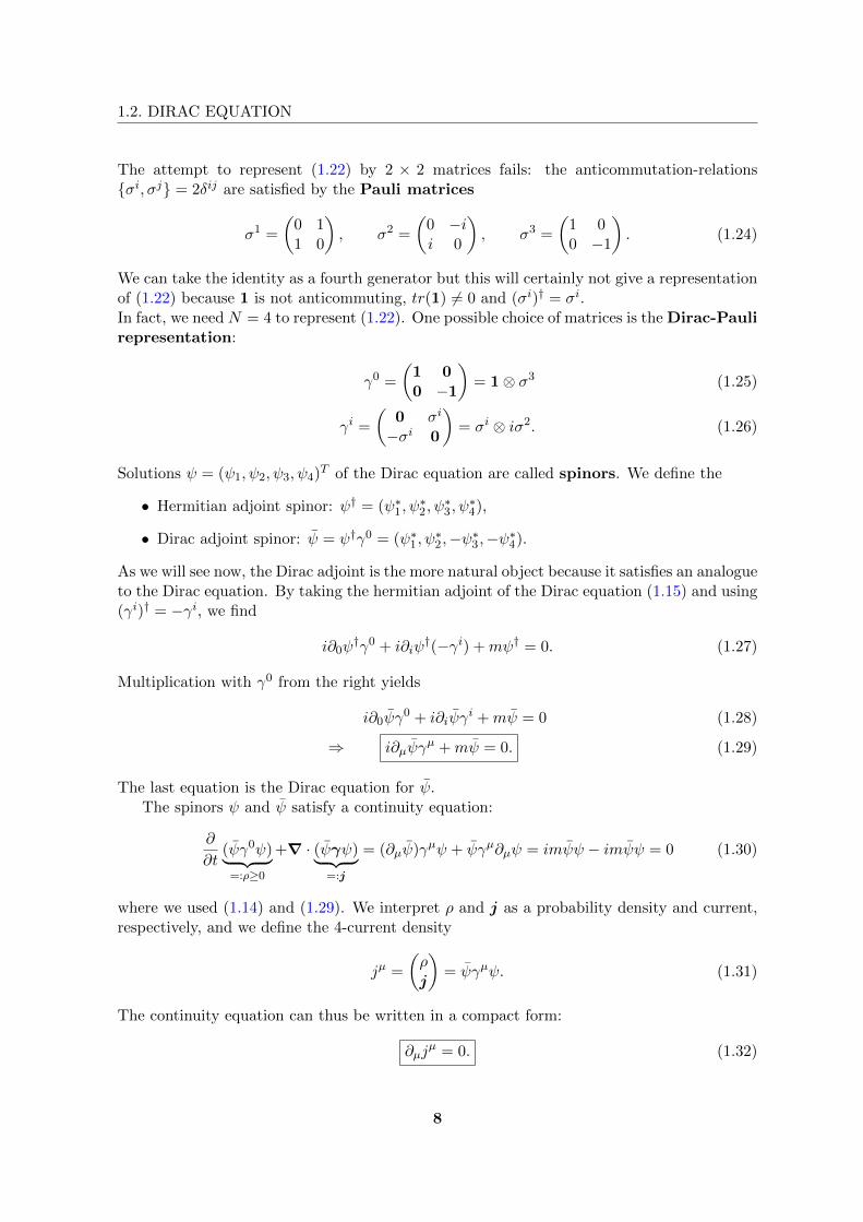
The attempt to represent (1.22) by 2 × 2 matrices fails: the anticommutation-relationsσi, σj = 2δij are satisfied by the Pauli matrices
σ1 =
(0 11 0
), σ2 =
(0 −ii 0
), σ3 =
(1 00 −1
). (1.24)
We can take the identity as a fourth generator but this will certainly not give a representationof (1.22) because 1 is not anticommuting, tr(1) 6= 0 and (σi)† = σi.In fact, we need N = 4 to represent (1.22). One possible choice of matrices is the Dirac-Paulirepresentation:
γ0 =
(1 00 −1
)= 1⊗ σ3 (1.25)
γi =
(0 σi
−σi 0
)= σi ⊗ iσ2. (1.26)
Solutions ψ = (ψ1, ψ2, ψ3, ψ4)T of the Dirac equation are called spinors. We define the
• Hermitian adjoint spinor: ψ† = (ψ∗1, ψ∗2, ψ
∗3, ψ
∗4),
• Dirac adjoint spinor: ψ = ψ†γ0 = (ψ∗1, ψ∗2,−ψ∗3,−ψ∗4).
As we will see now, the Dirac adjoint is the more natural object because it satisfies an analogueto the Dirac equation. By taking the hermitian adjoint of the Dirac equation (1.15) and using(γi)† = −γi, we find
i∂0ψ†γ0 + i∂iψ
†(−γi) +mψ† = 0. (1.27)
Multiplication with γ0 from the right yields
i∂0ψγ0 + i∂iψγ
i +mψ = 0 (1.28)
⇒ i∂µψγµ +mψ = 0. (1.29)
The last equation is the Dirac equation for ψ.The spinors ψ and ψ satisfy a continuity equation:
∂
∂t(ψγ0ψ)︸ ︷︷ ︸
=:ρ≥0
+∇ · (ψγψ)︸ ︷︷ ︸=:j
= (∂µψ)γµψ + ψγµ∂µψ = imψψ − imψψ = 0 (1.30)
where we used (1.14) and (1.29). We interpret ρ and j as a probability density and current,respectively, and we define the 4-current density
jµ =
(ρj
)= ψγµψ. (1.31)
The continuity equation can thus be written in a compact form:
∂µjµ = 0. (1.32)
8

1.3. THE DIRAC EQUATION IN AN ELECTROMAGNETIC FIELD
1.3 The Dirac Equation in an Electromagnetic Field
In the following we use the usual covariant momentum operators pµ = i∂µ = i(∂t,∇). Usingthe correspondence principle, this gives classical 4-momenta pµ = (E,−p) and pµ =
(E,p
),
respectively.The coupling of the Dirac equation to an electromagnetic field is done by a minimal substi-tution prescription:
pµ → pµ − eAµ with Aµ =
(φA
). (1.33)
In the position representation, this equation reads
i∂µ → i∂µ − eAµ with Aµ =
(φ−A
). (1.34)
which corresponds to H → H + eφ and p→ p− eA (well known minimal substitution fromquantum mechanics).The new Dirac equation reads
[iγµ(∂µ + ieAµ)−m]ψ = 0. (1.35)
Using the covariant derivative Dµ = ∂µ + ieAµ and the Feynman slash-notation γµaµ =aµγµ =: /a we can write this as
(i/∂ − e /A−m)ψ ≡ (i /D −m)ψ = 0. (1.36)
1.4 Lorentz Covariance of the Dirac Equation
Informally speaking, Lorentz covariance means that the laws of nature do not depend onthe choice of coordinates or the reference frame of our physical description.Let’s consider two inertial frames of reference I and I’ which are connected by the Poincaretransformation
x′µ = Λµνxν + aµ. (1.37)
There are 10 free parameters in this general Poincare transformation (3 rotations and 3 boostsin the Lorentz transformation Λµν and 4 coordinate displacements in aµ).Lorentz covariance of the Dirac equation means that it has the same form in I and in I’:
(iγµ∂µ −m)ψ(xµ) = 0 and (iγµ∂′µ −m)ψ′(x′µ) = 0. (1.38)
We want to determine the transformation behaviour of the spinor ψ under Poincare trans-formations, i.e. we want to find a transformation S(Λ) (represented as a 4 × 4-matrix) suchthat
ψ′(x′µ) = [S(Λ)ψ](xµ)
= S(Λ)ψ((Λ−1)µν(x′ν − aν)
). (1.39)
Using ∂µ = ∂x′ν
∂xµ∂
∂x′ν = Λνµ∂′ν and S(Λ)−1ψ′(x′ν) = ψ(xν) we can rewrite the Dirac equation
in I:(iγµΛνµ∂
′ν −m)S(Λ)−1ψ′(x′) = 0 (1.40)
9

1.4. LORENTZ COVARIANCE OF THE DIRAC EQUATION
Multiplying with S(Λ) from the left yields
(iS(Λ)ΛνµγµS(Λ)−1∂′ν −m)ψ′(x′) = 0. (1.41)
Comparison with the Dirac equation in I’ (c.f. (1.38)) gives the condition
S(Λ)−1γνS(Λ) = Λνµγµ. (1.42)
1.4.1 The Lorentz Group and the Poincare Group
The Poincare group is the group of all transformations which leave the equations of motionof light-waves invariant. They are represented by coordinate transformations (Λ, a) wherea describes a spacetime-translation (if a = 0 the transformation is called homogeneousLorentz transformation):
x′µ = Λµνxν + aµ, Λµν =
∂x′µ
∂xν. (1.43)
The invariance condition mentioned above means that = ∂2
∂t2−∆ = ∂µ∂
µ is invariant:
= ′ (1.44)
⇔ ∂x′λ
∂xµ∂′λ
︸ ︷︷ ︸=∂µ
gµν∂x′ρ
∂xν∂′ρ
︸ ︷︷ ︸=∂ν
!= ∂′λg
λρ∂′ρ (1.45)
⇔ ΛλµgµνΛρν = gλρ. (1.46)
This implies that det Λ = ±1 and Λ00 ≥ 1 or Λ0
0 ≤ −1.We have the following special cases:
• translations: (Λ, a) = (1, a)
• homogeneous LT: (Λ, a) = (Λ, 0)
• rotations: (Λ, a) = (R, 0)
• special LT (“boost”): (Λ, a) = (L, 0)
• spatial inversion: (Λ, a) = (P, 0) with P = diag(1,−1,−1,−1)
• time inversion: (Λ, a) = (T, 0) with T = diag(−1, 1, 1, 1)
• spacetime inversion: (Λ, a) = (PT, 0)
• proper LT: homogeneous LT which can be generated by repeated application of infinites-imal rotations and boosts. This is equivalent to det Λ = 1 and Λ0
0 ≥ 1. Proper LT arerepresented by 6 free parameters, 3 Euler angles to describe rotations and 3 velocitycomponents for boosts.A general infinitesimal proper LT can be written as
Λλµ = gλµ + ∆ωλµ. (1.47)
10

1.4. LORENTZ COVARIANCE OF THE DIRAC EQUATION
We want to use Eq. (1.46) in order to determine properties of ∆ωλµ:
ΛλµgµνΛρν = gλρ (1.48)
⇔ (gλµ + ∆ωλµ)gµν(gρν + ∆ωρν) = gλρ (1.49)
⇔ gλρ + ∆ωλρ + ∆ωρλ +O(∆ω2) = gλρ (1.50)
⇒ ∆ωλρ = −∆ωρλ (1.51)
We conclude that Λ has the following form:
Λµν =
1 ∆ω01 ∆ω02 ∆ω03
−∆ω01 −1 ∆ω12 ∆ω13
−∆ω02 −∆ω12 −1 ∆ω23
−∆ω03 −∆ω13 −∆ω23 −1
(1.52)
The parameters (∆ω01,∆ω02,∆ω03) in the first row describe special LT (e.g. ∆ω01 =
−∆ω01 = −∆β describes transformations into an inertial frame moving with c∆β inx-direction). The other three parameters describe infinitesimal rotations (e.g. ∆ω1
2 =−∆ω12 = ∆ϕ is a rotation around the z-axis by an angle ∆ϕ).
1.4.2 Transformation of Dirac-spinors
After this excursion into the theory of the Lorentz group we want to investiage Eq. (1.42)further. We consider an infinitesimal Lorentz transformation Λ as defined in Eq. (1.47) whichcorresponds to an S(Λ) of the following form:
S = 14 + τ, S−1 = 14 − τ with τ infinitesimal. (1.53)
The norm of ψ has to be invariant under the transformation which implies that detS = 1,hence tr(τ) = 0. Eq. (1.42) now reads
(1− τ)γµ(1 + τ) = γµ + γµτ − τγµ = γµ + ∆ωµνγν . (1.54)
This is solved by
τ =1
8∆ωµν(γµγ
ν − γνγµ). (1.55)
We define
σµν =i
2[γµ, γν ] (1.56)
and find the infinitesimal Lorentz transformation as it acts on Dirac-spinors
S(Λ) = 1− i
4∆ωµνσµν . (1.57)
Next we want to construct S(Λ) for finite Lorentz transformations Λ. Consider infinites-imal elements ∆ωµν of the infinitesimal LT. For example, a boost in dircetion n ∈ 1, ..., 6(corresponding to x, −x, ..., z, −z) yields
∆ωµν = ∆ω Iµνn with Iµν1 =
1 µν = 01
−1 µν = 10
0 else
(1.58)
11

1.4. LORENTZ COVARIANCE OF THE DIRAC EQUATION
and I2, ..., I6 analogously. We apply the LT which corresponds to this infinitesimal matrix Ntimes with ∆ω = ω
N in order to establish a finite boost in direction n:
x′ν = limN→∞
(g +
ω
NIn
)να1
(g +
ω
NIn
)α1
α2
· · ·(g +
ω
NIn
)αN−1
µxµ
=(eωIn
)νµxµ
= (cosh(ωIn) + sinh(ωIn))νµ xµ
=(1− I2
n + I2n coshω + In sinhω
)νµx
µ (1.59)
For example, the finite boost in x-direction reads
x′ν =
coshω − sinhω 0 0− sinhω coshω 0 0
0 0 1 00 0 0 1
ν
µ
xµ (1.60)
This is a finite Lorentz boost (in x-direction) with velocity v = β = tanhω (i.e. γ = coshω)as it acts on vectors. How does it act on spinors? Having derived Eq. (1.57), we can followthe same procedure as in the case of vectors:
ψ′(x′) = S(Λ)ψ(x)
= limN→∞
(1− i
4
ω
NIµνn σµν
)Nψ(x)
= exp
(− i
4ωIµνn σµν
)ψ(x) (1.61)
1.4.3 Spin of Dirac-Spinor
Our next goal is to show that Dirac-spinors show a similar behaviour under rotations as thePauli-spinors which we know from elementary quantum mechanics. In order to do so, weconsider an infinitesimal rotation ∆ϕ around the z-axis:
∆ω12 = −∆ω21 = −∆ϕ. (1.62)
According to Eqs. (1.56) and (1.57) this corresponds to
τ =i
2∆ϕσ12 =
i
2∆ϕ · i
2[γ1, γ2] =
i
2∆ϕ
(σ3 00 σ3
). (1.63)
This infinitesimal generator for rotations can be exponentiated in order to obtain a finiterotation with an angle ϕ. The resulting Dirac spinor is
ψ′(x′) = ei2ϕσ12ψ(x) = (cos
ϕ
2+ iσ12 sin
ϕ
2)ψ(x). (1.64)
We see that the spinor transforms such that a rotation around ϕ = 2π yields ψ′(x′) = −ψ(x).One has to perform a 4π-rotation in order to get back the initial object without the minussign. This is the same transformation behaviour that we are familiar with from the spinformalism of quantum mechanics.
12

1.4. LORENTZ COVARIANCE OF THE DIRAC EQUATION
Remark: In contrast to spinors, the ordinary 4-vectors stay unchanged when a rotation around2π is performed, of course. Rotations around ϕ on Minkowski space are implemented in thefamiliar way:
x′µ =
1 0 0 00 cosϕ sinϕ 00 − sinϕ cosϕ 00 0 0 1
µ
ν
xν . (1.65)
1.4.4 Parity and Time-reversal
The Lorentz transformation which describes a parity transformation is
Λµν =
1 0 0 00 −1 0 00 0 −1 00 0 0 −1
µ
ν
. (1.66)
It is an improper LT since det Λ = −1. In order to find S = S(P ), the representation of thisLT on Dirac spinors, we apply Eq. (1.42):
S−1γµS = Λµνγν = (γ0,−γ1,−γ2,−γ3)µ. (1.67)
This equation is solved by S = eiϕγ0 where eiϕ is an unobservable phase factor. So thetransformation of the Dirac spinor under spatial inversion is given by
ψ′(x′) = ψ′(t,x′) = ψ′(t,−x) = eiϕγ0ψ(t,x) = eiϕγ0ψ(x). (1.68)
Remembering that γ0 = 1⊗ σ3, we infer that the first two components ψ1, ψ2 of ψ have theopposite parity than ψ3, ψ4.In a very similar way one can deal with the time-reversal transformation. The result is
ψ′(x′) = ψ′(−t,x) = S(T )ψ∗(t,x) = S(T )ψ∗(x) with S(T ) = iγ1γ3. (1.69)
1.4.5 Transformation of ψ
We want to find out how ψ = ψ†γ0 transforms, given that ψ′ = Sψ. It clearly holds that
ψ′ = ψ′†γ0 = ψ†S†γ0. (1.70)
Taking the adjoint of Eq. (1.42) we find
(Λµνγν)† = S†(γµ)†(S†)−1 (1.71)
⇔ Λµνγ0γνγ0 = S†γ0γµγ0(S†)−1 (1.72)
where we used Eq. (1.23). Multiplying with γ0 from the left and from the right we obtain
Λµνγν
︸ ︷︷ ︸=S−1γµS
= (γ0S†γ0)γµ(γ0S†γ0)−1 (1.73)
⇒ γµ = (Sγ0S†γ0)γµ(Sγ0S†γ0)−1. (1.74)
13

1.4. LORENTZ COVARIANCE OF THE DIRAC EQUATION
But if (Sγ0S†γ0) commutes with all γµ, then it has to be a multiple of 14:
Sγ0S†γ0 = α1 (1.75)
⇒ S†γ0 = αγ0S−1 (1.76)
⇒ ψ′ = αψ†γ0S−1. (1.77)
Since Sγ0S† and γ0 are both hermitian and detS = 1 we infer from Eq. (1.75) that
α = α∗ and α4 = 1. (1.78)
So α = ±1. One can easily verify that the sign of α characterizes the type of Lorentztransformation that we are dealing with in the sense that
α = sgn(Λ00) (1.79)
so that finally
ψ′ = sgn(Λ00)ψS−1. (1.80)
1.4.6 Bilinear Covariants
We can build new matrices by multiplying γ-matrices together. Because of the Clifford algebrawhich they satisfy (in particular, different γ-matrices anticommute and the square of each ofthem is ±1), an arbitrary product of γ-matrices is proportional to one of the following 16linearly independent invariants which we call Γnαβ. We define:
• ΓS = 1 (1 matrix)
• ΓVµ = γµ (4 matrices)
• ΓTµν = σµν (6 matrices)
• ΓP = iγ0γ1γ2γ3 =: γ5 (1 matrix)
• ΓAµ = γ5γµ (4 matrices)
Properties of γ5:
• γ52 = 1
• γ5, γµ = 0
• γ†5 = iγ3γ2γ1γ0 = γ5
• trγ5 = 0
• Dirac-Pauli representation: γ5 =
(0 11 0
)
From the Clifford algebra one can very easily verify the following properties:
• (Γn)2 = ±1 for all n
14

1.5. CHARGE CONJUGATION
• For all a 6= b there exists an n 6= S, such that ΓaΓb = εΓn with ε ∈ ±1,±i.
• For all n 6= S there exists an m, such that ΓnΓm = −ΓmΓn.
⇒ ±trΓn = tr(ΓnΓmΓm)
= −tr(ΓmΓnΓm)
= −tr(ΓnΓmΓm)
= 0 (1.81)
• The Γn are linearly independent.proof: Consider
∑n anΓn = 0. From the previous point it follows that aS = 0 (just take
the trace of the linear combination). Due to the first two points, multiplication withΓm 6= ΓS and taking the trace yields am 6=s = 0. Hence an = 0 for all n.
We can use the quantities Γn to build objects of the form ψΓnψ which have a well definedcanonical transformation behaviour under orthochronous Lorentz transformations (Λ0
0 ≥ 1).In order to do so, remember the transformation behaviour of ψ and ψ:
ψ′(x′) = Sψ(x), ψ′(x′) = ψ(x)S−1. (1.82)
We infer the following transformation properties where we note a close analogy to the trans-formation behaviour of scalars, 4-vectors and tensors from the special theory of relativity:
Scalar: ψ′(x′)ψ′(x′) = ψ(x)ψ(x)Vector: ψ′(x′)γµψ′(x′) = Λµνψ(x)γνψ(x)Tensor: ψ′(x′)σµνψ′(x′) = ΛµλΛνρψ(x)σλρψ(x)Pseudoscalar: ψ′(x′)γ5ψ
′(x′) = (det Λ)ψ(x)γ5ψ(x)Pseudovector (Axial vector): ψ′(x′)γ5γ
µψ′(x′) = (det Λ)Λµνψ(x)γ5γνψ(x)
The pseudoscalars and pseudovectors transform exactly like scalars and vectors but pick upa minus sign if the LT is improper. The proof of the first three identities is trivial given Eqs.(1.42) and (1.82). The transformation properties of the pseudoscalar and pseudovector followfrom
• γ5, γ0 = 0 ⇒ γ5, P = 0
• [γ5, σµν ] = 0 ⇒ [γ5, S] = 0 for every proper LT S.
1.5 Charge Conjugation
We consider the Dirac equation in an electromagnetic field,
(i/∂ − e /A−m)ψ = 0. (1.83)
The same equation for an oppositely charged particle reads
(i/∂ + e /A−m)ψC = 0 (1.84)
where ψC is the (yet unknown) charge conjugate spinor. If we complex conjugate Eq. (1.83)we obtain
(−(i∂µ + eAµ)(γµ)∗ −m)ψ∗ = 0 (1.85)
15

1.6. SOLUTIONS OF DIRAC EQUATION FOR FREE PARTICLES
where we used that (i∂µ)∗ = −i∂µ and (Aµ)∗ = Aµ (the electromagnetic field can alwayschosen to be real2). Thus, in a sense, complex conjugation does something similar as chargeconjugation: it changes the relative sign of the derivative and the term containing the charge.We want to find a spinor ψC which is the solution to the charge conjugate Dirac equation(Eq. (1.84)). The above considerations motivate that there should exist a linear operator Csuch that
ψC = Cψ∗. (1.86)
We can impose conditions on C if we use the complex conjugate Dirac equation (1.85), replaceψ∗ by C−1Cψ∗ = C−1ψC and multiply with C from the left. Comparison with Eq. (1.84)leads to the following condition on C:
C(γµ)∗C−1 = −γµ. (1.87)
We rewrite this condition in order to find
C(γµ)∗ = −γµC. (1.88)
We use that (γa)∗ = γa for a = 0, 1, 3 whereas (γ2)∗ = −γ2 which implies
C, γa = 0 (a = 0, 1, 3) (1.89)[C, γ2
]= 0. (1.90)
From this we conclude thatC = αγ2. (1.91)
We can determine α by imposing another important condition on C: because the twofoldapplication of charge conjugation should give back the initial spinor, we demand that
ψ = Cψ∗C = C(Cψ∗)∗ = CC∗ψ. (1.92)
It follows thatCC∗ = 1
!= |α|2γ2(γ2)∗ ⇒ C = iγ2. (1.93)
Hence we find for the charge conjugate spinor
ψC = iγ2ψ∗ with iγ2 =
0 0 0 10 0 −1 00 −1 0 01 0 0 0
. (1.94)
1.6 Solutions of Dirac Equation for free particles
We want to find explicit solutions to the free Dirac equation
(−i/∂ +m)ψ(x) = 0. (1.95)
We begin by writing down an ansatz for solutions in the rest frame (p = 0, i.e. all but thetemporal derivatives vanish) where the Dirac equation reads
(−iγ0∂0 +m)ψ(x) = 0. (1.96)
2This is true also for oscillating fields.
16

1.6. SOLUTIONS OF DIRAC EQUATION FOR FREE PARTICLES
The solutions assume the form
ψ1,2(x, t) = u+,−(pµ)e−imt (1.97)
ψ3,4(x, t) = v−,+(−pµ)eimt (1.98)
with
u+(m,0) =√
2m
1000
, u−(m,0) =
√2m
0100
v−(−m,0) =√
2m
0010
, v+(−m,0) =
√2m
0001
.
(1.99)
Hence the eigenvalues E = m for ψ1,2 are positive whereas the energy E = −m of ψ3,4
is negative. We encountered this problem already in the Klein-Gordon formalism and aswe see now, the Dirac equation does not resolve this problem. But it gives an interestinginterpretation. We note that
ψ3 = −Cψ∗2 = −(ψ2)C (1.100)
ψ4 = +Cψ∗1 = (ψ1)C (1.101)
which means that ψ3,4 may be interpreted as being antiparticles of ψ2,1: they are essentiallythe same as the positive energy solutions ψ1,2 but with negative energy and opposite charge(and opposite momentum as we will see next).
In order to find solutions for moving particles we generalize the above solutions:
ψ1,2(x, t) = u+,−(pµ)e−ipx (1.102)
ψ3,4(x, t) = v−,+(−pµ)e+ipx. (1.103)
With p0 ≥ 0 we find Dirac equations for u and v:
(/p−m)u±(p) = 0 = u±(p)(/p−m)
(/p+m)v±(p) = 0 = v±(p)(/p+m).(1.104)
We observe that
/p/p = pµpν1
2γµ, γν = pµpνg
µν1 = p21 (1.105)
which leads us to(/p−m)(/p+m) = p2 −m2 = 0. (1.106)
Therefore the Eqs. (1.104) can be solved by applying [±/p+m] to the free solutions:
u±(p) = A(p)[/p+m]u±(m,0) (1.107)
v±(p) = B(p)[−/p+m]v±(m,0) (1.108)
u±(p) = A(p)u±(m,0)[/p+m] (1.109)
v±(p) = B(p)v±(m,0)[−/p+m]. (1.110)
17

1.6. SOLUTIONS OF DIRAC EQUATION FOR FREE PARTICLES
In order to determine A(p), B(p) we can use Lorentz invariance which implies
u±(p)u±(p) = u±(m,0)u±(m,0) = 2m, (1.111)
v±(p)v±(p) = v±(m,0)v±(m,0) = −2m. (1.112)
It follows that
2m = u±(p)u±(p) = A2(p)u±(m,0)[/p+m]2u±(m,0)
= A2(p)u±(m,0)[/p2 + 2m/p+m2]u±(m,0)
= A2(p)u±(m,0)[2m2 + 2m/p]u±(m,0)
= A2(p)u±(m,0)[2m2 + 2mp0γ0]u±(m,0)
= A2(p)[4m3 + 4m2p0] (1.113)
where we used u±(m,0)γiu±(m,0) = 0 for i = 1, 2, 3 from the third to the fourth line andu±(m,0)γ0u±(m,0) = 2m in the last step. Solving for A(p) yields
A(p) =
√1
2m(p0 +m). (1.114)
By analogous reasoning one finds that
B(p) = A(p). (1.115)
We can use two component Pauli spinors χ which represent “spin up” and “spin down”:
χ+ =
(10
), χ− =
(01
). (1.116)
We then have
u±(p) =√p0 +m
(χ±
σ·pp0+m
χ±
), v±(p) =
√p0 +m
( σ·pp0+m
χ∓χ∓
)(1.117)
and the following orthogonality relations:
ur(p)us(p) = 2mδrs ur(p)vs(p) = 0 (1.118)
vr(p)vs(p) = −2mδrs vr(p)us(p) = 0. (1.119)
Note that this normalization is invariant under ortochronous LT:
u′ru′s = u†rS
†γ0Sus = u†rγ0S−1Sus = δrs2m. (1.120)
Hence ψiψi is a Lorentz scalar.
18

1.6. SOLUTIONS OF DIRAC EQUATION FOR FREE PARTICLES
1.6.1 Energy Projection Operators
Our aim is to find a set of quantum numbers which labels all solutions of the Dirac equation.A first step in this direction is the definition of the projectors
Λ± =±/p+m
2m. (1.121)
The following relations hold:
Λ+u±(p) =/p+m
2mu±(p) = u±(p) (1.122)
Λ−u±(p) = 0 (1.123)
Λ−v±(p) = v±(p) (1.124)
Λ+v±(p) = 0 (1.125)
so Λ+ projects on particle states whereas Λ− projects on antiparticle states. The Λ± satisfythe following completeness relation:
Λ+ + Λ− = 1. (1.126)
We conclude that the u± form the subspace of all particle states and
∑
s=±us(p)us(p) = /p+m = 2mΛ+. (1.127)
Likewise the v± form the subspace of all antiparticle states:
∑
s=±vs(p)vs(p) = /p−m = −2mΛ−. (1.128)
1.6.2 Helicity and Chirality
As we have seen, every solution for a fixed energy is twofold degenerate. We want to interpretthis degeneracy as due to a quantum number “helicity”.First, we rewrite the Dirac equation in a Schrodinger form. The matrix representation of theDirac Hamiltonian reads
H = −iγ0γ ·∇ + γ0m = γ0(γ · p+m) =
(m1 σ · pσ · p −m1
)(1.129)
and so we can write
i∂
∂tψ = Hψ. (1.130)
Helicity is defined as the projection of the spin in the direction of motion:
h(p) =1
2Σ · p|p| =
1
2
(σ · p 0
0 σ · p
)(1.131)
19

1.6. SOLUTIONS OF DIRAC EQUATION FOR FREE PARTICLES
Because of [H,h(p)] = 0 there exists a common set of eigenfunctions of H and h(p). Thereforehelicity is a good quantum number which we shall call λ. Consider p = ez. Then we have
h(ez) =1
2
(σz 00 σz
). (1.132)
with eigenfunctions χ± of σz:σzχ± = ±χ± (1.133)
such that
h(ez)u±(p) = ±1
2u±(p) (1.134)
h(ez)v±(p) = ∓1
2v±(p). (1.135)
We interpret the particle solutions as follows:
λ =
+1
2 positive helicity (“right-handed“, u+), s ↑↑ p−1
2 negative helicity (”left-handed”, u−), s ↑↓ p(1.136)
In order to interpret the antiparticle solutions, we have to be a bit more careful. Considerthe fact that
ψ3,4(x, t) = v−,+(−pµ)eimt. (1.137)
Hence we find
λ =
+1
2 positive helicity (“right-handed“, v−), s ↓↓ p−1
2 negative helicity (”left-handed”, v+), s ↑↓ p(1.138)
(in the upper case, s and p are both anti-aligned such that the helicity is positive.)
Chirality exploits the symmetry of the Dirac equation for m = 0,
i/∂ψ0 = 0, (1.139)
where the upper index 0 indicates that we are dealing with the massless case. According toEq. (1.117) the solutions read
u0±(p) =
√|p|(
χ±σ·p|p| χ±
)=√|p|(χ±±χ±
)(1.140)
v0±(p) =
√|p|(∓χ∓χ∓
). (1.141)
In the massless case, it can be seen from Eq. (1.129) that because of γ5, γµ = 0, one finds
i/∂ψ0 = 0 ⇒ i/∂γ5ψ0 = 0 (1.142)
so γ5 maps solutions of the massless Dirac equation to solutions. Because of γ25 = 1 all
eigenvalues of the chirality operator γ5 are ±1. The eigenfunctions of γ5 form the so calledchirality basis:
γ5ψ0± = ±ψ0
±. (1.143)
20
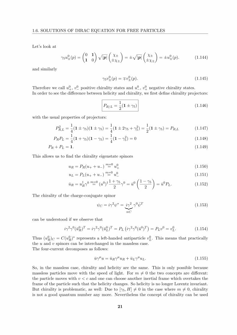
1.6. SOLUTIONS OF DIRAC EQUATION FOR FREE PARTICLES
Let’s look at
γ5u0±(p) =
(0 11 0
)√|p|(χ±±χ±
)= ±
√|p|(χ±±χ±
)= ±u0
±(p). (1.144)
and similarly
γ5v0±(p) = ∓v0
±(p). (1.145)
Therefore we call u0+, v0
− positive chirality states and u0−, v0
+ negative chirality states.In order to see the difference between helicity and chirality, we first define chirality projectors:
PR/L =1
2(1± γ5) (1.146)
with the usual properties of projectors:
P 2R,L =
1
4(1± γ5)(1± γ5) =
1
4(1± 2γ5 + γ2
5) =1
2(1± γ5) = PR,L (1.147)
PRPL =1
4(1 + γ5)(1− γ5) =
1
4(1− γ2
5) = 0 (1.148)
PR + PL = 1. (1.149)
This allows us to find the chirality eigenstate spinors
uR = PR(u+ + u−)m=0= u0
+ (1.150)
uL = PL(u+ + u−)m=0= u0
− (1.151)
uR = u†Rγ0 m=0
= (u0)†1 + γ5
2γ0 = u0
(1− γ5
2
)= u0PL. (1.152)
The chirality of the charge-conjugate spinor
ψC = iγ2ψ∗ = iγ2
︸︷︷︸≡C
γ0ψT (1.153)
can be understood if we observe that
iγ2γ0(u0R)T = iγ2γ0(u0
L)T = PL(iγ2γ0(u0)T
)= PLv
0 = v0L. (1.154)
Thus (u0R)C = C(u0
R)∗ represents a left-handed antiparticle v0L. This means that practically
the u and v spinors can be interchanged in the massless case.The four-current decomposes as follows:
uγµu = uRγµuR + uLγ
µuL. (1.155)
So, in the massless case, chirality and helicity are the same. This is only possible becausemassless particles move with the speed of light. For m 6= 0 the two concepts are different:the particle moves with v < c and one can choose another inertial frame which overtakes theframe of the particle such that the helicity changes. So helicity is no longer Lorentz invariant.But chirality is problematic, as well: Due to [γ5, H] 6= 0 in the case where m 6= 0, chiralityis not a good quantum number any more. Nevertheless the concept of chirality can be used
21

1.6. SOLUTIONS OF DIRAC EQUATION FOR FREE PARTICLES
in the m 6= 0 case via a decomposition of ψ into parts which are no longer solutions of theDirac equation but which transform independently under proper Lorentz transformations3
and which are well defined chiral eigenstates:
ψ︸︷︷︸solution of Dirac eq.
= ψL + ψR︸ ︷︷ ︸no longer solutions of Dirac eq.
. (1.156)
In the massless case this splitting of a solution is no longer necessary because ψR and ψLbecome independent solutions of the Dirac equation.From calculations like
ψLψL =1
4((1− γ5)ψ)† γ0(1− γ5)ψ
=1
4ψ(1 + γ5)(1− γ5)ψ
= ψPRPLψ
= 0 (1.157)
and similar considerations, it follows that the chirality structure of the Dirac Lagrangian is
L = ψ(iγµ∂µ −m)ψ (1.158)
= i[ψR /∂ψR + ψL/∂ψL]−m[ψRψL + ψLψR]. (1.159)
It can be seen that the mass term mixes different chiralities. If m = 0 the chiralities areindependent.
3This is simply because γ5 and σµν have common eigenspaces due to [σµν , γ5] = 0.
22

Chapter 2
Quantization of the Scalar Field
2.1 Classical Field Theory
In classical mechanics the dynamics of a particle described by coordinates q, q is completelydetermined by the Lagrangian function L(q, q) and the action principle
δS = δ
∫L(q, q)dt = 0 (2.1)
which leads to the Euler-Lagrange equations
d
dt
dL
dq− dL
dq= 0. (2.2)
Equivalently we can describe the system in a Hamiltonian formalism. We define
p :=dL
dq(2.3)
H(p, q) = pq − L(q, q) (2.4)
and can describe the system using the classical Poisson bracket relations
H, q = q, H, p = p, p, q = 1. (2.5)
This concept applies to point particles but it can be generalized to the concept of aLagrangian density when we replace phase space coordinates with fields. We define theLagrangian density L using the Lagrange function:
L =
∫d3x L(x, t) ⇒ S =
∫d4xL(x, t). (2.6)
Note that L depends on space and time only via fields:
L(x) = L(φ(x), ∂µφ(x)). (2.7)
Consider, for example, a vibrating string: position and time of string segments will not appearin the Lagrangian density but rather the state of the string at a given position and time isrelevant.
23

2.1. CLASSICAL FIELD THEORY
The principle of least action says that
0 = δS
=
∫d4x
[∂L∂φ
δφ+∂L
∂(∂µφ)δ(∂µφ)
]
=
∫d4x
[∂L∂φ
δφ− ∂µ(
∂L∂(∂µφ)
)δφ+ ∂µ
(∂L
∂(∂µφ)δφ
)
︸ ︷︷ ︸surface term
]. (2.8)
where we used partial integration. This leads to the Euler-Lagrange equations for φ (if weassume that the fields fall fast enough at infinity so that the surface term vanishes):
∂µ
(∂L
∂(∂µφ)
)− ∂L∂φ
= 0. (2.9)
As an example, consider classical electromagnetism which is described by
L = −1
4FµνF
µν − jµAµ (2.10)
with the field-strength tensor Fµν = ∂µAν − ∂νAµ and the 4-current jµ. This Lagrangiandensity leads to the equations of motion
∂µFµν = jν (2.11)
which are the inhomogeneous Maxwell equations.Note that for fields, there is also a Hamiltonian formalism. Define the canonical momentum
density
π(x) :=∂L∂φ
(2.12)
and write the Hamiltonian in terms of the Hamiltonian density H:
H =
∫d3x [π(x)φ(x)− L]︸ ︷︷ ︸
=:H
. (2.13)
2.1.1 Symmetries and Noether-Theorem
In the following we are interested in symmetries of a physical system which are always reflectedby the Lagrangian density. Analogous to classical mechanics, a transformation of the fields inthe Lagrangian density which does not change the equations of motions, is called a symmetry.More formally, we consider continuous transformations1 of φ(x) of the form
φ(x) −→ φ′(x) = φ(x) + α∆φ(x) (2.14)
with an infinitesimal constant α. It is called a symmetry transformation if the Euler-Lagrange equations remain invariant. This is the case if and only if L remains invariant orchanges only by a 4-divergence:
L −→ L+ α∂µJµ(x). (2.15)
1There may also be discontinuous symmetries (e.g. parity or time reversal). Noether’s theorem is notconcerned with such symmetries.
24

2.1. CLASSICAL FIELD THEORY
On the other hand, we can also calculate the change of L under the transformation (2.14)directly:
α∆L =∂L∂φ
(α∆φ) +∂L
∂(∂µφ)∂µ(α∆φ)
= α∂µ
(∂L
∂(∂µφ)∆φ
)+ α
(∂L∂φ− ∂µ
(∂L
∂(∂µφ)
))
︸ ︷︷ ︸=0 (Euler-Lagrange)
∆φ. (2.16)
Comparison of Eqs. (2.15) and (2.16) leads to a conserved current (Noether current)
jµ =∂L
∂(∂µφ)∆φ− Jµ with ∂µj
µ = 0. (2.17)
Noether’s theorem states precisely this fact that every continuous symmetry of the La-grangian density leads to such a conserved current. Note that jµ is only “conserved” if thefield φ is a solution to the Euler-Lagrange equation. Otherwise our derivation doesn’t work.From this conserved current we also get a conserved charge (“conserved” now meaning “con-served in time”)
Q =
∫d3x j0(x). (2.18)
Consider the following two examples:
• A massless scalar field is described by
L =1
2(∂µφ)(∂µφ). (2.19)
We see that L is invariant under φ→ φ+α. The corresponding Nother current is givenby
jµ = ∂µφ (2.20)
such that
∂µjµ = φ = 0. (2.21)
• A massive, complex, free, scalar field (Klein-Gordon field) is described by
L = (∂µφ)(∂µφ∗)−m2φφ∗. (2.22)
Now, L is invariant under φ → eiαφ with infinitesimal α ∈ R. The correspondingexpressions in Eq. (2.14) are
α∆φ = iαφ, α∆φ∗ = −iαφ∗. (2.23)
We conclude that
jµ = i ((∂µφ∗)φ− φ∗(∂µφ)) (2.24)
is conserved.
25

2.2. THE KLEIN-GORDON FIELD
2.1.2 Energy-Momentum Tensor
We can use Noether’s theorem for spacetime transformations, as well. For example, considerthe infinitesimal translation
x′µ = xµ + αµ. (2.25)
The Lagrangian changes by
∆L =∂L∂φ
∆φ+∂L
∂(∂µφ)∆(∂µφ) = αµ∂µL = αν∂µ(δµνL). (2.26)
where we used ∆φ = φ(x + α) − φ(x) = αµ∂µφ(x). The last step is neccessary in order toget the same form as in Eq. (2.15) but with αν instead of the scalar α. In the same sense asabove, this leads to four (!) conserved currents
Jµν =∂L
∂(∂µφ)∂νφ− δµνL (2.27)
∂µJµν = 0 (2.28)
which we call the energy-momentum tensor. Conventionally, we often denote it by
Tµν =∂L
∂(∂µφ)∂νφ− gµνL with ∂µT
µν = 0. (2.29)
We can easily check that due to Eq. (2.28) and Gauss’ theorem
Pν =
∫d3x J0
ν =
∫d3x
[π∂νφ− δ0
νL]
(2.30)
is conserved. The 0-component of Pν (the associated conserved Noether charge) is
P0 =
∫d3x J0
0 =
∫d3x
[πφ− L
]= H (2.31)
which we interpret as energy: the Hamiltonian alias energy appears as a conserved Noethercharge.The spatial components of Pν which are conserved due to translation invariance constitutejust the total momentum.
2.2 The Klein-Gordon Field
The Klein-Gordon equation for a real scalar field reads (in position-space):
( +m2)φ(x) = 0. (2.32)
To get the corresponding Lagrangian, we calculate backwards:
0 =
∫ t2
t1
dt
∫d3x
(∂2φ
∂t2−∆φ+m2φ
)δφ(x)
= −δ∫ t2
t1
dt
∫d3x
(1
2
(∂φ
∂t
)2
− 1
2(∇φ)2 − 1
2m2φ2
)(2.33)
26

2.2. THE KLEIN-GORDON FIELD
which can be seen using integration by parts. We used δφ(t1) = δφ(t2) = 0 and the fact thatφ falls off fast enough at infinity. Hence the Lagrangian for the Klein-Gordon field reads
L(φ, ∂µφ) =1
2(∂µφ)(∂µφ)− 1
2m2φ2. (2.34)
In this case, the canonical momentum operator (field-momentum density) and the energy-momentum tensor are
π(x, t) =∂L∂φ
= φ (2.35)
J00 = H(π, φ) = πφ− L =1
2
(π2 + (∇φ)2 +m2φ2
)(2.36)
→ H =
∫d3x H(x, t) (2.37)
J0i = −π∂iφ = −∂L∂φ
∂iφ (2.38)
→ P = −∫d3x π∇φ. (2.39)
2.2.1 Quantization of Classical Systems
In quantum mechanics we distinguish between the Schrodinger and the Heisenberg picture:
• In the Schrodinger picture, energy eigenstates evolve in time by means of a harmonictime dependence ∼ eiωpt. The field operators are time-independent.
• In the Heisenberg picture, the particle states are time-independent whereas the fieldoperators do depend on time.
A state ψH(x) in the Heisenberg picture is related to the corresponding Schrodinger state as
ψH(x) = eiHtψS(x, t). (2.40)
For operators, the relation is
OH(t) = eiHtOSe−iHt. (2.41)
The Schrodinger equation and the Heisenberg equation of motion for operators read respec-tively
i∂ψS(t)
∂t= HψS(t), (2.42)
idOH(t)
dt= [OH(t), H]. (2.43)
The Heisenberg equation (2.43) is valid for operators which are not explicitly time-dependent.It can be obtained by applying canonical quantization rules to the classical equation of motionin its Poisson-bracket notation. These quantization rules are
q(t)→ q(t) (2.44)
p(t)→ p(t) (2.45)
, → −i[ , ] (2.46)
27

2.2. THE KLEIN-GORDON FIELD
which leads to the relations
[qi, pj ] = iδij , [pi, pj ] = [qi, qj ] = 0. (2.47)
In quantum field theory we do something similar but with the difference that we want toquantize a continuum described by classical fields φ, φ instead of q and p. In the quantumcase the φ’s are no longer classical fields but field operators. For the moment, we workin the Schrodinger picture which may have been more convenient in elementary quantummechanics. Therefore we promote the time-independent field operators φ(x) and π(x). Inour quantization procedure we postulate the following commutation relations on the fieldswhich are analogous to the “usual” quantization rules for point particles:
[φ(x), π(y)] = iδ(3)(x− y)
[π(x), π(y)] = 0
[φ(x), φ(y)] = 0.
(2.48)
We will see soon that the Heisenberg picture is actually more appropriate in quantum fieldtheory. We will then impose similar commutation relations with an additional time-coordinate(in this sense, the above commutation relations are for fields at equal times).
2.2.2 Fourier Decomposition of the Klein-Gordon Field
From elementary quantum mechanics we know how to solve the simple harmonic oscillatorproblem. The Hamiltonian is
H = ω
(a†a+
1
2
)(2.49)
with
a =ωmx+ ip√
2ωm, a† =
ωmx− ip√2ωm
. (2.50)
Inverting these equations we find
x =1√
2ωm(a+ a†), p = −i
√ωm
2(a− a†). (2.51)
We want to attack the problem of the Klein-Gordon field in a similar way. To this end, webegin the quantization procedure by replacing the fields by operators. First, we write theKlein-Gordon field operator as a Fourier expansion (we have a continuum of “oscillators”now):
φ(x) =
∫d3p
(2π)3
(fp(x)ap + f∗p(x)a†p
)
=
∫d3p
(2π)3
1√2ωp
(ap + a†−p
)eip·x (2.52)
with fp(x) =eip·x√
2ωp, ωp =
√p2 +m2 = Ep.
28
2.2. THE KLEIN-GORDON FIELD
By analogy, we define the momentum density operator as
π(x) = (−i)∫
d3p
(2π)3ωp
(fp(x)ap − f∗p (x)a†p
)
= −i∫
d3p
(2π)3
√ωp2
(ap − a†−p
)eip·x (2.53)
We can write ap and a†p explicitly (although we will not use them very often):
ap =
∫d3x f∗p(x) (ωpφ(x) + iπ(x)) (2.54)
a†p =
∫d3x fp(x)
(ωpφ
†(x)− iπ†(x))
(2.55)
where φ† = φ, π† = π. We calculate the canoncical commutation relations (with x0 = y0 = t)using the postulates (2.48):
[ap, a†p′ ] =
∫d3xd3y
[f∗p (x)ωpφ(x) + f∗p (x)iπ(x),
fp′(y)ωp′φ†(y)− ifp′(y)π†(y)
]
=
∫d3xd3yf∗p (x)fp′(y)
(−iωp[φ(x), π†(y)] + iωp′ [π(x), φ†(y)]
)
=
∫d3xd3yf∗p(x)fp′(y)
(−iδ(3)(x− y)
) (iωp + iωp′
)
=
∫d3x
1√2ωp
1√2ωp′
(ωp + ωp′)e−ix·(p−p′)
= (2π)3 (ωp + ωp′)
2ωpδ(3)(p− p′)
= (2π)3δ(3)(p− p′). (2.56)
[ap, ap′ ] = 0 (2.57)
[a†p, a†p′ ] = 0. (2.58)
These are exactly the expected commutation relations for ladder operators in analogy to theharmonic oscillator known from quantum mechanics, but generalized to fields. Using thesecommutator relations one can check by analogous reasoning that our approach is consistent,i.e. it really holds true that
[φ(x), π(y)] = iδ(3)(x− y) (2.59)
[φ(x), φ(y)] = [π(x), π(y)] = 0. (2.60)
In order to quantize our classical model, we switch to a Hamiltonian formalism. From Eq.
29

2.2. THE KLEIN-GORDON FIELD
(2.37) we know what the Hamiltonian looks like in its explicitly field-dependent form:
H =
∫d3x
(1
2π2 +
1
2(∇φ)2 +
1
2m2φ2
)
=
∫d3p
(2π)3
1
2ωp
(a†pap + apa
†p
)
=
∫d3p
(2π)3ωp
(a†pap +
1
2[ap, a
†p]
). (2.61)
The explicit proof of this identity is a bit lengthy: one has to insert the field operators as givenin Eqs. (2.52) and (2.53) in the first line and use the commutation relations (→ exercise). Theform of H should be very familiar from the theory of the harmonic oscillator (cf. Eq. (2.49)):the Klein-Gordon Hamiltonian appears to be a continuous sum over harmonic oscillators: theterm a†a is known to be an occupation number operator.We can try to determine the vacuum energy by applying this Hamiltonian to the vacuumstate. This attempt causes serious problems because of the commutator of creation andannihilation operators of the same field mode:
H|0〉 =
∫d3p
(2π)3ωp
(a†p ap|0〉︸ ︷︷ ︸
=0
+1
2[ap, a
†p]
︸ ︷︷ ︸=(2π)3δ(3)(0)
|0〉)→∞. (2.62)
We see that although the (ground state) energy contribution∫ d3p
(2π)312 [ap, a
†p] is infinite, it
is still constant in the sense that it does not depend on any field configuration. It doesn’tmatter in which excitation mode the field is. The action of H on any state will always givethe state’s energy plus the same infinite constant, interpreted as the vacuum energy. Sinceexperiments always measure energies with respect to some reference level, the ground stateenergy is not observable, so we will omit it from now on, getting rid of the divergence in Eq.(2.62). The commutation relations
[H, a†p] = ωpa†p, [H, ap] = −ωpap (2.63)
are interpreted in the usual way: a and a† act as annihilation and creation operators of fieldmodes, respectively.The ground state is characterized by the property that it has zero energy:
ap|0〉 = 0. (2.64)
The excited states can be constructed by means of application of creation operators:
a†qa†p · · · |0〉 : has energy eigenvalue E = ωp + ωq + ... (2.65)
The momentum operator reads
P i =
∫d3x T 0i = −
∫d3x π(x)∇iφ(x) =
∫d3p
(2π)3pia†pap. (2.66)
Because the total energy of a state is degenerate being just the sum in (2.65), we interpret themomentum as a further quantum number which distinguishes excited states (one can easilyshow that [H,P i] = 0). The state
a†p|0〉 (2.67)
30

2.2. THE KLEIN-GORDON FIELD
has energy ωp = +√p2 +m2 = Ep and momentum p, both of which are the eigenvalues of
respective operators H and P . This is a first great success on our way towards a relativisticgeneralization of quantum mechanics.The statistics of a two-particle state is determined by the fact that
a†pa†q|0〉 = a†qa
†p|0〉 (2.68)
which implies that we are dealing with Bose-Einstein statistics. Therefore, every field modecan be excited arbitrarily often and
(a†p
)n|0〉 (2.69)
is a multiparticle state of a field mode which exists for all n ∈ N.We have to clarify the normalization of one-particle states, using 〈0|0〉 = 1. We normalize
as
|p〉 =√
2Epa†p|0〉 (2.70)
⇒ 〈p|q〉 =√
2Ep√
2Eq〈0|apa†q|0〉=√
2Ep√
2Eq〈0|[ap, a†q]|0〉= 2Ep(2π)3δ(3)(p− q). (2.71)
This normalization is Lorentz invariant (without the factor√Ep it would not be). In order
to see this, we apply a Lorentz boost in z-direction as a special but sufficient case:
δ(3)(p− q)d3p = δ(3)(p′ − q′)d3p′
= δ(3)(p′ − q′)dp′z
dpzd3p
= δ(3)(p′ − q′)γ(
1 + βdE
dpz
)d3p
= δ(3)(p′ − q′)E′
Ed3p (2.72)
⇒ Epδ(3)(p− q) = Ep′δ
(3)(p′ − q′) (2.73)
In QFT we are mostly concerned with single-particle states. We will collect some proper-ties of single-particle states now. First of all, we have a completeness relation:
1 =
∫d3p
(2π)3|p〉 1
2Ep〈p|. (2.74)
This relation is very useful because it allows us to cut a chain of operators by inserting aredundant 1 in this form and evaluate the left and right hand sides separately.The integration measure in this expression is Lorentz invariant:
∫d3p
(2π)3
1
2Ep=
∫d4p
(2π)4(2π)δ(p2 −m2)Θ(p0) (2.75)
where d4p is Lorentz invariant, p2 is Lorentz invariant being a Lorentz scalar and Θ(p0) is alsoLorentz invariant due to the sign of the energy, sgn(p0), being conserved under orthochronousLorentz transformations.
31

2.2. THE KLEIN-GORDON FIELD
In order to be able to describe any dynamical process we need to know something aboutthe time-dependence of the Klein-Gordon field. We can formalize these ideas best if we switchto the Heisenberg picture. It is far more natural in quantum field theory, because we wantto describe fields which vary in four dimensional space-time and not only in space. From theHeisenberg equation (2.43) we get the following equation for our fields:
id
dtφ(x, t) =
[φ(x, t),
∫d3x′
(1
2π2(x′, t) +
1
2(∇φ(x′, t))2 +
1
2m2φ2(x′, t)
)]
=
∫d3x′
(iδ(3)(x− x′)π(x′, t)
)
= iπ(x, t) (2.76)
id
dtπ(x, t) = −i(−∆ +m2)φ(x, t) (2.77)
where we used the Hamiltonian in x-space representation (cf. Eqs. (2.36), (2.37)). Combined,these two equations yield the Klein-Gordon equation:
∂2
∂t2φ(x, t) = (∆−m2)φ(x, t). (2.78)
We want to interpret the effect of φ(x, t) acting on states. To this end, we observe that
φ(x, t)|0〉 =
∫d3p
(2π)3
1√2p0
(ape−ipx
︸ ︷︷ ︸→0
+a†peipx
)|0〉
=
∫d3p
(2π)3
1
2p0|p〉eipx (2.79)
which is just the general one-particle momentum state (as a function of the momentum)
|p〉 transported to position space via Fourier transform (because a†p is the creation operatorin momentum space). So φ(x, t) creates a particle in position space at the point (t,x) inspacetime.On the other hand we have
〈0|φ(x, t) =
∫d3p
(2π)3
1√2p0〈0|(ape−ipx + a†pe
ipx
︸ ︷︷ ︸→0
)
=
∫d3p
(2π)3
1
2p0〈p|eipx. (2.80)
We interpret this formula in the sense that a particle is annihilated at the spacetime point(t,x).
2.2.3 Klein-Gordon Propagator
We now know how particles (field excitations) can be created and annihilated at certainpoints in space and time. This is a very important part of our theory since already elasticscattering involves particle annihilation and creation: the incoming particle is in anothermomentum eigenstate than the outgoing particle. But in order to know what happens to ourfield configuration in between two such events, we need to introduce a time evolution. In
32

2.2. THE KLEIN-GORDON FIELD
calculations in (perturbative) quantum field theory field operators appear at different times.For example, consider the creation of a particle in the spacetime point x, φ(x)|0〉, whichdecays in the spacetime point x′ (with t′ > t), 〈0|φ(x′). The transition amplitude for this(sub-)process is given by
〈0|φ(x′)φ(x)|0〉. (2.81)
In order to describe the system in between the creation and the decay of the particle, we needon the one hand, commutation relations for operators at different times to commute chainsof operators (like in Eq. (2.81)). On the other hand, we need a systematic prescription fortime-ordering.
In order to solve the first problem, consider the commutator
[φ(x), φ(x′)] =
∫d3pd3p′
(2π)6
1√2p0√
2p′0
([ap, a
†p′ ]e−i(px−p′x′) − [ap′ , a
†p]e−i(p
′x′−px))
=
∫d3pd3p′
(2π)6
1√2p0√
2p′0(2π)3δ(3)(p− p′)
(e−i(px−p
′x′) − e−i(p′x′−px))
=
∫d3p
(2π)3
1
2p0
(e−ip(x−x
′) − eip(x−x′))
=: i∆(x− x′) (2.82)
with
∆(x) :=1
i
∫d3p
(2π)3
1
2p0
(e−ipx − eipx
)(2.83)
=1
i
∫d4p
(2π)3δ(p2 −m2)e−ipx
(Θ(p0)−Θ(−p0)
). (2.84)
The Lorentz invariance can well be seen from Eq. (2.84). Spacetime integrals are more naturalin our context and they make some of the following properties more obvious:
• ∆(−x) = −∆(x)
• ∆(x) = ∆+(x) + ∆−(x) with ∆±(x) = ±1i
∫ d4p(2π)3
δ(p2 −m2)e∓ipxΘ(p0)
• ∆−(x) = −∆+(−x)
• ∆(x), ∆+(x) and ∆−(x) fulfill the Klein-Gordon equation,
( +m2)∆(±)(x) = 0 (2.85)
• ∆(x) is invariant under proper Lorentz transformations (by the same argument as be-fore)
• ∆(x) = 0 for space-like x (→ exercise)
33
2.2. THE KLEIN-GORDON FIELD
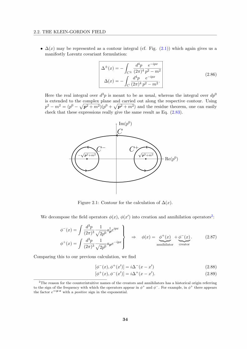
• ∆(x) may be represented as a contour integral (cf. Fig. (2.1)) which again gives us amanifestly Lorentz covariant formulation:
∆±(x) = −∫
C±
d4p
(2π)4
e−ipx
p2 −m2
∆(x) = −∫
C
d4p
(2π)4
e−ipx
p2 −m2.
(2.86)
Here the real integral over d3p is meant to be as usual, whereas the integral over dp0
is extended to the complex plane and carried out along the respective contour. Usingp2 −m2 = (p0 −
√p2 +m2)(p0 +
√p2 +m2) and the residue theorem, one can easily
check that these expressions really give the same result as Eq. (2.83).
Re(p0)
Im(p0)
C−−√p2+m2
C+√p2+m2
C
Figure 2.1: Contour for the calculation of ∆(x).
We decompose the field operators φ(x), φ(x′) into creation and annihilation operators2:
φ−(x) =
∫d3p
(2π)3
1√2p0
a†peipx
φ+(x) =
∫d3p
(2π)3
1√2p0
ape−ipx
⇒ φ(x) = φ+(x)︸ ︷︷ ︸annihilator
+φ−(x)︸ ︷︷ ︸creator
. (2.87)
Comparing this to our previous calculation, we find
[φ−(x), φ+(x′)] = i∆−(x− x′) (2.88)
[φ+(x), φ−(x′)] = i∆+(x− x′). (2.89)
2The reason for the counterintuitive names of the creators and annihilators has a historical origin referringto the sign of the frequency with which the operators appear in φ+ and φ−. For example, in φ+ there appearsthe factor e+ip·x with a positive sign in the exponential.
34

2.2. THE KLEIN-GORDON FIELD
This decomposition will prove useful when we consider time ordering. We define the time-ordered product of two Klein-Gordon field operators by
T(φ(x)φ(x′)
)=
φ(x)φ(x′) if t ≥ t′φ(x′)φ(x) if t < t′
= Θ(t− t′)φ(x)φ(x′) + Θ(t′ − t)φ(x′)φ(x). (2.90)
The Feynman propagator is the expectation value of the time-ordered product of twoKlein-Gordon field operators,
〈0|T(φ(x)φ(x′)
)|0〉 =: iDF (x− x′) = i∆F (x− x′). (2.91)
We observe that
〈0|φ(x)φ(x′)|0〉 = 〈0|φ+(x)φ−(x′)|0〉= 〈0|[φ+(x), φ−(x′)]|0〉= i∆+(x− x′) (2.92)
where we used that the additional term in the commutator annihilates the vacuum. For theinverse ordering we find
〈0|φ(x′)φ(x)|0〉 = 〈0|φ+(x′)φ−(x)|0〉= 〈0| − [φ−(x), φ+(x′)]|0〉= −i∆−(x− x′). (2.93)
Hence the Feynman propagator can be written as
∆F (x) = Θ(t)∆+(x)−Θ(−t)∆−(x)
= +
∫
CF
d4p
(2π)4e−ipx
1
p2 −m2(2.94)
using the contour as in Fig. (2.2) which has to be closed at infinity in the upper or lower halfplane. For x0 > 0, e−ip
0x0 → 0 if =(p0) < 0, so we close the path in the lower half plane. Ifx0 < 0, we close the path in the upper half plane, because in this case e−ip
0x0 → 0 only if=(p0) > 0.
Because we do not always want to keep track of these contours (in more complicatedprocesses, there will appear many fields or high powers of fields in perturbation theory), weintroduce a slight deformation of the contour which can be achieved if we shift the residues±√p2 +m2 just a little (see Fig. (2.3)). Then the contour can be deformed such that it goes
just along the real axis. This is equivalently represented by replacing (p2−m2)→ (p2−m2+iε)with infinitesimal ε and integration along the real line:
∆F (x) = limε→0+
∫d4p
(2π)4e−ipx
1
p2 −m2 + iε(2.95)
Now we can always integrate along the real line and we do not have to keep track of thecomplicated contours. It is understood that the contour always closes in such a way that thecontribution at infinity vanishes. We only have to keep track of the additional +iε.
35

2.2. THE KLEIN-GORDON FIELD
Re(p0)
Im(p0)
−√p2+m2
√p2+m2
CF
Figure 2.2: Contour for the calculation of the Feynman propagator. The countour has to beclosed at infinity either in the upper or in the lower half plane, depending on whether x0 < 0or x0 > 0.
Re(p0)
Im(p0)
−√p2+m2+iη
√p2+m2−iη
C
Figure 2.3: An infinitesimal shift of the poles simplifies the contour because we can alwaysuse one path C which is simply going along the real axis.
We want to interpret i∆F (x− x′) as the propagation of a Klein-Gordon particle betweenx and x′. This can be seen as part of a scattering process, see Fig. (2.4).
The two possible time-orderings described by i∆+(x−x′) and −i∆−(x−x′), respectively,cannot be distinguished by experiments because the virtual particle is not observable andits net effect on the two real particles is the same in both cases. The Feynman propagatorrespects this fact and describes both possibilities: it is the sum of both time orderings and assuch it is independent of the unobservable sequence of events in the scattering process.
Because the Feynman propagator is defined in a discontinuous manner, it does not nec-cessarily fulfill the Klein-Gordon equation. It turns out to be just the Green’s function of the
36

2.2. THE KLEIN-GORDON FIELD
t t t
x
x′
x
x′
x
x′
+ =
Figure 2.4: The Feynman propagator is the sum of both possible time orderings which areindistinguishable.
Klein-Gordon equation:
( +m2)∆F (x) = limε→0
∫d4p
(2π)4e−ipx
−p2 +m2
p2 −m2 + iε= −δ(4)(x). (2.96)
37

Chapter 3
Quantization of the Free Dirac Field
We now want to describe particles and fields with spin. We already know:
Spin 0 (scalar): Klein-Gordon field φ: ( +m2)φ = 0Spin 1
2 (spinor): Dirac spinor ψ: (i/∂ −m)ψ = 0Spin 1 (vector): Lorentz vector Aµ: Aµ = 0
We already found field operators for the Klein-Gordon field φ. Our next aim is to generalizethese ideas and to find field operators for ψ, Aµ.
3.1 Field Operator of the Free Dirac Field
We make some general remarks (postulates):
1. We need a relativistic generalization of the Heisenberg equation for an arbitraryfield operator A:
∂A
∂t= i[H,A] with H = p0,
∂
∂t≡ ∂
∂x0. (3.1)
⇒ ∂A
∂xµ= i[Pµ, A] with Pµ =
(H−p
)(4-momentum operator). (3.2)
2. Microcausality as known from special relativity has to be expressed in a quantummechanical language. It says that two events in spacetime points x and y can only havean influence on each other if their distance is time-like or light-like:
(x− y)2 ≥ 0. (3.3)
Otherwise there cannot be any causal relation between the events.The analogous statement in quantum mechanics is that two operators are causallydisconnected if they are commuting. This motivates that in quantum field theory, afield operator Φ, which represents an observable, has to satisfy the following causalitycondition:
[Φ(x),Φ(y)] = 0 for (x− y)2 < 0 (3.4)
⇔ [Φ(x, t),Φ(y, t′)] = 0 for |t− t′| < |x− y| 6= 0 (3.5)
38

3.1. FIELD OPERATOR OF THE FREE DIRAC FIELD
with x = (t,x), y = (t′,y). This yields the equal-time commutator
[Φ(x, t),Φ(y, t)] = 0 for x 6= y. (3.6)
As an example, consider the real Klein-Gordon field:
[φ(x), φ(y)] = i∆(x− y) (3.7)
with ∆(x− y) = 0 for (x− y)2 < 0.
Therefore φ(x) can in principle represent an observable because it does not contradictmicrocausality!
Remember that eigenfunctions of the Dirac Hamiltonian are equivalent to solutions of theDirac equation
us(p)e−ipx with eigenvalues Ep = +
√p2 +m2, (3.8)
vs(−p)eipx with eigenvalues Ep = −√p2 +m2. (3.9)
We postulate the following field operators for the Dirac field1:
ψ(x) =
∫d3p
(2π)3
1√2p0
∑
s=± 12
(as(p)us(p)e
−ipx + b†s(p)vs(p)eipx)
(3.10)
ψ(x) =
∫d3p
(2π)3
1√2p0
∑
s=± 12
(a†s(p)us(p)e
ipx + bs(p)vs(p)e−ipx
)(3.11)
with
a†s(p) : creator of particle with momentum p
b†s(p) : creator of antiparticle with momentum p
as(p) : annihilator of particle with momentum p
bs(p) : annihilator of antiparticle with momentum p.
In the case of the real scalar field, the field operator contained a creator as well as an annihi-lator. Now we see that there are two different types of solutions (particles and antiparticles)which appear in two spin states. If we imagine such a field operator acting on a given con-figuration of the external state, there are two possible effects: ψ can, for example, eitherannihilate a particle or create an antiparticle. Likewise, ψ either creates a particle or an-nihilates an antiparticle. In both cases, the effect of the two possible processes on the fieldconfiguration is the same (the total charge changes by the same amount).
We justify this postulate by looking at the Heisenberg equation for ψ(x) and ψ(x):
∂ψ
∂xµ= i
∫d3p
(2π)3
1√2p0
∑
s=± 12
(−pµas(p)us(p)e−ipx + pµb
†s(p)vs(p)e
ipx), (3.12)
∂ψ
∂xµ= i
∫d3p
(2π)3
1√2p0
∑
s=± 12
(pµa†s(p)us(p)e
ipx − pµbs(p)vs(p)e−ipx). (3.13)
1We choose the same normalization including factors of 1√2p0
as in the Klein-Gordon case. The purpose of
this is to avoid factors of 2p0 in the anticommutators of field operators and creation and annihilation operators.
39

3.1. FIELD OPERATOR OF THE FREE DIRAC FIELD
From this it follows that
[Pµ, a†s(p)] = pµa
†s(p) (3.14)
[Pµ, b†s(p)] = pµb
†s(p) (3.15)
[Pµ, as(p)] = −pµas(p) (3.16)
[Pµ, bs(p)] = −pµbs(p) (3.17)
which justifies the above explanations.In order for the Dirac field operators to describe fermions, we postulate equal-time anti-
commutation relations:
ψ(x, t), ψ(x′, t) = γ0δ(3)(x− x′) (3.18)
ψ(x, t), ψ(x′, t) = ψ(x, t), ψ(x′, t) = 0. (3.19)
It turns out that, in fact, we need exactly these anticommutation relations in order for thephysical observables to satisfy microcausality (commutation relations (3.4), (3.5)). Note thatψ, ψ are not observables but field operators. All observables in this Dirac theory are thebilinear covariants constructed earlier. Postulating microcausality, we demand that
[ψ(x, t)Γ1ψ(x, t), ψ(x′, t)Γ2ψ(x′, t)] = 0 for x 6= x′. (3.20)
Using
[AB,CD] = AB,CD −ACB,D − CA,DB + C,ADB (3.21)
this implies
[ψ(x, t)Γ1ψ(x, t), ψ(x′, t)Γ2ψ(x′, t)]
=(ψ(x, t)Γ1γ
0Γ2ψ(x′, t)− ψ(x′, t)Γ2γ0Γ1ψ(x, t)
)δ(3)(x− x′). (3.22)
One finds that these relations are fulfilled if the Dirac field operators satisfy their anticommu-tation relations. These are implied by anticommutation relations of creation and annihilationoperators,
ar(p), a†s(p′) = (2π)3δrsδ(3)(p− p′)
br(p), b†s(p′) = (2π)3δrsδ(3)(p− p′)
a†r(p), a†s(p′) = ar(p), as(p′) = 0
b†r(p), b†s(p′) = br(p), bs(p′) = 0.
(3.23)
As we will see in the next section, these relations encode the fact that we are really dealing withfermions, satisfying the Fermi-Dirac statistics and especially the Pauli principle. But they areinitially introduced because it is these anticommutation relations which give anticommutationrelations for the field operators (Eqs. (3.18), (3.19)) that are needed in order to obtain thecorrect commutation relations (3.20) for the physical observables (bilinear covariants) andtherefore to guarantee microcausality.
40

3.2. SINGLE-PARTICLE STATES IN THE DIRAC THEORY
As an example, we proof that the relations (3.23) imply Eq. (3.18):
ψ(x, t), ψ(x′, t) =
∫d3pd3p′
(2π)6
1√2p02p′0
∑
r,s
(eipxe−ip
′x′vr(p)vs(p′)b†r(p), bs(p′)
+ e−ipxeip′x′ur(p)us(p
′)ar(p), a†s(p′))
=
∫d3p
(2π)3
1
2p0
(e−ip·(x−x
′)∑
s
vs(p)vs(p)
+ eip·(x−x′)∑
s
us(p)us(p)
). (3.24)
Using the completeness relations∑
s
us(p)us(p) = /p+m,∑
s
vs(p)vs(p) = /p−m (3.25)
we find for (3.24)
ψ(x, t), ψ(x′, t) =
∫d3p
(2π)3
1
2p0
(e−ip·(x−x
′)(p0γ0 − pγ −m) + eip·(x−x′)(p0γ0 − pγ +m)
)
= γ0
∫d3p
(2π)3eip·(x−x
′)
= γ0δ(3)(x− x′). (3.26)
3.2 Single-Particle States in the Dirac Theory
As a starting point, we consider the vacuum state |0〉 with
Pµ|0〉 = 0. (3.27)
If we use
[Pµ, a†s(p)]|0〉 = Pµa†s(p)|0〉, (3.28)
we find (using Eq. (3.14))
Pµa†s(p)|0〉 = pµa†s(p)|0〉. (3.29)
Hence
|e−(p, s)〉 =√
2Epa†s(p)|0〉, (3.30)
|e+(p, s)〉 =√
2Epb†s(p)|0〉 (3.31)
are momentum eigenstates of a particle with momentum p and an antiparticle with momentump, respectively. The normalization of these states is Lorentz invariant:
〈e−(p′, r)|e−(p, s)〉 =√
2Ep√
2Ep′〈0|ar(p′)a†s(p)|0〉=√
2Ep√
2Ep′〈0|ar(p′), a†s(p)|0〉= δrs(2π)32Epδ
(3)(p− p′). (3.32)
41

3.3. CONSERVED QUANTITIES IN THE DIRAC THEORY
Next, we consider two-electron states which take the form
a†r(p1)a†s(p2)|0〉 = −a†s(p2)a†r(p1)|0〉 (3.33)
⇒ |e−(p1, r)e−(p2, s)〉 = −|e−(p2, s)e
−(p1, r)〉 (3.34)
which means that the state vector of this two-particle state is antisymmetric under interchangeof the two Dirac particles.
An arbitrary one-electron state (e.g. a wave packet) is of the form
|f〉 =
∫d3p
(2π)3
∑
s
fs(p)a†s(p)|0〉 (3.35)
with arbitrary, normalizable fs. By looking at a state vector with two electrons in the samequantum state,
|2f〉 =
∫d3p1d
3p2
(2π)6
∑
r,s
fr(p1)fs(p2)a†r(p1)a†s(p2)|0〉
= −∫d3p1d
3p2
(2π)6
∑
r,s
fr(p1)fs(p2)a†s(p2)a†r(p1)|0〉
= 0, (3.36)
we see that the Pauli principle is satisfied: the state |2f〉 for two spin-12 particles in the same
state automatically vanishes.
3.3 Conserved Quantities in the Dirac Theory
Starting from the Lagrangian
L = ψ(x)(i/∂ −m)ψ(x) (3.37)
we obtain the energy-momentum tensor and four momentum of the field (→ exercise):
Tµν = ψ(x)iγµ∂νψ(x) (3.38)
Pµ =
∫d3x T 0µ = i
∫d3x ψ(x)γ0∂µψ(x)
=
∫d3k
(2π)3kµ∑
s
(a†s(k)as(k)− bs(k)b†s(k)
). (3.39)
As in the case of the Klein-Gordon field, we have a divergent zero-point energy:
〈0|Pµ|0〉 = −∫
d3k
(2π)3kµ∑
s
〈0|bs(k)b†s(k)|0〉
= −2
∫d3k kµδ(3)(0). (3.40)
But again, this term has nothing to do with any field configurations and is an infinite constantin this sense. We introduce the normal ordering as a systematic procedure to subtract such
42

3.3. CONSERVED QUANTITIES IN THE DIRAC THEORY
divergent constants. Normal ordering is based on the following decomposition of the Diracfield operator into creation and annihilation operators:
ψ+ =
∫d3p
(2π)3
1√2p0
∑
s
e−ipxas(p)us(p) (“annihilators”) (3.41)
ψ− =
∫d3p
(2π)3
1√2p0
∑
s
eipxb†s(p)vs(p) (“creators“) (3.42)
and ψ± analogously. The normal-ordered product of field operators is defined as
: ψ1ψ2 : = : (ψ+1 + ψ−1 )(ψ+
2 + ψ−2 ) :
= ψ+1 ψ
+2 − ψ−2 ψ+
1 + ψ−1 ψ+2 + ψ−1 ψ
−2 . (3.43)
So the creators are always to be put left of the annihilators under correct application of theanticommutation-relations. The operators are then in an order which does not produce non-vanishing vacuum expectation values, so the divergences disappear.Physical obervables (composite Dirac operators) are always defined as normal-ordered, so
: Pµ :=
∫d3k
(2π)3kµ∑
s
(a†s(k)as(k) + b†s(k)bs(k)
)(3.44)
such that
〈0| : Pµ : |0〉 = 0. (3.45)
In order to introduce a charge operator, we consider the electromagnetic four-current
jµ(x) = q : ψ(x)γµψ(x) : (3.46)
which fulfills the continuity equation
∂µjµ = 0. (3.47)
This leads to the conserved charge (operator)
Q = q
∫d3x : ψ(x)γ0ψ(x) :=
∫d3x j0(x) with q(e±) = ±e. (3.48)
One can calculate this object using the expressions (3.10), (3.11) for the field operators. Thisyields
Q = −e∫
d3k
(2π)3
∑
s
(a†s(k)as(k)− b†s(k)bs(k)
). (3.49)
Furthermore, we observe that Pµ and Q have common eigenfunctions. In fact, using Eq.(3.44) and the relation (3.21), one can easily show (→ exercise) that
[Q,Pµ] = 0. (3.50)
This leads to the following physical picture:
43

3.4. THE FERMION PROPAGATOR
• H = P 0 is positive definite.
• Q is indefinite.
• ψ is the field operator of the fermion field.
• The particle states (momentum eigenstates) are given by
√2Epa
†s(p)|0〉 (particles)
√2Epb
†s(p)|0〉 (antiparticles).
They are eigenstates of Pµ with eigenvalues pµ.
3.4 The Fermion Propagator
The next step towards a theory which describes interactions, is to find a suitable propagator.To this end consider the non-equal-time anticommutators
ψ(x), ψ(x′) =
∫d3pd3p′
(2π)6
1√2p02p′0
∑
r,s
(eipxe−ip
′x′vr(p)vs(p′)b†r(p), bs(p′)
+ e−ipxeip′x′ur(p)us(p
′)ar(p), a†r(p′))
=
∫d3p
(2π)3
1
2p0
(eip(x−x
′)(/p−m) + e−ip(x−x′)(/p+m)
)
= (i/∂ +m)
∫d3p
(2π)3
1
2p0
(e−ip(x−x
′) − eip(x−x′))
= (i/∂ +m)i(∆+(x− x′) + ∆−(x− x′)
)(3.51)
=: iS(x− x′). (3.52)
We do essentially the same as before (cf. Eqs. (2.88) and (2.89)): we decompose ψ and ψinto creation and annihilation components:
ψ−(x), ψ+(x′) = (i/∂ +m)∆−(x− x′) =: iS−(x− x′) (3.53)
ψ+(x), ψ−(x′) = (i/∂ +m)∆+(x− x′) =: iS+(x− x′) (3.54)
Again, we can represent these expressions as contour integrals:
S±(x) =
∫
C±
d4p
(2π)4e−ipx
/p+m
p2 −m2
=
∫
C±
d4p
(2π)4e−ipx
1
/p−m(3.55)
where we used that p2 −m2 = (/p−m)(/p+m). Similarly we can write
S(x) =
∫d4p
(2π)4e−ipx
1
/p−m. (3.56)
44

3.4. THE FERMION PROPAGATOR
The time ordered product of two fermion operators reads
T (ψ(x)ψ(x′)) =
ψ(x)ψ(x′) (t > t′)
−ψ(x′)ψ(x) (t < t′)
= Θ(t− t′)ψ(x)ψ(x′)−Θ(t′ − t)ψ(x′)ψ(x) (3.57)
where the minus sign is due to the anticommutation relations. Note the subtleties in notation:both ψ(x)ψ(x′) and −ψ(x′)ψ(x) are 4× 4 matrices (bilinears) in Dirac space. The ordering,in this notation, just tells us in which order to apply creation and annihilation operators, butnot how to contract them. In both cases they are implicitly contracted such that a 4 × 4bilinear is obtained.
The vacuum expectation value of the time-ordered product of two fermion operators isthe Feynman propagator for fermions:
〈0|T (ψ(x)ψ(x′))|0〉 = iSF (x− x′). (3.58)
As in the case of the Klein-Gordon field we can consider the two possible time-orderingsseparately:
〈0|ψ(x)ψ(x′)|0〉 = 〈0|ψ+(x)ψ−(x′)|0〉= 〈0|ψ+(x), ψ−(x′)|0〉= iS+(x− x′) (3.59)
〈0|ψ(x′)ψ(x)|0〉 = 〈0|ψ+(x′)ψ−(x)|0〉= iS−(x− x′). (3.60)
We see that here, too, we have an additional minus sign as compared to the Klein-Gordoncase (cf. Eq. (2.93)). This is, of course, due to the relevance of anticommutation relationsinstead of commutation relations. We find
SF (x) = Θ(t)S+(x)−Θ(−t)S−(x)
= (i/∂ +m)∆F (x) (3.61)
which can be represented as a contour integral, using the same trick as in the Klein-Gordoncase:
SF (x) =
∫
CF
d4p
(2π)4e−ipx
1
/p−m
⇒ SF (x) = limε→0+
∫d4p
(2π)4e−ipx
/p+m
p2 −m2 + iε. (3.62)
Finally, we can verify that the Feynman propagator is the Green’s function of the Diracequation:
(i/∂ −m)SF (x) =
∫d4p
(2π)4e−ipx
(/p−m)(/p+m)
p2 −m2= δ(4)(x). (3.63)
Note that the Feynman propagator, too, does not discriminate between particles and antipar-ticles (it contains both) and that it contains both possible time-orderings. Mathematicallyspeaking, it is a distribution in its argument x. The bilinear ψ(x)ψ(x′) is a 4 × 4 matrix inDirac space.
45

Chapter 4
Quantization of theElectromagnetic Field
The electromagnetic field is characterized by the following data:
• Electromagnetic potential Aµ.
• The field strength tensor Fµν = ∂µAν − ∂νAµ.
• The Lagrangian density −14F
µνFµν . Variation of this Lagrangian yields the equations ofmotion ∂µF
µν = 0 (inhomogeneous Maxwell equations in vacuum). This can be writtenas Aν − ∂ν(∂µA
µ) = 0.
• Lorenz gauge: ∂µAµ = 0 which amounts to four equations. But the classical photon
field has only two polarization degrees of freedom. This mismatch of the number ofconstraints on the one hand and the number of degrees of freedom on the other hand,will lead to an additional degree of complexity: we have a certain gauge freedom.
4.1 Gauge Invariance of the Electromagnetic Field
Remember the physical E- and B-fields from electromagnetism:
E = −∇φ− ∂
∂tA (4.1)
B = ∇ ∧A. (4.2)
These fields are invariant under the gauge transformation
A 7→ A−∇Λ (4.3)
φ 7→ φ+∂
∂tΛ. (4.4)
In four-vector notation with Aµ = (φ,A), ∂µ = (∂t,−∇) we can write the gauge transforma-tion as
Aµ 7→ Aµ + ∂µΛ. (4.5)
There are different reasonable gauge conditions:
46

4.2. QUANTIZATION IN LORENZ GAUGE
• The gauge which is commonly used in relativistic theories is the Lorenz gauge in whichwe demand that Λ solves
Λ = −∂µAµ ⇒ ∂µAµ = 0. (4.6)
With this condition on Aµ we are still left with three degrees of freedom in the potentialAµ. Hence Aµ is not uniquely determined in the Lorenz gauge: if we choose Λ′ suchthat Λ′ = 0, we have
(∂µAµ + ∂µ∂
µΛ′) = 0. (4.7)
So the Lorenz gauge describes not a unique gauge but a certain class of gauge choices:one can still add ∂µΛ′ with Λ′ = 0 to Aµ without changing the fields.
• The Coulomb gauge condition demands
∂
∂tΛ′ = −φ. (4.8)
Then
φ = 0, ∇ ·A = 0. (4.9)
In the Coulomb gauge Aµ has only two degrees of freedom. Note that, in contrast tothe Lorenz gauge, the Coulomb gauge is not a Lorentz invariant condition.
We try to quantize the electromagnetic field canonically: on the one hand we have thefield operators Aµ, on the other hand we have canonical momentum operators πν = ∂L
∂Aν. By
analogy to the Klein-Gordon theory developed above, we postulate
[Aµ(x), πν(x′)] = igµνδ(3)(x− x′). (4.10)
Unfortunately this cannot work in the case of the electromagnetic field: the LagrangianL = −1
4FµνFµν does not contain ∂0A0 = A0. Therefore π0 = 0 and thus [A0, π0] = 0 which
is a contradiction. It seems that this ansatz does not work.In order to solve this problem, we do not alter the fields, but the Lagrangian: we can alwaysadd total derivatives to L since the equations of motion are not altered if the Lagrangian ischanged by total derivatives. After adding these additional terms to L we should in any caseget the correct equations of motion for the physical field modes (i.e. for Fµν). Also, all fieldmodes should satisfy canonical, Lorentz invariant commutation relations as in Eq. (4.10). Weshall use the Lorentz invariant Lorenz gauge as a condition on the physical field modes.
4.2 Quantization in Lorenz Gauge
As a starting point, we write down a Lagrangian that yields equations of motion which arealready Lorenz gauged:
L = −1
4FµνFµν −
1
2(∂µA
µ)2, (4.11)
The term −12(∂µA
µ)2 fixes the gauge. This is because the additional term can be seen asa constraint for the Lagrangian problem. The Lorenz gauge is exactly the condition which
47
4.2. QUANTIZATION IN LORENZ GAUGE
minimizes the energy. But note that so far we have not explicitly demanded the Lorenzgauge condition! We just implemented a term which is obviously related to the Lorenz gauge.Variation of L gives the equations of motion
Aµ = 0. (4.12)
The most general covariant gauge fixing would read
Lλ = −1
4FµνFµν −
λ
2(∂µA
µ)2 (4.13)
⇒ Aµ − (1− λ)∂µ(∂νAν) = 0. (4.14)
For λ = 1 this is called the Feynman gauge. The case λ =∞ is referred to as the Landaugauge. The so called unitary gauge corresponds to λ = 0.
We need the canonical momentum (in Feynman gauge)
π0 =∂L∂A0
= −∂µAµ. (4.15)
We see that π0 = 0 if the Lorenz gauge condition is fulfilled. But ∂µAµ = 0 cannot be fulfilled
as an operator equation because of the problems discussed at the end of the last section. Notethat we did not explicitly demand the Lorenz gauge! We just tried to implement it implicitlyin the Lagrangian. We now have to require it for the physically allowed states |ψphys.〉,
〈ψphys.|∂µAµ|ψphys.〉 = 0 (4.16)
This method is called Gupta-Bleuler-Quantization. The idea is that the space of operatorstates is now much larger than the space of physical states. We single out the physical statesby imposing this additional condition. In the Klein-Gordon case, the whole spectrum of fieldoperators was allowed as physical states. Now, we have more field operators than states whichare really physical.
We can construct the photon field operator using all its degrees of freedom without an apriori gauge condition:
Aµ(x) =
∫d3k
(2π)3
1√2k0
3∑
λ=0
(ε(λ)µ (k)a(λ)(k)e−ikx + ε(λ)
µ (k)∗a(λ)†(k)eikx)
(4.17)
with the four polarization vectors ε(0,1,2,3)µ which have a Lorentz invariant norm,
ε(λ) · ε(λ′) = ε(λ)µ ε(λ′)µ
= ε(λ)µ gµνε(λ′)
ν
= ε(λ)0 ε
(λ′)0 − ε(λ)
1 ε(λ′)1 − ε(λ)
2 ε(λ′)2 − ε(λ)
3 ε(λ′)3
= gλλ′. (4.18)
Since we have not yet fixed the gauge, there are still four degrees of freedom in the photonfield (from classical electrodynamics, we know that the photon field actually has only two
48

4.2. QUANTIZATION IN LORENZ GAUGE
degrees of freedom). We choose the representation
kµ =
k00k
and ε(0) =
1000
, ε(1) =
0100
, ε(2) =
0010
, ε(3) =
0001
such that
k · ε(1,2) = 0 (transverse polarizations) (4.19)
k · ε(0) = k (scalar polarization) (4.20)
k · ε(3) = −k (longitudinal polarization). (4.21)
We postulate the following commutator relations:
[Aµ(x, t), πν(x′, t)] = igµνδ(3)(x− x′) (4.22)
[Aµ(x, t), Aν(x′, t)] = [πµ(x, t), πν(x′, t)] = 0. (4.23)
We compute
πµ =∂L∂Aµ
= Fµ0 − gµ0(∂νAν) (4.24)
π0 = −A0 −∇ ·A (4.25)
πi = ∂iA0 − Ai. (4.26)
If we insert this in Eqs. (4.22) and (4.23), the spatial derivatives of Aµ obviously commutebecause they only act on the A0-component and the corresponding π0-component is a scalarquantity. The remaining temporal derivatives yield the only non-vanishing commutatorswhich can be written as
[Aµ(x, t), Aν(x′, t)] = igµνδ(3)(x− x′). (4.27)
This immediately gives the commutators for creators and annihilators,
[a(λ)(k), a(λ′)†(k′)] = −gλλ′(2π)3δ(3)(k − k′), (4.28)
especially
[a(0)(k), a(0)†(k)] = −(2π)3δ(3)(k − k′). (4.29)
This last commutator leads to a problem: if we have a look at the Hamiltonian operator (→exercise)
: H : =
∫d3k
(2π)3k0
(3∑
λ=1
a(λ)†(k)a(λ)(k)− a(0)†(k)a(0)(k)
), (4.30)
we see that the last term a(0)†(k)a(0)(k) gives a negative contribution which originates fromthe scalar polarization: the Hamiltonian counts states in spatial polarization states (1, 2, 3)
49
4.2. QUANTIZATION IN LORENZ GAUGE
but subtracts the number of states in scalar polarization. Therefore : H : is indefinite.As we have seen before, we cannot solve this problem by imposing commutator relations.Instead, we impose the Gupta-Bleuler condition for the physical states |ψ〉 of the photonfield:
〈ψ|∂µAµ|ψ〉 = 0. (4.31)
We can decompose this condition into constraints on the creators and annihilators:
0 = 〈ψ|∂µAµ|ψ〉 = 〈ψ|∂µAµ+ + ∂µAµ−|ψ〉
= 〈ψ|∂µAµ+|ψ〉+ 〈ψ|∂µAµ+|ψ〉∗ (4.32)
which is fulfilled if ∂µAµ+|ψ〉 = 0. Using the explicit representation of Aµ as given in Eq.
(4.17), we find
3∑
λ=0
kµε(λ)µ a(λ)(k) = 0. (4.33)
For the transverse polarization (λ = 1, 2) this condition is already fulfilled:
kµ · ε(λ=1,2)µ = 0. (4.34)
For the scalar and the longitudinal polarization, the conditions read
kµ · ε(λ=0)µ = k0 (4.35)
kµ · ε(λ=3)µ = −k0. (4.36)
This yields the following conditions on the physical states |ψ〉 of the photon field:(a(0)(k)− a(3)(k)
)|ψ〉 = 0. (4.37)
So the physical states can contain a longitudinal as well as a scalar polarization, in principle,but the condition (4.37) has to be fulfilled. It follows that for physical |ψ〉 it holds that
〈ψ|a(0)†(k)a(0)(k)|ψ〉 = 〈ψ|a(3)†a(3)(k)|ψ〉. (4.38)
So the expectation value of the occupation number operator for the (λ = 0)-polarization isequal to that of the (λ = 3)-component. Applying this to the Hamiltonian in Eq. (4.30)acting on physical states |ψ〉, we find
〈ψ| : H : |ψ〉 = 〈ψ|∫
d3k
(2π)3k0
2∑
λ=1
a(λ)†(k)a(λ)(k)|ψ〉 (4.39)
which is positive definite! To summarize, we can say that the Hamiltonian for the photonfield is a priori indefinite (the spectrum goes down to arbitrarily large negative energies).The Gupta-Bleuler condition fixes this problem by imposing a Lorenz gauge condition onthe Hamiltonian and thus making it positive definite as long as it acts on physical states.After imposing this condition, the four degrees of freedom effectively reduce to the usual twodegrees of freedom of the photon field because the contributions of two of the polarizationscancel each other if the operator is applied to physical states.
50

4.3. FOCK SPACE STATES
4.3 Fock Space States
We are now able to construct the Fock space states of the photon field. We will only considerthe transverse polarizations (λ = 1, 2) because other polarization states are allowed but canbe omitted according to the above considerations. If |0〉 denotes the vacuum, we have thesingle photon state
√2Eka
(λ)†(k)|0〉 = |(k, λ)〉 (4.40)
and two kinds of two photon states of the form
√2Ek1
√2Ek2a
(λ1)†(k1)a(λ2)†(k2)|0〉 = |(k1, λ1); (k2, λ2)〉 (4.41)
1√2
(2Ek)(a(λ)†(k)
)2|0〉 = |2(k, λ)〉 (4.42)
where we use the notation |n(k, λ)〉 to denote a state with n photons with momentum k andpolarization λ. Creation and annihilation operators act as follows on a multi-photon state:
√2Ekia
(λi)†(ki)|n1(k1, λ1); ...;ni(ki, λi); ...〉 =√ni + 1|n1(k1, λ1); ...;ni(ki, λi) + 1, ...〉
(4.43)
1√2Eki
a(λi)(ki)|n1(k1, λ1); ...;ni(ki, λi); ...〉 =√ni|n1(k1, λ1); ...;ni(ki, λi)− 1, ...〉
(4.44)
These normalizations guarantee that the number operators really measure the number ofphotons in a particular state.These normalizations also have profound implications for the interaction of a photon fieldwith atoms:
• The amplitude for the absorption of a photon is proprtional to√n(k, λ). Hence an
absorption is only possible if n(k, λ) 6= 0.
• The amplitude for the emission of a photon is proportional to√n(k, λ) + 1. Thus emis-
sion can take place also if n(k, λ) = 0. This gives rise to the spontaneous emissiondue to quantum properties of a photon field.Note that the amplitude for emission of a photon in a given state grows with the occu-pation of the state which gives rise to stimulated emission.1
In order to quantify the amplitudes for absorption, spontaneous emission and stimulatedemission, we consider an atom which is either in ground state A or excited state B. Thistransition is accompanied by a field mode (k, λ) with Ek = EB −EA. The state vector of thecombined system is
|atom state〉 ⊗ |photon field state〉 (4.45)
We treat the cases separately:
1Stimulated emission is the fundamental process which is used to construct lasers; LASER actually standsfor ”light amplification by stimulated emission“.
51

4.4. THE PHOTON PROPAGATOR
• Absorption of a photon: We are interested in the transition probability∣∣〈B; (n(k, λ)− 1)|Hint|A;n(k, λ)〉
∣∣2 = n(k, λ)∣∣〈B; 0|Hint|A; (k, λ)〉
∣∣2. (4.46)
• Emission of a photon: We calculate∣∣〈A; (n(k, λ) + 1)|Hint|B;n(k, λ)〉
∣∣2 = (n(k, λ) + 1)∣∣〈A; (k, λ)|Hint|B; 0〉
∣∣2. (4.47)
The principle of detailed balance says∣∣〈B; 0|Hint|A; (k, λ)〉
∣∣2 =∣∣〈A; (k, λ)|Hint|B; 0〉
∣∣2. (4.48)
Using this rule combined with the conditions for thermodynamic equilibrium in an ideal gas,one can easily derive Planck’s law of radiation (→ exercise):
n(k, λ) =1
e~ω/kT − 1with ~ω = EA − EB. (4.49)
4.4 The Photon Propagator
We start by considering the commutator of two photon field operators for non-equal times(→ exercise):
[Aµ(x), Aν(x′)] = −gµν∫
d3k
(2π)3
1
2k0
(e−ik(x−x′) − eik(x−x′)
)
= −gµνi∆(x− x′)≡ iDµν(x− x′). (4.50)
Photons are massless, hence
iDµν(x) = −gµν∫
d3k
(2π)3
1
2k0
(e−ikx − eikx
)
= −gµν∫
d4k
(2π)3δ(4)(k2)e−ikx
(Θ(k0)−Θ(−k0)
)
= −gµν(−i)∫
C
d4k
(2π)4
e−ikx
k2. (4.51)
For the propagator we need the time-ordered product of two photon field operators,
T (Aµ(x)Aν(x′)) =
Aµ(x)Aν(x′) (t > t′)
Aν(x′)Aµ(x) (t < t′), (4.52)
which finally gives the photon field propagator
iDµν(x− x′) = 〈0|T (Aµ(x)Aν(x′))|0〉= −gµνi∆F (x− x′) (4.53)
⇒ iDµν(x− x′) = i limε→0+
∫d4k
(2π)4
e−ikx
k2 + iε(−gµν). (4.54)
52

Chapter 5
Quantum Electrodynamics (QED)
QED is the theory of the interaction of electrically charged spin-12 particles (e.g. electrons).
Until now we exclusively dealt with free field situations. In order to describe interactions, theHeisenberg picture is not completely adequate.
5.1 The Interaction Picture and the Time Evolution Operator
We decompose the Hamilton operator of the Schrodinger picture into a free Hamilton operatorand a part which describes the interactions:
HS = H0,S +Hint,S . (5.1)
States and operators are defined as in the free Heisenberg picture:
ψI = eiH0,StψS (5.2)
H0,I = eiH0,StH0,Se−iH0,St = H0,S (5.3)
OI = eiH0tOSe−iH0t (5.4)
where H0 ≡ H0,S = H0,I . The time evolution of states ψI and operators OI , respectivelyreads
i∂
∂tψI = Hint,IψI , (5.5)
id
dtOI = −H0OI +OIH0 = [OI , H0]. (5.6)
Therefore, everything that we developed concerning free field operators remains valid. In-deed, operators in the interaction picture show a time evolution which is given by the freefield situation due to Eq. (5.6). The time evolution of states, on the other hand, is purelydue to the interaction part of the Hamiltonian.
We can summarize the three pictures as follows:
• Heisenberg picture: The state vector is completely time-independent. The operatorshave a time dependence which is determined by the Heisenberg equation.
53

5.1. THE INTERACTION PICTURE AND THE TIME EVOLUTION OPERATOR
• Schrodinger picture: State vectors contain the full time-dependence which is gov-erned by the Schrodinger equation. Operators are time-independent.
• Interaction picture: The time-dependence of the non-interacting system is containedin the free operators. The time dependence which is due to interactions affects only thestate vector. In particular, Hint,I consists of free field operators.
Due to these properties of the interaction picture, we have to think about the time evolutionof the state vector. It’s evolution is given by some time evolution operator,
ψI(t) = U(t, t0)ψI(t0). (5.7)
From
ψI(t) = eiH0tψS(t)
= eiH0te−iHS(t−t0)ψS(t0)
= eiH0te−iHS(t−t0)e−iH0t0ψI(t0) (5.8)
we can infer that
U(t, t0) = eiH0te−iHS(t−t0)e−iH0t0 (5.9)
Sometimes we will also need the corresponding time evolution of Heisenberg operators whichis given by
OH(x, t) = U †(t, t0)OIU(t, t0). (5.10)
The time evolution operator enjoys the following properties:
• U(t0, t0) = 1,
• U(t2, t1)U(t1, t0) = U(t2, t0),
• U−1(t0, t1) = U(t1, t0),
• U †(t1, t0) = U−1(t1, t0).
We can write the time evolution also in the form of a differential equation:
i∂
∂tU(t, t0) = Hint,I(t)U(t, t0). (5.11)
The equivalent integral equation (with boundary condition U(t0, t0) = 1) reads
U(t, t0) = 1 + (−i)∫ t
t0
dt1Hint,I(t1)U(t1, t0) (5.12)
which has a formal solution in the form of a Neumann series:
U(t, t0) = 1 + (−i)∫ t
t0
dt1Hint,I(t1)
+ (−i)2
∫ t
t0
dt1
∫ t1
t0
dt2Hint,I(t1)Hint,I(t2)
+ ...
+ (−i)n∫ t
t0
dt1 · · ·∫ tn−1
t0
dtnHint,I(t1) · · ·Hint,I(tn)
+ ... (5.13)
54

5.1. THE INTERACTION PICTURE AND THE TIME EVOLUTION OPERATOR
We can now find good approximations by truncating this expansion if Hint,I ≡ Hint is para-metrically ”small“, i.e. it depends on some independent constant which is comparably smalland can be controlled properly.For simplicity, we consider the second order term first:
∫ t
t0
dt1
∫ t1
t0
dt2Hint(t1)Hint(t2) =
∫ t
t0
dt2
∫ t
t2
dt1Hint(t1)Hint(t2)
=
∫ t
t0
dt1
∫ t
t1
dt2Hint(t2)Hint(t1) (5.14)
⇒ 2
∫ t
t0
dt1
∫ t1
t0
dt2Hint(t1)Hint(t2) =
∫ t
t0
dt1
∫ t1
t0
dt2Hint(t1)Hint(t2)
+
∫ t
t0
dt1
∫ t
t1
dt2Hint(t2)Hint(t1)
=
∫ t
t0
dt1
∫ t
t0
dt2T (Hint(t1)Hint(t2)) . (5.15)
The generalization to the n-th term reads
n!
∫ t
t0
dt1 · · ·∫ tn−1
t0
dtnHint(t1) · · ·Hint(tn) =
∫ t
t0
dt1 · · ·∫ t
t0
dtnT (Hint(t1) · · ·Hint(tn)) .
(5.16)
As a result we obtain a perturbation series of the time evolution operator (→ exercise):
U(t, t0) =∞∑
n=0
1
n!(−i)n
∫ t
t0
dt1 · · ·∫ t
t0
dtnT (Hint(t1) · · ·Hint(tn)) (5.17)
(5.18)
which can formally be written as
U(t, t0) = T exp
(−i∫ t
t0
dt′Hint(t′)
). (5.19)
We can check the validity of this result by showing that it solves the differential equation(5.11):
∂
∂tU(t, t0) = i
∞∑
i=0
1
n!(−i)nn
∫ t
t0
dt1 · · ·∫ t
t0
dtn−1T (Hint(t1) · · ·Hint(tn−1)Hint(t))
= Hint(t)∞∑
n=1
1
(n− 1)!(−i)n−1
∫ t
t0
dt1 · · · dtn−1T (Hint(t1) · · ·Hint(tn−1))
= Hint(t)U(t, t0). (5.20)
In terms of the interaction Lagrangian, we can write
Hint(t) = −∫d3x Lint(x) (5.21)
hence
U(t, t0) = T exp
(i
∫d4xLint(x)
). (5.22)
55

5.1. THE INTERACTION PICTURE AND THE TIME EVOLUTION OPERATOR
5.1.1 The Ground State
Next, we will have to think about the vacuum state. In the free theory, it was simply the state|0〉 with no particles whatsoever. It was characterized by H0|0〉 = 0. Now the vacuum |Ω〉will be the specific state which minimizes the energy eigenvalue of the full Hamiltonian, i.e.H|Ω〉 = E0|Ω〉 with minimal E0. The vacuum |Ω〉 does not have to be the zero particle-state,of course. As we will see next, this very ground state which is not really accessible, can berelated to the free vacuum state which we know much better. We will derive a formula whichrelates vacuum expectation values (with respect to the vacuum |Ω〉) to vacuum expectationvalues with respect to the free vacuum |0〉.
Consider the time evolution of |0〉 which is given by
e−iHT |0〉 =∑
n
e−iEnT |n〉〈n|0〉
= e−iE0T |Ω〉〈Ω|0〉+∑
n6=0
e−iEnT |n〉〈n|0〉 (5.23)
where |n〉 denotes the eigenstate of H with eigenvalue En. We can compute the limit asT → ∞(1 − iε). Then the term e−iE0t dominates because it goes to zero slowest and wecan forget about all the other terms with n 6= 0. We use the notation (1 − i0) meaninglimε→0(1− iε):
|Ω〉 = limT→∞(1−i0)
(e−iE0T 〈Ω|0〉
)−1e−iHT |0〉, (5.24)
provided that 〈Ω|0〉 6= 0, i.e. the vacuum of the interacting theory has a non-vanishing overlapwith the vacuum of the free theory. If we displace T by t0, we find
|Ω〉 = limT→∞(1−i0)
(e−iEo(T+t0)〈Ω|0〉
)−1e−iH(T+t0)|0〉
= limT→∞(1−i0)
(e−iE0(t0−(−T ))〈Ω|0〉
)−1e−iH(t0−(−T ))e−iH0(−T−t0)|0〉
= limT→∞(1−i0)
(e−iEo(t0−(−T ))〈Ω|0〉
)−1U(t0,−T )|0〉 (5.25)
where we multiplied |0〉 trivially with an exponential using H0|0〉 = 0 in the first step. Anal-ogously, one finds
〈Ω| = limT→∞(1−i0)
〈0|U(T, t0)(e−iE0(T−t0)〈0|Ω〉
)−1. (5.26)
We consider the two-point correlation function for x0 > y0 > t0 and for a field operatorφH in the Heisenberg picture:
〈Ω|φH(x)φH(y)|Ω〉 = limT→∞(1−i0)
(e−iE0(T−t0)〈0|Ω〉
)−1〈0|U(T, t0)U †(x0, t0)φI(x)U(x0, t0)
× U †(y0, t0)φI(y)U(y0, t0)U(t0,−T )|0〉(e−iE0(t0−(−T ))〈Ω|0〉
)−1
= limT→∞(1−i0)
(|〈0|Ω〉|2e−iE02T
)−1 〈0|U(T, x0)φI(x)U(x0, y0)
× φI(y)U(y0,−T )|0〉.(5.27)
56

5.2. WICK’S THEOREM
We divide this expression by
1 = 〈Ω|Ω〉 = limT→∞(1−i0)
(|〈0|Ω〉|2e−iE02T
)−1 〈0|U(T, t0)U(t0,−T )|0〉 (5.28)
and find quite a simple expression for the two-point correlation function in which only thefree vacuum |0〉 appears:
〈Ω|φH(x)φH(y)|Ω〉 = limT→∞(1−i0)
〈0|U(T, x0)φI(x)U(x0, y0)φI(y)U(y0,−T )|0〉〈0|U(T,−T )|0〉 . (5.29)
This can easily be generalized to expressions with arbitrary time ordering:
〈Ω|T (φH(x)φH(y))|Ω〉 = limT→∞(1−i0)
〈0|T[φI(x)φI(y) · exp
(−i∫ T−T dtHint,I(t)
)]|0〉
〈0|T[exp
(−i∫ T−T dtHint,I(t)
)]|0〉
(5.30)
Our task is now to find a way to simplify this complicated expression. It can immediately beseen that the exponential is suited for perturbation theory. This will finally lead us to thenotion of Feynman diagrams which will provide a very elegant way to rewrite this formula ina pictorial but nevertheless exact way.
5.2 Wick’s Theorem
If Hint is small compared to H0, we can expand U(t, t0) as a perturbation series that canbe truncated at some fixed order so as to find certain approximations. In general, we areinterested in calculating the expression
〈0|T (φI(x1) · · ·φI(xn)) |0〉. (5.31)
First of all, we write φ in terms of its creator (φ−) and annihilator (φ+) parts, which satisfyφ+|0〉 = 0 and 〈0|φ− = 0, respectively. We consider the time-ordered product of two bosonicfield operators A(x1), B(x2):
T (A(x1)B(x2))∣∣t1>t2
= A(x1)B(x2)
= A+(x1)B+(x2) +A−(x1)B+(x2) +A+(x1)B−(x2) +A−(x1)B−(x2).(5.32)
We see that the third term is not ”normal ordered“, i.e. its creator part does not standleft of the annihilator part. Using the relation
A+(x1)B−(x2) = B−(x2)A+(x1) + [A+(x1), B−(x2)] (5.33)
and applying it to the vacuum expectation value of (5.32), we can fix this problem:
〈0|T (A(x1)B(x2))∣∣t1>t2|0〉 = 〈0|A+(x1)B+(x2)|0〉+ 〈0|A−(x1)B+(x2)|0〉
+ 〈0|B−(x2)A+(x1)|0〉+ 〈0|A−(x1)B−(x2)|0〉+ [A+(x1), B−(x2)]t1>t2
= [A+(x1), B−(x2)]t1>t2 (5.34)
57

5.2. WICK’S THEOREM
which is a c-number and therefore appears without being inserted between two vacua. Wecan use this relation to express the time-ordered product as
T(A(x1)B(x2)
∣∣t1>t2
)= : A(x1)B(x2) : +[A+(x1), B−(x2)]
= : A(x1)B(x2) : +〈0|T (A(x1)B(x2)) |0〉. (5.35)
By analogous reasoning, one can verify that for the the case where t2 > t1 we obtain a differentcommutator in the first step but finally the result is the same:
T(A(x1)B(x2)
∣∣t2>t1
)= : A(x1)B(x2) : +[B+(x2), A−(x1)]
= : A(x1)B(x2) : +〈0|T (A(x1)B(x2)) |0〉. (5.36)
(The calculation for fermionic field operators leads to the same conclusions. )We define the contraction of two fields
φA(x1)φB(x2) ≡ 〈0|T (φA(x1)φB(x2)) |0〉
bosons=
[φ+A(x1), φ−B(x2)] (t1 > t2)
[φ+B(x2), φ−A(x1)] (t2 > t1).
(5.37)
Using this notation, we can write
T (φA(x1)φB(x2)) = : φA(x1)φB(x2) : +φA(x1)φB(x2). (5.38)
We will have to contract field operators in long expressions
: ABCDE · · ·KLM : = : ABF · · ·KM : CEDL×εp (fermions)
1 (bosons)(5.39)
where εp is the sign of the permutation which makes contracted operators adjacent.For example, consider the time-ordered product of three field operators:
T (A(x1)B(x2)C(x3))∣∣t1,t2>t3
= : A(x1)B(x2) : C(x3) +A(x1)B(x2)C(x3)
= : A(x1)B(x2)C(x3) : + : A(x1)B(x2)C(x3) :
+ : A(x1)B(x2)C(x3) : + : A(x1)B(x2)C(x3) : (5.40)
where we used
A+B+C− = A+(C−B+ +BC)
= (C−A+ +AC)B+ +A+BC
= C−A+B+ +B+AC +A+BC (5.41)
A−B+C− = A−C−B+ +A−BC (5.42)
B−A+C− = B−C−A+ +B−AC (5.43)
⇒ : AB : C = : ABC : +B+AC +A+BC +A−BC +B−AC (5.44)
in order to evaluate (A+B+ +A−B+ +B−A+ +A−B−)(C+ + C−).This result for three operators generalizes to
58

5.3. FEYNMAN DIAGRAMS
Wick’s Theorem:
The time-ordered product of operators is equal to the sum of all normal ordered products.This sum runs over all possible contractions of operators. Formally, this means that
T (ABC · · ·XY Z) = : ABC · · ·XY Z :
+ : ABC · · ·XY Z :
+ : ABC · · ·XY Z : + . . .
+ : ABC · · ·XY Z : + . . .
+ : ABCD · · ·XY Z :
+ : ABCD · · ·XY Z : + . . .
+ (terms with three contractions)
+ . . . (5.45)
The proof is done by induction. Because the truth of this theorem should seem quite obviousafter the above considerations and because the notation for the general proof is a bit clumsy,we omit the proof.
5.3 Feynman Diagrams
5.3.1 λφ4-Theory
Consider the real Klein-Gordon theory with interactions, described by
L =1
2(∂µφ)(∂µφ)− 1
2m2φ2 − λ
4!φ4 (5.46)
(known as λφ4-theory). We want to calculate
〈Ω|T (φH(x)φH(y)) |Ω〉 =〈0|T
(φ(x)φ(y) + φ(x)φ(y)
(−i∫dtHI(t)
)+ ...
)|0〉
〈0|T(−i∫dtHI(t) + ...
)|0〉 . (5.47)
We already know that the lowest order term is given by the propagator:
〈0|T (φ(x)φ(y)) |0〉 = iDF (x− y). (5.48)
Therefore we proceed with the first order term in the numerator inserting the interactionHamiltonian:
〈0|T(φ(x)φ(y)
(−iλ4!
)∫d4zφ(z)φ(z)φ(z)φ(z)
)|0〉 (5.49)
We want to use Wick’s theorem for the φ(x)φ(y)φ4(z) term. In order to do so, remember thatthe vacuum expectation value of any arbitrary normal-ordered product of operators triviallyvanishes. Therefore we can expand the expression (5.49) by means of Wick’s theorem andonly the terms where all field operators are contracted give a contribution. We only have to
59

5.3. FEYNMAN DIAGRAMS
count how many possibilities there are to contract the six operators φ(x)φ(y)φ4(z) and sumover all possibilities. This yields
(5.49) = 3
(−iλ4!
)iDF (x− y)
∫d4ziDF (z − z)iDF (z − z)
+ 12
(−iλ4!
)∫d4ziDF (x− z)iDF (y − z)iDF (z − z). (5.50)
We can represent the propagators pictorially:
iDF (x− y) =x y
This gives the representation
(5.50) = 3(−iλ
4!
) ∫d4z
(
x yz
)+ 12
(−iλ4!
) ∫d4z
(
x z y
)
Internal points (where four propagators meet) are called vertices. In the analytical expressiona factor −iλ4! shows up. If we calculate higher order terms, this factor is exponentiated bythe order of the term. Because of higher order terms quickly becoming far more complicated(the total number of possible contractions is (m − 1)!! where m = 4n + 2 is the number offield operators), we need some systematic presciption of how to calculate the contributions.Among all the possible contractions there are many equivalent ones. So, in principle, our taskis to find all topologically different contractions and multiply each of them with a suitablesymmetry factor.As an example, we write down one possible third-order term which is proportional to λ3:
〈0|φ(x)φ(y)1
3!
(−iλ4!
)3 ∫d4zφφφφ
∫d4wφφφφ
∫d4uφφφφ|0〉
=1
3!
(−iλ4!
)3 ∫d4z
∫d4w
∫d4uiDF (x− z)iDF (z − z)iDF (z − w)iDF (w − y)
× (iDF (w − u))2iDF (u− u) (5.51)
This product of Feynman propagators has the pictorial representation
x z w y
u
How many possibilities do we have to do different contractions but to obtain the same productof propagators (i.e. a topologically equivalent picture)?
• exchange of vertices z, w, u→ 3! possibilities to permute z, w , u.
60

5.3. FEYNMAN DIAGRAMS
• number of contractions in w-vertex→ 4! possibilities to permute the lines joining w to adjacent vertices.
• number of contractions in z-vertex→ 4!
2 possibilities to permute the lines ending at z. The factor 12 is due to the fact
that z has one contraction to itself. This limits the possibilities to permute the fourlines as one can easily verfiy by counting the possibilities to permute the φ(z)’s in theexpression (5.51).
• number of contractions in u-vertex→ 4!
2 possibilities (by the same reasoning as in the case of z).
• exchange of the contractions connecting w and u→ multiply the number of possibilities by 1
2 . This constraint is similar as the one leadingto a factor 1
2 in case of z and u.
This gives a total of 10368 possibilities! If we divide this number by the numbers that appearsin the analytic expression in front of the integral, we obtain 1
3!1
(4!)3· 10368 = 1
8 . As we shall
see now, this ”symmetry factor” 18 can more easily be derived by considering the symmetries
of the diagrammatic representation of the integral. This is due to the fact that many of thepoints made above are not special for this case but apply in general:
• The n! coming from the exchange of the vertices cancels the 1n! from the Taylor expansion
of the exponential.
• Generally, we have 4! contractions in a vertex ( ) except if two field operators
of the same vertex are contracted ( ). Indeed, there are only 4!2 possibilities to
contract φφφφ in such a way that two of the φ’s are contracted to each other and onlythe remaining two are contracted to external points or to another vertex. So we getexactly n times a factor 4! where n is the order of approximation and as many factors 1
2as there are contractions within one vertex (this corresponds to ”loops“ in the pictorialrepresentation going from a vertex to itself). This factor (4!)n always cancels the 1
(4!)n
from the(−iλ
4!
)n-term. Hence we can forget about some of the factorials and only con-
sider the symmetry factor which can be derived from the diagrammatic representationof the integral by considering its symmetries. For example, in the contraction describedby
x z w y
u
we get a factor 12 for each of the loops sitting at z and u (because these represent con-
tractions within one vertex) and a further factor 12 for the possibility to exchange the
two lines joining w and u. So the symmetry factor is 1s = 1
23= 1
8 in this case (which isexactly the same as 1
3!1
(4!)3· 10368, of course).
We thus made the following observations:
61

5.3. FEYNMAN DIAGRAMS
• Every propagator connecting a vertex to itself gives a symmetry factor 12 .
• We get a symmetry factor 1k! for k propagators jointly connecting two vertices.
We consider some more examples of symmetry factors. For instance, the diagram
x z w y
has s = 3! = 6 because there are 3! ways to interchange the propagators which connectw and z without changing the topology of the diagram.As another example, consider the diagram
x z y
w v
where the symmetry factor is s = 3! · 2 = 12 (3! possibilities to permute the three linesconnecting w and v. This is multiplied by 2 due to the possibility to interchange the linesconnecting z, w and z, v, respectively).
We have thus arrived at a way to calculate
〈0|T(φ(x)φ(y) exp
[−i∫dt HI(t)
])|0〉
= sum over all diagrams with external points x, y
(5.52)
where every diagram contained in the ”sum over all possible diagrams” corresponds to ananalytic expression that can be found using the following
Feynman Rules for λφ4-Theory in Position Space:
1. For each propagator: x y= iDF (x− y)
2. For each vertex:z
= (−iλ)∫d4z
3. For each external point: x = 1
4. Finally multiply with the symmetry factor 1s
We can rewrite these rules in momentum space (which is more useful for real experiments, ofcourse). To this end, we identify
iDF (x− y) =
∫d4p
(2π)4
i
p2 −m2 + iεe−ip(x−y). (5.53)
62
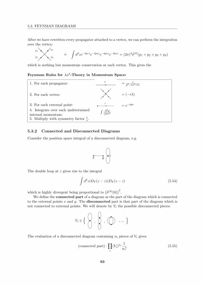
5.3. FEYNMAN DIAGRAMS
After we have rewritten every propagator attached to a vertex, we can perform the integrationover the vertex:
p2
p1p4
p3=
∫d4ze−ip1ze−ip2ze−ip3ze−ip4z = (2π)4δ(4)(p1 + p2 + p3 + p4)
which is nothing but momentum conservation at each vertex. This gives the
Feynman Rules for λφ4-Theory in Momentum Space:
1. For each propagator:p
= ip2−m2+iε
2. For each vertex: = (−iλ)
3. For each external point:p
= e−ipx
4. Integrate over each undeterminedinternal momentum:
∫ d4p(2π)4
5. Multiply with symmetry factor 1s .
5.3.2 Connected and Disconnected Diagrams
Consider the position space integral of a disconnected diagram, e.g.
x yz
The double loop at z gives rise to the integral
∫d4ziDF (z − z)iDF (z − z) (5.54)
which is highly divergent being proportional to(δ(4)(0)
)2.
We define the connected part of a diagram as the part of the diagram which is connectedto the external points x and y. The disconnected part is that part of the diagram which isnot connected to external points. We will denote by Vi the possible disconnected pieces:
Vi ∈
, , , ...
The evaluation of a disconnected diagram containing ni pieces of Vi gives
(connected part) ·∏
i
(Vi)ni
1
ni!(5.55)
63

5.3. FEYNMAN DIAGRAMS
where 1ni!
is due to the possibilitiy to permute the ni! identical disconnected pieces Vi. Wereorganize the complete two-point function by adding the terms for all possible combinationsof connected and disconnected pieces:
∑
connected
∑
ni
(connected part) ·∏
i
(Vi)ni
1
ni!(5.56)
where the second sum runs over all ordered sets of nonnegative integers. Thus
(5.56) =∑
(connected) ·(∑
n1
V n11
1
n1!
)(∑
n2
V n22
1
n2!
)· · ·
=∑
(connected) ·∏
i
(∑
ni
V nii
1
ni!
)
=∑
(connected) ·∏
i
exp(Vi)
=∑
(connected) · exp
(∑
i
Vi
). (5.57)
Inserting this into
limT→∞(1−iε)
〈0|T(φI(x)φI(y) exp
(−i∫ T
−TdtHI(t)
))|0〉 (5.58)
we find
(5.58) =(
+ +...)
exp(
+ +...)
.
We can use an analogous argument as that which lead to (5.57) in order to express the de-nominator of (5.47) as an exponential over disconnected diagrams:
limT→∞(1−iε)〈0|T(
exp(−i∫ T−T dtHI(t)
))|0〉 = exp
(+ +...
)
Therefore we have shown that the disconnected parts do not contribute in (5.47) becausethey appear in the nominator as well as in the denominator as a multiplicative factor andthus cancel:
〈Ω|T (φH(x)φH(y)) |Ω〉 =∑
(all connected diagrams with two external points). (5.59)
64
5.4. SCATTERING MATRIX
5.4 Scattering Matrix
The elements of the scattering matrix are probability amplitudes for the transition from aninitial state i to a final state f under the influence of an interaction.We have a time-dependent state vector |ψ(t)〉 which describes the state of the system. Theinitial state is
|φi〉 = limt→−∞
|ψ(t)〉. (5.60)
It is an eigenstate of the free Hamiltonian. The scattering matrix element Sfi is the projectionof the state vector onto the final state 〈φf |. Using limt→∞ |ψ(t)〉 = U(∞,−∞)|φi〉, we find
Sfi = limt→∞〈φf |ψ(t)〉
= 〈φf |S|φi〉 (5.61)
with the time evolution operator whose matrix elements read
Sfi = limt1→+∞t2→−∞
〈φf |U(t1, t2)|φi〉. (5.62)
We conclude that
S = U(+∞,−∞)
=∞∑
n=0
1
n!(−i)n
∫ ∞
−∞dt1 · · ·
∫ ∞
−∞dtnT (HI(t1) · · ·HI(tn)) . (5.63)
Note that this expression is unitary.We can decompose the S-matrix as
Sfi = δfi + i(2π)4δ(4)(pf − pi)Tfi (5.64)
where pf , pi denote the total momentum of final and inital state. The δ(4)(pf − pi) encodesfour-momentum conservation. We abbreviate this as
S = 1 + iT (5.65)
which we interpret as the superposition of a non-interacting contribution (for example, two in-coming particles which stay unaffected) and a contribution containing interactions (for exam-ple, the initial state could consist of two particles which interact and result in a multiparticlefinal state).
When we calculate the scattering matrix elements Sfi = 〈φf |S|φi〉, we have to deal withthe fact that 〈φf | and |φi〉 are eigenstates of the full theory.By a nontrivial generalization of the arguments leading to the relation between the freetheory’s vacuum |0〉 and the interacting theory’s vacuum |Ω〉, it follows that
Sfi = 〈φf |S|φi〉= 〈φ0
f |S|φ0i 〉∣∣connected diagrams
(5.66)
65

5.5. FEYNMAN RULES OF QED
where φ0i denotes the states of the non-interacting theory (without proof).
As an example, consider the S-matrix element for 2→ 2 scattering (k1 + k2 −→ k3 + k4):
Sfi =√
2E1
√2E2
√2E3
√2E4〈0|ak4ak3 |S|a†k1a
†k2|0〉. (5.67)
The only term in the S-matrix which does not give a vanishing contribution, has to beproportional to a†k3a
†k4ak2ak1 because only then all the operators can be cancelled (using
anticommutation relations which give rise to δ-functions) such that no operator which woulddestroy the vacuum remains.
5.5 Feynman Rules of QED
The Lagrange density of QED reads
L = LDirac0 + Lphoton
0 + LI (5.68)
with
LDirac0 = ψ(i/∂ −m)ψ
Lphoton0 = −1
4FµνFµν
LI = −eψγµψAµ = −jµAµ.(5.69)
As we know, LI describes the coupling of the free Maxwell theory (described by Lphoton0 )
to the free Dirac theory (described by LDirac0 ) in order to account for interactions between
fermions and photons. Accordingly, the quantized interaction Hamiltonian density assumesthe form
HI = −LI = eψγµψAµ. (5.70)
According to the expansion (5.63), the S-matrix is
S =
∞∑
k=0
1
k!(−ie)k
∫d4x1 · · · d4xk T
(ψ(x1)γµ1ψ(x1)Aµ1(x1) · . . . · ψ(xk)γµkψ(xk)A
µk(xk))
(5.71)
where we integrate also over spatial coordinates in order to obtain a Hamiltonian out of theHamiltonian density in (5.70). We expand in the small parameter e =
√4πα (≈ 1/3). The
structure of the summands is∑
contractions
(contracted operators)(x1, ..., xk) : (uncontracted operators) : (x1, ..., xk). (5.72)
For a scattering process, we find (denoting by 〈f | the mode of the annihilation operators aand by |i〉 those of the creation operators a†)
Sfi = 〈f |S|i〉. (5.73)
Only the matching terms in the n-th order S-matrix contribute. We can list all the operatorsappearing in the series expansion of S (time is running from left to right in the diagrams).By doing so, we make use of our results for the non-interacting theory. These rules constitutethe
66

5.5. FEYNMAN RULES OF QED
Feynman Rules for QED in Position Space:
We have the following external states:
• ψ+(x): absorption of an electron, x
• ψ+(x): absorption of a positron, x
• ψ−(x): emission of an electron, x
• ψ−(x): emission of a positron, x
• A+(x): absorption of a photon, x
• A−(x): emission of a photon, x
For the contractions, we have the following propagators:
• ψ(x2)ψ(x1) = iSF (x2 − x1): fermion propagator, x2x1
• Aµ(x2)Aν(x1) = iDµνF (x2−x1): photon propagator, x2,µx1,ν
The vertex is given by
• −ieψ(x)γµψ(x)Aµ(x) = ieqeγµ·(vertex in x): vertex in x,
5.5.1 S-operator to First Order
We can now illustrate the S-operator to first order (S(0) = 1):
S(1) = −ie∫d4x T
(ψ(x)γµψ(x)Aµ(x)
)
= −ie∫d4x : ψ(x)γµψ(x)Aµ(x) : +... (5.74)
where we ignore disconnected contributions. We can draw the corresponding diagrams:
The idea is that we have three operators ψ(x), ψ(x) and Aµ(x), each of which either creates
67
5.5. FEYNMAN RULES OF QED
or annihilates its associated particle (e.g. ψ(x) either creates an electron or annihilates apositron). So there are 23 possibilities of how to combine these operations. For example, thefirst graph corresponds to absorption of a photon and emission of an electron and a positron.
All of these processes are unphysical which we can show easily. Assume that any of theseprocesses satisfies energy and momentum conservation, i.e. we have
p2e+ = m2
e = p2e− and p2
γ = 0 (5.75)
and some combination of signs (depending on which process we are considering) in the fol-lowing expression:
±pe+ ± pe− ± pγ = 0, (5.76)
These relations lead to
(pe+ ± pe−)2 = (±pγ)2 = 0 (5.77)
⇔ 2m2e = 2pe+pe−
= 2Ee+Ee− − 2|pe+ ||pe− | cos θ
= 2√p2e+
+m2e
√p2e− +m2
e − 2|pe+ ||pe− | cos θ (5.78)
> 2m2e (5.79)
which is contradictory. None of the above graphs allows for simultaneous momentum andenergy conservation. So they can at most appear as virtual subprocesses.
5.5.2 S-Operator to Second Order
To second order, the S-operator reads
S(2) =1
2!(−ie)2
∫d4x1d
4x2T(ψ(x1)γµ1ψ(x1)Aµ1(x1)ψ(x2)γµ2ψ(x2)Aµ2(x2)
). (5.80)
Because it is very difficult to evaluate this expression directly, we make again use of Wick’stheorem and rewrite the time-ordered product as a sum over all possible normal-orderedcontractions (which can be represented as Feynman diagrams). All contractions of the formψ(x1)ψ(x2) or ψ(x1)ψ(x2) yield
〈0|T (ψ(x1)ψ(x2)) |0〉 = 0 (5.81)
because different particles are created or annihilated. Using the notation ψ1 ≡ ψ(x1), we canwrite down the remaining nonzero terms in (5.80):
68

5.5. FEYNMAN RULES OF QED
S(2) = (−ie)2
2!
∫d4x1d
4x2
: ψ1γµ1ψ1ψ2γµ2
ψ2Aµ1
1 Aµ2
2 : (a)
+ : ψ1γµ1ψ1ψ2γµ2
ψ2Aµ1
1 Aµ2
2 : (b)
+ : ψ1γµ1ψ1ψ2γµ2
ψ2Aµ1
1 Aµ2
2 : (c)
+ : ψ1γµ1ψ1ψ2γµ2
ψ2Aµ1
1 Aµ2
2 : (d)
+ : ψ1γµ1ψ1ψ2γµ2
ψ2Aµ1
1 Aµ2
2 : (e)
+ : ψ1γµ1ψ1ψ2γµ2
ψ2Aµ1
1 Aµ2
2 : (f)
+ : ψ1γµ1ψ1ψ2γµ2
ψ2Aµ1
1 Aµ2
2 : (g)
+ : ψ1γµ1ψ1ψ2γµ2
ψ2Aµ1
1 Aµ2
2 : (h)
+ : ψ1γµ1ψ1ψ2γµ2
ψ2Aµ1
1 Aµ2
2 : (i)
+ : ψ1γµ1ψ1ψ2γµ2
ψ2Aµ1
1 Aµ2
2 : (j)
+ : ψ1γµ1ψ1ψ2γµ2
ψ2Aµ1
1 Aµ2
2 :
(k)
(a)
(b) and (c)
(d)
(e) and (f)
(g)
(h) and (i)
(j)
(k)
It follows a discussion of the individual terms:
• (a): Independent emission/absorption (violates energy-momentum conservation)
• (b),(c): These terms describe several different processes. It is only specified thattwo electrons (positrons) and two photons are involved. But the arrows in the abovediagrams only indicate Fermion flow. If we specify a direction in time and draw whatexplicitly happens, there are several types of contribution to the above diagrams. Sinceit is unspecified from which of the operators we take the creators and annihilators, wecan have the following possibilities for the (b) and (c) graphs:
1. Compton scattering, i.e. γe− → γe−:
e− e− e− e−
69

5.5. FEYNMAN RULES OF QED
We cannot distinguish the processes by means of experiments because the physicalresult is the same in both cases. So we cannot tell which process takes place - infact, it is the superposition of the two possibilities which has to be seen as the“real” quantum process.
2. Compton scattering with positrons, i.e. γe+ → γe+
3. Electron-positron pair annihilation:
e−
e+
e−
e+
4. Electron-positron pair creation:
Aµ1
Aµ2
e−
e+
e−
e+
Aµ1
Aµ2
• (d): Processes with four electrons (positrons):
1. Møller scattering: e−e− → e−e− or e+e+ → e+e+
2. Bhaba scattering: e+e− → e+e−
• (e),(f): No interaction between external particles (no scattering process). These pro-cesses provide corrections to the fermion propagator (so-called self-energy).
• (g): Correction to the photon propagator (so-called vacuum polarization).
• (h),(i): Further corrections to the fermion propagator.
• (j),(k): Vacuum → vacuum transitions (disconnected graphs).
5.5.3 Contraction with External Momentum Eigenstates
In the end, we are not interested in the pure S-matrix but rather in S-matrix elements Sfi.So we need to think about how to contract the S-matrix with external states. Using theanticommutation relations for as′(p
′) and a†s(p), we find immediately for the electron
ψ(x)|e−(p, s)〉 =
∫d3p′
(2π)3
1√2Ep′
∑
s′
as′(p′)us′(p
′)e−ip′x√
2Epa†s(p)|0〉
= e−ipxus(p)|0〉 (5.82)
〈e−(p, s)|ψ(x) = eipx〈0|us(p). (5.83)
70

5.5. FEYNMAN RULES OF QED
In case of the positron, we have
ψ(x)|e+(p, s)〉 = e−ipxvs(p)|0〉 (5.84)
〈e+(p, s)|ψ(x) = eipx〈0|vs(p). (5.85)
For the photon, we infer that
Aµ(x)|γ(k, λ)〉 = e−ipxε(λ)µ (k) (5.86)
〈γ(k, λ)|Aµ(x) = eipxε(λ)∗µ (k) (5.87)
where the complex conjugation in the last line is for complex polarization vectors (e.g. circu-lar).
Example: Møller Scattering
We have
|i〉 = |e−(p1, s1)e−(p2, s2)〉 =√
2E12E2a†s1(p1)a†s2(p2)|0〉 (5.88)
〈f | = 〈e−(p′2, s′2)e−(p′1, s
′1)| =
√2E′12E′2〈0|as′2(p′2)as′1(p′1). (5.89)
Therefore the matrix element reads
Sfi = 〈f |S|i〉
=(−ie)2
2!
∫d4x1d
4x2
√16E1E2E′1E
′2
× 〈0|as′2(p′2)as′1(p′1) : ψ(x1)γµψ(x1)ψ(x2)γνψ(x2) : Aµ(x1)Aν(x2)a†s1(p1)a†s2(p2)|0〉.(5.90)
The only contractions which give nonzero contributions are those with precisely two creatorsand two annihilators which exactly saturate the annihilators and creators as′i and a†si , respec-tively (→ exercise). This leaves us with four graphs in position space:
p2 x2p′2
p1x1
p′1 p1 p′1x2
x1p′2p2
p1 p1x1 x2
p′2p′2
p2 p2 p′1p′1x2 x1
+ − −
The relative signs are due to the anticommutation relations between the involved operatorsas(p), a
†s(p) and ψ, ψ: every full contraction of (5.90) has to be “untangled” such that
contracted operators are adjacent. This process involves commuting the operators whichgives rise to some minus signs.With the momentum space photon propagator
iDµνF (q) = − igµν
q2 + iε, (5.91)
71

5.5. FEYNMAN RULES OF QED
we obtain (→ exercise)
Sfi = (−ie)2(2π)4δ(4)(p′1 + p′2 − p1 − p2)
(us′2(p′2)γµus2(p2) iDF (p′1 − p1) us′1(p′1)γνus1(p1)
− us′2(p′2)γµus1(p1) iDF (p′1 − p2) us′1(p′1)γνus2(p2)
).
(5.92)
We define the invariant amplitude Mfi:
Sfi = δfi + i(2π)4δ(4)(p′1 + p′2 − p1 − p2)Mfi. (5.93)
The computation of iMfi is done using the
Feynman Rules for QED in Momentum Space:
We have the following external states:
• us(p): incoming electron, p, s
• us(p): outgoing electron,p, s
• vs(p): incoming positron, p, s
• vs(p): outgoing positron,p, s
• εµ(λ)(p): incoming photon, λ, µ, p
• εµ∗(λ)(p): outgoing photon, λ, µ, p
Additionally, we have the following propagators (which are just the Fourier transforms ofx-space propagators):
• i(/p+m)
p2−m2+iε: electron propagator,
p
• −igµνk2+iε
: photon propagator, k
and the vertex
• ieqeγµ: electron-photon-electron vertex,
µ
qe
72

5.6. SCATTERING CROSS SECTION
Application of the Feynman Rules
• Energy-momentum conservation at each vertex. This condition fixes all the momentain terms of external momenta.
• For closed loops (no external momenta), we get an energy-momentum integral,∫ d4q
(2π)4.
• Each closed fermion loop yields a factor (−1) which is due to the operator ordering inthe contraction. For example, the loop
x1x2
stands for a contraction
ψ1ψ1ψ2ψ2 = (−1)tr(ψ1ψ2ψ2ψ1)
= (−1)tr(iSF (x1 − x2) · iSF (x2 − x1)). (5.94)
• Graphs with a different ordering of vertices along a fermion line are topologically dif-ferent and have to be added. For example, consider the following contributions to S(4)
which are not the same:
1 1 22
3 4 3 4
6=
5.6 Scattering Cross Section
So far, our observations and calculations do not give us observable quantities. In this sectionwe want to link the abstract S-matrix elements to observable quantities.The transition rate for a transition from the initial state i to the final state f per unit time is
wfi =|Sfi|2T
(5.95)
with Sfi = δfi + i(2π)4δ(4)(pf − pi)Mfi. In order to square Sfi, we have to think about howto square a δ-function. We write
[(2π)δ(p0f − p0
i )]2 =
∫ ∞
−∞dt ei(p
0i−p0f )t2πδ(p0
f − p0i )
= T (2π)δ(p0f − p0
i ) (5.96)
73

5.6. SCATTERING CROSS SECTION
where T denotes the total reaction time. Likewise
[(2π)3δ(3)(pf − pi)]2 = V (2π)3δ(3)(pf − pi) (5.97)
with the total reaction volume V . This simple approach thus yields
wfi = V (2π)4δ(4)(pf − pi)|Mfi|2. (5.98)
This heuristic approach can be made plausible if we consider a system inside a finite box.Consider a discrete space of states in a box where T and V are finite. The one particle statesψ(x) ∼ e−ipx satisfy
ψ(x+ L) = ψ(x). (5.99)
We thus find the usual quantized momenta
p =2π
Ln ⇒ dn =
L
2πdp and d3n =
(L
2π
)3
d3p =V
(2π)3d3p. (5.100)
This yields the following differential rate where the second δ-function is now absorbed in thevolume factor:
dwfi = (2π)4V δ(4)(Pf − Pi)|Mfi|2m∏
i=1
1
(2p0iV )
n∏
f=1
1
(2p0fV )
V
(2π)3d3pf
︸ ︷︷ ︸=d3nf
⇒ dwfi =V 1−m
(2π)3n−4δ(4)(Pf − Pi)|Mfi|2
m∏
i=1
1
2Ei
n∏
f=1
d3pf2Ef
(5.101)
for a reaction with m initial state particles and n final state particles with
Pi =m∑
i=1
pi, Pf =n∑
f=1
pf . (5.102)
The factors 12p0i V
and 12p0fV
ensure that we normalize to states with one particle in V . Recall
that our states in Mfi are normalized to 2p0: the normalization in Eq. (3.32) means thatthere is a continuum particle density of energy 2E per volume in momentum space. In orderto find the single particle state which describes one particle in a given volume, we need tomultiply with the (Lorentz invariant) factor 1√
2EpV. Since S-matrix elements refer to single
particle states but the calculation of Mfi uses continuum states, we need to multiply |Mfi|2in the above equations with the normalization factors.Usually we have only one or two particles in the initial states. If m = 1, this describes thedecay rate of a single particle and the expression simplifies considerably:
5.6.1 Decay Kinematics
Total decay rates (m = 1) for processes of the form a → p1 + ... + pn give rise to a decaywidth
Γa→n = wfa ⇒ lifetime = τa→n =1
Γa→n. (5.103)
74

5.6. SCATTERING CROSS SECTION
Integrating Eq. (5.101), we can write this decay width as
Γa→n =1
2Ea(2π)4
∫d3p1
(2π)32E1· · · d3pn
(2π)32Enδ(4)(Pf − pa)|Mfa|2 (5.104)
where |Mfa|2 can be calculated using the Feynman rules. An apparent problem arises if weconsider Lorentz invariance: the factor 1
2Eais not Lorentz invariant! Hence Γa→n does depend
on the reference frame. In fact, this is not a problem, but a reminiscent of the time dilation.The decay rate obviously has to depend on the reference frame because, in general, everyframe measures time differently. Consequently, when talking about “lifetime”, we mean thelifetime in the particle’s rest frame where Ea = ma.
5.6.2 Scattering Cross Sections
The second process which is of great importance, is scattering with m = 2 initial stateparticles. We are interested in the total scattering cross section σ(a+b → 1+2+ ...+n)which is defined as
σ =#transitions per unit of time
#incoming particles per surface per time=wfiflux
(5.105)
with the
flux =#particles
volume· |relative velocity|
=1
V|va − vb|. (5.106)
This yields
σ =1
4EaEb|va − vb|(2π)4
∫d3p1
(2π)32E1· · · d3pn
(2π)32Enδ(4)(Pf − Pi)|Mfi|2. (5.107)
We define the Møller function (quantities in the center of mass frame are denoted by a starand we use p∗a = −p∗b)
F = EaEb|va − vb|
= EaEb
∣∣∣∣paEa− pbEb
∣∣∣∣
= E∗aE∗b
∣∣∣∣p∗aE∗a− p∗bE∗b
∣∣∣∣= (E∗a + E∗b )|p∗a|= (E∗a + E∗b )
√(E∗a)2 −m2
a
=√
(pa · pb)2 −m2am
2b . (5.108)
The last step can easily be verified by using energy-momentum conservation. When we gofrom the second to the third line, we use that the whole expression is Lorentz invariant. Thisyields a manifestly Lorentz invariant expression for the cross section:
σ =1
4√
(pa · pb)2 −m2am
2b
(2π)4
∫d3p1
(2π)32E1· · · d3pn
(2π)32Enδ(4)(Pf − Pi)|Mfi|2. (5.109)
75
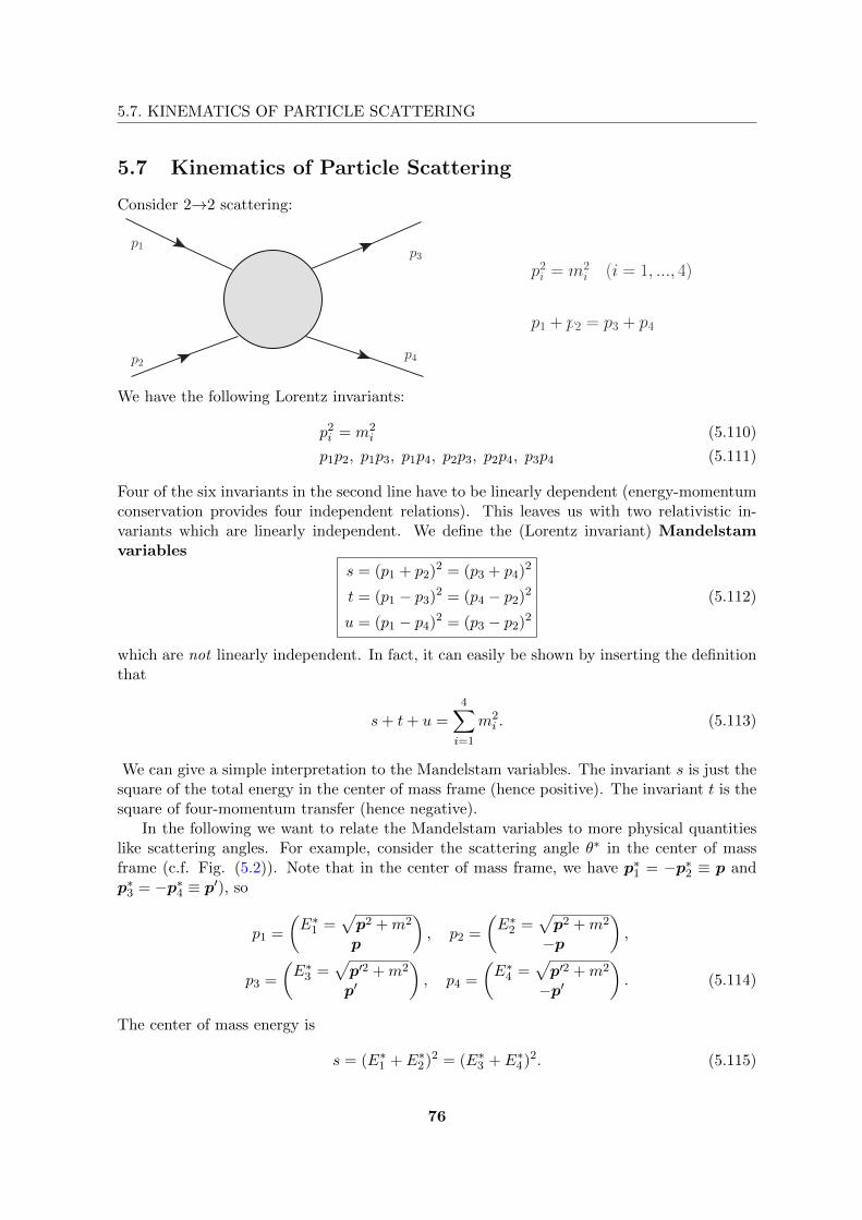
5.7. KINEMATICS OF PARTICLE SCATTERING
5.7 Kinematics of Particle Scattering
Consider 2→2 scattering:
p1
p2 p4
p3p2i = m2
i (i = 1, ..., 4)
p1 + p2 = p3 + p4
We have the following Lorentz invariants:
p2i = m2
i (5.110)
p1p2, p1p3, p1p4, p2p3, p2p4, p3p4 (5.111)
Four of the six invariants in the second line have to be linearly dependent (energy-momentumconservation provides four independent relations). This leaves us with two relativistic in-variants which are linearly independent. We define the (Lorentz invariant) Mandelstamvariables
s = (p1 + p2)2 = (p3 + p4)2
t = (p1 − p3)2 = (p4 − p2)2
u = (p1 − p4)2 = (p3 − p2)2
(5.112)
which are not linearly independent. In fact, it can easily be shown by inserting the definitionthat
s+ t+ u =
4∑
i=1
m2i . (5.113)
We can give a simple interpretation to the Mandelstam variables. The invariant s is just thesquare of the total energy in the center of mass frame (hence positive). The invariant t is thesquare of four-momentum transfer (hence negative).
In the following we want to relate the Mandelstam variables to more physical quantitieslike scattering angles. For example, consider the scattering angle θ∗ in the center of massframe (c.f. Fig. (5.2)). Note that in the center of mass frame, we have p∗1 = −p∗2 ≡ p andp∗3 = −p∗4 ≡ p′), so
p1 =
(E∗1 =
√p2 +m2
p
), p2 =
(E∗2 =
√p2 +m2
−p
),
p3 =
(E∗3 =
√p′2 +m2
p′
), p4 =
(E∗4 =
√p′2 +m2
−p′). (5.114)
The center of mass energy is
s = (E∗1 + E∗2)2 = (E∗3 + E∗4)2. (5.115)
76

5.7. KINEMATICS OF PARTICLE SCATTERING
p1
p2 p4
p3
s
t
u
Figure 5.1: Sketch of a 2→2 scattering process. The interaction region (visualized by acircle) is reigned by the superposition of many possible (partly complicated) processes likethose described in QED. At the moment we are concerned with the kinematics which can bedescribed using the Mandelstam variables s, t and u.
1 2
3
4
~p −~p
~p ′
−~p ′θ∗
Figure 5.2: Setup for 2→2 scattering in the center of mass frame. In this frame it is evenpictorially quite evident that the scattering angle and the center of mass energy are the onlydegrees of freedom.
This invariant s determines the energies Ei as well as the modulus of the momenta p, p′. Inorder to get the scattering angle θ∗, we need one further invariant. The scattering angle isgiven by
p · p′ = |p||p′| cos θ∗ (5.116)
p1p3 = E∗1E∗3 − |p||p′| cos θ∗. (5.117)
Using the relation
t = (p1 − p3)2 = m21 +m2
3 − 2p1p3 (5.118)
77

5.7. KINEMATICS OF PARTICLE SCATTERING
we can solve for cos θ∗ (→ exercise):
cos θ∗ =s(t− u) + (m2
1 −m22)(m2
3 −m24)√
λ(s,m21,m
22)√λ(s,m2
3,m24)
(5.119)
with λ(s,m21,m
22) = (s−m2
1 −m22)2 − 4m2
1m22.
Therefore we see that 2→2 scattering is described by two independent variables which canchosen to be
• either√s and θ∗
• or√s and t.
5.7.1 Angular Distribution
The incoming particles move straight along the z-axis. Thus we have a symmetry concerningthe azimuthal angle φ. Because this azimuthal angle φ is chosen with respect to some arbitraryreference point, physical processes cannot depend on it and we can write
dΩ∗ = dφ∗ d cos θ∗ = 2πd cos θ∗. (5.120)
Inserting (5.118) into (5.117) and solving for cos θ∗, this simplifies to
dΩ∗
dt=
π
|p||p′| . (5.121)
We see that the physical region of phase space is defined by
|p|2 ≥ 0 ⇒ s ≥ max
[(m1 +m2)2, (m3 +m4)2
](5.122)
−1 ≤ cos θ∗ ≤ 1 ⇒ tmax ≥ t ≥ tmin (5.123)
where tmax and tmin can be determinated from (5.119) (→ exercise).
5.7.2 Two-particle Phase Space
Again we consider 2→2 scattering (a+ b → 1 + 2) with the phase space
R2 =
∫d3p1
2E1
d3p2
2E2δ(4)(p1 + p2 − pa − pb)
=
∫d4p1d
4p2 δ(p21 −m2
1)δ(p22 −m2
2)θ(E1)θ(E2)δ(4)(p1 + p2 − pa − pb)
=
∫d4p1 δ(p
21 −m2
1)δ((pa + pb − p1)2 −m22)θ(E1)θ(Ea + Eb − E1)
=
∫ Ea+Eb
0dE1
∫ ∞
0|p1|2d|p1|dΩ δ(E2
1 − p21 −m2
1)δ((pa + pb − p1)2 −m22)
=
∫ Ea+Eb
0dE1dΩ
√E2
1 −m21
2δ(s− 2(pa + pb) · p1 +m2
1 −m22). (5.124)
78

5.8. TRACE TECHNIQUES
where we first switched to integrals over four momenta in order to integrate the four dimen-sional δ-function afterwards. After changing to polar coordinates, we used
δ(E21 − p2
1 −m21) =
1
2|p1|
[δ
(|p1| −
√E2
1 −m21
)+ δ
(|p1|+
√E2
1 −m21
)
︸ ︷︷ ︸=0 (unphysical)
](5.125)
in the last step. Because the expression (5.124) is manifestly Lorentz invariant, we can chosea suitable frame to compute it. In the center of mass frame we have
pa + pb = 0 and Ea + Eb =√s (5.126)
which allows us to write (5.124) in the following form:
R2 =
∫ √s
0dE∗1dΩ∗
|p|2δ(s− 2
√sE∗1 +m2
1 −m22)︸ ︷︷ ︸
= 12√sδ(E∗1−
12√s(s+m2
1−m22))
=
∫dΩ∗
|p|4√s
(5.127)
where |p| ≡ |pa| = |pb|. It is actually not the complete phase space R2 which we shallneed. Instead we will be interested in integrals of the form
∫dR2|Mfi|2 (in particular, the
expression (5.109) for the total cross section contains such a phase space integral). But theabove calculation tells us how to write dR2:
dR2 =|p|
4√sdΩ∗. (5.128)
5.8 Trace Techniques
As we have seen, the cross section takes the form
σ ∼ (Kinematical factors) · |Mfi|2
= (...) · |us,f (pf )Γus,i(pi)|2 (5.129)
where Γ is some combination of γ-matrices.We have to respect the following rules for spin summation:
• If the spin state of particles in the final state is not measured, then one has to sum overthe final spin states:
∑sf|...|2
• If particles in the initial state are unpolarized, we have to average over the initial spinstates: 1
2
∑si|...|2
79

5.8. TRACE TECHNIQUES
Defining Γ ≡ γ0Γ†γ0, we observe that
1
2
∑
si
∑
sf
|usf (pf )Γusi(pi)|2 =1
2
∑
si
∑
sf
(usf (pf )Γusi(pi)
)·(u†sf (pf )γ0Γusi(pi)
)†
=1
2
∑
si
∑
sf
usfΓusiu†si γ
0γ0
︸︷︷︸1
Γ†γ0usf
=1
2
∑
si
∑
sf
usfΓusi usiΓusf
=1
2
∑
si
∑
sf
tr(usfΓusi usiΓusf
)
=1
2tr(
Γ( /pi +m)Γ(/pf +m))
(5.130)
where we used the identity (1.127),∑
s=±us(p)us(p) = /p+m, (5.131)
and the cyclicity of the trace in order to simplify the trace. The object Γ reads explicitly
• Γ = γµ ⇒ Γ = γ0㵆γ0 = γµ,
• Γ = γµ1 · · · γµn ⇒ Γ = γ0γµn† · · · γµ1†γ0 = γµn · · · γµ1
In case of antiparticles, we have to interchange u and v and (instead of (5.131)) use∑
s
vs(p)vs(p) = /p−m. (5.132)
To summarize, we obtain the following results:
1
2
∑
si
∑
sf
|usf (pf )Γusi(pi)|2 =1
2tr(
Γ( /pi +m)Γ(/pf +m))
1
2
∑
si
∑
sf
|vsf (pf )Γvsi(pi)|2 =1
2tr(
Γ( /pi −m)Γ(/pf −m)) (5.133)
The following trace identities for γ-matrices will also prove very useful for explicit calculations:
• tr(1) = 4 and tr(γµ) = tr(γ5) = 0,
• tr(γµγν) = 12tr(γµ, γν) = 1
2 · 2gµνtr(1) = 4gµν ,
• tr(/a/b) = 4(a · b),• tr(γµγνγργσ) = 4(gµνgρσ + gµσgνρ − gµρgνσ)
proof:
tr(γµγνγργσ) = −tr(γνγµγργσ) + 2gµνtr(γργσ)
= tr(γνγργµγσ)− 2gµρtr(γνγσ + 8gµνgρσ
= − tr(γνγργσγµ)︸ ︷︷ ︸=tr(γµγνγργσ)
+8gµσgρν − 8gµρgνσ + 8gµνgρσ (5.134)
80

5.9. MØLLER SCATTERING
• The last two points generalize to
tr(/a1 · · · /an) = a1 · a2tr(/a3 · · · /a4)− a1 · a3tr(/a2 · · · /an) + . . .± a1 · antr(/a2 · · · /an−1)
(5.135)
and in particular: tr(γµ1 · · · γµn) ∈ R.
• tr(odd number of γ-matrices) = 0.proof:
tr(γµ1 · · · γµn γ5γ5
︸︷︷︸=1
) = tr(γ5γµ1 · · · γµnγ5)
= (−1)tr(γµ1γ5γµ2 · · · γµnγ5)
= (−1)n(γµ1 · · · γµnγ5γ5)
= (−1)ntr(γµ1 · · · γµn)
= 0 for odd n. (5.136)
• tr(γµ1 · · · γµ2n) =tr((γµ1 · · · γµ2n)†
)=tr(γ0γµ2nγ0 · · · γ0γµ1γ0) =tr(γµ2n · · · γµ1),
• Contractions of γ-matrices:
γµγµ =1
2γµ, γµ = gµµ = 4, (5.137)
γµ/aγµ = −γµγµ/a+ 2gµνaνγµ = −2/a, (5.138)
γµ/a/bγµ = ... = 4a · b, (5.139)
γµ/a/b/cγµ = −2/c/b/a. (5.140)
5.9 Møller Scattering
In terms of Feynman diagrams, we have the possibilities shown in Fig. (5.3). This gives rise
p2 p′2
p1 p′1
−
p2 p′2
p′1p1
Figure 5.3: Møller scattering Feynman graphs.
81

5.9. MØLLER SCATTERING
to the amplitude
iMfi = (−ie2)
[us′2(p′2)γµus2(p2)
−igµν(p1 − p′1)2
us′1(p′1)γνus1(p1)
− us′2(p′2)γµus1(p1)−igµν
(p1 − p′2)2us′1(p′1)γµus2(p2)
](5.141)
≡M1 −M2. (5.142)
We have to sum over final and average over initial spin states and square the matrix element:
|M |2 =1
4
∑
s1,s2,s′1,s′2
|M1|2 + |M2|2 − 2<(M1M∗2 ). (5.143)
Note that the center of mass energy is
s = (p1 + p2)2 = p21 + p2
2 + 2p1p2 ⇒ p1p2 = p′1p′2 =
s
2−m2 (5.144)
and similarly
p′2p2 = p′1p1 = m2 − t
2, (5.145)
p′2p1 = p′1p2 = m2 − u
2. (5.146)
Using these relations, we find
1
4
∑
s
|M1|2 =1
4
e4
t2tr(
(/p′2
+m)γµ(/p2+m)γµ
′)· tr(
(/p′1
+m)γµ(/p1+m)γµ′
). (5.147)
Using that any odd number of γ-matrices doesn’t contribute to the trace, we find that
(5.147) =1
4
e4
t2tr(/p′2γµ/p2
γµ′ +m2γµγµ′)· tr(/p′1γµ/p1
γµ′+m2γµγµ
′)
=1
4
e4
t2· 16(p′2µp2µ′ + p′2µ′p2µ − (p2p
′2 −m2)gµµ′
)·(p′µ1 p
µ′
1 + p′µ′
1 pµ1 − (p1p′1 −m2)gµµ
′)
=4e4
t2(2(p1p
′2)(p′1p2) + 2(p1p2)(p′1p
′2)− 2m2(p1p
′2 + p1p
′2) + 4m2
)
=2e4
t2(2s2 + t2 + 2st− 8m2s+ 8m4). (5.148)
We find the same expression for 14
∑s |M2|2 but with t replaced by u. The interference term
reads
−1
4
∑
s
2<(M1M∗2 ) = − e4
2tutr(
(/p′2
+m)γν(/p2+m)γµ(/p
′1
+m)γµ(/p1+m)γν
)
=2e4
tu(24m2 + 2s2 − 16sm2). (5.149)
82

5.10. COMPTON SCATTERING
The Mandelstam variables become useful if we switch to the center of mass frame where
p1 = −p2, p′1 = −p′2, E1 = E2 = E′1 = E′2 = E
⇒ |pi| = |p′i| =√E2 −m2. (5.150)
In this frame, the Mandelstam variables read
s = (2E)2 (5.151)
t = 2(m2 − E2 + (E2 −m2) cos θ∗) = 4(m2 − E2) sin2
(θ∗
2
)(5.152)
u = 2(m2 − E2 − (E2 −m2) cos θ∗) = 4(m2 − E2) cos2
(θ∗
2
). (5.153)
As we have seen in Eq. (5.128),
dR2 =|p|
4√sdΩ∗ =
√E2 −m2
8EdΩ∗. (5.154)
Remembering Eq. (5.109), we are now in the position to write down the total cross sectionfor this process where the phase space integration is now simplified by the above expressionfor dR2. The prefactor to the phase space integral in (5.109) looks quite simple because ofE1 = E2 = E∗1 = E∗2 = E and m1 = m2 = m:
σ =1
2· 1
8√E2(E2 −m2)
1
(2π)2
√E2 −m2
8E
∫dΩ∗|M |2
=1
512π2E2
∫dΩ∗|M |2 (5.155)
where the first factor 12 is due to the fact that there are two electrons resulting from the
interaction. So if we have a 4π-solid angle detector, we observe two identical electrons althoughonly one process took place. Accordingly, the measured total cross section is too large by afactor of 2 which is accounted for by the factor 1
2 in the above formula.Plugging in the explicit expression for |M |2 we arrive at the result (with e2 = 4πα)
dσ
dΩ∗=
α2
4E2
(2E2 −m2)2
(E2 −m2)2
[4
sin4 θ∗− 3
sin2 θ∗+
(E2 −m2)2
(2E2 −m2)2
(1 +
4
sin2 θ∗
)]. (5.156)
We can easily derive the non-relativistic limit by using E2 ' m2 and expanding v2 ' 1E2 (E2−
m2):
(dσ
dΩ∗
)
NR
=α2
m2
1
16v2
(1
sin4(θ2
) +1
cos4(θ2
) − 1
sin2(θ2
)cos2
(θ2
)). (5.157)
5.10 Compton Scattering
We consider the process
γ(k) + e−(p) −→ γ(k′) + e−(p′) (5.158)
83

5.10. COMPTON SCATTERING
p p′k + p
k, λ k′, λ′
ν µ
p p′ − k p′
ν µ
k′, λ′k, λ
+
Figure 5.4: Compton scattering Feynman graphs. The left graph is referred to as “s-channel”whereas the right graph is called “u-channel” because they give rise to the same amplitudebut with s and u interchanged.
giving rise to the Feynman diagrams shown in Fig. (5.4).The amplitude for Compton scattering is given by the sum of the two diagrams:
iM = ε∗µ(k′, λ′)εν(k, λ) · u(p′)[(−ieγµ)
i
/p+ /k −m(−ieγν) + (−ieγν)i
/p′ − /k −m(−ieγµ)
]u(p)
(5.159)
where we can use that
k2 = k′2 = 0 (5.160)
p2 = p′2 = m2 (5.161)
k · ε(k) = 0 (5.162)
k′ · ε(k′) = 0 (5.163)
where the first two equations keep track of the on-shell condition for external fermions andphotons. The latter two equations state the fact that the external photons are transversal.Before calculating this explicitly (which is essentially done as in the case of Møller scattering),we check the gauge invariance of this amplitude. Perform a gauge transformation
Aν −→ Aν + ∂νΛ (5.164)
⇔ εν −→ εν + βkν (5.165)
with arbitrary function Λ on the level of the potential or arbitrary β ∈ R in the case ofpolarization vectors. The change of the amplitude after such a transformation is
iM(εν → kν) = (−ie2)ε∗µ(k′, λ′) · u(p′)
(γµ
i
/p+ /k −m/k + /ki
/p′ − /k −mγµ)u(p)
= (−ie2)ε∗µ(k′, λ′) · u(p′) (γµ − γµ)u(p)
= 0 (5.166)
where we used the following identities which follow from the Dirac equations in (1.104):
1
/p+ /k −m/ku(p) =1
/p+ /k −m(/k + /p−m)u(p) = 1 · u(p), (5.167)
u(p′)/k1
/p′ − /k −m= u(p′)(/k − /p′ +m)
1
/p′ − /k −m= −u(p′). (5.168)
84

5.10. COMPTON SCATTERING
θL~k
~p′
~k′
~p = ~0
Figure 5.5: Compton-scattering in the laboratory frame of the e−.
We will be able to really appreciate the meaning of Eq. (5.166) in section 6.8 where we willprove the general Ward-Takahashi identity. So far we note that the complete amplitude isindeed gauge invariant. But we see immediately from Eq. (5.166) that each single amplitudefor one of the two diagrams is not gauge invariant! Only their sum is. Therefore we cannotconsider one diagram on its own. The whole expression is not really meaningful if we do nottake both diagrams into account. This observation will turn out to be very important whenwe consider divergent diagrams: in some cases the divergences of different diagrams canceleach other such that one diagram alone gives infinite contributions whereas the completespectrum of diagrams still yields finite results.
We can apply the usual techniques to compute the amplitude explicitly. Using
∑
λ′
ε∗µ(k′, λ′)ερ(k′, λ′) = −gµρ, (5.169)
∑
λ
εν(k, λ)ε∗σ(k, λ) = −gνσ, (5.170)
one can find the result
|M |2 =1
2
∑
λ
1
2
∑
s
∑
λ′
∑
s′
|M |2
= 2e4
[m2 − us−m2
+m2 − su−m2
+ 4
(m2
s−m2+
m2
u−m2
)+ 4
(m2
s−m2+
m2
u−m2
)2]
(5.171)
which yields the unpolarized Compton cross section
dσ
dt=
1
16π(s−m2)2|M |2. (5.172)
In the rest frame of the electron (laboratory frame), we have the situation as shown in Fig.
(5.5). The momenta are p =
(m0
)and p′ =
(E′Cp′
)with photon energies
85

5.10. COMPTON SCATTERING
ω = |k| = Eγ , ω′ = |k′| = Eγ′ . (5.173)
The Mandelstam variables read in this case
s−m2 = 2mω (5.174)
u−m2 = −2pk′ = −2mω′ (5.175)
t = −2ωω′(1− cos θL) (5.176)
and we have
ω′ = Eγ′ =1
2m(s+ t−m2)
= ω − ωω′
m(1− cos θL) (5.177)
where we used s+ t+ u = 2m2. We arrive at the result
1
ω′− 1
ω=
1
m(1− cos θL) (5.178)
⇒ ω′ =ω
1 + ωm(1− cos θL)
. (5.179)
Using
dt =ω′2
π2πd cos θL =
ω′2
πdΩL (5.180)
we find the Klein-Nishina formula,
dσ
dΩL=
α2
2m2
(ω′
ω
)2 [ω′ω
+ω
ω′− sin2 θL
](5.181)
which is fully relativistic and thus provides the correct expansions both for the non-relativisticas well as for the ultra-relativistic limit.
86

Chapter 6
Renormalization
If we go to higher orders in perturbation theory, the relevant Feynman diagrams also containclosed loops. We want to deal with the problem that closed loops in Feynman diagrams canyield divergent contributions to the scattering matrix element. Consider, for example, thetwo-point function in λφ4-theory: in position space we have elements like
x z y
=1
2(−iλ)
∫d4ziDF (0) → ∞.
In momentum space, this is divergent, as well:
x z y
=1
2(−iλ)
∫d4p
(2π)4
i
p2 −m2 + iε∼∫|p|d|p| → ∞.
We see that the divergences appear in the ultraviolet limit (large p).
6.1 Divergences in Feynman Diagrams
6.1.1 Divergences in λφ4-Theory
In λφ4-theory we have Feynman diagrams with
n vertices
E external lines
I internal lines
4 lines at each vertex ⇒ 4n = E + 2I (6.1)
L loops (6.2)
In d spacetime dimensions, we have an integral
∫ddp
(2π)d(6.3)
for each loop. We can classify the divergences for loop momenta pn →∞.First of all, we define the superficial degree of divergence
D = dL− 2I (6.4)
87

6.1. DIVERGENCES IN FEYNMAN DIAGRAMS
where dL comes from the integrals∫ddpn for loops: each of the L loops gives such an integral
which contributes pd to the numerator. The term 2I is due to the factor 1p2n
entering the
integral for each propagator.In d = 4 dimensions, we have the following divergent diagrams (subdiagrams) in λφ4-theory:
: D = 2 (quadratically divergent)
: D = 0 (logarithmically divergent)
Energy-momentum conservation at each vertex with one δ-function for global energy-momentumconservation give us n− 1 relations. So the number of independent loop momenta is
L = I − (n− 1) = I − n+ 1. (6.5)
The parameters L and I are determined exclusively by internal properties of the diagrams.We use Eqs. (6.1) and (6.5) to replace L and I in Eq. (6.4) by external parameters n and Eand find
D = d−(d
2− 1
)E + n(d− 4). (6.6)
In the case of d = 4 this is simply
D = 4− E. (6.7)
We conclude that in λφ4-theory only diagrams with E = 2 (D = 2) and E = 4 (D = 0)diverge. Diagrams with E > 4 have D < 0, so they don’t diverge according to our dimensionalanalysis. But we have to pay attention since they can contain divergent subdiagrams, as, forexample, in the case E = 6 (D = −2) which is shown in Fig. (6.1): although D < 0 holdstrue, two of the diagrams diverge because of a divergent subdiagram. This is why D is onlya superficial degree of divergence.
Divergences in a finite number of subdiagrams can (potentially) be compensated bya redefinition (renormalization) of parameters in the Lagrangian (mass, coupling, fieldstrength). However, there is the important prerequisite that D must not increase with n (orL). We distinguish the following cases (always for a fixed spacetime dimension d):
• D is independent of n. Then the degree of divergence is independent of the order in per-turbation theory. For example, the quadratically divergent D = 2 diagram from aboveis quadratically divergent at each order of perturbation theory. We can still calculatethe divergent contributions at every order in perturbation theory from a finite numberof subdiagrams but although we have a systematic prescription of how to do this, we stillhave to calculate infinitely many integrals. Such a theory is called renormalizable.
• D decreases with increasing n. Then only the first few orders of perturbation theorycontain divergent contributions to a finite number of subdiagrams. This case is calleda super-renormalizable theory.
88

6.1. DIVERGENCES IN FEYNMAN DIAGRAMS
Figure 6.1: Diagrams with six external legs. The leftmost diagram converges. The seconddiagram contains a quadratically divergent subdiagram. The subdiagrams which are markedin the third diagram diverge logarithmically. We easily see that any diagram of this type willdiverge as soon as it contains hidden (virtual) subdiagrams which diverge, irrespective of itssuperficial degree of divergence being negative.
• D increases with n. Then the theory is non-renormalizable because at higher andhigher order in perturbation theory, we need more and more parameters to absorb moreand more divergent subdiagrams. Since we only have a finite number of parameters, wecannot renormalize by redefinition of those.
Note that we cannot find the true degree of divergence just by means of power counting.This technique only gives a first idea of whether the integral diverges or not. For example,there are diagrams which should diverge quadratically according to power counting but theyactually diverge only logarithmically.
6.1.2 Divergences in QED
In QED the situation is slightly more complicated because we have two types of particles.We have
n vertices
Pe external photon lines
Pi internal photon lines
⇒ n = Pe + 2Pi (6.8)
Ee external electron lines
Ei internal electron lines
⇒ 2n = Ee + 2Ei (6.9)
L loops ⇒ L = Ei + Pi − n+ 1 (6.10)
The photon propagator is proportional to 1p2n
and each electron propagator gives a contribution
∼ /pnp2n∼ 1|pn| for large |p|. Therefore the superficial degree of divergence in QED is
D = dL− 2Pi − Ei= (d− 1)Ei + (d− 2)Pi − d(n− 1)
= d+ nd− 4
2− d− 1
2Ee −
d− 2
2Pe. (6.11)
89

6.2. DIMENSIONAL REGULARIZATION
In d = 4 this reduces to
D = 4− 3
2Ee − Pe (6.12)
which implies that QED is renormalizable!There is a short list of superficially divergent subdiagrams in QED. The amplitudes which doreally diverge are the following three:
, , ...
: Ee = 2, Pe = 0 : electron self-energy. (D = 1)
, , ... : Ee = 0, Pe = 2 : photon vacuum. polarization (D = 2)
, , ...: Ee = 2, Pe = 1 : vertex function (D = 0)
There are further potentially (i.e. superficially) divergent subdiagrams which are not a prob-lem because they are actually zero or finite due to symmetries. For example, consider thefollowing diagrams (three photon interaction) with Ee = 0, Pe = 3 (i.e. D = 1) which areactually divergent but pairwise cancel each other because they are equal up to a minus sign:
+ = 0 to all orders in perturbation theory.
In the case of four-photon interactions, Ee = 0 and Pe = 4 yields D = 0. This logarithmicdivergence is however vanishing because of gauge invariance. Badly divergent diagrams likethe zero-point function (vacuum-vacuum transition) only shift the vacuum energy but areuninteresting for the calculation of S-matrix elements.
6.2 Dimensional Regularization
In spherical coordinates, we have for a typical loop correction integral
∫ddp
(p2)n∼∫ ∞
0dppd−1
(p2)nwith <(d) ≥ 2n (6.13)
which is divergent for <(d) ≥ 2n (n denotes the number of internal legs in the diagram).Although we are able to compute the first terms in the perturbation series, we face theproblem that the higher order terms do not become smaller but diverge. Loosely speaking,the idea of renormalization is that we can separate the infinite part of the integral and absorb
90
6.2. DIMENSIONAL REGULARIZATION
it in the constants. In order to do so, we can rewrite the integral (for d = 4) by introducinga finite cutoff Λ2:
∫ ∞
0dp
p3
(p2)n= lim
Λ2→∞
∫ Λ2
0dp
p3
(p2)n. (6.14)
Divergences appear as lnΛ2, Λ2lnΛ2,... We are now in the situation that we have a finiteintegral from 0 to Λ2 and a divergent remainder. This method is actually not particularlyuseful (except for very simple cases) because we don’t know how to solve the integral anymore.
A more useful idea is to consider the integral (6.13) in d ∈ C dimensions. As we willsee, the divergences are hidden in the d-dependence of the integral. In order to computethe interesting d = 4 case, we will consider the limit (d − 4) → 0 and take the analyticalcontinuation. Writing the result as a Laurent series in the variable (d − 4), we will see howdivergences appear as proportional to 1
d−4 , 1(d−4)2
, ... So the initial expression (6.13) which is
convergent only in the half plane with <(d) < 2n, has an analytical continuation to the entirecomplex plane where the divergences manifest themselves through poles in d = 4.Although a bit unintuitive, dimensional regularization provides us with a regularizationscheme which preserves gauge invariance and keeps all the symmetries manifest.
Before we can work this program out in detail, we need to develop some tools which willallow us to handle d-dimensional integrals appropriately.
6.2.1 Dimensional Analysis in d Dimensions
The action in d dimensions reads
S =
∫ddxL. (6.15)
In order for S to be dimensionless, we need L to have units of
[L] = length−d = µd (6.16)
where µ is some mass scale (t’Hooft mass). We say that L has mass dimension d. Considertwo examples:
• λφ4-theory in d-dimensional Minkowski space with
L =1
2(∂µφ)(∂µφ)− 1
2m2φ2 − λ
4!φ4. (6.17)
According to Eq. (6.16) we need to have
[φ] = µd2−1, (6.18)
[λ] = µ4−d. (6.19)
We can thus write
L =1
2(∂µφ)(∂µφ)− 1
2m2φ2 − µ4−dλ
4!φ4 (6.20)
with a redefined dimensionless coupling λ.
91

6.2. DIMENSIONAL REGULARIZATION
• As another example, consider the QED Lagrangian:
L = ψ(i/∂ −m)ψ − 1
4FµνF
µν − eψ /Aψ (6.21)
with the following mass dimensions:
[ψ] = µd−12 (6.22)
[A] = µd2−1 (6.23)
[e] = µ2− d2 . (6.24)
Hence we can write L with new and dimensionless coupling:
L = ψ(i/∂ −m)ψ − 1
4FµνF
µν − µ2− d2 eψ /Aψ. (6.25)
6.2.2 Lorentz and Dirac Algebras in d Dimensions
In d dimensions every Lorentz index runs from 0 to d− 1. We obviously have gµµ = d.The Clifford algebra in 4 dimensions reads
γµ, γν = 2gµν . (6.26)
In d dimensions, we need d γ-matrices. The Clifford algebra stays the same. Fortunately, wedon’t need explicit expressions for the γ-matrices, because we always need to compute tracesof them. We have the following simple generalizations of the corresponding four-dimensionalidentities:
γµγµ = d (6.27)
γµγνγµ = (2− d)γν (6.28)
...
As sketched above, in the end we will be interested in the limit of such traces and use
limd→4
tr(1) = 4. (6.29)
Note that there is no obvious analogue of γ5 in d dimensions.
6.2.3 Integration in d Dimensions
We try to compute
=1
2λµ4−d
∫ddp
(2π)d1
p2 −m2 + iε
The translation of the diagram into an integral is done by application of the Feynman rulesin momentum space for λφ4-theory. Note that there are no external points (which wouldgive rise to exponentials e−ipx) because this diagram is to be understood as a loop correctionto a propagator in a larger diagram. As we will see next, this expression can be computed
92

6.2. DIMENSIONAL REGULARIZATION
explicitly using some typical tricks and it is divergent as d→ 4. The difference to the powercounting method is, that after performing the integral explicitly, we are able to tell exactlyhow strong the divergence is. The problem is that ddp and p2 live in Minkowski space. Wewill parametrize the Minkowski space vectors in terms of Euclidean vectors (which we knowhow to integrate) using the concept of Wick rotation: Define the Euclidean vector pE by
p0E = −ip0, (pE)i = pi. (6.30)
This definition yields
ddp = iddpE (6.31)
p2E = (p0
E)2 + |pE |2 = −p20 + |p|2 = −p2. (6.32)
Note that the direction of the Wick rotation is determined uniquely by the requirement thatthe same residues shall be enclosed by the Euclidean integral, i.e. by the “+iε”-prescription ofthe propagator. After performing a Wick rotation, the above integral becomes an integral inEuclidean space (where we know how to use polar coordinates in arbitrarily high dimensions):
=iλ
2µ4−d
∫ddpE(2π)d
1
−p2E −m2 + iε
.
= − iλ2µ4−d
∫ddpE(2π)d
1
p2E + ∆
(∆ ≡ m2 − iε)
= − iλ2µ4−d
∫dΩd
(2π)d
∫ ∞
0dpE
pd−1E
p2E + ∆
. (6.33)
where we switched to d-dimensional polar coordinates in the last step. In order to computethe first integral in (6.33), we need to find a formula for the unit sphere in d dimensions. Tothis end, observe that
(√π)d =
(∫dxe−x
2
)d
=
∫ddx exp
(−
d∑
i=1
x2i
)
=
∫dΩd
∫dxxd−1e−x
2
=
(∫dΩd
)1
2
∫d(x2)(x2)
d2−1e−(x2)
=
(∫dΩd
)1
2Γ
(d
2
)(6.34)
⇒∫dΩd =
2πd/2
Γ(d/2). (6.35)
93

6.2. DIMENSIONAL REGULARIZATION
Let’s turn to the radial integral in (6.33):
∫ ∞
0dpE
pd−1E
p2E + ∆
=1
2
∫ ∞
0d(p2
E)(p2E)
d2−1
p2E + ∆
=1
2
(1
∆
)1− d2∫ 1
0dxx−
d2 (1− x)
d2−1
=1
2
(1
∆
)1− d2 Γ(1− d
2
)Γ(d2
)
Γ(1)
=1
2
(1
∆
)1− d2
Γ
(1− d
2
)Γ
(d
2
)(6.36)
where we used the substitution x =p2E
p2E+∆and the following property of the β-function:
B(α, β) =
∫ 1
0dx xα−1(1− x)β−1 =
Γ(α)Γ(β)
Γ(α+ β). (6.37)
Putting these results together, we find
= − iλm2
32π2
(4πµ2
m2
)2− d2
Γ
(1− d
2
).
We can already see that divergences will appear if d → 4 because of the Γ-function havingpoles in 0, −1, −2, ...We need two more identities which can be proven in exactly the same way in which wecomputed (6.33) (→ exercise):
∫ddpE(2π)d
1
(p2E + ∆)n
=1
(4π)d/2Γ(n− d
2
)
Γ(n)∆
d2−n (6.38)
∫ddpE(2π)d
p2E
(p2E + ∆)n
=d
2
1
(4π)d/2Γ(n− d
2 − 1)
Γ(n)∆1+ d
2−n (6.39)
We can now compute a more complicated diagram (with q = p1 + p2 = p3 + p4):p
p4p2 p− q
p1 p3
=1
2λ2(µ2)4−d
∫ddp
(2π)d1
p2 −m2
1
(p− q)2 −m2
=1
2λ2(µ2)4−d
∫ddp
(2π)d
∫ 1
0dz
1
[p2 −m2 − 2pq(1− z) + q2(1− z)]2
=1
2λ2(µ2)4−d
∫ddp′
(2π)d
∫ 1
0dz
1
[p′2 −m2 + q2z(1− z)]2
=iλ2
2(µ2)4−d
∫ 1
0dz
∫ddpE(2π)d
1
[p2E +m2 − q2z(1− z)]2
=iλ2
32π2(µ2)2− d
2 Γ
(2− d
2
)∫ 1
0dz
(m2 − q2z(1− z)
4πµ2
) d2−2
(6.40)
94

6.3. DIVERGENT DIAGRAMS IN QED
where we used 1ab =
∫ 10
dz(az+b(1−z))2 in the first step and substituted p′ = p − q(1 − z) in the
second step. The advantage of this integral is that it is an integral over Euclidean space andit is of the form (6.38). Setting d = 4− 2ε, we find
∫ 1
0dz
(m2 − q2z(1− z)
4πµ2
)−2ε
= 1− 2ε
∫ 1
0dz ln
(m2 − q2z(1− z)
4πµ2
)(6.41)
for small ε.
We need a little more knowledge of Γ-functions in order to go on with these calculations.We have the following identities.
• Γ(n) = (n− 1)! for n ∈ N,
• Γ(z + 1) = zΓ(z),
• Γ(1) = Γ(2) = 1,
• Γ(z) has poles in z = 0,−1,−2, .... It is holomorphic in the rest of the complex plane.
• Γ(1 + ε) = e−εγ(
1 + ζ(2)2 ε2 − ζ(3)
3 ε3 + ζ(4)4 ε4 + ...
)where γ = 0.577215... is the Euler-
Gamma and ζ(n) =∑∞
k=1 k−n is the Riemann ζ-function. In particular, we note that
ζ(2) = π2
6 .
We can thus use (with d = 4− 2ε)
Γ
(1− d
2
)= Γ(−1 + ε) =
e−εγ
ε(−1 + ε)
(1 +
ε2π2
12+O(ε3)
)(6.42)
Γ
(2− d
2
)= Γ(ε) =
e−εγ
ε
(1 +
ε2π2
12+O(ε3)
). (6.43)
This quantifies the divergences of the two diagrams that we calculated above.
6.3 Divergent Diagrams in QED
So far we have dealt with λφ4-theory. We come to the task of calculating divergent diagramsin QED. In the following, we will calculate the three contributions at the one loop level. Notevery calculation is done in all details because some of them are quite lengthy. But besidesthe results, it is important to recognize the computational techniques which are applied.
• Electron self-energy (d = 4− 2ε):
p k p
p− k
= −iΣ2(p)
= (−ie)2µ2ε
∫ddk
(2π)dγµ
i(/k +m)
k2 −m2 + iεγµ
−i(p− k)2 + iε
(6.44)
95

6.3. DIVERGENT DIAGRAMS IN QED
where the index 2 in Σ2 denotes the order in perturbation series. Again, there are noexternal leg contractions because the above formula is just the general expression forloop corrections of this kind to the fermion propagator which can then be implementedinto any complete QED diagram.In order to simplify these expressions for calculations, we rewrite products of propaga-tors as integrals using the Feynman parametrization
1
k2 − p2
1
(p− k)2=
∫ 1
0dx
1
(k2 − 2xkp+ xp2 − (1− x)m2)2 (6.45)
and the following contraction rule for γ-matrices in d dimensions:
γµ(/k +m)γµ = (2− d)/k + dm. (6.46)
The second trick which we can use to calculate the expression (6.44) is to perform themomentum shift k′ = k − xp which yields
−iΣ2(p) = −e2µ2ε
∫ 1
0dx
∫ddk′
(2π)d(2− d)(/k
′+ x/p) + dm
(k′2 −∆)2(6.47)
with ∆ = −x(1− x)p2 + (1− x)m2. In d = 4− 2ε dimensions, we can reduce this to asingle integral over k′ because of the following useful fact: if we integrate any expressionwhich is odd in kµ over the complete range of kµ, then the integral vanishes. In this
case this means that the integral over /k′
(k′2−∆)2does not contribute. We are left with
(6.47) = −e2µ2ε
∫ 1
0dx(−(2− 2ε)x/p+ (4− 2ε)m
) ∫ ddk′
(2π)d1
(k′2 −∆)2
= −ie2µ2ε Γ(ε)
16π2(4π)−ε
∫ 1
0dx−(2− 2ε)x/p+ (4− 2ε)m
((1− x)m2 − x(1− x)p2)ε
= − ie2
16π2(4π)ε
(µ2
m2
)εΓ(1 + ε)
1
ε
∫ 1
0dx−(2− 2ε)x/p+ (4− 2ε)m(
(1− x)− x(1− x) p2
m2
)ε (6.48)
= −i α4πε
(4πµ2
m2
)εΓ(1 + ε)
(−/p+ 4m
)+ finite. (6.49)
where we used the identity (6.38) in the first step and εΓ(ε) = Γ(1 + ε) in the secondstep. In the last step, we set ε = 0 inside the integral. This is not completely rigorousbut the integral can also be done explicitly in which case one also finds the finite rest.But we are mainly interested in the term which diverges for ε→ 0, of course.
• Photon vacuum polarization:
q q
k
k + q
µ ν
= iΠµν2 (q)
= (−ie)2µ2ε(−1)
∫ddk
(2π)dtr
(γµ
i
/k −mγνi
/k + /q −m
)
= −e2µ2ε
∫ddk
(2π)dtr(γµ(/k +m)γν(/k + /q +m)
)
(k2 −m2)((k + q)2 −m2)(6.50)
96
6.3. DIVERGENT DIAGRAMS IN QED
where Πµν2 (q) is a second rank tensor that contains only gµν and qµqν . The notation
which we used in the second line of Eq. (6.50) is just shorthand for the third line (whichactually corresponds to the direct translation of the Feynman diagram according to theFeynman rules). Integrals as (6.50) can in principle be carried out explicitly but thisquickly becomes very tedious. We can use gauge invariance,
qµΠµν2 (q) = 0, (6.51)
to infer that Πµν2 (q) should be proportional to gµν − qµqν
q2.
The most general Lorentz invariant ansatz for Πµν2 (q) is
Πµν2 (q) = (q2gµν − qµqν)Π2(q) + qµqνΠ2,L(q) (6.52)
with scalar form factors Π2(q) and Π2,L(q). This reduction of tensorial integrals toscalar form factors simplifies the calculation. We can obtain these form factors usingprojectors:
Π2,L(q) =qµqνq4
Πµν2 (q) (6.53)
Π2(q) =1
q4(q2gµν − qµqν)
1
d− 1Πµν
2 (q). (6.54)
One can show (→ exercise) that (even without imposing gauge invariance)
Π2,L(q) = 0. (6.55)
It follows that
Π2(q) =1
q2
1
d− 1gµνΠµν
2 (q). (6.56)
With this relation, we can use Eq. (6.50) to find
Π2(p) = − i
q2
1
d− 1(−e2)µ2ε
∫ddk
(2π)dtr(γµ(/k +m)γµ(/k + /q +m)
)
(k2 −m2)((k + q)2 −m2)
= − i
q2
1
d− 1(−e2)µ2ε
∫ddk
(2π)d4(2− d)(k2 + k · q) + 4dm2
(k2 −m2)((k + q)2 −m2). (6.57)
This could be computed explicitly. But we can use the idea of Feynman parametrizationsagain which will simplify the calculation considerably. Before we do so, we use a trickto split the integral into simpler pieces. To this end, we introduce D1 = k2 −m2 andD2 = (k + q)2 −m2. This clearly implies k2 = D1 +m2 and kq = 1
2(D2 −D1 − q2). Ifwe use D1 and D2 in the integral (6.57), we obtain
Π2(q) = − i
q2
1
d− 1(−e2)µ2ε
∫ddk
(2π)d(4− 2d)(D1 +D2 + 2m2 − q2) + 4dm2
D1D2. (6.58)
97

6.3. DIVERGENT DIAGRAMS IN QED
We observe that∫ddkD1
k→k+q=
∫ddkD2
. We find
Π2(q) = − i
q2
1
d− 1(−e2)µ2ε
(8− 4d)
∫ddk
(2π)d1
k2 −m2
+ (8m2 − (4− 2d)q2)
∫ddk
(2π)d1
(k2 −m2)((k + q)2 −m2)
= − i
q2
1
3− 2ε(−e2)
− 8(1− ε) −i
16π2
(4πµ2
m2
)εΓ(−1 + ε)m2
+ (µ2)ε(8m2 + (1− ε)q2)
∫ 1
0dx
∫ddk′
(2π)d1
(k′2 + x(1− x)q2 −m2)
= − i
q2
1
3− 2ε(ie2)
1
16π2
(4πµ2
m2
)εΓ(ε)
×
8m2 − (8m2 + 4(1− ε)q2)
∫ 1
0dx
(1− x(1− x)
q2
m2
)−ε
= − α
3πε
(4πµ2
m2
)εΓ(1 + ε) + finite. (6.59)
• Photon-electron vertex function:We already know the photon-electron vertex in QED:
p p′
q
µ
= −ieµεγµ
By analogous reasoning, we consider the following one loop correction:
q
µ
k
p′ − kp− k
p p′
= −ieµεΛµ2 (p, q, p′)
= (−ieµε)3
∫ddk
(2π)dγν
i
/p′ − /k −mγµ
i
/p− /k −mγν−ik2. (6.60)
A complete computation of this diagram is lengthy but possible (→ exercise). We sketchthe essential steps to calculate only the divergent contribution. We use the followingFeynman parametrization for the product of three propagators:
1
abc= 2
∫ 1
0dx
∫ 1−x
0dy
1
(a(1− x− y) + bx+ cy)3 . (6.61)
98
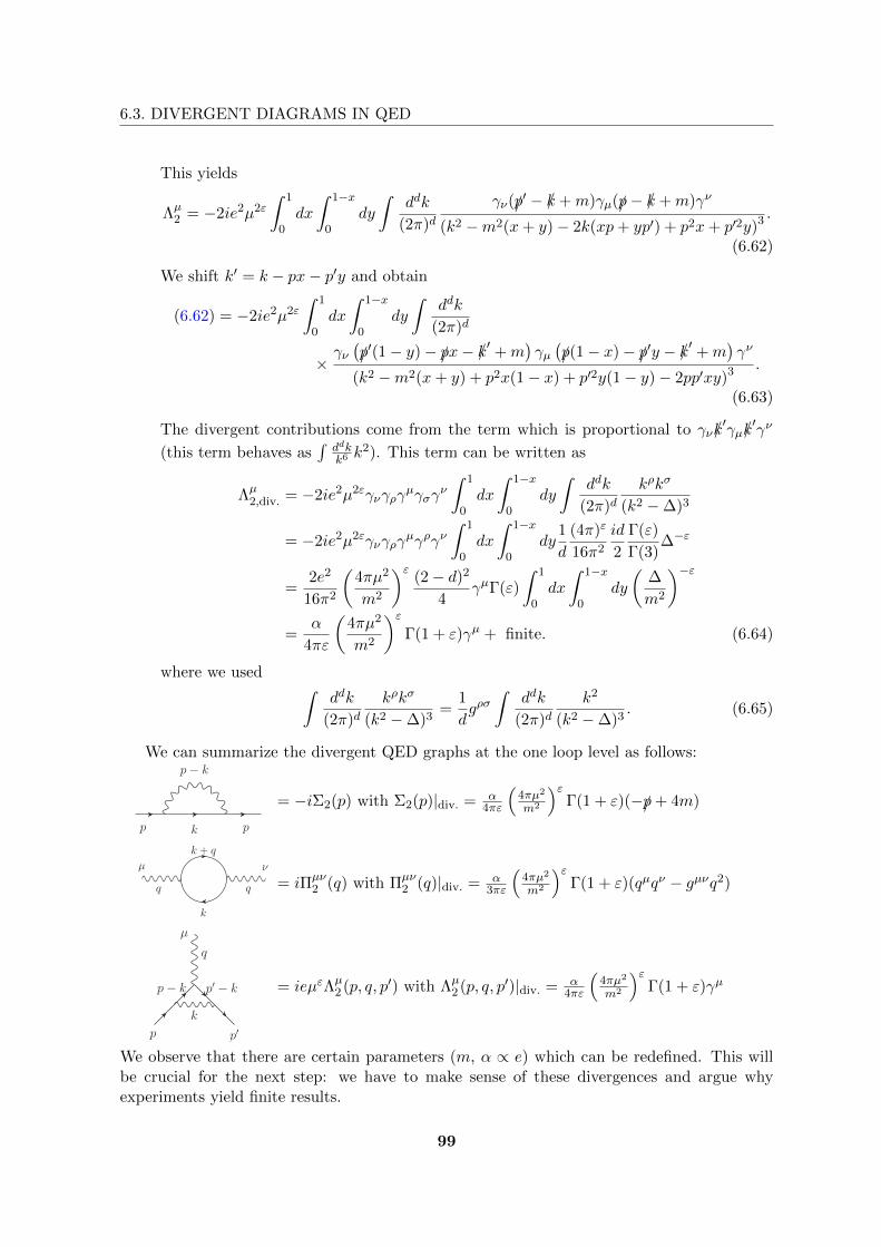
6.3. DIVERGENT DIAGRAMS IN QED
This yields
Λµ2 = −2ie2µ2ε
∫ 1
0dx
∫ 1−x
0dy
∫ddk
(2π)dγν(/p′ − /k +m)γµ(/p− /k +m)γν
(k2 −m2(x+ y)− 2k(xp+ yp′) + p2x+ p′2y)3 .
(6.62)
We shift k′ = k − px− p′y and obtain
(6.62) = −2ie2µ2ε
∫ 1
0dx
∫ 1−x
0dy
∫ddk
(2π)d
× γν(/p′(1− y)− /px− /k′ +m
)γµ(/p(1− x)− /p′y − /k′ +m
)γν
(k2 −m2(x+ y) + p2x(1− x) + p′2y(1− y)− 2pp′xy)3 .
(6.63)
The divergent contributions come from the term which is proportional to γν/k′γµ/k
′γν
(this term behaves as∫ddkk6k2). This term can be written as
Λµ2,div. = −2ie2µ2εγνγργµγσγ
ν
∫ 1
0dx
∫ 1−x
0dy
∫ddk
(2π)dkρkσ
(k2 −∆)3
= −2ie2µ2εγνγργµγργν
∫ 1
0dx
∫ 1−x
0dy
1
d
(4π)ε
16π2
id
2
Γ(ε)
Γ(3)∆−ε
=2e2
16π2
(4πµ2
m2
)ε(2− d)2
4γµΓ(ε)
∫ 1
0dx
∫ 1−x
0dy
(∆
m2
)−ε
=α
4πε
(4πµ2
m2
)εΓ(1 + ε)γµ + finite. (6.64)
where we used∫
ddk
(2π)dkρkσ
(k2 −∆)3=
1
dgρσ
∫ddk
(2π)dk2
(k2 −∆)3. (6.65)
We can summarize the divergent QED graphs at the one loop level as follows:
p k p
p− k
= −iΣ2(p) with Σ2(p)|div. = α4πε
(4πµ2
m2
)εΓ(1 + ε)(−/p+ 4m)
q q
k
k + q
µ ν
= iΠµν2 (q) with Πµν
2 (q)|div. = α3πε
(4πµ2
m2
)εΓ(1 + ε)(qµqν − gµνq2)
q
µ
k
p′ − kp− k
p p′
= ieµεΛµ2 (p, q, p′) with Λµ2 (p, q, p′)|div. = α4πε
(4πµ2
m2
)εΓ(1 + ε)γµ
We observe that there are certain parameters (m, α ∝ e) which can be redefined. This willbe crucial for the next step: we have to make sense of these divergences and argue whyexperiments yield finite results.
99
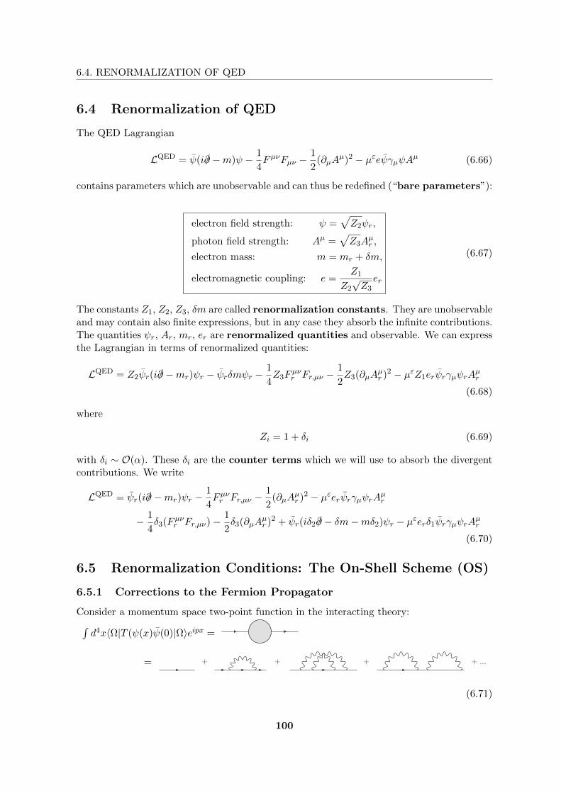
6.4. RENORMALIZATION OF QED
6.4 Renormalization of QED
The QED Lagrangian
LQED = ψ(i/∂ −m)ψ − 1
4FµνFµν −
1
2(∂µA
µ)2 − µεeψγµψAµ (6.66)
contains parameters which are unobservable and can thus be redefined (“bare parameters”):
electron field strength: ψ =√Z2ψr,
photon field strength: Aµ =√Z3A
µr ,
electron mass: m = mr + δm,
electromagnetic coupling: e =Z1
Z2
√Z3er
(6.67)
The constants Z1, Z2, Z3, δm are called renormalization constants. They are unobservableand may contain also finite expressions, but in any case they absorb the infinite contributions.The quantities ψr, Ar, mr, er are renormalized quantities and observable. We can expressthe Lagrangian in terms of renormalized quantities:
LQED = Z2ψr(i/∂ −mr)ψr − ψrδmψr −1
4Z3F
µνr Fr,µν −
1
2Z3(∂µA
µr )2 − µεZ1erψrγµψrA
µr
(6.68)
where
Zi = 1 + δi (6.69)
with δi ∼ O(α). These δi are the counter terms which we will use to absorb the divergentcontributions. We write
LQED = ψr(i/∂ −mr)ψr −1
4Fµνr Fr,µν −
1
2(∂µA
µr )2 − µεerψrγµψrAµr
− 1
4δ3(Fµνr Fr,µν)− 1
2δ3(∂µA
µr )2 + ψr(iδ2/∂ − δm−mδ2)ψr − µεerδ1ψrγµψrA
µr
(6.70)
6.5 Renormalization Conditions: The On-Shell Scheme (OS)
6.5.1 Corrections to the Fermion Propagator
Consider a momentum space two-point function in the interacting theory:
∫d4x〈Ω|T (ψ(x)ψ(0)|Ω〉eipx =
= + + + + ...
(6.71)
100

6.5. RENORMALIZATION CONDITIONS: THE ON-SHELL SCHEME (OS)
We define the one-particle-irreducible (1PI) diagrams as those diagrams that do not de-compose into subdiagrams by cutting a single line. For example:
(1PI diagram)
(not a 1PI diagram)
In the following, the set of all 1PI-diagrams will be denoted by a large circle with the label“1PI” as in the following calculation:
−iΣ(p) =
=
+ + + + ...
1PI
= −iΣ2(p) + (−iΣ4(p)) + ... (6.72)
We can thus write the Fourier transform of the two-point function (Eq. (6.71)) as
= + + + ...1PI 1PI 1PI
=i
/p−m+
i
/p−m(−iΣ(p))
i
/p−m+ ...
=i
/p−m+
i
/p−m
(Σ(p)
/p−m
)+
i
/p−m
(Σ(p)
/p−m
)2
+ ...
=i
/p−m− Σ(p)(6.73)
This propagator looks exactly like a tree level propagator but with a mass shifted by Σ(p).Since observations will never happen “outside of the vacuum”, we cannot neglect this shift(which is only due to vacuum corrections): whatever experiment we perform, the mass thatwe measure will always be the one which is corrected for loop diagrams. We will alwaysmeasure the renormalized mass mr which is defined by the on-shell requirement that
101

6.5. RENORMALIZATION CONDITIONS: THE ON-SHELL SCHEME (OS)
• mr is the position of the pole in the Fermion propagator:
[/p−m− Σ(p)]∣∣/p=mr
= 0. (6.74)
• If we do a Taylor expansion of Σ(p) in the vicinity of mr, the denominator of thecorrected propagator (6.73) reads
(/p−mr)
(1− dΣ
d/p
∣∣∣/p=mr
)+O
((/p−mr)
2). (6.75)
So, to lowest order in (/p −mr), we still get the physical mass mr as being the pole ofthe denumerator; but now we have an additional factor
(1− dΣ
d/p
∣∣∣∣/p=mr
)−1
' 1 +dΣ
d/p
∣∣∣∣/p=mr
(6.76)
multiplied with the propagator. It is the field strength renormalization factor Z2 fromEq. (6.67) with which the propagator of the free theory has to be multiplied in orderto account for loop corrections. So in our lowest order approximation, the additionalfactor (6.76) coincides with Z2 (see below).
These two conditions fix two of the four renormalization constants (namely δm and Z2). TheO(α)-term in
Σ = Σ2 + counter terms
= Σ2 − /pδ2 +mδ2 + δm (6.77)
yields the following identities which are also clear from the above considerations concerningEqs. (6.74) and (6.76) and which are true to lowest order (the explicit expressions can easilybe calculated from Eq. (6.48))1:
δmOS = −Σ2(/p = m)
= − α
4πε
(4πµ2
m2
)εΓ(1 + ε)m
∫ 1
0dx−2x+ 4 + 2ε(x− 1)
(1− x)2ε
= − α
4πε
(4πµ2
m2
)εΓ(1 + ε)
3− 2ε
1− 2εm (6.78)
δOS2 = +
dΣ2
d/p
∣∣∣/p=m
=α
4πε
(4πµ2
m2
)εΓ(1 + ε)
∫ 1
0dx
−(2− 2ε)x((1− x)− x(1− x) p
2
m2
)ε
− ε∫ 1
0dx−(2− 2ε)x/p+ (4− 2ε)m(
(1− x)− x(1− x) p2
m2
)ε+1
2/p
m(−x(1− x))
∣∣∣∣∣/p=m
.
(6.79)
1 To appreciate the role that Z2 plays in this context, see also Eq. (6.181): from very general considerationsone expects the fermion propagator with corrected mass to be rescaled by this factor.
102

6.5. RENORMALIZATION CONDITIONS: THE ON-SHELL SCHEME (OS)
The second term in (6.79) goes as ε for p2 6= m2 (i.e. /p 6= m). If, on the other hand, p2 = m2
(i.e. /p = m), then it is of order 1. Therefore we have an infrared divergence for on-shellelectrons which is part of δ2:
δOS2 =
α
4πε
(4πµ2
m2
)εΓ(1 + ε)
∫ 1
0dx−(2− 2ε)x
(1− x)2ε+ 2ε
∫ 1
0dx x
−2x+ 4 + 2ε(x− 1)
(1− x)1+2ε
=α
4πε
(4πµ2
m2
)εΓ(1 + ε)
− 1
1− 2ε− 2ε
1− εε(1− 2ε)
= − α
4πε
(4πµ2
m2
)εΓ(1 + ε)
3− 2ε
1− 2ε(6.80)
=1
mδmOS (6.81)
where
δOS2 = δOS,UV
2 + δOS,IR2 . (6.82)
with the pure UV-divergent contribution
δOS,UV2 = − α
4πε
(4πµ2
m2
)εΓ(1 + ε)
1
1− 2ε. (6.83)
The elegant fact that δOS2 = 1
mδmOS does not have a deep reason. In different theories, it
does not hold.
6.5.2 Corrections to the Photon Propagator
Next, we consider the photon two-point function:
= + + + ...µ ν µ ν µ ν µ ν
1PI 1PI1PI
=−igµνq2
+−igµρq2
[i(gρσq
2 − qρqσ)Π(q2)] −igσν
q2+ ... (6.84)
where Π(q) is defined analogous to the situation on page 97 concerning the photon vacuumpolarization at second order:
iΠµν(q2) = 1PIµ ν
= i(q2gµν − qµqν)Π(q2) (6.85)
iΠ(q2) = iΠ2(q2) + iΠ4(q2) + ...+ counterterms. (6.86)
We define
∆ρσ = gρσ − qρqσ
q2(6.87)
103

6.5. RENORMALIZATION CONDITIONS: THE ON-SHELL SCHEME (OS)
with the property
∆ρσ∆σ
ν = ∆ρν . (6.88)
We can then rewrite (6.84) as
(6.84) =−igµνq2
+−igµρq2
∆ρνΠ(q2) +
−igµρq2
∆ρσ∆σ
νΠ2(q2) + ...
=−igµνq2
+−igµρq2
[∆ρ
νΠ(q2) + ∆ρνΠ2(q2) + ∆ρ
νΠ3(q2)− ...]
=−igµνq2
+−igµρq2
∆ρν
1−Π(q2)+igµρ∆ρ
ν
q2
= −i 1
q2(1−Π(q2))
(gµν − qµqν
q2
)+−iq2
qµqν
q2
S-matrix=
−igµνq2(1−Π(q2))
(6.89)
where we summed a geometric series going from the second to the third line. The last stepis true if we recall that in any S-matrix calculation, the propagator will be connected to atleast one fermion line. According to the Ward identity, the terms which are proportional toqµ or qν vanish if we sum over all possibilities to connect the propagator to the fermion line.Therefore we can forget about these terms if our intention is to calculate S-matrix elements.
The O(α)-term in Π(q2) is
Π(q2) = Π2(q2)− δ3. (6.90)
The behaviour of the photon propagator for q2 → 0 determines the long-distance behaviourof QED and we should recover Coulomb’s law, i.e. the propagator should be
−igµνq2
for q2 → 0. (6.91)
We postulate that the long-distance behaviour of QED is unaffected by loop corrections, i.e.Π(0) = 0 such that (6.89) indeed gives Coulomb’s law for q2 → 0 (i.e. (6.91) is satisfied).Furthermore, according to Eq. (6.90),
δOS3 = Π2(0) = − α
3πε
(4πµ2
m2
)εΓ(1 + ε) + finite. (6.92)
6.5.3 Electron Vertex Corrections
The charge of the electron, er, should be defined from the long-distance behaviour of thevertex function (because all our experiments work at this scale).We consider the interaction of an on-shell electron with an electromagnetic field as sketchedin Fig. (6.2). We have the conditions
p2 = p′2 = m2, qµ = p′µ − pµ (6.93)
104

6.5. RENORMALIZATION CONDITIONS: THE ON-SHELL SCHEME (OS)
p p′
qµ
1PI
Figure 6.2: Interaction of on-shell electron with electromagnetic field (photon).
and the vertex factor
iM = −ieu(p′)Γµu(p)εµ (6.94)
where Γµ = γµ + O(α). The structure of Γµ = Γµ(p, q, p′) is determined by the followingconsiderations:
• We make the following ansatz:
Γµ = Aγµ +B(pµ + p′µ) + C(pµ − p′µ). (6.95)
This is the most general tensorial object of the assumed structure which depends onp and p′ only. The constants A, B, C could, in principle, depend on /p or /p′ but suchobjects are reduced to ordinary scalars in Eq. (6.94) by means of the Dirac equation(/pu(p) = mu(p) and u(p′)/p′ = u(p′)m). Therefore, A, B, C can only depend on q2 andm2 because there are no other non-trivial scalar objects available.
• Gauge invariance yields
qµuΓµu = 0 (6.96)
because of the Ward identity qµΓµ = 0 which we will prove later in a more generalcontext. Using the Dirac equation again, we find
0 = u(p′)qµΓµu(p) = Au(p′)(/p− /p′)u(p)
+B(p+ p′)(p− p′)u(p)u(p)
+ C(p− p′)2u(p′)u(p)
= Cq2u(p′)u(p) (6.97)
⇒ C = 0. (6.98)
• Without proof, we state that the Gordon identity holds:
u(p′)γµu(p) = u(p′)
[p′µ + pµ
2m+iσµνqν
2m
]u(p). (6.99)
105

6.5. RENORMALIZATION CONDITIONS: THE ON-SHELL SCHEME (OS)
If we put everything together, we obtain the final form of Γµ:
Γµ = γµF1(q2,m2) +iσµν
2mqνF2(q2,m2) (6.100)
which yields an expression purely in terms of bilinear covariants. The deeper reason for theabsence of pseudoscalar contributions is due to the fact that we only have axial polarizations.There is no scalar contribution because of the Gordon identity.The form factors F1,2(q2,m2) are given to order O(α0) by F1 = 1, F2 = 0.
Consider the interaction of the electron with the macroscopic (classical) electric and mag-netic fields:
1. electrostatic field (φ = const.):
Acl.µ (x) = (φ,0) (6.101)
Acl.µ (q) =
((2π)4δ(4)(q)φ,0
). (6.102)
This yields
iM = −ieF1(0,m2)u(p′)γ0u(p)(2π)4δ(4)(q)φ (6.103)
which defines the electrical charge being the constant of proportionality for the strengthof the interaction with an external electrical field. To be precise, eF1(0,m2) is theelectrical charge of the electron. The on-shell renormalization condition is F1(0,m2) = 1to all orders.
2. constant magnetic field:
Acl.µ (x) = (0,Acl.) (6.104)
Acl.µ (q) : is dominated by small values of q (6.105)
giving rise to the field
B = ∇ ∧Acl.(x) (6.106)
⇔ Bk(q) = −iεijkqiAj,k(q). (6.107)
This yields
iM = ieu(p′)
[γiF1 +
iσiνqν2m
F2
]u(p)(Acl.)i(q). (6.108)
We can expand this expression around q = 0:
iM ' ie2mχ′†[− i
2mεijkqjσk
[F1(0,m2) + F2(0,m2)
]]χ · (Acl.)i(q). (6.109)
where χ′ and χ are some two-component spinors describing the spin orientation of u(p′)and u(p) (this expansion can easily be carried out if one uses σiσj = δij + iεijkσk andif one neglects a term proportional to p′ + p which does not describe the interaction of
106

6.5. RENORMALIZATION CONDITIONS: THE ON-SHELL SCHEME (OS)
the magnetic moment with the external field but the spin-independent interaction fromelementary quantum mechanics).The expression (6.108) is nothing but the Fourier transform of the interaction of amagnetic moment in a magnetic field with
V = −µ ·B, (6.110)
µ =e
m[F1(0) + F2(0)]χ†
σ
2χ (6.111)
giving rise to the magnetic moment g of the electron via
µ = g( e
2m
)S. (6.112)
Therefore the gyromagnetic factor of the electron reads
ge = 2 [F1(0) + F2(0)] = 2 + 2F2(0) (6.113)
where the last equation is due to on-shell renormalization. We define the anomalousmagnetic moment
ae = F2(0) =ge − 2
2(6.114)
which is a well observable quantity.As we have seen, F1(0,m2) = 1 seems to be violated due to the O(α)-correctionto the vertex function which we denoted by Λµ2 . In order to save this condition,we have to subtract a counterterm which is proportional to the O(α0) vertex. TheO(α)-term in Γµ(p, q, p′) = Λµ2 (p, q, p′)|p2=p′2=m2 + δ1γ
µ can be found by calculatingΛµ2 (p, q, p′)|p2=p′2=m2, q2=0 (→ exercise). The result is
Λµ2 (p, q, p′)|p2=p′2=m2, q2=0 = γµ[α
4πε
(4πµ2
m2
)εΓ(1 + ε)
3− 2ε
1− 2ε
]+iσµν
2mqν
( α2π
)
(6.115)
where we note the separate UV- and IR-contributions again:
3− 2ε
1− 2ε=
1
1− 2ε
∣∣∣∣UV
+2− 2ε
1− 2ε
∣∣∣∣IR
. (6.116)
The on-shell condition reads
1 = F1(0,m2)
= 1 + δOS1 +
[α
4πε
(4πµ2
m2
)εΓ(1 + ε)
3− 2ε
1− 2ε
](6.117)
⇒ δOS1 = δOS
2 (6.118)
where we used the counterterm δ1 to save the condition F1(0,m2) = 1 also in thepresence of the O(α)-correction. The last equality is found by comparing Eqs. (6.117)and (6.80). Measurements of the anomalous magnetic moment of the electron whichis (according to (6.115)) given at order O(α) by ae = α
2π , yield an agreement with theO(α3)-theory which is better than 10 ppb. Very precise measurements can be done usingthe Josephson effect which does not receive any corrections of order O(α) or O(α2).
107

6.6. RENORMALIZATION CONDITIONS: MINIMAL SUBTRACTION
6.6 Renormalization Conditions: Minimal Subtraction
In the on-shell scheme, the renormalization constants were fixed by the large distance be-haviour of the interactions. Sometimes on-shell renormalization is not possible or does notmake sense. The first is the case in theories which consider degrees of freedom that are notobservable. For example, quarks in quantum chromodynamics cannot travel asymptotic dis-tances, so they don’t exist as free states and the on-shell scheme cannot be applied. Anotherproblem arises in processes in which only short distance interactions play a role. Then thewhole on-shell perturbation series can be very badly divergent. This is typically the case for
momentum transfers q2 m2 which result in large α2π log q2
m2 terms. If every α is accompaniedby a huge logarithmic term, then the idea to use α as a small parameter for the expansiondoes not make sense.Therefore we need some alternative renormalization scheme which is defined by using coun-terterms which contain UV-divergences (plus universal constants) only. The idea can thereforebe outlined as follows:
• Subtract UV-poles.
• Compensate the ad-hoc mass parameter µ by introduction of a (freely chosen) scale µRwhere the renormalization constants are defined.
• The universal constant is (4π)εe−εγ .
This yields the renormalization constants in the modified minimal subtraction (MS-)scheme. Using the results from section 6.5 and Γ(1 + ε) = e−εγ + O(ε2), we immediatelyfind:
δmMS = −Σ2(/p = m)|UV-div.
= − 3α
4πε
(4πµ2
µ2R
)εe−εγm (6.119)
δMS2 = +
dΣ
d/p
∣∣∣∣/p=m, UV-div.
= − α
4πε
(4πµ2
µ2R
)εe−εγ (6.120)
δMS3 = Π2(q2)|UV-div.
= − α
3πε
(4πµ2
µ2R
)εe−εγ (6.121)
δMS1 = −F1(0)|UV-div.
= − α
4πε
(4πµ2
µ2R
)εe−εγ = δMS
2 . (6.122)
The renormalized mass is mr = m− δm, so
m = mMSr + δmMS = mOS
r + δmOS (6.123)
108

6.7. RUNNING COUPLING CONSTANT
which implies
mMSr = mOS
r + δmOS − δmMS(µR)
= mOSr
(1− αOS
π
(1 +
3
4log
µ2R
m2
)+O(α2)
). (6.124)
6.6.1 Renormalized Coupling Constant
The renormalized coupling constant is
er =√Z3e. (6.125)
Because e has to be independent of which renormalization scheme we use, this yields thefollowing O(α)-equations (we use
√1 + δ ' 1− 1
2δ):
eMSr (µR)
(1− 1
2δMS
3
)= eOS
r
(1− 1
2δOS
3
)(6.126)
⇒ eMSr (µR) = eOS
r
(1− 1
2δOS
3 +1
2δMS
3
)+O(α2)
= eOSr
(1 +
α
6πlog
µ2R
m2+O(α2)
)(6.127)
⇒ αMS(µR) = αOS
(1 +
αOS
3πlog
µ2R
m2+O(α2)
)(6.128)
where we used α = e2
4π in the last step. We see that for µ2R > m2: αMS(µR) > αOS.
Furthermore, the constants mMS, αMS in the MS-scheme depend on the scale µR at which therenormalization is performed. At lowest order O(α0), we have mMS = mOS and αMS = αOS.
6.7 Running Coupling Constant
The renormalized coupling constant is
e =Z1
Z2
√Z3er =
1√Z3er. (6.129)
The parameter e appears as the bare coupling in the Lagrangian. It is divergent andindependent on the renormalization scheme. On the other hand, er is the physical couplingconstant (renormalized coupling). It is finite but it depends on which renormalization
scheme we use. Using Eq. (6.129) and α = e2
4π , we find (by means of expanding the squareroot and the fraction) the O(α)-identities
e =
(1− 1
2δ3
)er, (6.130)
α = (1− δ3)αr. (6.131)
According to Eq. (6.121), this yields in the MS-scheme
α =
(1 +
αMSr (µR)
3πε
(4πµ2
µ2R
)εe−εγ
)αMSr (µR). (6.132)
109

6.7. RUNNING COUPLING CONSTANT
Because e and α are independent of the renormalization scheme, they have to be independentof the scale µR, as well. Therefore
µ2R
d
dµ2R
α = 0 (6.133)
which, by means of Eq. (6.132), implies
µ2R
∂
∂µ2R
αMSr (µR) =
[αMSr (µR)
]2
3π+O(ε) +O
((αMS
r )3). (6.134)
The independence of the unrenormalized parameters or quantities q on the renormalizationscale µR imply
µ2R
d
dµ2R
q = 0. (6.135)
As a consequence, the renormalized parameters satisfy some renormalization group equa-tions which encode their dependence on the renormalization scale:
µ2R
∂
∂µ2R
qr = γq(αr) (6.136)
where γq is called the anomalous dimension of q.
The renormalization group equation for αMSr (µR) reads
µ2R
∂
∂µ2R
αMSr (µR) = β
(αMSr
)(6.137)
with the β-function of QED:
β(αMSr ) = −αMS
r
β0
αMSr
4π+ β1
(αMSr
4π
)2
+ ...
(6.138)
with β0 = −43 (cf. Eq. (6.134)). We want to solve the renormalization group equation (6.138)
to order O(β0):
µ2R
∂αr∂µ2
R
= −β0
4πα2r (6.139)
⇔ ∂αrα2r
= −β0
4π∂ logµ2
R (6.140)
⇔∫ αr(Q2)
αr(Q20)
dαrα2r
= −β0
4π
∫ logQ2
logQ20
d logµ2R (6.141)
⇔ − 1
αr(Q2)+
1
αr(Q20)
= −β0
4πlog
Q2
Q20
(6.142)
110

6.7. RUNNING COUPLING CONSTANT
αMSr
(1R2
)
R2
αMSr
(Q2
)
Q2
(large distance) (small distance)
αOSr ≃ 1
137
Figure 6.3: Behaviour of the physical coupling constant αr in the MS-scheme. There is avalue of Q2 where the graph on the right hand side is divergent, but this value is enormouslylarge (∼ 10278 GeV). However, in different theories (e.g. QCD) this Landau singularity willturn out to lie in the accessible region.
where Q20 denotes some scale where αr is known. This yields
1
αr(Q2)=
1
αr(Q20)
+β0
4πlog
Q2
Q20
(6.143)
which describes the evolution of the renormalized QED coupling as a function of Q2. Thisformula allows us to compare measurements at different scales. The relation to the on-shellcoupling is
αMSr (m2
e) = αOSr '
1
137(6.144)
at the one loop level. We use Q2 ' 1R2 and obtain a behaviour as in Fig. (6.3).
We interpret this distance dependent behaviour of the coupling as sketched in Fig. (6.4)(δ3 corresponds to the vacuum polarization). The positive charge in the center is screened atlarge distances by virtual e+e− pairs, which cause a dilution of the charge at large distancessuch that the positive charge observed at large distances appears smaller than it actually is.
The asymptotic behaviour for Q2 →∞ is as follows:If β0 < 0, then there exists a Q2 = Λ2
QED > Q20 with
1
αr(Q20)
+β0
4πlog
Q2
Q20
= 0. (6.145)
By rearranging this equation, it turns out that this Landau singularity is at
ΛQED = mee− 2π
β0αOSr ' 1.2 · 10278 GeV (6.146)
which is far beyond the Planck scale or any other accessible scale.
The general behaviour of the Landau singularity is as follows:
111

6.8. WARD-TAKAHASHI IDENTITY
e−e+
e+e−
Figure 6.4: Due to loop corrections in the photon propagator, an electric charge createsparticle-antiparticle clouds which effectively screen the charge. This is the physical interpre-tation of the dependence of the observed charge on distances. At very low distances, theoberved charge gets bigger because screening effects become less important.
• If β(α) < 0: Landau singularity in the UV region. The typical example is QED.
• If β(α) = 0: The theory is exactly scale-invariant (αr(Q2) =const.)
• If β(α) > 0: The Landau singularity is in the IR region. This means that the theory isasymptotically free in the UV region, i.e. αr(Q
2 → ∞) → 0. The typical examplefor this case is QCD.
6.8 Ward-Takahashi Identity
Recall that gauge-invariance for Feynman amplitudes with external photons can be realizedby demanding that
kµMµ = 0 (6.147)
where the momentum k belongs to an on-shell or off-shell external photon whereas all otherparticles are on-shell. From this it follows immediately that for an amplitude M = εµ(k)Mµ
of some QED process involving an external photon with momentum k, it holds kµMµ = 0.
In the following we will prove that this identity is true for any QED process with amplitudeM in the following more general sense: Given a certain QED process with external photonγ(k), there are many possible diagrams which contribute to the amplitude of this process. Ifwe take any of these contributing diagrams, then the above identity (6.147) holds true if wesum over all possibilities to attach the external photon to this specific diagram. Because thisis true for any contributing diagram, it is in particular true for the complete process. In orderto prove this statement, consider the following situations (possibilities to attach the externalphoton somewhere to a given diagram):
• The amplitude M0 denotes the process with one incoming and one outgoing electron lineand n external on-shell photons qn. This is the situation before we attach the externalphoton γ(k). A diagram in M0 is, for example, given by
112
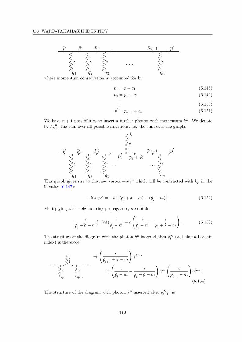
6.8. WARD-TAKAHASHI IDENTITY
. . .
q1 q2 q3 qn
p p1 p2 pn−1 p′
where momentum conservation is accounted for by
p1 = p+ q1 (6.148)
p2 = p1 + q2 (6.149)
... (6.150)
p′ = pn−1 + qn (6.151)
We have n + 1 possibilities to insert a further photon with momentum kµ. We denoteby Mµ
0,k the sum over all possible insertions, i.e. the sum over the graphs
q1 q2 q3 qn
p p1 p2 pn−1 p′
pi pi + k
k
... ...
This graph gives rise to the new vertex −ieγµ which will be contracted with kµ in theidentity (6.147):
−iekµγµ = −ie[(/pi + /k −m)− (/pi −m)
]. (6.152)
Multiplying with neighbouring propagators, we obtain
i
/pi + /k −m(−ie/k)i
/pi −m= e
(i
/pi −m− i
/pi + /k −m
). (6.153)
The structure of the diagram with the photon kµ inserted after qλii (λi being a Lorentzindex) is therefore
qi qi+1
k →(
i
/pi+1+ /k −m
)γλi+1
×(
i
/pi −m− i
/pi + /k −m
)γλi
(i
/pi−1−m
)γλi−1 .
(6.154)
The structure of the diagram with photon kµ inserted after qλi−1
i−1 is
113

6.8. WARD-TAKAHASHI IDENTITY
qi−1 qi qi+1
k→(
i
/pi+1+ /k −m
)γλi+1
(i
/pi + /k −m
)
× γλi(
i
/pi−1−m −
i
/pi−1+ /k −m
)γλi−1 . (6.155)
We see that if we sum over all possibilities to insert the photon, the terms cancel eachother pairwise. So the sum over all possible insertions of kµ will contain only contribu-tions from the very first and very last term. Using q = p′ + k, we have
p
q
= e ...
p
q − k
p + k
q
−kµ·Σ
( )...
where the dashed lines indicate the possible insertions of the photon. So
kµMµ0,k(p, q1, ..., qn, q) = e (M0(p, q1, q2, ..., qn, q − k)−M0(p+ k, q1, q2, ..., qn, q)) .
(6.156)
• Next, we consider the amplitude M1 with a closed fermion loop and n external photonsqn. A typical diagram in M1 is, for instance, given by
q2
q1
pnp3
q3
p2 p1
We have n possibilities to insert a further photon kµ:
pi
p1k
qi+1q1
q2
pi + k
114
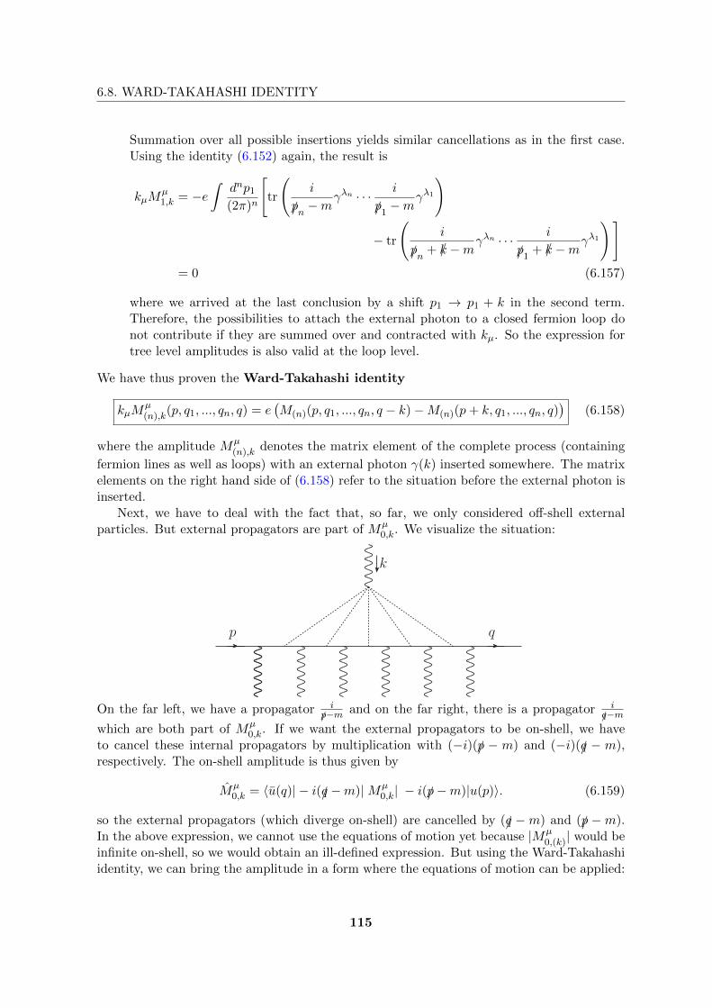
6.8. WARD-TAKAHASHI IDENTITY
Summation over all possible insertions yields similar cancellations as in the first case.Using the identity (6.152) again, the result is
kµMµ1,k = −e
∫dnp1
(2π)n
[tr
(i
/pn −mγλn · · · i
/p1−mγλ1
)
− tr
(i
/pn + /k −mγλn · · · i
/p1+ /k −mγλ1
)]
= 0 (6.157)
where we arrived at the last conclusion by a shift p1 → p1 + k in the second term.Therefore, the possibilities to attach the external photon to a closed fermion loop donot contribute if they are summed over and contracted with kµ. So the expression fortree level amplitudes is also valid at the loop level.
We have thus proven the Ward-Takahashi identity
kµMµ(n),k(p, q1, ..., qn, q) = e
(M(n)(p, q1, ..., qn, q − k)−M(n)(p+ k, q1, ..., qn, q)
)(6.158)
where the amplitude Mµ(n),k denotes the matrix element of the complete process (containing
fermion lines as well as loops) with an external photon γ(k) inserted somewhere. The matrixelements on the right hand side of (6.158) refer to the situation before the external photon isinserted.
Next, we have to deal with the fact that, so far, we only considered off-shell externalparticles. But external propagators are part of Mµ
0,k. We visualize the situation:
k
p q
On the far left, we have a propagator i/p−m and on the far right, there is a propagator i
/q−mwhich are both part of Mµ
0,k. If we want the external propagators to be on-shell, we haveto cancel these internal propagators by multiplication with (−i)(/p − m) and (−i)(/q − m),respectively. The on-shell amplitude is thus given by
Mµ0,k = 〈u(q)| − i(/q −m)|Mµ
0,k| − i(/p−m)|u(p)〉. (6.159)
so the external propagators (which diverge on-shell) are cancelled by (/q −m) and (/p −m).In the above expression, we cannot use the equations of motion yet because |Mµ
0,(k)| would beinfinite on-shell, so we would obtain an ill-defined expression. But using the Ward-Takahashiidentity, we can bring the amplitude in a form where the equations of motion can be applied:
115

6.8. WARD-TAKAHASHI IDENTITY
...
p q − kkµM
µ0,(k) = e〈u(q)| − i(/q −m)
(
...
p + k
−q
)(−i)(/p−m)|u(p)〉
= 0. (6.160)
where we used
〈u(q)|(/q −m) = 0 or (/p−m)|u(p)〉 = 0. (6.161)
This completes our diagrammatic derivation of kµMµ = 0 for on-shell amplitudes.
The Ward-Takahashi identity (WTI) answers the question of gauge invariance of on-shellamplitudes (at all loop orders). Whenever we state a set of renormalization constants, it hasto be in accordance with the WTI, so the WTI serves as a condition on any renormalizationscheme: the fulfilment of the WTI under renormalization ensures gauge invariance of theamplitudes of the renormalized theory. So checking the WTIs is always a good method toverify that one did not break any gauge symmetry in the renormalization procedure.
A nice example is already given in Eq. (6.157): We shifted the momentum during thecalculation. This shift is nothing but a Poincare transformation. We can only do this becauseour theory and the dimensional regularization procedure are Poincare-invariant.
The simplest WTI (with n = 0) is
( p + k
pk
)kµ µ = e
(−
p + k
p + kp
p
)
where we have a complete vertex −ie(γµ + Λµ) on the left hand side (as usual, Λµ describesthe corrections to the uncorrected vertex −ieγµ), and electron two-point functions (exactpropagators) S(p) = i
/p−m−Σ(p) and S(p+ k) on the right hand side. We need to consider the
amplitude
S(p+ k) [−ie(γµ + Λµ)(p, k, p+ k)]S(p). (6.162)
The WTI reads then
S(p+ k) [−iekµ(γµ + Λµ)(p, k, p+ k)]S(p) = e(S(p)− S(p+ k)) (6.163)
⇔ −iekµ(γµ + Λµ)(p, k, p+ k) = e(S−1(p+ k)− S−1(p)
)
= −ie(/k − Σ(p+ k) + Σ(p)) (6.164)
⇔ kµΛµ(p, k, p+ k) = Σ(p)− Σ(p+ k) (6.165)
(“WTI of the QED vertex function”). We note the following facts:
116

6.9. SPECTRAL REPRESENTATION
• The WTI is automatically fulfilled for diagrammatic contributions to Λµ and Σ.
• The mass shift δm drops out from Σ(p)− Σ(p+ k).
• We have the following relation for the renormalization constants which follows immedi-ately from (6.165)
/kZ1 = Z2(−/p+ (/p+ /k)) (6.166)
⇒ Z1 = Z2 (6.167)
which now holds true at all orders in perturbation theory.
6.9 Spectral Representation
Recall that for the free scalar Klein-Gordon field, we derived the scalar propagator in positionspace,
〈0|T(φ(x)φ(x′)
)|0〉 = i∆F (x− x′). (6.168)
The interpretation of this object was simple: it describes the amplitude for a particle to gofrom x′ to x. Consider the two-point correlation function in the interacting scalar theory:
〈Ω|T(φ(x)φ(x′)
)|Ω〉. (6.169)
We will use this simplest of all objects in the theory in order to develop tools for a frameworkwhich goes beyond perturbation theory.In the interacting theory, we have the following objects:
• the Hamilton operator H,
• the momentum operator P ,
• the “particle” states, in particular the state |λ0〉 which describes a particle at rest:
H|λ0〉 = mλ|λ0〉, P |λ0〉 = 0. (6.170)
A particle state with momentum p is denoted by |λp〉 and it satisfies
H|λp〉 =√p2 +m2|λp〉, P |λp〉 = p|λp〉. (6.171)
So we use the eigenstates of the full Hamiltonian H as the spectrum for our theory(before, we used the eigenstates of the free Hamiltonian!).
The particle states can be one-particle states or bound states of several particles. We get thespectrum which is shown in Fig. (6.5).
The completeness relation of the Hilbert space reads
1 = |Ω〉〈Ω|+∑
λ
∫d3p
(2π)3
1
2Eλ(p)|λp〉〈λp| (6.172)
117

6.9. SPECTRAL REPRESENTATION
where the sum runs over all “particle” states λ0. With this identity, we can break up thetwo-point function in the following way (for x0 > x′0):
〈Ω|φ(x)φ(x′)|Ω〉 = 〈Ω|φ(x)|Ω〉〈Ω|φ(x′)|Ω〉︸ ︷︷ ︸=0
+∑
λ
∫d3p
(2π)3
1
2Eλ(p)〈Ω|φ(x)|λp〉〈λp|φ(x′)|Ω〉.
(6.173)
We can calculate this expression if we note that
• Lorentz invariance yields
〈Ω|φ(x)|λp〉 = 〈Ω|eiP ·xφ(0)e−iP ·x|λp〉= 〈Ω|φ(0)|λp〉e−ip·x
∣∣p0=Eλ(p)
= 〈Ω|U−1Uφ(0)U−1U |λp〉e−ip·x
= 〈Ω|φ(0)|λ0〉e−ip·x∣∣p0=Eλ(p)
(6.174)
where we applied a Lorentz transformation with momentum p which acts through thematrix U (recall that Uφ(0)U−1 = φ(0) due to Lorentz invariance).
• Furthermore we use
∫d3p
(2π)3
e−ipx
2p0= −i
∫
C+
d4p
(2π)4
e−ipx
p2 −m2λ
. (6.175)
Summation over both time-orderings yields
〈Ω|T(φ(x)φ(x′)
)|Ω〉 =
∑
λ
∫d4p
(2π)4
i
p2 −m2λ + iε
e−ip(x−x′) · |〈Ω|φ(0)|λ0〉|2. (6.176)
Figure 6.5: Eigenvalues of H and P . Note that the two particle bound state has a rest energywhich is below the energy of two free particles 2m2.
118

6.9. SPECTRAL REPRESENTATION
The object |〈Ω|φ(0)|λ0〉|2 is called spectral function. In the free theory it is just a δ-functionwhich is non-vanishing on single particle states. We can rewrite this result in terms of theKallen-Lehmann spectral density function
ρ(M2) =∑
λ
(2π)δ(M2 −m2λ)|〈Ω|φ(0)|λ0〉|2 (6.177)
where we interpret the amplitude 〈Ω|φ(0)|λ0〉 as the probability amplitude for the transition|Ω〉 → |λ0〉 to happen through φ(0), i.e. for a particle being created out of the vacuum throughthe action of the full φ(0) at the origin.Accordingly, Eq. (6.176) reads
〈Ω|T(φ(x)φ(x′)
)|Ω〉 =
∫ ∞
0
dM2
2πρ(M2)i∆F (x− x′,M2) (6.178)
where the integral runs over the whole spectrum of our theory. In the case of a free theory,the spectral function is just a δ-function with pole at m2. The form of the spectrum of atypical interacting theory is sketched in Fig. (6.6).
In the OS-scheme, the contribution of single-particle states is
ρ(M2)∣∣1p
= 2πδ(M2 −m2r)Z (6.179)
where mr is the renormalized mass and Z is the field strength renormalization. Consider theFourier representation of the two point function:
∫d4x eipx〈Ω|T (φ(x)φ(0)) |Ω〉 =
∫ ∞
0
dM2
2πρ(M2)
i
p2 −M2 + iε
=iZ
p2 −m2r + iε︸ ︷︷ ︸
single-particle states
+
∫ ∞
∼(2m)2
dM2
2πρ(M2)
i
p2 −M2 + iε︸ ︷︷ ︸
multi-particle/bound states
.
(6.180)
1 particlestates
boundstates
2 particlestates
m2 (2m)2
continuum
ρ(M 2)
M 2
Figure 6.6: Spectrum of a typical interacting theory.
119
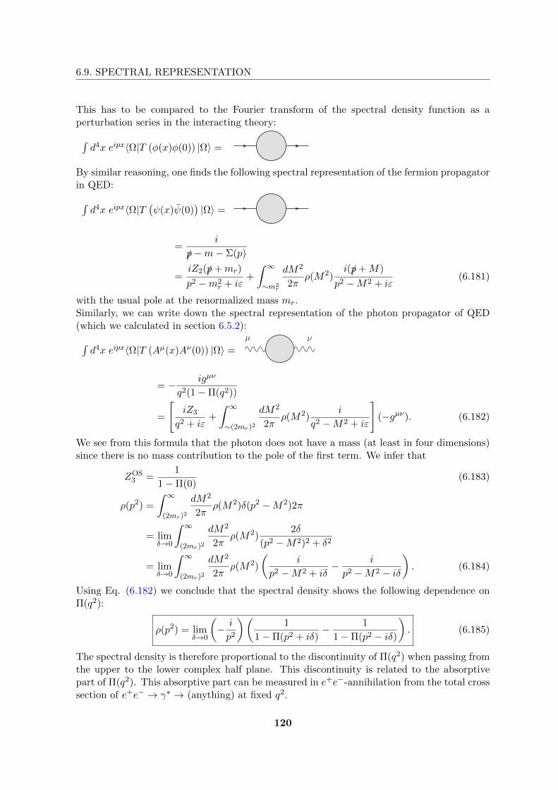
6.9. SPECTRAL REPRESENTATION
This has to be compared to the Fourier transform of the spectral density function as aperturbation series in the interacting theory:
∫d4x eipx〈Ω|T (φ(x)φ(0)) |Ω〉 =
By similar reasoning, one finds the following spectral representation of the fermion propagatorin QED:
∫d4x eipx〈Ω|T
(ψ(x)ψ(0)
)|Ω〉 =
=i
/p−m− Σ(p)
=iZ2(/p+mr)
p2 −m2r + iε
+
∫ ∞
∼m2r
dM2
2πρ(M2)
i(/p+M)
p2 −M2 + iε(6.181)
with the usual pole at the renormalized mass mr.Similarly, we can write down the spectral representation of the photon propagator of QED(which we calculated in section 6.5.2):
∫d4x eipx〈Ω|T (Aµ(x)Aν(0)) |Ω〉 =
µ ν
= − igµν
q2(1−Π(q2))
=
[iZ3
q2 + iε+
∫ ∞
∼(2mr)2
dM2
2πρ(M2)
i
q2 −M2 + iε
](−gµν). (6.182)
We see from this formula that the photon does not have a mass (at least in four dimensions)since there is no mass contribution to the pole of the first term. We infer that
ZOS3 =
1
1−Π(0)(6.183)
ρ(p2) =
∫ ∞
(2mr)2
dM2
2πρ(M2)δ(p2 −M2)2π
= limδ→0
∫ ∞
(2mr)2
dM2
2πρ(M2)
2δ
(p2 −M2)2 + δ2
= limδ→0
∫ ∞
(2mr)2
dM2
2πρ(M2)
(i
p2 −M2 + iδ− i
p2 −M2 − iδ
). (6.184)
Using Eq. (6.182) we conclude that the spectral density shows the following dependence onΠ(q2):
ρ(p2) = limδ→0
(− i
p2
)(1
1−Π(p2 + iδ)− 1
1−Π(p2 − iδ)
). (6.185)
The spectral density is therefore proportional to the discontinuity of Π(q2) when passing fromthe upper to the lower complex half plane. This discontinuity is related to the absorptivepart of Π(q2). This absorptive part can be measured in e+e−-annihilation from the total crosssection of e+e− → γ∗ → (anything) at fixed q2.
120

6.10. LEHMANN-SYMANZIK-ZIMMERMANN (LSZ) REDUCTION FORMULA
6.10 Lehmann-Symanzik-Zimmermann (LSZ) Reduction For-mula
We have defined S-matrix elements in the case that we have an overlap of |Ω〉 and |0〉. Butactually one can define them with much weaker conditions.The behaviour of the two-point correlation function in the on-shell limit (p2 → m2) in a scalartheory is
∫d4x eipx〈Ω|T (φ(x)φ(0)) |Ω〉 p
2→m2
−→ iZ
p2 −m2r + iε
(6.186)
which diverges. The fact that we have a pole in the correlation function means that we havea one-particle state with on-shell mass mr in our theory.More generally, consider the Fourier transform in one coordinate of the N -point function:
∫d4x eipx〈Ω|T (φ(x)φ(z1) · · · ) |Ω〉. (6.187)
In order to identify contributions which can potentially lead to poles in p0 with on-shellparticles, we split the temporal component of the integral:
∫dx0 =
∫ ∞
T+
dx0 +
∫ T+
T−dx0 +
∫ T−
−∞dx0 (6.188)
where T+ > max(z0i ), T− < min(z0
i ). The second of these integrals will certainly be analyticand it will not lead to singularities. So we have to consider the first and the third part indetail:
• The first contribution to (6.187) is (after noticing that φ(x) can be taken in front of thetime-ordering, x0 being larger than all the z0
i and inserting a complete set of states)
∫ ∞
T+
dx0
∫d3x eip
0x0e−ip·x∑
λ
∫d3q
(2π)3
〈Ω|φ(x)|λq〉〈λq|T (φ(z1) · · · ) |Ω〉2Eλ(q)
. (6.189)
We can use that
〈Ω|φ(x)|λq〉 = 〈Ω|φ(0)|λ0〉e−iq·x∣∣q0=Eλ(q)
(6.190)
and find
(6.189) =∑
λ
∫ ∞
T+
dx0
∫d3q
(2π)3
1
2Eλ(q)eip
0x0e−iq0x0〈Ω|φ(0)|λ0〉
× (2π)3δ(3)(p− q)〈λq|T (φ(z1) · · · ) |Ω〉
= limε→0
∑
λ
1
2Eλ(p)
iei(p0−Eλ(p)+iε)
p0 − Eλ(p) + iε〈Ω|φ(0)|λ0〉〈λp|T (φ(z1) · · · ) |Ω〉
p0=Ep−→ i
p2 −m2 + iε
√Z〈p|T (φ(z1) · · · ) |Ω〉 (6.191)
121
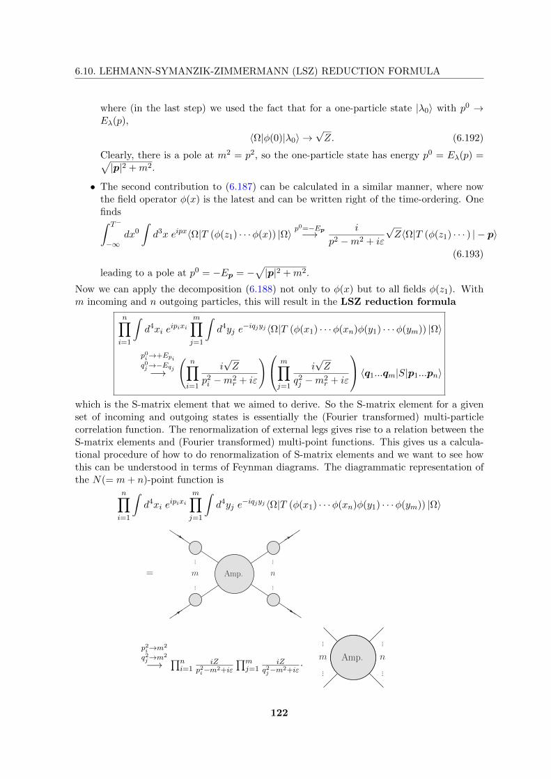
6.10. LEHMANN-SYMANZIK-ZIMMERMANN (LSZ) REDUCTION FORMULA
where (in the last step) we used the fact that for a one-particle state |λ0〉 with p0 →Eλ(p),
〈Ω|φ(0)|λ0〉 →√Z. (6.192)
Clearly, there is a pole at m2 = p2, so the one-particle state has energy p0 = Eλ(p) =√|p|2 +m2.
• The second contribution to (6.187) can be calculated in a similar manner, where nowthe field operator φ(x) is the latest and can be written right of the time-ordering. Onefinds∫ T−
−∞dx0
∫d3x eipx〈Ω|T (φ(z1) · · ·φ(x)) |Ω〉 p
0=−Ep−→ i
p2 −m2 + iε
√Z〈Ω|T (φ(z1) · · · ) | − p〉
(6.193)
leading to a pole at p0 = −Ep = −√|p|2 +m2.
Now we can apply the decomposition (6.188) not only to φ(x) but to all fields φ(z1). Withm incoming and n outgoing particles, this will result in the LSZ reduction formula
n∏
i=1
∫d4xi e
ipixi
m∏
j=1
∫d4yj e
−iqjyj 〈Ω|T (φ(x1) · · ·φ(xn)φ(y1) · · ·φ(ym)) |Ω〉
p0i→+Epiq0j→−Eqj−→
(n∏
i=1
i√Z
p2i −m2
r + iε
)
m∏
j=1
i√Z
q2j −m2
r + iε
〈q1...qm|S|p1...pn〉
which is the S-matrix element that we aimed to derive. So the S-matrix element for a givenset of incoming and outgoing states is essentially the (Fourier transformed) multi-particlecorrelation function. The renormalization of external legs gives rise to a relation between theS-matrix elements and (Fourier transformed) multi-point functions. This gives us a calcula-tional procedure of how to do renormalization of S-matrix elements and we want to see howthis can be understood in terms of Feynman diagrams. The diagrammatic representation ofthe N(= m+ n)-point function is
n∏
i=1
∫d4xi e
ipixi
m∏
j=1
∫d4yj e
−iqjyj 〈Ω|T (φ(x1) · · ·φ(xn)φ(y1) · · ·φ(ym)) |Ω〉
...
m
...
...
n
...
= Amp.
p2i→m2
q2j→m2
−→ ∏ni=1
iZp2i−m2+iε
∏mj=1
iZq2j−m2+iε
·
...
m
...
...
n
...
Amp.
122

6.11. INFRARED SINGULARITIES
where the inner part
...
m
...
...
n
...
Amp.
stands for the amputated N -point function (i.e. without any corrections on external legs).Finally, the S-matrix element in terms of Feynman diagrams reads
〈q1...qn|S|p1...pm〉 = (√Z)n+m
...
m
...
...
n
...
Amp.
For theories with different types of particles, the S-matrix element is the amputated N -pointfunction multiplied with factors
√Zi for each external particle.
6.11 Infrared Singularities
We consider the behaviour of Feynman amplitudes for photon momenta k → 0 (“soft infraredsingularities”).As an example, consider the photon-electron-vertex with the conditions p2 = p′2 = m2, q2 6= 0(as in Eq. (6.60)):
q
µ
k
p′ − kp− k
p p′
= (−ieµε)3∫
ddk(2π)d
γνi
/p′ − /k −m︸ ︷︷ ︸→/p′−m
γµi
/p− /k −m︸ ︷︷ ︸→/p−m
γν −ik2
= −ieµεΛµ2 (p, q, p′) (6.194)
where the limits are meant as k → 0 and
Λµ2 (p, q, p′) = −2ie2µ2ε
∫ 1
0dx
∫ 1−x
0dy
ddk′
(2π)d
× γν[/p′(1− y)− /px+ /k
′+m
]γµ[/p(1− x)− /p′y − /k′ +m
]γν
[k′2 −m2(x+ y) + p2x(1− x) + p′2y(1− y)− 2pp′xy]3. (6.195)
We make the following observations to extract the infrared divergences from this integral:
• We have already computed the term which is proportional to
∫ddk
(2π)dkµkν
[k2 −∆]3(6.196)
which gave rise to the UV-pole.
123
6.11. INFRARED SINGULARITIES
• We have also seen the on-shell limit
∆ = m2(x+ y)−m2x(1− x)−m2y(1− y) + (2m2 − q2)xy
= m2(x+ y)2 − q2xy > 0 for q2 < 0. (6.197)
We observe that ∆ = 0 for x = y = 0, which corresponds to the soft limit.
• We use∫
ddk
(2π)d1
[k2 −∆]3=i(4π)ε
16π2
Γ(1 + ε)
Γ(3)∆−1−ε. (6.198)
• We note that ∆→ 0 as x, y → 0. Introducing z = 1− x− y, we can write
∫ 1
0dx
∫ 1−x
0dy =
∫ 1
0dz
∫ 1−z
0dy (6.199)
and neglect the x- and y-terms in the numerator.
We thus find
Λµ2 (p, q, p′)∣∣on-shell, IR-div.
= −e2 (4πµ2)ε
16π2Γ(1 + ε)γν(/p
′ +m)γµ(/p+m)γν
∫ 1
0dz
∫ 1−z
0dy
×[m2(1− z)2 − q2(1− y − z)y
]−1−ε.
(6.200)
We can compute such an expression easily if we put it between on-shell states:
〈u(p′)|γν(/p′ +m)γµ(/p+m)γν |u(p)〉 = 4pp′〈u(p′)|γµ|u(p)〉
= (4m2 − 2q2)〈u(p′)|γµ|u(p)〉. (6.201)
We are finally in the position to compute the Feynman integral using z = 1 − b and y =(1− z)a = ab:
∫ 1
0b db
∫ 1
0da[m2b2 − q2a(1− a)b2
]−1−ε
=
∫ 1
0db b−1−2ε
(1
m2
)ε ∫ 1
0da
1[1− q2
m2a(1− a)]1+ε
= − 1
2ε
(1
m2
)1+ε
·
1 for q2 = 0
1√x(x+4)
log2+x+
√x(x+4)
2+x−√x(x+4)
for q2 6= 0(6.202)
with x = − q2
m2 . We introduce ξ =√x+4−
√x√
x+4+√x
which is the relative rapidity between the
incoming and outgoing electron. With this definition, we find x = (1−ξ)2ξ . This leads to
Λµ2 (p, q, p′)∣∣on-shell, IR-div.
= γµ[α
4π
(4πµ2
m2
)εΓ(1 + ε)
]· 2
ε
1 for q2 = 0
− (1+ξ2)(1−ξ2)
log ξ for q2 6= 0
(6.203)
124

6.11. INFRARED SINGULARITIES
This implies that the QED vertex function contains an IR-divergence for all q2. The coefficientof this singularity is not universal (as in the UV case) but depends on kinematic expressions.So we cannot simply get rid of it by considering a specific scale.
In the following we want to show how IR-divergences coming from different corrections tothe process e+e− → µ+µ− cancel. In the end we will cite a theorem which states that thisis the case in general. But first, we want to demonstate one of these cancellations. For thispurpose, consider the following two corrections, the first of which is a virtual correction andthe second of which is a real correction to the final state due to the unobservability of anadditional external photon:
• First, consider the following correction to the basic e+e− → µ+µ− process:
e−
e+ µ+(p)
µ−(p′)
which is IR-divergent at O(α3). Indeed, one finds for this process
dσ
dΩ
∣∣∣∣α3
=dσ
dΩ
∣∣∣∣Born,α2
· α
π︸︷︷︸2<(M,M∗0 )
1
ε
(−1 + ξ2
1− ξ2log ξ
︸ ︷︷ ︸from Λ2
− 1︸︷︷︸from δ1
)(µ2
m2
)ε(6.204)
where the m2 in the last factor is replaced by q2 for q2 m2. For q2 → 0, we have
ξ =
√s−√s− 4m2
√s+√s+ 4m2
. (6.205)
• Next, consider the process
e−
e+ µ+(p)
µ−(p′)
γ(k)
with an unresolved photon (Eγ → 0). This is experimentally indistinguishable frome+e− → µ+µ− because the soft photon remains unseen. Writing the basic process as
e−
e+ µ+(p)
µ−(p′)
= iu(p′)M0(p′, p)v(p)
125

6.11. INFRARED SINGULARITIES
the contribution of such a soft photon is
iM = −ieu(p′)
[M0(p′, p− k)
i(−/p+ /k +m)
(p+ k)2 −m2γµε∗µ(k)
+ γµε∗µ(k)i(/p′ + /k +m)
(p′ + k)2 −m2M0(p′ + k, p)
]v(p). (6.206)
If |k| |p|, |p′|, we have
M0(p′, p− k) 'M0(p′ + k, p) 'M0(p′, p) (6.207)
and (using the Clifford algebra and the Dirac equation)
(−/p+m)γµε∗µv(p) =[−2pµε∗µ + γµε∗µ(/p+m)
]v(p)
= −2pµε∗µv(p), (6.208)
u(p′)γµε∗µ(/p′ +m) = u(p′)2p′µε∗µ. (6.209)
Therefore Eq. (6.206) simplifies to
iM = u(p′)M0(p′, p)v(p)
[e
(p′ · ε∗p′ · k −
p · ε∗p · k
)](6.210)
where the momenta appearing in this expression belong to the external fermions. Thesingularity which appears for the photon becoming soft is thus universal and correspondsto an external propagator becoming on-shell. The last factor in Eq. (6.210) is nothingbut the eikonal approximation to the matrix element.The contribution to the cross section (dimensional regularisation) amounts to
dσ(e+e− → µ+µ−γ) = dσ(e+e− → µ+µ−) · e2
∫dd−1k
(2π)3
1
2k
∑
λ
∣∣∣∣p′ · ε∗λp′ · k −
p · ε∗λp · k
∣∣∣∣2
.
(6.211)
We want to carry out the calculation of the eikonal matrix element
∑
λ
|...|2 = 2p · p′
(k · p′)(k · p) −m2
(k · p′)2− m2
(k · p)2(6.212)
where we used the identity∑
λ εµλεν∗λ = −gµν . We can choose a particular frame of
reference. In the center of mass-frame, we have
s = (2E)2, pµ =
E00p
, p′µ =
E00−p
, kµ = k
1sin θ nd−2
cos θ
. (6.213)
and thus find for the matrix element
∑
λ
|...|2 =4E2 − 2m2
k2(E − p cos θ)(E + p cos θ)− m2
k2
(1
(E − p cos θ)2+
1
(E + p cos θ)2
).
(6.214)
126
6.11. INFRARED SINGULARITIES
The IR-divergence arises due to the integral over the photon energy:
∫ Eγ,max
0
kd−3
k2dk =
∫ Eγ,max
0k−1−2εdk
= − 1
2ε(E2
γ,max)−ε (6.215)
where Eγ,max is the maximum photon energy allowed to escape detection. We havesingled out the divergence and only have to find the coefficient of this divergence whichwill be finite and can thus be calculated in d = 4 (the denominators of the coefficientsin (6.214) cannot cause divergences). Writing the integral in (6.211) in the form
∫dd−1k
(2π)3
1
2k=
1
16π3
∫kd−3dk d cos θ(sin θ)d−4 dΩd−2, (6.216)
we find
1
16π3
∫dΩd−2
︸ ︷︷ ︸=2π
∫ 1
−1d cos θ
(∑
λ
|...|2 · k2
)= − 4√
s(s− 4m2)log ξ (6.217)
where we used
∫ 1
−1d cos θ
1
(E ± p cos θ)2=
2
E2 − p2=
2
m2(6.218)
∫ 1
−1d cos θ
1
(E + p cos θ)(E − cos θ)=
1
Eplog
(E + p
E − p
). (6.219)
This yields
dσ
dΩ
∣∣∣∣µ+µ−γ
=dσ
dΩ
∣∣∣∣Born
· απ
(−1
ε
)(−1 + ξ2
1− ξ2log ξ − 1
)(µ2
E2γ,max
)ε. (6.220)
which makes the divergence explicit and has a kinematics-dependent coefficient.
We see that the IR-divergences coming from the real and the virtual contributions are finite:
dσ
dΩ
∣∣∣∣e+e−→µ+µ−,IR
+dσ
dΩ
∣∣∣∣e+e−→µ+µ−γ
= IR-finite. (6.221)
We have thus seen a fundamental issue when doing calculations perturbatively: the differentprocesses which appear in the perturbation series do not make sense on their own. We haveto include both of them to get finite results. Experimentally we cannot distinguish betweena virtual photon correction and a photon which leaves the detector unresolved. So both ofthese possibilities have to be accounted for in order not to get infinities.
This result is in fact generally valid, since the IR-behaviour of loop amplitudes and realradiation is universal. This is the content of the
127

6.11. INFRARED SINGULARITIES
Kinoshita-Lee-Nauenberg Theorem:
In sufficiently inclusive observables, the infrared divergences from virtual and real correctionscancel each other.
By “sufficiently inclusive observables” we mean that certain questions about the final stateare not allowed. For example, we are not allowed to ask for a certain multiplicity of finalstate photons but we have to admit for unresolved radiation. In particular, we need to allowunresolved photons up to a certain resolution energy.
Note that we have a logarithmic dependence on the photon cut:
1
ε
(µ2
q2
)ε− 1
ε
(µ2
E2γ,cut
)ε∼ log
E2γ,cut
q2. (6.222)
The situation becomes even worse at high energies (s 4m2) when ξ → m2
s . This yieldsthen a double logarithmic correction
dσ
dΩ=dσ
dΩ
∣∣∣∣Born
· απ
logs
m2log
E2γ,cut
s(6.223)
(Sudakov-correction). This holds true at any order in perturbation theory in QED.
128