Harvesting Multiqubit Entanglement from Ultrastrong Interactions in CircuitQuantum Electrodynamics

F. Armata1, G. Calajo2, T. Jaako2, M. S. Kim1,3, and P. Rabl21QOLS and QuEST, Blackett Laboratory, Imperial College London, London SW7 2AZ, United Kingdom2Vienna Center for Quantum Science and Technology, Atominstitut, TU Wien, 1040 Vienna, Austria

3Korea Institute of Advanced Study, Dongdaemun-gu, Seoul, 02455, South Korea(Dated: November 3, 2017)

We analyze a multiqubit circuit QED system in the regime where the qubit-photon couplingdominates over the system’s bare energy scales. Under such conditions a manifold of low-energystates with a high degree of entanglement emerges. Here we describe a time-dependent protocol forextracting these quantum correlations and converting them into well-defined multipartite entangledstates of noninteracting qubits. Based on a combination of various ultrastrong-coupling effects theprotocol can be operated in a fast and robust manner, while still being consistent with experimentalconstraints on switching times and typical energy scales encountered in superconducting circuits.Therefore, our scheme can serve as a probe for otherwise inaccessible correlations in strongly coupledcircuit QED systems. It also shows how such correlations can potentially be exploited as a resourcefor entanglement-based applications.

Cavity QED is the study of quantum light-matter in-teractions with real or artificial two-level atoms coupledto a single radiation mode. In this context one is usuallyinterested in strong interactions between excited atomicand electromagnetic states, while the trivial ground state,i.e. the vacuum state with no atomic or photonic excita-tions, plays no essential role. This paradigm has recentlybeen challenged by a number of experiments [1–5], whereinteraction strengths comparable to the photon energyhave been demonstrated. In particular, in the field ofcircuit QED [6, 7], a single superconducting two-levelsystem can already be coupled ultrastrongly [8–10] toa microwave resonator mode [11–17]. In this regime thephysics changes drastically and even in the ground statevarious nontrivial effects like spontaneous vacuum polar-ization [18–20], light-matter decoupling [21, 22] and dif-ferent degrees of entanglement [22–25] can occur. How-ever, compared to the vast literature on cavity QED sys-tems in the weakly coupled regime, the opposite limitof extremely strong interactions is to a large extent stillunexplored. As a consequence, ideas for how ultrastrongcoupling (USC) effects can be controlled and exploitedfor practical applications are limited [26–31].

In this Letter we consider a prototype circuit QEDsystem consisting of multiple flux qubits coupled to asingle mode of a microwave resonator. It has recentlybeen shown that in the USC regime this circuit exhibitsa manifold of nonsuperradiant ground and low-energystates with a high degree of multiqubit entanglement [22].This entanglement, however, is a priori not of any par-ticular use, since any attempt to locally manipulate ormeasure the individual qubits would necessarily intro-duce a severe perturbation to the strongly coupled sys-tem. For this reason we describe the implementation ofan entanglement-harvesting protocol [32–38], which ex-tracts quantum correlations from USC states and con-verts these correlations into equivalent multipartite en-

tangled states of decoupled qubits. The protocol com-bines adiabatic and nonadiabatic parameter variationsand exploits the counterintuitive decoupling of qubitsand photons at very strong interactions [22] to make theentanglement extraction scheme intrinsically robust andconsistent with experimentally available tuning capabil-ities. The extracted Dicke and singlet states belong toa family of robust multipartite entangled states [39, 40]and form, for example, a resource for Heisenberg-limitedmetrology applications [41]. More generally, our analysisshows, how the interplay between different USC effectscan contribute to the realization of non-trivial controltasks in a strongly interacting cavity QED system.

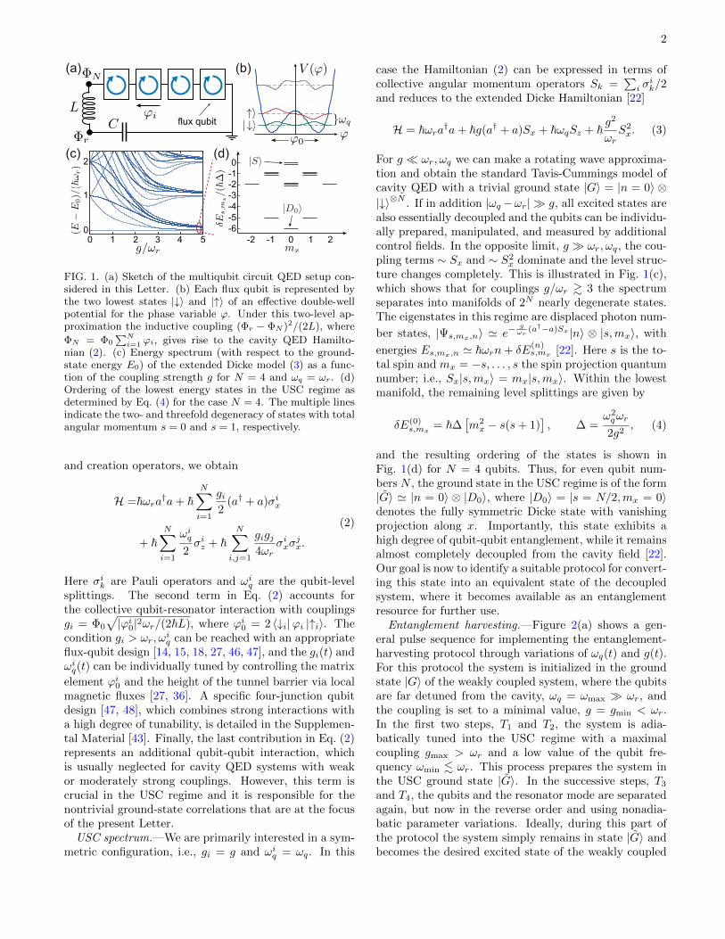
Model.—We consider a circuit QED system as shownin Fig. 1(a), where a single mode LC resonator with ca-pacitance C and inductance L is coupled collectively toan even number of N = 2, 4, 6, . . . flux qubits. This cir-cuit is described by the Hamiltonian [42, 43]

H =Q2r

2C+

(Φr − Φ0

∑Ni=1 ϕi)

2

2L+

N∑i=1

H(i)q , (1)

where Qr and Φr are charge and generalized flux op-erators for the resonator obeying [Φr, Qr] = i~, andΦ0 = ~/(2e) is the reduced flux quantum. For each qubit,

H(i)q denotes the free Hamiltonian and ϕi is the difference

of the superconducting phase across the qubit’s subcir-cuit. As usual we assume that the qubit dynamics can berestricted to the two lowest tunneling states |↓〉 and |↑〉 ofa symmetric double-well potential [cf. Fig. 1(b)]. Underthis approximation and writing Φr =

√~/(2Cωr)(a+a†)

and Qr = i√~Cωr/2(a†− a), where ωr =

√1/LC is the

resonator frequency and a and a† are the annihilation

arX

iv:1

707.

0896

9v3

[qu

ant-

ph]

2 N

ov 2

017

2

FIG. 1. (a) Sketch of the multiqubit circuit QED setup con-sidered in this Letter. (b) Each flux qubit is represented bythe two lowest states |↓〉 and |↑〉 of an effective double-wellpotential for the phase variable ϕ. Under this two-level ap-proximation the inductive coupling (Φr − ΦN )2/(2L), where

ΦN = Φ0

∑Ni=1 ϕi, gives rise to the cavity QED Hamilto-

nian (2). (c) Energy spectrum (with respect to the ground-state energy E0) of the extended Dicke model (3) as a func-tion of the coupling strength g for N = 4 and ωq = ωr. (d)Ordering of the lowest energy states in the USC regime asdetermined by Eq. (4) for the case N = 4. The multiple linesindicate the two- and threefold degeneracy of states with totalangular momentum s = 0 and s = 1, respectively.

and creation operators, we obtain

H =~ωra†a+ ~N∑i=1

gi2

(a† + a)σix

+ ~N∑i=1

ωiq2σiz + ~

N∑i,j=1

gigj4ωr

σixσjx.

(2)

Here σik are Pauli operators and ωiq are the qubit-levelsplittings. The second term in Eq. (2) accounts forthe collective qubit-resonator interaction with couplingsgi = Φ0

√|ϕi0|2ωr/(2~L), where ϕi0 = 2 〈↓i|ϕi |↑i〉. The

condition gi > ωr, ωiq can be reached with an appropriate

flux-qubit design [14, 15, 18, 27, 46, 47], and the gi(t) andωiq(t) can be individually tuned by controlling the matrix

element ϕi0 and the height of the tunnel barrier via localmagnetic fluxes [27, 36]. A specific four-junction qubitdesign [47, 48], which combines strong interactions witha high degree of tunability, is detailed in the Supplemen-tal Material [43]. Finally, the last contribution in Eq. (2)represents an additional qubit-qubit interaction, whichis usually neglected for cavity QED systems with weakor moderately strong couplings. However, this term iscrucial in the USC regime and it is responsible for thenontrivial ground-state correlations that are at the focusof the present Letter.

USC spectrum.—We are primarily interested in a sym-metric configuration, i.e., gi = g and ωiq = ωq. In this

case the Hamiltonian (2) can be expressed in terms ofcollective angular momentum operators Sk =

∑i σ

ik/2

and reduces to the extended Dicke Hamiltonian [22]

H = ~ωra†a+ ~g(a† + a)Sx + ~ωqSz + ~g2

ωrS2x. (3)

For g ωr, ωq we can make a rotating wave approxima-tion and obtain the standard Tavis-Cummings model ofcavity QED with a trivial ground state |G〉 = |n = 0〉 ⊗|↓〉⊗N . If in addition |ωq−ωr| g, all excited states arealso essentially decoupled and the qubits can be individu-ally prepared, manipulated, and measured by additionalcontrol fields. In the opposite limit, g ωr, ωq, the cou-pling terms ∼ Sx and ∼ S2

x dominate and the level struc-ture changes completely. This is illustrated in Fig. 1(c),which shows that for couplings g/ωr & 3 the spectrumseparates into manifolds of 2N nearly degenerate states.The eigenstates in this regime are displaced photon num-

ber states, |Ψs,mx,n〉 ' e−gωr

(a†−a)Sx |n〉 ⊗ |s,mx〉, with

energies Es,mx,n ' ~ωrn+ δE(n)s,mx [22]. Here s is the to-

tal spin and mx = −s, . . . , s the spin projection quantumnumber; i.e., Sx|s,mx〉 = mx|s,mx〉. Within the lowestmanifold, the remaining level splittings are given by

δE(0)s,mx

= ~∆[m2x − s(s+ 1)

], ∆ =

ω2qωr

2g2, (4)

and the resulting ordering of the states is shown inFig. 1(d) for N = 4 qubits. Thus, for even qubit num-bers N , the ground state in the USC regime is of the form|G〉 ' |n = 0〉 ⊗ |D0〉, where |D0〉 = |s = N/2,mx = 0〉denotes the fully symmetric Dicke state with vanishingprojection along x. Importantly, this state exhibits ahigh degree of qubit-qubit entanglement, while it remainsalmost completely decoupled from the cavity field [22].Our goal is now to identify a suitable protocol for convert-ing this state into an equivalent state of the decoupledsystem, where it becomes available as an entanglementresource for further use.Entanglement harvesting.—Figure 2(a) shows a gen-

eral pulse sequence for implementing the entanglement-harvesting protocol through variations of ωq(t) and g(t).For this protocol the system is initialized in the groundstate |G〉 of the weakly coupled system, where the qubitsare far detuned from the cavity, ωq = ωmax ωr, andthe coupling is set to a minimal value, g = gmin < ωr.In the first two steps, T1 and T2, the system is adia-batically tuned into the USC regime with a maximalcoupling gmax > ωr and a low value of the qubit fre-quency ωmin . ωr. This process prepares the system inthe USC ground state |G〉. In the successive steps, T3and T4, the qubits and the resonator mode are separatedagain, but now in the reverse order and using nonadia-batic parameter variations. Ideally, during this part ofthe protocol the system simply remains in state |G〉 andbecomes the desired excited state of the weakly coupled

3

(a)

USC

weakcoupling

120

0.20.40.60.8

1

0 4 8

(b)

13 13.5 142 6 10

USC

FIG. 2. (a) General pulse sequence for the qubit parame-ters ωq(t) and g(t) considered for the implementation of theentanglement harvesting protocol. (b) The fidelity F(t) isplotted as a function of time and for different qubit num-bers. The dashed line indicates the quantity 1− P(t), whereP(t) = Trρ2q(t) is the purity of the reduced qubit stateρq(t) = Trrρ(t) for the case N = 4. It shows that after anintermediate stage of finite qubit-resonator entanglement, thepurity of the qubit state is almost fully restored when the sys-tem enters deep into the USC regime. For all values of N thesame parameters ωmax/ωr = 20, ωmin/ωr = 0.5, gmax/ωr =4.5, gmin/ωr = 0.1 and times intervals T1 = T2 = 6.5ω−1

r andT3 = T4 = 0.5ω−1

r have been assumed.

system at the final time Tf =∑4n=1 Tn. This general

sequence achieves two main goals. First, the adiabaticpreparation stage can be implemented very rapidly, sinceit must only be slow compared to the fast time scales setby ω−1max and g−1max. At the same time the nonadiabatic de-coupling processes only need to be fast compared to theslow time scales ω−1r , ω−1min, and g−1min. This second condi-tion is most crucial for a time-dependent control of USCsystems, since it makes the required switching times ex-perimentally accessible and consistent with the two-levelapproximation assumed in our theoretical model.

In Fig. 2(b) we plot the fidelity F(t) =Trρ(t)|D0〉〈D0|, where ρ(t) is the density operator ofthe full system, for a specific set of pulse parameterslisted in the figure caption. We see that the entanglementextraction fidelity (EEF) FE = maxF(t)|t ≥ Tf, i.e.,the maximal fidelity after the decoupling step, reachesnear perfect values of FE ' 0.95 − 0.99 for differentnumbers of qubits, without any further fine-tuning ofthe control pulses. Note that the fidelity oscillations atthe end of the sequence are simply due to the fact that|D0〉 is not an eigenstate of the bare qubit Hamiltonian,Hq = ωqSz. However, this evolution does not affect thepurity or the degree of entanglement of the final qubitstate and can be undone by local qubit rotations.

Experimental considerations.—For a possible experi-mental implementation of the protocol we consider qubitswith a frequency of ωmax/(2π) ≈ 10 GHz coupled to a

(c)

0

0.5

1

0.9

0.7

0.4

0.6

0.8

1

0 0.5 1 1.5 2

1

2

0

(a)

(b)

USC

1 2 3 4 5

0.50.9 0.85 0.8

FIG. 3. (a) Evolution of the lowest eigenvalues during dif-ferent stages of the protocol for the case N = 2. Heregmin/ωr = 0.2, ωmin/ωr = 0.4, and in the final step of theprotocol ωmax/ωr = 5. For clarity only the s = 1 statesare shown and all time intervals have been stretched to equallengths. For different initial photon number states |n〉, thecolored segments and arrows indicate the ideal evolution ofthe systems, which maximizes the probability to end up inthe qubit state |D0〉 = (|↑↑〉 − |↓↓〉)/

√2. Nonadiabatic cross-

ings occur during the fast decoupling steps (T3 and T4), butalso for small avoided crossings in the excited state mani-folds during the preparation step (T2). (b) Plot of the EEFfor varying T4(= T3) and gmin and for N = 4. (c) EEF (solidline) for a resonator mode, which is initially in a thermal stateat temperature T , for N = 4. The dashed line indicates thecorresponding population of the ground state manifold. Allthe other pulse parameters in panels (a), (b) and (c) are thesame as in Fig. 2(b).

lumped-element resonator of frequency ωr/(2π) = 500MHz. The required maximal coupling strength of gmax '4.5ωr ≈ 2π×2.25 GHz is then consistent with experimen-tally demonstrated values [14, 15]. For these parameters,the nonadiabatic switching times assumed in Fig. 2(b)correspond to T3,4 ' 0.16 ns. These switching timesare within reach of state-of-the-art waveform generatorsand a sinusoidal modulation of flux qubits on such timescales has already been demonstrated [49]. At the sametime the duration of the whole protocol, Tf = 15/ωr ≈ 5ns, is still much faster than typical flux qubit coher-ence times of 1-100 µs [50] or the lifetime of a photon,Tph = Q/ωr, in a microwave resonator of quality factorQ = 104 − 106. Therefore, although many experimentaltechniques for implementing and operating circuit QEDsystems in the USC regime are still under development,these estimates clearly demonstrate the feasibility of re-alizing high-fidelity control operations in such devices.

In practice additional limitations might arise from thelack of complete tunability of g(t) and ωq(t). This is il-lustrated in Fig. 3(a), which shows the evolution of thelowest eigenenergies during different stages of the proto-

4

col for the case N = 2 and a nonvanishing value of gmin.In this case the appearance of several avoided crossingsduring the final ramp-up step prevents a fully nonadi-abatic decoupling. In Fig. 3(b) we plot the resultingEEF for varying gmin and T4. This plot demonstratesthe expected trade-off between the residual coupling andthe minimal switching time, but also that the protocol israther robust and fidelities of FE ∼ 0.9 are still possiblefor minimal couplings of a few hundred MHz or switchingtimes approaching ∼ 1 ns. Similar conclusions are ob-tained when a partial dependence between the pulses forg(t) and ωq(t) or nonuniform couplings gi(t) and frequen-cies ωiq(t) due to fabrication uncertainties are taken intoaccount. Numerical simulations of the protocol undersuch realistic experimental conditions [43] demonstratethat no precise fine-tuning of the system parameters isrequired.

Extracting entanglement from a thermal state.—Theabove-considered protocol relies on a rather low resonatorfrequency ωr in order to enhance both g/ωr as well asthe nonadiabatic switching times. This implies that evenat temperatures of T = 20 mK the equilibrium popu-lations of higher resonator states with n ≥ 1 cannotbe neglected. In Fig. 3(c) we plot the EEF as a func-tion of the temperature T , assuming an initial resonatorstate ρth =

∑n pn |n〉 〈n|, where pn = nn/(1 + n)n+1 is

the thermal distribution for a mean excitation numbern = 1/(e~ωr/kBT − 1). We see that the EEF is signif-icantly higher than one would naively expect from theinitial population in the ground state |G〉. The origin ofthis surprising effect can be understood from the eigen-value plot in Fig. 3(a). For example, the weak-coupling

eigenstate |n = 1〉 ⊗ |↓〉⊗N is efficiently mapped on thecorresponding USC state |n = 1〉 ⊗ |s = N/2,mx = 0〉,passing only through a weak, higher-order avoided cross-ing. Therefore, the intermediate—and as a result also thefinal—qubit state is one with the resonator being in state|1〉. Although for higher photon numbers the avoidedcrossings become more relevant, the protocol still approx-imately implements the mapping |n〉⊗|↓〉⊗N → |n〉⊗|s =N/2,mx = 0〉, independent of the resonator state |n〉.This feature makes it rather insensitive to thermal occu-pations and avoids additional active cooling methods forinitializing the system in state |G〉.

Entanglement protection.—Figure 1(d) shows thatapart from the ground state |G〉 there are many otherhighly entangled states within the lowest USC manifold.Of particular interest is the energetically highest state|E〉 = |n = 0〉 ⊗ |S〉, where |S〉 is a singlet state withtotal angular momentum s = 0 and Sz|S〉 = Sx|S〉 = 0.Therefore, once prepared, this state is an exact dark stateof Hamiltonian (3) and remains decoupled from the cav-ity field in all parameter regimes. Although this state isnot connected to any of the bare qubit states in a simpleadiabatic way, it can still be harvested by an adoptedprotocol, as described in Fig. 4(a) for the case N = 4.

120 1600

4

8

12

0 40 80

2

120 1600 40 800

0 5 10 15

0

1.6

0.8

120 1600 40 80

(a)

(b) (c)

1

2

0

1

FIG. 4. (a) Pulse sequence for harvesting the 4-qubit entan-gled state |S〉 with total angular momentum s = 0. As shownin the inset, during the first part of the protocol a finite dif-ference between the qubit frequencies ω1,2

q and ω3,4q is used to

break the symmetry and couple different angular momentumstates. (b) The expectation value of the total spin, 〈~S2(t)〉,(solid line) and the purity of the reduced qubit state, P(t),(dashed line) are plotted for the pulse sequence shown in (a)and for an initial state |Ψ0〉 = |0〉 ⊗ |↑↑↓↓〉. (c) Evolution ofthe extracted state |0〉 ⊗ |S〉 (characterized by the expecta-tion value of the total spin) after the protocol for differentfinal values of the couplings gf . For this plot an average overrandom distributions of the qubit frequencies, ωi

q = ωq(1+εi),has been assumed, where ωq/ωr = 10 and the εi are chosenrandomly from the interval [−0.05, 0.05]. For very strong cou-plings, the residual oscillations indicate that all transitionsinduced by the nonuniform εi from state |S〉 to other statesare highly detuned.

For this protocol the system is initially prepared in theexcited state |Ψ0〉 = |0〉 ⊗ |↑↑↓↓〉 and in a first step thequbit states are lowered below the resonator frequency inorder to avoid further level crossings with higher-photon-number states. The increase of the coupling combinedwith a frequency offset to break the angular momentumconservation then evolves the system into a state withs = 0 already for moderate couplings of g/ωr ≈ 1.8.Note that for N ≥ 4 there are multiple degenerate USCstates with s = 0 [51, 52] [cf. Fig. 1(d)], out of which theprotocol selects a specific superposition [43].

Although the harvesting protocol for state |S〉 losessome of the robustness of the ground-state protocol, itadds an important feature. By retaining a finite cou-pling gf = g(t = Tf) ∼ ωr at the end of the protocol,the extracted dark state |S〉 is energetically separatedfrom all other states with s 6= 0 and it is thereby pro-tected against small frequency fluctuations. This effectis illustrated in Fig. 4(c), which shows the evolution ofthe extracted state |S〉 in the presence of small randomshifts of the individual qubit frequencies. For gf = 0 this

5

leads to dephasing of the qubits and a rapid transitionout of the s = 0 subspace. This dephasing can be sub-stantially suppressed by keeping the coupling at a finitevalue. Thus, this example shows that USC effects can beused not only to generate complex multiqubit entangledstates, but also to protect them.

Conclusion.—We have presented a protocol for ex-tracting well-defined multiqubit-entangled states fromthe ground-state manifold of an ultrastrongly coupledcircuit QED system. The detailed analysis of this pro-tocol illustrates, how various–so far unexplored–USC ef-fects can contribute to a robust generation and protectionof complex multiqubit states. These principles can serveas a guideline for many other preparation, storage andcontrol operations in upcoming USC circuit QED exper-iments with two or more qubits.

Acknowledgments.—This work was supported by theAustrian Science Fund (FWF) through the SFB FoQuS,Grant No. F40, the DK CoQuS, Grant No. W 1210, andthe START Grant No. Y 591-N16, and the People Pro-gramme (Marie Curie Actions) of the European Union’sSeventh Framework Programme (FP7/2007-2013) underREA Grant No. 317232. F. A. wishes to express his grat-itude to the Quantum Optics Theory Group of Atomin-stitut (TU Wien) for the warm hospitality received dur-ing his numerous visits. M. S. K. acknowledges supportfrom the UK EPSRC Grant No. EP/K034480/1 and theRoyal Society.

[1] Y. Todorov, A. M. Andrews, R. Colombelli, S. De Liber-ato, C. Ciuti, P. Klang, G. Strasser, and C. Sirtori, “Ul-trastrong Light-Matter Coupling Regime with PolaritonDots”, Phys. Rev. Lett. 105, 196402 (2010).

[2] T. Schwartz, J. A. Hutchison, C. Genet, and T. W. Ebbe-sen, “Reversible Switching of Ultrastrong Light-MoleculeCoupling”, Phys. Rev. Lett. 106, 196405 (2011).

[3] M. Geiser, F. Castellano, G. Scalari, M. Beck, L. Nevou,and J. Faist, “Ultrastrong Coupling Regime and PlasmonPolaritons in Parabolic Semiconductor Quantum Wells”,Phys. Rev. Lett. 108, 106402 (2012).

[4] G. Scalari, C. Maissen, S. Cibella, R. Leoni, C. Reichl,W. Wegscheider, M. Beck, and J. Faist, “THz ultrastronglight-matter coupling”, Il Nuovo Saggiatore 31, 4 (2015).

[5] Q. Zhang, M. Lou, X. Li, J. L. Reno, W. Pan, J. D.Watson, M. J. Manfra, and J. Kono, “Collective non-perturbative coupling of 2D electrons with high-quality-factor terahertz cavity photons”, Nat. Phys. 12, 1005(2016).

[6] A. Wallraff, D. I. Schuster, A. Blais, L. Frunzio, R. S.Huang, J. Majer, S. Kumar, S. M. Girvin, and R. J.Schoelkopf, “Strong coupling of a single photon to a super-conducting qubit using circuit quantum electrodynamics”,Nature (London) 431, 162 (2004).

[7] A. Blais, R.-S. Huang, A. Wallraff, S. M. Girvin and R. J.Schoelkopf, “Cavity quantum electrodynamics for super-conducting electrical circuits: An architecture for quan-

tum computation”, Phys. Rev. A 69, 062320 (2004).[8] C. Ciuti, G. Bastard, and I. Carusotto, “Quantum vac-

uum properties of the intersubband cavity polariton field”,Phys. Rev. B 72, 115303 (2005).

[9] J. Casanova, G. Romero, I. Lizuain, J. J. Garcıa-Ripoll,and E. Solano, “Deep Strong Coupling Regime of theJaynes-Cummings Model”, Phys. Rev. Lett. 105, 263603(2010).

[10] Note that in this Letter we do not further distinguish be-tween the USC [8] and the deep strong-coupling regime [9].

[11] T. Niemczyk, et al., “Circuit quantum electrodynamicsin the ultrastrong-coupling regime”, Nat. Phys. 6, 772(2010).

[12] P. Forn-Diaz, J. Lisenfeld, D. Marcos, J. J. Garcia-Ripoll,E. Solano, C. J. P. M. Harmans, and J. E. Mooij, “Ob-servation of the Bloch-Siegert Shift in a Qubit-OscillatorSystem in the Ultrastrong Coupling Regime”, Phys. Rev.Lett. 105, 237001 (2010).

[13] A. Baust, E. Hoffmann, M. Haeberlein, M. J. Schwarz, P.Eder, J. Goetz, F. Wulschner, E. Xie, L. Zhong, F. Qui-jandrıa, D. Zueco, J.-J. Garcıa-Ripoll, L. Garcıa-Alvarez,G. Romero, E. Solano, K. G. Fedorov, E. P. Menzel, F.Deppe, A. Marx, and R. Gross, “Ultrastrong couplingin two-resonator circuit QED”, Phys. Rev. B 93, 214501(2016).

[14] P. Forn-Diaz, J. J. Garcıa-Ripoll, B. Peropadre, M. A.Yurtalan, J.-L. Orgiazzi, R. Belyansky, C. M. Wilson, andA. Lupascu, “Ultrastrong coupling of a single artificialatom to an electromagnetic continuum”, Nat. Phys. 13,39 (2017).

[15] F. Yoshihara, T. Fuse, S. Ashhab, K. Kakuyanagi, S.Saito, and K. Semba, “Superconducting qubit-oscillatorcircuit beyond the ultrastrong-coupling regime”, Nat.Phys. 13, 44 (2017).

[16] Z. Chen, Y. Wang, T. Li, L. Tian, Y. Qiu, K. Inomata,F. Yoshihara, S. Han, F. Nori, J. S. Tsai, and J. Q. You,“Multi-photon sideband transitions in an ultrastronglycoupled circuit quantum electrodynamics system”, Phys.Rev. A 96, 012325 (2017).

[17] S. J. Bosman, M. F. Gely, V. Singh, A. Bruno, D. Both-ner, and G. A. Steele, “Multi-mode ultra-strong couplingin circuit quantum electrodynamics”, arXiv:1704.06208(2017).

[18] P. Nataf and C. Ciuti, “Vacuum Degeneracy of a CircuitQED System in the Ultrastrong Coupling Regime”, Phys.Rev. Lett. 104, 023601 (2010).

[19] P. Nataf and C. Ciuti, “No-go theorem for superradiantquantum phase transitions in cavity QED and counter-example in circuit QED”, Nat. Commun. 1, 72 (2010).

[20] M. Bamba, K. Inomata, and Y. Nakamura, “Super-radiant Phase Transition in a Superconducting Circuitin Thermal Equilibrium”, Phys. Rev. Lett. 117, 173601(2016).

[21] S. De Liberato,“Light-Matter Decoupling in the DeepStrong Coupling Regime: The Breakdown of the PurcellEffect”, Phys. Rev. Lett. 112, 016401 (2014).

[22] T. Jaako, Z.-L. Xiang, J.J. Garcia-Ripoll, and P.Rabl, “Ultrastrong coupling phenomena beyond the Dickemodel”, Phys. Rev. A 94, 033850 (2016).

[23] G. Levine and V. N. Muthukumar, “Entanglement of aqubit with a single oscillator mode”, Phys. Rev. B 69,113203 (2004).

[24] A. P. Hines, C. M. Dawson, R. H. McKenzie, and G. J.Milburn, “Entanglement and bifurcations in Jahn-Teller

6

models”, Phys. Rev. A 70, 022303 (2004).[25] S. Ashhab and F. Nori, “Qubit-oscillator systems in the

ultrastrong-coupling regime and their potential for prepar-ing nonclassical states”, Phys. Rev. A 81, 042311 (2010).

[26] P. Nataf and C. Ciuti, “Protected Quantum Computa-tion with Multiple Resonators in Ultrastrong CouplingCircuit QED”, Phys. Rev. Lett. 107, 190402 (2011).

[27] G. Romero, D. Ballester, Y. M. Wang, V. Scarani, andE. Solano, “Ultrafast Quantum Gates in Circuit QED”,Phys. Rev. Lett. 108, 120501 (2012).

[28] T. H. Kyaw, S. Felicetti, G. Romero, E. Solano, and L.-C. Kwek, “Scalable quantum memory in the ultrastrongcoupling regime”, Sci. Rep. 5, 8621 (2015).

[29] Y. Wang, J. Zhang, C. Wu, J. Q. You, and G. Romero,“Holonomic quantum computation in the ultrastrong-coupling regime of circuit QED”, Phys. Rev. A 94, 012328(2016).

[30] Y. Wang, C. Guo, G.-Q. Zhang, G. Wang, and C. Wu,“Ultrafast quantum computation in ultrastrongly coupledcircuit QED systems”, Sci. Rep. 7, 44251 (2017).

[31] R. Stassi and F. Nori, “Quantum Memory in theUltrastrong-Coupling Regime via Parity Symmetry Break-ing”, arXiv:1703.08951 (2017).

[32] B. Reznik, A. Retzker, and J. Silman, “Violating Bell’sinequalities in vacuum”, Phys. Rev. A 71, 042104 (2005).

[33] M. Han, S. J. Olson, and J. P. Dowling, “Generatingentangled photons from the vacuum by accelerated mea-surements: Quantum-information theory and the Unruh-Davies effect”, Phys. Rev. A 78, 022302 (2008).

[34] A. Auer and G. Burkard, “Entangled photons from thepolariton vacuum in a switchable optical cavity”, Phys.Rev. B 85, 235140 (2012).

[35] S. J. Olson and T. C. Ralph, “Extraction of timelike en-tanglement from the quantum vacuum”, Phys. Rev. A 85,012306 (2012).

[36] C. Sabin, B. Peropadre, M. del Rey, and E. Martin-Martinez, “Extracting Past-Future Vacuum CorrelationsUsing Circuit QED”, Phys. Rev. Lett. 109, 033602 (2012).

[37] G. Salton, R. B. Mann, and N. C. Menicucci,“Acceleration-assisted entanglement harvesting andrangefinding”, New J. Phys. 17, 035001 (2015).

[38] L. Dai, W. Kuo and M. C. Chung, “Extracting entangledqubits from Majorana fermions in quantum dot chainsthrough the measurement of parity”, Sci. Rep. 5, 11188(2015).

[39] O. Guhne, F. Bodoky, and M. Blaauboer, “Multiparticleentanglement under the influence of decoherence”, Phys.Rev. A 78, 060301(R) (2008).

[40] M. Bergmann and O. Guhne, “Entanglement criteria forDicke states”, J. Phys. A: Math. Theor. 46, 385304 (2013).

[41] G. Toth and I. Apellaniz, “Quantum metrology from aquantum information science perspective”, J. Phys. A:Math. Theor. 47, 424006 (2014).

[42] U. Vool and M. Devoret, Introduction to Quantum Elec-tromagnetic Circuits, Int. J. Circ. Theor. Appl. 45, 897(2017).

[43] See Supplemental Material for additional details aboutthe circuit design and the performance of the protocol un-der nonideal conditions, which includes Ref. [44, 45].

[44] F. Beaudoin, J. M. Gambetta, and A. Blais, “Dissipationand ultrastrong coupling in circuit QED”, Phys. Rev. A84, 043832 (2011).

[45] A. Ridolfo, M. Leib, S. Savasta, and M. J. Hartmann.“Photon Blockade in the Ultrastrong Coupling Regime”,

Phys. Rev. Lett. 109, 193602 (2012).[46] J. Bourassa, J. M. Gambetta, A. A. Abdumalikov, O.

Astafiev, Y. Nakamura, and A. Blais, “Ultrastrong cou-pling regime of cavity QED with phase-biased flux qubits”,Phys. Rev. A 80, 032109 (2009).

[47] B. Peropadre, D. Zueco, D. Porras, and J. J. Garcia-Ripoll, “Nonequilibrium and Nonperturbative Dynamicsof Ultrastrong Coupling in Open Lines”, Phys. Rev. Lett.111, 243602 (2013).

[48] Y. Qiu, W. Xiong, X.-L. He, T.-F. Li, and J. Q.You, “Four-junction superconducting circuit”, Sci. Rep.6, 28622 (2016).

[49] C. M. Wilson, G. Johansson, A. Pourkabirian, J. R. Jo-hansson, T. Duty, F. Nori, and P. Delsing, “Observationof the dynamical Casimir effect in a superconducting cir-cuit”, Nature (London) 479, 376 (2011).

[50] F. Yan, S. Gustavsson, A. Kamal, J. Birenbaum, A.P.Sears, D. Hover, D. Rosenberg, G. Samach, T. J. Gud-mundsen, J. L. Yoder, T. P. Orlando, J. Clarke, A. J.Kerman, and W. D. Oliver, “The flux qubit revisited toenhance coherence and reproducibility”, Nat. Commun. 7,12964 (2016).

[51] R. H. Dicke, “Coherence in spontaneous radiation pro-cesses”, Phys. Rev. 93, 99 (1954).

[52] F. T. Arecchi, E. Courtens, R. Gilmore, and H. Thomas,“Atomic coherent states in quantum optics”, Phys. Rev.A 6, 2211 (1972).

7

Supplemental material

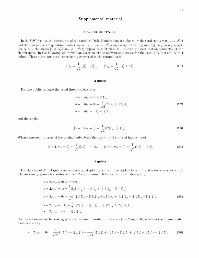
USC EIGENSTATES

In the USC regime, the eigenstates of the extended Dicke Hamiltonian are labeled by the total spin s = 0, 1, . . . , N/2

and the spin projection quantum number mx = −s, . . . , s, i.e., ~S2|s,mx〉 = s(s+1)|s,mx〉 and Sx|s,mx〉 = mx|s,mx〉.For N > 2 the states |s 6= N/2,mx 6= ±N/2〉 appear as multiplets [S1], due to the permutation symmetry of theHamiltonian. In the following we provide an overview of the relevant spin states for the case of N = 2 and N = 4qubits. These states are most conveniently expressed in the rotated basis

|↓〉x =1√2

(|↓〉 − |↑〉) , |↑〉x =1√2

(|↓〉+ |↑〉) . (S1)

2 qubits

For two qubits we have the usual three triplet states

|s = 1,mx = 1〉 = |↑↑〉x ,

|s = 1,mx = 0〉 =1√2

(|↑↓〉x + |↓↑〉x),

|s = 1,mx = −1〉 = |↓↓〉x ,

(S2)

and the singlet

|s = 0,mx = 0〉 =1√2

(|↑↓〉x − |↓↑〉x). (S3)

When expressed in terms of the original qubit basis the two mx = 0 states of interest read

|s = 1,mx = 0〉 =1√2

(|↓↓〉 − |↑↑〉), |s = 0,mx = 0〉 =1√2

(|↑↓〉 − |↓↑〉). (S4)

4 qubits

For the case of N = 4 qubits we obtain a quintuplet for s = 2, three triplets for s = 1 and a two states for s = 0.The maximally symmetric states with s = 2 are the usual Dicke states in the x-basis, i.e.,

|s = 2,mx = 2〉 = |↑↑↑↑〉x ,

|s = 2,mx = 1〉 =1

2(|↓↑↑↑〉x + |↑↓↑↑〉x + |↑↑↓↑〉x + |↑↑↑↓〉x),

|s = 2,mx = 0〉 =1√6

(|↓↓↑↑〉x + |↑↑↓↓〉x + |↓↑↑↓〉x + |↑↓↓↑〉x + |↓↑↓↑〉x + |↑↓↑↓〉x),

|s = 2,mx = −1〉 =1

2(|↓↑↓↓〉x + |↓↓↓↑〉x + |↓↓↑↓〉x + |↑↓↓↓〉x),

|s = 2,mx = −2〉 = |↓↓↓↓〉x .

(S5)

For the entanglement harvesting protocol, we are interested in the state |s = 2,mx = 0〉, which in the original qubitbasis is given by

|s = 2,mx = 0〉 =3√24

(|↑↑↑↑〉+ |↓↓↓↓〉)− 1√24

(|↑↑↓↓〉+ |↑↓↑↓〉+ |↑↓↓↑〉+ |↓↑↑↓〉+ |↓↑↓↑〉+ |↓↓↑↑〉). (S6)

8

Each of the s = 1 states is 3-fold degenerate and the corresponding states are

|s = 1,mx = 1〉 =

12 (|↑↑↑↓〉x + |↑↑↓↑〉x − |↑↓↑↑〉x − |↓↑↑↑〉x)12 (|↑↑↑↓〉x − |↑↑↓↑〉x + |↑↓↑↑〉x − |↓↑↑↑〉x)12 (|↑↑↑↓〉x − |↑↑↓↑〉x − |↑↓↑↑〉x + |↓↑↑↑〉x)

|s = 1,mx = 0〉 =

1√2(|↑↑↓↓〉x − |↓↓↑↑〉x)

1√2(|↑↓↑↓〉x − |↓↑↓↑〉x)

1√2(|↑↓↓↑〉x − |↓↑↑↓〉x)

|s = 1,mx = −1〉 =

12 (|↑↓↓↓〉x + |↓↑↓↓〉x − |↓↓↑↓〉x − |↓↓↓↑〉x)12 (|↑↓↓↓〉x − |↓↑↓↓〉x + |↓↓↑↓〉x − |↓↓↓↑〉x)12 (|↑↓↓↓〉x − |↓↑↓↓〉x − |↓↓↑↓〉x + |↓↓↓↑〉x)

(S7)

Finally, for N = 4 we obtain two singlet states with s = 0, which are given by

|s = 0,mx = 0〉 =

|S〉 = 1√

3(|↑↑↓↓〉x + |↓↓↑↑〉x)− 1√

12(|↑↓↑↓〉x + |↑↓↓↑〉x + |↓↑↑↓〉+ |↓↑↓↑〉x),

|S′〉 = 12 (|↑↓↑↓〉x − |↑↓↓↑〉x − |↓↑↑↓〉x + |↓↑↓↑〉x).

(S8)

Since the s = 0 subspace is invariant under rotations, the states have the same form as in the original qubit basis,

|s = 0,mx = 0〉 =

|S〉 = 1√

3(|↑↑↓↓〉+ |↓↓↑↑〉)− 1√

12(|↑↓↑↓〉+ |↑↓↓↑〉+ |↓↑↑↓〉+ |↓↑↓↑〉),

|S′〉 = 12 (|↑↓↑↓〉 − |↑↓↓↑〉 − |↓↑↑↓〉+ |↓↑↓↑〉).

(S9)

Note that in Eqs. (S8) and (S9) the specific choice of basis states has been used to match the state |S〉 generated inthe protocol described in Fig. 4 in the main text and in the following section.

PROTOCOL FOR THE GENERATION OF THE SINGLET QUBIT STATES WITH s = 0

Compared to the state |D0〉 the singlet states |s = 0,mx = 0〉, defined by ~S2|s = 0,mx = 0〉 = Sz|s = 0,mx = 0〉 =Sx|s = 0,mx = 0〉 = 0, are not directly adiabatically connected to any of the bare states. Nevertheless these statescan still be prepared by using an adapted protocol (Fig. 4 of the main text) that we are going to describe here inmore detail.

Similar to the ground-state protocol, we start from the decoupled regime where g ' 0 and ωiq ωr, but we initializethe system in the excited qubit state |Ψ0〉 = |0〉⊗ |↑↑↓↓〉 (|Ψ0〉 = |0〉⊗ |↑↓〉 for N = 2 ), where half of the qubits are inthe excited state and half in the ground state. Note that for N = 4 and a fully symmetric system, the s = 0 manifoldis two-fold degenerate and spanned, e.g., by the basis states given in Eq. (S9). To prepare a well-defined state, webreak the symmetry by creating an offset between the qubit frequencies, for example, by setting ω1,2

q 6= ω3,4q . Once

the state |Ψ0〉 is prepared, all the qubit frequencies are lowered below the resonator frequency such that ωiq < ωr/2.This is done in time step T1 while keeping g ' 0. As shown in Fig. S1, after this initial step all the relevant qubitstates are below the first excited photon state. This configuration avoids undesired level crossings with higher photonnumber states during the next step of the protocol and only the n = 0 manifold must be considered.

During the second step ωiq ≤ ωr/2, but we still keep a finite frequency difference between the qubits to separate thestate |↑↑↓↓〉 from other states with two qubits excited. This difference between the degenerate and non-degeneratequbit frequencies is visualized by Fig. S1(a) and (b). As the coupling g is slowly increased while the difference in thequbit frequencies is tuned to zero, the state |↑↑↓↓〉 is adiabatically transformed into the s = 0 state |S〉. During thisprocess the state |S〉 become almost completely degenerate with the other s = 0 state |S′〉 [see Fig. S1(b)]. However,also the non-adiabatic coupling between these two states is almost negligible, such that the preparation process is stilladiabatic on the timescale of the protocol.

In the last step of the protocol, the qubit frequencies are ramped up to the initial values as shown in Fig. 4 of themain text. At this point maintaining a frequency offset is not crucial anymore. Note that in this last protocol stepthere are not restrictions on the operational time T3 because the system is now in the dark state |S〉 and completelydecoupled from the resonator mode.

9

0 50 100 1500

0.5

1

0 50 100 1500

0.5

1

(a)

(b)

FIG. S1. Evolution of the eigenvalues during the second step of the protocol for extracting the state |S〉 [see Fig 4 in the maintext]. The colored lines indicate the states, which are adiabatically converted into the two s = 0 states, |S〉 and |S′〉. In plot (a)all qubit frequencies are the same, ωi

q = 0.48ωr, while in plot (b) values ω1,2q = 0.48ωr and ω3,4

q = 0.35ωr have been assumed.In both plots the couplings gi = g are raised symmetrically during the period T2, i.e., the plotted time span, from the valuegmin = 0 to the value gmax = 1.8ωr. Note that for these modest coupling values, the state |S〉 is not yet the energeticallyhighest state in the n = 0 manifold [compare Fig. 1(c) in the main text].

DISORDER

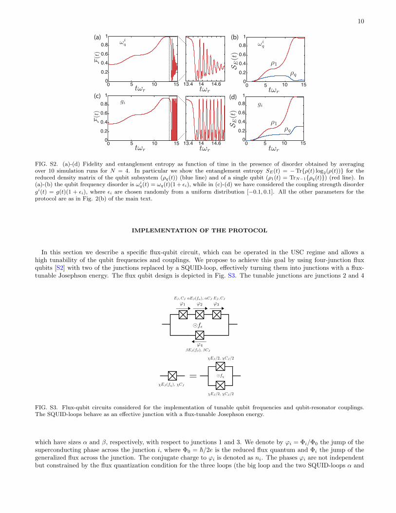
In the main text we have assumed that our qubits are perfectly identical with matching frequencies, and thateach of them couples to the resonator with the same coupling constant. However, due to fabrication disorder andcontrol imprecisions this assumption can be difficult to achieve in experiments with multiple qubits. To evaluate theinfluence of disorder on the entanglement-harvesting protocol, we show in Fig. S2 the results obtained from numericalsimulations of the protocol in the presence of frequency and coupling disorder. Figure S2(a) shows the average fidelity,assuming that in each run of the protocol the individual qubit frequencies evolve as ωiq(t) = ωq(t)(1 + εi), where ωq(t)follows the ideal pulse given in Fig. 2 of the main text and the εi are randomly chosen from the interval [−0.1, 0.1].We see that the main part of the protocol is essentially unaffected by frequency disorder, since the system is initiallyin the ground state and in the USC regime the system is dominated by the interaction terms. Frequency disorderonly becomes important in the final decoupled state, where it dephases the symmetric state |D0〉. Note, however, thatfor a fixed frequency distribution, this dephasing can be undone, since as shown in Fig. S2(a), it leads to almost nodegradation of the purity or the degree of entanglement of the qubit state. In Fig. S2(c) and (d) the same plots areshown for the case of coupling disorder gi(t) = g(t)(1+ εi). Although, this type of disorder has a stronger influence onthe evolution of the state, the plot shows that our protocol does not require strictly identical couplings and variationof around 10% still lead to EEF FE & 0.9 and almost no degradation of the qubit-qubit entanglement. The mainquantity affected is the entanglement entropy of the qubit subsystem, which does not approach the value of zero, thusshowing that qubits and resonator are not perfectly decoupled. However, we note that this measure of entanglementis very sensitive in our case, since the qubit state we achieve at the end of the protocol coincides with our target statewith fidelity above 90%.

10

0

0.2

0.4

0.6

0.81

0 5 10 15 13.4 14 14.6 0

0.2

0.4

0.6

0.81

0 5 10 15

0

0.2

0.4

0.6

0.81

0 5 10 15 13.4 14 14.6 0 5 10 150

0.2

0.4

0.6

0.81

(a) (b)

(c) (d)

FIG. S2. (a)-(d) Fidelity and entanglement entropy as function of time in the presence of disorder obtained by averagingover 10 simulation runs for N = 4. In particular we show the entanglement entropy SE(t) = −Trρ(t) log2(ρ(t)) for thereduced density matrix of the qubit subsystem (ρq(t)) (blue line) and of a single qubit (ρ1(t) = TrN−1ρq(t)) (red line). In(a)-(b) the qubit frequency disorder is ωi

q(t) = ωq(t)(1 + εi), while in (c)-(d) we have considered the coupling strength disorder

gi(t) = g(t)(1 + εi), where εi are chosen randomly from a uniform distribution [−0.1, 0.1]. All the other parameters for theprotocol are as in Fig. 2(b) of the main text.

IMPLEMENTATION OF THE PROTOCOL

In this section we describe a specific flux-qubit circuit, which can be operated in the USC regime and allows ahigh tunability of the qubit frequencies and couplings. We propose to achieve this goal by using four-junction fluxqubits [S2] with two of the junctions replaced by a SQUID-loop, effectively turning them into junctions with a flux-tunable Josephson energy. The flux qubit design is depicted in Fig. S3. The tunable junctions are junctions 2 and 4

FIG. S3. Flux-qubit circuits considered for the implementation of tunable qubit frequencies and qubit-resonator couplings.The SQUID-loops behave as an effective junction with a flux-tunable Josephson energy.

which have sizes α and β, respectively, with respect to junctions 1 and 3. We denote by ϕi = Φi/Φ0 the jump of thesuperconducting phase across the junction i, where Φ0 = ~/2e is the reduced flux quantum and Φi the jump of thegeneralized flux across the junction. The conjugate charge to ϕi is denoted as ni. The phases ϕi are not independentbut constrained by the flux quantization condition for the three loops (the big loop and the two SQUID-loops α and

11

β) ∑i∈1,2,3,4

ϕi + fε = 0,

∑i∈2,6

ϕi + fα = 0, (S10)

∑i∈4,5

ϕi + fβ = 0,

where fη = Φη/Φ0 and η = α, β, ε is the magnetic frustration through the loop created by external magnetic fluxesΦη. Using the above equations we eliminate phase jumps ϕ2, ϕ5 and ϕ6 from the problem. The standard quantizationprocedure for circuits then gives the Hamiltonian [S2, S3]

Hq =4EC

α+ β + 2αβ

[(α+ β + αβ)(n21 + n23) + (1 + 2α)n24 − 2αβn1n3 − 2α(n1 + n3)n4

](S11)

− EJ[cos(ϕ1) + α cos

(fα2

)cos(ϕ1 + ϕ3 + ϕ4 + fε) + cos(ϕ3) + β cos

(fβ2

)cos(ϕ4)

],

where ϕ4 = ϕ4 − fβ/2 and fε = fε + (fβ − fα)/2. From the shape of the Hamiltonian we can see that if we tune thefrustration parameters, fα, fβ and fε, in unison such that fε = (2π + fα − fβ)/2, the structure of the Hamiltonianstays the same except that the effective Josephson energy of the SQUID-loops vary sinusoidally with the frustration.This enables us to operate the flux qubits at the sweet spot, fε = π, while changing the potential landscape. Notethat in practice the cross-talk between the magnetic fluxes may complicate the qubit control, but in principle it isalways possible to measure this cross-talk and compensate it by appropriately chosen control pulses.

The flux qubit couples to the resonator through the phase jump over the entire qubit (see the main text), which,with our notation, is given by ∆ϕ = ϕ4. The coupling constant g between the resonator and the qubits is proportionalto the matrix element of ∆ϕ between the ground and excited states of the qubits, ∆ϕeg = 〈e|∆ϕ|g〉. Additionally,the coupling to the resonator renormalizes the qubit Hamiltonian by adding a term EL∆ϕ2/2, where EL = Φ2

0/L isthe inductive energy related to the resonator inductance L, to the qubit Hamiltonian.

Now we are ready to demonstrate the tunability of the qubit frequency and qubit-resonator coupling. We diago-nalize the qubit Hamiltonian Hq, plus the renormalization term coming from the coupling, numerically to find theeigenfrequencies and evaluate the transition matrix element ∆ϕeg. We choose the following parameters for the sim-ulation: α = 0.6, β = 6, EL/h = 2.57 GHz, EC/h = 4.99 GHz and EJ/h = 99.7 GHz. Our choice of EL sets theresonator inductance to L = 63.7 nH. In addition we choose C = 1.59 pF which determines the resonator frequencyand impedance to be ωr = (LC)−1/2 = 2π × 500 MHz and Zr =

√L/C = 200 Ω, respectively. In the simulation we

tune fα from 0 to 0.70π and fβ from 0 to 0.96π (fε changes accordingly to keep the qubit at its sweet spot).

FIG. S4. Tunability of the qubit. a) Transition frequency of the qubit, ωq, as a function of the external fluxes in the SQUID-loops in units of the resonator frequency. b) Normalized coupling constant g/ωr of the qubit to the LC-resonator. Parametersused to produce this plot are given in the text.

In Fig. S4 a) we plot the transition frequency of the qubit, normalized to the resonator frequency against theexternal fluxes in the two SQUID-loops. The qubit frequency is highly tunable ranging from ∼ 50ωr all the way to

12

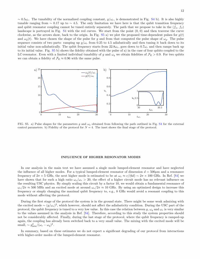
∼ 0.5ωr. The tunability of the normalized coupling constant, g/ωr, is demonstrated in Fig. S4 b). It is also highlytunable ranging from ∼ 0.17 up to ∼ 4.5. The only limitation we have here is that the qubit transition frequencyand qubit resonator coupling cannot be tuned entirely separately. The path that we propose to take in the (fα, fβ)landscape is portrayed in Fig. S4 with the red curves. We start from the point (0, 0) and then traverse the curveclockwise, as the arrows show, back to the origin. In Fig. S5 a) we plot the proposed time-dependent pulses for g(t)and ωq(t). We have chosen the shape of the pulse for g and from that computed the pulse shape of ωq. The pulsesequence consists of two parts: ramping up g/ωr from 0.25 to 4.5 adiabatically and then tuning it back down to itsinitial value non-adiabatically. The qubit frequency starts from 22.8ωr, goes down to 0.7ωr and then ramps back upto its initial value. Fig. S5 b) shows the fidelity obtained with the pulse of a) in the case of four qubits coupled to theLC-resonator. Even with a limited individual tunability of g and ωq we obtain fidelities of FE > 0.9. For two qubitswe can obtain a fidelity of FE ≈ 0.96 with the same pulse.

FIG. S5. a) Pulse shapes for the parameters g and ωq obtained from following the path outlined in Fig. S4 for the externalcontrol parameters. b) Fidelity of the protocol for N = 4. The inset shows the final stage of the protocol.

INFLUENCE OF HIGHER RESONATOR MODES

In our analysis in the main text we have assumed a single mode lumped-element resonator and have neglectedthe influence of all higher modes. For a typical lumped-element resonator of dimension d = 500µm and a resonancefrequency of 2π × 5 GHz, the next higher mode is estimated to be at ωe ≈ c/(6d) ∼ 2π × 100 GHz. In Ref. [S4] wehave shown that for such a high ratio ωe/ωr > 20, the effect of a higher circuit mode has no relevant influence onthe resulting USC physics. By simply scaling this circuit by a factor 10, we would obtain a fundamental resonance ofωr/2π ≈ 500 MHz and an excited mode at around ωe/2π ≈ 10 GHz. By using an optimized design to increase thisfrequency or simply changing the maximal qubit frequency to, e.g., 8 GHz would avoid a resonant coupling to thismode without affecting the protocol.

During the first stage of the protocol the system is in the ground state. There might be some weak admixing withthe excited mode ∼ (g/ωe)

2, which however, should not affect the adiabaticity condition. During the USC part of theprotocol, the qubit frequency is tuned to a very low value. In this case the relation between g, ωq and ωr is very similarto the values assumed in the analysis in Ref. [S4]. Therefore, according to this study the system properties shouldnot be considerably affected. Finally, during the last stage of the protocol, where the qubit frequency is ramped-upagain, the coupling has already been switched back to a very small value. The mixing with the excited mode will besmall, ∼ g2min/(ωe − ωq)2.

In summary, based on these estimates we do not expect a significant degrading of our protocol from interactionswith higher-order modes of the lumped-element resonator.

13

NUMERICAL SIMULATIONS

Coherent evolution

In this short paragraph we provide some details about the numerical simulations, which have been used to producethe plots in the main text.

For the plot of the eigenvalues in Fig. 1 in the main text we have diagonalized Hamiltonian (3) using a truncatedset of 140 number states for the resonator mode. For the implementation of the entanglement harvesting protocolsshown in Figs. 2, 3 and 4 in the main text we have numerically integrated the time-dependent Schrodinger equationusing 100 resonator states. In all calculations we have verified that increasing this number of basis states does notaffect our results.

In Fig. 3(c) in the main text we plot the EEF for N = 4 and for a resonator mode initially in a thermal stateρth =

∑n p(n) |n〉 〈n| with p(n) the Gibbs distribution at temperature T . The fidelity has been obtained by solving the

Schrodinger equation for each initial number state separately, and then averaging all the resulting fidelities accordingto the thermal probabilities, pn. For this plot we have included the first 10 resonator Fock-states and verified thataveraging over a thermal distribution including more resonator states does not change the result.

Master equation simulations

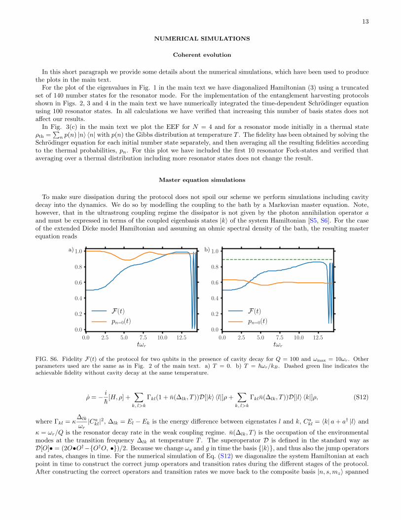
To make sure dissipation during the protocol does not spoil our scheme we perform simulations including cavitydecay into the dynamics. We do so by modelling the coupling to the bath by a Markovian master equation. Note,however, that in the ultrastrong coupling regime the dissipator is not given by the photon annihilation operator aand must be expressed in terms of the coupled eigenbasis states |k〉 of the system Hamiltonian [S5, S6]. For the caseof the extended Dicke model Hamiltonian and assuming an ohmic spectral density of the bath, the resulting masterequation reads

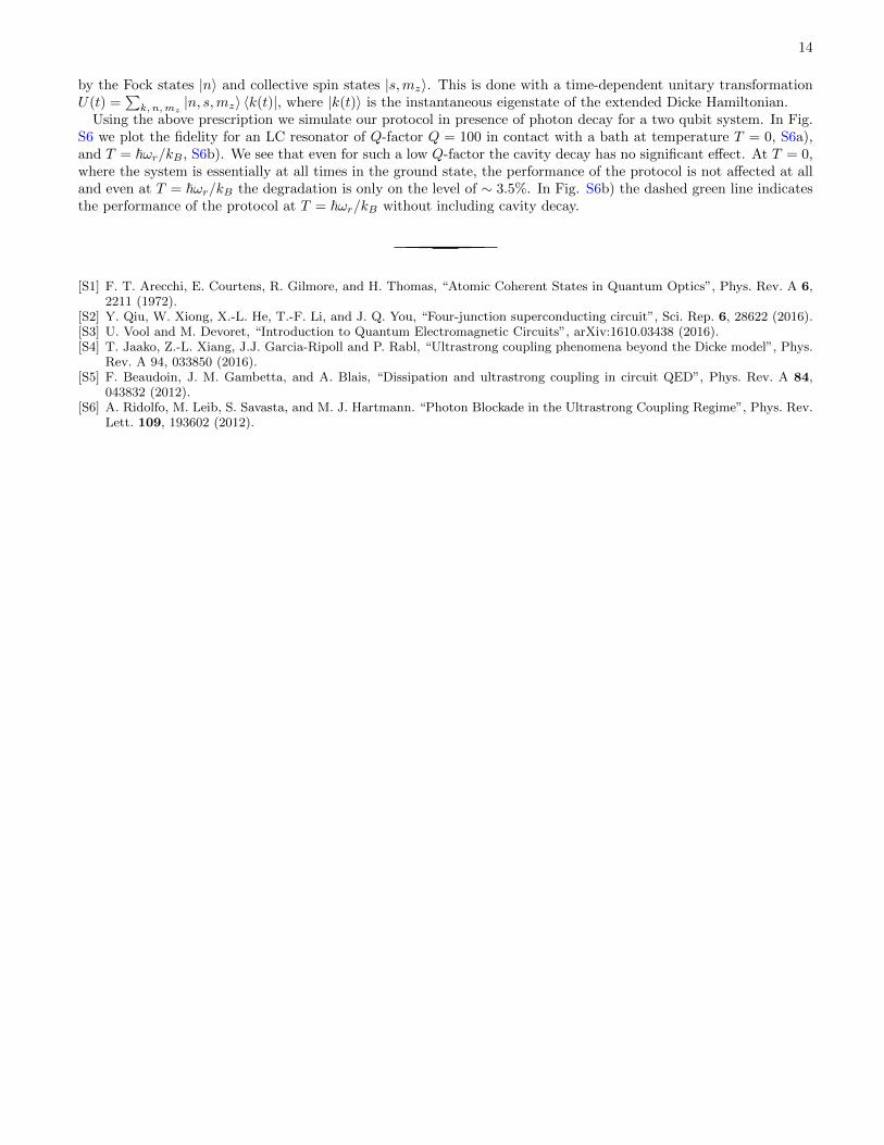
a) b)

FIG. S6. Fidelity F(t) of the protocol for two qubits in the presence of cavity decay for Q = 100 and ωmax = 10ωr. Otherparameters used are the same as in Fig. 2 of the main text. a) T = 0. b) T = ~ωr/kB . Dashed green line indicates theachievable fidelity without cavity decay at the same temperature.

ρ = − i~

[H, ρ] +∑k, l>k

Γkl(1 + n(∆lk, T ))D[|k〉 〈l|]ρ+∑k, l>k

Γkln(∆lk, T ))D[|l〉 〈k|]ρ, (S12)

where Γkl = κ∆lk

ωr|Cakl|2, ∆lk = El − Ek is the energy difference between eigenstates l and k, Cakl = 〈k| a+ a† |l〉 and

κ = ωr/Q is the resonator decay rate in the weak coupling regime. n(∆lk, T ) is the occupation of the environmentalmodes at the transition frequency ∆lk at temperature T . The superoperator D is defined in the standard way asD[O]• = (2O•O†−O†O, •)/2. Because we change ωq and g in time the basis |k〉, and thus also the jump operatorsand rates, changes in time. For the numerical simulation of Eq. (S12) we diagonalize the system Hamiltonian at eachpoint in time to construct the correct jump operators and transition rates during the different stages of the protocol.After constructing the correct operators and transition rates we move back to the composite basis |n, s,mz〉 spanned

14

by the Fock states |n〉 and collective spin states |s,mz〉. This is done with a time-dependent unitary transformationU(t) =

∑k, n,mz

|n, s,mz〉 〈k(t)|, where |k(t)〉 is the instantaneous eigenstate of the extended Dicke Hamiltonian.Using the above prescription we simulate our protocol in presence of photon decay for a two qubit system. In Fig.

S6 we plot the fidelity for an LC resonator of Q-factor Q = 100 in contact with a bath at temperature T = 0, S6a),and T = ~ωr/kB , S6b). We see that even for such a low Q-factor the cavity decay has no significant effect. At T = 0,where the system is essentially at all times in the ground state, the performance of the protocol is not affected at alland even at T = ~ωr/kB the degradation is only on the level of ∼ 3.5%. In Fig. S6b) the dashed green line indicatesthe performance of the protocol at T = ~ωr/kB without including cavity decay.

[S1] F. T. Arecchi, E. Courtens, R. Gilmore, and H. Thomas, “Atomic Coherent States in Quantum Optics”, Phys. Rev. A 6,2211 (1972).

[S2] Y. Qiu, W. Xiong, X.-L. He, T.-F. Li, and J. Q. You, “Four-junction superconducting circuit”, Sci. Rep. 6, 28622 (2016).[S3] U. Vool and M. Devoret, “Introduction to Quantum Electromagnetic Circuits”, arXiv:1610.03438 (2016).[S4] T. Jaako, Z.-L. Xiang, J.J. Garcia-Ripoll and P. Rabl, “Ultrastrong coupling phenomena beyond the Dicke model”, Phys.

Rev. A 94, 033850 (2016).[S5] F. Beaudoin, J. M. Gambetta, and A. Blais, “Dissipation and ultrastrong coupling in circuit QED”, Phys. Rev. A 84,

043832 (2012).[S6] A. Ridolfo, M. Leib, S. Savasta, and M. J. Hartmann. “Photon Blockade in the Ultrastrong Coupling Regime”, Phys. Rev.

Lett. 109, 193602 (2012).