1

PRACE Spring School in Computational Chemistry 2014

Quantum Chemistry Workshop (Advanced)Excitation Energies and Excited State Densities

Mikael Johanssonhttp://www.iki.fi/~mpjohans

Objective: To learn how to compute electronic excitation energies at density functional theoryand the approximate second-order coupled cluster (CC2) levels using the program systemTURBOMOLE, as well as visualising how the total electron density is changed upon excitation

2

TD-DFT excitation energies

· Computing electronic excitation spectra (UV/VIS) is these days possible for large molecules due toefficient implementations of time-dependent density functional theory (TD-DFT). Despite the name,the most common usage of TD-DFT is to compute excited state properties within the linear responseframework. In the case of excitation energies, no time dependence is actually modelled.

· Note that with excitation energies available, also excited state potential energy surfaces are available.

· With modern software (and hardware), TD-DFT calculations can routinely be performed formolecules with hundreds of atoms.

· The quality of excitation energies obtained by TD-DFT depends on the exchange-correlationfunctional used.o Relative excitation energies are reproduced better than absolute valueso Hybrid functionals usually perform better compared to GGA functionals. The part of exact

exchange that hybrids include help correct for the wrong asymptotic behaviour that mostfunctionals suffer from. Long-range corrected functionals (LC-DFT) usually fare even better.

· Generally, the results obtained by TD-DFT have been found to be satisfactory, especially consideringhow computationally cheap they are to compute.

3

TD-DFT excitation energies

· There are some special categories of excitations that approximate functionals describe quite poorly:o Conical intersections a the excited PES (multi-reference treatment necessary)o Excitations that have double excitation charactero Rydberg excited stateso Charge transfer excitations

· In CT excitations, the incoming photon excites an electron which then moves over a large distance inthe molecule. Standard TDDFT severely underestimates these excitation energies!o For a good overview with examples of this, see for example A. Dreuw, M. Head-Gordon, J. Am.

Chem. Soc. 126 (2004) 4007. http://dx.doi.org/10.1021/ja039556n

4

CC2 excitation energies

· The singles and approximate doubles coupled cluster model CC2 is an alternative to TDDFT forcomputing excitation energies on large systems.

· While not (yet) as fast as TDDFT, quite large systems can already be studied. Of the wave-functionbased methods of computing excitation energies, it has, arguably, the best price/performance ratio.o It can describe charge transfer excitationso Still problems with double excitations, but you can get a diagnostic telling you if it’s a problem!

· For a bit more background and an illustrative example, see C. Hättig, A. Hellweg, A. Köhn,”Intramolecular Charge-Transfer Mechanism in Quinolidines:  The Role of the Amino Twist Angle”, J.Am. Chem. Soc. 128 (2006) 15672. http://dx.doi.org/10.1021/ja0642010

Without further ado, let’s go through the basic usage of TURBOMOLE, the program of choice today.

5

The Program System TURBOMOLE — An Introduction

TURBOMOLE can compute a lot of stuff at HF, DFT, and correlated wave-function theory levels: Excitationenergies, vibrational spectra, circular dichroism spectra, excited state geometries, etc. Quite fast, and inmany cases has the nice ability to use very high symmetry groups, not only Abelian (non-degenerate) pointgroups.

Web pages:

· http://www.turbomole.como Manuals, tutorials

· http://www.turbo-forum.como Some user discussion

6

TURBOMOLE usage philosophy

· The usage adapted to the way a UNIX user is working:o Command line driveno Many different programs instead of one big binary, each specialised for a limited number of

method and/or propertieso Scripts used to combine the functionalities of the different programso Input can be changed by text editorso Output processed by standard UNIX tools (editors, grep, awk, ...)

Setting up the environment

· TURBOMOLE version 6.5 is installed on your exercise computers· If needed, initialisation will be performed interactively

7

Defining your calculations

· First, you will need a file that contains the coordinates of your molecule· In TM, this file is named coord, and has the following basic structure:

$coord 0.00000000000000 0.00000000000000 -0.77150594423227 o -1.43383351516326 0.00000000000000 0.38575297211615 h 1.43383351516326 0.00000000000000 0.38575297211615 h$end

· Note that the Cartesian coordinates are given in atomic units (Bohr), not Ångströms!o The tools x2t and t2x transform between TM format and standard XYZ formato OpenBabel can handle many more formats

§ babel –ixyz molecule.xyz –otmol coord§ babel –ipdb enzyme.pdb –otmol coord

· Second, you will use a program called define to specify what kind of calculation you want toperform; go to your working directory and give the command define

8

· define will interactively ask you plenty of questionso What are your coordinateso What is the symmetry of the moleculeo What basis set do you want to use? NOTE: Use the def2 basis sets instead of the older def!o The charge of your molecule?o Level of calculation?o etc.

We will go through these interactively during theexercise, but some points to consider

· At least the m4 grid is recommended· The following TDDFT XC functionals are available:

o LDA (s-vwn, pwlda)o BP86 (b-p)o PBE(0) (pbe, pbe0)o B3LYP (b3-lyp)o BHLYP (bh-lyp)o BLYP (b-lyp)o TPSS(h) (tpss, tpssh)

9

· After running define, you will have a file name control in your directory. This contains thespecifications of your calculations

· Most of the parameters that define has put in there are OK, but some need to manually bechanged:o Remove the line that says $scfdump. This keyword tells TM to save orbitals to disk after every

SCF cycle. This will slow down your calculations notably.§ Tip: You can quickly remove keywords from the control file with the kdg (kill data group)

command: kdg scfdumpo To further prevent disk usage, edit the line starting with $thize (threshold for integral size to be

saved onto disk), increasing its parameter to:§ $thize 0.10000000E+99 (only relevant for non-RI calcs)

o For response calculations, a well-converged reference ground state is necessary, so tighten theenergy and density convergence criteria:§ $scfconv 7 (even higher values could be necessary)§ $denconv 1.d-7

10

Running your calcs — HF and DFT single points

· SCF single points can be computed with two programs (relevant today)o dscf non-RI for Hartree—Fock and hybrid functionalso ridft RI-DFT for pure functionals (for GS, also usable for HF exchange)

· The GS calculation needs to be performed before response properties like excitation energies· When the job has finished, it is a good idea to check that the calculation has converged properly. A

quick check is to see if the file named energy contains a line with the final energy. Also look at theoutput of your calculation.

· Use eiger for a quick check that you haven’t ended up in an exited state configuration!o TM doesn’t change the orbital occupations during the SCF from that defined in the control

file, so if the initial EHT guess got the orbital configuration wrong, it will stay wrong unlessmanually corrected

o For excitation energy calcs, the HOMO—LUMO gap needs to be positive (at least for the orbitalsymmetry you want to excite); at DFT level, this is not always possible, even if your electronicconfiguration is correct...

11

DFT geometry optimisation

· It might be a good idea to optimise your molecular structure· At DFT level, this is simple, just run the jobex script:

o jobex –dscf non-RI DFTo jobex –dscf –ri RI-DFT

· After optimisation, the directory should contain a file named GEO_OPT_CONVERGEDo If it doesn’t, something went wrong...

· You can check how the gradient changed during optimisation with for example:o grep dE gradient

· For some speedup, the SCF convergence thresholds don’t usually need to be as tight as for theresponse calcs!

12

DFT singlet excitation energies

· To get TM to compute excitation energies after a successful ground state calculation, it needs someextra information on what to calculate. This can be done via define or by editing the control fileby hand. A few lines need to be inserted (before the $end keyword)

$scfinstab rpas$soes

a1 2 b2 2

$rpacor 500

· $scfinstab rpas tells TM to perform a TDDFT calculation for singlet excitations· The $soes keyword defines how many excitations in each irrep are to be computed (the existing

irreps depend on the symmetry of your molecule)o Note! After a successful run, you can increase the number of excitations in an irrep and start

the calculation anew; TM will reuse the already converged roots, saving time.· $rpacor tells the program to use about 500 MB of memory for the calc. The more, the faster,

usually.

13

· You can also tell TM to create a file for you with the excitation energies in brief form, by adding:o $spectrum eV / $spectrum nm / $spectrum 1/cm / $spectrum a.u.o Irritatingly, only irreps with allowed transitions are included

· The name of the program that computes excitation energies (at HF and DFT levels) is escfo escf > escf.out

· Check escf.out for the information you need

DFT triplet excitation energies

· Triplet excitation energies are obtained simply by changing the $scfinstab keyword:o $scfinstab rpat

DFT excitation energies from open-shell ground states

· For exciting open-shell species, change the $scfinstab keyword accordingly:o $scfinstab urpa

14

DFT circular dichroism (CD) spectra

· Easy, just add a keyword to control and run escf:o $cdspectrum eV / $cdspectrum nm / $cdspectrum 1/cm / $cdspectrum a.u.

Visualising how the electron moves when excited with DFT

· It is possible to compute the electron density difference between the ground and excited state· This shows how the electron moves within the system when excited· For this, excited state gradients are needed. Even if we will not optimise the excited state geometry

today, the gradient calculation provides the information needed for the density differenceo Gradients are not yet available for meta-GGAs (TPSS, TPSSh)

· Again, editing the control file is necessary. First, insert the following line to compute the differencedensities on a 3D grid:o $pointval fmt=cub

· fmt=cub tells TM that the output format of the grid should be in Gaussian cube format, whichmany visualisation programs know how to interpret.

15

· Next, specify which excitation you want to study more closely (only one at a time!), that is, edit the$soes keyword to only contain one irrep. Now, the highest excitation specified will be computed.Example:

$soes b1 2

· The above will lead to a computation of the gradient and at the same time the density difference foronly the second state in the b1 irrep of your molecule.

· To compute others, you need to change the $soes keyword and make another run

· The program computing excited state gradients (HF and DFT) is called egrad:o egrad > egrad.out

· When completed, you should see a file named ed.cub containing a 3D grid of the density difference· In an open-shell calculation, you should also have esd.cub, with the differential spin density.· Note! If you change the control file to compute the density difference for other irreps, remember

to save your ed.cub file with another name; it will be overwritten!

16

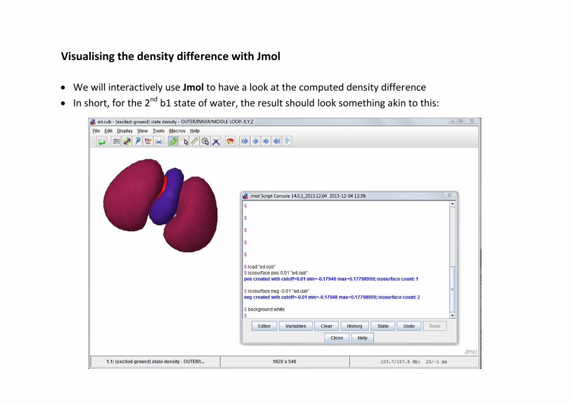
Visualising the density difference with Jmol

· We will interactively use Jmol to have a look at the computed density difference· In short, for the 2nd b1 state of water, the result should look something akin to this:

17

CC2 excitation energies

· For CC2 excitation energies, a well-converged Hartree—Fock calculation (with dscf) is aprerequisiteo Start in a new, fresh directory ensuring there’s no $dft keywords in the control file

· For correlated wave-function methods, the core orbitals should be frozen, that is, uncorrelated,unless special basis sets are used. Also, special auxiliary basis sets need to be specified. This is mostconveniently done with define:o Just press Enter until you reach the final screen of define, then choose the cc submenuo choose freeze and accept the suggested valueso choose cbas, which automatically should find the correct auxiliary basis set, and exit

· After this, let’s go manual on the control file. Insert the following lines:

$ricc2 cc2

· The $ricc2 keyword defines the model to use. The ricc2 program can actually do calcs atseveral levels of theory, today we want CC2o See the manual for other options; CCS/CIS, CIS(D), ADC(2), ...

18

· To get only (singlet) excitation energies, insert something like the following:

$excitations irrep=a1 multiplicity=1 nexc=2 irrep=b2 multiplicity=1 nexc=2

· The $excitations keyword is the CC2 equivalent of the $scfinstab and $soes keywordsused for DFT. Again, make separate lines for all irreps you are interested in.o multiplicity=1 defines singlet excitations (for triplet energies, simply change to 3)o nexc=2 says we want two excitations in the corresponding irrep

· To get oscillator strengths add this to the $excitations group:

spectrum states=all

o This is not implemented for triplet excitations, so the program will crash upon attempt.

· As for DFT, you can use the $spectrum and $cdspectrum keywords; at CC2 level, they evenseem to work properly!

19

Running CC2 calcs

· As mentioned, the program for performing CC2 calculations is called ricc2· In contrast to DFT calculations with TURBOMOLE, the same program does ”everything”, that is, GS

properties, excitation energies, gradients and so on are computed depending on the contents ofthe control file.o ricc2 > ricc2.out

· Note! Presently only non-degenerate point groups can be used for CC2 excitation energieso Practical consequence: If the symmetry is higher, you need to include all excitations that

have the same energy due to the true symmetry of the system (in different subsymmetries,including C1) in the calculations; otherwise you will most likely experience convergenceproblems!

20

CC2 densities

· To get the total density of the ground state add:

$response static relaxed

· This should produce a file named something like cc2-gsdn-1a1-000-total.cao

· To get the densities of excited states, gradients have to be computed, just as for DFT; add thefollowing to $excitations

xgrad states=(b1 2)

· Above, the gradient of 2nd excited state of the b1 irrep will be computed, and the excited statedensity should be produced, look for a file called cc2-xsdn-1b1-002-total.cao

· With ricc2, you can compute gradients for more than one state at a time, and thus for exampleget the densities of all computed excited states in one go via

xgrad states=all

21

· To get the density difference between the GS and XS, ricc2 has to be run in analysis mode afterobtaining the .cao files containing the densities

· Insert the following into the control file:

$anadens calc ED-1b1-2 from ← You can of course change the file name 1d0 cc2-xsdn-1b1-002-total.cao ← Check that you actually have these -1d0 cc2-gsdn-1a1-000-total.cao$pointval fmt=cub

· You should get a file named ED-1b1-2.cub by running:o ricc2 –fanal > ricc2-fanal.out

· To finish, have a look at the produced density difference with Jmol.