1

Quantum Annealing of Hard Problems

Thomas Jorg1, Florent Krzakala2,3, Jorge Kurchan4 and A. C . Maggs2

1 CNRS et ENS UMR 8549, 24 Rue Lhomond, 75005 Paris, France, LPTENS2 CNRS; ESPCI, 10 rue Vauquelin, Gulliver, Paris, France 75005, PCT

3 Theoretical Division and Center for Nonlinear Studies, Los Alamos NationalLaboratory, NM 87545 USA

4 CNRS; ESPCI, 10 rue Vauquelin, UMR 7636, Paris, France 75005, PMMH

Quantum annealing is analogous to simulated annealing with a tunneling mechanismsubstituting for thermal activation. Its performance has been tested in numerical simulationwith mixed conclusions. There is a class of optimization problems for which the e!ciency canbe studied analytically using techniques based on the statistical mechanics of spin glasses.

§1. Introduction

Solving hard combinatorial problems by temperature annealing is a classic methodin computer science.1) The problem is formulated in terms of a cost function, whichone can identify as an energy. The dynamics are then a combination of a systematicdescent in energy perturbed by a ’noise’, which is turned o! gradually, inducingoccasional upward jumps. This thermal activation allows the system to surmountbarriers and avoid getting blocked in a local minimum.

Quantum annealing is an analogous procedure, but with quantum tunneling sub-stituting for thermal activation. A major question is whether quantum algorithmsthat anneal by gradually turning o! the term that induces quantum jumps2), 3) –such as a transverse magnetic field in spin systems – can be an e"cient strategy thatoutperforms classical optimization methods.

In the past few years, there have been several attempts to simulate quantumannealing of simple ”benchmark” models, in order to estimate the scaling of thetime ! needed in terms of the system size N .2), 3), 5) This time is bounded by theminimal energy gap " between the ground state and the first excited state: onecan estimate2), 3), 13) the time needed for quantum annealing to find the ground stateas ! ! "!2 . In the most optimistic scenario,5) a problem taking ! " eaN in aclassical computer would be solved in ! " N! in a quantum one – corresponding toa minimal gap " N!!/2. A more modest achievement, would be that the problemstays exponential, but with a smaller coe"cient a (as is the case of the Grover7)algorithm): this is what would at best happen if the gap is exponentially small.

Because, at present, the simulations are done emulating quantum systems withclassical computers, the sizes accessible are rather small, and the extrapolation of thegap dependence to larger systems risky. For this reason, it is particularly desirableto have an analytic framework within which one can compute " for a representativeclass of models. In a recent work, we have considered the group of systems havinga ’Random First Order’ (RFO) glass transition.4) This class of models11) is cur-

typeset using PTPTEX.cls #Ver.0.9$

arX

iv:0

910.

5644

v1 [

quan

t-ph]

29

Oct

200

9

2 Jorge Kurchan

rently believed to be the mean-field version of the glass transition12) and randomheteropolymer folding.14) It also includes random constraint satisfaction problemssuch as random satisfiability15) (the energy to be minimized is the number of violatedconstraints) and is closely related to the random code ensemble in coding theory.17)

The phase diagrams of quantum spin glasses have been investigated extensivelyover the last thirty years, using a formalism combining the Replica10) and the Suzuki-Trotter methods18), 19), 23) in order to deal simultaneously with disorder and quantummechanics. This formalism was first applied by Goldschmidt18) to the paradigmof the class, the quantum Random Energy Model. An important result is thatthe quantum transition is of first order (with a discontinuity in the energy) at lowtemperature for all RFO models, unlike their classical transition in temperature,which is thermodynamically of second order.

In order to assess the e"ciency of quantum annealing knowledge of the thermo-dynamics of the model is not enough; we must compute the gap between the twolowest eigenvalues. This is not given by the usual replica solution, and one has todevelop stronger techniques to obtain it. In what follows, we shall first show howto solve the Quantum Random Energy Model by elementary methods, including thecalculation of the gap. Quantum Annealing turns out not to be an e"cient wayof computing its ground state for reasons that are very clear and require minimaltechnique to understand. Unfortunately, such elementary perturbative methods donot allow us to solve a general model of the class, and in particular to computethe minimal gap. We have hence to resort to more powerful, yet less transparent,methods which we have developed and we shall describe below.

As we shall see, the minimal gap between the lowest states in all models of theRFO class can be expected to be exponentially small in N , implying that quantumannealing is an exponentially slow algorithm for those problems.

§2. The simplest case: Random Energy Model

The random energy model9) is the simplest mean field spin-glass model,11) yetit allows us to understand the very complex mechanisms of the mean-field spin-glass11) and glass transitions.12) We shall first use this model to study the e!ect ofa quantum transverse field in the mean field transition in spin-glasses. The problemwas already investigated twenty years ago,18) by considering the p % & limit ofp-spin model using the replica method and the Suzuki-Trotter formalism, and manygeneralizations followed.23) Here we shall show that it can be solved in a very simpleway, that does not require the use of replica techniques. We consider N quantumspins # in a transverse field $ with the Hamiltonian

H({#}) = E({#z}) + $V = E({#z}) + $N!

i=1

#xi (2.1)

E({#z}) denotes a quenched random function that is diagonal in the basis |#z1$ '

|#z2$ ' ... ' |#z

N $ and consists of 2N random, uncorrelated values. These values aretaken from a Gaussian distribution of zero mean and variance N/2, as in the classical

Quantum annealing 3

REM.9) H is thus a 2N(2N matrix whose entries are Haa = Ea (the random energies)and Hab = $ if a and b are two configurations that di!er by a single spin flip, andzero otherwise. Note that since H is sparse, it can be studied numerically even whenits dimensions are large.

Just as in the classical case, a concrete implementation of the model is a spinglass with p-spin interactions, in the large p limit:

H = )!

i1<...<ip

Ji1...ip#zi1 . . . #z

ip ) $N!

i=1

#xi * T + $V, (2.2)

where Ji1...ip are Gaussian variables with variance"

p!Np!1

2.1. Two easy limitsThe model is trivially solved in the limits $ % 0 and $ %&.a) $ = 0: For $ = 0, we recover the classical REM with N Ising spins and 2N

configurations, each corresponding to an energy level E!:11) Call n(E) the numberof energy levels belonging to the interval (E,E+dE); its average over all realizationsis easily computed: n(E) = 2NP (E) ! eN((ln2!E2/N2)) = eNs(E/N), wheres(e) = ln2) e2 (with e = E/N). There is therefore a critical energy densitye0 = )

+ln2 such that, if e < e0, then with high probability there are no configura-

tions while if e > e0 the entropy density is finite. A transition between these tworegimes arises at 1

Tc= ds(e)

de

##e0

= 2+

ln2 and the thermodynamic behavior follows:i) For T < Tc, fREM = )

+ln2 and the system is frozen in its lowest energy states.

Only a finite number of levels (and only the ground state at T = 0) contributeto the partition sum. The energy gap between them is finite. (ii) For T > Tc,fREM = ) 1

4T ) T ln2; exponentially many configurations contribute to the partitionsum.

b): In the opposite case of $ % &, the REM contribution to the energy canbe neglected. In the #x basis, we find N independent classical spins in a field $ ; theentropy density is just given by the log of a binomial distribution between )$N and+$N and the free-energy density is fpara = )T ln2) T ln((cosh$/T )).

2.2. Perturbation theory

Between these two extreme limits, it turns out that nothing much happens: thesystem is either in the ”classical” or in the ”extreme quantum” phase, and it jumpssuddenly – in a first order fashion – from one to the other. This is important forus, since it means that most of the e!ort in quantum annealing is in fact wastedin staying on the same state, until suddenly the wave function projects onto theexact solution, and then never changes again. At low value of $ , the free-energydensity is that of the classical REM, while for larger values it jumps to the quantumparamagnetic (QP) value fQP; a first-order transition separates the two di!erentbehaviors at the value $ such that fREM = fQP (see center panel of Fig. 2).

Let us see how this comes about in the restricted case of zero temperature,

4 Jorge Kurchan

using Rayleigh-Schrodinger perturbation theory.20) Consider the set of eigenvaluesEk and eigenvectors |k$ of the unperturbed REM, when $ = 0. The series for agiven perturbed eigenvalue Ei($ ) reads

Ei($ ) = Ei +

$i

#####

"!

n=0

$V

%Q

Ei )H0(Ei ) Ei($ ) + $V )

&n##### i

',

where the projector Q =(

k #=i |k$#k| so that

Ei($ ) = Ei + $Vii +!

k #=i

$ 2VikVki

Ei ) Ek+ · · · . (2.3)

Since Vij ,= 0 if and only if i and j are two configurations that di!er by a single spinflip, odd order terms do not contribute in Eq. (2.3), as one requires an even numberof flips to come back to the initial configuration in the sums. If the starting energyEi is close to the ground state, it is negative and of order N . On the other hand,the vast majority of levels have energies Ek " O(

+N) . Hence, all terms of the form

(Ek )Ei) " O(N): the spin flips from the lowest levels induced by the #x operatorsdo not connect the lowest states amongst themselves. One obtains, starting from anlow eigenvalue [)Ei = O(N)], that

!

k #=i

V 2ik

Ei ) Ek=

1Ei

N!

k=1

)1 +

Ek

Ei+ · · ·

*=

N

Ei+ O

)1N

*,

where we have used that the Ek are random and typically of order+

N . Higher nthorders are computed in the same spirit and are found to be O(Nn/2!1). Therefore,to all (finite) orders, we have for the energy density %i = Ei

N :

%i($ ) = %i +$ 2

N%i+ ... = %i + O

)1N

*. (2.4)

This analytic result compares well with a numerical evaluation of the eigenvalues (leftpanel of Fig. 2). Note that the energy density of all extensive levels is independentof $ to leading order in N , as are hence s(e) and f(T ).

A similar expansion can also be performed around the extreme quantum limit,using $V as a starting point and H0 as a perturbation. Consider the ground statewith eigenvalue E0($ ) and the unperturbed ground state having all spins alignedalong the x-direction, with EV

0 ($ ) = )$N . In the base corresponding to the eigen-values of $V , we find

E0($ ) = EV0 ($ ) + #0 | H0 | 0$+

!

k #=0

|#k | H0 | 0$|2

EV0 ($ )) EV

k ($ )+ · · · .

The first-order term gives(2N

!=1 EREM! |v!|2. Since the energies of the REM are

random and uncorrelated with v! this sums to O(+

N2!N/2). For the second-order

Quantum annealing 5

term, one finds!

k #=0

|#k | H0 | 0$|2

EV0 ($ )) EV

k ($ )=

1EV

0 ($ )

!

k #=0

|#k | H0 | 0$|2

1) EVk ($ )/EV

0 ($ )

- 1EV

0 ($ )#0 | H2

0 | 0$ =N

2EV0 ($ )

+ o(1). (2.5)

Subsequent terms are treated similarly and give vanishing corrections so that %0($ ) =)$ ) 1

2N" + O( 1N2 ). Again this derivation holds for other states with extensive

energies )EVi ($ ) = O(N), the only tricky point being the degeneracy of the eigen-

values,21) and for these excited eigenstates, the perturbation starting from the large$ phase yields %i($ ) = %V

i ($ )) 12N" +O( 1

N2 ). Just as in the opposite classical limit,to leading order in N , energy, entropy and free-energy densities are not modified bythe perturbation.

2.3. Phase diagram and the closure of the gap

0

0.2

0.4

0.6

0.8

1

1.2

1.4

0 0.2 0.4 0.6 0.8 1 1.2

T

Γ

REM ’frozen’

REM ’unfrozen’

Quantum Paramagnet

f=-(ln2)1/2

f=-T ln(2)-1/4Tf=-T ln(2)

-T ln cosh(Γ/T)

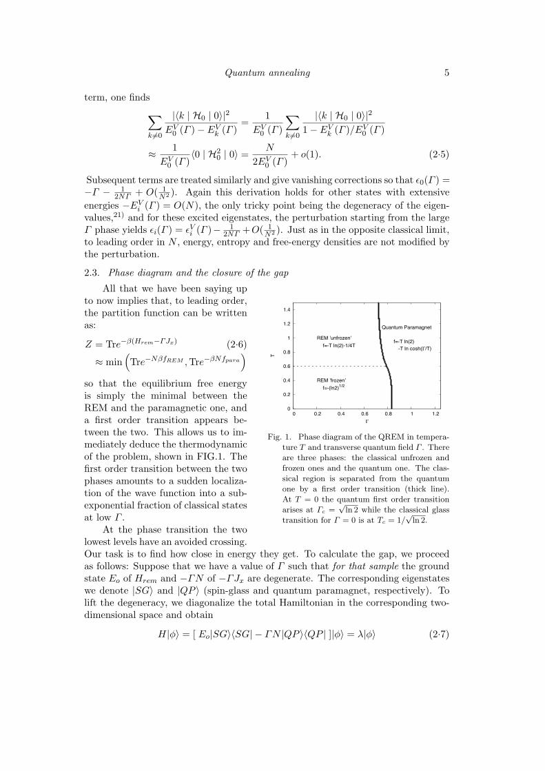
Fig. 1. Phase diagram of the QREM in tempera-ture T and transverse quantum field ! . Thereare three phases: the classical unfrozen andfrozen ones and the quantum one. The clas-sical region is separated from the quantumone by a first order transition (thick line).At T = 0 the quantum first order transitionarises at !c =

!ln 2 while the classical glass

transition for ! = 0 is at Tc = 1/!

ln 2.

All that we have been saying upto now implies that, to leading order,the partition function can be writtenas:

Z = Tre!#(Hrem!"Jx) (2.6)

- min+Tre!N#fREM ,Tre!#Nfpara

,

so that the equilibrium free energyis simply the minimal between theREM and the paramagnetic one, anda first order transition appears be-tween the two. This allows us to im-mediately deduce the thermodynamicof the problem, shown in FIG.1. Thefirst order transition between the twophases amounts to a sudden localiza-tion of the wave function into a sub-exponential fraction of classical statesat low $ .

At the phase transition the twolowest levels have an avoided crossing.Our task is to find how close in energy they get. To calculate the gap, we proceedas follows: Suppose that we have a value of $ such that for that sample the groundstate Eo of Hrem and )$N of )$Jx are degenerate. The corresponding eigenstateswe denote |SG$ and |QP $ (spin-glass and quantum paramagnet, respectively). Tolift the degeneracy, we diagonalize the total Hamiltonian in the corresponding two-dimensional space and obtain

H|&$ = [ Eo|SG$#SG|) $N |QP $#QP | ]|&$ = '|&$ (2.7)

6 Jorge Kurchan

Multiplying this equation by #SG| and #QP |, respectively:

) '#SG|&$ = Eo#SG|SG$#SG|&$ ) $ #SG|X$#SG|&$)'#QP |&$ = Eo#QP |SG$#SG|&$ ) $ #QP |QP $#QP |&$ (2.8)

In order for ' to be an eigenvalue, the determinant of this system must vanish

) (Eo ) ')($ + ') + Eo$ #SG|QP $2 = 0 (2.9)

where we have used that the states are normalized. The gap is the di!erence of thetwo solutions and reads

gap(N, $ )2 = ($ ) Eo)2 ) 4-)Eo$ + Eo$ #SG|QP $2

.(2.10)

and at its minimum with respect to $ , we thus get

gapmin(N) = 2|Eo|2!N/2 (2.11)

-26

-24

-22

-20

-18

-16

-14

0 0.2 0.4 0.6 0.8 1 1.2

E n(Γ

) for

N=2

0, 4

0 lo

west

eig

enva

lues

Γ

0.001

0.01

0.1

1

8 10 12 14 16 18 20 22 24

Δm

in(N

)

N

Analytics

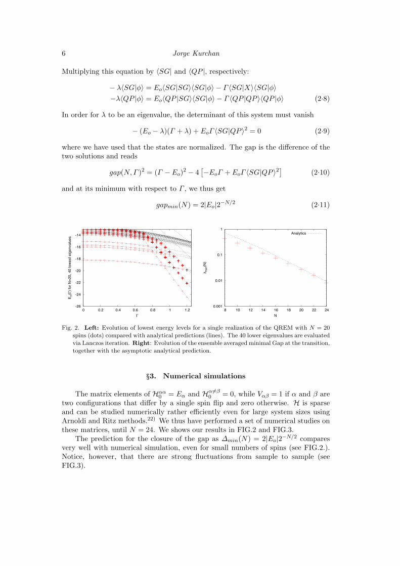
Fig. 2. Left: Evolution of lowest energy levels for a single realization of the QREM with N = 20spins (dots) compared with analytical predictions (lines). The 40 lower eigenvalues are evaluatedvia Lanczos iteration. Right: Evolution of the ensemble averaged minimal Gap at the transition,together with the asymptotic analytical prediction.

§3. Numerical simulations

The matrix elements of H!!0 = E! and H! #=#

0 = 0, while V!# = 1 if ( and ) aretwo configurations that di!er by a single spin flip and zero otherwise. H is sparseand can be studied numerically rather e"ciently even for large system sizes usingArnoldi and Ritz methods.22) We thus have performed a set of numerical studies onthese matrices, until N = 24. We shows our results in FIG.2 and FIG.3.

The prediction for the closure of the gap as "min(N) = 2|Eo|2!N/2 comparesvery well with numerical simulation, even for small numbers of spins (see FIG.2.).Notice, however, that there are strong fluctuations from sample to sample (seeFIG.3).

Quantum annealing 7

0

0.5

1

1.5

2

2.5

3

0 0.2 0.4 0.6 0.8 1 1.2 1.4

Δ

Γ

N=12

0

0.5

1

1.5

2

2.5

3

0 0.2 0.4 0.6 0.8 1 1.2 1.4

Δ

Γ

N=18

Fig. 3. Energy gaps between the ground state and the first excited state in the QREM for 10realizations for N = 12 (left) and N = 18 (right). Notice the strong fluctuations betweensamples. As N grows, the region where the gap closes shrinks and the slope around the criticalpoint is growing dramatically. This shows that one has to be extremely cautious when performingsimulation in this region.

§4. Computing the gap in the generic case within the replica method

The usual way of computing the free energy of a quantum spin system is to startwith the trace Tr[e!#H ]. One works in imaginary time and uses a a Suzuki-Trotterdecomposition.18), 25)–27) In this way one obtains an ansatz for the spin-glass phase,and a di!erent one for the quantum paramagnetic phase, yielding free energies FSG

and FQP , respectively through ))FSG " lnTr[e!#H ] or ))FQP " lnTr[e!#H ],depending on the phase.

Consider now the situation with the system near the phase transition, havingtwo almost degenerate ground states |SG$ and |QP $, HSG = #SG|H|SG$ " HQP =#QP |H|QP $ and a small interaction matrix element HI = #QP |H|SG$. To obtainthe gap between levels, we have already diagonalized this 2(2 matrix exactly in theprevious section. Alternatively, we can use the classical expansion:

Tr[e!#H ] =!

r

1r!

/dt1...dtre

![tSGtot HSG+tQP

tot HQP ] {HI}r (4.1)

where the system jumps at times t1, ..., tr between the states |SG$ and |QP $, tSGtot

and tQPtot = ) ) tSG

tot denote the total time spent in each state.What equation (4.1) tells us is that if we find a solution in imaginary time

that interpolates between the quantum paramagnet and the spin-glass solutions byjumping r times, t1, ..., tr, and we find that the free energy has a value:

)F{r jumps} " tSGtot FSG + tQP

tot FQP ) rG(interface) (4.2)

then by simple comparison lnHI " G(interface) leading to gap " eG. An extensivevalue of G for the interface implies an exponentially small matrix element, andhence an exponentially small gap. We shall now show that this is the situation forall models of the ‘Random First Order’ kind. Indeed, this is just the usual instanton

8 Jorge Kurchan

construction, the di!erence here will be that they take a rather unusual two-timeform in problems with disorder.

Let us look for solutions interpolating between vacua. We consider the p-spinmodel in transverse field and shall follow the presentation and notation$) of Obuchi,Nishimori and Sherrington.23) The Hamiltonian is:

H = )!

i1,...,ip

Ji1,...,ip#zi1 . . . #z

ip ) $!

i

#xi (4.3)

with P (Ji1,...,ip) =)

Np!1

*p!

*1/2

e!J2

i1,...,ipp! Np!1

(4.4)

In order to solve the system, we first apply the Trotter decomposition in orderto reduce the problem to a classical one with an additional “time” dimension:

Z = limM%"

Tr+e!#T/Me!#V/M

,M= lim

M%"ZM , (4.5)

where

ZM = CMNTr exp

0

1 )

M

M!

t=1

!

i1<...<ip

Ji1...ip#i1,t . . . #ip,t + BM!

t=1

!

i

#i,t#i,t+1

2

3 ,

(4.6)

and we have introduced the constants B = 12 ln coth #"

M and C =+

12 sinh 2#"

M

, 12 .

Replicating n times, and carrying over the averages over the interactions, weget:

[ZnM ] ! Tr exp

4)2J2N

4M2

M!

t,t"=1

n!

µ,$=1

41N

!

i

#µi,t#

$i,t"

5p

+ BM!

t=1

n!

µ=1

!

i

#µi,t#

µi,t+1

5,

where the replica indices are denoted by µ and +.In order to solve problem, it is then necessary to introduce a time-dependent

order parameter qµ$tt" and its conjugate Lagrange multiplier 6qµ$

tt" for the constraintqµ$tt" =

(i #

µi,t#

$i,t"/N . With these notations, the replicated trace reads:

[ZnM ] = e!N#F =

/ 7

µ<$

7

t,t"

dqµ$tt" d6qµ$

tt"

7

µ

7

t#=t"

dqµµtt" d6qµµ

tt"

( expN

8!

t,t"

!

µ<$

))2J2

2M2

9qµ$tt"

:p ) 1M2

6qµ$tt" q

µ$tt"

*

+!

t,t"

!

µ

))2J2

4M2

9qµµtt"

:p ) 1M2

6qµµtt" q

µµtt"

*+ Wo

;(4.7)

#) With the only exception of our qdtt! and qd

tt! , which correspond to their Rtt! and Rtt!

Quantum annealing 9

where Wo = log Tr exp ()He!), and:

He! = )B!

t

!

µ

#µt #µ

t+1 )1

M2

!

µ<$

!

t,t"

6qµ$tt" #

µt #$

t"

) 1M2

!

µ

!

t#=t"

6qµµtt" #

µt #µ

t" . (4.8)

We calculate the free energy of the replicated system in the thermodynamic limit bythe saddle-point method:

qµ$tt" = ##µ

t #$t"$ , 6qµ$

tt" =12)2J2p(qµ$

tt" )p!1,

qµµtt" = ##µ

t #µt"$ , 6qµµ

tt" =14)2J2p(qµµ

tt" )p!1 (4.9)

The brackets #· · · $ denote the average with the weight exp()He!).We now make the one-step replica symmetry broken ansatz: for every (t, t&) the

parameter qµ$tt" is as in Fig 4. Within the 1RSB ansatz, the replicated free energy

tt’

qµµ’ = ...

qdtt’qtt’

0

0

m

Fig. 4. The one-step replica symmetry breaking ansatz. The two-time two-replica overlap qµ!tt! has

the following structure. We divide replica in m groups and the overlap between replica indi"erent group is zero while the overlap between replicas of the same group is qtt! if the replicaare di"erent (/mu "= "), are qd

tt! is the replica are the same (µ = " on the diagonal).

reads:

) )f =/

dt dt&<))2J2

4(1)m)qp

tt"

+12(1)m)qtt"qtt" +

)2J2

4[qd

tt" ]p ) qd

tt"qdtt"

=)Wo[qd

t"t" , qtt" ] (4.10)

Up to here we have followed the standard steps18), 23), 25)–27) Solutions withinthis ansatz corresponding to the spin glass and the quantum paramagnet have beenstudied by several authors.18), 23), 25)–27) It turns out that the phenomenology forfinite the p is very close to that of the QREM.

10 Jorge Kurchan

We now part company with the previous literature, and consider a solutioncorresponding to the high-$ phase in the interval (0, t1), (t2, t3),..., that jumps to thelow-$ phase where it stays in the intervals (t1, t2), (t4, t5),.... The time-dependenceof qt,t" and qd

t,t" are is as in Fig. (5).

t t t

t

t

t

1 2 3

1

2

3

t

t’

(1,1)

(1,1)

(2,2)

(2,2)

(1,2) (1,2)

(1,2) (1,2)

(2,1) (2,1)

(2,1) (2,1)

1 2

1

2

(1,1)

(2,2)

(2,2)

1

2

1 2

(1,1)

Fig. 5. A multi-instanton configuration for qdt,t! , qt,t! , qd

t,t! and qt,t! . Three di"erent shadings cor-respond situations in which the system is in the glass phase at both times, the paramagneticphase at both times and in a di"erent phase at each time. In general, the functions qt,t! , qt,t!

are approximately constant well within each region, with smooth, finite width interfaces. Thediagonal elements qd

t,t! and qdt,t! have an additional crest along the diagonal t = t". In the large

p limit, we may neglect this crest, in the so-called ‘static approximation’. In addition qdt,t! and

qt,t! become either infinity or zero, with sharp interfaces: this allows for a complete solution atlarge p.

4.1. Recovering the REM resultLet us now specialize to the large-p situation, and we shall later indicate how

to proceed in general. Following Obuchi et al., we note the saddle point equationsimply that for large p either (qtt" , qd

tt" , qtt" , qdtt") = (1, 1,&,&) or (qtt" , qd

tt" , qtt" , qdtt") =

(< 1, < 1, 0, 0)). This implies that the form of the instanton configuration of qdtt"

and qtt" is the same as the one of (qtt" , qdtt" but with the values jumping from zero to

infinity. If in addition we make the ‘Static approximation’ that as applied to thiscase consists of assuming that inside each block the order parameters qd and qd areconstant, we conclude that for all times we can write the ‘tilde’ variables as:

2qdt"t" ) qt"t" = rd

t rdt" ; qt"t" = rtrt" (4.11)

where rt and rdt are large in the time intervals when the system is in the glass state,

and drop to zero when it is not. (The solutions in the literature correspond to time-independent r, taking a value corresponding to either the glass or the paramagneticphase)

Quantum annealing 11

Because qdt"t" , qt"t" are either zero or one, we can write:/

dt dt& qtt" qtt" "%/

dt r(t)&2

= I2

2/

dt dt& qtt" qdtt" =

/dt dt& [rd(t)rd(t&) + r(t)r(t&)] = I2

d + I2 (4.12)

with the definitions I *>

dt r(t) and Id *>

dt rd(t).We further decouple the replicas in the single-spin term in the usual way:

Wo = log Tr exp ()He!) = ) 1m

log</

Dz2

%/Dz3

Tr+e!B

Pt %t%t+1! 1

M

Pt(z2rt+z3rd

t )%t

,?m@(4.13)

We can go back to the quantum representation, to write the trace in (4.13) as asingle quantum-spin in a time-dependent field:

Tr+T e

Rdt"(A(t")%z+#"%x)

,(4.14)

where T denotes time-order (a necessity here because of the time-dependence in theexponent) , and A(t) * (z3rd

t + z2rt). In the periods where A is non zero, it has alarge real part and the spins are polarized along the z direction. During the periodswhen rt = rd

t = A = 0 only the transverse term proportional to $ plays a role. Thiscorresponds to the switching between spin-glass and quantum paramagnetic phases,respectively. The trace can be computed easily by changing bases accordingly. Atlow temperatures, the ‘field’ in the x direction )$ is strong, while the field in thez direction |A(t)| is either zero or |A(t)| >> )$ (for large p, cf. Eq. (4.9)). Weconclude then that only one polarization of the spin contributes in each time interval.Denoting

Tr+e

Rdt"(A(t")%z+#"%x)

," #z1|e

R tftn

dt"A(t")%z |z1$#z1|x$

#x|e#(tn!tn!1)"%x |x$ #x|z2$ . . . #zn|eR 0

t1dt"A(t")%z

|zn$ (4.15)

Where we have defined |x$ the lowest eigenvalue of #x, and the |zi$ are either thelowest or the highest eigenvalue of #z, depending on the sign of A(t) (which in turndepends on z2,z3) during that interval. Because, as mentioned above, at each timeonly one field dominates, and the way we chose the |zi$, we have:

#zi|eR tf

tndt"A(t")%z |zi$ " e

R tftn

dt"|A(t")| (4.16)

and#x|e#"%x |x$ " e#" (4.17)

Hence, if we denote tSG = ,) the total time in which rt, rdt are not zero, and

qt = qdt = 1, and tQP = (1),)) the rest, the action becomes:

) )f = ,2

<))2J2

4(1)m) +

)2J2

4

=) 1

2I2d )

m

2I2Wz

+ (1),))$ + (numb. of jumps)( ln |#x|z$| (4.18)

12 Jorge Kurchan

where

Wz = ) 1m

log</

Dz2

%/Dz3 e

Rdt|z2rt+z3rd

t |&m=

= ) 1m

log</

Dz2

%/Dz3 e|z2I+z3Id|

&m=

This can be evaluated by saddle point,18), 23) putting z3 = Idy3 and z2 = Iy2 andrecognizing that I, Id are large. There are two saddle points: (y2 = 1, y3 = 1) and(y2 = )1, y3 = )1) with the same contribution. A short calculation yields:

Wz "12I2d +

m

2I2 + ln(2) (4.19)

Equation (4.18) becomes

) )f = m,2 )2J2

4) ln(2)

m+ (1),))$ + (numb. of jumps)( ln |#x|z$| (4.20)

Taking saddle point with respect to m gives m = 2'

2&#J . We finally obtain

) )f = ,A

ln(2))J

2+ (1),))$ + (numb. of jumps)( ln |#x|z$| (4.21)

This formula is of the form (4.2). It gives the contribution to Tr[e!#H ] of the processwith a number of jumps spending a fraction , in the glass state and (1),) in theparamagnetic state. We have hence showed that the logarithm of matrix element isindeed the single-spin element " N ln |#x|z$| = )N ln(2) from which we recover thegap " 2!N obtained previously.

4.2. The general caseIn the general case, we need to determine the functions qd

tt" and qtt" for theinterval 0 < t, t& < ). It su"ces to compute a single jump solution, and to calculatethe free energy cost of the ”wall” in the two times. This may be done numerically,discretizing the times (i.e. working in a two-time grid) and minimizing with respectto qtt" while maximizing with respect to the diagonal replica parameters qd

tt" , as isusual in the replica trick.

The solution must be such that the order parameters qdtt" and qtt" are for small

t, t& close to those computed for the quantum paramagnet, for t, t& near ) close tothe solution for the glass phase, and for mixed times (one large and one small) aconstant corresponding to the phase-space overlap between both phases — typicallyzero.

At precisely the values of parameters such that the free energies of both puresolutions coincide, we have an extra free energy density cost is due exclusively the(smooth) walls separating the four quadrants in the two-time plane. Their preciseform, and their free energy cost, has to be determined numerically. If their cost infree energy density is larger than zero, this is the value of the exponential dependencein the gap.

Quantum annealing 13

An interesting situation arises in models where the one-step replica symmetrybreaking ansatz for the pure quantum phases is not exact, such as the quantumSherrington-Kirkpatrick model. In that case, we should generalize the ansatz toallow a full replica symmetry breaking. This will not be the end of the story in suchmodels, as the cost of the wall in the two-time plane may vanish to leading order inN , reflecting the fact that barriers are subextensive in height and equilibrium statesare at all possible distances. In such cases, one should compute the free energyof an instanton solution scaling slower than the system size, i.e. the subextensivecorrections. This is beyond our present technical capabilities.

§5. Discussion

We have described an analytic technique to compute the minimal gap betweenthe two lower quantum levels of a class of mean-field glass problems. The nature ofthe solution suggests that all models having the ”Random First Order” phenomenol-ogy will have an exponentially small gap, implying that quantum annealing cannotfind the ground state in subexponential time. The same two-time instanton tech-nique may be generalized to ”dilute” systems, where the connectivity is finite butlocally tree-like and it would thus be interesting to adapt it to the cavity settingdeveloped in.28) The reader interested in seeing how the computation works in asimpler setting, in absence of disorder, is referred to.29)

Notice also that over the last few months, the first order transition scenario hasbeen confirmed by numerical simulations in30) as well as with analytical results indiluted systems.31)

References

1) S. Kirkpatrick, C.D. Gelatt and M.P. Vecchi, Science 220:671 - 680 (1983).2) A.B. Finnila et al., Chem. Phys. Lett. 219, 343 (1994). T. Kadowaki and H. Nishimori,

Phys. Rev. E 58, 5355 (1998). E. Farhi et al., Science 292:472 (2001). Santoro GE, Mar-tonak R, Tosatti E, et al. Science 295 2427-2430 (2002)

3) Farhi E, Gutmann S Phys Rev A 57 2403 (1998)4) A short version of this work has appeared in: T. Jorg, F. Krzakala, J. Kurchan and A. C.

Maggs, Phys. Rev. Lett. 101 147204 (2008).5) A.P. Young, S. Knysh, V. N. Smelyanskiy Phys. Rev. Lett. 101, 170503 (2008)6) J. Brooke J et al., Science 284:779 (1999). J. Brooke et al., Nature, 413:610 (2001).7) Grover L.K. Proceedings, 28th Annual ACM Symposium on the Theory of Computing,

(1996) 2128) Valkin A, Ovadyahu Z, Pollak M (2000) Phys. Rev. Lett. 84:3402. Rogge S, Natelson D,

Oshero" DD (1996) Phys. Rev. Lett. 76:3136.9) B. Derrida, Phys. Rev. Lett. 45, 79 (1980) and Phys. Rev. B 24, 2613 (1981).

10) M. Mezard, G. Parisi and M.A. Virasoro Spin Glass Theory and Beyond, World ScientificSingapure (1984).

11) D. J. Gross and M. Mezard, Nuclear Physics B, 240 4 431 (1984).12) T. Kirkpatrick and D. Thirumalai, Phys. Rev. Lett. 58, 2091 (1987); T. Kirkpatrick, P.

Wolynes, Phys. Rev. A 35, 3072 (1987).13) J. Roland and N.J. Cerf, Phys. Rev. A 65, 042308 (2002). R. D. Somma et al.,

arXiv:0804.1571.14) J. D. BrynXgelson and P. G. Wolynes, Proc. Natl. Acad. Sci. 84, 7524 (1987). E.

Shakhnovich and A. Gutin, Biophys. Chem. 34, 187 (1989); J. Phys. A 22, 1647 (1989)15) M. Mezard, G. Parisi and R. Zecchina, Science 297, 812 (2002). F. Krzakala et al., Proc.

14 Jorge Kurchan

Natl. Acad. Sci. 104, 10318 (2007). T. Mora and L. Zdeborova, J. Stat. Phys. 131, 6(2008).

16) M. Mezard, G. Parisi and R. Zecchina, (2002) Science 297, 812815.17) M. Mezard and A. Montanari, Information, Physics and Computation, Oxford press 2009.18) Y. Y. Goldschmidt, Phys. Rev. B 41, 4858 (1990).19) V Dobrosavljevic and D Thirumalai, J. Phys. A: Math. Gen. 23 L767-L774, 1990.20) N. March, W. Young, and S. Sampanthan, The Many-Body Problem in Quantum Theory

(Cambridge University Press, Cambridge, England, 1967).21) Within each degenerate subspace the perturbation H0 acts as a random orthogonal matrix

of variance N2!N . This is tiny and weakly lifts the degeneracy.22) D. C. Sorenson, SIAM J. Matrix Anal. Appl. 13, 357 (1992); T. Kalkreuter and H. Simma,

Comput. Phys. Commun. 93, 33 (1996).23) T. Obuchi, H. Nishimori, and D. Sherrington, J. Phys. Soc. Jpn. 76 (2007) 054002, D. B.

Saakyan: Teor. Math. Fiz. 94 (1993) 173. J. Inoue: in Quantum Annealing and Relatedoptimization Methods, ed. A. Das and B. K. Chakrabarti (Springer, Berlin, Heidelberg,2005) Lecture Notes in Physics, Vol. 679, p. 259.

24) E. Schrodinger, Annalen der Physik, Vierte Folge, Band 80, p. 437 (1926); L. D. Landauand E. M. Lifschitz, ”Quantum Mechanics: Non-relativistic Theory”, 3rd ed.

25) T. M. Nieuwenhuizen and F. Ritort, Physica A, 250, 1, 8-45 (1998).26) G. Biroli and L. F. Cugliandolo, Phys. Rev. B 64, 014206 (2001).27) Leticia F. Cugliandolo et al., Phys. Rev. Lett. 85, 2589 - 2592 (2000) and Phys. Rev. B

64, 014403 (2001).28) F. Krzakala, A. Rosso, G. Semerjian and F. Zamponi Phys. Rev. B 78, 134428 (2008).29) T. Jorg, F. Krzakala, J. Kurchan, A. C. Maggs and J. Pujos, in preparation.30) A. P. Young, S. Knysh, V. N. Smelyanskiy, arXiv:0910.1378.31) T. Jorg, F. Krzakala, G. Semerjian and F. Zamponi, in preparation.