Quantum algorithmic information theory

K. SvozilInstitut fur Theoretische Physik

University of Technology Vienna

Wiedner Hauptstraße 8-10/136

A-1040 Vienna, Austria

e-mail: svozil@tph.tuwien.ac.at

www: http://tph.tuwien.ac.at/esvozil

http://tph.tuwien.ac.at/esvozil/publ/qait.tex

Abstract

The agenda of quantum algorithmic information theory, ordered ‘top-down,’ is the quantumhalting amplitude, followed by the quantum algorithmic information content, which in turnrequires the theory of quantum computation. The fundamental atoms processed by quantumcomputation are the quantum bits which are dealt with in quantum information theory. Thetheory of quantum computation will be based upon a model of universal quantum computerwhose elementary unit is a two-port interferometer capable of arbitrary U(2) transformations.Basic to all these considerations is quantum theory, which is most conveniently expressible inHilbert space.

1 Information is physical, so is computation

The reasoning in constructive mathematics [16, 19, 20] and recursion theory, at least insofar astheir applicability to worldly things is concerned, makes implicit assumptions about the opera-tionalizability of the entities of discourse. It is this postulated correspondence between practicaland theoretical objects, subsumed by the Church-Turing thesis, which confers power to the for-mal methods. Therefore, any finding in physics concerns the formal sciences; at least insofar asthey claim to be applicable in the physical universe. In this sense one might quite justifiably saythat the Church-Turing thesis is under permanent physical attack.1 Conversely, any feature ofthe (constructive or non-constructive [16, 19, 96]) formalism should correspond to some physicallyoperationalizable [21] property.

Hence, any theory of information, if applicable, has to deal with entities which are operational[21, 64, 62, 60, 65]. In Bridgman’s words [22, p. V],

“the meaning of one’s terms are to be found by an analysis of the operations whichone performs in applying the term in concrete situations or in verifying the truth ofstatements or in finding the answers to questions.”

1For an early discussion of this topic, see Davis [31, p. 11]:

“ . . . how can we ever exclude the possibility of our presented, some day (perhaps by some extrater-restrial visitors), with a (perhaps extremely complex) device or “oracle” that “computes” a non com-putable function?”

A main theme of Landauer’s work has been the connections between physics and computation; see, for example, his1967 article [62] “Wanted: a physically possible theory of physics,” or his more recent survey [64] “Information isphysical.” See also Rosen [84]. As Deutsch puts it more recently [34, p. 101],

“The reason why we find it possible to construct, say, electronic calculators, and indeed why we canperform mental arithmetic, cannot be found in mathematics or logic. The reason is that the lawsof physics ‘happen to’ permit the existence of physical models for the operations of arithmetic suchas addition, subtraction and multiplication. If they did not, these familiar operations would be non-computable functions. We might still know of them and invoke them in mathematical proofs (whichwould presumably be called ‘non constructive’) but we could not perform them.”

1

In particular, the fundamental atom of information, the bit, must be represented by whateverphysical theories are available and must be experimentally producible and manipulable by whateverphysical operations are available.

The classical digital computer, at least up to finite resources, seems to be a canonical examplefor physical information representation and processing. Classical digital computers, however, aredesigned to behave classically. That is, if functioning correctly, certain of their physical statescan be mapped one-to-one onto the set of classical bit states. (This is achieved by appropriatelyfiltering out noise.) The set of instructions implement the classical propositional calculus and soon.

In miniaturizing components, however, one encounters limits to the quasi-classical domain.The alternative is either to stop miniaturization before quantum effects become dominant, or totake the quantum domain seriously. The latter alternative (at least to the author) seems the onlyprogressive one, but it results in a head-on collision with long-held classical properties. Severallong-held assumptions about the character of information have to be adapted. Furthermore, theformal computational techniques in manipulating information have to be revised.

This can be rather negatively perceived as a failure of the old models; but I think that we arejustified to think of it in very positive terms: Physics, in particular quantum physics, stimulates usto re-consider our conceptions. We could hope that the outcome will be new tools and technologiesin computing.

Indeed, right now, we are experiencing an attack on the “Cook-Karp thesis,” putting intoquestion the robustness of the notion of tractability or polynomial time complexity class withrespect to variations of “reasonable” models of computation. In particular, factoring may requirepolynomial time on quantum computers within “reasonable statistics” [87]. I would suspect that itis wise of mathematicians and computer scientists to keep an eye on new developments in physics,just as we physicists are required to be open for the great advances in the formal sciences.

2 Hilbert space quantum mechanics

“Quantization” has been introduced by Max Planck in 1900 [79]. Planck assumed a discretizationof the total energy UN of N linear oscillators (“Resonatoren”), UN = Pε ∈ 0, ε, 2ε, 3ε, 4ε, . . .,where P ∈ N0 is zero or a positive integer and ε stands for the smallest quantum of energy. ε is alinear function of frequency ν and proportional to Planck’s fundamental constant h; i.e., ε = hν.That was a bold step in a time of the predominant continuum models of classical mechanics.

In extension of Planck’s discretized resonator energy model, Einstein [40] proposed a quantiza-tion of the electromagnetic field. Every field mode of frequency ν could carry a discrete numberof light quanta of energy hν per quantum.

The present quantum theory is still a continuum theory in many respects: for infinite systems,there is a continuity of field modes of frequency ω. Also the quantum theoretical coefficients char-acterizing the mixture between orthogonal states, as well as space and time and other coordinatesremain continuous — all but one: action. Thus, in the old days, discretization of phase spaceappeared to be a promising starting point for quantization. In a 1916 article on the structure ofphysical phase space, Planck emphasized that the quantum hypothesis should not be interpreted atthe level of energy quanta but at the level of action quanta, according to the fact that the volumeof 2f -dimensional phase space (f degrees of freedom) is a positive integer of hf [80, p. 387],2

Es bestatigt sich auch hier wieder, daß die Quantenhypothese nicht auf Energieele-mente, sondern auf Wirkungselemente zu grunden ist, entsprechend dem Umstand,daß das Volumen des Phasenraumes die Dimension von hf besitzt.

The following is a very brief introduction to quantum mechanics for logicians and computerscientists.3 To avoid a shock from a too early exposure to ‘exotic’ nomenclature prevalent in

2Again it is confirmed that the quantum hypothesis is not based on energy elements but on action elements,according to the fact that the volume of phase space has the dimension hf .

3Introductions to quantum mechanics can be found in Feynman, Leighton & M. Sands [44], Harris [52], Lipkin [69],Ballentine [3], Messiah [74], Dirac [38], Peres [78], von Neumann [99], and Bell [5], among many other expositions.The history of quantum mechanics is reviewed by Jammer [55]. Wheeler & Zurek [100] published a helpful resourcebook.

2

physics–the Dirac bra-ket notation–the notation of Dunford-Schwartz [39] is adopted.4

All quantum mechanical entities are represented by objects of Hilbert spaces [99]. A Hilbertspace is a linear vector space H over the field Φ of complex numbers (with vector addition andscalar multiplication), together with a complex function (·, ·), the scalar or inner product, definedon H × H such that (i) (x, x) = 0 if and only if x = 0; (ii) (x, x) ≥ 0 for all x ∈ H; (iii)(x + y, z) = (x, z) + (y, z) for all x, y, z ∈ H; (iv) (αx, y) = α(x, y) for all x, y ∈ H, α ∈ Φ; (v)(x, y) = (y, x) for all x, y ∈ H (α stands for the complex conjugate of α); (vi) If xn ∈ H, n = 1, 2, . . .,and if limn,m→∞(xn−xm, xn−xm) = 0, then there exists an x ∈ H with limn→∞(xn−x, xn−x) = 0.

The following identifications between physical and theoretical objects are made (a caveat: thisis an incomplete list):

(I) A physical state is represented by a vector of the Hilbert space H. Therefore, if two vectorsx, y ∈ H represent physical states, their vector sum z = x + y ∈ H represent a physical stateas well. This state z is called the coherent superposition of state x and y. Coherent statesuperpositions will become most important in quantum information theory.

(II) Observables A are represented by self-adjoint operators A on the Hilbert space H such that(Ax, y) = (x,Ay) for all x, y ∈ H. (Observables and their corresponding operators areidentified.)

In what follows, unless stated differently, only finite dimensional Hilbert spaces areconsidered.5 Then, the vectors corresponding to states can be written as usual vectorsin complex Hilbert space. Furthermore, bounded self-adjoint operators are equivalent tobounded Hermitean operators. They can be represented by matrices, and the self-adjointconjugation is just transposition and complex conjugation of the matrix elements.

Elements bi, bj ∈ H of the set of orthonormal base vectors satisfy (bi, bj) = δij , where δij isthe Kronecker delta function. Any state x can be written as a linear combination of the setof orthonormal base vectors b1, b2, · · ·, i.e., x =

∑Ni=1 βibi, where N is the dimension of

H and βi = (bi, x) ∈ Φ. In the Dirac bra-ket notation, unity is given by 1 =∑N

i=1 |bi〉〈bi|.Furthermore, any Hermitean operator has a spectral representation A =

∑Ni=1 αiPi, where

the Pi’s are orthogonal projection operators onto the orthonormal eigenvectors ai of A (non-degenerate case).

As infinite dimensional examples, take the position operator ~x = ~x = (x1, x2, x3), and themomentum operator ~px = ~

i~∇ = ~

i

(∂

∂x1, ∂

∂x2, ∂

∂x3

), where ~ = h

2π . The scalar product is

given by (~x, ~y) = δ3(~x − ~y) = δ(x1 − y1)δ(x2 − y2)δ(x3 − y3). The non-relativistic energyoperator (Hamiltonian) is H = ~p~p

2m + V (x) = − ~22m∇2 + V (x).

Observables are said to be compatible if they can be defined simultaneously with arbitraryaccuracy; i.e., if they are “independent.” A criterion for compatibility is the commutator.Two observables A,B are compatible, if their commutator vanishes; i.e., if [A,B] = AB −BA = 0. For example, position and momentum operators6 [x, px] = xpx − pxx = x~i

∂∂x −

~i

∂∂xx = i ~ 6= 0 and thus do not commute. Therefore, position and momentum of a state

cannot be measured simultaneously with arbitrary accuracy. It can be shown that thisproperty gives rise to the Heisenberg uncertainty relations ∆x∆px ≥ ~

2 , where ∆x and ∆px

is given by ∆x =√〈x2〉 − 〈x〉2 and ∆px =

√〈p2

x〉 − 〈px〉2, respectively. The expectationvalue or average value 〈·〉 is defined in (V) below.

It has recently been demonstrated that (by an analog embodiment using particle beams) everyself-adjoint operator in a finite dimensional Hilbert space can be experimentally realized [82].

(III) The result of any single measurement of the observable A on a state x ∈ H can only beone of the real eigenvalues of the corresponding Hermitean operator A. If x is in a coherent

4The bra-ket notation introduced by Dirac is widely used in physics. To translate expressions into the bra-ketnotation, the following identifications work for most practical purposes: for the scalar product, “〈≡ (”, “〉 ≡ )”,“,≡ |”. States are written as | ψ〉 ≡ ψ, operators as 〈i | A | j〉 ≡ Aij .

5Infinite dimensional cases and continuous spectra are nontrivial extensions of the finite dimensional Hilbertspace treatment. As a heuristic rule, it could be stated that the sums become integrals, and the Kronecker deltafunction δij becomes the Dirac delta function δ(i − j), which is a generalized function in the continuous variables

i, j. In the Dirac bra-ket notation, unity is given by 1 =R+∞−∞ |i〉〈i| di.

6the expressions should be interpreted in the sense of operator equations; the operators themselves act on states.

3

superposition of eigenstates of A, the particular outcome of any such single measurement isindeterministic; i.e., it cannot be predicted with certainty. As a result of the measurement,the system is in the state which corresponds to the eigenvector an of A with the associatedreal-valued eigenvalue αn; i.e., Ax = αnan (no summation convention here).

This “transition” x → an has given rise to speculations concerning the “collapse of the wavefunction (state).” But, as has been argued recently [50], it is possible to reconstruct coher-ence; i.e., to “reverse the collapse of the wave function (state)” if the process of measurementis reversible. After this reconstruction, no information about the measurement must be left,not even in principle. How did Schrodinger, the creator of wave mechanics, perceive theψ-function? In his 1935 paper “Die Gegenwartige Situation in der Quantenmechanik” (“Thepresent situation in quantum mechanics” [85, p. 53]), Schrodinger states,7

Die ψ-Funktion als Katalog der Erwartung: . . . Sie [[die ψ-Funktion]] ist jetzt dasInstrument zur Voraussage der Wahrscheinlichkeit von Maßzahlen. In ihr ist diejeweils erreichte Summe theoretisch begrundeter Zukunftserwartung verkorpert,gleichsam wie in einem Katalog niedergelegt. . . . Bei jeder Messung ist mangenotigt, der ψ-Funktion (=dem Voraussagenkatalog) eine eigenartige, etwasplotzliche Veranderung zuzuschreiben, die von der gefundenen Maßzahl abhangtund sich nicht vorhersehen laßt; woraus allein schon deutlich ist, daß diese zweiteArt von Veranderung der ψ-Funktion mit ihrem regelmaßigen Abrollen zwischenzwei Messungen nicht das mindeste zu tun hat. Die abrupte Veranderung durchdie Messung . . . ist der interessanteste Punkt der ganzen Theorie. Es ist genauder Punkt, der den Bruch mit dem naiven Realismus verlangt. Aus diesem Grundkann man die ψ-Funktion nicht direkt an die Stelle des Modells oder des Realdingssetzen. Und zwar nicht etwa weil man einem Realding oder einem Modell nichtabrupte unvorhergesehene Anderungen zumuten durfte, sondern weil vom realis-tischen Standpunkt die Beobachtung ein Naturvorgang ist wie jeder andere undnicht per se eine Unterbrechung des regelmaßigen Naturlaufs hervorrufen darf.

It therefore seems not unreasonable to state that, epistemologically, quantum mechanics ismore a theory of knowledge of an (intrinsic) observer rather than the platonistic physics“God knows.” The wave function, i.e., the state of the physical system in a particularrepresentation (base), is a representation of the observer’s knowledge; it is a representationor name or code or index of the information or knowledge the observer has access to.

(IV) The probability Py(x) to find a system represented by state x in some state y of an ortho-normalized basis is given by Py(x) = |(x, y)|2.

(V) The average value or expectation value of an observable A in the state x is given by 〈A〉x =∑Ni=1 αi|(x, ai)|2.

(VI) The dynamical law or equation of motion can be written in the form x(t) = Ux(t0), whereU† = U−1 (“† stands for transposition and complex conjugation) is a linear unitary evolutionoperator.

The Schrodinger equation i~ ∂∂tψ(t) = Hψ(t) is obtained by identifying U with U = e−iHt/~,

where H is a self-adjoint Hamiltonian (“energy”) operator, by differentiating the equation ofmotion with respect to the time variable t; i.e., ∂

∂tψ(t) = − iH~ e−iHt/~ψ(t0) = − iH

~ ψ(t).In terms of the set of orthonormal base vectors b1, b2, . . ., the Schrodinger equationcan be written as i~ ∂

∂t (bi, ψ(t)) =∑

j Hij(bj , ψ(t)). In the case of position base states

7The ψ-function as expectation-catalog: . . . In it [[the ψ-function]] is embodied the momentarily-attained sumof theoretically based future expectation, somewhat as laid down in a catalog. . . . For each measurement one isrequired to ascribe to the ψ-function (=the prediction catalog) a characteristic, quite sudden change, which dependson the measurement result obtained, and so cannot be foreseen; from which alone it is already quite clear that thissecond kind of change of the ψ-function has nothing whatever in common with its orderly development between twomeasurements. The abrupt change [[of the ψ-function (=the prediction catalog)]] by measurement . . . is the mostinteresting point of the entire theory. It is precisely the point that demands the break with naive realism. For thisreason one cannot put the ψ-function directly in place of the model or of the physical thing. And indeed not becauseone might never dare impute abrupt unforeseen changes to a physical thing or to a model, but because in the realismpoint of view observation is a natural process like any other and cannot per se bring about an interruption of theorderly flow of natural events.

4

ψ(x, t) = (x, ψ(t)), the Schrodinger equation takes on the form i~ ∂∂tψ(x, t) = Hψ(x, t) =[

pp2m + V (x)

]ψ(x, t) =

[− ~2

2m∇2 + V (x)]ψ(x, t).

For stationary ψn(t) = e−(i/~)Entψn, the Schrodinger equation can be brought into its time-independent form H ψn = En ψn. Here, i~ ∂

∂tψn(t) = En ψn(t) has been used; En and ψn

stand for the n’th eigenvalue and eigenstate of H, respectively.

Usually, a physical problem is defined by the Hamiltonian H. The problem of finding thephysically relevant states reduces to finding a complete set of eigenvalues and eigenstates ofH. Most elegant solutions utilize the symmetries of the problem, i.e., of H. There exist two“canonical” examples, the 1/r-potential and the harmonic oscillator potential, which can besolved wonderfully by these methods (and they are presented over and over again in standardcourses of quantum mechanics), but not many more. (See, for instance, [33] for a detailedtreatment of various Hamiltonians H.)

For a quantum mechanical treatment of a two-state system, see appendix A. For a review ofthe quantum theory of multiple particles, see appendix B.

3 Quantum information theory

The fundamental atom of information is the quantum bit, henceforth abbreviated by the term‘qbit’. As we shall see, qbits feature quantum mechanics ‘in a nutshell.’

Classical information theory (e.g., [51]) is based on the classical bit as fundamental atom. Thisclassical bit, henceforth called cbit, is in one of two classical states t (often interpreted as “true”)and f (often interpreted as “false”). It is customary to code the classical logical states by ptq = 1and pfq = 0 (psq stands for the code of s). The states can, for instance, be realized by somecondenser who is discharged (≡ cbit state 0) or charged (≡ cbit state 1).

In quantum information theory [1, 34, 43, 6, 7, 35, 36], the most elementary unit of informationis the quantum bit, henceforth called qbit. Qbits can be physically represented by a coherentsuperposition of the two orthonormal8 states t and f . The qbit states

xα,β = αt + βf (1)

form a continuum, with |α|2 + |β|2 = 1, α, β ∈ C.

3.1 Coding

Qbits can then be coded by

pxα,βq = (α, β) = eiϕ(sinω, eiδ cos ω) , (2)

with ω, ϕ, δ ∈ R (here, “(, )” does not denote the scalar product but just a qbit state). Qbits canbe identified with cbits as follows

(a, 0) ≡ 1 and (0, b) ≡ 0 , |a|, |b| = 1 , (3)

where the complex numbers a and b are of modulus one. The quantum mechanical states associatedwith the classical states 0 and 1 are mutually orthogonal.

Notice that, provided that α, β 6= 0, a qbit is not in a pure classical state. Therefore, anypractical determination of the qbit xα,β amounts to a measurement of the state amplitude of t orf . Any such single measurement will be indeterministic (provided again that α, β 6= 0). That is,the outcome of a single measurement occurs unpredictably. Yet, according to the rules of quantummechanics, the probabilities that the qbit xα,β is measured in states t and f is Pt(xα,β) = |(xα,β , t)|2and Pf (xα,β) = |(xα,β , f)|2 = 1− Pt(α,β), respectively.

The classical and the quantum mechanical concept of information differ from each other inseveral aspects. Intuitively and classically, a unit of information is context-free. That is, it isindependent of what other information is or might be present. A classical bit remains unchanged,no matter by what methods it is inferred. It obeys classical logic. It can be copied. No doubts canbe left.

8(t, t) = (f, f) = 1 and (t, f) = 0.

5

By contrast, quantum information is contextual [57, 58]. A quantum bit may appear different,depending on the method by which it is inferred. Quantum bits cannot be copied or “cloned”[102, 37, 72, 75, 46, 26]. Classical tautologies are not necessarily satisfied in quantum informationtheory. Quantum bits obey quantum logic. And, as has been argued before, they are coherentsuperpositions of classical information.

3.2 Reading the book of Nature—a short glance at the prediction cat-alog

To quote Landauer [63], “What is measurement? If it is simply information transfer, that is doneall the time inside the computer, and can be done with arbitrary little dissipation.” And, one mayadd, without destroying coherence.

Indeed, as has been briefly mentioned in (III), there is reason to believe that—at least up to acertain magnitude of complexity—any measurement can be “undone” by a proper reconstructionof the wave-function. A necessary condition for this to happen is that all information about theoriginal measurement is lost. In Schrodinger’s terms, the prediction catalog (the wave function)can be opened only at one particular page. We may close the prediction catalog before readingthis page. Then we can open the prediction catalog at another, complementary, page again. Byno way we can open the prediction catalog at one page, read and (irreversible) memorize the page,close it; then open it at another, complementary, page. (Two non-complementary pages whichcorrespond to two co-measurable observables can be read simultaneously.)

Can we then in some sense “undo” knowledge from conscious observation? This question re-lates to a statement by Wheeler [100, p. 184] that “no elementary phenomenon is a phenomenonuntil it is a[[n irreversible]] registered (observed) phenomenon.” Where does this irreversible ob-servation take place? Since the physical laws (with the possible exception of the weak force) aretime-reversible, the act of irreversible observation must, according to Wigner [101], occur in theconsciousness, thereby violating quantum mechanics.

4 Quantum recursion theory

4.1 Reversible computation and deletion of (q)bits

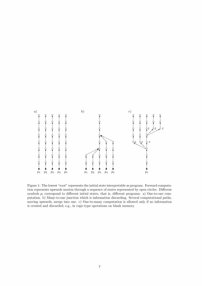
As a prelude to quantum computation, we briefly review classical reversible computation [61, 8,45, 9, 66]. This type of computation is characterized by a single-valued inverse transition function.In irreversible computations, logical functions are performed which do not have a single-valuedinverse, such as AND or OR; i.e., the input cannot be deduced from the output. Also deletion ofinformation or other many (states)-to-one (state) operations are irreversible. Reversible calculationrequires every single step to be reversible. Figure 1 [66] draws the difference between one-to-oneand many-to-one computation. This logical irreversibility is associated with physical irreversibilityand requires a minimal heat generation of the computing machine.

It is possible to embed any irreversible computation in an appropriate environment which makesit reversible. For instance, the computing agent could keep the inputs of previous calculations insuccessive order. It could save all the information it would otherwise throw away. Or, it could leavemarkers behind to identify its trail, the Hansel and Gretel strategy described by Landauer [66].That, of course, might amount to a tremendous overhead in dynamical memory space (and time)and would merely postpone the problem of throwing away unwanted information. But, as hasbeen pointed out by Bennett [8], for classical computations this overhead could be circumventedby making the computer to erase all intermediate results, leaving behind only the desired outputand the originally furnished input. Bennett’s trick is to do a computation reversible, then copy itsoutput9 and then, with one output as input for the reversible computation, run the computationbackwards. In order not to consume exceedingly large intermediate storage resources, this strategycould be applied after every single step. The price is a doubling of computation time, since itrequires one additional step for the back-computation.10 Since qbits cannot be copied, the trick

9Copying can be done reversible in classical physics, if the memory used for the copy is initially blank. Quantummechanically, this cannot be done on qbits; cf. below.

10If an irreversible computing agent exists which computes the input from a given output, then it is possible totranslate an irreversible computation from input to output into one which is reversible and erases everything elseexcept the final output, including the original input; i.e., that simply maps inputs into outputs. For details, see

6

s s s sc6

c6

c6

c6

c6

c6

c6

c6

c6

c6

c6

c6

c6

c6

c6

c6

c6

c6

c6

c6

c6

c6

c6

c6

c6

c6

c6

c6

c6

c6

c6

c6

sc6

c6

c6

c6

c6

c6

c6

c6

s s s sc6

c6 c

6

c6 c

6

c6

c6

c6

c6

c6

c6

c6

c6

c6

c6

c6

sc6

c6

c6

c6

©©©©*¡

¡µ

@@I

HHHHY

p1 p2 p3 p4 p5 p1 p2 p3 p4 p5

a) b) c) ccccccccs

p1

6

6

6

6

6

6

6

6

6

6

c cc6

c6 c

6

c6

cc6

c6

c6

c6

cc6

c6

c6

c6

HHHHY@

@I

¡¡µ

©©©©*

sss

ttt

Figure 1: The lowest “root” represents the initial state interpretable as program. Forward computa-tion represents upwards motion through a sequence of states represented by open circles. Differentsymbols pi correspond to different initial states, that is, different programs. a) One-to-one com-putation. b) Many-to-one junction which is information discarding. Several computational paths,moving upwards, merge into one. c) One-to-many computation is allowed only if no informationis created and discarded; e.g., in copy-type operations on blank memory.

7

does not work for quantum computations.

4.2 Selected features of quantum computation

The following features are important, but not sufficient qualities of quantum computers.

• Input, output, program and memory are represented by qbits.

• Any computation (step) can be represented by a unitary transformation of the computer asa whole.

• Any computation is reversible. Because of the unitarity of the quantum evolution operator,a deterministic computation can be performed by a quantum computer if and only if itis reversible, i.e., if the program does not involve ”deletion” of information or ”many-to-one” operations. Only one-to-one operations are allowed. Compared to classical irreversiblecomputation, this may result in a space and time overheads. Furthermore, no ”one-to-many”operations are allowed. Thus, unless classical, qbits cannot be copied.

• Unless classical, qbits are context-dependent. That is, their value may depend on the methodby which they have been inferred, and on the co-measured qbits.

• Measurements may be carried out on any qbit at any stage of the computation. But, unlessclassical, a qbit cannot be measured by a single experiment with arbitrary accuracy. Thecomputation process and the measurement have to be repeated in order to obtain sufficientstatistics.—Any such single measurement will yield merely a ”click” on some counter, fromwhich information about the qbit state must be inferred. Thereby, any single measurementis indeterminate and coherence is destroyed. Therefore, it seems more proper to realizethat there is no such operational concept of ”a single qbit.” Because of complementarity,single qbits cannot be determined precisely. What is henceforth called ”determination” or”measurement” of a qbit is, in effect, the observation of a successive number of such qbits, oneafter the other, from ”similar” computation processes (same preparation, same evolution).By performing these measurements on ”similar” qbits, one can ”determine” this qbit withinan epsilon-neighborhood only. The parameter epsilon depends on the number of successivemeasurements made.

• Quantum parallelism: during a computation (step), a quantum computer proceeds down allcoherent paths at once. If managed properly, this may give rise to speedups.

• Any subroutine must not leave around any qbits beyond it’s computed answer, because thecomputational paths with different residual information can no longer interfere.

In order to appreciate quantum computation, one should make proper use of the abovefeatures—quantum parallelism, unerasability of information, non-copying, context-dependence andimpossibility to directly measure the atoms of quantum information, the qbits, related to quantumindeterminism.

Thereby, the “solution” to a decision problem may yield the classical bit values at random. Itmay depend on other qbits of information which are inferred. It cannot be arbitrarily copied and,in this sense, is unique.

4.2.1 Copying of quantum bits

Can a non-classical qbit be copied? No! — This answer amazes the classical mind.11 Informallyspeaking, the reason is that, depending on the strategy, any attempt to copy a coherent superposi-tion of states results either in a state reduction, destroying coherence, or, most important of all, inthe addition of noise which manifests itself as the spontaneous excitations of previously nonexistingfield modes [102, 37, 72, 75, 46, 26]. Therefore, qbits can be copied if and only if they are (knownto be) classical. Only one-to-one computation processes depicted in Fig. 1a) are allowed.

Bennett [8, 9].11Copying of qbits would allow circumvention of the Heisenberg uncertainty relation by measuring two incompat-

ible observables on two identical qbit copies. It would also allow faster-than-light transmission of information, aspointed out by Herbert [53]. Herbert’s suggestion stimulated the development of “no-cloning theorems” reviewedhere.

8

This can be seen by a short calculation [102] which requires the multi-quantum formalismdeveloped in appendix B. A physical realization12 of the qbit state is a two-mode boson field withthe identifications

xα,β = αf + βt , (4)f = | 01, 12〉 , (5)t = | 11, 02〉 . (6)

The classical bit states are |01, 12〉 (field mode 1 unfilled, field mode 2 filled with one quantum)and |11, 02〉 (field mode 1 filled with one quantum, field mode 2 unfilled).

An ideal amplifier, denoted by A, should be able to copy a classical bit state; i.e., it shouldcreate an identical particle in the same mode

Ai|01, 12〉 → Af |01, 22〉 , Ai|11, 02〉 → Af |21, 02〉 . (7)

Here, Ai and Af stand for the initial and the final state of the amplifier.What about copying a proper qbit; i.e., a coherent superposition of the cbits f = |01, 12〉 and

t = |11, 02〉? According to the quantum evolution law, the corresponding amplification processshould be representable by a linear (unitary) operator; thus

Ai(α|01, 12〉+ β|11, 02〉) → Af (α|01, 22〉+ β|21, 02〉) . (8)

Yet, the true copy of that qbit is the state

(xα,β)2 | 01, 02〉 = (α a†2 + β a†1)2 | 01, 02〉

=[α2 (a†2)

2 + αβ (a†2a†1 + a†1a

†2) + β2 (a†1)

2]| 01, 02〉

=[α2 (a†2)

2 + 2αβ a†2a†1 + β2 (a†1)

2]| 01, 02〉

= α2|01, 22〉+ 2αβ|11, 12〉+ β2|21, 02〉 . (9)

By comparing (8) with (9) it can be seen that a reasonable (linear unitary quantum mechanicalevolution for an) amplifier which could copy a qbit exists only if the qbit is classical.

A more detailed analysis (cf. [72, 75], in particular [46, 26]) reveals that the copying (amplifica-tion) process generates an amplification of the signal but necessarily adds noise at the same time.This noise can be interpreted as spontaneous emission of field quanta (photons) in the process ofamplification.

One application of this feature is quantum cryptography [13, 12, 11]. Thereby, the impossibilityto copy qbits is used for a cryptographic communication via quantum channels.

4.2.2 Context dependence of qbits

This section could be skipped at first reading.Assume that in an EPR-type arrangement [41] one wants to measure the product

P = m1xm2

xm1ym2

ym1zm

2z

of the direction of the spin components of each one of the two associated particles 1 and 2 alongthe x, y and z-axes. Assume that the operators are normalized such that |mj

i | = 1, i ∈ x, y, z,j ∈ 1, 2. One way to determine P is measuring and, based on these measurements, “counter-factually inferring” [78, 73] the three “observables” m1

xm2y, m1

ym2x and m1

zm2z. By multiplying

them, one obtains +1. Another, alternative, way to determine P is measuring and, based on thesemeasurements, “counterfactually inferring” the three “observables” m1

xm2x, m1

ym2y and m1

zm2z. By

multiplying them, one obtains −1. In that way, one has obtained either P = 1 or P = −1. Asso-ciate with P = 1 the bit state zero 0 and with P = −1 the bit state 1. Then the bit is either instate zero or one, depending on the way or context it was inferred.

This kind of contextuality is deeply rooted in the non-Boolean algebraic structure of quantumpropositions. Note also that the above argument relies heavily on “counterfactual reasoning,” be-cause, for instance, only two of the six observables mj

i can actually be experimentally determined.12the most elementary realization is a one-mode field with the symbol 0 corresponding to | 0〉 (empty mode) and

1 corresponding to | 1〉 (one-quantum filled mode).

9

Here, the term “counterfactual reasoning” [78, 73] stands for arguments involving results of incom-patible experiments, i.e., experiments which could never be performed simultaneously, since theassociated operators do not commute. The results thus have to be inferred rather than measured,and the existence of such “elements of physical reality” thus have to be tacitly assumed [41].

4.3 Universal quantum computer based on the U(2)-gate

The “brute force” method of obtaining a (universal) quantum computer [6, 34, 66] by quantizingthe “hardware” components of a Turing machine suffers from the same problem as its classicalcounterpart–it seems technologically unreasonable to actually construct a universal quantum devicewith a “scaled down” (to nanometer size) model of a Turing machine in mind.

We therefore pursue a more fundamental approach [94, 95]. Recall that an arbitrary quantumtime evolution in finite-dimensional Hilbert space is given by x(t) = Ux(t0), where U is unitary.

It is well known that any n-dimensional unitary matrix U can be composed from elementaryunitary transformations in two-dimensional subspaces of Cn. This is usually shown in the context ofparameterization of the n-dimensional unitary groups (cf. [76, chapter 2] and [82, 81]). Thereby,a transformation in n-dimensional spaces is decomposed into transformations in 2-dimensionalsubspaces. This amounts to a successive array of U(2) elements, which in their entirety forms anarbitrary time evolution U(n) in n-dimensional Hilbert space.

Hence, all quantum processes and computation tasks which can possibly be executed must berepresentable by unitary transformations. Indeed, unitary transformations of qbits are a necessaryand sufficient condition for quantum computing. The group of unitary transformations in arbitrary-but finite-dimensional Hilbert space is a model of universal quantum computer.

Unitary quantum mechanical operations are a natural extension of Turing’s “simple” classicalpaper and pencil operations on a sheet of (one-dimensional) paper [97, section 9.I]. If one wantsto extend that notion further, one would have to extend physical theory, in particular quantumtheory. However, at the moment, such a further extension (beyond quantum mechanics) seemsonly a remote possibility.

It remains to be shown that the universal U(2)-gate is physically operationalizable. This is donein appendix D in the framework of Mach-Zehnder interferometry. Note that the number of elemen-

tary U(2)-transformations is polynomially bounded and does not exceed(

n2

)= n (n− 1)/2 =

O(n2).

4.4 Other models of universal quantum computation

Deutsch [35] has proposed a model of universal computation based on quantum computationnetworks. Thereby, the states in a 2n-dimensional Hilbert space are constructed as the productstate of n particles in two-dimensional Hilbert space. A set of gates that consists of all U(2)(one-bit) quantum gates and the two-bit exclusive-or gate (that maps Boolean values (x, y) to(x, x⊕ y)) is universal in the sense that all unitary operations on arbitrarily many bits n (U(2n))can be expressed as compositions of these gates [4].

This approach should be distinguished from the interferometric approach using U(2)-gatesdiscussed before, which is based on single particle states in 2n-dimensional Hilbert space. In theproduct state model, the addition of one particle effectively doubles the dimensionality of theassociated Hilbert space. In the interferometric model, this could only be achieved by doublingthe number of input and output ports. This could give rise to non-polynomial space overhead. Inthe case of the product state model, in order to obtain a mixing between different particle states,xor-gates are needed. The interferometric approach does not need xor-gates explicitly.

It has been claimed [87, 30] that certain supposedly NP -hard problems such as factoring canbe solved in polynomial time on quantum computers. However, it should be noted that this resultfaces difficulties. For, it might not be easy to keep the quantum computer in a coherent superposi-tion state over sufficient time and space scales in order to be able to execute tasks which are hard todo classically—the computation may “decohere,” reducing the qbits to classical ones [59]. Further-more, in order to obtain sufficient statistical data, a “great” (non-polynomially bounded) number ofsingle particles may be needed [91]. We shall not pursue these matters further [36, 14, 15, 6, 27, 87].

10

4.5 Nomenclature

Consider a (not necessarily universal) quantum computer C and its ith program pi, which, at timeτ ∈ Z, can be described by a quantum state C(τ, pi). Let C(p) = s stand for a computer C withprogram p which outputs s in arbitrary long time. In what follows we shall assume that the programpi is coded classically. That is, we choose a finite code alphabet A and denote by A∗ the set of allstrings over A. Any program pi is coded as a classical sequence ppiq = s1is2i · · · sni ∈ A∗, sji ∈ A.Whenever possible, ppiq will be abbreviated by pi. We assume prefix coding [51, 29, 28, 92, 23]; i.e.,the domain of C is prefix-free such that no admissible program is the prefix of another admissibleprogram. Furthermore, without loss of generality, we consider only empty input strings. |p| standsfor the length of p.

4.6 Diagonalization

This is neither the place for a comprehensive review of the diagonalization method [83, 77], norsuffices the author’s competence for such an endeavor. Therefore, only a few hallmarks are stated.As already Godel pointed out in his classical paper on the incompleteness of arithmetic [47], theundecidability theorems of formal logic [31] (and the theory of recursive functions [83, 77]) arebased on semantical paradoxes such as the liar [2] or Richard’s paradox. A proper translation ofthe semantic paradoxes results in the diagonalization method. Diagonalization has apparently firstbeen applied by Cantor to demonstrate the non-enumerability of real numbers [25]. It has alsobeen used by Turing for a proof of the recursive undecidability of the halting problem [97].

A brief review of the classical algorithmic argument will be given first. Consider a universalcomputer C. For the sake of contradiction, consider an arbitrary algorithm B(X) whose input is astring of symbols X. Assume that there exists a “halting algorithm” HALT which is able to decidewhether B terminates on X or not. The domain of HALT is the set of legal programs. The rangeof HALT are cbits (classical case) and qbits (quantum mechanical case).

Using HALT(B(X)) we shall construct another deterministic computing agent A, which has asinput any effective program B and which proceeds as follows: Upon reading the program B asinput, A makes a copy of it. This can be readily achieved, since the program B is presented to Ain some encoded form pBq, i.e., as a string of symbols. In the next step, the agent uses the codepBq as input string for B itself; i.e., A forms B(pBq), henceforth denoted by B(B). The agentnow hands B(B) over to its subroutine HALT. Then, A proceeds as follows: if HALT(B(B)) decidesthat B(B) halts, then the agent A does not halt; this can for instance be realized by an infiniteDO-loop; if HALT(B(B)) decides that B(B) does not halt, then A halts.

The agent A will now be confronted with the following paradoxical task: take the own code asinput and proceed.

4.6.1 Classical case

Assume that A is restricted to classical bits of information. To be more specific, assume that HALToutputs the code of a cbit as follows (↑ and ↓ stands for divergence and convergence, respectively):

HALT(B(X)) =

0 if B(X) ↑1 if B(X) ↓ . (10)

Then, whenever A(A) halts, HALT(A(A)) outputs 1 and forces A(A) not to halt. Conversely,whenever A(A) does not halt, then HALT(A(A)) outputs 0 and steers A(A) into the halting mode.In both cases one arrives at a complete contradiction. Classically, this contradiction can only beconsistently avoided by assuming the nonexistence of A and, since the only nontrivial feature of Ais the use of the peculiar halting algorithm HALT, the impossibility of any such halting algorithm.

4.6.2 Quantum mechanical case

Recall that a quantum computer C evolves according to a unitary operator U such that (τ standsfor the discrete time parameter) C(τ, pi) = UC(τ − 1, pi) = U tC(0, pi).

As has been pointed out before, in quantum information theory a qbit may be in a coherentsuperposition of the two classical states t and f . Due to this possibility of a coherent superposition

11

of classical bit states, the usual reductio ad absurdum argument breaks down. Instead, diagonal-ization procedures in quantum information theory yield qbit solutions which are fixed points ofthe associated unitary operators.

In what follows it will be demonstrated how the task of the agent A can be performed con-sistently if A is allowed to process quantum information. To be more specific, assume that theoutput of the hypothetical “halting algorithm” is a halting qbit

HALT(B(X)) = hα,β . (11)

One may think of HALT(B(X)) as a universal “watchdog” computer C ′ simulating C and containinga dedicated halting bit, which it outputs at every (discrete) time cycle [34]. Alternatively, it canbe assumed that the computer C contains its own halting bit indicating whether it has completedits task or not. Note that the halting qbit hα,β can be represented by a normalized13 vector intwo-dimensional complex Hilbert space spanned by the the orthonormal vectors “t” and “f .” Letthe halting state h1,0 = t (up to factors modulus 1) be the physical realization that the computerhas “halted;” likewise let h0,1 = f (up to factors modulus 1) be the physical realization thatthe computer has not “halted.” Note that, since quantum computations are governed by unitaryevolution laws which are reversible, the halting state does not imply that the computer does notchange as time evolves. It just means that it has set a signal — the halting bit — to indicated that ithas finished its task. α and β are complex numbers which are a quantum mechanical measure of theprobability amplitude that the computer is in the halting and the non-halting states, respectively.The corresponding halting and non-halting probabilities are |a|2 and |a|2, respectively.

Initially, i.e., at t = 0, the halting bit is prepared to be a 50:50 mixture of the classical haltingand non-halting states t and f ; i.e., h1/

√2,1/

√2. If later C ′ finds that C converges (diverges) on

B(X), then the halting bit of C ′ is set to the classical value t (f).The emergence of fixed points can be demonstrated by a simple example. Agent A’s diagonal-

ization task can be formalized as follows. Consider for the moment the action of diagonalizationon the cbit states. (Since the qbit states are merely a coherent superposition thereof, the action ofdiagonalization on qbits is straightforward.) Diagonalization effectively transforms the cbit value tinto f and vice versa. Recall that in equation (10), the state t has been identified with the haltingstate and the state f with the non-halting state. Since the halting state and the non-halting stateexclude each other, f, t can be identified with orthonormal basis vectors in a two-dimensional vec-tor space. Thus, the standard basis of Cartesian coordinates can be chosen for a representation oft and f ; i.e.,

t ≡(

10

)and f ≡

(01

). (12)

The evolution representing diagonalization (effectively, agent A’s task) can be expressed by theunitary operator D by

Dt = f and Df = t . (13)

Thus, D acts essentially as a not-gate. In the above state basis, D can be represented as follows:

D =(

0 11 0

). (14)

D will be called diagonalization operator, despite the fact that the only nonvanishing componentsare off-diagonal.

As has been pointed out earlier, quantum information theory allows a coherent superpositionhα,β = αt + βf of the cbit states t and f . D acts on cbits. It has a fixed point at the qbit state

h∗ := h 1√2, 1√

2=

t + f√2≡ 1√

2

(11

). (15)

h∗ does not give rise to inconsistencies [90]. If agent A hands over the fixed point state h∗ to thediagonalization operator D, the same state h∗ is recovered. Stated differently, as long as the outputof the “halting algorithm” to input A(A) is h∗, diagonalization does not change it. Hence, even ifthe (classically) “paradoxical” construction of diagonalization is maintained, quantum theory doesnot give rise to a paradox, because the quantum range of solutions is larger than the classical one.

13(hα,β , hα,β) = 1.

12

Therefore, standard proofs of the recursive unsolvability of the halting problem do not apply ifagent A is allowed a qbit.

Another, less abstract, application for quantum information theory is the handling of incon-sistent information in databases. Thereby, two contradicting cbits of information t and f areresolved by the qbit h∗ = (t + f)/

√2. Throughout the rest of the computation the coherence

is maintained. After the processing, the result is obtained by an irreversible measurement. Theprocessing of qbits, however, would require an exponential space overhead on classical computers incbit base [42]. Thus, in order to remain tractable, the corresponding qbits should be implementedon truly quantum universal computers.

It should be noted, however, that the fixed point qbit “solution” to the above halting problem,as far as problem solving is concerned, is of not much practical help. In particular, if one isinterested in the “classical” answer whether or not A(A) halts, then one ultimately has to performan irreversible measurement on the fixed point state. This causes a state reduction into the classicalstates corresponding to t and f . Any single measurement will yield an indeterministic result. Thereis a 50:50 chance that the fixed point state will be either in t or f , since Pt(h∗) = Pf (h∗) = 1

2 .Thereby, classical undecidability is recovered. Stated pointedly: With regards to the question ofwhether or not a computer halts, the “solution” h∗ is equivalent to the throwing of a fair coin.

Therefore, the advance of quantum recursion theory over classical recursion theory is not somuch classical problem solving but the consistent representation of statements which would giverise to classical paradoxes.

4.6.3 Proper quantum diagonalization

The above argument used the continuity of qbit states as compared to the two cbit states for aconstruction of fixed points of the diagonalization operator. One could proceed a step further andallow nonclassical diagonalization procedures. Such a step, albeit operationalizable, has no classicaloperational equivalent, and thus no classical interpretation.

Consider the entire range of two-dimensional unitary transformations [76]

U(2)(ω, α, β, ϕ) = e−i β

(ei α cosω −e−i ϕ sin ωei ϕ sin ω e−i α cosω

), (16)

where −π ≤ β, ω ≤ π, − π2 ≤ α,ϕ ≤ π

2 , to act on the qbit. A typical example of a nonclassicaloperation on a qbit is the “square root of not” gate (

√not

√not = D)

√not =

12

(1 + i 1− i1− i 1 + i

). (17)

Not all these unitary transformations have eigenvectors associated with eigenvalues 1 and thusfixed points. Indeed, it is not difficult to see that only unitary transformations of the form

[U(2)(ω, α, β, ϕ)]−1 diag(1, eiλ) U(2)(ω, α, β, ϕ) =

=

(cos ω2 + ei λ sin ω2 −1+ei λ

2 e−i (α+ϕ) sin(2ω)−1+ei λ

2 ei (α+ϕ) sin(2ω) ei λ cos ω2 + sin ω2

)(18)

have fixed points.Applying nonclassical operations on qbits with no fixed points

D′ = [U(2)(ω, α, β, ϕ)]−1 diag(eiµ, eiλ)U(2)(ω, α, β, ϕ)

=

(ei µ cos(ω)2 + ei λ sin(ω)2 e−i (α+p)

2

(ei λ − ei µ

)sin(2ω)

ei (α+p)

2

(ei λ − ei µ

)sin(2 ω) ei λ cos(ω)2 + ei µ sin(ω)2

)(19)

with µ, λ 6= nπ, n ∈ N0 gives rise to eigenvectors which are not fixed points, but which acquirenonvanishing phases µ, λ in the generalized diagonalization process.

5 Quantum algorithmic information

Quantum algorithmic information theory can be developed in analogy to algorithmic informationtheory [29, 28, 23, 68]. Before proceeding, though, one decisive strategic decision concerning the

13

physical character of the program has to be made. This amounts to a restriction to purely classicalprefix-free programs.

The reason for classical programs, as well as for the requirement of instant decodability,is the desired convergence of the Kraft sum over the exponentially weighted program length∑

p exp(|p| log k) ≤ 1, where |p| stands for the length of p and k is the base of the code (forbinary code, k = 2). If arbitrary qbits were allowed as program code, then the Kraft sum woulddiverge.

Nevertheless, qbits are allowed as output. Since they are objects defined in Hilbert space H,the basic definitions of algorithmic information theory have to be slightly adapted.

The canonical program associated with an object s ∈ H representable as vector in a Hilbertspace H is denoted by s∗ and defined by

s∗ = minC(p)=s

p . (20)

I.e., s∗ is the first element in the ordered set of all strings that is a program for C to calculates. The string s∗ is thus the code of the smallest-size program which, implemented on a quantumcomputer, outputs s. (If several binary programs of equal length exist, the one is chosen whichcomes first in an enumeration using the usual lexicographic order relation “0 < 1.”)

Let again “|x|” of an object encoded as (binary) string stand for the length of that string. Thequantum algorithmic information H(s) of an object s ∈ H representable as vector in a Hilbertspace H is defined as the length of the shortest program p which runs on a quantum computer Cand generates the output s:

H(s) = |s∗| = minC(p)=s

|p| . (21)

If no program makes computer C output s, then H(s) = ∞.The joint quantum algorithmic information H(s, t) of two objects s ∈ H and t ∈ H representable

as vectors in a Hilbert space H is the length of the smallest-size binary program to calculate s andt simultaneously.

The relative or conditional quantum algorithmic information H(s|t) of s ∈ H given t ∈ N is thelength of the smallest-size binary program to calculate s from a smallest-size program for t:

H(s|t) = minC(p,t∗)=s

|p| . (22)

Most features and results of algorithmic information theory hold for quantum algorithmic in-formation as well. In particular, we restrict our attention to universal quantum computers whosequantum algorithmic information content is machine-independent, such that the quantum algo-rithmic information content of an arbitrary object does not exceed a constant independent of thatobject. That is, for all objects s ∈ H and two computers C and C ′ of this class,

|HC −HC′ | = O(1) . (23)

Furthermore, let s and t be two objects representable as vectors in Hilbert space. Then (recallthat t ∈ N),

H(s, t) = H(t, s) + O(1) ; (24)H(s|s) = O(1) ; (25)

H(H(s)|s) = O(1) ; (26)H(s) ≤ H(s, t) + O(1) ; (27)

H(s|t) ≤ H(s) + O(1) ; (28)H(s, t) = H(s) + H(t|s∗) + O(1) (if s∗ is classical) ; (29)H(s, t) ≤ H(s) + H(t) + O(1) (subadditivity) ; (30)H(s, s) = H(s) + O(1) ; (31)

H(s,H(s)) = H(s) + O(1) . (32)

Notice that there exist sets of objects S = s1, . . . , sn, n < ∞ whose algorithmic informa-tion content H(S) is arbitrary small compared to the algorithmic information content of someunspecified single elements si ∈ S; i.e.,

H(S) < maxsi∈S

H(si) . (33)

14

6 Quantum omega

Chaitin’s Ω [29, 28, 89, 23] is a magic number. It is a measure for arbitrary programs to take a finitenumber of execution steps and then halt. It contains the solution of all halting problems, and henceof questions codable into halting problems, such as Fermat’s theorem. It contains the solution ofthe question of whether or not a particular exponential Diophantine equation has infinitely manyor a finite number of solutions. And, since Ω is provable “algorithmically incompressible,” it isMartin-Lof/Chaitin/Solovay random. Therefore, Ω is both: a mathematician’s “fair coin,” and aformalist’s nightmare.

Here, Ω is generalized to quantum computations.14

In the orthonormal halting basis t, f, the computer C with classical input pi can be repre-sented by C(τ, pi) = t (t, C(τ, pi)) + f (f, C(τ, pi)).

Recall that initially, i.e., at time τ = 0, the halting bit is in a coherent 50:50-superposition;i.e., in terms of the halting basis, C(0, pi) = (t + f)/

√2 for all pi ∈ A∗. This corresponds to

the fact that initially it is unknown whether or not the computer halts on pi. When during thetime evolution the computer has completed its task, the halting bit value is switched to t by someinternal operation. If the computer never halts, the halting bit value is switched to f by someinternal operation. Otherwise it remains in the coherent 50:50-superposition.

Alternatively, the computer could be initially prepared in the non-halting state f . After com-pletion of the task, the halting bit is again switched to the halting state t.

In analogy to the fully classical case [29, 28, 88, 23], the quantum halting amplitude15 Ω can bedefined as a weighted expectation over all computations of C with classical input pi (|pi| standsfor the length of pi)

Ω ≡∑

C(pi)∈H

2−|pi|/2(t, C(pi)) . (34)

Likewise, the halting amplitude for a particular output state s,

Υ(s) ≡∑

C(pi)=s

2−|pi|/2(t, C(pi)) . (35)

For a set of output states S = s1, s2, s3, . . . , sn which correspond to mutually orthogonal vectorsin Hilbert space,

Υ(S) ≡∑

C(pi)∈S

2−|pi|/2(t, C(pi)) . (36)

Terms corresponding to different programs and states have to be summed up incoherently.Thus, the corresponding probabilities are

|Ω|2 =∑

C(pi)∈H

2−|pi||(t, C(pi))|2 (37)

P (s) ≡ |Υ(s)|2 =∑

C(pi)=s

2−|pi||(t, C(pi))|2 (38)

P (S) ≡∑

C(pi)∈S

|Υ(s)|2 =∑

C(pi)∈S

2−|pi||(t, C(pi))|2 . (39)

The following relations hold,

Υ(S) =∑

si∈S

Υ(si) , (40)

Ω = Υ(H) =∑

si∈H

Υ(si) . (41)

For s ⊂ S ⊂ H,0 ≤ P (s) ≤ P (S) ≤ |Ω|2 ≤ 1 . (42)

14The quantum omega was invented in a meeting of G. Chaitin, A. Zeilinger and the author in a Viennese coffeehouse (Cafe Braunerhof) in January 1991. Thus, the group should be credited for the original invention, whereasany blame should remain with the author.

15The definition of Ω and Υ differ slightly from the ones introduced by the author previously [93].

15

Alternatively, the quantum halting probability and the quantum algorithmic information by thequantum algorithmic information content. That is,

P ∗(s) = 2−|s∗| = 2−H(s) (43)

P ∗(S) =∑

si∈S

P ∗(s) =∑

s∈S

2−H(s) (44)

P ∗(H) = |Ω∗|2 =∑

n∈H

2−H(n) . (45)

|Ω∗|2 ≤ |Ω|2 , (46)P ∗(s) ≤ P (s) , (47)P ∗(S) ≤ P (S) . (48)

The following relations are either a direct consequence of the definition (43) or follow from thefact that for programs in prefix code, the algorithmic probability is concentrated on the minimalsize programs, or alternatively, that there are few minimal programs:

H(s) = − log2 P ∗(s) ; (49)H(s) = − log2 P (s) + O(1) . (50)

Notice again that, because of complementarity, single qbits cannot be determined precisely.They just appear experimentally as some clicks in a counter. What we can effectively do isto observe a successive number of such qbits, one after the other, from “similar” computationprocesses (same preparation, same evolution). By performing these measurements on “similar”qbits, one can “determine” this qbit within an ε-neighborhood only.

For nontrivial choices of the quantum computer C, several remarks are in order. (In whatfollows, we mention only Ω, but the comments apply to Υ as well.) If the program is also codedin qbits, the above sum becomes an integral over continuously many states per code symbol of theprograms. In this case, the Kraft sum needs not converge. Just as for the classical analogue it ispossible to “compute” Ω as a limit from below by considering in the t’th computing step (timeτ) all programs of length τ which have already halted. (This “computation” suffers from a radiusof convergence which decreases slower than any recursive function.) The quantum Ω is complex.|Ω|2 can be interpreted as a measure for the halting probability of C; i.e., the probability that anarbitrary (prefix-free) program halts on C.

Finally, any irreversible measurement of |Ω|2 causes a state collapse. Since C(τ, pi) may not bein a pure state, the series in (34) and (35) will not be uniquely defined even for finite times. Thusthe nondeterministic character of Ω is not only based on classical recursion theoretic arguments[29, 28] but also on the metaphysical assumption that God plays the quantum dice.

Appendices

A Two-state system

Having set the stage of the quantum formalism, an elementary two-dimensional example of a two-state system shall be exhibited ([44, pp. 8-11]). Let us denote the two base states by 1 and2. Any arbitrary physical state ψ is a coherent superposition of 1 and 2 and can be written asψ = 1(1, ψ) + 2(2, ψ) with the two coefficients (1, ψ), (2, ψ) ∈ C.

Let us discuss two particular types of evolutions.First, let us discuss the Schrodinger equation with diagonal Hamilton matrix, i.e., with vanish-

ing off-diagonal elements,

Hij =(

E1 00 E2

). (51)

In this case, the Schrodinger equation decouples and reduces to

i~∂

∂t(1, ψ(t)) = E1(1, ψ(t)) , i~

∂

∂t(2, ψ(t)) = E2(2, ψ(t)) , (52)

16

resulting in(1, ψ(t)) = ae−iE1t/~ , (2, ψ(t)) = be−iE2t/~ , (53)

with a, b ∈ C, |a|2 + |b|2 = 1. These solutions correspond to stationary states which do not changein time; i.e., the probability to find the system in the two states is constant

|(1, ψ)|2 = |a|2 , |(2, ψ)|2 = |b|2 . (54)

Second, let us discuss the Schrodinger equation with with non-vanishing but equal off-diagonalelements −A and with equal diagonal elements E of the Hamiltonian matrix; i.e.,

Hij =(

E −A−A E

). (55)

In this case, the Schrodinger equation reads

i~∂

∂t(1, ψ(t)) = E(1, ψ(t))−A(2, ψ(t)) , (56)

i~∂

∂t(2, ψ(t)) = E(2, ψ(t))−A(1, ψ(t)) . (57)

These equations can be solved in a number of ways. For example, taking the sum and the differenceof the two, one obtains

i~∂

∂t((1, ψ(t)) + (2, ψ(t))) = (E −A)((1, ψ(t)) + (2, ψ(t))) , (58)

i~∂

∂t((1, ψ(t))− (2, ψ(t))) = (E + A)((1, ψ(t))− (2, ψ(t))) . (59)

The solution are again two stationary states

(1, ψ(t)) + (2, ψ(t)) = ae−(i/~)(E−A)t , (60)(1, ψ(t))− (2, ψ(t)) = be−(i/~)(E+A)t . (61)

Thus,

(1, ψ(t)) =a

2e−(i/~)(E−A)t +

b

2e−(i/~)(E+A)t , (62)

(2, ψ(t)) =a

2e−(i/~)(E−A)t − b

2e−(i/~)(E+A)t . (63)

Assume now that initially, i.e., at t = 0, the system was in state , 1) =, ψ(t = 0)). Thisassumption corresponds to (1, ψ(t = 0)) = 1 and (2, ψ(t = 0)) = 0. What is the probability thatthe system will be found in the state 2 at the time t > 0, or that it will still be found in the state1 at the time t > 0? Setting t = 0 in equations (62) and (63) yields

(1, ψ(t = 0)) =a + b

2= 1 , (2, ψ(t = 0)) =

a− b

2= 0 , (64)

and thus a = b = 1. Equations (62) and (63) can now be evaluated at t > 0 by substituting 1 fora and b,

(1, ψ(t)) = e−(i/~)Et

[e(i/~)At + e−(i/~)At

2

]= e−(i/~)Et cos

At

~, (65)

(2, ψ(t)) = e−(i/~)Et

[e(i/~)At − e−(i/~)At

2

]= i e−(i/~)Et sin

At

~. (66)

Finally, the probability that the system is in state , 1) and , 2) is

|(1, ψ(t))|2 = cos2At

~, |(2, ψ(t))|2 = sin2 At

~, (67)

respectively. This results in an oscillation of the transition probabilities.

17

µ´¶³H

µ´¶³H

µ´¶³H

µ´¶³N

PPPPPP ££££»»»»»»»»»

······ L

LLLLLLLL

cc

ccc

µ´¶³H

µ´¶³H

µ´¶³H

PPPPPP ££££»»»»»»»»»

µ´¶³N

AAAAAA ¡

¡¡

··

··

··

···

state 2state 1

Figure 2: The two equivalent geometric arrangements of the ammonia (NH3) molecule.

Let us shortly mention one particular realization of a two-state system which, among manyothers, has been discussed in the Feynman lectures [44]. Consider an ammonia (NH3) molecule.If one fixes the plane spanned by the three hydrogen atoms, one observes two possible spatialconfigurations , 1) and , 2), corresponding to position of the nitrogen atom in the lower or theupper hemisphere, respectively (cf. Fig. 2). The nondiagonal elements of the Hamiltonian H12 =H21 = −A correspond to a nonvanishing transition probability from one such configuration intothe other. If the ammonia has been originally in state , 1), it will constantly swing back and forthbetween the two states, with a probability given by equations (67).

B From single to multiple quanta — “second” field quanti-zation

The quantum formalism introduced in the main text is about single quantized objects. What ifone wants to consider many such objects? Do we have to add assumptions in order to treat suchmulti-particle, multi-quanta systems appropriately?

The answer is yes. Experiment and theoretical reasoning (the representation theory of theLorentz group [86] and the spin-statistics theorem [56, 71, 17, 54]) indicate that there are (at least)two basic types of states (quanta, particles): bosonic and fermionic states. Bosonic states havewhat is called “integer spin;” i.e., sb = 0, ~, 2~, 3~, . . ., whereas fermionic states have “half-integerspin;” sf = 1~

2 , 3~2 , 5~

2 . . .. Most important, they are characterized by the way identical copies ofthem can be “brought together.” Consider two boxes, one for identical bosons, say photons, theother one for identical fermions, say electrons. For the first, bosonic, box, the probability thatanother identical boson is added increases with the number of identical bosons which are already inthe box. There is a tendency of bosons to “condensate” into the same state. The second, fermionicbox, behaves quite differently. If it is already occupied by one fermion, another identical fermioncannot enter. This is expressed in the Pauli exclusion principle: A system of fermions can neveroccupy a configuration of individual states in which two individual states are identical.

How can the bose condensation and the Pauli exclusion principle be implemented? There areseveral forms of implementation (e.g., fermionic behavior via Slater-determinants), but the mostcompact and widely practiced form uses operator algebra. In the following we shall present thisformalism in the context of quantum field theory [52, 69, 56, 71, 17, 54, 46].

A classical field can be represented by its Fourier transform (“∗” stands for complex conjugation)

A(x, t) = A(+)(x, t) + A(−)(x, t) (68)A(+)(x, t) = [A(−)(x, t)]∗ (69)

A(+)(x, t) =∑

ki,si

aki,siuki,si(x)e−iωkit , (70)

where ν = ωki/2π stands for the frequency in the field mode labeled by momentum ki and si issome observable such as spin or polarization. uki,si stands for the polarization vector (spinor) at

18

ki, si, and, most important with regards to the quantized case, complex-valued Fourier coefficientsaki,si

∈ C.¿From now on, the ki, si-mode will be abbreviated by the symbol i; i.e., 1 ≡ k1, s1, 2 ≡ k2, s2,

3 ≡ k3, s3, . . ., i ≡ ki, si, . . ..In (second16) quantization, the classical Fourier coefficients ai become re-interpreted as opera-

tors, which obey the following algebraic rules (scalars would not do the trick). For bosonic fields(e.g., for the electromagnetic field), the commutator relations are (“†” stands for self-adjointness):

[ai, a

†j

]= aia

†j − a†jai = δij , (71)

[ai, aj ] =[a†i , a

†j

]= 0 . (72)

For fermionic fields (e.g., for the electron field), the anti-commutator relations are:

ai, a†j = aia

†j + a†jai = δij , (73)

ai, aj = a†i , a†j = 0 . (74)

The anti-commutator relations, in particular a†j , a†j = 2(a†j)2 = 0, are just a formal expression

of the Pauli exclusion principle stating that, unlike bosons, two or more identical fermions cannotco-exist.

The operators a†i and ai are called creation and annihilation operators, respectively. Thisterminology suggests itself if one introduces Fock states and the occupation number formalism. a†iand ai are applied to Fock states to following effect.

The Fock space associated with a quantized field will be the direct product of all Hilbert spacesHi; i.e., ∏

i∈IHi , (75)

where I is an index set characterizing all different field modes labeled by i. Each boson (photon)field mode is equivalent to a harmonic oscillator [46, 70]; each fermion (electron, proton, neutron)field mode is equivalent to the Larmor precession of an electron spin.

In what follows, only finite-size systems are studied. The Fock states are based upon theFock vacuum. The Fock vacuum is a direct product of states | 0i〉 of the i’th Hilbert space Hi

characterizing mode i; i.e.,

| 0〉 =∏

i∈I| 0〉i =| 0〉1⊗ | 0〉2⊗ | 0〉3 ⊗ · · ·

= |⋃

i∈I0i〉 =| 01, 02, 03, . . .〉 , (76)

where again I is an index set characterizing all different field modes labeled by i. “0i” stands for0 (no) quantum (particle) in the state characterized by the quantum numbers i. Likewise, moregenerally, “Ni” stands for N quanta (particles) in the state characterized by the quantum numbersi.

The annihilation operators ai are designed to destroy one quantum (particle) in state i:

aj | 0〉 = 0 , (77)aj | 01, 02, 03, . . . , 0j−1, Nj , 0j+1, . . .〉 =

=√

Nj | 01, 02, 03, . . . , 0j−1, (Nj − 1), 0j+1, . . .〉 . (78)

The creation operators a†i are designed to create one quantum (particle) in state i:

a†j | 0〉 =| 01, 02, 03, . . . , 0j−1, 1j , 0j+1, . . .〉 . (79)

More generally, Nj operators (a†j)Nj create an Nj-quanta (particles) state

(a†j)Nj | 0〉 ∝| 01, 02, 03, . . . , 0j−1, Nj , 0j+1, . . .〉 . (80)

16of course, there is only “the one and only” quantization, the term “second” often refers to operator techniquesfor multiquanta systems; i.e., quantum field theory

19

Lµ´¶³

©ª

D1

c

S1

S2

a

ϕP

d

­ ªD2

e

b M

M

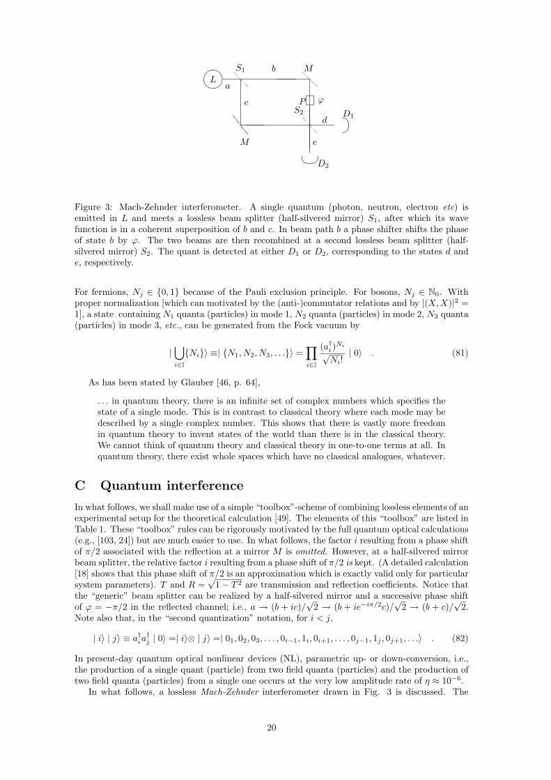
Figure 3: Mach-Zehnder interferometer. A single quantum (photon, neutron, electron etc) isemitted in L and meets a lossless beam splitter (half-silvered mirror) S1, after which its wavefunction is in a coherent superposition of b and c. In beam path b a phase shifter shifts the phaseof state b by ϕ. The two beams are then recombined at a second lossless beam splitter (half-silvered mirror) S2. The quant is detected at either D1 or D2, corresponding to the states d ande, respectively.

For fermions, Nj ∈ 0, 1 because of the Pauli exclusion principle. For bosons, Nj ∈ N0. Withproper normalization [which can motivated by the (anti-)commutator relations and by |(X, X)|2 =1], a state containing N1 quanta (particles) in mode 1, N2 quanta (particles) in mode 2, N3 quanta(particles) in mode 3, etc., can be generated from the Fock vacuum by

|⋃

i∈INi〉 ≡| N1, N2, N3, . . .〉 =

∏

i∈I

(a†i )Ni

√Ni!

| 0〉 . (81)

As has been stated by Glauber [46, p. 64],

. . . in quantum theory, there is an infinite set of complex numbers which specifies thestate of a single mode. This is in contrast to classical theory where each mode may bedescribed by a single complex number. This shows that there is vastly more freedomin quantum theory to invent states of the world than there is in the classical theory.We cannot think of quantum theory and classical theory in one-to-one terms at all. Inquantum theory, there exist whole spaces which have no classical analogues, whatever.

C Quantum interference

In what follows, we shall make use of a simple “toolbox”-scheme of combining lossless elements of anexperimental setup for the theoretical calculation [49]. The elements of this “toolbox” are listed inTable 1. These “toolbox” rules can be rigorously motivated by the full quantum optical calculations(e.g., [103, 24]) but are much easier to use. In what follows, the factor i resulting from a phase shiftof π/2 associated with the reflection at a mirror M is omitted. However, at a half-silvered mirrorbeam splitter, the relative factor i resulting from a phase shift of π/2 is kept. (A detailed calculation[18] shows that this phase shift of π/2 is an approximation which is exactly valid only for particularsystem parameters). T and R =

√1− T 2 are transmission and reflection coefficients. Notice that

the “generic” beam splitter can be realized by a half-silvered mirror and a successive phase shiftof ϕ = −π/2 in the reflected channel; i.e., a → (b + ic)/

√2 → (b + ie−iπ/2c)/

√2 → (b + c)/

√2.

Note also that, in the “second quantization” notation, for i < j,

| i〉 | j〉 ≡ a†ia†j | 0〉 =| i〉⊗ | j〉 =| 01, 02, 03, . . . , 0i−1, 1i, 0i+1, . . . , 0j−1, 1j , 0j+1, . . .〉 . (82)

In present-day quantum optical nonlinear devices (NL), parametric up- or down-conversion, i.e.,the production of a single quant (particle) from two field quanta (particles) and the production oftwo field quanta (particles) from a single one occurs at the very low amplitude rate of η ≈ 10−6.

In what follows, a lossless Mach-Zehnder interferometer drawn in Fig. 3 is discussed. The

20

physical process symbol state transformationreflection at mirror a → b = ia

a

b

M

“generic” beam splitter a → (b + c)/√

2

PPP³³³a b

c

transmission/reflection a → (b + ic)/√

2by a beam splitter a → Tb + iRc,(half-silvered mirror) T 2 + R2 = 1, T, R ∈ [0, 1]

b

c

S1

a

phase-shift ϕ a → b = aeiϕϕ

a b

parametric down-conversion |a〉 → η|b〉|c〉NL

b

c

a

parametric up-conversion |a〉 | b〉 → η|c〉NL

ca

b

amplification Aia → |b; G,N〉G,N

a b

Table 1: “Toolbox” of lossless elements for quantum interference devices.

21

computation proceeds by successive substitution (transition) of states; i.e.,

S1 : a → (b + ic)/√

2 , (83)P : b → beiϕ , (84)

S2 : b → (e + id)/√

2 , (85)

S2 : c → (d + ie)/√

2 . (86)

The resulting transition is

a → ψ = i

(eiϕ + 1

2

)d +

(eiϕ − 1

2

)e . (87)

Assume that ϕ = 0, i.e., there is no phase shift at all. Then, equation (87) reduces to a → id, andthe emitted quant is detected only by D1. Assume that ϕ = π. Then, equation (87) reduces toa → −e, and the emitted quant is detected only by D2. If one varies the phase shift ϕ, one obtainsthe following detection probabilities:

PD1(ϕ) = |(d, ψ)|2 = cos2(ϕ

2) , PD2(ϕ) = |(e, ψ)|2 = sin2(

ϕ

2) . (88)

For some “mindboggling” features of Mach-Zehnder interferometry, see [10].

D Universal 2-port quantum gate

The elementary quantum interference device Tbs21 depicted in Fig. (4.a) is just a beam splitter

followed by a phase shifter in one of the output ports. According to the “toolbox” rules of appendixC, the process can be quantum mechanically described by17

P1 : 0 → 0eiα+β , (89)P2 : 1 → 1eiβ , (90)S : 0 → T 1′ + iR 0′ , (91)S : 1 → T 0′ + iR 1′ , (92)

P3 : 0′ → 0′eiϕ . (93)

If 0 ≡ 0′ ≡(

10

)and 1 ≡ 1′ ≡

(01

)and R(ω) = sin ω, T (ω) = cos ω, then the corre-

sponding unitary evolution matrix which transforms any coherent superposition of 0 and 1 into asuperposition of 0′ and 1′ is given by

Tbs21(ω, α, β, ϕ) =

[ei β

(i ei(α+ϕ) sin ω eiα cosω

eiϕ cosω i sin ω

)]−1

= e−i β

( −i e−i(α+ϕ) sin ω e−iϕ cos ωe−iα cos ω −i sin ω

). (94)

The elementary quantum interference device TMZ21 depicted in Fig. (4.b) is a (rotated) Mach-

Zehnder interferometer with two input and output ports and three phase shifters. According tothe “toolbox” rules, the process can be quantum mechanically described by

P1 : 0 → 0eiα+β , (95)P2 : 1 → 1eiβ , (96)

S1 : 1 → (b + i c)/√

2 , (97)

17Alternatively, the action of a lossless beam splitter may be described by the matrix

T (ω) i R(ω)i R(ω) T (ω)

=

cos ω i sin ωi sin ω cos ω

. A phase shifter in a two-dimensional Hilbert space is represented by either

eiϕ 00 1

or

1 00 eiϕ

. The action of the entire device consisting of such elements is calculated by multiplying the matrices

in reverse order in which the quanta pass these elements [103, 24].

22

P3, ϕ

S(ω)

0 0′

1′1

Tbs21(ω, α, β, ϕ)

-

-

-

-

¡¡

¡¡

¡¡

¡¡

¡¡@@

@@

@@

@@

@@

@@

@@

@@

@@

@@¡¡

¡¡

¡¡

¡¡

¡¡P4, ϕ

M

M

S1( 12 ) S2( 1

2 )

0 0′

1′1 c

b

TMZ21 (α, β, ω, ϕ)

-

-

-

-

P3, ω

a)

b)

©©©©©©©©©©©©©©©©©©©HHHHHHHHHHHHHHHHHHH

P1, α + β

P1, α + β

P2, β

P2, β

Figure 4: Elementary quantum interference device. An elementary quantum interference devicecan be realized by a 4-port interferometer with two input ports 0,1 and two output ports 0′,1′.Any two-dimensional unitary transformation can be realized by the devices. a) shows a realizationby a single beam splitter S(T ) with variable transmission t and three phase shifters P1, P2, P3; b)shows a realization with 50:50 beam splitters S1( 1

2 ) and S2( 12 ) and four phase shifters P1, P2, P3, P4.

23

S1 : 0 → (c + i b)/√

2 , (98)P3 : c → ceiω , (99)

S2 : b → (1′ + i0′)/√

2 , (100)

S2 : c → (0′ + i1′)/√

2 , (101)P4 : 0′ → 0′eiϕ . (102)

When again 0 ≡ 0′ ≡(

10

)and 1 ≡ 1′ ≡

(01

), then the corresponding unitary evolution

matrix which transforms any coherent superposition of 0 and 1 into a superposition of 0′ and 1′

is given by

TMZ21 (α, β, ω, ϕ) = −i e−i(β+ ω

2 )

( −e−i (α+ϕ) sin ω2 e−i ϕ cos ω

2e−i α cos ω

2 sin ω2

). (103)

The correspondence between Tbs21(T (ω), α, β, ϕ) with TMZ

21 (α′, β′, ω′, ϕ′) in equations (94) (103)can be verified by comparing the elements of these matrices. The resulting four equations can beused to eliminate the four unknown parameters ω′ = 2ω, β′ = β − ω, α′ = α − π/2, β′ = β − ωand ϕ′ = ϕ− π/2; i.e.,

Tbs21(ω, α, β, ϕ) = TMZ

21 (α− π

2, β − ω, 2ω, ϕ− π

2) . (104)

Both elementary quantum interference devices are universal in the sense that every unitaryquantum evolution operator in two-dimensional Hilbert space can be brought into a one-to-onecorrespondence to Tbs

21 and TMZ21 ; with corresponding values of T, α, β, ϕ or α, ω, β, ϕ. This can

be easily seen by a similar calculation as before; i.e., by comparing equations (94) (103) with the“canonical” form of a unitary matrix, which is the product of a U(1) = e−i β and of the unimodularunitary matrix SU(2) [76]

T(ω, α, ϕ) =(

ei α cosω −e−i ϕ sin ωei ϕ sin ω e−i α cosω

), (105)

where −π ≤ β, ω ≤ π, − π2 ≤ α, ϕ ≤ π

2 . Let

T(ω, α, β, ϕ) = e−i βT(ω, α, ϕ) . (106)

A proper identification of the parameters α, β, ω, ϕ yields

T(ω, α, β, ϕ) = Tbs21(ω −

π

2,−α− ϕ− π

2, β + α +

π

2, ϕ− α +

π

2) . (107)

Let us examine the realization of a few primitive logical “gates” corresponding to (unitary)unary operations on qbits. The “identity” element I is defined by 0 → 0, 1 → 1 and can berealized by

I = T bs21 (−π

2,−π

2,π

2,π

2) = TMZ

21 (−π, π,−π, 0) =(

1 00 1

). (108)

The “not” element is defined by 0 → 1, 1 → 0 and can be realized by

not = T bs21 (0, 0, 0, 0) = TMZ

21 (− π

2, 0, 0,− π

2) =

(0 11 0

). (109)

The next element, “√not” is a truly quantum mechanical; i.e., nonclassical, one, since it

converts a classical bit into a coherent superposition of 0 and 1.√not is defined by 0 → 0 + 1,

1 → −0 + 1 and can be realized by

√not = T bs

21 (−π

4,−π

2,π

2,π

2) = TMZ

21 (−π,3π

4,−π

2, 0) =

1√2

(1 −11 1

). (110)

Note that√not · √not = not · diag(1,−1) = not (mod 1). The relative phases in the output ports

showing up in diag(1,−1) can be avoided by defining

√not

′= T bs

21 (− π

4, 0,

π

4, 0) = TMZ

21 (− π

2,π

2,− π

2,− π

2) =

12

(1 + i 1− i1− i 1 + i

). (111)

24

With this definition,√not

′√not

′= not.

It is very important that the elementary quantum interference device realizes an arbitraryquantum time evolution of a two-dimensional system. The performance of the quantum interferencedevice is determined by four parameters, corresponding to the phases α, β, ϕ, ω.

References

[1] Albert, D. Z. On quantum-mechanical automata. Physics Letters 94A, 5,6 (1983), 249–252.

[2] Anderson, A. R. St. Paul’s epistle to Titus. In The Paradox of the Liar, R. L. Martin,Ed. Yale University Press, New Haven, 1970. The Bible contains a passage which refers toEpimenides, a Crete living in the capital city of Cnossus: “One of themselves, a prophet oftheir own, said, ‘Cretans are always liars, evil beasts, lazy gluttons.’ ”,— St. Paul, Epistle toTitus I (12-13).

[3] Ballentine, L. E. Quantum Mechanics. Prentice Hall, Englewood Cliffs, NJ, 1989.

[4] Barenco, A., Bennett, C. H., Cleve, R., DiVincenzo, D. P., Margolus, N., Shor,P., Sleator, T., Smolin, J., and Weinfurter, H. Elementary gates for quantumcomputation.e-print http://xxx.lanl.gov/abs/quant-ph/9503016.

[5] Bell, J. S. Speakable and Unspeakable in Quantum Mechanics. Cambridge University Press,Cambridge, 1987.

[6] Benioff, P. A. Quantum mechanical hamiltonian models of turing machines. Journal ofStatistical Physics 29, 3 (1982), 515–546.

[7] Benioff, P. A. Quantum mechanical hamiltonian models of computers. Annals of the NewYork Akademy of Sciences 480 (1986), 475–486.

[8] Bennett, C. H. Logical reversibility of computation. IBM Journal of Research and Devel-opment 17 (1973), 525–532. Reprinted in [67, pp. 197-204].

[9] Bennett, C. H. The thermodynamics of computation—a review. In International Journalof Theoretical Physics [67], pp. 905–940. Reprinted in [67, pp. 213-248].

[10] Bennett, C. H. Night thoughts, dark sight. Nature 371 (1994), 479–480.

[11] Bennett, C. H., Bessette, F., Brassard, G., Salvail, L., and Smolin, J. Experi-mental quantum cryptography. Journal of Cryptology 5 (1992), 3–28.

[12] Bennett, C. H., and Brassard, G. Quantum cryptography: Public key distribution andcoin tossing. In Proceedings of the IEEE International Conference on Computers, Systems,and Signal Processing, Bangalore, India (1984), IEEE Computer Society Press, pp. 175–179.

[13] Bennett, C. H., Brassard, G., Breidbart, S., and Wiesner, S. Quantum cryptogra-phy, or unforgable subway tokens. In Advances in Cryptography: Proceedings of Crypto ’82(New York, 1982), Plenum Press, pp. 78–82.

[14] Bernstein, E., and Vazirani, U. Quantum complexity theory. In Proceedings of the 25thAnnual ACM Symposium on Theory of Computing, San Diego, California, May 16-18, 1993(1993), ACM Press, pp. 11–20.

[15] Berthiaume, A., and Brassard, G. The quantum challenge to structural complexitytheory. In Proceedings, Structure in Complexity Theory, seventh annual conference, BostonUniversity, Boston, Massachusetts, June 22-25, 1992 (1992), IEEE Computer Society Press,pp. 132–137.

[16] Bishop, E., and Bridges, D. S. Constructive Analysis. Springer, Berlin, 1985.

[17] Bogoliubov, N. N., and Shirkov, D. V. Introduction to the Theory of Quantized Fields.Wiley-Interscience, New York, 1959.

25

[18] Born, M., and Wolf, E. Principles of Optics: Electromagnetic Theory of Propagation,Interference and Diffraction of Light, 6th ed. Pergamon Press, Oxford, 1993.

[19] Bridges, D., and Richman, F. Varieties of Constructive Mathematics. Cambridge Uni-versity Press, Cambridge, 1987.

[20] Bridges, D. S. Computability. Springer, New York, 1994.

[21] Bridgman, P. W. A physicists second reaction to Mengenlehre. Scripta Mathematica 2(1934), 101–117, 224–234. Cf. R. Landauer [65].

[22] Bridgman, P. W. Reflections of a Physicist. Philosophical Library, New York, 1950.

[23] Calude, C. Information and Randomness—An Algorithmic Perspective. Springer, Berlin,1994.

[24] Campos, R. A., Saleh, B. E. A., and Teich, M. C. Fourth-order interference of jointsingle-photon wave packets in lossless optical systems. Physical Review A42 (1990), 4127.

[25] Cantor, G. Gesammelte Abhandlungen. Springer, Berlin, 1932.

[26] Caves, C. M. Quantum limits on noise in linear amplifiers. Physical Review D26 (1982),1817–1839.

[27] Cerny, V. Quantum computers and intractable (NP -complete) computing problems. Phys-ical Review A48 (1993), 116–119.

[28] Chaitin, G. J. Algorithmic Information Theory. Cambridge University Press, Cambridge,1987.

[29] Chaitin, G. J. Information, Randomness and Incompleteness, second ed. World Scientific,Singapore, 1990. This is a collection of G. Chaitin’s publications.

[30] Chuang, I., Laflamme, R., Shor, P., and Zurek, W. Quantum computers, factoring,and decoherence.e-print http://xxx.lanl.gov/abs/quant-ph/9503007.

[31] Davis, M. Computability and Unsolvability. McGraw-Hill, New York, 1958.

[32] Davis, M. The Undecidable. Raven Press, New York, 1965.

[33] Davydov, A. S. Quantum Mechanics. Addison-Wesley, Reading, MA, 1965.

[34] Deutsch, D. Quantum theory, the Church-Turing principle and the universal quantumcomputer. Proceedings of the Royal Society London A 400 (1985), 97–119.

[35] Deutsch, D. Quantum computational networks. Proceedings of the Royal Society LondonA 425 (1989), 73–90.

[36] Deutsch, D., and Jozsa, R. Rapid solution of problems by quantum computation. Pro-ceedings of the Royal Society London A 439 (1992), 553–558.

[37] Dieks, D. Communication by EPR devices. Physics Letters 92A, 6 (1982), 271–272.

[38] Dirac, P. A. M. The Principles of Quantum Mechanics. Oxford University Press, Oxford,1947.

[39] Dunford, N., and Schwartz, J. T. Linear Operators I. Interscience Publishers, NewYork, 1958.

[40] Einstein, A. Uber einen die Erzeugung und Verwandlung des Lichtes betreffenden heuris-tischen Gesichtspunkt. Annalen der Physik 17 (1905), 132–148.

[41] Einstein, A., Podolsky, B., and Rosen, N. Can quantum-mechanical description ofphysical reality be considered complete? Physical Review 47 (1935), 777–780. Reprinted in[100, pp. 138-141].

26

[42] Feynman, R. P. Simulating physics with computers. International Journal of TheoreticalPhysics 21 (1982), 467–488.

[43] Feynman, R. P. Quantum mechanical computers. Optics News 11 (February 1985), 11–20.

[44] Feynman, R. P., Leighton, R. B., and Sands, M. The Feynman Lectures on Physics.Quantum Mechanics, vol. III. Addison-Wesley, Reading, MA, 1965.

[45] Fredkin, E., and Toffoli, T. Conservative logic. International Journal of TheoreticalPhysics 21 (1982), 219–253.

[46] Glauber, R. J. Amplifyers, attenuators and the quantum theory of measurement. InFrontiers in Quantum Optics, E. R. Pikes and S. Sarkar, Eds. Adam Hilger, Bristol, 1986.

[47] Godel, K. Uber formal unentscheidbare Satze der Principia Mathematica und verwandterSysteme. Monatshefte fur Mathematik und Physik 38 (1931), 173–198. English translationin [48], and in [32].

[48] Godel, K. In Collected Works. Publications 1929-1936. Volume I, S. Feferman, J. W.Dawson, S. C. Kleene, G. H. Moore, R. M. Solovay, and J. van Heijenoort, Eds. OxfordUniversity Press, Oxford, 1986.

[49] Greenberger, D. B., Horne, M., and Zeilinger, A. Multiparticle interferometry andthe superposition principle. Physics Today 46 (August 1993), 22–29.

[50] Greenberger, D. B., and YaSin, A. “Haunted” measurements in quantum theory.Foundation of Physics 19, 6 (1989), 679–704.

[51] Hamming, R. W. Coding and Information Theory, second ed. Prentice-Hall, EnglewoodCliffs, NJ, 1980.

[52] Harris, E. G. A Pedestrian Approach to Quantum Field Theory. Wiley-Interscience, NewYork, 1971.

[53] Herbert, N. FLASH—a superluminal communicator based upon a new kind of quantummeasurement. Foundation of Physics 12, 12 (1982), 1171–1179.

[54] Itzykson, C., and Zuber, J.-B. Quantum Field Theory. MacGraw-Hill, New York, 1980.

[55] Jammer, M. The Philosophy of Quantum Mechanics. John Wiley & Sons, New York, 1974.

[56] Jauch, J. M., and Rohrlich. The Theory of Photons and Electrons. Addison-Wesley,Cambridge, MA, 1955.

[57] Kochen, S., and Specker, E. P. Logical structures arising in quantum theory. In Sympo-sium on the Theory of Models, Proceedings of the 1963 International Symposium at Berkeley(Amsterdam, 1965), North Holland, pp. 177–189.

[58] Kochen, S., and Specker, E. P. The problem of hidden variables in quantum mechanics.Journal of Mathematics and Mechanics 17, 1 (1967), 59–87.

[59] Landauer, R. Letter, june 1st, 1994.

[60] Landauer, R. Fundamental physical limitations of the computational process; an informalcommentary. Cybernetics Machine Group Newsheet (1/1/1987).

[61] Landauer, R. Irreversibility and heat generation in the computing process. In IBM Journalof Research and Development [67], pp. 183–191. Reprinted in [67, pp. 188-196].

[62] Landauer, R. Wanted: a physically possible theory of physics. IEEE Spectrum 4 (1967),105–109.

[63] Landauer, R. Computation, measurement, communication and energy dissipation. InSelected Topics in Signal Processing, S. Haykin, Ed. Prentice Hall, Englewood Cliffs, NJ,1989, p. 18.

27

[64] Landauer, R. Information is physical. Physics Today 44 (May 1991), 23–29.

[65] Landauer, R. Advertisement for a paper I like. In On Limits, J. L. Casti and J. F. Traub,Eds. Santa Fe Institute Report 94-10-056, Santa Fe, NM, 1994, p. 39.

[66] Landauer, R. Zig-zag path to understanding. In Proceedings of the Workshop on Physicsand Computation PHYSCOMP ’94 (Los Alamitos, CA, 1994), IEEE Computer Society Press,pp. 54–59.

[67] Leff, H. S., and Rex, A. F. Maxwell’s Demon. Princeton University Press, Princeton,1990.

[68] Li, M., and Vitanyi, P. M. B. Kolmogorov complexity and its applications. In Handbookof Theoretical Computer Sciences. Elsevier Science Publishers, Amsterdam, 1990. [98].

[69] Lipkin, H. J. Quantum Mechanics, New Approaches to Selected Topics. North-Holland,Amsterdam, 1973.

[70] Loudon, R., and Knight, P. L. Squeezed light. Journal of Modern Optics 34 (1987),709–759.

[71] Lurie, D. Particles and Fields. Interscience Publishers, New York, 1968.

[72] Mandel, L. Is a photon amplifier always polarization dependent? Nature 304 (1983), 188.

[73] Mermin, N. D. What’s wrong with these elements of reality? Physics Today 43, 6 (June1990), 9–10.

[74] Messiah, A. Quantum Mechanics, vol. I. North-Holland, Amsterdam, 1961.

[75] Milonni, P. W., and Hardies, M. L. Photons cannot always be replicated. PhysicsLetters 92A, 7 (1982), 321–322.

[76] Murnaghan, F. D. The Unitary and Rotation Groups. Spartan Books, Washington, 1962.

[77] Odifreddi, P. Classical Recursion Theory. North-Holland, Amsterdam, 1989.

[78] Peres, A. Quantum Theory: Concepts and Methods. Kluwer Academic Publishers, Dor-drecht, 1993.

[79] Planck, M. Ueber eine Verbesserung der Wien’schen Spectralgleichung. Verhandlungender deutschen physikalischen Gesellschaft 2 (1900), 202.

[80] Planck, M. Die physikalische Struktur des Phasenraumes. Annalen der Physik 50 (1916),385–418.

[81] Reck, M., and Zeilinger, A. Quantum phase tracing of correlated photons in opticalmultiports. In Quantum Interferometry (Singapore, 1994), F. D. Martini, G. Denardo, andA. Zeilinger, Eds., World Scientific.

[82] Reck, M., Zeilinger, A., Bernstein, H. J., and Bertani, P. Experimental realizationof any discrete unitary operator. Physical Review Letters 73 (1994), 58–61.

[83] Rogers, Jr., H. Theory of Recursive Functions and Effective Computability. MacGraw-Hill,New York, 1967.

[84] Rosen, R. Effective processes and natural law. In The Universal Turing Machine. A Half-Century Survey, R. Herken, Ed. Kammerer & Unverzagt, Hamburg, 1988, p. 523.

[85] Schrodinger, E. Die gegenwartige Situation in der Quantenmechanik. Naturwissenschaften23 (1935), 807–812, 823–828, 844–849. English translation in [100, pp. 152-167].

[86] Sexl, R. U., and Urbantke, H. K. Relativitat, Gruppen, Teilchen. Springer, Vienna,1976.

28

[87] Shor, P. W. Algorithms for quantum computation: discrete logarithms and factoring. InProceedings of the 35th Annual Symposium of on Foundations of Computer Science, SantaFe, NM, Nov. 20-22, 1994 (November 1994), IEEE Computer Society Press.e-print http://xxx.lanl.gov/abs/quant-ph/9508027.

[88] Solomonoff, R. J. A formal theory of inductive inference. part i. Information and Control7 (1964), 1–22.

[89] Solovay, R. M. unpublished manuscript.

[90] Svozil, K. The consistent use of paradoxes. Foundations of Physics Letters, in press.

[91] Svozil, K. Speedup in quantum computation is associated with attenuation of processingprobability.e-print http://tph.tuwien.ac.at/˜svozil/publ/kraft.pse-print http://xxx.lanl.gov/abs/hep-th/9412046.

[92] Svozil, K. Randomness & Undecidability in Physics. World Scientific, Singapore, 1993.

[93] Svozil, K. Halting probability amplitude of quantum computers. Journal of UniversalComputer Science 1, 3 (March 1995).

[94] Svozil, K. Quantum computation and complexity theory. part I. Bulletin of the EuropeanAssociation of Theoretical Computer Sciences 55 (1995), 170–207.e-print http://tph.tuwien.ac.at/˜svozil/publ/qct1.ps.

[95] Svozil, K. Quantum computation and complexity theory. part II. Bulletin of the EuropeanAssociation of Theoretical Computer Sciences 56 (1995), 116–136.e-print http://tph.tuwien.ac.at/˜svozil/publ/qct2.ps.

[96] Svozil, K. Set theory and physics. Foundations of Physics 25 (1995), 1541–1560.

[97] Turing, A. M. On computable numbers, with an application to the Entscheidungsproblem.Proceedings of the London Mathematical Society, Series 2 42 and 43 (1936-7 and 1937),230–265 and 544–546. reprinted in [32].

[98] van Leeuwen, J. Algorithms and Complexity, vol. A. Elsevier and MIT Press, Amsterdamand Cambridge, MA, 1990.

[99] von Neumann, J. Mathematische Grundlagen der Quantenmechanik. Springer, Berlin,1932. English translation: Mathematical Foundations of Quantum Mechanics, PrincetonUniversity Press, Princeton, 1955.

[100] Wheeler, J. A., and Zurek, W. H. Quantum Theory and Measurement. PrincetonUniversity Press, Princeton, 1983.

[101] Wigner, E. P. The unreasonable effectiveness of mathematics in the natural sciences.Richard Courant Lecture delivered at New York University, May 11, 1959. Communicationson Pure and Applied Mathematics 13 (1960), 1.

[102] Wooters, W. K., and Zurek, W. H. A single quantum cannot be cloned. Nature 299(1982), 802–803.

[103] Yurke, B., McCall, S. L., and Klauder, J. R. SU(2) and SU(1,1) interferometers.Physical Review A33 (1986), 4033–4054.

29

Contents

1 Information is physical, so is computation 1

2 Hilbert space quantum mechanics 2

3 Quantum information theory 53.1 Coding . . . . . . . . . . . . . . . . . . . . . . . . . . . . . . . . . . . . . . . . . . . 53.2 Reading the book of Nature—a short glance at the prediction catalog . . . . . . . 6

4 Quantum recursion theory 64.1 Reversible computation and deletion of (q)bits . . . . . . . . . . . . . . . . . . . . 64.2 Selected features of quantum computation . . . . . . . . . . . . . . . . . . . . . . . 8

4.2.1 Copying of quantum bits . . . . . . . . . . . . . . . . . . . . . . . . . . . . 84.2.2 Context dependence of qbits . . . . . . . . . . . . . . . . . . . . . . . . . . 9

4.3 Universal quantum computer based on the U(2)-gate . . . . . . . . . . . . . . . . . 104.4 Other models of universal quantum computation . . . . . . . . . . . . . . . . . . . 104.5 Nomenclature . . . . . . . . . . . . . . . . . . . . . . . . . . . . . . . . . . . . . . . 114.6 Diagonalization . . . . . . . . . . . . . . . . . . . . . . . . . . . . . . . . . . . . . . 11

4.6.1 Classical case . . . . . . . . . . . . . . . . . . . . . . . . . . . . . . . . . . . 114.6.2 Quantum mechanical case . . . . . . . . . . . . . . . . . . . . . . . . . . . . 114.6.3 Proper quantum diagonalization . . . . . . . . . . . . . . . . . . . . . . . . 13

5 Quantum algorithmic information 13

6 Quantum omega 15

Appendix 16

A Two-state system 16

B From single to multiple quanta — “second” field quantization 18

C Quantum interference 20

D Universal 2-port quantum gate 22

30