Embed Size (px)
Citation preview
Tesis Doctoral / Doktorego Tesia
Quantitative weighted estimatesfor
singular integrals and commutators
Autor / Egilea:
Israel Pablo Rivera Ríos
Director / Zuzendariek:
Carlos Pérez Moreno
2018
(cc)2018 ISRAEL PABLO RIVERA RIOS (cc by-nc-sa 4.0)


Doctoral Thesis
Quantitative weighted estimatesfor
singular integrals and commutators
Author:
Israel Pablo Rivera Ríos
Supervisor:
Carlos Pérez Moreno
2018


This research was carried out at IMUS (Instituto de Matemáticas de la Universi-dad de Sevilla), at the University of the Basque Country and at the Basque Center forApplied Mathematics (BCAM) within the research line of Harmonic Analysis. Theresearch was supported by the Ministry of Economy and Competitiveness within thePredoctoral contracts Program “Ayudas para contratos predoctorales para la forma-ción de doctores 2013” (Ref: BES-2013-064013), by the BCAM Severo Ochoa excellen-ce accreditation SEV-2013-0323 and by the Grants MTM2012-30748 and MTM2014-53850-P. The Basque Government supported this research as well through the BERC2014-2017 program and through the Grant IT-641-13.


Abstract
In this dissertation several quantitative weighted estimates for singular integral op-erators, commutators and some vector valued extensions are obtained. In particularstrong and weak type (p, p) estimates, Coifman-Fe�erman estimates, Fe�erman-Steinestimates, Bloom type estimates and endpoint estimates are provided. Most of theproofs of those results rely upon suitable sparse domination results that are providedas well in this dissertation. Also, as an application of the sparse estimates, local ex-ponential decay estimates are revisited, providing new proofs and results for vectorvalued extensions.


Summary
We say that w is a weight if it is a non-negative locally integrable function. A fun-damental family of classes of weights, due to the fact that it characterizes the bound-edness of the Hardy-Littlewood operators on weighted Lp spaces was introduced byB. Muckenhoupt in [116]. Those weights are the so called Ap weights. We say thatw ∈ Ap in the case 1 < p <∞ if
[w]Ap = supQ1|Q| ∫Q
w(
1|Q| ∫Q
w11−p
)p−1
<∞.
In the case p = 1, we say that w ∈ A1 if
[w]A1 =‖
‖
‖
‖
Mww
‖
‖
‖
‖L∞(ℝn)< ∞.
In this dissertation we shall study quantitative estimates on weighted Lp spaces forsingular integral operators such as Calderón-Zygmund operators satisfying a Dinicondition, operators with a kernel satisfying an A-Hörmander condition, rough sin-gular integrals (with homogeneous kernel without regularity) and also for commuta-tors of some of those operators with a symbol b or a vector of symbols b and somevector-valued extensions. Essentially if G is some of the aforementioned operators,we will be interested in estimates like
‖Gf‖Lp(w) ≤ cp,Gcv,w‖f‖Lp(v) 1 < p <∞
∫{|Gf |>t}w ≤ cGcv,w ∫ A
(
|f |t
)
v.
Our main concern will be to establish the constant cv,w in a “precise” way. For instance,in the case v = wwithw ∈ Aq and 1 ≤ q ≤ pwe will be interested in the quantitativerelation between cw,w and the constant [w]Aq .

iv �antitative weighted estimates for singular integrals and commutators
A fundamental tool to obtain quantitative estimates is the so called “sparse dom-ination”. We recall that it is possible to tile ℝn by cubes of sidelength 2j for everyinteger j with all it sides parallel to the axis. We call j(ℝn) that family of cubes anddenote (ℝn) =
⋃
j∈ℤ j(ℝn).
We say that ⊆ is an �-sparse family � ∈ (0, 1) if for each Q ∈ thereexists a measurable subset EQ ⊂ Q such that the sets EQ are pairwise disjoint and�|Q| ≤ |EQ|.
The sparse condition was implicit in the literature, probably since appearance ofthe Calderón-Zygmund decomposition [19], has been exploited in a number of appli-cations in harmonic analysis. However in the recent years, the understanding on howto exploit the sparse condition has allowed to obtain quite interesting results withinthe theory and more in particular in the scope of quantitative weighted estimates. Aparadigmatic example is the the simpli�cation of the proof of the A2 theorem [96]that motivated the development of such a “technology”.
The A2 theorem, established by T. Hytönen in [73], states that the dependenceon the A2 constant of the boundedness constant of Calderón-Zygmund operators islinear, namely if T is a Calderón-Zygmund operator then
‖Tf‖L2(w) ≤ cn,T ,2[w]A2‖f‖L2(w). (1)
Prior to Hytönen’s result, D. Cruz-Uribe, C. Pérez and J. M. Martell [38] estab-lished the preceding estimate for class of more regular operators. The technique theyemployed relied upon reducing the problem to a suitable dyadic operator, the sparseoperator. Given a sparse family we de�ne the sparse operator A by
Af (x) =∑
Q∈
1|Q| ∫Q
f�Q(x).
Establish (1) for this operator was easy so, a way to simplify theA2 theorem was to tryto reduce the result to for T to something in terms of sparse operators. That was whatA. K. Lerner [96] did, obtaining a control in norm which was good enough to settle(1). Not much later A. K. Lerner and F. Nazarov [101] and J. M. Conde-Alonso and G.Rey [33] independently established the fact that the domination is actually pointwise,namely, given a Calderón-Zygmund operator T , for each f “good enough”, there exist3n sparse operators such that
|Tf (x)| ≤ cT3n∑
j=1Aj |f |(x).

Summary v
Since the appearance of that pointwise domination result, the so called sparse dom-ination theory has rapidly developed with the contribution of a number of authors.Actually, sparse domination is going to be a fundamental ingredient in this disserta-tion. For each of the operators mentioned above we will present the sparse dominationresults in the literature and our contributions in that direction.
Throughout this dissertation we will see that sparse domination results allow toprovide a number of weighted estimates such as strong type and weak type (p, p) in-equalities, Coifman-Fe�erman and Fe�erman-Stein type estimates, A1 − A∞ quanti-tative estimates, Bloom type estimates and also quantitative weighted estimates. Alsoas an application of sparse domination results we will revisit the local exponential de-cay estimates introduced in [122]. The contents outlined in the preceding estimatesare organized in the dissertation as follows.
The purpose of Chapter 1 is to recall and �x notation about basic function spacesthat we will deal with throughout the dissertation such us Lebesgue function spaces.We will recall as well the de�nition and some basic properties of BMO and of thedyadic structures we will rely upon in many of our results. We will end up this chapterpresenting a result that allows, among other applications, to reprove John-Nirenbergtheorem.
Chapter 2 will be devoted to introduce the main operators of the dissertation.Among them its worth mentioning Hardy-Littlewood maximal operators and certaingeneralizations of it, A-Hörmander operators that are kind of an “intermediate step”in terms of regularity compared to Calderón-Zygmund operators and operators sat-isfying the classical Hörmander condition, commutators and certain vector-valuedextensions. We will try to provide some historical background when de�ning thoseoperators. We will also present some results with proofs that will be needed later onin this dissertation.
Chapter 3 is structured in two sections. The �rst of them will be devoted to presentAp weights. We will gather the fundamental properties that weights in that class en-joy. We will also present the A∞ class which is the union of the Ap classes and ischaracterized by the �niteness of the following quantity
[w]A∞ = supQ1
w(Q) ∫QM(w�Q)
as it was shown in [153, 59, 77]. We will also recall the sharp reverse Hölder inequality[77], namely, there exists cn such that for every weight w ∈ A∞ if 1 < r < 1 + 1
cn[w]A∞

vi �antitative weighted estimates for singular integrals and commutators
then(
1|Q| ∫Q
wr)
1r
≤ 2 1|Q| ∫Q
w.
We will end up that section presenting some corollaries of that estimate that will bequite useful in the remainder of the thesis. The second section will be devoted tothe history of Ap estimates, focusing especially on Calderón-Zygmund operators andcommutators, from what we could call the “qualitative era” when the dependence onthe Ap constant was not a matter of study to the “quantitative era” in which we couldsay that we currently are and in which determining the quantitative dependence onthe Ap constant is essentially the key question.
In Chapter 4 we present the sparse domination results on which will rely upon toprovide almost all the rest of the results in the thesis. Probably the most importantcontribution in that direction of this thesis is the pointwise domination for commu-tators established in a joint work with A. K. Lerner and S. Ombrosi [106]. Some othercontributions around sparse domination are covered in [21] where vector-valued ex-tensions of that result and of the corresponding results for Hardy-Littlewood maximaloperators and of Calderón-Zygmund operators were studied and in [81] where sparsedomination results were provided forA-Hörmander operators. In this thesis the afore-mentioned results for commutators have been extended to multisymbol commutators.
The �rst section of Chapter 5 is devoted to present quantitative strong and weaktype (p, p) estimates for the operators presented in Chapter 2. Some remarkable resultsin that direction are those ones devoted to vector-valued extensions, the estimates forrough singular integrals, which are the best known up until now, and the quantitativeestimates for A-Hörmander operators. In the second section we will address Bloomtype inequalities for commutators. We will show that the fact that b is in a modi�edBMO class will be a necessary and su�cient condition for a twoAp weights inequalityfor commutators to hold. We will end this chapter presenting Coifman-Fe�erman typeestimates, namely, inequalities such as
‖Gf‖Lp(w) ≤ cw‖Mf‖Lp(w) 0 < p <∞
where M is suitable maximal operator and w ∈ A∞. We will provide quantitativeversions of that estimate in the case 1 ≤ p < ∞. In the case A-Hörmander operatorswe will present as well negative result in terms of the size of the maximal operatorneeded in the right hand side of the estimate for it to hold. Our results in this estimateare essentially contained in [106, 105, 111, 81].
Summary vii
In Chapter 6 we obtain Fe�erman-Stein type estimates, namely two weight esti-mates with the following form
‖Gf‖Lp(w) ≤ ccMw‖f‖Lp(Mw)
where M is a certain maximal operator. From some of those estimates we will de-rive the corresponding A1 − A∞ estimates. We will end up the section presentingA1∕pq (Aexp∞ )1∕p′ − A∞ type estimates, improving Aq estimates known for Calderón-Zygmund operators, rough singular integrals with Ω ∈ L∞(Sn−1) and their commu-tators with a symbol in BMO, and some vector valued extensions. Most of the resultsobtained in this chapter are contained in [129, 111, 140] improving results previouslyobtained in [131].
Chapter 7 is devoted to settle weighted endpoint inequalities for the operatorspresented in Chapter 2. The kind of estimates we will consider will be the following
∫{|Gf |>t}w ≤ cGcv,w ∫ A
(
|f |t
)
v (2)
In case we assume that w ∈ A1 we will be interested in the case u = w. In othercase, our cases of interest essentially will be those when v = Mw where M is asuitable maximal operator. The strategy, when possible, will be to obtain a two weightestimates and deduce from it theA1 estimate. Probably the most remarkable results inthe chapter are the result for rough singular integrals [111], for which (2) holds withA(t) = t, v = w ∈ A1 and cv,w = [w]A∞[w]A1 log(e+[w]A∞), being that the best knownestimate, and the results in [106] for commutators, with v = ML logL(log logL)1+"w andcv,w =
1"
with " > 0 and A(t) = t log(e + t) and consequently in the case v = w ∈ A1,cv,w = [w]A∞[w]A1 log(e + [w]A∞) since they improve every known result. Results inthis chapter are established in [111, 106, 81].
In Chapter 8 we revisit local exponential decay estimates. Those estimates whereintroduced in [87] and thoroughly studied in [122] and have the following form. LetG a linear or a sublinear operator and Q a cube of ℝn and supp f ⊆ Q, then
|{x ∈ Q ∶ |Gf (x)| > tMGf (x)}| ≤ c exp(−'G(t))|Q|
where 'G is an increasing funcion and MG a maximal operator. Sparse dominationresults will allow to reprove known results and to obtain some new results with proofsbased on sparse domination. We will also prove that the subexpontential estimate forthe commutator obtained in [122] is sharp. The results in this section are taken from[130, 21, 81].

viii �antitative weighted estimates for singular integrals and commutators
We end this dissertation with Chapter 9 in which we present some open questionsthat naturally arise from the results presented along the memory.

Resumen
Diremos que w es un peso si es una función no negativa localmente integrable. Unafamilia de clases de pesos fundamentales, por el hecho de caracterizar la acotacióndel operador maximal de Hardy-Littlewood en espacios Lp con pesos, fue introducidapor B. Muckenhoupt en [116]. Son los llamados pesos Ap. Diremos que w ∈ Ap en elcaso en que 1 < p <∞ si
[w]Ap = supQ1|Q| ∫Q
w(
1|Q| ∫Q
w11−p
)p−1
<∞.
En el caso p = 1, diremos que w ∈ A1 si
[w]A1 =‖
‖
‖
‖
Mww
‖
‖
‖
‖L∞(ℝn)< ∞.
En la presente disertación se estudiarán estimaciones en cuantitativas espaciosLp con pesos para operadores singulares integrales, tales como los operadores deCalderón-Zygmund con condición de Dini, operadores con núcleo satisfaciendo unacondición A-Hörmander, integrales singulares rough (con núcleo sin regularidad) ytambién para conmutadores de estos operadores con un símbolo b o un vector desímbolos b y algunas extensiones vectoriales. Esencialmente si G es alguno de losoperadores anteriormente citados, estaremos interesados en desigualdades del tipo
‖Gf‖Lp(w) ≤ cp,Gcv,w‖f‖Lp(v) 1 < p <∞
∫{|Gf |>t}w ≤ cGcv,w ∫ A
(
|f |t
)
v.
En particular nos interesaremos con establecer establecer la constante cv,w con “pre-cisión”. Por ejemplo en el caso v = w con w ∈ Aq y 1 ≤ q ≤ p nos interesará larelación cuantitativa de la constante cw,w con la constante [w]Aq .

x �antitative weighted estimates for singular integrals and commutators
Una herramienta fundamental para obtener dichas estimaciones es la dominaciónsparse. Recordamos ahora que es posible particionar ℝn mediante cubos diádicos delongitud de lado 2j para todo entero j con sus lados paralelos a los ejes de coordenadas.Llamemos j(ℝn) a dicha familia de cubos y denotemos por (ℝn) =
⋃
j∈ℤ j(ℝn).
Diremos que ⊆ es una familia �-sparse con � ∈ (0, 1) (en castellano po-dríamos traducir �-dispersa) si para cada Q ∈ existe un medible EQ ⊂ Q tal quelos conjuntos EQ son disjuntos dos a dos y además �|Q| ≤ |EQ|.
La condición sparse estaba implícita en la literatura, posiblemente desde la in-troducción de la descomposición de Calderón-Zygmund [19], y ha sido empleada enmultitud the ocasiones dentro del contexto del análisis armónico. Sin embargo, en losúltimos años, el grado de comprensión de como explotar la condición sparse ha permi-tido obtener resultados sumamente interesantes dentro de la teoría y en particular enel ámbito de las desigualdades cuantitativas con pesos. Un ejemplo claro de esto es lasimpli�cación del teorema A2 que esencialmente fue la motivación para el desarrollode dicha “tecnología”.
El teoremaA2, que fue establecido por T. Hytönen en [73], a�rma que la dependen-cia de la constante A2 de la constante de acotación para todo operador de Calderón-Zygmund es lineal, es decir, si T es un operador de Calderón-Zygmund entonces
‖Tf‖L2(w) ≤ cn,T ,2[w]A2‖f‖L2(w). (3)
Anteriormente al resultado de T. Hytönen, D. Cruz-Uribe, C. Pérez y J. M. Martell [38]establecieron la estimación anterior para una clase de operadores con más regularidadque los operadores de Calderón-Zygmund. La técnica empleada se basaba en reducirel problema a un operador diádico adecuado, el operador sparse. Dada una familiasparse de�nimos al operador A como
Af (x) =∑
Q∈
1|Q| ∫Q
f�Q(x)
Demostrar la estimación en (3) para este operador resulta sencillo, de manera queuna posible forma de simpli�car, o al menos dar una prueba alternativa del resultadode T. Hytönen es intentar reducir el problema general a estos operadores. Este fueel camino que emprendió A. K. Lerner [96] que obtuvo una estimación en norma,su�ciente para establecer (3). No mucho más tarde, y de manera independiente, A. K.Lerner y F. Nazarov [101] y J.M. Conde-Alonso y G. Rey [33] establecieron que dichadominación es de hecho puntual, es decir, dado un operador de Calderón-Zygmund T ,

Resumen xi
para cada f “su�cientemente buena”, podemos encontrar 3n operadores sparse talesque
|Tf (x)| ≤ cT3n∑
j=1Aj |f |(x)
A partir de estos primeros resultados de dominación puntual ha tenido lugar unrápido desarrollo de la llamada teoría de dominación sparse, con la contribución deun gran número de autores. De hecho, la dominación sparse, será un ingrediente fun-damental en el desarrollo de la presente disertación. Para cada uno de los operadoresmencionados al comienzo de este resumen recordaremos los resultados de dominaciónsparse presentes en la literatura y presentaremos también nuestros resultados en dichadirección.
Como veremos a lo largo de esta memoria los resultados de dominación sparsepermiten obtener diversas estimaciones con pesos. Entre ellas, obtenemos desigual-dades de tipo fuerte y débil (p, p), estimaciones de tipo Coifman-Fe�erman, de tipoFe�erman-Stein, que junto con la desigualdad de Hölder inversa sharp nos permiteobtener estimacionesA1−A∞ cuantitativas, estimaciones de tipo Bloom, es decir, esti-maciones con dos pesos para conmutadores con símbolo en una clase BMO adaptadaa dichos pesos y también estimaciones en el extremo, en algunos casos obteniendo de-sigualdades con dos pesos con un operador maximal de tipo Orlicz en el lado derechode la desigualdad o directamente trabajando con pesos A1. También como aplicaciónde los resultados de dominación sparse, presentamos un capítulo en el cual revisamoslas estimaciones locales exponenciales profusamente estudiadas en [122].
Los contenidos que hemos resumido en los párrafos anteriores se organizan comosigue.
El propósito del Capítulo 1 es el de introducir, a modo de recordatorio y al ob-jeto de �jar notación, espacios de funciones básicos, como los espacios de Lebesgue,que serán el ambiente natural para los resultados de esta tesis. También recordare-mos la de�nición y algunas propiedades fundamentales del espacio de funciones deoscilación media acotada (BMO) así como las estructuras diádicas que serán funda-mentales en la muchos de nuestros resultados. Cerraremos dicho capítulo con un lemaque permite, entre otras aplicaciones, redemostrar el teorema de John-Nirenberg.
El Capítulo 2 lo dedicaremos a presentar los operadores que tendrán un rol pro-tagónico a lo largo de la disertación. Entre ellos cabe citar al operador maximal deHardy-Littlewood y ciertas generalizaciones del mismo, a los operadores de Calderón-

xii �antitative weighted estimates for singular integrals and commutators
Zygmund, a los operadores A-Hörmander, que resultan ser un “eslabón intermedio”en el sentido de la regularidad del núcleo entre los operadores satisfaciendo la condi-ción de Hörmander y los operadores de Calderón-Zygmund, las integrales singularesrough, los conmutadores y algunas extensiones vectoriales. Trataremos de contex-tualizar dando algunas pinceladas a nivel histórico la presentación de dichos oper-adores. Asimismo, también nos detendremos en la prueba de algunos resultados queserán necesarios en el resto de la disertación.
El Capítulo 3 está estructurado en dos secciones. La primera de dichas seccionesla dedicaremos a presentar a los pesos Ap. Se hará un compendio de las propiedadesfundamentales de las que gozan los pesos en dicha clase. También presentaremos ala clase A∞ que resulta ser la unión de las clases Ap y que está caracterizada por lasiguiente cantidad �nitud de la siguiente cantidad
[w]A∞ = supQ1
w(Q) ∫QM(w�Q)
tal como se estableció en [153, 59, 77]. Recordaremos la sharp reverse Hölder in-equality [77] (que podría traducirse como desigualdad de Hölder inversa precisa), quea�rma que existe una constante dimensional cn tal que para todo peso w ∈ A∞, si1 < r < 1 + 1
cn[w]A∞entonces
(
1|Q| ∫Q
wr)
1r
≤ 2 1|Q| ∫Q
w.
Cerraremos la sección proporcionando algunas consecuencias de dicha desigualdadde Hölder inversa que serán de gran utilidad en el desarrollo del resto de la tesis. Lasegunda sección la dedicaremos a un somero repaso histórico de las desigualdades conpesos Ap poniendo el foco especialmente en los operadores de Calderón-Zygmund ylos conmutadores, desde lo que podríamos denominar como “era cualitatitva” cuandose obtenian estimaciones con pesos sin darle mayor importancia a la dependencia a la“era cuantitativa” en la cual podría decirse que nos encontramos inmersos y en la queuno de los propósitos fundamentales es el determinar la dependencia cuantitativa dela constante de acotación del operador de la constante Ap, es decir, de [w]Ap .
El Capítulo 4 se centra en presentar los resultados de dominación sparse sobre loscuales construiremos gran parte del resto de resultados de la tesis. Probablemente lacontribución más importante es la dominación puntual para el conmutador estable-cida en un trabajo conjunto con A. K. Lerner y S. Ombrosi [106]. Algunas otras con-tribuciones que también se presentan en esta tesis en cuanto a dominación sparse se

Resumen xiii
encuentran en [21], donde se recogen extensiones vectoriales de dicho resultado y dela correspondiente dominación sparse para el operador maximal de Hardy-Littlewoody para operadores de Calderón-Zygmund, y en [81] donde se pueden encontrar resul-tados de dominación sparse para operadores A-Hörmander. En el caso de los resulta-dos de dominación sparse para el conmutador, los resultados en los trabajos citadoshan sido extendidos en la presente memoria para incluir el caso de los conmutadoresmultisímbolo.
La primera parte del Capítulo 5 estará dedicada a presentar estimaciones cuanti-tativas de tipo fuerte y de tipo débil (p, p) para los operadores que introdujimos enel Capítulo 2. Algunos resultados reseñables en esta dirección son los relativos a lasextensiones vectoriales, que completan y mejoran resultados cuantitativos ya cono-cidos, la estimación para los operadores rough, que es la mejor disponible hasta lafecha, y las estimaciones relativas a los operadores A-Hörmander, para los cuales nose había obtenido ninguna estimación cuantitativa hasta la fecha. En la segunda sec-ción se abordan las desigualdades de tipo Bloom para conmutadores. Veremos que elhecho de que b esté en un espacio BMO “modi�cado” es condición necesaria y su�-ciente para que se veri�que una desigualdad con dos pesos Ap para integrales singu-lares. Terminaremos el capítulo presentando algunas desigualdades de tipo Coifman-Fe�erman, es decir desigualdades del tipo
‖Gf‖Lp(w) ≤ cw‖Mf‖Lp(w) 0 < p <∞
donde M es un operador maximal adecuado y w ∈ A∞. Veremos que es posibleobtener versiones cuantitativas en el caso 1 ≤ p < ∞. En el caso de los operadoresde tipo A-Hörmander también presentamos un resultado negativo en términos deltamaño del operador maximal en el lado derecho de la estimación necesario paraequilibrar la desigualdad. Nuestros resultados de este capítulo están esencialmentecontenidos en [106, 105, 111, 81].
En el Capítulo 6 obtenemos desigualdades de tipo Fe�erman-Stein, es decir, de-sigualdades con dos pesos de la siguiente forma
‖Gf‖Lp(w) ≤ ccMw‖f‖Lp(Mw)
donde M es cierto operador maximal. De dichas desigualdades derivaremos las corre-spondientes estimaciones de tipo A1 − A∞. Terminamos la sección presentando esti-maciones de tipoA1∕pq (Aexp∞ )1∕p′ −A∞ que mejoran las estimaciones Aq conocidas paraoperadores de Calderón-Zygmund, integrales singulares rough con Ω ∈ L∞(Sn−1) ysus conmutdores con símbolo en BMO así como de algunas extensiones vectoriales.

xiv �antitative weighted estimates for singular integrals and commutators
Buena parte de los resultados presentados en este capítulo aparecen en [129, 111, 140]mejorando resultados obtenidos previamente en [131].
El Capítulo 7 se centra en establecer desigualdades con pesos en el extremo paralos operadores presentados en el Capítulo 2. El tipo de desigualdades que tendremosen consideración será el siguiente.
∫{|Gf |>t}w ≤ cGcv,w ∫ A
(
|f |t
)
v (4)
Si asumimos que w ∈ A1 estaremos interesados en el caso u = w. En caso contrario,los casos en los que estaremos interesados serán aquellos en los que v = Mw dondeM será un operador maximal adecuado. La estrategia, siempre que sea posible, será lade obtener una desigualdad con dos pesos y deducir de la misma el caso con un pesoen A1. Probablemente los resultados más reseñables de la sección son el resultadopara el operador rough [111] para el cual (4) se veri�ca con A(t) = t, v = w ∈A1 y cv,w = [w]A∞[w]A1 log(e + [w]A∞), siendo la mejor estimación conocida, y losresultados obtenidos en [106] para commutadores, con v =ML logL(log logL)1+"w, cv,w =1"
y A(t) = t log(e + t), y como consecuencia en el caso u = w ∈ A1, con cv,w =[w]A1[w]A∞ log(e + [w]A∞) ya que mejoran las mejores estimaciones conocidas. Losresultados de este capítulo provienen esencialmente de [129, 106, 81].
En el Capítulo 8 revisitamos las estimaciones de decaimiento exponencial local.Dicho tipo de estimaciones fueron introducidas en [87] y estudiadas en profundidaden [122] y tienen el siguiente aspecto. Si G es un operador lineal o sublineal y Q esun cubo de ℝn y supp f ⊆ Q entonces
|{x ∈ Q ∶ |Gf (x)| > tMGf (x)}| ≤ c exp(−'G(t))|Q|
donde 'G es una función creciente y MG un operador maximal. En este capítulodaremos demostraciones nuevas de muchos de los resultados contenidos en [122] yaportaremos algunos resultados nuevos como las estimaciones para extensiones vec-toriales de conmutadores y nuevas estimaciones para operadoresA-Hörmander y susconmutadores. También demostraremos que el decaimiento subexponencial estable-cido en [122] para el conmutador es sharp. Los resultados de esta sección provienende [130, 21, 81].
Terminaremos esta tesis con el Capítulo 9, en el cual presentaremos algunas pre-guntas abiertas que surgen de manera natural a partir de los resultados presentadosa lo largo de la memoria.
Contents
Abstract i
Summary iii
Resumen ix
1 Preliminaries and basic notation 1
1.1 Lebesgue spaces . . . . . . . . . . . . . . . . . . . . . . . . . . . . . . 1
1.2 Bounded mean oscillation functions . . . . . . . . . . . . . . . . . . . 3
1.3 Dyadic structures . . . . . . . . . . . . . . . . . . . . . . . . . . . . . 4
1.3.1 Dyadic lattices and adjacent dyadic systems . . . . . . . . . . 4
1.3.2 Sparse and Carleson Families . . . . . . . . . . . . . . . . . . 5
2 Main operators 13
2.1 Maximal operators . . . . . . . . . . . . . . . . . . . . . . . . . . . . . 15
2.1.1 Orlicz Maximal operators . . . . . . . . . . . . . . . . . . . . 15
2.1.2 Operators based on oscillations and the Lerner-Nazarov formula 21
2.2 Singular integral operators . . . . . . . . . . . . . . . . . . . . . . . . 24
2.3 Commutators . . . . . . . . . . . . . . . . . . . . . . . . . . . . . . . 29
xvi �antitative weighted estimates for singular integrals and commutators
2.4 Vector valued extensions . . . . . . . . . . . . . . . . . . . . . . . . . 31
2.4.1 Quantitative unweighted estimates of some vector valued ex-tensions . . . . . . . . . . . . . . . . . . . . . . . . . . . . . . 32
3 Ap weights 35
3.1 Some basic properties of Ap weights . . . . . . . . . . . . . . . . . . . 36
3.2 The A∞ class and the Reverse Hölder Inequality . . . . . . . . . . . . 39
3.2.1 Some corollaries of the reverse Hölder inequality . . . . . . . 41
3.3 Some historical remarks aboutAp estimates for singular integrals andcommutators . . . . . . . . . . . . . . . . . . . . . . . . . . . . . . . . 46
3.3.1 Qualitative estimates era . . . . . . . . . . . . . . . . . . . . . 46
3.3.1.1 Good-� estimates . . . . . . . . . . . . . . . . . . . 46
3.3.1.2 The connection with the Fe�erman-Stein M ♯ max-imal function . . . . . . . . . . . . . . . . . . . . . 48
3.3.1.3 Some remarks about the case of the commutator . . 49
3.3.2 Quantitative estimates era . . . . . . . . . . . . . . . . . . . . 49
4 Sparse domination 53
4.1 Sparse domination for singular operators . . . . . . . . . . . . . . . . 55
4.2 Sparse domination for commutators . . . . . . . . . . . . . . . . . . . 64
4.3 Rough singular integrals and commutators . . . . . . . . . . . . . . . 72
4.4 Sparse domination for vector valued extensions . . . . . . . . . . . . 78
4.4.1 Sparse domination for vector valued Hardy-Littlewood maxi-mal operators . . . . . . . . . . . . . . . . . . . . . . . . . . . 78
4.4.2 Sparse domination for vector valued Calderón-Zygmund op-erators and commutators . . . . . . . . . . . . . . . . . . . . . 80

CONTENTS xvii
5 Weighted strong and weak type (p, p) estimates 85
5.1 Ap − A∞ estimates . . . . . . . . . . . . . . . . . . . . . . . . . . . . . 85
5.1.1 Singular integrals . . . . . . . . . . . . . . . . . . . . . . . . . 85
5.1.2 The commutator and the conjugation method . . . . . . . . . 93
5.1.3 Estimates for vector valued extensions . . . . . . . . . . . . . 95
5.2 Bloom’s type estimates . . . . . . . . . . . . . . . . . . . . . . . . . . 97
5.3 Quantitative Coifman-Fe�erman estimates . . . . . . . . . . . . . . . 109
5.3.1 Rough singular integrals . . . . . . . . . . . . . . . . . . . . . 109
5.3.2 A-Hörmander operators . . . . . . . . . . . . . . . . . . . . . 113
6 Fe�erman-Stein type estimates and A1 − A∞ estimates 121
6.1 Estimates for rough singular integrals . . . . . . . . . . . . . . . . . . 122
6.2 The case of commutators . . . . . . . . . . . . . . . . . . . . . . . . . 127
6.3 A1pq (A
exp∞ )
1p′ estimates . . . . . . . . . . . . . . . . . . . . . . . . . . . . 137
7 Weighted endpoint estimates 141
7.1 Endpoint estimates forA-Hörmander and Calderón-Zygmund operators 143
7.2 An A1 − A∞ endpoint estimate for rough singular integrals . . . . . . 150
7.3 Endpoint estimates for commutators . . . . . . . . . . . . . . . . . . 155
7.3.1 A classical approach for Calderón-Zygmund operators . . . . 156
7.3.1.1 Case m = 1 . . . . . . . . . . . . . . . . . . . . . . . 156
7.3.1.2 Case m > 1 . . . . . . . . . . . . . . . . . . . . . . . 162
7.3.2 A sparse domination approach . . . . . . . . . . . . . . . . . 171
7.4 Endpoint estimates for vector valued extensions . . . . . . . . . . . . 179

xviii �antitative weighted estimates for singular integrals and commutators
8 Local decay estimates revisited 181
9 Open questions 189
Bibliography 191
Agradecimientos 203

1 Preliminaries and basic notation
The purpose of this chapter is to present the notions on which the rest of the disser-tation will rely on.
The two �rst sections review Lebesgue spaces and bounded mean oscillation func-tions. Those contents will be essentially based in classical references in the �eld andespecially among them [62], [50] and [63, 64].
We will also present some dyadic structures that will be the cornerstone for thesparse domination results that will be studied throughout the rest of the dissertation.The contents in that section will be borrowed essentially from [101].
1.1 Lebesgue spaces
De�nition 1.1. Let (X,, �) be a measure space and f a measurable function. Let1 ≤ p <∞. We de�ne
‖f‖Lp(X,�) ∶=(
∫X|f |pd�
)1p
and in the case p = ∞
‖f‖L∞(X,�) ∶= ess supx∈X |f (x)|
In both cases if the measure and/or the space are clear from the context we shalldrop them in our notation and just writeLp. We observe that the applications we havejust de�ned satisfy the following properties:
• ‖af‖Lp = |a|‖f‖Lp

2 �antitative weighted estimates for singular integrals and commutators
• ‖f + g‖Lp ≤ ‖f‖Lp + ‖g‖Lp
But there are functions f not identically zero such that ‖f‖Lp = 0. It readily followsfrom the de�nition of ‖ ⋅ ‖Lp that if ‖f‖Lp = 0, then f = 0 �-a.e. so considering thequotient set with the equivalence relation that identi�es functions that di�er onlyin a zero measure set we have that ‖ ⋅ ‖Lp is a norm over that quotient space. Takingthis remark into account we give the following de�nition.
De�nition 1.2. Let (X,, �) be a measure space. Let 1 ≤ p ≤ ∞. We de�ne thespace Lp(X, �)
Lp(X, �) ={
f � −measurable ∶ ‖f‖Lp < ∞}
∕
where fg if and only if f = g �-a.e.
In this case we shall also drop X and/or � from the notation whenever they areclear from the context and write simply Lp. We also will not take care about classesand will just write f ∈ Lp, since the relation considered allows us to think in a.eidentities.
De�nition 1.3. Given 1 ≤ p <∞ we de�ne the conjugated exponent p′ as
1p+ 1p′= 1.
In the case p = 1, abusing of notation we de�ne p′ = ∞.
Now we gather some basic properties of Lp spaces.
• Lp spaces equipped with their corresponding norms, namely ‖ ⋅‖Lp are Banachspaces.
• Hölder inequality: If 1 ≤ p <∞ then
∫X|fg|d� ≤ ‖f‖Lp(�)‖g‖Lp′ (�)
• Norm by duality: If 1 < p <∞ then, given f ∈ Lp(�) we have that
‖f‖Lp(�) = sup‖g‖Lp′ (�)=1
|
|
|
|
∫Xfgd�
|
|
|
|
We end up this section recalling Minkowski’s integral inequality. This inequalitywill have an important role in the proofs of some estimates for commutators.

1. Preliminaries and basic notation 3
Lemma 1.1. Let (X, �) and (Y , �) be two �-�nite measure spaces and let 1 ≤ p <∞.Then for every non-negative measurable function F de�ned on (X, �) × (Y , �) wehave that
(
∫Y
(
∫XF (x, y)d�(x)
)p
d�(y))
1p
≤ ∫X
(
∫YF (x, y)pd�(y)
)1p
d�(x).
1.2 Bounded mean oscillation functions
Bounded mean oscillation functions arise in a natural way in a number of situationsof Harmonic analysis. For instance, they appear in the so called T (1) theorem thatprovides a su�cient condition for singular integrals to be bounded on L2, or relatedto the behavior of singular integrals in the endpoint, since that class of operators doesnot map L∞ to L∞ but L∞ to BMO. One of our main concerns in this dissertation arecommutators and, as we shall see, the interplay between them andBMO is somethingalmost inextricable.
We say that a locally integrable function b is of bounded mean oscillation, namelythat b ∈ BMO if
‖b‖BMO = supQ
1|Q| ∫Q
|
|
b(x) − bQ|| dx <∞
where the supremum is taken over all the cubes of ℝn with sides parallel to the axisand bQ =
1|Q|
∫Q b
It is straightforward from the de�nition of BMO that L∞ ⊂ BMO. Actually thatinclusion is strict, since there exists functions such as log |x| that belong toBMO ⧵L∞.‖ ⋅ ‖BMO fails to be a norm since for every constant function b ≡ c, ‖b‖BMO = 0.Nevertheless, identifying functions that di�er just in a constant, we have that ‖ ⋅‖BMOturns out to be a norm over the quotient space, and equipped with that norm BMOis a Banach space. Some of the preceding facts and the following property of BMO,that will be vital for our purposes in this dissertation and which we end this sectionwith, are due F. John and L. Nirenberg [84].
Theorem 1.1. Let b ∈ BMO and a cube Q. Then we have that
|
|
|
{
x ∈ Q ∶ |b(x) − bQ| > �}
|
|
|
≤ e|Q|e−�
2ne‖b‖BMO � > 0.
Conversely, if b is a function satisfying the preceding property then b ∈ BMO.

4 �antitative weighted estimates for singular integrals and commutators
1.3 Dyadic structures
In this section we present some results and de�nitions related to certain dyadic struc-tures that will be fundamental during this dissertation since they are the cornerstoneof the notion of sparse operators that we will present in Chapter 4. The de�nitionsand results we present here are essentially borrowed from [101]. We remit the readerthere to a very thorough and self-contained treatment of the matter.
1.3.1 Dyadic la�ices and adjacent dyadic systems
We call (Q) the dyadic grid obtained repeatedly subdividing Q and its descendentsin 2n cubes.
De�nition 1.4. A dyadic lattice in ℝn is a family of cubes that satis�es the fol-lowing properties
1. If Q ∈ then each descendant of Q is in as well.2. For every 2 cubes Q1, Q2 we can �nd a common ancestor, that is, a cube Q ∈
such that Q1, Q2 ∈ (Q).3. For every compact set K there exists a cube Q ∈ such that K ⊆ Q.
A way to build such a structure is to consider a sequence of cubes {Qj} expandingeach time from a di�erent vertex (see Fig. 1.1). That choice of cubes gives that ℝn =∪jQj and it’s easy to check that
=⋃
j{Q ∈ (Qj)}
is a dyadic lattice.
Given a dyadic lattice and any cube Q, in some situations it would be desirableto have a cube P ∈ such that Q ⊂ P and |P | ≃ |Q|. By the de�nition of dyadiclattice it is clear that we can �nd a cube P such that Q ⊂ P . The problem is that sucha cube could be arbitrarily larger than P . Now we observe that we can �nd Q′ ∈ such that the center of Q, cQ ∈ Q′ and l(Q)
2≤ l(Q′) ≤ l(Q). We observe that also
Q ⊂ 3Q (see Figure 1.2). We may consider then the family
= {3Q′ ∶ Q′ ∈ }

1. Preliminaries and basic notation 5
Figure 1.1: Sequence of cubes in ℝ2
naively expecting that it is a dyadic lattice. Cubes in that family may overlap in veryfancy ways so in general this could not be the case. Nevertheless the situation is notas bad as we may think. is not a dyadic lattice but the union of 3n dyadic lattices asthe following lemma states.
Lemma 1.2 (3n Dyadic lattices trick). Given a dyadic lattice there exist 3n dyadiclattices j such that
{3Q ∶ Q ∈ } =3n⋃
j=1j
and for every cube Q ∈ we can �nd a cube RQ in each j such that Q ⊆ RQ and3lQ = lRQ
1.3.2 Sparse and Carleson Families
We start presenting the de�nition of sparse family (see Figure 1.3).
De�nition 1.5. ⊆ is a �-sparse family with � ∈ (0, 1) if for each Q ∈ we

6 �antitative weighted estimates for singular integrals and commutators
QQ′
3Q′
c(Q)
Figure 1.2: 3n-Dyadic Lattices Trick
can �nd a measurable subset EQ ⊆ Q such that
�|Q| ≤ |EQ|
and all the EQ are pairwise disjoint.
This explicit de�nition of sparse family is quite recent. Nevertheless, the conceptof sparse family was somehow implicit in the literature since the 50s. We may set the�rst appearance of that idea in the seminal paper of A. P. Calderón and A. Zygmund[19]. In that work they introduced a decomposition, nowadays named after them, thathas become the key to the study of a number operators in harmonic analysis usingreal variable techniques. The precise statement is the following.
Theorem1.2 (Calderón-Zygmund decomposition). Let f ∈ L1loc(ℝn) such that
1|Q|
∫Q f → 0 as |Q| → ∞ and � > 0. There exists a family of cubes {Qj} such that
� < 1|Qj| ∫Qj
|f (x)|dx ≤ 2n�
Furthermore, there exist functions g and b on ℝn such that f = g + b satisfying thefollowing properties.
1. ‖g‖L1 ≤ ‖f‖L1 and ‖g‖L∞ ≤ 2n�.2. b =
∑
j bj , where each bj is supported in a dyadic cube Qj and the cubes Qj arepairwise disjoint.

1. Preliminaries and basic notation 7
3. ∫Qj bj(x)dx = 0.4. ‖bj‖L1 ≤ 2n+1�|Qj|
5.∑
j |Qj| ≤1�‖f‖L1
As we can see Calderón-Zygmund decomposition essentially consists in breakinga function f in a “good part” g, which is bounded, and in a “bad part” b, which is builtupon “atoms” supported in disjoint cubes that have mean zero.
We observe that the collection of cubes {Qkj} obtained taking � = ak where a ≥
2n+1 for every k ∈ ℤ in Lemma 1.2 satis�es that for
EQkj = Qkj ⧵
⋃
jQk+1j
the sets EQkj are pairwise disjoint and satisfy that 12|Qk
j | ≤ |EQkj |. Hence {Qkj} is a
sparse family. This fact was exploited for the �rst time in [18] and it is also used,for instance, in the proof of the Reverse Hölder inequality that appears in [62]. Ap-parently, this fact was explicitly exploited for the �rst time in [125]. For a detailedhistorical background about dyadic grids and the sparse condition we encourage thereader to consult [35].
Let us focus now on Carleson families.
De�nition 1.6. A family ⊂ is called Λ-Carleson, Λ > 1, if for every cubeQ ∈ D ,
∑
P∈ ,P⊂Q|P | ≤ Λ|Q|.
It is not hard to see that every �-sparse family is (1∕�)-Carleson. The conversestatement is more involved and is established in [101, Lemma 6.3], where it is shownthat every Λ-Carleson family is (1∕Λ)-sparse. Also, [101, Lemma 6.6] says that if is Λ-Carleson and m ∈ ℕ such that m ≥ 2, then can be written as a union ofm families j , each of which is (1 + Λ−1
m)-Carleson. Relying on the above mentioned
relation between sparse and Carleson families, the latter fact may be stated as follows.
Lemma 1.3. If ⊂ is �-sparse and m ≥ 2, then there exist m mm+(1∕�)−1
-sparsefamilies j ⊂ such that = ∪mj=1j .
To end this section we present a method to produce sparse families from existingones adding families of cubes. Given a family of cubes contained in a dyadic lattice, we can associate to each cube Q ∈ a family (Q) ⊆ (Q) such that Q ∈

8 �antitative weighted estimates for singular integrals and commutators
Figure 1.3: Example of a 12-sparse family
(Q). In some situations it is useful to construct a new family that combines thefamilies (Q) and and remains a sparse family. One way to build such a family isthe following.
For each (Q) let (Q) be the family that consists of all cubes P ∈ (Q) that arenot contained in any cube R ∈ with R ⊊ Q. We de�ne the augmented family as
=⋃
Q∈ (Q).
We observe that by construction, that the augmented family contains the originalfamily . Furthermore, if and each (Q) are sparse families, then the augmentedfamily is also a sparse family. We state this fact more clearly in the following lemma.
Lemma 1.4. If ⊂ D is an �0-sparse family then the augmented family built upon�-sparse families (Q), Q ∈ , is an ��0
1+�0-sparse family.
The idea of augmentation and the preceding lemma were introduced in [101]. Acombination of that result and the idea of estimating by oscillations over a sparsefamily (see [60, 74, 95]) was exploited in [106] to provide a result that connects sparsefamilies and, essentially, BMO functions. Let us denote by Ω(b;Q) the standard mean

1. Preliminaries and basic notation 9
oscillation,Ω(b;Q) = 1
|Q| ∫Q|b − bQ|dx.
Lemma 1.5. Let be a dyadic lattice and let ⊂ be a -sparse family. Assumethat b ∈ L1loc . Then there exists a
2(1+ )-sparse family ⊂ D such that ⊂ and for
every cube Q ∈ ,
|b(x) − bQ| ≤ 2n+2∑
R∈ ,R⊆Q
Ω(b;R)�R(x) (1.1)
for a.e. x ∈ Q.
The proof of this lemma,
Proof. Fix a cube Q ∈ D . Let us show that there exists a (possibly empty) family ofpairwise disjoint cubes {Pj} ∈ (Q) such that
∑
j |Pj| ≤12|Q| and for a.e. x ∈ Q,
|b(x) − bQ| ≤ 2n+2Ω(b;Q) +∑
j|b(x) − bPj |�Pj . (1.2)
Consider the set
E ={
x ∈ Q ∶MdQ(b − bQ)(x) > 2
n+2Ω(b;Q)}
,
whereMd
Qf (x) = supP∈(Q)
1|P | ∫P
|f (y)|dy.
It is not hard to check that |E| ≤ 12n+2
|Q|. If E = ∅, then (1.2) holds trivially withthe empty family {Pj}. Suppose that E ≠ ∅. The Calderón-Zygmund decompositionapplied to the function �E on Q at height � = 1
2n+1produces pairwise disjoint cubes
Pj ∈ (Q) such that12n+1
|Pj| ≤ |Pj ∩ E| ≤12|Pj|
and |E ⧵ ∪jPj| = 0. It follows that∑
j |Pj| ≤12|Q| and Pj ∩ Ec ≠ ∅.
Therefore,
|bPj − bQ| ≤1
|Pj| ∫Pj|b − bQ|dx ≤ 2n+2Ω(b;Q) (1.3)
and for a.e. x ∈ Q,|b(x) − bQ|�Q⧵∪jPj ≤ 2
n+2Ω(b;Q).

10 �antitative weighted estimates for singular integrals and commutators
From this,
|b(x) − bQ|�Q ≤ |b(x) − bQ|�Q⧵∪jPj (x) +∑
j|bPj − bQ|�Pj
+∑
j|b(x) − bPj |�Pj
≤ 2n+2Ω(b;Q) +∑
j|b(x) − bPj |�Pj ,
which proves (1.2).
We now observe that if Pj ⊂ R, where R ∈ (Q), then R ∩Ec ≠ ∅, and hence Pjin (1.3) can be replaced by R, namely, we have
|bR − bQ| ≤ 2n+2Ω(b;Q).
Therefore, if ∪jPj ⊂ ∪iRi, whereRi ∈ (Q), and the cubes {Ri} are pairwise disjoint,then exactly as above,
|b(x) − bQ| ≤ 2n+2Ω(b;Q) +∑
i|b(x) − bRi|�Ri . (1.4)
Iterating (1.2), we obtain that there exists a 12-sparse family (Q) ⊂ (Q) such
that for a.e. x ∈ Q,
|b(x) − bQ|�Q ≤ 2n+2∑
P∈ (Q)Ω(b;P )�P .
We now augment by families (Q), Q ∈ . Denote the resulting family by .By Lemma 1.4, is
2(1+ )-sparse.
Let us show that (1.1) holds. Take an arbitrary cube Q ∈ . Let {Pj} be the cubesappearing in (1.2). Denote by (Q) a family of the maximal pairwise disjoint cubesfrom which are strictly contained inQ. Then, by the augmentation process, ∪jPj ⊂∪P∈(Q)P . Therefore, by (1.4),
|b(x) − bQ|�Q ≤ 2n+2Ω(b;Q) +∑
P∈(Q)|b(x) − bP |�P (x). (1.5)
Iterating this estimate completes the proof. Indeed, split (Q) = {P ∈ ∶ P ⊆ Q}into the layers (Q) = ∪∞k=0k, where 0 = Q, 1 =(Q) and k is the unionof the maximal elements of k−1. Iterating (1.5) k times, we obtain
|b(x) − bQ|�Q ≤ 2n+2∑
P∈(Q)
Ω(b, P )�P +∑
P∈k
|b(x) − bP |�P (x). (1.6)

1. Preliminaries and basic notation 11
Now we observe that since is 2(1+ )
-sparse,
∑
P∈k
|P | ≤ 1(k + 1)
k∑
i=0
∑
P∈i
|P | ≤ 1(k + 1)
∑
P∈(Q)
|P | ≤ 2(1 + ) (k + 1)
|Q|.
Therefore, letting k→∞ in (1.6), we obtain (1.1).


2 Main operators
The purpose of this chapter is to present the operators that will play a basic rolethroughout the rest of the dissertation. All of them are linear or sublinear operatorsso let us recall the de�nition of linear and subilinear operator.
De�nition 2.1. Let X and Y be K-vector spaces. Let x, y ∈ X and every �, � ∈ K.An operator T ∶ X → Y is linear if
T (�x + �y) = �T (x) + �T (y)
and sublinear if|T (�x + �y)| ≤ |�T (x)| + |�T (y)| .
Now we are going to establish what we mean by boundedness of an operator.
De�nition 2.2. Let (X, �) and (Y , �) be measure spaces. A linear (sublinear) opera-tor T is bounded from Lp(X, �) to Lq(Y , �) if for every f ∈ Lp(X, �)
‖Tf‖Lq(Y ,�) ≤ c‖f‖Lp(X,�)
where c > 0 is a constant independent of f . We will call ‖T ‖Lp(X,�)→Lq(Y ,�) the smallestconstant such that the preceding estimate holds. We observe that
‖T ‖Lp(X,�)→Lq(Y ,�) = sup‖f‖Lp(X,�)≠0
‖Tf‖Lq(Y ,�)‖f‖Lp(X,�)
.
In the case that the measure spaces are the same and p = q we may write just ‖T ‖Lp(�)to denote ‖T ‖Lp(X,�)→Lp(X,�).
In case an operator does not satisfy a strong type estimate there is still the chancethat it satis�es a suitable weaker condition.

14 �antitative weighted estimates for singular integrals and commutators
De�nition 2.3. Let (X, �) and (Y , �) be measure spaces. A linear or a sublinearoperator T is bounded from Lp(X, �) to Lq,∞(Y , �), or that it satis�es a weak-type (p, q)estimate if for every f ∈ Lp(X, �)
‖Tf‖Lq,∞(Y ,�) = sup�>0
�� ({y ∈ Y ∶ |Tf (y)| > �})1q ≤ c‖f‖Lp(X,�)
where c > 0 is a constant independent of f . Anagolously wewill denote ‖T ‖Lp(X,�)→Lq,∞(Y ,�)the smallest constant such that the preceding estimate holds. We observe that
‖T ‖Lp(X,�)→Lq,∞(Y ,�) = sup‖f‖Lp(X,�)≠0
‖Tf‖Lq,∞(Y ,�)‖f‖Lp(X,�)
.
It is not hard to check that from Chebyshev’s inequality it follows that
‖f‖Lp,∞(�) ≤ ‖f‖Lp(�).
Hence the condition we have just de�ned is weaker than the former.
The power of these weak-type estimates stems from the fact that they allow torecover strong-type estimates vía interpolation. We present as a sample the followingresult due to Marcinkiewicz.Theorem 2.1. Let (X, �) and (Y , �) �-�nite measure spaces and 0 < p0 < p1 ≤∞.
Let T be a sublinear operator de�ned on Lp0 + Lp1 and taking values in the space ofmeasurable functions on Y . Assume that there exist A0 , A1 <∞ such that
‖Tf‖Lp0 ,∞(Y ,�) ≤ A0‖f‖Lp0 (X,�)‖Tf‖Lp1 ,∞(Y ,�) ≤ A0‖f‖Lp1 (X,�)
Then, for all p0 < p < p1 and for all f ∈ Lp(X, �) we have the estimate
‖Tf‖Lp(Y ,�) ≤ A‖f‖Lp(X,�)where
A = 2(
pp − p0
+p
p1 − p
)1p
A
1p −
1p1
1p0− 1p1
0 A
1p0− 1p
1p0− 1p1
1 .
We will also need a quantitative version of the so called Kolmogorov’s Lemma sowe present it here.Lemma 2.1. LetS be a linear operator such thatS ∶ L1(�)→ L1,∞(�) and � ∈ (0, 1).Then if E is a measurable set such that 0 < �(E) <∞
∫E|Sf (x)|�d� ≤ 2 �
1 − �‖S‖�L1→L1,∞�(E)
1−�‖f‖�L1 .
Proof. It su�ces to track constants in [50, Lemma 5.6] choosingC = ‖S‖L1→L1,∞ .

2. Main operators 15
2.1 Maximal operators
Let f ∈ L1loc(ℝn). We de�ne the Hardy-Littlewood maximal operator as
Mf (x) = supx∈Q
1|Q| ∫Q
|f (y)|dy
where eachQ = [a1, a1+lQ]×⋯×[an, an+lQ]with lQ > 0 is a cube with sides parallelto the axis containing x. We point out that we could have de�ned this operator withaverages over balls instead of cubes or with open cubes. All those de�nitions arepointwise comparable with constants depending on n.
Hardy-Littlewood maximal function is a fundamental operator in harmonic anal-ysis. One remarkable fact is that it is possible to control singular operators in normusing this operator, as we will see later. One of its basic properties is the followingresult that was provided by G. H. Hardy and J. E. Littlewood in [66] in dimension 1and by N. Wiener in higher dimensions [152].
Theorem 2.2. Let 1 < p <∞. Then ‖M‖Lp(ℝn) ≤ cnp′.
In the case p = 1 he have that ‖M‖L1(ℝn) = ∞. This fact follows from quite simpleexamples. Indeed, it su�ces to consider the case n = 1 and to take f (x) = �[0,1](x) tosee that ‖Mf‖L1(ℝ) = ∞. Nevertheless Hardy-Littlewood maximal function satis�esa weak-type (1, 1) inequality as was also proved in [66].
Theorem 2.3. M is of weak-type (1, 1).
2.1.1 Orlicz Maximal operators
It is possible to de�ne “variations” of the Hardy-Littlewood maximal operator, suchas composing it with itself or for example taking Lr averages, namely given r > 0 wedenote by Mr the operator de�ned as Mrf (x) =M(|f |r)(x)
1r . All those variations of
the Hardy-Littlewood maximal operator are quite useful in harmonic analysis but forsome applications we need maximal operators de�ned in “more precise” scales. To beable to produce that kind of operators we will rely upon a de�nition of average overa cube that generalizes the standard Lp local norms.
Given a cube Q and a non negative function A with A(0) = 0 we de�ne the

16 �antitative weighted estimates for singular integrals and commutators
localized Luxembourg norm of a function f with respect to a function A as follows
‖f‖A,Q = ‖f‖A(L)(�),Q = inf{
� > 0 ∶ 1�(Q) ∫Q
A(
|f (x)|�
)
d� ≤ 1}
.
Among the functionsA considered to take that kind of local averages, it is usuallydesirable to restrict ourselves to a class of functions that satisfy certain properties.The class of functions that we will be dealing with most of the time is the following.We say thatA is a Young function if it is a continuous, nonnegative, strictly increasingand convex function de�ned on [0,∞) such that A(0) = 0 and limt→∞A(t) = ∞. If Ais a Young function ‖f‖A,Q is comparable to
‖f‖′A(�),Q = ‖f‖′A(L)(�),Q = inf�>0
{
� + ��(Qj) ∫Qj
A(
|f (x)|�
)
d�
}
.
This result is due to Krasnosel’skiı, M. A. and Rutickiı, Ja. B. [89, p. 92] (see also [137,p. 69]). In fact,
‖f‖A(�),Q ≤ ‖f‖′A(�),Q ≤ 2‖f‖A(�),Q.
In both de�nitions we shall drop � from the notation when � is the Lebesgue measureand write w instead of � when we deal with a measure � = wdx absolutely continu-ous with respect to the Lebesgue measure. We would like to point out that if we takeA(t) = tr for some 0 < r <∞ then
‖f‖A,Q =(
1�(Q) ∫Q
|f |rd�)
1r
.
In the sequel we denote ‖f‖A,Q = ⟨f ⟩A,Q = ⟨f⟩r,Q in the case of Lebesgue measure,⟨f ⟩�A,Q if the average is taken with respect to a measure � or ⟨f ⟩�A,Q if � = �dx.
Another interesting property of this kind of averages is that
‖f‖A(�),Q ≤ 1 ⇔ 1�(Q) ∫Q
A(|f (x)|)d� ≤ 1. (2.1)
This fact will be quite useful in the sequel. Also, it is not di�cult to prove that if A,Bare Young functions such that A(t) ≤ �B(t) for all t ≥ c, then
‖f‖A(�),Q ≤ (A(c) + �)‖f‖B(�),Q
for every cube Q.

2. Main operators 17
Given a non negative function A with A(0) = 0 we can de�ne the maximal func-tion associated to A as
MAf (x) =MA,�f (x) = supx∈Q
‖f‖A(�),Q.
Maximal operators built in this way where thoroughly studied in [125]. There it wasestablished that if A is a doubling Young function such that A ∈ Bp, namely if
∫
∞
1
A(t)tp
dtt<∞,
then ‖MA‖Lp < ∞. Later on T. Luque and L. Liu [112], showed that the doublingcondition on A is super�uous. Actually it is possible to provide a quite precise boundof ‖MA‖Lp . We are going that in the following lemma that we borrow from [78, Lem-mas 2.1 and 2.2]. Before that, we recall that associated to each Young functionA thereexists a complementary function A de�ned as follows
A(t) = sups>0{st − A(s)}
This complementary function is also a Young function and it satis�es the followingpointwise estimate
t ≤ A−1(t)A−1(t) ≤ 2t. (2.2)
Now we are in the position to introduce the promised lemma.
Lemma 2.2. Let A a Young function. Then
‖MA‖Lp ≤ cn�p(A)
where
�p(A) =(
∫
∞
1
A(t)tp
dtt
)1p
<∞
and also‖MA‖Lp ≤ cn��(A)
where
�p(A) =
(
∫
∞
A(1)
(
tA(t)
)p
dA(t)
)
1p
<∞.

18 �antitative weighted estimates for singular integrals and commutators
By using Lemma 2.2, it was established in [78] that, for A(t) = tp(1 + log+ t)p−1+�with 1 < p <∞ and 0 < � ≤ 1,
‖MA‖Lp′ ≤ cnp2(1�
)
1p′
. (2.3)
In the case A(t) = tpr (1 < p, r < ∞), by standard computations we have that
A(t) = t(rp)′(
1rp
)1
rp−1(
1 − 1rp
)
≤ t(rp)′ . (2.4)
Therefore MA ≤M(rp)′ . Again standard computations show that
‖M(rp)′‖Lp′ ≤ cnp(r′)1p′ . (2.5)
Now we gather some examples of maximal operators related to certain Young func-tions that will appear along this dissertation.
• A(t) = tr with 1 < r < ∞. In that case A(t) ≃ tr′ with 1r+ 1
r′= 1 and then
MA =Mr• A(t) = t log(e + t)� with � > 0. In this case A(t) ≃ et1∕� − 1,MA = ML logL� .
We observe that for every � > 0, M ≲ MA ≲ Mr for every 1 < r < ∞, and if� = k ∈ ℕ it can be proved that MA ≈Mk+1, where Mk+1 =M◦ k+1)… ◦M .
• If we consider A(t) = t log(e+ t)l log(e+ log(e+ t))� with l ≥ 0, � > 0, we shalldenote MA =ML(logL)l(log logL)� . We note that
ML(logL)l(log logL)1+"w ≤ c"ML(logL)l+"w " > 0.
Another useful property that makes interesting those “non-standard averages” isthe fact that under suitable conditions, generalized Hölder inequalities hold for them.
Lemma 2.3. Let A0, A1, A2,… , Ak be continuous, nonnegative, strictly increasingfunctions on [0,∞) with A(0) = 0 and limt→∞A(t) = ∞ such that
A−11 (t)A−12 (t)…A−1k (t) ≤ �A−10 (t) (2.6)
thenA0
(x1x2… xk�
)
≤ A1(x1) + A2(x2) +⋯ + Ak(xk). (2.7)
If additionally A0 is a Young function, then for all functions f1,… , fm and all cubesQ we have that
‖f1f2… fk‖A0(�),Q ≤ k�‖f1‖A1(�),Q‖f2‖A2(�),Q… ‖fk‖Ak(�),Q.

2. Main operators 19
Proof. Fix (x1,… , xk) and consider t0 = A1(x1) + A2(x2) +⋯ + Ak(xk). Combining(2.6) and the fact that each Ai is increasing it readily follows that
A0
(
A−11 (t0)A−12 (t0)…A−1k (t0)�
)
≤ t0
and sinceA−1i (t0) ≥ A−1i (Ai(xi)) = xi
and A0 is strictly increasing, (2.6) holds.
Let us consider now ti > ‖fi‖Φi,Q. Since A0 is convex A0(
tk
)
≤ 1kA0(t) and then
we have that using 2.7,
1�(Q) ∫Q
A0
(
|f1… fk|k�t1… tk
)
d� ≤ 1k
1�(Q) ∫Q
A0
(
|f1… fk|�t1… tk
)
d�
≤ 1k
(
1�(Q) ∫Q
A1
(
|f1|t1
)
d� +⋯ + 1�(Q) ∫Q
Ak
(
|fk|tk
)
d�)
< 1.
Consequently‖f1… fk‖A0,Q ≤ k�t1… tk
and it is enough to take the in�mum on each ti to �nish the proof of the Lemma.
Using generalized spaces we can de�ne subspaces of BMO as follows. We de�ne
‖f‖OscexpLs = supQ‖f − fQ‖Ψs,Q
whereΨs(t) = et
s − 1 t ≥ 0,
with s > 0, is a Young function. Then the space OscexpLs is de�ned as
OscexpLs ={
f ∈ L1loc(ℝn) ∶ ‖f‖OscexpLs <∞
}
.
We observe that John-Nirenberg’s theorem yields BMO = OscexpL. It’s also clear thatfor every s > 1
OscexpLs ⊊ BMO .
The following result is an almost straightforward consequence of Lemma 2.3 thatwill be useful for our purposes.

20 �antitative weighted estimates for singular integrals and commutators
Corollary 2.1. Let s1,… , sk ≥ 1 and denote∑k
i=11si
. Then
1|Q| ∫Q
|f1… fkg| ≤ cs‖f1‖expLs1 ,Q… ‖fk‖expLsk ,Q‖g‖L(logL) 1s ,Q
Proof. We denote '�(t) = et� − 1. Then '−1� (t) = log(x + 1)
1� and we have that
'−1s1 (t)…'−1sk (t)Φ−11s
(t) ≃ '−1s1 (t)…'−1sk (t)x
log (x + 1)1s
≤ x
and Lemma 2.3 gives the desired result.
We observe that from (2.2) and Lemma 2.3 it follows that
1�(Q) ∫Q
|fg|d� ≤ 4‖f‖A(�),Q‖g‖A(�),Q (2.8)
Another direct consequence of Lemma 2.3 of interest for us is the following. If B is aYoung function andA(t) is a strictly increasing continuous and non-negative functionon [0,∞) with A(0) = 0 such that limt→∞A(t) = ∞ and also A−1(t)B−1(t)C−1(t) ≤ �twith C−1(t) = et1∕m for t ≥ 1, then,
‖fg‖B(�),Q ≤ c‖f‖expL1∕m(�),Q‖g‖A(�),Q ≤ c�‖f‖expL1∕ℎ(�),Q‖g‖A(�),Q (2.9)
for all 1 ≤ ℎ ≤ m.
For all the maximal operators that we have presented in this section we can de�nedyadic counterparts just restricting the corresponding supremums to consider onlycubes in some dyadic lattice . We will denote that kind of maximal operator addinga superscript , that is, given a maximal operator MA its dyadic counterpart withrespect to the dyadic lattice is M
A . It is clear that if MA is any of the maximaloperators de�ned in this section then M
A f (x) ≤ MAf (x). The converse is not truein general but we still can obtain the following result as a direct consequence of thediscussion in Subsection 1.3.1.
Lemma 2.4. Let A be a Young function and � a doubling measure. Then there exist3n dyadic lattices j such that
MA(�)f (x) ≤ cn,�3n∑
j=1Mj
A(�)f (x)
2. Main operators 21
2.1.2 Operators based on oscillations and the Lerner-Nazarov formula
Now we are going to present another operator that plays an important role in thisdissertation. Given f ∈ L1loc(ℝ
n) we de�ne
M ♯f (x) = supx∈Q
1|Q| ∫Q
|f (x) − fQ|dx
where fQ =1|Q|
∫Q f .
This operator was introduced by C. Fe�erman and E. M. Stein in [58]. Its impor-tance stems from the fact that it is closely related to BMO since b ∈ BMO if and onlyif M ♯b ∈ L∞ and also from its relation with singular operators and commutators aswe will see quite soon. Given s > 0. We de�ne
M ♯s (f ) = sup
x∈Q
(
1|Q| ∫Q
|f − fQ|s)
1s
.
Now we present the de�nition of local oscillation [95] which is given in terms ofdecreasing rearrangements.
De�nition 2.4. Let � ∈ (0, 1), a measurable function f and a cube Q. We de�ne
w�(f ;Q) ∶= infc∈ℝ
(
(f − c)�Q)∗ (�|Q|).
Let x ∈ Q0 we de�nem�,Q0f (x) = sup
x∈Q⊂Q0w�(f ;Q)
For any function g we recall that its decreasing rearrangement g∗ is given by
g∗(t) = inf {� > 0 ∶ |{x ∈ ℝn ∶ |g| > �}| ≤ t} .
In particular,(
(f − c)�Q)∗ (�|Q|) = inf {� > 0 ∶ |{x ∈ Q ∶ |f − c| > �}| ≤ �|Q|} .
A result that was fundamental for the use of the local oscillation is the followingrepresentation formula that was introduced by A. Lerner in [95], and re�ned in by T.Hytönen in [74]. Here we present the latter version of the formula.

22 �antitative weighted estimates for singular integrals and commutators
Theorem 2.4. Let f be ameasurable function, andQ0 a �xed cube. Then there existsa (possibly empty) 1
2-sparse family ⊂ (Q0) such that for every � ∈ (0, 1∕2n+2],
|
|
|
f (x) − mf (Q0)|
|
|
≤∑
Q∈w� (f ;Q)�Q(x)
where mf (Q) stands for the median of f over Q, that is, a possibly non unique numbersuch that
|{x ∈ Q ∶ f (x) > mf (Q)}| ≤12|Q|,
|{x ∈ Q ∶ f (x) < mf (Q)}| ≤12|Q|.
Local oscillation has another interesting property that connects it to the Feferman-Stein maximal function. The following result tells us that the averages over cubes usedto de�ne M ♯
f with > 0 control the local oscillation.
Proposition 2.1. Let f be a locally integrable function,Q a cube, � ∈ (0, 1) and > 0.Then
(
(f − c)�Q)∗ (�|Q|) ≤
(
1�|Q| ∫Q
|f − c| dx)
1
.
Consequently
w�(f ;Q) ≤(
1�|Q| ∫Q
|f − fQ| dx)
1
.
Proof. We recall that(
(f − c)�Q)∗ (�|Q|) = inf {� > 0 ∶ |{x ∈ Q ∶ |f − c| > �}| ≤ �|Q|} .
Then if � =(
1�|Q|
∫Q |f − c| dx
)1 using Chebyshev
|
|
|
|
|
|
{
x ∈ Q ∶ |f − c| >(
1�|Q| ∫Q
|f − c| dx)
1
}
|
|
|
|
|
|
=|
|
|
|
|
{
x ∈ Q ∶ |f − c| > 1�|Q| ∫Q
|f − c| dx}
|
|
|
|
|
≤ �|Q|∫Q |f − c| dx ∫Q
|f − c| dx ≤ �|Q|

2. Main operators 23
This yields that
(
(f − c)�Q)∗ (�|Q|) ≤
(
1�|Q| ∫Q
|f − c| dx)
1
Now we de�ne Lerner-Nazarov oscillation [101]. We would like to observe thatdecreasing rearrangements are not involved in the de�nition.
De�nition 2.5. Let f be a measurable function. If � ∈ (0, 1) and Q is a cube, wede�ne the �-oscillation of f on Q as
w�(f ;Q) ∶= inf {w(f ;E) ∶ E ⊆ Q, |E| ≥ (1 − �)|Q|}
wherew(f ;E) = sup
Ef − inf
Ef.
In the following result, we prove that local oscillation controls Lerner-Nazarovoscillation.
Proposition 2.2. Given a measurable function f we have that for every � ∈ (0, 1)
w(f ;Q) ≤ 2w�(f ;Q).
Proof. We start the proof of this lemma recalling that
f ∗(t) = inf|E|≤t
‖f�Ec‖L∞ .
where E is any measurable set contained in ℝn (see [74] or [94]). Taking that identityinto account it is clear that
w�(f ;Q) = infc∈ℝinf
E⊆Q, |E|≤�|Q|
‖
‖
‖
(f − c)�Q⧵E‖
‖
‖L∞
since it allows us to write
infE⊆Q, |E|≤�|Q|
‖
‖
‖
(f − c)�Q⧵E‖
‖
‖L∞= inf {� > 0 ∶ |{x ∈ Q ∶ |f − c| > �}| ≤ �|Q|} .
Now we observe that
w�(f ;Q) = inf {w(f ;Q ⧵ E) ∶ E ⊆ Q, �|Q| ≥ |E|} .

24 �antitative weighted estimates for singular integrals and commutators
Let c > 0. We see thatw(f ;Q ⧵ E) = sup
Q⧵Ef − inf
Q⧵Ef = sup
Q⧵Ef − c + c − inf
Q⧵Ef
= supQ⧵E(f − c) + sup
Q⧵E(−f + c) ≤ 2‖(f − c)�Q⧵E‖L∞
And taking in�mum on both sides of the inequality
w�(f ;Q) ≤ 2w�(f ;Q).
To end this Section we introduce Lerner-Nazarov formula (cf. [101]).Theorem 2.5. Let f ∶ ℝn ←→ ℝ be a measurable function such that for each " > 0
|{x ∈ [−R,R]n ∶ |f (x)| > "}| = o(Rn).
Then for each dyadic lattice and every � ∈ (0, 2−n−2] we can �nd a 16-sparse family
of cubes ⊆ (depending on f ) such that
|f (x)| ≤ cn∑
Q∈w�(f ;Q)�Q(x) a.e.
We observe that this formula can be regarded as a re�nement of the formula thatwe presented in Theorem 2.4. Indeed, taking into account Proposition 2.2, the oscilla-tions involved are smaller than the ones involved in Theorem 2.4. The other improve-ment that this approach provides is the fact that it allows us to obtain a pointwiseestimate instead of an estimate involving the median.
2.2 Singular integral operators
The paradigmatic and somehow “model” singular integral operator is the Hilberttransform
Hf (x) = lim"→0 ∫
|x−y|>"
1x − y
f (y)dy.
M. Riesz [139] proved that the Hilbert transform is of strong type (p, p) for every p > 1and A. N. Kolmogorov [88] established that it is also of weak type (1, 1). The Hilberttransform and its n-dimensional counterparts, namely the Riesz transforms,
Rjf (x) = lim"→0 ∫|x−y|>"
xj − yj|x − y|n+1
f (y)dy 1 ≤ j ≤ n,

2. Main operators 25
had been studied using complex analysis techniques until the groundbreaking workof A. P. Calderón and A. Zygmund [19]. In that paper they introduced a decomposition(Lemma 1.2), that enabled them study the Lp boundedness of the class of convolutiontype operators that we present now. Let Ω ∈ L1(Sn−1) where Sn−1 denotes the n − 1dimensional sphere. Let us take �(t) such that
|Ω(u) − Ω(s)| ≤ � (|u − s|) and ∫
1
0�(t)dt
t<∞.
Then we de�ne
Tf (x) = lim"→0 ∫
|x−y|>"
Ω((x − y)∕|x − y|)|x − y|n
f (y)dy.
Later on, in 1978, R. Coifman and Y. Meyer [29] introduced the notion of standardkernel that allowed to study non-convolution type operators as well. Those opera-tors ended up being called Calderón-Zygmund operators. We will consider a slightlywider class of operators than Coifman and Meyer weakening the smoothness condi-tion imposed to the kernel.
De�nition 2.6. We say that a linear operator T is a !-Calderón-Zygmund operatorwith ! satisfying a Dini condition if T is bounded on L2 and it admits the followingrepresentation
Tf (x) = ∫ℝnK(x, y)f (y)dy (2.10)
whereK ∶ ℝn ×ℝn ⧵{(x, x) ∶ x ∈ ℝn} → ℝ is a locally integrable kernel that satis�esthe following conditions
• Size condition: If x ≠ y|K(x, y)| ≤
cK|x − y|n
(2.11)
• Smoothness condition: If |x − x′| ≤ 12|x − y|
[|K(x, y) −K(x′, y)| + |K(y, x′) −K(y, x)| ≤ 1|x − y|n
!(
|x − x′||x − y|
)
(2.12)
where! is a modulus of continuity satisfying a Dini condition, namely an increas-ing, subadditive function with !(0) = 0 such that
‖!‖Dini = ∫
1
0!(t)dt
t<∞

26 �antitative weighted estimates for singular integrals and commutators
We shall also consider operators satisfying a more restrictive condition, namelythe log-Dini condition.
‖!‖log-Dini = ∫
1
0!(t) log
(1t
) dtt<∞.
We observe that ‖!‖Dini ≤ ‖!‖log-Dini. Hence operators satisfying a log-Dini conditionsatisfy also a Dini condition. If we take !(t) = ct� with � > 0, clearly ! satis�es alog-Dini condition and we recover the original de�nition provided by Coifman andMeyer. In this case we will say that T is a Calderón-Zygmund operator satisfying aHölder-Lipschitz condition.
Using Calderón-Zygmund method it is a well known result that Calderón-Zygmundoperators are of weak-type (1, 1). We shall keep a fully quantitative version of thatresult that appears in [80] since we will need it later on.
Theorem 2.6. If T is a !-Calderón-Zygmund operator then
‖T ‖L1→L1,∞ ≤ cn(‖T ‖L2 + ‖!‖Dini) (2.13)
Besides Calderón-Zygmund operators there is a wide range of operators satis-fying quite diverse smoothness conditions, weaker than the pointwise smoothnesscondition that Calderón-Zygmund operators satisfy.
De�nition 2.7. Let A a Young function. We say that a kernel K , namely a locallyintegrable function K ∶ ℝn ×ℝn ⧵{(x, x) ∶ x ∈ ℝn} → ℝ satis�es an A-Hörmandercondition or that K ∈ A ifHK = max{HK,1,HK,2} <∞ where
HK,1 = supQ
supx,z∈ 1
2Q
∞∑
k=1
(
2k ⋅ l(Q))n‖
‖
‖
(K(x, ⋅) −K(z, ⋅))�2kQ⧵2k−1Q‖
‖
‖A,2kQ,
HK,2 = supQ
supx,z∈ 1
2Q
∞∑
k=1
(
2k ⋅ l(Q))n‖
‖
‖
(K(⋅, x) −K(⋅, z))�2kQ⧵2k−1Q‖
‖
‖A,2kQ.
We say that T is an A-Hörmander operator if there exists K ∈ A such that T admitsa representation like (2.10).
If A(t) = tr we shall write r to denote the corresponding Hörmander class. Abu-sing of notation, we may also consider the case A(t) = ∞ in the preceding de�nitionreplacing the A-norms by the L∞ norm. We will denote by ∞ that class.
2. Main operators 27
We observe that A classes of kernels are nested. Indeed, if A(t) ≤ �B(t) thenB ⊂ A. If we call Dini the class of kernels satisfying equations (2.11) and (2.12),then we have that
Dini ⊂ ∞ ⊂⋯ ⊂ A ⊂⋯ ⊂ 1
where 1 is the class of operators that satisfy the classical Hörmander condition,which for non-convolution type operators reads as follows
supQ
supx,z∈ 1
2Q∫ℝn ⧵Q
|K(x, y) −K(z, y)|dy <∞,
supQ
supx,z∈ 1
2Q∫ℝn ⧵Q
|K(y, x) −K(y, z)|dy <∞.
Hörmander condition made its �rst appearance in [72] where it was shown tobe a su�cient condition for the Lp boundedness. In the case of r classes they ap-peared implicitly in [90] �nding an interesting application to rough singular integralsin [151]. The gerneralized Hörmander condition in terms of Young functions is due toM. Lorente, M. S. Riveros and A. de la Torre [114]. In every case the Lp boundedness(1 < p < ∞) and the weak-type (1, 1) inequality that the A-Hörmander operatorssatisfy follows from the fact that operators sa�sfying a Hörmander condition enjoythose properties. Now we present a fully quantitative weak-type (1, 1) estimate sincewe will need later on.
Lemma 2.5. Let A be a Young function. If T is a A-Hörmander operator then
‖T ‖L1→L1,∞ ≤ cn(
‖T ‖L2→L2 +HA
)
and as a consequence of Marcinkiewicz theorem and the fact that the the dual of T isagain a A-Hörmander operator,
‖T ‖Lp→Lp ≤ cn(
‖T ‖L2→L2 +HA
)
.
Proof. For the endpoint estimate, following ideas in [80, Theorem A.1] it su�ces tofollow the standard proof using Hörmander condition, see for instance [50, Theorem5.10], but with the following small twist in the argument. When estimating the levelset {|Tf (x)| > �} the Calderón-Zygmund decomposition of f has to be taken at level�� and optimize � at the end of the proof.
For the strong type estimate it su�ces to use the endpoint estimate we have justobtained combined with theL2 boundedness of the operator to obtain the correspond-ing bound in the range 1 < p ≤ 2 and duality for the rest of the range.

28 �antitative weighted estimates for singular integrals and commutators
Another class of singular integrals that will be studied in this dissertation is theclass of rough homogeneous singular integrals of convolution type. This class is es-sentially the same that Calderón and Zygmund studied but without any regularity inthe kernel.De�nition 2.8. Let Ω ∈ L1(Sn−1) such that ∫Sn−1 Ω = 0. We de�ne the rough sin-
gular integral TΩ by
TΩf (x) = lim"→0 ∫|x−y|>"
Ω(
x−y|x−y|
)
|x − y|nf (y)dy.
The fact that no regularity condition is assumed on Ω makes TΩ an object thatturns out to be di�cult to handle in comparison to Calderón-Zygmund operators.We will be interested in the case in which some size condition is imposed. For Ω ∈L logL(Sn−1), A.P. Calderón and A. Zygmund [20] established that TΩ is boundedon Lp for every 1 < p < ∞. It is also known that TΩ is of weak type (1, 1). Thatfact was established by M. Christ [23] and S. Ho�man [69] in the case n = 2 andΩ ∈ Lq(S1) with 1 < q < ∞, by M. Christ and J. L. Rubio de Francia [24] in thecase Ω ∈ L logL(S1) and �nally by A. Seeger [145] in full generality, namely whenΩ ∈ Lq(Sn−1).
We end this section presenting a maximal version of singular integral operators.Given a locally integrable kernel K ∶ ℝn × ℝn ⧵ {(x, x) ∶ x ∈ ℝn} → ℝ, we de�nethe maximal operator T ∗ by
T ∗f (x) = sup">0
|
|
|
|
|
∫|x−y|>"
K(x, y)f (y)dy|
|
|
|
|
.
In the case of Calderón-Zygmund operators those operators are bounded on Lpand are of weak type (1, 1) as follows from a generalization of the classical Cotlar’sinequality (see [64, Theorem 4.2.4 p. 228]). We borrow the following fully quantitativeendpoint estimate from [80].Theorem 2.7. Let T ∗ a maximal !-Calderón-Zygmund operator with ! satisfying
a Dini condition. Then
‖T ∗‖L1→L1,∞ ≤ cn(
‖T ‖L2 + cK + ‖!‖Dini)
In the case of rough singular integrals it is known that if Ω ∈ L∞(Sn−1) with∫Sn−1 Ω = 0, then T ∗Ω is bounded on Lp (see for instance [46]). However it remains anopen question whether it is of weak type (1, 1) or not.

2. Main operators 29
2.3 Commutators
Let T be a linear operator and b ∈ L1loc(ℝn) that we will call the symbol. Given a
function f we de�ne the commutator of T and b by
[b, T ]f (x) = bT f − T (bf ).
Iterated versions of this operator are also of interest by themselves. Given b1, b2,… , bk ∈L1loc(ℝ
n) symbols such that bi1 ⋅ bi2 ⋅ ⋯ ⋅ bij ∈ Ljloc where is ∈ {1,… , m} we de�ne
Tbf = [bk, [bk−1,…[b1, T ]]]f = bk[bk−1,…[b1, T ]]f − [bk−1,…[b1, T ]](bkf ).
In case b1 = b2⋯ = bk we will denote Tbf = T kb f . Making a convenient abuse ofnotation we will also assume that T 0b = T .
In this dissertation we will be concerned about the case in which T is a singularintegral and b is a symbol in BMO or some other related class and we will refer themjust as commutators. Commutators of singular integrals and symbols in BMO wereintroduced by R. Coifman, R. Rochberg and G. Weiss [31] to study the factorization ofHardy spaces in several variables. In that paper the following theorem was proved.
Theorem 2.8. If T is a singular integral operator of convolution type, b ∈ BMOand 1 < p <∞ then [b, T ] is bounded on Lp.
Two proofs of that result were provided in [31]. The �rst one is quite involved,requires several pages of computations and only works for singular integrals. Thesecond one, the so called “conjugation method”, has been more in�uential since it isquite versatile, due to the fact that it works for every linear operator satisfying someweighted inequalities. We will give more details about that method in Subsection 5.1.2.
It was also established in [31] that the following converse result for Theorem 2.8holds.
Theorem 2.9. Let 1 < p <∞. If the Riesz transforms Rj 1 ≤ j ≤ n are bounded onLp then b ∈ BMO.
This fact shows the intimate connection between the boundedness of commuta-tors of singular integrals and the fact that the symbol belongs toBMO. That result wasimproved by S. Janson in [82] replacing the Riesz transforms for any operator givenby a smooth homogeneous kernel, and A. Uchiyama [149] provided an even more

30 �antitative weighted estimates for singular integrals and commutators
general condition for homogeneous kernels satisfying a Lipschitz condition. Thoseconditions where further weakened in [65]. In Section 5.2 we will further generalizeand weaken the condition in [65].
We have just recalled that commutators are of strong type (p, p) for 1 < p < ∞Now we turn our attention to the case p = 1. Commutators usually exhibit a more sin-gular behavior than singular integrals and their endpoint behavior is a paradigmaticexample of that additional singularity, since they are not of weak-type (1, 1). That factwas established by C. Pérez in [124] using an example. Let us take b(x) = log |x+ 1|,H the Hilbert transform and f (x) = �[0,1∕2]. It is clear that ∫ℝ f =
12. Now if x > e
then
∫[0,1∕2]
log |||
x + 12|
|
|
− log |||
y + 12|
|
|
x − ydy ≥ ∫
1∕2
0
log |||
x + 12|
|
|
− log |||
y + 12|
|
|
xdy ≥ c
log(
x + 12
)
x
Taking that into account we observe that calling '(t) = log(t)t
since it is a strictlydecreasing function for t > e, we have that
sup�>0
� |{x ∶ [b,H]f (x) > �}| ≥ c sup�>0
�|
|
|
|
|
{
x > e ∶log (x)x
> �}
|
|
|
|
|
= c sup�>0
� |{x > e ∶ '(x) > �}| = c sup�>0
�('−1(�) − e) = ∞
sincelim�→0
�('−1(�) − e) = lim�→∞
'(�)(� − e) = ∞.
Also in [124] a suitable replacement for the weak-type (1, 1) estimate of the commu-tator was provided.
Theorem2.10. Let T be a Calderón-Zygmund operator satisfying aHölder-Lipschitzcondition and b ∈ BMO. Then
|{x ∈ ℝn ∶ |[b, T ]f (x)| > �}| ≤ cT ∫ Φ(
|f |‖b‖BMO�
)
dx
where Φ(t) = t log(e + t).
We call this type of estimateL logL estimate. It seems natural to wonder whetherthis estimate is, in some sense, the most suitable one. Quite recently N. Accomazzo[1] has established the following result (see also [65] for similar results).

2. Main operators 31
Theorem 2.11. Let Ω ∈ L1(Sn) with ∫Sn Ω = 0 and assume aditionally that Ωsatis�es a Lipschitz condition. Let
TΩf (x) = lim"→0 ∫|x−y|>"
Ω(
|x−y||x−y|
)
|x − y|nf (y)dy.
Assume that the following estimate
|
|
|
{
x ∈ ℝn ∶ |[b, G]�E(x)| > �}
|
|
|
≤ cn,T ∫ Φ(
|�E|�
)
dx,
holds for G = TΩ, T ∗Ω. Then b ∈ BMO.
Hence, theL logL estimate turns out to be a quite good replacement for the weak-type (1, 1) estimate.
2.4 Vector valued extensions
The operators we have considered in the preceding sections admit vector-valued ex-tensions. Given a linear or a sublinear operator G, 1 < q < ∞ and f = {fj}∞j=1, wede�ne
Gqf (x) =
(
∞∑
j=1
|
|
|
Gfj(x)|
|
|
q)
1q
.
In case G is the Hardy-Littlewood maximal operator this operator was introducedby C. Fe�erman and E. M. Stein [57] as a generalization of both the scalar maximalfunctionM and the classical integral of Marcinkiewicz. They are of strong type (p, p)and of weak type (1, 1).
If G is a Calderón-Zygmund operator, the Lp boundedness of that operator wasobtained, for example in [34]. However, a study of that kind of operators replacing lqfor a Banach space had been carried out earlier in [9]. We also encourage the readerto consult [142] for some more interesting extensions.
The case G = [b, T ] made its �rst appearance in [133]. In that work severalweighted estimates were obtained.
We will devote the remainder of the section to collect some quantitative unweightedestimates for vector-valued extensions. These estimates are somehow implicit in the

32 �antitative weighted estimates for singular integrals and commutators
literature and will play an important role to establish pointwise sparse estimates forthose operators.
2.4.1 �antitative unweighted estimates of some vector valued ex-tensions
Proposition 2.3. Let 1 < q < ∞ and T a !-Calderón-Zygmund operator with !satisfying Dini condition. Then
‖T q‖L1→L1,∞ ≤ cn([!]Dini + ‖T ‖Lq→Lq ).
Furthermore, since ‖T ‖Lq→Lq ≤ cn,q(
[!]Dini + ‖T ‖L2→L2)
‖T q‖L1→L1,∞ ≤ cn,q([!]Dini + ‖T ‖L2→L2).
Proof. Fix � > 0 and let {Qj} be the family of non overlapping cubes that satisfy
�� < 1|Qj| ∫Qj
|f (x)|qdx ≤ 2n��, (2.14)
and that are maximal with respect to left hand side inequality. Let us denote by zj andby rj the center and side-length of each Qj , respectively. If we denote Ω =
⋃
j Qj ,then, it is clear that |f (x)|q ≤ �� a.e. x ∈ ℝn ⧵Ω.
Now we split f as f = g + b, in a slightly di�erent way to the usual. We considerg = {gi}∞i=1 given by
gi(x) ={
fi(x) for x ∈ ℝn ⧵Ω,(fi)Qj for x ∈ Qj ,
where, as usual, (fi)Qj is the average of fi on the cube Qj , and
b(x) = {bi(x)}∞i=1 =
{
∑
Qj
bij(x)
}∞
i=1
with bij(x) = (fi(x) − (fi)Qj )�Qj (x). Let Ω = ∪j2Qj . We then have
|
|
|
{y ∈ ℝn ∶ |T qf (y)| > �}|
|
|
≤ |
|
|
{y ∈ ℝn ⧵ Ω ∶ |T qg(y)| > �∕2}|
|
|
+ |
|
|
Ω|||
+ |
|
|
{y ∈ ℝn ⧵ Ω ∶ |T qb(y)| > �∕2}|
|
|
.
(2.15)

2. Main operators 33
The rest of the proof can be completed following standard computations (see for in-stance [133]) and choosing � = 1
‖T ‖Lq→Lqyields the desired conclusion.
In our next result we prove that Mq ∶ Lp,∞ → Lp,∞. For that purpose we will usethe following Fe�erman-Stein type estimate obtained in [127, Theorem 1.1]
Theorem 2.12. Let 1 < p < q < ∞ then, if g is a locally integrable function, wehave that
∫ℝn
(
Mqf)pg ≤ ∫ℝn
|f |pqMg.
As we anounced, using the estimate in Theorem 2.12, we can obtain the followingresult.
Theorem 2.13. Let 1 < p, q <∞. Then
‖
‖
‖
Mqf‖
‖
‖Lp,∞≤ cn,q
‖
‖
‖
|f |q‖
‖
‖Lp,∞.
Proof. Let us �x 1 < r < min {p, q}. Then
‖
‖
‖
Mqf‖
‖
‖Lp,∞=‖
‖
‖
‖
(
Mqf)
rr‖‖
‖
‖Lp,∞=‖
‖
‖
‖
(
Mqf)r‖
‖
‖
‖
1r
Lpr ,∞.
Now by duality
‖
‖
‖
‖
(
Mqf)r‖
‖
‖
‖
1r
Lpr ,∞=⎛
⎜
⎜
⎝
sup‖g‖
L( pr )′,1=1
|
|
|
|
∫ℝn
(
Mqf)r g
|
|
|
|
⎞
⎟
⎟
⎠
1r
,
and using Theorem 2.12
|
|
|
|
∫ℝn
(
Mqf)rg|
|
|
|
≤ ∫ℝn
|
|
|
|
(
Mqf)rg|
|
|
|
≤ ∫ℝn|f |rq |Mg|
≤ ‖ |f |rq ‖L pr ,∞‖Mg‖
L( pr )′,1
≤ cn,p,q‖ |f |q ‖rLp,∞‖g‖L( pr )
′,1 ≤ cn,p,q‖ |f |q ‖
rLp,∞ .
Summarizing
‖
‖
‖
Mqf‖
‖
‖Lp,∞=‖
‖
‖
‖
(
Mqf)r‖
‖
‖
‖
1r
Lpr ,∞
≤(
cn,p,q‖ |f |q ‖rLp,∞
)1r ≤ cn,p,q‖ |f |q ‖Lp,∞ .
34 �antitative weighted estimates for singular integrals and commutators
Another result that we will need in this dissertation is a fully quantitative esti-mate of the weak-type (1, 1) of T ∗q . We will obtain that estimate via a suitable Cotlarinequality. We recall that in [80, Theorem A.2] the following result is obtainedLemma 2.6. Let T a !-Calderón-Zygmund operator with ! satisfying a Dini condi-tion and � ∈ (0, 1). Then
T ∗f (x) ≤ cn,�(
M�(|Tf |)(x) +(
‖T ‖L2→L2 + [!]Dini)
Mf (x))
.
Armed with that lemma we are in the position to prove the following vector-valued Cotlar’s inequality.Lemma 2.7. Let T a !-Calderón-Zygmund operator with ! satisfying a Dini condi-tion, � ∈ (0, 1) and 1 < q <∞. Then
T ∗qf (x) ≤ cn,�(
M q�(|Tf |�)(x)
1� +
(
‖T ‖L2→L2 + [!]Dini)
Mqf (x))
where |Tf |� stands for{
|Tfj|�}∞
j=1.
Proof. It su�ces to apply Lemma 2.6 to each term of the sum.Theorem 2.14. Let T a !-Calderón-Zygmund operator with ! satisfying a Dini
condition, and 1 < q <∞. Then
‖T ∗qf‖L1,∞ ≤ cn,�,q(
‖T ‖L2→L2 + [!]Dini)
‖|f |q‖L1 .
Proof. Using the previous lemma
‖T ∗qf‖L1,∞ ≤ cn,�(
‖
‖
‖
M q�(|Tf |�)(x)
1�‖
‖
‖L1,∞+(
‖T ‖L2→L2 + [!]Dini)
‖
‖
‖
Mqf‖
‖
‖L1,∞
)
.
For the second term we have that‖
‖
‖
Mqf‖
‖
‖L1,∞≤ cn,q‖|f |q‖L1
so we only have to deal with the �rst term. We observe that
‖
‖
‖
M q�(|Tf |�)(x)
1�‖
‖
‖L1,∞= ‖
‖
‖
M q�(|Tf |�)(x)
1�‖
‖
‖
1�
L1� ,∞
≤ Cn,�,q‖
‖
‖
‖
|Tf |�q�
‖
‖
‖
‖
1�
L1� ,∞
= Cn,�,q‖
‖
‖
T qf‖
‖
‖L1,∞≤ Cn,�,q‖T q‖L1→L1,∞‖|f |q‖L1 .
Now, taking into account 2.3 we have that
max{
‖Tq‖L1→L1,∞ , ‖T ‖L2→L2 + [!]Dini}
≤ cn,q(
‖T ‖L2→L2 + [!]Dini)
we are done.
3 Ap weights
We say that a functionw is a weight if it is a non-negative locally integrable function.We may set the �rst appearance of a variant ofAp weights in the literature in the early60s in the work of M. Rosenblum [141]. That work was motivated by earlier resultsdue to H. Helson and G. Szegö [67] and was meant to deal with the convergence ofFourier series.
In 1955 E. M. Stein [146] proved that the Hardy-Littlewood maximal operator isbounded on Lp(|x|�) with n = 1, 1 < p < ∞ and � ∈
(
−1p, 1 − 1
p
)
and later in ajoint work with C. Fe�erman [57] he also proved that M is also bounded on Lp(w) ifMw(x) ≤ cw(x) a.e. for some constant. As we will see later, weights satisfying thiscondition are the so called A1 weights. B. Muckenhoupt [116] in the early 70s, char-acterized the weights w such that M is bounded on Lp(w) in the one dimensionalcase. His motivation to study that question were the fact that the error term of sev-eral orthogonal series could be bounded by some variant of the maximal operator,the possibility of obtaining some mean summability results and also to �nd all theweights for which the Hilbert transform is bounded on Lp. All in all, he establishedthe following result for n = 1.
Theorem 3.1. Let w be a weight and let 1 < p < ∞. The following statements areequivalent:
1. M is bounded on Lp(w).2. w ∈ Ap, namely
[w]Ap =(
supQ
1|Q| ∫Q
w(x)dx)(
1|Q| ∫Q
w(x)−1p−1dx
)p−1
<∞ (3.1)
If p = 1 then the following statements are equivalent
1. M ∶ L1(w)→ L1,∞(w)

36 �antitative weighted estimates for singular integrals and commutators
2. w ∈ A1, namely
[w]A1 =‖
‖
‖
‖
Mww
‖
‖
‖
‖L∞<∞ (3.2)
The classes of weights introduced in the preceding Theorem are the so called Apweights. Those classes have played a fundamental role in the growth of Harmonicanalysis since they were discovered, leading to important developments in the theory.For a very beautiful and well motivated introduction to the Ap classes we stronglyrecommend to read the classical book of J. García-Cuerva and J. L. Rubio de Francia[62, Chapter IV].
In the rest of the sections of this chapter we will present some basic propertiesthat will be important during the rest of the dissertation and we will try as well tomake a brief outline of the history of weighted inequalities involving Ap weights andsingular integrals.
3.1 Some basic properties of Ap weights
The purpose of this section is just to collect some basic properties and results relatedto Ap weights. We will not go into details in this section, so we remit the reader tobasic references such as [62, 63, 50] for the proofs of most of the results containedhere.
In the following proposition we gather some basic properties of Ap weights.Proposition 3.1. Let 1 ≤ p <∞ and w ∈ Ap.
1. If 1 < p <∞ then w− 1p−1 ∈ Ap′ . Furthermore
[
w− 1p−1
]
Ap′= [w]
1p−1Ap.
2. [w]Ap ≥ 1 and the equality holds if and only if w is a constant.3. The Ap classes are increasing as p increases. For 1 ≤ p < q < ∞ we have
[w]Aq ≤ [w]Ap4. w(x)dx is a doubling measure, namely, for every � > 1 and every cube Q we
have thatw(�Q) ≤ �np[w]Apw(Q)
where if E is a measurable set w(E) = ∫E w(x)dx.
3. Ap weights 37
For some applications it is fundamental to have methods to produce A1 weights.Now we present a way to produce that kind of weights departing from maximal op-erators.
Lemma 3.1. Let A a Young function. Then, if 0 < � < 1 we have that (MAf )� ∈ A1for every locally integrable function f . Furthermore
[
(MAf )�]
A1≤ cn
11 − �
.
We observe that in its original version, namely choosing MA to be the Hardy-Littlewood maximal operator, this result was pointed out to the authors of [34] by R.Coifman and appeared explicitly in [30] for the �rst time. It was later extended to theresult that we have just presented here in [78, Lemma 4.2].
Another way to produce A1 weights is the following easy and ingenious trick dueto J. L. Rubio de Francia [62, Section 5].
Lemma 3.2. Let 1 < q <∞. Let
Rℎ =∞∑
k=0
Mkℎ2k‖M‖
kLq
Then we have that1. ℎ ≤ Rℎ2. ‖Rℎ‖Lq ≤ 2‖ℎ‖Lq3. Rℎ ∈ A1. More precisely
[Rℎ]A1 ≤ 2‖M‖Lq .
This construction is called Rubio de Francia algorithm. We observe that the de�ni-tion ofRℎ relies upon the fact that we have chosenM to de�ne it. It is also possible tobuild this kind of algorithm replacing M by other operators suited to each situation.
Now we present a way to produce Ap weights that also characterizes the Ap class.
Lemma 3.3. If w ∈ Ap then there exist v1, v2 ∈ A1 such that
w = v1v1−p2 .
Conversely if v1, v2 ∈ A1 then v1v1−p2 ∈ Ap. Furthermore, in both cases,
[w]Ap ≤ [v1]A1[v2]p−1A1

38 �antitative weighted estimates for singular integrals and commutators
The second part of the result is a straightforward computation. The �rst part isthe so called Ap Factorization Theorem and it is due to P. Jones [85]. A much simplerproof of that result can be obtained exploiting variations of Rubio de Francia algorithm[28, 62].
We end up this section presenting a modi�cation of Rubio de Francia algorithmborrowed from [104, 78] that will be used later on in this dissertation.
Lemma 3.4. Denote S(ℎ) = v−1pM(ℎv
1p ), where v is a weight and 1 < p <∞. De�ne
a new operator R by
R(ℎ) =∞∑
k=0
12k
Skℎ‖S‖kLp(v)
.
Then, for every ℎ ∈ Lp(v), this operator has the following properties:
1. 0 ≤ ℎ ≤ R(ℎ),2. ‖R(ℎ)‖Lp(v) ≤ 2‖ℎ‖Lp(v),3. R(ℎ)v
1p ∈ A1 with
[
R(ℎ)v1p]
A1≤ cnp′. Furthermore, when v = MAw for some
Young function A, we also have that
[Rℎ]A∞ ≤ cn[Rℎ]A3 ≤ cnp′
(see the next section for the de�nition of the A∞ constant).
Proof. The proof of the result is essentially contained in [62, Section 5]. We establishhere just the last part, namely, the fact that when v =MAw for some Young functionA, we also have that [Rℎ]A∞ ≤ cn[Rℎ]A3 ≤ cnp′. The �rst estimate holds in general aswe will note in the following section. For the remaining one, using Lemma 3.1
[
v12p
]2
A1≤ cn
2p2p − 1
≤ 2cn
since 2p2p−1
= 1 + 12p−1
≤ 2. Taking that fact and Lemma 3.3 into account,
[Rℎ]A3 =[
R(ℎ)v1p
(
v−1
p(1−3)
)1−3]
A3
≤[
R(ℎ)v1p
]
A1
[
v12p
]2
A1≤ cnp
′.

3. Ap weights 39
3.2 The A∞ class and the Reverse Hölder Inequality
As a consequence of the Jensen inequality we have the following estimate
exp(
1|Q| ∫Q
log |ℎ(x)|dx)
≤(
1|Q| ∫Q
|ℎ(x)|qdx)
1q
for every 0 < q <∞. If w ∈ Ap, applying it to w−1 with q = 1p−1
then
w(Q)|Q|
exp(
1|Q| ∫Q
log(
w(x)−1)
dx)
≤ w(Q)|Q|
(
1|Q| ∫Q
w(x)−1p−1dx
)p−1
(3.3)
and it is possible to prove that the right hand side of this estimate tends to the termon the left hand side as p→ ∞.
Taking this into account we can de�ne A∞ weights as follows.De�nition 3.1. We say that a weight w is a A∞ weight if
[w]A∞,exp = supQw(Q)|Q|
exp(
1|Q| ∫Q
log(
w(x)−1)
dx)
<∞.
We observe that taking into account (3.3) we have that
[w]A∞,exp ≤ [w]Ap . (3.4)
Consequently⋃
1≤p<∞Ap ⊆ A∞.
In the following theorem we collect some of the characterizations of the A∞ class.Theorem 3.2. The following statements are equivalent:
1. w ∈ A∞.2. A Reverse Hölder inequality hods forw, that is, there exist 0 < c, " < ∞ such that
for all cubes Q we have that(
1|Q| ∫Q
w(x)1+"dx)
11+"
≤ c|Q| ∫Q
w(x)dx.
3. There exist 0 < c, � < ∞ such that for every cube Q and every measurable subsetA of Q then
w(A)w(Q)
≤ c(
|A||Q|
)�
. (3.5)

40 �antitative weighted estimates for singular integrals and commutators
4. There exists 1 ≤ pw, cw <∞ such that w ∈ Apw and [w]Apw ≤ cw.5. There exists c > 0 such that fore every cube Q and for every r ≥ 1
1|Q| ∫Q
w ≤ c( 1|Q| ∫Q
w1∕r)r
(3.6)
6. The following supremum is �nite
[w]A∞ = supQ1|Q| ∫Q
M(�Qw)(x)dx <∞.
For a thorough study of di�erent characterizations of the A∞ class we remit thereader to [52].
We observe that from the fourth part of the preceding theorem it follows that⋃
1≤p<∞Ap = A∞.
The last characterization is due to N. Fujii [59] and was rediscovered by J. M. Wilson[153]. From now and so on we call [w]A∞ the A∞ constant. We observe that this A∞constant satis�es that
[w]A∞ ≤ cn[w]A∞,exp ≤ cn[w]Ap w ∈ Ap 1 ≤ p <∞.
Besides the preceding estimate, the importance of this constant stems from the factthat it is, nowadays, the smallest possible constant characterizing the A∞ class as itwas proved in [77]. In several situations a fundamental tool to take advantage of thede�nition of the A∞ constant is the following sharp reverse Hölder inequality.
Lemma 3.5 (Reverse Hölder inequality). There exists �n > 0 such that for everyw ∈ A∞
(
1|Q| ∫Q
w(x)rwdx)rw
≤ 2 1|Q| ∫Q
w(x)dx (3.7)
with rw = 1+1
�n[w]A∞. Furthermore, the preceding estimate is optimal in the following
sense. If a weightw satis�es a Reverse-Hölder inequality with exponent r > 1, namely(
1|Q| ∫Q
w(x)rdx)r
≤ � 1|Q| ∫Q
w(x)dx
then [w]A∞ ≤ cn�r′.

3. Ap weights 41
Some precedents of this kind of that “precise” reverse Hölder inequality can betraced back to [103], where an estimate in terms of theA1 constant was obtained, andto [25], where an analogous estimate in terms of theA2 constant was proved. (3.7) wasestablished in [77] (see [79] for another proof) and also in that work it was provedto be a fundamental tool to obtain mixed-type quantitative estimates (see Subsection3.3.2). We will make use of this estimate several times along this dissertation.
3.2.1 Some corollaries of the reverse Hölder inequality
In this section we gather some useful corollaries of the reverse Hölder inequality. Webegin presenting the following quantitative version of (3.5) established in [81].
Lemma 3.6. There exists cn > 0 such that for everyw ∈ A∞, every cubeQ and everymeasurable subset E ⊂ Q we have that
w(E)w(Q)
≤ 2(
|E||Q|
)1
cn[w]A∞
Proof. Let us call rw = 1+1
�n[w]A∞where �n is the same as in Lemma 3.5. We observe
that using Reverse Hölder inequality,
w(E) = |Q| 1|Q| ∫Q
w�E ≤ |Q|(
1|Q| ∫Q
wrw
)1rw(
|E||Q|
)1r′w
≤ 2w(Q)(
|E||Q|
)1r′w
which yields the desired result, since r′w ≃ cn[w]A∞ .
Combining John-Nirenberg Theorem and Lemma 3.6 the following result was ob-tained in [81].
Lemma 3.7. Let b ∈ BMO and w ∈ A∞. Then we have that
‖b − bQ‖expL(w),Q ≤ cn[w]A∞‖b‖BMO.
Furthermore, if j > 0 then
‖|b − bQ|j‖expL 1j (w),Q
≤ cn,j[w]jA∞‖b‖jBMO.

42 �antitative weighted estimates for singular integrals and commutators
Proof. We recall that
‖f‖expL(w),Q = inf{
� > 0 ∶ 1w(Q) ∫Q
exp(
|f (x)|�
)
− 1 dw < 1}
where dw = wdx. Consequently, it su�ces to prove that
1w(Q) ∫Q
exp
(
|b(x) − bQ|cn[w]A∞‖b‖BMO
)
− 1 dw < 1,
for some cn independent of w, b and Q. Using layer cake formula, Lemma 3.5 andTheorem 1.1
1w(Q) ∫Q
exp(
|f (x)|�
)
− 1 dw = 1w(Q) ∫
∞
0etw
({
x ∈ Q ∶ |b(x) − bQ| > �t})
dt
≤2 1w(Q) ∫
∞
0et⎛
⎜
⎜
⎝
|
|
|
{
x ∈ Q ∶ |b(x) − bQ| > �t}
|
|
|
|Q|
⎞
⎟
⎟
⎠
1cn[w]A∞
w(Q)dt
≤2e∫
∞
0ete
− t�cn[w]A∞ ‖b‖BMOe2n dt,
so choosing � = �cne2n‖b‖BMO[w]A∞
2e∫
∞
0ete
− t�cn[w]A∞ ‖b‖BMOe2n dt = 2e∫
∞
0et(1−�)dt
and choosing � such that the right hand side of the identity is smaller than 1 we aredone.
To end the proof of the Lemma we observe that for every measure � such that�(Q) > 0,
1�(Q) ∫Q
exp(
|f (x)|j
�
)1j
− 1 d� = 1�(Q) ∫Q
exp
(
|f (x)|
�1j
)
− 1 d�.
Consequently‖|b − bQ|j‖expL 1
j (�),Q= ‖b − bQ‖
jexpL(�),Q (3.8)
and the desired result follows.
Another result that will be useful to deal with BMO symbols and A∞ weights inthe scale of Lp spaces is the following.

3. Ap weights 43
Lemma 3.8. Let b ∈ BMO and w ∈ A∞. Then we have that
‖b − bQ‖Lp(w),Q ≤ cnp[w]A∞‖b‖BMO.
Furthermore, if j > 0 then
‖|b − bQ|j‖Lp(w),Q ≤ (cnpj[w]A∞)j‖b‖jBMO.
Proof. Using the layer cake formula combined with Lemma 3.6 and John-NirenbergTheorem
1w(Q) ∫Q
|b(x) − bQ|pw(x)dx
=p
w(Q) ∫
∞
0tp−1w({x ∈ Q ∶ |b(x) − bQ| > t})dt
≤ pw(Q) ∫
∞
0tp−1
⎛
⎜
⎜
⎝
|
|
|
{
x ∈ Q ∶ |b(x) − bQ| > t}
|
|
|
|Q|
⎞
⎟
⎟
⎠
1cn[w]A∞
w(Q)dt
≤ p∫
∞
0tp−1e
− tcn[w]A∞ ‖b‖BMOe2n dt.
Now using the change of variables t = scn[w]A∞‖b‖BMOe2n
we have that
p∫
∞
0tp−1e
− tcn[w]A∞ ‖b‖BMOe2n dt ≤ p(cn[w]A∞‖b‖BMOe2
n)p ∫
∞
0sp−1e−sdt
= p(cn[w]A∞‖b‖BMOe2n)pΓ(p)
and this yields
(
1w(Q) ∫Q
|b(x) − bQ|pw(x)dx)
1p
≤ cnp[w]A∞‖b‖BMO.
To end the proof we observe that
(
1w(Q) ∫Q
|b(x) − bQ|jpw(x)dx)
1p
=(
1w(Q) ∫Q
|b(x) − bQ|jpw(x)dx)
1jp j
≤(
cnjp[w]A∞‖b‖BMO)j .

44 �antitative weighted estimates for singular integrals and commutators
Now we present a result that provides a precise control of the openness propertyof the Ap weights.
Lemma 3.9. Let w ∈ Ap with 1 < p < ∞ then, for s = p(1+")p+"
where " = 1�n[�]A∞
and
� = w− 1p−1 we have that w ∈ A p
sand [w]A p
s≤ 2[w]Ap .
Proof. Since w ∈ Ap we have that � = w− 1p−1 ∈ Ap′ . Now we observe that p − 1 =
(
ps− 1
)
(1 + ") with " > 0 to be chosen. Then
(
1|Q| ∫Q
w− 1ps −1
)ps−1
(
1|Q| ∫Q
w)
=(
1|Q| ∫Q
w− 1+"p−1
)p−11+"
(
1|Q| ∫Q
w)
.
If we choose 1 + " = 1 + 1�n[�]A∞
then by Lemma 3.5 we have that
(
1|Q| ∫Q
w− 1+"p−1
)p−11+"
(
1|Q| ∫Q
w)
≤ 2(
1|Q| ∫Q
w− 1p−1
)p−1( 1|Q| ∫Q
w)
≤ 2[w]Ap .
Hence, it su�ces to choose
s =p
1 + p−11+"
=p(1 + ")p + "
.
This ends the proof.
The following lemmas that we borrow from [75, Lemma 2.1], [77, Lemma 7.4] alsofollow from the Reverse Hölder inequality.
Lemma 3.10. Let p ∈ (1,∞),w ∈ Ap and b ∈ BMO. There exist constants "n,p, cn,p >0 such that
[
eRe(bz)w]
Ap≤ cn,p [w]Ap
for all z ∈ ℂ with|z| ≤
"n,p‖b‖BMO
(
[w]A∞ + [�]A∞) .
Lemma 3.11. Let w ∈ A∞ and b ∈ BMO. There exist constants "n, cn > 0 such that[
eRe(bz)w]
A∞≤ cn [w]A∞
for every z ∈ ℂ such that|z| ≤
"n‖b‖BMO[w]A∞
.
3. Ap weights 45
We would like to end this section presenting a result that exploits the interactionbetween A∞ weights and sparse families. To establish that result �rst we need the fo-llowing dyadic version of the Carleson embedding lemma that we borrow from [77].
Theorem 3.3. Let be a dyadic lattice and let {aQ}Q∈ be a sequence of nonneg-ative numbers satisfying the Carleson condition
∑
Q⊆RaQ ≤ Aw(R), R ∈ ,
for some constant A > 0. Then, for all p ∈ (1,∞) and f ∈ Lp(w),(
∑
Q∈DaQ
( 1w(Q) ∫Q
g(x)w(x)dx)p)1∕p
≤ A1∕p ⋅ p′ ⋅ ‖g‖Lp(w).
Now we present the announced result.
Lemma 3.12. Letw ∈ A∞. Let be a dyadic lattice and ⊂ be an �-sparse family.Let Ψ be a Young function. Given a measurable function f on ℝn de�ne
Φ,f (x) ∶=∑
Q∈S‖f‖Ψ(L),Q�Q(x).
Then we have‖Ψ,f‖L1(w) ≤
4�[w]A∞‖MΨ(L)f‖L1(w).
Proof. First, we see that
‖Ψ,f‖L1(w) =∑
Q∈‖f‖Ψ(L),Qw(Q) ≤
∑
Q∈
(
infQ∈z
MΨ(L)f (z))
w(Q)
≤∑
Q∈
( 1w(Q) ∫Q
(
MΨ(L)f (x))12w(x)dx
)2w(Q).
Applying Carleson embedding theorem (Theorem 3.3) with g = (MΨ(L)f )12 we have
that∑
Q∈
( 1w(Q) ∫Q
gw(x)d(x))2w(Q) ≤ 4A‖g‖2L2(w) = 4A‖MΨ(L)f‖L1(w)
provided we can show that the Carleson condition∑
Q⊆RR∈
w(Q) ≤ Aw(R)

46 �antitative weighted estimates for singular integrals and commutators
holds. We observe that∑
Q⊆RR∈
w(Q) ≤∑
Q⊆RR∈
w(Q)|Q|
|Q| ≤∑
Q⊆RR∈
infz∈Q
M(�Rw)(z)1�|EQ|
≤ 1� ∫R
M(�Rw)(z)dz ≤1�[w]A∞w(R).
Then we have that the Carleson condition holds with A = 1�[w]A∞ . This ends the
proof of the lemma.
3.3 Some historical remarks about Ap estimates forsingular integrals and commutators
3.3.1 �alitative estimates era
Essentially since the appearance of the Ap condition it became a question of interestthe study weighted inequalities for many di�erent operators. Let us state more clearlywhat we mean. Let G be a linear or a sublinear operator and 1 < p < ∞. Given aweight w ∈ Ap the question is whether there exists or not a constant c depending onw and maybe also on the dimension of the space, n and on p, such that
‖Gf‖Lp(w) ≤ c‖f‖Lp(w).
Usually in the case p = 1 the question is whether there exists or not a constant c > 0depending on w and maybe also on n such that
‖Gf‖L1,∞(w) ≤ c‖f‖L1(w).
Plenty of works have been devoted to the study of those kind of estimates for singularintegrals among other operators. In the rest of the section we will outline some of theclassical methods in the literature allowing to deal with weighted Ap estimates ofsingular integrals and commutators.
3.3.1.1 Good-� estimates
One of the �rst methods that found a fruitful application in order to prove strong typeweighted inequalities was based on the so called good-� inequalities. That technique

3. Ap weights 47
was introduced by D.L. Burkholder and R.F. Gundy [16] and relies upon obtaining asuitable estimate for level sets. Given a doubling measure � and operators G and Swe call good-� each estimate that has the following form
�({
x ∈ X ∶ |Gf (x)| > c1�, |Sf (x)| < '(�)�}
) ≤ c (�)�({x ∈ X ∶ |Gf (x)| > �})
where � ∈ (0, 1), ∶ [0, 1] → [0,∞) is a continuous function such that (�) → 0when � → 0 and '(�) ∈ [0,∞) for every � ∈ [0, 1]. It is not hard to prove that thiskind of estimates allow to prove Lp estimates, such as
∫X|Gf |pd� ≤ c ∫X
|Sf |pd�
and that is precisely the approach that was exploited by R. Coifman and C. Fe�erman[27]. In that work they obtained the following good-� estimate
w({T ∗f > 2�, Mf < ��}) ≤ c��w({T ∗f > �}) (3.9)
wherew ∈ A∞ and T ∗ stands for the maximal Calderón-Zygmund operator. To obtainsuch an estimate the idea is to localize {x ∈ ℝn ∶ T ∗f (x)} vía Whitney decomposi-tion. This reduces the problem to study
|{x ∈ Q ∶ T ∗f (x) > 2�, Mf (x) ≤ � }| ≤ c |Q|
where each Q is a Whitney cube and f is supported on Q. Once that estimate isestablished it su�ces to use (3) in Theorem 3.2 to obtain (3.9). Relying upon thatgood-� inequality, as we said before, R. Coifman and C. Fe�erman established thefollowing result.
Theorem 3.4. Let T ∗ a maximal Calderón-Zygmund operator and w ∈ A∞. Thenfor each 0 < p <∞
∫ℝn(T ∗f (x))pw(x)dx ≤ cT ,p,w ∫ℝn
Mf (x)pw(x)dx
This kind of estimates is nowadays known as Coifman-Fe�erman estimate. If weassume additionally that w ∈ Ap (1 < p < ∞), that estimate combined with the factthat M is bounded on Lp(w) yields that T is bounded on Lp(w) as well.
There are several references in which applications of the good-� method are pro-vided, among them we encourage the reader to consult [148, Chapter XIII] where thiskind of technique is presented as a general method and also [86] for some elegantexamples of the use of that technique.

48 �antitative weighted estimates for singular integrals and commutators
3.3.1.2 The connection with the Fe�erman-SteinM ♯ maximal function
As we announced in Subsection 2.1.2, there is an intimate connection betweenM ♯ andthe weighted boundedness of Calderón-Zygmund operators. Not much later than thegood-� techniques appeared, another di�erent approach showed up in [34]. Relyingupon the Fe�erman-Stein estimate for the M ♯ function, namely, that for every 1 <p <∞ and w ∈ A∞, then
‖Mf‖Lp(w) ≤ cw‖M♯f‖Lp(w),
it was enough to �nd some suitable control for the composition M ♯(Tf ). Indeed, forexample, if T is a Calderón-Zygmund operator it was established in [34] that
M ♯(Tf ) ≤ crMrf (3.10)
for every r > 1. Relying upon that control, given p > 1, if w ∈ Ap then for a suitablechoice of 1 < r < p we have that w ∈ Ap∕r and we can proceed as follows
‖Tf‖Lp(w) ≤ ‖M(Tf )‖Lp(w) ≤ cw‖M♯(Tf )‖Lp(w) ≤ cr,w‖Mrf‖Lp(w) ≤ cr,w‖f‖Lp(w).
The philosophy behind this approach is that a suitable control of the “oscillations” ofan operator provides useful information about the operator, in other words, the ideais that since M ♯f is de�ned in terms of the following oscillations
1|Q| ∫Q
|f (x) − fQ|dx
the study of such oscillations for Tf provides useful information to obtain weightedestimates. This approach can be re�ned studying a slightly small type of oscillations,namely
(
1|Q| ∫Q
|f (x) − fQ|�dx)
1�
.
In [3] it was proved thatM ♯
� (Tf ) ≤ c�Mf (3.11)where 0 < � < 1. Relying upon this estimate we can also obtain weighted inequalities.Indeed, given w ∈ A∞ we can obtain a new proof of Coifman-Fe�erman estimatearguing as follows
‖Tf‖Lp(w) ≤ c‖M�(Tf )‖Lp(w) ≤ ‖M ♯� (Tf )‖Lp(w) ≤ c‖Mf‖Lp(w).
Furthermore, in the range 1 < p <∞, if we additionally assume, that w ∈ Ap then
‖Tf‖Lp(w) ≤ c‖Mf‖Lp(w) ≤ c‖f‖Lp(w).

3. Ap weights 49
3.3.1.3 Some remarks about the case of the commutator
In the case of the commutator no good-� type estimate is available yet. If b ∈ BMOand T is an operator having a suitable theory of weights, namely if T is bounded onLp(w) provided that w ∈ Ap we have that [b, T ] is bounded on Lp(w) just applyingthe conjugation method (we will provide more details in Subsection 5.1.2).
In the particular case of T being a Calderón-Zygmund operator satisfying a log-Dini condition, an alternative way to establish the Lp boundedness of [b, T ] relies onthe following M ♯ pointwise estimate.
M ♯([b, T ]f )(x) ≤ cr‖b‖BMO(
Ms(Tf ) +Mrf)
1 < s < r < ∞ (3.12)
That proof appeared explicitly for �rst in [82] (see also [148, p. 417]) and it is appar-ently due to J. Strömberg. Again, a re�nement of (3.12) analogous to the one obtainedfor T is available. In this case, given 0 < � < " < 1 we have that
M ♯� ([b, T ]f )(x) ≤ c�,"‖b‖BMO
(
M"(Tf )(x) +ML logLf)
(3.13)
The subtle re�nement of having ML logL on the right hand side of (3.13) proved tobe crucial in [124] to obtain a suitable replacement of the good-� estimate that madepossible to provide the L logL estimate that we presented in Theorem 2.10. Anotherfundamental consecuence of this kind of estimate is that it allows to derive the cor-responding Coifman-Fe�erman estimate (see [126]), namely that if w ∈ A∞ then forevery 0 < p <∞ we have that
∫ℝn|[b, T ]f (x)|pw(x)dx ≤ cT ,p,w‖b‖
pBMO ∫ℝn
|ML logLf (x)|pw(x)dx (3.14)
3.3.2 �antitative estimates era
In 2001 K. Astala, T. Iwaniec and E. Saksman [4] conjectured the linear dependenceof the Ahlfors-Beurling transform B on the A2 constant, namely, that
‖Bf‖L2(w) ≤ c[w]A2‖f‖L2(w) w ∈ A2.
Their motivation to raise such a conjecture was to settle a self-improvement propertyof the integrability properties of the derivatives of the solution of the Beltrami equa-tion. One year later S. Petermichl and A. Volberg [136] gave a positive answer to that
50 �antitative weighted estimates for singular integrals and commutators
question. Those works may be considered the beginning of a still active trend in thetheory of weights, the study of quantitative estimates in terms of Ap constants. How-ever, the result of S. Petermichl and A. Volberg was not the �rst result establishingdealing with the quantitative dependence on theAp constant. In the early 90s, S. Buck-ley devoted a substantial part of his PhD dissertation [13] to study the dependence ontheAp constant of several operators. For instance, in the case of the Hardy-Littlewoodhe proved that if w ∈ Ap with 1 < p <∞ then
‖Mf‖Lp(w) ≤ c[w]1p−1Ap
‖f‖Lp(w)
being the exponent of the Ap constant sharp in the sense that it is not possible toreplace it for any smaller one. Coming back to singular integral operators, after thebefore mentioned work of S. Petermichl and A. Volberg, the interest in this kind ofestimates that provide a quantitative relation between the boundedness constant ofthe operator and the Ap constant grew, drawing the attention of a number of authors.In the following lines we make a brief overview of some of the contributions in thisdirection:
1. Vector valuedmaximal function: This result was obtained by D. Cruz-Uribe,J.M. Martell and C. Pérez [38]. Let 1 < p, q < ∞ Then
‖Mq(f )‖Lp(w) ≤ cn,p,q[w]max
{
1q ,
1p−1
}
Ap‖f‖Lp(w) (3.15)
2. Calderón-Zygmund operators: For this class of operators we have the fol-lowing estimate
‖Tf‖Lp(w) ≤ c[w]max
{
1, 1p−1
}
Ap‖f‖Lp(w) 1 < p <∞, w ∈ Ap.
In [134] and [135] S. Petermichl proved that the Hilbert and the Riesz transformsrespectively satisfy the following estimate. In [38] the conjecture was settled forkernels having some extra regularity. The problem was solved in full generalityfor Hölder-Lipschitz kernels by T. P. Hytönen [73] for the case p = 2. Thelinearity on the A2 constant was enough to provide the result for every p > 1in virtue of the sharp extrapolation theorem due to O. Dragicevic, L. Grafakos,M.C. Pereyra and S. Petermichl [48]. For kernels satisfying just a Dini conditionthe result is due to M. T. Lacey [91].
3. Rough Singular Integrals: In the caseΩ ∈ L∞(Sn−1), this question was adressedfor �rst in [80], where the linear dependence on the A2 constant for that class

3. Ap weights 51
of operators has been conjectured. Nowadays the best estimate available wasestablished in [111] and reads as follows. Given Ω ∈ L∞(Sn−1) we have that
‖TΩf‖Lp(w) ≤ cn‖Ω‖L∞(Sn−1)[w]p′Ap‖f‖Lp(w) 1 < p <∞, w ∈ Ap.
In the case Ω ∈ Lq,1 logL(Sn−1) where 1 < q < ∞ and Ω ∈ Lq,1 logL(Sn−1) ifand only if
‖Ω‖Lq,1 logL(Sn−1) = q ∫
∞
0t log(e + t) ||
|
{
� ∈ Sn−1 ∶ |Ω(�)| > t}
|
|
|
1q dtt<∞
it was established in [32] that
‖TΩf‖Lp(w) ≤ cn‖Ω‖Lq,1 logL(Sn−1)[w]max
{
1, 1p−q′
}
Ap∕q′‖f‖Lp(w) 1 < p <∞, w ∈ Ap∕q′ .
4. Commutators: Relying on the conjugation method that was introduced �rst in[31] (see also [2]) and that we present in Subsection 5.1.2, the following estimatewas provided in [25]. Given, b ∈ BMO and a linear operator T such that
‖T ‖L2(w) ≤ c'([w]A2)‖f‖L2(w)
then‖T kb ‖L2(w) ≤ ‖b‖kBMOc[w]
kA2'([w]A2)‖f‖L2(w).
Among the aforementioned results, the case of Calderón-Zygmund operators isquite signi�cant, since it has lead to the development of a very deep understandingof those operators that has materialized in the fact that it is possible to control themby the so called sparse operators. Sparse operators are positive operators that arede�ned in terms of sums of averages over dyadic cubes belonging to a suitable family.The so called sparse domination techniques have been applied successfully to otheroperators. The next chapter will be devoted to present results in that direction.
Further development in terms of quantitative estimates came as a consequenceof the inspiring work of T. Hytönen and C. Pérez [77]. In that work they introduced,or perhaps, to be more precise, rediscovered the A∞ constant that we presented inSubsection 3.2 and provided several mixed Ap − A∞ bounds which are sharper thanthe Ap bounds, since the A∞ constant is smaller than the Ap constant. We may alsooutline here other kind of estimates such as the endpoint estimates in terms of theA1 constant or even more sharply in terms of the A1 − A∞ constant, but since wewill present some results in that direction we will give more details about that kindof estimates as they show up.


4 Sparse domination
Let be a dyadic lattice and ⊂ a sparse family. A sparse operator S can beregarded as an operator build upon the sum over the sparse family as follows
Sf (x) =∑
Q∈�(f,Q)(x)�Q(x)
The paradigmatic example of this kind of operators is the linear and positive operatorde�ned taking �(f,Q)(x) = 1
|Q|∫Q f (y)dy that yields
f (x) =∑
Q∈
1|Q| ∫Q
f (y)dy�Q(x).
The relevance of stems from the fact that it is intimately connected to Calderón-Zygmund operators. This connection was �rstly found and exploited by A. K. Lernerin [96]. In that work, the following result was established.
‖Tf‖X ≤ cT sup ‖Af‖X (4.1)
where X is a Banach functions space and the supremum is taken over all the sparsefamilies of every dyadic lattice. That result relied upon the so called Lerner’s for-mula (See Theorem 2.4). Taking into account Proposition 2.1 this approach can beregarded as a re�nement of the approach to this result presented in Subsection 3.3.1based on the M ♯ function (see (3.11)). The idea is that, in this case, a more precisemeasure of the oscillation is studied. (4.1) combined with the following estimate thatappeared �rst in [38]
‖A‖L2(w) ≤ cn[w]A2‖f‖L2(w)provided a new proof of the A2 Theorem.
J. M. Conde-Alonso and G. Rey [33] and independently A. K. Lerner and F. Nazarov[101] proved that it is actually possible to obtain a pointwise domination for Calderón-Zygmund operators satisfying a log-Dini condition. The result they provided reads as
54 �antitative weighted estimates for singular integrals and commutators
follows. For every function f there exist 3n dyadic lattices j and sparse families j ⊂ j such that
|Tf (x)| ≤ cncT3n∑
j=1j |f |(x) (4.2)
Actually this estimate also works for maximal Calderón-Zygmund operators satisfy-ing just a Dini condition, as was proved by M. T. Lacey [91]. Furthermore it is possibleto provide precise quanti�cation of cT . We can choose cT = [w]Dini + cK + ‖T ‖L2 aswas established in [80]. In both papers [91, 80], establishing that the families built areactually sparse was a relatively involved task.
A. K. Lerner [97] adressed the case of Calderón-Zygmund operators obtaining thesame quantitative estimate provided in [80], with some extra advantages. The �rst ofthem, is that his way to build the sparse family is based on a wise use of Calderón-Zygmund decomposition, so checking the sparse condition of the family becomesstraightforward. The second advantage of his approach is that it actually provides aquite �exible method to obtain pointwise estimates. That second advantage will beexploited in this chapter to obtain several sparse domination results.
Besides being a tool to simplify the proof of the A2 Theorem, sparse dominationresults, both in a pointwise sense and in terms of a dual form, namely, estimates asthe following one,
∫ℝnTfg ≤ cT ,A
∑
Q∈∫Q�(f,Q)(x)dx‖g‖A,Q,
where is a Sparse family, have become a fruitful source of re�nements of knownresults and completely new results. In the following lines we are going to try to listsome of the contributions based on that approach.
• [15] and [108] are devoted to non-smooth multilinear singular integrals, theLr-Hörmander operators.
• [44] presents sparse domination of sharp variational truncations and a sparsedomination for multilinear commutators.
• In a series of papers by F. Di Plinio et. al several operators are studied obtainingbilinear type sparse domination results:
– In [45] sparse domination results for variational Carleson operators, namelyfor the following class of operators
Crf (x) = supN∈ℕ
sup�0<⋯<�N
(
N∑
j=1
|
|
|
|
|
∫
�j
�j−1
f (�) eix�d�|
|
|
|
|
r)1∕r
.

4. Sparse domination 55
when 2 < r <∞ are obtained.– In [41] the object of study are singular integrals and the sparse estimates
are obtained studying dyadic shifts.– Domination of multilinear singular integrals by positive sparse forms are
obtained in [40].– A sparse domination principle for rough singular integrals [32]. In this
work a general method to obtain sparse bounds is provided. The methodis applied to obtain sparse domination result for Calderón-Zygmund oper-ators,Lr-Hörmander, operators rough singular integrals and the Bochner-Riesz operator at the critical index. Relying upon this last applications se-veral beautiful consequences are provided in [111].
– In [46] the authors obtain a sparse bound for maximal rough singular in-tegrals. A convex body domination result for the matrix valued rough sin-gular integral is also provided in that paper.
• Following techniques in [32] a sparse control for bilinear rough singular inte-grals is obtained in [5].
• In [92] sparse bounds in the bilineal sense for spherical maximal functions areobtained. Relying upon them some new weighted inequalities for weights inthe intersection of some Muckenhoupt and reverse Hölder classes are derived.
• In [93] the authors establish sparse bounds for a a class of oscillatory and ran-dom singular integrals.
• In [26] the Hilbert transform along curves is studied via sparse operators.• In [8] the operators under study are the ones given by Bocher-Riesz multipliers.
Also several applications are provided.• Sparse techniques also provide interesting results in the discrete setting. In [42]• [7] provides some new applications relying upon suitable sparse domination
results.• In [10] it is shown that sparse domination techniques can be extended far be-
yond the standard Calderón-Zygmund theory, enabling the authors to controlnon-integral singular operators.
4.1 Sparse domination for singular operators
This section is devoted to present a pointwise sparse domination result forA-Hörmanderoperators. Prior to that we need the following de�nition.
De�nition 4.1. Given 1 ≤ p0 ≤ p1 <∞, we de�ne(p0, p1) as the class of functions

56 �antitative weighted estimates for singular integrals and commutators
A ∶ [0,∞) → [0,∞) for which there exist constants cA,p0 , cA,p1 , tA ≥ 1 such thattp0 ≤ cA,p0A(t) for every t > tA and tp1 ≤ cA,p1A(t) for every t ≤ tA.
Although the classes of functions (p0, p1) that we have just de�ned may seemrestrictive, they essentially contain every case of interest mentioned in Subsection2.1.1.
Armed with the preceding de�nition we are in the position to present the state-ment of the announced pointwise sparse domination theorem.Theorem 4.1. Let A ∈ (p0, p1) a Young function with complementary function A.
Let T be an A-Hörmander operator. For every compactly supported f ∈ ∞c (ℝn) there
exist 3n dyadic lattices j and sparse families j ⊆ j such that
|Tf (x)| ≤ cncT3n∑
j=1A,j (f )(x)
whereA,f (x) =
∑
Q∈‖f‖A,Q�Q(x)
and cT = cn,p0,p1 max{cA,p0 , cA,p1}(
HK + ‖T ‖L2→L2)
.
If T is a !-Calderón-Zygmund operator, then T is a L∞-Hörmander singular op-erator, with HK ≤ cn([!]Dini + cK). In that case the result follows applying Theorem4.3 with A(t) = t which yields the corresponding estimate with cT = ‖T ‖L2→L2 +[!]Dini + cK .
Proof of Theorem 4.1
The proof of Theorem 4.1 follows the scheme in [97], [108] and [106]. We start re-calling some basic de�nitions. Given T be a sublinear operator we de�ne the grandmaximal truncated operator ∞,T by
∞,Tf (x) = supQ∋x
ess sup�∈Q
|
|
|
T (f�ℝn⧵3Q)(�)|
|
|
where the supremum is taken over all the cubes Q ⊂ ℝn containing x. We also con-sider a local version of this operator
∞,T ,Q0f (x) = supx∈Q⊆Q0
ess sup�∈Q
|
|
|
T (f�3Q0⧵3Q)(�)|
|
|

4. Sparse domination 57
We are not aware of the appearance of the following result in the literature. Itessentially allows us to interpolate between Lp scales to obtain a modular inequalityand it will be fundamental to obtain a suitable control for ∞,T in Lemma 4.2.Lemma 4.1. Let A be a Young function such that A ∈ (p0, p1). Let G be a sublinearoperator of weak type (p0, p0) and of weak type (p1, p1). Then
|{x ∈ ℝn ∶ |G(x)| > t}| ≤ ∫ℝnA(
cA,G|f (x)|t
)
dx
where cA,G = 2max{cA,p0 , cA,p1}max{
‖G‖Lp0→Lp0 ,∞ , ‖G‖Lp1→Lp1 ,∞}
Proof. We recall that since A ∈ (p0, p1) there exist tA, cA,p0 , cA,p1 ≥ 1 such thattp0 ≤ cA,p0A(t) for every t > tA and tp1 ≤ cA,p1A(t) for every t ≤ tA. Let
� = 2max{
‖G‖Lp0→Lp0 ,∞ , ‖G‖Lp1→Lp1 ,∞}
and let us consider f (x) = f0(x) + f1(x) wheref0(x) = f (x)�{
|f (x)|> 1� tA�
}(x),
f1(x) = f (x)�{|f (x)|≤ 1
� tA�}(x).
Using the partition of f and the assumptions on G we have that|{x ∈ ℝn ∶ |Gf (x)| > �}|
≤|
|
|
|
{
x ∈ ℝn ∶ |Gf0(x)| >�2
}
|
|
|
|
+|
|
|
|
{
x ∈ ℝn ∶ |Gf1(x)| >�2
}
|
|
|
|
≤ 2p0‖G‖p0Lp0→Lp0 ,∞ ∫ℝn
(
|f0(x)|�
)p0dx + 2p1‖G‖p1Lp1→Lp1 ,∞ ∫ℝn
(
|f1(x)|�
)p1dx
≤ ∫ℝn
(
�|f0(x)|�
)p0dx + ∫ℝn
(
�|f1(x)|�
)p1dx
Now we observe that, using the hypothesis on A,
∫ℝn
(
�|f0(x)|�
)p0dx = ∫{
|f (x)|> 1� tA�
}
(
�|f (x)|�
)p0dx
≤ cA,p0 ∫{
|f (x)|> 1� tA�
}
A(
�|f (x)|�
)
dx
and analogously
∫ℝn
(
�|f1(x)|�
)p1dx = ∫{
|f (x)|≤ 1� tA�
}
(
�|f (x)|�
)p1dx
≤ cA,p1 ∫{
|f (x)|≤ 1� tA�
}
A(
�|f (x)|�
)
dx

58 �antitative weighted estimates for singular integrals and commutators
The preceding estimates combined with the convexity of A, namely, that cA(t) ≤A(ct) for every c ≥ 1, yield
|{x ∈ ℝn ∶ |Gf (x)| > �}| ≤ ∫ℝnA(
max{cA,p0 , cA,p1}�|f (x)|�
)
dx.
Now we are going to establish two properties that will be basic for us. The �rstone is contained in [97, Lemma 3.2] while the second one is a generalization of thatresult in the spirit of [108, Proof of Theorem 1.2].Lemma 4.2. LetA be a Young function such thatA ∈ (p0, p1)with complementaryfunction A. Let T be an A-Hörmander operator. The following estimates hold
1. For a.e. x ∈ Q0
|T (f�3Q0)(x)| ≤ cn‖T ‖L1→L1,∞f (x) +T ,Q0f (x).
2. For all x ∈ ℝn and � ∈ (0, 1) we have that
Tf (x) ≤ cn,�(
HAMAf (x) +M�(Tf )(x) + ‖T ‖L1→L1,∞Mf (x))
.
Furthermore|
|
|
{
x ∈ ℝn ∶ Tf (x) > �}
|
|
|
≤ ∫ℝnA(
max{cA,p0 , cA,p1}cn,p0,p1(
HK,A + ‖T ‖L2→L2)|f (x)|�
)
dx.(4.3)
Proof. The �rst part of the lemma was established in [97, Lemma 3.2], so we onlyhave to deal with the second part. We are going to follow ideas in [108]. Let x, x′, � ∈Q ⊂ 1
2⋅ 3Q. Then
|T (f�ℝn⧵3Q)(�)| ≤|
|
|
|
|
∫ℝn⧵3Q
(
K(�, y) −K(x′, y))
f (y)dy|
|
|
|
|
+ |Tf (x′)| + |T (f�3Q)(x′)|.
Now we observe that|
|
|
|
|
∫ℝn⧵3Q
(
K(�, y) −K(x′, y))
f (y)dy|
|
|
|
|
≤∞∑
k=12kn3nl(Q)n 1
|2k3Q| ∫2k3Q⧵2k−13Q|
|
|
(
K(�, y) −K(x′, y))
f (y)|||
dy
≤ 2∞∑
k=12kn3nl(Q)n ‖‖
‖
(
K(�, ⋅) −K(x′, ⋅))
�2k3Q⧵2k−13Q‖
‖
‖A,2k3Q‖f‖A,2k3Q
≤ cnHK,AMAf (x)

4. Sparse domination 59
Then we have that
|T (f�ℝn⧵3Q)(�)| ≤ cnHK,AMAf (x) + |Tf (x′)| + |T (f�3Q)(x′)|.
L�(
Q, dx|Q|
)
averaging with � ∈ (0, 1) and with respect to x′,
|T (f�ℝn⧵3Q)(�)|
≤ cn,�
(
HK,AMAf (x) +(
1|Q| ∫Q
|Tf (x′)|�dx′)
1�
+(
1|Q| ∫Q
|Tf�3Q(x′)|�dx′)
1�
)
≤ cn,�
(
HK,AMAf (x) +M�(Tf )(x) +(
1|Q| ∫Q
|Tf�3Q(x′)|�dx′)
1�
)
.
For the last term we observe that by Kolmogorov’s inequality (Lemma 2.1)
(
1|Q| ∫Q
|Tf�3Q(x′)|�dx′)
1�
≤ 2( �1 − �
)
1�‖T ‖L1→L1,∞
1|Q| ∫3Q
f
≤ cn( �1 − �
)
1�‖T ‖L1→L1,∞Mf (x).
Summarizing
|T (f�ℝn⧵3Q)(�)| ≤ cn,�(
HK,AMAf (x) +M�(Tf )(x) + ‖T ‖L1→L1,∞Mf (x))
,
and this yields
Tf (x) ≤ cn,�(
HK,AMAf (x) +M�(Tf )(x) + ‖T ‖L1→L1,∞Mf (x))
. (4.4)
Now we observe that ‖T ‖L1→L1,∞Mf (x) ≤ ‖T ‖L1→L1,∞MAf (x), and since Lemma2.5 provides the following estimate
‖T ‖L1→L1,∞ ≤ cn(HK,A + ‖T ‖L2→L2),
we have that
|
|
|
{
x ∈ ℝn ∶ HK,AMAf (x) + ‖T ‖L1→L1,∞Mf (x) > �}
|
|
|
≤ cn ∫ℝnA(cn(HK,A + ‖T ‖L2→L2)|f (x)|
�
)
dx.(4.5)

60 �antitative weighted estimates for singular integrals and commutators
Let us focus now on the remaining term. Since A ∈ (p0, p1) taking into accountLemma 4.1
|
|
|
{
x ∈ ℝn ∶ M�(Tf )(x) > �}
|
|
|
≤ ∫ℝnA(
CA,M�◦T|f (x)|�
)
dx
where � = 2max{cA,p0 , cA,p1}max{
‖M�◦T ‖Lp0→Lp0 ,∞ , ‖M�◦T ‖Lp1→Lp1 ,∞}
. Now weobserve that for every 1 ≤ p <∞
‖M�(Tf )‖Lp,∞ = ‖
‖
M(|Tf |�)‖‖
1�
Lp� ,∞
≤ cn,p,� ‖‖|Tf |�‖
‖
1�
Lp� ,∞
= cn,p,� ‖Tf‖Lp,∞ ≤ cn,p,�‖T ‖Lp→Lp,∞‖f‖Lp .
This estimate combined with Lemma 2.5 yields
‖M�◦T ‖Lp→Lp,∞ ≤ cn,p,�(
HK,A + ‖T ‖L2→L2)
.
Hence|
|
|
{
x ∈ ℝn ∶ M�(Tf )(x) > �}
|
|
|
≤ ∫ℝnA(
cn,p0,p1,� max{cA,p0 , cA,p1}(
HK,A + ‖T ‖L2→L2)|f (x)|�
)
dx.(4.6)
Since A(t)t
is non decreasing, it is not hard to see that for c ≥ 1 cA(t) ≤ A(ct). Usingthis fact combined with equations (4.4), (4.5) and (4.6) we obtain (4.3).
Armed with the preceding technical results we are in the position to prove Theo-rem 4.1
Proof of Theorem 4.1
We �x a cube Q0 ⊂ ℝn. We claim that there exists a 12-sparse family ⊆ (Q0) such
that for a.e. x ∈ Q0|
|
|
T (f�3Q0)(x)|
|
|
≤ cncT (f )(x) (4.7)
where (f )(x) =
∑
Q∈‖f‖A,3Q�Q(x)
Suppose that we have already proved (4.7). Let us take a partition of ℝn by cubesQj such that supp(f ) ⊆ 3Qj for each j. We can do it as follows. We start with a cube

4. Sparse domination 61
Q0 such that supp(f ) ⊂ Q0 and cover 3Q0 ⧵ Q0 by 3n − 1 congruent cubes Qj . Eachof them satis�es Q0 ⊂ 3Qj . We do the same for 9Q0 ⧵ 3Q0 and so on. The union ofall those cubes, including Q0, will satisfy the desired properties.
We apply the claim to each cube Qj . Then we have that since supp f ⊆ 3Qj thefollowing estimate holds a.e. x ∈ Qj
|Tf (x)|�Qj (x) =|
|
|
T (f�3Qj )(x)|
|
|
≤ cncTj (f )(x)
where each j ⊆ (Qj) is a 12-sparse family. Taking =
⋃
j we have that is a12-sparse family and
|Tf (x)| ≤ cncT (f )(x)
From the discussion in Subsection 1.3.1 it follows that there exist 3n dyadic latticessuch that for every cube Q of ℝn there is a cube RQ ∈ j for some j for which3Q ⊂ RQ and |RQ| ≤ 9n|Q|. Now since 3Q ⊂ RQ and |RQ| ≤ 3n|3Q| we have that‖f‖A,3Q, ≤ cn‖f‖A,RQ . Setting
j ={
RQ ∈ j ∶ Q ∈ }
and using that is 12-sparse, we obtain that each family j is 1
2⋅9n-sparse. Then we
have that
|Tf (x)| ≤ cncT3n∑
j=1A,j (f )(x)
Proof of the claim (4.7)
To prove the claim it su�ces to prove the following recursive estimate: There existpairwise disjoint cubes Pj ∈ (Q0) such that
∑
j |Pj| ≤12|Q0| and
|T (f�3Q0)(x)|�Q0 ≤ cncT‖f‖3Q0�Q0(x) +∑
j|T (f�3Pj )(x)|�Pj .
a.e. in Q0. Iterating this estimate we obtain (4.7) with = {P kj } where {P 0
j } = {Q0},{P 1
j } = {Pj} and {P kj } are the cubes obtained at the k-th stage of the iterative process.
It is also clear that is a 12-sparse family. Indeed, for each P k
j it su�ces to choose
EP kj = Pkj ⧵
⋃
jP k+1j .

62 �antitative weighted estimates for singular integrals and commutators
Let us prove then the recursive estimate. We observe that for any arbitrary family ofdisjoint cubes Pj ∈ (Q0) we have that
|
|
|
T (f�3Q0)(x)|
|
|
�Q0(x)
≤ |
|
|
T (f�3Q0)(x)|
|
|
�Q0⧵⋃j Pj(x) +
∑
j
|
|
|
T (f�3Q0)(x)|
|
|
�Pj (x)
≤ |
|
|
T (f�3Q0)(x)|
|
|
�Q0⧵⋃j Pj(x) +
∑
j
|
|
|
T (f�3Q0⧵3Pj )(x)|
|
|
�Pj (x) +∑
j
|
|
|
T (f�3Pj )(x)|
|
|
�Pj (x)
So it su�ces to show that we can choose a family of pairwise disjoint cubes Pj ∈(Q0) with
∑
j |Pj| ≤12|Q0| and such that for a.e. x ∈ Q0
|
|
|
T (f�3Q0)(x)|
|
|
�Q0⧵⋃j Pj(x) +
∑
j
|
|
|
T (f�3Q0⧵3Pj )(x)|
|
|
�Pj (x)
≤ cncT‖f‖3Q�Q(x)(4.8)
Now we de�ne the set E as
E ={
x ∈ Q0 ∶ |f | > �n‖f‖A,3Q0}
∪{
x ∈ Q0 ∶ ∞,T ,Q0 (f ) > �ncT‖f‖A,3Q0}
.
Taking into account the convexity of A and the second part in Lemma 4.2,
|E| ≤∫Q0 |f |
�n‖f‖A,3Q0
+ cn ∫3Q0A
(
max{cA,p0 , cA,p1}cn,p0,p1(
HA + ‖T ‖L2→L2)
|f |�ncT‖f‖A,3Q0
)
dx
≤ 3n1
|3Q0|∫3Q0 |f |
�n‖f‖A,3Q0|Q0| +
cn�n
|Q0|
|3Q0| ∫3Q0A
(
|f |‖f‖A,3Q0
)
dx
≤(
2 ⋅ 3n�n
+cn�n
)
|Q0|.
Then, choosing �n big enough, we have that
|E| ≤ 12n+2
|Q0|.

4. Sparse domination 63
Now we apply Calderón-Zygmund decomposition to the function �E on Q0 atheight � = 1
2n+1. We obtain pairwise disjoint cubes Pj ∈ (Q0) such that
�E(x) ≤12n+1
for a.e. x ∉⋃
Pj . From this it follows that |||
E ⧵⋃
j Pj|
|
|
= 0. Additionally that familysatis�es that
∑
j|Pj| =
|
|
|
|
|
|
⋃
jPj|
|
|
|
|
|
≤ 2n+1|E| ≤ 12|Q0|
and also that12n+1
≤ 1|Pj| ∫Pj
�E(x) =|Pj ∩ E||Pj|
≤ 12
from what it readily follows that |Pj ∩ Ec| > 0.
We observe now that for each Pj since Pj ∩ Ec ≠ ∅,
∞,T ,Q0 (f ) (x) ≤ �ncT‖f‖A,3Q0
for some x ∈ Pj and this implies
ess sup�∈Q
|
|
|
T (f�3Q0⧵3Q)(�)|
|
|
≤ �ncT‖f‖A,3Q0
which allows us to control the sum in (4.8).
Now, by (1) in Lemma 4.2 since by Lemma 2.5 ‖T ‖L1→L1,∞ ≤ cn(HA + ‖T ‖L2→L2)we know that a.e. x ∈ Q0,
|
|
|
T (f�3Q0)(x)|
|
|
≤ cncT |f (x)| +∞,T ,Q0 (|f |) (x)
Since |
|
|
E ⧵⋃
j Pj|
|
|
= 0, we have that, by the de�nition of E, the following estimateshold a.e. x ∈ Q0 ⧵
⋃
j Pj
|f (x)| ≤ �n‖f‖A,3Q0∞,T ,Q0 (f ) (x) ≤ �n‖f‖A,3Q0 .
Those estimates allow us to control the remaining term in (4.8) so we are done.
64 �antitative weighted estimates for singular integrals and commutators
4.2 Sparse domination for commutators
Intending to obtain a suitable sparse domination for commutators the �rst step is toguess which would be the most suitable candidate. We recall that if T is a Calderón-Zygmund operator it satis�es the following Coifman-Fe�erman estimate.
∫ℝn|Tf (x)|pw(x)dx ≤ c ∫ℝn
Mf (x)pw(x)dx w ∈ A∞, 0 < p <∞.
We observe that the sparse operators that control T are built upon L1 averages overcubes, which are the same kind of averages that are used to build M . In the case ofthe commutator we have that given b ∈ BMO the following Coifman-Fe�erman typeestimate holds (see [126])
∫ℝn|[b, T ]f (x)|pw(x)dx ≤ c‖b‖pBMO ∫ℝn
ML logLf (x)pw(x)dx w ∈ A∞, 0 < p <∞.
Arguing as before it would be natural to think that a suitable choice of sparse operatorto control [b, T ] is the following
Bf (x) =∑
Q∈‖f‖L logL,Q.
Even though this guess seems quite natural it is actually false. That fact is contained inthe following result obtained in a joint work with C. Pérez [130] and that we presentnow.
Theorem 4.2. Let T be a Calderón-Zygmund operator and b ∈ BMO. It is notpossible to �nd a �nite set of �-sparse families
{
j}Nj=1, with N depending just on n,
contained in the same or in di�erent dyadic lattices j and depending on f such that
|[b, T ]f (x)| ≤ cb,TN∑
j=1Bjf (x) a.e. x ∈ ℝn (4.9)
where Bjf (x) =∑
Q∈j‖f‖L logL,Q �Q(x).
In [130] two proofs of this result were provided. One of them relies upon an ap-plication of a Rubio de Francia algorithm and the dependence on p and p′ of the un-weighted strong type estimate. The other one will be a straightforward consequenceof the arguments provided in Chapter 8 so we postpone it until that point. Let uspresent then just the proof based on the Rubio de Francia algorithm.

4. Sparse domination 65
Proof. Suppose that (4.9) holds, then we can prove the following L1 inequality
‖[b, T ]f‖L1(w) ≤ c[w]A1‖M2f‖L1(w). (4.10)
Indeed, relying upon (4.9)
‖[b, T ]f‖L1(w) ≤ cb,TN∑
j=1‖Bjf‖L1(w) ≤ cb,T
N∑
j=1
∑
Q∈j
‖f‖L logL,Qw(Q)|Q|
|Q|
≤cb,T�
N∑
j=1
∑
Q∈j
‖f‖L logL,Qw(Q)|Q|
|E(Q)|
≤cb,T�
N∑
j=1
∑
Q∈j∫E(Q)
ML logLf (x)Mw(x)dx
≤ Ncb,T�[w]A1‖M
2f‖L1(w),
since M2 ≈ML logL. Using (4.10) we can obtain the following Lp version,
‖[b, T ]f‖Lp(ℝn) ≤ cnp‖M2f‖Lp(ℝn) p > 1. (4.11)
Indeed, by duality we can �nd g ≥ 0 in Lp′(ℝn) with unit norm such that
‖[b, T ]f‖Lp(ℝn) = ∫ℝn|[b, T ]f (x)|g(x)dx.
Now using the Rubio de Francia algorithm presented in Lemma 3.2 choosing q = p′
we have that[Rg]A1 ≤ 2‖M‖Lp′ ≤ cnp
and also that g ≤ Rg and ‖Rg‖Lp′ ≤ 2‖g‖Lp′ (ℝn) = 2. Then,
∫ℝn|[b, T ]f (x)|g(x)dx ≤ ∫ℝn
|[b, T ]f (x)|Rg(x)dx
and using (4.10) and Hölder inequality
∫ℝn|[b, T ]f (x)|Rg(x)dx ≤ c [Rg]A1 ∫ℝn
M2f (x)Rg(x)dx
≤ cp∫ℝnM2f (x)Rg(x)dx ≤ cp‖M2f‖Lp(ℝn)‖Rg‖Lp′ (ℝn)
≤ cp‖M2f‖Lp(ℝn).

66 �antitative weighted estimates for singular integrals and commutators
Hence (4.11) is established. Now since
‖M2‖Lp(ℝn) ≤ cn
(
p′)2 p > 1
we have that‖[b, T ]‖Lp(ℝn) ≤ cp
(
p′)2 p > 1 (4.12)
Now let us observe that if we take [b,H]with b(x) = log |x| and f (x) = �(0,1)(x) then
‖[b,H]f‖Lp(ℝ) ≥ cp2 p > 1,
and this leads to a contradiction when p → ∞. To prove this lower estimate �rst weare going to see that
|{x ∈ (0, 1) ∶ |[b,H]f (x)| > t}| ≥ c e−√
� t t > t0. (4.13)
We note that for x ∈ (0, 1) we have that
[b,H]f (x) = ∫
1
0
log(x) − log(y)x − y
dy = ∫
1
0
log(xy)
x − ydy = ∫
1∕x
0
log(1t)
1 − tdt.
Now we observe that
∫
1∕x
0
log(1t)
1 − tdt = ∫
1
0
log(1t)
1 − tdt + ∫
1∕x
1
log(1t)
1 − tdt
and since log( 1t )
1−tis positive for (0, 1) ∪ (1,∞) we have for 0 < x < 1 that
|[b,H]f (x)| > ∫
1∕x
1
log( 1t)
1 − tdt.
Finally, a computation shows that
∫
1∕x
1
log(1t)
1 − tdt ≈
(
log 1x
)2x→ 0.
Consequently, we have that for some x0 < 1
|[b,H]f (x)| > c(
log 1x
)20 < x < x0.
and then for some t0 > 0,
|{x ∈ (0, 1) ∶ |[b,H]f (x)| > t}|
≥|
|
|
|
|
{
x ∈ (0, x0) ∶ c(
log 1x
)2> t
}
|
|
|
|
|
= e−√
t∕c t > t0
4. Sparse domination 67
as we wanted to prove. Relying upon estimate (4.13), it follows that for some t0 > 0
‖[b,H]f‖Lp(ℝ) ≥ ‖ [b,H] f‖Lp,∞(ℝ) = supt>0
t|{x ∈ ℝ ∶ |[b,H]f (x)| > t}|1p
≥ supt>t0
t|
|
|
|
|
{
x ∈ (0, x0) ∶ c(
log 1x
)2> t
}
|
|
|
|
|
1p
≥ supt>t0
tce−√
tp ≥ c p2 t0e
−√
t0
and this concludes the proof.
Another possible approach that we may consider to look for a candidate can bemotivated as follows. We know that an !-Calderón-Zygmund operator satisfying aDini condition can be controlled pointwise by sparse operators, namely
Af (x) =∑
Q∈
1|Q| ∫Q
f (y)dy�Q(x).
We may consider the commutator [b, A] and look for a suitable sparse control for it.Assuming that b and f are good enough we can argue as follows.
[b, A]f (x) = bAf − A(bf ) = b(x)∑
Q∈fQ�Q(x) −
∑
Q∈(bf )Q�Q(x)
= b(x)∑
Q∈fQ�Q(x) −
∑
Q∈((b − bQ)f )Q�Q(x) −
∑
Q∈bQfQ�Q(x)
=∑
Q∈(b(x) − bQ)fQ�Q(x) −
∑
Q∈((b − bQ)f )Q�Q(x)
Then taking modulus we would have that
|[b, A]f (x)| ≤∑
Q∈|b(x) − bQ||f |Q�Q(x) +
∑
Q∈|(b − bQ)f )|Q�Q(x) (4.14)
The operators in the right hand side of (4.14) turn out to be the correct choiceto control [b, T ]. Actually we are going to obtain versions of this control suited formore general singular operators and for symbol multilinear commutators. This resultgeneralizes [106, Theorem 1.1] and [81, Theorem 1].
Theorem 4.3. Let A ∈ (p0, p1) a Young function with complementary functionA. Let T be an A-Hörmander operator. Let m be a positive integer. For every compactlysupported f ∈ ∞c (ℝ
n) and b1,… , bm ∈ L1loc(ℝn) such that ‖|b|�‖A,Q < ∞ for every

68 �antitative weighted estimates for singular integrals and commutators
cube Q and for every � ∈ Cj(b) where j ∈ {1,… , m}, there exist 3n dyadic lattices jand sparse families j ⊆ j such that
|Tbf (x)| ≤ cn,mcT3n∑
j=1
m∑
ℎ=0
∑
�∈Cℎ(b)�A,j(b, f )(x)
where�A,(b, f )(x) =
∑
Q∈
|
|
b(x) − bQ||�′‖
‖
‖
f |
|
b − bQ||�‖
‖
‖A,Q�Q(x)
and cT = cn,p0,p1 max{cA,p0 , cA,p1}(
HA + ‖T ‖L2→L2)
.
If T is a !-Calderón-Zygmund operator, T it is also is a L∞-Hörmander singularoperator, with HK ≤ cn([!]Dini + cK). In that case the corresponding result followsapplying Theorem 4.3 with A(t) = t which yields the corresponding estimate withcT = ‖T ‖L2→L2 + [!]Dini + cK . We end this section presenting the proof of Theorem4.3.
Proof of Theorem 4.3
From the discussion in Subsection 1.3.1 it follows that there exist 3n dyadic latticessuch that for every cube Q of ℝn there is a cube RQ ∈ j for some j for which3Q ⊂ RQ and |RQ| ≤ 9n|Q|
We �x a cube Q0 ⊂ ℝn. We claim that there exists a 12-sparse family ⊆ (Q0)
such that for a.e. x ∈ Q0
|
|
|
Tb(f�3Q0)(x)|
|
|
≤ cncTm∑
ℎ=0
∑
�∈Cℎ(b)�
(b, f )(x) (4.15)
where�
(b, f )(x) =∑
Q∈
|
|
|
b(x) − bRQ|
|
|�′‖
‖
‖
f |
|
|
b − bRQ|
|
|�
‖
‖
‖A,3Q�Q(x)
Suppose that we have already proved (4.15). We take exactly the same partition ofℝn by cubesQj such that supp(f ) ⊆ 3Qj that was taken in the proof of Theorem 4.1).Now we apply the claim to each cube Qj . Then, since supp f ⊆ 3Qj , the followingestimate holds a.e. x ∈ Qj
|
|
Tbf (x)||�Qj (x) =|
|
|
Tb(f�3Qj )(x)|
|
|
≤ cncTm,ℎj(b, f )(x)
4. Sparse domination 69
where each j ⊆ (Qj) is a 12-sparse family. Taking =
⋃
j we have that is a12-sparse family and
|
|
Tbf (x)|| ≤ cncTm∑
ℎ=0
∑
�∈Cℎ(b)�
(b, f )(x)
Now since 3Q ⊂ RQ and |RQ| ≤ 3n|3Q| we have that ‖f‖A,3Q, ≤ cn‖f‖A,R,. Setting
j ={
RQ ∈ j ∶ Q ∈ }
and using that is 12-sparse, we obtain that each family j is 1
2⋅9n-sparse. Then we
have that|
|
Tbf (x)|| ≤ cn,mcT3n∑
j=1
m∑
ℎ=0
∑
�∈Cℎ(b)�A,j(b, f )(x)
Proof of the claim (4.15)
To prove the claim it su�ces to prove the following recursive estimate: There existpairwise disjoint cubes Pj ∈ (Q0) such that
∑
j |Pj| ≤12|Q0| and a.e. in Q0,
|Tb(f�3Q0)(x)|�Q0
≤ cncTm∑
ℎ=0
∑
�∈Cℎ(b)
|
|
|
b(x) − bRQ0|
|
|�′‖
‖
‖
f |
|
|
b − bRQ0|
|
|�
‖
‖
‖A,3Q0�Q0(x)
+∑
j|Tb(f�3Pj )(x)|�Pj .
Iterating this estimate we obtain (4.15), exactly as in the proof of Theorem 4.1. Let usprove then the recursive estimate. We observe that for any arbitrary family of disjointcubes Pj ∈ (Q0) we have that
|
|
|
Tb(f�3Q0)(x)|
|
|
�Q0(x)
≤ |
|
|
Tb(f�3Q0)(x)|
|
|
�Q0⧵⋃j Pj(x) +
∑
j
|
|
|
Tb(f�3Q0)(x)|
|
|
�Pj (x)
≤ |
|
|
Tb(f�3Q0)(x)|
|
|
�Q0⧵⋃j Pj(x)
+∑
j
|
|
|
Tb(f�3Q0⧵3Pj )(x)|
|
|
�Pj (x) +∑
j
|
|
|
Tb(f�3Pj )(x)|
|
|
�Pj (x)

70 �antitative weighted estimates for singular integrals and commutators
So it su�ces to show that we can choose a family of pairwise disjoint cubes Pj ∈(Q0) with
∑
j |Pj| ≤12|Q0| and such that for a.e. x ∈ Q0
|
|
|
Tb(f�3Q0)(x)|
|
|
�Q0⧵⋃j Pj(x) +
∑
j
|
|
|
Tb(f�3Q0⧵3Pj )(x)|
|
|
�Pj (x)
≤ cncTm∑
ℎ=0
∑
�∈Cℎ(b)
|
|
|
b(x) − bRQ0|
|
|�′‖
‖
‖
f |
|
|
b − bRQ0|
|
|�
‖
‖
‖A,3Q0�Q0(x)
Following the computations of [132, p. 684] we can write
Tbf (x) =m∑
ℎ=0
∑
�∈Cℎ(b)(−1)k−ℎ
(
b(x) − �)
�′T((
b(y) − �)
�f)
(x). (4.16)
Using that identity we have that
|Tb(f�3Q0)|�Q0⧵∪jPj +∑
j|Tb(f�3Q0⧵3Pj )|�Pj
≤m∑
ℎ=0
∑
�∈Cℎ(b)
|
|
|
b − bRQ0|
|
|�′
|
|
|
|
T((
b − bRQ0
)
�f�3Q0
)
|
|
|
|
�Q0⧵∪jPj (4.17)
+m∑
ℎ=0
∑
�∈Cℎ(b)
|
|
|
b − bRQ0|
|
|�′
∑
j
|
|
|
|
T((
b − bRQ0
)
�f�3Q0⧵3Pj
)
|
|
|
|
�Pj . (4.18)
Now for ℎ = 0, 1,…m, � ∈ Cℎ(b) we de�ne the set E� as
E� ={
x ∈ Q0 ∶|
|
|
b − bRQ0|
|
|�|f | > �n
‖
‖
‖
|
|
|
b − bRQ0|
|
|�f‖‖‖A,3Q0
}
∪{
x ∈ Q0 ∶ ∞,T ,Q0
((
b − bRQ0
)
�f)
> �ncT‖
‖
‖
|
|
|
b − bRQ0|
|
|�f‖‖‖A,3Q0
}
and we call E =⋃m
ℎ=0⋃
�∈Cℎ(b)E� . Now we note that taking into account the convex-
ity of A and the second part in Lemma 4.2,
|E�| ≤∫Q0
|
|
|
b − bRQ0|
|
|�|f |
�n‖
‖
‖
|
|
|
b − bRQ0|
|
|�f‖‖‖A,3Q0
+ cn ∫3Q0A
⎛
⎜
⎜
⎜
⎝
max{cA,p0 , cA,p1}cn,p0,p1(
HA + ‖T ‖L2→L2)
|
|
|
b − bRQ0|
|
|�|f |
�ncT‖
‖
‖
|
|
|
b − bRQ0|
|
|�f‖‖‖A,3Q0
⎞
⎟
⎟
⎟
⎠
dx

4. Sparse domination 71
≤ 3n1
|3Q0|∫3Q0
|
|
|
b − bRQ0|
|
|�|f |
�n‖
‖
‖
|
|
|
b − bRQ0|
|
|�f‖‖‖A,3Q0
|Q0| +cn�n
|Q0|
|3Q0| ∫3Q0A
⎛
⎜
⎜
⎜
⎝
|
|
|
b − bRQ0|
|
|�|f |
‖
‖
‖
|
|
|
b − bRQ0|
|
|�f‖‖‖A,3Q0
⎞
⎟
⎟
⎟
⎠
dx
≤(
2 ⋅ 3n�n
+cn�n
)
|Q0|.
Then, choosing �n big enough, we have that
|E| ≤ 12n+2
|Q0|.
Now we apply Calderón-Zygmund decomposition to the function �E on Q0 atheight � = 1
2n+1. We obtain pairwise disjoint cubes Pj ∈ (Q0) such that
�E(x) ≤12n+1
for a.e. x ∉⋃
Pj . From this it follows that |||
E ⧵⋃
j Pj|
|
|
= 0. And also that familysatis�es that
∑
j|Pj| =
|
|
|
|
|
|
⋃
jPj|
|
|
|
|
|
≤ 2n+1|E| ≤ 12|Q0|
and also that12n+1
≤ 1|Pj| ∫Pj
�E(x) =|Pj ∩ E||Pj|
≤ 12
from which it readily follows that |Pj ∩ Ec| > 0.
We observe that then for each Pj we have that since Pj ∩ Ec ≠ ∅, then
∞,T ,Q0
((
b − bRQ0
)
�f)
(x) ≤ �ncT‖
‖
‖
|
|
|
b − bRQ0|
|
|�f‖‖‖A,3Q0
for some x ∈ Pj and this implies
ess sup�∈Q
|
|
|
|
T((
b − bRQ0
)
�f�3Q0⧵3Q
)
(�)|
|
|
|
≤ �ncT‖
‖
‖
|
|
|
b − bRQ0|
|
|�f‖‖‖A,3Q0
which allows us to control the summation in (4.18).
Now, by (1) in Lemma 4.2, since by Lemma 2.5 ‖T ‖L1→L1,∞ ≤ cn(HA + ‖T ‖L2→L2),we know that a.e. x ∈ Q0,|
|
|
|
T((
b − bRQ0
)
�|f |�3Q0
)
(x)|
|
|
|
≤ cncT|
|
|
b(x) − bRQ0|
|
|�|f (x)|+∞,T ,Q0
((
b − bRQ0
)
�|f |
)
(x)

72 �antitative weighted estimates for singular integrals and commutators
Since |||
E ⧵⋃
j Pj|
|
|
= 0, we have that, by the de�nition of E, the following estimate
|
|
|
b(x) − bRQ0|
|
|�|f (x)| ≤ �n
‖
‖
‖
|
|
|
b − bRQ0|
|
|�f‖‖‖A,3Q0
holds a.e. x ∈ Q0 ⧵⋃
j Pj and also
∞,T ,Q0
((
b − bRQ0
)
�|f |
)
(x) ≤ �n‖
‖
‖
|
|
|
b − bRQ0|
|
|�f‖‖‖A,3Q0
holds a.e. x ∈ Q0 ⧵⋃
j Pj . Consequently
|
|
|
|
T((
b − bRQ0
)
�f�3Q0
)
(x)|
|
|
|
≤ cncT‖
‖
‖
|
|
|
b − bRQ0|
|
|�f‖‖‖A,3Q0
.
Those estimates allow us to control the remaining terms in (4.17) so we are done.
4.3 Rough singular integrals and commutators
We begin this section presenting a sparse domination in the bilinear sense for roughsingular integrals. That result is a particular case that can be derived from the generalframework introduced in [32]. In that work, a general method to produce bilinearsparse domination results is introduced and applied to rough singular integrals, toCalderón-Zygmund operators and to Lr-Hörmander operators.
Theorem 4.4. Let Ω ∈ L1(Sn−1) and let TΩ the rough singular integral associatedto Ω. Then for all 1 < p <∞, f ∈ Lp(ℝn) and g ∈ Lp′(ℝn), we have that
|
|
|∫ℝnTΩ(f )gdx
|
|
|
≤ cnCT s′ sup
∑
Q∈
(
∫Q|f |
)( 1|Q| ∫Q
|g|s)1∕s
,
where each is a sparse family of a dyadic lattice ,{
1 < s <∞ if Ω ∈ L∞(Sn−1),q′ ≤ s <∞ if Ω ∈ Lq,1 logL(Sn−1)
and
CT =
{
‖Ω‖L∞(Sn−1), if Ω ∈ L∞(Sn−1),‖Ω‖Lq,1 logL(Sn−1) if Ω ∈ Lq,1 logL(Sn−1).
(4.19)

4. Sparse domination 73
In [99] the preceding result was reproved in the case Ω ∈ L∞(Sn−1). Relyingupon the techniques used in that paper, a suitable counterpart for commutators wasprovided in [140]. Here we extend that result to symbol multilinear commutators.Theorem4.5. Let TΩ be a rough homogeneous singular integral withΩ ∈ L∞(Sn−1).
Then, for every compactly supported f, g ∈ ∞(ℝn) every b1… bm ∈ BMO and 1 <p <∞, there exist 3n dyadic lattices j and 3n sparse families j ⊂ j such that
|⟨(TΩ)bf, g⟩| ≤ cn,mp′‖Ω‖L∞(Sn−1)
3n∑
j=1
m∑
ℎ=0
∑
�∈Cℎ(b)�
1,p,(b, f , g) (4.20)
where�
r,s,(b, f , g) =∑
Q∈⟨
|
|
b − bQ||�′ f⟩r,Q⟨g|b − bQ|�⟩s,Q|Q|
Proof of Theorem 4.5
The proof of Theorem 4.5 is a direct corollary of a series of results that we will presentthroughout this section. Those results are based in the scheme introduced in [99] andgeneralize the results obtained in [140].
Given an operator T we de�ne the bilinear operator T by
T (f, g)(x) = supQ∋x
1|Q| ∫Q
|T (f�ℝn⧵3Q)||g|dy,
where the supremum is taken over all cubes Q ⊂ ℝn containing x. Our �rst resultprovides a sparse domination principle based on that bilinear operator.Theorem 4.6. Let 1 ≤ q ≤ r and s ≥ 1 and m a positive integer. Assume that T is a
sublinear operator of weak type (q, q), andT mapsLr×Ls intoL�,∞, where 1�= 1
r+ 1
s.
Then, for every compactly supported f, g ∈ ∞(ℝn) and every b1,… bm ∈ BMO, thereexist 3n dyadic lattices j and 3n sparse families j ⊂ j such that
|⟨Tbf, g⟩| ≤ cn,m�3n∑
j=1
m∑
ℎ=0
∑
�∈Cℎ(b)�
r,s,j(b, f , g) (4.21)
where�
r,s,(b, f , g) =∑
Q∈⟨
(
b − bQ)
� f ⟩r,Q⟨(b − bQ)�′g⟩s,Q|Q|
and� = ‖T ‖Lq→Lq,∞ + ‖T‖Lr×Ls→L�,∞ .
74 �antitative weighted estimates for singular integrals and commutators
It is possible to relax the condition imposed on b for this result and the subsequentones, but we restrict ourselves to this choice for the sake of clarity.
Proof. From the discussion in Subsection 1.3.1 it follows that there exist 3n dyadiclattices j such that for every Q ⊂ ℝn, there is a cube R = RQ ∈ j for some j, forwhich 3Q ⊂ RQ and |RQ| ≤ 9n|Q|.
Let us �x a cube Q0 ⊂ ℝn. Now we can de�ne a local analogue of T by
T ,Q0(f, g)(x) = supQ∋x,Q⊂Q0
1|Q| ∫Q
|T (f�3Q0⧵3Q)||g|dy.
For every � ∈ Cm(b) we de�ne the sets E1(�), E2(�) as follows
E1(�) ={x ∈ Q0 ∶ |T (f (b − bRQ0 )��3Q0)(x)| > A1(�)⟨f (b − bRQ0 )�⟩q,3Q0},
E2(�) ={
x ∈ Q0 ∶T ,Q0(f (b − bRQ0 )�, g(b − bRQ0 )�′)(x)
> A2(�)⟨f (b − bRQ0 )�⟩r,3Q0⟨g(b − bRQ0 )�′⟩s,Q0|Q0|
}
.
We de�neΩ =
⋃
�E1(�) ∪ E2(�).
Taking
A1(�) = (cn)1∕q‖T ‖Lq→Lq,∞ and A2(�) = cn,r,�‖T‖Lr×Ls→L�,∞
with cn, cn,r,� large enough we have that
|Ω| ≤ 12n+2
|Q0|
Now applying Calderón-Zygmund decomposition to the function �Ω on Q0 at height� = 1
2n+1we obtain pairwise disjoint cubes Pj ∈ (Q0) such that
12n+1
|Pj| ≤ |Pj ∩ E| ≤12|Pj|
and also |Ω ⧵ ∪jPj| = 0. From the properties of the cubes it readily follows that∑
j |Pj| ≤12|Q0| and Pj ∩ Ωc ≠ ∅.
At this point we observe that since |Ω ⧵ ∪jPj| = 0, we have that
∫Q0⧵∪jPj|T ((b − bRQ0 )�f�3Q0)||(b − bRQ0 )�′g| ≤ A1(�)⟨f ⟩q,3Q0 ∫Q0
|g(b − bRQ0 )�′|.

4. Sparse domination 75
Also, since Pj ∩ Ωc ≠ ∅, we obtain
∫Pj|T ((b − bRQ0 )�f�3Q0⧵3Pj )||(b − bRQ0 )�′g|
≤ A2(�)⟨(b − bRQ0 )f ⟩r,3Q0⟨g(b − bRQ0 )�′⟩s,Q0|Q0|.
Our next step is to observe that for any family of pairwise disjoint cubes Pj ∈ (Q0),
∫Q0|Tb(f�3Q0)||g|
= ∫Q0⧵∪jPj|Tb(f�3Q0)||g| +
∑
j∫Pj
|Tb(f�3Q0)||g|
≤ ∫Q0⧵∪jPj|Tb(f�3Q0)||g| +
∑
j∫Pj
|Tb(f�3Q0⧵3Pj )||g|
+∑
j∫Pj
|Tb(f�3Pj )||g|.
For the �rst two terms, we recall that following the computations in [132, page 684]we can write
Tbf (x) =m∑
ℎ=0
∑
�∈Cℎ(b)(−1)k−ℎ
(
b(x) − �)
�′T((
b(y) − �)
�f)
(x). (4.22)
Hence,
∫Q0⧵∪jPj|Tb(f�3Q0)||g| +
∑
j∫Pj
|Tb(f�3Q0⧵3Pj )||g|
≤m∑
ℎ=0
∑
�∈Cℎ(b)∫Q0⧵∪jPj
|
|
|
b(x) − bRQ0|
|
|�′
|
|
|
|
T((
b − bRQ0
)
�f)
(x)|
|
|
|
|g(x)|dx (4.23)
+m∑
ℎ=0
∑
�∈Cℎ(b)
∑
j∫Pj
|
|
|
b(x) − bRQ0|
|
|�′
|
|
|
|
T((
b − bRQ0
)
�f)
(x)|
|
|
|
|g(x)|dx (4.24)
Therefore, combining all the preceding estimates with Hölder’s inequality (here wetake into account q ≤ r and s ≥ 1) and calling A =
∑
�(A1(�) + A2(�)) we have that
∫Q0|Tb(f�3Q0)||g| ≤
∑
j∫Pj
|Tb(f�3Pj )||g|
+ Am∑
ℎ=0
∑
�∈Cℎ(b)⟨f (b − bRQ0 )�⟩r,3Q0⟨(b − bRQ0 )�′g⟩s,Q0|Q0|.

76 �antitative weighted estimates for singular integrals and commutators
Since∑
j |Pj| ≤12|Q0|, iterating the above estimate, we obtain that there is a 1
2-
sparse family ⊂ (Q0) such that
∫Q0|Tb(f�3Q0)||g| ≤ A
m∑
ℎ=0
∑
�∈Cℎ(b)
∑
Q∈⟨(b − bRQ)�f ⟩r,3Q⟨(b − bRQ)�′g⟩s,Q|Q| (4.25)
To end the proof, take now a partition of ℝn by cubes Rj such that supp (f ) ⊂ 3Rjfor each j as in the proof of Theorem 4.1. Having such a partition, we apply (4.25) toeach Rj . We obtain a 1
2-sparse family j ⊂ (Rj) such that
∫Rj|Tb(f )||g| ≤ A
m∑
ℎ=0
∑
�∈Cℎ(b)
∑
Q∈j
⟨(b − bRQ)�f ⟩r,3Q⟨(b − bRQ)�′g⟩s,Q|Q|
Therefore, setting = ∪jj
∫ℝn|Tb(f )||g| ≤ A
m∑
ℎ=0
∑
�∈Cℎ(b)
∑
Q∈⟨(b − bRQ)�f ⟩r,3Q⟨(b − bRQ)�′g⟩s,Q|Q|
Now since 3Q ⊂ RQ and |RQ| ≤ 3n|3Q|, clearly ⟨ℎ⟩�,3Q ≤ cn⟨ℎ⟩�,RQ . Further,setting j = {R ∈ j ∶ Q ∈ }, since is 1
2-sparse, we obtain that each family j
is 12⋅9n
-sparse. Hence
∫ℝn|Tb(f )||g| ≤ cnA
3n∑
j=1
m∑
ℎ=0
∑
�∈Cℎ(b)
∑
Q∈⟨(b − bR)�f ⟩r,R⟨(b − bR)�′g⟩s,R|R|
and (4.21) holds.
Given 1 ≤ p ≤∞, we de�ne the maximal operator p,T by
p,Tf (x) = supQ∋x
(
1|Q| ∫Q
|T (f�ℝn⧵3Q)|pdy)1∕p
.
Our next step is to provide a suitable version of [99, Corollary 3.2] for the com-mutators. The result is the following.
Corollary 4.1. Let 1 ≤ q ≤ r and s ≥ 1 and a positive integer m. Assume that T isa sublinear operator of weak type (q, q), and s′,T is of weak type (r, r). Then, for

4. Sparse domination 77
every compactly supported f, g ∈ ∞(ℝn) and every b1… bm ∈ BMO, there exist 3ndyadic lattices j and 3n sparse families j ⊂ j such that
|⟨Tbf, g⟩| ≤ cn,m�3n∑
j=1
m∑
ℎ=0
∑
�∈Cℎ(b)�
r,s,j(b, f , g)
where�
r,s,(b, f , g) =∑
Q∈⟨
(
b − bQ)
� f ⟩r,Q⟨(b − bQ)�′g⟩s,Q|Q|
and� = ‖T ‖Lq→Lq,∞ + ‖s′,T‖Lr→Lr,∞ .
Proof. The proof is the same as [99, Corollary 3.2]. It su�ces to observe that
‖T‖Lr×Ls→L�,∞ ≤ Cn‖s′,T‖Lr→Lr,∞ (1∕� = 1∕r + 1∕s),
and to apply Theorem 4.6.
Remark 4.1. At this point we would like to note that if T is an!-Calderón-Zygmundoperator, with ! satisfying a Dini condition, since ∞,T is of weak-type (1, 1) with
‖∞,T‖L1→L1,∞ ≤ cn(
CK + ‖T ‖L2 + ‖!‖Dini)
as was established in [97, Lemma 3.2] and we have that
‖T ‖L1→L1,∞ ≤ cn(
‖T ‖L2 + ‖!‖Dini)
,
then from the preceding Corollary it follows that we can recover a bilinear versionsof the sparse domination established in [106, Theorem 1.1] and in [81, Theorem 1] inthe case of Calderón-Zygmund operators.
In order to use Corollary 4.1 to obtain Theorem 4.1, we need to borrow someresults from [99]. Given an operator T , we de�ne the maximal operator M�,T by
M�,Tf (x) = supQ∋x(T (f�ℝn⧵3Q)�Q)∗(�|Q|) 0 < � < 1.
That operator was proved to be of weak type (1, 1) in [99] where the following esti-mate was provided.
Theorem 4.7. If Ω ∈ L∞(Sn−1), then
‖M�,TΩ‖L1→L1,∞ ≤ Cn‖Ω‖L∞(Sn−1)(
1 + log 1�
)
0 < � < 1. (4.26)

78 �antitative weighted estimates for singular integrals and commutators
Also in [99] the following result showing the relationship between theL1 → L1,∞
norms of the operators M�,T and p,T was provided.
Lemma 4.3. Let 0 < ≤ 1 and let T be a sublinear operator. The following state-ments are equivalent:
1. There exists C > 0 such that for all p ≥ 1,
‖p,Tf‖L1→L1,∞ ≤ Cp ;
2. There exists C > 0 such that for all 0 < � < 1,
‖M�,Tf‖L1→L1,∞ ≤ C(
1 + log 1�
) .
At this point we are in the position to prove that Theorem 4.1 follows as a corollaryfrom the previous results. Indeed, Theorem 4.7 combined with Lemma 4.3 with = 1yields
‖p,TΩ‖L1→L1,∞ ≤ cnp‖Ω‖L∞(Sn−1)
with p ≥ 1. Also, by [145], we have that
‖TΩ‖L1→L1,∞ ≤ cn‖Ω‖L∞(Sn−1).
Hence, applying Corollary 4.1 with q = r = 1 and s = p > 1 we are done.
4.4 Sparse domination for vector valued extensions
The results that we present in this section are essentially part of a joint work with M.E. Cejas, K. Li and C. Pérez [21]
4.4.1 Sparse domination for vector valued Hardy-Li�lewood maximaloperators
This subsection is devoted to present a sparse domination for vector valued Hardy-Littlewood maximal operators. The proof will rely upon the Lerner-Nazarov formulathat we presented in Theorem 2.5.

4. Sparse domination 79
Theorem 4.8. Let 1 < q <∞ and f = {fj}∞j=1, such that for each " > 0
|
|
|
|
{
x ∈ [−R,R]n ∶ |Mqf (x)| > "}
|
|
|
|
= o(Rn).
Then there exists 3n dyadic lattices k and 3n16-sparse families k ⊆ k depending on
f such that
|Mqf (x)| ≤ cn,q3n∑
k=1q
k|f |q(x)
whereqk|f |q(x) =
(
∑
Q∈k
(
1|Q|
∫Q |f |q)q�Q(x)
)
1q
Proof. We are going to prove
Mqf (x) ≤ cn, q3n∑
k=1
(
∑
Q∈k
(
1|Q| ∫Q
|f |q
)q
�Q(x)
)1q
. (4.27)
First we observe that from Lemma 2.4 it readily follows that
Mf (x) ≤ cn3n∑
k=1Mkf (x).
Taking that into account it is straightforward that
Mqf (x) ≤ cn3n∑
k=1M
k
q f (x). (4.28)
Now we recall the following estimate for Lerner’s oscillations
w�
((
Mq f
)
q;Q)
≤cn,q�q
(
1|Q| ∫Q
|f |q
)q
,
that was established [38, Lemma 8.1]. Since by Proposition 2.2
w�
((
Mq f
)
q;Q)
≤ 2w�
((
Mq f
)
q;Q)
,
then,
w�
((
Mq f
)
q;Q)
≤cn,q�q
(
1|Q| ∫Q
|f |q
)q
.

80 �antitative weighted estimates for singular integrals and commutators
Using now Lerner-Nazarov formula (Lemma 2.5) there exists a 16-sparse family ⊂
such that
Mq f (x)
q ≤∑
Q∈w�
((
Mq f
)
q;Q)
�Q(x)
≤2cn,q�q
∑
Q∈
(
1|Q| ∫Q
|f |q
)q
�Q(x).
Consequently
Mq f (x) ≤ cn,q
(
∑
Q∈
(
1|Q| ∫Q
|f |q
)q
�Q(x)
)1q
Applying this to each Mk
q f (x) in (4.28) we obtain the desired estimate.
4.4.2 Sparse domination for vector valued Calderón-Zygmund oper-ators and commutators
Again exploiting techniques in [97] and in [106] we can obtain a suitable sparse con-trol for vector valued extensions of Calderón-Zygmund operators and commutators.Theorem 4.9. Let T a !-Calderón-Zygmund operator and 1 < q <∞. If f = {fj}
and |f |q ∈ L1(ℝn) is a compactly supported function, then there exist 3n dyadic latticesk and 3n
12-sparse families k ⊆ k. such that
|
|
|
T qf (x)|
|
|
≤ cncT3n∑
k=1k|f |q(x)
wheref (x) =∑
Q∈1|Q|
∫ f (y)dy�Q(x) and cT = cK + [!]Dini + ‖T ‖L2→L2 .
For symbol multilinear commutators the corresponding result reads as follows.Theorem 4.10. Let T a !-Calderón-Zygmund operator m a positive integer and1 < q < ∞. If f = {fj} and |f |q ∈ L∞(ℝn) is a compactly supported function andb1,… bm ∈ L1loc and such that |b|� ∈ Ljloc for every � ∈ Cj(b) where j ∈ {1,… , m},then there exist 3n dyadic lattices k and 3n
12-sparse families k ⊆ k. such that
|(Tb)qf (x)| ≤ cn,mcT3n∑
j=1
m∑
ℎ=0
∑
�∈Cℎ(b)�A,j(b, |f |q)(x)

4. Sparse domination 81
where�A,(b, f )(x) =
∑
Q∈
|
|
b(x) − bQ||�′‖
‖
‖
f |
|
b − bQ||�‖
‖
‖A,Q�Q(x)
and cT = cK + [!]Dini + ‖T ‖L2→L2 .
Proofs of Theorems 4.9 and 4.10
The proofs of Theorems 4.9 and 4.10 follow, with straightforward modi�cations, thesame scheme as the proofs of Theorems 4.1 and 4.3 respectively so we will omit thecorresponding proofs. The idea is that it essentially su�ces to replace the techni-cal Lemma 4.2 by suitable estimates for vector valued extensions. Those estimatesare provided in the following result. For the proof we will follow the scheme in [97,Lemma 3.2].
Lemma 4.4. Let T an !-CZO with ! satisfying Dini condition and 1 < q < ∞. Thefollowing pointwise estimates hold:
1. For a.e. x ∈ Q0
|T q(f�3Q0)(x)| ≤ cn‖T q‖L1→L1,∞|f |q(x) +T q ,Q0f (x)
2. For all x ∈ ℝn
T qf (x) ≤ cn,q([!]Dini + cK)Mqf (x) + T ∗qf (x).
Furthermore‖
‖
‖
T q‖
‖
‖L1→L1,∞≤ cn,qcT
where cT = cK + [!]Dini + ‖T ‖L2→L2
Proof. First we prove the estimate in (1). Fix x ∈ intQ0, and let x be a point ofapproximate continuity of T q(f�3Q0) (see [54, p. 46]). For every " > 0,
Es(x) ={
y ∈ B(x, s) ∶ |T q(f�3Q0)(y) − T q(f�3Q0)(x)| < "}
we have that lims→0|Es(x)||B(x,s)|
= 1, where B(x, s) = {z ∈ ℝn ∶ |x − z| < s}.
Denote byQ(x, s) the smallest cube centered at x and containingB(x, s). Let s > 0be so small that Q(x, s) ⊂ Q0. Then for a.e. y ∈ Es(x),
|T q(f�3Q0)(x)| ≤ |T q(f�3Q0)(y)| + " ≤ |T q(f�3Q(x,s))(y)| +T q ,Q0f (x) + "
82 �antitative weighted estimates for singular integrals and commutators
Now we can apply the weak type (1, 1) estimate of T q . Then
|T q(f�3Q0)(x)|
≤ ess infy∈Es(x)
|T q(f�3Q(x,s))(y)| +T q ,Q0f (x) + "
≤ ‖T q‖L1→L1,∞1
|Es(x)| ∫3Q(x,s)|f |q +T q ,Q0
f (x) + ".
Assuming that x is a Lebesgue point of |f |q and letting s → 0 and " → 0 proves theestimate in part (1).
Now we focus on part (2). Let x, � ∈ Q. Denote by Bx the closed ball centered atx of radius 2diamQ. Then 3Q ⊂ Bx, and we obtain
|T q(f�ℝn⧵3Q)(�)| ≤ |T q(f�ℝn⧵Bx)(�) + T q(f�Bx⧵3Q)(�)|
≤ |T q(f�ℝn⧵Bx)(�) − T q(f�ℝn⧵Bx)(x)|
+ |T q(f�Bx⧵3Q)(�)| + |T q(f�ℝn⧵Bx)(x)|
By the smoothness condition, since ||a|r − |b|r| ≤ cr|a − b|r for every r > 0 wehave that
|T q(f�ℝn⧵Bx)(�) − T q(f�ℝn⧵Bx)(x)|
=|
|
|
|
|
|
|
(
∞∑
j=1|T (fj�ℝn⧵Bx)(�)|
q
)1q
−
(
∞∑
j=1|T (fj�ℝn⧵Bx)(x)|
q
)1q|
|
|
|
|
|
|
≤ cq
(
∞∑
j=1
|
|
|
T (fj�ℝn⧵Bx)(�) − T (fj�ℝn⧵Bx)(x)|
|
|
q)
1q
Since |||
T (fj�ℝn⧵Bx)(�) − T (fj�ℝn⧵Bx)(x)|
|
|
≤ cn[!]DiniMfj(x) we have that
|T q(f�ℝn⧵Bx)(�) − T q(f�ℝn⧵Bx)(x)|
≤ cn,q[!]Dini
(
∞∑
j=1
|
|
|
Mfj(x)|
|
|
q)
1q
= cn,q[!]DiniMqf (x)

4. Sparse domination 83
On the other hand using the size condition
|T q(f�Bx⧵3Q)(�)| ≤|
|
|
|
|
|
|
(
∞∑
j=1|T (fj�Bx⧵3Q)(�)|
q
)1q|
|
|
|
|
|
|
≤ cncK
|
|
|
|
|
|
|
(
∞∑
j=1
(
1|Bx| ∫Bx
|fj|)q
)1q|
|
|
|
|
|
|
≤ cncK
|
|
|
|
|
|
|
(
∞∑
j=1
(
Mfj(x))q
)1q|
|
|
|
|
|
|
≤ cncKMqf (x)
To end the proof of the pointwise estimate we observe that
|T q(f�ℝn⧵Bx)(x)| ≤ T ∗qf (x).
Now, taking into account the pointwise estimate we have just obtained and Theorem2.14 it is clear that
‖
‖
‖
T q‖
‖
‖L1→L1,∞≤ cn,qcT .
This ends the proof.


5 Weighted strong and weak type(p, p) estimates
5.1 Ap − A∞ estimates
5.1.1 Singular integrals
In this section we are going to deal with strong and weak type estimates for singu-lar integrals. The approach we will follow will mainly rely upon sparse dominationresults. We start borrowing a result that was established in [76].
Theorem 5.1. Let 1 < p < ∞ and r > 0. Let a �-sparse family. Let w ∈ Ap and
let us also call � = w11−p . Then
‖Sr‖Lp(w) ≤ cn,p,r,�[w]
1pAp
(
[w](
1r−
1p
)+
A∞+ [�]
1pA∞
)
where Srf =
(
∑
Q∈
(
1|Q|
∫Q f (y)dy)r�Q(x)
)
1rand
(
1r− 1
p
)+= 1
r− 1
pif p > r and 0
otherwise. If additionally r ≠ p then
‖Sr‖Lp(w)→Lp,∞ ≤ cn,p,r,�[w]
1pAp[w]
(
1r−
1p
)+
A∞
Taking into account (4.2), the preceding result with r = 1 allows us to obtainquantitative weighted estimates for Calderón-Zygmund operators satisfying a Dinicondition that had been already obtained in [77] in the case of Calderón-Zygmundoperators satisfying a Hölder-Lipschitz condition.

86 �antitative weighted estimates for singular integrals and commutators
Theorem 5.2. Let T a !-Calderón-Zygmund operator satisfying Dini condition and1 < p <∞. If w ∈ Ap then
‖Tf‖Lp(w) ≤ cncT [w]1pAp
(
[w]1p′
A∞+ [�]
1pA∞
)
‖f‖Lp(w)
and also
‖Tf‖Lp,∞(w) ≤ cncT [w]1pAp[w]
1p′
A∞‖f‖Lp(w)
where cT = cK + [!]Dini + ‖T ‖L2→L2 .
Relying upon Theorem 5.1 result we can establish also a quantitative estimate forA-Hörmander operators. In order to do that we need an approximation result thatwas established in [17].
Lemma 5.1. Let A Young function and Q a cube. Then
‖f‖A,Q ≤ c
(
supt≥1
A(t)1r
t
)
(
1|Q| ∫Q
|f |rdx)
1r
r > 1
With the preceding results at our disposal we can state and prove the promisedquantitative estimate for A-Hörmander operators that was obtained in [81].
Theorem 5.3. Let A ∈ (p0, p1) be a Young function with complementary functionA and T an A-Hörmander operator. Let 1 < p < ∞ and 1 < r < ∞ and assume that
r,A = supt>1A(t)
1r
t<∞. Then, for every w ∈ Ap∕r,
‖Tf‖Lp(w) ≤ cncTr,A[w]1pAp∕r
(
[w]1p′
A∞+ [�p∕r]
1pA∞
)
‖f‖Lp(w). (5.1)
where �p∕r = w− 1pr −1 .
Proof. As we observed before, combining Lemma 5.1 and Theorem 5.1 and takinginto account the sparse domination in Theorem 4.1,
‖Tf‖Lp(w) ≤ cncT3n∑
j=1
(
∫ℝn(A,jf )
p)1∕p
= cncT3n∑
j=1
(
∫ℝn
(
∑
Q∈‖f‖A,Q�Q(x)
)p
dx
)1∕p

5. Weighted strong and weak type (p, p) estimates 87
≤ cncT3n∑
j=1r,A
(
∫ℝn
(
∑
Q∈
(
1|Q| ∫Q
|f |r)1∕r
�Q(x)
)p
dx
)1∕p
= cncT3n∑
j=1r,A‖
1∕r (|f |r)‖1∕r
Lp∕r(w)
≤ cncTr,A[w]1p∕r
1r
Ap∕r
(
[w](
r− rp
)
1r
A∞+ [�p∕r]
1p∕r
1r
A∞
)
‖|f |r‖1∕rLp∕r(w)
= cncTr,A[w]1pAp∕r
(
[w]1p′
A∞+ [�p∕r]
1pA∞
)
‖f‖Lp(w)
as we wanted to prove.
It is also possible to provide another quantitative result for A-Hörmander oper-ators that relies upon a “bumped” variant of the Ap class in the spirit of [39, 125].
Theorem 5.4. Let B ∈ (p0, p1) be a Young function with complementary func-tion B and let A, C be Young functions such that for a given t0 > 0 we have that
A−1(t)B−1(t)C−1(t) ≤ ct for every t ≥ t0 with A ∈ Bp. Let T be a B-Hörmander opera-
tor. Then if w ∈ Ap is a weight satisfying additionally the following condition
[w]Ap(C) = supQw(Q)|Q|
‖
‖
‖
‖
w− 1p‖
‖
‖
‖
p
C,Q<∞
we have that
‖Tf‖Lp(w) ≤ cn,p[w]1p
Ap(C)[w]
1p′
Ap‖f‖Lp(w). (5.2)
Proof. Using duality we have that
‖AB,Sf‖Lp(w) = sup‖g‖Lp′ (w)=1
∑
Q∈S‖f‖B,Q ∫Q
gw.
Now we observe that, since 1w(Q)
∫Q gw ≤ infQMdw(g), then
∑
Q∈S
(
1w(Q) ∫Q
g)p′
w(EQ) ≤∑
Q∈S∫EQ
Mdw(g)
p′w
≤ ∫ℝnMd
w(g)p′w ≤ cn,p‖g‖
p′
Lp′ (w)
(5.3)

88 �antitative weighted estimates for singular integrals and commutators
Since we know that A−1(t)B−1(t)C−1(t) ≤ ct for every t ≥ t0, some t0 > 0, applying
generalized Hölder inequality we have that
‖f‖B,Q = ‖fw1pw− 1
p‖B,Q ≤ c1‖fw
1p‖A,Q‖w
− 1p‖C,Q
Since A ∈ Bp, we have∑
Q∈S‖fw
1p‖
pA,Q|EQ|≤
∑
Q∈S∫EQ
MA(fw1p )p
≤ ∫ℝnMA(fw
1p )p
≤ cn,p ∫ℝn(fw
1p )p = cn,p‖f‖
pLp(w).
(5.4)
Then, taking into account (5.4) and (5.3),∑
Q∈S‖f‖B,Q ∫Q
g ≤∑
Q∈S‖fw
1p‖A,Q‖w
− 1p‖C,Q ∫Q
g
= cn,p∑
Q∈S‖fw
1p‖A,Q|EQ|
1p‖w− 1
p‖C,Q
|EQ|1p
w(Q)
w(EQ)1p′
(
1w(Q) ∫Q
g)
w(EQ)1p′
≤ cn,psupQ
⎧
⎪
⎨
⎪
⎩
‖w− 1p‖C,Q
|EQ|1p
w(Q)
w(EQ)1p′
⎫
⎪
⎬
⎪
⎭
(
∑
Q∈S‖fw
1p‖A,Q|EQ|
)1p
×
[(
∑
Q∈S
(
1w(Q) ∫Q
g)p′
w(EQ)
)]1p′
≤ cn,psupQ
⎧
⎪
⎨
⎪
⎩
‖w− 1p‖C,Q
|EQ|1p
w(Q)
w(EQ)1p′
⎫
⎪
⎬
⎪
⎭
‖f‖Lp(w)‖g‖Lp′ (w),
and we are left with controlling the supremum. Now we recall that for every mea-surable subset S ⊆ Q, as a direct consequence of the linear dependence on the Apconstant of the weak-type (p, p) of the maximal function,
w(Q) ≤ cn
(
|Q||S|
)p
[w]Apw(S).
Choosing S = EQ in the preceding inequality and taking into account the propertiesof EQ, we have that
w(Q) ≤ c[w]Apw(EQ)

5. Weighted strong and weak type (p, p) estimates 89
we have that
‖w− 1p‖C,Q
|EQ|1p
w(Q)
w(EQ)1p′
= ‖w−1∕p‖C,Q
w(Q)1∕p
|EQ|1∕pw(Q)1∕p′
w(EQ)1∕p′
= cp‖w− 1p‖C,Q
w(Q)1∕p
|Q|1∕pw(Q)1∕p′
w(EQ)1∕p′
≤ cp[w]1p
Ap(C)w(Q)1∕p′
w(EQ)1∕p′
≤ cn,p,�[w]1p
Ap(C)[w]
1p′
Ap.
This ends the proof.
In the case of rough singular integrals it is possible as well to provide a quantitativeestimate relying upon Theorem 4.4. The following result is borrowed from [32].Theorem 5.5. LetΩ ∈ Lq,1 logL(Sn−1) such that ∫Sn−1 Ω = 0 with 1 < q <∞ . For
every w ∈ Ap∕q′ with q′ < p <∞ we have that
‖TΩ‖Lp(w)→Lp(w) ≤ cp,q[w]max
{
1, 1p−q′
}
Ap∕q′.
In the case of Ω ∈ L∞. The �rst quantitative result was provided in [80]. Theapproach to the problem in that work is based in making some clever adjustmentsto the scheme that was successfully introduced in [53] (see also [151] and [49]). Themethod consists in using a decomposition of TΩ into more regular parts for which anunweighted L2 estimate with exponential decay is available. Then interpolation withchange of measure allows to combine the bounds for the pieces. Relying upon theseideas the following estimate was settled in [80]
‖TΩ‖L2(w) ≤ cn‖Ω‖L∞(Sn−1)[w]2A2 .
However the best possible estimate for every p > 1, that recovers the preceding esti-mate in the case p = 2, was obtained in [111] and reads as follows.Theorem 5.6. Let Ω ∈ L∞ satisfying ∫Sn−1 Ω = 0 and w ∈ Ap. Then
‖TΩ‖Lp(w) ≤ cn‖Ω‖L∞(Sn−1)[w]1pAp([w]
1p′
A∞+ [�]
1pA∞) min{[w]A∞ , [�]A∞}, 1 < p <∞.
In particular,
‖TΩ‖Lp(w) ≤ cn‖Ω‖L∞(Sn−1)[w]pp−1Ap, 1 < p <∞.

90 �antitative weighted estimates for singular integrals and commutators
We also have the following weak type estimate
‖TΩ‖Lp(w)→Lp,∞(w) ≤ cn‖Ω‖L∞(Sn−1)[w]1pAp[w]
1+ 1p′
A∞
which combined with the the strong type estimate yields
‖TΩ‖Lp(w)→Lp,∞(w) ≤ cn‖Ω‖L∞(Sn−1)[w]min
{
2, pp−1
}
Ap.
Proof. We begin observing that Theorem 4.1 with s = 1 + " yields
|⟨Tf, g⟩| ≤cn,T"
∑
Q∈|Q|⟨f ⟩Q⟨g⟩1+",Q.
Using [109, Theorem 1.2] with p0 = 1 and q′0 = 1 + ", have that
|⟨Tf, g⟩| ≤cn,T ,p"[v]
11+"−
1p′
Ar([u]
1pA∞+ [v]
1p′
A∞)‖f‖Lp(w)‖g‖Lp′ (�),
where
r =(
(1 + ")′
p
)′
(p − 1) + 1 = p +"p
p′ − (1 + ")
v = �1+"
1+"−p′ = w1+ "p′p′−(1+") , u = w
11−p = �.
By de�nition,
[v]11+"−
1p′
Ar= sup
Q
( 1|Q| ∫Q
w1+ "p′p′−(1+")
)11+"−
1p′( 1|Q| ∫Q
�)(r−1)( 1
1+"−1p′ )
= supQ
( 1|Q| ∫Q
w1+ "p′p′−(1+")
)
1p
1
1+ "p′p′−(1+")
( 1|Q| ∫Q
�)
1p′ .
Taking into account Lemma 3.5, let
"p′
p′ − (1 + ")= 12�n[w]A∞
.
Then
[v]11+"−
1p′
Ar≤ 2[w]
1pAp.
5. Weighted strong and weak type (p, p) estimates 91
Now we observe that choosing � = 14�n[w]A∞
, then
( 1|Q| ∫Q
v1+�)
11+� =
( 1|Q| ∫Q
w(1+�)(
1+ "p′p′−(1+")
)
)
1+ "p′p′−(1+")
(1+�)(
1+ "p′p′−(1+")
)
We observe that (1+�)(
1 + "p′
p′−(1+")
)
≤ 1+ 1�n[w]A∞
. Then, by reverse Hölder inequalitywe have that
( 1|Q| ∫Q
w(1+�)(
1+ "p′p′−(1+")
)
)
1+ "p′p′−(1+")
(1+�)(
1+ "p′p′−(1+")
)
≤ 4( 1|Q| ∫Q
w)1+ "p′
p′−(1+")
and from this point, by Jensen inequality
( 1|Q| ∫Q
w)1+ "p′
p′−(1+") ≤ 1|Q| ∫Q
w1+ "p′p′−(1+") = 1
|Q| ∫Qv
Hence by the second part of Lemma 3.5 we have that [v]A∞ ≤ cn[w]A∞ . Altogether,
|⟨Tf, g⟩| ≤ cn,T [w]1pAp[w]A∞([w]
1p′
A∞+ [�]
1pA∞)‖f‖Lp(w)‖g‖Lp′ (�).
The above estimate implies that
‖T (f )‖Lp(w) ≤ cn,T [w]1pAp[w]A∞([w]
1p′
A∞+ [�]
1pA∞)‖f‖Lp(w).
Since T is essentially a self-dual operator (observe that T t is associated to the kernelΩ(x) ∶= Ω(−x)), by duality, we have
‖T ‖Lp(w) = ‖T t‖Lp′ (�) ≤ cn,T [�]1p′
Ap′[�]A∞([w]
1p′
A∞+ [�]
1pA∞)
= cn,T [w]1pAp[�]A∞([w]
1p′
A∞+ [�]
1pA∞).
Thus altogether, we obtain
‖T ‖Lp(w) ≤ cn,p,T [w]1pAp([w]
1p′
Ap+ [�]
1pA∞) min{[�]A∞ , [w]A∞}
≤ cn,p,T [w]pp−1Ap.
Now let us consider the weak type inequality. By the sparse domination formulain Theorem 4.4, we get

92 �antitative weighted estimates for singular integrals and commutators
|⟨Tf, gw⟩| ≤ cT s′∑
Q∈⟨|f |⟩Q⟨|gw|
s⟩
1sQ|Q|.
Then, Hölder’s inequality yields
⟨|gw|s⟩1sQ ≤ ⟨|g|srw⟩
1srQ ⟨w
(s− 1r )r
′⟩
1sr′
Q .
Lets = 1 + 1
8p�n[w]A∞, r = 1 + 1
4p.
Then it is easy to check that
sr < 1 + 12p
< p′, and (s − 1r)r′ = s + s − 1
r − 1< 1 + 1
�n[w]A∞.
Combining the arguments above we obtain
|⟨Tf, gw⟩| ≤ cp,T [w]A∞∑
Q∈⟨|f |⟩Q⟨|g|
srw⟩1srQ ⟨w⟩
1− 1sr
Q |Q|
= cp,T [w]A∞∑
Q∈⟨|f |⟩Q
( 1w(Q) ∫Q
|g|srwdx)
1srw(Q)
≤ cp,T [w]A∞ ∫ℝn
∑
Q∈⟨|f |⟩Q�QM
wsrgwdx
≤ cp,T [w]A∞‖
‖
‖
‖
‖
∑
Q∈⟨|f |⟩Q�Q
‖
‖
‖
‖
‖Lp,∞(w)
‖Msrg‖Lp′ ,1(w)
Thus, we conclude that
|⟨Tf, gw⟩| ≤ cp,T [w]1+ 1
p′
A∞[w]
1pAp‖f‖Lp(w)‖g‖Lp′ ,1(w).
Finally by taking the supremum over ‖g‖Lp′ ,1(w) = 1 we have that
‖Tf‖Lp,∞ ≤ cn‖Ω‖L∞(Sn−1)[w]1+ 1
p′
A∞[w]
1pAp‖f‖Lp(w) ≤ cn‖Ω‖L∞(Sn−1)[w]2Ap‖f‖Lp(w).

5. Weighted strong and weak type (p, p) estimates 93
5.1.2 The commutator and the conjugation method
The following lines are devoted to introduce the so called conjugation method for thecommutator which can be traced back to [31].
Let T a linear operator. Let us call Tz(f ) = ezbT (fe−zb). We �rst observe that usingCauchy Integral Theorem
T mb f =ddzm
Tzf|
|
|z=0= 12�i ∫
|z|="
Tz(f )zm+1
dz, " > 0.
If ‖ ⋅ ‖ is a norm then using Minkowski inequality we may write
‖T mb f‖ ≤ 12�"m
sup|z|="
‖Tz(f )‖
Hence the question reduces to establish the following estimate
‖Tz(f )‖ ≤ �‖f‖
uniformly in z for a suitable ". In the following theorem we present aAq−A∞ estimatefor iterated commutators using this approach.
Theorem 5.7. Let 1 < p < ∞ and 1 < q1, q2 ≤ p. Let T a linear operator andb ∈ BMO. If w ∈ Aq1 , v ∈ Aq2 , and
‖Tf‖Lp(w) ≤ �T cn,p'(V ,W )‖f‖Lp(v)
where V = ([v]Aq2 , [v]A∞ , [�v]A∞), W = ([w]Aq1 , [w]A∞ , [�w]A∞) and ' is a non-decreasing, continuous function such that '(0) = 0, then
‖T mb f‖Lp(w) ≤ cn,p‖b‖mBMO�T ,w,v‖f‖Lp(w)
with�T ,w,v = �T'
(
V ′,W ′) ([w]A∞ + [�w]A∞ + [v]A∞ + [�v]A∞)m
where
V ′ = (cn,q2[v]Aq2 , cn[v]A∞ , cn[�v]A∞) and W ′ = (cn,q1[w]Aq1 , cn[w]A∞ , cn[�w]A∞).
Proof. As we noted before the statement of this result, we have to obtain a uniformestimate for ‖Tz(f )‖Lp(w) for a suitable choice of " > 0. We observe that
‖Tzf‖Lp(w) = ‖T (feRe (−bz))eRe pbz‖Lp(w) = ‖T (feRe (−bz))‖Lp(weRe (pbz)).
94 �antitative weighted estimates for singular integrals and commutators
Now we observe that taking " = min{"n,q1 ,"n,q2 ,"n}
2‖b‖BMO([w]A∞+[�w]A∞+[v]A∞+[�v]A∞)by Lemmas 3.10 and
3.11 we have that weRe (pbz) ∈ Aq1 and veRe (pbz) ∈ Aq2 . Then
‖T (feRe (−bz))‖Lp(weRe (pbz)) ≤ �‖feRe (−bz)‖Lp(veRe (pbz)) = ‖f‖Lp(v)
where
V = ([veRe (pbz)]Aq2 , [veRe (pbz)]A∞ , [�ve
Re (pbz)]A∞),
W = ([weRe (pbz)]Aq1 , [weRe (pbz)]A∞ , [�we
Re (pbz)]A∞)
and � = cn,p�T'(V , W ). Again, taking into account Lemmas 3.10 and 3.11 we havethat � ≤ cn,p�T'(V ′,W ′) and we are done.
The preceding result is very �exible, since it allows to obtain quantitative weightedestimates just having at our disposal quantitative estimates for the operator that wecommute with. Now we present a series of theorems that are a direct consequence ofTheorem 5.7 combined with Theorems 5.2, 5.3, 5.5 and 5.6 respectively.
Theorem 5.8. Let T be a !-Calderón-Zygmund operator. Let 1 < p < ∞, w ∈ Ap,m a positive integer and b ∈ BMO. Then
‖T mb f‖ ≤ cn,pcT‖b‖BMO[w]1pAp
(
[w]1p′
A∞+ [�]
1pA∞
)
([w]A∞ + [�]A∞)m‖f‖Lp(w)
Theorem 5.9. Let A ∈ (p0, p1) be a Young function with complementary functionA and T an A-Hörmander operator. Let b ∈ BMO and m a positive integer. Let 1 < p <
∞ and 1 ≤ r < p and assume that r,A = supt>1A(t)
1r
t<∞. Then, for every w ∈ Ap∕r,
‖T mb f‖Lp(w) ≤ cncT‖b‖mBMOr,A[w]
1pAp∕r
(
[w]1p′
A∞+ [�p∕r]
1pA∞
)
([w]A∞+[�p∕r]A∞)m‖f‖Lp(w).
(5.5)where �p∕r = w
− 1pr −1 .
Theorem 5.10. Let Ω ∈ L1(Sn−1) with ∫Sn−1 Ω = 0. Let TΩ be a rough singularintegral, m a positive integer and b ∈ BMO. Then if 1 < p <∞
‖(TΩ)mb f‖Lp(w) ≤ cn,p‖b‖mBMO�w,Ω‖f‖Lp(w)
where
�w,Ω = ‖Ω‖L∞(Sn−1)[w]1pAp([w]
1p′
A∞+ [�]
1pA∞) min{[w]A∞ , [�]A∞}([w]A∞ + [�]A∞)
m

5. Weighted strong and weak type (p, p) estimates 95
if Ω ∈ L∞(Sn−1) and w ∈ Ap and
�w,Ω = ‖Ω‖Lq,1 logL(Sn−1)[w]max
{
1, 1p−q′
}
Ap∕q′([w]A∞ + [�p∕q′]A∞)
m
if Ω ∈ Lq,1 logL(Sn−1) and w ∈ Ap∕q′ .
5.1.3 Estimates for vector valued extensions
The �rst result in this section is contained in [21]. And it is a straightforward conse-quence of the sparse domination results together with Theorem 5.1.
Theorem 5.11. Let 1 < p, q < ∞ and w ∈ Ap. Then
‖Mq(f )‖Lp(w) ≤ cn,p,q[w]1pAp
(
[w](
1q−
1p
)
+A∞
+ [�]1pA∞
)
‖|f |q‖Lp(w),
‖Mq(f )‖Lp,∞(w) ≤ cn,p,q[w]1pAp[w]
(
1q−
1p
)
+A∞
‖|f |q‖Lp(w) if p ≠ q.
If T is an !-Calderón-Zygmund operator. Then
‖T q(f )‖Lp(w) ≤ cn,p,q[w]1pAp
(
[w]1p′
A∞+ [�]
1pA∞
)
‖|f |q‖Lp(w) (5.6)
‖T q(f )‖Lp,∞(w) ≤ cn,p,q[w]1pAp[w]
1p′
A∞‖|f |q‖Lp(w) if p ≠ q.
We would like to point out that in the case of the maximal operator the sharpdependence on the Ap constant had been obtained in [38] but the mixed Ap − A∞estimates and the weak-type estimate are new. In the case of Calderón-Zygmund op-erators the Ap bound was obtained in [144] but again both, mixed Ap − A∞ boundsand the weak type estimate are new.
Now we turn our attention to commutators. We are going to prove that the con-jugation method can be extended to the vector valued setting as well.
Theorem 5.12. Let 1 < p, q < ∞ and 1 < q1, q2 ≤ p. Let T a linear operator. Ifw ∈ Aq1 , v ∈ Aq2 , and
‖T qf‖Lp(w) ≤ cn,p'(V ,W )‖f‖Lp(v)
96 �antitative weighted estimates for singular integrals and commutators
where V = ([v]Aq2 , [v]A∞ , [�v]A∞), W = ([w]Aq1 , [w]A∞ , [�w]A∞) and ' is a non-decreasing, continuous function such that '(0) = 0, then
‖
‖
‖
(T mb )qf‖
‖
‖Lp(w)≤ cn,p‖b‖
mBMO�w,v‖f‖Lp(w)
with�w,v = '
(
V ′,W ′) ([w]A∞ + [�w]A∞ + [v]A∞ + [�v]A∞)m
where
V ′ = (cn,q2[v]Aq2 , cn[v]A∞ , cn[�v]A∞) and W ′ = (cn,q1[w]Aq1 , cn[w]A∞ , cn[�w]A∞).
Proof. We know that
T mb f =ddzm
ezbT (fe−zb)|
|
|
|z=0= 12�i ∫
|z|="
Tz(f )zm+1
dz , " > 0
wherez→ Tz(f ) ∶= ezbT
(
fezb
)
z ∈ ℂ.
Taking that into account
‖
‖
‖
(T mb )qf‖
‖
‖Lp(w)=‖
‖
‖
‖
‖
‖
‖
(
∞∑
j=1
|
|
|
T mb fj(x)|
|
|
q)
1q‖
‖
‖
‖
‖
‖
‖Lp(w)
=‖
‖
‖
‖
‖
‖
‖
(
∞∑
j=1
|
|
|
|
|
12�i ∫
|z|="
Tz(fj)zm+1
dz|
|
|
|
|
q)1q‖
‖
‖
‖
‖
‖
‖Lp(w)
Now we use Minkowski inequality with respect to the measures dz and lq . Then‖
‖
‖
‖
‖
‖
‖
(
∞∑
j=1
|
|
|
|
|
12�i ∫
|z|="
Tz(fj)zm+1
dz|
|
|
|
|
q)1q‖
‖
‖
‖
‖
‖
‖Lp(w)
≤ 12�"m+1
‖
‖
‖
‖
‖
‖
‖
∫|z|="
(
∞∑
j=1|Tz(fj)|q
)1q
dz
‖
‖
‖
‖
‖
‖
‖Lp(w)
Now we can use Minkowski inequality again and we have that
12�"m+1
‖
‖
‖
‖
‖
‖
‖
∫|z|="
(
∞∑
j=1|Tz(fj)|q
)1q
dz
‖
‖
‖
‖
‖
‖
‖Lp(w)
≤ 12�"m
sup|z|="
‖
‖
‖
‖
‖
‖
‖
(
∞∑
j=1|Tz(fj)|q
)1q‖
‖
‖
‖
‖
‖
‖Lp(w)
The rest of the proof is analogous to the proof of Theorem 5.7 so we omit it.
The preceding result combined with (5.6) yields the following result.Theorem 5.13. Let T an !-Calderón-Zygmund operator, m a positive integer and
b ∈ BMO. If 1 < p, q < ∞ and w ∈ Ap then
‖
‖
‖
(T mb )qf‖
‖
‖Lp(w)≤ cn,p,q‖b‖
mBMO[w]
1pAp
(
[w]1p′
A∞+ [�]
1pA∞
)
(
[w]A∞ + [�]A∞)m
‖|f |q‖Lp(w).

5. Weighted strong and weak type (p, p) estimates 97
5.2 Bloom’s type estimates
In the 80s, S. Bloom [12] obtained an interesting two weights estimate for the com-mutator of the Hilbert transform H : if �, � ∈ Ap, 1 < p < ∞ and � = (�∕�)1∕p, thenb ∈ BMO� if and only if
‖[b,H]f‖Lp(�) ≤ c(p, �, �)‖b‖BMO�‖f‖Lp(�) (5.7)
where BMO� is a weighted variant of the BMO space which is de�ned as the class oflocally integrable functions b such that
‖b‖BMO� = supQ1
�(Q) ∫Q|b − bQ|dx <∞.
In the early 90s, J. García-Cuerva, E. Harboure, C. Segovia and J. L.Torrea [61]adressed this problem for iterated commutators of strongly singular integrals, namelygiven r > 0 and a smooth radial function �(x)with support in {x ∈ ℝn ∶ |x| ≤ 2}, theconvolution type operator Tf (x) = (k ∗ f )(x) de�ned with kernel k(x) = |x|−nei|x|−r .For that class of operators they established the following result.
Theorem 5.14. Let 1 < p < ∞ and �, � ∈ Ap. Let T a strongly singular integral
and m a positive integer. Then, if b ∈ BMO�1mwith � = (�∕�)
1p then
‖T mb f‖Lp(�) ≤ cb,�,�‖f‖Lp(�) (5.8)
The proof of that result relies upon a suitable M ♯ estimate and on extrapola-tion techniques. The authors claim that those arguments can actually be adapted toCalderón-Zygmund operators as well.
Quite recently, I. Holmes, M. Lacey and B. Wick [70] extended (5.7) to Calderón-Zygmund operators satisfying a Lipschitz condition relying heavily upon Hytönen’srepresentation theorem [73] for such operators. They also provided a natural coun-terpart for higher dimensions, namely if (5.7) holds for every Riesz transform thenb ∈ BMO� .
In the particular case when � = � = w ∈ A2 the approach in [70] seems to recoverthe quadratic dependence on the A2 constant that was established in [25]. That wasobserved in [71] where the authors show that
‖[b, T ]‖L2(�)→L2(�) ≤ cT‖b‖BMO[�]A2[�]A2[�]A2 .

98 �antitative weighted estimates for singular integrals and commutators
In the case of iterated commutators, besides the aforementioned estimate providedin Theorem 5.14, I. Holmes and B. Wick [71] proved that b ∈ BMO� ∩BMO is asu�cient condition for (5.8) to hold. Shortly after that result was simpli�ed by T.Hytönen [75] using the conjugation method. In view of 5.14 it was a natural questionto think whether a quantitative version of (5.8) could be provided, and also think aboutthe relation between the su�cient conditions b ∈ BMO� ∩BMO and b ∈ BMO
�1m
. Westart dealing with the latter. The following result, that was established very recently in[105] shows that b ∈ BMO� ∩BMO is contained and in some cases strictly containedin b ∈ BMO
�1m
.Lemma 5.2. Let u ∈ A2 and r > 1. Then
BMOu ∩BMO ⊆ BMOu 1r . (5.9)
Furthermore, the embedding (5.9) is strict, in general. Namely, for every r > 1, thereexists a weight u ∈ A2 and a function b ∈ BMO
u1r⧵BMO.
Proof. By (3.6),
1
u1r (Q) ∫Q
|b(x) − bQ|dx ≤ c
u(Q)1r|Q|
1r′∫Q
|b(x) − bQ|dx
= c(
1u(Q) ∫Q
|b(x) − bQ|dx)
1r(
1|Q| ∫Q
|b(x) − bQ|dx)
1r′
,
from which (5.9) readily follows.
To show the second part of the lemma, let u(x) = |x|�, 0 < � < n. Then u ∈ A2.Let b = u1∕r = |x|�∕r. Then b ∈ BMOu1∕r . However, b ∉ BMO, since it is clear that bdoes not satisfy the John-Nirenberg inequality.
Let us consider now some examples. Let n = 1 and letH be the Hilbert transform.Set � = |x|1∕2 and � = 1. Then we obviously have that �, � ∈ A2. De�ne � =(�∕�)1∕2 = |x|1∕4 and let b = �1∕2 = |x|1∕8. Then b ∈ BMO�1∕2 , since for everyinterval I ⊂ ℝ,
1�1∕2(I) ∫I
|�1∕2 − (�1∕2)I |dx ≤ 2.
Therefore, assuming that the remarks of the authors on Theorem 5.14 are true, whatas we will see in Theorem 5.15 is the case, thenH2
b ∶ L2(�)→ L2. On the other hand,
taking I" = (0, ") with " arbitrary small, we obtain
1�(I") ∫I"
|�1∕2 − (�1∕2)I"|dx =5
4"5∕4 ∫
"
0
|
|
|
x1∕8 − 89"1∕8||
|
dx ≥ c"1∕8
.
5. Weighted strong and weak type (p, p) estimates 99
Therefore, b ∉ BMO� and hence, by Bloom’s theorem, [b,H] ∶ L2(�) → L2.
On the other hand, set � = |x|−1∕2 and � = 1. Then again �, � ∈ A2. De�ne� = (�∕�)1∕2 = |x|−1∕4 and let b = �. Then, arguing exactly as above, we obtain thatb ∈ BMO� (and hence, [b,H] ∶ L2(�)→ L2) and b ∉ BMO�1∕2 .
In view of the preceding examples it is natural to wonder whether b ∈ BMO�1m
characterizes the two weighted Lp boundedness. We end up the section presenting aresult obtained in [105] in which we provide a quantitative versión of (5.8) and wesee as well that b ∈ BMO
�1m
actually characterizes the two weighted Lp boundednessfor pairs of Ap weights. We would like to observe as well that the necessity conditionthat we provide is the weakest known up until now (see [149, 82, 65]) and the mostgeneral since it allows to deal with two weight estimates.
Theorem 5.15. Let �, � ∈ Ap, 1 < p <∞. Further, let � =(
��
)1pand m ∈ ℕ.
(i) If b ∈ BMO�1∕m , then for every !-Calderón-Zygmund operator T on ℝn with !satisfying the Dini condition,
‖T mb f‖Lp(�) ≤ cm,T‖b‖mBMO�1∕m
(
[�]Ap[�]Ap)
m+12 max
{
1, 1p−1
}
‖f‖Lp(�). (5.10)
(ii) Let TΩ be an operator de�ned by
Tf (x) = ∫ℝnK(x, y)f (y)dy for all x ∉ suppf, (5.11)
with K(x, y) = Ω(
x−y|x−y|
)
1|x−y|n
, where Ω is a measurable function on Sn−1, whichdoes not change sign and is not equivalent to zero on some open subset from Sn−1.If there is c > 0 such that for every bounded measurable set E ⊂ ℝn,
‖(TΩ)mb (�E)‖Lp(�) ≤ c�(E)1∕p,
then b ∈ BMO�1∕m .
At this point some remarks are in order.
Remark 5.1. We would like to stress the fact that in (ii) of Theorem 5.15, no sizeand regularity assumptions on Ω are imposed. Now we present a class of operatorssatisfying both parts of the theorem. Assume that
TΩf (x) = p.v.∫ℝnf (x − y)
Ω(y∕|y|)|y|n
dy,

100 �antitative weighted estimates for singular integrals and commutators
where Ω is continuous on Sn−1, not identically zero and ∫Sn−1 Ω d� = 0. Assumingadditionally that
!(�) = sup|�−�′|≤�
|Ω(�) − Ω(�′)|
satis�es the Dini condition, we obtain that TΩ satis�es both parts of Theorem 5.15.
Arguing as in [31, 70, 149], Theorem 5.15 can be used to provide a weak factoriza-tion result for Hardy spaces. For example, following ideas by Holmes, Lacey and Wick[70], one can characterize the weighted Hardy space H1(�) but in terms of a singlesingular integral, in the spirit of A. Uchiyama [149]. To be more precise, under thehypotheses and notation of Theorem 5.15 and for the class of operators TΩ describedin Remark 5.1, we have
‖f‖H1(�) ≃ inf{
∞∑
i=1‖gi‖Lp′ (�1−p′ )‖ℎi‖Lp(�) ∶ f =
∞∑
i=1
(
gi(TΩ)ℎi − ℎi(TΩ)∗gi)
}
.
This can be proved exactly as Corollary 1.4 in [70].
Comparing both parts of Theorem 5.15, for the class of operators presented inRemark 5.1 we have that the Lp(�) → Lp(�) boundedness of (TΩ)mb is equivalent tothe restricted Lp(�) → Lp(�) boundedness. It is interesting that BMO�1∕m does notappear in this statement, though it plays a crucial role in the proof.
Theorem 5.15 answers as well the following question: what is the relation betweenthe boundedness properties of commutators of di�erent order? Again, if TΩ is a sin-gular integral as in Remark 5.1 and w ∈ Ap, then Theorem 5.15 implies immediatelythat for every �xed k, m ∈ ℕ, k ≠ m,
(TΩ)mb ∶ Lp(w)→ Lp(w)⇔ (TΩ)kb ∶ L
p(w)→ Lp(w). (5.12)
Again, BMO is fundamental in this result even though it does not show up in thestatement.
However, in the case of di�erent weights, an analogue of (5.12) is not true in anydirection, as it readily follows from the examples we presented before the statementof Theorem 5.15.
The rest of the section is devoted to establish Theorem 5.15. For the sake of claritywe will split the proof in two subsections.

5. Weighted strong and weak type (p, p) estimates 101
Proof of Theorem 5.15 - Part (i)
The proof of this result in the case m = 1 was provided in [106]. Here we present theargument provided in [105] which obviously contains the case m = 1.
Assuming by now that b ∈ Lmloc We rely upon the following sparse bound obtainedin Theorem 4.3, namely, there exist 3n dyadic lattices Dj and sparse families j ⊂ Djsuch that
|T mb f (x)| ≤ cncT3n∑
j=1
m∑
k=0
(
mk
)
∑
Q∈j
|b(x) − bQ|m−k(
1|Q| ∫Q
|b − bQ|k|f |)
�Q(x).
Hence it su�ces to provide suitable estimates for
Am,kb f (x) =
∑
Q∈|b(x) − bQ|m−k
(
1|Q| ∫Q
|b − bQ|k|f |)
�Q(x),
where is a sparse family from some dyadic lattice D .
We start observing that, by duality,
‖Am,kb f‖Lp(�) ≤ sup
‖g‖Lp′ (�)=1
∑
Q∈
(
∫Q|g�||b − bQ|m−k
)
1|Q| ∫Q
|b − bQ|k|f |. (5.13)
We observe that assuming that b ∈ BMO� , where � is a weight to be chosen later,using Lemma 1.5 we obtain
|b(x) − bQ| ≤ 2n+2‖b‖BMO�∑
P∈ , P⊆Q
�P�P (x).
Hence,
∑
Q∈
(
∫Q|g�||b − bQ|m−k
)
1|Q| ∫Q
|b − bQ|k|f |
≤ c‖b‖mBMO�∑
Q∈
( 1|Q| ∫Q
|g�|(
∑
P∈ , P⊆Q
�P�P)m−k)
×( 1|Q| ∫Q
(
∑
P∈ , P⊆Q
�P�P)k|f |
)
|Q|.
(5.14)

102 �antitative weighted estimates for singular integrals and commutators
Now we notice that since the cubes from are dyadic, for every l ∈ ℕ,
(
∑
P∈ , P⊆Q
�P�P
)l
=∑
P1,P2,…,Pl⊆Q, Pi∈
�P1�P2… �Pl�P1∩P2∩⋯∩Pl
≤ l!∑
Pl⊆Pl−1⊆⋯⊆P1⊆Q, Pi∈
�P1�P2… �Pl�Pl .
Therefore,
∫Q|ℎ|
(
∑
P∈ , P⊆Q
�P�P)l
≤ l!∑
Pl⊆Pl−1⊆⋯⊆P1⊆Q, Pi∈
�P1�P2… �Pl|ℎ|Pl|Pl|.
Further,
∑
Pl⊆Pl−1⊆⋯⊆P1⊆Q, Pi∈
�P1�P2… �Pt|ℎ|Pl|Pl|
=∑
Pl−1⊆⋯⊆P1⊆Q, Pi∈
�P1�P2… �Pl−1∑
Pl⊆Pl−1,Pl∈
|ℎ|Pl ∫Pl�.
≤∑
Pl−1⊆⋯⊆P1⊆Q, Pi∈
�P1�L2… �Pl−1 ∫Pl−1A(|ℎ|)�.
=∑
Pl−1⊆⋯⊆P1⊆Q, Pi∈
�P1�L2… �Pl−1(
A ,�|ℎ|)
Pl−1|Pl−1|,
where A ,�ℎ = A(ℎ)� and A(ℎ) =∑
Q∈ ℎQ�Q. Iterating this argument, we con-clude that
∫Q|ℎ|
(
∑
P∈ , P⊆Q
�P�P)l≲ ∫Q
Al ,�|ℎ|,
where Al ,�
denotes the operator A ,� iterated l times. From this we obtain that theright-hand side of (5.14) is controlled by
c‖b‖mBMO�∑
Q∈
(
1|Q| ∫Q
Ak ,�(|f |)
)(
1|Q| ∫Q
Am−k ,� (|g|�)
)
|Q|
= c‖b‖mBMO� ∫ℝnA
(
Ak ,�(|f |)
)
Am−k ,� (|g|�).

5. Weighted strong and weak type (p, p) estimates 103
Using that the operator A is self-adjoint, we proceed as follows:
∫ℝnA
(
Ak ,�(|f |)
)
Am−k ,� (|g|�) = ∫ℝn
A(
Ak ,�(|f |)
)
A(
Am−k−1 ,� (|g|�)
)
�
= ∫ℝnA
(
A(
Ak ,�(|f |)
)
�)
Am−k−1 ,� (|g|�) = ∫ℝn
A(
Ak+1 ,�(|f |)
)
Am−k−1 ,� (|g|�)
=⋯ = ∫ℝnA
(
Am ,�(|f |)
)
|g|�.
Combining the obtained estimates with (5.13) yields
‖Am,kb f‖Lp(�) ≲ ‖b‖mBMO�‖A
(
Am ,�(|f |)
)
‖Lp(�). (5.15)
Using now the well known estimate ‖A‖Lp(w) ≲ [w]max
{
1, 1p−1
}
Ap, we obtain
‖A(
Am ,�(|f |)
)
‖Lp(�) ≲ [�]max
{
1, 1p−1
}
Ap‖Am
,�(|f |)‖Lp(�)
= [�]max
{
1, 1p−1
}
Ap‖A
(
Am−1 ,� (|f |)
)
‖Lp(��p)
≲(
[�]Ap[��p]Ap
)max{
1, 1p−1
}
‖Am−1 ,� (|f |)‖Lp(��p)
≲(
[�]Ap[��p]Ap[��
2p]Ap…[��mp]Ap)max
{
1, 1p−1
}
‖f‖Lp(��mp).
Hence, setting � = �1∕m, where � = (�∕�)1∕p and applying (5.15), we obtain
‖Am,kb f‖Lp(�) ≲ ‖b‖mBMO�1∕m
(
[�]Ap[�]Ap
m−1∏
i=1[�1−
im�
im ]Ap
)max{
1, 1p−1
}
‖f‖Lp(�).
By Hölder’s inequality,m−1∏
i=1[�1−
im�
im ]Ap ≤
m−1∏
i=1[�]
1− im
Ap[�]
imAp= ([�]Ap[�]Ap)
m−12 ,
which, along with the previous estimate, yields
‖Am,kb f‖Lp(�) ≲ ‖b‖mBMO�1∕m
(
[�]Ap[�]Ap)
m+12 max
{
1, 1p−1
}
‖f‖Lp(�).
Finally we observe that similar arguments to the ones used to obtain the precedingestimate yield that if b ∈ BMO�1∕m then b ∈ Lmloc. Therefore the proof of part (i) iscomplete.

104 �antitative weighted estimates for singular integrals and commutators
Proof of Theorem 5.15 - Part (ii)
Prior to presenting the proof of Part (ii) we need a technical lemma. We start noticingthat that, by Chebyshev’s inequality,
supQ!�(f ;Q) ≤
1�‖f‖BMO (0 < � < 1). (5.16)
We remit to Subsection 2.1.2 for the de�nition and some properties of !�(f ;Q).
F. John [83] and J. Strömberg [147] established that the converse estimate holdsas well for � ≤ 1
2providing an alternative characterization of BMO in terms of local
mean oscillations.
Arguing analogously, for every weight �,
supQ!�(f ;Q)
|Q|�(Q)
≤ 1�‖f‖BMO� (0 < � < 1).
In our next lemma we will show that assuming � ∈ A∞, the full analogue of theJohn-Strömberg result holds for � ≤ 1
2n+2. This fact is a consequence of Theorem 2.4.
Lemma 5.3. Let � ∈ A∞. Then
‖f‖BMO� ≤ c supQ!�(f ;Q)
|Q|�(Q)
(
0 < � ≤ 12n+2
)
, (5.17)
where c depends only on �.
Proof. Due to the fact that !�(f ;Q) is non-increasing in �, it is enough to prove(5.17) for � = 1
2n+2. Let Q be an arbitrary cube. Then, by Theorem 2.4
∫Q|f − fQ|dx ≤ 2∫Q
|f − mf (Q)|dx ≤ 4∑
P∈ ,P⊆Q! 1
2n+2(f ;P )|P |
≤ 4(
supP! 1
2n+2(f ;P )
|P |�(P )
)
∑
P∈ ,P⊆Q�(P ).
Using that is sparse and arguing as in the proof of (3.12) since � is an A∞ weightwe obtain
∑
P∈ ,P⊆Q�(P ) ≤ c[�]A∞�(Q),
which, along with the previous estimate, completes the proof.

5. Weighted strong and weak type (p, p) estimates 105
With the preceding lemma at our disposal, we observe that, since �, � ∈ Ap implyby Hölder’s inequality that �1∕m ∈ A2, in order to establish part (ii) in Theorem 5.15it su�ces to show that there exists c > 0 such that for all Q,
! 12n+2(b;Q) ≤ c(�1∕m)Q. (5.18)
The proof of (5.18) is based on the following auxiliary statement.
Proposition 5.1. There exist 0 < "0, �0 < 1 and k0 > 1 depending only on Ω and nsuch that the following holds. For every cube Q ⊂ ℝn, there exist measurable setsE ⊂ Q,F ⊂ k0Q and G ⊂ E × F with |G| ≥ �0|Q|2 such that
(i) ! 12n+2(b;Q) ≤ |b(x) − b(y)| for all (x, y) ∈ E × F ;
(ii) Ω(
x−y|x−y|
)
and b(x) − b(y) do not change sign in E × F ;
(iii) |
|
|
Ω(
x−y|x−y|
)
|
|
|
≥ "0 for all (x, y) ∈ G.
Let us show �rst how to prove (5.18) using this proposition. Combining properties(i) and (iii) yields
! 12n+2(b;Q)m|G| ≤ 1
"0 ∬G|b(x) − b(y)|m
|
|
|
|
|
Ω(
x − y|x − y|
)
|
|
|
|
|
dxdy.
From this, and using also that |x − y| ≤ k0+12
diamQ for all (x, y) ∈ G, we obtain
! 12n+2(b;Q)m|G| ≤ 1
"0
(k0 + 12
√
n)n|Q|∬G
|b(x) − b(y)|m|
|
|
|
|
Ω(
x − y|x − y|
)
|
|
|
|
|
dxdy|x − y|n
.
By property (ii),(
b(x)−b(y))mΩ
(
x−y|x−y|
)
does not change sign inE×F . Hence, takingalso into account that |G| ≥ �0|Q|2, we obtain
! 12n+2(b;Q)m ≤ 1
"0�0
(k0 + 12
√
n)n 1
|Q| ∫E ∫F|b(x) − b(y)|m
|
|
|
|
|
Ω(
x − y|x − y|
)
|
|
|
|
|
dydx|x − y|n
= 1"0�0
(k0 + 12
√
n)n 1
|Q| ∫E
|
|
|
|
|
∫F
(
b(x) − b(y))mΩ
(
x − y|x − y|
)
dy|x − y|n
|
|
|
|
|
dx.
Observing that (TΩ)mb is represented as
(TΩ)mb f (x) = ∫ℝn
(
b(x) − b(y))mΩ
(
x − y|x − y|
)
f (y)dy
|x − y|n(x ∉ supp f ),

106 �antitative weighted estimates for singular integrals and commutators
the latter estimate can be written as
! 12n+2(b;Q)m ≤ c
|Q| ∫E|(TΩ)mb (�F )|dx, (5.19)
where c depends only on Ω and n.
By Hölder’s inequality,
1|Q| ∫E
|(TΩ)mb (�F )|dx ≤ 1|Q|
(
∫E|(TΩ)mb (�F )|
p�dx)1∕p(
∫Q�−
1p−1
)1∕p′
.
Using the main assumption on TΩ along with the facts that F ⊂ k0Q and � ∈ Ap andtaking into account that Ap weights are doubling, we obtain
(
∫E|(TΩ)mb (�F )|
p�dx)1∕p
≤ c�(F )1∕p ≤ c�(Q)1∕p,
which, along with the previous estimate and (5.19), implies
!1∕2n+2(b;Q)m ≤ c(
1|Q| ∫Q
�)1∕p( 1
|Q| ∫Q�−
1p−1
)1∕p′
.
Now we observe that (3.6) combined with Hölder’s inequality yields(
1|Q| ∫Q
�1∕r)r
≤(
1|Q| ∫Q
�1∕m)mp( 1
|Q| ∫I�
1r−mp
)r−mp
.
Therefore, taking r = mp + 1, we obtain
!1∕2n+2(b;Q)m ≤ c(
1|Q| ∫Q
�1∕m)m( 1
|Q| ∫Q�)1∕p( 1
|Q| ∫Q�−
1p−1
)1∕p′
≤ c(
1|Q| ∫Q
�1∕m)m
,
which proves (5.18).
We devote the rest of the subsection to the proof of Proposition 5.1. We proceedas follows. Let Σ ⊂ Sn−1 be an open set such that Ω does not change sign and notequivalent to zero there. Then there exists a point �0 ∈ Σ of approximate continuity(see, e.g., [54, p. 46] for this notion) of Ω and such that |Ω(�0)| = 2�0 for some �0 > 0.By the de�nition of approximate continuity, for every " > 0,
lim�→0
�{� ∈ B(�0, �) ∩ Sn−1 ∶ |Ω(�) − Ω(�0)| < "}�{B(�0, �) ∩ Sn−1}
= 1,
5. Weighted strong and weak type (p, p) estimates 107
where B(�0, �) denotes the open ball centered at �0 of radius �, and � denotes thesurface measure on Sn−1. Therefore, for every 0 < � < 1, one can �nd �� > 0 suchthat
B(�0, ��) ∩ Sn−1 ⊂ Σ
and
�{� ∈ B(�0, ��) ∩ Sn−1 ∶ |Ω(�)| ≥ "0} ≥ (1 − �)�{B(�0, ��) ∩ Sn−1}. (5.20)
Let Q ⊂ ℝn be an arbitrary cube. Take the smallest r > 0 such that Q ⊂ B(x0, r).Let � ∈ B(�0, ��∕2)∩Sn−1 and let y = x0+R�, whereR > 0will be chosen later. Ourgoal is to chooseR such that the estimate ||
|
x−y|x−y|
−�0|
|
|
< �� will hold for all x ∈ B(x0, r).
Write x ∈ B(x0, r) as x = x0 + �, where � ∈ Sn−1 and 0 < < r. We have
x − y|x − y|
= � + � − (R − |x − y|)�
|x − y|.
Further,
|
|
|
� − (R − |x − y|)�|x − y|
|
|
|
≤ |x − y|
+|R − |x − y||
|x − y|
≤ 2 |x − y|
≤ 2 R −
≤ 2rR − r
.
For every R ≥ (4+��)r��
we have 2rR−r
≤ ��2
and therefore,
|
|
|
x − y|x − y|
− �0|
|
|
≤ |� − �0| +2r
R − r< ��.
Hence, setting
� ={
x0 + R� ∶ � ∈ B(�0, ��∕2) ∩ Sn−1,(4 + ��)r
��≤ R ≤
(4 + ��)2r��
}
,
we obtain thatx − y|x − y|
∈ B(�0, ��) ∩ Sn−1 ⊂ Σ ((x, y) ∈ Q × �). (5.21)
Also, it follows easily from the de�nition of � that
� ⊂ k(��, n)Q and |�| ≥ �n|Q|��. (5.22)
108 �antitative weighted estimates for singular integrals and commutators
By (5.21),Ω(
x−y|x−y|
)
does not change sign onQ� . Let us show now that choosing
� small enough, we obtain that |||
Ω(
x−y|x−y|
)
|
|
|
< "0 on a small subset of Q × � . Set
N = {� ∈ B(�0, ��) ∩ Sn−1 ∶ |Ω(�)| < "0}
and� =
{
(x, y) ∈ Q × � ∶x − y|x − y|
∈ N}
.
Let us estimate |�|. For x ∈ Q denote
�(x) ={
y ∈ � ∶x − y|x − y|
∈ N}
.
Notice that by (5.20),
�(N) ≤ ��(B(�0, ��) ∩ Sn−1) ≤ cn��n−1� .
Next, for all (x, y) ∈ Q × � we have |x − y| ≤ c′nr��
, and hence,
|�(x)| ≤|
|
|
{
s� ∶ 0 ≤ s ≤ c′nr��, � ∈ N
}
|
|
|
≤ c′′n|Q|�n��(N) ≤ �n�
|Q|��.
Therefore,
|�| = ∫Q|�(x)|dx ≤ �n�
|Q|2
��.
Combining this with the second part of (5.22), we obtain that there exists �0 < 1depending only on n such that
|�0| ≤12n+5
|�0||Q|. (5.23)
By the de�nition of !1∕2n+2(b;Q), there exists a subset ⊂ Q with || = 12n+2
|Q|such that for every x ∈ ,
!1∕2n+2(b;Q) ≤ |b(x) − mb(�0)|. (5.24)
Next, there exist subsetsE ⊂ andF ⊂ �0 such that |E| = 12n+3
|Q| and |F | = 12|�0|,
and, moreover,|b(x) − mb(�0)| ≤ |b(x) − b(y)| (5.25)

5. Weighted strong and weak type (p, p) estimates 109
for all x ∈ E, y ∈ F and b(x) − b(y) does not change sign in E ×F . Indeed, take E asa subset of either
E1 = {x ∈ ∶ b(x) ≥ mb(�0)} or E2 = {x ∈ ∶ b(x) ≤ mb(�0)}
with |Ei| ≥12||, and the corresponding F will be either {y ∈ � ∶ b(y) ≤ mb(�0)}
with |F | = 12|�0| or its complement.
Combining (5.24) and (5.25) yields property (i) of Proposition 5.1. Also, sinceΩ(
x−y|x−y|
)
does not change sign onQ×�0 , we have that property (ii) holds as well. Next, settingG = (E × F ) ⧵ �0 , we obtain, by the second part of (5.22) and (5.23), that
|G| ≥ |E||F | − |�0| ≥12n+5
|�0||Q| ≥ �0|Q|2,
where �0 depends only on Ω and n, and, moreover, property (iii) follows from thede�nition of �0 . Finally, notice that by the �rst part of (5.22), F ⊂ �0 ⊂ k0Q withk0 = k(��0 , n). Therefore, Proposition 5.1 is completely proved.
5.3 �antitative Coifman-Fe�erman estimates
As we showed in Section 3.3.1.1 , R. Coifman and C. Fe�erman [27] proved that forevery Calderón-Zygmund operator T , every w ∈ A∞ and 0 < p <∞ we have that
∫ℝn|Tf (x)|pw(x)dx ≤ c ∫ℝn
|Mf (x)|pw(x)dx,
providing a way to establish the boundedness of T on Lp(w) with w ∈ Ap. Thisestimate is in the spirit of the so called Calderón principle, which says that for everysingular operator there exists a maximal operator that controls it in some sense. Aswe will see in the subsequent sections this philosophy also applies for several otheroperators.
5.3.1 Rough singular integrals
The �rst result that we establish in this section is a quantitative version of the Coifman–Fe�erman’s inequality, for 1 ≤ p <∞.

110 �antitative weighted estimates for singular integrals and commutators
Theorem 5.16. Let T be either TΩ with Ω ∈ L∞ satisfying ∫Sn−1 Ω = 0. Let p ∈[1,∞) and let w ∈ A∞, then
‖Tf‖Lp(w) ≤ cp,T [w]2A∞ ‖Mf‖Lp(w) (5.26)
for any smooth function such that the left-hand side is �nite.
It is interesting to note that we avoid the use of the good-� method, which weactually do not know if it works in this case. Indeed, we combine the sparse formulain Theorem 4.4 together with a Carleson embedding type argument in the case p = 1and the technique of principal cubes introduced in [117] for the case p > 1.
A natural question is whether estimate (5.26) holds as well for 0 < p < 1. Indeed,this is true in this range and it follows from the case p = 1 by means of an extrapola-tion theorem for A∞ weights from [36, 43] as stated in the next Corollary. Howeverthe estimates in that Corollary are not quantitative since it is not clear how to obtaina precise control on the constants from the extrapolation method. On the other hand,the method is very �exible allowing many other spaces and further extensions.Corollary 5.1. Let T be as in Theorem 5.16. Let p, q ∈ (0,∞) and w ∈ A∞. There isa constant c depending on the A∞ constant such that:
a) Scalar context.‖Tf‖Lp(w) ≤ c ‖Mf‖Lp(w) (5.27)
and‖Tf‖Lp,∞(w) ≤ c ‖Mf‖Lp,∞(w), (5.28)
for any smooth function such that the left-hand side is �nite.b) Vector-valued extension.
‖
‖
‖
(
∑
j|Tfj|
q)1∕q
‖
‖
‖Lp(w)≤ c ‖‖
‖
(
∑
j(Mfj)q
)1∕q‖
‖
‖Lp(w)(5.29)
and‖
‖
‖
(
∑
j|Tfj|
q)1∕q
‖
‖
‖Lp,∞(w)≤ c ‖‖
‖
(
∑
j(Mfj)q
)1∕q‖
‖
‖Lp,∞(w), (5.30)
for any smooth vector function such that the left-hand side is �nite.
Another interesting consequence from (5.27) is that we can extend the conjectureformulated by E. Sawyer [143] for the Hilbert transform to rough singular integrals.E. Sawyer proved for the maximal function in the real line that if u, v ∈ A1 then
‖
‖
‖
Mfv
‖
‖
‖L1,∞(uv)≤ c‖f‖L1(uv) (5.31)

5. Weighted strong and weak type (p, p) estimates 111
and posed the question whether a similar estimate with M replaced by the Hilberttransform would hold or not. A positive answer to this question was given in [37]where a more general version of this problem was obtained for Calderón-Zygmundoperators and the maximal function in higher dimensions. Furthermore, the main re-sult of [37] also solved and extended conjectures proposed by Muckenhoupt-Wheedenin [117] enlarging the class of weights for which this estimate holds, namely u ∈ A1,and v ∈ A1 or uv ∈ A∞. Some related results were also provided in [119], and thecase of the commutator is studied in [11].
Very recently, a conjecture extending the one proposed by Sawyer and raised in[37], has been solved by K. Li, S. Ombrosi and C. Pérez [110]. This new recent resultextends the class of weights for which Sawyer’s inequality (5.31) holds and it is thefollowing.Theorem 5.17. Let u ∈ A1 and v ∈ A∞. Then there is a �nite constant c depending
on the A1 constant of u and the A∞ constant v such that
‖
‖
‖
M(fv)v
‖
‖
‖L1,∞(uv)≤ c‖f‖L1(uv). (5.32)
Using this result we have the following.Theorem 5.18. Let T be as in Theorem 5.16. Let u ∈ A1 and suppose that v is a
weight such that for some � > 0, v� ∈ A∞. Then, there is a constant c such that
‖
‖
‖
Tfv‖
‖
‖L1,∞(uv)≤ c ‖‖
‖
Mfv
‖
‖
‖L1,∞(uv). (5.33)
Hence, if u ∈ A1 and v ∈ A∞, then there is a constant c such that
‖
‖
‖
‖
T (fv)v
‖
‖
‖
‖L1,∞(uv)≤ c ‖f‖L1(uv). (5.34)
Proof. The proof of (5.33) is a corollary of (5.27) (actually the range p ∈ (0, 1) is therelevant one) after applying [36, Thm. 1.1] or the more general case [43, Thm. 2.1].On the other hand, combining (5.32) with (5.28) (which we recall that it follows from(5.26)), the inequality (5.34) holds.
We end this section presenting a proof of Theorem 5.16.
Proof of Theorem 5.16
We are going to prove Theorem 5.16 for p = 1 and p > 1 separately.

112 �antitative weighted estimates for singular integrals and commutators
We deal with the case of p = 1 �rst. Since w ∈ A∞ we can use the reverse Hölderinequality (Lemma 3.5). Hence if s = 1 + 1
�n[w]A∞, then
(
1|Q| ∫Q
ws)
1s
≤ 2|Q| ∫Q
w.
Thus we have that s′ ≃ [w]A∞ and w ∈ Lsloc(ℝn). Now we let gR = w�QR where
QR is the cube centered at 0 with sidelength R. Then gR ∈ Ls(ℝn) and hence if f issmooth |⟨Tf, gR⟩| < ∞ by Hölder’s inequality and the boundedness of T in any Lq ,q ∈ (1,∞). Taking into account these facts, and after applying �rst Theorem 4.1, wehave
|⟨Tf, gR⟩| ≤ cT s′∑
Q∈|Q|⟨f ⟩Q⟨gR⟩s,Q.
≤ cT s′∑
Q∈|Q|⟨f ⟩Q⟨w⟩s,Q.
≤ 2cT [w]A∞∑
Q∈⟨f ⟩Qw(Q).
We are now in position to apply Lemma 3.12 hence
|⟨Tf, gR⟩| ≤ cT [w]2A∞ ‖Mf‖L1(w).
To conclude we just let R → ∞ recalling that by assumption the left-hand side is�nite, namely ‖Tf‖L1(w) <∞. All in all, we have proved
‖Tf‖L1(w) ≤ cT [w]2A∞ ‖Mf‖L1(w).
Now for p > 1. Observe that C∞c is dense in Lp′(w), for w ∈ A∞. Moreover, given
g ∈ C∞c , we have that gw�w≤R ∈ Lp
′ , where �w≤R ∶= {x ∶ w(x) ≤ R}. By the sparsedomination formula in Theorem 4.4, we get
|
|
⟨Tf, gw�w≤R⟩|| ≤ cT s′∑
Q∈⟨|f |⟩Q⟨|gw|
s⟩
1sQ|Q|.
Then, Hölder’s inequality yields
⟨|gw|s⟩1sQ ≤ ⟨|g|srw⟩
1srQ ⟨w
(s− 1r )r
′⟩
1sr′
Q .
Lets = 1 + 1
8p�n[w]A∞, r = 1 + 1
4p.

5. Weighted strong and weak type (p, p) estimates 113
Then it is easy to check that
sr < 1 + 12p
< p′, and (s − 1r)r′ = s + s − 1
r − 1< 1 + 1
�n[w]A∞.
Combining the arguments above we obtain
|
|
⟨Tf, gw�w≤R⟩|| ≤ cp,T [w]A∞∑
Q∈⟨|f |⟩Q⟨|g|
srw⟩1srQ ⟨w⟩
1− 1sr
Q |Q|
= cp,T [w]A∞∑
Q∈⟨|f |⟩Q
( 1w(Q) ∫Q
|g|srwdx)
1srw(Q)
≤ cp,T [w]A∞∑
F∈⟨|f |⟩F
( 1w(F ) ∫F
|g|srwdx)
1sr ∑
Q∈�(Q)=F
w(Q)
≤ cp,T [w]2A∞ ∫ℝnM(f )Mw
sr(g)wdx
≤ cp,T [w]2A∞‖Mf‖Lp(w)‖g‖Lp′ (w),
is the family of the principal cubes in the usual sense, namely,
=∞⋃
k=0k
whith 0 ∶= {maximal cubes in } and
k+1 ∶=⋃
F∈k
ch (F ), ch (F )= {Q ⊊ F maximal s.t. �(Q) > 2�(F )}
where �(Q) = ⟨|f |⟩Q(
1w(Q)
∫Q |g|srwdx
)1sr and also �(Q) is the minimal principal
cube which containsQ. Since we have assumed that ‖Tf‖Lp(w) is �nite, then we havethat ⟨|Tf |, |g|w⟩ is also �nite, by dominated convergence theorem. Thus, we con-clude that
|⟨Tf, gw⟩| ≤ cp,T [w]2A∞‖Mf‖Lp(w)‖g‖Lp′ (w).
Finally by taking the supremum over ‖g‖Lp′ (w) = 1 we complete the proof.
5.3.2 A-Hörmander operators
Now we turn our attention to A-Hörmander operators and their commutators. Westart presenting the following quantitative Coifman–Fe�erman inequality in the range1 ≤ p <∞.
114 �antitative weighted estimates for singular integrals and commutators
Theorem 5.19. Let B be a Young function such that B ∈ (p0, p1). If T is a B-Hörmander operator, then for any 1 ≤ p <∞ and any weight w ∈ A∞,
‖Tf‖Lp(w) ≤ cncT [w]A∞‖
‖
MBf‖‖Lp(w) (5.35)
If additionally b ∈ BMO, m is a non-negative integer and A is a Young function,such that A−1(t)B−1(t)C−1(t) ≤ t with C(t) = et1∕m for t ≥ 1, then for any 1 ≤ p < ∞and any weight w ∈ A∞
‖
‖
T mb f‖‖Lp(w) ≤ cn,mcT‖b‖mBMO[w]
m+1A∞
‖
‖
MAf‖‖Lp(w) (5.36)
Proof. We omit the proof of the case m = 0 since it su�ces to repeat the sameproof that we provide here for the case m > 0 with the obvious modi�cations. Letthen m > 0. Using Theorem 4.1 it su�ces to control each m,ℎ
A,(b, f ). We observethat taking into account Lemma 3.7 and Hölder inequality, without loss of generality,assuming f, g ≥ 0,
∫ℝnm,ℎB,(b, f )gwdx =
∑
Q∈
1w(Q) ∫Q
|b(x) − bQ|m−ℎg(x)w(x)dxw(Q)‖(b − bQ)ℎf‖B,Q
≤∑
Q∈‖(b − bQ)m−ℎ‖expL 1
m−ℎ (w),Q‖g‖L(logL)m−ℎ(w),Qw(Q)‖(b − bQ)ℎ‖expL 1
ℎ ,Q‖f‖A,Q
≤ cn[w]m−ℎA∞‖b‖mBMO
∑
Q∈‖g‖L(logL)m−ℎ(w),Q‖f‖A,Qw(Q)
Now we observe that∑
Q∈‖g‖L(logL)m−ℎ(w),Q‖f‖A,Qw(Q)
≤∑
F∈‖g‖L(logL)m−ℎ(w),F‖f‖A,F
∑
Q∈ ,�(Q)=Fw(Q)
≤ cn[w]A∞∑
F∈‖g‖L(logL)m−ℎ(w),F‖f‖A,Fw(F )
≤ cn[w]A∞ ∫ℝn(MAf )(ML logLm−ℎ(w)g)wdx
≤ cn[w]A∞ ∫ℝn(MAf )(Mm−ℎ+1
w g)wdx
where is the family of the principal cubes in the usual sense, namely,
= ∪∞k=0k

5. Weighted strong and weak type (p, p) estimates 115
with 0 ∶={maximal cubes in } and
k+1 ∶= ∪F∈k
ch (F ), ch (F ) = {Q ⊊ F maximal s.t. �(Q) > 2�(F )}
where �(Q) = ‖g‖L(logL)m−ℎ(w),Q‖f‖A,Q and �(Q) is the minimal principal cube whichcontains Q.
At this point we observe that
∫ℝn(MAf )(Mm−ℎ+1
w g)wdx ≤ ‖MAf‖Lp(w)‖Mm−ℎ+1w g‖Lp′ (w)
≤ cnpm−ℎ+1
‖MAf‖Lp(w)‖g‖Lp′ (w)and combining estimates
∫ℝnm,ℎB,(b, f )gwdx ≤ cn[w]A∞p
m−ℎ+1‖MAf‖Lp(w)‖g‖Lp′ (w).
Hence taking supremum on ‖g‖Lp′ (w) = 1 we end the proof.
We would like to point out that Theorem 5.19 was proved in [114] for operatorssatisfying an A-Hörmander condition. Later on in [113, Theorem 3.3] a suitable ver-sion of this estimate for commutators was also obtained. Theorem 5.19 improves theresults in [114, 113] in two directions. It provides quantitative estimates for the range1 ≤ p <∞ and in the case m > 0 the class of operators considered is also wider. Thisestimate can be extended to the full range 0 < p < ∞ using the extrapolation argu-ment obtained in [36] (see also [39]) but without a precise control of the dependenceon the A∞ constant.
Related to the sharpness of the preceding result, in [115] it was established thatLr-Hörmander condition is not enough for a convolution type operator to have a fullweight theory. In the following Theorem we extend that result to a certain family ofA-Hörmander operators.Theorem 5.20. Let 1 ≤ r < ∞, 1 ≤ p < r′ and p
r′< < 1. Let A be a Young
function such that there exists cA > 0 such that
A−1(t) ≃ t1r
'(t)for t > cA,
where ' is a positive function such that for every s ∈ (0, 1), there exists cs > 0 suchthat for every t > cs, 0 < '(t) < �sts. Then there exists an operator T satisfying anA-Hörmander condition such that
‖T ‖Lp(w)→Lp,∞(w) = ∞,

116 �antitative weighted estimates for singular integrals and commutators
where w(x) = |x|− n.
From this result, the an extrapolation theorem for A∞ weights, it also follows, us-ing ideas in [115] that the Coifman-Fe�erman estimate 5.35, does not hold for maximaloperators that are not large enough.
Theorem 5.21. Let 1 ≤ r <∞. Let A be a Young function satisfying the same con-ditions as in Theorem 5.20. Then, there exists an operator T satisfying an A-Hörmandercondition such that for each 1 < q < r′ and B(t) ≤ ctq , the following estimate
‖Tf‖Lp(w) ≤ c‖MBf‖Lp(w), (5.37)
where w ∈ A∞ does not hold for any 0 < p <∞ and any constant c depending on w.
We end this section providing proofs of Theorems 5.20 and 5.21.
Proof of Theorem 5.20
We are going to follow the scheme of the proof of [115, Theorem 3.2]. We considerthe kernel that appears in [114, Theorem 5]
k(t) = A−1(
1tn (1 − log t)1+�
)
�(0,1)(t).
We observe that K(x) = k(|x|) ∈ L1(ℝn). Indeed, since the convexity of A allows usto use Jensen inequality we have that
A
(
1|B(0, 1)| ∫ℝn
A−1(
|x|−n(
log e|x|
)−(1+�)
�(0,1)(|x|)
)
dx
)
= A
(
1|B(0, 1)| ∫
|x|<1A−1
(
|x|−n(
log e|x|
)−(1+�))
dx
)
≤ 1|B(0, 1)| ∫
|x|<1|x|−n
(
log e|x|
)−(1+�)
dx ≤ cn,� .
Then
∫ℝnA−1
(
|x|−n(
log e|x|
)−(1+�)
�(0,1)(|x|)
)
dx ≤ A−1(
cn,�)
|B(0, 1)|

5. Weighted strong and weak type (p, p) estimates 117
and henceK(x) ∈ L1. Now we de�ne K(x) = K(x−�)with |�| = 4, and we considerthe operator
Tf (x) = K ∗ f (x) = ∫ℝnK(x − � − y)f (y)dy. (5.38)
Since K ∈ L1 we have that T ∶ Lq → Lq for every 1 < q <∞. We observe now thatthe kernel K satis�es an A-Hörmander condition [114, Theorem 5].
Let us assume that T maps Lp(w) into Lp,∞(w). We de�ne
f (x) = |x + �|− 1np �{|x+�|<1}(x) ∈ Lp(ℝn)
with 1 ∈ (0, 1) to be chosen. If |x + �| < 1 then 3 < |x| < 5 and therefore
sup�>0
�pw {x ∈ ℝn ∶ |Tf (x)| > �}
≤ c(
∫ℝn|f (x)|w(x)dx
)
≤ c 13n
(
∫ℝn|f (x)|dx
)
<∞(5.39)
Let us choose 0 < s < min{
13r′, 1p
}
. We know that '(u) < �sus for every u > cs.Let us choose t1 ∈ (0, 1) such that for each t ∈ (0, t1) we have that 1
tn(1−log t)1+�>
max{cA, cs}. Then, for t ∈ (0, t1)
k(t)t− 1np +n = A−1
(
1tn (1 − log t)1+�
)
t− 1np +n
≃ 1
tnr (1 − log t)
1+�r '
(
1tn(1−log t)1+�
) t− 1np +n
≥ 1�s
1
(1 − log t)1+�r
(
1tn(1−log t)1+�
)s t− 1n
p
= 1�s(1 − log t)(1+�)
(
s− 1r
)
t− 1np +ns = 1
�sℎ(t).
(5.40)
Actually we can choose 0 < t0 ≤ t1 such that the preceding estimate holds andboth ℎ(t) and k(t) are decreasing in (0, t0) as well, note that in the case of ℎ, thatmonotonicity follows from the fact that s < 1
p. Let us call �0 =
23t0. We observe that

118 �antitative weighted estimates for singular integrals and commutators
for |x| < �0,
Tf (x) = ∫|�+y|<1
K(x − � − y)|y + �|− 1np dy = ∫
|y|<1K(x − y)|y|−
1np dy
= ∫|y|<1
k(|x − y|)|y|− 1np dy ≥ k
(32|x|
)
∫|y|< |x|
2
|y|− 1np dy
≥ k(32|x|
)
|x|− 1np
2− 1np
|x|n ≥ c 1�sℎ(
3|x|2
)
.
where the last step follows from (5.40). Now taking into account that ℎ(t) is decreasingin (0, t0) we have that
sup�>0
�pw {x ∈ ℝn ∶ |Tf (x)| > �}
≥ sup�>0
�pw{
|x| < �0 ∶ c1�sℎ(
3|x|2
)
> �}
≥ c sup�>ℎ(t0)
�pw{
|x| < �0 ∶ ℎ(
3|x|2
)
> �}
≥ c sup0<t<t0
ℎ(t)pw{
|x| < 2t3
}
= c sup0<t<t0
(1 − log t)(1+�)(
s− 1r
)
p t− 1n+pns ∫|y|< 2t
3
|x|− ndy
≃ sup0<t<t0
(1 − log t)(1+�)(
12−p
)
t− 1n+pns+n− n
(5.41)
At this point we we observe that
− 1n + pns + n − n < 0 ⇐⇒ 1 + ps < 1 + .
Hence, choosing 1 = 1 −pr′2
we have that, since s < 13r′
1 + = 1 −pr′2
+ > 1 −pr′2
+pr′= 1 +
p2r′
≥ 1 + ps.
In other words− 1n + pns + n − n < 0.
That inequality combined with (5.41) yields
sup�>0
�pw {x ∈ ℝn ∶ |Tf (x)| > �} = ∞.
This contradicts (5.39) and ends the proof of the theorem.
5. Weighted strong and weak type (p, p) estimates 119
Proof of Theorem 5.21
Assume that (5.37) with MB with B(t) ≤ ctq for every t ≥ c and 1 < q < r′ holds forevery operator in the conditions of theorem 5.21. Arguing as in the proof of Theorem3.1 in [115], it su�ces to disprove the estimate for some 0 < p0 < ∞. Let us chooseq < p0 < r′. Assume that for every w ∈ A1 ⊆ A∞ we have that ‖Tf‖Lp0 ,∞(w) ≤c‖MBf‖Lp0,∞ (w). Then we observe that
‖Tf‖Lp0 ,∞(w) ≤ c‖MBf‖Lp0,∞ (w) ≤ c‖Mqf‖Lp0,∞ (w) ≤ c‖f‖Lp0 ,∞(w).
and this in particular holds for the weightw(x) = |x|−n with ∈(
p0r′, 1)
contradict-ing Theorem 5.20.

6 Fe�erman-Stein type estimatesand A1 − A∞ estimates
The �rst and paradigmatic example of the so called Fe�erman-Stein estimates wasprecisely provided by C. Fe�erman and E. M. Stein in [57]. In that work they provedthat there exists a constant c > 0 such that for every weightw the following inequalityholds
‖Mf‖Lp(w) ≤ c‖f‖Lp(Mw) 1 < p <∞.
From this kind of estimate it is possible to derive the quantitative dependence on theA1 constant of the maximal function. Indeed, if w ∈ A1, since Mw ≤ [w]A1w(x) wehave that
‖Mf‖Lp(w) ≤ cn,p[w]1pA1‖f‖Lp(w)
This kind of estimate can be generalized to a wider class of operators. The idea is toobtain inequalities that �t in the following pattern
∫ |Gf (x)|pw(x)dx ≤ c ∫ |f (x)|pNw(x)dx 1 < p <∞
where N is a suitable maximal operator and c > 0 is a constant independent of w.For instance, if T is a Calderón-Zygmund operator it was proved in [34], and furtherre�ned in [104] to the quantitative version that we state here, that
‖Tf‖Lp(w) ≤ cpp′(r′)1p′‖f‖Lp(Mrw) 1 < p <∞. (6.1)
From this result it is possible to derive a quantitative A1−A∞ estimate. Indeed, usingthe reverse Hölder inequality (Lemma 3.5) we have that choosing r = 1 + 1
�n[w]A∞
Mrw ≤ 2Mw ≤ 2[w]A1w

122 �antitative weighted estimates for singular integrals and commutators
and also that r′ ≃ [w]A∞ . Then
‖Tf‖Lp(w) ≤ cpp′[w]1p′
A∞[w]
1pA1‖f‖Lp(w). (6.2)
Even though that (6.1) provides sharp weighted inequalities, the maximal operatorin the right hand side is not the best possible. In [123] it was established that
‖Tf‖Lp(w) ≤ c�‖f‖Lp(ML(logL)p−1+� (w).
Later on a more general and quantitative version of this estimate was obtained in [78].
Theorem 6.1. Let T an !-Calderón-Zygmund operator and A a Young function.Then for every weight w,
‖Tf‖Lp(w) ≤ cncT p′‖MA‖Lp′ (ℝn)‖f‖Lp(MA(w1∕p)p) 1 < p <∞.
In particular for every " > 0 we have that
‖Tf‖Lp(w) ≤ cncT p′p(1"
)
1p′
‖f‖Lp(ML(logL)p−1+"w)1 < p <∞.
6.1 Estimates for rough singular integrals
Relying upon the sparse control for rough singular integrals, it is possible to providethe corresponding counterparts to the estimates presented in the introduction of thischapter. The results in this section were obtained in [111]. Let us consider �rst thecase Ω ∈ L∞(Sn−1).Theorem 6.2. Let 1 < p < ∞ and let A be a Young function. Let TΩ be a rough
singular integral with Ω ∈ L∞(Sn−1) and ∫L∞(Sn−1)Ω = 0. Then, for any f ∈ C∞c (ℝ
n),
‖TΩf‖Lp(w) ≤ cn‖Ω‖L∞(Sn−1)(p′)2‖MA‖Lp′‖f‖Lp(MA(wp)1∕p). (6.3)
From the preceding theorem, by using (2.3) in below, we obtain the followingresult.Corollary 6.1. In the conditions of Theorem 6.2, if we chooseA(t) = tp
(
1 + log+ t)p−1+�
with � ∈ (0, 1], we have that
‖Tf‖Lp(w) ≤ cn‖Ω‖L∞(Sn−1)(p′)2p2(1�)1p′‖f‖Lp(ML(logL)p−1+�w)
. (6.4)
The inequality above is sharp in the sense that � = 0 is false.

6. Fefferman-Stein type estimates and A1 − A∞ estimates 123
We can also derive an improvement of some results obtained in [131] concerningthe A1 constant.
Corollary 6.2. In the conditions of Theorem 6.2, if 1 < r <∞ and we choose A(t) =trp in (6.3) then
‖Tf‖Lp(w) ≤ cn‖Ω‖L∞(Sn−1)p(p′)2(r′)1p′‖f‖Lp(Mr(w)). (6.5)
If, moreover, w ∈ A∞ then
‖Tf‖Lp(w) ≤ cn‖Ω‖L∞(Sn−1)p(p′)2[w]1p′
A∞‖f‖Lp(Mw). (6.6)
Furthermore, if w ∈ A1 then
‖T ‖Lp(w) ≤ cn‖Ω‖L∞(Sn−1)p(p′)2[w]1pA1[w]
1p′
A∞≤ CT p(p′)2[w]A1 . (6.7)
Now we turn our attention to the case Ω ∈ Lq,1 logL(Sn−1). First we present aresult for certain sparse operators.
Theorem 6.3. Let r > 1, w a weight and a sparse family. Let A be a Youngfunction such that A ∈ Bp′ . For f ≥ 0, set
r,(f )(x) =∑
Q∈⟨f ⟩r,Q�Q(x).
Then for p > r, the following estimate holds
‖r,(f )‖Lp(w) ≤ cn( 2rp − r
)1r‖MA‖Lp′‖f‖Lp(v)
Bearing in mind the sparse control that we have at our disposal for TΩ with Ω ∈Lq,1 logL(Sn−1) the counterpart of Theorem 6.2 for that kind of operators followsfrom the preceding Theorem. The result we obtain can be stated as follows.
Theorem 6.4. Given 1 < q <∞, letΩ ∈ Lq,1 logL(Sn−1) have zero average andwbe a weight. Let A be a Young function such that A ∈ Bp′ . Then for p > q′,
‖TΩ(f )‖Lp(w) ≤ cn,p,q‖Ω‖Lq,1 logL(Sn−1)‖MA‖Lp′‖f‖Lp(MApw),
for any f ∈ C∞c (ℝ
n).
As in the caseΩ ∈ L∞(Sn−1) the preceding result immediately yields the followingCorollary.

124 �antitative weighted estimates for singular integrals and commutators
Corollary 6.3. Let the hypotheses be the same as that in Theorem 6.4. Then for p > q′,we have
‖TΩf‖Lp(w) ≤ cn,p,q‖Ω‖Lq,1 logL(Sn−1)‖f‖Lp(M⌊p⌋+1w). (6.8)
Moreover, when A(t) = tpr, we obtain the following estimate:Corollary 6.4. In the conditions of Theorem 6.4, if 1 < r <∞, and we choose A(t) =trp in (6.8), then for p > q′
‖TΩ(f )‖Lp(w) ≤ cn,p,q‖Ω‖Lq,1 logL(Sn−1)(r′)1p′‖f‖Lp(Mrw),
which immediately implies
‖TΩ(f )‖Lp(w) ≤ cn,p,q‖Ω‖Lq,1 logL(Sn−1)[w]1pA1[w]
1p′
A∞‖f‖Lp(w), p > q′.
We end this section providing proofs of the preceding results.
Proofs of Theorem 6.2 and Corollaries 6.1 and 6.2
We begin with the proof of (6.3). We follow ideas from [126, 103, 104, 78] combinedwith the pointwise estimate in Theorem 4.4. Since T is essentially a self-dual operator,if we call Ap(t) = A(t1∕p) then, by duality, it su�ces to prove the following estimate
‖
‖
‖
‖
‖
TfMApw
‖
‖
‖
‖
‖Lp′ (MApw)
≤ c(p′)2‖MA‖Lp′‖
‖
‖
‖
fw‖
‖
‖
‖Lp′ (w). (6.9)
Let us denote v ∶= MApw. We compute the norm of the left-hand side by duality.Indeed, by the duality of C∞
c (ℝn) in weighted Lp spaces we have that
‖
‖
‖
‖
Tfv‖
‖
‖
‖Lp′ (v)= sup
‖ℎ‖Lp(v)=1
|
|
|∫ℝnTf (x)ℎ(x)dx||
|
= supℎ∈C∞c (ℝ
n)‖ℎ‖Lp(v)=1
|
|
|∫ℝnTf (x)ℎ(x)dx||
|
.
We de�ne operators S(ℎ) and R(ℎ) as in Lemma 3.4 (observe that, since ℎ ∈ C∞c ,
then ℎ ∈ Lp′(ℝn)). Then, using Theorem 4.1 and the �rst property of the operator Rin Lemma 3.4 we have that
|
|
|∫ℝnT (f )ℎdx||
|
≤ cT s′ sup
∑
Q∈
(
∫Q|f |
)( 1|Q| ∫Q
ℎs)1∕s
≤ cn,T s′ sup
∑
Q∈
(
∫Q|f |
)( 1|Q| ∫Q
(Rℎ)s)1∕s
(6.10)
6. Fefferman-Stein type estimates and A1 − A∞ estimates 125
with 1 < s <∞ to be chosen. Hence, it su�ces to control∑
Q∈
(
∫Q|f |
)( 1|Q| ∫Q
(Rℎ)s)1∕s
for every sparse family . To do this we are going to use the reverse Hölder inequality,namely, Lemma 3.5. We choose s = 1 + 1
�n[Rℎ]A∞so that s′ ≃ [Rℎ]A∞ ≤ cnp′. Then, by
reverse Hölder inequality, we get∑
Q∈
(
∫Q|f |
)( 1|Q| ∫Q
(Rℎ)s)1∕s
≤ 2∑
Q∈∫Q
|f | 1|Q| ∫Q
Rℎ = 2∑
Q∈
1|Q| ∫Q
|f ||Rℎ(Q).
(6.11)Using Lemma 3.12 with Ψ(t) = t and the weight w = Rℎ, we have that
∑
Q∈
1|Q| ∫Q
|f ||Rℎ(Q) ≤ cn[Rℎ]A∞‖Mf‖L1(Rℎ) ≤ cnp′‖Mf‖L1(Rℎ). (6.12)
From this point, by Hölder’s inequality and the second property of the operator R inLemma 3.4,
‖Mf‖L1(Rℎ) ≤(
∫ℝn(Mf )p′(v)1−p′
)1p′(
∫ℝn(Rℎ)pv
)1p
≤ 2‖
‖
‖
‖
Mfv
‖
‖
‖
‖Lp′ (v). (6.13)
Hence, combining estimates (6.10), (6.11), (6.12), and (6.13), we have that
‖
‖
‖
‖
Tfv‖
‖
‖
‖Lp′ (v)≤ c(p′)2
‖
‖
‖
‖
Mfv
‖
‖
‖
‖Lp′ (v). (6.14)
Let us recover the initial notation for v ∶=MApw. To end the proof of (6.3), we haveto prove that
‖
‖
‖
‖
‖
MfMApw
‖
‖
‖
‖
‖Lp′ (MApw)
≤ c‖MA‖Lp′‖
‖
‖
‖
fw‖
‖
‖
‖Lp′ (w)(6.15)
which in turn is equivalent to prove that
‖M(fw)‖Lp′ ((MApw)1−p′ ) ≤ c‖MA‖Lp′ ‖f‖Lp′ (w)
but this inequality was obtained in [78, pp. 618–619]. So this ends the proof of (6.3).
If we choose A(t) = tp(1 + log+ t)p−1+� with � > 0, since we know that
‖MA‖Lp′ ≤ cnp2(1�
)
1p′
,

126 �antitative weighted estimates for singular integrals and commutators
this yields (6.4), which was stated to be sharp in [78]. If we chooseA(t) = tpr we knowthat, taking into account (2.4),MA ≤M(rp)′ . Now recalling (2.5) and applying (6.3) forA(t) = tpr, we obtain (6.5). If we assume thatw ∈ A∞, choosing r = 1+ 1
�n[w]A∞in (6.5)
we have that r′ ≃ [w]A∞ and it readily follows from the reverse Hölder inequality(Lemma 3.5) that Mrw ≤ 2Mw for every x ∈ ℝn. This yields (6.6). Furthermore, ifw ∈ A1, from (6.6) and the de�nition of the A1 constant, we obtain (6.7). This �nishesthe proofs of Theorem 6.2 and Corollaries 6.1 and 6.2
Proof of Theorem 6.3
The proof we are going to provide relies upon ideas in [6]. Take B(t) = t12 (
pr+1), it is
easy to check B(t) ∈ Bp∕r. Observe that for any weightw and Young function A suchthat A ∈ Bp′ , we have
supQ
‖w1∕p‖A,Q‖(MApw)
−r∕p‖
1∕rB,Q ≤ sup
Qinfx∈Q(MApw)
1p‖(MApw)
−r∕p‖
1∕rB,Q ≤ 1.
Let us call v =MApw. Now we have,
‖r,(f )‖Lp(w) = sup‖g‖Lp′=1
∫ r,(f )w1pg
= sup‖g‖Lp′=1
∑
Q∈⟨f rv
rpv−
rp⟩
1rQ ∫Q
w1pg
≤ 4 sup‖g‖Lp′=1
∑
Q∈‖f rv
rp‖
1r
B,Q‖v−
rp‖
1rB,Q‖w
1p‖A,Q‖g‖A,Q|Q|
≤ 8 sup‖g‖Lp′=1
∑
Q∈‖f rv
rp‖
1r
B,Q‖g‖A,Q|EQ|
≤ 8 sup‖g‖Lp′=1
∫ MB(f rvrp )
1rMA(g)
≤ cn‖MA‖Lp′ (�p∕r(B))1r‖f‖Lp(v),
where in the last step, we have used the Hölder’s inequality and Lemma ??. A directcalculation yields
�p∕r(B) = ∫
∞
1
t12 (
pr+1)
tp∕rdtt= 2rp − r
.
Altogether, we obtain
‖r,(f )‖Lp(w) ≤ cn( 2rp − r
)1r‖MA‖Lp′‖f‖Lp(v). (6.16)
6. Fefferman-Stein type estimates and A1 − A∞ estimates 127
6.2 The case of commutators
Now we turn our attention to commutators. In this case we may wonder if a similarresult holds as well. A natural way to prove that kind of estimates should be via con-jugation method, but, actually, that is not the case since that method relies upon thefact that if w ∈ Ap then we(b�) ∈ Ap for b ∈ BMO and � small enough and that factdoes not necessarily hold for A1 weights. Hence we need a direct argument. The �rstresult in that direction was the following estimate provided by C. Pérez in [126]
‖T mb f‖Lp(w) ≤ c�‖b‖mBMO‖f‖Lp(ML(logL)(m+1)p−1+�w)
. (6.17)
Later on C. Ortiz-Caraballo [121, 120] proved the following estimate
‖T mb f‖Lp(w) ≤ cn,mcT‖b‖mBMO
(
pp′)m+1 (r′
)m+ 1p′‖f‖Lp(Mrw) r > 1.
Later on a quantitative version of (6.17) was provided in [129, Theorem 1]. The afore-mentioned estimates were proved to hold for Calderón-Zygmund operators satisfyinga log-Dini condition. The �rst result we present in this section extends [129, Theorem1] to operators satisfying a Dini condition and also improves the dependence on p′.Theorem 6.5. Let T a !-Calderón-Zygmund operator and bi ∈ OscexpLsi for i =1, 2,… , m with 1
s=∑m
i=11si. For every weight w we have that for each p ∈ (1,∞)
‖Tbf‖Lp(w) ≤ cn,m,scT‖b‖(
pp′)1+ 1
s
(
p − 1�
)1p′
‖f‖Lp(ML(logL)(1+
1s )p−1+�
w) (6.18)
where � ∈ (0, 1) and also,
‖Tbf‖Lp(w) ≤ cn,mcT‖b‖(
pp′)m+1 (r′
)m+ 1p′‖f‖Lp(Mrw) (6.19)
for each r > 1. Now if w ∈ A∞ then
‖Tbf‖Lp(w) ≤ cn,mcT‖b‖(
pp′)m+1 [w]
m+ 1p′
A∞‖f‖Lp(Mw),
and furthermore if w ∈ A1 then
‖Tbf‖Lp(w) ≤ cn,mcT‖b‖(
pp′)m+1 [w]
1pA1[w]
m+ 1p′
A∞‖f‖Lp(w).
In the case of commutators with rough singular integrals we recall that the pro-blem of determining the dependence on the A1 constant was considered for �rst in[131, Lemma 3.6]. Here we extend that result to the case of symbol-multilinear com-mutators.

128 �antitative weighted estimates for singular integrals and commutators
Theorem 6.6. Let Ω ∈ L∞(Sn−1) such that ∫Sn−1 Ω = 0 and bi ∈ BMO for i =1, 2,… , m. For every weight w we have that for each p ∈ (1,∞)
‖(TΩ)bf‖Lp(w) ≤ cn,m,s‖Ω‖L∞(Sn−1)‖b‖(
p′)2+ 1
s p1+1s
(
p − 1�
)1p′
‖f‖Lp(ML(logL)(1+
1s )p−1+�
w)
(6.20)where � ∈ (0, 1) and also,
‖(TΩ)bf‖Lp(w) ≤ cn,m‖Ω‖L∞(Sn−1)‖b‖(
p′)m+2 pm+1
(
r′)m+ 1
p′‖f‖Lp(Mrw) (6.21)
for each r > 1. Now if w ∈ A∞ then
‖(TΩ)bf‖Lp(w) ≤ cn,m‖Ω‖L∞(Sn−1)‖b‖(
p′)m+2 pm+1[w]
m+ 1p′
A∞‖f‖Lp(Mw)
and furthermore if w ∈ A1 then
‖(TΩ)bf‖Lp(w) ≤ cn,m‖Ω‖L∞(Sn−1)‖b‖(
p′)m+2 pm+1[w]
1pA1[w]
m+ 1p′
A∞‖f‖Lp(w)
To prove the preceding results we will need the following technical Lemma.
Lemma 6.1. Let w ≥ 0 be a weight. Let s ≥ 1 and 0 < � < 1. Then for everyp ∈ (1,∞) we have that
‖
‖
‖
‖
‖
‖
ML(logL)
1sf
v
‖
‖
‖
‖
‖
‖Lp′ (v)
≤ cp1+1s
(
p − 1�
)1p′‖
‖
‖
‖
fw‖
‖
‖
‖Lp′ (w). (6.22)
where v =ML(logL)(1+ 1s )p−1+�w.
The rest of the section will be devoted to presenting a proof of the precedingLemma �rst to continue and end up providing proofs for Theorems 6.5 and 6.6.
Proof of Lemma 6.1
The proof of Lemma 6.1 follows the scheme of the proof of the two weights inequalitythat appears in [126, Theorem 2]. Actually we will obtain a quantitative version of thatestimate. For that purpose we need have at our disposal precise estimates of certaininverse functions that we present in the following lemmas.

6. Fefferman-Stein type estimates and A1 − A∞ estimates 129
Lemma 6.2. Let � > 0, A�(t) = t(
1 + log+ (t))� and X�(t) =
t(1+log+(t))� . Then
(
11 + �
)�
t ≤ X�(A�(t)) ≤ t.
Proof. Observe that
X�(A�(t)) =t(
1 + log+ (t))�
(
1 + log+(
t(
1 + log+ (t))�))�
The upper bound is straightforward since(
1 + log+ (t))� ≤
(
1 + log+(
t(
1 + log+ (t))�))� .
Now we prove the lower bound. It su�ces to prove that
1 + log+ (t)1 + log+
(
t(
1 + log+ (t))�) ≥ 1
1 + �.
If 0 < t ≤ 1 there’s nothing to prove since log+ (t) = log+(
t(
1 + log+ (t))�) = 0.
Suppose now that t > 1. Then we have that
1 + log+ (t)1 + log+
(
t(
1 + log+ (t))�) =
1 + log (t)1 + log
(
t (1 + log (t))�)
=1 + log (t)
1 + log (t) + � log (1 + log (t))≥
1 + log (t)1 + log (t) + � (1 + log (t))
= 11 + �
.
Lemma 6.3. Let � > 1, A�(t) = t(
1 + log+ (t))� and X�(t) =
t(
1+log+(
tt�
))� with
t� = ��. Then(
1 − 1e
)�t ≤ A�(X�(t)) ≤ t (1 + � log (�))� .
Proof. Observe �rst that
A�(X�(t)) = t
⎛
⎜
⎜
⎜
⎜
⎜
⎜
⎜
⎝
1 + log+⎛
⎜
⎜
⎝
t(
1+log+(
tt�
))�
⎞
⎟
⎟
⎠
1 + log+(
tt�
)
⎞
⎟
⎟
⎟
⎟
⎟
⎟
⎟
⎠
�
= tΦ(t)�
130 �antitative weighted estimates for singular integrals and commutators
We begin studying the lower bound.If t ∈ (0, 1) then
A�(X�(t)) = tΦ(t)� = t
and there’s nothing to prove.If t ∈ [1, t�] then
A�(X�(t)) = tΦ(t)� = t(
1 + log+ (t))� ≥ t
Now if t > t�, it’s easy to check that t(
1+log(
tt�
))� ≥ 1. Then
A�(X�(t)) = t
⎛
⎜
⎜
⎜
⎜
⎜
⎜
⎜
⎝
1 + log⎛
⎜
⎜
⎝
t(
1+log(
tt�
))�
⎞
⎟
⎟
⎠
1 + log(
tt�
)
⎞
⎟
⎟
⎟
⎟
⎟
⎟
⎟
⎠
�
Now we observe that
1 + log⎛
⎜
⎜
⎝
t(
1+log(
tt�
))�
⎞
⎟
⎟
⎠
1 + log(
tt�
) =1 + log (t) − � log
(
1 + log(
tt�
))
1 + log(
tt�
) .
Let us choose t = e� and t� = e�� . Then
1 + � − � log(
1 + log(
e�
e��
))
1 + log(
e�
e��
) = 1 +�� − � log
(
1 + � − ��)
1 + � − ��= 1 + g�(�)
Now we minimize g�(�). It’s easy to check that g� reaches its minimum when � =
e1+��� + �� − 1. We observe that
g�
(
e1+��� + �� − 1
)
=−�
e1+���
and since t� = ��−�
e1+���
= −1e

6. Fefferman-Stein type estimates and A1 − A∞ estimates 131
and we obtain the desired lower bound. To �nish the proof we focus on the bound. Ift ∈ (0, 1), then A�(X�(t)) = t and there’s nothing to prove. If t ∈
[
1, t�]
then we havethat
A�(X�(t)) = t(1 + log t)� ≤ t(1 + log t�)� = t(1 + � log �)�.
Finally if t ∈(
t�,∞)
then it’s easy to check that
A�(X�(t)) ≤ t(
1 + log(
t�))� .
Finally, with the precise control of the inverses at our disposal we are ready togive the proof of Lemma 6.1.Proof. Proving (6.22) is equivalent to prove that
∫ℝnM
L logL1s
(
fw1p
)p′ (
ML(logL)(1+ 1s )p−1+�w
)1−p′
≤ cp′n(
p1+1s
)p′(
p − 1�
)
∫ℝn|f |p′
Using now the notation of Lemma 6.2, we can writeA 1s(t) = t(1+log+ t)
1s andX 1
s(t) =
t
(1+log+ t)1s
and we have that
A−11s
(t) ≥ X 1s(t)
We observe now that
X 1s(t) = t
(
1 + log+ t)1s
= t1p
(
1 + log+ t)1s+
p−1+�p
⋅ t1p′(
1 + log+ t)p−1+�p
=⎛
⎜
⎜
⎝
t(
1 + log+ t)
(
1+ 1s
)
p−1+�
⎞
⎟
⎟
⎠
1p(
t(
1 + log+ t)1+�(p′−1)
)1p′ = F1(t)
1p ⋅ F2(t)
1p′
Using again the notation of Lemma 6.2,
F1(t) = X(
1+ 1s
)
p−1+�(t) =t
(
1 + log+ t)
(
1+ 1s
)
p−1+�.
From that lemma it readily follows that
F1(t)1p ≥
⎛
⎜
⎜
⎜
⎝
1(
1 + 1s
)
p + �
⎞
⎟
⎟
⎟
⎠
(1+ 1s )p−1+�p
A−1(1+ 1
s
)
p−1+�(t)
1p . (6.23)
132 �antitative weighted estimates for singular integrals and commutators
Analogously, following the notation of Lemma 6.3
F2(t) = A1+�(p′−1)(t) = t(
1 + log+ t)1+�(p′−1)
From that lemma it follows that
F2(t)1p′ ≥
(e − 1e
)
1+�(p′−1)p′
X−11+�(p′−1)(t)
1p′ . (6.24)
Taking into account (6.23) and (6.24) we obtain the following estimate
A−11s
(t)(
e′)1+�(p′−1)
p′((
1 + 1s
)
p + �)
(1+ 1s )p−1+�p
≥ A−1(1+ 1
s
)
p−1+�(t)
1p X−1
1+�(p′−1)(t)1p′ t > 0.
Using now generalized Hölder inequality (Lemma 2.3) and taking into account that,since � ∈ (0, 1),
(
e′)1+�(p′−1)
p′ (2p + �)(1+ 1s )p−1+�
p ≤ cp1+1s
and also that ‖w‖Ψ(L) = ‖wp‖
1p
Ψ(L1∕p) if Ψ is a Young function, we have that
‖
‖
‖
‖
fw1p‖
‖
‖
‖L(logL)1s ,Q
≤ cp1+1s‖f‖X1+�(p′−1)(Lp′ ),Q ‖w‖
1p
A(1+ 1s )p−1+�(L),Q
and consequently
ML(logL)
1s
(
fw1p
)
≤ cp1+1sMX1+�(p′−1)(Lp
′ )(f )ML(logL)(1+ 1s )p−1+� (w)1p .
Using this estimate we have that
∫ℝnM
L(logL)1s
(
fw1p
)p′ (
ML(logL)(1+ 1s )p−1+�w
)1−p′
dx
≤ ∫ℝn
(
cp(
1+ 1s
)
MX1+�(p′−1)(Lp′ )(f )ML(logL)(1+ 1s )p−1+� (w)
1p
)p′(
ML(logL)(1+ 1s )p−1+�w
)1−p′
dx
=(
cp1+1s
)p′
∫ℝnMX1+�(p′−1)(Lp
′ )(f )p′dx
[78, Lemma 2.1] yields
(
∫ℝnMX1+�(p′−1)(Lp
′ )f (x)p′dx
)1p′
≤ c(
p − 1�
)1p′(
∫ℝn|f |p′(x)dx
)1p′
,

6. Fefferman-Stein type estimates and A1 − A∞ estimates 133
since(
∫
∞
1
X1+�(p′−1)(tp′)
tp′dtt
)1p′
=(
(1 + (p′ − 1)�)p′
log(
1 + (p′ − 1)�)
+ 1(p′ − 1)�
)1p′
and 0 < � < 1 allows us to write(
(1 + (p′ − 1)�)p′
log(
1 + (p′ − 1)�)
+ 1(p′ − 1)�
)1p′
≤ c(
p − 1�
)1p′
.
Consequently we have that
‖
‖
‖
‖
ML(logL)
1s
(
fw1p
)
‖
‖
‖
‖Lp′ (v1−p′ )≤ cp1+
1s
(
p − 1�
)1p′
‖f‖Lp′ (ℝn).
This concludes the proof of the lemma.
Proof of Theorem 6.5
Proof. We start pointing out that theA∞ and theA1−A∞ estimates are a direct conse-quence of (6.19) with r = 1+ 1
�n[w]A∞combined with the reverse Hölder inequality and
the de�nition ofA1. Let us denote by now indistinctively v =ML(logL)(1+ 1s )p−1+�w or Mrw.
If � = cT (p′)k+1 p1+
1s
(
p−1�
)1p′ , by duality, it su�ces to show that
‖
‖
‖
‖
‖
‖
T tbf
v
‖
‖
‖
‖
‖
‖Lp′ (v)
≤ �‖
‖
‖
‖
fw‖
‖
‖
‖Lp′ (w),
where T tb
is the adjoint of Tb. Using duality we can �nd a non-negative function g ∈Lp(v) with ‖g‖Lp(v) = 1 such that
‖
‖
‖
‖
‖
‖
T tbf
v
‖
‖
‖
‖
‖
‖Lp′ (v)
= ∫ℝn
|T tbf |
vgvdx = ∫ℝn
|T tbf | gdx = I.
Since T tb
is a commutator as well we can use apply Theorem 4.3. Then we have that
I ≤ cn,mcT3n∑
j=1
m∑
ℎ=0
∑
�∈Cℎ(b)
∑
Q∈∫Q
|
|
b(x) − bQ||�′ g1|Q| ∫Q
f |
|
b − bQ||�

134 �antitative weighted estimates for singular integrals and commutators
And it su�ces to control each term
I(�, g) =∑
Q∈∫Q
|
|
b(x) − bQ||�′ g1|Q| ∫Q
f |
|
b − bQ||� .
Let us consider now the Rubio the Francia algorithm R given in 3.4. Now we observethat taking into account the �rst property of R,
1|Q| ∫Q
|
|
b(x) − bQ||�′ g ≤ 1|Q| ∫Q
|
|
b(x) − bQ||�′ Rg
≤ 2
(
∏
i∈�′‖bi‖
)
OscexpLs
‖Rg‖L(logL)
∑
i∈�′1si ,Q
(6.25)
Arguing as in (??) we have that if we call =∑
i∈�′1si
, since [Rg]A∞ ≤ cnp′ then
‖Rg‖L(logL) ,Q ≤ 1�
(
1|Q| ∫Q
Rg1+� )
11+�
and choosing � = 1 �n[Rg]A∞
by Lemma 3.5 we have that
1�
(
1|Q| ∫Q
Rg1+� )
11+�
≤ 2[Rg] A∞ � n
1|Q| ∫Q
Rgdx.
This yields‖Rg‖
L(logL)∑
i∈�′1si ,Q
≤ cn,s(p′)∑
i∈�′1si1|Q| ∫Q
Rg
which combined with (6.25) leads to
1|Q| ∫Q
|
|
b(x) − bQ||�′ g ≤
(
∏
i∈�′‖bi‖OscexpLs
)
(p′)∑
i∈�′1si1|Q| ∫Q
Rg (6.26)
On the other hand we have that
1|Q| ∫Q
f |
|
b − bQ||� ≤ 2
(
∏
i∈�‖bi‖OscexpLs
)
‖f‖L(logL)
∑
i∈�1si ,Q. (6.27)
Combining (6.26) and (6.27), since [Rg]A∞ ≤ cnp′, we obtain
I(�, g) ≤ cn,s‖b‖(p′)∑
i∈�′1si∑
Q∈‖f‖
L(logL)∑
i∈�1si ,QRg(Q) (6.28)
6. Fefferman-Stein type estimates and A1 − A∞ estimates 135
Now using Lemma 3.12 with Ψ(t) = t log(e + t)∑
i∈�1si
∑
Q∈‖f‖
L(logL)∑
i∈�1si ,QRg(Q) ≤ [Rg]A∞
‖
‖
‖
‖
ML(logL)
∑
i∈�1sif‖
‖
‖
‖L1(Rg)
≤ cnp′ ‖‖
‖
‖
ML(logL)
∑
i∈�1sif‖
‖
‖
‖L1(Rg)
(6.29)
We observe that
‖
‖
‖
‖
ML(logL)
∑
i∈�1sif‖
‖
‖
‖L1(Rg)
≤(
∫ℝnM
L(logL)∑
i∈�1sif (x)p′v(x)1−p′dx
)1p′(
∫ℝnRg(x)pv(x)dx
)1p
≤ 2‖
‖
‖
‖
‖
‖
ML(logL)
∑
i∈�1sif
v
‖
‖
‖
‖
‖
‖Lp′ (v)
(6.30)
Combining (6.28), (6.29) and (6.30) we have that
I(�, g) ≤ cn,s‖b‖(p′)1+
∑
i∈�′1si
‖
‖
‖
‖
‖
‖
ML(logL)
∑
i∈�1sif
v
‖
‖
‖
‖
‖
‖Lp′ (v)
≤ cn,s‖b‖(p′)1+ 1
s
‖
‖
‖
‖
‖
‖
ML(logL)
1sf
v
‖
‖
‖
‖
‖
‖Lp′ (v)
And this yields‖
‖
‖
‖
‖
‖
T tbf
v
‖
‖
‖
‖
‖
‖Lp′ (v)
≤ cn,m,s‖b‖(p′)1+ 1
s
‖
‖
‖
‖
‖
‖
ML(logL)
1sf
v
‖
‖
‖
‖
‖
‖Lp′ (v)
Now in the case v = Mrw we have that, since ML(logL)
1s≤ MLlogLm , by [120,
Proposición 4.5.1]‖
‖
‖
‖
‖
ML(logL)mfMrw
‖
‖
‖
‖
‖Lp′ (Mrw)
≤ cnpm+1(r′)m+
1p′ ‖‖
‖
fw‖
‖
‖Lp′ (w).
and we are done.
In the case v = ML(logL)(1+ 1s )p−1+�w, to end the proof it su�ces to establish the
following estimate.‖
‖
‖
‖
‖
‖
ML(logL)
1sf
v
‖
‖
‖
‖
‖
‖Lp′ (v)
≤ cp1+1s
(
p − 1�
)1p′‖
‖
‖
‖
fw‖
‖
‖
‖Lp′ (w).

136 �antitative weighted estimates for singular integrals and commutators
We prove that estimate in Lemma 6.1, so this ends the proof.
Proof of Theorem 6.6
As in the case of Theorem 6.5, the A∞ and the A1 − A∞ estimates are a direct conse-quence of (6.21) combined with the Reverse Hölder inequality.
Let us establish then (6.20) and (6.21). The proof follows the same scheme as theproof of Theorem 6.5. Let us denote indistinctly v = Mrw or M
L(logL)(1+ 1s )p−1+�w. Byduality, it su�ces to prove (6.20) and (6.21) it su�ces to show that
‖
‖
‖
‖
‖
Tbfv
‖
‖
‖
‖
‖Lp′ (v)
≤ cn,m‖Ω‖L∞(Sn−1)‖b‖BMO(p′)m+2pm+1(r′)m+ 1
p′ ‖‖
‖
fw‖
‖
‖Lp′ (w).
We can calculate the norm by duality. Then,
‖
‖
‖
‖
TbfMrw
‖
‖
‖
‖Lp′ (Mrw)= sup
‖ℎ‖Lp(Mrw)=1
|
|
|
|
∫ℝnTbf (x)ℎ(x)dx
|
|
|
|
.
Now we consider the same Rubio de Francia algorithm R given in Lemma 3.4. UsingTheorem 4.5 and the �rst property of R,
|
|
|
|
∫ℝnTbf (x)ℎ(x)dx
|
|
|
|
≤ cn,ms′‖Ω‖L∞(Sn−1)
3n∑
j=1
m∑
ℎ=0
∑
�∈Cℎ(b)�
1,s,(b, f , Rℎ)
where�
r,s,(b, f , g) =∑
Q∈⟨
|
|
b − bQ||�′ f ⟩1,Q⟨g|b − bQ|�⟩s,Q|Q|
and it su�ces to obtain estimates for each I� = �r,s,j
(b, f , g).
Now we choose u, s > 1 such that su = 1+ 1�n[Rℎ]A∞
. For instance, choosing u = 1+1
2�n[Rℎ]A∞we have that s = 2 1+�n[Rℎ]A∞
1+2�n[Rℎ]A∞and also that su′ = 2(1 + �n[Rℎ]A∞) ≃ [Rℎ]A∞ .
Now we recall that for every 0 < t < ∞ it is a known fact (see for example [64,Corollary 3.1.8]) that
(
1|Q| ∫Q
|b(x) − bQ|tdx)
1t
≤ (tΓ(t))1t e
1t +12n‖b‖BMO

6. Fefferman-Stein type estimates and A1 − A∞ estimates 137
For t > 1 we have that (tΓ(t))1t e
1t +12n ≤ cnt. Taking into account the choice of u and
s, the preceding estimate, the reverse Hölder inequality (Lemma 3.5), and the fact that[Rℎ]A∞ ≤ [Rℎ]A3 ≤ cnp′, we have that
I� ≤∑
Q∈j
(
1|Q| ∫Q
|b(x) − bQ|�|Rℎ(x)|sdx)
1s
∫Q|b(x) − bQ|�′|f |dy
≤ cn∏
i∈�‖bi‖BMO
∑
Q∈j
(
1|Q| ∫Q
|b(x) − bQ|su′
� dx)
1su′
⟨Rℎ⟩su,Q‖f‖L(logL)♯�′ |Q|
≤ cn∏
i∈�‖bi‖BMO
∑
Q∈j
∏
i∈�
(
1|Q| ∫Q
|b(x) − bQ|su′mdx
)1
su′m
⟨Rℎ⟩su,Q‖f‖L(logL)♯�′ |Q|
≤ cn(su′m)♯�‖b‖∑
Q∈j
⟨Rℎ⟩su,Q‖f‖L(logL)♯�′ |Q|
≤ cn,m[Rℎ]♯�A∞‖b‖
∑
Q∈j
‖f‖L(logL)♯�′ ,QRℎ(Q)
≤ cn,m(p′)♯�‖b‖∑
Q∈j
‖f‖L(logL)♯�′ ,QRℎ(Q).
From this point arguing analogously as in the proof Theorem 6.5, the same argumentused to control (6.29) in the particular case of si = 1 for every i ∈ {1,… , m} yieldsthe following estimate
I� ≤ cn,m‖b‖(p′)m+1pm+1(r′)m+ 1
p′ ‖‖
‖
fw‖
‖
‖Lp′ (w).
in the case v =Mrw and
I� ≤ cn,m‖b‖(p′)m+1pm+1(p − 1�
)1p′ ‖‖
‖
fw‖
‖
‖Lp′ (w).
in the case v = ML(logL)(1+ 1s )p−1+�w. Taking into account that by the choice of s we
have that s′ ≃ [Rℎ]A∞ ≤ cnp′ and combining the estimates for each I� leads to thedesired estimate.
6.3 A1pq (A
exp∞ )
1p′ estimates
Using an extrapolation argument due to J. Duandikoetxea [51, Corollary 4.3] it ispossible to derive the following result from the estimates in the preceding sections.

138 �antitative weighted estimates for singular integrals and commutators
Theorem 6.7. Let T a Calderón-Zygmund operator or a rough singular integralwith Ω ∈ L∞(Sn−1). Then, if m is a non-negative integer and 1 ≤ q < p < ∞ then
‖T mb f‖Lp(w) ≤ cn,p,q,T [w]m+1Aq‖f‖Lp(w)
In [100] K. Moen and A. K. Lerner established the following estimate for Calderón-Zygmund operators
‖Tf‖Lp(w) ≤ cn,p,T
(
[w]A
1p−1p (Aexp∞ )1−
1p−1+ [w1−p′]
A1− 1
p′−1p′
(Aexp∞ )1−1p−1
)
‖f‖Lp(w)
where[w]A�r (Aexp∞ )� = sup
Q⟨w⟩�Q⟨w
1−r′⟩
�(r−1)Q ⟨w⟩�Q exp(⟨logw
−1⟩Q)�
Estimates in terms of that kind of one supremum mixed estimates were introduced in[77].
Also in [100] the following result, that has been recently proved in [107], wasconjectured.
Theorem 6.8. Let 1 ≤ q < p andw ∈ Aq . If T is an !-Calderón-Zygmund operatoror a Rough singular integral with Ω ∈ L∞(Sn−1) then
‖Tf‖Lp(w) ≤ cn,p,q[w]Aq
1p (Aexp∞ )
1p′‖f‖Lp(w)
The preceding result was extended in [140] to the case of commutators. Here weprovide a further extension for iterated commutators. We also observe that the sameargument works both for T being a Calderón-Zygmund operator or a rough singularintegral. The precise statement of the result is the following.
Theorem 6.9. Let T be a Calderón-Zygmund operator or a rough singular integralwithΩ ∈ L∞(Sn−1). Let b ∈ BMO and m a positive integer. Then for every 1 < q < p <∞
‖T mb f‖Lp(w) ≤ cn,p,qcT [w]mA∞[w]A1pq (A
exp∞ )
1p′‖f‖Lp(w) (6.31)
Proof. Assume that T is a rough singular integral with Ω ∈ L∞(Sn−1). Calculatingthe norm by duality and denoting by (T mb )
t the adjoint of T mb we have that
‖T mb f‖Lp(w) = sup‖g‖Lp′ (w)=1
|
|
|
|
∫ T mb (f )gw|
|
|
|
= sup‖g‖Lp′ (w)=1
|
|
|
|
∫ (T mb )t(gw)f
|
|
|
|
.

6. Fefferman-Stein type estimates and A1 − A∞ estimates 139
Taking into account that (T mb )t is a commutator too we can use the sparse domination
obtained in Theorem 4.3 so we have that
|
|
|
|
∫ (T mb )t(gw)f
|
|
|
|
≤ cn,mu′‖Ω‖L∞(Sn−1)
3n∑
j=1
m∑
ℎ=0
(
mℎ
)
m,ℎ1,u,(b, gw, f )
where
m,ℎ1,s,(b, gw, f ) =
∑
Q∈⟨
|
|
b − bQ||m−ℎ gw⟩1,Q⟨f |b − bQ|ℎ⟩u,Q|Q|.
and then the question reduces to control each m,ℎ1,s,(b, gw, f ). We begin observing
that, arguing as before, choosing 1 < s < p′ and for s1 > 1 to be chosen, taking intoaccount Lemma 3.8,
m,ℎ1,r,(b, gw, f ) =
∑
Q∈⟨
|
|
b − bQ||m−ℎ gw⟩1,Q⟨f |b − bQ|ℎ⟩u,Q|Q|
≤ (u′)ℎs1′‖b‖ℎBMO∑
Q∈⟨f ⟩us1,Q⟨g⟩
ws,Q⟨
|
|
b − bQ||m−ℎ
⟩
ws′,Qw(Q)
≤ (u′)ℎs1′‖b‖mBMO[w]m−ℎA∞
∑
Q∈⟨f ⟩us1,Q⟨g⟩
ws,Qw(Q).
We note that we can choose us1 as close to 1 as we want so let us rename us1 = r.Now denoting B(t) = t
pr(q−1) and arguing as in [107, Theorem 3.1] we have that
∑
Q∈j
⟨f ⟩r,Q⟨g⟩ws,Qw(Q) ≤ [w]
A1pq (A
exp∞ )
1p′
(
∑
Q∈⟨f rw
rp⟩
prB,Q|Q|
)1p
×(
∑
Q∈(⟨g⟩ws,Q)
p′ exp(⟨logw⟩Q)|Q|)
1p′
≤ cn −1p‖MB‖
1rLp∕r[w]
A1pq (A
exp∞ )
1p′‖f‖Lp(w)‖g‖Lp′ (w).
The last step follows from the sparsity of and the Carleson embedding theorem(Theorem 3.3). Indeed,
∑
Q⊂Rexp(⟨logw⟩Q)|Q| =
∑
Q⊂Rinfz∈Q
M0(w�R)(z)|Q| ≤ c∑
Q⊂Rinfz∈Q
M0(w�R)(z)|EQ|
= c ∫ M0(w�R) ≤ cnw(R).

140 �antitative weighted estimates for singular integrals and commutators
WhereM0f (x) = supx∈Q exp(⟨logw⟩Q) is an operator that was proved to be boundedon L1 in [77]. Then using Theorem 3.3 with p = p′
syields the desired conclusion.
Collecting all the estimates
m,ℎ1,r,(b, gw, f ) ≤ cm,p‖Ω‖L∞(Sn−1)[w]m−ℎA∞
[w]A1pq (A
exp∞ )
1p′‖f‖Lp(w)‖g‖Lp′ (w).
Consequently choosing the worst dependence on the A∞ constant, namely [w]mA∞ wecontrol every m,ℎ
1,r, uniformly and consequently T mb .
We end the proof of Theorem 6.9 observing that in the case of T being a Calderón-Zygmund operator, the corresponding sparse estimate can be reduced to the case wehave just presented just using Hölder inequality.
We end this section observing that for vector valued extensions exactly the sameproof that we have just presented combined with the corresponding sparse controlyields the following result.
Theorem 6.10. Let T be a Calderón-Zygmund operator or a rough singular integralwith Ω ∈ L∞(Sn−1). Let b ∈ BMO and m non negative integer. Then for every 1 < r <p <∞ and every 1 < q <∞
‖(T mb )qf‖Lp(w) ≤ cn,p,r,qcT [w]mA∞[w]A1pr (A
exp∞ )
1p′‖|f |q‖Lp(w).

7 Weighted endpoint estimates
Given T a Calderón-Zygmund operator and provided thatw ∈ A1, it is a well knownfact
w({x ∈ ℝn ∶ |Tf (x)| > �}) ≤ cT ,w ∫ℝn
|f (x)|�
w(x)dx � > 0.
The preceding estimate can be obtained in several ways. For instance, relying upon(3.9) and taking into account that the Hardy-Littlewood maximal function is of weaktype (1, 1) if and only if w ∈ A1 (see [63]), or combining the following consequenceof the good-� estimate between M and M ♯ (see [58, 86, 124])
supt>0
tw({
x ∈ ℝn ∶M�(f )(x) > t})
≤ cn,w supt>0
tw({
x ∈ ℝn ∶M ♯� (f )(x) > t
})
where w ∈ A∞ and � > 0 and (3.11).
A much more precise approach was provided by A.K. Lerner, S. Ombrosi and C.Pérez in [104] to derive the following quantitative estimate
w({x ∈ ℝn ∶ |Tf (x)| > �}) ≤ cT [w]A1 log(
e + [w]A1)
∫ℝn
|f (x)|�
w(x)dx (7.1)
and raised the so calledA1 conjecture, that is, whether the logarithmic factor is super-�uous or not in the preceding estimate. That conjecture found a negative answer inthe work of F. Nazarov, A. Reznikov, V. Vasyunin and A. Volberg [118]. It was estab-lished there that the logarithmic factor cannot be completely removed. Furthermore,very recently A.K. Lerner, F. Nazarov and S. Ombrosi [102] have established that (7.1)is fully sharp.
We recall that C. Fe�erman and E.M. Stein [57] proved the following estimate forthe maximal function. For every weight w
w({x ∈ ℝn ∶Mf (x) > �} ≤ cn ∫ℝn
|f (x)|�
Mw(x)dx � > 0.

142 �antitative weighted estimates for singular integrals and commutators
By analogy, B. Muckenhoupt and E. Wheeden raised the following conjecture for theHilbert transform.
w({x ∈ ℝn ∶ Hf (x) > �} ≤ cn ∫ℝn
|f (x)|�
Mw(x)dx � > 0.
Since the A1 conjecture is not true, the de�nition of A1 weights does not allow ei-ther the Muckenhoupt-Wheeden conjecture to hold. However, the Muckenhoupt-Wheeden conjecture was directly disproved earlier than the A1 conjecture by M. C.Reguera and C. Thiele [138]. Being that conjecture disproved, it made sense to won-der whether it would be possible or not to balance the estimate replacing M by alarger maximal operator M . Curiously the �rst result in the scale of Orlicz maximaloperators had been established almost 20 years earlier by C. Pérez [123] for Calderón-Zygmund operators and was the following.
w({x ∈ ℝn ∶ |Tf (x)| > �}) ≤ cT ," ∫ℝn
|f (x)|�
ML(logL)"w(x)dx " > 0. (7.2)
In the last years there have been some insightful works about this question. In [78],it was established that cn,T ," ≃ cn,T
1". Later on, C. Domingo-Salazar, M. T. Lacey and
G. Rey [47] provided a very beautiful argument based in the sparse domination of Tthat allowed them to obtain the following bound
w({x ∈ ℝn ∶ |Tf (x)| > �}) ≤ cT ," ∫ℝn
|f (x)|�
ML(log logL)1+"w(x)dx " > 0. (7.3)
Also a quite interesting negative result was obtained by M. Caldarelli, A. K. Lernerand S. Ombrosi [17]. They proved that if Ψ is a Young function such that
limt→∞
Ψ(t)t log log(ee + t)
= 0
then the following estimate does not hold
w({x ∈ ℝn ∶ |Hf (x)| > �}) ≤ c ∫ℝn
|f (x)|�
MΨ(L)w(x)dx (7.4)
for any constant c > 0 independent of w. Their approach relied upon a very precisecontrol of the weights built by M. C. Reguera and C. Thiele combined with a suitableextrapolation argument.
The estimates available for Calderón-Zygmund operators appear summarized inFigure 7.1. The red area depicts the scale of Young functions for which the Muckenhoupt-Wheeden type estimate has been disproved whilst the green area stands for the scales

7. Weighted endpoint estimates 143
L log logL
L(log logL)1+" ">0
L(logL)" ">0
L
\citeHP,P\citeDSLR\citeCLO ]()(](\citeRT Open problem\refMWholds with\\constant∖frac1∖varepsilon
\refMW does not hold
P
Figure 7.1: Known endpoint results for Calderón-Zygmund operators.
of Young functions for which the inequality holds. We would like to point out that itstill remains an open question whether the estimate holds or not in the case Ψ(t) =t log log(ee+ t). The available techniques do not seem to be precise enough to providean answer in that case.
7.1 Endpoint estimates forA-Hörmander and Calderón-Zygmund operators
As we stated in the previous section, C. Domingo-Salazar, M. T. Lacey and G. Rey [47]established the best known two weights endpoint estimate for Calderón-Zygmundoperators, namely (7.3). Actually they obtained that estimate as a Corollary of a moregeneral result in terms of sparse operators which can be stated as follows.
Theorem 7.1. Let be a sparse family and w a weight. Then
w({x ∈ ℝn ∶ |f (x)| > �}) ≤ cnc' ∫ℝn
|f (x)|�
M'(L)w(x)dx
where
c' = ∫
∞
1
'−1(t)t2 log(e + t)
<∞.
The preceding result combined with the sparse domination result allows to derivethe following Corollary.
Corollary 7.1. Let T a !-Calderón-Zygmund operator. Then
w({x ∈ ℝn ∶ |Tf (x)| > �}) ≤ cncT c' ∫ℝn
|f (x)|�
M'(L)w(x)dx
wherec' = ∫
∞
1
'−1(t)t2 log(e + t)
dt <∞.
If we choose

144 �antitative weighted estimates for singular integrals and commutators
• '(t) = t log(e + t)" with " > 0 then
w({x ∈ ℝn ∶ |Tf (x)| > �}) ≤ cncT1" ∫ℝn
|f (x)|�
ML(logL)"w(x)dx. (7.5)
• '(t) = t log(e + log(e + t))1+" with " > 0 then
w({x ∈ ℝn ∶ |Tf (x)| > �}) ≤ cncT1" ∫ℝn
|f (x)|�
ML(log logL)1+"w(x)dx. (7.6)
Furthermore, if w ∈ A∞ then
w({x ∈ ℝn ∶ |Tf (x)| > �}) ≤ cncT log(e + [w]A∞)∫ℝn
|f (x)|�
Mw(x)dx, (7.7)
and if additionally w ∈ A1 then
w({x ∈ ℝn ∶ |Tf (x)| > �}) ≤ cncT [w]A1 log(e + [w]A∞)∫ℝn
|f (x)|�
w(x)dx. (7.8)
Proof. We observe that to obtain (7.5) and (7.6) in both cases '(t) = tL(t). It wasestablished in [47] that L(t) ≲ '−1(t). Consequently, since we know that
t ≤ '−1'−1(t) ≤ 2t
then
c' = ∫
∞
1
'−1(t)t2 log(e + t)
dt ≤ 2∫
∞
1
1t'−1(t) log(e + t)
dt ≲ ∫
∞
1
1tL(t) log(e + t)
dt
and it is an straightforward computation to recover (7.5) and (7.6). Now we focus onthe rest of the estimates. Using that log t ≤ t�
�for t ≥ 1 and � > 0, we obtain
ML(logL)"w(x) ≤c�"ML1+"�w(x).
Next, by Lemma 3.5 for rw = 1 +1
�n[w]A∞, MLrww(x) ≤ 2Mw(x). Hence, if � is such
that "� = 1�n[w]A∞
, then
1"ML(logL)"w(x) ≤
cn"[w]"A∞Mw(x)
This estimate with " = 1∕ log(e+[w]A∞), gives (7.7). We end the proof observing that(7.8) follows from (7.7) just taking into account the de�nition of A1.

7. Weighted endpoint estimates 145
We would like to observe that (7.5) was established �rst in [78], where it wasalso established that it is possible to recover (7.7) and (7.8), estimates that had beenessentially obtained �rst in [104], from (7.5), as we have just shown in the proof ofthe preceding Corollary.
The technique used in [47] was based in ideas that somehow follow the philosophyof good-� inequalities. The argument provided in [47] was generalized in [106] andthat generalization was exploited in [81] to provide the following results.Theorem7.2. LetA be a Young function. Assume thatA is submultiplicative, namely,
A(xy) ≤ A(x)A(y). Let be a sparse family. Then we have that for every weightw ≥ 0,and every Young function ',
w({
x ∈ ℝn ∶ A,f (x) > �})
≤ cn�' ∫ℝnA(
|f (x)|�
)
M'w(x)dx,
where
�' = ∫
∞
1
'−1(t)A(log(e + t)2)t2 log(e + t)3
dt.
The preceding theorem combined with the sparse domination for A-Hörmanderoperators yields the following Corollary.Corollary 7.2. Let A ∈ (p0, p1) a Young function and T an A-Hörmander operator.Assume that A is submultiplicative, namely, that A(xy) ≤ A(x)A(y). Then we havethat for every weight w ≥ 0 and every Young function ',
w ({x ∈ ℝn ∶ |Tf (x)| > �}) ≤ cncT�' ∫ℝnA(
|f (x)|�
)
M'w(x)dx,
where�' = ∫
∞
1
'−1(t)A(log(e + t)2)t2 log(e + t)3
dt.
To establish Theorem 7.2 we will rely upon a key lemma that was obtained in[106] as a generalization of ideas in [47]. We start �xing some notation. Assume thatΨ is a Young function satisfying
Ψ(4t) ≤ ΛΨΨ(t) (t > 0,ΛΨ ≥ 1). (7.9)
Given a dyadic lattice D and k ∈ ℕ, denote
k = {Q ∈ D ∶ 4k−1 < ‖f‖Ψ,Q ≤ 4k}.
146 �antitative weighted estimates for singular integrals and commutators
We would like to point out that the following lemma in the case Ψ(t) = t wasproved in [47]. Our extension to any Young function satisfying (7.9), obtained in [106],relies on similar ideas.
Lemma 7.1. Suppose that the family k is(
1 − 12ΛΨ
)
-sparse. Let w be a weight andlet E be an arbitrary measurable set withw(E) <∞. Then, for every Young functionΨ,
∫E
(
∑
Q∈k
�Q)
wdx ≤ 2kw(E) +4ΛΨ
Ψ−1((2ΛΨ)2k) ∫ℝn
Ψ(4k|f |)MΨ(L)wdx.
Proof. By Fatou’s lemma, one can assume that the family k is �nite. Split k intothe layers k,� , � = 0, 1,… , where k,0 is the family of the maximal cubes in k andk,�+1 is the family of the maximal cubes in k ⧵
⋃�l=0 k,l.
Denote EQ = Q ⧵⋃
Q′∈k,�+1Q′ for each Q ∈ k,� . Then the sets EQ are pairwise
disjoint for Q ∈ k.
For � ≥ 0 and Q ∈ k,� denote
Ak(Q) =⋃
Q′∈k,�+2k ,Q′⊂QQ′.
Observe that
Q ⧵ Ak(Q) =2k−1⋃
l=0
⋃
Q′∈k,�+l ,Q′⊆QEQ′ .
Using the disjointness of the sets EQ, we obtain
∑
Q∈k
w(
E ∩ (Q ⧵ Ak(Q)))
≤∞∑
�=0
∑
Q∈k,�
2k−1∑
l=0
∑
Q′∈k,�+lQ′⊆Q
w(E ∩ EQ′)
≤ 2k∑
Q∈k
w(E ∩ EQ) ≤ 2kw(E). (7.10)
Now, let us show that
1 ≤2ΛΨ|Q| ∫EQ
Ψ(4k|f (x)|)dx (Q ∈ k). (7.11)
7. Weighted endpoint estimates 147
Fix a cube Q ∈ k,� . Since 4−k−1 < ‖f‖Ψ,Q, by (2.1) and by (7.9),
1 < 1|Q| ∫Q
Ψ(4k+1|f |) ≤ΛΨ|Q| ∫Q
Ψ(4k|f |). (7.12)
On the other hand, for any P ∈ k we have ‖f‖Ψ,P ≤ 4−k, and hence, by (2.1),
1|P | ∫P
Ψ(4k|f |) ≤ 1.
Using also that, by the sparseness condition, |Q ⧵ EQ| ≤12ΛΨ
|Q|, we obtain
1|Q| ∫Q
Ψ(4k|f |) = 1|Q| ∫EQ
Ψ(4k|f |) + 1|Q|
∑
Q′∈k,�+1∫Q′
Ψ(4k|f |)
≤ 1|Q| ∫EQ
Ψ(4k|f |) +|Q ⧵ EQ|
|Q|≤ 1
|Q| ∫EQΨ(4k|f |) + 1
2ΛΨ,
which, along with (7.12), proves (7.11).
Applying the sparseness assumption again, we obtain |Ak(Q)| ≤ (1∕2ΛΨ)2k|Q|.
From this and from Hölder’s inequality (2.8),
w(Ak(Q))|Q|
≤ 2‖�Ak(Q)‖Ψ,Q‖w‖Ψ,Q =2
Ψ−1(|Q|∕|Ak(Q)|)‖w‖Ψ,Q
≤ 2Ψ−1((2ΛΨ)2
k)‖w‖Ψ,Q.
Combining this with (7.11) yields
w(Ak(Q)) ≤4ΛΨ
Ψ−1((2ΛΨ)2k) ∫EQ
Ψ(4k|f |)MΨ(L)wdx.
Hence, by the disjointness of the sets EQ,
∑
Q∈k
w(Ak(Q)) ≤4ΛΨ
Ψ−1((2ΛΨ)2k) ∫ℝn
Ψ(4k|f |)MΨ(L)wdx,
which, along with (7.10), completes the proof.
Another result that will be needed to establish Theorem 7.2 is the following gen-eralization of the Fe�erman-Stein inequality.

148 �antitative weighted estimates for singular integrals and commutators
Lemma 7.2. Let Φ be a Young function. For an arbitrary weight w,
w({
x ∈ ℝn ∶ MΦf (x) > �})
≤ 3n ∫ℝnΦ(
9n|f (x)|�
)
Mw(x)dx.
Proof. By the Calderón-Zygmund decomposition adapted to MDΦ (see [39, p. 237]),
there exists a family of disjoint cubes {Qi} such that{
x ∈ ℝn ∶ MDΦ f (x) > �
}
= ∪iQi
and � < ‖f‖Φ,Qi ≤ 2n�. Since ‖f‖Φ,Qi > � implies ∫Qi Φ(|f |∕�) > |Qi| we have that
w(
{x ∈ ℝn ∶MDΦ f (x) > �}
)
=∑
iw(Qi)
<∑
iwQi ∫Qi
Φ(|f (x)|∕�)dx ≤ ∫ℝnΦ(|f (x)|∕�)Mw(x)dx.
Now we observe that by the convexity of Φ and Lemma 2.4, there exist 3n dyadiclattices D (j) such that
MΦf (x) ≤ 3n3n∑
j=1MD (j)
Φ f (x).
Combining this estimate with the previous one completes the proof.
We end this section providing a proof of Theorem 7.2.
Proof of Theorem 7.2
LetE =
{
x ∈ ℝn ∶ ,Af (x) > 4, MAf (x) ≤14
}
.
By homogeneity, taking into account Lemma 7.2, it su�ces to prove that
w(E) ≤ c�' ∫ℝnA (|f (x)|)M'wdx. (7.13)
Let us denote k ={
Q ∈ ∶ 4−k−1 < ‖f‖A,Q ≤ 4−k}
and set
Tkf (x) =∑
Q∈k
‖f‖A,Q�Q(x).

7. Weighted endpoint estimates 149
If E ∩Q ≠ ∅ for some Q ∈ then we have that ‖f‖A,Q ≤ 14
so necessarily
,Af (x) =∞∑
k=1Tkf (x) x ∈ E.
Since A is submultiplicative it satis�es (7.9) with ΛA = A(4). Using Lemma 7.1 withk = k combined with the fact that Tkf (x) ≤ 4−k
∑
Q∈k�Q(x) we have that
∫ETkfwdx ≤ 2−kw(E) + c 4−k+1A(4k)
'−1(
(
2ΛA)2k
) ∫ℝnA(|f |)M'wdx. (7.14)
Taking that estimate into account,
w(E) ≤ 14 ∫E
,Afwdx ≤ 14
∞∑
k=1∫ETkfwdx
≤ 14w(E) + c
∞∑
k=1
4−kA(4k)'−1
(
22k) ∫ℝn
A(|f |)M'wdx.
Now we observe that
∫
22k
22k−1
1t log(e + t)
dt ≥ c. (7.15)
Taking this into account, since A(t)t
is non-decreasing,
∞∑
k=1
4−kA(4k)'−1
(
22k)
≤ c∞∑
k=1∫
22k
22k−1
1t log(e + t)
dt4−kA(4k)'−1
(
22k)
≤ cA(4)4
∞∑
k=1∫
22k
22k−1
1t'−1 (t) log(e + t)
dtA(4k−1)4k−1
≤ cA(4)4
∞∑
k=1∫
22k
22k−1
A(log(e + t)2)
t'−1 (t) log(e + t) log(e + t)2dt
≤ c ∫
∞
1
'−1(t)A(log(e + t)2)t2 log(e + t)3
dt.
This yields that that (7.13) holds with �' = ∫ ∞1
'−1(t)A(log(e+t)2)t2 log(e+t)3
dt.

150 �antitative weighted estimates for singular integrals and commutators
7.2 AnA1−A∞ endpoint estimate for rough singularintegrals
As we noted in Section 2.2, rough singular integrals were proved to be of weak type(1, 1) in full generality by A. Seeger [145]. In the weighted setting a �rst partial resultfor Ω ∈ L∞(S1) was obtained by A. Vargas [150]. Later D. Fan and S. Sato [55, 56]established the result for Ω ∈ L∞(Sn−1) and n > 2.
The rest of this section is devoted to present a result from a joint work with K.Li, C. Pérez and L. Roncal [111]. In that result we provide a quantitative A1 − A∞endpoint estimate for rough singular integrals with Ω ∈ L∞(Sn−1). The dependenceobtained on the A1 and the A∞ constants is better than the dependences that appearimplicit in all the works mentioned above. The precise statement is the following.
Theorem 7.3. Let Ω ∈ L∞(Sn−1) such that ∫Sn−1 Ω = 0. Let w ∈ A1. Then
‖T ‖L1(w)→L1,∞(w) ≤ ‖Ω‖L∞(Sn−1)[w]A1[w]A∞ log2([w]A∞ + 1).
Proof. Let us call TΩ = T . To study the weighted weak (1, 1) bound, one needs toestimate the constant in the following inequality:
sup�>0
�w({x ∈ ℝn ∶ |TΩ(f )(x)| > �}) ≤ Cw‖f‖L1(w).
To this end, we need to use some estimates obtained by Seeger [145]. Denote
Kj(x) = K(x)(�(2−j+1|x|) − �(2−j+2|x|)),
where � ∈ C∞((0,∞)) satisfying �(t) = 1when t ≤ 1 and �(t) = 0when t ≥ 2. Thenit is obvious that
suppKj ⊂ {x ∶ 2j−2 ≤ |x| ≤ 2j}, (7.16)
andsup0≤l≤N
supjrn+l
|
|
|
|
( ))r
)l
Kj(r�)|
|
|
|
≤ CN,n‖Ω‖L∞ . (7.17)
Given � > 0, without loss of generality we assume f ≥ 0 and we form the Calderón-Zygmund decomposition of f at height �∕‖Ω‖L∞ . In this way, there is a collection ofnon-overlapping dyadic cubes {Q} such that f = g+b, where �
‖Ω‖L∞< ⟨f ⟩Q ≤ 2n�
‖Ω‖L∞and, for the good part,
0 ≤ g ≤ 2n�‖Ω‖L∞
,

7. Weighted endpoint estimates 151
whereas, for the bad part,
b =∑
QbQ =
∑
j
∑
Q∶l(Q)=2jbQ =∶
∑
jBj ,
and moreover,
supp bQ ⊂ Q, and ‖bQ‖L1 ≤2n+1�‖Ω‖L∞
|Q|.
Then
w({x ∈ ℝn ∶ |TΩf (x)| > �})
≤ w({
x ∉ E ∶ |TΩg(x)| >�2
})
+w({
x ∉ E ∶ |TΩb(x)| >�2
})
+w(E)=∶ I + II +w(E),
where E ∶= ∪Q3Q and we have
w(E) ≤∑
Q
w(3Q)|3Q|
3n|Q| ≤∑
Q3n[w]A1
‖Ω‖L∞� ∫Q
f inf3Qw(x)
≤ 3n[w]A1‖Ω‖L∞�
‖f‖L1(w).
It remains to estimate I and II . For I , by Chebyshev inequality, estimate (6.5) inCorollary 6.2, the fact that |g(x)| ≤ 2n�∕‖Ω‖L∞ , and an argument in [123, pp. 302–303] (see also [22, p. 282]), we have
I ≤ cp0n �−p0
∫ℝn⧵E|TΩg(y)|p0w(y) dy
≤ �−p0(cn‖Ω‖L∞p0(p′0)2)p0(r′)p0−1 ∫ℝn
|g(y)|p0Mr(w�ℝn ⧵E)(y) dy
≤ �−p0(cn‖Ω‖L∞p0(p′0)2)p0(r′)p0−1 �p0−1
‖Ω‖p0−1L∞∫ℝn
|g(y)|Mr(w�ℝn ⧵E)(y) dy
≤cn‖Ω‖L∞
�(
p0(p′0)2)p0(r′)p0−1 ∫ℝn
|f (y)|Mrw(y) dy
≤cn‖Ω‖L∞
�(
p0(p′0)2)p0(r′)p0−1[w]A1‖f‖L1(w)
≤cn‖Ω‖L∞
�[w]A1(log([w]A∞ + 1))
2‖f‖L1(w),

152 �antitative weighted estimates for singular integrals and commutators
where in the last step, we have chosen p0 = 1 + 1log([w]A∞+1)
and r = 1 + 1�n[w]A∞
, theexponent from the optimal reverse Hölder property as in Lemma 3.5. To estimate II ,by the decomposition of the kernel, for x ∉ E we have
T (b)(x) =∑
j∈ℤKj ∗
(
∑
s∈ℤBj−s
)
(x) =∑
s∈ℤ
∑
j∈ℤKj ∗ Bj−s(x) =
∑
s≥0
∑
j∈ℤKj ∗ Bj−s(x).
To proceed our argument, we need to use an auxiliary operator Γsj (for the precisede�nition, we refer the reader to [145, pp. 97–98], we are following the same notationtherein). Since we have checked that Kj satis�es (7.16) and (7.17), then it was shownby Seeger [145] that when N is su�ciently large (but depends only on dimension),then there exists � > 0 such that
‖
‖
‖
‖
‖
‖
∑
jΓsj ∗ Bj−s
‖
‖
‖
‖
‖
‖
2
L2
≤ cn2−s��∑
Q‖bQ‖L1 , (7.18)
and‖
‖
‖
(Kj − Γsj) ∗ bQ‖
‖
‖L1≤ cn2−s�‖bQ‖L1 . (7.19)
Indeed, inequalities (7.18) and (7.19) are contained essentially in [145, Lemma 2.1] and[145, Lemma 2.2], respectively. The latter implies immediately that
‖
‖
‖
‖
‖
‖
∑
j(Kj − Γsj) ∗ Bj−s
‖
‖
‖
‖
‖
‖L1
≤ cn‖Ω‖L∞2−s�∑
Q‖bQ‖L1 , (7.20)
where bQ are the bad functions from the Calderón–Zygmund decomposition of fdescribed above. Let
Es� ∶=
{
x ∉ E ∶ |||
∑
jKj ∗ Bj−s
|
|
|
> �}
.
Then for any � > 0, we have, by (7.18) and (7.20),
|Es�| ≤
cn‖Ω‖L∞�
2−s�∑
Q‖bQ‖L1 ≤ cn2−s�
∑
Q|Q|. (7.21)

7. Weighted endpoint estimates 153
On the other hand, taking into account (7.16), it is easy to check that∑
j‖Kj ∗ Bj−s‖L1(w)
≤∑
j
∑
Q∶l(Q)=2j−s∬ |Kj(x − y)||bQ(y)|dyw(x)dx
≤ ‖Ω‖L∞∑
j
∑
Q∶l(Q)=2j−s∫ |bQ(y)|∫
|x−y|≤2j2−jnw(x)dx dy
≤ ‖Ω‖L∞∑
j
∑
Q∶l(Q)=2j−s∫ |bQ(y)| infy′∈Q∫
|x−y′|≤cn2j+12−jnw(x)dx dy
≤ cn‖Ω‖L∞∑
Q‖bQ‖L1 infQ Mw
≤ cn �∑
Q|Q| inf
QMw.
(7.22)
Now we are in the position to use interpolation with change of measure. We followthe strategy of [55]. By [55, Lemma 6], (7.21) and (7.22) imply
∫Es�min(w(x), u)dx ≤ cn
∑
Q|Q|min(u2−s�, inf
QMw). (7.23)
Since, for A > 0,
∫
∞
0min(A, u)u−1+� du
u= 1�(1 − �)
A�,
then we get
∫Es�w(x)�dx = �(1 − �)∫Es� ∫
∞
0min(w(x), u)u−1+� du
udx
≤ cn�(1 − �)∑
Q|Q|∫
∞
0min(u2−s�, inf
QMw)u−2+�du
≤ cn2−s�(1−�)�−1‖Ω‖L∞ ∫ |f (x)|(Mw)�dx.
Rescaling the weight w we obtain
w(Es�) ≤ cn2−s�(1−�)�−1‖Ω‖∞ ∫ |f (x)|(M1∕�w)dx. (7.24)
To get a better constant than [55], in the last step, we shall split the summation in two

154 �antitative weighted estimates for singular integrals and commutators
terms. For s0 which will be determined later, we have
w({
x ∉ E ∶ |∑
s
∑
jKj ∗ Bj−s| > �
})
≤ w({
x ∉ E ∶ |s0∑
s=1
∑
jKj ∗ Bj−s| >
�2
})
+w({
x ∉ E ∶ |∞∑
s=s0+1
∑
jKj ∗ Bj−s| >
�2
})
≤ 2�
s0∑
s=1‖
∑
jKj ∗ Bj−s‖L1(w)
+∞∑
s=s0+1w({
x ∉ E ∶ |∑
jKj ∗ Bj−s| >
c�(1 − �)�2
2−(s−s0)�(1−�)∕3})
=∶ III + IV ,
where for the second term in the �rst inequality we turned � into c�(1−�)2−s�(1−�)∕3�,with c > 0 an absolute constant such that c�(1 − �)
∑
s≥1 2−s�(1−�)∕3 = 1. The estimateof III is easy,
III ≤ s0cn‖Ω‖L∞�−1∑
Q‖bQ‖L1 infQ Mw ≤ s0cn‖Ω‖L∞�−1[w]A1‖f‖L1(w).
To estimate IV , by (7.24), we have
IV ≤∞∑
s=s0+1
cn��(1 − �)
2−s0�(1−�)∕32−2s�(1−�)∕3‖Ω‖L∞ ∫ |f (x)|(M1∕�w)dx
≤∞∑
s=s0+1
cn��(1 − �)
2−s0�(1−�)2−2(s−s0)�(1−�)∕3‖Ω‖L∞ ∫ |f (x)|(M1∕�w)dx
≤cn
��2(1 − �)22−s0�(1−�)‖Ω‖L∞ ∫ |f (x)|(M1∕�w)dx
By the reverse Hölder inequality, one can take
� ≃cn[w]A∞
1 + cn[w]A∞.
Then(M1∕�w)(x) ≤ c[w]A1w(x).
Since � is an absolute constant, �nally, we can take
s0 ∶=1
�(1 − �)log2([w]A∞ + 1) ≂ [w]A∞ log2([w]A∞ + 1).

7. Weighted endpoint estimates 155
Then altogether,
w({
x ∉ E ∶|∑
s≥0
∑
jKj ∗ Bj−s| > �
})
≤ cn�−1[w]A1[w]A∞ log2([w]A∞ + 1)‖Ω‖L∞‖f‖L1(w).
7.3 Endpoint estimates for commutators
As we pointed out in Section 2.3, commutators of singular integrals with symbol inBMO are not of weak type (1, 1). This fact was established by C. Pérez in [124]. In thatpaper also a suitable replacement for that estimate was provided. The result obtainedin that work was the following. Given a Calderón-Zygmund operator T , a positiveinteger m and b ∈ BMO then
w({x ∈ ℝn ∶ |T mb f (x)| > t}) ≤ cT ,w ∫ℝnΦm
(
‖b‖mBMO|f (x)|t
)
w(x)dx
where w ∈ A1 and Φm(t) = t log(e + t)m.
Later on, in the spirit of the two weight estimates for Calderón-Zygmund op-erators obtained in [123], C. Pérez and G. Pradolini [128] proved the following twoweights estimate. For any weight w ≥ 0,
w({x ∈ ℝn ∶ |T mb f (x)| > t}) ≤ cm,T ," ∫ℝnΦm
(
‖b‖mBMO|f (x)|t
)
ML(logL)m+"w(x)dx
(7.25)where " > 0 and c" → ∞ when "→ 0.
C. Ortiz-Caraballo [121, 120], obtained another estimate that is less precise interms of the maximal operator in the right hand side of the inequality but sharp inthe rest of the parameters, namely for 1 < p, r < ∞
w({x ∈ ℝn ∶ |T mb f (x)| > t}) ≤ c(pp′)(m+1)p(r′)(m+1)p−1 ∫ℝnΦm
(
‖b‖mBMO|f |t
)
Mrwdx
And that estimate is sharp on p and r. It was also established in [120] that if w ∈ A1,
w({x ∈ ℝn ∶ |T mb f (x)| > t}) ≤ c[w]m+1A1log(e+[w]A∞)
m+1∫ℝn
Φm
(
‖b‖mBMO|f |t
)
wdx.

156 �antitative weighted estimates for singular integrals and commutators
In the rest of the section we will provide improvements of the preceding estimatesin several directions. We will prove that it is possible to obtain a quantitative versionof (7.25) result and we will show that m of the logarithms present in the A1 − A∞estimate are super�uous.
7.3.1 A classical approach for Calderón-Zygmund operators
In this section we establish the following resultTheorem 7.4. Let T an !-Calderón-Zygmund operator and bi ∈ OscexpLs for i =1,… , m with 1
s=∑m
i=11si. For every weight w we have that
w({
x ∈ ℝn ∶ |
|
Tbf || > �})
≤cs,m,T
"1s+1 ∫ℝn
Φ 1s
(
‖b‖|f (x)|�
)
ML(logL)
1s +"w(x)dx
for every " ∈ (0, 1) where Φ�(t) = t(1 + log+(t))�, � > 0.
The preceding theorem is a quantitative version of (7.25). The result we presenthere improves [129, Theorem 2] in two directions. In that work our techniques onlyallowed us to deal with!-Calderón-Zygmund operators with!(t) = ct� and to obtaina 1"m+1
blow up whilst the approach we follow here allows also to consider operatorssatisfying just a Dini condition and a more precise control of the blow up. Even thoughthe preceding result provides a better dependence on " than [129, Theorem 2] it is notthe best possible result as we will see in Subsection 7.3.2.
The approach in this section is, not surprisingly, based in Calderón-Zygmund de-composition. The bad part turns out to have a good behavior in terms of the weight.Is in the good part, which is the one that we deal with optimizing the strong typeestimate in Theorem 6.5, where we get the worst blow in " and the worst dependenceon the weight. Taking that into account, it is clear that any improvement of Theorem6.5 would lead to an improvement of the estimates obtained using this approach.
The next two subsubsections are devoted to establish Theorem 7.4. We will con-sider the cases m = 1 and m > 1 separately.
7.3.1.1 Case m = 1
By homogeneity we shall suppose that ‖b‖OscexpLs = 1. We consider the Calderón-Zygmund decomposition of f at height �. That decomposition allows us to obtain a

7. Weighted endpoint estimates 157
family of dyadic cubes {Qj} which are pairwise disjoint such that
� ≤ 1|Qj| ∫Qj
|f | ≤ 2n�.
Let us denoteΩ =
⋃
jQj
As usual, we write f = g + ℎ where g, the “good” part of f , is de�ned as
g(x) =
{
f (x) x ∈ Ωc
fQj x ∈ Qj
and veri�es that |g(x)| ≤ 2n� a.e. and ℎ =∑
ℎj where ℎj =(
f − fQj)
�Qj andfQj =
1|Qj |
∫Qj f (x)dx. We denote w∗(x) = w(x)�ℝn⧵Ω(x) and wj(x) = w(x)�ℝn⧵Qj
where Qj = 5√
nQj and Ω =⋃
j Qj . Using that decomposition we can write
w ({x ∈ ℝn ∶ |[b, T ]f (x)| > �}) ≤ w({
x ∈ ℝn ⧵ Ω ∶ |[b, T ]g(x)| > �2
})
+w(Ω)
+w({
x ∈ ℝn ⧵ Ω ∶ |[b, T ]ℎ(x)| > �2
})
= I + II + III
To end the proof we have to estimate I, II and III . Let us begin with I . If p > 0,Chebyschev’s inequality gives
w({
x ∈ ℝn ⧵ Ω ∶ |[b, T ]g(x)| > �2
})
≤ 2p�p ∫ℝn
|[b, T ]g(x)|pw∗(x)dx.
Let us choose 1 + "
3(
1+ 1s
) < p < 1 + "
2(
1+ 1s
) y � = " −(
1 + 1s
)
(p − 1). For that choice
of p and �, is easy to check that
(
pp′)
(
1+ 1s
)
p(
p − 1�
)pp′
≤ cs1
"1s+1
and(
1 + 1s
)
p − 1 + � = 1s+ ".
Using now Theorem 6.5, we have that
2p�p ∫ℝn
|[b, T ]g(x)|pw∗(x)dx
≤ c(
p′)
(
1+ 1s
)
p p(
1+ 1s
)
p(
p − 1�
)pp′
∫ℝn|g(x)|pM
L(logL)(1+ 1s )p−1+�w∗(x)dx

158 �antitative weighted estimates for singular integrals and commutators
≤ c 1
"1s+1
2p�p ∫ℝn
|g(x)|pML(logL)
1s +"w∗(x)dx
≤ c 1
"1s+1
1� ∫ℝn
|g(x)|ML(logL)
1s +"w∗(x)dx
≤ c 1
"1s+1
1�
(
∫ℝn⧵Ω|f (x)|M
L(logL)1s +"w(x)dx + ∫Ω
|g(x)|ML(logL)
1s +"w∗(x)dx
)
and it su�ces to estimate last integral. Indeed,
∫Ω|g(x)|M
L(logL)1s +"w∗(x)dx ≤
∑
j|f |Qj ∫Qj
ML(logL)
1s +"wj(x)dx
≤ c∑
j|Qj|
1|Qj| ∫Qj
|f (y)|dy infz∈Qj
ML(logL)
1s +"wj(z)
= c∑
j∫Qj
|f (y)| infz∈Qj
ML(logL)
1s +"wj(z)dy ≤ c
∑
j∫Qj
|f (y)|ML(logL)
1s +"wj(y)dy
≤ c ∫Ω|f (y)|M
L(logL)1s +"w(y)dy.
Summarizing, we obtain that
I ≤ c 1
"1s+1 ∫ℝn
|f (y)|�
ML(logL)
1s +"w(y)dy.
For II we have the following standard estimate
II = w(Ω) ≤∑
j∫5√nQj
w(x)dx =∑
j|5√
nQj|1
|5√
nQj|∫5√nQj
w(x)dx
≤∑
j
(
5√
n)n
|Qj| infz∈QjMw(z) ≤
(
5√
n)n∑
j
1� ∫Qj
f (y)dy infz∈Qj
Mw(z)
≤(
5√
n)n∑
j
1� ∫Qj
Mw(y)f (y)dy ≤(
5√
n)n
∫ℝn
f (y)�Mw(y)dy
To estimate III we split the operator as follows
[b, T ]ℎ =∑
j[b, T ]ℎj =
∑
j
(
bT (ℎj) − T (bℎj))
=∑
j
(
b − bQj)
T (ℎj) −∑
jT((
b − bQj)
ℎj)
.

7. Weighted endpoint estimates 159
Then we continue with
III ≤ w
({
x ∈ ℝn ⧵ Ω ∶|
|
|
|
|
|
∑
j
(
b(x) − bQj)
Tℎj(x)|
|
|
|
|
|
> �4
})
+w
({
x ∈ ℝn ⧵ Ω ∶|
|
|
|
|
|
∑
jT([
b − bQj]
ℎj)
(x)|
|
|
|
|
|
> �4
})
= A + B
To estimate A we use standard computations based on the smoothness property ofthe kernel K and the cancellation of each ℎj ,
A ≤ c� ∫ℝn⧵Ω
∑
j|b(x) − bQj |
|
|
|
Tℎj(x)|
|
|
w(x)dx
≤ c�∑
j∫ℝn⧵Qj
|b(x) − b|w(x)∫Qj|ℎj(y)|
|
|
|
K(x, y) −K(x, xQj )|
|
|
dydx
≤ c�∑
j∫Qj
|ℎj(y)|∫ℝn⧵Qj|K(x, y) −K(x, xQj )||b(x) − bQj |wj(x)dxdy
≤ c�∑
j∫Qj
|ℎj(y)|∫ℝn⧵Qj
|
|
|
y − xQj|
|
|
|
|
|
x − xQj|
|
|
n+ |b(x) − bQj |wj(x)dxdy
≤ c�∑
j∫Qj
|ℎj(y)|∞∑
k=1∫2kl(Qj )≤|x−xQj |<2k+1l(Qj )
|
|
|
y − xQj|
|
|
|
|
|
x − xQj|
|
|
n+ |b(x) − bQj |wj(x)dxdy
≤ c�∑
j
(
∫Qj|ℎj(y)|dy
)
∞∑
k=1
2− k|
|
|
2k+1Qj|
|
|
∫2k+1Qj|b(x) − bQj |wj(x)dx
We now �x one term of the sum. Using generalized Hölder inequality, Lemma 2.3, wehave
∞∑
k=0
2− k|
|
|
2k+1Qj|
|
|
∫2k+1Qj|b(x) − bQj |wj(x)dx
≤∞∑
k=0
2− k|
|
|
2k+1Qj|
|
|
∫2k+1Qj|b(x) − b2k+1Qj |wj(x)dx
+∞∑
k=0
2− k|
|
|
2k+1Qj|
|
|
∫2k+1Qj|b2k+1Qj − bQj |wj(x)dx

160 �antitative weighted estimates for singular integrals and commutators
≤∞∑
k=12− k‖b − b2k+1Qj‖expLs,2k+1Qj‖wj‖L logL
1s ,2k+1Qj
+∞∑
k=12− k(k + 1)‖b‖OscexpLs infz∈Qj
Mwj(z)
≤∞∑
k=12− k‖b‖OscexpLs infz∈Qj
ML logL
1swj(z)
+∞∑
k=12− k(k + 1)‖b‖OscexpLs infz∈Qj
Mwj(z)
≤ c
(
infz∈Qj
ML logL
1swj(z)
∞∑
k=12− k + inf
z∈QjMwj(z)
∞∑
k=12− k(k + 1)
)
≤ c infz∈Qj
ML logL
1swj(z)
Consequently,
A ≤ c�∑
j∫Qj
|ℎj(y)|dy infy∈QjM
L logL1s(wj)(y)
≤ c�∑
j∫Qj
ML logL
1s(wj)(y)|ℎj(y)|dy
≤ c�
(
∫ℝn|f (y)|M
L logL1s(wj)(y)dy +
∑
j∫Qj
ML logL
1s(wj)(y)|fQj |dy
)
≤ c�
(
∫ℝn|f (y)|M
L logL1s(wj)(y)dy +
∑
j∫Qj
f (y)dy infz∈Qj
ML logL
1s(wj)(z)dy
)
≤ c� ∫ℝn
|f (y)|ML logL
1s(wj)(y)dy
To end the proof we estimate B. We observe that (7.5) yields
B = w∗
({
x ∈ ℝn ∶|
|
|
|
|
|
∑
jT([
b − bQj]
ℎj)
(x)|
|
|
|
|
|
> �4
})
≤ c1"1� ∫ℝn
|
|
|
|
|
|
∑
j
(
b(x) − bQj)
ℎj|
|
|
|
|
|
(x)ML(logL)"(w∗)(x)dx
≤ c1"1�∑
j∫Qj
|
|
|
b(x) − bQj|
|
|
|
|
|
f (x) − fQj|
|
|
ML(logL)"(wj)(x)dx
7. Weighted endpoint estimates 161
≤ c 1"1�∑
jinfz∈Qj
ML(logL)"(wj)(z)∫Qj|
|
|
b(x) − bQj|
|
|
|f (x)| dx
+ c 1"1�∑
jinfz∈Qj
ML(logL)"(wj)(z)∫Qj|
|
|
b(x) − bQj|
|
|
|
|
|
fQj|
|
|
dx
= 1"(
B1 + B2)
.
For B2
B2 =c�∑
jinfz∈Qj
ML(logL)"(wj)(z)∫Qj|
|
|
b(x) − bQj|
|
|
|
|
|
fQj|
|
|
dx
≤ c�∑
j
1|Qj| ∫Qj
|
|
|
b(x) − bQj|
|
|
dx∫Qj|f (y)|ML(logL)"(wj)(y)dx
≤ c�∑
j‖b‖OscexpLs ∫Qj
|f (y)|ML(logL)"(wj)(y)dx
≤ c∑
j∫Qj
|f (y)|�
ML(logL)"(wj)(y)dy
≤ c ∫ℝn
|f (x)|�
ML(logL)"w(x)dx.
For B1 we use the generalized Hölder inequality Lemma 2.3 and we obtain
B1 =c�∑
jinfz∈Qj
ML(logL)"(wj)(z)∫Qj|
|
|
b(x) − bQj|
|
|
|f (x)| dx
≤ c∑
jinfz∈Qj
ML(logL)"(wj)(z)1�|
|
|
Qj|
|
|
‖b‖OscexpLs‖f‖L(logL) 1s L,Qj
= c∑
jinfz∈Qj
ML(logL)"(wj)(z)1�|
|
|
Qj|
|
|
‖f‖L(logL)
1s ,Qj
.
(7.26)
Now we see that1�|
|
|
Qj|
|
|
‖f‖L(logL)
1s ,Qj
≤ 1�|Qj| inf�>0
{
� +�
|Qj| ∫QjΦ 1
s
(
|f (x)|�
)
dx
}
≤ 1�|Qj|
(
� + �|Qj| ∫Qj
Φ 1s
(
|f (x)|�
)
dx
)
= |Qj| + ∫QjΦ 1
s
(
|f (x)|�
)
dx
≤ 1� ∫Qj
|f (x)|dx + ∫QjΦ 1
s
(
|f (x)|�
)
dx ≤ 2∫QjΦ 1
s
(
|f (x)|�
)
dx.
(7.27)

162 �antitative weighted estimates for singular integrals and commutators
Consequently
B1 ≤ c∑
jinfz∈Qj
ML(logL)"(wj)(z)∫QjΦ 1
s
(
|f (x)|�
)
dx
≤ c∑
j∫Qj
Φ 1s
(
|f (x)|�
)
ML(logL)"(wj)(x)dx
≤ c ∫ℝnΦ 1
s
(
|f (x)|�
)
ML(logL)"(w)(x)dx.
7.3.1.2 Case m > 1
Let us assume that the desired inequality holds for l ≤ m − 1 symbols. By homo-geneity we may assume that ‖b‖OscexpLs1 =⋯ = ‖b‖OscexpLsm = 1. Using the Calderón-Zygmund decomposition with the same notation used in the case m = 1we can write
w({
x ∈ ℝn ∶ |Tbf (x)| > �})
≤ w({
x ∈ ℝn ⧵ Ω ∶ |Tbg(x)| >�2
})
+w(Ω)
+w({
x ∈ ℝn ⧵ Ω ∶ |Tbℎ(x)| >�2
})
= I + II + III
We consider now each term separately. To estimate I we use Chebyschev’s inequalityfor p > 1 that will be chosen appropriately,
w({
x ∈ ℝn ⧵ Ω ∶ |Tbg(x)| >�2
})
≤ 2p�p ∫ℝ
|Tbg(x)|pw∗(x)dx.
Let us choose, as we did in the case m = 1, p such that 1 + "
3(
1+ 1s
) < p < 1 + "(
1+ 1s
)
2
and � = " −(
1 + 1s
)
(p − 1). For this choice of p and � we have that
(
p′p)
(
1+ 1s
)
p(
p − 1�
)1p′
≤ cs1
"1s+1
and(
1 + 1s
)
p − 1 + � = 1s+ "
7. Weighted endpoint estimates 163
Using now Theorem 6.5 and the choice of � and p we have that
2p�p ∫ℝ
|Tbg(x)|pw∗(x)dx
≤ cn(pp′)(
1+ 1s
)
p(
p − 1�
)1p′
∫ℝ|g(x)|pM
L(logL)(1+ 1s )p−1+�w∗(x)dx
≤ c 1
"1s+1
2p�p ∫ℝ
|g(x)|pML(logL)
1s +"w∗(x)dx
Arguing as in the case m = 1 we obtain that
I ≤ cn1
"1s+1 ∫ℝn
|f (y)|�
ML(logL)
1s +"w(y)dy.
For II , as in the case m = 1, we have the following estimate
II ≤ 3n ∫ℝn
f (y)�Mw(y)dy
It remains to estimate III . Following the computations of page 684 of [132] we canwrite
Tbf (x) = (b1(x) − �1)… (bm(x) − �m)Tf (x)+ (−1)mT
(
(b1 − �1)… (bm − �m)f)
(x)
+m−1∑
i=1
∑
�∈Ci(b)(−1)m−i
(
b(x) − �)
� ∫ℝn
(
b(y) − �)
�′K(x, y)f (y)dy.
(7.28)
Now we work on the last double summation. We observe that for each term we canwrite
(
b(x) − �)
� ∫ℝn
(
b(y) − �)
�′K(x, y)f (y)dy
= ∫ℝn
(
b(y) − �)
�′
(
[b(x) − b(y)] +[
b(y) − �])
�K(x, y)f (y)dy
�∪�′=�= ∫ℝn
(
b(y) − �)
�′
#�∑
j=0
∑
�∈Cj (�)(b(x) − b(y))�
(
b(y) − �)
�′K(x, y)f (y)dy
=#�∑
j=0
∑
�∈Cj (�)∫ℝn
(b(x) − b(y))�(
b(y) − �)
�′∪�′K(x, y)f (y)dy
=#�∑
j=0
∑
�∈Cj (�)T�
((
b − �)
�′∪�′f)

164 �antitative weighted estimates for singular integrals and commutators
= T(
(b1 − �1)… (bm − �m)f)
(x) +#�∑
j=1
∑
�∈Cj (�)T�
((
b − �)
�′∪�′f)
.
Plugging this into the double summation of (7.28), since � ∪ � ′ ∪ �′ = b we can write,m−1∑
i=1
∑
�∈Ci(b)(−1)m−i
(
b(x) − �)
� ∫ℝn
(
b(y) − �)
�′K(x, y)f (y)dy
= cmT(
(b1 − �1)… (bm − �m)f)
(x) +m−1∑
i=1
∑
�∈Ci(b)c�T�
((
b − �)
�′f)
where c� is a constant that counts the number of repetitions of each T� . Summarizing
Tbf (x) = (b1(x) − �1)… (bm(x) − �m)Tf (x)+ ckT
(
(b1 − �1)… (bk − �m)f)
(x)
+m−1∑
i=1
∑
�∈Ci(b)c�T�
((
b(y) − �)
�′f)
(x)
Using this for each ℎj and summing on j,
∑
jTbℎj(x) =
∑
j(b1(x) − �1)… (bm(x) − �m)Tℎj(x)
+∑
jckT
(
(b1 − �1)… (bm − �m)ℎj)
(x)
+∑
j
m−1∑
i=1
∑
�∈Ci(b)c�T�
((
b − �)
�′ℎj)
(x)
Then we can estimate III as follows
III
≤ w
({
ℝn ⧵ Ω ∶|
|
|
|
|
|
∑
j(b1 − (b1)Qj )… (bm − (bm)Qj )Tℎj
|
|
|
|
|
|
> �6
})
+w
({
ℝn ⧵ Ω ∶|
|
|
|
|
|
∑
jckT
(
(b1 − (b1)Qj )… (bm − (bm)Qj )ℎj)
|
|
|
|
|
|
> �6
})
+w
({
ℝn ⧵ Ω ∶|
|
|
|
|
|
∑
j
m−1∑
i=1
∑
�∈Cmi
c�T�(
(b − bQj )�′ℎj)
|
|
|
|
|
|
> �6
})

7. Weighted endpoint estimates 165
= L1 + L2 + L3
To estimate L1 we denote wj = �ℝn⧵5√
nQjw and B(x) =
∏mi=1
|
|
|
bi(x) −(
bi)
Qj
|
|
|
.Then
L1 ≤c� ∫ℝn⧵Ω
|
|
|
|
|
|
∑
j(b1(x) − (b1)Qj )… (bm(x) − (bm)Qj )Tℎj(x)
|
|
|
|
|
|
w(x)dx
≤∑
j
c� ∫ℝn⧵Ω
B(x) |||
Tℎj(x)|
|
|
w(x)dx =
≤∑
j
c� ∫ℝn⧵Ω
B(x)w(x)
(
∫Qj|ℎj(y)||K(x, y) −K(x, xQj )|dy
)
dx
≤∑
j
c� ∫Qj
|ℎj(y)|∫ℝn⧵5√
nQj
B(x)wj(x)|K(x, y) −K(x, xQj )|dxdy
A standard computation using the smoothness condition ofK yields that the latteris bounded by
∑
j
c� ∫Qj
|ℎj(y)|∑
k∫2kl(Qj )≤|x−xQj |≤2k+1l(Qj )
B(x)wj(x)|y − xQj |
|x − xQj |n+ dxdy
≤∑
j
c� ∫Qj
|ℎj(y)|∑
k
2−k
(2k+1l(Qj))n ∫|x−xQj |≤2k+1l(Qj )
B(x)wj(x)dxdy =(7.29)
Let us estimate the inner sum. We have that callingB�,k(x) =∏
i∈�|
|
|
bi(x) −(
bi)
2k+1Qj|
|
|
∑
k
2−k
(2k+1l(Qj))n ∫|x−xQj |≤2k+1l(Qj )
B(x)wj(x)dx
≤∑
k
2−k
(2k+1l(Qj))n ∫2k+1Qj
m∏
i=1
|
|
|
bi(x) −(
bi)
Qj
|
|
|
wj(x)dx
=∑
k
2−k
(2k+1l(Qj))n ∫2k+1Qj
m∏
i=1
(
|
|
|
bi(x) −(
bi)
2k+1Qj|
|
|
+ |
|
|
(
bi)
2k+1Qj−(
bi)
Qj
|
|
|
)
wj(x)dx
=∑
k
2−k
(2k+1l(Qj))n ∫2k+1Qj
m∑
l=0
∑
�∈Cml
B�,k(x)
(
∏
i∈�′
|
|
|
(
bi)
2k+1Qj−(
bi)
Qj
|
|
|
)
wj(x)dx
=∑
k
m∑
l=0
∑
�∈Cl(b)
(
∏
i∈�′
|
|
|
(
bi)
2k+1Qj−(
bi)
Qj
|
|
|
)
2−k
(2k+1l(Qj))n ∫2k+1QjB�,k(x)wj(x)dx
166 �antitative weighted estimates for singular integrals and commutators
≤∑
k
m∑
l=0
∑
�∈Cl(b)
(
∏
i∈�′‖bi‖OscexpLsi
)
2−k
(2k+1l(Qj))n ∫2k+1QjB�,k(x)wj(x)dx
Applying Corollary 2.1 we have that
1(2k+1l(Qj))n ∫2k+1Qj
(
∏
i∈�
|
|
|
bi(x) −(
bi)
2k+1Qj|
|
|
)
wj(x)dx
≤ c
(
∏
i∈�‖bi‖OscexpLsi
)
infz∈2k+1Qj
ML(logL)
∑
i∈�1si(wj)(x)
Then for each y ∈ Qj
∑
k
m∑
l=0
∑
�∈Cl(b)
(
∏
i∈�′‖bi‖OscexpLsi
)
2−k
(2k+1l(Qj))n ∫2k+1QjB�,k(x)wj(x)dx
≤ c∑
k
12k
m∑
l=0
∑
�∈Cl(b)
[(
∏
s∈�′‖bs‖Osc
expL1rs
)
×
(
∏
i∈�‖bi‖Osc
expL1ri
)
infz∈2k+1Qj
ML(logL)
∑
i∈�1si(wj)(x)
]
≤ cmML(logL)1s(wj)(y)
∑
k
12 k
= cmML(logL)1s(wj)(y).
Continuing the computation in (7.29) we have that by standard estimates,∑
j
c� ∫Qj
|ℎj(y)|∑
k
2−k"
(2k+1l(Qj))n ∫|x−xQj |≤2k+1l(Qj )
B(x)wj(x)dxdy
≤cm�∑
j∫Qj
|ℎj(y)|ML(logL)1s(wj)(y)dy
≤cm� ∫ℝn
|f (y)|ML(logL)
1s(w)(y)dy.
SummarizingL1 ≤
cm� ∫Qj
|f (y)|ML(logL)
1s(w)(y)dy.
We shall work now on L2. Using (7.5) we obtain
L2 = w
({
ℝn ∶|
|
|
|
|
|
cmT
(
∑
j(b1 − (b1)Qj )… (bm − (bm)Qj )ℎj
)
|
|
|
|
|
|
> �6
})

7. Weighted endpoint estimates 167
≤ c�1" ∫ℝn
|
|
|
|
|
|
∑
j[(b1(x) − (b1)Qj )… (bm(x) − (bm)Qj )ℎj]
|
|
|
|
|
|
ML(logL)"w(x)dx
≤ c�1" ∫ℝn
|
|
|
|
|
|
∑
j
[
(b1(x) − (b1)Qj )… (bm(x) − (bm)Qj )ℎj]
|
|
|
|
|
|
ML(logL)"w(x)dx
≤ c�1"∑
j∫Qj
B(x) |||
f (x) − fQj|
|
|
ML(logL)"wj(x)dx
≤ c�1"∑
jinfz∈Qj
ML(logL)"wj(z)
(
∫QjB(x)|f (x)|dx + ∫Qj
B(x)|fQj |dx
)
= c�1"∑
jinfz∈Qj
ML(logL)"wj(z)∫QjB(x)|f (x)|dx
+ c�1"∑
jinfz∈Qj
ML(logL)"wj(z)∫QjB(x)|fQj |dx
= 1"(
L21 + L22)
We estimate �rst L22 as follows
c�∑
jinfz∈Qj
ML(logL)"wj(z)∫QjB(x)|fQj |dx
= c�∑
jinfz∈Qj
ML(logL)"wj(z)
(
1|Qj| ∫Qj
B(x)dx
)(
∫Qj|f (x)|dx
)
Using Corrollary 2.1 with g = 1 and fi =|
|
|
bi − (bi)Qj|
|
|
, we obtain the followingestimate
1|Qj| ∫Qj
B(x)dx ≤ cm∏
i=1
‖
‖
‖
bi −(
bi)
Qj
‖
‖
‖expLsi ,Qj≤ c‖b‖ = c. (7.30)
Then
c�∑
jinfz∈Qj
ML(logL)"wj(z)
(
1|Qj| ∫Qj
B(x)dx
)(
∫Qj|f (x)|dx
)
≤ c�∑
jinfz∈Qj
ML(logL)"wj(z)
(
∫Qj|f (x)|dx
)
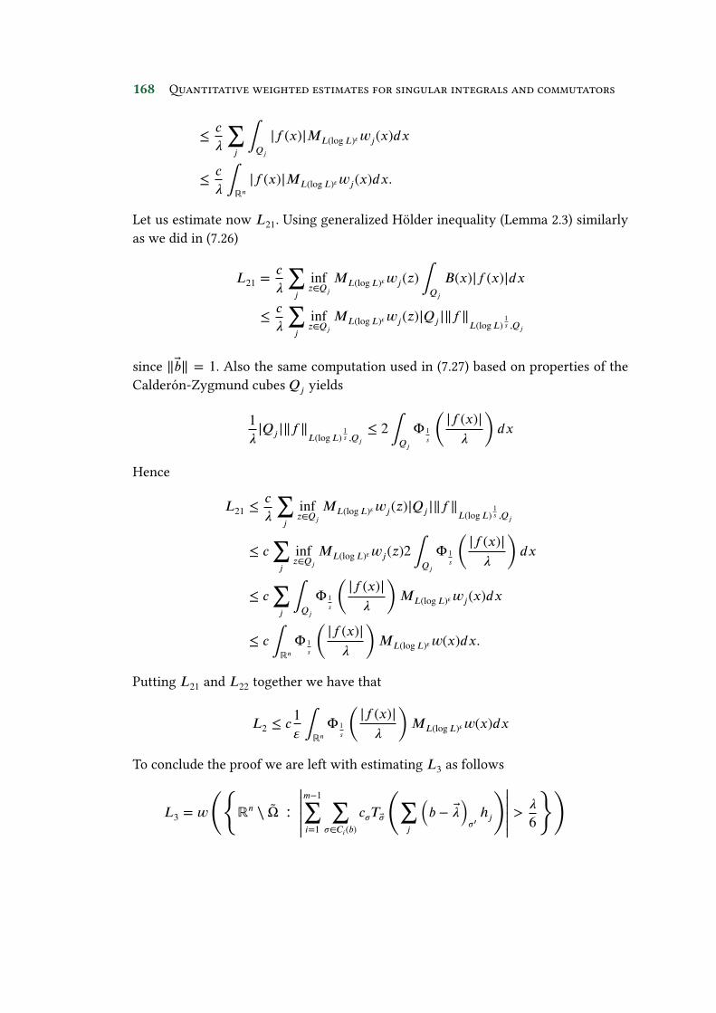
168 �antitative weighted estimates for singular integrals and commutators
≤ c�∑
j∫Qj
|f (x)|ML(logL)"wj(x)dx
≤ c� ∫ℝn
|f (x)|ML(logL)"wj(x)dx.
Let us estimate now L21. Using generalized Hölder inequality (Lemma 2.3) similarlyas we did in (7.26)
L21 =c�∑
jinfz∈Qj
ML(logL)"wj(z)∫QjB(x)|f (x)|dx
≤ c�∑
jinfz∈Qj
ML(logL)"wj(z)|Qj|‖f‖L(logL) 1s ,Qj
since ‖b‖ = 1. Also the same computation used in (7.27) based on properties of theCalderón-Zygmund cubes Qj yields
1�|Qj|‖f‖L(logL) 1s ,Qj
≤ 2∫QjΦ 1
s
(
|f (x)|�
)
dx
Hence
L21 ≤c�∑
jinfz∈Qj
ML(logL)"wj(z)|Qj|‖f‖L(logL) 1s ,Qj
≤ c∑
jinfz∈Qj
ML(logL)"wj(z)2∫QjΦ 1
s
(
|f (x)|�
)
dx
≤ c∑
j∫Qj
Φ 1s
(
|f (x)|�
)
ML(logL)"wj(x)dx
≤ c ∫ℝnΦ 1
s
(
|f (x)|�
)
ML(logL)"w(x)dx.
Putting L21 and L22 together we have that
L2 ≤ c1" ∫ℝn
Φ 1s
(
|f (x)|�
)
ML(logL)"w(x)dx
To conclude the proof we are left with estimating L3 as follows
L3 = w
({
ℝn ⧵ Ω ∶|
|
|
|
|
|
m−1∑
i=1
∑
�∈Ci(b)c�T�
(
∑
j
(
b − �)
�′ℎj
)
|
|
|
|
|
|
> �6
})

7. Weighted endpoint estimates 169
≤ w
({
ℝn ⧵ Ω ∶|
|
|
|
|
|
m−1∑
i=1
∑
�∈Ci(b)c�T�
(
∑
j
(
b − �)
�′f�Qj
)
|
|
|
|
|
|
> �12
})
+w
({
ℝn ⧵ Ω ∶|
|
|
|
|
|
m−1∑
i=1
∑
�∈Ci(b)c�T�
(
∑
j
(
b − �)
�′fQj�Qj
)
|
|
|
|
|
|
> �12
})
= L31 + L32
To estimate L31 we use the inductive hypothesis.
L31 = w
({
ℝn ⧵ Ω ∶|
|
|
|
|
|
m−1∑
i=1
∑
�∈Ci(b)c�T�
(
∑
j
(
b − �)
�′f�Qj
)
|
|
|
|
|
|
> �12
})
≤ cm−1∑
i=1
∑
�∈Ci(b)w
({
ℝn ⧵ Ω ∶|
|
|
|
|
|
T�
(
∑
j
(
b − �)
�′f�Qj
)
|
|
|
|
|
|
> �ck
})
≤ cm−1∑
i=1
∑
�∈Ci(b)
∑
j
(
1
"∑
i∈�1si+1
×∫QjΦ∑
i∈�1si
(
‖�‖|f (x)|�
(
b(x) − bQj)
�′
)
ML(logL)
∑
i∈�1si+"(wj)(x)dx
)
Since we are assuming that ‖b1‖OscexpLs1 = ‖b2‖OscexpLs2 = ⋯ = ‖bk‖OscexpLsm = 1, foreach � ⊆ b we have that ‖�‖ = 1. Then,
cm−1∑
i=1
∑
�∈Ci(b)
∑
j
[
1
"∑
i∈�1si+1
× ∫QjΦ∑
i∈�1si
(
|f (x)|�
(
b(x) − bQj)
�′
)
ML(logL)
∑
i∈�1si+"(wj)(x)dx
]
≤ cm−1∑
i=1
∑
�∈Ci(b)
∑
j
[
1
"∑
i∈�1si+1infz∈Qj
ML(logL)
∑
i∈�1si+"(wj)(z)
× ∫QjΦ∑
i∈�1si
(
|f (x)|�
(
b(x) − bQj)
�′
)
dx
]
Let us consider now
Φ−1u (t) =
tlog(e + t)u
'−1v (t) = log(1 + t)1v .

170 �antitative weighted estimates for singular integrals and commutators
Then
Φ−11s
(t)∏
i∈�'si
−1(t) = t
log(e + t)∑ 1
si
∏
i∈�log(1 + t)
1si ≤ t
log(e + t)∑
i∈�′1si
= Φ−1∑
i∈�′1si
(t)
and also we know that
Φu(t) ≃ t(
1 + log+ t)u , 'v(t) = et
v − 1.
Taking that into account, Lemma 2.3 gives
∫QjΦ∑
i∈�1si
(
|f (x)|�
(
b(x) − bQj)
�′
)
dx
≤ ∫QjΦ 1
s
(
|f (x)|�
)
dx +∑
i∈�∫Qj
(
exp(
|
|
|
bi(x) −(
bi)
Qj
|
|
|
si)
− 1)
dx
≤ ∫QjΦ 1
s
(
|f (x)|�
)
dx + c∑
i∈�|Qj|‖bi‖expLsi ,Qj
≤ ∫QjΦ 1
s
(
|f (x)|�
)
dx + c∑
i∈�|Qj|‖bi‖OscexpLsi
[
‖bi‖OscexpLsi = 1]
≤ ∫QjΦ 1
s
(
|f (x)|�
)
dx + cm|Qj|
≤ cm ∫QjΦ 1
s
(
|f (x)|�
)
dx.
(7.31)
In the last step we used properties of the Calderón-Zygmund cubes.
Plugging now that estimate, if we call 1s′= 1
s− mini
1si
cm−1∑
i=1
∑
�∈Cki
∑
j
(
1
"∑
i∈�1si+1infz∈Qj
ML(logL)
∑
i∈�′1si+"(wj)(z)
∫QjΦ∑
i∈�′1si
(
|f (x)|�
(
b(x) − bQj)
�
)
dx
)
≤ cmm−1∑
i=1
∑
�∈Cmi
∑
j
1
"∑
i∈�1si+1infz∈Qj
ML(logL)
∑
i∈�′1si+"(wj)(z)∫Qj
Φ 1s
(
|f (x)|�
)
dx
≤ cm1
"1s′ +1
∑
jinfz∈Qj
ML(logL)
1s +"(wj)(z)∫Qj
Φ 1s
(
|f (x)|�
)
dx

7. Weighted endpoint estimates 171
≤ cm1
"1s′ +1
∑
j∫Qj
ML(logL)
1s +"(wj)(x)Φ 1
s
(
|f (x)|�
)
dx
≤ cm1
"1s′ +1 ∫ℝn
ML(logL)
1s +"(wj)(x)Φ 1
s
(
|f (x)|�
)
dx
For L32 arguing in the same way we have that
E2 ≤ cm1
"1s′ +1
m−1∑
i=1
∑
�∈Cmi
∑
j
(
infz∈Qj
ML(logL)
1s +"wj(z)
× ∫QjΦ∑
i∈�′1si
(
|fQj |
�
(
b(x) − bQj)
�
)
dx
)
The same computation used to obtain (7.31) yields
∫QjΦ∑
i∈�′1si
(
|fQj |
�
(
b(x) − bQj)
�
)
dx ≤ ∫QjΦ 1
s
(
|fQj |
�
)
dx + cm|Qj|.
Now we see that using Jensen’s inequality,
∫QjΦ 1
s
(
|fQj |
�
)
dx ≤ |Qj|Φ 1s
(
|f |Qj�
)
≤ |Qj|1
|Qj| ∫QjΦ 1
s
(
|f (x)|�
)
dx = ∫QjΦ 1
s
(
|f (x)|�
)
dx.
Hence
∫QjΦ∑
i∈�′1si
(
|fQj |
�
(
b(x) − bQj)
�
)
dx ≤ ∫QjΦ 1
s
(
|f (x)|�
)
dx + cm|Qj|
and we �nish the estimate arguing as we did for L31.
7.3.2 A sparse domination approach
In this section we present an endpoint estimate for A-Hörmander operators. In thiscase we are going to restrict ourselves to the case of iterated commutators with justone symbol. The approach that we present here appeared �rst for commutators ofCalderón-Zygmund operators in [106] and was pushed even further in [81]. The mainresult of this section is borrowed precisely from [81].

172 �antitative weighted estimates for singular integrals and commutators
Theorem 7.5. Let b ∈ BMO and m be a positive integer. Let A0,… , Am be Young
functions, such that A0 ∈ (p0, p1) and A−1j (t)A−10 (t)C
−1j (t) ≤ t with Cj(t) = et
1j for
t ≥ 1. Let T be a A0-Hörmander operator. Assume that each Aj is submultiplicative,namely, that Aj(xy) ≤ Aj(x)Aj(y). Then we have that for every weight w, and everyfamily of Young functions '0,… , 'm
w({
x ∈ ℝn ∶ |T mb f (x)| > �})
≤ cncTm∑
ℎ=0
(
�'ℎ ∫ℝnAℎ
(
cT‖b‖BMO|f (x)|�
)
MΦm−ℎ◦'ℎw(x)dx)
,(7.32)
where Φj(t) = t log(e + t)j , 0 ≤ j ≤ m,
�'ℎ =
⎧
⎪
⎨
⎪
⎩
�n,m,ℎ + cn ∫∞1
'−1ℎ ◦Φ−1m−ℎ(t)Aℎ(log(e+t)
4(m−ℎ))
t2 log(e+t)3(m−ℎ)+1dt 0 ≤ ℎ < m,
∫ ∞1
'−1ℎ (t)Aℎ(log(e+t)2)
t2 log(e+t)3dt ℎ = m.
It is clear that from the preceding result it is possible to derive, as a particular case,the corresponding estimates for commutators of Calderón-Zygmund operators.Corollary 7.3. Let T be a !-Calderón-Zygmund operator with ! satisfying a Dinicondition. Let m be a non-negative integer and b ∈ BMO. Then we have that forevery weight w and every " > 0,
w({
x ∈ ℝn ∶ |T mb f | > �})
≤ cn,mcT1" ∫ℝn
Φm
(
|f |‖b‖mBMO�
)
ML(logL)m(log logL)1+"wdx
≤ cn,mcT1" ∫ℝn
Φm
(
|f |‖b‖mBMO�
)
ML(logL)m+"wdx
(7.33)
whereΦm(t) = t log(e+t)m and cT = CK+‖T ‖L2→L2+‖!‖Dini. If additionallyw ∈ A∞then
w({
x ∈ ℝn ∶ |T mb f | > �})
≤ cn,mcT [w]mA∞ log(
e + [w]A∞)
∫ℝnΦm
(
|f |‖b‖mBMO�
)
Mwdx.(7.34)
Furthermore if w ∈ A1
w({
x ∈ ℝn ∶ |T mb f | > �})
≤ cn,mcT [w]A1[w]mA∞log(e + [w]A∞)∫ℝn
Φm
(
|f |‖b‖mBMO�
)
wdx.(7.35)

7. Weighted endpoint estimates 173
Proof. Since T is an !-Calderón-Zygmund operator, we know that it satis�es anL∞-Hörmander with H∞ ≤ cn
(
‖!‖Dini + cK)
condition, then A0(t) = t. Let us callΦj(t) = t log(e + t)j . We are going to apply Theorem 7.5 with Aj(t) = Φj(t), so wehave to make suitable choices for each 'ℎ to obtain the desired estimate for each term
�'ℎ ∫ℝnAℎ
(
|f (x)|�
)
MΦm−ℎ◦'ℎw(x)dx.
We consider three cases. Let us assume �rst that 0 < ℎ < m. Then
�'ℎ = �n,m,ℎ + cn ∫
∞
1
'−1ℎ ◦Φ−1m−ℎ(t)Aℎ(log(e + t)4(m−ℎ))t2 log(e + t)3(m−ℎ)+1
dt
≲ �n,m,ℎ + cn ∫
∞
1
'−1ℎ (t) log(e + log(e + Φm−ℎ(t))4(m−ℎ))ℎ
Φm−ℎ(t)2 log(e + Φm−ℎ(t))1−(m−ℎ)Φ′m−ℎ(t)dt
≲ �n,m,ℎ + cn ∫
∞
1
'−1ℎ (t) log(e + log(e + Φm−ℎ(t))4(m−ℎ))ℎ
tΦm−ℎ(t) log(e + Φm−ℎ(t))1−(m−ℎ)dt
≲ �n,m,ℎ + cn ∫
∞
1
'−1ℎ (t) log(e + log(e + Φm−ℎ(t))4(m−ℎ))ℎ
t2 log(e + t)dt.
If we choose 'ℎ(t) = t log(e + t) log(e + log(e + t))1+� , � > 0, then
�'ℎ ≲ �n,m,ℎ + cn ∫
∞
1
log(e + log(e + Φm−ℎ(t))4(m−ℎ))ℎ
t log(e + t)2 log(e + log(e + t))1+�dt
≲ �n,m,ℎ + cn ∫
∞
1
dtt log(e + t) log(e + log(e + t))1+�
≲ 1"
and we observe that also
Φm−ℎ◦'ℎ ≲ t log(e + t)m log(e + log(e + t))1+". (7.36)
Then for 0 < ℎ < m
�'ℎ ∫ℝnAℎ
(
|f (x)|�
)
MΦm−ℎ◦'ℎw(x)dx
≤ c1" ∫ℝn
Φm
(
|f (x)|�
)
ML(logL)m(log logL)1+"w(x)dx
For the case ℎ = 0, arguing as in the �rst case, we obtain

174 �antitative weighted estimates for singular integrals and commutators
�'0 = �n,m + cn ∫
∞
1
'−10 ◦Φ−1m (t)A0(log(e + t)
4m)t2 log(e + t)3m+1
dt
≲ �n,m + cn ∫
∞
1
'−10 (t)t2 log(e + t)
dt
So it su�ces to choose '0(t) = t log(e + log(e + t))1+" and have that �'0 <1"
and
Φm◦'0 ≲ '0(t) log(e + t)m = t log(e + t)m log(e + log(e + t))1+". (7.37)
Consequently
�'0 ∫ℝnA0
(
|f (x)|�
)
MΦm◦'0w(x)dx ≤ c 1" ∫ℝn
|f (x)|�
ML(logL)m(log logL)1+"w(x)dx.
To end the proof we consider ℎ = m. We observe that
�'m = ∫
∞
1
'−1m (t)Am(log(e + t)2)t2 log(e + t)3
dt
= ∫
∞
1
'−1m (t) log(e + log(e + t)2)m
t2 log(e + t)dt
and taking 'm(t) = t log(e + t)m log(e + log(e + t))1+", we obtain �'m <1�
and sinceΦ0(t) = t
�'m ∫ℝnAm
(
|f (x)|�
)
MΦ0◦'mw(x)dx
≤ c 1" ∫ℝn
Φm
(
|f (x)|�
)
ML(logL)m(log logL)1+"w(x)dx
Collecting the preceding estimates
w({
x ∈ ℝn ∶ |T mb f | > �})
≤ cncTm∑
ℎ=0
(
�'ℎ ∫ℝnAℎ
(
|f |�
)
MΦm−ℎ◦'ℎwdx)
≤ cn,mcT1" ∫ℝn
Φm
(
|f |�
)
ML(logL)m(log logL)1+"wdx.
Now we observe that since t log(e + t)m log(e + log(e + t))1+" ≤ ct log(e + t)m+" fort ≥ 1 we also have that
w({
x ∈ ℝn ∶ T mb f (x) > �})
≤ cn,mcT1" ∫ℝn
Φm
(
|f (x)|�
)
ML(logL)m+"w(x)dx.

7. Weighted endpoint estimates 175
Now we turn our attention now to the remaining estimates. Assume that w ∈ A∞.To prove (7.34) we argue as in [78, Corollary 1.4]. Since log(t) ≤ t�
�, for every t ≥ 1
we have that1"ML(logL)m+"w ≤ c 1
"1
�m+"M1+(m+")�w.
Taking (m+")� = 1�n[w]A∞
where �n is chosen as in Lemma 3.5 we have that, precisely,using Lemma 3.5,
1"1�"M1+(m+")�w = 1
"(
(m + ")�n"[w]A∞)m+"M1+ 1
�n[w]A∞
w ≤ cm1"[w]m+"A∞
Mw.
Finally choosing " = 1log(e+[w]A∞)
we have that
1"ML(logL)m+"w ≤ cm
1"[w]m+"A∞
Mw ≤ cm log(e + [w]A∞)[w]mA∞Mw.
This estimate combined with (7.33) yields (7.34). We end the proof noting that (7.35)follows from (7.34) and the de�nition of w ∈ A1.
As we see, the estimates in the Corollary allow us to improve the results in theprevious section in two directions. We are able to prove that the estimate holds witha smaller maximal operator in the right hand side of the estimate and that the blowin " is just linear. Now we provide a proof of Theorem 7.5.
Proof of Theorem 7.5
Taking into account Theorem 4.1 it su�ces to obtain an endpoint estimate for each
m,ℎ (b, f )(x) =
∑
Q∈
|
|
b(x) − bQ||m−ℎ ‖
‖
‖
f |
|
b − bQ||ℎ‖‖
‖A,Q�Q(x).
We shall consider two cases.
Assume �rst that ℎ = m. Then we have that
m,m (b, f )(x) =
∑
Q∈‖f |b − bQ|m‖B,Q�Q(x) ≤ ‖b‖mBMO
∑
Q∈‖f‖Am,Q�Q(x)
and it su�ces to use Theorem 7.2, namely we have that
w
({
x ∈ ℝn ∶∑
Q∈‖f‖Am,Q�Q(x) > �
})
≤ c�'m ∫ℝnAm
(
|f (x)|�
)
M'mw(x)dx

176 �antitative weighted estimates for singular integrals and commutators
where
�'m = ∫
∞
1
'−1m (t)Am(log(e + t)2)t2 log(e + t)3
dt.
Now we consider the case 0 ≤ ℎ < m. Using generalized Hölder inequality if ℎ > 0we have that
m,ℎ (b, f )(x) ≤ c‖b‖ℎBMO
∑
Q∈|b(x) − bQ|m−ℎ‖f‖Aℎ,Q�Q(x) = ℎ
b f (x)
We de�neE = {x ∶ | ℎ
b f (x)| > 8,MAℎf (x) ≤ 1∕4}.
By the Fe�erman-Stein inequality (Lemma 7.2) and by homogeneity, it su�ces to as-sume that ‖b‖BMO = 1 and to show that
w(E) ≤ cC' ∫ℝnAℎ (|f |)M(Φm−ℎ◦'ℎ)(L)wdx.
Letk = {Q ∈ ∶ 4−k−1 < ‖f‖Aℎ,Q ≤ 4−k}
and for Q ∈ k, set
Fk(Q) ={
x ∈ Q ∶ |b(x) − bQ|m−ℎ >(32
)k}
.
If E ∩Q ≠ ∅ for some Q ∈ , then ‖f‖Aℎ,Q ≤ 1∕4. Therefore, for x ∈ E,
| ℎb f (x)| ≤
∞∑
k=1
∑
Q∈k
|b(x) − bQ|m−ℎ‖f‖Aℎ,Q�Q(x)
≤∞∑
k=1(3∕2)k
∑
Q∈k
‖f‖Aℎ,Q�Q(x) +∞∑
k=1
∑
Q∈k
|b(x) − bQ|m−ℎ‖f‖Aℎ,Q�Fk(Q)(x)
≡ 1f (x) + 2f (x).
Let Ei = {x ∈ E ∶ if (x) > 4}, i = 1, 2. Then
w(E) ≤ w(E1) +w(E2). (7.38)
Using (7.14) (with any Young function ℎ)
∫E1(1f )wdx ≤
(
∞∑
k=1(3∕4)k
)
w(E1) + cAΛA∞∑
k=1
(3∕8)kAℎ(4k)
−1ℎ
(
22k) ∫ℝn
Aℎ(|f |)M ℎwdx.

7. Weighted endpoint estimates 177
This estimate, combined with w(E1) ≤14∫E1(1f )wdx, implies
w(E1) ≤ cAΛA∞∑
k=1
(3∕8)kAℎ(4k)
ℎ−1 (22k
) ∫ℝnAℎ(|f |)M ℎwdx.
Now we observe that using (7.15)∞∑
k=1
(3∕8)kAℎ(4k)
ℎ−1 (22k
)
=∞∑
k=12k
Aℎ(4k)
ℎ−1 (22k
)
4k
≤ c∞∑
k=12k
Aℎ(4k)
ℎ−1 (22k
)
4k ∫
22k
22k−1
1t log(e + t)
dt
≤ c ∫
∞
1
−1ℎ (t)Aℎ(log(e + t)2)t2 log(e + t)3
dt.
We observe that since Aℎ(t)t
is not decreasing,
Aℎ(log(e + t)2)log(e + t)2
≤Aℎ(log(e + t)3(m−ℎ))log(e + t)3(m−ℎ)
≤Aℎ(log(e + t)4(m−ℎ))log(e + t)3(m−ℎ)
,
we have that c ∫ ∞1
−1ℎ (t)Aℎ(log(e+t)4(m−ℎ))
t2 log(e+t)3(m−ℎ)dt, and choosing ℎ = Φm−ℎ◦'ℎ,
w(E1) ≤ c�ℎ ∫ℝnAℎ(|f |)MΦm−ℎ◦'ℎwdx
Now we focus on the estimate ofw(E2). Arguing as in the proof of (7.11), forQ ∈ kwe can de�ne pairwise disjoint subsets EQ ⊆ Q and prove that
1 ≤ c|Q| ∫EQ
Aℎ(4k|f |)dx.
Hence,
w(E2) ≤ c∞∑
k=1
∑
Q∈k
14k( 1|Q| ∫Fk(Q)
|b − bQ|m−ℎwdx)
∫EQAℎ(4k|f |)dx. (7.39)
Now we apply twice the generalized Hölder inequality (2.8). First we obtain the fol-lowing inequality
1|Q| ∫Fk(Q)
|b − bQ|m−ℎwdx ≤ cn‖w�Fk(Q)‖L(logL)m−ℎ,Q. (7.40)

178 �antitative weighted estimates for singular integrals and commutators
Now we de�ne Φm−ℎ(t) = t log(e + t)m−ℎ, and Ψm−ℎ as
Ψ−1m−ℎ(t) =Φ−1m−ℎ(t)
'−1ℎ ◦Φ−1m−ℎ(t)
.
Since 'ℎ(t)∕t and Φ are strictly increasing functions, Ψm−ℎ is strictly increasing too.Hence, a direct application of (2.9) yields
‖w�Fk(Q)‖L(logL)m−ℎ,Q ≤ 2‖�Fk(Q)‖Ψ,Q‖w‖(Φm−ℎ◦'ℎ),Q (7.41)
= 2Ψ−1m−ℎ(|Q|∕|Fk(Q)|)
‖w‖(Φm−ℎ◦'ℎ),Q.
Now we observe that Theorem 1.1 assures that |Fk(Q)| ≤ �k|Q|, where �k =
min(1, e−(3∕2)
km−ℎ
2ne +1). That fact together with (7.40) and (7.41) yields
1|Q| ∫Fk(Q)
|b − bQ|jwdx ≤cn
Ψ−1m−ℎ(1∕�k)‖w‖(Φm−ℎ◦'ℎ),Q.
From this estimate combined with (7.39) it follows that
w(E2) ≤ cn∞∑
k=1
1Ψ−1m−ℎ(1∕�k)4k
∑
Q∈k
‖w‖(Φm−ℎ◦'ℎ),Q ∫EQAℎ(4k|f |)dx
≤ cn(
∞∑
k=1
1Ψ−1m−ℎ(1∕�k)
Aℎ(4k)4k
)
∫ℝnAℎ(|f |)M(Φm−ℎ◦'ℎ)(L)w(x)dx.
Now we observe that we can choose cn,m,ℎ such that for every k > cn,m,ℎ we have that1
�k−1= e
(3∕2)k−1m−ℎ
2ne −1 ≥ max{e2, 4k}. We note that
∫
1�k
1�k−1
1t log(e + t)
dt ≥ c.
Taking this into account, if 1�= (m− ℎ) log 4
log(3∕2), since A is submultiplicative and A(t)
tis
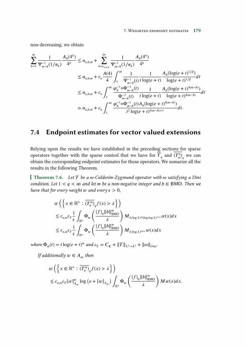
7. Weighted endpoint estimates 179
non-decreasing, we obtain
∞∑
k=1
1Ψ−1m−ℎ(1∕�k)
Aℎ(4k)4k
≤ �n,ℎ,m +∞∑
k=cn,m,ℎ
1Ψ−1m−ℎ(1∕�k)
Aℎ(4k)4k
≤ �n,ℎ,m + cnA(4)4 ∫
∞
1
1Ψ−1m−ℎ(t)
1t log(e + t)
Aℎ(log(e + t)1∕�)log(e + t)1∕�
dt
≤ �n,ℎ,m + cn ∫
∞
1
'−1ℎ ◦Φ−1m−ℎ(t)
Φ−1m−ℎ(t)
1t log(e + t)
Aℎ(log(e + t)4(m−ℎ))log(e + t)4(m−ℎ)
dt
≃ �n,ℎ,m + cn ∫
∞
1
'−1ℎ ◦Φ−1m−ℎ(t)Aℎ(log(e + t)4(m−ℎ))t2 log(e + t)3(m−ℎ)+1
dt.
7.4 Endpoint estimates for vector valued extensions
Relying upon the results we have established in the preceding sections for sparseoperators together with the sparse control that we have for T q and (T bm)q we canobtain the corresponding endpoint estimates for those operators. We sumarize all theresults in the following Theorem.
Theorem 7.6. Let T be a !-Calderón-Zygmund operator with ! satisfying a Dinicondition. Let 1 < q < ∞ and let m be a non-negative integer and b ∈ BMO. Then wehave that for every weight w and every " > 0,
w({
x ∈ ℝn ∶ (T mb )qf (x) > �})
≤ cn,mcT1" ∫ℝn
Φm
(
|f |q‖b‖mBMO�
)
ML(logL)m(log logL)1+"w(x)dx
≤ cn,mcT1" ∫ℝn
Φm
(
|f |q‖b‖mBMO�
)
ML(logL)m+"w(x)dx
where Φm(t) = t log(e + t)m and cT = CK + ‖T ‖L2→L2 + ‖!‖Dini.
If additionally w ∈ A∞ then
w({
x ∈ ℝn ∶ (T mb )qf (x) > �})
≤ cn,mcT [w]mA∞ log(
e + [w]A∞)
∫ℝnΦm
(
|f |q‖b‖mBMO�
)
Mw(x)dx.

180 �antitative weighted estimates for singular integrals and commutators
Furthermore if w ∈ A1
w({
x ∈ ℝn ∶ (T mb )qf (x) > �})
≤ cn,mcT [w]A1[w]mA∞log(e + [w]A∞)∫ℝn
Φm
(
|f |q‖b‖mBMO�
)
w(x)dx.
Proof. It su�ces to combine the proofs in the preceding sections and the correspond-ing sparse domination results.

8 Local decay estimates revisited
Calderón principle states that for each singular operator there exists a maximal op-erator that “controls” it. A paradigmatic example of that principle is the Coifman-Fe�erman estimate that we presented in Subsection 3.3.1.1, namely, for each 0 < p <∞ and every w ∈ A∞ there exists c = cn,w,p > 0 such that
‖T ∗f‖Lp(w) ≤ c‖Mf‖Lp(w).
where T ∗ stands for the maximal Calderón-Zygmund operator. In order to obtain suchan estimate as we showed in Subsection 3.3.1.1 a basic step consists in establishingthe following estimate
|{x ∈ Q ∶ T ∗f (x) > 2�, Mf (x) ≤ � }| ≤ c |Q|
where each Q is a Whitney cube and f is supported on Q.
In [14] , trying to obtain a quantitative weighted estimate for Calderón-Zygmundoperators by means of the good-� technique, S. Buckley obtained an exponential de-cay in � that reads as follows.
|{x ∈ Q ∶ T ∗f (x) > 2�, Mf (x) ≤ � }| ≤ ce−c |Q| .
Later on, Karagulyan [87] provided an improved version of the former estimate, namely,
|{x ∈ Q ∶ T ∗f (x) > tMf (x)}| ≤ ce−�t |Q| .
This inequality was later generalized for several operators by C. Ortiz-Caraballo, C.Pérez and E. Rela in [122]. Our purpose in this section is to extend their results to somenew operators, such as vector valued commutators orA-Hörmander operators as wellas reproving the results in that work relying upon the sparse domination results thatwe have obtained. We will end this section proving that the subexponential decay for

182 �antitative weighted estimates for singular integrals and commutators
[b, T ] where T is a Calderón-Zygmund is sharp, and providing an alternative proofof Theorem 4.2 based on that sharpness.
The proof of the corresponding exponential decay for each operator can be re-duced to proof the corresponding exponential decay for its sparse counterpart. Weprovide the estimates for sparse operators in the following Theorem.
Theorem 8.1. Let Q0 be a cube and f a function supported in Q0. Then
1. If 1 ≤ r <∞ then
|
|
|
{
x ∈ Q0 ∶ r |f | > tMf (x)
}
|
|
|
≤ c1e−c2tr
|Q0| (8.1)
2. If A is a Young function and ⊂ (Q0) then
|
|
|
|
|
|
{
x ∈ Q0 ∶∑
P∈‖f‖A,3Q�Q(x) > tMAf (x)
}
|
|
|
|
|
|
≤ ce−�t|Q0|. (8.2)
3. If A and B Young functions such that A−1(t)B−1(t)C−1(t) ≤ t with C(t) = et1∕m , mis a positive integer, b1,… , bm ∈ BMO and ⊂ (Q0), then for every � ∈ Ci(b)
|
|
|
|
{
x ∈ Q0 ∶ �B,f (x) > tMAf (x)
}
|
|
|
|
≤ ce−�
(
t∏mi=1 ‖bi‖BMO
)1
♯�′+1
|Q0|.
where
�B, (b, f )(x) =
∑
Q∈
|
|
b(x) − b3Q||�′‖
‖
‖
f |
|
b − b3Q||�‖
‖
‖B,3Q�Q(x)
Proof. First we observe that if P is an arbitrary cube such that P ∩ Q ≠ ∅ and|P | ≃ |Q| for some cube Q ∈ , then
|
|
|
|
|
|
{
x ∈ P ∶∑
R∈ , R⊆Q�R(x) > t
}
|
|
|
|
|
|
≤ ce−�t|P |. (8.3)
Indeed we observe that actually
|
|
|
|
|
|
{
x ∈ P ∶∑
R∈ , R⊆Q�R(x) > t
}
|
|
|
|
|
|
=|
|
|
|
|
|
{
x ∈ P ∩Q ∶∑
R∈ , R⊆Q�R(x) > t
}
|
|
|
|
|
|
≤|
|
|
|
|
|
{
x ∈ Q ∶∑
R∈ , R⊆Q�R(x) > t
}
|
|
|
|
|
|

8. Local decay estimates revisited 183
Now we observe that in [122, Theorem 2.1], it was established that|
|
|
|
|
|
{
x ∈ Q ∶∑
R∈ , R⊆Q�R(x) > t
}
|
|
|
|
|
|
≤ ce−�t|Q|
so recalling now that |P | ≃ |Q|, leads to (8.3). Armed with this estimate, we are inthe position to prove the estimates in the statement of the theorem.
We establish �rst (8.1). Assume that supp f ⊆ Q0 for some arbitrary cube Q0. It’sclear thatQ0 can be covered by cn pairwise disjoint cubes in , such that |Q0| ≃ |Qk|
and Q ∩Qj ≠ ∅. Let us denote by {Qj} that family of cubes. Then we have that
f =cn∑
j=1f�Qj .
Hence
|
|
|
{
x ∈ Q0 ∶ r |f | > tMf (x)
}
|
|
|
≤cn∑
j=1
|
|
|
|
|
{
x ∈ Q0 ∶ r |f�Qj | >
tcnMf (x)
}
|
|
|
|
|
We shall assume that each Qj ∈ . Indeed, if that was not the case we can add thosecubes to the family and call the resulting family. We check that as follows. LetR ∈ . We observe �rst that if R ⊆ Qj for some j or R ∩Qj = ∅ for every j, then Rsatis�es the same Carleson that it satis�ed with respect to the family . In the casethat R = Qj for some j, we have that
∑
P⊆Qj , P∈
|P | =∑
R∈R maximal in Qj
∑
P⊆R, P∈
|P | ≤ 1�
∑
R∈R maximal in Qj
|R| ≤ 1�|Qj|
and �nally in the case that R contains some Qj
∑
R⊆Qj , P∈
|P | =∑
R⊆P ,R∈|P | +
∑
Qj⊆P|P | ≤
(
1�+ cn
)
|P |.
Since every Λ-Carleson family is 1Λ
-sparse, the preceding estimates yield that is a�
1+�cn-sparse family. Now we observe that
r |f�Qj |(x) =
(
∑
P∈
(
1|P | ∫P
|f�Qj |)r
�P (x)
)1r
> tMf (x)
⇐⇒
∑
P∈
(
1|P |
∫P |f�Qj |)r�P (x)
Mf (x)r> tr

184 �antitative weighted estimates for singular integrals and commutators
Now we split the sparse operator as follows∑
P∈
(
1|P | ∫P
|f�Qj |)r
�P (x)
=∑
P∈ , P⊊Qj
(
1|P | ∫P
|f�Qj |)r
�P (x) +∑
P∈ , P⊇Qj
(
1|P | ∫P
|f�Qj |)r
�P (x).
Now we observe that trivially∑
P∈ , P⊊Qj
(
1|P |
∫P |f |)r�P (x)
Mf (x)r≤
∑
P∈ , P⊆Qj
�P (x)
On the other hand, since supp f ⊆ Qj and since Q0 ∩Qj ≠ ∅ we have that for everyx ∈ Q0, since 5Qj ⊃ Q0,
∑
P∈ , P⊇Qj
(
1|P |
∫P |f |)r�P (x)
Mf (x)r≤
∑
P∈ , P⊇Qj
(
1|P |
∫P |f |)r
(
1|5Qj |
∫5Qj |f |)r�P (x)
=∑
P∈ , P⊇Qj
(
1|P |
∫Qj |f |)r
(
1|5Qj |
∫Qj |f |)r�P (x)
=∑
P∈ , P⊇Qj
(
|5Qj|
|P |
)r
�P (x)
≤ 5nr∞∑
k=0
12nrk
= 2nr2nr − 1
= 5nr(2nr)′
Combining those estimates and taking into account (8.3),
|
|
|
|
{
x ∈ Q0 ∶ r |f�Qj | > tMf (x)
}
|
|
|
|
≤
|
|
|
|
|
|
|
|
⎧
⎪
⎨
⎪
⎩
x ∈ Q0 ∶∑
P∈P⊆Qj
�P (x) > tr − cn,r
⎫
⎪
⎬
⎪
⎭
|
|
|
|
|
|
|
|
≤ c1e−c2tr
|Q0|
and we are done.
To prove (8.2), assume that supp f ⊂ Q0. Then∑
Q∈ ‖f‖B,3Q�Q(x)MBf (x)
≤∑
Q∈�Q(x)

8. Local decay estimates revisited 185
and since ⊂ (Q0) direct application of (8.3) yields (8.2).
Now we turn our attention to (3). We can assume without loss of generality that‖bi‖BMO = 1 for every i. First we observe that
|b(x) − b3Q|�′ ≤ cn♯�′∑
j=0
∑
�∈Cj (�′)
(
∏
i∈�′‖bi‖BMO
)
|b(x) − bQ|� ≤ cn♯�′∑
j=0
∑
�∈Cj (�′)|b(x) − bQ|�
and also that by generalized Hölder inequality,
‖|b − b3Q|�f‖B,3Q ≤ c
(
∏
i∈�‖bi‖BMO
)
‖f‖A,3Q = c‖f‖A,3Q.
Then we have that|
|
|
|
|
|
{
x ∈ Q0 ∶�B, (b, f )MAf
> �
}
|
|
|
|
|
|
≤
|
|
|
|
|
|
|
|
⎧
⎪
⎨
⎪
⎩
x ∈ Q0 ∶
∑
Q∈
(
∑♯�′
j=0∑
�∈Cj (�′)|b(x) − bQ|�
)
‖f‖A,3Q�Q(x)
MAf> �c
⎫
⎪
⎬
⎪
⎭
|
|
|
|
|
|
|
|
= I
Lemma 1.5 provides sparse families i containing such that for every Q ∈ i,
|bi(x) − (bi)Q| ≤ cn∑
P∈i,P⊆Q
(
1|P | ∫P
|bi(x) − (bi)P |dx)
�P (x).
Since bi ∈ BMO with ‖bi‖BMO = 1 then we have that for every Q ∈ ,
|bi(x) − (bi)Q| ≤ cn∑
P∈ ,P⊆Q
(
1|P | ∫P
|b(x) − bP |dx)
�P (x) ≤ cn∑
P∈i,P⊆Q0
�P (x).
Then we have that∑
Q∈
(
∑♯�′
j=0∑
�∈Cj (�′)|b(x) − bQ|�
)
‖f‖A,3Q�Q(x)
MAf
≤ cn∑
Q∈
⎛
⎜
⎜
⎝
♯�′∑
j=0
∑
�∈Cj (�′)
∏
i∈�
⎛
⎜
⎜
⎝
∑
P∈i,P⊆Q0
�P (x)⎞
⎟
⎟
⎠
⎞
⎟
⎟
⎠
�Q(x)

186 �antitative weighted estimates for singular integrals and commutators
Now we observe that
=m⋃
i=1i
is a sparse family such that , 1,… , m ⊂ . Hence
∑
Q∈
⎛
⎜
⎜
⎝
♯�′∑
j=0
∑
�∈Cj (�′)
∏
i∈�
⎛
⎜
⎜
⎝
∑
P∈i,P⊆Q0
�P (x)⎞
⎟
⎟
⎠
⎞
⎟
⎟
⎠
�Q(x)
≤∑
Q∈
(
♯�′∑
j=0
∑
�∈Cj (�′)
∏
i∈�
(
∑
P∈ ,P⊆Q0
�P (x)
))
�Q(x)
≤ cm
(
∑
P∈�P (x)
)♯�′+1
and then, using again (8.3),
I ≤
|
|
|
|
|
|
|
|
⎧
⎪
⎨
⎪
⎩
x ∈ Q0 ∶
(
∑
P∈�P (x)
)♯�′+1
> �c
⎫
⎪
⎬
⎪
⎭
|
|
|
|
|
|
|
|
=|
|
|
|
|
|
{
x ∈ Q0 ∶∑
P∈�P (x) >
(�c
)
1♯�′+1
}
|
|
|
|
|
|
≤ ce−�(
�2c
)1
♯�′+1|Q|
as we wanted to prove.
Remark 8.1. Arguing as in the proof of (8.1) it is possible to remove the localizationcondition of the sparse family in the rest of the statements of Theorem 8.1, howeverwe chose to restrict ourselves to the localized version since it will be enough for ourpurposes.
As a direct consequence of the sparse domination results and the preceding esti-mates we have the following Theorem.
Theorem 8.2. Let Q be a cube. Then:
1. If T is a B-Hörmander operator such that B ∈ (p0, p1) and supp f ⊂ Q0 then
|
|
|
{
x ∈ Q0 ∶ |Tf (x)| > tMBf (x)}
|
|
|
≤ ce−�t
cncT|Q0|. (8.4)
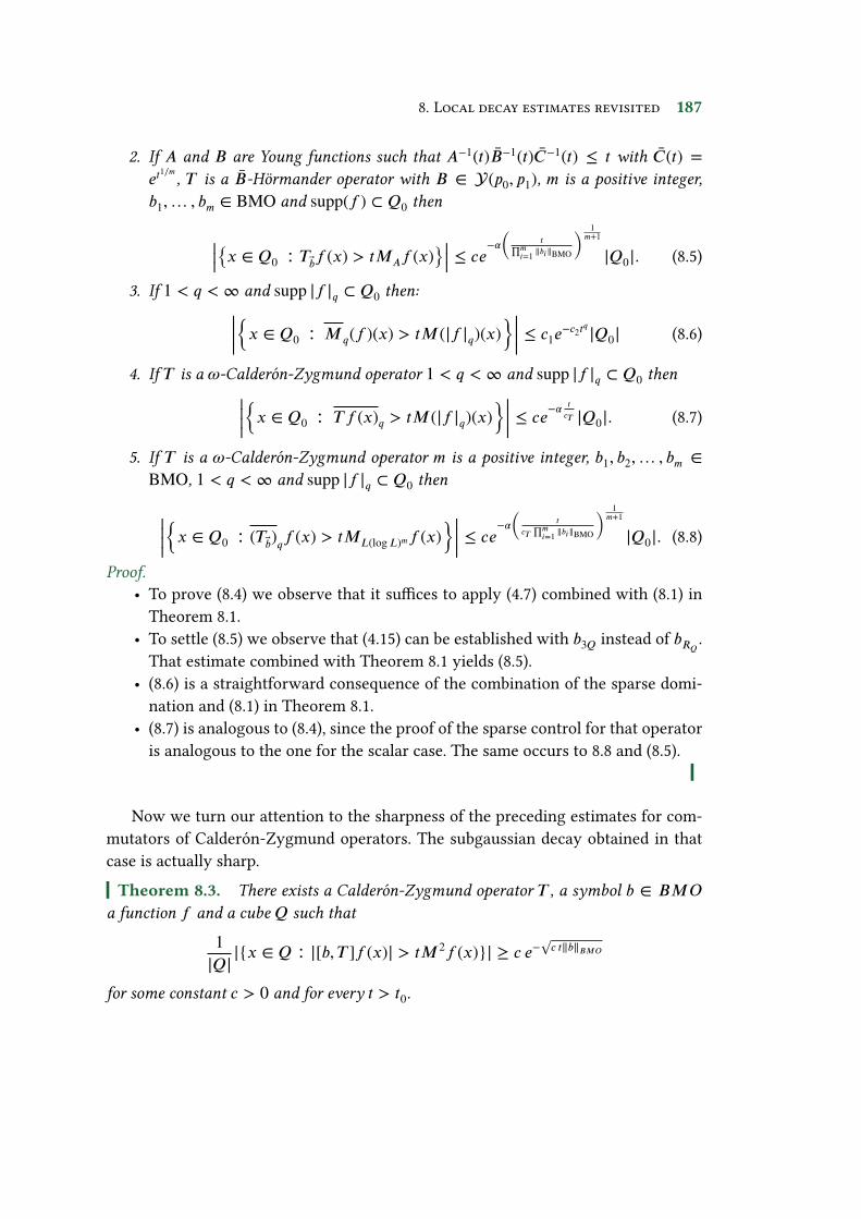
8. Local decay estimates revisited 187
2. If A and B are Young functions such that A−1(t)B−1(t)C−1(t) ≤ t with C(t) =et1∕m , T is a B-Hörmander operator with B ∈ (p0, p1), m is a positive integer,b1,… , bm ∈ BMO and supp(f ) ⊂ Q0 then
|
|
|
{
x ∈ Q0 ∶ Tbf (x) > tMAf (x)}
|
|
|
≤ ce−�
(
t∏mi=1 ‖bi‖BMO
)1
m+1
|Q0|. (8.5)
3. If 1 < q <∞ and supp |f |q ⊂ Q0 then:
|
|
|
|
{
x ∈ Q0 ∶ Mq(f )(x) > tM(|f |q)(x)}
|
|
|
|
≤ c1e−c2tq
|Q0| (8.6)
4. If T is a !-Calderón-Zygmund operator 1 < q <∞ and supp |f |q ⊂ Q0 then
|
|
|
|
{
x ∈ Q0 ∶ Tf (x)q > tM(|f |q)(x)}
|
|
|
|
≤ ce−�tcT|Q0|. (8.7)
5. If T is a !-Calderón-Zygmund operator m is a positive integer, b1, b2,… , bm ∈BMO, 1 < q <∞ and supp |f |q ⊂ Q0 then
|
|
|
|
{
x ∈ Q0 ∶ (Tb)qf (x) > tML(logL)mf (x)}
|
|
|
|
≤ ce−�
(
tcT
∏mi=1 ‖bi‖BMO
)1
m+1
|Q0|. (8.8)
Proof.• To prove (8.4) we observe that it su�ces to apply (4.7) combined with (8.1) in
Theorem 8.1.• To settle (8.5) we observe that (4.15) can be established with b3Q instead of bRQ .
That estimate combined with Theorem 8.1 yields (8.5).• (8.6) is a straightforward consequence of the combination of the sparse domi-
nation and (8.1) in Theorem 8.1.• (8.7) is analogous to (8.4), since the proof of the sparse control for that operator
is analogous to the one for the scalar case. The same occurs to 8.8 and (8.5).
Now we turn our attention to the sharpness of the preceding estimates for com-mutators of Calderón-Zygmund operators. The subgaussian decay obtained in thatcase is actually sharp.Theorem 8.3. There exists a Calderón-Zygmund operator T , a symbol b ∈ BMO
a function f and a cube Q such that
1|Q|
|{x ∈ Q ∶ |[b, T ]f (x)| > tM2f (x)}| ≥ c e−√
c t‖b‖BMO
for some constant c > 0 and for every t > t0.

188 �antitative weighted estimates for singular integrals and commutators
Proof. Let us choose b(x) = log |x|, T = H the Hilbert transform. Q = (0, 1) andf = �Q. Then we have that taking into account (4.13)
|{x ∈ (0, 1) ∶ |[b,H]f (x)| > tM2f (x)}|
= |{x ∈ (0, 1) ∶ |[b,H]f (x)| > t}| ≥ c e−√
� t t > t0.
This ends the end of the proof.
As we announced at the beginning of the section, relying upon the precedingresult we are in the position to provide the second proof of Theorem 4.2 that weannounced in Section 4.2.
Proof. Assume that (4.9) holds. Then, for some c > 1
|
|
|
{
x ∈ Q ∶ |[b, T ]f (x)| > tM2f (x)}
|
|
|
≤|
|
|
|
|
|
{
x ∈ Q ∶N∑
j=1
∑
P∈j
‖f‖L logL,P�P (x) >tcM2f (x)
}
|
|
|
|
|
|
.
It will be enough for our purposes to work on each term of the inner sum, namelyto control
|
|
|
|
|
|
{
x ∈ Q ∶∑
P∈j
‖f‖L logL,P�P (x) > tM2f (x)
}
|
|
|
|
|
|
Now, recalling that M2f ≃ ML logLf , is not hard to see that essentially the sameargument we used to prove (8.1) yields that
1|Q|
|
|
|
|
|
|
{
x ∈ Q ∶∑
P∈j
‖f‖L logL,P�P (x) > tM2f (x)
}
|
|
|
|
|
|
≤ ce−�t.
Hence, combining the preceding estimates we arrive to
1|Q|
|
|
|
{
x ∈ Q ∶ |[b, T ]f (x)| > tM2f (x)}
|
|
|
≤ ce−�t t > 0
which is a contradiction with Theorem 8.3.

9 Open questions
This chapter is devoted to provide a list of open questions that naturally arise fromthis dissertation.
1. Very recently A. K. Lerner proved [98] that
‖M◦TΩ‖L2(w) ≤ cn,Ω[w]2A2
where Ω ∈ L∞(Sn−1). Bearing in mind that the dependence on the A2 constantof M is linear it seems reasonable to consider the preceding estimate as a leadto think that
‖TΩ‖L2(w) ≤ cn,Ω[w]A2should be true. Taking that into account one may ask the following question.Would it be possible to replace s > 1 by 1 in the sparse domination resultsfor both rough singular integrals with Ω ∈ L∞ and their commutators? Thatkind of improvement would lead to a proof of the linear dependence on the A2constant and would allow to apply essentially the same arguments provided inChapter 7 to derive better endpoint estimates for those operators.
2. In Theorems 5.3 and 5.4 some strong type (p, p) estimates are provided for A-Hörmander operators. However, those estimates do not seem to be completelysatisfactory. If we assume that A(t) = tr′ , then we know that if T is an A-Hörmander operator and w ∈ Ap∕r, then T ∶ Lp(w)→ Lp(w) and we can evenprovide the possibly sharp dependence on [w]Ap∕r . Then a natural question isthe following. Would it be possible to de�ne some bumped Ap type class that�ts to A-Hörmander operators as well as the Ap∕r class does for tr′-Hörmanderoperators and that also allows to recover the Ap∕r class when A(t) = tr′?
3. Sparse domination estimates are provided for several vector valued extensions.Would it be possible to obtain any analogue result for vector valued extensionsof rough singular integrals and their commutators?

190 �antitative weighted estimates for singular integrals and commutators
4. The endpoint estimates provided that rely on the sparse domination are onlyobtained for the iterated commutator. It should be possible to prove analogousestimates for symbol multilinear commutators.
5. On the Muckenhoupt-Wheeden conjecture in the case of T being a Calderón-Zygmund operator after [47, 17, 138] essentially the only open question is whetherthe following estimate
w({x ∈ ℝn ∶ |Tf (x)| > t}) ≤ c ∫ℝn
|f (x)|t
ML(log logL)w(x)dx
is true or not for every weight w ≥ 0 with c > 0 independent of w. Howeverin the case of commutators no negative result has been obtained. The naturalconjecture, by analogy with [17] is the following. Does
w({x ∈ ℝn ∶ |[b, T ]f (x)| > t}) ≤ c ∫ℝnΦ(
|f (x)|t
)
ML(logL)(log logL)w(x)dx
hold for every weight w with constant c > 0 not depending on w?Following ideas in [68] it seems to be possible to disprove a partial dyadic ana-logue, namely, there exists a sparse family such that
w({x ∈ ℝ ∶ |f (x)| > t}) ≤ c ∫ℝnΦ(
|f (x)|t
)
M'w(x)dx
does not hold for every weight w with c > 0 independent of w where
f (x) =∑
Q∈
∑
Q∈|b(x)| 1
|Q| ∫Q|f (y)|dy�Q(x)
and ' is a Young function such that
limt→∞
'(t)t log(e + t) log(log(ee + t))
= 0.
6. Regarding the A1 conjecture, it was recently proved [102] that the dependenceon the A1 constant [w]A1 log(e + [w]A1) is sharp. What about the case of thecommutator? Is [w]2A1 log(e + [w]A1) sharp for the commutator or the sparseoperators that control it?

Bibliography
[1] Accomazzo, N. A characterization of BMO in terms of endpoint bounds forcommutators of singular integrals. (Preprint) (2017).
[2] Álvarez, J., Bagby, R. J., Kurtz, D. S., and Pérez, C. Weighted estimates forcommutators of linear operators. Studia Math. 104, 2 (1993), 195–209.
[3] Alvarez, J., and Pérez, C. Estimates with A∞ weights for various singularintegral operators. Boll. Un. Mat. Ital. A (7) 8, 1 (1994), 123–133.
[4] Astala, K., Iwaniec, T., and Saksman, E. Beltrami operators in the plane.Duke Math. J. 107, 1 (2001), 27–56.
[5] Barron, A. Weighted Estimates for Rough Bilinear Singular Integrals viaSparse Domination. ArXiv e-prints (Feb. 2017).
[6] Beltran, D. A Fe�erman-Stein inequality for the Carleson operator. ArXive-prints (Oct. 2014).
[7] Benea, C., and Bernicot, F. Conservation de certaines propriétés á traversun contrôle épars d’un opérateur et applications au projecteur de Leray-Hopf.ArXiv e-prints (Mar. 2017).
[8] Benea, C., Bernicot, F., and Luqe, T. Sparse bilinear forms for Bochner Rieszmultipliers and applications. Trans. London Math. Soc. 4, 1 (2017), 110–128.
[9] Benedek, A., Calderón, A.-P., and Panzone, R. Convolution operators onBanach space valued functions. Proc. Nat. Acad. Sci. U.S.A. 48 (1962), 356–365.
[10] Bernicot, F., Frey, D., and Petermichl, S. Sharp weighted norm estimatesbeyond Calderón-Zygmund theory. Anal. PDE 9, 5 (2016), 1079–1113.

192 �antitative weighted estimates for singular integrals and commutators
[11] Berra, F., Carena, M., and Pradolini, G. Mixed weak estimates of Sawyertype for commutators of singular integrals and related operators. ArXiv e-prints(Apr. 2017).
[12] Bloom, S. A commutator theorem and weighted BMO. Trans. Amer. Math. Soc.292, 1 (1985), 103–122.
[13] Buckley, S. M. Harmonic analysis on weighted spaces. ProQuest LLC, AnnArbor, MI, 1990. Thesis (Ph.D.)–The University of Chicago.
[14] Buckley, S. M. Estimates for operator norms on weighted spaces and reverseJensen inequalities. Trans. Amer. Math. Soc. 340, 1 (1993), 253–272.
[15] Bui, T. A., Conde-Alonso, J. M., Duong, X. T., and Hormozi, M. A note onweighted bounds for singular operators with nonsmooth kernels. Studia Math.236, 3 (2017), 245–269.
[16] Burkholder, D. L., and Gundy, R. F. Extrapolation and interpolation of quasi-linear operators on martingales. Acta Math. 124 (1970), 249–304.
[17] Caldarelli, M., Lerner, A. K., and Ombrosi, S. On a counterexample relatedto weighted weak type estimates for singular integrals. Proc. Amer. Math. Soc.145, 7 (2017), 3005–3012.
[18] Calderón, A. P. Inequalities for the maximal function relative to a metric.Studia Math. 57, 3 (1976), 297–306.
[19] Calderon, A. P., and Zygmund, A. On the existence of certain singular inte-grals. Acta Math. 88 (1952), 85–139.
[20] Calderón, A. P., and Zygmund, A. On singular integrals. Amer. J. Math. 78(1956), 289–309.
[21] Cejas, M. E., Li, K., Pérez, C., and Rivera-Ríos, I. P. Vector-valued operators,optimal weighted estimates and the Cp condition. ArXiv e-prints (2017).
[22] Chanillo, S., and Wheeden, R. L. Some weighted norm inequalities for thearea integral. Indiana Univ. Math. J. 36, 2 (1987), 277–294.
[23] Christ, M. Weak type (1, 1) bounds for rough operators. Ann. of Math. (2) 128,1 (1988), 19–42.

BIBLIOGRAPHY 193
[24] Christ, M., and Rubio de Francia, J. L. Weak type (1, 1) bounds for roughoperators. II. Invent. Math. 93, 1 (1988), 225–237.
[25] Chung, D., Pereyra, M. C., and Perez, C. Sharp bounds for general com-mutators on weighted Lebesgue spaces. Trans. Amer. Math. Soc. 364, 3 (2012),1163–1177.
[26] Cladek, L., and Ou, Y. Sparse domination of Hilbert transforms along curves.ArXiv e-prints (Apr. 2017).
[27] Coifman, R., and Fefferman, C. Weighted norm inequalities for maximalfunctions and singular integrals. Studia Mathematica 51, 3 (1974), 241–250.
[28] Coifman, R., Jones, P. W., and Rubio de Francia, J. L. Constructive decom-position of BMO functions and factorization of Ap weights. Proc. Amer. Math.Soc. 87, 4 (1983), 675–676.
[29] Coifman, R. R., and Meyer, Y. Au delà des opérateurs pseudo-di�érentiels, vol. 57of Astérisque. Société Mathématique de France, Paris, 1978. With an Englishsummary.
[30] Coifman, R. R., and Rochberg, R. Another characterization of BMO. Proc.Amer. Math. Soc. 79, 2 (1980), 249–254.
[31] Coifman, R. R., Rochberg, R., and Weiss, G. Factorization theorems for Hardyspaces in several variables. Ann. of Math. (2) 103, 3 (1976), 611–635.
[32] Conde-Alonso, J. M., Culiuc, A., Di Plinio, F., and Ou, Y. A sparse domina-tion principle for rough singular integrals. Anal. PDE 10, 5 (2017), 1255–1284.
[33] Conde-Alonso, J. M., and Rey, G. A pointwise estimate for positive dyadicshifts and some applications. Math. Ann. 365, 3-4 (2016), 1111–1135.
[34] Cordoba, A., and Fefferman, C. A weighted norm inequality for singularintegrals. Studia Math. 57, 1 (1976), 97–101.
[35] Cruz-Uribe, D. Two weight inequalities for fractional integral operators andcommutators. In Advanced courses of mathematical analysis VI, F. J. Martín-Reyes, P. Ortega Salvador, M. Lorente, and C. González, Eds. World Sci. Publ.,Hackensack, NJ, 2017, pp. 25–85.
[36] Cruz-Uribe, D., Martell, J. M., and Pérez, C. Extrapolation fromA∞ weightsand applications. J. Funct. Anal. 213, 2 (2004), 412–439.
194 �antitative weighted estimates for singular integrals and commutators
[37] Cruz-Uribe, D., Martell, J. M., and Pérez, C. Weighted weak-type inequali-ties and a conjecture of Sawyer. Int. Math. Res. Not., 30 (2005), 1849–1871.
[38] Cruz-Uribe, D., Martell, J. M., and Pérez, C. Sharp weighted estimates forclassical operators. Adv. Math. 229, 1 (2012), 408–441.
[39] Cruz-Uribe, D. V., Martell, J. M., and Pérez, C. Weights, extrapolation andthe theory of Rubio de Francia, vol. 215 of Operator Theory: Advances and Appli-cations. Birkhäuser/Springer Basel AG, Basel, 2011.
[40] Culiuc, A., Di Plinio, F., and Ou, Y. Domination of multilinear singular inte-grals by positive sparse forms. ArXiv e-prints (Mar. 2016).
[41] Culiuc, A., Di Plinio, F., and Ou, Y. Uniform sparse domination of singularintegrals via dyadic shifts. ArXiv e-prints (Oct. 2016).
[42] Culiuc, A., Kesler, R., and Lacey, M. T. Sparse Bounds for the Discrete CubicHilbert Transform. ArXiv e-prints (Dec. 2016).
[43] Curbera, G. P., García-Cuerva, J., Martell, J. M., and Pérez, C. Extrapola-tion with weights, rearrangement-invariant function spaces, modular inequal-ities and applications to singular integrals. Adv. Math. 203, 1 (2006), 256–318.
[44] de França Silva, F. C., and Zorin-Kranich, P. Sparse domination of sharpvariational truncations. ArXiv e-prints (Apr. 2016).
[45] Di Plinio, F., Do, Y. Q., and Uraltsev, G. N. Positive sparse domination ofvariational Carleson operators. To appear in Annali della Scuola Normale diPisa (2017).
[46] Di Plinio, F., Hytönen, T. P., and Li, K. Sparse bounds for maximal roughsingular integrals via the Fourier transform. ArXiv e-prints (June 2017).
[47] Domingo-Salazar, C., Lacey, M., and Rey, G. Borderline weak-type estimatesfor singular integrals and square functions. Bull. Lond. Math. Soc. 48, 1 (2016),63–73.
[48] Dragičević, O., Grafakos, L., Pereyra, M. C., and Petermichl, S. Extrapo-lation and sharp norm estimates for classical operators on weighted Lebesguespaces. Publ. Mat. 49, 1 (2005), 73–91.
[49] Duoandikoetxea, J. Weighted norm inequalities for homogeneous singularintegrals. Trans. Amer. Math. Soc. 336, 2 (1993), 869–880.

BIBLIOGRAPHY 195
[50] Duoandikoetxea, J. Fourier analysis, vol. 29 of Graduate Studies in Mathe-matics. American Mathematical Society, Providence, RI, 2001. Translated andrevised from the 1995 Spanish original by David Cruz-Uribe.
[51] Duoandikoetxea, J. Extrapolation of weights revisited: new proofs and sharpbounds. J. Funct. Anal. 260, 6 (2011), 1886–1901.
[52] Duoandikoetxea, J., Martín-Reyes, F. J., and Ombrosi, S. On the A∞ condi-tions for general bases. Math. Z. 282, 3-4 (2016), 955–972.
[53] Duoandikoetxea, J., and Rubio de Francia, J. L. Maximal and singular in-tegral operators via Fourier transform estimates. Invent. Math. 84, 3 (1986),541–561.
[54] Evans, L. C., and Gariepy, R. F. Measure theory and �ne properties of functions.Studies in Advanced Mathematics. CRC Press, Boca Raton, FL, 1992.
[55] Fan, D., and Sato, S. Weak type (1, 1) estimates for Marcinkiewicz integralswith rough kernels. Tohoku Math. J. (2) 53, 2 (2001), 265–284.
[56] Fan, D., and Sato, S. Weighted weak type (1, 1) estimates for singular integralsand Littlewood-Paley functions. Studia Math. 163, 2 (2004), 119–136.
[57] Fefferman, C., and Stein, E. M. Some maximal inequalities. Amer. J. Math.93 (1971), 107–115.
[58] Fefferman, C., and Stein, E. M. Hp spaces of several variables. Acta Math.129, 3-4 (1972), 137–193.
[59] Fujii, N. Weighted bounded mean oscillation and singular integrals. Math.Japon. 22, 5 (1977/78), 529–534.
[60] Fujii, N. A proof of the Fe�erman-Stein-Strömberg inequality for the sharpmaximal functions. Proc. Amer. Math. Soc. 106, 2 (1989), 371–377.
[61] García-Cuerva, J., Harboure, E., Segovia, C., and Torrea, J. L. Weightednorm inequalities for commutators of strongly singular integrals. Indiana Univ.Math. J. 40, 4 (1991), 1397–1420.
[62] García-Cuerva, J., and Rubio de Francia, J. L. Weighted norm inequalities andrelated topics, vol. 116 of North-Holland Mathematics Studies. North-HollandPublishing Co., Amsterdam, 1985. Notas de Matemática [Mathematical Notes],104.

196 �antitative weighted estimates for singular integrals and commutators
[63] Grafakos, L. Classical Fourier analysis, third ed., vol. 249 of Graduate Texts inMathematics. Springer, New York, 2014.
[64] Grafakos, L. Modern Fourier analysis, third ed., vol. 250 of Graduate Texts inMathematics. Springer, New York, 2014.
[65] Guo, W., Lian, J., and Wu, H. The uni�ed theory for the necessity of boundedcommutators and applications. ArXiv e-prints (Sept. 2017).
[66] Hardy, G. H., and Littlewood, J. E. A maximal theorem with function-theoretic applications. Acta Math. 54, 1 (1930), 81–116.
[67] Helson, H., and Szegö, G. A problem in prediction theory. Ann. Mat. PuraAppl. (4) 51 (1960), 107–138.
[68] Hoang, C., and Moen, K. Muckenhoupt–Wheeden conjectures for sparse op-erators. Arch. Math. (Basel) 109, 1 (2017), 49–58.
[69] Hofmann, S. Weak (1, 1) boundedness of singular integrals with nonsmoothkernel. Proc. Amer. Math. Soc. 103, 1 (1988), 260–264.
[70] Holmes, I., Lacey, M. T., and Wick, B. D. Commutators in the two-weightsetting. Math. Ann. 367, 1-2 (2017), 51–80.
[71] Holmes, I., and Wick, B. D. Two Weight Inequalities for Iterated Commutatorswith Calderón-Zygmund Operators. ArXiv e-prints (Sept. 2015).
[72] Hörmander, L. Estimates for translation invariant operators inLp spaces. ActaMath. 104 (1960), 93–140.
[73] Hytönen, T. P. The sharp weighted bound for general Calderón-Zygmundoperators. Ann. of Math. (2) 175, 3 (2012), 1473–1506.
[74] Hytönen, T. P. TheA2 theorem: remarks and complements. In Harmonic anal-ysis and partial di�erential equations, vol. 612 of Contemp. Math. Amer. Math.Soc., Providence, RI, 2014, pp. 91–106.
[75] Hytönen, T. P. The Holmes-Wick theorem on two-weight bounds for higherorder commutators revisited. Arch. Math. (Basel) 107, 4 (2016), 389–395.
[76] Hytönen, T. P., and Li, K. Weak and strong Ap-A∞ estimates for square func-tions and related operators. ArXiv e-prints (Sept. 2015).

BIBLIOGRAPHY 197
[77] Hytönen, T. P., and Pérez, C. Sharp weighted bounds involving A∞. Anal.PDE 6, 4 (2013), 777–818.
[78] Hytönen, T. P., and Pérez, C. The L(logL)� endpoint estimate for maximalsingular integral operators. J. Math. Anal. Appl. 428, 1 (2015), 605–626.
[79] Hytönen, T. P., Pérez, C., and Rela, E. Sharp reverse Hölder property for A∞weights on spaces of homogeneous type. J. Funct. Anal. 263, 12 (2012), 3883–3899.
[80] Hytönen, T. P., Roncal, L., and Tapiola, O. Quantitative weighted estimatesfor rough homogeneous singular integrals. Israel J. Math. 218, 1 (2017), 133–164.
[81] Ibañez-Firnkorn, G. H., and Rivera-Ríos, I. P. Sparse and weighted estimatesfor generalized Hörmander operators and commutators. ArXiv e-prints (Apr.2017).
[82] Janson, S. Mean oscillation and commutators of singular integral operators.Ark. Mat. 16, 2 (1978), 263–270.
[83] John, F. Quasi-isometric mappings. In Seminari 1962/63 Anal. Alg. Geom. eTopol., vol. 2, Ist. Naz. Alta Mat. Ediz. Cremonese, Rome, 1965, pp. 462–473.
[84] John, F., and Nirenberg, L. On functions of bounded mean oscillation. Comm.Pure Appl. Math. 14 (1961), 415–426.
[85] Jones, P. W. Factorization of Ap weights. Ann. of Math. (2) 111, 3 (1980), 511–530.
[86] Journé, J.-L. Calderón-Zygmund operators, pseudodi�erential operators and theCauchy integral of Calderón, vol. 994 of Lecture Notes in Mathematics. Springer-Verlag, Berlin, 1983.
[87] Karagulyan, G. A. Exponential estimates for the Calderón-Zygmund operatorand related problems of Fourier series. Mat. Zametki 71, 3 (2002), 398–411.
[88] Kolmogorov, A. N. Sur la convergence des séries de fonctions orthogonales.Math. Z. 26, 1 (1927), 432–441.
[89] Krasnosel′skii, M. A., and Rutickii, J. B. Convex functions and Orlicz spaces.Translated from the �rst Russian edition by Leo F. Boron. P. Noordho� Ltd.,Groningen, 1961.

198 �antitative weighted estimates for singular integrals and commutators
[90] Kurtz, D. S., and Wheeden, R. L. Results on weighted norm inequalities formultipliers. Trans. Amer. Math. Soc. 255 (1979), 343–362.
[91] Lacey, M. T. An elementary proof of the A2 bound. Israel J. Math. 217, 1 (2017),181–195.
[92] Lacey, M. T. Sparse Bounds for Spherical Maximal Functions. ArXiv e-prints(Feb. 2017).
[93] Lacey, M. T., and Spencer, S. Sparse bounds for oscillatory and random sin-gular integrals. New York J. Math. 23 (2017), 119–131.
[94] Lerner, A. K. On some pointwise inequalities. J. Math. Anal. Appl. 289, 1 (2004),248–259.
[95] Lerner, A. K. A pointwise estimate for the local sharp maximal function withapplications to singular integrals. Bull. Lond. Math. Soc. 42, 5 (2010), 843–856.
[96] Lerner, A. K. A simple proof of the A2 conjecture. Int. Math. Res. Not. IMRN,14 (2013), 3159–3170.
[97] Lerner, A. K. On pointwise estimates involving sparse operators. New York J.Math. 22 (2016), 341–349.
[98] Lerner, A. K. A note on weighted bounds for rough singular integrals. ArXive-prints (Sept. 2017).
[99] Lerner, A. K. A weak type estimate for rough singular integrals. ArXiv e-prints(May 2017).
[100] Lerner, A. K., and Moen, K. Mixed Ap-A∞ estimates with one supremum.Studia Math. 219, 3 (2013), 247–267.
[101] Lerner, A. K., and Nazarov, F. Intuitive dyadic calculus: the basics. ArXive-prints (Aug. 2015).
[102] Lerner, A. K., Nazarov, F., and Ombrosi, S. On the sharp upper bound relatedto the weak Muckenhoupt-Wheeden conjecture. ArXiv e-prints (Oct. 2017).
[103] Lerner, A. K., Ombrosi, S., and Pérez, C. Sharp A1 bounds for Calderón-Zygmund operators and the relationship with a problem of Muckenhoupt andWheeden. Int. Math. Res. Not. IMRN, 6 (2008), Art. ID rnm161, 11.

BIBLIOGRAPHY 199
[104] Lerner, A. K., Ombrosi, S., and Pérez, C. A1 bounds for Calderón-Zygmundoperators related to a problem of Muckenhoupt and Wheeden. Math. Res. Lett.16, 1 (2009), 149–156.
[105] Lerner, A. K., Ombrosi, S., and Rivera-Ríos, I. P. Commutators of singularintegrals revisited. ArXiv e-prints (Sept. 2017).
[106] Lerner, A. K., Ombrosi, S., and Rivera-Ríos, I. P. On pointwise and weightedestimates for commutators of Calderón-Zygmund operators. Advances inMath-ematics 319 (2017), 153 – 181.
[107] Li, K. Sharp weighted estimates involving one supremum. C. R. Math. Acad.Sci. Paris 355, 8 (2017), 906–909.
[108] Li, K. Sparse domination theorem for multilinear singular integral operatorswith Lr-Hörmander condition. to appear in Michigan Math. J (2017).
[109] Li, K. Two weight inequalities for bilinear forms. Collect. Math. 68, 1 (2017),129–144.
[110] Li, K., Ombrosi, S., and Pérez, C. Proof of an extension of E. Sawyer’s conjec-ture about weighted mixed weak-type estimates. ArXiv e-prints (Mar. 2017).
[111] Li, K., Pérez, C., Rivera-Ríos, I. P., and Roncal, L. Weighted norm inequalitiesfor rough singular integral operators. ArXiv e-prints (Jan. 2017).
[112] Liu, L., and Luqe, T. A Bp condition for the strong maximal function. Trans.Amer. Math. Soc. 366, 11 (2014), 5707–5726.
[113] Lorente, M., Martell, J. M., Riveros, M. S., and de la Torre, A. GeneralizedHörmander’s conditions, commutators and weights. J. Math. Anal. Appl. 342, 2(2008), 1399–1425.
[114] Lorente, M., Riveros, M. S., and de la Torre, A. Weighted estimates forsingular integral operators satisfying Hörmander’s conditions of Young type.J. Fourier Anal. Appl. 11, 5 (2005), 497–509.
[115] Martell, J. M., Pérez, C., and Trujillo-González, R. Lack of naturalweighted estimates for some singular integral operators. Trans. Amer. Math.Soc. 357, 1 (2005), 385–396.
[116] Muckenhoupt, B. Weighted norm inequalities for the Hardy maximal func-tion. Trans. Amer. Math. Soc. 165 (1972), 207–226.

200 �antitative weighted estimates for singular integrals and commutators
[117] Muckenhoupt, B., and Wheeden, R. L. Some weighted weak-type inequalitiesfor the Hardy-Littlewood maximal function and the Hilbert transform. IndianaUniv. Math. J. 26, 5 (1977), 801–816.
[118] Nazarov, F., Reznikov, A., Vasyunin, V., and Volberg, A. A Bellman functioncounterexample to the A1 conjecture: the blow-up of the weak norm estimatesof weighted singular operators. ArXiv e-prints (June 2015).
[119] Ombrosi, S., and Pérez, C. Mixed weak type estimates: examples and coun-terexamples related to a problem of E. Sawyer. Colloq. Math. 145, 2 (2016),259–272.
[120] Ortiz-Caraballo, C. Conmutadores de integrales singulares y pesos A1. PhDthesis, Universidad de Sevilla, 2011.
[121] Ortiz-Caraballo, C. Quadratic A1 bounds for commutators of singular inte-grals with BMO functions. Indiana Univ. Math. J. 60, 6 (2011), 2107–2129.
[122] Ortiz-Caraballo, C., Pérez, C., and Rela, E. Exponential decay estimates forsingular integral operators. Math. Ann. 357, 4 (2013), 1217–1243.
[123] Pérez, C. Weighted norm inequalities for singular integral operators. J. LondonMath. Soc. (2) 49, 2 (1994), 296–308.
[124] Pérez, C. Endpoint estimates for commutators of singular integral operators.J. Funct. Anal. 128, 1 (1995), 163–185.
[125] Pérez, C. On su�cient conditions for the boundedness of the Hardy-Littlewoodmaximal operator between weighted Lp-spaces with di�erent weights. Proc.London Math. Soc. (3) 71, 1 (1995), 135–157.
[126] Pérez, C. Sharp estimates for commutators of singular integrals via iterationsof the Hardy-Littlewood maximal function. J. Fourier Anal. Appl. 3, 6 (1997),743–756.
[127] Pérez, C. Sharp weighted inequalities for the vector-valued maximal function.Trans. Amer. Math. Soc. 352, 7 (2000), 3265–3288.
[128] Pérez, C., and Pradolini, G. Sharp weighted endpoint estimates for commu-tators of singular integrals. Michigan Math. J. 49, 1 (2001), 23–37.
[129] Pérez, C., and Rivera-Ríos, I. P. Borderline weighted estimates for commuta-tors of singular integrals. Israel J. Math. 217, 1 (2017), 435–475.

BIBLIOGRAPHY 201
[130] Pérez, C., and Rivera-Ríos, I. P. Three observations on commutators of sin-gular integral operators with BMO functions. In Harmonic analysis, partialdi�erential equations, Banach spaces, and operator theory. Vol. 2, M. C. Pereyra,S. Marcantognini, A. M. Stokolos, and W. Urbina, Eds., vol. 5 of Assoc. WomenMath. Ser. Springer, Cham, 2017, pp. 287–304.
[131] Perez, C., Rivera-Ríos, I. P., and Roncal, L. A1 theory of weights for roughhomogeneous singular integrals and commutators. to appear inAnnali dellaScuola Normale di Pisa - Classe di Scienze (2017).
[132] Pérez, C., and Trujillo-González, R. Sharp weighted estimates for multilin-ear commutators. J. London Math. Soc. (2) 65, 3 (2002), 672–692.
[133] Pérez, C., and Trujillo-González, R. Sharp weighted estimates for vector-valued singular integral operators and commutators. Tohoku Math. J. (2) 55, 1(2003), 109–129.
[134] Petermichl, S. The sharp bound for the Hilbert transform on weightedLebesgue spaces in terms of the classical Ap characteristic. Amer. J. Math. 129,5 (2007), 1355–1375.
[135] Petermichl, S. The sharp weighted bound for the Riesz transforms. Proc. Amer.Math. Soc. 136, 4 (2008), 1237–1249.
[136] Petermichl, S., and Volberg, A. Heating of the Ahlfors-Beurling operator:weakly quasiregular maps on the plane are quasiregular. Duke Math. J. 112, 2(2002), 281–305.
[137] Rao, M. M., and Ren, Z. D. Theory of Orlicz spaces, vol. 146 of Monographsand Textbooks in Pure and Applied Mathematics. Marcel Dekker, Inc., New York,1991.
[138] Reguera, M. C., and Thiele, C. The Hilbert transform does not map L1(Mw)to L1,∞(w). Math. Res. Lett. 19, 1 (2012), 1–7.
[139] Riesz, M. Sur les fonctions conjuguées. Mathematische Zeitschrift 27 (1928),218–244.
[140] Rivera-Ríos, I. P. Improved A1−A∞ and related estimates for commutators ofrough singular integrals. to appear in Proc. Edinb. Math. Soc. (2017).
[141] Rosenblum, M. Summability of Fourier series in Lp(d�). Trans. Amer. Math.Soc. 105 (1962), 32–42.

202 �antitative weighted estimates for singular integrals and commutators
[142] Rubio de Francia, J. L., Ruiz, F. J., and Torrea, J. L. Calderón-Zygmund theoryfor operator-valued kernels. Adv. in Math. 62, 1 (1986), 7–48.
[143] Sawyer, E. A weighted weak type inequality for the maximal function. Proc.Amer. Math. Soc. 93, 4 (1985), 610–614.
[144] Scurry, J. A Note On lr-Valued Calderon-Zygmund Operators. ArXiv e-prints(Oct. 2012).
[145] Seeger, A. Singular integral operators with rough convolution kernels. J. Amer.Math. Soc. 9, 1 (1996), 95–105.
[146] Stein, E. M. On certain operators on Lp spaces. ProQuest LLC, Ann Arbor, MI,1955. Thesis (Ph.D.)–The University of Chicago.
[147] Strömberg, J.-O. Bounded mean oscillation with Orlicz norms and duality ofHardy spaces. Indiana Univ. Math. J. 28, 3 (1979), 511–544.
[148] Torchinsky, A. Real-variable methods in harmonic analysis, vol. 123 of Pureand Applied Mathematics. Academic Press, Inc., Orlando, FL, 1986.
[149] Uchiyama, A. On the compactness of operators of Hankel type. Tôhoku Math.J. (2) 30, 1 (1978), 163–171.
[150] Vargas, A. M. Weighted weak type (1, 1) bounds for rough operators. J. LondonMath. Soc. (2) 54, 2 (1996), 297–310.
[151] Watson, D. K. Weighted estimates for singular integrals via Fourier transformestimates. Duke Math. J. 60, 2 (1990), 389–399.
[152] Wiener, N. The ergodic theorem. Duke Math. J. 5, 1 (1939), 1–18.
[153] Wilson, J. M. Weighted inequalities for the dyadic square function withoutdyadic A∞. Duke Math. J. 55, 1 (1987), 19–50.
Agradecimientos
Antes de comenzar con mis agradecimientos que, de alguna forma, son un poco tam-bién mi historia hasta ahora en el “mundillo” de las matemáticas, querría empezardando las gracias a mis colaboradores por todo lo aprendido de ellos y por haber po-dido llevar a buen puerto tantos proyectos durante este período. Esta tesis no habríasido posible sin vosotros. Querría también agradecer al Ministerio de Economía yCompetitividad el haber podido disfrutar del contrato predoctoral que me ha facili-tado llevar a cabo esta tesis y las ayudas para la realización de estancias. Asimismono querría dejar de agradecer la �nanciación para asistir a congresos brindada tantopor proyectos de dicho ministerio como del Gobierno Vasco. Finalmente, agradecer alprofesor Andrei Lerner y a la profesora Cristina Pereyra la realización de los informesnecesarios para obtener el doctorado con mención internacional y a los miembros deltribunal su disponibilidad para poder llevar a cabo el acto de defensa.
“Las funciones de�nidas por partes son algo que os habéis inventadolos matemáticos y no sirve para nada”
Israel P. Rivera-Ríos, durante una clase de Matemáticas impartida por la profesoraCarmen Domenech al grupo BT11, IES Mare Nostrum.
Ya lejos quedan aquellos años en el IES Mare Nostrum, de las clases de un fantás-tico profesorado, entre el cual tuve oportunidad de estar “de prestado” durante misprácticas en el máster de profesorado algo más de un mes hace algunos años. Poraquel entonces, mi concepción de las matemáticas era fundamentalmente instrumen-tal. “¿Para qué queremos las matemáticas si no es para resolver problemas?”, pensabaentonces. Entre tanto seguía las clases siempre al lado de mi gran amigo Gabriel, que,de hecho, me animó a participar en la fase provincial de las olimpiadas matemáticas enmi último año de bachillerato. Él volvió a vencer en dicha fase y a ir a la fase nacionaly yo, bueno, digamos que pasé un par de tardes entretenidas pensando.

204 �antitative weighted estimates for singular integrals and commutators
El haber llegado al momento de escribir estos agradecimientos ha sido, de algunaforma, el feliz desenlace de una serie de elecciones y circunstancias “accidentales”. Em-pecemos por el principio. Acabando el instituto llegaba el momento de elegir carrera.Desde pequeñito viendo a mi padre cacharrear con trozos de ordenadores, parecíaclaro que ese era el camino. Estudiar informática, aprender más sobre aquellas placasde silicio que eran capaces de tantas cosas. Sin embargo, y aquí está la primera elec-ción accidental, según se acercaba el momento de elegir, me hablaron de la posibilidadde estudiar de manera simultánea Informática de Gestión y Matemáticas y, persua-dido por mi madre, aunque tampoco necesitó insistir demasiado, me dije ¿por qué noprobar?, de últimas, si salía mal, siempre quedaría la opción de dejar una de las doscarreras y continuar con la otra. Con esta idea en la cabeza, me lancé a por ello.
Primer año. Primeras clases. El principio de inducción en no sé cuantas asignat-uras, demostraciones propiedades tan impactantes como que 1 > 0, la propiedad delsupremo, “qué nombre más rimbombante, para un concepto” pensaba. Todos, o casitodos, perdidísimos en aquellas primeras clases con Alberto de la Torre. Y bueno,si bien las asignaturas de informática se dieron bien, el primer parcial de AnálisisMatemático se saldó con una cali�cación de 2.2 puntos para mi. Quizá ahí empezó lomío con el análisis. “Esta la tengo que aprobar” me dije, y a base más de cabezoneríaque de talento, así acabó siendo. Al �nal de curso un 7. También fue mi primer veranovisitando septiembre, aunque con una carga llevadera, cosa que se repetiría durantelos siguientes cursos con excepción de los dos últimos.
Al siguiente año, y ya algo más asentado, viendo que la empresa era factible, to-caba seguir. También en ese segundo año, cosas de la vida, apareció Ana. Habíamoscompartido instituto, nos conocíamos de vista, pero jamás habíamos intercambiadouna palabra. Fue la carrera de matemáticas la que hizo que nos encontrásemos. Estaríaen mi vida durante más de 4 años y con ella su familia. Gracias. Gracias por habermehecho sentir siempre como en casa con vosotros y por el apoyo que me disteis en todomomento.
Durante los años de carrera aparecerían personas más que importantes en mi vida,Noel, Bea, Ana, Sonia, Dani Girela, Mario, José Carlos, Alejandro, gente de la doble,gente de matemáticas, compañeros de fatigas, compañeros de victorias. Estoy segurode que sin vosotros no habría llegado hasta aquí.
Gracias Noel, por tantos años de estudio, de charlas sobre música, cine, baloncestoy lo que tocase compartidos. Fue y espero seguirá siendo un placer tenerte en mi vida.
Gracias Dani, por haber sido un ejemplo y un apoyo tan importante para todos los

Agradecimientos 205
que hemos tenido la suerte de estudiar en tu promoción y en las colindantes, lástimaque seas del Madrid. Nadie es perfecto.
Gracias Mario, por tantas asignaturas, tanto humor negro y tanto sufrimiento enforma de ingeniería del software compartidos durante aquellos años. Fue un privilegiovivirlos contigo.
Gracias Ana, por tu gran humanidad, por tu serenidad al afrontar la vida y portantas veces que te preocupaste por mi cuando andaba jodido. Fue una gran suertecompartir esos años contigo y también con Adolfo, que desde pronto se convirtió enuno más de nosotros, porque "las matemáticas son nuestra vida".
Toca ahora detenerse en otro nombre clave en esta historia. En el tercer año to-caba cursar análisis matemático. A cargo de aquella asignatura estaban Kico y Pedro.Posiblemente el haber coincidido con Pedro es la segunda circunstancia “accidental”que me ha traído hasta aquí. Una persona para la cual de no existir la profesión do-cente habría que inventarla para que él la desempeñase. Un profesor modélico. Tuvela suerte de tenerlo como docente también en teoría de la medida, asignatura con lacual mi gusto por el análisis real empezó a hacerse más grande. Supongo que porDani y Noel, supe de la existencia de las Becas-Colaboración. A la vista de mi gustopor el análisis real, decidí ir a preguntarle si querría dirigirme en esta beca precisa-mente a Pedro, que accedió a hacerlo. Con esa respuesta positiva, el “mal” ya estabahecho. El tiempo que trabajé bajo la supervisión de Pedro, además de permitirme de-scubrir que no solo es un gran docente sino también una gran persona, me entró “elgusanillo” de la investigación. Fue ahí cuando me planteé el hacer un doctorado enanálisis matemático.
Los años de carrera y de máster fueron muy intensos. Llevar dos carreras adelanteno daba tiempo para mucho respiro. En cualquier caso, conseguía sacar rato para laparroquia, que por aquella época era un poco mi segunda casa, con mi gran amigoPepe al frente, con la gente de la ACG y con el coro en las misas los sábados, tocandola guitarra y cantando. Gracias a todos, por haber compartido el camino y por habermeenseñado tantas cosas.
Estando por acabar los máster llegó el momento de decidir cual sería mi siguientepaso. Aquel año las becas FPI salieron retrasadas, allá por agosto, con plazo de solici-tud para principios de septiembre, lo cual fue para mi una fantástica concidencia, yaque en el plazo habitual de solicitud, que solía ser alrededor de febrero, no tenía tanclaro el querer hacer la tesis. Decidí buscar entre los proyectos que ofrecían plaza yel que más me llamó la atención fue uno que llevaba como título “Análisis Armónico

206 �antitative weighted estimates for singular integrals and commutators
y Espacios de Banach”, cuyo investigador principal era un tal Carlos Pérez Moreno.Tras consultar con Pedro que básicamente me dijo algo del tipo “no te lo pienses”decidí escribirle. Al intercambio de algunos mails y llamadas telefónicas le siguió lainvitación de Carlos a asistir un curso que organizaba aquel mes de septiembre de2013 y que era impartido por Oliver Dragičević. En aquel curso conocí al propio Car-los, a Carmen Ortiz, que desde entonces siempre tiene una sonrisa que regalarme encada encuentro, o a Wendy. Hubo cosas curiosas, como la búsqueda del silbato azulpara el hijo de Oliver, pero además fue momento de reencontrarme con mi madrina,mi tía Maite y su familia, tras años alejados.
Pasado algún tiempo le escribí a Carlos esperando, de alguna manera, que me di-jese algo del tipo, “gracias por haber pedido la beca conmigo, pero al �nal nos decanta-mos por otro candidato” . Sin embargo, para mi gran sorpresa y alegría, la respuestafue la contraria. Me iba a Sevilla a hacer la tesis.
No mucho después de establecerme en Sevilla, Carlos me dijo que le habían conce-dido una plaza de profesor Ikerbasque en el País Vasco, nada menos, y que probable-mente la aceptaría, cosa que ocurrió. Supe desde pronto que no pasaría los 4 años demi tesis en Sevilla. Sin embargo, qué decir de esa etapa, tanto y tan bueno vivido conmi tía Maite, Juan, Carmen, Juanillo y Pablito, el recuperar a la familia de mi padre,esa Tribu de los Rivera, que siempre está ahí, Marithania, Carmen Ana, Vanesa, Alba,Eduardo, Reme, Diego, Marina, Alberto, Helena. Gracias a todos de corazón.
Querría agradecer también al IMUS el facilitarme enormemente la vida durante eltiempo que pasé trabajando allí. Gracias también a ti, Luis, por ser tan atento conmigoel tiempo que pasaste desempeñando el cargo de IP del proyecto del cual dependía micontrato.
Llegado este punto querría hacer mención especial a mi murciano favorito. Jose,eres de lo mejorcito que me ha pasado por meterme en este mundillo matemático.Gracias de todo corazón, por el tiempo compartiendo piso, además de o�cina, y porhaberme dejado un huequito en tu vida.
Asun, Marina, gracias, muchas gracias a las dos. Por esos meses tan sumamente di-vertidos que compartimos con Jose en el despacho, por aquella visita que me hicisteisen Bilbao, por ser gente tan fantástica y compartirlo conmigo. Gracias.
También en mi etapa en Sevilla pude disfrutar de algo de tiempo contigo, Wendy.Gracias por lo mucho que me ayudaste en mi llegada allí y por la buena relación quehemos tenido después y que espero no acabe.

Agradecimientos 207
En 2014 y con un ENEM en Málaga de por medio, en el cual tuve la enorme suertede poder participar como organizador, apareció Isa en mi vida. Compartimos cerca deun año de relación, en el que aprendí mucho. Gracias por ese tiempo a ti también.
En septiembre de 2015, llegaba el momento de cambiar Sevilla por Bilbao. El mes dejulio había solicitado el cambio de centro y entre tanto marchaba a Euskadi a trabajarcon mi director. Esta solicitud no habría ocurrido de no haber sido porque Luis Vegame puso en contacto con Miguel Ángel Benítez, el cual me indicó cómo llevarla acabo. Querría dar las gracias por ello a ambos. Gracias también al departamento dematemáticas de la UPV/EHU el haberme facilitado un espacio de trabajo aún estandoa la espera de que me fuese concedido el cambio de centro que no llegó hasta �nalesde marzo de 2017. Gracias también a Begoña, Javier e Itziar por la premura con la quegestionaron dicho cambio de centro una vez me fue concedido.
En esta segunda y última etapa de mi doctorado me ha acompañado también gentede la que he aprendido mucho. Gracias Miguel Ángel por tantas cenas y tanta vidacompartida en casa. Estoy seguro de que vas a llegar a ser un fantástico médico.
Santi, Aingeru, Naiara, Nerea, Álvaro, Jonathan, Marta, Javier (Duoandikoetxea),Alberto, Yannis, Sheila, Marialaura, Jone, Oihana, Şükran, Federico, Albert, Xuban,Judith, Montse e Ilya, gracias por haber hecho de la UPV/EHU un lugar más cálidopara mi.
Natalia, qué decir de ti. Ha sido una enorme suerte el haberte conocido y es unprivilegio que seas mi hermana académica. Espero que sigas formando ese equipo tanfantástico con Bruno y que nos quede mucho que compartir y también muchos másteoremas que probar, por qué no.
Gracias también Raúl, Pedro y Marta, por darme la oportunidad de participar enla semana de la ciencia durante dos ediciones. Resultó ser una experiencia fantástica.
BCAM, además de haberme dado la oportunidad de crecer matemáticamente, hapuesto en mi camino a gente maravillosa. Gracias por haber facilitado la venida deGonzalo y Eugenia, posibilitando así iniciar sendas colaboraciones que ojalá no seanlas últimas. Gracias Miguel Ángel, por lo mucho que trabajas para que BCAM funcionelo mejor posible, por lo mucho que me has ayudado y por esos ratos de charla política.Thank you very much Kangwei for being a model to me, so talented, nice and humbleat once. Gracias Luz, por todo lo compartido y por todo lo que esté por venir, desdela mayor de las admiraciones. Gracias Dani, por los buenos ratos, por ese fantásticoEARCO. Y �nalmente, gracias Javi, por ser como eres. Es una suerte que nos hayamos

208 �antitative weighted estimates for singular integrals and commutators
cruzado en esta vida y tanto o más tenerte como hermano académico.
Durante este periodo he realizado también 3 estancias en el extranjero. La primerade ellas transcurrió durante el año 2015 en la Universidad de Aalto, Finlandia. Megustaría agradecer al profesor Juha Kinnunen su hospitalidad, y a Nuria y familia,a José Antonio, a Luz y a Carlos por los buenos ratos que me regalaron en aquellosmeses, que he de reconocer, se me hicieron más cuesta arriba de lo que me hubiesegustado.
La segunda estancia la realicé el pasado año 2016 en la Universidad Nacional delSur, en Bahía Blanca, Argentina. Allí conocí gente repiola tanto en la universidadcomo fuera y empezaron dos “vicios” que aún arrastro como son el lindy hop y elmate. Gracias Flor, Orlando, Darío, Lyn, Jato, Claudia, Sole y Fede por los buenosmomentos compartidos y por vuestra gran paciencia conmigo en mis comienzos conel lindy. Gracias Miguel, gracias chicos por el fútbol, gracias chicas por vuestro buenhacer y por el buen ambiente que habéis creado en el departamento. Gracias Eduardo,Andrea, Viviana, Diego y Lucrecia por tantos almuerzos con la UMA hasta en la sopa.Gracias a Gladis por la invitación y a la familia matemática de Santa Fe por acogermetan bien durante mi visita. Y Sheldy, no puedo tener más que palabras de admiración yagradecimiento en todos los sentidos. Eres un tipo realmente excepcional, aún mejorpersona que matemático, lo cual no es poca broma. Gracias Clari, Uli y Facu por sercomo sois, por hacerme sentir como en casa estando al otro lado del mundo.
La última estancia realizada la disfruté en la universidad de Lund en el últimotrimestre de 2017. Since Adem told me that he would like to read these acknowledg-ments I’ll switch to English in this part. I would like to express my most sincere gra-titude to Sandra Pott, for being a fantastic hostess. Thank you very much for makingthings so simple and nice for me during my visit and for sharing your knowledgeof the vector valued world. Thank you Adem for so many insightful mathematicaland non-mathematical discussions shared. No doubt you’re going to be a great math-ematician. Thank you very much Tien, Dag, Douglas, Erik, Danielle, Bartosz, Arne,Alexandru, Eugenyi, Jens and Yacin for making me feel like comfortable during myvisit in the Department of Mathematics of Lund University.
También en este tiempo he tenido la oportunidad de compartir congresos y cursocon grandes matemáticos y personas más que interesantes. Ángel, Estefanía, Pablo,Gonzalo, Carolina, Olli Saari, Olli Tapiola, Eugenia, Andrea, Ezequiel, Diana, Pedro ymuchos más que seguro me dejo, gracias por haber compartido mates, co�ee breaks eintentos de no dormirnos en charlas. También más en congresos que en el día a día he
Agradecimientos 209
tenido el gusto de conocer a Eduard, mi “medio hermano” académico. Gracias Eduardpor los buenos ratos juntos. No dudes de que harás buena carrera académica.
Gracias también a la ANEM y en especial a los organizadores de los ENEM. Di-chos encuentros me han permitido disfrutar tanto de las matemáticas como de la co-munidad de estudiantes de matemáticas así como involucrarme en el nacimiento deTEMat. Gracias Isaac y Alberto por el enorme esfuerzo realizado para poner en mar-cha este humilde proyecto que ahora disfrutamos.
Gracias Carlos por en su día considerarme el candidato más idóneo dándome asíuna oportunidad que me ha permitido crecer tanto, a nivel matemático y a nivel per-sonal. Gracias por tu entusiasmo, por transmitirme tu enorme amor a las matemáticasy por la fantástica labor que has llevado a cabo en la dirección de mi tesis. Ahora, metocará volar, dentro de la �losofía que comparto contigo de que no es lo más deseablepasar la vida académica “bajo las faldas” de tu director, sin embargo, espero podervolver algún día.
Gracias Carlos, Julia, Alberto y a todos los que formáis esa pequeña familia quees Couchsur�ng Bilbao, por los buenos momentos, por hacerme ver día a día que elmundo es más amplio de lo que me podría imaginar.
Gracias a los miembros del CD Alsur, por las pachangas, por los terceros tiempos.Ni imagináis lo mucho que me de daban aquellos ratos con vosotros. Gracias, de todocorazón. Gracias Juan, por haberme invitado a unirme a vosotros.
Gracias a los y las hoppers de Bilbao, y a mis compañeros, los Getxo Hoppers, porcompartir ese vicio de bailar sin parar cada miércoles, cada domingo de museo, cadavez que hay oportunidad para ello. Gracias también a los hoppers de Malmö y Lund.Gracias por regalarme tanta vida mediante el baile.
Gracias Susana, Iñaki, Eneko, Joana, Isak, Javi, Sara, Miren, Esti y Miguel por losbuenos ratos compartidos y por los que estén por venir.
Gracias Gabriel, porque por más que pasen los años y los dos seamos tan suma-mente vagos que ni tan siquiera nos molestemos en escribirnos, aún seguimos siendoesos amigos que ponían patas arriba todos los ordenadores de la clase y compartíamosel no terminar de encajar allí. Gracias también a tu hermano David, a tu madre Patricia,a tu hermana Deby y al resto de la familia por tantos buenos momentos compartidosque espero que no terminen nunca.
Gracias Víctor, por haber estado siempre ahí. Eres como un hermano para mi, un

210 �antitative weighted estimates for singular integrals and commutators
hermano del que estoy enormemente orgulloso, por haber tenido el coraje de agarrarel petate y salir del país en busca de una vida mejor y de estar haciéndolo tan suma-mente bien allí. Gracias también Tamara, por lo que estás construyendo junto a él. Nopuedo más que desearos lo mejor.
Gracias tía Maite, Juan, Carmen, Juanillo y Pablo, por ser como sois, por habermeacogido y dado tanto cariño en el tiempo que compartimos. No fue un comienzo fácilel mío en Sevilla y, de no haber sido por vosotros, no estoy del todo seguro de quehubiese podido salir adelante.
Gracias a la Tribu, por vuestro aliento, cada uno de su padre y de su madre, consus problemas y sus cosas, pero únicos e irrepetibles. Ha sido una gran alegría, parami, el volver a teneros en mi vida estos años y espero que hayáis vuelto para quedaros.
Gracias tito Ñoño, Eli, Ernesto, Alejandra, tía Carmen, tío Pepe, primo Jose por es-tar siempre al quite. No somos familia de mucha �esta, cosa que igual nos deberíamosde hacer mirar, pero nunca nos fallamos los unos a los otros cuando las cosas se ponendifíciles. Espero que sigamos siempre así.
Gracias Jone, por darme tanto cada día, por ser como eres y haberme abierto laspuertas de tu vida y de tu corazón. Creo que jamás habría esperado encontrarmea alguien tan especial en el camino y ojalá quieras estar en mi vida durante mucho,mucho tiempo. Gracias también a tu familia, en especial a tu ama, Nieves, por habermehecho sentir tan acogido con vosotros.
Gracias Olga, por estar ahí, compartiendo penas y alegrías y por haberme regaladoun sobrino tan maravilloso como Alejandro.
Gracias Pepe, por haber compartido tanto tu vida con nosotros, por haber estadoahí en cada momento, en las buenas y en las malas, muy especialmente en las malas,más de lo imaginable. En todo.
Gracias Irina, por haber sido y ser un ejemplo de superación constante, de cómoencarar la vida, por difícil que se ponga, y salir adelante, ayudando también a losdemás, siempre con una entereza y una humanidad admirables.
Gracias abuela, por haberme cuidado tanto, por picarte conmigo cada vez quepongo un pie en Málaga. Posiblemente no haya casi nadie con quien me meta tantoni a quien le busque tanto las cosquillas. Tanto o más, muchísimo más, te quiero.
Finalmente, gracias mamá. Gracias por la educación que me has dado de valorar
Agradecimientos 211
el esfuerzo, el trabajo, el conocimiento. Gracias por haber sido mi mayor apoyo cadavez que he estado mal y alguien con quien poder contar siempre. Gracias, por habertirado siempre del carro, del tuyo, del nuestro y del de todo el que tuvieses alrededorque te necesitase. ¿Cómo te podré pagar?
Seguramente me habré dejado mucha gente sin mencionar que también deberíaestar aquí. Gracias a vosotros también.
Querría terminar agradeciéndoos a todos nuevamente vuestro apoyo y vuestracon�anza. Parafraseando a John Lennon al �nal del último y mítico concierto de losBeatles en el tejado, “espero haber superado la audición”.


![References978-3-7643-7582... · 2017. 8. 24. · [AnJ80] Andersen, K.F. and John, R.T., Weighted inequalities for vector-valued maxi-mal functions and singular integrals. Studia Math.69](https://img.dokumen.tips/doc/110x75/6019e98c57d7236c2e4ad219/references-978-3-7643-7582-2017-8-24-anj80-andersen-kf-and-john.jpg)


