Embed Size (px)
Citation preview


Quantitative Methods of Educational
Planning
HÉCTOR CORREA
This edition has been authorized by H E P and U N E S C O .
INTERNATIONAL TEXTBOOK COMPANY Scranton, Pennsylvania

UNESCO^ •s
s. &
Standard Book Number 7002 2249 9
© UNESCO 1969
All rights reserved. No part of the material protected by this copyright notice may be reproduced or utilized in any form or by any means, electronic or mechanical, including photocopying, recording, or by any informational storage and retrieval system, without written permission from the copyright owner. Printed in the United
States of America by The Haddon Craftsmen, Inc., Scranton, Pennsylvania.
Library of Congress Catalog Card Number: 70-86869

Preface
This book by D r . Héctor Correa1 is intended primarily as a learning aid for present and future practitioners of educational planning, though hopefully others m a y also find it useful.
It focuses on the quantitative aspects and methodologies, but recognizes that in coming years educational planners must be equally concerned with the qualitative aspects. The two, in fact, are frequently inseparable and undistinguishable, and to treat them as separate categories is false.
D r . Correa is concerned here not simply with diagnosing and planning the internal affairs of an educational system, but with showing h o w the vital input and output linkages and interactions between an educational system and its social and economic environment must be taken into account in integrating educational development with overall national economic and social development.
This volume is not intended to be a "cookbook" from which any planner can select a recipe to fit his particular country. Every nation must obviously create its o w n recipe to fit his particular country. Every nation must obviously create its o w n recipe appropriate to its o w n special circumstances.
Yet there are certain basic concepts, principles, and methodologies that can be useful and valid in a wide range of countries, provided they are appropriately interpreted and applied. It is these which D r . Correa attempts to m a k e clear and to demonstrate here, through the device of a hypothetical country which he uses as a working model.
Naturally, he had less trouble getting the facts he needed for this hypothetical country than planners in real countries have in getting the facts they need. The practicing planner frequently has to splice together the best available facts, then fill the gaps as ingeniously as he can. The assumption behind this book is that he will do these things better if he understands clearly the basic logic that underlies educational planning and its various essential methodologies. T h e book is aimed at revealing this
Formerly a staff member of the International Institute for Educational Planning (HEP) and subsequently Professor of Economics at Tulane University in N e w Orleans, La.

Preface
logic. (Another book on educational planning methodologies, prepared by M r . John Chesswas of the H E P , 2 is oriented toward the practical problems of diagnosing an educational system and projecting its future dimensions, in situations where the available facts m a y be scarce, incomplete, and untidy).
A n earlier version of D r . Correa's manuscript was submitted to a wide range of critics, w h o m a d e m a n y useful suggestions for its improve-' ment. It was also subjected to the practical test of usage in several training programs at the H E P , the four U N E S C O regional training centers for educational planning, and in a number of universities. T o all those w h o helped in this critical review and testing exercise, the Institute expresses its thanks. W e are especially grateful to D r . Correa w h o , even after leaving the Institute's staff to serve in a university, continued to devote his personal time to bringing this manuscript to its present form.
A final word of caution and encouragement should perhaps be said to those potential readers w h o , like so m a n y of us are inclined to drop a psychological curtain the m o m e n t they are confronted with an algebraic formula. A n earlier draft attempted to avoid all use of such frightening symbols and equations, using fully worked-out arithmetic examples instead, in the tradition of primary school teaching. It was a noble effort, but the results, quite frankly, seemed demeaning to the adult reader, covered too m a n y pages with simple calculations, and threatened to drive more readers away from it out of boredom than out of fear of algebra.
This revised version, therefore, retreats to a modest use of simple equations which anyone w h o has conquered first-year algebra should be able to follow. Getting through this book m a y indeed be a good test for those w h o think they want to be educational planners. Planning does not require one to be a higher mathematician; but there is no escape from getting one's hands dirty with a good deal of quantitative data, if one is going to be a good educational planner. If this allergy to statistics and simple mathematics is too strong, the aspiring planner m a y be well advised to consider another career.
October, 1969
PHILIP H . C O O M B S
Former Director, HEP
2J. D . Chesswas, Methodologies of Educational Planning for Developing Countries, Paris, U N E S C O / H E P , 1969.

Contents
List of Tables xi
chapter 7 Introduction 7
1-1 Purpose of This Chapter 1 1-2 Point of View Adopted on Social Development 1 1-3 Trie View of Education Adopted in This Book 2 1-4 Planning 3 1-5 Outline of This Study's Approach to
Educational Planning 6 1-6 Knowledge of Elementary Mathematics and
Statistics Required for the Understanding of This Book 6 References 7
chapter 2 Population and Labor Force 9
2-1 Content of This Chapter 9 2-2 A Photographic View of the Population 10 2-3 Changes of the Population over Time 16 2-4 Population Projections 18 2-5 Labor Force Projections 21
References 25
chapter 3 Economics 26
3-1 Content of This Chapter 26 3-2 National Accounts 27 3-3 Comparison of National Accounts for
Different Years 30 3-4 Economic Growth and Investment in Education 34 3-5 Economic Growth and Welfare 37 3-6 Economic and Employment Planning 39
References 41
chapter 4 Basis for the Quantitative Analysis of the
Educational System 43
4-1 Content of This Chapter 43
vii
W/7 Contents
4-2 Quantitative Relations Between Students, Teachers, and Physical Facilities 44
4-3 Flows of Students 54 4-4 Output of the Educational System 64
References 65 Glossary of Symbols 66
chapter 5 Flows of Students 67
5-1 Content of This Chapter 67 5-2 Method 68 5-3 Past and Present Characteristics of the
Student Flows 68 5-4 Projections of Student Flows 73
References 109
chapter 6 The Educational Structure of the Population 7 70
6-1 Content of This Chapter 110 6-2 Method to Be Used 110 6-3 Past Evolution of the Educational Structure
of the Population 112 6-4 Future Changes of the Educational Structure
of the Population 116 References 118
chapter 7 Manpower Needs 779
7-1 Content of This Chapter 119 7-2 Past and Present Relationship Between Educational
Structure of the Labor Force and Productivity 120 7-3 Estimation of the Educational Structure of the
Labor Force Required to Achieve the Targets of the Economic Plan 126
7-4 Limitations of the Method Used in Estimating the Manpower Needs 129
7-5 Extensions of the Method Introduced in This Chapter 131 References 132
chapter 8 Student Flows Required for Economic Growth 733
8-1 Content of This Chapter 133 8-2 Educational Structure of the Population Required
in Order to Reach Economic Growth Targets 134 8-3 Net Output Required from the Educational System to
Attain the Targets of the Economic Plan 139 8-4 Student Flows Required to Achieve the Targets
of the Economic Plan 144 References 151

Conienis ¡x
chapter 9 The First Stage in Target Setting 752
9-1 Content of This Chapter 152 9-2 Goals and Targets 152 9-3 Determination of the Provisional Targets
of Planiland's Educational Plan 154 9-4 Guidelines for Reaching the Provisional Targets 162 9-5 S o m e Implications of Provisional Targets
for Educational Content and Methods 163 References 164
chapter 10 Demand and Supply of Teachers 766
10-1 Content of This Chapter 166 10-2 Student Flows in Teacher Education 167 10-3 Supply of Teachers 171 10-4 N u m b e r and Qualifications of Teachers
Required to Achieve the Targets of the Educational Plan 175
10-5 Required Supply of People with Teachers'Education 186
10-6 Comparison Between Forecasted and Required Supplies of Teachers 189 References 190
chapter 7 7 Buildings and Other Facilities 797
11-1 Content of This Chapter 191 11-2 Method 191 11-3 Past Experience with Regard to Buildings
and Other Facilities 192 11 -4 Classrooms and Laboratories Needed to
Achieve the Provisional Targets of the Educational Plan 195
11-5 Some Additional Problems 202 References 204
chapter 72 Costing and Financing the Educational Plan 205
12-1 Content of This Chapter 205 12-2 Past and Present Costs of Education 206 12-3 Past and Present Sources of the Funds
Used in Education 212 12-4 Educational Expenditures Required to Attain
the Targets of the Educational Plan 214 12-5 Sources of the Funds Required to Attain the
Targets of the Educational Plan 220 12-6 Study of the Financial Feasibility of the Plan 224
References 224

x Contents
chapter 73 Planning When Alternative Ways to Achieve the
Targets Are Explicitly Considered 226
13-1 Approaches to the Technical Preparation of a Plan Content of This Chapter 226
13-2 Quantity Versus Quality in Teachers' Education 227
13-3 Concluding Remarks 231 References 232
Glossary of Symbols 233
Index 235

List of Tobies
2-1. Planiland: Population by Sex and Age 12 2-2. Planiland: Population Between 5 and 14 Years of Age 13 2-3. Planiland: Educational Structure of the Population of Six and
More Years of Age 15 2-4. Planiland: Educational Structure of the Labor Force 16 2-5. Planiland: Total Population and Rates of Growth Between
Years-12 and 0 17 2-6. Survival Rates of the Population of Six and M o r e Years of
Age f r o m - 1 2 t o - 6 and f r o m - 6 to 0 20 2-7. Planiland: Population Projections by Sex and Age 22-23 2-8. Planiland: Projections of Population Between Ages
5 and 14 24 2-9. Planiland: Total Labor Force Projections 25
3-1. Planiland: Values at Current Prices of Gross Domestic Product from Year - 1 2 to Year 0 29
3-2. Planiland: Distribution of Gross Domestic Product Between Public and Private Resources 29
3-3. Planiland: Price Indices 32 3-4. Planiland: Real Values of Gross Domestic Product 33 3-5. Substitution of Machines for Worjcers in Shoe Factory 36 3-6. Planiland: Per Capita Income for Several Years 38 3-7. Planiland: Goals for Per Capita Income 39 3-8. Planiland: Target Values for Gross Domestic Product,
Labor Force and Productivity per Worker 40 3-9. Planiland: Planned Future Growth of Total, Public,
and Private Resources 41
4-1. Timetable for Central High School 46 4-2. Central High School: Total N u m b e r of Class Periods
per W e e k 47 4-3. Teachers in Central High School 49 4-4. Central High School: Characteristics of the School Area 51 4-5. Central High School: Use of Classrooms and Laboratories 53 4-6. Central High School: Structure 0 55 4-7. Central High School: Dropouts, Graduates, and Deaths
from Structure 0 56 xi
List of
4-8. Central High School: Relationships 4-12 and 4-13 for Structure 0 61
4-9. Central High School: Indices for the Analysis of Student Flows Structure 0 '. 62
5-1. Planiland: Total Enrollment, N e w Entrants, and Repeaters in Elementary School 69
5-2. Planiland: Dropouts, Graduates, and Deaths Corresponding to Structure-6 for Elementary School 71
5-3. Planiland: Relationships 4-12 and 4-13 for the Three Levels of Education 74
5-4. Planiland: Indices for the Analysis of the Student Flows 75-77 5-5. Planiland: Qualitative Subdivision of Elementary
and High School Levels Structure-6 78 5-6. Planiland: Indices for the Qualitative Subdivisions of
Elementary School and High School Structure-6 79 5-7. Planiland: Population of 6 Years of Age and N e w
Entrants in First Grade of Elementary School by Age Groups 82 5-8. Relations Between Population and N e w Entrants in
First Grade 83 5-9. Ratios Thj Between N e w Entrants and Population 86 5-10. Projection of Ratios ry Between N e w Entrants in
Elementary School and Population 89 5-11. Planiland: Estimation of the N u m b e r of N e w Entrants
in Elementary School in Year 1 90 5-12. Planiland: N e w Entrants in Elementary School
in Structure 6 90 5-13. Planiland: N e w Entrants in Elementary School in
Structure 6, 12, and 18 90 5-14. Planiland: Projections of the Student Flows in Elementary
School Level Considering Only the Influence of Population Growth 92
5-15. Planiland: Projections of Student Flows at the High School Level Considering Only the Influence of Population Growth 95
5-16. Planiland: Projections of the Student Flows at the College Level Considering Only the Influence of Population Growth 95
5-17. Planiland: Elasticities of the N e w Entrants Ratios Thd with Respect to Per Capita Income 97
5-18. Estimation of the Rate of Growth of the N e w Entrants Ratio 99 5-19. Planiland: Projection of N e w Entrants Ratio Six Years of Age 99 5-20. Planiland: Values for Each Year Between 0 and 18 of the N e w
Entrants Ratio for Six Years of Age 100 5-21. Planiland: N e w Entrants Ratios for 6 up to 10 Years of Age 101 5-22. Planiland: Total N u m b e r of N e w Entrants in Elementary
School for Year Oto Year 18 . 101 5-23. Elasticities for the Parameters in the Equations Referring
to Elementary School Level 103

List of Tables XIII
5-24. Planiland: Projected Values of the Parameters a\ßl, 5ll,ô2\andpl 103
5-25. Planiland: Projections of Students Flows in Elementary School Considering the Influence of Population and Income Growth . . . . . 105
5-26. Elasticities for the Parameters in the Equations Referring to High School and College Levels 106
5-27. Planiland: Projected Values of the Parameters a', /?', ô", ô2 ' ,p' ,andr' 107
5-28. Planiland: Projections of Students Flows in High School and College Considering the Influences of Population and Income Growth 108
6-1. Planiland: Changes of the Population with Elementary Education from Year—12 to Y e a r - 6 112
6-2. Planiland: Survivals A m o n g Dropouts and Graduates from Structure-12 After They Left School 113
6-3. Planiland: Total N u m b e r of Dropouts and Graduates and N u m b e r of Their Deaths After They Have Left the Educational System and Before the Next Pivotal Year 114
6-4. Planiland: Educational Structure of the Population of Six and M o r e Years of Age 116
6-5. Planiland: Projection of the N u m b e r of Persons with S o m e High School Education from Year 6 117
6-6. Planiland: Projections of the Educational Structure of the Population 117
7-1. Planiland: Educational Structure of the Labor Force and Gross Domestic Product 120
7-2. Planiland: Inverse Productivities of the Labor Force Classified by Level of Education 122
7-3. Planiland: Rate of Growth of the Inverse Productivities of the Educational Strata of the Labor Force '. 124
7-4. Planiland: Elasticities of the Inverse Productivities of the Educational Strata of the Labor Force with Respect to the Inverse Productivities of the Total Labor Force 125
7-5. Corrected Average Elasticities Year - 1 0 to Y e a r - 0 126 7-6. Planiland: Target Values for Gross Domestic Product,
Labor Force, Inverse Productivities, and Their Rates ofGrowth 126
7-7. Rates of Growth of the Inverse Productivities of the Educational Strata of the Labor Force for the Period Between Year 0 and Year 5 ' 127
7-8. Estimated Changes in the Inverse Productivities from Year 0 to Year 5 and Estimated Inverse Productivities in Year 5 127
7-9. Planiland: Educational Structure of the Labor Force in Year 5 . . . . 128 7-10. Planiland: Educational Structure of the Labor Force and
Elasticities for Years 0, 5, 10, and 20 130
8-1. Planiland: Past and Required Future Educational Structures of the Labor Force 134

x/v List of Tables
8-2. Planiland: Educational Structure of the Labor Force, Actual and Future Required 135
8-3. Planiland: Educational Structure of the Population of Six and M o r e Years of Age 136
8-4. Planiland: Comparison of the Educational Structures of the Population Outside the Educational System (Table 8-2) and of the Labor Force (Table 8-3) 138
8-5. Planiland: Educational Structure of the Population Years 0, 6, 12, 18 Required to Attain the Targets of Economic Development 139
8-6. Planiland: Projected Survival Ratios for Six-Year Periods from Year Oto Year 18 140
8-7. Planiland: Estimation of Net Output Required from the Educational System to Attain the Targets of Economic Growth 140
8-8. Distribution of the N e w Output of the Educational System Between Years-6 and 0 . . .' 141
8-9. Distribution of the Output Leaving the Educational System from Y e a r - 6 to Year 0 and Alive in Year 0 142
8-10. Distribution of the Net Output Required from the Educational System A m o n g Graduates and Dropouts 142
8-11. Distribution of the Output Required from the Educational System A m o n g Graduates and Dropouts 143
8-12. Planiland: Student Flows in the College Level Required to Meet the Needs of Qualified Personnel for the Plant of Economic Growth 146
8-13. Planiland: N u m b e r of High School Graduates Required for Economic Development 148
8-14. Planiland: Student Flows at the High School Level Required to Meet the Needs for Qualified Personnel for the Plan of Economic Growth '. • . . . 150
8-15. Planiland: Student Flows at Elementary School Level Required to Meet the Needs for Qualified Personnel for
, the Plan of Economic Growth 150
9-1. Planiland: Comparison of the Estimates of Automatic and Required Student Flows for Elementary Education 155
9-2. Planiland: Comparison of the Estimates of Automatic and Required Student Flows for High School Education 156
9-3. Planiland: Comparison of the Estimates of Automatic and Required Student Flows for College Education 157
9-4. Planiland: Comparison of the Output of the Educational System Obtained with the Automatic and the Required Growths of the Student Flows 158
9-5. Planiland: Provisional Targets for the Students Flows 160 9-6. Planiland: Provisional Targets for Repeaters and Dropouts
for the Elementary School Level 161 9-7. Planiland: Indices of the Provisional Target Student Flows
at the Elementary School Level 162

List of Tables *v
9-8. Planiland: Indices of the Provisional Target Student Flows at the High School Level 163
9-9. Planiland: Indices of the Provisional Target Student Flows at the College Level 164
10-1. Planiland: Past Student Flows in Teacher Education Relationships 4-12 and 4-13 168
10-2. Planiland: Indices for the Students Flows in High School Level Teacher Education 169
10-3. Planiland: Indices for the Students Flows in College Education for Teachers 170
10-4. Planiland: Past Relationship Between Elementary School Graduates and N e w Entrants in High School Education for Teachers 171
10-5. Planiland: Past Relationship Between Numbers of High School Graduates and Numbers of N e w Entrants in College Level Education for Teachers 172
10-6. Planiland: Projection of the Student Flows in High School Education for Teachers 173
10-7. Planiland: Projection of Student Flows in College Education for Teachers 174
10-8. Planiland: Changes in the Supply of Graduates from High School Level Teacher Training Institutions from Year - 1 2 to Year 0 175
10-9. Planiland: Actual and Projected Supplies of Persons with Teachers'Education at Different Dates 175
10-10. Planiland: Elements in Equation 4-7, Y e a r - 6 176 10-11. Planiland: Teachers in the Different Levels of Education
Classified by Typesand N u m b e r of Periods They Teach 178 10-12. Planiland: N u m b e r of Teachers in the Qualitative Strata of
Elementary and High School Levels Y e a r - 6 179 10-13. Planiland: Estimation of the N u m b e r of Teachers Required
to Attain the Provisional Targets for Elementary Education 180
10-14. Planiland: N u m b e r and Qualifications of the Teachers Required to Attain the Provisional Targets for Elementary Education 181
10-15. Planiland: Estimation of the N u m b e r of Teachers Required to Attain the Provisional Targets for High School Education 183
10-16. Planiland: N u m b e r and Qualifications of the Teachers Required to Attain the Provisional Targets for High School Education 184
10-17. Planiland: N u m b e r of Periods Taught per W e e k Required to Attain the Targets of the Educational Plan 185
10-18. Planiland: Estimation of the N u m b e r of Teachers Required to Attain the Provisional Targets for College Education 186

XVI List of
10-19. Planiland: N u m b e r and Qualifications of the Teachers Required to Attain the Provisional Targets for College Education 186
10-20. Planiland: N u m b e r of Periods Taught per W e e k Required to Attain the Target of the Educational Plan for the College Level 186
10-21. Planiland: Relationships Between Persons with Teachers' Education in Teaching Positions and Total N u m b e r of Persons with Teachers'Education 187
10-22. Planiland: Total Numbers of Persons with Teachers' Education Required to Attain the Provisional Targets of the Educational Plan 188
11-1. Planiland: Values of the Variables Appearing in Eqs. 4-8 and 4-9 . . . 193 11-2. Planiland: Inventory of School Facilities, Size and Ownership
of R o o m s for Classes and Laboratories 194 11-3. Planiland: N u m b e r of Classrooms and Laboratories by Size
of Classroom and Qualitative Strata Y e a r - 6 195 11-4. Planiland: N u m b e r of Classrooms and Laboratories
Required to Attain the Provisional Targets for Elementary Education 196
11-5. Planiland: N u m b e r and Sizes of Classrooms and Laboratories Required to Attain the Provisional Targets for Elementary Education 198
11-6. Planiland: N u m b e r of Classrooms and Laboratories Required to Attain the Provisional Targets for High School Education 200
11-7. Planiland: N u m b e r and Sizes of the Classrooms and Laboratories Required to Attain the Provisional Targets for High School Education 201
11-8. Planiland: N u m b e r of Classrooms and Laboratories Required to Achieve the Provisional Targets for the College Level 201
11-9. Planiland: Numbers and Sizes of the Classrooms and Laboratories Required to Attain the Provisional Targets for the College Level 202
12-1. Planiland: Teachers'Salaries per Period 206 12-2. Planiland: Total Expenditures on Teachers'Salaries 207 12-3. Comparison of Growth Rates of Salaries of Type 1
Teachers with Growth Rates of Per Capita Income 207 12-4. Planiland: Classrooms and Laboratories Constructed
and Equipped 209 12-5. Planiland: Estimated Annual Expenditures for
Construction 209 12-6. Planiland: Yearly Rent per R o o m for Years - 1 2 ,
- 6 , a n d 0 210 12-7. Planiland: Annual Expenditures on Rent 210 12-8. Planiland; Maintenance Expenditures 210

List of Tables xvii
12-9. Other Current Expenditures 211 12-10. Planiland: Total Educational Expenditure 212 12-11. Planiland: Sources of the Funds Used in Education 212 12-12. Planiland: Sources and Uses of Educational Funds 213 12-13. Planiland: Comparison of National Resources Available
and Expenditures on Education 214 12-14. Planiland: Future Development of Salaries per Period 215 12-15. Planiland: Expenditures on Teachers'Salaries R e
quired to Attain the Targets of the Educational Plan 216 12-16. Planiland: N u m b e r of Classrooms and Laboratories That
Must be Constructed to Attain the Targets of the Educational Plan 218
12-17. Planiland: Construction and Equipment Expenditure and Rental Payments Required to Attain the Targets of the Educational Plan 219
12-18. Planiland: Maintenance Costs per R o o m 219 12-19. Planiland: Maintenance Expenditure Required to Attain
theTargetsof the Educational Plan 219 12-20. Planiland: "Other Expenditures" Past Experience and
Value Required to Attain Targets of the Plan 221 12-21. Planiland: Total Expenditures Required to Attain the
Targets of the Educational Plan 222 12-22. Average Elasticity of Private Funds Available to
Education with Respect to Total Private Resources 223 12-23. Planiland: Projection of National Resources Available
for Education 223 12-24. Planiland: Automatic Projection of Foreign Aid for
Education 223 12-25. Planiland: Automatic Projection of Funds Available
for Education 224 12-26. Planiland: Comparison of the Resources Required to Attain the
Targets of the Educational Plan and the Automatic Properties of the Resources Available 224
13-1. Lifetime Income for Persons with Different Types of Education 228

Quantitative Methods of Educational
Planning

chapter
Introduction
1-1 Purpose of This Chapter
A s the title of this book suggests, not all the aspects of educational planning are considered here. A n attempt is m a d e to locate the content of this book within the general context of educational planning. First, the aspects of society and of education that are considered are described. In this description the quantitative aspects are differentiated from the qualitative ones. Next, the aspects of the planning process covered by the present methodology as well as those omitted are mentioned.
1-2 Point of View Adopted on Social Development
A n appropriate analysis of educational planning and, actually, of any kind of planning should begin with a conceptual description of society as a whole and the place of education in it. Such a conceptual framework will permit us to see in the proper perspective items such as population, education, polity, or economics, and the interrelations a m o n g them. Only with reference to such a general framework is it meaningful to ask questions about social development, and educational planning for social development.
However, to present such a general frame of reference and to locate education in it falls outside the scope of this book. In fact, limitations of scientific knowledge m a k e it impossible at the present time to construct such a general frame of reference. Yet policy decisions are m a d e and must continue to be m a d e taking into consideration society as a whole. Rigorous scientific methods can be applied to certain aspects of the social processes; and in these aspects, a planner can help the policy-makers. There is very little a planner can do with respect to the other aspects. Foresight and intuition are still the best guides for the policy-makers.
In this book w e will consider some of the interrelations a m o n g three aspects of social life: education, population, economy. A description of these aspects will be given later. T h e main reason for the limited point of
J

2 Introduction
view adopted here is that I a m not qualified to cover a wider field. H o w ever, I strongly believe that an educational plan should not be prepared considering only the three aspects of education, population, and economy.
7-3 The View of Education Adopted in This Book
In every h u m a n society, large or small, the new members undergo a process of socialization—learning to be a participating m e m b e r of the society. This is particularly true in the case of national societies, with which most of our analysis will be concerned.
This socialization process takes different forms: preschool education of children; education in formal educational institutions and at h o m e for children, teenagers and adults; and in institutions not directly related to education, such as the army or in business firms. Literacy campaigns and mass media used for educational purposes should also be noted. In this book we will focus mainly on the formal educational institution, in brief, the school system, both general and vocational. T h e methods presented below can be successfully applied to other forms of education, for instance, on-the-job training; however, this possibility is not explored in detail. O n the other hand, the method below could not be applied to the socialization process in the family or through mass media.
The analysis further is restricted to the quantitative aspects of educational planning and of its integration with economic planning. It is customary to contrast quantitative and qualitative. However, I do not think that this dichotomy with respect to aspects of education can be accepted without qualification. The problem of education from the point of view of society as a whole and from that of a classroom are discussed below.
F r o m the first point of view, I show that the aspects of quantity and content must be considered together to judge the quality of an educational system. Later I show that a similar approach cannot be used w h e n the question is studied from the point of view of the classroom.
In studying the educational system from the point of view of the society as a whole one should be aware that the educational system is subject to pressures originating in two types of social needs. The first social need is the desire by m a n y individuals to be instructed in certain subjects. The second social need is seen in the demand from firms, governments, and families for a number of persons w h o have met certain educational qualifications. T h e first type can be called demand for education; the second, demand for educated persons. Social rewards such as prestige or income bring about adjustments between the two types of demands.
F r o m the previous observations it follows that to judge the quality of an educational system both quantitative and content aspects must be considered.

Introduction 3
Unfortunately, when a more refined analysis is attempted, the dichoto m y , defined as relationship of quantitative and content aspects contributing to the qualitative aspect, does not hold. T o see this one need only examine quantity, content, and quality on a classroom level.
In order to satisfy the social demands on the educational system, a certain number of teachers with certain qualifications is required. Similar statements can be m a d e with respect to buildings, laboratories, and equipment. This means that when an analysis is m a d e from the viewpoint of a classroom, it is reasonable to distinguish between quantitative and qualitative aspects.
In this book special attention is given to numerical measures of aspects of the educational process and of its integration with population and the economy. Thus questions such as number of students, number of graduates, or number of classrooms receive most of the attention. H o w ever, only marginal attention is given to the question of the correspondence between the content of the education received by students and the social needs and qualifications of teachers.
1-4 Planning
T w o main questions will be considered below with respect to planning: the functions that have to be performed in the planning process and the level of aggregation in which the planning functions are performed.
In planning, three main functions must be performed: (a) decision making, (b) technical preparation of the plan, and (c) implementation and control.
By decision making, w e m e a n here the determination of the main goals of the educational system. For instance, the decision to provide elementary education for all children of school age is part of the decision making in educational planning. Usually this function is performed by the highest governmental authorities.
T o achieve the goal decided on, the educational system needs certain inputs—teachers, buildings, equipment. In the technical preparation of the plan, the quality and quantity of inputs required are estimated, and an estimate is m a d e as to whether or not these inputs will be available. If the inputs are not available at all, the goals will have to be revised downward; but if they are available, the planners can proceed to more detailed planning. Such planning will include not only estimates of quantities of inputs needed to reach the goals but also a timetable showing when the inputs need to be available. In this sense, a plan can be summarized in terms of a sequence of steps that have to be taken in order to achieve the goals. The technical preparation of a plan is usually the duty of a group of experts w h o m w e shall call "planners."

4 Introduction
In the implementation and control of a plan, the steps needed to attain the goals are taken and control is exerted in order to insure that the steps are taken. This operation is carried out by the administration of a country.
O f the three functions described above, the second—the technical planning process—is the main topic of this book. T w o different approaches can be used in dealing with the technical aspects of planning. In the first approach, it is assumed that there is only one way to obtain the desired ends. In reality, of course, this simply is not true. For instance, to obtain a larger number of graduates it is possible to increase the number of n e w entrants or to reduce dropouts and repeaters. In order to increase production, it might be possible to substitute one engineer for several technicians, or vice versa. Bad teachers might be able to obtain the same number of graduates from a larger group of students as good teachers from a smaller group. A s a final example, the preparation of curriculum involves the choice of a set of subjects and a time distribution and the implicit rejection of all other sets of subjects and time distributions.
In the second approach, the different alternative methods available to obtain the targets of the plans are explicitly taken into consideration. Such analysis permits us to choose rationally the best possible alternative. In particular, this procedure might reduce substantially the expenditures required to achieve the targets.
The present work is devoted mainly to the first approach because the mathematical tools required are less sophisticated and there are fewer unk n o w n areas in the adaptation of these techniques to the study of education. In the final chapter, examples of the mathematical analysis required to solve a problem involving choice a m o n g alternative possibilities is presented.
Another aspect of planning that should be considered is the level of aggregation. T h e approach described below permits the preparation of a general overall long-term educational plan integrated with an economic plan. M a n y details which have not been considered here would have to be taken into account in the preparation and utilization of a complete educational plan for a country's educational system.
A more detailed study of such questions as the distribution of resources between the different levels, between general and vocational, and between public and private education, is required. Disaggregation in space provide m o r e detailed attention to the distribution of educational needs and resources by regions and by urban and rural areas. Finally, an extremely important step in the preparation of any plan is its disaggregation in time, i.e., the plan should be broken d o w n into a clear sequence of steps that should be taken in order to attain the goals.
In the process of disaggregation of an overall plan, it is important to

Introduction 5
take into consideration the subdivisions of the institutions charged with the administration of education. The disaggregation should continue to the point that the different governmental departments k n o w which part of the plan they must carry out. Little can be said in general of the w a y that this procedure should be carried out. Implementation depends to a large extent on the particular organization of the government of the country for which the plan is prepared. However , this step is perhaps the most important one when the enactment of the plan is considered.
In the preparation of detailed plans, a global plan should prove highly useful, especially because the results of the global plan can be taken as data for those aspects not being studied in a detailed plan.
Suppose, for instance, that a detailed regional plan for elementary education is to be prepared. In this case the results of the overall plan for high school and college-level education can be accepted along with the estimates of total funds available for the elementary school level. The detailed study can be compared to looking at a picture with a magnifying glass: w e obtain more information about one part of the picture while accepting as it is a large part of the picture that does not especially interest us.
A s a result of detailed studies, some modification of the overall plan might be found necessary. Unless these modifications are important ones, it is convenient to introduce them in the overall plan only after the results of all the detailed studies are k n o w n . W h e n this second formulation of the general plan, introducing all the results of the detailed studies, has been accomplished, it is possible to say that the plan is ready.
The two steps are necessary. The initial preparation of the overall plan gives terms of reference for the detailed studies, which otherwise would be inconsistent and uncoordinated. The detailed studies, on the other hand, give confirmation to the overall plan, for without them the overall plan would be too general and schematic and it would not be possible to implement it.
In order to prepare the plans by sectors, the methods described for the overall plan can be used. W h e n more detailed information is required, however, it is possible and convenient to use more judgment and less pure mathematics than in the case of the global plan. For instance, in the detailed plans, it is possible and convenient to use judgment to modify the parameters of certain equations when the statistical information available does not seem to take full account of important factors. In all of this it should be remembered that mathematics, statistics, and models are an aid for thinking but are not a substitute for thought.
Finally, a c o m m e n t on organization for planning: the overall plan such as the one described in this book can and should be prepared by a central planning organization. However, the detailed plans should nor-

ó Introduction
m ally be prepared by the agencies charged with implementing them. There are two important reasons for this. First, only in this way is it possible to obtain the emotional identification with the plan required to obtain its implementation. Second, only the persons directly in charge of a section have the experience and familiarity necessary to m a k e detailed judgments required in sectoral planning.
7-5 Outline of This Study's Approach to Educational Planning
W e begin with the presentation of the basic ideas of demographic and economic analysis. The object of this presentation is to familiarize the reader with the methods used in demography and economics, but not to provide a working knowledge in these two fields.
Next, the influence of population growth and economic development on flows of students in the educational system is considered. W e then proceed to consider the influence of these student flows on the output of the educational system and the manner in which this output modifies the educational structure of the population.
T h e next step involves consideration of the adaptation of the educational system to the economic development plans. After this analysis of the educational requirements of the economic development plan, a set of provisional targets for education output is determined. They take into account both the automatic growth of the student flows and the needs of the economic plan.
T h e teachers and buildings needed to attain the provisional targets are our next concern. Finally, the sources and uses of funds for the educational plan are considered.
A s w e m a k e our step-by-step study of the process of educational planning, w e shall prepare a complete, aggregated plan for an imaginary country which w e call Planiland. In this way, all the interrelations a m o n g the different elements in the formulation of a plan can be exhibited.
A s mentioned above, in actual planning, in addition to the aggregated plan presented here, a more detailed analysis of the educational process and of its interaction with population and the economic process is required. Fortunately, in this disaggregated analysis, the methodology presented here does not need any basic modification. Examples of this fact are presented below. This stability of the methodology when the level of aggregation is changed is one of the main advantages of the use of mathematics.
7-6 Knowledge of Elementary Mathematics and Statistics Required
for the Understanding of This Book
The object of this book is to present the basic framework that should be used in educational planning. This can be done on two levels; first,
Introduction 7
describing what steps must be taken to prepare a plan; second, explaining h o w these steps should be taken.
T h e first level is introduced at the beginning of each chapter. These introductions describe in detail the objective of each chapter, but do not indicate h o w to reach it. In the remaining portion of each chapter the process required to obtain the objective is presented. This process is essentially mathematical and statistical. However , an effort has been m a d e to simplify the mathematics and statistics as m u c h as possible.
In this book mathematics is used essentially as a form of shorthand. Formulas permit us to express concisely ideas that would otherwise require pages to present. It is usually easier to understand an idea concisely expressed in a formula than it is to grasp the same idea expressed in several pages of prose. T o understand the simple mathematics used in this book, only an understanding of elementary arithmetic is required.
Confining mathematical exposition to its simplest levels has not handicapped the book in any important way. Possibly the only important consequence is that the book is somewhat longer than it would be otherwise. Although some things can only be said with higher mathematics, I believe that all the important points in educational planning are included here without resort to mathematics beyond the elementary level.
T h e situation is somewhat different where statistical theory is concerned. Statistical theory does not aid in the presentation of the basic framework of educational planning. It is needed to apply such a framework to a particular country; but w e are not here concerned with this problem. A s a consequence, no formal statistical theory is used in this book, and readers do not need any preparation in the field. Statistical theory could be used in the application of the general framework of educational planning to the imaginary country Planiland. In particular, there are m a n y cases where the use of regression, correlation, and econometric methods could yield more reliable results than the methods actually e m ployed. However, these methods are not employed for the sake of simplicity.
W h e r e the framework introduced here is used for actual planning, the educational planners acquainted with this book could ask the help of a statistician or use some of the books mentioned in the reference at the end of this chapter.
References
The most advisable reference in statistics: Werdelin, I., Educational Statistics Methods and Problems. Parts A , B , C , and D .
Regional Centre for the Advanced Training of Educational Personnel in the Arab States. (Processed) December 1964.
Another elementary textbook is: Yamane, T . , Statistics: An Introductory Analysis. 2d ed. N e w York: Harper,
1967.

8 Introduction
A higher level of mathematics is required for: Hoel, P. G . , Introduction to Mathematical Statistics. 2d ed. N e w York: Wiley,
1954. M o o d , A . M . , and F. A . Graybill, Introduction to the Theory of Statistics. 2d ed.
N e w York: McGraw-Hill, 1963. Johnston, J., Econometric Methods. N e w York: McGraw-Hill, 1963.
A n attempt to study social planning in the way described in Sec. 1-2 appears in Correa, H . , "Social Development and Social Planning," in E . Reimer, (ed.),
Social Planning, University of Puerto Rico Press, 1968.

chapter
Population and Labor Force
2-1 Content of This Chapter
The interrelations between population and the educational system are one of the main elements that must be considered in an educational plan. In order to be able to consider these interrelations, the educational planners should be able to describe the information that they need to the demographers; hence, the planners need s o m e idea of the methods that demographers use to obtain that information.
The first type of population information of interest to the educational planners is the number of persons of school age. This number is used to determine whether or not all the children are receiving an education. In addition, a projection of this number is used to determine the educational facilities that will be required in the future.
The population of school age and that part of it actually enrolled in the educational system do not give a complete picture of the educational conditions in a country. The educational characteristics of the adult population, in general, and of the labor force, in particular, are the missing elements. These additional elements are especially necessary if one of the targets of an educational plan is to provide the educated workers required for economic development.
In" this chapter the methods used by demographers to study populations, their characteristics, and their development over time are briefly described. First, the approach used to determine the size and characteristics of a population at a designated time is presented. Next, the techniques used to forecast future population at given times are considered.
The description below deals mainly with the rationale of the techniques used by demographers. In the short space available, it is not possible to do justice to the detailed aspects of the methodology. Educational planners w h o have an elementary acquaintance with demography as presented here will need the assistance of professional demographers in the preparation of specific educational plans.
9

70 Population and Labor Force
2-2 A Photographic View of the Population
2-2.1 W h y a Photographic View of the Population?
At first glance, populations would seem to be solid and tangible. It might be thought that the only difficulty lies in establishing their size. In practice, however, the demographer's task is extremely complex and the real population of a country cannot even be studied at all.
W h y should this be so? A n example of part of the answer could be seen at the 1964-65 World's Fair in N e w York , where a huge clock indicated the size of the United States' population. Every minute, the figures changed as deaths, births, and migrations altered the population. M o r e over, it is not only the total size which changes: other characteristics of the population such as the proportion of m e n and w o m e n m a y likewise vary. In other words, far from being solid and unchanging, populations are very fleeting subjects of study.
It is possible, nonetheless, to obtain a "picture" or "image" of the population at any given m o m e n t , a picture that takes the form of statistical tables and graphs and from which useful information m a y be extracted.
2-2.2 Statistical Methods of Obtaining Population Data
The "cameras" used to obtain pictures of the population are census and sample survey.
A great deal of information is required in order to prepare a census. Area maps of the country are needed and should be sufficiently detailed to show even individual houses. S o m e idea of the number of persons living in each area is also necessary since each interviewer can be expected to deal only with a reasonable number of people in a specific area. In rural sectors, delimitation of such areas is a complex task. All hills, houses, and trees look very m u c h alike; yet delimitations must be m a d e in such a way that interviewers can recognize such landscape features from written instructions.
The m o m e n t of the census is usually defined as the first minute after midnight on a given day. Early in the morning of the day selected, therefore, the interviewers will set out from thousands of headquarters throughout the country and complications will immediately arise: in one house, the head of the family has just died (he should be included in the census); in another, a baby has just been born (he should not be included); and so on, all over the country.
W h e n the actual compilation of information is completed, it must then be processed, tabulated, and published. The "picture" of the population about which we have been speaking is printed in the census volumes.

Population and Labor Force 77
Yet, h o w accurate is this picture? Certain maps m a y have been inadequate, with the result that some arpas were covered twice and others not at all; elsewhere, there m a y have been a shortage of interviewers; some people m a y have refused to be interviewed while others m a y have given deliberately false answers. The fact is that any census will contain errors.
A sample survey differs from a census in that only a small fraction of the population is interviewed, samples of 10 or 20 percent usually being considered large enough.
This does not mean , unfortunately, that the work involved is only 10 or 20 percent of that required for a census. Better m a p s are needed, for instance, since any small error will be magnified when a sample is taken; more precise advance information about the population is required; although fewer interviewers will be engaged, they must be more highly skilled.
T w o types of errors m a y occur in a sample survey. O n the one hand, there are the errors arising from inaccurate maps, faulty interviewing, misleading answers, and the like. Such errors are c o m m o n to both censuses and sample surveys and can be reduced through careful preparation, while the fact that the sample covers only part of the population makes it easier to keep d o w n the significance of such errors.
O n the other hand, the necessity to generalize from the sample examined to the entire population opens the door to a second type of error. T h e methods used in preparing sample surveys m a y reduce but cannot eliminate these so-called sampling errors.
2-2.3 Final Results
In preparing an educational plan, it is useful to use the results of several population surveys. In Planiland three surveys are available, corresponding to the first minutes of years - 1 0 , - 5 and 0. The results of each of these surveys are given below.
Population by sex and age in Planiland
These data are shown in Table 2-1. T h e age intervals involved, i.e., the age groups into which the population has been divided, appear in the first column. The body of the table is divided into three main parts, representing the three surveys. Under each survey heading the total of both sexes, the number of m e n and the number of w o m e n , within each age interval is given. For instance, opposite the age interval 20-24 in columns 2, 3, and 4 are the numbers 282, 137, and 145, meaning that within that age interval, Planiland in year - 1 0 had a total of 282,000 people, consisting of 137,000 m e n and 145,000 w o m e n . Figures for the total population and male and female populations in each year studied are shown at the bottom of the table.

12 Population and Labor Force
The distribution of the population in age and sex intervals is called structure of the population. For instance, w o m e n 35-39 is an age and sex interval; 50-54 is an age interval; and finally, m e n and w o m e n are the sex intervals. In the case of Planiland, the total population of 4,160,000 inhabitants in year 0 is divided into 2,079,000 m e n and 2,081,000 w o m e n . This subdivision is the sex structure of the population. T h e age structure can be established in the same way.
Table 2-1. Planiland: Population by Sex and Age (thousands)
Age Intervals
(1)
0-4 5-9
10-14
15-19 20-24 25-29
30-34 35-39 40-44
45-49 50-54 55-59
60-64 65-69 70-74
75-79 80-84 85+
Total P,
Year* = -
Total (2)
526 498 369
316 282 238
197 173 143
117 100 77
59 43 29
16 15 12
3,156
Men (3)
267 228 190
158 137 116
97 85 69
57 51 39
28 20 13
7 6 5
1,571
10
W o m e n (4)
259 220 179
158 145 122
100 88 74
60 49
. 38
31 23 16
9 9 7
1,585
Year t = -
Total (5)
647 491 440
360 305 272
229 189 165
135 109 90
67 49 31
18 7
10
3,614
Men (6)
327 249 224
185 152 132
111 93 81
65 53 45
33 23 14
8 3 4
1,803
5
W o m e n (7)
320 242 216
175 153 140
118 96 84
70 56 45
34 26 17
10 4 6
1,811
Year / =
Total (8)
736 611 483
430 350 295
262 220 181
158 126 99
79 55 37
20 9 6
4,160
Men (9)
373 309 245
219 180 147
127 107 89
77 60 47
39 27 17
9 4 2
2,079
0
W o m e n (10)
363 302 238
211 170 148
135 113 92
81 66 52
40 28 20
11 5 4
2,081
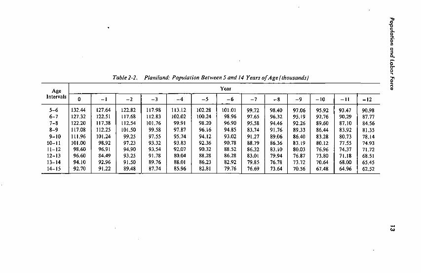
Population data covering those between ages 5 and 14 in intervals of one year are used in the preparation of projections of school enrollment. These figures are given for Planiland in Table 2-2. It is to be noted that children between ages 9 and 10 are included in the 5-9 interval and that the children 14 years old, but not yet 15, are included in the 10-14 interval. If the information in Table 2-2 is not available, it can be easily obtained by a demographer by using as a starting point the figures in Table 2-1. It should be observed that the data in Table 2-2 refer to years - 1 2 to 0 though the census information available, presented in Table 2-1, refers
Po
pu
latio
n an
d L
abo
r Fo
rce 13
S
u
>
fS
— 1
J
o 1
ov 1
OO
1
r-1
VO
1
vo 1
•t 1
m 1
CS
1
m 1
O
(/) 'S
&
>
<1 ••
^
00
Ov
Ö
Ov
r~
•* ro O
v
<S
O
v vo* O
v
vo
O
r-
Ov
O
•» od
ov
CN
r-; O
v
o\
s _J o
OO
C
N
r-i o
~
rs —
ro
-OO
O
V
P-'
-<N
°°. r-i <
N
•* vo
p
^ <
N
? r-i ro
VO
VO
r-r-
r-' 0
0
Ov
fN
Ö
OV
VO
p
^
r-i ov
ov -* in O
V
<N
m
vo
OV
vo V
O
r
OV
VO
O
v
OO
* O
v
•* r-i
g
^
CM
O
CM*
O
m
OO
CM
-OO
vO
r-*
-un
CM
' (N
CM
r-
CM
p^
VO
NO
un T
t O
O
o
p-
OO
o
*°. O
v 0
0
NO
C
M
CM*
ON
vO
,-^ Ov
OO
""ï un O
N
O
ON
NO
O
N
o tN
OO
O
N
ON
OÑ
ON
NO
P
»;
_J O
" »n
(N
-OO
rn
r-*
o
CM
(N
(N
OO
p~
un
rn m
00
CM
O
N
rn O
O
? NO
* O
O
m
rn
ON
O
O
VO
p--
—
ON
,-P-;
rn O
O
in O
O
Tf* O
N
NO
—
NO
O
N
p»
oq
p-" O
N
OO
u
n O
N
ON
O
•o
—,'
o
»n
CM
(N
OO
o p-
ON
0O
,-——
OO
p
-
m
P-;
Ö
OO
OO
C
M
rn O
O
o
•<t
NO
O
O
NO
o
ON
O
O
P-
CM
_J O
N
(N
O
en
ON
(N
—
rf O
N
Tf
P-;
V)
ON
un
un
P-"
ON
un
fS
ON
ON
* C
M
—i
O
NO
O
N
__j*
O
ON
m
ON
Tf
P-
un
Un
P-'
p»
CM
——
Ö
OO
ON
—
m*
00
NO
m
NO
O
O
ON
r-
00
00
00
p-
©
ON
NO
rn
CM
O
N
m
00
m'
ON
CM
rn
m*
ON
m
rs p»' O
N
(N
ON
00
ON
(N
P-(
M
P^
r-rn
-* p
-
NO
O
N
NO
P
-
rn
o
o
OO
o
rn 0
0
CM
m
NO
* 0
0
CM
un 0
0 0
0
(N
m
Ò
ON
P-
p
CM*
ON
T
"*¡ m
* O
N
O
ON
rr O
N
ON
VO*
ON
Un
od
NO
00
~ M
P-
o
OO
m'
r-p-
oo
NO
p»
Tj-O
N
ON
p-
p
m"
OO
OO
(N
NO
O
O
00
es oô
0
0
s d
00
00
P-;
_J O
N
un C
M
rn O
N
ON
•
^
^ OO
8 3 S
_ O
_H
*"* O
OO
O
N
es *-* —
NO
O
N
rn
—*
CM
»n
CM
•
^ u
n
»n C
M'
SO
N
O
©
NO
©
O
N
oo* •^•*
NO
N
O
Tt
OO
N
O
Tf
Ö
P
r- vo
CM
N
O
P-.
ir\
m* Ö
p
- r-
OO
^
P-.
vô
NO
' m
' p
- p
-
*r¡ O
N
00
NO
ON
N
O
P-
P-
CM
N
O
ON
P-;
CM
O
N
00
P-
m —
C
M
OO
NO* C
M"
00
00
—
\o
O
ON
o
o
»n
00
OO
VO
T
t P
-; P
^
ON
r-"
OO
O
O
O
OO
»
n T
t
— ON
ON
OO
NO
C
M
ON
C
M#
CM*
—'
ON
O
N
O
O
—
p-
Tf
CM
O
N
ON
^ —
rn ^
-

14 Population and Labor Force
to years - 1 0 up.to 0. A s a consequence, in any case, the help of a demographer is needed to obtain estimates for years - 1 1 and - 1 2 . The use of these figures is explained in Chapter 5.
It will be noted that Planiland carried out a population survey in year 0, simultaneously with the commencement of planning. In practice, of course, it rarely happens that countries have actually conducted a survey and published the results in the same year as that in which preparation of a plan was begun. But the absence of an exactly contemporaneous survey does not mean that it is impossible to apply quantitative methods to educational planning. W h a t is usually done is to estimate population for the year in which planning is due to begin and this can be done by competent demographers w h o will use the methods outlined below for estimating the growth of the population.
In order to simplify the presentation below, some mathematical notations will be used:
P, = total population in year t Ph, = population in the age interval h in year t
For instance, in Table 2-1,
P0 = 4,160,000
P M - M Í - S = 229,000
Educational structure of the population
Data on the educational structure of the population, that is, on the population broken d o w n by level of education, is shown in Table 2-3. In this table, all those with between one day up to six years—the whole cycle of elementary education, are included in the elementary stratum. Similarly, the high school and college data include all those w h o have received the relevant education whether for one day or for the duration of the cycle.
A n y other subdivision of the population by educational level would be equally valid and could be handled without difficulty. A n alternative method of dealing with the educational structure of the population, for instance, could include all those w h o had been graduated from a particular level in the stratum corresponding to that level; e.g., the elementary stratum would include all graduates from that level plus all those w h o had had some high school education but had not been graduated from high school.
Despite the flexibility in the definition of the educational strata, it is crucial to maintain the same definition in all the studies pertaining to the same educational plan. A n y adequate definition is sufficient as long as it is not changed.

Population and Labor Force 15
Table 2-3. Planiland: Educational Structure of the Population of Six and More Years of Age (thousands)
Without education
Elementary (0 to 6 years of schooling)
High school (over 6 to 12 years of schooling)
College (over 12 years of schooling)
Total population over six years of age
0
744.5
2,250.8
260.9
35.8
3,292.0
-5
966.2
1,662.6
209.5
26.4
2,864.7
Year
-6
1,012.1
1,557.4
199.8
24.7
2,794.0
-10
1,109.4
1,227.8
176.5
20.4
2,534.1
-12
1,152.8
1,077.6
165.2
18.4
2,414.0
It. should be observed that the data in Table 2-3 refer to the total population, including the population outside the educational system. In some cases below we consider the educational structure of the population outside the educational system.
In Table 2-3 w e see under the column corresponding to year - 1 0 , for example, that 1,109.4 thousand persons* over six years of age had received no formal education; 1,227.8 thousand had received or are receiving formal education at the elementary level; 176.5 thousand had received or are receiving at least some secondary schooling, but nothing beyond the secondary level; and 20.4 thousand had received or are receiving some education beyond the secondary level.
Besides the data on the educational structure of the population in years - 1 0 , - 5 and 0, Table 2-3 presents the structure for years - 1 2 and - 6 . A demographer can obtain these values by extrapolating or interpolating from the census values.
T h e sceptical reader will naturally feel that planning presents no difficulties when all the necessary data can be assumed to exist; but he will perhaps argue that nothing comparable to Table 2-3 could be prepared for his o w n country. In this he is most likely mistaken. W h a t is needed is at least one population survey with information about the educational structure of the population together with data on enrollment in different years in the various educational levels. In due course (Chapter 6), w e will see h o w these two elements m a y be combined to provide data on the educational structure of the population for several years.
*Here and throughout for simplicity w e use the British or Continental form of "thousand thousand" instead of "million." In the United States, "1,109.4 thousand" would be taken to mean 1.1094 million.

76 Population and Labor Force
Educational structure of the labor force
O n e of the basic sets of statistical information needed for the preparation of an educational plan is the educational structure of the labor force. In collecting the data for the educational structure of the labor force, it is important to take care that the definitions of the educational strata used coincide with those used in the data about the educational structure of the population.
It is often true that such information is difficult to obtain since it has not been collected in most countries. A n approximately correct picture can, however, be drawn if the educational structure of the total population is k n o w n . T h e data for Planiland are presented in Table 2-4.
In Table 2-4 the following notation is used: L, = total number of persons in the labour force in year / L'I = total number of workers with educational level /'in year /
/' = 0 without education i = 1 with elementary education /' = 2 with high school education / = 3 with college education
Table 2-4. Planiland: Educational Structure of the Labor Force (thousands)
i
0 1 2 3
Educational Strata
Without education Elementary High school College
Total L, .
Y e a r - 1 0 (2) ¿'-io
523 580 75 11
1,189
Year - 5 (3) £ - 5
537 686 103
15
1,341
YearO (4)4
580 781 149 22
1,532
2-3 Changes or the Population over Time
Demographers are all too well aware that not very m u c h can be learned from one picture of the population or even from several pictures. A s mentioned at the outset, account must be taken of the changes which occur in populations over time. For the present w e must first decide in which changes of the population we are interested, what factors determine these changes and what methods can be used to measure both the changes and the governing factors. W e are mainly concerned in this context with population growth and its influence on the age and sex structure of the population.
The factors determining population growth are birth, immigration, death, and emigration. The ways in which these factors affect the total population are obvious as are the methods of measuring them. Data on

Population and Labor Force 77
births and deaths are usually assembled by government offices of vital statistics while information about the movement of people into and out of the national territory m a y be obtained in immigration offices.
Let us concentrate first on the total population. A s regards Planiland in year - 1 2 , this amounted to 3,026,000. If w e add births and immigrations and subtract deaths and emigrations during - 1 2 , w e obtain the total population at the beginning of —11. W e can repeat this operation to establish the total population at the beginning of - 1 0 , - 9 , and so on.
Table 2-5. Planiland: Total Population and Rates of Growth Between Years —12 and 0 (thousands)
Years
(U
-12 -11 -10 -9 -8 -7 -6 -5 -4 -3 -2 -1
0
Total Population (thousands)
(2)
3,026
3,081 3,156 3,241 3,329 3,421 3,515 3,614 3,715 3,823 3,933 4,045 4,160
Rate of Growth
(3)
0.0182 0.0243 0.0269 0.0272 0.0276 0.0275 0.0282 0.0279 0.0290 0.0288 0.0285 0.0284
Average rate of growth - 0.0270
Table 2-5 shows the total population of Planiland for each year between -r 12 and 0. With these data, and the formula
P, - P,-i P,-i
the rate of growth from one year to the next can be computed. For instance, the rate of growth between year - 1 0 and year - 9 is
3 - 2 4 1 - 3 ' 1 5 6 = 0.0269 3,156
So far w e have considered only changes in total population over time, but changes in the different age and sex groups are also important. T h e basis for calculating such changes consists of information about the population similar to that contained in Table 2-1. O u r aim is to establish the relationship between one group in an interval of age and sex in, for

78 Population and Labor Force
example, year - 1 0 and the group in the next interval of age and the same interval of sex in year —5.
Let us begin by considering the age interval 0 -4 in year —5. Between the years - 1 0 and - 5 there are five years, and none of those in the 0 -4 age interval has attained five years of age. In other words, all of them were born after the beginning of year - 1 0 and are not included in the figures for year —10 given in Table 2-1.
W h e n any age interval other than 0 -4 is considered, the figures for year - 1 0 give a slightly distorted picture of the next age interval for year - 5 . Let us take the case, for instance, of the 20-24 age interval, c o m posed of 282 thousand persons in year - 1 0 , as shown in Table 2-1. The same table indicates that in year - 5 the group has decreased to 272 thousand in the 25-29 age interval. The difference between the two,
282 - 272 = 10 thousand
is due mainly to mortality (immigration and emigration m a y also have affected somewhat the size of the difference).
2-4 Population Projections
2-4.1 Method to Be Used
A projection of the population is an estimate of its future growth. The method to prepare such an estimate is similar to the method used for any projection in any science. First, w e must find out through observation the factors controlling the growth of the population and the relationship between such factors and the population. Second, an estimate of the development of these determining factors must be obtained. Finally, the knowledge of the development of the determining factors and of the relationship between them and the population permits us to obtain an estimate of the future growth of the population.
The factors determining the growth of the population are well k n o w n : births, deaths, immigrations and emigrations. Their relationship to population is simple: Births and immigrations add to the existing population; deaths and emigrations reduce it.
It has been observed that the future development of these four factors is closely related to the present population. So the following causal sequence can be used to project population: present population is directly related to births, deaths and migrations; hence, in turn, these factors are directly related to future populations. Thus, w e must begin with the projection of births, deaths, and migrations, using present population as a starting point.
A n attempt is m a d e below to present the major elements of the methods used to estimate the future of births, deaths and migrations. The

Population and Labor Force 19
procedures described below should not be used to carry out projections except when the lack of demographers forces the educational planner to obtain rough first approximations. The methods used by demographers expand upon these basic elements in order to eliminate sources of error that are not considered below.
2-4.2 Projections of Births
The number of births bears a more or less constant relationship to the total population. In other words, if the total population increases by one-third, the number of births per year will also increase by approximately one-third. There is an even closer statistical relationship between the number of births and the number of w o m e n of childbearing age (between 15 and 44 years).
The relationship between births, on the one hand, and total population of w o m e n between 15 and 44, on the other, is numerically measured in terms of birth rates. By way of example w e will concentrate on the relationship between the number of births and the number of w o m e n between ages 15 and 44. The birth rate in this case consists of the number of births per w o m a n between 15 and 44 per unit of time. T o obtain the figure, the number of births in, for example, year —10 is divided by the number of w o m e n in the 15-44 age interval at the beginning of that year.
In order to project the number of births, w e use the birth rate observed in the past and the number of w o m e n between 15 and 44 existing at the present. Establishing the number of births per year is merely a question of multiplication; if each w o m a n has, say, 0.22 births per year, what is the annual number of births for 687 thousand w o m e n ? The answer is obtained by multiplying 0.22 by 687 thousand.
M o r e refined projections can be obtained by making valid assumptions about the way in which birth rates will change over a period of time; for example, there is a tendency for an overall decrease in birth rates to occur with the passage of time.
Other factors besides the number and age of w o m e n might also be considered in projecting births; e.g., education tends to reduce natality. The inclusion of such factors would give rise to new methods of projection and lead to different results.
2-4.3 Projections of Deaths
The situation is more or less similar with regard to deaths. The only prerequisite for dying in the future is to be living n o w . People in each age and sex interval tend to die in roughly constant proportions. A m o n g those in the age and sex interval, for instance, of w o m e n between ages 20-24 in year - 1 0 , a certain proportion will die; this proportion is approximately the same as that observed for the same age and sex interval

20 Population and Labor Force
in, say, year —8. O n the other hand, the proportions change from one interval to another. The death rate is the number of deaths of persons within an age and sex interval per person in the age and sex interval per unit of time. This rate can be calculated by dividing the number of deaths a m o n g those between, say, 20 and 25 during year —5 by the total number of persons in that age interval at the beginning ofthat year.
Once the death rate is k n o w n , the number of deaths can be projected. Let us take the age and sex interval of m e n as 30-35 in year 0. If w e mul tiply the death rate ofthat age interval by the number of persons in it, w e obtain the number of deaths.
In preparing projections of deaths, it m a y be useful to assume different death rates so as to provide for various unforeseen contingencies. This technique is frequently employed in order to allow for changes in the factors determining the death rates even though such factors could be explicitly considered. For more refined projections, it is essential to give explicit consideration to these factors; mortality, for example tends to decrease with increase of income.
In some cases it is easier to use survival rates instead of death rates. This rate is the number of survivors within an age and sex interval per person in the age and sex interval per unit of time. The survival rate in Table 2-6 will be used later.
Table 2-6. Survival Rates of the Population of Six and More Years of Age from —12 to —6 and from —6 to 0
Period
- 1 2 to - 6 - 6 to 0
Six-Years Rates
0.9289 0.934
Yearly Rates
0.996 0.996
2-4.4 Projections of Migrations
Migration rates can likewise be computed for the different age and sex intervals. W h e n these rates are multiplied by population in the corresponding age and sex intervals, one obtains a projection of migrations. Migration rates, too, are subject to other influences such as income and are considerably less stable over time than birth and death rates.
2-4.5 Population Projections
Given projections of births, deaths and migrations, do w e have enough to m a k e population projections? Not altogether. A n important factor is still missing: the order in which the components must be c o m bined. In order to project the population, w e must proceed by stages. A n d , for each stage w e must project the whole population. Beginning in

Population and Labor Force 21
the year 0, w e can obtain births, deaths and migrations up to, say, year 5 so that w e can construct the population in that year and obtain the second column of Table 2-7. Once all the figures for year 5 are available, it becomes possible to go to year 10 and so on.
Demographers normally m a k e several projections—in most cases, a m a x i m u m , medium, and m i n i m u m . In the first of these, higher birth and immigration rates and/or lower death and emigration rates are assumed. A s regards the medium projection, the most likely developments are assumed. For the m i n i m u m projections, the assumptions m a d e for the m a x i m u m are reversed. The alternatives for the population projections in Planiland are given in Table 2-7 where only birth rate assumptions are varied.
In setting out the population data required for educational planning, w e noted that detailed census information for the 5-14 age interval was needed. This information must be supplemented by detailed projections for that age interval; as regards Planiland, these projections are shown in Table 2-8.
2-4.6 Projections of the Educational Structure of the Population
For the preparation of the population projections, w e have used the factors determining population growth—births, deaths and migrations. In the case of the projections of the educational structure of the population, w e must also consider its determinants, the output of the educational system. For this reason, before preparing projections of the educational structure of the population, w e must study the future growth of the educational system. This is done in Chapter 5. The projections of the educational structure of the population must wait until Chapter 6.
2-5 Labor Force Projections
Educational planners are not expected to prepare labor force projections; it is therefore unnecessary to give a detailed description of the methods used to m a k e such projections. It should be noted simply that while population projections require the rates of birth, death, and migration, labor force projections call for the rates of labor force participation. W h a t is this rate? It is established by taking the population and labor force figures for a given age and sex interval. Labor force divided by population gives the rate of participation; in other words, the rate of participation is the number of persons in the labor force per person in the population within a given age and sex interval. For projection purposes, rates of participation are assumed to be m o r e or less constant.

22 P
op
ula
tion
and
Lab
or F
orce
•<M
C
ÇJ <
r>
3
-s:
-—
«SC
« X
<u
i>>
C
O
<J
« p-^ o
d
a 3 §•
u.
"CT
s: w
w
a.
i\ CN
-22 -
Û
<3
b-I
O
CS
u
CO
> tri
CO
o —
>-vn
u
CO
U
u
<
c Eco
I 0
c ^-,
O
CS
S
w
o
^ H
w
E
o
l~ c _
Ä
ST
"cõ ^
-ö
S
H EP
O
*—•
S:
S
w
_-°J
•—«
o^
H c o
-^ ^ |s
"5 ^
¡2~
t/5
cd
i C
~
564 582 1,146 495 510 1,005 440 453 893 399 409 808
•<t i
o
483 497
086
427 438 865 384 393 777 347 355 702
ON
1 in
423 434 859 380 389 769 343 351 694 297 305
209
10-14 376 384 760 339 346
589
293 300 593 234 24! 475 15-19 333 340 673
882
294 582 229 235 464 206 2.4 420 20-24 282 287 569 224 230 454 201 208 409 166 175 341 25-29
219 225 444 197 203 500 161 170 33. 144 143 287 30-34 '
192 198 390 157 165 322 140
ON
C
O 279 .31 123 254 35-39
153
091
313 136 134 270 127 119 246 109 103 212 40-44
131 129 260 123 114 237 105
OO
O
s 203
OO
oo
oo 172 45-49
117 107 224 101
CS
ON
193
oo
ON
r-163
NO
t'es 148 50-54
in O
N
in 00 180
ON
t'
es r-151
t-in N
O 136
Ño
in 115 55-59
CS
3 136
in so
oo »n
123
in »n
00 103
P-
•«t
^
OO
oo 60-64
p-
•n
oo 105
00
Tt
O
00
00
o TT
m
t—
CO
CS
CO
NO
N
O 65-69
oo C
O
o CO
oo N
O
CS
CO
NO
C
S
00
in
r-cs
CS
in
CS
CS
o CS
CS 70-74
CS
CS
f-ON
C
O
00
in
CO
C
O
in
CO
oo C
S
CO
o CO
C
S 75-79

Po
pu
latio
n an
d L
abo
r Fo
rce 23
m
m
ON
VO
ON V© VO ON
vo in
TJ* m
VO Os —
in
—
p- oo
o
r- in Tj-
Tf
1,409 1,142
950 801
oo m
o
p- p-
O
m
Tj- T|-
»n \o os
ON
oo
O
»n Tj-
Tt
fO Os ON
P-
in
O
-^ Os 00
00 Tf
00
O
Tf Tt
O
—•
»n TT
O
OO
ON
—
Os oo
419 431 850
Tf OS Tf ON
i i "T
"T o in o *n
3,850 3,883 7,733 3,269 3,288 6,557 2,795 2,805 5,600 2,405 2,409 4,814
o <n
OO TJ-
00 ON
oo »n
*£> m
rt oo
r- •*
v-> CN
CN \£>
\o cn
•tf CN
O "">
80-84 85 +
3,575 3,599 7,174 3,120 3,135 6,255 2,726 2,735 5,462 2,384 2,837 4,771
m oo in
n
n »n o »n
in Tf Tt
m
p- o —« o
f*1 f» —
VO
»n TJ-
Tj- m
Q
OO s© (N
vo (N —
—
C^ ON OO P»
^
Tf
m
p- vo
m
00 (N t-
Tf Tf rn
—. —, r-
so Tf
m
ON
00 P*-
O
P-
m
p-
—« vo
Tf 00
— m
r* vo
00 P^
390 400 790
TT OS Tj-
OS
i i "T
"T O in o in
3,467 3,480 6,947 3,071 3,084 6,155 2,709 2,715 5,425 2,375 2,378 4,753

24 P
op
ula
tion a
nd
Lab
or F
orce
k*
o
"™
o
Vi
.. ca
Age terv c
s CS
N
O
r»
ro
ON
»n
r-NO
N
O
»n
Tf
ON
ro
O
(N
c-~
O
Tf
00 TT
r-"•
m
Tf
O
~-Tf
S
oo
m
NO
(N
m
m 132.44 1
»n
CN
r-00 <n
m
o
NO
in
(N
m
m
*n
ON
in
o m
O
00
r-Tf
o
Tf
? >n
—
_«
TT
vo
00
r~
m
Tf
in
Tf
m
Tf
r»
_* m
127.32
r-i
o
TT
m
»n
o r-<N
in
00 O
N
ON
Tf
o cs
r~
Tf
•t o\ ro
T
f
O
Tf
O
TT
m
~~ r-m
CS
oo
m
m
S M
m
m
oo
NO
(S
122.20 i
oo
O
(N
«n
r-rn
ON
T
f
s VO
T
f
00 T
f rr\ T
f
oo
o
o
Tf
o
Tf
VO
m
—
—•
fO
m
Tf
m
O
m
oo
m
vo
<N
vo
ov —
es 117.08
ov i oo
vo
p-
oo
Tf
8 vo
Ti
rs
O
m
Tf
VO
p
-O
V
m
(N
VO
m
O
Tf
<N
m
in
ON
C
S
ON
»O
CS
r-—i
<N
S
r-111.96
o i
ON
Tf
CM O
O
O
Tf
—
00
Tf
»n
ÍN
oo
»n
Tf
Tf
m
rn
NO (N
VO
O
<n
~
N
O C
N
n
ON in
N
•v
i í'i
r*í <
^i
Tf
Tf
m
r-T
f 0
0
<N
T
f O
N »
O C
N
OO
m
m
m (N
(N
O
Tf
NO
O
rn
N
O
NO
NO
(N
00
Tf
m
m
(N
ÍN
»n
(N
m
Tf
m
oo
oo
oo
(N
0
O T
f O
m
<
N cN
C
N
88
81
?
ON
in
— VO
(N
N
(M
—
Tf
Tf
CS
O
Tf
fs
ON
C
O
ifl -
\û
O
N
(S
- -
oo vo
—•
r»
Tf o
\ r-
oo
—
vo
o
ov
(N
—
—
O
N
Q
00
Tf
VO
O
N
(S
0
O
r- —
o
r~
—
—
O
O
N
Tf
es
m
T
f V
i V
O C
S
(N
—
Q
00 V
O
—
O
ON
O
N
101.00 98.60 96.60 94.10
—
rs
ro
Tf
1
1
1
1
O
— (N
m
vo
—•
<N
m
O
m
oo
CS
ON
T
f T
f
es-
OO
V
O
o CS
Tf
r~
VO
o
ON
s o
m
cS
ON
T
f
r»
ON
OO
00
»n
ON
<n
r
m
ON
92.70
V">
1
Tf
1-1
<N
ON
r-vo
Tf
m
(N
^
m
Age terv c
1—1
Tf
OO
m
O
CS
r-o _
M
O
CS
o
m
vo
ON
m
m
__ O
N
CN
r~
vo
oo
00 VO
o
00
VO
O
N
VO
r*.
Tf
es m
r-cs in
O
N
vo
o
oo
V"l
VO
VO
1
»n
es O
N
8 CM
»n
—
NO
O
N
OO
rn
—
i
ON
00 W
0 N
O
OO
Tf
m
O
00
Tf
oo N
O
r*
<N
~->
m
r
O
Tf
ON
VO
OO
N
O
»n
NO
m
ON
M
NO
i N
O 8 VO
O
N
ro
(N
«H
ON
? VO
00
o
Tf
o
00
Tf
1—
VO
r~
8 m
r-00 (N
O
N
NO
NO
<n
»n
NO
CN
O
O
_ NO
o »n
00 •n
00 1
r-
oo
o _•
ON
O
rn
NO
O
O
NO
C
N
o
oo
s VO
r—
vo
t'es r-V
O
ON
V
O
Tf
vo
vo
oo
CS
o
oo
Tf
in
vo
r-cs in
cs r-©
O
CS
O
rn
O
vo
oo
t-
5 S
NO
C
N
r* r-
oo oo
C
N
Tf
CM
r-P
* N
O
Tf
NO
O
ON
oo
m
N
O N
O
vo
vo 0
0
oo
VO
cs
in
VO
o
Tf
VO
V
I V
O
r-_M
VO
oo
CS
00 in
00
o in
u->
ON
I oo
_ri
VO
VO
o
oo
in
vo
r-Tf
in
in
VO
__ m
o i
ON
ss
OO
T
f T
f N
O
M-
P^
N
O *n
Tf
fN
oo —
r»
Tf
in
in
5?
Tf
O
«/"»
ir»
<N
O
N
(N N
O
in
Tf
(N
(N
CS
O
N
T?
Tf
—
CS
1
1
o —
cs 00
n
t~
o
ON
VO
VO
OO
cs m
V
O
in
—*
S
Os
Ov
VO
in
o
OO
n
in
i vo
m
o in
vo
r*-Tf
CI
Tf
TÍ
NO
M
Tf
T rsi
Q
NO
Tf
ON
N
O
—
NO
NO
~- rn
N
O
OO
CN
0
0
vo
m
ON O
N
Tf
NO
O
N m
»n
in
Tf
m
m
in
NO
CM
in
»n
NO
T
f ~
- m
m
O
N
<n
Tf
NO
C
N
ON
—
ON N
O
Tf
Tf
CO
NO
NO
rn
Tf
Tf
OO
O
N
oo
wo
rn
O
T
f T
f
O
O
—
00
Tf
rn
m
ON
m
en
Tf
*n
CO
T
f

Population and Labor Force 25
With the population projections and the rates of participation, w e are ready to proceed. Let us assume that w e want to k n o w the number of male workers between 20 and 24 in year 20. W e multiply the rate of participation by the number of persons in that age and sex interval as shown in the population projection. Without employing the detailed projections of the labor force by sex and age and merely using the total figures, Table 2-9 below shows the projections of the total labor force in Planiland.
At a later stage, w e will m a k e a detailed examination of the methods used to obtain projections of the educational structure of the labor force.
Table 2-9. Planiland: Total Labor Force Projections (thousands)
Year/
5 10 15 20
Labor Force L,
1,764 2,050 2,387 2,764
References
More complete elementary discussions of demographic methods appear in: Barclay, G . W . , Techniques of Population Analysis. N e w York: Wiley, 1958. Davis, R . C , Planning Human Resource Development. Chicago. Rand McNally,
1966. Methods for Population Projections by Sex and Age. N e w York: United Nations
Population Studies N o . 25, 1956. Pressât, R . , L'Analyse Démographique. Paris: Presses Universitaires de France,
1961.

chapter
Economics
3-7 Con/en/ of This Chapter
The past several years have witnessed an increased interest in economics generally and in economic development in particular. Economic development has become one of the main objectives of every government in the world—and of the revolutions that sometimes overthrow these governments. Even laymen are vitally interested in the fluctuations of per capita income.
This does not mean that economic problems are more deserving of attention n o w than in the past. It has always been true to say that nothing can be obtained without economic means and nothing of real value can be obtained with economic means alone; this will doubtless hold true for the future. Thus education, which virtually everyone agrees has great value, requires more than merely money; but nonetheless educational officials must ultimately solicit the help of the financial authorities. This is a fact of life which, as a realist, the educational planner must recognize from the outset.
But if education requires economic support, the economy in turn requires educated people. T h e educator is not obliged to beg for funds in order to satisfy an abstract right to education; he is in a position to "sell" valuable, qualified personnel to the economy. A s a result, economic officials have had to come to terms with educators. Discussions are n o w conducted on a basis of reciprocal interests.
Every discussion, however, calls for a c o m m o n language. While economists m a y have become familiar with educational terminology, educational planners must become familiar with economic terms. T o bring about this familiarity is one of the objectives of the present chapter. A n other objective, more important than the first, is to explain the role of education in economic development. Actually, since the content of this chapter occupies such a fundamental position in the intellectual preparation of the educational planner, no further introduction is necessary.
26

Economics 27
3-2 National Accounts
3-2.1 Definition of Gross Domestic Product
National accounts, social accounts, national income accounts, etc., m e a n exactly the same thing. They bear the same relation to a country as do business accounts to a commercial enterprise. Just as the latter enable the owner of a firm to see the value of goods and services produced by his firm and the costs of this production so the national accounts reveal the total amount of goods and services produced and the main production costs for the country as a whole.
At first glance, it would seem that one need only add up production of all the firms within a country in order to obtain the national accounts. In fact, however, while it is relatively easy to establish the value of each good and service produced, it is less easy to determine h o w m u c h of each good and service is being produced.
T o begin with, it is impossible to talk of production as a momentary thing. Whereas population figures refer to a given m o m e n t , production figures refer to a flow over a period of time. Hence w e must think in terms of production per month, production per year, and so on. National production is usually considered over a period of one year.
Let us n o w examine the case of a Planiland business which produces 2,200 items in the course of a year. If w e assume these items sell for $5 each, the firm received $11,000 for its annual output. F r o m this s u m , $6,000 is spent on the purchase of materials, $3,000 on salaries, $500 as interest on loans and $500 on factory rent (for the sake of simplicity, w e ignore depreciation of capital). In other words, $10,000 is paid out in the course of producing output worth $11,000 on the market. The owner's profit is the difference between total receipts and total payments to all others w h o have contributed to the production of the output (those receiving salaries, interest and rent, and those selling materials used in production).
H o w m u c h of the value of yearly output of the firm can be counted as addition to national output? Since the raw materials purchased from outside were obviously not produced by the firm itself, the amount involved is necessarily excluded from the value of the firm's net contribution to national production. N o other category of costs need be excluded and hence one can say that the firm's net contribution to national output is equal to the value of total sales (in this case, $11,000) less the amount paid to other firms for raw materials (in this case, $6,000). Thus w e obtain a figure of $5,000 for the firm's contributions to national output. This figure is equal to the sum of the firm's yearly payments for salaries, interest and rent plus the firm's profit.

28 Economics
If only the values added by the firms as defined above are considered, w e avoid the danger of counting any firm's production twice, a problem which would arise if the total sales of all the firms were to be added together.
. In order to evaluate the national production of Planiland, all that is needed is to add up the contributions of each individual firm, i.e., their value added. This sum is equal to the total of profits, salaries, rents, and interest paid out throughout the country. It should be noted that in order for the above to be true, one must count all producing units in the country including the government as a "firm."
Since profits, salaries, interest, and rents are paid to someone, it follows that national production and total personal income are equal. Total production and total income, in other words, are two sides of a single coin: the production process.
In the analysis above, w e have not paid attention to the fact that some goods and services are bought from foreign countries and sold to them. This fact does not introduce any modification in the method outlined to evaluate national production. However, the transactions with foreign countries are usually presented separately from the internal transactions in the national accounts. The national production is evaluated in the following way: First, the value added in "internal transactions" is c o m puted; that is, for each firm, the value of all goods sold for consumption or further processing in the economy minus the value of all the raw materials and semiprocessed goods bought in the economy is computed. Then these values for all firms are added. Second, the value of all the goods and services sold to foreign countries minus the value of all goods and services bought from other countries is computed. National production is equal to the sum of the two components described above.
Economists, of course, would distinguish between net and gross values, domestic and national production, production and income, and the like, but these differences are not particularly important for our purposes. From our point of view it is important to use just one concept. Hence in all that follows w e will be using a type of national output measure called "gross domestic product." Table 3-1 shows the values of the gross domestic product of Planiland from year - 12 to year 0.
O n e reason for studying national accounts is to m a k e the concept of national production less vague. Annual national production, whether large or small, is a fixed quantity confronting all planners with definite limitations. It is essential to stress an obvious fact but one whose full implications are not always recognized: resources are limited. They must be distributed a m o n g a variety of users. Resources used for one purpose cannot be used for another.
These considerations bring us to the crux of the discussions between

Economics 29
Table 3-1. Planiland: Values at Current Price? of Gross Domestic Product from Year —12 to
Year 0 (millions of dollars)
Year
-12 -11 -10 - 9 - 8 - 7 - 6 - 5 - 4 - 3 - 2 - 1 - 0
GDP
5,458 5,997 6,511 7,032 7,746 8,135 8,383 9,236
10,240 11,165 12,027 12,834 13,932
educators and economists. T h e former contend that education is a right and must be guaranteed. T h e latter argue that several rights must be safeguarded out of limited resources—the rights to shelter, to food, to health, to employment, or to education. T o increase expenditure on education means decreasing expenditure on safeguarding other rights. Hence, expenditure on education out of limited national output must be held within certain bounds.
3-2.2 Disaggregations of the National Accounts
In the study of the economic conditions of a country, in economic planning and its integration-with educational planning, in addition to the total value of national production, several subdivisions are used. S o m e of these are considered below.
In Table 3-2 the distribution of gross domestic product in years - 1 2 , - 6 , and 0 between public and private resources is presented. These data will be used when dealing with public and private funds used in education.
In actual uses of the national accounts, total production is subdivided according to its industrial origin. In this case, the value added by firms,
Table 3-2. Planiland: Distribution of Gross Domestic Product Between Public and Private Resources
(millions of dollars at current prices)
Year
- 1 2 - 6
0
G D P
5,458 8,383
13,932
Public
958 1,510 2,492
Private
4,500 6,873
11,440

30 Economics
for example, in agriculture, manufacturing and services, is presented. If it is necessary, more refined subdivisions can be used.
3-3 Comparison of National Accounts for Different Years
3-3.1 Price Changes and Real Changes in National Accounts
Educational planners, accustomed to dealing with figures showing the number of students, the number of teachers, and so on, m a y feel that, since there is no special problem in comparing those figures for different periods, it is unnecessary to devote particular attention to the comparison of national accounts for different years.
The number of students during a given period can be compared with the number during another period because a student is a student, irrespective of the time element; that is, the same unit of measurement is e m ployed at all points in time. Such is not the case when dealing with national accounts: accounts for different periods are measured in different units.
Table 3-1 shows the gross domestic product of Planiland year after year in Planiland dollars, but a dollar in year - 1 0 is not the same thing as a dollar in year - 5 . T h e fact is that the value of money steadily deteriorates. A household budget, for example, which was adequate six months previously, is found to be no longer sufficient because the prices of bread and meat have risen; the value of money in terms of bread and meat has declined. The dollar which bought four loaves in year —10 buys only three in year - 5 . In other words, the dollar is worth only three-fourths as m u c h .
This, of course, is crucial in dealing with national accounts. C o m paring the values for years - 1 0 and - 5 as shown in Table 3-1, it is impossible to say whether or not Planiland production has really increased. Production m a y not have risen but prices m a y have risen so that a reduced volume of goods is represented by an increased monetary value. Unless the effects of price changes are eliminated, changes in production, the real changes, cannot be seen.
3-3.2 Price Indices
In order to eliminate price changes, these changes must first be m e a sured by means oí price indices.
Let us examine a hypothetical family which in year - 1 0 consumed 700 loaves of bread and 500 pounds of meat. Assuming one loaf to cost one dollar and one pound of meat two dollars, food expenses amounted to
700 x 1 + 500 x 2 = $1,700

Economics 31
In year - 5 , the price of one loaf has risen to 1.2 dollars and the price of a pound of meat to 2.3 dollars, so that the hypothetical Planiland family must spend
700 x 1.2 + 500 x 2.3 = $1,990
to consume in year - 5 what it consumed in year - 1 0 . In other words, $1,700 in year - 10 represented the same amount of bread and meat as did $1,990 in year - 5. A simple division
indicates that one dollar in year —10 is the equivalent of 1.17 dollars in year - 5 . O r , to put it another way, on the average an item carrying a price of 1 in year —10 carries a price of 1.17 in year —5. These are the index numbers for the Planiland family.
Index numbers usually refer not to one monetary unit but to one hundred, so that prices are said to have risen not from 1 to 1.17 but from 100 to 117. All that has been done is to multiply the component elements of the index by 100.
Index numbers, therefore, reveal the change in price from one year to another. The year taken as a point of reference ( — 10 in the example used here) is known as the base year. If the base year is changed, it follows that the index numbers also change. For example, the index number for prices in - 5 would probably not be 1.17 if w e were to take year - 7 as the base year.
Index numbers for the whole society can be calculated in the same way as for a single family although all goods, and not merely food as in our simplified example, must be included. In Table 3-3, which shows Planiland price indices, year 0, when planning begins, has been selected as the base year. Accustomed as w e are to seeing prices rise rather than fall, w e m a y be surprised that all index numbers are below 100. These, h o w ever, refer to the past; e.g., four years earlier, in year —4, $91.4 was required to buy the same amount of goods that in year 0 can be bought with $100.
It is clear that index numbers are subject to a number of limitations. The index in the case of our hypothetical family, for instance, could be computed only because they ate bread and meat in both year - 1 0 and year - 5 . If they had replaced bread with vegetables in the interval, an insoluble problem would have arisen. If a new product is introduced into the consumption pattern or if the quality of old products alters, there is no way of measuring price changes.
Since new products c o m e on to the market every day, since qualities

32 Economics
Table 3-3. Planiland: Price Indices
Year Index
- 1 2 80.2 -11 80.8 - 1 0 81.7 - 9 ' 82.0 - 8 83.1 - 7 84.3 - 6 85.7 - 5 86.4 - 4 91.4 - 3 94.3 - 2 98.9 - 1 99.3
0 100.0
are continually changing and since index numbers cannot allow for such developments, h o w can index numbers be used significantly to measure changes in prices? Economists are well aware of the limitations involved. If they continue to use index numbers, it is because these are better than nothing at all. They provide only a very rough measurement of changes in prices, and this is duly recognized. For that matter, almost all economic figures are only rough measurements of real phenomena.
3-3 .3 Use of Price Indices: Gross Domestic Product in Real T e r m s
Table 3-1 shows the values at current prices of Planiland's gross domestic product from year —12 to 0; Table 3-3 gives the index numbers of Planiland prices. H o w are w e to eliminate the effect of price changes from the figures for the gross domestic product?
The point of departure is the base year (year 0 in Table 3-3). The first problem is to discover h o w m a n y dollars in year 0 are equivalent to one dollar in year - 1 . Table 3-3 shows that goods costing $99.3 in year - 1 cost $100 in year 0, so that $100 in the latter year is equivalent to $99.3 in the former. The simple division
gives the year 0 equivalent of one dollar in year - 1 . Table 3-1 shows that the value produced in year —1 was $12,834 mil
lion, measured in the prices prevailing in that year. Since one dollar in year —1 is equivalent to $1,007 in year 0, what is the equivalent of 12,834 million year - 1 dollars in year 0 dollars? The answer is
1.007 x 12,834 million = 12,924 million

Economics 33
representing the value which the goods produced in year - 1 would have had if the prices prevailing had been those of year 0.
T h e same computation can be m a d e for year - 2 . T h e ratio of year 0 dollars to year - 2 dollars is determined as follows:
100 98.9
= 1.01112
Thus w e are able to obtain the value of year - 2 production at year 0 prices:
1.01112 x 12,027 million = 12,161 million
T h e same operation can be used to obtain the real values for the gross domestic product for all years between —12 and 0 as well as for public and private resources. Results are shown in Table 3-4. T h e notation Y, represents gross domestic product at constant prices in year t. For instance, in Table 3-4 w e see that
y_5 = 10,690
Table 3-4. Planiland: Real Values of Gross Domestic Product (millions of dollars at year 0 prices)
Year
- 1 2 -11 - 1 0 - 9 - 8 - 7 - 6 - 5 - 4 - 3 - 2 - 1
0
Gross Domestic Product
6,805 7,422 7,969 8,576 9,321 9,650 9,782
10,690 11,204 11,840 12,161 12,924 13,932
Average rate of growth
Rate of Growth
0.090 0.073 0.076 0.087 0.035 0.014 0.092 0.048 0.057 0.027 0.063 0.080
0.062
Public
1,194
1,762
2,492
Private
5,611
8,020
11,440
3-3.4 Comparison of the Gross Domestic Product in Different Years
Rate of growth of the gross domestic product
It n o w becomes possible to compare the values of gross domestic product, Y„ since the dollar value for one year is the same as the dollar value for another year. A useful index for this comparison is the rate of

34 Economics
growth defined by the following equation:
Y, - y,-!
Y,-i
For instance, the rate of growth between years - 10 and - 9 is Y-9 - Y-lo 8,576 - 7,969
r. ,0 = —7^69 = ° 0 7 6
This means that 0.076 dollar was added to each dollar of output in year —10, or that 7.6 dollars were added to each 100 dollars. (This latter figure of 7.6 is the percent rate of growth of gross domestic product, a figure of great interest to those concerned with measuring and comparing economic growth.) A similar calculation can be m a d e for any two consecutive years; the results are shown in Table 3-4.
The year-to-year rates of growth in Table 3-3 do not, however, give any idea of conditions over the whole period. This can be obtained from the average of the rates of growth which indicates what the growth rate would have been from one year to the next if approximately the same rate had prevailed in each year. For the rates of growth in Table 3-4, the average is 0.062.
3-4 Economic Growth and Investment in Education
3-4.1 The Concept of Economic Growth
Economic growth is simply another phrase for the increase in national production. For example, the economic growth of Planiland between years - 1 2 and 0 m a y be seen in Table 3-4, for it gives the real values of the gross domestic product for those years. T o keep a record of a country's economic growth, of course, requires that the real values of national production be used. Changes in values at current prices show not only changes in real production levels but also changes in the price level.
Economists are not interested solely in keeping a record of economic growth. They are also anxious to discover its causes so as to be able to promote such growth.
3-4.2 Factors Outside Enterprises Which Influence Economic Growth
In the case of individual businesses, it is obvious that where one enterprise increases its production, the total production of the country will also increase unless another enterprise is simultaneously reducing production.
It is equally obvious that the decision to raise production within a given firm will depend on external institutional, political, and economic factors. These factors are normally beyond the control of individual

Economics 35
enterprises. They include the laws of the country concerned and especially those laws dealing with economic matters such as taxation. Also, the degree of political stability has an impact on economic growth since firms will be m u c h less interested in producing if there seems to be danger that the fruits of their efforts will be destroyed by political action.
A s to general economic conditions, it is scarcely necessary to point out that enterprises will not increase their output unless they are reasonably sure of being able to sell profitably what they produce. Without going into the question of w h y people buy things, it is clear that people must have m o n e y in order to m a k e purchases, and, for most people, this means that they must be employed. In other words, production is dependent on whether or not potential consumers are employed.
3-4.3 Factors Within Enterprises Which Influence Economic Growth
Turning back to the hypothetical business discussed earlier, w e will assume that during the previous year this firm used machinery worth $5,000, buildings worth $4,500 (a fixed investment not included in the current expenditures already listed), plus money from the owner's bank for the purchase of raw materials and the payment of workers plus, finally, eight workers. W h a t does this firm require in order to produce 4,400 items per year—that is, twice as m a n y as before?
T o begin with, it does not, as might be thought, need exactly twice as m a n y machines, buildings and workers; nor does it need exactly twice as much money .
In order to decide what new production factors are needed, w e must first see what use is being m a d e of the already existing factors. It is possible, for instance, that some of the workers and machines might be able to produce more if additional raw materials were forthcoming; similarly, it might be possible to install additional machinery in the existing buildings, and so on. W e will assume, however, that all the contributing factors are being utilized to the full. Does this m e a n simply that twice as m a n y factors are needed to produce twice as much? N o t necessarily. W e can merely say that what is needed is more machines, more buildings, more money and more workers. The fact that it is not necessarily the case that twice as m u c h is required is a vital consideration in economic growth.
At this point, two important items should be noted. First, when production factors are fully utilized and more machinery and buildings are required in order to increase production, part of the output of the country m a y be used to meet the firm's needs for equipment and factory space. But, for economic growth the firm cannot purchase already existing equipment or factory space from other firms, because, if this is done, the production of the firm will increase, but not that of the country as a whole. This operation of using part of a country's output to increase the stock of

36 Economics
machinery and buildings is k n o w n as investment. Since the volume of goods that can be invested must be taken from national production and since most of national output must be in the form of consumer's goods and services, investment will always be only a small fraction (normally at most y5) of the gross domestic product.
The second point to be noted is that the additional workers required in order to increase production must have certain skills and abilities, the possession of which is usually the direct or indirect result of previous formal education and on-the-job training. The size of the labor force is not all that sets a limit to output in the economy; the quality of that labor force is also a determinant of m a x i m u m possible output. It is thus true to say that resources applied to education in one period will enable the econo m y to produce more than would otherwise be possible in subsequent periods. This is one sense in which education may be considered an investment. This point is obviously vital as far as educational planners are concerned. .
Economic growth with a proportional increase in the utilization of
production factors
O n e way in which our hypothetical firm might double production is by using twice as m a n y workers and machines. In such a case, the increment in the utilization of the factors is proportional to the increment in production; but, as will be seen below, this is not an example of m u c h practical importance.
Economic growth and substitution of machines for workers
The firm might also double production by using more than twice as m a n y machines and less than twice as m a n y workers—that is, by substituting machines for workers. A n example of such substitution is given in Table 3-5.
This table is based on data supplied by the firm itself, total production, number of workers and number of machines. Production per worker and per machine (productivity per worker or per machine) m a y be calculated by dividing total production by the number of workers or machines.
Table 3-5. Substitution of Machines for Workers in Shoe Factory
Value of total production Number of workers Production per worker N u m b e r of machines Production per machine
Before
11,000 10
1,100 10
1,100
After
22,000 15
1,466.66 30
733.33
Economics 37
In the present example, productivity per worker is obtained as follows:
ILOoo = 1 1 0 0
The table indicates that, when machines are substituted for workers, productivity per machine is reduced while productivity per worker rises. This is normally the case.
This increment in labor productivity again involves formal education or on-the-job training in that the additional workers will need at least as m u c h education as those previously engaged. That additional workers with a certain level of qualification are required does not, however, necessarily imply that expenditure on education or training must be increased. Just as a firm m a y increase production without investment if it has some underutilized resources, so there m a y be workers whose qualifications are higher than those needed for the work they perform. If a more exacting position becomes available, one of them would be able to fill it without any additional education. This is a case where the educational equipment of the h u m a n resources available is underutilized. W e will assume, h o w ever, that such educational equipment is fully utilized and this means that some expenditure on education is required in order to increase the number of qualified workers, a specific example of the way in which education contributes to production.
Economic growth and increased productivity of workers and machines
Another way of increasing production consists of using not more , but better, machines. This method is normally adopted. With better m a chines, productivity per worker increases as does productivity per m a chine. Better-educated workers are usually required to operate the more complicated machines. Hence part of this increased labor productivity must be viewed as a return on previous investments in education.
Education, moreover, makes a contribution through the machines themselves insofar as scientific knowledge is applied to their construction. Thus at least part of the productivity increase attributable to the use of better machines can be looked upon as a return on earlier education investments.
T o sum up: There are various methods of increasing production and, in all of them, the education of the workers plays a very important part.
3-5 Economic Growth and Welfare
Increments in production are an essential prerequisite for increments in consumption and welfare. Per capita income is one very rough measure of such welfare. It is calculated by dividing total production or total in-
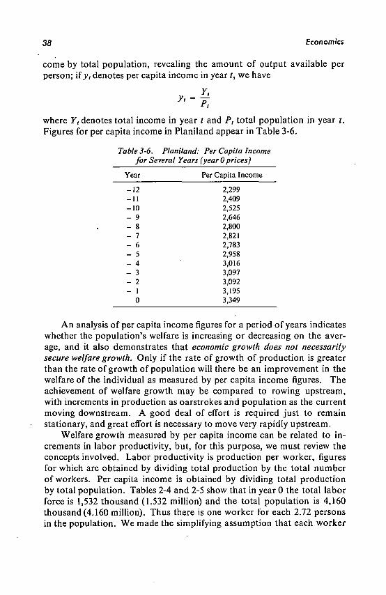
38 Economics
c o m e by total population, revealing the amount of output available per person; if y, denotes per capita income in year t, w e have
where Y, denotes total income in year / and P, total population in year /. Figures for per capita income in Planiland appear in Table 3-6.
Table 3-6. Planiland: Per Capita Income for Several Years (year 0 prices)
Year
-12 -11 -10 - 9 - 8 - 7 - 6 - 5 - 4 - 3 - 2 - 1
0
Per Capita Income
2,299 2,409 2,525 2,646 2,800 2,821 2,783 2,958 3,016 3,097 3,092 3,195 3,349
A n analysis of per capita income figures for a period of years indicates whether the population's welfare is increasing or decreasing on the average, and it also demonstrates that economic growth does not necessarily secure welfare growth. Only if the rate of growth of production is greater than the rate of growth of population will there be an improvement in the welfare of the individual as measured by per capita income figures. The achievement of welfare growth m a y be compared to rowing upstream, with increments in production as oarstrokes and population as the current moving downstream. A good deal of effort is required just to remain stationary, and great effort is necessary to m o v e very rapidly upstream.
Welfare growth measured by per capita income can be related to increments in labor productivity, but, for this purpose, w e must review the concepts involved. Labor productivity is production per worker, figures for which are obtained by dividing total production by the total number of workers. Per capita income is obtained by dividing total production by total population. Tables 2-4 and 2-5 show that in year 0 the total labor force is 1,532 thousand (1.532 million) and the total population is 4,160 thousand (4.160 million). Thus there is one worker for each 2.72 persons in the population. W e m a d e the simplifying assumption that each worker

Economics 39
is the head of a family (hence there are on the average 2.72 persons in each family). Thus the number of families in the population is the same as the number of workers. Productivity per worker and income per family, hence, are equal. Knowing the income per family, w e need only divide that figure by the average number of persons in each family (2.72) in order to find the income per person. Thus, assuming that there is no change in the number of persons in each family, the rate of growth of labor productivity and that of per capita income will be the same.
This is of the greatest importance since it enables us to relate welfare growth, as measured by increments in per capita income, to the education of the labor force, since increments in the productivity of the labor force are m a d e possible in part by previous investments in education.
3-6 Economic and Employment Planning
In both economic and educational planning, the first step consists of determining goals. In neither type of planning is there any scientific method of fixing the goals. Policy-makers usually determine goals for economic development without particular regard for economic theory; it is then up to the planners to decide whether these goals can be achieved. If it is decided that they are not feasible, they must be revised accordingly. Most of the technical aspects of economic planning are related to this verification of feasibility. W h e n it is verified that the goals can be attained they are called targets.
Goals for economic development are usually expressed as, or can be reduced to, a rate of growth of per capita income (used as an index of welfare). These goals for Planiland's economic plans are in Table 3-7. By using population data and projections, the planners can convert per capita income goals into total production goals.
Once the total production targets are established, the economic planners must determine the capital and labor required to reach these goals.
Table 3-7. Planiland: Goals for Per Capita Income
Year Per Capita Income ><(
0 3,349 5 3,945 6 4,075 10 4,655 12 4,967 15 5,492 18 6,052 20 6,469

40 Economics
A s regards capital, the problem is a simple one: on the basis of the current level of production and the current stock of capital, a reasonable determination can be m a d e as to the total amount of capital required to achieve a given future level of production. T h e problem with respect to labor is more complex because workers must be considered both as factors of production and as consumers. The economic planner must bear this dual aspect in mind when determining the number of workers required for achieving a certain rate of economic development.
The results obtained with respect to future capital and labor requirements must be checked against estimates of probable future supplies of capital and labor to see whether the production factors needed to reach the economic growth goals can possibly be m a d e available. Special attention must be paid to the availability of labor since economic plans must not only achieve production goals but also ensure full employment for the force if at all possible.
A s already mentioned, goals must be revised and a further analysis must be m a d e should it be found that the goals set by the policy-makers cannot be reached. If on the other hand it is found that enough capital is available and that there will be enough jobs for the labor force, then the goals are definitely adopted. W h e n this stage is reached the goals can be called targets of the plan.
This is the stage that has been reached in Planiland. T h e target for the rate of growth of the gross domestic product has been set at 0.062 per year; in other words, production is to increase at a rate of 6.2 percent per a n n u m . Since full employment is to be achieved, the number of workers employed will be equal to the number available according to the d e m o graphic projections. Table 3-8 shows the target values for gross domestic product, employment and productivity per worker.
The data given in Table 3-8 on future labor productivity are of particular interest to educational planners since the education of the labor force is one determinant of labor productivity. Thus when the targets are set for the labor force's productivity, implicitly the targets with respect to that force's education are also set.
Table 3-8. Planiland: Target Values for Gross Domestic Product, Labor Force and Productivity per Worker
Year
0 5
10 15 20
GDP (millions of dollars)
yt
13,932 18,822 25,428 34,354 46,412
Labor Force L,
1,531,540 1,763,509 2,049,624 2,386,816 2,764,249
Productivity per Worker
(dollars)
9,097 10,673 12,406 14,393 16,790

Economics 41
T h e first stage in preparing a plan for economic development ends with tables similar to Table 3-8. Thereafter, the economic planners must m o v e in several different directions.
T h e figures shown in Table 3-8 do not specify the amount of physical and h u m a n resources to be used in, say, agriculture, manufacturing or services. T h e economic planner must disaggregate the total target figures; in other words, he must establish the best w a y of distributing the total increment in production a m o n g the different sectors of the economy. A distribution of future production of interest for educational planners is that between public and private sectors (see Table 3-9).
Further planning puts economic and educational planners in direct contact. F r o m this point on, it is impossible to draw up socioeconomic plans without the collaboration of educational planners. T h e reason for this has already been mentioned: the productivity of the labor force depends in part upon the education of its members. Hence, economic and educational planners must work together to determine the educational structure of the labor force required to reach the productivity goals set up. The methods used to m a k e this determination are discussed in Chapter 7.
Table 3-9. Planiland: Planned Future Growth of Total, Public and Private Resources
(thousands of year 0 dollars)
Year
0 5 6
10 12 15 18 20
Total
13,932 18,823 19,782 25,428 28,098 34,354 39,885 46,412
Public
2,480 3,435 3,620 4,679 5,226 6,527 7,658 9,004
Private
11,452 15,387 16,162 20,749 22,872 27,827 32,227 37,408
References
The main concepts used in National Accounting are presented in all standard textbooks on economics. The reader may consult Samuelson, P. A . , Economics: An Introductory Analysis. 6th ed. N e w York:
McGraw-Hill, 1964.
A more complete presentation appears in A System of National Accounts and Supporting Tables. ("United Nations Studies
and Methods," Series F, N o . 2.) N e w York, 1964.
Basic references on economic development are Bruton, H . J., Principles of Development Economics. Englewood Cliffs, N.J . :
Prentice-Hall, 1965.

42 Economics
Lewis, A . W . , The Theory of Economic Growth. Homewood, 111.: Irwin, 1955.
O n the economics of education and related topics, see Correa, H . , "Measuring Education's Contribution to Economic Growth," in
S. Elam, and W . P, McLurr, (eds) Educational Requirements for the 1970's. N e w York: Frederick A . Praeger, 1967.
Schultz, T . W . , The Economic Value of Education. N e w York: Columbia U . P . , 1963.
Vaizey, J., The Economics of Education. London: Faberand Faber, 1961.

chapter 4
Basis for the Quantitative
Analysis of the
Educational System
4- 7 Content of This Chapter
This chapter does not deal directly with the preparation of an educational plan. Rather, it provides the educational background needed for such tasks. In this sense, it is the educational counterpart of Chapters 2 and 3.
T h e first step in the analysis of an educational system is to determine its main elements. Perhaps the most important a m o n g these elements are:
(a) Timetables comprising two elements: time allotted to direct interaction between teachers and students; and educational content, i.e., the subjects taught
(b) Teachers and administrative personnel (c) Buildings and other facilities (d) Students (e) Graduates and dropouts, which d o not form part of the educa
tional system itself, but are its output Several attempts have been m a d e to establish accounting relationships
a m o n g these elements. Examples of these are student-teacher ratioá, student-classroom ratios, and the like. Another example is the statistical data related to the n u m b e r of students in the educational system. All of these elements measure different aspects of the same system. A s a consequence, they must be defined with respect to each other. Actually, the elements of the educational system must give rise to systems of quantitative indices.
T h e object of this chapter is to present one such system of indices that places emphasis on the interrelations of the elements of the educational system.
In Sec. 4-2 weighted student-teacher and student-classroom ratios are 43

44 Basis for the Quantitative Analysis of the Educational System
introduced. For example, let us compare a class of 40 students with one teacher teaching all the subjects with a second class, also composed of 40 students, but with two teachers, each teaching half of the subjects. The student-teacher ratio for the first class is 40:1, while it is 20:1 for the second. F r o m the knowledge of these ratios, a planner might suggest that the number of students per teacher be increased in the second class. H o w ever, the teacher of the first class as well as the two teachers of the second class face a group of 40 students, evaluate h o m e w o r k and examinations for 40 students, etc. This means that the number of students per class should not, perhaps, be changed.
The reason for the misinterpretation is that the student-teacher ratios do not take into consideration the number of hours that, according to the timetables, teachers must face students. T h e three elements mentioned: timetables, teachers, and students, are considered in the weighted ratios.
A n analysis similar to the above could be m a d e with reference to classrooms. Such an analysis would permit us to explain the need and the main characteristics of the student-classroom ratios.
In Sec. 4-3, the flows of students are considered. The starting point for this analysis is the equation:
Students flowing in = Students flowing out
The students flowing into the educational system can be classified as new entrants, reentrants and repeaters. Those flowing out can be classified as graduates, repeaters going through the same grade during the next school year, dropouts and deaths. In Sec. 4-3 precise mathematical expressions are constructed using these elements. These expressions are the basic building blocks with which w e m a y construct indices to evaluate the characteristics of an educational system. W e also have available the instruments to study the future development of the number of student dropouts, graduates, and others. The use of these indices and instruments is explained mainly in Chapter 5.
Once the instruments for the analysis of the flows of students are available, it is possible to begin to describe the output of the educational system. In this description, it must be remembered that the output is not only the students successfully finishing their studies but also those dropping out. A precise definition of the output is the instrument by which w e can relate the educational system to the educational structure of the population and the labor force.
4-2 Quantitative Relations between Students, Teachers,
and Physical Facilities
4-2.1 Basic Definitions
In this section, perhaps the most important in this book, the basic definitions and main relations a m o n g the following are presented.
S = total number of students

Basis for the Quantitative Analysis of the Educational System 45
H = number of periods of education offered for unit of time (say a week)
N = number of periods of education received by all the students sh = average size of a class h¡ = average number of periods of education received by each student T o introduce these concepts, the timetable of Central High School
and the number of students per grade are presented in Table 4-1. Such information can be obtained only through direct observation, which is a simple task in the case of a single school but a m u c h more difficult undertaking where an entire educational system is concerned. For an entire educational system, a census or sample survey of schools would be needed to obtain such information.
It will be noted that the high school level is divided into six grades, some of which are further subdivided. All sections within the first two grades are taught the same subjects. For example, the three sections c o m prising the first grade have exactly the same curriculum; hence, all students could be grouped together or taught by a single instructional television series. The situation, however, is more complex in the case of the sixth grade, where curricula are not identical for all three sections. Students in 6 A , for instance, do not study the same subjects as students in 6B, nor with the same intensity. The situation is rendered still more complex by the fact that subjects 7, 8, 17, 19, 21, and 24 are taught to all sixth-grade students together.
T o introduce the basic definitions mentioned above, let us consider the case of a single grade first, say 1A, and one subject, say National language. According to Table 4-1, National language is offered five periods per week to the fifty students in grade 1A. The total number of periods received by the students is
5 x 50 = 250
N u m b e r of periods _. , . N u m b e r of periods j *• a j x Size of class = , . ,
education ottered education received A n alternative way of expressing this equation is
50 = 219-
Si7eofcla N u m b e r of periods of education received N u m b e r of periods of education offered
A second alternative is
s 250 ~ 50
N u m b e r of periods _ N u m b e r of periods of education received education offered ~ Size of class

46
B
asic for th
e Qu
an
titativ
e A
nalysis o
f the E
du
cation
al S
ystem
J? (periods per we School Timetable for Central High Table 4-1
• Grade
U
vo
pa V
O
<
VC
Wl
CQ
<
•t
CQ
<
en
U
CN
CQ
C
N
<
CN
y
CQ
<
3 u
Ë? 3
i i
m
m
i i
i i
m
m
t i
1
TT m
C
N
1
1
m
m
1
II
1
1*
1"
*
1
II
1 "
•- 1 1
1
II
1
1 1
1 1
m
in
m
i
i
i <N
C
N
l l
m
in
l | m
1 1
1 n
1 if
m
I
CN
1
1 n
N
1
IN
|t
n|
»n
||
m|
| r
<1
| 1 "
"**" 1
r^
llll
fn
ll°
l
i in
!
| I n
1 I
n
1
| T
I- TJ*
t
CO I I I I m
I I
C
N
1 "">
1
"">
1
1 cn
1 1
^
1
i m
m
m
i i 1 i i
tn N
i n
|«
n|
w-
ï|
|r
n|
i f
n|
i m
m
en
t 1
1 | |
m
CN l
C
N
»n
1
1
vn
| in
1
1
«n
II
^j
ll
1 1 1 1
1 m
CN
1
CN
in
1
1 >n
i in
1 |
m
il
""*
1 1
1
1 1
| 1
| m n | rt
>n i |
un i in
|
1
»n
i i
"
^1
11
| | | | | n
M | n
m | |
m
m | |
m |
II
"""III
1 1
| 1
1 n
1
NN
in I |
in
m I I
m
1
II
""'III
1 1
1 1
1 m
1
m
| |
m
in | |
m |
|| ^
| | |
i i i i i
m
| C
N
CN
1 National language 2 National literature 3 World literature 4 Mathematics 5 National history 6 Continental history 7 World history 8 National geography 9 Continental
geography 10 World geography 1 1 Economic and politi
cal geography 12 Nature study 13 Physics 14 Chemistry 15 Anatomy, physiology,
hygiene 16 Biology 17 Civics 18 Philosophy 19 Psychology 20 Logic and ethics 21 Foreign language 22 Art 23 Social education 24 Physical training
CN
m
CN
m
CN
m
CN
CN
en
CN
e
n
CN
c
n
CN
m
CN
m
CN
C
O
CN
m
CN
m
CN
m
CN
m
Total number of periods per week offered each class
00
00
VO
in
in
m
ov m
o in
CN
in
o
o T
f
m
Ti
ro
O
O
in
Number of students in each class

Basis for the Quantitative Analysis of the Educational System 47
The same relationship can be demonstrated if, instead of considering only National language, all the subjects taught to the students in grade 1A or in any other grade are considered. This can be expressed in the following formula:
s,N, = H, (4-1)
when i = IA, JIA = 50. H¡ is the number of periods of education offered to class i. For instance, H¡ = 32 for any /—that is, any grade in Central High School. N¡ is the number of periods of education received by all the students in class /—that is, in the case of the students in class 1A, N w = 50 x 32 = 1,600.
From Eq. 4-1 it follows that the size of the class is
N-Si = % (4-2)
•fri
a n d the n u m b e r o f periods received per student is
H, = Zi (4-3) s¡
Suppose n o w that several classes are considered, for example, all the grades in Central High School. In this case, the total number of students S is obtained from the last row of Table 4-1.
S = SiA + SIB + Sic + • • • + SôA + SôB + SóC = 50 + 50 + 43 + • • • + 16 + 18 + 18 = 555
The total number of periods of education offered per week H is the sum of periods offered to each class. A summary of the periods per week offered to each class appears in Table 4-2, which shows that each of the
Table 4-2. Central High School: Total Number of Class Periods per Week
Grades and Sections
1A, IB, 1C 2A, 2B, 2C 3 A . 3 B 4 A . 4 B 5
6A, 6B, 6C (separate)
6A, 6B, 6C (together)
Total
Number of Grades and Sections
11
3
1
Periods per Week per Grade
32
16
16
Total Number of Periods
352
48
16
416

48 Basis for the Quantitative Analysis of the Educational System
eleven grade sections from 1A to 5 receives 32 periods per week, making a total of
11 x 32 = 352 periods per week
Each of the three sixth-grade sections receives separately 16 periods per week, a total of
3 x 16 = 48 periods per week
In addition, the sixth grade taken as one section receives 16 periods per week. The sum of the three quantities gives a grand total of
H = 352 + 48 + 16 = 416 periods per week
Schematically, the total periods of education offered is
H = i/iA + His + H\c + • • • + Ht\ + H&B + flee + Hs
If data for all the schools of a given educational level in a particular country can be obtained, the value of H for that country can be determined.
In a similar way, the total number of periods of education received by all the students in Central High School is the sum of the periods received by the students in each class; i.e., using the figures in the last two rows of Table 4-1:
N = 7v"1A + Win + N\c + • • • + N6/i + N6B + Ntc + N6
= 1600 + 1600 + 1376 + • • • + 256 + 282 + 288 + 832 = 17,760
F r o m E q . 4-2, it follows that the average size of a class, J A , is
N Sh = 77
(4-4) - I * ™ 42.69
416
Further, from E q . 4-3, it follows that the average number of periods received by each student, h¡, is
(4-5) _ 17,760 _ „ v ' - 555 "
W h a t is the meaning of this figure for the average number of students attending each period? T w o meanings can be given: one if it is related to teachers and another if it is related to physical facilities. Let us examine these two interpretations.

Basis for the Quantitative Analysis of the Educational System 49
4-2 .2 N u m b e r of Teachers and Average Size of the Class
In order to relate the number of teachers to the average size of the class, the following equivalence is used: the number of periods of education offered is equal to the total number of periods taught by all the teachers. This is so because, by definition, a period of education in which a teacher teaches is a period of education offered.
Central High School's teachers, the subjects they teach, the grades in which they teach and the number of periods per week they teach are listed in Table 4-3 where the equivalence stated above can be observed—that is,
Table 4-3. Teachers in Central High School
Teacher
1 2 3 4 5 6 7 8 9
10 11 12 13 14 15 16 17 18 19 20 21 22 23 24
Total
Subject
1 1 2 3 4 4 4 4
5 ,6 ,7 5,6
7 8 9
10, 11 12 13 14
15,16 17,23
18, 19, 20 21 21 22 24
Grade
1A, IB, 1C 2A, 2B, 2C 3A, 3B, 4A, 4B, 6A 5, 6A, 6B, 6C 1A, 2A, 3A, 4A 1B.2B, 3 B . 4 B 1 C . 2 C , 5, 6A 6 B . 6 C IA, 1 B . 2 B . 4 A 1 C . 2 A . 2 C 3A, 3B.4B, 5, 6 1A, IB, 1C, 6 2A, 2B, 2 C 3A, 3 B , 4 A , 4 B , 5 1A, IB, 1C, 2A, 2B, 2C 3A, 3B, 4 A , 4B, 5, 6B 3A, 3B, 4A, 4B, 5, 6B, 6C 3A, 3B, 4A, 4B, 5, 6C 1A, IB, 1C, 6A, 6 B . 6 C 5, 6A, 6B, 6C 1A, IB, 1C, 2A, 2B, 2C 3 A , 3 B , 4 A , 4 B , 5 , 6 2A, 2B, 2C, 3A, 3B 1A, IB 6C
Periods per Week
15 15 24 16 20 20 17 8
18 15 15 18 15 15 30 23 22 18 9
15 18 16 10 24
416
the total number of periods taught each week by all the teachers (416) is the same figure as the number of periods offered per week (416). In other words, the same figure m a y be obtained by two different approaches.
W e can n o w establish the following relationship between the total number of periods offered per week and teachers:
H = hcT (4-6)

50 Basis for the Quantitative Analysis of the Educational System
where T = number of teachers (24 in Central High School)
hc = average number of periods taught by each teacher per week
The average number of periods per week per teacher in Central High School is
, _ H_ _ Total number of periods offered per week T Total number of teachers
= ± £ = 17.33 24
A s related to the number of teachers and average teaching hours per week, Sh, the average size of the class has the following precise meaning:
N hs x S .. _, H hc x T
This equation is derived by substitution in Eq. 4-4 of equivalent expressions for TV and H which are given in Eqs. 4-5 and 4-6. This equation tells us that the number of students per period is the student-teacher ratio weighted by the ratio of periods per student to periods per teacher. Put in another way , the average number of students per period is the average number of students that a teacher faces per period. The ratio in Eq. 4-7 is more meaningful as an index of quality of education than the unweighted student-teacher ratio since the quality of the system, if related at all to the number of students per teacher, must be related to the average number of students a teacher faces each hour in the classroom.
Equation 4-7 is useful in considering possible alternative reactions to an increase in the number of students. Solving Eq. 4-7 for T, w e find that
u T = 5-
hc x sh
This equation shows that to hold the number (sA) of pupils per period constant with rising student numbers (5), one must increase the number hc of periods taught per teacher per week and/or the number T of teachers, or one must decrease the number h, of periods of education received per student per week. Thus w e see that a school system confronted with a rising student population has some flexibility in meeting the increase in student numbers without allowing quality (measured by class size—that is, S/,) to decline. Hence, an increase in student population m a y not necessarily require an increase in the number of teachers, especially if the n u m ber hc of periods taught per teacher per week can be increased.
The equation above also reveals the different elements that should be considered in the estimation of the number of teachers required to teach a known number of students. If the number of students S to be taught is known and desired values for hs,hc, and si, are established, then the n u m ber of teachers needed for the students can easily be determined. Since

Basis for the Quantitative Analysis of the Educational System 51
the estimation of the number of teachers required for a k n o w n number of students is one of the central problems in educational planning, the value of Eq. 4-7 to educational planners is apparent.
Equation 4-7 can be modified to consider several different teaching situations such as the cases in which each teacher has several teacher assistants' or closed television circuits are used. In addition equations similar to E q . 4-7 can be used to relate students and teachers with personnel in administrative and supervisory positions.
4-2.3 Physical Facilities: N u m b e r of Classrooms and
Average Size of Class
The following classification will prove useful in studying the physical facilities involved in the educational process:
Plant consists of school buildings, areas set aside as playgrounds, sports fields, outdoor equipment and buildings for the housing of teachers and students. The various elements m a y be grouped under the general headings School Areas and Housing Areas. Elements under the former heading, primarily classrooms and laboratories, are c o m m o n to all schools.
Instruments consist of books, furniture, indoor or laboratory equipment, audio-visual aids, and other teaching devices.
Central High School provides no living accommodations for teachers or students so w e will not be concerned with Housing Area. The School Area is described in Table 4-4.
Table 4-4. Central High School: Characteristics of the School A rea
Use of Space Characteristics
Buildings Teaching
Classrooms Laboratories
Administration Auxiliary
Library Auditorium Storage Sanitary area Gymnasium Internal movement area Multipurpose
Open Space Playgrounds Sports fields Parking
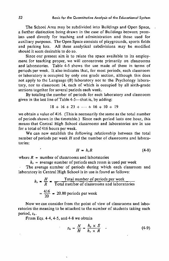
52 Basis for the Quantitative Analysis of the Educational System
The School Area m a y be subdivided into Buildings and Open Space, a further distinction being drawn in the case of Buildings between premises used directly for teaching and administration and those used for auxiliary purposes. The Open Space consists of playgrounds, sports fields and parking lots. All these analytical subdivisions m a y be modified should it seem desirable to do so.
Since our present aim is to relate the space available to its employment for teaching proper, w e will concentrate primarily on classrooms and laboratories. Table 4-5 shows the use made of these in terms of periods per week. It also indicates that, for most periods, each classroom or laboratory is occupied by only one grade section, although this does not apply to the Language (B) laboratory nor to the Psychology laboratory, nor to classroom 14, each of which is occupied by all sixth-grade sections together for several periods each week.
By totaling the number of periods for each laboratory and classroom given in the last line of Table 4-5—that is, by adding:
18 + 16 + 23 + • • • + 16 + 10 + 19
w e obtain a value of 416. (This is necessarily the same as the total number of periods shown in the timetable.) Since each period lasts one hour, this means that Central High School classrooms and laboratories are in use for a total of 416 hours per week.
W e can n o w establish the following relationship between the total number of periods per week H and the number of classrooms and laboratories:
H = hrR (4-8)
where R = number of classrooms and laboratories hr = average number of periods each room is used per week
The average number of periods during which each classroom and laboratory in Central High School is in use is found as follows:
, _ H_ _ Total number of periods per week R Total number of classrooms and laboratories
416 = IK = 2 0 - 8 ° P e r i o d s P e r w e e k
N o w w e can consider from the point of view of classrooms and laboratories the meaning to be attached to the number of students taking each period, sk.
F r o m Eqs. 4-4, 4-5, and 4-8 w e obtain
N_ = hs x S H hrxR
(4-9)
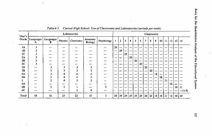
Basis fo
r the
Qu
an
titativ
e A
nalysis o
f the
Ed
ucatio
nal
System
53
Classrooms Laboratories
u
c
2
m
CS
—
O
o\
00
r
\c
u-l
•*
en
cs
-
Psychology Anatomy
Biology Chemistry Physics Languages B
Languages Grade
oo
+
i i
i i
i i
i i
i i
i i =
T
1 1
1 1
! 1
1 1
1 1
1 1
S
1
1 1
1 1
1 1
1 1
1 IS
1
1
1 1
1 1
1 1
1 1
1 1
S
1 1
1
1 1
1 1
1 1
1 1
1 s
1 1
1
1
I 1
1 1
1 !
1 2
1 1
1 M
1 1
1 1
1 II
S 1
1 1
1 1
1
1 1
1 1
i 1
«
1 1
1 1
1
1
1 1
1 1
1 S
1 1
1 1
1 1
1
1
1 1
1 ?
, 1 1
1 1
1 1
1
1
i i a
i
i i
i i
i i
i i
1 1
s
1 1
1 1
1 1
1 1
1 1
1
s 1
1 1
1 1
1 1
1 1
1
1
a
1 1
1 1
1 1
1 1
1 1
1
II
i i
i i
i i
i i
i i
i r
i
1
j i
i I
imc
nc
nc
nc
si
| *t
1
1
1
1
1
i n
n*
*n
i
-*
1
1
1
1
| 1 n
n
it
^
•*
I ui
I
1
1
1
1
1
i o
m
m ci
es
1 es
1
ci en
en m
m co
|
| |
| |
| |
|
<0
aU
<P
0U
<m
<«
<fflU
-
-'
Hr
st
Nt
Nm
fn
^^
tn
vo
**
o\
o
VO
es
oo
00
o
CS
o
CS
CS
CS
<3
\
CN
CS
CS
CS
m
00
CS
C
S
CS
V5
00
Total

54 Basis for the Quantitative Analysis of the Educational System
i.e., the number of students per period is the student-room ratio weighted by the ratio of the number of periods per student per week to number of periods per room per week. The fact that the weighted ratios 4-7 and 4-9 are equivalent bears out our intuition. It is obvious that the average n u m ber of students that a teacher faces must be equal to the average number of students in the classroom when all classrooms have teachers and no classroom has more than one teacher in a given period.
Observations similar to those m a d e with respect to the weighted student-teacher ratio can be m a d e with respect to the ratio in E q . 4-9.
Transforming eq. 4-9, w e obtain
hr x sh
Hence if the number of students S to be taught increases, and one wants to hold the size of a class si, constant so as to prevent deterioration in the quality of education, then either the number of periods per week hr and/ or the number of classrooms R must be increased; or the number of periods of education received per student per week hs must be decreased.
Thus w e see that a school system confronted with a rising'student population has, in the case of classrooms as in the case of teachers, some flexibility in meeting the increase in student numbers without allowing quality (measured by class size) to decline. A n increase in student population m a y not necessarily require an increase in the number of classrooms and laboratories, especially if the number of periods a classroom is used per week can be increased.
The equivalence between ratios 4-7 and 4-9 shows us another fact: it is impossible to change the weighted student-teacher ratio without also changing the weighted student-room ratio. This is a necessary consequence of the relationships between different factors in education. These relationships should also be considered in educational planning.
In the derivation of the relationship between the number of classrooms and laboratories and the size of the class, no mention has been m a d e of implements such as closed television circuits, teaching machines, etc. The basic equations can be modified to take into consideration cases such as the ones mentioned, but these modifications will not be presented here.
4-3 Flows of Students
4-3.1 Basic Equations for the Analysis of Flows of Students
Let us consider as before one grade in Central High School in a given year, say grade 1 in year 0 (Table 4-6). A basic equation can be estab-

Basis for the Quantitative Analysis of the Educational System 55
Table 4-6. Central High School: Structure 0
Grades
Total - 1 New Repeaters
Total - 2 New Repeaters
Total - 3 New Repeaters
Total - 4 New Repeaters
Total - 5 New Repeaters
Total - 6 New Repeaters
-5
115 108
7
-4
121 112
9
105 96 10
-3
126 112 14
110 97 13
80 74 6
To
-2
130 111 19
115 99 17
87 77 10
66 59 7
tal enr
-1
135 112 23
120 101 19
95 81 14
71 62 9
53 46
7
oilmen
Years
0
143 115 28
125 100 25
102 82 20
78 63 15
55 47 8
52 40 12
t year C
1
32
133 103 30
108 85 23
89 69 20
64 54 10
57 43 14
2
36
118 91 27
97 73 24
73 60 13
66 49 17
= 555
3
31
110 81 29
79 65 14
75 55 20
4
34
91 74 17
83 60 23
5 6
21
91 65 26 30
lished with respect to these students in the period under consideration:
Students flowing in = Students flowing out
The students flowing into a school grade at the beginning of a school period in a given year can be classified as new entrants, reentrants and repeaters coming from the previous school year; those flowing out during and at the end of the school period can be classified as graduates of the grade, dropouts, repeaters going to the same grade next school year, and deaths. This relation can be written in the following way:
N e w entrants + reentrants Graduates + dropouts + repeaters coming from = + deaths + repeaters
previous School year staying next school year
Taking into consideration the values for grade 1 in year 0 (Tables 4-6 and 4-7), the equation above has the following form:
115 + 0 + 28 = 103 + 7 + 1 + 32
This equation is represented in Fig. 4-1. The two main lines in this figure are the lower horizontal one and the oblique line above it. The

56 Basis for the Quantitative Analysis of the Educational System
Table 4-7. Central High School: Dropouts, Graduates, and Deaths from Structure 0
Grades
Total -1 Dropouts Deaths
Total - 2 Dropouts Deaths
Total -3 Dropouts Deaths
Total - 4 Dropouts Deaths
Total -5 Dropouts Deaths
Total -6 Graduates Deaths
-5
10 8 2 '
-4
10 7 3
19 19 0
-3
8 6 2
16 14 2
11 11 0
-2
6 5 1
16 14 2
11 11 0
11 11 0
-1
6 5 2
13 12 1
12 10 2
9 7 2
5 5 0
Years
0
8 7 1
10 10 0
10 9 1
4 4 0
2 2 0
38 38 0
1
6 4 2
8 8 0
5 4 1
2 2 0
40 40 0
2
6 5 1
3 3 0
4 3 1
46 45
1
3
2 2 0
2 2 0
52 52 1
4
5 5 0
57 56 1
5
N
61 61 0
Total 10 29 35 44 46 72 61 59 56 62 61 Dropouts 8 26 31 41 39 32 18 11 4 5 Graduates 38 40 45 52 56 61 Deaths 2 3 4 3 7 2 3 3 0 1 0
time period between the beginning and the end of the school period is represented by the horizontal line, and the number of students at any time is measured by the distance between the horizontal and the oblique lines. The largest number of students appears at the beginning of the school period, and this number declines to its m i n i m u m at the end of the period. The difference between the number of students at the beginning of the school year minus those in it at time t appears in the shaded area, representing dropouts and deaths.
In the analysis m a d e above, the time of reference has been the beginning of the period; however, there is no reason w h y the equation representing the students flowing in and flowing out could not be established with reference to any time between the beginning and the end of the period. Figure 4-2 is a graphical representation of the basic equation when the beginning of the school year is not taken as the time of reference. In this case, the number of students at time / can be expressed in

Basis for the Quantitative Analysis of the Educational System 57
New entrants + reentrants
+ repeaters
F IGURE 4-1 Graphical Representation of the Basic Equation for Student Flows when the Beginning of the
School Year Is the Time of Reference
Dropouts + death'
School year
Beginning of school year
Graduates + repeaters
End of school year
New students + reentrants + repeaters
F IGURE 4 - 2 Graphical Representation of the Basic Equation
for Student Flows when the Beginning of the School Year Is Not the Time of Reference
Dropouts before t +deaths before /
Number of students at time of reference
Dropouts after t + deaths after t
Graduates repeaters
School year-
Beginning of school year
End of school year
either of two ways: in terms of the students at the beginning of the period minus dropouts and deaths before /; or in terms of the graduates and repeaters at the end of the period plus dropouts and deaths after t.
These two ways to express the number of students at time t take the following form when mathematical symbols are used:
S, = n, + r, - b, - d]
S, = g, + a, + /•,+, + d]
where S, = number of students at time t n, = number of new entrants
(4-10)
(4-11)

58 Basis for the Quantitative Analysis of the Educational System
r, = number of repeaters coming from the previous school period b, = dropouts before time t d\ = deaths before time t g, = graduates a, = dropouts after time t
rl+l = repeaters going to the same grade next school period d] = deaths after time t
In the equations above, no attention has been paid to reentrants because it is considered that their number is small, and w e will work with this assumption in this book.
The equations above are particularly useful in educational planning because they serve as a frame of reference for the simultaneous consideration of several grades of the educational system, a level or several levels together, or even the whole system.
In considering the flow of students in an individual school or educational system, w e will use the analytical framework illustrated in Table 4-6. This table shows Central High School enrollment (divided into new entrants and repeaters) for the six grades in year 0 and for those grades in years before and after year 0 whose enrollments influence or are influenced by the enrollments in year 0. W e shall consider the enrollment figures in the table as one unit which w e shall call a structure. T h e year about which the structure is centered will be called the pivotal year, in Table 4-6 the pivotal year is year 0. Each structure carries the n a m e of its pivotal year; hence, the structure in Table 4-6 is called structure 0.
The whole history of an educational system or school can be analyzed in terms of a series of contiguous but nonoverlapping structures such as the structure shown in this table. Figure 4-3 represents several structures
FIGURE 4 - 3 —
Planiland High School Level Structures, Grades 6 Through 12
1 2 3 4 5 6
for one level of education which lasts six years. The steps going d o w n to the right show the boundaries between structures. T h e pivotal years of these structures are separated by six years—the number of years that a student normally spends in high school in Planiland. Statistical data for

Basis for the Quantitative Analysis of the Educational System 59
contiguous structures are presented in Table 5-1. In the general case, if a level of education (primary, secondary, or tertiary) lasts k years and a pivotal year is t, then the preceding pivotal year for that level of education is / - k and the succeeding pivotal year is / + k.
The numerical characteristics of the structure in Table 4-6 can be described by equations quite similar to those in Eqs. 4-10 and 4-11. It is required to modify only the meaning of the variables used in Eqs. 4-10 and 4-11. Below only these modified meanings will be used, so there is no risk of confusion. The modified interpretations of the variables given to the symbols are as follows:
S, = total enrollment at the beginning of pivotal year t n, = new entrants in structure / r, = repeaters coming to structure / from structure t — k b, = dropouts from structure / before pivotal year t a, = dropouts from structure t during and after pivotal year / g, = graduates from structure / d', = deaths a m o n g the students in structure t i = 1 before the pivotal year /' = 2 during and after the pivotal year
Let us clarify the meaning of "repeaters coming to structure t from structure/ - k." For this, data in Table 4-6 will be used; w e will refer to structure 0 and structure —6, which looks like structure 0 except that it extends from the first grade in year -11 to the sixth grade in year - 1 . The whole left flank of structure 0 between years —5 and 0 is open to the right flank structure —6. The students in the first grade in year —6 might repeat in year - 5 , thus becoming an input as regards structure 0. The same would apply to second grade repeaters in year —4, and so on. All these repeaters are accounted for under the heading "repeaters coming from structure - 6 . "
By using the notation introduced above, the following equations can be established:
S, = n, + r, - b, - d] (4-12)
S, = g, + a, + rl+k + d] (4-13)
Let us consider Eq. 4-12 as it applies to the structure shown in Table 4-6, i.e., with t = 0.
T o begin with, it is obvious that the number S0 of students in the different grades at the beginning of year 0 is equal to the number entering the structure (new enrollments, n0, plus repeaters, r0) minus the number which left the structure prior to year 0 (dropouts, b0, and deaths, dl
0. In Table 4-6 new entrants in the structure appear in the row for new
entrants in the first grade for years - 5 through 0. Their number is
no = 108 + 112 + 112 + 111 + 112 + 115 = 670

60 Basis for the Quantitative Analysis of the Educational System
The figure for the number of repeaters coming from structure - 6 is obtained by adding together the figures for repeaters in the first grade for year - 5 , repeaters in the second grade for year - 4 , and so on up to repeaters in the sixth grade for year 0. Thus the number of repeaters entering structure 0 from structure - 6 is
i-o - 7 + 10 + 6 + 7 + 7 + 12 = 49
The students leaving the educational system are not shown in Table 4-6 but appear in Table 4-7. However, the number of students leaving the school m a y be obtained from the data in Table 4-6. In the first grade for year - 5 , for example, there are 115 students. O f these, 9 become repeaters in year - 4 first grade and 96 go on to the second grade in year - 4 . The number of students leaving the first grade between years —5 and —4 is the number not accounted for by new entrants in the second grade or repeaters in the first grade for year - 4 :
115 - 9 - 96 = 10
The results of a similar analysis with respect to all the remaining figures in Table 4-6 are set out in Table 4-7. In addition, this table presents a breakdown (dropouts and deaths) of the students leaving the educational system. T o estimate the number of deaths, the appropriate death rate was multiplied by the number of students at the beginning of the period. By adding the totals for dropouts and deaths for year - 5 to - 1 given in the last rows of Table 4-7, w e obtain the figures for total dropouts and deaths from the structure 0 prior to pivotal year 0:
b0 = dropouts = 145
dl0 = deaths = 19
Equation 4-12 takes the following form for structure 0:
555 = 670 + 49 - 145 - 19
The possible destinations of the students in a pivotal year are given in Eq. 4-13. The students in pivotal year 0 can graduate, drop out, pass to the next structure as repeaters or die.
The data found in Tables 4-6 and 4-7 can be used to quantify relationship for structure 0. Enrollment in year 0, as mentioned already in connection with relationship 4-12, is equal to 555 (Table 4-6). The total n u m ber of dropouts between years 0 and 5 as shown in Table 4-7 is
a0 = 32 + 36 + 31 + 34 + 21 + 30 = 184
In order to obtain the figures relating to graduates which appear in Table 4-7, w e have assumed that all those leaving school after beginning the sixth grade either die or graduate. Actually, there are dropouts in the sixth grade also, but their number m a y be assumed to be negligible.

Basis for the Quantitative Analysis of the Educational System 61
Hence, w e ignore the complicating factor of sixth-grade dropouts. If it is * required, this assumption can be dropped and a more realistic point of view adopted. T o obtain the number leaving the sixth grade in a given year, the number of sixth-grade repeaters for the next year must be subtracted from the total sixth-grade enrollment for the year considered. Thus the number leaving the sixth grade at the end of year 0 is
52 - 14 = 38
The number of those leaving after having begun sixth grade includes both graduates and deaths; figures for each category are shown in the sixth-grade row of Table 4-7. The total number of graduates for structure 0 is the sum of the numbers of graduates for years 0 through 5.
go = 38 + 40 + 45 + 52 + 56 + 61 = 292
The number of deaths between year 0 and year 5 a m o n g those enrolled in year 0 is the sum of the figures for deaths given in the last row of Table 4-7 for years 0 to 5.
d\ = 2 + 3 + 3 + 0 + 1 + 0 = 9
With the values obtained, relationship 4-13 for structure 0 becomes:
555 = 70 + 184 + 292 + 9
A summary of the analysis made above appears in Table 4-8.
Table 4-8. Central High School: Relationships 4-12 and 4-13 for Structure 0
Before Pivotal Year, Relationship 4-12
N e w Entrants
+ "o
670
Repeaters
+ 'o
49
Dropouts -bo
145
Deaths
-do
19
Total Enrollment,
Pivotal Year 0
So
555
During and After Pivotal Year, Relationship 4-13
Dropouts + a0
70
Repeaters
+ r6
184
Graduates
+ go
292
Deaths
+ d\
9
4-3.2 Indices for the Analysis of Flows of Students
Taking the basic relationships just defined as a starting point, several indices for the analysis of the student flows in a school or educational system can be defined. S o m e of these and their values for structure 0 of Planiland Central High School are presented in Table 4-9. Such indices can be used for the comparison of schools or educational systems.
4-3.3 Use of the Basic Equations for the Analysis of the
Educational System as a W h o l e
In order to study an educational system as a whole, it is not enough to have an instrument to describe one of its levels. In this section the ex-

62 Basis for the Quantitative Analysis of the Educational System
Table 4-9. Central High School: Indices for the Analysis of Student Flows Structure 0
Definition
Repeaters r,
Total inputs* n, + r,
Dropouts before pivotal year b.
Total inputs* n, + r,
Deaths before pivotal year d,
Total inputs* n, + r,
Dropouts during and after pivotal year a, Enrollment pivotal year S,
Repeaters going to next structure r/+6 Enrollment pivotal year ~~ S ,
Deaths during and after pivotal year d, Enrollment pivotal year S,
Graduates g, Enrollment pivotal year S,
Value
49 670 + 49
1 4 5 0 T T 670 + 49 - ° ^
19 0 0"M 670 + 49
& - "»
H i . . , 3 ,
55s - °0 1 6
292
•Total inputs = new entrants + repeaters.
tensions required to use Eqs. 4-12 and 4-13 for the analysis of a complete educational system will be described.
In this book w e shall assume that the educational system is divided into two basic branches: general education and teacher education. T w o types of subdivisions of these branches will be considered: the usual subdivision of levels of education and a subdivision in qualitative strata. In this section w e will consider only the problem of the adaptation of Eqs. 4-12 and 4-13 for the study of the different levels of the educational system. In Chapter 5 the use of these equations in the case when the educational system is divided in qualitative strata will be considered. Finally, in Chapter 10 the use of the equations for the study of teachers' education is presented.
In the analysis below w e shall note that the educational system of Planiland is divided into three basic levels: elementary, high school, and college, and that the division into branches appears in high school and college. If for the time being no attention is paid to the division in branches, Eqs. 4-12 and 4-13 above should be distinguished only for each level. In this case they will be written as follows, with superscripts denoting educational level:
Si = n{ + r{- b{- d\}
S{ = gi + ai + ri+k + dV
[4-12]
[4-13]

Basis for the Quantitative Analysis of the Educational System 63
where j = 1, elementary level = 2, high school level = 3, college level
Already in Fig. 4-3 w e have seen h o w the successive structures of one educational level are related. In Fig. 4-4, w e see schematically h o w the
FIGURE 4 - 4
Structures - 6 Through 12 for Elementary, High School,and College Levels
Grades
1 2
3
4
5 6
/ = - 6 / = 0 1 1 i i
i
Elementary School
Years
r=6 1 1 1 i
'-i V '-ï
l_j
t=Yl
1 1
Grades
1 2 3 4
5 6
/ = - 6 t=0 1 1
i 1 i
L-, ^
n ! i
High School
Years
/=6 1 |
1_ ' * l_i
/=12
j |
L i <= L
Grades
1 2 3 4
5 6
f=-6 / = 0 1 1
1 1
College
Years
/=6 1 1
1 — i !
n_j
/ = 1 2 1 i
L A \ n
structures for the various levels of an educational system are related to each other. It is assumed in this figure that each level of education lasts six years; hence, pivotal years for all the education levels are six years apart and pivotal years for the different levels coincide. If levels within the system are of different lengths, the relations between the structures of

64 Basis for the Quantitative Analysis of the Educational System
the different levels are somewhat more complex but no conceptual change is required. W e can see in the figure that, where all educational levels are the same length, new entrants in the high school and college levels (i.e., n2 and n)) are the graduates of the previous lower-level structure centered on the preceding pivotal year (i.e., #,'_* and #?_*)• For instance, new entrants in structure 0 at the secondary level (i.e., n\) are the graduates of primary level structure - 6 (i.e., ^ L Ö ) .
The procedure described above can be summarized as follows: First, construct a set of basic equations, 4-12 and 4-13, for each one of the subdivisions of the educational system to be considered; second, establish the proper relationship between new entrants of one subdivision and graduates from the others. Following these rules, it is possible to use the basic equations to study any subdivision of the educational system. T o mention just a few of the most important subdivisions in practical application: subdivisions by sex of the students; subdivisions in public and private institutions; subdivisions in general and vocational education; and subdivisions according to type of vocational school.
It should be observed that the basic equations can be used also for the study of on-the-job training and adult education wherever some form of institutionalization exists. However, types of education without any formal structure (such as the mass media) cannot be studied with Eqs. 4-12 and 4-13.
i
4-4 Output of the Educational System
Perhaps the most important application of relationships 4-12 and 4-13 just introduced is that they permit definition in simple terms of the output of an educational system.
Here w e will consider the output of two educational levels, high school and college, denoted by the superscripts 2 and 3 respectively. Let
0J, = output of the educational system of persons with education level j = 2,3 between pivotal years t — k and /
Then
0? + t = g2 + (1 - y2)a2 + (1 - v2)b2+k (4-14)
+ 73a? + v3b3,+k - n3t+k
and
0?+* = g3, + (1 - Y > ? + (1 - r,3)b)+k (4-15)
where r¡J = proportion of dropouts from level j before the pivotal year that are considered a part of the output of the previous level
yJ = proportion of dropouts from level j during and after the pivotal year that are considered a part of the output of the previous level

Basis for the Quantitative Analysis of the Educational System 65
The coefficients tr* and y must be included, because it is a matter of definition whether a dropout from, say, the third year of high school will be considered an output of the high school or the elementary school level. T h e coefficient m a y be used to express all the possible alternative judgments as to what part of a levels' dropouts should not be counted as output ofthat level.
In Eq. 4-14 the output of high school between pivotal years t and / + £(0?+*) is equal to
g1,, i.e., graduates from high school between pivotal years t and t + k,
plus
(1 - 72)a2,i.e., those dropouts from high school structure t during and after the pivotal year t which are considered as output from high school
plus
(1 - v2)bj+k, i.e., the dropouts from structure t + & before year t + k which are considered as output from high school
plus
7 3 a 3 + T)lb]+\, i.e., those dropouts from college which are considered only high school output
minus
n)+k, i.e., the number of high school graduates from structure / entering college in structure t + k
Similarly, Eq . 4-15 tells us that output from college between pivotal years / and / + k(03,+k) is equal to the sum of:
g], i.e., graduates from college between pivotal years t and t + k
(1 - 73)a?, those dropouts from college structure t during and after pivotal year t that are considered as output from college
and
(1 - v3)b3,+k, those dropouts from structure / + k before pivotal year t + k which are considered as output from college
References
This chapter is an elaboration of Correa, H . , "Basis for the Quantitative Analysis of the Educational System,"
Journal of Experimental Education, Vol. 35, N o . 1 (Fall 1966).

66 Basis for the Quantitative Analysis of the Educational System
A mathematically more sophisticated version of this chapter appears in Correa, H . , " A Survey of Mathematical Models in Educational Planning," Math
ematical Models in Educational Planning. Paris: O . E . C . D . , 1967.
A comparison of the model in this chapter with other models appear in Davis, R . C , Planning Human Resource Development. Chicago: Rand McNally,
1966.
Glossary of Symbols
H n u m b e r of periods offered per unit of time TV n u m b e r of periods received by all students R n u m b e r of classrooms and laboratories S n u m b e r of students T n u m b e r of teachers hr average n u m b e r of periods that each r o o m is used per w e e k hs average n u m b e r of periods per w e e k per student hc average n u m b e r of periods per w e e k per teacher Sh average n u m b e r of students per period; weighted student-teacher
ratio; weighted student-room ratio a, dropouts from structure t during and after pivotal year t b, dropouts from structure t before pivotal year t d'i deaths of students in structure t;
/' = 1 before pivotal year t / * = 2 during and after pivotal year t
g, graduates from structure t k n u m b e r of years that an educational level lasts n, n u m b e r of new entrants in structure t r, n u m b e r of repeaters entering structure t from structure t - k 0, output of persons with education level, between pivotal years I — k
and / t]J proportion of the dropouts from level j before the pivotal year which
are considered a part of the output of the previous level yJ proportion of dropouts from level./ during and after the pivotal year
which are considered a part of the output of the previous level Superscripts are used to designate education level (1 = elementary; 2 = high school; 3 = college).

chapter
Flows of Students
5-1 Content of This Chapter
A basic problem in planning is the forecasting of the future evolution of student flows. W e find the basic information for such forecasts in the analysis of past and present characteristics and trends. Sec. 5-3.1 (Tables 5-1 and 5-2) contains the raw data required. Using the method introduced in Chapter 4, these data are summarized in Table 5-3.
O n c e the basic data are put into manageable form, it is possible to predict the future flows of students. Several methods can be used for this prediction. T w o of them are presented in this chapter.
The first method considers only the influence of population growth on the flows of students. T h e information concerning the growth of the school-age population is provided by demographers using the methods outlined in Chapter 2. In the first method it is assumed that the proportion of school-age children entering the educational system will be the same as it has been in the past, and consideration is given to the persons w h o have never enrolled in the educational system, distinguishing them from the dropouts. W h e n simpler approaches are used, it is likely that the number of children enrolling in the educational system will be overestimated.
T h e next step is to forecast the n u m b e r of children continuing in the educational system and the number leaving it. In the first approach it is assumed that fixed proportions of those entering will become dropouts, graduates, or deaths.
T h e details of the first approach are presented in Sec. 5-4.2. T h e results obtained appear in Tables 5-14, 5-15, and 5-16.
O n e limitation of the first method is that it does not take into consideration the fact that as economic development takes place, the proportions of children entering and remaining in the educational system will tend to increase. This limitation is eliminated in the second method, because this method takes into account the influence of per capita income growth on those proportions. A s a first step, the increase in the proportion of children entering the educational system due to increments in per capita
67

68 Flows of Students
income is evaluated. Next, a similar evaluation is m a d e with respect to the proportions of those dropping out and graduating. These computations give the information needed to forecast the flows of students. T h e details of the method appear in Sec. 5-4.3, the results in Tables 5-25 and 5-28.
A brief comparison of the results obtained by the two methods shows that they are different, but not incompatible. The first forecast represents the m i n i m u m growth of the educational system while the second represents a more likely alternative.
5-2 Method
T h e instrument to be used in the analysis of the student flows was described in Sec. 4-3.1. There two basic equations were introduced:
S, =_n, + r , - b , - d) [4-12] S, = g, + a, + rl+k + d) [4-13]
7 where / = pivotal years, not calendar years S, = number of students at the beginning of pivotal year / n, = new entrants in educational structure / r, = repeaters in structure / coming from structure t - k b, = dropouts from structure t before pivotal year / d\ = deaths a m o n g the students in structure /
/ = 1 before pivotal year t / = 2 during and after pivotal year t
g, = graduates from structure / a, = dropouts from structure / during and after pivotal year t
These two equations will be used to study the student flows in the educational system of Planiland.
T h e analysis of the student flows is the analysis of the variables in Eqs. 4-12 and 4-13. Below w e will obtain the values in the past of these variables using statistical data from Planiland's educational system, and w e will study the development of these values.
5-3 Past and Present Characteristics of the Student Flows
5-3.1 Study of the Student Flows in the Different Levels of the
Educational System
T h e educational system in Planiland is divided into three levels: elementary school, high school, and college. Each level lasts six years. Be low, the variables in Eq . 4-12 and 4-13 will be evaluated for each one of these three levels.
In Table 5-1 appear the statistical data required for elementary school

Flows o
f Stu
den
ts 69
VI u
c3
1)
> c -
o I
fN
1
rn 1
Tf
1
in
1
NO 1
P-.
1
oo 1
ON |
O
7 7"|
1
fN -13
n > 13
5
ON
P^
CN
ON
od
O
fN
ON
NO
ON
P^
OO
OO
™"
r-Tf
00
~~
P-;
p^
in
""
_ rN
SO
to
Tf
to
p~
fN
Tf
so
rn
Tf
sq
_J
Tf
sq
ro
m
°°. 00 123.8 12
— tal o ö
in
_
ö
to
CM
OS
Tf
—
os
TT
Os
as Tf
fN
OS
Tf
o
r»°
Tf
Tf
SO
Tf
fN
5'
°) to
Tf
p~
so
Tf
Tf
IO
Tf
_
to
Tf ers rt
8.
U
H
oí
OO
p^
NO
oo
od
in
"~
r-#
r-"
Tf
"
NO
OÑ
m
™"
oo
Tf
m
in
NO
CN
—
in
<N
od
O
in
od
ON
P-;
P^
ON
ON
Tf
ON
(N
od
oo
p-t
m*
oo
? u
Z
(N
m'
(N
ON
P^
„
_!
*~*
TT
S
o
to
o ~
m
8 NO
M
ON
rn
r-
oo
—.
00
p-
m
NO
p-
ON
CN
P-
Tf
CO
NO
OO
in 63.0 6
(N
*«
õ oo
H
fN
oq
M
tN
Tf
«
(N
Tf
«'
fN
°i
«
(N
t—
H
(N
IO
Ö
fN
fN
o
fN
t-;
00
oo
od
SO
00
p
00
oo
r~ ers M
fi
U
Tf
_J
O
_
sd
O
r-
Os
oo
p
to
oo
^
m'
oo
sq
od
t—
_,
M
p-
—
p-'
so
Tf
os
IO
»o
r--'
to
m
Tf
to
Tf
Ö
IO
p
od
Tf
•E
U
H 0Ä Z
Tf fN
os
só
os —
Os
—
m' sd
os —
Tf sq
p- to
oo —
fN »O
S2
ON ON
CN
in
00
—
TT Tf
p- in
r* —«
—
Tf
O
Tf
p-
—
m
—
NO Tf
NO —«
—« —
ON" m'
in
—
NO
—
p^ m'
in
—
OO ON
Tf fN
in
—
O
NO
CN CN
un
—
Tf in
Ö CN
in
—
oo
od
Tt
ers
"
rt
S 8.
O u
fN
m'
00
00
r
r*
oq
_J
p-
sq
00
so
p
p^
SO
O
fN
SD
P-;
tO
to
fN
fN
IO
O
SO
Tf
to
?
Os
_J
Tf
Tf
OÍ
m
°i
p^
m ï
u
H
oá z
to
O r~
os
IO
SO
oo
s Os
só
to
Tf
Tf
to
fN
Ö
to
r-5 P-;
__!
T*
CN
P-*
m
Tf
NO
m
r-#
Tf
m
m_
CN
m
oo
Ò 29.3 3
T*
2 o
H
Os O
t—
ö
m
Ö
o o
°i
Os
tO
Os
oo
od
to
od
00
p-
OS
r~
r-#
p-°
Tf
p-
ro
r~ ers
Õ fi
u
VO
ON
tO
fN
to
to
to
Ö
to
OS
vd
Tf
to
3"
r-ö
Tf
Os
to
fn
fN
rn
m
Tf
OS
fN
to
00
(N
O
P-
fN
OS
Tf
fN
to
rn
(N
S u
*Z
sq
so
Tf
OS
3'
Os
o
Tf
00
r~
m
p^
to'
rn
r-fN
m
._
OS
(N
Os
SO
fN
Tf
rn
fN
_
fN
fN
P-
H
fN
tO
OS
fN
od 16.8 1
to
"c3
õ to
to
SO
to
rn
to
—
to'
p
to
r~
Tf
Tf
Tf
fN
Tf
oo
rn
P-;
rn
P;
rn
to
rn
rn
rn ers B
s. u H
Tf
m
Os
m
so
to
m
r-fN
rn
P-
Ö
m
p
00
fN
P»
Tf
fN
P-.
fN
fN
SO
OS
Tf
od
p
00
_
SO
Os
Tf
ï U HûiZ
fN
od
m
fN
to'
m
^
fN
m
Tf
OS
fN
sq
p-
fN
O
to
fN
O
fN
fN
fN
Ö
fN
Tf
SO
Tf
SO
O
SO
O
to
to
Tf 14.0 1
to tal o
H
sq
m*
to
rn
r^t
rn
fN
rñ
mm
r^
s
as fN
SO
fN
to
(N
—
fN
fN
(N
fN
IN
_
fN
__
fN ers C3
8.
a
so
Tf
m t»;
-J
m
00
od
fN
r)
SO
fN
to
Tf
fN
—
fN
fN
Tf
OS
p-
p^
m
Tf
fN
Tf
00
rn
Os
fN
Tf
fN
i U
a z
oq
to
OS
to
p~
SO
SO
to
fN
OS
fN
to
Tf
rn
o
to
m
S
Tf
rn
_J
so
Tf
so
OS
Tf
O P^
OS
m
Os
s¿
to
m
Tf
fN
to
m
p-#
n
Tf
m
OS
Ö
fN
m
to
od 295.7 30 tal o
H

70 Flows of Siudenis
in Planiland from year - 1 3 up to year 0. Since the plan is being prepared for years 1 , 2 , . . . , our last pivotal year before the plan must be year 0; the previous pivotal year is - 6 , then - 1 2 , etc.
In Table 5-1 structure —6 is delineated by a heavy steplike line. This structure has a shape identical to the structure in Table 4-7. Structure - 6 is the only one that is complete in Table 5-1. However, data concerning the variables after pivotal year —12 and before pivotal 0 also appear in Table 5-1.
In order to separate structure —6 in Table 5-1 from the flow of students enrolling, repeating, or dropping out in elementary school, all students affecting enrollment in year - 6 as well as all those affected by enrollment in the same year were considered.
Let us n o w evaluate relationships 4-12 and 4-13 for structure - 6 . Equation 4-12 in this case (the superscript 1 representing elementary school) will be
Sl6 = nit + rls - bl6 - d]\
The values corresponding to the terms used in relationship 4-12 are obtained as follows:
N e w enrollment in the first grade appears a m o n g the data corresponding to first grade in Table 5-1. The value is
nit = 602.6 = 88.2 + 94.9 + 97.7 + 98.5 + 108.2 + 115.1
Repeaters coming from structure - 1 2 are obtained by adding together the repeaters in the first grade for year - 1 1 plus repeaters in the second grade for year —10, and so on up to repeaters in the sixth grade for year —6. This means that the number of repeaters from structure —12 will be
rlt = 91.7 = 45.4 + 18.6 + 13.1 + 7.8 + 4.2 + 2.6
Dropouts and deaths are not shown in Table 5-1 but appear in Table 5-2 with respect to structure —6. The number of students leaving the educational system m a y be obtained from the data in Table 5-1. In the first grade for year - 1 1 , for example, there are 133.6 thousand students. O f these, 46.7 thousand are repeaters (in year - 1 0 , first grade) and 54.3 thousand go on to the second grade, year - 1 0 . The number of students leaving the first grade between years - 1 1 and - 10 is therefore
133.6 - 46.7 - 54.30 = 32.6
The leaving students are divided into two groups in Table 5-2, representing dropouts and deaths respectively. Information concerning the latter was obtained with the aid of a death rate.

Flows o
f Stu
den
fs 71
tf) 1—
>
c a c t
c
1 1 1 1
in 1
VO
1 1
oo 1 1 -11 -10
0 } 3 5
33,652 648
35,882 618
28,629 571
39,426 574
32,066 37,634 534 566
Dropouts Deaths
-
10,999 401
7,534 366
10,751 349
5,388 312
11,295 305
9,308 292
Dropouts Deaths
(N
20,068 332
16,690 310
13,634 280.
15,735 265
11,564 236
14,870 230
Dropouts Deaths
m
10,772 228
11,482 218
9,399 201
7,021 179
8,033 167
5,851 149
Dropouts Deaths
•*
3,436 164
3,549 151
4,257 143
3,069 1 3 1
2,184 1 1 6
2,992 108
Dropouts Deaths
»n
31,459 141
28>72 128
25,982 1 1 8
24,290 110
21,800 100
19,012 88
Graduates Deaths
vo
3,436 14,321 35,807 40,157 64,025 73,393 51,432 65,591 32,066 46,942 Dropouts Total
141 292 497 803 1,143 1,677 1,507 1,268 1,109 534 858 Deaths Total

72 Flows of Students
The results of a similar analysis with respect to all the remaining figures in Table 5-1 are set out in Table 5-2.
By adding the totals of the columns from year —11 to year —7, w e obtain the dropouts and deaths prior to pivotal year - 6 :
ò!_6 = dropouts = 269.4
rfii = deaths = 5.3
with the preceding values, relationship 4-12 takes the following form:
419.6 = 602.6 + 91.7 - 269.4 - 5.3
The destination of students in a pivotal year constitutes relationship 4-13 which, for structure - 6 , takes the following form, with the superscript 1 representing elementary school:
Sl_6 = gl6 + a]_6 + r¿ + dlï-
The data appearing in Tables 5-1 and 5-2 can be used to quantify this relationship. T o begin with, enrollment in year —6, as mentioned already in connection with relationship 4-12, is equal to 419.6. Dropouts between • years - 6 and - 1 are shown in Table 5-2. The total number of dropouts (between years - 6 and - 1 ) is
al6 = 157,746 = 64,025 + 40,157 + 35,807 + 14,321 + 3,436
Repeaters going to structure 0 are shown in Table 5-1. T h e total n u m ber is
r¿ = 106.2 = 49.2 + 21.9 + 15.6 + 10.3 + 5.6 + 3.6
In order to obtain the figure relating to graduates which appear in Table 5-2, w e have assumed that all those leaving school after beginning sixth grade are graduates. Actually, however, there are dropouts in the sixth grade although their number m a y be assumed to be negligible. T o obtain the number of sixth grade leavers in the total enrolled in a given year, the number of repeaters'must be subtracted. At the end of year —6, for example, the number is
22.0 - 2.9 = 19.1
The number of those leaving after having begun sixth grade includes graduates and deaths; figures for these are shown in Table 5-2.
The total number of graduates is
g-I = 151,015 = 19,012 + 21,800 + 24,290 + 25,982 + 28,472 + 31,449
The number of deaths between year —6 and year —1 a m o n g those enrolled in year - 6 is
dl\ = 4,553 = 1,677 + 1,143 + 803 + 497 + 292 + 141 •

Flows of Students 73
With the values obtained, relationship 4-13 assumes the following form:
419.6 = 151.0 + 157.8 + 106.2 + 4.6
Similar evaluations were m a d e for E q . 4-13 for structure - 1 2 and for E q . 4-12 for structure 0. T h e results appear in Table 5-3. In this table results obtained for high school and college are also presented.
In Chapter 4 several indices based on the variables of E q . 4-12 and 4-13 were defined. By studying these indices, it is possible for us to obtain a better idea of the development of the educational system. Besides, these indices will be used later for the study of the future development of the student flows. The values of the indices are presented in Table 5-4.
5-3.2 Qualitative Subdivision of the Student Flows in Different Levels
of the Educational System
T h e analysis of the past and present data with respect to the different levels of the educational system is not enough. Additional information is required which can be obtained by studying qualitative strata of the different levels of the educational system, as shown for Planiland's elementary and high school levels in Table 5-5.
T h e reason for describing these subdivisions as "qualitative" is evident in Table 5-6 which shows the ratios between the different variables. These reveal that stratum A represents the lowest ratios (2), (3), (5), and (6) and the highest ratio (8), which means that the proportion of repeaters and dropouts is very low in this stratum and that of graduates very high. T h e reverse is true of stratum D while strata B and C reveal changes ranging from the most satisfactory conditions of A tò the least satisfactory conditions of D .
5-4 Projections of Student Flows
5-4.1 Basic Considerations with Respect to Projections of Student Flows •
T h e method used in making projections of future student flows is similar to that used for projections in any science, whether natural or social. In the case of student flows, projection involves the following steps.
(a) A clear definition of the elements in student flows. Such a definition is given in relationships 4-12 and 4-13.
(b) Specification of factors influencing changes in the values of the variables in 4-12 and 4-13 and of the nature of these influences. Population growth and per capita income growth are the most important factors which systematically influence the value of the variables; the nature of. the influence of these factors is considered in the following sections of this chapter.

74
F
low
s o
f Stu
de
nts
CL
1
.0
I I 3
Q
Ü o
D.
O
•a. M
-
Ï f: ] -Si
3
E ~
a
•-,-
W r*
li
o
S
ití
r-
(N
»
Oí
VI
o
— o
\ r«
i ^
- v
i
o\
00°
r-# es
5Ñ o
CM* vi
\5
00
II
—»
0
0
j=
<
j
(/3
.e
011
X
VI
0 _ —
V
I
00
r-VI
CM
-12
00
0 0.1
rM
VI
\o
m
Vï
? 00
O
O
00
in
CM
•* v
i
1 0
ON
*0
CI
VO
m
CM
Vi
v£>
•* r-0
0
O
ro
II
•-»
V
61) u
0
u
00
0
—
0
0
CM
r-
0
0
~" —'
—
O
vi
r~-
0
0
•<t
vi
—
CM
r-
—
o
\ n
«
00
r-
0
0
0
•g-
r«-» ^
*
\n r-
O
0
r-
0
0
t-
C
M
CM
«
5
O
7 '

Flo
ws
of S
iud
en
is
75
I I "3>
a c
•«
'S.
~ m
,
8 Ö
IN
VO
O
"""" 06.2
• "
+ <
N 875
m 378
06.2
~ + C
N 875
7.3 8 =
S o
o
r--Ov
+ V
O
CN
S
•*
VO
<
N
r-Ov
+ V
O
rN
tt
m
VO
419
CN
106 V
O 41?
4.6
vO 419
o 151
Ö
8
9.4
CN
8.5
o
P-;
o\
8.5
o
O
m
8.5
o
PO
^ oo
c E
zz o
w enr CJ
'A
¡on C3
O
a. läge o Scho
•-H
a Repe
rt tal ye e pivo s befor 3 Q. Dro
puts* Total in
1 yea pivota before
.c a Q
DUtS* otal in
H
ca
S. U
l pivot ng and after u. Dropout year ¡votai ment p
—
o
UJ
ture
1 to nex Suisse a.
o> Repeat year ¡votai ment p
-.^ o
c
W
ca 4
)
>-.
ivota after p g and Ui
•o Deaths year votai ment p
—
o
c BJ
ates Gradu

76 Flow
s of
Studenfs
i I
I
•Q
o
1 •s. ¡5 X
O - 0.57
Tt
00
©
_! in
3 Ö N
<N
|TC
t ht
in loo
illmenl w enro V
z —
o
! entary tes elem ca a
•a Gra
ON
= 0.06
in
vd
»n N
O
+ 87.4
oo o o II
5.1
—
vi +
ters Repea
puts* otal in
l-
c -i
= 0.25
>o tN
in
*¿ + 87.4
S
m
ò II
18.0 —
<n
+ tN
»n
u ca tal ye e pivol > befor
*•* 3 O
D
. Dro puts* otal in
b>
p rj
•* - 0.01
rn
>/"> V
O
+ 87.4
m
S
© II
00
o
—
u-i
+ <N
in
L. il yea pivota before to
£ B3
Q
puts* btal in
H
T 1-
CN
m
O
H
—
1 Wï
fi Ö
— !•*
00
m
© II
oo
l^ H
S
u ca
cd pivot ing and after g 3 ^ pout: Dro c
year ivotal ment p
—
o h» c; UJ
"»
I O II
ml":
*ls
00 O
(N
Ö II
«Is
ture u tstru to nex assing a » h. u s peat
Oí v
year ivotal ment p
~ o u C
UJ
5
0 O
Ö «
oo
|"î
oIS
Q
o
sis
u S
>>
1 after p ig and ;
.5 ï-3 •o aths
Q r-
year ivotal ment p
—
o L» C
UJ
VO
o\ ^ II
— 1
f\ Ö
O
C
NI
TÍ
m
•o •«t II
—-| «n
—
•*
— 1
(N
ates Gradu year ¡votai ment p
= o u-C
UJ
0 D «
¡L

Flows
of
Students 77
"8
3
c
<L> Heg Col r~
= 0.63
oo
l —
r-i
o
— 1
rs
Tf
OS
VO
© II
[-•»1 —
t~-'l~
illment New en re
**3 igh schoi aduates h u
rl
<N - 0.05
r
Ö
0.7 + 2.8
i © II 0.5
m
d + 7.7
ters Repea puts* Total in
r •j
VO - 0.32
•*
_
•*
0.7 + 2.8
VO
vo
ro
• O
II 3.0
w-i
d + 7.7
U-03
£ e pivotal outs befon o
. Dro puts* Total in
r ï
in - 0.01 0.2
0.5 + 7.7
CN
O
d H
0.1
vn
d + 7.7
im
ca pivotal j hs before 03
Q
puts* Total in
T r
S Tf
d N
•01-<N
|VO
OO r-m
d
II
rflr-. —
Im*
u yea
—;
5
1 luring and after pi
T3 pout: Dro »/
ivotal ye ollment p L» C
U
•ï
p-
c->
—
d il
t"""-|—'
dlv
n
»n
m
—~ d
n v
nlr-
©Ic
*
ture u tru to next s s passing Im
0> epeat
aí V
U
cd ¡votai ye ollment p t.
c
W
3
O
CN O
d
II
~|~
dl
vi
CN fN
O
d
ll
31 f.
dl m
ear »-. —
1
after pivi iring and ; 3 •o aths
D r
cd ivotal ye ollment p k»
c
U
-*
m
»n
m
d n
°°|-. -U
VO
VO
Tf
d II ates Gradu
ivotal ye ollment p t-c
U
o 0 03
Q,
O
%
«- 5

78
Flow
s of
Stu
de
nts
_ choc
GO
CO
-*-» c leme
tu
IM
cd o
>>
votai
£ After
•s •
-»
D"
0
CA
3
.-*°
'S"*
i-.
o C
A
1>
2 -o
u
Oí
CA
"a
o
«
a,-
i O
Q
Û
=" Enrollme Pivotal Year Ä-6
cd
u
> votai '
S
á
ä
vi
•£ —
o
a
- 1
D^
3
VI
3
O
*o
&-
1
O
-O
a 1«
CO
•—
i
8.-V
(A
c
cd
•f *o
•SM
s z
8. Ê
• © o
o
vO
io
w
i Tt
—
—
""
oo (N
m
—
; vo
oo
0
\ (N
CS
fO
vo
m
_ oo
—
1.0
20.1 30.8
vo
m
-r*1
©
(N
—
— o
C
N
t
©
p
p
(N
vi
Vi
1- O
O
v> m
o
\ m
oo
-
ö
ö —
ro
TÍ-
r*l O
O
ON
—í o
î es
CM T
f
c*t c
*i r*i
0\
en
r*">
O
O
s
OO
<N TJ-
r-# ro
oo
íN
vo
Ö
Tf
—
(N
^—
f—
l
^Í
Ü
* M
H
i °°.
t~
-1
o
™"
_ 54.2
oo
—•
u-í o\
VO
r-° vo
o
ON
C
N
vi C
\
_*
•<t i—
C
N
es
m
Q H
vo
•>fr
O
vri
N
06.2 00
K
«•>
VO
o\ ^ o
m
U">
§
"OV
vo
<N
O
t-
5\
vo
rvi
S
"cd
(2
|00 .e
w J
=
0B
iE
cd eu
>• "
M
o
> £
< c:
(A
J=
...S
O
"SÍ M
1
CO
T
N
1
CA
(D
eo ^
Cd 0
0
1-
Ü C
A
cã • *°
0-CA
3* o
*©
D
.ÍÑ 1
2
a
Q
ë"
« ^
vo
Jõ
gal 1
o
.i >
. to
tü
cd
U
Õ
>
E u
Um
«2 o
a
c
C/J
•£ —
o
ÏS
l D
"*
CA
"3
O
«
Q.C
Ñ 1
O -C
S
ha
D
CA
D.
V.
Ü
CC.
CA
C cd w
\o
iSa
R'
z
_ •»
co
TJ-
•*
m
o
N4
o
Ö O
Ö Ö
— —
m m
^
"ï "*. ^
n
in
o
6
" H
=
£3
8
o-
td
O-
0\
O
—
fi —
vn
Ö
•
* 1-
—
O
oo
—
vq
T
t —
' rvi C
N
— C
N
o
—
"¡j- o
ö
ö
ö
o
—
<N
n-
•*
Ol
I s; -
OJ
Ó
—
CN
rn
2 O
ov
—
ö
—
" rvi —
vo
o
o\
»o
—
r*;
rt
vi
•^
CN —
' >ri —
m
-^ «5
O
Q
Il II
H
II
O 00
o
—
ö
CS
W|
vo
—
ci
ö
Tt
00
o
p
od
^
W"¡
CN
•* vri
"cd

Flows o
f Stu
den
ts 79
NO
I cu
3 g o •5
ta s: e "*» o o s: eu
S
O)
S
ON
—
>n
o
O
Ö
o
m
CN
O
s •o —
O O
ON
O
(N
—
—
O
ö
©
ON
S
S
§
o
—
©
—
<N
—
<N
CN
o
d
ON
CN
—
ON
d
d
©
—
-<fr
O
Ö
m
o
in
o
d
ö
§ o
d
00
CN
d
o d
o
o
tü
CN
d
8
Ol
d
o d
ON
(S
o d
§
CN
«
S
O oo
8
_
—
NO
S
—
«n
CN
CN
d
d
i I CN
ON
d
I 8
d
¡3 "3 S
>>
—
ca Õ
.>
a g •B
1 •5
û
C/J
3 1 inp M
O
H
k»
c« U
>, CD
Õ
>
•a s £ •s a u
Q
9 5 3
3 .ï pivo menl o
c
cture tru 1 nex o ingt VI
cd rsp
.2 M
Repe
3 S, otal > nt pi u
E
roll c U
lyear ota
•ï ter p cd
•o
c CO
eu
c 'C
3
•o
VJ Death
S
S. otal :> ntpi' u
E
rolli c U
i/ï adua t-.
O
3 & otal > nt pi u
E
rolli c ta
•B
levi higher its in c ent o
z c/) u
I 5 1
o

80 Flows of Siudents
(c) Collection of data on past and present values of the variables in 4-12 and 4-13 and of the influencing factors mentioned in (b). Such data for Planiland is presented in Chapter 2 (about population) and Chapter 3 (about per capita income).
(d) Evaluation of the future development of the influencing factors. This development might be spontaneous, as in the case of population, or planned, as in the case of per capita income. Such data for Planiland is also presented in Chapters 2 and 3.
(e) Calculation of the future quantities in the basic relationships. These calculations will be based on the data collected in steps (b), (c), and (d). If, for instance, w e k n o w that a 10 percent increase in per capita income over a previous five-year period was accompanied by a 5 percent increase in the number of new entrants, and further, if w e estimate that there will be a 10 percent increase in per capita income over the next five years, w e can reasonably project an increase for the next five years of about 5 percent in the number of new entrants.
T w o examples of the method for projecting student flows outlined above are presented below. In Sec. 5-4.2 w e assume that the only determinant of future changes in the flows is population growth; in Sec. 5-4.3, per capita income is also taken into account as an influencing factor.
5-4.2 Projections of Student Flows Considering only Influence of Population Growth
The first step, definition of student flows, has already been completed and the second step, identification of the factors influencing the flows and the nature of that influence, has been partly completed since w e have specified that w e are only concerned with population growth.
In a discussion of the nature of the influence of population growth, a clear distinction can be m a d e at the outset: population growth influences directly only the number of new entrants in elementary school and has no direct influence on the numbers of repeaters, dropouts, deaths, and graduates at elementary and higher levels or on the numbers of new entrants in high school and college. O f course, population growth influences these latter elements in the flows, but only indirectly through its effects on the number of n e w entrants at the elementary level.
T h e distinction is important since it means that w e can concentrate on the impact of population growth on elementary level n e w entrants; w e can then calculate the effects of changes in the number of elementary level new entrants on the other variables for all three levels.
In the following illustration w e will begin by determining the nature of the influence of population growth on new entrants in elementary school and go on to a discussion of projections, based on estimated population growth of the elements in the student flows at the elementary

Flows of Students 87
level. W e will then proceed to projections relating to the high school and college levels.
Relationship b e t w e e n populat ion a n d n e w entrants in e lementary school
Table 5-7 shows new entrants in the first grade of elementary school between years - 1 2 and 0, classified according to age. A n important aspect of the figures in Table 5-7 is revealed in Tables 5-8 and Fig. 5-1.
In Fig. 5-1 all the main elements that should be considered in the relationship between population and new entrants are included. T h e figure is divided into three parts. At the left appear the years to be considered, —12 and - 1 1 . Limitations of space do not permit us to extend the number of years considered, but the characteristics of the figure do not change. The part of Fig. 5-1 just described corresponds to the column "year of entrance" in Table 5-8. At the center appears the changing distribution of the population between new entrants and nonentrants, and at the right, the change of the age group of the population caused by mortality. Let us begin with a detailed study of the right-hand portion of the figure.
At the bottom of the right side appears the age group of age 6 in year - 1 2 ; this is denoted by P-i2,6- In Table 5-8 it can be seen that P_i2,6Ís equal to 87,770. In year - 1 1 this group has become P-wy, that is, all the survivors are age 7. Their number is 87,100 in Table 5-8. The
FIGURE 5 - 1
Population and New Entrants in Elementary School
Year
-11
- 1 2
Distribution of the Population Between New Entrants and Nonentrants
i - \ /
^ $7 \ 7
Population Change
Caused by Mortality
P -12,6

F/o
ws o
f Stu
den
ts
—
~H
»n oo —
Tt
O oo
m m
oo m
>n vo
m o\
vo vo
Tt
m
CN ON
(N m
(N Tt
oo in
m m
oo vo
t *n
(N m Q
o m
vo
r
m
Os
(N
(N
vO
Vi
VO
(N
O
fN
Vi
00
<N
in oo
00 (N
m
v©
o
1 oC
in
00
1 °
1
\o
1 1
1 1
1 1
1 1
1 1
\C f-
Tt
*r
m
s ON
en
Tf
o
NO
en
r-ON
00
t—
CN
00
CÏ
00
00
o
r-Tf
(N
O
CN
Tf
in |
|
oo (N
m
m
o
CN
in
oo
en
oo
Tf
CN
o
00
—
m
ON
m
ON
00
CN
TT
m
CN
00
« NO
CN
m
Tf
CN
ON
CN
OO
CN
Cl
CN
en
__
en
(N
CN
en
CN
NO
Tien
oo
CN
NO
Tf
m
ON
in
NO
00
CN
NS
oo
CN
ON
00
ON
CN
CN
in
NO
CN
NO
m
Tf
CN
~—
in
Tien
en
r--NO
NO
ON
00
en
00
00
o
o
Ol
CN
NO
CN
CN
CN
CN
O
CN
CN
NO
t~
Ti
en
CN
NO
00
Tf
in
CN
en
NO
t—
CN
00
r—
00
00
CN
O
in
Tf
r-oo
CN
r-~
NO
en
-.
r-oo
ON
NO
r-r--CN
ON
P-
CT
O
NO
in
a NO CN
0
CN
—
CN
Tf
in
CN
NO
in
IN
IN
NO
"" en
r-Tf
O
NO
Tf 569
TÍ
OS
Os
Ti
en
TT
OS
in
NO
en
r-SO
CN
en
r-Tf
$
r-o
r—
r-en
ON
r-t-ON
NO
CN
O
CN
NO
r-OS
CN
ON —
CN
ON
-.
CN
OS
Tf
CN
O CN
00
CN
00
o
Tf
r-CN
r-CN
_
CN
Tf
Tf
OS
SO
en
in
8 Tf
OS
Tf
Tf
en in
o
CN
NO
CN
Tf
en
NO
Tf
CN
s Vi
m
r-\o
—
ON
r-00
"Í
ON
»n
ON
(N
O
<N
r«1
ON
(N
P-
r-m
(N
VO
CN
Tf
—
Vi 00
r-vo
s r-00 Vi
tmm
in
vo
in
Tf
m
m
Vi
ON
m
s 00 Tf
en
in
NO
es
in
es
NO
O
in
-r~
O
CN
00
o
en
P-
Tf
00
ON
ON
00
in
r--ON
en
ON
r*
Tf
ON
CN
O
CN
OO
00
en
O
t'
en
00 Total

Flows o
f Stu
den
ts 83
«) d New Entrants in First Grad dations Between Population ar Table 5-8. R
Total Population
in Age Group Phj
(b)
Number of New
Entrants
"hj
(a)
Year of Entrance
h
c I&.
N
Total Population
in Age Group Phj
(b)
Number of New
Entrants
•4/ (a)
Year of Entrance
*
Age of New
Entrants j
r
t-" m
m o
o
O
O
N <N
ÍN
<N o
\ —
co
h>
oo
t
oo
^
(N —
©
O
m (N
—
iO
OO
q
Ö Ö
ö ö
ö Ö
Ö Ö
Ö
©O
O©
©©
©©
©
(N
OO
iO
IN
nf
iO
VO
O
f*^*n
^o
o
~i
oo
, ^
f*
o^
r-
VJD
" w
í Tt"
t"
rn
" en
" en
"
ÍN*
CN
* O
NO
NO
NO
NO
NO
NO
NO
NO
N
Tf
oo
r*
oo
O
N (N
«
n
S o* °-
* """- ^ *°- °V
fS-n
N
-
oo
i^
vo
in
T}
-n
(S
-o
1
1
1
1
1
1
1
1
r* *©
o
vo
O
N r*
v>
<N
Õ
in
vo
TJ- (N
r-
vo O
«o
-<3- oo
m —
q
o
o <í N
- o
oo
ò
o ò
ò o
6 o
ci d
r- «
^
- ^
m m
fN
(N
o\
oo
oo
oo
oo
oo
oo
oo
oo
oo
N
- M
in
M
(N
O
O
O
*
J- vo_ to
vc rn
oo
w^
i/i
•*"
<N
" ci
r-"
ri
—T
r<i
(N
—
N«
00
\O
Ot
^v
ov
iT
j-
7 7
7
i i
i i
i i
NO P
00
ON
©
—' <
N m
T
f
1.0000 94,213 1.0000 86,357 Totals

84 Flows of Students
relationship between age 7 in year - 1 1 and population of age 6 in year - 1 2 is given by the formula
P-ixj = P-n,6(\ - v)
where v is the mortality rate. In the same way , the relationship (not shown in Fig. 5-1) of the
population 8 years of age in year - 1 0 to the population 7 years of age in year — 11 is
P-lO.t = P-11.70 - V)
which is equivalent to
P_,o,8 = P_12,6(l - ") 2
Using the same method, the relationship between population P-9t9 and P-»,ÍO to /Li2,6 can be established. In the center part of Fig. 5-1, the changing distribution of the population between n e w entrants and non-entrants is presented. Since w e are assuming that 6 years of age is the m i n i m u m required to enter school, the analysis begins with the age group of six years in year - 1 2 . This group is divided into those w h o enter the school system, represented by nli2,6, equal to 0 in Table 5-8, and those w h o do not enter. The total of those entering plus those not entering is equal to the age group; or, to put it another way , the n u m b e r of those entering is equal at most to the total population group. In symbols this is expressed by
w -12,6 < -P-12,6
In year - 1 1 w e should consider three things: First, the survivors of those entering in year —12. This is expressed by
«LIMO - ")
In addition, some persons enter school in year — 11 at the age of 7 and are denoted by n!.,,,?. Finally, a group of nonentrants might remain. Since all these three subgroups are part of the age group of 7 years of age in year - 1 1 w e can write
«-12,6(1 - V) + n!_„,7 < P_i,,7
with nonentrants excluded. In the same way , w e can write
"'-,2,6(1 - V)2 + /îLi,,7(l - P) + «'-,0,8 < P-10.S
and so on to year —4, in which
"'-.2,6(1 - V)* + n!_„.7(l - »Y + «'-,0,6(1 - „)6 + . . .
+ «-5.13G - «0 + «'-4,14 < ^-4,14
In the general case, let Phj = population of age j in year h (we use " A " here to denote year

Flows of Students 85
because our attention will not be restricted to pivotal years only, as in Chapters 4 and 5).
n{j = new elementary school entrants of agey in year h. Then the relationship between population and new entrants can be expressed by the formula
«JUG - * ) ' + «A+1.7Í1 - V)1 + -••
+ «A + 7,I3(1 - V) + «À + 8.I4 < A+8,14 (5-1)
Observations about the total number of new entrants by age can be translated into ratios between the number of new entrants of a given age and the population of that age. These ratios are shown in Table 5-8, columns 5 and 9.
Let THJ be the proportion of persons of age j in year h becoming new entrants in elementary school; i.e.,
TV = nf (5-2)
The values of this ratio are presented in Table 5-8 for years —12 to 0 and ages 6 to 14. With the aid of equation (1), it will be shown below that T_i2,6 + r_ii,7 + r_io,8 + • • • + T_5,i3 + T_4>M < 1; that is, the sum of r's, the ratio of new entrants in different years to the population of the same age, must be less than or equal to one. The equation for the general case is
Th,6 + 7"A+1,7 + TA+2,8 + • • • + T/, + 7,13 + TA + 8,14 < 1 (5"3)
This type of sum will be called a diagonal sum because the r's are the proportions of new entrants corresponding to n\j found in diagonals sloping d o w n to the right in tables such as 5-7. Also, the r's themselves are found in diagonals sloping d o w n to the right in Table 5-9.
In order to verify Eq. 5-3 w e observe that
Hhj = ThjPhj
If this equality is used in Eq. 5-1, w e obtain
T M f lwO - ")8 + Th+1.7^+1.7(1 - V)1 + • • •
+ 7"A + 7,13^ + 7,13(1 — ") + rA+8,14^A + 8,14 ^ A + 8,14
In addition, observe that (according to the right-hand side of Fig. 5-1) w e have
A.6(l - " ) 8 = ft + 8.14
A+ . .7 ( l - V)1 = />A+8,14
•PA + 8,14 = A + 8,14;
that is, w e have
Th,6Ph + tM + r * + l , 7 ^ + 8,14 + • • • + T A + 7 , 1 3 A + 8,14 + T/, + 8,14^ + 8,14 < ^A + 8,14

o
7 1
. m
1
•* 1
y»
1
so
1
1
00 1
Os 1
-10 1 -12
Ov
O\
I
VO
Ov N
O
OO
f
TJ- -
— t
in
os
—' m
O
s —
' SO 0
0 C
N t-~
•*
CN
—
• ci
o
CN
— —
O
o
O
O
Ö
Ö Ö
Ö O
Ö O
Ö Ö
•<
3-
0\l-
-s
oo
sC
NÇ
>0
0
oo
Tt
— —
h
in
o\ -
fn
t~- —
V
O0
0<
Nr^
-3-C
N—
<
fif*}CN
— —
o
oo
o
o
o
ö
ri o
o
ö
o
o
00 O
s t"»
SO
Os
CN
O
OO
C
N —
SO
00
CN
t-* -rt-C
N —
c>
m <N
— —
o
o
p
O
Ö
Ö Ö
o
o
Ö
o
O
Ö
oo
*o t
»
Q
"
oo
N
-
fl- vo
oo
o
M
n
«
it
>t
TO
OO
\^
OO
Vl
N-
-N
n
(N
-
; —
O
OO
O
ÖÖ
ÖÖ
ÖÖ
OO
Ö
1
cN
Os
u"
ir~
rn
mo
c»
iio
t X
N
Tt
N
-•
SO
00
t~-o
oc
Nw
s*3
-r-O
sû
cN
—
p
cic
icN
—;
—
oo
o
O
O- O
O
* Ö
O
o'
Ö
O
so m
r~
—
' O
n
MN
s
or~
cN
Os
r-~
so
cN
O
O
Os O
O
0 O
s —
r
-m
íN
O
— T
tCN
—
—
OO
O
o ö
o
o' o
' o ö
o' o
oo
r-T
í-in—
«
os
TJ-
»n
Q
^
I
«
N
ri oo
m
CN
p
pr
om
íN
—'
OO
O
o' o
o' ö
o
o' o
ö
o
so
CN s
o s
o r-
o
t r-
^- o
s s
o u->
—«
*n
OQ
OS
in
Tj-
Tf
Os
CN
p
pc
Nr
nc
N
—
OO
O
od
d
o'o
dd
o
'o
m
os o
r-.
r- os
o
m
^- m
o\
i
^-
sg
O
OO
SO
U-
1T
Î-
os
-3- (N
p
p
C
N m
C
N —
O
OO
d o
o
o
o
o
' öd
o
so s
p C
N r--
rs1 T
T w
O
s O
CN
»O 0
0 SO
00
88
.2S
SS
2S
S
d d
ò d
d
d
o
dd
r-
oo
— r
o
n
vi
N
m M
vo
(N
<S
(N
O
O
O
TT
ro —
; ~
O
O
ÖÖ
ÖÖ
ÖÖ
OO
Ö
©
©
—-
n
ON \o
*rj
oo
O
t
OO
\0
©
O
©
m »n
—< m
m
m
O
O
o
rn en
(N —
o
o
Ö
Ö Ö
Ö Ö
Ö Ö
Ö Ö
M
^
(N »
^
Tt
o\
*o v
o r
m
o\
r
oo
CN
Tt
vo
n
©
OO
íN
ro
íN
—
O
O
ö ö
ö ö
ö
ö
ö
ö
ö
vo t
oo
ON ©
—
«
M
n
^

Flows of Students 87
Dividing both sides of the equation by Ph+t,u, the relationship 5-3 is obtained.
Equations 5-1 and 5-3 have a very clear interpretation: the number of new entrants in different years at the elementary school level from a given group of the population defined by age and year cannot be larger than the number of persons in the group of the population considered.
Projection of n e w entrants in elementary school
If population growth is the only factor influencing" the number of new entrants, the ratios r between entrants and population will remain constant; in other words, the number of new entrants will increase if the population increases and not otherwise.
This general principle of constant T ratios m a y be used for projecting the numbers of new entrants in future years, when it is assumed that only population changes bring changes in the numbers of new entrants. H o w ever, if the values of the T'S over previous years have been changing due to influencing factors other than population changes, and if w e were to maintain constant their past values, this might being about "diagonal sums" of T'S greater than one. Whenever this is the case, the past values for T for the highest age levels must be sufficiently reduced (in m a n y cases to 0) to avoid diagonal sums in excess of one.
Let us assume that w e begin with the data in Table 5-9 for Planiland and m a k e a projection of the values of T in future years. Since w e assume that only population changes affect the numbers of new entrants, w e will assume the values of r for future years to be equal to the values for the different age levels in year 0 so long as diagonal sums do not exceed one. Thus for year 1, w e assume initially that the value of T for six-year-olds in that year will be 0.3939, for seven-year-olds, 0.3149 and so on up to 0.0130 for fourteen-year-olds. W e then check the diagonal sums and find that the diagonal sums ending at rli6, TI>7 and T | , 8 are all under 1.0000. Thus for 7-1,8, the diagonal sum is T_I,6 + T0J + TI,8 = 0.3784 + 0.3149 + 0.2617 + 0.9550. However, if 0.1816 (the value of T-0,9) is taken as the value of T|,9, the diagonal sum ending at TI,9 exceeds 1.0000.
r-2.6 + T _ , , 7 + TO,8 + T-,,, = 0.3248 + 0.3149 + 0.2617 + 0.1816
= 1.0830
Hence, the projected value of TI,9 must be reduced to m a k e the diagonal sum exactly equal to 1.0000. T h e amount of this reduction is the amount the diagonal sum exceeds 1.0000 (i.e., 0.0830); thus the final projected value for r,,9 is 0.1816 - 0.0830 = 0.0986. For all age levels above 9 in year 1, it will be found that T must be assumed to be 0.0000 if all diagonal sums are to be 1.0000 or less.

88 Flows of Students
For year 2, w e take the values obtained for year 1 and perform the same operation as above to eliminate values for the higher age levels which take the diagonal sums over 1.0000. Values for ages 6, 7, and 8 from year 1 are acceptable for year 2, but the value of T2¡9 must be reduced from 0.0986 to 0.0450 to m a k e the diagonal sum ending at T2,9 (i.e., T_I>6 + T_O,7 + 7-1,8 + 7-2,9) equal to 1.0000. A s in year 1, the values for T in year 2 for all age levels over 9 must be zero.
The same procedure can then be used in year 3 in which w e must again reduce the value for age 9 this time to 0.0295. F r o m year 4 on, the values for year 3 m a y be used for all age levels without having a diagonal s u m exceed one. Projections for values of T up to year 6 together with actual values of T for years - 9 to 0 are given in Table 5-10.
Once projections for the values of the ratios rhj for years h = 1 , 2 , . . . have been m a d e , the number of new elementary school entrants can be projected with the formula
n\j = ThJPhj (5-4)
This formula states that for year h, the number nj,j of new entrants of age j is equal to the proportion ThJ of new entrants of that age in that year times the size Phj of the population of the age level in question.
For example, one m a y obtain a projection for the number of new entrants age 9 in year 1 by means of the following multiplication:
«1,9 = Tii9Pi¡9
11.54 = .0986 x 117.04
( W e use the data for population by age presented in Table 2-8.) The computations for new entrants of different ages in year 1 are
presented in Table 5-11. The sum of such products for different age levels in a given year is the
projection for the total number of new entrants for that year. Table 5-11 indicates that for year 1 this figure is 135.29 thousands.
In order to use formulae 4-12 and 4-13 for future structures, w e need to estimate the number of new entrants for periods of six years. The number of new entrants in educational structure 6 m a y be obtained by adding the figure for new entrants in year 1 to that for new entrants in year 2, and so on up to year 6. This operation is carried out in Table 5-12. Table 5-13 shows the number of new entrants in educational structures 6, 12, and 18.
Projection of graduates, dropouts, repeaters, and deaths in
elementary school
In this section a method for estimating the numbers of graduates, dropouts, repeaters, and deaths—that is, variables other than new entrants in identities 4-12 and 4-13—will be presented. T o estimate future

Ho
ws o
f Stu
de
nts
89
nd Population in Elementary School a tion of Ratios ry Between New Entrants Projec i
«o Tabi
\o
«o
TJ"
m
(N
-O
T 1
1
1
1
1
r--1
CO 1
ON
1
0\
0\
r^
vi
OQ
OQ
Q
rn
rn
cN
OO
Oo
OO
Ö
ÖÖ
ÖÖ
ÖÖ
ÖÖ
ON
ON
r-
»*
no
oo
oo
d d
ò ò
ò ò
ö ö
ö
ON
O\
r»
<n
OO
O
mm
cN
Oo
OO
oO
ö ö
ö ö
ö ö
ö ö
ö
O\
0\
r-
-«
no
oo
oo
fn
í^
jí
NO
oo
oo
o
ö ö
ö ö
ö ö
ö ö
ö
O^
O^
r-
-©
OO
QO
Q
rn
rn
tN
OO
OO
OO
ö ö
ö ö
ö o
o o
ö
O\
0\
r-
VO
OQ
QO
O
o ö
ö ö
ö ö
ö ö
ö
0\
0\
r-
\0
0\
(N
OO
O
m^
j- —
— r-
»n o
\ — m
rn
rn
rs
— —
©
OO
O
OÖ
ÖÖ
ÖÖ
OÖ
Ö
•^
•o
\r
^\
oo
\<
NO
OO
oo
^
— —
p-w
-iON
—
m
m
rn c
s —
< —
O
OO
O
OÖ
ÖÖ
ÖÖ
OÖ
Ö
OO
ON
P-
^O
OS
(N
OO
O
rn
mt
N
— —
O
OO
O
OÖ
ÖÖ
ÖÖ
OÖ
Ö
^-
Tf
vo
oo
Oi
Nm
rn
rf
(N
rn
iN
^-
^-
OO
OO
O
ÖÖ
ÖÖ
ÖO
ÖÖ
iNo
s*n
t--r<
"im
©m
vn
qn
n
is -
— o
oo
O
ÖÖ
ÖÖ
ÖO
ÖÖ
\o n
h
-
o
m r-
rs
\or-(N
ON
r^
vo
<N
O
O
0\0
W W
- t--r
oíN
q
-^
N-
-o
oo
ö ö
ö ö
ö ö
ö ö
ö
oo
r-^
-v
^ —
os t
^
ov
ot--
—
(N
mm
mf
s
po
mm
cN
— o
oo
ö ö
ö ö
ö ö
ö ö
ö
\0
CN
vo
vp t
O
-t
r- Tt
ON
VD
w-i —
« m
Q
QO
\i
n^
^O
ji
5N
o
oc
Nm
cM
—
o
oo
O
ÖÖ
ÖÖ
ÖO
ÖÖ
m
ON O
r—
r* O
N o
w
> —
in os r»
—
<o
o
oo
vo
m^
gs
^c
N
q
q es
n N
-• o
o o
t
Ö
Ö Ö
Ö Ö
Ö Ö
Ö Ö
vo
vo
(N t-»
(N ^
o
o
0\
Q N
<n M
*0
O
O
©Q
mo
oo
vo
o^
tN
O
O
— T
tCN
—
—
OO
OÖ
ÖÖ
ÖÖ
OÖ
Ö
VO M
» 0
\ O -
N
n
^

90 • Flows of Students
Table 5-11. Planiland: Estimation of the Number of New Entrants in Elementary School in Year 1 (thousands)
Age j
6 7 8 9
10 11 12 13 14
Population (Table 3-7)
131.74 126.85 121.96 117.04 111.54 100.62 98.23 96.24 93.75
Ratios (Table 5-10)
0.3939 0.3149 0.2617 0.0986 0.000 0.000 0.000 0.000 0.000
N e w Entrants
51.89 39.94 31.92 11.54 0.0 0.0 0.0 0.0 0.0
Total of new entrants in year 1 = 135.29
Table 5-12. Planiland: New Entrants in Elementary School in Structure 6 (thousands)
Year N e w Entrants in Educational Structure 6
135.29 132.80 134.26 137.43 140.69 144.23
Total nl = 824.70
Table 5-13. Planiland: New Entrants in Elementary School in Structure 6,12, and 18
Structure N e w Entrants n,
t = 6 824.79 t = 12 927.06 t - ,18 1,056.00
values of these other variables, taking into account population changes and resulting changes in numbers of new entrants, w e will assume that the ratios between the variables which were presented in Table 5-4 remain constant in the years after year 0. In each of the Eqs. 4-12 and 4-13, if w e have or can estimate future values for four of the five variables, w e can then use the equation itself to project a value for the fifth variable. Various combinations of four variables can be the object of initial projections in the case of each equation, but w e will find it most convenient to proceed in the following manner: For E q . 4-12, w e have the number («,') of new entrants, and the number (r,1) of repeaters entering the struc-
l 2 3 4 5 6

Flows of Students 97
ture. W e will m a k e projections of dropouts before the pivotal year {b] ) and deaths before the pivotal year (d)1), using the ratios from Table 5-4. Once these four have been determined, the future values of 51,1 can be calculated by using E q . 4-12. For Eq . 4-13, w e have the value just obtained of S], and w e m a k e projections of the number of dropouts during and after pivotal years (a,1), the number of repeaters entering the next structure (r}+6), and the number of deaths during and after the pivotal year (djl) by means of the ratios from Table 5-4. Then the future values off,1 can be calculated directly from Eq. 4-13.
For using this method of projection of the values of the variables, w e will need the following equations, based on the ratios from Table 5-4:
b] = 0.385 {n] + r\) (5-5)
</," = 0.007 («J + r\) (5-6)
a) = 0.376 S] (5-7)
r]+6 = 0.253 S] (5-8)
</?' = 0.0115,' (5-9)
W e will n o w demonstrate the use of the procedures described above for Planiland Elementary School level structures 0, 6, 12, and 18. W e begin with Eq. 4-13 for structure 0:
So = g õ + al + r[6 + dl*
W e already have the value of one of these five variables, namely, enrollment in yearO, (So), which amounts to 595.8 thousand. This value is shown in Table 5-3 and is reproduced in Table 5-14.
In order to estimate the number of dropouts from structure 0 during and after year 0 w e must use Eq. 5-7:
a¿ = 0.376 S¡>
= 0.376 x 595.8
= 224.0 (all figures in thousands)
Equations 5-8 and 5-9 are used to estimate the numbers of repeaters (/•¿) and deaths (i/o1), 150.7 thousand and 6.5 thousand respectively (Table 5-14).
So far w e have the values of four of the five variables in Eq. 4-13 for structure 0, namely So, a0, rl
6, and d\l. In order to estimate the value of the fifth variable, i.e., gò, E q . 4-13 itself must be used, in the following form:
go = So - fli - ri - dlx
= 595.8 - 224.0 - 150.7 - 6.5
= 214.6

92
F
low
s of S
tud
en
ts
m 4-1 D.
J5
wi
C
O
— r, Re a
u
>
S
Q
£ t~
S
t—
<
*•
c
-Î
Tot u
o)
—
•^
>
O.
J=
c/l tion ed
"03
b*
cd
V
><
"rt
O
>
CU
cu
Ui
O Bef " c
S
VI
Cd
Û
"3
3
•o
CCJ
o V
i U
m
C3
cu Q
, <U
Oí
Cfl
3
O
Q.
O
o
. ! "3 i-
: o S
: o
.
3
Vi
cd
Q VI
3
O
O.
o
t-l
Q Vi
Um
4>
cd
u
o.
Ü
oá CA
*S
Ü
2
tu
i u-
»n
NO
\o
^ (N
r-c>
u-i
O
"* (N
íN
oo
<r¡
Os
rn
r
rn
od
r»
m
(N
NO
o
~
(N
in
r-oo
O
in
NO
NO
m
" <
N
O
O
trj
q
rn
(N
CN
—
c\
ON
oo
v¿
<T¡
»O
r-m
r-ö
<n
^H
r-t
(N
OO
NO
fN
t-
oo
in
m
(N
t-
trî
NO
ÍN
VO
^ tN
ON
Os
"^
(N
»O
-«fr
\o r-
in »n
f-
0
0
r- m
T
f' Ö
—
« r-
Tt
^-
p r-;
C
) v
! •O
N
O
~ ~~
— P
r-I
NO
es »o
ON
O
(N
OO
—
• _
M
^* <u
>
<u
^ o
(3
co-3
í
o
c §
3
o
<U
-s;
S
<U
Si
Sf
? o
l*¡
•»
^ luden
LO
<u
•s: >
^ u <u
n>
o
. Ü
c
w
c C
. -c
S
o
>-. O
o
a
§•
o.
^ «i
01
a
«,
? '-i
<u
-«• , s: O
tw
£•
-S "« a.
•^
^ "->
<U
•Cl
n
K
Ci
O

Flows of Students 93
All these values are reproduced in the first row of Table 5-14. All the variables in relationship 4-13 for structure 0 have n o w been
estimated and w e can proceed to relationship 4-12 for structure 6:
Sl6 = n \ + r\ - b\ - dlx
This also has five variables, two of which are already k n o w n : new entrants nl
6 (824.7), estimated on the basis of population growth (see Table 5-13), and repeaters r\ coming from structure 0 (150.7), estimated as one of the variables in relationship 4-13 for structure 0. All that remains, therefore, is to estimate the value of three variables.
T o estimate dropouts before the pivotal year 6, i.e., b\, w e must use Eq . 5-5, which yields
b\ = 0.385 (n¿ + r\) •
= 0.385 (824.7 + 150.7)
= 375.5
In a similar way Eq. 5-6 permits us to estimate the number of deaths before pivotal year 6, dl
6\ i.e., 6.8 thousand. W e n o w have the values for four of the five quantities in relationship
4-12 for structure 6. In order to estimate the value of the fifth variable— enrollment in pivotal year 6, Sl
6, w e must mal?e use of relationship 4-12 itself. The values so calculated for relation 4-12 for structure 6 are given in Table 5-14.
Having estimated total enrollment in year 6, w e can use this figure together with Eqs. 4-12, 4-13, and 5-5 to 5-9 to compute the values of all the variables for pivotal years 6, 12, and 18. The method is the same as that used for structures 0 and 6 and need not be described again. T h e results of calculations for structures 6, 12, and 18 are presented in Table 5-14.
Projection of student flows at the high school level
The method to be used for the high school level is quite similar to the one used for the projections for the elementary school level. For the secondary level, w e will use Eqs. 4-12 and 4-13 with superscript 2 denoting high school level:
S2 = n2 + r2 - b2 - d)2 [4-12]
S2 =g2 + a2 + rU + d22 [4-13]
and the following equations based on the ratios in Table 5-4:
n? = 0.642 g]_s (5-10) b2 = 0.251 («? + r2) (5-11)
di2 = 0.014 (n2 + r?) (5-12)

94 Flows of Students
. a) = 0.318 5? (5-13)
r?+6 = 0.160 5? (5-14)
df = 0.020 5? (5-15)
O f Eqs. 5-10 to 5-15, all but Eq . 5-10 parallel Eqs. 5-5 through 5-9 for the elementary school level. Equation 5-10 takes the place of Eq. 5-4 used to m a k e projections of elementary school new entrants. T h e reason for this change at the secondary level is that population growth as such has a direct influence only on new entrants in elementary school, while the number of graduates from the elementary level will influence the number of new entrants in high schools.
The process of estimation of the future values of variables for high school level structures is the same as that described above for elementary level structures; hence w e will not undertake a detailed description of such estimation here. Projected values for the variables for Planiland high school level structures 0, 6, 12, and 18 are given in Table 5-15.
Projection of student flows at the college level
The equations used for college level projections take the following forms for Planiland: .
5? = «? + #•? - b] - d?
S] =g] + a] + rle + df
n] = 0.694 g?_6
b] = 0.326 {n] = /•?)
d1,3 = 0.015 (n? + r?)
a] = 0.378 S]
rl6 = 0.135 5?
df = 0.020 5?
[4-12]
[4-13]
(5-16)
(5-17)
(5-18)
(5-19)
(5-20)
(5-21)
Applying these equations, w e obtain the results shown in Table 5-16 for Planiland college level structures 0, 6, 12, and 18.
5-4.3 Projections of Student Flows Considering the Influence of Population Growth and Change in Per Capita Income
The projections in Sec. 5-4.2 were m a d e on the assumption that only population growth causes changes in student flows; hence, w e could assume the indices in Tables 5-4 and 5-10 remain constant over the years. But in the real world there are other factors which influence the values of the variables in Eqs. 4-12 and 4-13. The existence of these other factors explains w h y the values of the indices needed to calculate the elements in future flows do not remain constant. A m o n g the factors other than

Flo
ws
of S
tud
en
ts
95
After Pivotal Year, Relationship 4-13
Deaths Graduates Repeaters Dropouts
Total Enrollment,
Pivotal Year
Before Pivotal Year, Relationship 4-12
c C
a
Deaths Dropouts Repeaters New
Entrants Year
Tf M (N
—ï <N CM*
in oq ~
TÍ Tf r-
m m <n
-; vq n
— r^ oo
q
M N
IN -nt vd
IN m
m
q ^ oo oo
OS Os C")
^
SO O — (N
rn — —i r*i
« IN (N IN
VO ^ OS VO
n ^ eo r*i
IN m m ^*
»n — so rn
so —* r-"
oo
Tf exs
CN r
r- r-
r-
—<
oo m m »o
O SO IN OO
? 2
s
•2
.« s
§• a. c <u
Qj
GO
'S
^
O b
o
.c <n
C
cs
-s:
! -o
fi
After Pivotal Year, Relationship 4-13
Deaths Graduates Repeaters Dropouts
Total Enrollment,
Pivotal Year
Before Pivotal Year, Relationship 4-12
c C
> a
Deaths Dropouts Repeaters New
Entrants Year
IN m >n
Ö ö Ö
-
00
^
•*t r-
<N
IN IN so
—•' IN f«"i
•* IN
p
n' \d
d
os in in in
oo so"
so od
« (N (N
IN Tt SO SO
Ö Ö O Ö
". ""*.
""".
"^ oo rn t"
t- IN IN s
o
© —< IN r
n
oq o\ p so
oi n co os
—
IN m ro
O so IN o
o

96 Flows of Students
population which influence student flows, the most important is probably change in per capita income.
Hence a more realistic method of projecting future student flows would take into consideration, in addition to the effects of population change, the effects of per capita income changes on the variables in relations 4-12 and 4-13. This more realistic method of estimating future flows is described in the remainder of this chapter. Essentially, this method follows the approach described in Sec. 5-4.2. First, w e calculate the relationships existing over time between determining factors (population and per capita income growth) and elements determined by these factors (the elements in the student flows). W e i h e n estimate the change of the determining factors and finally calculate the changes in the determined factors caused by changes in the determining factors. W e will use in the following projections the population data and forecasts presented in Chapter 2 and the economic development data and plans discussed in Chapter 3.
Relationship between numbers of n e w entrants at elementary school level and population and income changes
Over the long run, the key age level as far as new entrants are concerned is six years, since almost all systems attempt to enroll all children when they are six. Therefore, in this and the following sections w e shall concentrate most of our attention on the new entrants of six years of age.
In most countries where less than 100 per cent of six-year-olds enter the school system, the proportion of six-year-olds entering school is increasing. Thus not only does the actual number of new entrants increase with growing population (which w e saw in Sec. 5-4.2 where constant values for the T'S were assumed) but also there is a yearly increase in the proportion of six-year-olds entering the first grade. (This last development can be shown in terms of our symbols by a yearly increase in the value of T for the six-year age level.) Although other factors m a y sometimes play an important part in influencing change in the value of T , w e will assume, to simplify- the projection of future values of T for six-year-olds, that the only factor which causes changes in the proportion of six-year-olds entering school is change in per capita income.
It is important for our purpose to quantify this relationship between increasing proportions of six-year-olds entering school and increasing per capita income. T o do this w e use a concept called "elasticity" which is simply the value of the ratio of the two rates of change. T h e elasticity of special interest to us here is the elasticity of T with respect to per capita income. In symbols this elasticity, which w e shall write eT is represented by

Flows oí Students 97
eT =
ATH6
Th6
ày6
ye
(5-22)
where Arh6 = the change from year h to year h + 1 in the value of T for six-year-olds; i.e.,
_>>A = per capita income in year h (Chapter 3), and
Ayh = the change from year ft to year h + 1 in the value of per capita income; i.e.,
Ay h = yh+i - y h
By way of example, let us see h o w this elasticity for the period between years - 1 and 0 is computed. In Table 5-17 the rate of growth of
Years
h
0 - 1 - 2 - 3 - 4
Table 5-17. Planiland: Elasticities of the New Entrants Ratios with Respect to Per Capita Income
N e w Entrants Ratios
(Table 5-9)
TA 6
0.3939 0.3784 0.3248 0.2418 0.0842
Rate of Growth of the Ratios
A T A 6
TA 6
0.041 0.165 0.343 1.87
Per Capita Income (Ch. 3)
yh
3,349 3,195 3,092 3,097 3,016
Rate of Growth
¿VA
yh
0.048 0.033
-0.017 0.027
1"A6
Elasticities
A T A 6
TA6
yn
0.85 5.00
-201.80 69.33
Average elasticity for years - 1 and 0 = 2.925
the new entrant ratio, amounting to 0.041 (4.1 percent), appears in the first line of the third column; the rate of growth of per capita income, amounting to 0.048 (4.8 percent), appears in the fifth column. The elasticity is thus
0.041 0.048
= 0.85
This figure tells us that if the rate of growth of per capita income went up by one percentage point to 5.8 percent, the rate of increase in the value of new entrant ratio would go up by .85 percent to 4.95 percent.
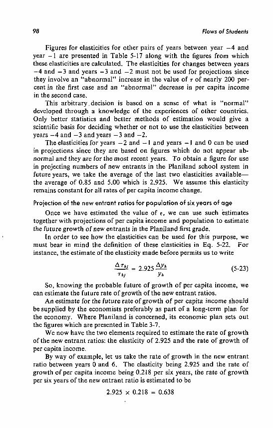
98 Flows of Students
Figures for elasticities for other pairs of years between year - 4 and year - 1 are presented in Table 5-17 along with the figures from which these elasticities are calculated. The elasticities for changes between years - 4 and - 3 and years - 3 and - 2 must not be used for projections since they involve an "abnormal" increase in the value of T of nearly 200 percent in the first case and an "abnormal" decrease in per capita income in the second case.
This arbitrary, decision is based on a sense of what is "normal" developed through a knowledge of the experiences of other countries. Only better statistics and better methods of estimation would give a scientific basis for deciding whether or not to use the elasticities between years - 4 and - 3 and years —3 and - 2 .
The elasticities for years - 2 and - 1 and years - 1 and 0 can be used in projections since they are based on figures which do not appear abnormal and they are for the most recent years. T o obtain a figure for use in projecting numbers of new entrants in the Planiland school system in future years, w e take the average of the last two elasticities available— the average of 0.85 and 5.00 which is 2.925. W e assume this elasticity remains constant for all rates of per capita income change.
Projection of the n e w entrant ratios for population of six years of age
Once w e have estimated the value of eT w e can use such estimates together with projections of per capita income and population to estimate the future growth of new entrants in the Planiland first grade.
In order to see h o w the elasticities can be used for this purpose, w e must bear in mind the definition of these elasticities in E q . 5-22. For instance, the estimate of the elasticity m a d e before permits us to write
^ I U = 2 . 9 2 5 ^ (5-23) Thj y/,
So, knowing the probable future of growth of per capita income, w e can estimate the future rate of growth of the new entrant ratios.
A n estimate for the future rate of growth of per capita income should be supplied by the economists preferably as part of a long-term plan for the economy. W h e r e Planiland is concerned, its economic plan sets out the figures which are presented in Table 3-7.
W e n o w have the two elements required to estimate the rate of growth of the new entrant ratios: the elasticity of 2.925 and the rate of growth of per capita income.
By way of example, let us take the rate of growth in the new entrant ratio between years 0 and 6. The elasticity being 2.925 and the rate of growth of per capita income being 0.218 per six years, the rate of growth per six years of the new entrant ratio is estimated to be
2.925 x 0.218 = 0.638

Flows of Students 99
The results of similar calculations for years 6 through 12 and 12 through 18 are given in Table 5-18.
Table 5-18. Estimation of the Rate of Growth of the New Entrants Ratio
Years
0-6 6-12
12-18
Elasticity
2.925 2.925 2.925
Rate of Growth of Per Capita
Income
0.218 0.220 0.218
Estimated Rate of Growth of N e w Entrants
Ratios
0.638 0.644 0.638
W e n o w use the results in Table 5-18 to estimate the future values of new entrant ratios. T h e rate of growth gives the increment in the new entrant ratio per unit of the ratio's values at the beginning of the period. For example, the rate of growth between year 0 and year 6 is estimated to be 0.638 which means that there will be an increment of 0.638 between year 0 and year 6 in respect to each unit of the new entrant ratio in year 0.
The initial value of the enrollment ratio in Table 5-19 is 0.3939, so that the total increment between years 0 and 6 will be
0.3939 x 0.638 = 0.2513
T o obtain the value of the new entrant ratio in year 6, w e must add the increment to the initial value, i.e.,
0.3939 + 0.2513 = 0.6452
The procedure must be repeated in order to obtain the projections for year 12, this time taking the new entrant ratio for year 6 as a starting point. The projected new entrant ratios for years 6 and 12 are shown in Table 5-19.
Table 5-19. Planiland: Projection of New Entrants Ratio for Six Years of Age
Year h
0 6
12 18
Ratio TA 6
0.3939 0.6452 1.0607
W e have previously observed that the diagonal sums of the new entrant ratios can never be greater than one, since the ratios represent the number of new entrants per person in an age level of the population and the number of new entrants must be equal to or less than the total in the age interval. For year 12, Table 5-19 shows the projected ratio to be 1.0607. T o avoid projecting an impossible value, w e must reduce the

700 Flows of Studenfs
projected ratio to 1.0000. This value is given to the ratio for year 12; w e assume that the ratio will maintain this value in years after 12. After having estimated the value of T A 6 for years 6, 12, and 18, it is possible to . obtain by interpolation the values for the ratios T A 6 for each year through 18. The results of the interpolation are presented in Table 5-20.
Table 5-20. Planiland: Values for Each Year Between 0 and 18 of the New Entrants Ratio for Six Years of Age
Year h
0 1 2 3 4 5 6
Ratio TA 6
0.3939 0.4278 0.4646 0.5056 0.5491 0.5963 0.6452
Year h
7 8 9
10 11 12
Ratio Th6
0.7010 0.7614 0.8270 0.8982 0.9756 1.000
Year h
13 14 15 16 17 18
Ratio T*6
1.000 1.000 1.000 1.000 1.000 1.000
Projection of the n e w entrant ratios for age levels above six years
W e have discussed the projection of future values of new entrant ratios for six-year-olds on the basis of the estimated future per capita income growth rate. W e n o w turn to the question of projections of new entrant ratios for higher age levels. W e will use as data for these projections the estimates of future n e w entrant ratios for six-year-olds which w e have calculated, and the year 0 ratios for higher age levels. M a k i n g use of the principle that diagonal sums cannot be greater than one, w e project the ratios for the higher age levels reducing their value if a diagonal sum otherwise would exceed one. T h e results are presented in Table 5-21.
If w e compare the ratios in Table 5-21 with those in Table 5-10, w e see the effect of the yearly increase in the value of new entrant ratios for six-year-olds. W h e n these were constant, all ratios for higher age level were likewise constant from year 3 onward. The growth of the ratio for age 6 brings about a progressive reduction in all the other ratios until the ratio for age 6 equals 1 and the ratios for other age levels equal 0. W h e n this point is reached, all children age 6 enter school and there are none left to be entrants at age 7 or more . F r o m this point on, the number of new entrants grows at the same rate as the six-year-old population.
Projections of n e w entrants in elementary school
Once the future values of the new entrant ratios are k n o w n , E q . 5-4 can be used to project numbers of new entrants in elementary school in future years. W e simply multiply the new entrant ratios which hold for various age levels in a given year by the number of children in the various age levels and add the figures thus obtained.

Flows
of S
iudents 101
3 ö
o e> q
ö —
' ö ö
ö ö
NO
oo LO
—
Q
Q
O
r-
o O
Q
Q
o
\. —
o
o o
ö ö
ö ö
ö
N
n ö
o g
OO (N
O
O
¿5
o ö
ö o
ö —
• O
s O
N
Q
O
VO
O
N rO
Q
Q
P-
<N
O
O
O
O
Ö
Ö
Ö
Ö
<N
ON O
»n
Tt N
O o
o t
- rtO
O
NO
m
—; O
O
O
Ö
Ö
Ö
Ö
«
ON
m
<n r*ï
(S Ö
O
d o
ö ö
ö vo
O
N m
in in
rj- r-
ON
Q
O
—
«n
(N
Q
•n ffj
N q
q d
o d
o o
NO
O
N r—
o
•*
r —
' «n
Q
NO —
• NO
5 Q
f
m
oí o
o Ö
O
Ö
Ö
Ö
00
ON
r- N
O
p-
r —
« oo o
(N
-H \0
ON
¿S
t
n N
q
q O
O
Ö
Ö
O
ON
O
N r-
NO
O
N
ró -t
-.
- h
-O
N
-H
NO
O
O
(N
en m
N
-_
-Ö
Ö
Ö
Ö
O
Tf O
N p
- N
O
ON
oo
r —
« —
r-p-
—
NO
oo es
m
m
oJ —
~
-ö
ö ö
ö d
00
ON
P-
NO
O
N
fS
—<
NO
O
O
CN
n ro
N
- -
ö S
d
G <ó
s 00 NO
*íf _
— Tf NO OO
Tf TT OO ON ,
<N rn (N —; —
O
O
O
O* O
ÍN
ON »n
p- m
^
oo (N
•*
(N
oo (N
«n
r r-
q n
n
N -
©
O
O
O
O
to
tü «-3 i:
o ti
3 3¡ 'S
£
^ <
Oo
tf I.
tu ,«)
<5
>«,
-O
5
New Entrants Year New Entrants Year New Entrants Year
TÍ
— oo in
NO
^_
ON m* NO
O NO —"
NO P- P- OO OO ON
m
Tt in
NO
p- oo
P-.
m •*
—
: o,
^
P*- v\ ON
^" ON
NO NO
vo *o r-
NO
p- OO
ON
O
~- <N
Co* oo
rn —- p oo p^
ON" ON" (N
ON O "•*
ON
m m
Tf Tj-
to in >n
O
^ N fl f
l
^O
1,077.9 1,010.7 895.7
1
NO
P
- 0O
O
N
O

102 Flows of Students
The totals of new entrants in years 0 to 18 and in structures 6, 12, and 18, appear in Table 5-22.
Projection of graduates, dropouts, repeaters, and
deaths in elementary school
In Sec. 5-4.2 w e used equations of the forms
S] = n) + r\ - b) - d)x [4-12]
SI = g) + a\ + r¡+6 + dV [4-13] b) = ß\n) + r)) with ßl = 0.385 (5-24)
</," = ô"(n) + r)) with ó" = 0.007 (5-25)
a] = a1 S] with a' = 0.376 (5-26)
r)+k = plSl, ' with pl = 0.253 (5-27)
d]x = Ô2[S] with Ô21 = 0.011 (5-28)
Since w e were considering only the influence of population changes on student flows, it was assumed that the parameters /?', ô", p \ ô21 were constant. W h e n w e take into account effects of per capita income growth, w e must consider changes in the values of these parameters resulting from income changes. O n the following pages, w e will first project the values of the parameters for years 6, 12, and 18. Then these values will be used in Eqs. 5-24 through 5-28 to calculate the values of the variables for structures 6, 12, and 18.
Projection of the values of the parameters
The parameters ô" and 521 relating to deaths change relatively little from structure to structure, as can be seen in Table 5-4. In addition, such changes as do occur in these ratios do not seem to be meaningfully related to change in per capita income. W e will therefore assume that these ratios for future structures will not change with changes in income. In projecting future student flows the values used for 5" and ô21 will be those given in Eqs. 5-6 and 5-9.
For the projection of the values of the other three parameters, elasticities must be calculated and used. Calculations of elasticities of a 1 , ß l , and p1 with respect to per capita income are shown in Table 5-23.
The use of elasticities for the projection of the six-year-olds new entrant ratio is explained in detail above. The procedure is the same for the projection of the parameters a1, ß l , and />'. For instance, let us project the value for structure 0 of the parameter a. T h e elasticity of this parameter with respect to per capita income is -0 .489 (Table 5-23).
T h e first step is to multiply the elasticity by 0.203, the rate of growth per six years of per capita income from pivotal year —6 to pivotal year 0; that is,
-0 .489 x 0.203 = -0.099

Flows of Students 103
The figure -0 .099 represents the six-year rate of growth of the value of the parameter a1. Since this is a negative figure, w e know that the value of a[ is projected to decline by 9.9% from structure —6 to structure 0.
Table 5-23. Elasticities for the Parameters in the Equations Referring to Elementary School Level
Pivotal Years
Past Values (Table 5-4)
Rate of Growth of
the Parameters («)
Per Capita Income
Rate of Growth of Per Capita
Income (6)
Elasticities a b
Elasticity for Dropouts Before Pivotal Year, ß
- 6 0
0.388 0.385
-0 .008 2,783 3,349
0.203 -0 .039
Elasticity for Dropouts After Pivotal Year, a
- 1 2 - 6
0.419 0.376
-0 .103 2,299 2,783
0.210 -0 .489
Elasticity for Repeaters, p
- 1 2 - 6
0.297 0.253
-0 .148 2,299 2,783
0.210 - 0 . 7 0 5
Since the value of a' for structure - 6 is 0.376, the value of a1 for structure 0 is
0.376 + (0.376X-0.099) = 0.339
The future values of the other parameters are estimated in the same way and are shown in Table 5-24.
With the values for the parameters of Eqs. 5-24 to 5-28 presented in Table 5-24, w e can proceed to the estimation of the values of the variables in these equations.
Table 5-24. Planiland: Projected Values of the Parameters a ', 0 ', 5 ", á21, and p '
Parameter
Dropouts before pivotal year, ß l
Deaths before pivotal year, S11
Dropouts after pivotal year, a
Repeaters, p Deaths after pivotal
year, Ô21
0
0.339 0.217
0.011
Year
6
0.382
0.007
0.303 0.184
0.011.
12
0.379
0.007
0.270 0.156
0.011
18
0.376
0.007
0.242 0.132
0.011

704 Flows of Students
In Sec. 5-4.2, three basic sets of figures were used to prepare projections of student flows at the elementary school level taking population growth alone into account: (1) information on the pivotal year 0; (2) projections of new entrants in elementary school; and (3) values of the parameters for the elementary school level.
The same elements are required in order to project future student flows when taking both population and per capita income changes into account.
The method has already been explained in the above-mentioned section. W e begin by estimating the values of the variables in relationship 4-13 for year 0. W e first use Eqs. 5-26 to 5-28 and the parameter values of Table 5-24 to estimate the values for dropouts (a¿) during and after the pivotal year, repeaters (/¿) passing to the next structure and deaths (d2}) during and after the pivotal year. The results appear in Table 5-25.
Once these three values have been obtained, the number of graduates m a y be established by using the actual figure for student enrollment in year 0 and Eq . 4-13.
Having computed the values of the variables for relationship 4-13 for structure 0, we can proceed to estimate values for the variables in relationship 4-12 for structure 6. N e w entrants have already been estimated and, with this value together with that for repeaters coming from structure 0, the value of total inputs can be calculated.
W e can use this value, the estimated values of parameters from Table 5-24 and Eqs. 5-24 and 5-25 to estimate the number of dropouts and deaths prior to pivotal year 6.
W e are n o w in a position to use relationship 4-12 to calculate total enrollment in pivotal year 6.
At this point, we have the same information with respect to structure 6 as w e had previously with respect to structure 0. By using the approach sketched above, w e can obtain estimates for the variables in relationship 4-13 for structure 6. These enable us to compute the values for relationship 4-12 for structure 12, and so on. The results of such calculations are shown in Table 5-25.
Projection of student flows at high school and college levels
For this projection the following steps are required: (a) Equations 5-10 through 5-15 for high school and 5-16 through
5-20 for college should be written, using in place of the constant indices the parameters a\ ß ' , ô", ô2', p', and T¡ with i = 2 for high school and í = 3 for college. The parameter T' will be used in equations of the form corresponding to Eqs. 5-10 and 5-16.
n\ = r'g'zi i = 2,3 (5-29)

Flows of S
tud
ents
705
After Pivotal Year, Relationship 4-13 h Graduates VI
<D
cd
+
D. v.
1) Dropouts
Total Enrollment,
Pivotal Year
sl
Before Pivotal Year, Relationship 4-12
CA
Q Dropouts
bl Repeaters
rl
New Entrants
nl Year
<n o\ vo
vo vo r-
o ^q
CO Tf 0\
»n — oo
cN fi m
n
(N co
ON
u-i r-'
OJ —
O
O
00 ON
tN ON NO"
O
00 OO
(N —
—
oq
m en
NO
iri \¿ - -'
ON
<N ON
m
w-i vo »o r-
(N ON n">
r-'
r- od
391.5 426.7 445.8
m tN co
o\ vi r*
<N —' O
895.7 1,010.7 1,077.9
O
NO <N 0O

706 Flows of Students
Table 5-26. Elasticities for the Parameters in the Equations Referring to High School and College Levels
HIGH SCHOOL
Pivotal Years
Past Values
Rate of Growth of
the Parameter a
Per Capita Income
Rate of Growth of Per Capita
Income b
Elasticities a b
Elasticity for N e w Entrants
- 6 0
0.642 0.579 -0 .109
2,783 3,349 0.203 -0 .537
Elasticity for Dropouts before Pivotal Year, ß 2
- 6 0
0.303 0.251
• -0 .172 2,783 3,349 0.203 -• -0.847
Elasticity for Dropouts after Pivotal Year, a
- 1 2 - 6
0.318 0.323 0.016 2,299
2,783 0.210 0.075
Elasticity for Repeaters, p 2
- 1 2 - 6
0.208 0.160
-0.231 2,299 2,783
0.210 -1 .100
COLLEGE
Pivotal Years
Past Values (Table 7-4)
Rate of Growth of
the Parameter a
Per Capita Income
Rate of Growth of Per Capita
Income b
Elasticities a
b
Elasticity for N e w Entrants
- 6 0
0.694 0.637
-0 .089 2,783 3,349
0.203 -0 .438
Elasticity for Dropouts before Pivotal Year, ß
- 6 0
0.366 0.326
-0 .109 2,783 3,349
0.203 -0 .537
Elasticity for Dropouts after Pivotal Year, a
- 1 2 - 6
0.378 0.490 0.296
2,299 2,783
0.210 1.404
Elasticity for Repeaters, p
- 1 2 - 6
0.135 0.137
0.016 2,299 2,783
0.210 0.074

Flows of Students 107
(b) Estimates should be m a d e of the elasticities with respect to per capita income changes of the parameters n a m e d in step (a). The values of these and the figures of which they are based are presented in Table 5-26.
'(c) Using the elasticities, w e should estimate the rates of growth of the parameters and the future values of the parameters themselves. These values are given in Table 5-27.
A n analysis of these values suggests that they are reasonable for high school, but not for college. In this level proportion a3 of dropouts after the pivotal year is larger than one, which would indicate that the number of dropouts is larger than the number of students enrolled. Since this is obviously absurd, a3 cannot be used.
(d) With the projected values of the parameters, Eqs. 4-12, 4-13 and 5-10 through 5-21, and the modifications introduced because of the unacceptable value of a3, the values of the variables refering to students flows can be obtained.
T h e modifications used to accommodate the rapid increase in college dropouts at the expense of graduates are as follows. Values for the n u m bers of repeaters and deaths are estimated using Eqs. 5-19 and 5-20 with the projected values for p3 and 623. T h e number of college graduates from structures 6 and 12 is assumed to be zero. Then , it is possible to estimate the n u m b e r of dropouts, using E q . 4-13 for the college level. T h e results for high school and college are shown in Table 5-28.
T h e assumption that there will be no graduates from structures 6 and 12, despite its being consistent with the trends observed in the past, is obviously unrealistic. In reality, before reaching this point, the parameter
Table 5-27. Planiland: Projected Values of the Parameters a, ß',5u, 521, p', and r'
Parameter YearO Year 6 Year 12 Year 18
High School/" = 2
N e w entrants, T Dropouts before pivotal year, ß Deaths before pivotal year, 5 Dropouts after pivotal year, a Repeaters, p Deaths after pivotal year, 8
0.328 0.124 0.020
0.642 0.205 0.014 0.333 0.094 0.0201
0.642 0.167 0.014 0.338 0.071 0.020
0.642 0.136 0.014 0.343 0.054 0.020
College í = 3
N e w entrants, T Dropouts before pivotal year, ß Deaths before pivotal year, 5 Dropouts after pivotal year, a Repeaters, p Deaths after pivotal year, 5
0.630 0.139 0.020
0.694 0.288 0.015 0.822 0.141 0.020
0.694 0.254 0.015 1.075 0.143 0.020
0.694 0.224 0.015
0.145 0.020

708 Flow
s o
f S
tudents
i «1
-s: bo c c
U <u
&o s>
~^ •^
c o
a 3
°J => "S
Si -s:
* .oo g
•S g
Er"5
3 c
] oo
After Pivotal Year, Relationship 4-13 h Graduates g\
Repeaters r't+6
Dropouts
Total Enrollment, Pivotal Year
Before Pivotal Year, Relationship 4-12
Q Dropouts Repeaters New
Entrants Year
CN
||
O
O
JZ u
C/3
S2 OO
ï
-3;
^t
VO
m
VO
OO
VO
CN
CN
O
Ov
VO
O
r-t
CN
rn
in
r-00
CN
en
«n -vO
m -
Tt
CN
r^
•n
ro
vq
od
vo
»n
vO
VO «n
rn
Tj-© o
in
cN
^
as <n
00
»n
r-—
p
rn
oq
in
m
CO
<N
OO
^ o <N
CN CO
<N
fN
CN
r-;
ro
r^
»n
m
in
CN
r-
oí
-
CN
OO
m II
-—
a, Ü
"5
O
(N
Ö
CT\
r"i
«5
•n
C\
00
o
TJ- CO
Ö Ö
O
O
ö ö
^o r-;
CN in
in P-;
in r-î
<n CN
od d
—
TJ-
TÍ OO
d d
vo Ov
r- rn
CN vq
— CN
ro p-i
in cN
CN »n
VO CN
#
r-
>n
—
Os
vO
r-;
in
r»
Ov
VO
OO

Flows of Students J 09
a 3 will become constant, or will begin reducing its value. Unfortunately there is no statistical data relevant to this question. Only with such information could a more realistic projection of the students flows in college be m a d e .
In s u m m a r y , projections of student flows are identical in form regardless of whether income changes are considered. W h e r e population growth is the only influence taken into account, the parameters used in calculations are constant.
W h e n the influence of per capita income is added, the parameters used are assumed to vary with changes in per capita income. These changing values for the parameters can be calculated using past elasticities of the parameters with respect to per capita income.
References
A more detailed analysis of the factors influencing student flows is given in Correa, H . , The Economics of Human Resources. Amsterdam: North Holland
Publishing C o . , 1963, Chapter 7.
A computerized application of the previous model is presented in Correa, H . , and E . Reimer, A Simulation Model for Educational Planning in
Puerto Rico. San Juan: Department of Public Instruction (Mimeographed), 1969.
Another mathematical model for the study of the educational system is given in Stone, R . , " A Model of the Educational System," Minerva, Winter 1965.

chapter O
The Educational Structure
of the Population
6-1 Conteni of This Chapter
In this chapter w e introduce the methods to forecast the educational structure of the population. These methods actually are simpler than those used to study the future development of the flows of students. T h e reason for this is that, excluding emigration, the only determinants of changes in the educational structure of the population are the output of the educational system and deaths. In fact, the basic accounting equation is the following: Present number of persons with, for example, a college education, plus the output from college, minus deaths equal the future number of. persons in the same category of education.
The elements that should be included in the output of the educational system were mentioned in Sec. 4-4. T h e forecasts of flows of students provide the main data required to evaluate these outputs. T h e only thing that remains is the detailed accounting work.
6-2 Method to Be Used
In Sec. 2-2.3, data on the distribution of the population by level of education were presented. W e call this distribution the educational structure of the population. O u r purpose in this chapter is to study the changes in time of that educational structure. T h e principle involved is quite simple: Take the structure in any given year, add to it the output of the educational system during a related period; subtract the number of deaths during that period; the result will be the educational structure at the end ofthat period. This can be expressed in formulas. Let
Pe't = number of persons other than students with educational level / in year t
O't = output of the educational system of persons of level / = 1,2,3 between pivotal years / - 6 and /
no

The Educational Structure of the Population 7 ? ?
The interpretation of the above statement is as follows:
/ V , + 6 = Pe\ + 0',+6 - deaths (6-1)
Let us study in more detail Eq. 6-1. In Chapter 2, all persons w h o had received any elementary schooling at all were considered part of the population with some elementary education. Similarly, figures for those with some high school or college education include all those w h o have received education of the relevant level whether for one day or through graduation. This means that the output Eqs. 4-14 and 4-15 will be reduced to
0 ; + 6 = g', + a) + b',+6 - n\X\ i = 1 and 2 (6-2)
and
(9?+6 = g) + a] + b)+(l (6-3)
For instance, for the period between - 1 2 and - 6 , the output of elementary school, according to the data in Table 5-3 is
0-6 = gin + a-12 + 6-6 - nif,
= 84.4 + 129.4 + 269.4 - 54.2
= 429.0
It is easy to see that Eq . 6-2 above is a particular case of the general output equation
0)+k = gi + (1 - yl)a] + (1 - TJ' )¿! + * + y2a2 + V2b2*i¿ - n2, + k
In E q . 6-2, ij', r¡2, y \ and y2 equal zero because dropouts from a level are counted as output from that level.
A n y other treatment of dropouts that was deemed useful could be handled without difficulty. A n alternative treatment, for instance, would be to include only those having graduated from a particular level in the stratum corresponding to that level; e.g., the elementary educational stratum would include all graduates from that level plus all those w h o had received s o m e high school education but had dropped out before graduating. In this case, r¡' and y' in the general output equation would both have values of one.
T h e third element in E q . 6-1, i.e., "deaths," is more difficult to handle. There are two types of deaths that should be considered: first, those a m o n g the persons Pe', already included in the stratum at date /; second, deaths a m o n g persons 0',+6 in the output of a given level between year t and year / + 6. T o see w h y this second group has to be considered w e should remember that Pe1, represents the persons with educational level i at instant t, while 0', + 6 represents the output of education between / and t + 6. But some of those leaving school during this period die before date / + 6, so they should be subtracted from the total added to Pe', to obtain Pe',+6.
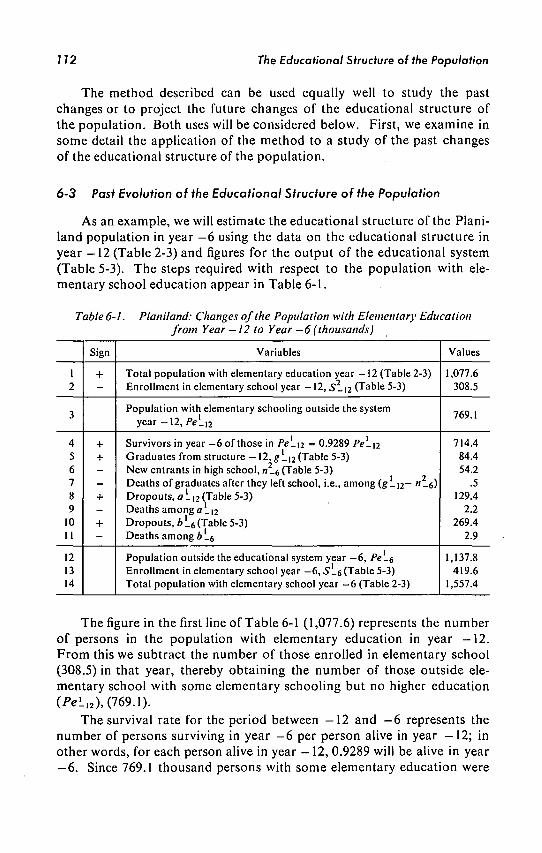
Ï72 The Educational Structure of the Population
The method described can be used equally well to study the past changes or to project the future changes of the educational structure of the population. Both uses will be considered below. First, w e examine in some detail the application of the method to a study of the past changes of the educational structure of the population.
6-3 Past Evolution of the Educational Structure of the Population
A s an example, w e will estimate the educational structure of the Plani-land population in year - 6 using the data on the educational structure in year - 1 2 (Table 2-3) and figures for the output of the educational system (Table 5-3). T h e steps required with respect to the population with elementary school education appear in Table 6-1.
Table 6-1. Planiland: Changes of the Population with Elementary Education from Year —12 to Year —6 (thousands)
1 2
3
4 5 6 7 8 9
10 11
12 13 14
Sign
+
1 +
1
+
1 l
+
+
Variables
Total population with elementary education year - 1 2 (Table 2-3) Enrollment in elementary school year —12, S -\2 (Table 5-3)
Population with elementary schooling outside the system year - 1 2 , />e!_i2
Survivors in year - 6 of those in Pe-n = 0.9289 Pe_\2 Graduates from structure — 12,g_|2(Table 5-3) N e w entrants in high school, n_6 (Table 5-3) Deaths of graduates after they left school, i.e., among (g_ l 2- n _6) Dropouts, o _ |2 (Table 5-3) Deaths amonga_i2 Dropouts, b !_6 (Table 5-3) Deaths among b _g
Population outside the educational system year - 6 , Pe_& Enrollment in elementary school year-6,5Î.6(Table 5-3) Total population with elementary school year - 6 (Table 2-3)
Values
1,077.6 308.5
769.1
714.4 84.4 54.2
.5 129.4
2.2 269.4
2.9
1,137.8 419.6
1,557.4
The figure in the first line of Table 6-1 (1,077.6) represents the number of persons in the population with elementary education in year —12. F r o m this w e subtract the number of those enrolled in elementary school (308.5) in that year, thereby obtaining the number of those outside elementary school with some elementary schooling but no higher education (Pel,,), (769.1).
The survival rate for the period between —12 and —6 represents the number of persons surviving in year - 6 per person alive in year - 1 2 ; in other words, for each person alive in year —12, 0.9289 will be alive in year - 6 . Since 769.1 thousand persons with some elementary education were

The Educational Structure of the Population 113
alive in year - 1 2 ,
769.1 thousand x .9289 = 714.4 thousand
will be alive in year - 6 . This number is shown in line 4 of Table 6-1. Let us consider n o w the output of the educational system. The total
number of graduates (f!_i2) and dropouts (a!_i2 and ¿ U ) must not be used without modification in estimating the number added to the elementary level stratum between years - 1 2 and —6. Several modifications must be introduced: First, not all graduates from elementary school leave the educational system; some of them enroll in high school and these must not be included in the net addition to the elementary level stratum of the population. This analysis explains why the number of new entrants in high school (54.2) is accompanied by a minus sign in line 6 of Table 6-1. Secondly, after leaving school between years - 1 2 and - 6 , some dropouts and graduates die.
Table 6-2 shows the method to estimate the number of deaths from year - 1 2 to year - 6 a m o n g dropouts (aLi2) and graduates (gin) after they leave school. In the first part of this table, figures for the total n u m ber of dropouts and graduates for each year from - 1 2 to - 7 are given. T o calculate the number of these persons leaving the school system w h o survive until year - 6 , w e use yearly survival rates (Table 2-6) as m a n y
Table 6-2. Planiland: Survivals A mong Dropouts and Graduates from Structure -12 After They Left School (units)
Elementary School
Graduates Dropouts
Year in Which the School Is Left
-12
12,342 62,224
-11
12,740 28,011
-10
13,736 24,766
-9
14,234 1,406
-8
13,834
-7
17,519
-6
Survivors in Year
-12
74,566
-11
74,268 40,751
-10
73,971 40,588 38,691
-9
73,675 40,426 38,536 27,000
-8
73,380 40,264 38,382 26,892 15,240
-7
73,086 40,103 38,228 26,784 15,179 17,519
-6
72,794 39,943 38,075 26,677 15,118 17,449
Total survivors year - 6 210,056
Total dropouts + graduates including deaths...' 213,767
N u m b e r of deaths 3,711

J14 The Educational Structure of the Population
times as there are years between the time of leaving the educational system and the next pivotal year. Thus with a yearly survival rate of 0.996, the number of those leaving the school system in - 1 2 as dropouts and graduates (74,566 from Table 6-2) w h o are still alive in year - 6 is
74,566 x 0.996 x 0.996 x 0.996 x 0.996 x 0.996 x 0.996
= 74,566 x (0.996)6 = 72,784
For those leaving in year - 8 , the number surviving in year - 6 is
15,240 x 0.996 x 0.996 = 15,240 x (0.996)2 = 15,118
The last column of Table 6-2 shows the survivors in year - 6 from a m o n g those leaving structure - 1 2 from year - 1 2 to year - 7 , the total being 210,056.
T h e total number of those leaving school in the six-year period, not taking into account subsequent deaths, is obtained by adding the number of those leaving each year:
74,566 + 40,751 + 38,691 + 27,000 + 15,240 + 17,519 = 213,767
The number of deaths m a y then be calculated:
213,767 - 210,056 = 3,711
Similar computations were m a d e for elementary school, high school and college levels for dropouts (b', and a',) and for graduates (g',) for all the years for which data were available. The results are shown in Table 6-3.
With the figures for the total number of dropouts and graduates and the number of deaths a m o n g them, it becomes possible to calculate the death rates for these groups. The values obtained for the death rates are shown in the last column of Table 6-3. With these rates the estimated number of deaths shown in Table 6-1 were computed.
W e have n o w analyzed all the figures shown in Table 6-1, together with the reasons for adding or subtracting them; the result of the indicated operations (1,137.8 thousand) appears in line 12. This figure represents those outside the educational system in year —6 w h o have received some elementary education but nothing more. In order to establish the total number in the elementary schooling strata, w e must add the figure for those attending elementary school in year —6 (419.6 thousand). Thereby w e obtain a figure of 1,557.4 thousand for the total number with only some elementary education in year —6.
The operations just described can be expressed in the following formula:

The Educational Structure of the Population 115
Table 6-3. Planiland: Total Number of Dropouts and Graduates and Number of Their Deaths After They Have Left the Educational System and Before the Next
Pivotal Year (thousands)
Leavers
Graduates (1)
Dropouts (2)
Totals (3)
Deaths* Before Next Pivotal Year
(4)
Rates
Column (3) Column (4)
Elementary School
F r o m structure - 1 2 during and after pivotal year
F r o m structure —6 before pivotal year
F r o m structure - 6 during and after pivotal year
F r o m structure 0 before pivotal year
84.4
151.0
129.4
269.4
157.8
378.3
213.8
269.4
308.8
378.3
3.7
2.9
5.0
3.9
0.017
0.011
0.016
0.010
High School
F r o m structure - 1 2 during and after pivotal year
F r o m structure - 6 before pivotal year
F r o m structure - 6 during and after pivotal year
F r o m structure 0 before pivotal year
11.1
20.1
7.8
18.0
13.1
23.6
18.9
18.0
33.2
23.6
0.5
0.3
0.89
0.4
0.027
0.017
0.027
0.017
College
F r o m structure - 1 2 during and after pivotal year
F r o m structure - 6 before pivotal year
F r o m structure - 6 during and after pivotal year
F r o m structure 0 before pivotal year
1.7
1.8
1.4
3.0
2.5
4.4
3.1
3.0
4.3
4.4
0.1
0.1
0.1
0.1
0.27
0.17
0.28
0.19
•There might be some difference between the values for the death rates and the values that can be computed with the figures for deaths appearing in this table. This difference is due to the rounding off of the figures in the table.
Pel6 = (1 - 0.0711) ¿>eL,2
+ (i - o.oi7)(¿rL12 - «2-6) + (1 - 0.017) ali2 + (1 - 0.011)6 L6 (6-4)
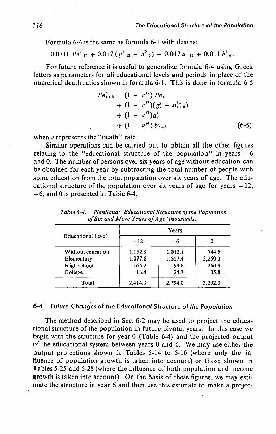
7 76 The Educational Structure of the Population
Formula 6-4 is the same as formula 6-1 with deaths:
0.0711 Pela + 0.017 (fL12 - nl6) + 0.017 ala + 0.011 ¿>L6.
For future reference it is useful to generalize formula 6-4 using Greek letters as parameters for all educational levels and periods in place of the numerical death ratios shown in formula 6-1. This is done in formula 6-5
Pe'l+6 = (1 - vn)Pe\
+ (1 - "'2)(¿fí - n'.Vt) + (1 - va)a', + (1 - rM)b',+t (6-5)
when v represents the "death" rate. Similar operations can be carried out to obtain all the other figures
relating to the "educational structure of the population" in years - 6 and 0. The number of persons over six years of age without education can be obtained for each year by subtracting the total number of people with some education from the total population over six years of age. The educational structure of the population over six years of age for years - 1 2 , - 6 , and 0 is presented in Table 6-4.
Table 6-4. Planiland: Educational Structure of the Population of Six and More Years of Age (thousands)
Educational Level
Without education Elementary High school College
Total
-12
1,152.8 1,077.6
165.2 18.4
2,414.0
Years
-6
1,012.1 1,557.4
199.8 24.7
2,794.0
0
744.5 2,250.3
260.9 35.8 .
3,292.0
6-4 Future Changes of the Educational Structure of the Population
T h e method described in Sec. 6-2 m a y be used to project the educational structure of the population in future pivotal years. In this case w e begin with the structure for year 0 (Table 6-4) and the projected output of the educational system between years 0 and 6. W e m a y use either the output projections shown in Tables 5-14 to 5-16 (where only the influence of population growth is taken into account) or those shown in Tables 5-25 and 5-28 (where the influence of both population and income growth is taken into account). O n the basis of these figures, w e m a y estimate the structure in year 6 and then use this estimate to m a k e a projec-

Table 6-5. Planiland: Projection of the Number of Persons with Some High School Education from Year 6 (thousands)
Total population six years and more, yearO
- Enrollment in pivotal year 0, Sn
Population outside the educational system year 0, Peo
Survivors in year 6 of population outside system
+ Graduates educational structure 0, go - Graduates entering college structure
year 6, tif, + Dropouts after pivotal year'O, an - Deaths of graduates and dropouts from
structure 0 after they left school, 2 , 2 3
i.e., go + flo - "6 + Dropouts from structure 6 before
pivotal year, b(, - Deaths a m o n g dropouts from structure
6 after they left school
Population outside the educational system year 6, Pe¿
+ Total enrollment in structure 6
Total population six year and more, year 6
Only Population Influences Considered (Tables 5-14 to 5-15)
260.9 - 69.0
191.9
179.6 + 34.5
- 23.9 + 22.0
- 0.9
+ 37.4
- 0.6
248.1 + 109.4
357.5
Population and Economic Growth
Influences Considered (Table 5-25, Table 5-28)
260.9 - 69.0
191.9
179.6 + 36.4
- 25.3 + 22.6
- 0.9
+ 35.7
- 0.6
247.5 + 136.1
383.6
Table 6-6. Planiland: Projections of the Educational Structure of the Population (thousands)
Educational Level 0 6
Years
12 18
Only the Influence of Population Growth Considered
Without education Elementary High school College
Total
744.6 2,250.8
260.9 35.7
3,292.0
701.9 2,809.8
357.5 57.0
3,926.2
659.4 3,470.4
438.6 91.7
4,660.1
633.3 4,219.5
528.7 126.1
5,507.7
Influence of Population and Income Growth Considered
Without education -Elementary
High school College
Total
744.6 2,250.8
260.9 35.7
3,292.0
631.6 2,852.6
383.6 58.4
3,926.0
509.5 3,530.6
513.1 106.9
4,660.1
467.3 4,202.5
667.3 170.5
5,507.6

778 The Educational Structure of the Population
tion of the structure to year 12, and so on. T h e process of projecting the n u m b e r of persons ¡n the'high school strata in year 6 is shown in Table 6-5; this table might well be studied in relation to the explanations given in Sec. 6-3.
Projections for the three levels for years 6, 12, and 18 are given in Table 6-6.
References
Correa, H . , " A Survey of Mathematical Models in Educational Planning," Mathematical Models in Educational Planning. Paris: O . E . C D . , 1967.
A computerized version of the model in this chapter appears in Correa, H . , and E . Reimer, A Simulation Model for Educational Planning in
Puerto Rico. San Juan: Department of Public Instruction (Mimeographed), 1969.

chapter
Manpower Needs
7-1 Content of This Chapter
In Chapter 3 it was observed that in order to increase production in an economy over the long run, the level of education of the economy's labor force must be raised. This is particularly true with respect to increases in labor productivity.
In the description of economic planning in the same chapter, w e noted that in order for a country to reach the targets of the economic plan, the labor force must have certain educational qualifications. The object of this chapter is to estimate the educational structure of Planiland's labor force required to achieve the targets of the economic plan.
The simple fundamental concepts involved in the method can be introduced with an example: Assume that in year 0 a production of 10 units is obtained by 20 workers with college education, and 30 with high school education. If the target of the plan is to produce 20 units in year 5, a first estimate of the number of workers required would be 40 with college education and 60 with high school education.
O n e of the limitations of this method is lack of attention to productivity changes. However, the method below considers the influence of productivity changes on the number of workers required and on their educational qualifications. Unfortunately, this is possible only through a somewhat m o r e elaborate approach.
In its general form the method used to forecast the educational structure of the labor force is similar to the one introduced in Chapter 5 to estimate the future development of the flows of students. The first step in Chapter 5 was to study the relationship observed in the past between on the one hand flows of students and on the other population and per capita income. The first step in this chapter is to study the relationship observed in the past between productivity of the labor force and its educational structure. W h e n this relationship is k n o w n , the targets of the economic plan will permit us to determine the educational structure required to attain these economic targets.
119

720 Manpower Needs
7-2 Past and Present Relationship between Educational Structure
of the Labor Force and Productivity
In the study of the relationship between the educational structure of the labor force, and productivity, it is possible to use two types of data: time-series and cross section. In the time series, the number of workers with different levels of education and the level of productivity in different time periods are considered. These data appear in Table 7-1 and-will be used in this book.
Table 7-1. Planiland: Educational Structure of the Labor Force and Gross Domestic Product
Labor Force (thousands)
Without education, L, With elementary education, L,
(between 0 and 6 years) With high school education, L,
(between 6 and 12 years) With college education, L,
(more than 12 years) Total labor force, L,
Gross domestic product, Y, (in millions of year 0 dollars)
Year
t 10
523
580
75
11 1,189
7,969
t = - 5
537
686
103
15 1,341
10,690
/ = 0
580
781
149
22 1,532
13,932
T h e second type of data consists of information about the education of the labor force and productivity similar to that presented in Table 7-1. However , in this case the data do not refer to different years but to different industries, regions of a country or different countries.
T h e method to be described below can be used equally well with time-series or cross-sectional data. In actual planning, it is convenient to use both types of information. However, it should be observed that it is easier to obtain cross-sectional than time-series data.
In order to study the relationship between the output of the educational system and the educational structure of the labor force, the same classifications should be used in both the analysis of the educational system and the educational structure of the labor force. In actual planning, an educational classification that should be taken into consideration is on-the-job training. In order to simplify this presentation, on-the-job training is not considered here. However, the methodology introduced in Chapter 4 for the analysis of the educational system and in this chapter for the study of the labor force can be adapted to the analysis of on-the-job training.
In the type of data mentioned above, the occupational distribution of

Manpower Needs 121
the labor force has not been taken into consideration since the purpose of this book does not require data on occupations. However, in actual planning, such data is required. This is so, because occupations are, while levels of education are not, natural subdivisions of the labor force in its relation to the economic process. F r o m the occupational classification of the labor force, information about managers can be obtained, and m a n agers are a crucial factor in economic development. F r o m the study of the quantitative and qualitative aspects of managerial roles, some of the important characteristics of the content of education can be observed. W h a t has been said with respect to managers is also true for other occupational classifications. The analysis of these can also provide information for an evaluation of the content of education. However, due to the influence of managers in the process of economic development, the managerial roles deserve special analysis.
7-2.1 Inverse Productivities
W e will find it convenient in this chapter to use instead of normal productivity figures, "inverse productivity" figures. Just as productivity figures m a y be obtained by dividing total production by the number of workers, so inverse productivity figures m a y be obtained by dividing the number of workers by the value of production. In considering the relationship between the educational structure of the labor force and productivity, w e will need to consider not only the inverse productivity of the total labor force but also the inverse productivities of the various educational strata in the labor force.
T h e following is the notation to be used. Let
L\ = number of workers with educational level /in year / / = 0 without education / = 1 with elementary education /' = 2 with high school education i = 3 with college education
L, = total number of workers Y, = gross domestic product in year t at constant prices
The inverse productivities (/', and /,) are defined
1',-Q f or /= 0 ,1 ,2 ,3 , (7-1)
and
'' - Y,
T h e inverse productivities for years - 1 0 , - 5 , and 0 m a y be calculated on the basis of the figures in Table 7-1. For example, in order to obtain the inverse productivity for that part of the labor force with no education in year - 1 0 , the number of workers in that strata in year - 1 0 (523 thou-
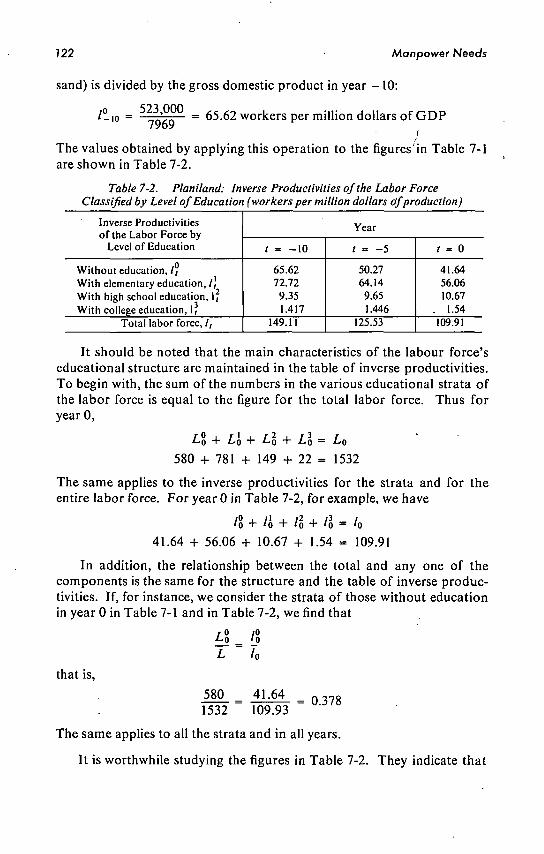
722 Manpower Needs
sand) is divided by the gross domestic product in year - 1 0 :
'-•o = nn¿n ~ 65.62 workers per million dollars of G D P 7969
i
T h e values obtained by applying this operation to the figures'in Table 7-1 are s h o w n in Table 7-2.
Table 7-2. Planiland: Inverse Productivities of the Labor Force Classified by Level of Education (workers per million dollars ófproduction)
Inverse Productivities of the Labor Force by
Level of Education
Without education, / , With elementary education, /, With high school education, 1, With college education, 1,
Total labor force, /,
Year
/ 10
65.62 72.72
9.35 1.417
149.11
/ 5
50.27 64.14 9.65 1.446
125.53
/ = 0
41.64 56.06 10.67
. 1.54 109.91
It should be noted that the main characteristics of the labour force's educational structure are maintained in the table of inverse productivities. T o begin with, the s u m of the numbers in the various educational strata of the labor force is equal to the figure for the total labor force. T h u s for year 0 ,
LQ + LQ + LQ + La = LQ
580 + 781 + 149 + 22 = 1532
The same applies to the inverse productivities for the strata and for the entire labor force. For year 0 in Table 7-2, for example, w e have
K + lh + ll + ll- /o 41.64 + 56.06 + 10.67 + 1.54 = 109.91
In addition, the relationship between the total and any one of the components is the s a m e for the structure and the table of inverse productivities. If, for instance, w e consider the strata of those without education in year 0 in Table 7-1 and in Table 7-2, w e find that
that is,
Io
_° / o
= 41.64 1532 109.93
L
580 0.378
T h e s a m e applies to all the strata and in all years.
It is worthwhile studying the figures in Table 7-2. They indicate that

Manpower Needs 123
Planiland experienced economic and welfare growth between years - 1 0 and 0, m a d e possible by increments in production per worker or (what amounts to the same thing) decreases in the number of workers per unit of output; i.e., decrease in the inverse productivity of the total labor force. T h e inverse productivity of the labor force as a whole dropped from 149 workers per million dollars of the G D P in year - 1 0 to 109 in year 0. This reduction was m a d e up of a reduction in the inverse productivities of workers with no education and those with only an elementary education and an increase in the inverse productivities of workers with high school or college education. These changes in inverse productivities indicate that over the years from year - 1 0 to year 0 fewer workers with low educational qualifications were employed per unit of output but more workers with high school and college education were employed per unit of final output.
7-2.2 Relationship between Educational Structure and Productivity
W e are interested in the relationships that hold between the educational structure of the labor force and its productivity. For this w e will use the following elasticities:
where /, and /', have the definition in Eq. 7-1, and
A / Í = l',+k - I1, A / , = / ,+* - /,
Since data on past educational structure in Planiland are available at five-year intervals, k will be 5 for Planiland.
A s in the case of the elasticities used in Chapter 5, the elasticity in E q . 7-2 is a quotient of two rates of growth. In the numerator appears
A/[ /{
that is, the rate of growth of the inverse productivity of labor with educational level /'; in the denominator appears A / , / / , , that is, the rate of growth of the inverse productivity of the total labor force.
Let us consider an example. Table 7-2 indicates that the inverse productivity of workers without education changed from 65.62 workers per million dollars of production in year - 1 0 to 50.27 workers per million dollars of production in year - 5 . This means the rate of growth of

724 Manpower Needs
inverse productivity was
Io Io Io
'-10 _ ' - 5 — '-10 Io
'-10 / ° ,
50.27 - 65.62 65.62
-0 .2339
Making similar calculations for all the educational strata for periods - 1 0 to - 5 and -5 to 0, w e obtain the rates of growth shown in Table 7-3.
Table 7-3. Planiland: Rate of Growth of the Inverse Productivities of the Educational Strata of the Labor Force
/', - / ' , - s
/¡-5
/
0 1
2
3
Educational Strata
Without education With elementary education
(from 0 to 6 years) With high school education
(from 6 to 12 years) With college education
(more than 12 years) Total labor force
Rates of Growth
Between Year —10 and Year - 5
-0.2339
-0.110
0.0321
0.0205 -0.1581
Between Year —5 and YearO
-0.1717
-0.1260
0.1057
0.0650 -0.1243
Let us n o w take the case of the stratum of workers with no education and see h o w the elasticities are computed. Table 7-3 shows that the rate of growth of inverse productivity for this stratum between years —10 and - 5 is -0 .2339. The rate of growth of the inverse productivity of all labor for the same period is -0.1581. T h e formula used to obtain the elasticity is the rate of growth of inverse productivity of the educational stratum divided by the rate of growth of the inverse productivity of the total labor force. W e thus obtain a value for this elasticity of
—0.2339 _ | 4794 -0.1581
T h e elasticity formula enables us to calculate the figures for elasticity shown in Table 7-4, columns 2 and 3. In column 4 appear the averages of these values for the two periods.
It would perhaps be worthwhile to try to clarify the meaning of the elasticity figures at this point. Let us consider the elasticity between years - 5 and 0 for the stratum with elementary education which in Table 7-4 is shown to be equal to 1.0136. This means that a change of a unit in the inverse productivity of the total labor force will be accompanied by a change of 1.0136 units in the inverse productivity of the labor force with elementary education.

Manpower Needs 125
Table 7-4. Planiland: Elasticities of the Inverse Productivities of the Educational Strata of the Labor Force with Respect to the Inverse Productivities of the
Total Labor Force i
I
0 1
2
3
Labor Force
Without education With elementary education
(from 0 to 6 years) With high school education
(from 6 to 12 years) With college education
(more than 12 years)
Between - 1 0 and - 5
1.4794
0.7457
-0.2029
-0.1294
Elasticities
Between - 5 andO
1.3814
1.0136
-0.8505
-0.5231
Average
1.4304
0.8796
-0.5267
-0.3263
So far w e have computed the elasticities of the inverse productivities without considering possible interrelations a m o n g the elasticities. Such interrelations do in fact exist because the larger the proportion of workers in one educational stratum the smaller can be the proportion of workers in the other strata. A s a result of this interrelation, the elasticities must fulfill the following condition:
«/ o ^j_
+ el h Li í2 ' J- * 3
e' 77 + £' T, i (7-3)
That is, the weighted sum of the elasticities must be equal to one, the weight being the quotients Lb/L0.
With the data in Tables 7-1 and 7-4 w e can verify that the elasticities between years - 5 and 0 fulfill condition 7-3:
1.3814 537 1341
+ 1.0136 686 1341
- 0.8505 103 1341
0.5231 15 1341
= 1
However, it is easy to show that the average elasticities in Table 7-4 do not fulfill condition 7-3 with year 0 weights. W e have for the average elasticities the following situation:
1.4304 580 1532
+ 0.8796 781 1532
0.5267 149 1532
0.3263 22 1532
= 0.935
Therefore the average elasticities in Table 7-4 must be corrected. T o do so, w e will multiply them by a correction factor that will m a k e both sides of the equation equal to one. This factor will be denoted by * . Performing this multiplication, w e obtain
1.4304* 580 1532
+ 0 .8796* 781 1532
- 0 .5267* 149 1532
- 0 .3263* 22 1532
0 .935* = 1

726 M a n p o w e r Needs
F r o m this w e see that
0 . 9 3 5 ^
= 1 0.935
= 1.070
T h e average elasticities multiplied by the correction factor are presented (Table 7-5).
Table 7-5. Corrected Average Elasticities Year -10 to Year -0
Educational Strata Corrected Elasticities
Without education Elementary High school College
1.5302 0.9409
- 0 . 5 6 7 3 - 0 . 3 4 8 9
7-3 Estimation of the Educational Structure of the Labor Force Required to Achieve the Targets of the Economic Plan
T h e target values for future gross domestic product and labor force are given in the economic plan. T h e y are presented in Table 3-8 and are reproduced in Table 7-6. In the latter table, the target inverse productivities of the total labor force and the rate of growth of these inverse productivities also are given. These data and the elasticities in Table 7-5 will be used to estimate the educational structure of the labor force required to achieve the targets of the economic plan. T o m a k e these estimates, w e will assume that the elasticities remain constant.
Table 7-6. Planiland: Target Values for Gross Domestic Product, Labor Force, Inverse Productivities, and Their Rates of Growth
Year
0 5
10 15 20
GDP (millions
of dollars) y,
13,932 18,822 25,428 34,354 46 ,412
Labor Force
L,
1,531 1,763 2,049 2,387 2,764
Inverse Productivities
Values 1,
109.93 93.69 80.61 69.48 59.56
Rates of G r o w t h AI, II,
- 0 . 1 4 7 7 - 0 . 1 0 7 6 - 0 . 1 3 8 1 - 0 . 1 4 2 7
T h e m e t h o d to be used follows from the definition in E q . 7-2 of the elasticities of the inverse productivities. A n elasticity is the value of the rate of growth of the inverse productivity of a labor force educational stratum corresponding to a value of o n e unit of the rate of growth of the inverse productivity of the total labor force. In Table 7-5, for example ,

Manpower Needs 127
the elasticity for the labor force having a college education is -0 .3489 . This means that a value of one in the rate of growth of the inverse productivity of the total labor force corresponds to a value of -0 .3489 of the rate of growth of the inverse productivity of the labor force having a college education. Table 7-6 indicates that the value of the rate of growth of the inverse productivity of the total labor force is estimated to be -0 .1477 for the period between years 0 and 5. Hence the rate of growth of inverse productivity of the labor force with college education is estimated to be
-0 .3489 x - 0.1477 = 0.051
This is a single application of the following general formula for calculating future growth rates of inverse productivities of the individual strata.
^ - . 1 ^ (7-4)
This formula is used to calculate the other rates of growth for the period between year 0 and year 5 shown in Table 7-7.
Table 7-7. Rates of Growth of the Inverse Productivities of the Educational Strata of the Labor Force for the Period Between
Year 0 and Year 5
Educational Strata
Without education Elementary High school College
Elasticities (Tables 7-5)
1.5302 0.9409
-0.5633 -0.3489
Rates of Growth
-0 .226 -0.139
0.083 0.051
T h e projected rates of growth of the inverse productivities of the educational strata enable us to estimate the change in the inverse productivities over five years. T h e results of such estimation are presented in Table 7-8.
Table 7-8. Estimated Changes in the Inverse Productivities from Year 0 to Year 5 and Estimated Inverse Productivities in Year 5
Educational Strata
Without education
Elementary High school College
Rate of Growth
(Table 9-7)
-0.226 -0.139
0.083 0.051
Inverse Productivities
(Table 9-2)
41.64 56.06 10.67
1.54
Change in Inverse
Productivity between
Year 0 and 5
-9.410 -7.790
0.887 0.079
Inverse Productivity
(year 5)
32.230 48.270 11.557
1.619

728 Manpower Needs
Once the future inverse productivities have been estimated, it becomes possible to estimate the educational structure of the labor force required in year 5 to achieve the targets of the economic plan. For this purpose the following formula should be applied:
V, = V, Y, (7-5)
This formula is obtained from the definition of inverse productivity introduced in Eq. 7-1.
A s an example of the use of Eq. 7-5, let us estimate the number of workers with a high school education required by the economic plan in year 5:
L\ = l\Ys= 11.557 x 18,822
= 217.5 thousand
The other values in column 4 of Table 7-9 were obtained by applying the same method; they show the educational structure of the labor force required in year 5 to achieve the targets of the economic plan.
A n important point to be noted is that the sum of the number of workers in the various educational strata as shown in Table 7-9 is equal to the total labor force in Table 7-6 which w e used as a starting point. This is a necessary consequence of using the corrected elasticities from Table 7-5.
The next step consists of estimating the educational structure of the labor force in year 10. It might seem reasonable to utilize the elasticities from Table 7-5 and apply the same method as was used going from year 0 to year 5. Unfortunately, the elasticities in Table 7-5 cannot be used as such for the period between years 5 and 10, for the elasticities in the table refer to the educational structure in year 0, which is not the same as the educational structure in year 5. Hence, we must first adapt the elasticities in Table 7-5 to the educational structure of the labor farce in year 5.
The method is the same as that used for adapting the average elasticities of Table 7-4 to the educational structure in year 0. First the weighted sum
Table 7-9. Planiland: Educational Structure of the Labor Force in Year 5
Educational Strata
Without education
Elementary High school College
Total
Inverse Productivities (Table 9-8)
32.230 48.270 11.560
1.619
GDP Year 5
(millions of dollars)
18,822
N u m b e r of Workers in Each Interval
of the Educational Strata (thousands)
607.0 909.0 217.5
30.0
1,763.5

Manpower Needs 129
1.5302 -^L- + 0.9409 - | § 2 - . 1763.5 1763.5
- ° - 5 6 3 3 TizÄ - ° 3 4 8 9 T^TT - ° - 9 3 6
is obtained. With this sum w e can then calculate the correction factor
X = — 1 — = 1.068 0.936
Using this correction factor, w e can obtain the corrected elasticities given in Table 7-10.
With these corrected elasticities, it becomes possible to project the educational structure of the labor force from year 5 to year 10, the method being the same as that used in projecting the structure from year 0 to year 5.
Projection of the structure from year 10 to year 15 involves the same process—correction of elasticities which are then used to obtain the structure for year 15. This projection is then used to correct the elasticities needed to estimate the required educational structure of the labor force in year 20; and so on.
The corrected elasticities and the required educational structure of the labor force for years 0, 5, 10, 15, and 20 are given in Table 7-10.
7-4 Limitations of the Method Used in Estimating the Manpower Needs
W h a t are the limitations of this method? Like the strengths of the method, they lie in the nature of statistical data used. It is obviously desirable that our method should be based on actual observations but statistical data available do not exactly describe the phenomena in which w e are primarily interested. W e are concerned with the labor force required for production whereas w e have statistics only on the labour force being used.
T h e method does not take into account the problems of underemployment of labor since the statistical data show no distinction between those w h o are fully employed and those w h o are underemployed. If the general level of underemployment were reduced, fewer workers in certain strata might be required to reach the economic targets than our estimates indicate.
A detailed study of the utilization of qualified m a n p o w e r within a given country and comparisons of the educational structures of the labor forces in different countries would give some indication of the amount of underemployment in the country in question. There is, however, no method of solving the problem of underemployment in the projection of required educational structures of the labor force.
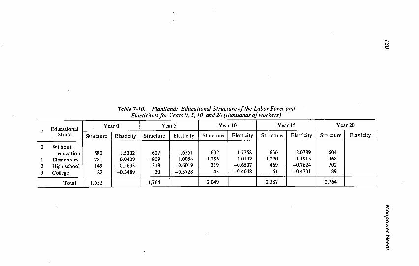
130
Ma
np
ow
er
Need
s
3
C
a
8^
£ b
•5"«
^>¡ a
-s:
go
¿
^ •2
o
c
-<j "o
C
ÏS
•a ^
's «s, Q
, .Si
SJ
•
m
u
tu
tü
UJ
o
00
r~
p
CN
m
o\
—
—
•*
(N
VO
P
-
Ö 1 —
m
P
-T
t
Ò 1
NO
©
ON
—
n
fs >o vo
VO <N
^1
OO (N
P- OO
m
O
N m
-rf p
- —
m
©
P
- ©
NO
Tf
— —
'• ©
ö
I I
CS in
O
N m
m
in —
Tt
vo
O
f»
—
Tt
ON
OO
»n
in —
(N
m
õ
©
p-
\o o
NO m
-
'-
òd
I
I
(N ON fl ON
© © r*1
OO
m Tt NO Tt
in ON in rn
-odd
I I
O — ON (N
OO OO
Tf M
in r- —
3 S
UJ
>.
a
2 c
ë Õ
o
J3
u
(A u
a)
•3
•t;
o
H
PH
! O
— (N m

Manpower Needs 737
7-5 Extensions of the Method Introduced in This Chapter
In the preparation of an educational plan integrated with an economic plan, it is likely that data m u c h more disaggregated than those introduced in the present section will be used.
T o begin with, the economic plan will provide information disaggregated by industrial sectors both for volume of production and for employment. With this data, it will be possible to observe the changes in the composition of national production and of the employment by the industrial sector. In addition, an economic plan is likely to be disaggregated by geographical regions.
The labor force will also be described in more detail than the one included in this chapter. For instance, the sex distribution of the labor force is one aspect that is usually considered in actual planning. Also, data about on the job training is likely to be included.
The important point that should be remembered is that the method described above for the estimation of the required educational structure of the labor force when only the level of education is considered needs no modification when being applied to more refined data.
T w o basic steps were involved in the method to estimate the educational structure of the labor force required for economic growth: First, the relationship in the past between educational structure and productivity was studied and some basic relationships, such as the elasticities, were established. Next, these elasticities and the production target of the economic plan were used to determine the required educational structure of the labor force for future years. Similar steps must be taken whenever it is necessary to estimate future needs for a specific type of manpower . First, w e note and quantify the past relationship between the number in the specific m a n p o w e r group and some other variable (such as total production or population). W e then estimate the future changes of the basic variable. By assuming that the past relationship between the basic variable and number in the m a n p o w e r group will be the same in the future, w e estimate the future need for the type of manpowe r in question.
Another example of this procedure is seen in Chapter 10 when the estimation of teachers needed to achieve the targets of the educational plan is presented. A further example is the estimation of the qualified persons required to fill government posts. Again the same steps described above can be applied to the female labor force in the textile industry. These examples show the main advantage of a mathematical model for planning: it can be widely applied.
In other cases, the method presented in this chapter requires s o m e modifications. W e can use at least two alternative approaches to estimate the number of doctors and other qualified persons in health services required in the future. O n e way is to relate the number of such persons to the need for them in terms of sickness. W e would say that to care for 100

732 Manpower Needs
persons in the population, the n u m b e r of doctors and nurses needed would be so m u c h . This coefficient permits us to find the n u m b e r of doctors and nurses required in the future. In the second approach, w e would recognize that the actual d e m a n d for medical services is related to per capita income. In this case, economists could estimate the relationship between d e m a n d for medical services and income. T h e estimated future changes in income will permit evaluation of the future need for doctors and nurses. T h e first approach would be m o r e useful w h e n medical care is provided as a social service, and the second w h e n it is obtained in the market for services. Appropriate mixtures of projection methods could also be used.
Detailed studies such as those described for teachers or doctors should be m a d e as part of the planning process. These specific studies would clarify and complement the aggregate estimates described in the previous sections of this chapter.
References
A n application of more sophisticated statistical techniques to the method of estimation of the elasticities of the inverse productivities is presented in
Correa, H . , "¿ H a prestado la Planificación Económica atención suficiente a la Education?" El Trimestre Económico, Mexico City, October-December 1964.
Other methods of estimating manpower needs are presented in Correa, H . , and J. Tinbergen, "Quantitative Adaptation of Education to Acceler
ated Growth," Kyklos, Vol. 15 (1962). "Econometric Models of Education." Paris: O . E . C D . , 1965.
A model for the estimation of manpower needs, when several economic sectors are considered, is presented in Correa, H . , The Economics of Human Resources. Amsterdam: North Holland
Publishing C o . , 1922, Chapter 14.
S o m e of the limitations in the use of statistical data for the estimation of m a n power needs are discussed in
Hollister, R . G . , "The Economics of Manpower Forecasting," International Labour Review, April 1964.
A complete, nonmathematical discussion of the estimation of manpower needs is presented in Parnés, H . S., "Forecasting Educational Needs for Economic and Social Develop
ment." Paris: O . E . C . D . , 1962.
Enlightening examples can be found in Folger, J. V . , "The Balance between Supply and D e m a n d for College Graduates,"
The Journal of Human Resources, Vol. 2, N o . 2, Spring 1967. Harbison, F., and C . Myers (eds.), Manpower and Education. N e w York: M c
Graw-Hill, 19653λ

chapter ö
Student Flows Required
for Economic Growth
8-1 Content of This Chapter
Having determined the future educational structure of the labor force required to ensure that economic growth targets are reached, w e n o w consider the problem of how the educational system should be adapted to produce the output required to achieve these educational structures.
In approaching this problem, it should be noted that the output of the educational system and the labor force are not equivalent. The output of the educational system is educated people, but not all educated people are members of the labor force. A s a consequence, the first step below is to determine the required educational structure of the population as a whole from which a labor force with the required educational structure can be drawn.
The data concerning the educational structure necessary in the population permit us to determine the required output of the educational system. This method follows from the one used to forecast the educational structure of the population in Chapter 6. T o the number of persons with, for example, college education in year 0, the output from college between years zero and five was added and the number of deaths subtracted. In the present case the number of persons with college education in years zero and five is k n o w n . The difference between the two figures corrected for deaths must be the output from college.
The final step is to evaluate the characteristics of the flows of students necessary to bring about the desired output of the educational system for the labor force and to provide enough entering students for higher educational levels. T h e relationship used in Chapter 6 between the flows of students and the output of the system is used below, but in the opposite direction.
133

134 Student Flows Required for Economic Growth
8-2 Educational Structure of the Population Required in Order to
Reach Economic Growth Targets
8-2.1 Statement of the Problem
Since the educational system produces educated people, some of w h o m do not become part of the labor force, the first essential is to calculate the future educational structure of the population as a whole from which the required labor force will emerge. For this purpose, w e have three sets of data concerning educational structures: the educational structures of the labor force in years prior to year 0; the educational structures of the population as a whole in years prior to year 0; and the required educational structures of the labor force in years after year 0.
8-2.2 Data Concerning the Labor Force
Data concerning the past and the required future educational structures of the labor force are set out in Table 8-1.
T h e estimates of requirements m a y vary according to the particular assumptions used to m a k e them. For this reason, educational planners must be carefully briefed by the economic planners w h o prepare the estimates of the educational structures required. Let us n o w review the characteristics of the data set out in Table 8-1, remembering that our remarks concern only these data.
Table 8-1. Planiland: Past and Required Future Educational Structures of the Labor Force (thousands)
Educational Level,
Without education
Elementary High school College
Total
Past Information (Table 2-4)
Years
-10
523 580
75 11
1,189
-5
537 686 103
15
1,341
0
580 781 149 22
1,532
Requirements According to Targets of Economic Plan
(Table 7-10)
Years
5
607 909 218
30
1,764
10
632 1,055
319 43
2,049
15
636 1,220
469 61
2,387
20
604 1,368
702 89
2,764
T o begin with, laborers are placed in the educational strata corresponding to the highest education level which they attained. (A student is considered to have "attained" an educational level upon entrance rather

Student Flows Required for Economic Growth 135
than upon graduation.) In addition, the Table 8-1 estimates reflect the Planiland situation in years - 10, - 5 , and 0 when there m a y have been an oversupply of certain types of labor with resulting underemployment for some types of manpower. The estimates would then show that still more such workers will be needed. A similar problem could arise in regard to past scarcities of certain types of skilled labor. Such considerations inevitably reduce the confidence which can be placed in the Table 8-1 figures.
Modifications of data required
Since our analysis of the output of an educational system has been in terms of six-year periods, it will be helpful to convert data and estimates on the educational structure of the labor force from five-year to six-year periods. This m a y be done most easily by interpolating or extrapolating (using rates of growth) from the five yearly figures in Table 8-1. The actual and the future required educational structures of the labor force for years - 1 2 , - 6 , 0, 6, 12, and 18 are presented in Table 8-2.
Table 8-2. Planiland: Educational Structure of the Labor Force, A dual and Future Required ( thousands)
Educational Level
Without education Elementary High school College
Total
Yeats
-12
515 542
66 10
1,133
-6
535 663
97 14
1,309
0
580 781 149 22
1,532
6
613.7 936.5 235.2
32.4
1.817.8
12
638.5 1,117.9
372.1 49.5
2,178.0
18
626.0 1,306.5
597.4 76.5
2,606.4
8-2.3 Educational Structure of the Population as Related
to that of the Labor Force
Table 2-3 set out the educational structure of the population for years - 1 2 , 6, and 0 and these data are reproduced in Table 8-3.
It should be noted that these data refer to the population age 6 and up rather than to the total population since only those age 6 and above can belong to the labor force. T h e data could be improved also in other directions; for instance, the working age begins around 14 or 15 so the population between 6 and 14 years of age, outside the educational system, should also be eliminated, but no data are available. W e must therefore rely on the information contained in Table 8-3.
The same table shows the number of those enrolled in the educational system in years - 1 2 , 6, and 0. Total population over six minus the n u m -

736 S
tud
en
t Flo
ws R
eq
uire
d fo
r Eco
no
mic
Gro
wth
ars u >-
o N
~
*0 | » -12 H
~
side itional tern
3 S
£a.
rolled c LU
Tota
Outside Educationa
System
P'e-6
led Enro
2 H
ide ional sm -12
Outs ducat
Systi
tt>
oiled L*
c UJ
"tf O
H
"rt tion -el
« f.
3 -J
•o a)
...
yo O
O
N O
O
Tt ui
—'
\¿
^ in
O
N
N
r-* \o^
—
oq O
O
s <n
o\
oo O
N ^O
*n
vo oq
O
N
r-# t
OQ
vi
r vi
NO
ro
[-- <N
^ <
N
<N*
—
oq ró
vq
<N
t-
O
N
ON
—
m
*o
—•
q ^ —
yq <
n -
•
ON
Ö
V*ï
—;
Tt
oq r-#
IN
r
o\
it «
"O
ON
(N
q
"o «
oq —
r-;
P-;
ri o
\ Ò
^
,
>n \o
Tt -H
—
^ p-
—
•n in
r>
oo* Tf
rn O
(N
m
oq vq
(S|
r
(N
r-- vi
od in
h vo
-—
;i O
—
.
t itior tary hoo
n F?
c o
u
Withoi educ
Eleme: Highs Colleg
O
—
<N
m
q
ON
(N
. co"
O t
ON
r-
tN
*
q ^
•'
^ (N"
5L7
o. tais o

Student Flows Required for Economic Growth 137
ber of students enrolled gives us the number of those in each educational stratum outside the system, i.e., Pe\ in the notation of Chapter 6. These figures must be compared with the numbers in the various educational strata of the labor force.
Certain problems arise when w e compare the number of those with a given level of education outside the educational system, as estimated in Table 8-3, and the figures for the educational structure of the labor force because some people are simultaneously students and workers. In a more elaborate study, data on the number of such working students would be required; but, in the present instance, it can only be assumed that the error introduced by ignoring this factor is not of great importance.
8-2.4 Comparison of the Educational Structures of the
Population and Labor Force
For this purpose, the most profitable index is the ratio between population outside the education system with a level of education and labor force with the same level of education. For instance, for the elementary education stratum in year —12 w e have
Pe^=J69A =
Lii2 542
This ratio tells us that for each worker with elementary education in year - 1 2 , there were 1.419 persons with that level of education in the population. A n equivalent statement is that for each 100 workers with some elementary schooling in year —12, there were 141.9 persons with that level of education in the population. The values of these ratios appear in Table 8-4.
8-2.5 Educational Structure of the Population Required to
Reach Economic Growth Targets
W e are n o w in a position to determine the educational structure of the population required in order to reach the economic growth targets; but before w e do so it would be well to review the actual concept involved.
Not all of the population exercises a direct influence on production: if all those w h o have retired, for instance, were to die, the production capacity would be in no way affected. W h y , then, must w e concern ourselves with the educational structure of the total population when dealing with economic growth targets? T h e reason is, of course, that the output of the educational system affects directly the educational structure of the population as a whole and not just the educational structure of the labor force.
In order to m a k e the transition from required labor force educational structures to required educational structures of the total population, the

738
Stu
de
nt F
low
s Re
qu
ired
for E
con
om
ic G
row
th
•2 S
CA Year
o
o 1
(N 1
~í?l--o
£l-J
Ut
ü
*í
S
£2 3
N
-'?
SI-E- 4"
i cd
o
&-S g a ¡2 o¿ í
Bu
C
i 1! «
o, H
t- ü
U
Sg
l*?-*
cd
D
3 c
¡5 x S
f*i_
i
O '5
O
W H
W
fc
O
u
w
^
•- 1
<Ü
a.
(N
-•* 1
-J
U
Ü
U
- N
•
.2
u
£¡ 2 S
ü * -° — '
p
w o
M
H
o*
o s
'•=
>
ca
a
Sí -J
%
tü -
Tj-
oo
CN
O
oo
»n
VO
3
r-<N
OO
v-1
w-t
<N
O^
OO
CN
CN
*o
*r\
00
CN
ion
3 o
o
a
J3
-O
.ti
u
O
o
oo
oo
—
0O
—
' —
C
N
(N
(N
—'
—
—
Ov
CN
O
O
TJ-
CN
ï—
—
O
C\ O
O
iX
—' V
O
W>
ON
C
N
VO
, —
vO
C
N
t-. 5
Tt
m
r* T
T
VO
0
\ ~
H
VO
oq rn
vo
t-
oÑ
oí
m
»n
—
"^
•"
C7
\ C
N
— m
r-
TT
—
T
f
—«
CN
-
^
CN
V
O
O
rr vo
—
W
-»
—. r-#
r-O
S
Ö
Tt
VO
Tj-
—<
r- —
>>
*3
M
O
5
J:
C
<->
4>
o
w
oo
Elem High Colle
H
M
m
• CN
m
»n
en
oo
3
CN
*
S
en.
00
od
CN
m
CN" !
rn
m
-*
m ,077.
<N
l/ï
13
—
o
H

Student Flows Required for Economic Growth 139
required number of workers in each stratum must be multiplied by the population labor force ratio for that stratum. Since the ratios for years - 1 2 and - 6 are not likely to be as relevant to the future as the ratios for year 0 w e will use these latter ratios in our projections.
Thus to calculate the number of college-educated people in the population required in year 6, w e multiply the number of workers with college education required in year - 6 by the population labor force ratio for the college stratum in year 0:
32.4 thousand x 1.218 = 39.5 thousand
In other words, only if Planiland in year 6 possesses 39,500 people with a college education will there be 32,400 people at that level in the labor force. Required values for the other levels and years are shown in Table 8-5.
Table 8-5. Planiland: Educational Structure of the Population Years 0,6,12,18 Required to Attain the Targets of Economic Development (thousands)
Educational Level
Without education Elementary High school College
Total
0
744.7 1,654.9
191.9 26.8
2,618.3
Years
6
788.0 1,984.4
302.9 39.5
3,114.8
12
819.8 2,368.8
479.3 60.3
3,728.2
18
803.8 2,768.5
769.5 93.2
4,435.0
8-3 Net Output Required from the Educational System to Attain the
Targets of the Economic Plan
8-3.1 Method to Be Used
The output of the educational system defined in Eqs. 4-14 and 4-15 includes persons w h o die shortly after they leave the educational system. W h e n these deaths are subtracted w e will speak of "net output." A precise definition is given below.
Formula 6-5 gave the relationship between population outside the educational system with a given level of education and the output of the educational system:
Pe'l+6 = (1 - va)Pe\ + (1 - Va)(g', - n',Ve)
+ (1 - ^ V i + 0 - vi4)b'l+e [6-5]
This formula will be used below as the starting point for estimates of the student flows required to attain the targets of the economic plan.

140 Siudeni Flows Required for Economic Growth
8-3.2 Estimation of the Required Net Output of the Educational System
The first step will be the estimation of
Pe'l + 6 - (1 - va) Pe',
This value will be called "required net output" of the educational system. The required values of Pe\ for years 6, 12 and 18 were presented in
the Table 8-5. The values of survival ratios (1 - v'2) should be provided by a demographer and are presented in Table 8-6. Figures for the required net output of the educational system in years 6, 12, and 18 are given in Table 8-7 along with the values from which these net output figures were calculated.
Table 8-6. Planiland: Projected Survival Ratios for Six- Year Periods
from Y ear Oto Y ear 18
Period Ratios
Year 0 to 6 Year6tq 12 Year 12 to 18
0.936 0.952 0.954
Table 8-7. Planiland: Estimation of Net Output Required from the Educational System to Attain the Targets of Economic Growth (thousands!
Fr
N u m b e r required in year t, Pe\
Survivals from numbers in / - 6
Required net output
N u m b e r required in year t.Pe)
-Survivals from numbers in ï - 6
Required net output
N u m b e r required in year t.Pe3,
-Survivals from numbers inf - 6
Required net output
t = 0 i = 6
o m Elementary School
1,654.9 1,984.4
1,549.0
435.4
From High School
191.9 302.9
179.6
123.3
From College
26.8 39.5
25.1
14.4
/ = 12
2,368.8
1,889.1
479.7
479.3
288.4
190.9
60.3
37.6
22.7
i= 18
2,768.5
2,259.8
508.7
769.5
457.2
312.3
93.2
57.5
35.7

Siudeni Flows Required for Economic Growth 141
8-3.3 Distribution of the Net Output Required A m o n g Net N u m b e r of
Graduates and Dropouts
F r o m E q . 6-3 we see that
Pe'l+6 - (1 - „")/»«{ = (1 - va)(*iîi) + (1 - v")a', + (l*/4)6i+6
In Table 8-7 we have the values of the left-hand side of this equation. N o w our problem is to distribute the total a m o n g the three components appearing on the right-hand side. T o do so w e will use information on the numbers of dropouts and graduates (net of deaths) in the past educational output. Such information appears in Table 8-8. It was prepared, but not
Table 8-8. Distribution of the Net Output of the Educational System Between Years —6 and0(thousands)
Line Nos. , Table
6-1
5 6 7
8
9
10
11
Graduates from educational structure - 6 -Graduates entering next level - Deaths among graduates after they left
school + Dropouts from structure - 6 during
and after pivotal year - 6 -Deaths among dropouts from structure
- 6 after they left school + Dropouts from structure 0 before
pivotal year -Deaths among dropouts from structure
0 after they left school
Total output from the educational system
Elementary School
151.00 -87.40
-1.02
+ 157.80
-2 .52
+ 378.30
-3 .90
592.26
High School
20.10 -12.80
- . 2 0
+ 13.10
- . 3 0
+23.60
- . 4 0
43.10
College
1.80 0.00
- . 0 5
+ 2.50
- . 0 7
+4.40
- . 1 0
8.48
presented, in the course of a study of the output of the educational system as it affected the educational structure of the population between years - 6 and 0 (Sec. 6-3). A s u m m a r y of the information is presented in Table 8-9.
The operations to be carried out at this stage are simple. Let us review the steps involved with reference to required elementary school graduates leaving the system between years 0 and 6. Table 8-7 shows that a net output from elementary school of 435,400 must be added to those with elementary education surviving from year 0 in order to reach the economic targets for year 6. Table 8-9 reveals that between years - 6 and 0 from an output of 592,260 only 62,580 are graduates, so that the rate of graduates to total net output is
- ^ ° _ _ 0.106 592,260

142 Sfudent Flows Required for Economic Growth
Table 8-9. Distribution of the Output Leaving the Educational System from Year -6 to Year 0 and A live in Year 0 (thousands)
Line Nos . , Table 8-8
5 , 6 , 7
8 ,9
10, 11
Components of Total Output
Graduates leaving the system between - 6 and 0 alive year 0 = (• - f )g-6 - n )
Dropouts between - 6 and 0 from structure - 6 alive year 0 = d - »'V-6
Dropouts between - 6 and 0 from structure 0 alive year 0 =
Total output
Elementary i - 1
62.58
155.28
374.40
592.26
High School 1 -2
7.1
. 12.8
23.2
43.1
College i = 3
1.75
2.43
4.3
8.48
If w e assume that this ratio can be used for years 0 to 6, w e can say
that 0.106 x 435,400 or 46,152 elementary school graduates leaving the
system (net of deaths) are required between years 0 and 6. A similar
computation with respect to all the other component elements and levels
gives the results shown in Table 8-10.
Table 8-10. Distribution of the Net Output Required from the Educational System Among Graduates and Dropouts (thousands)
Structure Year (1 - »") {gi-n, ) (1 - «'Vi (l--M)*i + 6
Total Pe'. + e-il-v'^Pe',
Elementary School i = 1
I =
t -
t =
/ =
-6 0 6
12
(actual) (required) (required) (re.quired)
62.58 46.1 50.7 53.7
155.28 114.1 125.8 133.4
374.40 275.2 303.2 321.6
592.26 435.4 479.7 508.7
High School ;' = 2
t= - 6 t= 0 « = 6 1= 12
(actual) (required) (required) (required)
7.1 20.4 31.5 51.6
12.8 36.4 56.4 92.2
23.2 66.5
103.0 168.5
43.1 123.2 190.9 312.3
College i = 3
t = - 6 i= 0 t= 6 / = 12
(actual) (required) (required) (required)
1.75 2.96 4.67 7.35
2.43 4.12 6.49.
10.21
4.3 7.32
11.54 18.14
8.48 14.4 22.7 35.7
Estimation of the required total number of graduates and dropouts
leaving the school system
W e have not yet obtained figures for the total number of graduates
and dropouts leaving the school system required by the economic growth

Siudenf Flows Required for Economic Growth 143
targets. Table 8-10 shows only figures on graduates and dropouts surviving to the next pivotal year. Our next step, therefore, is to use the required net output figures to establish required total output figures including subsequent deaths. W e know that adding the number of survivors in, for example, year 6 and the number of those w h o die between years 0 and 6 after leaving school will give us the number of those leaving school between years 0 and 6. W e must accordingly begin by estimating the n u m ber of deaths occurring before the next pivotal year a m o n g students leaving school. For this purpose w e make use of the death rates shown in the last column of Table 6-3.
Let us consider an example. In Table 8-10 for high school graduates in structure 0, w e see that
(1 - 0(S6
Table 6-3 shows us that
«6)
0.027
20.4
A s a consequence,
{gl - ni) = 20.4 = 20.97 (1 - 0.027)
The results of similar operations appear in Table 8-11.
Table 8-11. Distribution of the Output Required from the Educational System A mong Graduates and Dropouts (thousands)
Year t.
Il II
il
il
_
1
to
Ov
©
Ov
II II
II
II
—
1
to
Ov
O
Ov
r = - 6 / = 0 / = 6 / = 12
/ i +1 gi-n, + 6
Elerr
63.6 46.8 51.5 54.6
h
7.3 21.0 32.4 53.0
1.8 3.04 4.80 7.56
ai
entary School
157.8 116.0 127.8 135.6
igh School
13.1 37.4 58.0 94.8
College
2.5 4.24 6.67
10.50
bi + 6
378.3 278.1 306.4 324.9
23.6 67.7
104.8 171.4
4.4 7.46
11.76 18.49
Total
559.7 440.0 485.7 515.1
44.0 126.1 195.2 319.2
8.7 14.74 23.23 36.55

144 Sfudenf Flows Required for Economic Growth
8-4 Student Flows Required to Achieve the Targets of the Economic Plan
8-4.1 Method to Be Used
W e k n o w already that the basic instruments for the study of the student flows are Eqs. 4-12 and 4-13.
S', = n{ + r\ - b\ - d\' [4-12]
Si = g\ + a\ + r'l + 6 + dV [4-13]
where i = 1 elementary school i = 2 high school í = 3 college
A s w e have already seen, if w e can obtain values for four out of five variables in each equation, then w e can use the equations themselves to find values for the remaining variable in each equation.
In Table 8-11 the required values of two of these variables a\ and b',+6
are given for each of the three levels of the educational system. Likewise the required values g\ - n',+6 are given for the three levels. Since the graduates from college dò not enter any higher level of education, the values for g\ - n\%.\ given in Table 8-11 for the college level are also the values for g). Hence, w e have the values of three variables for college, namely g3, a], and b3 (two variables for Eq. 4-13 and one for E q . 4-12).
The conditions described suggest the following method for estimating the required values of all the variables in Eqs. 4-12 and 4-13 for all three levels. W e should begin with the student flows in college where w e already have values for three variables.
A method of estimating three variables for E q . 4-12 and two for Eq. 4-13 is still required. T o m a k e such estimates, Eqs. 5-18, 5-20, and 5-21, numbered below 8-1, 8-2, and 8-3 will be used, i.e.,
d\3 = ôl3(n3 + r3) (8-1)
r,+6 = P3S3 (8-2)
d]3 = ¿>23S3 (8-3)
where the parameters 513, ô23, and p3 will have the values observed in the past, presented in Table 5-4.
Equations 4-12, 4-13, 8-1, 8-2, and 8-3, and the values for g], a), and b) in Table 8-11 enable us to obtain the required values for all the variables in Eqs. 4-12 and 4-13 for the college level. A m o n g the values obtained is n). With this value and that oí g) - n]+6 in Table 8-11, w e can determine the required value of g2 . N o w w e have reached the position with respect to the high school level that w e were in with respect to the college level earlier. So, a method similar to the one used above will per-

Student Flows Required for Economic Growth 145
mit us to evaluate the student flows required for the high school level and will then put us in the position to study the required elementary level flows in the same way.
8-4.2 Required Student Flows at the College Level
Let us consider the problem of determining the required values for the variables in Eq . 4-13 for structure 12.
From Table 8-11 w e k n o w that
g\i = 7.56
a]2 = 10.50
In addition, with the value of 523 and p 3 from Table 5-4, Eqs. 8-2 and 8-3 take the form
rî, = 0.135 S]2 [8-2]
d2A = 0.020 S]2 [8-3]
Equation 4-13 can n o w be written in the following form for college level structure 12:
S]2 = 7.56 + 10.50 + 0.135 S]2 + 0.020 S]2
giving
(1 - 0.135 - 0.020)5,2 = 7.56 = 10.50
0.845 S\2 = 18.06
C3 18.06 S n = 0845
= 21.37
With the value of S]2 and Eqs. 8-2 and 8-3, w e can obtain the estimated "required" values for repeaters and deaths:
r]z = 0.135 x 21.37 = 2.88
dVi = 0.020 x 21.37 = 21.37 = 0.43
Similar methods can be applied to Eq. 4-13 for years 0 and 6. This must be done before estimating the values of the variables in Eq. 4-12. The required values in equation 4-13 in structures 0 and 6 appear in Table 8-12. Since in Table 8-11 the required values of g) and a) are not presented for years beyond year 12, it is not possible to solve by this method Eq. 4-13 for structures beyond structure 12.
Let us n o w examine the problem of estimating the required values of variables for relationship 4-12, considering again the case of structure 12.

146
Stu
den
t Flo
ws R
eq
uire
d fo
r Eco
no
mic
Gro
wth
(- «J
u
> Õ
CL. t-¿2
%
«
J=
rt
Q CA
rt 3
*a
rt t-i
o U Repea « 3
O
Drop
-r c rollme
Pivotal Year
c
LÜ
u
>
*rt O
>
a. u
k*
tS
4>
CQ
(A
JZ
eS
Q Cfl
3
O
CL
o
Um
Q CA
U
Ci Rep «
U
Um
Z£
ÜJ
u.
>
r- r-
—
<N
o
o
p
oo
rn
rf
\0
m
*~; °°.
<*
r»
(N
\0
Tf
\6
—
r-V
O
»n
od m
"
- -
<N
m
O
\o
^ r-' \o
0\
*~; o
(N
O
O m
-Ö
r-'
oo 2.8
o
»n
O
p-
oo
co
ro
—
t-
es
m
o
»n
v>
oo
O
Ö
vO
0\
P
TT
—
00*
m
oo
oo
oo
—'
ci
o
•*
oq
oq
—'
rn
m
in
(N O
O

Student Flows Required for Economic Growth 147
F r o m the left-hand side of Table 8-12, w e k n o w that
b]2 = 11.76
S]2 = 21.37
r\2 = 1.83
In addition, Eq. 8-1 above can be expressed as
d\\ = 0.015 (n]2 + r\2)
The values and equations given above permit us to state equation 4-12 as
21.37 = n\2 + 1.83 - 11.76 - 0.015 (n\2 + 1.83)
from which
21.37 = (1 - 0.015) n]2 + (1 - 0.015) 1.83 - 11.76
= 0.985 n]2 + 1.80 - 11.76
3 31.33 Wl2 = Õ 9 8 5
= 31.81
This value for n]2 enables us to establish the value for the number of deaths, as follows
d\\ = 0.015(31.81 + 1.83) = 0.50
These results and those obtained in a similar way for structure 6, are shown in Table 8-12. Lack of information about S) for t = 18, 2 4 , . . . prevents evaluation of E q . 4-12 for structures after 12.
It will be seen later that the value of n] in Eq. 4-12 for structure 18 is required for high school level estimates. For this reason, a method of estimating the required values of the variables in Eq. 4-12, valid only for structure 18 will be presented below. In this case the following equations will be used:
b\i = P3(AZI8 + r\s)
d\l= 513(^8 + r]s)
Sis = «18 + 18 — bit — d ig
W e have the following values resulting from previous calculations:
b]s = 18.43 (from Table 8-11)
r]s = 2.88 (from Table 8-12)
. p3 = 0.326 (from Table 5-4)
Ô 1 3 = 0.015 (from Table 5-4)

748 Student Flows Required for Economic Growth
With this information the values in Table 8-12 for structure 18 were obtained.
Another method of obtaining values for the variables in E q . 4-12 for structure 18 m a y also be noted although it will not be applied here. It involves using rates of growth to project values for g] and a] from structure 12 to structure 18. With these values for structure 18, it becomes possible to estimate the values of the other variables in relationship 4-13 for structure 18. Then the variables in relationship 4-12 for structure 18 can be estimated by the method used for structures 6 and 12. T h e sole reasons for not using this alternative solution here is that it yields a lower value for n\t than the method used above. T o avoid any possibility of setting our education targets too low, it would seem better to use the higher estimate.
8-4.3 Required Student Flows at High School Level
T h e first step in the estimation of the required student flows in high school is the following. With the data in Table 8-11 for required values for g] - «J+6 and the data in Table 8-12 on the required values of n], the required values of g) can be obtained. These values are given in Table 8-13.
With the information on required numbers of high school graduates set out in Table 8-13 and that on dropouts given in Table 8-11, w e are in the same position with respect to the high school level as w e were before with respect to the college level. W e m a y n o w use the procedure w e used for the college level to estimate required values for all the variables in relations 4-12 and 4-13 in structures 0, 6, and 12 at the high school level.
Table 8-13. Planiland: Number of High School Graduates Required for Economic Development (thousands)
Year
/ - 0 l = 6 t = 12
Required Outside the System, Year /
gi - n?+6 (Table 8-11)
21.0 32.4 53.0
Required as N e w Entrants in College,
Year l + 6 n}+6
(Table 8-12)
20.19 31.80 53.84
Total gl
41.19 64.20
106.84
For instance, to evaluate the variables in 4-13 for year 12, w e have the following system of equations:
g2l2 = 106.84 (Table 8-13)
a}2 = 94.8 (Table 8-11)
. /•?, = 0.160S?2withp = 0.160 (Table 5-4)

Student Flows Required for Economic Growth 149
d\\ = O m O S h with <522 = 0.020 (Table 5-4) \,
S2n = g2¡2 + «i2 + r2s + d\\
This system can be solved with exactly the same steps used for the i college level. The results for years 12, 6, and 0 appear in Table 8-14.
The next step is to estimate required values of the variables in relationship 4-12 for structures 6 and 12. T h e following values and equations are needed to estimate the required values of the variables in relation 4-12 for structure 12.
b2n = 104.8 (Table 8-11)
S\i = 245.90 (Table 8-14)
r22 = 23.80 (Table 8-14)
d\\ = 0.014(«22 + r2
2)withô12 = 0.014 (Table 5-4)
Sh = «?2 + r22 - b2
n = d}2
Solving this system of equations, and a similar one for year 6, w e * obtain the results presented in Table 8-14.
The final step consists of estimating the required values for the variables in relationship 4-12 for structure 18. In this case the equations needed are
b\t = 0.251 (nf, + /•?„)
d\¡ = 0.014(«28 + r2
iS)
S\s = ^18 + ''lS — ¿is — «18
The values obtained with these equations for the variables in relationship 4-12 for structure 18 are shown in Table 8-14.
A s in the case of relationship 4-12 for structure 18 at college level, there is an alternative method of estimation, identical to that outlined at the end of Sec. 8-4.3 for the college level. Since this alternative method i again gives lower values for the variables, w e do not use the results given by this method.
8-4.4 Required Student Flows in Elementary School
There is no need to repeat here the details of the method used. The ' results are set out in Table 8-15.
For estimating the required values for the variables in relation 4-12 for structure 18, w e again have a choice between two methods, the same as the two described in regard to college flows. This time, however, the second method yields the higher values for the variables; hence the values obtained by this method are given in Table 8-15. Such values for structure 18 are calculated in the following way: Rates of growth are used to estimateg2
{i - n\^, nl4, and a\%.

Siu
den
f Flo
ws R
eq
uire
d fo
r Eco
no
mic G
row
th
L.
a u
>-a o >
ester
< c a.
J "c b c u.
ear
>-"5 o
> ex 1—
«2 <
D
ffl
C/5
SZ
c3
û 4)
rt
3 *u
rt L
.
Ü w
"3 Repe E/l
2 O
a. Dro
„ 15
u-
O
u
cu un
J=
"c3 U
Q VI
3 'ropo
a C/l ter 03
U
Q.
C¿
M
£ S
U
L-
2 c
ÜÜ
IM
03
>
fN
°î a\
—
« •t m
rn
in
TT
P^
m
^ co in ov
O
30 ov fN
O
fN
Tt
VO
•r
co
q od
un
(N
q
aí •<
fr
p»
q
m'
P-;
vO
m
ro
•n
vO
Tf
fN
O
(N
vO
(N
Ov
t" * co
vO
O
rr rn
rn
CO
TT
ON
o
ON
"O
"3
-fN
O
vo
Ov
in
•*
aí
00
Tf
o
r-
— —
-oq
m
rn
O
N
(N
m
O
CÏ
CO
»
O
—"
ro
m
Tiro
vo
fN
OO
-s:
^ <-,
-53
"5 3
Ol
tu
s:
si a -s a s; § 'S
"S
55
-—
"o 5
•s §
S °"
s ¿5 I î
n
u
>-S3
O
>
CL
L
.
a <
Crt _
C
¿) Q
E/)
a>
z3 3
•o
:3 t_
O u
C3 U
Q
.
tn
3 O
O.
O
à
_-Imen otal :ar
-> *. E? -i-
•*"
c U
J
1 Year Q
CL
S
•i M
C3
U
Q (A Dropou tf)
u
iêd
D.
U
o¿ V3
£ S
Ü
u.
Z c
LU
h.
eu
>
vO
•<* in
\0 fN
Ov
•t (N
vO
in
in (N
q
vO
—
00
(N
vO
ON
-if O
TJ-
vo
r-
vO
Tf
fN
r-
ÍN o
—
rN
O
rn
"O
rn —
. fN
rn C
O
O
GO
O
v —
m
vo
fN
Ov
Ov
O
\o
in
TÎ-_
in
vo
vo
r-
oo
\o
—
fN
T
T
CO
o
o v
q
»n
p-
«
n
vo
ÎN
m
Tt
rn O
O
O
". r": "") -T
T rN
r*i
ON
<-n
-^-
vO
—^
00^
VO
T
t O
O
CO
—
"fN
vo
ö
in
—;
"^
ON
00
vo Tf"
r- o
fN
rN
rn
m
vO
Ov
Ov
in
vo
m
»n
tn
vo
rN
r- co
—
—
fN
m
m
ON
co
vq
—
rn
m
" r-"
in
r- O
v C
O
(N
OO
vO
fN
CO

Siudent Flows Required for Economic Growih T51
O n c e the required number of graduates and dropouts is estimated using rates of growth, it becomes possible to estimate the values of all the other variables in relationship 4-13 for structure 18. (The values are shown in Table 8-15.)
After the values of relationship 4-13 for structure 18 are k n o w n , w e can proceed to estimate the required values for relationship 4-12 for the same structure, using the method used for structures 6 and 12. Results are shown in Table 8-15.
Reference
Correa, H . , "Flows of Students and Manpower Planning," Comparative Education Review, Vol. 13, N o . 2, June 1969.
chapter z
The First Stage in
Target Setting
9-1 Content of This Chapter
Thus far, two different forecasts of the flows of students have been prepared. In the first, the influences on the flows of students of population and income growth were considered (Chapter 5). T h e second reflects the needs for qualified labor in economic development (Chapter 6).
In the first stage of target setting the educational planners, using the forecasts as guides, must determine the flows of students that they wish to attain in the future. This target for the flows of students does not need to be equal to either of the forecasts which are to be used as terms of reference. However , this target will probably use elements from both of the forecasts.
For Planiland a reasonable target seems to be the flows of students required for economic growth. However, in determining the flows of students required for economic growth, no attention was paid to the characteristics of the population. It might be that to achieve the required flows of students a school-age population larger than that forecasted (Chapter 2) would be necessary. If this is the case, the required flows of students should be modified before the provisional target of the educational plan is set. T h e proportion of dropouts and repeaters might also need modification. Once these modifications are completed, the first stage in target setting has been completed.
T h e targets obtained in this way are only provisional. The planners do not k n o w yet whether it is possible to attain them. That is, it must still be determined if the teachers, buildings, facilities, and financial resources will be available by appropriate time. The provisional targets set in this chapter will permit us to study the availability of the means to reach them.
152

The First Siage ¡n Target Setting 153
9-2 Goals and Targets
It is doubtful whether any two planners would agree on precise definitions of the terms "goal" and "target." In order to avoid any confusion, let us begin by setting out the meanings which are attached to these terms in this context.
. The world "goal" is used to denote the broad aspirations of countries or their governments. Universal elementary education, for example, represents an educational goal as does improvement in college education. Every country has thousands of such goals for all aspects of society.
Such goals are important in planning, but they are usually too general for use in the actual preparation of plans. The first step in preparing a plan, therefore, is to m o v e from general goals to more precise and concrete targets. While goals are imprecise and usually qualitative, targets are specific and usually quantitative.
In the case of Planiland, the government is committed to socioeconomic development. Its economic targets have been expressed in a definite and quantitative form and desired future per capita income and employment levels have been established (Chapter 3).
Our initial task in the course of the preparation of the plan is to help Planiland's government attach a precise meaning to its educational goals. This task was carried out in Chapter 5 with our study of automatic growth of the student flows and in Chapter 8 with our examination of the characteristics which such flows must possess if the educational system is to produce the qualified personnel needed for economic growth. N o w a problem appears. W e must choose between these two alternatives. Should the country endeaver to create the educational facilities needed to meet the automatic growth of the student flows or should it try to create the means to produce the qualified labor force required for economic growth? In order to answer this question, w e must take a closer look at the results of our calculations in Chapters 5 and 8; this is done later in the present chapter. W h e n this analysis is completed, it becomes possible to establish provisional target figures for future student flows at all levels.
Selection of provisional targets for the student flows is only the first step in target-setting. The next step is evaluation of the factors involved in attaining the provisional targets and a determination as to whether or not the provisional targets are feasible. For instance, estimates of the number of teachers required to attain the provisional targets necessarily imply needs for teacher training. If it seems impossible to train enough teachers, then the provisional targets must be adjusted accordingly. This also holds true with regard to constructing classrooms and laboratories, training administrators, and related work .
Estimates of the n u m b e r of teachers, schools, books, administrators,

754 The First Stage in Target Setting
and so on needed to attain the provisional targets also m a k e it possible to establish the financial costs of reaching the provisional targets. Such an estimate of total costs must be compared with sources of funds—for example, the national income or the government budget. If the costs cannot be met, the targets must be adjusted.
Once it is established that financial costs are in line with governmental financial resources and that the necessary human and economic resources can be made available, the provisional targets become definitive. In the description above, it should be clear that the passage from goals to definite targets is a process of successive approximations. In this process, goal-defining policy-makers and target-setting planners should work closely.
After the impracticable or inconsistent alternatives have been discarded, the remainder of the plan represents what is possible, and all the aspects are'equally important. However, in implementing a plan, a sequence of actions must be carried out, some immediately, others a month later, and so on. In other words, in the implementation of a plan not only the importance of a project which must be taken into account, but also the chronological position of that project in the total sequence. This time ordering of the projects attaches a different priority to each of them.
9-3 Determination of the Provisional Targets of Planiland's
Educational Plan
T h e estimates of student flows in Chapter 5 give a concrete quantitative expression to the educational aspirations of Planiland's people and government; those in Chapter 8 show the characteristics of the educational system required if economic growth targets are to be attained. These two elements must n o w be compared in order to establish the provisional targets of the educational plan.
T w o estimates of future student flows at elementary, high school, and college levels are set out in Tables 9-1, 9-2, and 9-3. The upper part of each table gives estimates of future student flows based on the influence of population and per capita income growth (Chapter 5); the lower part gives estimates of student flows required by the economic development plan (Chapter 8). The two estimates set out in each of these three tables will be referred to hereafter as the automatic growth of the educational system and the required growth of the eductional system respectively.
Let us consider the case of new entrants in the two estimates of student flows for each level.
A s regards elementary school, their number is lower in the automatic than in the required projection for structures 12 and 18. The automatic projection for structure 12, for instance, gives a figure of 1,010,700 as

The Firs
i Sfa
ge
in Ta
rge
i Se
tting
155
I I r*. -5
üj 2
•53
3 tu O
í
S
a a
S -s:
'S» s I •Q
S
.g 5 a
-o
(S
After Pivotal Year
Deaths Graduates Repeaters Dropouts
Enrollment, Pivotal
Year
Before Pivotal Year
n a. >
Deaths Dropouts Repeaters New
Entrants
WO
5-2 o x¡ rt
H (A
•Í O
LL
c u •v C
O
Q
o * o
o c3
F o 3
< O C
ü U
Cu
wo
NO
O
CO
ro
ON
rN
O
CN
O
fN
00
WO
O
N
wo
ro
p»
m
co r-ro
fN
NO
O
fN
wo
O
ON
vO
r Tt-
ro
fN
wo
—
CO
o no
—
ro
\o fN
O
fN
r-wo
__ O
N
ro
ro
ON
fN
p-
uo o> co
NO
NO
r»
o ON
O
O
(O
CO
P-
O
ON
vO
CO
—
ro
_-ON
N
O
ON
r-p-
NO
fN
T
*
fN
ro
—
P-
O 1,0
rN
NO
—
ro P
-
ro
CO
CO
Tf T
*
CO
r» o
ON
r-r-1,0
CO
„•^
WO
CO
u .o C3
(-c w
E
a o u > <L> û O
'i o c o o LU
T3 U
u.
*3 a-
u c¿ (A
Z _o LU
C
a> •o 3
CO
NO
Tj-
wo
NO
fN
oí Tt fN
NO
W
O
WO
fN
—
NO
O
NO
oo fN
N
O
ON
Tf
O
Tf N
O
P-"
O
ro
ro C
O
ro
ON
N
O
wo"
r»
—
ON
C
O
p-
fN
ro TÍ;
TT O
N
NO
NO
S
O
NO
—
00
r-fN
NO
W
O
wo
fN
ro oo ro w
o C
O
NO
NO
TT
rN
ro
CO
O
N
NO
ON
W
O
NO
C
O
fN
ON
\q W
O
ro
OO
p-_
fN
ro
—
Tt
o Tt
NO
O
ro
ON
N
O
'WO
r-.
ro N
O
ro p
-(N
fN
P-
fN
Ö
fN
wo
fN
Ö
fN
O
TT
NO
N
O
Tt
co w
o
NO
Tj-
o wo
ro T
t C
O
—T
CO
rN
uo
ON
"TT fN
ro
ON
w
o
NO
C
O
fN
ON
—
r-
ON
C
O
CO

756 The
Firsi Stage
in Target S
etting
a
-s:
s: .o S o
•5 C
O
.60
Î Oí
1 c .¡2 a I <J
s:
S
After Pivotal Year
Deaths Graduates Repeaters Dropouts
Enrollment, Pivotal Year
Before Pivotal Year
L C
>
Deaths Dropouts Repeaters New
Entrants
3
CO
fN i
in
u
.O
C3
H o
U.
c
0)
•a 0) JZ
o
.c
# o
o U c3
F
o D
< O
O
o
o
CL
1.4
rr
vo
ro
vo
00
vo
<N
CN
O
o\
VO
ro
_
VO
ro
<N
<n
vo
rT
P-
co
o
2.7
ro
m
p-
co
fN
ro
m rT
—
vO
ro
rT
<N
P-V)
ro
vO
CO
vO
»n
vO
vO
3.5
rr 100
iTí
fN
r*
ON
in
CO
m r-o
ro
co
>n
ro
00
fN
CO
_.
o
rN
fN
CO
(N
fN
rN
p-
ro
r»
<n
ro
in
fN
P»
Ov
rr
<N
CO
i_v
rr 1
CO
a)
,ß
CO
H c
a>
LUC O
u >
û
'Ë o
o u
ai
L.
O red 3
rr
V
at V3
Í
O
lu c
a>
3
on
rN
Ov
Ov
—•
_-.
rr
ro
ro
•tr,
—
rj-p-
rr
co
<n
Ov
O
CO
ON
CN
ON
—
rr
vO
p-oo
ro
rN
O
on
»n
<N
O
ON
rT
"~
P-
o ro
P-P-vO
ro
ro
in
vO
rr
rN
O
rN
vO
rN
ON
rr
rr
co
vo
o
TT
ro
ON
ro
CO
rr
ON
o
ON
in
rr
(N
O
ON
rr
oo
rr
o o
oo
CO
fN
O
CO
__
ro
ro
fN
ON
„_
O »n
vO
in
ON
rr
p-
rr
ro
ON
ro
ro
»n
ro
rt
vo
CO

Trie F
irst S
tage
in T
arget S
ettin
g
757
ca
>< "rt o
> Û
_
ë <
c F
= c u
ca u
>
•
"ra
g
<¿: O
J CO
t o
>
(/) J=
a D
û <u
ca 3 ca
O u-ate tu
ex u
c¿
3 O
o. o
û
í ~ã u
: g
u
>.>>. :
a. )
</) s: CO
u
Q
3 O
Q.
O
û hfl
U
D-
Cc.
gs ¿
c LU
0.2 1.9 1.2 5.6 8.9 0.2 4.4 0.7 12.8
o
0.4 0.0 2.6 .5.5 .8.5 0.4 7.6 1.2 25.3
VO
0.8 0.0 5.7 33.7 40.2 0.8 13.9 2.6 52.3
CN
57.4
-' 16.9 5.7 69.7
OO
0.17 0.27
3.04 4.80
1 . 1 6 1.83
4.24 6.67
8.61 13.57 0.32 7.46 1 . 1 6 20.19
O
vo
0.43 7.56 2.88 10.50 21.37 • 27.38
0.50 0.85
11 .76 18.49
m
oo
oo
oo
—'
fN
31.80 53.84
fN
OO

758 - The First Stage in Target Setting
against 1,273,630 in the required projection. Additionally, there is a rapid rise in the relative difference between the two projections. For structure 12, the required number of new entrants is only 1,273.63/1,010.70 = 1.260; that is, 26 percent higher than the automatic number. In the case of structure 18, the required number is 76 percent higher than the automatic. T h e relative difference between the automatic and required number of new entrants is even greater in the case of high school: for structure 18, the required figure is more than twice the automatic figure. W e find exactly the reverse situation at the college level, where the required number of new entrants is lower than the automatic.
The total automatic and required outputs from the various levels of the educational system computed from data in Tables 9-1 to 9-3 are shown in Table 9-4. Again the required output is in most cases higher than the automatic output for the elementary school and high school levels, while the reverse is true for the college level.
Table 9-4. Planiland: Comparison of the Output of the Educational System Obtained with the Automatic and the Required Growths of the Student Flows
0'l+6 = g\ + a', + b',+6 (thousands)
Pivoted Year
/
6 12 18
Elementary School i = 1
Automatic
851.5 930.9
1,021.7
Required
643.36 817.5
1,158.63
High School/ = 2
Automatic
94.7 156.4 195.5
Required
146.29 227.00 373.04
College i = 3
Automatic
15.1 29.4 50.6
Required
14.74 23.23 36.55
Since the differences between some of the values of variables in the two types of student flows are extensive, adequate attention must be paid to them. However, where differences are small, they m a y be ignored since the differences fall within the margins of error of our various estimates. For example, whereas w e can ignore the small difference between automatic and required outputs for college level structure 6, w e must consider the very large differences between automatic and required outputs for high school level structures 12 and 18. W h e r e the two types of estimates differ markedly, a choice must be m a d e between them.
In making this selection, w e must remember that the required growth of the student flows will provide the qualified labor force needed for economic growth. W e must also remember that, in the automatic growth estimates, factors such as the size of the school-age population are considered. Finally, at this stage, there is no need to consider in detail teachers, buildings, or various costs, but, keeping in mind such factors, w e might do well to adopt m i n i m u m provisional targets.
Let us see n o w h o w the provisional targets for Planiland's educational plan were fixed with the factors mentioned above taken into consideration.

The Firsi Stage in Target Setting 159
First, in the case of the college level, Table 9-3 shows that the required student flows are lower than the automatic ones. Taking into consideration that it is advisable to save resources wherever possible for use in other levels, the policy-makers adopt the estimates o/ required flows as provisional targets. They are presented in Table 9-5.
In the case of the high school level, the situation is reversed; that is, the required flows are higher than the automatic ones. Since the government of Planiland is committed to economic growth, the required flows are adopted as provisional targets (Table 9-5).
At the elementary school level, a situation similar to the one at the high school level appears. However, the decision must take into consideration the limit imposed on elementary school enrollment by the number of children of school age in the population.
The number of new elementary school entrants in the required projections is greater than the number of those w h o could enter the educational system; hence, these required projections cannot be accepted as provisional targets without modifications.
In modifying the required estimates, w e must note first that the automatic estimates of numbers of new entrants in elementary school are the m a x i m u m possible or very close to it. Therefore they must be accepted in the provisional targets of the plan.
W e next observe that the number of graduates (g!8) required for structure 18 of elementary school (1,210.25 thousand) is greater than the new number of new entrants (n|8) that could enter structure 18 (1,077.9 thousand). In order to c o m e as close as possible to the number of graduates required, w e would need the following situation:
¿»¡s = dropouts from structure 18 before pivotal year = 0 a\s = dropouts from structure 18 during and after pivotal year = 0
and r\4 = repeaters from structure 18 proceeding to the next structure = 0 It would not seem possible to attain such values except through a
step-by-step reduction in the numbers of dropouts and repeaters. Several trajectories would lead to such a situation for structure 18; the one used here is presented in Table 9-6 and is explained below. W e take as our starting point the values
bh = 378.3 (from Table 5-3)
al6 = 157.8 (from Table 5-3)
r¿ = 106.20 (from Table 5-3)
that is, the last observed values for each of the variables in question. All these values must be zero in structure 18. T o achieve this result it is assumed that a1 and /•' will be reduced by one-fourth passing from one structure to the next, while b1 will be reduced by one-third from one structure to the next. With this assumption, the results in Table 9-6 were

760
The F
irsi S
tage
in T
arg
et S
ettin
g
>
i Ü
CL
U
o
o.
o
1
1 I
:*
>i
1«
c F
<u
ÜJ
P- OO
ON
CO
^ r»
rN *3-
ON
vO
^
P-
(N «n
<n O
vO
—
ON
m
p- <n
<n"
m o\
CO CO
—
p»
ro fN
(N
m
fN VO
<n —
Tj- r»
rn
CO
vo
fN
fN
in
(N
m
vO
ON
P-
P-
in
Ov
CO
O vo rn
vO
fN
O
O
(N
fN vO
O vo
"* T-
in SO
CO C>_
»n
«n o
vO
O
(N
in
^ o
ON
O
m
in oi
(N r»
O
vO
m o\
ON
O
»n c-i
Tt r-
p-~ P-*
—
O
vO
O
ÍN
o
in
—
in
r-i vo
<n (N
P- ON
O
P-
— r-
q o
fN OO
fN CO
ON ON
—
fN
ON
O
—
fN
—
TT
rt vo
m
Tt
r* CO
in rn
—
fN
•3- O
P- CO
r*~i in
*
•t fN
CO
O
m
ON
ON TJ-
P-
O
m
vo
p-
VO
m m
in
vo
•<J-
fN
O
fN
O vo
fN
ON
TT
r
CO
o
Tf
m
ON
m
CO
Tp
ON
O
ON
rr
ÍN
o
ON
TJ-
OO
Tt
O
O
OO
m
fN
O OO
_
m m
fN —
o
vO
»n
ON
Tfr
_
P-
^
m
ON
m H">
in
m
TT
vO
OO
en
«
o
U
r
—
o
S
r*ï
vO
—
TT
fN
TT
vO
CO
O
p-
rn
rN TÍ-
O
O
O
vO
co «n
Tt r-
m so
CO OO
—
fN
p-
O
vo «n
vO
O
p- P- CO
un f*î
m
• z; ^
—
fN
m
fN o
«n
M in oo
dod
vO vO ON
^r r-
TT
P-" —" CO
vo m oo
—
ON
OO
—' — r4
20.19 31.80 53.84
VO fN CO

The First Stage in Target Setting 161
Table 9-6
Year
- 6 0 6
12 18
. Planiland: Provisional Targets for Repeaters and Dropouts for the Elementary School Level (thousands)
Dropouts Before Pivotal Year
b)
378.3 252.2
. 126.1 0
Dropouts During and After Pivotal Year
a)
157.8 118.35 78.9 39.45
0
Repeaters rl + 6
106.20 79.65 53.10 26.55
0
obtained. N o w in addition to «,', w e have values of three additional variables in Eqs. 4-12 and 4-13 for elementary level structures.
O u r problem n o w is to use the values of n), a), b) and r\ to obtain the values of the other variables in Eqs. 4-12 and 4-13. In this case, in addition to Eqs. 4-12 and 4-13, the following two equations will be used again:
</," = 0.007 («J + r\) (from Table 5-4) (9-1)
d)x = 0.0115,' (from Table 5-4) (9-2)
A s an example let us consider the case of structure 6. W e have
n\ = 895.7 (from Table 9-1)
(from Table 9-6)
(from Table 9-6)
(from Table 9-6)
(from Table 9-6)
a\ = 78.9
b\ = 252.2
r¡> = 79.65
53.10 r1
f|2
Hence
Then
and
SI = n\ + r\ - b\ - dlx
Se = g 6 + al6 + r\2 + dVi
d\' = 0.007 (/i,1 + r\)
df = 0.011 S¿
S\ = 895.7 + 79.65 - 252.2 - 0.007 (895.70 + 79.65)
= 716.32
dll = 0.011 x 716.32
= 7.88
[4-12]
[4-13]
gl = 716.32
= 576.44
53.10 - 78.9 - 7.88
These results and the results of similar calculations for structures 12 and 18 appear in Table 9-5.

?62 The First Stage in Target Setting
O n c e the provisional targets for an educational plan have been set, preparation of the plan involves evaluating the effort required to achieve these targets. Here, the data in Table 9-5 are of limited use and a better idea of effort required can be obtained by using the indices described in Table 4-9. The provisional target values for all the indices for structures 0, 6, 12, and 18 are given in Tables 9-7, 9-8, and 9-9, computed from Table 9-5.
9-4 Guidelines for Reaching the Provisional Targets
Tables 9-7, 9-8, and 9-9 indicate the characteristics which the educational system must possess if the provisional targets are to be reached.
Table 9-7. Planiland: Indices of the Provisional Target Student Flows at the Elementary School Level
Definition
Repeaters
Total inputs
Dropouts before pivotal year
Total inputs
Deaths before pivotal year
Total inputs
Dropouts during and after pivotal year
Enrollment pivotal year
Repeaters passing to next structure
Enrollment pivotal year
. Deaths after pivotal year
Enrollment pivotal year
Graduates Enrollment pivotal year
Structure 0
0.2617
0.17613
0.01093
0.55118
Structure 6
0.08166
0.25857
0.007
0.11015
0.07413
0.011
0.80472
Structure 12
0.04991
0.11854
0.007
0.04241
0.02854
0.011
0.91805
Structure 18
0.02404
0.000
0.007 -
0.000
0.000
0.011
0.98900
Our problem is to determine what must be done in order to create such a system; in other words, w e must discover what changes are needed in the present system in order to reach the provisional targets.
T h e only viable method of analysis is to find an existing educational system with indices similar to those implied by the provisional targets. Then data on teachers, buildings, and overhead in this existing system with the desired index values can be used to estimate the number and type of teachers, buildings, and overhead needed to attain the provisional targets for Planiland. For these purposes, the qualitative subdivisions of the Planiland educational system described in Table 5-6 can be used as existing systems with varying index values.

The First Stage in Target Setting 163
Table 9-8. Planiland: Indices of the Provisional Target Student Flows at the High School Level
Definition
N e w entrants Graduates elementary school
Repeaters
Total inputs
Dropouts before pivotal year
Total inputs
Deaths before pivotal year
Total inputs
Dropouts during and after pivotal year
Enrollment pivotal year
Repeaters passing next structure
Enrollment pivotal year
Deaths after pivotal year
Enrollment pivotal year
Graduates Enrollment pivotal year
Structure 0
0.39023
0.15995
0.020
0.42978
Structure 6
0.81224
0.07039
0.31085
0.014
0.38921
0.15995
0.020
0.43081
Structure 12
0.57560
0.06693
0.29471
0.014
0.38552
0.15995
0.020
0.43448
Structure 18
0.75353
0.05761
0.25100
0.014
Comparison of the indices in Tables 9-7 and 5-6 shows that the ratios for the provisional elementary level targets are similar to those of stratum A , while comparison of Tables 9-8 and 5-6 indicates that at the high school level the target indices are similar to those for stratum B . This information will be used later when the teachers, buildings, and overhead required to attain the provisional targets of the educational plan are estimated.
9-5 S o m e Implications of Provisional Targets for Educational Content
and Methods
Although the present work does not include any analysis of educational content and methods, s o m e observations on the subject m a y be usefully m a d e here, first, to reemphasize the close relationship between the quantitative and qualitative aspects of educational planning and, second, to indicate certain direct consequences of the provisional quantitative targets chosen.
O n e of the main quantitative results of the analysis is that elementary school should cease to be a terminal school and should become instead mainly a preparatory stage for high school. O n the other hand, the high
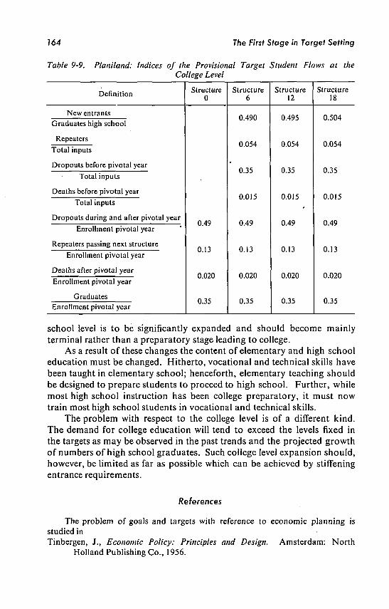
164 The First Stage in Target Setting
Table 9-9. Planiland: Indices of the Provisional Target College Level
Definition
N e w entrants
Graduates high school
Repeaters
Total inputs
Dropouts before pivotal year
Total inputs
Deaths before pivotal year
Total inputs
Dropouts during and after pivotal year
Enrollment pivotal year
Repeaters passing next structure
Enrollment pivotal year
Deaths after pivotal year
Enrollment pivotal year
Graduates Enrollment pivotal year
Structure 0
0.49
0.13
0.020
0.35
Structure 6
0.490
0.054
0.35
0.015
0.49
0.13
0.020
0.35
Student Flows at the
Structure 12
0.495
0.054
0.35
0.015
0.49
0.13
0.020
0.35
Structure 18
0.504
0.054
0.35
0.015
0.49
0.13
0.020
0.35
school level is to be significantly expanded and should become mainly terminal rather than a preparatory stage leading to college.
A s a result of these changes the content of elementary and high school education must be changed. Hitherto, vocational and technical skills have been taught in elementary school; henceforth, elementary teaching should be designed to prepare students to proceed to high school. Further, while most high school instruction has been college preparatory, it must n o w train most high school students in vocational and technical skills.
The problem with respect to the college level is of a different kind. T h e demand for college education will tend to exceed the levels fixed in the targets as m a y be observed in the past trends and the projected growth of numbers of high school graduates. Such college level expansion should, however, be limited as far as possible which can be achieved by stiffening entrance requirements.
References
The problem of goals and targets with reference to economic planning is studied in Tinbergen, J., Economic Policy: Principles and Design. Amsterdam: North
Holland Publishing Co . , 1956.

The Firsf Stage in Target Setting 165
The adaptation of the content of education to the needs of social economic development is considered in Anderson, C . A . , "The Adaptation of Education to a Mobile Society," The
Journal of Human Resources, Vol. 2, N o . 2, Spring 1967. Husén, T . , and U . Dahllöf, " A n Empirical Approach to the Problem of Curricu
lum Content," International Review of Education, Vol. 11 (1965). Ministerio de Educación Publica, Plan Ecuatoriano de Educación, Quito, 1964.

chapter
Demand and Supply
of Teachers
10-1 Contení of This Chapter
T h e first step in assuring the feasibility of the provisional targets set in Chapter 9 is to determine whether there will be enough teachers. This problem can be divided into the following parts:
T h e first part is to forecast the flows of students being educated as teachers, the output of this education and the current supply of teachers. The methodology for this forecast is quite similar to that employed to forecast the total flows of students, the total output of the educational system and the educational structure of the population.
T h e second part of the problem is the determination of the number and qualifications of the teachers needed to achieve the targets of the plan and of the supply of teachers from which the required teacher-force will emerge. All the persons with teacher education whether actually teaching or not are included in the current supply of teachers. The methodology used here is similar to that employed in Chapter 7 to estimate the m a n power needs and the educational structure of the population from which the required labor force will emerge.
Finally, the forecasted supply of teachers is compared with the required supply. This comparison permits us to determine whether or not there will be available the number of teachers required to achieve the provisional targets of the educational plan.
F r o m the observations above, it follows that the methodology used to prepare an educational plan integrated with an economic plan is conceptually similar to the methodology used to deal with the supply and demand of teachers. There are only differences of magnitude.
Actually, this chapter could be considered an exercise in the application of methods and techniques presented in Chapters 4 to 9.
J 66

Demand and Supply of Teachers 167
10-2 Student Flows in Teacher Education
10-2.1 Past Flows of Students in Teacher Training
T w o levels of teacher training exist in Planiland: high school and college. O u r task is to analyze the flow of students at each level.
T h e instruments used in analyzing past student flows were described in Chapter 4. The method set out in that chapter is summarized in the basic relationships 4-12 and 4-13. With respect to teacher training in years - 1 2 , - 6 , and 0, the values of the elements in these relationships appear in Table 10-1.
These values provide the bases for computing the indices a m o n g the variables shown in Tables 10-2 and 10-3. These indices enable us to detect changes in the characteristics of teacher education and are also useful in preparing projections. Additionally, comparisons between these ratios and those relating to general education at high school and college levels (Tables 5-5 and 5-6) can furnish valuable information.
T o complete the analysis of the student flows in teacher education, additional information is required with respect to new entrants. In the case of general education, w e began with new entrants in the elementary school level and allowed for the future growth of the population. In the case of the high school and college levels, w e used the relationships between new entrants at the higher level and graduates at the lower level in the previous structure.
N e w entrants to high school level teacher education are graduates of elementary schools. The relationships observed between numbers of new entrants in high school level teacher training and numbers of elementary school graduates in past structures are shown in Table 10-4.
O n the other hand, new entrants for college-level teacher training can be either graduates of high school level teacher training institutions or other high school graduates. Data for structures - 1 2 , - 6 , and 0 on these two sources of new entrants in college level teacher training institutions are shown in Table 10-5. These data call for some explanation. The total number of graduates from the high school level is 11,100 for structure - 1 2 and 20,100 for structure - 6 (see Table 5-3). These total figures are not shown in Table 10-5; instead, high school level graduates are divided into those coming from ordinary high schools and those coming from teacher training institutions. Likewise, in the table, new entrants to college level teacher training institutions are divided into two groups: those with a general high school education and those from teacher training high schools. Once w e k n o w the source and the meaning of the data in Table 10-5, computation of the ratios of new entrants to graduates presents no problem.

70S
Dem
and a
nd
Su
pp
ly o
f Te
ac
he
rs
O 3
O
D.
O
SE
S«
c I 8.
Z 2
12
J=
Lí
eo
4) H
o
ra
3
-o
UJ ool
J5
o
00
& X
00
ON
TT
r-
(N
Tt
CN
O
m
CN
o\
__ C
N
Ov
Tr -12 0
0
in
r—
00
m
in
CO
«
(N
Tf
00
q
v~
t a
\ oo
•*
CN
o\
m
in
•et-C
N
o
Tt-
m
(n
00 1 OO
VO
O
O
m
•fleo
•fl-m
vo
C
N
m
VO
<N
m
r-
•tf
v">
O
u
J=
u
a
u
H o
c
ç
C3
•
U-l
an
«
a
\o
o
—
00
r
—
—
O
—
V©
(N in
O
N ON
o
o\
r* o
\ (N
-*f
OO
3
Tfr
o
m
^o
7 i r>
j in
O
r-
00
in
m
vD
r*
»n
m
O

Dem
and an
d
Su
pp
ly o
f T
eachers
169
o i
u
o
3NO
1 I
¡7
§ 2 3 d
TT
CN
1,263
+ 15,473
3 fN
O
d H
o II
§
o d H
oo"
o —
—
' d
od —
"
§ d il
O
<N
r-l o
o
o »o
d
d
tn
Os
P-
SO
—
m
Os
00
p-
oo
>n
in
<n
o\
oo
p-
p-
00
r*1 in
o II o II
o o
_ r-l ON
•*
CM
O
—
_M
IN
ON
•tf"
ON
n
IN
O
N
•tf
TT
ri °° rM
_« rM
O
N
•tf"
¿ s
Ü
o
(U
tu 3 u.
o i ngt ass CL
u. C3
Q.
« C
¿.
rt u :>> 2 o > nt pi 3U1 i 0 c tu
8 >>
> Q
,
Sí Ü
m and c 3
73 V
I
n u Q
51 Ù5
Ü
o

770
Dem
and
an
d
Su
pp
ly
of
Te
ac
he
rs
•2 I I I 1
3
lo
s i
o II
•tf
o ci II
o ri o II
o o II
VO
r-+
tri
"~ 358
VO
r-351 +
—"
r-
m
O
s o II
CN
O
II
o o
o II c )
o oo <N
VO
OO
•* 3
o II
o II
o (N
o o II I <*
ov I -sr
o n
I Ov
00 | O
v O
v —
O
v
1
1
3 t3
C
I I
Um
U ~
-
S i
55
341
o II
152
o II
022 o
II
485
o II
lo
— lo
r-
m r»
I (N
—I
<N
*J me roi u
4.
acher training u ool
J=
bî an
J=
Graduates from
E
o
c
s z
«s s
o
CA
C
U
U
L-
3
tj 3 i_
CA next o
OU
c ass a.
CA
Um
U
ra
u
Q,
<U
Qtf
k*
ra
eu
>» "ra
ivot 5. t to men o
c W
Um
$ U >1
_>
a.
1 B and g.
•c 3
•o
c/î
£ es u
Q
o
>
'B.
1
I 1
1
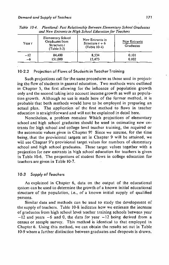
Demand and Supply of Teachers 171
Table 10-4. Planiland: Past Relationship Between Elementary School Graduates and New Entrants in High School Education for Teachers
Year/
- 1 2 - 6
Elementary School Graduates from
Structure t (Table 5-3)
84,400 151,000
N e w Entrants in Structure f + 6
(Table 10-1)
8,534 15,473
N e w Entrants Graduates
0.101 0.102
10-2.2 Projection of Flows of Students in Teacher Training
Such projections call for the same procedures as those used in projecting the flow of students in general education. T w o methods were outlined in Chapter 5, the first allowing for the influence of population growth only and the second taking into account income growth as well as population growth. Although no use is made here of the former method, it is probable that both methods would have to be employed in preparing an actual plan. T h e application of the first method to flows in teacher education is straightforward and will not be explained in detail here.
Nonetheless, a problem remains: Which projections of elementary school and high school graduates should be used in estimating new entrants for high school and college level teacher training, the required or the automatic values given in Chapter 9? Since w e assume, for the time being, that the provisional targets set in Chapter 9 will be attained, w e will use Chapter 9's provisional target values for numbers of elementary school and high school graduates. These target values together with a projection for new entrants in high school education for teachers is given in Table 10-6. T h e projections of student flows in college education for teachers are given in Table 10-7.
70-3 Supply of Teachers
A s explained in Chapter 6, data on the output of the educational system can be used to determine the growth of a k n o w n initial educational structure of the population, i.e., of a k n o w n initial supply of qualified persons.
Similar data and methods can be used to study the development of the supply of teachers. Table 10-8 indicates h o w w e estimate the increase of graduates from high school level teacher training schools between year - 1 2 and years - 6 and 0, the data for year —12 being derived from a census or sample survey. This method is identical to that employed in Chapter 6. Using this method, w e can obtain the results set out in Table 10-9 where a further distinction between graduates and dropouts is drawn.

772
Dem
and a
nd
Su
pp
ly o
f Te
ac
he
rs
-o
5 c
a
-§ 2
CO
K
•£?<£
vs 2
S
«a ¿
s •o
^3
g It) .3
-~
II r •C
i
fi
c tio rt
u Edu !2
<U
J3
U
cd
u H
c
o
ra •
cj
3
LU
2
u
c
CJ
Ü
W3
c
PI
kv
"c
z
(A
O
"ra
3
•o
ra kA
o
.Sv
O
- +
T
í t;
u
C
D
—
S
a
ïS
h
u Ü
>-*
2
«3
1
.5
o
w
**
c o a u
ES
S 3
h
HT
3
U
i- JZ
&
3
u w
.t; i:
ra u H
M
C
m
¿
c LU
U
Z
w
<u
"ra
3
" T
3
ra
Ü
C
.a
o
1 +
C7
S~
2
t.
U
~
— ^
u
c =
-S
[Il
—'
.O
s Ef-
u £ >-<
Z
M
C/3
•Sa
~
~
U
3
-°
g õ
s ,2
¿o
co
b
(g
ti
ra
>
(N
00
(N
«i">
^
- —
•
Ö
O
o
—
in *r\
fO
00
•*
t--
oo co
r- r*
<N
" U-T
•*
•*
m r«*>
o
o
ö ö
OO
O
(N
V
ï
OO
*" T
f*
(N vo
7 '

Dem
and an
d S
up
ply
of T
each
ers
173
5
5
-c Ü
a for Te c O
«
VJ
3
"Ç
! Ü1 O
O
CO
-c ."0
¡5
•5 «?
5
Flo , den 3
co
^ c o ü u
<u 5>
»*
0,
"O
C
a anil
X 1
o
-Si
K
ucture t + 6 h
"°
C/Î
X
2 a
C
P3
iz c
U
J
2
? o 4>
S ra
«
c ra
t-c
LU
tu
2
-o
tn
u ra
3
•u
ra
Urn
0
u
ra
3
^
•a •?
2 °* o
^
__
Xi
O
C3
f,t«
ra
u
c 2
UJ
L*
ra
tu
>
(N
O
—
". °°. ~". in
o
o
t-»* (S
"
OO
O
IN
(N
<N
O
O O
"
"*
. "
" "
"•
.
o o
o
VO
Tf
(N
<N
^
O
0\
\Ó
-rt •*t
P-
«-i (N
in
o
o
O
VO
<
N
After Pivotal Year
Deaths Graduates Repeaters Dropouts
Total Enrollment,
Pivotal Year
Before Pivotal Year
t ï c
Deaths Dropouts Repeaters New
Entrants Year
m
>n o
N
O
o
©
—'
—'
ío
in
Tf
o«
o\
>n vi
n
- n
in
(N
P-#
H"j
f;
(N
m*
OO
<
N
ON
(N
~
ON
— m
" r
ö
Os
O
N
OO
—
-
rn
rsî —
O
N
—
(N
»n
r--
TJ- O
N
O
Ö Ö
—'
n
oo q
rt O
N' »n
<N
r
m
N
n
oó
Tt
oq
—
•n
oo
V
(N
in
oo
O
NO
(N
00

774
Dem
and an
d S
up
ply
of T
ea
ch
ers
lege Education for Teachers Projection of Student Flows in Co¡ Table 10-7. Planiland.
Teacher Education
Total
c+f
New Entrants Structure
t + 6
f - d x e
New Entrants Graduates
(Table 10-6)
e
Teacher Training High School Graduates Structure t
(Table 10-3)
d
General Education
New Entrants Structure
/ + 6
c = a x b
New Entrants Graduates
(Table 10-5)
b
General High School
Graduates* Structure /
a
Year*
00
O
C
N
to
—
O
(N
Tf
OO
O
»O
O
N
to
Tf
to
—'
(N
tO
GO
0
0
CO
«n
to
in
oo
o
»O
IO
Tf
0\
iO
iO
—
ro
00
IO
C>
O
S
O
Tf
—:
—:
fsi
Tf
Tf
Tf
OO
O
o' o
o
P";
P-;
Tf
—' od
—'
n
Tf p
-
O
so
(N
After Pivotal Year, Relationship 4-13
Deaths Graduates Repeaters Dropouts
Total Enrollment,
Pivotal Year
Before Pivotal Year, Relationship 4-12 a
Deaths Dropouts Repeaters New
Entrants Year
- -
vo
\o CN
^
vo (N
671 1 , 3 1 1 2,093 4,035
Q
<N O
N
—
so —
OS
so —
m
T
f os
Q
O
Tf —
O
O
s (N
O
(N
m
^O
<N
(N
^
M
M
•O
»O 00
(N
O
©^ c^
r*\ —
*" ri rn" so
m
n
rsi ro
to O
m
p-
os p-
p-
r-v
oq
o
—" ri
Q
fS
Os
sO
— O
s —
m
T
f
ri T
f oo"
O
« N
OO

Demand and Supply of Teachers 175
Table 10-8. Planiland: Changes in the Supply of Graduates from High School Level Teacher Training Institutions from Year -12 to Year 0
Graduates with high school level teachers' education year t
Survivors in year t + 6 Graduates from high school teachers' education
structure 1 (Table 10-1) Graduates entering college structure t + 6 (Table 10-5) Deaths among graduates after they have left school Graduates with high school teachers' education
year / + 6
Years
-12
3,199 2,971
+2,874 - 3 5 0
- 6 8
5,427
-6
5,427 5,063
+5,387 -851 - 1 2 2
9,477
0
9,477
Table 10-9. Planiland: Actual and Projected Supplies of-Persons with Teachers' Education at Different Dates
Qualifications of Teachers by A m o u n t of Education
College graduates College dropouts High school graduates High school dropouts
Years
-12
106 342
3,199 3,572
-6
225 569
5,427 5,730
0
5L9 974
9,477 8,993
6
1,138 1,766
16,654 14,493
12
2,357 3,117
28,553 26,544
18
4,283 5,616
56,244 46,977
70-4 Number and Qualifications of Teachers Required to Achieve
the Targets of the Educational Plan
10-4.1 Basic Instrument for the Analysis of the D e m a n d for Teachers
The basic instrument for the analysis of the demand for teachers is
Eq . 4-7:
s" - KTT [4"7]
where sh = average number of students taking each period (weighted
student-teacher ratio)
hs = average number of periods per week per student
hc = average number of periods taught by each teacher per week
S = number of students
T = number of teachers
10-4.2 Past Experience with Regard to the D e m a n d for Teachers
In Table 5-5 the student flows at elementary, and high school levels
for structure - 6 were divided into four qualitative strata. In Table 10-10

176 D
emand
and
Su
pp
ly o
f Te
ac
he
rs
K
College High School Strata Elementary School Strata
> X i
Total
Q
U
CO
< Total
Û
u co
< Total
< 3
583 5.17
5.1 1 1 . 1 8 18.95
Vf)
—
m
vo 0
\ m
C
N
(N
OO
fN
m
>n
r
—;
fj\ S
O
fN
ÍN
fO
oo tN
n
m
os_ —
°°. S
O
»n —
"' (N
<
n V
i —
—
r*1
TJ* »n
to in
<N
o\ m
in
m
(N
«n •3-
<N
m
m
3 , 1 1 7 8.60
40.5 32 48.33
m
so p
fN
oo r-'
oo Tj-'
O
fN
SO
fN
»n
m 2,079
28
105.0 28 50.50
2,515 28
105.0 28 41.74
1,924 28
42.0 28 21.83
9,620 28
419.6 28 43.61
Number of teachers, T Periods per teacher, hc
Number of students, 5 (thousands)
Period per student, hs
Weighted student-teacher ratio

Demand and Supply of Teachers 177
the different elements of formula 4-7 are presented for each of these strata as well as for each of the three levels as a whole. Comparisons of figures in the two tables indicate that the weighted student-teacher ratio has a very definite influence on the quality of education.
The differences a m o n g the strata at the elementary and high school levels cannot be attributed, however, solely to the differences in weighted student-teacher ratios. There are m a n y other influential factors, the most important of which is doubtless the qualifications of the teachers.
Table 10-11 shows the qualifications of teachers in Planiland's educational system and shows that qualifications differ considerably even within the same level: for instance, high school teachers include both holders of college degrees and high school dropouts. In Table 10-12, the teachers in the qualitative strata in Table 5-5 are classified according to qualifications.
10-4.3 Teachers Needed to Achieve the Provisional Targets of the Educational Plan
Elementary school total number of teachers required
T o find out the total number of teachers needed in years 6, 12, and 18 w e have the following data:
(a) Total number of students Sl, in year 0 (Table 5-3) and target figures for years 6, 12, and 18 (Table 9-5).
(b) N u m b e r of periods per student per week (hs) and number of periods per teacher per week (hc). According to past experience (Table 10-10), A, and Ac will each equal 28 for years 6, 12, and 18.
(c) Actual value of sh, the weighted student-teacher ratio, in year 0 (41.15) and target value for year 18, i.e., the value for stratum A in year - 6 . The reason for this is that in order to come as close as possible to meeting requirements for elementary school graduates, planners must bring the entire elementary level of the educational system up to the standards of stratum A .
Once w e have actual and target values of sh for years 0 and 18, w e can use a rate of growth to interpolate the values of sh for years 6 and 12. The results appear in column 4 of Table 10-13. With the necessary target values for four variables (S), hs, hc, and sh) in Eq. 4-7, w e can compute the number of teachers required.
With respect to year 6, for example, w e have
T = hs x S _ 28 x 716,320 =
hc x sh 28 x 33.30
This result, together with those for years 12 and 18 appear in Table 10-13.

178
Dem
and an
d S
up
ply
of T
each
ers
«• S
i
o
>
•«
1 ^
3 Z
I
ai
u
o >
-c
D.
E f«.
3
z
= >
«
c
E
t-
C
X!
E
O
o
-C o
c/3
>-, L
. CO
c 4>
E
u
ÜJ
c» (N
NO
in
m
tn
oo fN
(N
00 O
N
(N
00 tN
«
S c ,o
rs' educ: u 1 teach< hoo u igh
-C V
) 4> «
3 T> ca u
OO <N
uo O
N OO (N
OO (N
<N
fO
P
-
oo (N
•r
OO O
N
C 1 educat n 1 gêner hoo v\ igh
_c V
3 CJ C3 3
•U 03 Um
OO fN
n •*t
m
•V
oo (N
•*
o\ *0 (N
OO <N
(N
s ion s' educa L* teache IOOI ghs
j=
</i
3 O
O.
o
b.
00 (N
CO
O
CO
OO (N
<n (N
OO (N
—-
OO
c o educati genera iooI U
Vi
.SP le
V)
3 O
OO (N
TI
CO
•
<*
00 (N
CO
r»
NO
00 (N
NO
»n
NO
schoo tary lernen u
VI
u
ra
3 a-D o
Um
CtJ
u
00 (N
wt
-3-
00 CN
00 00 (N
OO (N
ON
in r school ary = eme o (/)
3 O
Q.
O L_ O
Ü Q
Q Ü
Q
S S s 2 in Z
o
NO
r-•^ 2 o
fN
NO
O
N
CO
N
O
VI
NO
"n O
t-
r-
p-
ON
NO
NO
NO
^-
co
NO
C
O
CO
fS
NO
O
O
OO
OO
NO
rj
-U
Ot
NO
N
rO
OO
NO
^N
OO
OT
j-
—
s
r- r-
ON
NO
NO
NO
Tl-
— u
ouot--ro
ooco
«i-i
r-o
uo
eo
—
N
O^
-(
N
—
Tf
CO
tN
O^
-C
O
—
P-
P-
ON
NO
NO
NO
^-
CO
—
(N
—
r- C
M
CN
•2 -S § -g
3 -g
S
y 3 g
s J2 -M
«
•S 'S 3 S
2
S "n
*
U
is
C
fî Ü
B
»- —
• u
u
B
rr
2 u
B
S
eo
u
H.
U
r- I-
~J
00
~ x:
JÏ
tu
t/j uî
B 3
3
3 O
O
•a
o. D
. B
OO
o
C)
_c u
jr au o
O
-C (j
-C Ö
Ü
ao
oû
uo
ûû
P-
OO
ON
O
— <
N
o
o
*o m
fN
Tf
m
«r»
OO
o
o
\o u-i
fN
—
— m
•tf
O O
*o «n
OV
fN
wi
fN
c O c
opt IJE3 3
ü
"O
3
u -a
o co
-s «
ü
GO
U
U
o o
CJ
O
co
ca
3 3
•O
T
3
S3 CO
CN •
*
(N
fN
T fN
m
fN
•»
•»
fN ion B
O edu >-
•s tea col 3 O
ex o
»i-i
-* «J
0\
m
«AI
•*
\o
rn
a\
ii-i
•*
vo
m
r-ion B
O edu gener col trt
3 O
O.
O
t_
o
fN
m
fN
\o
fN
m
rt
«
fN
ro
c o B
U
•a
ache o
o
en
J= au le 3 T
5
O
O Q
Q O
r— OO
C\
r-VO 1,0
fN
00 m
t-m
-¿ O
r-
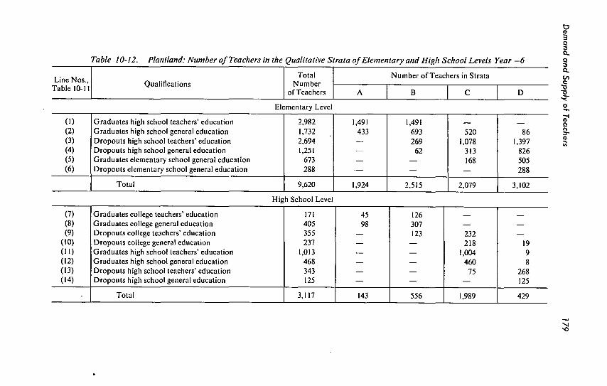
De
ma
nd
an
d S
up
ply
of T
eachers
1
79
1
^ o
Cu
S
s
•ft eve
>-J
o
•s
:
to
•*
:
.fcx¡
i; •M
ryan
«
c
«j
ä?
D
U)
"5>
«
IM
V.
05 itative ual
©J
cu
-s-e
tu
•«
•
Ü
«
Ã
^ 1»
«1
-C
i
? a
S;
>t sr
.5 Plan
<N
•
*-
,
O
~^ cu
rt K
co
CO
CO
CA
co
H O
Um
X)
£
3 £
Q
O
ca
< V)
-ö
l õ 1
g
"¿t O
c
0 •
^
u
3
"> "T 0
ó
z-oü
C
.O
J
et)
01
>
3 -"->
S
1) h
1
1 1,49 1,491
fN
00
Os
(N atio ' educ I teach hoo igh
JZ
a
3
•0
C3
*o
t—
OO
O
v 1,3
0 0
0
(N
r-in
O
e-i o
s
ON
N
0
NO
(N
433
ÍN
TT
m
ON
P
- \0
—
fN
ion tion
1
- -«
C
O
u.
gêner teache
§1
0
-s
»4 •s
=
u
ça
CO
3
3
O
•O
D.
CO
O
\o
fN
00
rn
m
<N
sO
'
_ in
(N
—
c
0 ducati genera ool ghs
J=
3
0
«n
0 sn
00
vo
1
1
m
»0 cation edu
! 0i> schoo tary eme
<u
3
O.T
3 O
cd
00
00
(N 1
1
1
00
fN
C
Ö
C3 duc nerale u
60 school ary eu
E
u
3
0 u.
n
OO
ÛÛ
OÛ
3 (N
m
•
* in
>o
CN
O
3,1
Os
r--2,0 2,51 1,924
0 CN
V
O
Os ta 0
r-
I I I
C\
ON O
O O
O m
—
N
O
<N
(N —
NO
r- m
rj
O
(N
—
m —
M
ill
lililí
•n >n
h
n
00
n
in
Q
»n m
—
N
O T
T «N
•^ m
(N
o
T
T en
—
1111
sëS
Iff
ñ-¿
"O
3
U
-o h
CJ "°
3
U
?>
h
"S
„„
«
t-egene
an
.Ile; U
U
t/3
3
U schoo! igh vi
0 «
•u
«1 school igh (A
U
cS
ñ
u
w chool
Uî
.SP
j= W)
3
C
U
00 chool
«
op
j= trt
3
^ 73
•J
O
f-0
33
O
CO
CO O
O
a
a
o
o
OD
ÛÛ
DO
UÛ
r~- 00
o
©
—
'(Nm
-^-

780 Demand and Supply of Teachers
Table 10-13. Planiland: Estimation of the Number of Teachers Required to Attain the Provisional Targets for Elementary Education
Year
0 6
12 18
N u m b e r of Students in
Targets Tables 5-3
and 9-5
595,800 716,320 930,250
1,096,720
N u m b e r of Periods
per Student Stratum
A
28 28 28 28
N u m b e r of Periods
per Teacher Stratum
A
28 28 28 28
Weighted Student-Teacher
Rat,io
41.15 33.30 26.96 21.83
N u m b e r of Teachers
14,476 21,511 34,505 50,239
Teacher qualifications
Once we have the total number of teachers required, w e can proceed to determine the qualifications they should have. Thé breakdown of teachers by qualification is k n o w n for year 0. W e k n o w also that the conditions in stratum A of elementary school in year - 6 (Table 10-12) must be extended to the entire educational system by year 18. This means that in year 18 the proportion of elementary school teachers with degrees of high school teachers' education was to be the one observed in stratum A in year - 6 . T h e same is true for the proportion of teachers with degrees from general high school. In Table 10-12 w e see that the first proportion must be
1,491 1,924
0.7749
and the second must be
433 1,924
= 0.2251
This means that the number of teachers with degrees from high school level teacher-training institutions for year 18 must be
0.7749 x 50,239 = 38,930
Elementary school teachers with degrees from high school general education in year 18 must number
0.2251 x 50,239 = 11,309
These results appear in Table 10-14. Next comes the problem of determining the required qualifications of
the teachers in years 6 and 12. For this, w e notice in Table 10-14 that in year 18 groups 3 to 6 are no longer present. This elimination of less qualified teachers should be gradual.

Demand and Supply of Teachers 181
Table 10-14. Planiland: Number and Qualifications of the Teachers Required to Attain the Provisional Targets for Elementary Education
Line Nos . , Table 10-11
(D
(2)
(3)
(4)
(5)
(6)
Levels of Qualification
Graduates from high school teachers' education Graduates from high school general education Dropouts from high school teachers' education Dropouts from high school general education Graduates from elementary school general education Dropouts from elementary school general education
Total
0
5,356
2,895
4,343
1,303
434
145
14,476
Years
6
11,266
6,093
2,897
869
289
97
21.511
12
21,051
11,377
1,449
435
144
49
34,505
18
38,930
11,309 '
0
0 •
0
0
50,239
In Table 10-14 it is assumed that one-third of the teachers in groups 3 to 6 leave the educational system between year 0 and year 6, another third between years 6 and 12 and the remainder between years 12 and 18.
Finally, w e must estimate the number of teachers required in categories 1 and 2 for years 6 to 12. The method used is as follows: There should be in year 6 a total of 21,511 teachers, 4,152 in categories 3 to 6, and the remaining 17,359 in categories 1 and 2. In order to estimate the number in each of the latter two categories, conditions in year 0 are observed (see Table 10-11). T h e proportion of teachers in category 1 as compared to those in categories 1 and 2 is
5,356 5,356 0.649
5,356 + 2,895 8,251
Thus the required number in category 1 in year 6 is estimated to be
0.649 x 17,359 = 11,266
The same method was used to obtain the values for categories 1 and 2 teacher requirements for year 12.
Periods per teacher per week for different types of teachers
In Table 10-13 the estimated average number of periods per teacher per week for years 0, 6, 12, and 18 is presented. Since teachers of all the types teach the same number of periods per week at the elementary school level, there is no problem of differences in periods per week a m o n g teachers with different qualifications.

782 Demand and Supply of Teachers
High school total number of teachers required
In the estimation of the total number of teachers required at the high school level, there is a problem that did not appear in the case of the teachers for the elementary school level. For this reason the process of estimating teacher requirements at this level will be explained in detail.
The data available are:
(a) Estimated total number of students (S2) for years 0, 6, 12, and 18 (Tables 5-3 and 9-5). These values are reproduced in Table 10-15.
(b) N u m b e r of periods per student per week (hs) for years 0, 6, 12, and 18. The value according to Table 10-10 is
hs = 32
(c) N u m b e r of periods per teacher per week hc. For this variable, estimation is not as simple as in the case of the elementary school level. First, w e use as target values those for qualitative stratum B in year - 6 and these values are different from the values for the level as a whole in year 0. Besides, the number of periods per week for teacher in stratum A is higher than in stratum B; that is, with the period load in stratum A , a smaller number of teachers would be required to provide a given quantity of education.- For this reason it is worthwhile to consider two alternatives for the number of periods per week per teacher hc, the number for stratum A as well as that for stratum B . It should be noted that conditions in stratum C should not be considered in any circumstances since high school education must be at least of stratum B quality in year 18 to assure attainment of output targets for the high school level.
(d) T h e actual or target values of sh, the weighted student-teacher ratio for years 0 and 18.
Again the method of computation of T is based on Eq. 4-7. The values of two variables (S2 and hs) in this equation are k n o w n for years 0, 6, 12, and 18, and the required value of two others (Acand sH) can be estimated for years 6 and 12 by interpolation using a rate of growth and values for years 0 and 18. With the values of the four variables for years 0, 6, 12, and 18, Eq . 4-7 will yield the number of teachers required in each of these years. For instance, with the first alternative value of hc, w e obtain the following value for T for year 18:
= h,xS _ 32 x 501,910 =
he x s„ 25.25 x 45
T h e other target values for T and the figures on which they are based are shown in Table 10-15.

Dem
and
and S
up
ply
of T
ea
ch
ers
183
S
I to
^
vu
6? s "5
•y «J
S
'S-
Oí
î tu -o 5
-o
Second Alternative First Alternative
Number of Teachers
Number of Periods per
Teacher Stratum B
(Table 10-10)
Number of Teachers
Number of Periods per
Teacher Stratum A
(Table 10-10)
Weighted Student-Teacher
Ratio
Number of Periods per
Student Stratum B
(Table 10-10)
Target Number of
Students (Tables 5-3)
and 9-5)
Year
—
r-
•*
—
<N ON ÏN ÍN
«n_ Ov OO vo
in Ov r*f
m*
—
(N
vo rn
«n —
od Ö N in
— — o\ in
(N (N
o m
T °. ~
«i-T oo* o\ *t
© — f> in
so n iq N
od (N
r- in
— — (N
in p »n o
vo vd
»n in
CN CN (N <N
m ro m
m
69,000 149,020 245,900 501,910
OVO
NGO

784 • Demand and Supply of Teachers
Teacher qualifications
Having calculated the total n u m b e r of teachers required, w e can continue a b r e a k d o w n of teacher requirements by level of qualification, using the s a m e method as in the case of the elementary level (see Table 10-16).
Table 10-16. Planiland: Number and Qualifications of the Teachers Required to Attain the Provisional Targets for High School Education
Line Nos . , Table 10-11
Qualifications 0
Year
6 12 18
First Alternative
(7) (8) (9)
(10) (11) (12) (13) (14)
Graduates college teachers' education Graduates college general education Dropouts college teachers' education Dropouts college general education Graduates high school teachers education Graduates high school general education Dropouts high school teachers' education Dropouts high school general education
Total
386 883 663 442
1,656 828 497 166
5,521
1,204 2,755 2,069
295 1,104
552 331 111
8,421
1,721 3,936 2,955
148 552 276 165 56
9,809
3,203 7,805 3,127
0 0 0 0 0
14,135
Second Alternative
(7) (8) (9)
(10) (11) (12) (13) (14)
Graduates college teachers' education Graduates college general education Dropouts college teachers' education Dropouts college general education Graduates high school teachers' education Graduates high school general education Dropouts high school teachers' education Dropouts high school general education
Total
386 883 663 442
1,656 828 497 166
5,521
1,519 3,475 2,610
295 1,104
552 331 111
9,997
2,523 5,771 4,333
148 552 276 165 56
13,824
5,353 13,043 5,225
0 0 0 0 0
23,621
Periods per teacher per week for different types of teachers
T h e estimation of periods per teacher per w e e k is m o r e complex at the high school level than elementary school level. T h e m e t h o d to be used for this purpose will be described below with reference to year 6.
W e have three sets of data: (a) H, the total n u m b e r of periods per week that will be offered by the
teachers available in year 6. This can be calculated with the formula
H = hcx T [4-6]
For year 6 w e have
103,662.51 = 12.31 x 8,421

Demand and Supply of Teachers 185
(b) The numbers of teachers of each type required in year 6. These requirements are presented in Table 10-16.
(c) The n u m b e r of periods that the teachers of each type taught in the previous pivotal year; i.e., pivotal year 0 for year 6. These figures appear in Table 10-11.
With the data in (b) and (c), it is possible to calculate the total n u m b e r of periods per week that would be taught in year 6 if the teachers of each type were to teach the s a m e number of periods per week as each type taught in year 0, i.e., 104,400.97 periods. This total will differ from the total in (a). The factor of change from year 0 to year 6 for the number of periods per week is then obtained by dividing the total in (a) by the total just calculated from (b) and (c). In the case of high school teachers for year 6 this factor of change is
103,662.51 = 0 9 9 2
104,400.97
T o obtain the n u m b e r of periods that the teachers of each type must teach in year 6 the factor above should be multiplied by the average n u m b e r of periods per week taught in pivotal year 0. For instance, the average teacher of type 7 will teach in year 6:
17.78 x .992 = 17.64 periods per week
T h e final results of similar calculations for all types of teachers for years 6, 12, and 18 appear in Table 10-17.
Table 10-17. Planiland: Number of Periods Taught per Week Required to A ttain the Targets of the Educational Plan
Line N o s . , Table 10-11
(7) (8) (9)
(10) (11) (12) (13) (14)
High School
Graduates college teachers' education Graduates college general education Dropouts college teachers' education Dropouts college general education Graduates high school teachers' education Graduates high school general education Dropouts high school teachers' education Dropouts high school general education
6
17.64 17.42 9.55 6.40 6.64 6.61 4.06 3.33
Year
12
22.72 22.44 12.30 8.24 8.55 8.51 5.23 4.29
18
25.25 25.25 25.25 0 0 0 0 0
College total number of teachers required
T h e method used to estimate the n u m b e r of teachers required at this level is identical to that outlined for the elementary and high school levels. The results for the college level are set out in Tables 10-18, 10-19, and 10-20.

786 Demand and Supply of Teachers
Table 10-18. Planiland: Estimation of the Number of Teachers Required to A ttain the Provisional Targets for College Education
Year
0 6
12 18
Target Number of Students (Tables 5-3
and 9-5)
8,900 13,570 21,370 37,380
N u m b e r of Periods per Student
Average (Table 10-10)
11.18 11.18 11.18 11.18
N u m b e r of Periods per Teacher
Average (Table 10-10)
5.17 5.17 5.17 5.17
Weighted Student-Teacher
Ratio
18.03 18.95 18.95 18.95
N u m b e r of Teachers
1,067 1,549 2,439 4,266
Table 10-19. Planiland: Number and Qualifications of the Teachers Required to A ttain the Provisional Targets for College Education
Line Nos. , Table 10-11
(15) (16) (17) (18) (19)
Qualifications
Graduates college teachers' education Graduates college general education Dropouts college teachers' education Dropouts college general education Graduates high school teachers' education
Total
Year
0
32 854
21 139 21
1,067
6
46 1,241
30 202
30
1,549
12
73 1,952
48 318
48
2,439
18
128 3,414
84 556
84
4,266
Table 10-20. Planiland: Number of Periods Taught per Week Required to A ttain the Target of the Educational Plan for the College Level
Line Nos. , Table 10-11
(15) (16) (17) (18) (19)
Qualifications
Graduates college teachers' education Graduates college general education Dropouts college teachers' education Dropouts college general education Graduates high school teachers' education
6
6.0 5.0 4.21 6.45 3.26
Year
12
6.0 5.0 4.21 6.45 3.26
18
6.0 5.0 4.21 6.45 3.26
J 0-5 Required Supply of People with Teachers' Education
A s shown in Sec. 8-2, figures for the required educational structure of the labor force are not sufficient to enable us to define the necessary characteristics of the educational system since the system produces educated nonworkers as well as educated m e m b e r s of the labor force. T h e immediate problem, therefore, was to establish the educational structure of the population as a whole required in order to produce a labor force with the necessary educational structure.
T h e same problem arises with respect to people w h o have attended teacher training institutions. N o t all those w h o have been trained as

Dem
and an
d S
up
ply o
f Teach
ers 187
o C3
>• 1 L~
C3
>
<N 1
1-1
CD
>-
O
'« a
l-° oá
00
c -C
Ä
u
-o
u
H
lumber : 10-9)
Total N (Table
a
o
ca ai-e
>
c¿
en
c •S
*
C3
H k*
.o
ON
¡2 Z
ü
o
Total (Tab
o M
OK
0¿
BD
C
•C
„
o
-d
es
H tu
^-v
.O
ON
3 —
Total N (Table
a
w
i-
lalifícation im Teache Training istitutions
3 O
i-
Ci
" „
t-
— o
-o -S —
ra s
c -Ç
—
3 t
O-cJ = 2—
-
(N
Tfr <N
—,
00
•^
•
ON
in
o
m
°î ~~
en
oo
«n
<N
(N
m
m
(N
_—
VO
O
O
VO
o
oilege graduates oilege
<J U
wt
r-
—
—
r-* o
C
Tf <N
^ "
-
•<t O
O
O
Tf
r» o\
o r»
^ "™
r-00
o\ \o
in
r» m
in
""
ro
<N
(N
(N
•*
en dropouts
igh school
X
ON
^S
— O
O
00
^-
v^ en
O
O
—
—1
en
o
m
tt O
oo
r»~
•
*•
r- n
r-
ON
oC
oo"
-* r-
VN
oo
en
O
O
—
—ï
ON
r-
4,00
3,03
r- o
(N
en
•
*.
r-^
irT
u-T
—
r-in
oo
en
oq
—
—
oo
en
^O
O
N
m
oo
<N
—
ON
<N
ON
r-m
" en
graduates igh school dropouts
X
en
"
en
tW)
e -s-<J <n
<tl
c-, e c o ~ <M duc
ki ¡?
ï) Teach
-s:
Si o <
*1
a ,ft kl
•s
<* £
â -«
rso
k, tu
tu
05 "i
.¡A,
-C
C
o ^ tu
«Í and.
r ci
a; •-* ^ ¿ --* <»
-15 PI b-. s § \s
i?
£ >
s si < <3
<TÏ k, >l s-a
.5 <n
O
k,

188
De
ma
nd
an
d S
up
ply
of T
each
ers
51
i Requii
s; •2
a
cj
-3 S
^
3 53
tq^
~5"S Q
j J
.
•s-s
LT
^
2; to
a-S
erson tsof
^K,
fc-*
Numb, visiona
~~ 51
a
v.
d: Tot, n the P
ilan ttai
5 <N
*>
51) Tab
OO
Urn cd 0)
>
CN
k» CS
>
NO
l-cd eu
O k»
cd 4>
>-
i
t-—
<U
Q
j cd
X)
Õ
E x
Hl"
ON
60 7
.£ J
-*
2
•g x
i "T
. <u
CO ,1
<
N^
F2
H_
"T
^
CN
—
C3 X
>
Õ
E X
H!° ON
60 „
T
.S 3
^2
cd <5 «
^ o H
— —
H
,4,
Ui
—
TO
tj cd
_o
õ E
x
Hl = ON
•Su
I .
u
a «
C
N *>
,u
H —
—
(- <
N
~~* t-i
cd X
I o
E x
Hl = O
N
60 T
.5
S-t«
x:
"TÍ —
.. S
M tN
N
O
u H
— "T
H
CN
*~" o
a> *-
—
—-
tN
™
Cd fN
l
«H
-
C
OÙ
« 'S
C
S 2
.2
\5
M
3
« tí
•-
o «J
S
en x
: «
;= u
c
IS
«
"ï
C
Q>
4> —
» 0
£-r
-; w
p -2 —
p-m
-^ ,^-m
oo CN
CN
CM""
ON
m
in
""l
o «n
ON
<n
oo -<
t
<N
<N
—'
cd 3
•a cd
CN
p
-
*n ^ ™
(N
NO
P
-r
^
•*
i en
ON
oo O
N
CN"
ON
8. CN"
•t
ON
NO
•<
*
CN
"" V)
3 & O
ox> *o •u oo
tt>
60
1
O
O
in
p*
P-
oC
0\
O
»n CN_
(N*
in
00 O
N
O
oo" m
<n C
\ N
O
0\
"*. °\ N
O*
CM
"
—
^
in
—
©_
NO^
r-T —r
(N
Q\
00
—
o> r-
O
N
NO
" in
"
fO
00
O
(N
-^
(N
ri rn
O
ro
OO O
S
oC oo""
m
o
O
00
p-" •*"
OO
00
•^-
»n
rn
oq
—
—.
w ._
u
j2
•o o«
cd O
"o "Õ
o o
u
o
CA
</]
00 00
¡2
ï
ON
» '^
^ rn"

Demand and Supply of Teachers 189
teachers actually teach; the educational system must therefore produce more people qualified to teach than are actually needed in the schools. The value of this required total output of qualified teachers will be estimated below.
The method of estimation is similar to that employed in Sec. 8-2. T o begin with, w e must determine the past relationships between the total number of those with different types of teacher training and those of each type actually teaching. These relationships are shown in Table 10-21 for each of the four types of qualified teachers with which w e are concerned. The table indicates that in year 0 there were 519 graduates from teacher training colleges of w h o m 418 were teaching. This means that there must be
| 1 | - 1-242
people with this level and type of training for each person of this level and type of training actually engaged in teaching.
Assuming that the ratios for year 0 in Table 10-21 will remain constant in the future, w e can estimate the total number of people with various types of teacher training required in the future. This involves using not only the ratios in Table 10-21 but also the required numbers of teachers estimated in Sec. 10-4 and shown in Tables 10-14, 10-16, and 10-19." These numbers appear in Table 10-22 along with the required total numbers of those qualified to teach. By way of example, let us consider the number of graduates from teacher-training colleges required in year 18, a figure which is calculated as
1.242 x 3,331 = 4,137
10-6 Comparison Between Forecasted and Required
Supplies of Teachers
The comparison between forecasted (Table 10-9) and required (Table 10-22) supplies of teachers will permit us to find out whether or not there will be enough teachers to achieve the provisional targets of the educational plan. F r o m this comparison, it can be seen that there is not a marked difference between the required numbers of those with teachers education and the numbers that will be available as a result of the projections in Table 10-6 and 10-7 of the growth of student flows in teacher training institutions. Hence the projected growth of the student flows in teacher training satisfies the requirements of the educational plan. Were this not so, it would be necessary to set targets for the growth of the student flows in teacher training by means of the methods employed in Chapter 9.

790 Demand and Supply of Teachers
References
S o m e limitations of the unweighted teacher-student ratios are studied in Hansen, W . L . , "Educational Plans and Teacher Supply," Comparative Education
Review, Vol. 6, N o . 2 (October 1962). , " H u m a n Capital Requirements for Educational Expansion: Teacher Shortages and Teacher Supply." Paper presented at the Conference on Education and Economic Development, Comparative Education Center, University of Chicago, April 1963.
A general analysis of demand and supply of teachers in developed countries appears in Caplow, T . , and R . M c G e e , The Academic Marketplace. N e w York: Basic Books,
1958. Vaizey, J., The Control of Education. Part IV. London: Faber and Faber, 1963.
The approach used to adapt the method presented in this chapter to a computer program appears in Correa, H . , and E . Reimer, A Simulation Model for Educational Planning in
Puerto Rico. San Juan: Department of Public Instruction (Mimeographed), 1969.

chapter I I
Buildings and
Other Facilities
7 7-7 Content of This Chapter
The purpose of this chapter is to determine the physical facilities required to reach the provisional targets of the educational plan. The first step is to study past experience with regards to buildings and other facilities. This analysis gives information about the facilities available and the relationships between the characteristics of the facilities and the flows of students and the output of the educational system. These relationships permit us to determine the characteristics that the school facilities should have in the future if the provisional targets for the flows of students are to be obtained.
7 7-2 Method
In the determination of the physical facilities required to reach the provisional targets of the educational plan, w e will take into account the number of students seeking education, the number of periods per week during which schoolrooms are used, the number of periods during which they could be used and the qualitative characteristics of these rooms. For this w e use E q . 4-9:
* = ^ [4-9] hr x R
where sh = average number of students taking each period; i.e., weighted student-room ratio
hs - average number of periods per week per student hr = average number of periods that each room is used per week S = number of students R = number of classrooms and laboratories
79T

792 Buildings and Other Facilities
It is useful to remember that s/,, h„ and S in formula 4-7 are the same variables as sh, hs, and S in formula 4-9. Hence, some of the results obtained in Chapter 10 can be used here.
In Chapter 4 the following equations were also introduced
H = hcT [4-6]
H = hrR [4-8]
where H = number of periods of education offered hc = average number of periods taught by each teacher per week T = number of teachers
hr = average number of periods that each room is used per week R = number of classrooms and laboratories
In Chapter 10 w e have already determined target values for each level for the number of periods per teacher per week hc and number of teachers T for years 6, 12, and 18. Equation 4-6 allows us to calculate from these figures target values for H for each level for years 6, 12, and 18.
In order to estimate the number and characteristics of classrooms and laboratories required to attain the targets of the educational plan, w e can use Eq . 4-9 or Eqs. 4-6 and 4-8. In both cases the results already obtained in Chapter 10 must be taken into consideration. D u e to their simplicity, w e will use mainly Eqs. 4-6 and 4-8.
7 7-3 Past Experience with Regard to Buildings and Other Facilities
In Table 11-1, the year - 6 values of different variables in formulas 4-8 and 4-9 for the three levels of education and their qualitative subdivision are presented.
T h e Table 11-2 gives more detailed data on types of classrooms in use in years - 1 2 , - 6 , and 0 and Table 11-3 gives data on types of classrooms used in the various qualitative strata at the elementary and high school levels in year - 6 . In these tables, classrooms are classified according to number of square meters of classroom space available per pupil in an average-sized class.
It will be observed that, at elementary and high school levels, the space available ranges from 0.8 to 3.8 square meters per student while, at college level, it varies from 2.3 to 4.3 square meters per student. T h e space available per student is estimated by dividing the area of each room by the average number of students taught in that room in each period.
It will be noted also that in Table 11-2 classrooms have been classified as "owned" and "not owned ," an important distinction inasmuch as the financing required for owned buildings is quite different' from that required for rented buildings.

Bu
ildin
gs an
d O
ther Fa
cilitie
s
193
Ov •
s: I
I •S
<u
2 '5 û
i Ja
-o 5
BO
U
O
U o o
J=
u
CO
JZ
00
X hool u
CO
>v
cd
c u lem
u X
-ë
=
C3
Õ
r-Û
O
ca
<
_ pj
r-Û
U
ca
<
"5 Tot;
•*
oo
—
m
•q-
oo
5-cr>
o
fN
OO
in
•*
ov
•* 2,18
o
vo
VO_
"-VO
VO
•
rj
O 2,02
Ov 8,33
o;
SUIOO i-ero
& B
3
Z
«I
m
vo"
S
fN
m
S
(N
m
r-so
od
fN
in
oq fN
fN
TT
m aí
fN
OÑ
en
oo
oo
Tt
en
oo
in
od
fN
r»
fN
VO
fN
_
en
fN
m *.
-« oom, •-s.
•o
.2 Per
<£
O eriod: a. ero
-D
E
3
Z
Ov
g
r-T
M 1,44
VO 13,36
—
O
^
oo"
_ 3,6
av
00^
vo" fN
VO 86,85
fN
(N 58,
o
r-•>t
o'
r-fN 53,87
o 269,41
¡5
•tf o (Tere ducation u
<o
(A luden vi
o
Um
U
J3
E
3 Z
—
in
vS
fN
fl
fN
fN
*-•
OO
M
in
ov
n"î
in
O
•<t
VO
r-'
vo
q
in
o —
p
in
O
p
fN
•<t
vq
ov
•* usand: o
•S
—' OO
•—
•
—.'
fN
en
fN
en
fN
en
fN
m
fN
en
oo
fN
OO
fN
OO
fN
OO
fN
OO
fN
«s: tuden u
.
E
o o
Um
ident-2
s pe ted;
*ë
-2 Per
j=
.SP «n
ON
od
OO
»n
m
<n
in
^
«n
m
r*i
en
oó
T
i
en
o
^
in
o
>n
Ö
<n
Tf
r-', Tt
fO
OO
M
fN
— sq
rn
T •c
"s
O
cd
k*

794 B
uildings an
d
Other
Facilitie
s
ies orato
-o a
>~J •w
c a £ »i ct
o k.
«8,
SUIOO ofR
•S--
Ç ers
Ol
•xs
«j Siz «Ï
<u
u
t*. <i
o
-a: <j
e> "5" ^ o
s-> s1
>--. a c a Sf a ^ <
N
-~. ~
•JO
s
1
1)
> NO
1 U
rn
> o 1)
>-?
Total
o
c Z
| O
T3 0>
c 5 O
cu Õ
H
o
c Z *
O
•a u
c 5 O
o
O
C
Z ï
O
"O
C
5 O
o
•o
ai
cr' C
/3
_ o
x; o
i/> >> P3
C
U
B
LU
O
O
vi T
t r-
(N
iO
O
—
T
m
cN
VI
-3-
o
oo
oo
m
fN
m
CN
0\
OO
o
\ m
es
m
—
oo
ON
—
—
O
NO
V
> \0
r*ï
»O
O
—
V)
CN
m
NO
3 m
oo
— —
oo
m
O
—
oo
m
•*
o
m
in
TT
\0
S
^ •3-
oo
(N
m
8r,
vi o
—
fN
vi r»
—
r-u
nrj-
—*
—
O
r- m
r-
p-
—
fN
O
o
0O
Oi
Vj
CO
—
O
— m
—
(N
m
oo
fN
(N
oo
n-i
—
fN
t o
r-
(N
vO
O
t o
r-
fN
\o
o
O
<*
O
•*
NO
O
N
ro
fN
« —«
O
O
OO
fN
O
N »O
fN
m
o
o
OO
fN
O
N IO
CN
rn
r*l O
O
m
m
oo
m
fN
ro
vi ro
io
vi
io
p-
p»
o
NO
r» T
f
ON
m
m
oo
fN
oo
0'l r-•o
fN
P»
íN
O
m
•o
m
v
r-p-
Tt
— otal
H
Schoo
J= an
I
—
o
NO
—
oo
m
O
NO
-
-t T
f IO
—
rs
—
NO
fN
fN
fN
«O
O
Tf- TÍ-
—
oo
m
o
o
n
« ^
t i/i
.
r» o
^
io
io
m,.
r*ï O
N fN
O
N fN
T
t
P-
IO
—
fN
Tt
OO
O
»o
ro
io
vj m
-
Tt
^ O
MN
^
—
fN
—
—
"O
r*->
ON
O
»O
OO
fN
fN
IO
P
- N
O
O
—
—
r*1 IO
fN
<N
io
m
oo
—
OO
fN
O
O
—
O
iO
0O
—
TT
r<i p
- N
O
O
—
fN
W
(N
(N
m
oo
m
oo
m
oo
—
—
fN
fN
rn
m"
1 1
1 1
! !
oo
rn
oo
m
oo
m
O
—"
—"
rN
fN
rñ
ON
IO
ON
O
N
O
fN
Tj-
"í-ON
r*1 •O
__ N
O
P-
o
•o 1,6
*o
ÏN
IN
•*
(N
^ otal
r-
—
ON
m
io
—
—
p»
r-
- O
N
M
in
—
—
r- r-
ON
fN
O
rn
fN
—
TJ-
Os
fN
O
rn
fN
—
Tt
ON
fN
ON
P-
m
ON
O
N
ON
fN
ON
P»
ro
ON
O
N
oo
n
o
o
n
fN
eñ
en
Tt 1
1 1
1 n
oo
n
co
fN
fN
m
" rn
178 178 184 184 337 337 Total

Buildings and Other Facilities 195
Table 11-3. Planiland: Number of Classrooms and Laboratories by Size of Classroom and Qualitative Strata Year —6
Square Meters per Student
Total N u m b e r of R o o m s
N o . of R o o m s in Schools of Strata
A B C D
Elementary School
0.8-1.3 '1.3-1.8 1.8-2.3 2.3-2.8 2.8-3.3 3.3-3.8
Total
2,280 338
1,700 737
1,360 • 1,924
8,339
96
... 1,924
2,020
369 737
1,360
2,466
338 1,331
1,669
2,184
2,184
High School
0.8-1.3 1.3-1.8 1.8-2.3 2.3-2.8 2.8-3.3 3.3-3.8
Total
137 90
324 95
125 143
914
15
143
158
52
21 95
125
293
70 45
303
418
45
45
In the case of classrooms and laboratories (as in the case of teachers), it is not enough to k n o w the various types of existing facilities. In the preparation of a plan, information must also be available concerning the influence which the different physical facilities have on the quality of education. This is particularly true of the elementary and high school levels where qualitative changes must be introduced.
Information on the relationship between physical facilities and educational quality can be obtained only by analyzing actual experience within a country. Data for the qualitative strata at the elementary and high school levels in Planiland in year - 6 are set out in Table 11-3.
7 7-4 Classrooms and Laboratories Needed to Achieve the Provisional
Targets of the Educational Plan
11-4.1 Elementary School Total N u m b e r of R o o m s Needed
In Table 11-4 the target numbers of periods of education to be offered (in elementary education) in years 0, 6, 12, and 18 are presented. These values are calculated from the data in Table 10-13 by means of formula 4-6, i.e.,
H = hcT [4-6]

796 Buildings and Other Facilities
Table 11-4. Planiland: Number of Classrooms and Laboratories Required to Attain the Provisional Targets for Elementary Education
Year
0 6
12 18
Number of Periods of Education Offered
H
405,328 602,308 966,140
1,406,692
First Alternative
Periods per R o o m
hr
31.15 29.57 28.08 26.67
N u m b e r of
R o o m s R
13,012 20,369 34,407 52,744
Second Alternative
Periods per R o o m
hr
31.15 33.11 35.20 37.33
N u m b e r of
R o o m s R
13,012 18,191 27,447 37,680
Third Alternative
Periods per R o o m
hr
31.15 35.14 39.70 44.80 .
N u m b e r of
R o o m s R
13,012 17,140 24,336 31,400
The target values of H in Table 11-4 and the formula 4-8 (H = h,R) will be used below to determine the total number of rooms (R) required.
Three different alternatives will be considered.' For the first alternative, the number of periods per week per room h, in stratum A in year - 6 (i.e., hr = 26.67) is used as a target value for year 18. Since the values of hr for years 0 and 18 are n o w k n o w n , target values for years 6 and 12 can be estimated by interpolation. The results appear in Table 11-4.
Once the target values of H and h, are obtained, target values of R can be obtained by using formula 4-8; for instance, for year 6 w e have
R = H 602,308 hr ~ 29.57
= 20,369
The second and third alternatives require some preliminary c o m ments. They are based on the notion that the physical facilities used in education m a y be used more frequently without any loss in educational quality.
Planiland elementary schools in year 0 for instance are in use 28.78 hours per week or 5.76 hours per day in a five-day week. They could, however, be used during at least 10 or 12 hours per day without loss of educational efficiency. O n the other hand, not all schools can be put to more intensive use since there m a y not be enough students to justify it. This applies, for example, to schools in lightly populated rural areas. Thus m a x i m u m possible utilization of classrooms and laboratories is directly related to the location of the schools. In fact; the two problems should be tackled together. Unfortunately, however, this would be complicated from a mathematical point of view.
In the case of the second alternative, it is assumed that half of the 1,406^692 periods in year 18 will be provided in rooms used during 28 periods per week and the remainder in rooms used during 56 hours per week. Hence, the number of rooms to be used during 28 hours per week

Buildings and Other Facilities 197
in year 18 is „„„ „„ , 70^346 =
28
while those to be used during 56 hours per week amount to
Z2| |46 = 1 2 5 6 0
56
The total number of rooms,
25,120 + 12,560 = 37,680
is shown in the "second alternative" column for year 18, Table 11-4. Assuming that 1,406,692 periods are offered in 37,680 rooms, the
average number of periods per room is
1,406,692 37,680
37.33
This figure also appears in Table 11-4. Knowing the average number of periods per room hr in years 0 and 18,
w e can n o w use the rate of growth between these two years to estimate hr
for years 6 and 12. With these values and those of H , the target values of R for the second alternative are calculated (Table 11-4).
The third-alternative is obtained by assuming that one-third of the periods H in year 18 will be offered in rooms used for 28 periods per week and two-thirds will be offered in rooms used for 56 hours per week. The results of this assumption are also given in Table 11-4. Again interpolation is used to estimate hr for years 6 and 12, and formula 4-8 is used to estimate R for these years.
There are two possibilities open to us in connection with these three alternatives: either to proceed with the analysis of all three or to select one from a m o n g them. Since at this stage w e have no criteria for selecting a m o n g the three alternatives, w e should proceed with the analysis of all three; but, although this would be essential in practice, it will suffice here to complete our analysis using the third alternative only.
O u r problem, n o w , is to determine the sizes of classrooms and laboratories required to meet the provisional targets of the plan. This step is similar to that taken in analyzing the types of teachers required in the various qualitative strata. The method used below follows the lines of the method applied in Chapter 10 to teacher qualifications.
W e must begin with the required distribution of the total number of rooms for year 18 a m o n g the different classroom size classifications. W e use here the fact that in year 18 all rooms must have the characteristics of stratum A rooms in year - 6 . These characteristics are shown in Table 11-3 and indicate that in stratum A the proportion of rooms with between

798 Buildings and Other Facilities
3.3 and 3.8 square meters per pupil is
T S Í = -952 2,020
If this proportion is to apply to the total number of elementary school rooms in year 18, the number of rooms with 3.3 to 3.8 square meters per pupil will have to be
0.952 x 31,400 = 29,893
Since in year - 6 the rooms in stratum A schools were in either the 0.8 to 1.3 square-meter classification or the 3.3 to 3.8 square meter classification and since the same conditions are to hold for the entire elementary school level in year 18, the number of rooms in the 0.8 to 1.3 square-meter interval can be established by a simple subtraction:
31,400 - 29,893 = 1,507
There are to be no rooms in any of the other intervals. These results are set out in Table 11-5.
Table 11-5. Planiland: Number and Sizes of Classrooms and Laboratories Required to Attain the Provisional Targets for Elementary Education (third alternative)
Meters per Student
0.8-1.3 in A 0.8-1.3 1.3-1.8 1.8-2.3 2.3-2.8 2.8-3.3 3.3-3.8
Total
0
96 1,565
350 1,771 2,730 2,980 3,520
13,012
Year
6
294 1,044
233 1,182 1,820 1,987
10,580 17,140
12
573 522 116 592 910 994
20,629 24,336
18
1,507 0 0 0 0 0
29,893 31,400
The next problem is to determine h o w the number of rooms in the four intervals between 1.3 and 3.3 square meters will decline between year 0 and year 18. The simplest approach is to assume that in each six-year period one-third of the rooms will cease to be used. With regard to the 2,730 rooms in the 2.3 to 2.8 square-meter interval, for instance,
% x 2,730 = 910
rooms will go out of service between year 0 and year 6. Thus there will be
2,730 - 910 = 1,820
rooms in use in year 6, then 910 in year 12, and 0 in year 18. The same method is applied to the other intervals between 1.3 and 3.3
square meters. For the 0.8 to 1.3 square-meter interval, the problem is
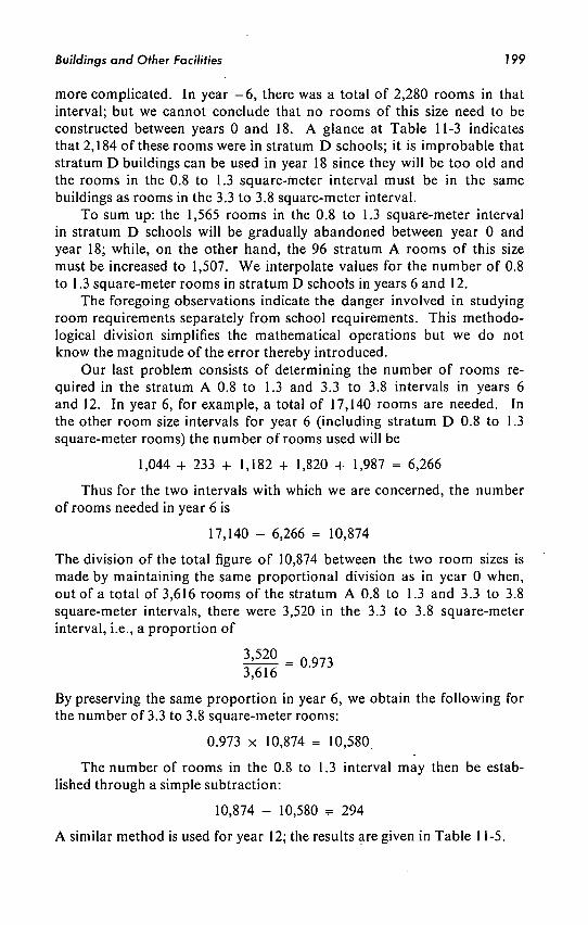
Buildings and Other Facilities 799
more complicated. In year - 6 , there was a total of 2,280 rooms in that interval; but w e cannot conclude that no rooms of this size need to be constructed between years 0 and 18. A glance at Table 11-3 indicates that 2,184 of these rooms were in stratum D schools; it is improbable that stratum D buildings can be used in year 18 since they will be too old and the rooms in the 0.8 to 1.3 square-meter interval must be in the same buildings as rooms in the 3.3 to 3.8 square-meter interval.
T o sum up: the 1,565 rooms in the 0.8 to 1.3 square-meter interval in stratum D schools will be gradually abandoned between year 0 and year 18; while, on the other hand, the 96 stratum A rooms of this size must be increased to 1,507. W e interpolate values for the number of 0.8 to 1.3 square-meter rooms in stratum D schools in years 6 and 12.
The foregoing observations indicate the danger involved in studying room requirements separately from school requirements. This methodological division simplifies the mathematical operations but w e do not know the magnitude of the error thereby introduced.
Our last problem consists of determining the number of rooms required in the stratum A 0.8 to 1.3 and 3.3 to 3.8 intervals in years 6 and 12. In year 6, for example, a total of 17,140 rooms are needed. In the other room size intervals for year 6 (including stratum D 0.8 to 1.3 square-meter rooms) the number of rooms used will be
1,044 + 233 + 1,182 + 1,820 + 1,987 = 6,266
Thus for the two intervals with which w e are concerned, the number of rooms needed in year 6 is
17,140 - 6,266 = 10,874
The division of the total figure of 10,874 between the two room sizes is made by maintaining the same proportional division as in year 0 when, out of a total of 3,616 rooms of the stratum A 0.8 to 1.3 and 3.3 to 3.8 square-meter intervals, there were 3,520 in the 3.3 to 3.8 square-meter interval, i.e., a proportion of
m • °™ By preserving the same proportion in year 6, w e obtain the following for the number of 3.3 to 3.8 square-meter rooms:
0.973 x 10,874 = 10,580.
The number of rooms in the 0.8 to 1.3 interval m a y then be established through a simple subtraction:
10,874 - 10,580 ,= 294
A similar method is used for year 12; the results are given in Table 11-5.

200 Buildings and Other Facilities
11-4.2 High School Total Number of Rooms Needed
The method used to estimate the number and sizes of rooms required to meet provisional targets at high school level is similar to the method employed with respect to the elementary school level: the first step is to estimate the total number of rooms required and the second is to determine the sizes required.
Once again, three alternatives are considered in estimating the total number of rooms needed. In the first case, rooms in year 18 are assumed to be in use for the same number of periods as stratum B rooms in year - 6 ; in the second case, half of the periods are assumed to be offered in rooms used for 32 hours per week and the other half in rooms used 64 hours per week; in the third case, one-third of the periods are assumed to be provided in rooms used for 32 hours per week and two-thirds in rooms used for 64 hours per week. Target values for these three alternatives are shown in Table 11-6.
Table 11-6. Planiland: Number of Classrooms and Laboratories Required to A ttain the Provisional Targets for High School Education
Year
0 6
12 18
Number of Periods of Education Offered
H
47,480.60 103,662.51 172,932.67 356,908.75
First Alternative
Periods per R o o m
hr
28.78 28.75 28.71 28.67
N u m b e r of R o o m s
R
1,650 3,606 6,024
12,449
Second Alternative
Periods per R o o m
hr
28.78 32.84 37.47 42.67
N u m b e r of R o o m s
R
1,650 3,157 4,615 8,365
Third Alternative
Periods per R o o m
hr
28.78 34.85 42.20 51.20
N u m b e r of R o o m s
R
1,650 2,975 4,098 6,971
Required sizes of the rooms are set out in Table 11-7, with the calculations m a d e for the third alternative only. In constructing this table, allowance was made for the fact that, in order to reach the educational output targets, all schools in year 18 must have at least the same facilities as stratum B schools had in year - 6 . It is also assumed that all strata A and B rooms in year 0 can be retained up to year 18 whereas this does not hold for strata C and D rooms, even if some of them m a y have characteristics in c o m m o n with strata A and B rooms needed. For example, there are rooms providing between 0.8 and 1.3 square meters per student in strata A , B , and C ; those in strata A and B can be retained but those in stratum C must be abandoned since the buildings themselves must be abandoned. The same applies to the rooms in intervals 1.3 to 1.8, 1.8 to 2.3 and 2.3 to 2.8.
Stratum A rooms are better than those required to meet the provisional targets and therefore will be not only retained but even increased in number although financial considerations m a y subsequently m a k e it necessary to limit such increases.

Buildings and Other Facilities 207
Table 11-7. Planiland: Number and Sizes of the Classrooms and Laboratories Required to A ttain the Provisional Targets for High School Education
(third alternative)
Square Meters per Student
0.8-1.3 in A - B 0.8-1.3 in C 1.3-1.8 in C - D 1.8-2.3 in B 1.8-2.3 in C 2.3-2.8 in C 2.3-2.8 in A - B 2.8-3.3 in B 3.3-3.8 in A
Total
0
61 64
123 19
340 85
485 265 208
1,650
Year
6
151 42 82 47
226 56
1,200 656 515
2,975
12
229 21 41 71
113 28
1,820 994 781
4,098
18
411 0 0
125 0 0
3,258 1,781 1,396
6,971
The procedure used in estimating the figures in Table 11-7 is identical to that employed above with respect to elementary schools.
11-4.3 College Total Number of Rooms Needed
Estimates of the number of rooms required to reach the provisional targets for the college level are presented in Table 11-8. Three alternatives are again considered.
Table 11-8. Planiland: Number of Classrooms and Laboratories Required to A chieve the Provisional Targets for the College Level
Year
0 6
12 18
N u m b e r of Periods of Education Offered
H
5,516.39 8,008.33
12,609.63 22,055.22
First Alternative
Periods per R o o m
h,
16.35 16.35 16.35 16.35
N u m b e r of R o o m s
R
337 482 759
1,327
Second Alternative
Periods per R o o m
hr
16.35 20.45 25.59 32.00
N u m b e r of R o o m s
R
337 385 485 678
Third Alternative
Periods per R o o m
hr
16.35 22.00 29.62 40.00
N u m b e r of R o o m s
R
337 358 419 542
The number of periods per week during which a room m a y be used at college level does not depend on the concentration of the population, in contrast to the case of the elementary and high school levels where some schools are in rural or semirural districts with enough students to justify no more than one shift.
All colleges are situated in cities but a limitation on hours of classroom utilization might nonetheless be imposed very often by the fact that large numbers of college students have jobs and find it difficult to attend classes during working hours. Planners must therefore evaluate the

202 Buildings and Other Facilities
possibility of inducing a change in this situation before determining the number of periods per week during which rooms m a y be used.
The operations used to obtain the values in Table 11-8 are identical with those used to calculate the value in Tables 11-4 and 11-6 for the elementary and high school levels.
It is easier in the case of the college level than in the case of elementary and high school levels to establish the sizes of rooms required because the conditions prevailing in year 0 must prevail in year 18. Thus, all that is necessary is to preserve the year 0 proportions in years 6, 12, and 18. Required numbers of different-sized classrooms are shown for the third alternative in Table 11-9.
Table i 1-9. Planiland: Numbers and Sizes of the Classrooms and Laboratories Required to A ttain the Provisional Targets for the College Level (third alternative)
Square Meters per Student
2.3-2.8 2.8-3.3 3.3-3.8
• 3.8-4.3
Total
0
9 32 199 97
337
Year
6
10 34 211 103
358
12
11 40 247 121
419
18
14 51 320 157
542
11-5 Some Additional Problems
Besides determining the numbers and sizes of the school rooms needed to achieve the provisional targets of the educational plan, the planner must solve other problems related to buildings and facilities.
O n e problem concerns the concentration of rooms for classes and laboratories. T h e choice is between small schools with a few single-section grades and large schools in which each grade is divided into several sections. The solution of this problem is closely related to the problem of the location of schools since, clearly, large schools are needed wherever there is a heavy concentration of the population.
There is then a second problem: the materials used in building schools and the frequency with which schools must be replaced. Brief comments will be m a d e below with respect to these two problems.
11-5.1 Optimum Size and Location of a School
In determining the sizes of classes and the characteristics of classrooms and laboratories required to attain educational planning targets w e have so far used the quality of education as our basic criterion.
However, if w e shift our attention from classrooms to schools, the problem is rather different. It seems reasonable to assume that by itself

Buildings and Other Facilities 203
the size of schools probably has little influence on educational quality or, at any rate, m u c h less influence than the characteristics of teachers and rooms. Let us consider two schools, one with three times as m a n y students as the other but both with teachers and rooms of similar characteristics and with the same number of students attending each period. T h e larger school has three first grades, three second grades and so on; the other has one of each. It would seem a justifiable conclusion that the quality of education in both schools is the same. Qualitative criteria therefore cannot be used to determine the appropriate size of schools. A n y decision as to the size of schools is dependent on the decision as to the number of schools; and both decisions are closely related to the problem of location.
Since there is no qualitative criterion with which to determine size of schools, it m a y be asked w h y they should not be reduced to a m i n i m u m dimension—that is, one-grade schools or, conversely, enlarged to the m a x i m u m extent, one high school for the whole country. The reason for rejecting these extremes is obvious. W h e n a school is unduly small, certain facilities such as laboratories and libraries are only partially utilized so that, for a given quality of education, excessively small schools are also excessively costly. O n the other hand, if schools are unduly large, s o m e students must travel long distances to school and there is thus a corresponding rise in transportation costs.
T h e problem confronting us is to find a way of minimizing the total costs involved in building and operating a school. W h a t must be borne in mind is that it is worthwhile to enlarge a school to the point at which additional savings effected through a more rational use of equipment become less than the additional cost of transporting students from farther away.
In these calculations w e must also consider the further complicating facts that transport costs are paid each day throughout the entire life of school buildings and that it is sometimes possible to provide substitutes for transport, such as student dormitories.
It is clear then that large schools are suitable for densely populated areas and small schools are suitable for areas with a sparse population. T h e question of the appropriate size for a school cannot, therefore, be decided unless something is k n o w n of the population in the area where it is to be located. Similarly, with respect to the ideal location of a school of a given size, a basic consideration is to reduce transport costs to a m i n i m u m .
It should be noted in this context that the cost of transporting students accounts for the vertical integration of schools; i.e., the fact that schools usually are composed of several grades rather than several sections of one grade. Within an area of reasonable size, it is easier to find enough students for several grades than for several sections of one grade.

204 Buildings and Other Facilities
Hence transportation costs will be lower in the case of vertically integrated schools. The need for such integration m a y be regarded merely as a particular form of the problem of opt imum school size.
11-5.2 Determination of the N u m b e r and Location of Schools
The educational planner is familiar with the characteristics of the rooms that must be constructed, the relation between laboratory periods and class periods required to provide education of a certain quality, and the geographical distribution of the population. His problem n o w is to decide h o w to combine laboratories and classrooms to form school buildings so that the cost of constructing schools and transporting students is held to a m i n i m u m . His final solution should include the number of schools required, the facilities which each must possess, the number of students to be taught in each school and the geographic location of the schools.
Since w e are concerned here with overall educational planning, w e shall not pursue further such questions which are primarily of interest to those preparing detailed educational plans.
11-5.3 Determination of Materials to be Used in Constructing Schools
Specific details obviously cannot be given in this regard. Often the central planning authority should m a k e the decision on type of construction, since materials suitable for one type of school in one area m a y not be suitable for other types of schools in other areas.
Nonetheless, all buildings have one characteristic in c o m m o n : they must be maintained. Maintenance costs vary with the age of buildings and the materials used in their construction. A s a general rule, the older the building and the lower the quality of the building materials, the higher the maintenance costs. Thus if construction costs are increased there is likely to be a long-run reduction in maintenance costs.
The planner, therefore, is confronted with the problem of balancing increased construction costs against reduced maintenance costs in order to find the type of construction which minimizes total costs in the long run.
References
Correa, H . , "Optima for Size and Number of Schools," Scientia Paedagogica Experimentalis, Vol. 3, N o . 1 (1966).
The approach described in this chapter is also used in Correa, H . , and E . Reimer, A Simulation Model for Education Planning in
Puerto Rico. San Juan: Department of Public Instruction (Mimeographed), 1969.

chapter I A
Costing and Financing
the Educational Plan
12-1 Content of This Chapter
In a study of the costs and financial aspects of an educational plan two basic elements must be considered: (a) the sources of the funds and (b) the uses of the funds. T h e method of analysis of these two aspects is similar to that of previous chapters. With respect to the sources of funds, w e will study their characteristics in the past and the factors determining the funds available to education. Next, the relationship between the sources of the funds and the factors determining them must be established. With this information and that of the development of the determining factors, it is possible to project the funds that will be available to education. A similar analysis should be m a d e with respect to the use of the funds.
A n additional step is required in the study of sources and use of educational funds. The past relationships between sources and use must be analyzed.
With the studies described above, w e will be able to estimate the cost of meeting the educational targets; then w e will be in a position to determine if these costs can be met out of funds likely to be available to education.
If estimated values for funds needed and funds available are in harm o n y or if the difference between them is not too large, it is likely that it will be possible to finance the educational plan as it is. If this is not the case, it will be necessary to study the possibility of reducing the expenditures on education while still attaining the provisional targets. If this were not possible, the targets themselves might need to be revised.
Unfortunately, the revision process would not stop there. If the educational targets could not be attained, there might be bottlenecks of qualified m a n p o w e r preventing the full implementation of the economic plan. Thus it might be necessary to revise the economic plan also. If the eco-
205

206 Costing and Financing the Educational Plan
nomic plan had to be revised, the initial estimate of resources available for education might also have to be altered. With this, w e would be right back to the place where w e started, and the process of successive approximations would have to be continued.
72-2 Past and Present Costs of Education
12-2.1 Cost Categories
Educational expenditures will be discussed below under three main headings: teachers, buildings, and equipment and other costs.
12-2.2 Past and Present Expenditures on Teachers
Figures on the n u m b e r and qualifications of teachers and the n u m b e r of hours that they teach in each of the levels of the educational system in Planiland were presented in Table 10-11. T h e data on salary per period for the teachers with different qualifications appear in Table 12-1. T h e
Table 12-1. Planiland: Teachers'Salaries per Period (thousands of year 0 dollars)
Line N o s . , Table 10-11
Qualifications Year
-12 -6 0
Elementary School
(1) (2) (3) (4) (5) (6)
Graduates high school teachers' education Graduates high school general education Dropouts high school teachers' education Dropouts high school general education Graduates elementary school Dropouts elementary school
12.09 9.25 6.14 3.51 3.05 2.99
14.75 11.25 7.50 4.25 3.75 3.50
17.80 13.75 9.05 5.10 4.25 4.00
High School
(7) (8) (9)
(10)
(11) (12) (13) (14)
Graduates college teachers' education Graduates college general education Dropouts college teachers' education Dropouts college general education Graduates high school teachers' education Graduates high school general education Dropouts high school teachers' education Dropouts high school general education
20.30 20.42 16.35 16.52 12.39 9.95 6.70 4.20
25.00 25.00 20.00 20.00 15.00 12.00 8.00 5.00
30.25 30.25 25.00 25.00 18.00 14.25 9.50 5.75
College
(15) (16) (17) (18) (19)
Graduates college teachers' education Graduates college general education Dropouts college teachers' education Dropouts college general education Graduates high school teachers' education
40.00 40.00 25.00 25.00 17.50
50.00 50.00 30.00 30.00 20.00
60.50 60.50 36.00 36.00 23.00

Costing and Financing the Educational Plan 207
data in these two tables permit us to calculate the total amount paid to teachers in years - 1 2 , - 6 , and 0. T h e operations used for this calculation are so simple that they are not described. The results appear in Table 12-2.
Table 12-2. Planiland: Total Expenditures on Teachers' Salaries (thousands of year 0 dollars)
Level
Elementary school High school College
Year
-12
67,765 11,899 3,526
-6
134,713 26,163
6,984
0
267,201 62,819 15,963
T h e study of past experience with regard to the expenditures on teachers'salaries does not end with the results presented in Table 12-2. Actually, the main objective of this analysis has not yet been attained since w e have not discussed past relationships between expenditures on teachers' salaries and the main factors determining the level of these expenditures.
In the computation of the total expenditures for teachers' salaries, the main determinants of these expenditures were considered: i.e., number of teachers, number of periods that each teacher teaches and salary per period. In Chapter 10, remarks were m a d e about the factors determining the demand for teachers, so attention will be paid here only to the question of salaries per period.
Economists in general and labor economists in particular have studied a great m a n y factors determining the changes of salaries. W h e n , in the preparation of an educational plan, the time comes to study teachers' salaries, it is advisable to consult the economists. However , if the planner cannot, for any reason, benefit from such expert advice, he himself can use the economists' most elementary technique: comparison of the rate of growth of teachers' salaries with the rate of growth of per capita income.
Table 12-3. Comparison of Growth Rates of Salaries of Type 1 Teachers with Growth Rates of Per Capita Income
Year
-12
-6
0
Annual Salaries, Type 1 Teachers
Salaries
17,306
21,476
25,917
Rate of Growth
0.241
0.207
Per Capita Income (Table 3-6)
Income
2,299
2,783
3,349
Rate of Growth
0.210
0.203

208 Costing and Financing the Educational Plan
Such a comparison for salaries of teachers with qualification level 1 is presented in Table 12-3. W e see that salaries for this type of teacher and per capita income have grown at almost the same rate. The same result can be obtained with regard to all other types of teachers. This information will be used in the estimation of the future growth of teachers' salaries per period.
12-2.3 Past and Present Expenditures for Buildings and Equipment
Including Construction and Equipment
The numbers of classrooms and laboratories of different dimensions owned by the educational system was shown in Table 11-2. These figures permit us to estimate the number of rooms constructed and equipped in the periods between years - 1 2 and - 6 and between years - 6 and 0. For this, w e use two steps which will be explained with reference to the period between years - 1 2 and - 6 . First, from the number of rooms in year - 1 2 , the number still in use in year —6 must be determined. Second, the n u m ber of rooms constructed can be found by subtracting from the number available in year —6 those surviving from year — 12.
The first step is always more or less arbitrary. In some cases it is omitted, based on the assumption that a building weil maintained will last forever. In any case, there is no scientific rule to determine the proportion of the buildings that will cease to be usable in any period. Here w e have assumed that each building lasts 75 years and that over each six-year period 8 percent of the buildings cease to be useable. In Table 12-4, the number of surviving rooms and the number constructed in two periods between years - 1 2 and 0 are presented.
In the same table the dollar costs of constructing and equipping classrooms and laboratories of different sizes are presented. It might seem surprising that the same prices are valid for construction in both the time periods considered. W e should remark that w e are dealing with "constant prices"; that is, the actual prices are deflated by means of a price index. Even in this case, it is likely that some changes in the prices will occur, but as a first approximation, if no other information is available, the prices of year 0 are taken as valid for years —6 and - 1 2 .
Another point that deserves comment is that the salaries of teachers measured in constant dollars change, while the costs of constructing buildings do not change. This might seem a contradiction, but actually it is the essence of welfare growth as measured in terms of per capita income in constant dollars. Real salaries increase because the productivity of labor increases; consequently the "constant dollar" prices of goods remain more or less unchanged.
Multiplying cost per room by the number of rooms constructed and equipped, w e calculate total expenditure on construction and equipment in six years. A rough estimate of expenditure in one year is obtained by

Costing and Financing the Educational Plan 209
Table 12-4. Planiland: Classrooms and Laboratories Constructed and Equipped
Size, Square Meters
per Student
Construction Cost per Unit
(year 0 dollars)
Between - 1 2 and - 6
Surviving from - 1 2
in - 6
Constructed in Period
Between - 6 and 0
Surviving from - 6
inO
Constructed in Period
Elementary School
0.8-1.3 1.3-1.8 1.8-2.3 2.3-2.8 2.8-3.3 3.3-3.8
Total
10,822 17,927 25,032 31,138 38,243 45,349
1,320 —
1,144 356 620 938
661 — 371 121 740 986
2,879
1,822
— 1,394
439 1,251 1,770
1,901 1,729 1,750
5,380
High School
0.8-1.3 1.3-1.8 1.8-2.3 2.3-2.8 2.8-3.3 3.3-3.8
Total
13,385 21,513 30,027 27,363 45,689 54,015
74 31
151 38 44 49
36 14 92 57 81 94
374
101 41
223 87
115 132
9 — 8
483 150 76
726
College
2.3-2.8 2.8-3.3 3.3-3.8 3.8-4.3
Total
39,800 49,791 57,954 68,116
10 17 67 . 14
—
5 43 29
77
8 20
101 40
1 12 98 57
168
dividing the six-year totals by six. Estimates of yearly construction ex
penditures for years - 6 and 0 m a y be m a d e in this w a y .
This method cannot be used to m a k e estimates for year —12. Data
for this year must be obtained from other sources. Yearly construction
figures for all three years are in Table 12-5.
Table 12-5. Planiland: Estimated A nnual Expenditure for Construction (thousands of year 0 dollars)
Level
Elementary school High school College
-12
8,324 976 311
Year
-6
15,537 2,409
786
0
34,106 4,894 1,700

270 Costing and Financing the Educational Plan
Expenditures for renting classrooms and other equipment
In Table 11-2 w e see that some of the facilities used by the educational system are rented. Figures on the rents paid are presented in Table 12-6; the total amounts of rental payments are given in Table 12-7. The rents per room in years - 1 2 , - 6 , and 0 are constant as were the construction costs, and for a similar reason.
Table 12-6. Planiland: Yearly Rent per Room for Years —12, -6, and 0 (thousands of year 0 dollars)
Size, Square Meters per Student
Elementary School
0.8-1.3 1.3-1.8 1.8-2.3 2.3-2.8
High School
0.8-1.3 1.3-1.8 1.8-2.3
Rents
541 896
1,252 1,557
669 1,075 1,502
Table 12-7. Planiland: Annual Expenditures on Rent (thousands of year 0 dollars)
Level
Elementary school High school College
-12
696 120
Year
-6
1,101 188
0
1,763 291
Maintenance expenditures
T h e information available on maintenance expenditures in Planiland is presented in Table 12-8.
Table 12-8. Planiland: Maintenance Expenditures (thousands of year 0 dollars)
Level
Elementary school High school College
-12
3,923 399 322
Year
-6
6,404 711 323
0
11,758 1,617
601

Costing and Financing the Educational Plan 277
1 2 - 2 . 4 Other Expenditures
In Table 12-9 figures on all the categories of expenditures not previously considered are presented. N o special analysis of the information in this table is required.
Table J2-9. Other Current Expenditures (thousands of year 0 dollars)
Type of Expenditure Year
-12 -6 0
Elementary School
Supervision Administration School materials Libraries Restaurants for students Board for students Scholarships
Total
4,973 13,937 8,297 7,543
15,765 — —
50,525
6,585 20,666 10,984 9,985
17,450 — —
65,670
7,913 27,816 13,200 12,000 25,080
— —
86,009
High School
Supervision Administration School materials Libraries Restaurants for students Board for students Scholarships
Total
2,234 7,299 1,397 984 —
1,995 2,236
16,145
3,814 13,424 2,294 1,616
— 3,405 3,668
28,221
5,242 21,504
3,281 2,312
— 4,680 5,248
42,267
College
Supervision Administration School materials Libraries Restaurants Board for students Scholarships
Total
420 1,824
181 80 —
375 363
3,243
706 3,285
291 130 —
630 583
5,625
1,176 6,233
493 220 —
1,050 985
10,157
12-2.5 Summary
A s u m m a r y of the results presented in Tables 12-2, 12-5, 12-7, and 12-9 appears in Table 12-10. In this table, the total expenditures by level of education and the total expenditures on education in Planiland are presented.
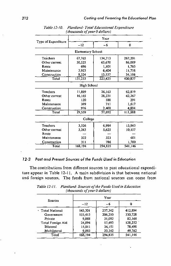
272 Costing and Financing the Educational Plan
Table 12-10. Planiland: Total Educational Expenditure (thousands of year 0 dollars!
Type of Expenditure Year
-12 -6 0
Elementary School
Teachers Other current Rents Maintenance Construction
Total
67,765 50,525
696 3,923 8,324
131,233
134,713 65,670
1,101 6,404
15,537 223,425
267,201 86,009
1,763 11,758 34,106
400,837
High School
Teachers Other current Rents Maintenance Construction
Total
11,899 16,165
120 399 976
29,559
26,163 28,221
188 711
2,409 57,692
62,819 42,267
291 1,617 4,894
111,888
College
Teachers Other current Rents Maintenance Construction
Total
3,526 3,243
— 322 311
168,194
6,984 5,625
— 323 786
294,835
15,963 10,157
— 601
1,700 541,146
72-3 Past and Present Sources of the Funds Used in Education
T h e contributions from different sources to past educational expendi
ture appear in Table 12-11. A main subdivision is that between national
and foreign sources. T h e funds from national sources can c o m e from
Table 12-11. Planiland: Sources of the Funds Used in Education (thousands of year 0 dollars)
Sources
• Total National Government Private
Total Foreign Aid Bilateral Multilateral
Total
-12
143,301 133,413
9,888 24,894 15,011 9,883
168,194
Year
-6
237,342 206,250
31,092 57,493 34,151 23,342
294,835
0
412,894 330,728
82,166 128,252 ' 78,490 49,762
541,146

Co
stin
g a
nd
F
inan
cin
g th
e E
du
catio
nal P
lan
213
Total College High School Elementary School
0 a t i ; 0
Total Capital Current Total Capital Current Total Capital Current
n
i H 3 1
330,728 82,166
3,513 1
1
3,513 11,812 13,561
1,514 351
10,298 13,210
315,403 68,605
13,504 3,773
301,899 64,832
Government sector Private sector
412,894 3,513 1 3,513 25,373 1,865 23,508 384,008 17,277 366,731 National total
78,490
49,762
16,309
8,599
1,700 14,809
8,599
48,351
38,164
1,199
1,830
47,152
36,324
13,830
2,999
13,830
2,999
1
1
Bilateral foreign aid
Multilateral foreign aid 128,252 24,908 1,700 23,208 86,515 3,029 83,486 16,829 16,829 1
Foreign aid total 541,146 28,421 1,700 26,721
oo oo O
O 4,894 106,994 400,837 34,106 366,731 Grand total

214 Costing and Financing the Educational Plan
either the government or private citizens and organizations. In s o m e cases, it m a y be useful to subdivide further government funds into those from the national government and those from provincial and local governments. However, this additional subdivision does not appear in Table 12-11.
Foreign assistance for education m a y c o m e from either bilateral or multilateral aid-giving agencies. Bilateral foreign aid is that given by one country to another; multilateral aid is that given by an international organization such as U N E S C O , I L O , or the World Bank ( I B R D ) . A m o r e detailed analysis of the data in Table 12-11 for year 0 is presented in Table 12-12.
T h e main reason for the study of the sources of funds used in education is to analyze the factors influencing the amount of money available for education.
O n e of the main determinants of the expenditure on education from national sources is the total amount of national output, i.e., G D P . A comparison of national expenditure on education and G D P appears in Table 12-13. In the same table, the expenditures from the public and pri-
Table 12-13. Planiland: Comparison of National Resources A vailable and Expenditures on Education (millions of year 0 dollars)
Year
- 1 2 - 6
0
Total Economy
GDP a
6,805 9,782
13,932
Education b
143 237 413
- x 100 a
2.10 2.42 2.96
Public Sector
Total c
1,194 1,762 2,492
Education d
133 206 331
- x 100 c
11.13 11.69 13.28
Private Sector
Total e
5,611 8,020
11,440
Education
I 10 31 82
£ x 100 e
0.18 0.39 0.72
vate sectors (elaborated from Tables 3-2 and 3-3) are compared with the total resources available to each sector. In some cases it is useful to divide even further the items in Table 12-13; for example, all items in the table could be subdivided into investment, on the one hand, and consumption and current expenditure, on the other.
T h e results in Table 12-13 will be used for estimating the future automatic development of the resources available for education.
72-4 Educational Expenditures Required to Attain the Targets of the
Educational Plan
12-4.1 Expenditures for Teachers
T o estimate the expenditures on teachers required to attain the targets of the educational plan, w e must have three sets of information: (a) N u m b e r and qualifications of teachers required in years 0, 6, 12, and

Costing and Financing the Educational Plan 215
18. This information, obtained in Sec. 10-4.3, appears in Tables 10-14, 10-16, and 10-19.
(b) Future development of the n u m b e r of periods taught by teachers of the different types. This information is presented in Tables 10-17 and 10-20.
(c) Future development of the salaries per period for the teachers of the different types. This information is obtained below.
Future development of teachers' salaries
For an estimate of the required expenditures on teachers, a projection of the future development of teachers' salaries is needed. In Sec. 12-2.2 w e noted that the person best qualified to prepare such a projection is a labor economist. Here, only the most elementary method used by labor economists will be employed.
In Table 12-3 the rate of growth of the salaries of teachers of type 1 was compared with the rate of growth of per capita income. C o m m e n t i n g
Table 12-14. Planiland: Future Development of Salaries Per Period (year 0 dollars)
Line Nos. , Table 10-11
Qualifications Year
6 12 18
Elementary School
(1) (2) (3) (4) (5) (6)
Graduates high school teachers' education Graduates high school general education Dropouts high school teachers' education Dropouts high school general education Graduates elementary school Dropouts elementary school
21.64 16.72 11.00 6.20 5.17 4.86
26.36 20.36 13.40 7.55 6.30 5.92
32.10 24.80 16.32 9.20 7.67 7.21
High School
(7) (8) (9)
(10) (11) (12) (13) (14)
Graduates college teachers' education Graduates college general education Dropouts college teachers' education Dropouts college general education Graduates high school teachers' education Graduates high school general education Dropouts high school teachers' education Dropouts high school general education
36.78 36.78 30.40 30.40 21.89 17.33 11.55 6.99
44.80 44.80 37.03 37.03 26.66 21.11 14.07 8.51
54.56 54.56 45.10 45.10 32.47 25.71 17.13 10.37
College
(15) (16) (17) (18) (19)
Graduates college teachers' education Graduates college general education Dropouts college teachers' education Dropouts college general education Graduates high school teachers' education
73.57 73.57 43.78 43.78 27.97
89.61 89.61 53.32 53.32 34.07
109.14 109.14 64.95 64.95 41.49

276 Costing and Financing ihe Educational Plan
on this comparison, w e observed that the salaries of all types of teachers in Planiland grew in the past at a rate similar to the growth rate of per capita income. For this reason, the estimates of the future development of teachers' salaries are m a d e on the assumption that teachers' salaries will grow in the future at the same rate as per capita income. These projections of teachers' future salaries appear in Table 12-14.
It is probable that in some countries the rates of growth of the salaries of teachers is different from the rate of growth of per capita income. In this case, it is advisable to use the elasticities of the teachers salaries with respect to per capita income. These elasticities are
Rate of growth of teachers salaries Rate of growth of per capita income
Since the use of elasticities to estimate the future values of a variable has been explained several times, no further elaboration of this procedure is presented here.
Estimation of future expenditures on teachers
There is no need to explain the operations used to estimate the required expenditures for teachers. T h e projections appear in Table 12-15.
Table 12-15. Planiland: Expenditures on Teachers' Salaries Required to A ttain the Targets of the Educational Plan (thousands of year 0 dollars)
Level
Elementary school High school College
6
560,386 179,200 28,190
Year
12
1,179,987 379,045
54,043
18
2,227,813 973,753 115,134
12-4.2 Expenditures for Buildings and Other Equipment
In Sec. 11-3 the number of rooms required to attain the targets of the educational plan w a s estimated; such estimates m a y be found in Tables 11-5, 11-7, and 11-9. Using these figures, w e must estimate construction and equipment costs, expenditures in rents and maintenance costs over future years.
Expenditures on construction, equipment, and rents
T o pass from the data concerning the number of rooms and laboratories needed to an estimate of construction and equipment costs, two sets of estimates are necessary: the number of rooms that must be constructed in future years and the future construction and equipment costs per r o o m . With these, w e m a y proceed to the determination of the total expenditures

Costing and Financing the Educational Plan 217
for construction and equipment necessary to attain the targets of the educational plan.
Number of rooms that must be constructed
In order to estimate the number of rooms that must be constructed, w e need to k n o w the proportion of new rooms that will be rented rather than owned. W e assume here that, as a matter of policy, all the new rooms required for the educational system will be owned. The rooms rented in previous years can be maintained if required; but, if a new room of a specified type is required, it must be constructed. With this assumption it is possible for us to determine the number of rooms that will have to be constructed as well as the number of rooms that will have to be rented. The steps required are explained with respect to the rooms to be constructed for elementary school between years 0 and 6.
The first step for this estimation is to determine the number of rooms existing in year 0 which will still be usable in year 6. The methods used for this estimation and their limitations are discussed in Sec. 12-2.3.
Next, comparing the number of year 0 rooms being used in year 6 to the number required in year 6 (see Tables 11-5, 11-7, and 11-9), w e can determine the number of rooms that have to be constructed, rented and abandoned between years 0 and 6. These figures are all found in Table 12-16.
Future development of construction and equipment costs and of rents
A s mentioned in Sec. 12-2.3, the use of year 0 dollar prices of goods and services in cost calculations allows us to suppose that the construction and equipment costs and rents in future years will remain at about the same level as in year 0. Hence, the values in Table 12-4 for construction and equipment costs and in Table 12-6 for rents will be assumed to be the values prevailing up to year 18.
It should tie observed that the construction and equipment costs given in Table 12-4 include the cost of the land on which buildings are built. However, some of the new buildings to be constructed to achieve the targets of the educational plan might be constructed on land already owned by the educational system. But, in this case other special types of expenditure are likely to be required. Since the computations in this book are intended to give an approximate picture, no modifications are introduced to handle such complications.
The data introduced above permit us to estimate construction and equipment costs for six-year periods. A s before, a rough estimation of yearly costs is obtained by dividing the six-year values by six. Estimated yearly cost figures appear in Table 12-17.

278
Costing a
nd
Financing the Educational P
lan
-ÇS <u
SJ
s v.
s:
U <u Mus
ï§ c
^
•S
ratones tional P
o
a
-O
NJ
3Í
§-$
^ O
<o
"3
SO
"3
».
•SfS
•- sí
NU -5
umb Atta
<s
Hand Plan
<N
<u Tabl
OO
•o
c
C
u
£
u
•o c
so
c
u
s
00
NO
•o c
o
c
s
CQ
Rented
f §1
g
u S
•^
.o
«
Re
qu
ired
™0
O
M
.- •-
O •-
u
U
*"* U
2>" >"
C/3 R
ented
2 ¿"S
Re
qu
ired
C«
N
O
>
i- E
•-
•Es.es
3>* •*
Ren
ted
o
¿ •o
*• .o
w
Re
qu
ired
BO
CV
S
O
'> S E !s
•> s s s C
/3
U S. c
S S
-ë
1
o
OO
o\
p-
o
in
p-
(N
in l
r*i O
m
m
p-
<n
o
(N 1
8 CM
•*
»
CN
00
oo
< c
m
—
00
o
1
1
1
o
oo
•g-1
1
«N
in
in
s ON
1
1
rs
•*
(N
< C
_, O
c
m
—
0
0
o
1
1
1
1 116 1
»o 1 233 1
rn
m
(N |
OO
-"• m
— 1
1
1
>n
•*r »n
I I
CN
O
N
»n 008
so
o
o 1
r
oo
SO
$ m
(N
OO
— 1
1
1
r-m
oo 1
1
O
ON
NO
1
1
O
oo
m
»n
(N
OO
<N
m
(N
1 1
•q-10,9
en
, °>
oo
O
N
CN
•* O
N
—
r-O
N
ON
00*
1
1
o\ .
*n 10,8
TC O
N
ON
(N
ON
N
O
O"
CN
O
en
oo
r—
—
O
N
1
1
CN
7,3
P-
O
oo
oo
as
m
—
O
(N
00
•^
m
P-
<N
(N
m
m
oo
m
m
oo m
(N
n-¡
1
S — 1
o
ON
ON
ON
1
»n
SO
CQ
1 1
1
ON
1
1
r-i
ON
m 1
1
CN
i
«n
•<
*
1 1
1 s
1
p^
1
,-J"
»n
I
<N
OO
C'
en
a «n
fN
»n
sO 1
OO
p^
m
-ít 1
O
m
p-
Tt
p-
1
1
1
1
Tt
o 1
1
rn
ON
m 1
VO
<N
(N
»n
ON
1
•* 1,5
00
un
CN_ en
*
•* 1,6 1
716 o
C
N
OO
en 1
Tt
in
p-
s 1,2
NO
5
1 1
i i
NO 1
1
OO
(N
(N 1
1
SO
<n
r-OQ
1
r-NO
O
O
00
t--_
•<t O
N
1 390
•t O
N
ON
1
(N
•*
NO
»n
N
O
? (N
1
r-NO
NO
O
N
en
ON
t-1 307
oo
r-Tt
Tt 1
Tf
CM
»n
*n
Os
<U
ÛC
Û<
JU
<C
Q<
c
m
—
oo
O
c
en
—
00
O
c
00
—
m
— c
m
<N
OO
—
C
m
(N
OO
— C
00
<N
f<ï
rN
c
00
ÍN
f>
(N
C
m
m
00
CM
C
oo
m
en
m
1
•*
2 o 1
CS
-ON
1
CN
O
00
2.3-2.8
1
TT
»n
p* 1
ON
? en 1
•n
en
ON
C
N 2.8-3.3
1
m
ON
320 227 1
en
N
O 247 194 1
oo
C
N 211 183 3.3-3.8
1
NO
157
-1
NO
C
N 121
in
ON
1
2 103
ON
o
o 3.8-4.3

Cosiing and Financing the Educational Plan 219
Table 12-17. Planiland: Construction and Equipment Expenditure and Rental Payments Required to A ttain the Targets of the Educational Plan
(thousands of year 0 dollars)
Elementary school High school College
Year
6
Construction
55,640 11,067
482
Rent
316 95
12
Construction
82,283 10,491
891
Rent
104 7
18
Construction
83,920 23,214
1,557
Rent
—
Maintenance costs
T h e data in Table 12-8 permit us to evaluate maintenance costs per classroom in years —12, —6, and 0. Figures for these costs appear in Table 12-18.
Table 12-18. Planiland: Maintenance Costs per Room (thousands of year 0 dollars)
Year
- 1 2 - 6
0
Elementary School
Total
3,923 6,404
11,758
Number of Rooms , Table 11-3
4,760 7,757
11,477
Dollars per
R o o m
824 882
1,024
High School
Total
399 711
1,617
N u m b e r of R o o m s , Table 11-3
420 761
1,424
Dollars per
. R o o m
950 934
1,135
College
Total
322 323 601
Number of Rooms , Table 11-3
178 184 337
Dollars per
Room
1,809 1,755 1,783
For the estimation of future maintenance costs it is assumed that the level of costs prevailing in year 0 will hold for future years. Table 12-18 shows that per r o o m maintenance costs in constant dollars generally rose over past years; but with a higher proportion of new buildings after year 0, average maintenance costs should not continue to rise. Hence, year 0 cost levels can be used in rough estimates of future maintenance costs.
Table 12-19. Planiland: Maintenance Expenditure Required to A ttain the Targets of the Educational Plan
(thousands of year 0 dollars)
Level
Elementary school High school College
Year
6
17,551 3,377
638
12
24,920 4,651
747
18
32,154 7,912
966

220 Costing and Financing the Educational Plan
With figures for maintenance costs per room and the number of rooms needed to attain the provisional targets of the educational plan, it is possible to estimate the total maintenance costs in future years. Such estimates appear in Table 12-19.
12-4.3 Other Expenditures
Finally, w e have to estimate the amount of "other expenditures" required to attain the targets of the educational plan. T o do so, the most appropriate method would be to study the factors determining these expenditures, the relationship between these factors and the expenditures, and the future changes in the determining factors. That is, to estimate the future changes of the other expenditures w e should apply the method that w e used for estimating the cost of teachers and buildings.
However, in this book w e will obtain a first rough approximation on the assumption that the "other expenditures" maintain a constant relationship to total expenditure on teachers and buildings.
T h e relationships holding in past years are shown in the left half of Table 12-20. Assuming that the proportion observed in year 0 will be maintained in the future, it is possible to estimate "other expenditures" in years 6, 12, and 18. These estimates are presented in the right half of Table 12-20.
12-4.4 S u m m a r y of the Previous Estimates of Expenditures Required to
Attain the Targets of the Educational Plan
A s u m m a r y of the results presented in previous tables appears in Table 12-21.
12-5 Sources of the Funds Required to Attain the Targets of the
Educational Plan
12-5.1 Introduction
A very important step in the preparation of an educational plan is the study of the possibility of obtaining the funds required to attain the targets of the plan. For this, it is necessary to estimate the future changes in the funds available for education, on the assumption that conditions similar to those existing in the past will exist in the future. This kind of estimation is called here "automatic projection."
12-5.2 Automatic Projection of the National Funds Available for
Education
In Table 12-13, expenditures on education from total national production, the public sector and the private sector, were compared to G D P ,

Co
stin
g a
nd
Fin
an
cin
g th
e E
du
ca
tion
al P
lan
2
21
03 ent fc
UJ
~-00 o
o
0\
m
vo
ON
rS
•
t
«n
m
CI
in
O
m
r-o\
8
vO
00
o
p-
VO
m
VO
<n
(N
in
o
in 3
u.
j=
•o
c
CO
0)
J=
u
to
O H
—
«
-,
-o
273
P-
O
oo
m -2,3
273 in
o
o
o
(N
P-
ÛO
(N
273
m
o
0\
OO
m
m
vo
CS
OO
O
C
S
Tt
m
416
»o
o
U"V
r-~
r-W\
626
o
o
00
00
c
•o
3
JO
O
es
vo 609,
VO
r-<N
0\
m
CN
S
VO
P-
P-
vo
es
es
'^
•
_«
es
es
OO
es
in
VO
VO
t-<
3
CU
-C
O
/^^L
a
-o
c
rt t/i
j= o
rt
H
-Cï
607
ON
O
p-
co 1,004,
607
^ o
O
v
Tí
a\
m
607
r-m
ov
607
— o
tN
V
O
Ov
VO
957
— o
r-T
t
ov
(N
206
T)-
—
<T\
m
m
vi
c
TJ
3
P-
^
in
vo
ON
in
o\ o
m
vo
o\ es V
O
p-
in
o
in
es V
O
in
m
TÎ-
CM
m 3 u
SI
•o
c C3
<l>
J=
u
s O
H
,—
s o ,—
-C
l
556
r- o
V
O
556
— o
oo
vo
vn
vv
556
o
o
m
Ov
es
556
3°
CN
oo
695
m
o
CT
v
o
00
779
CT
v O
»O
•<t
00
c T
D
3 ja
-o
a

222 Costing and Financing the Educational Plan
Table 12-21. Planiland: Total Expenditures Required to Attain the Targets of the Educational Plan (thousands of year 0 dollars)
Type of Expenditure Year
6 12 18
Elementary School
Teachers Other current Rents Maintenance Construction
Total
560,386 173,053
316 17,551 55,640
806,946
1,179,978 351,429
104 24,920 82,283
1,638,714
2,227,813 639,881 ,
— 32,154 83,920
2,983,768
High School
Teachers Other current Rents Maintenance Construction
Total
179,200 117,600
95 3,377
11,067 311,339
379,045 239,276
7 4,651
10,491 633,470
973,753 609,962
— 7,912
23,214 1,614,841
College
Teachers Other current Rents Maintenance Construction
Total
Grand total
28,190 16,296
638 482
45,606
1,163,891
54,043 30,959
747 891
86,640
2,358,824
115,134 65,417
966 1,557
183,074
4,781,683
total governmental expenditure and total private expenditure. Since public and private education expenditures seem to follow two different growth patterns, it is better to m a k e separate projections for public and private expenditures on education.
T h e division of G D P into public and private sectors is the concern of the economists. T h e division of the Planiland G D P was shown in Table 3-9.
Private and public resources likely to be available for education are projected using elasticities. T h e details of the method have already been explained and do not need to be repeated here. T h e values of the elasticities used are presented in Table 12-22. T h e projections of national funds available for education are shown in Table 12-23.
In order to judge the reliability of the results in Table 12-23, it is useful to compare them with data from other countries. F r o m such c o m parisons, it can be seen that the proportion of national resources available

Costing and Financing the Educational Plan 223
Table 12-22
Average Elasticity of Private Funds Average Elasticity of Public Funds Available to Education with Respect to Available to Education with Respect to
Total Private Resources Total Public Resources
4.378 1.308
for education is projected to reach levels higher than proportions found in most of the countries of the world. T h e reason for this is that the rapid past growth in the private resources for education in Planiland is assumed to continue in the future. It m a y be decided that a more refined projection of the national resources available to education is required. However , this and other refinements should wait until the complete picture is drawn; at that time, w e will have some idea of the financial feasibility or unfeasibility of the plan.
Table 12-23. Planiland: Projection of National Resources A mailable for Education (millions of year 0 dollars)
Year
6 12 18
Total Economy
GDP a
19,782 28,098 39,885
Education
b
760 1,480 3,143
- x 100 a
3.84 5.26 7.88
Public Sector
Total c
3,620 5,226 7,658
Education
d
530 835
1,343
- x 100 c
14.64 15.97 17.53
Private Sector
Total e
16,162 22,872 32,227
Education
230 645
1,800
£y. 100 e
1.42 2.82 5.58
12-5.3 Automatic Projection of Foreign Aid Funds Available for
Education
T o project the future amounts of foreign aid for education, w e need to k n o w the factors determining the amount of foreign aid for education received. Unfortunately no study of these determining factors is available.
The method to be used here can serve for a rough first approximation. W e m a k e the assumption that the aid-giving countries try to match the efforts of the aid-receiving country. Thus the growth of foreign aid is related to the increase in the amount of national resources devoted to education. In this case, the elasticity of foreign aid with respect to na-
Table 12-24. Planiland: Automatic Projection of Foreign Aid for Education
(millions of year 0 dollars)
Year Value
6 12 18
325 889
2,704

224 Costing and Financing the Educational Plan
tional expenditures on education is used; its value is 1.829. Using this elasticity, w e obtain the projected values s h o w n in Table 12-24.
12-5.4 S u m m a r y
In Table 12-25, the automatic projection of total funds available for education is presented.
Table 12-25. Planiland: A utomatic Projection of Funds A vailable for Education (millions of year 0 dollars)
Year
6 12 18
Total
1,085 2,369 5,847
National
760 1,480 3,143
Foreign Aid
325 889
2,704
72-6 Sfudy of the Financial Feasibility of the Plan
In Table 12-21, the total expenditures necessary to attain the targets of the educational plan were calculated. In Table 12-25, the automatic projection of the resources that can be used in education is presented. A comparison of the two sets of information is m a d e in Table 12-26.
T h e results shown in this table give reasons for an optimistic attitude toward the problem of the financial feasibility of the educational plan. A t least w e see that no major revision of the targets is required.
Table 12-26. Planiland: Comparison of the Resources Required to A ttain the Targets of the Educational Plan and the
Automatic Properties of the Resources A vailable (millions of year 0 dollars)
Year
6 12 18
Resources Required (Table 12-21)
1,164 2,359 4,782
Resources Available (Table 12-25)
1,085 2,369 5,847
H o w e v e r , w e must remember that the automatic projection of resources available for the plan has several serious defects. For this reason, a wise policy is to accept the provisional targets introduced in Chapter 12 while making every possible effort to reduce costs.
References
General studies on costs and educational finance appear in Benson, C . S., The Economics of Public Education. Boston: Houghton Mifflin,
1968. Vaizey, J., The Costs of Education. London: Allen and Unwin, 1958.

Costing and Financing the Educational Plan 225
O n foreign aid: Cerych, L . , Problems of Aid to Education in Developing Countries. N e w York:
Praeger, 1965.
A n application of the method of analysis presented in this chapter appears in Poignant, R . , and J. Hallak, Les Aspects Financiers de l'Education en Côte-d'Ivoire.
Paris: U N E S C O , 1966.
A computerized version of the model in this chapter appears in Correa, H . , and H . Reimer, A Simulation Model for Educational Planning in
Puerto Rico. San Juan: Department of Public Instruction (Mineographed), 1969.

chapter I O
Planning When Alternative
Ways to Achieve the
Targets Are Explicitly
Considered
13-1 Approaches to the Technical Preparation of a Plan Content of This Chapter
In Chapter 1 it was mentioned that two approaches can be used in the technical preparation of a plan. The first one has been presented in the previous chapters where it is assumed that there is only one w a y to obtain the desired ends. For instance, in the chapter dealing with m a n p o w e r requirements, no attention is paid to the possibility of substitution between persons with different kinds of qualifications. In the chapter dealing with costs, the possibility of reducing costs using different educational methods is not even raised. Actually, similar examples can be presented with respect to the topic of each one of the chapters of this book.
Another limitation of the previous chapters is that they omit one of the main problems of educational planning and its integration with economic planning; that is, the problem of adaptation to limited h u m a n and financial resources. W h e n the targets for the economic plan and those for the educational plan were set, it was observed that these targets were provisional because it was not k n o w n if there would be enough h u m a n and financial resources to reach them. Step by step w e verified that there were such resources. First, w e saw that the level of enrollment was high enough to provide the educated personnel required by the economy. Next, the availability of teachers was verified, and, finally, that of financial resources. However, this process of verification was m a d e somewhat outside the main trend of the analysis. In addition, there is no clearly outlined approach when it is found that, for example, the
226

Alternative Ways to Achieve the Targets 227
number of professors available will not be enough to attain the targets for enrollment. In the extreme case, it is necessary to revise downward the enrollment targets; but no practical method to do so is presented in the previous pages. The only possibility is a time-consuming trial-and-error approach.
In the second approach to the technical preparation of a plan, the different methods to obtain a desired end and the limitations of resources are explicitly taken into consideration, with the purpose of selecting the best possible method for the objectives in mind. A simple example which shows the characteristics and possibilities of this approach is presented below. Limitations of space do not permit us to go into all the details of this second approach. T h e interested reader should consult the references at the end of this chapter.
73-2 Quantity Versus Quality in Teachers' Education
In this section one of the mathematical techniques used to study the problem of choice a m o n g alternatives is applied to the problem of choice between quantity and quality in teachers' education.
Three main steps must be considered in the statement of the problem. The first is to define with precision the product of education; it should be noted that it is always possible to m a k e a definition useful for practical purposes. The second step is to relate the product of education to the inputs used to obtain it. Finally, the cost of the inputs and the limitations on financial resources are considered.
Below, to simplify the analysis, w e assume that it is possible to train two types of teachers. The first are well qualified, the second not so well qualified. The cost of training these two types is not the same; it will be more expensive to train the qualified type than the nonqualified type.
. In order to be able to choose between these two types of teacher training, it is necessary to relate them to the product of education. It is assumed that a group of students enrolls and without any dropouts attends school up to a certain level. Once this level is reached, all of the would-be dropouts actually leave school. The reduced group continues in school until graduation. Thus
n, = number of students w h o can be enrolled using teachers of type /, part of w h o m will drop out later, /' = 1, 2
gi = number of students w h o can be graduated with teachers of type /'
The distinction between the number of students enrolled up to a certain level and the number of graduates does not characterize with enough precision the product of education. A simple method to quantify the qualitative differences a m o n g the different types of graduates and dropouts is to consider the income that they will receive.

228 Alternative Ways to Achieve the Targets
In Table 13-1 the income levels of dropouts and graduates from educational types 1 and 2 are presented.
Table 13-1. Lifetime Income for Persons with Different Types of Education
(thousands of dollars)
Level of Education
Dropouts Graduates
Type of Education
Type 1
180 250
Type 2
150 200
With the income figures in Table 13-1 the total product of education is
Z = 180«, + 70s, + 150«2 + 50#2 (13-1)
In E q . 13-1 w e use 50 and 70 as coefficients of the number of graduates g| and g2 because it is simpler to consider the graduates and the dropouts together forming total enrollment n¡. Thus, to the total income obtained by those enrolled, the additional income of those graduating is added. With this, Zin Eq. 13-1 represents total income to be produced by the educated persons.
Educators will not be happy about using income as a measure of the quality of education, and there is no need to do so. Another simple measurement would be years of study. In this case, if one graduate attends school for six years and one dropout three, one graduate is worth twice as m u c h as one dropout. The meaning of Z , then, in E q . 13-1 will be the total number of years in school.
If the number of years spent in school are not equivalent, it could be said, for instance, that one year with type 1 teachers is equivalent to 1.5 years with type 2 teachers. Corrections of this sort can be introduced until the person w h o must m a k e the decision is satisfied. In principle, this is possible as long as criticism of one measure is accompanied by some idea of h o w it can be improved. In any case, the mathematical method would be the same as that already used; that is, the number of graduates and total enrollment will be multiplied by some weights. Thus Eq . 13-1 is general. T h e coefficients of n¡ and g¡ must be known if teacher training is to be evaluated and a choice among the different types of teacher training must be made . Perhaps a useful task would be to find the best possible weights to be used under different circumstances.
Once the function Z is defined, that is, once appropriate weights have been found, the optimum use of the resources available for teacher train-

Alternative Ways to Achieve the Targets 229
ing can be clearly stated. This optimum use is to maximize Z . There is no question about the usefulness of this procedure if the coefficients have been properly defined.
Another of the differences caused by the different types of teacher training is in the m a x i m u m proportion of graduates that can be obtained from a given enrollment. Let us suppose that at most 70 percent of the student teachers of type 1 and 50 percent of the students having teachers with type 2 reach graduation level. These proportions are characteristics of the methods used for training teachers; they are assumed to be k n o w n . The fact that they are the m a x i m u m proportion of graduates means that
gi < 0.7«, (13-2)
£2 < 0.5«2 (13-3)
T h e main characteristics of the product of education have been considered. N o w it is necessary to relate the desired output to the factor or factors that will be used to produce them. T o simplify the problem, here teachers are considered to be the only factor.
T o establish the relationship between output and input, the weighted student-teacher ratio will be used. F r o m the weighted student-teacher ratio, it is possible to obtain the coefficient relating the number of teachers to the number of students. T h e procedure was explained in Chapter 10. Let us suppose that [/50 is the coefficient for teachers of type 1 and '/40 for teachers of type 2. These values permit us to find that the number of teachers of type 1 required is
«i 50
and that of type 2 is Hi 40
The third step in our analysis is to relate the required input of teachers to costs and financial limitations. Let us suppose that $250,000 and $200,000 are the costs of teachers of types 1 and 2 respectively. In these costs, the training and salaries are included. For training only the part corresponding to a six-year period is considered since that is the time the student will spend in the school level under consideration.
Hence, the total cost of the teacher will be
250,000 Hi + 200,000 Hi 50 40
T h a t l s ' 5,000«, + 5,000« 2
Finally, let us assume that 100 million dollars are available for the level of education under consideration over the six-year period. Hence,

230 Alternative Ways to Achieve the Targets
the following condition must be satisfied by the costs:
5,000«, + 5,000«2 < 100,000,000 That is,
5«, + 5«2 < 100,000 (13-4)
At this stage, it is useful to summarize the problem; it is to maximize
Z = 180«, + 70g, + 150«2 + 50g2 [13-1] subject to
gx < 0.7«, [13-2]
gi < 0.5«2 [13-3]
5«, + 5«2 < 100,000 [13-4]
«,• > 0 g,> 0. (13-5)
The mathematical process for solving the model in Eqs. 13-1 to 13-5 will not be presented here. Rather, w e shall use an intuitive approach.
Let us first consider conditions 13-2 and 13-3. W e can observe that by increasing the number of graduates g, and g2 w e increase Z ; therefore, it is advisable to do so. The m a x i m u m number of graduates that can be produced is
gi = 0.7«, -(13-6)
gi = 0.5«2 (13-7)
Thus, instead of the conditions 13-2 and 13-3, Eqs. 13-6 and 13-7 will be used.
If Eqs. 13-6 and 13-7 are substituted in Eq. 13-1, w e obtain
Z = 180«, + 70 x 0.7«, + 150/i2 + 50 x 0.5«2
T h a t l S ' Z = 229.0«, + 175.0«2 (13-8)
and the problem becomes maximized; Eq. 13-8, subject to conditions 13-4 and 13-5.
Let us consider n o w condition 13-4. It tells us that w e cannot use more than a fixed amount of resources. It seems clear that w e can push Z to higher values if all the available resources are used. Thus, condition 13-4 should be transformed to
5«, + 5«2 = 100,000 or«, + n2 = 20,000 (13-9)
N o w condition 13-9 points out an essential problem. The only way to increase type 1 students is to trade them for type 2 students, and vice versa. T o increase the number of students of any type means a cost in students for the other type of teachers. So to trade teachers is to trade students.
The fact that students of one type of teachers are traded for students

Alternative Ways to Achieve the Targets 231
of the other type of teachers can be expressed more clearly in the following way:
«, = 20,000 - n2 (13-10)
N o w it can be seen that any increment in n2 has to bring about a reduction in n¡ and vice,versa.
The trade of students of one type of teachers for those of the other type of teachers might or might not pay. The payment that w e want to receive is in the values of the criterion function Z . Therefore, w e have to check the effect on Z of changing the number of students. Putting in Eq. 13-8 the value of «i in Eq. 13-10 w e have:
Z = 229(20,000 - n2) + I75n2
Z = 4,580,000 - 229n2 + 175n2
Z = 4,580,000 - 54« 2 (13-11)
From Eq. 13-11 it is clear that Z will be m a x i m u m if n2 = 0. So, from Eq. 13-10, it follows that «i = 20,000. The solution to our problem is to train teachers of type 1 only, and in this case, income of students will be
Z = 4,580,000
the number of students enrolled
n, = 20,000
and the number of graduates S1, = 14,000
The simple exercise presented has two advantages: First, it settles the problem of quality versus quantity in teacher training in an operational way. This means that w e can actually decide in a concrete situation which is the best option, in agreement with what w e want to accomplish. For this, the values assumed to be known in the model must be determined. This is a question of a sample survey or some other type of procedure to collect data.
The other advantage of the method is that it can be generalized to consider more types of teacher training and more products of education; for instance, levels or courses, etc., and finally, more limitations, such as the capacity of the existing institutions for teacher training.
13-3 Concluding Remarks
In this book some basic aspects of educational planning have been presented. However, even after all the steps presented above are c o m pleted, there is a long distance to cover before a complete educational plan

232 Alternative Ways to Achieve the Targets
is obtained. A description of the steps required is presented in Chapter 1 and will not be repeated here.
References
The main applications of decision models to educational planning appear in the following papers: Adelman, I., " A Linear Programming Model of Educational Planning: A Case
Study of Argentina," in I. Adelman, and E . Thorbecke (eds.), The Theory and Design of Economic Development. Baltimore, M d . : Johns Hopkins Press, 1966.
Benard, J., " U n modèle d'affectation optimale des ressources entre l'économie et le système e'ducatif," Metroeconomica, Vol. 19, N o . 1 (January, April 1967).
Bowles, S., "The Efficient Allocation of Resources in Education," The Quarterly JournalojEconomies, Vol. 8 1 , N o . 2 ( M a y 1967).
Correa, H . , The Economies of Human Resources. Amsterdam: North Holland Publishing C o . , 1967. , "Quantity vs. Quality in Teacher Education," Comparative Education Review, Vol. 8, N o . 2 (October 1964). , "Optimum Choice Between General and Vocational Education," Kyklos,
Vol. 18, Fase. 1(1965). , "Planning the Educational Curriculum," Kyklos, Vol. 18, Fase. 4 (1965). , "Optima for Size and N u m b e r of Schools," Scientia Paedagogica Experimentalis, Vol. 3, N o . 1 (1966). , "More Schools or Better Schools," Scientia Paedagogica Experimentalis,
Vol. 3, N o . 2 (1966). , " A Survey of Mathematical Models in Educational Planning," Mathematical Models in Educational Planning. Paris: O . E . C D . , 1967. , " A n Optimum Enrollment Policy for Developing Countries," in R . H . P. Kraft (ed.), Education and Economic Growth. Tallahassee: The Florida State University, 1968.
Correa, H . , and E . Reimer, "Planning a Literacy Campaign and Other Educational Programs," Scientia Paedagogica Experimentalis (to be published).
Davis, R . , Planning Human Resource Development: Models and Schemata. Chicago: Rand McNally, 1966.
Tu, P. N . V . , "Optimal Educational Investment Program in an Economic Planning Model," The Canadian Journal of Economics II, N o . 1 (February 1969).
Van Weizsäcker, C . C , "Training Policies Under Conditions of Technical Progress: A Theoretical Treatment," Mathematical Models in Educational Planning. Paris: O . E . C . D . , 1967.

Glossary of Symbols
Page Symbol Meaning References
a[ dropouts after pivotal year /, level y 58, 59 a¡ (alpha) dropouts during and after pivotal year/en
rollment pivotal year 62,102 b[ dropouts before pivotal year t, level y 58, 59 ßJ (beta) dropouts before pivotal year/total inputs 62, 102 d\' deaths before pivotal year /, levely 58, 62 d]' deaths after pivotal year t, level./ 58, 62 ë] (epsilon) elasticity of educational strata / of the labor
force respect to total labor force 123 eT elasticity of the ratio T (tau) respect to per capita
income 96 y (eta) proportion of dropouts from level j before the
pivotal year that are considered a part of the output of the previous level 64
g{ graduates, levely 58,62 yj ( g a m m a ) proportion of dropouts from level j during
and after the pivotal year that are considered a part of the output of the previous level 64
G D P Gross Domestic Product 29 H number of periods of education offered per unit of
time 45 hc average number of periods taught by each teacher
per week 50 A, average number of periods each room is used per
week 52 h, average number of periods of education received by
each student 45 233

234 Glossary of
Page Symbol Meaning References
L, total number of persons in the labor force in year t 16
L\ total number of workers with educational level / in year t 16
/, inverse productivity of employed worker 121 I', inverse productivity for workers with educational
level/ 121
N number of periods of education received by all the students 45
n, number of new entrants 57 n\j new elementary school entrants of age./ in year h 85 v (nu) mortality rate 84 0\ output of the educational system of persons of level
/' = 1,2,3 between pivotal years t - 6 and t 64 P, total population year / 13 Phl population in the age interval h in year / 13 Pe\ number of persons other than students with educa
tional level / in year t 110 R number of classrooms and laboratories 52 r, number of repeaters from the previous school period 58 pJ (rho) repeaters passing to next structure/enrollment
pivotal year 62, 102 S, number of students at time / 57 S/, average size of a class 45 T number of teachers 50 Thj (tau) proportion of persons of age y in year h becom
ing new entrants in elementary school 85 Y, gross domestic product at constant prices in year / 33
y, per capita income in year t 38 Z objective function 228

Author Index
Adelman, 1., 232 Anderson, C . A . , 165
Barclay, G . W . , 25 Benson, C . S., 225 Bernard, J., 232 Bowles, S., 232 Bruton, H . J.,41
Caplow.T., 190 Cerych, L . , 225 Correa, H . , 8, 66, 109, 118, 132, 15
204, 225, 232
Dahllöf, U . , 165 Davis, R . C , 25, 66, 232
Folger, J. K . , 132
Graybill, F. A . , 8
Hallak, J., 225 Hansen, W . L. , 190 Harbison, F. , 132 Hoel, P. G . , 8 Hollister, R . G . , 132 Husén, T . , 165
I .B .R.D. ,214 I.L.O.,214
Johnston, J., 8
Kraft, R . H . P . , 232
Lewis, A . W . , 42
M c G e e , R . , 190 M o o d , A . M . , 8 Myers, C , 132
O . E . C . D . , 132
Parnés, H . S., 132 , 190, Poignant, R . , 225
Pressât, R . , 25
Reimer, E . , 8, 109, 118, 190, 204, 225, 232
Samuelson, P. A . , 41 Schultz, T . W . , 42 Stone, R . , 109
Thorbecke, E . , 232 ' Tinbergen, J., 132, 164
T u , P. N . V. ,232
U N E S C O , 214 United Nations, 41
Vaizey, J., 40, 190, 225 Von Weizsäcker, C . C , 232
Wederlin, I., 7
Yamane , T . , 7
235

236 Indexes
Subject Index
Basic equations classrooms (4-6), (4-8), (4-9), 52, 191,
192, 196 deaths (4-12), (4-13), (5-25), (5-28), (8-1),
(8-3), (9-1), (9-2), 62, 68, 102, 144, 161
dropouts (4-12), (4-13), (5-24), (5-26), 62, 68, 102
educational structure (4-12), (4-13), 62, 68
of labor force (7-1), (7-2), 121, 123 of population (6-1), (6-5), 111, 116,
139 elasticities (5-22), (5-23), (7-2), (7-3), 97,
123,125,216 flows of students (4-12), (4-13), (5-24) to
(5-28), 62, 68, 91, 93, 144,161, 167 graduates (4-12), (4-13), 62, 68 new entrants (4-12), (4-13), (5-1), (5-2),
(5-3), (5-4), (5-29), 59, 62, 68, 85, 88, 104
output of education (4-14), (4-15), (6-2), (6-3), 64, 111, 139
projections(4-6) to (4-9), (4-12) to (4-15), (5-1) to (5-4), (5-22), (5-23), (5-29), (6-5), (7-2) to (7-5), (8-1) to (8-3), (9-1), (9-2), 49, 50-52, 68, 85, 88, 91,97, 104,111, 116, 123, 127, 128, 139, 144, 161, 175, 184, 191, 192, 195
repeaters (4-12), (4-13), (5-8), (5-14), (5-27), (8-2), 59, 62, 68, 91, 94, 102, 144
students/classrooms ratio (4-9), 52 students/teachers ratio (4-7), 50, 175 teachers (4-6), (4-7), (4-12), (4-13), 49,
50, 167,175,184, 191, 192,195 Buildings; see Classrooms
Class Size; see N u m b e r of students per period
Classrooms analysis of past data, 51, 53, 192, 208 basic equations (4-6), (4-8), (4-9), 52, •
191, 192, 196 buildings, 51, 192, 202, 208, 216 class size, 51 construction, 208, 216 cost, 203,208,216 data, 51, 53,192, 193,208 expenditures, 208, 216, 217 flows of students, 51, 191 maintenance, 208, 220 method, 51, 192, 197,208,216 owned, 192,208,216 projections, 191, 195, 197,216 quality, 54, 191, 192, 197, 198, 202 rented, 192,210,217 required, 3, 54, 153, 158, 195, 200, 216,
217 space, 51, 192, 197 targets, target setting, 152, 153, 191
Classrooms (continued) teachers, 54, 192 use, 52, 53, 196
College; see specific topic; e.g., Teachers Content of education; see Curriculum Cost
analysis of past data, 206 buildings, 203, 208 classrooms, 203, 208, 216 data, 206 equipment, 209, 216 maintenance, 204, 210, 220 method, 205 minimization, 203, 226 other, 211 rents, 210, 217 targets, target setting, 154, 205 teachers, 206, 227, 230
Curriculum targets, 3, 163 periods of education, 45 economic requirement, 121
Data births, 17, 19 census, 10, 45 classrooms, 51, 53, 192, 193, 208 costs, 206 curriculum, 45 deaths, 17, 19, 55, 70, 80, 167 dropouts, 70, 80 economic, 28, 120, 126, 214, 228 educational structure, 54, 68, 80
of labor force, 16, 120, 126, 134 of population, 13, 21, 110, 112, 135
expenditures, 206, 208, 210, 211 financial resources, 212 flows of students, 55, 68, 73, 80, 145,
154, 167, 175, 227 labor force, 16,21,39, 120, 134 migrations, 17 new entrants, 80, 81, 159, 167, 171 output of education, 112, 139, 158, 171,
227 population, 10-15,37,67,81, 111, 135 quality of education, 73, 175, 192 repeaters, 68, 80, 167 sample survey, 10, 45 schools, 51 students/classrooms ratio, 52, 192 students/teachers ratio, 45, 49, 177, 182 teacher education, 167, 214, 230 teachers, 49, 171, 175, 206, 229, 230 vital statistics, 17
Deaths analysis of past data, 19, 70, 110, 112,
139, 143, 167 basic equations (4-12), (4-13), (5-25),
(5-28), (8-1), (8-3), (9-1), (9-2), 62, 68, 102, 144, 161
data, 17, 19 ,55 ,70 ,80 , 167

Indexes 237
Deaths (continued) educational structure, 44, 55, 58, 68, 167
of population, 110, 111, 139, 141, 144, 175
flows of students, 55, 68, 70, 80, 88, 102, 103, 139, 144, 159, 161, 167, 175
indices, 73, 162, 169 methods, 19,80,88, 102, 159 output of education, 111, 143 population, 16, 17, 18, 19,68,80, 81, 88,
102, 110-111, 116, 139, 145, 161, 175
projections, 19, 84, 88, 93, 102, 104, 111, 116, 144, 158, 171
required, requirements, 141, 148, 149 target setting, 139, 141, 161
Decision making models, 226 planning function, 3, 153
D e m a n d educated persons, 2 education, 2 teachers, 175
Dropouts after pivotal year, 59, 68 analysis of past data, 70 basic equations (4-12), (4-13), (5-24),
(5-26), 62, 68, 102 before pivotal year, 59, 68 data, 70, 80 deaths, 112, 117, 141 economic growth, 102, 141 educational structure, 43, 55, 68, 228
of population, 111, 139, 141, 144 elasticities, 102 flows of students, 55, 68, 88, 103, 139,
159,226,228 indices, 73, 162, 169 methods, 80, 88, 102, 159 output of education, 43, 64, 70, 111,
141,158,161, 171, 175,227,228 population, 80, 88, 102, 111, 141 projections, 88, 93, 102, 104, 116, 142,
158,175 quality of education, 61, 73 requirements, 141, 148, 149, 152 targets, 4, 139, 141, 144, 154, 158, 159,
161 teacher education, 167, 173, 175
Economic aspects: development, planning data, 29, 98, 120, 126, 134, 205, 214,
223,227 education, 6, 26, 34 educational structure of labor force, 37,
39, 119 employment, 35, 39, 126, 135 financial resources, 28, 33, 41, 206, 212,
226,230 flows of students, 6, 67, 96, 102, 123,
133, 144, 154, 171,226 gross domestic product, 27, 33, 120, 214,
221 income, 28, 39, 67, 73, 94, 171, 206, 215,
227
Economic aspects: (continued) labor force, 21, 35, 119, .133, 166, 186,
226 new entrants, 96, 105 output of education, 26, 139. 154 planning, 2, 4, 39, 98, 119, 126, 129, 133,
166,205,226 population, 37, 39 prices, 30, 208, 217 productivity, 41, 121,216,217 projections, 39, 80, 119, 205, 221 requirements, 6, 152 repeaters, 96, 102 society, 1 targets, 6, 39,40, 98, 119, 126, 131, 133,
137, 153,205,226 teachers, 171,206 welfare, 31, 123
Education, educational aspects of planning system
branches, 62 class size; see N u m b e r of students per
period contribution to economic development,
26 elements, 43 formal, 2 general, 2, 4, 167 goals, 3, 153, 154 grades, 47 income, 228 indices; see Flows of students, indices;
Teachers, students/teachers ratio inputs, 3, 227 integration with economic planning, 2, 6 levels, 62, 68 literacy campaigns, 2 mass media, 2, 64 on-the-job training, 2, 120 personnel, 43 pivotal year, 58, 64, 68, 185 planning, 1,4,6, 129, 134, 152, 162, 166,
189, 205 preschool, 2 product, 227 socialization, 2 social needs, 3 structure, 58, 70, 88 targets, 9, 119, 152, 158, 171, 177, 191,
196,205,225,226 teaching aids, 54 vocational education, 2,4
Educational structure of labor force analysis of past data, 16, 134 basic equations (7-1), (7-2), 121, 123 data, 16, 120, 126, 134 economic development, 37-39, 119 educational structure of population,
135, 137, 166, 186 flows of students, 152 method, 25, 119, 126, 129, 137, 166 output of education, 44, 120, 133, 171,
186 productivity, 37, 39, 120, 123 projections, 126, 171, 186, 191

238 Indexes
Educational structure of labor force (continued)
required, requirements, 40, 119, 126, 134, 137, 152, 158, 186
requirements , government officials, 131 health personnel, 131 managers, 121 teachers, 131, 166, 175, 186
targets, target setting, 40, 119, 126, 131, 137, 153, 158, 166
teachers, teacher education, 171, 186 Educational structure of population
analysis of past data, 13, 112 basic equations (6-1), (6-5), 111, 116, 139 data, 13,21, 110, 112, 135 deaths, 110, 111, 139,141, 144, 175 dropouts, 111, 139, 141, 144 educational structure of labor force,
135, 137, 166, 186 flows of students, 6, 111, 112, 139, 141,
144 graduates, 111, 139, 141, 144 method, 21, 110, 116, 133, 134, 137, 166 new entrants, 112 output, 6, 21, 44, 110, 139, 141, 171 projections, 21, 110, 116,137, 171, 186 required, requirements, 133, 137, 152,
186 targets, target setting, 133, 137, 166 teachers, teacher education, 171, 186
Elasticity basic equations (5-22), (5-23), (7-2),
(7-3), 97, 123, 125,216 dropouts, 102 financial resources, 223 flows of students, 97, 102 indices, 102 inverse productivity, 123 new entrant ratios, 97 private resources, 223 projections, 98, 100, 102, 106, 126,216 public resources, 223 repeaters, 102 teacher salaries, 216
Elementary school; see specific topic, e.g., Teachers, Student flows
Equations; see Basic equations Expenditures
classrooms, 208, 216, 217 data, 206,208, 210,211 financial resources, 205,225 implements, 208 maintenance, 210, 220 method, 205 land, 217 other, 211,221 physical facilities, 208, 216 projections, 205, 214 requirements, 3, 154, 205, 214, 221 targets, target setting, 152, 154, 205, 214 teachers, 206, 214
Financial resources data, 212
Financial resources (continued) economic development, 28, 33, 41, 206,
212,226,230 elasticities, 223 expenditures, 205, 225 foreign, 212, 224 limited, 28, 226 method, 205, 212, 221 national, 212, 221 private, 19,212,223 projection, 205, 221,224 public, 29, 212, 223 required, requirements, 6, 152, 205, 221,
226 sources of funds, 205, 212, 221 target setting, 6, 152, 205, 226 uses, 205, 228
Flows of students analysis of past data, 68, 73 basic equations (4-12), (4-13), (5-24) to
(5-28), 54, 59, 62, 68, 91, 93, 144, 161,167
classrooms, 51, 191 data, 55, 68, 73, 80, 145, 154, 167, 175,
227 deaths, 55, 68, 70, 80, 88, 102, 103, 139,
144, 159, 161, 167, 175 dropouts, 55, 68, 88, 103, 139, 159, 226,
228 economic development, 6, 67, 96, 102,
123, 133, 144, 154, 171,226 educational structure
of labor force, 152 of population, 6, 111, 112, 139, 141,
144 elasticities, 97, 102 graduates, 55,68, 88, 103, 139, 159, 226 income per capita, 67, 73, 80, 94, 102 indices, 43, 61, 73, 76, 91, 102, 162, 167 labor force, 133 levels, 62 methods, 61, 67, 68, 73, 79, 80, 88, 96,
102, 144, 154, 162, 166, 171 new entrants, 44, 54, 55, 68, 80, 81, 96,
104, 144 number, 3, 44, 49, 51, 57, 62, 68, 91,
94, 102, 112, 144, 161, 167, 171, 175, 191,226
output, 64, 141, 144, 158, 159, 227 pivotal year, 58, 64, 68, 185 population, 6, 13, 67, 73, 80, 94, 96, 102 projections, 67, 73, 80, 83, 88, 93, 94,
96, 102, 104, 144, 152, 154, 171, 191 quality of education, 61, 73, 75, 77, 169,
227 reentrants, 44, 55, 58, repeaters, 4, 44, 54, 55, 68, 88, 96, 102,
103, 144, 159 required, 3, 133, 141, 145, 148, 149, 152,
154, 158, 171, 177, 189,226 structure, 58, 59, 70, 88 students employed, 137 targets, 6, 133, 144, 152, 154, 159, 161,
162, 171, 189, 191 teachers, 6, 152, 153, 164, 167, 171, 177,
189

Indexes 239
Forecasts; see Projections Funds; see Financial resources
Goals decision making, 3, 39 economic planning, 39 educational planning, 3, 39, 153, 154 targets, 3, 6, 39, 153
Gross domestic product; see Economic aspects: development, planning
High school; see specific topic, e.g., Teachers
Inverse productivity; see Economic aspects: development, planning
Labor force analysis of past data, 16, 21, 120 data, 16,21,39, 120, 134 economy, 35, 119, 120, 130, 135 educational structure; see Educational
structure of labor force employment, 35, 39, 130, 135 flows of students, 133 method, 21,39, 119, 166 occupational structure, 120, 130 participation rate, 21 population, 9, 16,21, 133 productivity, 36, 120 projection, 21, 119 required, requirements, 40, 119, 128,
131,133,226
Methods births, 19 classrooms, 51, 191, 192, 197, 208, 216 costs, 205 deaths, 19,80,88, 102, 159 dropouts, 80, 88, 102, 159 economy, 27, 32, 39, 144 educational structure
of labor force, 25, 119, 126, 129, 137, 166
of population, 21, 110, 116, 133, 134, 137, 166
expenditures, 205 financial resources, 205, 212, 221 flows of students, 61, 67, 68, 73, 79, 80,
88,96, 102, 144, 154, 162, 166, 171 government officials, 131 graduates, 80, 88, 102, 159 health personnel, 131 implements, 208 income per capita, 67, 96, 171,215 labor force, 21,39, 119, 166 maintenance cost, 210, 220 migrations, 20 new entrants, 73, 80, 96 output, 110, 133, 139, 158 planning, 3, 39, 41, 134, 152, 166, 205,
226
Methods {continued) population, 9, 16, 18, 20, 67, 80, 88, 96,
133,171 projections, 18, 73, 104, 110, 126, 162,
166, 171, 177, 184, 191, 197,205 quality, 61, 73, 162, 177, 180, 195, 227 repeaters, 73, 80, 88, 96, 102, 159 required, requirements, 119, 133, 144,
152, 166, 175, 189, 191, 195, 200, 214
schools, 199,202 students/classrooms ratio, 191 students/teachers ratio, 177, 182, 184,
191 target setting, 6, 39, 119, 126, 139, 144,
152, 153, 157, 162, 166, 171, 175, 191, 195,205,226
teachers, 50, 131, 166, 171, 175, 177, 186, 192,206,214,215
National accounts; see Economic aspects: development, planning
N e w entrants analysis of past data, 81, 171 basic equations (4-12), (4-13), (5-1),
(5-2), (5-3), (5-4), (5-29), 59, 62, 68, 85, 88, 104
data, 80, 81, 159, 167, 171 economic aspects: development, plan
ning, 96, 105 educational structure of population, 112 elasticities, 97 flows of students, 44, 54, 55, 68, 80, 81,
96, 104, 144 income per capita, 96 method, 73, 80, 96 population, 80, 82, 85, 96, 152, 159 projections, 82, 87, 96, 171 quality of education, 61, 73 ratios, 81,98 required, requirements, 144, 148 targets, 4, 144, 154, 159, 161 teacher education, 167
N u m b e r of classrooms, 51, 191 of periods
of classroom use (average), 52, 191 of classroom use (total), 52 of education offered (total), 45, 50,
192 of education received (average), 45,
175, 191 of education received (total), 45 taught (average), 50, 175, 192 taught (total), 49 per teacher, 49, 181, 184
of students per period, 44,46, 57, 59, 68, 70, 144, 159, 167, 175, 191
of.teachers, 50, 175, 184, 192
Output of education basic equations (4-14), (4-15), (6-2),
(6-3), 64, H I , 139 deaths, 111, 143

240 Indexes
Output of education (continued) definition, 64, 227 dropouts,43, 64, 70, 111, 141, 158, 161,
171, 175,227,228 economic development, 26, 139, 154 educational structure
of labor force, 120, 133, 171, 186 of population, 6, 21, 110, 139, 141,
171 flows of students, 64, 141, 144, 158, 159,
227 graduates, 43, 64, 111, 141, 161, 171,
227 methods, 110, 133, 139, 158 projections, 116, 139, 158 requirements, 3, 133, 139, 141, 158, 189 target setting, 6, 133, 139, 144, 158 teacher education, 166, 171, 189
Periods of education received, offered, etc.; see N u m b e r , of periods
Plan, planning aggregation, 4, 6, 29 choice among alternatives, 1, 4, 153,
158, 189, 203, 226 control, 3 decision making, 1, 3 disaggregation, 4-6, 129, 131, 203 economic, 2, 4, 39, 98, 119, 126, 133,
166,205,226 educational, 1, 4, 6, 129, 134, 152, 162,
166, 189,205 employment, 39, 126, 131, 133, 166, 205,
226 feasibility, 6, 152, 166, 189, 191, 205,
224, 226 functions, 3 goals, 3, 39, 153, 154 implementation, 3, 5, 154 integrated, 4, 41, 80, 98, 119, 126, 153,
166,205,226 long-term, 4 organization for, 5 planners, 3, 39, 41, 134, 152, 166, 205,
226 policy makers, 1, 39, 153, 159 population, 1,9 priorities, 154 sectorial, 5 targets; see Targets, target setting technical preparation, 4, 39, 226
Population age structure, 11, 16, 81 analysis of past data, 11 births, 16, 18 census, 10, 15, 171 data, 10, 15,37,67,81, 111, 135 deaths, 16-19, 68, 80, 81, 88, 102, 110,
111,116, 139,145,161, 175 dropouts, 80, 88, 102, 111, 141 economic development, 37 educational structure, see Educational
structure of population
Population (continued) flows of students, 6, 13, 67, 73-80, 88,
94,96, 102 graduates, 80, 88, 102 growth, 6, 18, 67, 80, 152 income per capita, 37, 39 labor force, 9, 16, 21, 133 method, 9, 16, 18, 20, 67, 80, 88, 96,
133, 171 migrations, 16, 20 new entrants, 80, 82, 85, 96, 152, 159 output, 110 planning, 1, 9 projections, 9, 16, 18, 20, 39, 67, 80, 116,
152 repeaters, 80, 88, 102 required, requirements, 152, 158 sample survey, 10-15 school age, 9, 158 sex structure, 12, 16 structure, 12, 16 survival rates, 114, 140 target setting, 152, 159
Projections basic equations (4-6) to (4-9), (4-12) to
(4-15), (5-1) to (5-4), (5-22), (5-23), (5-29), (6-5), (7-2) to (7-5), (8-1) to (8-3), (9-1), (9-2), 49, 50, 52, 68, 85, 88,91, 97, 104, 111, 116, 123, 127, 128, 139, 144, 161, 175, 184, 191, 192, 195
births, 19 classrooms, 191, 195, 197,216 curriculum, 164 deaths, 19,84,88,93, 102, 104, 111, 116,
144, 158,171 dropouts, 88, 93, 102, 104, 116, 142,
158, 175 economic, 39, 80, 119, 205, 221 educational structure
of labor force, 119, 126, 171, 186 of population, 21, 110, 116, 137, 171,
186 elasticities, use of, 98, 100, 102, 106, 126,
216 employment, 39, 119 expenditures, 205, 214, 216 financial resources, 205, 221, 224 flows of students, 67, 73, 80, 83, 88, 93,
94,96, 102, 104, 144, 152, 154, 171, 191
graduates, 88, 93, 102, 104, 116, 142, 158
income per capita, 39 indices flows, 91, 102, 106 labor force, 21, 119 maintenance cost, 220 methods, 18,73,104, 110, 126, 162, 166,
171, 177,184,191,197,205 migrations, 20 new entrants, 82, 87,96, 171 output of education, 116, 139, 158 population, 9, 16, 18, 20, 39, 67, 80, 116,
152

Indexes 241
Projections (continued) quality of education, 102, 162, 180, 197 repeaters, 88, 93, 102, 104, 144, 158 students/classrooms ratio, 195, 200,
201 students/teachers ratio, 177 target setting, 152, 153,205 teachers, 166, 177, 189, 214 teacher salaries, 215
Quality of education adaptation, 2, 26, 41, 163 classrooms, 54, 191, 202, 192, 197, 198 curriculum, 2 data, 73, 175, 192 dropouts, 61, 73 flows of students, 61, 73, 75, 77, 169, 227 graduates, 61, 73 indices, 50, 54, 61, 73, 102, 162, 169,
177, 191, 198 methods, 61, 73, 162, 177, 180, 195, 227 new entrants, 61, 73 projections, 102, 162, 180, 197 quantity, 1, 50, 54 repeaters, 61, 73, 162, 167 required, requirements, 162, 177, 180,
197, 200, 203 schools, 202, 203 strata, 73, 162 and target setting, 162 teachers, 4, 50, 166, 169, 175, 177, 180,
189,214,227
Relationships; see Basic equations Repeaters
analysis of past data, 68, 80, 167 basic equations (4-12), (4-13), (5-8),
(5-14), (5-27), (8-2), 59, 62, 68, 91, 94, 102, 144
data, 68, 80, 167 economic development, 96, 102 elasticities, 102 flows of students, 4, 44, 54, 55, 68, 88,
96, 102, 103, 144, 159 income per capita, 96, 102 indices, 61, 73, 102, 162, 167 method, 73, 80, 88, 96, 102, 159 population, 80, 88, 102 projections, 88, 93, 102, 104, 144, 158 quality of education, 61, 73, 162, 167 requirements, 144, 152 targets, 4, 144, 159 teacher education, 167
Required, requirements buildings, 3, 6, 152, 158, 162, 191, 202,
216, 220 capital, 40 classrooms, 3, 54, 153, 158, 195, 200,
216,217 curriculum, 163 deaths, 141, 148, 149 dropouts, 141, 148, 149, 152
Required, requirements (continued) economic plan, 6, 152 educational structure
of labor force, 40, 119, 126, 134, 137, 152, 158, 186
of population, 133, 137, 152, 186 expenditures, 3, 154, 205, 214, 221 financial resources, 6, 152, 205, 221, 226 flows of students, 3, 133, 141, 145, 148,
149, 152, 154, 158, 171, 177, 189, 226
graduates, 141, 148, 149 labor force, 40, 119, 128, 131, 133,226 method, 119, 133, 144, 152, 166, 175,
189, 191, 195,200,214 new entrants, 144, 148 output, 3, 133, 139, 141, 158, 189 population, 152, 158 quality, 162, 177, 180, 197, 200, 203 repeaters, 144, 152 school, 191,203 students/classrooms ratio, 195, 200, 201 students/teachers ratio, 50, 177 targets, 3, 6 teachers, teacher education, 3, 6, 50,
131, 152, 162, 166, 175, 180, 181, 186, 189, 192,214,226
Resources; see Financial resources
School buildings, 51 data, 51 location, 202 method, 199, 202 number, 204 plant, 51 quality, 202, 203 requirements, 191,203 size, 202
Student flows; see Flows of students Students/classrooms ratio
basic equations (4-9), 52 data, 52, 192 definition, 52 indices of quality, 54 methods, 191 not weighted, 43 number of periods
of classroom use (average), 52, 191 of classroom use (total), 52 of education offered (total), 45, 50, 52,
192 of education received (average), 45,
175, 191 of education received (total), 45
number of students per period, 44, 46, 57, 59, 68, 70, 144, 159, 167, 175, 191
projections, 195, 200, 201 requirements, 195, 200, 201 students/teachers ratio, 54, 192, 195 weighted, 43, 52, 191

242 Indexes
Students/teachers ratio basic equations (4-7), 50, 175 data, 45,49, 177, 182 definition, 50 indices of quality, 50 methods, 177, 182, 184, 191 not weighted, 43, 50 number of periods
of education offered (total), 45, 50, 192
of education received (average), 45, 175,191
of education received (total), 45 per teacher, 49, 177, 181, 184 taught (average), 50, 175, 192 taught (total), 49
number of students per period, 44, 46, 57, 59, 68, 70, 144, 159, 167, 175, 191
projection teachers, 177 requirements, 50, 177 students/classrooms ratio, 54, 192, 195 teachers, 43,49, 175, 177, 192,229 weighted, 43, 50, 175
Targets, target setting buildings, 152, 191 classrooms, 152, 153, 191 cost, 154,205 curriculum, 163 deaths, 139, 141, 161 decision making, 3-6, 153, 157 definitive, 154 disaggregation, 131 dropouts, 4, 139, 141, 144, 154, 158,
159, 161 económico, 39, 98, 119, 126, 131, 133,
137, 153,205,226 educational, 9, 119, 152, 158, 166, 171,
177,191, 196,205,225,226 educational structure
of labor force, 40, 119, 126, 131, 137, 153, 158, 166
of population, 133, 137, 166 employment, 40, 120, 126, 129, 131, 153,
166,226 expenditures, 152, 154, 205, 214 , financial resources, 6, 152, 205, 226 flows of students, 6, 133, 144, 152, 154,
159, 161, 162, 171, 189, 191 goals, 3, 6, 39, 153 graduates, 139, 141, 144, 158, 161 indices of flows, 162, 180, 196 method, 6, 39, 119, 126, 139, 144, 152,
153, 157, 162, 166, 171, 175, 191, 195,205,226
new entrants, 4, 144, 154, 159, 161 output of education, 6, 133, 139, 144,
158 population, 152, 159
Targets, target setting (continued) priorities, 154 and projections, 152, 153, 205 provisional, 6, 152, 158, 162, 166, 171,
177, 189, 191, 196,205,226 quality, 162 repeaters, 4,144, 159 requirements, 3, 6 revision, 3, 40, 152,205,225 teachers, 6, 131, 152, 166, 177, 186, 192,
226 technical preparation, 3, 39, 226
Teachers, teacher education analysis of past data, 49, 167, 175,206 basic equations (4-6), (4-7), (4-12),
(4-13), 49, 50, 167, 175, 184, 191, 192, 195
classrooms, 54, 192 costs, 206, 227, 230 data, 49, 167, 171, 175, 206, 214, 229,
230 demand, 175 dropouts, 167, 173, 175 economic aspects: development, plan
ning, 171,206 educational structure
of labor force, 171, 186 of population, 171, 186
expenditures, 206, 214 flows of students, 6, 152, 164, 167, 171,
177,189 indices of flows, 167 method, 50, 131, 166, 171, 175, 177,
186, 192,206,214,215 new entrants, 167 number, 49, 166, 180, 185, 192, 206,
214,227 output of education, 166, 171, 189 periods per teacher, 50, 177, 181, 184,
206 projections, 166, 177, 189,214 output, 166 quality, 4, 50, 166, 169, 175, 177, 180,
189,214,227 required, 3, 6, 50, 131, 152, 158, 162,
166, 175, 180, 181, 186, 189, 192, 214, 226
repeaters, 167 salaries, 206, 215 students interaction, 43 students/teachers ratio, 43,49, 175, 177,
192, 229 supply, 166, 171, 189,226 targets, target setting, 6, 131, 152, 166,
177, 186, 192,226
Time table; see Curriculum