Embed Size (px)
Citation preview

Quantitative Macroeconomics: An Introduction
Dirk Krueger1
Department of EconomicsUniversity of Pennsylvania
April 2007
1The Author thanks Jesus Fernandez Villaverde for sharing much of his materialon the same issue. This book is dedicated to my son Nicolo. c by Dirk Krueger.

Contents
I Motivation and Data 1
1 Introduction 31.1 The Questions . . . . . . . . . . . . . . . . . . . . . . . . . . . . 31.2 The Approach and the Structure of the Book . . . . . . . . . . . 3
2 Basic Business Cycle Facts 52.1 Decomposition of Growth Trend and Business Cycles . . . . . . . 52.2 Basic Facts . . . . . . . . . . . . . . . . . . . . . . . . . . . . . . 15
II The Real Business Cycle (RBC) Model and Its Ex-tensions 17
3 Set-Up of the Basic Model 213.1 Households . . . . . . . . . . . . . . . . . . . . . . . . . . . . . . 213.2 Firms . . . . . . . . . . . . . . . . . . . . . . . . . . . . . . . . . 243.3 Aggregate Resource Constraint . . . . . . . . . . . . . . . . . . . 273.4 Competitive Equilibrium . . . . . . . . . . . . . . . . . . . . . . . 273.5 Characterization of Equilibrium . . . . . . . . . . . . . . . . . . . 30
4 Social Planner Problem and Competitive Equilibrium 334.1 The Social Planner Problem . . . . . . . . . . . . . . . . . . . . . 334.2 Characterization of Solution . . . . . . . . . . . . . . . . . . . . . 344.3 The Welfare Theorems . . . . . . . . . . . . . . . . . . . . . . . . 354.4 Appendix: More Rigorous Math . . . . . . . . . . . . . . . . . . 36
5 Steady State Analysis 395.1 Characterization of the Steady State . . . . . . . . . . . . . . . . 395.2 Golden Rule and Modi�ed Golden Rule . . . . . . . . . . . . . . 40
6 Dynamic Analysis 436.1 An Example with Analytical Solution . . . . . . . . . . . . . . . 446.2 Linearization of the Euler Equation . . . . . . . . . . . . . . . . . 47
6.2.1 Preliminaries . . . . . . . . . . . . . . . . . . . . . . . . . 476.2.2 Doing the Linearization . . . . . . . . . . . . . . . . . . . 48
iii

iv CONTENTS
6.3 Analysis of the Results . . . . . . . . . . . . . . . . . . . . . . . . 546.3.1 Plotting the Policy Function . . . . . . . . . . . . . . . . 546.3.2 Impulse Response Functions . . . . . . . . . . . . . . . . . 546.3.3 Simulations . . . . . . . . . . . . . . . . . . . . . . . . . . 54
6.4 Summary . . . . . . . . . . . . . . . . . . . . . . . . . . . . . . . 56
7 A Note on Economic Growth 577.1 Preliminary Assumptions and De�nitions . . . . . . . . . . . . . 577.2 Reformulation of Problem in E¢ ciency Units . . . . . . . . . . . 587.3 Analysis . . . . . . . . . . . . . . . . . . . . . . . . . . . . . . . . 607.4 The Balanced Growth Path . . . . . . . . . . . . . . . . . . . . . 60
8 Calibration 638.1 Long Run Growth Rates . . . . . . . . . . . . . . . . . . . . . . . 638.2 Capital and Labor Share . . . . . . . . . . . . . . . . . . . . . . . 648.3 The Depreciation Rate . . . . . . . . . . . . . . . . . . . . . . . . 648.4 The Technology Constant A . . . . . . . . . . . . . . . . . . . . . 658.5 Preference Parameters . . . . . . . . . . . . . . . . . . . . . . . . 658.6 Summary . . . . . . . . . . . . . . . . . . . . . . . . . . . . . . . 66
9 Adding Labor Supply 679.1 The Modi�ed Social Planner Problem . . . . . . . . . . . . . . . 679.2 Labor Lotteries . . . . . . . . . . . . . . . . . . . . . . . . . . . . 689.3 Analyzing the Model with Labor . . . . . . . . . . . . . . . . . . 699.4 A Note on Calibration . . . . . . . . . . . . . . . . . . . . . . . . 729.5 Intertemporal Substitution of Labor Supply: A Simple Example 739.6 A Remark on Decentralization . . . . . . . . . . . . . . . . . . . 74
10 Stochastic Technology Shocks: The Full RBC Model 7710.1 The Basic Idea . . . . . . . . . . . . . . . . . . . . . . . . . . . . 7710.2 Specifying a Process for Technology Shocks . . . . . . . . . . . . 7810.3 Analysis . . . . . . . . . . . . . . . . . . . . . . . . . . . . . . . . 8010.4 What are these Technology Shocks and How to Measure Them? . 82
III Evaluating the Model 85
11 Technology Shocks and Business Cycles 8911.1 Impulse Response Functions . . . . . . . . . . . . . . . . . . . . . 8911.2 Comparing Business Cycle Statistics of Model and Data . . . . . 9211.3 Counterfactual Experiments . . . . . . . . . . . . . . . . . . . . . 94
IV Welfare and Policy Questions 95
12 The Cost of Business Cycles 99

List of Tables
2.1 Cyclical Behavior of Real GDP, US, 1947-2004 . . . . . . . . . . 15
8.1 Parameter Values . . . . . . . . . . . . . . . . . . . . . . . . . . 66
9.1 Labor and Consumption Allocations . . . . . . . . . . . . . . . . 74
11.1 Business Cycles: Data and Model . . . . . . . . . . . . . . . . . 93
vii

viii LIST OF TABLES

Preface
In these notes I will describe how to use standard neoclassical theory to explainbusiness cycle �uctuations.
ix

x LIST OF TABLES

Part I
Motivation and Data
1


Chapter 1
Introduction
1.1 The Questions
Business cycles are both important and, despite a large amount of economicresearch, still incompletely understood. While we made progress since the fol-lowing quote
The modern world regards business cycles much as the ancientEgyptians regarded the over�owing of the Nile. The phenomenonrecurs at intervals, it is of great importance to everyone, and naturalcauses of it are not in sight. (John Bates Clark, 1898)
there is still a lot that remains to be learned. In this class we will ask, andtry to at least try to partially answer the following questions
� What are them empirical characteristics of business cycles?
� What brings business cycles about?
� What propagates them?
� Who is most a¤ected and how large would be the welfare gains of elimi-nating them?
� What can economic policy, both �scal and monetary policy do in order tosoften or eliminate business cycles?
� Should the government try to do so?
1.2 The Approach and the Structure of the Book
Our methodological approach will be to use economic theory and empiricaldata to answer these questions. We will proceed in four basic steps with our
3

4 CHAPTER 1. INTRODUCTION
analysis. First we will document the stylized facts that characterize businesscycles in modern societies. Using real data, mostly for the US where the datasituation is most favorable we will �rst discuss how to separate business cycle�uctuations and economic growth from the data on economic activity, especiallyreal gross domestic product. The method for doing so is called �ltering. Ourstylized facts will be quantitative in nature, that is, we will not be content withsaying that the growth rate of real GDP goes up and down, but we want toquantify these �uctuations, we want to document how long a business cyclelasts, whether recessions and expansions last equally long, and how large andsmall growth rates of real GDP or deviations from the long run growth trend are.In a second step we will then construct a theoretical business cycle model thatwe will use to explain business cycles. We will build up this model up in severalsteps, starting as a benchmark with the neoclassical growth model. At each stepwe will evaluate how well the model does in explaining business cycles from aquantitative point. In the process we will also have to discuss how our modelis best parameterized (a process we will either call calibration or estimation,depending on the exact procedure) and how it is solved (it will turn out that wewill not always be able to deal with our model analytically, but sometimes willhave to resort to numerical techniques to solve the model). Into the basic growthmodel we will �rst introduce technology shocks and endogenous labor supply,which leads us to the canonical Real Business Cycle Model. Further extensionswill include capital adjustment costs, two sector models and sticky prices andmonopolistic competition. Once the last two elements are incorporated intothe model we have arrived at the New Keynesian business cycle model. Ina third step we will then evaluate the ability of the di¤erent versions of themodel to generate business cycles of realistic magnitude. Once the model(s)do a satisfactory job in explaining the data, we can go on and ask normativequestions. The �nal fourth step of our analysis will �rst quantify how largethe welfare costs of business cycles are and then analyze, within our models,how e¤ective monetary and �scal policy is to tame cyclical �uctuations of theeconomy.

Chapter 2
Basic Business Cycle Facts
In this chapter we want to accomplish two things. First we will discuss how todistill business cycle facts from the data. The main object of macroeconomistsis aggregate economic activity, that is, total production in an economy. This isusually measured by real GDP or, if one is more interested in living standardsof households, by real GDP per capita or worker. But plotting the time seriesof real GDP we see that not only does it �uctuate over time, but it also has asecular growth trend, that it, is goes up on average. For the study of businesscycle we have to purge the data from this long run trend, that is, take it out ofthe data. The procedure for doing so is called �ltering, and we will discuss howto best �lter the data in order to divide the data into a long run growth trendand business cycle �uctuations.Second, after having de-trended the data, we want to take the business cycle
component of the data and document the main stylized facts of business cycles,that is, study what are the main characteristics of business cycles. We wantto document the length of a typical business cycle, whether the business cycleis symmetric, the size of deviations from the long run growth trend, and thepersistence of deviations from the long-run growth trend.
2.1 Decomposition of Growth Trend and Busi-ness Cycles
In Figure 2.1 we plot the natural logarithm of real GDP for the US from 1947to 2004. The reason we start with US data, besides it representing the biggesteconomy in the world, is that the data situation for this country is quite favor-able. There are no obvious trend breaks, due to, say, major wars, change inthe geographic structure of the country (such as the German uni�cation), andreal data are available with consistent de�ation for price changes over the entiresample period. In exercises you will have the opportunity to study your countryof choice, but you should be warned already that for Germany consistent datafor real GDP are available only for much shorter time periods (not least because
5

6 CHAPTER 2. BASIC BUSINESS CYCLE FACTS
of the German uni�cation).
1950 1960 1970 1980 1990 2000
7.4
7.6
7.8
8
8.2
8.4
8.6
8.8
9
9.2
9.4
Time
Nat
ural
Log
Rea
l GD
P, in
$Real GDP, in 2000 Prices, Quaterly Frequency
DataLinear Trend
Figure 2.1: Natural Logarithm of real GDP for the US, in constant 2000 prices.
A short discussion of the data themselves. The frequency of the data is quar-terly, that is, we have one observation fro real GDP in each quarter. However,the observation is for real GDP for the preceding twelve months, not just thelast three months. In that way seasonal in�uences on GDP are controlled for.The base year for the data is 2000, that is, all numbers are in 2000 US dollars.In terms of units, the data are in billion US dollars (Milliarden). For examplefor 2004 real GDP is about
exp(9:3) � $10:000 Billion = $10 Trillion
or about $36; 000 per capita. Finally, why would we plot the natural logarithmof the data, rather than the data themselves. Here is the reason: suppose aneconomic variable, say real GDP, denoted by Y; grows at a constant rate, say g,

2.1. DECOMPOSITION OF GROWTH TREND AND BUSINESS CYCLES7
over time. Then we haveYt = (1 + g)
tY0 (2.1)
where Y0 is real GDP at some starting date of the data, and Yt is real GDP inperiod t: Now let us take logs (and whenever I say logs, I mean natural logs, thatis, the logarithm with base e; where e � 2:781 is Euler�s constant) of equation(2:1): This yields
log(Yt) = log�(1 + g)tY0
�= log(Y0) + log
�(1 + g)t
�= log(Y0) + t � log [1 + g]
where we made use of some basic rules for logarithms.What is important about this is that if a variable, say real GDP, grows at
a constant rate g over time, then if we plot the logarithm of that variable it isexactly a straight line with intercept Y0 and slope
slope = log(1 + g) � g
where the approximation in the last equation is quite accurate as long as g isnot too large.1 Similarly, we need not start at time s = 0: Suppose our datastarts at an arbitrary date s (in the example s = 1947). Then if our data growsat a constant rate g; the �gure for log(Yt) is given by
log(Yt) = log(Ys) + (t� s) log(1 + g);
and if s = 1947; then
log(Yt) = log(Y1947) + (t� 1947) log(1 + g)
Thus, if real GDP grew at a constant rate, a plot of the natural logarithm ofreal GDP should be straight line, with slope equal to the constant growth rate.Figure 2.1 shows that this is not too bad of a �rst approximation.In this course, however, we are mostly interested in the deviations of actual
real GDP from its long run growth trend. First we want to mention that thedecision what part of the data is considered a growth phenomenon and whatis considered a business cycle phenomenon is somewhat arbitrary. To quoteCooley and Prescott (1995)
1The fact that log(1 + g) � g can be seen from the Taylor series expansion of log(1 + g)around g = 0: This yields
log(1 + g) = log(1) +g � 01
� 1
2(g � 0)2 + 1
6(g � 0)3 + : : :
= g � 1
2g2 +
1
6g3 + : : :
� g
because the terms where g is raised to a power are small relative to g; whenever g is nottoo big.

8 CHAPTER 2. BASIC BUSINESS CYCLE FACTS
Every researcher who has studied growth and/or business cycle�uctuations has faced the problem of how to represent those featuresof economic data that are associated with long-term growth andthose that are associated with the business cycle - the deviationfrom the growth path. Kuznets, Mitchell and Burns and Mitchell[early papers on business cycles] all employed techniques (movingaverages, piecewise trends etc.) that de�ne the growth componentof the data in order to study the �uctuations of variables around thelong-run growth path de�ned by the growth component. Whateverchoice one makes about this is somewhat arbitrary. There is nosingle correct way to represent these components. They ares implydi¤erent features of the same observed data.
Thus, while it is clear that �business cycle �uctuations� are the deviationof a key economic variable of interest (mostly real GDP) from a growth trend,what is unclear is how to model this growth trend. In the Figure above wemade the choice of representing the long run growth trend as a function thatgrows at constant rate g over time. Consequently the business cycle componentassociated with this growth trend is given by
yt = log(Yt)�log(Y trendt ) = log
�Yt
Y trendt
�= log
�Yt � Y trendt
Y trendt
+ 1
�� Yt � Y trendt
Y trendt
By using logs, the deviation of the actual log real GDP from its trend roughlyequals its percentage deviation from the long run growth trend. In Figure 2.2we plot this deviation yt from trend, when the trend is de�ned simply as a lineargrowth trend. From now on we will always use yt to denote the business cyclecomponent of real GDP.The �gure shows that business cycles, so de�ned, are characterized by fairly
substantial deviations from the long run growth trend. The deviations havemagnitudes of up to 10%; and they are quite persistent: if in a given quarter realGDP is above trend, it looks as if it is more likely that real GDP is above trendin the next quarter as well. We will formalize this high degree of persistencebelow by de�ning and then computing autocorrelations of real GDP. Beforedoing this, however, observe that if we de�ne the trend component simply as alinear trend, the �gure suggest only three basic periods. From 1947 to 1965 realGDP was below trend, from 1966 to 1982 (or 1991) it was above trend, and thenit fell below trend again. According to this, the postwar US economy only hadtwo recessions and one expansion. This seems unreasonable and is due to thefact that by de�ning the trend they way we have we load everything in the datathis is not growing at a constant rate into the business cycle. More medium termchanges in the growth rate are attributed as business cycle �uctuations. While,as we argued above the division in trend and �uctuations is always somewhatarbitrary, most business cycle researchers and practitioners take the view thatthe growth trend should be de�ned more �exibly, so that the business cyclecomponent only captures �uctuations at the three to eight year frequency.

2.1. DECOMPOSITION OF GROWTH TREND AND BUSINESS CYCLES9
1950 1960 1970 1980 1990 2000
10
8
6
4
2
0
2
4
6
8
Time
Perc
enta
ge D
evia
tion
from
Tre
nd
Real GDP, Deviation from Trend, Quaterly Frequency
Zero LineDeviation from Trend
Figure 2.2: Deviations of Real GDP from Linear Trend, 1947-2004
So in practice most business cycle researchers measure business cycle �uctu-ations using one of three statistics: a) growth rates of real GDP, b) the cyclicalcomponent of Hodrick-Prescott �ltered data, c) the data component of the ap-propriate frequency of a band pass �lter. We will discuss the �rst two of thesemethods, and only brie�y mention the third, because its understanding requiresa discussion of spectral methods which you may know if you studied physics ora particular area of �nance, but which I do not want to teach in this class.
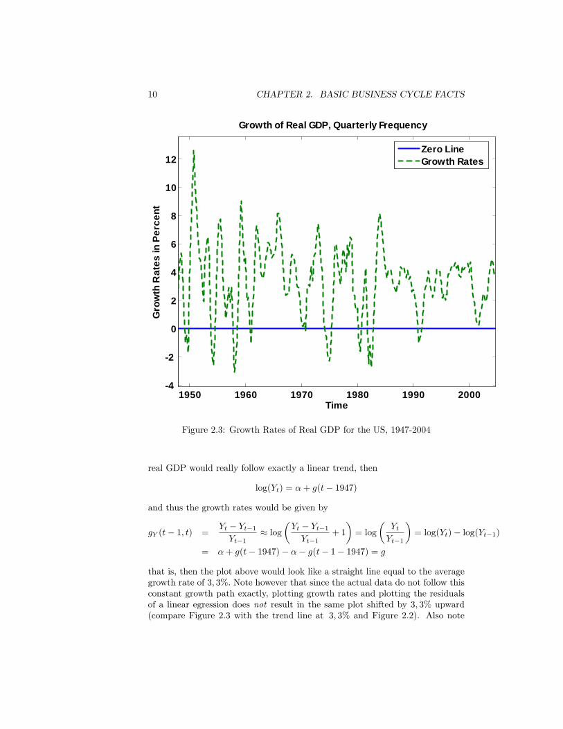
Figure 2.3 plots growth rates of real GDP for the US. Remember that eventhough the data frequency is quarterly, these are growth rates for yearly realGDP. The average growth rate over the sample period is 3; 3%: As a side remark,about one third of this growth is due to population and thus labor force growth,and two thirds are due to higher real GDP per capita. Note that if the log of
10 CHAPTER 2. BASIC BUSINESS CYCLE FACTS
1950 1960 1970 1980 1990 20004
2
0
2
4
6
8
10
12
Time
Gro
wth
Rat
es in
Per
cent
Growth of Real GDP, Quarterly Frequency
Zero LineGrowth Rates
Figure 2.3: Growth Rates of Real GDP for the US, 1947-2004
real GDP would really follow exactly a linear trend, then
log(Yt) = �+ g(t� 1947)
and thus the growth rates would be given by
gY (t� 1; t) =Yt � Yt�1Yt�1
� log�Yt � Yt�1Yt�1
+ 1
�= log
�YtYt�1
�= log(Yt)� log(Yt�1)
= �+ g(t� 1947)� �� g(t� 1� 1947) = g
that is, then the plot above would look like a straight line equal to the averagegrowth rate of 3; 3%: Note however that since the actual data do not follow thisconstant growth path exactly, plotting growth rates and plotting the residualsof a linear egression does not result in the same plot shifted by 3; 3% upward(compare Figure 2.3 with the trend line at 3; 3% and Figure 2.2). Also note

2.1. DECOMPOSITION OF GROWTH TREND AND BUSINESS CYCLES11
that, when dealing with yt = log(Yt); computing the growth rate
gY (t� 1; t) = log(Yt)� log(Yt�1) = yt � yt�1
amounts to plotting the data in deviations from its value in the previous quarter.Thus e¤ectively all variations of the data longer than one quarter are �ltered outby this procedure, leaving only the very highest frequency �uctuations behind.This is why the plot looks very �jumpy�, and observations in successive quartersnot very correlated. We will document this fact more precisely below.While the popular discussion mostly uses growth rates to talk about the
state of the business cycle, academic economists tend to separate growth andcycle components of the data by applying a �lter to the data. In fact, specifyingthe deterministic constant growth trend above and interpreting the deviationsas cycle was nothing else than applying one such, fairly heuristic �lter to thedata. One �lter that has enjoyed widespread popularity is the so-called Hodrick-Prescott �lter, or HP-�lter, for short. The goal of the �lter is as before : specifya growth trend such that the deviations from that trend can be interpreted asbusiness cycle �uctuations. Let us describe this �lter in more detail and tryto interpret what it does. As always we want to decompose the raw data,log(Yt) into a growth trend ytrendt = log(Y trendt ) and a cyclical componentyt = log(Y
cyclet ) such that
log(Yt) = log(Y trendt ) + log(Y cyclet )
yt = log(Yt)� ytrendt
Of course the key question is how to pick yt and ytrendt from the data? The HP-�lter proposes to make this decomposition by solving the following minimizationproblem
minfyt;ytrendt g
TXt=1
(yt)2+ �
TXt=1
�(ytrendt+1 � ytrendt )� (ytrendt � ytrendt�1 )
�2(2.2)
subject to
yt + ytrendt = log(Yt) (2.3)
where T is the last period of the data. Note that we are given the dataflog(Yt)gTt=0, so the right hand side of 2.3 is a known and given number, foreach time period. Implicit in this minimization problem is the following trade-o¤ in choosing the trend. We may want the trend component to be a smoothfunction, but we also may want to make the trend component track the actualdata to some degree, in order to capture also some �uctuations in the data thatare of lower frequency than business cycles. These two considerations are tradedo¤ by the parameter �: If � is big, we want to make the terms�
(ytrendt+1 � ytrendt )� (ytrendt � ytrendt�1 )�2

12 CHAPTER 2. BASIC BUSINESS CYCLE FACTS
small. But the term
(ytrendt+1 � ytrendt )� (ytrendt � ytrendt�1 )
=�log(Y trendt+1 )� log(Y trendt )
���log(Y trendt )� log(Y trendt�1 )
�= gY trend(t; t+ 1)� gY trend(t� 1; t)
is nothing else but the change in the growth rate of the trend component. Thusa high � makes it optimal to have a trend component with fairly constant slope.In the extreme as � ! 1; the weight on the second term is so big that it isoptimal to set this term to 0 for all time periods, that is,
gY trend(t; t+ 1)� gY trend(t� 1; t) = 0
gY trend(t; t+ 1) = gY trend(t� 1; t) = g
and thus
ytrendt � ytrendt�1 = g
ytrendt = ytrendt�1 + g
for all time periods t: But this is nothing else but our constant growth lineartrend that we started with. This is, the HP-�lter has the linear trend as aspecial case.Now consider the other extreme, in which we value a lot the ability of the
trend to follow the real data. Suppose we set � = 0; then the objective functionto minimize becomes
minfyt;ytrendt g
TXt=1
(yt)2 subject to yt + ytrendt = log(Yt)
or substituting in for yt
minfytrendt g
TXt=1
�log(Yt)� ytrendt
�2and the solution evidently is
ytrendt = log(Yt)
that is, the trend is equal to the actual data series and the deviations fromthe trend, our business cycle �uctuations, are identically equal to zero. Theseextremes show that we want to pick a � bigger than zero (otherwise there areno business cycle �uctuations and all of the data are due to the long run trend)and smaller than 1 (so that the trend picks up some medium run variation inaddition to long run growth and does not leave everything but the longest runmovements to the �uctuations part).Thus which � to choose must be guided by our objective of �ltering out
business cycle �uctuations, that is, �uctuations in the data with frequency of
2.1. DECOMPOSITION OF GROWTH TREND AND BUSINESS CYCLES13
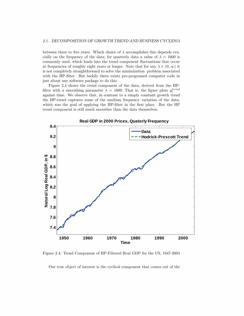
between three to �ve years. Which choice of � accomplishes this depends cru-cially on the frequency of the data; for quarterly data a value of � = 1600 iscommonly used, which loads into the trend component �uctuations that occurat frequencies of roughly eight years or longer. Note that for any � 2 (0;1) itis not completely straightforward to solve the minimization problem associatedwith the HP-�lter. But luckily there exists pre-programed computer code injust about any software package to do this.Figure 2.4 shows the trend component of the data, derived from the HP-
�lter with a smoothing parameter � = 1600: That is, the �gure plots ytrendt
against time. We observe that, in contrast to a simply constant growth trendthe HP-trend captures some of the medium frequency variation of the data,which was the goal of applying the HP-�lter in the �rst place. But the HPtrend component is still much smoother than the data themselves.
1950 1960 1970 1980 1990 2000
7.4
7.6
7.8
8
8.2
8.4
8.6
8.8
9
9.2
9.4
Time
Nat
ural
Log
Rea
l GD
P, in
$
Real GDP in 2000 Prices, Quaterly Frequency
DataHodrickPrescott Trend
Figure 2.4: Trend Component of HP-Filtered Real GDP for the US, 1947-2004
Our true object of interest is the cyclical component that comes out of the

14 CHAPTER 2. BASIC BUSINESS CYCLE FACTS
HP �ltering Figure 2.5 displays the business cycle component of the HP-�ltereddata, yt: As in Figures 2.3 and 2.2 this �gure shows that the cyclical variationin real GDP can be sizeable, up to 4�6% in both directions from trend. Clearlyvisible are the mid-seventies and early eighties recessions, both partially due tothe two oil price shocks, the recession of the early 90�s that cost George W.Bush�s dad his job and the fairly mild (by historical standard) recent recessionin 2001.
1950 1960 1970 1980 1990 2000
6
4
2
0
2
4
Time
Perc
enta
ge D
evia
tions
Fro
m T
rend
Deviations of Real per Capita GDP, Quarterly Frequency
Zero LineHodrickPrescott Cycle
Figure 2.5: Cyclical Component of HP-Filtered Real GDP for the US, 1947-2004
But now we want to proceed with a more systematic collection of businesscycle facts. We �rst focus on our main variable of interest, real GDP. In laterchapters, once we enrich our benchmark model with labor supply and otherrealistic features, we will augment these facts with facts about other variablesof interest.

2.2. BASIC FACTS 15
Variable Mean St. Dv. A(1) A(2) A(3) A(4) A(5) min max %(>0) %(>0,033)Growth Rate 3:3% 2; 6% 0; 83 0; 54 0; 21 �0; 09 �0; 20 �3; 1% 12; 6% 88; 6% 54; 0%HP Filter 0% 1:7% 0; 84 0; 60 0; 32 0; 08 �0; 10 �6; 2% 3; 8% 53; 9% N=A
Table 2.1: Cyclical Behavior of Real GDP, US, 1947-2004
2.2 Basic Facts
Now that we have discussed how to be measure business cycle facts, let usdocument the main regularities of business cycles. Sometimes the resulting factsare called stylized facts, that is, facts one gets from (sophisticatedly) eyeballingthe data. These facts will be the targets of comparison for our quantitativemodels to be constructed in the next part of this class. The goal of the modelsis to generate business cycles of realistic magnitude, and to explain what bringsthem about. In order to do so, we need empirical benchmark facts.
Table 2.1 summarizes the main stylized facts or quarterly real GDP for theUS between 1947 and 2004, both when using growth rates and when using thecyclical component of the HP-�ltered series. The mean and standard deviationof a time series fxtgTt=0 are de�ned as
mean(x) =1
T
TXt=0
xt
std(x) =
1
T
TXt=0
(xt �mean(x))2! 1
2
The autocorrelations are de�ned as follows
A(i) = corr(xt; xt�1) =1
T�iPt(xt �mean(x))(xt�i �mean(x))
std(x) � std(x)
and measure how persistent a time series is. For time series with high �rst orderautocorrelation tomorrow�s value is likely to be of similar magnitude as today�svalue. Finally the table gives the maximum and minimum of the time series andthe fraction of observations above zero, and, for the growth rate, the fraction ofobservations bigger than its mean, 3; 3%:We make the following observations. First, besides the fact that the mean
growth rate is 3; 3% whereas the cyclical component of the HP-�ltered serieshas a mean of 0; the main stylized facts derived from taking growth rates andHP-�ltering are about the same. They are:
1. Real GDP has a volatility of about 2% around trend, or more concretely,1; 7% when considering the HP-�ltered series.

16 CHAPTER 2. BASIC BUSINESS CYCLE FACTS
2. The cyclical component of real GDP is highly persistent (that is, positivedeviations are followed with high likelihood with positive deviations). Theautocorrelation declines with the order and turns negative for the �fthorder (that is if real GDP is above trend this quarter, it is more likely tobe below than above trend in �ve quarters from now).
3. Positive deviations from trend are more likely than negative deviationsfrom trend. This suggests that recessions are short but sharp, whereasexpansions are long but gradual.
4. It is rare that the growth rate of real GDP actually becomes negative, atleast for the US between 1947 and 2004.
It is an instructive exercise (that you will do with Philip�s help) to carry outthe same empirical exercise described in these notes for an alternative countryof your choice. All you need is a su¢ ciently long time series for real GDP fora country (preferably seasonably adjusted), a little knowledge of MATLAB (orsome equivalent software package) and a pre-programed HP �lter subroutine(which for MATLAB I will give you). But now we want to start constructingour theoretical model that we will use to explain existence and magnitude ofthe business cycles documented above.
Part II
The Real Business Cycle(RBC) Model and Its
Extensions
17