Embed Size (px)
Citation preview

Methodology for Quantitative Procurement Options Analysis Discussion Paper
Partnerships British Columbia Updated April 2014

Guidance for Quantitative Procurement Options Analysis – Discussion Paper April 2014
Table of Contents Part 1: Overview ............................................................................................................ 1 1. Purpose .................................................................................................................. 1
1.1 Policy Context ................................................................................................... 1 1.2 What is a PPP? ................................................................................................. 2 1.3 Potential Benefits of PPP Procurement ............................................................. 3 1.4 The Business Case Process ............................................................................. 4 1.5 Quantitative Analysis ......................................................................................... 5
Part 2: Quantitative Procurement Options Analysis ................................................... 7 2. Quantitative Elements ........................................................................................... 7
2.1 Project Cash Flow Estimates............................................................................. 8 2.2 PSC and Shadow Bid Adjustments ................................................................... 8 2.3 Discount Rate ................................................................................................... 8
3. Conducting the Analysis ....................................................................................... 9 3.1 Cost Inputs ........................................................................................................ 9 3.2 Business Case Phase Costs ........................................................................... 15 3.3 Procurement Phase Costs .............................................................................. 16 3.4 Construction Phase Costs ............................................................................... 17 3.5 Operations Phase Costs ................................................................................. 17 3.6 Inflation ........................................................................................................... 17
4. PSC and Shadow Bid Adjustments .................................................................... 18 4.1 Competitive Neutrality ..................................................................................... 18 4.2 Risk ................................................................................................................. 19
5. Public Sector Contributions during Construction............................................. 26 6. Discount Rate ...................................................................................................... 27
6.1 Debt / Equity and the Cost of Capital............................................................... 28 6.2 The Discount Rate and Quantified Risk in a PPP ............................................ 29 6.3 The Discount Rate and Government Cost of Borrowing .................................. 30 6.4 Estimating of the Cost of Capital ..................................................................... 30
7. Term ..................................................................................................................... 31 8. Summary .............................................................................................................. 31 Part 3: Interpretation and Presentation ..................................................................... 33 9. Interpreting the Results ...................................................................................... 33
9.1 Value for Money Context ................................................................................. 33 9.2 Link to Project Budgeting ................................................................................ 33 9.3 Scope of the Analysis ...................................................................................... 34 9.4 Funding Analysis Context ................................................................................ 35 9.5 Sensitivity Analyses ........................................................................................ 36
10. Presenting the Results ..................................................................................... 39
Partnerships BC Page i

Guidance for Quantitative Procurement Options Analysis – Discussion Paper April 2014
10.1 Risk Distributions ......................................................................................... 39 10.2 Quantitative Value for Money Table ............................................................. 41 10.3 Annual Service Payment (ASP) Table ......................................................... 42 10.4 PSC and Shadow Bid Annual Service Payment Comparison ....................... 43 10.5 Annual Service Payment Chart .................................................................... 44 10.6 Multiple Criteria Analysis ............................................................................. 45
11. After the Business Case................................................................................... 46 12. Conclusion ........................................................................................................ 46 Appendix 1: Financing and the PSC .......................................................................... 48 Appendix 2: Sample Risk Template ........................................................................... 49 Appendix 3: Risk Modelling Methodologies .............................................................. 50 1. Introduction ......................................................................................................... 50 2. Distributions ........................................................................................................ 50
2.1 Triangular ........................................................................................................ 51 2.2 Discrete ........................................................................................................... 53 2.3 What and How to Quantify .............................................................................. 56 2.4 How to Document Risks .................................................................................. 62 2.5 Monte Carlo Analysis ...................................................................................... 63
Appendix 4: Discounted Cash Flow Analysis .......................................................... 65 Appendix 5: Discount Rate Background .................................................................. 67 Appendix 6: Financial Model – Worked Example ..................................................... 71 Appendix 7: Glossary of Terms ................................................................................. 78
Partnerships BC Page ii

Guidance for Quantitative Procurement Options Analysis – Discussion Paper April 2014
Part 1: Overview
1. Purpose
The purpose of this draft discussion document is to describe the recommended methodology and rationale for Partnerships British Columbia’s (Partnerships BC) guidance for the quantitative analysis of infrastructure project procurement options.
The document is intended to support a rigorous standard and consistent approach for undertaking the procurement options analysis that is required as part of the business case development process for procuring publicly-funded infrastructure in British Columbia. To this end, the document:
• Outlines Partnerships BC’s guidance methodology for the quantitative analysis of procurement options,
• Provides guidance for conducting the quantitative analysis work as part of the comprehensive business case analysis for a project, and
• Demonstrates how the outcome of this analysis informs the procurement decision and funding analysis for a project.
This document can be used to guide the quantitative analysis of project procurement alternatives in business cases for all projects where a determination has been made that such projects are likely to benefit from public private partnership (PPP) procurement in terms of securing value for money for the public1. It is important to note, and account for, unique requirements, flexible methodology and outcomes in individual projects.
1.1 Policy Context
In the Province of British Columbia, the Ministry of Finance has mandated through its Capital Asset Management Framework (CAMF) that the following principles guide all public sector capital procurement:
• Fairness, openness and transparency,
• Allocation and management of risk,
• Value for money and protecting the public interest, and
• Competition.
1 Such a determination is currently made by applying Partnerships BC’s guidance with respect to early project screening. This approach is documented in the Capital Project Public Private Partnership Early Screening Tool, Partnerships BC, December, 2008.
Partnerships BC Page 1

Guidance for Quantitative Procurement Options Analysis – Discussion Paper April 2014
In addition, in 2008 the Province of British Columbia revised the Capital Standard requiring, for all capital projects in which the Provincial contribution exceeds $50 million, that a PPP be considered for procurement unless there is a compelling reason to do otherwise (e.g., a different procurement model will generate better value for money). Further, projects where the provincial government contribution is between $20 million and $50 million will be screened to determine whether a more comprehensive assessment of the project as a PPP is warranted.
In support of the CAMF mandate for the preparation of project business cases, in addition to the evaluation of PPP structures in particular under the Capital Standard, Partnerships BC continues to develop and refine approaches to quantitative analysis of procurement options. The status of this work as of April 2014 is summarized in this document. Ministries and agencies should contact Partnerships BC for the most recent developments.
1.2 What is a PPP?
Broadly speaking, a PPP is a form of procurement that uses a long-term, performance-based contract where appropriate risks associated with a project can be transferred cost-effectively to a private sector partner. These risks can include: construction, schedule, functionality of design, financing, and the long-term performance of the asset through the optimal allocation of responsibility for operations, maintenance and rehabilitation. In some cases, PPPs can also be structured so that the private partner assumes demand and price risk based on the availability of a facility, and they can also assume varying degrees of commercial risk with respect to market rents, tolls and other types of revenue.
Based on experience with existing projects, risk transfer is a key area in PPPs in the determination of value for money. The type, amount and effectiveness of possible risk transfer differs considerably based on the procurement method, contract structure chosen and characteristics of a particular project.
Traditional procurement has typically involved construction management (CM) and design bid build (DBB), representing points along a continuum of possible procurement methods where there is very little or no transfer of project-related risk to a private partner.
The range of procurement options that are generally accepted to be PPP structures include:
• Design build (DB)2
2 Although not a full PPP in terms of transferring long-term financing and operations, maintenance and rehabilitation responsibility, DB procurement can provide some of the benefits of a PPP, particularly in the areas of design and construction integration and project management. For this reason, DB is included in the
Partnerships BC Page 2
Guidance for Quantitative Procurement Options Analysis – Discussion Paper April 2014
• Design build finance (DBF)
• Design build finance maintain (DBFM) 3
• Design build finance operate (DBFO)4
The options ranging from DB to DBFO are considered to be partnership structures as they can be structured to require some degree of private financing, are longer term, can include responsibility for operations and life cycle performance of the asset, and are enforceable with a performance-based payment mechanism for the duration of the contract term. The financial incentive that is brought to bear through the length and enforceability of the PPP payment mechanism is the key to providing a stronger, more effective means of optimizing the life cycle costs of a project in a way that meets program and performance requirements.
1.3 Potential Benefits of PPP Procurement
Generally speaking, the main goal of a PPP is to secure value for money for the public through the procurement and contract structure chosen, while ensuring that the public interests of health, safety, equality, and sustainability, among others, are protected.
A PPP will typically have the following potential benefits which result in value for money:
Effective Risk Transfer: Although several procurement options can transfer similar risks, the effectiveness of the risk transfer varies with the amount and nature of the responsibility assumed by a private partner. For example, the DB, DBF, DBFM and DBFO procurement models all have a design component; however, the transferred risk of design functionality would be greater for a longer term contract such as a DBFM or DBFO, where the party is responsible for the asset performance over a 20- or 30-year period. In contrast, a DB arrangement may have a warranty period of only three to five years, thereby reducing the opportunity for risk transfer.
In addition, greater risk transfer can be achieved by transferring risk across a broader range of activities. For example, a DBFO partner would assume risk across key areas including design, construction, finance, operations, maintenance and rehabilitation, whereas a DB arrangement would transfer mainly design risk through a more limited range of activities over a shorter term warranty.
spectrum of PPP models as a transitional model, that involves greater private sector participation than a DBB approach. 3 The maintenance component of the DBFM is understood to include both ongoing maintenance and rehabilitation of an asset. 4 The operations component of a DBFO is typically understood to include ongoing maintenance and rehabilitation, and is more commonly associated with horizontal infrastructure projects such as roads.
Partnerships BC Page 3

Guidance for Quantitative Procurement Options Analysis – Discussion Paper April 2014
Improved value from this type of risk transfer is achieved when the party taking responsibility for a particular activity is better able to manage the associated risks (i.e., the likelihood of the risk occurring is reduced, or the expected cost if the risk does occur is reduced), and when the ability to manage the risk is supported by the added incentive of a long-term, fixed-price, performance-based contract. The contract will include a payment mechanism with clauses to specifically transfer identified risks to a private partner. Establishing a maximum payment, contingent on effective management of these risks by the private partner, also adds value by providing greater planning certainty for the owner.
Schedule and Cost Certainty: Under a PPP, the private partner typically begins to receive pre-determined annual service payments (ASP) only once the project is available for use. To realize its investment objective as a result of the private finance component, the private partner must ensure that the project does not cost more or take longer than planned, which provides greater certainty to the owner around the cost and schedule of a project.
Integration: Under a PPP, the private sector partner can be responsible for the design and construction, long-term operations, maintenance and rehabilitation of the asset. This creates opportunities and incentives to integrate these functions to optimize performance and result in a lower overall risk-adjusted cost of delivering the project over its lifecycle. In addition to integrating design and construction to ensure efficient and timely completion, the private partner can also integrate design, engineering, and construction materials and techniques with the long-term performance requirements of a project.
Innovation: PPP procurement encourages innovation through the development of performance-based output specifications drawn from the requirements of program service objectives, rather than being based on detailed, highly specified design. The added flexibility provided by this approach, in addition to the competitive nature of the bidding process and financial incentive, encourages PPP partners to develop innovative solutions in all aspects of a project, from design and engineering through to decommissioning.
To estimate the magnitude and potential value of these PPP benefits, a comprehensive and detailed quantification and procurement options analysis is necessary as part of a broader business case process.
1.4 The Business Case Process
The business case process generally involves the following four key parts:
Part A: Planning Future Service Delivery: Summarizes the discussion and analysis of the service delivery requirements that define the need for the project;
Partnerships BC Page 4

Guidance for Quantitative Procurement Options Analysis – Discussion Paper April 2014
Part B: Service Delivery Options: Presents the objectives, scope, program delivery options analysis and recommendation for the preferred service delivery option (the investment decision);
Part C: Procurement Options Analysis: Describes and evaluates the procurement options available for the preferred service delivery option (the procurement decision); and
Part D: Accounting and Funding Analysis: Provides a detailed funding and affordability analysis, including an accounting and financial statement analysis (affordability), for the recommended procurement option.
1.5 Quantitative Analysis
During the business case stage, some form of quantitative analysis is typically performed in Parts B, C and D, as described in the table below.
Business Case Section Analysis
Part B (Investment Decision) Multiple Criteria Analysis (MCA)
Net Present Cost (NPC) Analysis
Operational Efficiencies
Sensitivity Analysis (MCA)
Part C (Procurement Decision) Multiple Criteria Analysis (MCA)
Comprehensive Risk Analysis (includes Monte Carlo analysis)
Financial Analysis (PSC and Shadow Bid)
Sensitivity Analysis (Financial Model)
Part D (Recommended Option Affordability)
Accounting Analysis
Funding Analysis
Budget
Partnerships BC Page 5
Guidance for Quantitative Procurement Options Analysis – Discussion Paper April 2014
The focus of this paper is to describe the quantitative procurement options analysis that is used in Parts C and D of the business case. The quantitative procurement options analysis is used to:
• Assess the potential quantitative benefits of PPP procurement compared to traditional public sector procurement,
• If private finance is involved in the PPP, determine the optimal level of private finance,
• Support the qualitative analysis of procurement options based on non-financial criteria, and
• Provide input to the funding analysis to estimate the impact that a PPP procurement option would have on project accounting.
Partnerships BC Page 6

Guidance for Quantitative Procurement Options Analysis – Discussion Paper April 2014
Part 2: Quantitative Procurement Options Analysis The evaluation of procurement options is mainly concerned with identifying the method of delivering a project that will result in the greatest value for money on both a financial (quantitative) and qualitative basis. In financial terms, value for money is established by calculating the estimated cost of a project, based on a particular PPP procurement method, and comparing it to the estimated cost if the project were procured entirely by the public sector using a traditional method.
The evaluation of procurement options typically involves two main steps. The first step identifies key procurement objectives, and provides a qualitative assessment of a wide range of available procurement options including both traditional, public sector procurement and PPP models. The assessment of these procurement options is intended to identify the two most appropriate public and partnership procurement alternatives, which then form the basis of comparison in the detailed procurement options analysis for the project.
The second step in the assessment involves a more detailed, quantitative analysis that compares the preferred PPP approach to a traditional procurement method. To do this, a comprehensive risk analysis is conducted and financial models representing the two procurement methods are developed and compared. If private finance is involved in the PPP, the optimal level of private finance in the PPP must be determined. A financial model is developed for a project based on a traditional procurement method, also known as a public sector comparator (PSC5), and is compared to a financial model created based on PPP procurement, also known as a Shadow Bid. It is called a Shadow Bid because it is an estimate based on an expected bid.
The results of this quantitative comparison between the PSC and the Shadow Bid, together with the qualitative criteria, are used to determine the procurement method that provides the best potential value for money.
Quantitative value for money is achieved through lower overall project costs resulting from a particular procurement method. Qualitative value is achieved when a particular procurement method is best able to support the qualitative goals and objectives of a project.
2. Quantitative Elements
The quantitative procurement options analysis relies on three key elements: cash flow estimates, PSC adjustments, and the discount rate. These are summarized in the following sections and presented in greater detail in Section 3.
5 PSC is an internationally recognized term.
Partnerships BC Page 7
Guidance for Quantitative Procurement Options Analysis – Discussion Paper April 2014
2.1 Project Cash Flow Estimates
To establish cash flow estimates, both the PSC and Shadow Bid models typically consider the amount and timing of the following costs under each procurement method:
• Capital costs
• Operating and Maintenance costs
• Rehabilitation costs
• Financing costs
• Owner’s costs
• Inflation
These costs are estimated and incorporated into the PSC and Shadow Bid models as periodic cash flows.
2.2 PSC and Shadow Bid Adjustments
Adjustments are necessary to account for differences between traditional public procurement and PPP procurement. The key differences that need to be considered include adjustments for competitive neutrality (insurance and taxation) and adjustments for transferred and retained risks.
These adjustments are described in detail in Section 4.1.
2.3 Discount Rate
Another important consideration in the quantitative analysis of procurement options is the choice of discount rate. The discount rate reflects the time value of money as well as any risk premium associated with a project, and is determined based on the risk profile of a project and prevailing market conditions. Discounting enables nominal project cash flows6 that differ in terms of timing and amount to be discounted back to a common reference date, usually to their present value. Discounting in this way allows procurement methods with different cash flow impacts to be compared on a like-for-like basis. Comparing competing options in this way provides an objective means of determining the approach that provides the best value in terms of cost.
The key quantitative elements introduced above are discussed in detail in the following sections.
6 Nominal cash flows reflect the anticipated impact of inflation and/or construction escalation on the periodic costs of the project.
Partnerships BC Page 8

Guidance for Quantitative Procurement Options Analysis – Discussion Paper April 2014
3. Conducting the Analysis
The procurement options being considered are analyzed in order to estimate their financial impact from the perspective of the owner (public entity) that will be paying for the project. These costs are then compared in order to determine the procurement approach with the greatest potential to provide value for taxpayer dollars.
To meet the audit standards of the Office of the Auditor General, estimates used in the analysis must be carefully arrived at and must be accompanied by clearly documented, evidentiary support.
3.1 Cost Inputs
Capital cost inputs to the financial model represent a significant portion of project cash flows and are derived from an indicative design and output specifications for a project. In addition to the capital costs, operating costs, rehabilitation costs, bid development and financing costs and owner’s costs must also be included. Each of these components is explained in detail in the remainder of this section.
3.1.1 Capital Costs
Capital costs refer to the costs of constructing the asset. The majority of these costs include raw materials, labour and equipment (hard costs), project management fees, consulting fees, and costs associated with securing environmental and regulatory approvals (soft costs).
Capital costs assumed for the PSC are determined based on the existing procurement practices of the owner involved in the project delivery. PSC estimates, therefore, typically rely on the assumption that the project will be procured as a DBB. In some cases, however, where an owner has previously used a DB, or incorporated DB elements as part of their procurement of larger projects, a PSC estimate would be based on considering a similar approach. A key element in developing a realistic PSC model is to ensure that the traditional procurement methods for a particular owner are clearly understood.
Preliminary estimates of these capital costs are provided either by the owner or, preferably, by external consultants to the owner based on a project indicative design and output specifications that provide a graphical representation of a possible solution to the performance requirements for a project. The resulting project costs must be based, at a minimum, on the following:
• An estimate prepared by a professional quantity surveyor (QS) based on an
indicative design,
• Preliminary project schedule and spend profile, and
Partnerships BC Page 9

Guidance for Quantitative Procurement Options Analysis – Discussion Paper April 2014
• Outline performance specifications.
The resulting estimate should be documented in current dollars and then escalated to match the project schedule. The accuracy of the estimate, expressed as a percentage (+/-), should be highlighted. These capital costs and assumptions should be continually re-validated and updated in order to reflect any time delays, changes in the construction environment, or any changes in project scope.
As capital cost estimates at this early stage are based on an indicative rather than detailed design, a contingency is added to the capital cost estimate to account for the design’s preliminary nature. Typically, design and construction contingencies are included for all projects, and a contingency on soft costs may also be included.
3.1.1.1 Capital Cost Efficiencies Once PSC capital costs are estimated, efficiencies may be included to adjust the Shadow Bid as competition and innovation from the private sector can result in lower construction costs under PPP procurement.
The estimation of potential efficiencies needs to ensure that there is no double-counting of risk that would be addressed in the risk transfer analysis (discussed below), and that any estimated efficiencies are reasonably precise in order to have validity. Due to the variability of potential efficiencies that can be realized, efficiency estimates should be expressed as a range rather than as a single point estimate. Furthermore, estimated efficiencies should be determined based on specific capital components of a project, rather than being applied globally to the entire capital cost. Finally, estimates should also consider the unique characteristics of the particular PPP model chosen for the Shadow Bid that would support such efficiencies.
To achieve a reasonable estimate, it is necessary to define amounts under consideration as either an efficiency or a risk in order to avoid duplication. A general distinction is that efficiencies in the construction phase are the product of competitively bid design and construction approaches that can result in a lower cost than the estimated base cost. This lower cost would result in an adjustment to the base cost budgets. In contrast, a transferred risk may be added as a contingency in a bid and are evaluated separately through the risk analysis discussed in Section 4.2.
3.1.2 Operating and Maintenance Costs
Operating costs refer to costs incurred in operating and maintaining the asset and performing the services that are included within the project scope. Operations and maintenance costs include the cost of inputs, service provider wages and salaries, and
Partnerships BC Page 10

Guidance for Quantitative Procurement Options Analysis – Discussion Paper April 2014
other related expenses that are likely to be incurred7. These costs will vary from project to project.
Different terminology is used to describe operating costs across the B.C. Government ministries. In the education and health care sectors, operating costs are known as facility management costs, and are not directly associated with students or patients. Examples of facility management costs include: housekeeping, food services, security, laundry and linen, waste management, and physical plant utilities, among others.
In the health care sector, a second type of operating cost pertaining to services provided directly to patients is known as clinical services. Examples of clinical services include: laboratory work and diagnostics, allied services, medical affairs, general administration, and planning, among others. Responsibility for these services is not transferred to the private sector, and consequently, the associated costs have typically been excluded from both models as they remain costs incurred by the government regardless of the procurement option selected.
In the transportation sector, operating costs refer to the costs of services required to keep the road, bridge or transit line open and available for use. Examples of these costs include: incident management, debris removal, snow or mud removal and road condition reporting, among others. Depending on whether or not these are part of project scope, these costs may or may not be included in the PSC and Shadow Bid. If they are not in scope, then they are considered equal and not included.
Methods for estimating operating costs also differ slightly from sector to sector. In the case of facility replacement in the accommodations sectors (health care, education, justice), the owner estimates operating costs by refining the current operating budget for facilities to be replaced in order to incorporate changes in programming and/or demand levels for services. This may also include expected increases in facilities management costs due to an increased size of facilities and/or any expected efficiencies resulting from design improvements. In the transportation sector, operating cost estimates are generally based on relevant precedent projects, and the costing model is prepared on the basis of public sector (i.e., Ministry of Transportation and Infrastructure) operation.
3.1.3 Rehabilitation Costs
Rehabilitation costs represent the investment incurred on an ongoing and/or periodic basis during the course of the concession period to maintain assets according to agreed upon standards. Examples of rehabilitation activities include roof or window replacement for buildings, and bridge deck and road resurfacing for highways. Rehabilitation costs
7 Related costs may include: employee entitlements, insurance, training, development, travel, direct management costs, costs of providing ancillary services such as cleaning and catering, overhead costs, energy, equipment, administrative, electricity, etcetera.
Partnerships BC Page 11

Guidance for Quantitative Procurement Options Analysis – Discussion Paper April 2014
may also be referred to as life cycle costs or recapitalization costs, depending on the sector.
The analysis of rehabilitation costs during the business case stage is preliminary in nature; however, there is generally sufficient information available to establish an estimate of these costs for a project. The amount and frequency of rehabilitation investment for a particular project needs to be determined since optimum life cycles differ based on asset classes. The costs associated with these estimates are typically provided by owner’s engineers and/or external QS experts, and can be based on available data from past projects. These estimates form part of the initial cost estimate and assumed asset condition requirements that form part of the project agreement.
3.1.3.1 Life Cycle Cost Efficiencies As is the case with the development of the construction efficiencies discussed earlier, efficiencies related to operations, maintenance and rehabilitation (OMR), or life cycle, can form an integral part of the recommendations presented in a procurement analysis. Such efficiencies can be determined based on a detailed review of existing PSC life cycle budgets, and comparing them to current market place experience and practice to either confirm estimates or identify cost areas where efficiencies would be expected.
Once developed, such efficiencies inform the overall value for money proposition and benefits of a particular procurement method. To be considered accurate, efficiencies should be explored within the specific context of the project and the capacity, capabilities, policies and operating practices of the owner. As described with capital cost efficiencies, OMR cost efficiencies should identify a range of the most likely outcomes relating to specific elements of the OMR requirements, and based on the characteristics of the anticipated PPP model. These estimates also need to be carefully considered to ensure that adjustments do not double count amounts included in the risk analysis.
3.1.4 Incorporating Efficiencies into the Analysis
To appropriately incorporate construction cost and life cycle efficiencies into the business case analysis, all potential efficiencies should be estimated at the same time and by the same people as a means of avoiding duplication. Generally, construction efficiencies are estimated by the project team and consultants together. If construction efficiencies are identified under a PPP model, the total of these estimated efficiencies is subtracted from the QS construction cost estimate for the PSC. This adjusted cost estimate then becomes the construction cost estimate for the Shadow Bid.
In a similar way, anticipated life cycle cost efficiencies identified under a PPP are subtracted from the projected life cycle cost estimates based on traditional procurement.
It is important to consider that in identifying efficiencies, there may be occasions where a PPP approach results in an added cost, or negative efficiency, in which case it should be
Partnerships BC Page 12
Guidance for Quantitative Procurement Options Analysis – Discussion Paper April 2014
netted out of the overall capital or life cycle adjustments. For example, in constructing infrastructure that is part of a broader network (e.g., a bridge), the cost associated with maintaining it as a stand-alone item might be greater than incorporating it into a broader maintenance program already underway for the rest of the system. In such a case, a percentage inefficiency would be determined based on localized maintenance, and a corresponding adjustment would be added to the base cost estimate under a PPP to properly reflect this in the comparison.
3.1.5 Bid Development Costs
In responding to a PPP procurement, proponents incur expenses over and above those incurred in a traditional procurement. These costs are commonly referred to as bid development costs. In order to arrive at an accurate estimate of the overall cost of the Shadow Bid it is necessary to add an estimate for the bid development costs. Bid development costs are generally small in traditional procurements, and if they are not included in the base capital cost estimate, they are included as a discrete item.
3.1.6 Financing Costs
In developing the PSC cost estimate, it is assumed that the traditional public procurement is not financed, even though a comparison is made to a fully financed Shadow Bid. The rationale for this assumption is presented in Appendix 1.
Financing costs are the costs associated with arranging financing for a PPP with debt and equity, and can include items such as arrangement fees, commitment fees, and swap credit premiums. These costs need to be incorporated into the Shadow Bid as cash flows.
Based on precedent PPP transactions in B.C. and Canada as well as the current state of financial markets, Partnerships BC determines whether debt financing is obtained through bank debt or bonds. When bank debt financing is used, a lender approves the maximum amount of debt for a project, and draw-downs occur through the construction period until this maximum is reached. Interest is accrued periodically on the outstanding balance as the debt is drawn down through the construction period, with a commitment fee applied to the unused portion. When construction is complete and the ASP to the private partner begins, the debt is repaid via fixed payments of principal and interest.
Alternatively, when bond financing is used, the full amount of the required funds is raised up front and interest starts accruing right away. To lower overall carrying costs of bonds, the private sector may borrow several tranches of debt over the construction period. The repayment of bonds is similar to bank debt financing, as fixed payments of principal and interest are paid after project construction is complete.
Partnerships BC Page 13

Guidance for Quantitative Procurement Options Analysis – Discussion Paper April 2014
Equity providers structure their investments to be as efficient as possible. In addition to conventional equity investment, an efficient structure may also include a letter of credit or an equity bridge loan as a means of financing construction. Payments to equity holders are not constant, with the Shadow Bid allowing for a minimum equity return to be specified. This required equity return becomes the cost of equity to the project and is the internal rate of return (IRR) to the equity investor.
3.1.7 Owner’s Costs
Owner’s costs are project costs incurred by the project owner, and can include:
• Property acquisition,
• Owner’s project team and governance costs, and
• Advisors: technical, legal and financial.
Since these costs are retained by the owner, the private sector does not account for them in their bids and, therefore, they do not appear directly in the financial models. They must be included in the overall project budget, however, to ensure it is complete. As the private sector is not responsible for the owner’s costs, there is no need to attribute any private sector financing costs to owner’s costs.
The cash flow impact of the owner’s costs on the overall project budget will differ depending on whether a project budget is based on a PSC or on a Shadow Bid. For a project based on the PSC model, the owner’s costs are typically spread throughout the design and construction phases. In contrast, a project based on the Shadow Bid model will see a significant part of the owner’s costs spent before the project starts construction as the owner will typically spend more during the procurement process, both in choosing the best proponent and in drafting a project agreement. Following financial close, however, until the end of the project agreement, budgeted owner’s costs for a project based on Shadow Bid can be considerably lower as the owner is only required to manage a single contract (i.e., the project agreement).
Although the upfront procurement costs may be less for a project based on a PSC, the cost of ongoing contract administration is typically higher because the government is responsible for administering many different procurement contracts, and the ongoing contract management of these agreements and associated interfaces can be significant and costly. It should therefore not be assumed that the owner’s net present cost (NPC) is greater for a project based on a Shadow Bid than for the same project based on a PSC.
To arrive at reasonable estimates for these costs, a bottom-up approach to developing budget estimates is typically used, based on an organization chart and schedule that identifies the individuals associated with the activities identified below, and their cost and utilization.
Partnerships BC Page 14
Guidance for Quantitative Procurement Options Analysis – Discussion Paper April 2014
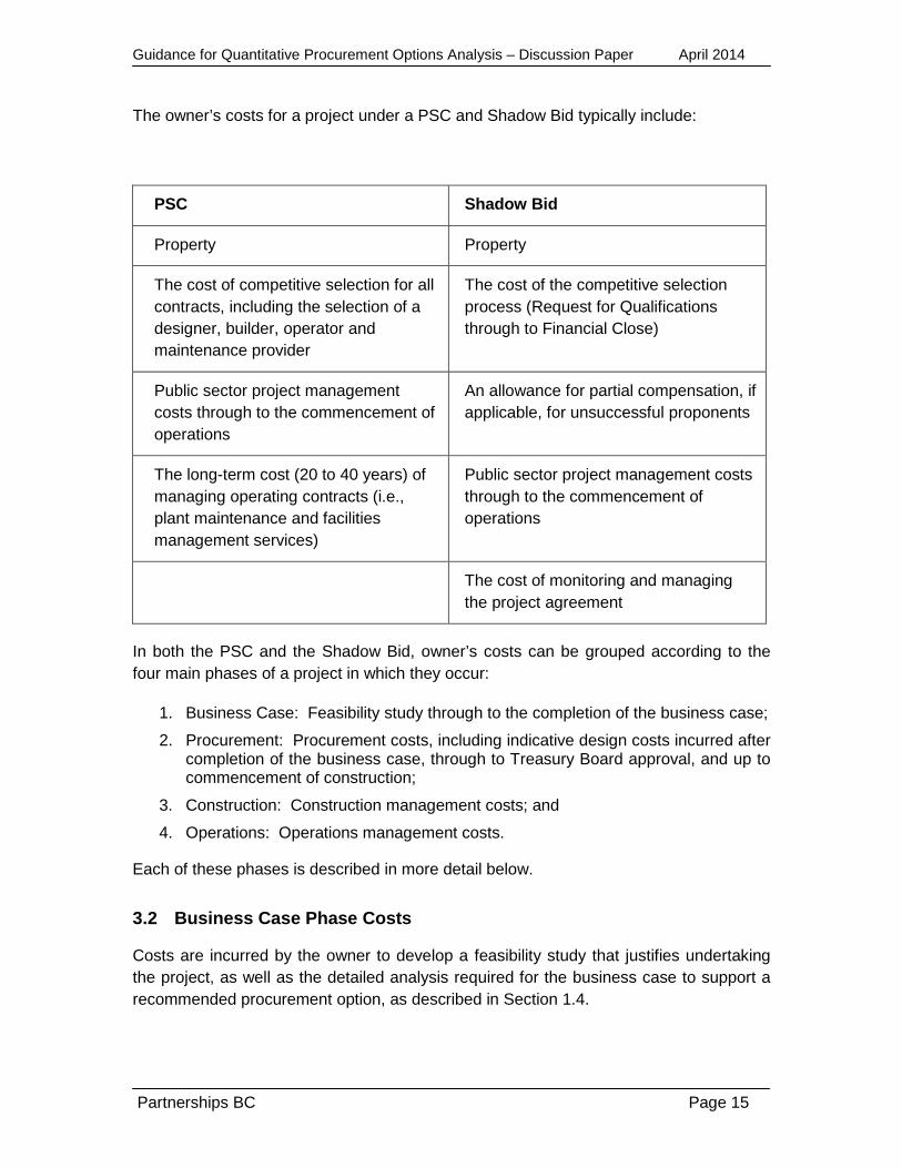
The owner’s costs for a project under a PSC and Shadow Bid typically include:
PSC Shadow Bid
Property Property
The cost of competitive selection for all contracts, including the selection of a designer, builder, operator and maintenance provider
The cost of the competitive selection process (Request for Qualifications through to Financial Close)
Public sector project management costs through to the commencement of operations
An allowance for partial compensation, if applicable, for unsuccessful proponents
The long-term cost (20 to 40 years) of managing operating contracts (i.e., plant maintenance and facilities management services)
Public sector project management costs through to the commencement of operations
The cost of monitoring and managing the project agreement
In both the PSC and the Shadow Bid, owner’s costs can be grouped according to the four main phases of a project in which they occur:
1. Business Case: Feasibility study through to the completion of the business case;
2. Procurement: Procurement costs, including indicative design costs incurred after completion of the business case, through to Treasury Board approval, and up to commencement of construction;
3. Construction: Construction management costs; and
4. Operations: Operations management costs.
Each of these phases is described in more detail below.
3.2 Business Case Phase Costs
Costs are incurred by the owner to develop a feasibility study that justifies undertaking the project, as well as the detailed analysis required for the business case to support a recommended procurement option, as described in Section 1.4.
Partnerships BC Page 15

Guidance for Quantitative Procurement Options Analysis – Discussion Paper April 2014
The business case phase costs include the cost of developing an Indicative Design for a project. For a PPP, an Indicative Design is usually completed by both internal and external consultants, to a sufficient degree that they can support the development of project costs and provide proponents with an understanding of facility requirements. The final, detailed design is completed by the private sector partner.
3.3 Procurement Phase Costs
Procurement phase costs are the costs incurred by the owner from completion of the business case up until the start of construction and are comprised of costs associated with the following key activities:
• Preparing and issuing procurement documents (request for qualifications and request for proposals),
• Obtaining an invitation to bid, • Drawing up a contract, • Evaluating proposals, • Negotiating with the preferred proponent, and • Dealing with any deviations from the contract conditions.
In addition, projects can typically incur the following costs:
• Cost estimates (capital and life cycle), • Geotechnical investigation, • Cost of legal advisor, • Indicative design, • Information technology (e.g., data room), • Asset studies, and • Ministry/public sector internal costs.
Owner’s costs that are unique to the Shadow Bid include:
• Partial compensation (honorarium), • Business/Financial advisor, • Procurement advisor, and • Additional legal advice to develop the project agreement.
These advisory elements are necessary to acquire the appropriate financial, procurement, and legal expertise required to ensure the final project agreement properly addresses all aspects of successful project completion and ongoing operations for up to 40 years.
Partnerships BC Page 16

Guidance for Quantitative Procurement Options Analysis – Discussion Paper April 2014
3.4 Construction Phase Costs
Construction management costs are incurred by the party responsible for overseeing work done during the construction phase of a project. These costs are less intensive for the public sector following procurement as a PPP, as the partner bears the costs associated with overseeing construction, contract administration and for the majority of the quality assurance work. Although there may continue to be some legal and advisory costs related to implementing the project agreement, the role of the owner is reduced and requires a smaller team to administer the contract and monitor the construction of the project on behalf of the government. This monitoring includes the cost of an independent certifier (IC) to verify completion of the project, and is done to ensure the requirements of the project agreement are met.
3.5 Operations Phase Costs
Operations management costs are the ongoing administrative costs to the government of managing the project agreement with the PPP partner during the operations phase. These costs are less significant under either procurement approach relative to the design and construction period; however, under traditional procurement the government will incur more direct costs as it operates the infrastructure itself, or contracts the work with one or more companies. Under the Shadow Bid model, the public sector’s role is again limited to monitoring the performance of the private partner operating the facility, according to the project agreement.
3.6 Inflation
Partnerships BC’s guidance on the selection of the discount rate, as detailed in Section 6, calls for the use of a nominal discount rate.8 In order to be consistent, the cash flows in both the PSC and Shadow Bid need to be nominal as well. Including an estimate for inflation is a key component of any cost estimates that are included to avoid undervaluing true project costs. Depending on the category of cost, specific inflation indices are used. For construction costs, a construction escalation index is estimated, usually by a QS, and is used to inflate construction-related cash flows. Construction escalation should assume expenditures are made at the mid-point of the construction period, or should be inflated according to the spend curve provided by the QS. Consideration can also be given to the applicability of escalating specific cost categories if there is sufficient, documented rationale for doing so.
To account for the effect of inflation on the long-term cost of operations, an index such as the consumer price index (CPI) is applied as part of the cost estimate of this component of the overall project cost.
8 A nominal, or market, Discount Rate takes into account the effect of inflation.
Partnerships BC Page 17

Guidance for Quantitative Procurement Options Analysis – Discussion Paper April 2014
4. PSC and Shadow Bid Adjustments
The Shadow Bid will reflect the fact that the private sector directly incorporates insurance costs and tax impacts into the model, in addition to the estimated cost of project risks that are transferred to the private partner. These items are added as adjustments to the PSC as public sector procurement does not directly account for them. In addition, an adjustment for retained risk is added to the PSC based on the expected cost of the project risk that is not transferred to a private partner, and is instead retained by the public sector (retained risk) under the PSC structure. A similar adjustment is made to the Shadow Bid, adding the expected cost to the PPP of the risks that are transferred to the private partner.
As was the case in the previous section with project costs, any estimates or assumptions made regarding the value of these adjustments must be evidentiary-based and clearly documented to meet the audit standards of the Office of the Auditor General.
4.1 Competitive Neutrality
The aim of the competitive neutrality adjustment is to reflect financial benefits and costs that are not equally available to proponents under different procurement models. Competitive neutrality ensures that a like-for-like comparison is being made in any value for money analysis which compares the PSC and Shadow Bid options. If competitive neutrality adjustments are not made then the PSC may be understated in some areas and will not necessarily reflect the true cost to government of traditional procurement. This may result in the selection of a sub-optimal procurement solution.
The two most common competitive neutrality adjustments made are for insurance and taxation, both of which are discussed in this section.
4.1.1 Insurance
When private sector companies take on risk they typically seek to insure against this risk if insurance is available and if it is not too costly. To make the PSC and Shadow Bid comparable in situations where the owner self-insures (bears the cost) when a retained risk occurs, an adjustment is made to the PSC model for insurance premiums paid by the private sector, based on current insurance cost estimates and insurance costs from precedent projects. These premiums reflect the actual value of these risks if they were retained and self-insured by the public sector under traditional procurement.
Further detail on the insurance value of risk is provided in Section 4.2.5.
Partnerships BC Page 18

Guidance for Quantitative Procurement Options Analysis – Discussion Paper April 2014
4.1.2 Taxation
Under the Shadow Bid model, the private sector pays incremental taxes to the government based on the project revenues and expenses that are not paid under the PSC. The primary taxes of interest are income taxes paid by the special purpose vehicle that equity investors set up to deliver the project. Income taxes paid by the contractor(s) building the infrastructure and the companies delivering the services are ignored as the same companies could be involved in either traditional or a partnership delivery model; in which case the income taxes from these entities would be identical. Taxes are thus additional costs to the special purpose vehicle and are included in the Shadow Bid. In contrast, if the government procures the project through traditional means, during the operating period it will not receive the provincial tax revenue nor the secondary benefits from the federal taxes collected that it would if the private sector had been awarded the project.. An adjustment is therefore made to account for the foregone taxes in order to accurately reflect the total cost of the PSC. Partnerships BC’s approach to this adjustment is based on applying 50 per cent of the Federal, and 100 per cent of the Provincial tax rate. Where appropriate, this approach can be adjusted on a case-by-case basis if there are specific project-related rationale determined by a project team that can be documented.
4.2 Risk
Partnerships BC, in conjunction with the B.C. Ministry of Finance Risk Management Branch (RMB), has developed an extensive risk management guidance. The Risk Management Branch is accountable for the effective management of the risks of loss to which the government is exposed by virtue of its assets, programs and operations, and provides risk management services in areas such as loss control, risk financing, risk identification and transfer, and in the development of coordinated enterprise risk management programs. This section provides an overview of the risk quantification process. A more detailed discussion of the risk analysis methodology is provided in Appendix 3.
4.2.1 Project Risk
Project risk is defined as the chance of an event happening which would cause the actual project circumstances to differ from those assumed when forecasting project benefits and costs. Risk is an inherent part of any project, and to ensure a successful project outcome, risk must be effectively managed. Depending on the amount of information available, risk can be measured qualitatively or quantitatively.
Generally, there are three types of project risks and five ways of dealing with them. The types of project risks can be described as:
Partnerships BC Page 19

Guidance for Quantitative Procurement Options Analysis – Discussion Paper April 2014
1. Variable risks: risks that represent movements in the project budget line items. It is known with 100 per cent certainty that the estimate for this type of risk will not be totally correct.
2. Estimable discrete events: discrete events that may or may not happen. They are identifiable specifically as risks in advance. Essentially all the risks in the risk matrix are estimable discrete events, identified as known unknowns.
3. Unknowns: risks that are not in the risk matrix because they are not foreseen by the project team, but they do happen and do have an impact on the project.
Five approaches to dealing with project risks include:
1. Avoidance 2. Transfer 3. Mitigation 4. Acceptance 5. Creating a contingency fund
Risk avoidance would likely lead to project scope changes or even canceling a project and is usually not desirable. Optimizing the other methods is a major goal of a PPP, and is achieved by evaluating the nature of the project risks in detail and allocating them to the parties best able to manage them. If a private partner is deemed better able to mitigate a risk, responsibility for the activity related to that risk would be transferred to them entirely. In addition to transferring risk, approaches to optimizing risk allocation include sharing responsibility for certain risk, and having the public sector retain risks where there is no advantage to transferring or sharing it. The desired outcome of this process is to price the overall project, including the estimated cost of the risks, based on this optimized, or efficient, risk allocation. The end result is to reduce the overall cost of a project on this risk-adjusted basis.
4.2.2 Risk Management
The risk allocation described above is part of an ongoing risk management process that enables parties to reduce the probability of a risk occurring as well as mitigating the consequences of a risk should it occur. The objective of risk management is to reduce potential negative outcomes by identifying risks and analyzing them on an ongoing basis. During the business case phase of the project, the risk management element can be broken down into the following steps:
1. Identifying and clearly describing the major potential risk events for a project;
2. Analyzing the range of possible consequences of the risks identified;
3. Evaluating the likelihood and potential impact of those consequences;
Partnerships BC Page 20

Guidance for Quantitative Procurement Options Analysis – Discussion Paper April 2014
4. Quantifying, where possible, the dollar value of these outcomes to the project;
5. Developing mitigation and treatment strategies for identified risks; and
6. Recording the results of this process in a risk matrix.
Beginning at the business case stage, this risk management approach is intended to provide the information needed to support the efficient risk transfer described above, as well as the effective ongoing management of these identified risks on the part of the parties ultimately responsible for them.
4.2.3 Risk Matrix
The steps outlined above are typically carried out in a series of risk workshops that result in the development of a project risk matrix, which is the primary tool used by the owner’s team to manage risks throughout the project. To effectively capture the nature of the risks being evaluated, the risk matrix will usually comprise the following components:
• Risk Category – identifies a broad category for the type of risks (e.g., design risk or construction risk);
• Risk Description – identifies individual risks, and their cause and effect if the risk event occurs;
• Risk Rating – identifies the likelihood of a risk occurring (e.g., high, moderate, low);
• Risk Valuation – identifies the potential financial risk premium based on the consequence and likelihood of a risk occurrence;
• Allocation of Risks – describes whether the risk is transferred, shared or retained; and
• Treatment Options – summarizes actions that can reduce the likelihood or consequences of a particular risk.
During a risk workshop, the project team will first identify all possible risks and brainstorm a detailed description of the actual risk event. The results of this work for each risk are documented into a risk template. A sample risk template is provided in Appendix 2.
Once the templates are complete for each risk, the results are summarized in a risk matrix for the entire project. A completed risk matrix for a large project can include as many as 50 risks.
The first column of the risk matrix categorizes the risk by number, the second column identifies the risk by its name, while the third column provides a detailed description of
Partnerships BC Page 21

Guidance for Quantitative Procurement Options Analysis – Discussion Paper April 2014
the risk. An example of some typical risks and their descriptions is shown below in Figure 1.
Figure 1: Sample Risk Identification
No. Risk Description
T1
Latent Defect New Asset
Latent Defect (any asset defect existing at the contract commencement date which could not reasonably have been discovered, ascertained or anticipated by a competent person acting in accordance with good industry practice during an inspection and examination of the asset or from an analysis of all relevant information available to the Contractor prior to the contract commencement date). Defect identified in a new asset may include running surfaces, structures, drainage and electrical assets. Cause: Improper design, incorrect construction methodology or defective materials. Errors not identified until well into the operations phase. Effect: Potential major rehabilitation required to correct the defect, with associated cost implications.
T2
Design Errors and Omissions
Incomplete or errors in design requiring additional design work to be performed. Poorly coordinated drawings between disciplines. Cause: Incomplete information (e.g. drawings missing utility connections), poor communication / coordination amongst the disciplines. Effect: Additional cost to correct the defect, potential delays to schedule to accommodate redesign and/or rectification of error.
T3
Scope Changes Initiated by Owner
The owner requires project scope changes during the design and construction phase without competition. Cause: Time pressure, change in service delivery, change in technology, changes resulting from consultation with user groups. Effect: Design changes, higher costs, protracted project schedule.
Next, the proposed cause, and potential consequences of the risk are identified. This is achieved based on determining the overall likelihood and potential consequences of a risk, in order to establish its risk ranking. Figure 2 below provides a general description of the various categories used for this type of risk ranking.
Partnerships BC Page 22

Guidance for Quantitative Procurement Options Analysis – Discussion Paper April 2014
Figure 2: Risk Ranking Categories
LIKELIHOOD
DescriptorApproximate Probability
(range / single value)Frequency (for
example, in a 30-year context)5 Almost Certain .90 - 1.00 [.95] e.g. Once a year or more.4 Likely .55 - .89 [.72] e.g. Once every three years.3 Possible .25 - .54 [.40] e.g. Once every ten years.2 Unlikely .05 - .24 [.15] e.g. Once every thirty years.1 Improbable; Rare .00 - .04 [.02] e.g. Once every hundred years.
CONSEQUENCEDescriptor Effect
5 Catastrophic4 Major3 Significant2 Minor1 Insignificant
RISK RANKING
Normal administrative difficulties.Negligible effects.
Project or program irrevocably finished.Program or project re-design, re-approval; i.e., fundamental re-work.Delay in accomplishing program or project objectives.
5 LOW MED HIGH EXT EXT 4 LOW MED HIGH HIGH EXT 3 LOW MED MED HIGH HIGH 2 LOW LOW MED MED MED 1 LOW LOW LOW LOW LOW
LIKELIHOOD 1 2 3 4 5 CONSEQUENCE
L x CScore 0 - 5 = LowScore 6 - 10 = MediumScore 12 - 16 = HighScore 20 - 25 = Extreme
In the risk matrix, the results of this risk ranking analysis are documented in corresponding columns, and are presented below in Figure 3 for the same three risk examples provided in Figure 1.
Figure 3: Sample Risk Rankings
No. Likelihood Consequence Ranking Allocation Mitigation Strategy
T1 Unlikely Minor LOW Transferred
Review design and construction data during design build phase. Ensure that a comprehensive construction quality management system is developed and implemented. This requirement needs to be incorporated into the contract agreement.
T2 Possible Significant MED Transferred
Undertake due diligence during the development of the indicative design and specification and ensure the requirements are clear in the contract agreement.
T3 Possible Significant MED Retained
Have a flexible design, ensure involvement of user groups in specifications and design evaluations, implement a no net change orders policy, manage user group expectations and input.
Partnerships BC Page 23

Guidance for Quantitative Procurement Options Analysis – Discussion Paper April 2014
Once the risks are identified, the associated allocations are assigned in one of three ways:
1. Transferred Risk – risks are fully transferred to the private sector. Latent defect of a new asset (T1) is an example of a transferred risk.
2. Retained Risk – risks impact the government (the government bears the costs). Scope changes initiated by the owner (T3) is an example of a retained risk.
3. Shared Risk – risks are shared based on a combination of the above two allocations using assumptions regarding the nature of the risk. An example of shared risk would be earthquake risk as the private sector may be only partially responsible for repairing the asset, depending on the extent of damage.
The next section of the risk matrix provides additional information related to the probability of the risk, assumptions about the nature of its distribution, outcomes and timing. These categories are identified below in Figure 4 for the same three risks.
Figure 4: Sample Risk Matrix – Quantification
No. Probability Risk Occurs Distribution
Range of values after probability risk occurs
(Nominal, $ thousands) Timing of
Risks
% 5% Most likely 95%
T1 20% Triangular 0 152 610 2013 – 2033
T2 100% Triangular 50 150 1000 2013 – 2016
T3 100% Triangular 0 2,000 10,000 2013 – 2016
4.2.4 Incorporating Risk into the Analysis
Once the identified risks have been quantified using the above process, their value (i.e., the likely cost of these risks should they occur) needs to be added to the quantitative analysis in order to compare procurement models on a risk-adjusted basis.
The Shadow Bid model is therefore adjusted to include the cost of bearing transferred risks in its costs of financing, as well as in its contingencies relating to both construction and operating budgets. The approach to risk quantification is to estimate the value a private sector proponent would add to their bid to compensate for accepting or sharing the risk. This reflects the ability of the private sector to mitigate and manage the risk as well as their contractual implications (i.e. financial consequences) of failing to successfully mitigate and manage the risk. It is critical to understand that the risk quantification does not assume the worst case scenario or without mitigation. The objective is to achieve an overall estimate of the Shadow Bid which reflects a “reasonable” bid price. This is integral part of how Partnerships BC usually manages
Partnerships BC Page 24

Guidance for Quantitative Procurement Options Analysis – Discussion Paper April 2014
procurements, which involve a mandatory cap on the bid price that proponents can submit.
Since the purpose of the PSC model is to estimate the cost of a project to the owner if it were procured traditionally, with no transfer of risks assumed to be allocated to the private sector under a PPP, the expected value of these retained risks must be added to the cost of the PSC. As with the Shadow Bid model, the approach to risk quantification is to estimate the possible ranges for the risk outcomes that are realistic and based on historical experience. The risk outcomes are far from the worst possible outcomes.
The incorporation of risk into the PSC can be accomplished in two ways:
1. Calculating the aggregated expected value of risk during construction and operational phases, then discounting them to a NPC to be added to the overall project NPC; or
2. Adjusting the annual cash flows in both the construction and operating periods to appropriately account for the risks, thereby making the project cash flows risk-adjusted. When the risk-adjusted cash flows are discounted to calculate the NPC of the project, the resulting NPC will also be risk-adjusted. Using this approach, project cash flows can also be adjusted to incorporate risks that will likely occur once or twice during the concession, as well as annual risk costs.
An important consideration in the allocation and corresponding quantification of risk is that the potential financial impact of a risk event is determined from the perspective of the party retaining the risk. A risk that is transferred to a private partner determined to be better able to avoid or mitigate that particular risk, would have a lower value under the Shadow Bid than the same risk under the PSC.
For example, in the absence of the discipline imposed by at-risk equity finance under a PPP, costs associated with the potential for construction delay risk might be considered more likely (higher) under traditional procurement where the incentives to achieve the construction schedule are less significant.
4.2.5 Insurance Value of Risk
In situations where there is commercial insurance available, private companies will insure themselves against identified project risks that are transferred to them. Such insurance typically includes construction and contractor insurance, third party liability, business interruption, equipment failure, technology-related risk, and others. The cost of the insurance is estimated by the project team, based on the applicable commercial insurance premiums.
If a risk can be insured, the cost to obtain the insurance (i.e., the insurance premiums) is used to value that risk in the Shadow Bid, rather than the expected value of the outcome of the risk if it were to occur. The premiums represent the actual cost of bearing the
Partnerships BC Page 25

Guidance for Quantitative Procurement Options Analysis – Discussion Paper April 2014
underlying transferred risk to the PPP. In the case of the PSC, the value of these insurance premiums is also used to represent the value of these risks if they are retained by the public sector.
4.2.6 Retained Risks
Risks that are not transferred to the private sector are considered retained by government, and represent a cost to the project regardless of the procurement model selected. Retained risks are quantified, where possible, using the same methodologies explained above, with the resulting expected value being equivalent to the government’s expected cost of self-insuring them. Partnerships BC recommends that a contingency fund, also referred to as an owner’s reserve, reflecting the value of these retained risks, be included in the financial model and identified in the project budget and funding analysis.
5. Public Sector Contributions during Construction
Rather than maximizing the amount of private finance in a PPP procurement, the quantitative analysis seeks to optimize private funds based on assessing the amount and cost of private finance, relative to the benefits of encouraging a competitive selection process and achieving effective risk transfer.
Where private finance is involved in the PPP, an analysis should be conducted to determine its optimal level. The objective is to have sufficient private finance to ensure the risk transfer is fully secured. The part of the PPP that is not financed by the private sector must be financed by Public Sector Contributions. The benefit of Public Sector Contributions is that the cost of public sector borrowing is lower than the cost of private finance. Based on empirical evidence, the cost of private finance, including the ratio of debt to equity and the cost of each of those components, does not adjust to differing levels of Public Sector Contributions, unless those contributions become unbalanced relative to the risks in a project. This is in contrast to the theory that capital markets are efficient and that the ratio of debt to equity and/or the cost of those components should adjust to changes in the level of Public Sector Contributions. High levels of Public Sector Contributions may result in potential higher costs for private finance as there may be an unacceptable concentration of risk over too small a pool of private finance. Another possibility with high levels of Public Sector Contributions is that the public sector may inadvertently end up taking risks back that it had thought were fully transferred.
The analysis involves both a quantitative and qualitative component. The quantitative analysis involves examining the estimated value and timing of the transferred risks as well as scenarios of low probability, high expected cost events and comparing it to the combination of the level of private finance at risk and the expected performance
Partnerships BC Page 26

Guidance for Quantitative Procurement Options Analysis – Discussion Paper April 2014
security.9 This analysis should consider different points over the project’s lifecycle as the expected value of transferred risks and the level of private finance invested in the project changes during the life of the project. The objective is to determine where the combined level of private finance and expected performance security is sufficient to cover the transferred risks at all times during the proposed term of the PPP. Consideration should also be given to absolute and relative amount of private finance in relation to the overall size of the project.
The qualitative analysis involves consideration of the amount of private finance relative to:
• Market interest for debt and equity providers to provide private finance;
• Efficiency of arranging private finance (it often is inefficient for small amounts); and;
• Market liquidity (this can be an issue with very large financing or in times of financial crisis).
6. Discount Rate
Once the quantitative elements outlined in Sections 2, 3 and 4 have been determined, decision makers considering a PPP will typically make a comparison of the financial impact of the procurement methods under consideration. The most common and effective way to make this comparison is to determine the NPC of the cash flow streams associated with each approach, based on the estimated value of the quantitative elements described above.
The NPC calculation depends primarily on two main inputs: the estimated cash flows of a project, and the rate at which these cash flows are discounted (the discount rate), from future periods to a common base period, usually present day. Discounting future cash flows to the present takes into account the time value of money so that cash flows that occur in different periods can be added together into one total amount: their net present cost. The NPC of two or more projects can then be compared to determine which one provided better value10.
In carrying out NPC analysis, the choice of discount rate is important and must be carefully determined as it can have a significant impact on the outcome. If an inappropriate discount rate is selected there is a significant risk that it will result in a suboptimal choice of procurement method.
9 Performance security includes bonding, letter of credit and parent company guarantees. 10 A sample discounted cash flow calculation is provided in Appendix 4.
Partnerships BC Page 27

Guidance for Quantitative Procurement Options Analysis – Discussion Paper April 2014
Partnerships BC’s approach to determining an appropriate discount rate involves basing the discount rate on the cost of capital for a particular project, as well as considering the discount rate used for other Partnerships BC analyses. The rationale for this cost of capital approach is based on formulating the problem facing government as an asset portfolio investment problem, rather than as a social investment or cost of funds problem; and standard investment portfolio theory. Setting the discount rate as the cost of capital is the solution that follows from the application of standard investment portfolio theory.
A detailed discussion of the asset portfolio investment and social investment alternatives is presented in Appendix 5.
6.1 Debt / Equity and the Cost of Capital
Applying standard investment portfolio theory, a project’s cost of capital is based on the weighted average cost of the various project funding sources, and incorporates the following finance principles:
• The cost of obtaining finance is separate from the cost of using finance,
• Risk is inherent in a particular asset, and
• Investors in the marketplace are the best estimators of risk.
The cost of capital is an output of the financial model, rather than an input, with the key determinants being the financial characteristics of a transaction, including the type of financial instruments used, and their relative proportion. In the case of PPPs, projects are typically financed using a combination of debt and equity.
Using this debt and equity combination, and assuming efficient markets, investors will adjust the capital structure of a project (i.e., the mix of debt and equity) based on the optimal amount of equity and loan investment. The mix becomes optimal when equity investors can borrow as much as lenders will allow, in addition to their equity, to finance a project (also known as leveraging their equity). Leveraging by equity investors is limited internally by the potential for an overly-leveraged project to make their investment too risky due to the requirement to make large, fixed debt repayments. Leveraging by equity investors is further balanced by lenders who typically only allow leverage to the point where their risk is just compensated by their expected return. The cost of these combined sources of funds is determined by averaging the weighted return to each source, resulting in the weighted average cost of capital (WACC).
In order to correctly apply the WACC as the discount rate for a project, consideration needs to be given to the manner in which the capital structure and consequently, the WACC, change over the life of the project. To accurately model the project over the term of the partnership, the time weighted cost of capital is used and will be equivalent to the project’s internal rate of return (IRR).
Partnerships BC Page 28
Guidance for Quantitative Procurement Options Analysis – Discussion Paper April 2014
In addition to determining the WACC as described above, Partnerships BC monitors financial markets to determine whether market pricing of risk is consistent with historical ranges. This is done to ensure that short term market anomalies do not inappropriately impact the cost of borrowing and resulting calculation of Project IRR. As an additional measure, Partnerships BC considers historical Project IRR to compare current projects with previous transactions where the risk profiles were similar.11
6.2 The Discount Rate and Quantified Risk in a PPP
The amount of risk premium included in the cash flows to be discounted will be determined by the private partner’s risk tolerance and its desire to be competitive in the bidding process.
Proponents that are more risk averse will include more of the quantified risks in their costs. If they are the successful proponent the result will be a higher ASP that increases the cash flow to the project. This, in turn, reduces the risk to the investors who will require a lower return in order to remain competitive. The lower return will be reflected in a lower WACC, and consequently, a lower discount rate for a project.
If proponents are less risk averse, on the other hand, the opposite will be the case. A proponent that decides to include fewer of the quantified risks in their price will have a lower ASP, potentially resulting in greater uncertainty in their cash flow. This increased uncertainty can be expected to result in investors demanding higher returns. These higher returns will increase the WACC, making the discount rate higher.
Although the discount rate takes into account the overall risk of a project, it is not directly related to the specific risks quantified in the risk analysis, and continues to address several sources of remaining uncertainty (risk) associated with a project. First, although the risk analysis is comprehensive, it is not possible to quantify the potential cost of every risk associated with a project. There remains the potential for unknown, and additional, un-quantified risks that can affect the outcome of a project. Second, with respect to the estimated cost of risks that are quantified, their expected cost is based on a specific probability level (i.e., P50). This estimate, although very useful for determining the potential financial impact of identified risks, still leaves some variability, or
11 In the fall of 2008, as a result of the global financial crisis, pricing for private sector debt increased substantially from pre-financial crisis levels. The increase in pricing had a number of contributing factors including: a reduced number of financial institutions capable and willing to lend; the need for financial institutions to repair their balance sheets; and a different assessment of risk (i.e. more risk averse). The resulting higher cost of debt increased projects’ IRRs.
For transactions based on availability structures, project IRRs typically ranged from six and a half per cent to eight per cent. Due to the higher cost of debt, project IRRs increased to nine per cent and more. For availability based structures, Partnerships BC views a discount rate of nine per cent as too high. Such a high rate, without the requisite risk transfer to justify it (such as the level of risk that might occur on a revenue-risk project), would result in a bias favouring PPPs due to the timing of its cashflows.
Partnerships BC Page 29

Guidance for Quantitative Procurement Options Analysis – Discussion Paper April 2014
uncertainty, regarding the actual outcomes around that value. Finally, correlation can exist between risks. This means that, although the expected cost of individual risks are estimated, additional risk lies in the degree of correlation between these risks (i.e. the extent to which they interact and move together when they occur), which can have the effect of amplifying their outcome. For these reasons it would not be appropriate to use a risk-free discount rate to evaluate project cash flows, even though an estimate of the potential cost of many key risks is included in the cost estimate.
6.3 The Discount Rate and Government Cost of Borrowing
The government cost of borrowing is based on the assumption that governments have recourse to the taxpayer. In short, a government can increase taxes if it ever needs more money to repay its debt. In this way, there is no relationship between the risk of a project and its cost. As a result, traditional government financing can actually expose taxpayers to greater risk if investment decisions are made on this basis.
Under a PPP, on the other hand, financing is fundamentally different because the financing is non-recourse (that is, without the backing of the ability to raise taxes). All of the risk in a PPP is contained within the project. The only way the private partner gets paid is by building and operating the asset correctly, according to the project agreement. The cost to finance a project in this way reflects risk inherent in the project and, as a result, better project investment decisions can be made.
If the government were to issue project bonds directly, with similar non-recourse terms, the rate of return required by investors would be similar to the PPP cost of borrowing for the same project.
6.4 Estimating of the Cost of Capital
In the early stages of project planning, the cost of capital is typically calculated using the rate of return determined based on a financial model of the capital structure of a project. This calculation requires developing a financial model that includes a potential PPP partner’s financing structure, based on a combination of debt and equity financing.
Following the selection of a preferred proponent for a PPP, the cost of capital can be validated using the proponent’s financial model, where a financial model has been requested as part of the procurement process.
Working with PPP proponent models is considered reliable for this purpose since the models are subjected to considerable scrutiny during the bidding process. The proponent financial models are provided to lenders, where debt financing commitments are required, and to equity sponsors, who provide an additional level of diligence in validating the model outputs.
Partnerships BC Page 30

Guidance for Quantitative Procurement Options Analysis – Discussion Paper April 2014
When calculating the cost of capital using a financial model it is recommended that all capital inflows and outflows be identified and modelled for the term of the partnership. The cost of capital should then be expressed as the IRR of cash flows from and to debt and equity capital.
Further detail on financial modelling and modelling the discount rate is provided in the worked example in Appendix 6.
For PPP procurement, the NPC of the cash flow estimates, based on the costs listed in Section 2.1, are evaluated based on the payment the owner would be required to make to the private partner that would cover these costs, and would also include the private partner’s required rate of return on their investment in the project. This payment from the public sector to the private partner is called the annual service payment (ASP).
7. Term
The length of the project varies by sector and by project, and includes both the construction and operating period. Often, the length is construction plus 30 years of operations, but the operations period can vary. An analysis needs to be undertaken that takes into account project-specific characteristics such as timing and amount of life cycle expenditures, including considering the potential for asset obsolescence and changes in service delivery approaches, to avoiding large capital outlays prior to an asset being no longer needed.
8. Summary
Figure 5 below summarizes the process described in Part 2 for determining the quantitative value for money by comparing the NPC of the alternative cash flows for a project.
Partnerships BC Page 31
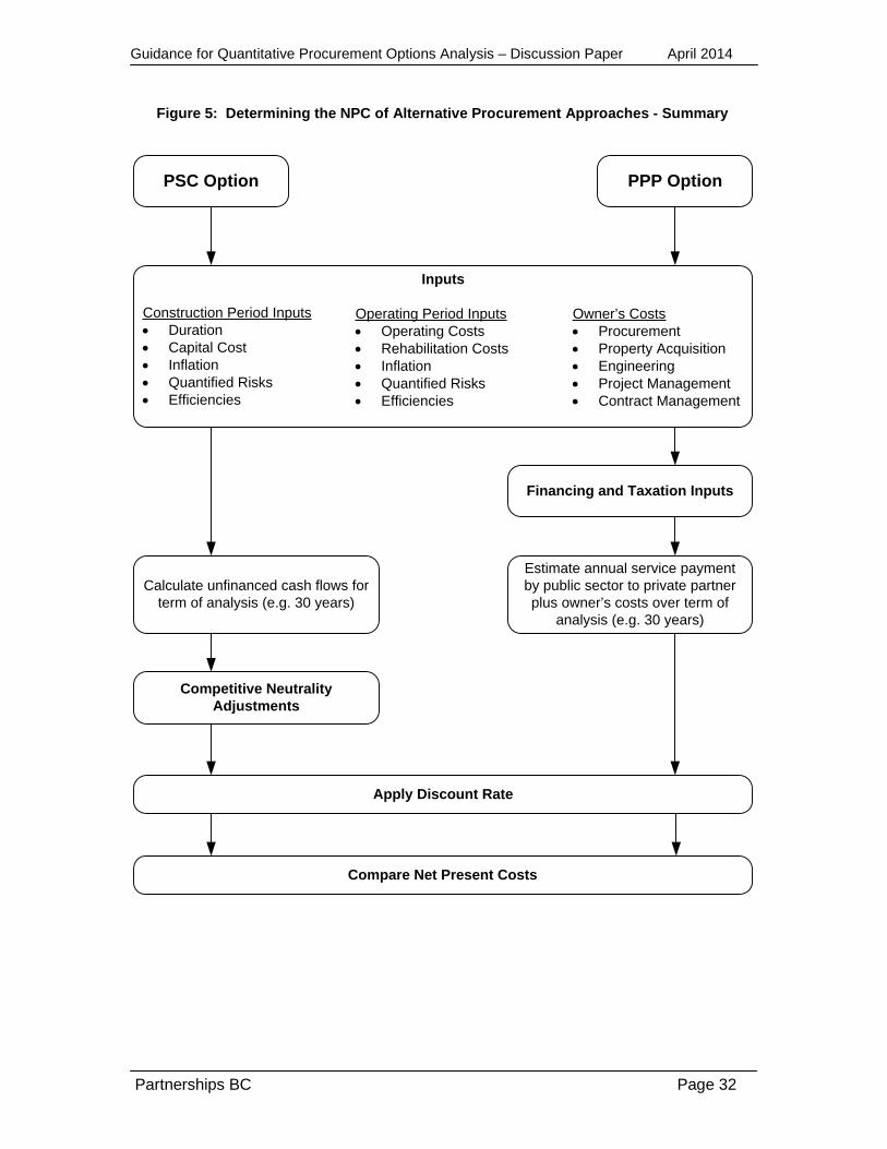
Guidance for Quantitative Procurement Options Analysis – Discussion Paper April 2014
Figure 5: Determining the NPC of Alternative Procurement Approaches - Summary
PSC Option PPP Option
Inputs
Owner’s Costs• Procurement• Property Acquisition• Engineering• Project Management• Contract Management
Construction Period Inputs• Duration• Capital Cost• Inflation• Quantified Risks • Efficiencies
Operating Period Inputs• Operating Costs• Rehabilitation Costs• Inflation• Quantified Risks• Efficiencies
Competitive Neutrality Adjustments
Apply Discount Rate
Calculate unfinanced cash flows for term of analysis (e.g. 30 years)
Estimate annual service payment by public sector to private partner plus owner’s costs over term of
analysis (e.g. 30 years)
Compare Net Present Costs
Financing and Taxation Inputs
Partnerships BC Page 32

Guidance for Quantitative Procurement Options Analysis – Discussion Paper April 2014
Part 3: Interpretation and Presentation
9. Interpreting the Results
This section describes how the outcomes of the quantitative analysis described in Part 2 are interpreted and integrated into the overall results of the business case process.
9.1 Value for Money Context
As introduced in Part 2, the purpose of the quantitative analysis of procurement options is to support the identification of the procurement model offering the best overall value to taxpayers. As value for money includes both qualitative and quantitative elements, the procurement option ultimately selected will be the alternative deemed to best meet the criteria established by the project team. These criteria are determined based on the desired outcomes of a project, and are used to assess a particular procurement option’s ability to support the project, with quantitative value as one key element. Additional detail on qualitative analysis is provided in Section 10.6. The inclusion of qualitative criteria in the value for money assessment means it is possible that the procurement option with the lowest NPC may not necessarily be the preferred option.
9.2 Link to Project Budgeting
The output from the Shadow Bid is an important element of a comprehensive project budget, but does not comprise the complete project budget12. A project budget is defined once the preferred procurement option has been identified, and includes the total amount of funding needed to complete the project within its proposed scope, including both capital and operating components. When constructing the PSC and Shadow Bid, only direct costs that vary based on the type of procurement option are considered in order to simplify the scope of the analysis13. Other important budget components such as the owner’s retained costs are generally not included in the models. These need to be estimated by the project team separately to be included with the Shadow Bid model output in order to create a complete project budget.
Figure 6 below illustrates how output from the Shadow Bid model forms part of the overall project budget.
12 The output from the Shadow Bid model for the purposes of a project budget would be the stream of annual service payments over the concession period, and not the net present cost of the PPP option.
13 Refer to Section 3.1 for more details associated with constructing both models.
Partnerships BC Page 33

Guidance for Quantitative Procurement Options Analysis – Discussion Paper April 2014
Figure 6: PPP Project Budget Components
Shadow Bid Output
+ Retained Costs
+ Expected Cost of Retained Risks
= Total Project Cost
9.2.1 Retained Costs
Retained costs are defined as costs incurred by the government in pursuing a project that are the same for both the traditional and the PPP options. For example, transition and move costs for a health care project are retained by the public sector as patients will have to be transitioned to the new facility regardless of the procurement model chosen. The cost of acquiring property for a transportation project is another example of a cost retained by the owner, as the price of the land along a particular alignment would be the same under both procurement options.
9.2.2 Retained Risks
In a PPP, retained risks are risks borne by the owner because either the cost of self-insuring against them is less than the cost to transfer them, or they cannot be transferred to the private sector at all. An example of a retained risk is owner-initiated scope changes during the design phase. This can lead to delays in the project schedule and possibly higher project costs, but is out of the control of a private partner. To account for retained risks, a contingency fund equal to their expected value should be included in the project budget and funding analysis.
9.3 Scope of the Analysis
Partnerships BC’s scope of work does not traditionally include the preparation of the entire project budget. Instead, it is the responsibility of the owner to complete this work; however, in order to ensure that the complete cost of the project is understood at the time of project approval, Partnerships BC monitors the preparation of the funding analysis, ensuring that the owner incorporates all the asset-specific costs of the project, including retained costs.
Partnerships BC Page 34

Guidance for Quantitative Procurement Options Analysis – Discussion Paper April 2014
9.4 Funding Analysis Context
The funding analysis is the key component of the affordability section of the business case (Part D). It is an estimate, given the information about the project available during the business case phase, of the total annual funding requirement for each year of the development, construction, and operating phases of the project. The calculated funding requirement is usually presented on an annual basis and can also include any costs incurred by the government during the development period, such as procurement costs.
The funding analysis can be thought of as an extension of the project budget. A complete project budget will include all elements listed in Figure 6; however, it excludes operating statement impacts such as interest and depreciation expense.
Figure 7 shows all of the components of a funding analysis. The first item is the ASP, or required revenue calculated by the Shadow Bid. Implied additional operating costs of the asset not included in the scope of the PPP are then added. An example of these would be the costs associated with delivering clinical services in a health care facility, or of faculty staffing costs in a post-secondary institution. In order for the funding analysis to be complete, the following items affecting the overall affordability of the project should be included:
• Any non-cash operating expenses such as depreciation,
• Other project-related costs not previously included, and
• A contingency fund for retained risks.
Figure 7: Relationship of PPP Output to Total Funding
Shadow Bid Output
(Required Revenue) or ASP
+ Implied Additional Operating Costs
+ Financial Statement Impacts (Interest Expense, Depreciation, etc.)
+ Other Project Related Costs
(not previously included)
+ Contingency Fund for Retained Risks
= Total Project Funding Requirement
Partnerships BC Page 35

Guidance for Quantitative Procurement Options Analysis – Discussion Paper April 2014
9.5 Sensitivity Analyses
Sensitivity analyses are conducted to test the impact of changes in key assumptions used in the financial models on the quantitative value for money proposition and/or the affordability of the project. The sensitivity analysis holds all variables constant except one, to determine how sensitive the estimate of the cost of the project is to changes in that particular variable. It is important for the project team to identify key cost drivers for sensitivity analyses, in order to understand the significance of changes to those variables.
Sensitivity analysis is performed on different variables and their selection depends on individual projects. The key variables that are generally covered for all projects include:
• Discount rate
• Cost of debt
• Construction escalation
• Project cost efficiencies
Sensitivity analysis practices pursued by Partnerships BC are explained in more detail in the following sections.
9.5.1 Discount Rate Sensitivity
In order to evaluate the robustness of the quantitative analysis with respect to varying discount rates, Partnerships BC’s guidance calls for a discount rate sensitivity analysis to examine a + / - percentage range around the discount rate determined for a project. The discount rate sensitivity also looks at the break even discount rate which is the discount rate that results in zero value for money. To carry out the analysis, all of the other inputs in both models are left unchanged and the discount rate applied to the cash flows is adjusted in 25 or 50 basis point increments14. The resulting net present costs are then compared to determine the revised value for money proposition.
The results of this analysis can be shown in two ways: as a discount rate sensitivity analysis table as in Figure 8, or in a quantitative value for money curve diagram as in Figure 9.
The table in Figure 8 shows a sample sensitivity analysis on the discount rate assumed for a project based on a range of + / - one per cent. The left column shows the base discount rate of 7.7 per cent, as well as the increments around that value that are tested. The right column shows the resulting quantitative value for money (VFM) expected from pursuing the project as a PPP for each increment contemplated. Given the link between
14 One basis point is equal to 1/100th of a percentage point.
Partnerships BC Page 36

Guidance for Quantitative Procurement Options Analysis – Discussion Paper April 2014
the discount rate and the Project IRR, changing the discount rate would require a re-assessment of a project’s risks.
Figure 8: Discount Rate Sensitivity Analysis
Sensitivity Discount Rate VFM PV ($m)
Base Case 7.7% 65
+1% 8.7% 109
-1% 6.7% 12
+0.5% 8.2% 88
-0.5% 7.2% 40
Break Even 6.5% 0
The quantitative value for money curve is an extension of the discount rate sensitivity analysis as it contemplates a range of possible discount rates, while highlighting the break even point (shown here as the switching point) between the PSC and PPP option selection. The discount rate values to the left of the switching point will produce negative quantitative value for money, consequently recommending the traditional procurement method. Values to the right of the switching point, on the other hand, will produce positive quantitative value for money, recommending the PPP option. A discount rate with the same value as the switching point would result in the same present value cost of the two alternatives and zero value for money.
Figure 9 shows an example of the quantitative value for money curve. The switching point in this example is a 6.5 per cent discount rate. The actual discount rate used in the example is 7.7 per cent.
Figure 9: Quantitative Value for Money Curve
Partnerships BC Page 37

Guidance for Quantitative Procurement Options Analysis – Discussion Paper April 2014
9.5.2 Cost of Debt Sensitivity
A similar sensitivity analysis is performed for cost of debt estimates. Again, Partnerships BC uses a percentage range around the base cost of debt. The results of this analysis are typically illustrated in a table that compares the impact of a change in the cost of debt on the ASP, and on the corresponding quantitative value for money. Figure 10 below shows the results of this analysis based on + / - one per cent range around the base cost of debt.
Figure 10: Cost of Debt Sensitivity Analysis
Sensitivity Actual Interest Rate VFM 1st Year ASP ($m)
Base Case 6% 65 68
+1% 7% 34 71
-1% 5% 93 65
9.5.3 Construction Escalation Sensitivity
In general, the escalation rates applied to costs incurred during the construction period are not constant. Depending on market conditions the cost of raw materials, transportation, qualified labour, and other costs related to construction can increase relatively quickly in comparison to more broadly based inflation measures. Therefore, rather than using a constant escalation rate, Partnerships BC applies an escalation profile in the financial model, determined by the QS, that changes from year to year. For example, the escalation rate for the first year may be five per cent, then eight per cent for second year, and four per cent for the fourth year.
6.5% -1% 7.7% +1% Discount Rate
Sensitivity Analysis
Switching Point
VFM
+
0
-
Partnerships BC Page 38

Guidance for Quantitative Procurement Options Analysis – Discussion Paper April 2014
In order to test the base range of values, a + / - percentage range around the assumed escalation rate for each year is used. For example, if a + / - one per cent sensitivity is used, and the base escalation for the first year of construction is five per cent, for the second year it is eight per cent, and for the third year it is four per cent, the sensitivity ranges would become four per cent to six per cent; seven per cent to nine per cent; and three per cent to five per cent respectively. The result of the sensitivity analysis is then presented in a table that compares the impact of construction escalation rate changes on the ASP and on the NPC of both the PSC and the Shadow Bid. An example of this table is shown below in Figure 11.
Figure 11: Construction Cost Escalation Sensitivity
Construction Cost Escalation VFM 1st Year ASP ($m)
Base 65 68
+1% 53 69
-1% 78 66
9.5.4 Project Cost Efficiency Sensitivity
As described in Section 3.1.1.1, efficiencies may be included in the Shadow Bid to adjust cost estimates. Accounting for these efficiencies involves a sensitivity analysis beginning with the estimated efficiencies for the Shadow Bid, then reducing them incrementally to zero as the worst case scenario, should the anticipated efficiencies not materialize. The results are compared on a quantitative value for money basis, as well as on the basis of the impact on the ASPs.
10. Presenting the Results
Once the quantitative analysis is complete, the results are presented according to the standard outputs presented in the following sections.
10.1 Risk Distributions
10.1.1 Probability Distribution
The Monte Carlo analysis15 produces several outputs.
15 Monte Carlo analysis is an analytical technique in which a large number of simulations are run using random quantities for uncertain variables and looking at the distribution of results to infer which values are most likely. More details on this approach are discussed in Appendix 2: Risk Modelling Methodologies.
Partnerships BC Page 39

Guidance for Quantitative Procurement Options Analysis – Discussion Paper April 2014
Figure 12 below shows the probability distribution for the expected value of all quantified project risks. The resulting distribution is normal, as evidenced by the shape of the curve, with the area in blue representing the expected values within the 90 per cent confidence interval. In the case of this example, the confidence interval states that there is a 90 per cent probability that the value of the risks is between $57 million and $137 million. The mean is $97 million. The areas in red at both ends of the curve represent the area outside the confidence interval. In this case each red area represents five per cent of all expected values.
Figure 12: Probability Distribution of Total Risk
As detailed in Section 4.2, the risks identified in the distribution are either: transferred to the private partner, retained by government, or shared.
10.1.2 Frequency Distribution
Figure 13 below provides a comparison of the probability distributions for the expected value of all costs under the PSC compared to those under the Shadow Bid (in this case a DBFO).
The distributions capture the following costs:
Partnerships BC Page 40
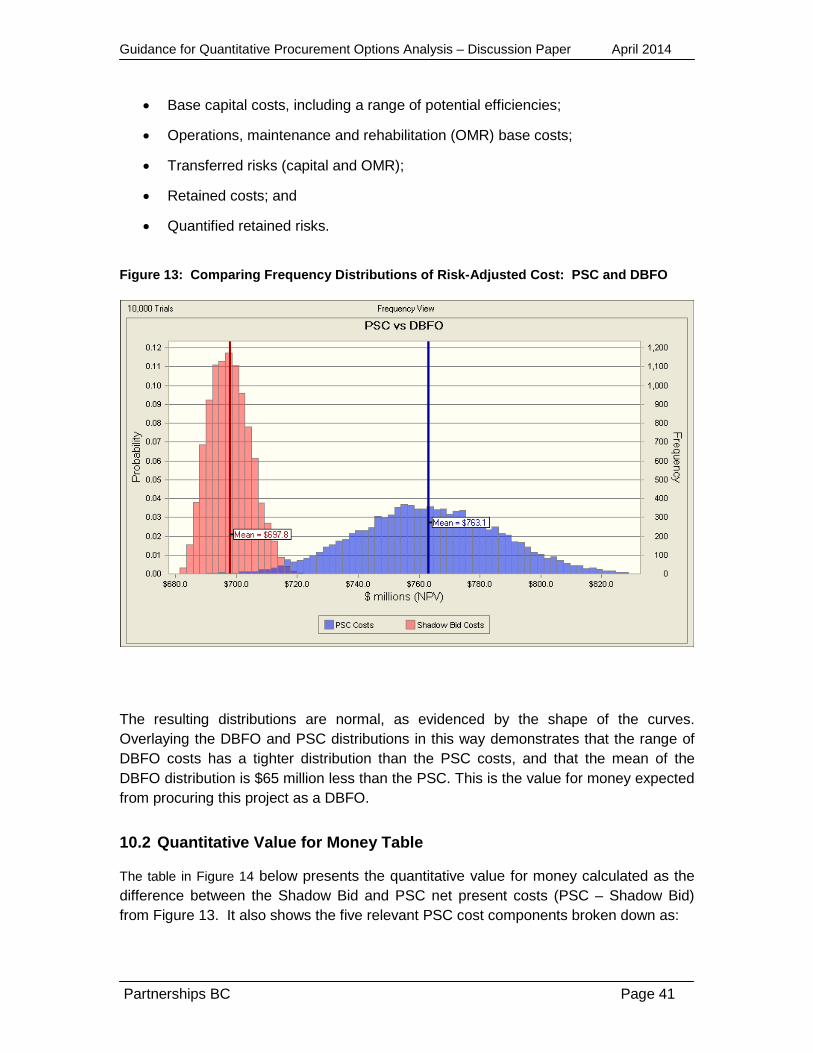
Guidance for Quantitative Procurement Options Analysis – Discussion Paper April 2014
• Base capital costs, including a range of potential efficiencies;
• Operations, maintenance and rehabilitation (OMR) base costs;
• Transferred risks (capital and OMR);
• Retained costs; and
• Quantified retained risks.
Figure 13: Comparing Frequency Distributions of Risk-Adjusted Cost: PSC and DBFO
The resulting distributions are normal, as evidenced by the shape of the curves. Overlaying the DBFO and PSC distributions in this way demonstrates that the range of DBFO costs has a tighter distribution than the PSC costs, and that the mean of the DBFO distribution is $65 million less than the PSC. This is the value for money expected from procuring this project as a DBFO.
10.2 Quantitative Value for Money Table
The table in Figure 14 below presents the quantitative value for money calculated as the difference between the Shadow Bid and PSC net present costs (PSC – Shadow Bid) from Figure 13. It also shows the five relevant PSC cost components broken down as:
Partnerships BC Page 41

Guidance for Quantitative Procurement Options Analysis – Discussion Paper April 2014
1. Capital 2. Life cycle or capital rehabilitation 3. Operations/Maintenance/Facilities management 4. Risk 5. Competitive neutrality adjustments
Figure 14: Value for Money Table
Traditional PPP (Shadow Bid)Capital Costs 463$ OMR Costs 95$ Cost 559$ Availability Payment 633$
Risks Retained under Traditional Delivery that would be transferred under PPPRisk adjustment to Capital Cost 68$ Total Risk Adjustment 68$
Tax and Insurance Adjustment Tax and Insurance AdjustmentInsurance 38$ Insurance Provincial Tax 10$ Income TaxesTotal Adjustment 48$ Total Adjustment
Retained Costs Retained CostsProject Management 59$ Project Management 48$ Retained Risk 30$ Retained Risk 17$
Total Retained Costs 89$ Total Retained Costs 65$
PSC 763$ Adjusted Shadow Bid 698$
VFM Shadow Bid - PSC 65$ % of PSC Costs including risk 8.6%
Value for Money Analysis 30 year OMR, Net Present Cost in $millions @ 7.70% to April 1, 2009
10.3 Annual Service Payment (ASP) Table
The ASP table is an alternative way to view results of quantitative analysis and show the payments the government would make to the private sector under a PPP. A cost breakdown of the ASP is presented for each year in the concession period and includes the following four parts:
1. Capital portion
2. Operations
3. Rehabilitation
4. Maintenance
Partnerships BC Page 42
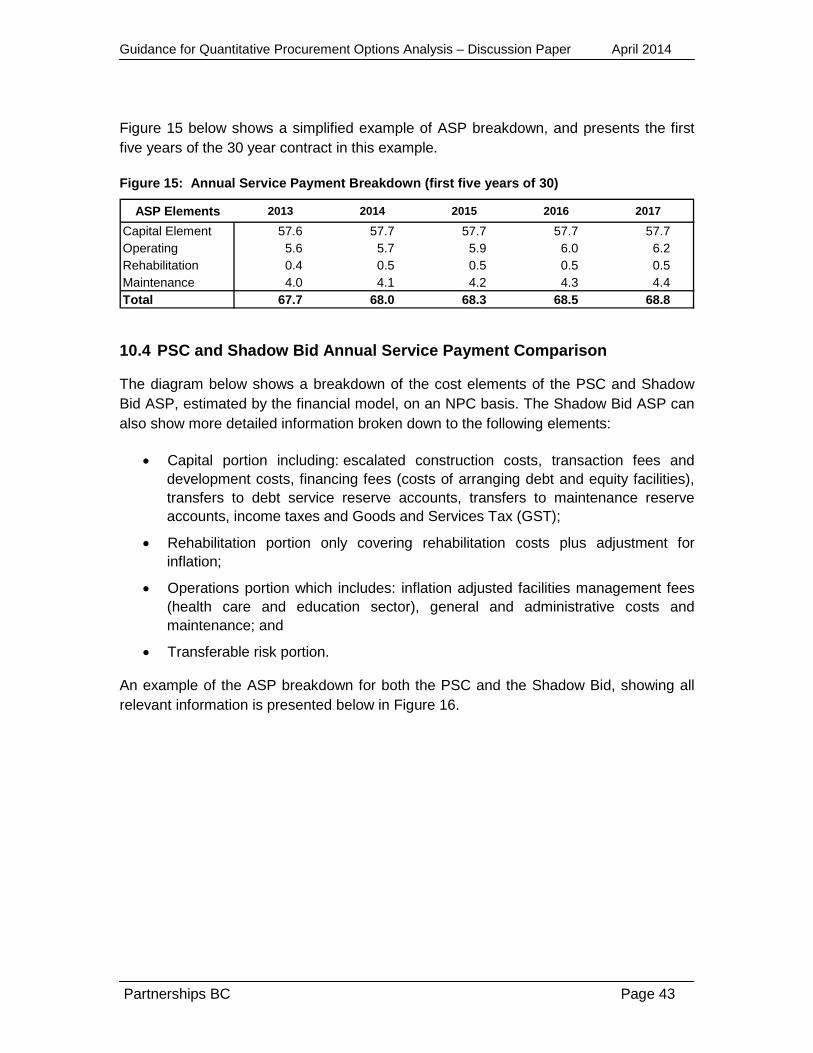
Guidance for Quantitative Procurement Options Analysis – Discussion Paper April 2014
Figure 15 below shows a simplified example of ASP breakdown, and presents the first five years of the 30 year contract in this example.
Figure 15: Annual Service Payment Breakdown (first five years of 30)
ASP Elements 2013 2014 2015 2016 2017
Capital Element 57.6 57.7 57.7 57.7 57.7Operating 5.6 5.7 5.9 6.0 6.2Rehabilitation 0.4 0.5 0.5 0.5 0.5Maintenance 4.0 4.1 4.2 4.3 4.4Total 67.7 68.0 68.3 68.5 68.8
10.4 PSC and Shadow Bid Annual Service Payment Comparison
The diagram below shows a breakdown of the cost elements of the PSC and Shadow Bid ASP, estimated by the financial model, on an NPC basis. The Shadow Bid ASP can also show more detailed information broken down to the following elements:
• Capital portion including: escalated construction costs, transaction fees and development costs, financing fees (costs of arranging debt and equity facilities), transfers to debt service reserve accounts, transfers to maintenance reserve accounts, income taxes and Goods and Services Tax (GST);
• Rehabilitation portion only covering rehabilitation costs plus adjustment for inflation;
• Operations portion which includes: inflation adjusted facilities management fees (health care and education sector), general and administrative costs and maintenance; and
• Transferable risk portion.
An example of the ASP breakdown for both the PSC and the Shadow Bid, showing all relevant information is presented below in Figure 16.
Partnerships BC Page 43

Guidance for Quantitative Procurement Options Analysis – Discussion Paper April 2014
Figure 16: Simplified NPC Breakdown of PSC and Shadow Bid
NPC BREAKDOWN OF PSC AND SHADOW BID
0
100
200
300
400
500
600
700
800
PSC Shadow Bid
$Mill
ions
Availbility PaymentAdjustmentMaintenanceLifecycleCapital RisksCapital CostsRetained RiskRetained Costs
10.5 Annual Service Payment Chart
The chart in Figure 17 presents a visual breakdown of the ASP over time into capital, life cycle (maintenance and rehabilitation) and operations categories.
Figure 17: Annual Service Payment Breakdown Chart
Annual Service Payment
-
10.0
20.0
30.0
40.0
50.0
60.0
70.0
80.0
90.0
2009
20
11
2013
20
15
2017
20
19
2021
20
23
2025
20
27
2029
20
31
2033
20
35
2037
20
39
2041
Year
$Mill
ions
OperatingMaintenanceRehabilitationCapital Element
Partnerships BC Page 44

Guidance for Quantitative Procurement Options Analysis – Discussion Paper April 2014
10.6 Multiple Criteria Analysis
Multiple Criteria Analysis (MCA) is used in the business case stage to evaluate options based on numerous criteria, including value for money. The MCA is an evaluation method used in the both Part B (Service Delivery Options) and Part C (Procurement Options Analysis) decision stages of the business case. In Part B, the MCA approach provides a framework for evaluating potential investment options by evaluating choices against criteria considered critical for the project’s success (for example, the project’s goals and objectives).
With respect to the analysis of procurement options in Part C, the outputs of quantitative analysis discussed in this paper are presented during the business case stage as a part of an MCA process as one of several elements considered in determining the optimal procurement approach for a project. Examples of other procurement-specific considerations include the ability to address stakeholder interests, meet environmental obligations and ensure a fair and transparent procurement process.
The MCA’s development early in the planning process enables the project team to address a wide variety of decision problems, and provides an opportunity to assess the potential of various options to address them. Also, options that are demonstrated to be clearly inappropriate at this stage can be eliminated before significant resources are spent on developing detailed quantitative analyses for them.
A key benefit of the MCA approach in both applications is that it is transparent and relatively easy to understand.
The main output from the MCA is a matrix that summarizes how each procurement option being considered “scores” against the criteria determined by the project team. The comparison between the procurement options is not based on a single, simple decision rule—it usually requires an explicit judgment or “importance weighting” between goals or criteria. Typically, the results from the MCA are summarized as shown in Figure 18 below. Qualitative factors vary from project to project and are judged ordinally with the options being ranked in terms of order of magnitude in satisfying criteria. For example, the “Competition” criterion in Figure 18 is considered to be “good” for the PSC option and “best” for the Shadow Bid. This can be interpreted to mean that the Shadow Bid is better than the PSC model for that criterion. It is important to note that it is up to decision-makers for the project to decide which criteria are the most important. Using the matrix below as an example, if allowing for innovation is the most important criterion, the Shadow Bid model would be the preferred model, but if user satisfaction is deemed to be the most important, the PSC model would prevail.
The most common quantitative criterion is the NPC of the project cash flows under each procurement model and is presented below in Figure 18.
Partnerships BC Page 45

Guidance for Quantitative Procurement Options Analysis – Discussion Paper April 2014
Figure 18: Multiple Criteria Analysis (MCA) Matrix
CRITERIA PSC Shadow Bid
Competition Good Best
Innovation Limited Best
Service Delivery Outcomes Good Good
User Satisfaction Best Good
Risk Adjusted NPC $763M $698M
11. After the Business Case
The comparison of the PSC and the Shadow Bid models represents a key part of the business case for any project, but the contribution of the quantitative analysis work to the project does not end with the approval of the business case by B.C. Treasury Board. The PSC and Shadow Bid are dynamic procurement tools and need to be continually updated during the procurement process to reflect any new information discovered about existing assumptions. The PSC model does not, however, reflect financial innovation coming from the private sector. When the Request for Proposals (RFP) responses are submitted, the PSC is locked down and no further changes are made to it. The resulting finalized PSC model is then used during the evaluation process to assess proposals. After selection of the preferred proponent is announced and financial close reached, the value for money analysis can be completed.
The value for money report is a document that assesses both the quantitative and qualitative benefits achieved by the government structuring the project as a PPP. In measuring the quantitative benefits achieved through the PPP, the PSC is compared directly to the winning bid. The two financial models are compared on an NPC basis and the difference between the two values (total NPC) is published in the Project Report: Achieving Value for Money as the net quantitative benefit achieved.
12. Conclusion
This paper presents Partnerships BC’s current approach to quantitative analysis of procurement options, based on incorporating its guidance in the areas of cost estimation, financial modelling, risk analysis, and appropriate discount rate methodology.
Partnerships BC Page 46

Guidance for Quantitative Procurement Options Analysis – Discussion Paper April 2014
Quantitative analysis is used during the business case stage as an essential part of the MCA process that brings together various analytical techniques to evaluate a range of project characteristics, options and potential impacts. This evaluation includes both quantitative and qualitative factors. The purpose of quantitative analysis is to identify which procurement option is most likely to provide quantitative value for money.
Quantitative analysis during the business case stage is based on developing and comparing the PSC and the Shadow Bid models that take into account several key factors including: capital and operating cost estimates, capital and operating cost efficiencies, financing costs, the discount rate, risk transfer, and competitive neutrality adjustments.
The PSC and Shadow Bid models are developed on a cash flow basis, and the appropriate discount rate is estimated in order to discount the cash flows of both models to their NPC. The cash flows of the models include capital, operating, rehabilitation, and financing costs for the Shadow Bid. Risks are identified, analyzed and quantified where meaningful, and then allocated to the private partner or retained by the owner based on the proposed risk allocation of the project. Competitive neutrality adjustments are then made for insurance and taxation. Finally the models’ results are presented in the form of a standardized value for money table that compares the alternatives based on their NPC, to determine which procurement method delivers quantitative value for money. To derive the overall value for money, both quantitative and qualitative benefits are assessed in the MCA analysis, and summarized in the MCA table.
The application of the quantitative analysis does not end with the approval of the business case. The PSC and Shadow Bid are dynamic procurement tools and are updated during the procurement process to reflect any new information, in support of a rigorous procurement evaluation.
The methodology for the quantitative analysis presented in this paper reflects current knowledge based on the approach used on projects in B.C., in addition to ongoing monitoring and interaction with other jurisdictions. As such, the process will continue to be refined and will evolve to ensure that Partnerships BC is applying the most effective techniques for measuring value in public infrastructure procurement.
Partnerships BC Page 47
Guidance for Quantitative Procurement Options Analysis – Discussion Paper April 2014
Appendix 1: Financing and the PSC The Partnerships BC analysis uses an unfinanced PSC for three key reasons that include: difficulty in identifying the precise source and associated cost of publicly raised funds; the cost of raising taxpayer supported public funds does not reflect the true cost of financing a project; and applying the risk adjusted, market-based discount rate to the PSC cash flows implicitly accounts for the project risk in the PSC model.
The public sector, regardless of whether it is at the municipal, provincial or federal level, has substantial ongoing cash receipts from its various revenue sources (duties, income taxes, capital taxes, user fees, etc). For any given infrastructure project, therefore, the public sector could fund the associated costs from existing cash receipts, newly issued debt or a combination of the two, and each funding source would have a different cost. More importantly, neither source of public funds would be an accurate estimator of the true cost of using public capital, as only the cost of issuing long-term government debt can be determined.
The public sector’s long-term borrowing rate, therefore, is an inappropriate estimator of the true cost of capital essentially because it only reflects the cost of RAISING capital, which can be very different from the cost of USING that capital. The public cost of raising capital does not include the full cost implications of retained project risk, nor does it typically include the cost of amortizing the debt. For example, if the public sector’s long-term cost of borrowing is five per cent, when the project risk implies that an Internal Rate of Return of seven per cent16 is required by the private sector, taxpayers are in effect subsidizing the traditionally procured project by covering the potential additional cost of the risks associated with the project17. Taxpayers are often not aware of this exposure to the true risks of a project, nor to the implied subsidy they are providing. It is usually only in the case of large cost overruns and project failure that taxpayers realize the cost implication of the public’s exposure. For this reason, using the public sector long-term cost of borrowing (e.g. five per cent) based on a bullet-type bond18, and applying a discount rate of seven per cent leads to an analysis that is unfairly biased in favour of the PSC.
In order for the taxpayer to avoid providing this subsidy, a financed PSC would need to assume a financing cost at a rate that reflects the risk inherent in a project, in the same way as the private sector cost of capital, and amortize the debt over the term of the contract19. When the true cost to the public sector of financing a project is reflected in the discount rate, the effect of financing is equal to discounting the unfinanced cashflows by the discount rate, and can therefore be ignored.
16 As determined by the private sector cost of capital for the project 17 Uncertainty and the Evaluation of Public Investment Decisions, Arrow, Kenneth J and Lind, Robert C., 1970, American Economic Review. 18 Bullet Bonds typically are non-callable and repay the full principle in a single payment at maturity. 19 This approach was used on the Sea-to-Sky Value for Money Report at the request of the Office of the Auditor General.
Partnerships BC Page 48

Guidance for Quantitative Procurement Options Analysis – Discussion Paper April 2014
Appendix 2: Sample Risk Template
Risk Name
Risk Register Number
Allocation:
Description:
Chance Risk Event Occurs
Base cost estimate
Is risk quantifiable?
Cost Impact Assumption Change in Base Cost Justification
Low: 95% certain if risk event occurs, cost will not be less than (1)
Most likely outcome
High: 95% certain if risk event occurs, cost will not exceed
Notes:
Risk Mitigation Plan:
Partnerships BC Page 49
Guidance for Quantitative Procurement Options Analysis – Discussion Paper April 2014
Appendix 3: Risk Modelling Methodologies A number of theoretical and statistical methods can be used to value risk. The method applied to risk quantification must correspond with the nature of information available about the risks. The following section outlines the methods used for risk valuation.
1. Introduction
Risk quantification is a key component of the analysis of procurement options. An important concept related to risk quantification is that, for most risk events, the result is not a single value but, rather, a distribution of many possible values.
While a definite process is followed to obtain inputs to calculate the distribution of values for a risk event, the result involves both art and science, and will be influenced by the unique experience of the project team, advisors and the facilitator.
The objective of the risk quantification stage is to value the project risks in order to develop two fully-costed (i.e., risk-adjusted) delivery models. These models include a public sector delivery model, or public sector comparator (PSC), and a private sector delivery model, also known as a Shadow Bid.
The PSC and Shadow Bid will take into account the value of risks that are transferred from the public sector to the private sector, as well as the value of risks that are retained by the public sector under both delivery models. The outcome of this process allows for the comparison of the cost of the two approaches on a risk adjusted basis.
When comparing the cost, a thorough understanding of the contingencies in the project’s base cost estimate is necessary to ensure there is no double counting of risk. Such double counting can occur if the contingencies include any amounts for project risk that are also being quantified in the risk analysis. To fully understand the contingencies, the quantity surveyor responsible for developing the cost estimate should be included as a member of the risk quantification team.
2. Distributions
There are many types of distributions, the most common of which is the normal distribution; however, the normal distribution is not very useful for the purposes of risk quantification as it requires the standard deviation or variance to be specified as an input which is typically not possible within the context of a risk workshop.
The two most commonly used distributions for risk quantification, therefore, are triangular and discrete. These distributions are appropriate for different types of risks, and the
Partnerships BC Page 50

Guidance for Quantitative Procurement Options Analysis – Discussion Paper April 2014
necessary inputs can be more readily identified by risk workshop participants. Triangular and discrete distributions are discussed in detail below.
2.1 Triangular
The triangular distribution is the most common distribution used to quantify risks that are assumed to be continuous random variables, but that cannot be defined as a normal distribution. A triangular distribution has one peak and uses the following three parameters to determine the expected value of the cost outcome of each risk:
• Maximum • Most likely • Minimum
The maximum scenario represents the most unfavourable outcome associated with a risk event. The most likely scenario, or mode, is the most likely consequence of a risk event and the minimum scenario represents the least severe outcome possible for a risk event.
In addition to specifying maximum and minimum amounts, confidence levels can be used to express the degree of certainty associated with these events. For example, an estimated maximum value of $100,000 for a triangular distribution can be made at the 95 per cent confidence level, meaning that values higher than $100,000 are possible but have no more than a five per cent chance of occurring.
Expressing estimates in terms of confidence intervals is useful for risk work, as individuals tend to be more comfortable providing estimates at 95 per cent, which means that one time out of 20 they will be incorrect, rather than being asked to say with 100 per cent certainty what a maximum value might be. This is particularly true as one moves towards the maximum tail of a distribution where values can increase rapidly. Asking for 100 per cent certainty can result in a very high maximum value, even if it is highly unlikely to happen (i.e., less than five per cent).
Triangular distributions will often be skewed meaning that, unlike symmetrical distributions, the values are not equally distributed about the mean and the most likely risk outcome will be closer to either the minimum or maximum values. In a right-skewed distribution there are more, very large values that result in a long tail after the peak when the curve is drawn from left to right. For example, a distribution for the risk of construction delays typically has a long right tail because more things are expected to go worse than planned rather than better, resulting in costly delays that generate greater cost for this risk. A left-skewed distribution has a greater number of very small cost values, relative to the median and mode, resulting in the tail appearing before the peak. Examples of triangular distributions, both symmetrical and skewed are shown in Figure 8.
Partnerships BC Page 51

Guidance for Quantitative Procurement Options Analysis – Discussion Paper April 2014
Figure 8: Triangular distribution forms
Symmetrical Left Skewed Right Skewed
Given a probability distribution for a particular risk, statistical software such as @RISK or Crystal Ball can be used to determine the expected value of that risk. In cases where the distribution is symmetrical, the expected value of each risk will be equal to the most likely scenario. For risks that are asymmetrical, or skewed, the expected value must be determined with the assistance of statistical software.
An example of the inputs and expected value for a skewed triangular distribution are summarized below in Figure 9.
Figure 9: Summary of Risk inputs and outputs for a triangular distribution
Triangular Distribution Inputs
Risk Min Value Most Likely = mode Max Value Expected
Value
1 16.5 17.2 21.0 18.4
Example (Risk 1) The price of cement is changing rapidly and there is 90 per cent probability that the price will be somewhere between $16.5 and $21.0 per 100 pounds for the next four years. Given that the price of cement will change, the most likely price during next four years is estimated to be about $17.2 per 100 pounds. The expected price of the cement using statistical software is $18.4:
Partnerships BC Page 52

Guidance for Quantitative Procurement Options Analysis – Discussion Paper April 2014
Figure 10: @Risk Distribution Diagram for Risk 1
2.2 Discrete
A discrete distribution is the second most common distribution used for risk quantification, and is the preferred method for quantifying risks with discrete (i.e., separate and individual) outcomes.
A discrete distribution relies on the assumption that risks are independent of each other, so that the occurrence of one risk will not affect the occurrence of another. A discrete distribution function can have multiple peaks, with the highest one representing the most likely outcome. Although the discrete distribution is not as simple as a triangular distribution to define due to its higher number of inputs and requirement of a 100 per cent confidence interval, the inputs for the discrete distribution can be as easily obtained during a risk workshop as those for triangular distributions.
Defining discrete distributions relies on the experience of the project team to determine estimates of the magnitude of consequence and probability of occurrence for a particular risk event. The project team determines a number of outcome points—usually three, but any number equal or greater than two can be used. For each potential outcome a probability of occurrence must be assigned that are often characterized as high, medium, and low in relation to the severity of consequence. The high scenario would represent a severe outcome with a significant cost consequence. The medium scenario would represent a moderate outcome, with a less severe cost consequence, and the low scenario would
Partnerships BC Page 53

Guidance for Quantitative Procurement Options Analysis – Discussion Paper April 2014
correspond to an even smaller consequence with different cost consequence assumptions associated with it.
The expected value of a discrete distribution can be calculated using a simple formula or with statistical software. The simple formula is:
E (VRISK) = PR x { P1C1 + P2C2 + P3C3 + … PiCi }
Where:
E (VRISK) = Expected value of risk
PR = Probability of the risk event occurring
Pi = Probabilities of i-th outcomes (Note: sum of all probabilities equals 1)
Ci = Cost consequences of i-th outcomes
Figure 11: Summary of Risk inputs and outputs for a Discrete Distribution
Following are two simplified examples of discrete distributions.
Example (Risk 2)
A project team responsible for a bridge the Ministry of Transportation and Infrastructure wants to build over a river estimates that there is 35 per cent probability that the project design will need to be altered during the procurement process. Given that project design must be altered, there is a 20 per cent probability that the changes are minor and the resulting increase in the design cost will be only $80; however, there is 45 per cent chance that changes will be more significant and will cost $140. There is also 35 per cent chance that the changes are major and will cost $180. The expected value of this particular risk is $49.70, calculated as follows:
E (VRISK) = 35% x { 20%($80) + 45%($140) + 35%($180)} = $49.70
Likelihood (Probability of cost impacts) Cost of Consequence Expected
Value
Risk Probability P1 P2 P3 P4 C1 C2 C3 C4
2 35% 20% 45% 35% 0% $80 $140 $180 $0 $49.70
3 65% 40% 15% 20% 25% $100 $150 $220 $250 $109.85
Partnerships BC Page 54

Guidance for Quantitative Procurement Options Analysis – Discussion Paper April 2014
The discrete distribution for Risk 2 is shown in Figure 12. The figure shows the shape of the discrete probability density function and its peak that indicates that the most likely outcome, if any risk is realized, will be somewhere around $140. The most likely outcome of the entire distribution is zero since there is a 65 per cent chance of not realizing the risk event.
Figure 12: Discrete Distribution (Risk 2)
Example (Risk 3)
A project team is contemplating a geotechnical risk of the land on which a new hospital will be built. There is a 65 per cent probability that the soil is unstable and that some areas will need pre-treatment before construction can begin. Given that soil is unstable, the engineers have estimated that there is:
• A 40 per cent chance that one area needs to be fixed at the cost of $100,
• A 15 per cent chance that two areas need to be fixed at the cost of $150,
• A 20 per cent chance that three areas need to be fixed at the cost of $220, and
• A 25 per cent chance that four areas need to be fixed at the cost of $250.
The expected value of geotechnical risk is $109.85, calculated as follows: E (VRISK) = 65% x { 40%($100) + 15%($150) + 20%($220) + 25%($250)} = $109.85
Partnerships BC Page 55

Guidance for Quantitative Procurement Options Analysis – Discussion Paper April 2014
The discrete distribution for this example is shown in Figure 13. The figure shows that this distribution has two peaks and the most likely outcome will be somewhere around $100.
Figure 13: Discrete distribution of Risk 3
2.3 What and How to Quantify
2.3.1 Which Risks to Quantify
A comprehensive risk register may contain up to 250 risks. There is no minimum or maximum number of risks that must be quantified, although typically there are between 20 and 40 risks that are calculated. To make the risk quantification more efficient, it is recommended that, where possible, risks be aggregated and quantified as a group. For example, there are many possible sources of delay (risks) that can be aggregated under a category of delay-related risk for quantification purposes. These different sources of delays can be considered possible scenarios. Rather than calculate the value of each individual risk, the value of the combined impact of these risks is determined. It is important to keep a large number of risks in the risk matrix even if only some of them are quantified. The reason is that most require a unique risk mitigation strategy.
Partnerships BC Page 56

Guidance for Quantitative Procurement Options Analysis – Discussion Paper April 2014
It is recommended that retained and transferred risks not be aggregated. Risks that are shared (usually a very small number), should also be kept separate and quantified individually. Once quantified, a decision can be made about how the risk should be shared (i.e., 50/50, all dollars above a certain threshold, etc.).
Examples of some of the larger risk categories include:
• Pre Construction o Approvals at various levels of government (e.g., Provincial Treasury Board,
municipal, zoning, development). • Design and Construction
o Construction delays, o Cost escalation (e.g., supply of materials, labour, equipment), o Scope changes by owner, o Geotechnical risks, o Errors and omissions, and o Estimating risk (errors).
• Operating Period o Failure to meet performance standards, and o Failure to meet hand-back requirements at the end of the contract term.
2.3.2 Design and Construction Period Risks vs. Operating Period Risks
Although the aggregate value of operating period risks is typically many times less than the aggregate value of design and construction risk, care must still be taken to determine the appropriate value of these risks as they will usually be transferred under a DBFM where the private sector partner will become responsible for maintenance and life cycle activity. By the time risk quantification is undertaken, there should be a cost estimate for the maintenance and life cycle obligations associated with the new asset that can be used for the purpose of quantifying the associated risks.
The approach to quantifying operating period risks is not always clear. To help clarify, assume for discussion purposes that the cost estimate for maintenance and life cycle of a project is $1 million per year. This estimate means that the public sector body under traditional delivery could be assumed to receive a $1 million allocation from the owner towards the maintenance and life cycle of the new asset, and is a necessary assumption for a like-for-like comparison of procurement alternatives. The actual amount of money spent by the public sector, however, on life cycle and maintenance, can be expected to be less than $1 million due to competing budgetary pressures and priorities. The extent to which the actual amount spent falls short of the assumed allocation depends on the owner, and can be determined based on historical life cycle and maintenance funding.
Partnerships BC Page 57

Guidance for Quantitative Procurement Options Analysis – Discussion Paper April 2014
This under-funding or delayed funding can result in significant risk in the public sector delivery model, since the asset will not be able to meet the intended performance standards. In addition, there is the risk that the cost of deferred life cycle and maintenance will be higher when it is eventually performed. This risk should be reflected by a premium that is sufficient to demonstrate what would be required to achieve hand-back standards at the end of the performance term under traditional delivery. When calculating this risk premium, care must be taken to ensure it addresses the additional cost of deferred life cycle and maintenance that would need to be incurred to achieve hand-back standards. If the premium is too low, the outcome of the deferral on an NPC basis will suggest that deferring these costs is the best economic decision, which is neither intuitive nor correct.
2.3.3 Timing of Risks
When risks are quantified, consideration must be given to the likely timing of the risks. As a result of discounting to determine the NPC, a $10 million dollar impact at the start of construction will have a greater impact in the financial model than a $10 million impact three years later during commissioning.
2.3.4 Risk Values
The initial calculation of risk values can be either in nominal or real dollars, and can be discounted or undiscounted. It is recommended that for construction period risks, undiscounted values be used (they can be nominal or real). These values can then be integrated into the financial model and ultimately converted into nominal amounts.
For operating period risks, costs are typically presented as real dollars, making it logical to do the analysis in real dollars. These real dollars can then be integrated into the financial model and ultimately converted into nominal amounts also.
Once all the values are expressed in nominal terms, they can be discounted to determine their NPC and added up, allowing a comparison to be made between the two models.
2.3.5 Quantification Pre/post Mitigation
Almost every risk has a possible mitigation strategy and risks should be quantified assuming that these risk mitigation strategies would be successfully deployed. Further, the mitigation strategies assumed for this purpose should reflect what the public sector body would actually do to mitigate the risk, rather than what it could do.
For example, if scope change from stakeholders is a key risk, a mitigation strategy might be to implement a stakeholder working committee that will explain the PPP process, including an explanation of when and how stakeholders can affect scope changes. The risk this mitigation strategy is intended to address should be quantified assuming that the working committee is in effect.
Partnerships BC Page 58

Guidance for Quantitative Procurement Options Analysis – Discussion Paper April 2014
In the case of geotechnical risk, on the other hand, this approach would not be appropriate if the mitigation strategy is to drill boreholes in the future to obtain new and/or better information. The geotechnical risk would need to be calculated pre-mitigation and then be re-quantified once the results of the boreholes has been obtained.
2.3.6 Probabilities
Probability is an important component for most risks regardless of the type of distribution, as there is a chance (or probability) that the risk event will occur and a chance the risk event will not occur. An example of this is provided in the Risk 3 example above. For other risks it is simpler to assume that there is a 100 per cent probability that the risk event will occur, and then accounting for the probability directly in the values for the distribution (e.g., CMin, CMod, and CMax, for a triangular distribution). This is particularly relevant for risks such as delays which tend to happen on almost all projects (i.e., 100 per cent certain), but with different consequences.
2.3.7 Correlation
Correlation is a systematic pattern that can be seen in the occurrences of events. A positive correlation means that as one value increases, the other value increases as well. A negative correlation means that as one value increases, the other value decreases. Correlation does not imply causation. Correlation values range from -1 to +1, and a value of zero indicates no correlation. During the business case stage, correlation is often assumed not to exist. This is a conservative assumption and tends to understate the aggregate risk value.
If correlation is pursued, correlation is typically assigned as follows:
Figure 14: Typical Correlations
Low positive correlation +0.3
Medium positive correlation +0.5
High positive correlation +0.7
Low negative correlation -0.3
Medium negative correlation -0.5
High negative correlation -0.7
The correlation values, if and when assigned, need to be loaded into the statistical software.
Partnerships BC Page 59

Guidance for Quantitative Procurement Options Analysis – Discussion Paper April 2014
2.3.8 Risk Quantification and Efficiency Estimates
A source of potential confusion with respect to risk quantification is how the risk estimates and efficiency estimates relate. In many business cases, an efficiency assumption has been used on capital costs, such as claiming that a DBFM will be six per cent less expensive on construction costs than traditional procurement. The guidance for establishing potential efficiencies is to hold a workshop to review the opportunities for efficiencies that the private sector can bring to a specific project. General rules of thumb are not acceptable.
The combination of risk quantification and efficiency estimates result in positive or negative value for taxpayers, and need to be looked at together in order to prevent double counting or omissions.
2.3.9 Risk Quantification PSC vs. Shadow Bid
The calculation of the PSC should reflect the total range of outcomes for the public sector. As most risks ultimately rest with the public sector, in a PSC the calculation is relatively straightforward, all the more so in that the owner’s team is likely to be built around individuals with public sector experience.
The calculation of the Shadow Bid is more challenging. It is a combination of:
a) Those risks to which the public sector continues to have exposure (because the risk may be shared or retained), and
b) Those risks that are transferred to the private sector.
When calculating the risk value for Shadow Bid risks, the following considerations must be taken into account:
• Is the risk exposure the same for the private partner? • Does the project agreement change how the risk is valued? • How will the private partner apply the risk value to their base cost (part of
base contingency or additional)?
It is not acceptable to pro-rate all PSC risks by the some factor (e.g., 35 per cent) to arrive at Shadow Bid values. The owner’s team may not have the private sector experience to adequately address the above considerations and outside experts may have to be called in.
2.3.10 How to Get Risk Inputs
The required inputs will vary according to the statistical distribution selected. Most often a small group of experts will work together to determine the appropriate inputs for each risk distribution. This group will include representatives from the owner’s team, hired experts, and Partnerships BC staff.
Partnerships BC Page 60

Guidance for Quantitative Procurement Options Analysis – Discussion Paper April 2014
It is common when using a distribution that is bounded like the triangular, or a discrete distribution to complete the process with a distribution that has a narrow range of potential outcomes than would be actually observed. This is often due to an over-confidence of the estimator in the middle point of their range. Some techniques to deal with this central tendency bias are:
i) If using a distribution that is bounded and has a defined mid point (e.g., a triangular distribution) a smaller range will generally result if the most likely result is identified first, then moving out to the points at the extremes. When an expert identifies a most likely estimate they will tend to then want to defend it and a larger range of potential outcomes can seem like they are unconfident in the most likely estimate. This can be overcome by first determining the extreme bounds of the distribution. The maximum value should be determined first. A good opening question to an expert is “What is the worst impact you have ever witnessed or know about for a similar risk in a comparable project”? The second step would be to determine what would be the best impact they have ever witnessed for a similar risk. Having set the bounds now the most likely impact can be determined.
ii) Experts and others providing inputs can be challenged with suggesting comparable bets. For example if someone said they were 90 per cent certain that a certain outcome would be less than a set amount they can then be offered a bet. The bet would be: would they risk $100 for the chance to win $1,000 if the actual outcome is greater than the set limit. If they say yes to that proposition then that indicates they really think the chance of realizing that outcome is greater than 90 per cent (they would rather have the bet). The goal is to reach a point of indifference. They should then be asked at what level of outcome they would be indifferent to the bet or the outcome.
2.3.11 How to Integrate Risks into the Financial Model
Once the inputs for all risks are obtained, they can be integrated into both the PSC and Shadow Bid financial models. The preferred approach for integrating the risks is to have separate sheets in the financial model, with at least two sheets required in the input section. These include:
• Timing – this sheet will indicate when each risk occurs and is typically shown as a percentage of occurrence in each period; and
• Inputs of Risks – this sheet will contain the raw inputs collected at the risk workshops and will also include the expected value calculated using a statistical software program. In many cases it is easier to have a separate input sheet for the construction and operating risks given the different approaches to calculating these risks and their different time horizons.
Partnerships BC Page 61

Guidance for Quantitative Procurement Options Analysis – Discussion Paper April 2014
In the calculation or output section of the model, one sheet will be required containing the Risk Output. The Risk Output sheet takes the information from the Timing sheet and Input of Risks sheet and creates nominal values for each risk for each period in the model.
Each risk should be calculated separately and grouped under construction or operating and transferred or retained. Columns should be added on the right hand side of the page for NPV, real and nominal totals. This is illustrated in Figure 15. One of the benefits of calculating risks separately is that it allows an analysis of individual risks in comparison to the total value of risks.
Figure 15: Extract from sample Risk Output sheet in financial model.
Transferred Construction Risks NPV @ Period Start: Nov-07 Nov-088.93% Total Total Change in
Item As of REAL $ NOMINAL value in this1-Jan-06 1-Jul-05 Dollars scenario
GC1Lightweight Fill in Segment 146 in capital cost estimate may be insufficient due to soft soils (0.055) (0.13) (0.10) (0.10) - -
2.4 How to Document Risks
Risks need to be documented in such a way that they can be readily reviewed by third parties and peers. The guidance in this area is to document each quantified risk in a separate template.
The characteristics of a good template are:
• Consistency across all risks.
• Formatted to print out on 8.5” x 11” paper.
• Each template should have the same header and footer, providing information about the project, page number etc.
• Contain sufficient information to understand the risk (this can come from qualitative fields taken from the risk matrix including: risk number, name, description, allocation, etc.).
• Include the underlying base cost on which the risk is calculated.
• Include information on the timing of the risk.
• Contain values for each quantified risk under both the public sector comparator and the Shadow Bid. For those risks that are retained, the calculation of an owner’s or project reserve may be appropriate.
• Most importantly, provide an explanation and justification for each risk value.
• Document who provided information to complete the template.
Partnerships BC Page 62

Guidance for Quantitative Procurement Options Analysis – Discussion Paper April 2014
As the templates will form part of a risk booklet, a table of contents with a summary of the risk value is extremely useful. Any template or group of templates with these characteristics is acceptable.
2.4.1 Due Diligence
Risk guidance involves the review of the risk outputs and initial value for taxpayers proposition by a group of peers and/or a group of external professionals. This should be separate from the peer review of the business case. Such a review allows time for more refinements and a longer in-depth examination of risks, which is not normally available at the business case peer review.
2.5 Monte Carlo Analysis
Monte Carlo analysis is an analytical technique in which a large number of simulations are run using random quantities for uncertain variables and looking at the distribution of results to infer which values are most likely.
Monte Carlo analysis overcomes significant limitations of both traditional sensitivity analysis and discrete analysis, which typically becomes very cumbersome beyond two model input variables. Monte Carlo analysis, on the other hand, can accommodate an almost unlimited number of input variables, and allows the overall effect to be observed on the desired outcomes. The sensitivity of one input on the outcome can still be measured and improvements relating to better measure of variability can be made. Monte Carlo analysis also allows the individual effects of each simulated input to be ranked according to their affect on the outcome relative to the other simulated inputs.
Monte Carlo simulation assigns a range of potential input values to each input variable. These input values can be based on a discrete analysis, outputs from a probability distribution, or direct user inputs (effectively a custom probability distribution). An output (or range of outputs) is defined before the simulation is run.
The Monte Carlo simulation runs ‘trials’ of the model a specified number of times (usually 10,000 or more). For each trial the simulation chooses and new input for each of the variable inputs according to the distribution selected for that input. The model is then calculated and the output result is logged. When all the trials are complete the range of results is available for statistical testing or display.
In order to show the values of risks and the whole cost of the public sector comparator and Shadow Bid as a range, it is essential to perform a Monte Carlo distribution. Figure 16 shows the range of costs for a PSC and a DBFO delivery model. In this figure the mean value for the cost of the DBFO is $70 million less than the PSC, indicating positive value for taxpayers.
Partnerships BC Page 63

Guidance for Quantitative Procurement Options Analysis – Discussion Paper April 2014
Figure 16: Overlay distribution of total PSC costs and DBFO costs
Generating the distribution for the PSC is relatively easy as there is no financing in the PSC. However, generating the distribution for the Shadow Bid, assuming it involves financing, is more complicated. A useful simplification is to determine the three points on the distribution that include:
• The expected value • Five per cent value • Ninety-five per cent value
For each of these three points the model will have to be re-optimized but once obtained, the distribution can be generated very easily.
The $70 million in value for money demonstrated in Figure 16 is based on comparing the means of the two distributions. The mean of the distribution can also be referred to as the P50 value, as 50 per cent of the values under the curve lie above and below the P50 value. Partnerships BC has used a range of P values from P50 to P85 depending on the amount and quality of information available to the project team. The project team needs to justify any level other than P50. As Partnerships BC has moved towards establishing a pass/fail affordability ceiling as its guidance, it is imperative that the correct value be chosen to calculate the affordability ceiling, otherwise proponents will be unduly eliminated and/or the scope of the project (and benefits) will have to be reduced.
Partnerships BC Page 64

Guidance for Quantitative Procurement Options Analysis – Discussion Paper April 2014
Appendix 4: Discounted Cash Flow Analysis Cash flow streams under PSC and Shadow Bid models will generally have different time profiles20 due to differing underlying construction schedules. This can result in different start dates and different completion dates. If the time profiles were the same, the cash flow streams would match in terms of timing of incurrence and could be directly compared to each other on a periodic (usually annual) basis; however, the substantial differences in cash flow timing make an overlay cost comparison impractical and sometimes impossible.
To be able to compare the procurement models, the cash flow streams are discounted to a common start date. This is typically present-day but it can be any point in time. The process of valuing an investment by discounting its cash flows is known as discounted cash flow analysis. The final output of discounted cash flow analysis is the net present value (NPV) or frequently, in PPP projects, the net present cost (NPC)—the difference being that NPV includes both revenue and cost streams whereas NPC includes only cost components.
The NPV or NPC is calculated using the same formula, shown below:
n
n
rCF
rCF
rCF
rCFNPV
)1()1()1()1( 3
3
2
2
1
1
+++
++
++
+=
Where:
=CFn Cash flow in period n
=r Discount rate
=n Number of periods
As shown in the formula, the two key components required to calculate discounted cash flows are the cash flow estimates and a discount rate. First, future cash flows over the term of a project are estimated by members of the project team. Then, a discount rate is applied to these cash flows to discount them to a common date.
To show how discounted cash flow analysis is performed, consider the following simplified example:
Assume a firm is considering two projects: Project A and Project B. Project A requires $100 at the end of year one, $200 at the end of year two, and $100 at the end of year three.
20 Refer to Appendix 6: Financial Model, for more details.
Partnerships BC Page 65

Guidance for Quantitative Procurement Options Analysis – Discussion Paper April 2014
Project B requires the firm to pay $400 at the end of year three. Both projects require a $400 cash outlay so which project has the lowest cost? Assuming the discount rate is 10 per cent and using the discounted cash flow formula, here is the summary of the NPC for both projects:
Project A: 321 )1.01(100$
)1.01(200$
)1.01(100$
++
++
+=NPC
13.75$29.165$91.90$ ++=NPC
33.331$=NPC
Project B: 3)1.01(400$
+=NPC
53.300$=NPC
This example demonstrates that even though at the first glance it appears that the costs for both projects are the same, comparing their cash flows by discounting them to a common date reveals that Project B costs less than Project A. Based on this analysis, the firm should pursue Project B.
Partnerships BC Page 66
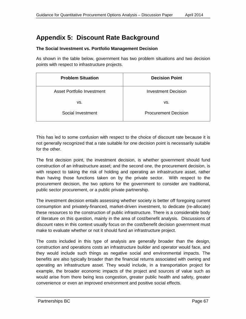
Guidance for Quantitative Procurement Options Analysis – Discussion Paper April 2014
Appendix 5: Discount Rate Background The Social Investment vs. Portfolio Management Decision
As shown in the table below, government has two problem situations and two decision points with respect to infrastructure projects.
Problem Situation Decision Point
Asset Portfolio Investment
vs.
Social Investment
Investment Decision
vs.
Procurement Decision
This has led to some confusion with respect to the choice of discount rate because it is not generally recognized that a rate suitable for one decision point is necessarily suitable for the other.
The first decision point, the investment decision, is whether government should fund construction of an infrastructure asset; and the second one, the procurement decision, is with respect to taking the risk of holding and operating an infrastructure asset, rather than having those functions taken on by the private sector. With respect to the procurement decision, the two options for the government to consider are traditional, public sector procurement, or a public private partnership.
The investment decision entails assessing whether society is better off foregoing current consumption and privately-financed, market-driven investment, to dedicate (re-allocate) these resources to the construction of public infrastructure. There is a considerable body of literature on this question, mainly in the area of cost/benefit analysis. Discussions of discount rates in this context usually focus on the cost/benefit decision government must make to evaluate whether or not it should fund an infrastructure project.
The costs included in this type of analysis are generally broader than the design, construction and operations costs an infrastructure builder and operator would face, and they would include such things as negative social and environmental impacts. The benefits are also typically broader than the financial returns associated with owning and operating an infrastructure asset. They would include, in a transportation project for example, the broader economic impacts of the project and sources of value such as would arise from there being less congestion, greater public health and safety, greater convenience or even an improved environment and positive social effects.
Partnerships BC Page 67

Guidance for Quantitative Procurement Options Analysis – Discussion Paper April 2014
These would be considerations that are not necessarily reflected in the price individuals would pay to use infrastructure. As a result, the infrastructure owner would not typically pay all the costs and receive all the benefits from a project. In addition, some costs and benefits may include intergenerational impacts that society chooses to discount on a basis that does not reflect asset valuation or financial market considerations.
The procurement decision is an asset portfolio management decision: whether the infrastructure asset under consideration be in government’s asset portfolio or a private partner’s. The risk profile, considerations, and returns appropriate for an infrastructure funding decision are not the same as the ones government would use for this procurement decision. Accordingly, the discount rates government would use for making the two decisions would not necessarily be the same. The portfolio management decision would generally hinge on how the rate of return government would expect to receive from an investment in the infrastructure asset compares with the rate of return it would expect to earn on other assets having a similar risk profile.
The Procurement Decision as an Asset Portfolio Decision
Government, when it chooses to use traditional procurement is investing directly in infrastructure and is thereby, in effect, adding an infrastructure asset to its investment portfolio. Recently, governments in Canada have even taken the step of including these assets, such as roads, bridges, schools and hospitals, on their balance sheets.
The financial return from holding this type of asset is in the form of a reduced cost: that is, not having to pay a private sector partner for the provision of infrastructure services. This means that where government payments to a private sector partner are the partner’s only source of revenues, the revenue return to government from a PPP investment is very similar to, if not exactly the same as, the revenue return to the private sector partner.
For the purposes of the business case analysis, it is typically assumed that government, under a traditional procurement model, would build the same infrastructure asset as the private sector would under a PPP, and would deliver the same quality and quantity of services. It can therefore be assumed that government would face a very similar profile of costs and risks.
Given that the risks are similar on both the revenue and cost side of the equation, a government investment in infrastructure should have roughly the same risks and returns as the corresponding investment by the private sector. It follows then that government should value the asset in the same way the private sector does. That is, government should discount costs and revenues using roughly the same cost of capital. As a matter of practice, the most practical approach is for government to estimate or obtain a measure of the private sector’s cost of capital, and to use this amount as an estimate of its own cost of capital.
Partnerships BC Page 68

Guidance for Quantitative Procurement Options Analysis – Discussion Paper April 2014
A similar argument holds even when the private partner has its own revenue sources, such as tolls. In the case where the private partner’s revenues are revenues that would otherwise be received by the public sector, such as tolls, the public sector would likely have to separately forecast the revenues it would receive were it to use traditional procurement.
The Investment Return Calculation for the Public Sector
The above implies that the relevant calculation for government is not so much a comparison of public sector infrastructure costs with the cost of a PPP, but rather an analysis of the return to the public sector of a direct investment in infrastructure. For a PPP where almost all the private partner’s revenues come from government, this can be done in two ways, which are equivalent in terms of their result:
1. Start from the premise that the public sector’s forecast net return is the forgone cost of paying a PPP partner, less government’s expected cost of building and operating the infrastructure itself. As a cash flow stream, this net return will appear, in the initial periods, as large upfront infrastructure investment cost cash outlays; followed by operations periods during which government will receive net revenues in the form of (a) forgone costs of paying a PPP partner, less (b) its own actual costs for operations, maintenance and capital rehabilitation. Government’s rate of return is the internal rate of return for this net cash flow stream, that is, the rate of interest for which the present value of the cash flow stream equals zero. On the basis of financial considerations, if the government’s forecast rate of return (i.e., internal rate of return) is less than the market rate, it should prefer PPP procurement; if it is greater than the market rate, it should prefer traditional procurement, and if it is equal to the market rate it should be indifferent.
2. Alternatively, start from the premise that if government expects to earn a market return from its investment, then the present value of government’s forecast return (which is the present value of the forgone or avoided costs of paying a PPP partner) should equal the present value of its own forecast costs. If government’s forecast revenues (i.e., the foregone cost of paying a PPP partner) discounted at the market rate of return exceeds its own forecast costs, discounted at the same rate, then traditional procurement is financially preferable, if the opposite is the case, the PPP option is financially better.
The appropriateness of using a market rate of return as a benchmark for government is more obvious if the private partner has access to its own source revenues, such as tolls. If government can earn a higher than market rate of return by investing directly in the asset, and collecting the revenues, it should make the investment, otherwise it should provide the investment opportunity to a private partner. The only caution with respect to this decision-making rule, where there are own-source revenues, is that the potential transaction may be more complicated than making an investment, providing services
Partnerships BC Page 69

Guidance for Quantitative Procurement Options Analysis – Discussion Paper April 2014
and collecting revenues. The PPP structure may, for example, have to be one in which government supplements the PPP partner’s revenues with some form of performance payment or shadow toll. In this case, government should consider these forgone costs when making its investment decision.
Partnerships BC Page 70

Guidance for Quantitative Procurement Options Analysis – Discussion Paper April 2014
Appendix 6: Financial Model – Worked Example
Introduction
The development and assessment of PSC and Shadow Bid models is an essential part of a project business case. Each model is constructed to address the unique circumstances of a particular project along with the potential impacts of the different procurement approaches.
The financial model assumptions presented here are based at a high level on a transportation project, and have been selected to give sufficient detail to provide an understanding of the key elements of the financial modelling process.
The following sections explain in further detail how the PSC and Shadow Bid models are structured, based on following major elements:
• Key dates,
• Inflation assumptions,
• Capital structure,
• Tax and accounting assumptions,
• Financing assumptions,
• Capital costs,
• Costs at financial close and OMR assumptions, and
• Availability payments.
Timing
This example calculates values annually, based on an assumption of a 33-year project agreement. The project starts at financial close and continues until the end of the operating period. The model assumes construction lasts three years and that the operating period continues for an additional 30 years. Construction is assumed to start April 1st, 2010, with the project agreement running to March 31st, 2043. Figure 1 below highlights the key dates.
Figure 1: Key Dates
Complete ConstructionMarch 31st, 2013
Financial Close / Start ConstructionApril 1st, 2010 End of Project Agreement
March 31st, 2043
CONSTRUCTION OPERATIONS / MAINTENANCE / REHABILITATION
Partnerships BC Page 71

Guidance for Quantitative Procurement Options Analysis – Discussion Paper April 2014
Inflation and Escalation
The model assumes that construction escalation is four per cent annually and that operating and life cycle costs are subject to inflation at two and half per cent per year.
Capital Structure
The capital structure (i.e., the combination of debt and equity) for the model is assumed to be 90 per cent bank debt and 10 per cent equity.
The bank debt assumes a base rate of three per cent, plus a three per cent margin, for a total interest rate of six per cent.
The after tax return on equity used is 10.50 per cent.
Capital Costs
The capital costs to construct the project are assumed to be $500 million. The owner’s retained costs for their project management office is estimated to be an additional $50 million that the owner will carry regardless of the procurement approach selected.
The overall capital cost efficiency rate used to adjust the capital cost estimate, determined using the approach described in Section 3.1.1.1, is four per cent.
Operations, Maintenance and Rehabilitation (OMR) Costs
The OMR costs are dynamic values that change each year due to base inflation (i.e., the two and a half per cent discussed above) that is applied to the estimated cost to operate and maintain the project over 30 years. In addition, the rehabilitation component will change based on the required work in a given period. In the first year of operation, the OMR payment for this project is estimated to be $4.5 million.
Public Sector Comparator (PSC)
The PSC is estimated by first using the raw inputs (non-risk adjusted) that include capital costs, operating costs, and major or capital rehabilitation costs for the whole project term.21 With just these raw inputs the PSC represents a risk-free project outcome; however, every project has risk. As discussed earlier, in order to make the PSC more accurately reflect potential project outcomes, it must also be adjusted to include risk. The risk adjusted PSC, in turn, can then be appropriately compared with the risk-adjusted Shadow Bid.
21 Refer to Section 3.1 for more details on capital, operating, and rehabilitation costs.
Partnerships BC Page 72

Guidance for Quantitative Procurement Options Analysis – Discussion Paper April 2014
Partnerships BC uses the extensive risk guidance developed for risk management and risk as it pertains to quantitative analysis discussed in detail in Section 4.2 and Appendix 3. Based on this approach, all the expected values of the risks—both construction and operating—are expressed as an NPC, and added to the NPC of the PSC.
In addition to an adjustment for risk to both the capital and OMR costs, additional adjustments are made as described in Section 4.
With these inputs, the PSC is constructed by compiling the costs to the owner of pursuing the project traditionally. Figure 2 below presents the corresponding cash flows from the owner’s perspective. The line graph shows the profile of capital costs, combined with operating costs and life cycle costs over the time period considered for the project. The bars in the top portion of the diagram show the various components of the line graph below.
Figure 2: PSC Financial Model
Spon
sor
Capital Costs
Operating Costs
Life-Cycle Costs
Transferred Risk, Insurance and Taxation
Required Cash Flow
PSC
-
50
100
150
200
250
300
2007 2010 2013 2016 2019 2022 2025 2028 2031 2034 2037 2040
Year
$ M
illio
ns
Public Expenditure - Construction and OMR
Partnerships BC Page 73

Guidance for Quantitative Procurement Options Analysis – Discussion Paper April 2014
Shadow Bid
The Shadow Bid is developed to provide an estimate of the annual service payment required by the private sector to pursue the project as a PPP. The ASP is the amount of revenue required to cover all expected costs, including an appropriate return to the private partner.
Figure 3 below shows that the Shadow Bid model, like the PSC, includes raw cost inputs like capital, operating, and life cycle costs. Rather than showing the private partner’s cash flow to construct and maintain the project, however, the Shadow Bid shows the required ASP to the private partner, reflecting the cost to project owner over the life of the project agreement. Insurance premiums and taxes that are direct costs to the private sector are incorporated into the calculation of the ASP. In addition, risk is directly incorporated into the calculation of the ASP in the following ways:
• Contingencies for risk in design and construction sub-contracts,
• Contingencies for risk in operating subcontracts, and
• Financing rates:
(a) Lenders will assign a cost of debt to the project based on the profile of risks they are exposed to, and
(b) Equity investors will demand a return commensurate with the level of risk they are taking on in the project.
The contingencies include the expected value of the risks that the government expects to transfer to the private sector.
The top of Figure 3 shows the project cost inputs to the Shadow Bid model that are included in the solution for the required ASP. The line graph at the bottom of Figure 3 shows the resulting ASP: the output of the Shadow Bid model. This ASP is what the owner pays to the private sector partner for delivering the project according to the terms of the project agreement.
Partnerships BC Page 74

Guidance for Quantitative Procurement Options Analysis – Discussion Paper April 2014
Figure 3: Shadow Bid Financial Model
Figure 4 shows a direct comparison of the public sector payment stream alternatives, including public control of construction and OMR, with the associated risks, and a more predictable ASP stream for the Shadow Bid, with significant risks and associated uncertainty transferred to the private partner.
-
50
100
150
200
250
300
2007 2010 2013 2016 2019 2022 2025 2028 2031 2034 2037 2040
Year
$ M
illio
ns
Public Expenditure - PPP ASP
Owner's Costs
PPP
Capital Costs
Debt Servicing & Return on Equity
Operations, Maintenance & Life-Cycle Costs
Required Annual Service Payment
Shadow Bid
Partnerships BC Page 75

Guidance for Quantitative Procurement Options Analysis – Discussion Paper April 2014
Figure 4: Public Sector Cash Flow Streams – Direct Comparison
Value for Money (VFM) Table
The VFM table described in detail in Section 10 is shown below as the consolidated representation of the results of the quantitative procurement options analysis for this example.
The VFM table compares the two procurement approaches based on the payment streams described above. When the cash flow streams for the two models are discounted to their NPC, the heavier, up-front and lower annual costs of the PSC can be compared to the more even ASP stream from the Shadow Bid.
The result of this comparison demonstrates that the NPC of the ASP stream is approximately $65 million dollars less than the NPC of the PSC. The Shadow Bid therefore provides quantitative value on a risk-adjusted basis of approximately $65 million, or roughly nine per cent of the risk adjusted capital costs of the PSC.
-
50
100
150
200
250
300
2007 2010 2013 2016 2019 2022 2025 2028 2031 2034 2037 2040
Year
$ M
illio
ns
Public Expenditure - Construction and OMR
Public Expenditure - Owner's Costs and ASP
Partnerships BC Page 76

Guidance for Quantitative Procurement Options Analysis – Discussion Paper April 2014
Figure 4: Value for Money Table
Traditional PPP (Shadow Bid)Capital Costs 463$ OMR Costs 95$ Cost 559$ Availability Payment 633$
Risks Retained under Traditional Delivery that would be transferred under PPPRisk adjustment to Capital Cost 68$ Total Risk Adjustment 68$
Tax and Insurance Adjustment Tax and Insurance AdjustmentInsurance 38$ Insurance Provincial Tax 10$ Income TaxesTotal Adjustment 48$ Total Adjustment
Retained Costs Retained CostsProject Management 59$ Project Management 48$ Retained Risk 30$ Retained Risk 17$
Total Retained Costs 89$ Total Retained Costs 65$
PSC 763$ Adjusted Shadow Bid 698$
VFM Shadow Bid - PSC 65$ % of PSC Costs including risk 8.6%
Value for Money Analysis 30 year OMR, Net Present Cost in $millions @ 7.70% to April 1, 2009
Partnerships BC Page 77

Guidance for Quantitative Procurement Options Analysis – Discussion Paper April 2014
Appendix 7: Glossary of Terms
Term Meaning
Annual Service Payment (ASP) The mechanism by which a private partner in a PPP arrangement is often compensated. According to performance standards specified in a project agreement, an ASP is paid to the private partner for capital and operating costs, as well as their required rate of return, over the term of the agreement.
Bank Debt Money lent by a bank that is often secured by the assets of the project and that is usually the most senior claim against project cash flows.
Bonds A certificate of debt (usually interest-bearing or discounted) that is issued by a government or corporation in order to raise money. The issuer is required to pay a fixed sum annually until maturity, at which time a fixed sum to repay the principal is made.
Business Case Document prepared in British Columbia by a project owner demonstrating the need and cost/benefit of a project, in addition to supporting a procurement method and providing an overview of the accounting impacts that a project may have.
Competitive Neutrality A circumstance where competitive advantages that typically accrue to government as a result of public sector ownership are neutralized through a series of adjustments that permit a fairer comparison of non-public sector alternatives.
Discount Rate A rate used to relate present and future dollars. Discount rates are expressed as a percentage and are used to reduce the value of future dollars in relation to present dollars. This equalizes varying streams of costs and benefits, so that different alternatives can be compared on a like-for-like basis.
Efficient Markets An efficient market is one in which securities prices reflect all publicly available information. This means that every security traded in the market is correctly valued given the available information.
Financial Close The point in the procurement process where negotiations with a preferred proponent are finalized and a project
Partnerships BC Page 78
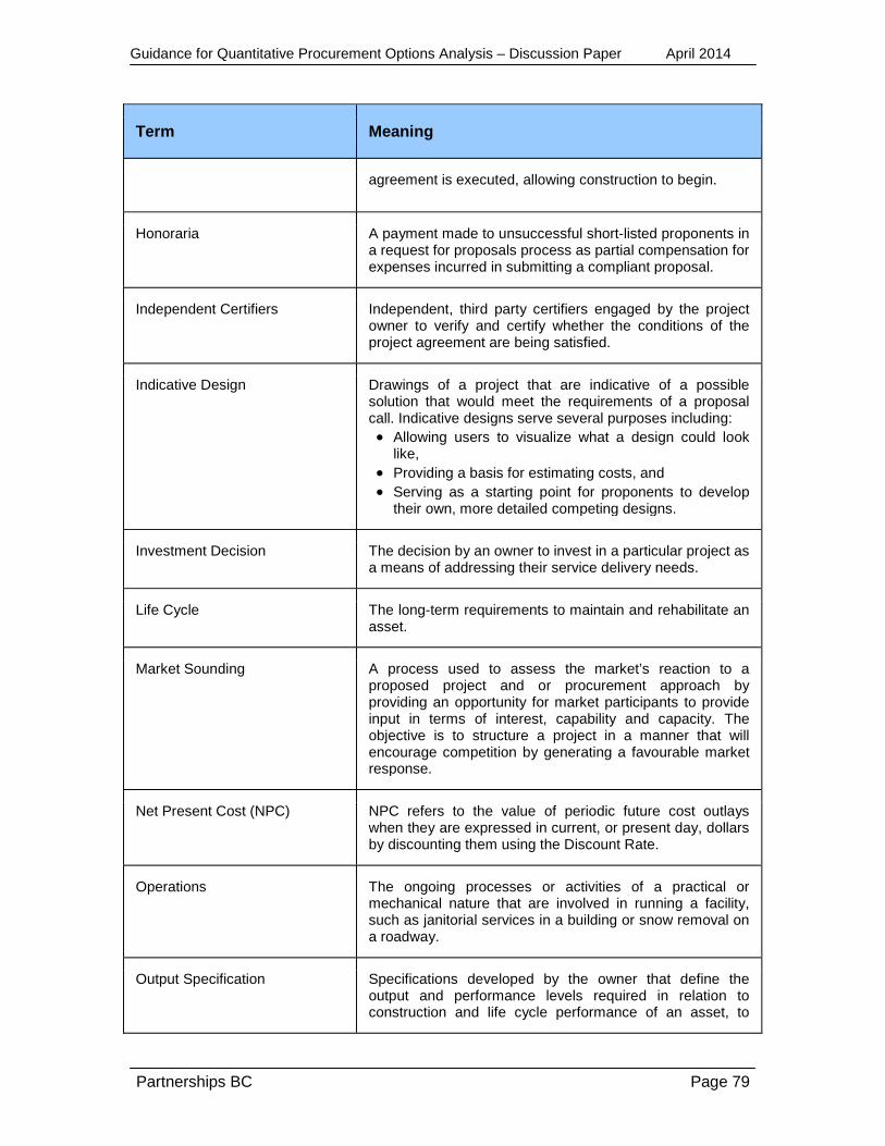
Guidance for Quantitative Procurement Options Analysis – Discussion Paper April 2014
Term Meaning
agreement is executed, allowing construction to begin.
Honoraria A payment made to unsuccessful short-listed proponents in a request for proposals process as partial compensation for expenses incurred in submitting a compliant proposal.
Independent Certifiers Independent, third party certifiers engaged by the project owner to verify and certify whether the conditions of the project agreement are being satisfied.
Indicative Design Drawings of a project that are indicative of a possible solution that would meet the requirements of a proposal call. Indicative designs serve several purposes including:
• Allowing users to visualize what a design could look like,
• Providing a basis for estimating costs, and • Serving as a starting point for proponents to develop
their own, more detailed competing designs.
Investment Decision The decision by an owner to invest in a particular project as a means of addressing their service delivery needs.
Life Cycle The long-term requirements to maintain and rehabilitate an asset.
Market Sounding A process used to assess the market’s reaction to a proposed project and or procurement approach by providing an opportunity for market participants to provide input in terms of interest, capability and capacity. The objective is to structure a project in a manner that will encourage competition by generating a favourable market response.
Net Present Cost (NPC) NPC refers to the value of periodic future cost outlays when they are expressed in current, or present day, dollars by discounting them using the Discount Rate.
Operations The ongoing processes or activities of a practical or mechanical nature that are involved in running a facility, such as janitorial services in a building or snow removal on a roadway.
Output Specification Specifications developed by the owner that define the output and performance levels required in relation to construction and life cycle performance of an asset, to
Partnerships BC Page 79

Guidance for Quantitative Procurement Options Analysis – Discussion Paper April 2014
Term Meaning
ensure the completed project satisfies the objectives of a project with respect to meeting the owner’s service delivery needs.
Owner Usually a provincial ministry, authority or agency that is undertaking a needs assessment and benefit analysis to determine if a project will satisfy service delivery requirements, and that will own the project and fund the annual service payments if a project proceeds as a PPP.
Owner’s Reserve A contingency fund reflecting the value of risks retained by the owner that is recommended to be included in the financial model, project budget and funding analysis.
Public Sector Contributions Public sector funding sources can include federal, provincial and municipal governments, regional hospital districts, authorities, municipalities and non-profit foundations, and are typically included in a project as contributions during construction.
These contributions can take multiple forms including: progress payments, milestone payments and substantial completion payments.
Public Private Partnership (PPP)
Public private partnership whereby public sector infrastructure is procured using a long-term performance-based agreement with a private sector partner to deliver and maintain an infrastructure asset, including significant, upfront capital investment.
Preferred Proponent A proponent selected from a short-list of bidders to enter into negotiations with a project owner to reach financial close and deliver a project.
Procurement Decision The decision by an owner to procure a project in a particular way in order to achieve value for money.
Project Agreement The project agreement sets out the requirements for the delivery of an asset under a PPP in terms of cost, schedule and life cycle performance that typically govern the performance-based payment of the ASP to a private partner.
Public Sector Comparator (PSC)
The public sector comparator, which is a financial model of a hypothetical public sector reference concept used in
Partnerships BC Page 80

Guidance for Quantitative Procurement Options Analysis – Discussion Paper April 2014
Term Meaning
quantitative procurement analysis to compare the risk adjusted, life cycle cost of traditional delivery with the cost of procuring the same project as a PPP.
Retained Risk Risks associated with delivering a project that are not transferred to the private partner under a PPP, representing a cost to the project regardless of the procurement approach.
Request for Proposals (RFP) Document issued by an owner for qualified proponents to submit formal proposals to deliver a project.
Request for Qualifications (RFQ)
Document issued by an owner inviting parties interested in participating in an RFP, to submit their qualifications for delivering a project.
Risk Management Branch Risk Management Branch (RMB) is the enterprise risk management agency within the B.C. Ministry of Finance that advises on risk management issues, reviews and approves indemnities given by government, and assists ministries in establishing their own comprehensive risk management programs.
Risk Matrix Primary tool used to identify, assess and manage project risks based on the following major components of risk:
• Category • Description • Rating • Valuation • Allocation • Treatment
Shadow Bid A financial model developed to represent the procurement of a project using a PPP approach. The Shadow Bid is used to develop a cost estimate to be compared to the PSC as a means of evaluating potential differences in the present value of the risk adjusted costs between traditional and PPP procurement.
Traditional Procurement Methods by which the public sector has traditionally procured projects in B.C, through design bid build (DBB), or a combination of DBB and design build (DB) contracts.
Transferred Risk Risk associated with delivering a project that is typically borne by the public sector under traditional procurement, that is transferred to the private sector under a PPP.
Partnerships BC Page 81
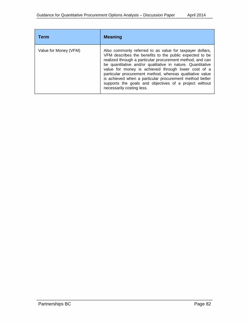
Guidance for Quantitative Procurement Options Analysis – Discussion Paper April 2014
Term Meaning
Value for Money (VFM) Also commonly referred to as value for taxpayer dollars, VFM describes the benefits to the public expected to be realized through a particular procurement method, and can be quantitative and/or qualitative in nature. Quantitative value for money is achieved through lower cost of a particular procurement method, whereas qualitative value is achieved when a particular procurement method better supports the goals and objectives of a project without necessarily costing less.
Partnerships BC Page 82