Embed Size (px)
Citation preview
Quantitative analysis of accuracy of aninertial/acoustic 6DOF tracking system.
Stuart J. Gilson1, Andrew W. Fitzgibbon2, Andrew Glennerster1
October 4, 2005
1: University Laboratory of Physiology,Parks Road,
Oxford
OX1 3PTUnited Kingdon
2: Department of Engineering Science,Parks Road,
Oxford
OX1 3PJUnited Kingdon
Pages (including figures and tables): 26
Figures: 11Tables: 1
Corresponding author: Stuart Gilson
University Laboratory of PhysiologyParks Road,
Oxford,
OX1 3PTUnited Kingdom
Phone: +44 (0)1865 272460Fax: +44 (0)1865 272469
Email: [email protected]

Abstract
An increasing number of neuroscience experiments are using virtual reality to provide a moreimmersive and less artificial experimental environment. This is particularly useful to navigation
and three-dimensional scene perception experiments. Such experiments require accurate real-
time tracking of the observer’s head in order to render the virtual scene. Here we present dataon the accuracy of a commonly used 6 degree of freedom tracker (Intersense IS900) when it
is moved in ways typical of virtual reality applications. We compared the reported location ofthe tracker with its location computed by an optical tracking method. When the tracker was
stationary, the root mean square error in spatial accuracy was 0.64mm. However, we found
that errors increased over ten-fold (up to 17mm) when the tracker moved at speeds common invirtual reality applications. We demonstrate that the errors we report here are predominantly
due to inaccuracies of the IS900 system rather than the optical tracking against which it was
compared.KEYWORDS: Virtual reality; Acoustic/inertial tracking; Psychophysics experiments; Ac-
tive vision; Real-time measurements; Metric accuracy.
1

1 Introduction
Virtual reality is an increasingly common research tool in neuroscience (for example, see re-views by Tarr and Warren (2002), Bulthoff and van Veen (2001); Loomis et al. (1999) and a
more skeptical view by Koenderink (1999)). Examples include work in sensory integration
(Ernst et al., 2000) and sensori-motor control (Kording and Wolpert, 2004), spatial perception(Christou and Bulthoff, 1999; Tcheang et al., 2005; Sahm et al., 2005), navigation (Mallot and
Gillner, 2000; Warren et al., 2001) and studies of social behaviour and psychiatric disorders(Slater et al., 2000; Freeman et al., 2005). There are clear advantages to using virtual reality
given the flexibility and control it allows the experimenter. Equally, there are limitations to
the technology that must be understood and accounted for when carrying out exeriments andinterpreting the results.
In this paper we measure the spatial precision of one of the trackers used in a wide variety
of experimental paradigms. Reporting the movement of the participant’s head or limbs is thefirst and in some ways the most critical part of the chain of operations that link these movements
to a change in the visual display. There are many different types of tracker. The criteria forchoosing the most suitable for a given application include limitations on cost, precision and
the volume of the tracked area required for experiments. The tracker we analyse here (an
inertial/acoustic tracker supplied by Intersense) is currently cheaper than optical systems ormechanical arm trackers and covers a wider area. It is therefore an attractive option for many
applications. However, the range and type of experiments that are appropriate depend on the
accuracy and precision of the tracker. To design experiments that are commensurate with thequality of tracking, therefore, depends on reliable data on the performance characteristics of
the tracking system that will be used, preferably under conditions similar to those that will beused in the experiment.
For example, in virtual reality experiments using small hand and finger movements, the
position of the fingertip has been measured with very high accuracy using a PHANToM (Sens-Able Technologies). These devices not only provide information on the location of the fingertip
(nominal accuracy of 0.02 mm) but also generate resisting force, allowing virtual haptic stim-uli to be presented (Ernst et al., 2000; Kording and Wolpert, 2004). At a slightly larger scale,
digitizing tablets have been used to track the position of limb (e.g GTCO Corporation, abso-
lute accuracy about 0.1 mm (Baddeley et al., 2003)). Similar high accuracy tracking has beenused to measure head position in virtual reality displays using a mechanical, multi-jointed arm
but the range of head movement is restricted (e.g Panerai et al. (1999), nominal accuracy 0.6
mm within a range of about 0.5m in each directions). Magnetic trackers (Polhemus, Flock ofBirds, Ascension) can be used to track the head but suffer from large spatial distortions outside
a restricted spatial range.Wider ranges of movement are possible with optical, inertial and acoustic tracking meth-
ods although again there is a trade off between precision and range of movement. Optical
2
methods fall into two categories, ‘camera in’ and camera out’ methods (Ribo et al., 2001).
Real-time ‘camera in’ systems (e.g. Vicon) use fixed calibrated cameras to compute the lo-cation of markers on the head or limb. The translation accuracy is high, e.g. less than 1mm
offset and RMS, but the working volume is typically limited (some very large installations ex-ist, but these are rare and extremely expensive). ‘Camera out’ systems, in which the camera
is placed on the head while markers are placed in the scene (usually on the ceiling), have the
advantage that they are very sensitive to head rotations. Accurate tracking of head rotationis particularly critical in augmented reality applications in which virtual objects are presented
within real scenes (Azuma, 1997). One example is the Hi-Ball tracking system (Welch et al.,
1999), which has been used in virtual reality experiments (Durgin et al., 2001) and can supportmovements over a considerable working volume (e.g. 40m2, spatial accuracy 0.2mm). Another
is the recently available Intersense ‘Vis-trak’, which combines camera out tracking with an in-ertial sensor (Foxlin and Naimark, 2003) (3mm positional accuracy). An inertial sensor is also
incorporated in the Intersense IS900 on which we report here (Foxlin et al., 1998). We have
chosen to analyse the performance of the Intersense inertial/acoustic tracker (IS900) becauseit is one of the most frequently adopted trackers in experiments using virtual reality (Rolland
et al., 2001; Sahm et al., 2005; Creem-Regehr et al., 2005; Foo et al., 2005; Slater et al., 2000).
For many applications, such as investigation of navigation (e.g Foo et al. (2005)), RMSerrors in tracking of about 1 cm may well not affect the conclusions of an experiment. However,
many experiments, for example investigating hand-eye coordination, require greater precision.A longer term goal should be the development of trackers that will allow freedom of movement
and yet provide accurate tracking of hand and head movements and so increase the range and
type of experiments that could be carried out. At present, a more limited goal is to characterisethe spatial errors in tracking of systems to determine the range of experiments for which each
is suitable.
The Intersense (Intersense Inc, Burlington, MA) IS900VET system is a hybrid acousticand inertial system (Foxlin et al., 1998). Information from the inertial sensors and triaxial ac-
celerometers in the tracking devices can be integrated twice to determine the tracker’s position.These positional measurements are prone to drift and so are corrected by the ultrasonic acoustic
system. Ultrasonic emitters are rigidly attached to the walls/ceiling of the tracked volume, and
microphones on the tracking devices detect the emitted acoustic signal. The acoustic and iner-tial signals are combined, errors rejected, smoothed and the resulting position and orientation
information transmitted to the host computer via a serial cable. The IS900 system works over
a large volume (e.g. 12 m by 12 m in the VENlab, (Foo et al., 2005)), has a reported latencyof < 10ms, is relatively low cost compared to optical systems, and is sufficiently compact and
light weight as to be unobtrusive.The accuracy of the computed tracker position depends critically on careful calibration of
the locations of the ultrasound emitters. Currently, this is done by surveying methods (using a
theodolite). In the Discussion, we consider the theoretical improvements that could be gained
3

by using time-of-flight information to calculate the locations of the emitters. Mis-estimates of
the emitter locations could account for variability in the reported tracker position.The technical specifications for the IS900 give statistics for a static tracker—resolution
of 1.5mm root mean square (RMS) error and an accuracy of 4mm RMS error (IS900 usermanual)—but for an experimenter the error whilst the tracker is in motion is more relevant.
Here we use on off-line optical tracking method to provide an accurate estimate of the true
path followed by the tracker and compare this to the 3D locations reported by the IS900. Weshow that at typical walking speeds, errors are significantly above the static values. We discuss
methods of calibration that might help improve the performance of this tracker and other types
of tracker that could give higher accuracy while maintaining the freedom of movement that theIS900 allows.
2 Methods/Apparatus
We compared the IS900’s reported positions with those derived from an independent tracking
method. This second method did not need to be real-time, nor as robust (i.e. we could af-ford to re-conduct failed trials) as a real tracking system—but it did need to give reproducible
positional estimates of the tracker to compare with the IS900’s reported position of the sametracker. We used a purpose-built optical tracking system which comprised two IEEE-1394
cameras (A602fc, Basler AG, Germany) which streamed 640×480 pixel 8bpp mono digital
images at 60Hz to the host computer (a desktop PC running GNU/Linux), which also receivedtracking information from the IS900 through a serial port. The host computer recorded the
stream of video data and serial data to disk in real time, without skipping any frames. Hav-
ing both video and coordinate data being received by the same computer allowed both to besynchronized—time stamps were recorded for the arrival of images and coordinates which
subsequently allowed the two data sets to be temporally aligned (see figure 1).The IS900 used Intersense’s latest firmware (v4.14). Important settings relevant to track-
ing quality are – perceptual enhancement: 2 (default); prediction interval: 0ms (default); rota-
tional sensitivity: 3 (default), ultrasonic emitter timeout: 20ms; ultrasonic emitter sensitivity: 1.The last two may vary between installations, but provide stable tracking in our laboratory. The
tracked area was 3.50×3.54×3.13 m and used 51 ultrasonic emitters.
A bright LED was firmly attached to the tracker which was then moved by hand along arandom path within a volume that was seen by both cameras. Images of the tracker and the
tracker’s position as reported by the IS900 were recorded during motion. Four conditions werestudied, from a static tracker up to typical walking speeds (1m/s). Over a 20s period, images of
the tracker were stored from the two cameras while at the same time position and orientation
reports from the IS900 were recorded.During recording, the operator moved the tracker in a random path within a volume visible
4

to both cameras (approximately 1m3). The LED is not at the tracked centre of the tracker
(there is no marker denoting where this is on the physical tracker) and, hence, any rotationof the wand would cause a translation of the LED relative to this tracked centre. Since such
translations would affect our tracking analysis, the tracker was held in a horizontal orientationas far as possible throughout the movement.
The location of the LED was extracted from the sequence of pairs of images yielding two
arrays of 2D coordinates (one array from each camera). The images were thresholded to findbright regions, and a weighted centroid technique used to find the centre of the densest cluster
of supra-threshold pixels. This centroid was measured to sub-pixel accuracy (see section 4.1) to
give the position of the light source. The centroid coordinates were corrected for lens distortion.Using standard photogrammetry techniques (Hartley and Zisserman, 2001), the path of
the LED was reconstructed in three dimensions from these 2D coordinate arrays. This recon-structed path was in its own arbitrary coordinate system and had to be mapped into IS900 space
before further analysis can be performed. A homography describes a one to one mapping of
points from one projective coordinate frame to another—transforming each point in the recon-structed path by this homography allowed a direct point-by-point analysis of the reconstructed
path and the IS900 recorded path to be performed. We found the homography that was maxi-
mally favourable to the IS900. Using the reconstructed data set as our ‘ground truth’ we wereable to make spatial measurements of the errors in the IS900’s tracking data.
[Figure 1 about here.]
3 Analysis
Figure 1 shows, for one tracker trajectory, part of the path recorded by the IS900 tracker
(crosses) and, overlaid, the reconstructed path from the camera images (solid line). Takingthe reconstructed optical path as the ‘ground truth’ (an assumption that we examine in sec-
tion 4), we calculated the errors in the IS900 coordinates. Figure 2 summarizes the data for all
trajectories, showing the errors as vectors, for the static, slow, medium and fast moving datasets. The error vectors have been rotated so that the x-component corresponds in each case to
the direction of travel (as measured by the optical tracker). Figure 3 shows the magnitudes of
the errors for the same conditions. The errors were slightly larger in the direction of travel (onaverage 1.3 times larger) but there was no systematic relationship between this ratio and the
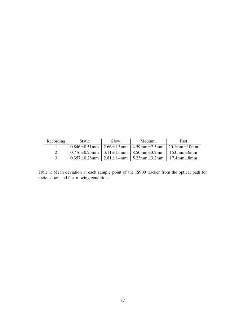
speed of the tracker.Three recordings were made for each of the static, slow, medium and fast moving tracker
conditions. The tracker’s deviations from the optical path are shown in table I. The mean
deviations at each sample point are 0.64, 2.86, 6.10 and 17.6mm respectively. The static erroris well within the specification supplied by Intersense, but the non-static conditions, which
5

span the speeds used in ‘typical’ applications, have errors that increase with speed, and at the
highest speed are significantly outside the quoted range.
[Table 1 about here.]
[Figure 2 about here.]
[Figure 3 about here.]
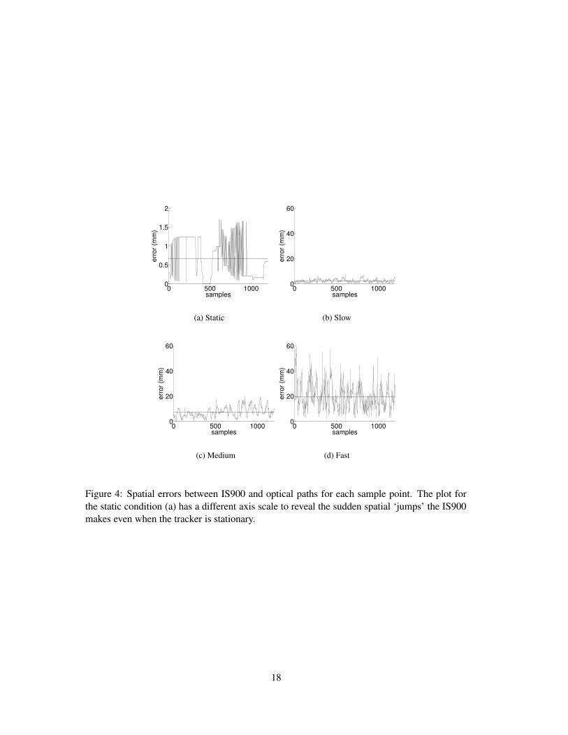
Figure 4 plots the magnitude of the IS900 spatial error over time for each of the four
conditions. The errors for the static wand reveal several distinct regions or plateaus. These,we believe, result from the IS900 using a different set of ultrasonic emitters to determine the
tracker’s position at each plateau region and this—due to small calibration errors in the mea-surement of the location of these emitters—gives a different positional ‘solution’ (see figure 5).
Figure 4 shows data for the moving conditions. The errors for the fast condition are signifi-
cantly larger than for the slow condition (t = 54.09, d.f. = 2398, p < 10−9).
[Figure 4 about here.]
[Figure 5 about here.]
Figure 6 shows how the speed of the tracker varied over the course of the moving condi-
tions. Speeds were obtained by smoothing the optical and IS900 paths with a Gaussian kernel
(σ = 1s) and taking first order differences (figure 6). There is evidence here of the IS900 failingto respond quickly to rapid changes in speed, which is characterised in the spatial domain as
the IS900 trajectory over-running the true path of motion, as can be seen in figure 1. Figure 7shows the RMS error in the three moving conditions plotted against speed. A linear fit to the
slow, medium and fast data sets (figure 7) have slopes that are significantly different from zero.
[Figure 6 about here.]
[Figure 7 about here.]
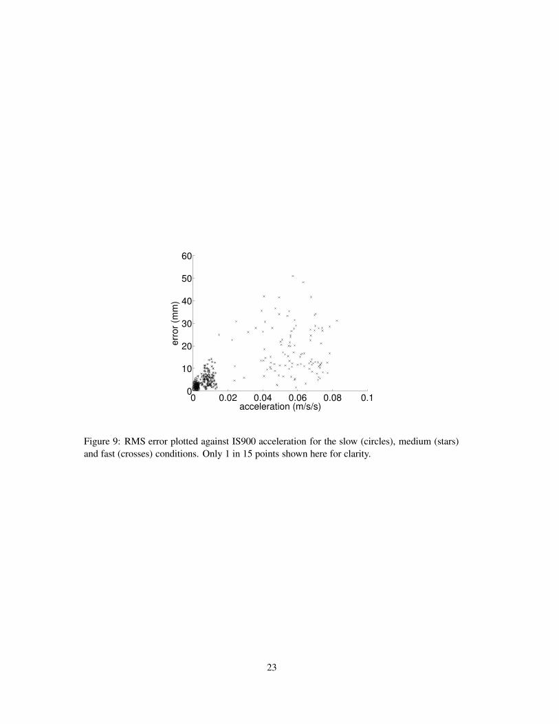
Figure 8 shows acceleration profiles of a typical trajectory for the three moving conditions,where acceleration was calculated in the same way as speed, but now taking second order
differences between smoothed samples. One might expect the largest errors between the IS900
and optical paths to occur during rapid changes of direction—equivalently regions of highacceleration. Figure 9 shows mean error against acceleration for the slow- and fast-moving
cases. We again measured a linear fit to the 9 motion trajectories, but in this case found no
consistent pattern (the range of slopes over all 9 moving trajectories was −0.57s2 to 0.51s2).We believe, then, the difference in errors across conditions result from differences in speed not
acceleration.
[Figure 8 about here.]
[Figure 9 about here.]
6

4 Sources of error
So far, we have used the reconstructed path for the optical tracking system as a measure of‘ground truth’. We consider here the extent to which this assumption is valid. The major
known errors in the system arise from pixel errors in the optical stages and timing errors in
receiving images from the camera and synchronizing these with the IS900 samples.
4.1 Pixel errors
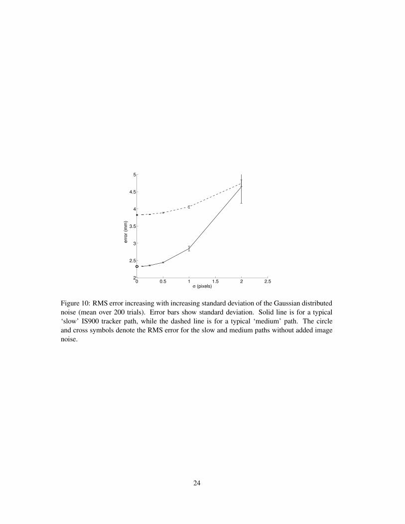
Pixel errors arose from the extraction of the light source in the video images. Image noise and
numerical errors in this thresholding process could have led to inaccuracies in this process.However, the standard deviation of the centroid extracted from images of a static light source
was less than a tenth of a pixel. To see how image noise affects our analysis of IS900 data, wedeliberately added Gaussian distributed random noise to the extracted image coordinates, and
repeated the whole extraction process to determine how RMS error increases with increasing
standard deviation of noise (figure 10). For standard deviations below 0.5 pixels, the RMSerror barely changes and, hence, pixel errors are unlikely to have contributed significantly to
overall RMS error.
[Figure 10 about here.]
4.2 Temporal misalignment
The synchronization of the images captured by the two cameras and the IS900 coordinates atthe moment of capture are important. Increasing delays between the capture of the two images
will result in reconstruction errors (notably in the depth of the reconstructed point), and delaysbetween image capture and IS900 coordinate capture will make mapping one path onto the
other difficult.
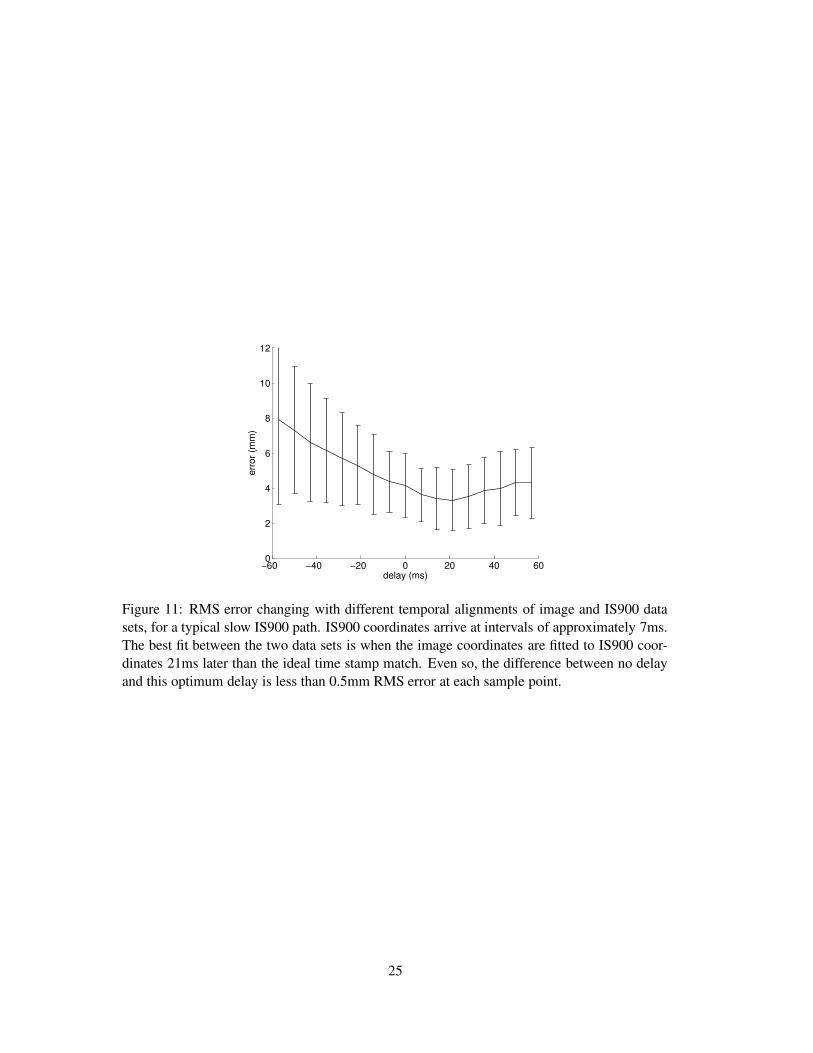
Although time stamps were recorded for the arrival of images and IS900 coordinates atthe host computer and were used in the subsequent fitting process, it is still possible that the
image pair that arrived at time t fits better with the IS900 coordinate that arrived at time t + εthan the coordinate that also arrived at time t. Therefore, we repeated our transformation of theoptical path onto IS900 path using different values of ε (see figure 11). There was a negligible
reduction in RMS error between ε = 0ms and the best fit (ε = 21ms).
[Figure 11 about here.]
7

4.3 Measuring IS900 error by plane fitting
We wanted to asses IS900 error without relying on our optical system, in order to verify that the
optical system introduces negligible error. We did this by mounting the tracker on a turntableto restrict its motion to a plane, and measuring the perpendicular error to the best-fitting plane
through the IS900 data. The speed of motion was comparable to the previous medium speedcondition. We found an RMS error of 2.7mm perpendicular to the plane. This is similar in
magnitude to the error perpendicular to the direction of travel in the freely moving tracker
condition (medium speed, 3.1mm), suggesting that the errors in both cases arise predominantlyfrom the IS900 tracker. The planar movement test alone is not an adequate test of the tracker
performance as it cannot identify the component of error in the direction of travel nor can it
identify situations where the IS900 has ‘over run’ the true trajectory as we have illustratedhappening at points of rapid change in direction.
5 Discussion
We have analysed one of the more commonly used tracking systems used in virtual reality
experiments and report the precision of this system (Intersense VET) over a range of trackerspeeds. Performance deteriorates with increasing tracker speed so that, at typical walking
speeds, errors are approximately 4 times those quoted for a static tracker. As we have arguedin the Introduction, an accurate assessment of the reliability of the tracker position estimate is
critical when designing experiments. It is necessary in order to judge the extent to which the
visual stimulus might differ from the correct one. Also, if the tracker output is being used toreport the subject’s movements (for example in intercepting a ball), the device’s precision must
be known. Of the types of experiments carried out to date using the IS900, many are unlikely to
be seriously affected by tracking errors of the magnitude reported here, including experimentson navigation (e.g. Foo et al., 2005) or social interactions (e.g. Slater et al., 2000). By contrast,
detailed studies of object manipulation or hand-eye coordination would be likely to suffer, bothin generation of a reliable stimulus and in records of the head and hand position.
We have assumed that it is valid to treat the position estimate derived from the optical
tracking system as ‘ground truth’. Specifically, section 4 lists the potential sources of errorin the optical tracking system and the ways in which we have ensured that these errors were
kept to a minimum. We have shown that some errors would not have a significant effect on the
computed optical tracking path even if they had been significantly larger (figure 10).We have suggested that the predominant source of errors in the IS900 system is likely
to be variations in calibration between different sub-sets of emitters. We have direct evidencefor this when the tracker is stationary: in this case errors correlate with changes in the subset
of emitters used (figure 5). The increase in errors with increasing tracker speed we found is
8
consistent with the hypothesis that moving between different subsets of chirpers is the main
cause of the errors.There are a number of ways in which this problem might be tackled. In our opinion,
transition between detector subsets can be smooth for a correctly calibrated system. The reasonthat abrupt transitions remain a perennial problem is that this calibration is extremely difficult
in practice. We have made progress towards ameliorating this problem by adapting techniques
from photogrammetric bundle adjustment (Duff and Muller, 2003), but these techniques arenot yet proved in real-world application. When inertial/acoustic systems can be calibrated
accurately they should provide substantially improved tracking in addition to the advantages of
cost and range that they have at the present.In principle, the problem of moving between subsets of sensors applies equally to optical
systems,but these are routinely calibrated using bundle-adjustment techniques, and do not ex-hibit such mis-measurement errors. It remains to be seen whether optical tracking systems will
provide an accurate, cheap and robust alternative to inertial/acoustic tracking systems.
6 Acknowledgements
Supported by the Wellcome Trust and the Royal Society.
9

References
Azuma, R. T. (1997). A survey of augmented reality. Presence: Teleoperators and Virtual
Environments, 6(4):355–385.
Baddeley, R. J., Ingram, H. A., and Miall, R. C. (2003). System identification applied to avisuomotor task: near-optimal human performance in a noisy changing task. Journal of
Neuroscience, 23(7):3066–3075.
Bulthoff, H. H. and van Veen, H. A. H. C. (2001). Vision and action in virtual environments:Modern psychophysics in spatial cognition research. In Jenkin, M. and Harris, L., editors,
Vision and Attention, pages 233–252. Springer-Verlag, New York, USA.
Christou, C. G. and Bulthoff, H. H. (1999). View dependence in scene recognition after active
learning. Memory and Cognition, 27(6):996–1007.
Creem-Regehr, S. H., Willemsen, P., Gooch, A. A., and Thompson, W. B. (2005). The influence
of restricted viewing conditions on egocentric distance perception: Implications for real and
virtual environments. Perception, 34(2):191–204.
Duff, P. and Muller, H. (2003). Autocalibration algorithm for ultrasonic location systems. In
Proceedings of the Seventh IEEE International Symposium on Wearable Computers, pages62–68. IEEE Computer Society.
Durgin, F. H., Gigone, K., and Scott, R. (2001). Perception of visual speed while moving.
Journal of Experimental Psychology: Human Perception and Performance, 31(2):339–353.
Ernst, M. O., Banks, M. S., and Bulthoff, H. H. (2000). Touch can change visual slant percep-
tion. Nature Neuroscience, 3(1):69–73.
Foo, P., Warren, W. H., Duchon, A., and Tarr, M. J. (2005). Do humans integrate routes into
a cognitive map? Map- versus landmark-based navigation of novel shortcuts. Journal of
Experimental Psychology: Learning, Memory, and Cognition, 31(2):195–215.
Foxlin, E., Harrington, M., and Pfeifer, G. (1998). Constellation: a wide-range wireless
motion-tracking system for augmented reality and virtual set applications. In Proceedings
of the 25th annual conference on Computer graphics and interactive techniques, pages 371–
378. ACM Press.
Foxlin, E. and Naimark, L. (2003). VIS-Tracker: A wearable vision-interial self-tracker. In
IEEE VR2003, March 22–26, Los Angeles, USA.
Freeman, D., Garety, P. A., Bebbington, P., Slater, M., Kuipers, E., Fowler, D., Green, C.,
Jordan, J., Ray, K., and Dunn, G. (2005). The psychology of persecutory ideation II: A
virtual reality experimental study. Journal of Nervous & Mental Disease, 193(5):309–315.
10

Hartley, R. and Zisserman, A. (2001). Multiple view geometry in computer vision. Cambridge
University Press, UK.
Koenderink, J. J. (1999). Virtual psychophysics. Perception, 28:669–674.
Kording, K. P. and Wolpert, D. M. (2004). Bayesian integration in sensorimotor learning.
Nature, 427:244–247.
Loomis, J. M., Blascovich, J. J., and Beall, A. C. (1999). Immersive virtual environment
technology as a basic research tool in psychology. Behavior Research Methods, Instruments
and Computers, 31:557–564.
Mallot, H. A. and Gillner, S. (2000). Route navigating without place recognition: What isrecognised in recognition-triggered responses? Perception, 29(1):43–55.
Panerai, F., Hanneton, S., Droulez, J., and Cornilleau-Peres, V. (1999). A 6-dof device tomeasure head movements in active vision experiments: geometric modelling and metric
accuracy. Journal of Neuroscience Methods, 90:97–106.
Ribo, M., Pinz, A., and Fuhrmann, A. (2001). A new optical tracking system for virtual and
augmented reality applications. In Proceedings of 18th IEEE Instrumentation and Measure-
ment Technology Conference, Budapest, Hungry, volume 3, pages 1932–1936.
Rolland, J. P., Davis, L. D., and Baillot, Y. (2001). A survey of tracking technologies for
virtual environments. In Barfield, W. and Caudell, T., editors, Fundementals of Wearable
Computers and Augmented Reality. Lawrence Erlbaum Assoc, Mahwah, NJ.
Sahm, C. S., Creem-Regehr, S. H., Thompson, W. B., and Willemsen, P. (2005). Throwingversus walking as indicators of distance perception in similar real and virtual environments.
ACM Transactions on Applied Perception, 2(1):35–45.
Slater, M., Sadagic, A., Usoh, M., and Shroeder, R. (2000). Small-group behaviour in a virtual
and real environment: A comparative study. Presence: Teleoperators and Virtual Environ-
ments, 9(1):37–51.
Tarr, M. J. and Warren, W. H. (2002). Virtual reality in behavioral neuroscience and beyond.Nature Neuroscience, 5:Supplement 1089–1092.
Tcheang, L., Gilson, S. J., and Glennerster, A. (2005). Systematic distortions of perceptualstability investigated using immersive virtual reality. Vision Research, 45:2177–2189.
Triggs, W., McLauchlan, P., Hartley, R., and Fitzgibbon, A. (2000). Bundle adjustment: Amodern synthesis. In Triggs, W., Zisserman, A., and Szeliski, R., editors, Vision Algorithms:
Theory and Practice, LNCS. Springer Verlag.
11

Warren, W. H., Kay, B. A., Zosh, W. D., Duchon, A. P., and Sahuc, S. (2001). Optic flow is
used to control human walking. Nature Neuroscience, 4(2):213–216.
Welch, G., Bishop, G., Vicci, L., Brumback, S., Keller, K., and Colucci, D. (1999). The HiBall
tracker: High-performance wide-area tracking for virtual and augmented environments. InSymposium on Virtual Reality Software and Technology, pages 1–10.
12

List of Figures
1 Path reconstructed from pairs of 2D images (solid line) with IS900 path (crosses)overlaid. Only a short segment of the path is shown (with only every fifth IS900coordinate shown for clarity) but deviations between the two paths can still beseen, especially during rapid changes of direction. . . . . . . . . . . . . . . . . 15
2 Error vectors between IS900 and optical paths for static, slow, medium andfast moving cases. Error vectors have been rotated to aligned so that the x-axiscorresponds to the tracker’s direction of travel. RMS errors along and perpen-dicular to the direction of travel were 2.0 and 1.4mm for the slow condition; 4.3and 3.1mm for the medium condition; and 10.9 and 9.9mm for the fast condition. 16
3 Histograms of spatial error magnitudes for static, slow, medium and fast mov-ing cases. To aid comparison, the axis for figures (a) and (b) have been clippedat 100 samples. . . . . . . . . . . . . . . . . . . . . . . . . . . . . . . . . . . 17
4 Spatial errors between IS900 and optical paths for each sample point. The plotfor the static condition (a) has a different axis scale to reveal the sudden spatial‘jumps’ the IS900 makes even when the tracker is stationary. . . . . . . . . . . 18
5 The X, Y and Z components of position reported by a static IS900 tracker (mid-dle, top and bottom solid black lines respectively), overlaid onto a plot of theultrasonic emitters active during each sample (crosses). Changes in reportedtracker position coincide with changes in the subset of ultrasonic emitters usedby the IS900. . . . . . . . . . . . . . . . . . . . . . . . . . . . . . . . . . . . 19
6 Speed profiles for the slow (circles), medium (stars) and fast (crosses) condi-tions showing IS900 versus optical path (solid line). Only 1 in 15 points shownhere for clarity. Deviations between IS900 and optical paths are apparent atlarge changes in speed. . . . . . . . . . . . . . . . . . . . . . . . . . . . . . . 20
7 RMS error plotted against IS900 tracker speed for the slow (circles), medium(stars) and fast (crosses) conditions. Only 1 in 15 points shown here for clarity.The slopes of linear fits through the data have slopes for the slow conditionwere: 0.0039 ± 0.00057 mm/m/s (t = 6.91, p < 10−9); medium: 0.0128 ±
0.0011 mm/m/s (t = 12.15, p < 10−9); fast: 0.0037± 0.00066 mm/m/s (t =
5.59, p < 10−9). . . . . . . . . . . . . . . . . . . . . . . . . . . . . . . . . . . 218 Acceleration profiles for the slow (circles), medium (stars) and fast (crosses)
conditions for the IS900 positions versus optical path (solid line). Only 1 in 15points shown here for clarity. . . . . . . . . . . . . . . . . . . . . . . . . . . . 22
9 RMS error plotted against IS900 acceleration for the slow (circles), medium(stars) and fast (crosses) conditions. Only 1 in 15 points shown here for clarity. 23
10 RMS error increasing with increasing standard deviation of the Gaussian dis-tributed noise (mean over 200 trials). Error bars show standard deviation. Solidline is for a typical ‘slow’ IS900 tracker path, while the dashed line is for a typ-ical ‘medium’ path. The circle and cross symbols denote the RMS error for theslow and medium paths without added image noise. . . . . . . . . . . . . . . . 24
13
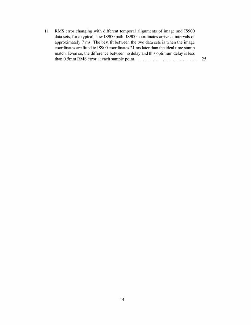
11 RMS error changing with different temporal alignments of image and IS900data sets, for a typical slow IS900 path. IS900 coordinates arrive at intervals ofapproximately 7 ms. The best fit between the two data sets is when the imagecoordinates are fitted to IS900 coordinates 21 ms later than the ideal time stampmatch. Even so, the difference between no delay and this optimum delay is lessthan 0.5mm RMS error at each sample point. . . . . . . . . . . . . . . . . . . 25
14

XY
Z
Figure 1: Path reconstructed from pairs of 2D images (solid line) with IS900 path (crosses)overlaid. Only a short segment of the path is shown (with only every fifth IS900 coordinateshown for clarity) but deviations between the two paths can still be seen, especially duringrapid changes of direction.
15

−50
0
50
−50
0
50−50
0
50
X (mm)Y (mm)
Z (mm)
(a) Static
−50
0
50
−50
0
50−50
0
50
X (mm)Y (mm)
Z (mm)
(b) Slow
−50
0
50
−50
0
50−50
0
50
X (mm)Y (mm)
Z (mm)
(c) Medium
−50
0
50
−50
0
50−50
0
50
X (mm)Y (mm)
Z (mm)
(d) Fast
Figure 2: Error vectors between IS900 and optical paths for static, slow, medium and fastmoving cases. Error vectors have been rotated to aligned so that the x-axis corresponds to thetracker’s direction of travel. RMS errors along and perpendicular to the direction of travel were2.0 and 1.4mm for the slow condition; 4.3 and 3.1mm for the medium condition; and 10.9 and9.9mm for the fast condition.
16

0 20 40 600
20
40
60
80
100
error (mm)
sam
ples
(a) Static
0 20 40 600
20
40
60
80
100
error (mm)
sam
ples
(b) Slow
0 20 40 600
20
40
60
80
100
error (mm)
sam
ples
(c) Medium
0 20 40 600
20
40
60
80
100
error (mm)
sam
ples
(d) Fast
Figure 3: Histograms of spatial error magnitudes for static, slow, medium and fast movingcases. To aid comparison, the axis for figures (a) and (b) have been clipped at 100 samples.
17
0 500 10000
0.5
1
1.5
2
samples
erro
r (m
m)
(a) Static
0 500 10000
20
40
60
samples
erro
r (m
m)
(b) Slow
0 500 10000
20
40
60
samples
erro
r (m
m)
(c) Medium
0 500 10000
20
40
60
samples
erro
r (m
m)
(d) Fast
Figure 4: Spatial errors between IS900 and optical paths for each sample point. The plot forthe static condition (a) has a different axis scale to reveal the sudden spatial ‘jumps’ the IS900makes even when the tracker is stationary.
18

0 2500 5000 7500 10000
10
20
30
40
50
sample
Em
itter
ID
−0.2
0
0.2
0.4
0.6
0.8
1
1.2
1.4
1.6
1.8
Position (m
)
Figure 5: The X, Y and Z components of position reported by a static IS900 tracker (middle, topand bottom solid black lines respectively), overlaid onto a plot of the ultrasonic emitters activeduring each sample (crosses). Changes in reported tracker position coincide with changes inthe subset of ultrasonic emitters used by the IS900.
19

0 200 400 600 800 1000 12000
0.5
1
1.5
2
sample
spee
d (m
/s)
Figure 6: Speed profiles for the slow (circles), medium (stars) and fast (crosses) conditionsshowing IS900 versus optical path (solid line). Only 1 in 15 points shown here for clarity.Deviations between IS900 and optical paths are apparent at large changes in speed.
20

0 0.5 1 1.50
20
40
60
speed (m/s)
erro
r (m
m)
Figure 7: RMS error plotted against IS900 tracker speed for the slow (circles), medium (stars)and fast (crosses) conditions. Only 1 in 15 points shown here for clarity. The slopes of linear fitsthrough the data have slopes for the slow condition were: 0.0039±0.00057 mm/m/s (t = 6.91,p < 10−9); medium: 0.0128±0.0011 mm/m/s (t = 12.15, p < 10−9); fast: 0.0037±0.00066mm/m/s (t = 5.59, p < 10−9).
21

0 200 400 600 800 1000 12000
0.02
0.04
0.06
0.08
0.1
sample
acce
lera
tion
(m/s
/s)
Figure 8: Acceleration profiles for the slow (circles), medium (stars) and fast (crosses) condi-tions for the IS900 positions versus optical path (solid line). Only 1 in 15 points shown herefor clarity.
22
0 0.02 0.04 0.06 0.08 0.10
10
20
30
40
50
60
acceleration (m/s/s)
erro
r (m
m)
Figure 9: RMS error plotted against IS900 acceleration for the slow (circles), medium (stars)and fast (crosses) conditions. Only 1 in 15 points shown here for clarity.
23
0 0.5 1 1.5 2 2.52
2.5
3
3.5
4
4.5
5
σ (pixels)
erro
r (m
m)
Figure 10: RMS error increasing with increasing standard deviation of the Gaussian distributednoise (mean over 200 trials). Error bars show standard deviation. Solid line is for a typical‘slow’ IS900 tracker path, while the dashed line is for a typical ‘medium’ path. The circleand cross symbols denote the RMS error for the slow and medium paths without added imagenoise.
24
−60 −40 −20 0 20 40 600
2
4
6
8
10
12
delay (ms)
erro
r (m
m)
Figure 11: RMS error changing with different temporal alignments of image and IS900 datasets, for a typical slow IS900 path. IS900 coordinates arrive at intervals of approximately 7ms.The best fit between the two data sets is when the image coordinates are fitted to IS900 coor-dinates 21ms later than the ideal time stamp match. Even so, the difference between no delayand this optimum delay is less than 0.5mm RMS error at each sample point.
25

List of Tables
I Mean deviation at each sample point of the IS900 tracker from the optical pathfor static, slow- and fast-moving conditions. . . . . . . . . . . . . . . . . . . . 27
26
Recording Static Slow Medium Fast1 0.846±0.51mm 2.66±1.3mm 4.59mm±2.5mm 20.1mm±10mm2 0.716±0.25mm 3.11±1.5mm 8.50mm±3.2mm 15.0mm±6mm3 0.357±0.28mm 2.81±1.4mm 5.23mm±3.2mm 17.4mm±8mm
Table I: Mean deviation at each sample point of the IS900 tracker from the optical path forstatic, slow- and fast-moving conditions.
27