Quantifying the Value of Iterative Experimentation

Jialiang MaoLinkedIn Corporation

Iavor BojinovHarvard Business School

November 4, 2021

Abstract

Over the past decade, most technology companies and a growing number of conven-

tional firms have adopted online experimentation (or A/B testing) into their product

development process. Initially, A/B testing was deployed as a static procedure in

which an experiment was conducted by randomly splitting half of the users to see the

control—the standard offering—and the other half the treatment—the new version.

The results were then used to augment decision-making around which version to re-

lease widely. More recently, as experimentation has matured, firms have developed a

more dynamic approach to experimentation in which a new version (the treatment)

is gradually released to a growing number of units through a sequence of randomized

experiments, known as iterations. In this paper, we develop a theoretical framework

to quantify the value brought on by such dynamic or iterative experimentation. We

apply our framework to seven months of LinkedIn experiments and show that iterative

experimentation led to an additional 20% improvement in one of the firm’s primary

metrics.

1

arX

iv:2

111.

0233

4v1

[st

at.A

P] 3

Nov

202

1

1 Introduction

Over the past decade, firms, particularly in the technology sector, have adopted randomized

experiments (often referred to as A/B tests) to guide product development and innovation

(Thomke, 2020). Companies including Airbnb (Lee and Shen, 2018), Google (Tang et al.,

2010), LinkedIn (Xu et al., 2015), Microsoft (Kohavi et al., 2013) and Yelp (Bojinov and

Lakhani, 2020) all developed in-house experimentation platforms to enable large-scale ex-

perimentation. Commercial A/B testing platforms such as Optimizely and Split have also

recently emerged to serve experimentation as a product to enable traditional firms as well

as start-ups to gain access to this valuable tool (Johari et al., 2017).

The operational benefits have primarily fueled the rapid uptick in the integration of

experimentation. We can categorize these into three pillars: reduced risk of product launches

and changes, fast product feedback, and accurate measurement of the effect of innovations

(Kohavi et al., 2009; Xia et al., 2019; Xu et al., 2018). There is an abundance of anecdotal

evidence for each pillar that illustrates the value to a firm (Kohavi and Thomke, 2017; Koning

et al., 2019). Most of this work focuses on A/B test as a two-step procedure: an experiment

is conducted, and a decision is made based on the results (Kohavi et al., 2013). However,

as firms reach a high level of experimentation maturity and integrate experimentation into

most product changes, experimentation becomes an iterative process where a feature change

is gradually released and is quickly changed based on the user feedback; this process is known

as a phased release (Xu et al., 2018).

A phased release cycle is divided into three steps; usually, firms decide to move from

one step to the next by examining the estimated impact of a change on multiple business

metrics (Xu et al., 2018). First, the change is introduced to a small random sample of

users; this stage is used to detect degradations. Second, we increase the proportion of

exposed users to 50%; at this point, we have maximum power to detect a change in business

2

metrics. Third, we choose to either make the change available to all users or roll back to

the original version. In practice, we found that most teams use the first step to learn how

to improve their product and fix bugs. The second step then measures the overall impact of

the innovation and, in almost all cases, is precisely the final released product. Changes can

be made to improve the product between the two steps, suggesting that we can quantify the

value of iterative experimentation by comparing the estimated effect in the first step to the

estimate obtained from the second step. This paper formalizes this intuition and develops a

framework for quantifying the value of transitioning from a two-step experimentation process

to an iterative approach. Our framework inherently captures aspects of the value of three

pillars but does not capture every potential benefit of A/B testing. When applied to seven

months of experiments at LinkedIn, our results suggest that iterative experimentation, or

phased release, leads to an additional 20% improvement in underlying metrics.

The key to our formulation is a framework that describes the inherently temporal nature

of A/B testing. Instead of focusing on one iteration at a time, we consider multiple iterations

of an experiment in a holistic way, which allows us to combine information from different

iterations and provides new perspectives to analyze the experiment results. In particular,

we define the value of an iteration experiment as a special causal estimand that includes

potential outcomes from multiple iterations to quantify the improvement we gain during the

experimentation period. Moreover, the general framework we build makes it easy to elucidate

the assumptions involved in identifying and estimating our causal estimand, especially those

related to the dynamics of the potential outcomes, which are usually made in practice in an

ambiguous and implicit way.

Interestingly, by combining the estimated value of a single experiment across all exper-

iments, we can obtain an overall estimate of the value of iterative experimentation. In

particular, the value of multiple experiments in a fixed time window can be aggregated to

estimate the overall value delivered by the transition to iterative experimentation. This

3

estimate can be considered as a lower bound of the value provided by an experimentation

platform that enables rapid iteration. Practically, it also allows us to define several metrics

that track the performance of the experimentation platform. First, such aggregation can be

done at the company level to provide metrics that directly evaluate the platform’s overall

performance. Unlike qualitative feedbacks or existing metrics used to assess the platform,

such as the experiment capacity and average experiment velocity, these value-based metrics

directly measure the platform’s performance in terms of key business metrics. Second, the

iterative value of experiments from the same team can be aggregated to quantify the learning

and innovation level of that team. Such metrics can provide insights into the dynamic of the

company’s product space and give feedback to the platform to further boost innovation.

Our proposed approach to quantify the value of iterative experiments has a “Bootstrap-

ping” nature: everything needed to compute the value of an experiment is already contained

in the data collected by a typical experimentation platform. To compute the value, the

practitioner needs to combine data from different iterations when computing the confidence

intervals or p-values. In most mature platforms, such data are usually tracked and stored in

offline databases in an easy-to-query manner (Gupta et al., 2018). Thus there is essentially

no engineering effort required to implement our proposal. From an information collection

perspective, the introduced metrics to quantify the value of an experimentation platform

synthesizes information from multiple randomized controlled experiments. It thus has a fla-

vor of meta-analysis of finished experiments and sits on top of the “hierarchy of evidence”

(Kohavi et al., 2020).

This paper is organized as follows. Section 2 introduces the experimentation design

and defines the potential outcomes. In Section 3, we define and estimate the value of a

single iterative experiment under two slightly different designs. The aggregated value of

an experimentation platform is then introduced in Section 4. In Section 5, we present

our analysis on the value of LinkedIn’s experimentation platform in the first half of 2019.

4

Section 6 concludes.

2 Treatments and potential outcomes

2.1 Formalizing the phased release with changing features

We first focus on a single feature being launched through a phased release and denote the

outcome of interest as Y . Suppose that the target population is fixed and contains n units

denoted by i ∈ [N ] = 1, 2, . . . , n. This fixed population perspective is attractive in our setting

as the units often comprise the entire population of interest; see Abadie et al. (2020) for a

review. A phased release is typically implemented as a sequence of iterative experiments,

each of which is often called a ramp (Xu et al., 2018). In each iteration, the treatment

is assigned to a randomly selected group of units. The treatment group starts small and

expands across different iterations before it reaches the entire target population when the

feature is fully launched. Companies in the tech industry usually have recommendations on

their ramping plans (Apple, 2021; Google, 2021). For example, LinkedIn limits the set of

potential ramping probabilities of its internal experiments to {1%, 5%, 10%, 25%, 50%} for

standardization and communication purpose.

The first few iterations before the 50% ramp correspond to the risk mitigation stage.

Ramps in this stage serve as test runs of the new feature and collect timely feedback to

help make product launch decisions and guide future product development. In addition, by

exposing the change only to a small group of users, the risk of launching a poor feature or

introducing unexpected bugs to the system is significantly reduced. Ramps at 50% corre-

spond to the effect estimation stage of a phased release and are usually referred to as the

“max power iterations” (MP). As the name suggests, it is straightforward to show1 that this

1An experiment with an even split between the treatment and control group minimizes the variance ofthe t-statistic used to analyze the results.

5

ramp offers maximum power to detect differences between the treatment and control and

provides the most accurate estimate of the treatment effect.

Practitioners assume that the feature remains the same throughout the release. However,

this assumption is often violated as developers use the feedback in earlier iteration to improve

the feature. Technically, if a feature is updated, it should go through an entirely new phased

release cycle. However, many of these changes are minor and do not introduce additional

risks. As the first few iterations in the cycle are mainly for risk mitigation, starting over

from the first iteration is undesirable whenever the changes are minor as it will introduce

significant opportunity costs and slow down the pace of innovation. In practice, a feature

after minor changes is often considered the same feature as long as these changes do not

modify the product at a conceptual level. A new phase release cycle is only required when

the changes are significant enough to alter the essence of the product.

For example, recently, at LinkedIn, a team released a new brand advertising product

with a new auto bidding strategy to improve advertiser return on investment by maximizing

the number of unique LinkedIn members reached by an advertising campaign. There was an

overall improvement in core metrics in the first iteration, like the number of unique members

reached and the click-through rate. However, further analysis suggested the change caused

a drop in the budget utilization of campaigns with a small target audience, decreasing the

revenue from this segment. The developers used the feedback and identified the problem: a

global parameter in the new algorithm that determined the auction behavior of all campaigns.

The team then came up with a solution to make the parameter adaptive and more campaign-

specific. Follow-up iterations showed that the adaptive parameter fixed the identified issue

and was eventually launched. Although modifications were made to the new bidding strategy

across iterations, the concept of this product did not change.

Here, we formally consider such modifications to the treatment with the following re-

strictions. Firstly, changes to the treatment must not alter the treatment at the conceptual

6

level and cannot introduce additional risks. Secondly, all changes must be made in the risk

mitigation stage, and no changes are allowed after the 50% ramps. Thirdly, the final version

of the treatment has to be tested with at least one 50% ramp to estimate its effect accurately.

With these requirements, we focus on two iterations that provide sufficient information to

quantify the value of an iterative experiment: the largest unchanged iteration (LU) and the

last most powerful iteration (LMP). Specifically, an unchanged iteration is an iteration in

which the treatment is in its original form without any modification. LU is the unchanged

iteration with the largest treatment ramping percentage. Intuitively, LU gives the most

accurate estimate of the effect of the original treatment, while LMP estimates the effect of

the final version of the treatment after incorporating learnings from previous iterations. In

practice, LU can range from the first iteration to MP. If changes are not clearly documented,

it is always safe to pick the first iteration as LU.

The new feature being tested in an phased release can have different variants. For ex-

ample, we might test different color schemes in an user interface change, different ranking

algorithms in a search engine, or different values of the bidding floor price in an ads serving

system. For illustration, we first assume that the feature only has a single variant or version

and denote it as v. Let t = 1, 2 denote the LU and the LMP respectively. We write the po-

tentially different versions of v in iteration t as vt for t = 1, 2. For unit i, let Zi,t ∈ {v1, v2, c}

be the product treatment she receives in iteration t and let Zi = (Zi,1, Zi,2) be her treatment

path (Bojinov and Shephard, 2019; Bojinov et al., 2021). We also use Z1:N to represent the

N × 2 matrix of the treatment paths of all units. We assume that the treatment assignment

follows a two-iteration stepped-wedge design (Brown and Lilford, 2006) in which the units

who receive the treatment in the first iteration will stay in the treatment group in the second

iteration. Formally, we have

Definition 1 (Two-iteration stepped-wedge design). LetH = {Z1:N : Zi ∈ V = {(c, c), (c, v2),

(v1, v2)}, i ∈ [N ]}, a two-iteration stepped-wedge design η = η(Z) is a probability distribu-

7

tion on H.

This stepped-wedge design can be implemented by introducing restrictions on the se-

quential assignment at the two iterations. For example, we can implement a completely

randomized design or a Bernoulli design at each iteration as long as we respect the “no

going back” constraint. In this work, we focus on the completely randomized design and let

0 < p1 ≤ p2 = 0.5 be the ramping probabilities at the two iterations. In the first iteration,

we randomly assign p1N units to the treatment group. In the second iteration, we keep

these units in the treatment group and randomly assign an additional (p2− p1)N units from

the previous control group to the treatment group. Most technology companies adopt the

stepped-wedge design in phased releases to ensure a consistent product experience. It is also

a common setup in medical and social science research where it is sometime referred to as

the staggered adoption design or the event study design (Brown and Lilford, 2006; Callaway

and Sant’Anna, 2020; Sun and Abraham, 2020; Athey and Imbens, 2021).

2.2 Potential outcomes

We adopt the Neyman-Rubin potential outcome framework for causal inference (Splawa-

Neyman et al., 1990; Rubin, 1974) and treat the potential outcomes as fixed. Specifically,

let Yi,t(Z1:N) be the potential outcome of unit i at iteration t under treatment path Z1:N . In

practice, each iteration of a phased release usually runs several days and there is no guarantee

that different iterations will last the same duration. For example, the first iteration typically

runs shorter than the second iteration. The majority of experiments at LinkedIn finish

both iterations within a week (Xu et al., 2018). Therefore, there is a time component

underlying the potential outcomes. In this paper, we interpret the potential outcome as the

daily average of metric Y measured over each iteration. Other interpretations such as the

aggregated measure within each iteration can also be applied.

8

We make the following assumptions, introduced in Bojinov and Shephard (2019), to limit

the dependence of the potential outcomes on assignment paths:

Assumption 1 (Non-anticipation). The potential outcomes are non-anticipating if for all

i ∈ [N ], Yi,1(z1:N,1, z1:N,2) = Yi,1(z1:N,1, z1:N,2) for all z1:N,1 ∈ {c, v1}N , and z1:N,2, z1:N,2 ∈

{c, v2}N .

Assumption 2 (No-interference). The potential outcomes satisfy no-interference if for all

i ∈ [N ] and t = 1, 2 Yi,t(z1:(i−1), zi, z(i+1):N) = Yi,t(z1:(i−1), zi, z(i+1):N) for all z1:(i−1), z1:(i−1) ∈

V i−1 and z(i+1):N , z(i+1):N ∈ VN−i.

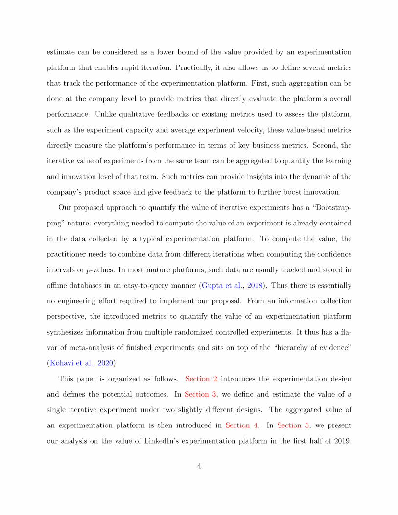
With these assumptions, we can write the potential outcomes of unit i as Yi,1(Zi,1) and

Yi,2(Zi,1, Zi,2). Illustrations of the potential outcomes under the stepped-wedge design given

p1 < p2 or p1 = p2 are shown in Figure 1 and Figure 2. Note that although practically v2 is

only available after the first iteration, we can still define Yi,1(v2) theoretically. These potential

outcomes capture the oracle scenario where the experimenter knows the best solution in the

first place.

3 Quantifying the operational value of iterative exper-

imentation

3.1 A single experiment

There are three cases when an iterative experiment creates direct quantifiable value:

1. The experiment iterations provide timely feedback and point the direction for further

feature improvements. The value of the experiment can be quantified as the improve-

ment in the treatment across the different iterations.

9

2. When the feature has a negative impact and is de-ramped after the mitigation stage

(i.e., reverted back to the control), the experiment helps prevent the exposure of bad

features directly to a larger group of users. The value of these types of experiments

can be estimated as the prevented loss.

3. When the feature has multiple versions, the experiment can help identify the best

possible version, avoiding random guesses on which version to launch and the cost

of trial and error. The value of these types of experiments can be thought of as the

difference between the best and worse performing versions.

In this section, we formally define these values and provide consistent estimators of them.

We first introduce the value from feature improvement. Within each iteration (t = 1

or 2), the direct comparison of any two potential outcomes of the same unit has a causal

interpretation. For example, Yi,1(v1) − Yi,1(c) is the effect of the treatment on unit i in the

first iteration and Yi,2(c, v2)−Yi,2(c, c) is the effect of the updated treatment on unit i in the

second iteration. Intuitively, the experiment provides value if v2 is better than v1. Below we

define the improvement due to iterative experimentation.

Definition 2 (Value of iterative experimentation). We define the value of iterative exper-

imentation (VOIE) on unit i as τi,1 = Yi,1(v2) − Yi,1(v1). We also define the population

average VOIE as

τ1 =1

N

N∑i=1

τi,1 =1

N

N∑i=1

[Yi,1(v2)− Yi,1(v1)]. (3.1)

Similar to the potential outcomes, the interpretation of τi,1 and τ1 also has to take into

account the underlying time component. Firstly, the “1” in the subscript indicates that these

estimands capture the value of the experiment at the calendar time of the first iteration. If

the experiment runs at a different time (i.e., in a different week), the value might change

without further assumptions on the dynamics of the potential outcomes. Secondly, τi,1 and

τ1 represent the daily average value of the experimentation as inherited from the definition

10

of the potential outcomes. The interpretation of VOIE can change if the experiment runs

for a different duration (i.e., run for two weeks instead of one).

In classical causal inference problems with a single treatment, one of the two potential

outcomes of each unit is missing and we have to deal with the “fundamental problem of causal

inference” (Holland, 1986). To estimate the population level causal estimands, identifiability

assumptions such as the strong ignorability assumption (Rosenbaum and Rubin, 1983) are

often made. Our estimate of the population level VOIE relies on the following identifiability

assumption:

Assumption 3 (Time-invariant control effect). The individual-level treatment effects are

time-invariant if Yi,2(c, v)− Yi,2(c, c) = Yi,1(v)− Yi,1(c) for i ∈ [N ], v ∈ {v1, v2}.

The time-invariant control effect assumption states that the effect of the treatment does

not change with the time it is adopted. This assumption is justifiable in most cases as units

were all assigned to control prior to the treatment release, therefore, an additional control

exposure should have no bearing on the causal effect. Under this assumption, we can write

τi,1 as

τi,1 = Yi,1(v2)− Yi,1(v1)

= [Yi,1(v2)− Yi,1(c)]− [Yi,1(v1)− Yi,1(c)]

= [Yi,2(c, v2)− Yi,2(c, c)]− [Yi,1(v1)− Yi,1(c)]

(3.2)

The definition of VOIE could also capture other types of values of iterative experimen-

tations. When the feature has a significantly negative effect and is de-ramped after the first

iteration, the value of the experiment is the avoided potential loss. In this case, there is no

second iteration in the experiment, and with a slight abuse of notation, we write “v2 = c”.

The VOIE in this case is

τ ′1 =1

N

N∑i=1

[Yi,1(v2)− Yi,1(v1)] = − 1

N

N∑i=1

{[Yi,1(v1)− Yi,1(c)]}, (3.3)

11

which is the opposite of the treatment effect in the first iteration.

We need to slightly modify our notations to account for the case when the feature has

multiple variants, and the practitioner needs to choose the best one to launch. Specifically,

let v(1), v(2), . . . , v(m) be the m treatment variants under consideration. Suppose that the m

variants are tested on a randomly selected group of p1N units in the first iteration. In this

paper, we consider a completely randomized design with group size (p11, p12, p1m, 1− p1) ·N

respectively, where∑m

j=1 p1j = p1. The ramping probabilities reflect the experimenter’s prior

knowledge and preference of different variants. Given feedback from the first iteration, one of

the m variants is picked to be further tested in the second iteration. We denote this winning

variant as v2. The potential outcomes defined in Section 2.2 can be easily generalized to the

case of multiple variants. Under assumption 3, we can define and simplify the VOIE in this

case as

τ ∗1 =1

N

N∑i=1

[Yi,1(v2)−

m∑j=1

p1j

p1

Yi,1(v1)

]

=1

N

N∑i=1

{[Yi,2(c, v2)− Yi,2(c, c)]− [

m∑j=1

p1j

p1

Yi,1(v1)− Yi,1(c)]

}.

Although τ1, τ ′1 and τ ∗1 are all defined and estimated in a similar manner, they capture

different aspects of the value of iterative experiments: τ1 estimates the value from guiding

product development; τ ′1 captures the value from risk mitigation; and τ ∗1 represents the value

of reducing uncertainties. Both τ1 and τ ∗1 can be viewed as capturing the value of learning

and they can be combined. For example, in τ ∗1 , v2 could be an improved version of the best

variant in the first iteration. In the following sections, we provide estimates of the VOIE

under two similar but slightly different designs. We will focus on τ1 as inference for τ ′1 and

τ ∗1 can be done in a similar manner.

12

3.2 Estimating VOIE with progressive iterations

In practice, it is common that learning starts in the risk mitigation stage before the 50%

ramp. Minor changes to the feature like a bug fix in the code can be made right after the

first iteration. In this case, the last unchanged iteration (LU) corresponds to a ramp with

p1 < p2 = 0.5. An illustration of potential outcomes under this design is given in Figure 1.

Under Assumption 3, the population level VOIE τ1 in (3.1) can be written as

τ1 =1

N

N∑i=1

{Yi,2(c, v2)− Yi,1(v1)−∆i]}, (3.4)

where ∆i = Yi,2(c, c)− Yi,1(c). To estimate τ1, we consider the following plug-in estimator

τ1 =1

Nc,v2

N∑i=1

Y obsi,2 1(Zi = (c, v2))− 1

Nv1

N∑i=1

Y obsi,1 1(Zi,1 = v1)

− 1

Nc,c

N∑i=1

[Y obsi,2 1(Zi = (c, c))− Y obs

i,1 1(Zi = (c, c))],

(3.5)

where Nc,v2 =∑N

i=1 1(Zi = (c, v2)) is the number of units receiving treatment path (c, v2),

i.e., those assigned to the control group in the first iteration and to the treatment group in the

second iteration; Nv1 and Nc,c are defined similarly. Y obsi,1 and Y obs

i,2 are the observed outcomes

of unit i in the first and second iteration respectively. Let Y2(c, v2) =∑N

i=1 Yi,2(c, v2)/N ,

Y1(v1) =∑N

i=1 Yi,1(v1)/N , Y2(c, c) =∑N

i=1 Yi,2(c, c)/N and Y1(c) =∑N

i=1 Yi,1(c)/N be the

population mean of potential outcomes under specific treatment paths.

Theorem 1. Under the two-iteration stepped-wedge design η with p1 < p2, the plug-in esti-

mator in (3.5) satisfies

E[τ1] = τ1, V[τ1] =1

Nc,v2

S2c,v2

+1

Nv1

S2v1

+1

Nc,c

S2∆ −

1

NS2τ ,

13

where

S2c,v2

=1

N − 1

N∑i=1

[Yi,2(c, v2)− Y2(c, v2)]2, S2v1

=1

N − 1

N∑i=1

[Yi,1(v1)− Y1(v1)]2,

S2∆ =

1

N − 1

N∑i=1

[(Yi,2(c, c)− Yi,1(c))− (Y2(c, c)− Y1(c))]2,

S2τ =

1

N − 1

N∑i=1

[Yi,2(c, v2)− Yi,1(v1)− (Yi,2(c, c)− Yi,1(c))− τ1]2.

Notice that S2τ involves product terms of potential outcomes of the same units under

different treatment paths and is generally not estimable. S2c,v2

, S2v1

and S2∆ can be consistently

estimated with their sample counterparts. For example, let

s2c,v2

=1

Nc,v2 − 1

∑i:Zi=(c,v2)

[Y obsi,2 − Y 2(c, v2)]2, Y 2(c, v2) =

1

Nc,v2

∑i:Zi=(c,v2)

Y obsi,2 , (3.6)

and Vτ1 = N−1c,v2s2c,v2

+N−1v1s2v1

+N−1c,c s

2∆.

Theorem 2. Under regularity conditions, the Wald-type interval (τ1−zα/2V 1/2τ1 , τ1+zα/2V

1/2τ1 )

has asymptotic coverage rate ≥ 1 − α, where zα/2 is the (1 − α/2) quantile of a standard

normal distribution.

It is important to note that the terms Y2(c, c) and Y1(c) in τ1 are estimated with the

same samples which were in control in both iterations. Thus, although we could have a more

accurate estimate of Y1(c) by using all samples in the control group in the first iteration, this

will result in a subset of samples also being used in the estimate of Y2(c, v2) and significantly

complicates the variance estimation of τ1.

When using an experiment to estimate the average treatment effect, practitioners usually

focus on a single iteration (i.e., the max-power iteration) and only uses observations from that

iteration in the estimate. On the contrary, τ1, involves observations from multiple iterations.

Although any direct comparison of potential outcomes in the same iteration has clear causal

14

Start

Yi,1(c)

Yi,2(c, c)

Yi,2(c, v2)

Yi,1(v1)

Yi,2(v1, c)

Yi,2(v1, v2)

Figure 1: Potential outcomes for unit i under the two-iteration stepped-wedge design whenp1 < p2. The gray node represents the potential outcome when the feature is de-ramped afterthe first iteration. The red path shows one possible realization of the potential outcomes.

interpretations, this is not necessarily true for cross-iteration comparisons. As shown in the

Online Supplementary Materials B, τ1 can be interpreted as the treatment effect of a special

treatment under additional identifiability assumptions. Namely, we refer to the treatment

underlying τ1 as the platform treatment which captures the ability to implement iterative

experiments vs. the control of no iterative experiments.

3.3 Estimating VOIE with repeated max-power iterations

In Section 3.2, τ1 are estimated under progressive ramps with p1 < p2. In practice, it may

be possible to repeat a certain iteration (usually the max-power iteration) and test the final

version of the product to be launched, in which case p1 = p2 = 0.5. In this section, explain

how to estimate τ1 under such designs.

Since ramps before the max-power iteration are for mitigating risk, with little emphasis

on treatment effect estimation, to avoid delaying the release, practitioners recommended

that this stage is relatively short-lived if no severe degradations are detected (Xu et al.,

2018). This is especially prominent when the experiment has deficient power. To overcome

15

Start

Yi,1(c) Yi,2(c, c)

Yi,1(v1)

Yi,2(v1, c)

Yi,2(v1, v2)

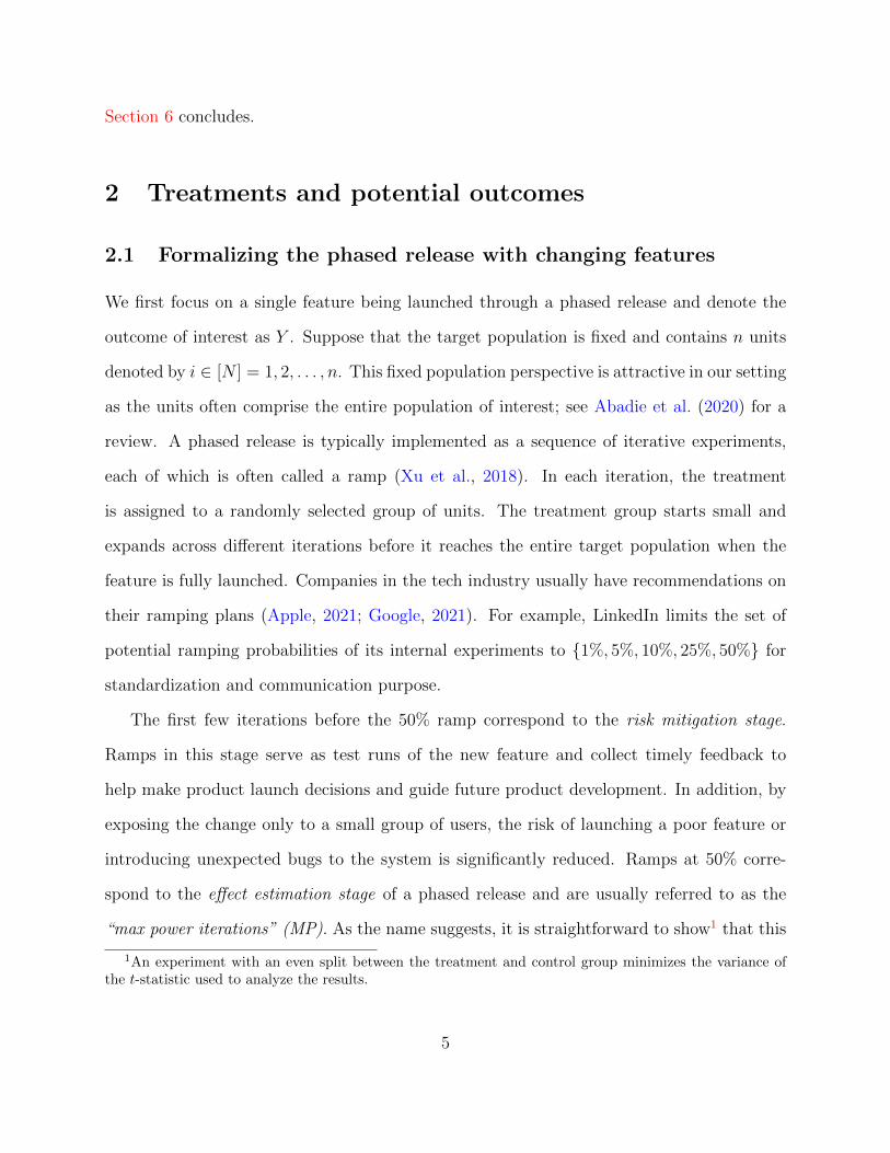
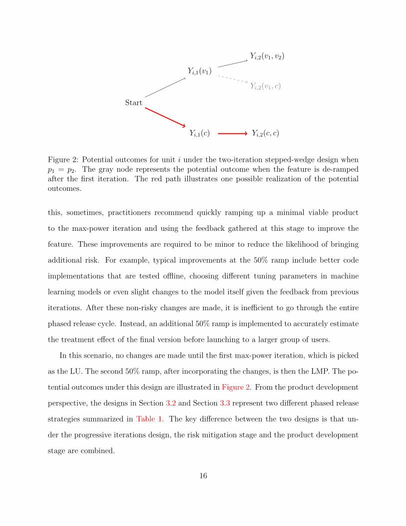
Figure 2: Potential outcomes for unit i under the two-iteration stepped-wedge design whenp1 = p2. The gray node represents the potential outcome when the feature is de-rampedafter the first iteration. The red path illustrates one possible realization of the potentialoutcomes.

this, sometimes, practitioners recommend quickly ramping up a minimal viable product

to the max-power iteration and using the feedback gathered at this stage to improve the

feature. These improvements are required to be minor to reduce the likelihood of bringing

additional risk. For example, typical improvements at the 50% ramp include better code

implementations that are tested offline, choosing different tuning parameters in machine

learning models or even slight changes to the model itself given the feedback from previous

iterations. After these non-risky changes are made, it is inefficient to go through the entire

phased release cycle. Instead, an additional 50% ramp is implemented to accurately estimate

the treatment effect of the final version before launching to a larger group of users.

In this scenario, no changes are made until the first max-power iteration, which is picked

as the LU. The second 50% ramp, after incorporating the changes, is then the LMP. The po-

tential outcomes under this design are illustrated in Figure 2. From the product development

perspective, the designs in Section 3.2 and Section 3.3 represent two different phased release

strategies summarized in Table 1. The key difference between the two designs is that un-

der the progressive iterations design, the risk mitigation stage and the product development

stage are combined.

16

Stage Progressive iterations Repeated MP iterations

I Risk Mitigation

Iterations before the50% ramp (∗)

Iterations up to the first50% ramp

II Product DevelopmentThe interim between the

two 50% ramps (∗)

III Effect Estimation The 50% ramp The second 50% ramp

Table 1: Comparison of the phase release cycle under two designs. ∗ indicates that non-riskychanges to the product are allowed at that stage.

To estimate τ1 under the repeated max-power iteration design, we require an additional

assumption.

Assumption 4 (No carryover effect). There is no carryover effect if Yi,2(c, v) = Yi,2(v1, v)

for v ∈ {v1, v2}.

The validity of the no carryover effect assumption depends on the feature being tested

and needs to be evaluated on a case-by-case basis. It is a good practice to allow a cool-down

period, in which all units are assigned to control, between the two iterations to make this

assumption more plausible. Under Assumption 3 and the no carryover effect assumption, τ1

in (3.4) becomes

τ1 =1

N

N∑i=1

{[Yi,2(v1, v2)− Yi,2(c, c)]− [Yi,1(v1)− Yi,1(c)]}.

Similar to (3.5), we consider the following plug-in estimator of τ1:

τ1 =1

Nv1,v2

N∑i=1

[Y obsi,2 1(Zi = (v1, v2))− Y obs

i,1 1(Zi,1 = v1)]

− 1

Nc,c

N∑i=1

[Y obsi,2 1(Zi = (c, c))− Y obs

i,1 1(Zi,1 = c)],

(3.7)

where Nv1,v2 =∑N

i=1 1(Zi = (v1, v2)) is the number of units in the treatment group, Nc,c the

17

number of units in the control group. Similar to Theorem 1, we have

Theorem 3. Under the multiple max-power iteration stepped-wedge design η, the plug-in

estimate in (3.7) satisfies

E[τ1] = τ1, V[τ1] =1

Nv1,v2

S2v1,v2

+1

Nc,c

S2c,c −

1

NS2τ ,

where

S2v1,v2

=1

N − 1

N∑i=1

[(Yi,2(1; v1, v2)− Yi,1(1; v1))− (Y2(v1, v2)− Y1(v1))]2,

S2∆ =

1

N − 1

N∑i=1

[(Yi,2(1; c, c)− Yi,1(1; c))− (Y2(c, c)− Y1(c))]2,

S2τ =

1

N − 1

N∑i=1

[Yi,2(1; v1, v2)− Yi,1(1; v1)− (Yi,2(1; c, c)− Yi,1(1; c))− τ1]2.

Let Vτ1 = N−1v1,v2

s2v1,v2

+N−1c,c s

2∆, Theorem 2 also holds.

4 Quantifiable value of an experimentation platform

Typically, the primary goal metric Y can be hard to move, especially when Y is a company-

level metric such as the overall revenue or the total page views of the website. Therefore,

the VOIE τ1 is likely to be small in absolute value, and so inference from a single experiment

would have low power, especially under the design in Section 3.2 where treatment allocation

in the first iteration is small. Fortunately, from an operational perspective, firms are more

interested in the aggregated value of multiple experiments at the team or platform level.

To this end, let Ej, j = 1, 2, . . . , J denote a set of iterative experiments whose values we

want to aggregate. We assume that the experiments all have the same target population

and are mutually independent. Let τ1,j be the value from the j-th iterative experiment. We

18

define the aggregated value of these experimentations as

δa =J∑j=1

ajτ1,j, (4.1)

where a = (a1, a2, . . . , aJ),∑J

j=1 aj = 1. For fixed a, the plug-in estimator δa is unbiased and

has the following estimated upper bound of its variance V[δa] =∑J

j=1 a2jV[τ1,j]. The weights

a can be selected based on the a priori evaluated importance of the tested features. When

no such prior knowledge is available, a reasonable default is to estimate the inverse-variance

weighted average

δinv =J∑j=1

(J∑j=1

V[τ1,j]−1)−1

V[τ1,j]−1τ1,j, (4.2)

which has the smallest variance among all δa’s. To estimate δinv, we have to treat the

estimated upper bounds of V[τ1,j] as its true variance. When the bounds are tight for each

experiment (or at least tight for those experiments with large weights), this gives a reasonable

approximation to δinv due to the large sample size in online experimentations. Note that the

definition of δa requires all experiments to have the same target population such that their

values are comparable. If this is not the case, the VOIE can be computed and aggregated

at the site-wide impact level (Xu et al., 2015).

Although the definition of δa is simple, it gives rise to a set of metrics by varying the

primary goal metric, Y , and the set of experiments under consideration. These metrics

provide a holistic picture of the learning behavior across teams and help identify weaknesses

and opportunities. In practice, δa can be defined at different granularity levels and estimated

on a monthly or quarterly basis. For example, computing δa at the platform level lets us

monitor the contribution of iterative experimentations to core metrics. The aggregated VOIE

on these metrics also serve as direct performance metrics of the experimentation platform

itself. As another example, for each core metric, we can compute the aggregated VOIE

19

at the organization or team level and identify which teams benefit the most from iterative

experimentation.

5 Aggregated value of LinkedIn’s experiment platform

LinkedIn uses an internally developed, unified, and self-served Targeting, Ramping and Ex-

perimentation Platform (T-REX) for iterative experimentations on a user population of over

700 million members worldwide. The platform has been evolving in the past decade from

a small experiment management system with limited functions into a full-fledged platform

that allows efficient iterative experimentation and can serve more than 40000 tests simulta-

neously at any given time (Xu et al., 2015; Ivaniuk, 2020). During this evolution, numerous

features and improvements have been incorporated into the platform include infrastructure

changes that accelerate the experiment velocity, optimizations of the offline analysis data

pipeline, supports of more advanced statistical methodologies for experimentation readout,

and user interface changes that improve developers’ experience with the platform.

LinkedIn has a culture to “test everything” — essentially, all new features have to go

through a “ramp up” process enabled by the T-REX platform, which provides instant feed-

back to help make product launch decisions. It is well acknowledged that T-REX provides

value in this regard, but there is little understanding of what that value is and how it changes

over time. On the other hand, although T-REX serves all other teams, it lacks a reliable way

to collect feedback on the impact of feature changes on the platform itself. Traditionally, the

team has been relying on indirect metrics such as the average experimentation duration or

user surveys to quantify the performance of the T-REX platform, which are inefficient and

non-standardized.

In this work, we recommend monitoring the company (platform) level VOIE as a natural

performance metric that captures the efficiency of the platform and its ability to guide

20

Month

Nu

m o

f E

xp

eri

me

nt

1 2 3 4 5 6 7

05

01

00

15

02

00

Treatment allocation percentage

Pro

po

rtio

n

5 10 15 20 25

0.0

0.1

0.2

0.3

0.4

0.5

0.6

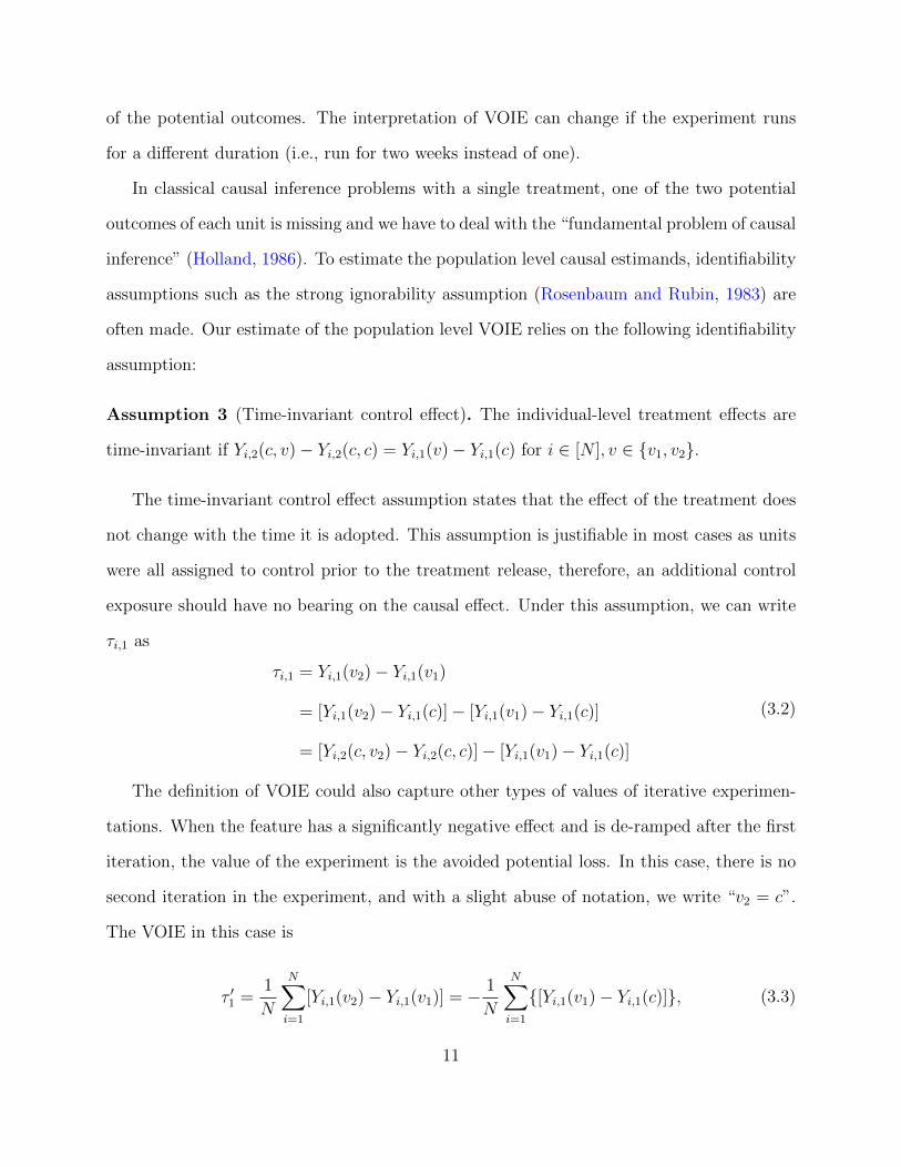
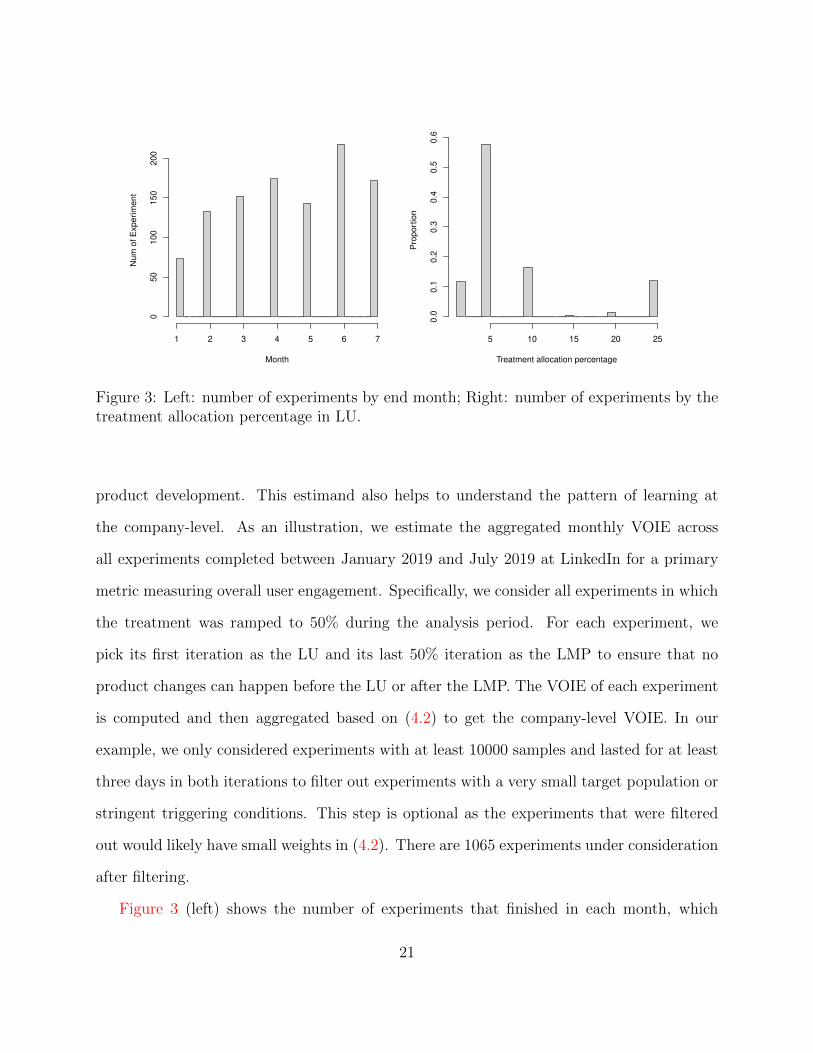
Figure 3: Left: number of experiments by end month; Right: number of experiments by thetreatment allocation percentage in LU.

product development. This estimand also helps to understand the pattern of learning at

the company-level. As an illustration, we estimate the aggregated monthly VOIE across

all experiments completed between January 2019 and July 2019 at LinkedIn for a primary

metric measuring overall user engagement. Specifically, we consider all experiments in which

the treatment was ramped to 50% during the analysis period. For each experiment, we

pick its first iteration as the LU and its last 50% iteration as the LMP to ensure that no

product changes can happen before the LU or after the LMP. The VOIE of each experiment

is computed and then aggregated based on (4.2) to get the company-level VOIE. In our

example, we only considered experiments with at least 10000 samples and lasted for at least

three days in both iterations to filter out experiments with a very small target population or

stringent triggering conditions. This step is optional as the experiments that were filtered

out would likely have small weights in (4.2). There are 1065 experiments under consideration

after filtering.

Figure 3 (left) shows the number of experiments that finished in each month, which

21

increases steadily in the first quarter of 2019 and fluctuates afterward, yielding an average

of 152 experiments per month. Figure 3 (right) summarizes the treatment percentage in the

LU iteration of the experiments. Most experiments follow the company’s recommendation to

start with small ramps with ramping percentage in P = {1%, 5%, 10%, 25%}. For experiment

iterations that last for more than two weeks, we only use their results in the first two weeks

to focus on the short-term treatment effect and limit the scope of uncontrolled time effects

to make the VOIE across experiments more comparable.

0 5 10 15 20 25 30

02

46

81

01

21

4

T

Pe

rce

nta

ge

Iter 1

Iter 2

2 4 6 8 10 12 14

T

Estim

ate

d e

ffe

cts

2.5

50

97.5

Week 1 Week 2

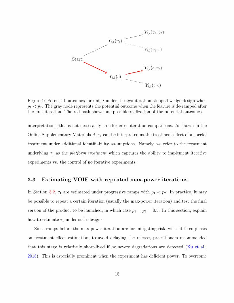
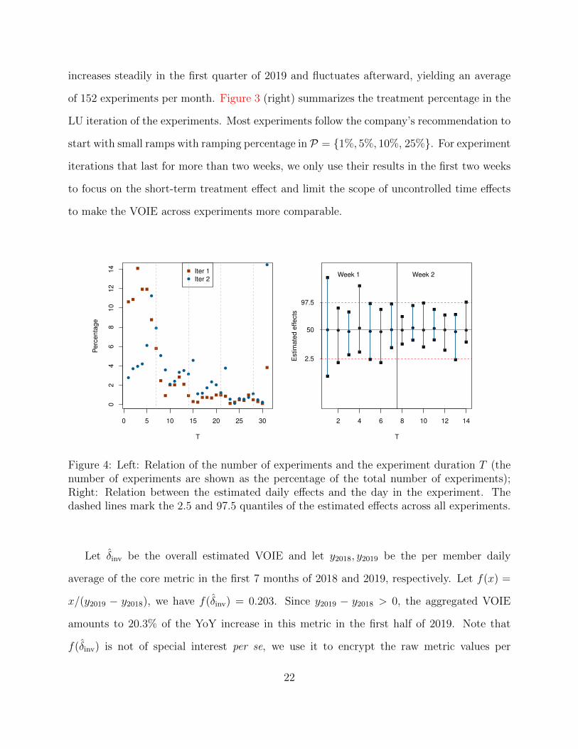
Figure 4: Left: Relation of the number of experiments and the experiment duration T (thenumber of experiments are shown as the percentage of the total number of experiments);Right: Relation between the estimated daily effects and the day in the experiment. Thedashed lines mark the 2.5 and 97.5 quantiles of the estimated effects across all experiments.

Let δinv be the overall estimated VOIE and let y2018, y2019 be the per member daily

average of the core metric in the first 7 months of 2018 and 2019, respectively. Let f(x) =

x/(y2019 − y2018), we have f(δinv) = 0.203. Since y2019 − y2018 > 0, the aggregated VOIE

amounts to 20.3% of the YoY increase in this metric in the first half of 2019. Note that

f(δinv) is not of special interest per se, we use it to encrypt the raw metric values per

22

company’s policy. Moreover, the p-value for testing H0 : δinv = 0 vs. H1 : δinv 6= 0 with

t-test and an estimate of V[δinv] based on the estimated upper bounds of V[τ1,j] is 0.068.

It is important to note the underlying time component in the definition of VOIE in (3.1)

inherited from the definition of the potential outcomes. Specifically, τ1,j is defined as the

daily average value of experiment j. Since different experiments have different running times,

their values are estimated based on different time ranges. The duration of the experiments

are shown in Figure 4 (left). Typically, the LU iteration of most experiments finishes within

a week and has a much shorter running time than the LMP iteration, as expected. Figure 4

(right) shows the quantiles of the estimated treatment effects at the T -th day of the exper-

iment for 1 ≤ T ≤ 14. For example, the bar at T = 8 shows the observed (2.5%, 97.5%)

quantiles of the estimated effects on the 8-th day of the iteration. Based on this plot, the

estimated treatment effects do not have a clear trend over time at the platform level. Thus

there is no sign of significant heterogeneity of VOIE by experiment duration, and the overall

VOIE δinv serves as a good summary of the value of experimentation at the platform level.

LU (first) Iteration

P−values of Estimated effects

De

nsity

0.0 0.2 0.4 0.6 0.8 1.0

0.0

0.5

1.0

1.5

2.0

2.5

3.0

MP (second) Iteration

P−values of Estimated effects

De

nsity

0.0 0.2 0.4 0.6 0.8 1.0

0.0

0.5

1.0

1.5

2.0

2.5

3.0

Estimated effects

−1.0 −0.5 0.0 0.5 1.0

Iter 1

Iter 2

Figure 5: Left and middle: p-values of estimated treatment effects in the LU and the LMPiteration; Right: estimated effects from all experiments in the two iterations.

Figure 5 shows the p-values and the estimated treatment effects in the two iterations of all

experiments in the analysis. As expected, the LMP iteration tends to show more statistically

23

significant results than the LU iteration and there are more positive effects than negative

ones in both iterations. In either iteration, the p-value distribution is a mixture of a spike

close to 0 and an almost uniform slab. This mixture reflects different roles of the metrics in

the experiments. For a small number of the features, this engagement metric is the primary

goal metric they hope to move. Experiments that test these features are more likely to see

smaller p-values. However, in most experiments, this metric serves as a guardrail metric on

which the treatment effect is expected to be neutral. The aggregated VOIE δinv captures the

VOIE on all experiments regardless of the role of the metric and is thus diluted. A triggered

analysis can be performed to remove this dilution effect by only looking at experiments that

treat the metric as the primary goal metric.

1 2 3 4 5 6 7

−5

00

50

10

0

Month

Sca

led

VO

IE

02

04

06

08

01

00

Treatment allocation

Sca

led

VO

E

1% 5% 10% 25%

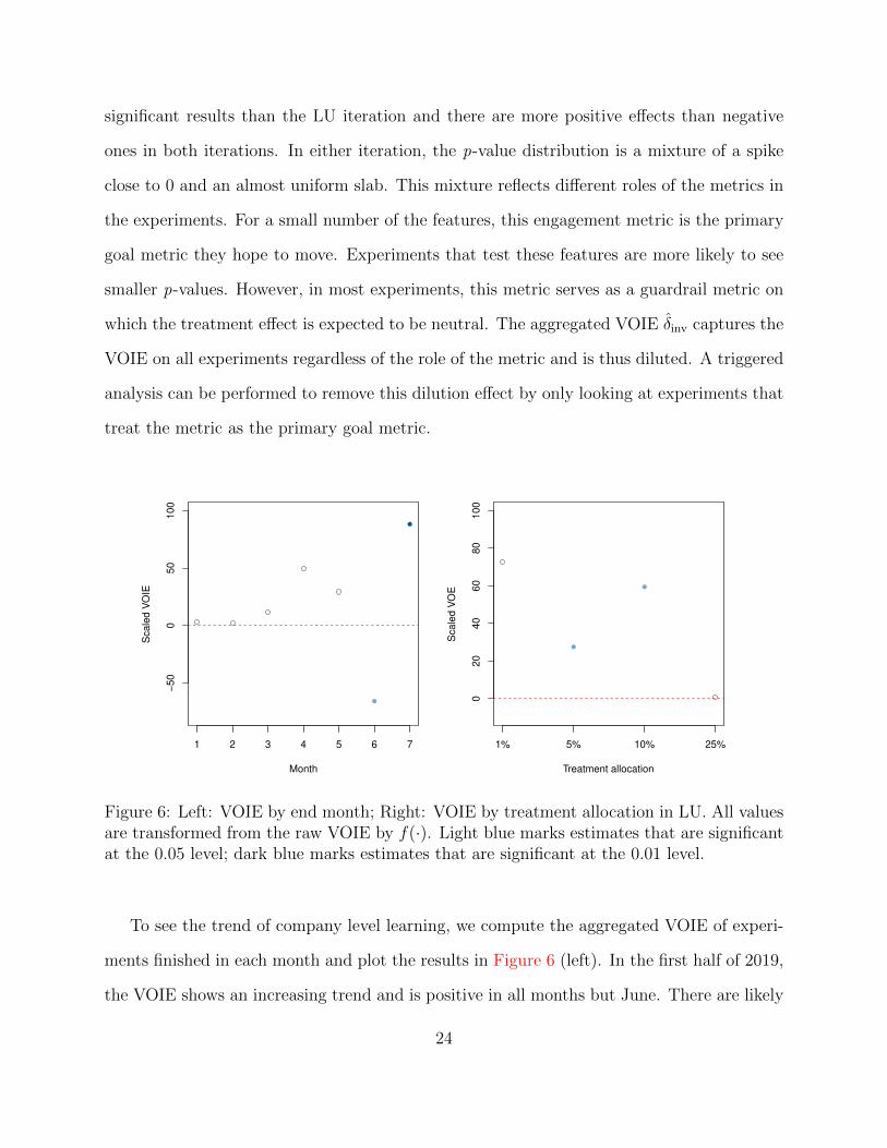
Figure 6: Left: VOIE by end month; Right: VOIE by treatment allocation in LU. All valuesare transformed from the raw VOIE by f(·). Light blue marks estimates that are significantat the 0.05 level; dark blue marks estimates that are significant at the 0.01 level.

To see the trend of company level learning, we compute the aggregated VOIE of experi-

ments finished in each month and plot the results in Figure 6 (left). In the first half of 2019,

the VOIE shows an increasing trend and is positive in all months but June. There are likely

24

two reasons for the unusual behavior of VOIE in June and July. First, there is a company

shutdown in the 4th of July week and the moratorium policy that no feature modifications

are allowed one week previous to the shutdown. As a result, feature improvements that

would have been made in June have to be pushed back in July, leading to an extremely high

VOIE in that month. Second, June and July is the transitional period of LinkedIn to a new

fiscal year. During this period, many metrics, including the one we analyzed here, are not

stable due to various reasons related to budgeting and customer spending.

Similarly, we also aggregate the VOIE of experiments according to their treatment al-

location in the LU iteration. The results are shown in Figure 6 (right). Since we take

the first iteration of an experiment as its LU, the treatment allocation in this iteration re-

flects the experimenter’s initial evaluation of the risk of the feature, which also serves as a

proxy for the feature’s room for improvement. For example, features that start the ramp at

1% tend to have larger risks, either because the features are premature or the engineering

implementations are unpolished. During the iterative process, both the features and their

implementations can be improved. These features are more likely to benefit from iterative

experimentation and thus have a larger VOIE. On the other hand, features that were directly

ramped up to 25% are believed to be safe and closer to completion. For these features, the

iterative process is usually shorter, and their VOIE tends to be close to zero.

6 Concluding remarks

We have introduced a novel way to quantify the value of an iterative experiment and the

overall value of an experimentation platform. VOIE has several attractive properties: (1) it

directly quantifies the value in terms of certain business metrics. Thus no transformation of

the metrics is required to interpret the results; (2) it only relies on the data that has already

been collected and does not require collecting any new information. Therefore, the cost of

25

implementing VOIE on top of a mature experimentation platform is negligible; (3) although

not discussed in this paper, our strategy of defining VOIE can be extended to more complex

designs with multiple iterations. How to estimate VOIE under various interference structures

such as in the social network setting or the bipartite marketplace setting (Pouget-Abadie

et al., 2019; Doudchenko et al., 2020; Liu et al., 2021) is an interesting direction to explore.

Moreover, since we formulate iterative experiment in a general way that directly accounts

for its multiple iteration nature, other causal estimands that depend on potential outcomes

in multiple iterations can be defined and estimated under the same framework.

Acknowledgement

We would like to thank Shan Ba, Min Liu and Kenneth Tay for their careful review and

feedback; We would also like to thank Parvez Ahammad and Weitao Duan for their continued

support.

References

Abadie, A., S. Athey, G. W. Imbens, and J. M. Wooldridge (2020). Sampling-based versus

design-based uncertainty in regression analysis. Econometrica 88 (1), 265–296.

Apple (2021). App store: Release a version update in phases.

Athey, S. and G. W. Imbens (2021). Design-based analysis in difference-in-differences settings

with staggered adoption. Journal of Econometrics .

Bojinov, I. and K. R. Lakhani (2020). Experimentation at yelp. Harvard Business School

Case 621-064 .

Bojinov, I., A. Rambachan, and N. Shephard ((2021). Panel experiments and dynamic causal

effects: A finite population perspective. Quantitative Economics .

26

Bojinov, I. and N. Shephard (2019). Time series experiments and causal estimands:

exact randomization tests and trading. Journal of the American Statistical Associa-

tion 114 (528), 1665–1682.

Brown, C. A. and R. J. Lilford (2006). The stepped wedge trial design: a systematic review.

BMC medical research methodology 6 (1), 54.

Callaway, B. and P. H. Sant’Anna (2020). Difference-in-differences with multiple time peri-

ods. Journal of Econometrics .

Doudchenko, N., M. Zhang, E. Drynkin, E. M. Airoldi, V. Mirrokni, and J. Pouget-Abadie

(2020). Causal inference with bipartite designs. Available at SSRN 3757188 .

Google (2021). Google play: Release app updates with staged rollouts.

Gupta, S., L. Ulanova, S. Bhardwaj, P. Dmitriev, P. Raff, and A. Fabijan (2018). The

anatomy of a large-scale experimentation platform. In 2018 IEEE International Conference

on Software Architecture (ICSA), pp. 1–109. IEEE.

Holland, P. W. (1986). Statistics and causal inference. Journal of the American statistical

Association 81 (396), 945–960.

Ivaniuk, A. (2020). Our evolution towards t-rex: The prehistory of experimentation infras-

tructure at linkedin.

Johari, R., P. Koomen, L. Pekelis, and D. Walsh (2017). Peeking at a/b tests: Why it

matters, and what to do about it. In Proceedings of the 23rd ACM SIGKDD International

Conference on Knowledge Discovery and Data Mining, pp. 1517–1525.

Kohavi, R., T. Crook, R. Longbotham, B. Frasca, R. Henne, J. L. Ferres, and T. Melamed

(2009). Online experimentation at microsoft. Data Mining Case Studies 11 (2009), 39.

Kohavi, R., A. Deng, B. Frasca, T. Walker, Y. Xu, and N. Pohlmann (2013). Online con-

trolled experiments at large scale. In Proceedings of the 19th ACM SIGKDD international

conference on Knowledge discovery and data mining, pp. 1168–1176.

Kohavi, R., D. Tang, and Y. Xu (2020). Trustworthy online controlled experiments: A

27

practical guide to a/b testing. Cambridge University Press.

Kohavi, R. and S. Thomke (2017). The surprising power of online experiments. Harvard

business review 95 (5), 74–82.

Koning, R., S. Hasan, and A. Chatterji (2019). Experimentation and startup performance:

Evidence from a/b testing. Technical report, National Bureau of Economic Research.

Lee, M. R. and M. Shen (2018). Winner’s curse: Bias estimation for total effects of features

in online controlled experiments. In Proceedings of the 24th ACM SIGKDD International

Conference on Knowledge Discovery & Data Mining, pp. 491–499.

Li, X. and P. Ding (2017). General forms of finite population central limit theorems with

applications to causal inference. Journal of the American Statistical Association 112 (520),

1759–1769.

Liu, M., J. Mao, and K. Kang (2021). Trustworthy and powerful online marketplace experi-

mentation with budget-split design. In Proceedings of the 27th ACM SIGKDD Conference

on Knowledge Discovery & Data Mining, pp. 3319–3329.

Pouget-Abadie, J., G. Saint-Jacques, M. Saveski, W. Duan, S. Ghosh, Y. Xu, and

E. M. Airoldi (2019). Testing for arbitrary interference on experimentation platforms.

Biometrika 106 (4), 929–940.

Rosenbaum, P. R. and D. B. Rubin (1983). The central role of the propensity score in

observational studies for causal effects. Biometrika 70 (1), 41–55.

Rubin, D. B. (1974). Estimating causal effects of treatments in randomized and nonrandom-

ized studies. Journal of educational Psychology 66 (5), 688.

Splawa-Neyman, J., D. M. Dabrowska, and T. Speed (1990). On the application of probabil-

ity theory to agricultural experiments. essay on principles. section 9. Statistical Science,

465–472.

Sun, L. and S. Abraham (2020). Estimating dynamic treatment effects in event studies with

heterogeneous treatment effects. Journal of Econometrics .

28

Tang, D., A. Agarwal, D. O’Brien, and M. Meyer (2010). Overlapping experiment infras-

tructure: More, better, faster experimentation. In Proceedings of the 16th ACM SIGKDD

international conference on Knowledge discovery and data mining, pp. 17–26.

Thomke, S. H. (2020). Experimentation works: The surprising power of business experiments.

Harvard Business Press.

Xia, T., S. Bhardwaj, P. Dmitriev, and A. Fabijan (2019). Safe velocity: a practical guide

to software deployment at scale using controlled rollout. In 2019 IEEE/ACM 41st Inter-

national Conference on Software Engineering: Software Engineering in Practice (ICSE-

SEIP), pp. 11–20. IEEE.

Xu, Y., N. Chen, A. Fernandez, O. Sinno, and A. Bhasin (2015). From infrastructure to

culture: A/b testing challenges in large scale social networks. In Proceedings of the 21th

ACM SIGKDD International Conference on Knowledge Discovery and Data Mining, pp.

2227–2236.

Xu, Y., W. Duan, and S. Huang (2018). Sqr: balancing speed, quality and risk in on-

line experiments. In Proceedings of the 24th ACM SIGKDD International Conference on

Knowledge Discovery & Data Mining, pp. 895–904.

29

Supplementary Materials

A Proofs

We provide proof of Theorem 1 and 2. Theorem 3 can be proved in a similar manner. At the

second iteration, units in the population can be divided into three non-overlapping buckets

based on their treatment paths. Specifically, let ξi ∈ {1, 2, 3} be the bucket indicator of unit

i and define ξi as

ξi =

1, if Zi,1 = v1,

2, if Zi = (c, v2),

3, if Zi = (c, c).

Let η denote the two-iteration stepped-wedge design. Instead of viewing η in a sequential

manner, we can view it as a “collapsed” design with three treatment variants. In this design,

ξi is the treatment label of unit i. We also define the potential outcomes associated with

this “collapsed” design as Yi(ξi = 1) = Yi,1(v1), Yi(ξi = 2) = Yi,2(c, v2) and Yi(ξi = 3) =

Yi,2(c, c)−Yi,1(1, c) = ∆i. We refer to this imaginary design as the auxiliary design and denote

it as η. In our case, η is implemented via two completely randomized designs. As a result, η

is a completely randomized design that randomly assigns N1 = p1N , N2 = (1− p1)p2N and

N3 = (1− p1)(1− p2)N units to the three treatment buckets, respectively. Under η, we can

write τ1 as

τ1 =1

N

N∑i=1

[Yi(ξi = 2)− Yi(ξi = 1)− Yi(ξi = 3)]. (S1)

It is natural to consider the following plug-in estimator of τ1:

τ1 =N∑i=1

3∑k=1

(−1)|2−k|1

Nk

1(ξi = k)Yobsi , (S2)

S1

where Yobsi is the observed outcome of unit i under η. Inference is straightforward once

noticing that samples used to estimate the three terms in (S1) do not overlap. In particular,

we have

Lemma 1. Let Y(k) = 1N

N∑i=1

Yi(ξi = k) for k = 1, 2, 3. Under the two-iteration stepped-

wedge design η, the plug-in estimate in (S2) satisfies

E[τ1] = τ1, V[τ1] =3∑

k=1

1

Nk

S2k −

1

NS2τ ,

where

S2k =

1

N − 1

N∑i=1

[Yi(ξi = k)− Y(k)]2, k = 1, 2, 3,

S2τ =

1

N − 1

N∑i=1

[Yi(ξi = 2)− Yi(ξi = 1)− Yi(ξi = 3)− τ1]2.

The proof of this lemma is straightforward following Theorem 3 in Li and Ding (2017)

under regularity conditions. Theorem 2 also follows from Theorem 5 in the same reference.

B Causal interpretation of VOIE

Formally, let W ∈ {0, 1} where W = 1 and W = 0 indicate the counterfactual status with

and without the iterative experiment platform, respectively. We refer to W as the platform

treatment to differentiate it from the product treatment Z. Let Wi,t ∈ {0, 1} be the platform

treatment on unit i at iteration t. Unlike the product treatment which can change over time,

we view the platform treatment as fixed. This requires that no changes can be made to the

experimentation platform during the experiment. Moreover, since the company can either

have the platform or not, every unit must receive the same platform treatment. Formally,

we have

Assumption S1 (Constant platform treatment). For t, t′ = 1, 2 and i, i′ ∈ [N ], Wi,t = Wi′,t′ .

S2

We write the constant platform treatment as W ∈ {0, 1}.

With this additional treatment, we rewrite the potential outcomes of unit i as Yi(W ;Z1:N)

and slightly modify the identifiability assumptions as follows:

Assumption S2 (Non-anticipation). The potential outcomes are non-anticipating if for all

i ∈ [N ], Yi,1(w; z1:N,1, z1:N,2) = Yi,1(w; z1:N,1, z1:N,2) for all w ∈ {0, 1}, z1:N,1 ∈ {c, v1}N , and

z1:N,2, z1:N,2 ∈ {c, v2}N .

Assumption S3 (No-interference). The potential outcomes satisfy no-interference if for all

i ∈ [N ], t = 1, 2 and w = 0, 1, Yi,t(w; z1:(i−1), zi, z(i+1):N) = Yi,t(w; z1:(i−1), zi, z(i+1):N) for all

z1:(i−1), z1:(i−1) ∈ V i−1 and z(i+1):N , z(i+1):N ∈ VN−i.

With these assumptions, the potential outcomes of unit i become Yi,1(W ;Zi,1) and

Yi,2(W ;Zi,1, Zi,2). We can now define VOIE as the treatment effect of the platform treatment:

Definition 3 (Value of iterative experiment). Let δi,1(W = 0) = Yi,1(0; v1) − Yi,1(0; c) and

δi,1(W = 1) = Yi,1(1; v2)− Yi,1(1; c). We define the value of iterative experiment (VOIE) on

unit i as τi,1 = δi,1(W = 1)− δi,1(W = 0). We also define the population average VOIE as

τ1 =1

N

N∑i=1

τi,1 =1

N

N∑i=1

[δi,1(W = 1)− δi,1(W = 0)]. (S3)

To estimate the population level VOIE τ1, we make the following assumption:

Assumption S4 (Full unawareness). The units are fully unaware of the experimentation if

Yi,t ⊥⊥ W for i ∈ [N ] and t = 1, 2.

Assumption S5 (Time-invariant treatment effect). The individual-level treatment effects

are time-invariant if Yi,2(W ; c, v) − Yi,2(W ; c, c) = Yi,1(W ; v) − Yi,1(W ; c) for i ∈ [N ], v ∈

{v1, v2} and W = 0, 1.

S3

Compared with the results in Section 3, we need an additional full unawareness assump-

tion to give VOIE a formal causal interpretation.The full unawareness assumption never

holds exactly as the experimentation platform adds latency to service loading. However,

such delay is typically controlled to a level such that the users’ experience is not harmed

and can be ignored in practice. In online controlled experiments, the experimental units are

always blind of the treatment assignment and usually have no information to tell whether

they are in an experiment or not. Therefore, the full unawareness assumption is mild in our

context. Under these assumptions, we can write τ1 as

τ1 =1

N

N∑i=1

{[Yi,1(1; v2)− Yi,1(1; c)]− [Yi,1(0; v1)− Yi,1(0; c)]}

=1

N

N∑i=1

{[Yi,2(1; c, v2)− Yi,2(1; c, c)]− [Yi,1(1; v1)− Yi,1(1; c)]}.

(S4)

In practice, we use the exact same estimator as in Section 3 to estimate the causal version of

VOIE. The only difference is the causal interpretability at the cost of additional identifiability

assumptions.

S4