Embed Size (px)
DESCRIPTION
Quantifying the organic carbon pump. Jorn Bruggeman Theoretical Biology Vrije Universiteit, Amsterdam PhD March 2004 – 2009. Contents. The project Organic carbon pump General aims Biota modeling Physics modeling New integration algorithm Criteria Mass and energy conservation - PowerPoint PPT Presentation
Citation preview
Quantifying the organic carbon pump
Jorn BruggemanTheoretical BiologyVrije Universiteit, AmsterdamPhD March 2004 – 2009
Contents
The project– Organic carbon pump– General aims– Biota modeling– Physics modeling
New integration algorithm– Criteria– Mass and energy conservation– Existing algorithms– Extended modified Patankar
Plans
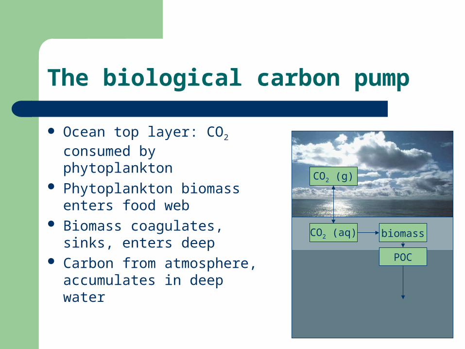
The biological carbon pump
Ocean top layer: CO2
consumed by phytoplankton Phytoplankton biomass
enters food web Biomass coagulates, sinks,
enters deep Carbon from atmosphere,
accumulates in deep water
CO2 (aq) biomass
POC
CO2 (g)
The project
Title– “Understanding the ‘organic carbon pump’ in meso-scale
ocean flows” 3 PhDs
– Physical oceanography, biology, numerical mathematics Aim:
– quantitative prediction of global organic carbon pump from 3D models
My role:– biota modeling, 1D water column
Biota modeling
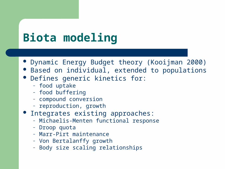
Dynamic Energy Budget theory (Kooijman 2000) Based on individual, extended to populations Defines generic kinetics for:
– food uptake– food buffering– compound conversion– reproduction, growth
Integrates existing approaches:– Michaelis-Menten functional response– Droop quota– Marr-Pirt maintenance– Von Bertalanffy growth– Body size scaling relationships
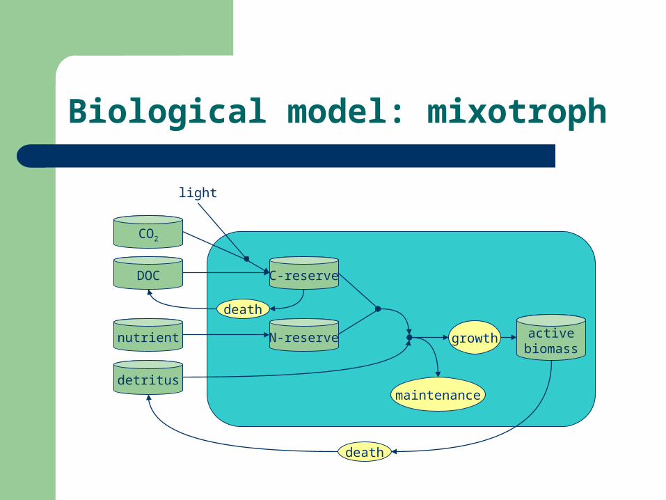
Biological model: mixotroph
maintenance
N-reserve
detritus
growth activebiomass
light
nutrient
CO2
DOC
death
C-reserve
death

Physics modeling
GOTM water column Open ocean test cases (less
influence of horizontal advection)
weather:• light• air temperature• air pressure• relative humidity• wind speed nutrient = 0
CO2
nutrient = constant
biotaturbulence
carbon transport
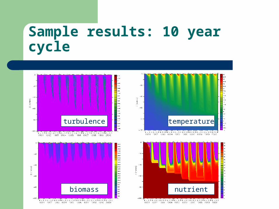
Sample results: 10 year cycle
biomass
turbulence
nutrient
temperature

Integration algorithms
(bio)chemical criteria:– Positive– Conservative– Order of accuracy
Even if model meets requirements, integration results may not

Mass and energy conservation
Model building block: transformation
Conservation– for any element, sums on left and right must be equal
Property of conservation– is independent of r– does depend on stoichiometric coefficients
Complete conservation requires preservation of stoichiometric ratios
2 2 2 6 12 6CO H O O6 6 6 1C H Or

Systems of transformations
Integration operates on (components of) ODEs Transformation fluxes distributed over multiple
ODEs:2
2
2
6 12 6
6
6
6
CO
H O
O
C H O
dcr
dtdc
rdtdc
rdt
dcr
dt
2 2 2 6 12 66 6 6CO H O O C H Or
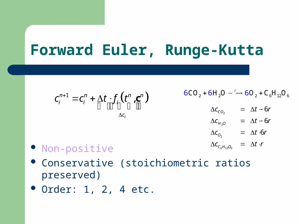
Forward Euler, Runge-Kutta
1 ,
i
n n n ni i i
c
c c t f t
c
Non-positive Conservative (stoichiometric ratios preserved) Order: 1, 2, 4 etc.
2
2
2
6 12 6
6
6
6
CO
H O
O
C H O
c t r
c t r
c t r
c t r
2 2 2 6 12 66 6 6CO H O O C H Or
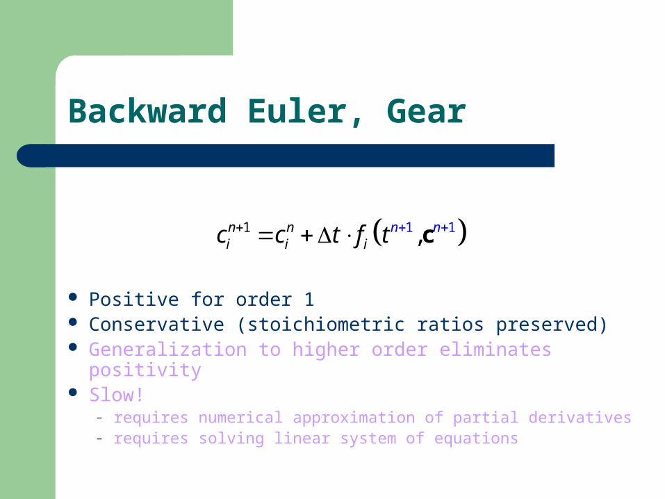
Backward Euler, Gear
1 11 ,n ni i i
n nc c t f t c
Positive for order 1 Conservative (stoichiometric ratios preserved) Generalization to higher order eliminates positivity Slow!
– requires numerical approximation of partial derivatives– requires solving linear system of equations
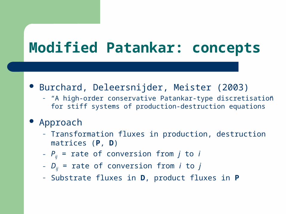
Modified Patankar: concepts
Burchard, Deleersnijder, Meister (2003)– “A high-order conservative Patankar-type discretisation for stiff
systems of production-destruction equations”
Approach– Transformation fluxes in production, destruction matrices (P, D)– Pij = rate of conversion from j to i
– Dij = rate of conversion from i to j
– Substrate fluxes in D, product fluxes in P
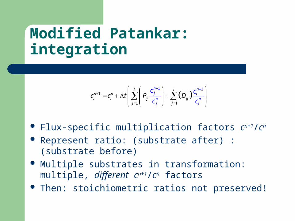
Modified Patankar: integration
1 1
1
1 1
I In ni
n n
i ij ijj j
j in nj i
c cc c t P D
c c
Flux-specific multiplication factors cn+1/cn
Represent ratio: (substrate after) : (substrate before) Multiple substrates in transformation: multiple,
different cn+1/cn factors Then: stoichiometric ratios not preserved!
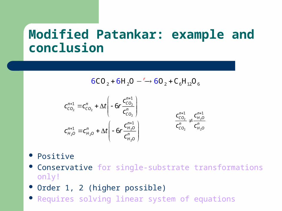
Modified Patankar: example and conclusion
2
2 2
2
2
2 2
2
11
11
6
6
nCOn n
CO CO nCO
nH On n
H O H O nH O
cc c t r
c
cc c t r
c
Positive Conservative for single-substrate transformations only! Order 1, 2 (higher possible) Requires solving linear system of equations
2 2
2 2
1 1n nCO H O
n nCO H O
c c
c c
2 2 2 6 12 66 6 6CO H O O C H Or
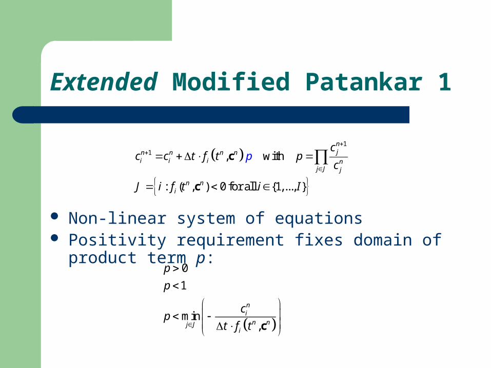
11 , with
: ( , ) 0 for all {1,..., }
njn n n n
i i i nj J j
n ni
cpc c t f t p
c
J i f t i I
c
c
Extended Modified Patankar 1
Non-linear system of equations Positivity requirement fixes domain of product term p:
0
1
min,
nin nj J
i
p
p
cp
t f t
c
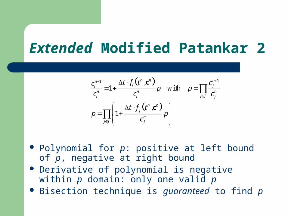
Extended Modified Patankar 2
11 ,1 with
,1
n n nni ji
n n nj Ji i j
n nj
nj J j
t f t ccp p
c c c
t f tp p
c
c
c
Polynomial for p: positive at left bound of p, negative at right bound
Derivative of polynomial is negative within p domain: only one valid p
Bisection technique is guaranteed to find p
Extended Modified Patankar 3
Positive Conservative (stoichiometric ratios preserved) Order 1, 2 (higher should be possible) ±20 bisection iterations (evaluations of polynomial)
– Always cheaper than Backward Euler, Modified Patankar
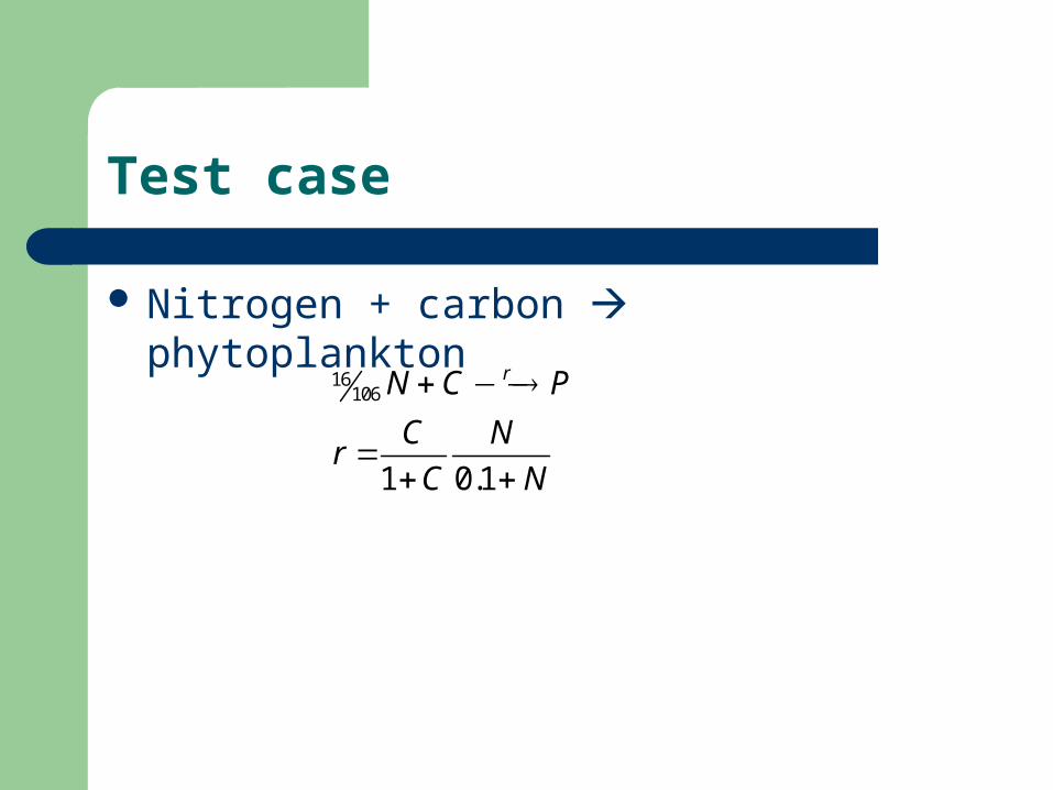
Test case
Nitrogen + carbon phytoplankton
16106
1 0.1
rN C P
C Nr
C N

Test case: Modified Patankar
Modified Patankar first order scheme
0
20
40
60
80
100
120
0,0 0,2 0,4 0,6 0,8 1,0 1,2 1,4 1,6 1,8 2,0
time (days)
con
cen
trat
ion
carbon MP1
carbon reference
nitrogen MP1
nitrogen reference
phytoplankton MP1
phytoplankton reference
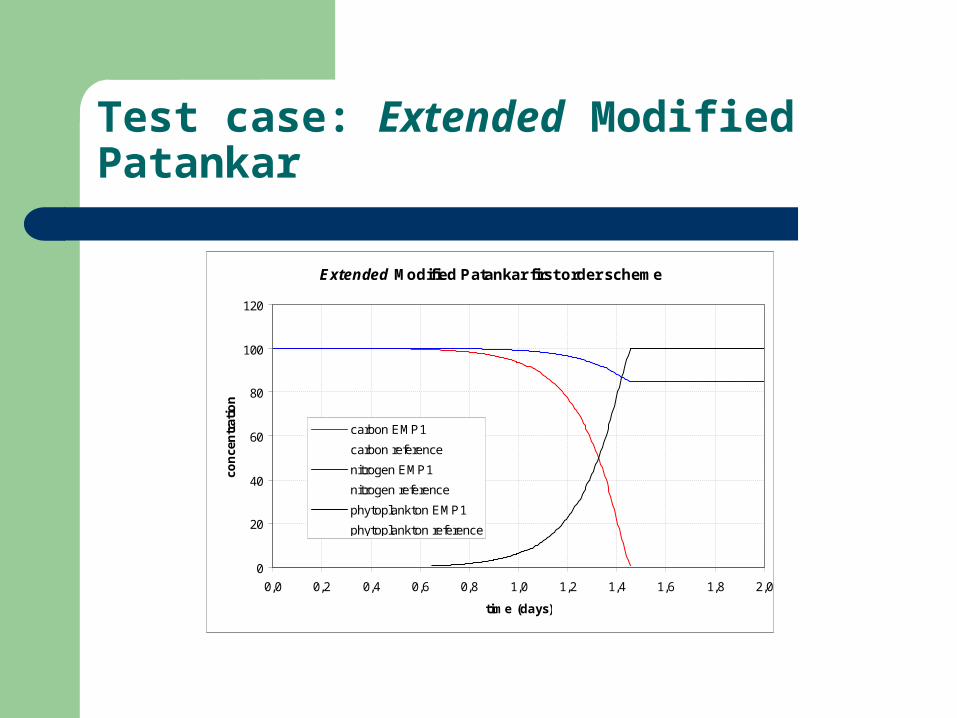
Test case: Extended Modified Patankar
Extended Modified Patankar first order scheme
0
20
40
60
80
100
120
0,0 0,2 0,4 0,6 0,8 1,0 1,2 1,4 1,6 1,8 2,0
time (days)
con
cen
trat
ion
carbon EMP1
carbon reference
nitrogen EMP1
nitrogen reference
phytoplankton EMP1
phytoplankton reference
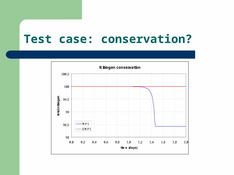
Test case: conservation?
Nitrogen conservation
98
98,5
99
99,5
100
100,5
0,0 0,2 0,4 0,6 0,8 1,0 1,2 1,4 1,6 1,8 2,0
time (days)
tota
l n
itro
gen
MP1
EMP1

Plans
Publish Extended Modified Patankar Short term
– Modeling ecosystems– Aggregation into functional groups– Modeling coagulation (marine snow)
Extension to complete ocean and world; longer timescales with surfacing of deep water
– GOTM in MOM/POM/…, GETM?– Integration with meso-scale eddy results