Quantifying the impacts of modeling uncertainties on the ...web.stanford.edu/~bakerjw/Publications/Gokkaya_et_al_(2016)_Design... · Quantifying the impacts of modeling uncertainties

EARTHQUAKE ENGINEERING & STRUCTURAL DYNAMICSEarthquake Engng Struct. Dyn. 2016; 45:1661–1683Published online 14 April 2016 in Wiley Online Library (wileyonlinelibrary.com). DOI: 10.1002/eqe.2740

Quantifying the impacts of modeling uncertainties on the seismicdrift demands and collapse risk of buildings with implications on

seismic design checks

Beliz U. Gokkaya�,�, Jack W. Baker and Greg G. Deierlein

Department of Civil & Environmental Engineering, John A. Blume Earthquake Engineering Center, StanfordUniversity, Stanford, CA 94305, USA

SUMMARY

Robust estimation of collapse risk should consider the uncertainty in modeling of structures aswell as variability in earthquake ground motions. In this paper, we illustrate incorporation of theuncertainty in structural model parameters in nonlinear dynamic analyses to probabilistically assessstory drifts and collapse risk of buildings. Monte Carlo simulations with Latin hypercube sampling areperformed on ductile and non-ductile reinforced concrete building archetypes to quantify theinfluence of modeling uncertainties and how it is affected by the ductility and collapse modes of thestructures. Inclusion of modeling uncertainty is shown to increase the mean annual frequency ofcollapse by approximately 1.8 times, as compared with analyses neglecting modeling uncertainty,for a high-seismic site. Modeling uncertainty has a smaller effect on drift demands at levels usuallyconsidered in building codes; for the same buildings, modeling uncertainty increases themean annual frequency of exceeding story drift ratios of 0.03 by 1.2 times. A novel method is intro-duced to relate drift demands at maximum considered earthquake intensities to collapse safety througha joint distribution of deformation demand and capacity. This framework enables linking seismicperformance goals specified in building codes to drift limits and other acceptance criteria. The distributionsof drift demand at maximum considered earthquake and capacity of selected archetype structures enablecomparisons with the proposed seismic criteria for the next edition (2016) of ASCE 7. Subject to the scopeof our study, the proposed drift limits are found to be unconservative, relative to the target collapse safetyin ASCE 7. Copyright © 2016 John Wiley & Sons, Ltd.

Received 18 August 2015; Revised 13 December 2015; Accepted 15 March 2016

KEY WORDS: modeling uncertainty; acceptance criteria; collapse; drift demands; demand-capacitydistributions

1. INTRODUCTION

Owing to the variability in earthquake ground motions and the uncertainty in structural model ide-alizations, any efforts to rigorously assess collapse safety should consider these effects. For collapseassessment by nonlinear dynamic analysis, this includes reliable characterization and propagation ofthe aforementioned sources of uncertainty through the analysis. Ground motion variability and itsimpacts on seismic response assessment has been studied by many researchers who have proposedground motion selection and analysis strategies for taking into account record-to-record variability[e.g., 1, 2, and others]. Another important contributor to the robustness of seismic response predic-tions is modeling uncertainty [3]. A blind prediction contest to analyze the response of a single bridge

�Correspondence to: Beliz U. Gokkaya, Department of Civil & Environmental Engineering, John A. Blume EarthquakeEngineering Center, Stanford University, Stanford, CA 94305.�E-mail: [email protected]

Copyright © 2016 John Wiley & Sons, Ltd.

1662 B. U. GOKKAYA, J. W. BAKER AND G. G. DEIERLEIN

column [4] highlighted the significance of modeling uncertainty in structural seismic response pre-dictions. The variability in the engineering parameters submitted by the contestants were remarkablefor this highly constrained experiment. Maximum displacements were predicted under different earth-quake ground motions with an average coefficient of variation of 0.4 and the median bias of thepredictions corresponding to different ground motions ranged from 5% to 35%.

Probabilistic approaches has been proposed for uncertainty analysis in seismic design and assess-ment of structures [e.g., 5, 6, and others] . Seismic fragility curves [7, 8] are commonly used forassessment of performance goals in structures. One of the major challenges in incorporating model-ing uncertainty into seismic response assessment is balancing computational demand and accuracy.Sensitivity analysis provides insight regarding relative importance of modeling parameters [9–11], andfirst-order second-moment is often used to propagate modeling uncertainty in seismic performanceassessment [e.g., 12,13] However, first-order second-moment can loose accuracy when the relationshipbetween input and response variables is nonlinear, which is a concern when modeling collapse. Meth-ods such as nonlinear response surface [14] and artificial neural network methods have been used toincorporate nonlinearities, although most of these methods do not scale efficiently or accurately whenthe number of random variables increase. Among the available methods, Monte-Carlo based methodsremain as the most flexible and scalable methods to account for modeling uncertainty, albeit sometimesat large computational expense [e.g., [15–17]].

In this paper, Monte-Carlo based simulations are used to incorporate the variability of structuralmodel parameters in nonlinear dynamic analyses for assessing deformations and collapse risk of build-ings under earthquake ground motions. A set of archetype buildings are analyzed to quantify thesignificance of modeling uncertainty and to examine its implication on design approaches that uti-lize nonlinear dynamic analysis. The effects of modeling uncertainty are evaluated for both ductileand non-ductile reinforced concrete structures to investigate whether the extent to which ductility andstrength irregularities influence the significance of modeling uncertainties. The procedures illustrateand contrast so-called multiple stripe analyses (MSA) versus incremental dynamic analyses (IDA) forground motion selection and scaling, each of which has its advantages and limitations. MSA conductedwith hazard consistent ground motions are used to directly evaluate collapse resistance in terms ofspectral ground motion intensity, whereas IDA are used to establish drift capacities of the buildings,which can then be used together with drift demands to assess collapse safety. In addition to outlin-ing consistent procedures for evaluating modeling uncertainties for collapse risk, results of the studyprovide benchmark data to help establish guidelines to account for modeling uncertainties in designand assessment.

The approach to evaluating collapse risk through drift demands is motivated in part by emergingmethods to validate building designs using nonlinear dynamic analysis. For example, guidelines forthe seismic design of tall buildings [18, 19] and a recently proposed update for the next edition ofASCE 7 [20] rely heavily on story drift limits, determined from nonlinear dynamic analyses, to helpensure that buildings meet minimum collapse safety targets. To investigate collapse drift capacities andtheir relationship to calculated drift demands, a probabilistic framework is proposed to jointly quan-tify joint drift demands and capacities, including uncertainties associated with both ground motionsand structural modeling parameters. This framework is employed in nonlinear analyses to charac-terize the joint distribution of peak drift at maximum considered earthquake level and capacity forselected archetype structures. The resulting distributions are used to assess the proposed acceptancecriteria for new provisions in ASCE 7 [20] and provide a strategy for improved calibration of suchacceptance criteria.

2. SEISMIC PERFORMANCE ASSESSMENT

A risk-based seismic assessment strategy is adopted for using nonlinear dynamic analyses to assessthe impacts of both ground motion and modeling uncertainty on drift demands and collapse. Illustratedin Figure 1 are key aspects of the assessment procedure. Referring to Figure 1(a), a so-called MSAapproach is used, wherein nonlinear dynamic analyses are conducted using suites of ground motionsthat are selected and scaled to match the unique seismic hazard at a building site. MSA involvesconducting nonlinear time history analyses at multiple levels of ground motion intensity, where at each

Copyright © 2016 John Wiley & Sons, Ltd. Earthquake Engng Struct. Dyn. 2016; 45:1661–1683DOI: 10.1002/eqe

QUANTIFYING THE IMPACTS OF MODELING UNCERTAINTIES 1663

Figure 1. Illustration of seismic performance assessment (a) Multiple stripes analyses at different groundmotion intensity levels (b) Collapse and drift-exceedance fragility functions (c) Seismic hazard curve (d)

Collapse risk deaggregation curves. SDR, story drift ratio.

intensity, the distribution of peak story drift ratio (SDR) and other engineering demand parametersof interest are recorded. In this study, the ground motions are selected and scaled using a conditionalspectra approach, where the ground motion intensity is defined based on the spectral acceleration at thefundamental period of structure, Sa.T1/, and the conditional spectra characterizes the target responsespectra, including mean and variability, that are derived from probabilistic seismic hazard analysis[21]. Hazard consistent ground motions are selected at different intensity levels, ideally from the onsetof significant inelasticity up to about the intensity where about half of the ground motions cause col-lapse. For the code-conforming buildings considered in this study, the ground motions are evaluated atfive intensities with frequencies of exceedance ranging from 5% in 50 years to 1% in 200 years.

In Figure 1(a), the points at each intensity stripe provide data to characterize the maximum storydrift demands and the frequency of collapse. Because the exact onset of collapse is not detected in thetypical MSA procedure, a SDR in excess of 10% is used as indicator of structural collapse becauseat this level most engineering structures are identified to have no or insufficient stiffness [22]. Thus,the incidences of collapse at each intensity can be used to compile vertical statistics to fit a lognormaldistribution of collapse probability, in terms of Sa.T1/. This distribution is illustrated by the collapseprobability density function (PDF) in Figure 1(a) and the corresponding collapse cumulative distribu-tion function (CDF) in Figure 1(b). Data at each ground motion intensity stripe are used to determinehorizontal statistics of drift exceedance probability distributions, shown by the drift PDF in Figure 1(a).Integrating regions of the drift PDF at each intensity level, such as the P.SDR > sdr/ shown inFigure 1(a), can then be used to develop drift exceedence CDF’s. As described later in Sections 5 and6, horizontal statistics of the drift data become relevant when evaluating drift demands at specifiedground motion intensities. Also discussed in Section 5 are the impacts of modeling uncertainty on driftexceedence CDF’s, which defines P.SDR > sdr/, for alternating values of sdr .

Collapse fragility curves obtained using MSA data are shown by the blue lines in Figure 1(b), wheretwo estimates of collapse fragility curves are provided. One estimate, shown by the dashed line, isobtained by analyses using median model parameters. As such, this estimate incorporates only record-to-record variability (RTR) in the ground motions and, hence, carries the subscript RTR. The second



estimate, shown in the solid line, is from analyses that incorporate both record-to-record variabilityas well as modeling uncertainty and carries the subscript T , indicating it includes a total estimate ofuncertainty. Collapse limit state is indicated with subscript c.

The collapse fragility curves in Figure 1(b) are represented by lognormal distributions, which aredescribed by a logarithmic mean (ln.�/ where � is the median) and logarithmic standard deviation(also known as dispersion, ˇ). All parameters of interest are used with appropriate subscripts, whereverapplicable, corresponding to their limit states and the type of uncertainty they include, that is, �c;Tversus �c;RTR.

Risk-based assessment of structural response provides the mean annual frequency of exceedance(�) of certain limit performance states (collapse or drift exceedence) given the seismic hazard at thedesign site of the structure. Figure 1(c) illustrates a seismic hazard curve. The � for each limit statecan be obtained by integrating the corresponding fragility curve with the seismic hazard curve. The �cdefining the mean annual frequency of collapse is obtained as follows:

�c D

Z 10

P.C jIM D im/

ˇˇd�IM .im/d.im/

ˇˇ d.im/ (1)

where P.C jIM D im/ defines the probability of collapse given the ground motion intensity IM D

im, andˇd�IM .im/d.im/

ˇdefines the absolute value of the slope of the hazard curve at im.

Deaggregation of �c helps identify the ground motion intensities that contribute most in estimating�c [23]. These curves plot the integrand of Equation (1) with respect to IM . Deaggregation curvesof �c with and without modeling uncertainty are provided in Figure 1(d), where the areas under thesecurves yield �c .

We see from Figure 1(b) that, in the presence of modeling uncertainty, the collapse fragility curvehas smaller median collapse capacity and higher dispersion. This results in ground motions havingsmaller intensities and higher rates of occurrence contributing more to �c as shown in Figure 1(d).

In the following sections, we use the aforementioned seismic performance assessment strategyalong with the presented performance metrics to quantify the impacts of modeling uncertainty for anextensive set of archetype structures.

3. CASE STUDY SEISMIC RESPONSE ANALYSIS WITH MODELING UNCERTAINTY

3.1. Structural models

Thirty ductile reinforced concrete frame buildings were designed by [13] using modern building codestandards [24, 25] for a high-seismicity site at Los Angeles (LA), California. These buildings rangein height from 1 to 20 stories, including a few designs that have varying amounts of strength irregu-larity up the building height. The structural systems are analyzed using Open System for EarthquakeEngineering Simulation Platform [26] using concentrated plasticity models. An illustrative structuralidealization is provided in Figure 2(a) and the detail of the beam-column connections is provided corre-sponding to ductile frames. Frame elements are modeled as elastic members having rotational springsat the ends, whose hysteretic behavior is governed by a trilinear backbone curve (Figure 2(b)) andcyclic and in-cycle degradation rules [27]. The parameters defining the M-� hinge model are deter-mined using empirical equations that are calibrated using a dataset consisting of experimental testresults of over two hundred reinforced concrete columns [28].

Three non-ductile reinforced concrete frame buildings of 2, 4, and 8 stories in height were designedby [29] according to the 1967 Uniform Building Code [30] for a high-seismicity site at Los Angeles,CA, USA. Similar to the ductile frames, the flexural response of beams and columns are modeled usingthe concentrated plasticity model as in Figure 2(b), but with less ductile properties. In addition, thecolumn models include zero-length shear and axial springs (Figure 2(c)) to idealize shear and axialfailure, respectively. Axial springs have limit surfaces defined by the force-displacement relationshipgiven by [31]. Shear springs have limit strengths defined by [32] in the small displacement range, whichis triggered in the case of a brittle shear failure, and they have a deformation limits defined by [31]



(a)

(b) (c)

Figure 2. (a) Illustrative structural idealization of the models used in this study. Details of beam-columnconnections for ductile and non-ductile frames are provided. (b) Backbone curve for concentrated plasticity

model (c) Illustration of the shear and axial failure models.

to characterize the behavior in the large displacement range. Detailed information about the design ofbuildings can be found in [29]. For both the ductile and non-ductile frames, Rayleigh damping is usedwith 3% equivalent critical damping in the first and third modes of the structure, and P-� effects aremodeled using a leaning-column. The analysis models used in this study are created in two-dimensionsfor typical three-bay frames. By using only one frame for analysis, it is implicitly assumed that theframes in a given direction are fully correlated. This is a source of modeling uncertainty which is notaddressed in this paper.

3.2. Seismic hazard analysis and ground motion selection

Each of the archetype structures are analyzed based on the seismic hazard at their correspondingdesign sites in Los Angeles, CA (ductile structures at 33:996ıN, 118:162ıW; non-ductile structuresat 34:05ıN, 118:25ıW), where both sites have National Earthquake Hazards Reduction Program SiteClass D soil. The hazard curves and deaggregation information at all sites are obtained from theUnited States Geological Survey (USGS) hazard curve application [33] and the 2008 USGS interac-tive deaggregations web tool [34], respectively. Ground motions at the five intensities, correspondingto exceedance probabilities of 5% in 50, 2% in 50, 1% in 50, 1% in 100, and 1% in 200 years, areselected using an algorithm by [2]. Suites of 200 ground motions are selected at each intensity levelto provide a different motion for each structural realization that will be considered in the modelinguncertainty analyses.

3.3. Modeling uncertainty

3.3.1. Characterization of modeling uncertainty. The six parameters that define the M-� hysteretichinge model are treated as random variables, including the five parameters that define the backbonecurve in Figure 2(b) and a sixth parameter that defines the cyclic energy dissipation capacity. Following[27], these parameters are the flexural strength (My), ratio of maximum moment and yield moment



capacity (Mc=My), effective initial stiffness which is defined by the secant stiffness to 40% of yieldforce (EIstf;40=EIg ), plastic rotation capacity (�cap;pl ), post-capping rotation capacity (�pc), andenergy dissipation capacity for cyclic stiffness and strength deterioration (� ).

For non-ductile frames, the uncertainty in the shear and axial parameters, Vn, ıs=L, ıa=L(Figure 2(c)) are likewise treated as random variables. These parameters were empirically calibratedand summary statistics of the predictive capacity models are reported in each respective studies [31,32].In addition to reporting the variability in the parameters, these studies also report small biases in themodel parameters (measured to calculated values of 1.05 for Vn and 0.97 for ıs=L, ıa=L) that areincorporated in the uncertainty analyses.

In addition to the parameters defining the beam and column component models, equivalent viscousdamping ratio (�), column footing rotational stiffness (Kf ), and joint shear strength (Vj ) are alsotreated as random. The modeling parameters are assumed to have lognormal distributions, and thevariability in these parameters are represented using logarithmic standard deviations given in Table I.

In addition to variability of the modeling parameters themselves, previous studies have shown thatthe assumed correlation between parameters can significantly affect the calculated collapse behavior[35]. In a previous study, we use random effects regression models on a database of reinforced concretecolumn tests [28] to quantify the correlations of random model parameters within and between thestructural components [36]. As described by [36], correlation of parameters within components (e.g.,the relationship of strength to ductility, My to �cap;pl , within a member) were determined using eachof the over two hundred column tests, and the correlation of parameters between components (e.g., therelationship of parameters for beams versus columns within a building) were determined by comparingresults of specimens that were constructed and tested at different labs. For the uncertainty analyses inthis study, we assumed parameters between beams within a building (beam-to-beam) and parametersbetween columns within a building (column-to-column) to be fully correlated, the reasoning beingthat they have the same details and are built by the same contractor. On the other hand, parametersbetween beams and columns within a building (beam-to-column) and within each component modelare assumed to be partially correlated. The correlation coefficients are shown in Table II, following[36], where the coefficients in the left matrix are for parameters within components (component i to i)and the right matrix is for parameters between components (component i to j). These coefficients definethe correlations using logarithms of the parameters, so that the natural logarithms of the parametersfollow a multivariate normal distribution. Other than the parameters for the beam and column hinges,all other parameters are assumed to be uncorrelated.

Table I. Logarithmic standard deviations of random variables.

Random variables & dispersion values

�cap;pl 0.59 EIstfEIg

0.27 My 0.31 Mc

My0.10 �pc 0.73 � 0.50

� 0.60 Kf 0.30 Vj 0.10 Vn 0.15 ıs=L 0.34 ıa=L 0.26

Table II. Correlation of random variables defining backbone curve and hysteretic behavior of a concentratedplasticity model.

Component i Component j

Component i �cap;pliEIstfEIg i

MyiMc

My i�pci �i �cap;plj

EIstfEIg j

MyjMc

My j�pcj �j

�cap;pli 1.0 0.0 0.1 0.3 0.2 0.0 0.7 0.0 0.0 0.1 0.1 0.0EIstfEIg i

1.0 0.1 �0.1 0.0 0.1 0.7 0.1 �0.1 0.0 0.0

Myi 1.0 0.3 0.1 0.1 0.9 0.2 0.1 0.1Mc

My i1.0 0.0 0.2 0.7 0.0 0.0

�pci (sym.) 1.0 0.2 (sym.) 0.3 0.0

�i 1.0 0.4



3.3.2. Propagation of modeling uncertainty. Monte-Carlo simulation-based uncertainty propagationmethods are intuitive and straightforward to implement, and aside from the computational expenseare fairly scalable to problems with many random variables. These methods involve drawing ran-dom realizations of the variables from the joint probability distributions and conducting analyses withthese realizations. Latin hypercube sampling is shown to be an effective sampling method for seis-mic response assessment [15, 16, 36]. The effectiveness of the method results from the stratificationof the probability distribution. It operates by drawing random realizations of model parameters fromequal probability disjoint intervals of the range of these parameters [37]. Considering the trade offof accuracy versus computational time, we ran 200 realizations of the model parameters using Latinhypercube sampling at each ground motion intensity. Stochastic optimization using simulated anneal-ing is applied to preserve the correlation structure among the random variables, which are obtainedusing Latin hypercube sampling [15]. The sampled model realizations are each matched randomlywith one of the 200 ground motions at each IM level. In addition, to distinguish the influence of mod-eling uncertainty from record-to-record variability, we re-analyze the structures using median modelparameters with the same ground motions.

4. IMPACTS OF MODELING UNCERTAINTY ON COLLAPSE RESPONSE

4.1. Effect of modeling uncertainty on collapse fragility parameters

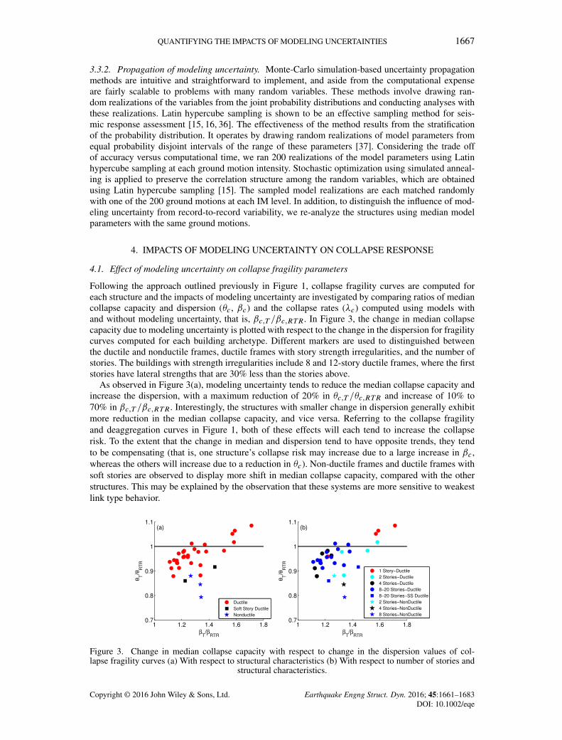
Following the approach outlined previously in Figure 1, collapse fragility curves are computed foreach structure and the impacts of modeling uncertainty are investigated by comparing ratios of mediancollapse capacity and dispersion (�c , ˇc) and the collapse rates (�c) computed using models withand without modeling uncertainty, that is, ˇc;T =ˇc;RTR. In Figure 3, the change in median collapsecapacity due to modeling uncertainty is plotted with respect to the change in the dispersion for fragilitycurves computed for each building archetype. Different markers are used to distinguished betweenthe ductile and nonductile frames, ductile frames with story strength irregularities, and the number ofstories. The buildings with strength irregularities include 8 and 12-story ductile frames, where the firststories have lateral strengths that are 30% less than the stories above.

As observed in Figure 3(a), modeling uncertainty tends to reduce the median collapse capacity andincrease the dispersion, with a maximum reduction of 20% in �c;T =�c;RTR and increase of 10% to70% in ˇc;T =ˇc;RTR. Interestingly, the structures with smaller change in dispersion generally exhibitmore reduction in the median collapse capacity, and vice versa. Referring to the collapse fragilityand deaggregation curves in Figure 1, both of these effects will each tend to increase the collapserisk. To the extent that the change in median and dispersion tend to have opposite trends, they tendto be compensating (that is, one structure’s collapse risk may increase due to a large increase in ˇc ,whereas the others will increase due to a reduction in �c). Non-ductile frames and ductile frames withsoft stories are observed to display more shift in median collapse capacity, compared with the otherstructures. This may be explained by the observation that these systems are more sensitive to weakestlink type behavior.

Figure 3. Change in median collapse capacity with respect to change in the dispersion values of col-lapse fragility curves (a) With respect to structural characteristics (b) With respect to number of stories and

structural characteristics.



In Figure 3(b), the same data are grouped with respect to the number of stories and structural charac-teristics. Here, it is interesting to observe that the single-story buildings and a couple of the two-storybuildings are the only ones to experience a large increase in dispersion, ˇc;T =ˇc;RTR, with little changein median �c;T =�c;RTR. The slight increase in median to �c;T =�c;RTR values above 1 seems to be anartifact of the large change in dispersion that flattens out the fragility curve. These buildings tend tohave only one collapse mode, such that the variability in model parameters is more directly linked tothe variability in response. This is in contrast to the other buildings that generally display multiple fail-ure modes, where the collapse mechanism can be idealized as a series of collapse mechanisms, wherethe weakest will generally govern. In these cases, while a particular perturbation of model parametersresult in the increase of the capacity of some mechanisms, the capacity in another mechanism mightdecrease and can govern the response. Therefore, in general, there is a decrease in median collapsecapacities for structures having more than one collapse mechanism.

4.2. Net effect of modeling uncertainty on collapse rates

The net effect of the change in median and dispersion due to modeling uncertainty can be quantifiedby integrating the resulting fragility curves with a seismic hazard curve to determine the change inmean annual frequency of collapse, �c . Using the hazard curves for the building sites in Los Angeles,we calculated the ratios of �c;T =�c;RTR for the 33 building archetypes. The average collapse rateratio is calculated to be about 1.8 with a coefficient of variation of 0.2, indicating that the modelinguncertainty increases the collapse risk by about 80%, relative to the risk for the median model. Tofurther investigate how sensitive this change is to the ground motion hazard curve, we integrated thecollapse fragilities with idealized hazard curves that are modeled with a power-law hazard curve ofthe form � D k0IM

�k , where the hazard curve slope k is varied and k0 is fit over the range betweenSa.T1/ values corresponding to 10% to 2% in 50-year exceedance probabilities (Figure 1(c)). Theresults of these analyses are shown in Figure 4, where each of the boxplots corresponds to the change in�c values for the set of archetype buildings for sites with varying hazard curve slopes. For comparison,the red boxplots (close to k equal to 3) are data from the collapse rates determined by the USGShazard curves for the Los Angeles building sites. Lower values of k are more representative of sites inthe central and eastern United States, where there are larger differences in the spectral intensities (Sa)between the 10% to 2% in 50-year exceedance probabilities.

As indicated in Figure 4, for hazard curves with smaller slopes, the modeling uncertainties tend tohave a smaller effect on collapse risk, as compared with the Los Angeles site with k � 3. Referringback to Figure 1, the reason for this relates to the relationship of the slope of the hazard curve relativeto the lower tail of the collapse fragility curve. Deaggregation of �c helps identify the ground motionintensities that contribute most to �c estimates. In the presence of modeling uncertainty, the dominant

Figure 4. Change in �c due to modeling uncertainty.



ground motion contributors in computing �c is shifted toward smaller intensities (Figure 1(d)). Themagnitude of the shift in dominant ground motion intensities depends on the change in fragility curvecharacteristics as well as the change in the instantaneous slope of the true (nonlinearized) hazard curve.The impacts of modeling uncertainty on �c would become more pronounced when the collapse fragilitycurve is pushed toward the regions of hazard curves having higher instantaneous slopes and this mightresult in different impacts on �c at different sites.

The collapse rate ratios calculated for the archetype models can be described by a closed-formexpression, shown by the green curve in Figure 4. The expression for this curve is derived using aclosed form expression for collapse rate �c by [38] as a function of median and dispersion of collapsefragility and the slope of the idealized hazard curve. Taking ratios of the rates, the change in collapserate due to modeling uncertainty in �c is obtained as follows:

�c;T

�c;RTRD

��c;T

�c;RTR

��ke12k2ˇ2c;M (2)

where ˇc;M represents the additional dispersion due to modeling uncertainty and the other terms areas defined previously. Assuming that the modeling and record-to-record effects are statistically inde-pendent, the modeling dispersion ˇc;M can be estimated using a square root of sum of squares (SRSS)approach through the equation given thereafter:

ˇc;T Dqˇ2c;RTR C ˇ

2c;M (3)

As shown in Figure 4, the predictions by Equation (2) give good agreement using the average valuesfrom the building archetype studies, where the average median shift is 0.95 (with a coefficient ofvariation of 0.12) and the average ˇc;M is 0.33 (with a coefficient of variation of 0.18).

4.3. Equivalent value of modeling uncertainty

To the extent that the results from the archetype studies are representative to other framed buildings, itis useful to examine how the effects of modeling uncertainties can be generalized. This would inform,for example recent performance-based guidelines [39, 40] that incorporate judgment-based modelinguncertainty factors that are combined, using an SRSS rule, with other sources of variability. Figure 5(a)provides an illustration of how modeling uncertainty parameters can be used to approximate the cal-culated collapse fragility for the 12-story building archetype (ID 2067). Shown in Figure 5(a) arethe collapse fragilities obtained from simulations for the median model (Pc;RTR) and for the modelsthat include modeling uncertainty (Pc;T ). In between are two approximate fragility curves, one thathas an adjustment to the median and dispersion and the second that has only a change to the disper-sion. The curve with the median shift and added dispersion is based on the average values from thearchetype study (average median shift of 0.95 and average modeling uncertainty of 0.33). The othercurve includes an equivalent value of modeling uncertainty of ˇ�c;M equal to 0.4, which is calibratedso as to match, on average, the collapse rates that are determined using the simulated collapse fragilitycurves (Pc;T ) and the hazard curves for the archetype building studies.

The approach to calibrate the equivalent modeling uncertainty ˇ�c;M is as follows: (i) determinethe �c;T for each archetype collapse study; (ii) develop fragility functions for each archetype thatare obtained using median model parameters for that archetype, i.e �c;RTR and ˇc;RTR, along withan estimate of ˇ�c;M that is combined with ˇc;RTR for each archetype using the SRSS approach;(iii) integrate the estimated collapse fragility curve with the hazard curve to find an estimate of �c;Tfor each archetype; and (iv) repeat steps 2 and 3, selecting updated estimates of ˇ�c;M to minimizethe error between the correct and estimated values of �c;T , until the desired accuracy is achieved.When run for the archetype buildings reported earlier, the resulting mean value of ˇ�c;M is 0.4. The



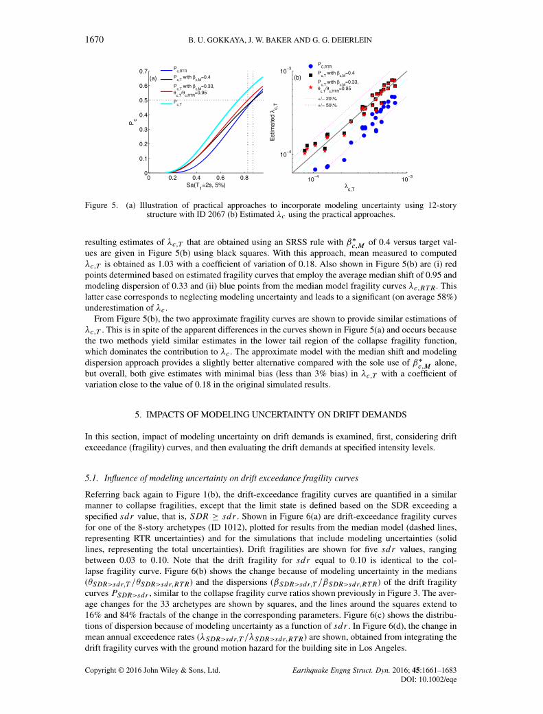
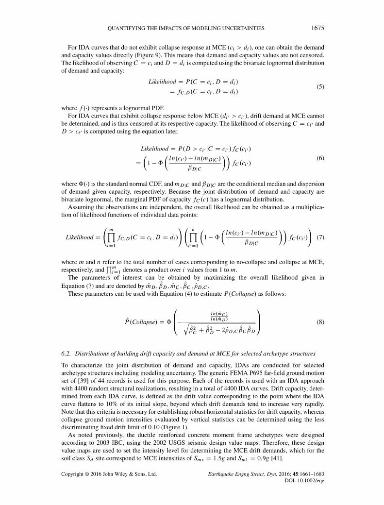
Figure 5. (a) Illustration of practical approaches to incorporate modeling uncertainty using 12-storystructure with ID 2067 (b) Estimated �c using the practical approaches.

resulting estimates of �c;T that are obtained using an SRSS rule with ˇ�c;M of 0.4 versus target val-ues are given in Figure 5(b) using black squares. With this approach, mean measured to computed�c;T is obtained as 1.03 with a coefficient of variation of 0.18. Also shown in Figure 5(b) are (i) redpoints determined based on estimated fragility curves that employ the average median shift of 0.95 andmodeling dispersion of 0.33 and (ii) blue points from the median model fragility curves �c;RTR. Thislatter case corresponds to neglecting modeling uncertainty and leads to a significant (on average 58%)underestimation of �c .

From Figure 5(b), the two approximate fragility curves are shown to provide similar estimations of�c;T . This is in spite of the apparent differences in the curves shown in Figure 5(a) and occurs becausethe two methods yield similar estimates in the lower tail region of the collapse fragility function,which dominates the contribution to �c . The approximate model with the median shift and modelingdispersion approach provides a slightly better alternative compared with the sole use of ˇ�c;M alone,but overall, both give estimates with minimal bias (less than 3% bias) in �c;T with a coefficient ofvariation close to the value of 0.18 in the original simulated results.

5. IMPACTS OF MODELING UNCERTAINTY ON DRIFT DEMANDS

In this section, impact of modeling uncertainty on drift demands is examined, first, considering driftexceedance (fragility) curves, and then evaluating the drift demands at specified intensity levels.

5.1. Influence of modeling uncertainty on drift exceedance fragility curves

Referring back again to Figure 1(b), the drift-exceedance fragility curves are quantified in a similarmanner to collapse fragilities, except that the limit state is defined based on the SDR exceeding aspecified sdr value, that is, SDR � sdr . Shown in Figure 6(a) are drift-exceedance fragility curvesfor one of the 8-story archetypes (ID 1012), plotted for results from the median model (dashed lines,representing RTR uncertainties) and for the simulations that include modeling uncertainties (solidlines, representing the total uncertainties). Drift fragilities are shown for five sdr values, rangingbetween 0.03 to 0.10. Note that the drift fragility for sdr equal to 0.10 is identical to the col-lapse fragility curve. Figure 6(b) shows the change because of modeling uncertainty in the medians(�SDR>sdr;T =�SDR>sdr;RTR) and the dispersions (ˇSDR>sdr;T =ˇSDR>sdr;RTR) of the drift fragilitycurves PSDR>sdr , similar to the collapse fragility curve ratios shown previously in Figure 3. The aver-age changes for the 33 archetypes are shown by squares, and the lines around the squares extend to16% and 84% fractals of the change in the corresponding parameters. Figure 6(c) shows the distribu-tions of dispersion because of modeling uncertainty as a function of sdr . In Figure 6(d), the change inmean annual exceedence rates (�SDR>sdr;T =�SDR>sdr;RTR) are shown, obtained from integrating thedrift fragility curves with the ground motion hazard for the building site in Los Angeles.



Figure 6. (a) Example drift-exceedance fragility curves for an 8-story structure with ID 1012 (b) Change inmedian collapse capacity with respect to change in the dispersion values of fragility curves defining drift-exceedance limit states (c) Dispersion due to modeling uncertainty as a function of story drift ratio (SDR)

(d) Boxplots showing the change in �SDR>sdr as a function of SDR.

Based on the results shown in Figure 6, for story drift ratios below 0.03, modeling uncertainties havea relatively small but measurable impact on the results. For example, at the 0.03 drift limit, modelinguncertainties increase the mean annual frequency of exceedence about on average by 20%. Comparedwith the reliability of nonlinear analyses, which are usually run with 10 or fewer ground motions, theinfluence of uncertainties would be difficult to assess. However, as there is a measurable increase inthe median drift, dispersion and annual frequency, one could envision applying a reliability factor toaccount for the modeling uncertainties, even at these comparatively low drift levels. At peak story driftsof 0.04 and beyond the modeling uncertainties have a greater effect and may be significant. In the limitof sdr about 0.07 to 0.10, the modeling uncertainty is on roughly the same order as the uncertaintiesin the collapse fragility, where the dispersion ratio (ˇSDR>sdr;T =ˇSDR>sdr;RTR) increase to about 1.3and the exceedance rate (�SDR>sdr;T =�SDR>sdr;RTR) increases by a factor of about 1.8. Also notethat the fragility functions for sdr equal to 0.08 coincide with the fragility functions for sdr equal to0.1 (These curves are indicated with cyan and magenta, respectively). As described previously for thecollapse fragility, at large drifts in excess of sdr of 0.07, the equivalent ˇc;M is about 0.33.

5.2. Influence of modeling uncertainty on drift demands

We next investigate the impacts of modeling uncertainty on story drift demands at different groundmotion intensity levels. This evaluation of drift demands at a specified intensity is particularly relevantto the manner in which drifts are assessed in design practice. As with the collapse fragilities, groundmotion intensities evaluated in this study correspond to exceedance probabilities of 5%, 2%, and 1%in 50 years, 1% in 100 years, and 1% in 200 years. The values of SDR observed at each IM arerecorded for each structure, and empirical CDFs corresponding to PSDR�sdr are obtained. Figure 7(a)compares the ECDFs of drift demands obtained using a median model (dashed lines, corresponding toRTR uncertainties) and models incorporating modeling uncertainty (solid lines, corresponding to totaluncertainties) for the 8-story building archetype (ID 1012).

It is observed from Figure 7(a) that the difference in deformation demands between the medianmodel and the model incorporating modeling uncertainty is negligible for drift ratios smaller thanabout 0.025. At the ground motion intensity of 2% probability of exceedance in 50 years (2/50 year),



Figure 7. (a) ECDF of drift demands using median model and with modeling uncertainty for the 8-storystructure with ID 1012 (b) Change in counted median of drift demand distributions w.r.t. drifts for differentstructures (c) Change in dispersion of the fitted lognormal distributions to sdr values of no-collapses (d)

Change in dispersion of the fitted lognormal distributions to sdr values up to median.

the probability that SDR will be smaller than 0.03 is 47% using a median model, increasing to 53% inthe presence of modeling uncertainty. On average for all of the building archetypes, at the 2/50 yearground motion, the probability that SDR will be smaller than 0.03 is about 4% larger in the presence ofmodeling uncertainty. This increases to 8% at SDR of 0.06, following the trend discussed previouslyof increasing impacts of modeling uncertainty with increasing drifts.

Figure 7(b) shows the change in counted medians in the presence of modeling uncertainty as afunction of ground motion intensities that are normalized with respect to Sa2=50 year. Counted medianscorrespond to SDR values at the 50% probability level of Figure 7(a). For each IM level, SDR valuesof the solid lines divided by that of dashed lines quantify the change in counted medians of drifts.At the 5/50 year ground motion, there is no change in median drifts, but at larger intensities the ratioincreases linearly, with a ratio of 1.05 at the 2/50 year intensity and up to about 1.2 at the 1/200 yearintensity. For some of the building archetypes and ground motion intensity levels, more than half of theanalyses results in collapse response (i.e., Figure 7(a), 1/200 year). While these collapse data points arenot shown in Figure 7(b), they are incorporated in the computation of the fitted line using a maximumlikelihood approach with a normal distribution by right-censoring these values at 1.

Figures 7(c) and (d) show the change because of modeling uncertainty in dispersion values of thefitted lognormal distributions to SDR values as a function of ground motion intensities that are nor-malized with respect to Sa2=50 year. Lognormal distributions are fitted to the entire set of no-collapsedata in Figure 7(c), whereas, in Figure 7(d), the distributions are fit to the SDR values that are smallerthan their respective medians. This latter approach was performed to better fit the lower tail of theECDFs, because the upper portion seems to be more affected by collapse occurrences than by thenon-collapse drifts.

Plots of dispersion ratios using either of the approaches (Figure 7(c) or (d)) indicate rather modestaverage changes of about 1.05 to 1.14 in the dispersion due to modeling. In addition, the plots do notreveal much if any trend between the change in dispersion with ground motion intensity. At first glance,this result appears to be inconsistent with the impacts observed at collapse (e.g., Figure 3); however,



the apparent difference is related to the consistent treatment of collapse and non-collapse cases, whichis addressed in the following section. Overall, however, the change in dispersion of drift demands dueto modeling uncertainty is practically negligible, whereas the change in median drift (Figure 7(b)) ismore significant.

6. MAXIMUM CONSIDERED EARTHQUAKE LEVEL DRIFT DEMAND ANDACCEPTANCE CRITERIA

In the previous sections, we have examined the influence of modeling uncertainties on collapse risk andon drift demands, treating the two as related but distinct measures of performance. However, emergingbuilding code design requirements that employ the use of nonlinear dynamic analysis, such as appliedto tall buildings [18, 19] or in the recently proposed ASCE 7 requirements [20], rely increasingly onstory drift limits to ensure building safety. Typically, these drift limits are checked under maximumconsidered earthquake (MCE) ground motions. In this section, we propose a framework for relatingstory drift demands and acceptance criteria to collapse safety goals, considering how variability due tomodeling uncertainty affects these criteria.

An essential first step in establishing drift-based acceptance criteria is to determine story drift limitsfor collapse. This can be performed using IDA, using an approach formalized by [22]. IDA methodsinvolve the scaling of ground motions through a range of increasing ground motion intensity levelsuntil the structure displays dynamic instability. This enables quantification of drift capacities, whichcan then be related to induced story drift demands at any ground motion intensity level. An exampleIDA curve for one ground motion is shown by the black line in Figure 8, where the collapse capacitycorresponds to the point where the curve flattens out, indicating the onset of instability.

As with MSA procedures (described previously in Figure 1), IDA procedures are usually performedwith multiple ground motions to obtain statistical values of drift demands and collapse capacity. So, forexample, the row of drift demands shown by the red points at the MCE intensity in Figure 8 could beone stripe of an MSA or IDA. However, an important distinction between MSA and IDA procedures isthat IDA approaches usually involve scaling a single set of ground motions to larger and larger values,whereas MSA procedures use different ground motions at each intensity, which ideally are selectedand scaled to match the target conditional spectra that varies with ground motion intensity. BecauseIDA procedures do not make this distinction, the IDA results may require adjustment of the groundmotion intensities (the vertical statistics in Figure 8). This is why, for example, the Federal EmergencyManagement Agency (FEMA) P695 [39] procedures apply a spectral shape factor adjustment to thespectral acceleration collapse intensity. For the same reason, MSA and IDA procedures run with dif-ferent record sets may have different drift demands at any ground motion intensity level. However,the IDA procedure is assumed to provide a reliable measure of the drift at collapse (using horizontalstatistics in Figure 8), which is a measure that is not readily obtained using MSA procedures.

Figure 8. An example IDA curve in comparison with multiple stripe analyses data.



Ultimately, it is proposed to use IDA procedures to determine the drift at collapse, which thencan be compared with the earthquake-induced drift demands determined using MSA with hazard-consistent ground motions. However, as a first step, IDA procedures will be used to characterize thejoint distribution of drift demands under MCE intensity ground motions and drift capacity at the onsetof collapse.

We first present the proposed framework for obtaining distributions of drift capacity and demandat MCE. Next, we apply this framework to selected archetypes and discuss the results. Finally, weexamine the implication of these results on the risk-based acceptance criteria for use of nonlineardynamic analysis in the proposed next update ASCE 7 [20].

6.1. Framework for obtaining distributions of building drift capacity and demand at MCE

Using distributions of drift capacity and demand at MCE, the probability of collapse at the MCEintensity, P.Collapse/, can be obtained using the equation thereafter:

P.Collapse/ D P.D > C/ (4)

where D and C represent the distributions of drift demand at MCE and drift capacity, respectively.To evaluate Equation (4), one needs the parameters defining the joint distribution of D and C . In thisstudy, we model the distribution of demands and capacities using a bivariate lognormal distribution,whose parameters are obtained using maximum likelihood estimation.

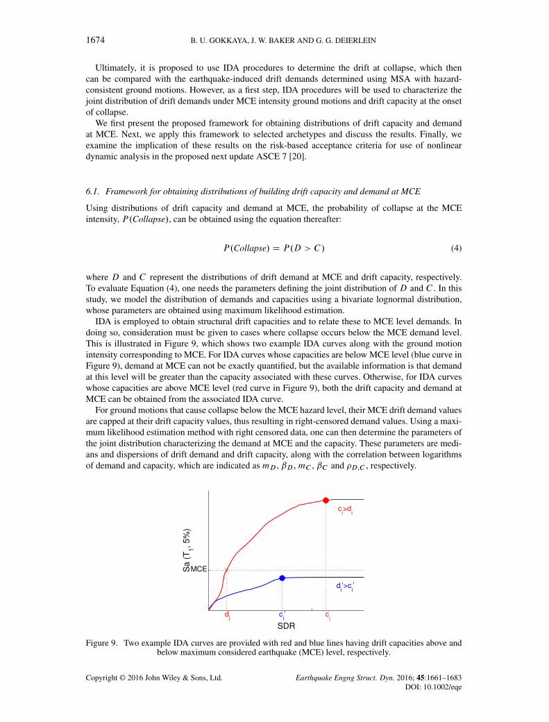
IDA is employed to obtain structural drift capacities and to relate these to MCE level demands. Indoing so, consideration must be given to cases where collapse occurs below the MCE demand level.This is illustrated in Figure 9, which shows two example IDA curves along with the ground motionintensity corresponding to MCE. For IDA curves whose capacities are below MCE level (blue curve inFigure 9), demand at MCE can not be exactly quantified, but the available information is that demandat this level will be greater than the capacity associated with these curves. Otherwise, for IDA curveswhose capacities are above MCE level (red curve in Figure 9), both the drift capacity and demand atMCE can be obtained from the associated IDA curve.

For ground motions that cause collapse below the MCE hazard level, their MCE drift demand valuesare capped at their drift capacity values, thus resulting in right-censored demand values. Using a maxi-mum likelihood estimation method with right censored data, one can then determine the parameters ofthe joint distribution characterizing the demand at MCE and the capacity. These parameters are medi-ans and dispersions of drift demand and drift capacity, along with the correlation between logarithmsof demand and capacity, which are indicated as mD , ˇD , mC , ˇC and �D;C , respectively.

Figure 9. Two example IDA curves are provided with red and blue lines having drift capacities above andbelow maximum considered earthquake (MCE) level, respectively.



For IDA curves that do not exhibit collapse response at MCE (ci > di ), one can obtain the demandand capacity values directly (Figure 9). This means that demand and capacity values are not censored.The likelihood of observingC D ci andD D di is computed using the bivariate lognormal distributionof demand and capacity:

Likelihood D P.C D ci ;D D di /

D fC;D.C D ci ;D D di /(5)

where f .�/ represents a lognormal PDF.For IDA curves that exhibit collapse response below MCE (di 0 > ci 0), drift demand at MCE cannot

be determined, and is thus censored at its respective capacity. The likelihood of observing C D ci 0 andD > ci 0 is computed using the equation later.

Likelihood D P.D > ci 0 jC D ci 0/fC .ci 0/

D

�1 �ˆ

�ln.ci 0/ � ln.mDjC /

ˇDjC

��fC .ci 0/

(6)

whereˆ.�/ is the standard normal CDF, andmDjC and ˇDjC are the conditional median and dispersionof demand given capacity, respectively. Because the joint distribution of demand and capacity arebivariate lognormal, the marginal PDF of capacity fC .c/ has a lognormal distribution.

Assuming the observations are independent, the overall likelihood can be obtained as a multiplica-tion of likelihood functions of individual data points:

Likelihood D

mYiD1

fC;D.C D ci ;D D di /

! nY

i 0D1

�1 �ˆ

�ln.ci 0/ � ln.mDjC /

ˇDjC

��fC .ci 0/

!(7)

where m and n refer to the total number of cases corresponding to no-collapse and collapse at MCE,respectively, and

QmiD1 denotes a product over i values from 1 to m.

The parameters of interest can be obtained by maximizing the overall likelihood given inEquation (7) and are denoted by OmD; OD; OmC ; OC ; O�D;C .

These parameters can be used with Equation (4) to estimate P.Collapse/ as follows:

OP .Collapse/ D ˆ

0B@� ln. OmC /

ln. OmD/qO2C C

O2D � 2 O�D;C

OCOD

1CA (8)

6.2. Distributions of building drift capacity and demand at MCE for selected archetype structures

To characterize the joint distribution of demand and capacity, IDAs are conducted for selectedarchetype structures including modeling uncertainty. The generic FEMA P695 far-field ground motionset of [39] of 44 records is used for this purpose. Each of the records is used with an IDA approachwith 4400 random structural realizations, resulting in a total of 4400 IDA curves. Drift capacity, deter-mined from each IDA curve, is defined as the drift value corresponding to the point where the IDAcurve flattens to 10% of its initial slope, beyond which drift demands tend to increase very rapidly.Note that this criteria is necessary for establishing robust horizontal statistics for drift capacity, whereascollapse ground motion intensities evaluated by vertical statistics can be determined using the lessdiscriminating fixed drift limit of 0.10 (Figure 1).

As noted previously, the ductile reinforced concrete moment frame archetypes were designedaccording to 2003 IBC, using the 2002 USGS seismic design value maps. Therefore, these designvalue maps are used to set the intensity level for determining the MCE drift demands, which for thesoil class Sd site correspond to MCE intensities of Sms D 1:5g and Sm1 D 0:9g [41].



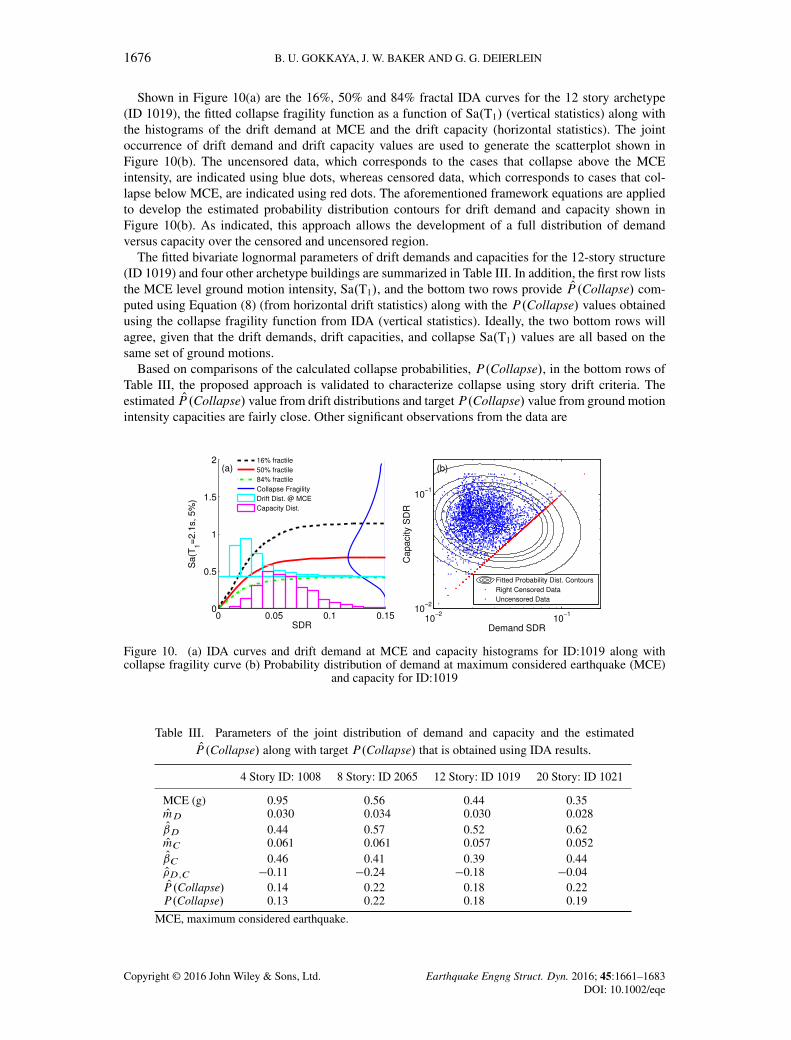
Shown in Figure 10(a) are the 16%, 50% and 84% fractal IDA curves for the 12 story archetype(ID 1019), the fitted collapse fragility function as a function of Sa.T1/ (vertical statistics) along withthe histograms of the drift demand at MCE and the drift capacity (horizontal statistics). The jointoccurrence of drift demand and drift capacity values are used to generate the scatterplot shown inFigure 10(b). The uncensored data, which corresponds to the cases that collapse above the MCEintensity, are indicated using blue dots, whereas censored data, which corresponds to cases that col-lapse below MCE, are indicated using red dots. The aforementioned framework equations are appliedto develop the estimated probability distribution contours for drift demand and capacity shown inFigure 10(b). As indicated, this approach allows the development of a full distribution of demandversus capacity over the censored and uncensored region.

The fitted bivariate lognormal parameters of drift demands and capacities for the 12-story structure(ID 1019) and four other archetype buildings are summarized in Table III. In addition, the first row liststhe MCE level ground motion intensity, Sa.T1/, and the bottom two rows provide OP .Collapse/ com-puted using Equation (8) (from horizontal drift statistics) along with the P.Collapse/ values obtainedusing the collapse fragility function from IDA (vertical statistics). Ideally, the two bottom rows willagree, given that the drift demands, drift capacities, and collapse Sa.T1/ values are all based on thesame set of ground motions.

Based on comparisons of the calculated collapse probabilities, P.Collapse/, in the bottom rows ofTable III, the proposed approach is validated to characterize collapse using story drift criteria. Theestimated OP .Collapse/ value from drift distributions and targetP.Collapse/ value from ground motionintensity capacities are fairly close. Other significant observations from the data are

Figure 10. (a) IDA curves and drift demand at MCE and capacity histograms for ID:1019 along withcollapse fragility curve (b) Probability distribution of demand at maximum considered earthquake (MCE)

and capacity for ID:1019

Table III. Parameters of the joint distribution of demand and capacity and the estimatedOP .Collapse/ along with target P.Collapse/ that is obtained using IDA results.

4 Story ID: 1008 8 Story: ID 2065 12 Story: ID 1019 20 Story: ID 1021

MCE (g) 0.95 0.56 0.44 0.35OmD 0.030 0.034 0.030 0.028OD 0.44 0.57 0.52 0.62OmC 0.061 0.061 0.057 0.052OC 0.46 0.41 0.39 0.44O�D;C �0.11 �0.24 �0.18 �0.04OP .Collapse/ 0.14 0.22 0.18 0.22P.Collapse/ 0.13 0.22 0.18 0.19

MCE, maximum considered earthquake.



� The median demands at MCE are about 0.03 with dispersion values ranging between 0.44 to 0.62,both of which are in line with expectations based on design level drift limits in building codes andresults of other dynamic analysis studies� The median drift capacities range from about 0.05 to 0.06 with dispersions of about 0.40 to 0.45.

The median drift capacities tend to coincide with when beam and column plastic hinges tend toreach their peak point.� The drift demands and capacities tend to be negatively correlated, where the correlation coeffi-

cients range from �00.04 to �0.24 with an average value of �0.14. This implies that in a givensimulation, if the drift demand is larger than average, then the drift capacity will tend to be lessthan average. This is plausible from the standpoint that weaknesses (lower stiffness and strength)that tend to produce larger drifts in a given realization will likewise tend to reduce the drift at theonset of collapse. The SAC/FEMA guidelines [5] also noted the tendency for negative correla-tions between drift demands and capacities, and they adopt a perfect negative correlation for theircomputations. Drift demands and capacities are also discussed by [42, 43] to be negatively corre-lated, and the assumption of uncorrelated demand and capacity will result in underestimation ofP.Collapse/.

6.3. Impacts of modeling uncertainty on the distributions of building drift capacity and demandat MCE

To evaluate the contribution of modeling uncertainty on the distributions of drift demands and capac-ities, we repeated the analyses just described, except using only median model parameters. This issimilar to how the modeling effects were distinguished previously, except in this case the RTR vari-ability is associated the generic FEMA P695 ground motions [39] that are used with an IDA approach.In Figure 11, the 16%, 50% and 84% fractal IDA curves and other collapse and drift distributionsare shown for the 4 story archetype (ID 1008) without (Figure 11(a)) and with modeling uncertainties(Figure 11(b)). Comparing the two reveals that the modeling uncertainty significantly increases thevariability in the drift capacity (magenta colored histogram) but otherwise results in relatively smallchanges to the other demands and capacities.

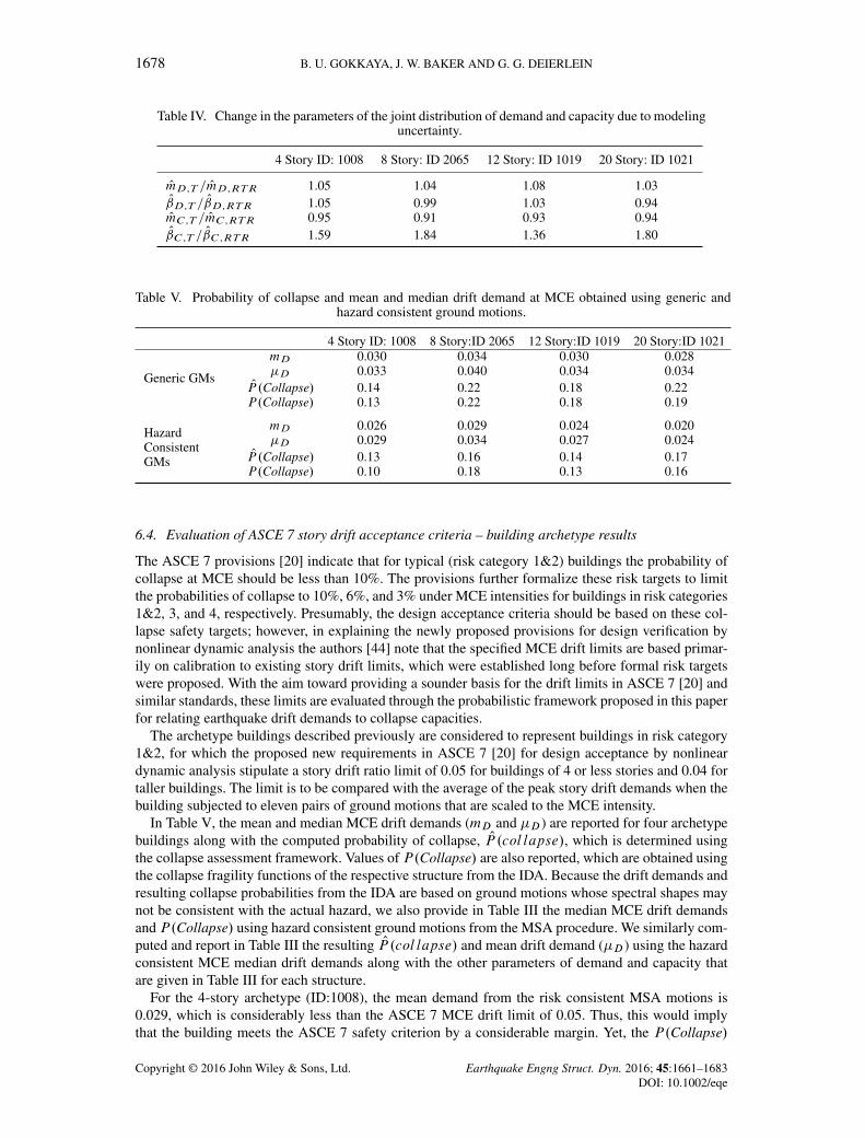
The change in the fitted bivariate lognormal parameters due to modeling uncertainty for the fourbuilding archetypes are shown in Table IV. As observed in Figure 11, the dispersion of drift capacityincreases significantly, ranging from 36% to 84% with an average of 65%. In addition, the median driftcapacity decreases by 5% to 9%. The MCE level median drift demand increases by about 3% to 8%,which parallels the trend noted in the counted median demands using MSA (Figure 7(b)). The reversetrends in median drift capacity and drift demands also follows from the negative correlations notedpreviously. The change in dispersion of MCE drift demands ranges from -6% to 5%, which is almostinsignificant and consistent with the results shown previously using MSA (Figures 7(c) and (d).

In summary, the major effects of modeling uncertainty are to (1) significantly increase the dispersionin the drift capacity by about 65%, and (2) reduce the margin between the median drift demands andcapacities by about 12%.

Figure 11. IDA curves and drift demand and capacity histograms in terms of drifts for ID:1008 (a) usingmedian model (b) with modeling uncertainty.



Table IV. Change in the parameters of the joint distribution of demand and capacity due to modelinguncertainty.

4 Story ID: 1008 8 Story: ID 2065 12 Story: ID 1019 20 Story: ID 1021

OmD;T = OmD;RTR 1.05 1.04 1.08 1.03OD;T = OD;RTR 1.05 0.99 1.03 0.94OmC;T = OmC;RTR 0.95 0.91 0.93 0.94OC;T = OC;RTR 1.59 1.84 1.36 1.80

Table V. Probability of collapse and mean and median drift demand at MCE obtained using generic andhazard consistent ground motions.

4 Story ID: 1008 8 Story:ID 2065 12 Story:ID 1019 20 Story:ID 1021

Generic GMs

mD 0.030 0.034 0.030 0.028�D 0.033 0.040 0.034 0.034

OP .Collapse/ 0.14 0.22 0.18 0.22P.Collapse/ 0.13 0.22 0.18 0.19

HazardConsistentGMs

mD 0.026 0.029 0.024 0.020�D 0.029 0.034 0.027 0.024

OP .Collapse/ 0.13 0.16 0.14 0.17P.Collapse/ 0.10 0.18 0.13 0.16

6.4. Evaluation of ASCE 7 story drift acceptance criteria – building archetype results

The ASCE 7 provisions [20] indicate that for typical (risk category 1&2) buildings the probability ofcollapse at MCE should be less than 10%. The provisions further formalize these risk targets to limitthe probabilities of collapse to 10%, 6%, and 3% under MCE intensities for buildings in risk categories1&2, 3, and 4, respectively. Presumably, the design acceptance criteria should be based on these col-lapse safety targets; however, in explaining the newly proposed provisions for design verification bynonlinear dynamic analysis the authors [44] note that the specified MCE drift limits are based primar-ily on calibration to existing story drift limits, which were established long before formal risk targetswere proposed. With the aim toward providing a sounder basis for the drift limits in ASCE 7 [20] andsimilar standards, these limits are evaluated through the probabilistic framework proposed in this paperfor relating earthquake drift demands to collapse capacities.

The archetype buildings described previously are considered to represent buildings in risk category1&2, for which the proposed new requirements in ASCE 7 [20] for design acceptance by nonlineardynamic analysis stipulate a story drift ratio limit of 0.05 for buildings of 4 or less stories and 0.04 fortaller buildings. The limit is to be compared with the average of the peak story drift demands when thebuilding subjected to eleven pairs of ground motions that are scaled to the MCE intensity.

In Table V, the mean and median MCE drift demands (mD and �D) are reported for four archetypebuildings along with the computed probability of collapse, OP .col lapse/, which is determined usingthe collapse assessment framework. Values of P.Collapse/ are also reported, which are obtained usingthe collapse fragility functions of the respective structure from the IDA. Because the drift demands andresulting collapse probabilities from the IDA are based on ground motions whose spectral shapes maynot be consistent with the actual hazard, we also provide in Table III the median MCE drift demandsand P.Collapse/ using hazard consistent ground motions from the MSA procedure. We similarly com-puted and report in Table III the resulting OP .col lapse/ and mean drift demand (�D) using the hazardconsistent MCE median drift demands along with the other parameters of demand and capacity thatare given in Table III for each structure.

For the 4-story archetype (ID:1008), the mean demand from the risk consistent MSA motions is0.029, which is considerably less than the ASCE 7 MCE drift limit of 0.05. Thus, this would implythat the building meets the ASCE 7 safety criterion by a considerable margin. Yet, the P.Collapse/



is calculated as 10% (bottom row of table) which is exactly equal to the maximum collapse risk tar-get in ASCE 7. The approximate procedure based on relating drift demands to capacity would giveOP .col lapse/ equal to 13%. Thus, one can imagine that if the building were less stiff or strong, such

that it just met the 0.05 drift limit that the structure would not meet the safety requirement. For compar-ison, although not directly relevant to this argument, the MCE drift demand (0.033) and probabilities ofcollapse (0.13 and 0.14) from the IDA procedure are slightly higher than those of the hazard consistentMSA procedure.

Similar results to the 4-story archetype are reported in Table III for the 8-story, 12-story, and 20-storyarchetypes, all of which meet by a reasonable margin the ASCE 7 MCE drift limit of 0.04 drift (with�D values for the MSA ground motions of 0.034, 0.027, and 0.024). However, all of the buildings failto meet the maximum collapse probability limit of 10% at MCE. As indicated in the bottom row of thetable, the calculated P.Collapse/ values range from 13% to 18%.

It should be noted that similar nonlinear analysis requirements for tall buildings [18, 19] specifymore stringent MCE drift limits of 0.03, as compared with the values of 0.04 to 0.05 in ASCE 7. Inlooking at the drift demands and collapse probabilities for the four building archetypes in Table III, the0.03 drift limit would appear to be more consistent with the target collapse probability limit of 10%at MCE.

6.5. Evaluation of ASCE 7 story drift acceptance criteria – parametric analysis

To further investigate the proposed ASCE 7 Chapter 16 drift requirements, we used the dispersions inthe drift demands and drift capacities from the building archetype studies to parametrically evaluate therelationship between the drift limits and the implied collapse probabilities. Based on the data shownpreviously in Table III, the dispersions in MCE drift demand and drift collapse capacity, ˇD and ˇC ,are assumed equal to 0.55 and 0.45, respectively. Using these values, the ratio of median (and mean)drift demands and capacities can be related to the probability of collapse using Equation (8).

As a first exercise, using the specified drift limits and target probabilities from ASCE 7 Chapter 16[20], the implied drift capacities can be back-calculated. For buildings in risk categories 1&2, 3, and4, the specified drift limits are 0.04, 0.03, and 0.02, and the target probabilities of collapse are 10%,6%, and 3%. Using the assumed dispersions with no correlation between drift demand and capacities,the resulting probability distributions are determined and plotted in the left column of Figure 12. Fromthese, the implied mean story drift capacities are 0.095, 0.086, and 0.072, for risk risk categories 1&2,3, and 4, respectively. A few observations of these values: (i) the values are all larger than the collapsemean drift ratios of 0.057 to 0.068 (obtained from the median drift capacities in Table III), and (ii) itis counter intuitive that the drift capacities would be smaller for the higher risk categories, suggestingthat there is a relative inconsistency between the drift limits and failure probabilities for the differentrisk categories.

As a second exercise, constant values of drift capacities will be assumed for buildings in all threerisk categories, and allowable drift limits will then be calculated. For this analysis, the mean driftcapacities are assumed to range between 0.06 and 0.10, where the 0.06 estimate is based on theresults of our archetype study and the 0.10 is an upper bound estimate. Similar values are assumedfor dispersions with a correlation between drift demand and capacities of �0.15, which is based onthe data shown previously in Table III. Shown in the right side of Figure 12 are probability distribu-tions for capacity and the corresponding drift limits assuming an intermediate collapse drift capacityof 0.08. In this case, the allowable drift limits would be 0.032, 0.026, and 0.020 for risk categories1&2, 3, and 4, respectively. Interestingly, the calculated drift limit of 0.032 for risk categories 1&2is close to the limit of 0.03 specified in the tall building guidelines [18], and the calculated driftlimit of 0.02 for risk category 4 is equal to the current limit specified in ASCE 7 [20]. These values,along with the calculated drift limits corresponding to drift capacities of 0.06 and 0.10 are summa-rized in Table VI. Comparing these with current standards suggest that the current ASCE 7 drift limitswould meet the target collapse risk if the story drift capacity is 0.10. However, to the extent that theupper bound drift capacity of 0.10 may be too optimistic (and well in excess of the values of 0.06calculated in the building archetype study), this would suggest that the ASCE 7 drift limits shouldbe reduced.



Figure 12. Back-calculated (left) and proposed (right) distributions of drift demands and capacities forbuildings having more than 4 stories (a) Risk categories 1 and 2 (b) Risk category 3, and (c) Risk category4. Red and blue lines represent the distributions of demand and capacity, respectively. Mean values are

indicated with dashed black lines.

Table VI. Story drift limits for global acceptance criteriacorresponding to drift capacities of 0.06 to 0.10.

Risk categories

�C 1 & 2 3 40.06 0.024 0.019 0.0150.08 0.032 0.026 0.0200.10 0.04 0.032 0.025

7. CONCLUSIONS

In this study, we characterize and propagate modeling uncertainty and quantify its impacts on theseismic response assessment of structures. The uncertainty in parameters defining analysis modelsand limit state surfaces are incorporated into nonlinear dynamic analysis for ductile and non-ductilereinforced concrete frame structures. Variability and correlations in structural model parameters arepropagated in the dynamic analyses using Monte-Carlo simulation with Latin hypercube sampling.Earthquake ground motions are incorporated through MSA with hazard consistent ground motionsthat are selected and scaled using a conditional spectra approach. Impacts of modeling uncertainty areevaluated for fragility functions and mean annual exceedance rates for drift limits and collapse as wellas drift (deformation) demands and capacities of thirty-three archetype building configurations.



In analyses of the archetype concrete moment frame buildings, the modeling uncertainty both shiftedthe medians and increased dispersion in the collapse fragility curves. The median collapse intensity(spectral accelerations) shifted by up to �20% downward or C10% upward, with an average shift ofdownward of about �5%. Dispersion (variability) in the collapse fragilities increased by about 10%to 70% with an average increase of about 30%. Cases with small upward (positive) shifts in medianswere usually accompanied by the largest increases in dispersion, which tends to flatten out the fragilitycurve. The largest downward (negative) shifts in median tend to occur in structures having weak storymechanisms and non-ductile frames, where weakest link failure mechanisms are more prevalent. Whenintegrated with earthquake hazard curves for a high-seismic region of California, the modeling uncer-tainty increased the mean annual frequencies of collapse, �c , by about 1.4 to 2.6 times, compared withthe analyses that only include ground motion record-to-record variability. Subject to the same assump-tions in modeling parameters, investigation of sites with hazard curves more representative of themid and eastern United States suggest that the influence of modeling uncertainties will be smaller forthese regions.

Equivalent parameters to represent modeling uncertainties in collapse fragilities are back calcu-lated using an SRSS approach to combine variabilities due to ground motions (record-to-record) andstructural modeling and by calibration to achieve consistent mean annual frequency rates for the high-seismic site. From these analyses, the average effect of modeling uncertainty on collapse fragility canbe represented by either (i) a shift in median by �5% combined with an added modeling dispersionˇc;M of 0.33, or (ii) no shift in median and an added modeling dispersion of ˇc;M of 0.40. These gen-eral values are, of course, subject to the limitations of the study of concrete moment frames designedfor a high-seismic site.

The impacts of modeling uncertainty on drift-exceedance limit states are observed to generally besmaller than for collapse and vary depending on the magnitude of the drifts (amount of inelasticity).For drift-exceedance fragility curves at drift ratios of 0.03, the modeling uncertainty resulted in a smallnegative shift in median and increase in dispersion, which increased the mean annual frequency ofdrift exceedance up to 1.3 times with an average increase of about 1.2, compared with the models withonly ground motion variability. At drift-exceedance ratios of 0.07, the changes in drift-fragility curvesand mean annual exceedance rates were about the same as for the changes in collapse fragilities, withincreases in mean annual frequencies of 1.4 to 2.6 times with an average increase of about 1.8 times,compared with cases with only ground motion variability.

To help inform the calibration of drift limits for design using nonlinear dynamic analysis, we devel-oped a framework for quantifying the joint probability distributions of story drift demands and storydrift collapse capacities. This framework considers joint treatment of analysis causing collapses andno-collapses to develop consistent estimates of story drift collapse capacities from IDA that includeboth ground motion and modeling uncertainties. Applying this framework to four archetype buildingsprovides estimates of drift demands at MCE-level ground motion intensity and drift collapse capaci-ties. The resulting median drift capacities range from story drift ratios of about 0.052 to 0.061, withand average dispersion of 0.45. Drift demands of the archetypes, calculated at MCE level conditionalspectra intensities, range from 0.028 to 0.034, with an average dispersion of 0.55. A small negative cor-relation of �0.14 is obtained between drift demands and capacities. The analyses further indicate thatmodeling uncertainty (i) increases the median MCE drift demands by about 5%, (ii) increases the dis-persion in MCE demand by a negligible amount, (iii) reduces the drift collapse capacity by about 7%,and (iv) increases the dispersion in drift collapse capacity by about 65%. Thus, the combined effectsof median shifts and increased dispersion on collapse drift capacity can have a significant effect onincreasing the probability of drift demands exceeding drift capacities.

Finally, the procedure and data for evaluating MCE level drift demands and drift capacities are usedto assess the nonlinear analysis procedures and drift limits in a recently proposed new chapter 16 inASCE 7 [20]. Subject to the limited scope of our study, the proposed MCE level drift limits are foundto be unconservative and inconsistent with the stated acceptable collapse risk targets in ASCE 7. Forexample, whereas the proposed drift limits for risk category 1&2 buildings range from 0.04 to 0.05,our analyses suggest that the limits should be about 0.03, which coincidentally is the specified driftlimit in tall building guidelines for design by nonlinear analysis [18, 19].



The methods and strategies employed in this paper to characterize and propagate modeling uncer-tainties are based on fairly well established approaches. The main challenge has been in characterizingthe model parameter uncertainties, developing and verifying the nonlinear analysis models, and set-ting up procedures to conduct the simulations and process the output. The tools and methods presentedin this paper can be used to explore the impacts of modeling for other building archetypes andperformance metrics. As shown in these examples, the importance of considering modeling uncer-tainty depends, in part, on the particular demand parameters or performance metrics of interest. Moreimportantly, these examples demonstrate the feasibility, through modern information and computingtechnologies, of rigorously propagating model uncertainty to develop more reliable and risk-consistentmethods for seismic assessment and design of buildings and other structures.

ACKNOWLEDGEMENTS

This project is financially supported by the National Science Foundation (NSF CMMI-1031722) andStanford University. Any opinions, findings and conclusions or recommendations expressed in this materialare those of the authors and do not necessarily reflect the views of the National Science Foundation orStanford University. The authors would like to thank Curt Haselton, Abbie Liel, and Meera Raghunandanfor sharing structural models of the frames used in this study, Professor Eduardo Miranda for his feedback,and two anonymous reviewers for their constructive comments.

REFERENCES

1. Bradley BA. A generalized conditional intensity measure approach and holistic ground-motion selection. EarthquakeEngineering & Structural Dynamics October 2010; 39(12):1321–1342 (en).

2. Jayaram N, Lin T, Baker JW. A computationally efficient ground-motion selection algorithm for matching a targetresponse spectrum mean and variance. Earthquake Spectra 2011; 27(3):797–815.

3. Bradley BA. A critical examination of seismic response uncertainty analysis in earthquake engineering. EarthquakeEngineering & Structural Dynamics September 2013; 42(11):1717–1729.

4. Terzic V, Schoettler MJ, Restrepo JI, Mahin SA. Concrete column blind prediction contest 2010: outcomes andobservations. Technical Report PEER 2015/01, Pacific Earthquake Engineering Research Center, University ofCalifornia at Berkeley: Berkeley, California, 2015.

5. Cornell C, Jalayer F, Hamburger R, Foutch D. Probabilistic Basis for 2000 SAC Federal Emergency ManagementAgency Steel Moment Frame Guidelines. Journal of Structural Engineering 2002; 128(4):526–533.

6. Wen YK, Ellingwood BR, Veneziano D, Bracci J. Uncertainty modeling in earthquake engineering. Technical ReportProject FD-2 Report, Mid-America earthquake center: Citeseer, 2003.

7. Kennedy RP, Ravindra MK. Seismic fragilities for nuclear power plant risk studies. Nuclear Engineering and Design1984; 79(1):47–68.

8. Wen YK, Ellingwood BR. The role of fragility assessment in consequence-based engineering. Earthquake Spectra2005; 21(3):861–877.

9. Porter KA, Beck JL, Shaikhutdinov RV. Sensitivity of building loss estimates to major uncertain variables.Earthquake Spectra 2002; 18(4):719–743.

10. Ibarra LF, Krawinkler H. Global collapse of frame structures under seismic excitations. Technical Report , John A.Blume Earthquake Engineering Center: Stanford, CA, 2005.

11. Celik OC, Ellingwood BR. Seismic fragilities for non-ductile reinforced concrete frames Role of aleatoric andepistemic uncertainties. Structural Safety January 2010; 32(1):1–12.

12. Lee TH, Mosalam KM. Seismic demand sensitivity of reinforced concrete shear-wall building using FOSM method.Earthquake Engineering & Structural Dynamics November 2005; 34(14):1719–1736.

13. Haselton CB. Assessing seismic collapse safety of modern reinforced concrete moment frame buildings. Ph.D.Thesis, Stanford University, 2006.

14. Liel AB, Haselton CB, Deierlein GG, Baker JW. Incorporating modeling uncertainties in the assessment of seismiccollapse risk of buildings. Structural Safety 2009; 31(2):197–211.

15. Dolsek M. Incremental dynamic analysis with consideration of modeling uncertainties. Earthquake Engineering &Structural Dynamics May 2009; 38(6):805–825.

16. Vamvatsikos D, Fragiadakis M. Incremental dynamic analysis for estimating seismic performance sensitivity anduncertainty. Earthquake engineering & structural dynamics 2010; 39(2):141–163.

17. Yin YJ, Li Y. Seismic collapse risk of light-frame wood construction considering aleatoric and epistemicuncertainties. Structural Safety July 2010; 32(4):250–261.

18. PEER. Guidelines for performance-based seismic design of tall buildings. Technical Report 2010/05, Pacific Earth-quake Engineering Research Center, University of California at Berkeley: Berkeley, California, 2010. Prepared bythe TBI Guidelines Working Group.



19. LATBSDC. An alternative procedure for seismic analysis and design of tall buildings located in the Los Ange-les Region. Technical Report 2014 Edition with 2015 Supplements, Los Angeles Tall Buildings Structural DesignCouncil: Los Angeles, 2015.

20. American Society of Civil Engineers Standards Committee. Proposal to revise the 2010 edition of asce/sei 7: Reston,VA, 2015.

21. Lin T, Harmsen SC, Baker JW, Luco N. Conditional spectrum computation incorporating multiple causal earth-quakes and ground-motion prediction models. Bulletin of the Seismological Society of America 2013; 103(2A):1103–1116.

22. Vamvatsikos D, Cornell CA. Incremental dynamic analysis. Earthquake Engineering & Structural Dynamics 2002;31(3):491–514.

23. Eads L, Miranda E, Krawinkler H, Lignos DG. An efficient method for estimating the collapse risk of structures inseismic regions. Earthquake Engineering & Structural Dynamics 2012; 42:25–41 (en).

24. IBC. International building code. International Code Council (ISBN: 189239797), 2003.25. American Society of Civil Engineers. ASCE standard 7-02: Minimum design loads for buildings and other

structures: Reston, VA, 2002.26. McKenna F, Fenves GL, Scott MH, Jeremic B. Open system for earthquake engineering simulation, 2014. Pacific

Earthquake Engineering Research Center, Berkeley, CA.27. Ibarra LF, Medina RA, Krawinkler H. Hysteretic models that incorporate strength and stiffness deterioration.

Earthquake Engineering & Structural Dynamics October 2005; 34(12):1489–1511.28. Haselton CB, Liel AB, Lange ST, Deierlein GG. Beam-column element model calibrated for predicting flexural

response leading to global collapse of RC frame buildings. Technical Report PEER 2007/03, Pacific EarthquakeEngineering Research Center, University of California at Berkeley: Berkeley, California, 2008.

29. Raghunandan M, Liel AB, Luco N. Collapse risk of buildings in the pacific northwest region due to subductionearthquakes. Earthquake Spectra 2015; 31(4):2087–2115.

30. UBC. Uniform building code, International Conference of Building Officials: Whittier: Pasadena, California, 1967.31. Elwood KJ. Modelling failures in existing reinforced concrete columns. Canadian Journal of Civil Engineering

October 2004; 31(5):846–859.32. Sezen H. Seismic behavior and modeling of reinforced concrete building columns. Ph.D. Thesis, Civil and

Environmental Engineering, University of California, Berkeley, 2002.33. USGS Hazard curve application. (Available from: http://geohazards.usgs.gov/hazardtool/application.php.)

[Accessed: 2015-08-09].34. USGS 2008 interactive deaggregations. (Available from: http://geohazards.usgs.gov/deaggint/2008/.) [Accessed:

2015-08-09].35. Haselton C, Mitrani-Reiser J, Goulet C, Deierlein GG, Beck JL, Porter KA, Stewart J, Taciroglu E. An assessment to

benchmark the seismic performance of a code-conforming reinforced-concrete moment-frame building. TechnicalReport 2007/12, Pacific Earthquake Engineering Research Center, University of California at Berkeley: Berkeley,California, 2007.

36. Ugurhan B, Baker JW, Deierlein GG. Uncertainty estimation in seismic collapse assessment of modern rein-forced concrete moment frame building, Proceedings of the 10th National Conference in Earthquake Engineering.Earthquake Engineering Research Institute: Anchorage, AK, 2014.

37. Helton JC, Davis FJ. Latin hypercube sampling and the propagation of uncertainty in analyses of complex systems.Reliability Engineering & System Safety 2003; 81(1):23–69.

38. Jalayer F. Direct Probabilistic seismic anaysis: implementing non-linear dynamic assessments. Ph.D. Thesis,Stanford University, 2003.

39. FEMA. Quantification of Building Seismic Performance Factors, FEMA-P695, Federal Emergency ManagementAgency: Washington DC, 2009.

40. FEMA. Seismic Performance Assessment of Buildings, FEMA-P58, Federal Emergency Management Agency:Washington, DC, 2012.

41. Haselton CB, Baker JW, Liel AB, Deierlein GG. Accounting for ground-motion spectral shape characteristics instructural collapse assessment through an adjustment for epsilon. Journal of Structural Engineering 2009; 137:332–344.

42. Kazantzi AK, Vamvatsikos D, Lignos DG. Seismic performance of a steel moment-resisting frame subject to strengthand ductility uncertainty. Engineering Structures November 2014; 78:69–77.

43. Jalayer F, Franchin P, Pinto PE. A scalar damage measure for seismic reliability analysis of RC frames. EarthquakeEngineering & Structural Dynamics October 2007; 36(13):2059–2079 (en).

44. Haselton CB, Fry A, Baker JW, Hamburger RO, Whittaker AS, Stewart JP, Elwood KJ, Luco N, Hooper JD, CharneyFA, Zimmerman RB, Pekelnicky RG. Response-history analysis for the design of new buildings: a fully revisedchapter 16 methodology proposed for the 2015 NEHRP Provisions and the ASCE/SEI 7-16 Standard, Proceedings ofthe 10th National Conference in Earthquake Engineering. Earthquake Engineering Research Institute: Anchorage,AK, 2014.


http://geohazards.usgs.gov/hazardtool/application.php

http://geohazards.usgs.gov/deaggint/2008/

Documents

Quantifying the impacts of modeling uncertainties on the ...web.stanford.edu/~bakerjw/Publications/Gokkaya_et_al_(2016)_Design... · Quantifying the impacts of modeling uncertainties