Quantifying the Impact of Global Climate Change on Potential Natural Vegetation

QUANTIFYING THE IMPACT OF GLOBAL CLIMATE CHANGE ONPOTENTIAL NATURAL VEGETATION

MARTIN T. SYKES1, I. COLIN PRENTICE1∗ and FOUZIA LAARIF2

1Plant Ecology, Ecology Building, Lund University, S-223 62 Lund, Sweden2Dynamic Palaeoclimatology, Lund University, Box 117, S-223 00 Lund, Sweden

Abstract. Impacts of climate change on vegetation are often summarized in biome maps, represent-ing the potential natural vegetation class for each cell of a grid under current and changed climate.The amount of change between two biome maps is usually measured by the fraction of cells thatchange class, or by the kappa statistic. Neither measure takes account of varying structural and floris-tic dissimilarity among biomes. An attribute-based measure of dissimilarity (1V ) between vegetationclasses is therefore introduced.1V is based on (a) the relative importance of different plant lifeforms (e.g. tree, grass) in each class, and (b) a series of attributes (e.g. evergreen-deciduous, tropical-nontropical) of each life form with a weight for each attribute.1V is implemented here for the mostused biome model, BIOME 1 (Prentice, I. C. et al., 1992). Multidimensional scaling of pairwise1V values verifies that the suggested importance values and attribute weights lead to a reasonablepattern of dissimilarities among biomes. Dissimilarity between two maps (1V) is obtained by area-weighted averaging of1V over the model grid. Using1V, present global biome distribution fromclimatology is compared with anomaly-based scenarios for a doubling of atmospheric CO2 concen-tration (2× CO2), and for extreme glacial and interglacial conditions. All scenarios are obtainedfrom equilibrium simulations with an atmospheric general circulation model coupled to a mixed-layer ocean model. The 2× CO2 simulations are the widely used OSU and GFDL runs from the1980’s, representing models with low and high climate sensitivity, respectively. The palaeoclimatesimulations were made with CCM1, with sensitivity similar to GFDL.1V values for the comparisonsof 2×CO2 with present climate are similar to values for the comparisons of the last interglacial andmid-Holocene with present climate. However, the two simulated 2×CO2 cases are much more likeeach other than they are to the simulated interglacial cases. The largest1V values were betweenthe last glacial maximum and all other cases, including the present. These examples illustrate thepotential of1V in comparing the impacts of different climate change scenarios, and the possibilityof calibrating climate change impacts against a palaeoclimatic benchmark.

1. Introduction

Global biome maps have been widely used to assess the impacts of simulatedpast and future climate change on ecosystems (e.g. Prentice et al., 1993; Neilson,1995; Prentice and Sykes, 1995). Biome distributions are typically simulated usingequilibrium biogeography models, also called biome models (Prentice et al., 1992;VEMAP Members, 1995; Haxeltine and Prentice, 1996). Such models use differentcombinations of a small number of plant functional types (PFTs) and climatic∗ Present address: Max Planck Institute for Biogeochemistry, Sophienstrasse 10, D-04473 Jena,

Germany

Climatic Change41: 37–52, 1999.© 1999Kluwer Academic Publishers. Printed in the Netherlands.

38 MARTIN T. SYKES ET AL.

variables to simulate the distribution of a number of discrete vegetation classesor ‘biomes’, which are defined as large-scale vegetation units characterized by thepredominance of one or more PFTs. When applied to climate scenarios for thenext centuries, these equilibrium model results describe thepotentialvegetation,i.e. the vegetation type towards which the natural (non-modified) vegetation woulddevelop under a simulated climate, rather than the actual (modified) vegetation.Transient responses of vegetation to continuing changes in climate can be simu-lated with dynamic global vegetation models (e.g. Foley et al., 1996), but these arestill under development, and not yet widely used in impact studies.

Assessments of the magnitude of climatically induced change from one simu-lated global biome map to another has often been based on visual comparisons.Quantification is however both possible and useful. An obvious quantitative mea-sure is the simple fraction of grid cells that show different biomes in the two maps(e.g. Claussen, 1994). Recently, the kappa statistic (Cohen, 1960; Landis and Koch,1977; Monserud and Leemans, 1992; Neilson, 1993; Haxeltine and Prentice, 1996)has also become popular for this purpose. The kappa statistic is derived from thefraction of grid cells that remain the same between two maps, but this fractionis corrected to allow for the fraction that would be expected to remain the samebetween two random maps with the same class frequencies. Although formal sta-tistical testing is inappropriate, there is an accepted subjective scale for interpretingvalues of kappa, ranging from ‘no agreement’ to ‘perfect agreement’ (Monserudand Leemans, 1992). As this terminology implies, the kappa statistic is well suitedto assessing thedegree of similaritybetween two maps that are expected a priori toagree. The kappa statistic has been used in this way to assess the similarity betweensimulated and observed vegetation maps (Prentice et al., 1992; VEMAP Members,1995; Haxeltine and Prentice, 1996).

The interpretation of the kappa statistic is less obvious when the aim is to quan-tify the amount of changebetween two maps derived using the same model. Herethe question of how many grid cells would stay the same under randomization is notrelevant. A further problem, which affects both the simple fractions and the kappastatistic, is that all biome changes are treated as equivalent. This is undesirable ina measure designed to quantify vegetation change. To take an extreme example,consider two grid cells occupied by boreal forest. The first changes to a mixed(coniferous-deciduous) forest, the second to a tropical savanna. We suggest thatthe second change should contribute more to a measure of dissimilarity than thefirst.

A related difficulty is that with increasing impacts, the simple fractions and thekappa statistic ‘saturate’ when all the grid cells have changed. We suggest that ameasure of dissimilarity should continue to increase, as extant vegetation types arereplaced by types that have less and less structurally and floristically in common.

We therefore need a non-trivial measure ofdissimilarity between biomes, i.e. ameasure that takes values other than the values 0 and 1 that are implied in the simplefraction and in the kappa statistic. That is what is done in this paper. Such a measure

QUANTIFYING THE IMPACT OF GLOBAL CLIMATE CHANGE 39

can be spatially averaged in order to yield an overall measure of the change betweentwo maps. We illustrate the use of our proposed measure by applying it to biomesimulations representing a range of past, present and future (high greenhouse gasconcentration) conditions.

2. Methods

2.1. DISSIMILARITY BETWEEN BIOMES

Here we develop the dissimilarity measure between biomes,1V , and its imple-mentation in the context of BIOME 1 (Prentice et al., 1992). We focus on BIOME 1because it is well known, because it has been applied more widely than any otherbiome model (apart from the earlier, non-mechanistic models such as the Holdridgescheme, which does not lend itself to biological interpretation in terms of plant lifeforms and attributes), and because of its relative simplicity.

We define:

1V (i, j) = 1−∑k{min(Vik, Vjk) ∗ [1−∑l wkl|aikl − ajkl|]} , (1)

where1V (i, j) is the dissimilarity between biomesi, j ; Vik, Vjk are the impor-tance values of plant life-formk in biomesi, j ; aikl, ajkl are the values of attributel for plant life form k in biomesi,j ; wkl is a weight for attributel of plant lifeform k.

It is assumed that both the importance values and the attribute values are all inthe range from 0 to 1; that the sum of importance values for each biome,

∑k Vik =

1 (this means in practice that we must define a dummy life form called ‘bareground’, e.g. to distinguish deserts from closed vegetation types); and that the sumof weights,

∑l wkl ≤ 1. If no attributes are defined for a given plant life form, the

term in square brackets is set to 1.Equation (1) can be understood by considering first the similarity index∑k min(Vik, Vjk). This index reflects only differences in plant life form compo-

sition. It takes the value 0 if and only if the two biomes are identical in plant lifeform composition, and 1 if and only if they have no plant life forms in common.In Equation (1), the terms of this simple index are each multiplied by a reductionfactor (the term in square brackets). This factor depends on the attributes of theplant life form involved, for example, whether or not the trees are evergreen. If theattributes of a given plant life form are the same in both biomes then the reductionfactor becomes 1, i.e. similarity is not reduced. If the attributes are completelydifferent and the sum of the weights is 1, then the reduction factor becomes zeroand the plant life form in question contributes nothing to similarity. The result-ing similarity index also ranges from 0 in the case of identity, to 1 in the caseof complete contrast. Subtraction from 1 converts this similarity measure to thedissimilarity index1V .


TABLE I

Importance values for plant life forms in each biome

Biome Life form

Trees Grass/shrub Bare ground

Forests 1

Tropical dry forest/

savanna 0.75 0.25

Xeric woods/scrub 0.50 0.50

Grass/shrub 1

Deserts 0.25 0.75

Tundra 1

Implementation of1V requires the definition of plant life forms, assignmentof importance values for life forms, definition of attributes, assignment of attributevalues, and assignment of attribute weights.

The definitions of plant life forms and attributes follow naturally from the struc-ture of the model. They could be different for different models, depending on whataspects of vegetation structure the model predicts. For example, BIOME 1 doesnot predict the distribution of grasses versus shrubs, so for this implementation wedefine only trees, grasses/shrubs, and bare ground as the three plant life forms.

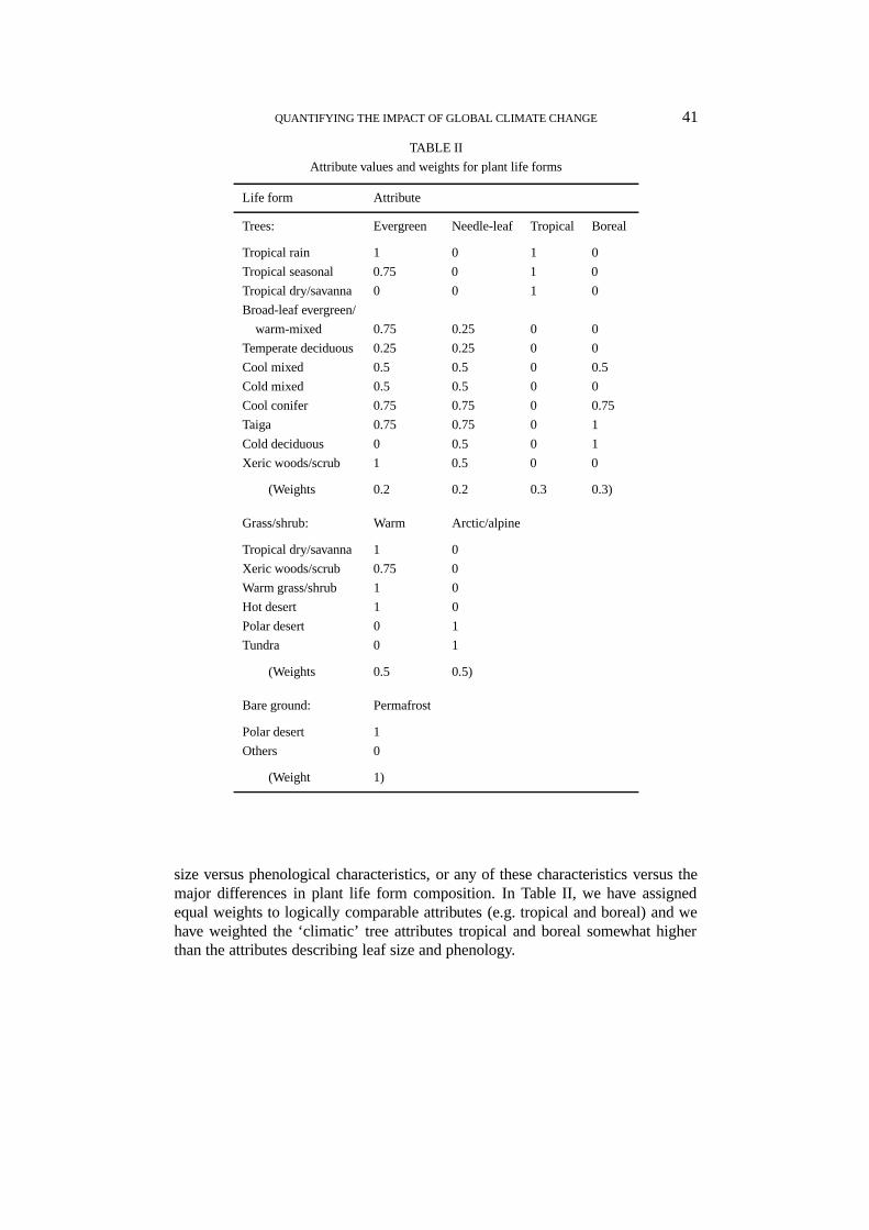
The importance values and attribute values that we have used in our imple-mentation of the method for BIOME 1 are given in Tables I and II. These valuesrepresent rough estimates of the dominance of different types of plant in each ofthe biomes. For example, forests are dominated by trees (hence the life form ‘trees’is given an importance value of 1); deserts are dominated by bare ground withsome amount of grass/shrub (hence ‘grass/shrub’ is given an importance value of0.25 while ‘bare ground’ gets 0.75); and so on. Further information is added byway of the importance values, so that, for example, the trees in tropical rainforestare tropical evergreen broad-leaved and therefore are assigned attribute values of1 for evergreen, 0 for needle-leaf, 1 for tropical, 0 for boreal; the trees in taigaare mainly boreal evergreen needle-leaved but with some boreal deciduous broad-leaved or needle-leaved, so they are assigned attribute values of 0.75 for evergreenand needle-leaved, 0 for tropical, 1 for boreal. These assignments are necessarilyrough and somewhat subjective; however, it is unlikely that different ecologistswould assign greatly differing values.

Note that in suggesting the weights in Table II, we imposed the additional con-straint that the sum of attribute weights,

∑l wkl = 1. This constraint amounts to

giving approximate parity to attribute distinctions and life form distinctions.The weights for attributes are explicitly subjective. This is unavoidable because

there is no obvious a priori basis for assigning relative significance to, say, leaf


TABLE II

Attribute values and weights for plant life forms

Life form Attribute

Trees: Evergreen Needle-leaf Tropical Boreal

Tropical rain 1 0 1 0

Tropical seasonal 0.75 0 1 0

Tropical dry/savanna 0 0 1 0

Broad-leaf evergreen/

warm-mixed 0.75 0.25 0 0

Temperate deciduous 0.25 0.25 0 0

Cool mixed 0.5 0.5 0 0.5

Cold mixed 0.5 0.5 0 0

Cool conifer 0.75 0.75 0 0.75

Taiga 0.75 0.75 0 1

Cold deciduous 0 0.5 0 1

Xeric woods/scrub 1 0.5 0 0

(Weights 0.2 0.2 0.3 0.3)

Grass/shrub: Warm Arctic/alpine

Tropical dry/savanna 1 0

Xeric woods/scrub 0.75 0

Warm grass/shrub 1 0

Hot desert 1 0

Polar desert 0 1

Tundra 0 1

(Weights 0.5 0.5)

Bare ground: Permafrost

Polar desert 1

Others 0

(Weight 1)

size versus phenological characteristics, or any of these characteristics versus themajor differences in plant life form composition. In Table II, we have assignedequal weights to logically comparable attributes (e.g. tropical and boreal) and wehave weighted the ‘climatic’ tree attributes tropical and boreal somewhat higherthan the attributes describing leaf size and phenology.


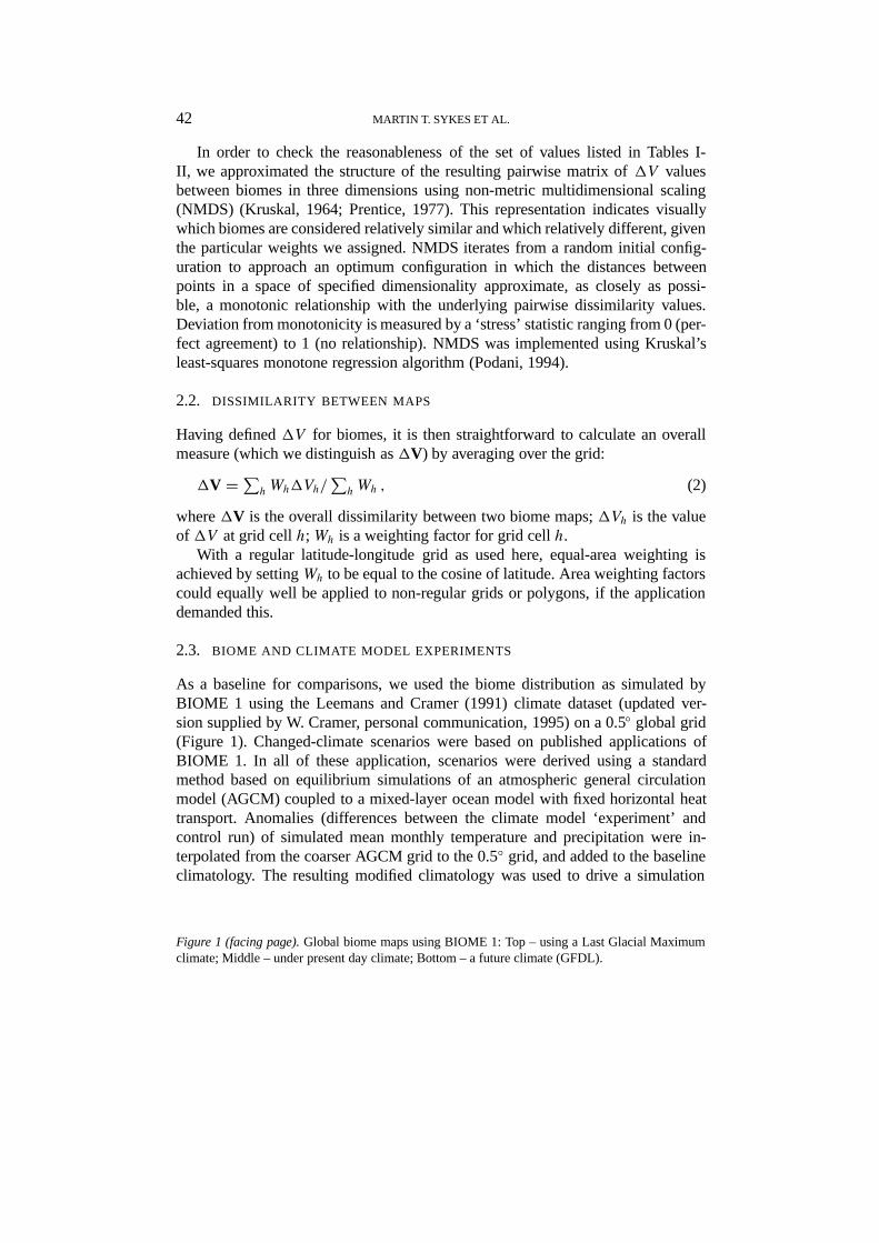
In order to check the reasonableness of the set of values listed in Tables I-II, we approximated the structure of the resulting pairwise matrix of1V valuesbetween biomes in three dimensions using non-metric multidimensional scaling(NMDS) (Kruskal, 1964; Prentice, 1977). This representation indicates visuallywhich biomes are considered relatively similar and which relatively different, giventhe particular weights we assigned. NMDS iterates from a random initial config-uration to approach an optimum configuration in which the distances betweenpoints in a space of specified dimensionality approximate, as closely as possi-ble, a monotonic relationship with the underlying pairwise dissimilarity values.Deviation from monotonicity is measured by a ‘stress’ statistic ranging from 0 (per-fect agreement) to 1 (no relationship). NMDS was implemented using Kruskal’sleast-squares monotone regression algorithm (Podani, 1994).

2.2. DISSIMILARITY BETWEEN MAPS

Having defined1V for biomes, it is then straightforward to calculate an overallmeasure (which we distinguish as1V) by averaging over the grid:

1V =∑h Wh1Vh/∑

h Wh , (2)

where1V is the overall dissimilarity between two biome maps;1Vh is the valueof 1V at grid cellh;Wh is a weighting factor for grid cellh.

With a regular latitude-longitude grid as used here, equal-area weighting isachieved by settingWh to be equal to the cosine of latitude. Area weighting factorscould equally well be applied to non-regular grids or polygons, if the applicationdemanded this.

2.3. BIOME AND CLIMATE MODEL EXPERIMENTS

As a baseline for comparisons, we used the biome distribution as simulated byBIOME 1 using the Leemans and Cramer (1991) climate dataset (updated ver-sion supplied by W. Cramer, personal communication, 1995) on a 0.5◦ global grid(Figure 1). Changed-climate scenarios were based on published applications ofBIOME 1. In all of these application, scenarios were derived using a standardmethod based on equilibrium simulations of an atmospheric general circulationmodel (AGCM) coupled to a mixed-layer ocean model with fixed horizontal heattransport. Anomalies (differences between the climate model ‘experiment’ andcontrol run) of simulated mean monthly temperature and precipitation were in-terpolated from the coarser AGCM grid to the 0.5◦ grid, and added to the baselineclimatology. The resulting modified climatology was used to drive a simulation

Figure 1 (facing page).Global biome maps using BIOME 1: Top – using a Last Glacial Maximumclimate; Middle – under present day climate; Bottom – a future climate (GFDL).


with BIOME 1. Finally we calculated1V between each of these changed-climatesimulations and the baseline simulation.

The ‘future’ simulations used were the OSU (Schlesinger and Zao, 1989) andGFDL (Manabe and Wetherald, 1987) runs, with atmospheric CO2 concentrationraised to twice its pre-industrial level (Figure 1). These two climate models werechosen because they have been extensively used in climate impact studies andbecause they represent approximately the lower and upper bounds, respectively, forthe ‘climate sensitivity’, i.e. the sensitivity of simulated global mean temperatureto the radiative forcing implied by a doubling of CO2 (Houghton et al., 1990).The palaeoclimate simulations were all made using the NCAR CCM1, which hasa climate sensitivity similar to that of GFDL (Gates et al., 1992). The followingpalaeoclimate simulations were used:

• TheP+T+ simulation (Harrison et al., 1995), represents the ‘peak interglacial’configuration of the Earth’s orbit, with the maximum potential for high-latitude warming that has occurred during the Late Quaternary. This potentialwas nearly achieved during the early part of the last (Eemian) interglacialaround 126 ka (1 ka= 1000 years before present). Atmospheric CO2 con-centration was set equal to the modern control run, consistent with the Vos-tok ice-core measurements (Barnola et al., 1987) showing CO2 concentrationreaching a peak approaching modern values around 126 ka.

• The 6 ka simulation (Kutzbach et al., 1998), represents a smaller thoughqualitatively similar orbital forcing, as experienced during the mid-Holocene.During the current glacial-interglacial cycle, the insolation anomaly was max-imal around the beginning of the Holocene, but the North American ice sheettook several thousand years to disappear. As a result, maximum warmth inregions ‘downstream’ did not occur until around 6 ka (Harrison et al., 1992;Huntley and Prentice, 1993). Atmospheric CO2 equivalent was set at 280 ppm,consistent with ice-core measurements showing little or no change from 6 kathrough to the immediate pre-industrial period.

• TheLGM simulation (Kutzbach et al., 1998) represents conditions at the lastglacial maximum, ca. 21 ka (Figure 1). At this time, although the Earth’s orbitwas not very different from present, the ice sheets (thanks to the accumulatedeffects of earlier low-insolation periods) were close to their maximum extentand concentrations of CO2 and other greenhouse gases were close to theirlowest Quaternary levels. In addition to the minor orbital change, ice-sheetsand sea-level were prescribed consistent with Peltier (1994) and atmosphericCO2 concentration was set to 200 ppm based on the ice-core measurements.1V was calculated in two ways in this case: points occupied by ice at theLGM were either considered as polar desert, or excluded from comparison.Points that formed part of the exposed continental shelf at the LGM (e.g. theSunda Shelf; see e.g. Prentice et al., 1993) were excluded from comparison.


These various palaeoclimate model runs can thus be considered to bracket therange of climatic forcing conditions that has been experienced by the Earth duringapproximately the past million years.

3. Results

3.1. DISSIMILARITY BETWEEN BIOMES

The NMDS analysis reached a stress level of 0.11 after 30 iterations. This is withinthe range 0.1–0.2 considered as ‘satisfactory’ (Podani, 1995). Inspection showedthat the relationship between distances and dissimilarities in the final configuration(Figure 2) was approximately proportional, so the distances in Figure 2 can betreated as a simple reflection of1V .

The configuration shown in Figure 2 seems appropriate to describe differencesamong biomes. The axis 1 separates treeless (desert, steppe and tundra) biomesfrom forested biomes, with xerophytic vegetation and dry forest/savanna appro-priately intermediate. Differences between biomes closely associated on axis 1are expressed in axis 2, which mainly shows a temperature-related gradient, bothamong the forests and among the non-forests. Axis 3 distinguishes deserts fromother treeless biomes, and further accentuates the difference between tropical andnon-tropical forests. Overall, there are large variations in the1V values calcu-lated for different pairs of biomes. For example, certain types of temperate forest(temperate deciduous, broad-leaved evergreen/warm mixed, and cool mixed) areconsidered very similar; this is reasonable because many species and genera runacross the boundaries and because the structure of all of these types is rathersimilar, with a closed canopy of moderate height consisting of some mixture ofbroad-leaved and needle-leaved trees. Forest types at the extreme of the thermalgradient (cold deciduous forest and tropical rain forest) are considered substantiallydifferent, which is reasonable because they have no species or genera in commonand are structurally very different. The largest differences are between forests andtreeless vegetation.

The fact that BIOME 1 distinguishes more temperate than tropical biomes prob-ably reflects the fact that it was devised by ecologists from temperate climates. The1V values correct for this bias, by not giving undue weight to changes amongtemperate biomes.

3.2. DISSIMILARITY BETWEEN MAPS

Table III show the global1V values (area-weighted averages across grid cells) forcomparisons between changed-climate and baseline simulations with BIOME 1.The largest value by far (i.e., the biome distribution differing most from the presentone) was for the LGM simulation, even when the then ice-covered areas wereexcluded from comparison. Next largest was for the P+T+ (maximum interglacial)


Figure 2. A non-metric multidimensional scaling ordination (3D plot) of the1V values for the17 BIOME 1 biomes. CLDE, cold deciduous forest; CLMX, cold mixed forest; COCO, coolconifer forest; COGS, cool grass/shrub; COMX, cool mixed forest; HODE, hot desert; PODE,polar desert; SEDE, semi-desert; TAIG, taiga; TEDE, temperate deciduous forest; TRDS, tropi-cal dry forest/savanna; TRRA, tropical rain forest; TRSE, tropical seasonal forest; TUND, tundra;WAGS, warm grass/shrub; WAMX, broad-leaved evergreen/warm mixed forest; XEWS, xerophyticwoods/scrub.

simulation, followed by the 6 ka simulation; however, the values for these twointerglacial simulations are only slightly greater than those for the two 2× CO2

simulations. Thus, these results suggest that the simulated impacts of CO2 dou-bling on biome distribution are of roughly comparable magnitude to the impacts ofthe change between peak-interglacial and modern climates. Among the 2× CO2

simulations,1V for the GFDL simulation was somewhat larger than that for theOSU simulation, consistent with the ranking of the two models’ sensitivities toatmospheric CO2 concentration.

It is at first sight surprising that the1V between the P+T+ simulation and thebaseline simulation is only slightly greater than the1V between the 6 ka simula-tion and the baseline simulation, given the large high-latitude changes (compared to6 ka) that were shown by Harrison et al. (1995) and the abundant palaeoecological


TABLE III

Calculated1V values (comparisons with present)

1V

Palaeoclimate:

LGM 0.445, 0.377a

P+T+ 0.229

6 ka 0.212

2×CO2 climate:

GFDL 0.210

OSU 0.173

a Excluding areas that were ice-covered at theLGM.

TABLE IV

Calculated1V values for 30◦ latitudinal sectionsof the globe (comparisons with present)

6 ka P+T+

90◦ N–60◦ N 0.215 0.371

60◦ N–30◦ N 0.218 0.238

30◦ N–0◦ 0.238 0.266

0◦–30◦ S 0.164 0.112

30◦ S–60◦ S 0.187 0.070

evidence for larger high-latitude warming at 126 ka than at 6 ka. However, a latitu-dinal breakdown (Table IV) shows that the greatest biome changes between P+T+and modern are just in the high northern latitudes. In the southern hemisphere,the changes between P+T+ and modern are less than the changes since 6 ka. At aglobal scale these differences almost cancel.

It is also instructive to analyse pairwise1V values among all simulations (Ta-ble V). The largest differences are, not surprisingly, between the LGM and the‘warm climate’ simulations (interglacial and 2× CO2). Next largest is the valuebetween LGM and the present day. However, the differences between interglacialsimulations and 2×CO2 simulations are consistently larger than the difference be-tween the two interglacial simulations, the difference between the two 2×CO2 sim-ulations, and the differences between the ‘warm climate’ simulations and present.In other words, the two 2× CO2 simulations – even though they are based on


TABLE V

Calculated1V across all climates

LGM 6 ka GFDL OSU Present

P+T+ 0.529 0.203 0.241 0.259 0.229

LGM 0.507 0.497 0.487 0.443

6 ka 0.273 0.241 0.212

GFDL 0.124 0.210

OSU 0.173

climate models with different climate sensitivity – produce quite similar biomeshifts, which are different in character from the shifts generated by the change inorbital forcing from peak-interglacial conditions to present.

4. Discussion

The two 2× CO2 simulations yielded different1V values, consistent with theranking of the climate models’ reported sensitivities to radiative forcing. How-ever, the differences in1V between the two models are not proportional to thesesensitivities. In this case the models differ less in their implications for biomedistributions than they do in their global mean temperature response. Furthermore,the biome shifts generated by these two models are similar, yielding the smallest ofall pairwise1V values. In contrast,1V values between the 2× CO2 simulationsand the two interglacial simulations are larger than the differences between eithertype of simulation and the present. This result supports the view that neither 6 kanor the last interglacial provides analogues for the changes in climate and vegeta-tion that are likely to occur in response to rising atmospheric CO2 concentration(Webb and Wigley, 1985; Gallimore and Kutzbach, 1989; Mitchell, 1990; Crowley,1993; Rind, 1993). Finally, none of the ‘warm climate’ scenarios produce a biomeresponse that approaches the magnitude of the difference between the present dayand the LGM.

It would be useful to carry out parallel calculations based on a larger sample ofpalaeoclimate simulations, making use of the standardized 6 ka and LGM resultsfrom the Paleoclimate Modeling Intercomparison Project (PMIP) (Harrison et al.,in press). Our preliminary comparisons suggest that the projected biome changesdue to a doubling of CO2 are of a magnitude comparable with (although qualita-tively different from) the natural, orbitally-induced changes in vegetation that havetaken place during the latter half of the Holocene. Based on PMIP results to date(Harrison et al., in press), we suppose that this result will not be radically changedby including other 6 ka simulations. However these natural changes took place


during 6000 years, whereas the predicted future changes are expected to take placealmost two orders of magnitude faster (Kattenberg et al., 1996). While climatechanges are taking place on the time scale of a century or less, actual vegetationis expected to be very different from potential natural vegetation, due to time lagsassociated with successional and migrational processes (Pitelka et al., 1997).

Some reasonable criticisms could be made with respect to the way we have em-ployed palaeoclimate simulations. One potential problem is the neglect of biogeo-physical feedbacks. We have treated the response of vegetation to climate changeas a one-way process, neglecting the fact that major changes in biome distributionare bound to evince further changes in climate. Several recent palaeoclimatic stud-ies have addressed this issue, with a focus on 6 ka. Sensitivity experiments withAGCMs, and experiments with coupled atmosphere-biosphere models, have estab-lished that biogeophysical feedbacks could potentially increase the extent of biomeboundary shifts between 6 ka and present by at least 50% and in some regions bymore than that (e.g. Foley et al., 1994; Kutzbach et al., 1996; Claussen and Gayler,1997; Texier et al., 1997). The inclusion of such feedbacks has been shown to bringthe simulated biome distributions more closely in line with available palaeoecolog-ical data (TEMPO, 1996; Texier et al., 1997; Harrison et al., in press). However ifsuch feedbacks were operative at 6 ka they presumably also were operative at othertimes and should be considered, along with the effects of land-use changes, whenprojecting climate changes into the future (Melillo et al., 1996). Thus, we supposethat inclusion of feedback effects would potentially increase all of the1V values inthis paper, but this can only be checked if all of the relevant simulations are carriedout using coupled models.

A further possible concern is with the sensitivity of vegetation to CO2 throughphysiological (non-climatic) responses by changing stomatal behaviour and thecompetitive balance between plants expressing the C3 and C4 photosynthetic path-ways. BIOME 1 does not include such responses. Recent experiments with newermodels, such as MAPSS (Neilson, 1995) and BIOME 3 (Haxeltine and Prentice,1996), suggest that these physiological effects could be important for biome dis-tribution changes both today (VEMAP, 1996) and during the transition betweenLGM and Holocene (Jolly and Haxeltine, 1997). Such effects should be takeninto account by implementing1V for a wider range of ecosystem models, andusing these models for global impact assessments. By turning on or off the directCO2 effects, it would then also be possible to quantify the relative contributions ofsimulated climate and CO2 effects.

A wide range of further extensions of the methodology presented in this papercan be imagined. It would be revealing to analyse a wider selection of 2×CO2 cli-mate model projections with1V. It would be instructive to compare1V for tran-sient versus equilibrium climate model results, and to follow the temporal evolutionof 1V during transient runs (bearing in mind that1V measures potential naturalvegetation; actual vegetation would not be expected to track1V). 1V could alsobe calculated for specific regions; this would undoubtedly reveal greater differ-


ences among models, for example in the response of winter-temperature controlledbiome boundaries to CO2, which differs substantially between the GFDL and OSUsimulations (Prentice and Sykes, 1995) and between different palaeoclimate modelsimulations for 6 ka (Harrison et al., in press).

We conclude with a remark on the design of1V. It may seem surprising tophysical or biological scientists that we have included an explicitly subjectiveelement into the design of a dissimilarity measure for analysing the output ofnatural-science based models. However, we consider this (a) unavoidable, becausethere is no given scale in which to compare different attributes of vegetation; and(b) desirable, in the sense that it allows alternative implementations to be developedfor specific purposes. If we had simply listed a number of attributes and assignedthem equal weight, we would merely have concealed the problem: some form ofweighting would still have been implicit in our choice of attributes to include orexclude. Alternative implementations, especially for policy-related assessments ofclimate change ‘severity’, might for example use subjective weights derived fromquestionnaire data. In this case the relevant benchmark would not be palaeocli-mates but might for example be more recent changes due to non-climatic causes,such as recent landscape transformation by human activities. The extent of suchtransformation could be estimated by comparing potential natural vegetation mapswith actual vegetation estimated by remote sensing.

Thus, we envisage our implementation of1V, and its possible extensions, astools with a wide range of uses in the contexts of both earth system science andintegrated assessment of global change impacts.

Acknowledgements

The idea of1V originated on the deck of the ‘Top of the Village’, Snowmass,Colorado, at a workshop held under the auspices of the Energy Modeling Forumof Stanford University. We thank Henry Jacoby, Jerry Mellilo and Lou Pitelka forthe discussions that led to this research, and John Weyant for inviting I.C.P. to theworkshop. Ben Smith wrote the 3D graph program. Additional research fundingwas provided by the Swedish Natural Science Research Council (NFR). This workforms part of the core research of the IGBP project Global Change and TerrestrialEcosystems.

References

Barnola, J. M., Raynaud, D., Korotkevich, Y. S., and Lorius, C.: 1987, ‘Vostok Ice Core Provides160,000-Year Record of Atmospheric CO2’, Nature329, 408–414.

Claussen, M.: 1994, ‘On Coupling Global Biome Models with Climate Models’,Clim. Res.4, 203–221.


Claussen, M. and Gayler, V.: 1997, ‘The Greening of the Sahara During the Mid-Holocene: Resultsof an Interactive Atmosphere-biome Model’,Global Ecol. Biogeog. Lett. 6, 369–377.

Cohen, J.: 1960, ‘A Coefficient of Agreement for Nominal Scales’,Educ. Psychol. Meas. 20, 37–46.Crowley, T. J.: 1993, ‘Use and Misuse of the Geologic “Analogs” Concept’, in Eddy, J. and Oeschger,

H. (eds.),Global Changes in the Perspective of the Past, Wiley, Chichester, pp. 17–28.Foley, J. A., Kutzbach, J. E., Coe, M. T., and Levis, S. T.: 1994, ‘Feedbacks Between Climate and

Boreal Forests During the Mid-Holocene’,Nature371, 52–54.Foley, J. A., Prentice, I. C., Ramankutty, N. M., Levis, S., Pollard, D., Sitch, S., and Haxeltine, A.:

1996, ‘An Integrated Biosphere Model of Land Surface Processes, Terrestrial Carbon Balance,and Vegetation Dynamics’,Global Biogeochem. Cycles10, 603–628.

Gallimore, R. G. and Kutzbach, J. E.: 1989, ‘Effects of Soil Moisture on the Sensitivity of a ClimateModel to Earth Orbital Forcing at 9000 yr BP’,Clim. Change14, 175–205.

Gates, W. L., Mitchell, J. F. B., Boer, G. J., Dubasch, U., and Meleshko, V. P.: 1992, ‘ClimateModelling, Climate Prediction and Model Validation’, in Houghton, J. T., Callander, B .A., andVarney, S. K. (eds.),Climate Change 1992, Cambridge University Press, Cambridge, pp. 97–132.

Harrison, S. P., Jolly, D., Laarif, F., Abe-Ouchi, A., Dong, B., Herterich, K., Hewitt, C., Joussaume,S., Kutzbach, J. E., Mitchell, J. F. B., de Noblet, N., and Valdes, P.: in press, ‘Intercomparison ofSimulated Global Vegetation Distributions in Response to 6 Kyr B.P. Orbital Forcing’,J. Climate2, 2721–2742.

Harrison, S. P., Kutzbach, J. E., Prentice, I. C., Behling, P. J., and Sykes, M. T.: 1995, ‘TheResponse of Northern Hemisphere Extratropical Climates to Orbitally-induced Changes in In-solation During the Last Interglacial: Results of Atmospheric General Circulation Model andBiome Simulations’,Quatern. Res.43, 174–184.

Harrison, S. P., Prentice, I. C., and Bartlein, P. J.: 1992, ‘Influence of Insolation and Glaciation onAtmospheric Circulation in the North Atlantic Sector: Implications of General Circulation ModelExperiments for the Late Quaternary Climatology of Europe’,Quatern. Sci. Rev.11, 283–300.

Haxeltine, A. and Prentice, I. C.: 1996, ‘BIOME 3: An Equilibrium Terrestrial Biosphere ModelBased on Ecophysiological Constraints, Resource Availability and Competition Among PlantFunctional Types’,Global Biogeochem. Cycles10, 693–709.

Houghton, J. T., Jenkins, G. J., and Ephraums, J. J. (eds.): 1990,Climate Change: The IPCC ScientificAssessment, Cambridge University Press, Cambridge, p. 365.

Huntley, B. and Prentice, I. C.: 1993, ‘Holocene Vegetation and Climates of Europe’, in Wright Jr.,H. E., Kutzbach, J. E., Webb III, T., Ruddiman, W. F., Street-Perrott, F. A., and Bartlein, P. J.(eds.),Global Climates since the Last Glacial Maximum, University of Minnesota, Minneapolis,pp. 136–168.

Jolly, D. and Haxeltine, A.: 1997, ‘Effect of Low Glacial Atmosphere CO2 on African TropicalMontane Vegetation’,Science276, 786–788.

Kattenberg, A., Giorgi, F., Grassl, H., Meehl, G. A., Mitchell, J. F. B., Stouffer, R. J., Tokioka, T.,Weaver, A. J., and Wigley, T. M. L.: 1996, ‘Climate Models – Projections of Future Climate’, inHoughton, J. T., Meira Filho, L. G., Callander, B. A., Harris, N., Kattenberg, A., and Maskell,K. (eds.),Climate Change 1995 The Science of Climate Change, Cambridge University Press,Cambridge, pp. 289–357.

Landis, J. R. and Koch, G. G.: 1977, ‘The Measurement of Observer Agreement for CategoricalData’,Biometrics33, 159–174.

Mitchell, J. F. B.: 1990, ‘Greenhouse Warming: Is the Mid-Holocene a Good Analogue?’,J. Climate3, 1177–1192.

Kruskal, J. B.: 1964, ‘Nonmetric Multidimensional Scaling: A Numerical Method’,Psychometrika29, 115–129.

Kutzbach, J. E., Bonan, G. B., Foley, J. A., and Harrison, S. P.: 1996, ‘Feedbacks Between Climateand Grasslands/Soils in Northern Africa During the Middle Holocene’,Nature384, 623–626.


Kutzbach, J. E., Gallimore, R., Harrison, S. P., Behling, P. J., Selin, R., and Laarif, F.: 1998, ‘Climateand Biome Simulations for the Past 21,000 years’,Quat. Sci. Rev.17, 473–506.

Manabe, S. and Wetherald, R. T.: 1987, ‘Large Scale Changes in Soil Wetness Induced by an Increasein Carbon Dioxide’,J. Atmos. Sci.44, 1211–1235.

Melillo, J., Prentice, I. C., Schulze, E.-D., Farquhar, G., and Sala, O.: 1996, ‘Terrestrial Biotic Re-sponses to Environmental Change and Feedbacks to Climate’, in Houghton, J. T., Meira Filho,L. G., Callander, B. A., Harris, N., Kattenberg, A., and Maskell K. (eds.),Climate Change 1995:The Science of Climate Change, Cambridge University Press, pp. 445–482.

Monserud, R. A. and Leemans, R.: 1992, ‘Comparing Global Vegetation Maps with the KappaStatistic’,Ecol. Modelling62, 275–293.

Neilson, R. P.:1993, ‘Vegetation Redsitribution: A Possible Biosphere Source of CO2 DuringClimatic Change’,Water, Air, Soil Pollut.70, 659–673.

Neilson, R. P.: 1995, ‘A Model for Predicting Continental Scale Vegetation Distribution and WaterBalance’,Ecol. Appl.5, 362–386.

Peltier, R. A.: 1994, ‘Ice Age Paleotopography’,Science265, 195–201.Pitelka, L., Ash, J., Berry, S., Bradshaw, R. H. W., Brubaker, L. B., Clark, J., Davis, M. B., Dyer, J.,

Gardner, R., Gitay, H., Hengeveld, R., Hope, G., Huntley, B., King, G., Lavorel, S., Mack, R.,Malanson, G., McGlone, M., Noble, I., Prentice, I. C., Reymanek, M., Solomon, A. M., Sugita,S., and Sykes, M. T.: 1997, ‘Plant Migration and Climate Change’,Am. Sci., 85, 463–473.

Podani, J.: 1994,Multivariate Analysis in Ecology and Systematics, SPB Academic Publishing, TheHague, p. 316.

Prentice, I. C.: 1977, ‘Non-metric Ordination in Ecology’,J. Ecol.65, 85–94.Prentice, I. C., Cramer, W., Harrison, S., Leemans, R., Monserud, R. A., and Solomon, A.: 1992, ‘A

Global Biome Model Based on Plant Physiology and Dominance, Soil Properties and Climate’,J. Biogeogr. 19, 117–134.

Prentice, I. C. and Sykes, M. T.: 1995, ‘Vegetation Geography and Global Carbon Storage Changes’,in Woodwell, G. M. and Mackenzie, F. T. (eds.),Biotic Feedbacks in the Global Climate System,Oxford University Press, New York, pp. 304–312.

Prentice, I. C., Sykes, M. T., Lautenschlager, M., Harrison, S. P., Denissenko, O., and Bartlein, P. J.:1993, ‘Modelling Global Vegetation Patterns and Terrestrial Carbon Storage at the Last GlacialMaximum’, Global Ecol. Biogeog. Lett. 3, 67–76.

Rind, D.: 1993, ‘How Will Future Climate Changes Differ from those of the Past?’, in Eddy, J., andOeschger, H. (eds.),Global Changes in the Perspective of the Past, Wiley, Chichester, pp. 39–50.

Schlesinger, M. E. and Zhao, Z. C.: 1989, ‘Seasonal Climatic Changes Induced by Doubled CO2 asSimulated by the OSU Atmospheric GCM/Mixed Layer Ocean Model’,J. Clim.2, 459–495.

TEMPO (Kutzbach, J. E., Bartlein, P. J., Foley, J. A., Harrison, S. P, Hostetler, S. W., Liu, Z., Pren-tice, I. C., and Webb III, T.): 1996, ‘The Potential Role of Vegetation Feedback in the ClimateSensitivity of High-latitude Regions: A Case Study at 6000 Years B.P’,Global Biogeochem.Cycles10, 727–736.

Texier, D., de Noblet, N., Harrison, S. P., Haxeltine, A., Jolly, D., Joussaume, S., Laarif, F., Prentice,I.C., and Tarasov, P.: 1997, ‘Quantifying the Role of Biosphere-atmosphere Feedbacks in Cli-mate Change: Coupled Model Simulations for 6000 yr BP and Comparison with Palaeodata forNorthern Eurasia and Northern Africa’,Clim. Dyn.13, 865–882.

VEMAP Members: 1995, ‘Vegetation/Ecosystem Mapping and Analysis Project (VEMAP): A Com-parison of Biogeography and Biogeochemistry Models in the Context of Global Change’,GlobalBiogeochem. Cycles9, 407–437.

Webb, T. III and Wigley, T.: 1985, ‘What Past Climates Can Indicate about a Warmer World’,in MacCracken M. and Luther, F. (eds.),The Potential Climatic Effects of Increasing CarbonDioxide, DOE/ER-0237, U.S. Department of Energy, Washington, D.C., pp. 239–257.

(Received 29 August, 1997; in revised form 11 May 1998)

Documents

Quantifying the Impact of Global Climate Change on Potential Natural Vegetation