Quantifying parameter sensitivity, interaction, and transferability

Quantifying parameter sensitivity, interaction, and transferability

in hydrologically enhanced versions of the Noah land surface model

over transition zones during the warm season

Enrique Rosero,1,2 Zong-Liang Yang,1 Thorsten Wagener,3 Lindsey E. Gulden,1,2

Soni Yatheendradas,4,5 and Guo-Yue Niu6

Received 10 March 2009; revised 24 June 2009; accepted 20 October 2009; published 3 February 2010.

[1] We use sensitivity analysis to identify the parameters that are most responsible forcontrolling land surface model (LSM) simulations and to understand complex parameterinteractions in three versions of the Noah LSM: the standard version (STD), a versionenhanced with a simple groundwater module (GW), and version augmented by a dynamicphenology module (DV). We use warm season, high-frequency, near-surface states andturbulent fluxes collected over nine sites in the U.S. Southern Great Plains. We quantifychanges in the pattern of sensitive parameters, the amount and nature of the interactionbetween parameters, and the covariance structure of the distribution of behavioralparameter sets. Using Sobol0’s total and first-order sensitivity indexes, we show that fewparameters directly control the variance of the model response. Significant parameterinteraction occurs. Optimal parameter values differ between models, and therelationships between parameters also change. GW decreases unwarranted parameterinteraction and appears to improve model realism, especially at wetter study sites. DVincreases parameter interaction and decreases identifiability, implying it isoverparameterized and/or underconstrained. At a wet site, GW has two functionalmodes: one that mimics STD and a second in which GW improves model function bydecoupling direct evaporation and base flow. Unsupervised classification of the posteriordistributions of behavioral parameter sets cannot group similar sites based solely on soilor vegetation type, helping to explain why transferability between sites and models isnot straightforward. Our results suggest that the a priori assignment of parametersshould also consider the climatic conditions of a study location.

Citation: Rosero, E., Z.-L. Yang, T. Wagener, L. E. Gulden, S. Yatheendradas, and G.-Y. Niu (2010), Quantifying parameter

sensitivity, interaction, and transferability in hydrologically enhanced versions of the Noah land surface model over transition zones

during the warm season, J. Geophys. Res., 115, D03106, doi:10.1029/2009JD012035.

1. Introduction

[2] Like other environmental models built to supportscientific reasoning and to test hypotheses to improve ourunderstanding of the Earth system, land surface models(LSMs) have grown in sophistication and complexity[Pitman, 2003; G.-Y. Niu et al., The community Noah land

surface model with multiphysics options, unpublished man-uscript, 2009]. The evaluation of LSM simulations isconsequently nontrivial and, especially when LSMs are tobe used in predictive mode for operational forecasting,policy assessments, or decision making, demands morepowerful methods for the analysis of their behavior [Saltelli,1999; Jakeman et al., 2006; Wagener and Gupta, 2005;Randall et al., 2007; Gupta et al., 2008; Abramowitz et al.,2008]. One powerful method in this context is sensitivityanalysis (SA). In this article, we inform LSM developmentby using sophisticated SA to guide the ongoing develop-ment of the commonly used Noah LSM [Ek et al., 2003].[3] SA is the process of investigating the role of the

various assumptions, simplifications and other factors(including input data and parameters) in controlling thesimulations made by a model. SA is a tool that enablesthe exploration of high-dimensional parameter spaces ofcomplex environmental models to better understand whatcontrols model performance [Saltelli et al., 2008]. MonteCarlo-based SA uses multiple model realizations to evaluatethe range of model outcomes and identifies the input

JOURNAL OF GEOPHYSICAL RESEARCH, VOL. 115, D03106, doi:10.1029/2009JD012035, 2010ClickHere

for

FullArticle

1Department of Geological Sciences, Jackson School of Geosciences,University of Texas at Austin, Austin, Texas, USA.

2Now at ExxonMobil Upstream Research Company, Houston, Texas,USA.

3Department of Civil and Environmental Engineering, PennsylvaniaState University, University Park, Pennsylvania, USA.

4Hydrological Sciences Branch, NASA Goddard Space Flight Center,Greenbelt, Maryland, USA.

5Also at Earth System Science Interdisciplinary Center, University ofMaryland, College Park, Maryland, USA.

6Biosphere 2 Earth Science, University of Arizona, Tucson, Arizona,USA.

Copyright 2010 by the American Geophysical Union.0148-0227/10/2009JD012035$09.00

D03106 1 of 21

http://dx.doi.org/10.1029/2009JD012035

parameters that give rise to this uncertainty [Wagener et al.,2001; Wagener and Kollat, 2007]. Used to its full potential,SAweighs model adequacy and relevance, identifies criticalregions in the space of the inputs, unravels parameterinteractions, establishes priorities for research, and, throughan interactive process of revising the model structure, leadsto simplified models and increased understanding of thenatural system [Saltelli et al., 2006].[4] Detailed SA has so far been underutilized in LSM

development and evaluation. If SA has been performed,then approaches to quantify ‘‘sensitivity’’ (the rate ofchange in model response with respect to a factor) are veryfrequently restricted to a simple exploratory analysis of theeffects of factors taken one at a time (OAT), without regardfor their interactions and only in the neighborhood of aninitial reference set of factors. Although OAT is onlyjustified for linear models [Saltelli, 1999; Bastidas et al.,1999; Saltelli et al., 2006], it has been used to explore theeffects of parameters [e.g., Pitman, 1994; Gao et al., 1996;Chen and Dudhia, 2001; Trier et al., 2008], meteorologicalforcing, and ancillary data sets [e.g., Kato et al., 2007;Gulden et al., 2008a]. Global sensitivity analysis, theevaluation of sensitivity across the full feasible factor space,is considered a more powerful and sophisticated approach,though one with higher computational demands. One of theearliest approaches to global SA is the regionalized sensi-tivity analysis (RSA) [Hornberger and Spear, 1981]. RSAsamples the entire parameter space and provides a robustassessment of the way parameter distributions changebetween subjectively defined ‘‘good’’ and ‘‘bad’’ (i.e.,behavioral and nonbehavioral) model simulations [e.g.,Bastidas et al., 2006; Prihodko et al., 2008] or within thebehavioral ranges of different models [e.g., Gulden et al.,2007; Demaria et al., 2007]. By not explicitly accountingfor interactions between parameters, RSA is prone to type IIerrors (nonidentification of an influential parameter) [Saltelliet al., 2008]. RSA does not quantify the extent to which aparameter affects the variance of the model output, and it istypically applied with the sole purpose of identifyingparameters that merit calibration [e.g., Bastidas et al.,1999] (see the auxiliary material).1 Another common ap-proach to SA is the factorial method, a global variance-based SA (VSA) that explicitly accounts for parameterinteractions. It uses a set of model runs whose parametershave been perturbed from an arbitrary reference value(default) to identify parameters that affect the variance ofmodel output. Because accounting for higher-order inter-actions requires a prohibitive number of model runs, facto-rial analyses in LSM research have been limited to twofactor interactions of few selected parameters [e.g., Hender-son-Sellers, 1993; Liang and Guo, 2003; Oleson et al.,2008] and have therefore not fully characterized parameterspace. When RSA and VSA are used separately, both thedearth of firm conclusions regarding the effect of dominantparameters (and their interactions) on the model variance[e.g., Bastidas et al., 2006] and the inability to draw cause-effect relationships between parameter regions and modelresponses [e.g., Liang and Guo, 2003] have precluded SAfindings from being widely used in LSM development.

[5] We employ SA to compare the performance andphysical realism of three versions of the Noah LSM: thestandard Noah (STD), a version augmented with a simplegroundwater model (GW) [Niu et al., 2007], and a versionaugmented with an interactive canopy model (DV)[Dickinson et al., 1998] simulate the land surface statesand fluxes at nine sites in a transition zone between wet anddry climates using the data sets of International H2O Project2002 (IHOP_2002) [LeMone et al., 2007]. Because of thestrength of the land-atmosphere coupling in transition zones[Koster et al., 2004], we focus on warm season climates ofthe U.S. Southern Great Plains. Neglecting uncertainty inthe meteorological forcing, we document how parameterinteraction and sensitivity varies with model, site, soil,vegetation, and climate.[6] We use the Monte Carlo-based VSA method of Sobol0

to quantify total and first-order sensitivity indexes. Themethod of Sobol0 is more robust (it employs a representativesample of the parameter space) and efficient than factorialanalysis [Saltelli, 2002], and it bypasses the perceivedcomplexities (e.g., the design of the calculation matrix)often associated with factorial analysis. Note that becauseLSM developers have attempted to use physical principleswhen designing their models, the parameters of such phys-ically based models are assumed to correspond to unchang-ing physical characteristics of a system. Consequently, thelevel of parameter interaction can be treated as an indirectmeasure of the physical realism of LSMs. That is, it isassumed that physically based models with less undesirableparameter interactions are better (i.e., more physicallyrealistic) [Beck, 1987; Spear et al., 1994; Gupta et al.,2005]. We show that only a few parameters directly controlmodel variance and that parameter interaction is significant.[7] We look at the marginal distributions of behavioral

parameters to investigate the ways in which ‘‘physicallymeaningful’’ LSM parameters function within alternatemodel structures. We focus on selected dominant parameterinteractions that dictate model response. Because LSMparameter are assumed to be physically meaningful values[e.g., Dickinson et al., 1986] that can either be measured inthe field (e.g., porosity) or be inferred from (remotelysensed) observations (e.g., leaf area index (LAI)), theirvalues should not change between models for a given site.We show that the distributions of the behavioral parametersdiffer between models and that the relationships betweenparameters change.[8] A priori assignment of parameters based on soil

texture and vegetation type is standard practice in theapplication of LSMs, justified by the assumption thatphysically meaningful parameters can be transferred be-tween locations that share the same physical characteristics[e.g., Sellers et al., 1996]. As a consequence of our SA-enabled model evaluation, we observe that LSM parametersare highly interactive and change between models andbetween sites, which implies that a priori assignment ofparameters may not be justified. We use unsupervisedclassification to test parameter transferability. The similarityof estimated multivariate posterior distributions of behav-ioral parameters and their sensitivity for each site arecompared to those obtained at other sites. We show thatthe changes between sites are not solely controlled by soil1Auxiliary materials are available in the HTML. doi:10.1029/

2009JD012035.

D03106 ROSERO ET AL.: SENSITIVITY AND INTERACTIONS IN NOAH LSM

2 of 21

D03106

texture or vegetation types but appear to be strongly relatedto the climatic gradient.[9] This paper is organized as follows. Experimental

design and driving questions are formulated in section 2.Data sets, models, and methods are described in section 3.Section 4 presents the patterns of sensitivity obtained by theglobal variance-based method of Sobol0. Section 5 presentsa case study demonstrating the use of SA to understand thefunctional relationships between behavioral parameters,whose interaction serves to characterize model structureand test hypotheses that regard the formulation of model.Section 6 discusses implications of the results for thetransferability of parameters between locations with similarphysical characteristics. Conclusions are summarized insection 7.

2. Driving Questions and Experimental Design

[10] Our research is guided by three questions that defineour experimental design.[11] 1. What are the dominant model parameters across

the study region? We run a suite of Monte Carlo simulationsto identify parameters that exert the greatest control on thevariability of simulated fluxes and states at each IHOP sitefor all three models (STD, GW, and DV). We quantifysensitivity using the method of Sobol0. The SA results guideour subsequent investigation.[12] 2. How do the dominant parameters’ interactions

change between models? With our focus toward modeldevelopment, we investigate the relationships betweenbehavioral model parameters and quantify how they changebetween models using the estimates of the total ordersensitivity, the multivariate posterior parameter distribu-tions, and the covariance structures.[13] 3. How do behavioral parameters change with dom-

inant physical characteristics of the study site? We summa-rize the relationships between model parameters andphysical characteristics by classifying the multivariate pos-terior parameter distributions according to the sites’ soil andvegetation types. Our classification provides insights intohow parameters can be transferred to ungauged locations.

3. Models, Data, and Methods

3.1. Hydrologically Enhanced Versions of the NoahLSM

[14] We compared the standard Noah LSM release 2.7(STD) to one that couples a lumped, unconfined aquifermodel to the model soil column (GW) and a version that weequipped with a short-term phenology module (DV).3.1.1. Noah Standard Release 2.7[15] Noah [Ek et al., 2003; Mitchell et al., 2004] is a one-

dimensional, medium complexity LSM used in operationalweather and climate forecasting. The model is forced byincoming short- and long-wave radiation, precipitation,surface pressure, relative humidity, wind speed and airtemperature. The computed state variables include soilmoisture and temperature, water stored on the canopy andsnow on the ground. Prognostic variables include turbulentheat fluxes, and fluxes of moisture and momentum. Noahhas a single canopy layer with climatologically prescribedalbedo and vegetation greenness fraction. The soil profile of

Noah is partitioned into 4 layers (lower boundaries at 0.1,0.4, 1.0 and 2.0 m below the surface). The vertical move-ment of water is governed by mass conservation and adiffusive form of the Richard’s equation. Infiltration isrepresented by a conceptual parameterization for the subgridtreatment of precipitation and soil moisture. Drainage at thebottom of the soil layer is controlled only by gravitationalforces; and the percolation process neglects hydraulic dif-fusivity. Direct evaporation from the topsoil layer, fromwater intercepted by the canopy and adjusted potentialPenman-Monteith transpiration are combined to representtotal evapotranspiration. The surface energy balance deter-mines the skin temperature of the combined ground vege-tation surface. Soil layer temperature is resolved with aCrank-Nicholson numerical scheme. Diffusion equationsfor the soil temperature determine ground heat fluxes. TheNoah LSM uses soil and vegetation lookup tables for staticsoil and vegetation parameters such as porosity, hydraulicconductivity, minimum canopy resistance, roughnesslength, leaf area index.3.1.2. Noah Augmented With a Simple GroundwaterModel[16] GW couples a lumped unconfined aquifer model

[Niu et al., 2007] to the lower boundary of the STD soilcolumn. In GW, water flows vertically in both directionsbetween the aquifer and the soil column. The modeledhydraulic potential is the sum of the soil matric andgravitational potentials. The relative water head betweenthe bottom soil layer and the water table determines eithergravitational drainage or upward diffusion of water drivenby capillary forces. Aquifer specific yield is used to convertthe water stored in the aquifer to water table depth. Whenwater is plentiful, the water table is within the model’s soilcolumn; if water is insufficient to maintain a near-surfaceaquifer, the water table falls below the soil column. Anexponential function of water table depth modifies themaximum rate of subsurface runoff (for computation ofbase flow) and determines the fraction of the grid cell that issaturated at the land surface (for calculation of surfacerunoff) [Niu et al., 2005]. Observed moderate recharge ratesfor nonirrigated agricultural ecosystems in the U.S. South-ern Great Plains [Scanlon et al., 2005] warrant the simplerepresentation of an aquifer for the simulation of surface-to-atmosphere fluxes in the region.3.1.3. Noah Augmented With a Short-Term DynamicPhenology Module[17] We coupled the canopy module of Dickinson et al.

[1998] to STD in order to compute changes in vegetationgreenness fraction that result from environmental perturba-tions. The module allocates carbon assimilated duringphotosynthesis to leaves, roots, and stems; the fraction ofphotosynthate allocated to each reservoir is a function of,among other things, the existing biomass density. Themodel also tracks growth and maintenance respiration andrepresents carbon storage. Unlike STD, which computesgreenness fraction by linear interpolation between monthlyclimatological values, DV represents short-term phenolog-ical variation by allowing leaf area to vary as a function ofsoil moisture, soil temperature, canopy temperature, andvegetation type. DV makes vegetation fraction an exponen-tial function of LAI [Yang and Niu, 2003]. Because DVlinks vegetation fraction to dynamic LAI, DV makes direct


3 of 21

D03106

soil evaporation, canopy evaporation, and transpirationmore responsive to environmental conditions than STD.Unlike Dickinson et al. [1998], we parameterized the effectof water stress on stomatal conductance as a function of soilmoisture deficit, not as a function of soil matric potential.

3.2. IHOP_2002 Sites and Data Sets

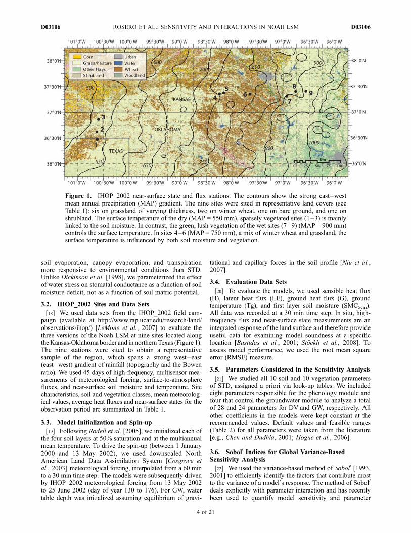
[18] We used data sets from the IHOP_2002 field cam-paign (available at http://www.rap.ucar.edu/research/land/observations/ihop/) [LeMone et al., 2007] to evaluate thethree versions of the Noah LSM at nine sites located alongtheKansas-Oklahoma border and in northern Texas (Figure 1).The nine stations were sited to obtain a representativesample of the region, which spans a strong west–east(east–west) gradient of rainfall (topography and the Bowenratio). We used 45 days of high-frequency, multisensor mea-surements of meteorological forcing, surface-to-atmospherefluxes, and near-surface soil moisture and temperature. Sitecharacteristics, soil and vegetation classes, mean meteorolog-ical values, average heat fluxes and near-surface states for theobservation period are summarized in Table 1.

3.3. Model Initialization and Spin-up

[19] Following Rodell et al. [2005], we initialized each ofthe four soil layers at 50% saturation and at the multiannualmean temperature. To drive the spin-up (between 1 January2000 and 13 May 2002), we used downscaled NorthAmerican Land Data Assimilation System [Cosgrove etal., 2003] meteorological forcing, interpolated from a 60 minto a 30 min time step. The models were subsequently drivenby IHOP_2002 meteorological forcing from 13 May 2002to 25 June 2002 (day of year 130 to 176). For GW, watertable depth was initialized assuming equilibrium of gravi-

tational and capillary forces in the soil profile [Niu et al.,2007].

3.4. Evaluation Data Sets

[20] To evaluate the models, we used sensible heat flux(H), latent heat flux (LE), ground heat flux (G), groundtemperature (Tg), and first layer soil moisture (SMC5cm).All data was recorded at a 30 min time step. In situ, high-frequency flux and near-surface state measurements are anintegrated response of the land surface and therefore provideuseful data for examining model soundness at a specificlocation [Bastidas et al., 2001; Stockli et al., 2008]. Toassess model performance, we used the root mean squareerror (RMSE) measure.

3.5. Parameters Considered in the Sensitivity Analysis

[21] We studied all 10 soil and 10 vegetation parametersof STD, assigned a priori via look-up tables. We includedeight parameters responsible for the phenology module andfour that control the groundwater module to analyze a totalof 28 and 24 parameters for DV and GW, respectively. Allother coefficients in the models were kept constant at therecommended values. Default values and feasible ranges(Table 2) for all parameters were taken from the literature[e.g., Chen and Dudhia, 2001; Hogue et al., 2006].

3.6. Sobol0 Indices for Global Variance-BasedSensitivity Analysis

[22] We used the variance-based method of Sobol0 [1993,2001] to efficiently identify the factors that contribute mostto the variance of a model’s response. The method of Sobol0

deals explicitly with parameter interaction and has recentlybeen used to quantify model sensitivity and parameter

Figure 1. IHOP_2002 near-surface state and flux stations. The contours show the strong east–westmean annual precipitation (MAP) gradient. The nine sites were sited in representative land covers (seeTable 1): six on grassland of varying thickness, two on winter wheat, one on bare ground, and one onshrubland. The surface temperature of the dry (MAP = 550 mm), sparsely vegetated sites (1–3) is mainlylinked to the soil moisture. In contrast, the green, lush vegetation of the wet sites (7–9) (MAP = 900 mm)controls the surface temperature. In sites 4–6 (MAP = 750 mm), a mix of winter wheat and grassland, thesurface temperature is influenced by both soil moisture and vegetation.


4 of 21

D03106

interactions in hydrology [e.g., Tang et al., 2006; Bois et al.,2008; Ratto et al., 2007; Yatheendradas et al., 2008; vanWerkhoven et al., 2008]. Our review of the literature showsthat it has not yet been used for LSM SA.[23] Sobol0 indices enable researchers to distinguish the

subset of independent input factors (such as the model

parameters) X = {x1, . . ., xi, . . ., xk} that account for mostof the variance of the model’s response Y = f (X) either bythemselves (first-order) or due to interaction with otherparameters (higher-order). For completeness, we brieflysummarize the Monte Carlo-based scheme presented by

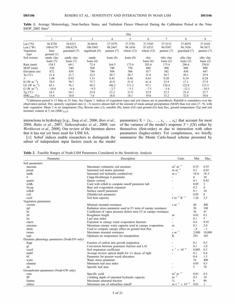
Table 1. Average Meteorology, Near-Surface States, and Turbulent Fluxes Observed During the Calibration Period at the Nine

IHOP_2002 Sitesa

Site

1 2 3 4 5 6 7 8 9

Lat (�N) 36.4728 36.6221 36.8610 37.3579 37.3781 37.3545 37.3132 37.4070 37.4103Lon (�W) 100.6179 100.6270 100.5945 98.2447 98.1636 97.6533 96.9387 96.7656 96.5671Vegetationtype

bareground (1)

grassland (7) sagebrush (9) pasture (7) wheat (12) wheat (12) pasture (7) grassland (7) pasture (7)

Soil texture sandy clayloam (7)

sandy clayloam (7)

sandyloam (4)

loam (8) loam (8) clayloam (6)

silty clayloam (2)

silty clayloam (2)

silty clayloam (2)

Rain (mm) 154.5 69.1 72.4 164.5 173.6 203.6 175.4 296.6 250.8MAP (mm) 530 540 560 740 750 800 900 880 900Elevation (m) 872 859 780 509 506 417 382 430 447Ta (�C) 21.4 21.7 22.5 20.7 20.7 21.0 20.7 20.1 19.9b 1.08 0.92 1.11 0.41 0.46 0.63 0.20 0.14 0.24H (W m�2) 70.5 70.7 75.7 43.9 51.9 61.4 25.9 17.1 27.9LE (W m�2) 65.1 76.1 68.2 106.2 111.2 97.1 126.4 122.8 115.3G (W m�2) �10.4 �6.4 �9.3 �2.7 �5.1 �7.5 �5.6 �12.1 �10.5Tg (�C) 24.1 24.1 25.8 23.2 21.9 22.9 22.3 22.4 22.7SMC5cm (%) 15.4 18.0 7.0 18.0 18.1 19.0 33.2 32.8 34.0

aCalibration period is 13 May to 25 June. See Figure 1. Indices of vegetation types and soil classes are in parenthesis. Rainfall is cumulative over theobservation period. Dry, sparsely vegetated sites (1–3) receive almost half of the amount of mean annual precipitation (MAP) than wet sites (7–9), withlush vegetation. Mean 2 m air temperature (Ta), Bowen ratio (b), sensible (H), latent (LE) and ground (G) heat flux, ground temperature (Tg) and soilmoisture content at 5 cm (SMC5cm).

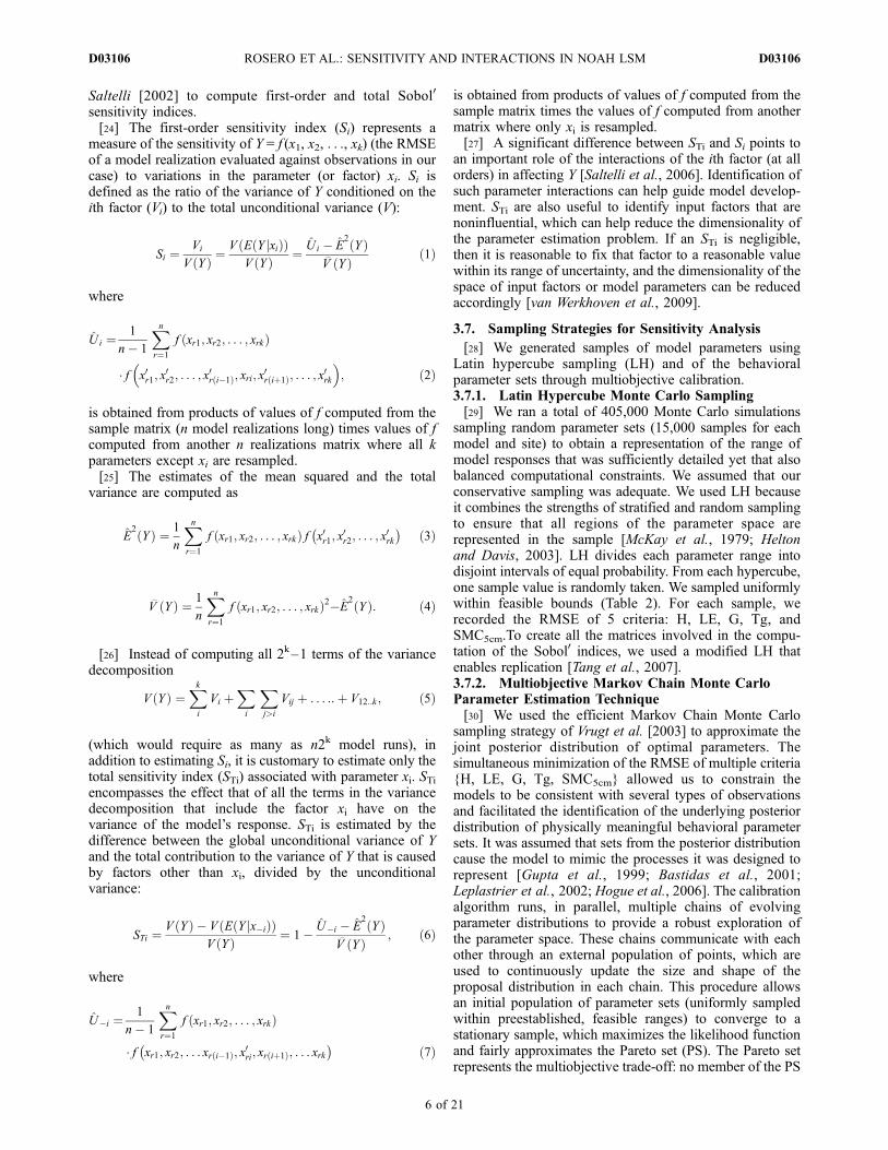
Table 2. Feasible Ranges of Noah-LSM Parameters Considered in the Sensitivity Analysis

Parameter Description Units Min Max

Soil parametersmaxsmc Maximum volumetric soil moisture m3 m�3 0.35 0.55psisat Saturated soil matric potential m m�1 0.1 0.65satdk Saturated soil hydraulic conductivity m s�1 1E-6 1E-5b Clapp-Hornberger b parameter - 4 10quartz Quartz content - 0.1 0.82refdk Used with refkdt to compute runoff parameter kdt 0.05 3fxexp Bare soil evaporation exponent - 0.2 4refkdt Surface runoff parameter 0.1 10czil Zilintikevich parameter - 0.05 8csoil Soil heat capacity J m�3 K�1 1.26 3.5

Vegetation parametersvrcmin Minimal stomatal resistance s m�1 40 400rgl Radiation stress parameter used in F1 term of canopy resistance 30 100hs Coefficient of vapor pressure deficit term F2 in canopy resistance 36 47z0 Roughness length m 0.01 0.1lai Leaf area index - 0.1 5cfactr Exponent in canopy water evaporation function - 0.4 0.95cmcmax Maximum canopy water capacity used in canopy evaporation m 0.1 2.0sbeta Used to compute canopy effect on ground heat flux - �4 �1rsmax Maximum stomatal resistance s m�1 2,000 10,000topt Optimum air temperature for transpiration K 293 303

Dynamic phenology parameters (Noah-DV only)fragr Fraction of carbon into growth respiration - 0.1 0.5gl Conversion between greenness fraction and LAI - 0.1 1.0rssoil Soil respiration coefficient s�1 � 10�6 0.005 0.5tauhf Average inverse optical depth for 1/e decay of light - 0.1 0.4bf Parameter for present wood allocation 0.4 1.3wstrc Water stress parameter 10 400xlaimin Minimum leaf area index - 0.05 0.5sla Specific leaf area - 5 70

Groundwater parameters (Noah-GW only)rous Specific yield m3 m�3 0.01 0.5fff e-folding depth of saturated hydraulic capacity m�1 0.5 10fsatmx Maximum saturated fraction % 0 90rsbmx Maximum rate of subsurface runoff m s�1 � 10�3 0.01 1


5 of 21

D03106

Saltelli [2002] to compute first-order and total Sobol0

sensitivity indices.[24] The first-order sensitivity index (Si) represents a

measure of the sensitivity of Y = f (x1, x2, . . ., xk) (the RMSEof a model realization evaluated against observations in ourcase) to variations in the parameter (or factor) xi. Si isdefined as the ratio of the variance of Y conditioned on theith factor (Vi) to the total unconditional variance (V):

Si ¼Vi

V Yð Þ ¼V E Y jxið Þð Þ

V Yð Þ ¼ U i � E2Yð Þ

V_

Yð Þð1Þ

where

U i ¼1

n� 1

Xnr¼1

f xr1; xr2; . . . ; xrkð Þ

� f x0r1; x0r2; . . . ; x0r i�1ð Þ; xri; x

0r iþ1ð Þ; . . . ; x0rk

� �; ð2Þ

is obtained from products of values of f computed from thesample matrix (n model realizations long) times values of fcomputed from another n realizations matrix where all kparameters except xi are resampled.[25] The estimates of the mean squared and the total

variance are computed as

E2Yð Þ ¼ 1

n

Xnr¼1

f xr1; xr2; . . . ; xrkð Þ f x0r1; x0r2; . . . ; x0rk

� �ð3Þ

V_

Yð Þ ¼ 1

n

Xnr¼1

f xr1; xr2; . . . ; xrkð Þ2�E2Yð Þ: ð4Þ

[26] Instead of computing all 2k–1 terms of the variancedecomposition

V Yð Þ ¼Xki

Vi þXi

Xj>i

Vij þ . . . ::þ V12::k ; ð5Þ

(which would require as many as n2k model runs), inaddition to estimating Si, it is customary to estimate only thetotal sensitivity index (STi) associated with parameter xi. STiencompasses the effect that of all the terms in the variancedecomposition that include the factor xi have on thevariance of the model’s response. STi is estimated by thedifference between the global unconditional variance of Yand the total contribution to the variance of Y that is causedby factors other than xi, divided by the unconditionalvariance:

STi ¼V Yð Þ � V E Y x�ijð Þð Þ

V Yð Þ ¼ 1� U�i � E2Yð Þ

V_

Yð Þ; ð6Þ

where

U�i ¼1

n� 1

Xnr¼1

f xr1; xr2; . . . ; xrkð Þ

� f xr1; xr2; . . . xr i�1ð Þ; x0ri; xr iþ1ð Þ; . . . xrk

� �ð7Þ

is obtained from products of values of f computed from thesample matrix times the values of f computed from anothermatrix where only xi is resampled.[27] A significant difference between STi and Si points to

an important role of the interactions of the ith factor (at allorders) in affecting Y [Saltelli et al., 2006]. Identification ofsuch parameter interactions can help guide model develop-ment. STi are also useful to identify input factors that arenoninfluential, which can help reduce the dimensionality ofthe parameter estimation problem. If an STi is negligible,then it is reasonable to fix that factor to a reasonable valuewithin its range of uncertainty, and the dimensionality of thespace of input factors or model parameters can be reducedaccordingly [van Werkhoven et al., 2009].

3.7. Sampling Strategies for Sensitivity Analysis

[28] We generated samples of model parameters usingLatin hypercube sampling (LH) and of the behavioralparameter sets through multiobjective calibration.3.7.1. Latin Hypercube Monte Carlo Sampling[29] We ran a total of 405,000 Monte Carlo simulations

sampling random parameter sets (15,000 samples for eachmodel and site) to obtain a representation of the range ofmodel responses that was sufficiently detailed yet that alsobalanced computational constraints. We assumed that ourconservative sampling was adequate. We used LH becauseit combines the strengths of stratified and random samplingto ensure that all regions of the parameter space arerepresented in the sample [McKay et al., 1979; Heltonand Davis, 2003]. LH divides each parameter range intodisjoint intervals of equal probability. From each hypercube,one sample value is randomly taken. We sampled uniformlywithin feasible bounds (Table 2). For each sample, werecorded the RMSE of 5 criteria: H, LE, G, Tg, andSMC5cm.To create all the matrices involved in the compu-tation of the Sobol0 indices, we used a modified LH thatenables replication [Tang et al., 2007].3.7.2. Multiobjective Markov Chain Monte CarloParameter Estimation Technique[30] We used the efficient Markov Chain Monte Carlo

sampling strategy of Vrugt et al. [2003] to approximate thejoint posterior distribution of optimal parameters. Thesimultaneous minimization of the RMSE of multiple criteria{H, LE, G, Tg, SMC5cm} allowed us to constrain themodels to be consistent with several types of observationsand facilitated the identification of the underlying posteriordistribution of physically meaningful behavioral parametersets. It was assumed that sets from the posterior distributioncause the model to mimic the processes it was designed torepresent [Gupta et al., 1999; Bastidas et al., 2001;Leplastrier et al., 2002; Hogue et al., 2006]. The calibrationalgorithm runs, in parallel, multiple chains of evolvingparameter distributions to provide a robust exploration ofthe parameter space. These chains communicate with eachother through an external population of points, which areused to continuously update the size and shape of theproposal distribution in each chain. This procedure allowsan initial population of parameter sets (uniformly sampledwithin preestablished, feasible ranges) to converge to astationary sample, which maximizes the likelihood functionand fairly approximates the Pareto set (PS). The Pareto setrepresents the multiobjective trade-off: no member of the PS


6 of 21

D03106

can perform better with respect to one objective withoutsimultaneously performing worse with respect to anothercompeting objective [Gupta et al., 1998]. We used a sampleof 150 parameter sets to represent the posterior distributionof ‘‘behavioral’’ parameter sets.

3.8. Hierarchical Clustering for Comparisonsof Parameter Distributions

[31] Unsupervised classification of the behavioral param-eter distributions allowed us to understand data similaritiesacross locations, with specific focus on the relationshipsbetween types of parameters and sites. We used a clusteringstrategy to classify the marginal posterior distributions ofcalibrated parameters sets into groups. Agglomerative hier-archical clustering methods start with n groups (one objectper group) and successively merge the two most similargroups until a single group is left. We used MATLAB’scomplete linkage algorithm to implement the clustering, inwhich the maximum distance between objects, one comingfrom each cluster, represents the smallest sphere that canenclose all objects in the two groups within a single cluster[Hair et al., 1995]. Because the distance measures (e.g.,Manhattan, Euclidean) used to measure dissimilaritybetween observations may influence the membership ofsamples to groups, we used the cophenetic correlationcoefficient to assess the quality of the linkage [Martinezand Martinez, 2002]. We used dendrograms to visualize thelinks between the objects as inverted U-shaped lines, whoseheight represents the distance between the objects.

4. Which Parameters Are Sensitive?

[32] VSA showed that there are only a few parametersthat, by themselves, exert significant influence on the modelpredictions. In contrast, parameter interaction dominates andis hence the principal mechanism for sensitivity. Figures 2, 3,and 4 present, for all sites, all considered parameters, and allmodels, the Sobol0 first-order sensitivity indexes (Si, whichis the fraction of the total variance of RMSE that can besolely attributed to the ith parameter) and the residualbetween Sobol0’s total and first-order sensitivity index(STi –Si, which is the fraction of total variance that resultsfrom the interaction of the ith parameter with other param-eters at all orders). When the influence of parameterschanged as we would physically expect, we interpret theresults as consistent with our hypothesis that, to a first order,a model adequately represents the site-to-site variation inthe water and energy cycles. Site-to-site variation in themost sensitive parameters is not chiefly governed by soil orvegetation type but, similar to other studies [e.g., Liang andGuo, 2003; Demaria et al., 2007; van Werkhoven et al.,2008], appears to be of secondary importance when com-pared to the influence of the predominant climatic gradient.Although we cannot rule out the potential importance ofother east–west gradients (e.g., the topographic or hydro-geologic gradient), in section 4.1 we provide explanationsfor the observed patterns that are consistent with theclimatological change between sites.

4.1. First-Order Sensitivity (Si)

[33] For several key parameters, a pattern of first-ordersensitivity can be linked to the hydrology of the sites. For

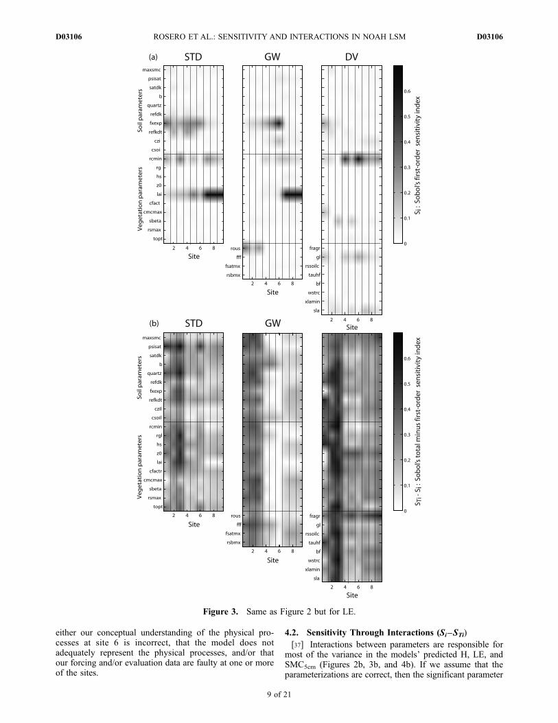
most sites and models, the greatest first-order control onsimulated top layer soil moisture is porosity (maxsmc)(Figure 4a). At dry sites 1–3, where direct evaporation ispresumably a major component of LE flux, for STD andGW, the bare soil evaporation exponent (fxexp) exerts thehighest first-order control on soil moisture. The LE fluxsimulated by GW at dry sites is controlled by fxexp andspecific yield (rous), which partially controls the depth tothe water table. Parameter lai directly controls transpirationand hence the surface energy budget; at the most vegetatedsites (7–9), lai consequently shapes most of the variance ofH and LE for both STD and GW (Figures 2a and 3a). Theinitial value of lai is not important to DV’s simulated H andLE because DV allows lai to change over time. Instead,minimum stomatal resistance (rcmin) exerts the most con-trol on DV-simulated LE. Two new parameters associatedwith DV, gl and sla, which control the calculation of lai, alsoexert first-order control on the simulated energy fluxes. Inthe sparsely vegetated sites (1–3), the Zilintikevich coeffi-cient (czil) plays a significant role in the variance of H.[34] The specific parameters that control model variance

change between models and between sites. In STD, as themean annual precipitation (MAP) increases, fxexp becomesless important to top layer soil moisture (SMC5cm) andrefkdt, a parameter involved in determining maximum ratesof infiltration, becomes more important (Figure 4a). Thispattern changes for GW, in which surface runoff is relativelydeemphasized and subsurface runoff is relatively empha-sized (see discussion about GW’s preferred modes ofoperation, section 5). In GW, although fxexp still exertsfirst-order control on SMC5cm at dry sites, refkdt has littledirect influence on SMC5cm at wet sites. The most sensitiveparameter for SMC5cm at sites 1–3 is rous, which controlswhether aquifer water is accessible to the near-surface soil.Consistent with our expectations, soil suction (psisat), whichin GW controls upward movement of water from the aquiferto the soil, has significant control on SMC5cm within GW butnot within STD, in which psisat plays a less dominant role inshaping soil hydraulic behavior (Figure 4a).[35] Especially in the case of STD and DV, as sites get

wetter, the surface exchange coefficient czil exerts progres-sively less influence and rcmin progressively more influ-ence on H (Figure 2a). The shift is consistent with ourexpectation that at more vegetated sites, stomatal resistanceshould be important to determining the surface energybalance. As a site’s MAP increases, rcmin and lai increas-ingly shape simulated LE, and fxexp becomes less influen-tial (Figure 3a). Even at the dry sites (1–3), DV favorslarger values of vegetation fraction (shdfac) than are pre-scribed by STD and GW. As a consequence, DV standsapart from GW and STD in that fxexp does not directlycontribute to variance of any objective at the three driestsites (with the exception of unvegetated site 1, at which LEis controlled by fxexp).[36] Examinations of Si that are not in line with expect-

ations may be used to help modelers diagnose likelyproblems with conceptualization, forcing data, and/or modelstructure. For instance, in STD, fxexp has the highest Si ofsimulated H and LE at site 6. We do not expect directevaporation to be a relatively more significant component ofthe LE flux at site 6 than at climatically similar sites 4 and 5or at the semiarid sites 1–3. The discrepancy implies that


7 of 21

D03106

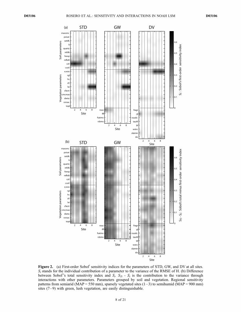
Figure 2. (a) First-order Sobol0 sensitivity indices for the parameters of STD, GW, and DV at all sites.Si stands for the individual contribution of a parameter to the variance of the RMSE of H. (b) Differencebetween Sobol0’s total sensitivity index and Si. STi - Si is the contribution to the variance throughinteractions with other parameters. Parameters grouped by soil and vegetation. Regional sensitivitypatterns from semiarid (MAP = 550 mm), sparsely vegetated sites (1–3) to semihumid (MAP = 900 mm)sites (7–9) with green, lush vegetation, are easily distinguishable.


8 of 21

D03106

either our conceptual understanding of the physical pro-cesses at site 6 is incorrect, that the model does notadequately represent the physical processes, and/or thatour forcing and/or evaluation data are faulty at one or moreof the sites.

4.2. Sensitivity Through Interactions (Si–STi)

[37] Interactions between parameters are responsible formost of the variance in the models’ predicted H, LE, andSMC5cm (Figures 2b, 3b, and 4b). If we assume that theparameterizations are correct, then the significant parameter

Figure 3. Same as Figure 2 but for LE.


9 of 21

D03106

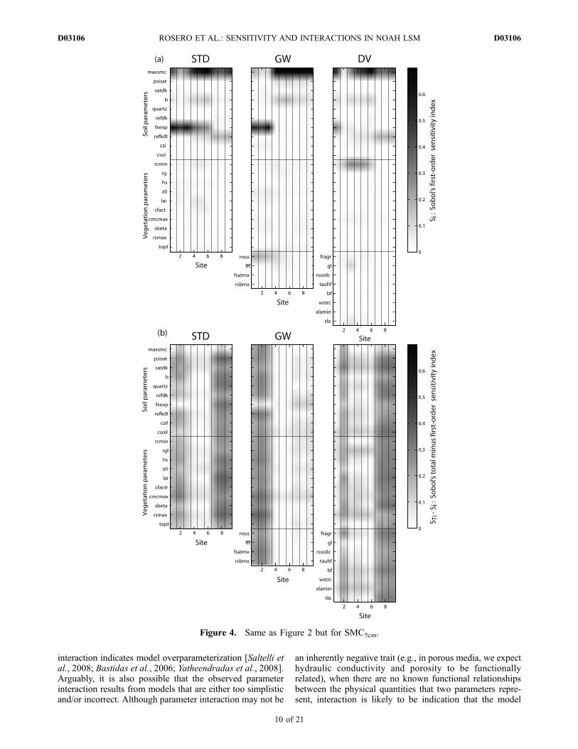
interaction indicates model overparameterization [Saltelli etal., 2008; Bastidas et al., 2006; Yatheendradas et al., 2008].Arguably, it is also possible that the observed parameterinteraction results from models that are either too simplisticand/or incorrect. Although parameter interaction may not be

an inherently negative trait (e.g., in porous media, we expecthydraulic conductivity and porosity to be functionallyrelated), when there are no known functional relationshipsbetween the physical quantities that two parameters repre-sent, interaction is likely to be indication that the model

Figure 4. Same as Figure 2 but for SMC5cm.


10 of 21

D03106

works in a way that is not consistent with the conceptualmodel from which the parameterizations were built.[38] All models exhibit the most parameter interaction at

the driest sites, consistent with the findings of Liang andGuo [2003] and suggesting the need to revise the formula-tion of all three models for semiarid regions [Hogue et al.,2005; Rosero and Bastidas, 2007]. Especially for H andSMC, GW reduces parameter interaction at the middlingmoisture (4–6) and semihumid sites (7–9) (e.g., Figure 5b).GW’s reduction of parameter interaction is evidence(although by no means conclusive) that GW is more realisticthan STD at sites 4–9. This result is consistent withforegoing observations on the robustness of GW [Guldenet al., 2007]. Conversely, GW appears to increase parameterinteraction at the driest sites (1–3), indicating STD betterrepresents semiarid processes than GW. DV parameters aremuch more interactive than those of STD and GW, espe-cially at the wettest sites when simulating LE and SMC5cm.The increased interaction between the DV-specific parame-ters and the rest of the conceptually unrelated STD param-eters suggests DV is not functioning as its developersintended. The significant parameter interaction is consistentwith the poor robustness of DV [Rosero et al., 2009].[39] Looked at in full, the models best represent the

surface water and energy balances at the intermediatemoisture and wet sites, where parameter interaction tends,within a given model, to be lowest. Because it reducesparameter interaction, GW is most likely of any of the threemodels to be representing the key physical processes withthe most realism.

5. How Do Sensitive Parameters Interact andShape Model Behavior? Case Study at Site 7

[40] Toward our objective of thoroughly evaluating thephysical realism of the three models presented, we per-formed a case study in which sensitivity analysis linkedmodel identification and model development. We followedthe impact of shifted preferred values of three physicallymeaningful parameters that made considerable contributionsto the output variance: porosity (smcmax), the muting factorfor vegetation’s effect on thermal conductivity (sbeta), and

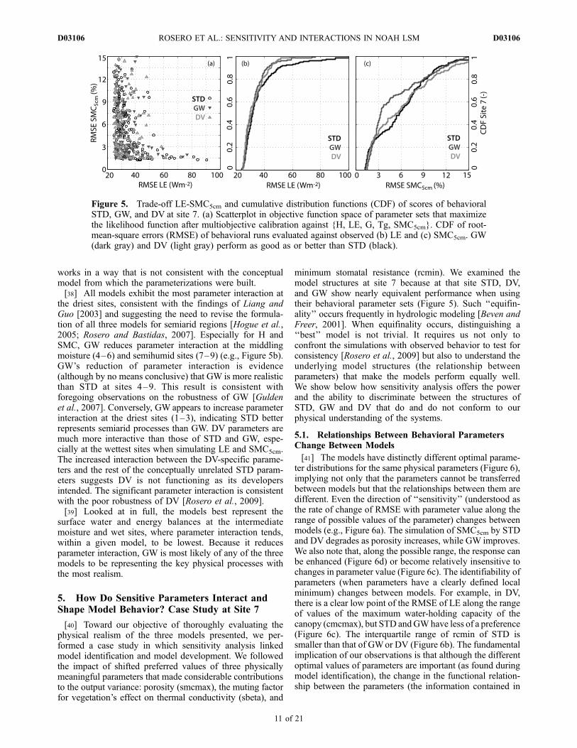
minimum stomatal resistance (rcmin). We examined themodel structures at site 7 because at that site STD, DV,and GW show nearly equivalent performance when usingtheir behavioral parameter sets (Figure 5). Such ‘‘equifin-ality’’ occurs frequently in hydrologic modeling [Beven andFreer, 2001]. When equifinality occurs, distinguishing a‘‘best’’ model is not trivial. It requires us not only toconfront the simulations with observed behavior to test forconsistency [Rosero et al., 2009] but also to understand theunderlying model structures (the relationship betweenparameters) that make the models perform equally well.We show below how sensitivity analysis offers the powerand the ability to discriminate between the structures ofSTD, GW and DV that do and do not conform to ourphysical understanding of the systems.

5.1. Relationships Between Behavioral ParametersChange Between Models

[41] The models have distinctly different optimal parame-ter distributions for the same physical parameters (Figure 6),implying not only that the parameters cannot be transferredbetween models but that the relationships between them aredifferent. Even the direction of ‘‘sensitivity’’ (understood asthe rate of change of RMSE with parameter value along therange of possible values of the parameter) changes betweenmodels (e.g., Figure 6a). The simulation of SMC5cm by STDand DV degrades as porosity increases, while GW improves.We also note that, along the possible range, the response canbe enhanced (Figure 6d) or become relatively insensitive tochanges in parameter value (Figure 6c). The identifiability ofparameters (when parameters have a clearly defined localminimum) changes between models. For example, in DV,there is a clear low point of the RMSE of LE along the rangeof values of the maximum water-holding capacity of thecanopy (cmcmax), but STD andGWhave less of a preference(Figure 6c). The interquartile range of rcmin of STD issmaller than that of GWor DV (Figure 6b). The fundamentalimplication of our observations is that although the differentoptimal values of parameters are important (as found duringmodel identification), the change in the functional relation-ship between the parameters (the information contained in

Figure 5. Trade-off LE-SMC5cm and cumulative distribution functions (CDF) of scores of behavioralSTD, GW, and DV at site 7. (a) Scatterplot in objective function space of parameter sets that maximizethe likelihood function after multiobjective calibration against {H, LE, G, Tg, SMC5cm}. CDF of root-mean-square errors (RMSE) of behavioral runs evaluated against observed (b) LE and (c) SMC5cm. GW(dark gray) and DV (light gray) perform as good as or better than STD (black).


11 of 21

D03106

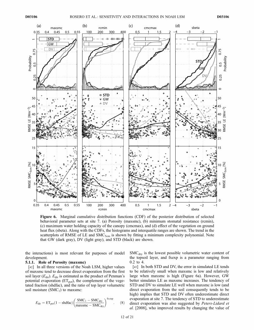
the interactions) is most relevant for purposes of modeldevelopment.5.1.1. Role of Porosity (maxsmc)[42] In all three versions of the Noah LSM, higher values

of maxsmc tend to decrease direct evaporation from the firstsoil layer (Edir). Edir is estimated as the product of Penman’spotential evaporation (ETpot), the complement of the vege-tated fraction (shdfac), and the ratio of top layer volumetricsoil moisture (SMC1) to maxsmc:

Edir ¼ ETpot 1� shdfacð Þ SMC1 � SMCdry

maxsmc� SMCdry

� �fx exp

: ð8Þ

SMCdry is the lowest possible volumetric water content ofthe topsoil layer, and fxexp is a parameter ranging from0.2 to 4.[43] In both STD and DV, the error in simulated LE tends

to be relatively small when maxsmc is low and relativelylarge when maxsmc is high (Figure 6a). However, GWbetter simulates LE as maxsmc increases. The tendency ofSTD and DV to simulate LE well when maxsmc is low (anddirect evaporation from the soil consequently tends to behigh) implies that STD and DV often underestimate directevaporation at site 7. The tendency of STD to underestimatedirect evaporation was also suggested by Peters-Lidard etal. [2008], who improved results by changing the value of

Figure 6. Marginal cumulative distribution functions (CDF) of the posterior distribution of selectedbehavioral parameter sets at site 7. (a) Porosity (maxsmc), (b) minimum stomatal resistance (rcmin),(c) maximum water holding capacity of the canopy (cmcmax), and (d) effect of the vegetation on groundheat flux (sbeta). Along with the CDFs, the histograms and interquatile ranges are shown. The trend in thescatterplots of RMSE of LE and SMC5cm is shown by fitting a minimum complexity polynomial. Notethat GW (dark gray), DV (light gray), and STD (black) are shown.


12 of 21

D03106

fxexp from 2 to 1. Given the same maxsmc, GW moreeasily simulates sufficient direct evaporation, perhapsbecause of wetter soil [Rosero et al., 2009].[44] In STD and DV, parameter maxsmc controls both

surface and subsurface runoff. Hydraulic conductivity(wcnd) is computed by scaling saturated hydraulic conduc-tivity (satdk) by wetness (SMC/maxsmc), raised to anexponent containing the Clapp and Hornberger parameter(b):

wcnd ¼ dksatSMC

maxsmc

� �2bþ3: ð9Þ

Lower maxsmc yields higher wcnd, which means watermoves through the soil more quickly. For subsurface runoff(Runoff2), wcnd controls lateral water movement throughthe soil. In STD and DV, Runoff2 is wcnd times the slope ofthe grid cell. Consequently, higher maxsmc decreasesRunoff2. Higher maxsmc also decreases surface runoff(Runoff1) by increasing the maximum rate of infiltration.Both changes increase soil wetness.[45] GW changes the way runoff is computed; maxsmc

does not control surface or subsurface runoff in GW, whicheliminates two of the three ways that maxsmc controls soilmoisture. Runoff2 is represented as an exponential functionof depth to water [Niu et al., 2007]:

Runoff2 ¼ rsbmx e�fff*ZWT ; ð10Þ

where rsbmx is the maximum rate of subsurface runoff, fffis the e-folding depth of saturated hydraulic conductivity,and ZWT is the depth to the water table, which is computedby the model. Runoff1 is computed using a version of thefunction used to compute Runoff2 [Niu et al., 2005]:

Runoff1 ¼ pcpdrp* fsatmx e�0:5*fff*ZWT

� �; ð11Þ

where pcpdrp is the effective incident water and the secondterm is the fraction of unfrozen grid cell that is saturated.[46] In STD (and DV), maxsmc couples two physically

unrelated (or very weakly related) processes (direct soilevaporation and lateral surface and subsurface runoff). GWdecouples these processes by eliminating the dependence ofparameterized lateral runoff on maxsmc. This decouplingreduces the spurious parameter interaction of maxsmc and,within GW, nearly eliminates the trade-off between goodsimulation of LE and SMC5cm. GW is, in this regard, abetter model for simulating fluxes at site 7.[47] The question remains – why does GW poorly

simulate SMC5cm when maxsmc increases? maxsmc is usedto compute vertical hydraulic conductivity (using the samefunction as STD). GW uses vertical hydraulic conductivityto regulate the flow of water between the aquifer and soildown a hydraulic gradient. Higher maxsmc yields lowerhydraulic conductivity, which, in addition to decreasing thetransfer of water between layers within the soil column,decreases the communication between the aquifer and thesoil profile (that is, it decreases the flow of water betweenthe two, increasing the potential for water to be retainednear the surface). At site 7, GW best simulates SMC5cm

when high vertical hydraulic conductivity connects theaquifer and soil.[48] Consistent with the work of others [e.g., Demaria et

al., 2007], parameter values and model sensitivity tomaxsmc are not consistent between sites along a climaticgradient or even within a set of sites with similar character-istics. Conclusions about model performance are thereforedifficult to generalize. This lack of continuity of behaviorbetween sites is consistent with at least one of the followingpossibilities: (1) model parameterizations do not representkey aspects of the system and/or (2) our multiobjectivecalibration provided insufficient constraint for the estima-tion of behavioral parameters. We suggest the use ofobserved infiltration and/or runoff to increase the strengthof conclusions drawn regarding the physical realism ofrunoff-related processes in GW.5.1.2. Role of the Thermal Conductivity Muting Factor(sbeta)[49] All three models compute ground heat flux (G) using

a flux-gradient relationship:

G ¼ DF1STC1 � T1

0:5*ZSOIL 1ð Þ; ð12Þ

in which STC1 is the temperature at the center of the firstsoil layer (0.5*ZSOIL(1)) and T1 is the surface temperature.DF1 is the heat conductivity of the topsoil layer.[50] Noah assumes that, as vegetation cover increases,

heat flux into the ground decreases. sbeta and the vegetatedfraction (shdfac) mute DF1:

DF1 ¼ DF1esbeta*shdfac: ð13Þ

[51] At site 7, the mode of the posterior probabilitydistribution of all three models is near the bound of theexplored parameter range (�1) (Figure 6d). The preferencefor near-bound values is more pronounced in DV, which atsite 7 tends to have shdfac values near 1.0 (putting down-ward pressure on the value of sbeta). The skewed posteriorparameter distributions suggest that an even less negativevalue of sbeta may have yielded better results at site 7.[52] The assumption that vegetation necessarily decreases

the thermal conductivity of the top layer of the soil may beincorrect. If the ‘‘vegetation effect’’ on thermal conductivityis real, then the model underestimates the top layer soilthermal conductivity. At site 7 (and at several other sites),there is a clear trade-off between H and G that is mediatedby the thermal conductivity. The trade-off suggest a need forrevised process representation.[53] When comparing site 7 simulations to those of the

other two wet sites (8 and 9), we see a roughly consistentpreference for near zero values of sbeta. At the drier sites(1–6), the model’s strong preference for near zero values ofsbeta is less obvious; however, shdfac is closer to zero atthese sites, which lowers the value of the muting factorequation (13).5.1.3. Role of Minimum Stomatal Resistance (rcmin)[54] Parameter rcmin controls much of the variance in H

and LE, especially at the wetter sites. As rcmin increases,the ratio of actual to potential evapotranspiration decreases.


13 of 21

D03106

Overall, rcmin has a more consistent influence on thevariance of H than on that of LE.[55] At site 7, all three models perform best with low

values for rcmin (Figure 6b), which increases LE for a givenpotential evapotranspiration; however, rcmin is less identi-fiable in GW and DV. The mode of the rcmin distribution ishigher for GW than for STD, perhaps because GW tends tohave a wetter soil and a more robust simulation of LE. Thespread of the posterior parameter distribution of rcmin forDV is significantly larger than that for STD, although bothmodels share the same mode. This decrease in identifiabilityof parameters functionally related to lai (as is rcmin) isconsistent with the added degrees of freedom available inDV (DV parameters gl and sla are most important inpredicting lai) (Figure 2). Because DV simulations includea wider spread of lai states, they also have a wider spread of‘‘good’’ rcmin values.

5.2. How Does GW Have to Be Adjusted to Make ItWork Better Than or as Well as STD at Site 7?

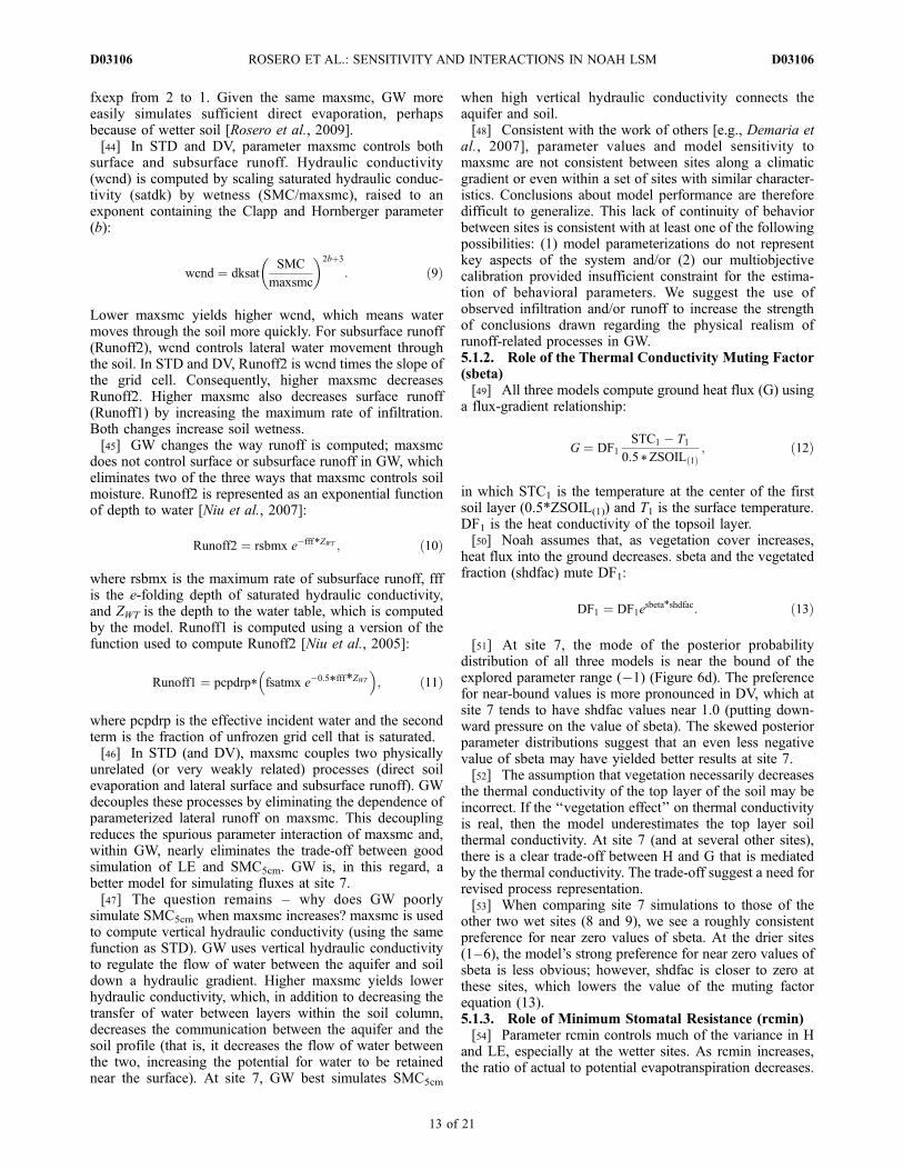
[56] The response surface of RMSE SMC5cm changesbetween STD and GW (Figure 7; e.g., see maxsmc versuspsisat). For GW, the shape of the bivariate posterior dis-tributions of soil parameters that are shared with STD issignificantly different, presumably because of interaction ofthe GW parameters and module with those of STD. Suchshifts in model function affect the model covariance struc-ture as shown in Table 3.[57] After multiobjective parameter estimation at site 7,

GW functions in one of two preferred modes (Figure 7b). Inthe slightly preferred first mode (m1), the parameters worktogether to help GW function as the developers likelyintended. Strong communication between the aquifer andthe soil column is supported by relatively high values ofsaturated hydraulic conductivity (satdk), low values of thereciprocal of the e-folding depth of hydraulic conductivity

Figure 7. Multivariate posterior distribution of the behavioral parameters of STD and GW at site 7shown for selected parameter combinations in bivariate plots. Higher density of parameter values areindicated with increasingly redder contours. The response surface of SMC5cm is shown in the back;darker regions have higher errors. The bimodal behavior of GW is signaled by m1 and m2. See text forexplanation.


14 of 21

D03106

(fff), and low porosity (maxsmc). A relatively low surfacerunoff scaling factor (fsatmx) and a relatively high subsur-face runoff scaling factor (rsbmx) ensure that subsurfacerunoff dominates surface runoff. Consistent with naturalprocesses, high soil suction (psisat) pulls water upward. Ahigh aquifer specific yield (rous) deepens the water table(weakening the direct influence of the saturated zone on themodel soil column) and transforms more water to runoffrather than to recharge.[58] In the second mode (m2), GW adopts parameter

values that make the model work as one would expectSTD to function (i.e., the model operates with parametersthat render GW nonfunctional) (Figure 7b). Relatively highvalues of fff effectively seal the bottom of the soil column,limiting communication between the aquifer and the soilcolumn; high maxsmc decreases the vertical conductivity,further inhibiting the already poor communication. Highmaxsmc favors decreased direct evaporation. Surface runoffis augmented by a relatively high fsatmx; subsurface runoffis lessened by the relatively low rsbmx.[59] These alternative behaviors are a possible explana-

tion for the issue identified by Rosero et al. [2009], whoshowed that despite very good performance of calibratedGW, the model suffered from low robustness (i.e., a highsensitivity to unmeasurable parameters).

5.3. How Does DV Have to be Adjusted to Make ItWork Better Than or as Well as STD at Site 7?

[60] STD and DV functionally differ in two ways: (1) STDprescribes shdfac using monthly climatological values (�0.7at site 7), while DV predicts it as a function of environmentalvariation in moisture and radiation availability and (2) STDtreats lai as a parameter, while DV uses shdfac to predict laivariation using a functional relationship:

lai ¼ max xlaimin;�1gl

log�1 1� shdfacð Þ� �

: ð14Þ

[61] Vegetation affects all components of LE flux (viashdfac): (1) vegetation shades the soil, modulating directevaporation (Edir); (2) vegetation retains water above thesoil, contributing to evaporation from the canopy (Ec); and(3) vegetation fuels transpiration (Etransp). In DV, a highvalue of conversion parameter gl fixes shdfac near 1 andyields a regime in which Ec and Etransp are strongly favoredover Edir. Low values of gl fix shdfac near zero and promote

a regime in which Edir is the dominant component of LE.When shdfac is near zero, both Ec and Etransp are minimized.At sites with sufficient vegetation, DV enables the model tocorrectly give more weight to Etransp. STD, unable to changethe value of shdfac to shift the balance of components ofLE, favors higher lai (which decreases stomatal resistanceand increases Etransp) as means for increasing total LE.[62] When compared to STD, DV can achieve ‘‘good’’

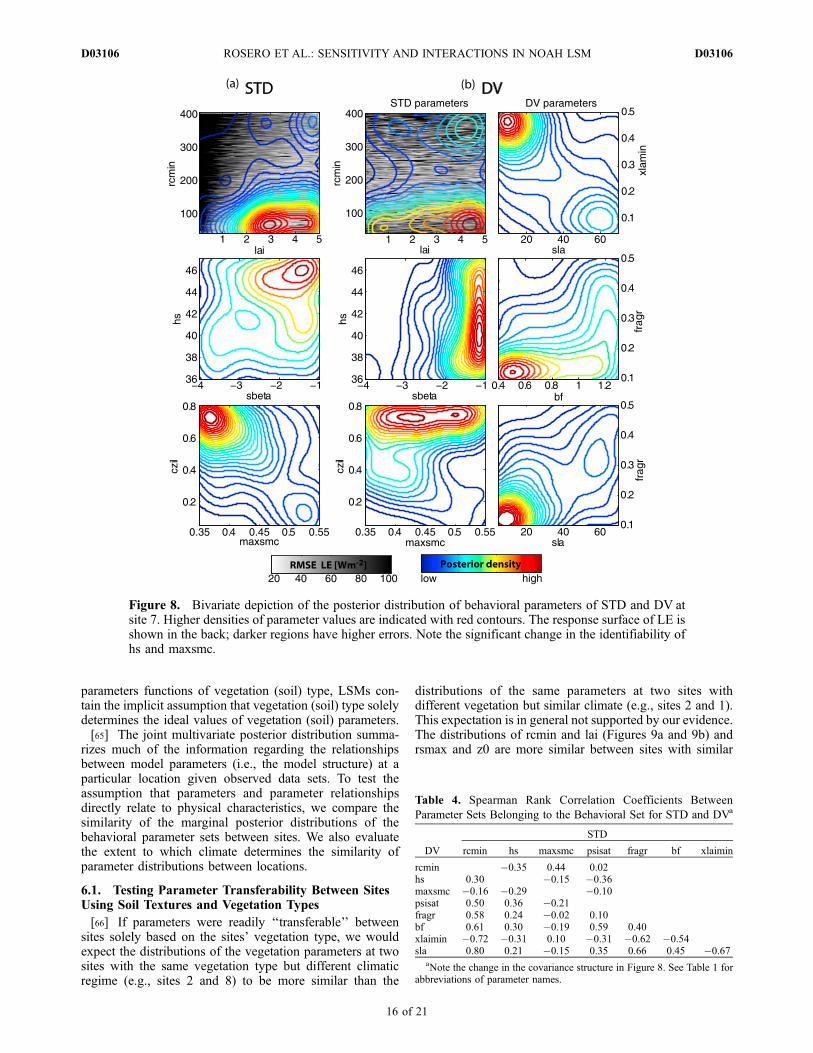
model performance using a wider range of values for shdfacand lai. We see this decreased identifiability of DV param-eters when comparing the bivariate posterior parameterdistributions of STD to those of DV at site 7 (Figure 8).The identifiability in the response surface of RMSE LE haschanged (e.g., lai versus rcmin) (Figure 8). The decrease inidentifiability of parameters that are functionally related toshdfac and/or lai can be seen across the IHOP sites (resultsnot shown). The interplay of the parameters of the DVmodule also leads to changes in parameter densities of STDand DV (Figure 8). We see additional evidence for increasedinteraction between parameters in DV when we note that themodels’ covariance structure has been altered (Table 4). Forexample, rcmin and maxsmc are positively correlated inSTD, but in DV they have a very slight negative correlation.[63] Although the increased flexibility of lai and shdfac

values may improve the model’s simulation of seasonal andinterannual variation in surface fluxes, over time scalesexamined here, DV does not appear to improve the model.The constraints imposed by the turbulent and near-surfacestates may be insufficient for the complexity of the modeland/or DV may need to be constrained with observations ofcarbon fluxes and plant growth. When there is little vege-tation (e.g., at sites 1–3), DV may be failing to considerspecial water use features associated with the semiaridvegetation [Unland et al., 1996]. The function of the DVmodule may also be hindered by Noah’s lack of a separatecanopy layer [Rosero et al., 2009] and/or by the absence ofa more complex Ball-Berry type of stomatal conductanceformulation (Niu et al., unpublished manuscript, 2009).

6. What Are the Implications of Our SensitivityAnalysis Results for Parameter Transferability?

[64] Our foregoing assessments have shown that param-eter interaction is a significant contributor to model variance(section 4) and that the behavioral posterior parameterdistributions for a given site change between models(section 5) and for a given model between sites (not shown;see Figure 9). These observations challenge the long-standingassumption of land surface modeling that LSM parametersare physically meaningful quantities. Because developershave attempted to use physical principles when designingLSMs, physically based model parameters have been as-sumed to correspond to physical characteristics of a system[e.g., Dickinson et al., 1986], which can be either measuredin the field (e.g., porosity) or inferred from (remotelysensed) observations (e.g., LAI). Identical LSM parametersare used in locations that share the same physical character-istics [e.g., Sellers et al., 1996]. ‘‘Parameter transferability,’’the a priori assignment of parameter values based on a site’sphysical characteristics (e.g., soil and vegetation type),depends on the appropriateness of the above stated assump-tion. By making sets of vegetation-related (soil-related)

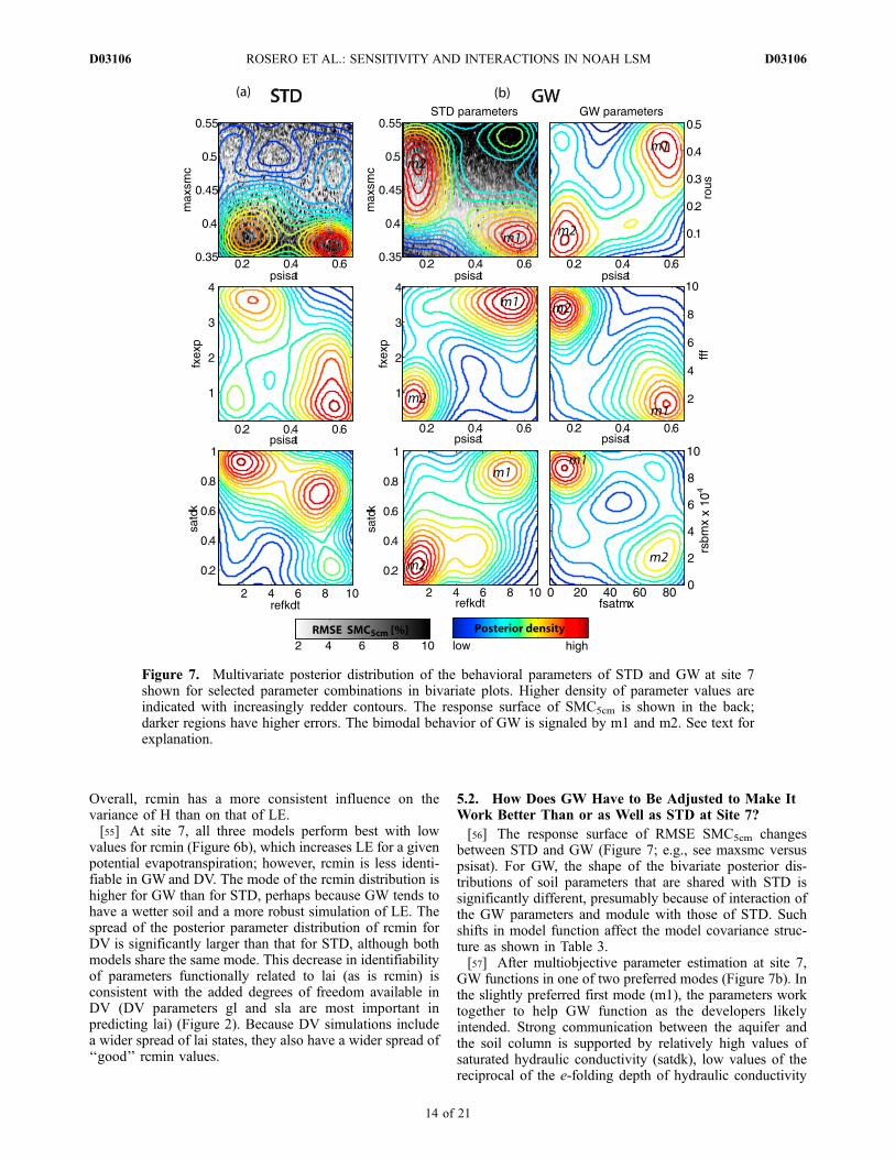
Table 3. Spearman Rank Correlation Coefficients Between

Parameter Sets Belonging to the Behavioral Set for STD and GWa

GW

STD

maxsmc psisat satdk fxexp rous fff fsatmx

maxsmc �0.10 �0.40 0.29psisat �0.33 �0.14 �0.32satdk �0.09 0.49 0.22fxexp �0.26 0.41 0.23rous �0.01 0.26 0.24 0.14fff 0.11 �0.46 �0.45 �0.49 �0.37fsatmx �0.22 �0.04 �0.17 0.09 �0.37 0.17rsbmx 0.11 �0.25 �0.13 �0.21 0.32 0.08 �0.24

aNote the change in the covariance structure in Figure 7. See Table 1 forabbreviations of parameter names.


15 of 21

D03106

parameters functions of vegetation (soil) type, LSMs con-tain the implicit assumption that vegetation (soil) type solelydetermines the ideal values of vegetation (soil) parameters.[65] The joint multivariate posterior distribution summa-

rizes much of the information regarding the relationshipsbetween model parameters (i.e., the model structure) at aparticular location given observed data sets. To test theassumption that parameters and parameter relationshipsdirectly relate to physical characteristics, we compare thesimilarity of the marginal posterior distributions of thebehavioral parameter sets between sites. We also evaluatethe extent to which climate determines the similarity ofparameter distributions between locations.

6.1. Testing Parameter Transferability Between SitesUsing Soil Textures and Vegetation Types

[66] If parameters were readily ‘‘transferable’’ betweensites solely based on the sites’ vegetation type, we wouldexpect the distributions of the vegetation parameters at twosites with the same vegetation type but different climaticregime (e.g., sites 2 and 8) to be more similar than the

distributions of the same parameters at two sites withdifferent vegetation but similar climate (e.g., sites 2 and 1).This expectation is in general not supported by our evidence.The distributions of rcmin and lai (Figures 9a and 9b) andrsmax and z0 are more similar between sites with similar

Figure 8. Bivariate depiction of the posterior distribution of behavioral parameters of STD and DV atsite 7. Higher densities of parameter values are indicated with red contours. The response surface of LE isshown in the back; darker regions have higher errors. Note the significant change in the identifiability ofhs and maxsmc.

Table 4. Spearman Rank Correlation Coefficients Between

Parameter Sets Belonging to the Behavioral Set for STD and DVa

DV

STD

rcmin hs maxsmc psisat fragr bf xlaimin

rcmin �0.35 0.44 0.02hs 0.30 �0.15 �0.36maxsmc �0.16 �0.29 �0.10psisat 0.50 0.36 �0.21fragr 0.58 0.24 �0.02 0.10bf 0.61 0.30 �0.19 0.59 0.40xlaimin �0.72 �0.31 0.10 �0.31 �0.62 �0.54sla 0.80 0.21 �0.15 0.35 0.66 0.45 �0.67

aNote the change in the covariance structure in Figure 8. See Table 1 forabbreviations of parameter names.


16 of 21

D03106

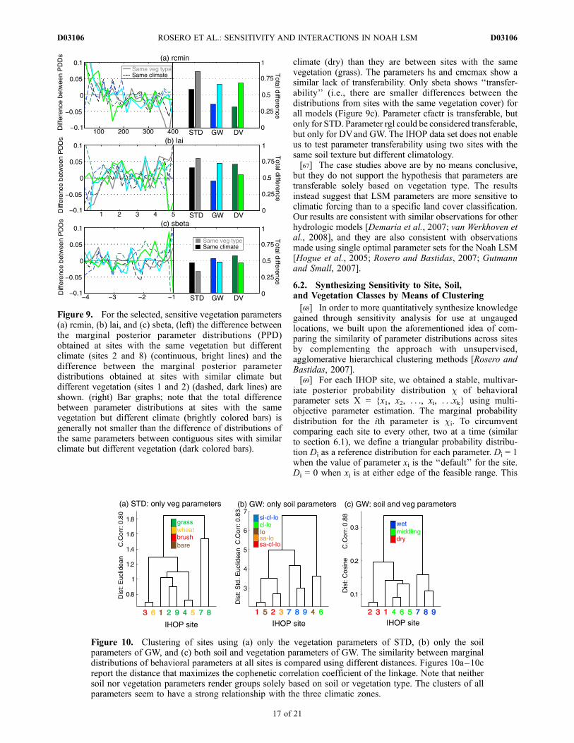
climate (dry) than they are between sites with the samevegetation (grass). The parameters hs and cmcmax show asimilar lack of transferability. Only sbeta shows ‘‘transfer-ability’’ (i.e., there are smaller differences between thedistributions from sites with the same vegetation cover) forall models (Figure 9c). Parameter cfactr is transferable, butonly for STD. Parameter rgl could be considered transferable,but only for DVand GW. The IHOP data set does not enableus to test parameter transferability using two sites with thesame soil texture but different climatology.[67] The case studies above are by no means conclusive,

but they do not support the hypothesis that parameters aretransferable solely based on vegetation type. The resultsinstead suggest that LSM parameters are more sensitive toclimatic forcing than to a specific land cover classification.Our results are consistent with similar observations for otherhydrologic models [Demaria et al., 2007; van Werkhoven etal., 2008], and they are also consistent with observationsmade using single optimal parameter sets for the Noah LSM[Hogue et al., 2005; Rosero and Bastidas, 2007; Gutmannand Small, 2007].

6.2. Synthesizing Sensitivity to Site, Soil,and Vegetation Classes by Means of Clustering

[68] In order to more quantitatively synthesize knowledgegained through sensitivity analysis for use at ungaugedlocations, we built upon the aforementioned idea of com-paring the similarity of parameter distributions across sitesby complementing the approach with unsupervised,agglomerative hierarchical clustering methods [Rosero andBastidas, 2007].[69] For each IHOP site, we obtained a stable, multivar-

iate posterior probability distribution c of behavioralparameter sets X = {x1, x2, . . ., xi, . . .xk} using multi-objective parameter estimation. The marginal probabilitydistribution for the ith parameter is ci. To circumventcomparing each site to every other, two at a time (similarto section 6.1), we define a triangular probability distribu-tion Di as a reference distribution for each parameter. Di = 1when the value of parameter xi is the ‘‘default’’ for the site.Di = 0 when xi is at either edge of the feasible range. This

Figure 9. For the selected, sensitive vegetation parameters(a) rcmin, (b) lai, and (c) sbeta, (left) the difference betweenthe marginal posterior parameter distributions (PPD)obtained at sites with the same vegetation but differentclimate (sites 2 and 8) (continuous, bright lines) and thedifference between the marginal posterior parameterdistributions obtained at sites with similar climate butdifferent vegetation (sites 1 and 2) (dashed, dark lines) areshown. (right) Bar graphs; note that the total differencebetween parameter distributions at sites with the samevegetation but different climate (brightly colored bars) isgenerally not smaller than the difference of distributions ofthe same parameters between contiguous sites with similarclimate but different vegetation (dark colored bars).

Figure 10. Clustering of sites using (a) only the vegetation parameters of STD, (b) only the soilparameters of GW, and (c) both soil and vegetation parameters of GW. The similarity between marginaldistributions of behavioral parameters at all sites is compared using different distances. Figures 10a–10creport the distance that maximizes the cophenetic correlation coefficient of the linkage. Note that neithersoil nor vegetation parameters render groups solely based on soil or vegetation type. The clusters of allparameters seem to have a strong relationship with the three climatic zones.


17 of 21

D03106

step allows us to introduce the assumption that theparameters relate to soil and vegetation types.[70] For each parameter, and at each site, we quantify the

closeness between the cumulative distribution of the ‘‘opti-mal’’ values of xi (i.e., the marginal ci) and the referencedistribution Di. We use the Hausdorff norm to quantify thedifference ci – Di. For each model, the matrix of similarityof the marginal distributions of k parameters at all the nevaluation sites is

S ¼c11 � D11 . . . ck1 � Dk1

. . . . . . . . .ck1 � Dk1 . . . ckn � Dkn

24

35: ð15Þ

S can be used to identify groups of parameters that aresimilar between locations or to identify locations wheregroups of parameters behave alike. We use the unsuper-vised, agglomerative hierarchical clustering algorithm(described in section 3.8) to find these groups withoutmaking any further assumptions about the number ofgroups.[71] If the previously described assumption of parameter

transferability based on site characteristics holds (and ifIHOP vegetation classifications are correct), then, given theset of similarity vectors created using the set of vegetationparameter distributions S(xveg,1..n), a clustering procedureshould be able to classify similar sites in groups thatresemble the IHOP vegetation type groupings (Table 1).Similarly, clustering of S(xsoil,1..n) would result in sitesgrouped according to the IHOP soil texture classification(Table 1).

[72] Applying a suite of distance metrics (e.g., Manhat-tan, Euclidean, Cosine), neither soil nor vegetation param-eters render groups of sites that partition solely based on theexpected soil or vegetation classifications. Figure 10a showsthe classification tree (dendrogram) for STD using theEuclidean distance, which maximizes the cophenetic corre-lation coefficient of the linkage (also shown). None of thedistance metrics allowed us to classify S(xveg,1..n) by loca-tion in a way that matched the IHOP vegetation classifica-tions. Given the subset S(xsoil,1..n), composed of thesimilarity vectors of the 10 soil parameters at all sites,classification of the IHOP sites according to soil character-istics was also not feasible (Figure 10b). Using similarityvectors for STD, GW, and DV, some (but not all) of thedistances identified sites 7, 8, and 9 as having the same soiland same vegetation type (although, because they also sharethe same climate type, we are unable to definitively attributesuch classification to shared vegetation type). The rest of thesites do not strongly coalesce according to physical prop-erties. For example, the pasture sites are not distinctivelygrouped; sites 5 and 6 (wheat crops) are never groupedaccording to vegetation (Figure 10a). Sites 1 and 2 (sandyclay loam) and sites 4 and 5 (loam) do not cluster togetherusing soil parameters (Figure 10b). These results are con-sistent with earlier findings presented here, which suggestthat interaction between soil and vegetation parameters issignificant (section 4), to the point that it shapes theposterior parameter distributions (section 5). These resultsalso suggest that soil and vegetation type are not, bythemselves, good physical characteristics by which totransfer parameters.[73] To account for interdependence between soil and

vegetation parameters, we classified the entire matrixS(xsoil,xveg). If parameters can be transferred based onshared vegetation and soil type, then the clustering of theentire matrix should identify groups of sites with the samevegetation and soil type (e.g., sites 7–9). Figure 10c showsa pattern (found with several distances) that is consistentacross models: sites 7–9 cluster together. Sites 7, 8, and 9also have similar climates, and the classification of the sitesshows strong resemblance to the climatic gradient. Giventhis data set, we cannot disprove the contention thatparameters can be transferred between sites that have boththe same vegetation and soil type.[74] If we instead cluster S looking for groups of param-

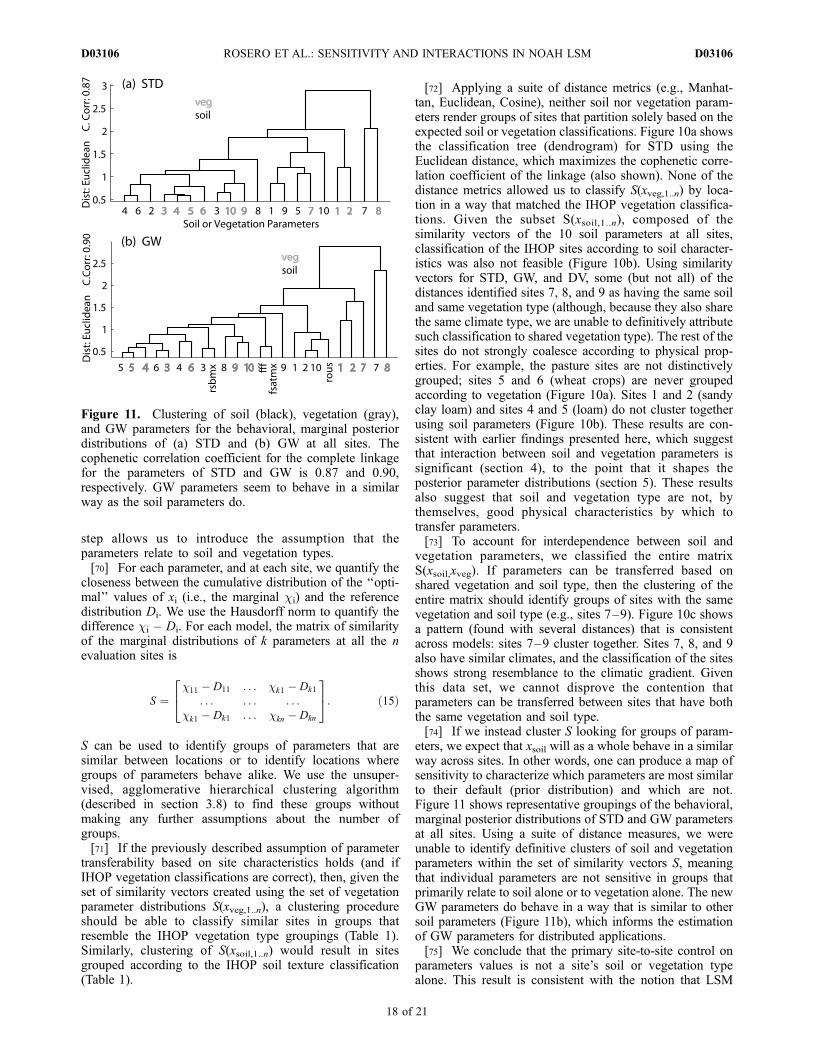
eters, we expect that xsoil will as a whole behave in a similarway across sites. In other words, one can produce a map ofsensitivity to characterize which parameters are most similarto their default (prior distribution) and which are not.Figure 11 shows representative groupings of the behavioral,marginal posterior distributions of STD and GW parametersat all sites. Using a suite of distance measures, we wereunable to identify definitive clusters of soil and vegetationparameters within the set of similarity vectors S, meaningthat individual parameters are not sensitive in groups thatprimarily relate to soil alone or to vegetation alone. The newGW parameters do behave in a way that is similar to othersoil parameters (Figure 11b), which informs the estimationof GW parameters for distributed applications.[75] We conclude that the primary site-to-site control on

parameters values is not a site’s soil or vegetation typealone. This result is consistent with the notion that LSM

Figure 11. Clustering of soil (black), vegetation (gray),and GW parameters for the behavioral, marginal posteriordistributions of (a) STD and (b) GW at all sites. Thecophenetic correlation coefficient for the complete linkagefor the parameters of STD and GW is 0.87 and 0.90,respectively. GW parameters seem to behave in a similarway as the soil parameters do.


18 of 21

D03106

parameters, which must represent physical processes acrossmultiple scales, are ‘‘effective’’ values rather than physical-ly derived quantities [Wagener and Gupta, 2005]. It is alsoconsistent with the assertion that interaction between classesof parameters (e.g., ‘‘soil’’ parameters and ‘‘vegetation’’parameters) is very important. Our clustering analysissuggests that climate is a major control of site-to-sitevariation in parameter values and supports recommenda-tions that climate be considered when transferring parametervalues between sites [Liang and Guo, 2003; Demaria et al.,2007; van Werkhoven et al., 2008].

7. Summary and Conclusion

[76] Sensitivity analysis allows us to draw conclusionsregarding land surface model (LSM) development andmodel assessment practices, the functioning of three ver-sions of the widely used versions of the Noah LSM, and thea priori estimation of parameter values. Our work yieldsseveral conclusions that can be generalized to LSM andother environmental models in general, and several con-clusions that are specific to the Noah LSM.[77] We show that the clear patterns of parameter impor-

tance identified by variance-based sensitivity analysis(VSA) are consistent with site-to-site variation in climateand with model-to-model changes in physical parameteri-zation. VSA shows that parameter interactions within modelsexert significant control on the model output variance.Shifts in parametric control on variance and covariance hintat whether a model represents the water and energy cycles ina way that is consistent with the assumptions underlying themodels. Although the optimal value of a parameter is usefulinformation, the change in the functional relationshipbetween parameters is more likely to be relevant for modeldevelopment and hypothesis testing.[78] Transfer of parameters based solely on similarity in

vegetation type or soil texture is not a viable method for apriori parameter estimation. The work presented here showsthat vegetation type and soil texture are not the mostsignificant contributors to site-to-site variation in optimalparameter values. Interaction between soil and vegetationparameters is significant and varies between sites; andexplains at least partially why the transfer of parametersbased solely on shared vegetation type or soil texture doesnot work. The primary factor controlling site-to-site varia-tion in parameters is likely to be climate, although, given therelatively small data set used here, the combination of asite’s vegetation type and soil texture or some unidentifiedfactor cannot be ruled out as the dominant controllingfactor. The lack of viability of parameter transfer basedsolely on soil and vegetation type is a conclusion that hassignificant implications for the field of regional and globalland surface modeling, which depends on parameter transferbased on stand-alone vegetation type and soil texture as ameans for a priori parameter estimation.[79] Looking specifically at the performance of the three

versions of the Noah LSM used in this study (STD, GW,and DV), we make several nonsite-specific conclusionsregarding model behavior. All three models exhibit signif-icant parameter interaction, indicating that the models areoverparameterized and/or underconstrained. All three showthe least parameter interaction at the middling moisture and

wet sites and the most parameter interaction at the threedriest sites. This difference suggests a need for reformula-tion of Noah LSM such that semiarid regions are morerealistically represented. On the whole, GW has lessparameter interaction than STD (except at dry sites), indi-cating that it represents land surface system with the mostrealism of any of the three models. GW is also least sensitiveto errant parameters at the wettest sites (where groundwateris likely the most influential). DV has much more parameterinteraction than STD, which provides evidence that themodel is not performing as its developers intended, doesnot add value to STD, and/or requires additional constraint.Specific to site 7, we make the following observations:(1) STD and DV tend to underestimate direct evaporationfrom the soil and (2) GW does not (maybe because of wetsoil). The assumption that vegetation decreases the thermalconductivity of the top layer of the soil is not well supportedby the data (this conclusion can be roughly generalized toother sites, especially the wet sites). At site 7, GW functionsin one of two modes – the slightly preferred mode works ina way that mirrors what the developers likely intended; thesecond mode makes GW function as one might expect STDto work. Constraining runoff may isolate the more realisticmode. GW has less spurious parameter interaction in partbecause it decouples direct evaporation and subsurfacerunoff (which are coupled via porosity in STD and DV).This decoupling appears to make the model function morerealistically, with less trade-off between the simulation ofsoil moisture and LE. Adding modules (DV, GW) decreasesthe identifiability of minimum stomatal resistance, althoughall three models prefer low minimum stomatal resistance(thus increasing LE for a given set of conditions). Acrossseveral sites, DV functions in one of two modes (1) the firstemphasizes direct soil and canopy evaporation over tran-spiration and (2) the second emphasizes transpiration overdirect evaporation from the soil and canopy.[80] Our approach to sensitivity analysis complements

new methods for characterizing typical modes of LSMbehavior [Gulden et al., 2008b; Rosero et al., 2009] withina model diagnostic framework [Gupta et al., 2008] thathelps bridge the gap between model identification anddevelopment. We encourage other modeling groups toperform similar analyses with their models as a way toensure rapid, continued improvement of our understandingand modeling of environmental processes.

[81] Acknowledgments. We thank Pedro Restrepo at OHD/NWS,Dave Gochis at NCAR and Ken Mitchell at NCEP for their insight. Weappreciated suggestions by M. Bayani Cardenas, Charles S. Jackson, andthe comments of two anonymous reviewers. We acknowledge the Interna-tional H2O Project for the data sets. We benefited from the computationalresources at the Texas Advanced Computing Center (TACC). The firstauthor was supported by the Graduate Fellowship of the HydrologyTraining Program of the OHD/NWS. This project was also funded by theNOAA grant NA07OAR4310216, NSF, and the Jackson School ofGeosciences.

ReferencesAbramowitz, G., R. Leuning, M. Clark, and A. Pitman (2008), Evaluatingthe performance of land surface models, J. Clim., 21, 5468–5481,doi:10.1175/2008JCLI2378.1.

Bastidas, L. A., H. V. Gupta, S. Sorooshian, W. J. Shuttleworth, and Z. L.Yang (1999), Sensitivity analysis of a land surface scheme using multi-criteria methods, J. Geophys. Res., 104(D16), 19,481 – 19,490,doi:10.1029/1999JD900155.


19 of 21

D03106

Bastidas, L. A., H. V. Gupta, and S. Sorooshian (2001), Bounding theparameters of land-surface schemes using observational data, in LandSurface Hydrology, Meteorology, and Climate: Observations and Modeling,Water Sci. Appl., vol. 3, edited by V. Lakshmi et al., pp. 65–76, AGU,Washington, D. C.

Bastidas, L. A., T. S. Hogue, S. Sorooshian, H. V. Gupta, and W. J.Shuttleworth (2006), Parameter sensitivity analysis for different com-plexity land surface models using multicriteria methods, J. Geophys.Res., 111, D20101, doi:10.1029/2005JD006377.

Beck, M. B. (1987), Water quality modeling: A review of the analysis ofuncertainty, Water Resour. Res., 23, 1393 – 1442, doi:10.1029/WR023i008p01393.

Beven, K. J., and J. Freer (2001), Equifinality, data assimilation, anduncertainty estimation in mechanistic modelling of complex environ-mental systems using the GLUE methodology, J. Hydrol., 249, 11–29,doi:10.1016/S0022-1694(01)00421-8.

Bois, B., et al. (2008), Using remotely sensed solar radiation data forreference evapotranspiration estimation at a daily time step, Agric. For.Meteorol., 148, 619–630, doi:10.1016/j.agrformet.2007.11.005.

Chen, F., and J. Dudhia (2001), Coupling an advanced land surface–hydrology model with the Penn State–NCAR MM5 Modeling System.Part I: Model implementation and sensitivity, Mon. Weather Rev., 129,569–585, doi:10.1175/1520-0493(2001)129<0569:CAALSH>2.0.CO;2.

Cosgrove, B. A., et al. (2003), Real-time and retrospective forcing in theNorth American Land Data Assimilation System (NLDAS) project,J. Geophys. Res., 108(D22), 8842, doi:10.1029/2002JD003118.

Demaria, E. M., B. Nijssen, and T. Wagener (2007), Monte Carlo sensitivityanalysis of land surface parameters using the Variable Infiltration Capa-city model, J. Geophys. Res., 112, D11113, doi:10.1029/2006JD007534.

Dickinson, R. E., A. Henderson-Sellers, P. J. Kennedy, and M. F. Wilson(1986), Biosphere-Atmosphere Transfer Scheme (BATS) for the NCARCommunity Climate Model, NCAR Tech. Note NCAR/TN-275+STR,69 pp., Natl. Cent. for Atmos. Res., Boulder, Colo.

Dickinson, R. E., M. Shaikh, R. Bryant, and L. Graumlich (1998), Inter-active canopies for a climate model, J. Clim., 11, 2823 – 2836,doi:10.1175/1520-0442(1998)011<2823:ICFACM>2.0.CO;2.

Ek, M. B., et al. (2003), Implementation of Noah land surface modeladvances in the National Centers for Environmental Prediction opera-tional mesoscale Eta model, J. Geophys. Res., 108(D22), 8851,doi:10.1029/2002JD003296.

Gao, X., S. Sorooshian, and H. V. Gupta (1996), Sensitivity analysis of thebiosphere-atmosphere transfer scheme, J. Geophys. Res., 101(D3),7279–7289, doi:10.1029/95JD03161.

Gulden, L. E., E. Rosero, Z.-L. Yang, M. Rodell, C. S. Jackson, G.-Y. Niu,P. J.-F. Yeh, and J. Famiglietti (2007), Improving land-surface modelhydrology: Is an explicit aquifer model better than a deeper soil profile?,Geophys. Res. Lett., 34, L09402, doi:10.1029/2007GL029804.

Gulden, L. E., Z.-L. Yang, and G.-Y. Niu (2008a), Sensitivity of biogenicemissions simulated by a land-surfacemodel to land-cover representations,Atmos. Environ., 42, 4185–4197, doi:10.1016/j.atmosenv.2008.01.045.

Gulden, L. E., E. Rosero, Z.-L. Yang, T. Wagener, and G. Niu (2008b),Model performance, model robustness, and model fitness scores: A newmethod for identifying good land-surface models, Geophys. Res. Lett.,35, L11404, doi:10.1029/2008GL033721.

Gupta, H. V., S. Sorooshian, and P. O. Yapo (1998), Toward improvedcalibration of hydrologic models: Multiple and non-commensurable mea-sures of information, Water Resour. Res., 34, 751–763, doi:10.1029/97WR03495.

Gupta, H. V., L. A. Bastidas, S. Sorooshian, W. J. Shuttleworth, and Z. L.Yang (1999), Parameter estimation of a land surface scheme using multi-criteria methods, J. Geophys. Res., 104(D16), 19,491 – 19,504,doi:10.1029/1999JD900154.

Gupta, H. V., K. J. Beven, and T. Wagener (2005), Model calibration anduncertainty estimation, in Encyclopedia of Hydrological Sciences, editedby M. G. Anderson et al., pp. 1–17, John Wiley, Chichester, U. K.

Gupta, H. V., T. Wagener, and Y. Liu (2008), Reconciling theory withobservations: Elements of a diagnostic approach to model evaluation,Hydrol. Processes, 22, doi:10.1002/hyp.6989.

Gutmann, E. D., and E. E. Small (2007), A comparison of land surfacemodel soil hydraulic properties estimated by inverse modeling and pedo-transfer functions, Water Resour. Res., 43, W05418, doi:10.1029/2006WR005135.

Hair, J. F., R. E. Anderson, R. L. Tatham, and W. C. Black (1995), Multi-variate Data Analysis With Readings, Prentice-Hall, Englewood Cliffs,N. J.

Helton, J., and F. Davis (2003), Latin hypercube sampling and the propaga-tion of uncertainty in analyses of complex systems, Reliab. Eng. Syst.Safety, 81(1), 23–69, doi:10.1016/S0951-8320(03)00058-9.

Henderson-Sellers, A. (1993), A factorial assessment of the sensitivity ofthe BATS land-surface parameterization scheme, J. Clim., 6, 227–247,doi:10.1175/1520-0442(1993)006<0227:AFAOTS>2.0.CO;2.

Hogue, T. S., L. A. Bastidas, H. V. Gupta, S. Sorooshian, K. Mitchell, andW. Emmerich (2005), Evaluation and transferability of the Noah landsurface model in semiarid environments, J. Hydrometeorol., 6, 68–84,doi:10.1175/JHM-402.1.

Hogue, T. S., L. A. Bastidas, H. V. Gupta, and S. Sorooshian (2006),Evaluating model performance and parameter behavior for varying levelsof land surface model complexity, Water Resour. Res., 42, W08430,doi:10.1029/2005WR004440.

Hornberger, G. M., and R. C. Spear (1981), An approach to the preliminaryanalysis of environmental systems, J. Environ. Manage., 12, 7–18.

Jakeman, A. J., R. A. Letcher, and J. P. Norton (2006), Ten iterative steps indevelopment and evaluation of environmental models, Environ. Modell.Software, 21, 602–614, doi:10.1016/j.envsoft.2006.01.004.

Kato, H., M. Rodell, F. Beyrich, H. Cleugh, E. van Gorsel, H. Liu, and T. P.Meyers (2007), Sensitivity of land surface simulations to model physics,land characteristics, and forcings, at four CEOP sites, J. Meteorol. Soc.Jpn., 85A, 187–204, doi:10.2151/jmsj.85A.187.

Koster, R. D., et al. (2004), Regions of strong coupling between soilmoisture and precipitation, Science, 305(5687), 1138, doi:10.1126/science.1100217.

LeMone, M. A., et al. (2007), NCAR/CU surface, soil, and vegetationobservations during the International H2O Project 2002 field campaign,Bull. Am. Meteorol. Soc., 88, 65–81, doi:10.1175/BAMS-88-1-65.

Leplastrier, M., A. J. Pitman, H. Gupta, and Y. Xia (2002), Exploring therelationship between complexity and performance in a land surface modelusing the multicriteria method, J. Geophys. Res., 107(D20), 4443,doi:10.1029/2001JD000931.

Liang, X., and J. Guo (2003), Intercomparison of land surface parameter-ization schemes: Sensitivity of surface energy and water fluxes to modelparameters, J. Hydrol., 279, 182–209, doi:10.1016/S0022-1694(03)00168-9.

Martinez, W., and A. Martinez (2002), Computational Statistics HandbookWith MATLAB, 2nd ed., 767 pp., Chapman and Hall, Boca Raton, Fla.

McKay, M., R. Beckman, and W. Conover (1979), A comparison of threemethods for selecting values of input variables in the analysis of outputfrom a computer code, Technometrics, 21(2), 239–245, doi:10.2307/1268522.

Mitchell, K. E., et al. (2004), The multi-institution North American LandData Assimilation System (NLDAS): Utilizing multiple GCIP productsand partners in a continental distributed hydrological modeling system,J. Geophys. Res., 109, D07S90, doi:10.1029/2003JD003823.

Niu, G.-Y., Z.-L. Yang, R. E. Dickinson, and L. E. Gulden (2005), A simpleTOPMODEL-based runoff parameterization (SIMTOP) for use in globalclimate models, J. Geophys. Res., 110, D21106, doi:10.1029/2005JD006111.

Niu, G.-Y., Z.-L. Yang, R. E. Dickinson, L. E. Gulden, and H. Su (2007),Development of a simple groundwater model for use in climate modelsand evaluation with Gravity Recovery and Climate Experiment data,J. Geophys. Res., 112, D07103, doi:10.1029/2006JD007522.

Oleson, K. W., G. B. Bonan, J. Feddema, and M. Vertenstein (2008), Anurban parameterization for a global climate model. Part II: Sensitivity toinput parameters and the simulated urban heat island in offline simula-tions, J. Appl. Meteorol. Climatol., 47, 1061 – 1076, doi:10.1175/2007JAMC1598.1.

Peters-Lidard, C. D., D. M. Mocko, M. Garcia, J. A. Santanello Jr., M. A.Tischler, M. S. Moran, and Y. Wu (2008), Role of precipitation uncer-tainty in the estimation of hydrologic soil properties using remotelysensed soil moisture in a semiarid environment, Water Resour. Res., 44,W05S18, doi:10.1029/2007WR005884.

Pitman, A. (1994), Assessing the sensitivity of a land-surface scheme to theparameter values using a single column model, J. Clim., 7, 1856–1869,doi:10.1175/1520-0442(1994)007<1856:ATSOAL>2.0.CO;2.

Pitman, A. J. (2003), Review: The evolution of, and revolution in, landsurface schemes designed for climate models, Int. J. Climatol., 23, 479–510, doi:10.1002/joc.893.

Prihodko, L., A. S. Denning, N. P. Hanan, I. Baker, and K. Davis (2008),Sensitivity, uncertainty and time dependence of parameters in a complexland surface model, Agric. For. Meteorol., 148, 268–287, doi:10.1016/j.agrformet.2007.08.006.

Randall, D. A., et al. (2007), Climate models and their evaluation, inClimate Change 2007: The Physical Science Basis: Contribution ofWorking Group I to the Fourth Assessment Report of the Intergovern-mental Panel on Climate Change, edited by S. Solomon et al., pp. 561–648, Cambridge Univ. Press, Cambridge, U. K.

Ratto, M., P. C. Young, R. Romanowicz, F. Pappenberger, A. Saltelli, andA. Pagano (2007), Uncertainty, sensitivity analysis and the role of data


20 of 21

D03106

based mechanistic modeling in hydrology, Hydrol. Earth Syst. Sci., 11,1249–1266.

Rodell, M., P. R. Houser, A. A. Berg, and J. S. Famiglietti (2005),Evaluation of 10 methods for initializing a land surface model,J. Hydrometeorol., 6, 146–155, doi:10.1175/JHM414.1.

Rosero, E., and L. A. Bastidas (2007), Evaluation of parameter transfer-ability for land surface models across semi-arid environments, paperpresented at 21st Conference on Hydrology, Am. Meteorol. Soc., SanAntonio, Tex., 15–18 Jan.

Rosero, E., Z.-L. Yang, L. E. Gulden, G.-Y. Niu, and D. J. Gochis (2009),Evaluating enhanced hydrological representations in Noah LSM overtransition zones: Implications for model development, J. Hydrometeorol.,10, 600–622, doi:10.1175/2009JHM1029.1.

Saltelli, A. (1999), Sensitivity analysis: Could better methods be used?,J. Geophys. Res., 104(D3), 3789–3793, doi:10.1029/1998JD100042.

Saltelli, A. (2002), Making best use of model evaluations to computesensitivity indices, Comput. Phys. Commun. , 145, 280 – 297,doi:10.1016/S0010-4655(02)00280-1.

Saltelli, A., M. Ratto, S. Tarantola, and F. Campolongo (2006), Sensitivityanalysis practices: Strategies for model-based inference, Reliab. Eng.Syst. Safety, 91(10–11), 1109–1125, doi:10.1016/j.ress.2005.11.014.

Saltelli, A., M. Ratto, T. Andres, F. Campolongo, J. Cariboni, D. Gatelli,M. Saisana, and S. Tarantola (2008), Global Sensitivity Analysis: ThePrimer, John Wiley, Chichester, U. K.

Scanlon, B. R., R. C. Reedy, D. A. Stonestrom, D. E. Prudic, and K. F.Dennehy (2005), Impact of land use and land cover change on ground-water recharge and quality in the southwestern US, Global Change Biol.,11, 1577–1593, doi:10.1111/j.1365-2486.2005.01026.x.

Sellers, P., S. Los, C. Tucker, C. Justice, D. Dazlich, G. Collatz, andD. Randall (1996), A revised land surface parameterization (SiB2) foratmospheric GCMs. Part II: The generation of global fields of terrestrialbiophysical parameters from satellite data, J. Clim., 9, 706 – 737,doi:10.1175/1520-0442(1996)009<0706:ARLSPF>2.0.CO;2.

Sobol0, I. M. (1993), Sensitivity analysis for nonlinear mathematicalmodels, Math. Modell. Comput. Exp., 1, 407–414.

Sobol0, I. M. (2001), Global sensitivity indices for nonlinear mathematicalmodels and their Monte Carlo estimates,Math. Comput. Simul., 55, 271–280, doi:10.1016/S0378-4754(00)00270-6.

Spear, R. C., T. M. Grieb, and N. Shang (1994), Parameter uncertainty andinteraction in complex environmental models, Water Resour. Res., 30,3159–3169, doi:10.1029/94WR01732.

Stockli, R., D. M. Lawrence, G.-Y. Niu, K. W. Oleson, P. E. Thornton,Z.-L. Yang, G. B. Bonan, A. S. Denning, and S. W. Running (2008), Useof FLUXNET in the Community Land Model development, J. Geophys.Res., 113, G01025, doi:10.1029/2007JG000562.

Tang, Y., P. Reed, T. Wagener, and K. van Werkhoven (2006), Comparingsensitivity analysis methods to advance lumped watershed model identi-fication and evaluation, Hydrol. Earth Syst. Sci. Discuss., 3, 3333–3395.

Tang, Y., P. Reed, K. van Werkhoven, and T. Wagener (2007), Advancingthe identification and evaluation of distributed rainfall-runoff modelsusing global sensitivity analysis, Water Resour. Res., 43, W06415,doi:10.1029/2006WR005813.

Trier, S. B., F. Chen, K. W. Manning, M. A. LeMone, and C. A. Davis(2008), Sensitivity of the PBL and precipitation in 12-day simulations ofwarm-season convection using different land surface models and soilwetness conditions, Mon. Weather Rev., 136, 2321–2343, doi:10.1175/2007MWR2289.1.

Unland, H., P. Houser, W. J. Shuttleworth, and Z.-L. Yang (1996), Surfaceflux measurement and modeling at a semi-arid Sonoran Desert site, Agric.For. Meteorol., 82, 119–153, doi:10.1016/0168-1923(96)02330-1.

van Werkhoven, K., T. Wagener, P. Reed, and Y. Tang (2008), Character-ization of watershed model behavior across a hydroclimatic gradient,Water Resour. Res., 44, W01429, doi:10.1029/2007WR006271.

van Werkhoven, K., T. Wagener, P. Reed, and Y. Tang (2009), Sensitivity-guided reduction of parametric dimensionality for multiobjective calibra-tion of watershed models, Adv. Water Resour., 32(8), 1154–1169.

Vrugt, J. A., H. V. Gupta, L. A. Bastidas, W. Bouten, and S. Sorooshian(2003), Effective and efficient algorithm for multiobjective optimizationof hydrologic models, Water Resour. Res., 39(8), 1214, doi:10.1029/2002WR001746.

Wagener, T., and H. V. Gupta (2005), Model identification for hydrologicalforecasting under uncertainty, Stochastic Environ. Res. Risk Assess.,19(6), 378–387, doi:10.1007/s00477-005-0006-5.

Wagener, T., and J. Kollat (2007), Numerical and visual evaluation ofhydrological and environmental models using the Monte Carlo analysistoolbox, Environ. Modell. Software, 22, 1021–1033, doi:10.1016/j.envsoft.2006.06.017.

Wagener, T., D. P. Boyle, M. J. Lees, H. S. Wheater, H. V. Gupta, andS. Sorooshian (2001), A framework for development and applicationof hydrological models, Hydrol. Earth Syst. Sci., 5, 13–26.

Weckwerth, T. M., et al. (2004), An overview of the International H2OProject (IHOP_2002) and some preliminary highlights, Bull. Am. Meteorol.Soc., 85, 253–277, doi:10.1175/BAMS-85-2-253.

Yang, Z.-L., and G.-Y. Niu (2003), Versatile integrator of surface and atmo-sphere processes: Part 1. Model description, Global Planet. Change, 38,175–189, doi:10.1016/S0921-8181(03)00028-6.

Yatheendradas, S., T. Wagener, H. Gupta, C. Unkrich, D. Goodrich,M. Schaffner, and A. Stewart (2008), Understanding uncertainty in dis-tributed flash flood forecasting for semiarid regions, Water Resour. Res.,44, W05S19, doi:10.1029/2007WR005940.

��L. E. Gulden and E. Rosero, ExxonMobil Upstream Research Company,

PO Box 2189, Houston, TX 77252, USA. ([email protected])G.-Y. Niu, Biosphere 2 Earthscience, University of Arizona, PO Box

8746, Tucson, AZ 85738, USA.T. Wagener, Department of Civil and Environmental Engineering,

Pennsylvania State University, 226B Sackett Bldg., University Park, PA16802, USA.Z.-L. Yang, Department of Geological Sciences, Jackson School of

Geosciences, University of Texas at Austin, 1 University Station C1100,Austin, TX 78712, USA. ([email protected])S. Yatheendradas, Hydrological Sciences Branch, NASA Goddard Space

Flight Center, Code 614.3, Greenbelt, MD 20771, USA.


21 of 21

D03106

Documents

Quantifying parameter sensitivity, interaction, and transferability