QUANTIFYING GROUNDWATER DISCHARGE FROM THE

VALLEY-FILL AQUIFER IN MOAB-SPANISH VALLEY

NEAR MOAB, UTAH

by

Nora Claire Nelson

A thesis submitted to the faculty of The University of Utah

in partial fulfillment of the requirements for the degree of

Master of Science

in

Geology

Department of Geology and Geophysics

The University of Utah

December 2017

Copyright © Nora Claire Nelson 2017

All Rights Reserved

T h e U n i v e r s i t y o f U t a h G r a d u a t e S c h o o l

STATEMENT OF THESIS APPROVAL

The thesis of Nora Claire Nelson

has been approved by the following supervisory committee members:

D. Kip Solomon , Chair 9/19/2017

Date Approved

Victor Heilweil , Member 9/19/2017

Date Approved

John M. Bartley , Member 9/20/2017

Date Approved

and by Thure Cerling , Chair/Dean of

the Department/College/School of Geology and Geophysics

and by David B. Kieda, Dean of The Graduate School.

ABSTRACT

Moab City and Grand County rely on groundwater for public water supply. Recent

development and an increase in water right applications prompted area water managers to call for

an updated evaluation of local groundwater resources. The purpose of this study is to (1) prepare

a conceptual groundwater flow model for lower Moab-Spanish Valley by delineating flow paths

and identifying sources of recharge to the valley-fill aquifer, in order to (2) quantify groundwater

outflow to the Colorado River to improve estimates of groundwater available for public use.

Samples were collected from 30 wells to analyze major ions, tritium, noble gases, CFCs, SF6, and

deuterium and oxygen-18 stable isotopes. The groundwater budget was evaluated by estimating

discharge to the Colorado River and loss to Mill Creek. Groundwater discharge was estimated

first by performing a Darcy Flux calculation. Twelve new observation wells were drilled and

installed in a transect across the Scott M. Matheson Wetlands Preserve, ranging in depth from 25

to 60 feet below ground surface. Eight single-well tests and two dual-well tests were performed

to determine transmissivity, which ranged from 90 to 5,400 ft2/day, with a median of

approximately 1000 ft2/day. The hydraulic gradient was determined by creating a potentiometric

surface map using water levels from both new observation wells and previously existing private

wells. Discharge was estimated to be 300 acre-feet per year. A second, independent estimate of

groundwater discharge was made using environmental tracer data to determine change in age

across some distance along a flow path. 3H/3He ages in the valley-fill aquifer range from 0 to 57

years. Average discharge had a value of 1,000 acre-feet per year. A bromide tracer test was

performed to evaluate whether some groundwater was lost to Mill Creek before discharging into

the Colorado River. Gain in Mill Creek was found to be negligible. Geochemical properties of

iv

valley wells indicate that the valley-fill aquifer is not recharged by water from Glen Canyon

Group Aquifer (GCGA), as previously hypothesized by Sumsion (1971); rather, it is more likely

recharged by loss from Mill and Pack Creeks.

TABLE OF CONTENTS

ABSTRACT ................................................................................................................................... iii

LIST OF FIGURES ........................................................................................................................ vi

LIST OF TABLES ....................................................................................................................... viii

1 INTRODUCTION ........................................................................................................................ 1

1.1 Background ......................................................................................................................... 1 1.2 Purpose and Scope .............................................................................................................. 2

2 SETTING ..................................................................................................................................... 5

2.1 Geology ............................................................................................................................... 5 2.2 Hydrogeology ..................................................................................................................... 6

3 METHODS ................................................................................................................................... 9

3.1 Drilling and Well Installation ............................................................................................. 9 3.2 Aquifer Testing ................................................................................................................. 10 3.3 Water Level Inventory ...................................................................................................... 12 3.4 Sample Collection and Analysis ....................................................................................... 13 3.5 Bromide Tracer Test ......................................................................................................... 21

4 RESULTS ................................................................................................................................... 27

4.1 Aquifer Properties ............................................................................................................. 27 4.2 Hydrochemistry................................................................................................................. 28 4.3 Environmental Tracers ...................................................................................................... 29 4.4 Mill Creek Seepage (Bromide Tracer Test) ...................................................................... 33

5 DISCUSSION ............................................................................................................................ 61

5.1 Conceptual Groundwater Model ....................................................................................... 61 5.2 Groundwater Discharge to Colorado River ...................................................................... 62

6 CONCLUSION .......................................................................................................................... 67

Appendices

A: BROMIDE TRACER TEST ................................................................................................... 68

B: AQUIFER TESTING .............................................................................................................. 73

REFERENCES .............................................................................................................................. 78

LIST OF FIGURES

Figure

1. Map of the study area. ................................................................................................................ 4

2. Geology of the study area ........................................................................................................... 8

3. Map of sampling network in the study area ............................................................................. 23

4. Preliminary results from an electrical resistivity survey .......................................................... 24

5. Lithologic logs for observation wells installed during this study. ............................................ 25

6. Reference diagram showing air-mixing curves for SF6; CFC-11, CFC-12, and CFC-113; and tritium in precipitation ................................................................................................................... 26

7. Aquifer testing transmissivity results from wetland preserve monitoring wells ...................... 35

8. Potentiometric surface (water table) map ................................................................................. 36

9. Graph displaying specific conductivity (SpC) profiles at U26 and MW-10-D ........................ 37

10. Map of groundwater hydrochemical type ............................................................................... 38

11. Map showing the tritium/helium-3 apparent ages from valley-fill aquifer samples............... 39

12. Plot showing the relationship between tritium/helium-3 and sulfur hexafluoride (SF6) apparent ages ................................................................................................................................................ 40

13. Graph showing replicate sulfur hexafluoride (SF6) ................................................................ 41

14. Study area map showing measured sulfur hexafluoride (SF6) concentrations. ...................... 42

15. Plot comparing the calculated sulfur hexafluoride (SF6) partial pressure to total dissolved solids (TDS) .................................................................................................................................. 43

16. Tracer-tracer plots .................................................................................................................. 44

17. Stable isotope results .............................................................................................................. 45

18. Establishing steady state at transport sites .............................................................................. 46

19. Transducer data ...................................................................................................................... 47

20. Synoptic .................................................................................................................................. 48

vii

21. Map depicting a flownet used to calculate the Darcy flux discharge to the Colorado River through the wetland preserve......................................................................................................... 66

22. Flow measurements along Mill Creek that prompted the tracer test ...................................... 71

23. Map of bromide tracer test; location of injection site, transport sites, pre-synoptic, and synoptic ......................................................................................................................................... 71

24. Sample correction (instrumental drift) ................................................................................... 72

LIST OF TABLES

Table

1. Transmissivity results, square feet per day ............................................................................... 49

2. Field Parameters and Alkalinity ............................................................................................... 50

3. Salinity profiles at select sites .................................................................................................. 51

4. Major ion results ....................................................................................................................... 52

5. Measured noble gas concentrations .......................................................................................... 53

6. Closed-system equilibration (CE) model (Aeschbach-Hertig et al., 2000) results, assuming recharge elevation of 1500 m ........................................................................................................ 54

7. Measured and calculated tritium results ................................................................................... 55

8. SF6 results ................................................................................................................................. 56

9. Measured CFC results, pMol/kg ............................................................................................... 57

10. Calculated CFC partial pressures ........................................................................................... 58

11. CFC apparent age results ........................................................................................................ 59

12. Stable isotope results, permil .................................................................................................. 60

1 INTRODUCTION

1.1 Background

The city of Moab is cradled in the northwest end of Moab-Spanish Valley1, near the

Colorado River, in Grand County. Moab-Spanish Valley extends southeast from Moab into San

Juan County, toward the headwaters of Mill Creek in the prominent La Sal Mountains.

In 2011, the San Juan Spanish Valley Special Service District (SJSVSSD), which

services an unincorporated area in San Juan County, applied to permanently transfer a 5,000 acre-

foot per year appropriation for surface water from the San Juan River to wells in Spanish Valley.

The proposed transfer was met with opposition from private citizens and local water managers

who feared additional groundwater withdrawals could negatively impact existing water rights. In

2013, the Utah Division of Water Rights granted a provisional 600 acre-feet per year out of the

5,000 requested. A decision about the remainder is pending. In 2015, a comprehensive

groundwater resource study was designed to help inform this and future water management

decisions. The study is jointly funded by the city of Moab, Grand County, San Juan County, the

Grand County Water and Sewer Service (GCWSS), the Utah Division of Water Rights (U6i), the

Bureau of Land Management (BLM), and the U.S. Forest Service (USFS).

The Moab Regional Groundwater Study is led in partnership by the USGS and the

University of Utah. The USGS investigated aspects of both recharge and discharge to improve

understanding of the aquifer system and its boundaries, and to update and refine the overall

groundwater budget for Moab-Spanish Valley and the surrounding area. The USGS study area

1 Moab-Spanish Valley refers to the contiguous topographic feature that, for the purposes of this report, combines the formally distinct political regions, Moab Valley and Spanish Valley, which are separated only by the county line and are located in Grand County and San Juan County, respectively.

2

primarily included the Mill Creek and Pack Creek drainage basins, consisting of Moab-Spanish

Valley, the western slopes of the La Sal Mountains, and the slickrock mesas in-between; it

extended as far north as Ice Box Canyon and included a small area of Kane Springs Creek to the

south (Figure 1).

1.2 Purpose and Scope

The purpose of this study is to (1) prepare a conceptual groundwater flow model for

lower Moab-Spanish Valley by delineating flow paths and identifying sources of recharge to the

valley-fill aquifer, in order to (2) quantify groundwater outflow to the Colorado River to improve

estimates of groundwater available for public use.

Sumsion (1971) estimated that approximately 8,000 acre-feet of groundwater per year

flowed to the Colorado River through the subsurface (not including 3,000 acre-feet consumed by

phreatophytes), and concluded that the primary source of recharge to the valley-fill aquifer was

premodern Glen Canyon Group Aquifer (GCGA) water from springs and groundwater from the

northeast. Gardner (2004), however, found that shallow groundwater near the discharge zone at

the Colorado River did not resemble the geochemical signature of GCGA water — the

implication being that “unless there is a considerable amount of GCG water discharging from an

unknown location, […] the total flow from the GCG aquifer has been significantly

overestimated.” Gardner (2004) used a Darcy Flux calculation along the length of the valley

adjacent to the Colorado River to estimate between 100 and 1,500 acre-ft per year of groundwater

discharge to the Colorado River. This study sought to follow up on the findings of that study by

collecting additional data to further investigate the groundwater in lower Moab-Spanish Valley,

by attempting to locate unaccounted-for GCGA water in order to refine and/or validate the

estimate of groundwater discharge to the Colorado River.

A conceptual groundwater flow model was developed for lower Moab-Spanish Valley

based on geology, physical aquifer properties, and geochemical characteristics. Groundwater

3

samples were collected from 30 wells in lower Moab-Spanish Valley, including 10 new

observation wells installed during this study within the Scott M. Matheson Wetlands Preserve

(hereafter, the wetland). Samples were analyzed for major ions, dissolved noble gases, tritium,

sulfur hexafluoride, chlorofluorocarbons, and stable water isotopes (18O and 2H). Geochemical

analyses were used to categorize the samples according to groundwater type, age (time since

recharge), recharge elevation, and recharge temperature.

With the conceptual model in mind, two independent methods were used to estimate

groundwater discharge to the Colorado River. One method used physical aquifer properties to

estimate discharge (the Darcy flux method) and the other used geochemical properties (the age

gradient method).

Lastly, a bromide tracer test was performed on the lower reaches Mill Creek to locate and

quantify any groundwater discharging to Mill Creek above the Colorado River.

4

Figure 1. Map of the study area in southeastern Utah, including the city of Moab, Moab-Spanish Valley, the Scott M. Matheson Wetlands Preserve, and the Colorado River. These features comprise the study area (outlined in black), which extends southeast from Moab toward the headwaters of Pack Creek and Mill Creek in the La Sal Mountains.

2 SETTING

2.1 Geology

Moab-Spanish Valley is located in the Colorado Plateau physiographic province. It is a

northwest-southeast trending topographic feature formed by the collapse of a salt anticline — one

of many in the region. The Middle Pennsylvanian Paradox Formation contains sequences of

evaporite salts (halite and gypsum), dolomite, and shale, which were deposited in the Paradox

Basin, in the shadow of the Uncompahgre Plateau. The buoyant salts migrated into elongated

diapirs, under pressure created by deposition of overlying sediments, resulting in both

depositionally and tectonically formed anticlines (Doelling, 1983). Groundwater dissolution of

the salts resulted in collapse of the anticlines. Paradox Formation caprock contains the leftover

anhydrite (dehydrated gypsum) and shale beds after evaporites were leached away; it is exposed

in the lower valley along the north and south walls of the canyon, just outside of the wetland

(Figure 2).

Steep, sandstone walls rim the valley, looming nearly 800 feet above the valley floor.

The oldest exposed sandstone in the lower valley is the Triassic Chinle Formation. Overlying the

Chinle is the cliff-forming Jurassic Glen Canyon Group, composed of the Wingate, Kayenta, and

Navajo Sandstones, in ascending order. The Moab Fault cuts through the center of the valley,

downdropping the northeastern block relative to the southwest, though displacement is more

pronounced in the valley north of the Colorado River.

The prominent La Sal Mountains are igneous in origin. They were intruded in the

Paleogene in the form of laccoliths (Doelling et al., 2002), and were subsequently exposed by

erosion of overlying sediments.

Moab-Spanish Valley is blanketed with Quaternary alluvial sediments deposited by Mill

6

Creek and Pack Creek as well as colluvial sediments from the valley walls. In general, finer-

grained sediment is deposited toward the lower end of the valley, but paleo-stream channels of

Mill Creek and the Colorado River have introduced lenses of coarse gravel.

2.2 Hydrogeology

In general, groundwater in Moab-Spanish Valley recharges at high altitudes in the La Sal

Mountains, where the tallest peak is just over 12,700 feet above sea level, and discharges into the

Colorado River at around 3,950 feet.

Moab-Spanish Valley has two major streams, Mill Creek and Pack Creek. Pack Creek

joins Mill Creek in downtown Moab before flowing into the Colorado River (Figure 1).

There are two aquifers in the study area, the Glen Canyon Group Aquifer (GCGA) and the valley-

fill aquifer. The public water supply for Moab City and Grand County is sourced from springs

emanating from, and wells completed in, the GCGA. Many irrigation wells produce water from

the valley-fill aquifer, which is not a suitable source of culinary water.

The GCGA is located in the Glen Canyon Group sandstone formations: the Navajo, the

Kayenta, and the Wingate. Although each of these formations contains at its base a lower-

permeability confining bed, fracturing in the northern valley wall along the Moab Fault is

sufficient to consider the formations to be hydraulically connected and thus to form one aquifer

(Fillmore, 2010). The GCGA is known to contain high-quality water suitable for public water

supply and is an EPA-designated sole source aquifer. The GCGA is likely recharged by high-

elevation precipitation in the La Sal Mountains (Gardner, 2004). The valley-fill aquifer is known

to have higher total dissolved solids (TDS) relative to the GCGA, as well as nitrate

contamination.

A deep brine layer under the wetland is thought to have evolved from groundwater

dissolving Paradox Formation salts (Gardner, 2004). The dimensions and extent of the brine are

unknown, except where it has been encountered at shallow depths in the wetland. The density

7

gradient between the brine and the overlying fresh groundwater creates a barrier to flow and

effectively delineates the bottom of the freshwater aquifer in the wetland.

8

Figure 2. Geology of the study area (modified from Doelling et al., 2002). Moab-Spanish Valley is a northwest-southeast trending topographic feature formed by the collapse of a salt-anticline, related to evaporate salt deposits in the Middle Pennsylvanian Paradox Formation. The geology exposed in the lower valley includes the Triassic Chinle Formation and the Jurassic Glen Canyon Group (Wingate, Kayenta, and Navajo sandstones). The Moab Fault cuts through the center of the valley, downdropping the northeastern block relative to the southwest. Moab-Spanish Valley is blanketed with Quaternary alluvial sediments deposited by Mill Creek and Pack Creek as well as colluvial sediments from the valley walls. The public water supply for the city of Moab comes from the Glen Canyon Group Aquifer, while the valley fill sediment aquifer is used for agricultural watering.

3 METHODS

3.1 Drilling and Well Installation

Twelve wells were drilled and installed in the wetland, including eight single-completion

and two dual-completion wells (Figure 3). The wells were used for aquifer testing, geochemical

sampling, and hydraulic head measurements.

Well siting was guided in part by preliminary results from an electrical resistivity survey

performed during this study along the Colorado River in the wetland (Briggs, written

communication, February 27, 2017). The survey was conducted to locate zones of freshwater

discharge along the Colorado River. The data demonstrated, at least qualitatively, that brines are

shallow in the north (i.e., the uppermost freshwater layer is thin or nonexistent), whereas a thicker

lens of fresh groundwater is probably present along an approximately 1 km stretch from the Mill

Creek confluence to the north, and that these are separated by a brackish transition zone in the

middle (Figure 4).

A Darcy flux calculation requires the dimensions of the cross-sectional area of

groundwater flow. Due to the variation in thickness of the fresh groundwater zone revealed by

the electrical resistivity survey, the complication of seasonal variation observed by Gardner

(2004), and the uncertainty introduced by evapotranspiration in the wetland (Pataki et al., 2005),

the transect of wells marking the cross-sectional area was installed on the eastern edge of the

wetland rather than along the river (wells U18 through U25, Figure 3). Unfortunately, the central

area between U22 and U24 was inaccessible with the drill rig due to the muddy nature of the

wetland. The locations of the two well pairs (wells U26 and U27, and wells U28 and U29) were

selected to verify the location and depth of the freshwater lens at its thickest point along the

Colorado River, as implied by the electrical resistivity survey.

10

Drilling and well installation was performed by RB&G Engineering using a single-axle auger rig.

The auger bit was 4 inches in outer diameter with a 1-inch flight, resulting in boreholes that are

approximately 6 inches in diameter.

Wells ranged in depth from 25 to 61 feet (Figure 5). Each well was constructed with 2.5-

inch schedule 40 PVC pipe with a 5-foot screened interval above a 1-foot cap. Wells were

completed with coarse-grained silica sand around the well screen, bentonite backfill, and 6 feet of

cement grout with either a steel or aluminum cap.

The materials encountered while drilling were primarily sand and gravel (Figure 5).

While gravel did not typically rise to the surface while drilling (it was probably pushed into the

sides of the borehole), it was known to be present by shaking and rattling of the drill rig. A split-

spoon sample was taken during one such occurrence, and revealed pebbles up to 2 inches in

diameter. Wells were completed within high-permeability gravels wherever possible.

Wells were developed using a Waterra Inertial Pump operated by a portable actuator until

the water was visibly clear prior to aquifer testing with a Grundfos submersible pump.

3.2 Aquifer Testing

Eleven aquifer tests were performed on the newly completed observation wells (nine

single-well aquifer tests, including one repeat, and two dual-well aquifer tests). A Grundfos

submersible pump was used to create drawdown, which was recorded every second on either a

Hobo or Troll transducer (1-second data were later reduced to 1-minute data for analysis).

Pumping rates were measured throughout the test using a calibrated 5-gallon bucket and

stopwatch and ranged from approximately 0.3—5 gpm. Duration of pumping was approximately

3 hours, after which water levels were allowed to recover for at least 30 minutes or until they had

returned to static level. (Complete drawdown data for each test are found in section A-2.)

Where possible, transmissivity was estimated using the Cooper-Jacob (1946) straight-line

method for drawdown data and the Theis (1935) recovery method for recovery data. In addition,

11

transmissivity was estimated from specific capacity.

The Cooper-Jacob (1946) straight-line method is a graphical approach to evaluating

aquifer properties from drawdown in a well or wells over time. From drawdown data,

transmissivity (𝑇𝑇) was calculated as

𝑇𝑇 = 2.3𝑄𝑄4𝜋𝜋∆𝑠𝑠

(1)

where 𝑄𝑄 is the pumping rate, and ∆𝑠𝑠 is the change in drawdown corresponding to one log-cycle

of time on a line fit to the late-time data on a semilog plot of time versus drawdown data.

Similarly, transmissivity was calculated from recovery data as

𝑇𝑇 = 2.3𝑄𝑄4𝜋𝜋∆𝑠𝑠′

(2)

where ∆𝑠𝑠′ is the change in recovery corresponding to one log-cycle of time on a semilog plot of

𝑡𝑡/𝑡𝑡′ versus ∆𝑠𝑠′, where 𝑡𝑡 is time since pumping started, and 𝑡𝑡′ is time since pumping stopped

(Theis, 1935; Brown et al., 1963).

The Cooper-Jacob method is an approximation of the Theis solution, and as such, the

assumptions remain that the aquifer is fully confined, of infinite extent, and uniform thickness;

the well is fully penetrating; and the pumping rate is constant. The Cooper-Jacob approximation

is valid for late-time data when pumping duration is sufficiently long, i.e., when 𝑢𝑢 = 𝑟𝑟2𝑆𝑆4𝑇𝑇𝑇𝑇

< 0.01,

where 𝑟𝑟 is the radius of the well for single-well tests and the distance from the pumping well to

the observation well or wells in multiple-well tests; 𝑆𝑆 is storativity (approximately equal to

specific yield (Sy) in an unconfined aquifer, assumed to be 0.3); 𝑇𝑇 is transmissivity, and 𝑡𝑡 is time

since pumping began (Cooper and Jacob, 1946). Values of 𝑢𝑢 ranged from 8E-7 to 0.008,

sufficiently small (less than 0.01) to justify the use of the Cooper-Jacob method.

12

Several assumptions were violated — namely, the aquifer was unconfined and the wells

were not fully penetrating. However, a study by Halford et al. (2006) that compared

transmissivity estimates of single-well tests using Cooper-Jacob analysis to known values found

that “more than 90% of the unconfined aquifer transmissivities […] were within a factor of 2 of

the known values” and concluded that “interpretation of single-well tests with the Cooper-Jacob

method remains more reasonable than most alternatives.”

Transmissivity was estimated from specific capacity by developing an empirical equation

for the area, similar to Driscoll (1986), using the following equation from Theis (1935):

𝑇𝑇 = 𝑄𝑄4𝜋𝜋𝑠𝑠𝑤𝑤

𝑊𝑊(𝑢𝑢) = �𝑊𝑊(𝑢𝑢)4𝜋𝜋

� 𝑄𝑄𝑠𝑠𝑤𝑤

(3)

where 𝑄𝑄 𝑠𝑠𝑤𝑤⁄ is the specific capacity of the well (the ratio of the pumping rate to the drawdown).

The [𝑊𝑊(𝑢𝑢)/4𝜋𝜋] term was developed from transmissivity data produced from the other methods,

resulting in the following empirical relationship:

𝑇𝑇 = 10 𝑄𝑄𝑠𝑠𝑤𝑤

(4)

3.3 Water Level Inventory

Water levels were measured over a 5-day period in February 2016. Each measuring point

was surveyed using a Trimble Real Time Kinematics (RTK) GPS to attain the elevation above

mean sea level, to an uncertainty of, for the most part, less than 0.1 feet. Water levels were taken

from the measuring point with either a chalked steel tape or an electronic water level probe.

13

3.4 Sample Collection and Analysis

Groundwater and surface water samples were collected in Spanish Valley and the

surrounding area to characterize water types and to delineate groundwater flow paths. The

sample data also provided insight into the fate of high-quality Glen Canyon Group Aquifer water

and the source(s) of recharge into the Spanish Valley valley-fill aquifer.

Prior to sample collection, a minimum of three casing-volumes of water were purged

from each well and field parameters were allowed to stabilize.

3.4.1 Field Parameters and Alkalinity

Field parameters, including temperature, specific conductance, pH, total dissolved gases

(TDG), and dissolved oxygen (DO), were collected on a calibrated Hydrolab multiparameter

water quality probe. The probe was also used to take salinity profiles at two locations in the

wetland, U26 and MW-10-D, to delineate the freshwater to brine transition with depth. Readings

were taken every foot; the water column and probe were allowed to equilibrate for approximately

1 minute each time the probe was moved to a new position. Alkalinity was measured in the field

in mg/L as CaCO3 using a Hach digital titrator.

3.4.2 Major Ions

Major-ion samples were pumped through a 0.45-micron filter capsule into 250 mL

polyethylene bottles that had been triple-rinsed with formation water. Cation and anion samples

were collected separately, the former being preserved with nitric acid. Surface water samples

were collected directly from the source, filtered, and preserved on-site. Samples were kept

refrigerated before analysis. Samples were analyzed on a Metrohm 883 Basic IC Plus ion

chromatograph at the Geomicrobiology Laboratory at the University of Utah in Salt Lake City,

Utah.

14

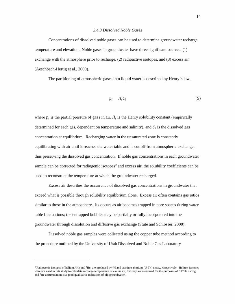
3.4.3 Dissolved Noble Gases

Concentrations of dissolved noble gases can be used to determine groundwater recharge

temperature and elevation. Noble gases in groundwater have three significant sources: (1)

exchange with the atmosphere prior to recharge, (2) radioactive isotopes, and (3) excess air

(Aeschbach-Hertig et al., 2000).

The partitioning of atmospheric gases into liquid water is described by Henry’s law,

𝑝𝑝𝑖𝑖 = 𝐻𝐻𝑖𝑖𝐶𝐶𝑖𝑖 (5)

where 𝑝𝑝𝑖𝑖 is the partial pressure of gas i in air, 𝐻𝐻𝑖𝑖 is the Henry solubility constant (empirically

determined for each gas, dependent on temperature and salinity), and 𝐶𝐶𝑖𝑖 is the dissolved gas

concentration at equilibrium. Recharging water in the unsaturated zone is constantly

equilibrating with air until it reaches the water table and is cut off from atmospheric exchange,

thus preserving the dissolved gas concentration. If noble gas concentrations in each groundwater

sample can be corrected for radiogenic isotopes2 and excess air, the solubility coefficients can be

used to reconstruct the temperature at which the groundwater recharged.

Excess air describes the occurrence of dissolved gas concentrations in groundwater that

exceed what is possible through solubility equilibrium alone. Excess air often contains gas ratios

similar to those in the atmosphere. Its occurs as air becomes trapped in pore spaces during water

table fluctuations; the entrapped bubbles may be partially or fully incorporated into the

groundwater through dissolution and diffusive gas exchange (Stute and Schlosser, 2000).

Dissolved noble gas samples were collected using the copper tube method according to

the procedure outlined by the University of Utah Dissolved and Noble Gas Laboratory

2 Radiogenic isotopes of helium, 3He and 4He, are produced by 3H and uranium-thorium (U-Th) decay, respectively. Helium isotopes were not used in this study to calculate recharge temperature or excess air, but they are measured for the purposes of 3H/3He dating, and 4He accumulation is a good qualitative indication of old groundwater.

15

(http://www.noblegaslab.utah.edu/pdfs/cu_tube_sampling.pdf). Samples were collected in 3/8-

inch diameter copper tubes cut to approximately 30 inches in length. To sample, water was

pumped through a copper tube from a connection as close to the wellhead as possible. The

outflow was back-pressured with a regulator valve to keep the dissolved gases in solution until

the sample could be sealed with refrigeration clamps. Special care was taken to ensure that gases

were not introduced to or allowed to escape from the sample during collection. Samples were

collected in duplicates.

Samples were analyzed at the Dissolved and Noble Gas Laboratory at the University of

Utah in Salt Lake City. Prior to analysis, the dissolved gases were extracted from the water

sample. In a closed system under high vacuum, the water sample was transferred from the copper

tube to a stainless-steel flask. The dissolved gases were driven into a second flask using a

temperature gradient induced by heating the water sample in the first flask and chilling the second

flask with liquid nitrogen. The gas sample was sealed again until it was transferred to the mass

spectrometer.

The heavier gases (Ne, Ar, Kr, and Xe) were analyzed on a Stanford Research Systems

RGA300 quadrupole mass spectrometer. Helium isotopes (3He and 4He) were analyzed on a

Mass Analyzer Products 215-50 magnetic sector field mass spectrometer.

Recharge temperature and excess air were determined using the closed-system

equilibration (CE) model, which “assumes equilibrium is attained in a closed system of initially

air-saturated water and finite volume of entrapped air under constant hydrostatic pressure,”

𝐶𝐶𝑖𝑖 = 𝐶𝐶𝑖𝑖∗ + (1−𝐹𝐹)𝐴𝐴𝑒𝑒𝑧𝑧𝑖𝑖1+𝐹𝐹𝐴𝐴𝑒𝑒𝑧𝑧𝑖𝑖 𝐶𝐶𝑖𝑖

∗⁄ (6)

where 𝐶𝐶𝑖𝑖 is the gas concentration in solution, 𝐶𝐶𝑖𝑖∗ is the moist-air solubility equilibrium

concentration (a function of temperature, salinity, and total atmospheric pressure), 𝐴𝐴𝑒𝑒 is the initial

16

volume ratio of trapped air to water, 𝑧𝑧𝑖𝑖 is volume fraction of each gas in dry air, and F is the

fractionation parameter describing the degree of excess air fractionation from no excess air to

pure excess air (Aeschbach-Hertig et al., 2000).

The system of four equations, one for each of four gases (Ne, Ar, Kr, and Xe), is

sufficient to solve for three parameters (𝐴𝐴𝑒𝑒, recharge temperature, and F). (Salinity was assumed

to be negligible because the source of recharge is meteoric; see section 4.3.4 on stable isotopes.)

Although in concept it is possible to also solve for recharge elevation (if unknown), the system of

equations would no longer be overdetermined and measurement errors would lead to a non-

unique determination of elevation (Manning and Solomon, 2003).

A best fit model is determined by minimizing the sum of chi-squared (χ2),

𝜒𝜒2 = ∑ �𝐶𝐶𝑖𝑖−𝐶𝐶𝑖𝑖𝑚𝑚𝑚𝑚𝑚𝑚�

2

𝜎𝜎𝑖𝑖2𝑖𝑖 (7)

where, 𝐶𝐶𝑖𝑖 is the measured concentration of gas i, 𝐶𝐶𝑖𝑖𝑚𝑚𝑚𝑚𝑚𝑚 is the modeled concentration, and 𝜎𝜎𝑖𝑖 is

standard deviation in the measurements (Aeschbach-Hertig et al., 1999). The modeled

concentrations are generated by perturbing the model parameters (𝐴𝐴𝑒𝑒, recharge temperature, and

F) within a theoretical range.

3.4.4 Tritium

Tritium (3H) is a radioactive isotope of hydrogen used to date young groundwater.

Tritium decays by beta emission to the noble gas 3He with a half-life of 12.32 years.

Small amounts of tritium are generated naturally through cosmic bombardment in the upper

atmosphere, but above-ground nuclear testing in the 1950s and 1960s introduced large quantities

17

of tritium to the atmosphere, increasing natural background concentrations of 3—6 TU3

(Kaufman and Libby, 1954) to concentrations in excess of 5000 TU at its peak in the 1960s

(Solomon and Cook, 2000) (Figure 6).

Tritium samples were collected with no head-space in 500 mL low density polyethylene

(LDPE) bottles, triple-rinsed with formation water. A duplicate sample was collected as backup.

The 3H/3He age is defined as

𝑡𝑡 𝐻𝐻 3 / 𝐻𝐻𝑒𝑒 3 = 𝜆𝜆−1𝑙𝑙𝑙𝑙 � 𝐻𝐻𝑒𝑒𝑡𝑡𝑡𝑡𝑖𝑖𝑡𝑡

3

𝐻𝐻 3+ 1� (8)

where 𝑡𝑡 𝐻𝐻 3 / 𝐻𝐻𝑒𝑒 3 is the 3H/3He age, 𝜆𝜆 is the 3H decay constant, and 𝐻𝐻𝐻𝐻𝑇𝑇𝑟𝑟𝑖𝑖𝑇𝑇

3 is tritiogenic 3He

(Solomon and Cook, 2000). The 3H component was measured at the Dissolved and Noble Gas

Laboratory at the University of Utah using the helium ingrowth method (Clarke et al., 1976)

using a Helix Split Flight Tube (SFT) sector field mass spectrometer.

The tritiogenic 3He component was attained by correcting total 3He ( 𝐻𝐻𝐻𝐻𝑇𝑇𝑚𝑚𝑇𝑇 3 ) (see section

3.4.3 on dissolved noble gas methods for description of helium measurement). The total amount

of 3He in the sample can be expressed as

𝐻𝐻𝐻𝐻𝑇𝑇𝑚𝑚𝑇𝑇 3 = 𝐻𝐻𝐻𝐻𝑎𝑎𝑇𝑇𝑚𝑚

3 + 𝐻𝐻𝐻𝐻𝑇𝑇𝑟𝑟𝑖𝑖𝑇𝑇 3 + 𝐻𝐻𝐻𝐻𝑛𝑛𝑢𝑢𝑛𝑛

3 + 𝐻𝐻𝐻𝐻𝑚𝑚𝑎𝑎𝑛𝑛 3 (9)

where 𝐻𝐻𝐻𝐻𝑎𝑎𝑇𝑇𝑚𝑚 3 is helium from the atmosphere, 𝐻𝐻𝐻𝐻𝑇𝑇𝑟𝑟𝑖𝑖𝑇𝑇

3 is helium produced by tritium decay used

for age dating, 𝐻𝐻𝐻𝐻𝑛𝑛𝑢𝑢𝑛𝑛 3 is helium produced by nuclear reactions in the subsurface, and 𝐻𝐻𝐻𝐻𝑚𝑚𝑎𝑎𝑛𝑛

3 is

helium from the mantle (Solomon and Cook, 2000). Mantle sources of 3He were assumed to be

negligible. Atmospheric helium is further subdivided into two components:

3 Tritium concentrations are reported in tritium units (TU), where one TU is equal to one molecule of 3H1HO in 1018 molecules of 1H2O.

18

𝐻𝐻𝐻𝐻𝑎𝑎𝑇𝑇𝑚𝑚 3 = 𝐻𝐻𝐻𝐻𝑠𝑠𝑚𝑚𝑠𝑠

3 + 𝐻𝐻𝐻𝐻𝑒𝑒𝑒𝑒𝑛𝑛 3 (10)

where 𝐻𝐻𝐻𝐻𝑠𝑠𝑚𝑚𝑠𝑠 3 is from solubility equilibrium with the atmosphere, and 𝐻𝐻𝐻𝐻𝑒𝑒𝑒𝑒𝑛𝑛

3 is from excess air

(Solomon and Cook, 2000). The following equation from Solomon and Cook (2000) was used to

solve for 𝐻𝐻𝐻𝐻𝑇𝑇𝑟𝑟𝑖𝑖𝑇𝑇 3 :

𝐻𝐻𝐻𝐻𝑇𝑇𝑟𝑟𝑖𝑖𝑇𝑇 3 = 𝐻𝐻𝐻𝐻𝑚𝑚

4 𝑅𝑅0 − 𝑅𝑅𝑠𝑠𝑚𝑚𝑠𝑠[ 𝐻𝐻𝐻𝐻𝑠𝑠𝑚𝑚𝑠𝑠 + (𝑁𝑁𝐻𝐻𝑚𝑚 − 𝑁𝑁𝐻𝐻𝑠𝑠𝑚𝑚𝑠𝑠)𝛼𝛼′𝑅𝑅𝐻𝐻𝑒𝑒−𝑁𝑁𝑒𝑒 4 ]

−𝑅𝑅𝑟𝑟𝑎𝑎𝑚𝑚[ 𝐻𝐻𝐻𝐻𝑚𝑚 4 − 𝐻𝐻𝐻𝐻𝑠𝑠𝑚𝑚𝑠𝑠

4 − (𝑁𝑁𝐻𝐻𝑚𝑚 − 𝑁𝑁𝐻𝐻𝑠𝑠𝑚𝑚𝑠𝑠)𝑅𝑅𝐻𝐻𝑒𝑒−𝑁𝑁𝑒𝑒] (11)

where 𝐻𝐻𝐻𝐻𝑚𝑚 4 is total measured 𝐻𝐻𝐻𝐻

4 , 𝑅𝑅0 is the 𝐻𝐻𝐻𝐻 3 / 𝐻𝐻𝐻𝐻

4 ratio in the sample at time of collection,

𝑅𝑅𝑠𝑠𝑚𝑚𝑠𝑠 is the 𝐻𝐻𝐻𝐻 3 / 𝐻𝐻𝐻𝐻

4 expected ratio for water in equilibrium with the atmosphere at the specified

recharge elevation, 𝐻𝐻𝐻𝐻𝑠𝑠𝑚𝑚𝑠𝑠 4 is the expected 𝐻𝐻𝐻𝐻

4 concentration for water in equilibrium with the

atmosphere at the specified recharge elevation, 𝑁𝑁𝐻𝐻𝑚𝑚 is total measured neon, 𝑁𝑁𝐻𝐻𝑠𝑠𝑚𝑚𝑠𝑠 is the

solubility neon concentration, 𝛼𝛼′ is the air-water isotope fractionation factor, 𝑅𝑅𝐻𝐻𝑒𝑒−𝑁𝑁𝑒𝑒 is the ratio

of helium to neon in the atmosphere, and 𝑅𝑅𝑟𝑟𝑎𝑎𝑚𝑚 is the ratio of 𝐻𝐻𝐻𝐻𝑛𝑛𝑢𝑢𝑛𝑛 3 / 𝐻𝐻𝐻𝐻𝑟𝑟𝑎𝑎𝑚𝑚

4 .

3.4.5 Sulfur Hexafluoride

SF6 is an industrial compound whose presence in the atmosphere can be used to date

young groundwater. Industrial production of SF6 began in 1953 for its use as an electrical

insulator (Busenberg and Plummer, 2000). It was first detected in the atmosphere in 1970 at 0.03

pptv (Lovelock, 1971). The low solubility of SF6 in water and subsequent long residence time in

the atmosphere has allowed the atmospheric mixing ratio to increase steadily over time to the

current (January 2017) value of 9.26 pptv (Figure 6). Its stable, non-reactive nature, even in very

reducing environments (Wilson and Mackay, 1993), adds to its usefulness as a tracer. Although

most SF6 in groundwater is anthropogenic in origin, it is naturally produced in relatively small

quantities in some igneous environments (Koh et al., 2007); Heilweil (2014) also found evidence

19

of natural production of SF6 from crustal sources.

SF6 samples are collected in 1-liter amber glass bottles that were safety coated on the

outside with plastic, and sealed with Polyseal cone-lined caps. To collect the sample, tubing from

the pump was placed at the bottom of the sample bottle, allowing water to overflow until at least

three sample-volumes have been purged through the sample bottle. The bottle was then capped

with no head space and sealed with electrical tape. Samples were collected in duplicate. After

collection, the samples were kept in a cooler to prevent overheating, water expansion, and bottle

breakage.

SF6 samples were analyzed at the Dissolved and Noble Gas Laboratory at the University

of Utah on a Shimadzu GC-8A gas chromatograph. The resulting measured concentrations were

corrected for excess air, determined independently from noble gas analysis (see section 3.4.3).

The partial pressure of SF6 during air-water equilibrium at the water table prior to recharge was

calculated using the following equation from Busenberg and Plummer (2000):

𝑥𝑥𝑆𝑆𝐹𝐹6 =𝑛𝑛𝑆𝑆𝑆𝑆6𝐾𝐾𝐻𝐻

�𝑃𝑃 − 𝑝𝑝𝐻𝐻2𝑂𝑂� (12)

where 𝑥𝑥𝑆𝑆𝐹𝐹6 is the dry air mole fraction of SF6, 𝑐𝑐𝑆𝑆𝐹𝐹6 is the concentration of SF6 in the sample,

corrected for excess air, 𝐾𝐾𝐻𝐻 is the Henry’s law constant, 𝑃𝑃 is the total atmospheric pressure, and

𝑝𝑝𝐻𝐻2𝑂𝑂 is the partial pressure of water. 𝐾𝐾𝐻𝐻 was calculated according to Bullister et al. (2002) and is

a function of salinity and recharge temperature (determined from dissolved noble gas analysis).

The resulting calculated partial pressure was related back to the air mixing curve through time

(Figure 6). Data prior to 1970 have been reconstructed by Maiss et al. (1994); subsequent data

were taken from NOAA measurements at Niwot Ridge, Colorado.

20

3.4.6 Chlorofluorocarbons

CFCs are industrial compounds whose presence in the atmosphere can be used to date

young groundwater. CFCs were developed in the 1930s as refrigerants. Overall production was

limited in 1987, after it was discovered that CFCs were significant contributors to atmospheric

ozone depletion. Production nearly ceased entirely in 1996 in accordance with the Clean Air Act.

Air mixing ratios peaked in 1994, 2002, and 1995, for CFC-11, CFC-12, and CFC-113,

respectively (Figure 6). CFC-11, CFC-12, and CFC-113 can be used to date groundwater back to

1947, 1941, and 1955, respectively (Plummer and Busenberg, 2000).

CFC samples were collected in 125 mL clear glass bottles, sealed with foil-lined caps.

Samples were collected through refrigeration-grade copper tubing to avoid desorption of

atmospheric CFCs from plastic tubing. Before collection, sample bottles and caps were triple-

rinsed with formation water. To collect samples, copper tubing was inserted into the sample

bottle to the bottom. Once the bottle is overflowing, it is submerged in a bucket of formation

water. The bottle was allowed to overflow until at least three sample-volumes were purged

through the bottle, and was capped while still underwater, without head space. Samples were

collected per the procedure outlined by the USGS Reston Groundwater Dating Laboratory.

Samples were collected in sets of four, and were stored at room temperature away from sunlight

before analysis.

CFC samples were analyzed at the Dissolved and Noble Gas Laboratory at the University

of Utah on a custom-fabricated line using a Shimadzu purge and trap system based on Bullister et

al. (2002).

3.4.7 Stable Isotopes

Stable isotope (𝛿𝛿18O and 𝛿𝛿2H) compositions can be used to trace groundwater provenance

because of the physical processes that govern their distribution. Stable isotope compositions are

reported in 𝛿𝛿 (delta) notation,

21

𝛿𝛿 = � 𝑅𝑅 𝑅𝑅𝑠𝑠𝑡𝑡𝑚𝑚

− 1� × 1000 ‰ (13)

where 𝑅𝑅 is the ratio of 18O/16O or 2H/1H in the sample, 𝑅𝑅𝑠𝑠𝑇𝑇𝑚𝑚 is the ratio in the standard (VSMOW,

Vienna Standard Mean Ocean Water), and ‰ is the unit permil.

Isotopic compositions of meteoric waters are linearly correlated, falling along the global

meteoric water line (GMWL) defined by Craig (1961) as:

𝛿𝛿𝛿𝛿 = 8 𝛿𝛿 𝑂𝑂 18 + 10 (14)

Mass-dependent isotope fractionation during phase changes (i.e., evaporation, condensation)

results in enrichment of the heavier isotope in the denser phase (e.g., during precipitation, the

heavy isotopes, 18O and 2H, are preferentially rained out). Removal of the precipitated water

from the cloud mass (by a process approximately described by Rayleigh distillation) results in

increasingly isotopically depleted waters, which can be correlated geographically with latitude,

distance from shorelines, and altitude.

Stable isotope samples were pumped through a 0.45-micron filter capsule into 60 mL

polyethylene bottles that had been triple-rinsed with formation water. Stable isotope samples

were analyzed in the Spatio-Temporal Isotope Analytics Laboratory (SPATIAL) on a Picarro

CRDS (cavity ring-down spectroscopy) water isotope analyzer.

3.5 Bromide Tracer Test

A bromide tracer test was performed along Mill Creek near the Colorado River to

evaluate whether groundwater was discharging into Mill Creek before reaching the Colorado

River. The need for the tracer test was prompted by flow measurements taken with a SonTek

FlowTracker Handheld-ADV (Acoustic Doppler Velocimeter) that indicated a gain of

22

approximately 1 cfs on a 1 mile reach of lower Mill Creek. A bromide tracer injection was

designed to locate and quantify the gain. A bromide tracer injection uses a concentrated solution

of sodium bromide (NaBr) injected at a constant, known rate, whereby any dilution in measured

concentrations of samples taken downstream indicate the occurrence of groundwater inflow

(seepage) into the stream. See a detailed description of bromide tracer test methods in section A-

1.

23

Figure 3. Map of sampling network in the study area, showing both the locations of newly installed observation wells and pre-existing wells. Wells sampled by the University of Utah in 2015-2016 are indicated in red; bright red indicates locations where wells were drilled and installed during the 2015-2016 field effort. Locations sampled by the U.S. Geological Survey (USGS) (data included in this report) are indicated in green; these locations include groundwater wells (circles), springs (diamonds), and surface water (triangles).

24

Figure 4. Preliminary results from an electrical resistivity survey (modified from Briggs, written communication, February 27, 2017) to investigate shallow alluvial groundwater discharge into the Colorado River. The map shows the total electrical conductivity (EC) in milliSiemens (mS) for shallow alluvial aquifer groundwater in the Matheson Wetlands. The data demonstrated groundwater discharge in the north is dominated by shallow brines with thin to no indication of freshwater. However, the data indicate that a thicker lens of fresh groundwater is present along the 0.5-mile reach from the Mill Creek confluence to the north. The brine and freshwater discharge areas are separated by a brackish transition zone in the middle.

25

Figure 5. Lithologic logs for observation wells installed during this study, showing simplified lithology, depth, and well screen interval. The 12 observation wells include 8 single-completion wells (U18 through U25) and two dual-completion wells (U26, U27; and U28, U29). The lithologic logs are aligned from approximately north to south (see Figure 3 for locations).

26

Figure 6. Reference diagram showing air-mixing curves for SF6 (in pptv x 100); CFC-11, CFC-12, and CFC-113 (in pptv); and tritium in precipitation (in tritium units, TU) (USGS Groundwater Dating Laboratory).

0

500

1000

1500

2000

2500

0

100

200

300

400

500

600

1940 1950 1960 1970 1980 1990 2000 2010

SF6 M

ixing Ratio x 100, pptv; Tritium in precipitation, TU

CFC

Mix

ing

Ratio

, ppt

vCFC-11

CFC-12

4 RESULTS

4.1 Aquifer Properties

4.1.1 Transmissivity

Transmissivity estimated using the Cooper-Jacob straight-line method for drawdown data

ranged from 60 to 4,100 ft2/day (Table 1). In several cases, drawdown affected the pumping rate

in such a way that the water level experienced an initial dramatic drop and then rose steadily for

the remainder of the test (see U23 and U24 drawdown curves, section A-2); as a result, in these

cases, transmissivity could not be estimated from Cooper-Jacob analysis of the drawdown data.

Transmissivity estimated from specific capacity ranged from 80 to 6,200 ft2/day. Transmissivity

estimated using the Theis recovery method ranged from 60 to 5,900 ft2/day. The recovery data

had too much noise in the case of U18, and the test was terminated prematurely in the case of

U23. Therefore, transmissivity could not be estimated in these cases.

Overall, average transmissivities at each aquifer test site using all available methods

ranged from 90 to 5,400 ft2/day, with a median of approximately 1000 ft2/day (Figure 7).

Standard deviation at each test site ranged from 0 to 920 ft2/day.

4.1.2 Potentiometric Surface (Water Table)

Hydraulic head values derived from water-level measurements were contoured to

evaluate general directions of groundwater flow (Figure 8). Head values range from 4,000 to

3,950 in the lower end of the valley. There is a notable flattening of the hydraulic gradient (from

0.02 to 0.005) to the west / northwest of the 3,990 ft contour. This could signify a change in

transmissivity, either because of an increase in aquifer thickness or an increase in hydraulic

conductivity. The hydraulic head contours abut the north valley wall at an angle less than 90

28

degrees, implying that some amount of groundwater is moving from the GCGA to the valley-fill

aquifer along the north wall of the valley near the wetland.

4.2 Hydrochemistry

4.2.1 Field Parameters

Field parameters and alkalinity data are summarized in Table 2. The lowest measured

specific conductivity was 680 µS/cm, and two samples exceeded the meter’s detection limit of

100,000 µS/cm. The data from specific conductivity profiles at two locations (U26 and U28) are

presented in Table 3; the data show the transition to brine occurring at approximately 30 feet

below the measuring point in both wells (Figure 9).

4.2.2 Major Ions and Alkalinity

Major ion concentrations are summarized in Table 4. Charge balances ranged from 0 to

23%. For freshwater samples, charge balances were within 10%. Samples with poor charge

balances (greater than 10%) were either from brine or brine-affected water. (The brines are high

in ammonia, and the elution time between chloride and ammonia is small, making it difficult to

separate the peaks.) Total dissolved solids (TDS) ranged from 533 to 159,201 mg/L. Stiff

diagrams of the major-ion chemistry (Figure 10) demonstrate that water types generally fall into

three categories: (1) low-TDS calcium-bicarbonate, (2) moderate-TDS calcium-sulfate, and (3)

high-TDS sodium-chloride. Alkalinity ranges from 124 to 314 mg/L as CaCO3.

High-quality low-TDS calcium-bicarbonate waters are characteristic of the Glen Canyon

Group Aquifer (Steiger and Susong, 1997; Gardner, 2004). This geochemical signature is

exhibited by wells located on the Glen Canyon Group slickrock plateau between Spanish Valley

and the La Sal Mountains, groundwater emanating from springs on the north wall of Spanish

Valley where it abuts the plateau, and surface water in Mill Creek prior to entering Spanish

Valley. Moderate-TDS calcium-sulfate type waters are ubiquitous in the valley-fill aquifer, and

29

are also found in Pack Creek before it enters the valley. The high-TDS sodium-chloride brines

are located at the distal end of the valley, near the Colorado River, and are attributed to

dissolution of Paradox Formation salts.

4.3 Environmental Tracers

4.3.1 Dissolved Noble Gases

Measured dissolved noble gas concentrations are presented in Table 5. Values of R/Ra

ranged from 0.067 to 2.053. Calculated recharge temperature (Trech) and excess air (Ae) results

calculated using the closed-system equilibration (CE) model assuming a recharge elevation of

1500 m are presented in Table 6. Recharge temperatures ranged from 8 to 19ºC (with one outlier

of 30 ºC removed), and excess air ranged from 4.3E-4 to 0.15. Most samples showed good fits to

the CE model; the average sum of chi squared was 0.5. The recharge temperature and excess air

parameters were used in the analyses of 3H/3He, SF6, and CFC apparent ages.

4.3.2 Tritium

Measured and calculated parameters associated with 3H/3He age dating are presented in

Table 7. Measured tritium values ranged from 0.01 to 4.79 TU. Calculated 4Heterr ranged from -

3.47×10-9 to 9.37×10-6. Calculated 3Hetrit ranged from -3.35 to 163 TU, resulting in 3H/3He ages

that ranged from 0§ to 164 years. In general, the 3H/3He ages increase down-gradient (Figure 11).

The uncertainty associated with 3H/3He ages ranges from 0 to 154 years, with many

values falling between 0 and 8 years. The uncertainty is calculated by perturbing the parameters

in equation 11 within their respective ranges of error. Groundwater ages of old waters are less

sensitive to error in the 3Hetrit component, because the proportion of 3Hetrit to total measured 3He

§ Negative 3H/3He ages from negative 3Hetrit were reported with an age of 0 years.

30

increases in any given sample over time as more 3H decays to tritiogenic 3He. However, the

3H/3He age uncertainty can also increase with large values of excess air and terrigenic 4He; the

fraction of total He that comes from 3Hetrit decreases with increasing 3HeAe (from excess air) and

3Herad (from 4Heterr), increasing the uncertainty in 3Hetrit, and with it, the apparent age (Solomon

and Cook, 2000).

For mixtures of young and old (i.e., tritiated and nontritiated) waters, the 3H/3He age is

biased toward the young fraction (Solomon and Cook, 2000). Several samples were flagged as

possible mixtures of young and old water. For example, the U11 sample had a calculated age of 0

years, which is consistent with a measured tritium of 3.14 TU (Table 7), but it has a low R/Ra

value, which is a first-order indicator of the presence of older water. An R/Ra of less than 1 is

likely due to the presence of terrigenic helium-4, which builds up over time in old waters due to

radiogenic decay of U and Th (Solomon and Cook, 2000).

In addition to analytical error, there are uncertainties due to sampling: ages vary due to

the depth of the well, and the screened interval of the well, and the permeability of the sediments

over the screened interval. Ideally, 3H/3He ages would represent a flow-weighted average over

the entire thickness of the aquifer.

Despite the uncertainty outlined above, 3H/3He age-dating is generally considered to be

the most robust of the groundwater age-dating methods used in this study because the 3H atom is

physically incorporated in the water molecule and is, therefore, a conservative tracer, unlike SF6

and CFCs, which are subject to contamination and degradation in some chemical environments.

4.3.3 Sulfur Hexafluoride

Measured SF6 concentrations range from 0 to 11 fMol/kg (Table 8). Calculated mixing

ratios range from 0 to 31 pptv. The current atmospheric mixing ratio of SF6 is 9.26 pptv (January

2017). Samples with no measurable SF6 presumably recharged before significant concentrations

of SF6 were introduced to the atmosphere and are considered “premodern.” Apparent ages range

31

from 0 to premodern, and correspond to recharge years from 2017 to pre-1953. Samples are

considered “contaminated” if the calculated mixing ratio is greater than what is possible simply

due to air-water equilibrium exchange during recharge (in other words, if the calculated mixing

ratio is greater than the current atmospheric mixing ratio). Ten of the 30 samples are

contaminated, up to three times the current (January 2017) atmospheric mixing ratio.

Samples were initially analyzed for SF6 for comparison to 3H/3He ages; however,

extensive contamination of lower Moab-Spanish Valley samples precludes this. Ten samples had

calculated mixing ratios above the theoretical maximum for mere air-water equilibration at the

water table prior to recharge. Additional samples, for which an SF6 apparent age was

theoretically calculable, generally skew younger than the corresponding 3H/3He apparent ages

(Figure 12), suggesting these are also affected by an additional source of SF6, whether natural or

anthropogenic.

Replicates were run for all but three samples, where either the bottle or cap was cracked.

Measured replicate concentrations are plotted in Figure 13. Standard deviations are within 10%

for the majority (18 out of 30) samples. The agreement between replicate samples suggests that

SF6 contamination is not due to error in sampling or analytical methods.

Busenberg and Plummer (2000) described total SF6 below,

𝑆𝑆𝑆𝑆6 𝑡𝑡𝑚𝑚𝑡𝑡𝑡𝑡𝑡𝑡 = 𝑆𝑆𝑆𝑆6 𝑒𝑒𝑒𝑒 + 𝑆𝑆𝑆𝑆6 𝑒𝑒𝑒𝑒𝑒𝑒 + 𝑆𝑆𝑆𝑆6 𝑡𝑡𝑒𝑒𝑡𝑡𝑡𝑡 + 𝑆𝑆𝑆𝑆6 𝑒𝑒𝑚𝑚𝑐𝑐𝑡𝑡 − 𝑆𝑆𝑆𝑆6 𝑡𝑡𝑚𝑚𝑠𝑠𝑠𝑠 (15)

where 𝑆𝑆𝑆𝑆6 𝑒𝑒𝑒𝑒 is due to equilibrium air-water exchange, 𝑆𝑆𝑆𝑆6 𝑒𝑒𝑒𝑒𝑒𝑒 is addition from excess air during

the dissolution and incorporation of air bubbles into the groundwater during water table rise,

𝑆𝑆𝑆𝑆6 𝑡𝑡𝑒𝑒𝑡𝑡𝑡𝑡 is addition of natural SF6, 𝑆𝑆𝑆𝑆6 𝑒𝑒𝑚𝑚𝑐𝑐𝑡𝑡 is the addition of anthropogenic concentration, and

𝑆𝑆𝑆𝑆6 𝑡𝑡𝑚𝑚𝑠𝑠𝑠𝑠 is any loss due to degradation. If terrigenic SF6 and SF6 from contamination and SF6 loss

are small, and excess air is determined independently, it is possible to date young groundwater

32

with SF6.

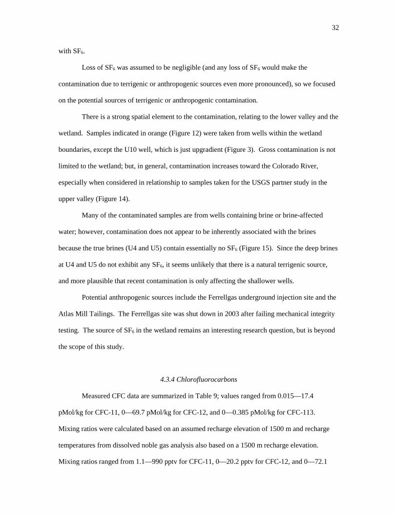
Loss of SF6 was assumed to be negligible (and any loss of SF6 would make the

contamination due to terrigenic or anthropogenic sources even more pronounced), so we focused

on the potential sources of terrigenic or anthropogenic contamination.

There is a strong spatial element to the contamination, relating to the lower valley and the

wetland. Samples indicated in orange (Figure 12) were taken from wells within the wetland

boundaries, except the U10 well, which is just upgradient (Figure 3). Gross contamination is not

limited to the wetland; but, in general, contamination increases toward the Colorado River,

especially when considered in relationship to samples taken for the USGS partner study in the

upper valley (Figure 14).

Many of the contaminated samples are from wells containing brine or brine-affected

water; however, contamination does not appear to be inherently associated with the brines

because the true brines (U4 and U5) contain essentially no SF6 (Figure 15). Since the deep brines

at U4 and U5 do not exhibit any SF6, it seems unlikely that there is a natural terrigenic source,

and more plausible that recent contamination is only affecting the shallower wells.

Potential anthropogenic sources include the Ferrellgas underground injection site and the

Atlas Mill Tailings. The Ferrellgas site was shut down in 2003 after failing mechanical integrity

testing. The source of SF6 in the wetland remains an interesting research question, but is beyond

the scope of this study.

4.3.4 Chlorofluorocarbons

Measured CFC data are summarized in Table 9; values ranged from 0.015—17.4

pMol/kg for CFC-11, 0—69.7 pMol/kg for CFC-12, and 0—0.385 pMol/kg for CFC-113.

Mixing ratios were calculated based on an assumed recharge elevation of 1500 m and recharge

temperatures from dissolved noble gas analysis also based on a 1500 m recharge elevation.

Mixing ratios ranged from 1.1—990 pptv for CFC-11, 0—20.2 pptv for CFC-12, and 0—72.1

33

pptv for CFC-113 (Table 10). These mixing ratios resulted in apparent ages that ranged from

premodern to 0 years for CFC-11 and CFC-12, and 32 to 74 for CFC-113 (Table 11).

Except for two samples (U7 and U15) that fall along the piston flow mixing line, CFC-11

appears to be degraded when plotted against CFC-12 (Figure 16). CFCs, especially CFC-11, are

known to degrade in some anaerobic environments (Plummer and Busenberg, 2000). CFC-12

and CFC-113 concentrations are somewhat consistent along a piston flow model for samples

older than approximately 35 years (Figure 16); the younger samples may have been affected by

loss of CFC-113 due to sorption (Plummer and Busenberg, 2000). CFC-12 is generally

considered to be the most stable CFC, and the most useful for groundwater age-dating.

4.3.5 Stable Isotopes

Stable isotope data are presented in Table 12. Isotopic compositions range from -15 to -

13.5 for δ18O and -108.8 to -101.5 for δ2H. The isotopic distribution was plotted in reference to

the global meteoric water line (GMWL) and the Utah meteoric water line (UMWL) in Figure 17.

All of the samples appear to be of meteoric origin, based on correlation with the GMWL. Several

samples (namely, the brines) plot below the GMWL, an indication of evaporative enrichment.

GCGA water is defined by Gardner (2004) as having δ18O of -14.5 to -15.0. Many of the

samples appear to have been sourced from precipitation occurring at high elevation, similar to the

GCGA end member.

4.4 Mill Creek Seepage (Bromide Tracer Test)

The injected bromide concentration in the stream reached steady-state after

approximately 4 hours (Figure 18). During the 18-hour period of steady-state, the bromide

concentration in the stream increased steadily over time; this is a result of the stream flow

declining steadily over the same time period, as the test was conducted on the tail-end of a rain

event, as indicated by transducer data (Figure 19).

34

A synoptic sampling campaign (Figure 20) showed a gain of approximately 2.7 cfs below

the confluence of Mill Creek and Pack Creek (due to inflow of Pack Creek), but less than 0.1 cfs

of gain between Pack Creek and the Colorado River.

The streamflow measurements that prompted the bromide tracer test indicated about 1 cfs

of gain into a stream with a total flow rate of approximately 10 cfs. The measured gain is

approximately 10 % of the total streamflow, which is near the error associated with manual

streamflow measurements (approximately 5 %). It is, however, possible that the measured gain

was real, but that it occurs intermittently.

35

Figure 7. Aquifer testing transmissivity results from wetland preserve monitoring wells (monitoring well locations shown in Figure 3), in square feet per day (ft2/day) using different analytical solutions; hatched fill indicates estimate from observation well. The average transmissivity is approximately 1000 ft2/day.

U18

U19

U20

U21

U22

U23

U24

U25

U26

, U27

U28

, U29

0

1000

2000

3000

4000

5000

6000

7000

Tran

smiss

ivity

, ft2 /

day

Cooper-JacobMethod

from SpecificCapacity

Theis RecoveryMethod

36

Figure 8. Potentiometric surface (water table) map showing groundwater flow generally to the northwest through the valley bottom toward the Colorado River. The potentiometric surface map was generated using water levels measured from alluvial wells; the contour interval is 5 feet. Given that groundwater flow is perpendicular to potentiometric surface contours, the map indicates that a large proportion of groundwater discharge to the Colorado River is occurring at the south end of the wetlands preserve, near Mill Creek.

37

Figure 9. Graph displaying specific conductivity (SpC) profiles at U26 (blue) and U28 (orange); SpC values are shown in microSiemens per centimeter (µS/cm). The profiles indicate a transition from fresh groundwater to brine around 30 feet below the measuring point (i.e., top of the well casing).

0

5

10

15

20

25

30

35

40

45 - 5,000 10,000 15,000 20,000 25,000 30,000 35,000 40,000 45,000 50,000

Dept

h, fe

et b

elow

MP

SpC, uS/cm

U26 U28

38

Figure 10. Map of groundwater hydrochemical type, based on major-ion chemistry. The three observed groundwater types include sodium chloride (Na-Cl, indicated in red), calcium sulfate (Ca-SO4, green), and calcium bicarbonate (Ca-HCO3, blue). Darker hues indicate higher total dissolved solids (TDS); brine is defined here as having greater than 100,000 mg/L TDS, brackish is less than 100,000 mg/L and greater than 1,000 mg/L, and fresh is less than 1,000 mg/L.

39

Figure 11. Map showing the tritium/helium-3 apparent ages from valley-fill aquifer samples (increasingly older samples are indicated by darker shades of blue), potentiometric contours (black lines) and groundwater flow direction (red arrow), and the sample groupings used to calculate a discharge rate to the Colorado River. The discharge calculation was performed by measuring the distance between the right and left sample groupings, and then dividing the distance by the age difference between the average age of each respective sample grouping.

40

Figure 12. Plot showing the relationship between tritium/helium-3 and sulfur hexafluoride (SF6) apparent ages. Samples collected more distant from the wetlands preserve (shown in blue) have calculated apparent ages that correlate closer to the tritium/helium-3 age 1:1 line compared to samples collected in or near the wetlands preserve (shown in orange). Many of the SF6 samples collected were “contaminated,” predominately those collected in the wetland preserve, as indicated by calculated apparent ages that were impossibly young (i.e., negative age). The results of this plot indicate that SF6 contamination is spatially correlated with the wetlands preserve.

U18

U10

U13

U14U15

U16l

U19

U20

U21

U22

U23

U31

U32

0

5

10

15

20

25

30

35

40

0 10 20 30 40 50 60

SF6

Age

3H/3He Age (Closed System Equilibrium Model)

41

Figure 13. Graph showing replicate sulfur hexafluoride (SF6) measured concentrations, shown in femtoMoles per kilogram (fMol/kg). In general, replicate concentrations are correlative, indicating that SF6 contamination is not a result of measurement error.

0

2

4

6

8

10

12

0 2 4 6 8 10 12

Run

1, f

Mol

/kg

Run 2, fMol/kg

42

Figure 14. Study area map showing measured sulfur hexafluoride (SF6) concentration in femtoMoles per kilogram (fMol/kg). Samples collected in and around the wetland preserve indicate SF6 contamination, meaning that the SF6 concentrations are above what is possible solely through atmospheric equilibration. The current atmospheric concentration of SF6 is approximately 2 fMol/kg.

43

Figure 15. Plot comparing the calculated sulfur hexafluoride (SF6) partial pressure, in parts per trillion by volume (pptv), to total dissolved solids (TDS), in milligrams per liter (mg/L). The samples from U4 and U5, both located in the wetland preserve, have TDS concentrations exceeding 100,000 mg/L (i.e., brine), and essentially no SF6. This finding suggests that the observed SF6 contamination is not inherently associated with brine, but rather to an unknown anthropogenic or terrigenic contamination source.

U4U5

0

5

10

15

20

25

30

35

40

45

100 1000 10000 100000 1000000

SF6,

ppt

v

Total Dissolved Solids (TDS), mg/L

44

Figure 16. Tracer-tracer plots show concentrations of two tracers in relation to the PFM (piston flow model, blue line) and EMM (exponential mixing model, red line). The top left diagram shows that, generally, CFC-11 is degraded relative to CFC-12. Top right shows that CFC-113 is also degraded relative to CFC-12, especially for younger samples. The bottom panel shows that older samples fall along the PFM or EMM mixing lines, and that the other samples may be captured by a binary mixing model (a tie-line between the PFM model and EMM model).

45

Figure 17. Stable isotope results. Upper Panel: Study area map showing oxygen and hydrogen stable isotope sampling locations. The symbols represent the type of water (e.g., groundwater versus surface water) collected at each location: Glen Canyon Group Aquifer, blue circle; valley-fill aquifer, green circle; brine, red circle; Mill Creek, blue triangle; Pack Creek, yellow triangle; and Mill Creek below the confluence with Pack Creek, green triangle. Lower Panel: Plot of stable isotope concentration (per mil) for hydrogen and oxygen; the solid line represents the global meteoric water line, and the dashed line is the Utah meteoric water line.

46

Figure 18. Establishing steady state at transport sites

-1

0

1

2

3

4

5

6

11/1

7/20

15 0

:00

11/1

7/20

15 1

2:00

11/1

8/20

15 0

:00

11/1

8/20

15 1

2:00

11/1

9/20

15 0

:00

11/1

9/20

15 1

2:00

11/2

0/20

15 0

:00

Brom

ide,

mg/

L

T1

T2

T3

T4

47

Figure 19. Transducer data

-2

-1

0

1

2

Tran

spor

t 1,

chan

ge in

wat

er

leve

l, in

ches

-2

-1

0

1

2

Tran

spor

t 2,

chan

ge in

wat

er

leve

l, in

ches

-2

-1

0

1

2

Tran

spor

t 3,

chan

ge in

wat

er

leve

l, in

ches

-2

-1

0

1

2

3

4

5

6

7

16-N

ov 1

2:00

17-N

ov 0

0:00

17-N

ov 1

2:00

18-N

ov 0

0:00

18-N

ov 1

2:00

19-N

ov 0

0:00

19-N

ov 1

2:00

20-N

ov 0

0:00

Tran

spor

t 4,

chan

ge in

wat

er le

vel,

inch

es

48

Figure 20. Synoptic

-1

0

1

2

3

4

5

0 5 10 15 20 25 30 35 40

Brom

ide,

mg/

L

Sample order, from upstream to downstream

Synoptic

Pre-Synoptic

Synoptic

49

Table 1. Transmissivity results, square feet per day

Site ID Cooper-Jacob method Specific Capacity Theis recovery method Average Standard Deviation

U18 60 120 — 90 30 U19 920 1300 1500 1300 250 U20 3700 3200 2000 3000 690 U21 1700 1300 2200 1700 350 U22 1200 290 460 640 390 U23 — 80, 150 340 190 100 U24 — 110 60 90 30 U25 270 630 1900 930 690 U26 30 310 640 330 250 U27 † 1500 — 500 1000 520 U28 4100 6200 5900 5400 920 U29 † 4100 — 4100 4100 0 † Observation well

50

Table 2. Field parameters and alkalinity

Site ID Temperature Specific Conductance pH Total Dissolved

Gases Dissolved Oxygen

Dissolved Oxygen Alkalinity

ºC uS/cm mmHg mg/L % mg/L as CaCO3 U1 16.6 30,535 6.6 740 0.2 3 255 U2 19.2 90,105 6.2 834 0.3 6 186 U3 16.2 11,930 7.2 750 0.3 4 300 U4 13.2 ODL 6.5 880 0.4 7 260 U5 13.7 ODL 6.2 1,274 0.1 2 165 U6 15.2 5,899 7.0 692 1.8 22 268 U7 16.8 1,092 6.8 680 3.5 45 270 U8 17.8 1,824 6.8 660 1.0 13 194 U9 16.1 2,115 7.0 800 1.8 21 124 U10 15.2 952 7.3 679 0.9 9 211 U11 15.7 680 7.0 720 1.5 18 300 U12 15.9 1,586 6.9 692 — — 234 U13 15.9 1,574 6.9 685 — — 216 U14 16.9 796 7.1 661 — — 228 U15 17.5 1,519 6.9 682 — — 216 U16 17.3 1,158 6.7 645 — — 230 U17 16.6 998 6.7 694 — — 314 U18 17.1 2,423 6.7 712 2.8 32 190 U19 15.4 987 7.2 700 0.3 4 180 U20 15.9 905 7.1 744 — — 170 U21 14.3 921 7.0 691 7.7 86 273 U22 12.6 899 7.1 664 — — 298 U23 16.9 3,581 6.6 712 1.1 13 174 U24 19.3 2,437 8.1 748 0.2 3 244 U25 13.6 3,306 7.0 760 2.9 33 310 U26 12.6 12,219 7.4 773 2.0 22 — U27 12.7 1,223 6.8 676 4.5 48 183 U28 12.5 46,341 6.9 741 0.4 6 — U29 13.4 5,188 7.0 727 1.2 12 216 U30 16.0 1,521 6.8 715 1.5 18 136 U31 16.3 906 6.6 682 0.1 2 275 U32 17.6 1,323 6.9 675 5.9 72 124 ODL, over detection limit

51

Table 3. Specific conductivity profiles at select sites Depth BMP Specific Conductivity

feet µS/cm MW-09 MW-11

12 3,482 — 13 3,515 — 14 3,513 8,466 15 3,515 8,567 16 3,517 8,591 17 3,518 8,568 18 3,520 8,572 19 3,520 8,582 20 3,520 8,584 21 3,522 8,590 22 3,520 8,591 23 3,517 9,073 24 3,517 9,537 25 3,514 10,147 26 3,518 10,246 27 3,665 10,877 28 3,878 11,347 29 4,174 12,419 30 6,422 13,970 31 7,652 18,125 32 9,083 20,251 33 12,028 22,550 34 12,873 27,131 35 13,130 34,912 36 13,295 36,966 37 13,391 41,050 38 13,454 42,414 39 13,589 46,341 40 13,631 — 41 12,219 — 42 11,272 —

BMP, below measuring point µS/cm, microSiemens per centimeter

52

Table 4. Major ion results

Site Name Sodium Potassium Calcium Magnesium Chloride Sulfate Bicarbonate TDS Charge Balance

mg/L mg/L mg/L mg/L mg/L mg/L mg/L mg/L % U1 6,648 67 1,118 206 19,932 683 311 28,964 -23 U2 24,309 179 2,615 693 66,287 4,273 227 98,581 -22 U3 2,553 52 202 68 6,258 882 366 10,381 -22 U4 32,426 667 1,909 554 84,907 5,352 317 126,131 -23 U5 41,072 969 1,977 664 108,183 6,136 201 159,201 -24 U6 905 12 237 128 2,216 951 327 4,776 -17 U7 36 3 173 42 28 292 329 902 6 U8 27 4 325 82 32 1,131 237 1,838 -8 U9 30 4 382 106 54 1,405 151 2,131 -7 U10 23 2 142 45 24 302 257 795 3 U11 13 2 71 41 5 36 366 533 4 U12 79 4 181 82 48 704 285 1,382 -3 U13 59 4 204 78 48 754 263 1,411 -5 U14 32 3 86 39 24 181 278 643 0 U15 79 6 175 72 42 701 263 1,338 -5 U16 53 5 114 64 58 326 280 900 1 U17 29 3 162 28 32 167 383 802 5 U18 179 6 274 111 170 1,239 232 2,212 -6 U19 24 2 127 43 22 281 219 719 4 U20 17 2 117 42 22 209 206 613 9 U21 19 2 124 42 21 143 333 684 8 U22 20 2 116 42 19 112 363 674 7 U23 234 7 601 114 283 2,561 206 4,005 -13 U24 506 4 23 5 696 219 298 1,752 -10 U25 544 9 143 74 925 440 378 2,513 -5 U27 49 5 136 55 36 345 223 850 7 U29 1,104 13 195 68 2,264 605 263 4,511 -12 U30 37 3 260 52 56 816 166 1,391 -6 U31 27 2 125 33 17 152 335 691 5 U32 75 6 139 66 78 538 151 1,053 0

53

Table 5. Measured noble gas concentrations

Site ID Neon + - Argon + - Krypton + - Xenon + - Helium-4 + - R/Ra † (ccSTP/g) (ccSTP/g) (ccSTP/g) (ccSTP/g) (ccSTP/g) (ccSTP/g) (ccSTP/g) (ccSTP/g) (ccSTP/g) (ccSTP/g) U1 1.9E-07 4E-09 3.2E-04 9E-06 7.3E-08 4E-09 1.0E-08 5E-10 3.1E-07 0.209 U2 1.7E-07 3E-09 3.0E-04 9E-06 7.1E-08 4E-09 8.8E-09 4E-10 8.6E-06 0.088 U3 2.1E-07 4E-09 3.7E-04 1E-05 8.8E-08 4E-09 1.2E-08 6E-10 7.0E-07 0.149 U4 1.7E-07 3E-09 3.2E-04 1E-05 7.8E-08 4E-09 9.9E-09 5E-10 7.4E-06 0.071 U5 1.7E-07 3E-09 3.3E-04 1E-05 7.5E-08 4E-09 1.0E-08 5E-10 9.4E-06 0.067 U6 1.9E-07 4E-09 3.3E-04 1E-05 7.6E-08 4E-09 1.0E-08 5E-10 7.5E-08 0.529 U7 1.9E-07 4E-09 3.3E-04 1E-05 7.7E-08 4E-09 1.0E-08 5E-10 4.7E-08 1.014 U8 1.7E-07 3E-09 2.7E-04 8E-06 6.0E-08 3E-09 8.5E-09 4E-10 6.3E-08 1.123 U9 1.7E-07 3E-09 3.0E-04 9E-06 7.3E-08 4E-09 1.0E-08 5E-10 5.0E-08 1.677 U10 2.0E-07 4E-09 3.7E-04 1E-05 8.2E-08 4E-09 1.2E-08 6E-10 6.8E-08 1.168 U11 2.3E-07 5E-09 3.9E-04 1E-05 8.5E-08 4E-09 1.2E-08 6E-10 1.1E-07 0.490 U12 1.9E-07 4E-09 3.6E-04 1E-05 8.0E-08 4E-09 1.1E-08 6E-10 5.0E-08 1.013 U13 1.9E-07 4E-09 3.6E-04 1E-05 7.8E-08 4E-09 1.1E-08 6E-10 5.4E-08 0.948 U14 1.8E-07 4E-09 3.3E-04 1E-05 7.4E-08 4E-09 1.1E-08 6E-10 4.3E-08 1.098 U15 1.8E-07 4E-09 3.2E-04 1E-05 7.8E-08 4E-09 1.0E-08 5E-10 4.5E-08 0.932 U16 1.7E-07 3E-09 3.2E-04 1E-05 7.3E-08 4E-09 1.0E-08 5E-10 5.0E-08 1.040 U17 1.7E-07 3E-09 3.1E-04 9E-06 7.4E-08 4E-09 1.0E-08 5E-10 4.2E-08 0.995 U18 2.1E-07 4E-09 3.6E-04 1E-05 7.1E-08 4E-09 1.0E-08 5E-10 6.6E-08 0.826 U19 2.1E-07 4E-09 3.5E-04 1E-05 7.3E-08 4E-09 1.0E-08 5E-10 7.2E-08 1.135 U20 2.0E-07 4E-09 3.7E-04 1E-05 7.6E-08 4E-09 1.1E-08 5E-10 5.5E-08 2.053 U21 2.0E-07 4E-09 3.4E-04 1E-05 7.8E-08 4E-09 1.0E-08 5E-10 4.8E-08 1.792 U22 8.4E-07 2E-08 9.0E-04 3E-05 1.4E-07 7E-09 1.5E-08 7E-10 3.9E-07 1.096 U23 2.1E-07 4E-09 3.6E-04 1E-05 7.6E-08 4E-09 1.0E-08 5E-10 8.7E-08 0.650 U24 2.3E-07 5E-09 3.9E-04 1E-05 8.3E-08 4E-09 1.0E-08 5E-10 1.4E-07 0.468 U25 2.0E-07 4E-09 3.6E-04 1E-05 7.5E-08 4E-09 9.5E-09 5E-10 1.2E-07 0.439 U27 2.0E-07 4E-09 3.6E-04 1E-05 7.7E-08 4E-09 1.0E-08 5E-10 1.1E-07 0.641 U29 2.0E-07 4E-09 3.8E-04 1E-05 7.8E-08 4E-09 1.1E-08 6E-10 3.6E-07 0.333 U30 2.1E-07 4E-09 3.7E-04 1E-05 7.9E-08 4E-09 1.1E-08 5E-10 2.9E-07 0.322 U31 2.1E-07 4E-09 3.6E-04 1E-05 8.0E-08 4E-09 1.0E-08 5E-10 5.0E-08 1.248 U32 1.7E-07 3E-09 3.0E-04 9E-06 7.2E-08 4E-09 9.0E-09 4E-10 4.8E-08 0.941 † R/Ra, where R is the ratio of 3He/4He measured in the sample, and Ra is the ratio of 3He/4He in the atmosphere (1.384E-6)

54

Table 6. Closed-system equilibration (CE) model (Aeschbach-Hertig et al., 2000) results, assuming recharge elevation of 1500 m

Site ID Recharge Temperature Excess Air Fractionation

Factor Sum of Chi

Squared ºC U1 12.1 0.001 0.00 2E-02 U2 16.3 0.119 0.94 2E+00 U3 8.7 0.029 0.74 5E-08 U4 13.0 0.130 0.95 8E-01 U5 11.6 0.134 0.96 6E-01 U6 12.9 0.048 0.84 8E-09 U7 13.6 0.132 0.86 1E-02 U8 19.0 0.001 0.00 6E-01 U9 12.4 0.001 0.00 5E-01 U10 10.0 0.070 0.81 2E-08 U11 11.3 0.062 0.70 1E-08 U12 11.1 0.143 0.85 7E-01 U13 11.8 0.141 0.84 7E-01 U14 9.8 0.000 0.00 3E-02 U15 12.2 0.051 0.92 2E-07 U16 13.0 0.131 0.93 4E-01 U17 12.5 0.017 0.93 8E-08 U18 15.7 0.132 0.75 6E-02 U19 16.6 0.125 0.73 2E-07 U20 13.2 0.138 0.79 8E-01 U21 16.3 0.128 0.78 1E-02 U22 30.0 0.153 0.13 2E-01 U23 15.7 0.133 0.75 2E-01 U24 18.6 0.130 0.64 2E+00 U25 17.3 0.127 0.75 3E+00 U27 15.1 0.133 0.77 4E-01 U29 12.1 0.143 0.79 2E+00 U30 14.8 0.137 0.73 4E-01 U31 14.9 0.134 0.76 9E-01 U32 15.1 0.116 0.80 3E-01

55

Table 7. Measured and calculated tritium results

Site ID Tritium + - R/Ra Tritiogenic Helium-3

Terrigenic Helium-4 ∆Neon Age + -

TU TU TU ccSTP/g % years years U1 0.49 0.03 0.209 4.80 2.69E-07 13 43 55 U2 0.29 0.03 0.088 163.32 8.56E-06 5 114 118 U3 2.23 0.09 0.149 14.60 6.57E-07 13 36 46 U4 0.27 0.03 0.071 65.84 7.31E-06 4 98 120 U5 0.01 0.09 0.067 68.60 9.37E-06 -9 164 154 U6 0.72 0.04 0.529 -3.35 3.01E-08 13 0 † 20 U7 3.12 0.13 1.014 0.14 -1.12E-09 25 1 4 U8 2.35 0.09 1.123 15.65 2.08E-08 16 37 3 U9 3.01 0.14 1.677 24.14 9.64E-09 6 39 2 U10 2.19 0.10 1.168 17.41 2.02E-08 17 39 3 U11 3.14 0.11 0.490 -0.52 5.86E-08 30 0 † 22 U12 1.59 0.08 1.013 4.31 6.67E-09 10 24 40 U13 2.33 0.11 0.948 0.91 3.93E-09 30 6 4 U14 2.31 0.10 1.098 1.66 -2.06E-09 10 10 21 U15 0.51 0.05 0.932 0.31 2.97E-09 6 9 6 U16 2.20 0.10 1.040 3.70 4.14E-09 12 18 4 U17 2.84 0.10 0.995 0.80 9.37E-10 -8 4 26 U18 1.34 0.11 0.826 2.89 1.68E-08 30 21 6 U19 1.73 0.13 1.135 18.69 2.44E-08 21 44 4 U20 3.36 0.24 2.053 36.36 6.87E-09 19 44 3 U21 3.82 0.35 1.792 19.63 -3.47E-09 36 33 3 U22 4.79 0.34 1.096 110.80 1.70E-07 347 57 4 U23 0.93 0.09 0.650 4.78 4.02E-08 20 33 0 U24 0.60 0.11 0.468 2.42 7.98E-08 46 29 26 U25 0.57 0.08 0.439 3.18 7.89E-08 19 34 27 U27 1.07 0.12 0.641 13.18 6.62E-08 16 46 8 U29 3.35 0.24 0.333 33.15 3.15E-07 15 43 16 U30 1.55 0.13 0.322 19.25 2.39E-07 14 47 23 U31 3.05 0.21 1.248 9.40 3.97E-09 18 25 3 U32 0.79 0.09 0.941 2.38 7E-09 9 25 8 Measured values: tritium, R/Ra; calculated values: 3Hetrit, 4Heterr, ΔNe, age † Computed negative ages are taken to be zero

56

Table 8. SF6 results

Well ID SF6 Apparent Age

Apparent Recharge Year

Calculated mixing ratio

Measured concentration

(years as of 2017) (pptv) (fMol/kg) U1 C C 25.63 10.29 U2 C C 30.69 9.12 U3 C C 10.73 5.23 U4 42.1 1973.5 0.35 0.12 U5 45.6 1970.0 0.23 0.08 U6 C C 17.86 6.97 U7 1.6 2014.0 8.38 3.18 U8 C C 26.19 8.53 U9 16.1 1999.5 4.55 4.47 U10 15.1 2000.5 4.69 2.10 U11 15.6 2000.0 4.57 2.24 U12 0 2017.0 9.42 3.71 U13 5.6 2010.0 7.15 2.78 U14 11.1 2004.5 5.59 2.24 U15 12.1 2003.5 5.43 2.02 U16 18.6 1997.0 3.91 1.32 U17 C C 9.65 3.45 U18 C C 20.96 8.45 U19 4.8 2011.5 7.57 3.18 U20 25.8 1990.5 2.54 1.00 U21 1.8 2014.5 8.64 3.36 U22 30.3 1986.0 1.68 3.16 U23 3.3 2013.0 8.15 3.19 U24 C C 12.86 5.51 U25 Premodern Pre-1953 -1.04 -0.39 U27 0 2017.0 9.36 3.59 U29 C C 13.69 5.62 U30 C C 20.02 8.21 U31 6.3 2010.0 7.12 2.78 U32 18.3 1998.0 4.17 1.28 “C” refers to “contaminated” samples, which have higher SF6 than possible from merely equilibrating with the atmosphere prior to recharge

57

Table 9. Measured CFC results, pMol/kg Site ID CFC-11 + - CFC-12 + - CFC-113 + - pMol/kg pMol/kg pMol/kg pMol/kg pMol/kg pMol/kg U1 0.051 0.005 0.151 0.005 0.003 0.004 U2 0.089 0.099 0.244 0.286 0.018 0.025 U3 0.066 0.021 0.090 0.004 0.003 0.004 U6 0.503 0.009 0.810 0.015 0.003 0.005 U7 1.904 0.024 0.924 0.098 0.113 0.002 U8 4.269 0.211 1.679 0.029 0.045 0.002 U9 0.029 0.003 0.451 0.002 0.000 0.000 U10 0.056 0.042 0.336 0.007 0.000 0.000 U11 0.172 0.130 0.583 0.090 0.385 0.647 U12 12.719 0.577 3.866 0.233 0.180 0.006 U13 0.878 0.011 0.951 0.010 0.024 0.001 U14 17.373 1.195 2.199 0.162 0.165 0.011 U15 3.863 0.025 1.780 0.005 0.152 0.001 U16 9.715 0.104 1.615 0.020 0.142 0.002 U17 0.194 0.001 0.352 0.003 0.011 0.008 U18 4.501 0.055 50.273 1.238 0.124 0.005 U19 0.769 0.714 1.014 0.860 0.055 0.055 U20 0.486 0.475 0.743 0.744 0.042 0.042 U21 0.381 0.565 1.017 1.642 0.140 0.229 U22 0.036 0.025 0.422 0.422 0.021 0.014 U23 1.348 0.027 69.709 1.294 0.035 0.001 U24 1.314 0.741 2.737 0.971 0.150 0.035 U25 0.892 0.826 0.984 0.003 0.079 0.047 U27 0.015 0.002 0.000 0.000 0.006 0.004 U29 1.891 0.067 1.993 0.028 0.155 0.010 U30 0.449 0.016 0.714 0.109 0.030 0.007 U31 0.134 0.004 0.822 0.050 0.008 0.011 U32 2.002 0.028 2.001 0.120 0.163 0.025

58

Table 10. Calculated CFC mixing ratios Site ID CFC-11 + - CFC-12 + - CFC-113 + - pptv pptv pptv pptv pptv pptv U1 3.3 0.3 37.1 1.3 0.6 0.8 U2 1.5 0.1 12.4 0.2 0.0 0 U3 3.6 1.1 18.8 0.9 0.5 0.7 U6 34.0 0.6 207.2 3.8 0.8 1.1 U7 133.2 1.7 244.0 25.8 26.0 0.4 U8 390.1 19.3 563.1 9.8 13.9 0.7 U9 1.9 0.2 112.4 0.6 0.0 0 U10 3.2 2.4 74.6 1.6 0.0 0 U11 10.6 8.0 138.0 21.3 2.3 3.3 U12 776.6 35.3 903.8 54.4 35.7 1.1 U13 55.7 0.7 230.1 2.5 5.0 0.1 U14 989.7 68.1 483.2 35.5 30.4 2.0 U15 250.3 1.6 438.8 1.2 32.3 0.3 U16 657.0 7.0 413.8 5.0 31.7 0.5 U17 12.8 0.1 88.2 0.8 2.3 1.6 U18 350.2 4.2 14600.5 359.5 32.2 1.2 U19 62.7 58.2 306.9 260.2 15.0 15.0 U20 33.2 32.5 192.3 192.5 9.5 9.5 U21 4.4 0.01 20.6 14.9 2.3 0.3 U22 1.2 0.8 54.8 54.8 2.0 1.3 U23 104.7 2.1 20199.3 374.9 9.2 0.3 U24 118.0 66.5 903.9 320.5 72.1 46.7 U25 75.2 69.6 307.1 0.8 22.3 13.3 U27 1.1 0.2 0.0 0 1.4 1.0 U29 122.3 4.3 490.7 6.8 32.9 2.1 U30 33.5 1.2 199.6 30.4 7.4 1.8 U31 10.0 0.3 230.6 13.9 1.9 2.7 U32 150.8 2.1 564.8 33.9 40.8 6.3

59

Table 11. CFC apparent age results Recharge Year Apparent Age (years)† Site ID CFC-11 CFC-12 CFC-113 CFC-11 + - CFC-12 + - CFC-113 + - U1 1955 1960 1949 63 0.41 57 0.24 68 8.49 U2 1952 1953 1943 65 0.25 64 0.25 74 0.00 U3 1955 1956 1949 62 1.18 62 0.41 69 7.78 U6 1966 1974 1950 51 0.24 43 0.24 67 9.43 U7 1976 1976 1981 41 0.00 41 1.41 36 0.25 U8 2014 2014 1976 4 0.00 4 0.00 41 0.41 U9 1953 1969 1943 64 0.24 48 0.24 74 0.00 U10 1954 1966 1943 63 2.22 51 0.22 74 0.00 U11 1959 1970 1952 59 3.64 47 1.24 65 13.20 U12 2014 2014 1983 4 0.00 4 0.00 34 0.24 U13 1970 1975 1969 48 0.00 42 0.24 48 0.24 U14 2014 1991 1982 4 0.00 27 2.55 35 0.62 U15 1988 1987 1983 29 0.24 30 0.00 35 0.00 U16 2014 1986 1982 4 0.00 31 0.47 35 0.24 U17 1961 1967 1958 56 0.00 50 0.00 59 10.85 U18 2014 2014 1983 4 0.00 4 0.00 35 0.50 U19 1965 1988 1963 52 9.75 29 25.75 55 19.50 U20 1961 Pre-1940 1961 56 9.15 Premodern — 56 17.75 U21 1956 Pre-1940 1963 62 0.00 Premodern — 54 1.08 U22 Pre-1940 Pre-1940 1959 Premodern — Premodern — 58 9.26 U23 1974 2014 1973 43 0.25 4 0.00 44 0.00 U24 1974 2014 1985 43 8.41 4 0.00 32 1.65 U25 1967 1980 1979 50 10.08 37 0.00 39 4.26 U27 1952 Pre-1940 1956 66 0.41 Premodern — 61 9.31 U29 1975 1990 1983 42 0.25 27 0.75 35 0.50 U30 1966 1974 1971 51 0.25 43 1.48 46 1.68 U31 1960 1975 1952 57 0.24 42 0.85 65 12.49 U32 1978 2008 1984 39 0.25 9 9.53 33 1.03

† As of 2017

60

Table 12. Stable isotope results, permil Site ID δ18O δ 2H ‰ ‰ U1 -14.7 -109 U2 -14.0 -108 U3 -13.1 -101 U4 -13.5 -105 U5 -13.3 -105 U6 -14.3 -107 U7 -14.3 -106 U8 -14.8 -109 U9 -14.5 -108 U10 -14.8 -108 U11 -14.6 -107 U12 -14.4 -106 U13 -14.5 -107 U14 -14.6 -107 U15 -14.7 -108 U16 -14.5 -106 U17 -14.2 -105 U18 -14.4 -106 U19 -14.7 -108 U20 -14.6 -107 U21 -14.5 -106 U22 -14.5 -106 U23 -14.6 -107 U24 -14.8 -109 U25 -14.7 -108 U27 -14.7 -108 U29 -13.8 -103 U30 -14.7 -108 U31 -14.5 -106 U32 -15.0 -109

5 DISCUSSION

5.1 Conceptual Groundwater Model

The valley-fill aquifer is an unconfined aquifer situated in Quaternary alluvial and

colluvial sediments that have accumulated in the elongated basin of Spanish Valley. The

collapsed salt anticline valley cuts off the thick Glen Canyon Group sandstones that rim the sides

of the valley; the cliff-forming valley walls form physical boundaries of the aquifer on its

northeastern and southwestern sides. At the distal end of the system, the shallow brines create a

boundary to freshwater flow and essentially mark the bottom of the freshwater, valley-fill aquifer.

Results of the electrical resistivity survey demonstrated, at least qualitatively, that the

lens of fresh groundwater discharging to the Colorado River is thickest near Mill Creek, that

brines are shallow in the north (i.e., the uppermost freshwater layer is thin or nonexistent), and

that these are separated by a brackish transition zone in the middle (Figure 4).

The potentiometric surface map shows that groundwater discharging near Mill Creek

comes from Spanish Valley, whereas groundwater discharging to the north comes from the

springs and groundwater from the ridge (Figure 8).

The bromide tracer test indicated that essentially no groundwater (less than 0.1 cfs) is

gained by Mill Creek in the wetland above the Colorado River. Valley-fill aquifer water must

discharge either through evapotranspiration on the wetland or subsurface groundwater discharge

to the Colorado River.

Gardner (2004) characterized the groundwaters in the wetland into three categories

according to geochemical observations. He defined GCGA water as having δ18O of -14.5 to -15.0

‰, 3H of less than 2 TU, and R/Ra less than 1; the valley-fill as having δ18O of -14.0 to -15.0 ‰,

3H of 6.5 to 17.5 TU, and R/Ra greater than 1; and the brine as having δ18O of -13 to -13.5 ‰,

62

very low 3H, and R/Ra less than 0.1.

Major ion chemistry reveals three geochemical water types: high-TDS sodium-chloride

(brines), moderate-TDS calcium-sulfate, and low-TDS calcium-bicarbonate. Results indicate

shallow brines in the wetland to the north and fresh groundwater near Mill Creek to the south,

even at similar depths, corroborating the results of the electrical resistivity survey.

Outside the wetland, samples from deeper wells exhibit the calcium-sulfate signature

typical of Pack Creek surface water, suggesting that loss from Pack Creek is a large contributor of

recharge to the valley-fill aquifer. Steiger and Susong (1997) reported that upper Moab-Spanish

Valley where Pack Creek comes into the valley was a significant recharge zone for the valley-fill

aquifer, and Pack Creek is known to be a losing stream that is dry in the upper valley much of the

year.

The low-TDS calcium-bicarbonate geochemical signature is observed in shallow wells on

the north side of Pack Creek. GCGA waters are characterized by the low-TDS calcium-

bicarbonate signature (Mill Creek above the valley is fed by GCGA groundwater); however, these

samples lack environmental tracer compositions expected from GCGA groundwater. Many of

the samples had high elevation δ18O signatures; however, these waters do not have the “age” of

GCGA water as given by 3H, R/Ra, and 4Heterr.

Sumsion (1971) postulated that the valley-fill aquifer was recharged primarily by GCGA

water from the northeast; however, we did not find significant amounts of “old” GCGA water in

the valley-fill aquifer in lower Moab-Spanish Valley. The low-TDS calcium-bicarbonate samples

could result from either loss from Mill Creek or runoff from GCGA springs along the northern

valley wall whose dissolved noble gas signatures have had time to re-equilibrate.

5.2 Groundwater Discharge to Colorado River

Throughout the western United States, groundwater budgets rely heavily on groundwater

discharge estimates, because in many systems, discharge is spatially focused and readily

63

measured (e.g., from wells, springs, or small streams). In Spanish Valley, some groundwater may

be discharging directly into a very large river, the Colorado, whose flow is not measurably

changed by Spanish Valley discharge.

Sumsion (1971) estimated that approximately 8,000 acre-feet of groundwater per year

flowed to the Colorado River through the subsurface. Gardner (2004) used a Darcy Flux

calculation along the length of the valley adjacent to the Colorado River to estimate between 100

and 1,500 acre-ft per year of groundwater discharge to the Colorado River. Two independent

methods were implemented during this study to estimate the amount of groundwater entering the

Colorado River from the subsurface, to follow up on the discrepancy between Sumsion (1971)

and Gardner (2004). The first, the Darcy Flux method, uses transmissivity estimates from aquifer

testing, the measured potentiometric surface, and the concept of flownet theory to estimate the

amount of subsurface discharge to the Colorado using physical properties of the aquifer. The

second method, the age gradient method, uses changes in apparent groundwater ages calculated

from geochemical analyses of environmental tracers to calculate flow to the Colorado River,

where the apparent age difference between samples gives us a direct measurement of the linear

groundwater velocity along the flow path between sample sites.

5.2.1 Darcy Flux Method

Using Darcy’s law alone, the cross-sectional area of flow is required to calculate

discharge. Because the thickness of the aquifer is not well defined, flownet theory is applied. A

flownet is a two-dimensional graphical representation of groundwater flow, valid for steady-state

conditions. A flownet is constructed of equipotential lines (hydraulic head contours), which are

perpendicularly intersected by flowlines (or streamlines). The flownet in Figure 18 was

generated from known hydraulic head contours (see section 4.1.2) as upper and lower boundaries.

According to flownet theory, the total discharge through a flownet is calculated by

64

𝑄𝑄 = 𝑇𝑇∆𝐻𝐻𝑙𝑙𝑓𝑓𝑠𝑠𝑚𝑚𝑤𝑤𝑇𝑇𝑢𝑢𝑓𝑓𝑒𝑒𝑠𝑠 (16)

where 𝑇𝑇 is transmissivity, ∆𝐻𝐻 is the hydraulic head contour interval, and 𝑙𝑙𝑓𝑓𝑠𝑠𝑚𝑚𝑤𝑤𝑇𝑇𝑢𝑢𝑓𝑓𝑒𝑒𝑠𝑠 is the total

number of flowtubes in the flownet.

Using a transmissivity of 1,000 ft2/day (section 4.1.1), ΔH of 5 ft in a flownet that

generates 8 flowtubes, the total discharge to the system (𝑄𝑄) is 40,000 ft3/day, or approximately

300 acre-ft/year.

5.2.2 Age Gradient Method

Assuming piston flow, the apparent age difference between samples along the same flow

path gives a direct measure of the average horizontal linear velocity (v) between those sample

sites, given by

𝑣𝑣 = 𝑚𝑚∆𝑇𝑇

(17)

where 𝑑𝑑 is the distance along the flowpath between sample sites, and ∆𝑇𝑇 is the age difference

between samples.

Average linear velocity (𝑣𝑣) is related to specific discharge (𝑞𝑞) through porosity (𝑙𝑙), by

𝑞𝑞 = 𝑣𝑣𝑙𝑙 (18)

The age difference between samples (ΔT) was determined using two “clusters” of samples,

approximately 2 miles apart (Figure 11). These samples were determined to be appropriately

related because they lie along similar flowpaths and have similar geochemistry (Figure 10).

Using 3H/3He apparent ages, the age difference between the upper and lower clusters was

65

determined to be 30 ± 14 years. The age difference was determined to be 28 ± 16 years using

CFC-12 analysis. SF6 apparent ages were discounted because of contamination (section 4.3.2),

and CFC-11 and CFC-113 were discounted because of degradation and sorption, respectively

(section 4.3.3). The distance was determined to be 9,000 ± 1,500 ft. The error quoted in the

distance includes uncertainty introduced by spatial variations within a cluster of samples from

which discharge was calculated.

Assuming a porosity (n) of 0.3, the resulting specific discharge (q) is 90 ± 45 ft/year for

3H/3He, and 96 ± 48 ft/year for CFC-12. Assuming an aquifer width of 5,000 ft and thickness of

100 ft, the resulting volumetric discharges according to 3H/3He and CFC-12 apparent age data are

approximately 1,000 and 1,100 acre-ft/year, respectively.

66

Figure 21. Map depicting a flownet used to calculate the Darcy flux discharge to the Colorado River through the wetland preserve. A flownet consists of equipotential lines (dark blue) and perpendicular flowlines (light blue); flowtubes are the regions between flowlines (eight total flowtubes).

6 CONCLUSION

Contrary to the conceptual model outlined by Sumsion (1971) that portrays the valley-fill

aquifer as primarily recharged by GCGA water along the northern wall of the valley, we did not

find “old” GCGA water in samples taken in the lower valley except for hints of mixtures that

could contain modest amounts of GCGA water. Our data suggest that most of the GCGA water is

discharging at the Moab City springs, and that the primary source of recharge to the valley-fill

aquifer is surface water from Pack Creek and Mill Creek, which was precipitated at high

elevation or at least above the study area.

Two independent methods were used to estimate the quantity of groundwater discharge in

the wetland, either directly to the Colorado River or via evapotranspiration by wetland

phreatophytes. The Darcy flux method yielded an estimate of approximately 300 acre-ft per year,

while the age-gradient method yielded approximately 1,000 acre-ft per year. These estimates are

significantly less than the previous estimate by Sumsion (1971) of 8,000 acre-ft per year, but

agree with the estimates made by Gardner (2004) of 100 to 1,500 acre-ft per year.

The bromide tracer test indicates that less than 0.1 cfs of groundwater is escaping the

flow system through Mill Creek above the Colorado River.

Our data indicate that the volume of water requested for water-rights transfer by the

SJSVSSD does not exist in the valley-fill aquifer. Better understanding of the valley-fill aquifer

system could be gained by gauging the streams that are the main inputs to the aquifer, Mill and

Pack Creeks, to better constrain gains and losses.

APPENDIX A

BROMIDE TRACER TEST

69

A bromide tracer test was performed along Mill Creek near the Colorado River to

evaluate whether groundwater was discharging into Mill Creek before reaching the Colorado

River. The need for the tracer test was prompted by flow measurements taken with a SonTek

FlowTracker Handheld-ADV (Acoustic Doppler Velocimeter) on an approximately 1-mile reach

of lower Mill Creek (Figure 22) that indicated a gain of approximately 1 cfs. A bromide tracer

injection was designed to locate and quantify the gain. A bromide tracer injection uses a

concentrated solution of sodium bromide (NaBr) injected at a constant, known rate, whereby any

dilution in measured concentrations of samples taken downstream indicates the occurrence of

groundwater inflow (seepage) into the stream.

The bromide injectate was created by mixing six 55 lb bags of NaBr with approximately

60 gallons of water to create a solution with a concentration of approximately 500,000 mg/L.

Stream measurements in the target area were approximately 9.8 cfs. The goal concentration for

the samples was 3 mg/L. The pump rate was set to approximately 100 mL/min to achieve the

target concentration (𝐶𝐶𝑠𝑠) determined by following equation:

𝐶𝐶𝑖𝑖𝑋𝑋𝑖𝑖 = 𝐶𝐶𝑠𝑠𝑋𝑋𝑠𝑠 (19)

where 𝐶𝐶𝑖𝑖 is the bromide concentration of the injectate, 𝑋𝑋𝑖𝑖 is the rate of injection, 𝐶𝐶𝑠𝑠 is the bromide

concentration in the stream, and 𝑋𝑋𝑠𝑠 is the maximum expected stream discharge.

An injection site was selected approximately one quarter mile upstream from the target

area (Figure 23) to insure the injectate was fully mixed into the stream water before reaching the

target area. A funnel was built using stream stones to funnel water just below the injectate to

facilitate mixing in the rocky, shallow stream.

Three transport sites were established before the test to show when the bromide

concentration in stream reached steady-state. At each site, an ISCO auto-sampler was set to

collect a stream sample once every hour. Locations of the transport sites are shown in Figure 20.

70

A presynoptic was preformed to establish a baseline bromide concentration in the stream

by identifying any natural sources of bromide; 12 presynoptic samples were collected. These

values would be subtracted from synoptic values after analysis.

The solution was injected into Mill Creek at a constant rate for a duration of 30 hours.

The bromide concentration in the stream reached steady state after approximately 4 hours,

determined by time series of samples collected at four locations (transport sites) along the stream

(Figure 18). After steady-state conditions were achieved, a synoptic of samples was collected at

24 locations along the stream.

After steady-state conditions were assumed to have been reached in the stream, a

synoptic was taken where samples were collected from the same locations as in the presynoptic.

The samples were analyzed for bromide at the geomicrobiology lab at the University of

Utah, in Salt Lake City, Utah. Samples were analyzed on a Metrohm 883 Basic IC Plus ion

chromatograph at the Geomicrobiology Laboratory at the University of Utah in Salt Lake City,

Utah. A standard was run every 10 samples, which allowed the concentrations to be corrected for

instrument drift (Figure 24).

71

Figure 22. Flow measurements along Mill Creek that prompted the tracer test

Figure 23. Map of bromide tracer test; location of injection site, transport sites, pre-synoptic, and synoptic

Figure 24. Sample correction (instrumental drift)

80

85

90

95

100

105

110

115

120

Brom

ide

(mg/

L)

Check StandardCorrected vs Uncorrected

Corrected

Uncorrected

72

APPENDIX B

AQUIFER TESTING

74

0

0.5

1

1.5

20

5

10

15

20

250 30 60 90 120 150 180 210

Pum

ping

Rat

e (g

pm)

Draw

dow

n (fe

et)

Time (minutes)

U18 Pump Test

0

1

2

3

4

5

6012345678

0 30 60 90 120 150 180

Pum

ping

Rat

e (g

pm)

Draw

dow

n (fe

et)

Time (minutes)

U19 Pump Test

75

0

1

2

3

4

5

60

1

2

3

40 30 60 90 120 150 180 210

Pum

ping

Rat

e (g

pm)

Draw

dow

n (fe

et)

Time (minutes)

U20 Pump Test

0

1

2

3

4

5

60

1

2

3

4

5

6

70 30 60 90 120 150 180

Pum

ping

Rat

e (g

pm)

Draw

dow

n (fe

et)

Time (minutes)

U21 Pump Test

0

0.5

1

1.5

20

2

4

6

8

10

120 30 60 90 120 150 180 210

Pum

ping

Rat

e (g

pm)

Draw

dow

n (fe

et)

Time (minutes)

U22 Pump Test

76

0

0.2

0.4

0.6

0.8

1

1.20

5

10

15

20

250 30 60 90 120 150 180

Pum

ping

Rat

e (g

pm)

Draw

dow

n (fe

et)

Time (minutes)

U23 Pump Test

0

0.2

0.4

0.6

0.8

1

1.2

1.4-202468

1012141618

0 30 60 90 120 150 180 210

Pum

ping

Rat

e (g

pm)

Draw

dow

n (fe

et)

Time (minutes)

U23 Pump Test Redo

0

0.2

0.4

0.6

0.8

1

1.2-113579

111315

0 30 60 90 120 150 180 210 240 270

Pum

ping

Rat

e (g

pm)

Draw

dow

n (fe

et)

Time (minutes)

U24 Pump Test

77

0

0.5

1

1.5

2

2.5-1

0

1

2

3

4

5

60 30 60 90 120 150 180

Pum

ping

Rat

e (g

pm)

Draw

dow

n (fe

et)

Time (minutes)

U25 Pump Test

0.0

0.2

0.4

0.6

0.8

1.00

1

2

3

4

5

0 30 60 90 120 150 180 210

Pum

ping

Rat

e (g

pm)

Draw

dow

n (ft

)

Time (minutes)

U26, U27 Pump Test

0

1

2

3

4

5

60.0

0.2

0.4

0.6

0.8

1.0

1.2

1.40 30 60 90 120 150 180 210

Pum

ping

Rat

e (g

pm)

Draw

dow

n (ft

)

Time (minutes)

U28, U29 Pump Test

REFERENCES

Aeschbach-Hertig, W., F. Peeters, U. Beyerle, and R. Kipfer, 1999, Interpretation of dissolved atmospheric noble gases in natural waters: Water Resources Research, v. 35, p. 2779-2792.

Aeschbach-Hertig, W., F. Peeters, U. Beyerle, and R. Kipfer, 2000, Palaeotemperature reconstruction from noble gases in ground water taking into account equilibration with entrapped air: Nature, v. 405, p. 1040-1044.

Brown, R., J. Ferris, C. Jacob, D. Knowles, R. Meyer, H. Skibitzke, and C. Theis, 1963, Methods of determining permeability, transmissibility and drawdown: US Geological Survey Water-Supply Paper, v. 1536, p. 341.

Bullister, J. L., D. P. Wisegarver, and F. A. Menzia, 2002, The solubility of sulfur hexafluoride in water and seawater: Deep Sea Research Part I: Oceanographic Research Papers, v. 49, p. 175-187.

Busenberg, E., and L. N. Plummer, 2000, Dating young groundwater with sulfur hexafluoride: Natural and anthropogenic sources of sulfur hexafluoride: Water Resources Research, v. 36, p. 3011-3030.

Clarke, W. B., W. Jenkins, and Z. Top, 1976, Determination of tritium by mass spectrometric measurement of 3He: The international journal of applied radiation and isotopes, v. 27, p. 515-522.

Cooper, H. H., and C. E. Jacob, 1946, A generalized graphical method for evaluating formation constants and summarizing well‐field history: Eos, Transactions American Geophysical Union, v. 27, p. 526-534.

Craig, H., 1961, Isotopic variations in meteoric waters: Science, v. 133, p. 1702-1703.

Doelling, H. H., 1983, Observations on Paradox Basin salt anticlines, in Averett, W.R., editor, Northern Paradox Basin-Umconpaghre uplift: Grand Junction Geological Society Field Trip, p. 81-90.

Doelling, H. H., M. L. Ross, and W. E. Mulvey, 2002, Geologic map of the Moab 7.5'quadrangle, Grand County, Utah, Utah Geological Survey, Utah Department of Natural Resources.

Driscoll, F. G., 1986, Groundwater and wells: St. Paul, Minnesota: Johnson Filtration Systems Inc., 1986, 2nd ed., v. 1.

Fillmore, R., 2010, Geological Evolution of the Colorado Plateau of Eastern Utah and Western Colorado, Including the San Juan River, Natural Bridges, Canyonlands, Arches, and the Book Cliffs, University of Utah Press.

Gardner, P. M., 2004, Environmental Tracer Investigation of Groundwater Conditions at the Scott M. Matheson Wetlands Preserve Near Moab, Utah, University of Utah.

Halford, K. J., W. D. Weight, and R. P. Schreiber, 2006, Interpretation of transmissivity estimates from single‐well pumping aquifer tests: Ground Water, v. 44, p. 467-471.

Heilweil, V. M., D. S. Sweetkind, and S. J. Gerner, 2014, Innovative environmental tracer techniques for evaluating sources of spring discharge from a carbonate aquifer bisected by a river: Groundwater, v. 52, p. 71-83.

Kaufman, S., and W. Libby, 1954, The natural distribution of tritium: Physical Review, v. 93, p. 1337.

Koh, D.-C., L. N. Plummer, E. Busenberg, and Y. Kim, 2007, Evidence for terrigenic SF 6 in groundwater from basaltic aquifers, Jeju Island, Korea: Implications for groundwater dating: Journal of Hydrology, v. 339, p. 93-104.

Lovelock, J. E., 1971, Atmospheric fluorine compounds as indicators of air movements: Nature, v. 230, p. 379.

Maiss, M., and I. Levin, 1994, Global increase of SF6 observed in the atmosphere: Geophysical Research Letters, v. 21, p. 569-572.

Manning, A. H., and D. K. Solomon, 2003, Using noble gases to investigate mountain-front recharge: Journal of Hydrology, v. 275, p. 194-207.

Pataki, D. E., S. Bush, P. Gardner, D. K. Solomon, and J. R. Ehleringer, 2005, Ecohydrology in a Colorado River riparian forest: implications for the decline of Populus fremontii: Ecological Applications, v. 15, p. 1009-1018.

Plummer, L. N., and E. Busenberg, 2000, Chlorofluorocarbons, Environmental tracers in subsurface hydrology, Springer, p. 441-478.

Solomon, D. K., and P. G. Cook, 2000, 3h and 3he, Environmental tracers in subsurface hydrology, Springer, p. 397-424.

Stute, M., and P. Schlosser, 2000, Atmospheric noble gases, Environmental tracers in subsurface hydrology, Springer, p. 349-377.

Sumsion, C., 1971, Geology and water resources of the Spanish Valley area: Grand and San Juan Counties, Utah: Utah Department of Natural Resources Technical Publication, v. 32, p. 45.

Theis, C. V., 1935, The relation between the lowering of the Piezometric surface and the rate and duration of discharge of a well using ground‐water storage: Eos, Transactions American Geophysical Union, v. 16, p. 519-524.

Wilson, R. D., and D. M. Mackay, 1993, The use of sulphur hexafluoride as a conservative tracer in saturated sandy media: Ground Water, v. 31, p. 719-724.

http://www.noblegaslab.utah.edu/pdfs/cu_tube_sampling.pdf

79

Reproduced with permission of copyright owner. Further reproduction prohibited without permission.