Embed Size (px)
Citation preview

QUANTIFICATION AND GEOSTATISTICAL MAPPING OF
SOLUBLE SULFATES IN SOILS ALONG
A PIPE LINE ALIGNMENT
by
JUSTIN DAVID THOMEY
Presented to the Faculty of the Graduate School of
The University of Texas at Arlington in Partial Fulfillment
of the Requirements
for the Degree of
MASTER OF SCIENCE IN GEOTECHNICAL CIVIL ENGINEERING
THE UNIVERSITY OF TEXAS AT ARLINGTON
May 2013

Copyright © by Justin David Thomey 2013
All Rights Reserved
iii
ACKNOWLEDGEMENTS
I would like to thank Tarrant Regional Water District (TRWD) and the Integrated
Pipeline Team (IPL) team for the opportunity to be involved with this research initiative as well
as their assistance with the research in soil sampling and coordination among various groups. I
also thank Geotechnical Consultants, Fugro Consultants Inc. for their help in transferring the
soils to University of Texas at Arlington laboratories and their assistance and input on the
research objectives. I would also like to thank the University of Texas at Arlington for the
opportunity to achieve excellence in research. In addition, I would like to thank the University of
Texas at Arlington for providing state of the art facilities and the availability of the necessary
resources to achieve excellence in research. I would also like to acknowledge the mentoring
and directions provided by Dr. Bhaskar Chittoori and Dr. Anand Puppala, without their help and
support this project and the results provided would not be possible. For their friendship and help
during the lab testing portion of this study, special thanks to Nagasreenivasu Talluri, Anil Raavi,
Tejovikas Bheemasetti, Priya Lad, Aravind Pedarla, Ranjan Rout, Minh Le, Ujwal Patil, Pinit
(Tom) Ruttanaporamakul, Chatuphat Savigamen , Praveen Reddy, Ahmed Gaily, Brett DeVries,
Sadikshya Poudel, Lisandro Murua, Carlos Esperanza, and Jeff Lewis.
Lastly, I would like to thank my wife, Bethany, for here unwavering support during my
educational career. Without her support none of this work would have been possible. I am also
very thankful for my beautiful daughter Kylie, who continues to motivate me throughout my life. I
am also thankful for my mother and father who have guided and supported me my entire life.
April 03, 2013

iv
ABSTRACT
QUANTIFICATION AND GEOSTASTICAL MAPPING OF
SOUBLE SULFATES IN SOILS ALONG
A PIPELINE ALINGNMENT
Justin David Thomey, M.S.
The University of Texas at Arlington, 2013
Supervising Professor: Anand Puppala
Sulfate induced heave is a growing concern for civil engineering projects utilizing
calcium based soil stabilizers in clay soils. Therefore, addressing sulfate concentrations in soils
is vital to the success of a civil engineering project. Pavement, foundations, tunnels,
embankments, pipe lines, etc. are all susceptible to sulfate induced heave if the appropriate
conditions and constituents are present. The work presented here within focuses on the soluble
sulfate testing completed on six (6) different geologic formations within the Integrated Pipe Line
Project (IPL) alignment of North Texas. The testing and analyses were conducted to identify
problematic zones and quantify sulfate values in order to prevent damage to the pipeline due to
sulfate induced volumetric expansion. By identifying problematic zones within the alignment,
maintenance costs due to pipeline damage caused by sulfate induced heave can be reduced or
prevented. In addition to testing, mapping of the soluble sulfate concentrations using Surfer 9
geostatistical software was implored in hopes to further identify and visualize sulfate
concentrations along the pipe line alignment. Following the contour mapping, geostatistical
validation was conducted to determine the validity of the contour map projections. Explanations
of the interpretation of the test data, map results, as well as recommendations are made. Due to
the random manifestation of sulfates in the soil, all analyses and test results presented in this

v
work are strictly dependent on the data set analyzed and further analysis of sulfate values can
change the interpretation and results of the work presented in this thesis.
vi
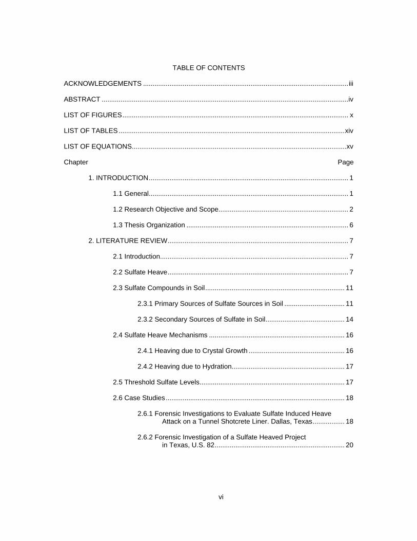
TABLE OF CONTENTS
ACKNOWLEDGEMENTS ............................................................................................................. iii
ABSTRACT ................................................................................................................................... iv
LIST OF FIGURES ........................................................................................................................ x
LIST OF TABLES ........................................................................................................................ xiv
LIST OF EQUATIONS .................................................................................................................. xv
Chapter Page
1. INTRODUCTION .......................................................................................................... 1
1.1 General .......................................................................................................... 1
1.2 Research Objective and Scope..................................................................... 2
1.3 Thesis Organization ...................................................................................... 6
2. LITERATURE REVIEW ................................................................................................ 7
2.1 Introduction .................................................................................................... 7
2.2 Sulfate Heave ................................................................................................ 7
2.3 Sulfate Compounds in Soil .......................................................................... 11
2.3.1 Primary Sources of Sulfate Sources in Soil ................................ 11
2.3.2 Secondary Sources of Sulfate in Soil .......................................... 14
2.4 Sulfate Heave Mechanisms ........................................................................ 16
2.4.1 Heaving due to Crystal Growth ................................................... 16
2.4.2 Heaving due to Hydration............................................................ 17
2.5 Threshold Sulfate Levels ............................................................................. 17
2.6 Case Studies ............................................................................................... 18
2.6.1 Forensic Investigations to Evaluate Sulfate Induced Heave Attack on a Tunnel Shotcrete Liner. Dallas, Texas ................. 18
2.6.2 Forensic Investigation of a Sulfate Heaved Project
in Texas, U.S. 82 ..................................................................... 20
vii
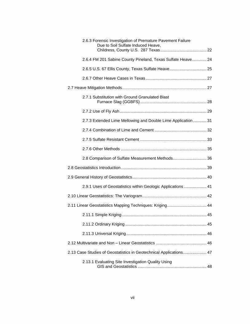
2.6.3 Forensic Investigation of Premature Pavement Failure Due to Soil Sulfate Induced Heave, Childress, County U.S. 287 Texas ......................................... 22
2.6.4 FM 201 Sabine County Pineland, Texas Sulfate Heave ............. 24
2.6.5 U.S. 67 Ellis County, Texas Sulfate Heave ................................. 25
2.6.7 Other Heave Cases in Texas ...................................................... 27
2.7 Heave Mitigation Methods ........................................................................... 27
2.7.1 Substitution with Ground Granulated Blast Furnace Slag (GGBFS) ........................................................... 28
2.7.2 Use of Fly Ash ............................................................................. 29
2.7.3 Extended Lime Mellowing and Double Lime Application ............ 31
2.7.4 Combination of Lime and Cement .............................................. 32
2.7.5 Sulfate Resistant Cement ........................................................... 33
2.7.6 Other Methods ............................................................................ 35
2.8 Comparison of Sulfate Measurement Methods.............................. 36
2.8 Geostatistics Introduction ............................................................................ 39
2.9 General History of Geostatistics .................................................................. 40
2.9.1 Uses of Geostatistics within Geologic Applications .................... 41
2.10 Linear Geostatistics: The Variogram ......................................................... 42
2.11 Linear Geostatistics Mapping Techniques: Kriging ................................... 44
2.11.1 Simple Kriging ........................................................................... 45
2.11.2 Ordinary Kriging ........................................................................ 45
2.11.3 Universal Kriging ....................................................................... 46
2.12 Multivariate and Non – Linear Geostatistics ............................................. 46
2.13 Case Studies of Geostatistics in Geotechnical Applications ..................... 47
2.13.1 Evaluating Site Investigation Quality Using GIS and Geostatistics ............................................................. 48

viii
2.13.2 Spatial and Temporal Variations in Grain Size of Surface Sediments in the Littoral Area of the Yellow River Delta ................................................ 50
2.13.4 Other Cases .............................................................................. 51
2.14 Summary ................................................................................................... 52
3. EXPERIMENTAL PROGRAM AND RESULTS ......................................................... 54
3.1 Introduction .................................................................................................. 54
3.2 Soil Selection and Sampling ....................................................................... 54
3.3 Soluble Sulfate Testing ............................................................................... 55
3.3.1 AASHTO T290 – 95 Determining Water – Soluble Sulfate Ion Concentration in Soil ............................................. 56
3.3.2 TXDOT Tex – 145 – E Determining Sulfate Content in
Soil Colorimetric Method ......................................................... 58
3.3.3 Modified UTA Method for Soluble Sulfates Determination in Soil ............................................................... 59
3.4 Sulfate Testing Introduction ........................................................................ 63
3.5 Deterministic Sulfate Concentration Bar Plots ............................................ 66
4. GEOSTATISTICAL ANALYSIS AND MAPPING ....................................................... 72
4.1 Introduction .................................................................................................. 72
4.2 Eagle Ford Formation ................................................................................. 73
4.3 Ozan Formation .......................................................................................... 79
4.4 Wolfe City Sand and Neylandville Formations ............................................ 84
4.5 Kemp Clay and Wills Point Formations ....................................................... 84
4.6 All Formations ............................................................................................. 92
4.7 Geostatistical Validation ............................................................................ 101
4.7.1 Eagle Ford Formation Validation .............................................. 103
4.7.2 Wolfe City and Neylandville Combination ................................. 103
4.7.3 All Formations ........................................................................... 104
5. CONCLUSIONS & RECOMMENDATIONS ............................................................. 112

ix
5.1 Conclusions of Testing and Mapping ........................................................ 112
5.2 Recommendations .................................................................................... 113
5.2.1 Eagle Ford Formation ............................................................... 113
5.2.2 Ozan Formation ........................................................................ 113
5.2.3 Kemp Clay Formation ............................................................... 113
5.2.4 Wolfe City Formation ................................................................. 114
5.3 Geostatistical Validation ............................................................................ 114
5.3.1 Eagle Ford Validation ................................................................ 114
5.3.2 Wolfe City/Neylandville ............................................................. 115
5.3.3 All Formations Validation .......................................................... 115
5.4 Implications for Further Study ................................................................... 115
REFERENCES .......................................................................................................................... 117
BIOGRAPHICAL INFORMATION ............................................................................................. 129

x
LIST OF FIGURES
Figure Page 1.1 IPL Project Alignment Map Showing Existing Pipeline and New Pipeline Source: TRWD .............................................................................................. 4 1. 2 Geophysical Map of the IPL Alignment Highlighting Test Formations Source: Fugro Consultants Inc .............................................................................. 5
2.1 Sulfate Concentrations and Locations of Test Soils (Gaily 2012) ........................................... .10
2.2 Location Map Showing Sulfate-bearing Soils in Texas (Harris et al., 2004) ........................... 10
2.3 Location of soils containing Gypsum in United State (Kota et al., 1996) ................................ 12
2.4.a through 2.4.e Various Types of Gypsum Manifestation in Test Soils ................................... 13
2.5Thenardite Sample form U.S. Natural History Museum ............................................................ 14
2.6 Epsomite from Dr. Grier Mine, Germany .................................................................................. 14
2.7 Distress Cracks form Sulfate Attack (Puppala 2010) ............................................................... 19
2.8 White Powder and Gel from Sulfate Reaction (Puppala 2010) ................................................ 19
2.9 Core Hole from Forensic Investigation (Puppala 2010) ........................................................... 20
2.10 Gypsum Crystals Retrieved from the Investigation Site (Chen et al. 2005) ........................... 21
2.11 Heaved Area on East side of Project Area (Chen et al. 2005) .............................................. 22
2.12 Gypsum Interbed near Baylor Creek U.S. 287 (Zhiming 2008) ............................................. 23
2.13 Gypsum Crystals Located in Drainage Wash Adjacent to the Roadway (Harris et al. 2006) ....................................................................... 24 2.14 Geologic Map Identifying the Eagle Ford Formation and U.S. 67 Project Location (Wimsatt 1999) ........................................................................................... 25
2.15 Heave Associated with US 67 near Midlothian, TX (Wimsatt 1999) ..................................... 26
2.16 Riverside Soil Sulfate Testing Results Comparison (Talluri et al. 2012) .............................. 38
2.17 Fort Worth Soil Sulfate Testing Results Comparison (Talluri et al. 2012) ........................... 38
2.18 Semivariogram Example Plot (Surfer 9)................................................................................ 43
2.19 Investigation Quality vs. Expense of Two Different Sampling Plans (Parsons and Frost 2002) ............................................................................ 48
xi
2.20 Experimental Variogram for Treasure Island Yerba Buena Shoals (Parsons and Frost 2002) .................................................................... 49
2.21 Multivariate Kriging Output for Clay, Silt and Sand (Ren et al. 2012) ................................... 51
3.1 a) & b) Samples Receipt and Preparation Prior to Testing c) Pulverized Sample after Drying ............................................................................................ 55 3.2 Platinum Crucible Used in AASHTO T 290 – 95 Method A (Gravimetric) Photo Source: VRS Laboratory ............................................................................................... .57
3.3 Photograph of a Colorimeter and Conductivity Meter .............................................................. 59
3.4 UTA Soluble Sulfate Determination for Soils Flow Chart (Puppala et al 2002) ....................... 61
3.5 Illustrated UTA Method for Soluble Sulfates Determination in Soil .......................................... 62
3.6 Straight Line Distance vs. Sulfate Concentration (Depth 5ft).................................................. 68
3.7 Straight Line Distance vs. Sulfate Concentration (Depth 10ft) ................................................ 69
3.8 Straight Line Distance vs. Sulfate Concentration (Depth 15ft) ................................................ 70
3.9 Straight Line Distance vs. Sulfate Concentration (Depth 20ft) ................................................ 71
4.1 Eagle Ford Contour Map with Approximate Pipeline Alignment and IPL Parcel Numbers (Depth –5ft) ............................................................................................. 75 4.2 Eagle Ford Contour Map with Approximate Pipeline Alignment and IPL Parcel Numbers (Depth – 10ft) ......................................................................................... 76 4.3 Eagle Ford Contour Map with Approximate Pipeline Alignment and IPL Parcel Numbers (Depth – 15ft) .......................................................................................... 77 4.4 Eagle Ford Contour Map with Approximate Pipeline Alignment and IPL Parcel Numbers (Depth – 20ft) .......................................................................................... 78 4.5 Ozan Contour Map with Approximate Pipeline Alignment and IPL Parcel Numbers (Depth – 5ft) ............................................................................................ 80 4.6 Ozan Contour Map with Approximate Pipeline Alignment and IPL Parcel Numbers (Depth – 10ft) .......................................................................................... 81 4.7 Ozan Contour Map with Approximate Pipeline Alignment and IPL Parcel Numbers (Depth – 15ft) .......................................................................................... 82 4.8 Ozan Contour Map with Approximate Pipeline Alignment and IPL Parcel Numbers (Depth – 20ft) .......................................................................................... 83 4.9 Wolfe City Sand and Neylandville Contour Map with Approximate Pipeline Alignment and IPL Parcel Numbers (Depth – 5ft) ...................................................... 86
xii
4.10 Wolfe City Sand and Neylandville Contour Map with Approximate Pipeline Alignment and IPL Parcel Numbers (Depth – 10ft) .................................................. 86 4.11 Wolfe City Sand and Neylandville Contour Map with Approximate Pipeline Alignment and IPL Parcel Numbers (Depth – 15ft) .................................................. 87 4.12 Wolfe City Sand and Neylandville Contour Map with Approximate Pipeline Alignment and IPL Parcel Numbers (Depth – 20ft) .................................................. 87 4.13 Kemp Clay and Wills Point Contour Map with Approximate Pipeline Alignment and IPL Parcel Numbers (Depth – 5ft) .................................................... 88 4.14 Kemp Clay and Wills Point Contour Map with Approximate Pipeline Alignment and IPL Parcel Numbers (Depth – 10ft) .................................................. 89 4.15 Kemp Clay and Wills Point Contour Map with Approximate Pipeline Alignment and IPL Parcel Numbers (Depth – 15ft) .................................................. 90 4.16 Kemp Clay and Wills Point Contour Map with Approximate Pipeline Alignment and IPL Parcel Numbers (Depth – 20ft) .................................................. 91 4.17 All Formations Contour map with Approximate Pipeline Alignment and Highlighting High Sulfate Borings (Depth – 5ft) ............................................ 93 4.18 All Formations Contour Map Overlaid on Geology Map (Depth – 5ft) .................................. .94 4.19 All Formations Contour map with Approximate Pipeline Alignment and Highlighting High Sulfate Borings (Depth – 10ft) ........................................... 95 4.20 All Formations Contour Map Overlaid on Geology Map (Depth – 10ft) ................................. 96 4.21 All Formations Contour map with Approximate Pipeline Alignment and Highlighting High Sulfate Borings (Depth – 15ft) ........................................... 97 4.22 All Formations Contour Map Overlaid on Geology Map (Depth – 15ft) ................................ 98 4.23 All Formations Contour map with Approximate Pipeline Alignment and Highlighting High Sulfate Borings (Depth – 20ft) ........................................... 99
4.24 All Formations Contour Map Overlaid on Geology Map (Depth – 20ft) .............................. 100
4.25 a&b Eagle Ford Validation Depth 5ft. & 10ft ........................................................................ 106
4.25 c&d Eagle Ford Validation Depth 15ft. & 20ft ...................................................................... 107
4.26 a&b Wolfe City/Neylandville Validation Depth 5ft. & 10ft ..................................................... 108
4.26 c&d Wolfe City/Neylandville Validation Depth 15ft. & 20ft ................................................... 109
4.27 a&b All Formations Validation Depth 5ft. and 10ft ............................................................... 110

xiii
4.27 c&d All Formations Validation Depth 15ft. and 20ft ............................................................. 111

xiv
LIST OF TABLES
Table Page PAGE
2.1 Soil Classification Information (Talluri et al. 2012) ................................................................... 37
2.2 Sulfate Measurement Techniques Comparison (Talluri et al. 2012) ........................................ 37
3.1 Sulfate Testing Breakdown by Geologic Formation ................................................................. 55
3.2 Eagle Ford Sulfate Concentrations .......................................................................................... 63
3.3 Ozan Sulfate Concentrations ................................................................................................... 64
3.4 Wolfe City Sand Sulfate Concentrations .................................................................................. 64
3.5 Neylandville Sulfate Concentrations ........................................................................................ 65
3.6 Kemp Clay Sulfate Concentrations .......................................................................................... 65
3.7 Wills Point Sulfate Concentrations ........................................................................................... 66
4.1 Variance Comparison from Variograms at Tested Depth Intervals ....................................... 102

xv
LIST OF EQUATIONS
Equation Page
2.10.1 Semivariogram Definition .................................................................................................... 42
1
CHAPTER 1
INTRODUCTION
1.1 General
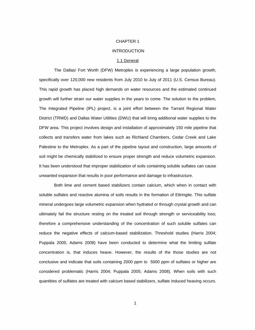
The Dallas/ Fort Worth (DFW) Metroplex is experiencing a large population growth,
specifically over 120,000 new residents from July 2010 to July of 2011 (U.S. Census Bureau).
This rapid growth has placed high demands on water resources and the estimated continued
growth will further strain our water supplies in the years to come. The solution to the problem,
The Integrated Pipeline (IPL) project, is a joint effort between the Tarrant Regional Water
District (TRWD) and Dallas Water Utilities (DWU) that will bring additional water supplies to the
DFW area. This project involves design and installation of approximately 150 mile pipeline that
collects and transfers water from lakes such as Richland Chambers, Cedar Creek and Lake
Palestine to the Metroplex. As a part of the pipeline layout and construction, large amounts of
soil might be chemically stabilized to ensure proper strength and reduce volumetric expansion.
It has been understood that improper stabilization of soils containing soluble sulfates can cause
unwanted expansion that results in poor performance and damage to infrastructure.
Both lime and cement based stabilizers contain calcium, which when in contact with
soluble sulfates and reactive alumina of soils results in the formation of Ettringite. This sulfate
mineral undergoes large volumetric expansion when hydrated or through crystal growth and can
ultimately fail the structure resting on the treated soil through strength or serviceability loss;
therefore a comprehensive understanding of the concentration of such soluble sulfates can
reduce the negative effects of calcium-based stabilization. Threshold studies (Harris 2004;
Puppala 2005; Adams 2008) have been conducted to determine what the limiting sulfate
concentration is, that induces heave. However, the results of the those studies are not
conclusive and indicate that soils containing 2000 ppm to 5000 ppm of sulfates or higher are
considered problematic (Harris 2004; Puppala 2005; Adams 2008). When soils with such
quantities of sulfates are treated with calcium based stabilizers, sulfate induced heaving occurs.
2
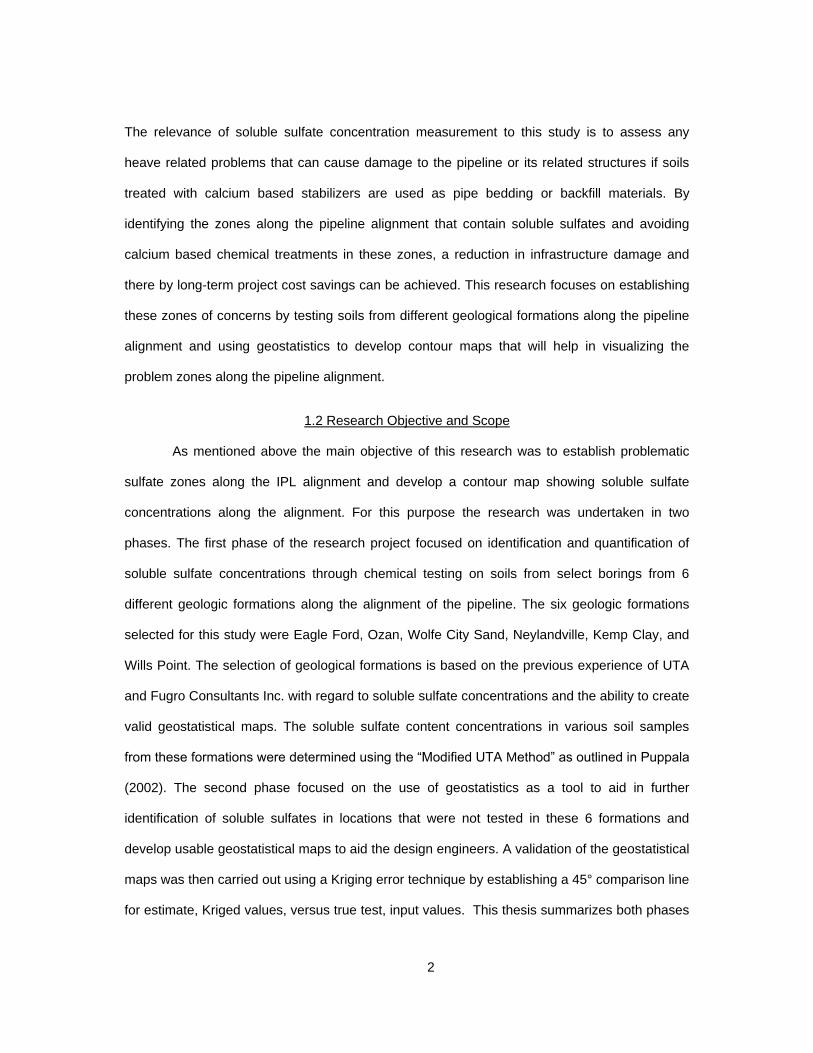
The relevance of soluble sulfate concentration measurement to this study is to assess any
heave related problems that can cause damage to the pipeline or its related structures if soils
treated with calcium based stabilizers are used as pipe bedding or backfill materials. By
identifying the zones along the pipeline alignment that contain soluble sulfates and avoiding
calcium based chemical treatments in these zones, a reduction in infrastructure damage and
there by long-term project cost savings can be achieved. This research focuses on establishing
these zones of concerns by testing soils from different geological formations along the pipeline
alignment and using geostatistics to develop contour maps that will help in visualizing the
problem zones along the pipeline alignment.
1.2 Research Objective and Scope
As mentioned above the main objective of this research was to establish problematic
sulfate zones along the IPL alignment and develop a contour map showing soluble sulfate
concentrations along the alignment. For this purpose the research was undertaken in two
phases. The first phase of the research project focused on identification and quantification of
soluble sulfate concentrations through chemical testing on soils from select borings from 6
different geologic formations along the alignment of the pipeline. The six geologic formations
selected for this study were Eagle Ford, Ozan, Wolfe City Sand, Neylandville, Kemp Clay, and
Wills Point. The selection of geological formations is based on the previous experience of UTA
and Fugro Consultants Inc. with regard to soluble sulfate concentrations and the ability to create
valid geostatistical maps. The soluble sulfate content concentrations in various soil samples
from these formations were determined using the “Modified UTA Method” as outlined in Puppala
(2002). The second phase focused on the use of geostatistics as a tool to aid in further
identification of soluble sulfates in locations that were not tested in these 6 formations and
develop usable geostatistical maps to aid the design engineers. A validation of the geostatistical
maps was then carried out using a Kriging error technique by establishing a 45° comparison line
for estimate, Kriged values, versus true test, input values. This thesis summarizes both phases

3
of the soluble sulfate study and the results of the geotechnical investigations conducted to
identify, quantify, and map soluble sulfate concentrations along the pipeline alignment.
Figure 1.1 shows the Integrated Pipe Line alignment highlighting the reservoirs and
lakes to be connected and the counties the IPL lies in. Figure 1.2 shows the IPL alignment
overlain on a geological map and highlights the formations utilized for testing in this project.

Figure 1.1 IPL Project Alignment Map Showing Existing Pipeline and New Pipeline Source: TRWD
4

Figure 1.2 Geophysical Map of the IPL Alignment Highlighting Test Formations Source: Fugro Consultants Inc.
Willis
Point
Kemp Wolfe
City
Ozan
City
Eagle Ford
Neylandville
5

6
1.3 Thesis Organization
This thesis consists of five chapters: Chapter 1: Introduction, Chapter 2: Literature
Review of Sulfates in Soil and Geostatistics, Chapter 3: Experimental Program and Results,
Chapter 4: Geostatistical Analysis and Mapping and Chapter 5: Conclusions, recommendations,
and future research needs/implications.
Chapter 1 provides the introduction to the sulfate study, the research objectives, and
thesis organization.
Chapter 2 provides a comprehensive summary of studies that include: Sulfate induced
heave in soils, the origins on sulfates in soils, the heaving mechanisms, case studies on sulfate
induced heave, sulfate attack on civil engineering projects, mitigation methods for high sulfate
soils, and a comparative evaluation of sulfate testing methods. Following sulfate heave review,
a brief review of the history of geostatistics and use of geostatistics in geotechnical projects is
discussed. All literature utilized for the compilation of this chapter is presented in text as well as
in the References section at the end of the paper.
Chapter 3 presents the three main test methods considered for the sulfate testing, the
procedures and equipment associated with those methods, the soil selection and sampling, the
results of sulfate testing, and the deterministic analysis of the sulfate test results.
Chapter 4 provides the geostatistical analysis and mapping results as well as the
validation of the geostatistical mapping.
Chapter 5 provides an overall summary of test results, geostatistical mapping, and
geostatistical validation. Conclusions and connections are also provided on the above
mentioned topics in this chapter. Lastly, implications on newer studies concerning the IPL
project as well as recommendations for further testing and analysis are provided in this chapter.
Following chapter five, all references and programming used for this study are cited.
.
7
CHAPTER 2
LITERATURE REVIEW
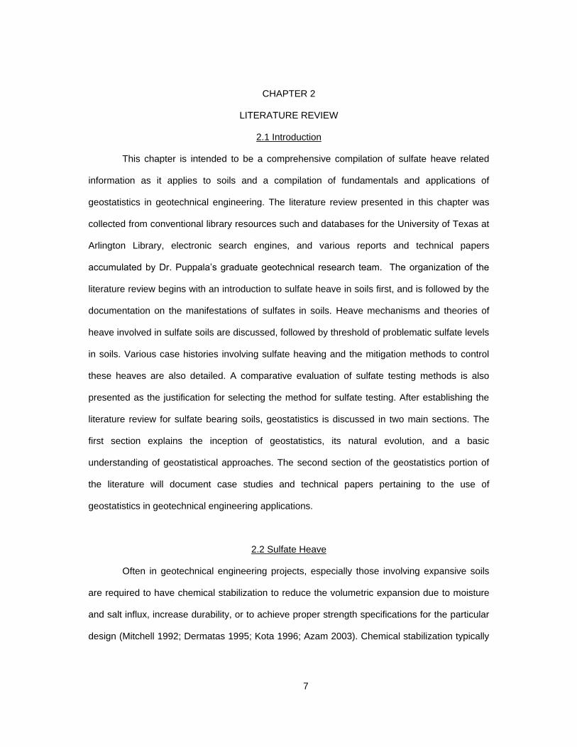
2.1 Introduction
This chapter is intended to be a comprehensive compilation of sulfate heave related
information as it applies to soils and a compilation of fundamentals and applications of
geostatistics in geotechnical engineering. The literature review presented in this chapter was
collected from conventional library resources such and databases for the University of Texas at
Arlington Library, electronic search engines, and various reports and technical papers
accumulated by Dr. Puppala’s graduate geotechnical research team. The organization of the
literature review begins with an introduction to sulfate heave in soils first, and is followed by the
documentation on the manifestations of sulfates in soils. Heave mechanisms and theories of
heave involved in sulfate soils are discussed, followed by threshold of problematic sulfate levels
in soils. Various case histories involving sulfate heaving and the mitigation methods to control
these heaves are also detailed. A comparative evaluation of sulfate testing methods is also
presented as the justification for selecting the method for sulfate testing. After establishing the
literature review for sulfate bearing soils, geostatistics is discussed in two main sections. The
first section explains the inception of geostatistics, its natural evolution, and a basic
understanding of geostatistical approaches. The second section of the geostatistics portion of
the literature will document case studies and technical papers pertaining to the use of
geostatistics in geotechnical engineering applications.
2.2 Sulfate Heave
Often in geotechnical engineering projects, especially those involving expansive soils
are required to have chemical stabilization to reduce the volumetric expansion due to moisture
and salt influx, increase durability, or to achieve proper strength specifications for the particular
design (Mitchell 1992; Dermatas 1995; Kota 1996; Azam 2003). Chemical stabilization typically

8
takes place in the form of lime or cement, both of which are cost effective and contain
appreciable amounts of calcium. Lime induced sulfate heave has been documented by Mitchell
(1986), and Mitchell (1992), among others. Stabilization with lime creates a chemical reaction
that forms an interlocking gel between the clay particles and ultimately increases strength,
reduces plasticity, increases workability, and reduces in swell behavior (Dempsey and
Thompson 1968; Bell 1989). Additionally, Kota (1996) and Ksaibati (1996) have shown that
cement based stabilizers also induce sulfate heave. Stabilization with cement creates a
poizzalonic reaction that lowers the plasticity of the soil and also produces gels that increase the
strength of the soil and reduce swelling potential (Bugge and Bartlesmeyer 1966; Nelson and
Miller 1992).
Clayey soils generally consist of three minerals with one generally dominating:
Kaolinite, Illite, and Montmorillonite and all three are susceptible to sulfate induced heave
(Wang 2004). All three of these minerals naturally contain alumina (Aluminum Oxide, ).
The introduction of calcium in the stabilizers in the presence of free alumina in the soil and
soluble sulfate minerals can create a calcium – alumina – sulfate hydrate compound known as
Ettringite ) ) ) or a calcium – silica – hydroxide – sulfate –
hydrate compound known as Thaumasite ) ) ) (Sherwood 1962;
Mehta and Klein 1966; Mehta and Wang 1982; Mitchell 1986; Hunter 1988; Perrin 1992; Petry
1994; Burkhart et al 1999). Sulfate heave in soils was introduce to geotechnical engineering in
1986 by Mitchell and since that time both minerals have been well documented to cause
heaving in soil (Dermatas 1995; Little 2005; Puppala 2007). The heave associated with these
reactions creates distress and eventually poor performance of the infrastructure and can
ultimately reduce the life time of the structures (Puppala 2002). Various case studies of sulfate
induced heave failures were reported across the United States (Mitchell, 1986; Hunter, 1988;
Kota et al., 1996). In some cases, the cost of repairs exceeded the cost of stabilization (Hunter,
1988).

9
Sulfate – bearing soils are found in many regions in the United States, particularly in the
Western and Southwestern United States (Puppala et al. 2002). These states include Texas,
Nevada, Louisiana, Kansas, Colorado and Oklahoma (Solanki et al. 2010). Studies conducted
by Burkhart et al. (1999) identified certain geologic formations that possess high sulfates and
that gypsum was the most common sulfate mineral in Dallas area soils. Therefore, in these
regions it is very important to identify and quantify sulfate bearing soils in order to prevent
damage to infrastructure due to sulfate induced heave. Sulfate related heave and failures have
gained notoriety over the years as more and more design professionals become aware of the
effects of sulfate related heave on civil engineering projects. One of the most severe cases of
sulfate induced heave in the DFW area was associated with the Eagle Ford formation, where
sulfate concentrations were found ranging from 4,000 ppm to 27,800 ppm (Chen et al., 2005).
High sulfate concentrations of 35,540 ppm have been reported in the Childress district located
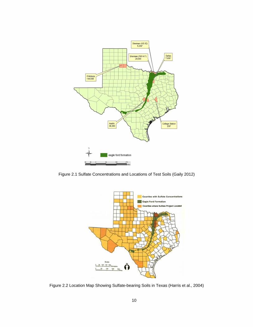
in the Pan Handle area of North Texas (Zhiming 2008). Gaily (2012) conducted further studies
on Texas soils containing sulfates to identify other factors such as soil type, lime dosage, and
mellowing period on sulfate related heave and Figure 2.1 on the following page identifies the
location and sulfate concentrations of these test soils.
Sulfate induced heave or chemical swelling is a long term scenario which often worsens
as time passes (Hunter 1988). Unlike physical heaving, the rate of chemical heaving often stays
constant or increases with time (Ferris et al. 1991). Figure 2.2 on the following page depicts
specific counties within the state of Texas that have sulfate bearing soils as well as highlights
the Eagle Ford formation, which has been previously established to be highly problematic for
sulfate induced heave (Harris et al. 2004; Chen et al. 2005).
10
Figure 2.1 Sulfate Concentrations and Locations of Test Soils (Gaily 2012)
Figure 2.2 Location Map Showing Sulfate-bearing Soils in Texas (Harris et al., 2004)

11
2.3 Sulfate Compounds in Soil
A variety of sulfate compounds exist in both nature and in soil and can manifest as a
solid, liquid, or a vapor (Chikyala 2007). Soils and rocks are examples of solid state sulfates,
while air and water examples in their respective states (Hawkins et al 1998). Sulfates in soils
can manifest in two different forms. The first form is primary sulfate sources and the other is
secondary sulfate sources. Primary sulfate sources come from compounds that exist or are
formed naturally, while secondary sources are the products of other chemical reactions, such as
oxidation, or from engineering practices. Both primary and secondary sulfate sources are
discussed in the sections below as both sources can contribute to sulfate heave.
2.3.1 Primary Sources of Sulfate Sources in Soil
Most sulfate minerals are created and deposited through evaporation of salt water
followed by the precipitation of salts (Zanbeck et al. 1986). Typically Anhydrite ),
Gypsum or Calcium Sulfate Dihydrate ( ), Halite ), and Dolomite
) ) are formed through this process (Zanbeck et al. 1986). Halite is more commonly
known as sea salt and is not a sulfate mineral nor is Dolomite, which is carbonate mineral.
These minerals were included in the discussion for the sake of completeness. Evaporation
minerals are more commonly found in the upper crust and manifest in as evaporate, clay, or fine
grain sediment deposits (Zanbeck et al. 1986). Texas soils are primarily made of clay or fine
grain sedimentary deposits; therefore the most common primary sulfate source of sulfate in
Texas soil is in the form of gypsum. In addition to being formed naturally through the
evaporation and precipitation method described previously, gypsum can also be formed as a
result of the breaking down of anhydrite into an aqueous solution that then recrystallizes to form
gypsum (Indiana Geological Survey).
In addition to gypsum, other primary sources of sulfates in soil are Thenordite or
Sodium Sulfate ), and Epsomite or Magnesioum Sulfate ). Sodium
sulfate and Magnesium sulfate tend to manifest in more arid regions (Hilgard 1906; FAO 2001;

12
Bing et al. 2007). Figure 2.3 shows other regions in the United States that have soils that
contain gypsum. Figures 2.4.a through 2.4.e display soil samples containing gypsum utilized in
this research project. Figure 2.5 shows a sodium sulfate sample from the National Museum of
Natural History and Figure 2.6 shows a sample of epsomite from the Dr. Geier Mine in
Germany.
Figure 2.3 Location of soils containing Gypsum in United State (Kota et al., 1996)

13
(a) (b)
(c) (d)
(e)
Figure 2.4.a through 2.4.e Various Types of Gypsum Manifestation in Test Soils
0.5”
2.5”
2.5”
8.0”
4.0”
2.5”
2.0”
0.25”

14
Figure 2.5 Thenardite Sample form U.S. Natural History Museum
Figure 2.6 Epsomite from Dr. Grier Mine, Germany
2.3.2 Secondary Sources of Sulfate in Soil
Secondary sulfate sources can manifest in many different ways. One secondary source
of sulfates in soils comes from the decomposition of pyrites ). Pyrites break down when

15
oxidized and can convert into sulfate minerals, like gypsum, that may then be dissolved and
transported by ground water (Steger and Desjardins 1977; Dubbe et al 1997, Bryant et al. 2003;
Harris et al. 2004). In addition to pyrite oxidation, the use of Chromite Ore Processing Residue
(COPR), a byproduct of the chromite ore lime – based roasting process used to isolate and
extract soluble chromate ), in structural fills can react under certain soil conditions to
from gypsum (Dermatas 2006). Other studies that discuss soluble sulfates and their ability to
be transported and redistributed by groundwater flows were conducted by Skousen et al.
(1996), and Puppala (2005). An example of transportation of sulfates through ground water
flows would be during the wet season when soluble sulfates in the top layers of the soil dissolve
and move downward by gravity into stabilized layers, and conversely during the dry season
dissolved sulfates move upward due to evaporation or capillary rise into the top layers
increasing their concentration (Dermatas, 1995; Natarajan 2004). Additionally, soluble sulfates
may come from water sources used in construction. For example, Rollings et al. (1999)
conducted a forensic investigation on the failure of Bush Road in Georgia. Five months after
construction, distress cracks and bumps from soil heave were observed. The investigation
concluded that the failure was due to the formation of Ettringite in the subgrade material.
However, initial geotechnical testing observed no sulfates in the subgrade soil and the subgrade
soil was treated with cement. It was determined at the conclusion of the study that water from a
nearby well used for mixing concrete and for field compaction purposes contained sulfates and
the introduction of this sulfate water to the subgrade soil combined with the cement stabilization
induced sulfate heave. Similarly, the Yongam Dam, China was also contaminated with sulfate
bearing water used in construction which ultimately led to the formation of Thaumasite and the
eventual degradation of the concrete used in the dam construction (Mingyu et al. 2006)

16
2.4 Sulfate Heave Mechanisms
Sulfate attack in Portland cement concrete was established in the early 19th century
(ACI1982; DePuy 1994). At that time it was proven that calcium rich cement mixed with sulfate
and free alumina could create Ettringite and Thaumasite minerals (ACI 1982). Additionally, the
formation of Ettringite and its subsequent growth in concrete was explained by Cohen (1983).
Cohen established two different growth mechanisms for Ettringite and Thaumasite, crystal
growth and hydration. Similarly, in soil the same two expansion mechanisms were established
(Dermatas 1995). The first mechanism causes expansion due to the formation and/or oriented
crystal growth of Ettringite (Ogawa and Roy, 1982). The second is a thorough solution
mechanism where expansion is related to swelling due to hydration Ettringite (Mehta 1973;
Mehta and Wang 1982).
2.4.1 Heaving due to Crystal Growth
Crystal growth theory dictates that aluminum, calcium, and sulfates can concentrate
around Ettringite nucleation sites and combine to form additional Ettringite, essentially building
onto the internal lattice structure of the Ettringite molecule (Ogawa and Roy 1982). As per the
theory, this crystal growth occurs at the beginning stages of cement hydration and as water is
introduced to the system, the crystals form their needle like shape. As the crystals build they
begin to come in contact with one another, exerted pressures on each other and causing the
whole system to swell. The pressure generated by the crystal growth is then exerted on the
surrounding soil inducing strains and pressures. Once the load applied through crystal growth
exceeds that of the capacity of the restraining medium, heave occurs. Crystal growth of
Ettringite is favored in high pH ranges. As a solution becomes more basic alkaline earth metals,
such as calcium, and alumina dissolve more readily. The dissolution of these constituents drives
the reaction and the formation of Ettringite. Soil is a more plastic substance than concrete and
allows for the accommodation of some Ettringite growth. However, at some point as the reaction

17
continues the soil can no longer absorb the strains and pressures exerted by the growth of the
Ettringite crystals and heaves, transferring the stress to the next path of least resistance.
2.4.2 Heaving due to Hydration
Swelling due to hydration was proposed by Mehta (1973). The theory suggests that
formation of Ettringite follows a thorough solution mechanism. In the presence of saturated
calcium hydroxide ) ) , the rate of hydration of aluminum decreases significantly, causing
the Ettringite to form gel – like and colloidal crystals. The resulting colloidal crystal gels are
hydroscopic in nature and can adsorb large quantities of water molecules due to their high
surface area and net negative charge. As more water molecules are absorbed into the system,
the gel begins to swell exerting pressures and strains on the surrounding medium. Mehta and
Wang (1982) observed that the amount of expansion of the Ettringite gel is directly related to
the amount of water adsorbed and the size of the crystals. Coarser colloidal crystal gels were
found to expand more than finer colloidal crystal gels. The factor influencing the type of crystals
is related to the hydroxyl levels. High hydroxyl levels develop colloidal crystal gels, whereas low
hydroxyl levels create rod like crystals that expand much less.
2.5 Threshold Sulfate Levels
Problematic threshold levels for sulfates in soils are a difficult concept to establish.
Some cases report these levels as being between 1,500 ppm to 5,000 ppm and in other cases
levels as high as 10,000 ppm are reported as threshold levels (Harris et al 2004; Puppala et al.
2005; Adams et al. 2008). Unfortunately, soil conditions such as plasticity, density, and void
ratio coupled with stabilization techniques and environmental factors largely affect these
threshold levels (Puppala 2005). Therefore, setting threshold levels “across the board” is nearly
impossible (Adams et al. 2008). There are studies hoping to determine sulfate threshold levels
based on mineralogy and geological depositional environments, but this will only address some

18
of the issues associated with sulfate heave thresholds (Adams et al. 2008). With this in mind, it
is the opinion of the author that until such studies can conducted and confirmed, threshold
levels for sulfate soils should be conducted on a case by case basis, considering all potential
factors related to sulfate heave.
2.6 Case Studies
There are many case studies from all over the United States to the United Kingdom and
China that document sulfate induced heave (Hawkins 1987; Little 1989; Wimsatt 1999; Chen et
al., 2005; Mingyu 2006; Rollings et al. 2006; Zhiming, 2008; Adams 2008; Bagley et al. 2009;
Puppala et al. 2010). Primarily these case studies were under taken as the direct result of
infrastructure failures and were conducted to determine the causes of failure. In the cases
presented in the following sections, the infrastructure failures are due to the growth of Ettringite
or Thaumasite and are primarily due to the improper stabilization or identification of sulfate soils.
The details of these studies, conclusions drawn, and innovations in sulfate heave forensics are
described
2.6.1 Forensic Investigations to Evaluate Sulfate Induced Heave Attack on a Tunnel Shotcrete
Liner. Dallas, Texas
Considering the similarity of a pipe line with a tunnel structure, the Puppala et al. 2010
study is the most relevant to this research project. As such, this study will be discussed in detail,
first. In this study, cracking and water leakage was discovered in the shotcrete liner of a tunnel
in Dallas, Texas. The tunnel was built in the Eagle Ford Formation, one of the test formations in
this sulfate pipeline study. The surrounding tunnel material was limestone. As part of the
forensic investigation coring was done on the liner at key areas of leakage and distress. Upon
completion a white powder like material and gel like substance were found both within and
behind the shotcrete liner. Samples of the powder and gel material as well as the rock core

19
samples from distress locations were collected and tested at the University of Texas at Arlington
(UTA) geotechnical laboratories. The samples were first subjected to mineralogical and
micromorpholoical testing by XRPD and EDAX methods. Rock core samples were subjected to
strength tests, such as, unconfined compressive strength (UCS), indirect tensile strength (ITS)
and unconsolidated undrained (UU) tests. Figures 2.7, 2.8., and 2.9 show some of the
distressed regions where samples were taken.
Figure 2.7 Distress Cracks form Sulfate Attack (Puppala 2010)
Figure 2.8 White Powder and Gel from Sulfate Reaction (Puppala 2010)

20
Figure 2.9 Core Hole from Forensic Investigation (Puppala 2010)
The results of the study discovered that the sulfate attack was due to the growth of both
Ettringite and Thaumasite. Additionally, high moisture contents were related to higher levels of
distress. UCS, UU, and ITS testing indicated a decrease in strength values with increasing
distress magnitude. It was also determined that sulfate levels in the distressed areas ranged
from 1,500 ppm and above. It was determined that sulfates percolated through the limestone
and accumulated at the shotcrete liner, ultimately leading to the sulfate reaction that caused the
distress in the tunnel liner. The results of this work indicated that the limestone had significant
strength loss and that the tunnel was a potential safety hazard that needed to be monitored
continuously.
2.6.2 Forensic Investigation of a Sulfate Heaved Project in Texas, U.S. 82
Considering the location of the IPL project, the discussion of case studies within the
state of Texas are considered very relevant. This particular case study involved U.S. Highway
82 and was a Texas Department of Transportation (TXDOT) study conducted by Chen et al.,
2005. The construction of U.S. 82 began in 2001 which made this study center on a relatively
new pavement construction. The pavement was a 50 mm asphalt concrete over 300 mm flexible

21
base, followed by 200 mm lime treated subgrade. As with the tunnel study previously discussed,
the soil in question for this project was part of the Eagle Ford Formation. The project was
initiated because heaving on the East side of the project area was observed and severely
affected the performance of the pavement structure. During the investigation it was noted that
within the sub grade soil, sparkling gypsum fragments were present, and this gypsum was likely
the culprit in the heave distress to the pavement. Figure 2.10 depicts some of the gypsum
crystals that were located at the site with their relative sizes. Figure 2.11, on the following page,
shows the heave associated with the east side of the project.
Figure 2.10 Gypsum Crystals Retrieved from the Investigation Site (Chen et al. 2005)
The study involved the coring of the pavement to obtain samples of the lime treated
subgrade and underlying, untreated subgrade. Scanning Electron Microscope (SEM) analysis
was conducted on the samples collected from the field. The SEM results on the treated
subgrade indicated that crystals had formed and were confirmed to be Ettringite. Interestingly,
no crystals were found in the untreated subgrades, either indicating that no sulfates were
present at those depths or that stabilizer had not leached into the lower sub grade. Further
testing included chemical analysis, conductivity, and pH for both the east and west side of the
project. Conductivity testing indicated that as the depth increased conductivity increased

22
significantly. Further investigation determined this increase in conductivity was due to soluble
gypsum that seeped into the lower sub grade. Therefore, it was concluded from the study that
conductivity measurements are a good indicator of soils with high amounts of soluble sulfates.
Specifically, soils from the east side of the project were determined to have anywhere from
4,000-27,800 ppm of soluble sulfates, while the west side contained very low sulfate values.
Figure 2.11 Heaved Area on East side of Project Area (Chen et al. 2005)
2.6.3 Forensic Investigation of Premature Pavement Failure Due to Soil Sulfate Induced Heave,
Childress, County U.S. 287 Texas
TXDOT’s Materials and Pavement Division investigated large cracks and swells in
pavement near Bear Creek Bridge on U.S. 287 in Childress County Texas (Zhiming 2008). Both
North and South bound lanes had been previously reconstructed around 2001. Approximately 2
years after reconstruction the section of pavement near Baylor Creek began experiencing
extensive fatigue cracking and swelling. At that point, restoration in the form of milling and inlays
were under taken. Figure 2.13 shows the distress to U.S. 287 after heave distress set in. The
culprit the heave associated with the premature failure of this pavement was due to the
interaction of gypsum interbeds with the 9 in sub grade that was treated with lime at 3% by dry

23
weight of soil. Figure 2.12 on the following page shows the gypsum interbeds as they appear
adjacent to the pavement structure.
Subgrade soil samples from North and South bound lanes were collected and sent out
for laboratory testing. Sulfate testing determined that soils in the North bound lane contained
sulfate concentrations above 35,000 ppm, which was confirmed by the fact that the North bound
lane experienced much worse distress and heave. Testing determined that the sulfate levels in
the South bound lane were low in concentration. Further testing identified North bound soils as
being fine grained whereas south bound soils were coarser in nature. This also helps to explain
why the heave was greater in the North bound lane.
Figure 2.12 Gypsum Interbed near Baylor Creek U.S. 287 (Zhiming 2008)
After extensive lab testing for Atterberg limits, linear shrinkage, conductivity, moisture
susceptibility tests, resonant column, and UCS, four basic remedy methods were suggested for
proper stabilization of the sub grade soil. The first suggestion was complete removal of the
sulfate soil and replacement with select fill. The second recommendation was the reworking of

24
the subgrade with a lime and fly ash. The third suggestion was the use of geosynthetics such as
a geogrid to mechanically reinforce the subgrade. The fourth option was to apply an over lay,
mill and apply composites to the shoulder area of the pavement.
2.6.4 FM 201 Sabine County Pineland, Texas Sulfate Heave
FM 201 is located just east of U.S. 96, in East Texas near the city of Lufkin. The
particular road in question was a TXDOT project and it was determined that large, “roller
coaster”, type bumps in the road were due to improper stabilization of expansive soils. The
project was constructed on the Eocene Yazoo Formation which is clay, sandy; with inter beds of
silt and glauconitic sand with marine fossils. Gypsum beds were seen the drainage wash
surrounding the pavement. Cores of the pavement and the sub grade were taken from areas of
high expansion and examined. Ettringite was found in these samples and Figure 2.11 below
shows some of the gypsum crystal formations detected within the drainage washes from the
study. The solution for this construction project was blanket removal of the top two feet of
subgrade and reconstruction with cement stabilized select fill (Harris et al. 2006). Figure 2.13
depicts gypsum crystals discovered in the drainage wash adjacent to the roadway.
Figure 2.13 Gypsum Crystals Located in Drainage Wash Adjacent to the Roadway (Harris et al.
2006)

25
2.6.5 U.S. 67 Ellis County, Texas Sulfate Heave
In a study conducted by Wimsatt 1999 in conjunction with TXDOT on U.S. 67 it was
determined that sulfate induced heave was responsible for the deterioration of a pavement
structure. The project was initiated as a widening project for U.S. 67. The location of the project
and the geologic formation associated with the project is indicated by Figure 2.14. The
subgrade was stabilized with 10% and 11% lime by dry weight of soil. The stabilized subgrade
was then sealed to cure. During curing a large rain event occurred and upon arriving at the site
the following day, construction crews notice many evenly spaced heave ridges as shown in
Figure 2.15. The research was initiated to determine exactly what the caused the distress
heaves.
Figure 2.14 Geologic Map Identifying the Eagle Ford Formation and U.S. 67 Project Location
(Wimsatt 1999)
As with the U.S. 82 project, the Eagle Ford Formation was a part of a research study
involved with distress heave. The Eagle Ford is referred to as a selenetic formation. Selenite is

26
simply another name for gypsum. In this particular case study it was determined that gypsum
present in the soil interacted with the lime stabilization to form Ettringite. The Ettringite growth
induced heave in the pavement structure ultimately causing its failure before the completion of
construction. The use of X – ray diffraction and SEM analysis confirmed that the expansive
mineral was indeed Ettringite. Open full completion of laboratory testing it was determined that
U.S. 67 soils had sulfate concentrations ranging from 11,000 to 32,000 ppm. Ultimately, the
best option for this project was to remove the sub grade and replace it with select fill that did not
need to be stabilized. This was chosen because there still remained a fair amount of unreacted
gypsum in the soil that could cause further expansion. One conclusion of this study was the
more proper identification of sulfates in the field prior to construction through the use of the
Geologic Atlas of Texas, conductivity tests, and sulfate concentration testing.
Figure 2.15 Heave Associated with US 67 near Midlothian, TX (Wimsatt 1999)

27
2.6.7 Other Heave Cases in Texas
Other cases of heave in Texas include the SH 161 and SH183 interchange in the Dallas
County. In that case, sulfate concentrations as high as 27,000 ppm were discovered. Based on
this discovery, the soil was treated with a combination of lime and Ground Granulated Blast
Furnace Slag (GGBFS) prior to construction. Another case was on FM 3338 in Webb, County in
2005. In this study sulfates in the order of 40,000 ppm were discovered and had to be mitigated
through the use of a combination of lime, GGBFS, and clay star product. Also, SH 118 in
Brewster County in far West Texas near the city of El Paso experienced sulfate related heave.
In the more arid regions of Texas lime is not typically used for stabilization, however cement is
typically used to prevent erosion of sub grade material. In this case large amounts of
evaporated gypsum were discovered at the top of the sub grade. Currently, studies are still
ongoing to determine the best approach for the rehabilitation of the pavement. Suggestions
such as fly ash have been suggested, but no method has been chosen yet Yet another example
of sulfate related issues was observed in Culberson County in TXDOT’s El Paso District on SH
54. In this case head walls were cracked and culverts were deforming due to sulfate heave. It
was determined that gypsum in the soil reacted with the cement stabilizer to induce sulfate
heave. The solution was to replace the culverts and use an untreated backfill. All of the cases
presented were collected from Harris (2006), the USFHWA Report FHWATX-06/0-4240-4. It
can be seen from these cases that sulfate related heave in Texas is primarily due to stabilizer
reactions with gypsum. In addition the location of the project in Texas, climate, soil type, and
stabilizer type vary from project to project while still experiencing sulfate heave.
2.7 Heave Mitigation Methods
The mitigation of sulfate induced heave is a complex and difficult subject to address
due to the various components of the reaction, climatic factors, and soil properties. Various
techniques have been generated over the years from adjustment and substitution of stabilizers

28
to extending mellowing and even complete removal of the sulfate soil. It has even been
suggested that lime or cement treatment of sulfate laden soils should be avoided completely
(Mitchell, 1986). However, in most cases the soil must be stabilized to achieve the proper
strength and behavioral characteristics needed for the particular design specifications.
Therefore, this section will address the possible solutions to achieve proper stabilization without
inducing detrimental sulfate heave. First, the adjustment and substitution of typical stabilizers
are discussed and then other topics such as the use of geosynthetics, other materials, and
changes in engineering practice for mitigation of sulfate induced heave are addressed.
2.7.1 Substitution with Ground Granulated Blast Furnace Slag (GGBFS)
Substitution of materials typically used in construction with byproducts of industrial
processes that would normally be discarded can be a cost effective and sustainable option.
GGBFS is the result of the ferro – silica industry and is the material formed when molten iron
blast furnace slag is rapidly chilled (quenched) by immersion in water. It is a coarse glassy
product that is then grinded in a granular product with very limited crystal formation, is highly
cementitious in nature and, and hydrates like Portland cement (PC) (USFHWA). The use of
GGBFS in soil applications have been discussed by Tasong et al. (1999), Wild et al.(1999),
Puppala et al. (2003), Wang et al. (2003), Chavva et al. (2005), Higgins (2005), Deepti et al.
(2007), McCarthy et al (2009), Jegandan et al. (2010), and Wilkinson et al. (2010). In those
studies a variety of blends were tested to observe the effects of GGBFS and its viability for soil
stabilization as well as the mitigation of sulfate induced heave.
Studies conducted by Jaganden et al. (1999) concluded that GGBFS in conjunction with
other binders such as PC and Lime can increase Unconfined Compressive Strength (UCS) of
the soil, making it a viable option for increasing strength of the soil, which is one of the main
goals in chemical stabilization of soils. In most cases, the use of GGBFS as a replacement for
some PC or Lime content resulted in an increase in UCS beyond the use of PC or Lime alone

29
as well as the rate of increase in strength(Jaganden et al. 1999; Wilkinson et al. 2010). In
addition, GGBFS helped to reduce the linear expansion of soil samples during wetting, which is
one of the other main goals of chemical stabilization of soils (Higgins 2005). Lastly, the plasticity
of the soil is reduced and the undrained shear strength was increased when GGBFS is used
(Wilkinson et al. 2010).
In studies conducted by Tasong et al. (1999), Wild et al. (1999), Puppala. et al. (2003)
all focused on the use of GGBS to specifically mitigate the sulfate expansion. Tasong et al.
(1999) determined that the use of GGBFS caused a progressive change in the microstructure of
the Ettringite molecule and the change was the result of reducing the amount of available
calcium needed for the Ettringite reaction. Wild et al. (1999) determined that for kaolinite clays
contacting gypsum that anywhere from 60% - 80% of chemical stabilizer should be in the form
of GGBFS in order to sufficiently reduce the effects of sulfate induced expansion from Lime
treatment. In other words, 60%-80% of the determined Lime content from the Eades and Grim
Test should be substituted with GGBFS. The study conducted by Puppala et al. (2003)
determined that when only GGBFS is used, 20% GGBFS from dry weight of soil was the most
effective at reducing liquid limit of the sulfate soil and therefore the plasticity as well as reducing
the free swell characteristics.
2.7.2 Use of Fly Ash
Like GGBFS, Fly Ash is a byproduct of industrial processes. Fly ashes are finely divided
residue resulting from the combustion of ground or powdered coal. They are generally finer than
cement and consist mainly of glassy-spherical particles as well as residues of hematite and
magnetite, char, and some crystalline phases formed during cooling (USFHWA). The use of fly
ash in concrete started in the United States in the1930's. One of the first large scale uses of fly
ash in concrete was the construction of Hungry Horse Dam in Montana in 1948, which used
120,000 metric tons of fly ash. The uses of byproducts such as fly ash have been become an
established practice for changing the engineering and behavioral properties of soil (Wilkinson et

30
al. 2010). Fly ash, like cement, creates a poizzalonic bond within the soil particles, increasing
strength and workability while reducing plasticity.
Fly ash has a history of suppressing sulfate heave in concrete, and while the
compositions and constituents of sulfate reaction in concrete differ from that of soil, they are
similar (McCarthy et al. 2009). Therefore it is a logical step to introduce fly ash into sulfate
bearing soils to reduce the negative effects of sulfate heave. Studies have been conducted by
Puppala et al. (2003), Wang et al. (2003), Chavva et al. (2005), Punthutaecha etal. (2006),
Deepti et al. (2007), McCarthy et al. (2009), Solanki et al. (2010), and Wilkinson et al. (2010) to
assess the effect of fly ash on the suppression of sulfate induced heave.
The study conducted by Puppala et al. (2003) utilized class F fly ash, as this type is low
in calcium and would yield the best result for the mitigation of sulfate heave. Class C fly ash
contains higher amounts of calcium and yields better strength properties; however the
introduction of the calcium is known to increase the probability of Ettringite formation. Three mix
designs were used in the study, first a control soil with no stabilizer, next 10% fly ash by dry
weight of soil, and last 20% of fly ash by dry weight of soil. It was determined that the class F fly
ash improved the physical and engineering properties of the soil by plasticity of the soil,
increasing UCS, and reducing the free swell and shrinkage characteristics of the test soils.
When compared to other methods, such as sulfate resistant cements and GGBFS, the strength
gain using class F fly ash was not as high, but the cost effectiveness of this method exceeds
that of the other mentioned methods.
The McCarthy etal. (2009) study focused on the use of fly ash in conjunction with lime.
This study also utilized class F fly ash so as to reduce the amount of calcium present in the
stabilizer. For this study four mixes were created. All four mixes contained 3% Lime by dry
weight of soil and the addition of fly ash was done by 3%, 6%, 9%, and 12% by dry weight of
soil. The results of the study indicated that swelling decreased with the reduction of Lime and
the increase of fly ash. Surprisingly, the study found nearly the same amount of Ettringite

31
growth in control samples and fly ash samples that contained the same amount of Lime leading
the researchers to believe that mitigation of Ettringite in soils and concrete do not follow the
same mechanisms. In addition, the mellowing period was determined to have an effect on
swelling due to Ettringite growth. It was found that in increase in mellowing time before
reintroduction of Lime and fly ash significantly decreased volumetric swell. The final results of
the study determined the optimum Lime to fly ash mix to contain 3% Lime and10%-15% fly ash
by weight and a mellowing period of at least one day. Overall, the use of class F fly was
determined to be a viable and cost effective means of stabilizing soil while mitigating swell
associated with Ettringite growth.
2.7.3 Extended Lime Mellowing and Double Lime Application
As the McCarthy study showed in regards to fly ash and lime combination, mellowing
periods have a large effect on swelling of soils. Therefore a study was conducted by Talluri et
al. (2013) to determine the effects of extended lime mellowing in stabilized soils. For this
research initiative, six natural expansive soils from the state of Texas were used. Additional
sulfates were added to the soils with lower sulfate concentrations to observe the effects of
mellowing on high sulfate soils The study examined three different mellowing periods of 0, 3
and 7 days, and basic classification and chemical tests were performed to establish the clay
mineralogy of the soils. After each specified mellowing period, the samples were subjected to
three dimensional (3-D) volumetric swell, shrinkage and UCS tests. The results of study showed
that soils with 0 days of mellowing exhibited the observed largest swell. As the mellowing period
increased the early formation of ettringite began. The remixing of the samples after mellowing
and before final compaction seemed to break the ettringite minerals apart and separate them
from the sulfate minerals needed to continue further growth. Extended mellowing can also force
the formation of other deleterious compounds before remixing and final compaction (Berger et

32
al., 2001; Harris et al., 2004). As with the Talluri et al. (2013) study, mellowing before remixing
and final compaction of periods from 1 – 7 days was recommended to achieve heave arrest.
The double application of lime has also been shown to mitigate swell behavior due to
Ettringite growth in sulfate soils; however it is limited to soils with sulfate values lower than
7,000 ppm and soils that do not contain pyrites (Kota et al. 1996; Harris et al. 2004). The initial
application of lime allows for the beginning stages of Ettringite growth while the second
application, which is applied after a mellowing period, creates the poizzalonic bonds needed to
improve the strength of the soil. After the initial lime treatment water must be added to the soil in
order to dissolve the sulfate compounds and encourage the initial growth of Ettringite. Then, the
mixing and reapplication of lime can break up the Ettringite and disperse it within the soil. As
long as all of the soluble sulfates have been eradicated through the wetting and initial Ettringite
growth processes after the initial Lime application, there will be no sulfates left to continue the
reaction and future heave will be arrested.
2.7.4 Combination of Lime and Cement
Srivitmaitrie et al. (2008) conducted a study to see the effects of Lime and Cement
combined on sulfate induced heave in soils with low to medium sulfate levels. In this study, soils
were treated with 12% lime only and a combination of 6% lime and 6% cement. The UCS, free
swell, and linear shrinkage properties were then monitored and evaluated. Test sections
selected for the study were constructed in the Arlington, Texas area. The test sections were
pavements built on Southmoor and International Street Prior to construction laboratory tests
were conducted to establish the properties of the stabilization mixes. The initial Atterberg Limit
Tests concluded that cement and lime combination created a lower Plasticity Index than lime
alone. In addition, lime and cement mixed soils exhibited higher UCS values than lime alone.
The swell and shrinkage characteristics were also examined and the lime cement combination
showed nearly no swelling or shrinkage and showed less water absorbing capability. After the

33
laboratory tests were conducted, the sub grades for the test roads were stabilized and the roads
constructed. Field cores were then obtained and compared to the laboratory testing done prior
to construction. The results of the field samples versus the laboratory samples were very similar
with the field samples showing slightly less strength characteristics, indicating good field
performance prediction and high quality results.
2.7.5 Sulfate Resistant Cement
Portland cement has been used in various aspects of civil engineering projects. PC is
primarily used as the binder in concrete but has also been used in soil applications. There are
five basic types of cement that are used to meet the various requirements of different civil
engineering projects. The first, Type I cement is the most commonly used cement and is widely
used in reinforced concrete applications. Type II is used when low to moderate sulfate ions are
assumed to present before, during or after construction. Type III cement is used for projects that
require high early strength values but gain little strength over time. Type IV cement is known as
a low heat of hydration cement and is ideal for concrete applications that are in constant contact
with water, such as dam structures. Lastly, Type V cement is known as high sulfate resistant
cement and is used for projects where high sulfate are encountered before, during, or after
construction. Sulfates are highly corrosive to concrete; therefore using Type II and Type IV
cement is ideal for reducing the negative effects of sulfate and concrete interaction. With this
knowledge known, the next logical step is to attempt to use sulfate resistant cements in soil
stabilization applications.
In non-sulfate resistant cements (Type I/III/IV), tricalcium aluminate ) is formed
during the mixing and hydration process. The tricalcium aluminate provides the free alumina
required to form Ettringite (Rollings et al., 1999). However, sulfate resistant cement inhibits the
formation of Ettringite by limiting the availability of reactive alumina, because tricalcium
aluminate concentrations in sulfate resistant cements are low. The reduction of the needed

34
alumina for Ettringite formation inhibits the ability for the reaction to occur. On this principal,
sulfate resistant cements have been used in soil stabilization situations where sulfates are
present in the soil.
One experimental study on stabilization of soil using sulfate resistant cement was
conducted by Puppala et al. (2004). In the study, the effects of sulfate resistant cement on UCS,
plasticity, free swell and linear shrinkage. Control soils were compared to treated soils to
observe the absolute difference between all stabilization mixes. Two basic mixes were utilized
for the study. First, Type I/II cement was used in 4 soils at a dosage of 5% and 10% by dry
weight of soil. Next, Type V cement was used on the same 4 test soils at dosage of 5% and
10%. The 4 test soils had varying ranges of sulfate levels: Soil1 <1,000 ppm, Soil 2 = 1,000 –
2,000 ppm, Soil 3 = 2,000 – 5,000 ppm, and Soil 4 > 5,000 ppm. Both cement treatments
showed a reduction in soil plasticity, which is to be expected with cement treatment. In addition
UCS strengths were increased with cement treatment, again an effect that is expected. It is
interesting to note, however, that the Type V cement generated a larger UCS strength than
Type I/II cement. Free swell of the treated samples was reduced to nearly no expansion in both
cement treated samples, and linear shrinkage was reduced by the addition of cement. The Type
V cement treatment showed lower linear shrinkage percentages during 14 day curing than Type
I/II cement, but at 90 days the shrinkage strains were equal. Overall the sulfate resistant cement
treatment showed good results in increasing strength, reducing plasticity, and reducing swell
and shrinkage. However, many practitioners are still skeptical of this method due to the large
amounts of alumina present in clay soils. This natural alumina content can counteract the low
alumina content of sulfate resistant cements, therefore, further studies must be conducted on
the viability of sulfate resistant cements in soil stabilization.

35
2.7.6 Other Methods
Harris (2006) suggests a myriad of techniques that can be utilized to achieve proper
stabilization of problematic soils in Texas while inhibiting sulfate heave. Other researchers such
as, Zhiming (2008) suggest, that geogrids can be used as an alternative to chemical
stabilization of high sulfate soils, and geogrids were successfully used on stabilization of high
sulfate soils in that study. Cement kiln dust (CKD) has also been used in various studies as a
cement substitute. Like fly ash and GGBFS, the CKD reduces the amount of calcium introduced
to the sulfate soil and reduces the amount of swell due to Ettringite growth (Solanki et al. 2009).
Barium hydroxide ) has also been used in a study by Walker (1992). In the study barium
hydroxide was added to lime in hopes to form new, less soluble compounds with the sulfate
minerals in order to prevent sulfate heave. Amorphous silica has also been used to prevent
sulfate heave by deterring the formation of Ettringite (McKennon et al. 1993). Nylon fibers have
been used to mitigate sulfate heave by reducing swell pressures in a study conducted by
Punthutaecha etal. (2006). This study, however did not observe the effects of fiber stabilization
on sulfate bearing soils. Aihong et al. (2009) utilized a heavy cover technique to reduce swelling
of soil. In this technique large overburden pressures are induced to prevent swelling by
overriding the pressures induced by swelling, however this method may not be very practical in
most cases and has not been applied to sulfate heave. Other suggested heave mitigation
techniques arise in the form of modifying engineering practices such as compaction. An
investigation of soils in Las Vegas, Nevada by Hunter (1989) identified Ettringite/Thaumasite is
treated soil and suggested that the heave was worsened because the soil was so heavily
compacted. Other researchers have noted that decreased density may reduce sulfate heave
because less dense soils contain more void space to allow for the accommodation of expansive
minerals (Mitchell and Dermatas, 1992; Wild et al., 1999; Kota et al., 1996; Harris et al., 2004).

36
2.8 Comparison of Sulfate Measurement Methods
Comparison of the AASHTO, TXDOT and UTA method was conducted by comparing
the inherent advantages and disadvantages of the methods. The advantages and
disadvantages are discussed as they relate to speed of testing, accuracy of testing, and need
for certain hazardous or expensive reagents. After comparisons were made the UTA method
was deemed to be the most useful testing procedure given the categories of advantages and
disadvantages. The results of this comparison are presented in this section.
Talluri et al. 2012 conducted an experiment to verify the accuracy of the UTA method,
the gravimetric AASHTO T 290 – 95, and TXDOT Tex – 145 – E. The colorimetric AASAHTO
method is less accurate than the gravimetric as stated by AASHTO T – 290 – 95 and therefore
was not used for comparison in this study. Known concentrations of sulfates were added to two
control soils from Fort Worth, Texas and from College Station Texas (Riverside).The control
soils contained no sulfates. Table below displays some soil characteristics of the two control
soils prior to addition of sulfates. The soils with known concentration of sulfates were then test
using all three methods to compare their accuracy. It was determined that the UTA method
resulted in the most accurate readings of sulfate concentrations for both test soils (See Table
2.2 and Figures 2.16 and 2.17). It can be seen that the AASHTO method achieved good
accuracy for the Fort Worth soil, but was less accurate when used on the Riverside soil. It can
also be seen that the AASHTO and UTA method were more accurate at higher sulfate levels.
The TXDOT method results were not consistent and either over or under predicted sulfate
values. Given the nature of the findings for accuracy, UTA was most accurate at all sulfate
levels, while AASHTO was only slightly less accurate, and TXDOT was inconsistent and the
least accurate of all three methods.

37
Table 2.1 Soil Classification Information (Talluri et al. 2012)
Soil Property Soil Locations
Fort Worth Riverside
Liquid Limit (LL, %) 61 35
Plastic Limit (PL. %) 24 11
Plastic Index (PI, %) 37 24
Specific Gravity 2.7 2.56
USCS Classification CH CL
Soluble sulfates, ppm 0 0
Table 2.2 Sulfate Measurement Techniques Comparison (Talluri et al. 2012)
Soil Location
Sulfate content,
ppm*
Modified UTA T 290-95 Tex-145-E
Trial 1 Trial 2 Average Trial 1 Trial 2 Average Trial 1 Trial 2 Average
Riverside
10000 9141 9724 9432.5 8552 8589 8570.5 13920 13600 13760
5000 4970 5128 5049 3972 4428 4200 5120 4800 4960
3000 2860 2667 2763.5 2342 2725 2533.5 2460 3040 2750
1500 1457 1525 1491 1560 1440 1500 1440 1440 1440
Fort Worth
10000 9174 10091 9632.5 6877 6959 6918 12800 11200 12000
5000 4638 4441 4539.5 4190 4173 4181.5 4480 4320 4400
3000 2935 2710 2822.5 2235 2660 2447.5 2507 2880 2693.5
1500 1432 1476 1454 1366 1375 1370.5 1440 1280 1360

38
Figure 2.16 Riverside Soil Sulfate Testing Results Comparison (Talluri et al. 2012)
Figure 2.17 Fort Worth Soil Sulfate Testing Results Comparison (Talluri et al. 2012)
0
2000
4000
6000
8000
10000
12000
14000
10000 ppm 5000 ppm 3000 ppm 1500 ppm
Re
cord
ed
Su
lfat
e V
alu
es
(pp
m)
Sulfate Value Test Category (ppm)
Riverside Sulfate Value Comparison
Actual Values
UTA Method
AASHTO
TXDOT
0
2000
4000
6000
8000
10000
12000
14000
10000 ppm 5000 ppm 3000 ppm 1500 ppm
Re
cord
ed
Su
lfat
e V
alu
es
(pp
m)
Sulfate Value Test Category (ppm)
Fort Worth Sulfate Value Comparison
Actual Values
UTA Method
AASHTO
TXDOT

39
The last two comparisons deal with the need for dangerous or expensive reagents and
the speed of testing. The UTA method only requires the use of Barium Chloride as precipitation
reaction inducer as well as diluted Hydrochloric Acid ) to adjust the pH level of the sample
to range of 5.0 to 7.0 allowing for the most efficient precipitation reaction. The AASHTO method
requires the use of Hydrofluoric Acid ), which is a very strong and dangerous acid. The
AASHTO method also requires the use of Sulfuric Acid ) and Silver Nitrate ). In
addition, the gravimetric AASHTO method requires the combustion of the final precipitate at
800°C which is more dangerous than the simple weighing of the precipitate at the end of testing
as in the UTA Method. The TXDOT method requires the use of sulfate indicator tablets which
are hazardous, but on nearly the same level as barium chloride which is used in both the
AASHTO and the UTA method. Speed was also a factor in the decision on what method to use
as speed was a major constraint on the project. The TXDOT method can be done in about two
days but requires the guessing of sulfate values. In order to find the correct sulfate value, the
tester must start at the 1:20 dilution which can only detect sulfates up to 4,000 ppm. If the
sample contains more than 4,000 ppm an error message is received from the calorimeter and
the dilution must then ben increased and the test re – conducted. This is not satisfactory when
testing over 300 in situ soils of which no concentrations are known. The AASHTO method
typically only takes 2 to 3 days to complete which is quite comparable to the UTA method which
takes 3 to 4 days to complete, however the volatility of the experiment as well as the dangerous
reagents makes the UTA method the most useful for accuracy, safety and speed. Based on the
accuracy study by Talluri et al. 2012, the speed of testing, and the examination of the methods
for safety, the UTA method is the best choice.
2.8 Geostatistics Introduction
The introduction of geostatistics as a tool to aid in mining and petroleum operations was
brought about in as early as the 1940’s. Since that time the use of geostatistics has been

40
proven to be a valuable tool for visualizing geologic phenomenon and for predicting quantities
values of geologic data beyond testing points. Within the realm of geostatistics, there are three
basic approaches, linear, nonlinear, and multivariate geostatistics. Linear geostatistics was
developed first and is the most widely used and non – linear geostatistics is the second kind
and is used much less due to its complex mathematical nature (Rivoirard 1994). Lastly
multivariate geostatistics attempts to use two fields of data that are related to each other in one
analysis. Linear geostatistics is discussed in more detail in this literature review as it was the
approach taken in this research study. Multivariate and non – linear techniques will only be
briefly addresses for completeness of the discussion. In addition to the discussion of the
fundamentals of geostatistics, various case studies pertaining more to geotechnical applications
are discussed.
2.9 General History of Geostatistics
One of the first pioneers to attempt quantification of geologic related data using
statistical approaches was Sichel (1947) in South African mining operations. Previous to Sichel
many frequency distributions and statistical modeling had been attempted, but with little
success (Krige 2000). Additionally, Vistelius (1949) attempted to use Markov chain analysis to
aid in quantification geologic related data, but this analysis only allowed for analysis in one
direction (Dubrule 1998). Daniel G. Krige furthered Sichel’s work by submitting two very
impactful papers in 1951 and 1952. This eventually led to the recognition of his contributions to
the evaluations of mineral deposits through the coining of the term ‘Kriging’ that is used to
describe a spatial mineral evaluation .These papers eventually made their way to France and
were studied by Dr. Allais and his students. One of his students was G. Matheron who
eventually became a professor and developed the theory of Regionilsed Variables (Krige 2000).
Around 1960, G. Matheron propounded linear geostatistics, which embodied the use of the
variogram and Kriging (Rivoirard 1994). Geostatistics offers a way of describing the special

41
continuity that is an essential feature of many natural phenomena and provides adaptations of
classical regression techniques to take advantage of this continuity (Isaaks and Srivastava
1989). Initially, over 40 years ago, geostatistics proved its superiority as a method for estimating
reserves in most types of mines and as recent as the 1990’s has been applied to the petroleum
industry, particularly for contour mapping and for modeling of internal heterogeneity (Armstrong
1998). Contour maps of Kriging may be used to spot areas needing more sampling, if possible
(Hohn 1999). This proves to be a useful tool to reduce the cost of drilling and sampling for a
variety of projects. In the recent past geostatistics has evolved and moved from the oil fields
and mines in to the geotechnical world to study phenomena such as, hydrocarbon deposition in
soil, erosion of soil near coastlines, improving site investigations, and many others (Parsons
and Frost 2002; Lloyd and Atkinson 2006; Kim et al. 2008; Vamerali et al. 2008; Li et et al.
2010; Fasona et al. 2011; Ren et al. 2012).
2.9.1 Uses of Geostatistics within Geologic Applications
Armstrong (1998) describes in great detail several applications for geostatistics as they
apply to geologic data. First, the estimations on total reserves for mining and petroleum
operations are an ability of geostatistics. Using this type of approach allows for an accurate
estimate of the total tonnage or other quantity being examined as well as the grade, or quality,
of the deposit helping the investigator determine if further investment in the project is warranted.
Next, is error estimates. The quantification of error generated in the prediction associated with
geostatistics is essential to adding validity to the analysis. Kriging variance can be used to
identify the error involved with geostatistical analysis. Acceptable error in Kriging can also be
used from the onset of the analysis to determine the most effective sample spacing. Gridding
and contour mapping can also be done with geostatistics. Most recently petroleum geologists
and environmental scientists have been using contouring techniques. The options presented
are just some of the possibilities when using geostatistics, other options include: estimating
block reserves, simulating deposits to evaluate an exploration plan, and estimating recovery.

42
These options apply more to mining and petroleum geology and as such were not discussed in
further detail.
2.10 Linear Geostatistics: The Variogram
All geostatistical analyses begin with the evaluation of the data set acquired from
testing or site investigations. The variogram also known as the semivariogram is the tool by
which the variance of the data set is analyzed. The variogram is the basic geostatistical tool for
measuring spatial autocorrelation of a regionalized variable (Isaaks and Srivastava 1989; Hohn
1999). The variogram is simply the cumulative variance of the data set over a lag distance
(Cressie 1993). The total lag is the distance linearly that describes the special extent of the
data. Therefore, data must be examined from four directions if the analysis it to be considered in
2D.This total lag is then broken up into sub lags. For example, if the longest distance in the x or
y direction of the measurements for a particular data set is 1000m, then the total lag is 1000m.
The total lag can be broken into as many sub lags as the user wants. Therefore, for this
particular example one could break the total lag into 10 sub lags of 100m. In doing this, the
cumulative variance will be calculated for all data points with the first 100m of lag. This becomes
the first point on the semivariogram. The next point on the semivariogram considers all points
within the first 200m, extending the lag by 100m each time. Eventually, ten points are calculated
on the semivariogram. Figure 2.18 below shows a typical semivariogram plot created by Surfer
9 Software.
Equation 2.10.1 Semivariogram Definition
) ∑ ) )

43
Figure 2.18 Semivariogram Example Plot (Surfer 9)
Equation 2.10.1 is the calculation by which the semivariogram derived. This expression
is a straightforward way of measuring how a variable z changes in value between site x and
another site h. The quantity ) is the semivariogram quantity that belongs in the y axis
(Armstrong 1998; Hohn 1999). Note that this calculated variance is not the same as simple
variance used in regular stochastic models. Unlike the simple variance about a mean value, the
semivariogram measures the variance between two samples. Upon completion of the
semivariogram plot a mathematical function is then applied to fit the data. A properly fitted
mathematical model then allows for a computer program to calculate linear estimates that
reflect the spatial extent and orientation of autocorrelation in the variable to be mapped (Hohn
1999). All variograms that have mathematical functions fitted to them have a range and a sill by
which predictions are no longer valid due to a lack of correlation between data points
(Armstrong 1998; Hohn 1999). This sill is the limiting value of the mathematical model and the
range is the lag distance from the origin of the variogram to sill. Figure 2.17 shows and example
of a range and sill on a variogram plot. Not all models reach a sill. In some cases the sill
continues to increase with distance. Figure 2.18 is an example of a variogram that does not

44
reach a sill and therefore has unlimited range. Variograms that reach a sill and have a finite
range are named as bounded and variograms that do not reach a sill are named as unbounded
(Armstrong 1998). In many cases mathematical model fitting can be a difficult task to achieve.
In those cases it may be necessary to change the lag intervals by increasing or shortening them
to achieve a more distinct trend (Armstrong 1984).
2.11 Linear Geostatistics Mapping Techniques: Kriging
A myriad of mapping techniques can be used in conjunction with a semivariogram. The
most common mapping technique and the one utilized, and the one utilized for the soluble
sulfate study, is Kriging. Kriging can be done using linear geostatistical approaches, non – linear
approaches, and multivariate approaches depending on the wanted outcome of the analysis.
Kriging is deterministic interpolation method that focuses on estimation that gives the best
unbiased (minimum variance) linear estimate of point values or block averages (Armstrong
1998; Dubrele 1998; Olea 2009). Sampling only provides information at discrete data points,
Kriging is the tool used to describe what is happening at the intermediate points between
sampling data. The method was created by Dr. D.G. Krige, for the South African mine fields and
was improved by Professor G. Matheron into the techniques used today (Dubrule 1998; Stein
1999). The accuracy of Kriging projections depends on several factors. The number of samples
and the quality of the data at each point, the positions and spacing of the samples, the distance
between samples, the spatial continuity and inherent variability of the data are all extremely
important when developing sound and accurate Kriging models (Armstrong 1998; Hohn 1999).
Kriging approaches in linear geostatistics can be done in many different ways. Simple Kriging,
Ordinary Kriging, Universal Kriging, and are the most common approaches (Olea 2009). The
following sections will discuss in detail the different forms of Kriging. It is important to note that
within all forms of Kriging, two basic approaches can be made. The first is Point Kriging were
the data points are known to be discrete and random and cannot be generalized in a block of

45
certain larger dimensions than the test point. The second is Block Kriging, where the data point
can be attributed to a larger area called a block. Once the Kriging technique has been used to
“fill in the gaps” of the data, simple 2D contouring can be done to connect the points and then
build a 3D model.
2.11.1 Simple Kriging
Simple Kriging involves the use of weights, such that they minimize the error variance.
Such weights turn out to be the solution to a system of equations called, the normal system of
equations. Equation 2.11.1 illustrates the typical form of this system of equations and the
definitions of its constituents. The assumptions made in Simple Kriging are: 1) the sample is the
partial realization of a random function Z(s), where (s) denotes the spatial location; 2) Z(s) is
second order stationary; 3) the mean is not only constant but known. These assumptions make
simple Kriging the most restrictive form and the least accurate (Olea 2009). Simple Kriging is
rarely used in day to day applications because the mean must be known and in most cases the
mean is not known. There are some cases where the mean is known such as mine fields that
have been mined for decades and in that case the mean value of samples can be known
(Armstrong 1998).
2.11.2 Ordinary Kriging
Ordinary Kriging is the original form of Kriging, is the most widely used, and the most
robust form (Haining et al. 2010). Ordinary Kriging is usually referenced with the acronym
B.L.U.E. meaning best linear unbiased estimator. Ordinary Kriging is “linear” because its
estimates are weighted linear combinations of the data used in analysis; it is “unbiased” since it
tries to have the mean residual error equal zero; is “best” because it aims at minimizing the
variance of the errors associated with the analysis (Isaaks and Srivastava 1989). The whole
idea behind Ordinary Kriging is to find the optimal weights that minimize the mean square
46
estimation error (Olea 2009).The assumptions made in Ordinary Kriging are: 1) the sample is
the partial realization of a random function Z(s), where (s) denotes the spatial location; 2) Z(s) is
second order stationary or can honor the intrinsic hypothesis; 3) the mean is constant but
unknown (no trend) (Olea 2009).
2.11.3 Universal Kriging
Universal Kriging is a form of Ordinary Kriging that allows for the accommodation of a
trend (Isaaks and Srivastava 1989). Matheron (1969) introduced this to help examine data that
had a strong deterministic component. Examples of this type of data could be ocean depth near
the shore line or temperature changes in the upper atmosphere (Olea 2009). Therefore, this
form of Kriging analysis is not well suited for random phenomenon with little to no predictable
trend. Universal Kriging removes the both the requirement that the data must contain a constant
mean and that the user must know that mean (Olea 2009). The assumptions of Universal
Kriging are: 1) the residuals Y(s) are a partial realization of a random function ) )
), where )is the trend or drift of the function Z(s); 2) Z(s) is second order stationary or
can honor the intrinsic hypothesis; 3) The mean is now neither know nor constant; 4) the trend
in the mean is considered a deterministic component amenable to analytical modeling, usually
polynomials (Hohn 1999; Olea 2009).
2.12 Multivariate and Non – Linear Geostatistics
Multivariate geostatistics is used when one wants to study and exploit the covariance
between two or more regionalized variables (Hohn 1999; Olea 2009). In other words, this
technique may be used when two unrelated phenomenon a share some sort of correlation with
each other. For example, density of a certain soil may have a direct link with permeability and
multivariate techniques can allow for the analysis and prediction of both qualities
simultaneously. One advantage of this technique is that one attribute may be more expensive to
examine than the other and by using the correlation of the more expensive attribute to one that
47
is less expensive to sample Kriging can still be done accurately. Matheron (1965) developed
this method called Co Kriging. Multivariate geostatistics is considered to be a form of linear
geostatistics. Other forms of multivariate geostatistics, which are less well known include:
regression Kriging, Kriging with an external drift, simple Kriging with locally varying means,
collocated Kriging, and multivariate factorial Kriging (Goovaerts 1993; Hohn 1999; Haining et al.
2010). Non – linear geostatistics is less well known and used due to the complicated
mathematical nature of the analysis (Rivoirard 1994). Linear geostatistics deals only with linear
combinations of one variable under study Y(x), but sometimes we need to estimate, not Y(x)
itself, but one or more functions f[Y(x)] of Y(x). To do this, only non-linear methods will suffice
(Rivoirard 1994). The two main non – linear approaches are Disjunctive Kriging, Log Normal
Kriging, and Indicator Kriging (Rivoirard 1994; Hohn 1999; Haining et al. 2010). Disjunctive
Kriging was developed by Matheron (1973) and aims normalizing the raw data, creating a
variogram based on the normalized raw data, calculating coefficients and finally estimation local
averages and frequency distributions (Hohn 1999; Haining et al. 2010). Lognormal Kriging
involves the transformation of the initial raw data by the use of logarithms, which when
completed makes the data appear to be normally distributed. Next, the variogram is modeled
from the transformed data, then the data is Kriged, and finally back transformed into the original
units (Hohn 1999).
2.13 Case Studies of Geostatistics in Geotechnical Applications
In this portion of the literature review, various case studies involving the use of
geostatistics and geotechnical applications are discussed in detail. Tradition dictates that most
case studies involve the use of geostatistics in mining and petroleum operations, however over
the last two decades the use of geostatistics has become more prevalent in other forms of
engineering. The case studies presented over a wide variety of applications for geostatistics in
soil applications.

48
2.13.1 Evaluating Site Investigation Quality Using GIS and Geostatistics
The current practice of geotechnical site investigations relies heavily on the
characterization of sub surface conditions and usually involves the interpretation of data from
laboratory and in situ testing. The purpose of the study conducted by Parsons and Frost (2002)
was to create a method of evaluation for the quality of the deterministic results of laboratory and
in situ testing. The paper aims at the development and implementation of a performance –
based investigation and monitoring approach for assessing the quality, or thoroughness, of site
investigation and monitoring activities in a quantitative, spatially sensitive manner. A quality
geotechnical investigation ultimately reduces the cost of a project by making more accurate
information available, which ultimately leads to a more optimized design. Figure 2.19 below
illustrates the comparison of a poor and quality investigation as it pertains to potential cost.
Figure 2.19 Investigation Quality vs. Expense of Two Different Sampling Plans (Parsons and Frost 2002)
The approach for developing a quality measurement on site investigation was based on
the principle of the best linear unbiased estimator (B.L.U.E.). For the study linear geostatistics
in the form of ordinary block Kriging was used to help define quality for systems with valid
enough data that a geostatistical approach can be made. The particular case study used
involved the evaluation of SPT blow counts on Treasure Island, an artificial island, in the San
Francisco Bay. The evaluation of the SPT considered the effects of the change in SPT method

49
and depth. The analysis focused on the possibility of liquefaction as it relates to the corrected
SPT for granular soils N1(60). The soils used to build Treasure consist of a fill layer composed of
the Yerba Buena Shoals and an underlying layer of Young Bay Mud followed by Old Bay Mud.
The Yerba Buena Shoals consist of dense sand; the Young Bay Mud is a normally
consolidated, medium plastic to medium stiff, to stiff silty clay that may experience strength loss
under dynamic loading; the Old Bay Mud is sandy, silty, peaty clay that is dense but is impacted
very little by dynamic loads due to its depth and strength level. The primary cause of
engineering concern is the Yerba Buena Shoals which is susceptible to liquefaction, later
spreading, and settlement under dynamic loading. Figure 2.18 shows the experimental
variogram created for the Yerba Buena Shoals fill layer. The geostatistical analysis was done
using GIS – ASSESS software. A spherical model with a nugget effect was chosen as the
model for the variogram. The nugget effect represents short scale, test variability, and the range
and sill indicate the limits of the models prediction capability. With the variogram block Kriging
techniques were implored using 100 m2 x 100 m
2 blocks. Figure 2.20 depicts the experimental
variogram utilized in the study.
Figure 2.20 Experimental Variogram for Treasure Island Yerba Buena Shoals (Parsons and Frost 2002)

50
The thoroughness of the data was then examined by Kriging error. Additionally, the
potential of liquefaction based on the SPT values was Kriged, and lastly the amount of data
points needed for a thorough investigation was determined through Kriging in order to
determine if a less involved site investigation is needed. The results of the study indicated areas
of potential liquefaction and areas of inadequate thoroughness when it comes to the necessary
information required for a quality geostatistical evaluation as well as the fact that additional
sampling does increase the accuracy of the investigation, but the rate of increase continuously
declines as more samples are added. This begs the question and offers a new portion of the
study to determine what the proper threshold for additional data points might be.
2.13.2 Spatial and Temporal Variations in Grain Size of Surface Sediments in the Littoral Area
of the Yellow River Delta
This study was conducted by Ren et al. 2012 in China and focused on the mapping of
particular grain sizes of sediments and their pathways as well as the grain size response to the
drastic decrease in riverine sediment discharge in the Littoral area of the Yellow River Delta
from 2000 to 2007. For this study the grain sizes were determined using a Coulter SL100Q
laser particle sizer and categorized into sands, silts, and clays using the Folk’s Triangular
Diagram. Ordinary point Kriging techniques were used in conjunction with the semivariogram to
create the maps used for studying the sediments. Figure 2.21 shows the results of the
geostatistical study on sediment deposits and their transport change characteristics from 2000
to 2007.

51
Figure 2.21 Multivariate Kriging Output for Clay, Silt and Sand (Ren et al. 2012)
2.13.4 Other Cases
Other cases where geostatistics was used to map the spatial correlation of soil related
phenomena are becoming more common in the 2000’s. One example is the monitoring of beach
erosion in Lagos, Nigeria by Fasona (2011). In this study, remote sensing and geostatistics
were used to monitor land degradation on the Mud Beach Coast of Southwest Nigeria. This
case study used a new form of geostatistics called binary logistic regression, which utilizes the
natural log function. The study actually used geostatistics to predict the future degradation of
the coast for the next 100 years. Another case deals with the identification of root structures,
which can be a very important issue for foundation related issues as roots can be a primary
source of natural dewatering of a sub grade. This study was conducted by Vamerali et al (2008)

52
and used Ordinary Kriging to evaluate root length density for maize fields in Italy to improve
crop performance. While this application lends itself more to agriculture, the same concept
could be applied to larger rooting structures that could severely impact the performance of
shallow foundations. A study conducted by Li et al. (2010) involves the use multivariate
geostatistics to evaluate the deposition of toxic hydrocarbons into the soil in an industrial area of
China. These concepts could also be applied to leeching of contaminated groundwater in a land
fill structure. Similarly, a study conducted by Hooshmand et al. (2011) used Kriging and
CoKriging to evaluate groundwater quality parameters in Iran. Kim et al.(2008) used ordinary
Kriging to evaluate soil properties along coastal dunes in Korea. This study was done in
conjunction with Texas A&M for the Journal of Coastal Research. Lastly, Lloyd and Atkinson
(2006) use ordinary Kriging in conjunction with LiDAR readings to create surface elevation
maps in the United Kingdom. Many other studies are now turning to the use of geostatistics as
an analysis tool and it appears the applications are unlimited. Carroll and Oliver (2005) utilized
electrical conductivity readings for geostatistical analysis on soil properties. Kilic et al. (2003)
use SPT resistances in a geostatistical analysis in hopes of reducing the amount of SPT in a
geotechnical investigation. Recently Peterson et al. (2007) implemented geostatistical analysis
in intelligent compaction procedures in order to reduce the number of test beds required to
calibrate the intelligent compaction machinery.
2.14 Summary
It can be seen from the literature review provided in this chapter that sulfate bearing
soils are a major concern in civil engineering projects due to the heave created upon chemical
stabilization with calcium based stabilizers. The knowledge of this phenomenon stretches back
to the 1980’s when Mitchell brought the issue to the forefront of geotechnical engineering.
Sulfates in soils can be derived from many sources from natural primary sources to more
complex secondary reactions or even through engineering practice. The heave mechanisms
associated with soil sulfate heave are comparable to those established in concrete. There is

53
currently no set threshold on problematic sulfate levels as this depends on many other factors
related to the soil and environment. Currently, many mitigation practices have been established
and can successfully be carried out to achieve proper stabilizations without contributing to
detrimental sulfate related heave. Many case studies are available to describe the nature and
extent of the damage that can be caused by sulfate heave. Many of those cases were the direct
result of improper stabilization as a result of poor site investigation in relation to soluble sulfates
It can also be seen from the second portion of the literature review that geostatistics,
while complex and heavily rooted in stochastic and mathematics, can be a very useful tool in
geological and geotechnical arenas. From the inception of geostatistics by Sichel and Krige for
the South African gold mines to the use of geostatistics on geotechnical site investigation, it can
be seen that possibilities with geostatistics are endless. The varying forms and analysis
approaches allow the user to evaluate many different types of data sets to evaluate the spatial
correlation of data and increase the accuracy and efficiency of engineering practices.

54
CHAPTER 3
EXPERIMENTAL PROGRAM AND RESULTS
3.1 Introduction
The following chapter contains the soil sampling and selection, descriptions of the
testing procedures and equipment for sulfate testing, the results of sulfate testing, and a
deterministic evaluation of sulfate results. In addition to the presentation of results, discussions
are presented to explain the nature and results of the deterministic analyses. The chapter
begins with the presentation of three different sulfate testing procedures. Next, deterministic Bar
Plots are presented to show the distribution of sulfate vales along a straight line distance
through all formations. This is a useful tool in highlighting the variability of the deterministic
sulfate values along all formations of the testing.
3.2 Soil Selection and Sampling
Soil sampling locations were selected by Fugro Consultants, Inc. A total of 302 samples
were collected from six different formations along the pipeline alignment. Table 3.1 specifies the
six chosen formations for soluble sulfate testing, as well as the distribution of the samples within
the given formations. Regular, 5ft depth intervals were chosen for study (i.e. 5ft, 10ft, 15ft, and
20ft). Considering the placement of the proposed pipe at depth and the contribution of
overburden pressure to nullify any expansive nature of the soil, the maximum depth chosen to
test was 20 ft. Representative samples were collected from the field by the program – wide
geotechnical consultants (Fugro Consultants Inc.) under the contract with TRWD and these
materials were transported to UTA for soluble sulfate studies. These soils were then prepared
and tested using the Modified UTA Method for Soluble Sulfate Determination in Soils. This
method is preferred due to its accuracy and speed (Talluri et al. 2012). Summary of test
procedures and test results are presented in the following sections. In Figure 3.1, parts a) and
b) depict samples after receiving from Fugro Consultants, Inc., while part c) of the figure shows
a pulverized soil sample after drying.

55
Table 3.1 Sulfate Testing Breakdown by Geologic Formation
Geologic Formation Total # of Borings Total # of Samples
Eagle Ford 20 80
Ozan 15 60
Wolfe City Sand 10 46
Neylandville - Marlbrook 4 16
Kemp Clay 10 40
Wills Point 15 60
Totals 74 302
a) c)
b)
Figure 3.1 a) & b) Samples Receipt and Preparation Prior to Testing c) Pulverized Sample after
Drying
3.3 Soluble Sulfate Testing
A myriad of soluble sulfate testing methods are available for use in soils. Specifically,
the AASHTO Method, TXDOT Method, and the Modified UTA Method for Determination of

56
Soluble Sulfates in Soils will be discussed and compared for their inherent advantages and
disadvantages given the project constraints. Ultimately, the Modified UTA Method was
determined to be the most accurate and could be conducted with the greatest speed, therefore
it was chosen as the test methodology for this research project. The details of the method are
presented in later sections. For the sake of comparison and completeness the AASHTO Method
and the TXDOT Method will be discussed in detail as well.
3.3.1 AASHTO T290 – 95 Determining Water – Soluble Sulfate Ion Concentration in Soil
The American Association of State Highway and Transportation Officials (AASHTO)
created two different methods for determining soluble sulfate concentrations in soil in 2007,
Method A and Method B. Method A is a gravimetric approach, while Method B is colorimetric.
Both procedures will be discussed in detail so as to create a comparison with The UTA Method
for Soluble Sulfate Determination in Soil, which is gravimetric, and the TXDOT 145 – E method,
which is colorimetric. Method A is noted as being more time consuming than Method B, but it
yields more accurate results. Both methods begin by taking the field sample and oven drying
the sample at no higher than 60°C (140°F), this temperature is considered “air drying” and is not
sufficient to evaporate gypsum. Then the aggregated sample is then pulverized in a mechanism
that does destroy the natural particle size. Sieving is then carried out on the pulverized sample
through a 2.0 mm (U.S. No. 10) sieve. All material retained on higher sieves must be re-
pulverized until they pass a No. 10 sieve. A representative sample is then taken for testing by
Method A or Method B.
Method A, the gravimetric method, begins by adding 100g of the soil sample and 300g
of deionized water (DI) into a 500mL Erlenmeyer flask. The flask is then stoppered and shaken.
Next the soil is extracted from the sample by centrifugation. The resulting solution is then
filtered through a 0.45 μm filter membrane. A drop of concentrated Nitric Acid may be added at
this time to precipitate finely suspended particles. Next the sulfate ion solution is added to a 250

57
mL beaker and the volume of the solution is adjusted to 200mL by adding DI water or through
evaporation by boiling. Next, the solution’s acidity is adjusted to the methyl orange endpoint and
10 mL of hydrochloric acid is added to the solution. The solution is then heated to boiling and 5
mL of 10% w/w barium chloride solution is added. The solution is then removed from heat and
allowed to sit for a minimum of 2 hours. Filter the now barium sulfate solution is filtered onto a
fine, ash less filter paper and is washed with warm water to remove free chloride ions. The
solution is checked with 10% w/w silver nitrate solution to ensure nearly all chloride ions have
been washed away. The contents of the filter paper are then placed on a tarred, platinum
crucible (Figure 3.2). The sample is then charred without flaming at 800 °C for one hour. The
sample is then removed from heat and a few drops of hydrofluoric acid and sulfuric acid are
added and the evaporation is released in a fume hood. The sample is then reignited at 800 °C
and is cooled in a desiccator. The mass of the barium sulfate is then determined through
weighing.
Figure 3.2 Platinum Crucible Used in AASHTO T 290 – 95 Method A (Gravimetric) Photo Source : VRS Laboratory
Method B, the calorimetric method is less accurate than Method A, but is faster. Method
B begins by adding 100g of the soil sample and 300g of deionized water (DI) into a 500mL

58
Erlenmeyer flask. The flask is then stoppered and shaken. Next the soil is extracted from the
sample by centrifugation. The resulting solution is then filtered through a 0.45 μm filter
membrane. A drop of concentrated Nitric Acid may be added at this time to precipitate finely
suspended particles. Next, 50mL of the sample is taken and added it to a beaker. 10 mL of 1:1
glycerin to water solution is added to the beaker. A sodium chloride solution is prepared using
240 g of sodium chloride 20mL of hydrochloric acid and the solution is diluted to 1L. 50 mL of
the sodium chloride solution is also added to the beaker. A 40 mm colorimeter vial is then filled
with the solution and is zeroed out in the colorimeter. The sample is then transferred from the
vial to another free and clean beaker and 0.3 of barium chloride dehydrate is added and stirred.
That solution is then poured back into the vial and is tested in the colorimeter for the sulfate
content.
3.3.2 TXDOT Tex – 145 – E Determining Sulfate Content in Soil Colorimetric Method
The TXDOT method was created in 2005 by the Texas Department of Transportation.
This method is a turbidity based technique. The sample preparation for this technique begins
with drying of 300 g of collected field sample at 60°C (140°F). Once dry the soil is pulverized to
pass a 0.422 mm (U.S. No. 40) sieve. Duplicates must be run on this particular method and the
resulting concentrations are averaged to obtain the final sulfate value. Next, 10g of sample is
placed in a flask and 200 mL of DI water is added. The flask is then stoppered and shaken
vigorously by hand for approximately 1 minute. The sample is then allowed to sit for a minimum
of 12 hours. After sitting for 12 hours, the sample is agitated by shaking for 1 min and is then
filtered through a Whatman 42® (fine porosity), or equivalent, filter paper. The filtrate is then
collected and a pipette is used to transfer 10 ml of filtrate into the glass vile used in the specific
colorimetric device. Kimwipes® , or equivalent, are then used to clean the glass vile to remove
dirt or fingerprints that may cause erroneous readings. The glass vile is then placed in the
colorimetric device (Figure 3.3) and the device is zeroed, this ensures the device is calibrated.

59
The vial is then removed and one sulfate tablet is added and completely crushed with a plastic
rod. If sulfates are present the solution will become hazy or milky colored. The vile is then
placed back in the colorimeter and is tested. A minimum of three readings are required when
using this method and the readings are then averaged. The resulting average reading number is
multiplied by the initial dilution ratio to determine the ppm of the sample (Ex: 1:20 dilution with
average reading of 100 = 2000 ppm).
Figure 3.3 Photograph of a Colorimeter and Conductivity Meter
3.3.3 Modified UTA Method for Soluble Sulfates Determination in Soil
This test is performed to assess the concentration of soluble sulfates in the soil. The
method is a modified procedure from the standard gravimetric method by Clesceri (1989). The
overall goal of the test is to dissolve the soluble sulfate and then precipitate the sulfate by using
barium chloride. Barium (Ba2+
) is insoluble in water and is a divalent cation; therefore it will
attach itself to the sulfate molecule (SO42-
) and will be precipitated out as barium sulfate
(BaSO4). The resulting barium sulfate precipitate is then weighed and stoichiometry techniques
are utilized to isolate the weight of the sulfate ion from entire molecule. This resulting weight of

60
sulfate is then transferred into a ppm value which is the unit typically used to describe soluble
sulfates.
The test begins with preparation of the soil sample. Soils received from Fugro
Consultants Inc. were visually inspected and then approximately 100g to 1.0 kg of soil was
removed from the sample and oven dried at temperatures no higher than 60°C (140°F), as
gypsum readily evaporates at temperatures higher than 60°C. The oven dried sample was then
pulverized to a particle size less than 4.75mm (U.S. No. 4) to ensure proper dissolution of the
sulfate mineral. Next, 10g of the prepared soil is placed in flask and 100g of DI is added. The
soil and DI are allowed to react, covered for 24 hrs. ensuring the maximum dissolution of the
sulfate mineral. After 24 hrs., the sample is shaken in an Eiberbach shaker for 30 min to break
any further crystals remaining in the solution. Then, the soil is extracted from the dissolved
solution through centrifugation and is discarded. If necessary, hydrochloric acid is added to the
solution in order to keep the pH values within the range of 5 to 7. The dissolved solution, now
free of the majority of soil particles, is filtered through a 0.1μm filter paper to remove smaller
particles not extracted through centrifugation. The resulting filtrate is then heated, covered to
near boiling and 40 mL of barium chloride 10% w/w solution is added. The final solution is then
removed from heat and allowed to cool and is then transferred to an oven for an incubation
period of at least 12hrs. This allows for the reaction to continue and facilitates maximum
precipitation. Next, the solution is filtered through a 0.1μm filter paper and is oven dried for 18 to
24 hrs. until constant weight is achieved. Finally, the resulting barium sulfate precipitate is
weighed and the portion of sulfate in the precipitate is calculated. Figure 3.4 presents a flow
chart of this method while Figure 3.5 presents an, illustration of the testing procedure.

61
Figure 3.4 UTA Soluble Sulfate Determination for Soils Flow Chart (Puppala et al 2002)

Figure 3.5 Illustrated UTA Method for Soluble Sulfates Determination in Soil
62

63
3.4 Sulfate Testing Introduction
The following tables present the results of the sulfate testing program that was
conducted as per Modified UTA Method for Determining Soluble Sulfates in Soil presented in
the previous chapter. Tables 3.2 through 3.7 present the soluble sulfate concentrations of the
several soil samples from Eagle Ford, Ozan, Wolfe City Sand, Neylandville Marl, Kemp Clay
and Wills Point formation, respectively. Geostatistical analysis was performed on this data to
develop sulfate contour maps for each of these formations. The details of the geostatistical
analysis are presented in the following sections. Note that all cells with the notation N/A indicate
that samples were not available at those depths and locations. Following the testing results, Bar
Chart Plots of the entire testing data set are presented for all depth intervals.
Table 3.2 Eagle Ford Sulfate Concentrations
Boring Section Formation
Soluble Sulfate at Different Depth Interval
5 ft. 10 ft. 15 ft. 20 ft.
(ppm) (ppm) (ppm) (ppm)
B-013 13 Eagle Ford 490 500 N/A N/A
B-015 11 Eagle Ford N/A 1320 1270 N/A
B-051 13 Eagle Ford 2005 525 N/A 540
B-059 13 Eagle Ford 40 185 300 185
B-061 13 Eagle Ford 450 200 140 130
B-062 13 Eagle Ford 8450 2250 1915 8080
B-063 13 Eagle Ford 12,000 18,300 715 750
B-090 13 Eagle Ford 12,700 1620 1160 18,450
B-093 13 Eagle Ford 14,400 3620 16,160 19,620
B-164 11 Eagle Ford 960 560 640 15,260
B-168 12 Eagle Ford 1810 890 15,670 9360
B-084 12 Eagle Ford 4600 1050 3800 4200
B-198 12 Eagle Ford 580 15,100 17,500 7000
B-201 12 Eagle Ford 3710 15,200 1560 5530
B-202 12 Eagle Ford 420 6300 530 14,050
B-196 12 Eagle Ford 60 370 60 75
B-199 12 Eagle Ford 400 180 1030 2200
B-200 12 Eagle Ford 325 105 275 3340
B-209 13 Eagle Ford 17,960 11,725 17,100 16,000
B-318 11 Eagle Ford 735 280 290 1320
B-319 11 Eagle Ford 485 N/A N/A N/A
B-326 12 Eagle Ford 11,625 1090 1095 1005
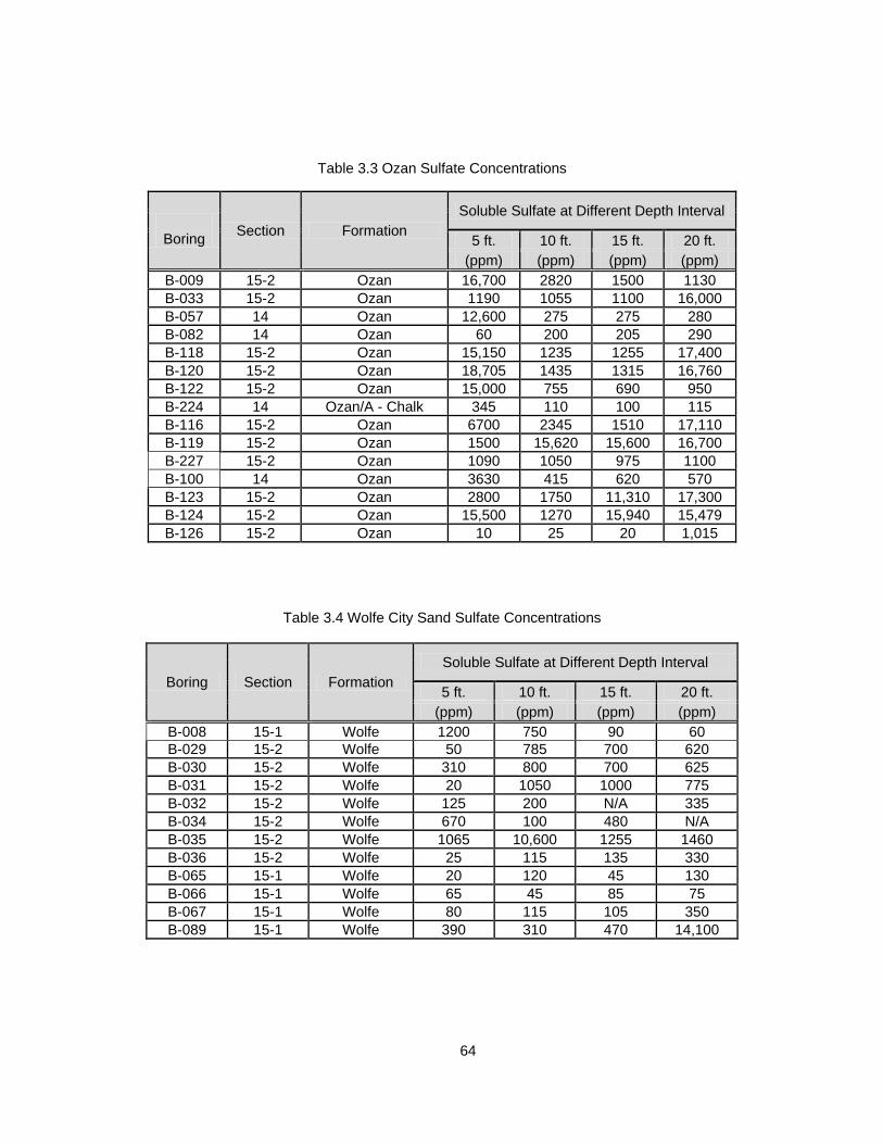
64
Table 3.3 Ozan Sulfate Concentrations
Boring
Section Formation
Soluble Sulfate at Different Depth Interval
5 ft. 10 ft. 15 ft. 20 ft.
(ppm) (ppm) (ppm) (ppm)
B-009 15-2 Ozan 16,700 2820 1500 1130
B-033 15-2 Ozan 1190 1055 1100 16,000
B-057 14 Ozan 12,600 275 275 280
B-082 14 Ozan 60 200 205 290
B-118 15-2 Ozan 15,150 1235 1255 17,400
B-120 15-2 Ozan 18,705 1435 1315 16,760
B-122 15-2 Ozan 15,000 755 690 950
B-224 14 Ozan/A - Chalk 345 110 100 115
B-116 15-2 Ozan 6700 2345 1510 17,110
B-119 15-2 Ozan 1500 15,620 15,600 16,700
B-227 15-2 Ozan 1090 1050 975 1100
B-100 14 Ozan 3630 415 620 570
B-123 15-2 Ozan 2800 1750 11,310 17,300
B-124 15-2 Ozan 15,500 1270 15,940 15,479
B-126 15-2 Ozan 10 25 20 1,015
Table 3.4 Wolfe City Sand Sulfate Concentrations
Boring Section Formation
Soluble Sulfate at Different Depth Interval
5 ft. 10 ft. 15 ft. 20 ft.
(ppm) (ppm) (ppm) (ppm)
B-008 15-1 Wolfe 1200 750 90 60
B-029 15-2 Wolfe 50 785 700 620
B-030 15-2 Wolfe 310 800 700 625
B-031 15-2 Wolfe 20 1050 1000 775
B-032 15-2 Wolfe 125 200 N/A 335
B-034 15-2 Wolfe 670 100 480 N/A
B-035 15-2 Wolfe 1065 10,600 1255 1460
B-036 15-2 Wolfe 25 115 135 330
B-065 15-1 Wolfe 20 120 45 130
B-066 15-1 Wolfe 65 45 85 75
B-067 15-1 Wolfe 80 115 105 350
B-089 15-1 Wolfe 390 310 470 14,100

65
Table 3.5 Neylandville Sulfate Concentrations
Boring Section Formation
Soluble Sulfate at Different Depth Interval
5 ft. 10 ft. 15 ft. 20 ft.
(ppm) (ppm) (ppm) (ppm)
B-026 15-1 Neylandville 975 1500 605 710
B-027 15-1 Neylandville 535 690 790 450
B-174 15-1 Neylandville 90 135 110 315
B-194 15-1 Neylandville 460 180 210 840
Table 3.6 Kemp Clay Sulfate Concentrations
Boring Section Formation
Soluble Sulfate at Different Depth Interval
5 ft. 10 ft. 15 ft. 20 ft.
(ppm) (ppm) (ppm) (ppm)
B-007 15-1 Kemp 180 280 325 100
B-025 15-1 Kemp 1880 17,000 1100 2400
B-068 15-1 Kemp 1270 255 215 470
B-069 15-1 Kemp 11,600 16,100 1360 2430
B-070 15-1 Kemp 2120 8420 10,000 18,080
B-094 15-1 Kemp 260 255 90 250
B-095 15-1 Kemp 115 300 220 200
B-096 15-1 Kemp 1065 690 700 620
B-097 15-1 Kemp 1400 840 850 1170
B-180 15-1 Kemp 3215 1070 970 15,120
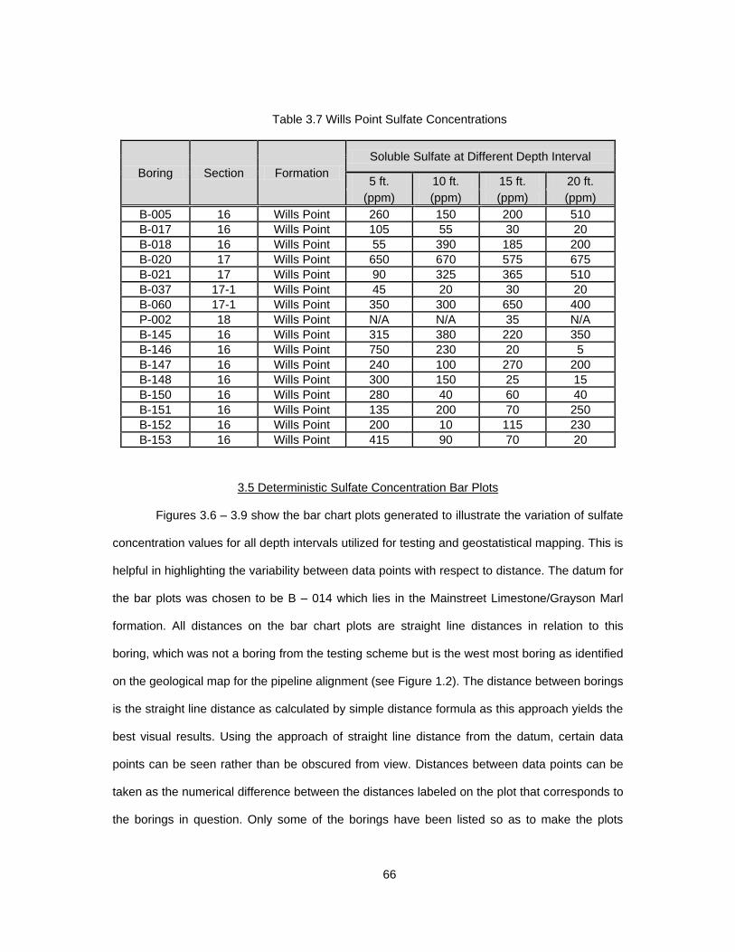
66
Table 3.7 Wills Point Sulfate Concentrations
Boring Section Formation
Soluble Sulfate at Different Depth Interval
5 ft. 10 ft. 15 ft. 20 ft.
(ppm) (ppm) (ppm) (ppm)
B-005 16 Wills Point 260 150 200 510
B-017 16 Wills Point 105 55 30 20
B-018 16 Wills Point 55 390 185 200
B-020 17 Wills Point 650 670 575 675
B-021 17 Wills Point 90 325 365 510
B-037 17-1 Wills Point 45 20 30 20
B-060 17-1 Wills Point 350 300 650 400
P-002 18 Wills Point N/A N/A 35 N/A
B-145 16 Wills Point 315 380 220 350
B-146 16 Wills Point 750 230 20 5
B-147 16 Wills Point 240 100 270 200
B-148 16 Wills Point 300 150 25 15
B-150 16 Wills Point 280 40 60 40
B-151 16 Wills Point 135 200 70 250
B-152 16 Wills Point 200 10 115 230
B-153 16 Wills Point 415 90 70 20
3.5 Deterministic Sulfate Concentration Bar Plots
Figures 3.6 – 3.9 show the bar chart plots generated to illustrate the variation of sulfate
concentration values for all depth intervals utilized for testing and geostatistical mapping. This is
helpful in highlighting the variability between data points with respect to distance. The datum for
the bar plots was chosen to be B – 014 which lies in the Mainstreet Limestone/Grayson Marl
formation. All distances on the bar chart plots are straight line distances in relation to this
boring, which was not a boring from the testing scheme but is the west most boring as identified
on the geological map for the pipeline alignment (see Figure 1.2). The distance between borings
is the straight line distance as calculated by simple distance formula as this approach yields the
best visual results. Using the approach of straight line distance from the datum, certain data
points can be seen rather than be obscured from view. Distances between data points can be
taken as the numerical difference between the distances labeled on the plot that corresponds to
the borings in question. Only some of the borings have been listed so as to make the plots
67
easier to visualize. Additionally, the formations have been added to the plots by using brackets
and can be seen above the formations they represent. It can be seen from both the bar plots in
Figures 3.6 through 3.9 and the above Tables 3.2 through 3.7 that sulfate values are quite
random with respect to distance. Considering the Eagle Ford formation show in Figures 3.6
through 3.9, it can be seen that sulfate values tend to spike and fall randomly in close proximity
to one another. Looking at the Ozan in Figures 3.6 through 3.9 we see the same pattern. Again
we see the same pattern with regards to Wolfe City Sand and Kemp Clay in Figures 3.6 through
3.9. The rising and falling of sulfate values does not appear in the Neylandville and Wills Point
Formations. The Neylandville and Wills Point Formations exhibited consistently low sulfate
values throughout the entire testing length and depth. These patterns of rising and falling sulfate
levels carry over into all depth intervals tested for the Eagle Ford, Ozan, Wolfe City Sand and
Kemp Clay as indicated by Figures 3.6 through 3.9. This information reiterates the random
manifestation of sulfates in soil (See Figures 2.3.a – 2.3.e). The random manifestation of such
sulfates might possibly be due to ground water transportation of the sulfate minerals or due to
the complex nature of the initial formation and deposition of sulfates through the evaporation
and precipitation reactions of salt water. Never the less, the prediction and mapping of sulfate
values using a deterministic approach is impossible, therefore the use of geostatistics must be
implored. The next chapter focuses on the development and analysis of the geostatistical
portion of the research.

Figure 3.6 Straight Line Distance vs. Sulfate Concentration (Depth 5ft)
68

Figure 3.7 Straight Line Distance vs. Sulfate Concentration (Depth 10ft)
69

Figure 3.8 Straight Line Distance vs. Sulfate Concentration (Depth 15ft)
70

Figure 3.9 Straight Line Distance vs. Sulfate Concentration (Depth 20ft)
71

72
CHAPTER 4
GEOSTATISTICAL ANALYSIS AND MAPPING
4.1 Introduction
The following chapter contains various aspects of the geostatistical analysis of sulfate
values. In addition to the presentation of results, discussions are presented to explain the nature
and results of the analyses. The chapter begins with the presentation of individual formation
contour maps. Next, the overall mapping of all formations collectively is presented. This is a
useful tool in comparing the individual formation maps with the overall formation maps. Lastly,
the Kriging error associated with the geostatistical analysis is presented in order to bring validity
to the mapping. This is done by plotting the most variable formation maps, least variable
formation maps, as well as all formations collectively.
The geostatistical analysis was conducted using Surfer 9 Software manufactured by
Golden Software Inc. ©. 2-D Aerial contours were generated for each formation individually as
well as all formations collectively at the unique depth interval specified. The 2-D analysis was
not conducted using sulfate values other than the values determined at the specific depth
interval. In other words, only 5ft. depth sulfate values were used to generate the 5ft. depth
maps. Point Kriging techniques were utilized in conjunction with experimental variograms.
Ordinary Kriging principles and techniques have been developed specifically for data points that
are discreet and without trend (Armstrong 1998). Therefore, Ordinary Point Kriging was chosen
to analyze the discrete non-continuous data set that describes the soluble sulfate
concentrations for the pipeline alignment. Due to the irregularity in the data a linear model was
used for the variograms. Sulfate concentrations are inherently random and in the current data
set only the linear trend model proved useful for geostatistical analysis.
A total of 4 maps (at 5 ft., 10 ft., 15 ft. and 15 ft. depths) were developed for each
formation and also for all formations together. This generated a total of 32 maps for the 6
different formations that were tested in this project. In order to reduce the number of maps, Wills
Point and Kemp Clay were combined in mapping as well as the Wolfe City Sand and
73
Neylandville formations based on their proximity to each other and the number of data points
available to make successful predictions. Eagle Ford and Ozan maps were not combined due to
the gap in data associated with the Austin Chalk formation, which was not tested as part of this
research project. After combining formations, the number of maps was reduced to 16 individual
formation maps and 4 collective formation maps. The collective formation maps are also shown
overlain onto the geologic formation map supplied by Fugro Consultants Inc., totaling 24 maps.
Each of the formation’s maps corresponds to the unique selected depth interval for testing (i.e.
5ft., 10ft., 15ft., & 20ft.). Therefore, the maps can be read regardless of elevation changes. In
other words, the generated maps will indicate possible sulfate values at the depth specified by
the map in any location within that particular formation. Each map was designed to predict
sulfate values at the corresponding depth only. Interpretation of sulfate values in between depth
intervals would be done at the risk of the interpreter.
4.2 Eagle Ford Formation
The Eagle Ford formation results indicate that it is one of the more problematic
formations when it comes to high soluble sulfate values and sulfate values greater than 2000
ppm. The range of sulfate values in the Eagle Ford ranges from 40 ppm to 19,620 ppm. Figure
4.1 indicates several zones of concern where sulfate values range from 5000 ppm to 14,000
ppm. In addition, Figure 4.1 indicates there are zones of sulfates lower than 2000 ppm.
Specifically, from B-51 to B-196 values of sulfate are below typical problematic threshold levels.
Also, from B-164 to B-84 a zone of low sulfate values is present. However, in the 10ft map,
Figure 4.2 shows that in the same zone of low sulfate values for Figure 4.1, there is a pocket of
high sulfates ranging from 4000 ppm to 14,000 ppm. This is due to the random manifestation of
sulfates in the soil).
Also, it can be seen in Figure 4.3 that a large portion of the formation appears to have
sulfate values in the acceptable range. Looking at Figure 4.4, 3 major zones of concern with
sulfate values higher than 5000 ppm and ranging to 15,000 ppm are present. These high sulfate

74
zones are located near B-209, B-198, and B-93. Figure 4.8, the 20ft. map, shows the highest
concentrations of sulfate values for the Eagle Ford. Sulfate values range from 75 ppm to 19,620
ppm. The specific zones of interest are located near B-164, B-202, B-93, and B-209. Looking at
all depths it can see that certain zones appear to be below problematic threshold values.
Specifically, B-84 and B-318 appear to have very low sulfate values. In addition, B-61 and B-59
are observed to have very low sulfate ranges throughout all depths. Conversely, zones around
B-93 and B-198 have consistently high sulfate values throughout all depths tested. Overall the
Eagle Ford is very problematic and must be treated with caution.

75
Figure 4.1 Eagle Ford Contour Map with Approximate Pipeline Alignment and IPL Parcel Numbers (Depth – 5ft)
11
12
13
Approximate Pipe Line Alignment

76
Figure 4.2 Eagle Ford Contour Map with Approximate Pipeline Alignment and IPL Parcel Numbers (Depth – 10ft)
11 12
13
Approximate Pipe Line Alignment

77
Figure 4.3 Eagle Ford Contour Map with Approximate Pipeline Alignment and IPL Parcel Numbers (Depth – 15ft)
13
12
11
Approximate Pipe Line Alignment

78
Figure 4.4 Eagle Ford Contour Map with Approximate Pipeline Alignment and IPL Parcel Numbers (Depth – 20ft)
13
12
11
Approximate Pipe Line Alignment

79
4.3 Ozan Formation
The Ozan Formation, much like the Eagle Ford, is also very problematic in regards to
high sulfate values. From Figure 4.5, the 5ft. depth map, it can see that there are several
problem areas with sulfate values higher than 5000 ppm and there appear to be a few zones of
sulfate values less than 2000 ppm. However, Figure 4.6 indicates that much of the formation
has sulfate levels less than 2000 ppm with only one zone of high sulfate near B-119 and B-120.
Sulfate values for B-119 and B-120 are as high as 16,760 ppm. Moving to Figure 4.7, the 15ft.
map, it can see that much of the formation seems to be below typical threshold levels of sulfate,
but there are zones of high sulfates near B-119, B-120, B-123 and B-124. In these locations the
sulfate values range from 1300 ppm to 16,000 ppm which far exceeded problematic levels of
sulfates. Lastly, in the Figure 4.8, the 20ft. map, the most problematic sulfate conditions are
observed. Similar to the 5ft. map, Figure 4.8, those zones near B-116 and B-118 have high
sulfate pockets. In addition, zones near B-119, B-120, B-124, and B-33 have significantly high
sulfate values. Looking at all maps combined a trend of low sulfate areas near B-224 and B-87
is observed, located in the northwest corner of the formation. In addition B-227 appears to have
sulfate values in below problematic threshold ranges for all depths. Overall, the Ozan has
several pockets of excessively high sulfate values at all depths and must be considered with
extreme caution.

Figure 4.5 Ozan Contour Map with Approximate Pipeline Alignment and IPL Parcel Numbers
(Depth – 5ft)
15-2
14
Approximate Pipe Line Alignment
80

Figure 4.6 Ozan Contour Map with Approximate Pipeline Alignment and IPL Parcel Numbers
(Depth – 10ft)
14
15-2
Approximate Pipe Line Alignment
81
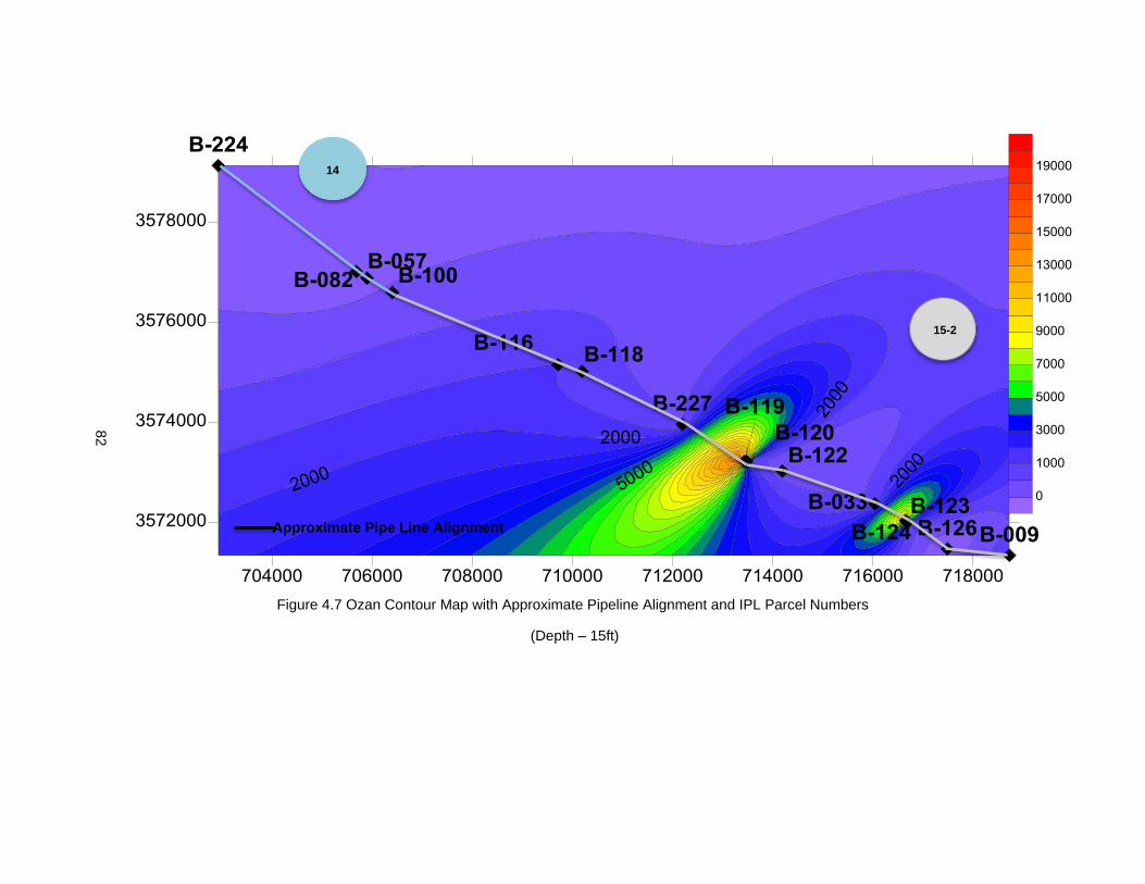
Figure 4.7 Ozan Contour Map with Approximate Pipeline Alignment and IPL Parcel Numbers
(Depth – 15ft)
15-2
14
Approximate Pipe Line Alignment
82

Figure 4.8 Ozan Contour Map with Approximate Pipeline Alignment and IPL Parcel Numbers
(Depth – 20ft)
15-2
14
Approximate Pipe Line Alignment
83

84
4.4 Wolfe City Sand and Neylandville Formations
The Wolfe City Sand and Neylandville portions of the alignment appear to have very
satisfactory sulfate levels. As the Figure 4.9 indicates the entire 5ft. portion of the alignment
appears to have sulfate values less than 2000 ppm. Figure 4.10, the 10ft. section, also has
sulfate levels predominately below 2000 ppm; however there is a zone of high sulfate in the
Wolfe City Sand near B- 34, B-35 and B-36. Figure 4.11, the 15ft. map, also appears to have all
sulfate values less than 2000 ppm. Lastly, the 20ft. map, Figure 4.12 shows only one zone of
high sulfates at B-89. Specifically, the sulfate value is around 14,100 ppm. Overall, the
Neylandville section has consistently low sulfate zones lower than 2000 ppm and the Wolfe City
only has two zones of high sulfate at 10ft. depth near B- 34 and B-35, and also at the 20ft.
depth near B-89.
4.5 Kemp Clay and Wills Point Formations
It can be seen from the mapping analysis that the Kemp Clay and Wills Point sections
show relatively low sulfate values. In fact, the Wills Point borings only showed sulfate values
between 5 ppm and 750 ppm throughout all depths and is considered very low risk for chemical
stabilization. Looking at Figure 4.13, the 5ft. map shows only one zone of high sulfate located in
the Kemp portion of the alignment near B-69 and B-70, and the sulfate level is as high as
11,000 ppm. The rest of the 5ft. sulfate values are at or below 2000 ppm. The 10 ft. map, Figure
4.14, indicates again that the Kemp Clay has a zone of high sulfate near B-97, B-69, B-70, and
B-25, with values ranging from 840 ppm to 17,000 ppm. Figure 4.15, the 15ft. map, indicates
that the majority of the alignment has levels of sulfate lower than 2000 ppm, but again a hot
spot is located at B-70 where the sulfate value increases. Lastly, the 20ft. map, Figure 4.16,
shows zones of highly problematic sulfate values near B-70 and B-180. For those particular
locations the sulfate values are as high as 18,000 ppm and 15,000 ppm, respectively. Overall,

85
much of this portion of the alignment shows low values of sulfates; however, consistently high
values at B-69 and B-70 are observed at all depths, as well as B-180 at 20ft. depth. Therefore,
chemical stabilization is cautioned in the Kemp Clay portion of the alignment.

Figure 4.9 Wolfe City Sand and Neylandville Contour Map with Approximate Pipeline Alignment and IPL Parcel Numbers (Depth – 5ft)
Figure 4.10 Wolfe City Sand and Neylandville Contour Map with Approximate Pipeline Alignment and IPL Parcel Numbers (Depth – 10ft)
15-2
15-2
15-1
15-1
Approximate Pipe Line Alignment
Approximate Pipe Line Alignment
86

Figure 4.11 Wolfe City Sand and Neylandville Contour Map with Approximate Pipeline Alignment and IPL Parcel Numbers (Depth – 15ft)
Figure 4.12 Wolfe City Sand and Neylandville Contour Map with Approximate Pipeline Alignment and IPL Parcel Numbers (Depth – 20ft)
15-2
15-2
15-1
15-1
Approximate Pipe Line Alignment
Approximate Pipe Line Alignment
87
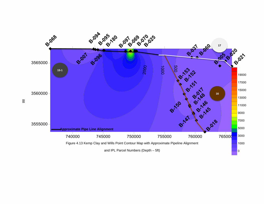
Figure 4.13 Kemp Clay and Wills Point Contour Map with Approximate Pipeline Alignment
and IPL Parcel Numbers (Depth – 5ft)
15-1
16
17
Approximate Pipe Line Alignment
88

Figure 4.14 Kemp Clay and Wills Point Contour Map with Approximate Pipeline Alignment
and IPL Parcel Numbers (Depth – 10ft)
15-1
16
17
Approximate Pipe Line Alignment
89

Figure 4.15 Kemp Clay and Wills Point Contour Map with Approximate Pipeline Alignment
and IPL Parcel Numbers (Depth – 15ft)
15-1
16
z 17
Approximate Pipe Line Alignment
90

Figure 4.16 Kemp Clay Contour Map with Approximate Pipeline Alignment
and IPL Parcel Numbers (Depth – 20ft)
15-1
16
17
Approximate Pipe Line Alignment
91

92
4.6 All Formations
From Figure 4.17, the 5ft. map, it can be observed that throughout the entire alignment
there are trouble zones in the Eagle Ford, Ozan, and Kemp Clay, with highly problematic zones
of high sulfates in the Eagle Ford and Ozan. In general, Figure 4.17 parallels greatly with the
individual map analysis, indicating consistent results. Figure 4.19 presents the overall map for
10ft. depth; again the parallel with the individual maps generated is present. Large trouble
zones in the Eagle Ford and in the Ozan were observed in Figure 4.19. Additionally, the Kemp
Clay has one large high sulfate zone in the easternmost portion of the formation. This is the
same result as with the individual maps at the corresponding depth interval of 10 feet Figure
4.221, the 15 ft. depth map, indicates the results of collective formation mapping parallel the
individual formation maps. High sulfate zones are observed in the Eagle Ford and Ozan, while
in the Wolfe City, Kemp Clay and Wills Point contain very low sulfate values. Lastly, the 20ft
map, Figure 4.23 indicates the most extreme conditions along the alignment. Several high
sulfate zones exist in all formations except for Wills Point and Neylandville. Overall, the same
trends are seen in the collective formation map at 20ft. depth as in the individual maps.
The contour map generation indicates that Eagle Ford, Ozan, and portions of Kemp
Clay and Wolfe City Sand show high values of sulfate pockets. Conversely, the map generation
indicates that Neylandville and Wills Point have very low sulfate values consistently under 2000
ppm. The location and intensities of the sulfate values have a good correlation with all
experimental data indicating a good deterministic portion of the geostatistical analysis. As with
all geostatistical analyses, the maps generated are a prediction and not to be taken as exact
values, only an indication of sulfate values in zones both tested and not tested. Extreme caution
should be utilized when interpreting the geostatistical maps generated for this research project.
Figures 4.18, 4.20, 4.22, & 4.24 depict the geostatistical maps approximately overlaid onto the
geologic formations to give a more clear indication as to the actual zones of sulfate
concentration. Further discussion of map validation id discussed in the next section.

Figure 4.17 All Formations Contour map with Approximate Pipeline Alignment and Highlighting High Sulfate Borings
(Depth – 5ft)
B- 326
B - 93
B - 209,
B -063
B - 118
B- 57
B -
120 B - 124,
B - 009 B -
069
93

Figure 4.18 All Formations Contour Map Overlaid on Geology Map (Depth – 5ft)
94

Figure 4.19 All Formations Contour Map with Approximate Pipeline Alignment and Highlighting High Sulfate Borings
(Depth – 10ft)
B - 198,
B - 201
B - 119
B- 063,
B-209
B - 035 B - 025,
B - 069
95

Figure 4.20 All Formations Contour Map Overlaid on Geology Map (Depth – 10ft)
96

Figure 4.21 All Formations Contour Map with Approximate Pipeline Alignment and Highlighting High Sulfate Borings
(Depth – 15ft)
B - 168,
B - 198
B - 093
B - 209
B - 119
B – 123,
B - 124
B - 070
97

98
Figure 4.22 All Formations Contour Map Overlaid on Geology Map (Depth – 15ft)
98

99
Figure 4.23 All Formations Contour Map with Approximate Pipeline Alignment and Highlighting High Sulfate Borings (Depth – 20ft)
B - 084
B - 164 B - 209
B - 168,
B - 198
B - 062, B - 090,
B - 093
B - 033, B - 123,
B - 124
B - 119,
B - 120
B - 116,
B - 118
B - 089 B - 180 B - 070
99
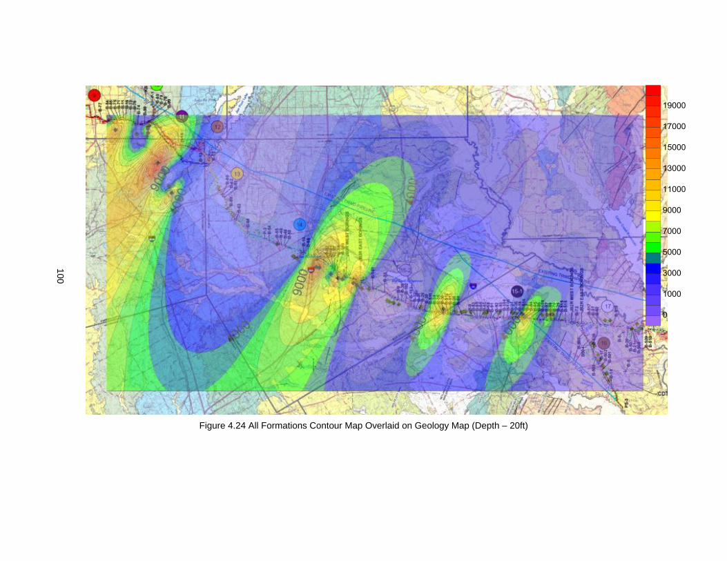
Figure 4.24 All Formations Contour Map Overlaid on Geology Map (Depth – 20ft)
100
101
4.7 Geostatistical Validation
Validation of the geostatistical analysis was completed by using a 45° validation line
technique comparing actual input data points to predicted data points. The Kriging process is an
optimization process, by which the variance between test points and estimations is to be
reduced. During this optimization process some of the test point values are adjusted to
accommodate the least amount of variance between actual and unknown predicted values.
Therefore, an easy approach to determine the validation of Kriging maps is to compare the true
input values to the adjusted values created through the optimization and mapping process
(Armstrong 1998). If the Kriging process was valid then the true values of the input data versus
the adjusted input values will lie close to a 45° validation line, indicating that the true input
values are similar to the Kriged output values. No model is perfect, as such, no geostatistical
mapping will lie perfectly on the 45° line; however the ultimate goal is to observe little variation
from the input points to the optimized and adjusted points. The generated maps were used to
identify the borings and their corresponding adjusted values.
The approach to determine the error associated with the Kriging for this project focused
on the variance generated by the variogram used in conjunction with the Kriging technique. The
maximum variance generated by the variogram was compared for all individual formations. The
formations with the lowest and highest variance are compared with the idea in mind that all
variance ranges within the highest and lowest will also be valid. Upon completion of the highest
and lowest the overall maps at all depths were evaluated using the 45° validation line
technique. This was done because a variation from individual maps to the overall maps was
observed in some test areas. The maximum cumulative variance associated with all formation’s
variograms is presented in Table 4.1. For consistency with the geostatistical formation mapping
combinations presented in the previous sections, the validation process was carried out in the
same manner by analyzing the variance generated by the formations mapped by individually,
Eagle Ford and Ozan, as well as the formations mapped in combination, Wolfe City/Neylandville

102
and Kemp Clay/Wills Point. The formations determined to have the lowest and highest
maximum cumulative variances were the Wolfe City - Neylandville and Eagle Ford, respectively.
Following Table 4.1, all depth intervals for Wills Point and Eagle Ford are presented using the
45° validation line (Figures 4.25 – 4.26). Then, the entire collective formation maps are
inspected at all depth intervals using the 45° trend line technique (Figures 4.27). The actual
input and adjusted input values are provided next to the figures. Following the validation figures
a brief evaluation of the validation results is given. One important note to observe from the
validation plots is that points that lie above the validation line indicate that the estimated value
was lower than the true value and conversely points that lie below indicate the estimated value
is higher than the actual value. In some cases higher estimation are not desired. Such
applications would pertain to mineral quality prediction. In this case, estimation higher values
would negatively impact the gross profit of the mineral mining operation. In other cases over
estimating values may prove helpful or conservative. Such applications would be soluble sulfate
prediction and mapping. In this case, the over estimation of sulfate values would be safe and
conservative. The validation line technique can indicate exactly how conservative the over
estimation may be. If values are over predicted, the analysis becomes too conservative and is
counterproductive.
Table 4.1 Variance Comparison from Variograms at Tested Depth Intervals
Formation(s) Eagle Ford Ozan
Wolfe/ Neylandville
Kemp/ Wills Depth
5 ft. 1.00E+08 1.40E+08 6.50E+05 4.50E+07
10 ft. 1.25E+08 5.00E+07 2.50E+07 1.10E+08
15 ft. 1.20E+08 7.50E+07 3.00E+05 1.25E+07
20 ft. 1.80E+08 1.25E+08 1.00E+08 6.50E+07
Cumulative Variance
5.25E+08 3.90E+08 1.26E+08 2.33E+08

103
4.7.1 Eagle Ford Formation Validation
The Eagle Ford formation exhibited the highest amount of variance as computed by the
semivariogram (see Table 4.1). Therefore, the Eagle Ford should provide the largest variation
from the 45° validation line. Figure 4.25.a shows very little variation between input and output
values indicating good prediction and reliability in mapping. Figure 4.25.b shows some variation
between input and output values primarily at very low and very high sulfate levels. One would
expect the largest variations in these locations because the optimization process affects values
that generate the highest variance. In other words, very low values will be augmented and very
high values are reduced. Figure 4.25.c shows very good correlation at low sulfate values;
however at high sulfate values the estimated values are often lower than the true values. This is
due to the higher frequency of lower sulfate values that cause the higher sulfate values to be
reduced. Figure 4.25.d shows the highest variation from input to output values. This is due to
the fact the 20ft. depth in the Eagle Ford had the highest variance of any formation at any depth
(see Table 4.1). Overall, the most variable formation, Eagle Ford, indicated good results using
the 45° validation line technique.
4.7.2 Wolfe City and Neylandville Combination
The Wolfe City and Neylandville formation combination yielded the lowest amount of
variance as computed by the semivariogram (see Table 4.1). Therefore, this map combination
should provide the smallest variation from the 45° validation line. Figure 4.26.a, the 5 ft.
validation plot, shows a good correlation of input and output values. There are some outlying
points at the lower and higher end of the sulfate values. As mentioned in the previous Eagle
Ford formation discussion, this is due to the optimization procedure carried out in the Kriging
process. The lowest and highest values, the ones creating the largest variance, are optimized
and increased or decreased to reduce variance between points. The 10 ft. validation plot, Figure
4.26.b also shows a very good correlation of input and output values and only has three points

104
that exhibit a significant amount of error. In the case of the highest value, this error is quite
acceptable considering sulfate concentrations above 800 ppm are known to be very
problematic. In the case of the lower values, the Kriging output estimated higher values than the
true values. For this type of analysis higher values are more conservative and therefore
acceptable. Figure 2.26.c, the 15 ft. validation, shows a very good correlation as well with the
same trend of over predicted lower values and under predicting higher values. The 20ft.
validation map, Figure 2.26.d shows the best correlation with the validation line indicating an
almost exact input and output. This is due to the fact that most of the input values were in the
same range, from 0 to 200 ppm, and there was only one major variant of 15,000 ppm. This
major variant came from the Wolfe City portion and was not directly close spatially to other test
points, so its variation was essentially nullified over distance.
4.7.3 All Formations
The All formations maps exhibited the highest amount of deviation from the validation
line. In most cases, the addition of data points strengthens a geostatistical analysis, however in
this case the addition of data points weakened the analysis. This is due to the extreme variation
of the added input values. Increasing the data set is helpful if the values do not exhibit large
variation. By adding large variation numbers to the data set, one creates a larger overall
variance and thus weakens the accuracy of the analysis. This is the case with all formations
maps in this research. The overall maps are still quite useful and exhibit good visualization
qualities, however the predictability associated with these maps is not as strong as the
individual maps. Two reasons exist to explain the large variation in input values. The first deals
with the random nature of sulfate values, which is due to the random manifestation and forming
of sulfate minerals through natural processes. The second deals with the numerical difference in
sulfate values due to the ppm scale. For instance, if one value of sulfate is 1000 ppm and its
nearest neighbor, the most influential value in the Kriging process, is 18,000, then the resulting

105
variance of those two numbers as computed by the semivariogram is over 72,000,000 ppm. The
exact calculation is provided below.
) ∑ ) )
) ∑
)
)
This is an incredible variance. This number can be reduced by the addition of data
points that are closer together in value, thus explaining why the maximum variances presented
in Table 4.1 are not much higher than this example calculation. Figures 4.27.a through 4.27.d all
exhibit the same type of deviation from the validation line, which is the same as with the Eagle
Ford and combined Wolfe City/Neylandville. The deviation from the validation line increases as
the values of sulfate are at the very low and very high end. Additionally and further reiterating
the increase in optimization error through Kriging, data points in the middle range of analysis
also seem to be both over and under predicted, with an equal amount of incorrect predictions on
both sides of the validation line.

a) b)
Figure 4.25 a&b Eagle Ford Validation Depth 5ft. & 10ft.
10
6

c) d)
Figure 4.25 c&d Eagle Ford Validation Depth 15ft. & 20ft.
10
7

a) b)
Figure 4.26 a&b Wolfe City/Neylandville Validation Depth 5ft. & 10ft.
10
8
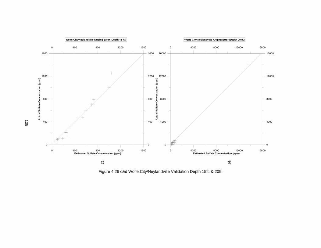
c) d)
Figure 4.26 c&d Wolfe City/Neylandville Validation Depth 15ft. & 20ft.
109

a) b)
Figure 4.27 a&b All Formations Validation Depth 5ft. and 10ft.
11
0

c) d)
Figure 4.27 c&d All Formations Validation Depth 15ft. and 20ft.
111

112
CHAPTER 5
CONCLUSIONS & RECOMMENDATIONS
5.1 Conclusions of Testing and Mapping
Based on the data obtained by testing select samples from 6 different soil formations
along the IPL pipeline alignment the following conclusions can be made:
1. Over 300 samples were tested using the Modified UTA Method of Soluble Sulfate
Determination in Soil. The results of the tests (Tables 3.2 – 3.7) indicate that sulfates in soil
are inherently random and often have large variation over spatially related distances as also
indicated by the deterministic bar plots (Figures 3.6 – 3.9).
2. The test results also indicate that the Neylandville and Wills Point formations have sulfate
values below the typical problematic thresholds and may not have issues if treated with
calcium based stabilizers.
3. The test data also clearly indicates that the Eagle Ford and Ozan formations are very
problematic at all depths (5 ft., 10 ft., 15 ft., and 20 ft.,) and calcium based stabilization
could be problematic leading to the formation of ettringite. However, further testing is
recommended to narrow down problematic zones and clear areas that are not an issue
along the pipeline.
4. Additionally, test data indicates the Kemp Clay and Wolfe City Sand formations show some
zones that appear to be problematic and are considered moderately problematic. Additional
testing is recommended in these zones to further assess the problem in these zones.
5. The deterministic data was then used for geostatistical analyses in aims to visualize and
predict sulfate values. The analyses were conducted using Linear Geostatistics, specifically
Ordinary Point Kriging. The results of the analyses indicate that the geostatistical analysis
of sulfate values is quite difficult due to the random nature of sulfate values over spatial
regions.

113
6. Validation was conducted on the various contour maps generated by the geostatistical
analysis. The validation indicated that individual formation mapping was more accurate than
the overall combination mapping of all formations.
5.2 Recommendations
5.2.1 Eagle Ford Formation
It is recommended that further testing be completed on the Eagle Ford Formation at all
depths due to the high intensity and distribution of sulfate concentrations. Specifically, further
testing should focus on the zones listed in the previous sections indicated by the contour maps
and test results, but are not limited to those zones as sulfate concentrations are inherently
random. Further testing will not only aid in the proper stabilization of sulfate soils along the
pipeline alignment, but will also provide further validation of the contour mapping.
5.2.2 Ozan Formation
It is recommended that further testing be completed on the Ozan Formation at all
depths, especially the 5ft. and 20ft. zones as they appear to be most problematic. Specifically,
testing should focus on the zones listed in the previous sections indicated by the contour maps
and test results, but are not limited to those zones as sulfate concentrations are inherently
random. Further testing will not only aid in the proper stabilization of sulfate soils along the
pipeline alignment, but will also provide further validation of the contour mapping.
5.2.3 Kemp Clay Formation
It is recommended that further testing be completed on the Kemp Clay Formation in the
vicinity of: B-69 at 5ft. and 10ft. depth, B-70 at all depths, B-25 at 10ft. depth, and B-180 at 20ft.
depth. However, sulfate concentrations are inherently random and further testing may be

114
necessary in zones other than previously stated or as indicated by the contour maps and test
data.
5.2.4 Wolfe City Formation
It is recommended that further testing be completed on the Wolfe City Formation in the
vicinity of: B-35 at a depth of 10ft. and B-89 at 20ft. depth. It appears that other locations and
depths have acceptable sulfate values, however sulfate concentrations are inherently random
and further testing may be necessary in zones other than previously stated or as indicated by
the contour maps and test data.
5.3 Geostatistical Validation
Based on the validation process on the geostatistical maps utilizing Kriging error
evaluation, it can be seen that good prediction correlation exists with the mapped data. The
approach of examining the formation with the least amount of variability and the formation with
largest amount of variability shows that all formations in between should have good correlation
from predicted values to true values. As with all geostatistical analyses the prediction accuracy
is dependent on data variability, test spacing, and test borehole orientation. Based on the
method of Validation, it can be seen that when data points lie below the 45° line, the predicted
value is higher than the actual value. Conversely, if the data point lies above the 45 line, the
actual value is higher than the predicted value. In most cases, we see that the predicted values
are higher than actual values at lower sulfate concentrations and actual values are higher than
predicted values at high sulfate concentrations. The implications of such phenomena are
addressed in the following section which breaks down the analysis into each validation set
5.3.1 Eagle Ford Validation
The Eagle Ford formation was the most variable formation from a statistical stand point.
Therefore, the fact that the validation points were so close to the 45° validation line indicates

115
that the Kriging approach does have validity. There are a few outlying points on the validation
maps; however these outliers appear to be in an acceptable range.
5.3.2 Wolfe City/Neylandville
The Wolfe City/Neylandville combination map also had good correlation to the 45°
validation line. As with the Eagle Ford formation there were some outlying points, but relatively
few. The explanation for the outlying points is simply that this particular data set also includes
Wolfe City, which shows much larger variation than the Neylandville alone. Therefore, all
outlying points are due to the Wolfe City variation.
5.3.3 All Formations Validation
Upon analyzing the results from the validation on all formations collectively, it can be
seen that there is quite a bit of variation from the 45° validation line. In most geostatistical
applications the addition of data points is a positive. However, it can be seen that when the
addition of data points are quite variable, the accuracy of the analysis is compromised. The
addition of variation from formations such as Ozan, Wolfe City, and Neylandville caused the
Kriging optimization process to lose accuracy. In this case it appears that the use of all
formations collectively is not as accurate or as appropriate and the maps should be studied on
an individual formation basis.
5.4 Implications for Further Study
The implications from a study such as this are far reaching. The identification of soluble
sulfates in enough abundance to create adverse reactions post soil stabilization is present in
many of the test formations. Previous studies conducted by UTA indicate that much of the
bedding and haunch material utilized for pipeline construction will be reused and chemically
stabilized. If such bedding and haunch material is utilized from certain established problematic
formations, such as the Eagle Ford and Ozan, then detrimental sulfate will be observed. If
certain bedding and haunch material is stabilized and reused in the Kemp and Wolfe City

116
formations in certain areas, then detrimental sulfate heave will occur. The sulfate heave will
ultimately reduce the performance and could fail the pipeline in certain areas. Further sulfate
testing should be conducted in situ as the pipeline is being trenched and the bedding and
haunch stabilized in order to prevent sulfate heave due to isolated pockets of sulfates. It has
also been suggested by UTA that CLSM mixes using soils along the pipeline could save vast
amounts of time and money in regards to pipeline construction. Therefore, CLSM mixes utilizing
sulfate soil need to be studied rigorously for swelling, shrinkage, Ettringite/Thaumasite
formation, and durability effects.
In regards to soluble sulfate reactions, further study must be conducted on the contribution
of free alumina to the Ettringite reaction. A link between the alumina silica ratios has been
observed in recent studies as being impactful in the reaction; however no studies have been
conclusive in determining the extent of free alumina’s role in the reaction. Considering the pipe
line may be constructed with steel and precast concrete pipe, further study must be carried out
to determine if sulfate heave will cause distress issues to these materials.
Lastly, more studies should be conducted in the geotechnical arena using geostatistics as
a tool of analysis. Sulfate values show very large variations, making geostatistical analysis more
difficult and potentially less accurate. However other aspects of civil engineering properties,
such as friction angle, compaction density, permeability, etc. generally exhibit less numerical
variation over spatial regions. Therefore analyses using these variables might prove to be
easier and more accurate. Additionally, many other geotechnical parameters have correlation
with one another. For example density and permeability are related and multivariate
geostatistical analyses can be used to predict and map both characteristics at the same time.
Overall, there are many advantages of geostatistical tools in geotechnical engineering and the
use of such tools in geotechnical investigations is warranted.

117
REFERENCES
1. AASHTO (2007). “T 290 – 95 Determining Water – Soluble Sulfate Ion Concentration in
Soil.”
2. ACI (1982) George Verbeck Symposium on Sulfate Resistance of Concrete, ACI
Publication
SP-77, 7 papers, 94 pp.
3. Adams, A.G., Dukes, O.M., Cerato, A.B., and Miller, A.G. (2008). “Sulfate Induced
Heave in Oklahoma Soils due to Lime Stabilization”. Geotechnical Special Publication,
n 179, p 444-451, (2008), Proceedings of Sessions of GeoCongress 2008 -
GeoCongress 2008: Characterization, Monitoring, and Modeling of GeoSystems, GSP
179
4. Aihong, W.U., Liangcia, C.A.I., Qaingkang, G.U., Zenhui, W. (2009) “Ground Treatment
of Airport by Heavy Cover Technique in Sulphate Saline Soil Region.” ASCE,
International Conference on Transportation Engineering, pp. 657-662.
5. Armstrong, M. (1984). “Common Problems Seen in Variograms”. Mathematical
Geology, Vol. 16, No. 3, pp. 305–313.
6. Armstrong, M. (1998). “Basic Linear Geostatistics”. Springer – Verlag Berlin Heidelberg.
Ch. 7: pp. 83-102
7. ASTM C1580-09e1. “Standard Test Method for Water-Soluble Sulfate in Soil.”
8. Azam, S. (2003). “Influence of Mineralogy on Swelling and Consolidation of Soils in
eastern Saudi Arabia.” Canadian Geotechnical Journal. Vol. 40, Iss. 5, 964-975.
9. Bagley, A.D., Cesare, J.A. (2009). “Case History: Sulfate Induced Heave in Lime
Treated Soils beneath a Structure in Western Colorado.” ASCE, Proceedings 5th
Congress on Forensic Engineering, pp. 234-243.
10. Bell, F.G. (1989). “Lime Stabilization of Clay Soils.” Bulletin of the International
Association of Engineering Geology, Vol. 39, Iss. 1, pp. 67-74.

118
11. Berger, E., Little, D.N., and Graves, R. (2001). “Technical Memorandum: Guidelines for
Stabilization of Soils Containing Sulfates”. www.lime.org/publications.html.
12. Bing, H., He, P., Yang, C., Shi, Y., Zhao, S., Bian, X. (2007). “Impact of Sodium Sulfate
on Soil Frost Heaving in an Open System.” Applied Clay Science, Vol. 35, pp. 189-193.
13. Bryant, L., Mauldon, M., Mitchell, J.K. (2003). “Impact of Pyrite and Behavior of Soil and
Rock.” Proceedings of 12th Pan American Conference on Soil Mechanics and
Geotechnical Engineering, Cambridge, MA, U.S.A, Vol.1, pp. 759-767.
14. Bugge, W. A., and R. R. Bartelsmeyer (1961) ‘‘Soil Stabilization with Portland Cement.’’
Highway Research Board, Bulletin 292, National Research Council, Washington, D.C.,
pp. 1–15.
15. Burkhart, B., Gross, G., Kern, J. (1999). “The Role of Gypsum in Production of Sulfate
Induced Deformation of Lime Stabilized Soils. Environmental & Engineering
Geoscience, Vol. 5, No. 2, pp. 173.
16. Carroll, Z.L., Oliver, M.A., (2005). “Exploring the Spatial Relations between the Soil’s
Physical Properties and Apparent Electrical Conductivity”. Geoderma, Vol. 128, pp.
354–374.
17. Chavva, P.K., Vanapalli, S.K., Puppala, A.J., Hoyos, L. (2005). “Evaluation of Strength,
Resilient Moduli, Swell, and Shrinkage Characteristics of Four Chemically Treated
Sulfate Soils from North Texas.” ASCE, Geotechnical Special Publication, Iss. 130, pp.
1841-1850.
18. Chen, D.H., Harris, P., Scullion, T., and Bilyeu, J. (2005). “Forensic Investigation of a
Sulfate-Heaved Project in Texas”. Journal of Performance of Constructed Facilities, v
19, n 4, p 324-330, November 2005.
19. Chikyala, V. (2007). “Experimental Studies to Address Strengths of Limestone Cores,
Sulfate Heave in Limestone Cores and Tunnel Lining.” M.S. Thesis, University of Texas
at Arlington.

119
20. Clesceri, L. S., Greenberg, A. E. and Trussell, R. R., (1989). “Standard methods for the
examination of water and wastewater”. Washington, DC: American Public Health
Association.
21. Cohen, M.D. (1983). “Theories of Expansion in Sulfoaluminate – Type Expansive
Cements: Schools of Thought. Cement and Concrete Research, Vol.13, pp.809-818.
22. Cressie, N., 1993, Statistics for spatial data, Wiley Interscience.
23. Deepti, V., Puppala, A.J., Sirivitmaitrie, C. (2007). “Field Studies on Rigid Pavement
Sections Built on Stabilized Sulfate Soils.” ASCE, Geotechnical Special Report 169.
24. Dempsey, B. J., and Thompson, M. R. (1968). ‘‘Durability Properties of Lime-Soil
Mixtures.’’ Highway Research Record 235, Highway Research Board, Washington,
D.C., 61–75.
25. Dermatas, D. (1995). “Ettringite-induced Swelling in Soils: State-of-the-art.” Applied
Mechanics Rev, Vol. 48, pp. 659-673.
26. Dermatas, D. et al. (2006). “Ettringite Induced Heave in Chromite Ore Processing
Residue (COPR) upon Ferrous Sulfate Treatment.” Environmental Science Technology,
Vol. 40, pp. 5786-5792.
27. DePuy, G. W. (1994). “Chemical Resistance of Concrete: Significance of Tests and
Properties of Concrete and Concrete Making Materials.” ASTM 169C, pp. 263-281.
28. Dubbe, D.D., M.A. Usman, and L.K. Moulton. “Expansive Pyritic Shales.” Transportation
Research Record 993, TRB, National Research Council, Washington, D.C., 1997,
pp.19-27.
29. Dubrule, O., (1998). “Geostatistics in Petroleum.” The American Association of
Petroleum Geologists. Tulsa, OK.
30. Fasona, M. (2010). “A Study of Land Degradation Pattern in the Mahin Mud – Beach
Coast of Southwest Nigeria with Spatial – Statistical Modeling Geostatistics”. Journal of
Geography and Geology, Vol. 3, No. 1, pp. 141–159.

120
31. Ferris, G. A., Eades, J. L., Graves, R. E., and McClellan, G. H. (1991)."Improved
Characteristics in Sulfate Soils Treated with Barium Compounds before Lime
Stabilization." Transportation Research Record 1295, Transportation Research Board,
Washington, D.C., 45-51.
32. Food and Agriculture Organization of the United Nations (2001). “Lecture Notes on the
Major Soils of the World: Set #7 Mineral Soils Conditioned by a Semi-Arid Climate.”
FAO World Source Soil Reports.
33. Gaily, A. (2012). “Engineering Behavior of Lime Treated Soils.” M.S. Thesis. The
University of Texas at Arlington.
34. Goovaerts, P. (1993). “Factorial Kriging Analysis of Spring-Water in the Dyle River
Basin, Belgium”. Water Resources Research, Vol. 29, No. 7, pp. 2115–2125.
35. Grapher 8 Modeling Software, Golden Software Inc. ©.
36. Haining, R. P. et al., (2010). “Geography, Spatial Data Analysis and Geostatistics: An
Overview.” Geographical Analysis. Vol. 42, pp. 7-31.
37. Harris, J. P., Sebesta, S., and Scullion, T. (2004). “Hydrated lime stabilization of sulfate-
bearing vertisols in Texas.” Transportation Research Record. 1868, Transportation
Research Board, Washington, D.C., 31–39.
38. Harris, P., Holdt, J.V., Sebesta, S., and Scullion, T. (2006) “Recommendations for
Stabilization of High Sulfate Soils in Texas”. Texas Department of Transportation,
FHWA/TX-06/0-4240.
39. Harris, P., Holdt, J.V., Sebesta, S., and Scullion, T. (2006). “Database of sulfate
stabilization projects in Texas”. Texas Department of Transportation, FHWA/TX-06/0-
4240-4.
40. Hawkins, A B; Pinches, G M (1987) “Expansion due to Gypsum Growth.” Proceedings
6th International Conference on Expansive Soils, New Delhi, 1-4 December 1987 P183-
187.
121
41. Hawkins, A.B. (1998). “Engineering Significance of Ground Sulfates.” Geotechnical Site
Characterization, pp. 685-692.
42. Higgins, D.D. (2005). “Soil Stabilisation with Ground Granulated Blast Furnace Slag.”
United Kingdom Cementitious Slag Makers Association.
43. Hilgard, E. W., (1906). “Soils, Their Formation, Properties, Composition, and …” The
MacMillan Company, London.
44. Hohn, M.E., “Geostatistics and Petroleum Geology 2nd Ed.” Kluwer Academic. Norwell,
MA.
45. Hooshmand, A., et al., (2011). “Application of Kriging and CoKriging in Spatial
Estimation of Groundwater Quality Parameters”. African Journal of Agricultural
Research, Vol. 6(14), pp. 3402–3408.
46. Hunter, D. (1988). “Lime-induced heave in sulfate-bearing clay soils,” Journal of
Geotechnical Engineering, ASCE, 114(2), pp.150-167.
47. Isaaks, E.H., Srivastava, R.M., (1989). “An Introduction to Applied Geostatistics”.
Oxford University Press. New York, NY.
48. Jegandan, S., Liska, M., Osman, A., Al – Tabba, A. (2010). “Sustainable Binders for
Soil Stabilisation.” Proceedings of the Institution of Civil Engineers, Ground
Improvement Ground Improvement, Vol. 163, Iss. G11, pp. 53-61
Kilic, K., et al., (2003). “Assessment of Spatial Variability in Penetration Resistance as
related to Some Soil Physical Properties of Two Fluvents in Turkey”, Soil and Tillage
Research, Vol. 76, pp. 1–11.
49. Kim, D., et al., (2008). “Identification and Visualization of Complex Spatial Pattern of
Coastal Dune Soil Properties Using GIS – Based Terrain Analysis and Geostatistics”.
Journal of Coastal Research, Vol. 24(4C), pp. 50–60.

122
50. Kota, P. B. V. S., Hazlett, D., and Perrin, L. (1996). ‘‘Sulfate-Bearing Soils: Problems
with calcium based stabilizers.’’ Transportation Research Record 1546, Transportation
Research Board, Washington, D.C.
51. Ksaibati, K., and Huntington, George S. (1996). ‘‘Evaluation of Sulfate Expansion in
Soil-Cements.’’ Geotechnical Testing Journal, Vol.19, Iss. 3, pp. 269–276.
52. Krige, D.G., (2000). “Half a Century of Geostatistics from a South African Perspective.”
Keynote Address 6th Annual Geostatistics Congress, South Africa.
53. Li, J., et al., (2010). “Polycyclic Aromatic Hydrocarbons in Soils of an Industrial Area in
China: Multivariate Analyses and Geostatistics”, Chemistry and Ecology, Vol. 26, No. 1,
pp. 35–48.
54. Little, D.N., Deuel, L. (1989), “Evaluation of Sulfate – Induced Heave at Joe Pool Lake,
Chemical Lime Company, June.
55. Little, D., Herbert, B., and Kungalli, S., (2005), “Ettringite Formation in Lime-Treated
Soils: Establishing Thermodynamic Foundations for Engineering Practice.”
Transportation Research Record, No. 1936, pp. 51 -59, Journal of the Transportation
Research Board, Washington, D.C.
56. Lloyd, C.D., Atkinson, P.M., (2006). “Deriving Ground Surface Digital Elevation Models
from LiDAR Data with Geostatistics.” Vol. 20, No. 5, pp. 535-563.
57. Matheron, G. (1965). “Les Variable Regionalisees et Leur Estimation.” Paris, Masson,
pp. 306.
58. Matheron, G. (1969). “Le Krigeage Universel.” Le Cahiers du Centre de Morphologie
Mathématique de Fontainebleau, No. 1. Ecole Nationale Supérieure de Paris,
Fontainebleau.
59. Matheron, G. (1973). “Le Krigeage Disjonctif.” Note of Centre Geostatistique, pp. 360.

123
60. McCarthy, M.J., Csetenyi, L.J., Sachdeva, A., Jones, M.R. (2009). “Role of Fly Ash in
the Mitigation of Swelling in Lime Stabilised Sulfate Bearing Soils.” 2009 World of Coal
Ash Conference, Lexington, KY, U.S.A.
61. McKennon, J.T., Hains, N.L., Hoffman, D.C. (1993). “Method for Preventing the
Adverse Effects of Swell in Sulfate Bearing Expansive Clay Soils.” U.S. Patent No.
5,228,808, Chemical Lime Company, Ft. Worth, TX.
62. Mehta, P. K., and Klein, A. (1966). “Investigation on the Hydration Products in the
System 4CaO3Al2O3SO3-CaSO4-CaO-H2O.” Highway Research Board, Special.
Report No. 90, National Research Council, Washington, D.C. 328–352.
63. Mehta, P. K. (1973). “Mechanism of Expansion Associated with Ettringite Formation.”
Cement and Concrete Research, Vol. 3, Iss. 1, pp. 1–6.
64. Mehta, P.K., Wang, S. (1982). “Expansion of Ettringite by Water Absorption.” Cement
and Concrete Research, Vol. 12, Iss. 3, pp. 409-410.
65. Mingyu, H., Fumei, L., Mingshu, T., (2006), “The Thaumasite Form of Sulfate Attack in
Concrete of Yongam Dam,” Cement and Concrete Research, Vol. 36, Iss. 10, pp. 2006-
2008.
66. Mitchell, J. K. (1986). “Practical problems from surprising soil behavior,” ASCE Journal
of Geotechnical Engineering, Vol. 112, No.3, p.259-289.
67. Mitchell, J. K. and Dermatas, D. (1992). “Clay soil heave caused by lime-sulfate
reactions,” ASTM STP 1135: Innovations and Uses for Lime, Philadelphia,
Pennsylvania.
68. Natarajan, S.K. (2004). “An Integrated Approach to Predicting Ettringite Formations in
Sulfate Soils and Identifying Sulfate Damage Along SH 130. M.S. Thesis, Texas A & M
University.
69. Nelson, D. J. and Miller, J. D. (1992). “Expansive soils: problems and practice in
foundation and pavement engineering,” John Wiley & Sons. pp. 259.

124
70. Ogawa, K., and Roy, D. M. (1982). “C4A3S hydration ettringite formation and its
expansion mechanism. II: Microstructural observation of expansion.” Cement and
Concrete Research, Vol. 12 , 101–109.
71. Olea, R. A. (2009). “A Practical Primer on Geostatistics.” USGS, Open File Report
2009-1103.
72. Parsons, R.L., Frost, J.D., (2002). “Evaluating Site Investigation Quality Using GIS and
Geostatistics”. Journal of Geotechnical and Geoenvironmental Engineering, Vol. 128,
No. 6, pp. 451–461.
73. Perrin, L. (1992). “Expansion of Lime-treated Clays Containing Sulfates.” ASCE
Expansive Soils Research Council, New York, Vol. 1, p. 409-414.
74. Peterson, D.L., et al., (2007). “Intelligent Soil Compaction: Geostatistical Data Analysis
and Construction Specifications”. Transportation Research Board Annual Meeting
Paper #07–2858.
75. Petry, T. (1994). “Studies of Factors Causing and Influencing Localized Heave of Lime-
Treated Clay Soils (Sulfate-Induced Heave),” Technical Report for U.S. Army Corps of
Engineers, Waterways Experiment Station, Vicksburg, MS.
76. Punthutaecha, K., Puppala, A.J., Vanapalli, S.K., Inyang, H. (2006). “Volume Change
Behaviors of Expansive Soils Stabilized with Recycled Ashes and Fibers.” ASCE,
Journal of Materials in Civil Engineering, Vol. 18, No. 2, pp.295-306.
77. Puppala, A. J., Viyanant, C., Kruzic, A. P., and Perrin, L. (2002). “Evaluation of a
Modified Soluble Sulfate Determination Method for Fine Grained Cohesive Soils.”
Geotechnical Testing Journal, Vol. 2, Iss. 1, pp. 85–94.
78. Puppala, A.J., Wattanasantichatoen E., Punthutaecha, K. (2003). “Experimental
Evaluations on Stabilization Methods for Sulphate – Rich Expansive Soil,” Ground
Improvement, Vol. 7, No.1, pp. 25-35.
125
79. Puppala, A.J., Griffin, J.A., Hoyos, L.R., Chomtid, S. (2004). “Studies on sulfate
resistant cement stabilization methods to address sulfate induced heave problems.”
Journal of Geotechnical and Geoenvironmental Engineering, v 130, n 4, p 391-402,
April 2004.
80. Puppala, A.J., Intharasombat, N., and Vempati,R.K.(2005). “Experimental Studies on
Ettringite - Induced Heaving in Soils”. Journal of Geotechnical and Geoenvironmental
Engineering, v 131, n 3, p 325-337, March 2005.
81. Puppala, A.J., Wattanasanticharoen, E., Venkata, S.D., Hoyos, L.R. (2007). “Ettringite
Induced Heaving and Shrinking in Kaolinite Clay”. Geotechnical Special Publication, n
162, p 7, 2007, Proceedings of Sessions of Geo-Denver 2007 Congress: Problematic
Soils and Rocks and In Situ Characterization.
82. Puppala, A.J., et al., (2010) “Forensic Investigations to Evaluate Sulfate – Induced
Heave Attack on a Shotcrete Tunnel Liner,” Journal of Materials in Civil Engineering,
ASCE, Vol 22 pp. 914-922.
83. Rivoirard, J. (1994). “Introduction to Disjunctive Kriging and Non-Linear Geostatistics”.
Oxford University Press. New York, NY.
84. Ren, R., et al., (2012). “Spatial and Temporal Variations in Grain Size of Surface
Sediments in the Littoral Area of Yellow River Delta”. Journal of Coastal Research, Vol.
28(1A), pp. 44–53.
85. Rollings,R.S., Rollings,M.P., Poole, Toy., Wong, G.S., and Gutierrez, Gene (2006).
“Investigation of Heaving at Holloman Air Force Base, New Mexico”. Journal of
Performance of Constructed Facilities, v 20, n 1, p 54-63, February 2006
86. Rollings R.S., Burkes, J. P., Rollings M.P. (1999). “Sulfate Attack on Cement Stabilized
Sand Journal of Geotechnical and Geoenvironmental Engineering, Vol. 125, No. 5, pp.
364-372.

126
87. Sherwood, P.T. (1962). “Effect of Sulfates on Cement and Lime Treated Soils.”
Highway Research Board, Bulletin 353, pp. 98-107.
88. Sichel, H.S., (1947). “An Experimental and Theoretical Investigation of Bias Error in
Mine Sampling with Special Reference to Narrow Gold Reefs.” Transaction of the
Institute of Mining and Metallurgy, London, 56, 403-473.
89. Sirivitmaitrie, C.., Puppala, A.J., Vivek, C., Sireesh, S., and Hoyos, L.R. (2008).
“Combined Lime and Cement Treatment of Expansive soils with Low to Medium
Soluble Sulfate Levels”. Geotechnical Special Publication, n 178, p 646-653, 2008,
Proceedings of session of GeoCongress 2008 - GeoCongress 2008: Geosustainability
and Geohazard Mitigation, GSP 178.
90. Skousen, J., Ziemkiewicz, P. (1996). “Overview of Acid Mine Drainage at Source:
Control Strategies.” Acid Mine Drainage: Control and Treatment, Morgantown, WV,
University and the National Mine Land Reclamation Center, pp. 69-78.
91. Solanki, P., and Zaman, M. M. (2009), “Effects of Lime and Cement Kiln Dust on the
Performance of Lean Clays,” International Journal of Geotechnical Engineering, 3(4),
pp. 455-465.
92. Solanki, P., and Zaman, M. M. (2010), “Laboratory Performance Evaluation of
Subgrade Soils Stabilized with Sulfate-Bearing Cementitious Additives,” ASTM Journal
of Testing and Evaluation, Vol. 38, Iss.1, pp. 1-12.
93. Solanki, P., Zaman, M. M., and Dean, J. (2010). “Resilient Modulus of Clay Subgrades
Stabilized with Lime, Class C Fly Ash, and Cement Kiln Dust for Pavement Design,”
Transportation Research Record: Journal of the Transportation Research Board, No.
2186, pp. 101–110.
94. Steger, A.F., Dejardins, L.E. (1977). “Oxidation of Sulfide Minerals, 4. Pyrite,
Chalcopyrite, and Pyrrhotite.” Chemical Geology, Vol. 23, pp. 225-237.

127
95. Stein, M.L. (1999). “Interpolation of Spatial Data: Some Theory on Kriging”. Springer –
Verlag. New York, NY.
96. Surfer 9 Modeling Software, Golden Software Inc. ©.
97. Talluri, N., Gaily, A., Puppala, A. J, and Chittoori, B. (2012), “A Comparative Study of
Soluble Sulfate Measurement Techniques”, GeoCongress 2012, Oakland, GSP 225,
March 25-29 2012, pp. 3372-3381.
98. Talluri, N., et al. (2013). “Stabilization of High Sulfate Soils by Extended Mellowing.”
Transportation Research Board Annual Meeting 2013, Washington, D.C., U.S.A.
99. Tasong, W.A., Wild, S., Tilley, R.J.D. (1999). “Mechanisms by which Ground
Granulated Blast Furnace Slag Prevents Sulphate Attack on Lime Stabilized Kaolinite.”
Cement and Concrete Research, Vol. 29, pp. 975-982.
100. Tex-Dot manual. (2005). “Tex-145-E Determining Sulfate Content in Soils—Colorimetric
method.”
101. United States Federal Highway Administration. “Ground Granulated Blast Furnace
Slag.” Infrastructure, Materials Group.
http://www.fhwa.dot.gov/infrastructure/materialsgrp/ggbfs.htm
102. United States Federal Highway Administration. “Fly Ash.” Infrastructure, Materials
Group. http://www.fhwa.dot.gov/infrastructure/materialsgrp/flyash.htm
103. Vamerali, T., et al., (2008). “Studying Root Distribution with Geostatistics”. Plant
Biosystems, Vol. 142, No. 2, pp. 428–433.
104. Vistelius, A. B. (1949). “On the Question of the Mechanism of Formation of Strata.”
Dockl Akad, Nauk USSR, Vol. 65, No. 2, pp. 191-194.
105. Walker, D.D. (1992). “Method for Improving the Characteristics of Sulfate Bearing Soil.”
U.S. Patent Number 5,122,012, Chemical Lime Company, Ft. Worth, TX.
128
106. Wang, L, Roy, A., Seals, R., Metcalf, J.B. (2003). “Stabilization of Sulfate-Containing
Soil by Cementitious Mixtures: Mechanical Properties.” Transportation Research
Record: Journal of the Transportation Research Board, Vol. 1837, pp. 12-19.
107. Wang, L., Roy, A., Tittsworth, R., Seals, R. (2004). “Mineralogy of Soils Susceptible to
Sulfate Attack after Stabilization.” ASCE, Journal of Materials in Civil Engineering, Vol.
16, No. 4, pp. 375-382.
108. Wild, S., Kinuthia, J.M., Jones, G.I., Higgins, D.D. (1999). “Suppression of Swelling
Associated with Ettringite Formation in Lime Stabilized Sulphate Bearing Clay Soil by
Partial Substitution of Lime with Ground Granulated Blast Furnace Slag.” Engineering
Geology, Vol.51, pp. 257-277.
109. Wilkinson, A., Haque, A., Kodikara, J. (2010). “Stabilization of Clayey Soils with
Industrial By-Products Part A, and B.” Proceedings of the Institution of Civil Engineers,
Ground Improvement, Vol. 163, Iss. G14, pp. 149-172.
110. Zanbeck, C., Arthur, C.R. (1986). “Geochemical and Engineering Aspects of
Anhydrite/Gypsum Phase Transitions.” Bulletin of the Association of Engineering
Geologists, No. 4, pp. 419-433.
111. Zhiming, S. (2008). “Forensic Investigation of Pavement Premature Failure due to Soil
Sulfate-Induced Heave”. Journal of Geotechnical and Geoenvironmental Engineering, v
134, n 8, p 1201-1204, August 2008.

129
BIOGRAPHICAL INFORMATION
Justin David Thomey was born in Rogers, Arkansas and grew up in both Louisiana and
Texas. Thomey graduated with a Bachelor of Science degree in Civil Engineering, emphasizing
Geotechnical Engineering, from The University of Texas at Arlington in May of 2011. He worked
on two civil engineering projects as an EIT under the direction of Mark A. Thomey, CEO of
Structural Engineering, located in Arab, Alabama. The projects included the design and
fabrication a steel stage extension for an Arlington, Texas entertainment venue as well as the
sizing design for geotechnical stability of two (2) reinforced concrete cantilever retaining walls
for a Fuel City in Lufkin, Texas.
In the fall of 2011 the author enrolled in the Master Program at The University of Texas
at Arlington College of Engineering as a Master of Science candidate in Geotechnical Civil
Engineering and worked under the guidance of Dr. Anand J. Puppala and Bhaskar Chittori.
During the course of his study the author worked as a graduate research assistant under Dr.
Anand J. Puppala and had a chance to work on various research projects, including: sulfate
testing, fully softened shear strength, slope stability using sustainable stabilizers, and
sustainability as it pertains to reuse of fill and haunch material for pipelines.