Grant agreement n°607405

Date: 18 November 2016

Lead Beneficiary: IUP-UB (#3)

Nature: Report

Dissemination level: PU

QA4ECV Report / Deliverable n° D3.9 version 1.0

Quality indicators on uncertainties and representativity of atmospheric reference data.

2 / 47

Work-package WP3 Deliverable Deliverable 3.9 Title Quality indicators on uncertainties and representativity of

atmospheric reference data. Nature R Dissemination PU Lead Beneficiary IUP-UB Date 18-11-2016 Status Update to QA4ECV Deliverable 1.1 Authors Alkiviadis Bais (AUTH), Bart Dils (IASB-BIRA), Clio Gielen (IASB-

BIRA), Francois Hendrick (IASB-BIRA), Gaia Pinardi (IASB-BIRA), Enno Peters (IUP-UB), Ankie Piters (KNMI), Julia Remmers (MPIC), Andreas Richter (IUP-UB), Thomas Wagner (MPIC), Shanshan Wang (CSIC), Yang Wang (MPIC)

Editors Andreas Richter (IUP-UB) Reviewers Contact Andreas.Richter@iup.physik.uni-bremen.de URL http://www.qa4ecv.eu/

This document has been produced in the context of the QA4ECV project (Quality Assurance for Essential Climate Variables). The research leading to these results has received funding from the European Union's Seventh Framework Programme (FP7 THEME [SPA.2013.1.1-03]) under grant agreement n° 607405. All information in this document is provided "as is" and no guarantee or warranty is given that the information is fit for any particular purpose. The user thereof uses the information at its sole risk and liability. For the avoidance of all doubts, the European Commission has no liability in respect of this document, which is merely representing the authors’ view.

3 / 47

Executive Summary / Abstract

Uncertainties for the reference data to be used in the validation of the QA4ECV precursor products of NO2, HCHO and CO were investigated in detail. Reflecting the differences in maturity and status of the different products, different approaches were taken for the individual products:

For NO2, a detailed study was performed evaluating the uncertainties introduced by “hidden” differences in retrievals not usually discussed in publications or reports by intercomparing fit results on a common data set provided by 17 international groups. In addition, sensitivity studies were performed using the IUP-UB retrieval code. The main conclusion from this study was, that differences in treatment of the reference spectrum introduces the largest uncertainties

For HCHO, a similar approach was taken – intercomparison of fit results from 20 groups and sensitivity studies using the IASB-BIRA code. The main outcome of this analysis was that for HCHO, systematic uncertainties dominate the error budget for scientific grade instruments, while random errors are larger for mini-DOAS type instruments.

For the AMFs used in NO2 and HCHO, a series of sensitivity studies was performed to evaluate the main sources of uncertainty. Overall, uncertainties in trace gas and aerosol profile dominate the error budget of the air mass factors, in particular in highly polluted regions. Uncertainties can be reduced by using the 30° elevation measurements and not the 15° measurements.

The effect of clouds on MAX-DOAS measurements of NO2 and HCHO were also investigated in detail. The main conclusion is that with the exception of fog and thick clouds, VMR profiles, surface concentrations of aerosols and gases and VCDs can always be retrieved, but AOD and aerosol extinction profiles are not reliable in the presence of clouds.

For CO, uncertainties of ground-based FTIR observations were discussed for the different networks and recent advancements in uncertainty determination and reporting are highlighted.

4 / 47

Table of Contents

Table of Contents

1 Uncertainty assessment of QA4ECV NO2 DOAS analysis ........................................... 5 1.1 Introduction ............................................................................................................................... 5 1.2 Noon reference (v1 fit parameters) ........................................................................................... 6 1.3 Sequential reference (v1a fit parameters) ................................................................................. 9 1.4 Effect of the reference spectrum ............................................................................................. 11 1.5 Effects of other algorithmic differences .................................................................................. 13 1.6 Summary and Conclusions ....................................................................................................... 13

2 Uncertainty assessment of QA4ECV HCHO DOAS analysis ..................................... 15 2.1 Introduction ............................................................................................................................. 15 2.2 Sensitivity tests and common settings definition .................................................................... 15 2.3 Intercomparison study ............................................................................................................. 18 2.4 Error budget ............................................................................................................................. 22

2.4.1 Systematic uncertainties ...................................................................................................... 23 2.4.2 Random uncertainties .......................................................................................................... 23 2.4.3 Overall error budget ............................................................................................................ 24

3 Uncertainty assessment of QA4ECV NO2 and HCHO DAMF look-up tables ....... 26 3.1 Introduction ............................................................................................................................. 26 3.2 Sensitivity studies .................................................................................................................... 27

3.2.1 AOD ...................................................................................................................................... 28 3.2.2 Profile shape ........................................................................................................................ 29 3.2.3 BLH ....................................................................................................................................... 31 3.2.4 Surface albedo ..................................................................................................................... 31 3.2.5 Aerosol parameters ............................................................................................................. 31

3.3 Overall uncertainty budget ...................................................................................................... 32

4 The impact of clouds on MAX-DOAS aerosol and trace-gas retrievals. ............. 33 4.1 Introduction ............................................................................................................................. 33 4.2 Case study: impact on retrievals .............................................................................................. 33

4.2.1 Impact on model DSCD retrievals ........................................................................................ 33 4.2.2 Impact on the vertical profile .............................................................................................. 35 4.2.3 Comparison to independent data sets ................................................................................. 37

4.3 General recommendations overview ...................................................................................... 38

5 Quality assessment of CO ................................................................................................... 39 5.1 Introduction ............................................................................................................................. 39 5.2 TCCON CO measurements ....................................................................................................... 39 5.3 NDACC CO measurements ....................................................................................................... 39

6 References ............................................................................................................................... 43

5 / 47

1 Uncertainty assessment of QA4ECV NO2 DOAS analysis E.Peters (IUP-UB)

1.1 Introduction

For NO2, many previous studies have intercompared measurements of slant columns, vertical columns and vertical profiles and discussed uncertainties (see for example Roscoe et al., 1999, Vandaele et al., 2005, Roscoe et al., 2010). In most cases, the resulting differences are a combination of differences in instrument, retrieval code and settings used. Here, we focus on aspects not treated previously which are linked to details of the individual retrieval codes. The approach was therefore to use the same data by several groups applying their respective retrieval code. All settings were harmonised so that in theory, identical results should have been found. The details of this study can be found in (Peters et al., 2016). The intercomparison was performed on spectra recorded by the University of Bremen (IUPB) instrument during the Multi-Axis DOAS Comparison campaign for Aerosols and Trace gases (MAD-CAT) carried out in Mainz, Germany, in summer 2013 (http://joseba.mpch-mainz.mpg.de/mad_cat.htm). Data was distributed not only within the QA4ECV project but to 17 international groups working on ground-based DOAS applications. Each group analysed these spectra using their own DOAS retrieval code but prescribed fit settings for fitting window, cross-sections, polynomial, and offset correction. Resulting slant columns from all groups were then compared to IUPB results chosen as the arbitrary reference, evaluating the level of agreement and systematic differences and investigating their algorithmic origins. With this set-up, nearly all sources of disagreement were removed, and only those differences between retrieval codes were investigated which are not excluded by using harmonized settings.

Figure 1: NO2 slant columns and fit residual root mean square (RMS) obtained from the IUPB retrieval code for 16.06.2013, the intercomparison day used. Different elevation angles are color-coded. The fit settings correspond to v1 settings as described in Peters et al, 2016

This intercomparison exercise concentrates on one day (18 June 2013) during the MAD-CAT campaign having the best weather and viewing conditions. As an example, Figure 1 shows NO2 slant columns (left) and fit RMS residual (right) retrieved with the IUPB software. It is nicely seen that NO2 slant columns measured at different elevation angles are separated as a result of differences in the light path. It should be mentioned that NO2 slant columns are relatively large as a result of anthropogenic pollution at the densely populated and industrialized measurement location and thus the findings of this study correspond to polluted urban environments. However, these are normally of interest for NO2 observations.

6 / 47

Figure 1 also shows that the RMS of the fit residuals (in the following simply denoted as RMS) separates with elevation angles as well. In addition, the shape of the RMS in small elevation angles is very similar to that of NO2 slant columns, indicating that predominantly NO2 related effects such as the wavelength dependence of the NO2 AMF (which was not included in the fit shown here) limit the fit quality.

Table 1: List of institutes participating in the intercomparison exercise

Abbr. Retrieval Institute

IUPB NLIN Institute for Environmental Physics, University of Bremen, Germany

AUTH QDOAS Aristotle University of Thessaloniki, Greece

BIRA QDOAS Belgian Institute for Space Aeronomy, Brussels, Belgium

JAMSTEC QDOAS Japan Agency for Marine-Earth Science and Technology, Japan

Toronto QDOAS Department of Physics, University of Toronto, Ontario, Canada

IUPHD DOASIS Institute of Environmental Physics, University of Heidelberg, Germany

Boulder QDOAS University of Colorado, Boulder, USA

KNMI KMDOAS Royal Netherlands Meteorological Institute, De Bilt, The Netherlands

INTA LANA National Institute for Aerospace Technology, Madrid, Spain

MPIC MDOAS, WinDOAS

Max Planck Institute for Chemistry, Mainz, Germany

CSIC QDOAS Department of Atmospheric Chemistry and Climate, Institute of Physical Chemistry Rocasolano, CSIC, Madrid, Spain

NIWA STRATO National Institute of Water and Atmospheric Research, Lauder, New Zealand

IAP RS.DOAS A. M. Obukhov Institute of Atmospheric Physics, Russian Academy of Sciences, Moscow, Russia

BSU WinDOAS Belarusian State University, Minsk, Belarus

USTC QDOAS University of Science and Technology, Hefei, China

UNAM QDOAS National Autonomous University of Mexico, Mexico

NUST QDOAS Institute of environmental sciences and engineering (IESE), National University of Sciences and Technology, Islamabad, Pakistan

1.2 Noon reference (v1 fit parameters)

Differences between groups for the 425-490 nm fit using a noon reference (v1 fit settings, see Table 2) are shown in Figure 2 for individual measurements at an elevation angle of 2°. Small elevation angles above the horizon are associated with long tropospheric light paths and therefore important for the detection of tropospheric absorbers. Differences shown in Figure 2 are relative to IUPB results. For the objective of identifying retrieval-code specific effects, the use of a single retrieval code as a reference seems advantageous in comparison to using the mean of all retrieval codes which would average over all retrieval-specific features. Note that this does not exclude IUPB from the intercomparison as problems of the IUPB retrieval would be easily detected as leading to the same systematic patterns in all lines shown in Figure 2. Absolute differences (institute-IUPB) and relative differences (absolute difference/IUPB) of NO2 slant columns and fit RMS are shown in Figure 2a-d. In general, NO2 slant column differences are in the range of ±2-3x1015 molec/cm2 or <2%. This is about a factor of 2-3 larger than NO2 slant column errors, which are typically <1x1015molec/cm2, resp. <0.6% for 2° elevation. A clearly enhanced disagreement is observed for the first data point in the INTA time-series as well as for all data from MPIC_WD. The latter could be linked to the

7 / 47

reference spectrum, which in this case was not chosen as the one having smallest sun zenith angle (SZA). The outlier in the INTA timeseries was identified to arise from different implementations of the intensity offset correction. Note that these NO2 differences for individual measurements are much smaller than the variability (diurnal cycle) of NO2 and thus almost invisible in Figure 2e where absolute NO2 slant columns from each group (including IUPB in black) are plotted.

Figure 2: Results from v1 fit settings in 2° elevation angle as a function of time. (a, b) Absolute NO2 slant column and

RMS differences, (c, d) relative NO2 slant column and RMS differences, (e) NO2 slant columns, (f) RMS, (g, h) fitted spectral shift (h is a zoom-in of g without INTA and KNMI lines). (a-d) are differences w.r.t. IUPB, (e-h) are absolute

results and IUPB where shown in black.

Interestingly, most groups show a smooth behaviour (constant offset) in absolute NO2 differences (Figure 2a), which is mostly an effect of the choice of the reference (see section 0) while relative differences (Figure 2c) reflect the shape of NO2 slant columns in Figure 2e (smaller slant columns lead to larger relative differences and vice versa). However, some groups show a smooth line not for absolute, but for relative differences, e.g. NIWA. Thus, two types of disagreements are observed, 1) constant in absolute, and 2) constant in relative differences. These two types are linked to differences in retrieval codes, which is investigated in detail in Peters et al., 2016 and summarised in section 1.5

8 / 47

Table 2: Summary of fit settings used for the NO2 intercomparison. These fit settings were agreed on during the MAD-CAT campaign and can be found also at http://joseba.mpch-mainz. mpg.de/mad_analysis.htm.

Fit V1 Fit V1a

Reference spectrum Noon sequential

Fitting window 425 – 490 nm

Polynomial 6 coefficients

Offset correction constant

NO2 low temperature 298K (Vandaele et al., 1996), I0-correction using 10

17 molec/cm

2

NO2 high temperature 220K (Vandaele et al., 1996) orthogonalized to 298K

O3 223K (Bogumil et al., 2003)

O4 O4 Hermans et al., unpublished, http://spectrolab.aeronomie.be/o2.htm

H2O HITEMP (Rothman et al., 2010)

Ring NDSC2003 (Chance and Spurr, 1997)

Absolute RMS differences (w.r.t. IUPB) in Figure 2b show the same shape as NO2 slant columns. This is because at small elevations the RMS itself reflects the shape of the NO2, which was already demonstrated and discussed in Figure 1. A better measure for the identification of differences between retrieval codes is thus the relative RMS disagreement shown in Figure 2d. Interestingly, the first data point for INTA showing a large disagreement with IUPB and other groups in NO2 slant columns is prominent in absolute RMS differences as well, but not in relative RMS differences. The reason is that the RMS in the morning is very large (Figure 2f, compare also to Figure 1) and thus decreases the relative difference. Remarkably, relative RMS differences are found to be up to 80-100%, which is substantially more than NO2 slant column differences (only a few percent). In addition, some clusters can be seen in Figure 2d: A group of smallest RMS comprising e.g. IUPB, BIRA, CU Boulder, AUTH, IAP, and a group of slightly enhanced RMS ~20%) comprising e.g., MPIC_WD, NIWA, BSU. In the group of largest RMS (up to 80-100%), only UNAM and NUST show similar features, while the timeseries of INTA and USTC are different. The IUPB spectra provided were wavelength pre-calibrated using nightly HgCd line lamp measurements. However, the DOAS fit quality can be improved (RMS reduced) by applying a post-calibration. In addition, the wavelength calibration can change during the day as a result of temperature drifts. This is accounted for by DOAS retrieval codes in terms of a nonlinear shift fit (for a more detailed discussion, see Peters et al., 2016). Figure 2g and h (being a zoom-in of g) show the reported shift resulting from the wavelength calibration in participating retrieval codes. Note that absolute values for the shift are shown here and the IUPB result is explicitly included. For an ideal spectrometer without drifts, only a very small shift would be expected caused by a non-commutivity of convolution and DOAS polynomial, which is known as the tilt effect and typically in the order of less than 1-2pm, depending on the instrument resolution (Sioris et al., 2003, Lampel et al., 2016). The shift retrieved here is larger than that and driven by overheating of the system on this day. Time-series of shifts shown in Figure 2h agree well in shape. A small offset is observed for NIWA, which could be caused by NIWA not centring the slit function precisely in the making of their cross sections, but this does not affect their results. Also, the intensity offset calculation was previously implemented in a different way in the NIWA retrieval and changed for this exercise to meet the common fit settings, but this new code had a fault which was discovered after data submission and successfully corrected (the corrected results are not shown here). In contrast, as shown in Figure 2g, KNMI is fitting a rather different shift (and provides the shift

9 / 47

only in 0.01 nm resolution which leads to the displayed discrete steps). This is caused by different definitions of the shift: KNMI is fitting the shift of the optical depth relative to the cross sections while the other groups are fitting the shift of I relative to the reference spectrum I0. As a result, the shift of KNMI and other groups cannot be expected to match. Apart from KNMI, only INTA is retrieving clearly different shifts. The effect of the wavelength calibration is investigated in more detail in Peters et al., 2016. To further quantify the agreement between groups and include also other elevation angles, correlation plots were calculated for each group w.r.t. IUPB NO2 slant columns (not shown) and a linear regression was performed for each plot providing a slope, offset, and the correlation coefficient. The results are summarized in Figure 3, color-coded for different elevation angles. As expected, the correlation coefficient is >99.98% with the only exception of the INTA 2° elevation which is predominantly caused by the outlier already seen in Figure 2. The slope ranges between 0.995 and 1.01, the offset between -4 to 2.5x1015 molec/cm2.

Figure 3: Linear regression results (slope, intercept, correlation) for different elevation angles (w.r.t. IUPB) for fit settings

v1 (noon reference).

Apart from USTC and INTA, no large separation of slope and offset with elevation angle is observed. An important observation is that groups using the same retrieval code (QDOAS) do not necessarily show the same systematic behaviour in Figure 3, implying that the influence of remaining fit parameters different from the harmonized general settings is still larger than the effect of the specific retrieval software used. In general, the best agreement in terms of regression line slope, offset and correlation coefficient is found between IUPB, AUTH, IAP, and CU Boulder, which are all using different retrieval codes.

1.3 Sequential reference (v1a fit parameters)

In a second exercise, the agreement between groups was quantified in the same way using a sequential reference instead of a noon reference spectrum (see Table 2), which is often

10 / 47

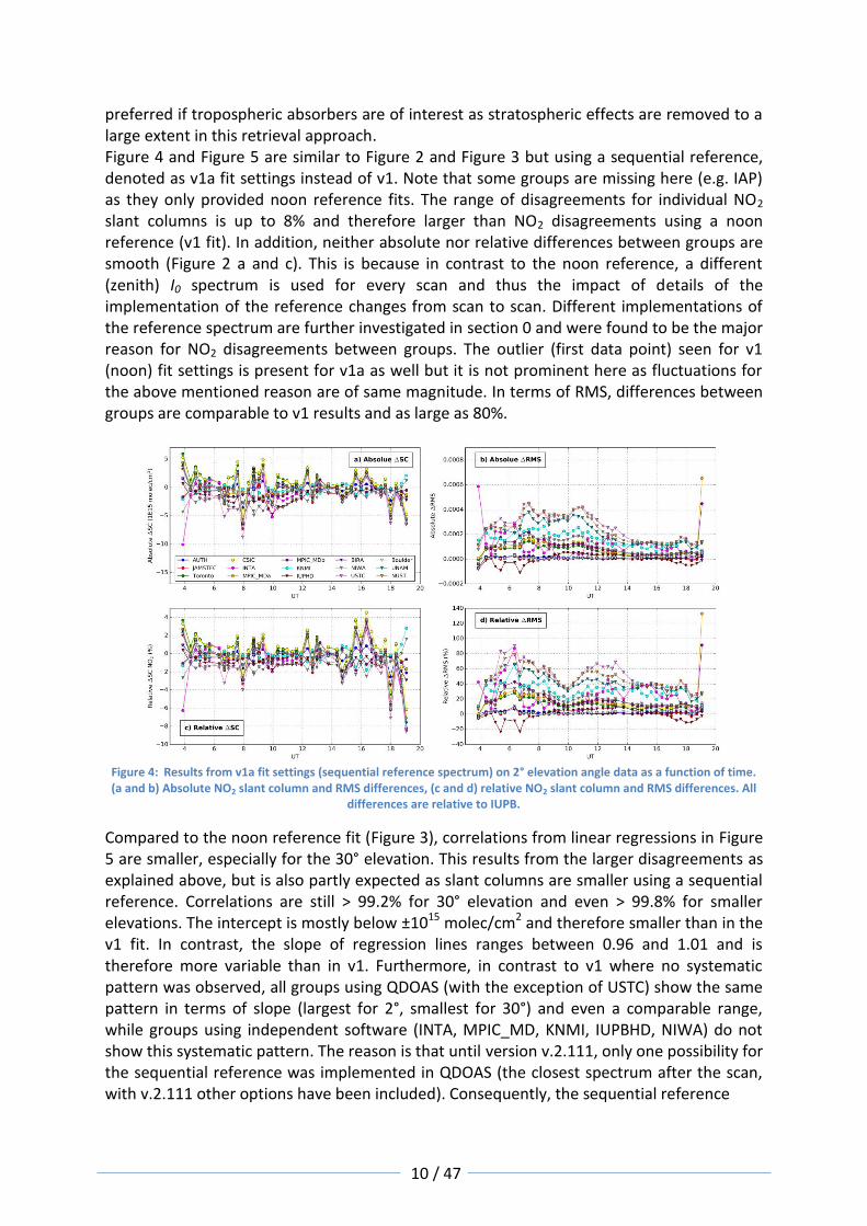
preferred if tropospheric absorbers are of interest as stratospheric effects are removed to a large extent in this retrieval approach. Figure 4 and Figure 5 are similar to Figure 2 and Figure 3 but using a sequential reference, denoted as v1a fit settings instead of v1. Note that some groups are missing here (e.g. IAP) as they only provided noon reference fits. The range of disagreements for individual NO2 slant columns is up to 8% and therefore larger than NO2 disagreements using a noon reference (v1 fit). In addition, neither absolute nor relative differences between groups are smooth (Figure 2 a and c). This is because in contrast to the noon reference, a different (zenith) I0 spectrum is used for every scan and thus the impact of details of the implementation of the reference changes from scan to scan. Different implementations of the reference spectrum are further investigated in section 0 and were found to be the major reason for NO2 disagreements between groups. The outlier (first data point) seen for v1 (noon) fit settings is present for v1a as well but it is not prominent here as fluctuations for the above mentioned reason are of same magnitude. In terms of RMS, differences between groups are comparable to v1 results and as large as 80%.

Figure 4: Results from v1a fit settings (sequential reference spectrum) on 2° elevation angle data as a function of time. (a and b) Absolute NO2 slant column and RMS differences, (c and d) relative NO2 slant column and RMS differences. All

differences are relative to IUPB.

Compared to the noon reference fit (Figure 3), correlations from linear regressions in Figure 5 are smaller, especially for the 30° elevation. This results from the larger disagreements as explained above, but is also partly expected as slant columns are smaller using a sequential reference. Correlations are still > 99.2% for 30° elevation and even > 99.8% for smaller elevations. The intercept is mostly below ±1015 molec/cm2 and therefore smaller than in the v1 fit. In contrast, the slope of regression lines ranges between 0.96 and 1.01 and is therefore more variable than in v1. Furthermore, in contrast to v1 where no systematic pattern was observed, all groups using QDOAS (with the exception of USTC) show the same pattern in terms of slope (largest for 2°, smallest for 30°) and even a comparable range, while groups using independent software (INTA, MPIC_MD, KNMI, IUPBHD, NIWA) do not show this systematic pattern. The reason is that until version v.2.111, only one possibility for the sequential reference was implemented in QDOAS (the closest spectrum after the scan, with v.2.111 other options have been included). Consequently, the sequential reference

11 / 47

Figure 5: Linear regression results (slope, intercept, correlation) for different elevation angles (w.r.t. IUPB) for fit

settings v1a (sequential reference).

selection is applied in the same way in all QDOAS data sets shown here. This is consistent with findings of Figure 4 where the exact implementation of the sequential reference was already found to dominate NO2 differences between groups.

1.4 Effect of the reference spectrum

In the IUPB spectra provided to intercomparison partners, two different zenith spectra having the same SZA were reported at noon, which is of course non-physical. Actually, the second zenith spectrum is the one having the smallest SZA, but for rounding reasons (the SZA was a 4-digits number in the spectra file provided), both spectra had the same SZA. Consequently, for the noon reference fits within this intercomparison exercise (v1), four options exist: 1) taking the first zenith spectrum of smallest SZA, 2) taking the second one, 3) taking the first for a.m. and the second for p.m. (i.e. always taking the closest in time), and 4) taking the average of both spectra. Similarly, different options exist for calculating the sequential references for fits v1a: 1) always taking the zenith spectrum closest in time, 2) always taking the last zenith spectrum before the actual measurement, 3) always taking the next zenith spectrum after the measurement, 4) taking the average of the two (before and after), and 5) interpolating the two zenith spectra to the time of the actual measurement. All different options for noon and sequential reference fits were evaluated using the IUPB retrieval code NLIN. Figure 6 shows the resulting absolute and relative slant column differences (top and middle) as well as relative RMS differences (bottom) for noon reference (left) and sequential reference (right) w.r.t. v1, resp. v1a fit results.

12 / 47

Figure 6: Different test results (see Tab. 4) in 2° elevation angle as a function of time. Top: Absolute NO2 SC differences,

Middle: Relative SC differences, Bottom: Relative RMS differences. Left is for noon reference (differences are w.r.t. IUPB v1 fit results), right is for sequential references (differences are w.r.t. IUPB v1a fit results).

Taking another noon reference spectrum results in a constant offset in absolute NO2 differences (Figure 6, top left). Test TR0 (using the first spectrum) yields the same results as the IUPB v1 fit from section 1.2, because there the first zenith spectrum was used as a reference as well. In contrast, using the second zenith spectrum as a reference (TR1) results in a constant offset of 1.5x1015 molec/cm2 (0.5-2.5% in relative differences, depending on the actual NO2 slant column), because the second zenith spectrum had apparently a smaller NO2 content. The change of the NO2 content could be related to changes of the atmospheric NO2 amount or the atmospheric light path. In terms of RMS, TR1 is up to 3% larger (Figure 6}, bottom left). The main reason for this is probably the larger NO2 slant columns as associated effects like the wavelength-dependence of the NO2 slant column (Pukite et al., 2010) were not compensated in this intercomparison exercise as discussed before. Test TR2 yields results which are identical to TR0 am and TR1 pm values. This is not seen for any groups in Figure 2 above, i.e. this option is apparently not present in any retrieval code. Not surprisingly, TR3 (averaging both zenith spectra) yields results which are between TR0 and TR2. In contrast to noon reference tests, sequential references show no smooth behaviour, neither for absolute, nor for relative differences (Figure 6, right). The reason is that for each vertical scanning sequence (from which only the 2° elevation is shown here and in Figure 4) another reference spectrum is used and consequently reference-related differences between groups are also changing from scan to scan. Note that almost no difference can be seen in Figure 6 between TR4 and TR5 as the 2° elevation angle is shown here and consequently the closest zenith measurement in time is normally the one before the scan as IUPB measurements proceed from low to large elevations. TR8 (interpolation to the measurement time) resembles the sequential reference treatment normally implemented in the IUPB code, and thus the TR8 line is zero. For TR6 and TR7, absolute and relative

13 / 47

differences (up to 8%) are remarkably similar to observed differences between groups using v1a fit settings, both in shape and in absolute values (compare to Figure 4). To conclude, the exact treatment of reference spectra is the major reason for observed NO2 discrepancies between groups in section 1.3, causing differences of up to 8%. Unfortunately, no clear recommendation can be derived from relative RMS differences in Figure 6 (bottom right) as all lines scatter around zero. However, the relative difference in RMS can be as large as 6% and in general, using a single zenith reference spectrum before or after the scan tends to produce larger RMS. However, while the reference treatment explains the majority of NO2 disagreements, it cannot explain the large RMS differences (up to 100%) between groups.

1.5 Effects of other algorithmic differences In addition to differences in the choice and computation of the reference spectrum, a number of algorithmic differences were analysed in Peters et al., 2016 using the IUPB software:

Slit function treatment

Intensity offset treatment

I0 correction

Numerical approach to solve the linear least squares fit

Wavelength calibration approach (nonlinear fit) All of the above were found to affect the slant columns and RMS results, however at very different levels. For the detailed results, the reader is referred to the paper; a summary and the main conclusions are given in the next section.

1.6 Summary and Conclusions Table 3: Summary of performed tests (differences in retrieval codes) and associated impacts on NO2 slant columns and RMS.

Reason for disagreement ΔNO2 (%) ΔRMS (%) Remarks

Reference treatment (noon)

2.5 3 Produces constant absolute NO2 SC offsets

Reference treatment (sequential)

8 6

Slit function treatment 1.3 6.5 Produces constant relative NO2 SC offsets

Intensity offset correction 2 (typical) 10 (outlier)

20 (typical) 60 (outlier)

I0 correction 0.25 20 Produces constant absolute NO2 SC offsets

Numerical methods (for linear fit)

0.3 (0.7) 2.5 Produces constant absolute NO2 SC offsets Disagreement increases with RMS

Wavelength calibration (nonlinear fit)

0.4 Up to 80

An intercomparison of DOAS retrieval codes using measured spectra from the same instrument during the MAD-CAT campaign and harmonized fit settings was performed. Excellent agreement was found between different DOAS fit algorithms from 17 international groups. For noon reference fits, the correlation in terms of NO2 slant columns was found to be larger (> 99.98%) than for sequential references (> 99.2%), which is caused by different implementations of the sequential reference. For individual measurements, differences of up to 8% in resulting NO2 slant columns (which is substantially larger than NO2 slant column fit errors), and up to 100% for the fit RMS were observed.

14 / 47

In general, the wavelength calibration and the intensity offset correction were found to produce the majority of observed RMS differences, but have a negligible impact on NO2 slant columns (< 0.4%, resp. < 2% except for the first measurement of the day affected by stray light and possibly direct light in the telescope). In contrast, the reference selection explains the majority of observed NO2 slant column differences between groups while having a minor impact on the RMS. Thus, if harmonization of NO2 slant columns is of interest, the reference treatment needs to be harmonized (otherwise differences of up to 8% have to be expected) while for RMS reduction/harmonization, the offset intensity correction and the wavelength calibration need to be harmonized. In terms of NO2, two types of disagreements between groups have been observed, which are (1) constant in absolute, or (2) constant in relative differences. The latter was found to arise from the numerical approach used for solving the DOAS equation as well as the treatment of the slit function while the choice of the reference spectrum causes absolute differences. Recommendations aiming at improvement of the fit quality and harmonization between MAX-DOAS retrievals derived from this study are:

1. Reference treatment: Using averaged or interpolated sequential reference spectra matches the atmospheric conditions at the measurement time better and was found to produce slightly smaller RMS (6 %).

2. Slit function: Using a measured slit function performed better than fitting line parameters in the data set used here. However, slit function measurements then have to be performed regularly (e.g., daily to monitor possible instrument changes).

3. Intensity offset: An approach based on I instead of I0 is recommended. Surprisingly, the simple approach performs better for measurements pointing close to sunrise but this could be just a coincidence in this data set. Inclusion of an additional Ring spectrum multiplied by wavelength is preferred over adding a linear term to the offset as this mostly compensates the wavelength-dependence of the Ring slant column.

4. Numerical approaches: Using an SVD is most stable and produces slightly smaller RMS than LU decomposition.

5. Wavelength calibration: Although HgCd line lamp calibration measurements lead to absolute accuracies (in this case) of 0.03 nm, a Fraunhofer shift fit reduces the RMS by up to 40-50%. For the I0 fit w.r.t. the Fraunhofer spectrum, inclusion of all trace gases showed no advantage over inclusion of a polynomial only. Temperature instabilities of the spectrometer produced shifts of I relative to I0 changing over the day. Compensation of this effect within DOAS retrieval codes further improves the RMS by up to 40-50% when using a noon reference spectrum.

15 / 47

2 Uncertainty assessment of QA4ECV HCHO DOAS analysis

G. Pinardi (BIRA-IASB)

2.1 Introduction

One important tasks of the QA4ECV WP3 has been to intercompare different DOAS retrieval software packages for NO2 and HCHO slant columns harmonization. This exercise has involved a larger community than the QA4ECV partners, leading to 17 groups for the NO2 and 20 for the HCHO intercomparison. The tested settings have been defined by performing several sensitivity tests that are briefly discussed in Section 2.2. From the intercomparison results, two recommended DOAS settings have been selected, as described in Section 2.3. The error budget on HCHO dSCD (SCDα - SCD90; α being the elevation angle) is presented in Section 2.4. We will focus on 30° elevation, which is the baseline for the QA4ECV VCD calculation (see equation below), but also on the 3° elevation dSCDs, which are more sensitive to HCHO close to the ground.

90

90

AMFAMF

SCDSCD

DAMF

DSCDVCD

2.2 Sensitivity tests and common settings definition

In order to define the common settings to be tested by every group on common spectra, some preliminary sensitivity tests have been performed on the spectra recorded by the IUP-Bremen MAXDOAS spectrometer on 18/06/2013 during the MADCAT intercomparison campaign. The main purpose was to revisit the settings based on previous SCD comparison studies carried out within the framework of the CINDI-1 and MADCAT campaigns (see Pinardi et al. (2013) and http://joseba.mpch-mainz.mpg.de/mad_analysis.htm, respectively). The parameters investigated were new cross-section data sets (such as O4 cross-sections of Thalman and Volkamer (2013) or the O3 cross-sections of Serdyuchenko et al (2014)), the wavelength interval by going further down in the UV (Y. Wang, personal communication) and the improvement of the consistency with the satellites HCHO retrievals, and the Ring effect, identified in Pinardi et al. (2013) as one of the main parameters affecting the DOAS fit results of HCHO (up to 20% in a systematic way when considered together with the HCHO and O3 cross-section uncertainties). Sensitivity tests were performed by starting on recommended settings of Pinardi et al. (2013) and assessing the variability of the retrieved slant columns for various changes in the fit parameters, as described in the last column of Table 4. This exercise focused on the minimization of the interferences and the misfit related to Ring effect and O4 and BrO absorption cross sections. The first test was to check whether the new O4 cross-section of Thalman and Volkamer (2013) did not introduce un-wanted interferences between O4, HCHO and BrO absorption features, as seen with the Hermans et al. (2003) cross-sections. The Hermans dataset is leading to larger HCHO columns and larger spread in the BrO DSCDs retrieved at different viewing elevations (see Pinardi et al.,2013), which is not to be expected for a stratospheric absorber like BrO. The Thalman and Volkamer (2013) cross-sections did not introduced such instabilities, and responded

16 / 47

Table 4: baseline DOAS settings (from Pinardi et al. 2013, referred as “BL” in figures) and tested changes.

Parameter Baseline settings (as Pinardi et al., 2013)

Tested changes

Fitting interval 336.5-359 nm Other window lower in the UV (324.6-359nm)

Wavelength calibration

Calibration based on reference solar atlas (Chance and Kurucz, 2010)

Cross sections

HCHO Meller and Moortgat (2000), 293°K

O3 Bogumil et al. (2003), 223° and 243°K, I0-corrected

Serdyuchenko et al (2014)

NO2 Vandaele et al. (1998), 298°K, I0-corrected

BrO Fleischmann et al. (2004), 223°K

O4 wavelength corrected Greenblatt et al. (1990)

Thalman and Volkamer (2013)

Ring effect Chance and Spurr (1997), ring_NDSC_2003.xs

Several approaches

Closure term Polynomial of order 5 (corresponding to 6 coefficients)

Intensity offset Linear correction

Wavelength adjustment

All spectra shifted and stretched against reference spectrum

Reference spectra Fixed reference: zenith at minimum SZA

Sequential reference: zenith of the scan

similarly to the wavelength corrected Greenblatt et al. (1990) dataset, and was thus selected for our new baseline. The second step was to test the new O3 cross-section of Serdyuchenko et al (2014), and several approaches for the Ring treatment: an update of the Ring NDSC 2003 file (Chance and Spurr, 1997) has been created with the QDOAS software based on the SAO high resolution solar atlas, and the option of normalizing it as in Wagner et al (2009) has also been tested. Moreover, similarly to Pinardi et al. (2013), other Ring approaches have been tested:

Ring_saohr: updated Ring NDSC 2003 file created with QDOAS following Chance and Spurr (1997) from the SAO high resolution solar atlas, without any normalization; it is an updated version of the baseline of Pinardi et al. (2013).

Ring_saohr-norm: application of the normalization proposed in Wagner et al (2009) while creating the cross-section with QDOAS; it is an updated version of case A of Pinardi et al. (2013).

Ring_sciatran: high resolution Ring cross section derived from SCIATRAN radiative transfer calculations in a Rayleigh atmosphere; it is case B of Pinardi et al. ( 2013).

Ring_Wang: approach proposed by Yang Wang (MPIC) during the MADCAT HONO DSCD comparison. It includes a term that takes into account the λ-4 variation of the Ring.

17 / 47

Figure 7: Illustration of variations on HCHO dSCD and RMS differences for the analysis of Bremen spectra of 18/6/2013 at 3° elevation, when changing O4, O3, and Ring cross-sections.

Sensitivity test results are presented in Figure 7 for the dSCD at 3° elevation and in Figure 8 for 30° elevation. A small impact of the Serdyuchenko O3 cross sections is obtained, while larger differences appear when using the different Ring cross-sections. Relative differences up to ±5% are found at 3° elevation, and up to ±15% at 30° elevation. A new baseline BL1, combining the use of the Thalman and Volkamer O4 and Serdyuchenko O3 cross-sections, and the updated high resolution Ring cross-sections from the SAO solar atlas (red curve in Figure 7 and Figure 8), was selected for further testing the stability of the HCHO retrievals when changing Ring cross-sections and the wavelength interval. As done in Pinardi et al. (2013), these tests are performed by investigating the consistency of VCDs retrieved using two calculation methods: 1) from the geometrical approximation at 30° elevation angle (Hönninger et al., 2004; Ma et al., 2012), and 2) from direct conversion of the zenith-sky observations using HCHO AMFs calculated for clear-sky aerosol-free conditions using the UVspec/DISORT model (Mayer and Kylling, 2005). Results for the 324.5-359nm range are shown in Figure 9.

Figure 8: As Figure 7, but for 30° elevation.

18 / 47

Figure 9: Impact of the different Ring approaches on HCHO dSCD and VCD retrieved in the window 324.6-358nm from Bremen spectra recorded on 18/6/2013 during the MADCAT campaign.

Overall, we can see from Figure 9 that the sensitivity to the choice of the Ring effect cross sections is significant in the 324.6-359nm interval (also true for 333-358nm; not shown here) where only the normalized Ring and the approach from Y. Wang gives physical results (good agreement between zenith and geometrical approximation VCDs). In the baseline BL1 window however (not shown), consistent VCD results are obtained for all the tested Ring cross-sections. The normalized high resolution Ring from SAO is chosen as in the 324.6-359 nm range since Wang’s approach gives slightly less good consistency between the 2 VCD approaches. Differences in terms of HCHO dSCD columns in the 324.6-359 window wrt to the new baseline window BL1 can be up to ±1x1016 molec/cm2 for the 30° elevation case (i.e., up to 20 to 50 %) if the Ring cross sections are not normalized, while when the Ring is normalized, the differences are smaller and more stable during the day. Moreover, the errors on the DOAS fit are much smaller (around 2 times smaller) in this wavelength region compared to BL1. Similar tests have been performed when using a sequential reference instead of a fixed noon reference. The same findings are obtained, with differences of about ±10% in the BL1 window and larger differences up to 50% if the Ring is not normalized when using the interval 324.6-359nm. For the intercomparison exercise between the different groups, 4 common settings have been defined with fixed and sequential reference in both the 336.5-359 nm and 324.6-359 nm wavelength regions, and using the O4 Thalman and Volkamer and O3 Serdyuchenko cross-section datasets, the SAO high resolution (HR) normalized Ring cross-sections, and a linear offset, as described in Table 5.

2.3 Intercomparison study

The intercomparison study focused on comparing the HCHO DSCD analysis performed by each group with their own retrieval codes and following the common settings of Table 5. In addition to the spectra, the absorption cross-sections and the solar atlas, two slit function files were provided to the participants: the Bremen measured slit function at 346nm (file SLITFUNCTION_18JUN2013_UV(346NM).DAT), and an optimized slit function in 2 dimensions (file slf_2D_fromKur.slf) that has been obtained during the QDOAS calibration procedure by allowing some stretch of the slit function wings in the different wavelengths sub-intervals. This optimized 2D slit function allows shape changes with wavelength, as illustrated in Figure 10.

19 / 47

Table 5: Common DOAS settings for the intercomparison exercise between the different groups.

Setting #

Reference Spectrum

Window (nm)

Cross sections

Intensity Offset

Polynomial order

Wavelength calibration

Additional adjustment

1 Fixed (zenith noon)

336,5-359

1,2,3,4,5,6,7 Order 1 5 (6 coeff.)

Based on reference SAO solar spectra (Chance and Kurucz, 2010)

All spectra shifted and stretched against the reference spectrum

2 Sequential (zenith of the scan)

336,5-359

1,2,3,4,5,6,7 Order 1 5

3 Fixed

324,6-359

1,2,3,4,5,6,7 Order 1 5

4 Sequential 324,6-359

1,2,3,4,5,6,7 Order 1 5

Cross-sections: 1=o4_thalman_volkamer_293K_inAir.xs, 2= Ring_QDOAScalc_HighResSAO_Norm.xs, 3=o3_223K_SDY_air.xs, 4=o3a_243K_SDY_air.xs, 5=no2_298K_vanDaele.xs, 6=bro_223K_Fleischmann.xs, 7=hcho_297K_Meller.xs

The results of the intercomparison were analysed by comparing the DSCDs to the BIRA analysis selected as reference. Scatter plots, histograms and relative and absolute differences were investigated, following the methods described in Roscoe et al. (2010) and Pinardi et al. (2013). An example of the intercomparison result is given in Figure 11, where the HCHO dSCD at 30° elevation angle for the 4 settings are shown for all groups. In addition, participants were asked to fill in a questionnaire that helped in the interpretation of the results and highlighted, e.g. the use of the measured or optimized slit function, differences in the calibration procedure and in the way the sequential reference was selected.

Figure 10: (a) optimized 2D slit function obtained during the QDOAS calibration procedure, and (b) comparison of the slit function optimized at 346nm to the Bremen measured slit function at 346 nm.

20 / 47

Figure 11: Overview of the HCHO dSCD results of all groups wrt BIRA, for 30° elevation angles and for the 4 common settings.

Investigations of the impact of these differences have been performed. An example of the impact of optimizing the slit function or using the measured one, and the details of the calibration procedure is presented in Figure 12, for dSCD relative differences at 3 and 30° elevation. Depending on the settings (and thus on the wavelength range), the behaviours are quite different: in the window 336.5-359nm (settings #1 and #2), the slit function optimization has a large impact (up to 5% for 3° and 10% for 30°) while the inclusion of O3 and/or Ring cross-sections in the calibration has a minor impact. In the 324.6-359 nm window (settings #3 and #4), the slit function optimization has a smaller impact than in 336.5-359 nm interval and the inclusion of O3 in the calibration has also a minor impact.

Figure 12: Impact of optimizing the slit function and including absorbers in the calibration.

Linear regression statistics of the scatter plots of each group with respect to BIRA are reported in Figure 13 and Figure 15 for several elevation angles. Figure 13 shows a generally good agreement, with most of the groups being within ±15% (dotted lines in the slope panel at 0.85 and 1.15). Tests have been made by BIRA in order to verify if the differences seen

21 / 47

between the groups could be related to the way the calibration and the slit function are treated and how the sequential reference is selected. These are illustrated in Figure 13 and Figure 15 by including BIRA_2 (which is an analysis performed with the measured slit function at 346nm, but with the possibility to fit an improved version during the calibration procedure that includes O3 and Ring), BIRA_3 (analysis performed with the measured slit function at 346nm) and BIRA_4 (analysis performed with the optimized slit function in 2D, and using a sequential reference obtained by averaging the zenith spectra before and after the scan, instead of the zenith after the scan). Moreover, color-coded information has been added in the top panel of each setting results in Figure 13 and Figure 15, including the information on the choices made by each group for the slit function (optimization, measured, or other) and for the selection of the sequential reference. We can see that most of the differences between groups are of the same order of magnitude than the differences found with BIRA_2, BIRA_3 and BIRA_4. Larger differences with settings #3 and #4 (Figure 15) are however found for some groups, which should be investigated in more details.

Figure 13: Overview of the HCHO dSCD scatter plots statistics for the 336.5-359nm wavelength window (settings #1 and #2) for every group wrt BIRA, for several elevation angles.

From this exercise, the following recommendations were deduced: (1) fitting and optimizing the slit function during the calibration procedure without inclusion of Ring but with inclusion of O3 and (2) using as reference the average of the zenith spectra before and after the scan. Two datasets for QA4ECV processing were selected: one in the 336.5-359 nm range (wavelength interval which gives the best coherence between the different groups) and one in the 324.6-359 nm (wavelength interval which minimizes error/noise), and are described in Table 6.

22 / 47

Figure 14: Same as Figure 13, but for the 324.6-359nm window (settings #3 and #4)

Table 6: Recommended DOAS settings for HCHO. Two different data sets will be generated using two different wavelength range: 336.5-359 and 324.6-359 nm.

2.4 Error budget

The total uncertainties on the HCHO dSCDs retrieval can be divided into two categories: (1) errors affecting the slant columns in a systematic way, as already partly covered in previous sections, and (2) the random errors mostly caused by measurement noise.

23 / 47

Several possible optimisations of the HCHO DOAS retrieval, in order to minimise both systematic interferences and misfits related to Ring effect and O4 absorption cross sections have already been presented in Section 2.2. In section 2.3 we have seen how missing precisions/information in the pre-defined settings definition could lead to systematic differences between analyses performed by different groups, which gives a typical limit on the coherence that could be achieved based on the analysis of the same spectra. A few other uncertainties are investigated here, related to the cross-section choices. It should be noted that the quality and performance of the different instruments operated at QA4ECV stations are also an important factor in the random contribution.

2.4.1 Systematic uncertainties

The remaining contributions are the impact of the chosen cross-sections. Two sources of HCHO absorption cross-sections have been used in the literature, the Cantrell et al. (1990) and the Meller and Moortgat (2000) datasets, the latter being adopted for our baseline. In the 336.5-359 nm interval and at the resolution of the Bremen spectrometer, the cross-sections differ by approximately 9%, a difference that propagates directly to the slant column retrievals: ~10% difference at 3° and between 10 to 15% at 30°. For BrO, two main sources of cross-sections are the Wilmouth et al. (1999) and Fleischmann et al. (2004) datasets. These datasets are highly consistent in shape and their use was found to result in very small differences in the HCHO dSCD, of the order of a few 1014 molec/cm². For a median dDSCD of 7.5x1016 molec/cm² at 3° elevation, the difference is therefore less than 1%. The baseline intercomparison settings used for NO2 are the Vandaele et al. (1996) cross-sections at 298°K. Switching to the alternative dataset of Burrows et al. (1998), HCHO dSCDs are found to vary by 5 to 15% in the 336.5-359 nm, and less than 2% in the 324.6-359 nm range. The baseline intercomparison settings for O3 used the Serdyuchenko cross-sections. The impact of using the alternative dataset from Bogumil et al. (2003), is very small: for the median dDSCD at 3° elevation, the difference is below 2% during the day, while it varies between 2 and 5% for 30° elevation. The choice of the O4 cross-section has been already largely discussed in Sect. 2.2. Differences between the wavelength corrected Greenblatt et al. (1990) dataset or the Thalman and Volkamer (2013) dataset are very small, less than 2% on the HCHO dSCD. Although the cross-talk between HCHO and the Ring effect has been strongly reduced using the new baseline settings defined in Sect. 2.2, some level of correlation persists between these parameters. HCHO uncertainties are expected to be linked to the strength of the Ring effect, which itself is a function of the geometry, SZA and aerosol content (Wagner et al., 2009). When using the Ring cross-section from the Wang approach (see Sect. 2.2), the uncertainties on the HCHO dSCD reaches up to 10% (2 x1015 molec/cm²) in the 336.5-359nm window and up to 40% (8x1015 molec/cm²) in the 324.6-359nm range. As seen in Section 2.3, uncertainties in key instrumental calibration parameters can cause large differences in the HCHO dSCD. This effect e.g., lead to changes in the HCHO dDSCD relative differences at 3° elevation of around 3 to 5%, and at 30° elevation up to 10%. Between the two tested windows (336.5-359nm and 324.6-359nm) typical differences are of about 10% to 20% for 3° elevation and up to 20% for 30° elevation when using an average sequential reference.

2.4.2 Random uncertainties

DOAS random errors are mostly related to the measurement noise which for silicon array detectors is generally limited by the photon shot noise. Assuming uncorrelated errors for

24 / 47

the individual detector pixels and if the DOAS fit residuals are dominated by instrumental noise, the random contribution to the DSCD error can be derived from the DOAS least-squares fit error propagation (e.g, Stutz and Platt, 1996), and the random errors are represented by the slant column fit errors. As shown in Pinardi et al. (2013), scientific grade instruments display small random errors (of the order of 1x1015 molec/cm2 in the case of instruments deployed during the CINDI-1 campaign) while mini-DOAS types of instruments are significantly noisier (typical errors reaching 5x1015 molec/cm2 or more). This is mostly related to the use of small and uncooled (or less cooled) detectors with low quantum efficiency for the second type of instruments. Temperature instabilities can also lead to systematic features in the residuals that can affect DSCD error estimates. For the 18/6/2013 Bremen spectra , mean errors at 3° and 30° are of the order of 1.93x1015 molec/cm2 (2.6% of the mean column) and 1.47x1015 molec/cm2 (8.5%) for the 336.5-359nm interval and of about 1x1015 molec/cm2 (1.5% of the mean column) and 7.2x1014 molec/cm2 (4.4%) in the 324.6-359nm interval. The random uncertainties are related to the signal-to-noise ratio (S/N) of each instrument, which have been estimated here as the inverse of the DOAS fit RMS. Table 7 gives an overview of the typical S/N values estimated at each QA4ECV station. These values depend on the detector type, but also on illumination and therefore location, season, time of the day and integration time. Table 7: Typical S/N ranges in the HCHO wavelength range, for the QA4ECV stations.

Station Lat, Long Data Source

S/N estimation = 1/RMS of DOAS fit

De Bilt/Cabauw (NL) 52°N, 5°E KNMI Tbc

Uccle (BE) 50°N, 4°E BIRA between 500 and 2000 Beijing (CHN) 40°N, 116°E MPIC Tbc

Xianghe (CHN) 39°N, 117°E BIRA between 5000 and 10000 Bujumbura (BU) 3°S, 29°E BIRA between 3000 and 10000 Bremen (DE) 53°N, 9°E IUPB between 2000 - 9000 Nairobi (KEN) 1°S, 37°E IUPB between 1000 - 6000 Athens (GR) 38°N, 23°E IUPB between 1000 - 4000 Mainz (DE) 50°N, 8°E MPIC ~1700 Greater Noida (IND) 28°N, 77°E MPIC Tbc

Thessaloniki (GR) 41°N, 23°E AUTH preliminary SNR we calculated for HCHO ranges between 500 and 1000

Madrid (ESP) 40°N, 3°W CSIC estimated based on O4 analysis in UV: about 2100 S/N for UV

2.4.3 Overall error budget

Based on the results discussed above, an overall assessment of the total uncertainties on HCHO dSCDs has been performed, including the main contributions of systematic and random errors from the comparison study using the MADCAT Bremen spectra (see Table 8). We have assumed uncorrelated effects for each tested parameter, and summed all deviations in quadrature to obtain an estimate of the overall systematic uncertainty. Total systematic uncertainties on HCHO dSCDs are of about 15 to 30% if not considering the large sensitivity to Ring in the 324.6-359nm range and can be up to 45% otherwise. For scientific grade instruments like the one used by the Bremen group during the MADCAT campaign,

25 / 47

the systematic errors are the main source of uncertainty. For mini-DOAS type of instruments, both random and systematic uncertainties contribute similarly, and the random uncertainty can be reduced by means of longer integration time. Table 8: Typical total errors for the 2 HCHO wavelength ranges, for typical median DSCD of 7.8x10

16 molec/cm²

at 3° elevation angle and 1.8x1016

molec/cm² at 30° elevation angle..

336.5-359 nm, seq. average 324.6-359 nm, seq. average

3° elevation 30° elevation 3° elevation 30° elevation

Systematic contribution

- NO2 xs 5 to 15% 5 to 15% <2% <1%

- BrO xs <1% <1% <0.5% <1%

- O3 xs <2% 2 to 5% <2% <5%

- O4 xs <1.5% ~2% ~1% ~2%

- HCHO xs ~10% 10 to 15% ~10% 10 to 15%

- Ring <6% <10% up to 15% Up to 40%

- Slit function & calibration

<5% Up to 10% <3% Up to 10%

Total systematic 19.8 % [1.54x1016

molec/cm²]

26% [0.47x1016

molec/cm²]

18.5% [1.44x1016

molec/cm²]

44.5% [0.8x1016

molec/cm²]

Random (scient. grade)

2.6% 8.5% 1.5% 4.4%

Total errors 20% 27.4% 18.6% 44.7%

26 / 47

3 Uncertainty assessment of QA4ECV NO2 and HCHO DAMF look-up tables

F. Hendrick (BIRA-IASB)

3.1 Introduction

One of the main tasks of the QA4ECV WP3 is to build a consistent historical record of independent reference data for the quality assessment of NO2, HCHO, and CO atmospheric ECV precursors. For NO2 and HCHO, a systematic approach has been adopted to harmonise MAX-DOAS retrievals of these species at 12 sites (see Table 9) selected for inclusion in the project database. This harmonisation effort is described in details in the Deliverable D3.8 available on the QA4ECV website at http://www.qa4ecv.eu/sites/default/files/QA4ECV_D3.8_v1.0_web.pdf. In brief, it consists of three steps: (1) an intercomparison of NO2 and HCHO slant column densities (SCDs) retrievals from a common set of measured spectra in order to assess the consistency of DOAS retrieval tools in use in the community and to derive recommendations for standardised analysis settings, (2) the development of generic look-up tables of air mass factors (AMFs) generally applicable within the network to convert SCDs into vertical column densities (VCDs), and (3) the systematic use of the Generic Earth Observation Metadata Standard (GEOMS) hdf format for data reporting.

Table 9: List of QA4ECV MAX-DOAS reference stations.

Station Lat, Long Class Data Source

De Bilt/Cabauw (NL) 52°N, 5°E Sub-urban KNMI

Uccle (BE) 50°N, 4°E Urban IASB-BIRA

Beijing (CHN) 40°N, 116°E Urban IASB-BIRA, MPG

Xianghe (CHN) 39°N, 117°E Sub-urban IASB-BIRA

Bujumbura (BU) 3°S, 29°E Sub-urban IASB-BIRA

Bremen (DE) 53°N, 9°E Urban IUP-UB

Nairobi (KEN) 1°S, 37°E Rural / Urban IUP-UB

Athens (GR) 38°N, 23°E Urban IUP-UB

Mainz (DE) 50°N, 8°E Urban MPIC

Greater Noida (IND) 28°N, 77°E Urban MPIC

Thessaloniki (GR) 41°N, 23°E Urban AUTH

Madrid (ESP) 40°N, 3°W Urban CSIC

In the AMF LUT approach (step 2), the differential SCDs with respect to the zenith (90°elevation) of the scan are divided by the corresponding differential AMFs:

90

90

AMFAMF

SCDSCD

DAMF

DSCDVCD

where α represents an off-axis elevation angle of the scan, generally chosen between 15 and 30° in order to minimize the impact of aerosols on the retrieval. NO2 and HCHO DAMF LUTs have been generated by using the bePRO/LIDORT radiative transfer suite (Clémer et al., 2010; Spurr, 2008) for the following parameter values:

27 / 47

Table 10: Parameter values for which the LUTs were calculated.

In order to extract appropriate DAMF values for each QA4ECV station, an extraction/interpolation tool has been developed (see Deliverable D3.8). It is a Fortran executable fed by the following parameters in addition to the DAMF LUTs:

Geometry parameters (solar zenith, relative azimuth, and elevation angles)

Boundary layer height (BLH; which is used in a first approximation to initialise the trace gas and aerosol extinction profiles scaling heights (SH); see Vlemmix et al., 2015)

aerosol optical depth (AOD)

Surface albedo

For harmonisation purposes, BLH/SH, AOD, and surface albedo values are extracted in a transparent way from coupled climatologies based on collocated ECMWF (http://apps.ecmwf.int/datasets/data/macc-reanalysis/levtype=sfc/), AERONET (http:// aeronet.gsfc.nasa.gov/), and GOME (Koelemeijer et al., 2008) data, respectively. Here, we present the uncertainty assessment of the NO2 and HCHO DAMFs, which will contribute, together with the uncertainties related to the DOAS fitting, to the total uncertainty budget on harmonized NO2 and HCHO VCDs. Such a budget is needed for evaluating the quality of the atmosphere reference data sets that will be used in the project. The uncertainties on the NO2 and HCHO DAMFs are estimated based on sensitivity tests on the main parameters affecting the DAMF calculation and/or extraction. This sensitivity study is described in Section 3.2. The overall uncertainty budget on the DAMFs is presented in Section 3.3.

3.2 Sensitivity studies

Sensitivity tests are performed on the following parameters: AOD, trace gas and aerosol extinction profile shapes, trace gas profile shapes (BLH/SH), and surface albedo. Those have been identified in Vlemmix et al. (2010) as the main parameters affecting tropospheric trace gas DAMFs. Here it should be noted that especially for NO2 the SH might be systematically

Parameter Value(s)

Wavelength NO2: 360, 427, 477nm; HCHO: 343 nm

Altitude grid 0-2km/step 0.1 km ; 2-20km/step 1km

p,T,O3 profiles AFGL 1976

Viewing elevation angle

10, 15, 20, 25, 30, 35o (+zenith)

Relative azimuth angle 0, 30, 60, 90, 120, 150, 180o

Solar zenith angle 0, 20, 30, 40, 50, 60, 65, 70, 75, 80, 82, 84, 86, 88o

Surface albedo 0, 0.5, 1

NO2 and HCHO vertical Profiles

Exponentially-decreasing profile: Scaling Height (SH)= 0.2, 0.5, 1, 1.5, 3 km; Tropospheric NO2 and HCHO VCDs: 2e16 molec/cm2

Aerosol scenarios Exponentially-decreasing profile: Scaling Height (SH)= 0.2, 0.5, 1, 1.5, 3 km; AOD: 0, 0.2, 0.5, 1, 2, 4; single scattering albedo: 0.90; asymmetry factor: 0.72; Henyey-Greenstein phase function

Cloud scenarios Clear-sky only

28 / 47

lower than the BLH because of the rather short atmospheric lifetime. The impact of parameters having a minor effect like aerosol properties (single scattering albedo, asymmetry factor) will also briefly be discussed. The sensitivity study focuses on the Xianghe (Beijing suburban area) and Uccle (Brussels) stations, which are representative of urban/highly polluted and urban/polluted atmospheric conditions, respectively. As can be seen in Table 9, these conditions are representative of all the other QA4ECV stations. Although only VCDs at 30° elevation will be reported in the QA4ECV MAX-DOAS data files, uncertainties are calculated here for both 30° and 15° elevations in order to have a better estimation of the uncertainty range since MAX-DOAS at 15° elevation are more sensitive to aerosols than at 30°. The target species are NO2 visible (460 nm) and HCHO (343 nm).

3.2.1 AOD

For the sensitivity test on AOD, NO2 and HCHO DAMF have been extracted for both stations for the years 2011 (Xianghe) and 2012 (Uccle) using (1) the coupled AERONET-based AOD climatology and (2) timely coincident measured AODs from the collocated AERONET/CIMEL instruments. Since both Xianghe and Uccle are urban/polluted locations, the climatology is not able to capture the high-amplitude AOD variations which can occur on a short time scale, especially in Xianghe. Therefore, with this test, the uncertainty related to use of such a climatology instead of timely coincident AOD measurement, and the impact of the AOD uncertainty on DAMFs, in general, will be assessed. It should be noted that in a first approximation, SH values are here chosen identical for aerosols, HCHO, and NO2, and correspond to values interpolated from the ECMWF-based BLH climatology coupled to the DAMF extraction tool (see Section 3.1). Figure 15 shows the ratio between the climatological and timely coincident AODs at 360 nm for both Uccle and Xianghe.

Figure 15: Ratio between the climatological and timely coincident AODs (360 nm) for Xianghe 2011 (upper plot)

and Uccle 2012 (lower plot). The solid thick line in each plot corresponds to the mean ratio value, while thin solid lines mark the ratio of unity

29 / 47

The mean ratio values are 1.45 ± 1.39 and 1.25 ± 0.91 for Xianghe and Uccle, respectively, but values up to 8-10 are found in some extreme cases in Xianghe. The corresponding impact on the HCHO DAMFs −and correspondingly on VCDs− is illustrated in Figure 16 where the ratio of HCHO DAMFs extracted using both AOD data sets are plotted for both stations for 15 and 30° elevation.

Figure 16: Ratio between HCHO DAMFs at 15 and 30° elevation extracted using climatological and timely coincident AODs for Xianghe 2011 (upper plot) and Uccle 2012 (lower plot). The solid thick lines in each plot correspond to the

mean ratio values at both elevation angles, while thin solid lines mark the ratio of unity.

HCHO DAMF ratio values of up to 4 are found in Xianghe while in Uccle, this ratio does not exceed 1.5 most of the time. Similar features are found for NO2 in the visible range at both stations. DAMF ratio values for both HCHO and NO2 are summarized in Table 12. As expected, the uncertainty on the AOD has a larger effect on DAMF at 15° than 30° elevation. These ratio values are used in Section 3 for the overall uncertainty budget assessment on DAMF.

Table 11: Mean ratios between HCHO (NO2) DAMFs at 15 and 30° elevation extracted using climatological and timely coincident AODs for Xianghe (2011) and Uccle (2012). The corresponding standard deviations are also included in the

table.

3.2.2 Profile shape

Exponentially-decreasing profile shapes for both trace gas and aerosol extinction vertical profiles have been used to generate NO2 and HCHO DAMF LUTs. This shape is chosen

Xianghe (2011) Uccle (2012)

15° elevation 30° elevation 15° elevation 30° elevation

HCHO DAMF ratio 1.179 ± 0.445 1.100 ± 0.210 1.037 ± 0.162 1.013 ± 0.053

NO2 DAMF ratio 1.145 ± 0.407 1.093 ± 0.197 1.041 ± 0.181 1.029 ± 0.078

30 / 47

because, once scaled to the VCDs retrieved by the AMF LUT approach, these profiles were found to give, after convolution with the satellite nadir averaging kernels (see Deliverable D3.8), VCDs which are in significantly better agreement with satellite VCDs than when using block profiles. In order to test the impact of the profile shape on DAMFs, similar LUTs have been calculated using block profiles (constant concentration within the BLH and concentration equal to zero outside the BLH), all the other parameters, including BLH, being kept identical to those described in Table 11. As for the sensitivity test on AOD, time-series of DAMF have been extracted for Xianghe (2011) and Uccle (2012) from both types of LUTs. The ratios between HCHO DAMFblock and DAMFexp are shown in Figure 17 as an example, and ratio values for both NO2 and HCHO are summarized in Table 13. As can be seen, an effect of up to -20% is found when changing the profile shape from exponential to block. On average the effect is <10%. Here it is interesting to note that DAMFblock are always systematically larger than DAMFexp.

Figure 17: Ratios between HCHO DAMFblock and DAMFexp extracted for 15 and 30° elevation angles for Xianghe 2011 (upper plot) and Uccle 2012 (lower plot). The solid thick lines in each plot correspond to the mean ratio

values at both elevation angles.

Table 12: Mean ratios between HCHO (NO2) DAMFblock and DAMFexp extracted for 15 and 30° elevation angles for Xianghe (2011) and Uccle (2012). The corresponding standard deviations are also included in the table.

Xianghe (2011) Uccle (2012)

15° elevation 30° elevation 15° elevation 30° elevation

HCHO DAMF ratio 1.077 ± 0.039 1.066 ± 0.039 1.078 ± 0.041 1.045 ± 0.032

NO2 DAMF ratio 1.098 ± 0.022 1.078 ± 0.024 1.072 ± 0.022 1.045 ± 0.016

31 / 47

3.2.3 BLH

The DAMF extraction tool is coupled to a BLH climatology built from the ECMWF ERA-Interim BLH output at the location of each QA4ECV station. By comparing ECMWF data with radiosonde measurements, Seidel et al. (2012) have shown that the uncertainty related to the ECMWF BLH product is more than 50% for BLH lower than 1 km and less than 20% for higher BLH (see also von Engeln and Teixeira, 2013). As a sensitivity test, the BLH values given by the climatology for Xianghe (2011) and Uccle (2012) are multiplied by a factor of 0.5 and 1.5, and the corresponding NO2 and HCHO DAMFs are compared to those extracted using the standard climatological values. The largest effect is obtained when multiplying the BLH by 0.5. The corresponding DAMFBLHx0.5/DAMFstandard_BLH ratios are presented in Table 13 for both NO2 and HCHO. Table 13: Mean ratios between HCHO (NO2) DAMFBLHx0.5 and DAMFstandard_BLH extracted for 15 and 30° elevation

for Xianghe (2011) and Uccle (2012). The corresponding standard deviations are also included in the table.

As can be seen, the uncertainty on the BLH has an impact ranging between 1.5 and 8.5%, depending on the station, species, and elevation angle.

3.2.4 Surface albedo

The surface albedo climatology coupled to the DAMF extraction tool is built from the Koelemeijer et al. (2008) global climatology of Lambert-equivalent reflectivity derived from GOME observations. The sensitivity of the NO2 and HCHO DAMFs to the surface albedo is estimated by adding and subtracting the highest absolute error (0.02) associated to the Koelemeijer et al. (2008) albedo product to the mean surface albedo values at Xianghe (0.08) and Uccle (0.06). At both stations and for both species, the effect on the extracted DAMFs is on average lower than 1%, in agreement with the Vlemmix et al. (2010) sensitivity study results.

3.2.5 Aerosol parameters

Uncertainties on aerosol parameters like asymmetry factor (AS) and single scattering albedo (SSA) can also affect the calculation of trace gas DAMF. However, Vlemmix et al. (2010) have shown that their impact on the NO2 DAMF in the UV range is smaller than 4% and 1%, respectively for AS and SSA. These values are used as a first approximation for the assessment of the overall uncertainty budget (see Section 3.3).

Xianghe (2011) Uccle (2012)

15° elevation 30° elevation 15° elevation 30° elevation

HCHO DAMF ratio 1.084 ± 0.044 1.054 ± 0.032 1.079 ± 0.047 1.035 ± 0.029

NO2 DAMF ratio 1.032 ± 0.017 1.017 ± 0.013 1.036 ± 0.019 1.014 ± 0.011

32 / 47

Table 14: Mean uncertainties (in %) on QA4ECV MAX-DOAS NO2 and HCHO DAMF at 15 and 30° elevation angles for Xianghe and Uccle. The uncertainty upper limits appear between brackets.

3.3 Overall uncertainty budget

The overall uncertainty budget of the QA4ECV NO2 and HCHO DAMF is presented in Table 14. It is derived by converting the mean and upper limit (mean + standard deviation) of the DAMF ratios obtained in the different sensitivity tests into relative errors. The total uncertainty is calculated by adding the relative uncertainties of the different sources in Gaussian quadrature. The total uncertainty is dominated by the uncertainties of the aerosol and trace gas profiles (see also Shaiganfar et al., 2011). Since Uccle and Xianghe represent two extreme cases among the QA4ECV stations in terms of atmospheric conditions (urban/moderately polluted and urban/highly polluted, respectively), it is recommended for all stations to average the uncertainty upper limits at Uccle and Xianghe in order to estimate the uncertainty related to the use of DAMF LUTs. Such a conservative approach should ensure homogeneity between stations in uncertainty reporting, given the fact that a thorough DAMF uncertainty budget assessment as done here for Uccle and Xianghe is not possible at all the QA4ECV stations. The corresponding DAMF uncertainty budget to be applied by all groups is therefore the following:

Table 15: Recommended NO2 and HCHO DAMF uncertainties to be used at all QA4ECV stations for 15 and 30° elevation angles.

Similar error estimates have been found by Shaiganfar et al. (2011). It should be noted that since only VCDs at 30° elevation will be reported in the QA4ECV MAX-DOAS data files, only the uncertainty at this elevation should be used.

Parameter

NO2 (in %) HCHO (in %)

Xianghe (2011)

Uccle (2012) Xianghe (2011)

Uccle (2012)

15° 30° 15° 30° 15° 30° 15° 30°

AOD 14(55) 9(29) 4(22) 3(11) 18(62) 10(31) 4(20) 1(7)

Profile shape 10(12) 8(10) 7(9) 5(6) 8(12) 7(11) 8(12) 5(8)

BLH 3(5) 2(3) 4(6) 1(3) 8(13) 5(9) 8(11) 4(6)

Surface albedo <1 <1 <1 <1 <1 <1 <1 <1

Aerosol – AS <4 <4 <4 <4 <4 <4 <4 <4

Aerosol – SSA <1 <1 <1 <1 <1 <1 <1 <1

Total 18(57) 13(31) 10(25) 7(14) 22(65) 14(34) 13(26) 8(13)

NO2 DAMF HCHO DAMF

15° elevation 30° elevation 15° elevation 30° elevation

Total uncertainty (%) 41 22 45 23

33 / 47

4 The impact of clouds on MAX-DOAS aerosol and trace-gas retrievals.

Yang Wang (MPIC), Clio Gielen (BIRA-IASB), Thomas Wagner (MPIC), Julia Remmers (MPIC)

4.1 Introduction

MAX-DOAS retrievals of trace-gas columns and aerosol optical depths typically assume clear-sky conditions in the forward model. However, MAX-DOAS measurements are often strongly affected by clouds, leading to significant data quality degradation and larger uncertainties on the retrievals. This, in turn, strongly impairs the use of ground-based retrievals in the context of satellite and model validation. Cloud-free sky conditions are ideal for the profile inversion, as under cloudy skies the atmospheric light paths are complicated, especially for rapidly changing cloud conditions. In principle it would be possible to include clouds in the radiative transfer simulations, but usually the necessary information on cloud properties is not available (e.g., Erle et al., 1995; Wagner et al., 1998, 2002, 2004; Winterrath et al., 1999). So it is important to identify and classify clouds and aerosols for each measurement in order to characterise the quality of the measurement result. Cloud information derived from MAX-DOAS observations, instead of other sources like e.g. visual inspection or camera images, is very important, because it can be directly assigned to individual MAX-DOAS observations without any spatio-temporal interpolation and without requiring the installation of additional instrumentation. This is especially important for future harmonised MAX-DOAS data processing in global monitoring networks of tropospheric species. Several cloud-screening methods using MAX-DOAS measurements have been developed recently (Wagner et al. 2014, Gielen et al. 2014, Wang et al. 2015, Wagner et al. 2016), based on parameters such as the colour index and the absorption of the oxygen dimer. These cloud-screening schemes typically differentiate between a few primary sky conditions, such as: clear sky (with low/high aerosol load), continuous clouds, cloud holes, broken/scattered clouds, and secondary conditions such as thick clouds or fog.

4.2 Case study: impact on retrievals

To show the effect of different sky conditions on the MAX-DOAS inversion retrieval results of aerosols and trace gases, we present the results from studies by Wang et al. (2015, and private communication) and Gielen et al. (2014, and private communication). The first uses data taken in the Chinese city of Wuxi from 2011 to 2013, whereas the latter used observations made at the rural site of the Observatoire de Haute Provence (OHP), France, from August 2014 to 2016.

4.2.1 Impact on model DSCD retrievals

Wang et al. find that in general for cloudy sky conditions, especially for continuous clouds and optically thick clouds, larger discrepancies are found compared to cloud-free sky conditions, as can be seen in Figure 18. The effect of clouds on the inversion is stronger for the retrieval of aerosols than for trace gases. Gielen et al. (2014; private communication) apply a similar cloud-screening method, and find similar results for the impact of sky conditions on the DCSD retrieval fit. They define a

percent root mean square difference RMS = √∑(meas−retr)2

∑meas2 , to quantify the fit of the

modelled DSCDs to the measured ones. Here too a clear correlation is seen between the sky

34 / 47

condition and the model RMS for the aerosol retrieval (Figure 19), with the lowest RMS values associated with clear skies or skies with thin clouds, and the highest RMS values with the presence of thick continuous clouds. For the NO2 retrieval the distribution is much more even, showing that the presence of clouds has a lesser impact on the model retrievals. At this stage, a first selection of bad profile retrievals should be implemented, to keep only those inversion retrievals for which the differences between measured and modelled DSCDs are smaller than a given limit. Wang et al. use limits of 2x1042 molecules2 cm-5 for the O4 dSCDs difference and 5x1015 molecules cm-2 for the trace gas retrievals, whereas Gielen et al. selected retrievals with RMS <30%.

Figure 18: Histograms of the differences between the measured and modelled dSCDs of O4 (a), NO2 (b), SO2 (c) and HCHO (d) for all elevation angles. The colour bars show the relative frequencies of the different sky conditions for each bin (top). From top to bottom the different colour represent: green= thick clouds, yellow = fog, dark red = continuous clouds, light red = broken clouds, pink = cloud holes, dark blue = clear with high aerosol load, purple = clear with low aerosol load. The grey hollow bars (bottom) represent the relative frequencies of the number of measurements compared to the total number of observations.}

35 / 47

Figure 19: Overview of the impact of cloud conditions, as defined by the cloud-screening method of Gielen et al. (2014), on the DSCD retrieval RMS of aerosols (left) and NO2 (right). The top panels give the total frequency of the different sky conditions versus the model RMS. The middle panels denote the relative frequency of the different sky conditions. The bottom panels show the average vertical profiles, for retrievals with RMS <30%. The sky conditions are represented by: green = clear skies with low aerosol load, red = continuous thick clouds, blue = thin cloud and/or intermediate aerosol load, orange = cloud holes, purple = scattered clouds.}

4.2.2 Impact on the vertical profile

Both Wang et al. and Gielen et al. find that the effect of clouds on the profile inversion is stronger for aerosols than for trace gases (see Figure 19 and Figure 20). For all cloudy scenarios (incl. fog), the maximum aerosol extinction is not found at the surface, but at higher altitudes, as observed also by Nasse et al., (2015). This can be explained by the fact that clouds act as a diffusing screen. The effect on MAX-DOAS observations is that the light paths, especially for low elevation angles, become longer than for cloud-free conditions. Consequently, also increased O4 absorptions are measured for such conditions. A similar effect can also be caused by elevated aerosol layers. Since the forward model does not explicitly include clouds, usually elevated cloud-induced aerosol layers are derived in the profile inversion under cloudy conditions. The diffusing screen effect depends on the cloud optical thickness. The most pronounced cloud-induced elevated aerosol layers are retrieved for optically thick clouds. Interestingly, also for measurements under foggy conditions, elevated aerosol layers are obtained from the MAX-DOAS inversion. This is at first sight surprising, but can be explained by two aspects: first, for most measurements classified as fog, still a systematic dependence of the O4 dSCDs on elevation angles is found, indicating

36 / 47

that during most fog events the visibility is still not close to zero. Second, for most of the measurements classified as fog also the presence of clouds (including thick and broken clouds) was detected. This finding indicates that, for most observations classified as fog, increased aerosol scattering close to the surface indeed occurred, but at higher altitudes, even larger extinction was present.

Figure 20: Mean profiles of aerosol extinctions and NO2 VMRs, SO2 VMRs and HCHO VMRs from all MAX-DOAS

observations under individual sky conditions. The subfigures on the right show the total averaging kernels of the four species under individual sky conditions.

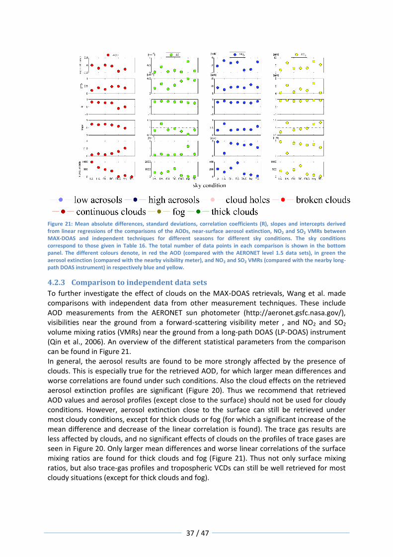
37 / 47

Figure 21: Mean absolute differences, standard deviations, correlation coefficients (R), slopes and intercepts derived from linear regressions of the comparisons of the AODs, near-surface aerosol extinction, NO2 and SO2 VMRs between MAX-DOAS and independent techniques for different seasons for different sky conditions. The sky conditions correspond to those given in Table 16. The total number of data points in each comparison is shown in the bottom panel. The different colours denote, in red the AOD (compared with the AERONET level 1.5 data sets), in green the aerosol extinction (compared with the nearby visibility meter), and NO2 and SO2 VMRs (compared with the nearby long-path DOAS instrument) in respectively blue and yellow.

4.2.3 Comparison to independent data sets

To further investigate the effect of clouds on the MAX-DOAS retrievals, Wang et al. made comparisons with independent data from other measurement techniques. These include AOD measurements from the AERONET sun photometer (http://aeronet.gsfc.nasa.gov/), visibilities near the ground from a forward-scattering visibility meter , and NO2 and SO2 volume mixing ratios (VMRs) near the ground from a long-path DOAS (LP-DOAS) instrument (Qin et al., 2006). An overview of the different statistical parameters from the comparison can be found in Figure 21. In general, the aerosol results are found to be more strongly affected by the presence of clouds. This is especially true for the retrieved AOD, for which larger mean differences and worse correlations are found under such conditions. Also the cloud effects on the retrieved aerosol extinction profiles are significant (Figure 20). Thus we recommend that retrieved AOD values and aerosol profiles (except close to the surface) should not be used for cloudy conditions. However, aerosol extinction close to the surface can still be retrieved under most cloudy conditions, except for thick clouds or fog (for which a significant increase of the mean difference and decrease of the linear correlation is found). The trace gas results are less affected by clouds, and no significant effects of clouds on the profiles of trace gases are seen in Figure 20. Only larger mean differences and worse linear correlations of the surface mixing ratios are found for thick clouds and fog (Figure 21). Thus not only surface mixing ratios, but also trace-gas profiles and tropospheric VCDs can still be well retrieved for most cloudy situations (except for thick clouds and fog).

38 / 47

4.3 General recommendations overview Based on the comparisons of the retrieved columns and profiles under different sky conditions (Figure 18, Figure 19, and Figure 20), and the comparison results with independent data sets (Figure 21), recommendations have been developed, under which sky conditions which data product might be still useful or should better not be used. These recommendations, as summarized in Table 16, should not be seen as generally binding, but rather as a general indication of the usefulness of a given observation, and might change for improved inversion algorithms in the future.

Table 16: Filter scheme of aerosol and trace gas results derived from MAX-DOAS observations, using the sky condition classification scheme as described in Wang et al. (2014) and Wagner et al. (2016). Plus signs (+) denote that the use of

the retrieved result is recommended, minus signs (-) denote that use of the retrieved is not recommended.

AOD Aerosol surface

extinction

Aerosol extinction

profile

VCD Surface VMR

VMR profile

Clear + low aerosol load + + + + + +

Clear + high aerosol load + + + + + +

Cloud holes - + - + + +

Broken clouds - + - + + +

Continuous clouds - + - + + +

Fog - - - - - -

Thick clouds - - - - - -

39 / 47

5 Quality assessment of CO Bart Dils (IASB-BIRA)

5.1 Introduction

The CO reference datasets used within QA4ECV are derived from two distinct sources, namely TCCON (Total Carbon Column Observing Network) and NDACC (Network for the Detection of Atmospheric Composition Change). While both use solar-absorption FTIR measurements, they fundamentally differ in the spectroscopic region used and methodology employed.

5.2 TCCON CO measurements TCCON measures CO2, CO, N2O, CH4, H2O, HDO and HF in the near-infrared and uses the GFit algorithm to scale a fixed a priori shape so as to best reproduce the observed spectra. It also simultaneously measures O2 to derive the total column dry air mole fraction of CO, typically labelled XCO. All stations within TCCON adhere to the very same retrieval and analysis protocol and the results are validated (and bias-corrected) by using in situ aircraft measurements (Wunch et al., 2010). The sources of uncertainty within TCCON are well documented on their website (https://tccon-wiki.caltech.edu/Network_Policy/Data_Use_Policy/Data_Description#Sources_of_Uncertainty, Wunch et al. 2011). For XCO the measurement precision varies somewhat from site to site but is generally below 1% under good measurement conditions. The correction factor derived from aircraft and balloon measurements is 1.0672±0.02, which implies an accuracy (1 sigma) of 1.9%.

5.3 NDACC CO measurements NDACC measurements (covering a much wider range of species) are performed in the mid and far infrared, using optimal estimation techniques which allow (within boundaries) variation of the profile shape itself. Therefore apart from the total column, the retrievals can provide limited information on the vertical distribution of gases. Given that the network originated from a more research oriented objective, it is less harmonized compared to TCCON (which was set up with the distinct purpose of satellite validation) although constant efforts are being made by the community to come to a uniform retrieval strategy for the wide range of species observed. During the past year a detailed study was made concerning the uncertainty calculation routines for the two most important retrieval software packages used in the NDACC infrared working group, PROFFIT and SFIT4. The uncertainty on the spectroscopy and the estimation of the uncertainty on the a-priori state of the atmosphere (temperature, pressure, water vapour, …) and other important input parameters for the optimal estimation retrieval of the target gas are now fixed and consistent for all participating sites. See Figure 22 where the uncertainty on the NCEP temperature profile is estimated from an ensemble of differences between NCEP profiles and sonde profiles measured throughout the day at Reunion.

40 / 47

Figure 22: Representation of an ensemble of differences from which the random and systematic uncertainty matrices for the a-priori temperature are estimated (blue lines in right plot, x axis is in Kelvin, vertical axis is height in km).

The harmonized uncertainty treatment was presented during the latest IRWG workshop meeting in South-Korea. Apart from the uncertainty component, the updated NDACC FTIR CO time series will have a similar shaped AVK across the different sites. A numerical artefact (caused by the C-shaped CO profile, attaining a minimum at ±30km) caused very high AVK values as a matrix acting on VMR profiles.

Figure 23: AVK shape harmonization in updated time series. The higher altitude kernels (red) contained a numerical artefact causing high values at 30km altitude (left). This is no longer present in the updated time series (right).

FTIR NDACC time series are currently being reprocessed by the different PIs. The updated BIRA-IASB time series at Reunion StDenis and Maido are publicly available on NDACC since October 2016, the time series at St Petersburg since November 2016. Updates to the time series of Jungfraujoch, Bremen, Paramaribo, Toronto, Eureka, Thule, Mauna Loa are imminent. All updated time series will have the GEOMS file attribute FILE_PROJECT_ID set to “QA4ECV”. The time series of Izana was not updated, but can be considered harmonized. The error budgets are currently under assessment. From the data from Reunion and St.

41 / 47

Petersburg we estimate the random error (see Figure 24) to lie around 2.5% while the systematic error lies around 3.5% (see Figure 25) with some (but far less than prior to the harmonization) station-to-station variability.

Figure 24: Random error component of the derived CO columns at Maido (Reunion Island) and St. Petersburg (Russia)

42 / 47

Figure 25: Systematic error component of the derived CO columns at Maido (Reunion Island) and St. Petersburg (Russia)

43 / 47

6 References

Bogumil, K., Orphal, J., Homann, T., Voigt, S., Spietz, P., Fleischmann, O. C., Vogel, A., Hartmann, M., Bovensmann, H., Frerik, J., and Burrows, J. P.: Measurements of molecular absorption spectra with the SCIAMACHY Pre-Flight Model: Instrument characterization and reference spectra for atmospheric remote sensing in the 230–2380 nm region, J. Photochem. Photobiol. A., 157, 167–184, 2003.

Burrows, J.P., Dehn, A., Deters, B., Himmelmann, S., Richter, A., Voigt, S. and J. Orphal, Atmospheric remote-sensing reference data from GOME: Part 1. Temperature-dependent absorption cross-sections of NO2 in the 231-794 nm range, J. Quant. Spectrosc. Radiat. Transfer 60, 1025-103, 1998.

Cantrell, C. A., J. A. Davidson, A. H. McDaniel, R. E. Shetter, and J. G. Calvert: Temperature-dependent formaldehyde cross sections in the near ultraviolet spectra region, J. Phys. Chem., 94, 3902–3908, 1990.

Chance, K. V. and Spurr, R. J. D.: Ring effect studies: Rayleigh scattering, including molecular parameters for rotational Raman scattering, and the Fraunhofer spectrum, Appl. Optics, 36, 5224–5230, 1997.

Chance, K., and R.L. Kurucz: An improved high-resolution solar reference spectrum for Earth’s atmosphere measurements in the ultraviolet, visible, and near infrared, http://www.cfa.harvard.edu/atmosphere (last access: July 2011), 2010.

Clémer, K., M. Van Roozendael, C. Fayt, F. Hendrick, C. Hermans, G. Pinardi, R. Spurr, P. Wang, and M. De Mazière, Multiple wavelength retrieval of tropospheric aerosol optical properties from MAXDOAS measurements in Beijing, Atmos. Meas. Tech., 3, 863-878, 2010.

Erle, F., Pfeilsticker, K., and Platt, U: On the influence of tropospheric clouds on zenith scattered light measurements of stratospheric species, Geophys. Res. Lett., 22, 2725-2728, 1995.

Fleischmann, O. C., Hartmann, M., Burrows, J. P., and Orphal, J.: New ultraviolet absorption cross-sections of BrO at atmospheric temperatures measured by time-windowing Fourier transform spectroscopy, J. Photochem. Photobiol. A, 168, 117–132, 2004.

Gielen, C., Van Roozendael, M., Hendrick, F., Pinardi, G., Vlemmix, T., De Bock, V., De Backer, H., Fayt, C., Hermans, C., Gillotay, D., and Wang, P.: A simple and versatile cloud-screening method for MAX-DOAS retrievals, Atmos. Meas. Tech., 7, 3509-3527, doi:10.5194/amt-7-3509-2014, 2014.

Greenblatt, G. D., J. J. Orlando, J. B. Burkholder, and A. R. Ravishankara: Absorption measurements of oxygen between 330 and 1140 nm, J. Geophys. Res., 95, 18,577–18,582, 1990.

Hermans, C., A.C. Vandaele, S. Fally, M. Carleer, R. Colin, B. Coquart, A. Jenouvrier, M.-F. Mérienne: Absorption cross-section of the collision-induced bands of oxygen from the UV to the NIR, in: Proceedings of the NATO Advanced Research Workshop, Weakly Interacting Molecular Pairs: Unconventional Absorbers of Radiation in the Atmosphere, Fontevraud, France, 24 April-2May 2002, eds C. Camy-Peyret and A.A. Vigasin, Kluwer Academic Publishers, Boston, NATO Science Series IV Earth and Environmental Sciences, vol 27, pp 193-202, 2003.

Hönninger, G., von Friedeburg, C., and Platt, U.: Multi axis differential optical absorption spectroscopy (MAX-DOAS), Atmos. Chem. Phys., 4, 231–254, doi:10.5194/acp-4-231-2004, 2004.

44 / 47

Koelemeijer, R. B. A., J. F. de Haan, and P. Stammes, A database of spectral surface reflectivity in the range 335 – 772 nm derived from 5.5 years of GOME observations, J. Geophys. Res., 108(D2), 4070, doi:10.1029/2002JD002429, 2003

Lampel, J.; Wang, Y.; Beirle, S.; Sihler, H.; Pukite, J.; Hilboll, A.; Richter, A., and Wagner, T. The tilt-effect in passive DOAS observations. in preparation for Atmospheric Measurement Techniques, 2016.

Ma, J.Z., Beirle, S., Jin, J.L., Shaiganfar, R., Yan P. and T. Wagner: Tropospheric NO2 vertical column densities over Beijing: results of the first three-years of ground-based MAX-DOAS measurements (2008–2011) and satellite validation, Atmos. Chem. Phys. Discuss., 12, 26719–26781, http://www.atmos-chem-phys-discuss.net/ 12/26719/2012/acpd-12-26719-2012.html, 2012.

Mayer, B. and Kylling, A.: Technical note: The libRadtran software package for radiative transfer calculations – description and examples of use, Atmos. Chem. Phys., 5, 1855–1877, http://www.atmos-chem-phys.net/5/1855/2005/, 2005.

Meller, R. and Moortgat, G. K.: Temperature dependence of the absorption cross sections of formaldehyde between 223 and 323K in the wavelength range 225–375 nm, J. Geophys. Res., 105, 7089–7101, 2000.

Nasse, J.-M. and Zielcke, J. and Frieß, U. and Lampel, J. and König-Langlo, G. and Platt, U., Inference of cloud altitude and optical properties from MAX-DOAS measurements, EGU General Assembly 2015, Abstract id 7232

Peters, E., Pinardi, G., Seyler, A., Richter, A., Wittrock, F., Bösch, T., Burrows, J. P., Van Roozendael, M., Hendrick, F., Drosoglou, T., Bais, A. F., Kanaya, Y., Zhao, X., Strong, K., Lampel, J., Volkamer, R., Koenig, T., Ortega, I., Piters, A., Puentedura, O., Navarro, M., Gómez, L., Yela González, M., Remmers, J., Wang, Y., Wagner, T., Wang, S., Saiz-Lopez, A., García-Nieto, D., Cuevas, C. A., Benavent, N., Querel, R., Johnston, P., Postylyakov, O., Borovski, A., Elokhov, A., Bruchkouski, I., Liu, C., Hong, Q., Liu, H., Rivera, C., Grutter, M., Stremme, W., Khokhar, M. F., and Khayyam, J.: Investigating differences in DOAS retrieval codes using MAD-CAT campaign data, Atmos. Meas. Tech. Discuss., doi:10.5194/amt-2016-358, in review, 2016.

Pinardi, G., Van Roozendael, M., Abuhassan, N., Adams, C., Cede, A., Clémer, K., Fayt, C., Frieß, U., Gil, M., Herman, J., Hermans, C., Hendrick, F., Irie, H., Merlaud, A., Navarro Comas, M., Peters, E., Piters, A. J. M., Puentedura, O., Richter, A., Schönhardt, A., Shaiganfar, R., Spinei, E., Strong, K., Takashima, H., Vrekoussis, M., Wagner, T., Wittrock, F., and Yilmaz, S.: MAX-DOAS formaldehyde slant column measurements during CINDI: intercomparison and analysis improvement, Atmos. Meas. Tech., 6, 167-185, doi:10.5194/amt-6-167-2013, 2013.

Platt, U. and Stutz, J.: Differential Optical Absorption Spectroscopy, Principles and Applications, ISBN 978-3-540-21193-8, Springer, Berlin, 2008.

Pukite, J.; Kühl, S.; Deutschmann, T.; Platt, U., and Wagner, T. Extending differential optical absorption spectroscopy for limb measurements in the UV. Atmospheric Measurement Techniques, 3, doi: 10.5194/amt-3-631-2010, 2010.

Qin, M., Xie, P. H., Liu, W. Q., Li, A., Dou, K., Fang, W., Liu, J. G. Zhang, W. J.: Observation of atmospheric nitrous acid with DOAS in Beijing, China, Journal of Environmental Sciences, 18, 69-75, 2006.

Roscoe, H. K.; Johnston, P. V.; Van Roozendael, M.; Richter, A.; Sarkissian, A.; Roscoe, J.; Preston, K. E.; Lambert, J. C.; Hermans, C.; Decuyper, W.; Dzienus, S.; Winterrath, T.; Burrows, J.; Goutail, F.;

45 / 47

Pommereau, J. P.; D'Almeida, E.; Hottier, J.; Coureul, C.; Didier, R.; Pundt, I.; Bartlett, L. M.; McElroy, C. T.; Kerr, J. E.; Elokhov, A.; Giovanelli, G.; Ravegnani, F.; Premuda, M.; Kostadinov, I.; Erle, F.; Wagner, T.; Pfeilsticker, K.; Kenntner, M.; Marquard, L. C.; Gil, M.; Puentedura, O.; Yela, M.; Arlander, D. W.; Kastad Hoiskar, B. A.; Tellefsen, C. W.; Karlsen Tornkvist, K.; Heese, B.; Jones, R. L.; Aliwell, S. R., and Freshwater, R. A. Slant column measurements of O3 and NO2 during the NDSC intercomparison of zenith-sky UV-visible spectrometers in June 1996. Journal

of Atmospheric Chemistry, 32(2):281{314, 1999. ISSN 01677764.doi: 10.1023/A:1006111216966.

Roscoe, H.K, M. Van Roozendael, C. Fayt, A. du Piesanie, N. Abuhassan, C. Adams, M. Akrami, A. Cede, J. Chong, K. Clemer, U. Friess, M. Gil Ojeda, F. Goutail, R. Graves, A. Griesfeller, K. Grossmann, G. Hemerijckx, F. Hendrick, J. Herman, C. Hermans, H. Irie, P.V. Johnston, Y. Kanaya, K. Kreher, R. Leigh, A. Merlaud, G.H. Mount, M. Navarro, H. Oetjen, A. Pazmino, M. Perez-Camacho, E. Peters, G. Pinardi, O. Puentedura, A. Richter, A. Schoenhardt, R. Shaiganfar, E. Spinei, K. Strong, H. Takashima, T. Vlemmix, M. Vrekoussis, T. Wagner, F. Wittrock, M. Yela, S. Yilmaz, F. Boersma, J. Hains, M. Kroon, A. Piters, Y.J. Kim: Intercomparison of slant column measurements of NO2 and O4 by MaxD0AS and zenith-sky UV and visible spectrometers, Atm. Meas. Tech. 3, 1629-1646, 2010.

Rothman, L. S.; Gordon, I. E.; Barber, R. J.; Dothe, H.; Gamache, R. R.; Goldman, A.; Perevalov, V. I.; Tashkun, S. A., and Tennyson, J. HITEMP, the high-temperature molecular spectroscopic database. Journal of Quantitative Spectroscopy and Radiative Transfer, 111(15):2139{2150, 2010, doi: 10.1016/j.jqsrt.2010.05.001.

Seidel, D. J., Y. Zhang, A. Beljaars, J.-C. Golaz, A. R. Jacobson, and B. Medeiros, Climatology of the planetary boundary layer over the continental United States and Europe, J. Geophys. Res., 117, D17106, doi:10.1029/2012JD018143, 2012.

Serdyuchenko, A., Gorshelev, V., Weber, M., Chehade, W., and Burrows, J. P.: High spectral resolution ozone absorption cross-sections – Part 2: Temperature dependence, Atmos. Meas. Tech., 7, 625-636, doi:10.5194/amt-7-625-2014, 2014.

Shaiganfar, R., Beirle, S., Sharma, M., Chauhan, A., Singh, R. P. and Wagner, T.: Estimation of NOx emissions from Delhi using Car MAX-DOAS observations and comparison with OMI satellite data, Atmos. Chem. Phys., 11(21), 10871-10887, doi:10.5194/acp-11-10871-2011, 2011.

Sioris, C. E.; Haley, C. S.; McLinden, C. A.; von Savigny, C.; McDade, I. C.; McConnell, J. C.; Evans, W. F. J.; Lloyd, N. D.; Llewellyn, E. J.; Chance, K. V.; Kurosu, T. P.; Murtagh, D.; Frisk, U.; Pfeilsticker, K.; Bösch, H.; Weidner, F.; Strong, K.; Stegman, J., and Megie, G. Stratospheric profiles of nitrogen dioxide observed by Optical Spectrograph and Infrared Imager System on the Odin satellite. Journal of Geophysical Research: Atmospheres, 108(D7), 2003.

Spurr, R., LIDORT and VLIDORT: Linearized pseudo-spherical scalar and vector discrete ordinate radiative transfer models for use in remote sensing retrieval problems, Light Scattering Reviews, Volume 3, ed. A. Kokhanovsky, Springer, 2008.

Stutz, J., U. Platt: Numerical analysis and error estimation of differential optical absorption spectroscopy measurements with least-squares methods, Appl. Opt. 35, 6041-6053, 1996.

Thalman, R. and R. Volkamer, Temperature dependent absorption cross-sections of O2-O2 collision pairs between 340 and 630 nm and at atmospherically relevant pressure., Phys. Chem. Chem. Phys., 15(37), 15371–81, doi:10.1039/c3cp50968k, 2013.

46 / 47

Vandaele, A. C., Hermans, C., Simon, P. C., Van Roozendael, M., Guilmot, J. M., Carleer, M., and Colin, R.: Fourier transform measurement of NO2 absorption cross-section in the visible range at room temperature, J. Atmos. Chem., 25, 289–305, 1996.

Vandaele, A. C., C. Hermans, P. C. Simon, M. Carleer, R. Colin, S. Fally, M.-F. Mérienne, A. Jenouvrier, and B. Coquart, Measurements of the NO2 absorption cross section from 42000 cm-1 to 10000 cm-1 (238-1000 nm) at 220 K and 294 K, J. Quant. Spectrosc. Radiat. Transfer, 59,171-184, 1998

Vandaele, A. C.; Fayt, C.; Hendrick, F.; Hermans, C.; Humbled, F.; Van Roozendael, M.; Gil, M.; Navarro, M.; Puentedura, O.; Yela, M.; Braathen, G.; Stebel, K.; Tornkvist, K.; Johnston, P.; Kreher, K.; Goutail, F.; Mieville, A.; Pommereau, J. P.; Khaikine, S.; Richter, A.; Oetjen, H.; Wittrock, F.; Bugarski, S.; Friess, U.; Pfeilsticker, K.; Sinreich, R.; Wagner, T.; Corlett, G., and Leigh, R. An intercomparison campaign of ground-based UV-visible measurements of NO2, BrO, and OClO slant columns: Methods of analysis and results for NO2. Journal of Geophysical

Research- Atmospheres, 110(D8), 2005. Doi:10.1029/2004jd005423.

Vlemmix, T., Piters, A. J. M., Stammes, P., Wang, P., and P. F. Levelt, Retrieval of tropospheric NO2 using the MAX-DOAS method combined with relative intensity measurements for aerosol correction, Atmos. Meas. Tech., 3, 1287–1305, 2010.

Von Engeln, A. and J. Teixeira, A Planetary Boundary Layer Height Climatology Derived from ECMWF Reanalysis Data, J. of Climate, vol 26, 6575-6590, DOI: 10.1175/JCLI-D-12-00385.1, 2013.

Wagner, T., Erie, F., Marquard, L., Otten, C., Pfeilsticker, K., Senne, T., Stutz, J., and Platt, U.: Cloudy sky optical paths as derived from differential optical absorption spectroscopy observations, J. Geophys. Res., 103, 25307, doi:10.1029/98JD01021, 1998.

Wagner, T., Friedeburg, C. von, Wenig M., Otten, C., and Platt, U.: UV/vis observations of atmospheric O4 absorptions using direct moon light and zenith scattered sunlight under clear and cloudy sky conditions, J. Geophys. Res., 107, D204424, doi:10.1029/2001JD001026, 2002.

Wagner, T., B. Dix, C. von Friedeburg, Frieß, U., Sanghavi, S., Sinreich, R., and Platt, U.: MAX-DOAS O4 measurements: A new technique to derive information on atmospheric aerosols - Principles and information content, J. Geophys. Res., 109, D22205, doi:10.1029/2004JD004904, 2004.

Wagner, T., Beirle, S., and Deutschmann, T.: Three-dimensional simulation of the Ring effect in observations of scattered sun light using Monte Carlo radiative transfer models, Atmos. Meas. Tech., 2, 113–124, http://www.atmos-meas-tech.net/2/113/2009, 2009.

Wagner, T., Apituley, A., Beirle, S., Dörner, S., Frieß, U., Remmers, J., and Shaiganfar, R.: Cloud detection and classification based on MAX-DOAS observations, Atmos. Meas. Tech., 7, 1289-1320, doi:10.5194/amt-7-1289-2014, 2014.

Wagner, T., Beirle, S., Remmers, J., Shaiganfar, R., Wang, Y.: Absolute calibration of the colour index and O4 absorption derived from Multi AXis (MAX-)DOAS measurements and their application to a standardised cloud classification algorithm, Atmos. Meas. Tech., 9, 4803-4823, doi:10.5194/amt-9-4803-2016,2016.

Wang, Y., Penning de Vries, M., Xie, P. H., Beirle, S., Dörner, S., Remmers, J., Li, A., and Wagner, T.: Cloud and aerosol classification for 2.5 years of MAX-DOAS observations in Wuxi (China) and comparison to independent data sets, Atmos. Meas. Tech., 8, 5133-5156, doi:10.5194/amt-8-5133-2015, 2015.

Wilmouth, D. M., T. F. Hanisco, N. M. Donahue, and Anderson J. G.: Fourier transform ultraviolet spectroscopy of the A(2_3/2) _(2_3/2) transition of BrO, J. Phys. Chem., 103, 8935– 8944, 1999.

47 / 47

Winterrath, T., Koruso, T. P., Richter, A., and Burrows, J. P.: Enhanced O3 and NO2 in thunderstorm clouds: convection or production, Geophys. Res. Lett., 26, 1291-1294, doi:10.1029/1999GL900243, 1999.

Wunch, D., Toon, G. C., Wennberg, P. O., Wofsy, S. C., Stephens, B. B., Fischer, M. L., Uchino, O., Abshire, J. B., Bernath, P., Biraud, S. C., Blavier, J.-F. L., Boone, C., Bowman, K. P., Browell, E. V., Campos, T., Connor, B. J., Daube, B. C., Deutscher, N. M., Diao, M., Elkins, J. W., Gerbig, C., Gottlieb, E., Griffith, D. W. T., Hurst, D. F., Jiménez, R., Keppel-Aleks, G., Kort, E. A., Macatangay, R., Machida, T., Matsueda, H., Moore, F., Morino, I., Park, S., Robinson, J., Roehl, C. M., Sawa, Y., Sherlock, V., Sweeney, C., Tanaka, T., and Zondlo, M. A.: Calibration of the Total Carbon Column Observing Network using aircraft profile data, Atmos. Meas. Tech., 3, 1351-1362, doi:10.5194/amt-3-1351-2010, 2010.

Wunch, D., G. C. Toon, J.-F. L. Blavier, R. A. Washenfelder, J. Notholt, B. J. Connor, D. W. T. Griffith, V. Sherlock, P. O. Wennberg. The Total Carbon Column Observing Network, doi: 10.1098/rsta.2010.0240 Phil. Trans. R. Soc. A 28 May 2011 vol. 369 no. 1943 2087-2112. Available from: http://rsta.royalsocietypublishing.o.../2087.full.pdf