1

QUALITY CONTROL ANDIMPROVEMENT BASED ON

GROUPED DATA

By

STEFAN HANS STEINER, B.MATH, M.SC.

A ThesisSubmitted to the School of Graduate Studies

in Partial Fulfillment of the Requirementsfor the Degree

Doctor of Philosophy (Management Science/Systems)

McMaster University(c) Copyright by Stefan Hans Steiner, January 1994

2

DOCTOR OF PHILOSOPHY (1994) McMASTER UNIVERSITY

(Management Science/Systems) Hamilton, Ontario

TITLE: Quality Control and Improvement Based on Grouped Data

AUTHOR:

Stefan Hans Steiner, B.Math (University of Waterloo)

M.Sc. (University of British Columbia)

SUPERVISOR: Professor G.O. Wesolowsky

NUMBER OF PAGES: ix, 165

3

Abstract

This thesis develops quality control and improvement techniques based on

grouped data. Grouped data occur frequently in industry. However, in the past, most

techniques have failed to directly take this grouping into account, and as a result do not

perform well in many circumstances.

Two major areas of application are considered. First, acceptance sampling plans,

acceptance control charts, and Shewhart control charts based on grouped data are

developed. These forms of statistical process control have broad application and are in

use widely. The design and implementation methodology is derived assuming either a

normal or Weibull process, but is easily adapted to any other underlying distribution. A

number of design approaches are presented and their relative advantages and

disadvantages are discussed. The second application involves estimating the correlation

between destructively measured strength properties. This problem arises in the area of

structural design. To obtain an estimate of the correlation censoring of the strength data

is required. The censoring or proof-testing results in grouped data. A number of simple

estimation procedures are presented and compared.

4

Acknowledgments

My sincere appreciation goes to my supervisor, Dr. George O. Wesolowsky, for

all his encouragement and support.

I would also like to thank the rest of my supervisory committee, Dr. P.D.M

Macdonald, and Dr. R. Love, for their careful reading of the text and helpful comments

along the way.

Thanks also go to Lee Geyer, a fellow graduate student, for helpful discussions at

the beginning of this research, and to anonymous associate editors and referees whose

comments and suggestions improved the research articles based on this work.

Acknowledgment must also go to Dr. Balakrishnan who pointed out to me at my thesis

defense the equivalence of the optimization problem discussed in Section 5.3 with some

work in different field. See the beginning of Chapter 5 for a more detailed explanation.

Last, but not least, I thank my wife Anne Marie Mingiardi. Without her this

would have seemed a much longer and lonelier journey.

5

Statement of Contribution

The work presented in this thesis is original. For the most part, the research was

done without any outside assistant apart from general helpful comments and suggests

from my supervisor. The only exceptions being some contribution from P. Lee Geyer, a

fellow graduate student, for the material presented in Sections 3.1 and 3.3.2. The

additional contribution for the aforementioned sections consisted of stimulating

discussions and the suggestion for the use of the likelihood ratio test with specific

alternative hypotheses.

6

TABLE OF CONTENTS

List of Figures ............................................................................... viii

List of Tables ................................................................................ ix

CHAPTER 1Introduction ....................................................................... 1

1.1 Grouped Data ................................................................................................ 51.2 Areas of Application ..................................................................................... 9

1.2.1 Shewhart Control Charts ................................................................... 91.2.2 Acceptance Sampling Plans .............................................................. 171.2.3 Correlation Estimation from Destructive Testing ............................. 22

1.3 Thesis Outline ............................................................................................... 26

CHAPTER 2Preliminaries ..................................................................... 29

2.1 Useful Definitions ......................................................................................... 302.1.1 Normal and Weibull Distributions .................................................... 302.1.2 Grouped Data Definition................................................................... 312.1.3 Likelihood and Log-likelihood Ratios .............................................. 32

2.2 Parameter Estimation Based on Grouped Data ............................................. 332.2.1 Normal Parameter MLEs .................................................................. 342.2.2 Weibull Parameter MLEs.................................................................. 362.2.3 Translating Mean and Variance to Weibull Parameters ................... 37

2.3 Ad hoc Quality Control Techniques for Grouped Data ................................ 38

CHAPTER 3Statistical Process Control Based on Grouped Data ......... 45

3.1 One-Sided Acceptance Sampling Plans ........................................................ 463.2 Two-Sided Acceptance Sampling Plans ....................................................... 50

3.2.1 Two Sets of Weights Approach ........................................................ 513.2.2 Maximum Likelihood Estimate Approach........................................ 543.2.3 Comparison of Approaches............................................................... 56

3.3 Shewhart Control Charts ............................................................................... 583.3.1 Two Sets of Weights Approach ........................................................ 59

7

3.3.2 One Set of Weights Approach .......................................................... 603.3.3 Maximum Likelihood Estimate Approach........................................ 653.3.4 Generalized Likelihood Ratio Test Approach .................................. 673.3.5 Comparison of the Approaches ......................................................... 72

3.4 Small Sample Size Plans and Charts............................................................. 753.4.1 Determining Actual Error Rates ....................................................... 783.4.2 Designing Small Sample Size Plans and Charts ............................... 83

CHAPTER 4Parameter Estimation under Destructive Testing ............. 86

4.1 Estimation of the Correlation Only ............................................................... 874.1.1 Procedure I: One-way Estimation .................................................... 874.1.2 Procedure II: Symmetric Procedure ................................................. 994.1.3 Comparison of Results with the De Amorim Method ...................... 108

4.2 Estimating all Five Bivariate Normal Parameters......................................... 1094.2.1 Procedure III ..................................................................................... 1104.2.2 Procedure IV ..................................................................................... 113

4.3 Comparison of Procedures I, II, III and IV ................................................... 117

CHAPTER 5Optimal Grouping Criteria ................................................ 119

5.1 One-Sided Acceptance Sampling Plans ........................................................ 1205.2 Two-Sided Acceptance Sampling Plans ....................................................... 1275.3 Shewhart Control Charts ............................................................................... 128

5.3.1 Normal Process ................................................................................. 1295.3.2 Weibull Process................................................................................. 134

5.4 Destructive Testing Procedure I.................................................................... 138

CHAPTER 6Summary, Conclusion and Possible Extensions ............... 141

Bibliography ..................................................................... 145

APPENDICESAppendix A: Notation ........................................................................................... 152Appendix B: Interpretation of Weights................................................................. 154Appendix C: Expected Value of Proof-load MLEs .............................................. 156Appendix D: Gradient of Sample Size Formula ................................................... 160Appendix E: Normal Information Gradient .......................................................... 162Appendix F: Weibull Information Gradients ........................................................ 164

8

LIST OF FIGURES

Figure 1.1: A Four-Step Gauge ....................................................................... 7

Figure 1.2: Typical Control Chart for a Stable Process .................................. 10

Figure 1.3: Operating Characteristic Curve for X chart when n = 5 .............. 15

Figure 2.1: Gauge Limits Superimposed on Normal Distribution .................. 40

Figure 2.2: Mean Estimate Bias Using Current Approaches .......................... 42

Figure 3.1: Acceptance/Rejection Regions for One-Sided Shifts ................... 46

Figure 3.2: Acceptance/Rejection Regions for Two-Sided Shifts .................. 50

Figure 3.3: Signal Regions for Stability Test .................................................. 58

Figure 3.4: Two Sets of Weights Control Chart.............................................. 60

Figure 3.5: Weibull Process Probability Density Function ............................. 64

Figure 3.6: Distribution of z when µ = 1 ....................................................... 76

Figure 3.7: Distribution of z when µ = 0 and 2 ............................................ 77

Figure 3.8: True Error Rates with 2 Gauge Limits ......................................... 80

Figure 3.9: True Error Rates with 3 Gauge Limits ......................................... 81

Figure 3.10: True Error Rates with 5 Gauge Limits ........................................ 81

Figure 4.1: Grouping for One-way Procedure ................................................ 89

Figure 4.2: Bias of Simulated ρab*

- Procedure I ............................................. 96

Figure 4.3: Standard Deviation of Simulated ρab*

- Procedure I ...................... 96

Figure 4.4: Bias of Simulated ρab*

versus n - Procedure I, ρab = 0.6 ............... 97

Figure 4.5: Standard Deviation of ρab*

versus n - Procedure I......................... 97

Figure 4.6: Contour Plot of the ρab*

Bias - Procedure I ................................... 98

Figure 4.7: Grouping for Symmetric Procedure.............................................. 100

Figure 4.8: Standard Deviation of Simulated ρab*

- Procedure II ..................... 105

Figure 4.9: Standard Deviation of ρab*

versus pa and pb - Procedure II ......... 106

Figure 4.10: Bias of ρab*

versus Proof-load Levels - Procedure II .................... 106

Figure 4.11: Grouping for Procedure III ........................................................... 111

Figure 4.12: Grouping for Procedure IV ........................................................... 114

Figure 4.13: Standard Deviation of Simulated ρab*

I - Procedure IV ................ 116

Figure 4.14: Standard Deviation of Simulated ρab*

II - Procedure IV ............... 117

Figure 5.1: Optimal pa and pb Values to Estimate ρab .................................. 139

9

LIST OF TABLES

Table 1.1: Comparison of Two, Multiple and Many Group Data ................... 8

Table 1.2: Summary of Stevens’ Grouping..................................................... 13

Table 2.1: Comparison of Ad hoc Control Chart Approaches ........................ 43

Table 3.1: Sample Size Comparison - Two Sided Tests ................................. 57

Table 3.2: Sample Size Comparison - Shewhart Mean Charts ....................... 73

Table 3.3: Sample Size Comparison - Shewhart Sigma Charts ...................... 73

Table 3.4: Advantages and Disadvantages - Shewhart Charts ........................ 75

Table 3.5: Number of Ways to Partition a Sample of Size n .......................... 78

Table 3.6: Actual Error Rate Comparison....................................................... 82

Table 3.7: Error rates for different designs ..................................................... 85

Table 4.1: Comparison of Procedures I, II and the De Amorim Method........ 108

Table 4.2: Comparison of Procedures I, II, III and IV .................................... 118

Table 5.1: Optimal Group Limits and Weights Standard Normal

Distribution, α = β ....................................................................... 123

Table 5.2: Optimal Group Limits and Weights Standard Normal

Distribution, α = 0.001, β = 0.005 ................................................. 124

Table 5.3: Optimal Group Limits and Weights Standard Weibull

Distribution, α = β ........................................................................ 125

Table 5.4: Optimal Group Limits and Weights Standard Weibull

Distribution, α = 0.001, β = 0.005................................................ 126

Table 5.5: Optimal Group Limits to Detect Mean Shifts ................................ 131

Table 5.6: Optimal Group Limits to Detect Sigma Shifts ............................... 132

Table 5.7: Suggested 3-Group Limits to Detect Mean and Sigma Shifts ....... 134

Table 5.8: Optimal Group Limits to Detect Mean and Sigma Shifts .............. 134

Table 5.9: Optimal Group Limits to Detect Shape Shifts ............................... 136

Table 5.10: Optimal Group Limits to Detect Scale Shifts ................................ 136

Table 5.11: Optimal Group Limits to Detect Shape and Scale Shifts ............... 137

1

CHAPTER 1Introduction

In the current world of continually increasing global competition it is imperative

for all manufacturing and service organizations to improve the quality of their products.

Quality has been defined in many ways (Evans and Lindsay, 1992). The American

National Standards Institute and the American Society for Quality Control (1978) defined

quality as “the totality of features and characteristics of a product or service that bears on

its ability to satisfy given needs.” The quality of a product or service has always been of

interest to both the provider and the customer. In fact, as Duncan (1986) states in the first

line of his book, “Quality Control is as old as industry itself.” In the ages before the

industrial revolution, good craftsmen and artisans learned quickly through intimate

contact with their customers that quality products meant satisfied customers, and satisfied

customers meant continued business. However, with the industrial revolution came the

mass production of products by people who rarely interacted with customers. As a result,

although costs decreased, the emphasis on quality also decreased. In addition, as the

products made and the services provided became more complex, the need for a formal

system to ensure the quality of the final product and all its components became

increasingly important.

In modern firms, the quality of their products is dependent on a number of factors

such as the organization and control of the firm’s employees, and more technical

concerns like the quality of design and the quality of production. From a technical

perspective, true progress toward improving and monitoring quality on a mass scale did

not begin until the advent of statistical quality control usually called statistical process

2

control, or SPC. SPC was first introduced in the 1920s by the inspection department at

Bell Telephone Laboratories led by Walter A. Shewhart, Harold F. Dodge, Donald A.

Quarles, and George D. Edwards. SPC refers to the statistical techniques used to control

or improve the quality of the output of some production or service process. Interest in

quality has recently been growing rapidly in North America in response to the obvious

success of the Japanese quality initiative started in the 1950s. Many SPC techniques,

especially control charts, are now used in most manufacturing environments. Although

service industries have been slower to adopt SPC, mainly due to difficulties in measuring

quality, the increased use of SPC in the service sector is now a growing trend.

Most products, even very simple ones, have many characteristics or dimensions,

possibly correlated, that affect their quality. For example, a nail is defined by its length,

diameter, hardness, etc. However, most SPC techniques restrict attention to one

characteristic at a time.

Quality control can be considered from two orientations: we can take a product or

a process perspective. Taking a product orientation, the focus is on the parts or units after

they are manufactured. Considering a single quality dimension at a time, the quality of a

part is defined based on the target value and specification limits for that quality

dimension. Specification limits, usually determined by engineering considerations,

specify the range of quality dimensions within which it is acceptable for a part’s quality

dimension to fall. The target value is the most desirable quality dimension value, and is

often centred between the specification limits. A non-conforming unit is usually defined

as a part whose quality characteristic of interest lies outside the engineering specification

limits, whereas if a part’s quality dimension falls within specification it is called a

conforming unit. In past work a non-conforming item was often called a defective item,

but due to legal considerations the term “defective” is no longer recommended. A lot of

products is considered acceptable if only a very small proportion of them have quality

3

characteristics outside the specification limits, and the lot is called rejectable if a fairly

large number of units fall outside the specification limits. For example, lots with less

than 1 part in a thousand non-conforming may be considered acceptable, whereas lots

with 5 parts in a thousand non-conforming are rejectable, with an indifference region in-

between. Clearly, it is desirable to produce parts within the specification limits, since

from engineering considerations such parts should perform as desired. However, it is

even better if all the quality dimensions are at the target. This is especially true for parts

that make up large complex final products such as automobiles. When a number of parts

must work together the closer each individual part is to the ideal the more likely the final

product will work as designed. This idea is formalized by the Taguchi loss function

(Taguchi, 1979). Taguchi believes it is best to produce all parts as close to the target as

possible, i.e., any deviation from the target is undesirable. With this in mind, Taguchi

assigns each part a “loss to society,” that reflects how far the part’s dimension is from the

target. This loss is usually modelled by a quadratic function (Taguchi, 1979).

The process perspective, on the other hand, takes the focus back to the process

that is producing the parts. This is an advantage since once a non-conforming part is

produced it may be expensive to fix. Better to monitor the system that produces the parts

trying to fix problems before many non-conforming products are made. In the process

perspective, it is assumed that all the variation in a system arises from one of two sources.

First, there is a certain amount of variability inherent in the system that is due to the

cumulative effect of many uncontrollable causes. This type of variation is called the

“natural variation,” and when it is small the process is considered acceptable or “in

control.” The second source of variation, called an “assignable cause,” is usually large

compared with the natural variation, and is due to a cause that is feasible to detect,

identify and remove. When a process is operating with only natural variation present the

process is said to be in a state of statistical control and is called a stable process. When a

4

process is operating with an assignable cause it is considered “out of control.” Notice

that an “in control” process does not necessarily produce parts within specifications. An

“in control” process produces parts that only differ due to system variability, but the

process may still have an inherent variability that is large compared with the spread of the

specification limits, and/or the process may not be producing parts with dimensions near

the target value.

To address the relationship between the quality of parts produced by an “in

control” process and the specification limits we define the process capability measure.

There are many different definitions (Ryan, 1989), and all try, in some way, to quantify

how many non-conforming (out of specifications) parts the process will produce. The

process capability index Cpk is defined below (e.g. Ryan, 1989),

Cpk =min USL − µ , µ − LSL( )

3σ

where USL and LSL are the upper and lower specification limits respectively, and the

variables µ and σ denote the current process mean and standard deviation respectively.

Large Cpk values indicate better performance, since it is a function of the number of

sigma or standard deviation units between the specification limits. A process with a large

Cpk value is called a capable process, since it is likely to produce the vast majority of

parts in specification. In Japan, a decade ago, the minimum acceptable Cpk value was

1.33 (Sullivan, 1984). This corresponds, assuming a normal process, to only 6 non-

conforming units for every 100,000 produced. However, all manufacturers should be

continually working to decrease the variability in their production processes, thus

increasing Cpk and increasing the quality of their products.

One goal of SPC techniques is to determine whether a process is stable or if a lot

of products is acceptable. This involves a test of hypothesis. By convention, the null

5

hypothesis is defined as a stable process or an acceptable lot. Excellent conclusions can

usually be made using 100% inspection, i.e. examining all the items in a lot or coming

from a process, but this is very costly and time consuming. As a result, in most

applications, it is preferable to try to estimate or infer the state of a process or lot from a

small random sample of units. However, using the methods of estimation and inference

introduces the possibility of making an incorrect conclusion, since the small sample may

not be truly representative of the process or lot. As a result, the hypothesis test may

conclude that there is evidence against the null hypothesis when in actuality the process is

stable or the lot is acceptable. If this occurs we have made what is called a type I error,

also called a false alarm. The probability of making such an error is usually denoted as

α . If, on the other hand, we fail to reject the null hypothesis when in fact the process is

out of control or the lot is rejectable, then we have made a type II error. The type II error

probability is usually denoted by β . Naturally we never wish to make an error, but short

of using 100% inspection a certain probability of error must be tolerated. The tolerable

error rates depend in each case on a number of factors including the cost of sampling, the

cost of investigating false alarms and the cost of failing to detect a deviation from the null

hypothesis.

1.1 Grouped Data

Quantification of the quality characteristic is another important consideration in

SPC. Traditionally, the measurement strategies considered have resulted almost

exclusively of two types of data: variables data and dichotomous pass/fail data. For

example, in variables data, the length of a nail could be quantified in centimeters accurate

to two significant digits. In dichotomous data, the nails could be classified as greater than

or less than 6.2 centimeters. However, grouped data is a third alternative.

6

Categorical data arise when observations are classified into categories rather than

measuring their quality characteristic(s) precisely. In the important special case where

the categories are defined along an underlying continuous scale the data is called

grouped. It has long been recognized that even when there is an underlying continuous

measurement, it may be more economical to “gauge” observations into groups than to

measure their quantities exactly. Exact measurements often require costly skilled

personnel and sophisticated instruments (Ladany and Sinuary-Stern 1985), whereas it is

usually quicker, easier, and therefore cheaper to classify articles into groups. This is of

great practical interest, especially when SPC techniques are used in difficult

environments such as factory shop floors. This has clearly been one of the motivational

factors behind the development of acceptance sampling plans and control charts based on

dichotomous attribute data (see Sections 1.2.1 and 1.2.2).

As Edwards (1972, p. 6) wrote, “data will invariably be either discrete or grouped

... the fineness of the grouping reflecting the resolving power of the experimental

technique.” In this light, dichotomous attribute data can be thought of as classifying

units into one of two groups, and variables data as classifying units into one of many

groups, approaching an infinite number of groups as measurement precision increases.

With this perspective, assuming some underlying continuous scale, variables data and

dichotomous attribute data are not totally distinct, but rather at two ends of a continuum.

As a result, it is logical and very appealing to attempt a compromise between the often

low data collection costs of dichotomous attribute data and the high information content

of variables data. An example is multi-group attribute data where units are classified into

one of three or more groups (such as low, medium, and high). This extension to multiple

groups has also been suggested very recently in the literature. Pyzdek (1993) suggests

there are ways to extract additional information from attribute data:

7

• Make the attribute less discrete by adding more classification groups;

• Assign weights to the groups to accentuate different levels of quality.

He does not provide a mechanism to formalize this suggestion. This thesis addresses this

issue from a statistical perspective.

In industry, when variables measurements are difficult or expensive, step gauges

are often used. A k-step gauge is a device that classifies units into one of k+1 groups

based on some quality characteristic that is theoretically measurable on a continuous

scale. An idealization of a four-step gauge is shown in Figure 1.1.

Figure 1.1: A Four-Step Gauge

Step-gauges are used, for example, in the quality control of metal fasteners in a

progressive die environment at the Eaton Yale Corporation in Hamilton, Ontario. At

Eaton, good control of an opening gap dimension is required; however calipers will

distort the measurements since the parts are made of rather pliable metal. As a result, the

only way to obtain a measurement of high precision is to use a prohibitively expensive

laser. Consequently, the only economical alternative, on the shop floor, is to use a step

gauge that has pins of different diameters. The pins classify parts according to which

diameter of pin is the smallest that the part’s opening gap does not fall through.

Another example of an application of grouped data is the proof-loading used in

materials testing. Proof-loads are testing strengths up to which units are stressed; units

are thereby classified into groups based on which proof-loads the unit survived. Proof-

loading is often used for strength testing, since determining exact breaking strength can

be difficult and very expensive due to waste through damaged product and/or the possible

8

need for sophisticated measuring devices. More information on this application is

presented in Chapter 4.

In general for reasonable choices of group limits the information content of data

increases as the number of groups increases. However, the best possible incremental

increase in information decreases as more groups are used. Although variables data

maximizes the information content of a sample, as will be shown in Chapter 5, the

difference in information content between variables data and multiple group data may be

small. This loss in efficiency could easily be compensated for by lower data collection

costs. The usual trade-off with respect to information content and data collection costs

between two, multiple, and many groups (variables) data is summarized below in Table

1.1.

Table 1.1: Comparison of Two, Multiple and Many Group Data

Two Groups Multiple Groups Many Groups

Information Content Low Medium High

Data Collection Costs Low Medium High

There are few SPC techniques for data classified into three or more groups.

Almost all the past work in developing control charts and acceptance sampling plans has

emphasized only two types of data, namely exact (variable) measurements, and

dichotomous attribute data such as pass/fail or conforming/non conforming. It is true that

some researchers have considered the three-group case for acceptance sampling plans and

Shewhart control charts. These approaches are covered in Sections 1.2.1 and 1.2.2.

However, I am aware of no techniques that have been extended to the general multi-

group data case or even the four-group case. In addition, the few techniques that have

been developed can not be easily extended to the more general case of multiple groups.

9

1.2 Areas of Application

This section introduces the areas of application considered in this thesis. First we

discuss control charts, explaining their purpose and reviewing past literature in the area

with a special emphasis on research pertaining to grouped data. Section 1.2.2 turns to the

related application of acceptance sampling, again explaining its purpose and reviewing

the literature. Section 1.2.3, introduces a more specific application that arises in material

testing: estimation of the correlation between two strength properties whose values can

only be determined through destructive testing. Destructive testing leads naturally to

grouped data, since to estimate the correlation between two strength modes proof-loading

must be used. Proof-loads are specific testing strengths that are applied in order to group

units as breaking or not breaking under the proof-load strength.

1.2.1 Shewhart Control Charts

“A statistical (Shewhart) control chart is a graphical device for monitoring a

measurable characteristic of a process for the purpose of showing whether the process is

operating within its limits of expected variation” (Johnson and Kotz, 1989). The inventor

of the first and most common type of control chart was Walter A. Shewhart of Bell

Telephone Laboratories. Shewhart made the first sketch of a control chart (now called a

Shewhart control chart) in 1924, and published his seminal book Economic Control of

Quality of Manufactured Product in 1931.

The goal of a Shewhart control chart is to indicate or signal whenever a process is

“out of control,” i.e. an assignable cause has occurred, but not to signal when a process is

“in control,” i.e. operating with only natural variation. In other words, we want to know

as soon as possible after an assignable cause has occurred, however false alarms are

undesirable. In general, there is a tradeoff between a chart’s power of detection and its

10

false alarm rate. Shewhart control charts do not use specification limits (as in acceptance

sampling), but rather compare the observed sample to what is expected from the process

based on its past performance. Since control charts are used on-line, they provide the

user a way of quickly detecting undesirable behaviour in an important quality

characteristic, and thus allow for quick corrective action. Control charts are used for two

purposes: to prevent bad products from being produced, and for process improvement.

Both purposes are achieved due to the timely nature of the provided information. If we

are quickly aware of deterioration in quality, the process can be stopped before many bad

parts are produced. In addition, many valuable clues are obtained regarding the nature of

the problem which may lead to greater understanding of the process and subsequently to

improvements.

Centre Line

UpperControl limit

Lower Control Limit

Figure 1.2: Typical Control Chart for a Stable Process

In a control chart, the quality characteristic is monitored by the repeated sampling

of the process. Based on each sample a test statistic is calculated and plotted on the

control chart. A control chart consists of three lines, the centre line (CL), and the upper

and lower control limits (UCL and LCL respectively), see Figure 1.2. A control chart

11

distinguishes between random and assignable causes of variation through its choice of

control limits. If a sample test statistic plots outside the control limits we conclude that

the process is no longer stable, and the cause of instability is investigated. The control

limits are constructed from confidence intervals so that if the process is “in control”

nearly all sample test statistics will plot between them. As such, each point of a control

chart can be considered a statistical test of a hypothesis (Box and Kramer, 1992).

Considering a control chart a repeated hypothesis test is somewhat controversial the

literature. In fact, as eminent a quality control scholar as Deming (1986) feels that this

approach may be misleading. Deming believes that it is inappropriate to consider

specific alternative hypotheses because the way a process becomes “out of control” is

very unpredictable. This thesis takes the view that specific alternative hypotheses are

necessary to enable comparisons between the efficiencies of various process control

approaches.

Shewhart control charts are used to test the assumption that a process is stable

over a period of time. Consequently, by definition, Shewhart charts monitor a process for

parameter shifts in both upward and downward directions. As such, a Shewhart chart to

detect parameter shifts implicitly tests the hypothesis system defined by:

H0 : θ = θ0

H1 : θ ≠ θ0 .

where, for example, θ0 is the mean value at which the process is currently stable, and

thus the mean value from which we wish to detect any deviation. The parameter θ0 is

typically estimated from the output of the current “in control” process. In this way, the

expected type of products are determined, and subsequently a chart can be designed that

will detect all significant departures from this “in control” setting.

12

Shewhart control charts have a “process” orientation. The decision whether or not

a sample is acceptable is based solely on what is expected of the process, since the

control limits do not depend on the engineering specification limits. Thus, it is

determined not whether the parts made are conforming or non-conforming, but rather

whether the process is stable and producing consistent parts.

Shewhart control charts have been developed for a number of different types of

data (see Duncan 1986, Juran et al. 1979, and Wadsworth et al. 1986). Attribute control

charts apply to binomial data where units are classified as either conforming or non-

conforming. Percentage charts (also called p charts) monitor the percentage non-

conforming rate of a process, while np charts monitor the number of defectives. Control

charts for variables include charts for individual measurements (X charts), charts for

sample averages ( X charts), and charts to monitor the process dispersion, range (R or

moving range charts) and standard deviation (s) charts. In all cases, the control limits are

derived based on estimates of the mean and standard deviation of the plotted statistic

obtained while the process is “in control.” For most control charts, it is standard practice

for the control limits to be set equal to the average of the statistic ±3 times the standard

deviation ( σ ) of the statistic. If the plotted statistic has a normal distribution, the ±3σ

control limits imply that 99.7% of the charted values will fall within the control limits

when only natural variation is present. The remaining 0.3% are type I errors, which are

false alarms. Notice that although the graphical aspect of a control chart is unnecessary

to simply decide whether to accept or reject the null hypothesis at each sample, it does

provide a visual representation of a process’ past behaviour, and is easy for production

personnel to understand.

A few researchers have considered deriving Shewhart control charts for grouped

data. Tippett (1944) and Stevens (1948) were the first to make a strong case for the use

of a two-step gauge, which divides observations into three groups. Stevens proposed two

13

simple Shewhart control charts for simultaneously monitoring the mean and standard

deviation of a normal distribution using a two-step gauge. He considered testing the

hypotheses H0 : µ = µ0 vs. H1 : µ ≠ µ0 and H0 : σ = σ0 vs. H1 : σ ≠ σ0 , and classified

observations into one of three groups using a pair of gauge limits placed at x1 and x2 .

Let p, q and r represent the probability that an observation falls into group 1, 2 or

3, respectively, and let a, b and c equal the actual number of units of a sample of size n

that are classified into the three groups. This is summarized below:

Table 1.2: Summary of Stevens’ Grouping

Group Group Probability Observed Number

1: x ≤ x1 p a

2: x1 < x < x2 q b

3: x ≥ x2   r c

Stevens proposes monitoring a + c to detect shifts in the process standard

deviation, and monitoring c − a to detect shifts in the process mean. He derives control

limits by noting that a + c is binomially distributed with probability p + r , and that c − a

is approximately normal with mean n(r − p) and variance n ( p + r) − ( p + r)2{ } . Stevens

notes, however, that a + c and c − a are not independent measures of variation in the

mean and variance. He also considered the optimal design of the gauge limits by

maximizing the expected Fisher’s information in a single observation. Stevens concludes

that if the gauge limits are properly chosen, grouped data are an excellent alternative to

exact measurement. However, it is not straightforward to extend Stevens’ methodology

to more than three groups, and it is difficult to determine his proposed control charts’

operating characteristics.

More recently, advocates of Pre-control, sometimes called Stoplight control, have

proposed the use of three classes to monitor the statistical control of a process. See, for

example, Traver (1985), Silvia (1988), Shainan and Shainan (1989) and Ermer and

14

Roepke (1991). With Pre-control, classification is commonly based on specification

limits. One class consists of the central half of the tolerance range (green), another is

based on the remaining tolerance range (yellow), and the third consists of measurements

beyond tolerance limits (red). A number of different stopping criteria for on-going

process control have been proposed. For example, take a sample of size two; if either are

red, stop and search for an assignable cause, if both are green, continue to run the process,

if either are yellow, sample up to an additional 3 units until you get 3 greens (continue

process) or either 3 yellows or 1 red (stop process). Pre-control, although appealing due

to its simplicity, suffers from a number of shortcomings. The charts are based on

specification limits and as such cannot easily detect shifts in the process mean unless the

shift is of sufficient magnitude to cause the process to produce a significant number of

parts out of specification. As a result, if the process is not very capable (small Cpk ) many

false alarms will register, and if the process is very capable (large Cpk ) the test will have

no power. As a result, the method is not sensitive to changes or improvements in process

capability. In addition, Pre-control can not independently monitor for both mean and

standard deviation shifts.

In the design of Shewhart control charts it is instructive to consider the chart’s

operating characteristic curve (OC curve). An OC curve is a plot of the probability that a

single sample statistic will fall within the control limits versus true value of a process

parameter, and is a useful measure of the chart’s effectiveness. The OC curve shows how

sensitive a particular chart is in detecting process changes of various degrees. Examining

OC curves, one potential pitfall with the classical control chart design methodology (and

all tests of pure significance) becomes apparent. The false alarm error rate (type I error)

is usually set to be quite small (due to the choice of ±3σ control limits), but the

probability of correctly identifying an important shift in the process follows directly from

the sample size chosen, and may not be very large. If the sample size is small, only large

15

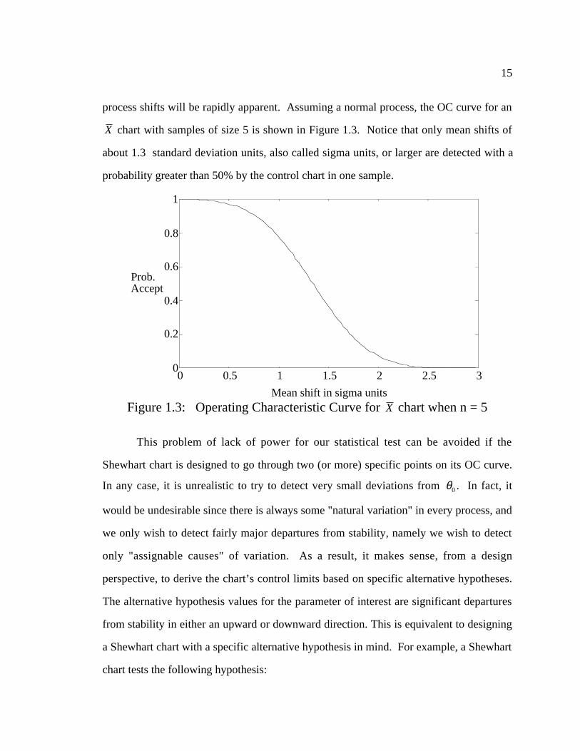
process shifts will be rapidly apparent. Assuming a normal process, the OC curve for an

X chart with samples of size 5 is shown in Figure 1.3. Notice that only mean shifts of

about 1.3 standard deviation units, also called sigma units, or larger are detected with a

probability greater than 50% by the control chart in one sample.

0

0.2

0.4

0.6

0.8

1

0 0.5 1 1.5 2 2.5 3

Prob.Accept

Mean shift in sigma unitsFigure 1.3: Operating Characteristic Curve for X chart when n = 5

This problem of lack of power for our statistical test can be avoided if the

Shewhart chart is designed to go through two (or more) specific points on its OC curve.

In any case, it is unrealistic to try to detect very small deviations from θ0 . In fact, it

would be undesirable since there is always some "natural variation" in every process, and

we only wish to detect fairly major departures from stability, namely we wish to detect

only "assignable causes" of variation. As a result, it makes sense, from a design

perspective, to derive the chart’s control limits based on specific alternative hypotheses.

The alternative hypothesis values for the parameter of interest are significant departures

from stability in either an upward or downward direction. This is equivalent to designing

a Shewhart chart with a specific alternative hypothesis in mind. For example, a Shewhart

chart tests the following hypothesis:

16

H0 : θ = θ0

H1 : θ = θ1 or θ = θ−1 .

In other words, the control chart should signal whenever the process mean shifts to θ1 or

θ−1, where without loss of generality, it is assumed that θ1 > θ0 , and θ−1 < θ0 . Since, in

many cases, Shewhart charts assign equal importance to parameter shifts in both

directions, we may also assume θ1 – θ0 = θ0 – θ−1. The analysis that follows could be

performed for the case when θ1 – θ0 θ0 –θ−1, but this case is not usually of interest in

practice. Considering an alternate hypothesis can ensure that the charts will usually

detect important assignable causes quickly, and yet not give many false alarms. This is

accomplished by determining what sample size is required so that our chart will be able

to detect specified parameter shifts. Another consideration in the design of control charts

and acceptance sampling plans is determining desirable levels for the type I and II error

rates of the hypothesis tests. In the case of Shewhart charts, given specific type I and II

error rates α and β , we wish to find a sample size and control limits such that

Pr(chart signals | process “in control”) = α

Pr(chart signals | process “out of control”) = 1 – β

A chart’s error rates pertain to the performance of the chart based on a single

sample. Often interest lies in a chart’s performance based on many samples. Since we

can assume that each sample is independent, the type I and II error rates are directly

related to a chart’s average run length (ARL), where the ARL is the average number of

sample taken before the chart signals. ARL = 1

Pr(signal), where Pr(signal) is the

probability the chart signals based on a single sample. Therefore under the null

17

hypothesis the ARL = 1 α which is large, whereas under the alternate hypothesis the

ARL = 1 1 − β( ) which is small.

1.2.2 Acceptance Sampling Plans

The purpose of an acceptance sampling plan is to determine, based on a random

sample, whether a particular lot is likely to contain an “acceptable” or “rejectable” quality

of products. Based on the results of an inspection of a small sample, we try to surmise

the quality of the complete lot, and make a decision to either accept or reject the complete

lot based solely on the quality of the sample. For example, if a dimension is such that

either smaller is better or larger is better, we may wish to test the one-sided hypothesis

test:

H0 : θ = θa

H1: θ = θr

where θa is a parameter value that leads to only a very small number of non-conforming

units (i.e. acceptable level), and θr is an unacceptable, also called a rejectable, parameter

level. When the quality dimension is acceptable only when it falls into a range a two

sided acceptance sampling plan is needed. If the range of acceptable values is θa− to θa

+ ,

the implicit hypothesis test for a two-sided acceptance sampling plan is:

H0 : θa− ≤ θ ≤ θa

+

H1 : θ ≤ θr− OR θ ≥ θr

+ .

where θr+ and θr

− are the alternate parameter values on the upper and lower sides

respectively. Define a lot whose parameter value falls into the range specified by the null

hypothesis as an acceptable lot, whereas a lot whose parameter value satisfies the

condition specified by the alternative hypothesis is called a rejectable lot.

18

In the design of acceptance sampling plans, we wish to determine the sample size

and limits so that the sampling plan has appropriate error rates. Given type I and II error

rates α and β , we must determine the sample size and decision criterion so that:

Pr(reject lot | lot is “acceptable”) = α ,

Pr(accept lot | lot is “rejectable”) = β .

The first acceptance sampling plans were developed by Harold F. Dodge and

Harry G. Romig in their historic paper, “A method of sampling inspection,” that appeared

in The Bell System Technical Journal, in October 1929. The Dodge and Romig plans are

based on attribute data. Some time later, Jennett and Welch (1939) developed the first

sampling plans based on variables data. As a result, traditional sampling plans are based

either on conforming/nonconforming attribute data or on variables data. It is well known

that variables based sampling plans may require considerably smaller sample sizes than

conformance/non-conformance data based plans to achieve the same error rates (Duncan,

1986).

The simplest type of sampling plan involves a single sample, although more

advanced procedures such as double sampling, multiple sampling, item by item

sequential sampling, chain sampling and many others have been devised. In single

sampling with variables data, a sample of size n is taken, and the decision to accept or

reject the lot is based on a comparison of a statistic computed from exact measurements

(usually the mean) and a critical value (called A) derived from process specifications and

distributional assumptions. With conformance attribute data, the number of

nonconforming units in a sample of size n, denoted d, is compared with an acceptance

criterion c, and the lot is accepted if d c. In both cases the sampling plan design

problem is to find the sample size, n, and critical value, A or c, so that the sample plan has

19

the desired error rates, or equivalently, a specified operating characteristic curve (see

Schilling, 1981, and Hamaker, 1979).

Acceptance sampling plans have a “product” orientation since the samples are

taken from a lot of products. Thus, we make inferences about the quality of the lot, not

the process that made the products. This is in contrast with the “process” orientation of

control charts. For this reason, acceptance sampling plans have recently been subjected

to valid criticism. Sayings such as "You can't inspect quality into a product" summarize

the major complaint. However, sampling plans should not be discarded out of hand; in

some circumstances they can still provide a valid and valuable form of SPC. For

example, firms engaging new suppliers may wish to use acceptance sampling until the

new supplier has established a good track record. Vardeman (1986) and Schilling (1981)

provide excellent discussions of how and when acceptance sampling plans should be used

in a modern quality environment.

Two-sided acceptance sampling plans are also of interest because they are

statistically equivalent to acceptance control charts. Acceptance control charts are a cross

between Shewhart control charts and acceptance sampling plans. They are applicable

when the process is very capable but the process average is not stable, and may drift due

to some explainable yet uncontrollable factor. Tool wear is a good example. As the tool

wears the process average begins to shift, but if the process is very capable, the process

average has a considerable amount of room to move before an unacceptable number of

defective items are produced. Replacing tools can be expensive, so we may wish to

tolerate a certain amount of drift in the process mean before taking corrective action. In

this situation, a Shewhart type control chart is not applicable. It is no longer desired to

detect whenever the process average changes. In acceptance control charts, a process is

defined as “out of control” only when the process has drifted too far, and is producing an

unacceptably large number of non-conforming units. Unlike acceptance sampling, the

20

samples are taken directly from the production process and do not randomly choose

samples from a lot. Therefore, acceptance control charts tell us not about the

acceptability or rejectability of lots, but rather when action should be taken to improve

the process. As such, an acceptance control chart can be used for process improvement

like a Shewhart control chart, and yet bases its control limits on specification limits like

acceptance sampling plans.

The first to try to combine the ideas of Shewhart control charts and acceptance

sampling was Winterhalter (1945). He recommended that in addition to the standard

control limits one should add “reject limits.” These additional limits serve as a guarantee

against producing out-of-specification products. As long as the standard control limits lie

inside the reject limits, virtually all product will meet specifications. Hill (1956)

expanded this idea by suggesting the use of reject limits in place of standard control

limits when the process is very capable. Freund (1957) extended the ideas of

Winterhalter and Hill to design a chart that also allowed specifying a desired protection

from not detecting a significant parameter shift. He coined the term “acceptance control

chart,” and called his control limits “acceptance control limits.” For a full discussion of

acceptance control charts and additional references see Duncan (1986) and Wadsworth,

Stephens, and Godfrey (1986).

The question of how to design acceptance sampling plans for grouped data has

been considered by few researchers. When the standard deviation of the variable of

interest is known and an underlying process distribution can be assumed, savings in

inspection costs can be realized by using a dichotomous attribute plan with compressed

specification limit gauging (also called narrow limit gauging or increased severity

testing). Compressed limit sampling plans are a type of grouping and are discussed by

Dudding and Jennett (1944), Ott and Mundel (1954), Mace (1952), Ladany (1976) and

Duncan (1986). These plans do not classify units in the sample as conforming or non-

21

conforming according to the actual specification limits, but instead classify units as

greater than or less than an artificial specification limit. Compressed limit gauging uses

assumptions about the process distribution (e.g. normal) and standard deviation to

translate the proportion “defective” under the stricter compressed limits to an equivalent

true proportion defective based on the actual specification limits. When the actual

proportion defective is small, very few units will be classified as non-conforming using a

standard acceptance sampling plan. Thus the classification process will not provide much

information. Compressed limit plans, on the other hand, can be designed to have a large

number of units fall into each class and thus provide much more information about

parameters of interest. Thus compressed limit plans require smaller sample sizes than

standard dichotomous attribute plans especially when the actual proportion defective is

very small.

Extensions to more than two groups are quite rare in the literature. Beja and

Ladany (1974) proposed using three attributes to test for one-sided shifts in the mean of a

normal distribution when the process dispersion is known. They consider hypothesis

tests such as H0: µ = µ0 versus H1: µ = µ1 . They show that optimal partition of the

acceptance and rejection regions must be based on the Neyman-Pearson lemma, in other

words, on the likelihood ratio. They find the best gauge limit design by assuming that the

best limits must be symmetric about the midpoint of the null and alternate means.

Ladany and Sinuary-Stern (1985) discuss the curtailment of artificial attribute sampling

plans with two or three groups, whereby inspection of a sample is concluded as soon as

the number of nonconforming units either exceeds the acceptance number or can not

possibly exceed the acceptance number with the remaining unexamined units. They

show that their three group curtailed sampling plan requires, on average, a smaller sample

size than a variable plan! Unfortunately, the approach of Beja and Ladany (1974) and

22

Ladany and Sinuary-Stern (1985) is not easily extended to more than three groups, where

gains in efficiency can be realized.

Bray, Lyon and Burr (1973) consider three-class distribution-free attribute plans.

They classify units as good, marginal or bad, and define the rejection region by

specifying the critical numbers of marginal and bad units: c1 and c2 respectively. To

simplify the analysis they focus on the subset of all sampling plans that has c2 = 0, i.e.,

plans that tolerate no “bad” units. Their results are not easily applied in practice, since it

is difficult to devise a sampling plan using their tables that will attain specific error rates.

In addition, the approach is not easily extended to the more general three group case or to

more groups. Nevertheless, their methods have found some application in the food

sciences area (Ingram et al. 1978), where in testing for food quality a certain level of

contamination is totally unacceptable, but moderate levels of contamination can be

tolerated to a certain degree. Another similar type of control chart for use with

categorized data was first suggested by Duncan (1950), and further developed by

Marcucci (1985) and Nelson (1987). The so called chi-square control chart generalizes a

p-chart to multiple groups. However, the method does not consider an underlying

distribution and it is thus difficult compare the performance of this type chart with more

traditional charts. Depending on the way in which the data is categorized the method

may be very inefficient, especially if the categorization is done in a manner similar to the

traditional p chart. In addition, the chart would require a great deal of prior experience

with the process to determine the number of units expected to fall into each category.

No two sided acceptance sampling plans or acceptance control charts have been

developed for any type of grouped data, even dichotomous data. However, since the

formulation of acceptance sampling plans and acceptance control charts is very similar, it

may be possible to combine two of Beja and Ladany (1974) one-sided tests to create a

three-group two-sided acceptance sampling plan.

23

1.2.3 Correlation Estimation from Destructive Testing

Many materials used in construction and other applications can be characterized

by two or more important physical strength properties. In assessing the acceptability of

the materials, the correlation between the various strength properties can be very

important. For physical structures subject to a variety of stresses, large correlations

between strength modes have the effect of increasing the variability of a structure's load-

carrying capacity, thus making it less reliable. Suddarth, Woeste and Galligan (1978) and

Galligan, Johnson and Taylor (1979), studied the effect of the degree of correlation

between bending and tensile strength in metal-plate wood trusses used in the roof

structure of most homes. They concluded, based on theoretical and simulated results, that

a large correlation may significantly affect the structure's reliability.

In many applications, however, the strength of an item can only be determined

through destructive testing. Lumber, for example, has a number of physical properties

such as bending strength, tensile strength, shear strength, and compression strength, that

can only be determined destructively. As a result, one is able to ascertain the precise

breaking strength in only a single mode for each unit. In such situations, the correlations

among the various strength properties cannot be measured directly and must be

approximated. A number of past studies such as those given by Evans, Johnson and

Green (1984), Amorim (1982), Amorim and Johnson (1986), Green, Evans and Johnson

(1984), Johnson and Galligan (1983) and Galligan, Johnson and Taylor (1979) have

addressed the problem of estimating the correlation between destructively determined

variables by using proof-loading. Proof-loading means stressing units only up to a

prescribed (proof) load, thereby breaking only the weaker members of a population

(Johnson, 1980). This way, although some units break before the proof-load is reached,

others survive and can be subjected to further testing in other strength modes. As such,

24

proof-loading leads naturally to grouping data based on whether the unit breaks or

survives the testing stress.

The strategy employed in past studies to estimate the correlation (Evans et al.,

1984 and Amorim, 1982) involves proof-loading units on the first mode followed by

stressing the survivors until failure on a second mode and recording the exact load at

failure for each unit. By assuming the strength properties have a bivariate normal

distribution with known means and standard deviations both Evans et al. (1984) and

Amorim (1982) were able to solve numerically for the maximum likelihood estimate

(MLE) of the correlation for various sample sizes n, and actual correlation value. A

simulation study evaluated the mean and standard deviation of the MLE at different

proof-load levels. Determining that the MLE was approximately unbiased, they

compared the standard deviation of the MLE with the theoretical lower bound given by

evaluating the reciprocal of the Fisher information.

Bartlett and Lwin (1984) considered a variation of the correlation estimation

problem where a third property, C, can be measured non-destructively. They split the test

sample into three groups. For the first group they measured C and the breaking strength

on A for all units, thus allowing them to estimate the mean strength in A and C and the

correlation between A and C. Similarly, for the second group, they estimate the means

and the correlation of C and B. A third test group was first measured on C, then

subjected to a proof-load on A and finally failed on test B. This third group then gave

information on the property of interest, the correlation between A and B. They then used

the Fisher information matrix to determine a lower bound on the variance of their

estimate for the correlation between A and B.

Johnson and Galligan (1983) and Galligan, Johnson and Taylor (1979) also

present a similar extension. They consider estimating the correlation between two

destructively measured properties where each is a function of several properties that can

25

be measured non-destructively. They present results comparing the correlation estimate

calculated ignoring the additional dependence on the non-destructively measured

properties and estimates obtained utilizing the additional information. The procedure was

performed on real data, but the results were inconclusive due to a poor choice of proof-

load levels.

All the methods previously developed utilize proof-loading (grouping) in one of

the strength modes, but no methods have been developed that utilize grouping in both

modes. This is a logical extension since, as mentioned, grouped data are often easier and

cheaper to collect.

One should note that all procedures based on proof-loading implicitly assume that

survivors of the proof-load are not damaged. Experimental studies by Madsen (1976),

and Strickler et al. (1970) suggest that this may be a reasonable assumption regarding the

static strength of lumber, although a few pieces whose strength is only slightly greater

than the proof-load stress will likely be weakened. In addition, according to cumulative

damage theory, Gerhards (1979), “the theoretical results suggest that some percentage of

the population will fail during the proof-load, a very small additional percentage will be

weakened, but the remainder will have residual strength virtually equal to original

strength.” These theoretical results are based on the reasonable assumption that the

proof-loading is done at a rapid rate.

1.3 Thesis Outline

The goal of this research is to apply estimation procedures and hypothesis testing

based on grouped data in a quality control and improvement context. More specifically,

acceptance sampling plans, acceptance control charts, Shewhart control charts, and

correlation estimates under destructive testing are developed that are applicable when

observations from an underlying distribution are classified into groups. This research

26

fulfills a need from both a theoretical and practical standpoint. Multi-group data can be

thought of as a natural compromise between binomial and variables data, and are often

collected in industry to monitor the output of a production process. However, statistical

process control techniques have been designed only for variables data, and the special

case of two and to some extent three group data. Consequently, it is desirable to extend

statistical process control methodology to also encompass the general multiple group

case.

To handle multi-group data, notice that when observations from a single

underlying distribution are classified into groups, the appropriate model is multinomial

with group probabilities being known functions of the unknown parameters. Due to the

grouping, the multinomial remains the appropriate distribution for any underlying

distribution including multivariate distributions. As a result, all the design methodologies

presented in this thesis can be very easily adapted for any underlying distribution. To

illustrate this point many of the results in the thesis are given for the Weibull distribution

as well as the normal.

The thesis is organized in the following manner. Chapter 2 discusses some

preliminary items that are necessary for a full understanding of the subsequent work.

Much of the notation is defined, and some background literature on maximum likelihood

parameter estimation from grouped data is presented. In addition, the problems inherent

in utilizing SPC techniques designed for variables data when the data are grouped are

illustrated.

Chapter 3 turns to the question of designing acceptance sampling plans,

acceptance control charts and Shewhart charts for grouped data. For each application a

number of different solutions are considered. The approaches can be classified into two

distinct design philosophies; namely, MLE based approaches, and “weights” based

approaches. MLE based approaches utilize either the MLE itself or the generalized

27

likelihood ratio as test statistic. Using the MLE of the parameter of interest for grouped

data directly may be considered an extension of the methodology used in X charts for

variables data. The “weights” approach derives from considering the likelihood ratio

with specific alternative hypotheses. It is well known that for multinomial data the

uniformly most powerful test for comparing simple parameter values is based upon the

likelihood ratio of the multinomial probabilities. This is because all the information that

a sample provides regarding the relative merits of hypotheses is contained in the

likelihood ratio of these hypotheses on the sample (Edwards, 1972). Thus the specific

alternative approach, or “weights” approach, is optimal for one-sided tests, and, as will be

shown, is near optimal for some two-sided tests. The various approaches all have their

strengths and weaknesses that are discussed in detail. The design of small sample size

plans or charts is also discussed in some detail.

Chapter 4 considers estimating the correlation coefficient of a bivariate normal

distribution based on destructive testing. Again, a number of different testing procedures

are considered. Two simple procedures provide good estimates of the correlation given

the individual means and standard deviations are known. The results of these procedures

are compared with the results of past studies. Two slightly more advanced procedures

extend to the case where none of the five bivariate normal parameter are known.

The question of optimal gauge limit design for acceptance sampling plans and

Shewhart control charts and correlation estimates from destructive testing is addressed in

Chapter 5. Initially it was assumed that the grouping criterion design is predetermined.

However, in some circumstances it is possible to design the step-gauge. If step-gauge

design is feasible, there are two decisions to be made in specifying the grouping criteria:

how many groups should be used, and how are these groups to be distinguished. As more

groups are used, more information becomes available about the parameters of the

underlying distribution, but data collection costs increase. The limiting case occurs when

28

the variable is measured to arbitrary precision. Even if the number of groups is fixed, not

all gauge limits will provide the same amount of information about the parameters of the

underlying distribution. Gauge limits placed very close to one another provide little more

information then a single limit, and gauge limits in the extreme tail of the underlying

distribution provide almost no information. Also, what may be a beneficial gauge limit

placement for estimation of the mean of a distribution is not necessarily very good for

estimating a distribution's standard deviation or correlation. It is not intuitively clear how

to set the k-gauge limits to optimize the testing procedure.

Finally, in Chapter 6 the major results are summarized and possible extensions are

discussed.

Some of this original research has appeared in research papers. Specifically, one-

sided acceptance sampling plans for grouped data based on the weights method, Sections

3.1 and 5.1, in Steiner et al. (1994A), Shewhart control charts for grouped data based on

the one set and two sets of weights approaches, Sections 3.3.1, 3.3.2 and 5.3.1, in Steiner

et al. (1994B), correlation estimation based on grouped data, Sections 4.1 and 5.4, in

Steiner and Wesolowsky (1994A) and a review paper on the drawbacks of the ad hoc

SPC techniques currently in common use, Section 2.3, in Steiner and Wesolowsky

(1994B).

29

CHAPTER 2Preliminaries

The purpose of this chapter is to set the stage for subsequent work. The three

sections are somewhat unrelated, but contain background work that is necessary to fully

understand the subsequent chapters.

Section 2.1 introduces much of the notation, and the likelihood function. The

normal distribution is the standard choice for work in quality control. However, often the

normal distribution provides a poor fit to the data and is not applicable. As the

methodology that will be presented in later chapters is easily adaptable to other

distributions, Shewhart control charts using the Weibull as underlying distribution are

also presented. The Weibull distribution is often a good choice when the normal provides

a poor fit, since it allows skewness in either direction. In addition, the exponential

distribution is a special case of the Weibull. As a result, the Weibull distribution works

especially well for applications where the observations represents a service or waiting

time.

Parameter estimation is often a very important part of quality control. To design

control charts and to calculate process capability indices we must be able to estimate the

parameters of the underlying distribution accurately. The problem of parameter

estimation from grouped data has been well studied (Rao, 1973). Section 2.2 gives a

short literature survey of the area, discusses the existence conditions for the estimates,

and presents algorithms that derive the maximum likelihood estimates of the normal and

Weibull parameters from grouped data in our notation. Also presented is an algorithm

which when given the mean and variance values, finds the Weibull parameters that

30

correspond. This procedure is useful since the transformation is not trivial, and is

necessary when deriving Shewhart control charts based on the Weibull distribution.

This Chapter concludes in Section 2.3 with an analysis of some ad hoc quality

control techniques currently used with grouped data. These techniques are used in

industry since multiple grouped data is quite common and yet no acceptance sampling

plans or control charts have been designed to deal with this type of data. The ad hoc

procedures assume away the data grouping and use charting techniques designed for

variables data. As will be shown these approaches are unreliable.

2.1 Useful Definitions

This section introduces and defines many of the variables that will be used

throughout the thesis. See also the glossary in Appendix A.

2.1.1 Normal and Weibull Distributions

I will consider observations that have either a normal or a Weibull distribution.

The normal distribution is the standard choice for most quality control applications. The

well known normal probability density function (p.d.f.), f N y( ), and cumulative density

function (c.d.f.), FN y( ) , are given below as equations (2.1). The variable y represents a

measurement of the quality characteristic of interest, e.g. the length of a nail.

f N y( ) =1

2π σexp −

y − µ( )2

2σ 2

FN y( ) = f N s( )−∞

y

∫ ds (2.1)

The two parameter Weibull is also considered. The Weibull has probability

density function fW y( ) and cumulative density function FW y( ) given by:

31

fW y( ) =a

baya−1 exp − y

b

a

y > 0

FW y( ) = Pr 0 ≤ Y ≤ y( ) = 1− exp − y

b

a

, (2.2)

where the parameters a and b are called the shape and scale parameters respectively. The

mean µW and variance σW2 of the Weibull are given by:

µW = bΓ 1+ 1a

(2.3)

σW2 = b2 Γ 1+ 2

a

− Γ2 1+ 1

a

,

where Γ x( ) is the Gamma function as defined by Abramowitz and Stegun (1970), 6.1.1.

The two-parameter Weibull is a very flexible distribution although it is only defined for

y > 0 . In most quality control applications the measurements are positive valued

dimensions. For time to failure applications the parameter a has a special interpretation.

Namely, if a > 1, the failure rate increases with time, whereas if a = 1, the Weibull

distribution is an exponential distribution, and the failure rate is memoryless, i.e. constant

over time, and if 0 < a < 1 the failure rate decreases with time.

2.1.2 Grouped Data Definition

This thesis considers grouped data. Define the grouping criterion as follows. Let

the k interval endpoints of the step-gauge be denoted by xj , j = 1, 2, ..., k; then the

probability that an observation is classified as belonging to group j is given by:

π1 = φ(y)dy−∞

x1

∫

π j = φ(y)dyx j−1

x j

∫ j = 2, ..., k (2.4)

32

πk+1 = φ(y)dyxk

∞

∫

where φ y( ) represents the probability density function of the observations.

We can specify explicitly the group probabilities using the normal and Weibull

p.d.f.s defined in equation (2.1) and (2.2). For the normal distribution φ y( ) =

f N y;µ ,σ( ). Then, defining ti = xi − µ( ) σ , the ti‘s are the standardized gauge limits.

Also defining t0 = −∞ and tk +1 = ∞ for notational convenience, the normal group

probabilities can be compactly written as:

π j µ ,σ( ) = f N µ ,σ( )dyt j−1

t j

∫ . j = 1,K,k +1 (2.5)

If the observations are Weibull then φ y( ) = fW y;a,b( ), y > 0. The Weibull cumulative

distribution function can be written explicitly and the k +1 group probabilities are

π1 a,b( ) = 1− exp − x1

b

a

π j a,b( ) = exp −xj−1

b

a

− exp −

xj

b

a

j = 2,K,k (2.6)

πk+1 a,b( ) = exp − xk

b

a

where all the xj' s are greater than or equal to zero.

2.1.3 Likelihood and Log-likelihood Ratios

Let Q be a (k+1) column vector whose jth element Qj denotes the total number of

observations in a sample of size n that are classified into the jth group. Then, defining θ

as the parameter(s) of interest, the likelihood of any hypothesis about θ , given the

sample Q, is defined as (Edwards, 1972):

33

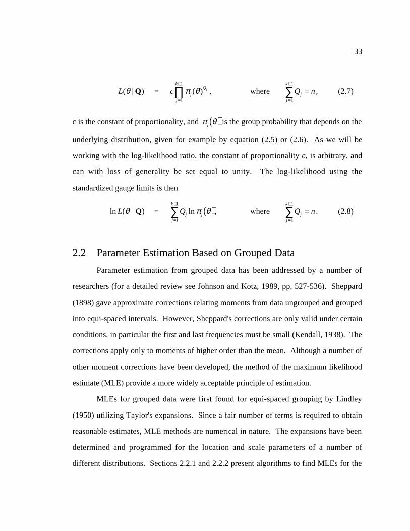
L(θ | Q) = c π j (θ )Qj

j=1

k+1

∏ , where Qjj =1

k +1

∑ = n , (2.7)

c is the constant of proportionality, and π j θ( ) is the group probability that depends on the

underlying distribution, given for example by equation (2.5) or (2.6). As we will be

working with the log-likelihood ratio, the constant of proportionality c, is arbitrary, and

can with loss of generality be set equal to unity. The log-likelihood using the

standardized gauge limits is then

ln L(θ Q) = Qj ln π j θ( )j=1

k+1

∑ , where Qjj =1

k +1

∑ = n . (2.8)

2.2 Parameter Estimation Based on Grouped Data

Parameter estimation from grouped data has been addressed by a number of

researchers (for a detailed review see Johnson and Kotz, 1989, pp. 527-536). Sheppard

(1898) gave approximate corrections relating moments from data ungrouped and grouped

into equi-spaced intervals. However, Sheppard's corrections are only valid under certain

conditions, in particular the first and last frequencies must be small (Kendall, 1938). The

corrections apply only to moments of higher order than the mean. Although a number of

other moment corrections have been developed, the method of the maximum likelihood

estimate (MLE) provide a more widely acceptable principle of estimation.

MLEs for grouped data were first found for equi-spaced grouping by Lindley

(1950) utilizing Taylor's expansions. Since a fair number of terms is required to obtain

reasonable estimates, MLE methods are numerical in nature. The expansions have been

determined and programmed for the location and scale parameters of a number of

different distributions. Sections 2.2.1 and 2.2.2 present algorithms to find MLEs for the

34

normal and Weibull parameters respectively. One potential shortcoming of maximum

likelihood estimates is that in some circumstances they may not exist. This is usually not

a concern with continuous data. However in our case, due to the discrete nature of

grouped data, it is an issue that must be considered. In general, a set of sufficient

conditions for the existence and uniqueness of the MLE θ of the likelihood function

L θ( ) is (Kulldorff, 1961):

i)∂ ln L

∂θ is continuous for all θ

ii) The sign of ∂ ln L

∂θ is different at the two extremes of the parameter space.

iii)∂ 2 ln L

∂θ 2 is negative when θ = θ

For each of the different parameters of interest, these general conditions are translated

into specific conditions on the observed sample in the following subsections.

2.2.1 Normal Parameter MLEs

A very efficient and general procedure for finding the MLEs, called the expected

maximization (EM) technique, was provided by Dempster et al. (1977). Since the EM

technique provides excellent estimates in an efficient manner this is the strategy utilized

to find MLEs of normal parameters from grouped data. Wolynetz (1979) presents the

EM technique to solve for the MLEs of the location ( µ ) and scale parameter ( σ ) of the

normal distribution. The equations to solve are given below in our notation. The MLEs

can be found by setting either the derivative of likelihood function itself or the log-

likelihood (equations 2.7 or 2.8) equal to zero. Doing so gives the following equations:

∂ ln L µ,σ Q( )∂µ

µ =µ ,σ =σ

=1σ

Qjj =1

k +1

∑f N t j −1;µ ,σ( ) − f N t j ;µ ,σ( )

π j µ ,σ( ) = 0

35

∂ ln L µ,σ Q( )∂σ

µ =µ ,σ =σ

=1σ

Qj

tj−1 f N tj−1;µ ,σ( ) − tj f N tj ;µ ,σ( )π j µ ,σ( )j=1

k+1

∑ = 0

Defining

wj = E yj tj−1 < yj < tj ; µ ,σ( ) j = 1,K,k +1

= µ + σf N tj−1;µ ,σ( ) − f N tj ;µ ,σ( )

π j µ ,σ( ) (2.9)

We get

µ =Qjwj

nj=1

k+1

∑ , (2.10)

σ =

Qjwj − µ( )2

j =1

k +1

∑f N t j −1;µ ,σ( ) − f N t j ;µ ,σ( )

π j µ ,σ( )

2

−t j −1 f N t j −1;µ ,σ( ) − t j f N t j ;µ ,σ( )

π j µ ,σ( )

j =1

k +1

∑ (2.11)

These equations are solved in an iterative fashion. Initial estimates for µ and σ

are substituted into (2.9) to determine the current estimates for each wi . These values of

wi substituted into (2.10) and (2.11) will yield improved estimates for µ and σ . The

performance of the EM algorithm is very good, and iterations converge in a short time

even for “wild” initial conditions. In our application, fairly good initial estimates can be

ensured by using each group interval’s midpoint as a weight in (2.10) and (2.11) to give

initial estimates of the underlying distribution’s mean and standard deviation. However,

as mentioned by Kulldorff (1961), the MLEs for µ and σ only exist if some mild

conditions are met. The MLE µ exists if and only if Q1 < n and Qk+1 < n (Kulldorff,

1961, theorem 8.1). In other words, the maximum likelihood estimate of the mean exists

only so long as not all the observations fall into one of the outside groups. The MLE σ

exists if and only if either

36

1) Q1 + Qk+1 < n and Qi > 0 for some j satisfying µ < xj−1 or µ > xj

2) Q1 + Qk+1 = n, 0 < Q1 < n and Q1 x1 − µ( ) > Qk+1 xk − µ( ).

For fairly large sample sizes, and reasonable grouping criteria, the chances of

observing a sample that does not have a MLE is very small. For small sample sizes, on

the other hand, nonexistence of the MLEs can be of significant concern.

2.2.2 Weibull Parameter MLEs

The maximum likelihood estimates for the Weibull distribution can be found by

differentiating the log likelihood function (2.8) with respect to a and b, and solving the

resulting system of two equations for a and b . Substituting into expression (2.6), the

two equations to solve are (assuming x0 = 0 and xk+1 = ):

∂∂a

Qj ln exp −x j −1

b

a

− exp −

x j

b

a

j =1

k +1

∑a= a, b= b

= 0

∂∂b

Qj ln exp −x j −1

b

a

− exp −

x j

b

a

j =1

k +1

∑a= a, b= b

= 0

These equations can not be solved explicitly, but the Newton-Raphson method (Press, et

al. 1988) works very well. Use as initial estimates, a0 = cv n( )−1 0.94 , where cv(n) is the

sample coefficient of variation (i.e. cv = 100 times the sample standard deviation over the

sample mean) and b0 = the sample mean. This approach was suggested by Harlow

(1989), and is based on the approximation cv ≈ a−0.94 . The conditions on the existence of

these MLE have been determined by Marymont (1975). The MLE b exists if and only if

Q1 < n and Qk+1< n, whereas the MLE a exists if and only if either:

37

a) Q1 + Qk+1 < n and there exists at least one i such that Qi > 0, and b < xi−1

or b > xi .

b) Q1 + Qk+1 = n, 0 < Qk+1 < n and if x1 < b then we must have xk < b .

2.2.3 Translating Mean and Variance to Weibull Parameters

When using the Weibull distribution to represent an underlying distribution it is

often of interest to work in terms of the mean and standard deviation rather than the

Weibull parameters a and b. Translating from the Weibull parameters a and b to the

Weibull mean and variance can be done through equations (2.3) above. An algorithm,

developed by Macdonald (1993), that does the reverse is presented below. The algorithm

works by noticing that the variable b can be eliminated by considering a simple function

of the mean and variance. Then using well known properties of the Gamma function

gives:

µ = bΓ 1 + 1 a( ) =b

aΓ 1

a

σ 2 = b2 Γ 1 + 2 a( ) − Γ2 1 + 1 a( )( ) =2b2

aΓ 2

a

− b2

a2 Γ2 1a

σ 2 + µ 2

2µ 2 =b2 aΓ 2 a( ) − Γ2 1 a( ) + Γ2 1 a( )( )

b2Γ2 1 a( ) =aΓ 2 a( )Γ2 1 a( )

Then it is possible to write:

0 =µ 2 + σ 2

2µ 2

Γ2 1 a( )Γ 2 a( ) − a

Newton’s method can be used to interactively solve for the root of the above equation.

The derivative of Γ x( ) can be easily determined in terms of the Digamma or ψ function

38

(Abramowitz and Stegun, 1970, p. 258). Then once the equation has been solved for the

parameter a,

b =aµ

Γ 1 a( ) .

This algorithm quickly converges to the correct Weibull parameters. For example, given

a Weibull distribution with mean µ = 68, and standard deviation σ = 2.2, the above

algorithm gives corresponding Weibull parameters a = 38.93 and b = 68.98.

2.3 Ad hoc Quality Control Techniques for Grouped Data

As previously mentioned, grouped data is fairly common, but few SPC techniques

have been developed that consider such data. As a result, in current industrial practice,

grouped data is usually treated as variables data in control charts. All observations in a

given sample are assumed to be either at the interval midpoint or at an endpoint. The

midpoint approach assigns any observation that falls into a particular group a value equal

to the midpoint of the grouping interval. For example, if a unit is gauged to fall

somewhere between 6 and 7, the midpoint approach assigns that unit a value of 6.5. The

endpoint approach works in a similar manner except that the value assigned to each part

will be equal to either the interval’s lower endpoint or its upper endpoint. In the above

example, the unit is assigned a value of 6 if we are using the lower endpoint strategy and

a value of 7 if we are using the upper endpoint method. These representative values for

each unit are then used as though they were variable measurements on a continuous scale,

and combined into overall measures such as averages to create control charts such as X

charts. While these ad hoc methods have some intuitive appeal, they suffer from a

number of shortcomings since they ignore grouping in the data. As stated by Kulldorff

(1961), "for reasons of practicability it is customary to treat grouped samples also as if

they were non-grouped, giving all the observations in a group an individual value equal to

39

the central value of that group interval. This procedure represents an approximation that

often leads to considerable systematic errors ...."

One concern pertains to the number of groups necessary. For end-groups the

interval midpoint does not exist, since the interval extends to plus or minus infinity.

Similarly, for the lower (upper) endpoint strategy no lower (upper) interval endpoint

exists for the leftmost (rightmost) end-group. These problems can be avoided by utilizing

a sufficient number of groups, so that no observations are likely to fall into the end-

groups. However, using very many groups increases the measurement costs, and thus

may eliminate the advantage of grouped data.

Another major problem especially acute for the endpoint based methods, but also

a concern with the midpoint approach, is that parameter estimates derived by using the

interval endpoint or midpoint as a representative value will usually be biased. Consider

the case where we wish to estimate the process mean. Clearly, assigning each unit a

value equal to the lower endpoint of its group will consistently under-estimate the actual

values of the process, and vice-versa for the upper endpoint approach. The midpoint

approach also introduces a bias, but the source of bias is not as obvious. Consider Figure

2.1 below:

40

I II IVIII V

Figure 2.1: Gauge Limits Superimposed on Normal Distribution

Assuming the underlying normal distribution shown on the figure is an accurate

approximation of the process’ true distribution, any observation that falls into group II is

more likely to actually come from the right side of that interval. Using the interval

midpoint as a representative value will also introduce a bias in the estimate of the mean

and standard deviation (unless the underlying distribution is uniform), though the bias is

usually smaller than the bias introduced by the endpoint approaches.

The amount of bias introduced is easily quantified. Suppose we have a normal

process with mean µ and variance σ 2 , and the gauge limits are placed at t1 , t2 , ..., tk .

Then the probability of an observation falling into each group is given by π j µ( ), j = 1,...,

(k+1), equation (2.5), where j represents the group, and µ is the mean of the underlying

process. Then using the midpoint approach, and assigning units that fall into the end-

groups the end gauge limits, the group value representation is given by:

41

V(midpoint) =

t1(t1 + t2 ) 2

if unit falls in 1st group

if unit falls in 2nd group

M

(tk-1 + tk ) 2

tk

if unit falls in kth group

if unit falls in (k +1)st group

and the expected value of V(midpoint) is thus

E(V(midpoint)) = t1π1 + t1 + t2

2

π2 + K + tk−1 + tk

2

πk + tkπk+1

With the upper endpoint approach, assigning units that fall into the upper end-

group the end group limit, the group value representation is given by:

V(upper endpoint) =

t1 if unit falls in 1st group

t2 if unit falls in 2nd group

M

tk if unit falls in kth group

tk if unit falls in (k +1)st group

and the expected value of V(upper endpoint) is

E(V(upper endpoint)) = t1π1 + t2π2 + K + tkπk + tkπk+1

A similar derivation can be performed for the lower endpoint approach. The

amount of bias generated by the various approaches clearly depends both on the group

limit and the underlying process mean. Figure 2.2 shows the amount of mean bias

created by using the various methods for different actual mean values. Note that using

many groups also has the advantage of reducing the bias problems discussed previously.

Many groups means shorter group intervals which in turn translates into less potential for

biasing each observation. However, as mentioned, using many groups often comes at a

price, since finer classification usually results in higher data collection costs.

42

True Mean Level

-0.6

-0.4

-0.2

0

0.2

0.4

0.6

-2 -1.5 -1 -0.5 0 0.5 1 1.5 2

Midpoint Approach

Upper EndpointApproach

Lower EndpointApproach

Bias

Figure 2.2: Mean Estimate Bias Using Current ApproachesGauge Limits [-2, -1, 0, 1, 2]

The final concern is that variable based acceptance sampling plans and control

charts, such as X charts, have been designed to yield particular error rates assuming that

the quality characteristic of interest is measured exactly. With discrete data, such as

grouped data, these error rates are not likely to still hold precisely. Typically, due to the

discreteness of the data, the true error rates are underestimated. As a result, the properties

of the control charts and acceptance sampling plans based on these ad hoc approaches are

not clearly known. As an example, consider creating an X chart utilizing either the right

endpoint or the midpoint approach. Assume the process is N(0,1), and a sample of size 5

is taken with control limits set at the standard ±3 standard deviations (i.e. LCL = –0.447,

UCL = 0.447). Table 2.1 compares the probability of the chart not signaling an out-of-

control for both the midpoint point and upper endpoint approaches for a variety of group

limits. For comparison purposes, the last row of the table gives the error rates assuming

variables data. Note that using the lower endpoint approach would give results that are

the mirror image of the results for the upper endpoint approach.

43

The end-group problem is avoided in this case by deriving logical midpoint and

endpoint values used for the end-groups by considering the interval width. For example,

when the group limits are [-1, 0, 1] the midpoints used are (-1.5, -0.5, 0.5, 1.5) and the

upper-endpoints used are (-1, 0, 1, 2). This method works fairly well in this case, but is

more difficult to apply when the group intervals are not all equally wide.

Table 2.1: Comparison of Ad hoc Control Chart Approaches

Probability of “in control” signal

group limits method µ = –2 µ = –1 µ = 0 µ = 1 µ = 2

[-1,0,1] midpoint 0.5784 0.9687 0.9998 0.9687 0.5784

[-1,0,1] upper-endpoint 1.0 1.0 0.9723 0.4514 0.0185

[-1.5,-.75,.75,1.5] midpoint 0.1789 0.8581 0.9983 0.8581 0.1789

[-1.5,-.75,.75,1.5] upper-endpoint 0.6100 0.9840 0.9610 0.3740 0.0088

[-2,-1,0,1,2] midpoint 0.1243 0.8301 0.9980 0.8301 0.1243

[-2,-1,0,1,2] upper-endpoint 0.4519 0.9733 0.9595 0.3405 0.0052

- variables 0.0705 0.7775 0.9973 0.7775 0.0705

An X chart is meant to signal for any major deviation from the target (or current) mean

value, but not to signal while the process is still stable. As a result, in Table 2.1, we

would like large probability values when µ = 0, and small values otherwise. Clearly,

increasing the number of groups has a beneficial effect, but the probability of making an

error is still considerably higher with the ad hoc approaches than with the variables

method. The results are on occasion very striking. For example, the upper-endpoint

approach with the 4 group limits given in the table has a 61% chance of not detecting a

minus two standard deviation mean shift, whereas the variables based chart has only a 7%

chance of failing to detect a mean shift of that magnitude.

44

When devising charts to detect standard deviation shifts, the poor result exhibited

by the ad hoc approaches is even more evident. For example, consider using a range (R)

chart with either the midpoint or endpoint approaches. An R chart is the standard type of

control chart used in practice to detect process standard deviation shifts. Utilizing

standard notation, control limits for R charts are set at UCL = D4R and LCL = D3R . For

a sample size of 5, from Table M in Appendix II of Duncan (1986), D3 = 0 and D4 =

2.115. Assume the group limits are given by (-2, -1, 0, 1, 2) and the process is standard

normal. An initial analysis would give, on average, R ≅ 2.4. Thus, we would set LCL =

0 and UCL > 5. With this setup the control chart will never signal an upward standard

deviation shifts since based on the group limits the maximum range value is 5.

In summary, the midpoint and endpoint approaches typically used in industry for

grouped data introduce a bias into all calculations, require a large number of groups to be

effective, and provide no way of determining the true error rates of the resulting control

charts. These problems are, of course, especially acute when the number of groups used

is fairly small, or if the underlying process distribution only covers a few of the groups.

To get more reliable results, the fact that the data is grouped must be taken into account

in a more direct way.

45

CHAPTER 3Statistical Process Control Based on Grouped Data

This Chapter develops acceptance sampling plans, acceptance control charts, and

Shewhart control charts based on grouped data. Section 3.1 discusses one-sided

acceptance sampling plans. Sampling plans for one-sided parameter shifts based on the

likelihood ratio are derived. Using the likelihood ratio with specific alternatives leads

naturally to assigning each unit a weight determined by the group into which the unit is

classified. This approach will be called the “weights” method. To detect one-sided

parameter shifts this method is optimal in the sense that it will require the smallest sample

size to achieve given error rates.

Section 3.2 extends the method to a two-sided test where there is a range of

parameter values that are considered acceptable. This type of test is applicable to two-

sided acceptance sampling plans and acceptance control charts. Two different

approaches are considered. First, the optimal approach based on combining two one-

sided tests is described. However, since this method requires the simultaneous use of two

sets of weights, another method based on the MLE is also discussed. The MLE based

approaches are often nearly optimal and require only one test statistic, but have a number

of drawbacks, the most important of these are the possible non-existence of the MLE, the

iterative nature of the MLE calculations, and the difficulty of determining the distribution

of the MLE for small sample sizes.

In Section 3.3, Shewhart control charts are discussed. Now the purpose of the

chart is to detect any parameter shifts from stability. Four different solutions are

discussed and contrasted. The two approaches from Section 3.2 are again applicable. In

46

addition, an approach that utilizes one set of weights, and an approach based on the

generalized likelihood ratio (GLR) are presented. Thus, two different weights-based

methods and two approaches that require the calculation of the MLE are considered. The

various solution methodologies each have certain advantages and disadvantages that are

explored in detail.

The design methodology proposed in the first three sections depends on the

applicability of the central limit theorem or of some asymptotic property. Often however,

the sample sizes used are quite small, especially for control charts. Section 3.4 discusses

designing acceptance sampling plans and control charts when the sample size is small.

3.1 One-Sided Acceptance Sampling Plans

Consider a sampling plan to monitor one-sided shifts in the parameter of a

distribution using grouped data. Suppose that the quality characteristic of interest is a

random variable Y that has probability density function φ y;θ( ) where θ is the parameter

of interest. Assume also, without loss of generality, that large parameter values are

undesirable, and that the process parameter is acceptable if less than or equal to θa , and

that a process parameter greater than or equal to θr is considered unacceptable

(rejectable). Thus the one-sided sampling plan tests the simple hypothesis system:

H0 : θ = θa

H1 : θ = θr .

where the desired acceptance and rejection regions are depicted in Figure 3.1.

RejectAccept

θaθr

Figure 3.1: Acceptance/Rejection Regions for One-Sided Shifts

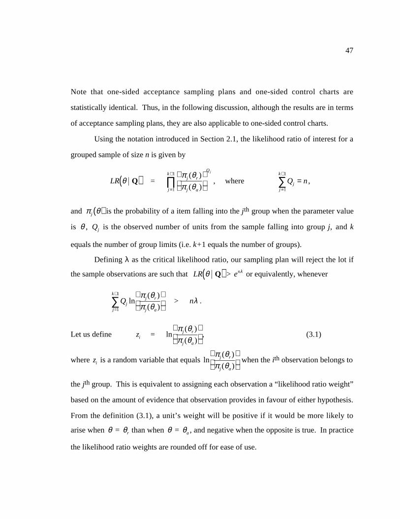
47

Note that one-sided acceptance sampling plans and one-sided control charts are

statistically identical. Thus, in the following discussion, although the results are in terms

of acceptance sampling plans, they are also applicable to one-sided control charts.

Using the notation introduced in Section 2.1, the likelihood ratio of interest for a

grouped sample of size n is given by

LR θ Q( ) =π j (θr )

π j (θa )

Qj

j =1

k +1

∏ , where Qjj =1

k +1

∑ = n ,

and π j θ( ) is the probability of a item falling into the jth group when the parameter value

is θ , Qj is the observed number of units from the sample falling into group j, and k

equals the number of group limits (i.e. k+1 equals the number of groups).

Defining λ as the critical likelihood ratio, our sampling plan will reject the lot if

the sample observations are such that LR θ Q( ) > enλ or equivalently, whenever

Qj lnπ j (θr )

π j (θa )

j=1

k+1

∑ > nλ .

Let us define zi = lnπ j (θr )

π j (θa )

, (3.1)

where zi is a random variable that equals lnπ j (θr )

π j (θa )

when the ith observation belongs to

the jth group. This is equivalent to assigning each observation a “likelihood ratio weight”

based on the amount of evidence that observation provides in favour of either hypothesis.

From the definition (3.1), a unit’s weight will be positive if it would be more likely to

arise when θ = θr than when θ = θa , and negative when the opposite is true. In practice

the likelihood ratio weights are rounded off for ease of use.

48

Our sampling plan is designed to reject the lot whenever the average likelihood

ratio weight z = zi ni=1

n

∑ = Qj

nln

π j (θr )

π j (θa )

j =1

k +1

∑ of a sample is greater than λ . Then, if α

and β are the desired probabilities of type I and II errors respectively, our sampling plan

design problem is to find the sample size n, and the critical value or control limit λ so that

α = Pr z > λ θ = θa( ) , (3.2)and

1 – β = Pr z > λ θ = θr( ) . (3.3)

An approximate solution to (3.2) and (3.3) may be obtained by appealing to the

central limit theorem. For large sample sizes, z will have an approximate normal

distribution with mean µ z θ( ), and variance σ z2 θ( ) n , where

µ z θ( ) = π j (θ ) lnπ j µ r( )π j µa( )

j =1

k +1

∑

σ z2 θ( ) = π j (θ ) ln

π j µ r( )π j µa( )

2

j =1

k +1

∑ − µ z2 (θ ) .

Assuming normality, and solving (3.2) and (3.3) for the required sample size and critical

value gives the solution:

n θa,θr( ) =Φ−1(1 − β )σ z (θr ) − Φ−1(α )σ z (θa )

µ z (θr ) − µ z (θa )

2

, (3.4)

and

λ θa,θr( ) =Φ−1(α )σ z (θa )µ z (θr ) − Φ−1(1 − β )σ z (θr )µ z (θa )

Φ−1(α )σ z (θa ) − Φ−1(1 − β )σ z (θr ), (3.5)

where Φ−1( ) denotes the inverse of the cumulative distribution function of the standard

normal distribution. Note however that the value obtained from equation (3.4) for the

sample size will not, in general, be an integer. Therefore, in the implementation of a

sampling plan, the theoretical sample size suggested by equation (3.4) must be rounded

49

up to obtain a practical sample size. Rounding up the sample size results in more

conservative plans.

It is possible that this rounding up of the sample size is a significant increase. If

this occurs it may be desirable to adjust the critical likelihood ratio value obtained from

equation (3.5) to take into account this increase in sample size. Using intermediate

results from the derivation of equations (3.4) and (3.5), there are two ways to make this

adjustment. Denoted the adjustment based on the equations (3.2) and (3.3) as λα and λβ

respectively, then

λα = µz θa( ) − Φ−1 α( ) σz θa( )n

(3.6)

λβ = µz θr( ) − Φ−1 1− β( ) σz θr( )n

(3.7)

Using λα will decrease the critical value, and thus increase the actual α denoted ′α and

decrease the actual β denoted ′β . Using λβ will have the opposite effect. Which, if

either, of these adjustments to use depends on the purpose of the acceptance sampling

plan. In most cases, we are more interested in ensuring that the type I error rate α , also

called the false alarm rate, is not too large. As a result, using the adjustment λβ is

recommended if the rounded up sample size is much different from the n given by (3.4).

Notice that the design methodology presented can be used for any parameter of

interest. For different parameters, only the group probabilities π j and the group weights

change. For grouped data with any underlying distribution the appropriate distribution to

use is the multinomial. Also, since in any case the average weight is used, the central

limit theorem is applicable.

As an example, consider a one-sided acceptance sampling plan to test for an

increase in the standard deviation of a normal process. Assume that the mean is stable at

50

zero, and that we are interested in comparing the hypothesis H0 : σ = 1 versus H1: σ =

2. If the step-gauge has group limits defined by [-2, -1, 1, 2], then equation (3.1) gives

group weights (rounded to one decimal place) of z = (1.9, 0.1, –0.6, 0.1, 1.9). Then

choosing error rates of α = β = 0.05 equations (3.4) and (3.5) suggest n = 14.7 and λ =

–0.0354. Thus the sampling plan will reject the lot if the average weight z from a

sample of size 15 is greater than –0.0354. As a matter of interest, from Section 3.4, using

n = 15, with λ = –0.0354 gives an acceptance sampling plan that has true error rates of

′α = 0.04 and ′β = 0.06.

3.2 Two-Sided Acceptance Sampling Plans

Often, interest lies not just in parameter shifts in one direction, but also in

parameter shifts in both the upward and downward directions. This is the case for two-

sided acceptance sampling plans and acceptance control charts. For these applications

the hypothesis test of interest can be expressed as:

H0 : θa− ≤ θ ≤ θa

+

H1 : θ ≥ θr+ OR θ ≤ θr

−

where θa+ , θr

+ and θa− , θr

− are the acceptable and rejectable parameter levels on the

upward and downward shift side respectively. Figure 3.2 shows this situation.

RejectAccept

Reject

θr− θa

− θa+ θr

+

Figure 3.2: Acceptance/Rejection Regions for Two-Sided Shifts

51

Note that two-sided acceptance sampling plans and acceptance control charts are

statistically identical, and thus in terms of the plan or chart design they can be considered

interchangeable. For a discussion on their differences see Section 1.3.

Two-sided acceptance sampling plans and acceptance control charts should only

be used when an "in control" process can produce the vast majority of its units within

specifications. In other words, they are only applicable when a process is capable (see

Section 1.2 for a discussion on process capability), and thus the process standard

deviation is small compared with the spread of the specification limits, i.e. θa+ is much

greater than θa− in terms of the process standard deviation. If the process is not capable,

it will be incapable of producing units that are consistently within the specifications, and

acceptance sampling will not be effective. Sections 3.2.1 and 3.2.2 present two design

approaches.

3.2.1 Two Sets of Weights Approach

If the process is capable, the two sides of the hypothesis tests do not interact, in

the sense that if the true parameter value is θa+ or θr

+ the chance of concluding that the

parameter is θr− is negligible, and if the parameter value is θa

− or θr− the chance of

concluding that the parameter isθr+ is negligible. As a result, one can design an

acceptance sampling plan for two-sided shifts with specified error rates as two one-sided

shift acceptance sampling plans with the same error rates. In other words, the two sets of

weights for the two-sided test will be based on the following two hypothesis tests:

Upside Hypotheses Downside Hypotheses

H0+ : θ = θa

+ H0− : θ = θa

−

H1+ : θ = θr

+ H1− : θ = θr

−

52

The two-sided sampling plan or acceptance control chart is designed so that it

rejects a lot or signals “out of control” if either H0+ or H0

− are rejected.

The logistics of combining two one-sided parameter shift hypothesis tests to

create one two-sided acceptance sampling plan or acceptance control chart is straight-

forward. Since the two one-sided shifts can be considered independently, the two sets of

weights based on the likelihood ratio (3.1) can be utilized. One set of weights tests for an

upward shift, while the other set tests for a downward shift. For each hypothesis test, the

results from Section 3.1 can be used to determine the required sample size and critical

value. n+ = n θa+ ,θr

+( ) , λ+ = λ θa+ ,θr

+( ) , n− = n θa−,θr

−( ) and λ− = λ θa−,θr

−( ) , as

expressed by equations (3.4) and (3.5), are the required sample sizes and control limits

for the upward and downward shifts respectively.

A two-sided acceptance sampling plan could then be administered as follows:

1. Derive the required sample sizes, critical values and weights for the two one-sided

tests, i.e. derive n+ , λ+ , z+ and n− , λ− , z− . Choose a sample of size n where n =

max( n+ , n−).

2. Take a random sample of size n from the lot, classify all the units in the sample

into the appropriate group, and calculate the average weight of the sample using

both sets of weights to get z + and z − .

3. Reject the lot if either z + > λ+ or z − > λ− , and accept otherwise.

For acceptance control charts, the procedure is very similar. In step 2, rather than take a

sample from a lot of products, take the sample directly from the process. Also, the results

are presented graphically, either on two separate charts or on one chart with different

colours for the two tests. The critical values λ+ and λ− are the control limits and the

average samples z + and z − are the plotted statistics. In any case the larger average

weight signifies which alternative hypothesis is more likely.

53

The above procedure is simplified when monitoring the mean of a normal

distribution and there is symmetry in the problem; if the group limits are placed

symmetrically about the acceptable and rejectable mean values, the required sample sizes

and critical values for upward and downward tests will be the same. In this case it is

possible to use only one chart, plotting only the larger of the two average weights.

This section concludes with an example. Suppose we are interested in detecting

two-sided shifts in the mean of a normal distribution. The process operates with a stable

standard deviation of 0.17, and the specification limits are specified as 10 and 12. As the

process mean is known to be currently centred between the specification limits, this is a

very capable process ( Cpk = 1.96). As a result, an acceptance control chart or two-sided

acceptance sampling plan is applicable. As is typical, the acceptable and rejectable

process or lot is defined in terms of the proportion non-conforming, i.e. the proportion of

the units falling outside the specification limits. One in 10000 is deemed to be an

acceptable proportion of non-conforming units, whereas one in 200 is considered

unacceptable. As the process standard deviation is known, these requirements can be

translated into acceptable and rejectable mean values on the upper and lower side of the

specification range. Performing the calculations gives µr+ = 11.56, µa

+ = 11.37, µa− =

10.63, and µr− = 10.44 as acceptable and rejectable mean levels. Assuming the group

limits are [10.25, 10.5, 10.75, 11.25, 11.5, 11.75], the equations (3.1), (3.3), and (3.4) will

give the group weights, required sample size, and required control limit respectively.

Error rates of α = 0.001 and β = 0.005 result in the following for the upper and lower

hypothesis tests:

z+ = (–8.3, –6.7, –5, –2, –0.5, 0.9, 2.4)

z− = (2.4, 0.9, –0.5, –2, –5, –6.7, –8.3)

n+ = n− = 28.7, λ+ = λ− = 0.0478

54

The symmetry is evident. The implementation of this example proceeds as follows: take

a sample of size 29, assign weights to each unit based on z+ and z− above, and calculate

the average sample weights z + and z − . If either average weight is greater than 0.0478,

reject the lot or signal “out of control.”

3.2.2 Maximum Likelihood Estimate Approach

An alternative design procedure can be derived based on the maximum likelihood

estimate. Section 2.2 presents algorithms that calculate the MLEs based on grouped data.

The asymptotic distribution of a MLE is normal (Kendall and Stuart, 1979, Chapter 18),

and its asymptotic variance equals the minimum variance bound given by the Rao-

Cramér inequality. Using these results, it is possible to derive control limits that are

appropriate asymptotically.

The variance of the asymptotic distribution of the MLE for the parameter θ can

be easily derived. Define θ as the MLE of θ given a sample of grouped data. Using the

Rao-Cramér inequality, the variance of the asymptotic distribution of the θ , denoted

AsVar θ( ), is:

AsVar θ( ) =1

n E∂ ln L

∂θ

2 (3.8)

Define SD θ( ) as n∗AsVar θ( ) . The SD θ( ) value depends on the actual parameter

value. As a shorthand, let SD θ0( ) = SD θ θ = θ0( ). As an example, the derivation of the

variance of the asymptotic distribution for the MLE of the mean and standard deviation

of the normal distribution from grouped data follows. The variance of the asymptotic

distribution of the MLE µ , denoted AsVar µ( ) can be determined from (3.8):

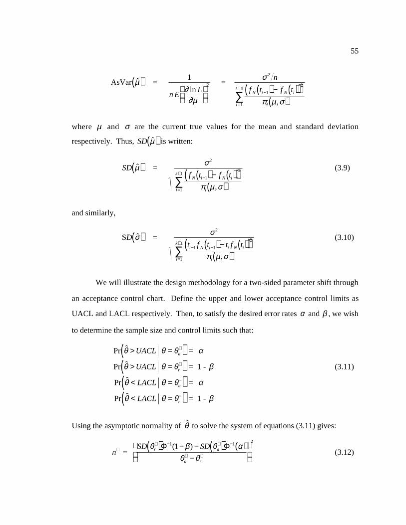
55

AsVar µ( ) =1

n E∂ ln L

∂µ

2 =σ 2 n

f N ti−1( ) − f N ti( )( )2

π i µ ,σ( )i=1

k +1

∑

where µ and σ are the current true values for the mean and standard deviation

respectively. Thus, SD µ( ) is written:

SD µ( ) =σ 2

f N ti−1( ) − f N ti( )( )2

πi µ ,σ( )i=1

k+1

∑(3.9)

and similarly,

SD σ( ) =σ 2

ti−1 f N ti−1( ) − ti f N ti( )( )2

πi µ ,σ( )i=1

k+1

∑(3.10)

We will illustrate the design methodology for a two-sided parameter shift through

an acceptance control chart. Define the upper and lower acceptance control limits as

UACL and LACL respectively. Then, to satisfy the desired error rates α and β , we wish

to determine the sample size and control limits such that:

Pr θ > UACL θ = θa+( ) = α

Pr θ > UACL θ = θr+( ) = 1 - β (3.11)

Pr θ < LACL θ = θa−( ) = α

Pr θ < LACL θ = θr−( ) = 1 - β

Using the asymptotic normality of θ to solve the system of equations (3.11) gives:

n+ =SD θr

+( )Φ−1(1− β ) − SD θa+( )Φ−1 α( )

θa+ − θr

+

2

(3.12)

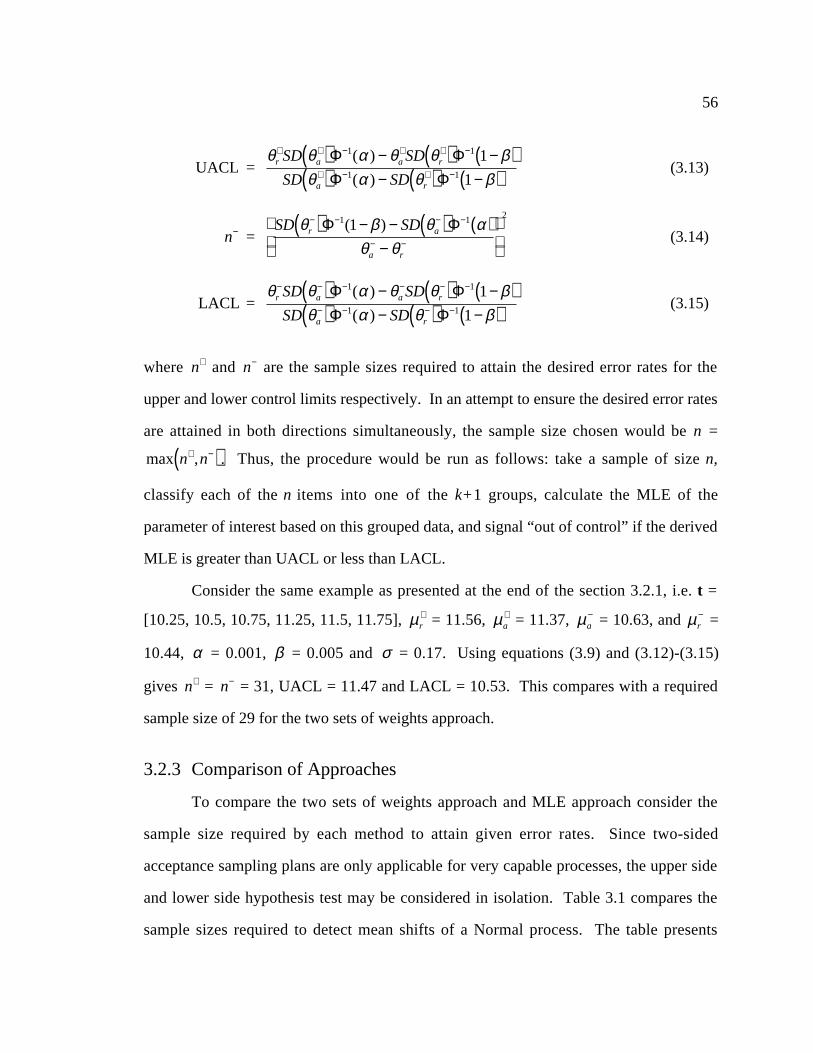
56

UACL =θr

+SD θa+( )Φ−1(α ) − θa

+SD θr+( )Φ−1 1− β( )

SD θa+( )Φ−1(α ) − SD θr

+( )Φ−1 1− β( ) (3.13)

n− =SD θr

−( )Φ−1(1− β ) − SD θa−( )Φ−1 α( )

θa− − θr

−

2

(3.14)

LACL =θr

−SD θa−( )Φ−1(α ) − θa

−SD θr−( )Φ−1 1− β( )

SD θa−( )Φ−1(α ) − SD θr

−( )Φ−1 1− β( ) (3.15)

where n+ and n− are the sample sizes required to attain the desired error rates for the

upper and lower control limits respectively. In an attempt to ensure the desired error rates

are attained in both directions simultaneously, the sample size chosen would be n =

max n+ ,n−( ). Thus, the procedure would be run as follows: take a sample of size n,

classify each of the n items into one of the k+1 groups, calculate the MLE of the

parameter of interest based on this grouped data, and signal “out of control” if the derived

MLE is greater than UACL or less than LACL.

Consider the same example as presented at the end of the section 3.2.1, i.e. t =

[10.25, 10.5, 10.75, 11.25, 11.5, 11.75], µr+ = 11.56, µa

+ = 11.37, µa− = 10.63, and µr

− =

10.44, α = 0.001, β = 0.005 and σ = 0.17. Using equations (3.9) and (3.12)-(3.15)

gives n+ = n− = 31, UACL = 11.47 and LACL = 10.53. This compares with a required

sample size of 29 for the two sets of weights approach.

3.2.3 Comparison of Approaches

To compare the two sets of weights approach and MLE approach consider the

sample size required by each method to attain given error rates. Since two-sided

acceptance sampling plans are only applicable for very capable processes, the upper side

and lower side hypothesis test may be considered in isolation. Table 3.1 compares the

sample sizes required to detect mean shifts of a Normal process. The table presents

57

results for different grouping criteria when the problem has been rescaled so that the

acceptable mean value is zero and the standard deviation is unity. Note that since only

one side of the hypothesis test was considered when creating Table 3.1, to attain the

sample sizes reported, there must also be another set of group limits on the opposite side.

For example, if µr+ = 11.56, µa

+ = 11.37, µa− = 10.63, µr

− = 10.44 and σ = 0.17, as in the

previous example, then the results given under t = [-1, 0, 1] correspond to actual group

limits [10.46, 10.63, 10.8, 11.2, 11.37, 11.54].

Table 3.1: Sample Size Comparison - Two Sided Testsµa = 0, α = 0.001, β = 0.005

t µ rn (MLE) n (weights)

[-1, 1] 0.5 174.7 174.5" 1.0 44.7 43.5" 1.5 21.3 19.0

[-1, 0, 1] 0.5 147.5 145.5" 1.0 38.6 36.3" 1.5 18.8 16.0

[–1.5, –0.5, 0.5, 1.5] 0.5 141.6 140.8" 1.0 36.1 35.0" 1.5 16.8 15.3

[-2, -1, 0, 1, 2] 0.5 139.8 139.5" 1.0 35.2 34.8" 1.5 16.0 15.2

Table 3.1 shows that the MLE approach is near optimal in terms of the sample

size required to give the desired error rates. However, there are also other important

considerations when deciding which method is the best one for a particular application.

The two sets of weights approach is optimal in terms of required sample size, and

calculations required are very simple and can be done on a factory floor without a

computer. But, the weights approach requires the charting or calculation of two test

statistics, and for small sample sizes may need a special design procedure (Section 3.4) to

result in an a sampling plan with the desired error rates. The MLE approach, on the other

hand, requires a computer to find the MLEs, but only one test statistic is required, and the

58

statistic represents a more meaningful value. In addition, although the required sample

size for the MLE approach is near optimal (Table 3.1), for small sample sizes the MLE is

fairly likely not to exist.

In summary, the MLE approach is a good choice if the sample size is not small,

and computer calculation of the MLE does not present a problem. Otherwise the two sets

of weights approach is likely the better one.

3.3 Shewhart Control Charts

For Shewhart control charts detecting two-sided parameter shifts is necessary;

however, there is no longer a range of acceptable parameter values. Instead, any

deviations from stability or equivalently from the current parameter value are undesirable.

Thus, if the current parameter value is θ = θ0 where this is a desirable level, the Shewhart

control chart is designed based on the hypothesis test:

H0 : θ = θ0

H1 : θ = θ1 OR θ = θ−1 ,

where θ1 and θ−1 are parameter values of interest in the upward and downward direction

(from θ0 ) respectively. This situation is shown in Figure 3.3. The control chart will be

designed with a false alarm rate of α , and will signal with probability 1 – β if the

parameter value has shifted to one of the specific alternatives.

Signal Up

Signal Down

θ0 θ1θ−1

Figure 3.3: Signal Regions for Stability Test

59

We have developed four possible solution methodologies. The first utilizes two

sets of weights and is optimal. The second is not optimal, but adapts the “weights”

method so that only one set of weights is required. The MLE approach previously

discussed in Section 3.2.2 and another MLE based approach that utilizes the generalized

likelihood ratio test are also considered. Each of these different approaches has its own

advantages and disadvantages that are compared and contrasted. Due to the relatively

small advantage, in terms of required sample size, of the two sets of weights approach in

most circumstances where Shewhart charts are applicable, either the one set of weights

approach or the MLE approach is recommended for general use.

3.3.1 Two Sets of Weights Approach

One solution strategy is to consider two one-sided tests, i.e. testing

H0 : θ = θ0 versus H1 : θ = θ1 , and

H0 : θ = θ0 versus H−1: θ = θ−1.

Note that this is a different hypothesis test than the one used in Section 3.2, since now

both hypothesis tests have the same null hypothesis. Based on a sample, one could

calculate an average weight (or likelihood ratio) associated with each hypothesis test from

Section 3.1. For each sample, the larger average weight signifies which alternative

hypothesis ( H1 or H−1) is more likely. When θ = θ0 , the chance of either average weight

being larger is 50% due to symmetry. When θ = θ1 , and the difference between θ−1 and

θ1 is fairly large with respect to the process standard deviation, the average weight

associated with first test will almost certainly be larger, and vice versa when θ = θ−1.

This means that it is possible to design the two sided testing procedure with error rates α

and β based one two one-sided procedures with error rates α 2 and β . The

implementation issues are the same as ones discussed in Section 3.2.1. One option is to

maintain two separate charts, one for each hypothesis test. However, if the group limits

60

are placed symmetrically about θ0 (as is optimal, see Section 5.3) the critical value for

each test is the same, and one could plot both average weights on one chart using

different colours or different symbols, signaling if either point lies above the critical

value. See Figure 3.4 for a simulated example.

Notice also from Figure 3.4, that the up (down) average weight plotting above the

down (up) average weight is equivalent to a point plotting above (below) the centre line

in the standard Shewhart chart. Therefore, the runs criterion, which is 8 successive points

on one side of the centre line, sometimes recommended for use in addition to the standard

control limits for an X chart (Juran et al. 1979), can also be applied to this chart.

-1

-0.8

-0.6

-0.4

-0.2

0

1 2 3 4 5 6 7 8 9 10

Control Limit

Sample Number

Average Weight

Figure 3.4: Two Sets of Weights Control Chartα = 0.01, β = 0.05, n = 18, λ = 0.081, µ0 = 0, µ1 = 1, µ = 0.1

‘o’, ‘x’ = average weight for H0 vs. H1 and H0 vs. H−1 respectively

3.3.2 One Set of Weights Approach

An alternative approach is to use one set of weights based on the likelihood of

ratio of θ−1 versus θ1. This approach has been used in the sequential analysis of multi-

hypothesis problems (Ghosh and Sen, 1991). In other words, consider the following

hypothesis test:

H−1: θ = θ−1

61

H1 : θ = θ1

Using the notation from section 3.1, this likelihood ratio for a grouped sample of

size n is given by

LR θ Q( ) =π j (θ1)

π j (θ−1)

Qj

j =1

k +1

∏ where Qjj =1

k +1

∑ = n .

Based on this likelihood ratio we can create a two-sided hypothesis test. Letting λU and

λ L equal the critical values or the upper and lower control limits of the plotted statistic

respectively, the chart signals the process parameter has shifted upwards whenever

LR θ Q( ) > enλ U , and signals a downward parameter shift whenever LR θ Q( ) < enλ L .

Equivalently, the process is deemed “in control,” i.e. the parameter has not shifted, as

long as

nλL ≤ Qj lnπ j (θ1)

π j (θ−1)

j=1

k+1

∑ ≤ nλU .

Let α and β be the desired probabilities of type one and two errors respectively, and let

wi = lnπ j (θ1)

π j (θ−1)

(3.16)

when the ith observation falls in the jth group. Then each unit that falls into the jth group

is assigned the weight lnπ j (θ1)

π j (θ−1)

. Based on these definitions, the chart signals if w <

λ L

or w > λU , where w = wi n

i=1

n

∑ , and we wish to find n, λU and λ L so that

Pr w > λU θ = θ0( ) + Pr w < λL θ = θ0( ) = α , (3.17)

Pr w > λU θ = θ1( ) + Pr w < λL θ = θ1( ) = 1 -β , (3.18)

62

andPr w > λU θ = θ−1( ) + Pr w < λL θ = θ−1( ) = 1 -β . (3.19)

Assuming that false alarms in the upward and downward direction are equally

undesirable, equation (3.17) can divided into two separate equations, namely:

α 2 = Pr w > λU θ = θ0( ), (3.20)

α 2 = Pr w < λL θ = θ0( ), (3.21)

Also, it is easily shown that the second term of the right hand side of (3.18) and the first

term of the right hand side of (3.19) are negligible. Clearly, since θ1 > θ0 ,

Pr w < λL θ = θ1( ) << Pr w < λL θ = θ0( ) = α , and similarly, since θ−1 < θ0 ,

Pr w > λU θ = θ−1( ) << Pr w > λU θ = θ0( ) = α . As a result, since α < 1–β, the two sets

of equations (3.18), (3.20) and (3.19), (3.21) can be considered identical to equations

(3.2) and (3.3) given in Section 3.1. Then, continuing along similar lines as in Section

3.1, for large sample sizes, w will have an approximate normal distribution with mean

µw θ( ) , and variance σw2 θ( ) n, where

µw θ( ) = π j (µ ) lnπ j θ1( )π j θ−1( )

j =1

k +1

∑

σw2 θ( ) = π j (θ ) ln

π j θ1( )π j θ−1( )

2

j =1

k +1

∑ − µw2 (θ ) .

Solving the two sets of equations for n and λU and λ L gives the central limit theorem

(CLT) solution:

nU =Φ−1(α / 2)σw (θ0 ) − Φ−1(1 − β )σw (θ1)

µw (θ0 ) − µw (θ1)

2

(3.22)

λU =Φ−1(α / 2)σw (θ0 )µw (θ1) − Φ−1(1 − β )σw (θ1)µw (θ0 )

Φ−1(α / 2)σw (θ0 ) − Φ−1(1 − β )σw (θ1), (3.23)

63

nL =Φ−1(α / 2)σw (θ0 ) − Φ−1(1 − β )σw (θ−1)

µw (θ0 ) − µw (θ−1)

2

(3.24)

λ L =Φ−1(α / 2)σw (θ0 )µw (θ−1) − Φ−1(1 − β )σw (θ−1)µw (θ0 )

Φ−1(α / 2)σw (θ0 ) − Φ−1(1 − β )σw (θ−1), (3.25)

where nU and nL are the solutions for the sample size on the upward side and downward

side respectively, and Φ−1( ) denotes the inverse of the cumulative distribution function

of the standard normal distribution. This set of solutions are identical to the solutions

obtained for the one-sided shift chart, except that α is replaced with α 2 , and the

weights used are different. Implement of this control chart requires a sample size equal to

max nU ,nL( ) rounded up to the nearest integer to ensure the desired error rates are attained

in both directions. If the group limits are symmetric about µ0 the above formulation is

simplified since λU = – λ L , and nU = nL .

As in Section 3.1, the rounded up sample size may be a significant increase,

especially if nU nL . One simple method to improve the CLT solution is to adjust the

control limits derived by equations (3.23) & (3.25) to reflect the rounded up sample size

that will actually be used. This can be accomplished by considering an intermediate

result derived directly from equations (3.18)-(3.21) that expresses λU and λL in terms of

the sample size n. These adjustment equations are given below:

λU =−σw µ0( )Φ−1 α / 2( )

n + µw µ0( ) (3.26)

λL =σw µ0( )Φ−1 α / 2( )

n + µw µ0( ) (3.27)

It is interesting to note that when monitoring the mean of the normal distribution

the weights used in this approach can be rescaled to have a physical interpretation in the

64

original units. Dividing lnπ j µ1( )π j µ−1( )

, the weight for group j, by twice the shift in σ -

units we wish to detect, gives in a weight that is approximately equal to

E y y ∈ j th group, µ = µ0( ). This is the expected value of any observation that falls into

group j, given that µ = µ0 . See Appendix B for more details. Using this result, the

control chart can be maintained in physically significant units that may be easier for

production personnel to interpret.

For an example of the design strategy, consider a control chart whose purpose is

to monitor the Weibull mean. The current process produces parts that match a Weibull

p.d.f. with mean 101.3 and standard deviation 0.73. Figure 3.5 illustrates the output of

the process. Notice that the distribution of the output is skewed right. Clearly, it is easier

to detect upward shifts in the mean than downward shifts. If the process mean shifts up,

the process is likely to produce parts that are extremely unlikely under the current

parameter values. For example, the process may produce many parts with quality

dimension greater than or equal to 103 units.

0

0.1

0.2

0.3

0.4

0.5

0.6

0.7

98 99 100 101 102 103 104

Prob.

Mean

Figure 3.5: Weibull Process Probability Density Functionµ = 101.3, σ = 0.75, a = 172.5, b = 101.6

65

Let us assume we have a step-gauge that classifies parts based on the group limits

[99, 100, 101, 102], and that we wish to detect mean shifts of one standard deviation

upwards and one and a half standard deviation units downwards with a probability 0.75,

and will tolerate only one false alarm in 1000 opportunities. This implies µ0 = 101.3, σ

= 0.75, µ1 = 102.05, µ−1 = 100.175, α = 0.001, and β = 0.25. Based on comparing the

alternative hypothesis µ1 and µ−1, gives the five group weights: w = (–3.2, –3, –2, 1.1,

11.8). Then, utilizing equation (3.22)-(3.25) gives nU = 12.4, λU = 6.08, nL = 16.3, and

λL = –1.86. This shows that although we were less stringent in terms of power on the

downward side, we still require a larger sample size to achieve the desired error rates on

the downward side due to the long lower tail of the Weibull. In fact a sample of size 17 is

required. Since this is a significant increase over nU , we will adjust the upper control

limit to λU = 5.53 using adjustment equation (3.26). Using the results from Section 3.4,

shows that this control chart has true error rates of ′α = 0.0014, ′βU = 0.122 and ′βL =

0.238.

3.3.3 Maximum Likelihood Estimate Approach

This section uses methodology similar to that presented in Section 3.2.2; however,

the problem is formulated in a slightly different way to conform with the standard

notation used for Shewhart charts. Shewhart control charts based on this MLE approach

are the logical extension of standard X charts. An X chart plots the MLE of the mean

based on variables data and uses control limits set at ±3 times the standard deviation of

the sample mean. These MLE charts are based on plotting the MLE where the control

limits are ±m times the asymptotic standard deviation of the MLE. Using the asymptotic

normality of the MLEs, and the hypothesis system suggested for a Shewhart chart, when

H0 holds, θ ~ N θ0,AsVar θ0( )( ), whereas when H1 holds, θ ~ N θ1,AsVar θ1( )( ) or θ ~

N θ−1,AsVar θ−1( )( ). These approximate results allow the derivation of the theoretically

66

required sample size and upper and lower control limits, UCL and LCL. If the type I and

II error rates are to be α and β respectively, we wish to find the sample size and control

limits such that:

Pr θ > UCL θ0( ) + Pr θ < LCL θ0( ) = α (3.28)

Pr θ > UCL θ1( ) + Pr θ < LCL θ1( ) = 1 − β (3.29)

Pr θ > UCL θ−1( ) + Pr θ < LCL θ−1( ) = 1 − β (3.30)

where as defined, UCL = θ0 + mSD θ0( )

n and LCL = θ0 − m

SD θ0( )n

. The only

unknowns in equations (3.28)-(3.30) are the sample size n, and the multiple of sigma

units that the control limits are away from the centre line, namely m. Then, using the

same arguments as in Section 3.3.2, this system of equations can be split into two

independent systems of equations, one for the upward side and one for the lower side.

For the upper side equations (3.28)-(3.30) can be rewritten as:

Φ−1 α 2( ) =mU SD θ0( ) nU + θ0 − θ0

SD θ0( ) nU

(3.31)

Φ−1 1− β( ) =mU SD θ0( ) nU + θ0 − θ1

SD θ1( ) nU

(3.32)

where nU and mU represent the sample size and sigma multiple required to give the

desired error rates on the upper side. A similar system of equations would be given in

terms of nL and mL with θ1 replaced by θ−1. The solutions for n and m can be written:

mU = mL = Φ−1 α 2( ) (3.33)

nU =Φ−1 1− β( )SD θ1( ) − Φ−1 α 2( )SD θ0( )

θ0 − θ1

2

(3.34)

67

nL =Φ−1 1− β( )SD θ−1( ) − Φ−1 α 2( )SD θ0( )

θ0 − θ−1

2

(3.35)

In general, the solution given by equations (3.34) and (3.35) will not be the same, since

SD θ( ) depends on the location of the gauge limits.

As an example, assume that the process of interest is currently stable and

producing parts based on a normal distribution with a mean of 73.3 and standard

deviation of 1.3. We wish to derive a Shewhart control chart to detect mean shifts of one

sigma unit (1.3) in either direction with probability 0.75. The step-gauge used has group

limits at [73, 74, 75, 76]. With a false alarm rate of 0.005, we have α = 0.005, β = 0.25,

µ1 = 75.6, and µ−1 = 73.0. From equation (3.9), under the null hypothesis, SD µ0( ) =

1.36. Equations (3.33)-(3.35) give m = 2.81, nU = 13.4, and nL = 13.6. Thus, the charting

procedure is as follows: take a sample of size 14, classify each unit into one of 5 groups

based on the step-gauge define above, calculate the MLE of the mean µ based on the

data, plot µ , and signal if µ is greater than 75.3 (74.3+2.8*1.36 14 ) or less than 73.3

(74.3-2.8*1.36 14 ).

3.3.4 Generalized Likelihood Ratio Test Approach

An alternative design strategy that also utilizes MLEs is the generalized likelihood

ratio (GLR) approach. The GLR method proposed by Neyman and Pearson (1928) is a

method of test construction closely allied with maximum likelihood estimation. The

methodology is quite general, allowing the testing for shifts in any number of parameters

simultaneously. However, the approach is only applicable for omnibus tests, which are

tests of the null hypothesis against all other possible parameter values. As such, the GLR

test approach can be used to develop Shewhart type control charts, but is not applicable

for acceptance sampling plans or acceptance control charts.

68

Consider a situation with parameters of interest θ = θr ,θs( ), r ≥ 1, s ≥ 0 , and we

wish to test H0 : θr = θr0 vs. H1: θr ≠ θr0 . Note that both θr and θs represent vectors.

For example, to test for shifts in the mean of a normal distribution we would have θr = µ

and θs = σ . It is convenient to use minus two times the log of the GLR as the test

statistic. Consider the statistic γ defined as:

γ = −2 lnL Q θr0, ˆθs

L Q θr ,θs( )

, (3.36)

where θr and θs are the MLEs of θr and θs respectively given the data Q, and ˆθs is the

MLE for θs given θr0 . In general ˆθs will not equal θs ; however, the MLE iteration

formulas given in Section 2.2 can also be used to find ˆθs

If the null hypothesis holds, the value of γ should be close to zero, as the

likelihood ratio will be close to unity. If, on the other hand, the true parameter value(s) is

not θr0 , the likelihood ratio will be less than unity and the value of γ will be greater than

zero. As a result, a control chart based on the statistic γ will have only an upper control

limit, since any parameter shifts in either the upward or downward directions tend to

increase γ. This means that a control chart based on the GLR approach is somewhat

easier to implement, but requires more investigation to determine the nature of a

parameter shift that leads to an “out of control” signal.

The appropriate control limit (or critical likelihood ratio) γ * , and sample size n,

for this chart can be determined in the asymptotic case. When H0 holds, Wilks (1938)

showed that γ is asymptotically distributed as χr2 , a chi-square with r degrees of freedom.

On the other hand, if the true parameter value(s) is θr1, γ is asymptotically distributed as

χr,δ2 , a non-central chi-square with r degrees of freedom, and non-centrality parameter δ

(Wald, 1943). For a sample of size n, the non-centrality parameter is given as:

69

δ = θr1 − θr0( )TVr1

−1 θr1 − θr0( ), (3.37)

where Vr1−1 represents minus the matrix of expected information values, from a sample of

size n, evaluated at the alternative hypothesis. Thus,

Vr1−1 = −E

∂ 2 ln L

∂θi∂θ j

θ =θr1

i, j ∈r (3.38)

As information is additive over samples, Vr1−1 is n times the expected information

available in a sample of size one (Edwards, 1972). Therefore, for all parameter values

except θr0 , the non-centrality parameter increases linearly in n.

Note that when i = j, Vr1−1 can be written (Kendall and Stuart, 1979, 17.24) as

Vr1−1 = E

∂ ln L

∂θ

2

θ =θr1

. (3.39)

This expression is the expected information based on a single parameter. Expressions for

(3.39) based on a sample of size one for the parameters of the normal and Weibull

distributions are given in Chapter 5. Using the Chapter 5 results, the expression for Vr1−1

can be calculated when we wish to detect mean and standard deviation shifts from a

normal distribution and scale and shape parameter shifts from a Weibull.

To design a Shewhart chart using this approach, the appropriate sample size and

critical likelihood ratio value that give type I and II error rates less than or equal to α and

β , respectively must be determined. Since the distribution of γ under the null hypothesis

does not depend on the sample size, we can derive the critical likelihood ratio value γ * ,

based solely only on the desired type I error rate. Given α , we must solve (3.40) for an

appropriate γ * value.

70

Pr χr2 > γ *( ) = α (3.40)

This can done by inverting the central chi-square (Johnson and Kotz, 1970).

Computer algorithms that perform this task are quite common; most simply use a root-

finding technique along with a routine that finds chi-square probabilities. However, the

power of the chart must also be sufficient. Under the alternative hypothesis, the non-

centrality parameter δ increases linearly with the sample size. Thus given γ * from

(3.40), we need only determine the required sample size so that

β = Pr χr,δ2 < γ *( ) . (3.41)

Inverting this equation for the general non-central chi-square is difficult. However, the

non-central chi-square probability integral can be written in terms of the central chi-

square and an infinite sum of Laguerre polynomials P s( ) (Tiku, 1965):

Pr χr,δ2 ≥ γ *( ) = Pr χr 2

2 ≥ γ * 2( ) + P s( ) γ * 2;r( )s=1

∞

∑

This series is useful because it converges rapidly to the true value, especially for small

values of δ . The Laguerre polynomials themselves can be calculated in an iterative

fashion using the equations given below:

P 0( ) x ;r( ) = 0

P 1( ) x ;r( ) =δ exp −x( )xr 2

2Γ r2

+1

P s( ) x ;r( ) = −δ r 2 + 2∗s − 3 − 3x( )P s−1( ) x( )

2∗s r 2 + s −1( ) −δ 2 s − 2( )P s−2( ) x( )

4∗s s −1( ) r 2 + s −1( )

71

where Γ x( ) is the gamma function as defined by formula 6.1.1 in Abramowitz and

Stegun (1970).

Thus, for any given sample size and γ * value the corresponding actual error rate

′β = Pr χr,δ n( )2 < γ *( ) can be easily found. Since the appropriate γ * value can be

determined from (3.40), we can simply increment n until ′β β . One may start initially

with n = 1, or if it is known, set the initial sample size equal to the sample size required

when using variables data.

The design of GLR based control charts thus proceeds as follows

1. Find the critical likelihood ratio value λ* , by inverting the c.d.f. of the χr2

distribution such that equation (3.40) is satisfied.

2. Find the non-centrality parameter at each specified alternative hypothesis using

equation (3.37). Choose the smallest one, denoting it as δ .

3. Initially set the sample size equal to unity or to the sample size required with

variables data. Increment the sample size, one unit at a time, until ′β =

Pr χr,δ n( )2 < γ *( ) < β .

As an example, consider a grouped data control chart to detect simultaneously

mean and standard deviation shifts for a normal distribution. Then θr = {µ ,σ} and

θs = ∅{ } and r = 2. Assume that the process is standard normal, the group limits are [–2,

–1, 0, 1, 2], and we desire a false alarm rate less than or equal to 0.005, and a 50%

probability of detecting either a mean shift of one sigma unit in either direction or a

standard deviation shift to σ = 2 . Equation (3.40) suggests a control limit of 10.8573.

Using (3.37), we can derive expressions for the non-centrality parameters for each of the

three specific alternative hypotheses. Since the group limits are symmetric about the null

hypothesis (µ = 0) , the non-centrality parameters for µ = 1 and µ = −1 are the same.

Denoting δµ andδσ as the non-centrality parameters of the mean and standard deviation

72

shifts respectively, we get δµ = 0.9027n and δσ = 0.5599n . Since δσ is smaller,

detecting the specified shift in the standard deviation is more difficult than detecting the

mean shift. Therefore, to ensure the desired error rates for both the mean and standard

deviation shift, the sample size that satisfies equation (3.41) will be found using δσ .

Incrementing the sample size until the type II error rates are theoretically satisfied for

both the specified mean and standard deviation shifts suggests a sample size of 18 units.

3.3.5 Comparison of the Approaches

The four approaches suggested in Sections 3.3.1 to 3.3.4 each have certain

advantages and disadvantages. A first comparison can be made on the basis of the

sample size each method requires to achieve given error rates. Tables 3.2 and 3.3 present

this comparison based on the theoretically required sample size using the asymptotic

results from the previous sections. “GLR n,” “MLE n,” “w n” and “z n” refer to the

sample size required by the generalized likelihood approach (§ 3.3.4), the maximum

likelihood approach (§ 3.3.3), the one set of weights approach (§ 3.3.2), and the two sets

of weights approach (§ 3.3.1) respectively.

73

Table 3.2: Sample Size Comparison - Shewhart Mean Chartsµ0 = 0, µ1 = µ−1, α = 0.001

t β µ1zn

wn

MLEn

GLRn

[-1, 0, 1] 0.005 1.5 17.3 17.7 20.1 24

[-1, 0, 1] 0.005 1 39.0 39.3 41.3 45

[-1, 0, 1] 0.005 0.5 156.1 156.3 158.1 161

[-1, 0, 1] 0.05 1.5 13.1 13.5 13.7 17

[-1, 0, 1] 0.05 1 28.4 28.7 28.8 32

[-1, 0, 1] 0.05 0.5 111.2 111.5 111.5 114

[-2, -1, 0, 1, 2] 0.005 1.5 16.4 16.4 17.1 18

[-2, -1, 0, 1, 2] 0.005 1 37.3 37.3 37.7 39

[-2, -1, 0, 1, 2] 0.005 0.5 149.6 149.6 149.9 151

[-2, -1, 0, 1, 2] 0.05 1.5 11.8 11.8 12.0 13

[-2, -1, 0, 1, 2] 0.05 1 26.5 26.6 26.6 27

[-2, -1, 0, 1, 2] 0.05 0.5 106.0 106.0 106.0 107

Table 3.3: Sample Size Comparison - Shewhart Sigma Chartsσ0 = 1, σ1 = 1.625, σ−1 = 0.5, α = 0.001, β = 0.05

t zn

wn

MLEn

GLRn

[–2, –1, 1, 2] 57.8 58.4 61.2 76

[–2.25, –1.5, –0.75, 0.75, 1.5, 2.25] 52.9 53.5 55.8 69

Tables 3.2 and 3.3 suggest that the approaches were presented in the order of

increasing sample size requirements. The one set of weights approach requires the

smallest sample size, followed closely by the two sets of weights method. The MLE

approach requires virtually identical sample sizes as the weights based approaches for

moderate β values, but requires larger sample sizes when β is small. In all cases, the

GLR approach requires larger sample sizes. Note however that the sample sizes reported

in the tables are only accurate when the asymptotic properties used to derive them hold.

74

In fact, utilizing the small sample size solution methodology from Section 3.4, we can

determine (see Table 3.6) that, in most cases, the proposed methods require sample sizes

that are quite similar to achieve the desired error rates. In other words, many of the

differences in the above tables are due to inaccuracy in the asymptotic solution strategy.

This problem is, of course, especially acute when using few group limits. See Section 3.4

for more details.

Another important basis for a comparison of the various approaches is the ease of

design and implementation. Sections 3.3.1-3.3.4 show that all the approaches lead to

sampling plans and/or control charts where the required sample size and control limits are

easily determined with a computer. On the other hand, the approaches differ

considerably in their ease of implementation. In general, the two-weights approaches are

very easy to use. The weight assigned to each group is pre-determined in the design

phase, and on-line the only requirement is the calculation of the sample’s average

weight(s). Note that the two sets of weights approach has the disadvantage of requiring

the calculation of two average weights. This means that the weights methods can be

easily applied on the shop floor. In contrast, the MLE and GLR approaches require the

on-line use of a computer for the calculation of the MLE. An additional concern when

using the MLE or GLR approach with a small sample size and few group limits is the

possible non-existence of the MLE. However, the MLE approach is useful since the

plotted statistic, the MLE, is a more physically meaningful value to production personnel

than an average likelihood weight. Also, the GLR method is the only approach that can

test for shifts in more than one parameter simultaneously. Table 3.4 summarizes the

major advantages and disadvantages of the four proposed approaches.

75

Table 3.4: Advantages and Disadvantages - Shewhart Charts

Method Advantages Disadvantages

two sets of optimal sample size two test statistics

weights no computer required on-line weights have no physical meaning

small sample size analysis

one set of no computer required on-line not optimal sample size

weights small sample size analysis weights have no physical meaning

one test statistic

MLE direct extension of variables approach not optimal sample size

plot meaningful values MLE may not exist

computer required on-line

GLR direct extension of variables approach not optimal sample size

extendible to multiple parameters likelihood ratio may be undefined

statistic has no physical interpretation

computer required on-line

one control limit

Based on Table 3.4, the one set of weights approach seems the best compromise.

It is very easy to use, does not require computer calculations on-line, and requires a near

optimal sample size.

3.4 Small Sample Size Plans and Charts

The solutions presented in the previous sections assumed that the resulting sample

size would be large enough so that either the central limit theorem is applicable or some

asymptotic results hold. This is not true in general, especially since, traditionally, small

sample sizes have been used for Shewhart control charts. Also, since sample sizes must

be discrete, only a discrete number of different error rates is possible, none of which are

likely to match precisely the desired error rates. The question of how large a sample is

required for the asymptotic solutions to be sufficiently accurate is an important one.

76

Clearly the answer depends on many factors, including the number of group limits used,

the location of group limits, the magnitude of parameter shift we wish to readily detect,

and the accuracy required for a particular application.

For example, when the sample size is small, the CLT solutions for the weights

based approaches will often have error rates that are larger than desired. This can be due

to the inherent discreteness, but can also result from a skewed distribution of the average

weight. The distribution of the average weight will be significantly skewed if the sample

size is small and the group limits are not placed symmetrically about the true parameter

value. This skewness problem is, of course, most pronounced when using few group

limits, or if the group limits are poorly chosen. As an illustration, consider Figures 3.6-

3.7. The figures show the distribution of z , the average weight for the one-sided test,

when using a sample size of 9, with group limits placed at 0.5 and 1.5. This example was

created by considering a normal process with standard deviation equal to unity, where

the one-sided hypothesis test is H0 : µ = 0 vs. H1: µ = 2 . With this setup, we get from

(3.1), group weights equal to (-2.2, 0, 2.2). If the desired error rates are α = 0.001 and

β = 0.001, the CLT solution from equations (3.4) and (3.5) suggest a sample size of 9

with critical likelihood ratio λ = 0 .

0

0.05

0.1

0.15

-2 -1 0 1 2

Figure 3.6: Distribution of z when µ = 1

77

µ = 0 µ = 2

0

0.05

0.1

0.15

0.2

-2.5 -2 -1.5 -1 -0.5 0 0.5 -0.5 0 0.5 1 1.5 2 2.50

0.05

0.1

0.15

0.2

Figure 3.7: Distribution of z when µ = 0 and 2

At the mean value µ = 1 (see Figure 3.6) the group limits are symmetrically placed, and

as a result the distribution of z is approximately normal, although still quite discrete.

However, when the mean value is not centred between the group limits, as in Figure 3.7,

we see a definite skewing of the distribution of z . Typically, as in this example, the long

tail of the distribution overlaps the critical likelihood ratio value, and as a result the true

error rates will be larger than desired.

Therefore, to design sampling plans or control charts for small sample sizes it is

necessary to take into account the discreteness and possible skewness of the distribution.

For moderate sample sizes and number of group limits it is possible, using a computer, to

determine the distribution of z (one-sided test) or w (two-sided test) by using

enumeration. For example, the plots in Figures 3.6 and 3.7 were created by considering

each possible sample in turn, calculating the corresponding average weight value, and

ordering the samples based on their z values. For the MLE based approaches a similar

analysis can be performed, however it involves much more work. For each possible

sample it would be necessary to iterate to find the corresponding MLE. In addition, we

must determine and eliminate all possible samples where the MLE does not exist.

78

Nevertheless, enumeration is possible for the MLE and GLR approaches if the sample

size and number of group limits are sufficiently small (see Table 3.6).

3.4.1 Determining Actual Error Rates

Using the distribution of the plotted statistic (z , w , θ or γ ), it is possible to

compute the actual α and β values, denoted α ' and β ' , for a sampling plan or control

chart. Given the sample of size n and k group limits all partitions, without regard to

order, of the n observations into (k+1) groups must be determined. Let Q{ } represent the

set of all such partitions. The number of elements in the set Q{ } grows exponentially as

the number of groups increases and polynomially as the sample size increases.

It is of interest to calculate the total number of different possible samples in the

set Q{ }. For a sample size of n units, Table 3.5 gives the total number of ways to

partition n units into k+1 groups. The expressions in sum notation are derived by

induction, and then translated into polynomials in n by well-known series formulae.

Thus, the number of partitions is given by the expression n + k( )! n!k!( ) . From Table

3.5, the histograms in Figures 3.6 and 3.7 have a total number of possible samples equal

to 55, since n = 9 and there are 3 groups.

Table 3.5: Number of Ways to Partition a Sample of Size nnumber of

groups sum notation polynomial in n

2 1i=1

n+1

∑ n +1

3 ii=1

n+1

∑ n + 1( ) n + 2( )2

4 jj=1

i

∑i=1

n+1

∑ n + 1( ) n + 2( ) n + 3( )6

5 kk=1

j

∑j=1

i

∑i=1

n+1

∑ n + 1( ) n + 2( ) n + 3( ) n + 4( )24

79

Define Qr{ } as the subset of Q{ } that contains all the elements that lead to

rejection of the lot or an “out of control” signal. Given Q{ } and the control limit(s) it is

easy to find the subset Qr{ } . Then determining the probability of occurrence for each

element in Qr{ } under the null and alternative hypothesis the actual error rates ′α and ′β

can be determined. See Steiner et al. (1993A) for a Branch and Bound algorithm that

finds Qr{ } and the actual error rates for the one-sided test without having to explicitly

consider all possible partitions. Unfortunately, the Branch and Bound algorithm is not

applicable when dealing with two rejection regions.

In general, there are two competing influences on the actual error rates. Rounding

up the sample size to the nearest integer will tend to improve the error rates, especially

the ′α level, whereas the discreteness of the test statistic tends to increase the error rates,

especially the ′β levels.

For one-sided acceptance sampling plans with critical value λ the probability that

a lot is rejected when the true parameter value is θ , is given by the following

multinomial sum:

Pr LR θ Q( ) > enλ( ) =

n!

Q1!Q2 !KQk+1!Qr{ }∑ π j (θ )Qj

j=1

k+1

∏ .

Therefore, the true error rates are ′α = 1− Pr LR θa Q( ) > enλ( ) and ′β =

Pr LR θr Q( ) > enλ( ). Similarly, for the one set of weights approach to two-sided tests

with control limits λU and λ L , the probability that the chart signals is given by

Pr LR θ Q( ) > enλ U or LR θ Q( ) < enλ L( ) =

n!

Q1!Q2 !KQk+1!Qr{ }∑ π j (θ )Qj

j=1

k+1

∏ .

Then the false alarm rate is ′α = 1 − Pr LR θ0 Q( ) > enλ U or LR θ0 Q( ) < enλ L( ) , and the

probability of not immediately detecting upward parameter shifts to θ1 and downward

80

parameter shifts to θ−1 are ′β1 = Pr LR θ1 Q( ) > enλ U( ) and ′β−1 = Pr LR θ−1 Q( ) < enλ L( )respectively. Expressions for the true error rates for the MLE and GLR methods are

written similarly.

As an example, consider Figures 3.8, 3.9 and 3.10. The figures show ′α and ′β

for sampling plans designed with the CLT solution (equations (3.4) and (3.5)) to detect

one-sided mean shifts with 2, 3 and 5 gauge limits respectively and desired error rates α

= β = 0.005.

Error Rates

Sample Size

0

0.005

0.01

0.015

0.02

0.025

0.03

10 20 30 40 50 60

α '

β '

Figure 3.8: True Error Rates with 2 Gauge Limitst = [0.25 1.25]

Figures 3.8-3.10 all show that, due to skewness in the distribution of z , the true

error rates are always somewhat larger than expected. This underestimation of the error

rates by the CLT solution is expected, and the CLT solution may be considered is

appropriate if the deviations of the true error rates from the desired rates is small. With

this evaluation criterion, the effect of the number of gauge limits, as expressed in the

figures, is significant. In the two gauge limit case, the fluctuations in the true error rates

are still apparent at sample size 50. However, for more gauge limits the CLT solution

performs much better. When using three gauge limits, the error rates become quite

81

stable, and close to the desired levels by sample size 20. In the five gauge limit case, the

same is true at sample size 15. These results are, of course, dependent on the location of

the gauge limits.

Error Rates

Sample Size

0

0.005

0.01

0.015

0.02

0.025

0.03

5 10 15 20 25 30

β '

α '

Figure 3.9: True Error Rates with 3 Gauge Limitst = [0, 0.75 1.5]

Error Rates

Sample Size

0

0.005

0.01

0.015

0.02

0.025

0.03

5 10 15 20 25 30

α '

β '

Figure 3.10: True Error Rates with 5 Gauge Limitst = [–0.25, 0.25, 0.75 1.25, 1.75]

A similar analysis may be performed on the asymptotic results that compare the

various approaches for grouped Shewhart charts presented in Table 3.2. Consider the

82

case where we are interested in detecting a 1.5 sigma shift in the mean. This leads to

sufficiently small sample sizes so that our small sample size analysis can be performed.

Table 3.6 shows the actual error rates for the various approaches based on the sample size

and control limits recommended by the asymptotic results. Note that due to

computational limitations, for the MLE and GLR approaches we are restricted to

considering the case with only three group limits.

Table 3.6: Actual Error Rate Comparisonα = 0.001, µ1 = 1.5

t Method β n α ' β1' , β−1

'

[–1, 0, 1] z weights 0.005 18 0.00075 0.0091

[–1, 0, 1] w weights 0.005 18 0.00062 0.0106

[–1, 0, 1] MLE 0.005 20 0.0015 0.0025

[–1, 0, 1] GLR 0.005 24 0.0011 0.0005

[–1, 0, 1] z weights 0.05 14 0.00076 0.049

[–1, 0, 1] w weights 0.05 14 0.00077 0.049

[–1, 0, 1] MLE 0.05 14 0.0015 0.038

[–1, 0, 1] GLR 0.05 17 0.0011 0.0128

[–2, –1, 0, 1, 2] z weights 0.005 17 0.00094 0.0046

[–2, –1, 0, 1, 2] w weights 0.005 17 0.00098 0.0046

[–2, –1, 0, 1, 2] z weights 0.05 12 0.0011 0.044

[–2, –1, 0, 1, 2] w weights 0.05 12 0.0012 0.043

Table 3.6 shows that the weights based methods do very well in attaining the

desired false alarm rate; however, when the desired β value is small, the weights based

methods underestimate the required sample size. The table also shows that the

asymptotically designed MLE approach gives quite conservative β values, but does not

attain the desired false alarm rate. For the GLR method, the false alarm rate is only

marginally larger than desired, but the β value is much lower. In other words, the

required sample size was overestimated. As a conclusion, Table 3.6 suggests that much

83

of the differences in sample sizes reported in Table 3.2 are due to problems with the

asymptotic solutions, and do not reflect on the true power of the various tests.

3.4.2 Designing Small Sample Size Plans and Charts

It is also possible to use the set Q{ } and subset Qr{ } in a more proactive manner

to design the sampling plans and control charts to have desired actual error rates. The

following algorithm is recommended to determine the best sample size and control limits

when designed control charts for grouped data with small sample sizes. Assume the

group limits, the alternative parameter values, and the desired type I and type II error

rates are given. The algorithm for the determination of the best n and λ is as follows:

1. Estimate n using the asymptotic results from Sections 3.3.1-3.3.4. Use this n as

an initial estimate for the best sample size.

2. Using the current sample size, derive the set Q{ } by determining the test statistic

under all possible sample outcomes. Also find the probability of occurrence of

each element assuming the null hypothesis (i.e. derive the distribution of test

statistic, e.g. z or w , under the null hypothesis). Using the distribution of test

statistic determine the control limit(s) (given as a range) that yield a type I error

rate less than or equal to α , and the largest possible power. Note that for charts

with two control limits determine the limits such that the false alarm rate is less

than or equal to α 2 in either direction.

3. Using the determined control limit(s) determine the subset Qr{ } , and the

probability of occurrence of each element under the alternative hypothesis. From

this information, calculate the actual type II error rate(s). For the one-sided test

denote the type II error rate as ′β , for the two-sided test denote ′β1 and ′β−1 as the

type II error rates for upward and downward shifts respectively.

4. If ′β or ′β = max ′β1, ′β−1( ) is less than or equal to β the required sample size is n,

otherwise increment n by one and repeat the algorithm starting at step 2.

84

Note that finding the set Q{ } by determining the test statistic under all possible

sample outcomes is much easier for the weights based approaches than the MLE and

GLR approaches. For the weights based approaches each sample is assigned a

predetermined weight depending on the group it falls into. As a result, the set Q{ } is

found simply by determining all the possible average weight values. For the MLE and

GLR approaches we must determine the MLE under each possible sample. Finding the

MLE requires an iterative process that is much more computationally intensive than

simply finding an average. Consequently, although for each approach the same number

of possible sample must be considered, the weights based approaches are more readily

analyzed using the above algorithm.

However, an important question is: when is this more computationally intensive

method warranted? For the CLT solution of the weights based approaches the sample

size required to give good answers is highly dependent on the magnitude of β . For large

β levels (0.05 < β < 0.5), the CLT solution, or the CLT solution with adjusted control

limits (equations (3.6), (3.7), (3.26) and (3.27)), provided conservative error rates in most

cases. This is due to the influence of rounding up the required sample size. For small β

levels (β < 0.05), the skewness of the distribution of z or w is more important, since

we are now trying to match the normal distribution to the extreme tail of a skewed

distribution. Small deviations from normality of z or w can have a significant effect,

and thus usually the required sample size must increment to create a control chart with

conservative error rates. For MLE and GLR methods similar problems occur, although

they are more related to the sample size and number of group limits than the β level.

To illustrate the use of this solution methodology for a two sided test consider the

following example with three cases. Assume we desired a Shewhart control chart to

detect a shift of 2 σ units in a standard normal mean with false alarm rate less than α =

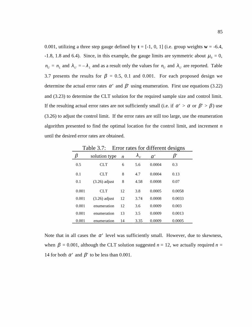
85

0.001, utilizing a three step gauge defined by t = [-1, 0, 1] (i.e. group weights w = -6.4,

-1.8, 1.8 and 6.4). Since, in this example, the gauge limits are symmetric about µ0 = 0,

nU = nL and λU = – λ L and as a result only the values for nU and λU are reported. Table

3.7 presents the results for β = 0.5, 0.1 and 0.001. For each proposed design we

determine the actual error rates ′α and ′β using enumeration. First use equations (3.22)

and (3.23) to determine the CLT solution for the required sample size and control limit.

If the resulting actual error rates are not sufficiently small (i.e. if ′α > α or ′β > β ) use

(3.26) to adjust the control limit. If the error rates are still too large, use the enumeration

algorithm presented to find the optimal location for the control limit, and increment n

until the desired error rates are obtained.

Table 3.7: Error rates for different designsβ solution type n λU ′α ′β

0.5 CLT 6 5.6 0.0004 0.3

0.1 CLT 8 4.7 0.0004 0.13

0.1 (3.26) adjust 8 4.58 0.0008 0.07

0.001 CLT 12 3.8 0.0005 0.0058

0.001 (3.26) adjust 12 3.74 0.0008 0.0033

0.001 enumeration 12 3.6 0.0009 0.003

0.001 enumeration 13 3.5 0.0009 0.0013

0.001 enumeration 14 3.35 0.0009 0.0005

Note that in all cases the ′α level was sufficiently small. However, due to skewness,

when β = 0.001, although the CLT solution suggested n = 12, we actually required n =

14 for both ′α and ′β to be less than 0.001.