Embed Size (px)
Citation preview
Quality Assessment Report:
NATIONAL CEILING AND VISIBILITY ANALYSIS PRODUCT
Tressa L. Fowler1, Anne Holmes1, Matthew J. Pocernich1, Jamie T. Braid1, Barbara G. Brown1, Jennifer Luppens Mahoney2
1National Center for Atmospheric Research, Boulder, Colorado
2 Forecast Systems Laboratory, NOAA, Boulder, Colorado
Quality Assessment Product Development Team
FAA Aviation Weather Research Program
May 2005

2
Table of Contents
SUMMARY ………………………………………………………………………………… 4
1 INTRODUCTION...................................................................................................... 5
2 DATA ....................................................................................................................... 6
2.1 NCV analysis product ........................................................................................... 6
2.2 METARs ............................................................................................................... 8
3 METHODS ............................................................................................................. 10
3.1 Matching the gridded NCV product to METAR sites.......................................... 10
3.2 Cross-validation.................................................................................................. 11
3.3 Verification statistics ........................................................................................... 12
4 RESULTS .............................................................................................................. 13
4.1 Flight category results from cross-validation analyses ....................................... 14
4.2 Ceiling results from cross-validation analyses.................................................... 15
4.3 Visibility results from cross-validation analyses.................................................. 21
5 DISCUSSION AND CONCLUSIONS..................................................................... 26
Appendix: Results for Operational Product………………………………………...…28

3
Table of Figures
Figure 1: Example of NCV analysis product.................................................................... 8
Figure 2: Map showing METAR sites across the CONUS............................................... 9
Figure 3: Histogram showing error in ceiling height (METAR – NCV). .......................... 16
Figure 4: Quantile-quantile plot showing distribution of NCV vs. METAR ceiling values
on log-log scale. ...................................................................................................... 17
Figure 5: Boxplots of METAR ceiling below 20K ft by range of NCV ceiling (ft). ........... 19
Figure 6: Boxplots of METAR ceiling below 6K ft by range of NCV ceiling (outliers
eliminated)............................................................................................................... 20
Figure 7:Contour plot showing density of METAR and NCV ceiling pairs. .................... 21
Figure 8: Quantile-quantile plot showing relationship between distributions of METAR
and NCV visibility fields. .......................................................................................... 23
Figure 9: Histogram of errors in the NCV visibility field (METAR – NCV). ..................... 24
Figure 10: Boxplots showing METAR visibility values for categories of NCV visibility... 25
Figure 11: Boxplots of NCV visibility (mi.) by METAR visibility category (mi.) ............... 26
Figure A: An example of AIRMETs ............................................................................... 30

4
SUMMARY The National Ceiling and Visibility (NCV) Analysis Product combines surface
observations with satellite data to produce analyses of current ceiling and visibility
conditions. The quality of the resulting product was evaluated, and the results of the
evaluation are detailed in this report.
The NCV analysis product was evaluated over the winter of 2004/2005 and is
compared with measurements from routine aviation weather reporting sites. The results
are summarized via standard verification statistics and presented through a variety of
plots. For purposes of comparison, the statistics for the operational ceiling and visibility
aviation advisories are also included.
The results of this evaluation indicate that the NCV visibility field matches well with
the visibility observations. The NCV ceiling matches less well with the ceiling
observations and is somewhat biased. Further improvements to the NCV analysis
product should probably include some adjustment of the ceiling values to reduce the
bias.
Overall, the NCV analyses are skillful. When the NCV product is compared to the
operational ceiling and visibility advisories, the two forecasts perform differently in
determining flight categories, but with roughly equal skill, each having better statistics
than the other on some of the included measures. The NCV product shows promise for
future operational use to identify ceiling and visibility conditions.

5
1 INTRODUCTION
With funding from the Federal Aviation Administration’s Aviation Weather
Research Program, the National Ceiling and Visibility Product Development Team has
developed an initial product to analyze and forecast ceiling and visibility on a grid across
the continental U.S. (CONUS). The diagnostic capabilities of the National Ceiling and
Visibility (NCV) analysis field are evaluated in this report as part of the process of
determining whether this product should be granted “experimental” status through the
FAA and National Weather Service (NWS) Aviation Weather Technology Transfer
(AWTT) process. The NCV forecast product will be evaluated at a later date. Note that
the AWTT defines experimental products as those products that “show promise” to
become useful operational products in the future.
Performance of the NCV analysis product is evaluated for the fall/winter of
2004/2005 over the CONUS. The ceiling and visibility visual and instrument flight rule
categories defined for aviation safety are the primary focus of the evaluation, but the
accuracy and skill of the ceiling and visibility components are also examined separately.
Because the algorithm provides an analysis of ceiling and visibility conditions (i.e. as
opposed to a forecast), the performance will be nearly perfect at the observation
locations. Thus, this evaluation focuses on performance at locations between
observation sites, using a cross-validation method (see Section 3).
Section 2 of this report describes the data used in the analyses. In Section 3, the
evaluation methodology is discussed, and the results are presented in Section 4.
Finally, Section 5 contains the discussion and conclusions. The appendix contains
information and statistics for the operational advisories.

6
2 DATA
For this study, NCV hourly analyses and surface ceiling and visibility observations
(METARs) over the CONUS during the period 25 October 2004 through 18 January
2005 are examined. These datasets are described in more detail in the following
subsections.
2.1 NCV analysis product
The NCV analysis product is a ceiling and visibility diagnostic that combines
observational data from satellite and surface observations to produce an analysis of
ceiling and visibility conditions on a grid across the Continental U.S. To produce ceiling
and visibility diagnoses operationally, forecasters subjectively examine these datasets
and use established "rules of thumb" to reach conclusions about ceiling and visibility
conditions that might be hazardous to aircraft. The NCV algorithm interpolates surface
observations and satellite information to produce a grid of ceiling and visibility values.
The current version of the NCV analysis produces these ceiling and visibility values on a
two-dimensional grid corresponding to the horizontal grid structure of the Rapid Update
Cycle (RUC; Benjamin et al., 2001) numerical weather prediction model. The NCV
analysis product uses ceiling and visibility observations to determine ceiling and visibility
values at the observation sites, and then applies an interpolation scheme to estimate
ceiling and visibility values between sites. The product is updated hourly as each new
RUC model run is available and again each 15 minutes thereafter as new satellite
information becomes available. However, for this report, only the analyses produced on

7
the hour, with both updated RUC and satellite information are evaluated for the period
25 October 2004 through 18 January 2005.
The ceiling and visibility values from the NCV product are converted into flight
categories using the rule set in Table 1. The lowest of the ceiling and visibility conditions
determine the flight rule. For instance, if the ceiling is 800 ft and visibility is 6 mi. the 800
ft ceiling causes the flight rule to be IFR.
Table 1: Flight Rules and Associated Ceiling Levels and Visibility Limits. Flight Rules (FR) Ceiling (ft) Visibility (s mi)
Visual (VFR) ceiling > 3000 visibility > 5 Modified Visual (MVFR) 1000 ≤ ceiling ≤ 3000 3 ≤ visibility ≤ 5 Instrument (IFR) 500 ≤ ceiling < 1000 1 ≤ visibility < 3 Low Instrument (LIFR) ceiling < 500 visibility < 1
An example of the NCV analysis product is shown in Figure 1. Note that the
product has a speckled appearance in some locations, for example, west of the Great
Lakes. Each individual grid point on the NCV analysis grid is treated separately in the
verification process, and there is no need for the flight category at one grid point to
correspond in any way to the points around it. In fact, some IFR-or-worse conditions
exist at a single location which is surrounded by less severe conditions.

8
Figure 1: Example of NCV analysis product.
2.2 METARs
Surface observations of ceiling and visibility, which are available in METARs
(Aviation Routine Surface Weather Reports), are used to evaluate the NCV analysis
product. The METARs measure ceiling in hundreds of feet near the surface and
thousands of feet at higher levels. Similarly, visibility measures are given in fractions of
a mile for lower visibility values, and in whole miles for higher visibility values.
Observations are taken at least once per hour, though special or changing weather
conditions can result in more frequent observations.
9
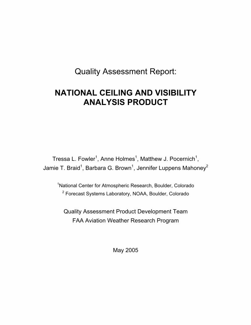
During the time period of interest, approximately 1600 METAR stations across the
CONUS gave reports of ceiling and visibility values. Figure 2 shows the locations of
these stations. Some states, such as North Carolina and Iowa, have a dense network of
METAR stations. Other states, like Nevada and Montana, have a sparse network. Still
other states, like California and Texas, have many stations located in the vicinity of
metropolitan areas but relatively few stations in the remaining areas.
Figure 2: Map showing METAR sites across the CONUS.
The verification statistics may be impacted by the station density. For example, the
San Francisco Bay area has several stations while the coast just north of this area has
very few. Correctly identified IFR-or-worse conditions will be rewarded by more correct
matching observations near San Francisco than along the more northerly coast. Thus,

10
conditions in areas with a great density of stations are naturally given somewhat more
weight in the statistics than conditions in areas with fewer stations.
Recently, most U.S. METAR stations have been converted from human observing
systems to Automated Surface Observing Systems (ASOS) (Bradley and Imbembo
1985; US DoC 1992). However, some stations still have observations from a human
observer. Thus, the METARs may have some internal inconsistencies. While
inconsistencies such as these are commonplace in meteorological observations,
awareness of such issues is essential when interpreting results.
3 METHODS
3.1 Matching the gridded NCV product to METAR sites
The NCV analysis product is matched to the METAR observations. For each
METAR location to be used in verification, the minimum ceiling and visibility
measurements from the four surrounding grid points from the NCV analysis grid are
selected. In particular, for each variable (ceiling and visibility) the minimum value from
one of the four surrounding grid points on the NCV analysis grid is matched to the
ceiling/visibility measurement from the METAR station observation to create a
verification pair. The ceiling and visibility measurements may come from different
gridpoints. Since the NCV product is on the RUC 20-km grid, the maximum distance
between a METAR site and its matching grid location for the NCV analysis is less than
30 km.

11
3.2 Cross-validation
A cross-validation technique (Neter et al. 1996) was applied in the evaluation of the
NCV analyses to ensure independence between the METAR stations used for
verification and those used to create the product. Because the NCV analysis product
uses METAR observations to determine ceiling and visibility values at the METAR sites,
verification using the same METAR observations as were used to create the analysis
would produce perfect verification statistics. In particular, in this case, the METAR
observations would serve as both nowcasts and observations. The METARs will always
match themselves exactly. Thus, the goal of this study is to evaluate the performance at
analysis locations between METAR locations. The cross-validation approach makes this
evaluation possible.
Using the cross-validation approach, 1300 METAR reports (referred to as the
training set) out of nearly 1600 METAR sites, were randomly selected to produce each
NCV analysis. The remaining 300 METAR stations (referred to as the testing set) were
used to verify the product. In order to prevent a “bad” selection of METAR sites from
affecting the statistical results, and to ensure that enough locations were chosen for
verification, this procedure was repeated ten times for each analysis time to provide ten
different testing/training METAR sets. Thus, ten different NCV analyses were produced
at each time: one for each of the ten training sets. The verification statistics are based
on the ten testing sets of METAR reports, accumulated across all of the NCV analyses
included in the verification sample.1,2
1 A smaller number of METAR sites may be available at any given time for producing or verifying the analysis in the event of sensor or data outages.

12
Since ten different cross-validation versions of the NCV analyses were produced
on each hour during the 25 October 2004 to 18 January 2005 time period, a total of
20,140 NCV analyses are available for verification.
3.3 Verification statistics
Overall verification statistics are calculated based on binary event/non-event
categories. The four flight categories listed in section 2.1 are condensed into two by
combining the bottom and top two categories, yielding the categories IFR or worse and
MVFR or better. The verification statistics computed include the probability of detection
(POD), the probability of detection for non-events (PODNo), Bias, and the False Alarm
Ratio (FAR). In addition, three skill scores are included: (a) the Heidke Skill Score
(HSS), (b) the Gilbert Skill Score (GSS), and (c) the True Skill Statistic (TSS). The
percent of the CONUS covered by the average event area (Percent Area) is used as a
measure of over-warning. Finally, the POD per unit area, known as Area Efficiency, is
also included. Each statistic is calculated using the formulas listed in Table 3, based on
a standard 2 by 2 contingency table as shown in Table 2.
Table 2: Standard 2x2 contingency table for verification statistics. Entries in the table represent counts of each forecast/observation pair.
METAR Flight Category
NCV Flight Category IFR or worse MVFR or better
IFR or worse YY YN
MVFR or better NY NN
2 The results of the verification study may be somewhat sensitive to the proportion of “held-out” stations. Although this sensitivity is not expected to be large, it may have some impact on the results and is currently being investigated further.

13
Table 3: Verification statistics and their associated formulas based on counts from Table 2.
Statistic Formula
POD YY / ( YY + NY )
PODNo NN / ( NN + YN )
Bias (YY + YN) / (YY + NY)
FAR YN / ( YN + YY )
HSS (YY + NN – C1) / (N – C1) { where C1 = [ (YY + YN) (YY + NY) + (NY + NN) (YN + NN) ] / (YY + YN + NY + NN) }
GSS (YY– C2) / (YY - C2 + YN +NY) [ where C2 = (YY + YN) (YY + NY) / (YY + YN + NY + NN) ]
TSS POD + PODNo -1
Percent Area Average Event Area * 100 / Total CONUS Area
Area Efficiency 100 * POD / Area
The actual ceiling and visibility values are examined separately as well. In
particular, the bias in the NCV ceiling and visibility values is assessed. Boxplots,
histograms, and a contour plot (essentially a 3-dimensional scatter plot) are used to
examine errors in and agreement between NCV and METAR values. Quantile-quantile
(qq) plots are used to compare the distributions of NCV versus METAR values. Linear
models are overlaid on the qq-plot to quantify the differences in distributions.
4 RESULTS
The verification results are summarized by flight category using the 2x2 verification
statistics. In addition, actual values of ceiling and visibility are examined using
exploratory analysis techniques.

14
4.1 Flight category results from cross-validation analyses
Verification statistics for the NCV analysis product are provided in Table 4. The
NCV analysis achieves a POD of 0.57 and PODn of 0.97. The NCV product has a low
false alarm ratio (0.19). On average, the NCV analysis product covers roughly 17% of
the CONUS. The bias of 0.7 indicates that the NCV product identifies IFR-or-worse
conditions about 30% less often than they occur. The NCV product has positive skill, as
indicated by the HSS, GSS, and TSS values. Should a standard of comparison be
desired, these statistics computed for the operational advisories (AIRMETs) are
available in the appendix.
Table 4: Verification statistics for the NCV analysis product.
POD POD No FAR Bias HSS GSS TSS Percent
Area Area
Efficiency
0.57 0.97 0.19 0.70 0.60 0.43 0.54 17 35
When examining the statistics in Table 4, it is important to remember that these
statistics represent the algorithm performance between METAR stations. The POD at
the METAR locations included in the analysis is close to 1 and the FAR is close to 0.
Verification statistics were also computed separately for day and night. However,
the results differed very little from each other and from the overall results presented in
Table 4. Thus, those statistics have been excluded from this report since they contain
no new information.

15
4.2 Ceiling results from cross-validation analyses
For this analysis, METAR observations and NCV analyses of ceiling (again, at
locations between the stations included in the product) are compared. In the majority of
cases, about 6.6 million, the ceiling heights observed from the METAR reports and
analyzed by the NCV are “unlimited”. Since these correctly identified non-event cases
are the least interesting and are difficult to analyze since “unlimited” is not a numeric
value, they are excluded from this analysis. Only cases that have measurable NCV or
METAR ceilings are examined, resulting in over 4 million cases. However, this large
sample size is often difficult to examine, so a random selection of 10,000 cases was
used for some of the analyses and displays.
Ceiling observations are censored at 20K ft. Thus, any observation or forecast for
ceilings above 20K ft is set to 20K ft. Censoring prevents large but meaningless
differences, say between 25K ft and 35K ft, from overwhelming the analyses.
Furthermore, when instruments are used to measure ceiling, the ceiling height is often
capped, which is not the case with a human observed ceiling. By censoring the data,
the instrument and human observations are more likely to be consistent.
A histogram of errors in the ceiling field (METAR – NCV) is shown in Figure 3. The
great majority of the errors are small, typically less than one thousand feet. However,
the negative skew in the histogram indicates that the NCV analysis is more likely to
indicate the ceiling is too high than too low. In other words, the NCV product is biased
toward higher ceilings than are observed. The average error is -1417 feet while the
median error is -348 feet, also indicating that the NCV product typically tends to produce
somewhat higher ceilings than are observed.

16
Figure 3: Histogram showing error in ceiling height (METAR – NCV).
A quantile-quantile (qq) plot shown in Figure 4 compares the distributions of NCV
and METAR ceiling fields on a log-log scale. This type of plot shows the relationships
between the overall distributional characteristics of each variable (e.g., the range,
variance) rather than characteristics of their individual differences. The vertical stacks of
values on the lower left of the plot, near the origin, are due to the discreteness of the
METAR ceiling values, which is especially noticeable near the surface on the log scale.
Multiple NCV ceiling points match each discrete METAR ceiling value at those levels.
If the distributions of these two fields were identical, all points would fall along the
one-to-one line. Instead, the points are shifted almost linearly above the line. This result

17
indicates that (in the original scale) the distribution of the NCV ceiling field is
approximately the same as the distribution of the METAR ceiling field except that it is
shifted higher (by about 0.65, the intercept of the linear model shown in the figure) in the
log-log scale. Thus, in the original scale, the NCV ceiling distribution is approximately
the same as the METAR ceiling distribution times 1.9 (e0.65).
Figure 4: Quantile-quantile plot showing distribution of NCV vs. METAR ceiling values on log-log scale.
At each end of the distribution, the points are somewhat non-linear. At the bottom
end, this is probably due to the discreteness of the METAR measurements rather than
any real difference in the distributions of ceiling values. However, at the top end, the
departure from linearity implies that the difference in NCV and METAR ceiling values

18
are even larger than would be expected based on the estimated shift of the rest of the
distribution (i.e., the NCV product is even more biased in the higher ranges).
Figure 5 shows boxplots3 of the NCV ceiling versus the observed METAR ceiling for
cases in which at least one of the METAR or NCV ceilings were less than unlimited,
stratified by the NCV analysis ceiling value. Uneven ranges of NCV ceiling values were
used in this plot for two reasons. First, operationally, it is more important to distinguish
between lower ceiling values than higher, so the lower ranges are smaller and the
higher ranges are larger. Second, the great majority of the ceiling measurements are
concentrated at lower levels, so the boxes representing the lowest three altitude ranges
represent approximately the same number of cases in spite of their differing altitude
ranges. Some outliers extend up to 20K ft, where the measurements are censored.
3 Box plots show the distribution of values. The line at the center of each box is the median, while the top and bottom of the box represent the 75th and 25th percentiles, respectively. Thus, the box shows the range of the center half of the data. The whiskers extend to the maximum and minimum values that are not outliers, each showing the range of the top and bottom quarters of the data. The dots above or below the whiskers are outliers. The width of each box is scaled to the number of cases represented by that category. Thus, narrower boxes represent fewer cases than wider boxes.

19
Figure 5: Boxplots of METAR ceiling below 20K ft by range of NCV ceiling (ft).
With over 4 million observations used to create this graphic, the outliers represent a
very small number of cases; thus, it is informative to focus on the bulk of the
observations (i.e. the boxes) below 6K ft. A similar graphic, with the outliers removed, is
shown in Figure 6. Ideally, the boxes should be centered along the diagonal line from
the lower left corner to the upper right corner. Although the boxes do not follow the
diagonal, the first three do increase from left to right. The box for the NCV ceiling
measurements of 10-20K ft generally corresponds to lower METAR ceiling values. The
last box, for unlimited NCV ceiling values, is based on too few cases to be meaningful.
However, typically when the NCV ceiling value was unlimited, the associated METAR
value was also unlimited.

20
Figure 6: Boxplots of METAR ceiling below 6K ft by range of NCV ceiling (outliers eliminated).
A contour plot of the density of a random sample of 100,000 ceiling observations
below 5,000 ft is given in Figure 7. Areas with a great number of points are shaded in
warmer colors. Cooler colors indicate areas with fewer points. This plot is an alternative
to a scatter plot. In a scatter plot, the areas with warm colors would be an
indecipherable mass of points; the blue areas would have some points and the purple
areas would be nearly empty. Ideally, warm colors should fall along the one-to-one line
(in red) with cooler colors filling the remaining areas of the plot, which would indicate a
good correspondence between the NCV analysis ceiling values and the observed
ceilings provided by the METARs. Indeed, this is nearly the case as shown by the warm
colors located along the diagonal. To the upper left of the one-to one line, there is an

21
area with a small group of points in dark blue. These points are those for which the NCV
product gave slightly higher ceiling values than were observed by the METAR.
Figure 7: Contour plot showing density of METAR and NCV ceiling pairs.
4.3 Visibility results from cross-validation analyses
This section presents a comparison of METAR and NCV visibility values, again for
locations representing the interpolation points between METAR stations. Once again,
more than 6 million cases where both the METAR and NCV reported “unlimited”
visibility were excluded from this analysis. Visibility measures are censored at 10 miles,
as visibility greater than ten miles is essentially considered unlimited.

22
A quantile-quantile (qq) plot, provided in Figure 8, compares the distributions of
the NCV analyzed visibility and observed visibility from the METAR. If the distributions
of these two measures are the same, then the points on this plot will fall along the one-
to-one line. Although the discreteness of the METAR measurements makes this nearly
impossible, the two distributions are very similar as most of the points fall near to the
one-to-one line. The slope of the linear model fit to these points is about 0.8, not quite
the slope of one that would indicate perfect agreement. The NCV visibility field
somewhat overestimates visibilities on the lower end and underestimates them on the
higher end, resulting in a slightly narrower distribution of values than is observed. This is
fairly common behavior when measurements are created using linear methods, such as
those used to derive the NCV visibility field.

23
Figure 8: Quantile-quantile plot showing relationship between distributions of METAR and NCV visibility fields.
The histogram in Fig. 10 shows the relative frequencies of the visibility errors
(METAR – NCV) for cases in which at least one of the two visibility values (METAR or
NCV analysis) is less than unlimited. The great majority of the errors in the visibility field
are small, less than 1 mile. Further, the errors appear approximately symmetrical,
indicating that the NCV is relatively unbiased (i.e., it is not likely to consistently over- or
under-estimate the visibility, overall).

24
Figure 9: Histogram of errors in the NCV visibility field (METAR – NCV).
Figure 10 shows boxplots of NCV and METAR visibility. The center lines of the
boxes (i.e. the medians) tend to fall along the diagonal line from the lower left to the
upper right. This result indicates that the NCV visibility analysis roughly corresponds to
the measured METAR visibility. The spread, or variability, as measured by the height of
the boxes increases as the visibility increases. This common behavior indicates that the
uncertainty in the NCV visibility increases as the NCV visibility value increases (i.e.,
smaller values are more certain than larger values).

25
Figure 10: Boxplots showing METAR visibility values for categories of NCV visibility.
Figure 11 shows a similar plot to Figure 10, with the axes switched. Again the
centers of the boxes tend to increase from left to right as they should, indicating that
typically, the observed and analyzed data agree well. However, the spread (i.e.,
variability) of the NCV visibility does not increase as the observed visibility value
increases, it stays about the same. Thus, the confidence interval around the NCV
visibility value is about the same regardless of whether a user observes high or low
visibility conditions.

26
Figure 11: Boxplots of NCV visibility (mi.) by METAR visibility category (mi.)
5 DISCUSSION AND CONCLUSIONS
This study used a cross-validation approach to evaluation the performance of the
NCV analysis algorithm at interpolated locations between METAR stations. Overall
results indicate that the algorithm is skillful at these locations, with somewhat varying
performance depending on the component being evaluated.
The analyzed NCV visibility field closely matched the observed METAR visibility at
all levels, as indicated by the small errors in the results and matching distributions.
Overall, the analyzed NCV ceilings matched well with the METAR ceilings, especially
when ceilings were unlimited or below 10K ft. However, the NCV analyzed ceiling field
is biased, producing higher ceiling values than are typically observed. For instance,
when the NCV ceiling field is between 10 and 20K ft, the matching METAR ceiling was
often below 5K ft.

27
The flight category verification statistics are somewhat mixed. As shown by the
bias, the NCV analyses under-identify IFR events. The false alarm ratio is very low and
the product does a good job of detecting events and a great job of detecting non-events.
With these caveats, the NCV analysis product shows positive skill in identifying
IFR conditions and ceiling and visibility values, and thus it shows promise for future use
as an operational tool.
ACKNOWLEDGEMENTS
This research is in response to requirements and funding by the Federal Aviation Administration (FAA). The views expressed are those of the authors and do not necessarily represent the official policy of the FAA.
REFERENCES
Benjamin, S. J. and G. A. Grell, S. S. Weygandt, T. L. Smith, T. G. Smirnova, B. E. Schwartz, D. Kim, D. Devenyi, K. J. Brundage, J. M. Brown, and G. S. Manikin, 2001: The 20-km version of the RUC. 14th Conference on Numerical Weather Prediction, Ft. Lauderdale, FL. Amer. Meteor. Soc., Boston
Bradley, J.J. and Imbembo, S.M., 1985: "Automated Visibility Measurements for Airports," American Institute of Aeronautics and Astronautics: Preprints, Reno, NV.
Neter, J., M. H. Kunter, C. J. Nachtsheim, and W. Wasserman, 1996: Applied Linear Statistical Models. McGraw Hill / Irwin, Chicago, Ill.
NWS, 1991: National Weather Service Operations Manual, D-22. National Weather Service. (Available at Website http://wsom.nws.noaa.gov ).
Petty, K., A. Bruce Carmichael, Gerry M. Wiener, Melissa A. Petty, and Martha N.
Limber, 2000: A fuzzy logic system for the analysis and prediction of cloud ceiling and visibility. Ninth Conference on Aviation, Range, and Aerospace Meteorology. Orlando, FL. September. Amer. Meteor. Soc., Boston, 331-333.
Takacs, A., L. Holland, M. Chapman, B. Brown, T. Fowler, and A. Holmes, 2004: Graphical turbulence guidance 2 (GTG2): Results of the 2004 post analyses. Quality Assessment Report. Report to the FAA, October 2004.
U.S. Dept. of Commerce, NOAA, 1992: ASOS Users Guide, Government Printing Office
28
Appendix: Results for Operational Product
For the purposes of comparison, the operational advisories of ceiling and visibility
conditions (i.e., AIRMETs) have been evaluated at the same METAR stations and using
the same methods as the NCV analysis product. The results of the evaluation are
detailed in this appendix and compared and contrasted with the results for the NCV
analysis product.
AIRMETs are the operational 0-to-6 hour forecasts of IFR-or-worse flight
conditions. The AIRMETs are an advisory issued when expected ceilings are below
1,000 ft and/or expected visibility is below 3 mi. The AIRMETs are issued every six
hours and are often amended or canceled when ceiling and visibility conditions change
during the forecast period. Furthermore, an AIRMET must cover a minimum area of
3,000 sq. mi. in which the conditions are expected to cover most of the forecast area
(NWS 1991). In this regard, the AIRMETs are quite different from the NCV analysis,
which only attempts to analyze current conditions at points on a grid. Figure A shows an
example of some AIRMET polygons (outlined in red). The METARs have been overlaid
in Fig. A in green (for IFR-or-worse conditions) and purple (for VFR-or-better
conditions).

29
Figure A: Example map of CONUS showing IFR AIRMETs (outlined in red; solid polygon shapes) and METARs (IFR conditions in green, VFR in purple).
To establish a baseline for the flight category comparison, the results for the NCV
analysis product can be compared to those computed for the AIRMETs. However, the
basic differences between the two products must be kept in mind when considering
these comparisons; for example, AIRMETs are forecasts of ceiling and visibility
conditions for a six-hour period, while the NCV is an analysis of current conditions.
When a gridded forecast verification strategy is employed, a smoother forecast will often
achieve better statistics than a less smooth forecast even when the smoother forecast is
less useful and/or less skillful. (e.g., Takacs et al, 2004). The AIRMETs are required to
be a smoother product, while the NCV analysis may or may not produce smooth areas.
This phenomenon should be kept in mind during interpretation of these results.

30
Verification statistics for the NCV analysis product as compared to the AIRMETs
are provided in Table A. The NCV analysis achieves a lower POD (0.57 vs. 0.83) and
higher PODn (0.97 vs. 0.81) as compared to the AIRMETS. The NCV product has a
much lower false alarm ratio than the AIRMETs (0.19 vs. 0.43). On average, the NCV
analysis product covers roughly 75% of the area covered by the AIRMETs. Both
products are quite biased, but in opposite directions. The NCV product has a bias of
0.7, and thus identifies IFR-or-worse conditions less often than they occur. The
AIRMETs’ bias is 1.45, so they identify these conditions more often than they occur.
The minimum size and time restrictions placed on the AIRMETs almost require an over-
warning bias. Thus, the bias statistic for the AIRMETs should be viewed as a
characteristic rather than a performance measure. The NCV product has slightly larger
values of both the HSS and the GSS than the AIRMETs, but a smaller TSS value. The
area efficiencies of the two products are roughly comparable, 35 for the NCV vs. 39 for
the AIRMETs.
Table A: Verification statistics for the NCV analysis product and the AIRMETs.
POD POD No FAR Bias HSS GSS TSS Percent
Area Area
Efficiency
NCV 0.57 0.97 0.19 0.70 0.60 0.43 0.54 17 35
AIRMETs 0.83 0.81 0.43 1.45 0.55 0.38 0.64 22 39
The statistics in Table A indicate that the NCV analyses and AIRMETs perform
differently (thus the differing statistics) from each other, but with approximately equal
quality.