Qualitative Simulation* - Department of Computer Science · MCS-8303640 and DCR-8417934. ... nature of its decision criteria, ... We discuss the implications of these results for

ARTIFICIAL INTELLIGENCE 289

Qualitative Simulation*

Benjamin Kuipers D e p a r t m e n t o f C o m p u t e r Sciences, Universi ty o f Texas at

A u s t i n , A u s t i n , T X 78712, U . S . A .

Recommended by Johan de Kleer

ABSTRACT

Qualitative simulation is a key inference process in qualitative causal reasoning. However, the precise meaning of the different proposals and their relation with differential equations is often unclear. In this paper, we present a precise definition of qualitative structure and behavior descriptions as abstractions of differential equations and continuously differentiable functions. We present a new algorithm for qualitative simulation that generalizes the best features of existing algorithms, and allows direct comparisons among alternate approaches. Starting with a set of constraints abstracted from a differential equation, we prove that the OSIM algorithm is guaranteed to produce a qualitative behavior corresponding to any solution to the original equation. We also show that any qualitative simulation algorithm will sometimes produce spurious qualitative behaviors: ones which do not correspond to any mechanism satisfying the given constraints. These observations suggest specific types of care that must be taken in designing applications of qualitative causal reasoning systems, and in constructing and validating a knowledge base of mechanism descriptions.

I. Introduction

An expert system is often a "shallow model" of its application domain, in the sense that conclusions are drawn directly from observable features of the presented situation. Researchers have long felt that genuinely expert perfor- mance must also rest on knowledge of "deep models," in which an underlying mechanism, whose state variables may not be directly observable, accounts for the observable facts [13].

One major line of research toward the representation of deep models is the study of qualitative causal models [3-20, 24, 25]. Research on qualitative causal models differs from more general work on deep models in focusing on qualitative descriptions of the deep mechanism, capable of representing incom- plete knowledge of the s t ructure and behav io r of the mechan i sm. Symbol ic

* This research was supported in part by the National Library of Medicine through NIH Grants LM 03603, LM 04125, and LM 04374, and by the National Science Foundation through grants MCS-8303640 and DCR-8417934.

Artificial Intelligence 29 (1986) 289-338 0004-3702/86/$3.50 © 1986, Elsevier Science Publishers B.V. (North-Holland)

290 B.J. KUIPERS

manipulation of qualitative descriptions also appears to be a plausible model of human expertise [18, 19].

Qualitative causal reasoning consists of a number of different operations. A set of constraint equations describing the relevant structural relationships in a system may be derived by examination of its physical structure. The possible behaviors of the system may be predicted by qualitative simulation from the constraint equations and an initial state. The behavioral description may be used to explain a set of observations or the way a mechanism produces its behavior.

Researchers working in different problem domains have taken very different approaches to the derivation of constraint equations from physical structure. De Kleer and Brown [8] and Williams [25] describe a physical system in terms of components and connections. Constraint equations are derived from the component models and from the interaction paths provided by the connections. This point of view has led them to propose principles of good form, such as "no-function-in-structure," which states that component models must be formulated independently of the device contexts in which they will appear [8]. Studying naive physics reasoning about everyday physical situations, Forbus [12] determines the current set of active processes. The constraint equations are derived from the complete set of currently active processes. Working primarily in medical physiology, Kuipers [16, 19] treats constraint equations as given, either by textbook or experimental learning, but outside the scope of immediate causal problem solving.

The central inference within all of these approaches is qualitative simulation: derivation of a description of the behavior of a mechanism from the qualitative constraint equations. Differential equations provide a useful analogy (Fig. 1). A differential equation describes a physical system in terms of a set of state variables and constraints. The solution to the equation may be a function representing the behavior of the system over time. A description of structure in terms of constraint equations is a further abstraction of the same system, and qualitative simulation is intended to yield a corresponding abstraction of its behavior.

The goal of this paper is to clarify and formalize the qualitative mathematics behind the prediction of behavior from qualitative constraint equations. The results presented here apply across approaches to qualitative physics. The representation for constraints and behavior was originally described in [16]. The QSIM algorithm presented here replaces the previous ENV qualitative simulation algorithm. QsIM is both more efficient and more amenable to clear mathematical proof of correctness and limitations.

A theory and algorithm for qualitative reasoning must address several issues, which provides a framework for comparing the proposals of different researchers, and the contribution of this paper: - h o w quantities are described qualitatively,

QUALITATIVE SIMULATION 291

Physical Actual |

numerical or analytic solution , fi : ~ --*

Jv Qual ative qualitative simulation Beh ioral |

Constraints Description

Fro. 1. Qualitative simulation and differential equations are both abstractions of actual behavior.

- h o w state transitions are selected, - w h e t h e r quantities correspond to standard mathematical analysis, - w h e t h e r qualitative simulation produces all and only valid behaviors.

All qualitative simulation systems describe quantities in terms of their ordinal relations with a small set of landmark values. De Kleer, Bobrow, and Brown [6, 8] and Williams [24, 25] normally take the only landmark to be zero, and thus define three qualitative values, {+, 0 , - } . While they allow for the possibility of more complex quantity spaces, the definitions of addition and multiplication as operators over qualitative values do not extend usefully to the more complex situation, and all of their results use the " { + , 0, - } semantics." A nonzero landmark a of a quantity x can be accommodated by defining an auxiliary quantity y = x - a whose zero refers to the value x = a. Values defining operating region boundaries may also be used, but they are not part of the qualitative addition and multiplication operations.

Forbus [10, 12] and Kuipers [16] define a quantity space as a partially ordered set of landmark values, so that a quantity is described in terms of its ordinal relations with the landmarks. The Kuipers [16] approach is different from the others in allowing new landmarks to be discovered during the qualitative simulation, and used to define new qualitative distinctions. The QSIM algorithm presented here describes quantities in terms of a linearly ordered set of landmarks, but still allowing new landmarks to be discovered and inserted. In this paper, we demonstrate that without discovering and using new landmark values, important qualitative distinctions can be missed, such as the distinction between increasing, decreasing, and stable oscillation.

292 B.J. KU1PERS

Different qualitative simulation systems take different positions on whether quantities should be an abstraction of the standard mathematical notion of real numbers--in which case E is described as an alternating sequence of points and open intervals--or whether a nonstandard model should be used, allowing two points to be infinitesimally separated. Both Forbus [10, 12] and de Kleer and Brown [8] adopt nonstandard models of time in which "mythical" or "infinites- imal" time may separate qualitative states that correspond to the same physical point in time. Such sequences of states appear to be required when the computational inference cycle must run more than once to generate a state corresponding to the next physical state. De Kleer and Bobrow [6] adopt the standard model for quantities, but appear less committed to alternating points and intervals in the time domain. Kuipers [16] and Williams [24, 25] follow the standard model. As Williams' work and this paper demonstrate, the standard model makes it possible to state and prove useful theorems about the validity of the predictions made by qualitative simulation.

All qualitative simulation systems produce the set of possible behaviors by generating and filtering the set of possible transitions from one qualitative state description to its successors. Most systems simulate forward, by generating all possible successors of the current state; de Kleer, Brown, and Bobrow [6, 8] generate all possible qualitative states, then determine the valid transitions among them. De Kleer's approach can only succeed if there is a fixed set of qualitative values, so that the set of possible states can be generated in advance. In both cases, the filtering criteria are local: they depend on the quantities in the two state descriptions, and on the structural constraints.

An important class of filtering criteria are transition-ordering rules [6, 16, 25]. For example, if A + B = C with A, B, C > 0 , and B and C are approaching zero, then B must reach zero before C. A large number of these rules can be formulated, corresponding to different signs, directions of approach, and combinations of quantities approaching limits. In designing a system, it is difficult to be sure that all possible such rules have been captured; in implementing it, it is difficult to check that they have been written correctly. As described in Appendix B, all of the transition-ordering rules can be recognized as special cases of a simple test of valid relationships between the current values of a set of quantities and a set of corresponding values. These tests, applying to the ADD, MULT, M +, and M constraints, capture all single-constraint transition-ordering criteria of this type, can be implemented efficiently, and most importantly, can be straightforwardly proven correct.

All qualitative simulation systems predict multiple possible behaviors given certain sets of qualitative constraints and initial conditions. Researchers in this area (myself included) have hoped to prove that the predicted behaviors include all and only the possible behaviors of real mechanisms satisfying the given constraints. Half of this is correct: we prove below that qualitative simulation cannot miss any actual behavior. However, because of the local


nature of its decision criteria, qualitative simulation can predict behaviors that are not possible for any real mechanism satisfying the given description, and we construct a counterexample. We discuss the implications of these results for the construction of a qualitative causal reasoning system.

Qualitative simulation systems vary widely in speed, l In order to be useful as part of an expert problem solver, a qualitative simulation system must be efficient. The QSIM algorithm is very fast. Furthermore, experiments with semantic variants (e.g. the { + , 0 , - } semantics) can be made easily by changing the entries in a table of possible state transitions. It has been implemented in LISP on the Symbolics 3600, and all examples in this paper have been run, as well as numerous others in elementary physics and in medical physiology [20].

1.1. Overview

This section provides an overview of qualitative simulation and the QSIM algorithm. The concepts presented here are defined more formally below.

Qualitative simulation of a system starts with a description of the known structure of the system, and an initial state, and produces a directed graph consisting of the possible future states of the system and the "immediate successor" relation between states. The possible behaviors of the system are the paths from the initial state through the graph. After defining terminology, the next section discusses the constraints and behavior describing a simple mechanism in both informal and formal terms.

The structure of a system is described by a set of symbols representing the physical parameters of the system (continuously differentiable real-valued functions), and a set of constraint equations describing how those parameters may be related to each other. The constraints are two- or three-place relations on physical parameters. Some specify familiar mathematical relationships: DERIV(vel,acc), ADD(net,out,in), MULT(mass,acc,force), MINUS(fwd,rev). Others assert qualitatively that there is a functional relationship between two physical parameters, but only specify that the relationship is monotonically increasing or decreasing: M+(price,power) and M (mph,mpg). The constraints are designed to permit a large class of differential equations to be mapped straightforwardly into qualitative constraint equations.

Each physical parameter is a continuously differentiable real-valued function of time. Its value at any given point in time is specified qualitatively in terms of its relationship with a totally ordered set of landmark values. The landmark values may be either numerical (e.g. zero) or symbolic; their ordinal relationships are their essential properties. As the qualitative simulation proceeds, it can discover and add new landmark values to the sequence. The qualitative

~De Kleer, personal communication; Forbus, personal communication.

294 B.J. KUIPERS

state of a parameter consists of its ordinal relations with the landmark values and its direction of change.

Time, similarly, is represented as a totally ordered set of symbolic distinguished time-points. The current time is either at or between distinguished time-points. All of the time-points are generated as a result of the qualitative simulation process.

At a distinguished time-point, if several physical parameters linked by a single constraint are equal to landmark values, they are said to have corresponding values which can be discovered and used by the qualitative simulation. The special case of a monotonic function constraint with corresponding values (0, 0) is sufficiently common that it is signified by the constraints M~ and M o.

A set of constraints on the physical parameters of the system is only valid in some operating region, defined by the legal ranges of values that some parameters may take on. The legal range of a parameter is a closed interval whose endpoints are landmark values of that parameter. These endpoints may be associated with transitions to other operating regions where a different set of constraints apply.

The initial state of the system is defined by the operating region and a s~ of qualitative values for the physical parameters. The qualitative simulation proceeds by determining all of the possible changes in qualitative value permitted to each parameter, then filtering the combinations by applying progressively broader constraints. If more than one qualitative change is possible, the current state has multiple successors, and the simulation branches.

Two qualitative states in the same operating region are identical if all parameters are equal to the same landmark values, and all the directions of change are the same. If one of the successors to a given state is identical to a direct predecessor, a cyclic behavior can be created, resulting in a graph of states.

1.2. Example: The U-tube

A U-tube, consisting of two partially filled tanks connected at the bottom by a thin tube, is in equilibrium when an increment of water is added to one side (Fig. 2). The system reaches a new equilibrium with the level in both tanks higher than before.

Constraints - E a c h tank has a pressure which depends on its amount of water. - T h e rate of flow through the tube depends on the difference between the

pressures. - A flow through the tube increases the amount in one tank and decreases the

other.


o

©

A B

FIG. 2. The U-tube in equilibrium receives an increment of water.

Behavior - After the increment of water, the amount and pressure are increased in tank

A, leading to a flow from A to B. - W a t e r flows from A to B. The level in A falls, the level in B rises, and the

pressure difference and rate of flow approach zero. - T h e pressure difference and rate of flow become zero as the U-tube reaches

equilibrium with the level in both tanks higher than before the increment. Qualitative simulation determines the essentially different regions of the

system's behavior. It need not be given the initial levels nor the amount of the increment. It does not determine how high the level in A is increased, what its final position is, or how long the equilibration process requires. It does guarantee, however, that the level in A falls, the level in B rises, that neither tank returns to its initial level, and that a new equilibrium is reached. The parameters and constraints describing the structure of the U-tube are shown graphically in Fig. 3. The qualitative behaviors of the six parameters, responding to an increment of water, is shown by the six "qualitative plots" in Fig 4.

A qualitative plot graphically describes the qualitative behavior description of a parameter. The vertical axis represents the set of landmark values for that parameter; the only meaningful vertical positions are at, or midway between, landmark values. The horizontal axis is slightly more complex. Known states are shown first for reference, followed by the sequence of time-points. To reduce visual clutter in the plot, time-points are not labeled, though distinguished time-points are indicated by tick-marks on the axis, and other time- points are plotted midway between adjacent ticks. In Fig. 4, the four positions on the horizontal axis represent the known state NORMAL and the three time- points to, (to, t 1), and t 1. Although the plot of level(A) is horizontal from t o to (to, t l ) , its value is not constant. Rather, the qualitative state description of level(A) remains the same (i.e. between two landmarks and decreasing) while the underlying real value changes. The graphical conventions for qualitative behavior plots are somewhat unfamiliar, but the graphical output improves the comprehensibility of the output of qualitative simulation, and thus facilitates development and debugging of sets of constraints.

296 B.J. KUIPERS

FIG. 3. The constraints describing the structure of the U-tube.

" ~ HA*

l- . . . . . . . . . . . . . ~. . . . . . . . . . . . . . . . . . . . . . . . . . . . . . . . . . . . . t e N O R I q R L

level(A) I" ................. t . . . . . . . . . . . . . . . . . . . . . . . . . . . . . . . . . . . t

I d ~ I M N .

level(B) e

,4, . . . . . ~ . . .

I - . . . . . . . . . . . . {. . . . . . . . . . . . . . . . . . . . . . . . . . . . . . . . . . t IIORP~I.

pressure(A) F . . . . . . . . . . . . t . . . . . . . . . . . . . . . . . . . . . . . . . . . . t

pressure(B)

P B 1

p I l *

t

.4, . . . . . 4, .

pressure difference

I .4, ..... 4,.,. ........... E ................................ 2 . 0 .

flow rate(A->B} :1

FIG. 4. The behavior of the U-tube given an increment in tank A.


2. Qualitative Behavior

In the following sections, we present a more rigorous definition of qualitative simulation, leading up to a definition of the QsIM algorithm and the proof of several theorems characterizing its strengths and limitations. The validity proofs for several steps of the algorithm are contained in the appendices.

A physical system is characterized by a number of real-valued parameters, which vary continuously over time. We consider each physical parameter to be a function f : [a, b]---> ~*, where ~* = [ - ~ , ~], the extended real number line. The domain and range of a function f are both closed intervals in the extended reals, ~*. We use ~* instead of ~, treating ~ as a genuine landmark value, because it is useful (though not essential) to have the invariant that t and f(t) are always bounded by explicitly stated landmark values in the domain and range of f. The function f : [0, ~]--> ~* is defined to be continuous at ~ exactly if l i m , ~ f(t) exists. For example, both e - ' and e' are continuously differentiable on [0, ~], but sin t is not. This allows us to express asymptotic approach as a move to a limit, where the limit is reached at t = ~.

2.1. Behavior of a single function

We will define the qualitative behavior description first for a single, continuously differentiable function f : [ a , b]--> ~*.

Definition 2.1. For [a, b] C_ lt~*, define f : [a, b]--> ~* to be a reasonable function if

(1) f is continuous on [a, b], (2) f is continuously differentiable on (a, b), (3) f has only finitely many critical points in any bounded interval, (4) lim, ~,f '(t) and lim, r bf'(t) exist in ~*; define f '(a) and f ' (b) to be equal

to these limits. The restriction to finitely many critical points in any bounded interval

excludes examples like f(t) = t 2 sin 1/t that are continuously differentiable, but whose behavior changes infinitely quickly around t = 0. Without the fourth restriction, f '(t) can still behave pathologically around the endpoints of the interval, even without crossing zero.

Definition 2.2. Every reasonable function f : [ a , b]--> E* has associated with it a finite set of landmark values. The landmark values must include 0, f(a), f(b), and the value of f(t) at each of its critical points, and may include any number of additional values.

Definition 2.3. Where f is a reasonable function, t E [a, b] is a distinguished time-point of f if t is a boundary element of the set { t E [a, b] I f(t) = x, where x is a landmark value of f} .

298 ]E~. j. KUIPERS

That is, the distinguished time-points are those points where something important happens to the value of f, such as passing a landmark value or reaching an extremum. The restriction to boundary elements handles the case where f becomes constant over an interval: only the endpoints of the interval are distinguished time-points. De Kleer and Bobrow [6] eliminate this case by assuming that parameters have derivatives of all orders, in which case any function which is constant over an interval is constant everywhere.

All functions mentioned in the rest of this paper should be presumed reasonable unless specified otherwise. A reasonable function f :[a, b]--, ~* has the finite set of distinguished time-points:

a = t~j < t t < . • • < t , , = b ,

and the finite set of landmark values:

l~ < 1~ < • • • < l~ .

We can now define the qualitative state of f a t t in terms of its ordinal relations with its landmarks, and its direction of change.

We reluctantly contribute to the proliferation of notations for qualitative description of continuous functions. The advantages of the notation used here are that it (1) naturally allows for an arbitrary and changing set of landmark values, (2) uses a single term for the qualitative description of a function's magnitude and derivative, and (3) emphasizes that the qualitative description of the derivative is of low and fixed resolution, while qualitative description of magnitude is of higher and possibly changing resolution.

Definition 2.4. Let 11 < ' ' ' < l k be the landmark values of f : [ a , b]---~ ~*. For any tE[a, b], QS(f , t), the qualitative state o f f at t, is a pair (qval ,qdir) , defined as follows:

(1)

lj, if f(t) = lj, a landmark value,

qva l= (lj, l,+~), if flt) E(li, lj+,);

(2)

inc, if f ' ( t )>O,

qdir = std, if f ' ( t) =0 ,

dec, if f ' ( t )<O.

For example, QS(water-temp, now)= <(32°F, 212°F), inc).


Proposition 2.5. W h e r e a = t o < • • • < t,, = b are the d i s t ingu i shed t ime -po in t s o f

f , cons ider s, t @ (a, b) such that t i < s < t < ti+ l f o r s o m e i. Then QS(f , s) = Qs(L t).

Proof. By the Intermediate Value Theorem, since f is continuously differentiable, f ( t ) cannot pass a landmark value, and f ' ( t ) cannot change signs between adjacent distinguished time-points. []

This justifies our basic intuition that the qualitative state of the function is constant over intervals between landmarks. Hence, we may make the following definitions.

Definition 2.6. For adjacent distinguished time-points t i and t~+~, define QS(f , ti, t~+l), the qual i ta t ive state o f f on (t i, ti+l), to be QS(f , t) for any t E (t,, ti+,).

Definition 2.7. The qual i ta t ive b e h a v i o r of f on [a, b] is the sequence of qualitative states of f :

QS(f , to), QS(f , t 0, q) , QS(f , tl) . . . . . QS(f , t ,_ l , t ,) , QS(f , t ,)

alternating between qualitative states at distinguished time-points, and qualitative states on intervals between distinguished time-points.

2.2. Systems of functions

Definition 2.8. A s y s t e m is a set F = {fl . . . . , fro} of reasonable functions f : [ a , b]--->~*, each with its own set of landmarks and distinguished time- points. The dis t ingu i shed t ime -po in t s o f a s y s t e m F are the union of the distinguished time-points of the individual functions f, E F. The qual i ta t ive state

of a system F of m functions is the m-tuple of individual qualitative states:

QS(F, t,) = [QS(f~, t,) . . . . . QS(fm, t ,)] , QS(F, t,, t,+,) = [QS(fz, t,, t , + , ) , . . . , QS(fm, ti, t ,+,)].

If ti, and/or ti+ ~ are not distinguished time-points of a particular ~, then ti and the interval (ti, t~+ 1) must be between two distinguished time-points o f ~ , say t k and tk+ ~. Then QS(~ , t~) and QS(~ , t~, t~+~) are defined to be the same as the containing QS(f j , t k, tk+l). The qual i ta t ive b e h a v i o r of F is the sequence of qualitative states of F:

QS(F, to) , QS(F, to, t~), QS(F, tl) . . . . . QS(F, t , ) .

300 B.J. KUIPERS

These definitions give us a precise semantics for the qualitative description of continuous functions, and clarifies the concept of the "next state." Every state has a qualitative description QS(F, t), but that description changes only at discrete distinguished time-points, and remains constant on the open intervals between them. Thus the "next state" of a mechanism is more properly called the next distinct qualitative state description of the mechanism.

2.3. Qualitative state transitions

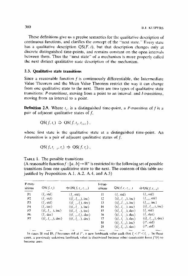
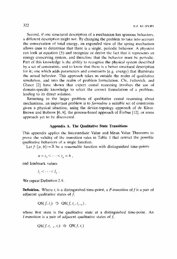
Since a reasonable function f is continuously differentiable, the Intermediate Value Theorem and the Mean Value Theorem restrict the way it can change from one qualitative state to the next. There are two types of qualitative state transitions: P-transitions, moving from a point to an interval, and I-transitions, moving from an interval to a point.

Definition 2.9. Where t~, is a distinguished time-point, a P-transition of f is a pair of adjacent qualitative states of f,

QS(f , t,) ~ OS(f, t,, t~+l),

whose first state is the qualitative state at a distinguished time-point. An I-transition is a pair of adjacent qualitative states of f,

OS(f , t~ ~, ti) ~ OS(f , t i ) ,

TABLE 1. The possible transitions (A reasonable function f : [a, b] ~ ~* is restricted to the following set of possible transitions from one qualitative state to the next. The contents of this table are justified by Propositions A.1, A.2, A.4, and A.5)

P-tran- l-transitions QS(J; L) ~ Q S ( f , ti, t i ~t) sitions QS(f, L, ti, ,) ~ Q S ( f , ti, ,)

P1 (lj. std) (lj. std) 11 (1,. std) ( / . std) P2 {/~. std) {(l/. lj,, ). inc) 12 ((l i, lj,, ). inc) (/j+ ,. std) P3 (lj, std) ((/j ~, lj), dec) 13 ((lj, Is+ ,), inc) (lj+ ,, inc) P4 (1,, inc) ((//,/j, ,), inc) 14 ((/j, l,+ ,), inc) ((/~,/~+ ,), inc) P5 ((I,, l,+ ,), inc) ( ( / , 1~ ,), inc) 15 ((l,, l,, ,), dec) (/,, std) P6 (l~, dec) ((1i_,, li), dec) 16 ((Ij, l , , ,) ,dec) (/j, dec) P7 ((l , , l , . , ) ,dec) ( ( / / , / / , , ) ,dec) 17 ((1,, 1,+ ~), dec) ( (6 , (+ , ) , dec )

18 ((l~, l~ ~), inc) (l*, std} 19 ((lj, l~+,),dec) (l*, std)

In cases 18 and 19, f becomes std at l*, a new landmark value such that lj < l* < lj+ ~. In these cases, a previously unknown landmark value is discovered because other constraints force f '(t) to become zero.


whose first state is the qualitative state on the interval between distinguished time-points.

Table 1 specifies the set of possible transitions that can take place in the qualitative behavior of a single function. The validity of this table is proved by the propositions in Appendix A.

3. Qualitative Structure

The structure of a mechanism may be described by a set of qualitative constraint equations applied to the parameters that represent the state of the mechanism. Simulation attempts to assign behaviors to the parameters. Con- straints holding between parameters in the structural description serve to limit the possible combinations of qualitative behavior. The constraint notation used here has the advantage, like de Kleer's confluences, of having a clear correspondence with differential equations by making explicit all the functions and operators in the equation.

Constraints are expressed as predicates rather than as functions for two reasons. First, they will be used as predicates in the QsIM algorithm to test the consistency of sets of qualitative values. Second, if a constraint were to be treated as a function, it is unclear how to define precisely the function's range. On the other hand, while keeping these semantic considerations in mind, the reader will probably find it clearer to read constraints as functions: mpg = M-(mph) rather than M-(mph,mpg).

3.1. Arithmetic constraints

Constraints corresponding to the basic arithmetic and differential operators are fundamental to a structural description.

Definition 3.1. ADD(f , g, h) is a three-place predicate on reasonable functions f, g, h :[a, b]--~ E* which holds iff f(t) + g(t) = h(t) for every t C [a, b].

Definition 3.2. MULT(f , g, h) is a three-place predicate on reasonable functions f, g, h:[a, b]--* ~* which holds iff f ( t ) . g(t) = h(t) for every t E [a, b].

Definition 3.3. MINUS(f, g) is a two-place predicate on reasonable functions f, g:[a, b]--~ R* which holds iff f(t) = -g( t ) for every tE[a , b].

Since addition and multiplication are commutative,

ADD(f , g, h) ¢:~ ADD(g, f, h), MULT(f , g, h) ¢:~ MULT(g, f, h) , MINUS(f, g) ¢:~ MINUS(g, f ) .

302 B.J. KUIPERS

Definition 3.4. DERIV(f , g) is a two-place predicate on reasonable functions f, g:[a, b]---> ~* which holds iff f '(t) = g(t) for every t ~ [a, b].

3.2. Qualitative function constraints

In describing the qualitative structure of a mechanism, one might need to state that one physical parameter is a function of another, without specifying the function completely. Rather, the relationship should be described qualitatively in terms of regions of monotonic increase or decrease, and landmark values passed through.

The most common and important cases are functional relationships that are strictly monotonic everywhere. The monotonic function constraint M ÷ applies in the situation when the function is strictly monotonically increasing, and M when it is decreasing. In fact, the definition is slightly more restrictive: the derivative of the function must be nonzero, except possibly at the endpoints of the domain.

Definition 3.5. M + is a two-place predicate on reasonable functions f, g : [a , b]--> I~*. M+(f, g) is true iff f(t) = H(g(t)) for all tE[a, b], where H is a function with domain g([a, b]) and range f([a, b]), differentiable and with H'(x) > 0 for all x in the interior of the domain. M is defined similarly, except that H'(x) < O.

The restrictions on H are motivated by two requirements. First, the critical points o f f and g must match across an M+(f , g) constraint. Second, it must be possible to break a function such as sin x "at the joints" into regions of monotonic increase and decrease, so H'(x)= 0 must be allowed at the boundary of the domain.

Clearly, M+(f , g)¢:> M+(g, f ) , and M - ( f , g)C:>M-(g, f ) . Note that M+(f , g) does not imply that f and g are monotonic functions on

[a, b]. For example, M+(2 sin t, sin t) holds on [0, 2"rr], where H(x)= 2x.

Proposition 3.6. Consider two continuously differentiable functions f, g: [a, b]---> [~*, where M+(f, g). Then for all tE(a, b),

f ' ( t )>O iff g'(t)>O, f ' ( t)=O iff g'(t)=O, f ' ( t)<O iff g'(t)<O.

Proof. M+(f , g) means that f(t) = H(g(t)), so f '(t) = H'(g(t)). g'(t). Since H'(x) > 0, g'(t)= 0 if and only if f ' ( t )= 0. The two strict inequalities follow from the monotonicity of H. []


Thus, the sets of distinguished time-points may not correspond precisely across f and g, but the subset of distinguished time-points which are critical points, and hence the regions of constant directions-of-change, are identical.

Although constraints for expressing monotonic relationships are used by all researchers on qualitative simulation, the precise definition of the constraint varies significantly. Kuipers [16] expresses an increasing monotonic relationship between X and Y as Y = M+(X) or M+(X, Y), meaning that there is some well-defined but unspecified function f with the desired properties, such that Y=f (X) . Forbus [12] uses the notation X~Q+Y, meaning that Y = f( . . . . X , . . . ) where the dependence of Y on X is monotonically increasing, all else held equal. The reason for this is that constraints are associated with processes, and only when the complete process configuration is known can the set of constraints be closed and the final dependencies computed. Thus, these qualitative proportionality constraints are implicitly added once the complete set is known. De Kleer, Brown, and Bobrow [6, 8] express the same relationship with the confluence aX = 0Y, meaning sgn dX/dt = sgn dY/dt. Strictly speaking, X(t) and Y(t) need not have any functional relationship at all, as long as the signs of their derivatives remain identical. The implications of these different definitions have not yet been fully explored. However, the correctness proof for the QSIM algorithm presented in this paper relies on the strong definition of the monotonic constraints M + and M .

A qualitative functional relationship need not be strictly monotonic if it can be divided into sections that are alternately increasing or decreasing monotonic, with critical points at the joints between sections. For example, suppose that x = c o s 0 for x E [ - 1 , 1 ] and 0E[0 ,2 r r ] . We may say that FC(0, x, descrip), where

descrip =

(0, 1) ((0, 'n'), (-1, 1), M-) (w, -1) ((~, 2'r¢), (-1, 1), M +) (2~, 1)

That is, if 0 = 0, x = 1; when 0 E (0, ~), then x E ( - 1 , 1) and M (0, x); and so on. At the joints between monotonic sections, the restrictions on permissible combinations of directions of change are weakened. In particular, it is possible for one parameter to have direction of change std while the other is inc or dec. Between the joints, qualitative simulation can treat an FC constraint exactly like the specified M + or M .

In a similar spirit, we may define S + and S- constraints, which behave like monotonic function constraints in the interval between two sets of corresponding values, and leave one parameter constant while the other is unconstrained

304 B.J. KUIPERS

outside that interval. It is not difficult to imagine other extensions such as "log-like," "polynomial-l ike," and "exponential-l ike" monotonic function constraints which support inferences about relative asymptotic magnitudes. These topics are beyond the scope of this paper.

3.3. Qualitative differential equations

The constraint definitions now allow us to define precisely the abstraction relation between qualitative constraint equations and ordinary differential equations (ODEs). If a mechanism can be described by an O D E meeting certain restrictions there is a corresponding but weaker set of qualitative constraint equations for the same mechanism. "Weaker" in this context means that any behavior that satisfies the ODE must satisfy the constraints, but not necessarily vice versa. Thus the constraints constitute a form of qualitative differential equation.

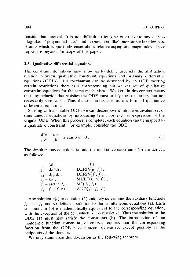
Starting with a suitable ODE, we can decompose it into an equivalent set of simultaneous equations by introducing terms for each subexpression of the original ODE. When this process is complete, each equation can be mapped to a qualitative constraint. For example, consider the ODE:

d2u du + arctan k u = O. (1)

dt 2 dt

The simultaneous equations (a) and the qualitative constraints (b) are derived as follows:

(a) (b) L =du/dt , DERIV(u, )"~), f2 = df~/dt, DERIV(f,, L), L = ku, Mt0LV(k, u, L) , f4 = arctan L , M+(L, f4), L - f , + L =0, ADD(L, L, f , ) .

Any solution u( t ) to equation (1) uniquely determines the auxiliary functions f~ . . . . . f4, and so defines a solution to the simultaneous equations (a). Each constraint in (b) is mathematically equivalent to the corresponding equation, with the exception of the M +, which is less restrictive. Thus the solution to the O D E (1) must also satisfy the constraints (b). The introduction of the monotonic function constraint, of course, requires that the corresponding function from the ODE have nonzero derivative, except possibly at the endpoints of the domain.

We may summarize this discussion as the following theorem.


Theorem 3.7. Let

F [ u ( t ) , u ' ( t ) . . . . . u~")(t)] = 0 (2)

be an ordinary differential equation of order n, to be satisfied by a function u:[a, b]--*E, where F is defined only in terms of the arithmetic operations addition, multiplication, and negation, along with functions of continuous and strictly nonzero derivative. Then a set of parameters and constraints can be defined, corresponding with (2), such that any reasonable function u:~--* which satisfies (2) also satisfies the set of constraints.

The procedure for decomposing an ODE into simultaneous equations can easily be specified so that each ODE generates a unique set of constraints. However, different functions may be mapped to the same M + constraint so a given qualitative differential equation can be the abstraction of multiple ODEs.

4. Qualitative Simulation

This section describes the QS|M qualitative simulation algorithm, and refers to the proofs of the various steps, appearing in the appendices.

4.1. Input and output

The qualitative simulation algorithm is given the following description of a mechanism.

(l) A set { f ~ , . . . , fm} of symbols representing the functions in the system. (2) A set of constraints applied to the function symbols: M+(f, g),

M - ( f , g), ADD(f , g, h), MULT(f , g, h), MINUS(f, g), or DERIV(f, g). Each constraint may have associated corresponding values for its functions.

(3) Each function is associated with a totally ordered set of symbols representing landmark values; each function has at least the basic set of landmarks { - ~ , 0, ~}.

(4) Each function may have upper and lower range limits, which are landmark values beyond which the current set of constraints no longer apply. A range limit may be associated with a new operating region which has its own constraints and range limits.

(5) An initial time-point symbol, to, and qualitative values for each of the fi at t o are given.

The result of the qualitative simulation is one or more qualitative behavior descriptions for the function symbols given. Each qualitative behavior description consists of the following:

(1) A sequence {t o . . . . , tn} of symbols represents the distinguished time- points of the system's behavior.

306 B.J. KUIPERS

(2) Each function fi has a totally ordered set of landmark values, possibly extending the originally given set.

(3) Each function has at each distinguished time-point or interval between adjacent time-points, a qualitative state description expressed in terms of the landmark values of that function.

4.2. The algorithm QSIM

The qualitative simulation algorithm, QSIM, repeatedly takes an active state and generates all possible successor states, filtering out states that violate some consistency criterion. Because it may not be able to determine the next state uniquely, QsIM builds a tree of states representing the possible behaviors of the mechanism.

Place the initial state on the list ACTIVE of states whose successors need to be determined. Repeat the following steps until ACTIVE becomes empty or a resource limit is exceeded.

Step 1. Select a qualitative state from ACTIVE. Step 2. For each function, determine (from Table 1) the set of transitions

possible from the current qualitative state. Step 3. For each constraint, generate the set of tuples (pairs or triples) of

transitions of its arguments. Filter for consistency with that constraint. Step 4. Perform pairwise consistency filtering on the sets of tuples associated

with the constraints in the system, applying the consistency criterion that adjacent constraints must agree on the transition assigned to the shared parameter.

Step 5. Generate all possible global interpretations from the remaining tuples. If there are none, mark the behavior as inconsistent. Create new qualitative states resulting from each interpretation, and make them successors of the current state.

Step 6. Apply global filtering rules to the new qualitative states, and place any remaining states on ACXIVE.

After an example, the individual steps of the algorithm are discussed in detail.

4.3. Example: The Bali system

To illustrate one cycle of the QsIM algorithm, consider a very simple system consisting of a ball thrown upward in a constant gravitational field. This section will demonstrate the derivation from its predecessor of the third qualitative state (t = t t), where the ball reaches its maximum height. The constraints are:

DERIV(Y, V ) , DERIV(V, A ) , A(t) = g < O.


Y

V

A

B~

Height

~ . u ~

-..¢ ..... ¢ ..... ¢

Velocity

F . . . . . . . . . . . . . . . . . . . . . -I . . . . . . . . . . . . . . . . . . . . . . . . $ . . . . . . . . . . . . . 0

- O - . . . . - O - . . . . - O - . . . . - O - . . . . - O - . . . . - O -

Accel lerat ion

FIG. 5. The ball thrown upwards: constraints and behavior.

Figure 5 shows a graphical representation of the constraints and a qualitative plot of the behavior of Y(t).

We start with an active state, t = (t 0, t]), whose description is:

QS(A, t o , t , ) = (g, s td ) , QS(V, t o, t,) = ((0, oo), d e c ) , QS(Y, t 0, t ,) = ((0, ~), inc) .

For each function, retrieve from Table 1 the set of possible qualitative state transitions from the current state of that function. Since the current state represents the time-interval (to, q) , only I-transitions are applicable. For simplicity, we exclude the possibility that Y(t 1) = ~, and so exclude transitions I2 and I3 from Y's list. Even without this assumption, the methods in Appendix A.2 would exclude these behaviors.

A II: (g , std) ~ (g, s td ) ;

V I5: ((0, oo), dec) ~ (0, s td ) , I6: ( ( 0 , ~ ) , d e c ) ~ (0, d e c ) , I7: ((0, oo),dec) ~ ((0, oo),dec), I9: ((0, oo),dec) ~ ( L * , s t d ) ;

Y I4: ( (O,~) , inc) ~ ((O, oo),inc), I8: ( (O,~) , inc) =), (L*, s td ) .

308 B.J. KUIPERS

Next, each constraint forms a set of transition tuples. Those marked with c are eliminated by constraint consistency filtering. For example, tuple (I4, |5) would require Y to continue to increase while V= 0, an obvious inconsisten- cy. Then those marked with w are eliminated by pairwise consistency filtering. The tuple (I4, I9) finds no remaining tuple associated with DERIV(V, A) that can agree that V might take transition I9.

D E R I V ( Y , V ) DERIV{V,A)

(I4, I5) c (I5, I1) c (I4, I6) c (I6, II) (I4,17) (IT, II) (I4, I9) w (I9, I1) c (I8, I5) w (I8, I6) (I8, I7) c (I8, I9) c

The remaining tuples can be formed into the following two global interpretations:

Y V A

14 I7 I1 I8 I6 I1

The first of these interpretations would leave states (t 0, t~), t~ and (t 1, t2) with identical qualitative state descriptions, and the problem of determining the state at t: would be precisely what we have just done. This possibility is already adequately described by the qualitative state over (t 0, t~), so we need not generate a successor state for it.

Every time-interval must have an endpoint (see Appendix A.2), so the only remaining possibility becomes the unique successor, defining a new landmark value for Y.

QS(A, t , ) = ( g, std) , QS(V, tl) = (0, dec) , QS(Y, t,) = ( Ym,x, inc) ,

The following sections explain the steps of the QSIM algorithm in detail and discuss the proofs of their validity.

4.4. Function consistency

The possible transitions that a single parameter can take from one qualitative


state to the next are given in Table 1. In Step 2, the current state of each function is used to retrieve the set of applicable transition patterns from Table 1. Constraints between neighboring functions are not considered until Step 3. Transitions are also checked against invariant assertions at this stage, to eliminate impossible transitions for functions that are (e.g.) always finite or never negative.

For any particular qualitative state, Table 1 provides at most 4 possible transitions. Thus, if there are n functions in the system, the possible next states are to be found within a product space of at most 4 n points. At this stage, however, we do not explicitly generate this product space, so we need create at most 4n individual transitions.

Appendix A presents the proofs that justify the possible transitions given in Table 1. It also discusses the handling of divergence to ~ and asymptotic approach to limiting values.

4.5. Constraint consistency

Step 3 of the QSIM algorithm aggregates the individual transitions into 2-tuples and 3-tuples corresponding to the arguments of individual constraints. These tuples can then be checked for consistency according to two criteria local to individual constraints (see Appendix B).

(1) The directions-of-change tuple must be consistent with the constraint in the state resulting from the transition.

(2) The result of the transition tuple can be compared with corresponding values of the arguments to that constraint.

Definition 4.1. Landmark values p and q are corresponding values o f f and g if there is some t E [a, b] such that f ( t ) = p and g(t) = q.

Mo( f, g) and Mo( f, g) are abbreviations for M+(f, g) and M-( f , g), respectively, with corresponding values (0, 0).

Definition 4.2. Suppose QS(f, t i, t i+l )= ( ( l k, lk+l) , inc). Then lk+ t is the limit o f f during (ti, ti+l). If f(ti+l)= lk+l, we say that f has moved to its limit. Otherwise, f(ti+l)< lk+l, and we say that f has moved toward, but not reached, its limit. Similarly if f is decreasing during QS(f, t~, t~+ ~).

Informally, if f is between landmark values but moving toward a limit, it may or may not reach that limit by the next distinguished time-point. If several functions are moving toward limits, constraints between functions limit the space of possibilities. For example, if M+(f, g) is true, and f and g are moving toward corresponding limit values, then either both will reach their limits, or neither will. Similarly, if f + g = h, and two functions are moving toward

310 B.J. KUIPERS

corresponding limits, while one is bounded away from the third corresponding value, the possible transitions can be filtered.

These constraint-based consistency criteria generalize the transition-ordering rules of Williams [24, 26] to quantity spaces which may contain nonzero landmark values, and where sets of corresponding landmark values play a significant role. Appendix B discusses the generalization to quantity spaces with nonzero landmarks, and justifies the comparison of proposed transition tuples with known corresponding values.

4.6. Pairwise consistency filtering

Two constraints are adjacent if they share an argument. At this point, each constraint has an associated set of transition tuples, consistent with that individual constraint. A tuple is a proposed assignment of transitions to the functions in that constraint. To be pairwise consistent, tuples on adjacent constraints must assign the same transition to the function they share. For certain tuples, there may be no opposite number to make such a consistent pair. If so, that tuple may be deleted.

Waltz [23] developed this local consistency filtering algorithm to converge quickly on a small set of possible labelings for a graph representing the edges, vertices, and regions of a visual scene. (Mackworth and Freuder [21,22] present this and a related class of algorithms, and assess their relative complexities.) A key step in the development of the QsIM algorithm was the observation that if transitions, rather than qualitative states are taken as the analog of edge labels, the Waltz algorithm could be applied directly.

Filtering on transitions rather than states simplifies several steps of the algorithm. The possibility of creating new landmarks can be considered without actually creating landmarks that might have to be retracted. The pairwise and global consistency filtering can match atomic transition names rather than much more expensive structure-matching on the predicted next state. Finally, some of the global filters (Section 4.8) depend on the sequence of transitions leading up to a proposed state, and would be more difficult to express in terms of state descriptions.

The Waltz algorithm visits each constraint in turn, looking at all the adjacent constraints and the function joining the pair. It applies the following rule to each transition tuple associated with the constraint it is visiting.

if that tuple assigns a transition to the function which is not assigned by any tuple associated with the other constraint,

then delete that tuple.

The algorithm then visits each constraint adjacent to a constraint at which a tuple was deleted, and terminates when no more filtering is possible. This


process is important to the efficiency of the QSIM algorithm, since deleting a single tuple eliminates an entire region of the cross-product space of global interpretations.

4.7. Generating global interpretations

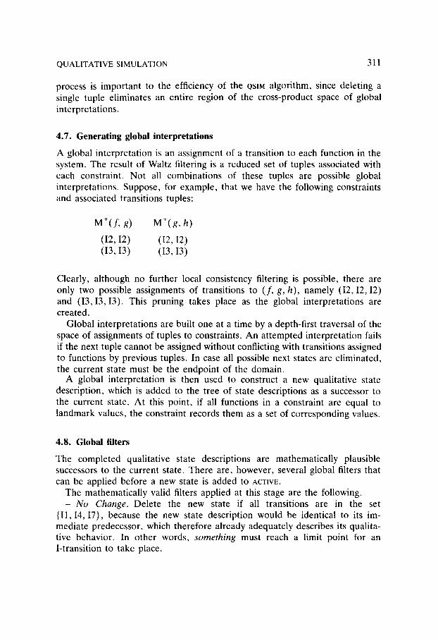
A global interpretation is an assignment of a transition to each function in the system. The result of Waltz filtering is a reduced set of tuples associated with each constraint. Not all combinations of these tuples are possible global interpretations. Suppose, for example, that we have the following constraints and associated transitions tuples:

M + ( f , g ) M+(g, h)

(I2, I2) (I2, I2) (I3,13) (I3, I3)

Clearly, although no further local consistency filtering is possible, there are only two possible assignments of transitions to (f , g, h), namely (12, I2, I2) and (I3, 13, I3). This pruning takes place as the global interpretations are created.

Global interpretations are built one at a time by a depth-first traversal of the space of assignments of tuples to constraints. An attempted interpretation fails if the next tuple cannot be assigned without conflicting with transitions assigned to functions by previous tuples. In case all possible next states are eliminated, the current state must be the endpoint of the domain.

A global interpretation is then used to construct a new qualitative state description, which is added to the tree of state descriptions as a successor to the current state. At this point, if all functions in a constraint are equal to landmark values, the constraint records them as a set of corresponding values.

4.8. Global filters

The completed qualitative state descriptions are mathematically plausible successors to the current state. There are, however, several global filters that can be applied before a new state is added to ACTIVE.

The mathematically valid filters applied at this stage are the following. - N o Change. Delete the new state if all transitions are in the set

{I1, I4, I7}, because the new state description would be identical to its immediate predecessor, which therefore already adequately describes its qualitative behavior. In other words, something must reach a limit point for an I-transition to take place.

312 B.J. KUIPERS

- C y c l e . If the new state is identical to one of its predecessors (all functions have identical l a n d m a r k values, and all directions of change are the same), then mark the behavior as cyclic, install a pointer to the identical predecessor, and do not add the new state to ACTIVE.

-- D i v e r g e n c e . If any function takes on the value ~ or - 2 , the current t ime-point must be the endpoint of the domain, so the new state does not go onto ACTIVE.

The first filter does not reduce the number of behaviors described, but only eliminates a redundant description. The second detects when all the consequences of a particular state have already been determined, and need not be explored anew. The third determines when a state must be at the endpoint of the domain, and thus can have no successors.

We refer to the qualitative simulation algorithm described here as the p u r e

QsIM algorithm. For a particular application, additional heuristic filters may be added .2

4.9. Complexity

The process of formalizing qualitative simulation led to the improved QS1M algorithm, which turned out to be 30 to 60 times faster than its predecessor ENV [15, 16] on a variety of examples ranging f rom 3 parameters and 2 constraints (the ball) up to 16 parameters and 14 constraints (the Starling equilibrium [18, 19]). We can estimate the algorithmic complexity of QSIM as follows. Suppose there are p parameters in the system, c constraints, and the longest behavior has length t. ( t ' i s then, on average, log of the total number of qualitative states.) Since a constraint can have no more than three parameters , p = o ( c ) .

- A set of possible state transitions is assigned to each paramete r from a fixed-length table, and no more than 4 transitions can be assigned to any parameter . This defines a search space of 4 p state transitions, but only 4p transitions need actually be created, requiring o ( p ) time.

- A constraint can have no more than 43= 64 transition tuples. Filtering a tuple against the direction-of-change tables (Appendix B) takes constant time, but the number of corresponding values grows linearly (though slowly) with the length t of the behavior. Thus constraint filtering requires o ( c t ) time.

~' Some possible heuristics include: - Quiescence. If all functions have derivative zero, conclude that the system is quiescent, the

new time-point is the endpoint of the domain (possibly t = ~c), and do not place the new state on ACTIVE.

- No Divergence. In physical systems, elimi,late transitions in which any state goes to ~ or :~. A more accurate description of the system would include an operating region change corresponding to some component breaking.


-Waltz filtering visits each constraint at least once, but beyond that visits only neighbors of constraints where it was able to delete a tuple. Thus, the number of constraints visited is proportional to the total number of tuples, which is linear in the number of constraints. Each visit takes bounded time. Thus, Waltz filtering takes o(c) time [22].

-Generating the global interpretations explicitly constructs the remaining parts of the product space. Typically, the remaining space is small, but unfortunately there are pathological cases which yield 2 p possible successor states.

- The most expensive of the global filters is the check for previous identical states, which requires o(pt) time.

Mackworth and Freuder [22] show that in a sparse graph such as this, an interpretation satisfying the constraints may be generated in linear time. However, the number of global interpretations may be exponential in the number of parameters, and the OslM algorithm generates them all. An example of this pathological case can be constructed easily. Consider a system with three parameters f, g, and h, and two constraints, DERIV(f, g) and DERIV( g, h), in a state where f, g, and h are all positive and increasing. Then the possible tuples are:

DERIV( f ,g ) DERIV(g, h)

(I3, I3) (I3, I3) (I3, I4) (I3,14) (14,13) (14,13) (14, I4) (14, I4)

Neither local consistency filtering nor the formation of global interpretations eliminate any of the possible assignments, so for p parameters linked by a chain of DERIV constraints, there are 2 p interpretations.

f g h

I3 I3 13 I3 13 I4 I3 14 13 I3 14 14 I4 13 I3 I4 13 14 I4 14 13 14 14 I4

In practice, creation of the global interpretations significantly reduces the number of compatible assignments. While this estimates the complexity of a

314 B.J. KUIPERS

single cycle of QSIM, the algorithm need not halt, and can continue forever producing longer and longer behaviors, each of which satisfies the qualitative constraints.

Although the QSIM algorithm is exponential in the worst case, in practice generating the successors of a given state appears to be approximately o(ct). A rough sense of the effective speed of QsiM on the Symbolics 3600 can be seen from the following examples.

Example 4.3. The Spring example (3 parameters, 3 constraints) produces a three-way branching behavior of length 8 with 11 states, simulation halting after one branch is identified as a cycle (see Fig. 7). Run time: approximately 0.4 seconds.

Example 4.4. The Starling mechanism (16 parameters, 14 constraints) [18, 19] produces a single unbranching behavior of 3 states in response to a perturba- tion from equilibrium, halting on reaching a new equilibrium state. Run time: approximately 1.0 seconds.

5. Questions and Answers

Now that we have defined the QSIM algorithm, with a clear structure and mathematically accessible properties, we can examine it to answer some of our questions about the utility of qualitative simulation as a reasoning method. We can also compare different approaches to qualitative simulation by changing the table of permissible transitions.

5.1. Should simulation create landmarks?

The most important semantic difference between QSIM and other approaches to qualitative simulation is that QSIM can create new landmark values during the simulation, while the other algorithms require all landmarks to be specified when the structure is defined. In this section, we show that the inability to create new landmark values makes it impossible to express certain important qualitative distinctions, such as that between increasing, decreasing, and stable oscillation.

The fixed-landmark assumption is particularly deeply embedded in the de Kleer, Brown and Bohrow approach [6, 8], which depends on arithmetic operators defined over a fixed set of qualitative values, { +, 0, - } . A change in landmarks would change the qualitative values, and thus require the operators to be redefined. Such a redefinition is not always possible.

The structure of QSIM makes it possible to experiment with { + , 0 , - } semantics for qualitative simulation simply by replacing Table 1 with an alternate table of legal transitions (Table 2).

QUALITATIVE SIMULATION

TABLE 2. Possible transitions under {+, 0, - } semantics

315

P-tran- I-transitions QS(f, t~) :ff QS(f, t,, tl. ,) sitions QS(f, t~, t,+x) ::> QS(f, t,+l)

P1 (lj, std) (1, std) Ia (lj, std) ( I , std) P2 ( l , std) ((l,, l,. ~), inc) I2 ((l,. l ~ ) , inc) (lj~ ~, std) P3 (lj, std) ((l, .... l,), dec) I3 ((l,, lj+L), inc) (lj+ ~, inc) P4 (l,, inc) ((l,. l,+ ~). inc) I4 ((l,, lj+, ), inc) ((//, l~+ ~), inc) P5 ((l~, l,. ~), inc) ((1,, 1+, ), inc} I5 ((lj, lj+ ,), dec) (lj, std) P6 (/, ,dec) ((l~ , , / , ) ,dec) 16 ((/j,/j~,), dec) (/j, dec) P7 ((li, l,+,),dec) ( ( l , , / ~ ) , dec) I7 ((/j, 1,+1), dec) ((l~,l/+~),dec) Q8 ((/,,/,+,), std) ((/,,/,+,), std) J8 ((1,,/,+~), inc) {(/, , / , , ,) , std) Q9 ((l,,/,+t), std) ((/,, /i+,), inc) J9 ((Ij,/j+,), dec) ((/j,/~+,). std) Q10 ((1, l , / ,) ,std) ((1, , , / , ) ,dec) J10 ((li, lj~,),std ) ((l , , l , , , ) ,std}

The landmarks are fixed as { - 2 0, co}. The transitions that create new landmarks (18 and 19 from Table I) are eliminated, and new transitions are added (with Q and J names) to permit direction of change std between landmarks.

Figure 6 shows the behavior of the spring system under the { + , 0 , - } semantics. This behavior can be considered a cycle only if two functions are allowed to match between landmark values. That is, only if we may conclude from this simulation that V(t4) = V(lo). m match between the states t 4 and t o in this behavior suppresses the distinction between increasing, stable, or decreasing amplitude (see Fig. 7). De Kleer and Bobrow [6] present an example of a

f Mf "'~,---o---~'"

A(t)

l i f t

-o---¢. .t---o-

"'¢---o---*r"

v(t)

f " .,---o---¢.

X(tl FIG. 6. The spring behavior with {+, 0 , - } semantics. In this behavior, we have QS(V, to)= ((0, ~), std) = QS(V, ta), but not necessarily V(to) = V(t,).

316 B.J. KUIPERS

spring with frictional damping, whose actual behavior is a decreasing oscillation. The behavioral description they present is cyclic, and similar to that given in Fig. 6, with the addition of terms for the frictional force. Their description accurately captures the repetitive series of increase and decrease in the different parameters, but since it does not express a distinction between increasing, decreasing and steady amplitude, it cannot even ask which qualitative behavior is correct.

The heart of the problem is the inability to create new landmarks, or equivalently, to give n a m e s to newly discovered critical values. Without representing the initial value (or subsequent critical values) of a parameter in a way that permits ordinal comparison, it is not possible to ask whether the next repetition of a cycle leaves that parameter increased, decreased, or stable. If. in addition, states can be matched between landmark values, three very distinct types of behavior can be collapsed into a single, apparently cyclic, behavior. Thus, we argue that the { +, 0, - } semantics, and in fact any semantics with a fixed set of landmarks, can collapse importantly distinct behaviors.

5.2. Is the real behavior found?

In this section, we show that all actual behaviors of a mechanism are predicted by its qualitative simulation. We take as our "gold standard" the solutions to the ordinary differential equation describing the mechanism.

We say that a real-valued function sa t i s f i e s a given qualitative behavior description if the qualitative description of the function matches the given qualitative behavior. We then prove that any solution to a differential equation satisfies some qualitative behavior produced by the corresponding constraint equations. The proof is straightforward, since the bulk of the work has already been done in validating the individual steps of the QSIM algorithm. The algorithm generates a space including all possible behaviors of a given set of functions and constraints, and then discards only behaviors which are internally inconsistent. Thus, the remaining behaviors necessarily include all of the actual behaviors of the mechanism.

Definition 5.1. Suppose we have a reasonable function u : [ a , b ] - - - ~ l ~ and a qualitative behavior description of the function symbol f,

OS(f , to) , OS(f , t o, t,) . . . . . OS(f , tn ~, t . ) . QS(f , t,,)

with distinguished time-points {t 0 . . . . . tn} and landmarks {l~ . . . . . l k } . We say that u sa t i s f i es the behavior description if there is an order-preserving mapping m of { t o . . . . . tn} into [a, b] with m ( t o ) = a and m ( t n ) = b, and an order-preserving mapping of {l 1 . . . . . lk} into ~, such that, for all distinguished time-points t i, QS(u, m ( t i ) ) matches QS(f , t i ) and QS(u, m ( t i ) , m ( t i + l ))

matches QS( f, t i, t i + l ).


Theorem 5.2. Let

F[u(t), u'(t) . . . . . u~")(t)] = 0 (3)

be an ordinary differential equation of order n, and let {U(to)= Yo, u '( to)= y ~ , . . . , u~")(to) = y,} be the initial conditions on the solution to (3). Suppose that (3) and its initial conditions are satisfied by a reasonable function u :[a, b]---> ~. Let C be the set of functions and constraints derived from (3) by the methods of Section 3.3, and let QS(F, to) be the qualitative state description derived from the given set of initial conditions. Let T be the tree of qualitative state descriptions derived from C and QS(F, to) by the pure QSlM algorithm. Then the function u and the subexpression functions derived from it satisfy some behavioral description in T.

Proof. QSIM works by progressively restricting the region of a space of qualitative behaviors that it is considering. By showing that any actual solution u is initially in the space, and that no filtering operation can eliminate a genuine solution, we conclude that u and its derived functions must satisfy some behavior in T.

The function u satisfies the initial state description QS(F, to) because it is a qualitative abstraction of the initial conditions to equation (3). Step 2 in QSlM generates all possible qualitative state transitions for the functions in C from a given qualitative state, using Table 1 which is justified by Propositions A.1, A.2, A.4, and A.5. Thus, any change in qualitative state of the system must be included in the possibilities generated. Step 3 of QsIM filters out combinations of transitions whose result is a state which fails to satisfy individual constraints. Inconsistent sets of directions of change are detected by comparison with tables in Appendix A. The proper implications of sets of corresponding values are checked against Propositions B.1-B.3, and B.9. The pairwise consistency filtering of Step 4 simply eliminates from consideration transitions tuples which are inconsistent with all neighboring tuples, and thus could not contribute to a global interpretation. Step 5, similarly, eliminates combinations of tuples which do not make consistent assignments of state transitions to particular functions. Finally, the global filters included in the pure QsIM algorithm are discussed in Section 4.8 and shown not to eliminate possible behaviors of the system. Thus, at each stage of the simulation, all possible successors to the current qualitative state lie in the space generated, and no genuinely possible successor is eliminated. []

5.3. Are all the behaviors real?

In this section, we show that the QSIM algorithm, and local qualitative simulation algorithms in general, cannot be guaranteed against producing spurious

318 B.J. KUIPERS

behaviors: behaviors which are not actual behaviors for any physical system satisfying the constraint equations.

A qualitative differential equation may provide few constraints, and thus predict many possible behaviors. However, the constraints are also consistent with many possible ODEs, and we might hope that each qualitative behavior corresponds to the solution to some O D E corresponding to the constraints. Although this is often the case, and has been conjectured to be universally true, there are cases where spurious behaviors are generated. Thus, if several behaviors are generated, some of them may not be possible behaviors of the mechanism.

One of the attractive applications of qualitative simulation is to predict possible future states, particularly to warn of surprising or disastrous events. Theorem 5.2 guarantees that there can be no false negatives: every actual behavior is predicted. However, if a valid description of the mechanism can produce invalid predictions (false positives), its usefulness is limited. As we discuss below, the problem is not fatal, but requires substantial care in the construction and use of a problem solver.

Theorem 5.3. Let C be a set of function symbols and qualitative constraints, and let QS(F, to) be the initial qualitative state description. Let T be the tree of qualitative state descriptions derived from C and QS(F, to) by the pure OSIM algorithm. For some C and QS(F, to) there are behaviors in T which do not correspond to any solution u :[a, b]--~ ~ to any differential equation and initial condition corresponding to C and QS(F, to).

Proof. Consider a mass on a spring, oscillating on a frictionless surface. The constraints for this system are

DERIV(X, V ) , DERIV(V, A ) , M{7 (A, X ) , (4)

which might also be written in the form of a second-order differential equation:

d2X - M i ~ ( X ) . (5 )

dt 2

With initial state X(to) = 0, V(to) = Vm., A(to) = 0, this system is periodic for +

any function A = - M o ( X ), because if we define total energy as

TE(x, v) j + dy ½v 2 = M o ( y ) + , 0

then (5) implies that d T E / d t = 0. The local inference methods of QSIM are not able to determine, at the end of


one cycle, whether the oscillation of the system is periodic, or increases or decreases in magnitude. It does, however, branch to express all three behaviors.

Figure 7 shows the behavioral description produced by qualitative simulation of the spring system. The simulation proceeds without branching through the cycle, predicting and creating new landmarks for the extrema of X, V, and A until they approach 0, V* and 0, respectively. X and A must reach their limits together, but the simulation branches according to whether V reaches its limit at the same time (behavior 1), later (behavior 2), or earlier (behavior 3). In the first case, the state at t 4 matches the state at t 0, so the behavior is stable and periodic. In the second, the oscillation is decreasing with a new critical point less than V*. And in the third case, motion continues past V* to a different new critical point greater than V*. Furthermore, having taken this branch, there is no way to represent the decision as a permanent selection of divergence, convergence, or stable oscillation. The same choice recurs at approaches to other landmarks.

Only the stable periodic behavior is an actual behavior possible for the constraints, but the local inference methods of QS~M cannot prove this fact. Thus, there are behaviors produced by the qualitative simulation algorithm which do not correspond to the behavior of any system satisfying the qualitative constraints. []

The problem also occurs with the algorithms of de Kleer and Forbus, even without creating new landmarks, if we can describe the initial state completely in terms of landmark values. In Forbus' case, we introduce a landmark value initial-length(S) for the initial displacement of the spring mass, such that A[initial-length(S)] > A[rest-length(S)] [12, pp. 144-146]. In de Kleer and Brown's case we may define a translated variable W(t)= V(t)- V* so that W(t) = 0 corresponds to V(t)= V* [8]. In both cases, when the system is approaching its initial state both position and velocity are approaching limits, with no way to determine which arrives first. Without the translated variable, neither approach expresses the distinction between increasing, steady, and decreasing amplitudes [17].

The underlying problem is the combination of locality with qualitative description. Both numerical and qualitative simulation are inherently local: the transition to a state is derived from its immediate predecessor. In numerical simulation, excluding truncation errors, the numerical values of the parameters implicitly encode invariant relations such as energy conservation that might be derivable from the equation. A numerical simulation of the oscillating spring will thus identify the single periodic behavior. In qualitative simulation, however, the qualitative state description of the spring is compatible with a variety of states, not all of which satisfy the invariant. There is simply not enough information in the previous state, or even the complete history of

t~

k~f

$ fll

Y~

r

be

ha

vio

r 1:

A

(t)

~NIf

be

ha

vio

r 1

: V

(t)

~,-.'.~

-....,..

..-~'.~

+~.:

:..~.¢

°

be

ha

vio

r 1:

X

(t)

~Y

AI

be

ha

vio

r 2

: A

(t)

........

..... _

..~.~

.~...

-...+

--..:

..,,<

....--

.~

,

4. ~

e='1

' ~,

,

PO,~

f

be

ha

vio

r 2

: V

(t)

.-4~z

K1

I, tlN

r

be

ha

vio

r 2

: X

(t)

A1

be

ha

vio

r 3

: A

(t)

u*

01

be

ha

vio

r 3

: V

(t)

-~-..

~1

yaf

be

ha

vio

r 3

: X

(t)

FIG

. 7.

T

he

sp

rin

g s

imu

lati

on

. A

s th

e si

mu

lati

on

a

pp

roa

ch

es

t =

t~

, th

ere

is

no

lo

cal

rule

th

at

can

de

term

ine

w

he

the

r V

re

ac

he

s V

*

be

fore

, af

ter,

o

r at

th

e sa

me

ti

me

as X

a

nd

A

re

ach

zer

o.

Th

e

sim

ula

tio

n

bra

nc

he

s th

ree

way

s. e

ve

n t

ho

ug

h

on

ly

on

e

be

ha

vio

r is

val

id.

~Z

L.

7~


states, to exclude all impossible behaviors. This combination of locality with qualitative state descriptions leads to the problem of spurious predictions. Thus none of the qualitative simulation algorithms can avoid this problem.

If we explicitly add the constraints representing conservation of energy to the oscillating spring constraint equations, the single correct behavior is found. However, although the additional constraints are derivable from the original equations, it is not at all clear how to do such a derivation automatically for an arbitrary mechanism.

These observations yield some important warnings about the proper use of qualitative descriptions of mechanisms, and the result of their simulation.

- Theorems 5.2 and 5.3 have a corollary that highlights their implications for knowledge engineering.

Corollary 5.4. I f a set of constraints is consistent, and if QsIM predicts a single behavior, then that behavior represents the actual behavior of the mechanism.

- T h e consistency of a set of constraints must be demonstrated, to ensure that the qualitative simulation includes at least one genuine behavior (Theorem 5.2). When the constraints are constructed by hand, this can be done by exhibiting the ODE that they abstract. However if the set of constraints is to be derived automatically from the current process structure [12], guaranteeing consistency may be more difficult.

- If qualitative simulation yields several possible behaviors, further analysis is required before concluding that they represent possible futures.

Qualitative simulation is an important step in the process of qualitative reasoning about the behavior of mechanisms, and QSIM is a particularly complete, efficient implementation of it. However, like all tools, it has important limitations. The formal analysis we have used in this paper is valuable both for the design of the OSIM algorithm and for determining the strengths and limitations of qualitative simulation in general.

5 . 4 . W h a t n e x t ?

Two directions for further research appear promising for more accurate qualitative predictions of behavior. First, the dynamical systems approach to qualitative analysis of differential equations (e.g. [1]) has greater expressive and inferential power than local qualitative simulation methods. By describing the behaviors of the spring as trajectories through phase space rather than temporal sequences of qualitative states, it is possible to take a single branch between increasing, decreasing, and stable oscillation, rather than repeating the choice at each move toward limits. The theory of dynamical systems also includes global classification theorems delimiting the possible qualitatively distinct behaviors. Further study is needed to determine how practical problems can be stated and solved, and how the solutions can be applied.

322 B.J. KUIPERS

Second, if one structural description of a mechanism has spurious behaviors, a different description might not. By changing the problem to take into account the conservation of total energy, an expanded view of the spring mechanism allows QSIM to determine that there is a single, periodic behavior. A physicist can look at equation (5) and recognize or derive the fact that it represents an energy conserving system, and therefore that the behavior must be periodic. Part of this knowledge is the ability to recognize the physical system described by a set of constraints, and to know that there is a better structural description for it; one which adds parameters and constraints (e.g. energy) that illuminate the actual behavior. This approach takes us outside the realm of qualitative simulation, and into the realm of problem formulation. Chi, Feltovich, and Glaser [2] have shown that expert causal reasoning involves the use of domain-specific knowledge to select the correct formulation of a problem, leading to its direct solution.

Returning to the larger problem of qualitative causal reasoning about mechanisms, an important problem is to formulate a suitable set of constraints given a physical situation, using the device-topology approach of de Kleer, Brown and Bobrow [6, 8], the process-based approach of Forbus [12], or some approach yet to be discovered.

Appendix A. The Qualitative State Transitions

This appendix applies the Intermediate Value and Mean Value Theorems to prove the validity of the transition rules in Table 1 that restrict the possible qualitative behaviors of a single function.

Let f : [ a , b]---~E be a reasonable function with distinguished time-points

a = t o < . • . < t,, = b ,

and landmark values

l~ < . - . < / k .

We repeat Definition 2.9.

Definition. Where t~ is a distinguished time-point, a P-transition of f is a pair of adjacent qualitative states of f,

QS(f , ti) ~ QS( f , t i, t i+ , ) ,

whose first state is the qualitative state at a distinguished time-point. An l-transition is a pair of adjacent qualitative states of f,

QS(f , t i 1, t~) ~ QS(f , ti)


whose first state is the qualitative state on the interval between distinguished time-points.

Proposition A.1. Let QS(f , ti) and QS(f , t i, ti+~) be adjacent qualitative states o f f. Then there is some landmark value lj such that f(ti) = lj, and the only possible P-transitions o f f are given by the table below:

OS(f , t,) :ff QS(f , t~, t~+~)

P1. (lj, std) (lj, std) P2. (lj, std) ( (6 ' 6+1),inc) V3. (lj, std) ((lj_t, l j) ,dec} P4. (lj, inc) ((li, l~+,),inc) P6. (l i, dec) ((It t, It), dec}

Proof. If t~ is a distinguished time-point, then by definition there must be a landmark value lj such that f(ti)= 6. In cases P1-P3, there are reasonable functions f with QS(f , t , )= (lj, s td), and with direction of change std, inc, or dec in QS(f , t~, t~+ ~), so no subsequent direction of change can be excluded. In these cases, by the Mean Value Theorem, f( t) must be equal to, greater than, or less than f(ti) = lj, respectively, on the interval (t~, tg+~). By Proposition 2.5 and the Intermediate Value Theorem, f i t ) must be within (6, 6+~) if it is increasing, or (6 ,, 6) if it is decreasing. In case P4, if the direction of change is inc, then f'(t~) > 0. Since the derivative is continuous, there is an interval around t = t i in which f ' ( t ) > 0. By Proposition 2.5, since there are points within (t,, ti+ ~) where the direction of change is inc, it must be inc throughout (ti, t,+ ~), so f i t ) must be within (lj, lj+~). Case P6 is similar. []

The three P-transitions from the state ( l j, std) handle the case where a higher-order derivative, which is not explicitly represented by QsIM, determines the direction of motion. In such a situation, all three transitions are generated, and other constraints filter out the impossible cases. De Kleer and Bobrow [6] determine and use higher-order derivatives explicitly to make that decision, at least for linear equations. Their approach determines the order of the structural description, and thus knows how many higher-order derivatives to compute. The advantages of the current approach are that it places much weaker conditions on the differentiability of the parameters, and that it is not restricted to linear equations.

Proposition A.2. Let OS(f , t i, ti+l) and QS(f , ti+l) be adjacent qualitative states o f f . Then there are landmark values lj and Ij +~ such that the only possible I-transitions are given by the table below:

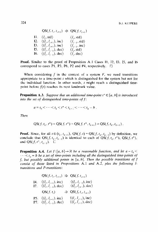
324 B.J. KUIPERS

OS(f, t i, ti+,) © OS(f, t i l l )

I1. (lj ,std> (lj, std) I2. <(lj, lj+x), inc) (lj+~, std) I3. ((lj, lj+,), inc) (li+,, inc) I5. ((lj, lj+,), dec> ( lj, std) I6. ((l/, l/+~), dec) ( / / ,dec)

Proof. Similar to the proof of Proposition A.1 Cases I1, 12, I3, I5, and I6 correspond to cases P1, P3, P6, P2 and P4, respectively. []

When considering f in the context of a system F, we need transitions appropriate to a time-point t which is distinguished for the system but not for the individual function. In other words, t might reach a distinguished time- point before f ( t ) reaches its next landmark value.

Proposition A.3. S u p p o s e that an addi t ional t ime-po in t t* @ [ a, b] is i n t roduced

into the set o f d is t inguished t ime-poin ts o f f :

a = t o < • • • < t k < t* < t k + i < " " " < tn = b .

Then

QS(f, t k, t*) = QS(f , t*) = QS(f, t*, tk+,) = OS(f, t k, t~+.).

Proof. Since, for all t E (t k, tk+l), QS(f , t ) = QS(f , t k, tk+~) by definition, we conclude that QS(f, t k, tk+~) is identical to each of QS(f, t~., t*), QS(f, t*), a n d Q S ( f , t * , t k+~). []

Proposition A.4. Le t f : [a, b]---~ ~ be a reasonable f u n c t i o n , and let a = t o < • • • < t n = b be a set o f t ime-poin ts inc lud ing all the d is t inguished t ime-poin ts o f

f , bu t poss ib ly addi t ional po in t s in [a, b]. Then the poss ib le transi t ions o f f

consist o f those listed in Propos i t ions A.1 and A.2, p lus the f o l l o w i n g l-

transi t ions and P-transi t ions:

OS(f, t,, ti+,) ~ OS(f, ti+l) I4. ((lj, 6+~), inc) ((lj, l/+~), inc) I7. ((l~, lj+,), dec) ((li, li+~), dec )

QS(L t~) ~ QS(f, t~, t~+,)

P5. ((6, 6+,), inc) ((6, l,+,), inc) p7. ((/,, 6+,), dec) ((6, 6+,), dec)


Proof. Consider an I-transition beginning with QS(f , t~, ti+l). If ti+ 1 is a distinguished time-point of f, the transition is specified by Proposition A.2. If ti+ 1 is not a distinguished time-point of f, Proposition A.3 shows that the qualitative state remains constant across the transition, providing the above alternatives as the only additional possibilities. If the transition is a P-transition beginning with QS(f , ti) the proof is similar, depending on whether t~ is a distinguished time-point of f. []

A.1. Discovering a new landmark

Suppose that QS(f , t i, ti+l)= ((lj, l j+l) , inc) . Since there is no landmark in (Ij, li÷i), we can exclude the transition to

OS(f , ti+,) = ((l i, li+l), std)

because that would imply that f'(ti+ 1) = O, making f(t~+ 1 ) a landmark value, by definition. However, if l~ < . . . < l k is only a partial set of the landmarks of f, then the above transition is possible, but only when f(tg+l)= l*, a landmark value of f such that lj < 1" < lj+t.

In this case, the following partial behavior is possible:

qualitative state known landmarks

QS(f , t i, t/+l) -- ((lj, lj+l), inc) lj < li+ 1 QS(f , t,+l) = (l*, std) lj < l* < lj+ t

QS(f , t i, t~+l) is now seen to be syntactically incorrect, given subsequent information acquired about the true set of landmarks. It should be revised to be QS(f , t i, ti+l) = ((lj, l*), inc). Furthermore, it is possible for f to move across l* several times before encountering the critical point that reveals its existence as a landmark. However , the modifications needed to correct the behavioral description are straightforward and locally computable. In the ball system example discussed above, the maximum height of the ball is such a new landmark, discovered when V(t), and therefore Y'(t), become zero. We summarize this discussion in:

Proposition A.5. Suppose that 11 < . . . < I k are all the known landmarks of a reasonable function f, which may have other landmarks as yet unknown. Then, in addition to the transitions listed in Propositions A.1, A.2, and A.4 the following l-transitions are possible:

Qs(L t,, t,+l) ~ QS(L ti+,)

IS. ((li, lj+l), inc ) (/*, std) I9. ((lj, li+l), dec} ( l* , s td )

326 B.J. KUIPERS

In case one of these transitions is followed, the set of landmark values in QS(f , ti+,) is augmented by lj < l* < lj+ 1. Note that the total ordering on the set of landmarks is preserved.

Table 1 collects and names the transitions permit ted by Propositions A.1, A.2, A.4, and A.5 for use in the QSIM algorithm.

A.2. Infinity and asymptotic approach

I-transitions express the possible consequences of a changing paramete r reaching a limiting landmark value. But what if a paramete r approaches its limit asymptotically? By allowing both domain and range to include + ~ and - ~ as endpoints, we can express asymptotic approach as reaching the limit point at t = ~. The same method allows us to treat divergence to infinite values as a possible behavior. Thus, every time-interval has an endpoint, but some distinguished time-points (e.g. t = ~, or t such that f ( t) = ~) may have no successor states. There are two constraints on these types of behavior.

First, at t = ~, every function in the system must be equal to some landmark value and must, if that landmark is finite, have derivative zero (i.e. direction of change std). Recall that oscillatory systems are handled with a finite domain and repeated states, rather than with an infinite domain.

Proposition A.6. Let f : [a, oo] --~ ~* be a reasonable function. I f the limit o f f ( t ) as t - - ~ is finite, then l i m , ~ f ' ( t ) = 0.

Proof. If l i m , ~ f ' ( t ) > 0, then for some interval (c, ~), f ' ( t ) must be bounded away from zero. In this interval, f ( t ) = f ( c ) + f ' ( t * ) . ( t - c ) for some t * E (c, oo), by the Mean Value Theorem. Thus, l i m , ~ f ( t ) = ~. Similarly in case l i m , ~ f ' ( t ) < 0 , so the limit must be zero. []

Second, if f ( t) = ~, then t = b, the right-hand endpoint of the domain, since a function cannot be continuously differentiable across ~. If b < ~, then the direction of change must be inc.

Proposition A.7. Let f:[a,b]--->E* be a reasonable function such that i im,~bf( t ) = ~, where b is finite. Then l im ,~b f ' ( t ) = ~.

Proof. Suppose that l imt~bf ' ( t ) has a finite limit M > 0 . Then for some interval (b - 6, b), f ' ( t ) E (M - e, M + e), which implies that

f ( b - ~ ) + 6 . ( M - e ) < f ( b ) < f ( b - ~ ) + ~ ' ( M + e)

which contradicts f ( b ) = ~. []


Using these propositions, we can test whether a distinguished time-point can match t = 2, and test moves to ~ for consistency. With these observations, the extended reals [ - 2 , 2] can be treated like any other closed interval, and asymptotic approach is handled.

Appendix B. Constraint Consistency

This appendix specifies the rules by which each type of constraint tests a tuple of qualitative state transitions for consistency. There are separate tests for consistency of the qualitative magnitudes and the directions of change.

B.1. Qualitative magnitude consistency

This appendix defines and justifies the evaluation of M +, M-, ADD, or MULT constraints when applied to particular qualitative values.

The magnitude of a quantity is described qualitatively in terms of its ordinal relations with a set of landmark values. The validity of a particular application of an M +, M-, ADD, or MULT predicate is tested using not only the signs of the arguments, but also their relations with other sets of corresponding values. For example, if we know that A D D ( p , q, r) is true, then (p, q, r) is a set of corresponding values for this ADD constraint, and i f p ' < p and r' > r, we can determine that ADD(p ' , q, r ' ) must be false. In the QSIM algorithm, these predicates are evaluated in order to test the validity of a possible tuple of transitions at a particular constraint.

The criteria below compare transition tuples with known sets of corresponding values. Each criterion checks whether the ordinal relations between the current values of the functions and the corresponding values will be consistent with the constraint after the proposed transition. The qualitative state before the transition is presumed to be consistent.

These criteria generalize the transition-ordering rules of Williams [24, 25], which evaluate combinations of transitions to zero across various constraints. The presence of nonzero landmark values means that, for example, a particular function could be moving toward zero, but be separated from it by an intervening landmark. Thus, transition-ordering rules must take into account not only of directions of change, but also relative position in an ordering. Furthermore, a problem with transition-ordering rules in general is that their proofs, while not deep, often consist of numerous cases and are difficult to check. The simple and transparently valid criteria of Propositions B.3 and B.9 subsume the other rules and are more efficiently applied.

B. 1.1. Monotonic function constraints

If two function f and g, related by M÷(f , g), are approaching corresponding limits, we know that either both reach their limits together, or neither does.

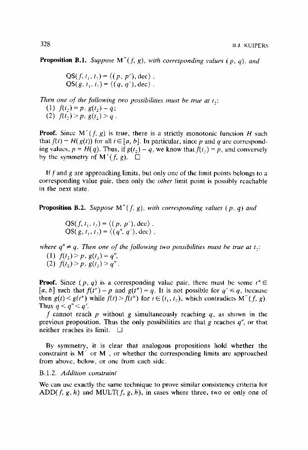
328 B.J. KUIPERS

Proposition B.I. Suppose M+(f , g), with corresponding values (p , q), and

QS(f , t,, t2) = ( ( p , p ' ) , d e c ) , OS(g, t , , t2 ) = ( ( q, q' ), dec) .

Then one o f the following two possibilities must be true at t2: (1) f ( t : ) = p, g(t:) = q; (2) f ( tz ) > p , g(t2) > q .

Proof. Since M+( f, g) is true, there is a strictly monotonic function H such that f ( t ) = H(g( t ) ) for all t E [a, b]. In particular, since p and q are corresponding values, p = H(q) . Thus, if g(t2) = q, we know that f(t2) = p, and conversely by the symmetry of M+(f , g). []

If f and g are approaching limits, but only one of the limit points belongs to a corresponding value pair, then only the other limit point is possibly reachable in the next state.

Proposition B.2. Suppose M+(f , g), with corresponding values (p , q) and

QS(f , tl, t2) = ( ( p , p ' ) , d e c ) , QS(g, t,, t2) = ((q", q ' ) , dec) ,

where q" ~ q. Then one o f the following two possibilities must be true at t2:

(1) f ( t z ) > p , g(t2) = q", (2) f ( tz ) > p, g(t2) > q".

Proof. Since (p , q) is a corresponding value pair, there must be some t* E [a, b] such that f ( t* ) = p and g(t*) = q. It is not possible for q' ~< q, because then g(t) < g(t*) while f ( t ) > f ( t * ) for t ~ (t~, t2), which contradicts M-~(f, g). Thus q < q" < q'.

f cannot reach p without g simultaneously reaching q, as shown in the previous proposition. Thus the only possibilities are that g reaches q", or that neither reaches its limit. []

By symmetry, it is clear that analogous propositions hold whether the constraint is M + or M-, or whether the corresponding limits are approached from above, below, or one from each side.

B.1.2. Addit ion constraint

We can use exactly the same technique to prove similar consistency criteria for A D D ( f , g, h) and M U L T ( f , g, h), in cases where three, two or only one of


the limit points belongs to a known set of corresponding values. The complexity of determining, implementing, and verifying all such tests is formidable. Fortunately, there is a general relationship that captures all possible such criteria.

Proposition B.3. Let p , q, and r be corresponding values o f f , g, and h, where ADD( f , g, h). Then, for any t E [ a , b], the fo l lowing holds:

( f ( t ) - p) + ( g(t) - q) = (h(t) - r). (B.1)

Proof. f ( t ) + g(t) = h(t) and p + q = r. []

If we know that ADD(f , g, h), and if the limits approached by f, g, and h intersect with the corresponding values p + q = r, then (B. 1) may be applied. A proposed transition tuple is checked for consistency by seeing whether its result would change the sign of any of the terms in (B. 1). The signs of the three terms can be determined directly from the ordinal relations among function values and landmarks, and the resulting state is checked for consistency with the ADD relation by table lookup.

The following propositions demonstrate the effect of this filter on cases where the limits of f, g, and h share three, two, or only one value with a particular correspondence.

Proposition B.4. Suppose ADD(f , g, h), with corresponding values p + q = r, and

QS(f, ti, t2) = ( (p , p ' ) , d e c ) , OS(g, t 1, tz) = ( (q , q ' ) , dec ) , QS(h, t 1, t2) = ((r, r ' ) , dec) .

Then exactly one o f the fo l lowing four possibilities mus t be true at t2: (1) f ( t2) = p , g(t2) = q, h(t2) = r; (2) f(t2) = p, g(t2) > q, h(t2) > r; (3) f(t2) > p , g(t2) = q, h(t2) > r; (4) f ( t2) > p, g(t2) > q, h(t2) > r.

Proof. For t E [tl, t2], f ( t ) - p >10, g(t) - q >10, and h(t) - r >lO. The three terms of (B.1) must have compatible signs, and cannot change discontinuously from their state in (tl , t2), so (1)-(4) are the only possibilities. []

In case we are not so fortunate as to have f, g, and h approaching corresponding limits, we may have two of the functions approaching corresponding limits, and know where the corresponding value of the third function is with

330 B.J. KUIPERS

respect to its limit. This allows us fur ther to constrain the set of possible next states.

Proposition B.5. Suppose A D D ( f , g, h) , with corresponding values p + q = r, and

Q S ( f , t~, t2) = ( ( p , p ' ) , d e c ) , Q S ( g , tl, t2) = ( ( q , q ' ) , dec) , QS(h , t l , t2) = ( ( r " , r ' ) , dec) ,

where r" ~ r. Then it is not possible to have both f ( t2) = p and g(t2) = q.

Proof. Cons ider (B.1) . If r>~r ', then the t e rm h ( t ) - r is negat ive for t E (t~, t2), while the o the r two te rms are posi t ive, which is a contradict ion. Thus r ~ r".

All t e rms of (B. 1 ) are posi t ive on (t~, t2), and h(t) - r must be strictly posit ivc at t = t 2, so at most one of the o the r te rms can be zero at t 2. []


o s ( f , '1, t 2 )= ( ( p , p ' ) , d e c ) , QS(g , t 1 , t2) = ((q", q ' ) , dec) , QS(h, t l , t2 ) = ( ( r , r ' ) , dec) ,

where q " ¢ q. Then it is not possible to have both f ( t 2 ) = p and h ( t2 )= r. I f q < q", it is impossible to have h(t2) = r. l f q > q", it is i m p o s s i b l e f o r f ( t 2 ) = p.

Proof. If q < q", the middle t e rm of equa t ion (B.1) is strictly posit ive on Its, t2], so only the first t e rm can possibly b e c o m e zero at t 2, so only f a n d g can possibly reach their limits. If q > q", then the second te rm of (B.1) is strictly negat ive on (t 1, t2], so only the third t e rm can possibly b e c o m e zero at t 2, so only g and h can possibly reach their limits. []

The same technique can be used in case only one of a set of cor responding values appea r s in the current set of limits.


Q S ( f , t , , t2) = ( ( p , p ' ) , dec) , O S ( g , t I, t2)--- ( (q" , q ' ) , d e c ) , OS(h , tl, t2) = {(r", r ' ) , dec) ,


where q" # q and r" # r. Then if q" > q and r" < r, or if q" < q and r" > r, it is impossible for f(t2) -- p.

Proof. Examination of (B.1) shows that these cases would result in the first term being zero, while the other two have opposite signs, which is impossible. []

Proposition B.8. Suppose ADD(f , g, h), with corresponding values p + q = r, and

OS(f, tl, t2) = ((p", p ' ) , dec) , OS(g, tt, t2) = {(q", q') , dec ) , QS(h, 6, t2) = ( (r, r'), dec) ,

where p" ~ p and q" ~ q. Then if p" > p and q"> q, or if p" < p and q" < q, it is impossible for h(t2) = r.

Proof. Examination of (B.I) shows that these cases would result in the last term being zero, while the other two have the same signs, which is impossible. []

By symmetry, similar propositions hold in the cases where f, g, and h are approaching their limits from various combinations of directions, not only when all are decreasing. Fortunately, equation (B.1) makes it unnecessary to implement checks based directly on Propositions B.4-B.8.

B. 1.3. Multiplication constraint

If the three functions in a MULT constraint are approaching related limits, we can constrain the possible results, similarly to what we did with ADD constraints in the previous section. A separate consistency test checks for legal combinations of signs (+, 0 , - ) at a multiplication constraint.

Proposition B.9. Let p, q, and r be nonzero corresponding values o f the functions f, g, and h, respectively, where MULT(f , g, h). Then, for any t ~ [a, b], the following holds:

<.=> p / ~ q /

Proof. f ( t ) ' g ( t ) = h ( t ) a n d p - q = r . []

As with the addition constraint, QSIM uses equation (B.2) directly to test the

332 B.J. KUIPERS

consistency of various combinations o f f , g, and h reaching their limit values, in comparison with a corresponding set of values, p • q = r. When f ( t ) and p have the same sign, we can retrieve their ordinal relations to classify the term f ( t ) / p as greater than, less than, or equal to 1. With respect to this classification, the legal combinations of A, B, and C, where MULT(A, B, C) are given by the following table:

A • <1 =1 >1

<1 <1 <1 any

=1 <1 =1 >1

>1 any >1 >1

Note that it is not necessary for the value 1 to be a landmark value of any of the functions involved. The table is a guide to the implementation of a consistency test for M U L T ( f , g, h), rather than representing an inference that QSIM makes explicitly. The consistency test applies when the ordinal relation between f ( t ) and p changes as f reaches its limit.

Propositions can be proved to demonstrate the degree of filtering possible with different sets of corresponding values, similar to Propositions B.4-B.8 for addition, but they are omitted here.

B.1.4. Landmark values as a representation for critical points

There are several ways to represent the critical values of a parameter, but they are not identical in power and cost. QSIM creates landmark values in the quantity space of a parameter to represent critical values, where the derivative of the parameter becomes zero. The { +, 0, - } semantics can express nonzero landmarks by appending a new, translated parameter and constraint to the set of constraints. Thus, given a parameter V(t), if we wish to represent a new landmark value Vma X > 0 , we define a translated parameter W(t) and the constraint W(t) = V(t) - Vm,~x.

The translated parameter technique captures many, but not all, of the properties of landmark values. In particular, each constraint in a QsIM model records sets of corresponding landmark values that are known to satisfy it. These corresponding values are very useful for limiting the possible next states predicted by QSIM, by applying the qualitative magnitude filtering methods of this appendix. The translated parameter technique does not support this filtering method in any straightforward way, if at all.

Suppose we have parameters x, y, and z, such that x + y = z. At some


time-point, all three are observed to be equal to landmark values, so the addition constraint stores the corresponding values (p , q, r). Now suppose that we are in a state where x > p, y > q, and z > r, all decreasing toward their landmark values. In the OSIM representation, the methods of Propositions B.3 and B.4 let us conclude that only four of the eight possible resulting qualitative states are consistent.

Using the technique of translated parameters, in order to represent the landmark values p, q, and r, we need to define additional parameters and redescribe the current state, as follows:

x ' = x - p , x ' > 0 , y ' = y - q , y ' > O , z ' = z - - r , z ' > O .

Existing techniques, such as Williams' transition-ordering rules [24, 25] would then be able to reason about the order that x', y' , and z ' would reach zero, except that we do not necessarily have the constraint that x ' + y ' = z ' !

The event that led OSIM to record a set of corresponding values would be represented using translated parameters as x ' = 0, y ' = 0, and z ' = 0. Short of deriving all algebraic consequences of all combinations of constraints, it is not clear how a qualitative simulation algorithm would focus its attention sufficiently to derive the relation x ' + y ' = z ' as a way of capturing the correspondence (p , q, r). There is at least no straightforward translation of corresponding values into the translated parameter technique.

Without the corresponding values, the translated parameter approach must predict eight possible successor states for the three parameters, while QSIM can restrict the set to four.

B.2. Direction-of-change consistency

An important difference between QSIM and the algorithms used by de Kleer and Forbus is that quantities are rePresented by qualitative descriptions rather than qualitative values. Thus, rather than being a partial function that sometimes fails to compute a result, A D D is a three-place relation evaluating to true or false according to whether its arguments satisfy the addition constraint. This appendix specifies the tables of acceptable directions of change for A D D and MULT. The corresponding tables for M + and M- are obvious.

B.2.1. ADD(] ' , g, h)

The following table summarizes the combinations of directions of change that satisfy the A D D ( f , g, h) constraint.

334 B.J. KUIPERS

X inc

std

dec

inc std

inc inc

inc std

any dec

dec

any

dec

dec

inc std dec

any dec dec

inc std dec

inc inc any

dec dec any

dec std inc

any inc inc

dec

inc std dec

inc inc any

inc std dec

any dec dec

(3) If

(2) If

inc

std

dec

f <O,g<O,h>O,

f ~ inc std

inc

std

dec

f > O , g<O, h<O,

X inc

std

dec

B.2.2. MULT(f , g, h)

The combinations of directions of change that satisfy the MULT constraint depend on the signs of f, g, and h, as shown in the following tables, derived from the identity h' = f 'g + fg'.

(1) I f f > 0 , g > 0 , h > 0 ,

QUALITATIVE SIMULATION

In case f < 0 and g > 0, the table is transposed.

(4) I f f > 0 , g = 0 , h = 0 ,

f ~ inc std dec

inc inc std dec

std inc std dec

dec inc std dec

335

In case f < 0, the table remains the same, but with the signs reversed. If f = 0 and g ~ 0, the table is transposed.

(5) If f = 0 , g = 0 , h =0 ,

inc std dec

std std std

std std std

std std std

inc

std

dec

Appendix C. The QSIM Program and its Output

This appendix provides the constraints, the initialization, and a trace of one cycle of the output of OSlM on the spring mechanism

(define-structure spring (functions a v x) (landmarks (v (minf 0 v* inf))) (constraints (d//dt v a) (d//dt x v) (m0-a x)) (invariants

(a ((minf inf) nil)) (v ((minf inf) nil)) (x ((minf inf) nil))))

(defun initialize-spring () (make-initialization spring (generate-time-point)

"((x (0 inc)) (v (v* std)) (a (0 dec)))))

With appropriate trace switches set, the QSIM program will print out information about the quantitative progress of the filtering algorithm. The following

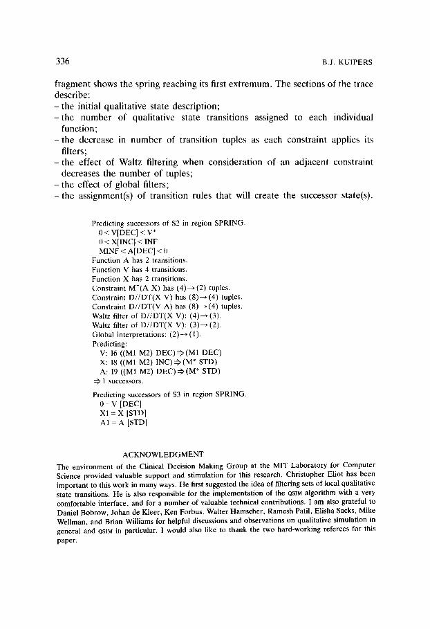
336 B.J. KUIPERS

fragment shows the spring reaching its first extremum. The sections of the trace describe: - t h e initial qualitative state description; - t h e number of qualitative state transitions assigned to each individual

function; - t h e decrease in number of transition tuples as each constraint applies its

filters; - t h e effect of Waltz filtering when consideration of an adjacent constraint

decreases the number of tuples; - the effect of global filters; - t h e assignment(s) of transition rules that will create the successor state(s).

Predicting successors of $2 in region SPRING. 0 < V[DEC] < V* 0 < X[INC] < INF MINF < A[DEC] < 0

Function A has 2 transitions. Function V has 4 transitions. Function X has 2 transitions. Constraint M (A X) has (4)---~(2) tuples. Constraint D/ /DT(X V) has (8)---~ (4) tuples. Constraint D/ /DT(V A) has (8)---,(4) tuples. Waltz filter of D/ /DT(X V): (4)---~ (3). Waltz filter of D/ /DT(X V): (3)---*(2). Global interpretations: (2)---~ (1). Predicting:

V: I6 ((M1 M2) D E C ) ~ (M1 DEC) X: I8 ((M1 M2) I N C ) ~ (M* STD) A: 19 ((M1 M2) D E C ) ~ (M* STD) 1 successors.

Predicting successors of $3 in region SPRING. 0 = V [DEC] X1 = X [STD] A1 = A [STD]

ACKNOWLEDGMENT

The environment of the Clinical Decision Making Group at the MIT Laboratory for Computer Science provided valuable support and stimulation for this research. Christopher Eliot has been important to this work in many ways. He first suggested the idea of filtering sets of local qualitative state transitions. He is also responsible for the implementation of the 0SlM algorithm with a very comfortable interface, and for a number of valuable technical contributions. I am also grateful to Daniel Bobrow, Johan de Kleer, Ken Forbus, Walter Hamscher, Ramesh Patil, Elisha Sacks, Mike Wellman, and Brian Williams for helpful discussions and observations on qualitative simulation in general and QSIM in particular. I would also like to thank the two hard-working referees for this paper.


AVAILABILITY OF THE QSIM PROGRAM

The QSlra program is available to researchers interested in qualitative simulation, in order to encourage detailed exploration and evaluation of these ideas and their possible applications beyond what is possible in a published paper. The current implementation runs in ZETALISP on the Symbolics 3600. It is not advertised or warranted as a software product, and any commercial rights to the program are retained. Please contact me if you are interested.

REFERENCES

1. Arnold, V.I., Ordinary Differential Equations (MIT Press, Cambridge, MA, 1973) (translated and edited by R.A. Silverman).

2. Chi, M.T.H., Feltovich, P.J. and Glaser, R., Categorization and representation of physics problems by experts and novices, Cognitive Sci. 5 (1982) 121-152.

3. de Kleer, J., Multiple representations of knowledge in a mechanics problem-solver, in: Proceedings Fifth International Joint Conference on Artificial Intelligence, Cambridge, MA, 1977.

4. de Kleer, J., Causal and teleological reasoning in circuit recognition, MIT Artificial Intelli- gence Laboratory TR-529, Cambridge, MA, 1978.

5. de Kleer, J., The origin and resolution of ambiguities in causal arguments, in: Proceedings Sixth International Joint Conference on Artificial Intelligence, Tokyo, Japan, 1979.

6. de Kleer, J., and Bobrow, D.G., Qualitative reasoning with higher-order derivatives, in" Proceedings Fourth National Conference on Artificial Intelligence, Austin, TX (William Kaufman, Los Altos, CA, 1984).

7. de Kleer, J. and Brown, J.S., The origin, form, and logic of qualitative physical laws, in: Proceedings Eighth International Joint Conference on Artificial Intelligence, Karlsruhe, F.R.G. (William Kaufman, Los Altos, CA, 1983).

8. de Kleer, J. and Brown, J.S., A qualitative physics based on confluences, Artificial Intelligence 24 (1984) 7-83.

9. Forbus, K.D., Qualitative reasoning about physical processes, in: Proceedings Seventh Inter- national Joint Conference on Artificial Intelligence, Vancouver, BC (William Kaufman, Los Altos, CA, 1981).

10. Forbus, K.D., Qualitative process theory, MIT Artificial Intelligence Laboratory Memo 664, Cambridge, MA, 1982.

11. Forbus, K.D., Measurement interpretation in qualitative process theory, in: Proceedings Eighth International Joint Conference on Artificial Intelligence, Karlsruhe, F.R.G. (William Kaufman, Los Altos, CA, 1983).

12. Forbus, K.D., Qualitative process theory, Artificial Intelligence 24 (1984) 85-168. 13. Gentner, D. and Stevens, A., (Eds.), Mental Models (Erlbaum, Hillsdale, NJ, 1983). 14. Hayes, P.J., The naive physics manifesto, in: D. Michie (Ed.), Expert Systems in the

Micro-electronic Age (Edinburgh University Press, Edinburgh, 1979). 15. Kuipers, B.J., Getting the envisionment right, in: Proceedings Second National Conference on

Artificial Intelligence, Pittsburgh, PA, 1982. 16. Kuipers, B.J., Commonsense reasoning about causality: Deriving behavior from structure,

Artificial Intelligence 24 (1984) 169-203. 17. Kuipers, B.J., The limits of qualitative simulation, in: Proceedings Ninth International Joint

Conference on Artificial Intelligence, Los Angeles, CA (William Kaufman, Los Altos, CA, 1985).

18. Kuipers, B.J. and Kassirer, J.P., How to discover a knowledge representation for causal reasoning by studying an expert physician, in: Proceedings Eighth International Joint Confer- ence on Artificial Intelligence, Karlsruhe, F.R.G. (William Kaufman, Los Altos, CA, 1983).

338 B.J. KUIPERS

19. Kuipers, B.J. and Kassirer, J.P., Causal reasoning in medicine: Analysis of a protocol, Cognitive Sci. 8 (1984) 363-385.

20. Kuipers, B.J. and Kassirer, J.P., Qualitative simulation in medical physiology: A progress report, MIT Laboratory for Computer Science TM-280, Cambridge, MA, 1985.

21. Mackworth, A.K., Consistency in networks of relations, Artificial Intelligence 8 (1977) 99-118. 22. Mackworth, A.K. and Freuder, E.C., The complexity of some polynomial network consistency

algorithms for constraint satisfaction problems, Artificial Intelligence 25 (1985) 65-74. 23. Waltz, D., Understanding line drawings of scenes with shadows, in: P.H. Winston (Ed.), The

Psychology of Computer Vision (McGraw-Hill, New York, 1975). 24. Williams, B.C., The use of continuity in a qualitative physics, in: Proceedings Fourth National

Conference on Artificial Intelligence, Austin, TX (William Kaufman, Los Altos, CA, 1984). 25. Williams, B.C., Qualitative analysis of MOS circuits, Artificial Intelligence 24 (1984) 281-346.

Received December 1984, revised version received January 1986

Documents

Qualitative Simulation* - Department of Computer Science · MCS-8303640 and DCR-8417934. ... nature of its decision criteria, ... We discuss the implications of these results for