Environ. Sci. Technol. 1993, 27, 2063-2071

Qualitative Determination of Source Regions of Aerosol in Canadian High Arctic

Meng-Dawn Cheng,'"i* Phllip K. Hopke,'pt Leonard Barrie,§ Ann Rlppe,t Marvin Olson,§ and Sheldon Landsbergerli

Department of Chemistry, Clarkson University, Potsdam, New York 13699-581 0, Atmospheric Environment Services, Downsview, Toronto, Ontario, Canada, and Department of Nuclear Engineering, University of Illinois at Urbana-Champaign, Urbana, Illinois

A hybrid receptor model that combines both chemical and meteorological information was employed to identify the potential regions of source emission for aerosol measured at Alert, Northwest Territories (82.3' N, 62.5' W) in the Canadian Arctic. This model explores the use of 5-day air parcel backward trajectories to describe the long-range transport of atmospheric heavy metals and sulfate species through the potential source contribution function (PSCF) receptor model. The modeling results presented are for the observations made between November 1 and March 20 from 1982 to 1987, i.e., the Arctic winter, since concentrations of trace elements are generally higher in the winter. A number of geographical locations in the former USSR and Europe are found to be of high potential to be the emission source areas. The usefulness of using elemental ratios in the PSCF analysis for identifying source regions contributing to the pollution in the Arctic was explored.

Introduction

The Arctic is quite distant from most major sources of pollution and had been traditionally considered a remote region where the air and water were pristine. However, after 20 years of measurements and a number of intensive studies, it is known that between October and May each year the Arctic troposphere is found to have high con- centrations of airborne particles commonly called "Arctic haze" (1-4).

During the mid-l970s, based on a limited number of measurements, the haze was thought to consist of soil particles originating in the deserts of eastern China and Mongolia. However, more extensive measurements showed that particles collected at ground-level stations were enriched in vanadium, sulfate, and other elements of anthropogenic origin. Discovery of anthropogenically enhanced chemical species such as Sod2-, V, Ni, In, Pb (2, 3); man-made organic compounds such as light hydro- carbons (5); and a large number of polycyclic aromatic hydrocarbons, polychlorinated dibenzo-p-dioxins, and pesticides (6) in the Arctic raises aseries of questions about the long-range transport and transformation of airborne chemicals in the atmosphere, the impact of the man-made chemicals on the fragile polar ecosystems, the atmospheric chemistry that occurs in the cold polar region, and the origin of chemical species.

Multivariate statistical techniques such as factor anal- ysis have been used to address the last question (7-10).

* Authors to whom correspondence should be addressed. + Clarkson University.

Present address: Oak Ridge National Laboratory, Energy

Atmospheric Environment Services. Division, MS-6200, Oak Ridge, TN 37831.

11 University of Illinois at Urbana-Champaign.

0013-936X/93/0927-2063$04.00/0 0 1993 American Chemical Society

Measured concentrations in the Norwegian Arctic have been related to sources in the industrialized areas of Eurasia using backward air parcel trajectories (11). Lo- wenthal and Rahn (L&R) (12) first applied a simple linear mass balance model similar to the chemical mass balance (CMB) model (13) with seven chemical tracers to the Arctic aerosol mass on a hemispheric scale. Receptor models such as CMB have been less frequently used at spatial scales larger than a few hundred of kilometers because over large distances atmospheric removal and chemical transformation processes can significantly reduce the strength of the source-receptor relationships. Gordon (14) has provided an excellent review of the current research and developments in receptor-oriented models for studying global and regional air pollution problems.

Chemical and meteorological data have often been used to assist in understanding the regional sources of pollut- ants. For instance, particulate concentrations of 14 elements measured in Sweden were related to air mass trajectories (15) classified into five predetermined direc- tional sectors. A strong dependence of the elemental concentration variations with air mass history was found. Similarly, Hopper et al. (16) used lead isotope observations in Sweden with trajectories to characterize European lead sources and thereby assist in the identification of the origins of Arctic lead (17) . Davies et al. (18) employed the Lambert weather-type classification system to categorize chemical composition measured in precipitation in Scot- land. Several studies have examined the origin of atmos- pheric C02, particles, and 03 concentrations observed in the Arctic by classifying trajectories that are associated with "episodic events" (19, 20). Receptor models were applied on a regional scale (21, 22), but not on the scale of the Arctic. The potential for using trajectories in air pollution studies over long distances has been demon- strated, for example, by studies of dust transport from the deserts of Asia to the mid-Pacific (23).

To better understand the source-receptor relationships and thereby develop effective control strategies for the Arctic pollution problem, there is a need to more precisely identify the sources that contribute pollutants on a hemisphere scale to the north. A receptor model that explicitly incorporates meteorological information in the analysis scheme to produce a probability field for source emission potential called potential source contributions function (PSCF) may be suitable for such a task (24,25). PSCF was proposed to identify geographical regions that might have high probabilities of being source areas for airborne sulfate in the southwestern United States (26). This report explores the feasibility of using an extended PSCF model to study the long-range transport of chemical species to the Arctic using weekly aerosol chemistry data obtained in the high Arctic.

Environ. Sci. Technol., Vol. 27, No. 10, 1993 2083

Description of Data

Chemistry Data. Airborne particle samples were collected at Alert, Northwest Territories, Canada (latitude 82.3" N, longitude 62.5" W), by the Atmospheric Envi- ronment Services of Canada (AES). Sampling operations began in July 1980, and the station is still operating. However, only data between January 1982 and May 1987 were used in this analysis because trajectories were not available beyond this time. Details of the sampling and analytical procedures for ionic species are given by Barrie and Hoff (27). Major ionic species such as S04%, C1-, NOa-, and so on were analyzed by ion chromatography. Ele- mental data were obtained using instrumental neutron activation analysis (INAA) performed at the University of Illinois at Urbana-Champaign. The INAA procedure was described by Landsberger et al. (28, 29). Pb was analyzed by inductively coupled plasma emission spec- troscopy. Detailed summary statistics are reported and a comprehensive analysis of the frequency distributions of these chemical species shows that most of them are log normally distributed (30).

It is known that meteorology and atmospheric chemical activities in the Arctic between summer and winter are substantially different. Moreover, many summer con- centration values were below detection limits. The data was therefore divided into two sets. Since polar sunrise is in late March and sunset is in late October each year, the period from March 21 to October 31 was designated the LIGHT period, and the DARK period was defined as November 1-March 20. Only the DARK data were used in this study, because a large fraction of LIGHT data were below detection limits.

Trajectory Data. The three-dimensional AES tra- jectory model (31) was used to reconstruct the air parcel movements in the horizontal as well as the vertical directions. The movements were described by segment end points of coordinates in terms of latitude, longitude, and height of each point. Five-day backward trajectories were calculated every 6 h four times a day at 00, 06, 12, and 18 UTC for 1000-, 925, and 850-hPa levels using wind data available every 6 h from the Canadian Meteorological Centre. The model used three-dimensional objectively- analyzed wind fields at four pressure levels: 1000, 850, 700, and 500 hPa. Cubic interpolation was used to obtain winds at intermediate levels in the vertical direction and between horizontal grid points. The trajectory compu- tations were performed on the standard Canadian Me- teorological Centre grid of 381 km.

Single-Layer Potential Source Contribution Function. The construct of PSCF can be described as follows: if a trajectory end point lies at a cell of address (i,j), the trajectory is assumed to collect material emitted in the cell. Once the material is incorporated into the air parcel, it is assumed to be transported along the trajectory to the receptor site. Atmospheric removal and chemistry that would take place from the sources to the receptor are currently not treated in the model development. This study explores the usefulness of PSCF as a receptor model applicable to long-range transport problems.

If the total number of end points at the kth pressure level that fall in the cell is nij, then the cumulative

probability of these end points, P[Aijl, can be given by

PCAkijl = n,/N (1) where k indicates the pressure level number, and N is the total number of end points summarized over all cells in the modeling region. The probability PIAk] represents the potential transport of material to the receptor site at the pressure level indexed I t . Among the nij counts, there will be mij points for which the measured concentration exceeds a criterion value selected for a chemical species. Note that the criterion value is obtained through a series of off-line statistical analyses. The cumulative probability of these high concentrations, Bij, can be defined as

PIBkijl = mij/N (2) The single-layer conditional probability, PSCF, can then be defined as

m.. PSCFkij = P[Bk,lA$ = P[B$/P[Ak,] = -3 (3)

nij The single-layer PSCF can be interpreted as a conditional probability function describing the spatial distribution of probable geographical source locations inferred by using trajectories arriving at the kth pressure level. Cells for which high PSCF values are calculated are the "potential" sources areas. It should be emphasized that the PSCF result does not yield the emission inventory of a chemical pollutant but rather the preferred source region of pollution to the site.

Description of Total Potential Source Contribution Function. Zeng and Hopke (24) explored the use of 1000- hPa pressure level 2-day back-trajectory data in the PSCF analysis based on both principal component scores and individual species concentrations. They noted differences in the geographical source patterns between sulfate and nitrate. Using surface trajectories may not be reliable for a study like this one, because the vertical air parcel movement across a variety of rough terrains before it reaches Alert can significantly affect the position of the calculated trajectory endpoints.

It is proposed that the weekly concentration of an aerosol constituent measured at the Alert ground station results from material transfer from different heights directly above the ground sampling station. The heights used in this study are represented by trajectory segment end point at the 1000-, 925, and 850-hPa levels directly above the site. Despite a climatologically persistent surface-based inver- sion height of about 500-1000 m at Alert, the vertical mixing of air from aloft to the ground can be effected by mesoscale katabatic winds in areas of orography or by mechanical turbulence in situations of high winds. A t the Alert site, 600-800-m high hills within 5 km and 1500 m mountains in the region ensure that katabatic winds deliver free troposphereic air to the site during frequent calm or low wind speed periods (32).

A new potential source contribution function is needed for computing the total probability of material transfer from multiple vertical heights to the samples. Material above the maximum height of the three pressure levels, i.e., 850 hPa, is assumed not to be mixed with air below and to be collected at surface sampling site, because, from the hydrostatic equation, the 850-hPa level is approxi- mately 1.3 km above the surface. At approximately the height at which mountains are likely to mix air, it was

2064 Envlron. Sci. Technol., Vol. 27, No. 10, 1993

assumed to represent the ceiling of atmospheric mixing above which material transfer to the surface would be inefficient. The major question in this approach is the relative probability of downward transfer to chemical species from all three levels over a week-long sampling period. There is no evidence at the present time to indicate that the transfer probabilities are very different. There- fore, the three layers are assumed to be equally potential to contribute material to the ground-level samples in the following formulation.

The integrated probability of an elevated concentration, B, over these pressure heights is given by

p[qj] = ~PIBkijAkijlPIAk,jl =I

(4)

P[Bl is the total probability associated with the “polluted” air masses arriving at these three height levels. The TPSCF can be normalized to give

?

~ [ B k i j A k i j l P I A k i j l =1

(5) - - P[Bijl 3

TPSCF, =

k = l

such that the numeric range of the TPSCF is between 0 and 1. A grid cell of the TPSCF value of 0 is unlikely to be a source region, while a value of 1 is likely to indicate a source region. It is important to note that a grid cell with no end points (nij = 0) cannot be identified as a source area in the analysis even in the grid cell is a known emission source. This problem, however, is embedded in the current TPSCF model and represents a limitation of the model imposed by the backward trajectory.

Since PSCF or TPSCF is computed as a ratio of the counts of selected events (rnij) to the counts of all events (nij), it is likely that a small but nonzero mij ( In$ may result in a PSCFij in the class of 0.8-1.0. PSCFij would end up equal to unity if n and m are identical. A larger n means more trajectory end points have been counted in the grid cell than that for a small n. The more trajectory end points that lie in the grid cell, the higher the probability that material emitted from the cell is affecting the sample. Thus, to discriminate the cases of smaller nijs from the larger ones, a weight as a function of nij, is fabricated by choice. The weight function is defined as follows:

[LOO, if nii I 4) 0.85, if nii = 3

0.50, if nij = W(nij) = 10.65, if nij = 4 J

The maps shown in the next section are those of weighted TPSCF results.

The grid size chosen for the TPSCF computations should be sufficiently large to assimilate the uncertainty of a trajectory end point. Kahl et al. (33) noted the displace- ment from the median value of a 5-day back-trajectory is on the order of 1000 km. Thus, for this TPSCF analysis, a 5 O X 5 O grid size corresponding to a distance of about 500 km in the latitudinal direction and about 48-355 km in the longitudinal direction was chosen.

It should be emphasized that the TPSCF analysis theoretically identifies source areas that have high prob- abilities to contribute to high concentrations measured at

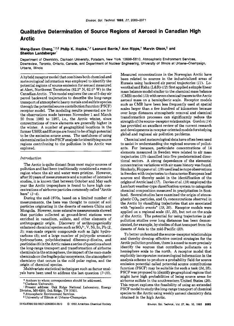
Data Measured at Alert, N.W.T. Concentrntlon of IC-NMSO4 (XlOOO)

I I I

4

Scp Mar Sep Peb Jun Nov Apr Aug Jan May Oct Mar d98h 1983 I 1984 1 1985 I 1986 119871

Flgure 1. Time series plot of concentration of NM SO4.

Alert or preferred pathways of high concentration episodes that originate beyond the reach of 5-day back-trajectories. However, the analysis does not yield quantitative estimates of source areal contributions. Thus, the TPSCF results should not be interpreted as surrogates for emission inventories. However, emission regions should coincide with TPSCF “hot spots” in major source areas.

Results

The chemical species selected for this study include nonmarine SO4 (NM sod), Ni, In, As, As/Sb, V, and Excess-V, Excess-V/Sb (Exs-V/Sb), Zn and Zn/Sb. These elements are typical of anthropogenic origins and have been used as ”tracers” of man-made sources in previous receptor modeling studies (34). Sodium (Na), which is general of natural origin, was used to empirically evaluate the methodology by comparing the results with that of the literature (35). The nonmarine sulfate (NM SO4) is calculated as

(7) where the subscript a denotes aerosol component, and brackets indicate the mass concentration (in ng m-3). The ratio of S04:Na for seawater is 0.25 (36). Exs-V is the excess vanadium concentration calculated as above the background soil level:

[ExsV], = [VI, - 1.3 X 10-3[A11, (8) The ratio of average concentration of V to the average concentration of AI for the local soil at Alert is about 1.35 X (37) and is similar to that found in average crustal rock (35).

Individual Chemical Species. Figure 1 shows the time series of the calculated NM SO4 concentration (in ng m-3) from 1982 to 1987. A strong regularity can be observed in which concentrations rise from summer to peaks generally centered in March and April. This pattern is consistent with the current knowledge about the Arctic haze (3).

It is generally believed that the NM SO1 concentration observed in a remote area is related to both the anthro- pogenic emission of SO2and the biogenic emission of sulfur- containing compounds, e.g., DMS (dimethyl sulfide) or DMDS (dimethyl disulfide) from the surface of the ocean (38). Yin et al. (39) outlined a detailed photooxidation mechanism for DMS and DMDS. DMS was found to be

[NM SOJ, = [SO,], - 0.25[NaIa

Environ. Scl. Technol., Vol. 27, No. IO, 1993 2065

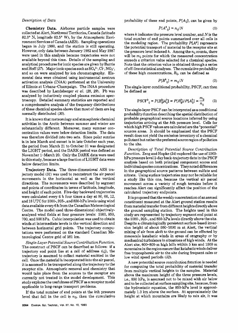
Data Measured at Alert, N.W.T.

F b v n 2. TPSCF map for NM SO, during tiw DARK perlods.

Figure 9. SO2 emlsslon from 5’ X 5’ (!aIltude by iongltude) cells.

themajor component (more than80% relative abundance) among various sulfur species emitted from the ocean surface in the North Sea (40). Li and Barrie (41) analyzed oxidized sulfur data that were measured over a decade at Alert and concluded that biogenic contribution to NM SO4 is negligible during the DARK period. Thus, the sources identified by the TPSCF are mostly likely to be anthropogenic.

The TPSCF result for NM SO, shown in Figure 2 is obtained using the annual average concentration of 977 ng m a as the criterion value. In this paper, the annual average concentration for each chemical species was used unless it is described otherwise. Grid cells with TPSCF values larger than 0.8 in Figure 2 are found in several areas of Europe including a cell a t the border of France and Germany, in the area of the Rhine River Valley, in the Baltic states close to Donetsk area (10, and in Urds, Kuznetsk. The Yakutsk areas in Siberia are also found to be significant sources. Areas from the Rhine River valley to the Donetsk area were also found to have TPSCF values in the range of 0.6-0.8. Comparing these regions with the emission map of SO1 in Figure 3, potential sources areas identified in Europe (Figure 2) appear to be in the locations of known emission (42,43). The areas in eastern Siberia appear to be an indication of preferred transport pathway from emission areas further south. An area in Canada close to Prudhoe Bay, AK, was found to have a TPSCF value higher than 0.8 in Figure 2.

There are four grid cells in the northeastern United States and the Quebec province of Canada which were

2066 Envbn. Sd. T e c M . . Vd. 27. No. 10. 1993

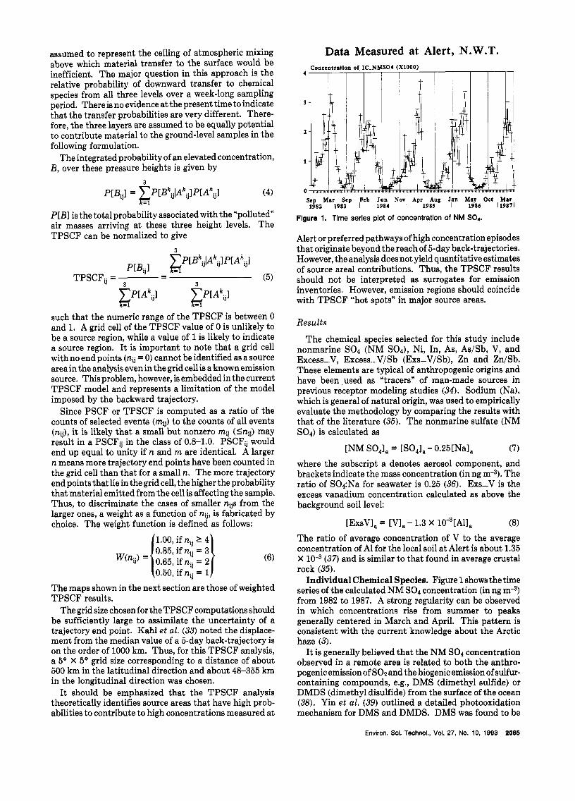
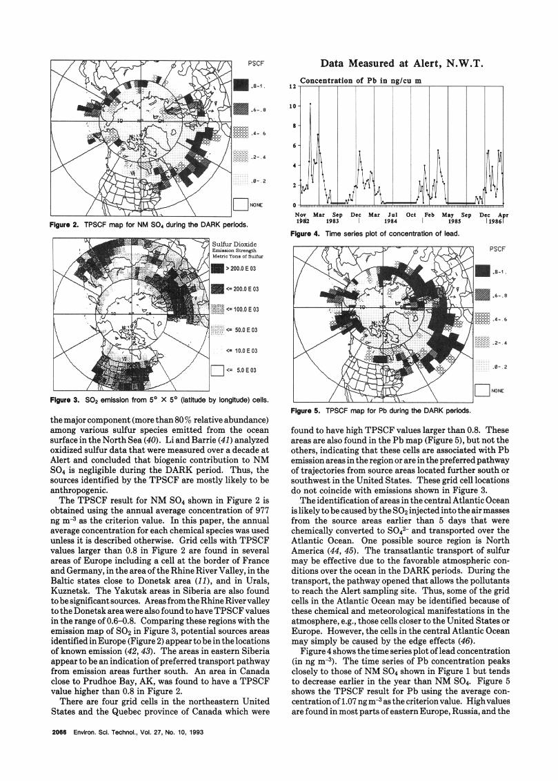
N a Mar Sip Dec Mar 1 ~ 8 1 Os1 Pib May Sep Des A I Ita 1983 1 1984 I 1985 I1986Y

Fbure 4. Time series plot of concentratlon of lead.

*re 5. TPSCF map for Pb during me DARK perMs.

found to have high TPSCF values larger than 0.8. These areas are also found in the Pb map (Figure 5), but not the others, indicating that these cells are associated with Pb emission areas in the region or are in the preferred pathway of trajectories from source areas located further south or southwest in the United States. These grid cell locations do not coincide with emissions shown in Figure 3.

The identification of areas in the central Atlantic Ocean islikelytobecausedbytheSO~injectedintotheairmasses from the source areas earlier than 5 days that were chemically converted to SO? and transported over the Atlantic Ocean. One possible source region is North America (44,45). The transatlantic transport of sulfur may be effective due to the favorable atmospheric con- ditions over the ocean in the DARK periods. During the transport, the pathway opened that allows the pollutants to reach the Alert sampling site. Thus, some of the grid cells in the Atlantic Ocean may be identified because of these chemical and meteorological manifestations in the atmosphere, e.g., those cells closer to the United States or Europe. However, the cells in the central Atlantic Ocean may simply be caused by the edge effecta (46).

Figure 4 shows the time series plot of lead concentration (in ng m3). The time series of Pb concentration peaks closely to those of NM SO4 shown in Figure 1 but tends to decrease earlier in the year than NM SO,. Figure 5 shows the TPSCF result for Pb using the average con- centration of 1.07 ng m4 as the criterion value. Highvalues are found in most parts of eastern Europe, Russia, and the

Data Measured at Alert, NWT Data Measured at Alert, N.W.T.

N- AP. oct ~ . r 1.1 D ~ O m y oca M., 1.1 DIS mal l )d l 1983 1 1984 I 1985 I 1986 119811

Nor Apr Os1 Mar Am. Do0 Hay Os1 Mar Am. Dee May l$dZ 1983 1 1984 i 1985 I 1986 119811

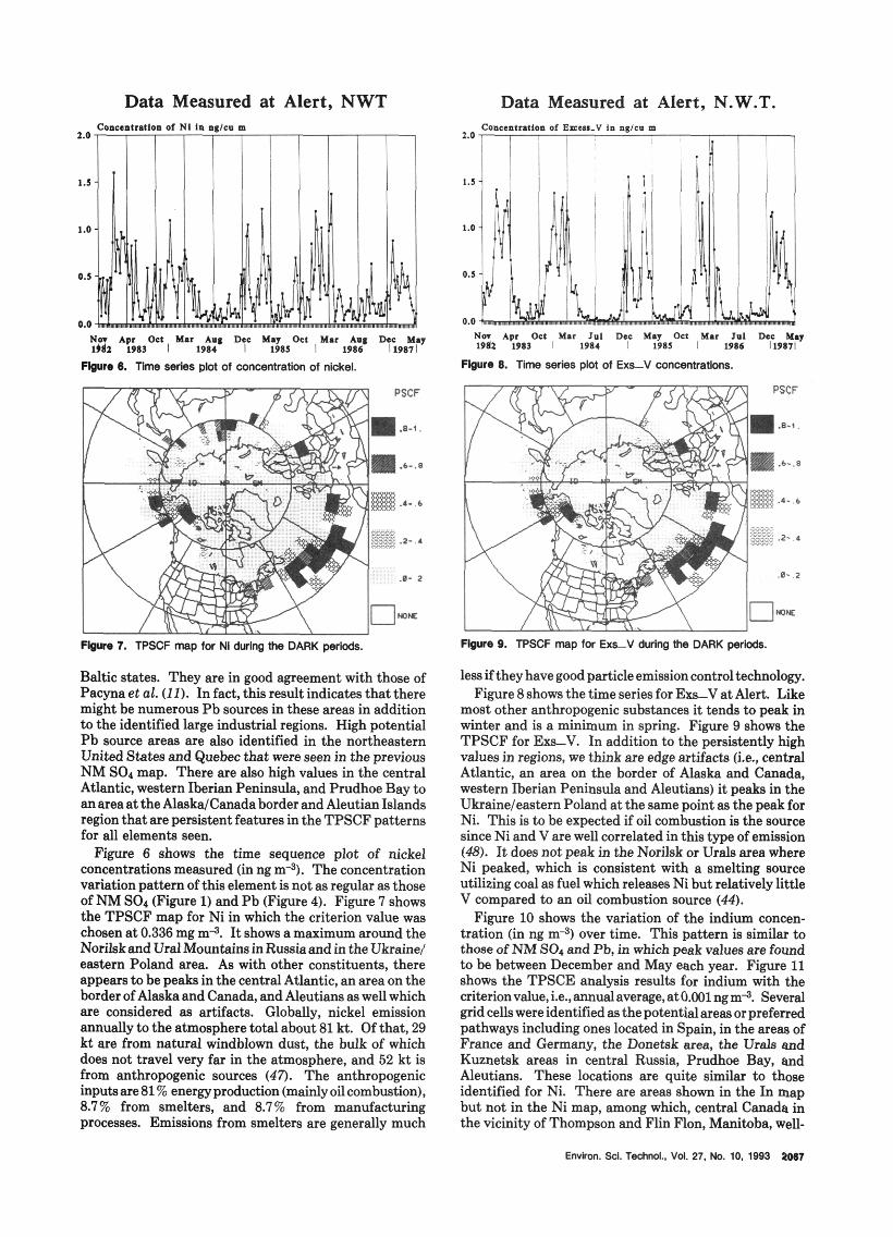
Figure 6. Tlme wries plot of concentration of nickel. Flgure 8. Time series pia of EXLV concentrations.

+re 7. TPSCF map for Ni during the DARK periods.

Baltic states. They are in good agreement with those of Pacyna et al. (11). In fact, this result indicates that there might be numerous Pb sources in these areas in addition to the identified large industrial regions. High potential Pb source areas are also identified in the northeastern United States and Quebec that were seen in the previous NM SO1 map. There are also high values in the central Atlantic, western Iherian Peninsula, and Prudhoe Bay to an areaat the AlaskdCanada border and Aleutian Islands region that are persistent features in the TPSCF patterns for all elements seen.

Figure 6 shows the time sequence plot of nickel concentrations measured (in ng m*). The concentration variation pattern of this element is not as regular as those of NM SO, (Figure 1) and Pb (Figure 4). Figure 7 shows the TPSCF map for Ni in which the criterion value was chosen at 0.336 mg m-l. It shows a maximum around the Norilsk and Ural Mountains in Russia and in the Ukraine/ eastern Poland area. As with other constituents, there appears to be peaks in the central Atlantic, an area on the border of Alaska and Canada, and Aleutians as well which are considered as artifacts. Globally, nickel emission annually to the atmosphere total about 81 kt. Of that, 29 kt are from natural windblown dust, the bulk of which does not travel very far in the atmosphere, and 52 kt is from anthropogenic sources (47). The anthropogenic inputsare 81 % energyproduction (mainly oilcombustion), 8.7% from smelters, and 8.7% from manufacturing processes. Emissions from smelters are generally much

Figure 9. TPSCF map for Exs-V during the DARK plods.

less if they have good particle emission control technology. Figure 8 shows the time series for Exs-V at Alert. Like

most other anthropogenic substances it tends to peak in winter and is a minimum in spring. Figure 9 shows the TPSCF for ExaV. In addition to the persistently high values in regions, we think are edge artifacts (i.e., central Atlantic, an area on the border of Alaska and Canada, western Iberian Peninsula and Aleutians) it peaks in the Ukraine/eastern Poland at the same point as the peak for Ni. This is to be expected if oil combustion is the source since Ni and V are well correlated in this type of emission (48). It does not peak in the Norilsk or Urds area where Ni peaked, which is consistent with a smelting source utilizing coal as fuel which releases Ni but relatively little V compared to an oil combustion source (44).

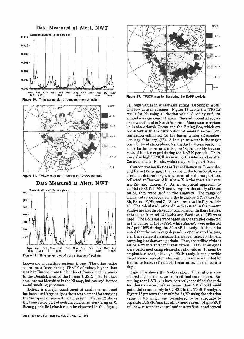
Figure 10 shows the variation of the indium concen- tration (in ng m3) over time. This pattern is similar to those of NM SO, and Pb, in which peak values are found to be between December and May each year. Figure 11 shows the TPSCE analysis results for indium with the criterionvalue, i.e., annualaverage, atO.001 ngm-l. Several grid cells were identified as the potential areas or preferred pathways including ones located in Spain, in the areas of France and Germany, the Donetsk area, the Urds and Kuznetsk areas in central Russia, Prudhoe Bay, and Aleutians. These locations are quite similar to those identified for Ni. There are areas shown in the In map but not in the Ni map, among which, central Canada in the vicinity of Thompson and Flin Flon, Manitoba, well-

Enukon. Scl. Techol.. Vol. 27. No. 10, I993 2087

Data Measured at Alert, NWT

No. Apr Oct M u Jul Dee May Oct Mer a d OIS May I)d2 1983 1 1984 1 1985 I 1986 119871

F w r e IO. Time series plot of concentration of indium.

Figure 11. TPSCF map for In during the DARK periods.

Data Measured at Alert, NWT

Nor Apt Oct Mar lo1 Dee May Srp Peb luo NOI Apr I$dZ 1983 1984 1 1983 I 1986 119811

Flgure 12. Time series plot of concantration of sodium.

known metal smelting regions, is one. The other major source area (considering TPSCF of values higher than 0.6) is in Europe, from the border of France and Germany to the Donetsk area of the former USSR. The last two areas are not identified in the Ni map, indicating different metal smelting processes.

Sodium is a major constituent of marine aerosol and has been used frequently as the tracer element for studying the transport of sea-salt particles (49). Figure 12 shows the time series plot of sodium concentration (in ng m-9. Strong periodic behavior can be observed in this figure,

2066 Envkoon. Scl. Teehnol.. Vd. 27, No. IO. 1993

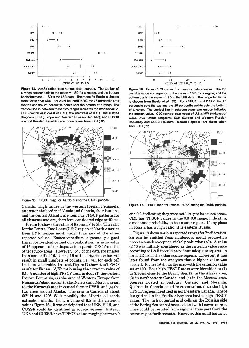
i.e., high values in winter and spring (December-April) and low ones in summer. Figure 13 shows the TPSCF result for Na using a criterion value of 152 ng m-3, the annual average concentration. Several potential source areas were found in North America. Major source regions lie in the Atlantic Ocean and the Bering Sea, which are consistent with the distribution of sea-salt aerosol con- centration estimated for the boreal winter (December- January-February) (33). Although seawater is the major contributor of atmhspheric Na, the Arctic Ocean was found not to be the source area in Figure 13 presumably because most of it is ice-caped during the DARK periods. There were also high TPSCF areas in northeastern and central Canada, and in Russia, which may be edge artifacts.

ConcentrationRatios of TraceElements. Lowenthal and Rahn (12) suggest that ratios of the form X/Sb were useful in determining the sources of airborne particles collected at Barrow, AK, where X is the trace elements As, Zn, and Excess-V. As an empirical approach to validate PSCF/TPSCF and to explore the utility of these ratios, they were used in the analyses. The range of elemental ratios reported in the literature (12,35) for As/ Sb, Excess-V/Sb, and Zn/Sb are presented in Figures 14- 18. The calculated ratios of the data used in the present studies arealsodisplayed for comparison. In these figures, data taken from ref 12 (L&R) and Barrie et al. (35) were used. The L&R data were based on the samples collected in the winter of 1974-1980, while Barrie’s were collected in April 1986 during the AGASP-I1 study. It should be noted that the ratios vary depending upon several factors, e.g., trace element emissionschange over time, at different sampling locations and periods. Thus, the utility of these ratios warrants further investigation. TPSCF analyses were performed using elemental ratio values. It must be emphasized that, although PSCF analysis can provide direct source-receptor information, its range is limited by the finite length of reliable trajectories: in this case, 5 days.

Figure 14 shows the As/Sb ratios. This ratio is con- sidered a good indicator of fossil fuel combustion. As- suming that L&R (12) have correctly identified the ratio for these sources, values larger than 5.0 should yield potential areas mainly in CUSSR in the TPSCF analysis. Figure 15 presents the result for As/Sb using the criterion value of 6.5 which was considered to be adequate to separateCUSSRfromtheothersourceareas. HighPSCF values were found in central and eastern Russia and central

CEC

CUSSR

M R R l E

ANNUAL

DARK

- 1

2 - 3

1 - 2

3 - 4

LO - 11 3-6

5-0

6-9

0 1 2 3 I 5 6 7 8 9 1 0 1 1 1 2 Ratlo of As to Sb

Flgun 14. As/Sb ratios from various data sources. The top bar of a ranae wrresoonds to the mean + 1 SD for a reaion. and the bottom

~ ~ S~~~ ~~ ~~ ~ - . bar is the mean -1 SD in the ULR data. The range for Barrie is chosen from Barrle eta/. (35). For ANNUAL and DARK, the 75 percentile sets the top and the 25 percentile points sets the bonom of a range. The vertical line in between these two ranges indicates the median value. CEC (central east coast of US.). MW (muwest of U.S.). U K S (unned Kingdon), EUR (Europe and Western Russian Republic). and CUSSR (central Russian Republic) are those taken from L&R (1.2).

Flgun IS. TF’SCF map for AsISb durlng the DARK periods.

Canada. High values in the western Iberian Peninsula, anareaonthe border ofAlasdaandCanada, the Aleutians, and the central Atlantic are found in TPSCF patterns for all elements and are, therefore, considered edge artifacts. Figure16showstheratiosofExcess-VtoSb. The ratio

for the CentralEast Coast (CEC) region of North America from L&R ranges much wider than any of the other reported values. Excess vanadium is generally a good tracer for residual or fuel oil combustion. A ratio value of 16 appears to be adequate to separate CEC from the other source areas. However, 75% of the data are smaller than one-half of 16. Using 16 as the criterion value will result in small numbers of counts, i.e., mij, for each cell that is not desirable. Instead, Figure 17 shows the TPSCF result for Excess-V/Sb ratio using the criterion value of 6.5. AnumberofhighTPSCFarea~include (1) thewestern Iberian Peninsula, (2) the area of Western Europe from FrancetoPolandandontotheDonetskandMoscow areas, (3) the Kuznetsk area in central former USSR, and (4) the two areas around Alaska. The area in Canada a t about 60° N and 120° W is possibly the Alberta oil sands extraction plants. Using a value of 6.5 as the criterion value (Figure 16), it was anticipated that UKS, EUR, and CUSSR could he identified as source regions. Instead, UKS and CUSSR have TPSCF values ranging between 0

MW

CUSSP

BARRIE

ANNUAL

DARK

16 I , 36

“ 2

5 - 9

6 - 16

5 - 9

-6

4 + 9

4 + 9

0 LO 2 0 SO 40

Ratlo of Excess-V lo Sb

Flgure IO. Excess VlSb ratios from various data sources. The top bar of a range corresponds to the mean +I SD for a reglon. and the bottom bar is the mean -1 SD In the L8R data. The range for B a d is chmen from Barrie et a/. (35). For ANNUAL and DARK, the 75 percentile sets the top and ilm 25 percentile points sets the bottom of a range. The vertical line in between these two ranges indicates the median value. CEC (central east coast of US.), MW (muwest of US.) , UKS (Unned Kingdom). EUR (Europe and Western Russian Republic), and CUSSR (Central Russian Republic) are those taken from L8R (la.

Flgure 17. TPSCF map for ExceSS-VISb during the DARK periods.

and 0.2, indicating they were not likely to he source areas. CEC has TPSCF values in the 0.6-0.8 range, indicating a moderate probability to be a source region. If any place in Russia has a high ratio, it is eastern Russia.

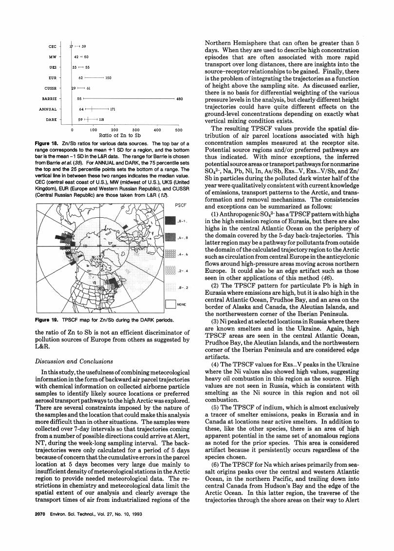
Figure 18 shows various reported ranges for ZdSb ratios. Zn can be emitted from nonferrous metal production processes such as copper-nickel production (43). A value of 70 was initially considered as the criterion value since according to L&R it could provide an adequate separation for EUR from the other source regions. However, it was later found from the analyses that a higher value was needed. Figure 19 shows the map with the criterion value set a t 100. Four high TPSCF areas were identified as (1) in Siberia close to the Bering Sea, (2) in the Alaska area, (3) in northeastern Canada, and (4) in the Moscow area. Sources located at Sudbury, Ontario, and Noranda, Quebec, in Canada could have contributed to the high TPSCF regions identified in northeastern Canada. There is a grid cell in the Prudhoe Bay area having high TPSCF value. The high potential grid cells on the Russian side ofthe Bering Seacannot beassociated with known sources. They could be resulted from regional transport from the source region further south. However, this result indicates

~nvirm. sci. Tsdnci.. VOI. 27. NO. IO. 1993 mas

CEC - M W -

VIS -

EUR -

CUSSR -

BARPIE -

ANNUAL -

DARK -

Flour0 19. TPSCF map fw ZnlSb during thz DARK periods.

the ratio of Zn to Sb is not an efficient discriminator of pollution sources of Europe from others as suggested by L&R.

Discussion and Conclusions

In thisstudy, the usefulnessofcombiningmeteorological information in the form of backward air parcel trajectories with chemical information on collected airborne particle samples to identify likely source locations or preferred aerosol transport pathways to the high Arctic was explored. There are several constraints imposed by the nature of the samples and the location that could make this analysis more difficult than in other situations. The samples were collected over 7-day intervals so that trajectories coming from a number of possible directions could arrive at Alert, NT, during the week-long sampling interval. The hack- trajectories were only calculated for a period of 5 days because of concern that the cumulative errors in the parcel location at 5 days becomes very large due mainly to insufficient density ofmeteorologicalstations in the Arctic region to provide needed meteorological data. The re- strictions in chemistry and meteorological data limit the spatial extent of our analysis and clearly average the transport times of air from industrialized regions of the

2070 Envlrm. Sd. Techol.. VoI. 27. No. IO. 1993

I? - 39

42 H 50

35 - 55

62 I50

2 9 3 61

55 I , 480

64 171

59 -+- 118

Northern Hemisphere that can often be greater than 5 days. When they are used to describe high concentration episodes that are often associated with more rapid transport over long distances, there are insights into the sourcereceptor relationships to be gained. Finally, there is the problem of integrating the trajectories as a function of height above the sampling site. As discussed earlier, there is no basis for differential weighting of the various pressure levels in the analysis, but clearly different height trajectories could have quite different effects on the ground-level concentrations depending on exactly what vertical mixing condition exists.

The resulting TPSCF values provide the spatial dis- tribution of air parcel locations associated with high concentration samples measured a t the receptor site. Potential source regions and/or preferred pathways are thus indicated. With minor exceptions, the inferred potentialsourceareas ortransportpathwaysfornonmarine Sodz, Na, Pb, Ni, In, As/Sb, Exs-V, Exs-V/Sb, and Zn/ Sb in particles during the polluted dark winter half of the year were qualitatively consistent with current knowledge of emissions, transport patterns to the Arctic, and trans- formation and removal mechanisms. The consistencies and exceptions can be summarized as follows:

(1) AnthropogenicS04z has aTPSCFpatternwithhzhs in the high emission regions of Eurasia, but there are also highs in the central Atlantic Ocean on the periphery of the domain covered by the 5-day back-trajectories. This latter regionmay be apathway for pollutants fromoutside the domainof thecalculated trajectoryregion to the Arctic such as circulation from central Europe in the anticyclonic flows around high-pressure areas moving across northern Europe. It could also be an edge artifact such as those seen in other applications of this method (46).

(2) The TPSCF pattern for particulate Pb is high in Eurasia where emissions are high, but it is also high in the central Atlantic Ocean, Prudhoe Bay, and an area on the border of Alaska and Canada, the Aleutian Islands, and the northerwestern comer of the Iberian Peninsula.

(3) Ni peaked at selected locations in Russia where there are known smelters and in the Ukraine. Again, high TPSCF areas are seen in the central Atlantic Ocean, Prudhoe Bay, the Aleutian Islands, and the northwestern corner of the Iberian Peninsula and are considered edge artifacts.

(4) The TPSCF values for Exs-V peaks in the Ukraine where the Ni values also showed high values, suggesting heavy oil combustion in this region as the source. High values are not seen in Russia, which is consistent with smelting as the Ni source in this region and not oil combustion.

(5 ) The TPSCF of indium, which is almost exclusively a tracer of smelter emissions, peaks in Eurasia and in Canada at locations near active smelters. In addition to these, like the other species, there is an area of high apparent potential in the same set of anomalous regions as noted for the prior species. This area is considered artifact because it persistently occurs regardless of the species chosen.

(6) The TPSCF for Na which arises primarily from sea- salt origins peaks over the central and western Atlantic Ocean, in the northern Pacific, and trailing down into central Canada from Hudson’s Bay and the edge of the Arctic Ocean. In this latter region, the traverse of the trajectories through the shore areas on their way to Alert

may mean that continental area end points are connected with high Na events, and there are few if any trajectories from this region to Alert without passing through a source region. Part of the central Atlantic peak is the same region as for the other species, suggesting that this area may be an edge artifact. However, the western Atlantic peak region is new and consistent with a stormy region of high sea-salt generation in the winter months.

(7) Similar to the central Atlantic region discussed above, there are several other persistent peaks, including one in the Aleutian Islands south of Alaska and at a n area on the Alaskan-Canadian border, for all of the species investi- gated. These regions again are likely to be artifacts rather than an indication of real sources or preferred pathways.

(8) T h e TPSCF values for the As/Sb ratio were high in Russia as predicted by L&R, but in addition, high locations were also observed in eastern Russia. The Exs-V/Sb ratio values were not inconsistent with L&R except i t also tends to be high in eastern Russia. T h e Zn/Sb ratio values that should show high values in Europe according to L&R do not have high values, suggesting that this ratio is not a n effective source indicator.

Thus, t he TPSCF analysis in many cases, appears to point t o real source areas, bu t the duration of the samples, the question of the degree of vertical mixing, t he limited length of the calculated trajectories, and their uncertainties in their positions as they get further from the receptor site limits the extent to which these values can be relied upon as definitive indicators of source location. Further study of the problem is currently in progress using daily samples taken during spring 1992 that may help to resolve the sample duration question. Additional detailed study of the vertical motion of the trajectories will be needed to resolve the question of weights for the different pressure levels.

Acknowledgments This research was supported by the National Science

Foundation under Grants ATM 9114750, D P P 9122944, and N S F REU CHEM-9101219. Mention of trade names or commerical products does not constitute an endorse- ment or recommendation for use.

Literature Cited Rahn, K. A.; McCaffrey, R. J Proc. WMO Symp. 1979, No. 538, 25. Rahn, K. A.; McCaffrey, R. J. Ann. N . Y. Acad. Sci. 1980, 486-503. Barrie, L. A. Atmos. Environ. 1986, 20, 643. Ottar, B. Atmos. Environ. 1989, 23, 2349. Hov, 0.; Penkett, S. K.; Isaksen, I. S. A.; Semb, A. Geophys. Res. Lett. 1985, 11, 425. Oehme, M.; Furst, F.; Kruger, C.; Meenken, H. A.; Groebel, W. Chemosphere 1988,17, 1291. Heidam, N. Z. Atmos. Environ. 1981, 15, 1421. Heidam, N. Z. Atmos. Enuiron. 1984, 18, 329. Barrie, L. A.; Barrie, M. J. J . Atmos. Chem. 1990,11, 211. Li, S. M.; Winchester, J. W. J . Geophys. Res. 1990,95,1797. Pacyna, J. M.; Ottar, B.; Tomza, U.; Maenhaut, W. Atmos. Environ., 1985, 19, 857. Lowenthal, D. H.; Rahn, K. A. Atmos. Environ. 1985, 19, 2011.

(13) Friedlander, S. K . Environ. Sci. Technol. 1973, 7, 235. (14) Gordon, G. E. Environ. Sci. Technol. 1991, 25, 1822. (15) Oblad, M.; Selin, E. Atmos. Environ. 1986, 20, 1419. (16) Hopper, J. F.; Ross, H. B.; Sturges, W. T.; Barrie, L. A.

(17) Sturges, W. T.; Barrie, L. A. Atmos. Environ. 1989,23,2513. (18) Davis, T. D.; Farmer, G.; Barthelmie, R. J . Atmos. Environ.

(19) Higuchi, K.; Trivett, N. B. A.; Daggupaty, S. M. Atmos.

(20) Peterson, J. T.; Hanson, K. J.; Bodhaine, B. A.; Oltmans,

(21) Keeler, G. J. Ph.D. Thesis, University of Michigan, Ann

(22) Barrie, L. A. J . Geophys. Res. 1988,930, 3773. (23) Duce, R. A.; Unni, C. K.; Ray, B. J.; Prospero, J. M.; Merrill,

(24) Zeng, Y.; Hopke, P. K. Atmos. Environ. 1989,23, 1499. (25) Cheng, M. D.; Hopke, P. K.; Landsberger, S.; Barrier, L. A.

In Applications of AirPollution Meteorology; Boston, 1991. (26) Malm, W. C.; Johnson, C. E.; Bresch, J. F. In Receptor

Methods for Source Approtionment; Pace, T., Ed.; Air Pollution Control Association: Pittsburgh, PA, 1986; pp

(27) Barrie, L. A,; Hoff, R. M. Atmos. Environ. 1985,19, 1995. (28) Landsberger, S.; Hopke, P. K.; Cheng, M. D. Nucl. Sci.

Eng. 1992, 110, 79. (29) Landsberger, S.; Hopke, P. K.; Cheng, M. D.; Barrier, L. A.

Environ. Pollut. 1992, 75, 181. (30) Cheng, M. D.; Hopke, P. K.; Landsberger, S.; Barrier, L. A.

Atmos. Environ. 1991,25A, 2903. (31) Olson, M. P.; Oikawa, K. K.; Macafee, A. W. A Trajectory

Model Applied to the Long-Range Transport of Air Pollutants; Atmospheric Environmental Services: Canada, 1978.

Tellus 1991,43B, 45.

1990,24A, 63.

Environ. 1987, 21, 1915.

S. J. Geophys. Res. Lett. 1980, 7 , 349.

Arbor, 1987.

J. T. Science 1980,209,1522.

127-148.

(32) Manins, P. C. Boundary-Layer Meteorol. 1992, 60, 169. (33) Kahl, J. D.; Harris, J. M.; Herbert, G. A.; Olson, M. P. Tellus

1989,41B, 524. (34) Hopke, P. K. In Receptor Modeling for Air Quality

Management; Hopke, P. K. , Ed.; Elsevier Science: New York, 1989.

(35) Erickson, D. J.; Merrill, J. T.; Duce, R. A. J . Geophys. Res. 1986, 91 (Dl), 1067.

(36) Mason, B. Principles of Geochemistry, 3rd ed.; John Wiley & Sons: New York, 1966.

(37) Barrie, L. A.; den Hartog, G.; Bottenheim, J. W.; Lands- berger, S. J . Atmos. Chem. 1989,9, 101.

(38) Erickson, D. J.; Ghan, S. J.; Penner, J. E. J . Geophys. Res.

(39) Yin, F.; Grosjean, D.; Seinfeld, J. H. J . Atmos. Chem. 1990,

(40) Leck, C.; Rodhe, H. J . Atmos. Chem. 1991, 12, 63. (41) Li, S. M.; Barrie, L. A. J. Geophys. Res., in press. (42) Hameed, S.; Dignon, J. J . Air Waste Manage. Assoc. 1992,

(43) Dignon, J. Atmos. Environ. 1992, 26A, 1157. (44) Whelpdale, D. M.; Eliassen, A.; Galloway, J. N.; Dovland,

(45) Tarrasson, L.; Iversen, T. Tellus 1992,44B, 114. (46) Cheng, M. D.; Hopke, P. K.; Zeng, Y. J. Geophys. Res.

(47) Nriagu, J. 0. Global Metal Pollut. Environ. 1990, 32, 7. (48) Henry, W. M.; Knap, K. T. Environ. Sci. Technol. 1980,14,

(49) Warneck, P. Chemistry of the Natural Atmosphere; Ac-

1990, 95, (D6), 7543-7552.

11, 309.

42, 159.

H.; Miller, J. M. Tellus 1988, 40B, 1.

[Atmos.], in press.

450.

ademic Press: New York, 1988.

Received for review November 16, 1992. Revised manuscript received May 21, 1993. Accepted June 1, 1993.

Environ. Sci. Technol., Vol. 27, No. 10, 1993 2071