QConBridge II - Theoretical Manual€¦ · Web viewSteel Beam Bridge Product Models. For steel beam bridge product models (built-up and rolled shapes), the end diaphragms are described

THEORETICAL MANUAL

FOR

QCONBRIDGE IIA MEMBER OF THE ALTERNATE ROUTE PROJECT

VERSION 1.0

AUGUST 10, 2000

RICHARD BRICE, PEWSDOT

RICHARD PICKINGS, PEBRIDGESIGHT SOFTWARE

document.doc

Theoretical Manual

REVISION CHART

Version Primary Author(s) Description of Version Date Completed

1.0 RAB, RDP Original Document 8/10/2000

document.doc (08/11/00) Page 1

Theoretical Manual

CONTENTS

1. INTRODUCTION.......................................................................................................... 7

1.1 OVERVIEW............................................................................................................ 71.2 DOCUMENT ORGANIZATION..................................................................................7

2. MATERIAL PROPERTIES............................................................................................ 8

2.1 CONCRETE............................................................................................................. 82.2 STEEL.................................................................................................................... 8

3. FLEXIBLE SPAN LENGTHS.........................................................................................9

3.1 SKEW EFFECTS...................................................................................................... 93.2 HORIZONTAL CURVATURE EFFECTS......................................................................9

3.2.1 Left Curves..........................................................................................................103.2.2 Right Curves........................................................................................................10

3.3 EFFECTS OF CONNECTIONS..................................................................................10

4. SECTION PROPERTIES............................................................................................. 11

4.1 GENERAL............................................................................................................ 114.1.1 Superstructure Elements......................................................................................114.1.2 Substructure Elements..........................................................................................11

4.2 CONCRETE SLAB ON BEAM BRIDGES...................................................................114.2.1 Section Properties for Non-composite Beams.......................................................114.2.2 Section Properties for Composite Beams..............................................................12

4.2.2.1 Effective Slab Area..........................................................................................124.3 CAP BEAMS......................................................................................................... 154.4 COLUMNS............................................................................................................ 15

5. LIVE LOAD DISTRIBUTION FACTORS......................................................................16

5.1 CROSS SECTION TYPES........................................................................................165.2 METHOD OF CALCULATION.................................................................................165.3 SPAN LENGTH USED IN CALCUATIONS.................................................................165.4 SKEW CORRECTION FACTORS.............................................................................165.5 DISTRIBUTION FACTORS FOR REACTIONS............................................................175.6 DISTRIBUTION FACTORS FOR DEFLECTION..........................................................175.7 DISTRIBUTION FACTORS FOR ROTATIONS............................................................175.8 DISTRIBUTION OF PEDESTRIAN LIVE LOAD.........................................................17

6. LONGITUDINAL BRIDGE ANALYSIS MODELS..........................................................18

6.1 MODEL TOPOLOGY.............................................................................................. 186.1.1 Superstructure Elements......................................................................................18


Theoretical Manual

6.1.2 Substructure Elements..........................................................................................196.1.2.1 Abutments.......................................................................................................196.1.2.2 Piers................................................................................................................20

6.1.3 Modeling Connections.........................................................................................236.1.3.1 Abutment Connection......................................................................................236.1.3.2 Continuous Pier Connection.............................................................................256.1.3.3 Integral Pier Connection..................................................................................266.1.3.4 Simple Support Pier Connection......................................................................27

6.2 ANALYSIS STAGES............................................................................................... 286.2.1 Staged Analysis Constraints.................................................................................28

6.3 LOADS................................................................................................................. 296.3.1 Dead Load...........................................................................................................29

6.3.1.1 Load in Main Span..........................................................................................296.3.1.2 Loads in Connection Region............................................................................38

6.3.2 Live Load.............................................................................................................506.3.2.1 Vehicular Live Load........................................................................................506.3.2.2 Pedestrian Live Load.......................................................................................50

6.3.3 Temperature Load................................................................................................506.3.4 Support Settlement Load......................................................................................506.3.5 Slab Shrinkage.....................................................................................................51

6.4 SPECIAL ANALYSIS CONSIDERATIONS.................................................................516.4.1 Dead Load Deflections.........................................................................................526.4.2 Live Load Deflections..........................................................................................52

6.4.2.1 For Evalution of Deflection Criteria.................................................................526.4.2.2 For HL93 Live Load........................................................................................53

6.4.3 Calculation of Rotations......................................................................................536.5 ANALYSIS RESULTS............................................................................................. 53

6.5.1 The Basic Process................................................................................................536.5.1.1 Analysis and Results Processing......................................................................556.5.1.2 Enveloping Simple/Continuous Results............................................................566.5.1.3 Load Cases and Limit States involving Live Load............................................57

6.5.2 Computing Analysis Results.................................................................................596.5.2.2 Load Case Dependencies..................................................................................606.5.2.3 Distribution of Live Load to Girder Lines........................................................616.5.2.4 Deflections......................................................................................................61

6.5.3 Reactions.............................................................................................................626.5.3.1 Limit State Combinations for Reactions...........................................................626.5.3.2 Zero Height Abutments and Piers.....................................................................626.5.3.3 Fixed Height Abutments..................................................................................626.5.3.4 Fixed Height Piers...........................................................................................63

6.5.4 Deflections for evaluation LRFD 2.5.2.6.2...........................................................636.5.5 Pedestrian Only Bridges......................................................................................63

7. TRANSVERSE BRIDGE ANALYSIS MODELS..............................................................64

7.1 MODEL TOPOLOGY.............................................................................................. 647.1.1 Cap Beam Modeling............................................................................................647.1.2 2D Zero-Height Piers...........................................................................................65


Theoretical Manual

7.1.3 3D Zero-Height Piers...........................................................................................657.1.4 2D Fixed Height Piers.........................................................................................657.1.5 3D Fixed Height Piers.........................................................................................657.1.6 Full Product Model Piers.....................................................................................66

7.2 LOADS................................................................................................................. 667.2.1 Adjustments for Skew...........................................................................................667.2.2 Pier Loads...........................................................................................................67

7.2.2.1 Pier Self Weight..............................................................................................677.2.2.2 Other Loads.....................................................................................................67

7.2.3 Superstructure Loads...........................................................................................677.2.3.1 Girder Self Weight...........................................................................................677.2.3.2 Slab Self Weight..............................................................................................677.2.3.3 Intermediate Diaphragms.................................................................................677.2.3.4 End Diaphragms..............................................................................................677.2.3.5 Traffic Barrier..................................................................................................687.2.3.6 Median Barrier.................................................................................................687.2.3.7 Overlay............................................................................................................687.2.3.8 Sidewalk..........................................................................................................687.2.3.9 Live Loads.......................................................................................................68

7.3 ANALYSIS RESULTS............................................................................................. 777.3.1 The Basic Process................................................................................................777.3.2 TBAM Results......................................................................................................797.3.3 Total Pier Results (Combining LBAM Results).....................................................79


Theoretical Manual

LIST OF FIGURES

Figure 1 Skew Effects for computing Flexible Span Length........................................................9

Figure 2 Connection Effects for computing Flexible Span Length.............................................10

Figure 3 Effective Span Lengths for computing Effective Flange Width....................................13

Figure 4 Procedure for computing Effective Flange Width........................................................14

Figure 5 Effective Slab Depth...................................................................................................14

Table 1 Skew Angle for computing Skew Correction Factors....................................................17

Figure 6 Model Geometry for Slab on Girder Bridges...............................................................18

Figure 7 BAM Detail for Zero-Height Idealized Abutments......................................................19

Figure 8 BAM Detail for Fixed-Height Idealized Abutments.....................................................20

Figure 9 LBAM Model of Zero-Height Idealized Piers..............................................................21

Figure 10 LBAM Model of Fixed-Height Idealized Piers..........................................................21

Figure 11 LBAM Modeling of Full Product Model Piers..........................................................22

Figure 12 Column Height when Bottom Elevation is specified..................................................23

Figure 13 Abutment Connection on a Zero Height Abutment....................................................24

Figure 14 Abutment Connection on a Fixed Height Abutment..................................................25

Figure 15 Continuous Pier Connection on a Zero Height Idealized Pier.....................................25

Figure 16 Continuous Pier Connection on a Fixed Height Idealized Pier...................................26

Figure 17 Integral Pier Connection on a Zero Height Idealized Pier...........................................26

Figure 18 Integral Pier Connection on a Fixed Height Idealized Pier.........................................27

Figure 19 Simple Support Pier Connection on a Zero Height Idealized Pier...............................27

Figure 20 Simple Support Pier Connection on a Fixed Height Idealized Pier.............................28

Figure 21 Modeling of Main Span Loads..................................................................................29

Figure 22 Tributary Slab Width................................................................................................31

Figure 23 Tributary Slab Width for an Exterior Girder..............................................................31

Figure 24 Slab Pad (Haunch) Load...........................................................................................33

Figure 25 Abutment Connection Loads.....................................................................................38

Figure 26 Simple Support Pier Connection Loads.....................................................................44

Figure 27 Slab Shrinkage Moments..........................................................................................51

Figure 28 Section Geometry for Slab Shrinkage Moments........................................................51

Figure 29 Basic LBAM Analysis Process..................................................................................54


Theoretical Manual

Figure 30 Analysis and Results Processing...............................................................................55

Figure 31 Analysis and Results Processing for Simple/Continuous Envelopes...........................57

Figure 32 Maximum Limit States with Live Load.....................................................................58

Figure 33 Minimum Limit States with Live Load......................................................................59

Figure 34 Load Case Dependencies...........................................................................................60

Figure 35 Basis for computing Limit State Deflections.............................................................62

Figure 36 Structural Modeling of Cap Beam.............................................................................64

Figure 37 TBAM for a 3D Zero Height Idealized Pier...............................................................65

Figure 38 Analysis Modeling of Fixed Height 3D Piers............................................................65

Figure 39 TBAM for Multicolumn and Hammerhead Piers.......................................................66

Figure 40 Representation of Vehicular Live Load Reactions in TBAM's...................................69

Figure 41 Lane Configurations..................................................................................................70

Figure 42 Design Lane Configuration with one sidewalk...........................................................71

Figure 43 Design Lane Configuration with two sidewalks.........................................................71

Figure 44 Design Lane Configuration for TBAM's....................................................................72

Figure 45 Permutations of Loaded Design Lanes for a 3 Lane Structure....................................73

Figure 46 Permutations of Loaded Design Lanes for a 3 Lane Structure with a Sidewalk...........74

Figure 47 Permutations of Loaded Design Lanes for a 3 Lane Structure with two Sidewalks.....75

Figure 48 Rigid Links Load Transfer Model.............................................................................76

Figure 49 Drop-Through Load Transfer Model.........................................................................77

Figure 50 Basic TBAM Analysis Process..................................................................................78

Figure 51 LBAM Reactions Transformed to plane of TBAM....................................................79


Theoretical Manual

1. INTRODUCTION

1.1 OverviewThe purpose of this document is to provide a detailed description of how QConBridge II performs its analytical work.

1.2 Document OrganizationThis document is broken into seven main sections: Section 1 - Introduction explains the purpose of this document. Section 2 - Material Properties details how QConBridge II computes material properties. Section 3 - Flexible Span Lengths details how the various geometric parameters effect the flexible span length used in several of the analyzes. Section 4 - Section Properties describes how QConBridge II computes section properties for the supported product models. Section 5 - Live Load Distribution Factors details how distribution factors are calculated and how the ambiguous portions of the LRFD specification are dealt with. Section 6 - Longitudinal Bridge Analysis Models describe in detail how LBAMs are created, loaded, analyzed, and how the raw results are post-processed. Section 7 - Transverse Bridge Analysis Models provides in-depth coverage of TBAMs.


Theoretical Manual

2. MATERIAL PROPERTIES

Material properties will be determined as described in this section. All materials must have a modulus of elasticity, unit weight/density for weight calculations, unit weight/density for strength calculations, and a coefficient of thermal expansion.

2.1 ConcreteProperties for concrete will be as specified in LRFD 5.4.2. The 28 day compressive strength must be between 4ksi and 10ksi (28MPa and 70MPa).

The modulus of elasticity of concrete will be computed in accordance with LRFD 5.4.2.4.

US - For unit weights between 0.090 and 0.155 kip/ft3, Ec is computed as . For analyses done in accordance with WSDOT criteria the range of unit weights is 0.090 to 0.160 kip/ft3.1

SI - For densities between 1440 and 2500 kg/m3, Ec is computed as . For analyses done in accordance with WSDOT criteria the range of densities is 1440 to 2560 kg/m3.1

2.2 SteelProperties for reinforcing steel will be as specified in LRFD 5.4.3

Properties for structural steel will be as specified in LRFD 6.4.1

1 See Design Memorandum 03-2000 (Dated 4/18/2000)1


Theoretical Manual

3. FLEXIBLE SPAN LENGTHS

In product models, the pier-to-pier span length is generally not the same as the flexible span length for a girder line. Skew, horizontal curvature of the roadway, and connection details all factor into the flexible span length. Flexible span lengths are used in analysis models.

The flexible span length of a girder is computed as , where:

Lpp Pier to pier span length - For curved structures, this may be measured as a chord or a distance along the curve. Built-up steel plate girders are generally curved. Rolled-I beams and Precast Beams are generally straight.

Eskew Effect of skew at start and end of the girder

Ecurve Effect of horizontal curve at start and end of girder

Econnect Effect of connections at start and end of girder

3.1 Skew EffectsSkew effects occur when the piers at either end of a span are skewed.

Figure 1 Skew Effects for computing Flexible Span Length

3.2 Horizontal Curvature EffectsHorizontal curve effects occur when a bridge is curved in plan. The pier to pier span length is measured long a survey line. Girder lines that are offset from the survey line are either longer or


Theoretical Manual

shorter because the radius of the curve defining the girder line (or the end points of the girder line if it is a chord) is larger or smaller.

3.2.1 Left CurvesFor curves towards the left, when looking ahead on station, the horizontal curve effect can be computed as .

3.2.2 Right CurvesFor curves towards the right, when looking ahead on station, the horizontal curve effect can be computed as .

3.3 Effects of ConnectionsConnections define the location of the point of bearing relative to the centerline of the pier. The flexible span length must be adjusted for the effects of the Girder Bearing Offset defined in Section 3.1.2.5 of the System Design Manual. The Girder Bearing Offset is measured normal to the pier centerline and must be adjusted for skew angle.

The effects of connections can be computed as

Figure 2 Connection Effects for computing Flexible Span Length


Theoretical Manual

4. SECTION PROPERTIES

QConBridge II will perform its structural analysis using stiffness methods. In order to perform this analysis, section properties need to be computed.

4.1 GeneralSection properties can be changed at each analysis stage. For Bridge Analysis Model Projects, the user is responsible for computing and inputting section properties. For Product Model Projects, QConBridge II will compute the appropriate section properties for each stage of analysis.

QConBridge II requires cross sectional area and moment of inertias for superstructure and substructure elements

4.1.1 Superstructure ElementsTwo sets of section properties are required for every superstructure element: One set is required for computing moments, shears, and reactions,another set is required for computing deflections.

Section properties for deflection are governed by LRFD 2.5.2.6.2 and 4.6.2.6.1. LRFD 2.5.2.6.2 applies to deflections from vehicular live load and states, For composite design, the design cross-section should include the entire width of the roadway and any structurally continuous portions of the railings, sidewalks, and median barriers. LRFD 4.6.2.6.1 applies to deflections from permanent loads in girder line models and states, The calculation of deflections should be based on the full flange width.

In order to compute limit state deflections for a longitudinal bridge analysis model, the live load deflection will have to be scaled to a single girder line. The details of this are described in Sections 5.6 and 6.4.2.

4.1.2 Substructure ElementsOnly one set of section properties is needed for substructure elements. Section properties are required for elements that represent the columns and the cap beam.

4.2 Concrete Slab on Beam BridgesThe following sections describe how QConBridge II will compute section properties of superstructure elements for generic Slab on Beam Bridges. Section properties are based on gross or transformed cross section dimensions unless stated otherwise.

The slab on beam bridges supported by QConBridge II all have stages where the beams are non-composite and then later made composite with the concrete slab.

4.2.1 Section Properties for Non-composite BeamsSection properties for non-composite beams will be computed using conventional means.


Theoretical Manual

4.2.2 Section Properties for Composite BeamsComposite cross sectional properties will be computed using transformed sections. The effective slab area will be transformed into an equivalent girder section by scaling its properties by

.

4.2.2.1 Effective Slab AreaAn effective flange width and an effective slab depth define the effective slab area. For the purposes of computing section properties, the effective slab area is assumed to be directly on top of the top flange of the girder unless specified otherwise.

4.2.2.1.1 EFFECTIVE FLANGE WIDTHThe effective flange width is the limits of the width of a concrete slab, taken as effective in composite action for determining resistance for all limit states. The effective flange width is computed in accordance with LRFD 4.6.2.6.1

4.2.2.1.1.1 Effective Flange Width for Interior GirdersThe effective flange width for interior girders is taken to be the lesser of:

One-quarter of the effective span length

12.0 times the average thickness of the slab, plus the greater of web thickness or one-half the width of the top flange of the girder; or

The average spacing of adjacent beams.

4.2.2.1.1.2 Effective Flange Width for Exterior GirdersThe effective flange width for exterior girders is taken to be one-half the effective flange width of the adjacent interior girder plus the lesser of:

One-eighth of the effective span length

6.0 times the average thickness of the slab, plus the greater of half the web thickness or one-quarter of the width of the top flange of the basic girder; or

The width of the overhang.

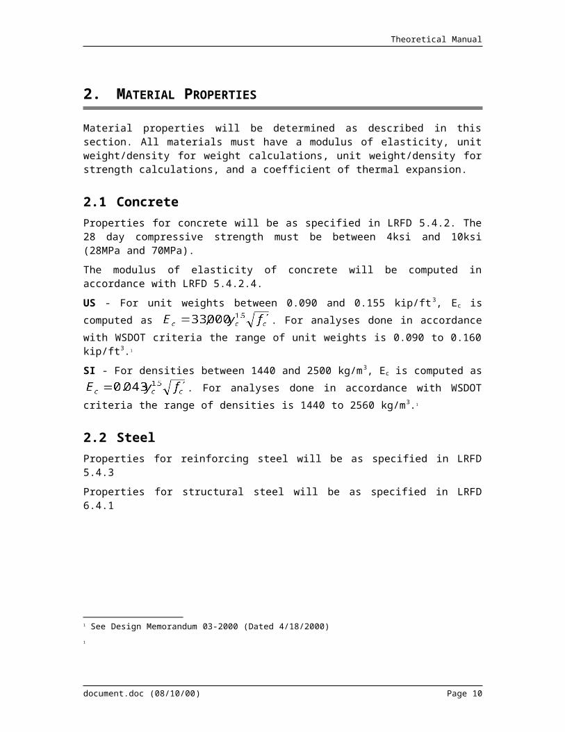
4.2.2.1.1.3 Effective Span LengthThe effective flange width is based on the effective span length. The effective span length is defined as the actual span length for simply supported spans and the distance between points of permanent load inflection for continuous spans, as appropriate for either positive or negative moments. Figure 3 illustrates how the effective span lengths are determined for a three span continuous structure. If the effective span length controls the effective flange width calculation, an iterative solution for effective span length is required. When the effective flange width changes, the section properties change as well. This causes the inflection points due to permanent load to move. When the inflection points move, the effective span lengths change, the effective flange width changes, and the cycle repeats until you converge on the effective span length and effective flange width. This iterative computation is shown in Figure 4.


Theoretical Manual

Figure 3 Effective Span Lengths for computing Effective Flange Width at Different Locations along a Bridge


Theoretical Manual

Figure 4 Procedure for computing Effective Flange Width

4.2.2.1.2 EFFECTIVE SLAB DEPTHThe effective slab depth is equal to the gross slab depth less the sacrificial depth. For exterior beams, the effective slab depth varies between the depth at the edge of the slab and the effective depth of the main slab.

Figure 5 Effective Slab Depth


Theoretical Manual

4.3 Cap BeamsOnly one set of section properties need to be computed for cap beams. The cross sectional area and moment of inertia need to be computed. Cap Beam section properties only apply to TBAM's.

4.4 ColumnsOnly one set of section properties needs to be computed for columns. Column properties are required for cross sectional area and moment of inertia about axes transverse and longitudinal to the plane of the pier.

For LBAM's the cross sectional area and moment of inertia are summed for all columns and then divided by the number of girder lines. If the pier is skewed, the section properties are transformed into a coordinate system that is transverse and longitudinal to the alignment at the location of the pier. The moment of inertia for bending about an axis normal to the alignment is used in the analysis model. The product of inertia will likely be non-zero in this case, but will be ignored, as the analysis method used by QConBridge II does not account for the skew effects except as provided for in the live load distribution factors, and for load transfer between LBAM’s and TBAM’s (see Section below).

For TBAM's, the cross sectional area and moment of inertia for bending about an axis normal to the bent for each individual column are used.


Theoretical Manual

5. LIVE LOAD DISTRIBUTION FACTORS

Live load distribution factors are used to approximate the amount of live load a single girder line will carry. For BAM Projects, the user is responsible for determining the appropriate distribution factors and inputting them into the program. For Product Model Projects, QConBridge II will compute live load distribution factors with applicable LRFD and WSDOT criteria.

5.1 Cross Section TypesFor the purpose of computing live load distribution factors, precast girder bridge product models are classified as cross section type K and rolled steel beams and built-up plate girder bridge product models are classified as cross section type A.

5.2 Method of CalculationLive load distribution factors are computed in accordance with LRFD 4.6.2.2. If the WSDOT BDM option is selected, distribution factors for precast girders will be computed in accordance with Design Memorandum 2-1999.

5.3 Span Length used in CalcuationsThe span length parameter L will be determined in accordance with table C4.6.2.2.1-1. Table C4.6.2.2.1-1 does not cover the case of interior reactions of simple spans (multi-span bridge without moment continuity between spans). For this case, L will be taken as the length of the longer of the adjacent spans.

In the rare occasion when the continuous span arrangement is such that an interior span does not have any positive uniform load moment, i.e., no uniform load points of contraflexure, the region of negative moment near the interior supports would be increased to the centerline of the span, and the L used in determining the live load distribution factors would be the average of the two adjacent spans.

5.4 Skew Correction FactorsWhen the lines of support are skewed the distribution factors must be adjusted to account for skew effects. Skew adjustment for moments are given in LRFD 4.6.2.2.2e. Skew adjustments for shear are given in LRFD 4.6.2.2.3c.

For the purposes of computing the skew correction factors the skew angle will be defined as:

Force Effect Skew Angle

Moment Average skew angle of the adjacent supports

Shear Average skew angle of the adjacent supports

Reactions Skew angle at the pier where the reaction occurs

Table 1 Skew Angle for computing Skew Correction Factors


Theoretical Manual

5.5 Distribution Factors for ReactionsDistribution factors for reactions are not specifically defined in the LRFD specification, though they are alluded to in table C4.6.2.2.1-1. For type A and K cross sections, shear distribution factors are independent of span length, except when they are corrected for skew. QConBridge II will use the basic shear distribution factors for reactions, and adjust them for skew using the span lengths defined in Section 5.3 and skew angles defined in Section 5.4

Support elements that are modeled with a column member generate reactions for moment, axial, and shear forces. Vertical loads imparted onto the substructure from the superstructure generate these force effects. For this reason, the distribution factors for reaction will be applied to all three of these reaction components.

5.6 Distribution Factors for DeflectionWhen computing live load deflections the live load distribution factors for moments shall be used, except when computing deflections for evaluation of LRFD 2.5.2.6. For upward deflections, the distribution factor for negative moment will be used. For downward deflections, the distribution factor for positive moment will be used.

When computing live load deflections for the truck and lane configuration defined in LRFD 3.6.1.3.2 for use in evaluating LRFD 2.5.2.6, the procedure defined in Section 6.4.1 shall be used.

5.7 Distribution Factors for RotationsWhen computing rotations due to live load the distribution factors for moment shall be used. For rotations relating to negative moments near the support, QconBridge II shall use the negative moment distribution factor. For rotations relating to positive moments near the support, QconBridge II shall use the positive moment distribution factor.

5.8 Distribution of Pedestrian Live LoadThe LRFD Specification does not provide guidance for the distribution of pedestrian live load to a girder line. Because pedestrian live load is a uniform load applied to a sidewalk, QConBridge II will distribute it the same way the uniform sidewalk dead load is distributed. Distribution of sidewalk dead load is described in Section below.


Theoretical Manual

6. LONGITUDINAL BRIDGE ANALYSIS MODELS

The primary reason that Bridge Product Models are used in QConBridge II is to provide a simplified, efficient, and intuitive way to describe a bridge structure. Before a longitudinal structural analysis can be performed on a Product Model bridge, it must be idealized as a LBAM. The process of idealization is called Model Generation. This Section describes the modeling techniques and assumptions used when generating LBAM’s from the Product Models supported by QConBridge II.

6.1 Model TopologyThe basic topology of a LBAM is similar for all types of slab on girder bridges. Figure 6 shows the mapping from a product model to an analysis model for a typical slab on girder bridge.

Note that Figure 6 leaves out much detail. Details are given in the Sections following.

Figure 6 Model Geometry for Slab on Girder Bridges

6.1.1 Superstructure ElementsFor the simplified method of analysis, the superstructure is divided into girder lines and each girder line is analyzed independently. Superstructure elements are modeled between points of bearing as a series of prismatic segments. The first segment begins at the left edge of a span. The remaining segments continue end to end until the right edge of the span is reached. The span


Theoretical Manual

length of the superstructure elements is taken to be the flexible span length as described in Section above.

6.1.2 Substructure ElementsThis Section describes how the product model descriptions of substructure elements are represented in the LBAM. Note that substructure elements need not be modeled consistently between the LBAM and the corresponding TBAM. For example, in the LBAM, a substructure element can be modeled as a knife-edge idealization and in the TBAM could represent the same pier as a complete 2D bent model.

6.1.2.1 AbutmentsThis section describes how abutment product models are described in the LBAM.

6.1.2.1.1 ZERO-HEIGHT IDEALIZED ABUTMENTSFigure 7 shows how this type of abutment is modeled. The location of the support is located at the centerline of bearing. Note that the bearing heights from the connection are ignored.

Figure 7 BAM Detail for Zero-Height Idealized Abutments

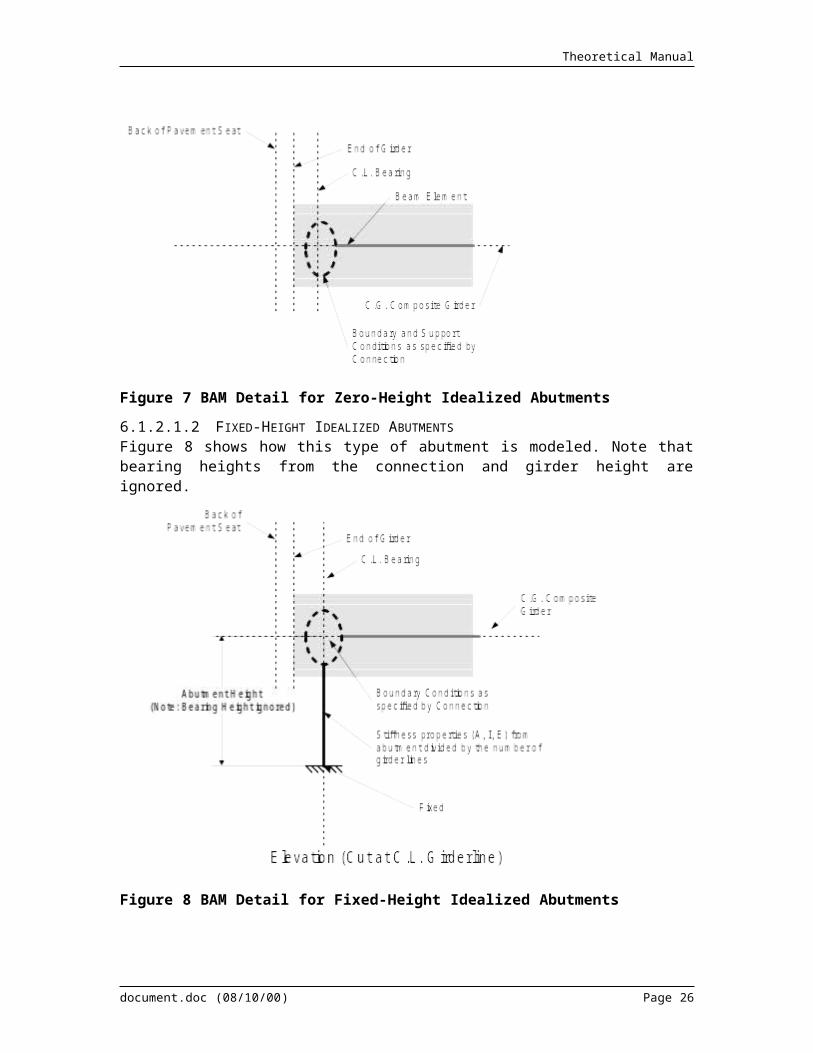
6.1.2.1.2 FIXED-HEIGHT IDEALIZED ABUTMENTSFigure 8 shows how this type of abutment is modeled. Note that bearing heights from the connection and girder height are ignored.


Theoretical Manual

Figure 8 BAM Detail for Fixed-Height Idealized Abutments

6.1.2.2 PiersPier product models can be 2D or 3D zero height idealized, 2D or 3D fixed height idealized, or full product models. LBAMs are only concerned about the components of the pier product description dealing with the longitudinal force analysis for 3D and full product models. Pier connections can be Continuous, Simply Supported, or Simply Supported made Continuous.

6.1.2.2.1 ZERO-HEIGHT IDEALIZED PIERS shows how zero height piers are modeled for continuous and simple support connections. Note that bearing heights from the connection are ignored and for the simple support condition, the left and right bearings share a common point of support located at the centerline of the pier.


Theoretical Manual

Figure 9 LBAM Model of Zero-Height Idealized Piers

6.1.2.2.2 FIXED HEIGHT IDEALIZED PIERSFigure 10 shows how fixed height piers are modeled for continuous and simple support connections. The analysis model supports correspond to the centerline pier in the product model. Note that bearing heights from the connection and the vertical height between the girder C.G. and the top of the cap are ignored. For the simple support condition, the left and right bearings share a common point of support located at the centerline of the pier.

Figure 10 LBAM Model of Fixed-Height Idealized Piers

6.1.2.2.3 FULL PRODUCT MODEL PIERSThe modeling of full product model piers is shown in Figure 11 for continuous and simple support connections. Note that this model takes the entire height of the product model pier into account including bearing heights. If bearing heights differ due to different girder depths, the average bearing height and average Ycg for the girder are used.


Theoretical Manual

Figure 11 LBAM Modeling of Full Product Model Piers

The column height is computed as the difference between the top of column and bottom of column elevations. The top of column elevation is computed by tracing the elevation at the roadway surface at the intersection of the survey line and the centerline of the pier, along the roadway surface to the reference girder, down the depth of the reference girder to the cap beam, along the top surface of the cap beam to the centerline of the column and down the depth of the cap beam at the column. If the columns are different height, the average column height is used. This is shown in Figure 12.


Theoretical Manual

Figure 12 Column Height when Bottom Elevation is specified

6.1.3 Modeling ConnectionsConnections define the boundary conditions between adjacent superstructure members and the boundary conditions between superstructure members and substructure members. For zero height abutments and piers, connections define the support condition as well.

The sections that follow illustrate how product model connections are mapped to analysis model connections for the various combinations of support type and connection type.

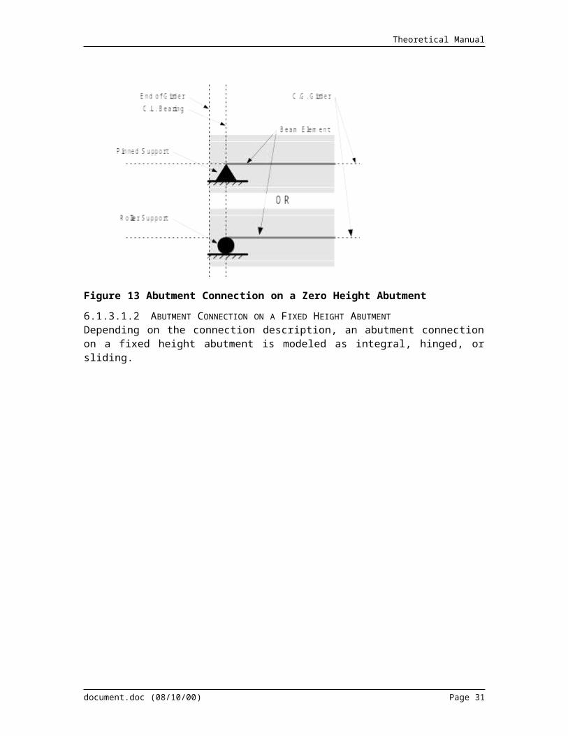
6.1.3.1 Abutment Connection6.1.3.1.1 ABUTMENT CONNECTION ON A ZERO HEIGHT ABUTMENTDepending on the connection description, an abutment connection on a zero height abutment is modeled as a pinned or roller support.


Theoretical Manual

Figure 13 Abutment Connection on a Zero Height Abutment

6.1.3.1.2 ABUTMENT CONNECTION ON A FIXED HEIGHT ABUTMENTDepending on the connection description, an abutment connection on a fixed height abutment is modeled as integral, hinged, or sliding.


Theoretical Manual

Figure 14 Abutment Connection on a Fixed Height Abutment

6.1.3.2 Continuous Pier Connection6.1.3.2.1 CONTINUOUS PIER CONNECTION ON A ZERO HEIGHT PIERDepending on the connection description, a continuous pier connection on a zero height pier is modeled as a pinned or roller support.

Figure 15 Continuous Pier Connection on a Zero Height Idealized Pier


Theoretical Manual

6.1.3.2.2 CONTINUOUS PIER CONNECTION ON A FIXED HEIGHT PIERA continuous pier connection on a fixed height pier is modeled with a hinge or slider at the top of the column member.

Figure 16 Continuous Pier Connection on a Fixed Height Idealized Pier

6.1.3.2.3 CONTINUOUS PIER CONNECTION ON A FULL PRODUCT MODEL PIERConnections for a full product model pier are the same as for Fixed Height Idealized Piers

6.1.3.3 Integral Pier Connection6.1.3.3.1 INTEGRAL PIER CONNECTION ON A ZERO HEIGHT PIERIntegral pier connections on zero height-idealized piers are modeled with a pinned support condition.

Figure 17 Integral Pier Connection on a Zero Height Idealized Pier

6.1.3.3.2 INTEGRAL PIER CONNECTION ON A FIXED HEIGHT PIERIntegral pier connections on fixed height idealized piers are modeled with an integral connection between the two superstructure elements and the column element.


Theoretical Manual

Figure 18 Integral Pier Connection on a Fixed Height Idealized Pier

6.1.3.3.3 INTEGRAL PIER CONNECTION ON A FULL PRODUCT MODEL PIERConnections for a full product model pier are the same as for Fixed Height Idealized Piers

6.1.3.4 Simple Support Pier Connection6.1.3.4.1 SIMPLE SUPPORT PIER CONNECTION ON A ZERO HEIGHT PIERSimple support pier connections on a zero height pier are modeled with pinned or roller supports and a hinge at the right end of the left span.

Figure 19 Simple Support Pier Connection on a Zero Height Idealized Pier

6.1.3.4.1.1 Made ContinuousIf this connection is made continuous at some later stage in the analysis, the connection for that stage will be modeled as described in Section 6.1.3.2.1.


Theoretical Manual

6.1.3.4.1.2 Made IntegralIf this connection is made integral at some later stage in the analysis, the connection for that stage will be modeled as described in Section 6.1.3.3.1. Note that if a roller support is used in the simple span stage, it will be changed to a pinned support in the integral stage.

6.1.3.4.2 SIMPLE SUPPORT PIER CONNECTION ON A FIXED HEIGHT PIERSimple support pier connections on a fixed height pier are modeled with hinges at the ends of the spans framing into the connection. If the top of column is hinged, the hinge at the left end of the right span is omitted.

Figure 20 Simple Support Pier Connection on a Fixed Height Idealized Pier

6.1.3.4.2.1 Made ContinuousIf this connection is made continuous at some later stage in the analysis, the connection for that stage will be modeled as described in Section 6.1.3.2.2.

6.1.3.4.2.2 Made IntegralIf this connection is made integral at some later stage in the analysis, the connection for that stage will be modeled as described in Section 6.1.3.3.2.

6.1.3.4.3 SIMPLE SUPPORT PIER CONNECTION ON A FULL PRODUCT MODEL PIERConnections for a full product model pier are the same as for Fixed Height Idealized Piers

6.2 Analysis StagesQConBridge II supports staged analysis. Each bridge construction stage is modeled with a stage in the bridge analysis model. The analysis stage consists of a LBAM that represents the structure during the current stage and the loads that are applied to or removed from the structure during this stage.

6.2.1 Staged Analysis ConstraintsThere are two constraints that must be imposed on the stages of analysis models. The first constraint is that boundary conditions can only be added. For example, a hinge can be added to a


Theoretical Manual

span, but one cannot be taken away. The second constraint is that the member stiffness parameters (A, I and E) must not decrease as the stage number increases.

With the product models supported by QConBridge II, this is not a concern. These constraints are adhered to by the very nature of the product models supported by the software.

6.3 LoadsThe sections that follow describe how the various loads are generated from the product model description and applied to the LBAM.

6.3.1 Dead LoadProduct model dead loads for longitudinal analysis consists of the self weight of the girders, roadway slab, end diaphragms, intermediate diaphragms, traffic barriers, median barriers, sidewalks, and overlays. This section describes how these loads are computed and represented in LBAM's.

Permanent loads of and on the roadway slab may either be distributed uniformly over all the girder lines (See LRFD 4.6.2.2.1) or may be distributed based on tributary areas and simple distribution rules (WSDOT Design Practice). This section will describe how the dead loads are computed and applied to the LBAM's for both cases. When the loads are evenly distributed over all girders, the loads specified in Section 6.3.1.1.8, except for girder self weight, are not applied to the analysis models.

6.3.1.1 Load in Main SpanSuperimposed dead loads are applied to the main span, between the centerlines of bearing as a uniform load or a series of linear load segments as appropriate. The figure below illustrates how superimposed dead loads in the main span are modeled.

Figure 21 Modeling of Main Span Loads

6.3.1.1.1 GIRDER SELF-WEIGHTThe self-weight of the girder is modeled as a series of uniform load segments that correspond to the segments in the product model. The intensity of a load segment is taken to be where,


Theoretical Manual

w Intensity of the uniform load

Ai Cross-sectional area of the ith element

i Density of the material for the ith element of the cross section

g gravitational acceleration

i ith element in the cross section

6.3.1.1.2 SLAB

6.3.1.1.2.1 Uniform Distribution to All Girder Lines

The load per girder line using a uniform distribution of the slab load is taken to be

where,

w Intensity of the uniform load

Vslab Volume of the slab

c Density of the slab concrete

g gravitational acceleration

N Number of girder lines

Lm Total length of the analysis model to which this load is applied

The volume of the slab is taken to be where,

Vslab Volume of the slab

Ai cross section area of the slab, including the slab pad, at section i

Li Distance between section i and i+1, measure along the center line of the bridge

NS Number of sections. Slab sections begin and end at the ends of the girders at the start and end of the bridge and occur at all points of interest.

6.3.1.1.2.2 Distribution of Load to Girder Lines Based on Tributary AreaThis section describes how the slab load is distributed to girder lines based on tributary area. The slab load is divided into two parts; the main slab and the slab pad.

6.3.1.1.2.2.1 Main SlabThe load from the main portion of the slab on interior girders is a uniform load along the entire length of the girder line. For exterior girders, the main slab loads varies with location due to the thickening of the overhang at the exterior girder and curvature of the slab edge.


Theoretical Manual

6.3.1.1.2.2.1.1 Interior Girders

Figure 22 Tributary Slab Width

The main slab load for interior girders is , where:

wslab Main slab load

tslab Gross thickness of the slab

wtrib Tributary width of the slab

c Weight density of slab concrete

g Gravitational acceleration

6.3.1.1.2.2.1.2 Exterior GirdersThe main slab load for an exterior girder line is divided into two parts; one for the inboard side and one for the outboard side. On the inboard side, the slab load is uniform. On the outboard side, the slab load varies with the haunch and curvature of the slab edge.

Figure 23 Tributary Slab Width for an Exterior Girder

6.3.1.1.2.2.1.3 Inboard SideThe load for the main slab on the inboard side of exterior girders is taken to be

, where



Theoretical Manual


w1 Tributary width of the slab, computed as half the distance to the next girder plus half of the top flange width. For curved structures, with straight girders, w1 must be divided by the cosine of the angle formed between a radial line passing through the point under consideration and a line that is normal to the girder.



6.3.1.1.2.2.1.4 Outboard SideThe intensity of the load on the outboard side of exterior girders at any point in the span is taken to be

where



w2 Tributary width of the slab, computed as the distance from the centerline of the girder to the edge of the slab, measured normal to the alignment. For curved structures, with straight girders2, w2 must be divided by costo account for the girder not being parallel to the tangent to the alignment.



x Distance along the girder, measure from the centerline of bearing

EL(x) The elevation of the surface of the roadway at x, directly above the outboard side of the top flange.

L Bearing to bearing span length (flexible span length)

2 Actually, all horizontal dimensions can be divided by cos. Only for the case of curve bridge with straight girders is cos not equal to 1.


Theoretical Manual

F Depth of fillet (distance from top of girder to top of slab at mid-span is assumed to be tslab+F).

A Distance from top of girder to top of slab, measured at the intersection of centerline bearing and centerline girder.

y(x) Elevation of the outboard edge of the top flange. It is assumed that the top flange of the girder forms a parabolic shape along its length.

m Crown slope at x Angle between the vector that is normal to the alignment, passing though x, and a

vector that is normal to the girder line.

wtf width of the top flange, measured normal to the girder

The main slab load on the outboard side of exterior girders will be applied linearly between all points of interest.

6.3.1.1.2.2.2 Slab Pad (Haunch)

Figure SEQ Figure \* ARABIC 24 Slab Pad (Haunch) Load

The slab pad, or haunch, is defined to be that area of concrete between the main slab and the girder. The slab pad has a constant width, but its depth varies due to the effects of camber and vertical curvature of the roadway surface. The slab pad load is approximated with segments of linear loads. The intensity of the linear load at any point is taken to be:

where

wpad Slab pad load


Theoretical Manual

t(x) Depth of the slab pad at point x

wtf Width of the top flange

whoh Width of the haunch overhang



x Distance along the girder, measured from the centerline of bearing

EL(x) The elevation of the surface of the roadway at x, directly above the outboard side of the top flange.

L Bearing to bearing span length (flexible span length)

F Depth of fillet (distance from top of girder to top of slab at mid-span is assumed to be tslab+F).

A Distance from top of girder to top of slab, measured at the intersection of centerline bearing and centerline girder. Value is equal at both ends of the girder.

y(x) Elevation of the outboard edge of the top flange. It is assumed that the top flange of the girder forms a parabolic shape along its length.

6.3.1.1.3 INTERMEDIATE DIAPHRAGMSIntermediate diaphragm loads are applied to the main span as concentrated loads. The loads are positioned in accordance with the diaphragm layout rules specified by the product model. The magnitude of the load is computed differently depending on product model type.

6.3.1.1.3.1 Precast Girder Bridge Product ModelsFor precast girder bridge product models, the magnitude of the intermediate diaphragm load is

computed as for interior girders and for

exterior girders, where

P Magnitude of the load

Adia Cross sectional area of the diaphragm



SL Girder spacing on the left hand side

SR Girder spacing on the right hand side

Si Girder spacing on the side of the interior girder

tweb Width of the web


Theoretical Manual

6.3.1.1.3.2 Steel Beam Bridge Product ModelsFor steel beam bridge product models (built-up and rolled shapes), the product model of the intermediate diaphragms is described by a uniform load along the diaphragm, which is transverse to the girder. The magnitude of the intermediate diaphragm load is taken to be

for interior girder lines and for exterior girder

lines where


wdia weight per unit length of the diaphragm transverse to the girder line



SI Girder spacing on the side of the interior girder

tweb Width of the web

6.3.1.1.4 TRAFFIC BARRIER LOADThe traffic barrier load is applied to the main span as a uniform load. The intensity of the traffic barrier load is where

w Load intensity for the entire traffic barrier

Atb Cross sectional area of the traffic barrier



6.3.1.1.4.1 Uniform Distribution of Load to All Girder LinesIn accordance with LRFD 4.6.2.2.1, the total traffic barrier load is distributed evenly over all girder lines. The total traffic barrier load is computed as , where Wtb is the total weight of the traffic barrier and Ltb is the length of the traffic barrier, measured from back of pavement seat to back of pavement seat and adjusted for the connections at the first and last pier.

The load per girder is taken to be , where N is the number of girder lines and Lm is the

length of the LBAM that the load is applied to.

6.3.1.1.4.2 Distribution of Load to Exterior Girder LinesAlternatively, the load can be distributed over n exterior girder lines, if there is 2n or more girder

lines, otherwise the load per girder line is , where N is the number of girder lines. If the

traffic barriers on the left and right side of the bridge differ and the number of girder lines is less

than 2n the load per girder line is , where wL and wR are the intensities of the left and

right loading respectively.


Theoretical Manual

6.3.1.1.5 MEDIAN BARRIER LOADSMedian barrier loads are applied to the main span as a uniform load. The basic load is

where

w Load intensity for the entire barrier

Ab Cross sectional area of the barrier



6.3.1.1.5.1 Uniform Distribution of Load to All Girder LinesIn accordance with LRFD 4.6.2.2.1, the total barrier load is distributed evenly over all girder lines. The total barrier load is computed as , where Wb is the total weight of the barrier and Lb is the length of the barrier, measured from back of pavement seat to back of pavement seat and adjusted for the connections at the first and last pier. The load per girder is

take to be , where N is the number of girder lines and Lm is the length of the LBAM

that the load is applied to.

6.3.1.1.5.2 Distribution of Load to Adjacent Girder LinesAlternatively, the load can be distributed over the n nearest girder lines. If the total number of girder lines, N, is less than n, then the barrier load is evenly distributed amongst all girder lines. If the case occurs where there are two outer girders that are equidistant from the barrier location, and this makes the total number of girders equal to n+1, the load will be distributed evenly over n+1 girders.

6.3.1.1.6 SIDEWALKSThe sidewalk load is applied to the main span as a uniform load. The intensity of the sidewalk load is where

w Load intensity for the entire traffic barrier

Asw Cross sectional area of the sidewalk



6.3.1.1.6.1 Uniform Distribution of Load to All Girder LinesIn accordance with LRFD 4.6.2.2.1, the total sidewalk load is distributed evenly over all girder lines. The total sidewalk load is computed as , where Wsw is the total weight of the sidewalk and Lsw is the length of the sidewalk, measured along its centerline from back of pavement seat to back of pavement seat and adjusted for the connections at the first and last pier.

The load per girder is take to be , where N is the number of girder lines and Lm is the

length of the LBAM that the load is applied to.


Theoretical Manual

6.3.1.1.6.2 Distribution of Load to Exterior Girder LinesAlternatively, the load can be distributed over n exterior girder lines, if there is 2n or more girder

lines, otherwise the load per girder line is , where N is the number of girder lines. If the

sidewalk on the left and right side of the bridge differ and the number of girder lines is less than

2n the load per girder line is , where wL and wR are the intensities of the left and right

loading respectively.

6.3.1.1.7 OVERLAY LOADSWhen roadway surfacing is present dead load must be accounted for.

6.3.1.1.7.1 Uniform Distribution of Load to All Girder LinesIn accordance with LRFD 4.6.2.2.1, the total overlay load is distributed evenly over all girder lines. The uniform load for a girder line, based on the total overlay load, is computed as

, where

w Uniform load intensity

Aslab Surface area of the slab receiving the overlay material

tolay Thickness of the overlay

olay Density of the overlay material


Lb Length of the bridge back of pavement seat to back of pavement seat and adjusted for connections at the first and last piers

N Number of girder lines

Lm Length of the longitudinal bridge analysis model to which this load is applied

6.3.1.1.7.2 Distribution of Load to Girder Lines Based on Tributary AreaAlternatively, the overlay load may be distributed to girder lines based on its tributary area. The dead load is computed as , where

w Load intensity for the specified tributary width

wtrib Tributary width




6.3.1.1.8 BOTTOM LATERALS ON BUILT-UP STEEL BEAMSBuilt-Up Steel Plate Girder Bridge Product Models describe bottom laterals as a weight per length for each girder line. For LBAM's, this load is applied along the flexible span length of the model.


Theoretical Manual

6.3.1.2 Loads in Connection RegionA portion of the load due to bridge components extends beyond the points of bearing for most connection types. The product model of the connection defines the geometry of the end of the girder, and how this load is applied to the structure. The connection definitions specify if the loads beyond the point of bearing are supported by the girder, applied directly to the bearing, or are ignored. This section describes how the product model loads in connection regions are represented in analytical models.

When loads in the main span are applied using a uniform distribution over all girder lines, the loading defined in this section is not applied to the analysis model. Girder self weight loads, as defined in this section, are always applied to the analysis models.

6.3.1.2.1 ABUTMENT CONNECTIONS

Figure 24 Abutment Connection Loads

Product model loads for abutment connections are represented by an equivalent concentrated force and moment applied to the support point when the load is imposed on the girder. When the load is imposed directly on the support, only the concentrated load is applied.

Note that Girder End Distance is measured normal to the back of pavement seat. The Girder End Distance must be corrected for skew.

6.3.1.2.1.1 Girder Self WeightThe equivalent loads are given by:


Theoretical Manual

where

P Equivalent concentrated force

M Equivalent concentrated moment

Ag Area of the girder

c Density of concrete


GED Girder End Distance

6.3.1.2.1.2 SlabThe equivalent loads are given by:

where



wtrib Tributary width of the slab at the centerline bearing

tslab Gross slab thickness

A Distance from top of girder to top of slab at intersection of the centerline of girder and the centerline of bearing

wtf Width of the top flange of the girder

woh Width of the haunch overhang




6.3.1.2.1.3 End DiaphragmsEnd diaphragm loads are applied to the ends of the analysis models as concentrated loads and moments. The product connection description specifies if the diaphragm load is applied to the end of the girder or directly to the bearing.

The magnitudes of the loads are computed differently depending on product model type.

6.3.1.2.1.3.1 Precast Girder Bridge Product ModelsFor precast girder bridge product models, the magnitude of the end diaphragm load is computed

as for interior girders and for exterior girders, where


Theoretical Manual


Adia Cross sectional area of the diaphragm (Computed as width times height)






The moment is taken to be where E is the distance from the centerline of bearing to the point of application of P.

6.3.1.2.1.3.2 Steel Beam Bridge Product ModelsFor steel beam bridge product models (built-up and rolled shapes), the end diaphragms are described by a uniform load transverse to the girder. The magnitude of the end diaphragm load is

taken to be for interior girder lines and for exterior girder lines

where






The moment is taken to be where E is the distance from the centerline of bearing to the point of application of P.

6.3.1.2.1.4 Traffic BarrierThe equivalent loads are given by:

where



Atb Area of the traffic barrier



Theoretical Manual



k A factor representing the distribution of the traffic barrier weight amongst the exterior girder lines. See 6.3.1.1.4.2 for details.

6.3.1.2.1.5 Median BarriersThe equivalent loads are given by:

where



Ab Area of the median barrier




k A factor representing the distribution of the barrier weight amongst the nearby girder lines. See 6.3.1.1.5.2 for details.

6.3.1.2.1.6 SidewalksThe equivalent loads are given by:

where



Asw Area of the sidewalk




k A factor representing the distribution of the sidewalk weight amongst the exterior girder lines. See 6.3.1.1.6.2 for details.


Theoretical Manual

6.3.1.2.1.7 OverlayThe equivalent loads for overlays are:



wtrib Tributary width, measured at the point of bearing




GED Girder end distance

6.3.1.2.2 CONTINUOUS PIER CONNECTIONFor a continuous pier connection, all of the loads in the connection region, except for diaphragm loads, are represented in the main span portion of the analysis model.

6.3.1.2.2.1 End DiaphragmsEnd diaphragm loads are applied to the support points of the analysis models as concentrated loads, if the product description of the connection specifies that the diaphragm weight should be included in the analysis models.

The magnitude of the load is computed differently depending on product model type.










6.3.1.2.2.1.2 Steel Beam Bridge Product Models


Theoretical Manual

For steel beam bridge product models (built-up and rolled shapes), the product model of the end diaphragms is described by a uniform load transverse to the girder. The magnitude of the end

diaphragm load is taken to be for interior girder lines and for

exterior girder lines where







Theoretical Manual

6.3.1.2.3 SIMPLE SUPPORT PIER CONNECTION

Figure 25 Simple Support Pier Connection Loads

Simple span support conditions can change to continuous support conditions in a given stage. To correctly apply the loads in this connection region, consideration must be given to the connection type at time of loading. The loading of the connection region is described by two cases. Case 1 is for application of loading during a stage with simple support condition. Case 2 is for application of load during a stage with continuous support conditions.

Product model loads for this connection type are represented by an equivalent concentrated force and moment applied to the support point when the load is imposed on the girders. When the load is imposed directly on the support, only the concentrated load is applied.


Theoretical Manual

Note that Girder End Distance is measured normal to the back of pavement seat. The Girder End Distance must be corrected for skew.

6.3.1.2.3.1 Case 1 - Loading for Simple Support ConditionsThe product model of the simple support stage of this connection specifies if superimposed loads in the connection region are transferred to the girders or pier. If the loads are transferred to the girders, concentrated moments are applied at the ends of the girders and a concentrated vertical load is applied directly to the support point. If the loads are transferred directly to the pier, only a concentrated load is applied at the connection point.

6.3.1.2.3.2 Case 2 - Loading for Continuous Support ConditionsIf the load is applied to the connection region during a stage that has a continuous span connection, regardless of whether the superstructure is integral with the substructure, the load is modeled as a concentrated force and applied to the support point.

6.3.1.2.3.3 Equivalent Loads

6.3.1.2.3.3.1 Girder Self WeightThe equivalent loads are given by:

where


ML Equivalent concentrated moment applied to the left hand girder

MR Equivalent concentrated moment applied to the right hand girder

Ag Area of the girder



LGED Left Girder End Distance

RGED Right Girder End Distance

LGBO Left Girder Bearing Offset

RGBO Right Girder Bearing Offset

6.3.1.2.3.3.2 SlabThe equivalent loads are given by:


Theoretical Manual

where




wtrib Tributary width of the slab at the centerline bearing

tslab Gross slab thickness

A Distance from top of girder to top of slab at intersection of the centerline of girder and the centerline of bearing

wtf Width of the top flange of the girder







6.3.1.2.3.3.3 End Diaphragms

6.3.1.2.3.3.3.1 Precast Girder Bridge Product ModelsFor precast girder bridge product models, the equivalent load is only a concentrated force and

taken to be for interior girders and , for exterior girders,

where








Theoretical Manual


6.3.1.2.3.3.3.2 Steel Beam Bridge Product ModelsFor steel beam bridge product models (built-up and rolled shapes), the product model of the end diaphragms is described by a uniform load transverse to the girder. The magnitude of the end








6.3.1.2.3.3.4 Traffic BarrierThe equivalent loads are given by:

where




Atb Area of the traffic barrier








Theoretical Manual


6.3.1.2.3.3.5 Median BarriersThe equivalent loads are given by:

where




Ab Area of the barrier








6.3.1.2.3.3.6 OverlayThe equivalent loads for overlays are:




Theoretical Manual


wtrib Tributary width, measured at the point of bearing








6.3.1.2.4 INTEGRAL PIER CONNECTIONFor a integral pier connection, all of the loads in the connection region, except for diaphragm loads, are represented in the main span portion of the analysis model.

6.3.1.2.4.1 End DiaphragmsEnd diaphragm loads are applied to the support points of the analysis models as concentrated loads, if the product description of the connection specifies that the diaphragm weight should be included in the analysis models.

The magnitude of the load is computed differently depending on product model type.










6.3.1.2.4.1.2 Steel Beam Bridge Product ModelsFor steel beam bridge product models (built-up and rolled shapes), the product model of the end diaphragms is described by a uniform load transverse to the girder. The magnitude of the end




Theoretical Manual






6.3.2 Live LoadLBAM's will analyze both vehicular and pedestrian live loads. Live loads are modeled as a full lane of load. The application of live load distribution factors and combinations of vehicular and pedestrian live loads are described in Section 6.5.2.3.

6.3.2.1 Vehicular Live LoadLive loads are modeled as a series of concentrated static loads. The design live load is defined in LRFD 3.6.1.2 and applied in accordance with LRFD 3.6.1.3. Vehicular live load is not applied to pedestrian only bridges.

6.3.2.2 Pedestrian Live LoadPedestrian live load is modeled as a uniform load with the intensity specified in LRFD 3.6.1.6. QConBridge II analyzes pedestrian only bridges with the live load specified in LRFD 3.6.1.6.

6.3.3 Temperature LoadQConBridge II applies deformation loads for a uniform temperature rise and fall. The temperature rise is computed as and the temperature fall is computed as

where Trise is the temperature rise, Tfall is the tempature fall, Tmax is the maximum temperature, Tmin is the minimum temperature, and Tsetting is the temperature at which the bridge is constructed. The minimum, maximum, and setting temperatures are specified by the user input.

6.3.4 Support Settlement LoadQConBridge II models support settlement as differential settlement. That is, the structure is analyzed for the forces induced by the difference in settlement between two points of support. If all of the supports in the structure settle equally, it is assumed that load is not imparted onto the structure.

6.3.5 Slab ShrinkageA slab shrinkage load is applied to Rolled and Built-Up Steel girder bridge product models. Slab shrinkage is modeled as equal and opposite concentrated moments applied at the beginning and ending of each segment in a span as shown in Figure 26.


Theoretical Manual

Figure 26 Slab Shrinkage Moments

The magnitude of the shrinkage moment is taken to be (See BDM 7.3.11), where

Ms Moment due to slab shrinkage

A Cross sectional area of the transformed slab.

Ec Modulus of elasticity of slab concrete

sh Shrinkage strain

S Moment arm

The cross sectional area of the transformed slab is based on long-term section properties (3n). Figure 27 shows the section geometry.

Figure 27 Section Geometry for Slab Shrinkage Moments

6.4 Special Analysis ConsiderationsThe following sections detail special analysis considerations for LBAM's.

6.4.1 Dead Load DeflectionsThe basic LBAM computes deflections and rotations based on the section properties for the various analysis stages. In stages where the roadway deck is made composite, deflections and rotations are based on the effective flange width. Per LRFD 4.6.2.6.1 these deflections must be based on the full flange width of the girder line. To accomplish this, QConBridge II will compute

dead load deflections and rotations for composite sections as where


Theoretical Manual

DL Dead load deflection or rotation

DL Dead load deflection or rotation computed from the LBAM

Ieffective flange Moment of inertia based on the effective flange width

Ifull flange Moment of inertia based on the full flange width

6.4.2 Live Load Deflections

6.4.2.1 For Evalution of Deflection CriteriaThe deflections computed for the live load defined in LRFD 3.6.1.3.2 is used in evaluating the defection criteria specified in LRFD 2.5.2.6.2. To perform this analysis, QConBridge II analyzes the basic LBAM for the live load defined in 3.6.1.3.2 using the girder line section properties for the stage when the live load is applied to the model. For all of the bridge product models supported by this version of QConBridge, the live load is applied in a stage when the roadway deck is made composite with the girders. The deflections are computed using composite section properties based on the effective slab area.

The computed deflections must be adjusted to conform to the requirements of LRFD 2.5.2.6.2. The computed deflection is multiplied by the moment of inertia used in the LBAM, effectively normalizing the deflection to a moment of inertia of 1.0. The deflection is then multiplied by the number of design lanes to simulate all lanes loaded, is multiplied by the appropriate multiple presence factor, and divided by the moment of inertia for the entire bridge cross section. The live load deflection for LRFD 2.5.2.6.2 is taken to be

where

LL per girder Live load deflection for LRFD 2.5.2.6.2 per girder line

m Multiple presense factor

vehicular LL per lane based on Ic Vehicular live load deflection per lane based on the moment of inertia used in the LBAM

Ic Moment of inertia used in the LBAM

NL Number of design lanes

pedestrian LL base on Ic Pedestrian live load deflections per sidewalk based on the moment of inertia used in the LBAM

Ibridge Moment of inertia for the entire bridge cross section, including structurally continuous barries and sidewalks.

Deflections are computed for both the vehicular live load only and the vehicular live load plus pedestrian live load cases. Limit state combinations are not created for deflection.

6.4.2.2 For HL93 Live LoadThe basic LBAM computes deflections and rotations based on the section properties for the various analysis stages. In stages where the roadway deck is made composite, deflections and


Theoretical Manual

rotations are based on the full flange width of the girder line (See LRFD 4.6.2.6.1). To accomplish this, QConBridge II will compute composite section properties based on the full flange width. Live load deflections and rotations will then be computed as

where

LL Live load deflection or rotation

LL Live load deflection or rotation computed from the LBAM

Ieffective flange Moment of inertia based on the effective flange width

Ifull flange Moment of inertia based on the full flange width

Distibution factors for this live load are defined in 5.6

6.4.3 Calculation of RotationsTo facilitate the design and analysis of bridge bearings, QConBridge II will compute some basic rotations at bearing locations. Rotations will be computed for all Load Groups and Load Cases. Rotations are not computed for Limit States.. Live load rotations will not be computed for the special live loading for deflection criteria.

6.5 Analysis ResultsAfter the LBAM is generated from the product model, the problem being solved by QConBridge II becomes the same as for Analysis Model Projects. This section describes how QConBridge II takes the raw analysis results from the LBAM and combines them into Load Case and Limit State results.

6.5.1 The Basic ProcessFigure 28 illustrates the basic process for analyzing a LBAM and computing Load Case and Limit State Results. Note that much detail is omitted. This detail will be covered throughout Section 6.5.


Theoretical Manual

Figure 28 Basic LBAM Analysis Process

Every rectangle in Figure 29 through Figure 32 represent Load Case and Limit State Results QConBridge II computes.


Theoretical Manual

6.5.1.1 Analysis and Results ProcessingFor the basic procedure described above, the majority of the work to be done is the analysis is results processing. Analysis and results processing is seen in more detail in Figure 29.

Figure 29 Analysis and Results Processing

The LBAM loading consists of named groups of loads (i.e. Group: Self-weight - consists of linear loads, concentrated loads, and concentrated moments) which represent the loads applied to the structure during a given stage. The LBAM for each stage is used to analyze the structure's response to these loads and determines moments, shears, and displacements at all points of interest. The analysis also computes reactions and rotations at support locations.

For this stage, these Load Group results are then added together to form Load Case results (i.e. Load Case: DC - sum of Load Group: Self-Weight, Load Group: Slab Weight, and Load Group: Diaphragm Weight).

The total response of a structure at any stage is the sum of the response of all previous stages. QConBridge II adds the Load Group responses and the Load Case responses for all previous stages to the current stage.

Finally, the total Load Case responses for this stage are combined into Limit State results. For all stages, except the final stage, the following Limit State results are computed:

Strength I (Yields the same results as Strength III and Strength V)

Strength IV

Service I

For the final stage, the following Limit State results are computed:


Theoretical Manual

Strength I

Strength II (using Permit and Special Live Loads)

Strength III (If WA, WS, FR, TU, CR, SH, TG, and SE load cases are empty, this Limit State will not control over Strength I and need not be reported to the user)

Strength IV

Strength V (If WA, WS, WL, FR, TU, CR, SH, TG, and SE load cases are empty, this Limit State will not control over Strength I and need not be reported to the user)

Extreme Event I (If EQ load case is empty, this Limit State will not control over Strength I and need not be reported to the user)

Extreme Event II (If IC, CT, and CV load cases are empty, this Limit State will not control over Strength I and need not be reported to the user)

Service I

Service IA (if LBAM represents a prestressed girder bridge product model - LRFD 5.9.4.2.1 - one-half dead load case)

Service II (if LBAM represents a steel bridge product model)

Service III (if LBAM represents a prestressed girder bridge product model)

Fatigue

User Defined Limit States (using HL93 Live Load, Permit Live Load or Special Live Load)

6.5.1.2 Enveloping Simple/Continuous ResultsWhen the Envelope Simple/Continuous Results analysis option is enabled, and the LBAM uses simple support connections that are made continuous, the Analysis and Results Processing becomes a bit more complex than illustrated in Figure 29. For the Continuity Stage and each stage thereafter, QConBridge II maintains two LBAMs, one for simple span analysis and one for continuous span analysis. For each model, QConBridge II processes the results as shown in Figure 29. Then, the program envelops the results, creating the controlling cases for this stage. This is shown in Figure 30.


Theoretical Manual

Figure 30 Analysis and Results Processing for Simple/Continuous Envelopes

6.5.1.3 Load Cases and Limit States involving Live LoadLive loads differ from other load cases in that they consist of not a single load, but of a combination of loading situations (Design Tandem + Lane, Design Truck + Lane, etc.), rules for applying the load to the structure, and which force effects are attributed to those loading situations (negative moment between points of contraflexure and reactions at interior piers). Live load cases also produce minimum and maximum results (envelopes).

Figure 31 and Figure 32 illustrate the myriad of Live Load Cases and Limit State combinations that QConBridge II must produce. For each point of interest in the LBAM, QConBridge II determines the extreme Limit State result for each force effect (moment, shear, etc.) considering the various combinations of Load Cases that make up the Limit State. For the combination of Load Cases that cause an extreme Limit State result at a point of interest, QConBridge II computes the corresponding Limit State results for all points of interest in the LBAM, for all force effects. For example, if the maximum moment at the base of Pier 2 for the Strength V Limit State occurs when the Design Truck with its rear axle at the minimum spacing is positioned at the center of Span 1 and the Design Lane Load occupies all of Span 1, the Breaking Force is applied, and a uniform Temperature Drop is applied, then QConBridge II will compute the Strength V Limit State Response for all points of interest in the LBAM for corresponding shear, reaction, and deflection. This scenario is carried out for every Limit State at every point of interest, for every force effect.


Theoretical Manual

If QConBridge II envelopes simple span and continuous span results, as described in Section 6.5.1.2, the Load Cases and Limit States presented in Figure 31 and Figure 32 are created for the simple and continuous cases and enveloped as illustrated in Figure 30.

Figure 31 Maximum Limit States with Live Load


Theoretical Manual

Figure 32 Minimum Limit States with Live Load

6.5.2 Computing Analysis Results6.5.2.1.1 LOAD FACTORSLRFD Table 3.4.1-1 presents single values for the load factors for transient loads. QConBridge II recognizes that these are maximum load factors. For transient loads, the case of the load not being present must be considered when determining extreme force effects. QConBridge II considers a minimum load factor of 0.00 for transient loads when computing Limit State Combinations.

6.5.2.1.1.1 Load Factors for TU, CR, and SH Load CasesPer LRFD 3.4.1 the smaller of the Load Factors given for the TU, CR, and SH Load Cases in LRFD Table 3.4.1-1 are used for computing all force effects except deflections.

6.5.2.1.2 LOAD MODIFIERSThe load modifiers ( factors) described in LRFD 1.3.2.1 are to be considered on a per component basis. For QConBridge II, components are considered to be superstructure components and substructure components. That is, one set of load modifiers is input for the entire superstructure, and one set of load modifiers is input for each pier and abutment.


Theoretical Manual

6.5.2.1.3 SPECIAL NOTESFor LBAM's where permit and/or special live load is considered and the Strength II combinations are reported, QConBridge II outputs the following notice taken from LRFD C4.6.2.2.1.

In Strength Load Combination II, applying a distribution factor procedure to a loading involving a heavy permit load can be overly conservative unless lane-by-lane distribution factors are available. Use of a refined method of analysis will circumvent this situation.

6.5.2.2 Load Case DependenciesCertain Load Cases logically depend upon the existence of other Load Cases. For example, force effects due to Wind on Live Load cannot occur if Live Load is not present. With transient loads, the possibility that a load is not present ( = 0) must always be considered.

While QConBridge II does not compute loads for Braking, Centrifugal Force, Wind, Stream Flow, Earthquakes, etc, the software does provide an opportunity for the user to directly input loads to simulate these Load Cases. QConBridge II considers the logical dependency between load cases when performing Limit State combinations. Figure 33 shows the logical dependency between the LRFD Load Cases. The force effects of a Load Case are not included in a Limit State Combination if the Load Case(s) it depends on is not applicable to the Limit State.

Figure 33 Load Case Dependencies

6.5.2.3 Distribution of Live Load to Girder LinesIn the LBAM's, all load cases are on a per girder line bases except live load. Vehicular live load and impact are on a per design lane bases. Pedestrian live load is on a per sidewalk basis. To


Theoretical Manual

form the Limit State combinations, the live loads must be distributed to a girder line. This is accomplished through the use of distribution factors.

The general Limit State formulation is where

Q Limit State Force Effect

i Load Modifier

i Load Factor

Qi Load Case Force Effect

g Live Load Distribution Factor, which is taken to be the maximum of one loaded lane and two or more loaded lanes.

fADTT Reduction factor for low ADTT.

See LRFD C3.6.1.1.2

LL+IM Load Modifier for Live Load + Impact

LL+IM Load Factor for Live Load + Impact

QLL+IM Force Effect for Live Load + Impact

gPL Distribution Factor for Pedestrian Load (Scales a full sidewalk of Pedestrian Load to a girder line of pedestrian load).

PL Load Modifier for Pedestrian Live Load

PL Load Factor for Pedestrian Live Load

QPL Cumulative Force Effect for Pedestrian Live Load on both the Left and Right Sidewalks.

6.5.2.4 DeflectionsQConBridge II computes deflections for the various Limit States due to the HL93 Live Load model and User Defined Live Loads. This section describes special considerations that are made when computing limit state deflections.

6.5.2.4.1 LOAD FACTORS FOR TU, CR, AND SH LOAD CASESPer LRFD 3.4.1 the larger of the Load Factors given for the TU, CR, and SH Load Cases in LRFD Table 3.4.1-1 are used for computing deflections.

6.5.2.4.2 BASIS FOR MEASUREMENTQConBridge II computes force effects for differential settlement between piers and abutments. However, the input for settlement is absolute measurement. That is, the actual settlement of a support is input and QConBridge II determines the differential settlement. The deflections computed by QConBridge II can be reported based on differential settlement or overall


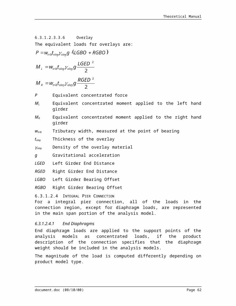
Theoretical Manual

settlement. The basis for Limit State Deflections computed by QConBridge II is shown in Figure34.

Figure 34 Basis for computing Limit State Deflections

6.5.3 ReactionsQConBridge II computes and reports reactions for abutments and piers.

6.5.3.1 Limit State Combinations for ReactionsTwo sets of limit state reactions are reported for all piers and abutments. One set of reactions is for foundation elements above the ground surface and one is for the elements below the ground surface. For the foundation elements below the ground surface, the dynamic load allowance (impact) factor is taken to be 0% (See LRFD 3.6.2.1).

6.5.3.2 Zero Height Abutments and PiersFor zero-height abutments and piers, QConBridge II computes a vertical reaction. Reactions for all load groups, load cases, and limit states are reported on a per girder line basis. Vehicular and Pedestrian Live Load Reactions are reported on a per lane basis.

6.5.3.3 Fixed Height AbutmentsFor fixed-height abutments, QConBridge II computes vertical, horizontal, and moment reactions. Reactions for all load groups, load cases, and limit states are reported on a per girder line basis. Vehicular and Pedestrian Live Load Reactions are also reported on a per lane basis.

6.5.3.4 Fixed Height PiersFor fixed-height piers, QConBridge II computes a vertical reaction at the top of the column and vertical, horizontal, and moment reactions at the bottom of the column. The top of column vertical reaction is transferred into TBAM models at the bearing locations.


Theoretical Manual

Reactions for all load groups, load cases, and limit states are reported on a per girder line basis. Vehicular and Pedestrian Live Load Reactions are also reported on a per design lane basis.

6.5.4 Deflections for Evaluation of LRFD 2.5.2.6.2QConBridge II computes live load deflections for evaluation of LRFD 2.5.2.6.2 as specified in Section 6.4.2.1. These deflections are computed at all Points of Interest in the superstructure elements of the LBAM. These deflections are not Limit States. Deflections for vehicular live load only and vehicular live load plus pedestrian loads are computed and reported as different deflection criteria may apply.

6.5.5 Pedestrian Only BridgesFor Pedestrian Only Bridges, QConBridge II computes the same Limit States as for bridges with vehicular live load, except the intermediate Limit States relating to vehicular live load are omitted. The special deflection analysis for LRFD 2.5.2.6.2 is performed for Pedestrian Only Bridges.


Theoretical Manual

7. TRANSVERSE BRIDGE ANALYSIS MODELS

QConBridge II will perform a transverse dead load and live load analysis if a 3D pier structure has been defined. This section describes how the information from the product model is used to generate a TBAM.

7.1 Model TopologyThis section describes how the model geometry is generated for the various types of pier product models supported by QConBridge II.

7.1.1 Cap Beam ModelingThe model of the cap beam is similar for all pier types supported by the program. Figure 35 shows the basic geometry of the cap beam elements along the rectangular cap beam. Cap beam elements are positioned at the centroid of the cap beam section at the location of each column. The cap beam elements are connected to the top of the column elements and have full connectivity with the column elements. Cap overhangs are projected along the same geometry as the cap beam of the exterior bays of the bent. For single column piers, hammerhead piers, and zero-height idealized piers, the cap beam is taken to be horizontal. Non-prismatic caps are modeled with a series of prismatic segments. Segment boundaries will occur at the face of each column and where ever the depth of the cross section is more than 10% different than the depth of the adjacent segment.

Figure 35 Structural Modeling of Cap Beam


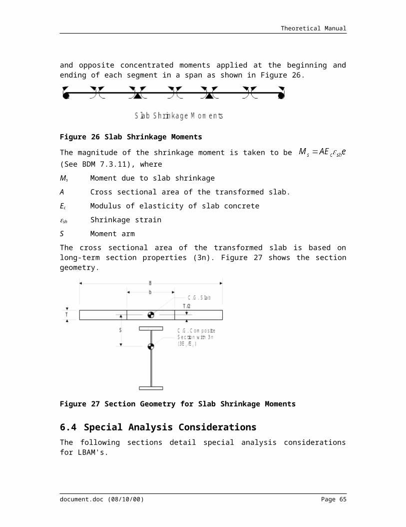
Theoretical Manual

7.1.2 2D Zero-Height PiersA TBAM is not created for 2D Zero-Height Piers.

7.1.3 3D Zero-Height PiersThe product model for zero-height idealized pier defines support locations that represent columns or other supporting elements for a cap beam. A 3D Zero-Height Idealized Pier is modeled as a horizontal cap beam on pinned supports as shown in Figure 36.

Figure 36 TBAM for a 3D Zero Height Idealized Pier

7.1.4 2D Fixed Height PiersA TBAM is not created for 2D Fixed-Height Piers.

7.1.5 3D Fixed Height PiersFigure 37 shows how fixed height piers are modeled for the transverse analysis. The bent frame is made up of n equally spaced columns. The cap beam extends beyond the exterior bays of the bent by the overhang distance. The columns are assumed to be the same height and as such, the cap beam is modeled as horizontal. The bases of the columns are fixed. The stiffness of each column is equal to 1/n times the stiffness defined in the product model for the pier.

Figure 37 Analysis Modeling of Fixed Height 3D Piers


Theoretical Manual

7.1.6 Full Product Model PiersThe typical geometry for a full product model pier is shown in Figure 38. The column heights in the analysis model are equal to the column heights in the product model plus the distance from the bottom of the cap beam to its centroid.

Non-prismatic columns are modeled using a series of prismatic segments starting from the bottom of the column and working upwards.

The bottoms of the column elements are fixed at the bottom and have full continuity with the cap beam elements at the top.

Figure 38 TBAM for Multicolumn and Hammerhead Piers

Column heights are computed as described in Section 6.1.2.2.3.

7.2 LoadsThe loads imparted on a pier (as far as this version of QConBridge II is concerned) come from two different sources, the pier itself and loads from the superstructure. This section will describe how these loads are modeled in TBAMs.

7.2.1 Adjustments for SkewFor piers that are skewed with respect to the alignment, the transverse spacing of the load from the superstructure must be adjusted for skew.

7.2.2 Pier LoadsThe loads described in this section are load applied directly to the pier model as opposed to loads that are transferred to the pier model from the superstructure.


Theoretical Manual

7.2.2.1 Pier Self WeightSelf-weight of pier cap beam and columns are calculated as where,

w weight per unit length of the column or cap beam segment

A cross sectional area of the column or cap beam segment

c density of the pier concrete

g gravitational acceleration.

7.2.2.2 Other LoadsSome other loads that would logically fall into this section are seismic, wind, and stream flow. However, this version of QConBridge II does not support these loading conditions. This is only mentioned so as to help distinguish loads applied directly to the pier from those transferred to the pier from the superstructure.

7.2.3 Superstructure LoadsThis section describes the loads that are transferred to the pier from the superstructure. These loads come in the form of reactions taken from the girder line LBAM's.

7.2.3.1 Girder Self WeightSelf-weight of structural girder calculated using the girder area and girder material’s weight density. Girder reactions are applied to cap beam at bearing locations.

7.2.3.2 Slab Self WeightSlab self weight includes the tributary self-weight of slab including haunch, sacrificial wearing surface, and overhang, if applicable. Girder reactions are applied to cap beam at bearing locations.

The effects of parabolic haunch depth due to camber are accounted for.

7.2.3.3 Intermediate DiaphragmsApplies tributary weight of Intermediate Diaphragms to girders. Girder reactions are applied to cap beam at bearing locations.

7.2.3.4 End DiaphragmsFor connections where the weight of the diaphragm is carried by the girder, the weight of the end diaphragm is applied at bearing locations based on a tributary distribution of the weight to the girder lines. For connections where the weight of the diaphragm is applied directly tot he support element, the total weight of the diaphragm is distributed over the cap beam and applied as a uniform load.

7.2.3.5 Traffic BarrierThis load is derived from a uniform load based on the weight of the Traffic Barrier. If the load in the longitudinal model is distributed to all girder lines, then the girder reactions are applied to all points of bearing. If the load in the longitudinal model is distributed to n exterior girder lines, then only the bearing locations associated with those girder lines are loaded.


Theoretical Manual

7.2.3.6 Median BarrierThis load is derived from a uniform load based on the weight of the Median Barrier (if it exists). If the load in the longitudinal model is distributed to all girder lines, then the girder reactions are applied to all points of bearing. If the load in the longitudinal model is distributed to n adjacent girder lines, then only the bearing locations associated with those girder lines are loaded.

7.2.3.7 OverlayThis load is derived from a uniform load based on the depth of the overlay, the overlay material properties, and the curb-to-curb width of the roadway surface. Regardless if this load is uniformly distributed amongst all girder lines or is applied to each girder line based on its tributary area, the girder line reactions are applied to the cap beam at the bearing locations.

7.2.3.8 SidewalkThis load is derived from a uniform load based on the weight of the Sidewalk (if it exists). If the load in the longitudinal model is distributed to all girder lines, then the girder reactions are applied to all points of bearing. If the load in the longitudinal model is distributed to n exterior girder lines, then only the bearing locations associated with those girder lines are loaded.

7.2.3.9 Live LoadsThe longitudinal analysis models compute live load reactions on the bases of one loaded lane. These reactions must be imparted onto the TBAM for all permutations of loaded lanes and design lane configurations. The sections that follow describe:

how the live load reactions are modeled as loads in a TBAM

where the loads are applied to the TBAM (location of the design lanes and the location of a within a design lane)

how the loads are transferred from the superstructure to the substructure models

7.2.3.9.1 MODELING OF LIVE LOAD REACTIONSThe live load reactions computed from the LBAM's for each girder line are simply a vertical force per design lane. For the vehicular live load, there is a truck load portion and lane load portion. For pedestrian live load, there is only a lane load portion. The method for representing the truck load and lane load portions of the live load reactions are described below.

Potentially, each girder line and its associated LBAM is a different length, resulting in different live load reactions per lane across the width of the structure. QConBridge II simplifies this situation by using the maximum live load reaction for all girder lines.

When the envelope simple/continuous option is enabled, the maximum of the simple span and continuous span reaction is used, but not both.

7.2.3.9.1.1 Live Load Reactions applied to the TBAMFor the HL93 Live Load model, only the lane/truck combination that creates the maximum reaction are applied to the live load transfer model. QConBridge II does not analyze the TBAM for all the elements of HL93.

For Special and Permit Trucks, only the controlling cases are applied to the TBAM.


Theoretical Manual

7.2.3.9.1.2 Truck Load reactionsQConBridge II has two methods of representing truck load reactions in TBAM's as illustrated in Figure 39.

Figure 39 Representation of Vehicular Live Load Reactions in TBAM's

7.2.3.9.1.2.1 Wheel Line ReactionsFor this option, the total truck load reaction per lane is divided by two to compute the reaction per wheel line. The wheel line reactions are positioned in a design lane spaced in accordance with LRFD 3.6.1.2 (1800 mm apart - not closer than 600 mm from the lane edge). The transverse wheel line spacing must be adjusted for skew.

7.2.3.9.1.2.2 Lane ReactionsFor this option, the total truck load reaction per lane is uniformly distributed over the same width as the lane load as specified in LRFD 3.6.1.2.4, adjusted for skew.

7.2.3.9.1.3 Lane Load ReactionsThe lane load portion of vehicular live load reaction is uniformly distributed over the distance specified in LRFD 3.6.1.2.4 (3000 mm), adjusted for skew.

7.2.3.9.1.4 Pedestrian Load ReactionsPedestrian load reactions are distributed over the width of the sidewalk, adjusted for skew.

7.2.3.9.2 DESIGN LANE CONFIGURATIONSThe width of a design lane is specified in LRFD 3.6.1.1.1. In general, a whole number of design lanes does not exactly fill the curb-to-curb width of the bridge as seen in Figure 40. There is usually some excess space, denoted as Wexcess. Because the design lanes must be positioned to cause the extreme force effects, the configuration of the design lanes must change for the various force effects in the structure. It is not practical to analyze a pier for every possible design lane configuration or to determine the optimum lane configuration for each force effect. QConBridge II positions the design lanes are shown in Figure 43.


Theoretical Manual

Design lanes are always positioned curb to curb. QConBridge II ignores the presence of median barriers when determining design lane configurations.

Figure 40 Lane Configurations

When sidewalks are present in the product model, and they have sufficient width to warrant loading per LRFD 3.6.1.6, QConBridge II models design lane configurations with and without the effect of the sidewalk. When the sidewalk is accounted for in the load transfer model, pedestrian live load is applied to the model. If the structure has sidewalks on each side, design lane configurations are considered for no sidewalks, one sidewalk on the left, one sidewalk on the right, and two sidewalks.


Theoretical Manual

Figure 41 Design Lane Configuration with one sidewalk

Figure 42 Design Lane Configuration with two sidewalks


Theoretical Manual

Figure 43 Design Lane Configuration for TBAM's

7.2.3.9.2.1 Location of Live Load Within a Design LaneA lane of live load does not occupy the full width of a design lane. The design lane loads occupies 3000 mm of the 3600 mm design lane. Truck loads occupy 1800 mm of the design lane, and the wheel lines cannot be closer that 600 mm from the lane edge. The sections that follow describe how the live load reactions, applied to load transfer models, are positioned within the design lanes.

7.2.3.9.2.1.1 Case 1 - Design Lanes Centered Between Curb LinesWhen the design lanes are centered between curb lines, the location of the live load within the design lane varies. For the leftmost design lane, the live load is positioned as far to the left as possible. For the rightmost design lane, the live load is positioned as far to the right as possible. The live load is positioned in the center of the center design lane (if there is an odd number of design lanes). The offset of the live load in all other design lanes is taken as a linear interpolation between the center and edge design lanes.

7.2.3.9.2.1.2 Case 2 - Design Lanes At Left or Right Curb LineWhen the design lanes are positioned either at the left or right curb line, the live load is positioned as far to the left or right edge of the design lane as possible.

7.2.3.9.2.2 Permutations of Loaded LanesThe TBAM must be loaded with the combination of lane loads that cause the extreme force effects. To facilitate this, QConBridge II applies various permutations of loaded design lanes to the analysis model. QConBridge II analyzes the TBAM for all possible combinations of loaded


Theoretical Manual

lanes. Figure 44 through Figure 46 show the various permutations of loaded lanes for a structure with two sidewalks. Per LRFD 3.6.1.1.2, sidewalks loaded with pedestrian load are considered to be equivalent to one loaded lane, except the case of pedestrian load only is not considered for vehicular bridges. The actual transverse placement of the design lanes is specified in Section 7.2.3.9.2.

Figure 44 shows the case when pedestrian load is not considered. Sidewalk dead load (and median barrier dead load if applicable) is still accounted for in this loading situation. In this configuration, the structure can accommodate three design lanes.

Figure 44 Permutations of Loaded Design Lanes for a 3 Lane Structure

Figure 45 shows the case when pedestrian load is considered to be only on one sidewalk. Load of a sidewalk on only one side of the bridge produces maximum magnitudes of certain force effects3. Sidewalk dead load (and median barrier dead load if applicable) is still accounted for in this loading situation. In this configuration, the structure can still accommodate three design lanes.

3 Loading the sidewalk on only one side of the bridge is consistent with LFD 3.14.1.2.


Theoretical Manual

Figure 45 Permutations of Loaded Design Lanes for a 3 Lane Structure with a Sidewalk

Figure 46 shows the case when pedestrian load is considered to be on both sidewalks. In this configuration, the structure can accommodate two design lanes.


Theoretical Manual

Figure 46 Permutations of Loaded Design Lanes for a 3 Lane Structure with two Sidewalks

7.2.3.9.3 LOAD TRANSFER MODELSLive load reactions are distributed to the cap beam through a load transfer model. The two load transfer models support by QConBridge II are described below.

7.2.3.9.3.1 Rigid Links (Lever Rule)For this transfer model, live load reactions are applied to a model of rigid links as shown in Figure 47. This is basically a lever rule distribution. Reaction points in the transfer model represent the bearing locations. The rigid beams are simple spans between girder lines. The exterior transfer beams have cantilever sections that represent the overhang of the bridge deck.


Theoretical Manual

Figure 47 Rigid Links Load Transfer Model

7.2.3.9.3.2 Drop ThroughFor this transfer model, the live load reactions are applied directly to the cap beam elements of the transverse analysis model. This is shown in Figure 48. When the curb to curb width of the roadway exceeds the width of the cap beam, the load extending beyond the cap beam is applied to the end of the cap beam as a concentrated load and as an equivalent couple at the base of the exterior columns (for single columns piers, a concentrated moment is used). The loads shown below are for illustrative purposes. For actual modeling of the live load reactions as loads in the TBAM, see section 7.2.3.9.1. This transfer model is used in WSDOT's office practice, as described in BDM 9.1.1C.


Theoretical Manual

Figure 48 Drop-Through Load Transfer Model

7.3 Analysis ResultsAfter the TBAM is generated from the product model, the problem being solved by QConBridge II becomes the same as for Analysis Model Projects or Transverse Only Analysis Model. This section describes how QConBridge II takes the raw analysis results from the TBAM and combines them into Load Case and Limit State results. The process that QConBridge II uses for TBAMs is very similar to the process for LBAMs, though somewhat less complex. TBAMs do not need to consider staging, the various components of the HL93 Live Load, or enveloping simple span and continuous structures.

7.3.1 The Basic ProcessFigure 49 illustrates the basic process for analyzing a TBAM and computing Load Case and Limit State Results. The TBAM is loaded as described above. The live load is applied in various combinations to produce the minimum and maximum load cases.


Theoretical Manual

Figure 49 Basic TBAM Analysis Process

The total Load Case responses for the TBAM are combined into Limit State results. The following Limit State results are computed:

Strength I

Strength II (using Permit and Special Live Loads)

Strength III (If WA, WS, FR, TU, CR, SH, TG, and SE load cases are empty, this Limit State will not control over Strength I and need not be reported to the user)

Strength IV

Strength V (If WA, WS, WL, FR, TU, CR, SH, TG, and SE load cases are empty, this Limit State will not control over Strength I and need not be reported to the user)

Extreme Event I (If EQ load case is empty, this Limit State will not control over Strength I and need not be reported to the user)

Extreme Event II (If IC, CT, and CV load cases are empty, this Limit State will not control over Strength I and need not be reported to the user)

Service I

Fatigue

User Defined Limit States (using either/or HL93 Live Load or User Defined Live Load)


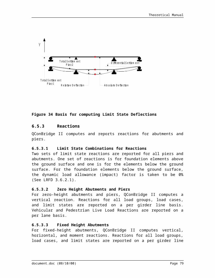
Theoretical Manual

7.3.2 TBAM ResultsFor each of the Load Groups, Load Cases, and Limit States, QConBridge II will compute moments and shears in the cap beam and moments, shears, and axial each column. QConBridge II will also compute reactions at the base of columns. Limit State reactions will be computed for above ground and below ground components of the foundation. QConBridge II will report analysis results at all points of interest.

7.3.3 Total Pier Results (Combining LBAM Results with TBAM Results)QConBridge II approximates the total structural response at a pier by factoring in the LBAM response. The total response is reported separately from the TBAM results so as to avoid confusion.

The total response at the base of the columns is reported in a coordinate system parallel to the plane of the TBAM. The reactions in the plane of the TBAM are reported per girder, per column, and for Vehicular and Pedestrian Live Load, per design lane. Figure 50 illustrates how QConBridge II transforms the LBAM reactions into the plane of the TBAM. Note that eccentricities due to bearing locations at the connections are not modeled. This means that torsion in the cap beam and moment in the columns due to eccentricity of the bearing line are not modeled.

Figure 50 LBAM Reactions Transformed to plane of TBAM

QConBridge II will combine the transformed reactions from the LBAM with the TBAM reactions when reporting 3D pier reactions. The reactions from the TBAMs will be per column.


Theoretical Manual

The transformed LBAM reactions per column are computed as

where

RPer Column Per column reaction

RPer Girder Per girder line reaction

NGirders Number of Girders

NColumns Number of Columns


Documents

QConBridge II - Theoretical Manual€¦ · Web viewSteel Beam Bridge Product Models. For steel beam bridge product models (built-up and rolled shapes), the end diaphragms are described