QCDVis: a tool for the visualisation of Quantum Chromodynamics (QCD) Data

Dean P.Thomasa,b, Rita Borgoc, Robert S.Larameea, Simon J.Handsb

aDepartment of Computer Science, College of Science, Swansea University, United KingdombDepartment of Physics, College of Science, Swansea University, United Kingdom

cInformatics Department, Kings College London, London, United Kingdom

Abstract

Quantum chromodynamics, most commonly referred to as QCD, is a relativistic quantum field theory for the strong interactionbetween subatomic particles called quarks and gluons. The most systematic way of calculating the strong interactions of QCDis a computational approach known as lattice gauge theory or lattice QCD. Space-time is discretised so that field variables areformulated on the sites and links of a four dimensional hypercubic lattice. This technique enables the gluon field to be representedusing 3 × 3 complex matrices in four space-time dimensions. Importance sampling techniques can then be exploited to calculatephysics observables as functions of the fields, averaged over a statistically-generated and suitably weighted ensemble of fieldconfigurations. In this paper we present a framework developed to visually assist scientists in the analysis of multidimensionalproperties and emerging phenomena within QCD ensemble simulations. Core to the framework is the use of topology-drivenvisualisation techniques which enable the user to segment the data into unique objects, calculate properties of individual objectspresent on the lattice, and validate features detected using statistical measures. The framework enables holistic analysis to validateexisting hypothesis against novel visual cues with the intent of supporting and steering scientists in the analysis and decision makingprocess. Use of the framework has lead to new studies into the effect that variation of thermodynamic control parameters has onthe topological structure of lattice fields.

Keywords: visualization, framework, topology, flexible isosurface, high dimensional, lattice quantum chromodynamics

1. Introduction

Gravity and electromagnetism are two fundamental forces whichwe directly observe and experience. Physicists however iden-tify four fundamental forces in nature: electromagnetic force,gravitational force, weak interaction, and strong interaction. Theweak and strong interaction forces work at the atomic level: thestrong interaction holds the nucleus together and the weak inter-action is responsible for radioactive decay. Strong force alongwith electromagnetism and weak interaction, underpins all ofnuclear physics and the vast array of phenomena from the mi-croscopic to the cosmological level which we all experience.With respect to analytical frameworks the gravitational forceis governed by Einstein’s theory of general relativity while thestrong interaction, electromagnetic force, and weak interactionare described by quantum field theory — theoretical frame-works for constructing quantum mechanical models of subatomicparticles in particle physics.

Quantum chromodynamics (QCD) is a relativistic quantumfield theory used to describe the strong interaction force. QCDacts at nuclear level where it predicts the existence of force-carrier particles called gluons and quarks. Gluons and quarksare confined in the protons and neutrons that make up everydaymatter and transmit the strong force between particles of matter.

While fundamentals of QCD can be deemed simple and el-egant [1] due to its compact Lagrangian, its phenomenologyis characterised by multidimensional properties and emergingphenomena with complex dynamics making analysis an elabo-

rate task. QCD simulations are performed on a discrete space-time lattice as an approximation of the theory known as latticeQuantum Chromodynamics (lattice QCD). Due to the complex-ity of the simulation data, it is crucial to extract possible fea-tures and provide semantics to become information. This workis therefore driven by a desire to support scientists in the valida-tion, inspection, and understanding of the properties of latticeQCD data. To achieve this goal we contribute a system to sup-port physicists in the process of:

• validation and analysis of simulated QCD data sets;• generation of visual designs that provide novel insight

into the structure and evolution of phenomena representedby simulated QCD data;

• simultaneous comparison of both quantitative and quali-tative aspects of QCD phenomena.

In the development of our framework we leverage the strengthof topology-driven analysis, successfully introduced in differentresearch domains and range of applications all sharing a com-mon goal — to achieve an efficient and compact description ofthe basic shapes co-existing in an arbitrary set of data.

2. Background

In this section we introduce the relevant background topics re-quired to understand the techniques used in the QCDVis frame-work. We give a brief overview of lattice QCD, covering topics

Preprint submitted to SCCG 2017 April 18, 2017

relevant to this application paper. Lattice QCD is a widely re-searched and expansive field of theoretical physics, hence, amore comprehensive review of the topic is included in the Ap-pendix. We limit the application background to visualisationin lattice QCD, for a more general discussion of visualisationtechniques in the physical sciences we refer the reader to thesurvey paper by Lipsa et al. [2].

2.1. Domain background

Quantum Chromodynamics defines a theory of interaction be-tween subnuclear quark and gluon particles. Matter that is madeup of quarks bound together by the exchange of massless gluonparticles is referred to Hadronic matter. The Hadron groupcan be subdivided into two categories; tri-quark systems arebaryons and quark-anti-quark pairs are mesons. Protons andneutrons, collectively known as nucleons, are members of thebaryon class of particle.

Quarks and gluons always exist in “colour neutral” states,making it near to impossible to observe them in isolation [3].This phenomena, known as colour-confinement, sees the amountof energy required to separate bound particles increase expo-nentially with distance. For this reason QCD is often modelledusing a discrete computational model of quark-gluon systemsknown as lattice QCD.

The lattice structure, first proposed by Kenneth Wilson [4],is a hyper-torus in four space-time dimensions. Lattice QCDuses Euclidean representation of space-time where space andtime are treated as equivalent. This allows the structure to bethought of as being composed of hypercubic cells. Periodic,or translationally-invariant, boundary conditions in all four di-mensions mean that all vertices on the lattice are treated equally,with no cell being sited on a boundary.

Quarks exist at vertices, or sites, on the lattice with integerindices. Each site has four link variables represented by SU(n)matrices modelling the gluon potential between neighbouringsites in the x, y, z and t directions. The value of n is used torepresent the number of charge colours used in the gauge the-ory, where true QCD uses n = 3. The work described here usesa simplified theory where n = 2, this allows certain thermody-namic control parameters including chemical potential (µ) to bevaried. This affects the relative balance of positive and negativecharge in the system, which is thought to be characterised bytopological variations in the scalar fields.

Various fields exist on the lattice, defined as closed loopsfrom a site. Mathematically these are represented as a pathordered matrix multiplication of link variables. The smallestclosed loop in a 2D plane is referred to as a plaquette. Inthis work we are primarily interested in the plaquette fields,Polyakov loop fields, and topological charge density field. Pla-quette fields are the averages of three plaquettes, categorised asspace-like (xy, xz, yz) or time-like (xt, yt, zt). The Polyakovloop is a three dimensional field computed as a product of alllink variables in the time direction in path order, looping at theboundary. Topological charge density is a loop in all four space-time directions that predicts the existence of pseudo-particlesnamed instantons [5].

Instantons are one of the primary observables that physicistsworking in a lattice QCD study. Their name comes from thefact that they have a finite existence in the time-dimension andare able to appear and disappear, unlike real particles. Instan-tons are generally able to persist in the data even when subjectto a lattice based noise reduction technique called cooling [6].However, overuse of the algorithm can destroy the instanton-anti-instanton pairs that are intended to be measured [7]. Dueto the discrete nature of the lattice and the fact the size of an in-stanton can vary, it is possible to shrink objects until they disap-pear. The effect of annihilation of an observable by overcoolingis referred to an object “falling through the lattice” on accountof the discrete spacing between lattice sites.

2.2. Visualisation in Lattice QCDThe traditional use of visualisation in lattice QCD is often lim-ited to dimension independent forms such as line graphs to plotproperties of simulations as part of a larger ensemble. Visu-alisation of a space-time nature is less frequently observed butdoes occasionally occur in literature on the subject. Surfaceplots were used by Hands [8] to view 2D slices of data and givea basic understanding of energy distributions in a field.

Application of visualisation of QCD in higher dimensionsfirst appears in the form of three dimensional plots [9] of in-stantons showing their correlation to other lattice observables.Primarily, these were monopole loops, instantons that persistthroughout the entire time domain of a simulation. Prior tovisualisation, simulations are subjected to iterative cooling toremove noise whilst keeping the desired observables intact. In-stantons are visualised using their plaquette, hypercube, andLüscher definitions, each of which make it possible to viewinstantons and monopole loops. Visualisation is a useful toolin this case to confirm that monopole loops and instantons areable to coexist in a simulation, a fact that can help theoreticalphysicists understanding of the QCD vacuum structure.

A more detailed visualisation, making use of establishedcomputer graphics techniques, was performed by Leinweber [10]as a way of conveying to the physics community that visualisa-tion of large data sets would help their understanding of QCD.An area of lattice QCD investigated is the view that instanton-anti-instanton pairs can attract and annihilate one another dur-ing cooling phases. Topological charge density, also referred toas topological charge density, and Wilson action, also referredto as action measurements are used to show separate spheri-cal instantons and anti-instantons in the lattice hyper-volume.Using animation it is possible to see that instantons in vicinityof anti-instantons deform and merge. Leinweber explains theneed for sensible thresholds when discarding isosurfaces thathave action densities below a critical value as their disappear-ance can be incorrectly interpreted as them falling through thelattice.

More recently DiPierro et al. [11, 12, 13, 14] produced sev-eral visual designs as part of a larger project with the aim of uni-fying various active lattice QCD projects. Expectations of thework were that visualisations could be used to identify errorswith the simulation process, along with increasing understand-ing of lattice QCD. Many existing file structures used within

2

the lattice QCD community could be processed and output us-ing the VTK, this could then be rendered using a number ofpre-existing visualisation tools including VisIt [15] and Par-aview [16]. In addition, the evolution of instantons over Eu-clidean time spans could be rendered into movies. A web frontend application and scripting interface was also provided thatallowed users to set up an online processing chain to analysesimulations on a large scale. Despite the apparent success ofthe work it would appear that it is no longer maintained andmany of the links present with the project literature are inacces-sible.

2.3. Topology Driven VisualisationTopological descriptions of data aim to achieve an efficient de-piction of the basic components and their topological changesas a function of a physical quantity significant for the specifictype of data. Contour trees, a direct derivative of Morse Theory,provide a compact data structure to encapsulate and representthe evolution of the isocontours of scalar data, or height func-tion, as the height varies and relate these topological changes tothe criticalities of the function.

De Berg et al. [17] made the observation that an isosurfaceis the level set of a continuous function in 3D space suggest-ing that a whole contour could be traced starting from a singleelement — a seed. An entire contour can be computed for thedesired isovalue from the seed that is bounded by two super-nodes at the critical points of the contour. Carr et al. [18] inves-tigated the use of contour trees in higher dimensional datasets,whilst also improving upon the algorithm proposed by Tarasovand Vyalyi [19]. They introduced the concept of augmentedcontour trees, an extension that added non-branching verticesto provide values for isosurface seeding. Separate isosurfacescan be generated for each non-critical value identified in thecontour tree, separately colour coded and manipulated by theend user. This enables users to identify regions of interest anddistinguish them accordingly [20].

Chiang et al. [21] introduce a modified contour tree con-struction algorithm that improves processing time by only sort-ing critical vertices in the merge tree construction stage. Thisvastly increases processing speeds in very large data sets. How-ever, as observed by the authors, critical vertices are difficultto identify in data with dimensionality of four or more. Fur-ther increases in speed are offered by storing multiple seeds forthe monotone path construction algorithm [22] used to gener-ate surfaces. This results in an increased storage overhead butwith the advantage that a surface does not require complete re-extraction each time the isovalue is changed.

Limitations in the merge tree computation phase of the con-tour tree algorithm prevent it from correctly handling data thatis periodic in nature. However, the Reeb graph [23], a directdescendent of the contour tree, can be used to compute thetopology of scalar data with non-trivial boundaries. As with thecontour tree, the Reeb graph can be applied to models of anydimension provided it is represented on a simplicial mesh [24].Tierny et al. proposed an optimized method for computing Reebgraphs using existing contour tree algorithms by applying a pro-cedure that they called loop surgery [25]. This method is able

to take advantage of the speed of contour trees with a minimaloverhead in complexity. The Reeb graph has also been usedto assist in the design of transfer functions in volume visual-isation [26], by assigning opacity based upon how many ob-jects were obscured by nested surfaces and their proximity tothe edge of a scalar field.

In comparison to previous tools in lattice QCD that relyupon static visualisation, using existing scientific software pack-ages, our system is a bespoke dynamic environment designedcollaboratively with physicists. The inclusion of topologicalstructures in the system allows us to present unique interpreta-tions of the data which to our knowledge has not been carriedout in the domain before. As the system is dynamic, the useris able to explore data in real-time by adjusting visualisationparameters such as isovalue or to interact with the data at levelcaptured by the scalar topology.

Unique features of QCDVis directly influenced a study byThomas et al. [27], where topological features of the Polyakovloop are examined as chemical potential and temperature arevaried. Initial visual analysis of the polyakov loop data showeda complex interaction between isosurfaces with scalar valuesacross the field range. When the surfaces were viewed withthe additional context of the Reeb graph capturing the topol-ogy, it was questioned if there could potentially be a bias inthe number and structure of the objects in the field. In orderto capture details of the topology as quantitative data, aspectsof the Reeb graph and geometric properties were computed formultiple data sets.

3. Research Aims

Scientists are particularly interested in examining behavioursof observables computed via path integral equations, for fieldconfigurations generated using the unphysical value Nc = 2 andwith the addition of a term proportional to a parameter µ knownas the chemical potential [28, 29, 30]. When µ > 0, the MonteCarlo sampling is biased towards configurations with an excessof quarks q over anti-quarks q. As a result exploration of sys-tems with quark density nq > 0, relevant for understanding theultra-dense matter found within neutron stars, is made possible.Study of “Two Colour QCD” is an exploratory step in this di-rection: in the presence of quarks, the action S is supplementedby an additional contribution S q(U; µ) from quarks which is ingeneral non-local and extremely expensive to calculate.

For the physical case Nc = 3, it can be shown that S q(µ) =

S ∗q(−µ), where the star denotes complex conjugate, so that forµ , 0 the action is neither real nor positive definite, makingimportance sampling inoperable. For Nc = 2, S q(µ) is real andthe problem disappears.

For any relativistic system with µ , 0, the t direction isdistinguished, because nq > 0 implies particle world-lines arepreferentially oriented in one time-like direction (a world-lineis the trajectory of a particle through space-time, and is orientedfor a particle such as a quark carrying a conserved charge). Aninteresting question is how this implied space-time anisotropyis reflected in the properties of the topological fluctuations. Pre-vious studies [31] suggest instanton sizes shrink as µ increases

3

but it is also possible that their shape and relative displacementfrom neighbouring (anti-)instantons may have different charac-teristic distributions in t and x, y, z directions.

Attempts at visualisation of QCD data have so far concen-trated on single aspects of the analysis, no framework existscapable of supporting the scientist through the entire analyti-cal pipeline from beginning to end and back. Our frameworkhas been developed to fill this gap. QCDVis (Figs. 1, 2, 3)has been designed with the user in mind. The framework ad-dresses the fundamental aspects of data validation, visualisationand estimation of QCD objects and observables, manipulationand traversal of data. Core to the analysis is support for identi-fication of discrete objects and their characteristics using topo-logical structures data such as the Reeb graph. This enablesresearch questions to be tackled in a quantitative fashion. Thefollowing sections provide detailed descriptions of each aspectof our framework and its implementation.

4. QCDVis

QCDVis has been designed as an interactive environment to en-able physicists to visually explore their data and its underly-ing topology. Figure 1 summarizes the key stages of the vi-sual analytic pipeline upon which our system is constructed.Along with 3D rendered views of user selected scalar fields, wealso include data representations that are commonly found inthe QCD domain. Histograms, in particular, are firmly estab-lished in physics community for identifying underlying trendsin data. Therefore, they are included to allow physicists to gainan overview of their data and promote a focus on the parts ofthe data they find most interesting.

In order to explain the functioning of the system we firstdefine some terminology specific to lattice QCD:

Action A function of the lattice variables computed by com-pleting closed loops on the lattice. In this work we usethe term to indicate the Wilson action, defined by unitloops on the lattice referred to as plaquettes.

Configuration A unique lattice representing the Quark-Gluonfield at a specified step along the simulation Markov chain.

Cooling A form of algorithm used by physicists used to re-move noise and stabilise output from lattice QCD simu-lations.

Ensemble A collection of configurations with common ther-modynamic control parameters, for example chemical po-tential (µ).

Euclidean space-time A four dimensional manifold with threereal coordinates representing Euclidean space, and oneimaginary coordinate, representing time, as the fourth di-mension.

Plaquette A unit closed 2D loop around links on the lattice,starting and ending at the same vertex.

Space-like plaquette A plaquette existing in the xy, xz or yzplanes.

Time-like plaquette A plaquette existing in the xt, yt or ztplanes.

The QCDVis framework currently consists of two main mod-ules; the first processes ensemble data and is used to transformraw lattice configurations into discrete scalar fields represent-ing a number of lattice field operators. The second, workingat the configuration level, is used to visualise and probe thesefields using topological methods. Each module can work inde-pendently or can be used together to semi-autonomously probethe ensemble with respect to its topological features. In thisscenario, the ensemble tool is used to invoke the visualisationand analysis application with given sets of configurations.

4.1. Ensemble module

Figure 2 shows the interface of the ensemble computation mod-ule made up of our main components discussed below. LatticeQCD simulations are stored as 4D array-like structures referredto as lattice configurations. These are not the direct observablesand require processing to generate data for visualisation pur-poses. The resultant data is 4D, sliced into 3D volumes along auser defined axis.

Ensemble cooling histogram generation (Fig. 2.1). Upon se-lecting an ensemble for inspection, physicists can view under-lying patterns under cooling by computing graphs of the ac-tion and topological charge density statistics (e.g., Wilson ac-tion and topological charge density respectively). This can steerthem towards interesting features in the derived scalar fields.

Location of field maxima and minima (Fig. 2.2). The coolingprogram is able to detect the position in space-time of minimaand maxima of the action and topological charge density fieldsas it is cooled. This data is available for each cooling stagefor each configuration and can be called up by the user fromthe main interface. Physicists can use this data to determine theprobable existence of (anti-)instantons in the topological chargedensity field, signified by corresponding minima and maximain both fields. In QCDVis we include this data to provide anadditional method for determining interesting stages of coolingin each configuration.

Configuration selection (Fig. 2.3). The vast quantity of con-figurations created for an ensemble under cooling mean thatit is not viable for the physicists to view all possible configu-ration/cooling combinations. Additionally, it is unusual for adomain physicist to retain configurations early in the coolingcycle, as the configurations are too noisy for use in calcula-tions. Therefore, physicists can select exactly which configura-tions they intend to further investigate using information gath-ered from generated histograms and localization of maxima andminima (see above). Singular configurations can be selected bychecking the relevant cell in the grid but we also offer the con-venience of selecting all configurations across a level of coolingor within a configuration.

Field variable selection (Fig. 2.4). At present the system isable to calculate a range of field variables including topologicalcharge density, polyakov loops, plaquettes, and fields derivedfrom the averages of time-like and space-like plaquettes. Most

4

External Database

Seeded contoursTree / Graph VisualizationsInfovis techniquesInteraction

selection / manipulation

Visualisations

Field interactions, effects of cooling

Slice refinementDomainScientists

ConfigurationsCooling slicesField variables

Action (Wilson action)Topological charge density

Data Selection

Extract overview of topologyReeb GraphContour TreeJoint contour net

Volumetric properties

Statistical analysis

TopologyCompute

Contour TreesReeb GraphsJoint contour net

Ensemble simulationsFORTRAN generated4D lattice structure

Data Set

Validation3D scalar fields

Polyakov loop4D scalar fields

Plaquette fieldsAverage Plaquette

Difference PlaquetteTopological charge density

Field Generation

Visualisation moduleEnsemble module

user refactoring

4D > 3D slicesxyzxyt, yzt, xzt

Hypervolume Slicing

Figure 1: QCDVis Visual Analytics pipeline.

1.

2.

3.

4.

5.

Figure 2: Ensemble interface. Physicists can select multiple cooling slices,configurations and field variables of interest.

lattice fields require the calculation of the space-like and time-like plaquettes in order to create the final scalar field. In orderto optimize the computation of these values, they are computedand cached on demand.

Differing field variables may be required depending on thenature of the study being conducted; hence, we provide a se-lection of variables that are calculated at runtime. For example,use of the Polyakov loop field is a basic method of detecting“breaking of symmetry” on the lattice. The topological charge

density, average plaquette, and difference plaquette fields canall be used to predict the presence of instanton observables.

Field variables calculations from configuration data (Fig. 2.5).Data is stored on a four dimensional Euclidean lattice with theSU(2) matrices (denoted µ, ν, ρ, σ) assigned to edges in the x,y, z, and t dimensions. Field strength variables are defined bymoving around the lattice from a given origin in closed loops.

To calculate different lattice fields we complete closed loopsfrom a given lattice site in the µ, ν, ρ, σ directions. Movementsacross the lattice in a positive direction require multiplicationby the relevant SU(2) link variable. Equivalently, movement ina negative direction requires a multiplication by the matrix inits adjoint, or conjugate transpose, form. Hence, to complete aunit loop in the xy plane a path-ordered multiplication of twolink variables (µ, ν) and the two link variables in their adjointform (µ†, ν†) is performed.

The main field variables of interest are topological charge,Polyakov loops, space-like and time-like plaquettes, and theiraverage/difference (as shown in Fig. 2.4). Topological chargedensity for example is a loop around all four dimensions froman origin point. Thus values are a multiplicative combination ofthree spatial plaquettes and three time-like plaquettes. The ad-joint variations of each plaquette, representing a loop in reverse,are subtracted from these to form the difference plaquettes.

5

1.

2.

3.

5.

4.

6.

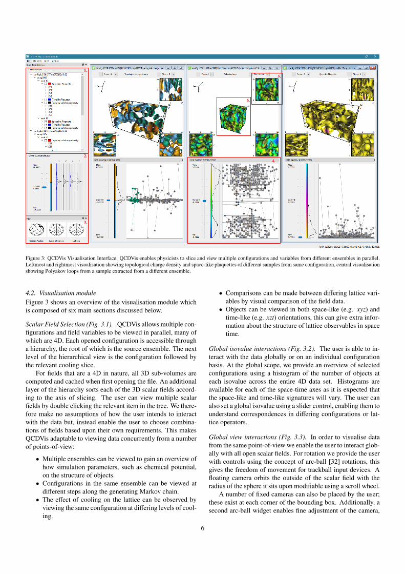
Figure 3: QCDVis Visualisation Interface. QCDVis enables physicists to slice and view multiple configurations and variables from different ensembles in parallel.Leftmost and rightmost visualisation showing topological charge density and space-like plaquettes of different samples from same configuration, central visualisationshowing Polyakov loops from a sample extracted from a different ensemble.

4.2. Visualisation moduleFigure 3 shows an overview of the visualisation module whichis composed of six main sections discussed below.

Scalar Field Selection (Fig. 3.1). QCDVis allows multiple con-figurations and field variables to be viewed in parallel, many ofwhich are 4D. Each opened configuration is accessible througha hierarchy, the root of which is the source ensemble. The nextlevel of the hierarchical view is the configuration followed bythe relevant cooling slice.

For fields that are a 4D in nature, all 3D sub-volumes arecomputed and cached when first opening the file. An additionallayer of the hierarchy sorts each of the 3D scalar fields accord-ing to the axis of slicing. The user can view multiple scalarfields by double clicking the relevant item in the tree. We there-fore make no assumptions of how the user intends to interactwith the data but, instead enable the user to choose combina-tions of fields based upon their own requirements. This makesQCDVis adaptable to viewing data concurrently from a numberof points-of-view:

• Multiple ensembles can be viewed to gain an overview ofhow simulation parameters, such as chemical potential,on the structure of objects.

• Configurations in the same ensemble can be viewed atdifferent steps along the generating Markov chain.

• The effect of cooling on the lattice can be observed byviewing the same configuration at differing levels of cool-ing.

• Comparisons can be made between differing lattice vari-ables by visual comparison of the field data.

• Objects can be viewed in both space-like (e.g. xyz) andtime-like (e.g. xzt) orientations, this can give extra infor-mation about the structure of lattice observables in spacetime.

Global isovalue interactions (Fig. 3.2). The user is able to in-teract with the data globally or on an individual configurationbasis. At the global scope, we provide an overview of selectedconfigurations using a histogram of the number of objects ateach isovalue across the entire 4D data set. Histograms areavailable for each of the space-time axes as it is expected thatthe space-like and time-like signatures will vary. The user canalso set a global isovalue using a slider control, enabling them tounderstand correspondences in differing configurations or lat-tice operators.

Global view interactions (Fig. 3.3). In order to visualise datafrom the same point-of-view we enable the user to interact glob-ally with all open scalar fields. For rotation we provide the userwith controls using the concept of arc-ball [32] rotations, thisgives the freedom of movement for trackball input devices. Afloating camera orbits the outside of the scalar field with theradius of the sphere it sits upon modifiable using a scroll wheel.

A number of fixed cameras can also be placed by the user;these exist at each corner of the bounding box. Additionally, asecond arc-ball widget enables fine adjustment of the camera,

6

initially fixed upon the centre of the data. The user can alsomove the relative position of the lighting using a third arc-ballcontrol.

Data topology overview and isovalue selection (Fig. 3.4). Scalarfields can be explored using a localised isovalue range. The usercan steer towards regions of interest in the domain via either acontour tree or Reeb graph (Fig. 4) representation of the do-main. Selection in the contour tree or Reeb graph (Fig. 3.4) arereflected in the flexible-isosurface view, as shown in the left-most visualisation in Fig. 3. Selected nodes, arcs, and corre-sponding contours are coloured green. Nodes, arcs, and cor-responding contours under the mouse cursor are highlighted inorange. Following a similar approach as to Bajaj et al. [33]the histogram presented alongside the isovalue selection slidershows the number of distinct objects in the scalar field acrossthe isovalue range.

In many lattice QCD field data sets the regions of interestare the positive and negative extremes; however, the contourspectrum can also show interesting features in the region of per-colation (the region around zero). Signatures of (anti-)instantonsshow up in the histogram as highly persistent objects in the pos-itive or negative direction. Other field variables, such as thePolyakov loop, usually show a measure of symmetry aroundzero.

Orthographic projections of surfaces (Fig. 3.5). We also presentsurfaces existing in the scalar field using orthographic projec-tions from each 2D plane. These have a fixed footprint with thescale adjusted according to the extent of axis, with the temporalextent of the data often different to that of the spacial axes. Thisis because in lattice QCD the temperature is given as an inversefunction of the number of time steps. In situations where thephysicist prefers not to use these projections they can be hid-den.

Orthographic projections can be a useful tool for physi-cists when tracking objects in specific fields, for instance (an-ti-)instantons in the topological charge density field, and is bestsuited to verifying and analysing phenomena identified by thecooling code. As part of the cooling process the position ofminima and maxima in the action and topological charge den-sity fields is output by the program. By identifying these objectsusing the orthogonal views their structure can visualised in var-ious 3D configurations of the 4D hypervolume. Occlusion fromoverlapping surfaces is rarely a problem in this view, as the ob-jects of most interest appear in sparse areas of the scalar topol-ogy.

Flexible isosurface view (Fig. 3.6). The core visual interface isa 3D rendered view of the selected scalar field. Use of the con-tour tree algorithm enables the transition from a basic isosur-face to representation of connected contours in the data. Thishas two benefits; first, optimized visualisation techniques canbe applied to the data. Second, properties can be calculated ondistinct contours as opposed to the level set as a whole, allowingthe calculation of physical measurements of objects existing inthe data.

Each arc in the contour tree is representative of a unique ob-ject, the mesh for which is generated using a modified form ofthe flexible isosurface algorithm [34]. Each isosurface can becontinuously deformed between upper and lower bounds of thecontour tree arc. This offers the possibility for parallel compu-tation of complex contours.

Properties of topological objects. The triangle meshes createdfor rendering also allow us to query properties of the objectsthat are beyond the statistical mechanics features usually avail-able to physicists. The simplest of these is evaluation of thesurface area and volume of the mesh.

To calculate more advanced properties we use the mathe-matical concept of moments — using methods initially imple-mented by Zhang and Chin [35]. The zeroth moment representsthe signed volume of a contour; the first moment, the centre ofmass; and the second representing moments of inertia. A pre-requisite for correct moment calculations is for a mesh to beclosed. An initial step to determine this is to calculate the Euler-Poincaré characteristic (χ = V − E + F) of a mesh. Followingthis approach it is possible that a contour which spans two ormore boundaries can be incorrectly identified as an n-torus. Tocounteract this, objects are also tested to see if vertices lie onthe height field boundaries. A more in-depth discussion of theuse of moments in visualisation can be found in [36] and [37].We calculate the centre of mass using the three first-order mo-ments, however we only show centre of mass and moment ofinertia for closed contours.

Centre of mass requires the calculation of three first-ordermoments by computing a weighted average in the x, y, and zplanes of each triangle. This is scaled by its contributing vol-ume, calculated by placing an additional vertex at the originto make a tetrahedron. The final centre of mass for the objectis calculated as a positional vector that must be scaled by theentire objects volume. We only show the centre of mass forclosed contours in the main display by a marker. The momentof inertia requires the computation of the eigenvectors of the2nd-order tensor. First-order mixed moments, which take intoaccount averages on the plane, need to be calculated along withsecond-order moments. Eigenvalues and eigenvectors of the in-ertia tensor are computed, normalised, and sorted in order ofmagnitude of their derived eigenvalue with the largest being theprinciple component axis. Comparison of the relative magni-tudes of the eigenvalues, and orientation of the correspondingeigenvectors with respect to the t-axis, reveals any tendency forinstanton distortion, either oblate or prolate, as µ is increased.

Periodic boundary conditions. A substantial challenge is posedby the periodic nature of the data being handled in this appli-cation. To ensure translational invariance of quantum averages,lattice QCD simulations are performed with periodic boundaryconditions for the gauge variables in the time and three spatialdimensions. Hence, the extreme vertices of each dimension ofthe data are considered as being neighbours with a cell existingbetween them, as shown by Fig. 4. For the purposes of genera-tion this gives the illusion of an infinite universe but complicates

7

1. 2. 1. 2.

Figure 4: Left: An object (green) crossing a periodic boundary on the t axis, a second object (blue) crosses on the y boundary. Right: Two objects crossing the xand y axes in a time-slice of topological charge density. Both visualisations are shown alongside their Reeb graph (1.) and the contour Tree (2.) representations toillustrate the difference in these topological structures when dealing with periodic boundaries.

computation of the contour tree. The Reeb graph representa-tion, however, does not suffer from this limitation. We thereforesupply the user with both representations to further support theanalysis. In Figure 4 comparison of the Reeb graph and contourtree for each view shows that the Reeb graph correctly sees theobject as one distinct superarc (topological object). However,in the contour tree the surfaces are represented by two separatesuperarcs. Periodicity of data is a feature not limited to QCDdatasets but also appears in other fields of science includingcomputational chemistry [38] and computation biology [39].

5. Results

The QCDVis framework was developed following a nested modelapproach [40]. Close collaboration with physicists was crucialthroughout the four stages of characterisation, abstraction, anddesign. The model was merged with a standard iterative de-sign with each stage revised at the end of each cycle togetherwith the domain experts. The approach we adopted allowedthe domain experts to gradually familiarise with the frameworkraising suggestions, questions, and proposal of new directionsfor development of novel or alternative features.

In order to demonstrate possible uses of the QCDVis frame-work, we carried out user testing by implementing two casestudies. The two tasks were designed in conjunction with thedomain experts to reflect an optimal work flow for identify-ing topological objects within existing lattice QCD data sets.Data sets are obtained from the UK based DiRAC facility which

computes and maintains a number of lattice QCD projects. Datais pre-cooled using code supplied by Hands and Kenny [31] —this process is beyond the scope of this paper.

Here we review the feedback from the case studies, a moredetailed written account of the studies can be found in the ap-pendix. A video is available at https://vimeo.com/205054908that shows the system in operation.

5.1. Domain expert feedback and observations

Feedback gathered during the hands-on case studies sessionswas largely positive with the framework welcomed as a newway of viewing and understanding lattice QCD data. Domainexperts were taken aback by the possibility of visualising in-stanton shapes and computing physical variables such as sur-face areas and volumes, features they had never been able tovisually inspect and measure before. Particularly in the casewhere an anomaly was detected the visual feedback compelleda new way of interaction with the data.

New suggestions on how to enhance existing visualisationswere also brought forward; for example, the ability to view en-semble average isovalue histograms in addition to configurationhistograms on the global isovalue slider. It was felt that this en-hancement could further steer users towards interesting featuresin the data that were previously beyond the reach of physicistswho were unable to calculate the topology of their data.

One domain expert was particularly interested in the possi-bility of using the program to view data from other simulationsbelonging to research projects he is currently involved. Their

8

work focuses upon 2 colour configurations generated by theMILC collaboration using a variation of the cooling algorithm.They believed that the tool represents an interesting method forvisually examining the difference between differing cooling al-gorithms. The existing modular design of QCDVis should allowthe relevant file format to be incorporated into the program withminimal effort.

Additionally, we noticed a difference in the ability to makefull use of the contour tree or Reeb graph between physiciststhat had been involved in the development of the frameworkfrom the very beginning. Experts with less prior experience ofusing the contour trees tended to focus more on the isosurfacerepresentations of the data. However, as the interaction with theframework progressed, they felt that the contour tree and Reebgraph were offering interesting tools for obtaining an overviewand navigating through the data.

6. Conclusions

We have presented a framework for visualisation and analysisof lattice QCD data sets using topological features for segmen-tation. The system is designed with domain scientists to ensurethat the abilities suit the requirements of a typical user in thefield. The system is able to extract the topology of field vari-ables and compute multiple object meshes using established al-gorithms in parallel on a single system. The system already al-lows researchers to look at their data in new ways, encouragingthem to think about properties of their data in ways previouslybeyond their reach.

The ability to view data from multiple fields in parallel withinthe application allows the user to make observations about cor-relations between lattice fields. This was found to be particu-larly useful when examining the plaquette fields and the topo-logical charge density in parallel as the values in the plaquettefields contribute to topological charge density. Viewing sur-faces extracted from the data alongside the topological struc-ture, as captured by the Reeb graph, also allows new under-standings to be formed in less ordered fields such as the Polyakovloop.

At present the system has been used to view data from a spe-cific set of 2 colour QCD experiments, which it is able to handlewith a satisfactory computation time. As a result feedback fromthe case studies, we have also had interest in using the tool ontwo colour simulations from the MILC QCD project. Thesediffer from the existing configurations in using a less discreteform of cooling. We therefore envisage the use of the systemto help physicists to evaluate the relative merits and side effectsresultant from the choice of cooling algorithm.

However, the potential for larger configurations could re-quire the application of distributed computing environments inorder to and maintain interactive framework. Therefore, fur-ther optimisations to the application could be incorporated, asdiscussed by Bremer et al. [41].

7. Future work

Feedback from physicists suggested an interest in the compari-son of scalar fields of different variables. This is demonstratedin the first case study by the close proximity of minima andmaxima within the Wilson action and topological charge den-sity fields. As a result of insights gathered from the use of QCD-Vis we are in the process of an ongoing study into effects thatvarying chemical potential has on topological structures exist-ing on the lattice.

8. Acknowledgements

This work used the resources of the DiRAC Facility jointlyfunded by STFC, the Large Facilities Capital Fund of BIS andSwansea University, and the DEISA Consortium (www.deisa.eu),funded through the EU FP7 project RI- 222919, for supportwithin the DEISA Extreme Computing Initiative. The workwas also partly funded by EPSRC project: EP/M008959/1. Theauthors would like to thank Dave Greten for proof reading thisdocument.[1] Wilczek, F.. QCD made simple. PhysToday 2000;53N8:22–28.[2] Lipsa, D.R., Laramee, R.S., Cox, S.J., Roberts, J.C., Walker,

R., Borkin, M.A., et al. Visualization for the Physical Sciences.Computer Graphics Forum 2012;31(8):2317–2347. doi:10.1111/j.1467-8659.2012.03184.x.

[3] Creutz, M.. Quarks, gluons and lattices. Cambridge: Cambridge Univer-sity Press; 1983. ISBN 0 521 31535 2.

[4] Wilson, K.G.. Confinement of quarks. Physical Review D1974;10(8):2445.

[5] Belavin, A.A., Polyakov, A.M., Schwartz, A.S., Tyupkin, Y.S..Pseudoparticle solutions of the Yang-Mills equations. Physics Letters B1975;59(1):85–87.

[6] Teper, M.. Instantons in the Quantized SU(2) Vacuum: A Lattice MonteCarlo Investigation. PhysLett 1985;B162:357.

[7] Kenny, P.. Topology and Condensates in Dense Two Colour Matter. Phdthesis; Swansea University; 2010.

[8] Hands, S.. Lattice monopoles and lattice fermions. Nuclear Physics B1990;329(1):205–224.

[9] Feurstein, M., Markum, H., Thurner, S.. Visualization of topological ob-jects in QCD. Nuclear Physics B - Proceedings Supplements 1997;53(1-3):553–556. doi:10.1016/S0920-5632(96)00716-5.

[10] Leinweber, D.B.. Visualizations of the QCD Vacuum. arXiv preprinthep-lat/0004025 2000;.

[11] Di Pierro, M., Zhong, Y., Schinazi, B.. mc4qcd: Online Analysis Toolfor Lattice QCD. arXiv preprint arXiv:10053353 2010;326.

[12] Di Pierro, M.. Visualization for lattice QCD. Proceedings of Science2007;.

[13] Pierro, M.D., Clark, M., Jung, C., Osborn, J., Negele, J., Brower,R., et al. Visualization as a tool for understanding QCD evolution algo-rithms. In: Journal of Physics: Conference Series; vol. 180. IOP Publish-ing; 2009, p. 12068. doi:10.1088/1742-6596/180/1/012068.

[14] Di Pierro, M.. Visualization Tools for Lattice QCD-Final Report. Tech.Rep.; DOE; 2012.

[15] Childs, H.. VisIt: An end-user tool for visualizing and analyzing verylarge data 2013;.

[16] Ahrens, J., Geveci, B., Law, C.. ParaView: An End-User Tool forLarge Data Visualization. In: Hansen, C.D., Johnson, C.R., editors.Visualization Handbook; chap. 36. Amsterdam, Netherlands: Elsevier.ISBN 978-0123875822; 2005, p. 717—-732.

[17] De Berg, M., van Kreveld, M.. Trekking in the Alps Without Freezingor Getting Tired. 1997. doi:10.1007/PL00009159.

[18] Carr, H., Snoeyink, J., Axen, U.. Computing contour trees in all di-mensions. Computational Geometry 2003;24:75–94. doi:10.1016/S0925-7721(02)00093-7.

9

[19] Tarasov, S.P., Vyalyi, M.N.. Construction of contour trees in 3D in O(n log n) steps. In: Proceedings of the fourteenth annual symposium onComputational geometry. ACM; 1998, p. 68–75.

[20] Carr, H., Panne, M.V.. Topological manipulation of isosurfaces. Phdthesis; The University of British Columbia; 2004.

[21] Chiang, Y.J., Lenz, T., Lu, X., Rote, G.. Simple and optimal output-sensitive construction of contour trees using monotone paths. Computa-tional Geometry 2005;30(2):165–195.

[22] Takahashi, S., Ikeda, T., Shinagawa, Y., Kunii, T.L., Ueda, M.. Algo-rithms for extracting correct critical points and constructing topologicalgraphs from discrete geographical elevation data. In: Computer GraphicsForum; vol. 14. 1995, p. 181–192.

[23] Cole-McLaughlin, K., Edelsbrunner, H., Harer, J., Natarajan, V., Pas-cucci, V.. Loops in Reeb graphs of 2-manifolds. In: Proceedings of thenineteenth annual symposium on Computational geometry. ACM; 2003,p. 344–350.

[24] Pascucci, V., Scorzelli, G., Bremer, P.T., Mascarenhas, A.. Robuston-line computation of Reeb graphs: simplicity and speed. In: ACMTransactions on Graphics (TOG); vol. 26. ACM; 2007, p. 58.

[25] Tierny, J., Gyulassy, A., Simon, E., Pascucci, V.. Loop surgery forvolumetric meshes: Reeb graphs reduced to contour trees. Visualizationand Computer Graphics, IEEE Transactions on 2009;15(6):1177–1184.

[26] Fujishiro, I., Takeshima, Y., Azuma, T., Takahashi, S.. Volume datamining using 3D field topology analysis. IEEE Computer Graphics andApplications 2000;(5):46–51.

[27] Thomas, D.P., Borgo, R., Carr, H., Hands, S.J.. Joint Contour Net anal-ysis of lattice QCD data. In: Topology-Based Methods in Visualization.2017, p. (under review).

[28] Hands, S., Kim, S., Skullerud, J.I.. Deconfinement in dense 2-colorQCD. EurPhysJ 2006;C48:193.

[29] Hands, S., Kim, S., Skullerud, J.I.. A Quarkyonic Phase in Dense TwoColor Matter? PhysRev 2010;D81:91502.

[30] Cotter, S., Giudice, P., Hands, S., Skullerud, J.I.. Towards the phasediagram of dense two-color matter. Physical Review D 2013;87(3):34507.

[31] Hands, S., Kenny, P.. Topological fluctuations in dense matter with twocolors. Physics Letters B 2011;701(3):373–377.

[32] Shoemake, K.. Animating rotation with quaternion curves. 1985.doi:10.1145/325165.325242.

[33] Bajaj, C.L., Pascucci, V., Schikore, D.R.. The contour spectrum. In:Proceedings of the 8th conference on Visualization’97. IEEE ComputerSociety Press; 1997, p. 167—-173.

[34] Carr, H., Snoeyink, J., van de Panne, M.. Flexible isosurfaces: Simplify-ing and displaying scalar topology using the contour tree. ComputationalGeometry 2010;43(1):42–58.

[35] Zhang, C., Chen, T.. Efficient feature extraction for 2D/3D objectsin mesh representation. In: Image Processing, 2001. Proceedings. 2001International Conference on; vol. 3. IEEE; 2001, p. 935–938.

[36] Schlemmer, M., Heringer, M., Morr, F., Hotz, I., Bertram, M.H., Garth,C., et al. Moment invariants for the analysis of 2d flow fields. Visual-ization and Computer Graphics, IEEE Transactions on 2007;13(6):1743–1750.

[37] Bujack, R., Hotz, I., Scheuermann, G., Hitzer, E.. Moment invariantsfor 2d flow fields using normalization. In: Pacific Visualization Sympo-sium (PacificVis), 2014 IEEE. IEEE; 2014, p. 41–48.

[38] Beketayev, K.. Extracting and visualizing topological information fromlarge high-dimensional data sets. Ph.D. thesis; UCDavis; 2014.

[39] Alharbi, N., Laramee, R.S., Chavent, M.. MolPathFinder: Interac-tive Multi-Dimensional Path Filtering of Molecular Dynamics SimulationData. The Computer Graphics and Visual Computing (CGVC) Confer-ence 2016 2016;:9—-16.

[40] Munzner, T.. A Nested Model for Visualization Design and Vali-dation. IEEE Transactions on Visualization and Computer Graphics2009;15(6):921–928.

[41] Bremer, P.T., Weber, G., Tierny, J., Pascucci, V., Day, M., Bell,J.. Interactive exploration and analysis of large-scale simulations usingtopology-based data segmentation. Visualization and Computer Graphics,IEEE Transactions on 2011;17(9):1307–1324.

10

Appendix A. Extended domain background

Quantum Chromodynamics. Quantum Chromodynamics (QCD)is the modern theory of the strong interaction between elemen-tary particles called quarks and gluons, responsible for bindingthem into strongly-bound composites called hadrons. The mostfamiliar examples are the protons and neutrons found in atomicnuclei. It is an example of a relativistic quantum field theory(RQFT), meaning it is formulated in terms of field variables,generically denoted φ(x), living in a four dimensional space-time (note we often use x to stand for the set of four space-timecoordinates x, y, z, t). It is convenient to work in Euclidean met-ric where time is considered as a dimension on the same footingas x, y, z; technically, this is done by analytic continuation fromMinkowski space-time via t 7→ it a combination of Euclideanspace and time into a four dimensional manifold. In this Eu-clidean setting, any physical observable O(φ) in QCD can beaccessed via its quantum expectation value

〈O〉 = Z−1∫DφO(φ) exp(−S (φ)), (A.1)

where the action S =∫

d4xL(φ, ∂φ) is defined as the spatialintegral of a Lagrangian density L which is local in the fieldsand their space-time derivatives, andZ is a normalisation factorsuch that 〈1〉 ≡ 1, in other words, the expectation value of theunit operator is defined to be one. The symbol Dφ denotesa functional measure implying all possible field configurationsφ(x) are integrated over. The expression (A.1) is known as apath integral.

Lattice Simulations. The most systematic way of calculatingthe strong interactions of QCD is a computational approachknown as lattice gauge theory or lattice QCD. Space-time isdiscretised so that field variables are formulated on a four di-mensional hypercubic lattice (Fig. A.5). Gluon fields are de-scribed by link variables Uµ(x) emerging from the site x (spec-ified by 4 integers) in one of four directions µ (Fig. A.6). Uµ(x)is an element of the Lie group SU(Nc), where the number ofcolours Nc = 3 for QCD, and is thus represented by an Nc × Nc

unitary matrix of unit determinant. The Uµ are oriented vari-ables, namely U−µ(x + µ) ≡ U†µ(x), where the dagger denotesthe adjoint of the link variable, ie. the complex conjugate of itstranspose. The action S is given in terms of a product of linkvariables around an elementary square known as a plaquette(see Fig. A.7)

S (U) = −β

Nc

∑µ<ν

∑x

RetrUµν(x) ≡ −β∑

x

s(x)

with Uµν(x) = Uµ(x)Uν(x + µ)U†µ(x + ν)U†ν (x). (A.2)

where µ is a one-link lattice translation vector along the µdirection. Lattice QCD provides a precise definition of the pathintegral measure Dφ as the product of the SU(Nc) Haar mea-sure dU over each link in the lattice. The multidimensionalintegral (A.1) is then estimated by a Monte Carlo importance

sampling based on a Markov chain of representative configura-tions {Uµ} generated with probability ∝ e−S (U). The parameter βin (A.2) determines the strength of the interaction between glu-ons; large β drives the plaquette variables to the vicinity of theunit matrix 1Nc×Nc resulting in weakly fluctuating fields, andvice versa. Such calculations, known (even if imprecisely) assimulations, require state-of-the-art high performance comput-ing resources, particularly if the influence of quark degrees offreedom is included.

Figure A.5: Arrangement of latticevertices for one 4D cell (dashed linesrepresent t dimension).

ν

ρσ

μ

μ, ν, ρ, σ ∈ SU(2)

Figure A.6: Placement of data on the4D lattice edges (σ is a link in t di-mension).

XZ PlaneXY Plane YZ Plane

XT Plane

x

z

z

xyy

t

x

z-x

-t

-y

-x

-x

-z -z

-y

-t

t

x

yz

t

-y

y

-t

t

YT Plane ZT Plane

-z

U(X) U(X) U(X)

U(X)U(X) U(X)

X ∈ ℤ4

Figure A.7: Top: the three space-like plaquettes on the lattice. Bottom: thethree time-like plaquettes on the lattice.

Instantons and Topological Fluctuations. The non-linear fieldequations of QCD admit solutions with interesting topologicalproperties. Consider a solution whose action density s(x) is lo-calised near a particular space-time point, and becomes neg-ligible on a hypersphere S 3 of large radius r centred at thispoint. If we denote the corresponding link fields in this limitby Uµ = exp(iω∂µω−1) where ω(θ1, θ2, θ3) ∈ SU(Nc) and the θi

parametrise S 3, then the quantity

Q = −1

24π2

∫dθ1dθ2dθ3trεi jkω∂iω

−1ω∂ jω−1ω∂kω

−1 ∈ Z.(A.3)

11

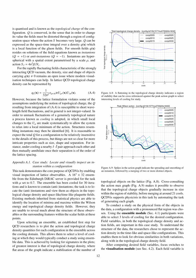
is quantised and is known as the topological charge of the con-figuration. Q is conserved, in the sense that in order to changeits value the fields must be distorted through a region of config-uration space where the action S becomes very large. Q can beexpressed as the space-time integral over a density q(x) whichis a local function of the gluon fields. For smooth fields q(x)resides on solutions of the field equations known as instantons(Q = +1) or anti-instantons (Q = −1). Instantons are hyper-spherical with a spatial extent parametrised by a scale ρ, andaction S I = 4π2β/Nc.

For the rapidly fluctuating fields characteristic of the stronglyinteracting QCD vacuum, the density, size and shape of objectscarrying q(x) , 0 remains an open issue where modern visual-isation techniques can help. In lattice QCD topological chargedensity can be represented by

qL(x) =1

32π2 εµνλκtrUµν(x)Uλκ(x). (A.4)

However, because the lattice formulation violates some of theassumptions underlying the notion of topological charge, the Qresulting from integration of (A.4) is susceptible to short wave-length field fluctuations, and in general is not integer-valued. Inorder to unmask fluctuations of a genuinely topological naturea process known as cooling is adopted, in which small localchanges to the Uµ are made systematically to allow the systemto relax into a local minimum of the action. Structures resem-bling instantons may then be identified [6]. It is reasonable toexpect the total Q for a configuration to be relatively insensitiveto the details of this process, but things are not so clear for moreintricate properties such as size, shape and separation. For in-stance, under cooling a nearby I -I pair approach each other andthen mutually annihilate once their separation is of the order ofthe lattice spacing.

Appendix A.1. Case study: Locate and visually inspect an in-stanton within a configuration

This task demonstrates the core purpose of QCDVis by enablingvisual inspection of lattice observables. A 163 × 32 ensem-ble from the Edinburgh DiRAC server is provided for the taskwith µ set to 0.7. The ensemble has been cooled for 30 itera-tions and is known to contain (anti-)instantons; the task is to lo-cate the (anti-)instantons and view them as objects in the topo-logical charge density and space-like/time-like plaquette fields.Existing methods inherited from statistical physics are able toidentify the location of minima and maxima within the Wilsonenergy and topological charge density fields. However, theyare unable to reveal much about the structure of these observ-ables or the surrounding features within the scalar fields at thesepoints.

Upon selecting an ensemble, an established first step forQCD researchers is to plot the action and topological chargedensity quantities for each configuration in the ensemble acrossthe cooling domain. This allows them to select a level of cool-ing at which they would typically conduct a study using ensem-ble data. This is achieved by looking for signatures in the plots;of greatest interest is that of topological charge density, whereflat areas of the graph indicate a stabilisation of the number of

0 5 10 15 20 25 30

cools

−10

−5

0

5

10

15

Tota

ltop

olog

ical

char

gede

nsity

QTOTAL

Total topological charge density - [config.b210k1577mu0700j02s16t32]

conp0005conp0010conp0015

conp0020conp0025conp0030

Figure A.8: A flattening in the topological charge density indicates a regionof stability that can be cross referenced against the peak action graph to selectinteresting levels of cooling for study.

0 5 10 15 20 25 30

cools

0

1

2

3

4

5

6Pe

akW

ilson

actio

nSPEAK

Peak Wilson action - [config.b210k1577mu0700j02s16t32]

conp0005conp0010conp0015conp0020conp0025conp0030

Figure A.9: Spikes in the action graph indicate the spreading and smoothing ofan instanton, followed by a merging of two or more distinct objects.

topological objects on the lattice (Fig. A.8). Cross-consultingthe action max graph (Fig. A.9) makes it possible to observethat the topological charge objects gradually increase in sizewithin the region of stability, before merging at around 21 cools.QCDVis supports physicists in this task by automating the taskof generating each graph.

To conduct a study on the physical form of the objects inthe data, a configuration with a pronounced flat region was cho-sen. Using the ensemble module (Sec. 4.1) participants wereable to select 3 levels of cooling for the desired configuration.Field variables, in both the topological charge density and ac-tion fields, are important in this case study. To understand thestructure of the data, the researchers chose to represent the ac-tion density in the time-like and space-like configurations. Thisenables them to look for obvious similarities in both variations,along with in the topological charge density field.

After computing desired field variables, focus switches tothe visualisation module (see Sec. 4.2). Each field variable is

12

Figure A.10: Top: user examining the position of Topological Charge Densityminima (anti-instanton) in the xyt, xzt and yzt sub-volumes. Bottom: comparingthe location of peak Wilson action and Topological Change Density minima inxyz sub-volumes.

loaded concurrently into the tool and the hyper-volume data cutinto 3D configurations. Feedback about the location of minimaand maxima steers the researchers toward areas of interest foreach field variable, observable in the contour tree. Researcherstended to favour the 3D volumes split by time to locate variablesin each field. The global isovalue slider allows them to comparethe relative similarities in each field in parallel. Additionally,researchers study the location and structure of objects in thetime-like 3D volumes (xyt, yzt, xzt) to validate that the objectscoincide in all view configurations (Fig. A.10).

Appendix A.2. Case study: View an irregularity within a cooledconfiguration.

The task illustrates how QCDVis is used to view and understandthe cooling process in greater detail. For this task a 163 × 32ensemble from the Edinburgh DiRAC server is provided; how-ever, in this ensemble µ = 0.45. The data has been cooled for100 iterations to try to emphasise the phenomena of observ-ables dropping through the lattice. An unexpected irregularityis found within one of the configurations, where a positive max-ima becomes a negative minima in successive cooling cycles.The task intends to visually inspect this phenomena and assignreason to it.

Whilst 100 cools represents a vast over exaggeration of howcooling would be applied in a real study, it promotes the possi-bility of witnessing an instanton falling through the lattice. Thisoccurs when an instanton contracts to exist at a single point,whereas typically, instantons exist across multiple neighbour-ing sites. In a typical QCD study this can only be detectedusing plots of topological charge density and action by lookingfor known signatures.

Initially upon loading a configuration the users consult thetopological charge density and action max graphs. However, inthis scenario the focus is a gradual increase followed by a fairlyinstantaneous drop in the action max graph (Fig. A.12). Usu-ally this will indicate one of two events; first, an annihilation ofan instanton/anti-instanton pair; or second, an indication that anobject has fallen through the lattice. Features in the topologicalcharge density graph (Fig. A.13) suggest that rather than an an-nihilation, as would be signified by a distinct drop, somethingelse is happening.

Further investigation takes the form of computing the topo-logical charge density at 3 consecutive levels of cooling. Thefield data is loaded into the visual tool so that it can be in-vestigated in parallel. Again, physicists instinctively open thespace-like configuration (xyz) to search for highlighted minimaand maxima. Upon opening the relevant time slice for all threecooling slices, the most immediate feature is a distinct changein the contour tree for each volume. The slices before the peakshow a relatively large maxima beyond the noise at the centreof the data set; however, the data on the downward slope in-stead shows that the maxima has disappeared to be replaced bya minima of roughly equal magnitude.

Visual inspection allows the physicists to look at the phe-nomena from different angle and formulate hypothesis about itsprovenance and nature. As can be seen in Fig. A.11, this irreg-ularity is characterised by a continual deformation of the objectrelating to a peak in topological charge density. Additionally,the minima in the field appears to exist in the same position onthe lattice, whereas there are no objects of the relevant isovaluein the earlier slices. An exact reason for this is not yet known,but physicists that have witnessed it were able to reflect uponand develop several possible hypothesis.

13

Slice 35 Slice 36 Slice 37 Slice 37, anomaly.

Figure A.11: Cooling slices 35, 36 and 37, shown at the same isovalue. At cooling step 37 the large object on the left starts to deform and disappears, being replacedby a global minima (right image). This phenomena can also be observed in the contour trees for each cooling phase.

14

30 35 40

cools

0

1

2

3

4

Peak

Wils

onac

tion

SPEAK

Peak Wilson action - [config.b210k1577mu0450j02s16t32]

conp0005conp0010conp0015conp0020conp0025

Figure A.12: An instanton falling through the lattice is characterised by the rel-atively high gradient drop in the peak action graph, this can be cross referencedwith the topological charge density graph.

30 35 40

cools

3.0

3.5

4.0

4.5

5.0

Tota

ltop

olog

ical

char

gede

nsity

QTOTAL

Total topological charge density - [config.b210k1577mu0450j02s16t32]

conp0005conp0010conp0015conp0020conp0025

Figure A.13: Physicists look for a flattening of the topological charge densityindicating stability. A short lived peak in the graph can characterise an instantonfalling through the lattice or an instanton-anti-instanton annihilation.

15