The Pennsylvania State University

The Applied Research Laboratory

P.O. Box 30

State College, PA 16804

Python Scripting for Gluing CFD Applications: A Case Study

Demonstrating Automation of Grid Generation, Parameter Variation,

Flow Simulation, Analysis, and Plotting

by

Eric G. PatersonDivision Scientist, Computational Mechanics Division

Associate Professor of Mechanical Engineeringemail: eric-paterson@psu.edu

Technical Report No. TR 09-00113 January 2009

Supported by:Naval Sea Systems Command Contract No. N00024-02-D-6604/0524

Approved for public release, distribution unlimited

Abstract

One of the simplest yet most useful applications of scripting is the automation of manual interactionwith the computer. Here, it means running programs for mesh generation, flow simulation, post–processing analysis, and plotting, and doing it over a complex matrix of initial conditions, boundaryconditions, fluid properties, and geometry variants. Python scripting provides the ability to interactwith both the operating system and each of the component codes, and to perform complex analysisand plotting.

A case study using OpenFOAM to solve the decaying Taylor–Green vortex, which is an ana-lytical solution to the transient two–dimensional Navier–Stokes equations, is developed. A pythonscript is used to perform a mesh–refinement study for ten different flux–interpolation schemes, andto automatically generate meshes, specify initial conditions, run the flow code, run a custom post-processor which computes solution error in comparison to the benchmark, and create line plots,contour maps, and vector plots. Concluding remarks are provided which summarize readiness forapplication to ship hydrodynamics, and which identify areas for future work.

Contents

1 Introduction 3

1.1 Motivation . . . . . . . . . . . . . . . . . . . . . . . . . . . . . . . . . . . . . . . . . 31.2 Objective . . . . . . . . . . . . . . . . . . . . . . . . . . . . . . . . . . . . . . . . . . 51.3 Requirements . . . . . . . . . . . . . . . . . . . . . . . . . . . . . . . . . . . . . . . . 5

2 Case Study 6

2.1 Python Scripting . . . . . . . . . . . . . . . . . . . . . . . . . . . . . . . . . . . . . . 62.2 Analytical Benchmark: 2D Taylor-Green Vortex . . . . . . . . . . . . . . . . . . . . 92.3 Use of PyFoam . . . . . . . . . . . . . . . . . . . . . . . . . . . . . . . . . . . . . . . 92.4 Mesh Generation . . . . . . . . . . . . . . . . . . . . . . . . . . . . . . . . . . . . . . 92.5 Variation of the divScheme . . . . . . . . . . . . . . . . . . . . . . . . . . . . . . . . 112.6 Initial Conditions: funkySetFields . . . . . . . . . . . . . . . . . . . . . . . . . . . . 112.7 Flow Solver: icoFoam . . . . . . . . . . . . . . . . . . . . . . . . . . . . . . . . . . . 122.8 Solution Post–Processing . . . . . . . . . . . . . . . . . . . . . . . . . . . . . . . . . 12

2.8.1 Error Computation: analyticalSolutionTaylorVortex . . . . . . . . . . . . . . 132.8.2 Solution sampling . . . . . . . . . . . . . . . . . . . . . . . . . . . . . . . . . 132.8.3 Contour Maps and Vector Plots . . . . . . . . . . . . . . . . . . . . . . . . . . 132.8.4 Grid Studies: Point–Data Comparison . . . . . . . . . . . . . . . . . . . . . . 142.8.5 Grid Studies: Average Error vs. Mesh Refinement . . . . . . . . . . . . . . . 14

3 Concluding Remarks 22

Bibliography 23

A OpenFOAM Solver: icoFoam 25

A.1 Incompressible Navier-Stokes Equations . . . . . . . . . . . . . . . . . . . . . . . . . 25A.2 Finite Volume Discretization . . . . . . . . . . . . . . . . . . . . . . . . . . . . . . . 25

A.2.1 Spatial Discretization . . . . . . . . . . . . . . . . . . . . . . . . . . . . . . . 26A.2.2 Temporal Discretization . . . . . . . . . . . . . . . . . . . . . . . . . . . . . . 28

A.3 Solution Algorithm for the Navier-Stokes Equations . . . . . . . . . . . . . . . . . . 29A.3.1 Linearization . . . . . . . . . . . . . . . . . . . . . . . . . . . . . . . . . . . . 29A.3.2 Derivation of the Pressure Equation . . . . . . . . . . . . . . . . . . . . . . . 29

A.4 Pressure-Velocity Coupling . . . . . . . . . . . . . . . . . . . . . . . . . . . . . . . . 30

1

List of Figures

2.1 Python Script for Controlling Ship Hydrodynamics Simulations . . . . . . . . . . . . 72.2 Python Script for Controlling Taylor Vortex Simulations . . . . . . . . . . . . . . . . 82.3 Analytical Solution for the Taylor–Green Vortex Problem at time = 1 . . . . . . . . 102.4 Typical Solution Convergence with Mesh Refinement. . . . . . . . . . . . . . . . . . 152.5 Comparison Error for Each Scheme . . . . . . . . . . . . . . . . . . . . . . . . . . . . 172.6 Comparison of Velocity and Pressure to Analytical Solution. . . . . . . . . . . . . . . 192.7 Average Error vs. Grid Resolution for Different divScheme. . . . . . . . . . . . . . . 21

A.1 Parameters in finite volume discretization . . . . . . . . . . . . . . . . . . . . . . . . 26

2

CHAPTER 1

Introduction

1.1 Motivation

Computational fluid dynamics (CFD) has matured to its current status where multiphysics anddesign-relevant simulations are realizable. Marine engineering examples include integrated designof surface ships, design of marine-propulsors made of advanced materials, and integration of fidelitywake simulations into prediction of ship and submarine acoustic and non-acoustic signatures. How-ever, there are several high–level challenges in performing these simulations. First, the top–leveldriver/calling program has to see CFD (and the entire “CFD Process”) as a modular “black-blox”which can be reliably automated. Second, top–level programs often require large–amounts of fluiddynamics data over a large parameter space. This requires that the driver program manage amatrix of simulations, and resultant data. Third, CFD and other analysis tools (e.g., finite-elementanalysis), must be coordinated and data must be passed between them. This process is knownas code gluing. It is proposed that Python scripting will play an important role in meeting thesechallenges.

CREATE-Ships has the broad objective to impact acquisition and design of future ships byleveraging high-performance computing. Focus areas include rapid, and automated, simulation ofhull resistance and associated boundary–layer and free–surface hydrodynamics using fidelity RANSCFD, and development of an Integrated Hydro Design Environment (IHDE) to more tightly coupledesign and analysis tools. It is envisioned that the IHDE will interface with adjustable–fidelitysimulation tools, ranging from empirical databases to potential-flow codes to RANS/DES/LESCFD codes, however, the IHDE will only see the various tools through an interface. Behind thisinterface, however, is the “CFD Process” which itself is comprised of a number of highly–specializedstand–alone programs.

The Applied Research Lab (ARL) at Penn State University (PSU) is a leader in marine com-posites and has designed and fabricated numerous composite structures for the U.S. Navy. Currentinterest is focused on coupling CFD, FEA, and in-house acoustics tools for prediction of fully–coupled fluid–structural–hydroacoustic performance. This is a clear example of a need for codeautomation and code gluing. Water–tunnel tests of metal and composite hydrofoils are currentlybeing planned/performed as part of student thesis research. The purpose of these tests are todevelop understanding and validation databases for fluid-structure interaction (FSI) simulations.

3

ARL/PSU is also the developer of the Technology Requirements Model (TRM) which is a dig-ital simulation tool for torpedoes. The software supports the full system technology developmentcycle; i.e., research, design, development, testing, and technology transition to acquisition. TRM’sarchitecture allows for the acoustic interactions (mutual interference) between surface ships, sub-marines, countermeasures, counter-fire weapons, salvo fired torpedoes, and anti-torpedo torpedoes.However, it lacks the ability to easily incorporate physics–based models of wakes. Current workis focused on integration of CFD into the TRM process, including ships undergoing transient ma-neuvers. In this case, TRM should be able to either interrogate existing CFD databases, or call aCFD module for development of new data.

From this short list of examples, it should be obvious that there is a large need for improvingthe interface of CFD to other tools. One of the simplest yet most useful applications of scriptingis the automation of manual interaction with the computer. Here, it means running programsfor mesh generation, flow simulation, post–processing analysis, and plotting, and doing it over acomplex matrix of initial conditions, boundary conditions, fluid properties, material properties, andgeometry (hullform, propulsors, etc.) variants. Python scripting provides the ability to interactwith both the operating system and each of the component codes, and to perform complex analysisand plotting.

As advertised on the python.org website [1], “Python is a dynamic object-oriented programminglanguage that can be used for many kinds of software development. It offers strong support forintegration with other languages and tools, comes with extensive standard libraries, and can belearned in a few days. Many Python programmers report substantial productivity gains and feelthe language encourages the development of higher quality, more maintainable code.”

There are a number of libraries which greatly extend Python and make it a powerful tool forcomputational science. Numpy [2] is the fundamental package needed for scientific computing withPython. It contains: a powerful N-dimensional array object; sophisticated broadcasting functions;basic linear algebra functions; basic Fourier transforms; sophisticated random number capabilities;tools for integrating Fortran code; and tools for integrating C/C++ code. Scipy [3] is open-source software for mathematics, science, and engineering. The SciPy library is built to work withNumPy arrays, and provides many user-friendly and efficient numerical routines such as routinesfor numerical integration and optimization. Together, they run on all popular operating systems,are quick to install, and are free of charge. Matplotlib [4] is a python 2D plotting library whichproduces publication quality figures in a variety of hardcopy formats and interactive environmentsacross platforms. Matplotlib can be used in python scripts, the ipython shell (in a fashion similarto MATLAB), web application servers, and six graphical user interface toolkits.

An indicator of the importance of python in computational science is the fact that most com-mercial CFD visualization tools (Ensight, Fieldview, Paraview, Tecplot) are now providing pythonbindings for controlling the analysis and visualization from a python script. There are also pythonbindings for MPI (message passing interface) and PETSc (parallel extensible toolkit for scientificcomputing). Finally, python can interfaced with Fortran and C/C++ by using f2py and swig,respectively.

With regard to OpenFOAM, there are several python related development activities. The first,is PyFOAM [5] which is a library that can be used to: analyze the logs produced by OpenFoam-solvers;execute OpenFoam-solvers and utilities and analyze their output simultaneously; manipulate theparameter files and the initial-conditions of a run in a non-destructive manner; and plots theresiduals of OpenFOAM solvers using GNUPLOT. The second is an effort by Hrv Jasak to useswig to create python bindings for OpenFOAM libraries. While the latter is in a very preliminarystage, it offers rapid prototyping and debugging, and even easier systems integration.

4

1.2 Objective

The objective of this report is to demonstrate the use of python scripting for gluing CFD appli-cations. A case study using the decaying Taylor–Green vortex is developed. This problem is ananalytical solution to the transient two–dimensional Navier–Stokes equations, and is commonlyused for computing the order–of–accuracy of the numerical schemes. [6, 7] A python script is usedto perform parameter variation (mesh resolution and convective–scheme flux interpolation), gen-erate meshes, specify initial conditions, run the flow code, run a custom post-processor whichcomputes solution error in comparison to the benchmark, and create line plots, contour maps, andvector plots. Concluding remarks are provided which summarize readiness for application to shiphydrodynamics, and which identify areas for future work.

1.3 Requirements

If you have downloaded the case study tarball, you will need the following software installed onyour computer to run the python script:

• OpenFOAM 1.5.x [8]

• python [1]

• matplotlib [4]

• NumPy [2]

• SciPy [3]

OpenFOAM 1.5.x can be obtained from the OpenCFD git repository. Note that this versionis source code only, so it will require full compilation. The bug-fix/patched version repositoryis available at git://repo.or.cz/OpenFOAM-1.5.x.git. The repository can be obtained using thecommand:

[08:54:10][egp@egpMBP:~/OpenFOAM]$git clone git://repo.or.cz/OpenFOAM-1.5.x.git

This will create an OpenFOAM-1.5.x directory that the user can subsequently update to the latestpublished copy using

[08:55:05][egp@egpMBP:~/OpenFOAM]$git pull git://repo.or.cz/OpenFOAM-1.5.x.git

While it is not required, iPython [9] is nice to have since it permits interactive running of thescript. It gives an interface similar to MATLAB.

5

CHAPTER 2

Case Study

2.1 Python Scripting

To meet the goals of the multi-physics examples previously mentioned, an approach needs to bedeveloped where fidelity CFD simulations can be performed rapidly and automatically, and wheredata is returned back to a driver code (e.g., IHDE) for integration in the design/analysis cycle.A notional flow chart to accomplish this is shown in figure 2.1. This flow chart shows iterativeloops over hullform geometry, ship speed, and mesh refinement (all of w. Inside the loops is thetypical CFD Process: mesh generation; setting of initial conditions, boundary conditions, and fluidproperties; flow solution; analysis; and plotting and visualization.

Instead of using a practical surface–ship example for the case study, a simplified problem waschosen so that it would run fast (i.e., a few minutes on a laptop), and be easy to distribute byemail or website download. The flow chart for the case study of the Taylor–Green vortex problemis shown in figure 2.2. It is nearly identical to the flow chart for the ship, except for the iterationloops are over the type of flux interpolation scheme divScheme and mesh refinement. Also, severalother utilities are used: funkySetfields, and analyticalSolutionTaylorVortex.

The python script runScript.py for the case study is located in the root of the tarball. It is 190lines long, and could be greatly shortened with definition of a few functions or classes/members. Itis executed at the command line with the command

[16:10:39][egp@TaylorVortex]$ ./runScript.py

The script loops over 4 meshes, and 10 divScheme represented by the python lists

meshDir = [’mesh8’, ’mesh16’, ’mesh32’, ’mesh64’]

divSchemes=[ ’linear’, ’cubic’, ’downwind’, ’midPoint’, ’MUSCL’,

’Minmod’, ’QUICK’, ’filteredLinear’, ’upwind’, ’vanLeer’]

The loops are executed using the python for loop, e.g.,

for mesh in meshDir:

meshIndex =meshDir.index(mesh)

# further processing on mesh

6

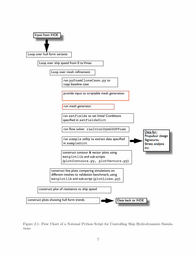
Loop over hull form variants

Loop over mesh refinement

run pyFoamCloneCase.py to copy baseline case

provide input to scriptable mesh generation

run mesh generator

run setFields to set Initial Conditions specified in setFieldsDict

run flow solver rasInterDym6DOFFoam

run sample utility to extract data specified in sampleDict

construct contour & vector plots using matplotlib and sub-scripts

(plotContours.py, plotVectors.py)

construct line plots comparing simulations on different meshes to validation benchmark, using matplotlib and sub-script (plotLines.py)

construct plot of resistance vs. ship speed

Loop over ship speed from 0 to Vmax

construct plots showing hull form trends

Figure 2.1: Flow Chart of a Notional Python Script for Controlling Ship Hydrodynamics Simula-tions

7

Loop over divSchemes

Loop over mesh refinement

run pyFoamCloneCase.py to copy baseline case

set grid size in blockMeshDict using pyFoam BlockMesh class and refine member

run blockMesh to generate grid

run funkySetFields to set Initial Conditions specified in funkySetFieldsDict

run flow solver icoFoam

run custom analysis tool, analyticalSolutionTaylorVortex

run sample utility to extract lines and surfaces of data specified in sampleDict

construct contour & vector plots using matplotlib and sub-scripts

(plotContours.py, plotVectors.py)

construct line plots comparing simulations on different meshes to analytical solution, using matplotlib and sub-script (plotLines.py)

construct plot of error vs. grid resolution for all divSchemes, using matplotlib and sub-

script (plotError.py)

Figure 2.2: Flow Chart of a Python Script for Controlling Simulations of Taylor Vortex

8

2.2 Analytical Benchmark: 2D Taylor-Green Vortex

The 2D Taylor-Green Vortex is an analytical solution to the Navier–Stokes equations, and has longbeen used for testing and validation of temporal and spatial accuracy of the numerical scheme.[6, 7, 10,11].

In the domain −π2 ≤ x, y ≤ π

2 , the solution is given by

u = sin x cos yF (t) v = − cos x sin yF (t) (2.1)

where F (t) = e−2νt, ν being the kinematic viscosity of the fluid. The pressure field p can beobtained by substituting the velocity solution in the momentum equations and is given by

p =ρ

2(cos 2x + sin 2y) F 2(t) (2.2)

Equations 2.1 and 2.2 are used to prescribe the initial conditions at time = 0. Figure 2.3, whichshows velocity vectors, velocity–magnitude contours, and pressure contours, illustrates the solutionat time = 1.0, for the case where ν = 1.0m2/s. The velocity field has odd-symmetry and thepressure-field is periodic in x and y directions. This information is used in assigning boundaryconditions. Symmetry conditions are applied on all boundaries (except for the empty faces in thez-direction).

2.3 Use of PyFoam

Referring back to figure 2.2, the first steps inside the loop are to clone the baseline case and torefine the mesh. For both of these steps, the pyFoam utilities [5] are utilized.

pyFoamCloneCase.py is a pyFoam application which creates a copy of a case with only the mostessential files (0, constant, system directories). It has two command line arguments: the sourcecase (../../baseline) and the destination case (mesh, where mesh is a list member which refersto the mesh resolution). In the text that follows, which is from runScript.py, the string cmd ispassed to the call member of the subprocess module.

# use pyFoam to clone the baseline case

cmd=’pyFoamCloneCase.py ../../baseline %s’ % mesh

pipefile = open(’output’, ’w’)

retcode = call(cmd,shell=True,stdout=pipefile,stderr=pipefile)

pipefile.close()

os.remove(’output’)

The subprocess module allows you to spawn processes, connect to their input/output/error pipes,and obtain their return codes. cmd is passed to the shell using the short cut function call which runsthe command with arguments, waits for command to complete, and then returns the returncode

attribute. It is used to run all of the component codes in the CFD Process.

2.4 Mesh Generation

Since one of the loops is to iterate over mesh resolution (8x8, 16x16, 32x32, 64x64), the input tothe mesh generation tool needs to be modified inside the script. In this simple case, the Open-FOAM mesher blockMesh is used. It reads a dictionary constant/polymesh/blockMeshDict andgenerates a hex mesh using algebraic methods. In the script runScript.py, the pyFoam class

9

(a) Velocity Vectors (b) Velocity Magnitude Contours

(c) Pressure Contours

Figure 2.3: Analytical Solution for the Taylor–Green Vortex Problem at time = 1

10

# set block size in blockMeshDict

dict=‘‘constant/polyMesh/blockMeshDict’’ # blockMeshDict

bm=BlockMesh(dict) # define bm to be a pyFoam BlockMesh object

number=meshDir.index(mesh) # find index of current mesh: 0, 1, 2, 3

bm.refineMesh\left( 2**number,2**number,1)) # refineMesh by factor of 2^number over baseline

meshDim = 8*2**number

A (BlockMesh) object and member (refineMesh) are used to change the values in blockMeshDict.The blockMesh utility is run with the subprocess.call function.

# run blockMesh

cmd=’blockMesh’

pipefile = open(’output’, ’w’)

retcode = call(cmd,shell=True,stdout=pipefile)

pipefile.close()

os.remove(’output’)

2.5 Variation of the divScheme

When looping over the divSchemes list, the system/fvSchemes dictionary has to be modified withthe divScheme of the current iteration. pyFoam has a series of utilities for modifying dictionaries.At the time of writing this report, pyFoamWriteDictionary.py was not able to process the string‘‘div(phi,U)’’. Therefore, a small piece of python code was written to read the dictionary, searchfor ‘‘div(phi,U)’’, and replace the divScheme with the value of the current iteration. The codein runScript.py responsible for this is listed below.

# change the divScheme for ‘‘div(phi,U) Gauss linear;’’ in the fvSchemes file

infilename=’system/fvSchemes’

outfilename=’system/fvSchemesTemp’

ifile = open( infilename, ’r’)

ofile = open(outfilename, ’w’)

lines = ifile.readlines()

for line in lines:

words = line.split()

for word in words:

index = words.index(word)

if word == ’div(phi,U)’:

words[index+2] = divScheme+’;’

continue

newline=’ ’.join(words)

ofile.write(’%s\n’ % newline)

ifile.close()

ofile.close()

os.remove(infilename)

os.rename(outfilename,infilename)

2.6 Initial Conditions: funkySetFields

The funkySetFields utility of Gschaider [12] is used to prescribe the initial conditions from theanalytical solution in equations 2.1 and 2.2. funkySetFields was designed to set the value of ascalar or a vector field depending on an expression that can be entered via the command line or adictionary. It can also be used to set the value of fields on selected patches or set non-uniform initial-conditions without programming. It has been described as the OpenFOAM setFields utility onsteroids.

11

To use the analytical solution as the initial conditions, the following text is inserted into thedictionary system/funkySetFieldDict.

expressions

(

TaylorVortexVelocity

{

field U;

expression ‘‘vector( -cos(pos(.x)*sin(pos(.y)),

(sin(pos(.x)*cos(pos(.y)),

0)’’;

}

TaylorVortexPressure

{

field p;

expression ‘‘-0.25*(cos(2.*pos(.x)+cos(2.*pos(.y))’’;

}

);

As with the other component programs, funkySetFields -time 0 is sent to the shell using thesubprocess.call function. The portion of runScript.py which executes this utility is listed below.

#run funkySetFields to set initial conditions

cmd=’funkySetFields -time 0’

pipefile = open(’output’, ’w’)

retcode = call(cmd,shell=True,stdout=pipefile)

pipefile.close()

os.remove(’output’)

2.7 Flow Solver: icoFoam

Since the Taylor-Green vortex is a transient, laminar flow problem, the icoFoam solver is used tosolve for velocity and pressure fields. icoFoam solves the incompressible laminar Navier-Stokesequations using the PISO algorithm which is a time-accurate algorithm requiring initial andboundary conditions. The icoFOAM solver reads the following dictionaries: system/controlDict,system/fvSchemes, system/fvSolution, constant/transportProperties. Details of the ico-Foam solver are provided in the Appendices.

In the runScript.py script, the flow code is executed with the following commands.

# run icoFoam to solve Navier Stokes equations

cmd=’icoFoam > log 2>&1’

pipefile = open(’output’, ’w’)

retcode = call(cmd,shell=True,stdout=pipefile)

pipefile.close()

os.remove(’output’)

2.8 Solution Post–Processing

Solution post–processing includes manipulation of data, comparison of simulation and benchmark(which, in this case, is an analytical solution), and plotting. The following sections will explain thepost–processing, and present some of the results.

12

2.8.1 Error Computation: analyticalSolutionTaylorVortex

The easiest way to compute error E = S−A, where S is the simulation result and A is the analyticalsolution, is to write a custom OpenFOAM utility which can access the various OpenFOAM datastructures. For the case study, analyticalSolutionTaylorVortex was written and is located inthe tools directory. It reads the mesh and simulation results, computes the analytical solutionat the cell centers, and calculates the error E. It is compiled with the standard OpenFOAMwmake machinery. The following code from runScript.py shows that the utility is run with thesubprocess.call function, and that stdout is written to the pipefile named ASTVOutput. Then,the script parses this file and searches for the strings ’Maximum’ and ’Average’. After these stringsare found, the value of maxError and aveError are read and held in memory for plotting.

# run custom post-processor for computing analytical solution at each time step,

# and for computing comparison error

cmd=’analyticalSolutionTaylorVortex -time 1’

pipefile = open(’ASTVOutput’, ’w’)

retcode = call(cmd,shell=True,stdout=pipefile)

pipefile.close()

# extract maximum error at endTime (time = 1) from STDOUT

pipefile = open(’ASTVOutput’, ’r’)

lines = pipefile.readlines(

for line in lines:

words = line.split()

for word in words:

if word == ’Maximum’:

value=float(words[len(words)-1])

maxError.append(value)

if word == ’Average’:

value=float(words[len(words)-1])

aveError.append(value)

pipefile.close()

2.8.2 Solution sampling

Solution sampling is accomplished using the OpenFOAM utility sample, which reads the dictionarysystem/sampleDict. It is executed by the shell using the call function.

# run sample utility

cmd=’sample -time 1’

pipefile = open(’output’, ’w’)

retcode = call(cmd,shell=True,stdout=pipefile)

pipefile.close()

os.remove(’output’)

2.8.3 Contour Maps and Vector Plots

Contour maps and vector plots are created using matplotlib [4]. The runScript.py calls twosub-scripts, tools/plotContours.py and tools/plotVectors.py. These sub-scripts expect 3command-line arguments, which are used primarily for naming the plot files. After creation, theplot files are moved to a directory in the root of the case study named figures.

# construct contour & vector plots

cmd=’python ../../../tools/plotContours.py ’+ str(meshDim)+’ ’+divScheme+’ ’+mesh

pipefile = open(’output’, ’w’)

retcode = call(cmd,shell=True,stdout=pipefile)

13

pipefile.close()

os.remove(’output’)

cmd=’python ../../../tools/plotVectors.py ’+ str(meshDim)+’ ’+divScheme+’ ’+mesh

pipefile = open(’output’, ’w’)

retcode = call(cmd,shell=True,stdout=pipefile)

pipefile.close()

os.remove(’output’)

# move pdf image files to figures directory

filelist=glob.glob(’*.pdf’)

for file in filelist:

shutil.move(file, origdir+‘‘/figures/.’’)

Figure 2.4 shows contours of velocity magnitude and pressure, for the four different meshes. Inthis case, the solutions all used the upwind scheme for the convective terms in the Navier-Stokesequations.

Figure 2.5 shows the comparison error E = S − A on the fine mesh for each of the convectiveschemes. Here, it can be seen that the first–order schemes (upwind, downwind) have the largesterrors (on the order of 1%).

2.8.4 Grid Studies: Point–Data Comparison

Detailed point–data comparisons are made along a sampling line which corresponds to y = 0. Theseplots were created by using the plotLines.py sub-script and the following code in runScript.py.

# construct line plots comparing all meshes for a given divScheme

cmd=’python ../../tools/plotLines.py ’+divScheme

pipefile = open(’output’, ’w’)

retcode = call(cmd,shell=True,stdout=pipefile)

pipefile.close()

os.remove(’output’)

filelist=glob.glob(’*.pdf’)

for file in filelist:

shutil.move(file, origdir+‘‘/figures/.’’)

Figure 2.6 shows a comparison of velocity and pressure to the analytical solution for eachdivScheme and for each mesh.

2.8.5 Grid Studies: Average Error vs. Mesh Refinement

The last plot is to extract global data from each simulation and compute and plot average errorover the domain, as a function of grid resolution. This is accomplished by running the subscriptplotError.py. The snippet of code from runScript.py that performs this step is listed below.

cmd=’python ../tools/plotError.py’

pipefile = open(’output’, ’w’)

retcode = call(cmd,shell=True,stdout=pipefile)

pipefile.close()

os.remove(’output’)

filelist=glob.glob(’*.pdf’)

for file in filelist:

shutil.move(file, origdir+‘‘/figures/.’’)

14

(a) 8x8, velocity (b) 8x8, pressure

(c) 16x16, velocity (d) 16x16, pressure

(e) 32x32, velocity (f) 32x32, pressure

Figure 2.4: Typical Solution Convergence with Mesh Refinement.

15

(g) 64x64, velocity (h) 64x64, pressure

Figure 2.4: Typical Solution Convergence with Mesh Refinement, continued.

Figure 2.7 shows the result of this analysis. In this plot, the comparison error E is normalizedby the maximum velocity magnitude in the domain. This is plotted again the grid resolutionnormalized by the fine grid ∆x. This means that ∆x

∆xfinest= 1,2,4,8 correspond to the finest, fine,

medium, and coarse grids, respectively. The plot in Figure 2.7 shows that the 1st–order schemes(upwind, downwind) have lower rate of grid convergence, whereas the remaining 2nd–order schemeshave the same slopes, but with different absolute errors. It should be noted that all simulationswere performed with the 2nd-order temporal scheme, CrankNicholson, and with a maxCo = 0.1.This means that the ∆t is reduced as the grid is refined, and that Figure 2.7 is a measure of bothoverall temporal and spatial error.

16

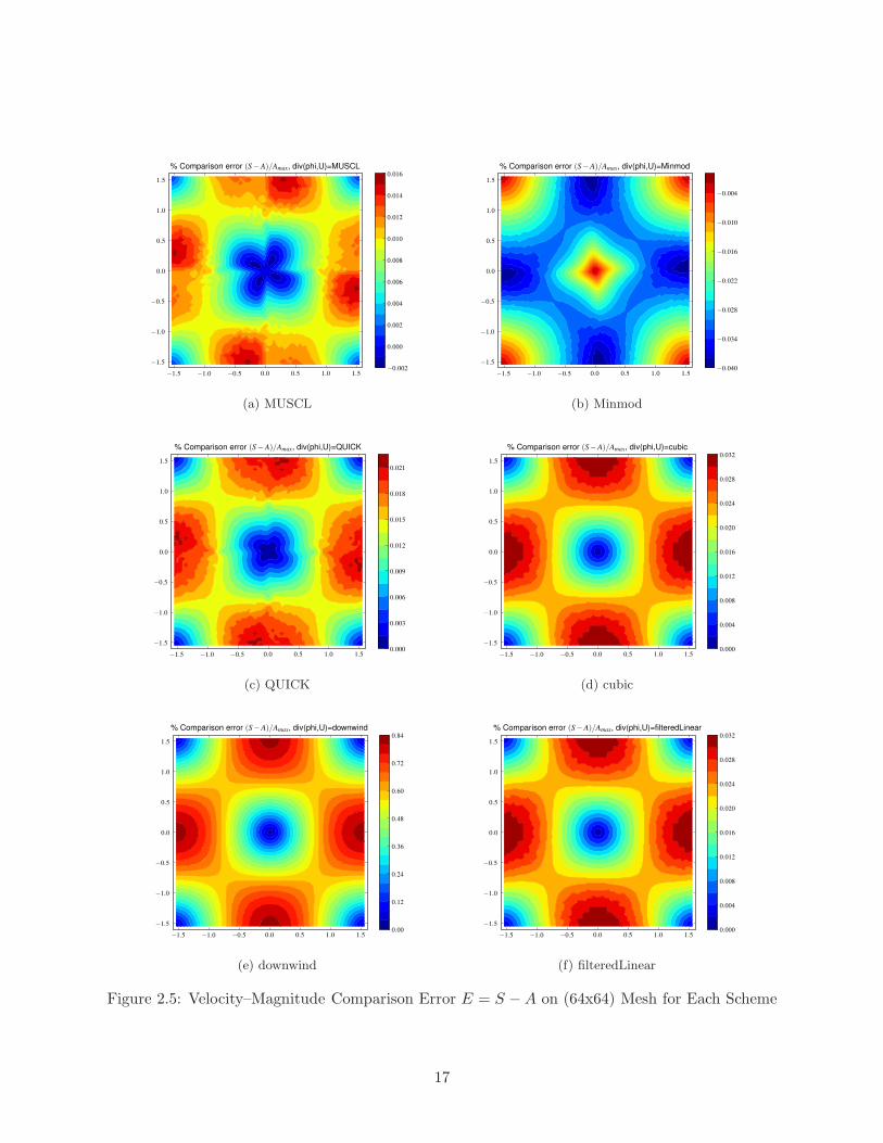
(a) MUSCL (b) Minmod

(c) QUICK (d) cubic

(e) downwind (f) filteredLinear

Figure 2.5: Velocity–Magnitude Comparison Error E = S − A on (64x64) Mesh for Each Scheme

17

(g) linear (h) midPoint

(i) upwind (j) vanLeer

Figure 2.5: Velocity–Magnitude Comparison Error E = S − A on (64x64) Mesh for Each Scheme,continued

18

(a) MUSCL (b) Minmod

(c) QUICK (d) cubic

(e) downwind (f) filteredLinear

Figure 2.6: Comparison of Velocity and Pressure to Analytical Solution.

19

(g) linear (h) midPoint

(i) upwind (j) vanLeer

Figure 2.6: Comparison of Velocity and Pressure to Analytical Solution, continued.

20

Figure 2.7: Average Error vs. Grid Resolution for Different divScheme.

21

CHAPTER 3

Concluding Remarks

In this report, a case study demonstrating the use of python for code gluing was developed. Apython script was used to perform a mesh–refinement study for ten different flux–interpolationschemes, and to automatically generate meshes, specify initial conditions, run the flow code, run acustom post-processor which computes solution error in comparison to the benchmark, and createline plots, contour maps, and vector plots.

For certain classes of problems, the approach is fully ready for application to ship hydrody-namics. These problems include simple geometries, and problems where grid generation can beperformed prior to CFD simulation. This is due to the fact that automated, and robust, meshgeneration for complex ship hullforms is currently not possible. Possible solutions which needto be further investigated are: use and improvement of hex-dominant meshing techniques suchas Harpoon and snappyHexMesh; use of Gridgen in batch–mode with Pointwise Glyph scripting;and testing of NASA Ames approach of scripting overset meshes with hyperbolic near field, andbox-mesh far-field [13]. In addition, CREATE has an infrastructure component with the goal ofdeveloping more automated grid generation capabilities. As progress is made on this front, theability to fully automate the CFD process for complex geometries will improve.

22

Bibliography

[1] Python Home Page. http://www.python.org/, January 2009.

[2] NUMPY Website. http://numpy.scipy.org/, January 2009.

[3] SCIPY Website. http://www.scipy.org/, January 2009.

[4] MATPLOTLIB Website. http://matplotlib.sourceforge.net/, January 2009.

[5] B. Gschaider. PyFOAM Website. http://openfoamwiki.net/index.php/Contrib_PyFoam.

[6] A.J. Chorin. Numerical solution of the Navier-Stokes equations(Finite difference solution oftime dependent Navier-Stokes equation for incompressible fluids, using velocities and pressureas variables). Mathematics of Computation, 22:745–762, 1968.

[7] J. Kim and P. Moin. Application of a fractional-step method to incompressible Navier-Stokesequations. Journal of Computational Physics, 59:308–323, 1985.

[8] OpenFOAM Website. http://www.opencfd.co.uk/openfoam/download.html#download,January 2009.

[9] iPython Home Page. http://ipython.scipy.org/moin/, January 2009.

[10] D.C. Lyons, L.J. Peltier, Zajaczkowski, and E.G. F.J., Paterson. Assessment of DES Modelsfor Separated Flow from a Hump in a Turbulent Boundary Layer. ASME Journal of Fluids

Engineering, (accepted for publication), 2009.

[11] Taylor-Green Vortex Entry on Wikipedia. http://en.wikipedia.org/wiki/Taylor-Green_vortex.

[12] B. Gschaider. OpenFOAM Utility: funkySetFields. http://openfoamwiki.net/index.php/

Contrib_funkySetFields, December 2008.

[13] W.M. Chan. Enhancements to the Grid Generation Script Library and Post-Processing Util-ities in Chimera Grid Tools. In 9th Symposium on Overset Composite Grids and Solution

Technology, State College, PA, October 2008.

23

[14] H. Jasak. Error Analysis and Estimation for the Finite Volume Method with Applications to

Fluid Flows. Ph.d. thesis, Imperial College of Science, Technology and Medicine, Universityof London, June 1996.

[15] OpenCFD Ltd. OpenFOAM Users Guide, Version 1.5, July 2005.

[16] OpenCFD Ltd. OpenFOAM Programmers Guide, Version 1.5, July 2005.

[17] R.I. Issa. Solution of the implicitly discretized fluid flow equations by operator-splitting.Journal of Computational Physics, 62:40–65, 1985.

[18] S.V. Patankar. Numerical heat transfer and Fluid Flow. Hemisphere Publishing Corporation,1981.

24

APPENDIX A

OpenFOAM Solver: icoFoam

In following Appendices, details on the numerical methods used in icoFoam are presented. Most ofthe material has been directly extracted from Hrv Jasak’s PhD thesis [14], OpenCFD User and Pro-grammers Guides [15,16], and the OpenFOAM Wiki http://openfoamwiki.net/index.php/IcoFoam.

A.1 Incompressible Navier-Stokes Equations

The 2D incompressible Navier-Stokes equation in the absence of body force is given by

∂u

∂x+

∂v

∂y= 0 (A.1)

∂u

∂t+ u

∂u

∂x+ v

∂u

∂y= −

1

ρ

∂p

∂x+ ν

(

∂2u

∂x2+

∂2u

∂y2

)

(A.2)

∂v

∂t+ u

∂v

∂x+ v

∂v

∂y= −

1

ρ

∂p

∂y+ ν

(

∂2v

∂x2+

∂2v

∂y2

)

(A.3)

where equations A.1 and A.2–A.3 represent the conservation of mass and linear momentum, re-spectively.

A.2 Finite Volume Discretization

The governing equations for conservation of mass, conservation of momentum, and transport ofscalars can be represented by the generic transport equation for φ

∂ρφ

∂t+ ∇ · (ρUφ) −∇ · (ρΓφ∇φ) = Sφ (φ) (A.4)

which is comprised of 4 basic terms: temporal acceleration; convective acceleration; diffusion;and a source term. The finite volume method requires that each term in Eq. (A.4) be satisfied over

25

the control volume Vp around the point P in the integral form

∫ t+∆t

t

[

∂

∂t

∫

Vp

ρφ dV +

∫

Vp

∇ · (ρUφ) dV −

∫

Vp

∇ · (ρΓφ∇φ) dV

]

dt

=

∫ t+∆t

t

[

∫

Vp

Sφ (φ) dV

]

dt (A.5)

The discretization of each term will be discussed in the following sections.

A.2.1 Spatial Discretization

The solution domain is discretized into computational cells, or finite volumes, on which the gov-erning equations are discretized, reduced to algebraic form, and solved with numerical methods.As shown in Figure (A.1), OpenFOAM is based upon general polyhedral cells. The cells are con-tiguous, i.e., they do not overlap one another and completely fill the domain. Dependent variablesand other properties are principally stored at the cell centroid P, although they may be stored onfaces or vertices. The cell is bounded by a set of faces, given the generic label f . Since the meshcan be a general polyhedral, there is no limitation on the number of faces bounding each cell, norany restriction on the alignment of each face.

The first step in spatial discretization is to transform the volume integrals in Eq. (A.5) tosurface integrals by using Gauss’s Theorem (also known as the Divergence theorem). In it’s mostgeneral form, Gauss’s Theorem can be written as

∫

V

∇ ⋆ φ dV =

∫

S

dS ⋆ φ (A.6)

where S is the surface area vector, φ represents any tensor field, and the star operator ⋆ is used torepresent any tensor product, i.e., inner, outer, cross and the respective derivatives (div, grad, curl).Volume and surface integrals are then linearized using appropriate schemes which are described foreach term.

Figure A.1: Parameters in finite volume discretization

26

Convection Term

The convection term is integrated over a control volume and linearized as follows:

∫

V

∇ · (ρUφ) dV =

∫

S

dS · (ρUφ) =∑

f

Sf · (ρU)f φf =∑

f

Fφf (A.7)

where the face field φf can be evaluated using a variety of schemes including central, upwind,and blended differencing. Central (or linear) differencing, which is second-order accurate, can bewritten as:

φf = fxφP + (1 − fx) φ (A.8)

fx =fN

PN(A.9)

OpenFOAM also includes two other centered schemes: cubicCorrection and midPoint. Upwinddifferencing for φf , which guarantees boundedness but is first-order accurate, can be written as

φf =

{

φP for F ≥ 0φN for F < 0

(A.10)

In addition to the standard upwind scheme, linearUpwind, skewLinear and Quick schemes arevariants of upwinded schemes which are available in OpenFOAM. Finally, there are a number ofblended schemes which attempt to preserve both boundedness and accuracy of the solution. Thegamma scheme can be written as

φf = (1 − γ) (φf )UD

+ γ (φf )CD

(A.11)

where the blending factor 0 ≤ γ ≤ 1 determines how much dissipation is introduced.The mass flux F in Eq. (A.7) is calculated from interpolated values of ρ and U. Similar to

interpolation of φf , F can be evaluated using a variety of schemes including centered, upwinded,and blended schemes, the latter of which includes a number of TVD/NVD schemes (such as limit-edLinear, vanLeer, MUSCL, limitedCubic, SFCD, and Gamma).

Laplacian Term

The Laplacian term is integrated over a control volume and linearized as follows:

∫

V

∇ · (Γ∇φ) dV =

∫

S

dS · (Γ∇φ) =∑

f

ΓfSf · (∇φ)f (A.12)

The face gradient discretization is implicit when the length vector d between the center of the cellof interest P and the center of the neighboring cell N is orthogonal to the face plane, i.e., parallelto Sf :

Sf · (∇φ)f = |Sf |φN − φP

|d|(A.13)

In the case of non-orthogonal meshes, an additional explicit term is introduced which is evaluated byinterpolating cell center gradients, themselves calculated by central differencing cell center values.

27

Source Terms

Source terms can be specified in three ways: explicit, implicit, and implicit/explicit. For explicitsource terms, they are incorporated into an equation simply as a field of values. For example, tosolve Poisson’s equation ∇2φ = f , φ and f would be defined as volScalarField and then do

solve(fvm::laplacian(phi) == f)

In contrast, an implicit source term is integrated over a control volume and linearized by∫

V

Sφ(φ) dV = SpVP φP

The Implicit/Explicit approach changes between the two based upon the sign of the source term.If the source is positive, it is treated as an implicit source term so that it increases the diagonaldominance of the matrix. If the source is negative, it is treated as an explicit source term. Inmathematical terms, the mixed source approach can be written as

∫

V

Sφ (φ) dV = SuVP + SpVP φP (A.14)

A.2.2 Temporal Discretization

Temporal Derivatives

The first derivative ∂∂t is integrated over a control volume with one of two schemes: 1st-orderEuler implicit, or 2nd-order backward difference

∂

∂t

∫

V

ρφ dV =(ρP φP VP )n − (ρP φP VP )0

∆t(A.15)

∂

∂t

∫

V

ρφ dV =3 (ρP φP VP )n − 4 (ρP φP VP )0 + (ρP φP VP )00

2∆t(A.16)

where the new values are φn = φ(t + ∆t), the old values are φ0 = φ(t), and the old-old values areφ00 = φ(t − ∆t).

Treatment of Spatial Derivatives in Transient Problems

Reconsider the integral form of the transport equation Eq. (A.5).

∫ t+∆t

t

[

∂

∂t

∫

Vp

ρφ dV +

∫

Vp

∇ · (ρUφ) dV −

∫

Vp

∇ · (ρΓφ∇φ) dV

]

dt

=

∫ t+∆t

t

[

∫

Vp

Sφ (φ) dV

]

dt

Using Eqs. (A.7), (A.12), and (A.14), Eq. (A.5) can be written in a semi-discretized form

∫ t+∆t

t

∂

∂t

∫

Vp

ρφ dV +∑

f

Fφf −∑

f

(ρΓφ)S · (∇φ)f

dt

=

∫ t+∆t

t

(SuVP + SpVP φP ) dt (A.17)

28

For an Euler implicit approach, this equation can be reduced to

(ρP φP VP )n − (ρP φP VP )0

∆t+∑

f

Fφnf −

∑

f

(ρΓφ)S · (∇φ)nf = (SuVP + SpVP φnP ) (A.18)

In contrast, Eq. (A.17) can also be evaluated with a Crank-Nicholson scheme. The result is

(ρP φP VP )n − (ρP φP VP )0

∆t+∑

f

F

(

φnf + φ0

f

2

)

−∑

f

(ρΓφ)S ·

(

(∇φ)nf + (∇φ)0f

2

)

= SuVP + SpVP

(

φnP + φ0

P

2

)

(A.19)

Regardless of the approach, the equations can be reduced to the algebraic system for every controlvolume

aP φnP +

∑

N

aNφnN = RP (A.20)

where the coefficients aP and aN are the diagonal and off-diagonal coefficients, respectively, andRP is the source-term vector.

A.3 Solution Algorithm for the Navier-Stokes Equations

Solution of the incompressible Navier-Stokes equations requires that three items be addressed:derivation of an equation for pressure; linearization of the momentum equations; and implemen-tation of a pressure-velocity coupling algorithm. These items will be discussed in the followingsections.

A.3.1 Linearization

The nonlinear convection terms in equations A.2 are reduced to∑

f Fφnf where F = S · (U)f .

The challenge is that F , and aP and aN from Eq. (A.20), are functions of (U). The importantissue is that the fluxes F should satisfy the continuity equation, equation A.1. Linearization ofthe convection term means that the existing velocity (or flux) field that satisfies continuity will beused to calculate aP and aN . For strongly nonlinear phenomenon, two approaches can be used tocapture the nonlinearity: sub-iteration over the entire algorithm such that the lagged velocities,and therefore the fluxes and coefficients, are iteratively updated; or use of small time-s such thatthe error in not updating the fluxes and coefficients remains small. Both impose a computationalcost.

A.3.2 Derivation of the Pressure Equation

A semi-discrete form of the momentum equations is used to derive the pressure equation:

aPUP = H(U) −∇p (A.21)

This equation is clearly an extension of Eq. (A.20), however, the pressure term has been brokenout, and H(U) consists of two parts, the ”transport part” which includes the matrix of coefficientsfor all neighbors multiplied by corresponding velocities, and the ”source-term part” which includespart of the transient term and all other source terms (apart from the pressure gradient). For

29

example, H(U) for the incompressible NS equations (excluding source terms due to gravity andturbulence) using Euler implicit temporal differencing is

H(U) = −∑

N

aNUN +U0

∆t(A.22)

Equation (A.21 can also be solved for the velocity at the cell center by dividing by aP

UP =H(U)

aP

−1

aP

∇p (A.23)

From this, the velocity at the cell face can be found through interpolation, i.e.,

Uf =

(

H(U)

aP

)

f

−

(

1

aP

)

p

(∇p)f (A.24)

To derive the pressure equation, the discrete incompressible continuity equation is written

∑

f

S · Uf = 0 (A.25)

and Eq. (A.24) is inserted,

∇ ·

(

1

aP

∇p

)

=∑

f

S ·

(

H(U)

ap

)

f

(A.26)

The Laplacian operator on the left-hand side can be discretized using the method described in Sec-tion A.2.1, which results in the final form of the discretized incompressible Navier-Stokes equations

aP UP = H(U) −∑

f

S(p)f (A.27)

∑

f

S ·

[

(

1

aP

)

f

(∇p)f

]

=∑

f

S ·

(

H(U)

aP

)

f

(A.28)

Finally, if the face fluxes F are computed using Uf from Eq. (A.24),

F = S · Uf = S ·

[

(

H(U)

aP

)

f

−

(

1

aP

)

p

(∇p)f

]

(A.29)

then the fluxes are guaranteed to be conservative.

A.4 Pressure-Velocity Coupling

The discretized form of the Navier-Stokes system in Eqs. (A.27) and (A.28) are coupled in thateach contains velocity and pressure. While there are algorithms for solving the fully-coupled setof equations, this remains computationally expensive in comparison to the segregated methods forcoupling the pressure and velocity fields. The most common segregated methods are the PISO[17] and SIMPLE [18] algorithms and their derivatives (e.g., SIMPLE-C, SIMPLER). Both arecommonly used in OpenFOAM, however, SIMPLE and PISO are typically used for steady andtransient problems, respectively. Each is briefly discussed in the following sections.

30

The pressure-implicit split-operator (PISO) algorithm is a predictor-corrector approach for solv-ing transient flow problems. For the PISO algorithm, the momentum equation is solved first, how-ever, since the exact pressure gradient source term is not known at this stage, the pressure fieldfrom the previous time-step is used instead. This stage is called the momentum predictor and givesan approximation of the new velocity field. Using the predicted velocities, the H(U) operator canbe assembled and the pressure equation can be formulated. The solution of the pressure equationgives the first estimate of the new pressure field. This step is called the pressure solution.

Next, conservative fluxes consistent with the new pressure field are computed using Eq. (A.29).The velocity field should also be corrected as a consequence of the new pressure distribution.Velocity correction is done in an explicit manner, using Eq. (A.23). This is the explicit velocitycorrection stage.

A closer look at Eq. (A.23) reveals that the velocity correction actually consists of two parts:

a correction due to the change in the pressure gradient(

1aP

∇p)

and the transported influence

of corrections of neighboring velocities(

H(U)aP

)

. The fact that the velocity correction is explicit

means that the latter part is neglected. It is therefore necessary to correct the H(U) term, formulatethe new pressure equation and repeat the procedure. In other words, the PISO loop consists ofan implicit momentum predictor followed by a series of pressure solutions and explicit velocitycorrections. The loop is repeated until a pre-determined tolerance is reached.

Another issue is the dependence of H(U) coefficients on the flux field. After each pressuresolution, a new set of conservative fluxes is available. It would be therefore possible to recalculatethe coefficients in H(U). This, however, is not done: it is assumed that the non-linear coupling isless important than the pressure-velocity coupling, consistent with the linearization of the momen-tum equation. The coefficients in H(U) are therefore kept constant through the whole correctionsequence and will be changed only in the next momentum predictor.

The overall PISO algorithm can be summarized as follows:

1. Set the initial conditions.

2. Begin the time-marching loop.

3. Assemble and solve the momentum predictor equation with the available face fluxes (andpressure field).

4. Solve the pressure equation, and explicitly correct the velocity field. Iterate until the tolerancefor pressure-velocity system is reached. At this stage, pressure and velocity fields for thecurrent time-step are obtained, as well as the new set of conservative fluxes.

5. Using the conservative fluxes, solve all other equations in the system. If the flow is turbulent,calculate the eddy viscosity from the turbulence variables.

6. Go to the next time step, unless the final time has been reached.

31