PySimulator – A Simulation and A nalysis Environment in ...elib.dlr.de/77223/1/ecp12076523_PfeifferHellererHartwegOtter.pdf · PySimulator – A Simulation and A nalysis Environment

PySimulator – A Simulation and Analysis Environment in Python with Plugin Infrastructure

A. Pfeiffer, M. Hellerer, S. Hartweg, M. Otter, M. Reiner DLR Institute of System Dynamics and Control, Oberpfaffenhofen, Germany

{Andreas.Pfeiffer, Matthias.Hellerer, Stefan.Hartweg, Martin.Otter, Matthias.Reiner}@dlr.de

Abstract

A new simulation and analysis environment in Py-thon is introduced. The environment provides a graphical user interface for simulating different model types (currently Functional Mockup Units and Modelica Models), plotting result variables and ap-plying simulation result analysis tools like Fast Fou-rier Transform. Additionally advanced tools for line-ar system analysis are provided that can be applied to the automatically linearized models. The modular concept of the software enables easy development of further plugins for both simulation and analysis. Keywords: PySimulator; Python; Simulator; FMI; FMU; Modelica; Plugin; Simulation; Analysis; Lin-ear System Analysis

1 Introduction

In this article the open source environment PySimu-lator1 is introduced and its design is discussed. The central idea is to provide a generic framework • to perform simulations with different simulation

engines in a convenient way, • organize the persistent storage of results, • provide plotting and other post-processing fea-

ture such as signal processing or linear system analysis, and

• export simulation and analysis results to other environments.

1.1 Design

From an end-user’s point of view, PySimulator con-sists of a convenient graphical user interface so that all these operations can be defined mostly with the mouse. This is similar to many other, usually com-mercial, simulation environments.

1 PySimulator builds on other Python packages with dif-ferent license conditions. The most restrictive used is LGPL. Non-GUI functions are under the BSD license.

However, the major innovation is that PySimulator is constructed as a plugin system: Nearly all operations are defined as plugins with defined interfaces. Sever-al useful plugins are already provided, but anyone can extend this environment by his/her own plugins and there is no formal difference to plugins already provided by the authors of the paper.

Introducing a new plugin means to copy a template and adapt it by writing Python code. Hereby it is possible to build upon the results of other plugins and provide own results to other plugins. All plugin functionality available via the graphical user inter-face shall also be easily accessible in Python scripts. This will allow a modeler to define and automatical-ly execute Python scripts.

1.2 Related Work

There are several existing Python packages that aim to simulate dynamic systems of standardized physi-cal models like Modelica or FMI [MC10]: • The software package BuildingsPy [LBN+12]

provides functions in Python to start simulations of Modelica models in Dymola [DS12]. Fur-thermore the result file can be read to process the signals.

• The OMPython package [GFR+12] interfaces the OpenModelica environment with Python. Hence, many functionalities of OpenModelica can be controlled by Python scripts.

• The packages PyFMI and Assimulo [AAF+12] provide Python interfaces for calling functions of a general Functional Mock-Up Unit. Moreover, sophisticated numerical integration algorithms are interfaced or implemented in Assimulo. The user mainly interacts with the packages by Py-thon scripts. A graphical user interface for plot-ting simulation results is currently available.

These packages concentrate the functionalities on a specific type of model and simulation engine and do not provide a wide range of post-processing features.

DOI Proceedings of the 9th International Modelica Conference 523 10.3384/ecp12076523 September 3-5, 2012, Munich, Germany

Also, the license conditions are partially restrictive since, e.g., GPL is used. In the Python package index (http://pypi.python.org) about 130 Python simulation packages are listed. Most of these packages are dedi-cated to the simulation of specific models (like neu-ron networks, biological systems, discrete event sys-tems) or are low level generic packages that require to define a model as Python code (like Assimulo, pyDDE, ScipySim).

2 Architecture and GUI

The environment PySimulator is implemented in Python and depends on several Python packages. The Graphical User Interface (GUI) is built by Py-Side [P12], a Qt-Interface to Python. Plotting fea-tures are realized by integrating Chaco [E12] into the Qt [NC12] framework.

The main GUI of PySimulator (see Figure 1) has a menu bar on the top, the Variable Browser, a plot-ting area and an Information output window. The

menu bar shown in Figure 2 provides functionalities for opening models, opening and conversion of result files, running the simulation and starting analysis tools. In the Variable Browser all models and simu-lation results are managed to get access to the varia-bles, their attributes and their numeric data. Struc-tured plots show the numeric data in the plotting ar-ea.

Figure 2: Menu bar of PySimulator GUI.

The environment is intended to provide features for two kinds of users. In a first step the user interactive-ly works with the graphical user interface by loading models, simulating them, plotting variables, applying

Figure 1: Main Graphical User Interface of PySimulator.


524 Proceedings of the 9th International Modelica Conference DOI September 3-5, 2012, Munich Germany 10.3384/ecp12076523

http://pypi.python.org/

analysis tools and inspecting the results. An ad-vanced user can profit from Python’s scripting fea-tures because it is possible to load, simulate and ana-lyze models by API function calls in custom scripts.

The implemented software is structured as shown in Figure 3. Some main modules are hosted in the top level directory PySimulator. Under Plugins all code and data of plugins is organized. Plugin interfaces for model simulators and simulation analysis tools are provided. This plugin concept leads to very mod-ular software that can be easily extended by further plugins. In the following subsections the main GUI elements and the modular plugin structure are pre-sented.

Figure 3: Main directory structure of PySimulator.

2.1 Model and Result Management

A central element of the PySimulator GUI is the Variable Browser, see Figure 1. It can show several variable trees of different models. Such a variable tree is either generated by opening a simulation re-sult file, or by opening a model. To open a model the Simulator plugin has firstly to be selected in the menu Open Model (see in Figure 2; for more details see Section 3). Secondly the model file itself is to be specified. Each top level item in the Variable Brows-

er has an ID number followed by a colon and the name of the model. The ID number also marks vari-ables uniquely in plot windows.

By selecting Open Result File the user can load a result file of different formats into the Variable Browser. In such a case there is no model to be simu-lated and the item is displayed in grey color like items number 3 and 6 in Figure 5. Currently two re-sult formats are supported: the proposed standard time series file format MTSF [PBO12] in HDF5, and the binary format generated by Dymola’s [DS12] simulation executable in Matlab 4 format [M12].

Figure 5: Top level items in the Variable Browser. Black color: Model and result file; grey color: only result file.

For each top level item an information text window (tool tip) is displayed when the user holds the mouse pointer some moment over the name of the item. The text informs about properties of the model. Its struc-ture depends on the model type. An example for an FMU [MC10] is displayed in Figure 4.

After opening a model the variable tree is construct-ed according to the names of all model variables. New tree branches are introduced by variable names containing dots ‘.’ representing a hierarchy or squared brackets ‘[‘, ‘]’ representing arrays. The unit

Figure 4: Variable Browser with information text (on the right) for the FMU model.

Session 5A: Simulation Tools


of the variable is shown if there is any. The values of independent parameters or the initial values of state variables may be edited in the Variable Browser e.g. for 1:clutch.cgeo or 1:clutch.fn_max. Further-more, variables to be plotted can be defined before the numerical integration starts. The attributes of each variable depending on the model or result file type can be displayed by opening the leaf in the vari-able tree, e.g. for the variable 1:clutch.a_rel in Figure 4.

During the numerical integration of a model a result file is generated that is associated with the model. A context menu Results for the top level items in the Variable Browser informs about the associated result file, see Figure 6. By selecting the context menu Model one can close a model and the associated re-sult file. Also, the user can duplicate a loaded model. Each duplicate has its own top level item in the Vari-able Browser like any other model. It is based on the same model file (e.g. Friction.fmu or Friction.mo), but has a separate result file, separate settings for the numerical integration and separate values for param-eters or initial values set before the numerical inte-gration. For example, the top level item 5 in Figure 5 is a duplicate of model 2 (Rectifier model).

This approach has the advantage that comparing a reference simulation with a tuning simulation of the same original model is very easily possible. The user just duplicates the reference version of the model and experiments on the duplicate. The effects can be di-rectly inspected in plots for the reference and the

tuned version of the model.

Figure 6: Standard context menus for a top level item in the Variable Browser.

2.2 Plotting Features

Simulation data and analysis results must be pro-cessed to make them comprehensible for humans. In PySimulator, the data is visualized using graphical plots. For this purpose PySimulator provides a plot-ting framework, based on the 2D plotting library Chaco [C12]. Chaco was chosen because it is com-patible with the Qt/PySide UI-framework, it is li-censed under the new BSD license, and it is a native Python library. The last feature not only facilitates the integration but also allows making full use of its object oriented structure at all levels of the inher-itance tree for manipulation and extendibility to fit our needs. The primary advantage of Chaco and what sets it apart from other plotting solutions for Python lies in its focus on interactivity.

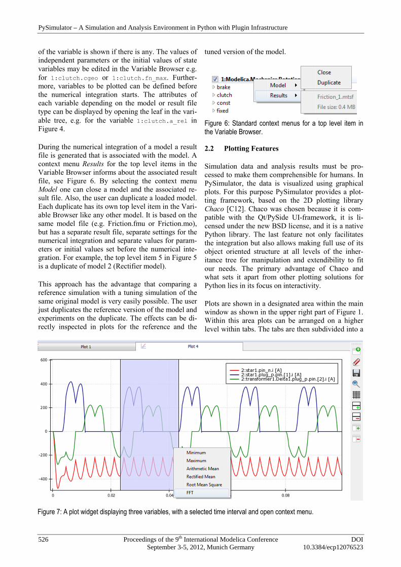
Plots are shown in a designated area within the main window as shown in the upper right part of Figure 1. Within this area plots can be arranged on a higher level within tabs. The tabs are then subdivided into a

Figure 7: A plot widget displaying three variables, with a selected time interval and open context menu.



grid in which the plots are arranged. To achieve all this, a base class called PlotWidget was implemented that acts as an adapter between Chaco and our appli-cation or respectively Qt/PySide. All plots are sup-posed to be implemented as extensions of this base class.

Based on the Chaco framework and PlotWidget a default plot widget (DefaultPlotWidget) for display-ing a variable value over time was implemented while paying special attention to the fact that future plugin developers can both easily use the existing material and still have access to Chaco’s full versatil-ity. Marking a variable in the Variable Browser plots the variable value over the time of the simulation in the currently active plot, unmarking it removes the plot line. An example of three variables of a simulat-ed model plotted in a default plot widget can be seen in Figure 7. The following features are based on de-fault Chaco elements and can easily be used individ-ually on any plot, specifically plots by plugins, either out-of-the-box as described here or derived from them to fit special needs: • Panning: Left clicking and dragging within the

plot pans the view. • Zooming: Turning the mouse wheel while hov-

ering over the plot zooms in and out. Hovering over an axis only zooms along the respective axis. Zooming and panning works very fast, and is even reasonably fast with millions of points in the plot window.

• Selecting: Left clicking and dragging on the X-axis selects a time period. Double clicking the axis opens a menu for textual input of selection limits.

• Context menu: Right clicking on the plot opens a context menu. In the DefaultPlotWidget it shows callbacks for plugins.

• Marker: While hovering over one plot, the plot's time stamp under the mouse is displayed as a vertical line in this and all related plots.

Additionally, plots can be saved as images, either as bitmaps in PNG format or as vector graphics in SVG or PDF format.

2.3 Plugin Structure

Currently, infrastructure for two kinds of plugins is available in PySimulator: Simulator and Analysis plugins. The plugin interfaces are designed to easily integrate own simulator and analysis code.

Simulator plugins are intended to provide the infra-structure to simulate a certain kind of model and write/read the result file of the simulation. In princi-ple all types of simulation engines can be included, provided time series are produced as results and var-iables and parameters are identified with a hierar-chical naming structure. Currently, plugins are avail-able for FMUs [FC10], for Dymola [DS12], and for OpenModelica [GFR+12].

The name of each Simulator plugin appears in the main menu bar (Figure 2) under Open Model. To include a Simulator plugin only the plugin code has to be inserted in a new directory of Plugins/Simulator, e.g. FMUSimulator in Figure 8.

Figure 8: Directory and main Python class structure for plugins in PySimulator.

The main Python code of a Simulator plugin has to be inside a class Model that is derived from the class Plugins.Simulator.SimulatorBase.Model. Im-portant variables, classes and function of the main class Model are: • modelType: String, e.g. ‘FMU1.0’, ‘Dymola’. • integrationSettings: Class including start,

stop time, algorithm name, etc. • integrationStatistics: Class including

number of events, grid points, elapsed real time, etc.

• integrationResults: Class including result file access.

• setVariableTree(): Function to generate da-ta for a variable tree.



• getAvailableIntegrationAlgorithms(): Function to get a list of available integration algorithms.

• simulate(): Function to start the numerical integration of the model.

• initialize(t): Function to initialize the model.

• getDerivatives(t,x): Function to evaluate the right hand side of the system.

• getEventIndicators(t,x): Function to evaluate the event indicators (= switching functions to detect events) of the system.

• getStates(): Function to get the values of all continuous model states.

• getStateNames(): Function to get a list of all names of the continuous model states.

• getValue(name): Function to retrieve the val-ue of a certain variable.

For example, the file FMUSimulator.py has a Python class Model that provides model typical methods and data as listed for an FMU.

Analysis plugins provide functionality for analyzing the model or result data in the post-processing stage of a simulation. They contain functions which work on variables, models and plots after a model is load-ed or a simulation is finished. In order to integrate the Analysis plugins, they are automatically loaded by PySimulator from the Analysis folder. An initiali-zation function is called for every plugin to enable the initial setup, like declaration of variables or own classes. The Analysis plugin is further able to regis-ter callback functions in the main program which allows access to the plugin’s functions. The call of a plugin’s function from the GUI takes place by either pull-down menus, a custom button bar or a context menu appearing when the user clicks on an appropri-ate GUI element like the model’s name.

For processing the data, the plugins can implement own algorithms or use shared functionality stored in the Algorithms folder. It is furthermore possible for such a plugin to initialize a model or to start a simu-lation, as this might be necessary for some function-ality like linearization of the model. In this case, the features of the Simulator plugins are utilized. The feedback of the Analysis plugin can be sent to the textual Information output window, a plot window or stored in every other way Python allows, e.g. in a file on disk.

It follows a simple example for an Analysis plugin to find the maximum value of a time trajectory and plot a label at the maximum point: def findMax(widget): for plot in widget.plots: data = plot.data maxVal = data[0] for time, value in data: if value > maxVal[1]: maxVal = (time, value) maxLabel = DataLabel( component=plot, data_point=maxVal, label_format=str('(%(x)f, %(y)f)')) plot.overlays.append(maxLabel) def getPlotCallbacks(): return [["Find Maximum", findMax]]

3 Simulator Plugins

Figure 9: Integrator control GUI in PySimulator.

One of the main features of PySimulator is running and controlling the numerical integration of different types of models (= simulation). Those models re-quire different simulation engines interfaced by the



Simulator plugins in PySimulator. All the Simulator plugins are controlled by the same Integrator Control GUI, see Figure 9. Some menu entries depend on properties of the Simulator plugin.

Start and stop time for the integration may be edited and one of the integration algorithms available for the Simulator plugin can be selected. Depending on the property of the algorithm the user can edit the error tolerance or the fixed step size. The simulation results are mainly discretized, time depending trajec-tories. The discretization points (= grid points, dense output points) of the time can be given either by the number of equidistant grid points or by the width of an equidistant time grid. A third option is to use the steps of the integration algorithm for the grid points. The name of the result file can also be specified. If Plot online is selected in the GUI, the plots of the simulation results are updated during the integration process. This may increase the elapsed real time for the integration, but gives information about the re-sults at once. This feature is especially intended for model simulations that take some time.

The simulation is run in a separate thread, so Varia-ble Browser and Plot area are still available for user interactions. During the numerical integration several statistical parameters inform about the progress: cur-rent simulation time, number of time and state events, number of computed result points, the size of the result file and the elapsed real time so far. In some cases it is very helpful to see that for example lots of events are generated and therefore the integra-tion is getting stuck, or the result settings lead to a huge result file and therefore the simulation is slow-ing down.

3.1 FMU Simulator

The FMU simulator provides an interface to models exported as a Functional Mockup Unit for Model Exchange (FMU, see [MC10]). This interface is sup-ported by more than 30 simulation environments (www.functional-mockup-interface.org/tools.html). An FMU is basically composed of two components: Firstly, a description file in XML-format holds all information about the variables of the model and other model information. Secondly, binaries for one or several target machines are contained, such as Windows dynamic link libraries (.dll) or Linux shared object libraries (.so). They contain the code for evaluating the model’s equations.

This way, the FMU interface allows the evaluation of the right hand side 𝑓 of the governing equations of a model, as well as its outputs 𝑦 and its event indica-tor signals 𝑧. They depend in generally on the mod-el’s states 𝑥, its parameters 𝑝, inputs 𝑢 and the time 𝑡. Additionally, time events can be triggered by the FMU. The event indicator signals are used to detect state events, which may occur in many physical models. With this information, it is possible for a numerical integration solver to perform the time in-tegration of the model to obtain a solution, see Fig-ure 10.

The single steps performed by PySimulator are the following. First, the XML description file of the se-lected model is parsed. The information from this file is visualized in the Variable Browser of the main GUI. The Variable Browser can thus also be used independently as an FMU description viewer.

Next, the Functional Mockup Interface (FMI) func-tions in the shared library are interfaced to make them available in PySimulator. This way, it is possi-ble for the integrator to call the model functions. While these parts are sufficient for some basic opera-tions like initialization, the time integration itself utilizes the Sundials Solver Suite [HBG05]. Sundials provides solvers for explicit and implicit dynamical systems: CVODE and IDA. CVODE numerically integrates ordinary differential equations by linear multistep methods. Depending on the solution CVODE switches between solvers for stiff and non-stiff problems. IDA uses BDF (Backwards Differen-tiation Formulas) to solve systems of differential-algebraic equations. Sundials supports root finding during the numerical integration. In summary, the Sundials solvers are prepared to be applied to FMUs. The Sundials integrator suite is implemented in C and is accessed from PySimulator via the python-sundials [T12] interface.

Figure 10: Interface from the FMU model to the SUNDI-ALS solver.

�̇� = 𝒇(𝒙,𝒑,𝒖, 𝑡) 𝒚 = 𝒈(𝒙,𝒑,𝒖, 𝑡) 𝒛 = 𝒉(𝒙,𝒑,𝒖, 𝑡)

FMU

t, u �̇�,𝒚, 𝒛 x

SUNDIALS Solver



http://www.functional-mockup-interface.org/tools.html

The FMU Simulator can be interfaced both by code from e.g. an Analysis plugin as well as by the GUI elements described in Section 3. In both cases the important simulation parameters can be adjusted by the user to the specific problem. After simulation, the results are stored in the MTSF file format, the pro-posed standard time series file format [PBO12] that is based on HDF5 [THG12]. This format offers a way to read and write variable information and numeric data in a convenient and standardized way. The for-mat is especially designed to support both small and very large files. In [PBO12] MTSF files up to 200 GBytes have been generated and variables have been read from the file. Most simulation programs do not support generating and plotting result files of such a size.

For example, a result file for the full robot model from the Modelica Standard Library (FMU generated by Dymola) is generated with 30 Mio. result points. The result file has a size of 171 GΒytes. When plot-ting signals from this file, the loaded signal is downsampled to 5 Mio. points to get acceptable plot-ting performance.

3.2 Dymola Simulator

The second Simulator plugin is based on the simula-tion executable (dymosim[.exe]) generated by the commercial Modelica environment Dymola [DS12] from Dassault Systèmes. PySimulator supports se-lecting a Modelica model by asking for the package file and the model name. Then, the Modelica model is automatically compiled by Dymola in the back-ground if there is a version of Dymola installed. The executable includes object code for both the model equations and the numerical integration algorithms.

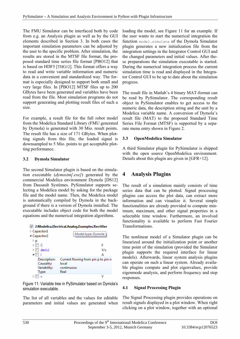
Figure 11: Variable tree in PySimulator based on Dymola’s simulation executable.

The list of all variables and the values for editable parameters and initial values are generated when

loading the model, see Figure 11 for an example. If the user wants to start the numerical integration the function model.simulate of the Dymola Simulator plugin generates a new initialization file from the integration settings in the Integrator Control GUI and the changed parameters and initial values. After the-se preparations the simulation executable is started. During the numerical integration process the current simulation time is read and displayed in the Integra-tor Control GUI to be up to date about the simulation progress.

The result file in Matlab’s 4 binary MAT-format can be read by PySimulator. The corresponding result object in PySimulator enables to get access to the numeric data, the description string and the unit by a Modelica variable name. A conversion of Dymola’s result file (MAT) to the proposed Standard Time Series File Format (MTSF) is supported by a sepa-rate menu entry shown in Figure 2.

3.3 OpenModelica Simulator

A third Simulator plugin for PySimulator is shipped with the open source OpenModelica environment. Details about this plugin are given in [GFR+12].

4 Analysis Plugins

The result of a simulation mainly consists of time series data that can be plotted. Signal processing plugins can access the plot data, can extract more information and can visualize it. Several simple functionalities are already provided to compute min-imum, maximum, and other signal properties in a selectable time window. Furthermore, an involved functionality is available to perform Fast Fourier Transformations.

The nonlinear model of a Simulator plugin can be linearized around the initialization point or another time point of the simulation (provided the Simulator plugin supports the required interface for linear models). Afterwards, linear system analysis plugins can operate on such a linear system. Already availa-ble plugins compute and plot eigenvalues, provide eigenmode analysis, and perform frequency and step responses.

4.1 Signal Processing Plugin

The Signal Processing plugin provides operations on result signals displayed in a plot window. When right clicking on a plot window, together with an optional



selection of a time range, a window (see Figure 7) pops up to select the desired signal processing opera-tion on the selected time range.

Figure 12: Example for marking of a minimum.

An example of how the result of an operation is shown in a plot is given in Figure 12, where the min-imum of a signal is determined in the range 𝑡 ∈[1.0, 2.7].

The operations to be carried out have the following mathematical definition:

Name Operation on 𝒚(𝒕) with

tmin ≤ t ≤ tmax, T = tmax − tmin Minimum 𝑦𝑚𝑖𝑛 = min𝑦(𝑡)

Maximum y𝑚𝑎𝑥 = max𝑦(𝑡)

Arithmetic Mean

𝑦𝐷𝐶 =1𝑇∙ � 𝑦(𝑡)

𝑡𝑚𝑎𝑥

𝑡𝑚𝑖𝑛

∙ 𝑑𝑡

Rectified Mean

𝑦𝑅𝑀 =1𝑇∙ � |𝑦(𝑡)|

𝑡𝑚𝑎𝑥

𝑡𝑚𝑖𝑛

∙ 𝑑𝑡

Root Mean Square

𝑦𝑅𝑀𝑆 = �1𝑇∙ � 𝑦(𝑡)2

𝑡𝑚𝑎𝑥

𝑡𝑚𝑖𝑛

∙ 𝑑𝑡

FFT

𝑓𝑠 =𝑛 − 1𝑇

,

𝑓 = �0,𝑓𝑠𝑛

,2𝑓𝑠𝑛

,⋯ ,𝑓𝑠2�

,

∆𝑦𝑟 = 𝑦(𝑡𝑟) − 𝑦𝐷𝐶 ,

𝑦𝐹𝐹𝑇,𝑘(𝑓𝑘) = 1𝑛𝑓

� ∆𝑦𝑟

𝑛𝑓−1

𝑟=0

𝑒−𝑖2𝜋𝑘 𝑟𝑛𝑓

The integrals in the operations are computed by us-ing the trapezoidal integration rule on the selected signal y (basically, the result points of y are linearly interpolated and then exactly integrated).

The Fast Fourier Transform (FFT, [RKH10]) is used to analyze which frequencies with which amplitudes

are contained in a periodic result signal. For this, a complex vector yFFT is computed as function of a real frequency vector f. Since an FFT requires equidistant time points, the (potentially) non-equidistant result points of a signal, y = y(t), are linearly interpolated and mapped to an equidistant grid of the desired number of points n. The frequency vector f consists of nf = div(n,2) + 1 points. For even n, the last point of vector f is fs/2, otherwise it is fs/2∙(n-1)/n (with fs = (n-1)/T and T as the selected time range). The variant of FFT is used, that subtracts the arithmetic mean of y from the signal y itself and normalizes the FFT re-sult with nf (in order that amplitudes of yFFT corre-spond to the amplitudes in the underlying result sig-nal).

The core FFT calculation is performed with Python function numpy.fft.rfft which in turn is an inter-face to the Fortran package fftpack [Swa82]. This package computes the FFT of an equidistant vector y of any length n in O(n2) and if n is expressed as a multiple of 2, 3, 4, or 5, that is 𝑛 = 2𝑖3𝑗4𝑘5𝑙 in O(n∙log(n)) operations. Note, the non-prime factor 4 gives a speed-up with respect to purely 2 factors [Tem83].

A natural question is what number n to select. There are two requirements: (1) all frequencies up to a de-sired frequency should be included, and (2) the dis-tance between two frequency points should be small enough. With (1) the number of points n can be computed as (T is the time range on which the FFT is applied):

𝑓𝑚𝑎𝑥 =𝑓𝑠2

=𝑛 − 1

2𝑇 → 𝑛 ≈ 2𝑇𝑓𝑚𝑎𝑥.

The distance d between two frequency points of vec-tor f for an even number of n is computed as (for an odd n the result is the same, but with a slightly dif-ferent derivation):

𝑑 =𝑓𝑚𝑎𝑥

𝑛𝑓 − 1=

𝑓𝑠 2⁄𝑛𝑓 − 1

=𝑛 − 1

2𝑇𝑛2 + 1 − 1

=1𝑇𝑛 − 1𝑛

≈1𝑇

.

This means that the frequency resolution depends only on the examined time interval T and can there-fore only be enlarged by enlarging this interval (and it is not related to the number of points used in the FFT calculation). For example, if the base frequency is f0 and the examined time interval T is over k peri-ods of this base frequency, then the distance d is:



𝑑 =1

𝑘 𝑓0⁄ =𝑓0𝑘

.

In other words, in order to get at least a resolution of 10 % of the base frequency, the examined time inter-val should have at least a range of 10 base periods.

As a simple example consider the following addition of two sines with different amplitudes (𝐴1 = 1,𝐴2 =0.2) and frequencies (𝑓1 = 5,𝑓2 = 20):

𝑦(𝑡) = 𝐴1 sin(2𝜋𝑓1𝑡) + 𝐴2 sin(2𝜋𝑓2𝑡).

If 10 periods of 𝑓1 are analyzed, the FFT-plot up to 2𝑓2 (𝑛 ≈ 2 ∙ 10

5∙ 40 + 1 → 𝑛 = 160) results in Fig-

ure 13.

Figure 13: FFT of example with n = 160.

As can be seen the 5 and 20 Hz frequencies are cor-rectly identified with small errors in the amplitudes. (the width of the plot bars are selected as 2 5 ∙ 𝑑⁄ ). Extending the frequency range to 10𝑓2 does not change the resolution (𝑑 = 5 10⁄ = 0.5 𝐻𝑧), but re-duces the amplitude errors as seen in Figure 14.

Figure 14: FFT of example with n = 800.

4.2 Linear System Analysis Plugin

For many control applications it is necessary to have a linear approximation of a nonlinear system. In ad-dition a linear representation of a nonlinear system

can be helpful to analyze specific properties of the system, for example local stability.

The Linear System Analysis plugin allows to auto-matically linearize a model that is loaded into Py-Simulator. If the plugin is loaded, its functionality can be accessed by right-clicking a loaded model in the GUI of PySimulator. If a loaded model is linear-ized using the GUI the parameter set 𝑝 ∈ ℝ𝑛𝑝, as defined in the Variable Browser is used for the line-arization around the operating point. If it is called from a Python-script, a set (Python dictionary) of parameters and values can be used. A model (nonlin-ear dynamic system) can be represented as a set of equations:

�̇� = 𝑓(𝑥,𝑝,𝑢, 𝑡), 𝑥(𝑡0) = 𝑥0, 𝑦 = 𝑔(𝑥, 𝑝,𝑢, 𝑡).

For the plugin it is necessary that a set of inputs 𝑢 ∈ ℝ𝑛𝑢 and outputs 𝑦 ∈ ℝ𝑛𝑦 are defined in the model, where 𝑛𝑢 ∈ ℕ is the number of inputs and 𝑛𝑦 ∈ ℕ is the number of outputs of the system.

The linearization procedure uses a numerical central difference quotient for the calculation of the Jacobi-ans. For a function 𝑞(𝑣) depending on a scalar 𝑣 we use the approximation:

𝑞𝑣(𝑣) ≈𝑞(𝑣 + 𝛿) − 𝑞(𝑣 − 𝛿)

2𝛿

with a step size 𝛿 = √𝜀3 max(|𝑣|, 1) and the ma-chine precision 𝜀. The step size is computed to find a compromise between a minimum discretization error and a minimum numerical error.

The central difference quotient is successively ap-plied to every component of 𝑥 and 𝑢 at a steady state point 𝑤𝑠𝑠 ≔ (𝑥𝑠𝑠,𝑝,𝑢𝑠𝑠, 𝑡0). The linear approxima-tion of the nonlinear system is a linear time invariant (LTI) system that is represented by the matrices 𝐴 ∈ ℝ𝑛𝑥×𝑛𝑥, 𝐵 ∈ ℝ𝑛𝑥×𝑛𝑢, 𝐶 ∈ ℝ𝑛𝑦×𝑛𝑥 and 𝐷 ∈ℝ𝑛𝑦×𝑛𝑢:

𝐴 = 𝑓𝑥(𝑤𝑠𝑠), 𝐵 = 𝑓𝑢(𝑤𝑠𝑠), 𝐶 = 𝑔𝑥(𝑤𝑠𝑠), 𝐷 = 𝑔𝑢(𝑤𝑠𝑠).

The default case is 𝑥𝑠𝑠 ∶= 𝑥0 ∈ ℝ𝑛𝑥 and 𝑢𝑠𝑠 = 0. If no user defined steady state point is given, 𝑥𝑠𝑠 is cal-culated by calling the simulator’s initialization func-tion. It is also possible to linearize around an arbi-trary user-defined steady state 𝑥𝑠𝑠.



The linear system is generated as an instance of a Python class inside the Linear System Analysis plugin, and can be accessed by other plugins inside PySimulator for further analysis. The class provides functions to return the matrices A, B, C, D, names and sizes of the input, output and state vectors. In addition it allows writing the matrices along with the state, input and output names to a file in Matlab’s MAT-format, see Figure 15, so that they can be di-rectly used for controller synthesis inside Matlab [M12].

Figure 16: Frequency responses of a 2x2 system.

Furthermore, the plugin provides various analysis operations on the linear input/output system. Most important, the frequency responses from the inputs to

the outputs are computed and plotted. An example of the frequency responses of a system with 2 inputs and 2 outputs is shown in Figure 16.

4.3 Eigenvalue Analysis Plugin

For the analysis of many systems, the eigenvalues and eigenmodes are of special interest. They support the understanding of the system by providing damp-ing and frequency information when eigenmodes or states are excited.

The Eigenvalue Analysis plugin needs the function-ality to linearize a system as a starting point for fur-ther analysis. For this, the Linear System Analysis plugin from Section 4.2 is utilized. Βased on this, functions for the visualization of both eigenvalues and eigenmodes can be called, see Figure 17.

Figure 17: Menu of the Eigenvalue Analysis plugin.

The eigenvalues are plotted in the complex domain as can be seen in Figure 18. This provides infor-mation about the stability in the point of linearization as well as about the dynamics of the corresponding eigenmodes. When clicking with the left mouse but-ton on an eigenvalue, additional information to this

Figure 15: Linear System Analysis plugin inside PySimulator.



eigenvalue is displayed such as frequency, damping and controllability.

Figure 18: Plot of eigenvalues and frequency response with additional information.

The eigenmodes themselves can be visualized if the model has been exported with an own visualization routine. This is e.g. the case, if a Modelica model is exported with the DLR Visualization library [Bel09]. The eigenmodes are a linear combination of the model’s states. Therefore, they can be visualized if the states have some form of visualization. The se-lected eigenmodes, see Figure 19, are excited by a periodic sine, making it possible to see their impact on the system, not only in a figure, but in a dynamic way.

Figure 19: GUI and animation of the 8th eigenmode, show-ing a clear coupling of the flexible states.

The shown example is a mechanical model of a mul-ti-robot cell of the DLR Center of Lightweight Pro-duction Technology. The visualized Eigenmode 8 shows a clear coupling of the left and middle beam due to the portal shown in the upper left part of the

figure. The GUI in Figure 20 shows some dynamic properties which can also be seen in the eigenvalue plot in Figure 18. As an additional possibility, the user can furthermore visualize the states of the sys-tem.

Figure 20: GUI to control the visualization of eigenmodes and states.

The combination of the two abilities Plot Eigenval-ues and Animate Eigenvectors/States enables the en-gineer to understand and visualize the dynamics of the system. This might help to adapt parameters of the system to e.g. stabilize it or reduce the impact of a periodic disturbance.

5 Algorithms

The algorithms used in the plugins are mostly based on the standard Python packages numpy and scipy. However, several new algorithms had to be imple-mented that seemed to be not yet available in other Python packages. These algorithms are provided un-der directory Plugins/Algorithms. All functions in this directory can be used also in any other context, since there is no relationship to PySimulator (just that plugins from PySimulator are calling these func-tions). Especially, in this directory functions are pro-vided for the Signal Processing and the Linear Sys-tem Analysis plugins.

For example, class LTI in file Algorithms/Control/ lti.py provides various functions for multi-input-multi-output Linear Time Invariant systems. In the current version, two representations of continuous linear systems are supported:



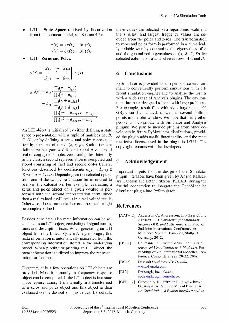
• LTI – State Space (derived by linearization from the nonlinear model, see Section 4.2):

�̇�(𝑡) = 𝐴𝑥(𝑡) + 𝐵𝑢(𝑡), 𝑦(𝑡) = 𝐶𝑥(𝑡) + 𝐷𝑢(𝑡).

• LTI – Zeros and Poles:

𝑦(𝑠) = �𝑔11 … 𝑔1𝑚⋮ ⋱ ⋮𝑔𝑛1 … 𝑔𝑛𝑚

� ∙ 𝑢(𝑠),

𝑔𝑖𝑗(𝑠) = 𝑘𝑖𝑗 ∙∏ �𝑠 − 𝑧𝑖𝑗,𝑙�𝑙

∏ �𝑠 − 𝑝𝑖𝑗,𝑙�𝑙

= 𝑘𝑖𝑗 ∙∏ �𝑠 + 𝑛1,𝑖𝑗,𝑙�𝑙

∏ �𝑠 + 𝑑1,𝑖𝑗,𝑙�𝑙

∙∏ �𝑠2 + 𝑛2,𝑖𝑗,𝑙𝑠 + 𝑛3,𝑖𝑗,𝑙�𝑙

∏ �𝑠2 + 𝑑2,𝑖𝑗,𝑙𝑠 + 𝑑3,𝑖𝑗,𝑙�𝑙

An LTI object is initialized by either defining a state space representation with a tuple of matrices (A, B, C, D), or by defining a zeros and poles representa-tion by a matrix of tuples (k, z, p). Such a tuple is defined with a gain 𝑘 ∈ ℝ, and z and p vectors of real or conjugate complex zeros and poles. Internally in the class, a second representation is computed and stored consisting of first and second order transfer functions described by coefficients 𝑛𝑞,𝑖𝑗,𝑙 , 𝑑𝑞,𝑖𝑗,𝑙 ∈ℝ with 𝑞 = 1, 2, 3. Depending on the selected opera-tion, one of the two representation forms is used to perform the calculation. For example, evaluating a zeros and poles object on a given s-value is per-formed with the second representation form, since then a real-valued s will result in a real-valued result. Otherwise, due to numerical errors, the result might be complex-valued.

Besides pure data, also meta-information can be as-sociated to an LTI object, consisting of signal names, units and description texts. When generating an LTI object from the Linear System Analysis plugin, this meta information is automatically generated from the corresponding information stored in the underlying model. When plotting or printing an LTI object, the meta-information is utilized to improve the represen-tation for the user.

Currently, only a few operations on LTI objects are provided. Most importantly, a frequency response object can be computed. If the LTI object is in a state space representation, it is internally first transformed to a zeros and poles object and this object is then evaluated on the desired 𝑠 = 𝑗𝜔 values. By default,

these values are selected on a logarithmic scale and the smallest and largest frequency values are de-duced from the poles and zeros. The transformation to zeros and poles form is performed in a numerical-ly reliable way by computing the eigenvalues of A and the generalized eigenvalues of (A, B, C, D) for selected columns of B and selected rows of C and D.

6 Conclusions

PySimulator is provided as an open source environ-ment to conveniently perform simulations with dif-ferent simulation engines and to analyze the results with a wide range of Analysis plugins. The environ-ment has been designed to cope with large problems. For example, result files with sizes larger than 100 GByte can be handled, as well as several million points in one plot window. We hope that many other people will contribute with Simulator and Analysis plugins. We plan to include plugins from other de-velopers in future PySimulator distributions, provid-ed the plugin adds useful functionality, and the most restrictive license used in the plugin is LGPL. The copyright remains with the developers.

7 Acknowledgement

Important inputs for the design of the Simulator plugin interfaces have been given by Anand Kalaiar-asi Ganeson and Peter Fritzson (PELAB) during the fruitful cooperation to integrate the OpenModelica Simulator plugin into PySimulator.

References

[AAF+12] Andersson C., Andreasson, J., Führer C. and Åkesson J.: A Workbench for Multibody Systems ODE and DAE Solvers. In Proc. of 2nd Joint International Conference on Multibody System Dynamics, Stuttgart, Germany, 2012.

[Bel09] Bellmann T.: Interactive Simulations and advanced Visualization with Modelica. Pro-ceedings of 7th International Modelica Con-ference, Como, Italy, Sep. 20-22, 2009.

[DS12] Dassault Systèmes AB: Dymola, www.dymola.com.

[E12] Enthough, Inc.: Chaco. code.enthought.com/chaco.

[GFR+12] Ganeson A. K., Fritzson P., Rogovchenko O., Asghar A., Sjölund M. and Pfeiffer A.: An OpenModelica Python Interface and its



http://www.dymola.com/

http://code.enthought.com/chaco

use in PySimulator. Accepted for publica-tion in the Proceedings of 9th International Modelica Conference, Munich, Germany, Sept. 2012.

[HBG05] Hindmarsh A. C., Brown P. N., Grant K. E., Lee S. L., Serban R., Shumaker D. E. and Woodward C. S.: SUNDIALS: Suite of Non-linear and Differential/Algebraic Equation Solvers. ACM Transactions on Mathemati-cal Software, 31(3), pp. 363-396, 2005.

[LBN+12] Lawrence Berkeley National Laboratory: BuildingsPy. simulationrese-arch.lbl.gov/modelica.

[M12] MathWorks: Matlab. www.mathworks.com/products/matlab.

[MC10] MODELISAR consortium: Functional Mock-up Interface for Model Exchange, Version 1.0, 2010. www.functional-mockup-interface.org.

[NC12] Nokia Corporation: Qt. www.qt.nokia.com. [P12] PySide. www.pyside.org. [PBO12] Pfeiffer A., Bausch-Gall I. and Otter M.:

Proposal for a Standard Time Series File Format in HDF5. Accepted for publication in the Proceedings of 9th International Modelica Conference, Munich, Germany, Sept. 2012.

[RKH10] Rao K. R., Kim D. N. and Hwang J.-J.: Fast Fourier Transform: Algorithms And Appli-cations. Springer, Dordrecht, Heidelberg, London, 2010.

[Swa82] Swarztrauber P.N.: Vectorizing the FFTs. In: Parallel Computations, Ed. G. Rodrigue, Academic Press, 1982, pp. 51-83. www.netlib.org/fftpack

[T12] Tenfjord R.: Python-sundials. www.code.google.com/p/python-sundials.

[Tem83] Temperton C.: Self-Sorting Mixed-Radix Fast Fourier Transforms. Journal of Com-putational Physics, 52, pp. 1-23, 1983. www.sciencedirect.com/science/article/pii/002199918390013X.

[THG12] The HDF Group. www.hdfgroup.org.



http://simulationresearch.lbl.gov/modelica

http://simulationresearch.lbl.gov/modelica

http://www.mathworks.com/products/matlab

http://www.functional-mockup-interface.org/

http://www.functional-mockup-interface.org/

http://www.qt.nokia.com/

http://www.pyside.org/

http://www.netlib.org/fftpack

http://www.code.google.com/p/python-sundials

http://www.sciencedirect.com/science/article/pii/002199918390013X

http://www.sciencedirect.com/science/article/pii/002199918390013X

http://www.hdfgroup.org/

Documents

PySimulator – A Simulation and A nalysis Environment in ...elib.dlr.de/77223/1/ecp12076523_PfeifferHellererHartwegOtter.pdf · PySimulator – A Simulation and A nalysis Environment